Problem solving and quantum computation - CiteSeerX

Problem solving and quantum computation

Luıs Tarrataca and Andreas WichertDepartment of Informatics

INESC-ID / IST - Technical University of LisbonPortugal

luis.tarrataca,[email protected]

Abstract

Is quantum computing suitable for modeling problem solving, a do-

main which is traditionally reserved for the symbolic approach? We pro-

pose a hybrid quantum problem solving model. Our approach is moti-

vated by several important theories from the fields of physics, computer

science and psychology. We demonstrate our approach through a model

for a quantum production system, based on the n-puzzle. The developed

model can be extended in order to tackle any N-level depth search re-

quired by other problems. No preliminary knowledge concerning quantum

computation is required.

Keywords: Inference, quantum computation, problem solving, production sys-tem, reversible computation

1 Introduction

Cognitive computation has focused for a long focused on concepts such as knowl-edge representation and the reasoning processes that allow knowledge to beapplied. Traditionally, these concepts have been modeled with the assistanceof classical probability theory which allows the representation of possible statetransitions as a graph of probabilities. However, such an assumption may beinadequate depending on the physical laws in play during possible applications.This theory was exploited in [1, 2, 3, 4, 5] where quantum probability theorywas explored in order to justify empirical variations that classical probabilitytheory failed to explain. By employing quantum von Neumann probabilities theauthors were able to obtain a closer fit to experimental data.

Additionally, knowledge can be employed by problem-solving agents trying todetermine adequate actions when dealing with complex environments [6]. Il-lustrating examples include IBM’s Deep Blue [7] and Watson initiatives whichfocus, respectively, on chess playing and the Jeopardy! quiz show. Both these

1

system employ knowledge alongside massive amounts of parallel computation.However, these tasks are routinely performed by human brains through neuronalprocessing on a time-scale of 10−3 seconds. Manin draws attention to these facts[8] and suggests quantum processing as a theoretical alternative. Additionally,some of the possible relationships between artificial intelligence and quantumcomputation have been established in [9]. In this work we extend these views byintroducing a possible problem-solving technique from a quantum computationperspective. Our approach will be based on production system theory since it iswell suited for problem solving scenarios. The following sections are organized asfollows: Section 1.1 introduces some key concepts of production systems whilstSection 1.2 establishes the links between production system theory and classicalsearch strategies.

1.1 Production System

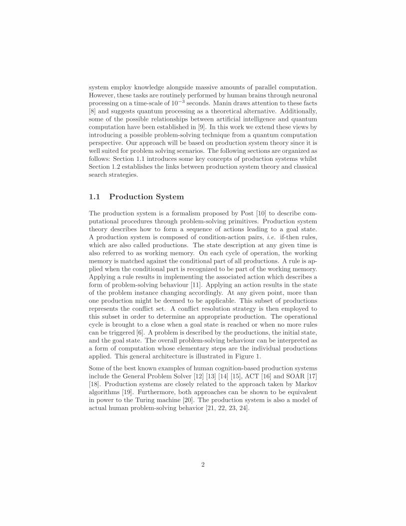
The production system is a formalism proposed by Post [10] to describe com-putational procedures through problem-solving primitives. Production systemtheory describes how to form a sequence of actions leading to a goal state.A production system is composed of condition-action pairs, i.e. if-then rules,which are also called productions. The state description at any given time isalso referred to as working memory. On each cycle of operation, the workingmemory is matched against the conditional part of all productions. A rule is ap-plied when the conditional part is recognized to be part of the working memory.Applying a rule results in implementing the associated action which describes aform of problem-solving behaviour [11]. Applying an action results in the stateof the problem instance changing accordingly. At any given point, more thanone production might be deemed to be applicable. This subset of productionsrepresents the conflict set. A conflict resolution strategy is then employed tothis subset in order to determine an appropriate production. The operationalcycle is brought to a close when a goal state is reached or when no more rulescan be triggered [6]. A problem is described by the productions, the initial state,and the goal state. The overall problem-solving behaviour can be interpreted asa form of computation whose elementary steps are the individual productionsapplied. This general architecture is illustrated in Figure 1.

Some of the best known examples of human cognition-based production systemsinclude the General Problem Solver [12] [13] [14] [15], ACT [16] and SOAR [17][18]. Production systems are closely related to the approach taken by Markovalgorithms [19]. Furthermore, both approaches can be shown to be equivalentin power to the Turing machine [20]. The production system is also a model ofactual human problem-solving behavior [21, 22, 23, 24].

2

Control

Recognize Act

Working Memory

Prodution Rules(Conditon, Action)

C1 A1

C2 A2

Cn An

Figure 1: General architecture for a production system (adapted from [6]).

1.2 Search as a decision problem

From a computer science perspective, the control structure of a production sys-tem can be defined in terms of classical tree-search procedures which is appropri-ate to artificial intelligence tasks trying to mimick problem-solving behaviour.This fact makes production system theory particularly well suited for problem-solving scenarios. In general, tree algorithms are applied when when we wishto perform an exhaustive examination of all possible combinations for the statespace. For these cases, the search space can be viewed as forming a hierarchyreflecting the spectrum of combinations. All that is required to formulate asearch problem is a set of states, a set of operators that map states into succes-sor states, an initial state and a set of goal states [25]. The overall objective isto find a sequence of operators that map the initial state to a goal state.

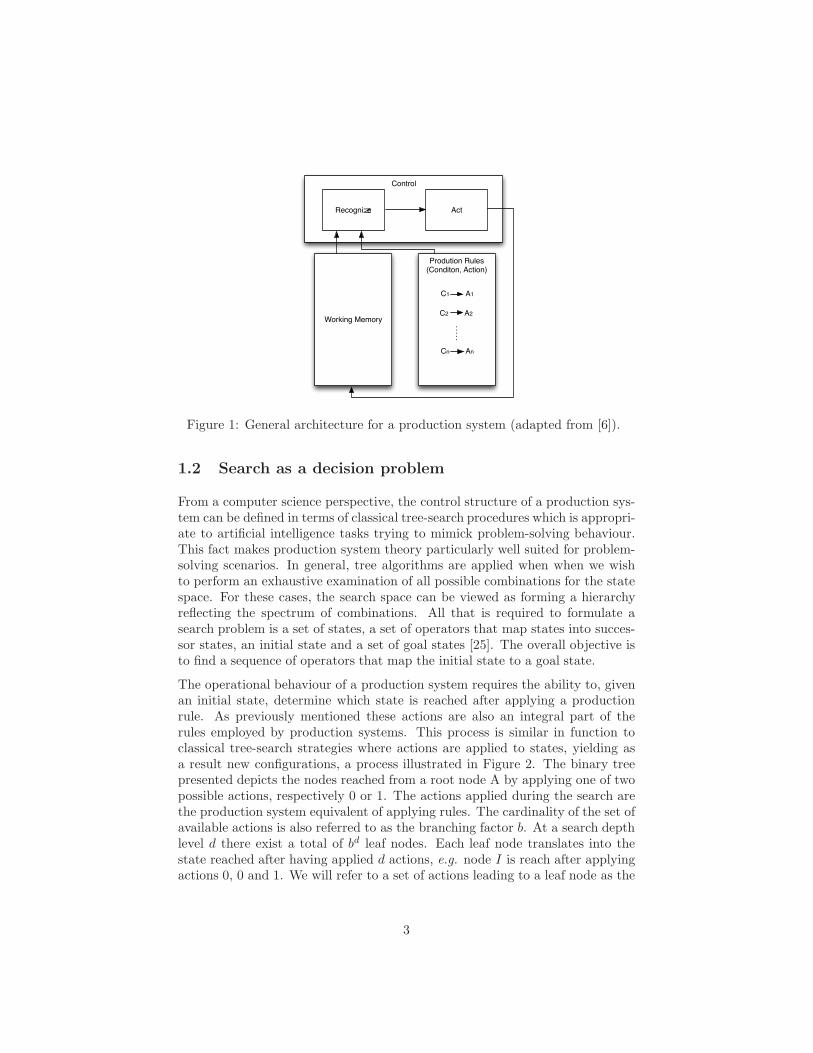
The operational behaviour of a production system requires the ability to, givenan initial state, determine which state is reached after applying a productionrule. As previously mentioned these actions are also an integral part of therules employed by production systems. This process is similar in function toclassical tree-search strategies where actions are applied to states, yielding asa result new configurations, a process illustrated in Figure 2. The binary treepresented depicts the nodes reached from a root node A by applying one of twopossible actions, respectively 0 or 1. The actions applied during the search arethe production system equivalent of applying rules. The cardinality of the set ofavailable actions is also referred to as the branching factor b. At a search depthlevel d there exist a total of bd leaf nodes. Each leaf node translates into thestate reached after having applied d actions, e.g. node I is reach after applyingactions 0, 0 and 1. We will refer to a set of actions leading to a leaf node as the

3

path taken during the tree-search.

A

B

D E

H I J K

C

F G

L M N O

Path 2

001

Path 3

010

Path 4

011

Path 5

100

Path 6

101

Path 7

110

Path 8

111

Height = 3

Depth 0

Depth 1

Depth 2

Depth 3

0

0

0 0 0 0

0

1

1 1

1 1 1 1

Path 1

000

Figure 2: The possible paths for a binary search tree of depth 3.

1.3 Problem

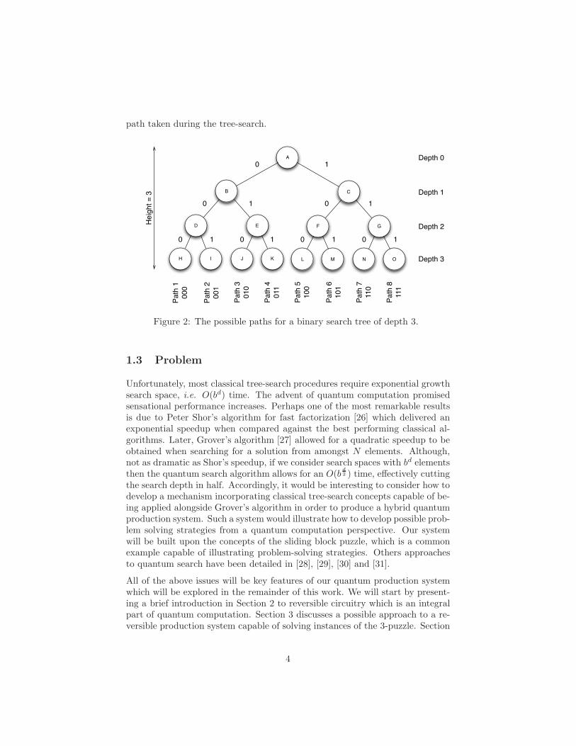
Unfortunately, most classical tree-search procedures require exponential growthsearch space, i.e. O(bd) time. The advent of quantum computation promisedsensational performance increases. Perhaps one of the most remarkable resultsis due to Peter Shor’s algorithm for fast factorization [26] which delivered anexponential speedup when compared against the best performing classical al-gorithms. Later, Grover’s algorithm [27] allowed for a quadratic speedup to beobtained when searching for a solution from amongst N elements. Although,not as dramatic as Shor’s speedup, if we consider search spaces with bd elementsthen the quantum search algorithm allows for an O(b

d2 ) time, effectively cutting

the search depth in half. Accordingly, it would be interesting to consider how todevelop a mechanism incorporating classical tree-search concepts capable of be-ing applied alongside Grover’s algorithm in order to produce a hybrid quantumproduction system. Such a system would illustrate how to develop possible prob-lem solving strategies from a quantum computation perspective. Our systemwill be built upon the concepts of the sliding block puzzle, which is a commonexample capable of illustrating problem-solving strategies. Others approachesto quantum search have been detailed in [28], [29], [30] and [31].

All of the above issues will be key features of our quantum production systemwhich will be explored in the remainder of this work. We will start by present-ing a brief introduction in Section 2 to reversible circuitry which is an integralpart of quantum computation. Section 3 discusses a possible approach to a re-versible production system capable of solving instances of the 3-puzzle. Section

4

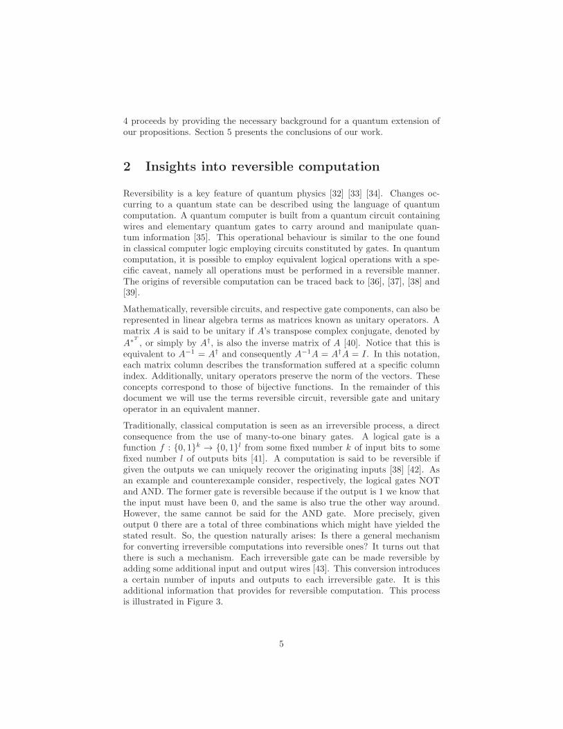
4 proceeds by providing the necessary background for a quantum extension ofour propositions. Section 5 presents the conclusions of our work.

2 Insights into reversible computation

Reversibility is a key feature of quantum physics [32] [33] [34]. Changes oc-curring to a quantum state can be described using the language of quantumcomputation. A quantum computer is built from a quantum circuit containingwires and elementary quantum gates to carry around and manipulate quan-tum information [35]. This operational behaviour is similar to the one foundin classical computer logic employing circuits constituted by gates. In quantumcomputation, it is possible to employ equivalent logical operations with a spe-cific caveat, namely all operations must be performed in a reversible manner.The origins of reversible computation can be traced back to [36], [37], [38] and[39].

Mathematically, reversible circuits, and respective gate components, can also berepresented in linear algebra terms as matrices known as unitary operators. Amatrix A is said to be unitary if A’s transpose complex conjugate, denoted by

A∗T

, or simply by A†, is also the inverse matrix of A [40]. Notice that this isequivalent to A−1 = A† and consequently A−1A = A†A = I. In this notation,each matrix column describes the transformation suffered at a specific columnindex. Additionally, unitary operators preserve the norm of the vectors. Theseconcepts correspond to those of bijective functions. In the remainder of thisdocument we will use the terms reversible circuit, reversible gate and unitaryoperator in an equivalent manner.

Traditionally, classical computation is seen as an irreversible process, a directconsequence from the use of many-to-one binary gates. A logical gate is afunction f : 0, 1k → 0, 1l from some fixed number k of input bits to somefixed number l of outputs bits [41]. A computation is said to be reversible ifgiven the outputs we can uniquely recover the originating inputs [38] [42]. Asan example and counterexample consider, respectively, the logical gates NOTand AND. The former gate is reversible because if the output is 1 we know thatthe input must have been 0, and the same is also true the other way around.However, the same cannot be said for the AND gate. More precisely, givenoutput 0 there are a total of three combinations which might have yielded thestated result. So, the question naturally arises: Is there a general mechanismfor converting irreversible computations into reversible ones? It turns out thatthere is such a mechanism. Each irreversible gate can be made reversible byadding some additional input and output wires [43]. This conversion introducesa certain number of inputs and outputs to each irreversible gate. It is thisadditional information that provides for reversible computation. This processis illustrated in Figure 3.

5

Irreversible

FunctionInput Output

(a)

Reversible

Function

Input

AuxiliaryInput

Output

AuxiliaryOutput

(b)

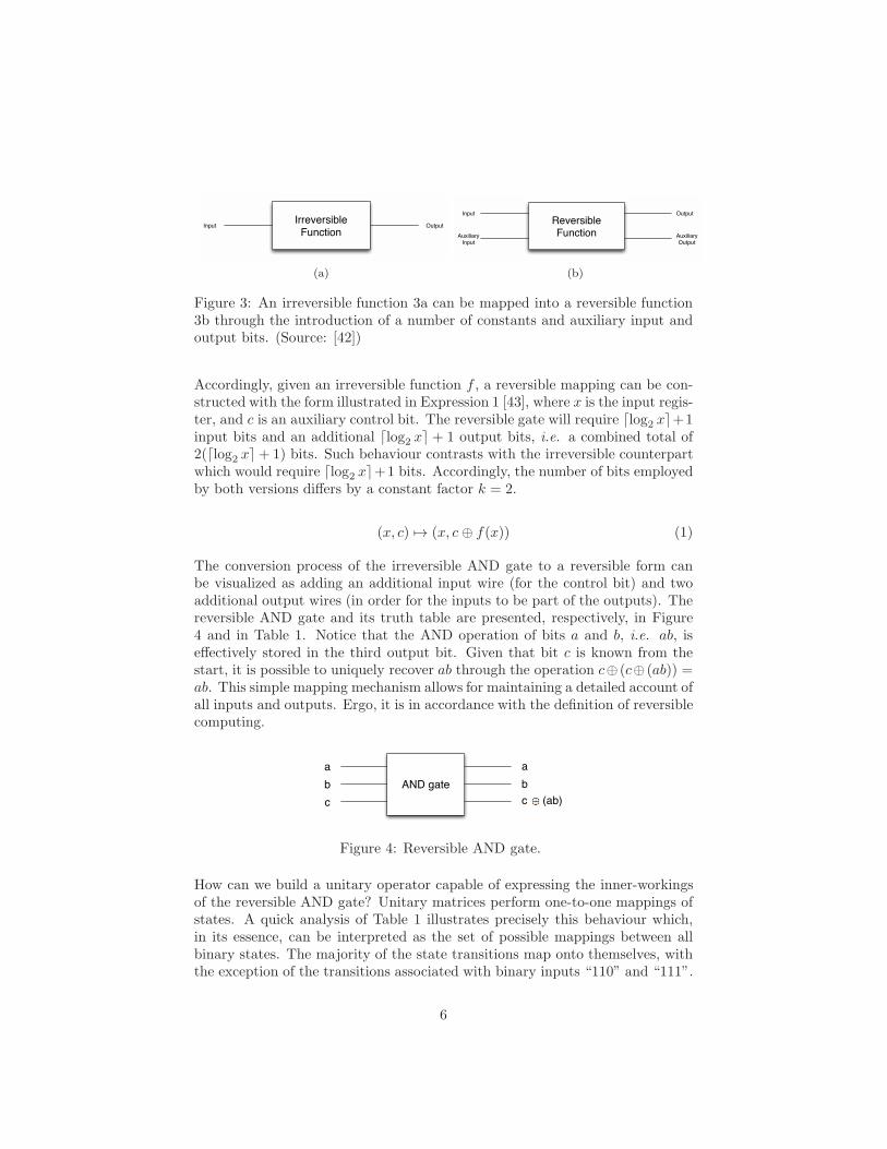
Figure 3: An irreversible function 3a can be mapped into a reversible function3b through the introduction of a number of constants and auxiliary input andoutput bits. (Source: [42])

Accordingly, given an irreversible function f , a reversible mapping can be con-structed with the form illustrated in Expression 1 [43], where x is the input regis-ter, and c is an auxiliary control bit. The reversible gate will require ⌈log2 x⌉+1input bits and an additional ⌈log2 x⌉ + 1 output bits, i.e. a combined total of2(⌈log2 x⌉+ 1) bits. Such behaviour contrasts with the irreversible counterpartwhich would require ⌈log2 x⌉+1 bits. Accordingly, the number of bits employedby both versions differs by a constant factor k = 2.

(x, c) 7→ (x, c⊕ f(x)) (1)

The conversion process of the irreversible AND gate to a reversible form canbe visualized as adding an additional input wire (for the control bit) and twoadditional output wires (in order for the inputs to be part of the outputs). Thereversible AND gate and its truth table are presented, respectively, in Figure4 and in Table 1. Notice that the AND operation of bits a and b, i.e. ab, iseffectively stored in the third output bit. Given that bit c is known from thestart, it is possible to uniquely recover ab through the operation c⊕ (c⊕ (ab)) =ab. This simple mapping mechanism allows for maintaining a detailed account ofall inputs and outputs. Ergo, it is in accordance with the definition of reversiblecomputing.

AND gate

a

b

c

a

b

c (ab)

Figure 4: Reversible AND gate.

How can we build a unitary operator capable of expressing the inner-workingsof the reversible AND gate? Unitary matrices perform one-to-one mappings ofstates. A quick analysis of Table 1 illustrates precisely this behaviour which,in its essence, can be interpreted as the set of possible mappings between allbinary states. The majority of the state transitions map onto themselves, withthe exception of the transitions associated with binary inputs “110” and “111”.

6

Inputs Outputsa b c a b c ⊕ (ab)0 0 0 0 0 00 0 1 0 0 10 1 0 0 1 00 1 1 0 1 11 0 0 1 0 01 0 1 1 0 11 1 0 1 1 11 1 1 1 1 0

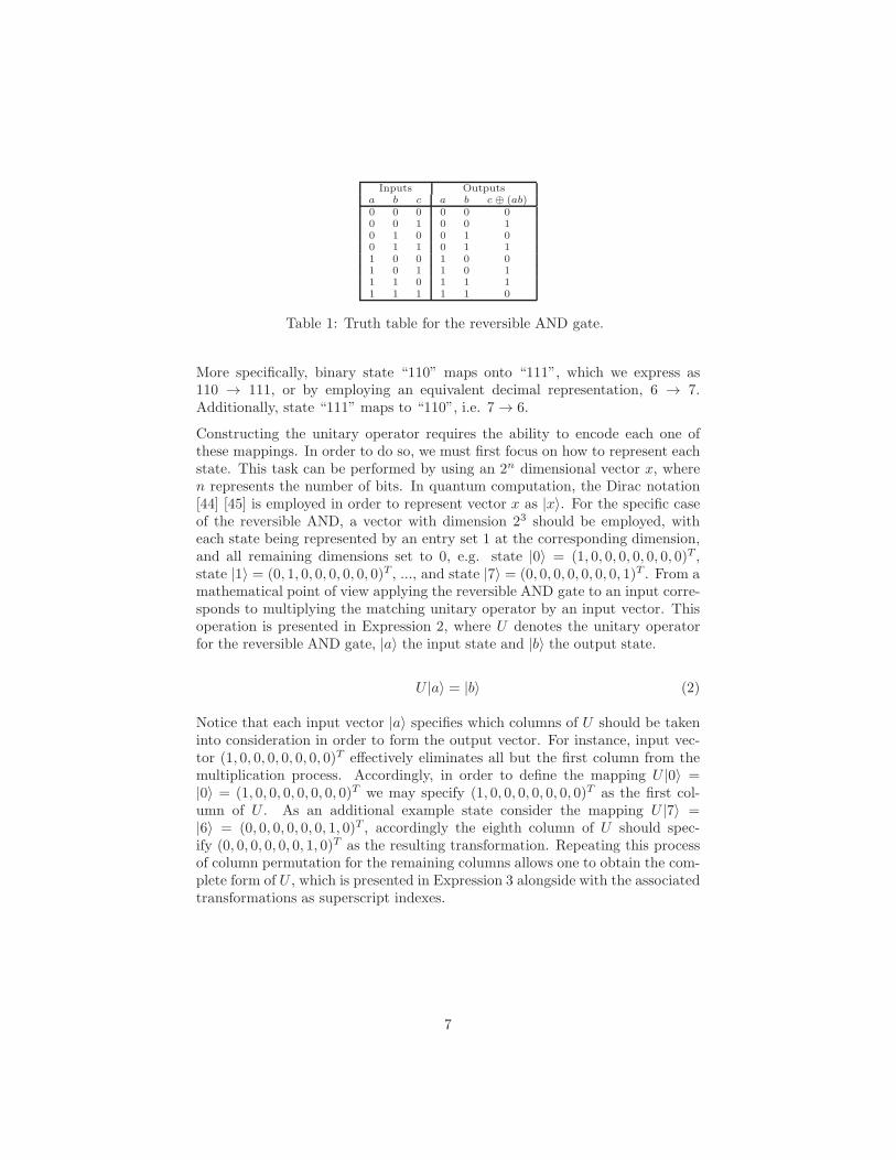
Table 1: Truth table for the reversible AND gate.

More specifically, binary state “110” maps onto “111”, which we express as110 → 111, or by employing an equivalent decimal representation, 6 → 7.Additionally, state “111” maps to “110”, i.e. 7 → 6.

Constructing the unitary operator requires the ability to encode each one ofthese mappings. In order to do so, we must first focus on how to represent eachstate. This task can be performed by using an 2n dimensional vector x, wheren represents the number of bits. In quantum computation, the Dirac notation[44] [45] is employed in order to represent vector x as |x〉. For the specific caseof the reversible AND, a vector with dimension 23 should be employed, witheach state being represented by an entry set 1 at the corresponding dimension,and all remaining dimensions set to 0, e.g. state |0〉 = (1, 0, 0, 0, 0, 0, 0, 0)T ,state |1〉 = (0, 1, 0, 0, 0, 0, 0, 0)T , ..., and state |7〉 = (0, 0, 0, 0, 0, 0, 0, 1)T . From amathematical point of view applying the reversible AND gate to an input corre-sponds to multiplying the matching unitary operator by an input vector. Thisoperation is presented in Expression 2, where U denotes the unitary operatorfor the reversible AND gate, |a〉 the input state and |b〉 the output state.

U |a〉 = |b〉 (2)

Notice that each input vector |a〉 specifies which columns of U should be takeninto consideration in order to form the output vector. For instance, input vec-tor (1, 0, 0, 0, 0, 0, 0, 0)T effectively eliminates all but the first column from themultiplication process. Accordingly, in order to define the mapping U |0〉 =|0〉 = (1, 0, 0, 0, 0, 0, 0, 0)T we may specify (1, 0, 0, 0, 0, 0, 0, 0)T as the first col-umn of U . As an additional example state consider the mapping U |7〉 =|6〉 = (0, 0, 0, 0, 0, 0, 1, 0)T , accordingly the eighth column of U should spec-ify (0, 0, 0, 0, 0, 0, 1, 0)T as the resulting transformation. Repeating this processof column permutation for the remaining columns allows one to obtain the com-plete form of U , which is presented in Expression 3 alongside with the associatedtransformations as superscript indexes.

7

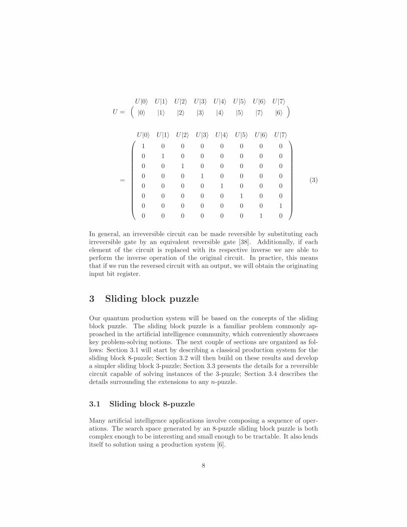
U =(U |0〉 U |1〉 U |2〉 U |3〉 U |4〉 U |5〉 U |6〉 U |7〉|0〉 |1〉 |2〉 |3〉 |4〉 |5〉 |7〉 |6〉

)

=

U |0〉 U |1〉 U |2〉 U |3〉 U |4〉 U |5〉 U |6〉 U |7〉1 0 0 0 0 0 0 0

0 1 0 0 0 0 0 0

0 0 1 0 0 0 0 0

0 0 0 1 0 0 0 0

0 0 0 0 1 0 0 0

0 0 0 0 0 1 0 0

0 0 0 0 0 0 0 1

0 0 0 0 0 0 1 0

(3)

In general, an irreversible circuit can be made reversible by substituting eachirreversible gate by an equivalent reversible gate [38]. Additionally, if eachelement of the circuit is replaced with its respective inverse we are able toperform the inverse operation of the original circuit. In practice, this meansthat if we run the reversed circuit with an output, we will obtain the originatinginput bit register.

3 Sliding block puzzle

Our quantum production system will be based on the concepts of the slidingblock puzzle. The sliding block puzzle is a familiar problem commonly ap-proached in the artificial intelligence community, which conveniently showcaseskey problem-solving notions. The next couple of sections are organized as fol-lows: Section 3.1 will start by describing a classical production system for thesliding block 8-puzzle; Section 3.2 will then build on these results and developa simpler sliding block 3-puzzle; Section 3.3 presents the details for a reversiblecircuit capable of solving instances of the 3-puzzle; Section 3.4 describes thedetails surrounding the extensions to any n-puzzle.

3.1 Sliding block 8-puzzle

Many artificial intelligence applications involve composing a sequence of oper-ations. The search space generated by an 8-puzzle sliding block puzzle is bothcomplex enough to be interesting and small enough to be tractable. It also lendsitself to solution using a production system [6].

8

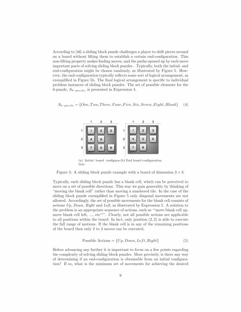
According to [46] a sliding block puzzle challenges a player to shift pieces aroundon a board without lifting them to establish a certain end-configuration. Thisnon-lifting property makes finding moves, and the paths opened up by each moveimportant parts of solving sliding block puzzles . Typically, both the initial- andend-configuration might be chosen randomly, as illustrated by Figure 5. How-ever, the end-configuration typically reflects some sort of logical arrangement, asexemplified in Figure 5b. The final logical arrangement is specific to individualproblem instances of sliding block puzzles. The set of possible elements for the8-puzzle, S8−puzzle, is presented in Expression 4.

S8−puzzle = One, Two, Three, Four, F ive, Six, Seven,Eight, Blank (4)

4

7

2

5 8

3

6

1

1 2 3

1

2

3

(a) Initial board configura-tion.

4

7

2

5

8

3

6

1

1 2 3

1

2

3

(b) End board configuration.

Figure 5: A sliding block puzzle example with a board of dimension 3× 3.

Typically, each sliding block puzzle has a blank cell, which can be perceived tomove on a set of possible directions. This way we gain generality by thinking of“moving the blank cell” rather than moving a numbered tile. In the case of thesliding block puzzle exemplified in Figure 5 only diagonal movements are notallowed. Accordingly, the set of possible movements for the blank cell consists ofactions Up, Down, Right and Left, as illustrated by Expression 5. A solution tothe problem is an appropriate sequence of actions, such as “‘move blank cell up,move blank cell left, ..., etc‘””. Clearly, not all possible actions are applicableto all positions within the board. In fact, only position (2, 2) is able to executethe full range of motions. If the blank cell is in any of the remaining positionsof the board then only 2 to 3 moves can be executed.

Possible Actions = Up,Down,Left, Right (5)

Before advancing any further it is important to focus on a few points regardingthe complexity of solving sliding block puzzles. More precisely, is there any wayof determining if an end-configuration is obtainable from an initial configura-tion? If so, what is the minimum set of movements for achieving the desired

9

Condition Actiongoal state in working memory → haltblank is not on the top edge → move the blank upblank is not on the right edge → move the blank right

blank is not on the bottom edge → move the blank downblank is not on the left edge → move the blank left

Table 2: Production rules set for the 8-puzzle. (Source: [6])

state? As is to be expected a wide number of authors have tried to tackle thissubject. Surprisingly, not a great deal of progress has been achieved. Shortof trial and error, it is impossible to present an answer to these questions [47].This apparent inability to solve efficiently sliding block puzzles stems from com-putational complexity theory. Sliding-block puzzles have been shown to belongto a class of problems known as PSPACE-complete [48] [49]. PSPACE consistsof those problems which can be solved using few spatial resources but poten-tially requiring significant time. PSPACE is thought to be even harder thanNP-complete, although this has never been proved.

As previously stated, in order to solve a problem using a production system,we must specify the working memory, the productions and the control strategy.Lets say we initialize the working memory with the initial board configurationdepicted in Figure 5a and we aim to reach the target board configuration illus-trated in Figure 5b. We can then define an illustrating set of production rulesas presented in Table 2. The only remaining issue is due to the control strategyemployed, which might be defined as [6]

1. Try each production in order;

2. Do not allow loops;

3. Stop when goal state is reached.

3.2 Sliding block 3-puzzle

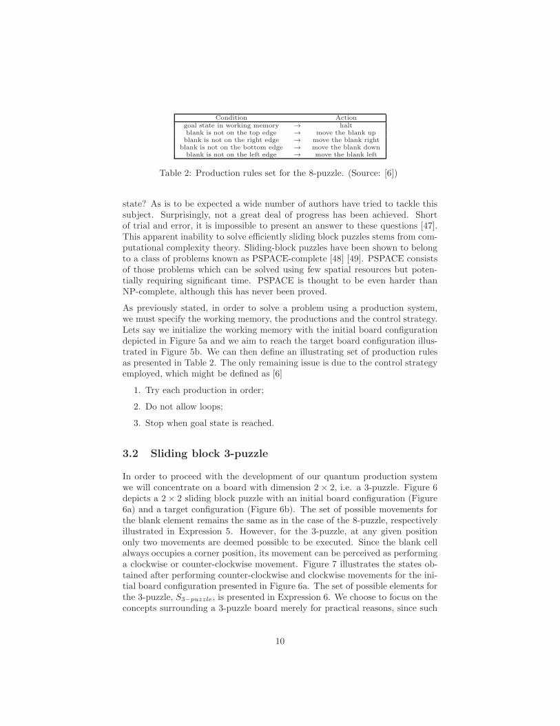
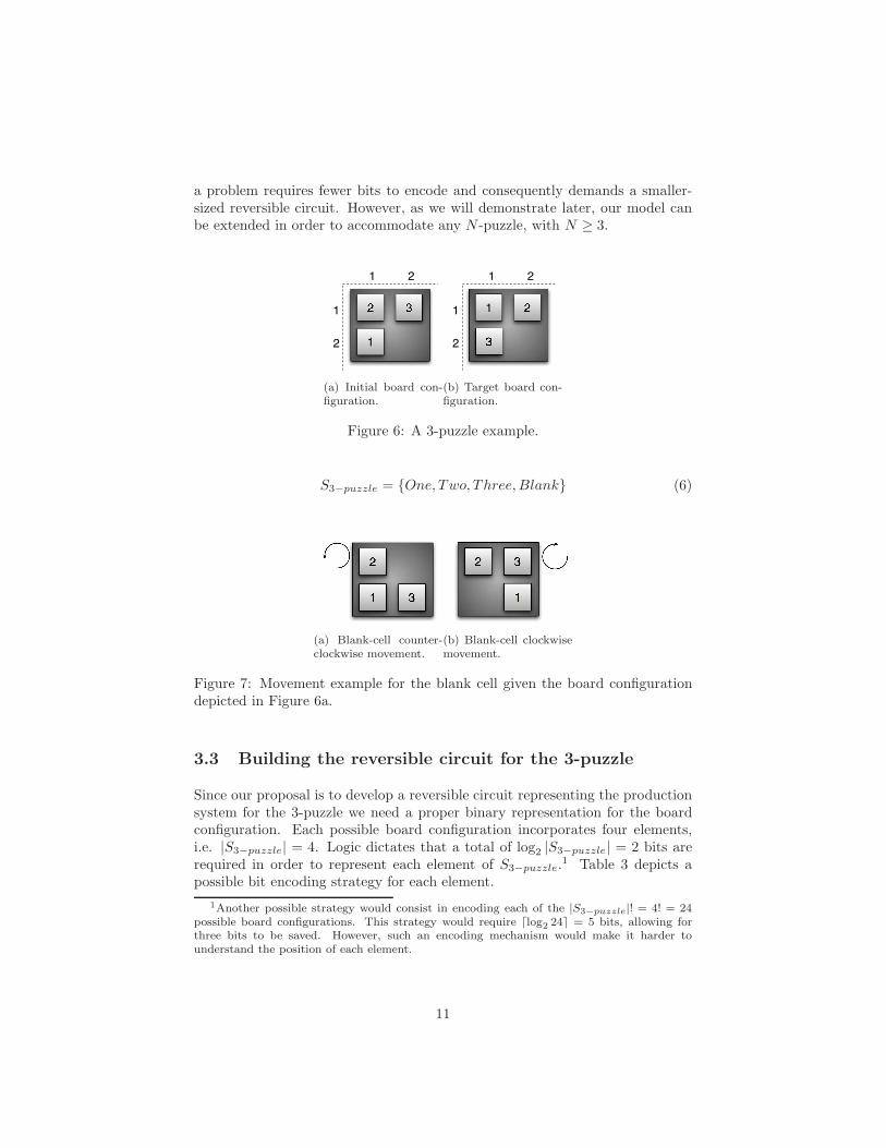
In order to proceed with the development of our quantum production systemwe will concentrate on a board with dimension 2 × 2, i.e. a 3-puzzle. Figure 6depicts a 2 × 2 sliding block puzzle with an initial board configuration (Figure6a) and a target configuration (Figure 6b). The set of possible movements forthe blank element remains the same as in the case of the 8-puzzle, respectivelyillustrated in Expression 5. However, for the 3-puzzle, at any given positiononly two movements are deemed possible to be executed. Since the blank cellalways occupies a corner position, its movement can be perceived as performinga clockwise or counter-clockwise movement. Figure 7 illustrates the states ob-tained after performing counter-clockwise and clockwise movements for the ini-tial board configuration presented in Figure 6a. The set of possible elements forthe 3-puzzle, S3−puzzle, is presented in Expression 6. We choose to focus on theconcepts surrounding a 3-puzzle board merely for practical reasons, since such

10

a problem requires fewer bits to encode and consequently demands a smaller-sized reversible circuit. However, as we will demonstrate later, our model canbe extended in order to accommodate any N -puzzle, with N ≥ 3.

2 3

1

1 2

1

2

(a) Initial board con-figuration.

2

3

1

1 2

1

2

(b) Target board con-figuration.

Figure 6: A 3-puzzle example.

S3−puzzle = One, Two, Three,Blank (6)

2

31

(a) Blank-cell counter-clockwise movement.

2 3

1

(b) Blank-cell clockwisemovement.

Figure 7: Movement example for the blank cell given the board configurationdepicted in Figure 6a.

3.3 Building the reversible circuit for the 3-puzzle

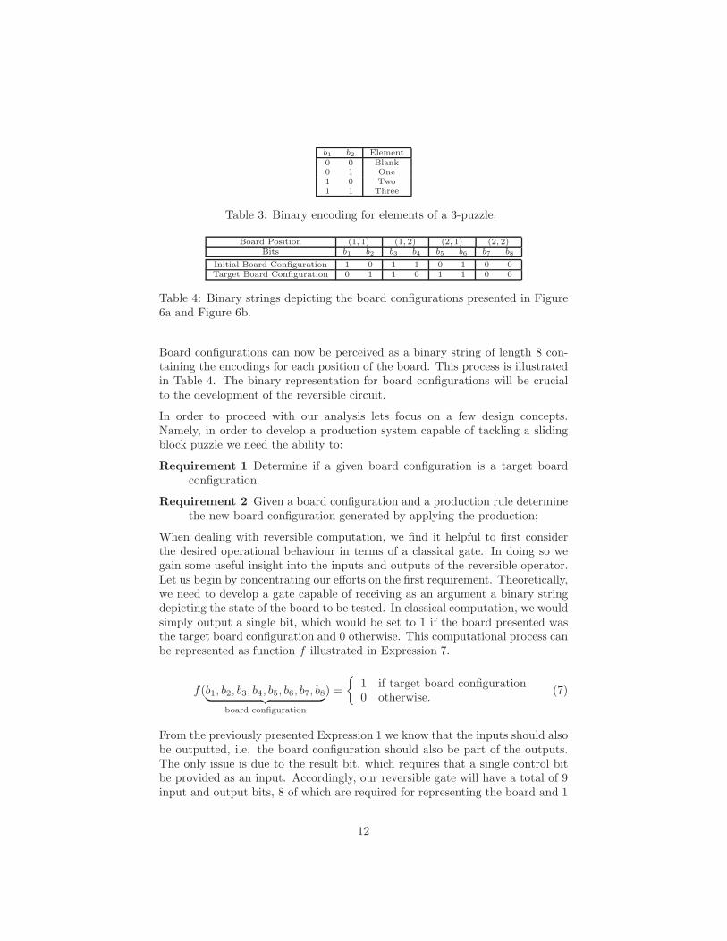
Since our proposal is to develop a reversible circuit representing the productionsystem for the 3-puzzle we need a proper binary representation for the boardconfiguration. Each possible board configuration incorporates four elements,i.e. |S3−puzzle| = 4. Logic dictates that a total of log2 |S3−puzzle| = 2 bits arerequired in order to represent each element of S3−puzzle.

1 Table 3 depicts apossible bit encoding strategy for each element.

1Another possible strategy would consist in encoding each of the |S3−puzzle|! = 4! = 24possible board configurations. This strategy would require ⌈log2 24⌉ = 5 bits, allowing forthree bits to be saved. However, such an encoding mechanism would make it harder tounderstand the position of each element.

11

b1 b2 Element0 0 Blank0 1 One1 0 Two1 1 Three

Table 3: Binary encoding for elements of a 3-puzzle.

Board Position (1, 1) (1, 2) (2, 1) (2, 2)Bits b1 b2 b3 b4 b5 b6 b7 b8

Initial Board Configuration 1 0 1 1 0 1 0 0Target Board Configuration 0 1 1 0 1 1 0 0

Table 4: Binary strings depicting the board configurations presented in Figure6a and Figure 6b.

Board configurations can now be perceived as a binary string of length 8 con-taining the encodings for each position of the board. This process is illustratedin Table 4. The binary representation for board configurations will be crucialto the development of the reversible circuit.

In order to proceed with our analysis lets focus on a few design concepts.Namely, in order to develop a production system capable of tackling a slidingblock puzzle we need the ability to:

Requirement 1 Determine if a given board configuration is a target boardconfiguration.

Requirement 2 Given a board configuration and a production rule determinethe new board configuration generated by applying the production;

When dealing with reversible computation, we find it helpful to first considerthe desired operational behaviour in terms of a classical gate. In doing so wegain some useful insight into the inputs and outputs of the reversible operator.Let us begin by concentrating our efforts on the first requirement. Theoretically,we need to develop a gate capable of receiving as an argument a binary stringdepicting the state of the board to be tested. In classical computation, we wouldsimply output a single bit, which would be set to 1 if the board presented wasthe target board configuration and 0 otherwise. This computational process canbe represented as function f illustrated in Expression 7.

f(b1, b2, b3, b4, b5, b6, b7, b8︸ ︷︷ ︸

board configuration

) =

1 if target board configuration0 otherwise.

(7)

From the previously presented Expression 1 we know that the inputs should alsobe outputted, i.e. the board configuration should also be part of the outputs.The only issue is due to the result bit, which requires that a single control bitbe provided as an input. Accordingly, our reversible gate will have a total of 9input and output bits, 8 of which are required for representing the board and 1

12

Inputs Outputsb1 b2 b3 b4 b5 b6 b7 b8 c b1 b2 b3 b4 b5 b6 b7 b8 c ⊕ f(b)

0 0 0 1 1 0 1 1 0 0 0 0 1 1 0 1 1 0

0 0 0 1 1 0 1 1 1 0 0 0 1 1 0 1 1 1

0 0 0 1 1 1 1 0 0 0 0 0 1 1 1 1 0 0

0 0 0 1 1 1 1 0 1 0 0 0 1 1 1 1 0 1

.

.

.

.

.

.

.

.

.

.

.

.

.

.

.

.

.

.

.

.

.

.

.

.

.

.

.

.

.

.

.

.

.

.

.

.

.

.

.

.

.

.

.

.

.

.

.

.

.

.

.

.

.

.

0 1 1 0 1 1 0 0 0 0 1 1 0 1 1 0 0 1

0 1 1 0 1 1 0 0 1 0 1 1 0 1 1 0 0 0

.

.

.

.

.

.

.

.

.

.

.

.

.

.

.

.

.

.

.

.

.

.

.

.

.

.

.

.

.

.

.

.

.

.

.

.

.

.

.

.

.

.

.

.

.

.

.

.

.

.

.

.

.

.

1 1 1 0 0 1 0 0 0 1 1 1 0 0 1 0 0 0

1 1 1 0 0 1 0 0 1 1 1 1 0 0 1 0 0 1

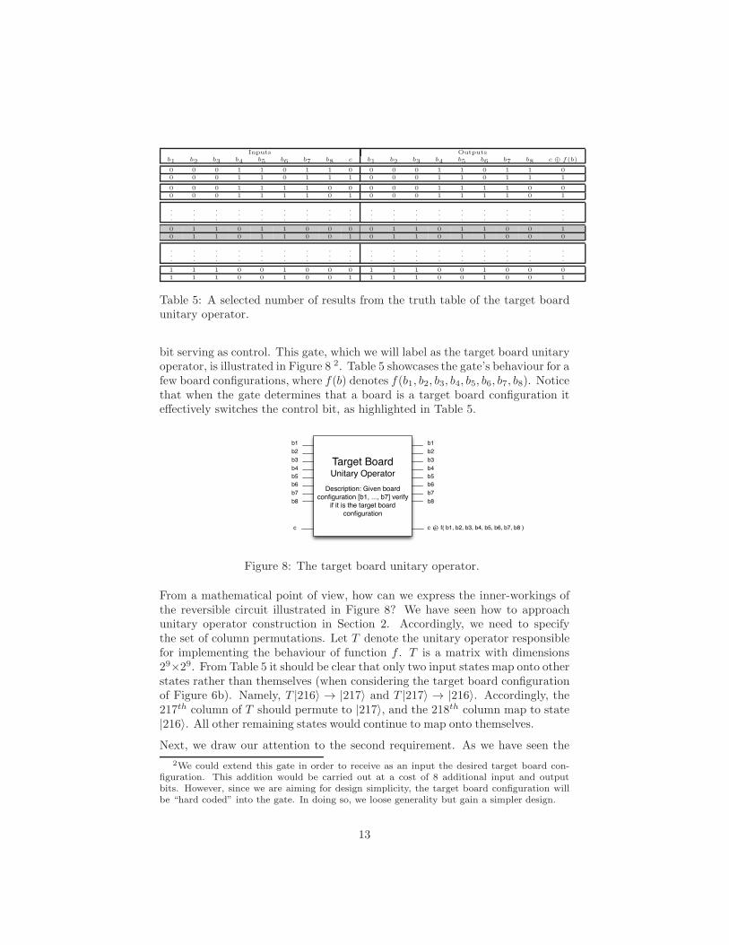
Table 5: A selected number of results from the truth table of the target boardunitary operator.

bit serving as control. This gate, which we will label as the target board unitaryoperator, is illustrated in Figure 8 2. Table 5 showcases the gate’s behaviour for afew board configurations, where f(b) denotes f(b1, b2, b3, b4, b5, b6, b7, b8). Noticethat when the gate determines that a board is a target board configuration iteffectively switches the control bit, as highlighted in Table 5.

Target BoardUnitary Operator

Description: Given board

configuration [b1, ..., b7] verify

if it is the target board

configuration

b1

b2

b3

b4

b5

b6

b7

b8

c c

b1

b2

b3

b4

b5

b6

b7

b8

f( b1, b2, b3, b4, b5, b6, b7, b8 )f( b1, b2, b3, b4, b5, b6, b7, b8 )

Figure 8: The target board unitary operator.

From a mathematical point of view, how can we express the inner-workings ofthe reversible circuit illustrated in Figure 8? We have seen how to approachunitary operator construction in Section 2. Accordingly, we need to specifythe set of column permutations. Let T denote the unitary operator responsiblefor implementing the behaviour of function f . T is a matrix with dimensions29×29. From Table 5 it should be clear that only two input states map onto otherstates rather than themselves (when considering the target board configurationof Figure 6b). Namely, T |216〉 → |217〉 and T |217〉 → |216〉. Accordingly, the217th column of T should permute to |217〉, and the 218th column map to state|216〉. All other remaining states would continue to map onto themselves.

Next, we draw our attention to the second requirement. As we have seen the

2We could extend this gate in order to receive as an input the desired target board con-figuration. This addition would be carried out at a cost of 8 additional input and outputbits. However, since we are aiming for design simplicity, the target board configuration willbe “hard coded” into the gate. In doing so, we loose generality but gain a simpler design.

13

original board configuration provided as input should also be part of the outputs.The new gate should also output a new board configuration. Also, in the contextof a production system we are interested in applying the move blank cell unitaryoperator if and only if the inputted board configuration is not a target boardconfiguration. Otherwise, the production system would systematically discardany potential solutions found. This process can be performed by including areference to function f in the new function g’s definition.

The only issue is due to how to output the new board configuration in a re-versible manner. Expression 1 illustrated how this process could be performedfor a single result bit. In this specific case we are interested in having 8 resultbits representing the new board configuration. Accordingly, since the gate mustrespect the principles of reversible computation, an additional 8 control bitsshould be included as input. Expression 1 can be extended in order to accom-modate any number of control bits, as illustrated by Expression 8 [43] where ciare control bits, and f(x) = (y1, y2, · · · , yn).

(x, c1, c2, · · · , cn) 7→ (x, c1 ⊕ y1, c2 ⊕ y2, · · · , cn ⊕ yn) (8)

Such a reversible gate formulation will require 2(⌈log2 x⌉ + n) input and out-put bits, whilst its irreversible equivalent would be satisfied with ⌈log2 x⌉ + n

bits. Again, both versions differ by a constant factor k = 2. From a compu-tational complexity perspective such a factor effectively doubles the space em-ployed by a reversible formulation when compared against classical irreversibleones. However, since such growth is not exponential it can still be described asmoderate.

Expression 8 makes it possible to define a function g responsible for produc-ing the new board configuration. Function g should receive as inputs the cur-rent board configuration and a bit m indicating whether the blank cell shouldperform a clockwise (m = 1) or counter-clockwise movement (m = 0). Bysystematically checking for the position of the blank cell and with the move-ment described in bit m we can generate the new board configuration. Letg : 0, 19 → 0, 18 with g(b,m) = (y1, y2, y3, y4, y5, y6, y7, y8), where b denotesa valid board configuration (b1, b2, b3, b4, b5, b6, b7, b8), and m the type of move-ment. By valid board configuration we mean that a board configuration must bean un-ordered collection of size four composed of distinct elements taken from

14

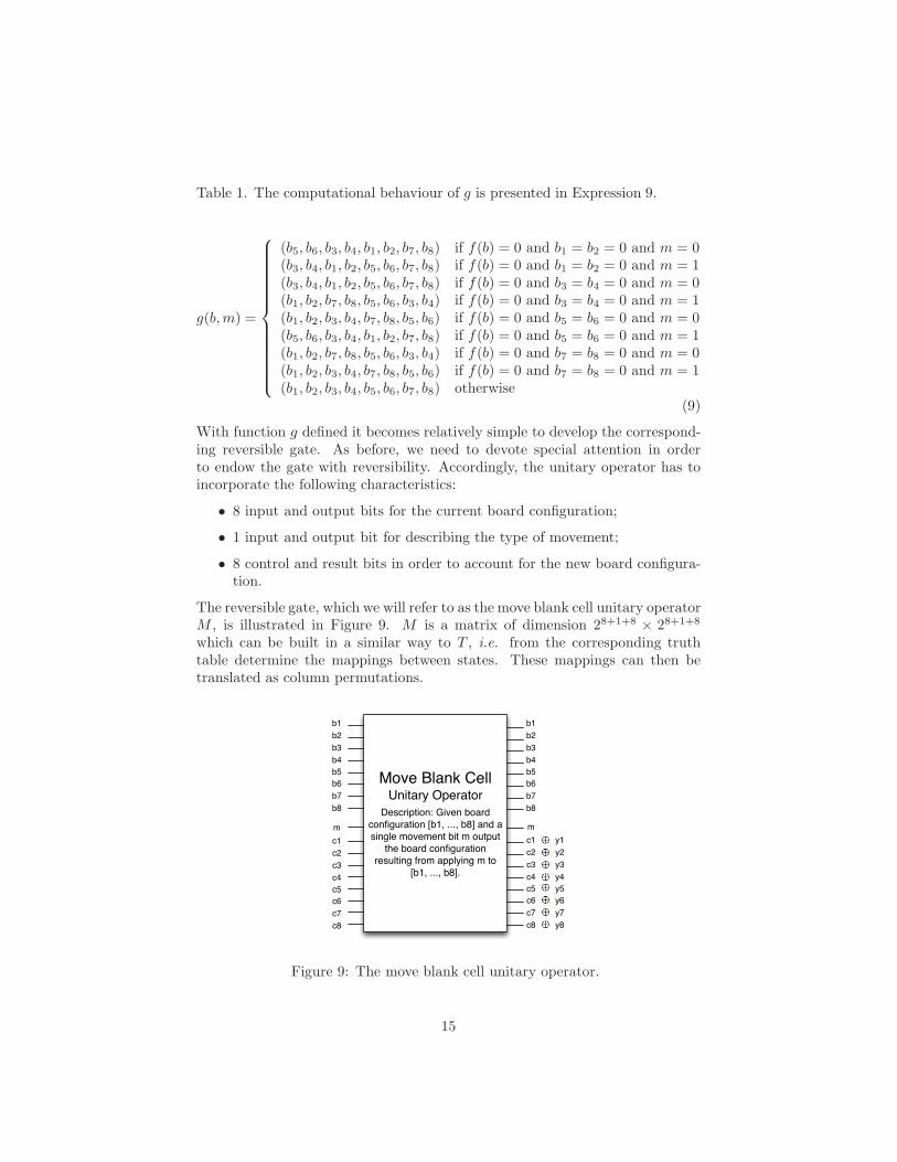
Table 1. The computational behaviour of g is presented in Expression 9.

g(b,m) =

(b5, b6, b3, b4, b1, b2, b7, b8) if f(b) = 0 and b1 = b2 = 0 and m = 0(b3, b4, b1, b2, b5, b6, b7, b8) if f(b) = 0 and b1 = b2 = 0 and m = 1(b3, b4, b1, b2, b5, b6, b7, b8) if f(b) = 0 and b3 = b4 = 0 and m = 0(b1, b2, b7, b8, b5, b6, b3, b4) if f(b) = 0 and b3 = b4 = 0 and m = 1(b1, b2, b3, b4, b7, b8, b5, b6) if f(b) = 0 and b5 = b6 = 0 and m = 0(b5, b6, b3, b4, b1, b2, b7, b8) if f(b) = 0 and b5 = b6 = 0 and m = 1(b1, b2, b7, b8, b5, b6, b3, b4) if f(b) = 0 and b7 = b8 = 0 and m = 0(b1, b2, b3, b4, b7, b8, b5, b6) if f(b) = 0 and b7 = b8 = 0 and m = 1(b1, b2, b3, b4, b5, b6, b7, b8) otherwise

(9)

With function g defined it becomes relatively simple to develop the correspond-ing reversible gate. As before, we need to devote special attention in orderto endow the gate with reversibility. Accordingly, the unitary operator has toincorporate the following characteristics:

• 8 input and output bits for the current board configuration;

• 1 input and output bit for describing the type of movement;

• 8 control and result bits in order to account for the new board configura-tion.

The reversible gate, which we will refer to as the move blank cell unitary operatorM , is illustrated in Figure 9. M is a matrix of dimension 28+1+8 × 28+1+8

which can be built in a similar way to T , i.e. from the corresponding truthtable determine the mappings between states. These mappings can then betranslated as column permutations.

Move Blank CellUnitary Operator

Description: Given board

configuration [b1, ..., b8] and a

single movement bit m output

the board configuration

resulting from applying m to

[b1, ..., b8].

b1

b2

b3

b4

b5

b6

b7

b8

c1

c2

c3

c4

c5

c6

c7

c8

m

b1

b2

b3

b4

b5

b6

b7

b8

c1

c2

c3

c4

c5

c6

c7

c8

m

y1

y2

y3

y4

y5

y6

y7

y8

Figure 9: The move blank cell unitary operator.

15

With both the target board and the move blank cell gates designed we are now ina position to continue with the development of our reversible production system.Recall that a production system has the following elements: working memory,set of production rules and a control strategy. The auxiliary bits employed byeach of the previously defined gates can be perceived as the working memory ofthe system. Functions f and g can be seen as enforcing the policies of a controland act cycle specific to the problem at hand. For now we will be deliberatelyomissive regarding the set of production rules. Instead, we will focus on certainfeatures of the working memory and control strategy.

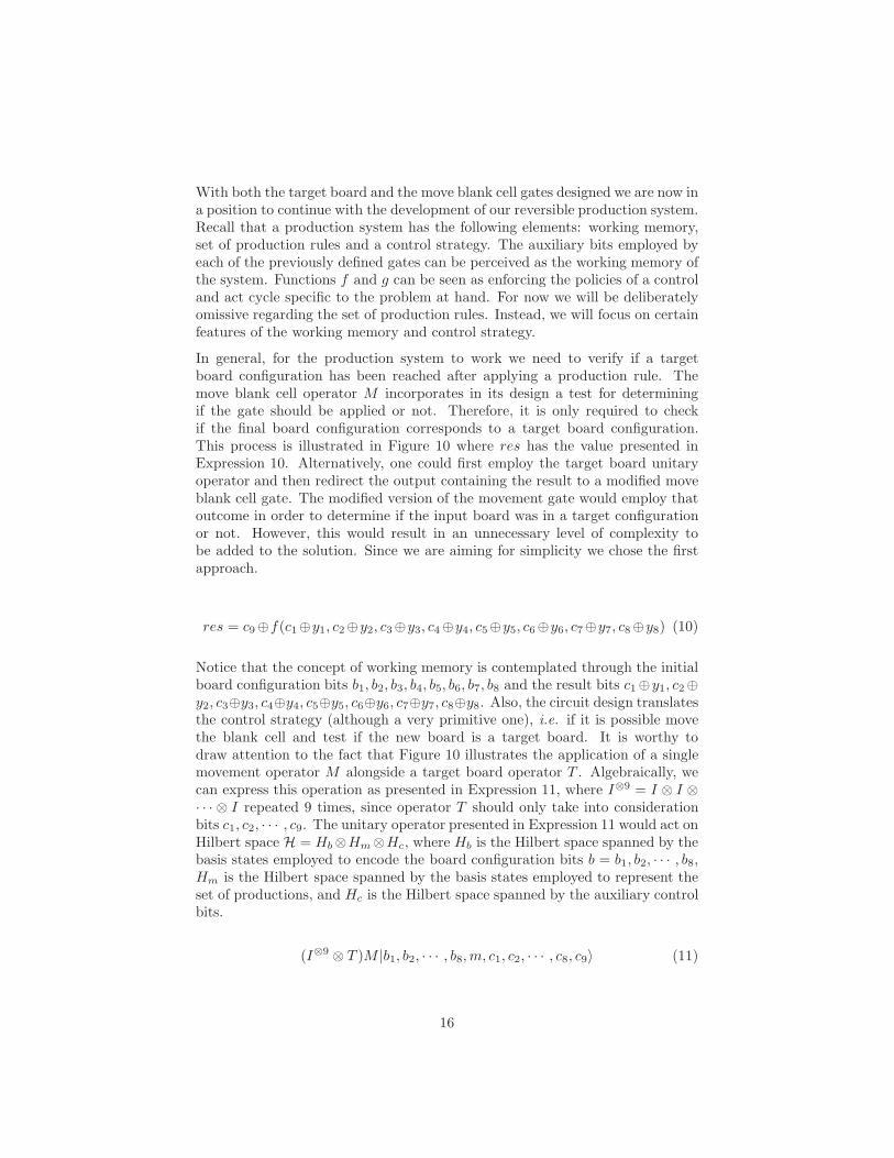
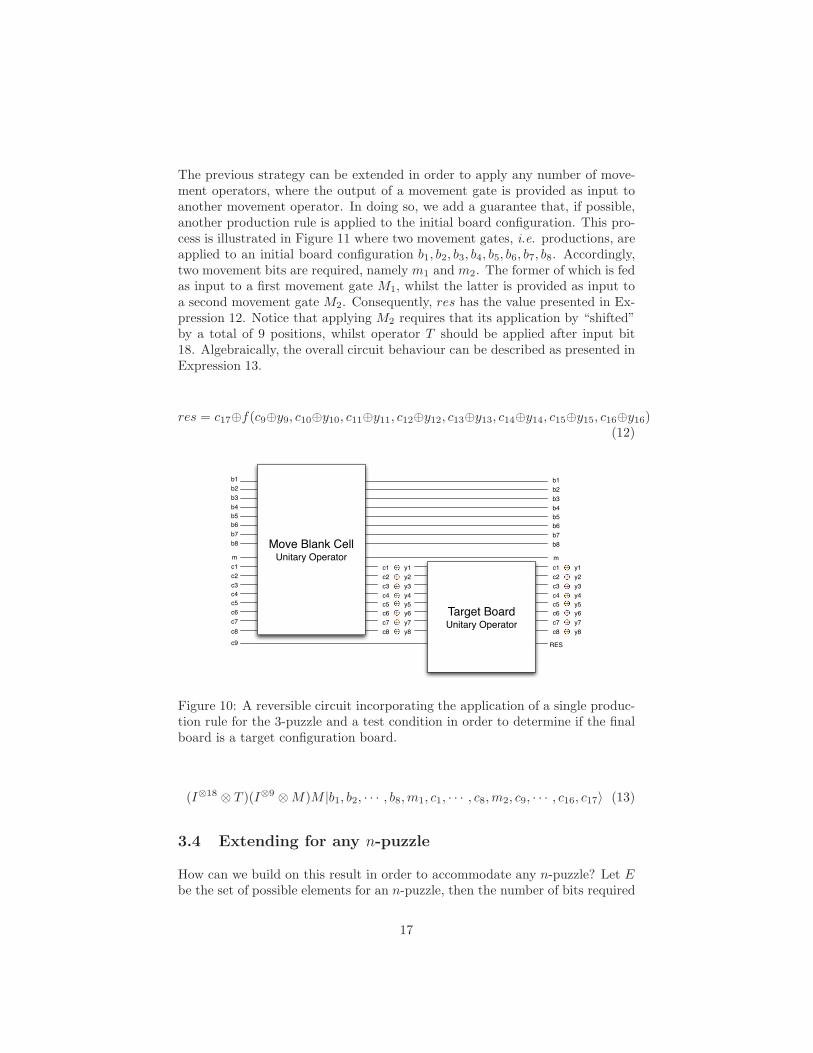
In general, for the production system to work we need to verify if a targetboard configuration has been reached after applying a production rule. Themove blank cell operator M incorporates in its design a test for determiningif the gate should be applied or not. Therefore, it is only required to checkif the final board configuration corresponds to a target board configuration.This process is illustrated in Figure 10 where res has the value presented inExpression 10. Alternatively, one could first employ the target board unitaryoperator and then redirect the output containing the result to a modified moveblank cell gate. The modified version of the movement gate would employ thatoutcome in order to determine if the input board was in a target configurationor not. However, this would result in an unnecessary level of complexity tobe added to the solution. Since we are aiming for simplicity we chose the firstapproach.

res = c9⊕f(c1⊕y1, c2⊕y2, c3⊕y3, c4⊕y4, c5⊕y5, c6⊕y6, c7⊕y7, c8⊕y8) (10)

Notice that the concept of working memory is contemplated through the initialboard configuration bits b1, b2, b3, b4, b5, b6, b7, b8 and the result bits c1⊕y1, c2⊕y2, c3⊕y3, c4⊕y4, c5⊕y5, c6⊕y6, c7⊕y7, c8⊕y8. Also, the circuit design translatesthe control strategy (although a very primitive one), i.e. if it is possible movethe blank cell and test if the new board is a target board. It is worthy todraw attention to the fact that Figure 10 illustrates the application of a singlemovement operator M alongside a target board operator T . Algebraically, wecan express this operation as presented in Expression 11, where I⊗9 = I ⊗ I ⊗· · · ⊗ I repeated 9 times, since operator T should only take into considerationbits c1, c2, · · · , c9. The unitary operator presented in Expression 11 would act onHilbert space H = Hb⊗Hm⊗Hc, where Hb is the Hilbert space spanned by thebasis states employed to encode the board configuration bits b = b1, b2, · · · , b8,Hm is the Hilbert space spanned by the basis states employed to represent theset of productions, and Hc is the Hilbert space spanned by the auxiliary controlbits.

(I⊗9 ⊗ T )M |b1, b2, · · · , b8,m, c1, c2, · · · , c8, c9〉 (11)

16

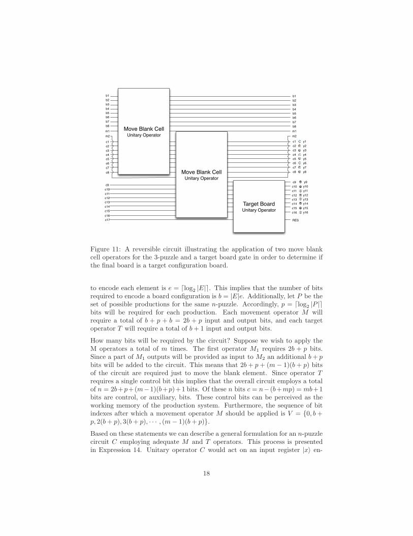
The previous strategy can be extended in order to apply any number of move-ment operators, where the output of a movement gate is provided as input toanother movement operator. In doing so, we add a guarantee that, if possible,another production rule is applied to the initial board configuration. This pro-cess is illustrated in Figure 11 where two movement gates, i.e. productions, areapplied to an initial board configuration b1, b2, b3, b4, b5, b6, b7, b8. Accordingly,two movement bits are required, namely m1 and m2. The former of which is fedas input to a first movement gate M1, whilst the latter is provided as input toa second movement gate M2. Consequently, res has the value presented in Ex-pression 12. Notice that applying M2 requires that its application by “shifted”by a total of 9 positions, whilst operator T should be applied after input bit18. Algebraically, the overall circuit behaviour can be described as presented inExpression 13.

res = c17⊕f(c9⊕y9, c10⊕y10, c11⊕y11, c12⊕y12, c13⊕y13, c14⊕y14, c15⊕y15, c16⊕y16)(12)

b1

b2

b3

b4

b5

b6

b7

b8

m

c1

c2

c3

c4

c5

c6

c7

c8

c9

b1

b2

b3

b4

b5

b6

b7

b8

c1

c2

c3

c4

c5

c6

c7

c8

y1

y2

y3

y4

y5

y6

y7

y8

m

c1

c2

c3

c4

c5

c6

c7

c8

y1

y2

y3

y4

y5

y6

y7

y8

Target BoardUnitary Operator

Move Blank CellUnitary Operator

RES

Figure 10: A reversible circuit incorporating the application of a single produc-tion rule for the 3-puzzle and a test condition in order to determine if the finalboard is a target configuration board.

(I⊗18 ⊗ T )(I⊗9 ⊗M)M |b1, b2, · · · , b8,m1, c1, · · · , c8,m2, c9, · · · , c16, c17〉 (13)

3.4 Extending for any n-puzzle

How can we build on this result in order to accommodate any n-puzzle? Let Ebe the set of possible elements for an n-puzzle, then the number of bits required

17

b1

b2

b3

b4

b5

b6

b7

b8

m1

c1

c2

c3

c4

c5

c6

c7

c8

b1

b2

b3

b4

b5

b6

b7

b8

m1

c1

c2

c3

c4

c5

c6

c7

c8

y1

y2

y3

y4

y5

y6

y7

y8

c9

c10

c11

c12

c13

c14

c15

c16

m2

c17

c9

c10

c11

c12

c13

c14

c15

c16

y9

y10

y11

y12

y13

y14

y15

y16

m2

Target BoardUnitary Operator

Move Blank CellUnitary Operator

Move Blank CellUnitary Operator

RES

Figure 11: A reversible circuit illustrating the application of two move blankcell operators for the 3-puzzle and a target board gate in order to determine ifthe final board is a target configuration board.

to encode each element is e = ⌈log2 |E|⌉. This implies that the number of bitsrequired to encode a board configuration is b = |E|e. Additionally, let P be theset of possible productions for the same n-puzzle. Accordingly, p = ⌈log2 |P |⌉bits will be required for each production. Each movement operator M willrequire a total of b + p + b = 2b + p input and output bits, and each targetoperator T will require a total of b+ 1 input and output bits.

How many bits will be required by the circuit? Suppose we wish to apply theM operators a total of m times. The first operator M1 requires 2b + p bits.Since a part of M1 outputs will be provided as input to M2 an additional b+ p

bits will be added to the circuit. This means that 2b+ p+ (m− 1)(b + p) bitsof the circuit are required just to move the blank element. Since operator Trequires a single control bit this implies that the overall circuit employs a totalof n = 2b+p+(m−1)(b+p)+1 bits. Of these n bits c = n− (b+mp) = mb+1bits are control, or auxiliary, bits. These control bits can be perceived as theworking memory of the production system. Furthermore, the sequence of bitindexes after which a movement operator M should be applied is V = 0, b +p, 2(b+ p), 3(b+ p), · · · , (m− 1)(b+ p).Based on these statements we can describe a general formulation for an n-puzzlecircuit C employing adequate M and T operators. This process is presentedin Expression 14. Unitary operator C would act on an input register |x〉 en-

18

compassing the initial board configuration, the set of productions and also theauxiliary control bits. Accordingly, operator C would act upon a Hilbert spaceH spanned by the computational basis states required to encode x.

C = (I⊗m(b+p) ⊗ T )∏

k∈V

(I⊗k ⊗M

)(14)

Finally, the number of movement operators M grows linearly with the depthof the search, which is a key component of the input register. The reversiblecircuits presented in Figure 10 Figure 11 apply, respectively, one and two move-ment gates, the former can be perceived as performing a depth-limited searchof level 1, whilst the latter performs a search up to depth 2. This is a com-mon strategy in computer science where a cutoff is performed at a depth-leveld in order to provide an answer in a constant time. Traditionally, some typeof heuristic function is employed in order to help decide which state may becloser to providing a solution. In addition, our proposition only contemplatestree-search involving a constant branching factor. However, it is not unusualfor tree-search to deal with non-constant branching factors. Since potential en-coding strategies are always required to reflect the complete range of actionsthis fact can adversely affect the performance of the system when comparedagainst classical equivalent. This is due Grover’s speedup being a function ofthe number of bits n employed. For more on these issues we refer the reader to[50] which presents a detailed examination.

4 Quantum extensions

Hitherto, we have only focused on how to build a reversible circuit for the3-puzzle. However, reversible computation by itself does not provide any com-putational advantage. In order to gain a quantum advantage we need to employquantum superpositions alongside Grover’s algorithm. The following sectionsare organized as follows: Section 4.1 presents the quantum superposition prin-ciple; Section 4.2 introduces Grover’s algorithm and Section 4.3 builds on theseresults to illustrate how the proposed reversible circuit can be extended in orderto reap the benefits provided by quantum computation.

4.1 Quantum superpositions

The quantum superposition principle allows a register to be in several states atthe same time. Associated with each quantum state i is an amplitude αi ∈ C.By requiring the vector (α1, · · · , αn) to be unit-length preserving we ensurethat |α1|2 + · · · + |αn|2 = 1, where n is the number of states. Since we havea set of values that sum up to 1 then the |αi|2 values may be considered astranslating the probability of observing state i. However, due to the effects of

19

a process known as quantum decoherence only one of the states conveying theanswer can be obtained. This collapse from a multitude of states into a single onetakes into account the probabilities associated with each state [40]. Accordingly,states with a higher probability are more likely to be obtained, whilst stateswith smaller probabilities are less likely to be obtained. Notice that this doesnot imply that only those states with higher probabilities will be obtained.The Hadamard gate allows one to configure an input register configured tostate |00 · · ·0〉 in an uniform superposition of 2n states, where n is the numberof bits of the input register. This behaviour is presented in Expression 15.Traditionally, the |ψ〉 symbol is employed to denote a superposition of values.Superposition |ψ〉 can be employed alongside unitary operator C, a proceduretranslated as C|ψ〉, which effectively evaluates all possible states in a singlecomputational step.

|ψ〉 = H⊗n |00 · · · 0〉︸ ︷︷ ︸

n bits

=1√2n

︸ ︷︷ ︸

amplitude

2n−1∑

x=0

|x〉 (15)

In order to proceed with our analysis lets concentrate on the circuit presentedin Figure 10. Conceptually, we can differentiate between three inputs, respec-tively:

• the board configuration bits, b1, b2, · · · , b8 which we will refer to as an8-bit register |b〉.

• the movement bit m, which is basically a one bit register |m〉;• the control bits, c1, c2, · · · , c17, which we will refer to as a 17-bit register|c〉.

Let Ug refer to the unitary operator characterizing the reversible circuit pre-sented in Figure 10. The behaviour of Ug can be described as illustrated byExpression 16.

Ug : |b〉|m〉|c〉 7→ |b〉|m〉|c1⊕y1, c2⊕y2, c3⊕y3, c4⊕y4, c5⊕y5, c6⊕y6, c7⊕y7, c8⊕y8, res〉(16)

The input register |b〉|m〉|c〉 can be configured to a specified value and by apply-ing Ug it becomes possible to obtain the respective result. In the specific case ofthe unitary operator Ug we are interested in evaluating a combined superposi-tion containing all possible board configurations and productions. The controlbits not need not to be placed in a superposition since they are only employedin order to assist the overall process. Accordingly, the control bit register canbe configured to |0〉⊗c, where c is the number of control bits. Let |ψ〉 denotethe superposition of all board configurations, |ψb〉, and productions, |ψm〉 , asillustrated in Expression 17.

20

|ψ〉 = |ψb〉|ψm〉|0〉⊗c

=1√28

28−1∑

x=0

|x〉 1√21

21−1∑

x=0

|x〉|0〉⊗c

=1√29

29−1∑

x=0

|x〉|0〉⊗c (17)

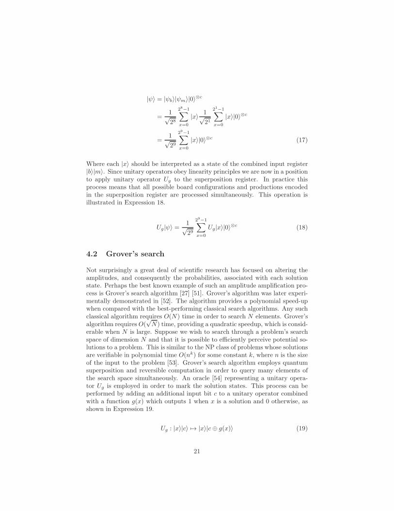
Where each |x〉 should be interpreted as a state of the combined input register|b〉|m〉. Since unitary operators obey linearity principles we are now in a positionto apply unitary operator Ug to the superposition register. In practice thisprocess means that all possible board configurations and productions encodedin the superposition register are processed simultaneously. This operation isillustrated in Expression 18.

Ug|ψ〉 =1√29

29−1∑

x=0

Ug|x〉|0〉⊗c (18)

4.2 Grover’s search

Not surprisingly a great deal of scientific research has focused on altering theamplitudes, and consequently the probabilities, associated with each solutionstate. Perhaps the best known example of such an amplitude amplification pro-cess is Grover’s search algorithm [27] [51]. Grover’s algorithm was later experi-mentally demonstrated in [52]. The algorithm provides a polynomial speed-upwhen compared with the best-performing classical search algorithms. Any suchclassical algorithm requires O(N) time in order to search N elements. Grover’salgorithm requires O(

√N) time, providing a quadratic speedup, which is consid-

erable when N is large. Suppose we wish to search through a problem’s searchspace of dimension N and that it is possible to efficiently perceive potential so-lutions to a problem. This is similar to the NP class of problems whose solutionsare verifiable in polynomial time O(nk) for some constant k, where n is the sizeof the input to the problem [53]. Grover’s search algorithm employs quantumsuperposition and reversible computation in order to query many elements ofthe search space simultaneously. An oracle [54] representing a unitary opera-tor Ug is employed in order to mark the solution states. This process can beperformed by adding an additional input bit c to a unitary operator combinedwith a function g(x) which outputs 1 when x is a solution and 0 otherwise, asshown in Expression 19.

Ug : |x〉|c〉 7→ |x〉|c⊕ g(x)〉 (19)

21

The algorithm then employs a process of amplitude amplification, known asGrover’s iterate, in order to amplify the amplitudes of the solutions and in theprocess diminish those of the non-solutions. This process is performed by settingthe control register c to a specified value, which, when combined with Grover’siterate can be mathematically proven to perform an inversion about the meanof the amplitudes [43]. As a direct result of Grover’s iterate, the probability ofthe solution states increases. However, the amplitude of the solution value isamplified only in a linear way. If the function g is provided as a black box, thenΩ(

√N) applications of the black box are necessary in order to solve the search

problem with high probability for any input [54] A number of improvementshave been proposed since Grover’s original work [55] [56]. These improvementsessentially targeted reduced time complexity bounds for non-query operationsand overall robustness. For a number of several novel search related applicationsplease refer to [51] [57] [58].

4.3 Oracle development

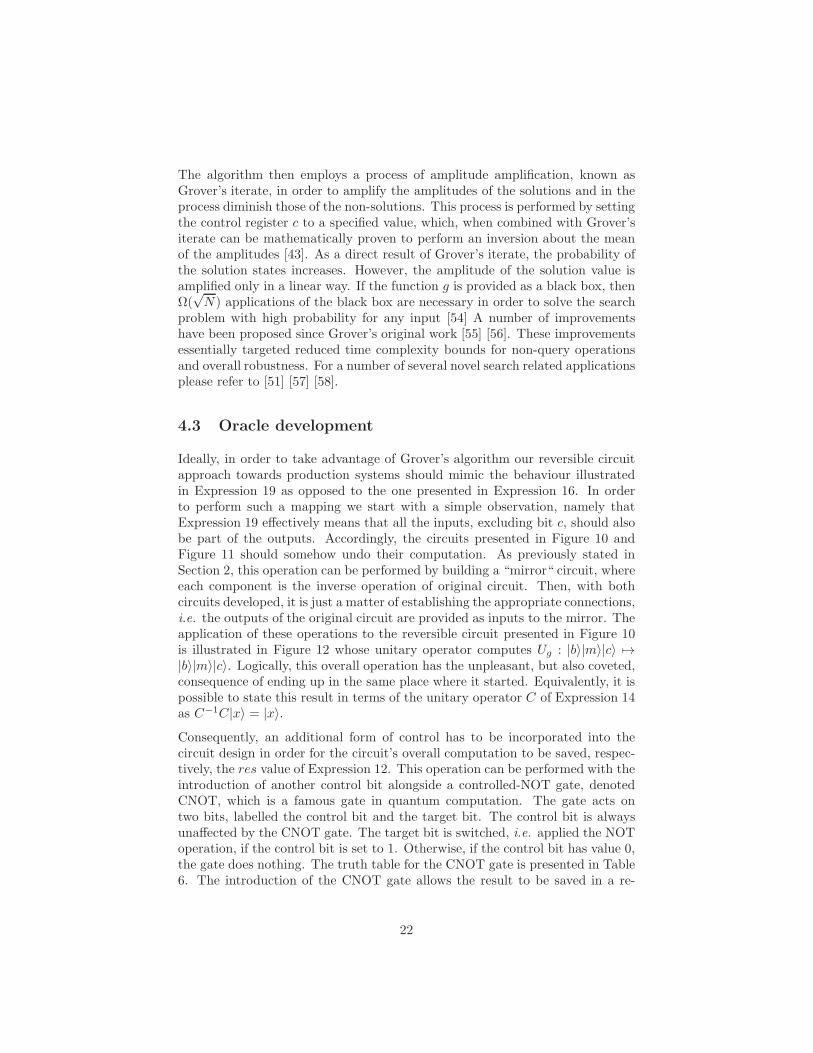
Ideally, in order to take advantage of Grover’s algorithm our reversible circuitapproach towards production systems should mimic the behaviour illustratedin Expression 19 as opposed to the one presented in Expression 16. In orderto perform such a mapping we start with a simple observation, namely thatExpression 19 effectively means that all the inputs, excluding bit c, should alsobe part of the outputs. Accordingly, the circuits presented in Figure 10 andFigure 11 should somehow undo their computation. As previously stated inSection 2, this operation can be performed by building a “mirror“ circuit, whereeach component is the inverse operation of original circuit. Then, with bothcircuits developed, it is just a matter of establishing the appropriate connections,i.e. the outputs of the original circuit are provided as inputs to the mirror. Theapplication of these operations to the reversible circuit presented in Figure 10is illustrated in Figure 12 whose unitary operator computes Ug : |b〉|m〉|c〉 7→|b〉|m〉|c〉. Logically, this overall operation has the unpleasant, but also coveted,consequence of ending up in the same place where it started. Equivalently, it ispossible to state this result in terms of the unitary operator C of Expression 14as C−1C|x〉 = |x〉.Consequently, an additional form of control has to be incorporated into thecircuit design in order for the circuit’s overall computation to be saved, respec-tively, the res value of Expression 12. This operation can be performed with theintroduction of another control bit alongside a controlled-NOT gate, denotedCNOT, which is a famous gate in quantum computation. The gate acts ontwo bits, labelled the control bit and the target bit. The control bit is alwaysunaffected by the CNOT gate. The target bit is switched, i.e. applied the NOToperation, if the control bit is set to 1. Otherwise, if the control bit has value 0,the gate does nothing. The truth table for the CNOT gate is presented in Table6. The introduction of the CNOT gate allows the result to be saved in a re-

22

b1

b2

b3

b4

b5

b6

b7

b8

m

c1

c2

c3

c4

c5

c6

c7

c8

c9

b1

b2

b3

b4

b5

b6

b7

b8

m

c1

c2

c3

c4

c5

c6

c7

c8

c9

Move Blank Cell^(-1)

Unitary Operator

Move Blank CellUnitary Operator

Target BoardUnitary Operator

Target Board^(-1)Unitary Operator

Figure 12: A reversible circuit showcasing the application of a single movementgate for the 3-puzzle, and then undoing the previously performed computations.

Inputs Outputsc t c c ⊕ t

0 0 0 00 1 0 11 0 1 11 1 1 0

Table 6: Truth table for the CNOT gate.

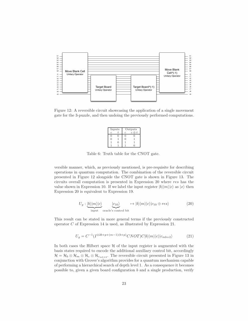
versible manner, which, as previously mentioned, is pre-requisite for describingoperations in quantum computation. The combination of the reversible circuitpresented in Figure 12 alongside the CNOT gate is shown in Figure 13. Thecircuits overall computation is presented in Expression 20 where res has thevalue shown in Expression 10. If we label the input register |b〉|m〉|c〉 as |x〉 thenExpression 20 is equivalent to Expression 19.

Ug : |b〉|m〉|c〉︸ ︷︷ ︸

input

|c10〉︸︷︷︸

oracle’s control bit

7→ |b〉|m〉|c〉|c10 ⊕ res〉 (20)

This result can be stated in more general terms if the previously constructedoperator C of Expression 14 is used, as illustrated by Expression 21.

Ug = C−1(I⊗2b+p+(m−1)(b+p)CNOT )C|b〉|m〉|c〉|cmb+2〉 (21)

In both cases the Hilbert space H of the input register is augmented with thebasis states required to encode the additional auxiliary control bit, accordinglyH = Hb ⊗Hm ⊗Hc ⊗Hcmb+2

. The reversible circuit presented in Figure 13 inconjunction with Grover’s algorithm provides for a quantum mechanism capableof performing a hierarchical search of depth level 1. As a consequence it becomespossible to, given a given board configuration b and a single production, verify

23

b1

b2

b3

b4

b5

b6

b7

b8

m

c1

c2

c3

c4

c5

c6

c7

c8

c9

b1

b2

b3

b4

b5

b6

b7

b8

m

c1

c2

c3

c4

c5

c6

c7

c8

c9

c10 CNOT

Move Blank Cell^(-1)

Unitary Operator

Move Blank CellUnitary Operator

Target BoardUnitary Operator

Target Board^(-1)Unitary Operator

RES

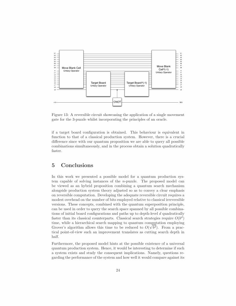
Figure 13: A reversible circuit showcasing the application of a single movementgate for the 3-puzzle whilst incorporating the principles of an oracle.

if a target board configuration is obtained. This behaviour is equivalent infunction to that of a classical production system. However, there is a crucialdifference since with our quantum proposition we are able to query all possiblecombinations simultaneously, and in the process obtain a solution quadraticallyfaster.

5 Conclusions

In this work we presented a possible model for a quantum production sys-tem capable of solving instances of the n-puzzle. The proposed model canbe viewed as an hybrid proposition combining a quantum search mechanismalongside production system theory adjusted so as to convey a clear emphasison reversible computation. Developing the adequate reversible circuit requires amodest overhead on the number of bits employed relative to classical irreversibleversions. These concepts, combined with the quantum superposition principle,can be used in order to query the search space spanned by all possible combina-tions of initial board configurations and paths up to depth-level d quadraticallyfaster than its classical counterparts. Classical search strategies require O(bd)time, while a hierarchical search mapping to quantum computation employingGrover’s algorithm allows this time to be reduced to O(

√bd). From a prac-

tical point-of-view such an improvement translates as cutting search depth inhalf.

Furthermore, the proposed model hints at the possible existence of a universalquantum production system. Hence, it would be interesting to determine if sucha system exists and study the consequent implications. Namely, questions re-garding the performance of the system and how well it would compare against its

24

classical counterpart would be relevant. In addition, the dynamics of productionsystem theory make it well suited for exploitation by classical learning mecha-nisms. This makes it plausible for the unitary operator, and consequently thereversible circuit associated, to be developed by such mechanisms. Additionalissues may focus on determining appropriate choices for search-depth d and if arelated technique is used during problem solving by human cognition.

6 Acknowledgments

This work was supported by FCT (INESC-ID multiannual funding) through thePIDDAC Program funds and FCT grant DFRH - SFRH/BD/61846/2009.

References

[1] Busemeyer JR, Wang Z, Townsend JT. Quantum dynamics of humandecision-making. Journal of Mathematical Psychology. 2006;50(3):220 –241. Jean-Claude Falmagne: Part II.

[2] Busemeyer JR, Trueblood J. Comparison of Quantum and Bayesian Infer-ence Models. In: Bruza P, Sofge D, Lawless W, van Rijsbergen K, KluschM, editors. Quantum Interaction. vol. 5494 of Lecture Notes in ComputerScience. Springer Berlin / Heidelberg; 2009. p. 29–43. 10.1007/978-3-642-00834-4-5.

[3] Busemeyer JR, Wang Z, Lambert-Mogiliansky A. Empirical comparison ofMarkov and quantum models of decision making. Journal of MathematicalPsychology. 2009;53(5):423 – 433. Special Issue: Quantum Cognition.

[4] Pothos EM, Busemeyer JR. A quantum probability explanation for vio-lations of ‘rational’ decision theory. Proceedings of the Royal Society B:Biological Sciences. 2009;.

[5] Trueblood J, Busemeyer JR. A Comparison of the Belief-Adjustment Modeland the Quantum Inference Model as Explanations of Order Effects inHuman Inference. In: COGSCI 2010 The annual meeting of the cognitivescience society; 2010. p. 1166–1171.

[6] Luger GF, Stubblefield WA. Artificial Intelligence: Structures andStrategies for Complex Problem Solving: Second Edition. The Ben-jamin/Cummings Publishing Company, Inc; 1993.

[7] Campbell M, Hoane Jr AJ, Hsu Fh. Deep Blue. Artificial Intelligence.2002;134:57–83.

[8] Manin YI. Classical computing, quantum computing, and Shor’s factoringalgorithm. ArXiv Quantum Physics e-prints. 1999 Mar;.

25

[9] Ying M. Quantum computation, quantum theory and AI. Artificial Intel-ligence. 2010;174:162–176.

[10] Post E. Formal reductions of the general combinatorial problem. AmericanJournal of Mathematics. 1943;65:197–268.

[11] Brownston L, Farell R, Kant E, Martin N. Programming Expert Systemsin OPS5: An Introduction to Rule-Based Programming. Addison-Wesley;1985.

[12] Newell A, Shaw JC, Simon HA. Report on a general problem-solving pro-gram. In: Proceedings of the International Conference on InformationProcessing; 1959. p. 256–264.

[13] Newell A. A guide to the general problem-solver program GPS-2-2. SantaMonica, CA, USA: RAND Corporation; 1963. RM-3337-PR.

[14] Ernst GW, Newell A. GPS: a case study in generality and problem solving.Academic Press; 1969.

[15] Newell A, Simon HA. Human problem solving. 1st ed. Prentice Hall; 1972.

[16] Anderson JR. The Architecture of Cognition. Cambridge, Massachusetts,USA: Harvard University Press; 1983.

[17] Laird JE, Rosenbloom PS, Newell A. Chunking in Soar: The anatomy ofa general learning mechanism. Machine Learning. 1986 03;1(1):11–46.

[18] Laird JE, Newell A, Rosenbloom PS. SOAR: An architecture for generalintelligence. Artificial Intelligence. 1987;33(1):1–64.

[19] Markov A. A theory of algorithms. USSR: National Academy of Sciences;1954.

[20] Turing AM. On Computable Numbers, with an Aoolication to the Entschei-dungsproblem. ProcLondonMathSoc. 1936;42(2):230–265.

[21] Newell A, Simon HA. Human Problem Solving. Prentice-Hall; 1972.

[22] Anderson JR. The Architecture of Cognition. Harvard University Press;1983.

[23] Klahr P, Waterman DA. Expert Systems: Techniques, Tools and Applica-tions. Addison-Wesley; 1986.

[24] Newell A. Unified Theories of Cognition. Harvard University Press; 1990.

[25] Hart TP, Edwards DJ. The tree prune (TP) algorithm. Artificial Intelli-gence project memo 30. Cambridge, Massachusetts: Massschusetts Insti-tute of Technology; 1961.

[26] Shor PW. Algorithms for quantum computation: discrete logarithms andfactoring. In: Proceedings 35th Annual Symposium on Foundations ofComputer Science; 1994. p. 124–134.

26

[27] Grover LK. A fast quantum mechanical algorithm for database search. In:STOC ’96: Proceedings of the twenty-eighth annual ACM symposium onTheory of computing. New York, NY, USA: ACM; 1996. p. 212–219.

[28] Hogg T, Huberman BA, Williams CP. Phase transitions and the searchproblem. Artif Intell. 1996;81(1-2):1–15.

[29] Hogg T. Quantum computing and phase transitions in combinatorialsearch. J Artif Int Res. 1996;4(1):91–128.

[30] Hogg T. A Framework for Structured Quantum Search. PHYSICA D.1998;120:102.

[31] Hogg T. Quantum search heuristics. Phys Rev A. 2000 Apr;61(5):052311.

[32] Feynman RP. Simulating Physics with Computers. International Journalof Theoretical Physics. 1982;21(6):467–488.

[33] Feynman RP. Quantum mechanical computers. Foundations of Physics.1986;16(6):507–531.

[34] Deutsch D. Quantum theory, the Church-Turing principle and the universalquantum computer. In: Proceedings of the Royal Society of London- SeriesA, Mathematical and Physical Sciences. vol. 400; 1985. p. 97–117.

[35] Deutsch D. Quantum Computational Networks. In: Proceedings of theRoyal Society of London A. vol. 425; 1989. p. 73–90.

[36] Bennett CH. Logical Reversibility of Computation. IBM Journal of Re-search and Development. 1973 November;17:525–532.

[37] Toffoli T. Computation and construction universality of reversible cellularautomata. Journal of Computer and System Sciences. 1977;15(2):213–231.

[38] Toffoli T. Reversible Computing. In: Proceedings of the 7th Colloquiumon Automata, Languages and Programming. London, UK: Springer-Verlag;1980. p. 632–644.

[39] Fredkin E, Toffoli T. Conservative logic. International Journal of Theoret-ical Physics. 1982;21:219–253.

[40] Hirvensalo M. Quantum Computing. Berlin Heidelberg: Springer-Verlag;2004.

[41] Mano MM, Kime CR. Logic and Computer Design Fundamentals: 2ndEdition. Prentice Hall; 2002.

[42] Toffoli T. Reversible Computing. Massschusetts Institute of Technology,Laboratory for Computer Science; 1980.

[43] Kaye PR, Laflamme R, Mosca M. An Introduction to Quantum Computing.USA: Oxford University Press; 2007.

27

[44] Dirac PAM. A New Notation for Quantum Mechanics. In: Proceedings ofthe Cambridge Philosophical Society. vol. 35; 1939. p. 416–418.

[45] Dirac PAM. The Principles of Quantum Mechanics - Volume 27 of Interna-tional series of monographs on physics (Oxford, England) Oxford sciencepublications. Oxford University Press; 1981.

[46] Hordern E. Sliding Piece Puzzles. Recreations in Mathematics, No 4.Oxford University Press, USA; 1987.

[47] Gardner M. The hypnotic fascination of sliding-block puzzles. ScientificAmerican. 1964;210:122–130.

[48] Hearn RA, Demaine ED. PSPACE-completeness of sliding-block puzzlesand other problems through the nondeterministic constraint logic model ofcomputation. Theoretical Computer Science. 2005;343(1-2):72 – 96. GameTheory Meets Theoretical Computer Science.

[49] Hearn RA. The Complexity of Sliding-Block Puzzles and Plank Puzzles.In: Tribute to a mathemagician. A K Peters; 2005. p. 1–11.

[50] Tarrataca L, Wichert A. Tree search and quantum computation. QuantumInformation Processing. 2010;p. 1–26. 10.1007/s11128-010-0212-z. Avail-able from: http://dx.doi.org/10.1007/s11128-010-0212-z.

[51] Grover LK. A framework for fast quantum mechanical algorithms. In:STOC ’98: Proceedings of the thirtieth annual ACM symposium on Theoryof computing. New York, NY, USA: ACM; 1998. p. 53–62.

[52] Chuang IL, Gershenfeld N, Kubinec M. Experimental Implementation ofFast Quantum Searching. Phys Rev Lett. 1998 Apr;80(15):3408–3411.

[53] Edmonds J. Paths, Trees, and Flowers. Canadian Journal of Mathematics.1965;17:449–467.

[54] Nielsen MA, Chuang IL. Quantum Computation and Quantum Informa-tion. Cambridge University Press; 2000.

[55] Grover LK. Trade-offs in the quantum search algorithm. Phys Rev A. 2002Nov;66(5):052314.

[56] Grover LK. Fixed-Point Quantum Search. Phys Rev Lett. 2005Oct;95(15):150501.

[57] Grover LK. Quantum Computers Can Search Rapidly by Using AlmostAny Transformation. Phys Rev Lett. 1998 May;80(19):4329–4332.

[58] Grover LK. Quantum Search on Structured Problems. Chaos, Solitons &Fractals. 1999;10(10):1695 – 1705.

28