PROBABILITY AND STATISTICS - iare.ac.in

LECTURE NOTES

ON

PROBABILITY AND STATISTICS

B. Tech III semester

Ms. B.PRAVEENA

Assistant Professor

CIVIL ENGINEERING

INSTITUTE OF AERONAUTICAL ENGINEERING (Autonomous)

Dundigal, Hyderabad - 500 043

PROBABILITY AND STATISTICS

III Semester: MECH/CIVIL

Course Code Category Hours / Week Credits Maximum Marks

AHS010 Foundation

L T P C CIA SEE Total

3 1 - 4 30 70 100

Contact Classes: 45 Tutorial Classes: 15 Practical Classes: Nil Total Classes: 60

OBJECTIVES:

The course should enable the students to:

I. Enrich the knowledge of probability on single random variables and probability distributions.

II. Apply the concept of correlation and regression to find covariance.

III. Analyze the given data for appropriate test of hypothesis.

UNIT-I SINGLE RANDOM VARIABLES AND PROBABILITY

DISTRIBUTION Classes: 09

Random variables: Basic definitions, discrete and continuous random variables; Probability distribution:

Probability mass function and probability density functions; Mathematical expectation; Binomial

distribution, Poisson distribution and normal distribution.

UNIT-II MULTIPLE RANDOM VARIABLES Classes: 09

Joint probability distributions, joint probability mass, density function, marginal probability mass, density

functions; Correlation: Coefficient of correlation, the rank correlation; Regression: Regression coefficient,

the lines of regression, multiple correlation and regression.

UNIT-III SAMPLING DISTRIBUTION AND TESTING OF HYPOTHESIS Classes: 09

Sampling: Definitions of population, sampling, statistic, parameter; Types of sampling, expected values

of sample mean and variance, sampling distribution, standard error, sampling distribution of means and

sampling distribution of variance.

Estimation: Point estimation, interval estimations; Testing of hypothesis: Null hypothesis, alternate

hypothesis, type I and type II errors, critical region, confidence interval, level of significance. One sided

test, two sided test.

UNIT-IV LARGE SAMPLE TESTS Classes: 09

Test of hypothesis for single mean and significance difference between two sample means, Tests of

significance difference between sample proportion and population proportion and difference between two

sample proportions.

UNIT-V SMALL SAMPLE TESTS AND ANOVA Classes: 09

Small sample tests: Student t-distribution, its properties: Test of significance difference between sample

mean and population mean; difference between means of two small samples. Snedecor’s F-distribution

and its properties; Test of equality of two population variances Chi-square distribution and it’s properties;

Test of equality of two population variances Chi-square distribution, it’s properties, Chi-square test of

goodness of fit; ANOVA: Analysis of variance, one way classification, two way classification

Text Books:

1. Erwin Kreyszig, “Advanced Engineering Mathematics”, John Wiley & Sons Publishers, 9th Edition,

2014. 2. B. S. Grewal, “Higher Engineering Mathematics”, Khanna Publishers, 42

nd Edition, 2012.

Reference Books:

1. S. C. Gupta, V. K. Kapoor, “Fundamentals of Mathematical Statistics”, S. Chand & Co., 10th Edition,

2000.

2. N. P. Bali, “Engineering Mathematics”, Laxmi Publications, 9th Edition, 2016.

3. Richard Arnold Johnson, Irwin Miller and John E. Freund, “Probability and Statistics for Engineers”,

Prentice Hall, 8th Edition, 2013.

Web References:

1. http://www.efunda.com/math/math_home/math.cfm

2. http://www.ocw.mit.edu/resourcs/#Mathematics

3. http://www.sosmath.com

4. http://www.mathworld.wolfram.com

E-Text Books:

1. http://www.keralatechnologicaluniversity.blogspot.in/2015/06/erwin-kreyszig-advanced-engineering-

mathematics-ktu-ebook-download.html

2. http://www.faadooengineers.com/threads/13449-Engineering-Maths-II-eBooks

http://www.mathworld.wolfram.com/

UNIT-I

SINGLE RANDOM VARIABLES

AND PROBABILITY

DISTRIBUTION

Probability

Trial and Event: Consider an experiment, which though repeated under essential and identical

conditions, does not give a unique result but may result in any one of the several possible outcomes. The

experiment is known as Trial and the outcome is called Event

E.g. (1) Throwing a dice experiment getting the no’s 1,2,3,4,5,6 (event)

(2) Tossing a coin experiment and getting head or tail (event)

Exhaustive Events:

The total no. of possible outcomes in any trial is called exhaustive event.

E.g.: (1) In tossing of a coin experiment there are two exhaustive events.

(2) In throwing an n-dice experiment, there are n6 exhaustive events.

Favorable event:

The no of cases favorable to an event in a trial is the no of outcomes which entities the happening of the

event.

E.g. (1) In tossing a coin, there is one and only one favorable case to get either head or tail.

Mutually exclusive Event: If two or more of them cannot happen simultaneously in the same trial then

the event are called mutually exclusive event.

E.g. In throwing a dice experiment, the events 1,2,3,------6 are M.E. events

Equally likely Events: Outcomes of events are said to be equally likely if there is no reason for one to be

preferred over other. E.g. tossing a coin. Chance of getting 1,2,3,4,5,6 is equally likely.

Independent Event:

Several events are said to be independent if the happening or the non-happening of the event is not

affected by the concerning of the occurrence of any one of the remaining events.

An event that always happen is called Certain event, it is denoted by ‘S’.

An event that never happens is called Impossible event, it is denoted by ‘ ’.

Eg: In tossing a coin and throwing a die, getting head or tail is independent of getting no’s 1 or 2 or 3 or 4

or 5 or 6.

Definition: probability (Mathematical Definition)

If a trial results in n-exhaustive mutually exclusive, and equally likely cases and m of them are favorable

to the happening of an event E then the probability of an event E is denoted by P(E) and is defined as

P(E) = casesexaustiveofnoTotal

eventtocasesfavourableofno =

n

m

Sample Space:

The set of all possible outcomes of a random experiment is called Sample Space .The elements of this set

are called sample points. Sample Space is denoted by S.

Eg. (1) In throwing two dies experiment, Sample S contains 36 Sample points.

S = {(1,1) ,(1,2) ,----------(1,6), --------(6,1),(6,2),--------(6,6)}

Eg. (2) In tossing two coins experiment , S = {HH ,HT,TH,TT}

A sample space is called discrete if it contains only finitely or infinitely many points which can be

arranged into a simple sequence w1,w2,……. .while a sample space containing non denumerable no. of

points is called a continuous sample space.

Statistical or Empirical Probability:

If a trial is repeated a no. of times under essential homogenous and identical conditions, then the limiting

value of the ratio of the no. of times the event happens to the total no. of trials, as the number of trials

become indefinitely large, is called the probability of happening of the event.( It is assumed the limit is

finite and unique)

Symbolically, if in ‘n’ trials and events E happens ‘m’ times , then the probability ‘p’ of the happening

of E is given by p = P(E) = n

m

n lim .

An event E is called elementary event if it consists only one element.

An event, which is not elementary, is called compound event.

Random Variables

A random variable X on a sample space S is a function X : S R from S onto the set of real

numbers R, which assigns a real number X (s) to each sample point ‘s’ of S.

Random variables (r.v.) bare denoted by the capital letters X,Y,Z,etc..

Random variable is a single valued function.

Sum, difference, product of two random variables is also a random variable .Finite linear

combination of r.v is also a r.v .Scalar multiple of a random variable is also random variable.

A random variable, which takes at most a countable number of values, it is called a discrete r.v. In

other words, a real valued function defined on a discrete sample space is called discrete r.v.

A random variable X is said to be continuous if it can take all possible values between certain

limits .In other words, a r.v is said to be continuous when it’s different values cannot be put in 1-1

correspondence with a set of positive integers.

A continuous r.v is a r.v that can be measured to any desired degree of accuracy. Ex : age , height,

weight etc..

Discrete Probability distribution: Each event in a sample has a certain probability of occurrence .

A formula representing all these probabilities which a discrete r.v. assumes is known as the

discrete probability distribution.

The probability function or probability mass function (p.m.f) of a discrete random variable X is

the function f(x) satisfying the following conditions.

i) f(x) 0

ii) x

xf )( = 1

iii) P(X =x) = f(x)

Cumulative distribution or simply distribution of a discrete r.v. X is F(x) defined by F(x) = P(X

x) = xt

tf )( for x

If X takes on only a finite no. of values x1,x2,……xn then the distribution function is given by

F(x) = 0 - < x < x1

f(x1) x1x<x2

f(x1)+f(x2) x2x<x3

………

f(x1)+f(x2)+…..+f(xn) xn x <

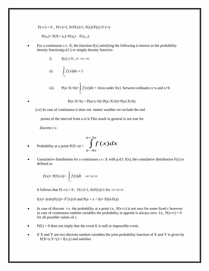
F(-) = 0 , F()=1, 0F(x)1, F(x)F(y) if x<y

P(xk)= P(X= xk)=F(xk) – F(xk-1)

For a continuous r.v. X, the function f(x) satisfying the following is known as the probability

density function(p.d.f.) or simply density function:

i) f(x) 0 ,- <x <

ii)

1)( dxxf

iii) P(a<X<b)= b

a

dxxf )( = Area under f(x) between ordinates x=a and x=b

P(a<X<b) = P(ax<b)=P(a<Xb)=P(aXb)

(i.e) In case of continuous it does not matter weather we include the end

points of the interval from a to b.This result in general is not true for

discrete r.v.

Probability at a point P(X=a) =

xa

xa

dxxf )(

Cumulative distribution for a continuous r.v. X with p.d.f. f(x), the cumulative distribution F(x) is

defined as

F(x)= P(Xx)=

dttf )( -<x<

It follows that F(-) = 0 , F()=1, 0F(x)1 for -<x<

f(x)= d/dx(F(x))= F1(x)0 and P(a < x < b)= F(b)-F(a)

In case of discrete r.v. the probability at a point i.e., P(x=c) is not zero for some fixed c however

in case of continuous random variables the probability at appoint is always zero. I.e., P(x=c) = 0

for all possible values of c.

P(E) = 0 does not imply that the event E is null or impossible event.

If X and Y are two discrete random variables the joint probability function of X and Y is given by

P(X=x,Y=y) = f(x,y) and satisfies

(i) f(x,y) 0 (ii)x y

yxf ),( = 1

The joint probability function for X and Y can be reperesented by a joint probability table.

Table

X Y

y1 y2 …… yn Totals

x1 f(x1,y1) f(x1,y2) …….. f(x1,yn) f1(x1)

=P(X=x1)

x2 F(x2,y1) f(x2,y2) …….. f(x2,yn) f1(x2)

=P(X=x2)

…….. ……. ……… ……… ……… ……..

xm f(xm,y1) f(xm,y2) ……. f(xm,yn) f1(xm)

=P(X=xm)

Totals f2(y1)

=P(Y=y1)

f2(y2)

=P(Y=y2)

…….. f2(yn)

=P(Y=yn)

1

The probability ofX = xj is obtained by adding all entries in arrow corresponding to X = xj

Similarly the probability of Y = yk is obtained by all entries in the column corresponding to Y

=yk

f1(x) and f2(y) are called marginal probability functions of X and Y respectively.

The joint distribution function of X and Y is defined by F(x,y)= P(Xx,Yy)= xu yv

vuf ),(

If X and Y are two continuous r.v.’s the joint probability function for the r.v.’s X and Y is defined

by

(i) f(x,y) 0 (ii)

dxdyyxf ),( =1

P(a < X < b, c< Y < d) =

b

ax

d

cy

dxdyyxf ),(

The joint distribution function of X and Y is F(x,y) = P( X x,Y y)=

u v

dudvvuf ),(

),(2

yxfyx

F

The Marginal distribution function of X and Y are given by P( X x) = F1(x)=

u v

dudvvuf ),( and P(Y y) = F2(y) =

u v

dudvvuf ),(

The marginal density function of X and Y are given by

f1(x) =

v

dvvxf ),( and f2(y) =

u

duyuf ),(

Two discrete random variables X and Y are independent iff

P(X = x,Y = y) = P(X = x)P(Y = y) x,y (or)

f(x,y) = f1(x)f2(y) x, y

Two continuous random variables X and Y are independent iff

P(X x,Y y) = P(X x)P(Y y) x,y (or)

f(x,y) = f1(x)f2(y) x, y

If X and Y are two discrete r.v. with joint probability function f(x,y) then

P(Y = y|X=x) =)(

),(

1 xf

yxf = f(y|x)

Similarly, P(X = x|Y=y) =)(

),(

2 yf

yxf = f(x|y)

If X and Y are continuous r.v. with joint density function f(x,y) then )(

),(

1 xf

yxf = f(y|x) and

)(

),(

2 yf

yxf =

f(x|y)

Expectation or mean or Expected value : The mathematical expectation or expected value of r.v. X is

denoted by E(x) or and is defined as

E(X)= ContinuousisXdxxxf

discreteisXxfxi

ii

)(

)(

If X is a r.v. then E[g(X)] = )()( xfxg

x

FOR Discrete

dxxfxg )()(

For Continuous

If X, Y are r.v.’s with joint probability function f(x,y) then

E[g(X,Y)] = x y

yxfyxg ),(),( for discrete r.v.’s

dxdyyxfyxg ),(),( for continuous r.v.’s

If X and Y are two continuous r.v.’s the joint density function f(x,y) the conditional expectation or the

conditional mean of Y given X is E(Y |X = x) =

dyxyyf )|(

Similarly, conditional mean of X given Y is E(X |Y = y) =

dxyxxf )|(

Median is the point, which divides the entire distribution into two equal parts. In case of

continuous distribution median is the point, which divides the total area into two equal parts.

Thus, if M is the median then

M

dxxf )( =

M

dxxf )( =1/2. Thus, solving any one of the

equations for M we get the value of median. Median is unique

Mode: Mode is the value for f(x) or P(xi) at attains its maximum

For continuous r.v. X mode is the solution of f1(x) = 0 and f

11(x) <0

provided it lies in the given interval. Mode may or may not be unique.

Variance: Variance characterizes the variability in the distributions with same mean can still

have different dispersion of data about their means

Variance of r.v. X denoted by Var(X) and is defined as

Var(X) = E ) - (X 2 = )()( 2 xfx

x

for discrete

dxxfx )()( 2

for continuous

where = E(X)

If c is any constant then E(cX) = c E(X)

If X and Y are two r.v.’s then E(X+Y) = E(X)+E(Y)

IF X,Y are two independent r.v.’s then E(XY) = E(X)E(Y)

If X1,X2,-------,Xn are random variables then E(c1X1 +c2X2+------+cnXn) = c1E(X1)+c2E(X2)+-----

+cnE(Xn) for any scalars c1,c2,------,cn If all expectations exists

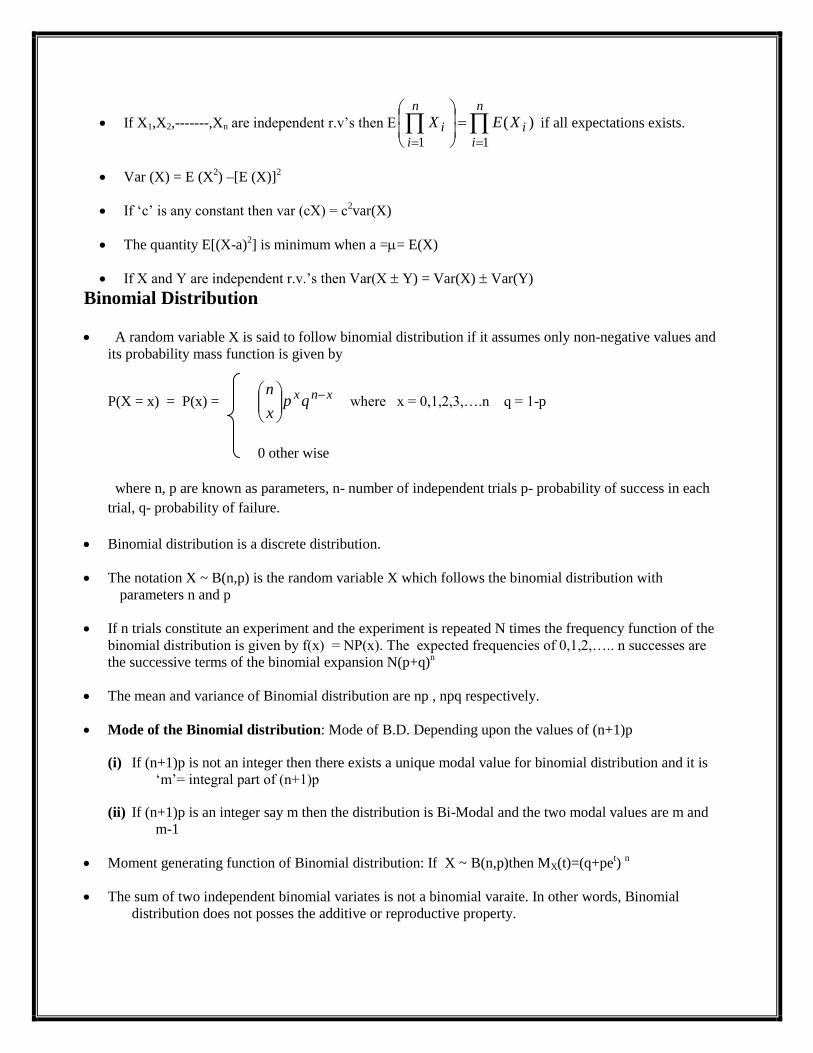
If X1,X2,-------,Xn are independent r.v’s then E

n

i

i

n

i

i XEX

11

)( if all expectations exists.

Var (X) = E (X2) –[E (X)]

2

If ‘c’ is any constant then var (cX) = c2var(X)

The quantity E[(X-a)2] is minimum when a == E(X)

If X and Y are independent r.v.’s then Var(X Y) = Var(X) Var(Y)

Binomial Distribution

A random variable X is said to follow binomial distribution if it assumes only non-negative values and

its probability mass function is given by

P(X = x) = P(x) = xnxqp

x

n

where x = 0,1,2,3,….n q = 1-p

0 other wise

where n, p are known as parameters, n- number of independent trials p- probability of success in each

trial, q- probability of failure.

Binomial distribution is a discrete distribution.

The notation X ~ B(n,p) is the random variable X which follows the binomial distribution with

parameters n and p

If n trials constitute an experiment and the experiment is repeated N times the frequency function of the

binomial distribution is given by f(x) = NP(x). The expected frequencies of 0,1,2,….. n successes are

the successive terms of the binomial expansion N(p+q)n

The mean and variance of Binomial distribution are np , npq respectively.

Mode of the Binomial distribution: Mode of B.D. Depending upon the values of (n+1)p

(i) If (n+1)p is not an integer then there exists a unique modal value for binomial distribution and it is

‘m’= integral part of (n+1)p

(ii) If (n+1)p is an integer say m then the distribution is Bi-Modal and the two modal values are m and

m-1

Moment generating function of Binomial distribution: If X ~ B(n,p)then MX(t)=(q+pet)

n

The sum of two independent binomial variates is not a binomial varaite. In other words, Binomial

distribution does not posses the additive or reproductive property.

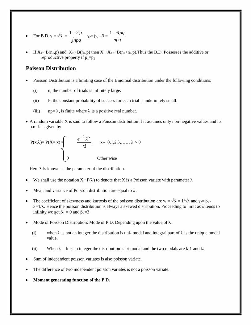
For B.D. 1= 1 = npq

p21 2= 2 –3 =

npq

pq61

If X1~ B(n1,p) and X2~ B(n2,p) then X1+X2 ~ B(n1+n2,p).Thus the B.D. Possesses the additive or

reproductive property if p1=p2

Poisson Distribution

Poisson Distribution is a limiting case of the Binomial distribution under the following conditions:

(i) n, the number of trials is infinitely large.

(ii) P, the constant probability of success for each trial is indefinitely small.

(iii) np= , is finite where is a positive real number.

A random variable X is said to follow a Poisson distribution if it assumes only non-negative values and its

p.m.f. is given by

P(x,)= P(X= x) = !x

e x: x= 0,1,2,3,…… > 0

0 Other wise

Here is known as the parameter of the distribution.

We shall use the notation X~ P() to denote that X is a Poisson variate with parameter

Mean and variance of Poisson distribution are equal to .

The coefficient of skewness and kurtosis of the poisson distribution are 1 = 1= 1/ and 2= 2-

3=1/. Hence the poisson distribution is always a skewed distribution. Proceeding to limit as tends to

infinity we get 1 = 0 and 2=3

Mode of Poisson Distribution: Mode of P.D. Depending upon the value of

(i) when is not an integer the distribution is uni- modal and integral part of is the unique modal

value.

(ii) When = k is an integer the distribution is bi-modal and the two modals are k-1 and k.

Sum of independent poisson variates is also poisson variate.

The difference of two independent poisson variates is not a poisson variate.

Moment generating function of the P.D.

If X~ P() then MX(t) = )1( tee

Recurrence formula for the probabilities of P.D. ( Fitting of P.D.)

P(x+1) = )(1

xpx

Recurrence relation for the probabilities of B.D. (Fitting of B.D.)

P(x+1) = )(.1

xpq

p

x

xn

Normal Distribution

A random variable X is said to have a normal distribution with parameters called mean and 2 called

variance if its density function is given by the probability law

f(x; , ) = 2

1exp

2

2

1

x , - < x < , - < < , > 0

A r.v. X with mean and variance 2 follows the normal distribution is denoted by

X~ N(, 2)

If X~ N(, 2) then Z =

X is a standard normal variate with E(Z) = 0 and var(Z)=0 and we write

Z~ N(0,1)

The p.d.f. of standard normal variate Z is given by f(Z) = 2/2

2

1 ze

, - < Z<

The distribution function F(Z) = P(Z z) =

z

t dte 2/2

2

1

F(-z) = 1 – F(z)

P(a < z b) = P( a z < b)= P(a <z < b)= P(a z b)= F(b) – F(a)

If X~ N(, 2) then Z =

X then P(a X b) =

aF

bF

N.D. is another limiting form of the B.D. under the following conditions:

i) n , the number of trials is infinitely large.

ii) Neither p nor q is very small

Chief Characteristics of the normal distribution and normal probability curve:

i) The curve is bell shaped and symmetrical about the line x =

ii) Mean median and mode of the distribution coincide.

iii) As x increases numerically f(x) decreases rapidly.

iv) The maximum probability occurring at the point x= and is given by

[P(x)]max = 1/2

v) 1 = 0 and 2 = 3

vi) 2r+1 = 0 ( r = 0,1,2……) and 2r = 1.3.5….(2r-1)2r

vii) Since f(x) being the probability can never be negative no portion of the curve lies below x- axis.

viii) Linear combination of independent normal variate is also a normal variate.

ix) X- axis is an asymptote to the curve.

x) The points of inflexion of the curve are given by x = , f(x) = 2/1

2

1 e

xi) Q.D. : M.D.: S.D. :: 3

2:

5

4: ::

3

2:

5

4: 1 Or Q.D. : M.D.: S.D. ::10:12:15

xii) Area property: P(- < X < + ) = 0.6826 = P(-1 < Z < 1)

P(- 2 < X < + 2) = 0.9544 = P(-2 < Z < 2)

P(- 3 < X < +3 ) = 0.9973 = P(-3 < Z < 3)

P( |Z| > 3) = 0.0027

m.g.f. of N.D. If X~ N(, 2) then MX(t) = e

t +t

2

2/2

If Z~ N(0,1) then MZ(t) = 2/2te

Continuity Correction:

The N.D. applies to continuous random variables. It is often used to approximate distributions of

discrete r.v. Provided that we make the continuity correction.

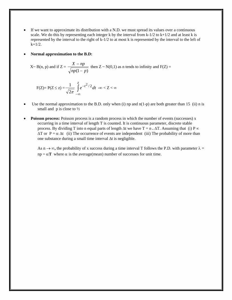
If we want to approximate its distribution with a N.D. we must spread its values over a continuous

scale. We do this by representing each integer k by the interval from k-1/2 to k+1/2 and at least k is

represented by the interval to the right of k-1/2 to at most k is represented by the interval to the left of

k+1/2.

Normal approximation to the B.D:

X~ B(n, p) and if Z = )1( pnp

npX

then Z ~ N(0,1) as n tends to infinity and F(Z) =

F(Z)= P(Z z) =

z

t dte 2/2

2

1

- < Z <

Use the normal approximation to the B.D. only when (i) np and n(1-p) are both greater than 15 (ii) n is

small and p is close to ½

Poisson process: Poisson process is a random process in which the number of events (successes) x

occurring in a time interval of length T is counted. It is continuous parameter, discrete stable

process. By dividing T into n equal parts of length t we have T = n . T. Assuming that (i) P

T or P = t (ii) The occurrence of events are independent (iii) The probability of more than

one substance during a small time interval t is negligible.

As n , the probability of x success during a time interval T follows the P.D. with parameter =

np = T where is the average(mean) number of successes for unit time.

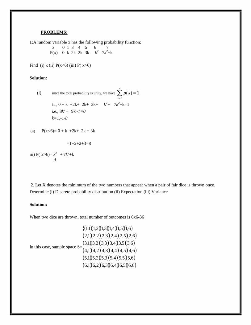
PROBLEMS:

Find (i) k (ii) P(x<6) (iii) P( x>6)

Solution:

(i) since the total probability is unity, we have

n

x

xp0

1)(

i.e., 0 + k +2k+ 2k+ 3k+ k2+

7k

2+k=1

i.e., 8k2+

9k

-1=0

k=1,-1/8

(ii) P(x<6)= 0 + k +2k+ 2k + 3k

=1+2+2+3=8

iii) P( x>6)= k2

+ 7k

2+k

=9

2. Let X denotes the minimum of the two numbers that appear when a pair of fair dice is thrown once.

Determine (i) Discrete probability distribution (ii) Expectation (iii) Variance

Solution:

When two dice are thrown, total number of outcomes is 6x6-36

In this case, sample space S=

6,65,64,63,62,61,6

6,55,54,53,52,51,5

6,45,44,43,42,41,4

6,35,34,33,32,31,3

6,25,24,23,22,21,2

6,15,14,13,12,11,1

1:A random variable x has the following probability function:

x 0 1 3 4 5 6 7

P(x) 0 k 2k 2k 3k k2

7k2+k

If the random variable X assigns the minimum of its number in S, then the sample space S=

654321

554321

444321

333321

222221

111111

The minimum number could be 1,2,3,4,5,6

For minimum 1, the favorable cases are 11

Therefore, P(x=1)=11/36

P(x=2)=9/36, P(x=3)=7/36, P(x=4)=5/36, P(x=5)=3/36, P(x=6)=1/36

The probability distribution is

X 1 2 3 4 5 6

P(x) 11/36 9/36 7/36 5/36 3/36 1/36

(ii)Expectation mean = ii xp

36

16

36

35

36

54

36

73

36

92

36

111)( xE

Or 5278.236

96152021811

36

1

(ii) variance =22 ii xp

25278.236

36

125

36

316

36

59

36

74

36

91

36

11)( xE

=1.9713

3: A continuous random variable has the probability density function

, 0, 0( )

0,

xkxe for xf x

otherwise

Determine (i) k (ii) Mean (iii) Variance

Solution:

(i) since the total probability is unity, we have 1

dxxf

100

0

dxkxedx x

i.e., 10

dxkxe x

2

0

21

koree

xkxx

(ii) mean of the distribution dxxxf

0

2

0

0 dxekxdx x

0

32

22 22

xxx ee

xe

x

=

2

Variance of the distribution 222

dxxfx

2

22 4

dxxfx

2

0

432

232 4663

xxxx ee

xe

xe

x

2

2

4:

Out of 800 families with 5 children each, how many would you expect to have (i)3 boys

(ii)5girls (iii)either 2 or 3 boys ? Assume equal probabilities for boys and girls

Solution(i)

P(3boys)=P(r=3)=P(3)=16

5

2

13

5

5C per family

Thus for 800 families the probability of number of families having 3 boys= 25080016

5

families

(iii)

P(5 girls)=P(no boys)=P(r=0)= 32

1

2

10

5

5C per family

Thus for 800 families the probability of number of families having 5girls= 2580032

1

families

(iv) P(either 2 or 3 boys =P(r=2)+P(r=3)=P(2)+P(3)

3

5

52

5

5 2

1

2

1CC =5/8 per family

Expected number of families with 2 or 3 boys = 5008008

5 families.

5: Average number of accidents on any day on a national highway is 1.8. Determine the

probability that the number of accidents is (i) at least one (ii) at most one

Solution:

Mean= 8.1

We have P(X=x)=p(x)

=

(i)P (at least one) =P( x≥1)=1-P(x=0)

=1-0.1653

=0.8347

P (at most one) =P (x≤1)

=P(x=0)+P(x=1)

= 0.4628

6: The mean weight of 800 male students at a certain college is 140kg and the standard deviation is 10kg

assuming that the weights are normally distributed find how many students weigh I) Between 130 and

148kg ii) more than 152kg

Solution:

Let be the mean and be the standard deviation. Then =140kg and =10pounds

(i) When x= 138, 12.010

140138z

xz

When x= 138, 28.010

140148z

xz

P(138≤x≤148)=P(-0.2≤z≤0.8)

=A( 2z )+A( 1z )

=A(0.8)+A(0.2)=0.2881+0.0793=0.3674

Hence the number of students whose weights are between 138kg and 140kg

=0.3674x800=294

(ii) When x=152,

=

=z1

Therefore P(x>152)=P(z>z1)=0.5-A(z1)

=0.5-0.3849=0.1151

Therefore number of students whose weights are more than 152kg =800x0.1151=92.

Exercise Problems:

1. Two coins are tossed simultaneously. Let X denotes the number of heads then find i) E(X) ii)

E(X2) iii)E(X

3) iv) V(X)

2. If f(x)=kx

e

is probability density function in the interval, x , then find i) k ii)

Mean iii) Variance iv) P(0<x<4)

3. Out of 20 tape recorders 5 are defective. Find the standard deviation of defective in the sample

of 10 randomly chosen tape recorders. Find (i) P(X=0) (ii) P(X=1) (iii) P(X=2) (iv) P (1<X<4).

Fit the expected frequencies.

5.If X is a normal variate with mean 30 and standard deviation 5. Find the probabilities that i)

P(26 X40) ii) P( X 45)

6. The marks obtained in Statistics in a certain examination found to be normally distributed. If

15% of the students greater than or equal to 60 marks, 40% less than 30 marks. Find the mean

and standard deviation.

7.If a Poisson distribution is such that3

( 1) ( 3)2

P X P X then find (i) ( 1)P X (ii)

( 3)P X (iii) (2 5) P X .

Then find (i) k (ii) mean (iii) variance (iv) P(0 < x < 3)

4. In 1000 sets of trials per an event of small probability the frequencies f of the number of x of

successes are

f 0 1 2 3 4 5 6 7 Total

x 305 365 210 80 28 9 2 1 1000

8. A random variable X has the following probability function:

X -2 -1 0 1 2 3

P(x) 0.

1

K 0.2 2K 0.3 K

UNIT-II

MULTIPLE RANDOM VARIABLES

Joint Distributions: Two Random Variables

In real life, we are often interested in several random variables that are related to each other. For

example, suppose that we choose a random family, and we would like to study the number of

people in the family, the household income, the ages of the family members, etc. Each of these is

a random variable, and we suspect that they are dependent. In this chapter, we develop tools to

study joint distributions of random variables. The concepts are similar to what we have seen so

far. The only difference is that instead of one random variable, we consider two or more. In this

chapter, we will focus on two random variables, but once you understand the theory for two

random variables, the extension to n

random variables is straightforward. We will first discuss joint distributions of discrete random

variables and then extend the results to continuous random variables.

Joint Probability Mass Function (PMF)

Remember that for a discrete random variable X, we define the PMF as PX(x)=P(X=x).

Now, if we have two random variables X and Y, and we would like to study them jointly, we

define the joint probability mass function as follows:

The joint probability mass function of two discrete random variables X and Y is defined as

PXY(x,y)=P(X=x,Y=y). Note that as usual, the comma means "and," so we can write

PXY(x,y)=P(X=x,Y=y)=P((X=x) and (Y=y)).

We can define the joint range for X and Y as

RXY={(x,y)|PXY(x,y)>0}.

In particular, if RX={x1,x2,...} and RY={y1,y2,...}, then we can always write

RXY⊂RX×RY={(xi,yj)|xi∈RX,yj∈RY}.

In fact, sometimes we define RXY=RX×RY to simplify the analysis. In this case, for

some pairs (xi,yj) in RX×RY, PXY(xi,yj) might be zero. For two discrete random

variables X and Y, we have

∑(xi,yj)∈RXYPXY(xi,yj)=1

Marginal PMFs

The joint PMF contains all the information regarding the distributions of X and Y. This means that, for

example, we can obtain PMF of X from its joint PMF with Y. Indeed, we can write

PX(x)=P(X=x)=∑yj∈RYP(X=x,Y=yj)=∑yj∈RYPXY(x,yj).law of total probablity

Here, we call PX(x) the marginal PMF of X. Similarly, we can find the marginal PMF of Y as

PY(Y)=∑xi∈RXPXY(xi,y).

Marginal PMFs of X and Y

:

PX(x)PY(y)=∑yj∈RYPXY(x,yj), for any x∈RX=∑xi∈RXPXY(xi,y), for any y∈RY

Correlation: In a bivariate distribution, if the change in one variable effects the change in

other variable, then the variables are called correlated.

Covariance between two random variables X and Y is denoted by Cov(X,Y) is defined as

E(XY)-E(X)E(Y)

If X and Y are independent then Cov(X,Y) = 0

Karl Pearson Correlation Coefficient between two r.v. X and Y usually denoted by r(X,Y)

or simply rXY is a numerical measure of a linear relationship between them and is defined as r

= r(X,Y) = cov(X,Y)/xy

It is also called product moment correlation coefficient.

If (xi,yi); I = 1,2…n is bivariate distribution then, then

Cov (X,Y) = E[{X-E(X)}{Y-E(Y)}]

= (1/n)(xi- x )(yi- y ) = (1/n)xiyi - x y

X2 = E[ X-E(X)]

2 = (1/n) 2)( xxi = (1/n)xi

2 –( x )

2

Y2 = E[ Y-E(Y)]

2 = (1/n) 2)( yyi = (1/n)yi

2 –( y )

2

Computational formula for r(X,Y) =

2222 11

1

yyn

xxn

yxxyn

-1 r 1

If r = 0 then X,Y are uncorrelated.

If r = -1 then correlation is perfect and negative.

If r = 1then the correlation is perfect and positive.

r is independent of change of origin and scale

Two independent variables are uncorrelated. Converse need not be true.

The correlation coefficient for Bivariate frequency distribution:

The bivariate data on X on Y are presented in a two-way correlation table with n classes of

Y placed along the horizontal lines and m classes of X along vertical lines and fij is the

frequency of the individuals lying in i, j th cell.

x

yxf ),( =g(y),is the sum of the frequencies along any row and

y

yxf ),( =f(x),is the sum of the frequencies along any column.

x y

yxf ),( =y x

yxf ),( =x

xf )( =y

yg )( =N

x = x

xxfN

)(1

, y = y

yygN

)(1

2

X =22 )(

1xxfx

N x

and 2

Y =22 )(

1yygy

N y

Cov(X,Y) = x y

yxxyfN

),(1

- yx

r= YX

YXCov

),(

Rank Correlation: Let (xi,yi) for I = 1,2,…n be the ranks of the ith

individuals in the

characteristics A and B respectively, Pearsonian coefficient of correlation between xi and yi

are called rank correlation coefficient between A and B for that group of individual.

The Spearman’s rank correlation between the two variables X and Y takes the values

1,2…n denoted by and is defined as = 1 – )1( 2

1

2

nn

dn

i

i

where di = xi-yi ( In general xi yi)

In case, common ranks are given to repeated items, the common rank is the average of the ranks

which these items would have assumed if they were slightly different from each other and the next

item will get the rank next to the rank already assumed. The adjustment or correction is made in the

rank correlation formula. In the formula we add factor12

)1( 2 mm to d

2, where m is the number of

times an item is repeated. This correction factor is to be added to each repeated value in both X-series

and Y- series.

-1 1

Regression analysis is a mathematical measure of the average relationship between two or

more variables in terms of the original units of the data.

The variable whose value is influenced or is to be predicted is called dependent variable and

the variable, which influences the values or is used for the prediction is called independent

variable. Independent variable is also known as regressor or predictor or explanatory

variable while the dependent variable is also known as regressed or explained variable.

If the variables in bivariate distributions are related we will find that the points in the scatter

diagram will cluster round some curve called the “ curve of regression”. If the curve is a

straight line, it is called line of regression and

there is said to be linear Regression between the variables, otherwise the regression is said to

be curvilinear. The line of regression is line of best fit and is obtained by principle of least

squares.

In the bivariate distribution (xi,yi) ; i = 1,2,….n Y is dependent variable and X is independent

variable. The line of regression Y on X is Y = a + b X.

i.e. Y- y = r )( xXX

Y

Similarly the line of regression X on Y is X = a + b Y

i.e.,X- x = r )( yYY

X

If X and Y are any random variables the two regression lines are

Y – E(Y) = 2

),(

X

YXCov

[X – E(X)]

X – E(X) = 2

),(

Y

YXCov

[Y – E(Y)]

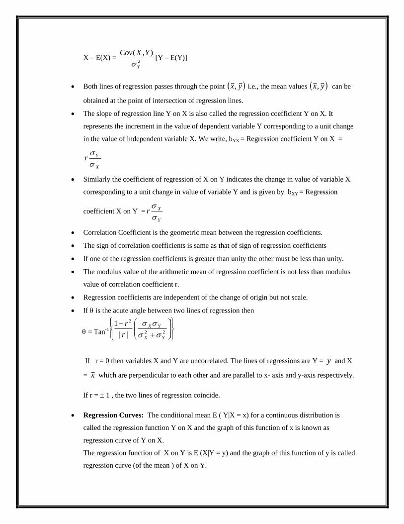
Both lines of regression passes through the point yx, i.e., the mean values yx, can be

obtained at the point of intersection of regression lines.

The slope of regression line Y on X is also called the regression coefficient Y on X. It

represents the increment in the value of dependent variable Y corresponding to a unit change

in the value of independent variable X. We write, bYX = Regression coefficient Y on X =

X

Yr

Similarly the coefficient of regression of X on Y indicates the change in value of variable X

corresponding to a unit change in value of variable Y and is given by bXY = Regression

coefficient X on Y =Y

Xr

Correlation Coefficient is the geometric mean between the regression coefficients.

The sign of correlation coefficients is same as that of sign of regression coefficients

If one of the regression coefficients is greater than unity the other must be less than unity.

The modulus value of the arithmetic mean of regression coefficient is not less than modulus

value of correlation coefficient r.

Regression coefficients are independent of the change of origin but not scale.

If is the acute angle between two lines of regression then

= Tan-1

22

2

||

1

YX

YX

r

r

If r = 0 then variables X and Y are uncorrelated. The lines of regressions are Y = y and X

= x which are perpendicular to each other and are parallel to x- axis and y-axis respectively.

If r = 1 , the two lines of regression coincide.

Regression Curves: The conditional mean E ( Y|X = x) for a continuous distribution is

called the regression function Y on X and the graph of this function of x is known as

regression curve of Y on X.

The regression function of X on Y is E (X|Y = y) and the graph of this function of y is called

regression curve (of the mean ) of X on Y.

Multiple Regression analysis is an extension of (simple) regression analysis in which two or

more independent variables are used to estimate the value of dependent variable.

Least square regression planes fitting of N data points (X1,X2,X3) in a three dimensional

scatter diagram. The least square regression plane of X1 on X2 and X3 is X1 = a + b X2+cX3

where a,b,c are determined by solving simultaneously the normal equations:

321 XcXbanX

32

2

2221 XXcXbXaXX

2

332331 XcXXbXaXX

Similarly for the regression plane of X2 on X1 and X3 and the regression plane of X3 on X1

and X2

The linear regression equation of X1 on X2 ,X3 and X4 can be written as

X1 = a + b X2 + c X3 + d X4

PROBLEMS:

1. Let x and y are two random variables with a joint probability density function

otherwise

yxeyxf

y

,0

0,),( . Find the marginal probability density function of x

and y.

Solution: Given that

otherwise

yxeyxf

y

,0

0,),(

Marginal probability density functionof x is

dyyxfxf x ),()(

x

ydye

x

ye

xee

xe

Marginal probability density functionof y is

dxyxfyf y ),()(

y

ydxe0

yyxe 0

0 yye

yye

2. Determine b for joint probability density function

Otherwise

yaxbeyxf

yx

.0

0,0,),(

)(

Solution: Given

Otherwise

yaxbeyxf

yx

.0

0,0,),(

)(

1),( dxdyyxf

0 0

)( 1y

a

x

yx dxdybe

10

0

dyebeax

y

y

10

0

dyeebe a

y

y

1)1(0

dyeeby

ya

1)1( 0 dyeeb ya

1)1( 0 eeb a

1)1( aeb

)1(

1ae

b

3. Calculate the coefficient of correlation from the following data

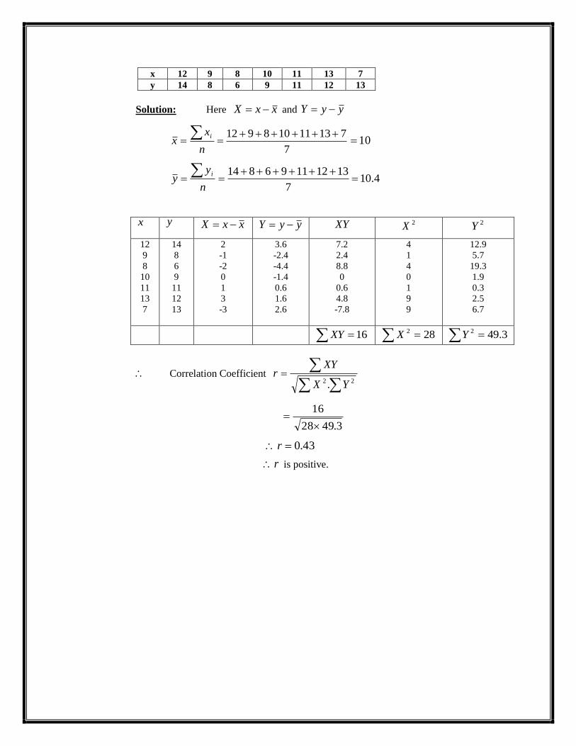
x 12 9 8 10 11 13 7

y 14 8 6 9 11 12 13

Solution: Here xxX and yyY

7

71311108912

n

xx

i10

4.107

13121196814

n

yy

i

x y xxX yyY XY 2X 2Y

12

9

8

10

11

13

7

14

8

6

9

11

12

13

2

-1

-2

0

1

3

-3

3.6

-2.4

-4.4

-1.4

0.6

1.6

2.6

7.2

2.4

8.8

0

0.6

4.8

-7.8

4

1

4

0

1

9

9

12.9

5.7

19.3

1.9

0.3

2.5

6.7

16XY 282X 3.492 Y

Correlation Coefficient

22 . YX

XYr

3.4928

16

43.0r

r is positive.

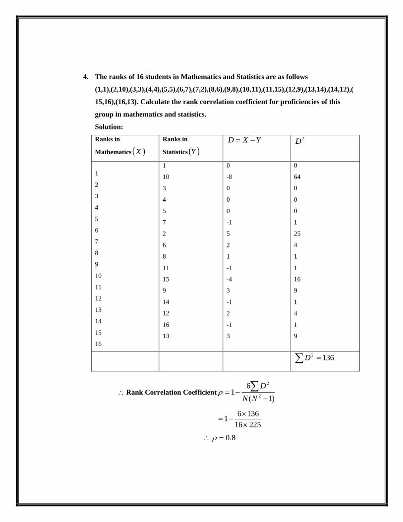
4. The ranks of 16 students in Mathematics and Statistics are as follows

(1,1),(2,10),(3,3),(4,4),(5,5),(6,7),(7,2),(8,6),(9,8),(10,11),(11,15),(12,9),(13,14),(14,12),(

15,16),(16,13). Calculate the rank correlation coefficient for proficiencies of this

group in mathematics and statistics.

Solution:

Ranks in

Mathematics X

Ranks in

Statistics Y

YXD 2D

1

2

3

4

5

6

7

8

9

10

11

12

13

14

15

16

1

10

3

4

5

7

2

6

8

11

15

9

14

12

16

13

0

-8

0

0

0

-1

5

2

1

-1

-4

3

-1

2

-1

3

0

64

0

0

0

1

25

4

1

1

16

9

1

4

1

9

1362 D

Rank Correlation Coefficient)1(

61

2

2

NN

D

22516

13661

8.0

5. Determine the regression equation which best fit to the following data:

x 10 12 13 16 17 20 25

y 10 22 24 27 29 33 37

Solution: The regression equation of y on x is bxay

The normal equations are

xbnay

2xbxaxy

x y 2x xy

10

12

13

16

17

20

25

10

22

24

27

29

33

37

100

144

169

256

289

400

625

100

264

312

432

493

660

925

113x 182y 19832 x 3186xy

Substitute the above values in normal equations

11137182 baxbnay

2198311331862 baxbxaxy

Solve equations 1 and 2 we get

7985.0a and 5611.1b

Now substitute a, b values in regression equation

The regression equation of y on x is xy 5611.17985.0

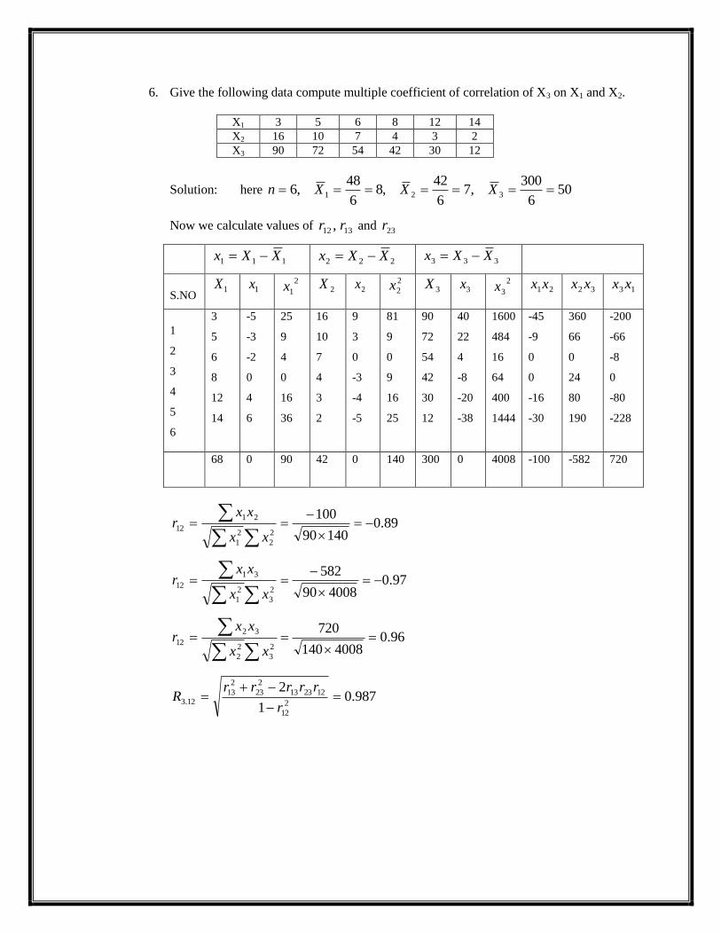
6. Give the following data compute multiple coefficient of correlation of X3 on X1 and X2.

X1 3 5 6 8 12 14

X2 16 10 7 4 3 2

X3 90 72 54 42 30 12

Solution: here 506

300,7

6

42,8

6

48,6 321 XXXn

Now we calculate values of 1312 , rr and 23r

111 XXx

222 XXx 333 XXx

S.NO 1X 1x 2

1x 2X 2x 2

2x 3X 3x 2

3x 21xx 32 xx 13 xx

1

2

3

4

5

6

3

5

6

8

12

14

-5

-3

-2

0

4

6

25

9

4

0

16

36

16

10

7

4

3

2

9

3

0

-3

-4

-5

81

9

0

9

16

25

90

72

54

42

30

12

40

22

4

-8

-20

-38

1600

484

16

64

400

1444

-45

-9

0

0

-16

-30

360

66

0

24

80

190

-200

-66

-8

0

-80

-228

68 0 90 42 0 140 300 0 4008 -100 -582 720

89.014090

100

2

2

2

1

21

12

xx

xxr

97.0400890

582

2

3

2

1

31

12

xx

xxr

96.04008140

720

2

3

2

2

32

12

xx

xxr

987.01

22

12

122313

2

23

2

1312.3

r

rrrrrR

Exercise Problems:

1. Calculate the Karl Pearson’s coefficient of correlation from the following data x 15 18 20 24 30 35 40 50

y 85 93 95 105 120 130 150 160

2. A sample of 12 fathers and their elder sons gave the following data about their elder sons.

Calculate the coefficient of rank correlation.

Fathers 65 63 67 64 68 62 70 66 68 67 69 71

Sons 68 66 68 65 69 66 68 65 71 67 68 70

3. Find the most likely production corresponding to a rainfall 40 from the following data:

Rain fall(X) Production(Y)

Average 30 500Kgs

Standard deviation 5 100Kgs

Coefficient of correlation 0.8

Determine A.

6. Determine the regression equation which best fit to the following data:

x 10 12 13 16 17 20 25

y 10 22 24 27 29 33 37

4. If is the angle between two regression lines and S.D. of Y is twice the S.D. of X and r=0.25,

5. find tan The joint probability density function x y

Ae ,0 x y,0 yf (x, y)

0. Otherwise

.

UNIT-III

SAPLING DISTRIBUTION AND

TESTING OF HYPOTHESIS

Sampling Distribution

Population is the set or collection or totality of the objects, animate or inanimate, actual or

hypothetical under study. Thus, mainly population consists of set of numbers measurements or

observations, which are of interest.

Size of the population N is the number of objects or observations in the population.

Population may be finite or infinite.

A finite sub-set of the population is known as Sample. Size of the sample is denoted by n.

Sampling is the process of drawing the samples from a given population.

If n 30 the sampling is said to be large sampling.

If n < 30 then the sampling is said to be Small sampling.

Statistical inference deals with the methods of arriving at valid generalizations and predictions

about the population using the information contained in the sample.

Parameters Statistical measures or constants obtained from the population are known as

population parameters or simply parameters.

Population f(x) is a population whose probability distribution is f(x).If f(x) is binomial, Poisson

or normal then the corresponding population is known as Binomial Population, Poisson

population or normal Population.

Samples must be representative of the population, sampling should be random.

Random Sampling is one in which each member of the population has equal chances or

probability of being included in the sample.

Sampling where each member of a population may be chosen, more than once is called Sampling

with replacement. A finite population, which is sampled with replacement, can theoretically be

considered infinite since samples of any size can be drawn with out exhausting the population.

For most practical purpose sampling from a finite population, which is very large, can be

considered as sampling from an infinite population.

If each member cannot be chosen more than once it is called sampling with out replacement.

Any quantity obtained from a sample for the purpose of estimating a population parameter is

called a sample statistics or briefly Statistic. Mathematically a sample statistic for a sample of size

n can be defined as a function of the random variables X1, X2……Xn i.e., g(X1, X2……Xn). The

function g(X1, X2……Xn) is another random variable whose values can be represented by g(X1,

X2……Xn). The word statistic is often used for the r.v. or for its values.

Random samples (Finite population): A set of observations X1, X2……Xn, constitute a random

sample of size n from a finite population of size N, if its values are chosen so that each subset of n

of the N elements of the population has same probability if being selected.

Random sample (Infinite Population): A set of observations X1, X2……Xn constitute a random

sample of size n from infinite population f(x) if:

(i) Each Xi is a r.v. whose distribution is given by f(x)

(ii) These n r.v.’s are independent

Sample Mean X1, X2……Xn is a random sample of size n the sample mean is a r.v. defined by

X =n

XXX n.......21

Sample Variance X1, X2……Xn is a random sample of size n the sample variance is a r.v. defined

by S2 =

n

XXn

i

i

1

2)(

and is a measure of variability of data about the mean.

Sample Standard deviation is the positive square root of the sample variance.

Degrees of freedom (d o f) of a statistic is the positive integer denoted by , equals to n-k where n

is the number of independent observations of the random sample and k is the number of

population parameters which are calculated using sample data. Thus d o f = n – k is the

difference between n, the sample size and k, the number of independent constraints imposed on

the observations in the sample.

Sampling Distributions: The probability distribution of a sample statistic is often called as

sampling distribution of the statistic.

The standard deviation of the sampling distribution of a statistic is called Standard Error(S.E)

The mean of the sampling distribution of means, denoted by x

, is given by E( X ) = x

=

where is the mean of the population.

If a population is infinite or if sampling is with replacement, then the variance of the sampling

distribution of means, denoted by 2

x is given by E[(

2)X ]=2

x =

n

2 where

2 is the

variance of the population.

If the population is of siqe N, if sampling is without replacement, and if the sample size is nN then

2x

=n

2

1N

nN

The factor

1N

nN is called the finite population correction factor, is close to 1 (and can be

omitted for most practical purposes) unless the samples constitutes a substantial portion of the

population.

(Central limit theorem) If X is the mean of a sample of size n taken from a population having the

mean and the finite variance 2 , then Z=

n

X

is a r.v. whose distribution function

approaches that of the standard normal distribution as n

If X is the mean of a sample of size n taken from a finite population of size N with mean

and variance 2 then Z=

1

NnN

n

X

is a r.v whose distribution function approaches that of the

standard normal distribution as n

The normal distribution provides an excellent approximation to the sampling distribution of the

mean X for n as small as 25 or 30

If the random samples come from a normal population, the sampling distribution of the mean is

normal regardless of the size of the sample

Estimation

To find an unknown population parameter, a judgment or statement is made which is an estimate.

The method or rule to determine an unknown population parameter is called an Estimator. For

example sample mean is an estimator of population mean because sample mean is a method of

determining the population mean. A parameter can have many or 1,2 estimators. The estimators

should be found so that they are very near to parameter values.

An estimate of a population parameter given by a single number is called a point estimate of

the parameter. If we say that a distance in 5.28 mts , we are giving a point estimate.

An estimate of a population parameters given by two numbers between which the parameter may

be considered to lie is called an interval estimate of the parameter. The distance lie between

5.25 and 5.31 mts.

A statement of the error or precision of the estimate is called Reliability.

Let be the parameter of the interest and be a statistic, the hat notation distinguishes the

sample-based quantity from the parameter.

A statistic is said to be unbiased estimator or its value an unbiased estimate iff the mean of the

sampling distribution of the estimator equals to .

E( X ) = and E 2S = 2 so that X and 2S are unbiased estimators of the population mean

and variance 2

A statistic 1 is said to be more efficient unbiased estimator of the parameter than the statistic

2 if

(i) If 1 and

2 are both unbiased estimators of

(ii) The variance of the sampling distribution of the first estimator is less than that of second.

E.g. the sampling distribution of the mean and median both has same namely the

population mean. However., the variance of the sampling distribution of means is smaller

than that of the sampling distribution of the medians. Thus the mean provides a more

efficient estimate than the median.

Maximum error E of a population mean by using large sample mean is

E = n

Z

2/

The most widely used values for 1- are 0.95 and 0.99 and the corresponding values of Z/2

are Z0.025 = 1.96 and Z0.005 = 2.575

Sample size n =

2

2/

EZ

Confidence interval for ( for large samples n 30 ) known

x -n

Z

2/ < < x +n

Z

2/

If the sampling is without replacement from a population of finite size N then the confidence

interval for with known is

x -n

Z

2/1

N

nN < < x +

nZ

2/

1

N

nN

Large sample confidence interval for - unknown is

x -n

SZ 2/ < < x +

n

SZ 2/

Large sample confidence interval for 1 - 2 ( where 1 and 2 are unknowns)

( 21 xx ) Z /2

2

2

2

1

2

1

n

S

n

S

The end points of the confidence interval are called Confidence Limits.

In Bayesian estimation prior feelings about the possible values of are combined with the direct

sample evidence which give the posterior distribution of approximately normally distributed

with

mean 1 = 22

0

2

0

2

0

n

xn and standard deviation 1= 22

0

2

0

2

n. In the computation and

1 and 1, 2 is assumed to be known. When

2 is unknown which is generally the case,

2 is

replaced by sample variance S2 provided

n 30(Large sample)

Bayesian Interval for :

(1-)100% Bayesian interval for is given by

1- 12/ Z < < 1+ 12/ Z

Inferences concerning means

Statistical decisions are decisions or conclusions about the population parameters on the basis of a

random sample from the population.

Statistical hypothesis is an assumption or conjecture or guess about the parameters of the

population distribution

Null Hypothesis (N.H) denoted by H0 is statistical hypothesis, which is to be actually tested for

acceptance or rejection. NH is the hypothesis, which is tested for possible rejection under the

assumption that it is true.

Any Hypothesis which is complimentary to the N.H is called an Alternative Hypothesis denoted

by H1

Simple Hypothesis is a statistical Hypothesis which completely specifies an exact parameter. N.H

is always simple hypothesis stated as a equality specifying an exact value of the parameter. E.g.

N.H = H0 : = 0 N.H. = H0 : 1- 2=

Composite Hypothesis is stated in terms of several possible values.

Alternative Hypothesis(A.H) is a composite hypothesis involving statements expressed as

inequalities such as < , > or

i) A.H : H1: > 0 (Right tailed) ii) A.H : H1: < 0 (Left tailed)

iii) A.H : H1: 0 (Two tailed alternative)

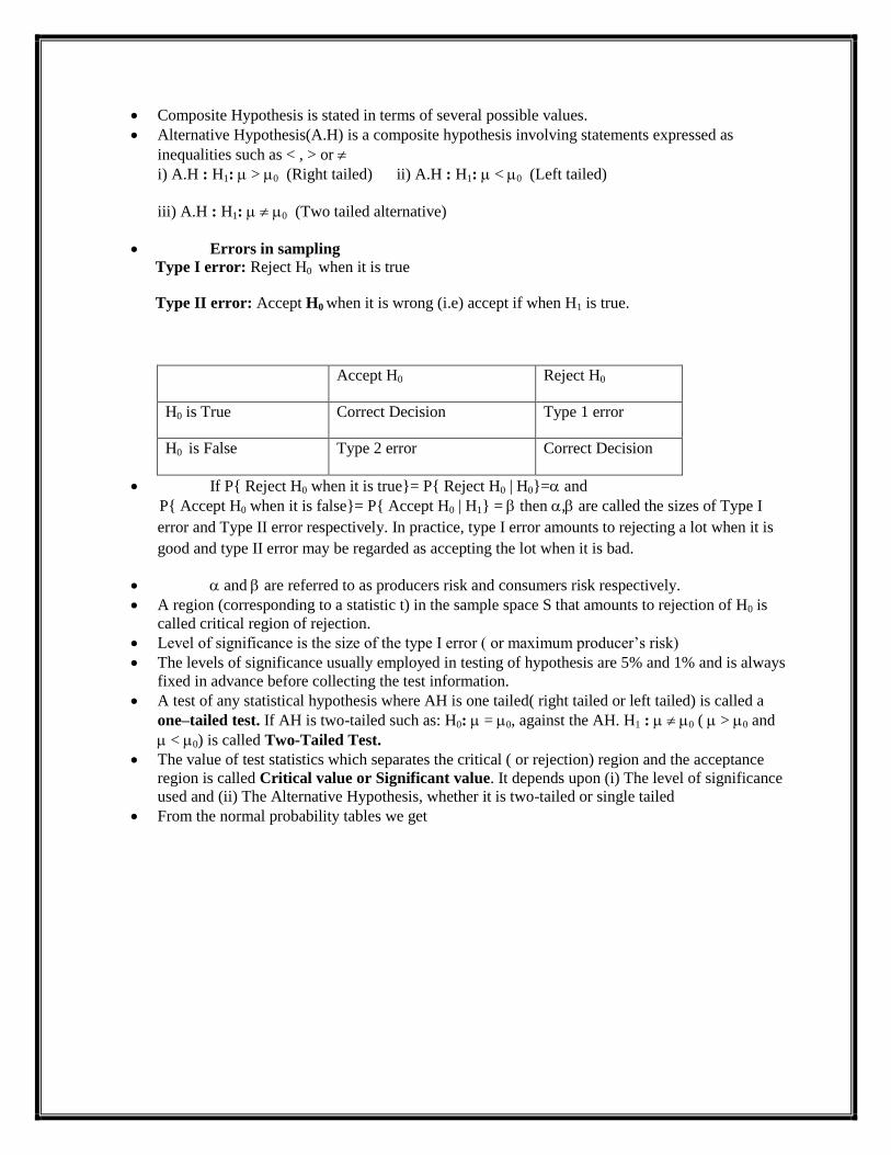
Errors in sampling

Type I error: Reject H0 when it is true

Type II error: Accept H0 when it is wrong (i.e) accept if when H1 is true.

Accept H0 Reject H0

H0 is True Correct Decision Type 1 error

H0 is False Type 2 error Correct Decision

If P{ Reject H0 when it is true}= P{ Reject H0 | H0}= and

P{ Accept H0 when it is false}= P{ Accept H0 | H1} = then , are called the sizes of Type I

error and Type II error respectively. In practice, type I error amounts to rejecting a lot when it is

good and type II error may be regarded as accepting the lot when it is bad.

and are referred to as producers risk and consumers risk respectively.

A region (corresponding to a statistic t) in the sample space S that amounts to rejection of H0 is

called critical region of rejection.

Level of significance is the size of the type I error ( or maximum producer’s risk)

The levels of significance usually employed in testing of hypothesis are 5% and 1% and is always

fixed in advance before collecting the test information.

A test of any statistical hypothesis where AH is one tailed( right tailed or left tailed) is called a

one–tailed test. If AH is two-tailed such as: H0: = 0, against the AH. H1 : 0 ( > 0 and

< 0) is called Two-Tailed Test.

The value of test statistics which separates the critical ( or rejection) region and the acceptance

region is called Critical value or Significant value. It depends upon (i) The level of significance

used and (ii) The Alternative Hypothesis, whether it is two-tailed or single tailed

From the normal probability tables we get

Critical Value

(Z)

Level of significance ()

1% 5% 10%

Two-Tailed test -Z/2 = -2.58 -Z/2 = -1.96 -Z/2 = -1.645

Z/2 = 2.58 Z/2 = 1.96 Z/2 = 1.645

Right-Tailed test Z = 2.33 Z = 1.645 Z = 1.28

Left-Tailed Test -Z = -2.33 - Z = -1.645 -Z = -1.28

When the size of the sample is increased, the probability of committing both types of error I and

II (i.e) and are small, the test procedure is good one giving good chance of making the correct

decision.

P-value is the lowest level ( of significance) at which observed value of the test statistic is

significant.

A test of Hypothesis (T. O.H) consists of

1. Null Hypothesis (NH) : H0

2. Alternative Hypothesis (AH) : H1

3. Level of significance:

4. Critical Region pre determined by

5. Calculation of test statistic based on the sample data.

6. Decision to reject NH or to accept it.

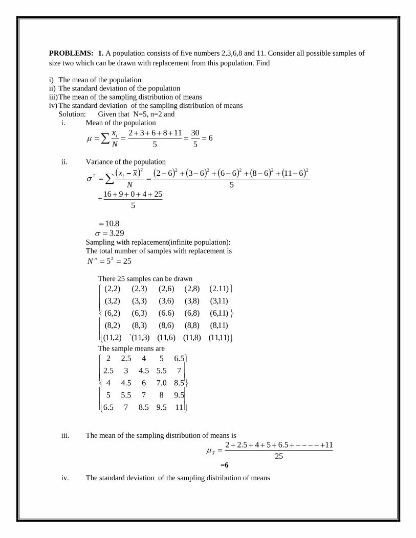
PROBLEMS: 1. A population consists of five numbers 2,3,6,8 and 11. Consider all possible samples of

size two which can be drawn with replacement from this population. Find

i) The mean of the population

ii) The standard deviation of the population

iii) The mean of the sampling distribution of means

iv) The standard deviation of the sampling distribution of means

Solution: Given that N=5, n=2 and

i. Mean of the population

65

30

5

118632

N

xi

ii. Variance of the population

5

61168666362222222

2

N

xxi

=5

2540916

8.10

29.3

Sampling with replacement(infinite population):

The total number of samples with replacement is

2552 nN

There 25 samples can be drawn

)11,11()8,11()6,11()3,11`()2,11(

)11,8()8,8()6,8()3,8()2,8(

)11,6()8,6()6.6()3,6()2,6(

)11,3()8,3()6,3()3,3()2,3(

)11.2()8,2()6,2()3,2()2,2(

The sample means are

115.95.875.6

5.9875.55

5.80.765.44

75.55.435.2

5.6545.22

iii. The mean of the sampling distribution of means is

25

115.6545.22 x

=6

iv. The standard deviation of the sampling distribution of means

25

)611()65.2()62( 2222 x

= 40.5

32.2x

iv) the standard deviation of the sampling distribution of means

Solution: Given that N=6, n=2 and

i. Mean of the population

146

84

6

2420161284

N

xi

ii. Variance of the population

6

14241420141614121481442222222

2

N

xxi

=6

100364436100

67.46

29.3

Sampling without replacement (finite population):

The total number of samples without replacement is

There 15 samples can be drawn

`)24,20(

)24,16()20,16(

)24,12()20,12()16,12(

)24,8()20,8()16,8()12,8(

)24,4()20,4()16,4()12,4()8,4(

The sample means are

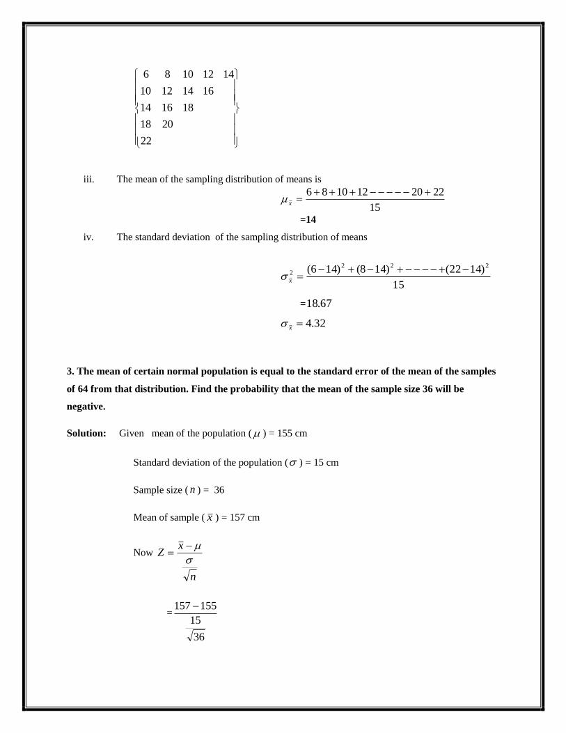
2. A population consists of five numbers4, 8, 12, 16, 20, 24. Consider all possible samples of size two

which can be drawn without replacement from this population. Find




22

2018

181614

16141210

14121086

iii. The mean of the sampling distribution of means is

15

2220121086 x

=14

iv. The standard deviation of the sampling distribution of means

15

)1422()148()146( 2222 x

= 67.18

32.4x

3. The mean of certain normal population is equal to the standard error of the mean of the samples

of 64 from that distribution. Find the probability that the mean of the sample size 36 will be

negative.

Solution: Given mean of the population ( ) = 155 cm

Standard deviation of the population ( ) = 15 cm

Sample size ( n ) = 36

Mean of sample ( x ) = 157 cm

Now

n

xZ

=

36

15

155157

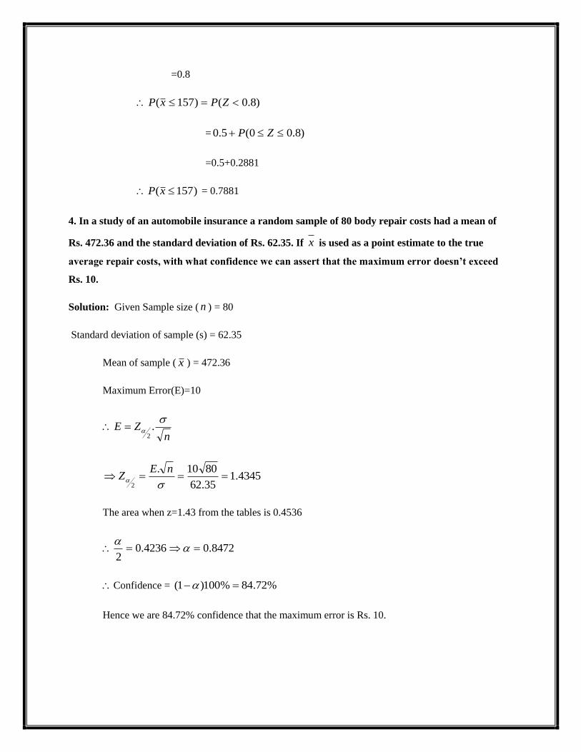
=0.8

)8.0()157( ZPxP

= )8.00(5.0 ZP

=0.5+0.2881

)157( xP = 0.7881

4. In a study of an automobile insurance a random sample of 80 body repair costs had a mean of

Rs. 472.36 and the standard deviation of Rs. 62.35. If x is used as a point estimate to the true

average repair costs, with what confidence we can assert that the maximum error doesn’t exceed

Rs. 10.

Solution: Given Sample size ( n ) = 80

Standard deviation of sample (s) = 62.35

Mean of sample ( x ) = 472.36

Maximum Error(E)=10

nZE

.

2

4345.135.62

8010.

2

nEZ

The area when z=1.43 from the tables is 0.4536

8472.04236.02

Confidence = %72.84%100)1(

Hence we are 84.72% confidence that the maximum error is Rs. 10.

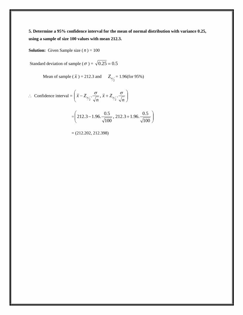
5. Determine a 95% confidence interval for the mean of normal distribution with variance 0.25,

using a sample of size 100 values with mean 212.3.

Solution: Given Sample size ( n ) = 100

Standard deviation of sample ( ) = 5.025.0

Mean of sample ( x ) = 212.3 and 2

Z = 1.96(for 95%)

Confidence interval =

nZx

nZx

.,.

22

=

100

5.0.96.13.212,

100

5.0.96.13.212

= (212.202, 212.398)

Exercise Problems:

iv) The standard deviation of the sampling distribution of means

2. If a 1-gallon can of paint covers on an average 513 square feet with a standard deviation of 31.5 square

feet, what is the probability that the mean area covered by a sample of 40 of these 1-gallon cans will be

anywhere from 510to 520 square feet?

3. What is the size of the smallest sample required to estimate an unknown proportion to within a

maximum error of 0.06 with at least 95% confidence.

4. A random sample of 400 items is found to have mean 82 and standard deviation of 18. Find the

maximum error of estimation at 95% confidence interval. Find the confidence limits for the mean if

x =82.

5. A sample of size 300 was taken whose variance is 225 and mean is 54. Construct 95% confidence

interval for the mean.

1. Samples of size 2 are taken from the population 1, 2, 3, 4, 5, 6. Which can be drawn without

replacement? Find




UNIT - IV

LARGE SAMPLE TESTS

Test statistic for T.O.H. in several cases are

1. Statistic for test concerning mean known

Z = n

X

/

0

2. Statistic for large sample test concerning mean with unknown

Z = nS

X

/

0

3. Statistic for test concerning difference between the means

Z =

2

2

2

1

2

1

21

nn

XX

under NH H0 : 1 - 2 = against the AH, H1: 1 - 2 > or H1: 1 - 2 <

or H1: 1 - 2

4. Statistic for large samples concerning the difference between two means (1 and 2 are

unknown)

Z =

2

2

2

1

2

1

21

n

S

n

S

XX

Statistics for large sample test concerning one proportion

Z = )1( 00 pnp

npX o

under the N.H: H0: p = po against H1: p p0 or p > p0 or p <P0

Statistic for test concerning the difference between two proportions

Z= ))(ˆ1(ˆ

21

11

2

2

1

1

nnpp

n

X

n

X

with p =21

21

nn

XX

under the NH : H0: p1=p2 against the AH H1:p1 < p2 or

p1 > p2 or p1 p2

To determine if a population follows a specified known theoretical distribution such as

ND,BD,PD the 2(chi-square) test is used to assertion how closely the actual distribution

approximate the assumed theoretical distribution. This test is based on how good a fit is there

between the observed frequencies and the expected frequencies is known as “goodness-of-fit-

test”.

Large sample confidence interval for p

n

n

x

n

x

Zn

x

1

2/ < p < n

n

x

n

x

Zn

x

1

2/ where the degree of confidence is 1-

Large sample confidence interval for difference of two proportions (p1- p2) is

2

2

2

2

2

1

1

1

1

1

2/

2

2

1

1

11

n

n

x

n

x

n

n

x

n

x

Zn

x

n

x

Maximum error of estimate E = Z/2

n

pp )1( with observed value x/n substituted for p we

obtain an estimate of E

Sample size n = p(1-p)

2

2/

E

Z when p is known

n= 4

12

2/

E

Z when p is unknown

One sided confidence interval is of the form p < (1/2n)2 with (2n+1) degrees of freedom.

Problems:

1. A sample of 400 items is taken from a population whose standard deviation is 10.The mean

of sample is 40.Test whether the sample has come from a population with mean 38 also

calculate 95% confidence interval for the population.

Solution: Given n=400, 40x and =38 and =10

1. Null hypothesis(H0): =38

2. Alternative hypothesis(H1): 38

3. Level of significance: =0.05 and Z =1.96

4. Test statistic:

n

xZ

n

xZ

=

400

10

3840 =4

Z 4

5. Conclusion:

Z > Z

We reject the Null hypothesis.

Confidence interval =

nZx

nZx

,

=

400

1096.140,

400

1096.140

= 98.40,02.39

2. Samples of students were drawn from two universities and from their weights in kilograms mean

and S.D are calculated and shown below make a large sample test to the significance of

difference between means.

MEAN S.D SAMPLE SIZE

University-A 55 10 400

University-B 57 15 100

Solution: Given n1=400, n2=100, 1x =55, 2x =57

S1=10 and S2=15

1. Null hypothesis(H0): 1x = 2x

2. Alternative hypothesis(H1): 1x 2x


4. Test statistic:

2

2

2

1

2

1

21

n

S

n

S

xxZ

=

100

225

400

100

5755

=-1.26

Z 1.26

5. Conclusion:

Z < Z

We accept the Null hypothesis.

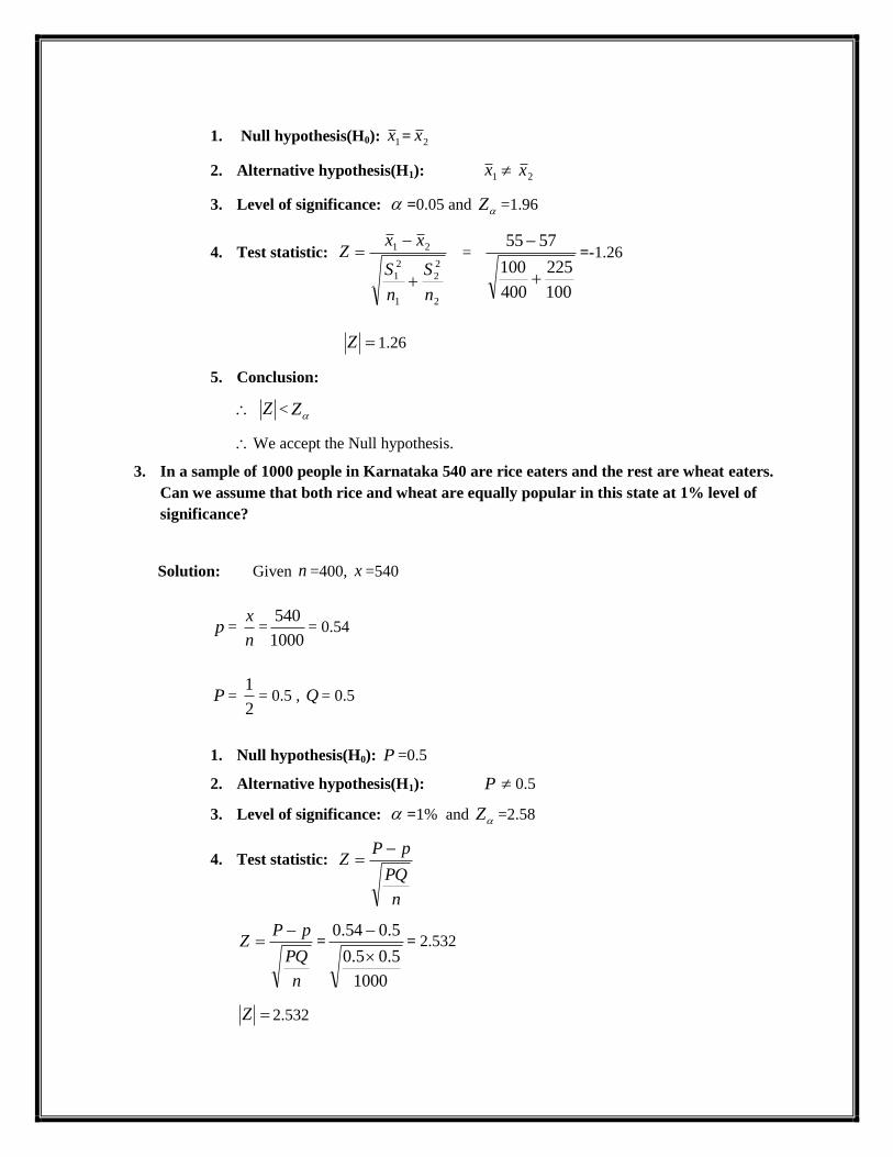
3. In a sample of 1000 people in Karnataka 540 are rice eaters and the rest are wheat eaters.

Can we assume that both rice and wheat are equally popular in this state at 1% level of

significance?

Solution: Given n =400, x =540

p = n

x=

1000

540= 0.54

P = 2

1= 0.5 , Q = 0.5

1. Null hypothesis(H0): P =0.5

2. Alternative hypothesis(H1): P 0.5

3. Level of significance: =1% and Z =2.58

4. Test statistic:

n

PQ

pPZ

n

PQ

pPZ

=

1000

5.05.0

5.054.0

= 2.532

Z 2.532

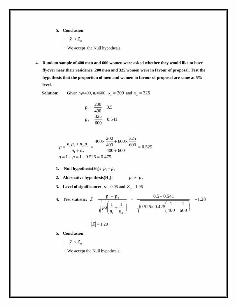
5. Conclusion:

Z < Z


4. Random sample of 400 men and 600 women were asked whether they would like to have

flyover near their residence .200 men and 325 women were in favour of proposal. Test the

hypothesis that the proportion of men and women in favour of proposal are same at 5%

level.

Solution: Given n1=400, n2=600 , 2001 x and 3252 x

5.0

400

2001 p

541.0600

3252 p

525.0600400

600

325600

400

200400

21

2211

nn

pnpnp

475.0525.011 pq

1. Null hypothesis(H0): 1p = 2p

2. Alternative hypothesis(H1): 1p 2p


4. Test statistic:

21

21

11

nnpq

ppZ = 28.1

600

1

400

1425.0525.0

541.05.0

Z 1.28

5. Conclusion:

Z < Z


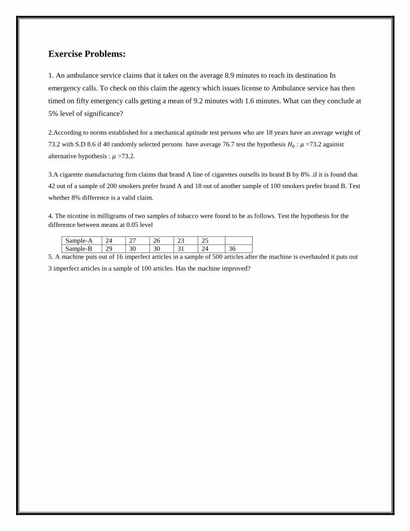
Exercise Problems:

1. An ambulance service claims that it takes on the average 8.9 minutes to reach its destination In

emergency calls. To check on this claim the agency which issues license to Ambulance service has then

timed on fifty emergency calls getting a mean of 9.2 minutes with 1.6 minutes. What can they conclude at

5% level of significance?

2.According to norms established for a mechanical aptitude test persons who are 18 years have an average weight of

73.2 with S.D 8.6 if 40 randomly selected persons have average 76.7 test the hypothesis : =73.2 againist

alternative hypothesis : >73.2.

3.A cigarette manufacturing firm claims that brand A line of cigarettes outsells its brand B by 8% .if it is found that

42 out of a sample of 200 smokers prefer brand A and 18 out of another sample of 100 smokers prefer brand B. Test

whether 8% difference is a valid claim.

4. The nicotine in milligrams of two samples of tobacco were found to be as follows. Test the hypothesis for the

difference between means at 0.05 level

Sample-A 24 27 26 23 25

Sample-B 29 30 30 31 24 36

5. A machine puts out of 16 imperfect articles in a sample of 500 articles after the machine is overhauled it puts out

3 imperfect articles in a sample of 100 articles. Has the machine improved?

UNIT - V

SMALL SAMPLE TESTS AND

ANOVA

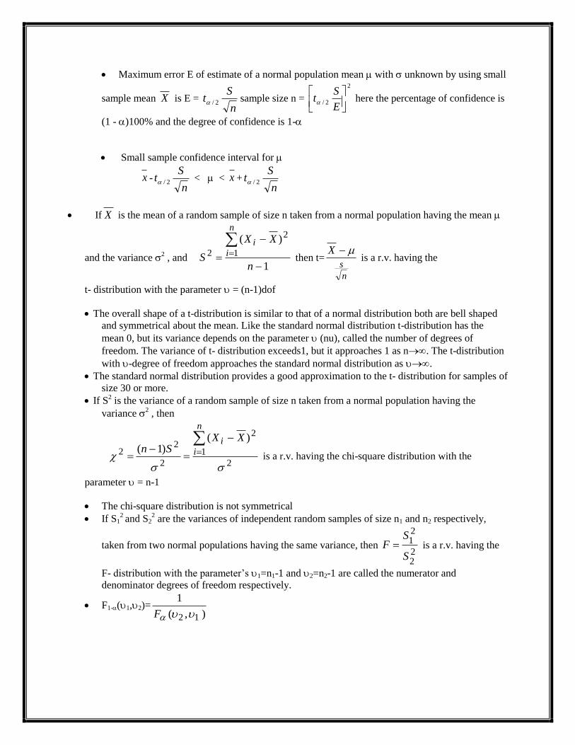
Maximum error E of estimate of a normal population mean with unknown by using small

sample mean X is E = n

St 2/ sample size n =

2

2/

E

St here the percentage of confidence is

(1 - )100% and the degree of confidence is 1-

Small sample confidence interval for

x -n

St 2/ < < x +

n

St 2/

If X is the mean of a random sample of size n taken from a normal population having the mean

and the variance 2 , and

1

)(

1

2

2

n

XX

S

n

i

i

then t=

n

s

X is a r.v. having the

t- distribution with the parameter = (n-1)dof

The overall shape of a t-distribution is similar to that of a normal distribution both are bell shaped

and symmetrical about the mean. Like the standard normal distribution t-distribution has the

mean 0, but its variance depends on the parameter (nu), called the number of degrees of

freedom. The variance of t- distribution exceeds1, but it approaches 1 as n. The t-distribution

with -degree of freedom approaches the standard normal distribution as .

The standard normal distribution provides a good approximation to the t- distribution for samples of

size 30 or more.

If S2 is the variance of a random sample of size n taken from a normal population having the

variance 2 , then

2

1

2

2

22

)()1(

n

i

i XXSn

is a r.v. having the chi-square distribution with the

parameter = n-1

The chi-square distribution is not symmetrical

If S12 and S2

2 are the variances of independent random samples of size n1 and n2 respectively,

taken from two normal populations having the same variance, then 22

21

S

SF is a r.v. having the

F- distribution with the parameter’s 1=n1-1 and 2=n2-1 are called the numerator and

denominator degrees of freedom respectively.

F1-(1,2)=) ,(

1

12 F

ANALYSIS OF VARIANCE

ANOVA:

It is abbreviated form for ANALYSIS OF VARIANCE which is a method for comparing several

population means at the same time. It is performed using F-distribution

Assumptions of ANALYSIS OF VARIANCE:

1. The data must be normally distributed.

2. The samples must draw from the population randomly and independently.

3. The variances of population from which samples have been drawn are equal.

Types of Classification:

There are two types of model for analysis of variance

1. One-Way Classification

2. Two-Way Classification.

ONE –WAY CLASSIFICATION:

PROCEDURE FOR ANOVA

Step 1 : State the null and alternative hypothesis.

H0: 321 (The means for three groups are equal).

H1 : At least one pair is unequal.

Step 2: Select the test criterion to be used.

We have to decide which test criterion or distribution should be used. As our assumption involves means

for three normally distributed populations. We should use the F-distribution to test the hypothesis.

Step 3. Determine the rejection and non-rejection regions

We decide to use 0.05 level of significance. As on one-way ANOVA test is always right-tail, the area in

the right tail of the F-distribution curve is 0.05, which is the rejection region. Now, we need to know the

degrees of freedom for the numerator and the denominator. Degrees of freedom for the numerator=k-1,

where k is the number of groups. Degree of freedom for denominator =n-k where n is total number of

observations

Step 4. Calculate the value of the test statistics by applying ANOVA. i.e., F Calculated

Step 5: conclusion

I) If F Calculated<F Critical , then H0 is accepted

ii) if F calculated<F critical , then H0 is rejected

TWO –WAY CLASSIFCATION:

The analysis of variance table for two-way classification is taken as follows;

Source of variation Sum of squares SS Degree of freedom df Mean squares Ms

Between columns SSC (c-1) MSC=SSC/(c-1)

Within rows SSR (r-10 MSR=SSR/(r-1)

Residual(ERROR) SSE (c-1)(r-1) MSE=SSE/(c-1)(r-1)

total SST Cr-1

The abbreviations used in the table are:

SSC= sum of squares between column s.

SSR= sum of square between rows.

SST=total sum of squares;

SSE= sum of squares of error, it is obtained by subtracting SSR and SSC from SST.

(c-1)=number of degrees of freedom between columns.

(r-1)=number of degrees of freedom between rows.

(c-1)(r-1)=number of degree of freedom for residual.

MSC=mean of sum of squares between columns

MSR= mean of sum of squares between rows.

MSE= mean of sum of squares between residuals.

It may be noted that total number of degrees of freedom are =(c-1)+(r-1)+(c-1)(r-1)=cr-1=N-1

Problems:

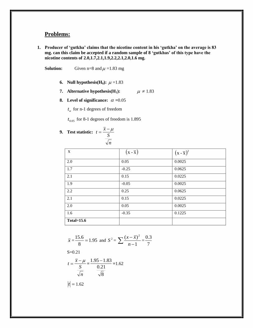
1. Producer of ‘gutkha’ claims that the nicotine content in his ‘gutkha’ on the average is 83

mg. can this claim be accepted if a random sample of 8 ‘gutkhas’ of this type have the

nicotine contents of 2.0,1.7,2.1,1.9,2.2,2.1,2.0,1.6 mg.

Solution: Given n=8 and =1.83 mg

6. Null hypothesis(H0): =1.83

7. Alternative hypothesis(H1): 1.83

8. Level of significance: =0.05

t for n-1 degrees of freedom

05.0t for 8-1 degrees of freedom is 1.895

9. Test statistic:

n

S

xt

x x-x 2x-x

2.0 0.05 0.0025

1.7 -0.25 0.0625

2.1 0.15 0.0225

1.9 -0.05 0.0025

2.2 0.25 0.0625

2.1 0.15 0.0225

2.0 0.05 0.0025

1.6 -0.35 0.1225

Total=15.6

x = 95.18

6.15 and

2S =

1

)( 2

n

xx=

7

3.0

S=0.21

n

S

xt

=

8

21.0

83.195.1 =1.62

t 1.62

10. Conclusion:

t < t


2. The means of two random samples of sizes 9,7 are 196.42 and 198.82.the sum of squares of

deviations from their respective means are 26.94,18.73.can the samples be considered to

have been the same population?

Solution: Given n1=9, n2=7, 1x =196.42, 2x =198.82 and 2

1)( xxi =26.94,

2

2 )( xxi =18.73

2

)()(

21

2

2

2

12

nn

xxxxS

ii=3.26

S=1.81

6. Null hypothesis(H0): 1x = 2x

7. Alternative hypothesis(H1): 1x 2x


t for 221 nn degrees of freedom

05.0t for 9+7-2=14 degrees of freedom is 2.15

9. Test statistic:

21

21

11

nnS

xxt

=

7

1

9

1)81.1(

82.19842.196

=-2.63

t 2.63

10. Conclusion:

t > t


3. In one sample of 8 observations the sum of squares of deviations of the sample values from

the sample mean was 84.4 and another sample of 10 observations it was 102.6 .test whether

there is any significant difference between two sample variances at at 5% level of

significance.

Solution: Given n1=8, n2=10, 2

1)( xxi =84.4 and 2

2 )( xxi =102.6

057.127

4.84

1

)(

1

2

12

1

n

xxS

i

4.119

6.102

1

)(

2

2

12

2

n

xxS

i

1. Null hypothesis(H0): 2

1S =2

2S

2. Alternative hypothesis(H1): 2

1S 2

2S


F For )1,1( 21 nn degrees of freedom

05.0F For (7,9) degrees of freedom is 3.29

4. Test statistic: 2

2

2

1

S

SF =

4.11

057.12=1.057

5. Conclusion:

F < F


4. The following table gives the classification of 100 workers according to gender and nature

of work. Test whether the nature of work is independent of the gender of the worker.

Stable Unstable Total

Male 40 20 60

Female 10 30 40

Total 50 50 100

057.1F

Solution: Given that

Expected frequencies =

200

10090=45

200

10090=45

90

200

10090=55

200

10090=55

110

100 100 200

Calculation of 2 : Observed

Frequency(Oi)

Expected

Frequency(Ei) )E-(O ii

2

i

2

ii

E

)E-(O

60 45 225 5

30 45 225 5

40 55 225 4.09

70 55 225 4.09

18.18

2 =

i

ii

E

EO 2)(=18.18

1. Null hypothesis(H0): ii EO

2. Alternative hypothesis(H1): ii EO


2

For (r-1)(c-1) degrees of freedom

2

05.0 For (2-1)(2-1)=1 degrees of freedom is 3.84

4. Test statistic: 2 =

i

ii

E

EO 2)(=18.18

5. Conclusion:

2 >

2


057.12

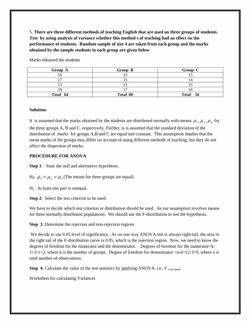
5. There are three different methods of teaching English that are used on three groups of students.

Test by using analysis of variance whether this method s of teaching had an effect on the

performance of students. Random sample of size 4 are taken from each group and the marks

obtained by the sample students in each group are given below

Marks obtained the students

Group A Group B Group C

16 15 15

17 15 14

13 13 13

18 17 14

Total 64 Total 60 Total 56

Solution:

It is assumed that the marks obtained by the students are distributed normally with means 1 , 2 , 3 for

the three groups A, B and C. respectively. Further, is is assumed that the standard deviation of the

distribution of marks for groups A,B and C are equal and constant. This assumption implies that the

mean marks of the groups may differ on account of using different methods of teaching, but they do not

affect the dispersion of marks.

PROCEDURE FOR ANOVA


H0: 321 (The means for three groups are equal).

H1 : At least one pair is unequal.





We decide to use 0.05 level of significance. As on one-way ANOVA test is always right-tail, the area in

the right tail of the F-distribution curve is 0.05, which is the rejection region. Now, we need to know the

degrees of freedom for the numerator and the denominator. Degrees of freedom for the numerator=k-

1=3-1=2, where k is the number of groups. Degree of freedom for denominator =n-k=12-3=9, where n is

total number of observations.

Step 4. Calculate the value of the test statistics by applying ANOVA. i.e., F Calculated

Worksheet for calculating Variances

Group A Group B Group C

X1j (x1j- xi) (x1j- xi)2 X2j (x2j- xi) (x2j- xi)

2 X3j (x3j- xi) (x3j- xi)

2

16 0 0 15 0 0 15 1 1

17 1 1 15 0 0 14 0 0

13 -3 9 13 -2 4 13 -1 1

18 2 4 17 2 4 14 0 0

Total 64 Total 60 Total 56

Mean 16 Mean 15 Mean 14

The sample variances for the groups are

S12 = 5.314

4

11 1

1

2

11

1

n

j

j xxn

S22 = 28

4

11 2

1

2

22

2

n

j

j xxn

S32 = 5.014

4

11 31

1

2

33

3

n

j

j xxn

We can now estimate the variance by the pooled variance method as follows;

3

2

2

n

xx iij

The denominator is n1+n2+n3=3

Applying the value in the formulas,

3

2

2

n

xx iij =

13

]151415151516[4222

=4(This is the variance between the samples)

Now, F is to be calculated . F=ratio of two variances

= 498.167.2

42

2

sampleswithinestimateof

samplesbetweenestimateof

The foregoing calculations can be summarized in the form of an ANOVA TABLE.

Source of variation Sum of squares SS Degrees of freedom

df

Mean of equares Variance ratio

F

Between sampling SSB k-1 MSB=SSB/(k-1)

Within sampling SSW n-k MSW=SSW/(n-k) F=MSB/MSW

total SST n-1

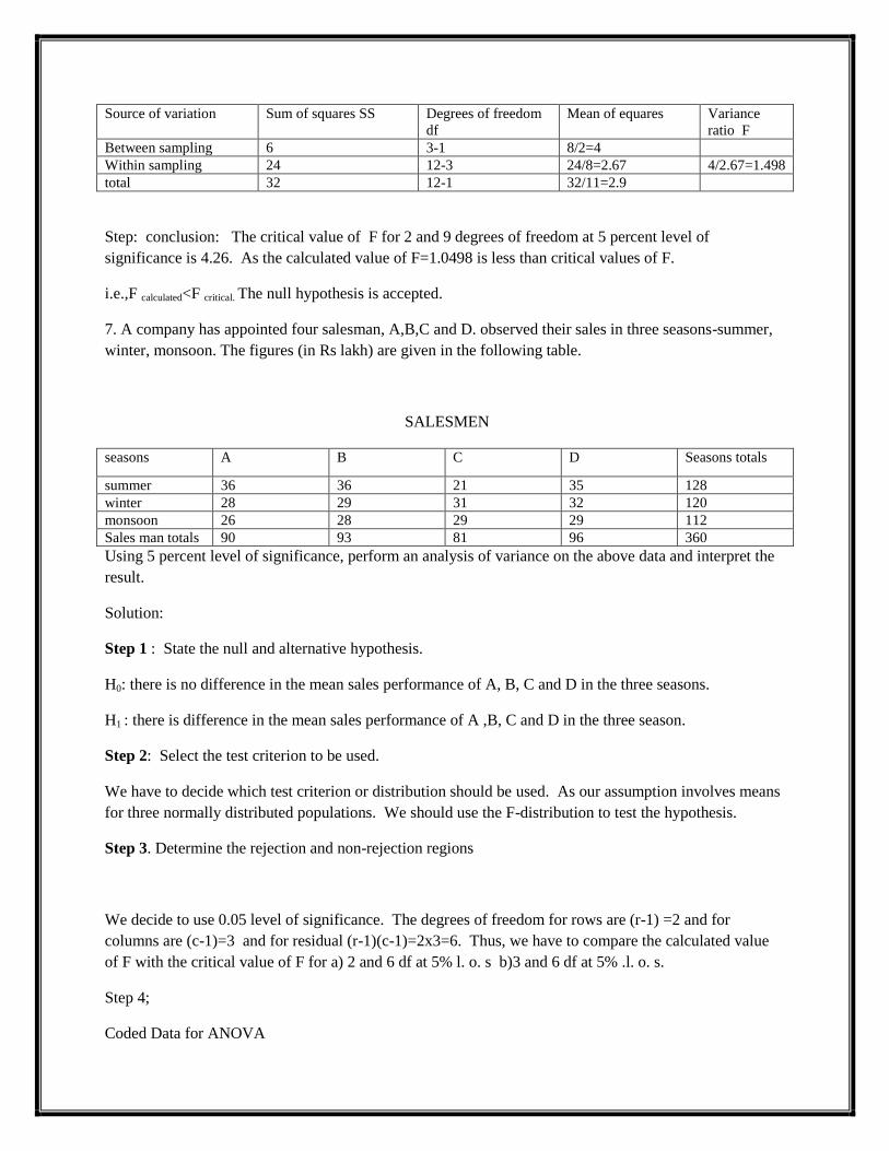
Source of variation Sum of squares SS Degrees of freedom

df

Mean of equares Variance

ratio F

Between sampling 6 3-1 8/2=4

Within sampling 24 12-3 24/8=2.67 4/2.67=1.498

total 32 12-1 32/11=2.9

Step: conclusion: The critical value of F for 2 and 9 degrees of freedom at 5 percent level of

significance is 4.26. As the calculated value of F=1.0498 is less than critical values of F.

i.e.,F calculated<F critical. The null hypothesis is accepted.

7. A company has appointed four salesman, A,B,C and D. observed their sales in three seasons-summer,

winter, monsoon. The figures (in Rs lakh) are given in the following table.

SALESMEN

seasons A B C D Seasons totals

summer 36 36 21 35 128

winter 28 29 31 32 120

monsoon 26 28 29 29 112

Sales man totals 90 93 81 96 360

Using 5 percent level of significance, perform an analysis of variance on the above data and interpret the

result.

Solution:


H0: there is no difference in the mean sales performance of A, B, C and D in the three seasons.

H1 : there is difference in the mean sales performance of A ,B, C and D in the three season.





We decide to use 0.05 level of significance. The degrees of freedom for rows are (r-1) =2 and for

columns are (c-1)=3 and for residual (r-1)(c-1)=2x3=6. Thus, we have to compare the calculated value

of F with the critical value of F for a) 2 and 6 df at 5% l. o. s b)3 and 6 df at 5% .l. o. s.

Step 4;

Coded Data for ANOVA

SALESMEN

seasons A B C D Seasons totals

summer 6 6 -9 5 8

winter -2 -1 1 2 0

monsoon -4 -2 -1 -1 -8

Sales man totals 0 3 -9 6 0

Correction factor C=T2/N=(0)

2/12=0

Sum os squares between salesmen

=02/3+3

2/3+(-9

2/3)+6

2/3=0+3+27+12=42

Sum of squares between seasons=82/4+0

2/4+(-8

2/4)=16+0+16=32

Total sum of squares

=(6)2+(-2)

2+(-4)

2+(6)

2+(-1)

2+(-2)

2+(-9)

2+(1)

2+(-1)

2+(5)

2+(2)

2+(-1)

2

=210

Analysis of variance table

Source of variation Sum of squares SS Degree of freedom df Mean squares Ms

Between columns 42 4-1=3 14.00

Within rows 32 3-1=2 16.00

Residual(ERROR) 136 3x2=6 22.67

total 210 12-1=11

We now test the hypothesis (i) that there is no difference in the sales performance among the four

salesmen and (ii) there is no difference in the mean sales in the three seasons. For this, we have to first

compare the salesman variance estimate with the residual estimate. This is shown below:

FA =14/22.67=0.62

In the same manner, we have to compare the season variance estimate with the residual variances

estimate. This is shown below;

FB=16/22.67=0.71

Step 5:

It may noted that the critical value of F for 3 and 6 degree of freedom at 5 percent level of significance is

4.76. Since the calculated value of FA is 0.62 is less than critical value of F. Therefore there is no

significance difference among salesmen.

Also the critical value of F for 2 and 6 degree of freedom at 5 percent level of significance is 4.76. Since

the calculated values of FB=16/22.67=0.71 is less than critical value of F. Therefore there is no

significance difference among seasons

The overall conclusion is that the salesmen and seasons are alike in respect of sales.

Exercise problems:

Test whether the samples came from the same population or not?

2. Use chi square test to asset the correctness of the hypothesis that the digits are distributed in equal number

in the table

4. A group of 5 patients treated with medicine A weigh 42, 39, 48, 60 and 41 kgs . Second group of 7 patients from

the same hospital treated with medicine B weigh 38, 42, 56, 64, 68, 69 and 62 kgs. Do you agree with the claim that

medicine B increases the weigh significantly?

5. A company has derived three training methods to train its workers. It is keen to know which of these

three training methods would lead to greatest productivity after training. Given below are productivity

measures for individual workers trained by each method.

Method 1 30 40 45 38 48 55 52

Method 2 55 46 37 43 52 42 40

Method 3 42 38 49 40 55 36 41

Find out whether the three training methods lead to different levels of productivity at the 0.05 level of

significance.

6. Consider the following ANOVA TABLE, based on information obtained for three randomly selected

samples from three independent population, which are normally distributed with equal variances.

Source of variance Sum of squares SS Degree of freedom

df

Mean squares MS Value of test

statistics

Between samples 60 ? 20 F=

Within samples ? 14 ?

1. Two random samples gave the following results

Sample size Sample

mean

Sum of squares of

deviations from mean

I 10 15 90

II 12 14 108

200 digits were chosen at random from set of tables the frequency of the digits are

digit 0 1 2 3 4 5 6 7 8 9

frequency 18 19 23 21 16 25 22 20 21 15

3. 5 dice were thrown 96 times the number of times showing 4,5 or 6 obtain is given below

Fit a binomial distribution and test for goodness of fit

x 0 1 2 3 4 5

frequency 1 10 24 35 18 8

(A) Complete the ANOVA table by filling in missing values.

(B) test the null hypothesis that the means of the three population are all equal, using 0.01 level of

significance.

7. The following represent the number of units of production per day turned out by four different workers

using five different types of machines

Machine type

Worker A B C D E TOTAL

1 4 5 3 7 6 25

2 5 7 7 4 5 28

3 7 6 7 8 8 36

4 3 5 4 8 2 22

TOTAL 19 23 21 27 21 111

On the basis of this information, can it be concluded that (i) The mean productivity is the same for

different machines. (ii) The workers don’t differ with regard to productivity.

PROBABILITY AND STATISTICS - iare.ac.in

Documents