Scilab Textbook Companion for Principles Of Linear Systems And Signals by B. P. Lathi 1 Created by A. Lasya Priya B.Tech (pursuing) Electrical Engineering NIT, Surathkal College Teacher H. Girisha Navada, NIT Surathkal Cross-Checked by S.M. Giridharan, IIT Bombay August 11, 2013 1 Funded by a grant from the National Mission on Education through ICT, http://spoken-tutorial.org/NMEICT-Intro. This Textbook Companion and Scilab codes written in it can be downloaded from the ”Textbook Companion Project” section at the website http://scilab.in

Principles Of Linear Systems And Signals_B. P. Lathi.pdf
Oct 25, 2015
signals
Welcome message from author
This document is posted to help you gain knowledge. Please leave a comment to let me know what you think about it! Share it to your friends and learn new things together.
Transcript

Scilab Textbook Companion forPrinciples Of Linear Systems And Signals
by B. P. Lathi1
Created byA. Lasya Priya
B.Tech (pursuing)Electrical Engineering
NIT, SurathkalCollege Teacher
H. Girisha Navada, NIT SurathkalCross-Checked by
S.M. Giridharan, IIT Bombay
August 11, 2013
1Funded by a grant from the National Mission on Education through ICT,http://spoken-tutorial.org/NMEICT-Intro. This Textbook Companion and Scilabcodes written in it can be downloaded from the ”Textbook Companion Project”section at the website http://scilab.in
Book Description
Title: Principles Of Linear Systems And Signals
Author: B. P. Lathi
Publisher: Oxford University Press
Edition: 2
Year: 2009
ISBN: 0-19-806227-3
1

Scilab numbering policy used in this document and the relation to theabove book.
Exa Example (Solved example)
Eqn Equation (Particular equation of the above book)
AP Appendix to Example(Scilab Code that is an Appednix to a particularExample of the above book)
For example, Exa 3.51 means solved example 3.51 of this book. Sec 2.3 meansa scilab code whose theory is explained in Section 2.3 of the book.
2
Contents
List of Scilab Codes 4
1 signals and systems 10
2 time domain analysis of continuous time systems 26
3 time domain analysis of discrete time systems 42
4 continuous time system analysis 60
5 discrete time system analysis using the z transform 78
6 continuous time signal analysis the fourier series 89
7 continuous time signal analysis the fourier transform 97
8 Sampling The bridge from continuous to discrete 111
9 fourier analysis of discrete time signals 117
10 state space analysis 134
3
List of Scilab Codes
Exa 1.2 power and rms value . . . . . . . . . . . . . . . . . . . 10Exa 1.3 time shifting . . . . . . . . . . . . . . . . . . . . . . . 11Exa 1.4 time scaling . . . . . . . . . . . . . . . . . . . . . . . . 14Exa 1.5 time reversal . . . . . . . . . . . . . . . . . . . . . . . 15Exa 1.6 basic signal models . . . . . . . . . . . . . . . . . . . . 17Exa 1.7 describing a signal in a single expression . . . . . . . . 21Exa 1.8 even and odd components of a signal . . . . . . . . . . 22Exa 1.10 input output equation . . . . . . . . . . . . . . . . . . 23Exa 2.5 unit impulse response for an LTIC system . . . . . . . 26Exa 2.6 zero state response . . . . . . . . . . . . . . . . . . . . 29Exa 2.7 graphical convolution . . . . . . . . . . . . . . . . . . 32Exa 2.8 graphical convolution . . . . . . . . . . . . . . . . . . 33Exa 2.9 graphical convolution . . . . . . . . . . . . . . . . . . 38Exa 3.1 energy and power of a signal . . . . . . . . . . . . . . 42Exa 3.8 iterative solution . . . . . . . . . . . . . . . . . . . . . 44Exa 3.9 iterative solution . . . . . . . . . . . . . . . . . . . . . 45Exa 3.10 total response with given initial conditions . . . . . . . 46Exa 3.11 iterative determination of unit impulse response . . . . 50Exa 3.13 convolution of discrete signals . . . . . . . . . . . . . . 50Exa 3.14 convolution of discrete signals . . . . . . . . . . . . . . 52Exa 3.16 sliding tape method of convolution . . . . . . . . . . . 53Exa 3.17 total response with given initial conditions . . . . . . . 54Exa 3.18 total response with given initial conditions . . . . . . . 55Exa 3.19 forced response . . . . . . . . . . . . . . . . . . . . . . 56Exa 3.20 forced response . . . . . . . . . . . . . . . . . . . . . . 59Exa 4.1 laplace transform of exponential signal . . . . . . . . . 60Exa 4.2 laplace transform of given fsignal . . . . . . . . . . . . 60Exa 4.3.a laplace transform in case of different roots . . . . . . . 62
4
Exa 4.3.b laplace transform in case of similar roots . . . . . . . . 62Exa 4.3.c laplace transform in case of imaginary roots . . . . . . 63Exa 4.4 laplace transform of a given signal . . . . . . . . . . . 63Exa 4.5 inverse laplace transform . . . . . . . . . . . . . . . . 64Exa 4.8 time convolution property . . . . . . . . . . . . . . . . 64Exa 4.9 initial and final value . . . . . . . . . . . . . . . . . . 65Exa 4.10 second order linear differential equation . . . . . . . . 65Exa 4.11 solution to ode using laplace transform . . . . . . . . . 66Exa 4.12 response to LTIC system . . . . . . . . . . . . . . . . 66Exa 4.15 loop current in a given network . . . . . . . . . . . . . 67Exa 4.16 loop current in a given network . . . . . . . . . . . . . 67Exa 4.17 voltage and current of a given network . . . . . . . . . 67Exa 4.23 frequency response of a given system . . . . . . . . . . 68Exa 4.24 frequency response of a given system . . . . . . . . . . 69Exa 4.25 bode plots for given transfer function . . . . . . . . . . 69Exa 4.26 bode plots for given transfer function . . . . . . . . . . 69Exa 4.27 second order notch filter to suppress 60Hz hum . . . . 74Exa 4.28 bilateral inverse transform . . . . . . . . . . . . . . . . 75Exa 4.29 current for a given RC network . . . . . . . . . . . . . 76Exa 4.30 response of a noncausal sytem . . . . . . . . . . . . . 76Exa 4.31 response of a fn with given tf . . . . . . . . . . . . . . 77Exa 5.1 z transform of a given signal . . . . . . . . . . . . . . 78Exa 5.2 z transform of a given signal . . . . . . . . . . . . . . 78Exa 5.3.a z transform of a given signal with different roots . . . 80Exa 5.3.c z transform of a given signal with imaginary roots . . 81Exa 5.5 solution to differential equation . . . . . . . . . . . . . 82Exa 5.6 response of an LTID system using difference eq . . . . 82Exa 5.10 response of an LTID system using difference eq . . . . 83Exa 5.12 maximum sampling timeinterval . . . . . . . . . . . . 84Exa 5.13 discrete time amplifier highest frequency . . . . . . . . 84Exa 5.17 bilateral z transfrom . . . . . . . . . . . . . . . . . . . 84Exa 5.18 bilateral inverse z transform . . . . . . . . . . . . . . . 85Exa 5.19 transfer function for a causal system . . . . . . . . . . 86Exa 5.20 zero state response for a given input . . . . . . . . . . 87Exa 6.1 fourier coefficients of a periodic sequence . . . . . . . . 89Exa 6.2 fourier coefficients of a periodic sequence . . . . . . . . 90Exa 6.3 fourier spectra of a signal . . . . . . . . . . . . . . . . 91Exa 6.5 exponential fourier series . . . . . . . . . . . . . . . . 92
5
Exa 6.7 exponential fourier series for the impulse train . . . . . 94Exa 6.9 exponential fourier series to find the output . . . . . . 95Exa 7.1 fourier transform of exponential function . . . . . . . . 97Exa 7.4 inverse fourier transform . . . . . . . . . . . . . . . . . 99Exa 7.5 inverse fourier transform . . . . . . . . . . . . . . . . . 101Exa 7.6 fourier transform for everlasting sinusoid . . . . . . . . 102Exa 7.7 fourier transform of a periodic signal . . . . . . . . . . 104Exa 7.8 fourier transform of a unit impulse train . . . . . . . . 105Exa 7.9 fourier transform of unit step function . . . . . . . . . 107Exa 7.12 fourier transform of exponential function . . . . . . . . 109Exa 8.8 discrete fourier transform . . . . . . . . . . . . . . . . 111Exa 8.9 discrete fourier transform . . . . . . . . . . . . . . . . 113Exa 8.10 frequency response of a low pass filter . . . . . . . . . 114Exa 9.1 discrete time fourier series . . . . . . . . . . . . . . . . 117Exa 9.2 DTFT for periodic sampled gate function . . . . . . . 118Exa 9.3 discrete time fourier series . . . . . . . . . . . . . . . . 120Exa 9.4 discrete time fourier series . . . . . . . . . . . . . . . . 123Exa 9.5 DTFT for rectangular pulse . . . . . . . . . . . . . . . 125Exa 9.6 DTFT for rectangular pulse spectrum . . . . . . . . . 127Exa 9.9 DTFT of sinc function . . . . . . . . . . . . . . . . . . 129Exa 9.10.a sketching the spectrum for a modulated signal . . . . . 131Exa 9.13 frequency response of LTID . . . . . . . . . . . . . . . 132Exa 10.4 state space descrption by transfer function . . . . . . . 134Exa 10.5 finding the state vector . . . . . . . . . . . . . . . . . 134Exa 10.6 state space descrption by transfer function . . . . . . . 135Exa 10.7 time domain method . . . . . . . . . . . . . . . . . . . 135Exa 10.8 state space descrption by transfer function . . . . . . . 136Exa 10.9 state equations of a given systems . . . . . . . . . . . 136Exa 10.10 diagonalized form of state equation . . . . . . . . . . . 137Exa 10.11 controllability and observability . . . . . . . . . . . . . 137Exa 10.12 state space description of a given description . . . . . 138Exa 10.13 total response using z transform . . . . . . . . . . . . 138
6
List of Figures
1.1 time shifting . . . . . . . . . . . . . . . . . . . . . . . . . . . 121.2 time shifting . . . . . . . . . . . . . . . . . . . . . . . . . . . 131.3 time scaling . . . . . . . . . . . . . . . . . . . . . . . . . . . 151.4 time scaling . . . . . . . . . . . . . . . . . . . . . . . . . . . 161.5 time reversal . . . . . . . . . . . . . . . . . . . . . . . . . . . 181.6 time reversal . . . . . . . . . . . . . . . . . . . . . . . . . . . 191.7 basic signal models . . . . . . . . . . . . . . . . . . . . . . . 201.8 describing a signal in a single expression . . . . . . . . . . . 211.9 even and odd components of a signal . . . . . . . . . . . . . 231.10 even and odd components of a signal . . . . . . . . . . . . . 24
2.1 unit impulse response for an LTIC system . . . . . . . . . . 272.2 unit impulse response for an LTIC system . . . . . . . . . . 282.3 zero state response . . . . . . . . . . . . . . . . . . . . . . . 302.4 zero state response . . . . . . . . . . . . . . . . . . . . . . . 312.5 graphical convolution . . . . . . . . . . . . . . . . . . . . . . 342.6 graphical convolution . . . . . . . . . . . . . . . . . . . . . . 352.7 graphical convolution . . . . . . . . . . . . . . . . . . . . . . 362.8 graphical convolution . . . . . . . . . . . . . . . . . . . . . . 372.9 graphical convolution . . . . . . . . . . . . . . . . . . . . . . 392.10 graphical convolution . . . . . . . . . . . . . . . . . . . . . . 40
3.1 energy and power of a signal . . . . . . . . . . . . . . . . . . 433.2 iterative solution . . . . . . . . . . . . . . . . . . . . . . . . 443.3 iterative solution . . . . . . . . . . . . . . . . . . . . . . . . 453.4 total response with given initial conditions . . . . . . . . . . 473.5 total response with given initial conditions . . . . . . . . . . 483.6 iterative determination of unit impulse response . . . . . . . 493.7 convolution of discrete signals . . . . . . . . . . . . . . . . . 51
7

3.8 convolution of discrete signals . . . . . . . . . . . . . . . . . 523.9 sliding tape method of convolution . . . . . . . . . . . . . . 533.10 total response with given initial conditions . . . . . . . . . . 543.11 total response with given initial conditions . . . . . . . . . . 553.12 forced response . . . . . . . . . . . . . . . . . . . . . . . . . 573.13 forced response . . . . . . . . . . . . . . . . . . . . . . . . . 58
4.1 laplace transform of exponential signal . . . . . . . . . . . . 614.2 frequency response of a given system . . . . . . . . . . . . . 684.3 frequency response of a given system . . . . . . . . . . . . . 704.4 frequency response of a given system . . . . . . . . . . . . . 714.5 bode plots for given transfer function . . . . . . . . . . . . . 724.6 bode plots for given transfer function . . . . . . . . . . . . . 734.7 second order notch filter to suppress 60Hz hum . . . . . . . 74
5.1 z transform of a given signal . . . . . . . . . . . . . . . . . . 795.2 response of an LTID system using difference eq . . . . . . . 83
6.1 fourier coefficients of a periodic sequence . . . . . . . . . . . 906.2 fourier coefficients of a periodic sequence . . . . . . . . . . . 916.3 exponential fourier series . . . . . . . . . . . . . . . . . . . . 936.4 exponential fourier series for the impulse train . . . . . . . . 946.5 exponential fourier series to find the output . . . . . . . . . 96
7.1 fourier transform of exponential function . . . . . . . . . . . 987.2 inverse fourier transform . . . . . . . . . . . . . . . . . . . . 1007.3 fourier transform for everlasting sinusoid . . . . . . . . . . . 1037.4 fourier transform of a periodic signal . . . . . . . . . . . . . 1047.5 fourier transform of a unit impulse train . . . . . . . . . . . 1067.6 fourier transform of unit step function . . . . . . . . . . . . 1087.7 fourier transform of exponential function . . . . . . . . . . . 109
8.1 discrete fourier transform . . . . . . . . . . . . . . . . . . . . 1128.2 discrete fourier transform . . . . . . . . . . . . . . . . . . . . 1138.3 frequency response of a low pass filter . . . . . . . . . . . . . 115
9.1 discrete time fourier series . . . . . . . . . . . . . . . . . . . 1189.2 DTFT for periodic sampled gate function . . . . . . . . . . . 1199.3 discrete time fourier series . . . . . . . . . . . . . . . . . . . 120
8
9.4 discrete time fourier series . . . . . . . . . . . . . . . . . . . 1239.5 discrete time fourier series . . . . . . . . . . . . . . . . . . . 1249.6 DTFT for rectangular pulse . . . . . . . . . . . . . . . . . . 1269.7 DTFT for rectangular pulse spectrum . . . . . . . . . . . . . 1289.8 DTFT of sinc function . . . . . . . . . . . . . . . . . . . . . 1299.9 sketching the spectrum for a modulated signal . . . . . . . . 131
9

Chapter 1
signals and systems
Scilab code Exa 1.2 power and rms value
1 // s i g n a l s and sys t ems2 // power and rms v a l u e o f a s i g n a l3 clear all
4 close
5 clc
6 // pa r t a i s a p e r i o d i c f u n c t i o n with p e r i o d 2∗ p i /w078 disp(” c o n s i d e r the power f o r a lmost i n f i n i t e range ”)
;
9 disp( ’ p a r t ( a ) ’ )10 disp(” i n t e g r a t i n g ( ( c ∗ co s (w0∗ t +t h e t a ) ) ˆ2) f o r t h i s
b i g range g i v e s c ˆ2/2 as the power which i si r r e s p e c t i v e o f w0”);
11 disp(” rms v a l u e i s the squa r e r o o t o f power andt h e r e f p r e e q u a l to s q r t ( c ˆ2/2) \n\n”);
12 // pa r t b i s the sum o f 2 s i n u s o i d s13 disp( ’ p a r t ( b ) ’ )14 disp(” aga in i n t e g r a t i n g i n the same way and i g n o r i n g
the z e r o terms we g e t ( c1ˆ2+c2 ˆ2) /2 ”);15 // pa r t c d e a l s with a complex s i g n a l16 disp( ’ p a r t ( c ) ’ )
10

17 disp(” i n t e g r a t i n g the e x p r e s s i o n we g e t |D | ˆ 2 as thepower and |D | as the rms v a l u e ”);
Scilab code Exa 1.3 time shifting
1 // s i g n a l s and sys t ems2 // t ime s h i f t i n g3 clear all
4 close
5 clc
6 t=[ -4:0.001:4];
7 a=gca();
8 plot(t,(exp(-2*t)).*(t>0))
9 a.thickness =2;
10 a.y_location=” middle ”;11 xtitle =( ’ the s i g n a l x ( t ) ’ )12 // d e l a y i n g the f u n c t i o n by 1 second we o b t a i n13 figure
14 a=gca();
15 plot(t,(exp(-2*(t-1))).*((t>1)))
16 a.thickness =2;
17 a.y_location=” middle ”;18 title=( ’ the s i g n a l x ( t−1) ’ )19 // advanc ing the f u n c t i o n by 1 second we o b t a i n20 figure
21 a=gca();
22 plot(t,(exp(-2*(t+1))).*(t>-1))
23 a.thickness =2;
24 a.y_location=” middle ”;25 xtitle =( ’ the s i g n a l x ( t +1) ’ )
11

Figure 1.1: time shifting
12

Figure 1.2: time shifting
13
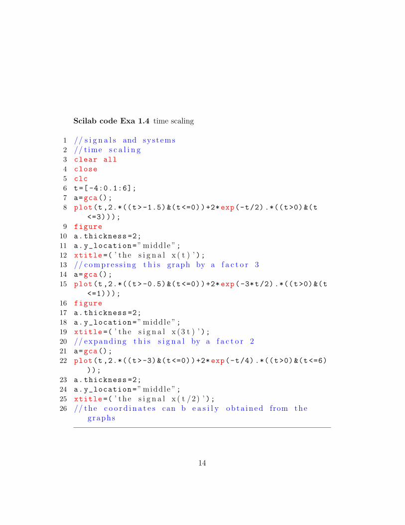
Scilab code Exa 1.4 time scaling
1 // s i g n a l s and sys t ems2 // t ime s c a l i n g3 clear all
4 close
5 clc
6 t=[ -4:0.1:6];
7 a=gca();
8 plot(t ,2.*((t>-1.5)&(t<=0))+2*exp(-t/2) .*((t>0)&(t
<=3)));
9 figure
10 a.thickness =2;
11 a.y_location=” middle ”;12 xtitle =( ’ the s i g n a l x ( t ) ’ );13 // compre s s i ng t h i s graph by a f a c t o r 314 a=gca();
15 plot(t ,2.*((t>-0.5)&(t<=0))+2*exp(-3*t/2) .*((t>0)&(t
<=1)));
16 figure
17 a.thickness =2;
18 a.y_location=” middle ”;19 xtitle =( ’ the s i g n a l x (3 t ) ’ );20 // expanding t h i s s i g n a l by a f a c t o r 221 a=gca();
22 plot(t ,2.*((t>-3)&(t<=0))+2*exp(-t/4) .*((t>0)&(t<=6)
));
23 a.thickness =2;
24 a.y_location=” middle ”;25 xtitle =( ’ the s i g n a l x ( t /2) ’ );26 // the c o o r d i n a t e s can b e a s i l y o b t a i n e d from the
graphs
14
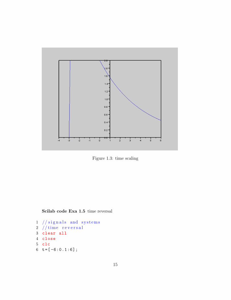
Figure 1.3: time scaling
Scilab code Exa 1.5 time reversal
1 // s i g n a l s and sys t ems2 // t ime r e v e r s a l3 clear all
4 close
5 clc
6 t=[ -6:0.1:6];
15

Figure 1.4: time scaling
16
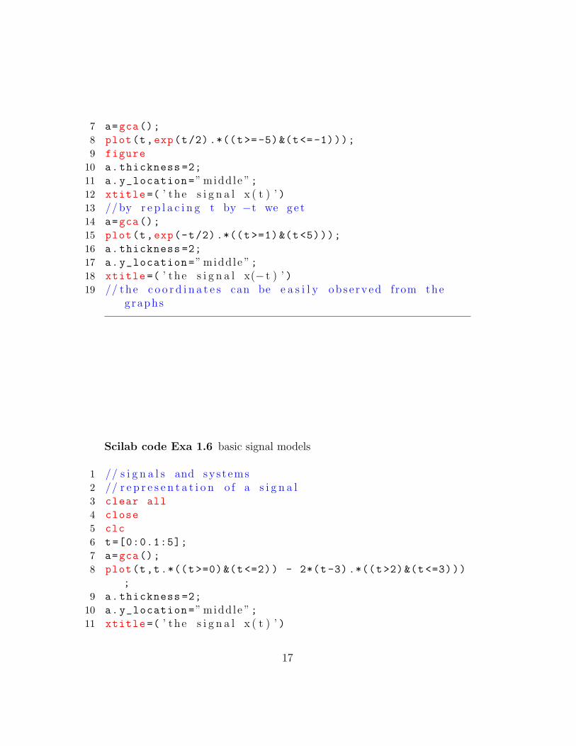
7 a=gca();
8 plot(t,exp(t/2) .*((t>=-5)&(t<=-1)));
9 figure
10 a.thickness =2;
11 a.y_location=” middle ”;12 xtitle =( ’ the s i g n a l x ( t ) ’ )13 // by r e p l a c i n g t by −t we ge t14 a=gca();
15 plot(t,exp(-t/2) .*((t>=1)&(t<5)));
16 a.thickness =2;
17 a.y_location=” middle ”;18 xtitle =( ’ the s i g n a l x(− t ) ’ )19 // the c o o r d i n a t e s can be e a s i l y ob s e rv ed from the
graphs
Scilab code Exa 1.6 basic signal models
1 // s i g n a l s and sys t ems2 // r e p r e s e n t a t i o n o f a s i g n a l3 clear all
4 close
5 clc
6 t=[0:0.1:5];
7 a=gca();
8 plot(t,t.*((t>=0)&(t<=2)) - 2*(t-3) .*((t>2)&(t<=3)))
;
9 a.thickness =2;
10 a.y_location=” middle ”;11 xtitle =( ’ the s i g n a l x ( t ) ’ )
17
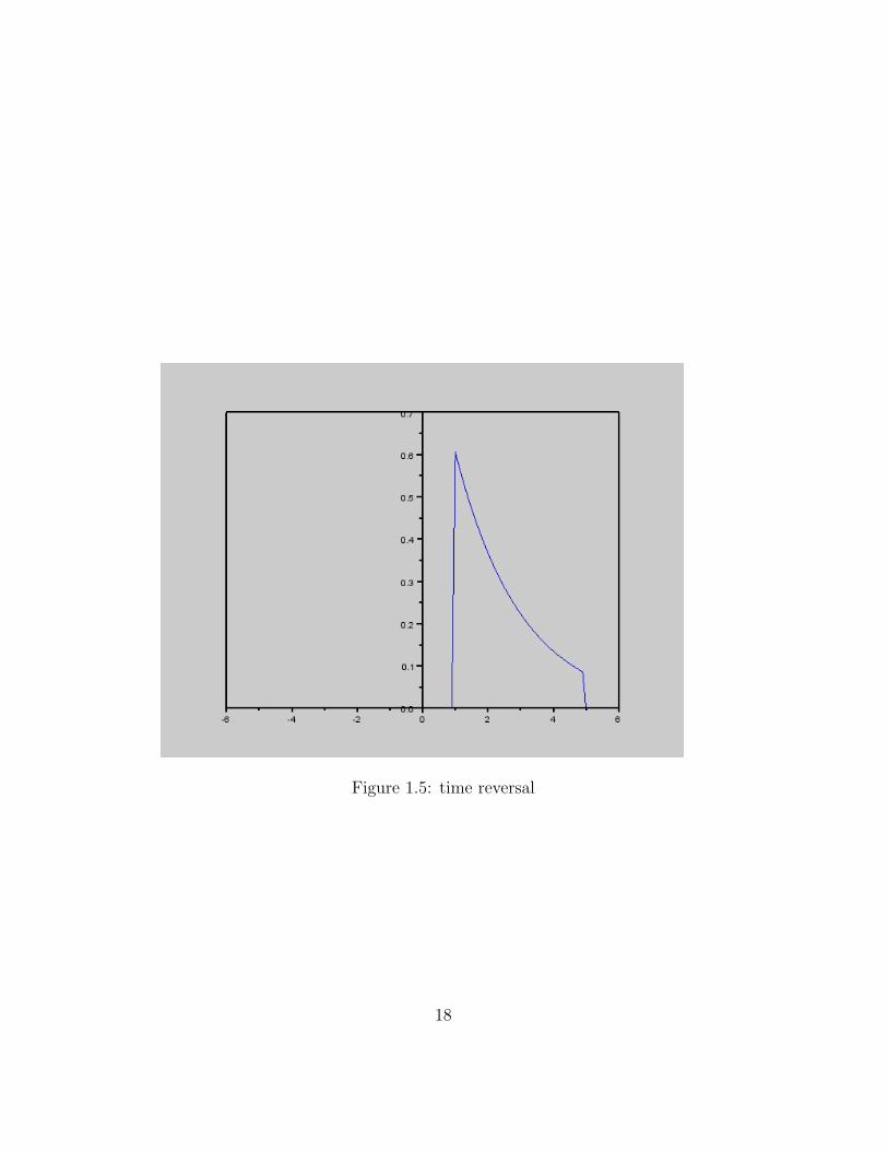
Figure 1.5: time reversal
18

Figure 1.6: time reversal
19
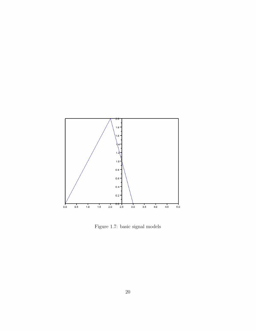
Figure 1.7: basic signal models
20
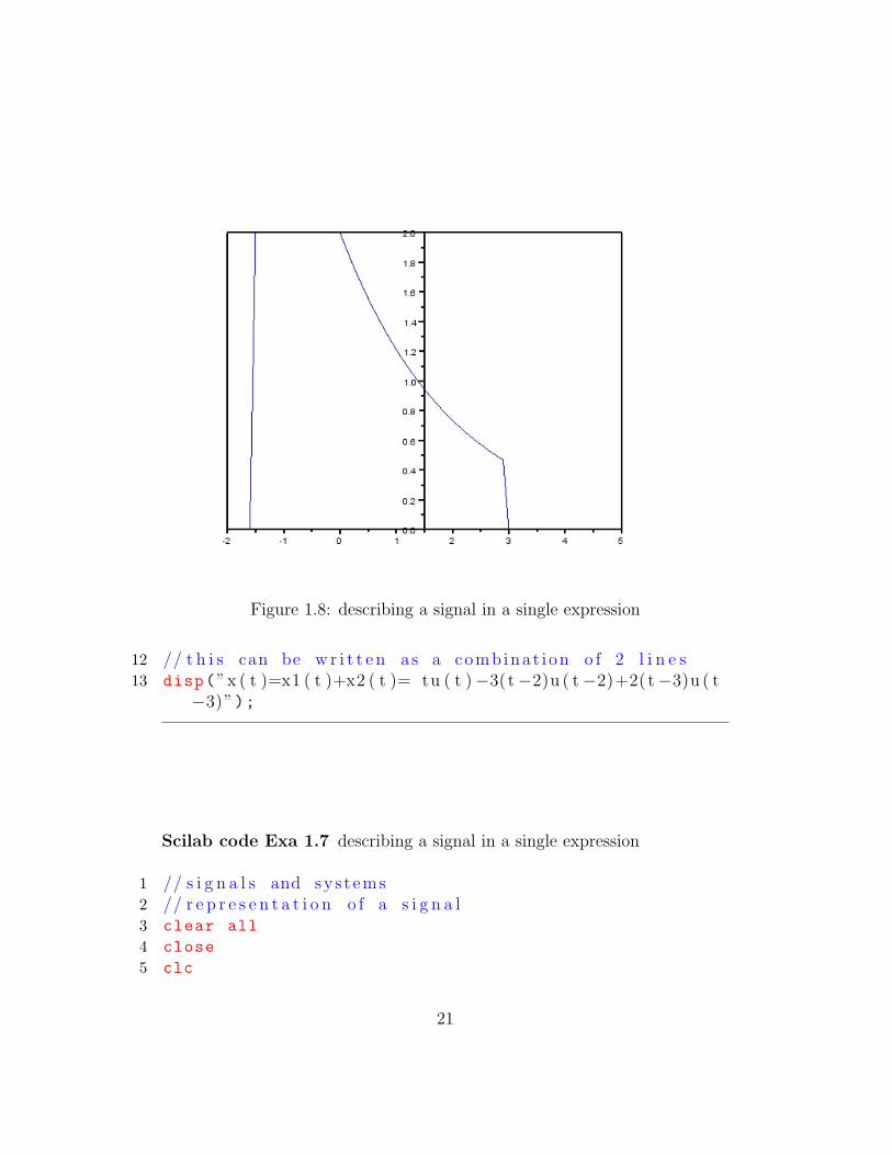
Figure 1.8: describing a signal in a single expression
12 // t h i s can be w r i t t e n as a combinat ion o f 2 l i n e s13 disp(”x ( t )=x1 ( t )+x2 ( t )= tu ( t )−3(t−2)u ( t−2)+2( t−3)u ( t
−3)”);
Scilab code Exa 1.7 describing a signal in a single expression
1 // s i g n a l s and sys t ems2 // r e p r e s e n t a t i o n o f a s i g n a l3 clear all
4 close
5 clc
21

6 t=[ -2:0.1:5];
7 a=gca();
8 plot(t ,2.*((t>= -1.5)&(t<0))+2*exp(-t/2) .*((t>=0)&(t
<3)));
9 a.thickness =2;
10 a.y_location=” middle ”;11 xtitle =( ’ the s i g n a l x ( t−1) ’ )12 // t h i s i s a c o b i n a t i o n o f a c o n s t a n t f u n c t i o n and an
e x p o n e n t i a l f u n c t i o n13 disp(”x ( t )=x1 ( t )+x2 ( t )= 2u ( t +1.5)−2(1−exp(− t /2) ) u ( t )
−2exp(− t /2) u ( t−3)”);
Scilab code Exa 1.8 even and odd components of a signal
1 // s i g n a l s and sys t ems2 // odd and even components3 clear all
4 close
5 clc
6 t = 0:1/100:5;
7 x=exp(%i.*t);
8 y=exp(-%i.*t);
9 even=x./2+y./2;
10 odd=x./2-y./2;
11 figure
12 a=gca();
13 plot2d(t,even)
14 a.x_location= ’ o r i g i n ’15 xtitle =( ’ even ’ )16 figure
17 a=gca();
18 plot2d(t,odd./%i)
19 a.x_location= ’ o r i g i n ’20 xtitle =( ’ odd ’ )
22
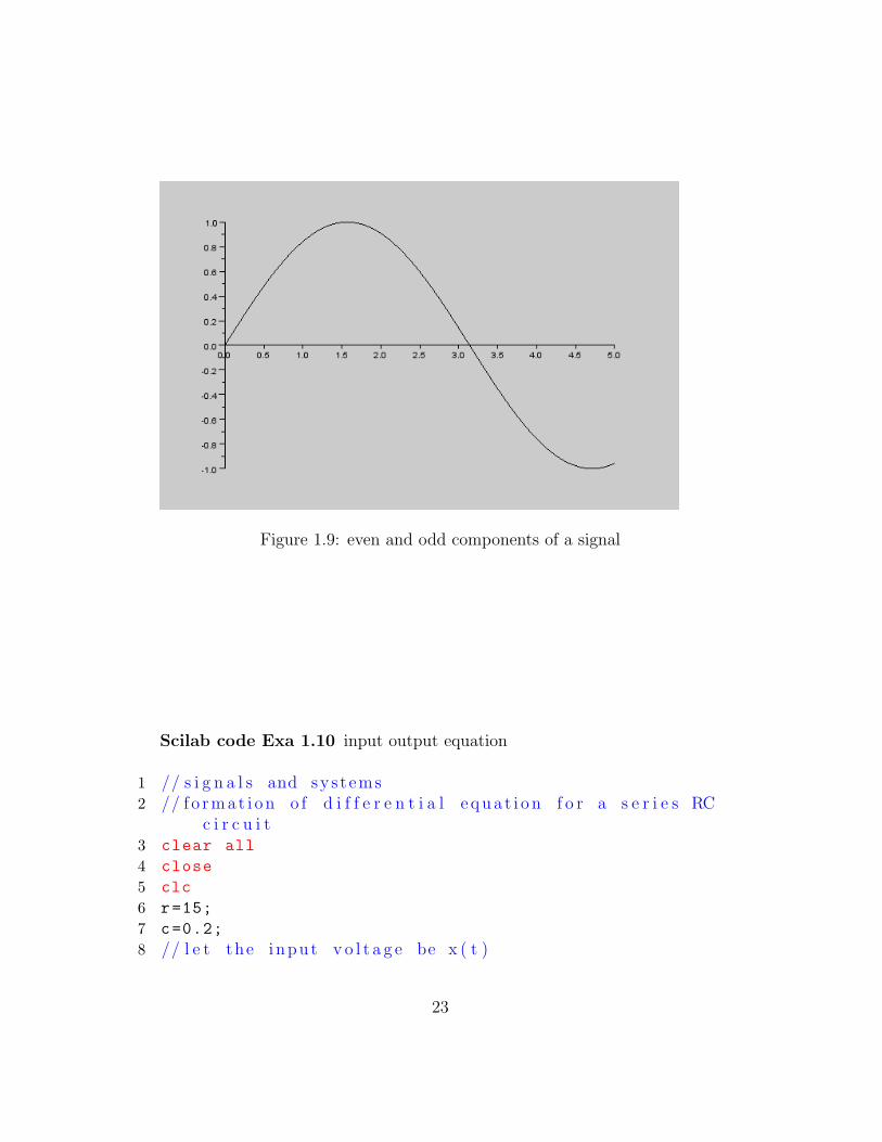
Figure 1.9: even and odd components of a signal
Scilab code Exa 1.10 input output equation
1 // s i g n a l s and sys t ems2 // f o r m a t i o n o f d i f f e r e n t i a l e q u a t i o n f o r a s e r i e s RC
c i r c u i t3 clear all
4 close
5 clc
6 r=15;
7 c=0.2;
8 // l e t the input v o l t a g e be x ( t )
23

Figure 1.10: even and odd components of a signal
24
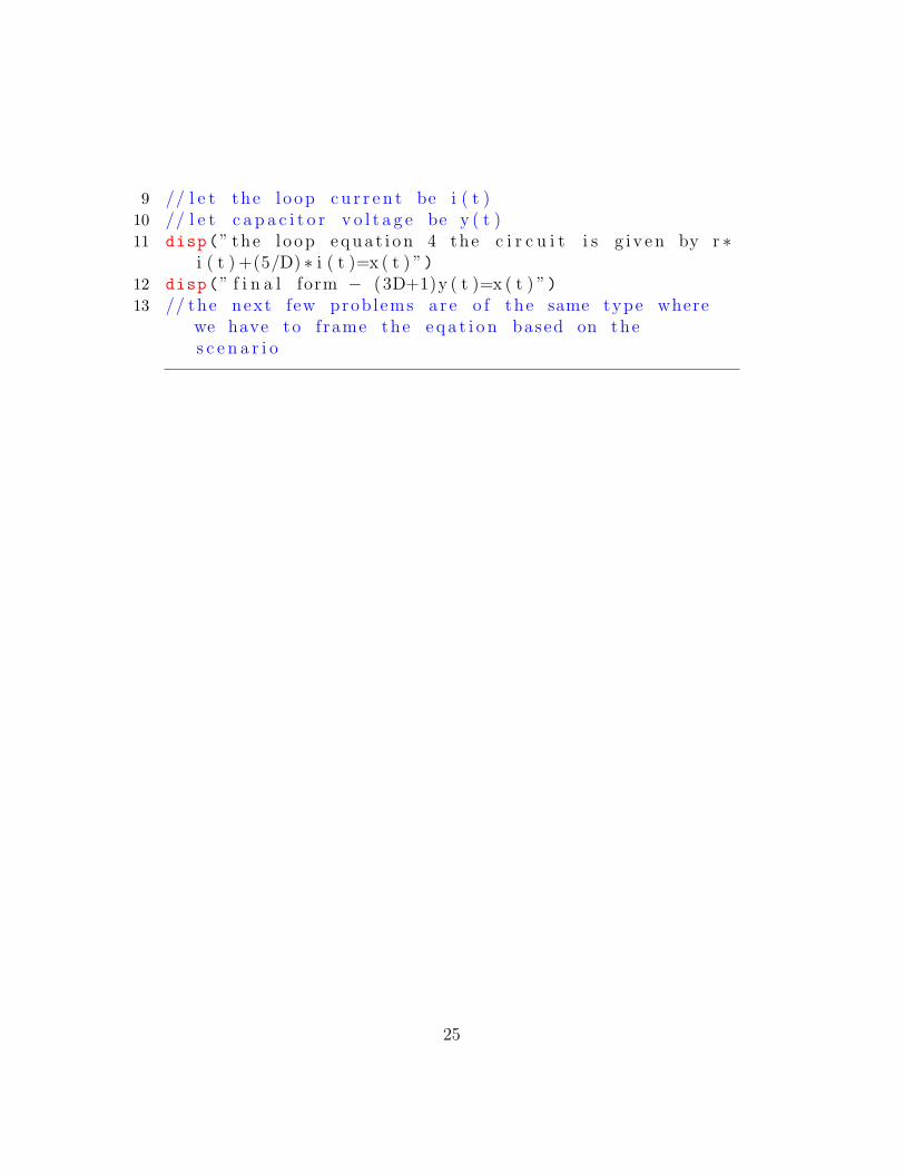
9 // l e t the l oop c u r r e n t be i ( t )10 // l e t c a p a c i t o r v o l t a g e be y ( t )11 disp(” the l oop e q u a t i o n 4 the c i r c u i t i s g i v e n by r ∗
i ( t ) +(5/D) ∗ i ( t )=x ( t ) ”)12 disp(” f i n a l form − (3D+1)y ( t )=x ( t ) ”)13 // the next few prob lems a r e o f the same type where
we have to frame the e q a t i o n based on thes c e n a r i o
25
Chapter 2
time domain analysis ofcontinuous time systems
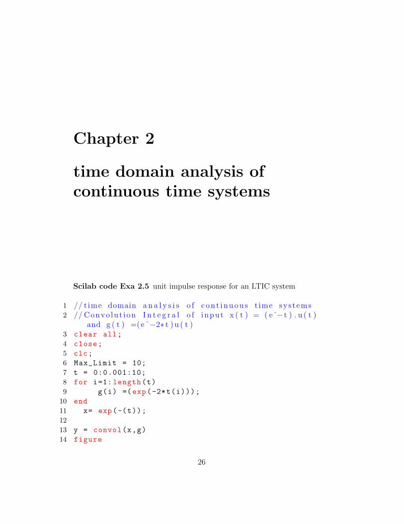
Scilab code Exa 2.5 unit impulse response for an LTIC system
1 // t ime domain a n a l y s i s o f c o n t i n u o u s t ime sys t ems2 // Convo lu t i on I n t e g r a l o f i nput x ( t ) = ( eˆ−t ) . u ( t )
and g ( t ) =(eˆ−2∗ t ) u ( t )3 clear all;
4 close;
5 clc;
6 Max_Limit = 10;
7 t = 0:0.001:10;
8 for i=1: length(t)
9 g(i) =(exp(-2*t(i)));
10 end
11 x= exp(-(t));
1213 y = convol(x,g)
14 figure
26
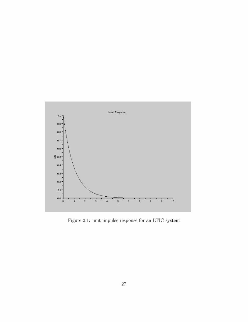
Figure 2.1: unit impulse response for an LTIC system
27

Figure 2.2: unit impulse response for an LTIC system
28
15 a=gca();
16 plot2d(t,g)
17 xtitle( ’ Impul se Response ’ , ’ t ’ , ’ h ( t ) ’ );18 a.thickness = 2;
19 figure
20 a=gca();
21 plot2d(t,x)
22 xtitle( ’ Input Response ’ , ’ t ’ , ’ x ( t ) ’ );23 a.thickness = 2;
24 figure
25 a=gca();
26 T=0:0.001:20;
27 plot2d(T,y)
28 xtitle( ’ Output Response ’ , ’ t ’ , ’ y ( t ) ’ );29 a.thickness = 2;
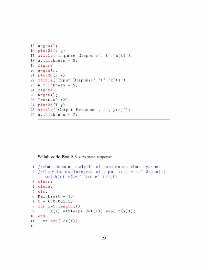
Scilab code Exa 2.6 zero state response
1 // t ime domain a n a l y s i s o f c o n t i n u o u s t ime sys t ems2 // Convo lu t i on I n t e g r a l o f i nput x ( t ) = ( eˆ−3 t ) . u ( t )
and h ( t ) =(2∗ eˆ−2∗ t−eˆ−t ) u ( t )3 clear;
4 close;
5 clc;
6 Max_Limit = 10;
7 t = 0:0.001:10;
8 for i=1: length(t)
9 g(i) =(2* exp(-2*t(i))-exp(-t(i)));
10 end
11 x= exp(-3*(t));
12
29

Figure 2.3: zero state response
30
Figure 2.4: zero state response
31

13 y = convol(x,g)
14 figure
15 a=gca();
16 plot2d(t,g)
17 xtitle( ’ Impul se Response ’ , ’ t ’ , ’ h ( t ) ’ );18 a.thickness = 2;
19 figure
20 a=gca();
21 plot2d(t,x)
22 xtitle( ’ Input Response ’ , ’ t ’ , ’ x ( t ) ’ );23 a.thickness = 2;
24 figure
25 a=gca();
26 T=0:0.001:20;
27 plot2d(T,y)
28 xtitle( ’ Output Response ’ , ’ t ’ , ’ y ( t ) ’ );29 a.thickness = 2;
Scilab code Exa 2.7 graphical convolution
1 // t ime domain a n a l y s i s o f c o n t i n u o u s t ime sys t ems2 // Convo lu t i on I n t e g r a l o f i nput x ( t ) = ( eˆ−t ) . u ( t )
and g ( t ) =u ( t )3 clear all;
4 close;
5 clc;
6 Max_Limit = 10;
7 t = -10:0.001:10;
8 for i=1: length(t)
910 g(i)=exp(-t(i));
11 x(i)=exp(-2*t(i));
12 end
1314 y = convol(x,g)
32
15 figure
16 a=gca();
17 plot2d(t,g)
18 xtitle( ’ Impul se Response ’ , ’ t ’ , ’ h ( t ) ’ );19 a.thickness = 2;
20 figure
21 a=gca();
22 plot2d(t,x)
23 xtitle( ’ Input Response ’ , ’ t ’ , ’ x ( t ) ’ );24 a.thickness = 2;
25 figure
26 a=gca();
27 T= -20:0.001:20;
28 plot2d(T,y)
29 xtitle( ’ Output Response ’ , ’ t ’ , ’ y ( t ) ’ );30 a.thickness = 2;
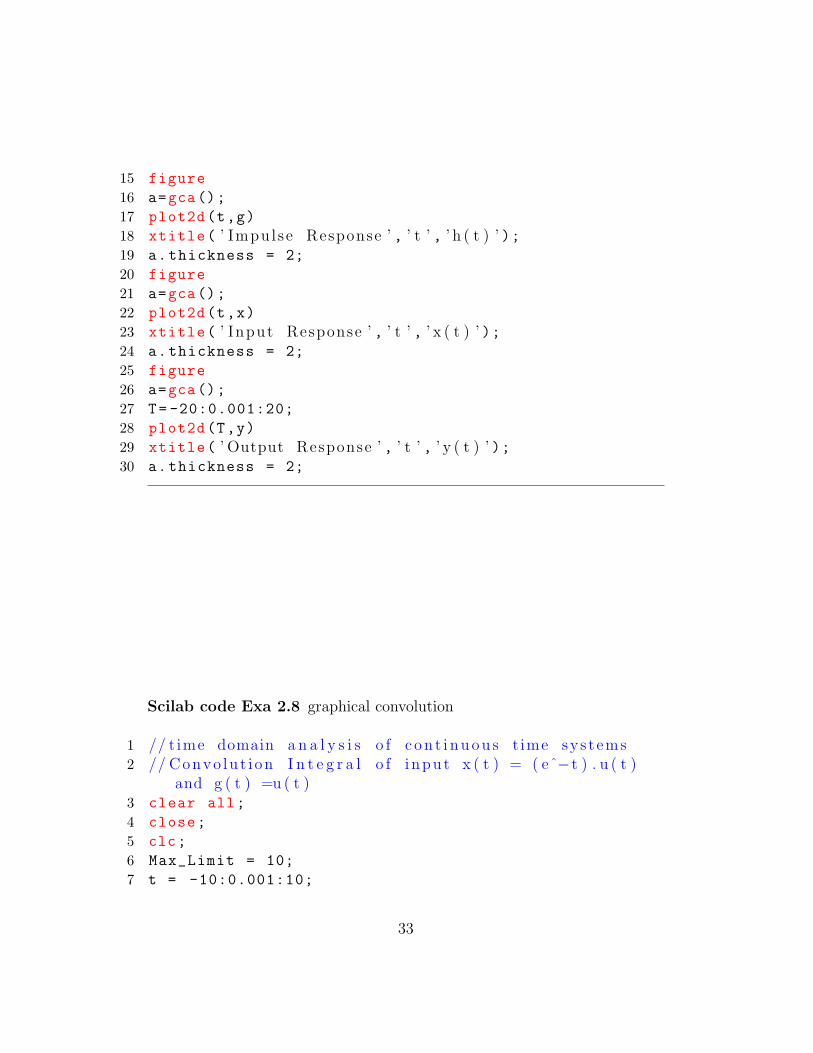
Scilab code Exa 2.8 graphical convolution
1 // t ime domain a n a l y s i s o f c o n t i n u o u s t ime sys t ems2 // Convo lu t i on I n t e g r a l o f i nput x ( t ) = ( eˆ−t ) . u ( t )
and g ( t ) =u ( t )3 clear all;
4 close;
5 clc;
6 Max_Limit = 10;
7 t = -10:0.001:10;
33
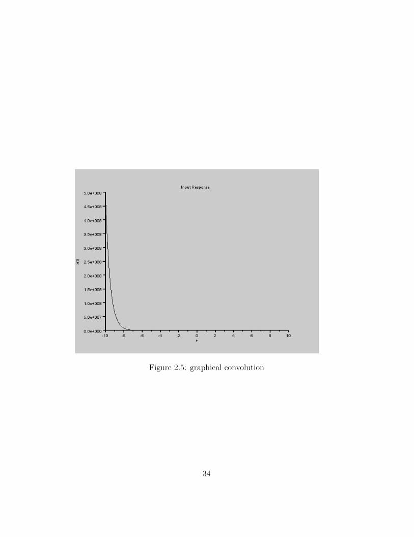
Figure 2.5: graphical convolution
34
Figure 2.6: graphical convolution
35

Figure 2.7: graphical convolution
36

Figure 2.8: graphical convolution
37
8 for i=1: length(t)
9 if t(i)<0 then
10 g(i)=-2*exp (2*t(i));
11 x(i)=0;
12 else
13 g(i)=2*exp(-t(i));
14 x(i)=1;
15 end
16 end
1718 y = convol(x,g)
19 figure
20 a=gca();
21 plot2d(t,g)
22 xtitle( ’ Impul se Response ’ , ’ t ’ , ’ h ( t ) ’ );23 a.thickness = 2;
24 figure
25 a=gca();
26 plot2d(t,x)
27 xtitle( ’ Input Response ’ , ’ t ’ , ’ x ( t ) ’ );28 a.thickness = 2;
29 figure
30 a=gca();
31 T= -20:0.001:20;
32 plot2d(T,y)
33 xtitle( ’ Output Response ’ , ’ t ’ , ’ y ( t ) ’ );34 a.thickness = 2;
Scilab code Exa 2.9 graphical convolution
1 // t ime domain a n a l y s i s o f c o n t i n u o u s t ime sys t ems
38
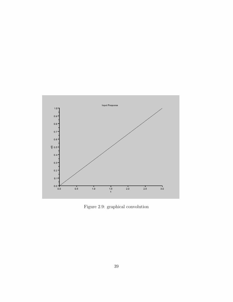
Figure 2.9: graphical convolution
39
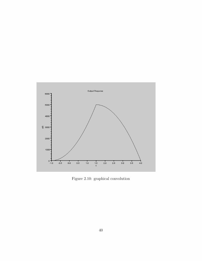
Figure 2.10: graphical convolution
40
2 // Convo lu t i on I n t e g r a l o f i nput x ( t ) = ( eˆ−t ) . u ( t )and g ( t ) =u ( t )
3 clear all;
4 close;
5 clc;
6 Max_Limit = 10;
7 t =linspace ( -1,1 ,10001);
8 for i=1: length(t)
9 g(i)=1;
10 end
11 t1=linspace (0 ,3 ,10001);
12 for i=1: length(t1)
13 x(i)= t1(i)/3;
14 end
15 y = convol(x,g);
16 figure
17 a=gca();
18 size(t)
19 size(g)
20 plot2d(t,g)
21 xtitle( ’ Impul se Response ’ , ’ t ’ , ’ h ( t ) ’ );22 a.thickness = 2;
23 figure
24 a=gca();
25 size(x)
26 plot2d(t1,x)
27 xtitle( ’ Input Response ’ , ’ t ’ , ’ x ( t ) ’ );28 a.thickness = 2;
29 figure
30 a=gca();
31 T=linspace (-1 ,4,20001);
32 size(y)
33 plot2d(T,y)
34 xtitle( ’ Output Response ’ , ’ t ’ , ’ y ( t ) ’ );35 a.thickness = 2;
41
Chapter 3
time domain analysis ofdiscrete time systems
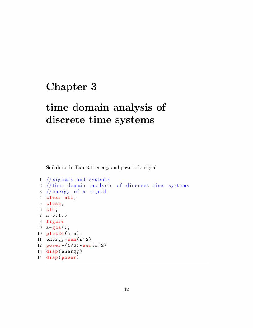
Scilab code Exa 3.1 energy and power of a signal
1 // s i g n a l s and sys t ems2 // t ime domain a n a l y s i s o f d i s c r e e t t ime sys t ems3 // ene rgy o f a s i g n a l4 clear all;
5 close;
6 clc;
7 n=0:1:5
8 figure
9 a=gca();
10 plot2d(n,n);
11 energy=sum(n^2)
12 power =(1/6)*sum(n^2)
13 disp(energy)
14 disp(power)
42

Figure 3.1: energy and power of a signal
43
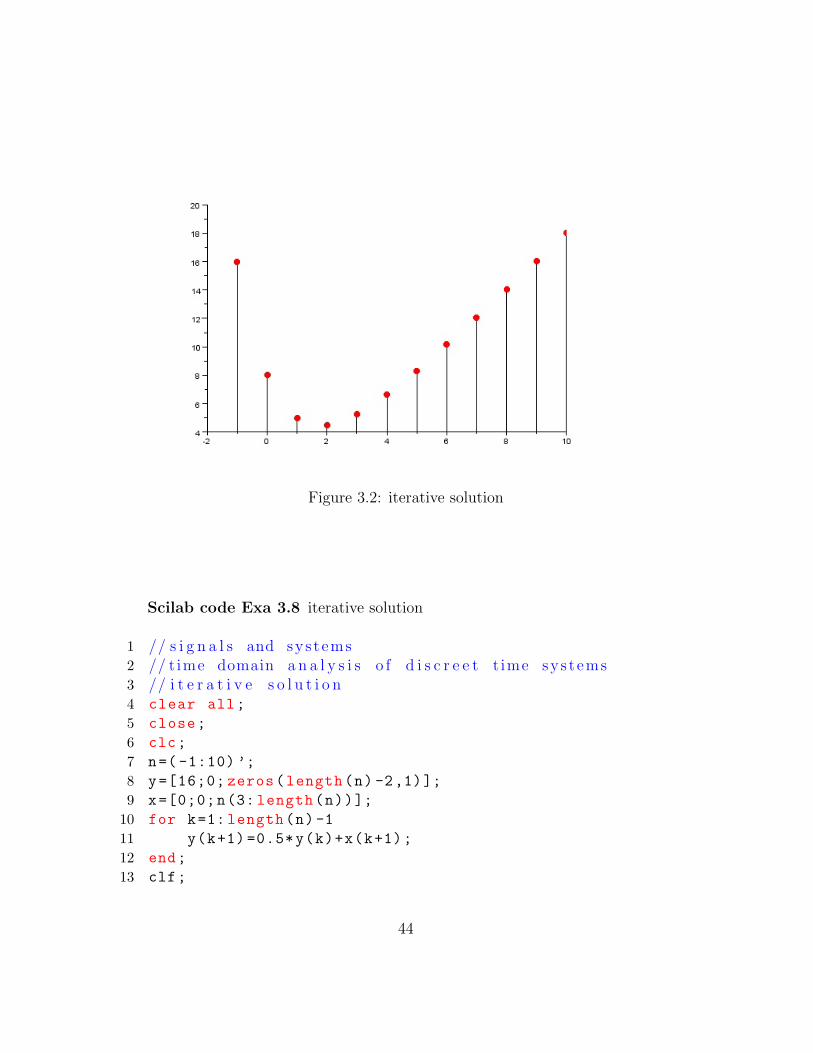
Figure 3.2: iterative solution
Scilab code Exa 3.8 iterative solution
1 // s i g n a l s and sys t ems2 // t ime domain a n a l y s i s o f d i s c r e e t t ime sys t ems3 // i t e r a t i v e s o l u t i o n4 clear all;
5 close;
6 clc;
7 n=( -1:10) ’;
8 y=[16;0; zeros(length(n) -2,1)];
9 x=[0;0;n(3: length(n))];
10 for k=1: length(n) -1
11 y(k+1) =0.5*y(k)+x(k+1);
12 end;
13 clf;
44
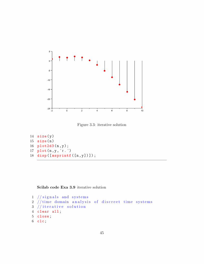
Figure 3.3: iterative solution
14 size(y)
15 size(n)
16 plot2d3(n,y);
17 plot(n,y, ’ r . ’ )18 disp([ msprintf ([n,y])]);
Scilab code Exa 3.9 iterative solution
1 // s i g n a l s and sys t ems2 // t ime domain a n a l y s i s o f d i s c r e e t t ime sys t ems3 // i t e r a t i v e s o l u t i o n4 clear all;
5 close;
6 clc;
45

7 n=( -2:10) ’;
8 y=[1;2; zeros(length(n) -2,1)];
9 x=[0;0;n(3: length(n))];
10 for k=1: length(n) -2
11 y(k+2)=y(k+1) -0.24*y(k)+x(k+2) -2*x(k+1);
12 end;
13 clf;
14 plot2d3(n,y);
15 disp([ msprintf ([n,y])]);
Scilab code Exa 3.10 total response with given initial conditions
1 // s i g n a l s and sys t ems2 // t ime domain a n a l y s i s o f d i s c r e e t t ime sys t ems3 // t o t a l r e s p o n s e with i n i t i a l c o n d i t i o n s4 clear all;
5 close;
6 clc;
7 n=( -2:10) ’;
8 y=[25/4;0; zeros(length(n) -2,1)];
9 x=[0;0;4^ -n(3: length(n))];
10 for k=1: length(n) -2
11 y(k+2) =0.6*y(k+1) +0.16*y(k)+5*x(k+2);
12 end;
13 clf;
14 a=gca();
15 plot2d3(n,y);
1617 y1 =[25/4;0; zeros(length(n) -2,1)];
18 x=[0;0;4^ -n(3: length(n))];
19 for k=1: length(n) -2
20 y1(k+2)=-6*y1(k+1) -9*y1(k)+2*x(k+2)+6*x(k+1);
21 end
22 figure
23 a=gca();
46
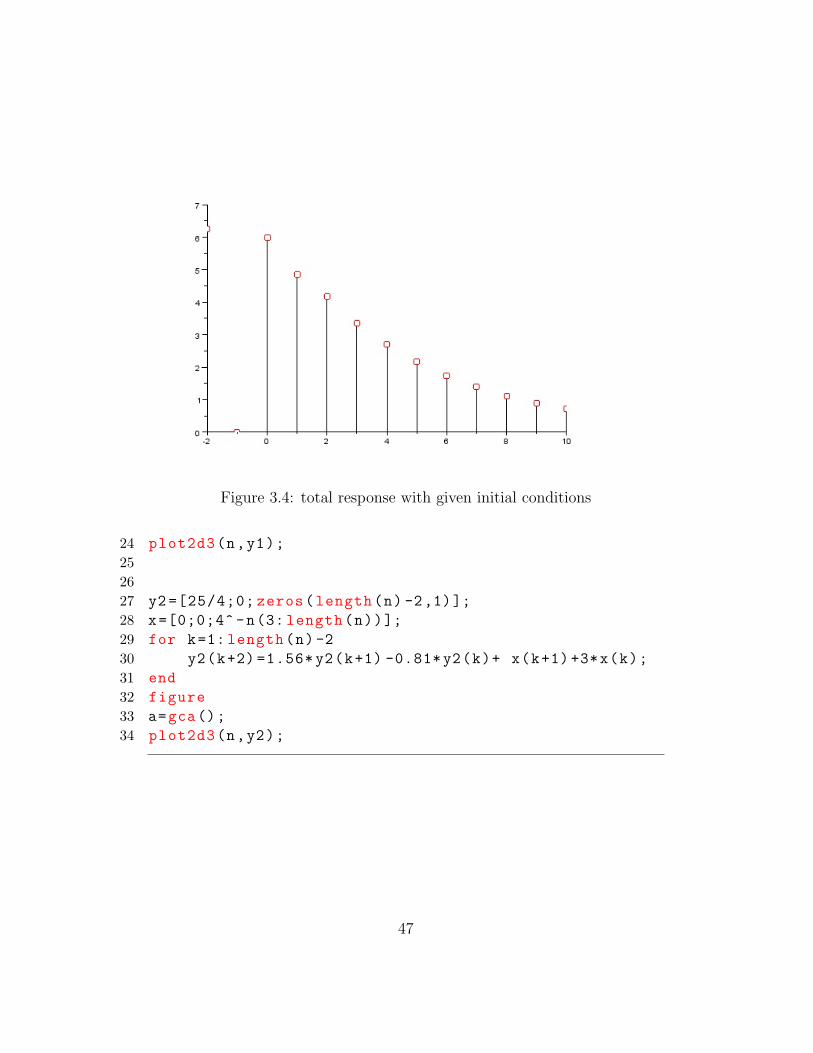
Figure 3.4: total response with given initial conditions
24 plot2d3(n,y1);
252627 y2 =[25/4;0; zeros(length(n) -2,1)];
28 x=[0;0;4^ -n(3: length(n))];
29 for k=1: length(n) -2
30 y2(k+2) =1.56* y2(k+1) -0.81*y2(k)+ x(k+1)+3*x(k);
31 end
32 figure
33 a=gca();
34 plot2d3(n,y2);
47
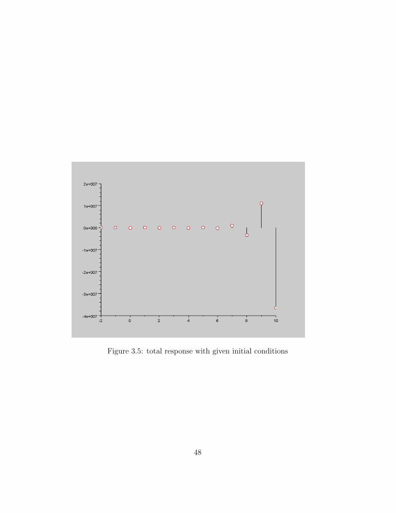
Figure 3.5: total response with given initial conditions
48
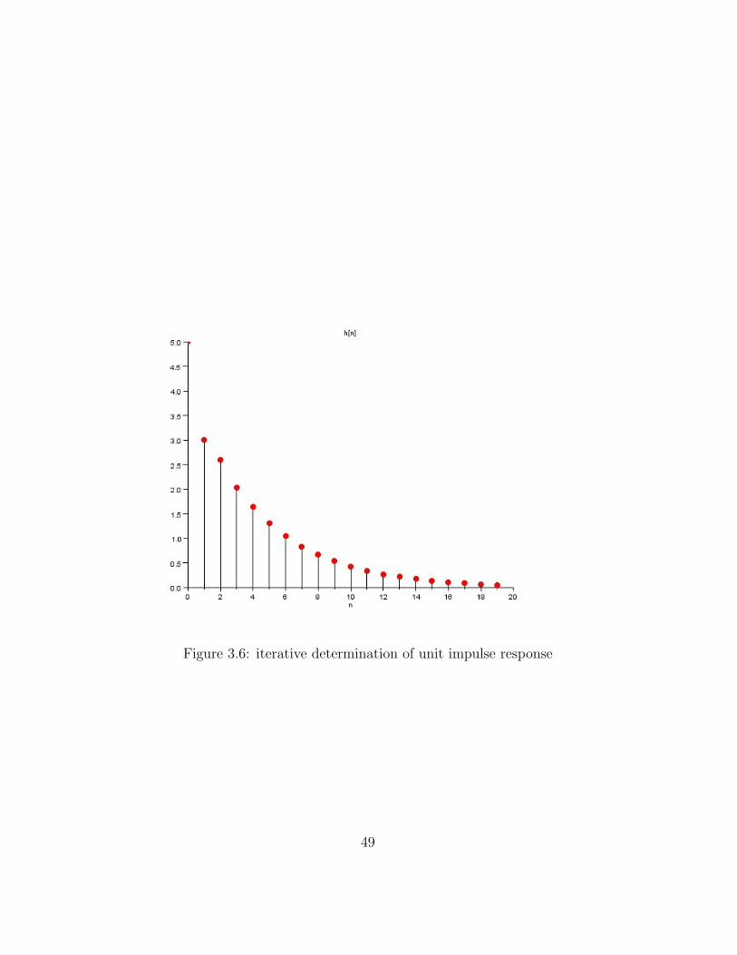
Figure 3.6: iterative determination of unit impulse response
49

Scilab code Exa 3.11 iterative determination of unit impulse response
1 // s i g n a l s and sys t ems2 // t ime domain a n a l y s i s o f d i s c r e e t t ime sys t ems3 // impu l s e r e s p o n s e with i n i t i a l c o n d i t i o n s4 clear all;
5 close;
6 clc;
7 n=(0:19);
8 x=[1 zeros(1,length(n) -1)];
9 a=[1 -0.6 -0.16];
10 b=[5 0 0];
11 h=filter(b,a,x);
12 clf;
13 plot2d3(n,h); xlabel( ’ n ’ ); ylabel( ’ h [ n ] ’ );
Scilab code Exa 3.13 convolution of discrete signals
1 // s i g n a l s and sys t ems2 // t ime domain a n a l y s i s o f d i s c r e e t t ime sys t ems3 // c o n v o l u t i o n4 clear all;
5 close;
6 clc;
7 n=(0:19);
8 x=0.8^n;
9 g=0.3^n;
10 n1 =(0:1: length(x)+length(g) -2);
11 c=convol(x,g);
12 plot2d3(n1,c);
50

Figure 3.7: convolution of discrete signals
51

Figure 3.8: convolution of discrete signals
Scilab code Exa 3.14 convolution of discrete signals
1 // s i g n a l s and sys t ems2 // t ime domain a n a l y s i s o f d i s c r e e t t ime sys t ems3 // c o n v o l u t i o n4 clear all;
5 close;
6 clc;
7 n=(0:14);
8 x=4^-n;
9 a=[1 -0.6 -0.16];
10 b=[5 0 0];
11 y=filter(b,a,x);
52
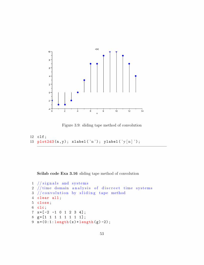
Figure 3.9: sliding tape method of convolution
12 clf;
13 plot2d3(n,y); xlabel( ’ n ’ ); ylabel( ’ y [ n ] ’ );
Scilab code Exa 3.16 sliding tape method of convolution
1 // s i g n a l s and sys t ems2 // t ime domain a n a l y s i s o f d i s c r e e t t ime sys t ems3 // c o n v o l u t i o n by s l i d i n g tape method4 clear all;
5 close;
6 clc;
7 x=[-2 -1 0 1 2 3 4];
8 g=[1 1 1 1 1 1 1 1];
9 n=(0:1: length(x)+length(g) -2);
53
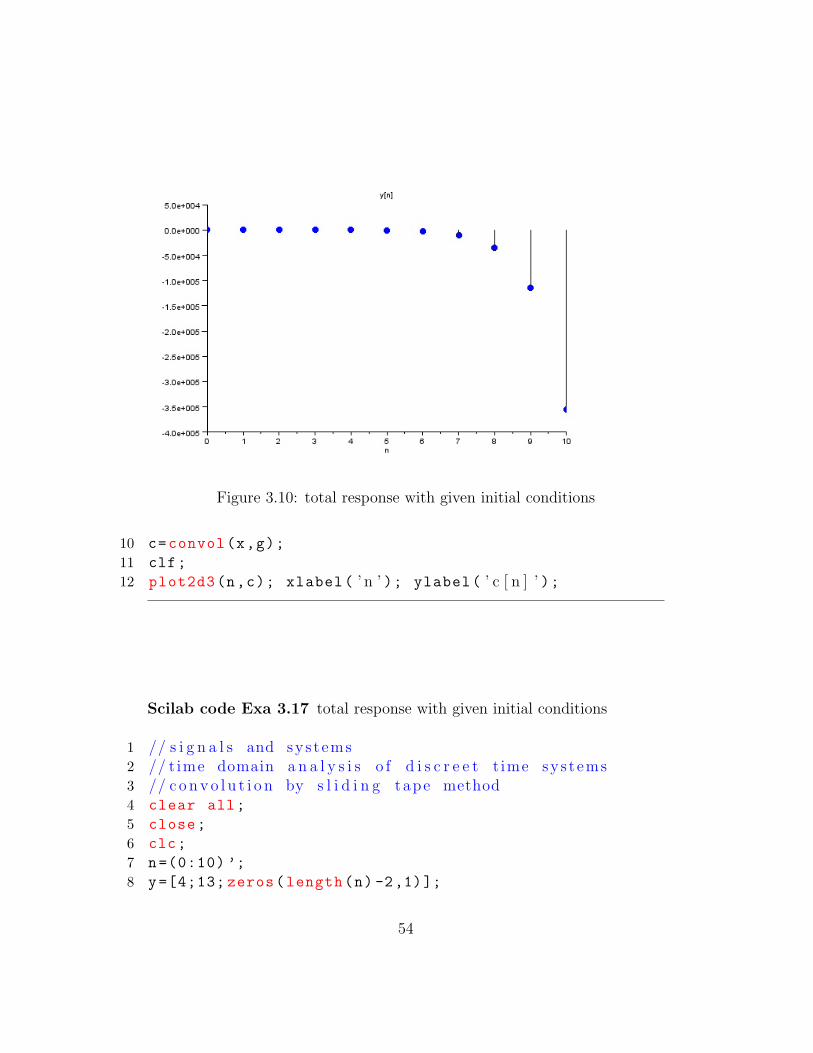
Figure 3.10: total response with given initial conditions
10 c=convol(x,g);
11 clf;
12 plot2d3(n,c); xlabel( ’ n ’ ); ylabel( ’ c [ n ] ’ );
Scilab code Exa 3.17 total response with given initial conditions
1 // s i g n a l s and sys t ems2 // t ime domain a n a l y s i s o f d i s c r e e t t ime sys t ems3 // c o n v o l u t i o n by s l i d i n g tape method4 clear all;
5 close;
6 clc;
7 n=(0:10) ’;
8 y=[4;13; zeros(length(n) -2,1)];
54

Figure 3.11: total response with given initial conditions
9 x=(3*n+5).*(n>=0);
10 for k=1: length(n) -2
11 y(k+2)=5*y(k+1) -6*y(k)+x(k+1) -5*x(k);
12 end
13 clf;
14 plot2d3(n,y); xlabel( ’ n ’ ); ylabel( ’ y [ n ] ’ );15 disp( ’ n y ’ );16 disp(msprintf( ’ %f\ t \ t%f\n ’ ,[n,y]));
Scilab code Exa 3.18 total response with given initial conditions
1 // s i g n a l s and sys t ems2 // t ime domain a n a l y s i s o f d i s c r e e t t ime sys t ems3 // c o n v o l u t i o n by s l i d i n g tape method
55
4 clear all;
5 close;
6 clc;
7 n=(0:10) ’;
8 y=[0; zeros(length(n) -1,1)];
9 x=(n+1)^2;
10 for k=1: length(n) -1
11 y(k+1)=y(k)+x(k);
12 end;
13 clf;
14 a=gca();
15 plot2d3(n,y);xtitle( ’ sum ’ , ’ n ’ )16 plot(n,y, ’ b . ’ )
Scilab code Exa 3.19 forced response
1 // s i g n a l s and sys t ems2 // t ime domain a n a l y s i s o f d i s c r e e t t ime sys t ems3 // c o n v o l u t i o n by s l i d i n g tape method4 clear all;
5 close;
6 clc;
7 n=(0:14);
8 x=3^n;
9 a=[1 -3 2];
10 b=[0 1 2];
11 y=filter(b,a,x);
12 clf;
13 plot2d3(n,y); xlabel( ’ n ’ ); ylabel( ’ y [ n ] ’ );
56

Figure 3.12: forced response
57
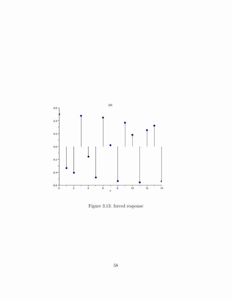
Figure 3.13: forced response
58

Scilab code Exa 3.20 forced response
1 // s i g n a l s and sys t ems2 // t ime domain a n a l y s i s o f d i s c r e e t t ime sys t ems3 // c o n v o l u t i o n by s l i d i n g tape method4 clear all;
5 close;
6 clc;
7 pi =3.14;
8 n=(0:14);
9 x=cos(2*n+pi/3);
10 a=[1 -1 0.16];
11 b=[0 1 0.32];
12 y=filter(b,a,x);
13 clf;
14 plot2d3(n,y); xlabel( ’ n ’ ); ylabel( ’ y [ n ] ’ );
59
Chapter 4
continuous time system analysis
Scilab code Exa 4.1 laplace transform of exponential signal
1 // s i g n a l s and sys t ems2 // Lap lace Transform x ( t ) = exp(−at ) . u ( t ) f o r t
n e g a t i v e and p o s i t i v e3 syms t s;
4 a = 3;
5 y =laplace( ’%eˆ(−a∗ t ) ’ ,t,s);6 t1 =0:0.001:10;
7 plot2d(t1,exp(-a*t1));
8 disp(y)
9 y1 = laplace( ’%eˆ( a∗−t ) ’ ,t,s);10 disp(y1)
Scilab code Exa 4.2 laplace transform of given fsignal
1 // s i g n a l s and sys t ems2 // ( a ) l a p l a c e t r a n s f o r m x ( t ) = d e l ( t )3 syms t s;
60
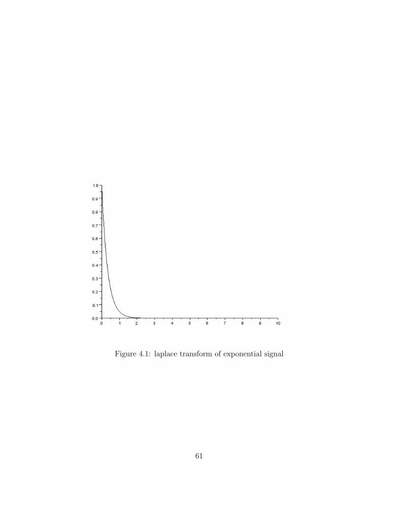
Figure 4.1: laplace transform of exponential signal
61
45 y =laplace( ’ 0 ’ ,t,s)6 disp(y)
7 // ( b ) Lap lace Transform x ( t ) = u ( t )89 y1 =laplace( ’ 1 ’ ,t,s);
10 disp(y1)
11 // ( c ) l a p l a c e t r a n s f o r m x ( t ) = co s (w0∗ t ) u ( t )1213 y2 =laplace( ’ c o s (w0∗ t ) ’ ,t,s);14 disp(y2)
Scilab code Exa 4.3.a laplace transform in case of different roots
1 // s i g n a l s and sys t ems2 // I n v e r s e Lapa l c e Transform3 // ( a ) X( S ) = (7 s−6)/ sˆ2−s−6 Re ( s )>−14 s =%s ;
5 syms t ;
6 [A]=pfss ((7*s-6)/((s^2-s-6))); // p a r t i a l f r a c t i o n o fF( s )
7 F1 = ilaplace(A(1),s,t)
8 F2 = ilaplace(A(2),s,t)
9 //F3 = i l a p l a c e (A( 3 ) , s , t )10 F = F1+F2;
11 disp(F,” f ( t )=”)
Scilab code Exa 4.3.b laplace transform in case of similar roots
1 // example 4 . 32 // ( b ) X( S ) = (2∗ s ˆ2+5) / s ˆ2−3∗ s+2 Re ( s )>−13 s =%s ;
4 syms t ;
62

5 [A]=pfss ((2*s^2+5) /((s^2-3*s+2))); // p a r t i a lf r a c t i o n o f F( s )
6 F1 = ilaplace(A(1),s,t)
7 F2 = ilaplace(A(2),s,t)
8 //F3 = i l a p l a c e (A( 3 ) , s , t )9 F = F1+F2;
10 disp(F,” f ( t )=”)
Scilab code Exa 4.3.c laplace transform in case of imaginary roots
1 // example4 . 32 // ( c ) X( S ) = 6( s +34)/ s ( s ˆ2+10∗ s +34) Re ( s )>−13 s =%s ;
4 syms t ;
5 [A]=pfss ((6*(s+34))/(s*(s^2+10*s+34))); // p a r t i a lf r a c t i o n o f F( s )
6 F1 = ilaplace(A(1),s,t)
7 F2 = ilaplace(A(2),s,t)
8 //F3 = i l a p l a c e (A( 3 ) , s , t )9 F = F1+F2;
10 disp(F,” f ( t )=”)
Scilab code Exa 4.4 laplace transform of a given signal
1 // s i g n a l s and sys t ems2 // Lapa l c e Transform x ( t ) = ( t−1)u ( t−1)−(t−2)u ( t−2)−u
( t−4) , 0<t<T3 syms t s;
4 a = 3;
5 T = 1;
6 // t = T;7 y1 = laplace( ’ t ’ ,t,s);8 y2 = laplace( ’ t ’ ,t,s);
63

9 y3 = laplace( ’ 1 ’ ,t,s);10 y=y1*(%e^(-s))+y2*(%e^(-2*s))+y3*(%e^(-4*s))
11 disp(y)
Scilab code Exa 4.5 inverse laplace transform
1 // s i g n a l s and sys t ems2 // example4 . 53 // X( S ) = s+3+5∗exp (−2∗ s ) /( s +1) ∗ ( s +2) ) Re ( s )>−14 s1 =%s ;
5 syms t s;
6 [A]=pfss((s1+3)/((s1+1)*(s1+2))); // p a r t i a l f r a c t i o no f F( s )
7 F1 = ilaplace(A(1),s,t)
8 F2 = ilaplace(A(2),s,t)
9 //F3 = i l a p l a c e (A( 3 ) , s , t )10 Fa = F1+F2;
11 disp(Fa,” f 1 ( t )=”)12 [B]=pfss ((5) /((s1+1)*(s1+2))); // p a r t i a l f r a c t i o n o f
F( s )13 F1 = ilaplace(B(1),s,t)
14 F2 = ilaplace(B(2),s,t)
15 Fb = (F1+F2)*(%e^(-2*s));
16 disp(Fb,” f 2 ( t )=”)17 disp(Fa+Fb,” f ( t )=”)
Scilab code Exa 4.8 time convolution property
1 // s i g n a l s and sys t ems2 // Example 4 . 83 // Lapa l c e Transform f o r c o n v o l u t i o n4 s=%s
5 syms t ;
64
6 a=3;b=2;
7 [A]=pfss (1/(s^2-5*s+6)); // p a r t i a l f r a c t i o n o f F( s )8 F1 = ilaplace(A(1),s,t)
9 F2 = ilaplace(A(2),s,t)
10 //F3 = i l a p l a c e (A( 3 ) , s , t )11 F = F1+F2;
12 disp(F,” f ( t )=”)
Scilab code Exa 4.9 initial and final value
1 // I n i t i a l and f i n a l Value Theorem o f Lapa laceTransform
2 syms s;
3 num =poly ([30 20], ’ s ’ , ’ c o e f f ’ )4 den =poly ([0 5 2 1], ’ s ’ , ’ c o e f f ’ )5 X = num/den
6 disp (X,”X( s )=”)7 SX = s*X;
8 Initial_Value =limit(SX,s,%inf);
9 final_value =limit(SX ,s,0);
10 disp(Initial_Value ,”x ( 0 )=”)11 disp(final_value ,”x ( i n f )=”)
Scilab code Exa 4.10 second order linear differential equation
1 // s i g n a l s and sys t ems2 // U n i l a t e r a l Lap lace Transform : S o l v i n g D i f f e r e n t i a l
Equat ion3 // example 4 . 1 04 s = %s;
5 syms t;
6 [A] = pfss ((2*s^2+20*s+45) /((s+2)*(s+3)*(s+4)));
7 F1 = ilaplace(A(1),s,t)
65

8 F2 = ilaplace(A(2),s,t)
9 F3 = ilaplace(A(3),s,t)
10 F = F1+F2+F3
11 disp(F)
Scilab code Exa 4.11 solution to ode using laplace transform
1 // s i g n a l s and sys t ems2 // U n i l a t e r a l Lap lace Transform : S o l v i n g D i f f e r e n t i a l
Equat ion3 // example 4 . 1 14 s = %s;
5 syms t;
6 [A] = pfss ((2*s)/(s^2+2*s+5));
7 F1 = ilaplace(A(1),s,t)
8 //F2 = i l a p l a c e (A( 2 ) , s , t )9 //F3 = i l a p l a c e (A( 3 ) , s , t )
10 F = F1+F2+F3
11 disp(F)
Scilab code Exa 4.12 response to LTIC system
1 // s i g n a l s and sys t ems2 // U n i l a t e r a l Lap lace Transform : S o l v i n g D i f f e r e n t i a l
Equat ion3 // example 4 . 1 24 s = %s;
5 syms t;
6 [A] = pfss ((3*s+3)/((s+5)*(s^2+5*s+6)));
7 F1 = ilaplace(A(1),s,t)
8 F2 = ilaplace(A(2),s,t)
9 F3 = ilaplace(A(3),s,t)
10 F = F1+F2+F3
66
11 disp(F)
Scilab code Exa 4.15 loop current in a given network
1 // s i g n a l s and sys t ems2 // U n i l a t e r a l Lap lace Transform : S o l v i n g D i f f e r e n t i a l
Equat ion3 // example 4 . 1 54 s = %s;
5 syms t;
6 [A] = pfss ((10)/(s^2+3*s+2));
7 F1 = ilaplace(A(1),s,t)
8 F2 = ilaplace(A(2),s,t)
9 //F3 = i l a p l a c e (A( 3 ) , s , t )10 F = F1+F2+F3
11 disp(F)
Scilab code Exa 4.16 loop current in a given network
1 // s i g n a l s and sys t ems2 // U n i l a t e r a l Lap lace Transform : t r a n s f e r f u n c t i o n3 // example 4 . 1 64 s = %s;
5 syms t s;
6 y1 =laplace( ’ 24∗%eˆ(−3∗ t ) +48∗%eˆ(−4∗ t ) ’ ,t,s);7 disp(y1)
8 y2 =laplace( ’ 16∗%eˆ(−3∗ t )−12∗%eˆ(−4∗ t ) ’ ,t,s);9 disp(y2)
Scilab code Exa 4.17 voltage and current of a given network
67
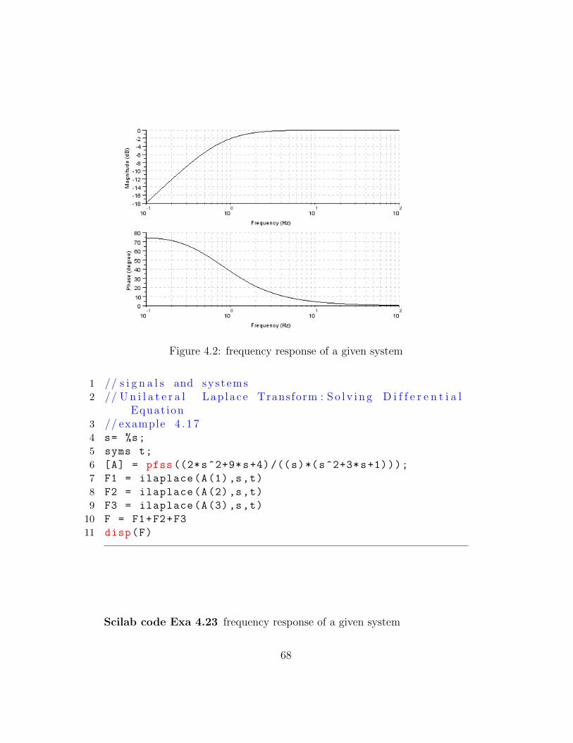
Figure 4.2: frequency response of a given system
1 // s i g n a l s and sys t ems2 // U n i l a t e r a l Lap lace Transform : S o l v i n g D i f f e r e n t i a l
Equat ion3 // example 4 . 1 74 s= %s;
5 syms t;
6 [A] = pfss ((2*s^2+9*s+4) /((s)*(s^2+3*s+1)));
7 F1 = ilaplace(A(1),s,t)
8 F2 = ilaplace(A(2),s,t)
9 F3 = ilaplace(A(3),s,t)
10 F = F1+F2+F3
11 disp(F)
Scilab code Exa 4.23 frequency response of a given system
68

1 s=poly(0, ’ s ’ )2 h=syslin( ’ c ’ ,(s+0.1)/(s+5))3 clf();bode(h,0.1 ,100);
Scilab code Exa 4.24 frequency response of a given system
1 s=poly(0, ’ s ’ )2 h=syslin( ’ c ’ ,(s^2/s))3 clf();bode(h,0.1 ,100);
4 h1=syslin( ’ c ’ ,(1/s))5 clf(); bode(h1 ,0.1 ,100);
Scilab code Exa 4.25 bode plots for given transfer function
1 s=poly(0, ’ s ’ )2 h=syslin( ’ c ’ ,((20*s^2+2000*s)/(s^2+12*s+20)))3 clf();bode(h,0.1 ,100);
Scilab code Exa 4.26 bode plots for given transfer function
1 s=poly(0, ’ s ’ )2 h=syslin( ’ c ’ ,((10*s+1000) /(s^2+2*s+100)))3 clf();bode(h,0.1 ,100);
69
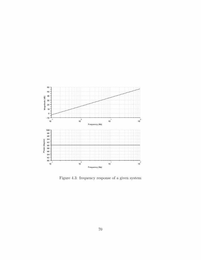
Figure 4.3: frequency response of a given system
70
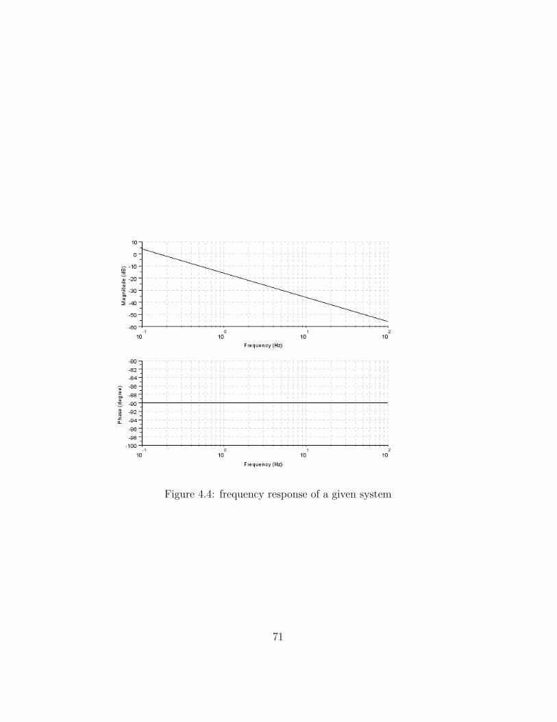
Figure 4.4: frequency response of a given system
71
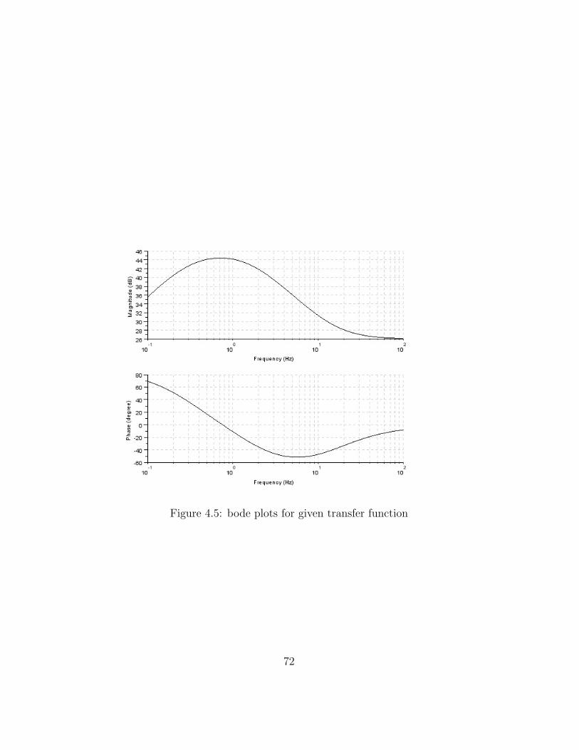
Figure 4.5: bode plots for given transfer function
72
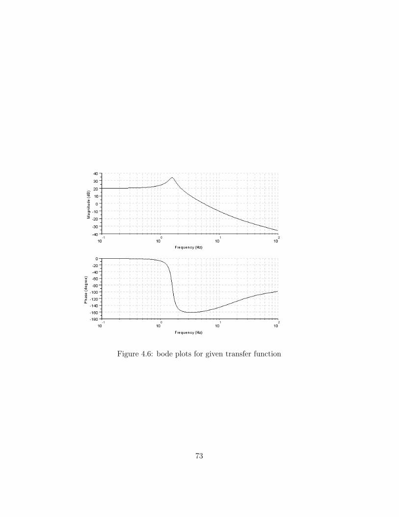
Figure 4.6: bode plots for given transfer function
73
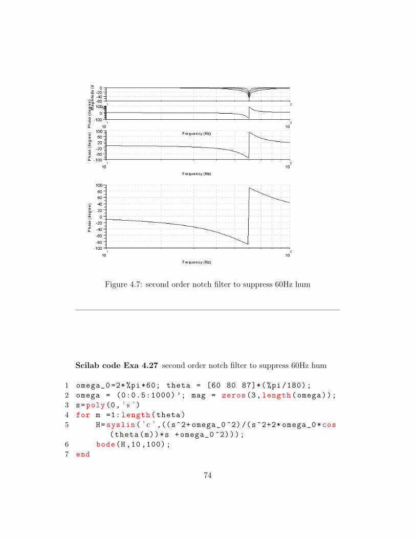
Figure 4.7: second order notch filter to suppress 60Hz hum
Scilab code Exa 4.27 second order notch filter to suppress 60Hz hum
1 omega_0 =2*%pi *60; theta = [60 80 87]*( %pi /180);
2 omega = (0:0.5:1000) ’; mag = zeros(3,length(omega));
3 s=poly(0, ’ s ’ )4 for m =1: length(theta)
5 H=syslin( ’ c ’ ,((s^2+ omega_0 ^2)/(s^2+2* omega_0*cos(theta(m))*s +omega_0 ^2)));
6 bode(H,10 ,100);
7 end
74
8 f=omega /((2* %pi))plot(f,mag(1,:), ’ k− ’ ,f mag(2,:), ’ k−− ’ ,f,mag(3,:), ’ k−. ’ );
9 xlabel( ’ f [ hz ] ’ ); ylabel( ’ |H( j 2 / p i f ) | ’ );10 legend( ’ \ t h e t a =60ˆ\ c i r c ’ , ’ \ t h e t a = 80ˆ\ c i r c ’ , ’ \ t h e t a
= 87ˆ\ c i r c ’ ,0)
Scilab code Exa 4.28 bilateral inverse transform
1 // s i g n a l s and sys t ems2 // b i l a t e r a l I n v e r s e Lapa l c e Transform3 //X( S ) = 1 / ( ( s−1) ( s +2) )4 s =%s ;
5 syms t ;
6 [A]=pfss (1/((s-1)*(s+2))) // p a r t i a l f r a c t i o n o f F( s )7 F1 = ilaplace(A(1),s,t)
8 F2 = ilaplace(A(2),s,t)
9 F=F1+F2;
10 disp(F,” f ( t )=”)111213 //X( S ) = 1 / ( ( s−1) ( s +2) ) Re ( s )> −1,Re ( s )< −214 s =%s ;
15 syms t ;
16 [A]=pfss (1/((s-1)*(s+2))) // p a r t i a l f r a c t i o n o f F( s )17 F1 = ilaplace(A(1),s,t)
18 F2 = ilaplace(A(2),s,t)
19 F = -F1 -F2;
20 disp(F,” f ( t )=”)212223 //X( S ) = 1 / ( ( s−1) ( s +2) ) −2< Re ( s )< 124 s =%s ;
25 syms t ;
26 [A]=pfss (1/((s-1)*(s+2))) // p a r t i a l f r a c t i o n o f F( s )27 F1 = ilaplace(A(1),s,t)
75
28 F2 = ilaplace(A(2),s,t)
29 F = -F1+F2;
30 disp(F,” f ( t )=”)
Scilab code Exa 4.29 current for a given RC network
1 // s i g n a l s and sys t ems2 // U n i l a t e r a l Lap lace Transform : S o l v i n g D i f f e r e n t i a l
Equat ion3 // example 4 . 3 04 s= %s;
5 syms t;
6 [A] = pfss((-s)/((s-1)*(s-2)*(s+1)));
7 F1 = ilaplace(A(1),s,t)
8 F2 = ilaplace(A(2),s,t)
9 F3 = ilaplace(A(3),s,t)
10 F = F1+F2+F3
11 disp(F)
Scilab code Exa 4.30 response of a noncausal sytem
1 // s i g n a l s and sys t ems2 // U n i l a t e r a l Lap lace Transform : S o l v i n g D i f f e r e n t i a l
Equat ion3 // example 4 . 3 04 s= %s;
5 syms t;
6 [A] = pfss ((-1)/((s-1)*(s+2)));
7 F1 = ilaplace(A(1),s,t)
8 F2 = ilaplace(A(2),s,t)
9 //F3 = i l a p l a c e (A( 3 ) , s , t )10 F = F1+F2
11 disp(F)
76
Scilab code Exa 4.31 response of a fn with given tf
1 // s i g n a l s and sys t ems2 // U n i l a t e r a l Lap lace Transform : S o l v i n g D i f f e r e n t i a l
Equat ion3 // example 4 . 1 74 s= %s;
5 syms t;
6 // Re s>−17 [A] = pfss (1/((s+1)*(s+5)));
8 F1 = ilaplace(A(1),s,t)
9 F2 = ilaplace(A(2),s,t)
10 //F3 = i l a p l a c e (A( 3 ) , s , t )11 F = F1+F2
12 disp(F)
13 //−5< Re s <−214 [B] = pfss (-1/((s+2)*(s+5)));
15 G1 = ilaplace(B(1),s,t)
16 G2 = ilaplace(B(2),s,t)
17 //F3 = i l a p l a c e (A( 3 ) , s , t )18 G = G1+G2
19 disp(G)
77

Chapter 5
discrete time system analysisusing the z transform
Scilab code Exa 5.1 z transform of a given signal
1 // s i g n a l s and sys t ems2 // Zt rans fo rm o f x [ n ] = ( a ) ˆn . u [ n ]3 syms n z;
4 a = 0.5;
5 x =(a)^n;
6 n1 =0:10;
7 plot2d3(n1,a^n1); xtitle( ’ aˆn ’ , ’ n ’ );8 plot(n1,a^n1, ’ r . ’ )9 X = symsum(x*(z^(-n)),n,0,%inf)
10 disp(X,” ans=”)
Scilab code Exa 5.2 z transform of a given signal
1 // example 5 . 2 ( c )
78

Figure 5.1: z transform of a given signal
79
2 //Z−t r a n s f o r m o f s i n e s i g n a l3 syms n z;
4 Wo =%pi/4;
5 a = (0.33)^n;
6 x1=%e^(sqrt(-1)*Wo*n);
7 X1=symsum(a*x1*(z^(-n)),n,0,%inf)
8 x2=%e^(-sqrt(-1)*Wo*n)
9 X2=symsum(a*x2*(z^(-n)),n,0,%inf)
10 X =(1/(2* sqrt(-1)))*(X1+X2)
11 disp(X,” ans=”)1213 // example 5 . 2 ( a )14 //Z−t r a n s f o r m o f Impul se Sequence15 syms n z;
16 X=symsum (1*(z^(-n)),n,0,0);
17 disp(X,” ans=”)1819 // example 5 . 2 ( d )20 //Z−t r a n s f o r m o f g i v e n Sequence21 syms n z;
22 X=symsum (1*(z^(-n)),n,0,4);
23 disp(X,” ans=”)2425 // example 5 . 2 ( b )26 //Z−t r a n s f o r m o f u n i t f u n c t i o n Sequence27 syms n z;
28 X=symsum (1*(z^(-n)),n,0,%inf);
29 disp(X,” ans=”)
Scilab code Exa 5.3.a z transform of a given signal with different roots
1 // s i g n a l s and sys t ems2 // I n v e r s e Z Transform :ROC | z |>1/33 z = %z;
4 syms n z1;//To f i n d out I n v e r s e z t r a n s f o r m z must
80

be l i n e a r z = z15 X =(8*z-19) /((z-2)*(z-3))
6 X1 = denom(X);
7 zp = roots(X1);
8 X1 = (8*z1 -19) /((z1 -2)*(z1 -3))
9 F1 = X1*(z1^(n-1))*(z1-zp(1));
10 F2 = X1*(z1^(n-1))*(z1-zp(2));
11 h1 = limit(F1 ,z1,zp(1));
12 disp(h1, ’ h1 [ n]= ’ )13 h2 = limit(F2 ,z1,zp(2));
14 disp(h2, ’ h2 [ n]= ’ )15 h = h1+h2;
16 disp(h, ’ h [ n]= ’ )
Scilab code Exa 5.3.c z transform of a given signal with imaginary roots
1 // s i g n a l s and sys t ems2 // I n v e r s e Z Transform :ROC | z |>1/33 z = %z;
4 syms n z1;//To f i n d out I n v e r s e z t r a n s f o r m z mustbe l i n e a r z = z1
5 X =(2*z*(3*z+17))/((z-1)*(z^2-6*z+25))
6 X1 = denom(X);
7 zp = roots(X1);
8 X1 = 2*z1*(3*z1+17) /((z1 -1)*(z1^2-6*z1+25))
9 F1 = X1*(z1^(n-1))*(z1-zp(1));
10 F2 = X1*(z1^(n-1))*(z1-zp(2));
11 h1 = limit(F1 ,z1,zp(1));
12 disp(h1, ’ h1 [ n]= ’ )13 h2 = limit(F2 ,z1,zp(2));
14 disp(h2, ’ h2 [ n]= ’ )15 h = h1+h2;
16 disp(h, ’ h [ n]= ’ )
81

Scilab code Exa 5.5 solution to differential equation
1 // LTi Systems c h a r a c t e r i z e d by L i n e a r Constant2 // C o e f f i c i e n t D i f f e r e n c e e q u a t i o n s3 // I n v e r s e Z Transform4 // z = %z ;5 syms n z;
6 H1 = (26/15) /(z -(1/2));
7 H2 = (7/3)/(z-2);
8 H3 = (18/5) /(z-3);
9 F1 = H1*z^(n)*(z -(1/2));
10 F2 = H2*z^(n)*(z-2);
11 F3 = H3*z^(n)*(z-3);
12 h1 = limit(F1 ,z,1/2);
13 disp(h1, ’ h1 [ n]= ’ )14 h2 = limit(F2 ,z,2);
15 disp(h2, ’ h2 [ n]= ’ )16 h3 = limit(F3 ,z,3);
17 disp(h3, ’ h3 [ n]= ’ )18 h = h1 -h2+h3;
19 disp(h, ’ h [ n]= ’ )
Scilab code Exa 5.6 response of an LTID system using difference eq
1 // LTi Systems c h a r a c t e r i z e d by L i n e a r Constant2 // C o e f f i c i e n t D i f f e r e n c e e q u a t i o n s3 // I n v e r s e Z Transform4 // z = %z ;5 syms n z;
6 H1 = (2/3)/(z+0.2);
7 H2 = (8/3)/(z+0.8);
8 H3 = (2)/(z+0.5);
82
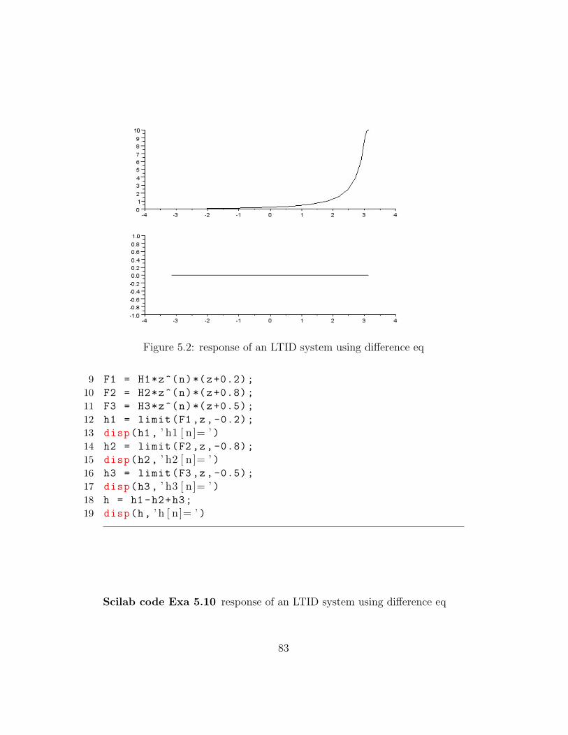
Figure 5.2: response of an LTID system using difference eq
9 F1 = H1*z^(n)*(z+0.2);
10 F2 = H2*z^(n)*(z+0.8);
11 F3 = H3*z^(n)*(z+0.5);
12 h1 = limit(F1 ,z, -0.2);
13 disp(h1, ’ h1 [ n]= ’ )14 h2 = limit(F2 ,z, -0.8);
15 disp(h2, ’ h2 [ n]= ’ )16 h3 = limit(F3 ,z, -0.5);
17 disp(h3, ’ h3 [ n]= ’ )18 h = h1 -h2+h3;
19 disp(h, ’ h [ n]= ’ )
Scilab code Exa 5.10 response of an LTID system using difference eq
83

1 omega= linspace(-%pi ,%pi ,106);
2 H= syslin( ’ c ’ ,(s/(s-0.8)));3 H_omega= squeeze(calfrq(H,0.01 ,10));
4 size(H_omega)
5 subplot (2,1,1); plot2d(omega , abs(H_omega));
6 // x l a b e l ( ’\ omega ’ ) ;7 // y l a b e l ( ’ |H[ e ˆ{ j \omega } ] | ’ ) ;8 subplot (2,1,2); plot2d(omega ,atan(imag(H_omega),real
(H_omega))*180/ %pi);
9 // x l a b e l ( ’\ omega ’ ) ;10 // y l a b e l ( ’\ a n g l e H[ e ˆ{ j \omega } ] [ deg ] ’ ) ;
Scilab code Exa 5.12 maximum sampling timeinterval
1 // s i g n a l s and sys t ems2 //maximum sampl ing i n t e r v a l3 f=50*10^3;
4 T=0.5/f;
5 disp(T)// i n s e c o n d s
Scilab code Exa 5.13 discrete time amplifier highest frequency
1 // s i g n a l s and sys t ems2 // h i g h e s t f r e q u e n c y o f a s i g n a l3 T=25*10^ -6
4 f=0.5/T
5 disp(f)// i n h e r t z
Scilab code Exa 5.17 bilateral z transfrom
84

1 //Z t r a n s f o r m o f x [ n ] = aˆn . u [ n]+bˆ−n . u[−n−1]2 syms n z;
3 a=0.9
4 b = 1.2;
56 x1=(a)^(n)
7 x2=(b)^(-n)
8 // p l o t 2 d 3 ( n1 , x1+x2 )9 X1=symsum(x1*(z^(-n)),n,0,%inf)
10 X2=symsum(x2*(z^(n)),n,1,%inf)
11 X = X1+X2;
12 disp(X,” ans=”)
Scilab code Exa 5.18 bilateral inverse z transform
1 // s i g n a l s and sys t ems2 // I n v e r s e Z Transform :ROC | z |>23 z = %z;
4 syms n z1;//To f i n d out I n v e r s e z t r a n s f o r m z mustbe l i n e a r z = z1
5 X =-z*(z+0.4) /((z -0.8)*(z-2))
6 X1 = denom(X);
7 zp = roots(X1);
8 X1 = -z1*(z1+0.4) /((z1 -0.8) *(z1 -2))
9 F1 = X1*(z1^(n-1))*(z1-zp(1));
10 F2 = X1*(z1^(n-1))*(z1-zp(2));
11 h1 = limit(F1 ,z1,zp(1));
12 disp(h1, ’ h1 [ n]= ’ )13 h2 = limit(F2 ,z1,zp(2));
14 disp(h2, ’ h2 [ n]= ’ )15 h = h1+h2;
16 disp(h, ’ h [ n]= ’ )1718 // I n v e r s e Z Transform :ROC 0.8 < | z |<219 z = %z;
85
20 syms n z1;
21 X =-z*(z+0.4) /((z -0.8)*(z-2))
22 X1 = denom(X);
23 zp = roots(X1);
24 X1 = -z1*(z1+0.4) /((z1 -0.8) *(z1 -2))
25 F1 = X1*(z1^(n-1))*(z1-zp(1));
26 F2 = X1*(z1^(n-1))*(z1-zp(2));
27 h1 = limit(F1 ,z1 ,zp(1));
28 disp(h1* ’ u ( n ) ’ , ’ h1 [ n]= ’ )29 h2 = limit(F2 ,z1 ,zp(2));
30 disp((h2)* ’ u(−n−1) ’ , ’ h2 [ n]= ’ )31 disp((h1)* ’ u ( n ) ’ -(h2)* ’ u ( n−1) ’ , ’ h [ n]= ’ )3233 // I n v e r s e Z Transform :ROC | z |<0.834 z = %z;
35 syms n z1;
36 X =-z*(z+0.4) /((z -0.8)*(z-2))
37 X1 = denom(X);
38 zp = roots(X1);
39 X1 = -z1*(z1+0.4) /((z1 -0.8) *(z1 -2))
40 F1 = X1*(z1^(n-1))*(z1-zp(1));
41 F2 = X1*(z1^(n-1))*(z1-zp(2));
42 h1 = limit(F1 ,z1 ,zp(1));
43 disp(h1* ’ u(−n−1) ’ , ’ h1 [ n]= ’ )44 h2 = limit(F2 ,z1 ,zp(2));
45 disp((h2)* ’ u(−n−1) ’ , ’ h2 [ n]= ’ )46 disp(-(h1)* ’ u(−n−1) ’ -(h2)* ’ u(−n−1) ’ , ’ h [ n]= ’ )
Scilab code Exa 5.19 transfer function for a causal system
1 // LTi Systems c h a r a c t e r i z e d by L i n e a r Constant2 // C o e f f i c i e n t D i f f e r e n c e e q u a t i o n s3 // I n v e r s e Z Transform4 // z = %z ;5 syms n z;
86

6 H1 = -z/(z-0.5);
7 H2 = (8/3)*z/(z-0.8);
8 H3=( -8/3)*z/(z-2);
9 F1 = H1*z^(n-1)*(z -0.5);
10 F2 = H2*z^(n-1)*(z -0.8);
11 F3 = H3*z^(n-1)*(z-2);
12 h1 = limit(F1 ,z,0.5);
13 disp(h1, ’ h1 [ n]= ’ )14 h2 = limit(F2 ,z,0.8);
15 disp(h2, ’ h2 [ n]= ’ )16 h3 = limit(F3 ,z,2);
17 disp(h3, ’ h3 [ n]= ’ )18 h = h1+h2+h3;
19 disp(h, ’ h [ n]= ’ )
Scilab code Exa 5.20 zero state response for a given input
1 // LTi Systems c h a r a c t e r i z e d by L i n e a r Constant2 // C o e f f i c i e n t D i f f e r e n c e e q u a t i o n s3 // I n v e r s e Z Transform4 // z = %z ;5 syms n z;
6 H1 = ( -5/3)*z/(z -0.5);
7 H2 = (8/3)*z/(z-0.8);
8 H3=5*z/(z-0.5);
9 H4=-6*z/(z-0.6);
10 F1 = H1*z^(n-1)*(z -0.5);
11 F2 = H2*z^(n-1)*(z -0.8);
12 F3 = H3*z^(n-1)*(z -0.5);
13 F4 = H4*z^(n-1)*(z -0.6);
14 h1 = limit(F1 ,z,0.5);
15 disp(h1, ’ h1 [ n]= ’ )16 h2 = limit(F2 ,z,0.8);
17 disp(h2, ’ h2 [ n]= ’ )18 h3 = limit(F3 ,z,0.5);
87

19 disp(h3, ’ h3 [ n]= ’ )20 h4 = limit(F4 ,z,0.6);
21 disp(h4, ’ h4 [ n]= ’ )22 h = h1+h2+h3+h4;
23 disp(h, ’ h [ n]= ’ )
88

Chapter 6
continuous time signal analysisthe fourier series
Scilab code Exa 6.1 fourier coefficients of a periodic sequence
1 n=0:10;
2 a_n =0.504*2* ones(1,length(n))./(1+16*n.^2);
3 a_n (1) =0.504
4 b_n =0.504*8*n./(1+16*n.*n);
5 size(n)
6 size(a_n)
7 size(b_n)
8 disp(b_n(1))
9 C_n=sqrt(a_n .^2+( b_n).^2);
10 theta_n (1)=0; theta_n=atan(-b_n ,a_n);
11 //n =[0 , n ] ;12 clf;
13 size(n)
14 subplot (2,2,1); plot2d3(n,a_n);xtitle( ’ a n ’ , ’ n ’ );plot(n,a_n , ’ ro ’ );
15 subplot (2,2,2); plot2d3(n,b_n);xtitle( ’ b n ’ , ’ n ’ );plot(n,b_n , ’ r . ’ );
89

Figure 6.1: fourier coefficients of a periodic sequence
16 subplot (2,2,3); plot2d3(n,C_n);xtitle( ’ C n ’ , ’ n ’ );plot(n,C_n , ’ ro ’ );
17 subplot (2,2,4); plot2d3(n,theta_n ,);xtitle( ’ t h e t a n ’, ’ n ’ );plot(n,theta_n , ’ r . ’ )
Scilab code Exa 6.2 fourier coefficients of a periodic sequence
1 n=0:10;
2 a_n=zeros(1,length(n));
3 size(a_n)
4 b_n =(8/ %pi^2*n.^2).*sin(n.*%pi/2);
5 size(n)
6 size(a_n)
7 size(b_n)
90
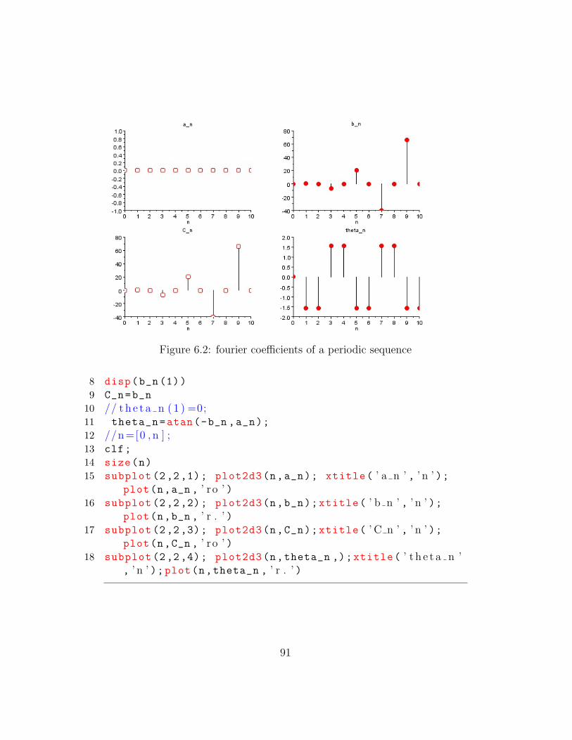
Figure 6.2: fourier coefficients of a periodic sequence
8 disp(b_n(1))
9 C_n=b_n
10 // t h e t a n ( 1 ) =0;11 theta_n=atan(-b_n ,a_n);
12 //n =[0 , n ] ;13 clf;
14 size(n)
15 subplot (2,2,1); plot2d3(n,a_n); xtitle( ’ a n ’ , ’ n ’ );plot(n,a_n , ’ ro ’ )
16 subplot (2,2,2); plot2d3(n,b_n);xtitle( ’ b n ’ , ’ n ’ );plot(n,b_n , ’ r . ’ )
17 subplot (2,2,3); plot2d3(n,C_n);xtitle( ’ C n ’ , ’ n ’ );plot(n,C_n , ’ ro ’ )
18 subplot (2,2,4); plot2d3(n,theta_n ,);xtitle( ’ t h e t a n ’, ’ n ’ );plot(n,theta_n , ’ r . ’ )
91
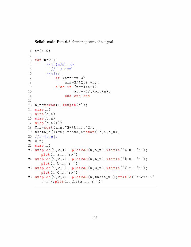
Scilab code Exa 6.3 fourier spectra of a signal
1 n=0:10;
23 for n=0:10
4 // i f (n%2==0)5 // a n =0;6 // e l s e7 if (n==4*n-3)
8 a_n =2/( %pi.*n);
9 else if (n==4*n-1)
10 a_n=-2/(%pi.*n);
11 end end end
1213 b_n=zeros(1,length(n));
14 size(n)
15 size(a_n)
16 size(b_n)
17 disp(b_n(1))
18 C_n=sqrt(a_n .^2+( b_n).^2);
19 theta_n (1)=0; theta_n=atan(-b_n ,a_n);
20 //n =[0 , n ] ;21 clf;
22 size(n)
23 subplot (2,2,1); plot2d3(n,a_n);xtitle( ’ a n ’ , ’ n ’ );plot(n,a_n , ’ ro ’ );
24 subplot (2,2,2); plot2d3(n,b_n);xtitle( ’ b n ’ , ’ n ’ );plot(n,b_n , ’ r . ’ );
25 subplot (2,2,3); plot2d3(n,C_n);xtitle( ’ C n ’ , ’ n ’ );plot(n,C_n , ’ ro ’ );
26 subplot (2,2,4); plot2d3(n,theta_n ,);xtitle( ’ t h e t a n ’, ’ n ’ );plot(n,theta_n , ’ r . ’ );
92
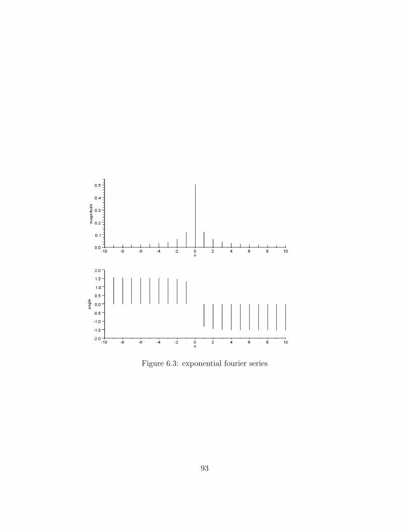
Figure 6.3: exponential fourier series
93
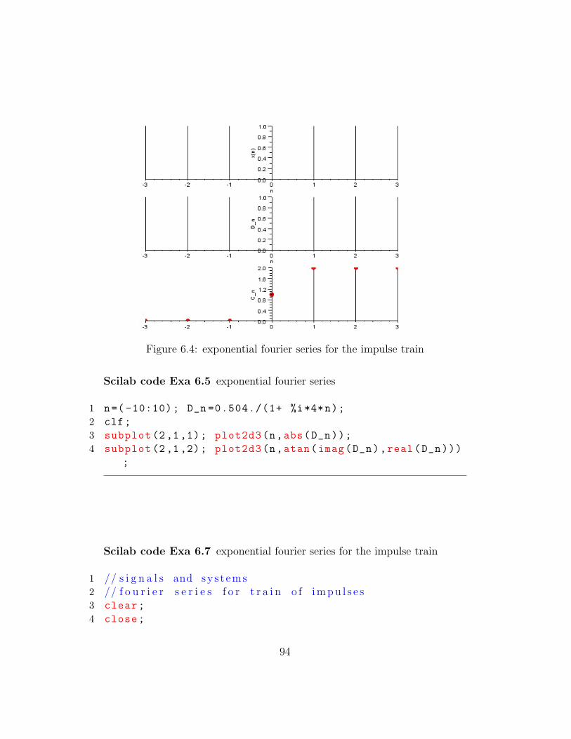
Figure 6.4: exponential fourier series for the impulse train
Scilab code Exa 6.5 exponential fourier series
1 n=( -10:10); D_n =0.504./(1+ %i*4*n);
2 clf;
3 subplot (2,1,1); plot2d3(n,abs(D_n));
4 subplot (2,1,2); plot2d3(n,atan(imag(D_n),real(D_n)))
;
Scilab code Exa 6.7 exponential fourier series for the impulse train
1 // s i g n a l s and sys t ems2 // f o u r i e r s e r i e s f o r t r a i n o f i m p u l s e s3 clear;
4 close;
94

5 clc;
6 n= -3:1:3
7 x = ones(1,length(n))
8 D_n=ones(1,length(n));
9 C_n =[0 0 0 1 2 2 2]
10 subplot (3,1,1)
11 a = gca();
12 a.y_location = ” o r i g i n ”;13 a.x_location = ” o r i g i n ”;14 plot2d3(n,x)
15 subplot (3,1,2)
16 a = gca();
17 a.y_location = ” o r i g i n ”;18 a.x_location = ” o r i g i n ”;19 plot2d3(n,D_n)
20 subplot (3,1,3)
21 a = gca();
22 a.y_location = ” o r i g i n ”;23 a.x_location = ” o r i g i n ”;24 plot2d3(n,C_n); plot(n,C_n , ’ r . ’ )
Scilab code Exa 6.9 exponential fourier series to find the output
1 n=( -10:10); D_n =2/(3.14*(1 -4.*n.^2) .*(%i*6.*n+1));
2 clf;
3 subplot (2,1,1); plot2d3(n,abs(D_n));
4 subplot (2,1,2); plot2d3(n,atan(imag(D_n),real(D_n)))
;
95

Figure 6.5: exponential fourier series to find the output
96
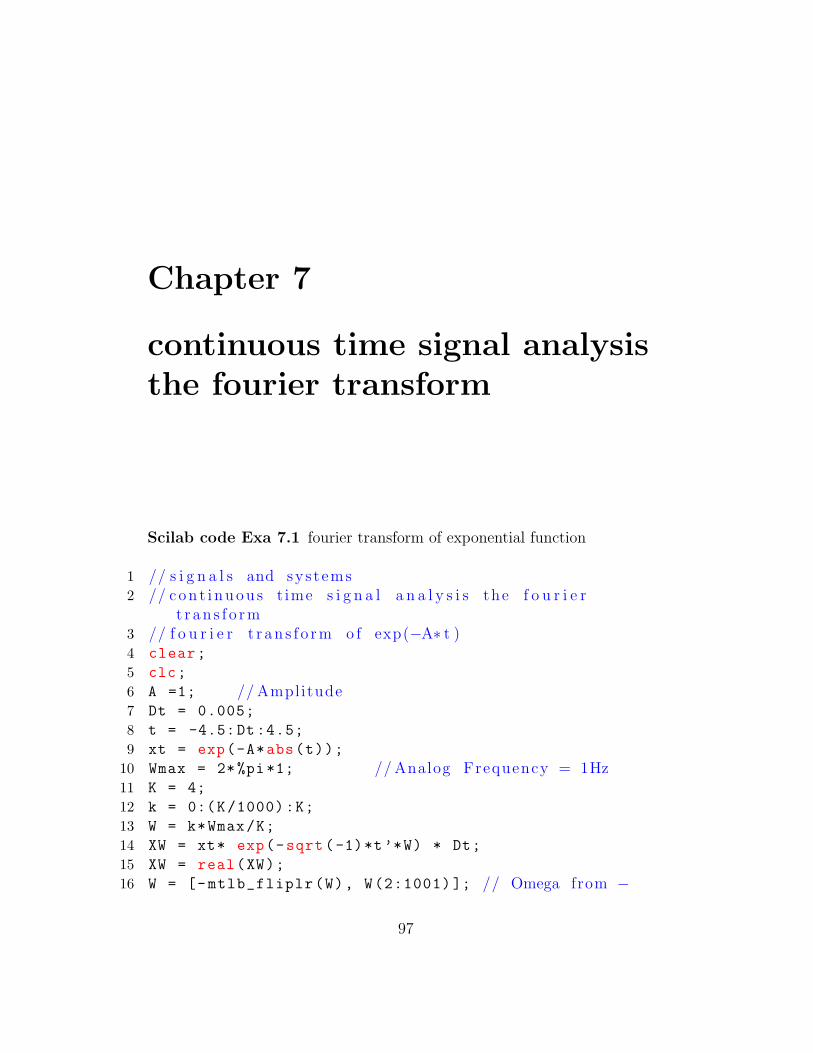
Chapter 7
continuous time signal analysisthe fourier transform
Scilab code Exa 7.1 fourier transform of exponential function
1 // s i g n a l s and sys t ems2 // c o n t i n u o u s t ime s i g n a l a n a l y s i s the f o u r i e r
t r a n s f o r m3 // f o u r i e r t r a n s f o r m o f exp(−A∗ t )4 clear;
5 clc;
6 A =1; // Amplitude7 Dt = 0.005;
8 t = -4.5:Dt:4.5;
9 xt = exp(-A*abs(t));
10 Wmax = 2*%pi*1; // Analog Frequency = 1Hz11 K = 4;
12 k = 0:(K/1000):K;
13 W = k*Wmax/K;
14 XW = xt* exp(-sqrt(-1)*t’*W) * Dt;
15 XW = real(XW);
16 W = [-mtlb_fliplr(W), W(2:1001) ]; // Omega from −
97

Figure 7.1: fourier transform of exponential function
98

Wmax to Wmax17 XW = [mtlb_fliplr(XW), XW (2:1001) ];
18 subplot (2,1,1);
19 a = gca();
20 a.y_location = ” o r i g i n ”;21 plot(t,xt);
22 xlabel( ’ t i n s e c . ’ );23 ylabel( ’ x ( t ) ’ )24 title( ’ Cont inuous Time S i g n a l ’ )25 subplot (2,1,2);
26 a = gca();
27 a.y_location = ” o r i g i n ”;28 plot(W,XW);
29 xlabel( ’ Frequency i n Radians / Seconds W’ );30 ylabel( ’X(jW) ’ )31 title( ’ Continuous−t ime F o u r i e r Transform ’ )
Scilab code Exa 7.4 inverse fourier transform
1 // Example 4 . 52 // I n v e r s e Cont inuous Time F o u r i e r Transform3 // impu l s e f u n t i o n4 clear;
5 clc;
6 close;
7 // CTFT8 A =1; // Amplitude9 Dw = 0.005;
10 W1 = 4; //Time i n s e c o n d s11 w = -W1/2:Dw:W1/2;
12 for i=1: length(w)
13 XW(1)=1;
14 end
99

Figure 7.2: inverse fourier transform
100
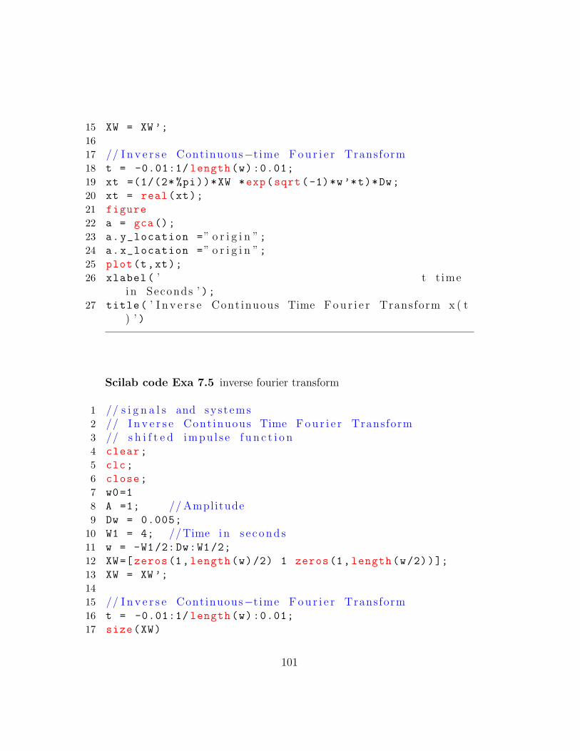
15 XW = XW ’;
1617 // I n v e r s e Continuous−t ime F o u r i e r Transform18 t = -0.01:1/ length(w):0.01;
19 xt =(1/(2* %pi))*XW *exp(sqrt(-1)*w’*t)*Dw;
20 xt = real(xt);
21 figure
22 a = gca();
23 a.y_location =” o r i g i n ”;24 a.x_location =” o r i g i n ”;25 plot(t,xt);
26 xlabel( ’ t t imei n Seconds ’ );
27 title( ’ I n v e r s e Cont inuous Time F o u r i e r Transform x ( t) ’ )
Scilab code Exa 7.5 inverse fourier transform
1 // s i g n a l s and sys t ems2 // I n v e r s e Cont inuous Time F o u r i e r Transform3 // s h i f t e d impu l s e f u n c t i o n4 clear;
5 clc;
6 close;
7 w0=1
8 A =1; // Amplitude9 Dw = 0.005;
10 W1 = 4; //Time i n s e c o n d s11 w = -W1/2:Dw:W1/2;
12 XW=[ zeros(1,length(w)/2) 1 zeros(1,length(w/2))];
13 XW = XW ’;
1415 // I n v e r s e Continuous−t ime F o u r i e r Transform16 t = -0.01:1/ length(w):0.01;
17 size(XW)
101
18 size(t)
19 xt =(1/(2* %pi))*XW *exp(sqrt(-1)*w’.*t).*exp(sqrt
(-1).*t)*Dw;
20 xt = real(xt);
21 figure
22 a = gca();
23 a.y_location =” o r i g i n ”;24 a.x_location =” o r i g i n ”;25 plot(t,xt);
26 xlabel( ’ t t imei n Seconds ’ );
27 title( ’ I n v e r s e Cont inuous Time F o u r i e r Transform x ( t) ’ )
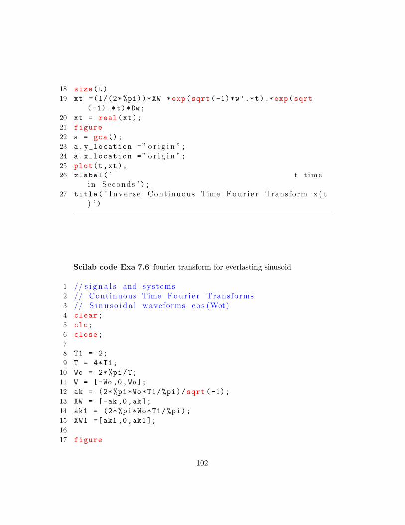
Scilab code Exa 7.6 fourier transform for everlasting sinusoid
1 // s i g n a l s and sys t ems2 // Cont inuous Time F o u r i e r Trans forms3 // S i n u s o i d a l waveforms co s (Wot)4 clear;
5 clc;
6 close;
78 T1 = 2;
9 T = 4*T1;
10 Wo = 2*%pi/T;
11 W = [-Wo ,0,Wo];
12 ak = (2*%pi*Wo*T1/%pi)/sqrt(-1);
13 XW = [-ak ,0,ak];
14 ak1 = (2*%pi*Wo*T1/%pi);
15 XW1 =[ak1 ,0,ak1];
1617 figure
102

Figure 7.3: fourier transform for everlasting sinusoid
103

Figure 7.4: fourier transform of a periodic signal
18 a = gca();
19 a.y_location =” o r i g i n ”;20 a.x_location =” o r i g i n ”;21 plot2d3( ’ gnn ’ ,W,XW1 ,2);22 poly1 = a.children (1).children (1);
23 poly1.thickness = 3;
24 xlabel( ’
W’ );25 title( ’CTFT o f co s (Wot) ’ )
Scilab code Exa 7.7 fourier transform of a periodic signal
1 // s i g n a l s and sys t ems
104

2 // Cont inuous Time F o u r i e r Transform o f Symmetric3 // p e r i o d i c Square waveform4 clear;
5 clc;
6 close;
78 T1 = 2;
9 T = 4*T1;
10 Wo = 2*%pi/T;
11 W = -%pi:Wo:%pi;
12 delta = ones(1,length(W));
13 XW(1) = (2* %pi*Wo*T1/%pi);
14 mid_value = ceil(length(W)/2);
15 for k = 2: mid_value
16 XW(k) = (2* %pi*sin((k-1)*Wo*T1)/(%pi*(k-1)));
17 end
18 figure
19 a = gca();
20 a.y_location =” o r i g i n ”;21 a.x_location =” o r i g i n ”;22 plot2d3( ’ gnn ’ ,W(mid_value:$),XW ,2);23 poly1 = a.children (1).children (1);
24 poly1.thickness = 3;
25 plot2d3( ’ gnn ’ ,W(1: mid_value -1),XW($: -1:2) ,2);26 poly1 = a.children (1).children (1);
27 poly1.thickness = 3;
28 xlabel( ’W i n r a d i a n s / Seconds ’ );29 title( ’ Cont inuous Time F o u r i e r Transform o f P e r i o d i c
Square Wave ’ )
Scilab code Exa 7.8 fourier transform of a unit impulse train
1 // s i g n a l s and sys t ems
105

Figure 7.5: fourier transform of a unit impulse train
2 // c o n t i n u o u s t ime s i g n a l a n a l y s i s the f o u r i e rt r a n s f o r m
3 // P e r i o d i c Impul se Tra in4 clear;
5 clc;
6 close;
7 T = -4:4;;
8 T1 = 1; // Sampl ing I n t e r v a l9 xt = ones(1,length(T));
10 ak = 1/T1;
11 XW = 2*%pi*ak*ones(1,length(T));
12 Wo = 2*%pi/T1;
13 W = Wo*T;
14 figure
15 subplot (2,1,1)
16 a = gca();
17 a.y_location =” o r i g i n ”;18 a.x_location =” o r i g i n ”;
106
19 plot2d3( ’ gnn ’ ,T,xt ,2);20 poly1 = a.children (1).children (1);
21 poly1.thickness = 3;
22 xlabel( ’
t ’ );23 title( ’ P e r i o d i c Impul se Tra in ’ )24 subplot (2,1,2)
25 a = gca();
26 a.y_location =” o r i g i n ”;27 a.x_location =” o r i g i n ”;28 plot2d3( ’ gnn ’ ,W,XW ,2);29 poly1 = a.children (1).children (1);
30 poly1.thickness = 3;
31 xlabel( ’
t ’ );32 title( ’CTFT o f P e r i o d i c Impul se Tra in ’ )
Scilab code Exa 7.9 fourier transform of unit step function
1 // s i g n a l s and sys t ems2 // c o n t i n u o u s t ime s i g n a l a n a l y s i s the f o u r i e r
t r a n s f o r m3 // f o u r i e r t r a n s f o r m o f u n i t s t e p f u n c t i o n u ( t )4 clear;
5 clc;
6 A =0.000000001; // Amplitude7 Dt = 0.005;
8 t = 0:Dt :4.5;
9 xt = exp(-A*abs(t));
10 Wmax = 2*%pi*1; // Analog Frequency = 1Hz11 K = 4;
107

Figure 7.6: fourier transform of unit step function
12 k = 0:(K/500):K;
13 W = k*Wmax/K;
14 XW = xt* exp(-sqrt(-1)*t’*W) * Dt;
15 XW = real(XW);
16 W = [-mtlb_fliplr(W), W(2:501) ]; // Omega from −Wmaxto Wmax
17 XW = [mtlb_fliplr(XW), XW (2:501) ];
18 subplot (2,1,1);
19 a = gca();
20 a.y_location = ” o r i g i n ”;21 plot(t,xt);
22 xlabel( ’ t i n s e c . ’ );23 ylabel( ’ x ( t ) ’ )24 title( ’ Cont inuous Time S i g n a l ’ )25 subplot (2,1,2);
26 a = gca();
27 a.y_location = ” o r i g i n ”;28 plot(W,XW);
108
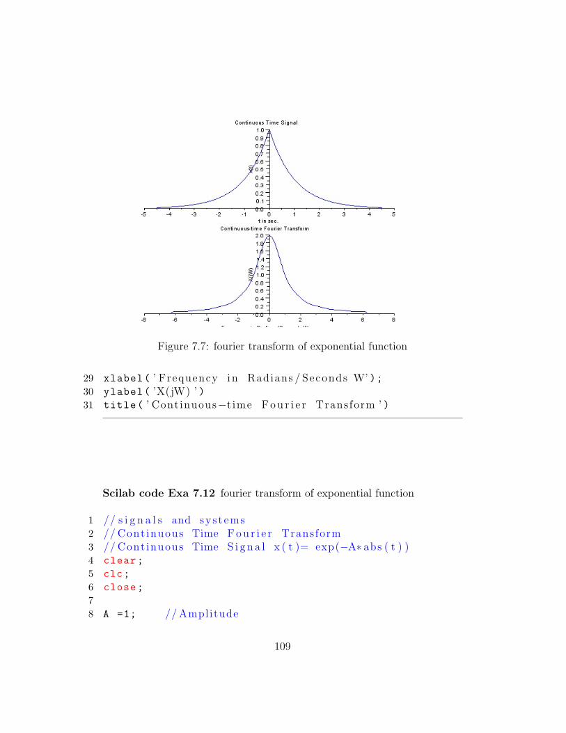
Figure 7.7: fourier transform of exponential function
29 xlabel( ’ Frequency i n Radians / Seconds W’ );30 ylabel( ’X(jW) ’ )31 title( ’ Continuous−t ime F o u r i e r Transform ’ )
Scilab code Exa 7.12 fourier transform of exponential function
1 // s i g n a l s and sys t ems2 // Cont inuous Time F o u r i e r Transform3 // Cont inuous Time S i g n a l x ( t )= exp(−A∗ abs ( t ) )4 clear;
5 clc;
6 close;
78 A =1; // Amplitude
109
9 Dt = 0.005;
10 t = -4.5:Dt:4.5;
11 xt = exp(-A*abs(t));
1213 Wmax = 2*%pi*1; // Analog Frequency = 1Hz14 K = 4;
15 k = 0:(K/1000):K;
16 W = k*Wmax/K;
17 XW = xt* exp(-sqrt(-1)*t’*W) * Dt;
18 XW = real(XW);
19 W = [-mtlb_fliplr(W), W(2:1001) ]; // Omega from −Wmax to Wmax
20 XW = [mtlb_fliplr(XW), XW (2:1001) ];
21 subplot (1,1,1)
22 subplot (2,1,1);
23 a = gca();
24 a.y_location = ” o r i g i n ”;25 plot(t,xt);
26 xlabel( ’ t i n s e c . ’ );27 ylabel( ’ x ( t ) ’ )28 title( ’ Cont inuous Time S i g n a l ’ )29 subplot (2,1,2);
30 a = gca();
31 a.y_location = ” o r i g i n ”;32 plot(W,XW);
33 xlabel( ’ Frequency i n Radians / Seconds W’ );34 ylabel( ’X(jW) ’ )35 title( ’ Continuous−t ime F o u r i e r Transform ’ )
110
Chapter 8
Sampling The bridge fromcontinuous to discrete
Scilab code Exa 8.8 discrete fourier transform
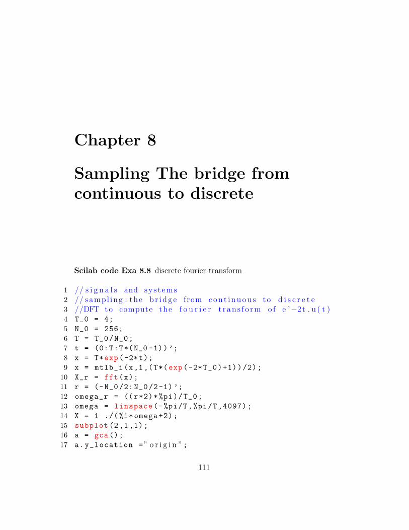
1 // s i g n a l s and sys t ems2 // sampl ing : the b r i d g e from c o n t i n u o u s to d i s c r e t e3 //DFT to compute the f o u r i e r t r a n s f o r m o f eˆ−2 t . u ( t )4 T_0 = 4;
5 N_0 = 256;
6 T = T_0/N_0;
7 t = (0:T:T*(N_0 -1))’;
8 x = T*exp(-2*t);
9 x = mtlb_i(x,1,(T*(exp(-2*T_0)+1))/2);
10 X_r = fft(x);
11 r = (-N_0/2: N_0/2-1) ’;
12 omega_r = ((r*2)*%pi)/T_0;
13 omega = linspace(-%pi/T,%pi/T ,4097);
14 X = 1 ./(%i*omega +2);
15 subplot (2,1,1);
16 a = gca();
17 a.y_location =” o r i g i n ”;
111

Figure 8.1: discrete fourier transform
112

Figure 8.2: discrete fourier transform
18 a.x_location =” o r i g i n ”;19 plot(omega ,abs(X),”k”,omega_r ,fftshift(abs(X_r)),” ko
”);20 xtitle(” magnitude o f X( omega ) f o r t r u e FT and DFT”);21 subplot (2,1,2);
22 a = gca();
23 a.y_location =” o r i g i n ”;24 a.x_location =” o r i g i n ”;25 plot(omega ,atan(imag(X),real(X)),”k”,omega_r ,
fftshift(atan(imag(X_r),real(X_r))),” ko ”);26 xtitle(” a n g l e o f X( omega ) f o r t r u e FT and DFT”);
Scilab code Exa 8.9 discrete fourier transform
113
1 // s i g n a l s and sys t ems2 // sampl ing : the b r i d g e from c o n t i n u o u s to d i s c r e t e3 //DFT to compute the f o u r i e r t r a n s f o r m o f 8 r e c t ( t )4 T_0 = 4;
5 N_0 = 32;
6 T = T_0/N_0;
7 x_n = [ones (1,4) 0.5 zeros (1,23) 0.5 ones (1,3)]’;
8 size(x_n)
9 x_r = fft(x_n);r = (-N_0 /2:( N_0/2) -1) ’;
10 omega_r = ((r*2)*%pi)/T_0;
11 size(omega_r)
12 size(omega)
13 omega = linspace(-%pi/T,%pi/T ,4097);
14 X = 8*( sinc(omega /2));
15 size(X)
16 figure (1);
17 subplot (2,1,1);
18 plot(omega ,abs(X),”k”);19 plot(omega_r ,fftshift(abs(x_r)),” ko ”)20 xtitle(” a n g l e o f X( omega ) f o r t r u e FT and DFT”);21 a=gca();
22 subplot (2,1,2);
23 a = gca();
24 a.y_location =” o r i g i n ”;25 a.x_location =” o r i g i n ”;26 plot(omega ,atan(imag(X),real(X)),”k”,omega_r ,
fftshift(atan(imag(x_r),real(x_r))), ’ r . ’ );27 xtitle(” a n g l e o f X( omega ) f o r t r u e FT and DFT”);
Scilab code Exa 8.10 frequency response of a low pass filter
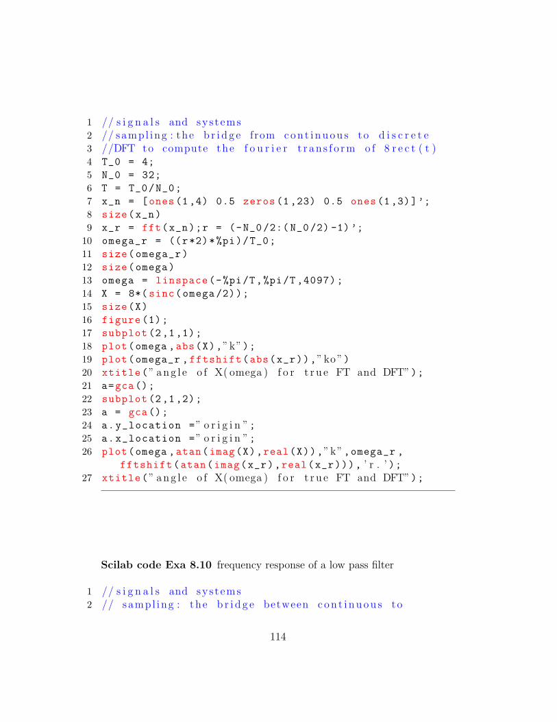
1 // s i g n a l s and sys t ems2 // sampl ing : the b r i d g e between c o n t i n u o u s to
114
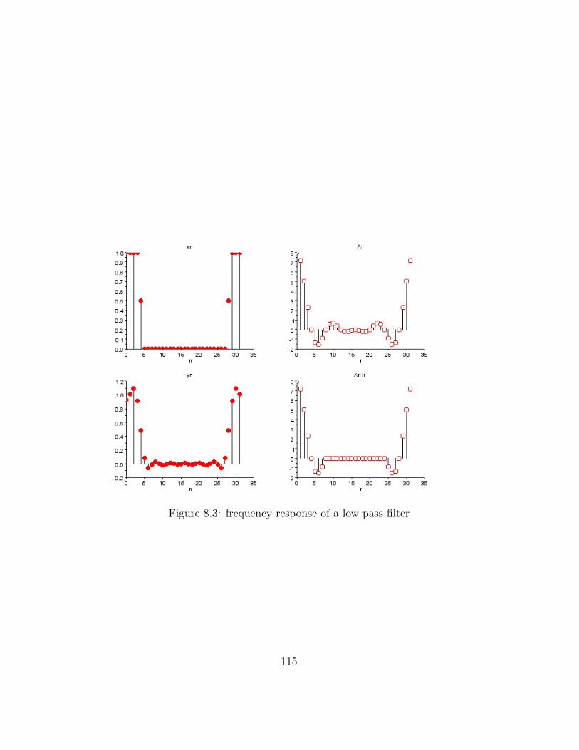
Figure 8.3: frequency response of a low pass filter
115

d i s c r e t e3 T_0 = 4;
4 N_0 = 32;
5 T = T_0/N_0;n = 0:N_0 -1;r = n;
6 x_n = [ones (1,4) ,0.5,zeros (1,23) ,0.5,ones (1,3)]’;
7 H_r = [ones (1,8) ,0.5,zeros (1,15) ,0.5,ones (1,7)]’;
8 X_r = fft(x_n ,-1);
9 Y_r = H_r .*( X_r);y_n = mtlb_ifft(Y_r);
10 subplot (2,2,1);
11 plot2d3(n,x_n);
12 plot(n,x_n , ’ r . ’ )13 xtitle( ’ xn ’ , ’ n ’ )14 subplot (2,2,2);
15 plot2d3(r,real(X_r));
16 plot(r,real(X_r), ’ ro ’ )17 xtitle( ’ Xr ’ , ’ r ’ )18 subplot (2,2,3);
19 plot2d3(n,real(y_n));
20 plot(n,real(y_n), ’ r . ’ )21 xtitle( ’ yn ’ , ’ n ’ )22 subplot (2,2,4);
23 plot2d3(r,(X_r).*H_r);
24 plot(r,(X_r).*H_r , ’ ro ’ )25 xtitle( ’ XrHr ’ , ’ r ’ )
116
Chapter 9
fourier analysis of discrete timesignals
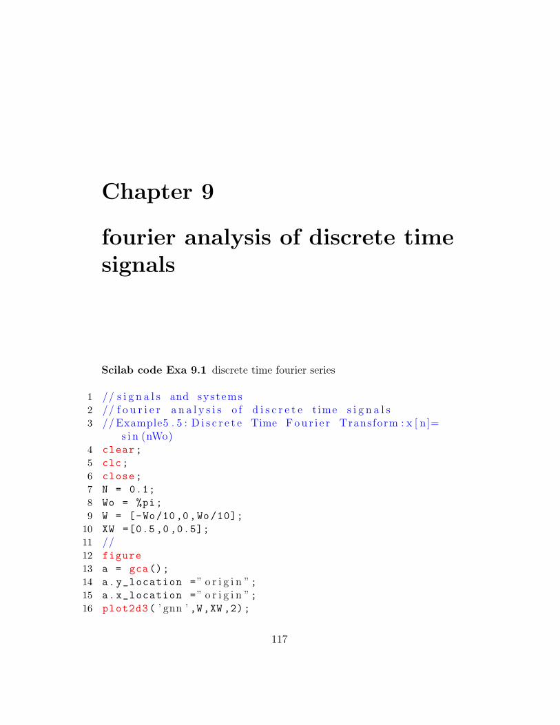
Scilab code Exa 9.1 discrete time fourier series
1 // s i g n a l s and sys t ems2 // f o u r i e r a n a l y s i s o f d i s c r e t e t ime s i g n a l s3 // Example5 . 5 : D i s c r e t e Time F o u r i e r Transform : x [ n]=
s i n (nWo)4 clear;
5 clc;
6 close;
7 N = 0.1;
8 Wo = %pi;
9 W = [-Wo/10,0,Wo/10];
10 XW =[0.5 ,0 ,0.5];
11 //12 figure
13 a = gca();
14 a.y_location =” o r i g i n ”;15 a.x_location =” o r i g i n ”;16 plot2d3( ’ gnn ’ ,W,XW ,2);
117
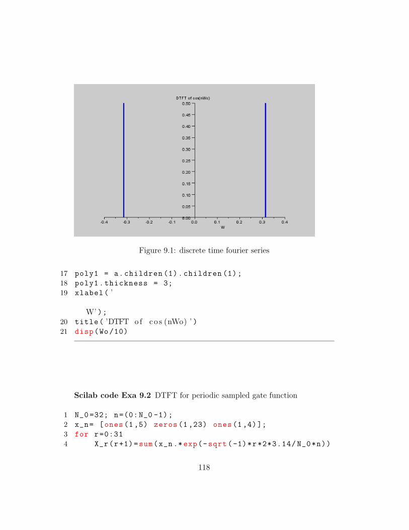
Figure 9.1: discrete time fourier series
17 poly1 = a.children (1).children (1);
18 poly1.thickness = 3;
19 xlabel( ’
W’ );20 title( ’DTFT o f co s (nWo) ’ )21 disp(Wo/10)
Scilab code Exa 9.2 DTFT for periodic sampled gate function
1 N_0 =32; n=(0:N_0 -1);
2 x_n= [ones (1,5) zeros (1 ,23) ones (1,4)];
3 for r=0:31
4 X_r(r+1)=sum(x_n.*exp(-sqrt(-1)*r*2*3.14/ N_0*n))
118
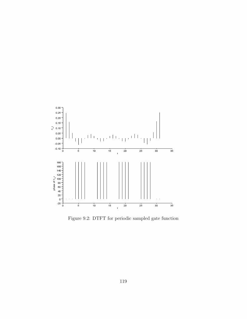
Figure 9.2: DTFT for periodic sampled gate function
119

Figure 9.3: discrete time fourier series
/32;
5 end
6 subplot (2,1,1); r=n; plot2d3(r,real(X_r));
7 xlabel( ’ r ’ ); ylabel( ’ X r ’ );8 X_r=fft(x_n)/N_0;
9 subplot (2,1,2);
10 plot2d3(r,phasemag(X_r));
11 xlabel( ’ r ’ ); ylabel( ’ phase o f X r ’ );12 disp(N_0 , ’ p e r i o d= ’ )13 disp (2*%pi/N_0 , ’ omega= ’ )
120

Scilab code Exa 9.3 discrete time fourier series
1 // s i g n a l s and sys t ems2 // D i s c r e t e Time F o u r i e r Transform o f d i s c r e t e
s equence3 //x [ n]= ( aˆn ) . u [ n ] , a>0 and a<04 clear;
5 clc;
6 close;
7 // DTS S i g n a l8 a1 = 0.5;
9 a2 = -0.5;
10 max_limit = 10;
11 for n = 0:max_limit -1
12 x1(n+1) = (a1^n);
13 x2(n+1) = (a2^n);
14 end
15 n = 0:max_limit -1;
16 // D i s c r e t e−t ime F o u r i e r Transform17 Wmax = 2*%pi;
18 K = 4;
19 k = 0:(K/1000):K;
20 W = k*Wmax/K;
21 x1 = x1 ’;
22 x2 = x2 ’;
23 XW1 = x1* exp(-sqrt(-1)*n’*W);
24 XW2 = x2* exp(-sqrt(-1)*n’*W);
25 XW1_Mag = abs(XW1);
26 XW2_Mag = abs(XW2);
27 W = [-mtlb_fliplr(W), W(2:1001) ]; // Omega from −Wmax to Wmax
28 XW1_Mag = [mtlb_fliplr(XW1_Mag), XW1_Mag (2:1001) ];
29 XW2_Mag = [mtlb_fliplr(XW2_Mag), XW2_Mag (2:1001) ];
30 [XW1_Phase ,db] = phasemag(XW1);
31 [XW2_Phase ,db] = phasemag(XW2);
32 XW1_Phase = [-mtlb_fliplr(XW1_Phase),XW1_Phase
(2:1001) ];
33 XW2_Phase = [-mtlb_fliplr(XW2_Phase),XW2_Phase
121

(2:1001) ];
34 // p l o t f o r a>035 figure
36 subplot (3,1,1);
37 plot2d3( ’ gnn ’ ,n,x1);38 xtitle( ’ D i s c r e t e Time Sequence x [ n ] f o r a>0 ’ )39 subplot (3,1,2);
40 a = gca();
41 a.y_location =” o r i g i n ”;42 a.x_location =” o r i g i n ”;43 plot2d(W,XW1_Mag);
44 title( ’ Magnitude Response abs (X(jW) ) ’ )45 subplot (3,1,3);
46 a = gca();
47 a.y_location =” o r i g i n ”;48 a.x_location =” o r i g i n ”;49 plot2d(W,XW1_Phase);
50 title( ’ Phase Response <(X(jW) ) ’ )51 // p l o t f o r a<052 figure
53 subplot (3,1,1);
54 plot2d3( ’ gnn ’ ,n,x2);55 xtitle( ’ D i s c r e t e Time Sequence x [ n ] f o r a>0 ’ )56 subplot (3,1,2);
57 a = gca();
58 a.y_location =” o r i g i n ”;59 a.x_location =” o r i g i n ”;60 plot2d(W,XW2_Mag);
61 title( ’ Magnitude Response abs (X(jW) ) ’ )62 subplot (3,1,3);
63 a = gca();
64 a.y_location =” o r i g i n ”;65 a.x_location =” o r i g i n ”;66 plot2d(W,XW2_Phase);
67 title( ’ Phase Response <(X(jW) ) ’ )
122
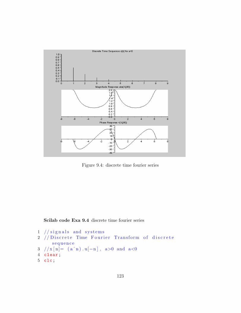
Figure 9.4: discrete time fourier series
Scilab code Exa 9.4 discrete time fourier series
1 // s i g n a l s and sys t ems2 // D i s c r e t e Time F o u r i e r Transform o f d i s c r e t e
s equence3 //x [ n]= ( aˆn ) . u[−n ] , a>0 and a<04 clear;
5 clc;
123

Figure 9.5: discrete time fourier series
6 close;
7 // DTS S i g n a l8 a = 0.5;
9 max_limit = 10;
10 for n = 0:max_limit -1
11 x1(n+1) = (a^n);
12 end
13 n = 0:max_limit -1;
14 // D i s c r e t e−t ime F o u r i e r Transform15 Wmax = 2*%pi;
16 K = 4;
17 k = 0:(K/1000):K;
18 W = k*Wmax/K;
19 x1 = x1 ’;
20 XW1 = x1* exp(-sqrt(-1)*n’*W);
2122 XW1_Mag = abs(XW1);
23 W = [-mtlb_fliplr(W), W(2:1001) ]; // Omega from −
124
Wmax to Wmax24 XW1_Mag = [mtlb_fliplr(XW1_Mag), XW1_Mag (2:1001) ];
25 [XW1_Phase ,db] = phasemag(XW1);
26 XW1_Phase = [-mtlb_fliplr(XW1_Phase),XW1_Phase
(2:1001) ];
27 // p l o t f o r a>028 figure
29 subplot (3,1,1);
30 plot2d3( ’ gnn ’ ,-n,x1);31 xtitle( ’ D i s c r e t e Time Sequence x [ n ] f o r a>0 ’ )32 subplot (3,1,2);
33 a = gca();
34 a.y_location =” o r i g i n ”;35 a.x_location =” o r i g i n ”;36 plot2d(W,XW1_Mag);
37 title( ’ Magnitude Response abs (X(jW) ) ’ )38 subplot (3,1,3);
39 a = gca();
40 a.y_location =” o r i g i n ”;41 a.x_location =” o r i g i n ”;42 plot2d(W,XW1_Phase+%pi/2);
43 title( ’ Phase Response <(X(jW) ) ’ )
Scilab code Exa 9.5 DTFT for rectangular pulse
1 // s i g n a l s and sys t ems2 // D i s c r e t e Time F o u r i e r Transform3 //x [ n]= 1 , abs ( n )<=N14 clear;
5 clc;
6 close;
7 // DTS S i g n a l8 N1 = 2;
125

Figure 9.6: DTFT for rectangular pulse
126
9 n = -N1:N1;
10 x = ones(1,length(n));
11 // D i s c r e t e−t ime F o u r i e r Transform12 Wmax = 2*%pi;
13 K = 4;
14 k = 0:(K/1000):K;
15 W = k*Wmax/K;
16 XW = x* exp(-sqrt(-1)*n’*W);
17 XW_Mag = real(XW);
18 W = [-mtlb_fliplr(W), W(2:1001) ]; // Omega from −Wmax to Wmax
19 XW_Mag = [mtlb_fliplr(XW_Mag), XW_Mag (2:1001) ];
20 // p l o t f o r abs ( a )<121 figure
22 subplot (2,1,1);
23 a = gca();
24 a.y_location =” o r i g i n ”;25 a.x_location =” o r i g i n ”;26 plot2d3( ’ gnn ’ ,n,x);27 xtitle( ’ D i s c r e t e Time Sequence x [ n ] ’ )28 subplot (2,1,2);
29 a = gca();
30 a.y_location =” o r i g i n ”;31 a.x_location =” o r i g i n ”;32 plot2d(W,XW_Mag);
33 title( ’ D i s c r e t e Time F o u r i e r Transform X( exp (jW) ) ’ )
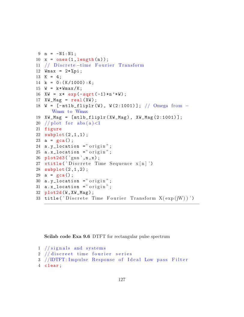
Scilab code Exa 9.6 DTFT for rectangular pulse spectrum
1 // s i g n a l s and sys t ems2 // d i s c r e e t t ime f o u r i e r s e r i e s3 //IDTFT : Impul se Response o f I d e a l Low pas s F i l t e r4 clear;
127

Figure 9.7: DTFT for rectangular pulse spectrum
5 clc;
6 close;
7 Wc = 1; // 1 rad / s e c8 W = -Wc:0.1: Wc; // Passband o f f i l t e r9 H0 = 1; // Magnitude o f F i l t e r
10 HlpW = H0*ones(1,length(W));
11 // I n v e r s e D i s c r e t e−t ime F o u r i e r Transform12 t = -2*%pi:2* %pi/length(W):2*%pi;
13 ht =(1/(2* %pi))*HlpW *exp(sqrt(-1)*W’*t);
14 ht = real(ht);
15 figure
16 subplot (2,1,1)
17 a = gca();
18 a.y_location =” o r i g i n ”;19 a.x_location =” o r i g i n ”;20 a.data_bounds =[-%pi ,0;%pi ,2];
21 plot2d(W,HlpW ,2);
22 poly1 = a.children (1).children (1);
128
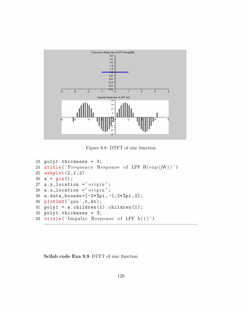
Figure 9.8: DTFT of sinc function
23 poly1.thickness = 3;
24 xtitle( ’ Frequency Response o f LPF H( exp (jW) ) ’ )25 subplot (2,1,2)
26 a = gca();
27 a.y_location =” o r i g i n ”;28 a.x_location =” o r i g i n ”;29 a.data_bounds =[-2*%pi ,-1;2*%pi ,2];
30 plot2d3( ’ gnn ’ ,t,ht);31 poly1 = a.children (1).children (1);
32 poly1.thickness = 3;
33 xtitle( ’ Impul se Response o f LPF h ( t ) ’ )
Scilab code Exa 9.9 DTFT of sinc function
129
1 // s i g n a l s and sys t ems2 // d i s c r e e t t ime f o u r i e r s e r i e s3 //IDTFT : Impul se Response o f I d e a l Low pas s F i l t e r4 clear;
5 clc;
6 close;
7 Wc = 1; // 1 rad / s e c8 W = -Wc:0.1: Wc; // Passband o f f i l t e r9 H0 = 1; // Magnitude o f F i l t e r
10 HlpW = H0*ones(1,length(W));
11 // I n v e r s e D i s c r e t e−t ime F o u r i e r Transform12 t = -2*%pi:2* %pi/length(W):2*%pi;
13 ht1 =(1/(2* %pi))*HlpW *exp(sqrt(-1)*W’*t);
14 size(ht1)
15 n= -21:21;
16 size(n)
17 ht=ht1.*(%e^%i*2*t);
18 ht = real(ht);
19 figure
20 subplot (2,1,1)
21 a = gca();
22 a.y_location =” o r i g i n ”;23 a.x_location =” o r i g i n ”;24 a.data_bounds =[-%pi ,0;%pi ,2];
25 plot2d(W,HlpW ,2);
26 poly1 = a.children (1).children (1);
27 poly1.thickness = 3;
28 xtitle( ’ Frequency Response o f LPF H( exp (jW) ) ’ )29 subplot (2,1,2)
30 a = gca();
31 a.y_location =” o r i g i n ”;32 a.x_location =” o r i g i n ”;33 a.data_bounds =[-2*%pi ,-1;2*%pi ,2];
34 size(t)
35 size(ht)
36 plot2d3( ’ gnn ’ ,t,ht);37 poly1 = a.children (1).children (1);
38 poly1.thickness = 3;
130

Figure 9.9: sketching the spectrum for a modulated signal
39 xtitle( ’ Impul se Response o f LPF h ( t ) ’ )
Scilab code Exa 9.10.a sketching the spectrum for a modulated signal
1 // s i g n a l s and sys t ems2 // d i s c r e t e f o u r i e r t r a n s f o r m3 // Frequency S h i f t i n g Proper ty o f DTFT4 clear;
5 clc;
6 close;
7 mag = 4;
131
8 W = -%pi /4:0.1: %pi /4;
9 H1 = mag*ones(1,length(W));
10 W1 =W+%pi/2;
11 W2 = -W-%pi /2;
12 figure
13 subplot (2,1,1)
14 a = gca();
15 a.y_location =” o r i g i n ”;16 a.x_location =” o r i g i n ”;17 a.data_bounds =[-%pi ,0;%pi ,2];
18 plot2d(W,H1);
19 xtitle( ’ Frequency Response o f the g i v e n H( exp (jW) ) ’ )20 subplot (2,1,2)
21 a = gca();
22 a.y_location =” o r i g i n ”;23 a.x_location =” o r i g i n ”;24 a.data_bounds =[-2*%pi ,0;2*%pi ,2];
25 plot2d(W1 ,0.5*H1);
26 plot2d(W2 ,0.5*H1);
27 xtitle( ’ Frequency Response o f modulated s i g n a l H1(exp (jW) ) ’ )
Scilab code Exa 9.13 frequency response of LTID
1 // LTi Systems c h a r a c t e r i z e d by L i n e a r Constant2 // f o u r i e r a n a l y s i s o f d i s c r e t e sy s t ems3 // I n v e r s e Z Transform4 // z = %z ;5 syms n z;
6 H1 = ( -5/3)/(z-0.5);
7 H2 = (8/3)/(z-0.8);
8 F1 = H1*z^(n)*(z -0.5);
9 F2 = H2*z^(n)*(z -0.8);
10 h1 = limit(F1 ,z,0.5);
11 disp(h1, ’ h1 [ n]= ’ )
132

12 h2 = limit(F2 ,z,0.8);
13 disp(h2, ’ h2 [ n]= ’ )14 h = h1 -h2;
15 disp(h, ’ h [ n]= ’ )
133
Chapter 10
state space analysis
Scilab code Exa 10.4 state space descrption by transfer function
1 // s i g n a l s and sys t ems2 // s t a t e space a n a l y s i s3 // s t a t e space d e s c r i p t i o n4 clear all;
5 close;
6 clc;
7 s=poly(0, ’ s ’ );8 H=[(4/3) /(1+s) ,-2/(3+s), (2/3) /(4+s)];
9 Sys=tf2ss(H)
10 clean(ss2tf(Sys))
11 disp(Sys)
Scilab code Exa 10.5 finding the state vector
1 syms t s
2 A=[-12 2/3; -36 -1]; B=[1/3;1]; q0 =[2;1]; X=1/s;
3 size(A)
4 size(s*eye(2,2))
134
5 Q=inv(s*eye(2,2)-A)*(q0+B*X);
6 q=[];
7 q(1)=ilaplace(Q(1));
8 q(2)=ilaplace(Q(2));
9 disp(q* ’ u ( t ) ’ ,” [ q1 ( t ) ; q2 ( t ) ] ”)
Scilab code Exa 10.6 state space descrption by transfer function
1 A=[0 1;-2 -3];
2 B=[1 0;1 1];
3 C=[1 0;1 1;0 2];
4 D=[0 0;1 0; 0 1];
5 syms s;
6 H=C*inv(s*eye(2,2)-A)*B+D;
7 disp(H,” the t r a n s f e r f u n c t i o n matr ix H( s )=”)8 disp(H(3,2),” the t r a n s f e r f u n c t i o n r e l a t i n g y3 and
x2 i s H32 ( s )=”)
Scilab code Exa 10.7 time domain method
1 // s i g n a l s and sys t ems2 // s t a t e space3 // t ime domain method to f i n d the s t a t e v e c t o r4 clc;
5 clf;
6 s=poly(0, ’ s ’ );7 A=[s+12 -2/3; 36 s+1];
8 y=roots(det(A))
9 t=poly(0, ’ t ’ );10 beta=inv([1 y(1); 1 y(2)])*[%e^-y(1)*t; %e^-y(2)*t];
11 disp(beta)
12 size(beta)
13 W=beta (1)*[1 0;0 1]+ beta (2)*[-12 2/3; -36 -1];
135
14 zir=W*[2;1];
15 disp(zir);
16 zsr=W*[1/3;1];
17 disp(zsr);
18 total=zir+zsr;
19 disp(total);
Scilab code Exa 10.8 state space descrption by transfer function
1 syms t s;
2 F1=ilaplace ((s+3)/((s+1)*(s+2)))
3 F2=ilaplace (1/((s+1)*(s+2)))
4 F3=ilaplace ( -2/((s+1)*(s+2)))
5 F4=ilaplace(s/((s+1)*(s+2)))
6 F=[F1 F2;F3 F4];
7 disp(F,” f ( t )=”)8 A=[1 0;1 1;0 2];
9 B=[0 0;1 0;0 1];
10 h=A*F*[1 0;1 1]+B*eye(2,2);// he r e 1 r e p r e s e n t s d e l ( t)
11 disp(h,”h ( t )=”)
Scilab code Exa 10.9 state equations of a given systems
1 A=[0 1;-2 -3];
2 B=[1;2];
3 P=[1 1;1 -1];
4 Ahat= P*A*inv(P)
5 Bhat=P*B
6 disp(Ahat ,”Aˆ=”)7 disp(Bhat ,”Bˆ=”)
136
Scilab code Exa 10.10 diagonalized form of state equation
1 A=[0 1;-2 -3];
2 [V,lambda ]=spec(A);
3 B=[1;2];
4 Bhat=P*B
5 disp(P,”P=”)6 disp(Bhat ,”Bˆ=”)7 disp(lambda ,” lambda=”)
Scilab code Exa 10.11 controllability and observability
1 A=[1 0;1 -1];
2 [V,lambda ]=spec(A);
3 B=[1;0];
4 C=[1 -2];
5 P=inv(V);
6 Bhat=P*B
7 Chat=C*inv(P)
8 disp( ’ ( a ) : ’ )9 disp(Bhat ,”Bˆ=”)
10 disp(Chat ,”Cˆ=”)11 A=[-1 0;-2 1];
12 [V,lambda ]=spec(A);
13 B=[1;1];
14 C=[0 1];
15 P=inv(V);
16 Bhat=P*B
17 Chat=C*inv(P)
18 disp( ’ Part ( b ) : ’ )19 disp(Bhat ,”Bˆ=”)20 disp(Chat ,” cˆ=”)
137

Scilab code Exa 10.12 state space description of a given description
1 A=[0 1;-1/6 5/6];
2 B=[0;1];
3 C=[-1 5];
4 D=0;
5 sys=syslin( ’ d ’ ,A,B,C,D);6 N=25;
7 x=ones(1,N+1);n=(0:N);
8 q0 =[2;3];
9 [ y q]=csim( ’ s t e p ’ ,n,sys);10 y=dsimul(sys ,x);
11 plot2d3(y)
Scilab code Exa 10.13 total response using z transform
1 // LTi Systems c h a r a c t e r i z e d by L i n e a r Constant2 // I n v e r s e Z Transform3 // z = %z ;4 syms n z;
5 H1 = (-2*z)/(z -(1/3));
6 H2 = (3*z)/(z-0.5);
7 H3 = (24*z)/(z-1);
8 F1 = H1*z^(n-1)*(z -(1/3));
9 F2 = H2*z^(n-1)*(z -0.5);
10 F3 = H3*z^(n-1)*(z-1);
11 h1 = limit(F1 ,z ,(1/3));
12 disp(h1, ’ h1 [ n]= ’ )13 h2 = limit(F2 ,z,0.5);
14 disp(h2, ’ h2 [ n]= ’ )15 h3 = limit(F3 ,z,1);
138
16 disp(h3, ’ h3 [ n]= ’ )17 h = h1+h2+h3;
18 disp(h, ’ h [ n]= ’ )
139
Related Documents