Pricing Bermudan options using regression: optimal rates of convergence for lower estimates

SFB 649 Discussion Paper 2009-023

Pricing Bermudan options using regression: optimal rates of convergence for

lower estimates

Denis Belomestny*

*Weierstrass Institute Berlin, Germany

This research was supported by the Deutsche Forschungsgemeinschaft through the SFB 649 "Economic Risk".

http://sfb649.wiwi.hu-berlin.de

ISSN 1860-5664

SFB 649, Humboldt-Universität zu Berlin Spandauer Straße 1, D-10178 Berlin

SFB

6

4 9

E

C O

N O

M I

C

R

I S

K

B

E R

L I

N

Pricing Bermudan options using regression: optimal

rates of convergence for lower estimates

Denis Belomestny1, ∗

April 21, 2009

Abstract

The problem of pricing Bermudan options using Monte Carlo anda nonparametric regression is considered. We derive optimal non-asymptotic bounds for a lower biased estimate based on the subop-timal stopping rule constructed using some estimates of continuationvalues. These estimates may be of different nature, they may be localor global, with the only requirement being that the deviations of theseestimates from the true continuation values can be uniformly boundedin probability.

Keywords: Bermudan options; Regression; Boundary condition.

1 Introduction

An American option grants the holder the right to select the time at whichto exercise the option, and in this differs from a European option which maybe exercised only at a fixed date. A general class of American option pricingproblems can be formulated through an R

d Markov process X(t), 0 ≤ t ≤T defined on a filtered probability space (Ω,F, (Ft)0≤t≤T ,P). It is assumedthat X(t) is adapted to (Ft)0≤t≤T in the sense that each Xt is Ft measurable.Recall that each Ft is a σ-algebra of subsets of Ω such that Fs ⊆ Ft ⊆ F

for s ≤ t. We interpret Ft as all relevant financial information available upto time t. We restrict attention to options admitting a finite set of exerciseopportunities 0 = t0 < t1 < t2 < . . . < tL = T , sometimes called Bermudanoptions. If exercised at time tl, l = 1, . . . , L, the option pays fl(X(tl)), forsome known functions f0, f1, . . . , fL mapping R

d into [0,∞). Let Tn denotethe set of stopping times taking values in n, n + 1, . . . , L. A standardresult in the theory of contingent claims states that the equilibrium price

1Weierstrass Institute for Applied Analysis and Stochastics, Mohrenstr. 39, 10117

Berlin, Germany. [email protected] Subject Classification: G14; C15.∗supported in part by the SFB 649 ‘Economic Risk’.

1

Vn(x) of the American option at time tn in state x given that the option wasnot exercised prior to tn is its value under an optimal exercise policy:

Vn(x) = supτ∈Tn

E[fτ (X(tτ ))|X(tn) = x), x ∈ Rd.

Pricing an American option thus reduces to solving an optimal stoppingproblem. Solving this optimal stopping problem and pricing an Americanoption are straightforward in low dimensions. However, many problemsarising in practice (see e.g. Glasserman (2004)) have high dimensions, andthese applications have motivated the development of Monte Carlo meth-ods for pricing American option. Pricing American style derivatives withMonte Carlo is a challenging task because the determination of optimal ex-ercise strategies requires a backwards dynamic programming algorithm thatappears to be incompatible with the forward nature of Monte Carlo sim-ulation. Much research was focused on the development of fast methodsto compute approximations to the optimal exercise policy. Notable exam-ples include the functional optimization approach in Andersen (2000), meshmethod of Broadie and Glasserman (1997), the regression-based approachesof Carriere (1996), Longstaff and Schwartz (2001), Tsitsiklis and Van Roy(1999) and Egloff (2005). A common feature of all above mentioned algo-rithms is that they deliver estimates C0(x), . . . , CL−1(x) for the so calledcontinuation values:

Ck(x) := E[Vk+1(X(tk+1))|X(tk) = x], k = 0, . . . , L − 1.(1.1)

An estimate for V0, the price of the option at time t0 can then be defined as

V0(x) := maxf0(x), C0(x), x ∈ Rd.

This estimate basically inherits all properties of C0(x). In particular, it isusually impossible to determine the sign of the bias of V0 since the bias ofC0 may change its sign. One way to get a lower bound (low biased estimate)for V0 is to construct a (generally suboptimal) stopping rule

τ = min0 ≤ k ≤ L : Ck(X(tk)) ≤ fk(X(tk))

with CL ≡ 0 by definition. Simulating a new independent set of trajectoriesand averaging the pay-offs stopped according to τ on these trajectories givesus a lower bound V0 for V0. As was observed by practitioners, the so con-structed estimate V0 has rather stable behavior with respect to the estimatesof continuation values C0(x), . . . , CL−1(x), that is even rather poor estimatesof continuation values may lead to a good estimate V0. The aim of this paperis to find a theoretical explanation of this observation and to investigate theproperties of V0. In particular, we derive optimal non-asymptotic bounds forthe bias V0 −E V0 assuming some uniform probabilistic bounds for Cr − Cr.

2

It is shown that the bounds for V0−E V0 are usually much tighter than onesfor V0−E V0 implying a better quality of V0 as compared to the quality of V0

constructed using one and the same set of estimates for continuation values.The issues of convergence for regression algorithms have been already

studied in several papers. Clement, Lamberton and Protter (2002) were firstwho proved the convergence of the Longstaff-Schwartz algorithm. Glasser-man and Yu (2005) have shown that the number of Monte Carlo paths hasto be in general exponential in the number of basis functions used for regres-sion in order to ensure convergence. Recently, Egloff, Kohler and Todorovic(2007) (see also Kohler (2008)) have derived the rates of convergence forcontinuation values estimates obtained by the so called dynamic look-aheadalgorithm (see Egloff (2004)) that“interpolates”between Longstaff-Schwartzand Tsitsiklis-Roy algorithms. They presented the convergence rates for V0

which coincide with the rates of C0 and are determined by the smoothnessproperties of the true continuation values C0, . . . , CL−1. It turns out that theconvergence rates for V0 depend not only on the smoothness of continuationvalues (as opposite to V0), but also on the behavior of the underlying pro-cess near the exercise boundary. Interestingly enough, there are cases wherethese rates become almost independent either of the smoothness propertiesof Ck or of the dimension of X and the bias of V0 decreases exponentiallyin the number of Monte Carlo paths used to construct Ck.

The paper is organized as follows. In Section 2.1 we introduce and dis-cuss the so called boundary assumption which describes the behavior of theunderlying process X near the exercise boundary and heavily influences theproperties of V0. In Section 2.2 we derive non-asymptotic bounds for thebias V0−E V0 and prove that these bounds are optimal in the minimax sense.Finally, we illustrate our results by a numerical example.

2 Main results

2.1 Boundary assumption

For the considered Bermudan option let us introduce a continuation regionC and an exercise (stopping) region E :

C := (i, x) : fi(x) < Ci(x) ,(2.2)

E := (i, x) : fi(x) ≥ Ci(x) .

Furthermore, let us assume that there exist constants B0,k > 0, k = 0, . . . , L−1 and α > 0 such that the inequality

(2.3) Ptk |t0(0 < |Ck(X(tk)) − fk(X(tk))| ≤ δ) ≤ B0,kδα, δ > 0,

holds for all k = 0, . . . , L − 1, where Ptk |t0 is the conditional distributionof X(tk) given X(t0). Assumption (2.3) provides a useful characterization

3

of the behavior of the continuation values Ck and payoffs fk near theexercise boundary ∂E. Although this assumption seems quite natural tolook at, we make in this paper, to the best of our knowledge, a first attemptto investigate its influence on the convergence rates of lower bounds basedon suboptimal stopping rules.

In the situation when all functions Ck − fk, k = 0, . . . , L− 1 are smoothand have non-vanishing derivatives in the vicinity of the exercise boundary,we have α = 1. Other values of α are possible as well. We illustrate this bytwo simple examples.

Example 1 Fix some α > 0 and consider a two period (L = 1) Bermudanpower put option with the payoffs

f0(x) = f1(x) = (K1/α − x1/α)+, x ∈ R+, K > 0.(2.4)

Denote by ∆ the length of the exercise period, i.e. ∆ = t1−t0. If the processX follows the Black-Scholes model with volatility σ and zero interest rate,then one can show that

C0(x) := E[f1(X(t1))|X(t0) = x] = K1/αΦ(−d2)

− x1/αe∆(α−1−1)(σ2/2α)Φ(−d1)

with Φ being the cumulative distribution function of the standard normaldistribution,

d1 =log(x/K) +

(1α − 1

2

)σ2∆

σ√

∆

and d2 = d1 − σ√

∆/α. As can be easily seen, the function C0(x) − f0(x)satisfies |C0(x) − f0(x)| ≍ x1/α for x → +0 and C0(x) > f0(x) for all x > 0if α ≥ 1. Hence

P(0 < |C0(X(t0)) − f0(X(t0))| ≤ δ) . δα, δ → 0, α ≥ 1.

Taking different α in the definition of the payoffs (2.4), we get (2.3) satisfiedfor α ranging from 1 to ∞.

In fact, even the extreme case “α = ∞” may take place as shown in thenext example.

Example 2 Let us consider again a two period Bermudan option suchthat the corresponding continuation value C0(x) = E[f1(X(t1))|X(t0) = x]is positive and monotone increasing function of x on any compact set in R.Fix some x0 ∈ R and choose δ0 satisfying δ0 < C0(x0). Define the payofffunction f0(x) in the following way

f0(x) =

C0(x0) + δ0, x < x0,

C0(x0) − δ0, x ≥ x0.

4

1 2 3 4 5 6 7 8

0.0

0.5

1.0

1.5

2.0

2.5

3.0

x

f0(x)

C0(x)

Figure 1: Illustration to Example 2.

So, f0(x) has a “digital” structure. Figure 1 shows the plots of C0 and f0 inthe case where X follows the Black-Scholes model and f1(x) = (x−K)+. Itis easy to see that

Pt0(0 < |C0(X(t0)) − f0(X(t0))| ≤ δ0) = 0.

On the other hand

C = x ∈ R : C0(x) ≥ f0(x) = x ∈ R : x ≥ x0,E = x ∈ R : C0(x) < f0(x) = x ∈ R : x < x0.

So, both continuation and exercise regions are not trivial in this case.The last example is of particular interest because as will be shown in

the next sections the bias of V0 decreases in this case exponentially in thenumber of Monte Carlo paths used to estimate the continuation values, alower bound V0 was constructed from.

2.2 Non-asymptotic bounds for V0 − E V0

Let Ck,M , k = 1, . . . , L−1, be some estimates of continuation values obtainedusing M paths of the underlying process X starting from x0 at time t0. Wemay think of (X(1)(t), . . . ,X(M)(t)) as being a vector process on the productprobability space with σ-algebra F⊗M and the product measure P⊗M

x0defined

on F⊗M via

P⊗Mx0

(A1 × . . . × AM ) = Px0(A1) · . . . · Px0(AM ),

5

with Am ∈ F, m = 1, . . . ,M . Thus, each Ck,M , k = 0, . . . , L − 1, ismeasurable with respect to F⊗M . The following proposition provides non-asymptotic bounds for the bias V0 − E V0,M of a lower bound V0,M given

uniform probabilistic bounds for Ck,M.

Proposition 2.1. Suppose that there exist constants B1, B2 and a positive

sequence γM such that for any δ > δ0 > 0 it holds

P⊗Mx0

(|Ck,M(x) − Ck(x)| ≥ δγ

−1/2M

)≤ B1 exp(−B2δ)(2.5)

for almost all x with respect to Ptk|t0 , the conditional distribution of X(tk)given X(t0), k = 0, . . . , L − 1. Define

V0,M := E[fτM

(X(tτM))|X(t0) = x0

](2.6)

with

τM := min

0 ≤ k ≤ L : Ck,M(X(tk)) ≤ fk(X(tk))

.(2.7)

If the boundary condition (2.3) is fulfilled, then

0 ≤ V0 − EP⊗Mx0

[V0,M ] ≤ B

[L−1∑

l=0

B0,l

]γ−(1+α)/2M

with some constant B depending only on α, B1 and B2.

The above convergence rates are, in fact, optimal in the following sense.

Proposition 2.2. Fix a set of non-zero payoff functions f0, . . . , fL and let

Pα be a class of pricing measures such that the boundary condition (2.3) is

fulfilled with some α > 0. For any positive sequence γM satisfying

γ−1M = o(1), γM = O(M), M → ∞,

there exist a subset Pα,γ of Pα and a constant B > 0 such that for any

M ≥ 1, any stopping rule τM and any set of estimates Ck,M measurable

w.r.t. F⊗M , we have for some δ > 0 and k = 0, . . . , L − 1,

supP∈Pα,γ

P⊗M(|Ck,M (x) − Ck(x)| ≥ δγ

−1/2M

)> 0

for almost all x w.r.t. any P ∈ Pα,γ and

supP∈Pα,γ

supτ∈T0

EFt0P [fτ (X(tτ ))] − EP⊗M [E

Ft0P fτM

(X(tτM))]

≥ Bγ

−(1+α)/2M .

6

Finally, we discuss the case when “α = ∞”, meaning that there existsδ0 > 0 such that

Ptk |t0(0 < |Ck(X(tk)) − fk(X(tk))| ≤ δ0) = 0(2.8)

for k = 0, . . . , L − 1. This is very favorable situation for pricing. It turnsout that if the continuation values estimates Ck,M satisfy a kind of expo-

nential inequality and (2.8) holds, then the bias of V0,M converges to zeroexponentially fast in γM .

Proposition 2.3. Suppose that for any δ > 0 there exist constants B1, B2

possibly depending on δ and a sequence of positive numbers γM not depending

on δ such that

P⊗Mx0

(|Ck,M(x) − Ck(x)| ≥ δ

)≤ B1 exp(−B2γM )(2.9)

for almost all x with respect to Ptk |t0, k = 0, . . . , L − 1. Assume also that

there exist a constant Bf > 0 such that

(2.10) E

[max

k=0,...,Lf2

k (X(tk))

]≤ Bf , k = 0, . . . , L.

If the condition (2.8) is fulfilled with some δ0 > 0, then

0 ≤ V0 − EP⊗Mx0

[V0,M ] ≤ B3 exp(−B4γM )

with some constant B3 and B4 depending only on B1, B2 and Bf .

Discussion Let us make a few remarks on the results of this section. First,Proposition 2.1 implies that the convergence rates of V0,M are always faster

than the convergence rates of Ck,M provided that α > 0. Indeed, while the

convergence rates of Ck,M are of order γ−1/2M , the bias of V0,M converges to

zero as fast as γ−(1+α)/2M . As to the variance of V0,M , it can be made arbitrary

small by averaging V0,M over a large number of sets, each consisting of Mtrajectories, and by taking a large number of new Monte Carlo paths usedto average the payoffs stopped according to τM .

Second, if the condition (2.8) holds true, then the bias of V0,M decreasesexponentially in γM , indicating that even very unprecise estimates of thecontinuation values would lead to the estimate V0,M of acceptable quality.

Finally, let us stress that the results obtained in this section are quitegeneral and do not depend on the particular form of the estimates Ck,M,only the inequality (2.5) being crucial for the result to hold. This inequalityholds for various types of estimators. These may be global least squaresestimators or local polynomial estimators. In particular, it can be shownthat if all continuation values Ck belong to the Holder class Σ(β,H, Rd)and the conditional law of X satisfies some regularity assumptions, thenthe local polynomial estimates of continuation values satisfy inequality (2.5)with γM = M2β/(2β+d) log−1(M).

7

3 Numerical example: Bermudan max call

This is a benchmark example studied in Broadie and Glasserman (1997) andGlasserman (2004) among others. Specifically, the model with d identicallydistributed assets is considered, where each underlying has dividend yield δ.The risk-neutral dynamic of assets is given by

dXk(t)

Xk(t)= (r − δ)dt + σdWk(t), k = 1, ..., d,

where Wk(t), k = 1, ..., d, are independent one-dimensional Brownian mo-tions and r, δ, σ are constants. At any time t ∈ t0, ..., tL the holder of theoption may exercise it and receive the payoff

f(X(t)) = (max(X1(t), ...,Xd(t)) − K)+.

We take d = 2, r = 5%, δ = 10%, σ = 0.2 and ti = iT/L, i = 0, ..., L, withT = 3, L = 9 as in Glasserman (2004, Chapter 8). First, we estimate allcontinuation values via the dynamic programming algorithm using the socalled Nadaraya-Watson regression estimator

(3.11) Cr,M(x) =

∑Mm=1 K((x − X(m)(tr))/h)Y

(m)r+1∑M

m=1 K((x − X(m)(tr))/h)

with Y(m)r+1 = max(fr+1(X

(m)(tr+1)), Cr+1,M (X(m)(tr+1))), r = 0, . . . , L − 1.

Here K is a kernel, h > 0 is a bandwidth and (X(m)(t1), . . . ,X(m)(tL)),

m = 1, . . . ,M, is the set of paths of the process X, all starting from thepoint x0 = (90, 90) at t0 = 0. As can be easily seen the estimator (3.11) isa local polynomial estimator of degree 0. Upon estimating C1,M , we definean estimate for the price of the option at time t0 = 0 as

V0 :=1

M

M∑

m=1

Y(m)1 .

Next, using the so constructed estimates of continuation values we constructa stopping policy τ which is defined pathwise as

τ (n) := min

1 ≤ k ≤ L : Ck,M(X(n)(tk)) ≤ fk(X(n)(tk))

, n = 1, . . . , N,

where (X(n)(t1), . . . , X(n)(tL)), n = 1, . . . , N, is a new independent set of

trajectories of the process X, all starting from x0 = (90, 90) at t0 = 0. Thestopping policy τ yields a lower bound

V0 =1

N

N∑

n=1

fτ (n)(X(n)(tτ (n))).

8

hat V_0 tilde V_0

67

89

10

h=5

hat V_0 tilde V_0

78

910

h=40

hat V_0 tilde V_0

78

910

1112

13

h=60

hat V_0 tilde V_0

810

1214

1618

h=100

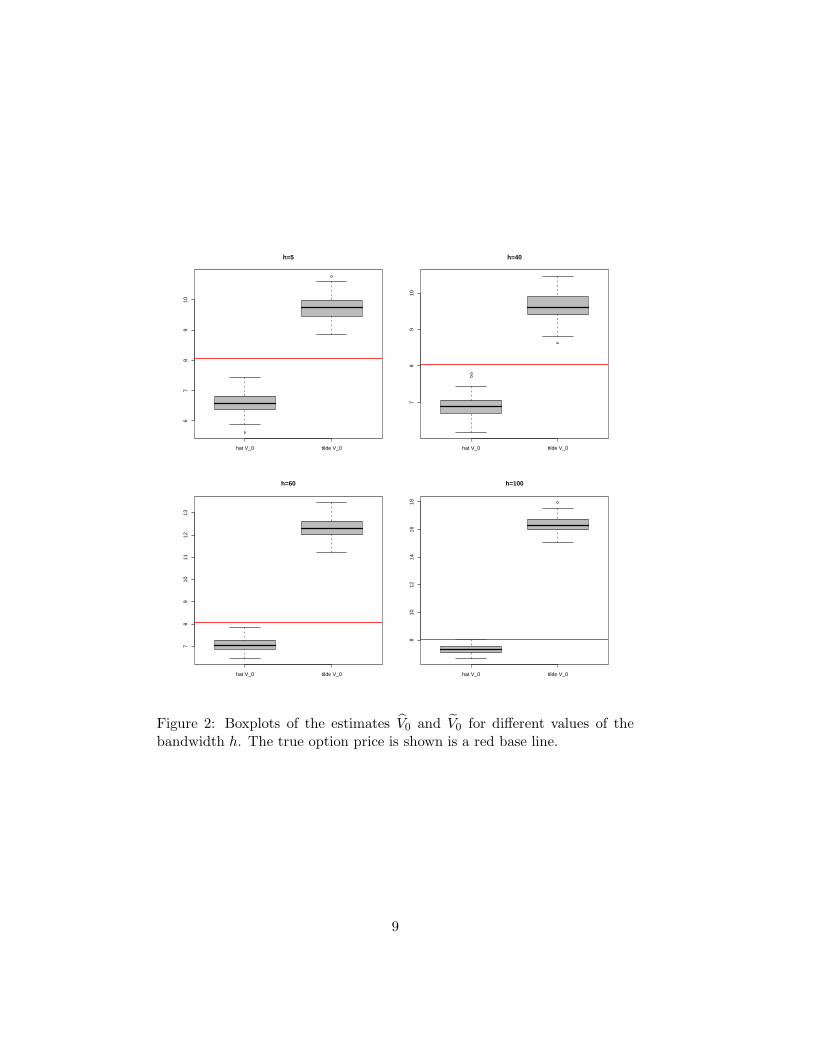
Figure 2: Boxplots of the estimates V0 and V0 for different values of thebandwidth h. The true option price is shown is a red base line.

9

In Figure 2 we show the boxplots of V0 and V0 based on 100 sets of tra-jectories each of the size M = 1000 for different values of the bandwidth h,where the triangle kernel K(x) = (1 − ‖x‖2)+ is used to construct (3.11).Also the true value V0 of the option (8.08 in this case), computed using atwo-dimensional binomial lattice, is shown as a red base line. Several obser-vations can be made by an examination of Figure 2. First, while the bias ofV0 is always smaller then the bias of V0, the largest difference takes place forlarge h. This can be explained by the fact that for large h more observations

Y(m)r+1 with X(m)(tr) lying far away from the given point x become involved

in the construction of Cr,M(x). This has a consequence of increasing thebias of the estimate (3.11). The most interesting phenomenon is, however,the behavior of V0 which turns out to be quite stable with respect to h. Soeven in the case of rather poor estimates of continuation values (when h islarge) V0 still looks reasonable.

We stress that the aim of this example is not to show the strength of thelocal polynomial estimation algorithms (for this we would take larger M andhigher order kernels) but rather to illustrate the main claim of this paper,namely the claim about the efficiency of V0 as compared to the estimatesbased on the direct use of continuation values estimates.

4 Conclusion

In this paper we have derived optimal rates of convergence for lower biasedestimates of the price of a Bermudan option based on suboptimal exercisepolicies obtained from some estimates of the optimal continuation values.We have shown that these rates are usually much faster than the convergencerates of the corresponding continuation values estimates. This may explainthe efficiency of these lower bounds observed in practice. Moreover, it turnsout that there are some cases where the expected values of the lower boundsbased on suboptimal stopping rules achieve very fast convergence rates whichare exponential in the number of paths used to estimate the correspondingcontinuation values. This suggests that the algorithms based on suboptimalstopping rules (e.g. Longstaff-Schwartz algorithm) rather than on the directuse of the continuation values estimates might be preferable.

5 Proofs

5.1 Proof of Proposition 2.1

Define

τj := minj ≤ k < L : Ck(X(tk)) ≤ fk(X(tk)), j = 0, . . . , L,

τj,M := minj ≤ k < L : Ck(X(tk)) ≤ fk(X(tk)), j = 0, . . . , L

10

and

Vk,M(x) := E[fτk,M(X(tτk,M

))|X(tk) = x], x ∈ Rd.

The so called Snell envelope process Vk is related to τk via

Vk(x) = E[fτk(X(tτk

))|X(tk) = x], x ∈ Rd.

The following lemma provides a useful inequality which will be repeatedlyused in our analysis.

Lemma 5.1. For any k = 0, . . . , L − 1, it holds with probability one

(5.12) 0 ≤ Vk(X(tk)) − Vk,M(X(tk))

≤ EFtk

[L−1∑

l=k

|fl(X(tl)) − Cl(X(tl))|

×(1τl,M >l, τl=l + 1τl,M =l, τl>l

)].

Proof. We shall use induction to prove (5.12). For k = L − 1 we have

VL−1(X(tL−1)) − VL−1,M (X(tL−1)) =

= EFtL−1

[(fL−1(X(tL−1)) − fL(X(tL)))1τL−1=L−1, τL−1,M =L

]

+ EFtL−1

[(fL(X(tL)) − fL−1(X(tL−1)))1τL−1=L, τL−1,M =L−1

]

= |fL−1(X(tL−1)) − CL−1(X(tL−1))|1τL−1,M 6=τL−1

since events τL−1 = L and τL−1,M = L are measurable w.r.t. FtL−1.

Thus, (5.12) holds with k = L−1. Suppose that (5.12) holds with k = L′+1.Let us prove it for k = L′. Consider a decomposition

fτL′ (X(tτL′ )) − fτL′,M(X(tτL′ ,M

)) = S1 + S2 + S3

with

S1 :=(fτL′ (X(tτL′ )) − fτL′,M

(X(tτL′ ,M))

)1τL′>L′, τL′,M>L′

S2 :=(fτL′ (X(tτL′ )) − fτL′,M

(X(tτL′ ,M))

)1τL′>L′, τL′,M=L′

S3 :=(fτL′ (X(tτL′ )) − fτL′,M

(X(tτL′ ,M))

)1τL′=L′, τL′,M>L′.

Since

EFtL′ [S1] = EFt

L′

[(VL′+1(X(tL′+1)) − VL′+1,M (X(tL′+1))

)]1τL′>L′, τL′,M>L′,

EFtL′ [S2] =

(EFt

L′

[fτL′+1

(X(tτL′+1))

]− fL′(X(tL′))

)1τL′>L′, τL′,M=L′

= (CL′(X(tL′)) − fL′(X(tL′)))1τL′>L′, τL′,M=L′

11

and

EFtL′ [S3] =

(fL′(X(tL′)) − EFt

L′

[fτL′+1,M

(X(tτL′+1,M))

])1τL′=L′, τL′,M >L′

= (fL′(X(tL′)) − CL′(X(tL′)))1τL′=L′, τL′,M>L′

+ EFtL′

[(VL′+1(X(tL′+1)) − VL′+1,M(X(tL′+1))

)1τL′=L′, τL′,M>L′

],

we get with probability one

VL′(X(tL′)) − VL′,M (X(tL′) ≤ |fL′(X(tL′)) − CL′(X(tL′))|×

(1τL′,M>L′, τL′=L′ + 1τL′,M=L′, τL′>L′

)

+ EFtL′

[VL′+1(X(tL′+1)) − VL′+1,M (X(tL′+1))

].

Our induction assumption implies now that

VL′(X(tL′)) − VL′,M (X(tL′)) ≤

EFtL′

[L−1∑

l=L′

|fl(Xl) − Cl(Xl)|(1τl,M >l, τl=l + 1τl,M =l, τl>l

)]

and hence (5.12) holds for k = L′.

Let us continue with the proof of Proposition 2.1. Consider the setsEl, Al,j ⊂ R

d, l = 0, . . . , L − 1, j = 1, 2, . . . , defined as

El :=x ∈ R

d : Cl,M (x) ≤ fl(x), Cl(x) > fl(x)

∪x ∈ R

d : Cl,M(x) > fl(x), Cl(x) ≤ fl(x)

,

Al,0 :=x ∈ R

d : 0 < |Cl(x) − fl(x)| ≤ γ−1/2M

,

Al,j :=x ∈ R

d : 2j−1γ−1/2M < |Cl(x) − fl(x)| ≤ 2jγ

−1/2M

, j > 0.

We may write

V0(X(t0)) − V0,M (X(t0)) ≤ EFt0

[L−1∑

l=0

|fl(X(tl)) − Cl(X(tl))|1X(tl)∈El

]

=

∞∑

j=0

EFt0

[L−1∑

l=0

|fl(X(tl)) − Cl(X(tl))|1X(tl)∈Al,j∩El

]

≤ γ−1/2M

L−1∑

l=0

Ptl|t0

(0 < |Cl(X(tl)) − fl(X(tl))| ≤ γ

−1/2M

)

+

∞∑

j=1

EFt0

[L−1∑

l=0

|fl(X(tl)) − Cl(X(tl))|1X(tl)∈Al,j∩El

].

12

Using the fact that

|fl(X(tl)) − Cl(X(tl))| ≤ |Cl,M (X(tl) − Cl(X(tl))|, l = 0, . . . , L − 1,

on El, we get for any j ≥ 1 and l ≥ 0

EFt0 EP⊗Mx0

[|fl(X(tl)) − Cl(X(tl))|1X(tl)∈Al,j∩El

]

≤ 2jγ−1/2M EFt0 EP⊗M

x0

[1|Cl,M (X(tl)−Cl(X(tl))|≥2j−1γ

−1/2M

×10<|fl(X(tl))−Cl(X(tl))|≤2jγ

−1/2M

]

≤ 2jγ−1/2M EFt0

[P⊗M

x0(|Cl,M (X(tl)) − Cl(X(tl))| ≥ 2j−1γ

−1/2M )

×10<|fl(X(tl))−Cl(X(tl))|≤2jγ

−1/2M

]

≤ B12jγ

−1/2M exp

(−B22

j−1)Ptl|t0(0 < |fl(X(tl)) − Cl(X(tl))| ≤ 2jγ

−1/2M )

≤ B1B0,l2j(1+α)γ

−(1+α)/2M exp

(−B22

j−1),

where Assumption 2.3 is used to get the last inequality. Finally, we get

V0(X(t0)) − EP⊗Mx0

[V0,M (X(t0))]

≤[

L−1∑

l=0

B0,l

]γ−(1+α)/2M + B′

[L−1∑

l=0

B0,l

]γ−(1+α)/2M

∑

j≥1

2j(1+α) exp(−B22j−1)

≤ B

[L−1∑

l=0

B0,l

]γ−(1+α)/2M

with some constant B depending on B1, B2 and α.

5.2 Proof of Proposition 2.2

For the sake of simplicity we consider the case of a three period Bermu-dan option with two possible exercise dates t1 and t2 (exercise at t0 is notpossible). We also assume that the payoff function f2 has a “digital” struc-ture, i.e. it takes two values 0 and 1. The extension to a general case isstraightforward but somewhat cumbersome.

We have

(5.13) V0(X(t0)) − V0,M (X(t0)) =

= EFt0 [(f1(X(t1)) − f2(X(t2)))1(τ1 = 1, τ1,M = 2)]

+ EFt0 [(f2(X(t2)) − f1(X(t1)))1(τ1 = 2, τ1,M = 1)]

= EFt0

[|f1(X(t1)) − C1(X(t1))|1τ1,M 6=τ1

].

13

For an integer q ≥ 1 consider a regular grid on [0, 1]d defined as

Gq =

(2k1 + 1

2q, . . . ,

2kd + 1

2q

): ki ∈ 0, . . . , q − 1, i = 1, . . . , d

.

Let nq(x) ∈ Gq be the closest point to x ∈ Rd among points in Gq. Consider

the partition X′1, . . . ,X

′qd of [0, 1]d canonically defined using the grid Gq (x

and y belong to the same subset if and only if nq(x) = nq(y)). Fix an integerm ≤ qd. For any i ∈ 1, . . . ,m, define Xi = X′

i and X0 = Rd \ ⋃m

i=1 Xi, sothat X0, . . . ,Xm form a partition of R

d. Denote by Bq,j the ball with thecenter in nq(Xj) and radius 1/2q.

Define a hypercube H = Pσ : σ = (σ1, . . . , σm) ∈ −1, 1m of probabil-ity distributions Pσ of the r.v. (X(t1), f2(X(t2))) valued in R

d×0, 1 as fol-lows. For any Pσ ∈ H the marginal distribution of X(t1) (given X(t0) = x0)does not depend on σ and has a bounded density µ w.r.t. the Lebesgue mea-sure on R

d such that Pµ(X0) = 0 and

Pµ(Xj) = Pµ(Bq,j) =

∫

Bq,j

µ(x) dx = ω, j = 1, . . . ,m

for some ω > 0. In order to ensure that the density µ remains bounded weassume that qdω = O(1).

The distribution of f2(X(t2)) given X(t1) is determined by the proba-bility Pσ(f2(X(t2)) = 1|X(t1) = x) which is equal to C1,σ(x). Define

C1,σ(x) = f1(x) + σjφ(x), x ∈ Xj, j = 1, . . . ,m,

and C1,σ(x) = f1(x) on X0, where φ(x) = γ−1/2M ϕ(q[x − nq(x)]), ϕ(x) =

Aϕθ(‖x‖) with some constant Aϕ > 0 and with θ : R+ → R+ being a non-increasing infinitely differentiable function such that θ(x) ≡ 1 on [0, 1/2] andθ(x) ≡ 0 on [1,∞). Without loss of generality we may assume that f1(x) isstrictly positive on [0, 1]d, i.e. there exist two real numbers 0 < f− < f+ < 1such that f− ≤ f1(x) ≤ f+. Taking Aϕ small enough, we can then ensure

that 0 ≤ C1,σ(x) ≤ 1 on Rd. Obviously, it holds φ(x) = Aϕγ

−1/2M for

x ∈ Bq,j. As to the boundary assumption (2.3), we have

Pµ(0 < |f1(X(t1)) − C1,σ(X(t1))| ≤ δ) =m∑

j=1

Pµ(0 < |f1(X(t1)) − C1,σ(X(t1))| ≤ δ,X(t1) ∈ Bq,j)

=

m∑

j=1

∫

Bq,j

10<φ(x)≤δµ(x) dx = mω1Aϕγ

−1/2M ≤δ

14

and (2.3) holds provided that mω = O(γ−α/2M ). Let τM be a stopping time

measurable w.r.t. F⊗M , then the identity (5.13) leads to

EFt0Pσ

[fτ (X(τ))] − EP⊗Mσ

[EFt0 fτM(X(τM ))]

= EP⊗Mσ

EFt0Pµ

[|∆σ(X(t1))|1τ1,M 6=τ1

],

with ∆σ(X(t1)) = f1(X(t1)) − C1,σ(X(t1)). By conditioning on X(t1), weget

EP⊗Mσ

EFt0Pµ

[|∆σ(X(t1))|1τ1,M 6=τ1

]

= ω

m∑

j=1

EP⊗Mσ

EFt0Pµ

[φ(X(t1))1τ1,M 6=τ1|X(t1) ∈ Bq,j

]

= Aϕmωγ−1/2M E

Ft0Pµ

P⊗Mσ (τ1,M 6= τ1).

Using now a well known Birge’s or Huber’s lemma (see, e.g. Devroye, Gyorfiand Lugosi, 1996, p. 243), we get

supσ∈−1;+1m

P⊗Mσ (τ1,M 6= τ1) ≥

[0.36 ∧

(1 − MKH

log(|H|)

)],

where KH := supP,Q∈HK(P,Q) and K(P,Q) is a Kullback-Leibler distancebetween two measures P and Q. Since for any two measures P and Q fromH with Q 6= P it holds

K(P,Q) ≤ supσ1,σ2∈−1;+1m

σ1 6=σ2

EFt0Pµ

[C1,σ2(X(t1)) log

C1,σ1(X(t1))

C1,σ2(X(t1))

+(1 − C1,σ2(X(t1))) log

1 − C1,σ1(X(t1))

1 − C1,σ2(X(t1))

]

≤ (1 − f+ − Aϕ)−1(f− − Aϕ)−1 EFt0Pµ

[φ2(X(t1))1X(t1)6∈X0

]

for small enough Aϕ, and log(|H|) = m log(2), we get

supσ∈−1;+1m

E

Ft0Pσ

[fτ,σ(X(τ))] − EP⊗Mσ

[EFt0 fτM ,σ(X(τM ))]≥

Aϕmωγ−1/2M (1 − AMγ−1

M ω) & γ−(1+α)/2M ,

provided that mω > Bγ−α/2M for some B > 0 and AMω < γM , where A is

a positive constant depending on f−, f+ and Aϕ. Using similar arguments,we derive

supσ∈−1;+1m

P⊗Mσ (|C1,σ(x) − C1,M (x)| > δγ

−1/2M ) > 0

for almost x w.r.t. Pµ, some δ > 0 and any estimator C1,M measurablew.r.t. F⊗M .

15

5.3 Proof of Proposition 2.3

Using the arguments similar to ones in the proof of Proposition 2.1, we get

(5.14) V0(X(t0)) − EP⊗Mx0

[V0,M (X(t0))] ≤

δ0

L−1∑

l=0

Ptl|t0(0 < |Cl(X(tl)) − fl(X(tl))| ≤ δ0)

+L−1∑

l=0

EFt0 EP⊗Mx0

[|Cl(X(tl)) − fl(X(tl))|

×1X(tl)∈El1|Cl(X(tl))−fl(X(tl))|>δ0

]

with El defined as in the proof of Proposition 2.1. The first summand onthe right-hand side of (5.14) is equal to zero due to (2.8). Hence, Cauchy-Schwarz and Minkowski inequalities imply

V0(X(t0)) − EP⊗Mx0

[V0,M (X(t0))] ≤L−1∑

l=0

[EFt0 |EFtl

[fτl+1

(X(tτl+1))

]− fl(X(tl))|2

]1/2

×[EFt0 P⊗M

x0(|Cl(X(tl)) − Cl,M(X(tl))| > δ0)

]1/2

≤ 2B1/2f

L−1∑

l=0

[EFt0 P⊗M

x0(|Cl(X(tl)) − Cl,M(X(tl))| > δ0)

]1/2.

Now the application of (2.9) finishes the proof.

References

L. Andersen (2000). A simple approach to the pricing of Bermudan swap-tions in the multi-factor Libor Market Model. Journal of Computational

Finance, 3, 5-32.

D. Belomestny, G.N. Milstein and V. Spokoiny (2006). Regression methodsin pricing American and Bermudan options using consumption processes,to appear in Quantitative Finance.

D. Belomestny, Ch. Bender and J. Schoenmakers (2007). True upper boundsfor Bermudan products via non-nested Monte Carlo, to appear in Math-

ematical Finance.

M. Broadie and P. Glasserman (1997). Pricing American-style securities us-ing simulation. J. of Economic Dynamics and Control, 21, 1323-1352.

J. Carriere (1996). Valuation of early-exercise price of options using simu-lations and nonparametric regression. Insuarance: Mathematics and Eco-

nomics, 19, 19-30.

16

E. Clement, D. Lamberton and P. Protter (2002). An analysis of a leastsquares regression algorithm for American option pricing. Finance and

Stochastics, 6, 449-471.

L. Devroye, L. Gyorfi and G. Lugosi (1996). A probabilistic theory of patternrecognition. Application of Mathematics (New York), 31, Springer.

R. M. Dudley (1999). Uniform Central Limit Theorems, Cambridge Univer-sity Press, Cambridge, UK.

D. Egloff (2005). Monte Carlo algorithms for optimal stopping and statisticallearning. Ann. Appl. Probab., 15, 1396-1432.

D. Egloff, M. Kohler and N. Todorovic (2007). A dynamic look-ahead MonteCarlo algorithm for pricing Bermudan options, Ann. Appl. Probab., 17,1138-1171.

E. Gine and A. Guillou (2002). Rates of strong uniform consistency formultivariate kernel density estimators. Ann. I. H. Poincare, 6, 907-921.

P. Glasserman (2004). Monte Carlo Methods in Financial Engineering.Springer.

P. Glasserman and B. Yu (2005). Pricing American Options by Simula-tion: Regression Now or Regression Later?, Monte Carlo and Quasi-MonteCarlo Methods, (H. Niederreiter, ed.), Springer, Berlin.

M. Kohler (2008). Universally consistent upper bounds for Bermudan op-tions based on Monte Carlo and nonparametric regression. Working paper.

D. Lamberton and B. Lapeyre (1996). Introduction to Stochastic CalculusApplied to Finance. Chapman & Hall.

F. Longstaff and E. Schwartz (2001). Valuing American options by simula-tion: a simple least-squares approach. Review of Financial Studies, 14,113-147.

M. Talagrand (1994). Sharper bounds for Gaussian and empirical processes.Ann. Probab., 22, 28-76.

J. Tsitsiklis and B. Van Roy (1999). Regression methods for pricing complexAmerican style options. IEEE Trans. Neural. Net., 12, 694-703.

17

SFB 649 Discussion Paper Series 2009

For a complete list of Discussion Papers published by the SFB 649, please visit http://sfb649.wiwi.hu-berlin.de.

001 "Implied Market Price of Weather Risk" by Wolfgang Härdle and Brenda López Cabrera, January 2009.

002 "On the Systemic Nature of Weather Risk" by Guenther Filler, Martin Odening, Ostap Okhrin and Wei Xu, January 2009.

003 "Localized Realized Volatility Modelling" by Ying Chen, Wolfgang Karl Härdle and Uta Pigorsch, January 2009. 004 "New recipes for estimating default intensities" by Alexander Baranovski, Carsten von Lieres and André Wilch, January 2009. 005 "Panel Cointegration Testing in the Presence of a Time Trend" by Bernd Droge and Deniz Dilan Karaman Örsal, January 2009. 006 "Regulatory Risk under Optimal Incentive Regulation" by Roland Strausz,

January 2009. 007 "Combination of multivariate volatility forecasts" by Alessandra

Amendola and Giuseppe Storti, January 2009. 008 "Mortality modeling: Lee-Carter and the macroeconomy" by Katja

Hanewald, January 2009. 009 "Stochastic Population Forecast for Germany and its Consequence for the

German Pension System" by Wolfgang Härdle and Alena Mysickova, February 2009.

010 "A Microeconomic Explanation of the EPK Paradox" by Wolfgang Härdle, Volker Krätschmer and Rouslan Moro, February 2009.

011 "Defending Against Speculative Attacks" by Tijmen Daniëls, Henk Jager and Franc Klaassen, February 2009.

012 "On the Existence of the Moments of the Asymptotic Trace Statistic" by Deniz Dilan Karaman Örsal and Bernd Droge, February 2009.

013 "CDO Pricing with Copulae" by Barbara Choros, Wolfgang Härdle and Ostap Okhrin, March 2009.

014 "Properties of Hierarchical Archimedean Copulas" by Ostap Okhrin, Yarema Okhrin and Wolfgang Schmid, March 2009.

015 "Stochastic Mortality, Macroeconomic Risks, and Life Insurer Solvency" by Katja Hanewald, Thomas Post and Helmut Gründl, March 2009.

016 "Men, Women, and the Ballot Woman Suffrage in the United States" by Sebastian Braun and Michael Kvasnicka, March 2009.

017 "The Importance of Two-Sided Heterogeneity for the Cyclicality of Labour Market Dynamics" by Ronald Bachmann and Peggy David, March 2009.

018 "Transparency through Financial Claims with Fingerprints – A Free Market Mechanism for Preventing Mortgage Securitization Induced Financial Crises" by Helmut Gründl and Thomas Post, March 2009.

019 "A Joint Analysis of the KOSPI 200 Option and ODAX Option Markets Dynamics" by Ji Cao, Wolfgang Härdle and Julius Mungo, March 2009.

020 "Putting Up a Good Fight: The Galí-Monacelli Model versus ‘The Six Major Puzzles in International Macroeconomics’", by Stefan Ried, April 2009.

021 "Spectral estimation of the fractional order of a Lévy process" by Denis Belomestny, April 2009.

022 "Individual Welfare Gains from Deferred Life-Annuities under Stochastic Lee-Carter Mortality" by Thomas Post, April 2009.

SFB 649, Spandauer Straße 1, D-10178 Berlin http://sfb649.wiwi.hu-berlin.de

This research was supported by the Deutsche

Forschungsgemeinschaft through the SFB 649 "Economic Risk".

SFB 649 Discussion Paper Series 2009

For a complete list of Discussion Papers published by the SFB 649, please visit http://sfb649.wiwi.hu-berlin.de.

SFB 649, Spandauer Straße 1, D-10178 Berlin http://sfb649.wiwi.hu-berlin.de

This research was supported by the Deutsche

Forschungsgemeinschaft through the SFB 649 "Economic Risk".

023 "Pricing Bermudan options using regression: optimal rates of conver- gence for lower estimates" by Denis Belomestny, April 2009.