Uniform convergence rates for nonparametric regression and

The Annals of Statistics2010, Vol. 38, No. 6, 3321–3351DOI: 10.1214/10-AOS813© Institute of Mathematical Statistics, 2010

UNIFORM CONVERGENCE RATES FOR NONPARAMETRICREGRESSION AND PRINCIPAL COMPONENT ANALYSIS IN

FUNCTIONAL/LONGITUDINAL DATA

BY YEHUA LI1 AND TAILEN HSING2

University of Georgia and University of Michigan

We consider nonparametric estimation of the mean and covariance func-tions for functional/longitudinal data. Strong uniform convergence rates aredeveloped for estimators that are local-linear smoothers. Our results are ob-tained in a unified framework in which the number of observations withineach curve/cluster can be of any rate relative to the sample size. We showthat the convergence rates for the procedures depend on both the numberof sample curves and the number of observations on each curve. For sparsefunctional data, these rates are equivalent to the optimal rates in nonparamet-ric regression. For dense functional data, root-n rates of convergence can beachieved with proper choices of bandwidths. We further derive almost surerates of convergence for principal component analysis using the estimatedcovariance function. The results are illustrated with simulation studies.

1. Introduction. Estimating the mean and covariance functions are essentialproblems in longitudinal and functional data analysis. Many recent papers focusedon nonparametric estimation so as to model the mean and covariance structuresflexibly. A partial list of such work includes Ramsay and Silverman (2005), Linand Carroll (2000), Wang (2003), Yao, Müller and Wang (2005a, 2005b), Yao andLee (2006) and Hall, Müller and Wang (2006).

On the other hand, functional principal component analysis (FPCA) based onnonparametric covariance estimation has become one of the most common di-mension reduction approaches in functional data analysis. Applications includetemporal trajectory interpolation [Yao, Müller and Wang (2005a)], functional gen-eralized linear models [Müller and Stadtmüller (2005) and Yao, Müller and Wang(2005b)] and functional sliced inverse regression [Férre and Yao (2005), Li andHsing (2010)], to name a few. A number of algorithms have been proposed forFPCA, some of which are based on spline smoothing [James, Hastie and Sugar(2000), Zhou, Huang and Carroll (2008)] and others based on kernel smoothing

Received October 2009; revised February 2010.1Supported by NSF Grant DMS-08-06131.2Supported by NSF Grants DMS-08-08993 and DMS-08-06098.AMS 2000 subject classifications. Primary 62J05; secondary 62G20, 62M20.Key words and phrases. Almost sure convergence, functional data analysis, kernel, local polyno-

mial, nonparametric inference, principal components.

3321

http://www.imstat.org/aos/

http://dx.doi.org/10.1214/10-AOS813

http://www.imstat.org

http://www.ams.org/msc/

3322 Y. LI AND T. HSING

[Yao, Müller and Wang (2005a), Hall, Müller and Wang (2006)]. As usual, large-sample theories can provide a basis for understanding the properties of these esti-mators. So far, the asymptotic theories for estimators based on kernel smoothingor local-polynomial smoothing are better understood than those based on splinesmoothing.

Some definitive theoretical findings on FPCA emerged in recent years. In par-ticular, Hall and Hosseini-Nasab (2006) proved various asymptotic expansions forFPCA for densely recorded functional data, and Hall, Müller and Wang (2006)established the optimal L2 convergence rate for FPCA in the sparse functionaldata setting. One of the most interesting findings in Hall, Müller and Wang (2006)was that the estimated eigenfunctions, although computed from an estimated two-dimensional surface, enjoy the convergence rate of one-dimensional smoothers,and under favorable conditions the estimated eigenvalues are root-n consistent. Incontrast with the L2 convergence rates of these nonparametric estimators, less isknown in term of uniform convergence rates. Yao, Müller and Wang (2005a) stud-ied the uniform consistency of the estimated mean, covariance and eigenfunctions,and demonstrated that such uniform convergence properties are useful in manysettings; some other examples can also be found in Li et al. (2008).

In classical nonparametric regression where observations are independent, thereare a number of well-known results concerning the uniform convergence ratesof kernel-based estimators. Those include Bickel and Rosenblatt (1973), Härdle,Janssen and Serfling (1988) and Härdle (1989). More recently, Claeskens and VanKeilegom (2003) extended some of those results to local likelihood estimatorsand local estimating equations. However, as remarked in Yao, Müller and Wang(2005a), whether those optimal rates can be extended to functional data remainsunknown.

In a typical functional data setting, a sample of n curves are observed at a setof discrete points; denote by mi the number of observations for curve i. The ex-isting literature focuses on two antithetical data types: the first one, referred toas dense functional data, is the case where each mi is larger than some powerof n; the second type, referred to as sparse functional data, is the situation whereeach mi is bounded by a finite positive number or follows a fixed distribution. Themethodologies used to treat the two situations have been different in the literature.For dense functional data, the conventional approach is to smooth each individualcurve first before further analysis; see Ramsay and Silverman (2005), Hall, Müllerand Wang (2006) and Zhang and Chen (2007). For sparse functional data, limitedinformation is given by the sparsely sampled observations from each individualcurve and hence it is essential to pool the data in order to conduct inference ef-fectively; see Yao, Müller and Wang (2005a) and Hall, Müller and Wang (2006).However, in practice it is possible that some sample curves are densely observedwhile others are sparsely observed. Moreover, in dealing with real data, it mayeven be difficult to classify which scenario we are faced with and hence to decidewhich methodology to use.

UNIFORM CONVERGENCE RATES FOR FUNCTIONAL DATA 3323

This paper is aimed at resolving the issues raised in the previous two paragraphs.The precise goals will be stated after we introduce the notation in Section 2. In anutshell, we will consider uniform rates of convergence of the mean and the covari-ance functions, as well as rates in the ensuing FPCA, using local-linear smoothers[Fan and Gijbels (1995)]. The rates that we obtain will address all possible scenar-ios of the mi ’s, and we show that the optimal rates for dense and sparse functionaldata can be derived as special cases.

This paper is organized as follows. In Section 2, we introduce the model anddata structure as well as all of the estimation procedures. We describe the asymp-totic theory of the procedures in Section 3, where we also discuss the results andtheir connections to prominent results in the literature. Some simulation studiesare provided in Section 4, and all proofs are included in Section 5.

2. Model and methodology. Let {X(t), t ∈ [a, b]} be a stochastic process de-fined on a fixed interval [a, b]. Denote the mean and covariance function of theprocess by

μ(t) = E{X(t)}, R(s, t) = cov{X(s),X(t)},which are assumed to exist. Except for smoothness conditions on μ and R, we donot impose any parametric structure on the distribution of X. This is a commonlyconsidered situation in functional data analysis.

Suppose we observe

Yij = Xi(Tij ) + Uij , i = 1, . . . , n, j = 1, . . . ,mi,

where the Xi’s are independent realizations of X, the Tij ’s are random observa-tional points with density function fT (·), and the Uij ’s are identically distributedrandom errors with mean zero and finite variance σ 2. Assume that the Xi ’s, Tij ’sand Uij ’s are all independent. Assume that mi ≥ 2 and let Ni = mi(mi − 1).

Our approach is based on the local-linear smoother; see, for example, Fan andGijbels (1995). Let K(·) be a symmetric probability density function on [0,1] andKh(t) = (1/h)K(t/h) where h is bandwidth. A local-linear estimator of the meanfunction is given by μ(t) = a0, where

(a0, a1) = arg mina0,a1

1

n

n∑i=1

1

mi

mi∑j=1

{Yij − a0 − a1(Tij − t)}2Khμ(Tij − t).

It is easy to see that

μ(t) = R0S2 − R1S1

S0S2 − S21

,(2.1)

where

Sr = 1

n

n∑i=1

1

mi

mi∑j=1

Khμ(Tij − t){(Tij − t)/hμ}r ,


Rr = 1

n

n∑i=1

1

mi

mi∑j=1

Khμ(Tij − t){(Tij − t)/hμ}rYij .

To estimate R(s, t), we first estimate C(s, t) := E{X(s)X(t)}. Let C(s, t) = a0,where

(a0, a1, a2)

= arg mina0,a1,a2

1

n

n∑i=1

[1

Ni

∑k �=j

{YijYik − a0

(2.2)− a1(Tij − s) − a2(Tik − t)}2

× KhR(Tij − s)KhR

(Tik − t)

],

with∑

k �=j denoting sum over all k, j = 1, . . . ,mi such that k �= j . It follows that

C(s, t) = (A1R00 − A2R10 − A3R01)B−1,

where

A1 = S20S02 − S211, A2 = S10S02 − S01S11, A3 = S01S20 − S10S11,

B = A1S00 − A2S10 − A3S01,

Spq = 1

n

n∑i=1

1

Ni

∑k �=j

(Tij − s

hR

)p(Tik − t

hR

)q

KhR(Tij − s)KhR

(Tik − t),

Rpq = 1

n

n∑i=1

1

Ni

∑k �=j

YijYik

(Tij − s

hR

)p(Tik − t

hR

)q

KhR(Tij − s)KhR

(Tik − t).

We then estimate R(s, t) by

R(s, t) = C(s, t) − μ(s)μ(t).(2.3)

To estimate σ 2, we first estimate V (t) := C(t, t) + σ 2 by V (t) = a0, where

(a0, a1) = arg mina0,a1

1

n

n∑i=1

1

mi

mi∑j=1

{Y 2ij − a0 − a1(Tij − t)}2KhV

(Tij − t).

As in (2.1),

V (t) = Q0S2 − Q1S1

S0S2 − S21

,(2.4)

where

Qr = 1

n

n∑i=1

1

mi

mi∑j=1

KhV(Tij − t){(Tij − t)/hV }rY 2

ij .


We then estimate σ 2 by

σ 2 = 1

b − a

∫ b

a{V (t) − C(t, t)}dt.

For the problem of mean and covariance estimation, the literature has focusedon dense and sparse functional data. The sparse case roughly refers to the situa-tion where each mi is essentially bounded by some finite number M . Yao, Müllerand Wang (2005a) and Hall, Müller and Wang (2006) considered this case andalso used local-linear smoothers in their estimation procedures. The difference be-tween the estimators in (2.1), (2.3) and those considered in Yao, Müller and Wang(2005a) and Hall, Müller and Wang (2006) is essentially that we attach weights,m−1

i and N−1i , to each curve i in the optimizations [although Yao, Müller and

Wang (2005a) smoothed the residuals in estimating R]. One of the purposes ofthose weights is to ensure that the effect that each curve has on the optimizers isnot overly affected by the denseness of the observations.

Dense functional data roughly refer to data for which each mi ≥ Mn → ∞ forsome sequence Mn, where specific assumptions on the rate of increase of Mn

are required for this case to have a distinguishable asymptotic theory in the es-timation of the mean and covariance. Hall, Müller and Wang (2006) and Zhangand Chen (2007) considered the so-called “smooth-first-then-estimate” approach,namely, the approach that first preprocesses the discrete functional data by smooth-ing, and then adopts the empirical estimators of the mean and covariance based onthe smoothed functional data. See also Ramsay and Silverman (2005).

As will be seen, our approach is suitable for both sparse and dense functionaldata. Thus, one particular advantage is that we do not have to discern data type—dense, sparse or mixed—and decide which methodology should be used accord-ingly. In Section 3, we will provide the convergence rates of μ(t), R(s, t) and σ 2,and also those of the estimated eigenvalues and eigenfunctions of the covarianceoperator of X. The novelties of our results include:

(a) Almost-sure uniform rates of convergence for μ(t) and R(s, t) over the entirerange of s, t will be proved.

(b) The sample sizes mi per curve will be completely flexible. For the spe-cial cases of dense and sparse functional data, these rates match the bestknown/conjectured rates.

3. Asymptotic theory. To prove a general asymptotic theory, assume that mi

may depend on n as well, namely, mi = min. However, for simplicity we continueto use the notation mi . Define

γnk =(n−1

n∑i=1

m−ki

)−1

, k = 1,2, . . . ,


which is the kth order harmonic mean of {mi}, and for any bandwidth h,

δn1(h) = [{1 + (hγn1)−1} logn/n]1/2

and

δn2(h) = [{1 + (hγn1)−1 + (h2γn2)

−1} logn/n]1/2.

We first state the assumptions. In the following hμ,hR and hV are bandwidths,which are assumed to change with n.

(C1) For some constants mT > 0 and MT < ∞, mT ≤ fT (t) ≤ MT for all t ∈[a, b]. Further, fT is differentiable with a bounded derivative.

(C2) The kernel function K(·) is a symmetric probability density function on[−1,1], and is of bounded variation on [−1,1]. Denote ν2 = ∫ 1

−1 t2K(t) dt .(C3) μ(·) is twice differentiable and the second derivative is bounded on [a, b].(C4) All second-order partial derivatives of R(s, t) exist and are bounded on

[a, b]2.(C5) E(|Uij |λμ) < ∞ and E(supt∈[a,b] |X(t)|λμ) < ∞ for some λμ ∈ (2,∞);

hμ → 0 and (h2μ + hμ/γn1)

−1(logn/n)1−2/λμ → 0 as n → ∞.(C6) E(|Uij |2λR) < ∞ and E(supt∈[a,b] |X(t)|2λR) < ∞ for some λR ∈ (2,∞);

hR → 0 and (h4R + h3

R/γn1 + h2R/γn2)

−1(logn/n)1−2/λR → 0 as n → ∞.(C7) E(|Uij |2λV ) < ∞ and E(supt∈[a,b] |X(t)|2λV ) < ∞ for some λV ∈ (2,∞);

hV → 0 and (h2V + hV /γn1)

−1(logn/n)1−2/λV → 0 as n → ∞.

The moment condition E(supt∈[a,b] |X(t)|λ) < ∞ in (C5)–(C7) hold rather gener-ally; in particular, it holds for Gaussian processes with continuous sample paths[cf. Landau and Shepp (1970)] for all λ > 0. This condition was also adopted byHall, Müller and Wang (2006).

3.1. Convergence rates in mean estimation. The convergence rate of μ(t) isgiven in the following result.

THEOREM 3.1. Assume that (C1)–(C3) and (C5) hold. Then

supt∈[a,b]

|μ(t) − μ(t)| = O(h2

μ + δn1(hμ))

a.s.(3.1)

The following corollary addresses the special cases of sparse and dense func-tional data. For convenience, we use the notation an � bn to mean an = O(bn).

COROLLARY 3.2. Assume that (C1)–(C3) and (C5) hold.

(a) If max1≤i≤n mi ≤ M for some fixed M , then

supt∈[a,b]

|μ(t) − μ(t)| = O(h2

μ + {logn/(nhμ)}1/2)a.s.(3.2)


(b) If min1≤i≤n mi ≥ Mn for some sequence Mn where M−1n � hμ � (logn/n)1/4

is bounded away from 0, then

supt∈[a,b]

|μ(t) − μ(t)| = O({logn/n}1/2) a.s.

The proofs of Theorem 3.1, as the proofs of other results, will be given in Sec-tion 5. First, we give a few remarks on these results.

Discussion.

1. On the right-hand side of (3.1), O(h2μ) is a bound for bias while δn1(hμ) is a

bound for supt∈[a,b]|μ(t) − E(μ(t))|. The derivation of the bias is easy to un-derstand and is essentially the same as in classical nonparametric regression.The derivation of the second bound is more involved and represents our maincontribution in this result. To obtain a uniform bound for |μ(t) − E(μ(t))| over[a, b], we first obtained a uniform bound over a finite grid on [a, b], wherethe grid grows increasingly dense with n, and then showed that the differencebetween the two uniform bounds is asymptotic negligible. This approach wasinspired by Härdle, Janssen and Serfling (1988), which focused on nonpara-metric regression. One of the main difficulties in our result is that we needto deal within-curve dependence, which is not an issue in classical nonpara-metric regression. Note that the dependence between X(t) and X(t ′) typicallybecomes stronger as |t − t ′| becomes smaller. Thus, for dense functional data,the within-curve dependence constitutes an integral component of the overallrate derivation.

2. The sparse functional data setting in (a) of Corollary 3.2 was considered byYao, Müller and Wang (2005a) and Hall, Müller and Wang (2006). ActuallyYao, Müller and Wang (2005a) assumes that the mi ’s are i.i.d. positive randomvariables with E(mi) < ∞, which implies that 0 < 1/E(mi) ≤ E(1/mi) ≤ 1by Jensen’s inequality; this corresponds to the case where γn1 is boundedaway from 0 and also leads to (3.2). The rate in (3.2) is the classical non-parametric rate for estimating a univariate function. We will refer to this asa one-dimensional rate. The one-dimensional rate of μ(t) was eluded to in Yao,Müller and Wang (2005a) but was not specifically obtained there.

3. Hall, Müller and Wang (2006) and Zhang and Chen (2007) address the densefunctional data setting in (b) of Corollary 3.2, where both papers take the ap-proach of first fitting a smooth curve to Yij ,1 ≤ j ≤ mi , for each i, and thenestimating μ(t) and R(s, t) by the sample mean and covariance functions, re-spectively, of the fitted curves. Two drawbacks are:(a) Differentiability of the sample curves is required. Thus, for instance, this

approach will not be suitable for the Brownian motion, which has continu-ous but nondifferentiable sample paths.


(b) The sample curves that are included in the analysis need to be all denselyobserved; those that do not meet the denseness criterion are dropped eventhough they may contain useful information.

Our approach does not require sample-path differentiability and all of the dataare used in the analysis. It is interesting to note that (b) of Corollary 3.2 showsthat root-n rate of convergence for μ can be achieved if the number of obser-vations per sample curve is at least of the order (n/ logn)1/4 while a similarconclusion was also reached in Hall, Müller and Wang (2006) for the smooth-first-then-estimate approach.

4. Our nonparametric estimators μ, R and V are based local-linear smoothers, butthe methodology and theory can be easily generalized to higher-order local-polynomial smoothers. By the equivalent kernel theory for local-polynomialsmoothing [Fan and Gijbels (1995)], higher-order local-polynomial smoothingis asymptotically equivalent to higher-order kernel smothing. Therefore, apply-ing higher-order polynomial smoothing will result in improved rates for the biasunder suitable smoothness assumptions. The rate for the variance, on the otherhand, will remain the same. In our sparse setting, if pth order local polynomialsmoothing is applied under suitable conditions, for some positive integer p, theuniform convergence rate of μ(t) will become

supt

|μ(t) − μ(t)| = O(h2([p/2]+1)

μ + δn1(hμ))

a.s.,

where [a] denotes the integer part of a. See Claeskens and Van Keilegom (2003)and Masry (1996) for support of this claim in different but related contexts.

3.2. Convergence rates in covariance estimation. The following results givethe convergence rates for R(s, t) and σ 2.

THEOREM 3.3. Assume that (C1)–(C6) hold. Then

sups,t∈[a,b]

|R(s, t) − R(s, t)| = O(h2

μ + δn1(hμ) + h2R + δn2(hR)

)a.s.(3.3)

THEOREM 3.4. Assume that (C1), (C2), (C4), (C6) and (C7) hold. Then

σ 2 − σ 2 = O(h2

R + δn1(hR) + δ2n2(hR) + h2

V + δ2n1(hV )

)a.s.(3.4)

We again highlight the cases of sparse and dense functional data.

COROLLARY 3.5. Assume that (C1)–(C7) hold.

(a) Suppose that max1≤i≤n mi ≤ M for some fixed M . If h2R � hμ � hR , then

sups,t∈[a,b]

|R(s, t) − R(s, t)| = O(h2

R + {logn/(nh2R)}1/2)

a.s.(3.5)

If hV + (logn/n)1/3 � hR � h2V n/ logn, then

σ 2 − σ 2 = O(h2

R + {logn/(nhR)}1/2)a.s.


(b) If min1≤i≤n mi ≥ Mn for some sequence Mn where M−1n � hμ,hR,hV �

(logn/n)1/4, then both sups,t∈[a,b]|R(s, t) − R(s, t)| and σ 2 − σ 2 areO({logn/n}1/2) a.s.

Discussion.

1. The rate in (3.5) is the classical nonparametric rate for estimating a surface(bivariate function), which will be referred to as a two-dimensional rate. Noteσ 2 has a one-dimensional rate in the sparse setting, while both R(s, t) and σ 2

have root-n rates in the dense setting. Most of the discussions in Section 3.1obviously also apply here and will not be repeated.

2. Yao, Müller and Wang (2005a) smoothed the products of residuals instead ofYijYik in the local linear smoothing algorithm in (2.2). There is some evidencethat a slightly better rate can be achieved in that procedure. However, we werenot successful in establishing such a rate rigorously.

3.3. Convergence rates in FPCA. By (C5), the covariance function has thespectral decomposition

R(s, t) =∞∑

j=1

ωjψj (s)ψj (t),

where ω1 ≥ ω2 ≥ · · · ≥ 0 are the eigenvalues of R(·, ·) and the ψj ’s are the cor-responding eigenfunctions. The ψj ’s are also known as the functional principalcomponents. Below, we assume that the nonzero ωj ’s are distinct.

Suppose R(s, t) is the covariance estimator given in Section 2, and it admits thefollowing spectral decomposition:

R(s, t) =∞∑

j=1

ωj ψj (s)ψj (t),

where ω1 > ω2 > · · · are the estimated eigenvalues and the ψj ’s are the corre-sponding estimated principal components. Computing the eigenvalues and eigen-functions of an integral operator with a symmetric kernel is a well-studied problemin applied mathematics. We will not get into that aspect of FPCA in this paper.

Notice also that ψj(t) and ψj (t) are identifiable up to a sign change. As pointedout in Hall, Müller and Wang (2006), this causes no problem in practice, exceptwhen we discuss the convergence rate of ψj . Following the same convention as inHall, Müller and Wang (2006), we let ψj take an arbitrary sign but choose ψj suchthat ‖ψj − ψj‖ is minimized over the two signs, where ‖f ‖ := {∫ f 2(t) dt}1/2

denotes the usual L2-norm of a function f ∈ L2[a, b].Below let j0 be a arbitrary fixed positive constant.

THEOREM 3.6. Under conditions (C1)–(C6), for 1 ≤ j ≤ j0:


(a) ωj − ωj = O((logn/n)1/2 + h2μ + h2

R + δ2n1(hμ) + δ2

n2(hR)) a.s.;(b) ‖ψj − ψj‖ = O(h2

μ + δn1(hμ) + h2R + δn1(hR) + δ2

n2(hR)) a.s.;(c) supt |ψj (t) − ψj(t)| = O(h2

μ + δn1(hμ) + h2R + δn1(hR) + δ2

n2(hR)) a.s.

Theorem 3.6 is proved by using the asymptotic expansions of eigenvaluesand eigenfunctions of an estimated covariance function developed by Hall andHosseini-Nasab (2006), and by applying the strong uniform convergence rate ofR(s, t) in Theorem 3.3. In the special case of sparse and dense functional data, wehave the following corollary.

COROLLARY 3.7. Assume that (C1)–(C6) hold. Suppose that max1≤i≤n mi ≤M for some fixed M . Then the following hold for all 1 ≤ j ≤ j0:

(a) If (logn/n)1/2 � hμ,hR � (logn/n)1/4 then ωj − ωj = O({logn/n}1/2) a.s.(b) If hμ + (logn/n)1/3 � hR � hμ then both of ‖ψj − ψj‖ and supt |ψj (t) −

ψj(t)| have the rate O(h2R + {logn/(nhR)}1/2) a.s.

If min1≤i≤n mi ≥ Mn for some sequence Mn where M−1n � hμ,hR � (logn/n)1/4,

then, for 1 ≤ j ≤ j0, all of ωj − ωj , ‖ψj − ψj‖ and supt |ψj (t) − ψj(t)| have therate O({logn/n}1/2).

Discussion.

1. Yao, Müller and Wang (2005a, 2005b) developed rate estimates for the quan-tities in Theorem 3.6. However, they are not optimal. Hall, Müller and Wang(2006) considered the rates of ωj − ωj and ‖ψj − ψj‖. The most striking in-sight of their results is that for sparse functional data, even though the estimatedcovariance operator has the two-dimensional nonparametric rate, ψj convergesat a one-dimensional rate while ωj converges at a root-n rate if suitablesmoothing parameters are used; remarkably they also established the asymp-totic distribution of ‖ψj − ψj‖. At first sight, it may seem counter-intuitivethat the convergence rates of ωj and ψj are faster than that of R, since ωj

and ψj are computed from R. However, this can be easily explained. For ex-ample, by (4.9) of Hall, Müller and Wang (2006), ωj − ωj = ∫∫

(R(s, t) −R(s, t))ψj (s)ψj (t) ds dt + lower-order terms; integrating R(s, t) − R(s, t) inthis expression results in extra smoothing, which leads to a faster convergencerate.

2. Our almost-sure convergence rates are new. However, for both dense and sparsefunctional data, the rates on ωj − ωj and ‖ψj − ψj‖ are slightly slower thanthe in-probability convergence rates obtained in Hall, Müller and Wang (2006),which do not contain the logn factor at various places of our rate bounds. Thisis due to the fact that our proofs are tailored to strong uniform convergence ratederivation. However, the general strategy in our proofs is amenable to derivingin-probability convergence rates that are comparable to those in Hall, Müllerand Wang (2006).


3. A potential estimator the covariance function R(s, t) is

R(s, t) :=Jn∑

j=1

ωj ψj (s)ψj (t)

for some Jn. For the sparse case, in view of the one-dimensional uniform rateof ψj (t) and the root-n rates of ωj , it might be possible to choose Jn → ∞ sothat R(s, t) has a faster rate of convergence than does R(s, t). However, thatrequires the rates of ωj and ψj (t) for an unbounded number of j ’s, which wedo not have at this point.

The proof of the theorems will be given in Section 5, whereas the proofs of thecorollaries are straightforward and are omitted.

4. Simulation studies.

4.1. Simulation 1. To illustrate the finite sample performance of the method,we perform a simulation study. The data are generated from the following model:

Yij = Xi(Tij ) + Uij with Xi(t) = μ(t) +3∑

k=1

ξikψj (t),

where Tij ∼ Uniform[0,1], ξik ∼ Normal(0,ωj ) and Uij ∼ Normal(0, σ 2) are in-dependent variables. Let

μ(t) = 5(t − 0.6)2, ψ1(t) = 1,

ψ2(t) = √2 sin(2πt), ψ3(t) = √

2 cos(2πt)

and (ω1,ω2,ω3, σ2) = (0.6,0.3,0.1,0.2).

We let n = 200 and mi = m for all i. In each simulation run, we generated 200trajectories from the model above, and then we compared the estimation resultsfor m = 5, 10, 50 and ∞. When m = ∞, we assumed that we know the wholetrajectory and so no measurement error was included. Note that the cases of m = 5and m = ∞ may be viewed as representing sparse and complete functional data,respectively, whereas those of m = 10 and m = 50 represent scenarios between thetwo extremes. For each m value, we estimated the mean and covariance functionsand used the estimated covariance function to conduct FPCA. The simulation wasthen repeated 200 times.

For m = 5,10,50, the estimation was carried out as described in Section 2.For m = ∞, the estimation procedure was different since no kernel smoothing isneeded; in this case, we simply discretized each curve on a dense grid, then themean and covariance functions were estimated using the gridded data.

Notice that m = ∞ is the ideal situation where we have the complete informa-tion of each curve, and the estimation results under this scenario represent the best


TABLE 1Bandwidths in simulation 1

hμ hR hV

m = 5 0.153 0.116 0.138m = 10 0.138 0.103 0.107m = 50 0.107 0.077 0.084

we can do and all of the estimators have root-n rates. Our asymptotic theory showsthat m → ∞ as a function of n, and if m increases with a fast enough rate, theconvergence rates for the estimators are also root-n. We intend to demonstrate thisbased on simulated data.

The performance of the estimators depends on the choice of bandwidths forμ(t), C(s, t) and V (t), and the best bandwidths vary with m. The bandwidth se-lection problem turns out to be very challenging. We have not come across a data-driven procedure that works satisfactorily and so this is an important problem forfuture research. For lack of a better approach, we tried picking the bandwidths bythe integrated mean square error (IMSE); that is, for each m and for each func-tion above, we calculated the IMSE over a range of h and selected the one thatminimizes the IMSE. The bandwidths picked that way worked quite well for theinference of the mean, covariance and the leading principal components, but lesswell for σ 2 and the eigenvalues. After experimenting with a number of bandwidths,we decided to used bandwidths that are slightly smaller than the ones picked byIMSE. They are reported in Table 1. Note that undersmoothing in functional prin-cipal component analysis was also advocated by Hall, Müller and Wang (2006).

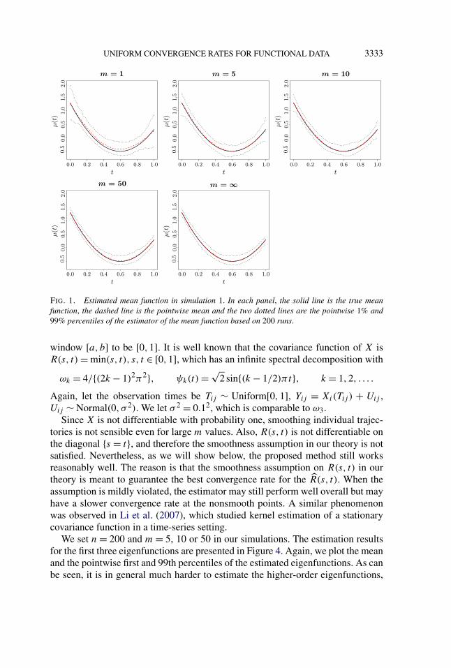
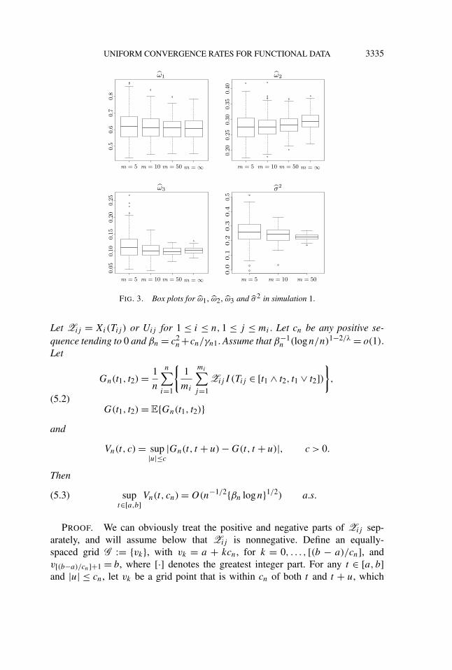
The estimation results for μ(·) are summarized in Figure 1, where we plot themean and the pointwise first and 99th percentiles of the estimator. To comparewith standard nonparametric regression, we also provide the estimation results forμ when m = 1; note that in this case the covariance function is not estimablesince there is no within-curve information. As can be seen, the estimation resultfor m = 1 is not very different from that of m = 5, reconfirming the nonparametricconvergence rate of μ for sparse functional data. It is somewhat difficult to describethe estimation results of the covariance function directly. Instead, we summarizethe results on ψk(·) and ωk in Figure 2, where we plot the mean and the pointwisefirst and 99th percentiles of the estimated eigenfunctions. In Figure 3, we also showthe empirical distributions of ωk and σ 2. In all of the scenarios, the performanceof the estimators improve with m; by m = 50, all of the the estimators performalmost as well as those for m = ∞.

4.2. Simulation 2. To illustrate that the proposed methods are applicable evento the cases that the trajectory of X is not smooth, we now present a secondsimulation study where X is standard Brownian motion. Again, we set the time


FIG. 1. Estimated mean function in simulation 1. In each panel, the solid line is the true meanfunction, the dashed line is the pointwise mean and the two dotted lines are the pointwise 1% and99% percentiles of the estimator of the mean function based on 200 runs.

window [a, b] to be [0,1]. It is well known that the covariance function of X isR(s, t) = min(s, t), s, t ∈ [0,1], which has an infinite spectral decomposition with

ωk = 4/{(2k − 1)2π2}, ψk(t) = √2 sin{(k − 1/2)πt}, k = 1,2, . . . .

Again, let the observation times be Tij ∼ Uniform[0,1], Yij = Xi(Tij ) + Uij ,Uij ∼ Normal(0, σ 2). We let σ 2 = 0.12, which is comparable to ω3.

Since X is not differentiable with probability one, smoothing individual trajec-tories is not sensible even for large m values. Also, R(s, t) is not differentiable onthe diagonal {s = t}, and therefore the smoothness assumption in our theory is notsatisfied. Nevertheless, as we will show below, the proposed method still worksreasonably well. The reason is that the smoothness assumption on R(s, t) in ourtheory is meant to guarantee the best convergence rate for the R(s, t). When theassumption is mildly violated, the estimator may still perform well overall but mayhave a slower convergence rate at the nonsmooth points. A similar phenomenonwas observed in Li et al. (2007), which studied kernel estimation of a stationarycovariance function in a time-series setting.

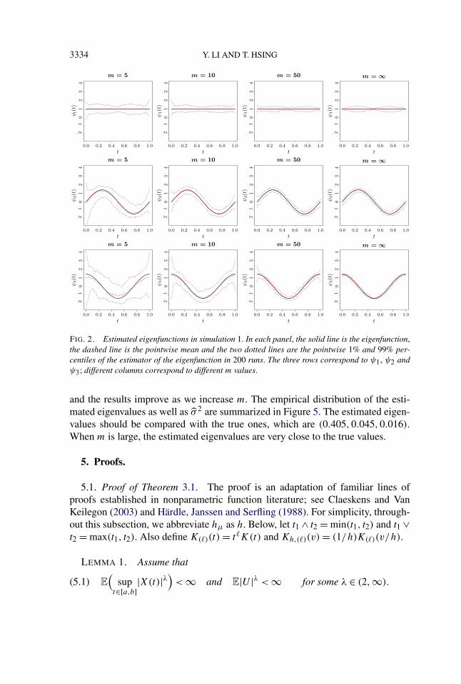
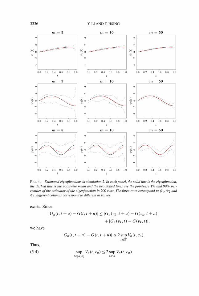
We set n = 200 and m = 5, 10 or 50 in our simulations. The estimation resultsfor the first three eigenfunctions are presented in Figure 4. Again, we plot the meanand the pointwise first and 99th percentiles of the estimated eigenfunctions. As canbe seen, it is in general much harder to estimate the higher-order eigenfunctions,


FIG. 2. Estimated eigenfunctions in simulation 1. In each panel, the solid line is the eigenfunction,the dashed line is the pointwise mean and the two dotted lines are the pointwise 1% and 99% per-centiles of the estimator of the eigenfunction in 200 runs. The three rows correspond to ψ1, ψ2 andψ3; different columns correspond to different m values.

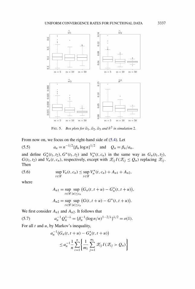
and the results improve as we increase m. The empirical distribution of the esti-mated eigenvalues as well as σ 2 are summarized in Figure 5. The estimated eigen-values should be compared with the true ones, which are (0.405,0.045,0.016).When m is large, the estimated eigenvalues are very close to the true values.

5. Proofs.

5.1. Proof of Theorem 3.1. The proof is an adaptation of familiar lines ofproofs established in nonparametric function literature; see Claeskens and VanKeilegon (2003) and Härdle, Janssen and Serfling (1988). For simplicity, through-out this subsection, we abbreviate hμ as h. Below, let t1 ∧ t2 = min(t1, t2) and t1 ∨t2 = max(t1, t2). Also define K(�)(t) = t�K(t) and Kh,(�)(v) = (1/h)K(�)(v/h).

LEMMA 1. Assume that

E

(sup

t∈[a,b]|X(t)|λ

)< ∞ and E|U |λ < ∞ for some λ ∈ (2,∞).(5.1)


FIG. 3. Box plots for ω1, ω2, ω3 and σ 2 in simulation 1.

Let Zij = Xi(Tij ) or Uij for 1 ≤ i ≤ n,1 ≤ j ≤ mi . Let cn be any positive se-quence tending to 0 and βn = c2

n+cn/γn1. Assume that β−1n (logn/n)1−2/λ = o(1).

Let

Gn(t1, t2) = 1

n

n∑i=1

{1

mi

mi∑j=1

Zij I (Tij ∈ [t1 ∧ t2, t1 ∨ t2])},

(5.2)G(t1, t2) = E{Gn(t1, t2)}

and

Vn(t, c) = sup|u|≤c

|Gn(t, t + u) − G(t, t + u)|, c > 0.

Then

supt∈[a,b]

Vn(t, cn) = O(n−1/2{βn logn}1/2) a.s.(5.3)

PROOF. We can obviously treat the positive and negative parts of Zij sep-arately, and will assume below that Zij is nonnegative. Define an equally-spaced grid G := {vk}, with vk = a + kcn, for k = 0, . . . , [(b − a)/cn], andv[(b−a)/cn]+1 = b, where [·] denotes the greatest integer part. For any t ∈ [a, b]and |u| ≤ cn, let vk be a grid point that is within cn of both t and t + u, which


FIG. 4. Estimated eigenfunctions in simulation 2. In each panel, the solid line is the eigenfunction,the dashed line is the pointwise mean and the two dotted lines are the pointwise 1% and 99% per-centiles of the estimator of the eigenfunction in 200 runs. The three rows correspond to ψ1, ψ2 andψ3; different columns correspond to different m values.

exists. Since

|Gn(t, t + u) − G(t, t + u)| ≤ |Gn(vk, t + u) − G(vk, t + u)|+ |Gn(vk, t) − G(vk, t)|,

we have

|Gn(t, t + u) − G(t, t + u)| ≤ 2 supt∈G

Vn(t, cn).

Thus,

supt∈[a,b]

Vn(t, cn) ≤ 2 supt∈G

Vn(t, cn).(5.4)


FIG. 5. Box plots for ω1, ω2, ω3 and σ 2 in simulation 2.

From now on, we focus on the right-hand side of (5.4). Let

an = n−1/2{βn logn}1/2 and Qn = βn/an,(5.5)

and define G∗n(t1, t2),G

∗(t1, t2) and V ∗n (t, cn) in the same way as Gn(t1, t2),

G(t1, t2) and Vn(t, cn), respectively, except with Zij I (Zij ≤ Qn) replacing Zij .Then

supt∈G

Vn(t, cn) ≤ supt∈G

V ∗n (t, cn) + An1 + An2,(5.6)

where

An1 = supt∈G

sup|u|≤cn

(Gn(t, t + u) − G∗

n(t, t + u)),

An2 = supt∈G

sup|u|≤cn

(G(t, t + u) − G∗(t, t + u)

).

We first consider An1 and An2. It follows that

a−1n Q1−λ

n = {β−1n (logn/n)1−2/λ}λ/2 = o(1).(5.7)

For all t and u, by Markov’s inequality,

a−1n

(Gn(t, t + u) − G∗

n(t, t + u))

≤ a−1n

1

n

n∑i=1

{1

mi

mi∑j=1

Zij I (Zij > Qn)

}


≤ a−1n Q1−λ

n

1

n

n∑i=1

{1

mi

mi∑j=1

Z λij I (Zij > Qn)

}

≤ a−1n Q1−λ

n

1

n

n∑i=1

{1

mi

mi∑j=1

Z λij

}.

Consider the case Zij = Xi(Tij ), the other case being simpler. It follows that

1

mi

mi∑j=1

Z λij ≤ Wi where Wi = sup

t∈[a,b]|Xi(t)|λ.

Thus,

a−1n

(Gn(t, t + u) − G∗

n(t, t + u)) ≤ a−1

n Q1−λn

1

n

n∑i=1

Wi.(5.8)

By the SLLN, n−1 ∑ni=1 Wi

a.s.−→ E(supt∈[a,b] |X(t)|λ) < ∞. By (5.7) and (5.8),

a−1n An1

a.s.−→ 0. By (5.7) and (5.8) again, a−1n An2 = 0, and so we have proved

limn→∞(An1 + An2) = o(an) a.s.(5.9)

To bound V ∗n (t, cn) for a fixed t ∈ G , we perform a further partition. Define

wn = [Qncn/an + 1] and ur = rcn/wn, for r = −wn,−wn + 1, . . . ,wn. Note thatG∗

n(t, t + u) is monotone in |u| since Zij ≥ 0. Suppose that 0 ≤ ur ≤ u ≤ ur+1.Then

G∗n(t, t + ur) − G∗(t, t + ur) + G∗(t, t + ur) − G∗(t, t + ur+1)

≤ G∗n(t, t + u) − G∗(t, t + u)

≤ G∗n(t, t + ur+1) − G∗(t, t + ur+1) + G∗(t, t + ur+1) − G∗(t, t + ur),

from which we conclude that

|G∗n(t, t + u) − G∗(t, t + u)| ≤ max(ξnr , ξn,r+1) + G∗(t + ur, t + ur+1),

where

ξnr = |G∗n(t, t + ur) − G∗(t, t + ur)|.

The same holds if ur ≤ u ≤ ur+1 ≤ 0. Thus,

V ∗n (t, cn) ≤ max−wn≤r≤wn

ξnr + max−wn≤r≤wn

G∗(t + ur, t + ur+1).

For all r ,

G∗(t + ur, t + ur+1) ≤ QnP(t + ur ≤ T ≤ t + ur+1)

≤ MT Qn(ur+1 − ur) ≤ MT an.


Therefore, for any B ,

P{V ∗n (t, cn) ≥ Ban} ≤ P

{max−wn≤r≤wn

ξnr ≥ (B − MT )an

}.(5.10)

Now let Zi = m−1i

∑mi

j=1 Zij I (Zij ≤ Qn)I (Tij ∈ (t, t + ur ]) so that ξnr = | 1n

×∑ni=1{Zi − E(Zi)}|. We have |Zi − E(Zi)| ≤ Qn, and

n∑i=1

var(Zi) ≤n∑

i=1

EZ2i ≤ M

n∑i=1

(c2n + cn/mi) ≤ Mnβn

for some finite M . By Bernstein’s inequality,

P{ξnr ≥ (B − MT )an} ≤ exp{− (B − MT )2n2a2

n

2∑n

i=1 var(Zi) + (2/3)(B − MT )Qnnan

}

≤ exp{− (B − MT )2n2a2

n

2Mnβn + (2/3)(B − MT )nβn

}≤ n−B∗

,

where B∗ = (B−MT )2

2M+(2/3)(B−MT ). By (5.10) and Boole’s inequality,

P

{supt∈G

V ∗n (t, cn) ≥ Ban

}≤

([b − a

cn

]+1

)(2[Qncn

an

+1]+1

)n−B∗ ≤ C

Qn

an

n−B∗

for some finite C. Now Qn/an = βn/a2n = n/ logn. So P{V ∗

n (t, cn) ≥ Ban} is sum-mable in n if we select B large enough such that B∗ > 2. By the Borel–Cantellilemma,

supt∈G

V ∗n (t, cn) = O(an) a.s.(5.11)

Hence, (5.3) follows from combining (5.4), (5.6), (5.9) and (5.11). �

LEMMA 2. Let Zij be as in Lemma 1 and assume that (5.1) holds. Leth = hn be a bandwidth and let βn = h2 + h/γn1. Assume that h → 0 andβ−1

n (logn/n)1−2/λ = o(1) For any nonnegative integer p, let

Dp,n(t) = 1

n

n∑i=1

[1

mi

mi∑j=1

Kh,(p)(Tij − t)Zij

].

Then we have

supt∈[a,b]

√nh2/(βn logn)|Dp,n(t) − E{Dp,n(t)}| = O(1) a.s.

PROOF. Since both K and tp are bounded variations, K(p) is also a boundedvariation. Thus, we can write K(p) = K(p),1 − K(p),2 where K(p),1 and K(p),2 areboth increasing functions; without loss of generality, assume that K(p),1(−1) =


K(p),2(−1) = 0. Below, we apply Lemma 1 by letting cn = 2h. It is clear that theassumptions of Lemma 1 hold here. Write

Dn(t) = 1

n

n∑i=1

{1

mi

mi∑j=1

Kh,(p)(Tij − t)Zij

}

= 1

n

n∑i=1

{1

mi

mi∑j=1

Zij I (−h ≤ Tij − t ≤ h)

∫ Tij−t

−hdKh,(p)(v)

}

=∫ h

−h

1

n

n∑i=1

{1

mi

mi∑j=1

Zij I (v ≤ Tij − t ≤ h)

}dKh,(p)(v)

=∫ h

−hGn(t + v, t + h)dKh,(p)(v),

where Gn is as defined in (5.2). We have

supt∈[a,b]

|Dp,n(t) − E{Dp,n(t)}|

≤ supt∈[a,b]

Vn(t,2h)

∫ h

−h

∣∣dKh,(p)

∣∣(5.12)

≤ {K(p),1(1) + K(p),2(1)

}h−1 sup

t∈[a,b]Vn(t,2h),

and the conclusion of the lemma follows from Lemma 1. �

PROOF OF THEOREM 3.1. Define

R∗r = Rr − μ(t)Sr − hμ(1)(t)Sr+1.

By straightforward calculations, we have

μ(t) − μ(t) = R∗0S2 − R∗

1S1

S0S2 − S21

,(5.13)

where S0, S1, S2 are defined as in (2.1). Write

R∗r = 1

n

∑i

[1

mi

mi∑j=1

Kh(Tij − t){(Tij − t)/h}r{Yij − μ(t) − μ(1)(t)(Tij − t)}]

= 1

n

∑i

[1

mi

mi∑j=1

Kh(Tij − t){(Tij − t)/h}r

× {εij + μ(Tij ) − μ(t) − μ(1)(t)(Tij − t)

}].


By Taylor’s expansion and Lemma 2, uniformly in t ,

R∗r = 1

n

∑i

1

mi

∑j

Kh(Tij − t){(Tij − t)/h}rεij + O(h2),(5.14)

and it follows from Lemma 2 that

R∗i = O

(h2 + δn1(h)

)a.s.(5.15)

Now, at any interior point t ∈ [a + h,b − h], since f has a bounded derivative,

E{S0} =∫ 1

−1K(v)f (t + hv)dv = f (t) + O(h),

E{S1} = O(h), E{S2} = f (t)ν2 + O(h),

where ν2 = ∫v2K(v)dv. By Lemma 2, we conclude that, uniformly for t ∈ [a +

h,b − h],S0 = f (t) + O

(h + δn1(h)

), S1 = O

(h + δn1(h)

),

(5.16)S2 = f (t)ν2 + O

(h + δn1(h)

).

Thus, the rate in the theorem is established by applying (5.13). The same rate canalso be similarly seen to hold for boundary points. �

5.2. Proofs of Theorems 3.3 and 3.4.

LEMMA 3. Assume that

E

(sup

t∈[a,b]|X(t)|2λ

)< ∞ and E|U |2λ < ∞ for some λ ∈ (2,∞).(5.17)

Let Zijk be X(Tij )X(Tik), X(Tij )Uik or UijUik . Let cn be any positive sequencetending to 0 and βn = c4

n + c3n/γn1 + c2

n/γn2. Assume that β−1n (logn/n)1−2/λ =

o(1). Let

Gn(s1, t1, s2, t2)

= 1

n

n∑i=1

{1

Ni

∑k �=j

ZijkI (Tij ∈ [s1 ∧ s2, s1 ∨ s2],(5.18)

Tik ∈ [t1 ∧ t2, t1 ∨ t2])},

G(s1, t1, s2, t2) = E{Gn(s1, t1, s2, t2)} and

Vn(s, t, δ) = sup|u1|,|u2|≤δ

|Gn(s, t, s + u1, t + u2) − G(s, t, s + u1, t + u2)|.

Then

sups,t∈[a,b]

Vn(s, t, cn) = O(n−1/2{βn logn}1/2) a.s.


PROOF. The proof is similar to that of Lemma 1, and so we only outline themain differences. Let an,Qn be as in (5.5). Let G be a two-dimensional grid on[a, b]2 with mesh cn, that is, G = {(vk1, vk2)} where vk is defined as in the proofof Lemma 1. Then we have

sups,t∈[a,b]

Vn(s, t, cn) ≤ 4 sup(s,t)∈G

Vn(s, t, cn).(5.19)

Define G∗n(s1, t1, s2, t2),G

∗(s1, t1, s2, t2) and V ∗n (s, t, δ) in the same way as

Gn(s1, t1, s2, t2), G(s1, t1, s2, t2) and Vn(s, t, δ) except with ZijkI (Zijk ≤ Qn)

replacing Zijk . Then

sup(s,t)∈G

Vn(s, t, cn) ≤ sup(s,t)∈G

V ∗n (s, t, cn) + An1 + An2,(5.20)

where

An1 = sup(s,t)∈G

sup|u1|,|u2|≤cn

|Gn(s, t, s + u1, t + u2) − G∗n(s, t, s + u1, t + u2)|,

An2 = sup(s,t)∈G

sup|u1|,|u2|≤cn

|G(s, t, s + u1, t + u2) − G∗(s, t, s + u1, t + u2)|.

Using the technique similar to that in the proof of Lemma 1, we can show An1and An2 is o(an) almost surely. To bound V ∗

n (s, t, cn) for fixed (s, t), we createa further partition. Put wn = [Qncn/an + 1] and ur = rcn/wn, r = −wn, . . . ,wn.Then

V ∗n (s, t, cn) ≤ max−wn≤r1,r2≤wn

ξn,r1,r2

+ max−wn≤r1,r2≤wn

{G∗(s, t, s + ur1+1, t + ur2+1)

− G∗(s, t, s + ur1, t + ur2)},where

ξn,r1,r2 = |G∗n(s, t, s + ur1, t + ur2) − G∗(s, t, s + ur1, t + ur2)|.

It is easy to see that var(ξn,r1,r2) ≤ Mnβn for some finite M , and the rest of theproof completely mirrors that of Lemma 1 and is omitted. �

LEMMA 4. Let Zijk be as in Lemma 3 and assume that (5.17) holds. Leth = hn be a bandwidth and let βn = h4 + h3/γn1 + h2/γn2. Assume that h → 0and β−1

n (logn/n)1−2/λ = o(1). For any nonnegative integers p,q , let

Dp,q,n(s, t) = 1

n

n∑i=1

[1

Nj

∑k �=j

ZijkKh,(p)(Tij − s)Kh,(q)(Tik − t)

].

Then, for any p,q ,

sups,t∈[a,b]

√nh4/(βn logn)|Dp,q,n(s, t) − E{Dp,q,n(s, t)}| = O(1) a.s.


PROOF. Write

Dp,q,n(s, t)

=n∑

i=1

[1

Ni

∑k �=j

ZijkI (Tij ≤ s + h)I (Tik ≤ t + h)

× Kh,(p)(Tij − s)Kh,(q)(Tik − t)

]

=∫ ∫

(u,v)∈[−h,h]2

1

n

n∑i=1

[1

Ni

∑k �=j

Zijk

× I (Tij ∈ [s + u, s + h])

× I (Tik ∈ [t + v, t + h])]dKh,(p)(u) dKh,(q)(v)

=∫ ∫

(u,v)∈[−h,h]2Gn(s + u, t + v, s + h, t + h)dKh,(p)(u)dKh,(q)(v),

where Gn is as in (5.18). Now,

sup(s,t)∈[a,b]2

|Dp,q,n(s, t) − E{Dp,q,n(s, t)}|

≤ sups,t∈[a,b]

Vn(s, t,2h)

∫ ∫(u,v)∈[−h,h]2

∣∣d{Kh,(p)(u)

}∣∣∣∣d{Kh,(q)(v)

}∣∣= O[{βn logn/(nh4)}1/2] a.s.

by Lemma 3, using the same argument as in (5.12). �

PROOF OF THEOREM 3.3. Let Spq,Rpq,Ai and B be defined as in (2.3).Also, for p,q ≥ 0, define

R∗pq = Rpq − C(s, t)Spq − hRC(1,0)(s, t)Sp+1,q − hRC(0,1)(s, t)Sp,q+1.

By straightforward algebra, we have

(C − C)(s, t) = (A1R∗00 − A2R

∗10 − A3R

∗01)B

−1.(5.21)

By standard calculations, we have the following rates uniformly on [a + hR,b −hR]2:

E(S00) = f (s)f (t) + O(hR), E(S01) = O(hR),

E(S10) = O(hR), E(S02) = f (s)f (t)ν2 + O(hR),

E(S20) = f (s)f (t)ν2 + O(hR), E(S11) = O(hR).


By these and Lemma 4, we have the following almost sure uniform rates:

A1 = f 2(s)f 2(t)ν22 + O

(hR + δn2(hR)

),

A2 = O(hR + δn2(hR)

),

(5.22)A3 = O

(hR + δn2(hR)

),

B = f 3(s)f 3(t)ν22 + O

(hR + δn2(hR)

).

To analyze the behavior of the components of (5.21), it suffices now to analyzeR∗

pq . Write

R∗00 = 1

n

n∑i=1

[1

Ni

∑k �=j

{YijYik − C(s, t)

− C(1,0)(s, t)(Tij − s)

− C(0,1)(s, t)(Tik − t)} × KhR

(Tij − s)KhR(Tik − t)

].

Let ε∗ijk = YijYik − C(Tij , Tik). By Taylor’s expansion,

YijYik − C(s, t) − C(1,0)(s, t)(Tij − s) − C(0,1)(s, t)(Tik − t)

= YijYik − C(s, t) − C(Tij , Tik) + C(Tij , Tik)

− C(1,0)(s, t)(Tij − s) − C(0,1)(s, t)(Tik − t)

= ε∗ijk + O(h2

R) a.s.

It follows that

R∗00 = 1

n

n∑i=1

1

Ni

∑k �=j

ε∗ijkKhR

(Tij − s)KhR(Tik − t) + O(h2

R).(5.23)

Applying Lemma 4, we obtain, uniformly in s, t ,

R∗00 = O

(δn2(hR) + h2

R

)a.s.(5.24)

By (5.22),

A1B−1 = [f (s)f (t)]−1 + O

(hR + δn2(hR)

).(5.25)

Thus, R∗00A1B−1 = O(δn2(hR)+h2

R) a.s. Similar derivations show that R∗10A2 ×

B−1 and R∗01A3B−1 are both of lower order. Thus, the rate in (3.3) is obtained

for s, t ∈ [a + hR,b − hR]. As for s and/or t in [a, a + h) ∪ (b − h,b], similarcalculations show that the same rate also holds. The result follows by taking intoaccount of the rate of μ. �


PROOF OF THEOREM 3.4. Note that

σ 2 − σ 2 = 1

b − a

∫ b

a{V (t) − V (t)}dt − 1

b − a

∫ b

a{C(t, t) − C(t, t)}dt.

To consider V (t) − V (t) we follow the development in the proof of Theorem 3.1.Recall (2.4) and let Q∗

r = Qr − V (t)Sr − hV (1)(t)Sr+1. Then, as in (5.13), weobtain

V (t) − V (t) = Q∗0S2 − Q∗

1S1

S0S2 − S21

.

Write

Q∗r = 1

n

n∑i=1

1

mi

mi∑j=1

KhV(Tij − t){(Tij − t)/hV }r{Y 2

ij − V (t) − V (1)(t)(Tij − t)}

= 1

n

n∑i=1

1

mi

mi∑j=1

KhV(Tij − t){(Tij − t)/h}r{Y 2

ij − V (Tij )} + O(h2V ),

which, by Lemma 1, has the uniformly rate O(h2V + δn1(hV )) a.s. By (5.16), we

have

V (t) − V (t) = 1

f (t)n

∑i

1

mi

mi∑j=1

Kh(Tij − t){Y 2ij − V (Tij )}

+ O(h2

V + δ2n1(hV )

)a.s.

Thus,∫ b

a{V (t) − V (t)}dt = 1

n

n∑i=1

1

mi

mi∑j=1

{Y 2ij − V (Tij )}

∫ b

aKhV

(Tij − t)f −1(t) dt

+ O(h2

V + δ2n1(hV )

)a.s.

Note that ∣∣∣∣∫ b

aKhV

(Tij − t)f −1(t) dt

∣∣∣∣ ≤ supt

f −1(t).

By Lemma 5 below in this subsection,∫ b

a{V (t) − V (t)}dt = O

((logn/n)1/2 + h2

V + δ2n1(hV )

)a.s.(5.26)

Next, we consider C(t, t) − C(t, t). We apply (5.21) but will focus onR∗

00A1B−1 since the other two terms are dealt with similarly. By (5.23)–(5.25),

R∗00A1B

−1 = 1

f (s)f (t)n

n∑i=1

1

Ni

∑k �=j

ε∗ijkKhR


(5.27)+ O

(h2

R + δ2n2(hR)

)a.s.


Thus, ∫ b

a{C(t, t) − C(t, t)}dt

= 1

n

n∑i=1

1

Ni

∑k �=j

ε∗ijk

∫ b

aKhR

(Tij − t)KhR(Tik − t)f −2(t) dt

+ O(h2

R + δ2n2(hR)

)a.s.

Write ∫ b

aKhR

(Tij − t)KhR(Tik − t)f −2(t) dt

=∫ 1

−1K(u)KhR

((Tik − Tij ) + uhR

)f −2(Tij − uhR)du.

A slightly modified version of Lemma 1 leads to the “one-dimensional” rate:

supu∈[0,1]

∣∣∣∣∣1

n

n∑i=1

1

Ni

∑k �=j

ε∗ijkKhR

((Tik − Tij ) + uhR

)f −2(Tij − uhR)

∣∣∣∣∣= O(δn1(hR)) a.s.

It follows that∫ b

a{C(t, t) − C(t, t)}dt = O

(h2

R + δn1(hR) + δ2n2(hR)

)a.s.(5.28)

The theorem follows from (5.26) and (5.28). �

LEMMA 5. Assume that ξni,1 ≤ i ≤ n, are independent random variableswith mean zero and finite variance. Also assume that there exist i.i.d. random vari-ables ξi with mean zero and finite δth moment for some δ > 2 such that |ξni | ≤ |ξi |.Then

1

n

n∑i=1

ξni = O((logn/n)1/2)

a.s.

PROOF. Let an = (logn/n)1/2. Assume that ξni ≥ 0. Write

ξni = ξni� + ξni≺ := ξniI (|ξni | > a−1n ) + ξniI (|ξni | ≤ a−1

n ).

Then∣∣∣∣∣ 1

ann

n∑i=1

ξni�∣∣∣∣∣ ≤ 1

ann

n∑i=1

|ξni�|δ|ξni�|1−δ ≤ aδ−2n

1

n

n∑i=1

|ξi |δ → 0 a.s.


by the law of large numbers. The mean of the left-hand side is also tending tozero by the same argument. Thus, n−1 ∑n

i=1(ξni� − E{ξni�}) = o(an). Next, byBernstein’s inequality,

P

(1

n

n∑i=1

(ξni≺ − E{ξni≺}) > Ban

)≤ exp

{− B2n2a2

n

2nσ 2 + (2/3)Bn

}

= exp{− B2 logn

2σ 2 + (2/3)B

},

which is summable for large enough B . The result follows from the Borel–Cantellilemma. �

5.3. Proof of Theorem 3.6. Let � be the integral operator with kernel R − R.

LEMMA 6. For any bounded measurable function ψ on [a, b],sup

t∈[a,b]|(�ψ)(t)| = O

(h2

μ + δn1(hμ) + h2R + δn1(hR) + δ2

n2(hR))

a.s.

PROOF. It follows that

(�ψ)(t) =∫ b

s=a(C − C)(s, t)ψ(s) ds −

∫ b

s=a{μ(s)μ(t) − μ(s)μ(t)}ψ(s) ds

=: An1 − An2.

By (5.21),

An1 =∫ b

s=a(A1R

∗00 − A2R

∗10 − A3R

∗01)B

−1ψ(s) ds.

We focus on∫ bs=a A1R

∗00B

−1ψ(s) ds since the other two terms are of lower orderand can be dealt with similarly. By (5.23) and (5.25),∫ b

s=aA1R

∗00B

−1ψ(s) ds

= 1

f (t)n

n∑i=1

1

Ni

∑k �=j

ε∗ijkKhR

(Tik − t)

∫ b

s=aKhR

(Tij − s)ψ(s)f (s)−1 ds

+ O(h2

R + δ2n2(hR)

).

Note that∣∣∣∣∫ b

s=aKhR


∣∣∣∣ ≤ sups∈[a,b]

(|ψ(s)|f (s)−1)

∫ 1

u=−1K(u)du.


Thus, Lemma 1 can be easily improvised to give the following uniform rate over t :

1

f (t)n

n∑i=1

1

Ni

∑k �=j

ε∗ijkKhR

(Tik − t)

∫ b

s=aKhR


= O(δn1(hR)) a.s.

Thus, ∫ b

s=aA1R

∗00B

−1ψ(s) ds = O(δn1(hR) + h2

R + δ2n2(hR)

)a.s.,

which is also the rate of An1. Next, we write

An2 = μ(t)

∫ b

s=a{μ(s) − μ(s)}ψ(s) ds − {μ(t) − μ(t)}

∫ b

s=aμ(s)ψ(s) ds,

which has the rate O(h2μ + δn1(hμ)) by Theorem 3.1. �

PROOF OF THEOREM 3.6. We prove (b) first. Hall and Hosseini-Nasab (2006)give the L2 expansion

ψj − ψj = ∑k �=j

(λj − λk)−1〈�ψj,ψk〉φk + O(‖�‖2),

where ‖�‖ = (∫∫ {R(s, t) − R(s, t)}2 ds dt)1/2, the Hilbert–Schmidt norm of �.

By Bessel’s inequality, this leads to

‖ψj − ψj‖ ≤ C(‖�ψj‖ + ‖�‖2).

By Lemma 6 and Theorem 3.3,

‖�ψj‖ = O(h2

μ + δn1(hμ) + h2R + δn1(hR) + δ2

n2(hR)),

‖�‖2 = O(h4

μ + δ2n1(hμ) + h4

R + δ2n2(hR)

)a.s.

Thus,

‖ψj − ψj‖ = O(h2

μ + δn1(hμ) + h2R + δn1(hR) + δ2

n2(hR))

a.s.,

proving (b).Next, we consider (a). By (4.9) in Hall, Müller and Wang (2006),

ωj − ωj =∫ ∫

(R − R)(s, t)ψj (s)ψj (t) ds dt + O(‖�ψj‖2)

=∫ ∫

(C − C)(s, t)ψj (s)ψj (t) ds dt

−∫ ∫

{μ(s)μ(t) − μ(s)μ(t)}ψj(s)ψj (t) ds dt + O(‖�ψj‖2)

=: An1 − An2 + O(‖�ψj‖2).


Now,

An1 =∫ ∫

(A1R∗00 − A2R

∗10 − A3R

∗01)B

−1ψj(s)ψj (t) ds dt.

Again it suffices to focus on∫∫

A1R∗00B

−1ψj(s)ψj (t) ds dt . By (5.23) and (5.25),∫ ∫A1R

∗00B

−1ψj(s)ψj (t) ds dt

= 1

n

n∑i=1

1

mi(mi − 1)

∑k �=j

ε∗ijk

∫ ∫KhR


× ψj(s)ψj (t){f (s)f (t)}−1 ds dt

+ O(h2

R + δ2n2(hR)

)a.s.,

where the first term on the right-hand side can be shown to be O((log /n)1/2) a.s.by Lemma 5. Thus,

An1 = O((log/n)1/2 + h2

R + δ2n2(hR)

).

Next, write

An2 =∫

{μ(s) − μ(s)}ψj(s) ds

∫μ(t)ψj (t) dt

+∫

μ(s)ψj (s) ds

∫{μ(t) − μ(t)}ψj(t) dt,

and it can be similarly shown that

An2 = O((log/n)1/2 + h2

μ + δ2n1(hμ)

)a.s.

This establishes (a).Finally, we consider (c). For any t ∈ [a, b],

ωj ψj (t) − ωjψj (t)

=∫

R(s, t)ψj (s) ds −∫

R(s, t)ψj (s) ds

=∫

{R(s, t) − R(s, t)}ψj(s) ds +∫

R(s, t){ψj (s) − ψj(s)}ds.

By the Cauchy–Schwarz inequality, uniformly for all t ∈ [a, b],∣∣∣∣∫ R(s, t){ψj (s) − ψj(s)}ds

∣∣∣∣ ≤{∫

R2(s, t) ds

}1/2

‖ψj − ψj‖

≤ |b − a|1/2 sups,t

|R(s, t)| × ‖ψj − ψj‖

= O(‖ψj − ψj‖) a.s.


Thus,

ωj ψj (t) − ωjψj (t) = O(h2

μ + δn1(hμ) + h2R + δn1(hR) + δ2

n2(hR))

a.s.

By the triangle inequality and (b),

ωj |ψj (t) − ψj(t)|= |ωj ψj (t) − ωjψj (t) − (ωj − ωj )ψj (t)|≤ |ωj ψj (t) − ωjψj (t)| + |ωj − ωj | sup

t|ψj (t)|

= O((logn/n)1/2 + h2

μ + δn1(hμ) + h2R + δn1(hR) + δ2

n2(hR))

a.s.

Note that (logn/n)1/2 = o(δn1(hμ)). This completes the proof of (c). �

Acknowledgments. We are very grateful to the Associate Editor and two ref-erees for their helpful comments and suggestions.

REFERENCES

BICKEL, P. J. and ROSENBLATT, M. (1973). On some global measures of the deviations of densityfunction estimates. Ann. Statist. 1 1071–1095. MR0348906

CLAESKENS, G. and VAN KEILEGOM, I. (2003). Bootstrap confidence bands for regression curvesand their derivatives. Ann. Statist. 31 1852–1884. MR2036392

FAN, J. and GIJBELS, I. (1995). Local Polynomial Modelling and Its Applications. Chapman andHall, New York. MR1383587

FERRÉ, L. and YAO, A. (2005). Smoothed functional sliced inverse regression. Statist. Sinica 15665–685.

HALL, P. and HOSSEINI-NASAB, M. (2006). On properties of functional principal componentsanalysis. J. R. Stat. Soc. Ser. B Stat. Methodol. 68 109–126. MR2212577

HALL, P., MÜLLER, H.-G. and WANG, J.-L. (2006). Properties of principal component methodsfor functional and longitudinal data analysis. Ann. Statist. 34 1493–1517. MR2278365

HÄRDLE, W. (1989). Asymptotic maximal deviation of M-smoothers. J. Multivariate Anal. 29 163–179. MR1004333

HÄRDLE, W., JANSSEN, P. and SERFLING, R. (1988). Strong uniform consistency rates for estima-tors of conditional functionals. Ann. Statist. 16 1428–1449. MR0964932

JAMES, G. M., HASTIE, T. J. and SUGAR, C. A. (2000). Principal component models for sparsefunctional data. Biometrika 87 587–602. MR1789811

LANDAU, H. J. and SHEPP, L. A. (1970). On the supremum of Gaussian processes. Sankhya Ser. A32 369–378. MR0286167

LI, Y. and HSING, T. (2010). Deciding the dimension of effective dimension reduction space forfunctional and high-dimensional data. Ann. Statist. To appear.

LI, E., LI, Y., WANG, N.-Y. and WANG, N. (2008). Functional latent feature models for data withlongitudinal covariate processes. Unpublished manuscript, Dept. Statistics, Texas A&M Univ.,College Station, TX.

LI, Y., WANG, N., HONG, M., TURNER, N., LUPTON, J. and CARROLL, R. J. (2007). Nonpara-metric estimation of correlation functions in spatial and longitudinal data, with application tocolon carcinogenesis experiments. Ann. Statist. 35 1608–1643. MR2351099

LIN, X. and CARROLL, R. J. (2000). Nonparametric function estimation for clustered data when thepredictor is measured without/with error. J. Amer. Statist. Assoc. 95 520–534. MR1803170

http://www.ams.org/mathscinet-getitem?mr=0348906












MASRY, E. (1996). Multivariate local polynomial regression for time series: Uniform strong consis-tency and rates. J. Time Ser. Anal. 17 571–599. MR1424907

MÜLLER, H.-G. and STADTMÜLLER, U. (2005). Generalized functional linear models. Ann. Statist.33 774–805. MR2163159

RAMSAY, J. O. and SILVERMAN, B. W. (2005). Functional Data Analysis, 2nd ed. Springer, NewYork. MR2168993

WANG, N. (2003). Marginal nonparametric kernel regression accounting for within-subject correla-tion. Biometrika 90 43–52. MR1966549

YAO, F. and LEE, T. C. M. (2006). Penalized spline models for functional principal componentanalysis. J. Roy. Statist. Soc. Ser. B 68 3–25.

YAO, F., MÜLLER, H.-G. and WANG, J.-L. (2005a). Functional data analysis for sparse longitudinaldata. J. Amer. Statist. Assoc. 100 577–590. MR2160561

YAO, F., MÜLLER, H.-G. and WANG, J.-L. (2005b). Functional linear regression analysis for lon-gitudinal data. Ann. Statist. 33 2873–2903. MR2253106

ZHANG, J.-T. and CHEN, J. (2007). Statistical inferences for functional data. Ann. Statist. 35 1052–1079. MR2341698

ZHOU, L., HUANG, J. Z. and CARROLL, R. J. (2008). Joint modelling of paired sparse functionaldata using principal components. Biometrika 95 601–619.

DEPARTMENT OF STATISTICS

UNIVERSITY OF GEORGIA

ATHENS, GEORGIA 30602-7952USAE-MAIL: [email protected]

DEPARTMENT OF STATISTICS

UNIVERSITY OF MICHIGAN

ANN ARBOR, MICHIGAN 48109-1107USAE-MAIL: [email protected]








mailto:[email protected]

mailto:[email protected]

Uniform convergence rates for nonparametric regression and

Documents