Price Stability and Monetary Policy Effectiveness when ...

Center for Financial Studies an der Johann Wolfgang Goethe-Universität § Taunusanlage 6 § D-60329 Frankfurt am Main

Tel: (+49)069/242941-0 § Fax: (+49)069/242941-77 § E-Mail: [email protected] § Internet: http://www.ifk-cfs.de

No. 2003/13

Price Stability and Monetary Policy Effectiveness when Nominal Interest Rates

are Bounded at Zero

Günter Coenen, Athanasios Orphanides, Volker Wieland

* Correspondence: Coenen: Directorate General Research, European Central Bank, Kaiserstrasse 29, 60311 Frankfurt am Main, Germany, phone +49 69 1344-7887, E-mail: [email protected] Orphanides: Division of Monetary Affairs, Board of Governors of the Federal Reserve System, Washington, D.C. 20551, tel: (202) 452-2654, E-mail: [email protected] Wieland: Professur für Geldtheorie und -politik, Johann-Wolfgang-Goethe Universität, Mertonstrasse 17, 60325 Frankfurt am Main, Germany, phone: +49 69 798-25288, E-mail: [email protected], homepage: http://www.volkerwieland.com. † We have benefited from presentations of earlier drafts at meetings of the Econometric Society, the European Economic Association, the Society of Economic Dynamics, the System Committee Meeting on Macro-economics, the NBER, and seminars at the University of Michigan, Rutgers University, University of Frankfurt, University of Cologne, University of St.Gallen, the European Central Bank and the Canadian Department of Finance. We would also like to thank Todd Clark, Bill English, Andrew Haldane, David Lindsey, Yvan Lengwiler, Brian Madigan, Allan Meltzer, Richard Porter, John Williams and Alex Wolman for useful comments. The opinions expressed here are those of the authors and do not necessarily reflect views of the European Central Bank or the Federal Reserve Board. .

CFS Working Paper No. 2003/13

Price Stability and Monetary Policy Effectiveness when Nominal Interest Rates are Bounded at Zero*†

Günter Coenen, Athanasios Orphanides, Volker Wieland

Revised Version: March 2003

Abstract: This paper employs stochastic simulations of a small structural rational expectations model to investigate the consequences of the zero bound on nominal interest rates. We find that if the economy is subject to stochastic shocks similar in magnitude to those experienced in the U.S. over the 1980s and 1990s, the consequences of the zero bound are negligible for target inflation rates as low as 2 percent. However, the effects of the constraint are non-linear with respect to the inflation target and produce a quantitatively significant deterioration of the performance of the economy with targets between 0 and 1 percent. The variability of output increases significantly and that of inflation also rises somewhat. Also, we show that the asymmetry of the policy ineffectiveness induced by the zero bound generates a non-vertical long-run Phillips curve. Output falls increasingly short of potential with lower inflation targets. JEL Classification: E31, E52, E58, E61 Keywords: Inflation targeting, price stability, monetary policy rules, liquidity trap.

1 Introduction

There is fairly widespread consensus among macroeconomists that the primary long-term

objective of monetary policy ought to be a stable currency. Studies evaluating the costs of

inflation have long established the desirability of avoiding not only high but even moderate

inflation.1 However, there is still a serious debate on whether the optimal average rate of

inflation is low and positive, zero, or even moderately negative.2 An important issue in this

debate concerns the reduced ability to conduct effective countercyclical monetary policy

when inflation is low. As pointed out by Summers (1991), if the economy is faced with

a recession when inflation is zero, the monetary authority is constrained in its ability to

engineer a negative short-term real interest rate to damp the output loss. This constraint

reflects the fact that the nominal short-term interest rate cannot be lowered below zero—the

zero interest rate bound.3

This constraint would be of no relevance in the steady state of a non-stochastic model

economy. In an equilibrium with zero inflation, the short-term nominal interest rate would

always equal the equilibrium real rate. Stabilization of the economy in a stochastic environ-

ment, however, presupposes monetary control which leads to fluctuations in the short-run

nominal interest rate. Under these circumstances, the non-negativity constraint on nomi-

nal interest rates may occasionally be binding and so may influence the performance of the

economy. This bound is more likely to be reached, the lower the average rate of inflation and1Fischer and Modigliani (1978), Fischer (1981), and more recently Driffill et al. (1990) and Fischer (1994),

provide a detailed accounting of the costs of inflation. An early analysis of the costs of both inflation anddeflation is due to Keynes (1923).

2The important contributions by Tobin (1965) and Friedman (1969) provided arguments in favor ofinflation and deflation, respectively. But theoretical arguments alone cannot provide a resolution. Thesurvey of the monetary growth literature by Orphanides and Solow (1990) suggests that equally plausibleassumptions yield conflicting conclusions regarding the optimal rate of inflation. Similarly, recent empiricalinvestigations suggest a lack of consensus. Cross-country studies confirm the cost of high average inflation ongrowth but find no robust evidence at low levels of inflation. (See Sarel, 1996, and Clark, 1997.) Judson andOrphanides (1999) find that the volatility rather than the level of inflation may be detrimental to growth atlow levels of inflation. Feldstein (1997) identifies substantial benefits from zero inflation due to inefficienciesin the tax code. Akerlof, Dickens and Perry (1996), however, estimate large costs due to downward wagerigidities.

3The argument has its roots in Hicks’s (1937) interpretation of the Keynesian liquidity trap. Hicks (1967)identified the question regarding “the effectiveness of monetary policy in engineering recovery from a slump”as the key short-run concern arising from the trap (p. 57).

1

the greater the variability of the nominal interest rate. In this context, “inflation greases

the wheels of monetary policy,” as Fischer (1996) points out (p. 19). The experience of

the Japanese economy that has been at the zero bound over the past several years and the

uncomfortable resemblance of this experience to the U.S. economy during the 1930s serve

as evidence that the zero bound presents a challenge of significant practical importance.

The purpose of this paper is to conduct a systematic empirical evaluation of the zero

bound constraint in a stochastic environment and assess the quantitative importance of this

constraint for the performance of alternative monetary policy rules. Recent quantitative

evaluations of policy rules suggest that rules that are very effective in stabilizing output

and inflation do indeed entail substantial variability in the short-term nominal interest rate.

(See Taylor, 1999.) Most often, however, the simulated models are linear and neutral to

the average rate of inflation and abstract from the zero bound. Alternative policy rules are

then evaluated based on their performance in terms of the variability of output and inflation

they induce in such models. This approach to policy evaluation is appropriate with a high

average rate of inflation when the non-negativity constraint on nominal interest rates would

be unlikely to bind. However, since policy is not only concerned with stabilizing output and

inflation but also with maintaining a low average inflation rate, evaluation of the impact of

the zero bound on economic performance is important. To the extent that both inflation

and deflation hamper economic performance and are otherwise equally undesirable, the

zero bound constraint effectively renders the risks of deviating from an inflation rate of zero

asymmetric. As Chairman Greenspan noted recently, “... deflation can be detrimental for

reasons that go beyond those that are also associated with inflation. Nominal interest rates

are bounded at zero, hence deflation raises the possibility of potentially significant increases

in real interest rates.” (From Problems of Price Measurement, remarks at the Annual

Meeting of the American Economic Association and the American Finance Association,

Chicago, Illinois, Jan 3, 1998.)

Efforts to evaluate the quantitative importance of the zero bound have been hampered

by the nonlinearity it introduces a nonlinearity in otherwise linear models. In the context

2

of policy rule evaluations, Rotemberg and Woodford (1997, 1999) indirectly address the

constraint by penalizing policies resulting in exceedingly variable nominal interest rates.

They show that such constrained optimal policies significantly differ from the optimal rules

that ignore the constraint. A first assessment of the effect of the zero bound that explicitly

introduces this nonlinearity in a small linear model is provided by Fuhrer and Madigan

(1997). Their results, based on a set of deterministic simulations, suggest that the reduced

policy effectiveness at low inflation rates may have a modest effect on output in recessions.

In this paper we estimate a small rational expectations macroeconomic model of the U.S.

economy in which monetary policy has temporary real effects due to sluggish adjustment

in wages and prices. We then compare the stochastic properties of the economy in the

presence of the zero bound on nominal interest rates when monetary policy is set according

to an interest rate rule estimated over the 1990s but with alternative long-run inflation

targets. We find that if the economy is subject to stochastic shocks similar in magnitude

to those experienced in the U.S. over the 1980s and 1990s, the consequences of the zero

bound constraint are negligible for target inflation rates as low as 2 percent. However,

the effects of the constraint are non-linear with respect to the inflation target and become

increasingly important for determining the effectiveness of policy with inflation targets

between 0 and 1 percent. We find that economic performance deteriorates significantly

with such low inflation targets. The variability of output increases noticeably, while the

variability of inflation also rises somewhat. The stationary distribution of output is distorted

with recessions becoming somewhat more frequent and longer lasting. Moreover, in our

model the asymmetry of policy ineffectiveness induced by the zero bound generates a non-

vertical long-run Phillips curve. Output falls increasingly short of potential, on average, as

the inflation target, and therefore the average rate of inflation, becomes smaller. At zero

average inflation, the output loss is in the order of 0.1 percent of potential output.

The remainder of this paper is organized as follows. Section 2 discusses interest rate

rules and the role of money in the presence of the zero bound on nominal interest rates.

Our estimated model of the U.S. economy is presented in section 3. Section 4 assesses

3

the quantitative importance of the zero bound for stabilization policy based on stochastic

simulation results. Section 5 concludes.

2 Monetary policy, money demand and the zero bound

Under normal circumstances, that is when the short-term nominal interest rate is not con-

strained at zero, monetary policy can be broadly characterized in terms of a Taylor-style

interest rate rule. We have estimated a generalized form of such a policy rule for the United

States over the 1980:Q1 to 1999:Q4 period, a period over which the zero bound has not

constrained policy in any way (standard errors in parentheses):

it = − .0015(.0028)

+ .733(.062)

it−1 + .581(.107)

π(4)t + 1.038

(.239)

yt − .852(.223)

yt−1 + εi,t. (1)

Here, it is the short-term interest rate, π(4)t reflects the rate of change of the chain-weighted

GDP deflator over four quarters ending in quarter t and yt the output gap, based on the

Congressional Budget Office (2002) estimate of potential output.

The estimated slope parameters in this policy rule capture the pattern of stabilization

policy during the 1980s and 1990s. The estimated intercept (virtually zero) reflects the

central bank’s implicit inflation target, π∗, and equilibrium real interest rate, r∗, over this

period. In particular, the policy rule may be rewritten as:

it = (1 − .733)(r∗ + π∗) + .733 it−1 + .581 (π(4)t − π∗) + 1.038 yt − .852 yt−1 + εi,t (1′)

with the implicit relationship, 0 = (1 − .733)(r∗ + π∗) − .581π∗, connecting these concepts.

For example, the estimation suggests an implicit inflation target of 1.7 percent over this

period, assuming a value of 2 percent for r∗.

In this description of policy, the money supply is hidden in the background. As long as

the short-term interest rate is not constrained by the zero bound, the central bank can be

viewed as providing liquidity as needed to achieve the desired interest rate prescribed by the

interest rate rule (1). The appropriate quantity of the monetary base required for this can

be determined from the relevant money demand equation. The details of that specification

4

are not important for modeling policy if the monetary transmission channel can be described

in terms of interest rates, as is usually the case in macroeconometric models used for policy

analysis. To illustrate this point define the inverse of the GDP velocity of the monetary

base (the Marshallian K), Kt = Mt/PtQt, where Mt is the monetary base, Qt is real GDP

and Pt the GDP deflator, and consider the simple money demand relation (for the log of

Kt, kt):

it − i∗ = −κ(kt − k∗) + εk,t.

Here i∗ = r∗+π∗ and k∗ denote the corresponding equilibrium levels that would obtain if the

economy were to settle down to the policymaker’s inflation target π∗, and εk,t summarizes

other short-term influences to the demand for money.

Although this equation may usefully summarize the relation between money and interest

rates when the short rate is above zero, once the zero bound is reached further injections of

liquidity are no longer reflected in the short-term interest rate. Simply, market participants

need not accept negative interest rates as currency can always serve as an alternative asset

with a zero rate. A complete description of interest rates ought to reflect the zero bound

constraint:

it = [ i∗ − κ(kt − k∗) + εk,t ]+, (2)

where the function [ · ]+ imposes the bound. Figure 1 illustrates the resulting non-linearity

in the relationship between the monetary base and the short-term interest rate by drawing

on the historical experience of the United States in the 1930s and in Japan in the 1990s.

The figure shows annual data for the three-month interest rate and the Marshallian K of

the monetary for each country. As can be seen, the usual downward relationship between

the Marshallian K and the short-term interest rate evident under normal circumstances (in

each case this reflects the early years of the sample) was distorted at the zero bound.

Similarly, characterizations of monetary policy with the interest rate rule (1) or (1′)

must account for the zero bound in stochastic policy evaluation experiments. In particular,

in an economy that is otherwise neutral to the policymaker’s choice of a long-run inflation

5

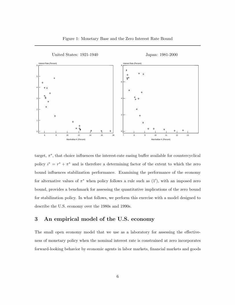
Figure 1: Monetary Base and the Zero Interest Rate Bound

United States: 1921-1940 Japan: 1981-2000

0

1

2

3

4

5

6

6 8 10 12 14 16 18

Interest Rate (Percent)

Marshallian K (Percent)

0

2

4

6

8

7 8 9 10 11 12 13

Interest Rate (Percent)

Marshallian K (Percent)

target, π∗, that choice influences the interest-rate easing buffer available for countercyclical

policy i∗ = r∗ + π∗ and is therefore a determining factor of the extent to which the zero

bound influences stabilization performance. Examining the performance of the economy

for alternative values of π∗ when policy follows a rule such as (1′), with an imposed zero

bound, provides a benchmark for assessing the quantitative implications of the zero bound

for stabilization policy. In what follows, we perform this exercise with a model designed to

describe the U.S. economy over the 1980s and 1990s.

3 An empirical model of the U.S. economy

The small open economy model that we use as a laboratory for assessing the effective-

ness of monetary policy when the nominal interest rate is constrained at zero incorporates

forward-looking behavior by economic agents in labor markets, financial markets and goods

6

markets.4 Expectations of endogenous variables are formed rationally and fully reflect the

choice of monetary policy rule. Monetary policy, however, still has temporary real effects

due to the presence of staggered wage contracts which induce nominal rigidity. The policy

instrument (the nominal short-term interest rate) is set according to the estimated rule (1′)

presented in the preceding section. Due to the presence of nominal rigidity, monetary policy

affects the real interest rate and the real exchange rate, which in turn affect the various

components of aggregate demand. Deviations of aggregate demand from potential output

then have consequences for wage and price setting.

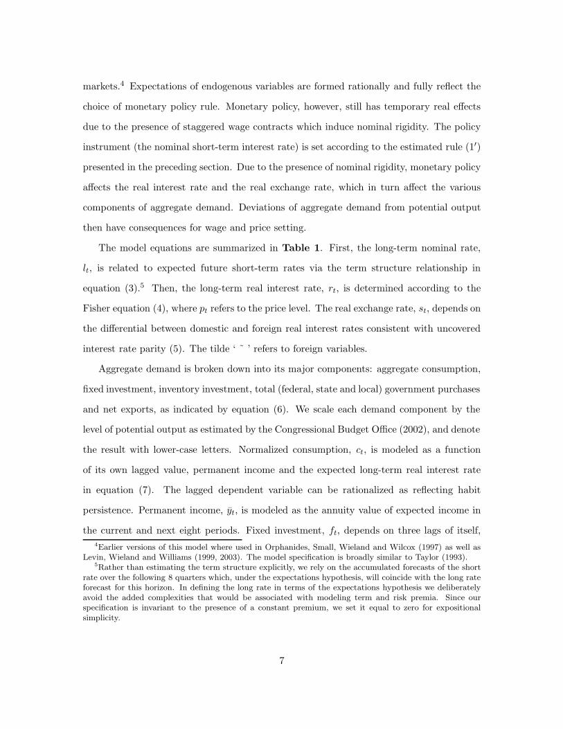
The model equations are summarized in Table 1. First, the long-term nominal rate,

lt, is related to expected future short-term rates via the term structure relationship in

equation (3).5 Then, the long-term real interest rate, rt, is determined according to the

Fisher equation (4), where pt refers to the price level. The real exchange rate, st, depends on

the differential between domestic and foreign real interest rates consistent with uncovered

interest rate parity (5). The tilde ‘ ˜ ’ refers to foreign variables.

Aggregate demand is broken down into its major components: aggregate consumption,

fixed investment, inventory investment, total (federal, state and local) government purchases

and net exports, as indicated by equation (6). We scale each demand component by the

level of potential output as estimated by the Congressional Budget Office (2002), and denote

the result with lower-case letters. Normalized consumption, ct, is modeled as a function

of its own lagged value, permanent income and the expected long-term real interest rate

in equation (7). The lagged dependent variable can be rationalized as reflecting habit

persistence. Permanent income, yt, is modeled as the annuity value of expected income in

the current and next eight periods. Fixed investment, ft, depends on three lags of itself,4Earlier versions of this model where used in Orphanides, Small, Wieland and Wilcox (1997) as well as

Levin, Wieland and Williams (1999, 2003). The model specification is broadly similar to Taylor (1993).5Rather than estimating the term structure explicitly, we rely on the accumulated forecasts of the short

rate over the following 8 quarters which, under the expectations hypothesis, will coincide with the long rateforecast for this horizon. In defining the long rate in terms of the expectations hypothesis we deliberatelyavoid the added complexities that would be associated with modeling term and risk premia. Since ourspecification is invariant to the presence of a constant premium, we set it equal to zero for expositionalsimplicity.

7

Table 1: Model Equations

Interest and Exchange Rates

Long-Term Nominal Rate lt = Et

[18

∑8j=1 it+j−1

](3)

Long-Term Real Rate rt = lt − 4 Et

[18 (pt+8 − pt)

](4)

Real Exchange Rate st = Et [st+1] + 0.25 ( it − 4 Et [pt+1 − pt] )

− 0.25(it − 4 Et [pt+1 − pt]

)(5)

Aggregate Demand Components

Aggregate Demand yt = ct + ft + nt + et + gt − 1 (6)

Consumption ct = α1 ct−1 + α2 yt + α3 rt + εc,t, (7)

where yt = (1−.9)1−(.9)9

∑8i=0(.9)iyt+i

Fixed Investment ft =∑2

i=1 βi ft−i + β3 yt + β4 rt + εf,t (8)

Inventory Investment nt =∑3

i=1 γi nt−i +∑3

i=1 γ3+i yt−i−1 + εn,t (9)

Net Exports et = δ1et−1 + δ2yt + δ3y∗t + δ4st + εe,t (10)

Government Spending gt = ρgt−1 + εg,t (11)

Prices and Wages

Price Level pt =∑3

i=0 ωi xt−i, (12)

where ωi ≥ 0, ωi ≥ ωi+1 and∑3

i=0 ωi = 1

Contract Wage xt = Et

[∑3i=0 ωi vt+i + χ

∑3i=0 ωi yt+i

]+ εx,t, (13)

where vt =∑3

i=0 ωi (xt−i − pt−i)

Notes: l: long-term nominal interest rate; i : short-term nominal interest rate; r: ex-ante long-term real

interest rate; p: aggregate price level; s: real exchange rate; y: output gap; c: consumption; y: permanent

income; f : fixed investment; n: inventory investment; e: net exports; g: government spending; x: nominal

contract wage; v: real contract wage index; ε(·): random white-noise shocks; the tilde ‘ ˜ ’ indicates foreign

variables.

8

permanent income as a measure of expected future sales, and the real interest rate (equation

(8)), while inventory investment, nt, instead is (nearly) of the accelerator type (equation

(9)). Net exports, et, depend on the level of income at home and abroad, and on the (trade-

weighted) real exchange rate (equation (10)). Finally, government spending, gt, follows a

simple autoregressive process with a near-unit root (equation (11)). (Random white noise

shocks are denoted by ε.,t).

As to the short-run supply-side of the model we follow Fuhrer and Moore (1995a,b)

rather than Taylor (1980) in modeling staggered wages and prices. Fuhrer and Moore

assume that workers and firms set the real wage in the first period of each new contract

with an eye toward the real wage agreed upon in contracts signed in the recent past and

expected to be signed in the near future.6 As they show, models specified in this manner

exhibit a greater (and hence more realistic) degree of inflation persistence than do models

in which workers and firms care about relative wages in nominal terms. Equation (12)

indicates that the price level is related to the weighted average of wages on contracts that

are currently in effect assuming a constant markup. Equation (13) specifies that the real

wage under contracts signed in the current period, xt − pt, is set in reference to a centered

moving average of initial-period real wages established under contracts signed as many as

three quarters earlier as well as contracts to be signed as many as three quarters ahead.

Furthermore, the negotiated real wage is assumed to depend also on expected excess-demand

conditions. The maximum contract length is four quarters.

In the deterministic steady state of this model output is at potential and the sectoral

allocation of GDP is constant for a given combination of equilibrium real interest and

exchange rates. The steady-state value of inflation is determined exclusively by the inflation

target and the policy rule, because the wage-price block does not impose any restriction on

the steady-state inflation rate.

Model estimation. The model allows for inflation and output persistence. While the6By contrast, Taylor assumed that workers and firms set the nominal wage in the first period of each

new contract with an eye toward the nominal wage settlements of recently signed and soon-to-be signedcontracts.

9

presence of these lags is not explicitly derived from optimizing behavior of representative

agents they are consistent with the presence of habit persistence in consumption, adjust-

ment costs in investment and overlapping wage contracts. The advantage of such a model is

that it can fit empirical inflation and output dynamics for the U.S. economy up to a set of

white-noise structural shocks.7 The demand side equations are estimated on an equation-

by-equation basis using instrumental variables. As to the supply side, we follow Fuhrer

and Moore (1995a,b) and use price data in estimation. We estimate the parameters of the

wage-price block by simulation-based indirect inference methods so as to fit the empirical

output and inflation dynamics as summarized by an atheoretical VAR model.8 The individ-

ual equations fit the data well. In addition we have evaluated the overall fit of the complete

model. The series of historical structural shocks computed under model-consistent expecta-

tions show no remaining serial correlation. Furthermore, the degree of inflation and output

persistence implied by the model fits the observed degree of persistence as summarized by

an unconstrained VAR model. Individual parameter estimates and evidence regarding the

empirical fit of the model are presented in the appendix.

Global stability and fiscal policy. The zero bound constraint is the only effective nonlin-

earity in the model. However, when it is introduced, the global stability of our otherwise

linear system is no longer ensured. Once shocks to aggregate demand or supply push the

economy into a sufficiently deep deflation, a zero-interest-rate policy may not be able to

return the economy to the original equilibrium. With a series of shocks large enough to

sustain deflationary expectations and to keep the real interest rate above its equilibrium

level, aggregate demand is suppressed further sending the economy into a deflationary spi-

ral. This points to a limitation inherent in linear models such as this which rely on the real7An alternative approach following Rotemberg and Woodford (1997) is to estimate a model with opti-

mizing agents and achieving empirical fit by introducing ad-hoc serially correlated shocks as criticized byEstrella and Fuhrer (2000). In both cases, the degree of output and inflation persistence is important forthe analysis of monetary policy.

8For a more detailed discussion of this estimation methodology see Coenen and Wieland (2000). Weinvestigated both Taylor’s (1980) as well as Fuhrer and Moore’s (1995) specification. Our findings confirmedthe earlier results of Fuhrer and Moore, who showed that under the assumption of rational expectations andperfect credibility of monetary policy Taylor’s specification does not induce sufficient inflation persistenceto match U.S. data.

10

interest rate as the sole channel for monetary policy and also brings into focus the extreme

limiting argument regarding the ineffectiveness of monetary policy in a liquidity trap.

To ensure global stability in the presence of the zero-bound constraint, we introduce

a second nonlinearity. We specify a fiscal policy that, if deflation becomes so severe that

the zero bound restricts the real interest rate at a level high enough to induce a growing

aggregate demand imbalance, boosts aggregate demand to rescue the economy from falling

into a deflationary spiral.9

4 The quantitative importance of the zero bound

To evaluate whether the zero bound on nominal interest rates would be of quantitative

significance in practice, it is necessary to assess how frequently monetary policy would

be expected to be constrained if the economy were subjected to stochastic shocks with

properties similar to those we anticipate to obtain in practice. To this end, we employ

stochastic simulations of our model economy. As a baseline, we assume the economy is

subject to shocks drawn from a joint normal distribution with the covariance of the shocks

we estimated for the 1980s and 1990s.10 With these simulations we construct the stationary

distribution of interest rates, inflation and output and investigate the extent to which their

statistical properties are altered when the policymaker adopts alternative values of the

inflation target, π∗, in the estimated policy rule (1′). In particular, we examine the influence

of the inflation target on the means and variances of inflation and output, which would be

central for welfare analysis based on a quadratic loss function. The equilibrium real interest

rate r∗ will be maintained at 2 percent.11

9The extent of fiscal impetus is related to the deviation of the actual federal funds rate, it, (which cannotbe negative), from the notional rate, int , that would be prescribed by the estimated interest rate rule in theabsence of the zero bound. The fiscal impetus comes into play with a half-year delay and responds onlyto a moving average of of negative deviations of the prescribed interest rate from zero. To ensure fiscalconsolidation in the long-run, we also restrain government expenditure in a symmetric fashion whenever theeconomy experiences very favorable economic conditions, that is, in a situation when output is so far abovepotential that the interest rate rule prescribes a rate of more than twice the steady-state value.

10The derivation of historical shocks and the solution methodology are discussed in the appendix.11Nevertheless, it is straightforward to assess the effect of alternative values of r∗. The zero bound regards

the nominal interest rate which in deterministic steady state equals the sum of r∗ and π∗. Thus, changes inone parameter can be offset by changes in the other. For example, our results for π∗ equal to 1 percent with

11

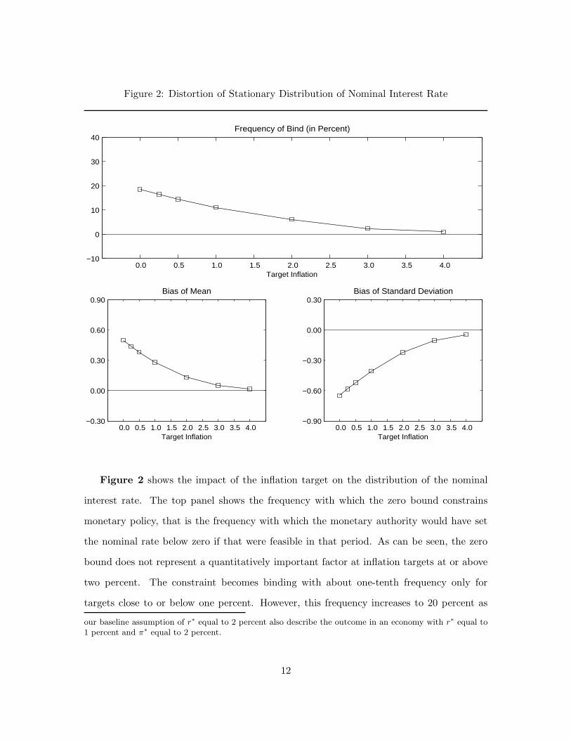
Figure 2: Distortion of Stationary Distribution of Nominal Interest Rate

0.0 0.5 1.0 1.5 2.0 2.5 3.0 3.5 4.0 −10

0

10

20

30

40Frequency of Bind (in Percent)

Target Inflation

0.0 0.5 1.0 1.5 2.0 2.5 3.0 3.5 4.0 −0.30

0.00

0.30

0.60

0.90Bias of Mean

Target Inflation 0.0 0.5 1.0 1.5 2.0 2.5 3.0 3.5 4.0

−0.90

−0.60

−0.30

0.00

0.30Bias of Standard Deviation

Target Inflation

Figure 2 shows the impact of the inflation target on the distribution of the nominal

interest rate. The top panel shows the frequency with which the zero bound constrains

monetary policy, that is the frequency with which the monetary authority would have set

the nominal rate below zero if that were feasible in that period. As can be seen, the zero

bound does not represent a quantitatively important factor at inflation targets at or above

two percent. The constraint becomes binding with about one-tenth frequency only for

targets close to or below one percent. However, this frequency increases to 20 percent as

our baseline assumption of r∗ equal to 2 percent also describe the outcome in an economy with r∗ equal to1 percent and π∗ equal to 2 percent.

12

the inflation target drops towards zero.

The bottom panels of Figure 2 describe the resulting distortion of the stationary dis-

tributions of the nominal interest rate. The bottom left panel shows the distortion in the

average level of the nominal interest rate. This is computed as the mean of the stationary

distribution of the short nominal interest rate, it, minus r∗ + π∗, which corresponds to the

mean nominal rate in the absence of the constraint. This property is indeed confirmed in

the figure with the constraint in place when the inflation target is large enough for the bind

to occur very infrequently. With inflation targets near zero, however, the asymmetric na-

ture of the constraint on policy introduces a significant bias. Since the constraint provides

a lower bound on the nominal interest rate, it effectively forces policy to be tighter than it

would be in the absence of the constraint under some circumstances. Since no comparable

upper bound is in place, policy is tighter on average. This bias increases with the frequency

with which the constraint binds. As can be seen from the figure, a policymaker following

the estimated rule with a zero inflation target would set the nominal interest rate about

50 basis points higher, on average, than if the zero-bound constraint were not in place.

Furthermore, since this constraint restricts the variability of interest rates, the standard

deviation of the interest rate falls somewhat as the inflation target drops to zero as shown

in the bottom-right panel of Figure 2.

The distortions of the distribution of nominal interest rates translate into distortions

of the stationary distributions of output and inflation. Compared to the unconstrained

case, in which the distributions would be normal, the left tails of the output and inflation

distributions will be noticeably thicker. When either output or inflation fall considerably

below their means, policy without the constraint would engineer an easing in order to return

output to potential and inflation to its target level. With the constraint binding, this is no

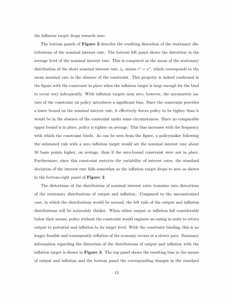
longer feasible and consequently reflation of the economy occurs at a slower pace. Summary

information regarding the distortion of the distributions of output and inflation with the

inflation target is shown in Figure 3. The top panel shows the resulting bias in the means

of output and inflation and the bottom panel the corresponding changes in the standard

13

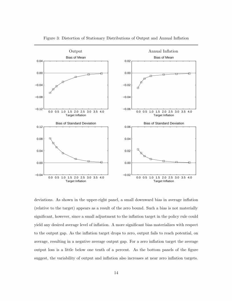
Figure 3: Distortion of Stationary Distributions of Output and Annual Inflation

Output Annual Inflation

0.0 0.5 1.0 1.5 2.0 2.5 3.0 3.5 4.0 −0.12

−0.08

−0.04

0.00

0.04Bias of Mean

Target Inflation 0.0 0.5 1.0 1.5 2.0 2.5 3.0 3.5 4.0

−0.06

−0.04

−0.02

0.00

0.02Bias of Mean

Target Inflation

0.0 0.5 1.0 1.5 2.0 2.5 3.0 3.5 4.0 −0.04

0.00

0.04

0.08

0.12Bias of Standard Deviation

Target Inflation 0.0 0.5 1.0 1.5 2.0 2.5 3.0 3.5 4.0

−0.02

0.00

0.02

0.04

0.06Bias of Standard Deviation

Target Inflation

deviations. As shown in the upper-right panel, a small downward bias in average inflation

(relative to the target) appears as a result of the zero bound. Such a bias is not materially

significant, however, since a small adjustment to the inflation target in the policy rule could

yield any desired average level of inflation. A more significant bias materializes with respect

to the output gap. As the inflation target drops to zero, output fails to reach potential, on

average, resulting in a negative average output gap. For a zero inflation target the average

output loss is a little below one tenth of a percent. As the bottom panels of the figure

suggest, the variability of output and inflation also increases at near zero inflation targets.

14

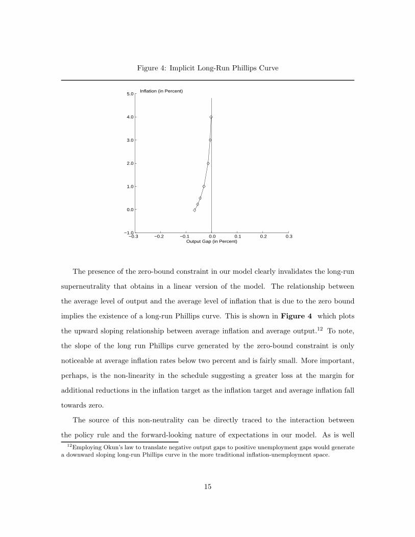
Figure 4: Implicit Long-Run Phillips Curve

−0.3 −0.2 −0.1 0.0 0.1 0.2 0.3−1.0

0.0

1.0

2.0

3.0

4.0

5.0

Output Gap (in Percent)

Inflation (in Percent)

The presence of the zero-bound constraint in our model clearly invalidates the long-run

superneutrality that obtains in a linear version of the model. The relationship between

the average level of output and the average level of inflation that is due to the zero bound

implies the existence of a long-run Phillips curve. This is shown in Figure 4 which plots

the upward sloping relationship between average inflation and average output.12 To note,

the slope of the long run Phillips curve generated by the zero-bound constraint is only

noticeable at average inflation rates below two percent and is fairly small. More important,

perhaps, is the non-linearity in the schedule suggesting a greater loss at the margin for

additional reductions in the inflation target as the inflation target and average inflation fall

towards zero.

The source of this non-neutrality can be directly traced to the interaction between

the policy rule and the forward-looking nature of expectations in our model. As is well12Employing Okun’s law to translate negative output gaps to positive unemployment gaps would generate

a downward sloping long-run Phillips curve in the more traditional inflation-unemployment space.

15

known, in models with rational expectations such as ours, the sacrifice ratio—the ratio of

the cumulative output gap loss (gain) required for a given reduction (rise) in the inflation

rate—is a function of the policy responsiveness to inflation and output. With a linear policy

reaction function, as is the case when the inflation target is sufficiently high for the zero

bound to be irrelevant, output losses when inflation is above the steady state and falls

towards it exactly offset output gains when inflation is below the steady state and rising

towards it. The responsiveness of policy to inflation and output is the same in both cases.

Symmetry prevails and on average the output gap is zero. This is not the case when the zero

bound becomes important. When the constraint is binding, the responsiveness of policy to

marginal changes in inflation is nil—the interest rate is constrained at zero. When the

constraint is not binding, the usual responsiveness of policy is restored. But the former is

more likely when inflation is below its target than above its target so symmetry fails and

a bias in the average output gap appears. It is worth noting that if expectations were of

a backward-looking, adaptive nature, the long-run Phillips curve would be vertical as in

that case the sacrifice ratio would be invariant to the policy responsiveness altogether. Of

course, introducing additional non-linearities in policy might offset this bias but it would

also move the policy away from its original unrestricted linear specification and distort the

higher moments of the stationary distributions of inflation and output.

5 Conclusion

Our analysis for the United States indicates that if the economy is subject to stochastic

shocks similar in magnitude to those experienced over the 1980s and 1990s, the consequences

of the zero bound are negligible for target inflation rates as low as 2 percent. However, the

effects of the constraint become increasingly important for determining the effectiveness of

policy with inflation targets between 0 and 1 percent. Although these results are suggestive,

it is important to recognize that some uncertainty remains regarding the magnitude of the

distortions introduced by the zero bound when targeting zero inflation. For example, since

our model was estimated for the 1980s and 1990s, a relatively calm period for the U.S.

16

economy, the variances of demand and supply shocks may be smaller than in earlier periods.

Larger disturbances will render the zero bound more important. Similarly, the assumption

that policymakers observe the data and the relevant model parameters without error may

lead us to underestimate the impact of the zero bound. Recognition of data uncertainty

(see for example Orphanides (2001) or parameter uncertainty (see for example Wieland

(1998)) would raise the importance of the zero bound as a constraint on monetary policy in

practice. However, our estimate would be reduced to the extent that channels of monetary

policy transmission other than the interest or exchange rate channel would remain effective

important when the zero bound renders the interest rate channel ineffectual. Similarly,

policy outcomes might be improved if a non-linear policy rule for the interest rate or for the

exchange rate designed to explicitly reduce the distortions resulting from the zero bound

were followed.

In summary, our results point to a fundamental difficulty associated with the evaluation

of stabilization policies with a price stability objective based on simple linear models. The

presence of the zero bound constraint invalidates the underlying superneutrality properties

of otherwise linear models. At low rates of inflation, the zero bound distorts the stochastic

properties of the economy and induces a tradeoff between the average level of inflation and

the variability of inflation and output. As a result, the optimal average rate of inflation

cannot be investigated independently of the variability of output and inflation. Since our

results suggest that deflation potentially engenders greater dangers than inflation, it may

be optimal to pursue a price stability objective that allows for a small but positive bias in

the average rate of inflation. The optimal size of such a bias, however, remains an open

question. Furthermore, the optimal policy rule in the presence of the zero bound on nominal

interest rates is likely to be nonlinear and asymmetric in a low or zero inflation environment.

Characterizing the optimal rule represents an important issue for future research.

17

References

Akerlof, George, William Dickens and George Perry (1996), “The Macroeconomics of LowInflation,” Brookings Papers on Economic Activity, 1, 1-76.

Anderson, Gary S. (1987), “A Procedure for Differentiating Perfect-Foresight-Model Reduced-Form Coefficients,” Journal of Economic Dynamics and Control, 11, 465-81.

Anderson, Gary S. and George R. Moore (1985), “A Linear Algebraic Procedure For SolvingLinear Perfect Foresight Models,” Economics Letters, 17, 247-52.

Blanchard, Olivier and Charles Kahn (1980), “The solution of linear difference models underrational expectations,” Econometrica, 48(5), 1305-1311.

Boucekkine, Raouf (1995), “An Alternative Methodology for Solving Nonlinear Forward-Looking Models,” Journal of Economic Dynamics and Control, 19(4), 771-734.

Clark, Todd (1997). “Cross-Country Evidence on Long-Run Growth and Inflation,” Eco-nomic Inquiry, 35(1), January, 70-81.

Coenen, Gunter (2000), “Asymptotic confidence bands for the estimated autocovarianceand autocorrelation functions of vector autoregressive models” European Central Bank,Working Paper No. 9.

Coenen, Gunter and Volker Wieland (2000), “A small estimated euro area model withrational expectations and nominal rigidities,” ECB Working Paper, No. 30.

Congressional Budget Office (2002), The Economic and Budget Outlook, United StatesGovernment Printing Office.

Driffill, John, Grayham Mizon, and Alistair Ulph (1990), “Costs of Inflation,” in Handbookof Monetary Economics, Benjamin M. Friedman, and Frank H. Hahn eds., Amsterdam:North Holland.

Estrella, Arturo and Jeffrey Fuhrer, (2002) “Dynamic Inconsistencies: Counterfactual Im-plications of a Class of Rational Expectations Model,” American Economic Review.

Fair, Ray, and John B. Taylor(1983),“Solution and Maximum Likelihood Estimation ofDynamic Nonlinear Rational Expectations Models” Econometrica 51, 1169-85.

Feldstein, Martin (1997), “The Costs and Benefits of Going from Low Inflation to PriceStability,” in Reducing Inflation: Motivation and Strategy Christina D. Romer and DavidH. Romer, eds., Chicago: University of Chicago.

Fischer, Stanley, (1981), “Towards an Understanding of the Costs of Inflation: II” in TheCosts and Consequences of Inflation, Carnegie-Rochester Conference Series on PublicPolicy, Vol. 15.

Fischer, Stanley (1994), “Modern Central Banking,” in The Future of Central Banking, TheTercentenary Symposium of the Bank of England, Cambridge: Cambridge University.

Fischer, Stanley (1996), “Why Are Central Banks Pursuing Long-Run Price Stability?,” inAchieving Price Stability, Federal Reserve Bank of Kansas City.

Fischer, Stanley and Franco Modigliani (1978), “Towards an Understanding of the RealEffects of Inflation,” Weltwirtschaftliches Archiv, 114, 810-832.

18

Fuhrer, Jeffrey and Brian Madigan (1997), “Monetary Policy when Interest Rates areBounded at Zero,” Review of Economics and Statistics, November.

Fuhrer, Jeffrey C. and George R. Moore (1995a) “Inflation Persistence” Quarterly Journalof Economics 110(1), February, 127-59.

Fuhrer, Jeffrey C. and George R. Moore (1995b) “Monetary Policy Trade-offs and theCorrelation between Nominal Interest Rates and Real Output,” American EconomicReview, 85(1), 219-39.

Friedman, Milton (1969), The Optimum Quantity of Money and Other Essays, Chicago:University of Chicago.

Hicks, John (1937), “Mr. Keynes and the ‘Classics’,” Econometrica, 5(2), April.

Hicks, John (1967), Classical Essays in Monetary Theory, London: Oxford University.

Juillard, Michel (1994), “DYNARE - A Program for the Resolution of Non-linear Modelswith Forward-looking Variables,” Release 1.1, mimeo, CEPREMAP.

Laffargue, Jean-Pierre (1990) “Resolution d’un modele macroeconomique avec anticipationsrationnelles,” Annales d’Economie et de Statistique 17, 97-119.

Judson, Ruth, and Athanasios Orphanides (1999), “Inflation, Volatility and Growth,” In-ternational Finance, 2(1), 117-138, April.

Keynes, John M. (1923), “Social Consequences of Changes in the Value of Money,” in Essaysin Persuasion, London: MacMillan, 1931.

Levin Andrew, Volker Wieland and John Williams (1999), “Robustness of Simple PolicyRules Under Model Uncertainty,” in Taylor, John B. (ed.), Monetary Policy Rules,NBER and Chicago Press.

Levin Andrew, Volker Wieland and John Williams (2003), “The Performance of Forecast-Based Monetary Policy Rules Under Model Uncertainty,” forthcoming, American Eco-nomic Review.

Orphanides, Athanasios, and Robert M. Solow (1990), “Money, Inflation, and Growth,”in Handbook of Monetary Economics, Benjamin M. Friedman, and Frank H. Hahn eds.Amsterdam: North Holland.

Orphanides, Athanasios (2001), “Monetary Policy Rules Based on Real-Time Data,” Amer-ican Economic Review , September.

Orphanides, Athanasios, David Small, David Wilcox, and Volker Wieland (1997), “A Quan-titative Exploration of the Opportunistic Approach to Disinflation,” Finance and Eco-nomics Discussion Series, 97-36, Board of Governors of the Federal Reserve System,June.

Rotemberg, Julio and Michael Woodford (1999), “Interest-rate rules in an estimated sticky-price model.’ in J.B. Taylor, ed., Monetary Policy Rules, NBER and Chicago Press.

Rotemberg, Julio and Michael Woodford (1997), “An Optimization-Based EconometricFramework for the Evolution of Monetary Policy.” NBER Macroeconomics Annual, 12,297-346.

19

Sarel, Michael (1996), “Nonlinear Effects of Inflation on Economic Growth,” IMF StaffPapers, 43(1), 199-215.

Summers, Lawrence (1991), “How Should Long-Term Monetary Policy Be Determined,”Journal of Money, Credit and Banking , 23(3), 625-31, August, Part 2.

Taylor, John B. (1980), “Aggregate Dynamics and Staggered Contracts,” Journal of Polit-ical Economy, 88(1), 1-23.

Taylor, John B. (1993), Macroeconomic Policy in the World Economy: From EconometricDesign to Practical Operation, New York: W.W. Norton.

Taylor, John B. (1999), ed., Monetary Policy Rules, Chicago: University of Chicago.

Tobin, James (1965), “Money and Economic Growth,” Econometrica, 33, 334-361.

Wieland, Volker (1998), “Monetary Policy under Uncertainty about the Natural Unemploy-ment Rate,” Finance and Economics Discussion Series, 98-22, Board of Governors of theFederal Reserve System.

20

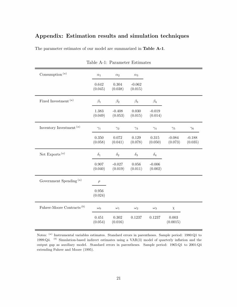
Appendix: Estimation results and simulation techniques

The parameter estimates of our model are summarized in Table A-1.

Table A-1: Parameter Estimates

Consumption (a) α1 α2 α3

0.642 0.304 -0.062(0.045) (0.038) (0.015)

Fixed Investment (a) β1 β2 β3 β4

1.383 -0.408 0.030 -0.019(0.049) (0.053) (0.015) (0.014)

Inventory Investment (a) γ1 γ2 γ3 γ4 γ5 γ6

0.350 0.072 0.129 0.315 -0.084 -0.188(0.058) (0.041) (0.078) (0.050) (0.073) (0.035)

Net Exports (a) δ1 δ2 δ3 δ4

0.907 -0.027 0.056 -0.006(0.040) (0.019) (0.011) (0.002)

Government Spending (a) ρ

0.956(0.024)

Fuhrer-Moore Contracts (b) ω0 ω1 ω2 ω3 χ

0.451 0.302 0.1237 0.1237 0.003(0.054) (0.016) (0.0015)

Notes: (a) Instrumental variables estimates. Standard errors in parentheses. Sample period: 1980:Q1 to

1999:Q4. (b) Simulation-based indirect estimates using a VAR(3) model of quarterly inflation and the

output gap as auxiliary model. Standard errors in parentheses. Sample period: 1965:Q1 to 2001:Q4

extending Fuhrer and Moore (1995).

21

In preparation for the stochastic simulations, we first computed the structural shocksof the model based on U.S. data from 1980 to 1999.13 Since the non-negativity constraintfor nominal interest rates was never binding during this period and our model is otherwiselinear, we obtained the structural shocks by solving the model analytically for the reducedform using the AIM implementation (Anderson and Moore, 1985, and Anderson, 1997) ofthe Blanchard and Kahn (1980) method for solving linear rational expectations models.The structural shocks also provide a good indication of the historical fit of our model.Figure A-1 shows the correlogram of historical structural shocks, which overall reveals nosignificant serial correlation.

A further indication of the good empirical fit of our model is obtained from a com-parison of the implied autocorrelation functions of inflation and output with the empiricalautocorrelation functions implied by an unconstrained bivariate VAR.14 The comparison ofautocorrelation functions of inflation and output in the U.S. economy is reported in FigureA-2. The solid lines refer to the autocorrelation functions implied by the model. The thindotted lines in each panel correspond to the asymptotic 95% confidence bands associatedwith the autocorrelation functions of the bivariate unconstrained VAR(3) model used in theestimation of the staggered contracts specifications.15

Based on the covariance matrix of structural historical shocks, we generated 100 setsof artificial normally-distributed shocks with 100 quarters of shocks in each set from whichthe first 20 twenty quarters of shocks were discarded in order to guarantee that the effectof the initial values die out. We then used the sets of retained shocks to conduct stochasticsimulations under alternative inflation targets, while imposing the non-negativity constrainton nominal interest rates.16

We simulate the model using an efficient algorithm implemented in TROLL and basedon work by Boucekkine (1995), Juillard (1994) and Laffargue (1990). It is related to theFair-Taylor (1983) extended path algorithm. A limitation of the algorithm is that themodel-consistent expectations of market participants are computed under the counterfactual

13The process of calculating the structural shocks would be straightforward if the model in question werea purely backward-looking model. For a rational expectations model, however, structural shocks can becomputed only by simulating the full model and computing the time series of model-consistent expectationswith respect to historical data. The structural shocks differ from the estimated residuals to the extent ofagents’ forecast errors.

14Such an approach has also been used by Fuhrer and Moore (1995a) who argued that autocorrelationfunctions are more appropriate for confronting macroeconomic models with the data than impulse responsefunctions because of their purely descriptive nature.

15For a detailed discussion of the methodology and the derivation of the asymptotic confidence bands forthe estimated autocorrelation functions the reader is referred to Coenen (2000).

16If it were not for this nonlinearity, we could use the reduced form of the model corresponding to thealternative policy rules to compute unconditional moments of the endogenous variables without having toresort to stochastic simulations.

22

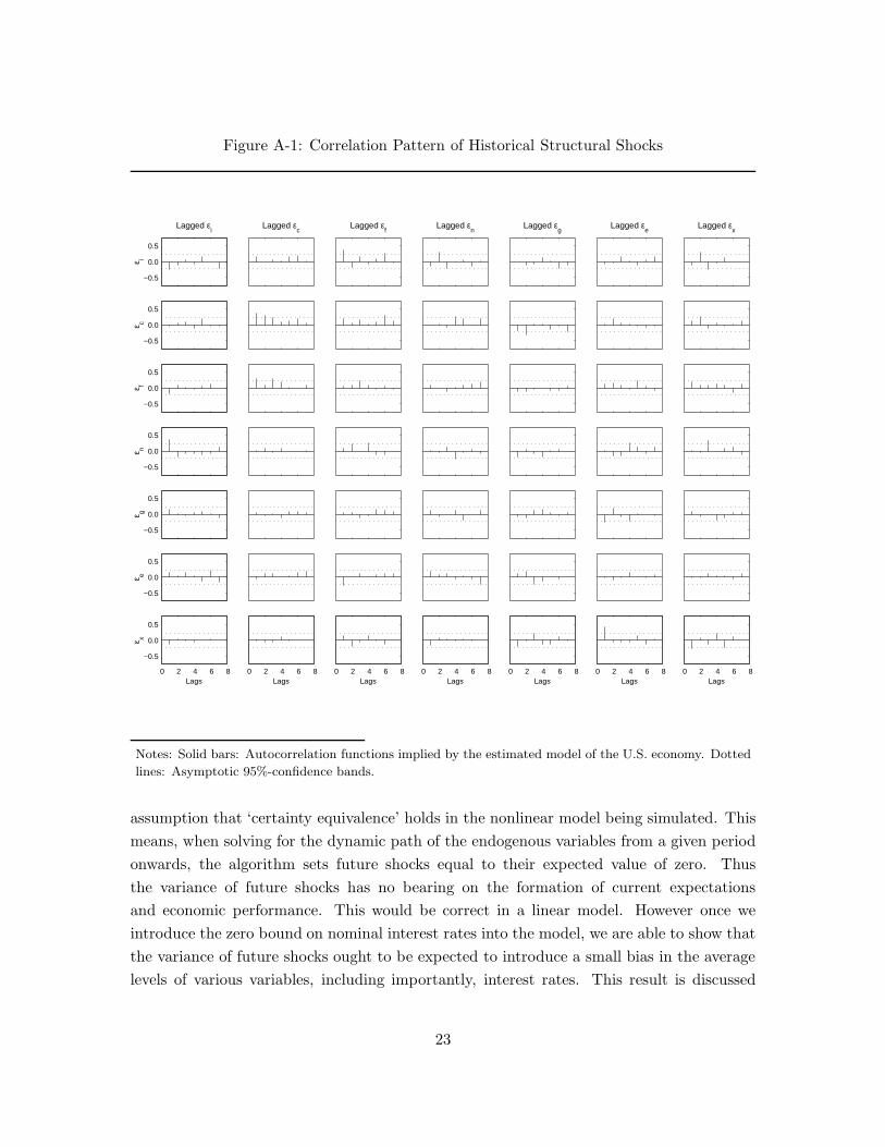
Figure A-1: Correlation Pattern of Historical Structural Shocks

−0.5

0.0

0.5

Lagged εi

ε i

Lagged εc

Lagged εf

Lagged εn

Lagged εg

Lagged εe

Lagged εx

−0.5

0.0

0.5

ε c

−0.5

0.0

0.5

ε f

−0.5

0.0

0.5

ε n

−0.5

0.0

0.5

ε g

−0.5

0.0

0.5

ε e

0 2 4 6 8

−0.5

0.0

0.5

ε x

Lags 0 2 4 6 8

Lags 0 2 4 6 8

Lags 0 2 4 6 8

Lags 0 2 4 6 8

Lags 0 2 4 6 8

Lags 0 2 4 6 8

Lags

Notes: Solid bars: Autocorrelation functions implied by the estimated model of the U.S. economy. Dotted

lines: Asymptotic 95%-confidence bands.

assumption that ‘certainty equivalence’ holds in the nonlinear model being simulated. Thismeans, when solving for the dynamic path of the endogenous variables from a given periodonwards, the algorithm sets future shocks equal to their expected value of zero. Thusthe variance of future shocks has no bearing on the formation of current expectationsand economic performance. This would be correct in a linear model. However once weintroduce the zero bound on nominal interest rates into the model, we are able to show thatthe variance of future shocks ought to be expected to introduce a small bias in the averagelevels of various variables, including importantly, interest rates. This result is discussed

23

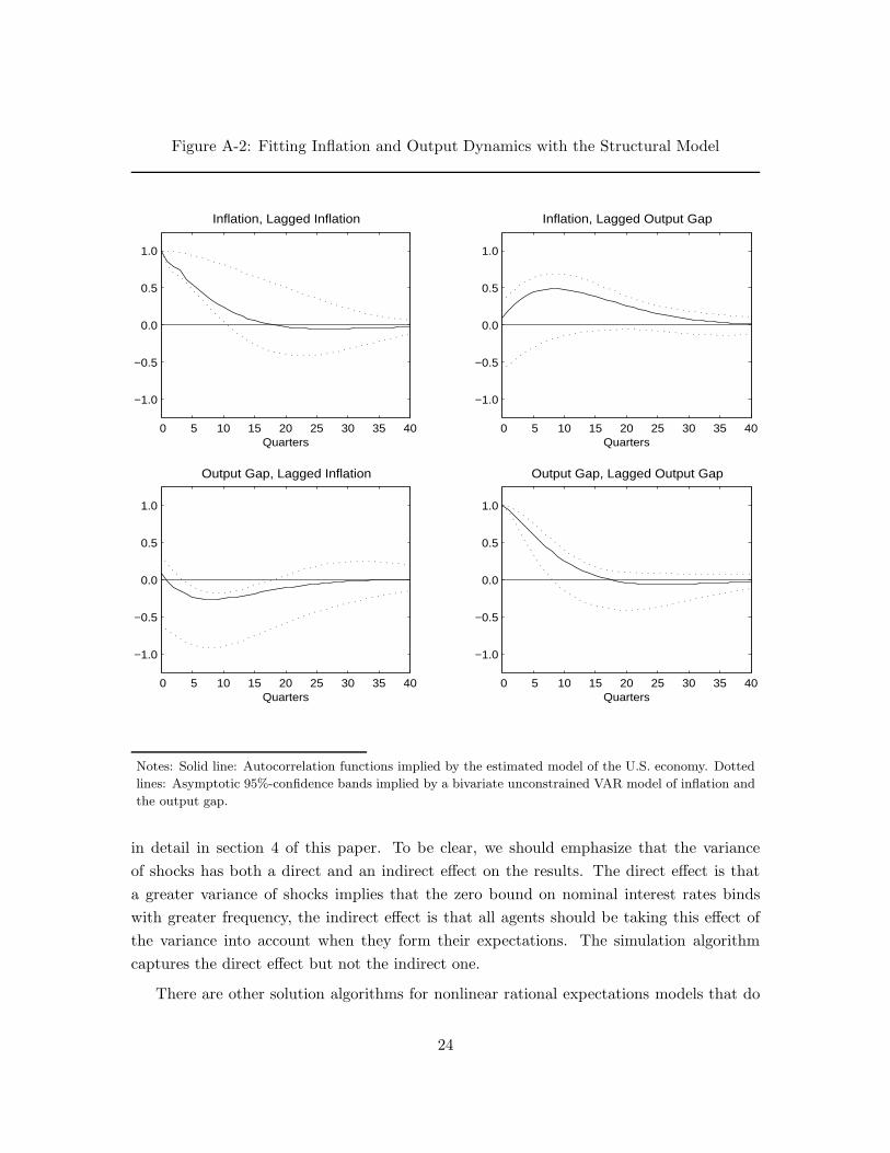
Figure A-2: Fitting Inflation and Output Dynamics with the Structural Model

0 5 10 15 20 25 30 35 40

−1.0

−0.5

0.0

0.5

1.0

Quarters

Inflation, Lagged Inflation

0 5 10 15 20 25 30 35 40

−1.0

−0.5

0.0

0.5

1.0

Quarters

Inflation, Lagged Output Gap

0 5 10 15 20 25 30 35 40

−1.0

−0.5

0.0

0.5

1.0

Quarters

Output Gap, Lagged Inflation

0 5 10 15 20 25 30 35 40

−1.0

−0.5

0.0

0.5

1.0

Quarters

Output Gap, Lagged Output Gap

Notes: Solid line: Autocorrelation functions implied by the estimated model of the U.S. economy. Dotted

lines: Asymptotic 95%-confidence bands implied by a bivariate unconstrained VAR model of inflation and

the output gap.

in detail in section 4 of this paper. To be clear, we should emphasize that the varianceof shocks has both a direct and an indirect effect on the results. The direct effect is thata greater variance of shocks implies that the zero bound on nominal interest rates bindswith greater frequency, the indirect effect is that all agents should be taking this effect ofthe variance into account when they form their expectations. The simulation algorithmcaptures the direct effect but not the indirect one.

There are other solution algorithms for nonlinear rational expectations models that do

24

not impose certainty equivalence. But these alternative algorithms would be prohibitivelycostly to use with our model, which has more than twenty state variables. Even with thealgorithm we are using, stochastic analysis of nonlinear rational expectations models witha moderate number of state variables remains fairly costly in terms of computational effort.

25

CFS Working Paper Series:

No. Author(s) Title

2003/03 Klaus Adam Learning and Equilibrium Selection in a Monetary Overlapping Generations Model with Sticky Prices

2003/04 Stefan Mittnik Marc S. Paolella

Prediction of Financial Downside-Risk with Heavy-Tailed Conditional Distributions

2003/05 Volker Wieland Monetary Policy and Uncertainty about the Natural Unemployment Rate

2003/06 Andrew Levin Volker Wieland John C. Williams

The Performance of Forecast-Based Monetary Policy Rules under Model Uncertainty

2003/07 Günter Coenen Andrew Levin Volker Wieland

Data Uncertainty and the Role of Money as an Information Variable for Monetary Policy

2003/08 Günter Coenen Volker Wieland

A Small Estimated Euro Area Model with Rational Expectations and Nominal Rigidities

2003/09 Günter Coenen Volker Wieland

The Zero-Interest-Rate and the Role of the Exchange Rate for Monetary Policy in Japan

2003/10 Stefan Reitz Frank Westerhoff

Nonlinearities and Cyclical Behavior: The Role of Chartists and Fundamentalists

2003/11 Stefan Reitz Ralf Ahrens

Heterogeneous Expectations in the Foreign Exchange Market Evidence from the Daily Dollar/DM Exchange Rate

2003/12 Klaus Adam Optimal Monetary Policy with Imperfect Common Knowledge

2003/13 Günter Coenen Athanasios Orphanides Volker Wieland

Price Stability and Monetary Policy Effectiveness when Nominal Interest Rates are Bounded at Zero

Copies of working papers are available at the Center for Financial Studies or can be downloaded (http://www.ifk-cfs.de).