Welcome message from author
This document is posted to help you gain knowledge. Please leave a comment to let me know what you think about it! Share it to your friends and learn new things together.
Transcript
Technical Appendices
Public Environmental Review Methanol Complex
Burrup Peninsula Western Australia
Prepared forMethanex Australia Pty Ltd
April 2002
The concepts and information contained in this document are the property of Methanex Australia. Use or copying of this documentin whole or part without written permission of Methanex Australia constitutes an infringement of copyright.

Index to Appendices
Appendix 1: Economic Assessments of the Proposed Methanol Complex
Appendix 2: Preliminary Geotechnical Investigation
Appendix 3: Vegetation, Flora and Fauna Assessment
Appendix 4: Baseline Marine Survey of King Bay
Appendix 5: Air Quality Assessment
Appendix 6: Preliminary Environmental Noise Assessment
Appendix 7: Preliminary Risk Analysis of Proposed Methanol Plant and Facilities
Appendix 8: Methanol Shipping Hazards Assessment

Economic Assessments of theProposed Methanol Complex
Appendix 1
While every effort has been made to ensure the accuracy of this document, the uncertain nature of economic data, forecasting and analysis means that Access Economics Pty Ltd is unable to make any warranties in relation to the information contained herein. Access Economics Pty Ltd, its employees and agents disclaim liability for any loss or damage which may arise as a consequence of any person relying on the information contained in this document.
SUPPLEMENTARY REPORT
THE WESTERN AUSTRALIAN ECONOMIC IMPACT OF THE METHANEX METHANOL PROJECT
prepared for
Methanex Australia Pty Ltd
by
ACCESS ECONOMICS
Canberra December 2001
WA supplement: December 2001 Access Economics
Table of contents
1. Executive Summary .........................................................................................................1
2. Introduction......................................................................................................................4
2.1. The project .............................................................................................................................................................4 2.2. Modeling approach ..............................................................................................................................................6
3. Western Australian economic impacts...........................................................................7
3.1. Direct impacts .......................................................................................................................................................7 3.2. Flow-on impacts ....................................................................................................................................................8
4. Western Australian Budget Impacts ............................................................................ 11
5. Overall impact on Western Australian economic welfare .......................................... 13
5.1. Conclusion ...........................................................................................................................................................14
6. Appendix: methodology................................................................................................. 15
6.1. Modeling the WA economic impacts ...............................................................................................................15 6.2. Modeling the state budget .................................................................................................................................16
WA supplement: December 2001 Access Economics
1
1. Executive Summary Methanex has commissioned Access Economics to assess the national and Western Australian economic impacts of the proposed methanol project using gas from the North West Shelf.
Our accompanying report1 contained an assessment of the national economic and budgetary impacts. This supplement explores the corresponding Western Australian impacts. It should be read in conjunction with the main report, which provides a fuller description of the project and modelling approach.
The project
The core methanol project considered in this report comprises the methanol plant, together with upstream developments by the North West Shelf Consortium to supply the natural gas input, and port and other infrastructure developments associated with the project. Additional downstream developments may be stimulated by the success of the Methanex project. Their impacts are considered separately below.
Key statistics for the core project, as modeled in this study, include:
• total capital expenditure in excess of A$2 billion between 2003 and 2008. Construction of the methanol plant will provide employment for around 1,000 on-site construction employees for most of that time. This investment will provide a substantial boost to the WA economy.;
• annual production of 2.1 million tonnes of methanol from 20062, rising to 4.2 million tonnes from 2009 with the completion of the second production train. The modelling horizon extends to 2030. Each train will use approximately 70 PJ of natural gas annually;
• a direct contribution to the balance of payments from methanol exports and import replacement of A$460 million from 2006, and A$940 million from 2009. This production and exports add to WA gross state product;
• direct employment at the methanol plant of approximately 150 people, together with flow-ons to the WA economy from the project’s operational expenditures;
• additional payments to the WA government of payroll and other indirect taxes, together with the bringing forward of royalty payments from the exploitation of the state’s natural gas resources. In net present value terms this will amount to some $70 million in net present value terms at a 5 percent real discount rate.
Modeling results
According to our modeling - consistent with the national findings - the core methanol project would generate substantial positive economic impacts in Western Australia.
1 Access Economics, The Australian national economic impact of the Methanex methanol project, Report to Methanex Australia Pty Ltd, Canberra, December 2001 2 Project start -up is in 2005, but the analysis commences based on the first full year of operation in 2006
WA supplement: December 2001 Access Economics
2
During the initial investment phase (between 2003 and 2008):
• the project’s investment raises aggregate demand economy-wide and especially in WA. There is some leakage to imports (international and interstate), and an increase in output and employment;
• on average over this period, gross state product is some $200 million higher (at today’s prices 3) and employment 3,100 above the level in the world without the project. Private consumption is also on average some $60 million higher, reflecting wage incomes generated by the investment expenditure, as well as the fruits of initial project exports;
• the increases in GSP and consumption are larger at the end of this period since the first train is now producing, while the second is being built.
During full operation (from 2009 onwards):
• the project causes a substantial increase in gross domestic product and exports. This in turn allows an increase in imports. The economy benefits also from accelerated exploitation of North West Shelf gas resources;
• the project raises government revenues, allowing a cut in personal income taxes. Higher consumer demand reflects in higher imports, but also an increase in Australian production and employment;
• Between 2009 and 2020, annual GSP is on average $430 million (at today’s prices) above the level in a world without the project. Private consumption is some $160 million higher. Employment is up, on average, by some 900. The net present value of the increase in GSP is $4.6 billion at a 5 per cent real discount rate;
• in the project as modeled, the North West Shelf consortium contributes less to exports and government revenues from about 2020 onwards as gas and condensate production fall below the levels in the baseline. This in turn reflects in a weaker overall stimulus to GSP, employment and private consumption.
Impacts on Western Australian public finances and economic welfare
Key measures of the core methanol project’s potential contribution to the Australian economy are its overall impacts on overall public sector finances, the Commonwealth budget and on economic welfare.
We measure the overall impact on public sector finances as the net increase in WA General Government sector tax revenues and Commonwealth transfers:
• on this definition, the net present value of the impact on general government finances is an estimated $480 million in 2001 at a real discount rate of 5 percent.
3 Throughout the report and analysis, “today’s prices” are defined as being in dollars of 1999/00. This year is used as a base because it is the year in terms of which constant price series of the Australian National Accounts are expressed.
WA supplement: December 2001 Access Economics
3
In AE-MACRO the best measure of the project’s overall impact on WA economic welfare is:
A. the increase in annual flows of private consumption and general government current expenditures that it allows, and
B. the decrease in public sector debt at the end of the simulation period 4.
As modeled, in net present value terms, the welfare impact is mainly on the private sector.
• At a real discount rate of 5 percent the project improves Western Australian economic welfare by an estimated $2.0 billion (net present value in 2001).
Potential for additional downstream development
Once the Methanex deal goes ahead it is expected that other world scale gas feedstock customers will be more likely to be attracted to the Burrup Peninsula than would otherwise be the case. The portfolio of additional customers for North West Shelf feedstock gas is understood to include customers each with gas demand in the range of 90 - 500 TJ/d. The Methanex deal is expected to lead to an increased probability of each of these developments going ahead, such that the total expected gas demand is increased by around 100 TJ/d.
• The additional expected macro benefits above the base analysis have not been explicitly modeled, but are likely to be about one quarter of those estimated for the core methanol project (which will use about four times the amount of gas).
• Based on the modeling of the core methanol project, this could mean an expected additional annual $100 million of GSP, annual $40 million of WA private consumption, and additional WA employment of 200 persons during the project(s)’ operation. As a rough indication, the net present values of the increases in WA General Government revenues and GSP could be of the order of $120 million and $1.2 billion respectively.
Conclusion
As modeled, the core project comprising Methanex’ proposed Western Australian methanol plant, associated infrastructure development, and the expansion of natural gas supply by the North West Shelf Consortium would have a substantial positive impact on:
• Western Australian exports, GSP, employment and private consumption;
• public sector finances; and on
• Western Australian economic welfare.
The impacts would be higher were full account taken of investment in additional gas supply, and the expected stimulus to other large scale gas -based industrial developments.
Access Economics December 2001
4 We should ideally include an estimate of the increase in WA private wealth. However, the model does not generate an estimate of this.
WA supplement: December 2001 Access Economics
4
2. Introduction Methanex has commissioned Access Economics to assess the national and Western Australian economic impacts of the proposed methanol project using gas from the North West Shelf.
Our accompanying report5 contained an assessment of the national economic and budgetary impacts. This supplement explores the corresponding Western Australian impacts. It should be read in conjunction with the main report, which provides a fuller description of the project and modelling approach.
2.1. The project
Core methanol project
The core project considered in this report comprises the methanol plant, together with upstream developments by the North West Shelf Consortium to supply the natural gas input, and port and other infrastructure developments associated with the project.
The methanol project will convert natural gas from the North West Shelf into methanol, using a catalytic process. The plant will be located on the Burrup Peninsula in the Pilbara region. The methanol will primarily be exported to Asia. A small proportion of production (3 percent initially) will replace imports in the Australian market..
Additional downstream developments may be stimulated by the success of the Methanex project. Their impacts are considered separately below.
Key statistics for the core project, as modeled in this study, include:
• total capital expenditure in excess of A$2 billion between 2003 and 2008. Construction of the methanol plant will provide employment for around 1,000 on-site construction employees for most of that time. This investment will provide a substantial boost to the WA economy.;
• annual production of 2.1 million tonnes of methanol from 2006, rising to 4.2 million tonnes from 2009 with the completion of the second production train. The modelling horizon extends to 2030. Each train will use approximately 70 PJ of natural gas annually;
• a direct contribution to the balance of payments from methanol exports and import replacement of A$460 million from 2006, and A$940 million from 2009. This production and exports add to WA gross state product;
• direct employment at the methanol plant of approximately 150 people, together with flow-ons to the WA economy from the project’s operational expenditures;
• additional payments to the WA government of payroll and other indirect taxes, together with the bringing forward of royalty payments from the exploitation of the state’s natural gas resources. In net present value terms this will amount to some $70 million in net present value terms at a 5 percent real discount rate.
5 Access Economics, The Australian national economic impact of the Methanex methanol project, Report to Methanex Australia Pty Ltd, Canberra, December 2001
WA supplement: December 2001 Access Economics
5
Wider economic impacts
WA will also share in the wider national economic benefits generated by the project. WA consumers will benefit from the lower prices of imports brought about by the impact of project exports on the balance of payments and the exchange rate. They will also benefit from a projected reduction in Commonwealth income tax rates.
The WA budget will benefit from higher Commonwealth transfers of GST revenues, generated by higher national consumption spending.
Potential for further economic development in the Pilbara
The core methanol project is a conservative approach to the estimation of economic benefits. It makes limited allowance for the stimulus that the methanol project will give to the development of new offshore gas reserves to replace those committed by the North West Shelf; and no allowance for possible development of other gas -based industrial plants in the Pilbara.
The North West Shelf is an attractive location for large-scale gas customers including gas-to-liquids, petrochemical and mineral processing/refining plants. Over the medium term it is likely that some of these projects will come to fruition, attracted to the vicinity of the Burrup Peninsula by the supply of competitively priced feedstock gas and infrastructure.
Once the Methanex deal goes ahead it is expected that other world scale gas feedstock customers will be more likely to be attracted to the Burrup Peninsula than would otherwise be the case. They will see Methanex’ investment as a catalyst to providing a business, infrastructure, regulatory and gas supply environment conducive to world scale industrial development. Any of these developments would require the investment of many hundreds of millions of dollars and generate many hundreds of construction jobs, substantial export or import replacement revenues and taxes.
The portfolio of additional customers for North West Shelf feedstock gas is understood to include customers each with gas demand in the range of 90 - 500 TJ/d. Methanex’ investment is expected to lead to an increased pr obability of each of these developments going ahead, such that the total expected gas demand is increased by around 100 TJ/d by around 2010 (i.e. equivalent to a new feedstock gas customer using 100 TJ/d due to the presence of Methanex).
The additional expected macro benefits above the base analysis have not been explicitly modeled, but are likely to be about one quarter of those estimated for the core methanol project (which will use about four times the amount of gas).
• Based on the modeling of the core me thanol project, this could mean an expected additional annual $100 million of GSP, annual $40 million of WA private consumption, and additional WA employment of 200 persons during the project(s)’ operation. As a rough indication, the net present values of the increases in WA General Government revenues and GSP could be of the order of $120 million and $1.2 billion respectively.

WA supplement: December 2001 Access Economics
6
2.2. Modeling approach
As described in the Interim Report, we analysed the national economic impacts of the project using the Access Economics AE-MACRO macroeconomic model of the Australian economy.
To estimate the economic impacts on Western Australia, we employ the state and industry modules of AE-MACRO. These allocate a national simulation of the model to states and industries, in line with average historical experience. The initial results from AE-MACRO are adjusted to take account of the particular features and location of the project, drawing on insights from state-level computable general equilibrium and input-output analysis of comparable resource projects.
We estimate the impacts of the project on the Commonwealth, NT and SA budgets using spreadsheet analysis similar to that which underlies Access Economics’ regular published projections of Commonwealth and state budgets. The analysis involves using a long-run version of these spreadsheets; economic parameters generated by the AE-MACRO model; and assumptions about reactions of state/territory and federal policy makers; in order to compare the development of budgets in the presence or absence of the project.
The analysis involves comparing two long-term simulations of the AE-MACRO model. The first (“No change” scenario) is a standard long-run projection, based on Access Economics assumptions about trends in major economic variables. In the second, we take the model used in the standard projection and add the methanol project. The difference between the two simulations provides an indication of the likely economic impact of the project.
Methanex and the North West Shelf Consortium provided most of the necessary data for the project, including projections of production and input quantities, capital and current expenditures, and financing. Access Economics has adjusted this data to fit its own long-term projections of inflation and exchange rates, but has not sought otherwise to verify the data provided.
The results reported in this paper are a projection, on the assumption that past economic trends and current policies continue. The results are conditional on the numerous assumptions required in the modeling. They represent a potential outcome, rather than an exact forecast of the long-term behaviour of the economy. Further details of the modeling approach are given in the Interim Report (Appendix A).
WA supplement: December 2001 Access Economics
7
3. Western Australian economic impacts Results of the modeling are summarised in the following charts and table.
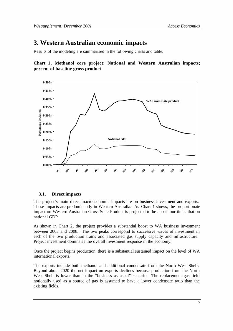
Chart 1. Methanol core project: National and Western Australian impacts; percent of baseline gross product
0.00%
0.05%
0.10%
0.15%
0.20%
0.25%
0.30%
0.35%
0.40%
0.45%
0.50%
2002
2004
2006
2008
2010
2012
2014
2016
2018
2020
2022
2024
2026
2028
2030
Perc
enta
ge d
evia
tion
WA Gross state product
National GDP
3.1. Direct impacts
The project’s main direct macroeconomic impacts are on business investment and exports. These impacts are predominantly in Western Australia. As Chart 1 shows, the proportionate impact on Western Australian Gross State Product is projected to be about four times that on national GDP.
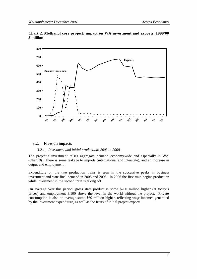
As shown in Chart 2, the project provides a substantial boost to WA business investment between 2003 and 2008. The two peaks correspond to successive waves of investment in each of the two production trains and associated gas supply capacity and infrastructure. Project investment dominates the overall investment response in the economy.
Once the project begins production, there is a substantial sustained impact on the level of WA international exports.
The exports include both methanol and additional condensate from the North West Shelf. Beyond about 2020 the net impact on exports declines because production from the North West Shelf is lower than in the “business as usual” scenario. The replacement gas field notionally used as a source of gas is assumed to have a lower condensate ratio than the existing fields.
WA supplement: December 2001 Access Economics
8
Chart 2. Methanol core project: impact on WA investment and exports, 1999/00 $ million
0
100
200
300
400
500
600
700
800
2002
2004
2006
2008
2010
2012
2014
2016
2018
2020
2022
2024
2026
2028
2030
Exports
Business investment
3.2. Flow-on impacts
3.2.1. Investment and initial production: 2003 to 2008
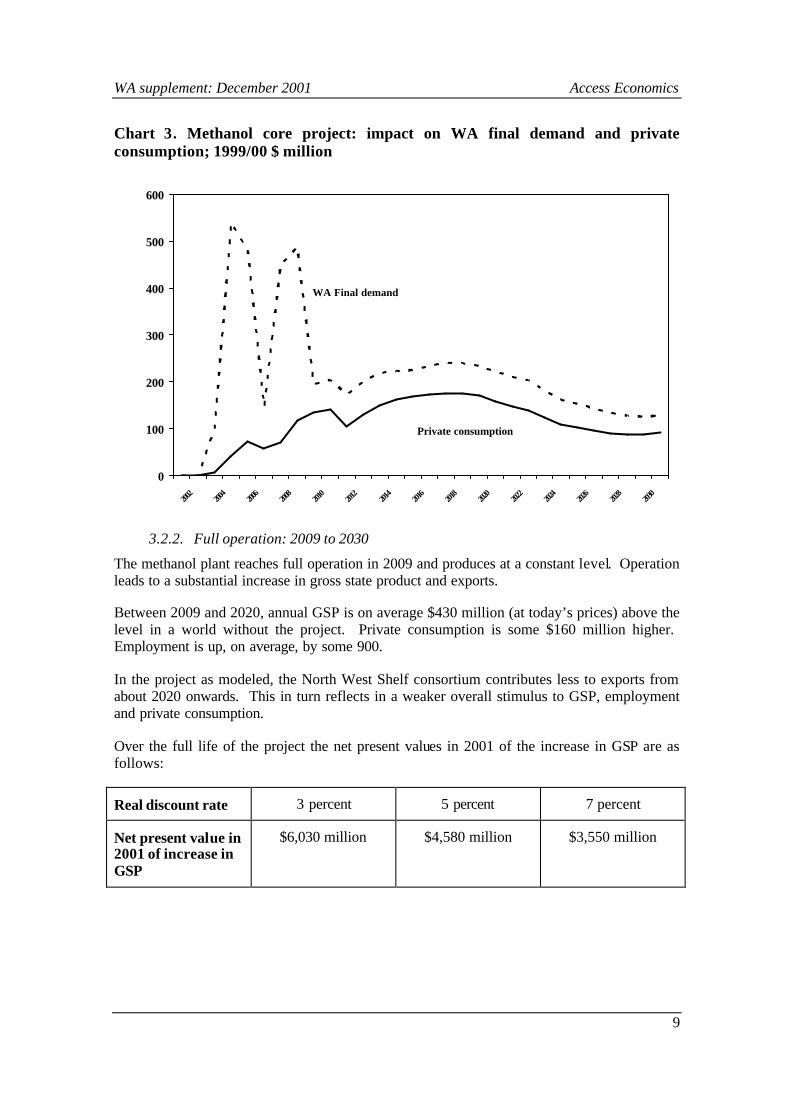
The project’s investment raises aggregate demand economy-wide and especially in WA (Chart 3). There is some leakage to imports (international and interstate), and an increase in output and employment.
Expenditure on the two production trains is seen in the successive peaks in business investment and state final demand in 2005 and 2008. In 2006 the first train begins production while investment in the second train is taking off.
On average over this period, gross state product is some $200 million higher (at today’s prices) and employment 3,100 above the level in the world without the project. Private consumption is also on average some $60 million higher, reflecting wage incomes generated by the investment expenditure, as well as the fruits of initial project exports.
WA supplement: December 2001 Access Economics
9
Chart 3. Methanol core project: impact on WA final demand and private consumption; 1999/00 $ million
0
100
200
300
400
500
600
2002
2004
2006
2008
2010
2012
2014
2016
2018
2020
2022
2024
2026
2028
2030
Private consumption
WA Final demand
3.2.2. Full operation: 2009 to 2030
The methanol plant reaches full operation in 2009 and produces at a constant level. Operation leads to a substantial increase in gross state product and exports.
Between 2009 and 2020, annual GSP is on average $430 million (at today’s prices) above the level in a world without the project. Private consumption is some $160 million higher. Employment is up, on average, by some 900.
In the project as modeled, the North West Shelf consortium contributes less to exports from about 2020 onwards. This in turn reflects in a weaker overall stimulus to GSP, employment and private consumption.
Over the full life of the project the net present values in 2001 of the increase in GSP are as follows:
Real discount rate 3 percent 5 percent 7 percent
Net present value in 2001 of increase in GSP
$6,030 million $4,580 million $3,550 million
WA supplement: December 2001 Access Economics
10
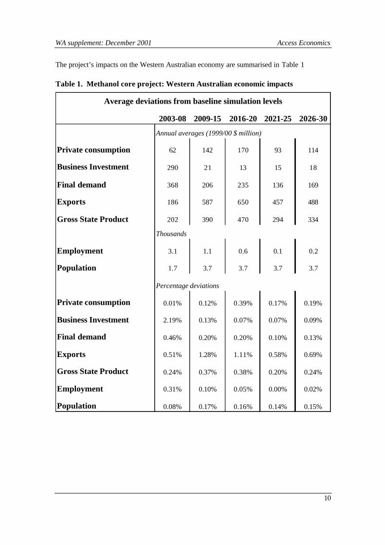
The project’s impacts on the Western Australian economy are summarised in Table 1
Table 1. Methanol core project: Western Australian economic impacts
Average deviations from baseline simulation levels
2003-08 2009-15 2016-20 2021-25 2026-30
Annual averages (1999/00 $ million)
Private consumption 62 142 170 93 114
Business Investment 290 21 13 15 18
Final demand 368 206 235 136 169
Exports 186 587 650 457 488
Gross State Product 202 390 470 294 334
Thousands
Employment 3.1 1.1 0.6 0.1 0.2
Population 1.7 3.7 3.7 3.7 3.7
Percentage deviations
Private consumption 0.01% 0.12% 0.39% 0.17% 0.19%
Business Investment 2.19% 0.13% 0.07% 0.07% 0.09%
Final demand 0.46% 0.20% 0.20% 0.10% 0.13%
Exports 0.51% 1.28% 1.11% 0.58% 0.69%
Gross State Product 0.24% 0.37% 0.38% 0.20% 0.24%
Employment 0.31% 0.10% 0.05% 0.00% 0.02%
Population 0.08% 0.17% 0.16% 0.14% 0.15%
WA supplement: December 2001 Access Economics
11
4. Western Australian Budget Impacts The project’s impacts on the Western Australian Budget were assessed using the methodology underlying Access Economics’ State Budget Monitor publication. State Budget Monitor operates over a six to seven year horizon, with comparisons against the current State Government outlooks (two to three years). It has recently been updated to use the new accrual accounting framework being progressively implemented by State Treasuries (currently Tasmania and the Northern Territory are the only areas not to have changed over).
For the purpose of this analysis, Access’ standard short term forecast horizon has been maintained (in line with the modelling of the Commonwealth Budget presented previously). Longer term projections have been obtained with policy consistency being maintained as much as possible. This is particularly important for revenue from the Commonwealth (in the form of GST and other payments), which is assumed to be distributed on the same basis as at present.
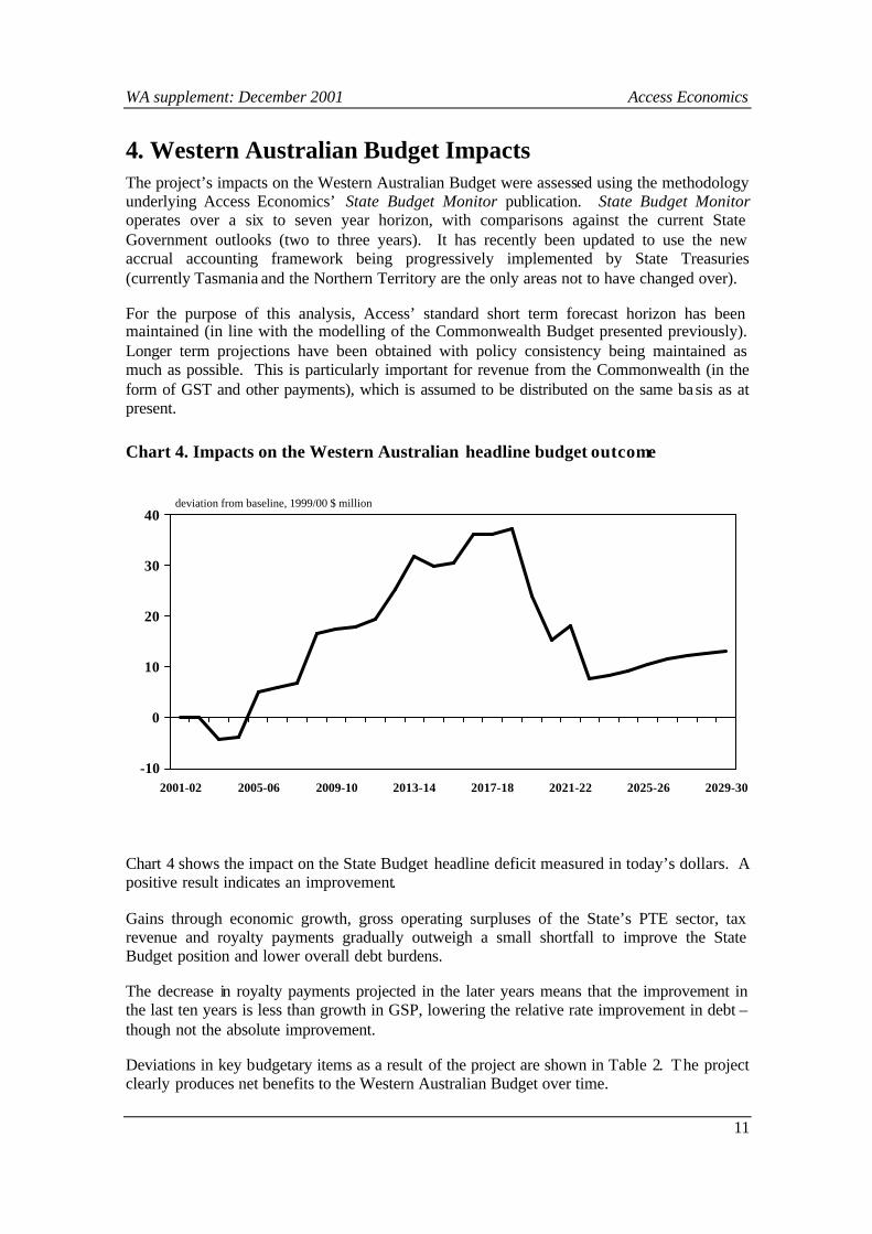
Chart 4. Impacts on the Western Australian headline budget outcome
-10
0
10
20
30
40
2001-02 2005-06 2009-10 2013-14 2017-18 2021-22 2025-26 2029-30
deviation from baseline, 1999/00 $ million
Chart 4 shows the impact on the State Budget headline deficit measured in today’s dollars. A positive result indicates an improvement.
Gains through economic growth, gross operating surpluses of the State’s PTE sector, tax revenue and royalty payments gradually outweigh a small shortfall to improve the State Budget position and lower overall debt burdens.
The decrease in royalty payments projected in the later years means that the improvement in the last ten years is less than growth in GSP, lowering the relative rate improvement in debt – though not the absolute improvement.
Deviations in key budgetary items as a result of the project are shown in Table 2. The project clearly produces net benefits to the Western Australian Budget over time.
WA supplement: December 2001 Access Economics
12
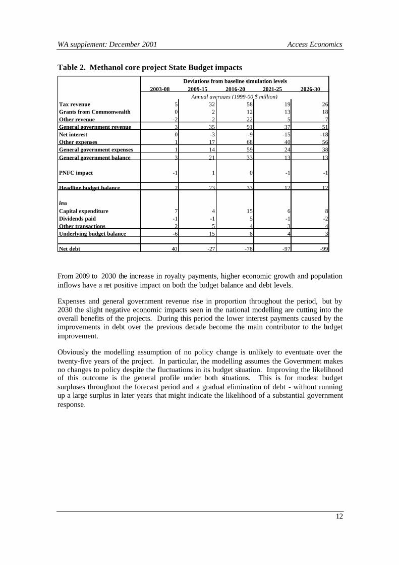
Table 2. Methanol core project State Budget impacts
2003-08 2009-15 2016-20 2021-25 2026-30
Tax revenue 5 32 58 19 26Grants from Commonwealth 0 2 12 13 18Other revenue -2 2 22 5 7General government revenue 3 35 91 37 51Net interest 0 -3 -9 -15 -18Other expenses 1 17 68 40 56General government expenses 1 14 59 24 38General government balance 3 21 33 13 13
PNFC impact -1 1 0 -1 -1
Headline budget balance 2 23 33 12 12
lessCapital expenditure 7 4 15 6 8Dividends paid -1 -1 5 -1 -2Other transactions 2 5 4 3 4Underlying budget balance -6 15 8 4 3
Net debt 40 -27 -78 -97 -99
Deviations from baseline simulation levels
Annual averages (1999-00 $ million)
From 2009 to 2030 the increase in royalty payments, higher economic growth and population inflows have a net positive impact on both the budget balance and debt levels.
Expenses and general government revenue rise in proportion throughout the period, but by 2030 the slight negative economic impacts seen in the national modelling are cutting into the overall benefits of the projects. During this period the lower interest payments caused by the improvements in debt over the previous decade become the main contributor to the budget improvement.
Obviously the modelling assumption of no policy change is unlikely to eventuate over the twenty-five years of the project. In particular, the modelling assumes the Government makes no changes to policy despite the fluctuations in its budget situation. Improving the likelihood of this outcome is the general profile under both situations. This is for modest budget surpluses throughout the forecast period and a gradual elimination of debt - without running up a large surplus in later years that might indicate the likelihood of a substantial government response.
WA supplement: December 2001 Access Economics
13
5. Overall impact on Western Australian economic welfare As with the national model, the state module of AE-MACRO allows the estimation of the project’s overall impact on state economic welfare. Since we do not have a good estimate of private wealth at the state level, the measure is less comprehensive than the national measure. It includes:
A. the increase in annual flows of private consumption and general government current expenditures that it allows, and
B. the decrease in public sector debt at the end of the simulation period.
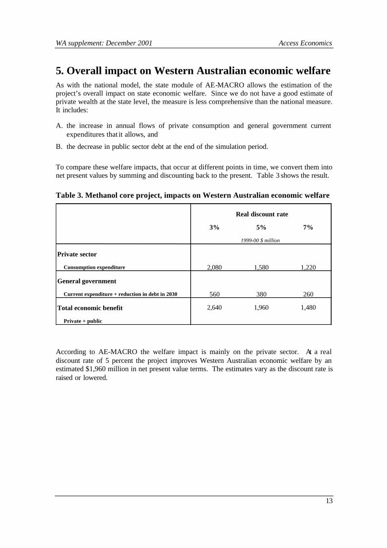
To compare these welfare impacts, that occur at different points in time, we convert them into net present values by summing and discounting back to the present. Table 3 shows the result.
Table 3. Methanol core project, impacts on Western Australian economic welfare
Real discount rate
3% 5% 7%
1999-00 $ million
Private sector
Consumption expenditure 2,080 1,580 1,220
General government
Current expenditure + reduction in debt in 2030 560 380 260
Total economic benefit 2,640 1,960 1,480
Private + public
According to AE-MACRO the welfare impact is mainly on the private sector. At a real discount rate of 5 percent the project improves Western Australian economic welfare by an estimated $1,960 million in net present value terms. The estimates vary as the discount rate is raised or lowered.
WA supplement: December 2001 Access Economics
14
5.1. Conclusion
Consistent with the national economic results, the methanol core project (comprising the methanol plant and associated infrastructure, plus upstream development by the North West Shelf Consortium) would have a substantial positive impact on:
• Western Australian exports, GSP, private consumption and employment;
• public sector finances; and on
• Western Australian economic welfare.
The impacts would be higher were full account taken of investment in additional gas supply, and the expected stimulus to other large scale gas -based industria l developments.
Access Economics December 2001
WA supplement: December 2001 Access Economics
15
6. Appendix: methodology 6.1. Modeling the WA economic impacts
The AE-MACRO model contains a State Forecasting Module which is fully integrated with the main mode. All simulations conducted on the AE-MACRO model can produce output for state variables.
State and territory forecasts are produced for output (both nominal and real), measures of inflation (the GSP deflator and consumer price index), population, and the number of people employed and unemployed, as well as motor vehicle registrations. The state module is linked to an industry module, which is used to calculate employment in the public sector (important for government wage expenditure) as well as some industry output variables that are used in the Budget modelling.
State and industry forecasts are produced initially using a ‘top down’ approach. National forecasts of components of final demand are produced from the main AE-MACRO model and these are split into state forecasts, using the methods outlined below.
The national forecasts used are:
• components of final demand (public and private consumption and investment, exports and imports etc);
• output, employment, unemployment and population;
• export, import and GDP price deflators.
The following methodology is used to calculate both state and industry output forecasts. As an example, consider the case where demand is rising (adding to the return to capital) yet bond yields are falling (reducing the required return to capital). That combination of factors will clearly induce extra investment by businesses.
• One implication is that the mining sector grows under this methodology, as mining growth is closely correlated to investment growth.
• Therefore, if the mining sector grows, then Western Australian output and employment do well relative to the rest of Australia, as Western Australia is relatively over -endowed with mining.
• To the extent mining is a relatively capital intensive industry, the boost to Western Australia’s employment is proportionately less than the boost to its output (and the same is true for employment at the national level).
The basic methodology links changes in output measures with the expected growth in industries, and then the expected implications for state economies.
At the same time, an estimate is made of the expected change in the state’s components of output. In general, the relative growth rates in consumption and investment are linked either to:
WA supplement: December 2001 Access Economics
16
• estimated output growth (calculated using the first methodology);
• estimated population growth, either total (for consumption measures) or in key demographic groups (in particular, dwelling investment, which is driven by growth in the 20-44 year-old population);
• one-off impacts (such as the initial investment in the core methanol project) which are added to Western Australian investment levels; or
• longer term implications of the core methanol project’s investment – for example a relatively large share of the expected boost to national merchandise exports.
In deciding what allowance to make for the impacts of the core methanol project, we have been influenced by results obtained in earlier Access Economics analyses of comparable resource projects using the AE-CGE computable general equilibrium model.
The increases in employment over the course of the project have implications for the state’s population. In general, population will move towards employment prospects, so a boost to employment levels will – in the long term – draw relatively more of the national population to Western Australia. Because the projected decline in the stimulus to employment in the later years of the forecast occurs across Australia (rather than just in Western Australia) the population does not ebb back to the rest of Australia as job gains in the West are lost. This would only occur if WA were doing worse than elsewhere.
The output figures determined in the main model (as well as the components of final demand) are all in real terms. To obtain nominal GSP forecasts (required for Budgetary modelling), the real forecasts are multiplied by a state GSP deflator. This is calculated using each state’s share of Australia’s imports and exports, as well as import, export and GDP price deflators.
The GDP price deflator is stripped of the effects of import price changes and has export price changes added on. This gives a GNE deflator. By adding back import changes and removing export changes proportionally to their impor tance in a given state gives a state GSP deflator.
State nominal GSP is then calculated using the state deflator, and normalised to ensure the state values sum to the national forecast for nominal GDP.
State interim unemployment is calculated by altering the rate of national unemployment growth to account for changes in labour force and employment in each state. The formula ensures that states with higher employment growth, and lower population growth, have lower unemployment growth. These figures are also normalised to sum to the national forecast, providing final state unemployment estimates.
6.2. Modeling the state budge t
The main analytical focus of the modeling is the State non-financial public sector as a whole (the “State sector”). However, Access Economics analyses the fiscal performance and position of the State sector for each State by distinguishing the contributions made by the two component sectors, namely:
• the general government sector (“GG sector”) – comprising the units of government mainly engaged in the provision of goods and services free of charge or at nominal charge well below the cost of production and mainly funded from taxation revenues ; and
WA supplement: December 2001 Access Economics
17
• the public non-financial corporation sector (“PNFC sector”, previously public trading enterprises (PTEs)) – comprising the government-owned businesses mainly engaged in the production of goods and services of a non-financial nature for sale in the market place at economically significant prices.
The GG sector is the sector over which individual state governments exercise direct control. Control over the PNFC sector is indirect, exercised mainly in a manner akin to a controlling shareholder.
In compiling the sector statistics, transactions and debtor -creditor relationships between the two component sectors are eliminated to avoid double counting.
The State sector excludes all public financial corporations (PFCs). Central borrowing authorities are classified as being in the public financial sector and so are outside the State sector.
The State Budget modelling undertaken by Access Economics now also focuses on the accruals-based government finance statistics (GFS) series being published by State governments and the Australian Bureau of Statistics (ABS). This replaced the cash-based methodology used previously. The accruals methodology changes the timing of a number of transactions, and limits the ability of State s to move these transactions from year to year without reasonable justification. The main aggregates determined under the accruals methodology do not differ significantly from earlier cash based calculations – it is usually in the detail that differences appear.
In the statistical series provided under the new GFS guidelines, four indicators of a government “fiscal balance” are provided, namely:
• the net operating balance : an accruals-based measure of the operating (or current) balance;
• the net cash flow from operations : a cash-based measure of the operating balance;
• the net lending(+)/borrowing(-): an accruals -based measure of the overall fiscal balance; and
• the cash surplus(+)/deficit(-): a cash-based measure of the overall fiscal balance.
Access Economics adds two indicators to this list:
• the underlying cash deficit(+)/surplus(-): the cash-based measure of the overall fiscal balance but using the previous sign convention; and
• the net borrowing requirement(+)/repayment(-) : which measures the change in net debt as a consequence of annual financial transactions.
While the sign convention in State Budget Monitor are as shown above, for the Methanex analysis the reverse has been used to maintain the convention that a positive outcome means an improvement in the Budget conditions in Western Australia.
The use of all indicators will invariably lead to confusion. Moreover, discretion as to the use of indicator will lead to a temptation for some to choose the indicator(s) which put a State
WA supplement: December 2001 Access Economics
18
government in the best (or worst) light. We prefer to make a transparent choice up front, and have opted to use the ‘net operating balance’ indicator largely on pragmatic grounds: the States provide a more detailed breakdown of their income and expenses items than they do of their cash operating revenues and cash operating payments items, which therefore provides a stronger basis for forecasting. The ‘net operating balance’ is described as the ‘headline Budget balance’ in the tables.
The overall fiscal balance (or ‘underlying Budget balance’) is generally calculated by one of two means. One is an accruals-based measure (the ‘net lending/borrowing’ indicator) while the others are cash-based measures (the ‘overall surplus/deficit’, its obverse the ‘underlying cash deficit’ and the ‘net borrowing requirement’).
The Commonwealth Treasury (“Fiscal Policy Under Accrual Accounting”, April 1999) has stated that:
“The two measures will differ due to differences between accrual transactions and cash flows. In the medium-term both should indicate a similar fiscal stance and hence government contribution to the external current account deficit. …
Nevertheless, the two fiscal indicators will diverge in the short-term. The [net lending/borrowing indicator of the] fiscal balance will detect non-monetary effects, such as increases in accruing superannuation entitlements which would be ignored by the underlying cash balance. Conversely, the underlying cash balance will detect cash transactions such as superannuation payouts (outlays), that do not effect the fiscal balance. Neither indicator will perfectly detect demand effects. …Both indicators … will need to be observed in reaching conclusions about the demand effect of the fiscal stance.” (p.12)
For the purposes of this analysis the difference to the baseline of the Methanex core project under the two measures are identical, and both are labelled as ‘underlying Budget balance’ in the tables.
The final aggregate value (Net debt) changes with the underlying Budget balance in each year. Overall changes to net debt therefore, are the aggregate changes to the underlying Budget balance. Of course, a change in net debt in one year will also affect later underlying deficits or surpluses, mainly through changes to interest payments on debts. While (in nominal terms, rather than the real terms reported above) net debt is roughly $222 million lower by 2029-30, this roughly matches the lower interest repayments required over the period.
While every effort has been made to ensure the accuracy of this document, the uncertain nature of economic data, forecasting and analysis means that Access Economics Pty Ltd is unable to make any warranties in relation to the information contained herein. Access Economics Pty Ltd, its employees and agents disclaim liability for any loss or damage which may arise as a consequence of any person relying on the information contained in this document.
THE AUSTRALIAN NATIONAL ECONOMIC IMPACT OF THE METHANEX METHANOL PROJECT
prepared for
Methanex Australia Pty Ltd
by
ACCESS ECONOMICS
Canberra December 2001
National report: December 2001 Access Economics
1
Table of contents
1. Executive Summary .........................................................................................................2
2. Introduction......................................................................................................................5
2.1. The project...................................................................................................................................................................5
2.2. Modeling approach....................................................................................................................................................6
3. Results of the modeling ....................................................................................................8
3.1. Direct impacts .............................................................................................................................................................8
3.2. Flow-on impacts .........................................................................................................................................................9
4. Overall impacts on public sector finances and economic welfare ............................. 13
4.1. Impact on overall public sector finances .............................................................................................................13
4.2. Impact on the Commonwealth Budget..................................................................................................................14
4.3. Impact on Australian economic welfare...............................................................................................................15
4.4. Conclusion.................................................................................................................................................................16
5. Appendix A. Application of the AE -MACRO Model................................................. 17
5.1. Introduction...............................................................................................................................................................17
5.2. Modeling the methanol project..............................................................................................................................18
5.3. Economic assumptions ............................................................................................................................................19
5.4. Application to the core methanol project.............................................................................................................20
5.5. Commonwealth Budget impacts ............................................................................................................................25
5.6. Measurement of economic welfare........................................................................................................................26
5.7. Limitations of the modeling results .......................................................................................................................27
National report: December 2001 Access Economics
2
1. Executive Summary Methanex has commissioned Access Economics to assess the national and Western Australian economic impacts of the proposed methanol project using gas from the North West Shelf. We have done this using national and state modules of the Access Economics’ AE-MACRO model of the Australian economy.
This report contains our assessment of the national economic and budgetary impacts. Western Australian impacts are explored in a supplementary report1.
The project
The core methanol project considered in this report comprises the methanol plant, together with upstream developments by the North West Shelf Consortium to supply the natural gas input, and port and other infrastructure developments associated with the project. Additional downstream developments may be stimulated by the success of the Methanex project. Their impacts are considered separately below.
Key statistics for the core project, as modeled in this study, include:
• total capital expenditure in excess of A$2 billion between 2003 and 2008. Construction of the methanol plant will provide employment for around 1,000 on-site construction employees for most of that time;
• annual production of 2.1 million tonnes of methanol from 20062, rising to 4.2 million tonnes from 2009 with the completion of the second production train. The mode lling horizon extends to 2030. Each train will use approximately 70 PJ of natural gas annually;
• a direct contribution to the balance of payments from methanol exports and import replacement of A$460 million from 2006, and A$940 million from 2009;
• direct employment at the methanol plant of approximately 150 people;
• additional tax and royalty payments to governments estimated at some $4.0 billion (in today’s prices) over the life of the project, under current tax arrangements. In net present value terms this comes to $2.0 billion at a 5 percent real discount rate.
Modeling results
According to our modeling, the core methanol project would generate substantial positive economic impacts.
During the initial investment phase (between 2003 and 2008):
• the project’s investment temporarily raises aggregate demand economy-wide. There is some leakage to imports, and an increase in output and employment;
1 Access Economics, The Western Australian economic impact of the Methanex methanol project , Supplementary report to Methanex Australia Pty Ltd, Canberra, December 2001 2 Project start -up is in 2005, but the analysis commences based on the first full year of operation in 2006.
National report: December 2001 Access Economics
3
• GDP increases by $480 million (at today’s prices 3) in the year 2005, and employment by 5,700. Private consumption is over $200 million higher at this point;
• the increases in GDP and consumption are still larger at the end of this period since the first train is now producing, while the second is being built.
• there is a rise in inflation and interest rates, but these are falling again by the end of the period.
During full operation (from 2009 onwards):
• the project causes a substantial increase in gross domestic product and exports. This in turn allows an increase in imports. The economy benefits also from accelerated exploitation of North West Shelf gas resources;
• the project raises government revenues, allowing a cut in personal income taxes. Higher consumer demand reflects in higher imports, but also an increase in Australian production and employment;
• between 2009 and 2020, annual GDP is on average $1,050 million (at today’s prices) above the level in a world without the project. The net present value of the increase in GDP is $11.4 billion at a 5 per cent real discount rate. Private consumption is some $620 million higher. Employment is up, on average, by some 2,700;
• in the project as modeled, the North West Shelf consortium contributes less to exports and government revenues from about 2020 onwards as gas and condensate production fall below the levels in the baseline. This in turn reflects in a weaker overall stimulus to GDP, employment and private consumption.
Impacts on public sector finances and Australian economic welfare
Key measures of the core methanol project’s potential contribution to the Australian economy are its overall impacts on overall public sector finances, the Commonwealth budget and on economic welfare.
We measure the overall impact on public sector finances as the sum of the model’s estimates of additional public sector revenues, plus the revenue foregone through income tax cuts:
• on this definition, the net present value of the impact on overall public sector finances is an estimated $3.3 billion in 2001 at a real discount rate of 5 percent;
• using a similar definition of net impact, the ne t present value of the impact on Commonwealth budget finances is an estimated $1.8 billion in 2001 at a real discount rate of 5 percent.
3 Throughout the report and analysis, “today’s prices” are defined as being in dollars of 1999/00. This year is used as a base because it is the year in terms of which constant price series of the Australian National Accounts are expressed.

National report: December 2001 Access Economics
4
In AE-MACRO the best measures of the project’s overall impact on economic welfare are:
A. the increase in annual flows of private consumption and public sector final expenditures that it allows, and
B. the increase in public and private sector wealth at the end of the simulation period. [This is the best available indicator of the possible impact beyond that date.]
As modeled, in net present value terms, the welfare impact is mainly on the private sector.
• At a real discount rate of 5 percent the project improves Australian economic welfare by an estimated $8.3 billion (net present value in 2001).
Potential for additional downstream development
Once the Methanex deal goes ahead it is expected that other world scale gas feedstock customers will be more likely to be attracted to the Burrup Peninsula than would otherwise be the case. The portfolio of additional customers for North West Shelf feedstock gas is understood to include customers each with gas demand in the range of 90 - 500 TJ/d. Methanex’ investment is expected to lead to an increased probability of each of these developments going ahead, such that the total expected gas demand is increased by around 100 TJ/d.
• The additional expected macro benefits above the base analysis have not been explicitly modeled, but are likely to be about one quarter of those estimated for the core methanol project (which will use about four times the amount of gas).
• Based on the modeling of the core methanol project, this could mean an expected additional annual $250 million of GDP, annual $130 million of private consumption, and national employment of 700 persons during the project(s)’ ope ration. As a rough indication, the net present values of the increases in Commonwealth budget finances and GDP could be of the order of $450 million and $2.8 billion respectively.
Conclusion
As modeled, the core project comprising Methanex’ proposed Western Australian methanol plant, associated infrastructure development, and the expansion of natural gas supply by the North West Shelf Consortium would have a substantial positive impact on:
• exports, GDP, employment and private consumption;
• public sector finances and the Commonwealth budget; and on
• Australian economic welfare.
The impacts would be higher were full account taken of investment in additional gas supply, and the expected stimulus to other large scale gas -based industrial developments.
Access Economics December 2001
National report: December 2001 Access Economics
5
2. Introduction Methanex has commissioned Access Economics to assess the national and Western Australian economic impacts of the proposed methanol project using gas from the North West Shelf.
This report contains our assessment of the national economic and budgetary impacts. Western Australian impacts are explored in a supplementary report4.
2.1. The project
Core methanol project
The core project considered in this report comprises the methanol plant, together with upstream developments by the North West Shelf Consortium to supply the natural gas input, and port and other infrastructure developments associated with the project.
The methanol project will convert natural gas from the North West Shelf into methanol, using a catalytic process. The plant will be located on the Burrup Peninsula in the Pilbara region. There will be two production trains, each with annual methanol capacity of 2.1 million tonnes, coming on stream in 2006 and 2009. The modelling horizon extends to 2030. Each train w ill use approximately 70 PJ of natural gas annually.
The methanol will primarily be exported to Asia. A small proportion of production (3 percent initially) will replace imports in the Australian market. There will be a substantial positive impact on the balance of payments.
The initial investment will be in excess of $2 billion spread over the period 2003 to 2008. There will be work for around 1,000 on-site construction employees for most of that time. During operation the plant will directly employ approximately 150 persons. There will be additional employment for subcontractors.
The North West Shelf Consortium advises that it will invest an additional $A100 million between 2003 and 2008 to expand natural gas production. Other capital costs to explo it the natural gas reserves will also be incurred earlier than would otherwise be the case. Supply to the methanol project will bring forward production of condensate (for export) and the payment of royalties to the Commonwealth and Western Australian governments. This raises export income and tax payments in the next 20 years. In the latter part of the period (beyond 2020), the consortium’s reserves become depleted. Gas and condensate sales from the consortium’s resources, and tax and royalty payments, are then lower than might otherwise have been the case.
The methanol project will also require investment in infrastructure for channel dredging, provision of methanol loading berths, seawater supply and desalination, and access roads and service corridors.
In addition to the direct impacts on net exports and employment, Methanex and the North West Shelf will have ongoing local operational expenditures. There will also be substantial payments of company tax and natural gas royalties to the Commonwealth. In the case of the 4 Access Economics, The Western Australian economic impact of the Methanex methanol project , Supplementary report to Methanex Australia Pty Ltd, Canberra, December 2001
National report: December 2001 Access Economics
6
North West Shelf Consortium, these payments will be partly a bringing forward of a revenue stream. For the methanol plant, tax payments would not eventuate unless the investment proceeds.
Potential for downstream economic development
The core methanol project is a conservative approach to the estimation of economic benefits. It makes limited allowance for the stimulus that the methanol project will give to the development of new offshore gas reserves to replace those committed by the North West Shelf; and no allowance for possible development of other gas -based industrial plants in the Pilbara.
The North West Shelf is an attractive location for large-scale gas customers including gas-to-liquids, petrochemical and mineral processing/refining plants. Over the medium term it is likely that some of these projects will come to fruition, attracted to the vicinity of the Burrup Peninsula by the supply of competitively priced feedstock gas and infrastructure.
Once the Methanex deal goes ahead it is expected that other world scale gas feedstock customers will be more likely to be attracted to the Burrup Peninsula than would otherwise be the case. They will see Methanex’ investment as a catalyst to providing a business, infrastructure, regulatory and gas supply environment conducive to world scale industrial development. Any of these developments would require the investment of many hundreds of millions of dollars and generate many hundreds of construction jobs, substantial export or import replacement revenues and taxes.
The portfolio of additional customers for North West Shelf feedstock gas is understood to include customers each with gas demand in the range of 90 - 500 TJ/d. Methanex’ investment is expected to lead to an increased probability of each of these developments going ahead, such that the total expected gas demand is increased by around 100 TJ/d by around 2010 (i.e. equivalent to a new feedstock gas customer using 100 TJ/d due to the presence of Methanex).
The additional expected macro benefits above the base analysis have not been explicitly modeled, but are likely to be about one quarter of those estimated for the core methanol project (which will use about four times the amount of gas).
• Based on the modeling of the core methanol pr oject, his could mean an expected additional annual $250 million of GDP, annual $130 million of private consumption, and national employment of 700 persons during the project(s)’ operation. As a rough indication, the net present values of the increases in Commonwealth budget finances and GDP could be of the order of $450 million and $2.8 billion respectively.
2.2. Modeling approach
We have analysed the national economic impacts of the project using Access Economics AE-MACRO macroeconomic model of the Australian economy.
AE-MACRO is a relatively small dynamic model of the Australian economy. It was developed in 1992 by Access Economics, and is based on standard modeling practice. It has a stable long-term growth path that accords with neoclassical economic theory, together with short-term dynamics derived from Australian economic experience over the past 25 years.
National report: December 2001 Access Economics
7
The analysis involves comparing two long-term simulations of the AE-MACRO model. The first (“No change” scenario) is a standard long-run projection, based on Access Economics assumptions about trends in major economic variables. In the second, we take the model used in the standard projection and add the methanol project. The difference between the two simulations provides an indication of the likely macroeconomic impact of the project.
Methanex and the North West Shelf Consortium provided most of the necessary data for the project, including projections of production and input quantities, capital and current expenditures, and financing. Access Ec onomics has adjusted this data to fit its own long-term projections of inflation and exchange rates, but has not sought otherwise to verify the data provided.
One important area where Access Economics has relied on its own judgements concerns the prices of methanol, natural gas and condensate byproduct.
For reasons of commercial confidentiality, Methanex did not provide us with a projection of the Australian methanol export price. They did provide consultants’ reports analysing price trends in the US methanol market, together with indications of the likely relationship to Asian prices and of transport costs from the Pilbara to Asian destinations. Based on these indications, and on our own projections of the $US/$A exchange rate, we have derived an Australian export price for methanol. This price is based on a projected US methanol price that is constant at $US140 per tonne up till 2010 and then escalates at the projected US general inflation rate.
For natural gas sold to Methanex, we have relied on an indicative pricing formula that allows for price escalation. In relation to this price, we note that higher prices (lower profits) to Methanex would translate directly to higher revenues (higher profits) to the consortium. As a result varying this formula would mostly have little net effect on the economic impacts computed by the model (though it would have some impact on projected royalty payments by the consortium).
For condensate exported by the consortium, we have assumed that the price is fixed in $US terms until 2010 and then escalates in line with US inflation. Similarly, for natural gas purchased by the consortium beyond 2020 to supplement dwindling North West Shelf reserves, we have assumed that the price escalates in line with the US inflation.
The results reported in this paper are a projection, on the assumption that past economic trends and current policies continue. The results are conditional on the numerous assumptions required in the modeling. They represent a potential outcome, rather than an exact forecast of the long-term behaviour of the economy. Further details are of the modeling approach are given in Appendix A.
National report: December 2001 Access Economics
8
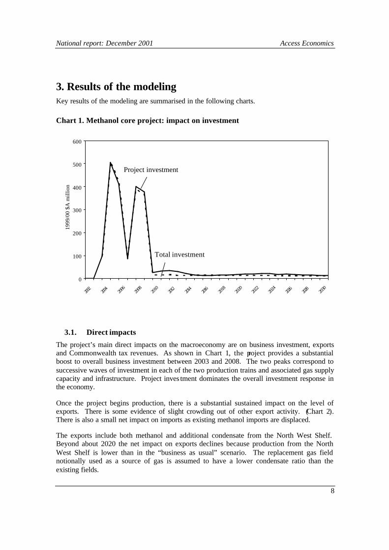
3. Results of the modeling Key results of the modeling are summarised in the following charts.
Chart 1. Methanol core project: impact on investment
0
100
200
300
400
500
600
2002
2004
2006
2008
2010
2012
2014
2016
2018
2020
2022
2024
2026
2028
2030
1999
/00
$A m
illio
n
Total investment
Project investment
3.1. Direct impacts
The project’s main direct impacts on the macroeconomy are on business investment, exports and Commonwealth tax revenues. As shown in Chart 1, the project provides a substantial boost to overall business investment between 2003 and 2008. The two peaks correspond to successive waves of investment in each of the two production trains and associated gas supply capacity and infrastructure. Project inves tment dominates the overall investment response in the economy.
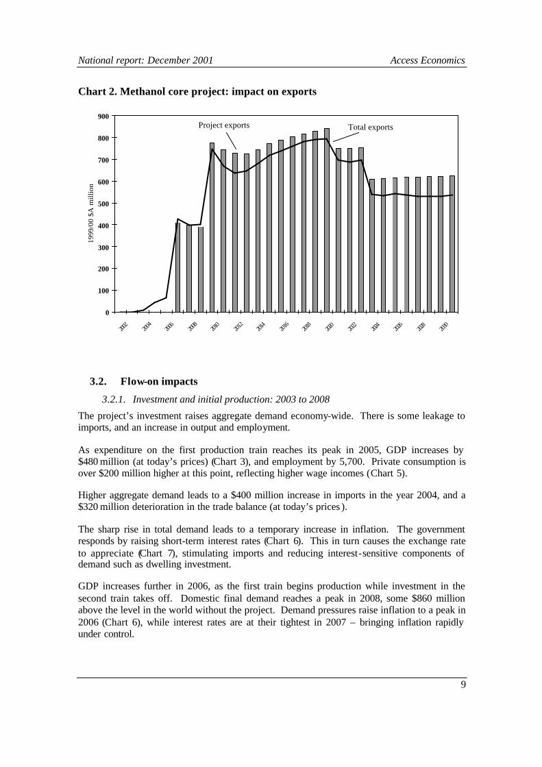
Once the project begins production, there is a substantial sustained impact on the level of exports. There is some evidence of slight crowding out of other export activity. (Chart 2). There is also a small net impact on imports as existing methanol imports are displaced.
The exports include both methanol and additional condensate from the North West Shelf. Beyond about 2020 the net impact on exports declines because production from the North West Shelf is lower than in the “business as usual” scenario. The replacement gas field notionally used as a source of gas is assumed to have a lower condensate ratio than the existing fields.
National report: December 2001 Access Economics
9
Chart 2. Methanol core project: impact on exports
0
100
200
300
400
500
600
700
800
900
2002
2004
2006
2008
2010
2012
2014
2016
2018
2020
2022
2024
2026
2028
2030
1999
/00
$A m
illio
n
Total exportsProject exports
3.2. Flow-on impacts
3.2.1. Investment and initial production: 2003 to 2008
The project’s investment raises aggregate demand economy-wide. There is some leakage to imports, and an increase in output and employment.
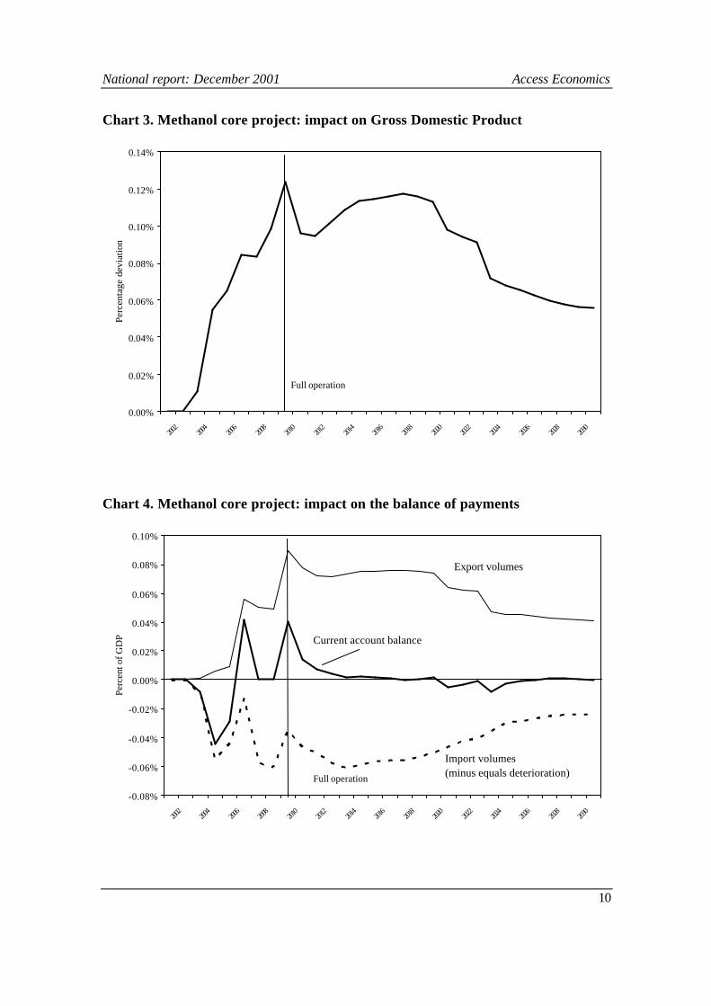
As expenditure on the first production train reaches its peak in 2005, GDP increases by $480 million (at today’s prices) (Chart 3), and employment by 5,700. Private consumption is over $200 million higher at this point, reflecting higher wage incomes (Chart 5).
Higher aggregate demand leads to a $400 million increase in imports in the year 2004, and a $320 million deterioration in the trade balance (at today’s prices ).
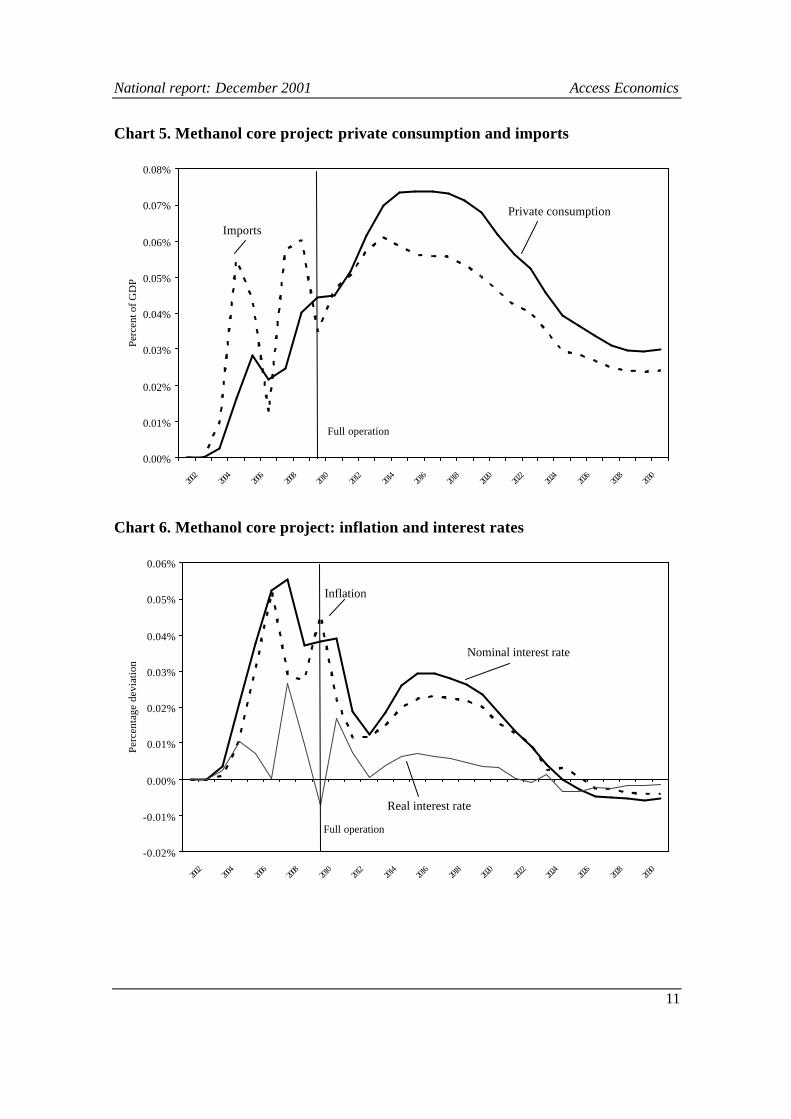
The sharp rise in total demand leads to a temporary increase in inflation. The government responds by raising short-term interest rates (Chart 6). This in turn causes the exchange rate to appreciate (Chart 7), stimulating imports and reducing interest-sensitive components of demand such as dwelling investment.
GDP increases further in 2006, as the first train begins production while investment in the second train takes off. Domestic final demand reaches a peak in 2008, some $860 million above the level in the world without the project. Demand pressures raise inflation to a peak in 2006 (Chart 6), while interest rates are at their tightest in 2007 – bringing inflation rapidly under control.
National report: December 2001 Access Economics
10
Chart 3. Methanol core project: impact on Gross Domestic Product
0.00%
0.02%
0.04%
0.06%
0.08%
0.10%
0.12%
0.14%
2002
2004
2006
2008
2010
2012
2014
2016
2018
2020
2022
2024
2026
2028
2030
Perc
enta
ge d
evia
tion
Full operation
Chart 4. Methanol core project: impact on the balance of payments
-0.08%
-0.06%
-0.04%
-0.02%
0.00%
0.02%
0.04%
0.06%
0.08%
0.10%
2002
2004
2006
2008
2010
2012
2014
2016
2018
2020
2022
2024
2026
2028
2030
Perc
ent o
f GD
P
Import volumes(minus equals deterioration)
Current account balance
Export volumes
Full operation
National report: December 2001 Access Economics
11
Chart 5. Methanol core project: private consumption and imports
0.00%
0.01%
0.02%
0.03%
0.04%
0.05%
0.06%
0.07%
0.08%
2002
2004
2006
2008
2010
2012
2014
2016
2018
2020
2022
2024
2026
2028
2030
Perc
ent o
f GD
P
Private consumption
Imports
Full operation
Chart 6. Methanol core project: inflation and interest rates
-0.02%
-0.01%
0.00%
0.01%
0.02%
0.03%
0.04%
0.05%
0.06%
2002
2004
2006
2008
2010
2012
2014
2016
2018
2020
2022
2024
2026
2028
2030
Perc
enta
ge d
evia
tion
Inflation
Nominal interest rate
Full operation
Real interest rate
National report: December 2001 Access Economics
12
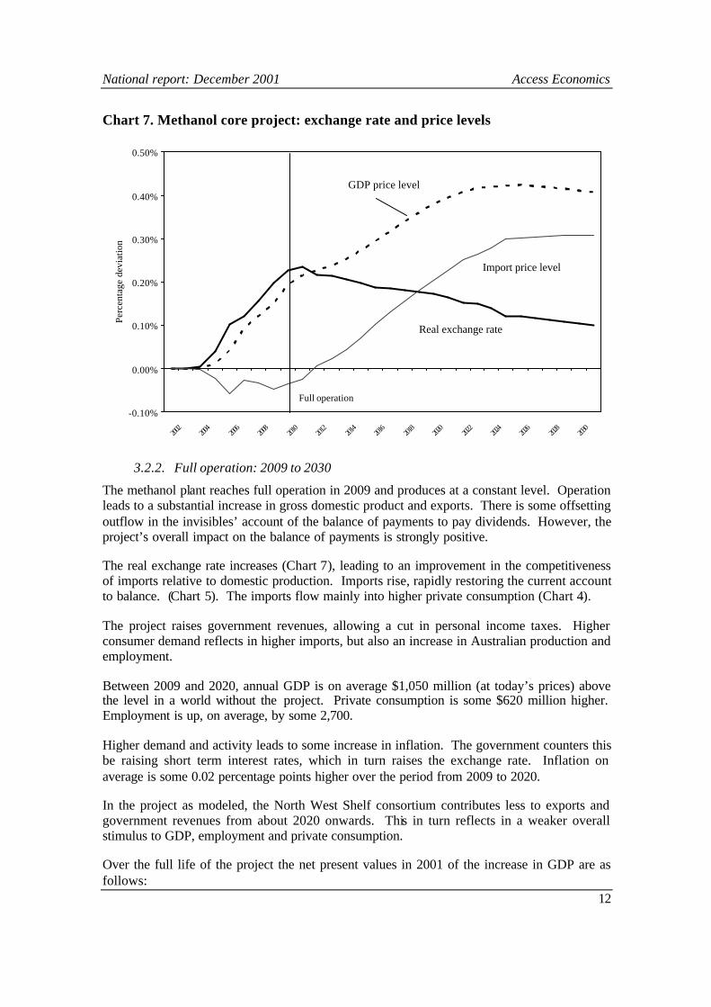
Chart 7. Methanol core project: exchange rate and price levels
-0.10%
0.00%
0.10%
0.20%
0.30%
0.40%
0.50%
2002
2004
2006
2008
2010
2012
2014
2016
2018
2020
2022
2024
2026
2028
2030
Perc
enta
ge d
evia
tion
GDP price level
Import price level
Full operation
Real exchange rate
3.2.2. Full operation: 2009 to 2030
The methanol plant reaches full operation in 2009 and produces at a constant level. Operation leads to a substantial increase in gross domestic product and exports. There is some offsetting outflow in the invisibles’ account of the balance of payments to pay dividends. However, the project’s overall impact on the balance of payments is strongly positive.
The real exchange rate increases (Chart 7), leading to an improvement in the competitiveness of imports relative to domestic production. Imports rise, rapidly restoring the current account to balance. (Chart 5). The imports flow mainly into higher private consumption (Chart 4).
The project raises government revenues, allowing a cut in personal income taxes. Higher consumer demand reflects in higher imports, but also an increase in Australian production and employment.
Between 2009 and 2020, annual GDP is on average $1,050 million (at today’s prices) above the level in a world without the project. Private consumption is some $620 million higher. Employment is up, on average, by some 2,700.
Higher demand and activity leads to some increase in inflation. The government counters this be raising short term interest rates, which in turn raises the exchange rate. Inflation on average is some 0.02 percentage points higher over the period from 2009 to 2020.
In the project as modeled, the North West Shelf consortium contributes less to exports and government revenues from about 2020 onwards. This in turn reflects in a weaker overall stimulus to GDP, employment and private consumption.
Over the full life of the project the net present values in 2001 of the increase in GDP are as follows:

National report: December 2001 Access Economics
13
Real discount rate 3 percent 5 percent 7 percent
Net present value in 2001 of increase in GDP
$15.1 billion $11.4 billion $8.9 billion
4. Overall impacts on public sector finances and economic welfare
Key elements of the methanol project’s potential contribution to the Australian economy are via its overall impacts on overall public sector finances, the Commonwealth budget and on national economic welfare. We consider these in the following sections.
4.1. Impact on overall public sector finances
The project and the additional economic growth it stimulates generate substantial additional revenue for governments. The Australian public sector includes:
• the Commonwealth budget sector
• the combined state/territory budget sectors
• Commonwealth and state/territory off -budget authorities
• local government
This section considers the impact on the public sector as a whole.
4.1.1. Core methanol project’s direct contribution
The core methanol project itself is projected to make additional tax and royalty payments to governments estimated at some $4.1 billion (in today’s prices) over the life of the project, under current tax arrangements. In net present value terms this comes to $2.0 billion at a 5 percent real discount rate (and $2.6 billion and $1.6 billion at real discount rates of 3 percent and 7 percent respectively).
The largest contribution is in the form of additional company tax paid to the Commonwealth.
4.1.2. Core methanol project’s overall impact
Governments are assumed to respond to increased revenues from the project and the additional growth stimulated by it. They do this by increasing expenditures in line with the growth in the economy, and reducing the average personal income tax rate to keep the ratio of public debt to GDP from falling too rapidly. Income tax reductions in turn stimulate further growth.
Table 1 summarises these impacts as net present values in $ million in 2001, for a variety of real discount rates.

National report: December 2001 Access Economics
14
Table 1. Methanol core project: Impact on public sector finances
Total public sector 3% 5% 7% 1999-00 $ million
Additional expenditure plus 1,760 1,360 1,070Net lending -700 -580 -470 equals Revenue increase 1,060 780 600 plus Revenue foregone through tax cut 3,080 2,540 2,190 equals Total public sector gains 4,140 3,320 2,790
Real discount rateNet present values over the period 2001 to 2030
The overall public sector gain is defined as the sum of additional revenue actually received, together with that foregone through the tax cut. This in turn equals the sum of additional expenditure by governments and their additional net lending to other sectors of the economy. This latter item is negative in Table 1, indicating that the projected tax cut runs ahead of the additional revenue less additional expenditure.
At a discount rate of 5 percent in real terms, the project generates a positive contribution of $3.3 billion.
4.2. Impact on the Commonwealth Budget
The impacts of the project on the Commonwealth budget can also be isolated. The Commonwealth receives direct company tax and some royalty payments as a result of the project. Commonwealth tax receipts also benefit from the increased economic activity the project generates, while there is reduced cyclical expenditure on the likes of unemployment benefits.
Recorded budget revenues decline given the induced income tax cut which arises as a reaction to the revenue growth the project creates. However, adding back the tax revenue foregone via the income tax cut shows the solid Budget gains which would accrue to the Commonwealth.
Table 2 summarises these impacts as in 2001 in $ million, for a variety of real discount rates. The total Commonwealth budget gains are defined in the same way as in Table 1. At a real discount rate of 5 percent the net present value of overall Commonwealth budget gains is projected at some $1.8 billion.
Further details on the impacts on Commonwealth revenue and expenditure items are provided in the Appendix.
National report: December 2001 Access Economics
15
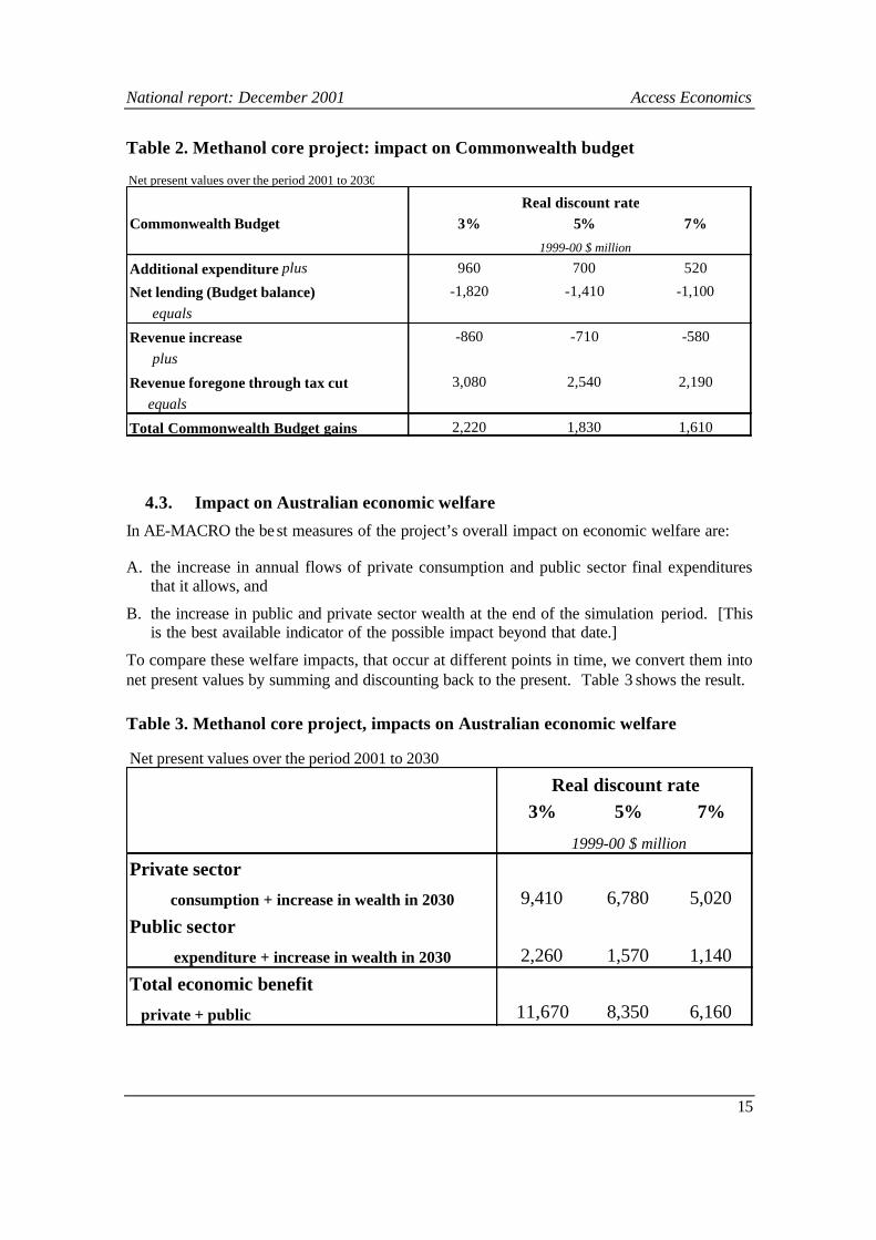
Table 2. Methanol core project: impact on Commonwealth budget
Commonwealth Budget 3% 5% 7%
1999-00 $ million
Additional expenditure plus 960 700 520
Net lending (Budget balance) -1,820 -1,410 -1,100 equals
Revenue increase -860 -710 -580 plus
Revenue foregone through tax cut 3,080 2,540 2,190 equals
Total Commonwealth Budget gains 2,220 1,830 1,610
Net present values over the period 2001 to 2030
Real discount rate
4.3. Impact on Australian economic welfare
In AE-MACRO the best measures of the project’s overall impact on economic welfare are:
A. the increase in annual flows of private consumption and public sector final expenditures that it allows, and
B. the increase in public and private sector wealth at the end of the simulation period. [This is the best available indicator of the possible impact beyond that date.]
To compare these welfare impacts, that occur at different points in time, we convert them into net present values by summing and discounting back to the present. Table 3 shows the result.
Table 3. Methanol core project, impacts on Australian economic welfare
3% 5% 7%
1999-00 $ million
Private sector
consumption + increase in wealth in 2030 9,410 6,780 5,020
Public sector
expenditure + increase in wealth in 2030 2,260 1,570 1,140
Total economic benefit
private + public 11,670 8,350 6,160
Net present values over the period 2001 to 2030
Real discount rate

National report: December 2001 Access Economics
16
According to AE-MACRO the welfare impact is mainly on the private sector. At a real discount rate of 5 percent the project improves Australian economic welfare by an estimated $8.3 billion in net present value terms. The estimates vary as the discount rate is raised or lowered.
4.4. Conclusion
As modeled, the methanol core project (comprising the methanol plant and associated infrastructure, plus upstream development by the North West Shelf Consortium) would have a substantial positive impact on:
• exports, GDP, private consumption and employment;
• public sector finances; and on
• Australian economic welfare.
The impacts would be higher were full account taken of investment in additional gas supply, and the expected stimulus to other large scale gas -based industrial developments.
Access Economics December 2001
National report: December 2001 Access Economics
17
5. Appendix A. Application of the AE-MACRO Model 5.1. Introduction
AE-MACRO is a relatively small dynamic model of the Australian economy (with 16 stochastic equations − 84 behavioural and accounting identities). It was developed in 1992 by Access Economics, and is based on standard modeling practice. It has a theoretically-consistent long-term open-economy growth path, together with short-term dynamics derived from Australian economic experience over the past 20 years.
AE-MACRO is a ‘new Keynesian’ model with neoclassical long run properties. It features:
• a deregulated financial sector, with a floating exchange rate and market-determined bond rate;
• an integrated treatment of the investment, jobs, production, importing, exporting and pricing decisions of firms;
• it is data consistent - most of the model’s parameters are estimated using quarterly data extending from 1976 to the present. Special attention is paid to dynamics and diagnostic testing.
The model incorporates the current changes to indirect tax arrangements, but makes no allowance for possible changes to business taxation stemming from the current review.
A complete description of AE-MACRO and its properties is contained in The AEM in Detail: A Manual, Access Economics, Canberra, 1998.
The predominant use of the model is as an aid to forecasting and policy analysis. Its record in this is excellent − though in our experience, substantial elements of judgement are required in any short-term practical application, given the extensive structural changes in Australia in recent years, and the degree of “noise” in the short-term statistical data.
The model has also been used to assess the long-term macroeconomic impact of major investment projects. We would in no way claim that a model such as AE-MACRO could reliably predict the future course of the Australian economy over a 35-year horizon. Rather, the purpose of such applications is to explore the possible medium-term macroeconomic impact of the exogenous shocks to investment, exports and tax receipts provided by the project, measured as deviations from a control simula tion about the model’s long-run growth path. The focus of the analysis is the aggregate economic response over periods from one to ten years, rather than on the long-run growth path of the overall economy.
Simulations using AE-MACRO help throw light on the possible economic impacts of the project. They can also throw light on the validity of the employment impacts generated by input-output multiplier analysis.
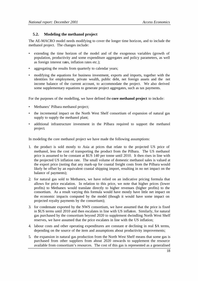
National report: December 2001 Access Economics
18
5.2. Modeling the methanol project
The AE-MACRO model needs modifying to cover the longer time horizon, and to include the methanol project. The changes include:
• extending the time horizon of the model and of the exogenous variables (growth of population, productivity and some expenditure aggregates and policy parameters, as well as foreign interest rates, inflation rates etc.);
• aggregating the results from quarterly to calendar years;
• modifying the equations for business investment, exports and imports, together with the identities for employment, private wealth, public debt, net foreign assets and the net income balance of the current account, to accommodate the project. We also derived some supplementary equations to generate project aggregates, such as tax payments.
For the purposes of the modelling, we have defined the core methanol project to include:
• Methanex’ Pilbara methanol project;
• the incremental impact on the North West Shelf consortium of expansion of natural gas supply to supply the methanol plant;
• additional infrastructure investment in the Pilbara required to support the methanol project.
In modeling the core methanol project we have made the following assumptions:
1. the product is sold mostly to Asia at prices that relate to the projected US price of methanol, less the cost of transporting the product from the Pilbara. The US methanol price is assumed to be constant at $US 140 per tonne until 2010. It then rises in line with the projected US inflation rate. The small volume of domestic methanol sales is valued at the export price (noting that any mark-up for coastal freight costs from the Pilbara would likely be offset by an equivalent coastal shipping import, resulting in no net impact on the balance of payments);
2. for natural gas sold to Methanex, we have relied on an indicative pricing formula that allows for price escalation. In relation to this price, we note that higher prices (lower profits) to Methanex would translate directly to higher revenues (higher profits) to the consortium. As a result varying this formula would have mostly have little net impact on the economic impacts computed by the model (though it would have some impact on projected royalty payments by the consortium);
3. for condensate exported by the NWS consortium, we have assumed that the price is fixed in $US terms until 2010 and then escalates in line with US inflation. Similarly, for natural gas purchased by the consortium beyond 2020 to supplement dwindling North West Shelf reserves, we have assumed that the price escalates in line with the US inflation;
4. labour costs and other operating expenditures are constant or declining in real $A terms, depending on the source of the item and assumptions about productivity improvements;
5. the expansion in natural gas production from the North West Shelf means that some gas is purchased from other suppliers from about 2020 onwards to supplement the resource available from consortium’s resources. The cost of this gas is represented as a generalised
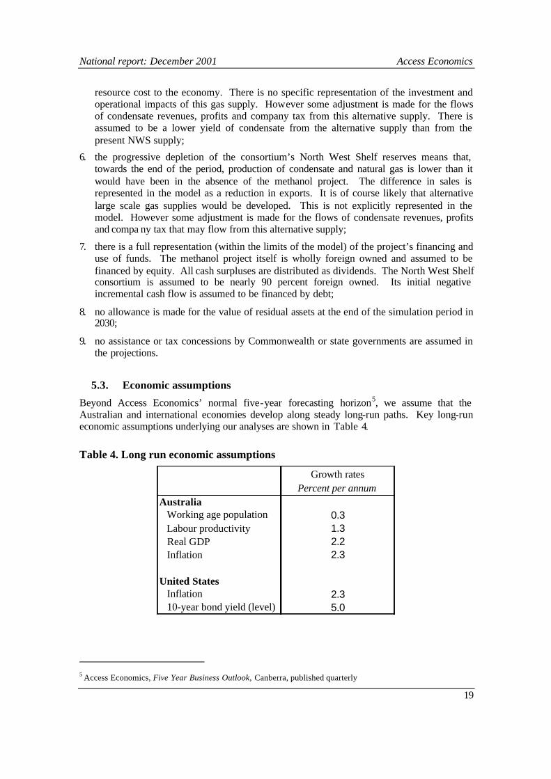
National report: December 2001 Access Economics
19
resource cost to the economy. There is no specific representation of the investment and operational impacts of this gas supply. However some adjustment is made for the flows of condensate revenues, profits and company tax from this alternative supply. There is assumed to be a lower yield of condensate from the alternative supply than from the present NWS supply;
6. the progressive depletion of the consortium’s North West Shelf reserves means that, towards the end of the period, production of condensate and natural gas is lower than it would have been in the absence of the methanol project. The difference in sales is represented in the model as a reduction in exports. It is of course likely that alternative large scale gas supplies would be developed. This is not explicitly represented in the model. However some adjustment is made for the flows of condensate revenues, profits and compa ny tax that may flow from this alternative supply;
7. there is a full representation (within the limits of the model) of the project’s financing and use of funds. The methanol project itself is wholly foreign owned and assumed to be financed by equity. All cash surpluses are distributed as dividends. The North West Shelf consortium is assumed to be nearly 90 percent foreign owned. Its initial negative incremental cash flow is assumed to be financed by debt;
8. no allowance is made for the value of residual assets at the end of the simulation period in 2030;
9. no assistance or tax concessions by Commonwealth or state governments are assumed in the projections.
5.3. Economic assumptions
Beyond Access Economics’ normal five-year forecasting horizon5, we assume that the Australian and international economies develop along steady long-run paths. Key long-run economic assumptions underlying our analyses are shown in Table 4.
Table 4. Long run economic assumptions
Growth ratesPercent per annum
Australia Working age population 0.3 Labour productivity 1.3 Real GDP 2.2 Inflation 2.3
United States Inflation 2.3 10-year bond yield (level) 5.0
5 Access Economics, Five Year Business Outlook, Canberra, published quarterly

National report: December 2001 Access Economics
20
These assumptions are stylised. They do not make allowances for specific disturbances that will affect the Australian and world economies in coming decades. There is an implicit assumption that governments will follow sound fiscal and monetary policies, and that current views on policy objectives (e.g. for inflation) will continue. The future will no doubt deviate from the stylised assumptions in ways that are difficult to predict.
5.4. Application to the core methanol project
Further results from introducing the core methanol project as an exogenous shock to the AE-MACRO model are summarised in the following tables.
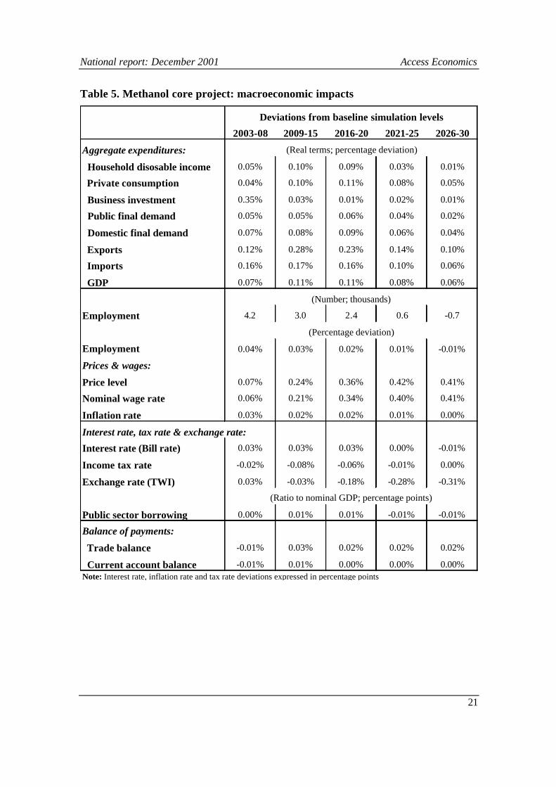
National report: December 2001 Access Economics
21
Table 5. Methanol core project: macroeconomic impacts
Deviations from baseline simulation levels
2003-08 2009-15 2016-20 2021-25 2026-30
Aggregate expenditures: (Real terms; percentage deviation)
Household disosable income 0.05% 0.10% 0.09% 0.03% 0.01%
Private consumption 0.04% 0.10% 0.11% 0.08% 0.05%
Business investment 0.35% 0.03% 0.01% 0.02% 0.01%
Public final demand 0.05% 0.05% 0.06% 0.04% 0.02%
Domestic final demand 0.07% 0.08% 0.09% 0.06% 0.04%
Exports 0.12% 0.28% 0.23% 0.14% 0.10%
Imports 0.16% 0.17% 0.16% 0.10% 0.06%
GDP 0.07% 0.11% 0.11% 0.08% 0.06%
(Number; thousands)
Employment 4.2 3.0 2.4 0.6 -0.7
(Percentage deviation)
Employment 0.04% 0.03% 0.02% 0.01% -0.01%
Prices & wages:
Price level 0.07% 0.24% 0.36% 0.42% 0.41%
Nominal wage rate 0.06% 0.21% 0.34% 0.40% 0.41%
Inflation rate 0.03% 0.02% 0.02% 0.01% 0.00%
Interest rate, tax rate & exchange rate:
Interest rate (Bill rate) 0.03% 0.03% 0.03% 0.00% -0.01%
Income tax rate -0.02% -0.08% -0.06% -0.01% 0.00%
Exchange rate (TWI) 0.03% -0.03% -0.18% -0.28% -0.31%
(Ratio to nominal GDP; percentage points)
Public sector borrowing 0.00% 0.01% 0.01% -0.01% -0.01%
Balance of payments:
Trade balance -0.01% 0.03% 0.02% 0.02% 0.02%
Current account balance -0.01% 0.01% 0.00% 0.00% 0.00%Note: Interest rate, inflation rate and tax rate deviations expressed in percentage points
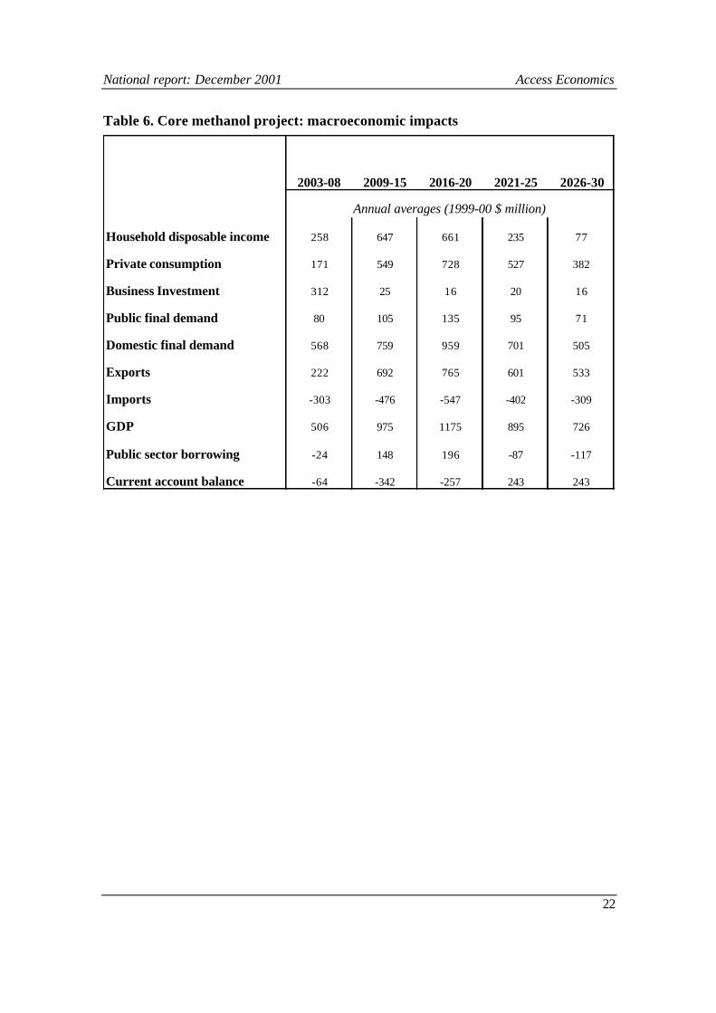
National report: December 2001 Access Economics
22
Table 6. Core methanol project: macroeconomic impacts
2003-08 2009-15 2016-20 2021-25 2026-30
Annual averages (1999-00 $ million)
Household disposable income 258 647 661 235 77
Private consumption 171 549 728 527 382
Business Investment 312 25 16 20 16
Public final demand 80 105 135 95 71
Domestic final demand 568 759 959 701 505
Exports 222 692 765 601 533
Imports -303 -476 -547 -402 -309
GDP 506 975 1175 895 726
Public sector borrowing -24 148 196 -87 -117
Current account balance -64 -342 -257 243 243
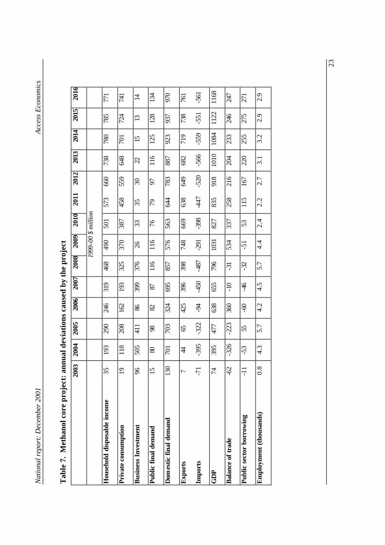
Nat
iona
l rep
ort:
Dec
embe
r 20
01
Acc
ess
Eco
nom
ics
23
Tab
le 7
. M
etha
nol c
ore
proj
ect:
ann
ual d
evia
tion
s ca
used
by
the
proj
ect
20
03
2004
20
05
2006
20
07
2008
20
09
2010
20
11
2012
20
13
2014
20
15
2016
19
99-0
0 $
mill
ion
Hou
seho
ld d
ispo
sabl
e in
com
e 35
19
3 29
0 24
6 31
9 46
8 49
0 50
1 57
3 66
0 73
8 78
0 78
5 77
1
Priv
ate
cons
umpt
ion
19
118
208
162
193
325
370
387
458
559
648
701
724
741
Bus
ines
s In
vest
men
t 96
50
5 41
1 86
39
9 37
6 26
33
35
30
22
15
13
14
Publ
ic fi
nal d
eman
d 15
80
98
82
87
11
6 11
6 76
79
97
11
6 12
5 12
8 13
4
Dom
estic
fina
l dem
and
130
701
703
324
695
857
576
563
644
783
887
923
937
970
Exp
orts
7
44
65
425
396
398
748
669
638
649
682
719
738
761
Impo
rts
-71
-395
-3
22
-94
-450
-4
87
-291
-3
98
-447
-5
20
-566
-5
59
-551
-5
61
GD
P
74
395
477
638
655
796
1031
82
7 83
5 91
8 10
10
1084
11
22
1168
Bal
ance
of t
rade
-6
2 -3
26
-223
36
0 -1
0 -3
1 53
4 33
7 25
8 21
6 20
4 23
3 24
6 24
7
Publ
ic s
ecto
r bo
rrow
ing
-11
-53
55
-60
-46
-32
-51
53
115
167
220
255
275
271
Em
ploy
men
t (th
ousa
nds)
0.
8 4.
3 5.
7 4.
2 4.
5 5.
7 4.
4 2.
4 2.
2 2.
7 3.
1 3.
2 2.
9 2.
9
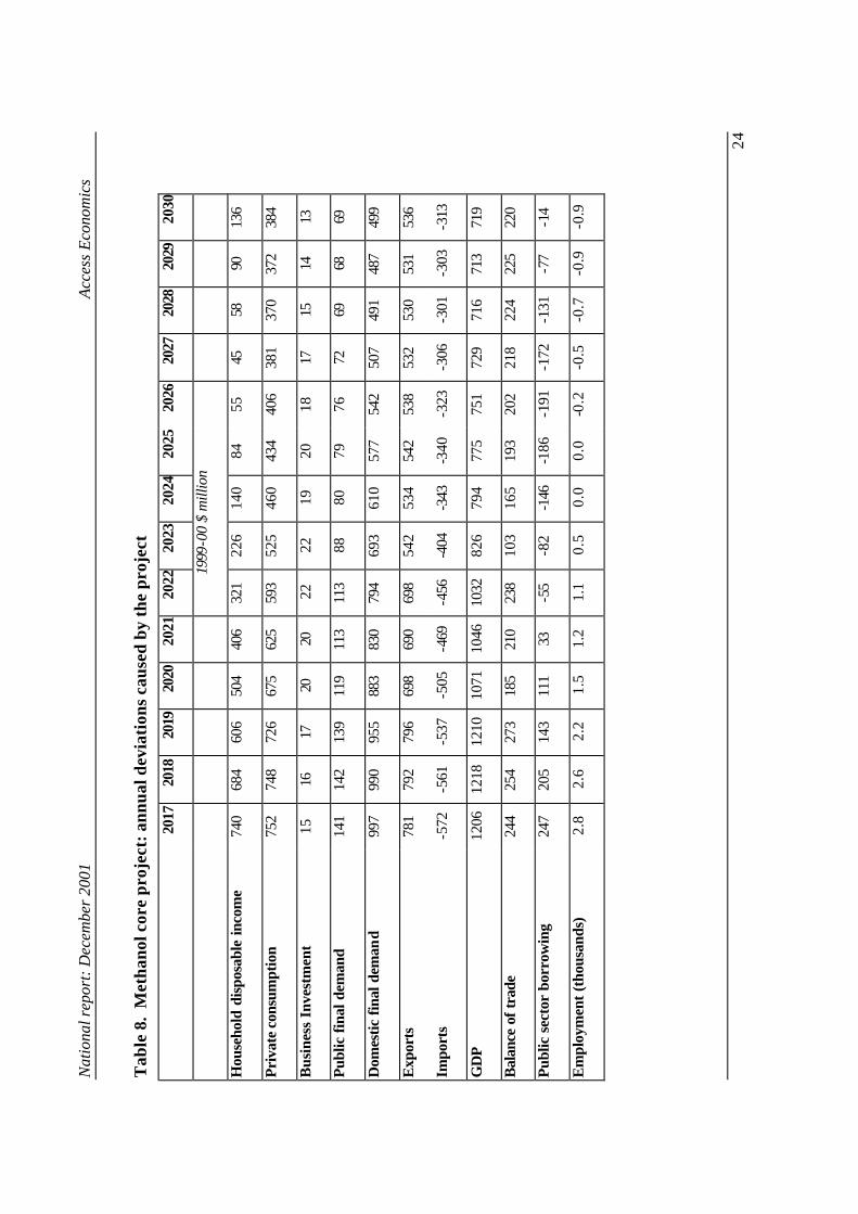
Nat
iona
l rep
ort:
Dec
embe
r 20
01
Acc
ess
Eco
nom
ics
24
Tab
le 8
. M
etha
nol c
ore
proj
ect:
ann
ual d
evia
tion
s ca
used
by
the
proj
ect
20
17
2018
20
19
2020
20
21
2022
20
23
2024
20
25
2026
20
27
2028
20
29
2030
1999
-00
$ m
illio
n
Hou
seho
ld d
ispo
sabl
e in
com
e 74
0 68
4 60
6 50
4 40
6 32
1 22
6 14
0 84
55
45
58
90
13
6
Priv
ate
cons
umpt
ion
752
748
726
675
625
593
525
460
434
406
381
370
372
384
Bus
ines
s In
vest
men
t 15
16
17
20
20
22
22
19
20
18
17
15
14
13
Publ
ic fi
nal d
eman
d 14
1 14
2 13
9 11
9 11
3 11
3 88
80
79
76
72
69
68
69
Dom
estic
fina
l dem
and
997
990
955
883
830
794
693
610
577
542
507
491
487
499
Exp
orts
78
1 79
2 79
6 69
8 69
0 69
8 54
2 53
4 54
2 53
8 53
2 53
0 53
1 53
6
Impo
rts
-572
-5
61
-537
-5
05
-469
-4
56
-404
-3
43
-340
-3
23
-306
-3
01
-303
-3
13
GD
P
1206
12
18
1210
10
71
1046
10
32
826
794
775
751
729
716
713
719
Bal
ance
of t
rade
24
4 25
4 27
3 18
5 21
0 23
8 10
3 16
5 19
3 20
2 21
8 22
4 22
5 22
0
Publ
ic s
ecto
r bo
rrow
ing
247
205
143
111
33
-55
-82
-146
-1
86
-191
-1
72
-131
-7
7 -1
4
Em
ploy
men
t (th
ousa
nds)
2.
8 2.
6 2.
2 1.
5 1.
2 1.
1 0.
5 0.
0 0.
0 -0
.2
-0.5
-0
.7
-0.9
-0
.9

National report: December 2001 Access Economics
25
5.5. Commonwealth Budget impacts
The impacts on the Commonwealth Budget of the project were analysed within the framework used for Access Economics’ Commonwealth Budget Monitor publication. Commonwealth Budget Monitor operates over a four year forecasting horizon and has a well known track record for accurately assessing the Commonwealth budgetary position and outlook.
For the purposes of analysing the project Access’ standard short term Budget forecasting horizon to 2003-04 has been maintained. Longer ter m projections have been established using relevant relationships to macroeconomic variables for major revenue and expenditure items. The forecasts assume indexation of tax brackets on average beyond 2003-04 i.e. the revenue benefits of fiscal drag for the Budget are not included.
Deviations in key Budgetary items as a result of the project are shown in Table 9. It shows that the project produces significant gains for the Commonwealth Budget over time.
Table 9. Methanol core project Commonwealth Budget impacts
Deviations from baseline simulation levels
2003-08 2009-15 2016-20 2021-25 2026-30
Individuals income tax -24 -327 -313 -75 -1
Company taxes 24 94 115 95 81
Excises and sales tax 7 23 39 25 19
Customs duty 3 -3 -2 -5 -8
Other taxes and revenue 10 22 26 20 16
Total revenue 20 -191 -135 61 107
Total expenditure 18 38 120 80 48
Recorded Budget balance 2 -229 -254 -19 58
Revenue foregone through tax cut 66 334 292 60 12
Total Commonwealth Budget gains 86 143 157 122 119
Annual averages (1999-00 $ million)
Access Economics’ modelling of the project assumes a stability function whereby the public sector budget (not just the Commonwealth) is restored to balance over the long term. The mechanism to achieve this is via movements in the rate of income tax – that is: public sector surpluses are given back in the form of income tax cuts with all other taxes assumed unaffected. This mechanism varies in magnitude over time – the tax rate reacts with a lag to changes in the stock of public debt, so overshoots both up and down. Over the full time horizon however, the project allows for a substantial reduction in income tax. Adding this
National report: December 2001 Access Economics
26
revenue foregone back to the recorded Budget balance produces strong gains to the Commonwealth Budget.
Other revenue items benefit from the economic stimulus the project provides. Company tax collections benefit from the profit the project makes as well as tax revenue from increased business activity elsewhere. An increase in private consumption sees higher receipts from the GST (though this accrues to States and Territories) as well as other sales taxes and excises. The Commonwealth receives a share of royalty payments for gas extracted from the North West Shelf. This is recorded in Commonwealth revenue under crude oil excise (within excises and sales tax above). As the project brings forward these royalty payments this item rises strongly and then moderates.
On the expenditure side, many of the government’s functions and payments are assumed to move in line with GDP, and thus are boosted by the stimulus the project creates. However, the project also creates some short term reductions in unemployment, reducing benefit payments required to be paid by the Commonwealth. The government’s wage bill falls from the small reduction in real wages, while the boost to revenues helps to reduce Commonwealth debt in the short term, and consequently expenditure on debt repayments. These reduced spending requirements help lock in the gains to the Commonwealth Budget.
5.6. Measurement of economic welfare
To measure the impact of the core methanol project on Australian economic welfare, we need to consider the impacts over time on the Australian private and public sectors.
The benefit to Australians is the flow of additional household consumption and additional public services that the project makes possible. These we can measure as the annual increase in real private consumption expenditure and the annual increase in real government current expenditure. By summing and discounting at an appropriate social discount rate, we can construct a single net present value estimate of the increase in Australian economic welfare made possible by the project.
Reflecting the scope of the model, this welfare estimate has limitations:
(1) there is a presumption that markets for public and private goods and services are efficient and free from distortion, so that an increase in expenditures in base period (1999/00) prices represents an improvement in w elfare;
(2) no account is taken of changes in the distribution of income or wealth, as a result of the project; nor of any environmental impacts; and
(3) the measure is limited to the time horizon of the model – in this case 35 years.
We can make some allowance for impacts beyond the model’s time horizon by adding to the welfare estimate the net present value in 2001 of the change in public and private sector wealth in the final year (2030) as a result of the project. If in the final year, Australians have increased the stock of assets they own, they will be able to generate a higher level of consumption expenditure beyond that date. If, on the other hand, they have financed previous increases in consumption through a deterioration in the balance of payments, then net liabilities to foreigners will have increased (resulting in a reduction in Australian wealth).
National report: December 2001 Access Economics
27
Private sector wealth includes:
– currency holdings
– Australian public sector debt held by residents
– the replacement value of the business capital stock owned by Australians
– the replacement value of the dwelling stock
– the replacement value of private business farm and non-farm inventories
– less net private sector debt liabilities to foreigners.
Public sector wealth includes:
– the replacement value of general gove rnment and public enterprise capital stocks
– the replacement value of public enterprise inventories
– less public sector net financial liabilities
5.7. Limitations of the modeling results
The results reported in the paper reflect the assumptions and parameter estimates built into AE-MACRO. In turn, these assumptions and estimates reflect the actual experience of the Australian economy in the past twenty years.
The model exhibits a traditional Keynesian response to domestic demand stimuli. It also incorporates a strong expectations link from monetary policy to wage behaviour. The latter reduces the extent to which demand stimuli dissipate in higher inflation. This tends to increase the initial impact on employment, but to have the opposite (and offsetting, as far as consumption spending is concerned) effect on real wages.
The moderate inflationary response keeps the pressures on interest rates and the exchange rate within manageable bounds. The assumed fiscal policy reaction function also ensures that government uses the additional revenue flowing from higher economic activity to reduce taxes rather than to increase spending.
The results are an indicative guide to the likely impact of the project. Macroeconomic simulations of a project such as the methanol project can only provide a broad indication of its likely impact. While the model is internally consistent, and in accordance with economic theory, it is highly aggregate and may therefore miss some important detail. The project itself is still at the planning stage. The economy itself will change, and the overall economic environment will certainly not be as smooth as that implied by the baseline scenario. The effectiveness and emphasis of Australian economic policy may fluctuate.
If different assumptions had been built into the model, the macroeconomic impacts would still have been significant and positive. For example, if we had assumed a stronger response of wages to increased demand for labour, then the employment impact would have been smaller, but the average real wage would have been higher. There would still have been a substantial increase in private consumption.
Similarly, if we had assumed that governments increased spending more and reduced taxes less, there would still have been a significant impact on aggregate demand and activity.

Preliminary Geotechnical Investigation
Appendix 2
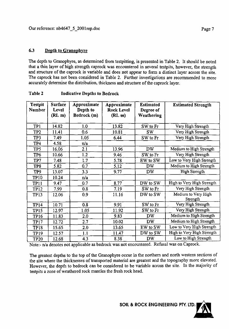


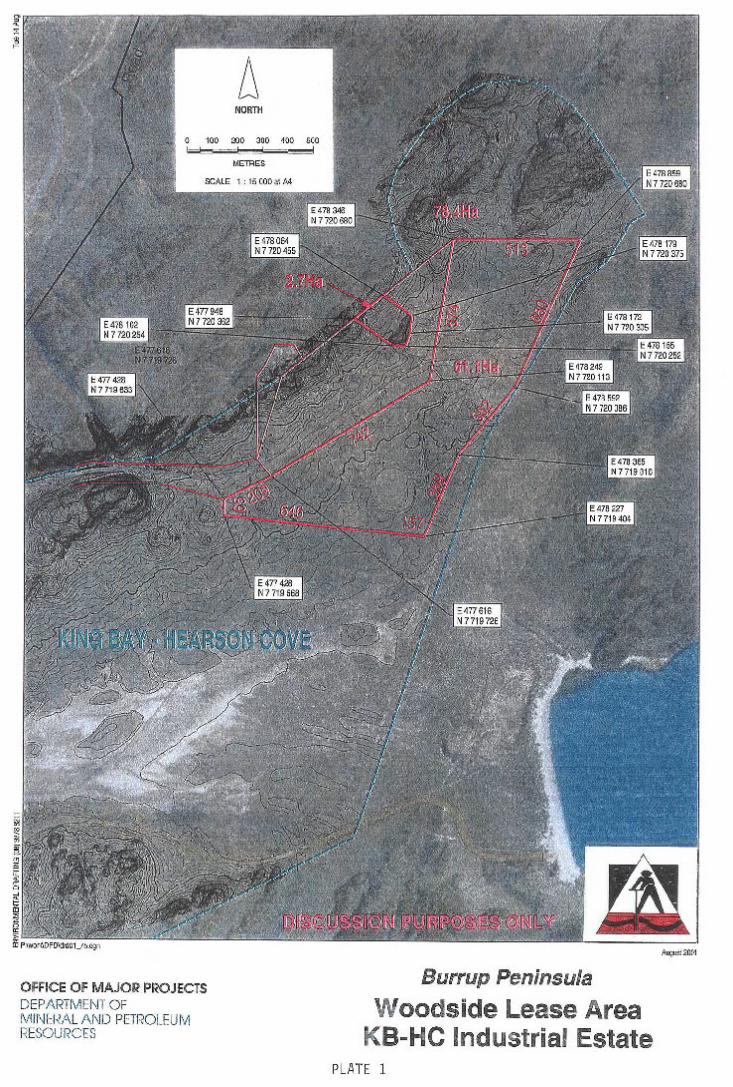
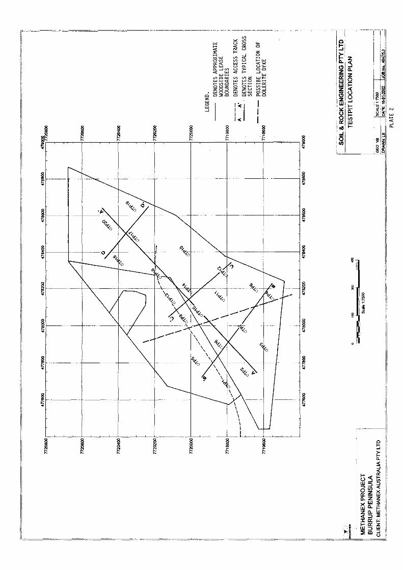
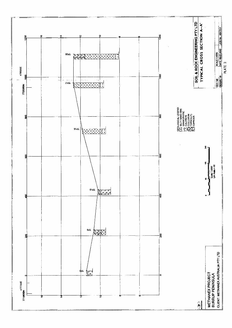
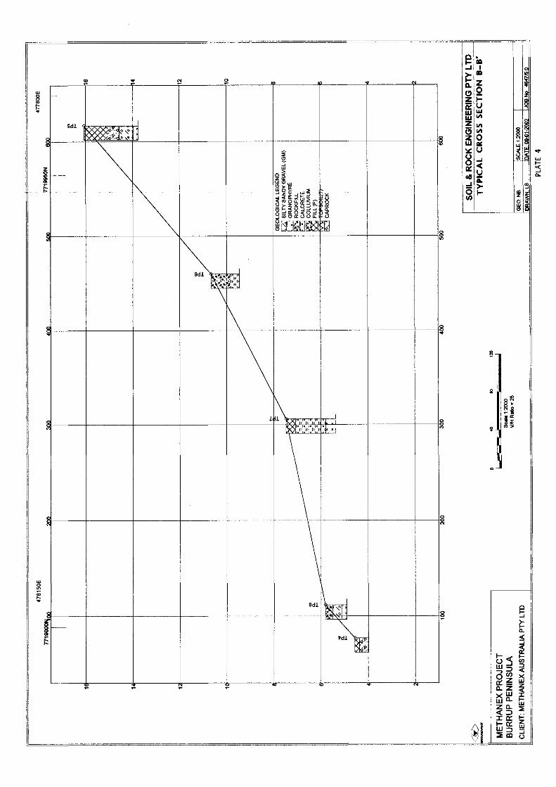
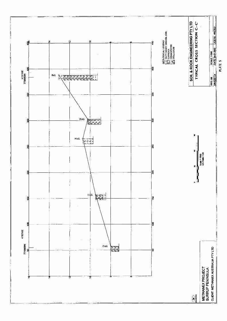
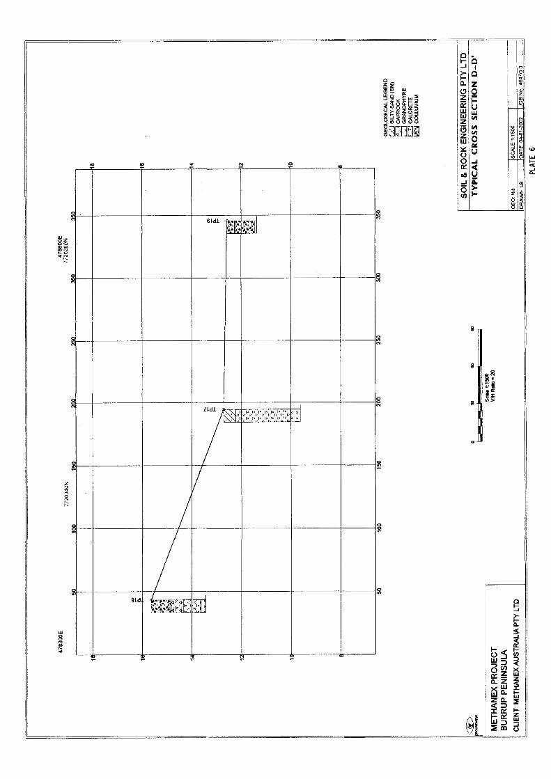
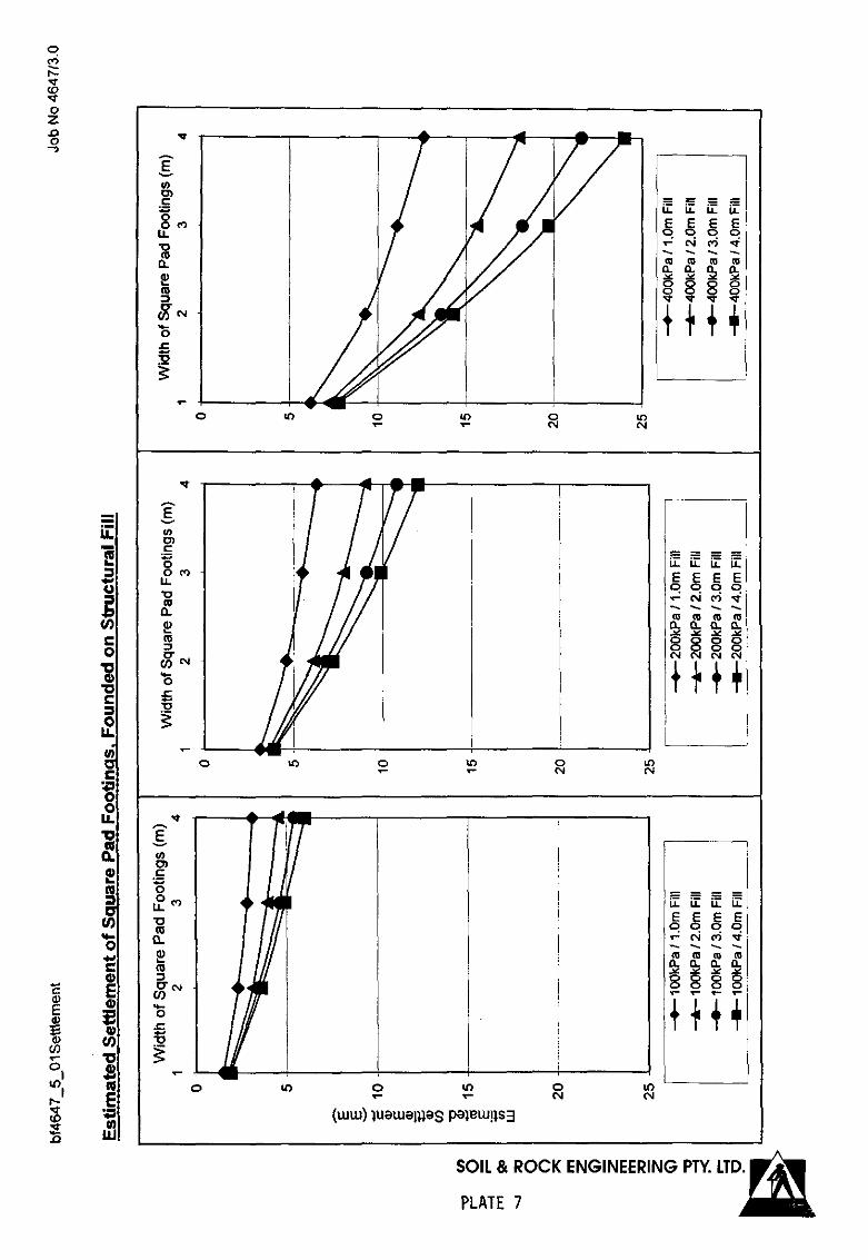
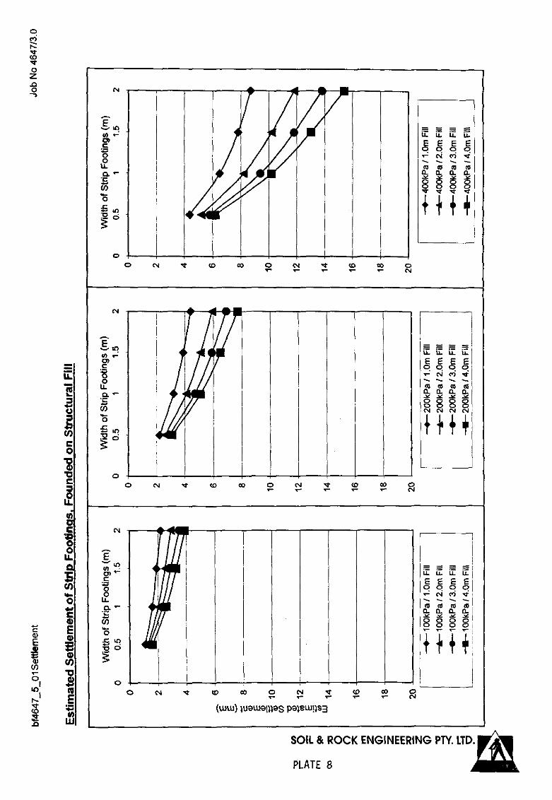

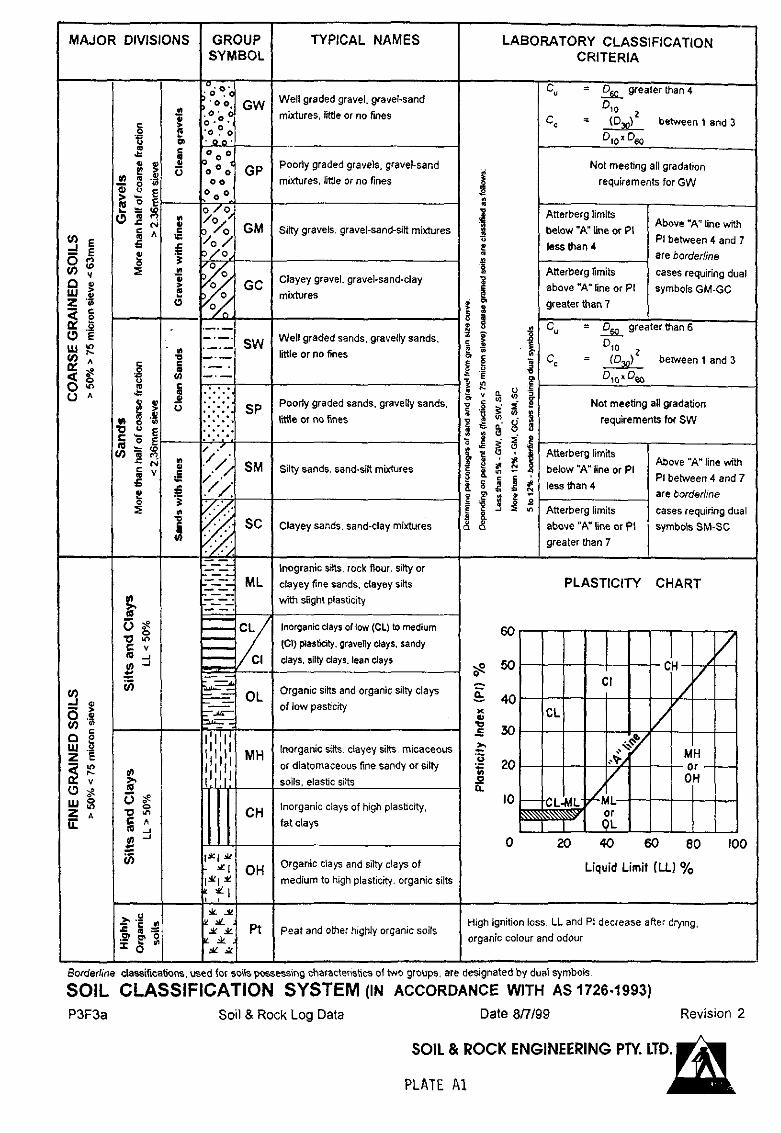
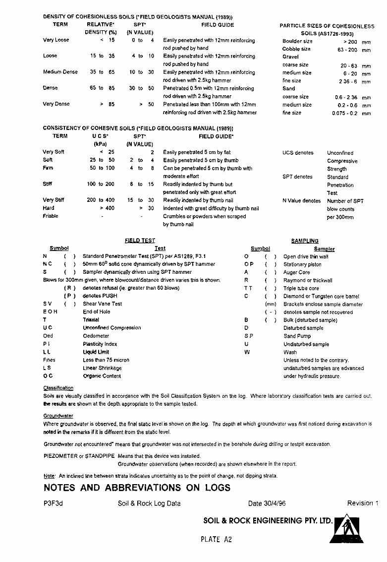
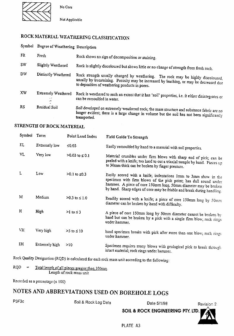
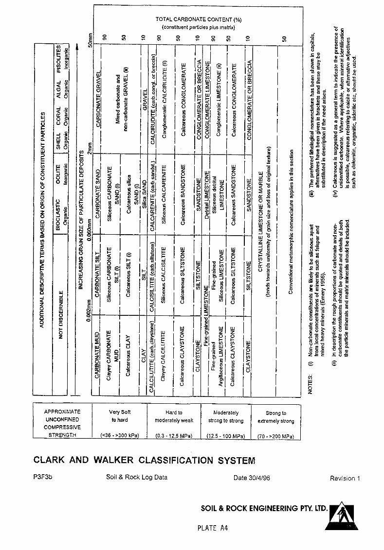
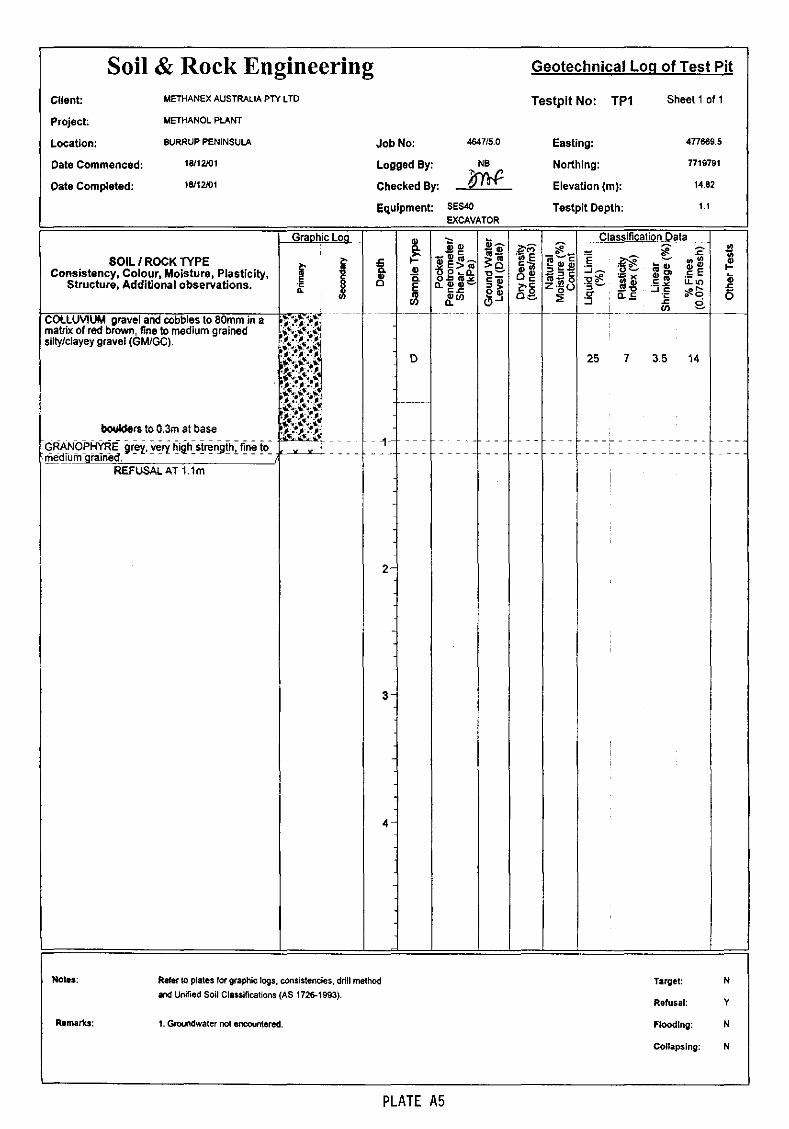
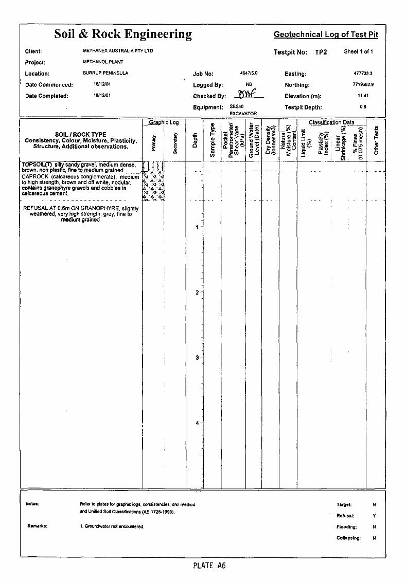
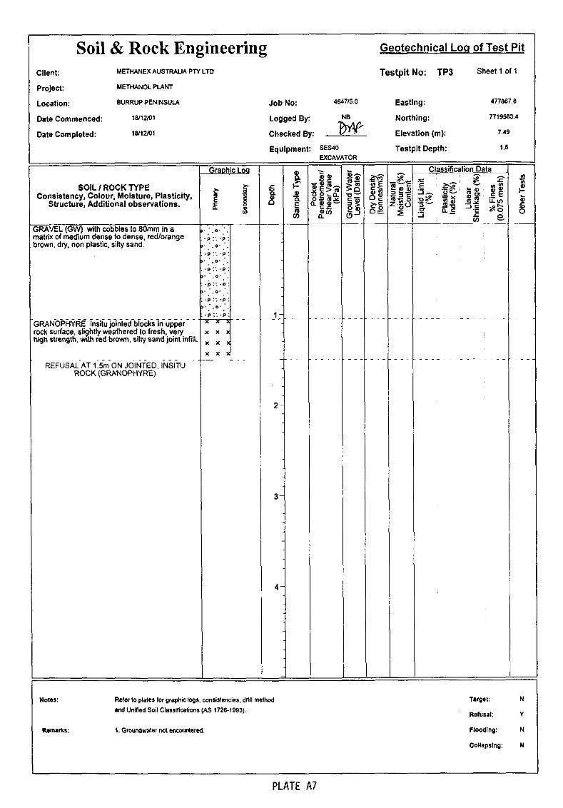
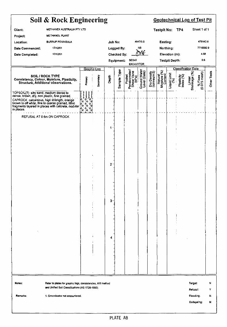
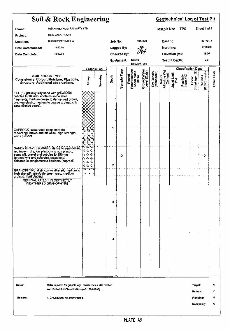
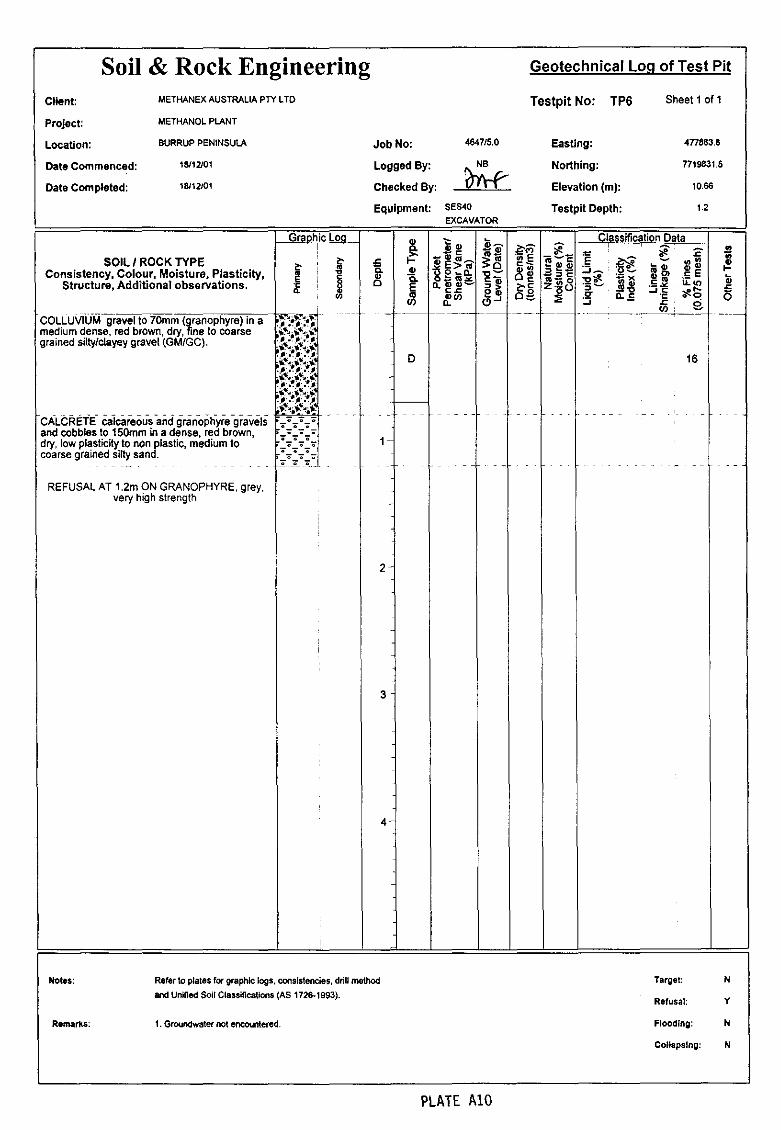
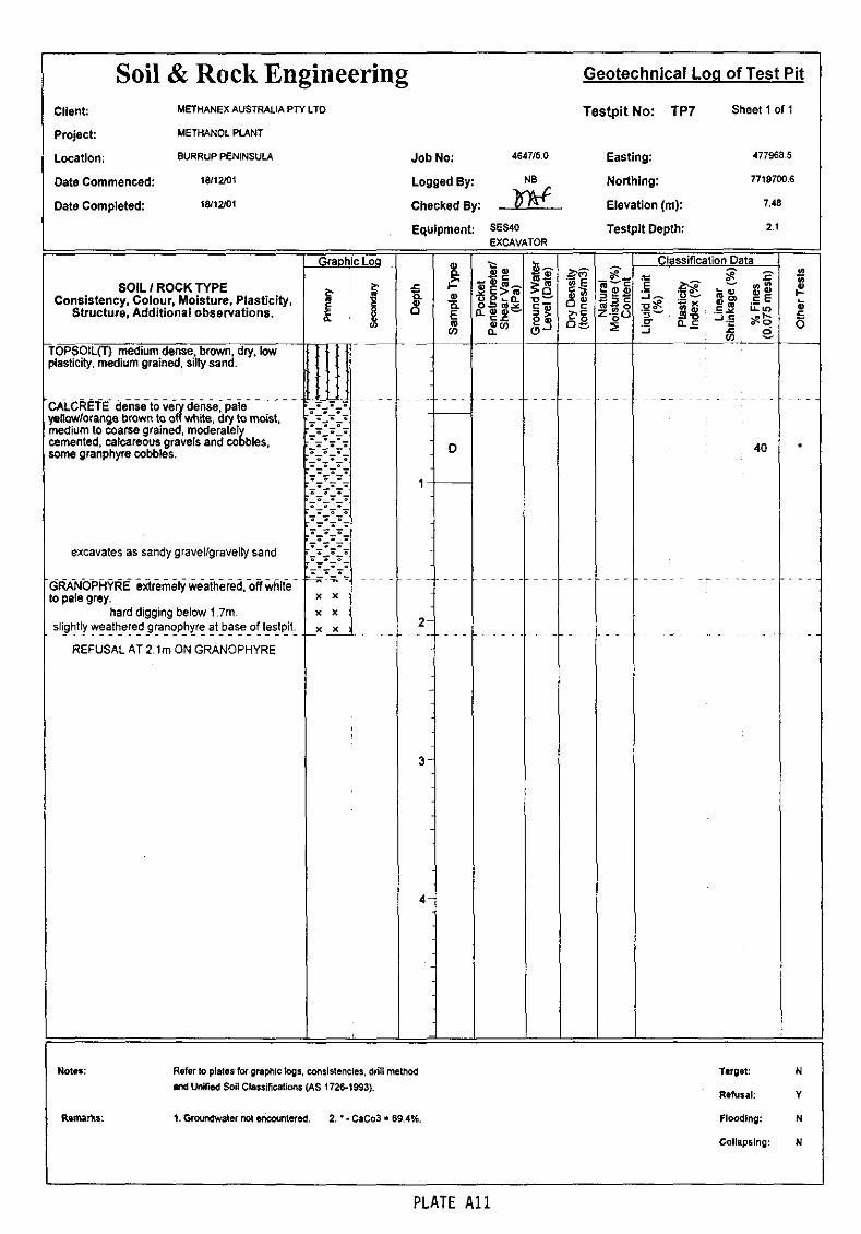
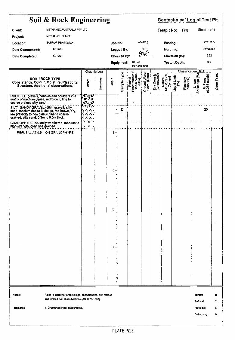
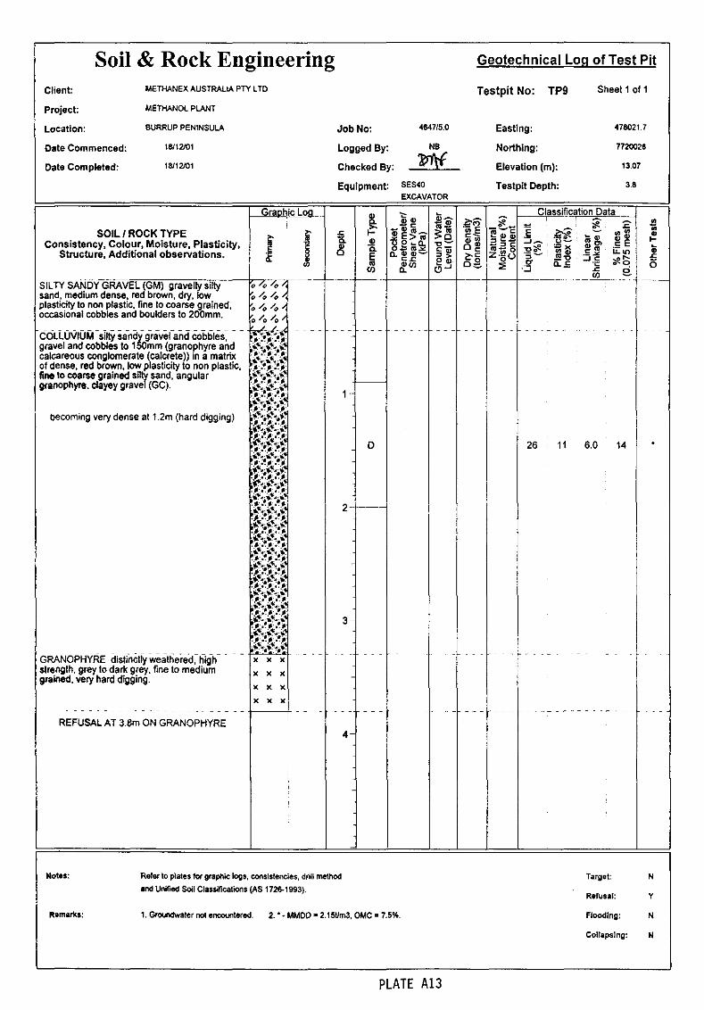
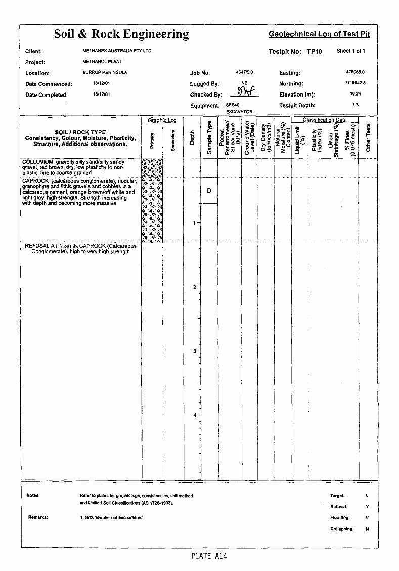
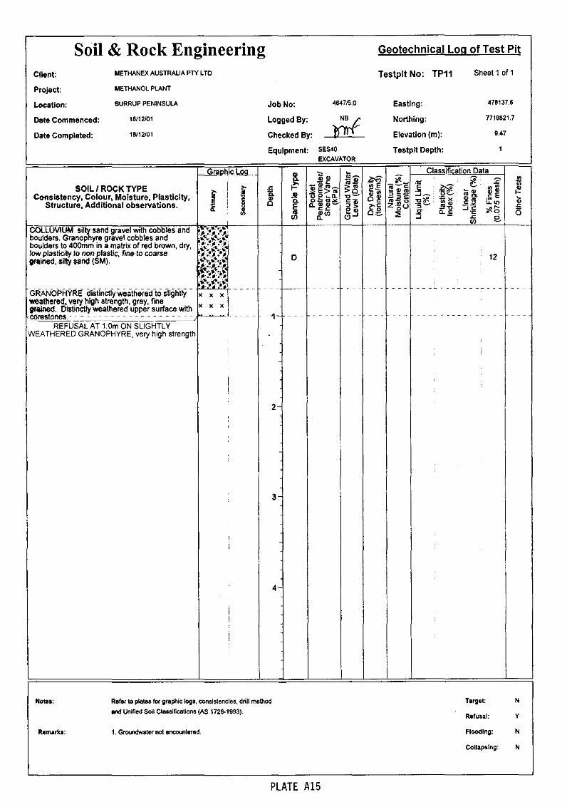
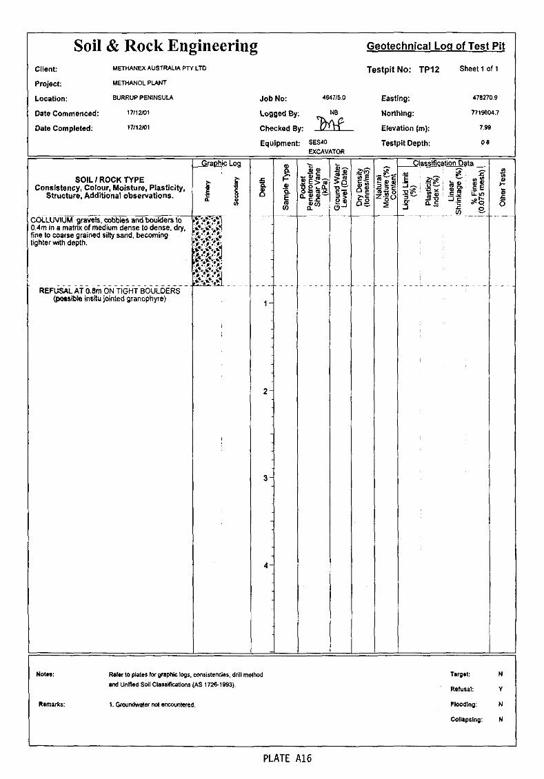
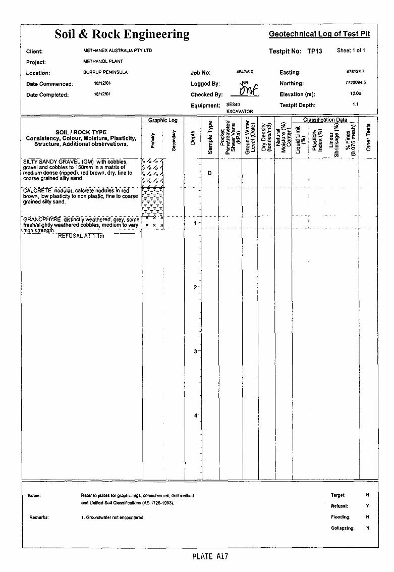
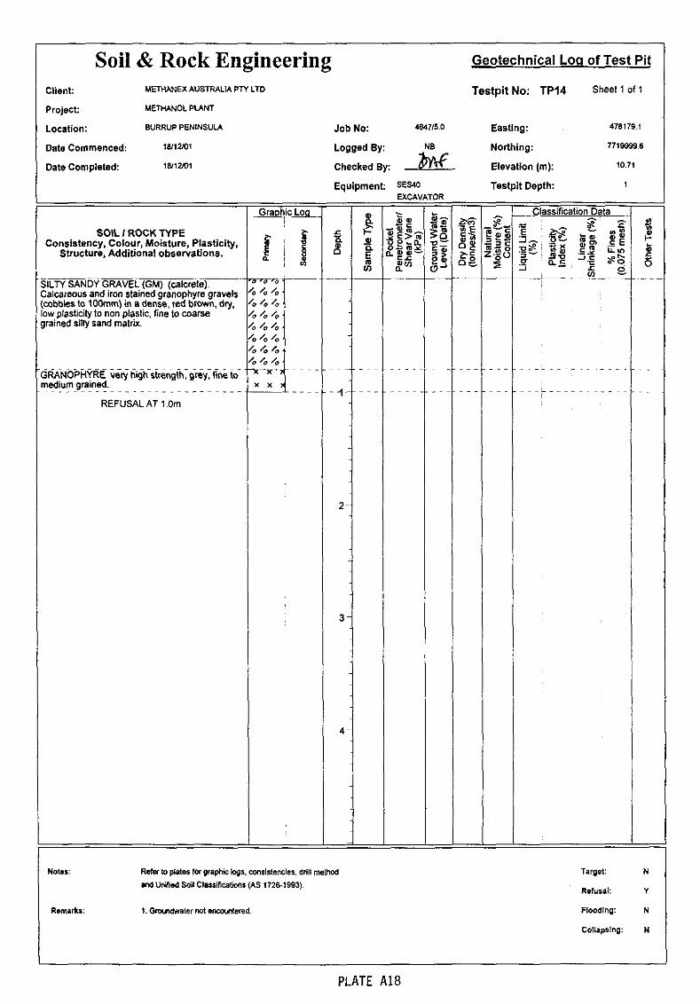

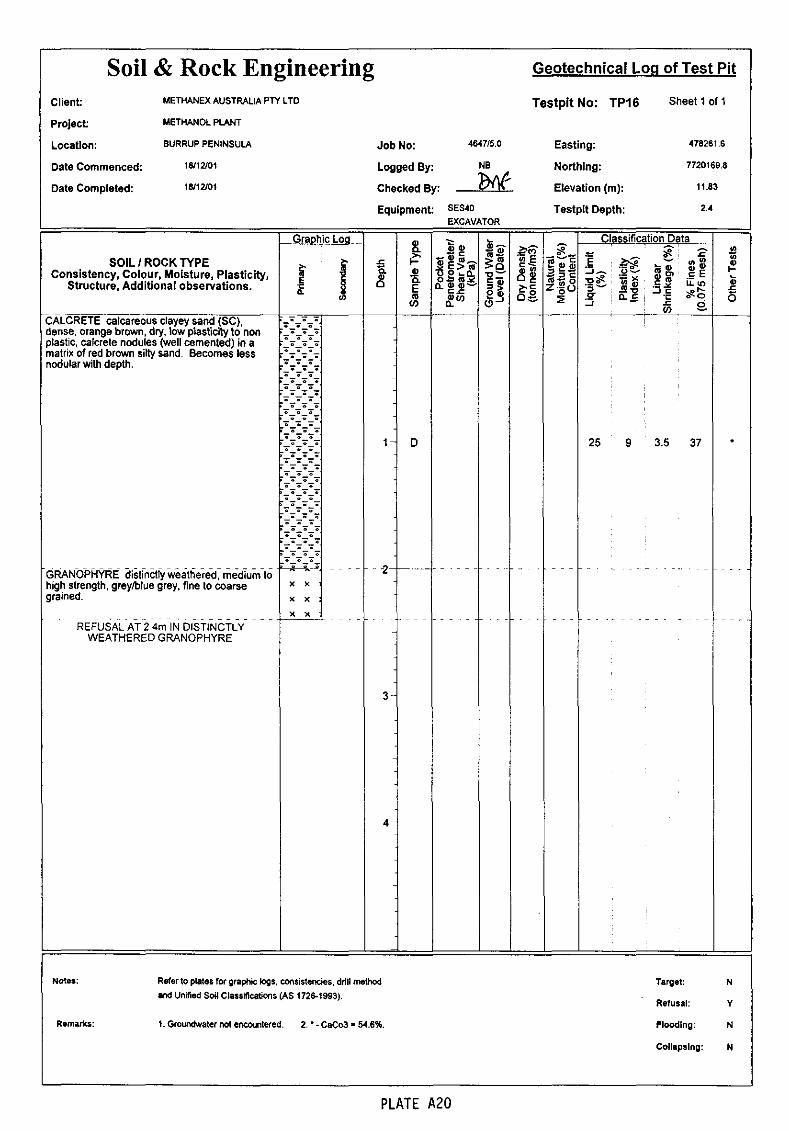
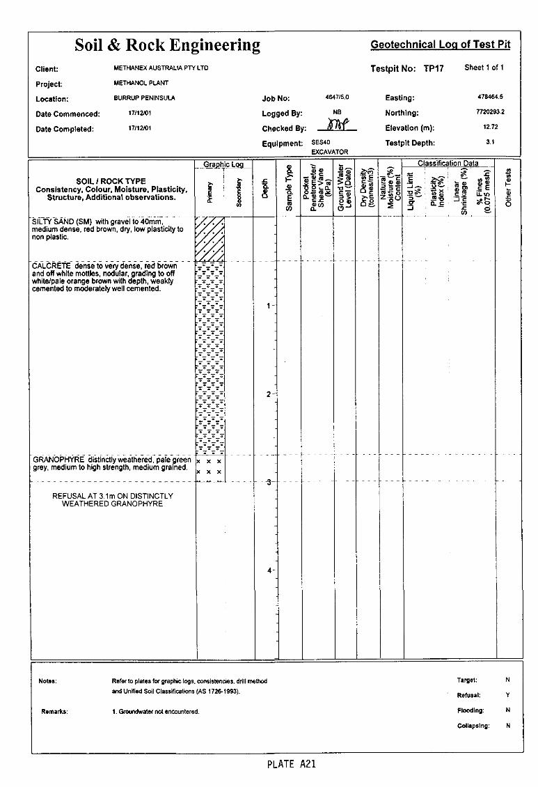
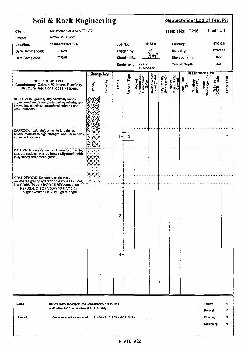

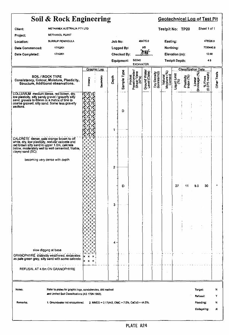
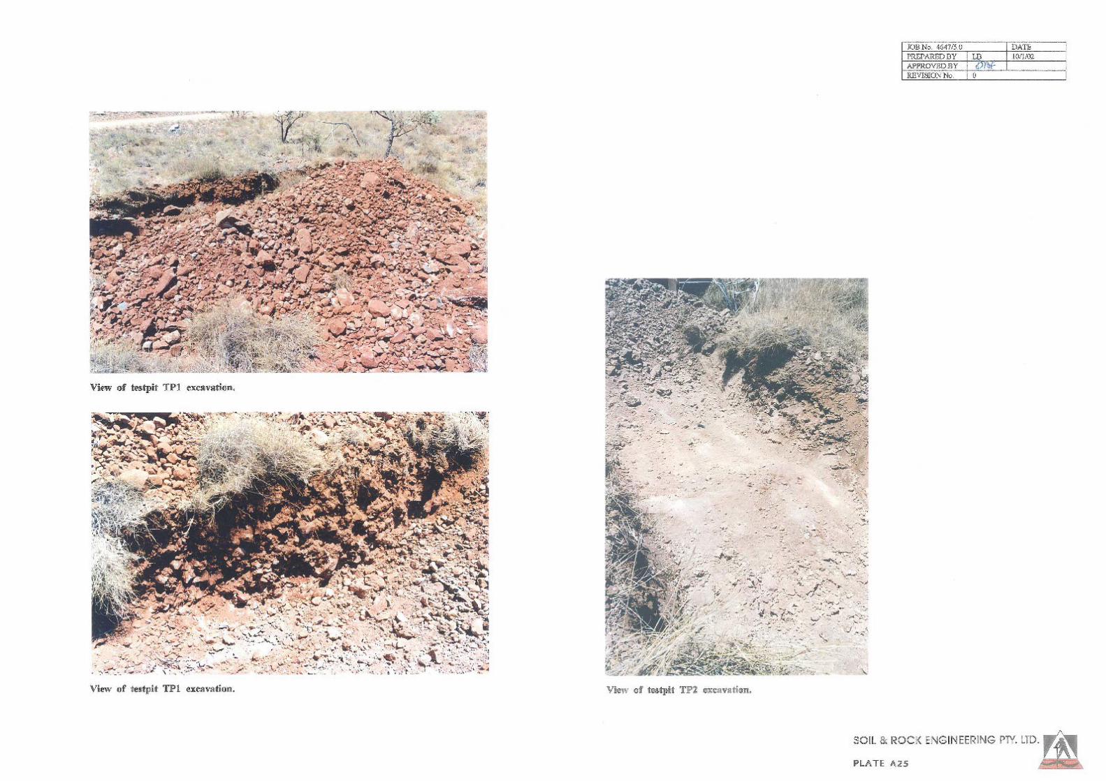
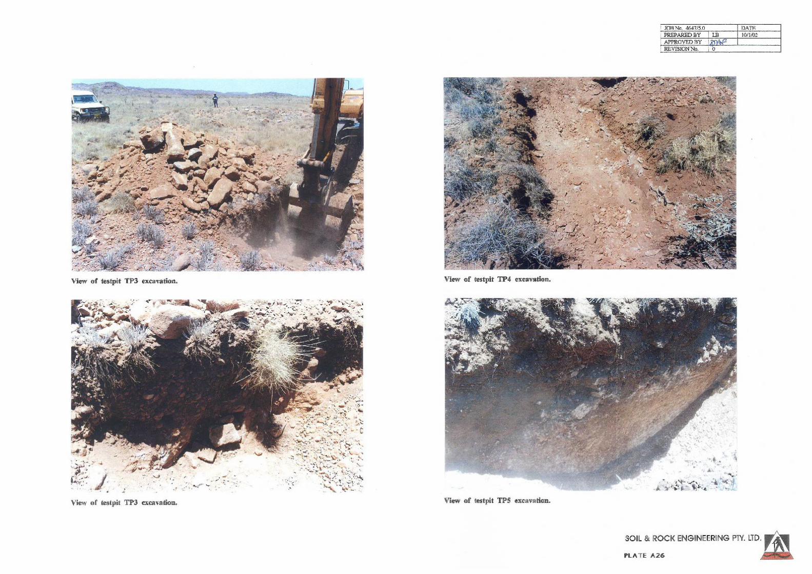
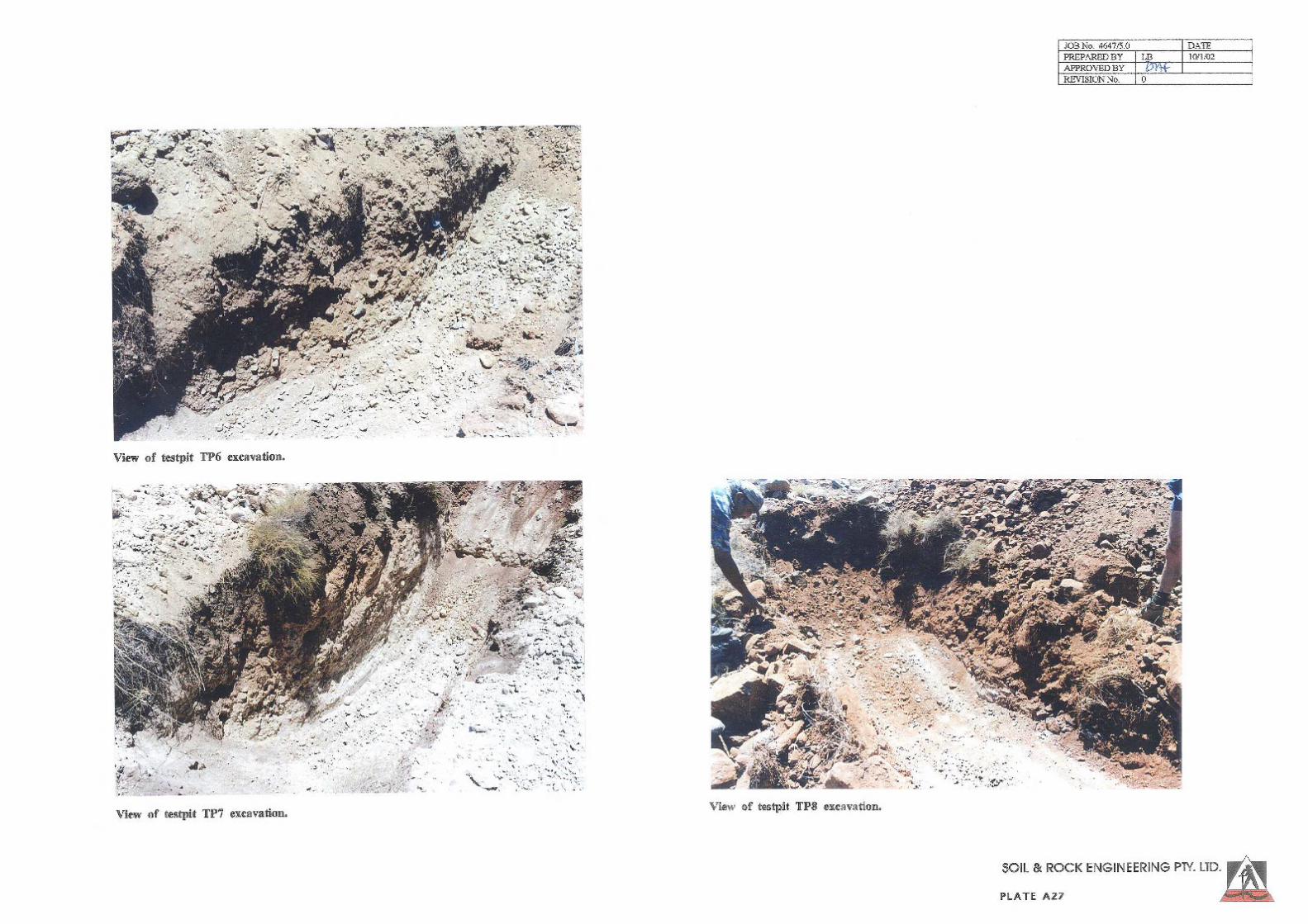
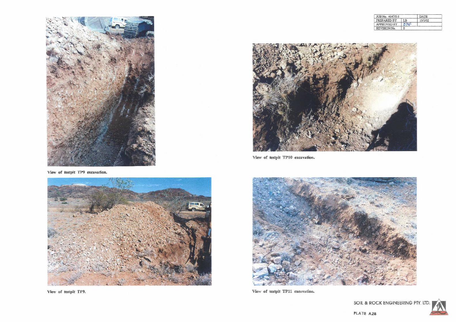
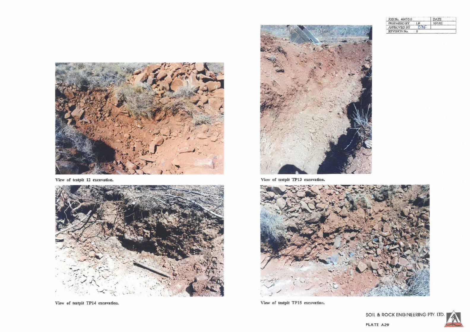
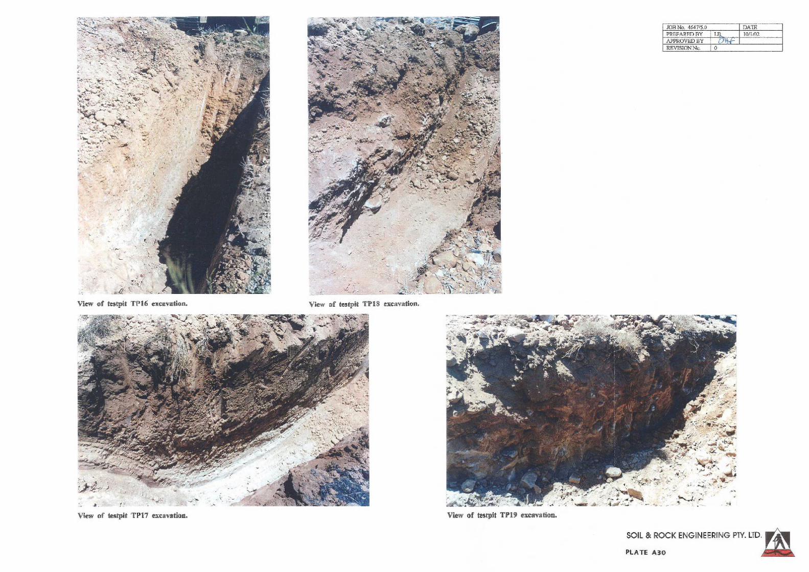
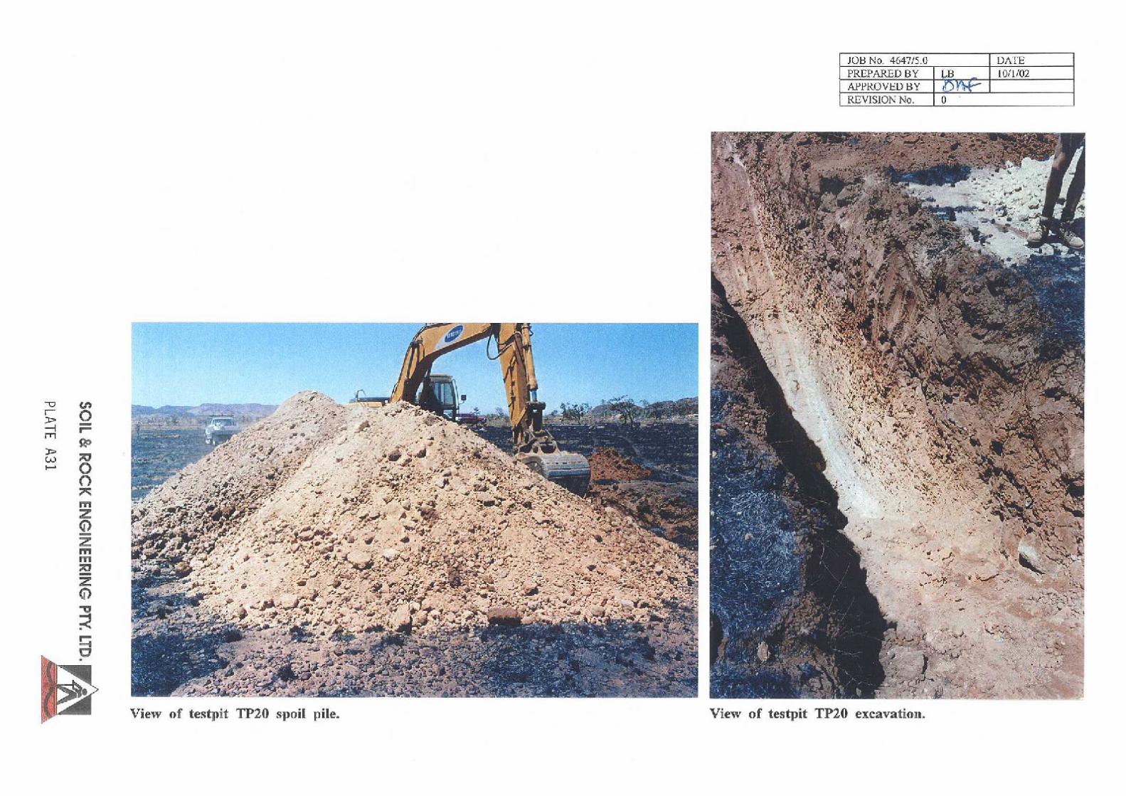

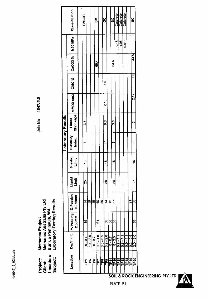
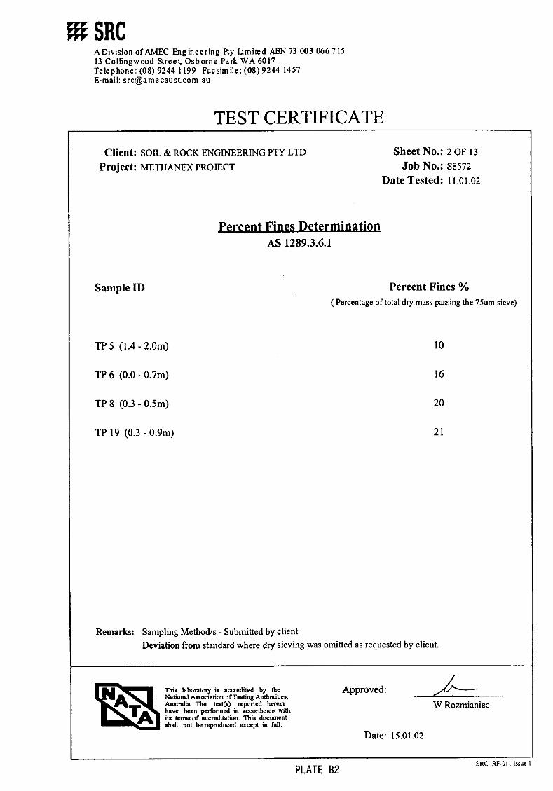

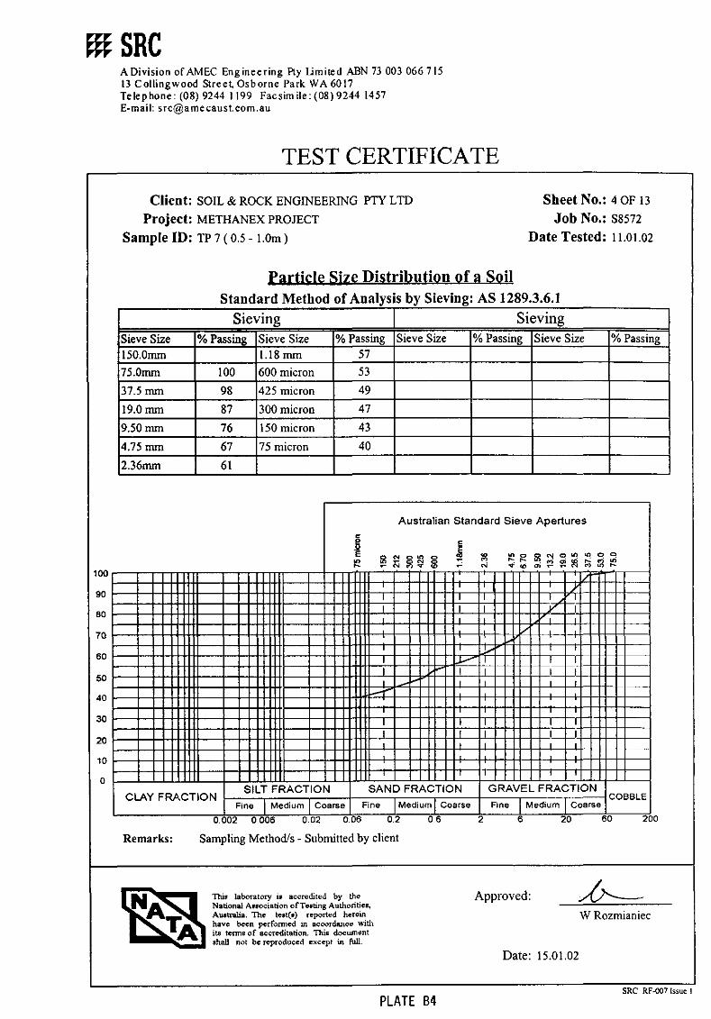
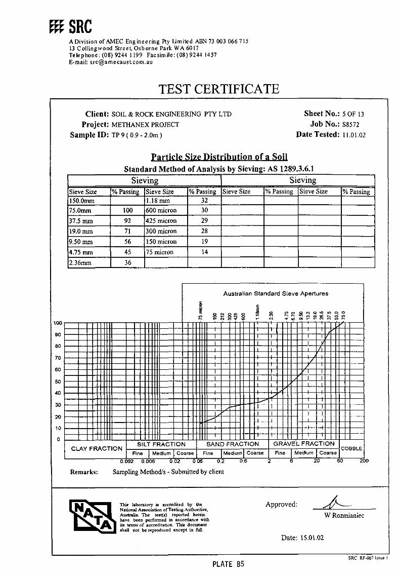
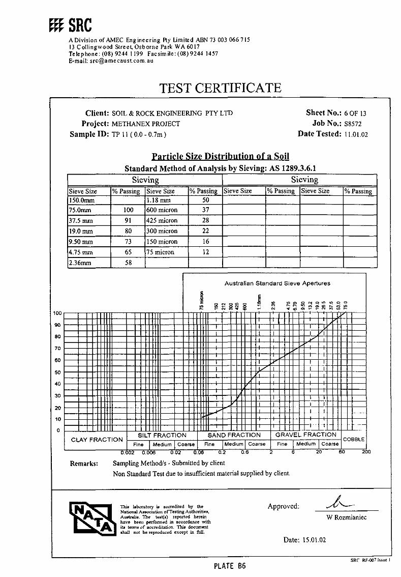
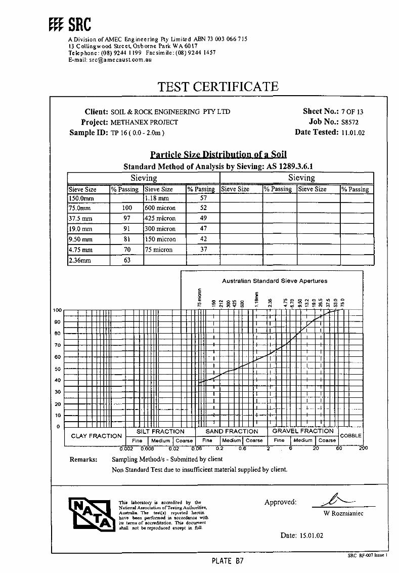
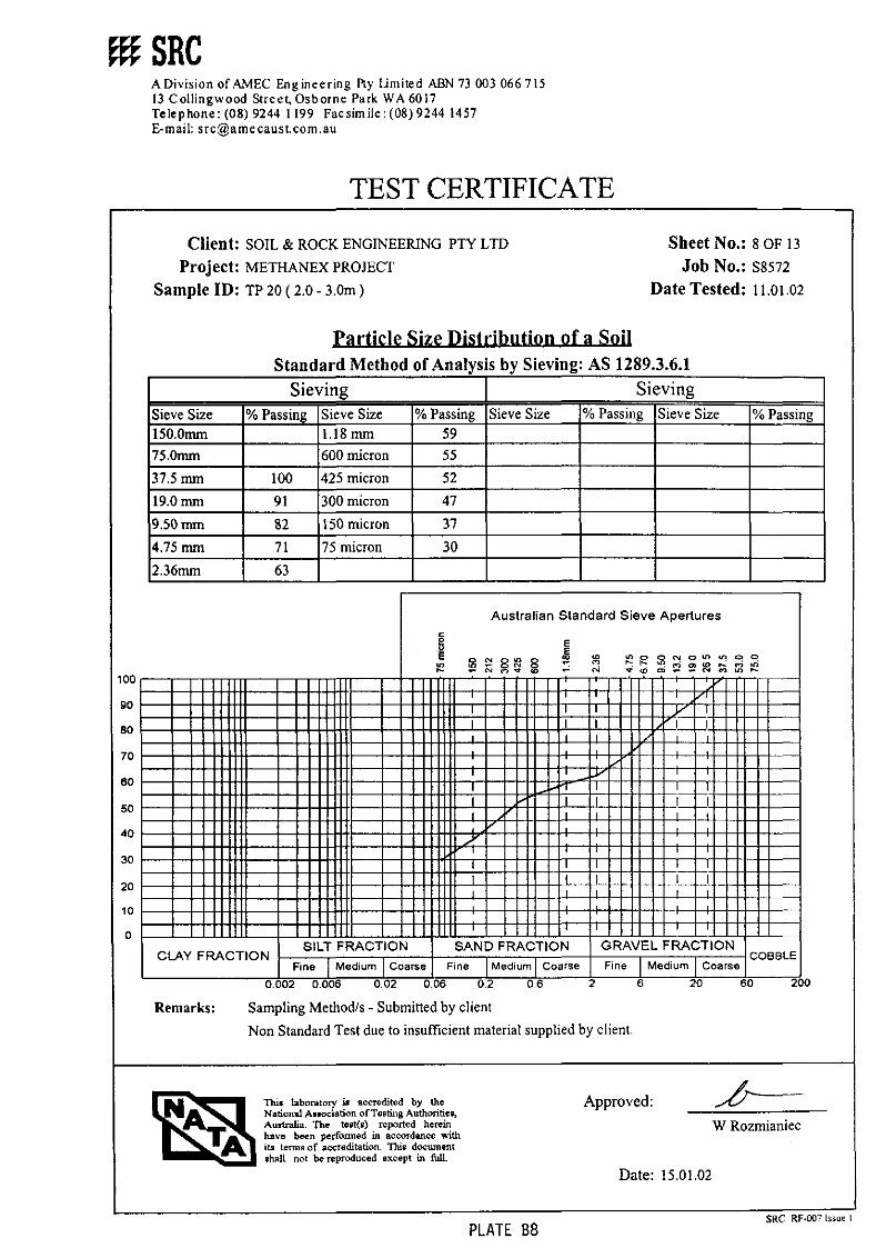
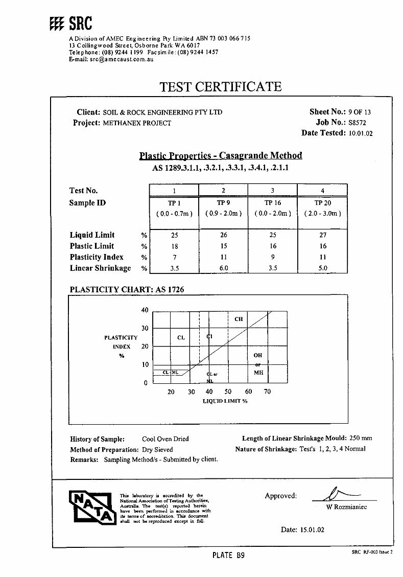
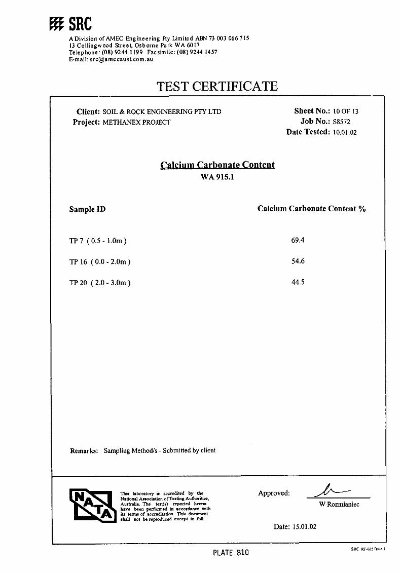
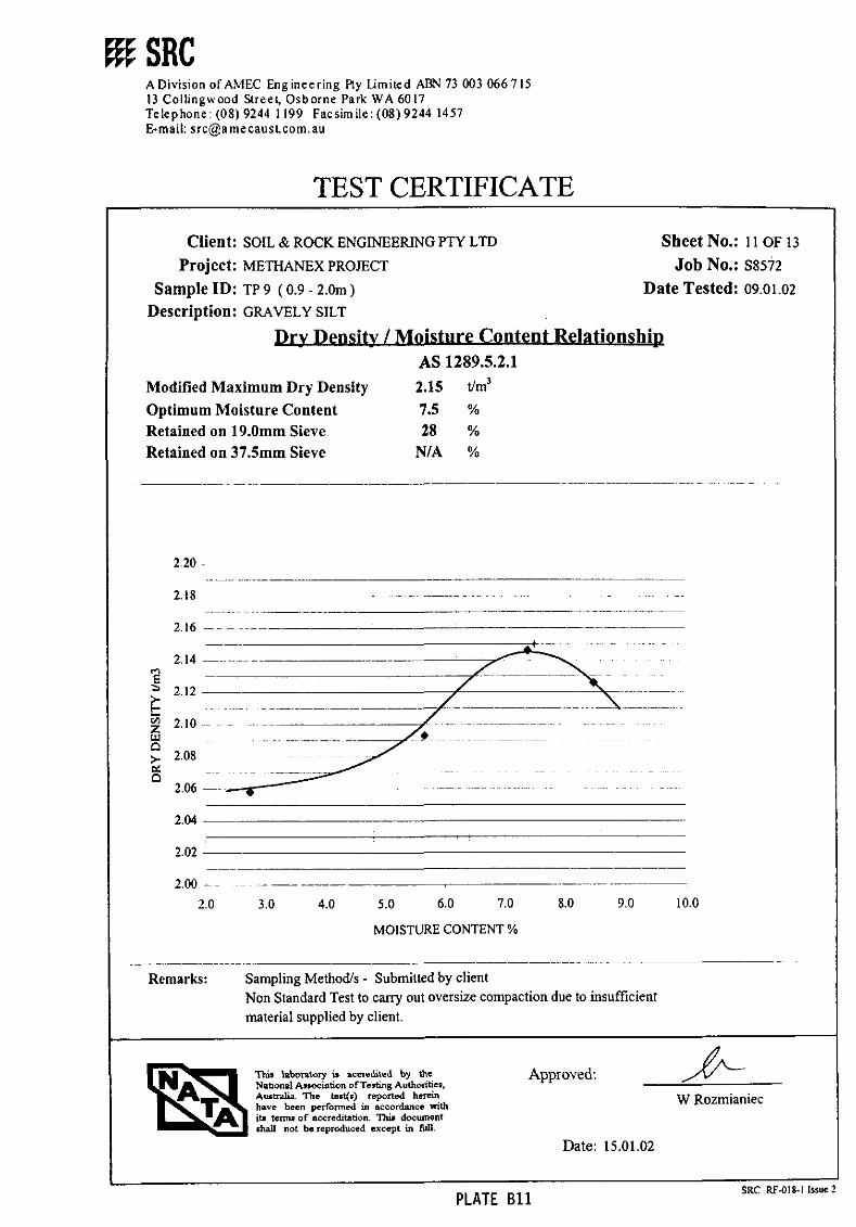
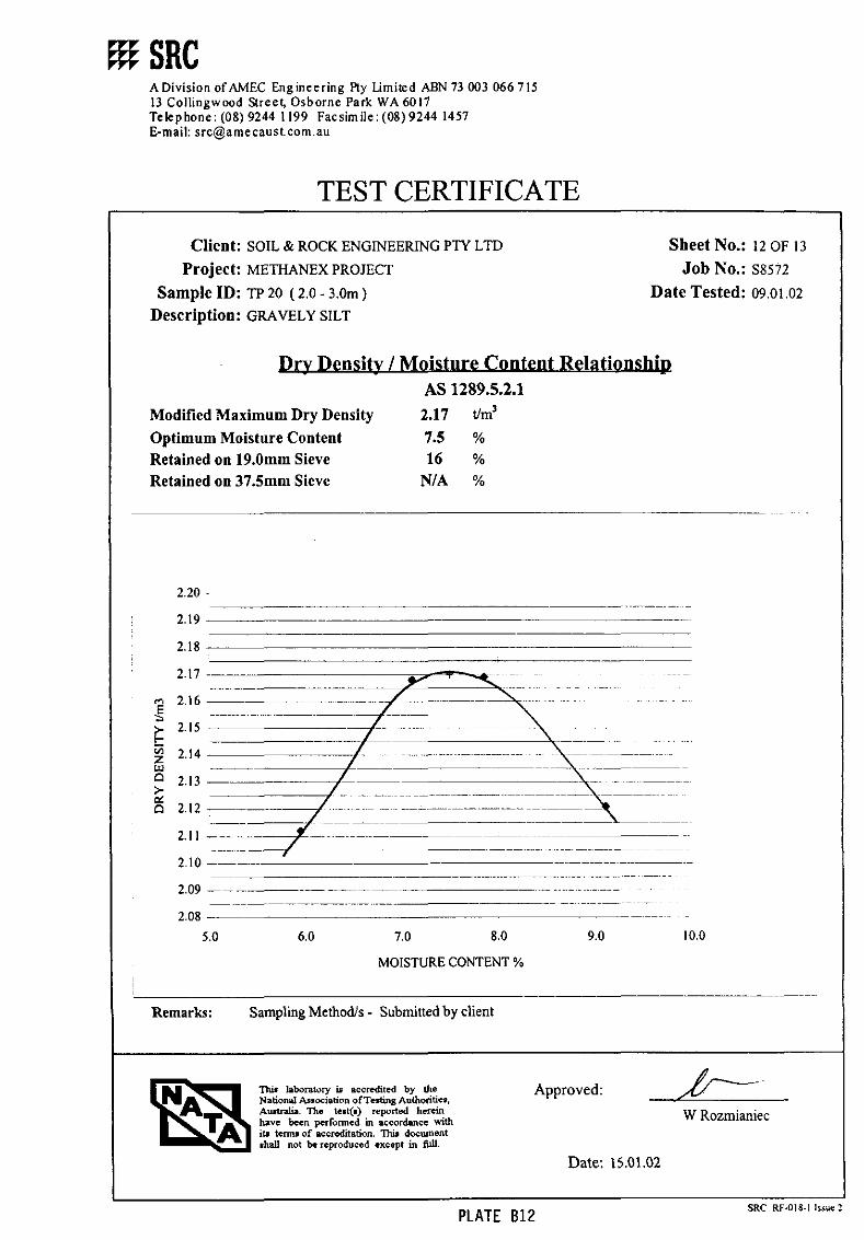
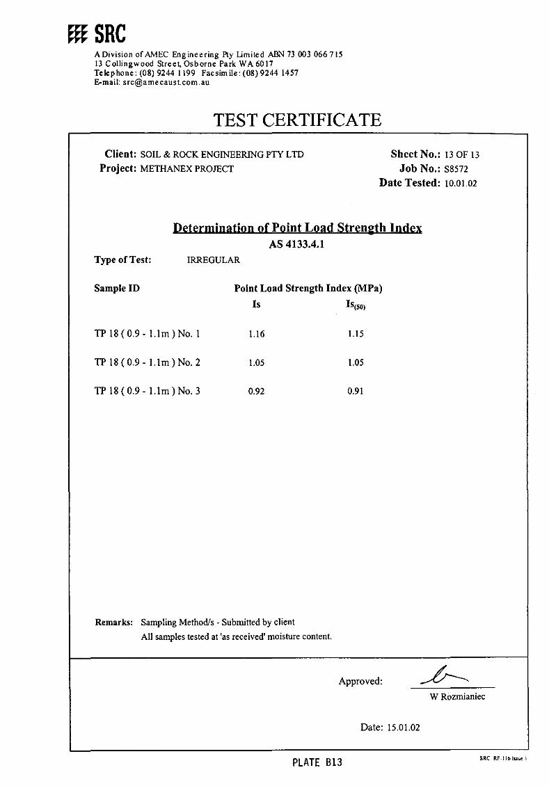

Vegetation, Flora and Fauna Assessment
Appendix 3
Methanex Burrup SiteVegetation, Flora and FaunaAssessment
Sinclair Knight Merz
Vegetation, Flora and Fauna Survey
January 2002
Methanex Burrup Site Vegetation, Flora and Fauna Assessment
2
© Biota Environmental Sciences Pty Ltd 2002ABN 49 092 687 119
2 / 183 Scarborough Beach RdMt Hawthorn WA 6010
Ph: 9201 9955 Fax: 9201 9599
Project No.: 098
Prepared by: M. MaierK. Armstrong
Checked by: G. Humphreys
This document has been prepared to the requirements of the client identified on the coverpage and no representation is made to any third party. It may be cited for the purposes ofscientific research or other fair use, but it may not be reproduced or distributed to any third
party by any physical or electronic means without the express permission of the client forwhom it was prepared or
Biota Environmental Sciences Pty Ltd.
Methanex Burrup Site Vegetation, Flora and Fauna Assessment
3
Methanex Burrup Site Vegetation, Flora andFauna Assessment
Contents
1.0 Summary 4
2.0 Introduction 72.1 Background 72.2 Scope of the Study 72.3 Previous Biological Studies 8
3.0 Methods 103.1 Vegetation and Flora 103.2 Fauna 12
4.0 Vegetation and Flora 154.1 Vegetation 154.2 Flora 24
5.0 Fauna 285.1 Land snails 285.2 Pseudomys chapmani 345.3 Planigale sp. and Lerista ‘muelleri’ 345.4 Bats 355.5 Other Fauna 38
6.0 Conclusions and Recommendations 416.1 Vegetation and Flora 416.2 Fauna 436.3 Recommendations 44
7.0 Acknowledgements 45
8.0 References 46
Appendix ARaw Data for Detailed Flora Survey Sites
Appendix BExtract of Dendrogram Produced by PATN Analysis of Data from theBurrup Peninsula and Surrounds
Appendix CVascular Flora Recorded from the Methanex Study Area
Appendix DRare Flora Report Forms
Appendix EFauna Recorded Previously from the Burrup Peninsula
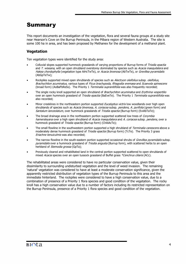
Methanex Burrup Site Vegetation, Flora and Fauna Assessment
4
Summary
This report documents an investigation of the vegetation, flora and several fauna groups at a study sitenear Hearson's Cove on the Burrup Peninsula, in the Pilbara region of Western Australia. The site issome 100 ha in area, and has been proposed by Methanex for the development of a methanol plant.
Vegetation
Ten vegetation types were identified for the study area:
• Colluvial slopes supported hummock grasslands of varying proportions of Burrup forms of Triodia epactiaand T. wiseana, with an open shrubland overstorey dominated by species such as Acacia inaequilatera andHakea chordophylla (vegetation type AiHcTwTe), or Acacia bivenosa (AbTwTe), or Grevillea pyramidalis(AbGpTeTw);
• Rockpiles supported mixed open shrublands of species such as Alectryon oleifolius subsp. oleifolius,Brachychiton acuminatus, various types of Ficus brachypoda, Rhagodia eremaea and Scaevola spinescens(broad form) (AoBaFbReSs). The Priority 1 Terminalia supranitifolia was also frequently recorded;
• The single rocky knoll supported an open shrubland of Brachychiton acuminatus and Erythrina vespertilioover an open hummock grassland of Triodia epactia (BaEveTe). The Priority 1 Terminalia supranitifolia wasalso recorded;
• Minor creeklines in the northeastern portion supported Eucalyptus victrix low woodlands over high openshrublands of species such as Acacia bivenosa, A. coriacea subsp. pendens, A. pyrifolia (green form) andSantalum lanceolatum, over hummock grasslands of Triodia epactia (Burrup form) (EviAbTaTe);
• The broad drainage area in the northeastern portion supported scattered low trees of Corymbiahamersleyana over a high open shrubland of Acacia inaequilatera and A. coriacea subsp. pendens, over ahummock grassland of Triodia epactia (Burrup form) (ChAiAcTe);
• The small flowline in the southwestern portion supported a high shrubland of Terminalia canescens above amoderately dense hummock grassland of Triodia epactia (Burrup form) (TcTe). The Priority 3 grassEriachne tenuiculmis was also recorded;
• The narrow flowline in the south-eastern portion supported occasional shrubs of Grevillea pyramidalis subsp.pyramidalis over a hummock grassland of Triodia angusta (Burrup form), with scattered herbs to an openherbland of Stemodia grossa (GpTa);
• Previously cleared and rehabilitated land in the central portion supported scattered to open shrublands ofmixed Acacia species over an open tussock grassland of Buffel grass *Cenchrus ciliaris (ACc).
The rehabilitated areas were considered to have no particular conservation value, given theirdissimilarity to surrounding undisturbed vegetation and the level of weed invasion. The remaining'natural' vegetation was considered to have at least a moderate conservation significance, given theapparently restricted distribution of vegetation types of the Burrup Peninsula to this area and theimmediate hinterland. The rockpiles were considered to have a high conservation value, due to acombination of presence of a Priority 1 flora species and good condition of the vegetation. The rockyknoll has a high conservation value due to a number of factors including its restricted representation onthe Burrup Peninsula, presence of a Priority 1 flora species and good condition of the vegetation.
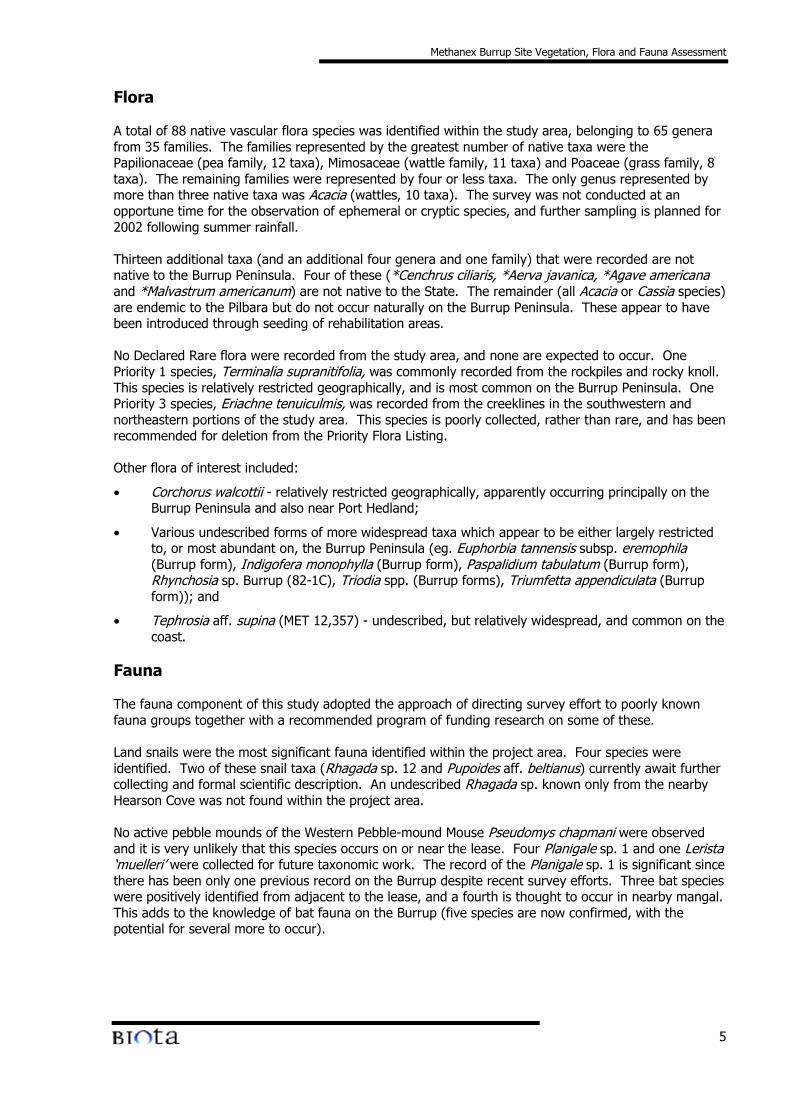
Methanex Burrup Site Vegetation, Flora and Fauna Assessment
5
Flora
A total of 88 native vascular flora species was identified within the study area, belonging to 65 generafrom 35 families. The families represented by the greatest number of native taxa were thePapilionaceae (pea family, 12 taxa), Mimosaceae (wattle family, 11 taxa) and Poaceae (grass family, 8taxa). The remaining families were represented by four or less taxa. The only genus represented bymore than three native taxa was Acacia (wattles, 10 taxa). The survey was not conducted at anopportune time for the observation of ephemeral or cryptic species, and further sampling is planned for2002 following summer rainfall.
Thirteen additional taxa (and an additional four genera and one family) that were recorded are notnative to the Burrup Peninsula. Four of these (*Cenchrus ciliaris, *Aerva javanica, *Agave americanaand *Malvastrum americanum) are not native to the State. The remainder (all Acacia or Cassia species)are endemic to the Pilbara but do not occur naturally on the Burrup Peninsula. These appear to havebeen introduced through seeding of rehabilitation areas.
No Declared Rare flora were recorded from the study area, and none are expected to occur. OnePriority 1 species, Terminalia supranitifolia, was commonly recorded from the rockpiles and rocky knoll.This species is relatively restricted geographically, and is most common on the Burrup Peninsula. OnePriority 3 species, Eriachne tenuiculmis, was recorded from the creeklines in the southwestern andnortheastern portions of the study area. This species is poorly collected, rather than rare, and has beenrecommended for deletion from the Priority Flora Listing.
Other flora of interest included:
• Corchorus walcottii - relatively restricted geographically, apparently occurring principally on theBurrup Peninsula and also near Port Hedland;
• Various undescribed forms of more widespread taxa which appear to be either largely restrictedto, or most abundant on, the Burrup Peninsula (eg. Euphorbia tannensis subsp. eremophila(Burrup form), Indigofera monophylla (Burrup form), Paspalidium tabulatum (Burrup form),Rhynchosia sp. Burrup (82-1C), Triodia spp. (Burrup forms), Triumfetta appendiculata (Burrupform)); and
• Tephrosia aff. supina (MET 12,357) - undescribed, but relatively widespread, and common on thecoast.
Fauna
The fauna component of this study adopted the approach of directing survey effort to poorly knownfauna groups together with a recommended program of funding research on some of these.
Land snails were the most significant fauna identified within the project area. Four species wereidentified. Two of these snail taxa (Rhagada sp. 12 and Pupoides aff. beltianus) currently await furthercollecting and formal scientific description. An undescribed Rhagada sp. known only from the nearbyHearson Cove was not found within the project area.
No active pebble mounds of the Western Pebble-mound Mouse Pseudomys chapmani were observedand it is very unlikely that this species occurs on or near the lease. Four Planigale sp. 1 and one Lerista‘muelleri’ were collected for future taxonomic work. The record of the Planigale sp. 1 is significant sincethere has been only one previous record on the Burrup despite recent survey efforts. Three bat specieswere positively identified from adjacent to the lease, and a fourth is thought to occur in nearby mangal.This adds to the knowledge of bat fauna on the Burrup (five species are now confirmed, with thepotential for several more to occur).
Methanex Burrup Site Vegetation, Flora and Fauna Assessment
6
Comprehensive lists of species previously recorded from the Burrup Peninsula are provided. The risk ofsignificant impact to fauna species including migratory birds, the Pilbara Olive Python Liasis olivaceusbarroni, the Water-rat Hydromys chrysogaster and the Bush Stone-curlew Burhinus grallarius is low.
Recommendations
In order to minimise impacts to the biological values of the study area, the following recommendationsare made:
1. Further seasonal floristic survey work should be conducted in 2002 following summer rainfall.The outcomes of this study may result in additional recommendations.
2. Given the moderate to high conservation value of the vegetation and flora of the study area,development should be restricted to historically disturbed areas (vegetation type ACc) as far aspossible. These areas are already degraded and have no particular conservation significance.
3. If clearing of additional areas is required, locations of Priority flora must be taken into accountand protected from disturbance. If this is not possible, then liaison should be undertaken withCALM to develop suitable management procedures.
4. Clearing of significant vegetation types (particularly the rocky knoll and rockpile units BaEveTeand AoBaFbReSs) should be avoided. Disturbance to the remaining vegetation types should beminimised.
5. Disturbed areas remaining after construction of the plant should be rehabilitated. Species used inseed mixes must be appropriate to the area, and seed should be collected locally on the BurrupPeninsula.
6. It is recommended that the proponent support the following three fauna research projects: landsnail taxonomy (Rhagada sp. 12 and Rhagada sp. Hearson Cove), morphological comparison ofWA Planigale sp. and specimen curation, and a genetic investigation of the legless lizard Delmapax.
7. In keeping with the spirit of adjacent developers, participate and assist in a collaborative study ofmeasures to minimise bird impacts and encourage their continued use of habitats on the Burrupthrough the development of an industry group for the King Bay - Hearson Cove Industrial Area.
8. The proponent should be aware of the potential for the Pilbara Olive Python Liasis olivaceusbarroni to occur within the plant area. A management plan should be developed andimplemented to reduce potential causes of mortality, and facilitate the removal and translocationof individuals that are found on the site.
Methanex Burrup Site Vegetation, Flora and Fauna Assessment
7
2.0 Introduction
2.1 Background
This report documents an investigation of the vegetation, flora and several fauna groups at a study sitenear Hearson's Cove on the Burrup Peninsula, in the Pilbara region of Western Australia. The site issome 100 ha in area, and has been proposed by Methanex for the development of a methanol plant(see Figure 2.1).
2.2 Scope of the Study
Vegetation and flora were generally assessed to determine features of significance existing within thestudy area. The fauna study, however, involved a more targeted approach. Given that the Departmentof Conservation and Land Management (CALM) has previously completed general fauna survey work onthe Burrup Peninsula, including within the project area, the scope of the current study with respect tothe fauna component was as follows:
• Conduct a brief survey of land snails (Gastropoda: Pulmonata) within the project area;
• Survey for mounds of the Western Pebble-mound Mouse Pseudomys chapmani, determine theactivity status of any mounds located, and conduct trapping to confirm the presence of this speciesif appropriate. P. chapmani was previously regarded as a Schedule 1 species (rare andendangered, and likely to become extinct), however more recent survey work and researchprompted a review of the conservation status of this species (Start et al. 2000). It wassubsequently down-graded from the Schedule fauna listing to the Priority fauna list. The presenceof this species within the project area would be of interest since it is currently regarded as extincton the Burrup;
• Collect specimens of Planigale sp. from the project area and habitats nearby. There is only asingle record of a Planigale sp. from the Burrup Peninsula which is on the Western AustralianMuseum (WAM) mammal database as P. maculata (M19669, road kill collected by W.H. Butler,Mount Burrup 20° 36' 05", 116° 46' 25", 28/6/1981). Given that there is only one previous record,and that taxonomic work is currently underway on Planigale taxa in Western Australia, this taxonwas targeted through pit trapping to confirm the earlier record and to add material to thetaxonomic study;
• Collect specimens of the Lerista ‘muelleri’ species complex from the project area and nearbyhabitats on the Burrup Peninsula to contribute to studies currently underway on the taxonomywithin this group; and
• Conduct a brief survey of bat fauna in the project area and nearby habitats, given the paucity ofinformation on bat species occurrence and distribution on the Burrup Peninsula.
These five fauna groups were targeted as they are considered to be the least understood, either interms of their taxonomy or distribution, at the proposed site or on the Burrup generally. In addition,current lists of the vertebrate fauna that occur on the Burrup Peninsula were compiled from variousreputable sources, including records from previous CALM survey work in the area.
The EPA (1995) states that when specific development proposals arise for the King Bay – Hearsonregion of the Burrup, the impacts on the nearby mangal at King Bay and the potential ecological riskassociated with the development of industry in a storm surge area need to be considered. There have
Methanex Burrup Site Vegetation, Flora and Fauna Assessment
8
been previous assessments of the fauna in the storm surge area (mangroves, low tidal sand and mudflats; Worley Astron 1999). Presumably, the recommendations of the EPA (1995) would also berelevant for the mangal at Cowrie Cove, which is adjacent to the project area. The present study doesnot address these issues directly since the project area does not include such areas. Outfalls from theproposed infrastructure are to enter King Bay but provision has been made for this in conjunction withanother project (the Syntroleum development; Water Corporation of Western Australia 2001).
2.2.1 Limitations of the Study
The findings of the botanical survey are subject to a number of limitations:
• Sites within the study area were only sampled once, and further flora species would undoubtedlybe collected with additional survey effort;
• The timing of the field survey was inappropriate for the detection of many ephemeral and crypticflora species, as it followed several months with no significant rainfall;
• Only vascular flora were targeted (ie. fungi, algae, mosses and liverworts were not specificallysampled).
Further flora sampling is planned for 2002 following summer rainfall.
The fauna survey was similarly subject to limitations:
• The trapping effort (4 nights) was not adequate to sample the entire vertebrate faunaassemblage at the proposed plant site, however a comprehensive listing was not the intention ofthe present study. Instead, the study represented a targeted survey for fauna groups thatrequire further work on taxonomy and distribution. The Burrup Peninsula is regarded as wellsurveyed, especially given the trapping program by CALM. Directing survey effort to poorlyknown fauna groups was agreed with CALM as a more appropriate strategy than duplicatinggeneral survey work.
• The collection of live snails is usually more productive after rains, however there were no suchopportunities within the timeframe of this project. Some species of snail can only be identifiedfrom live or fresh material. The collection of live material also confirms the presence of thepopulation since empty shells may not always be indicative of the presence of live animals.Snails would be surveyed in more detail during a seasonal survey planned after sufficient rain inKarratha.
2.3 Previous Biological Studies
The flora and vegetation of the Burrup Peninsula have been surveyed previously at various levels ofintensity. Broad-scale (1:1,000,000) vegetation mapping of the Pilbara was prepared by Beard (1975).The peninsula occurs within the Fortescue Botanical District of the Pilbara Region, as defined by Beard(1975). It forms part of the broad Abydos Plain physiographic unit, which extends from Cape Prestoneast to Pardoo Creek, and south to the Chichesters. The unit includes alluvial plains, low stony hills andgranite outcrops, and comprises largely granitic soils, with alluvial sands on the coastal portion (Beard,1975).
Methanex Burrup Site Vegetation, Flora and Fauna Assessment
9
The vegetation of the peninsula itself was mapped as Triodia epactia (referred to as T. pungens byBeard) hummock grassland with very few shrubs.
The flora and vegetation of the Fortescue Botanical District as a whole are relatively poorly known.Surveys of varying intensity have been conducted on a sporadic basis through the region, chiefly formining approvals or other development proposals. The Burrup Peninsula has been subject to a higherintensity of sampling than much of the remainder of the district. A detailed study of the vegetation andflora of almost 200 sites on the Peninsula was conducted on behalf of the Department of ResourcesDevelopment (Trudgen and Long, in prep.). The reporting for this study is currently being finalised.Additional botanical studies have been conducted for various individual proposals on the Burrup (seeTable 2.1), including an adjoining lease (Morgan & Trudgen, in prep.), however these are largelyunpublished and difficult to obtain.
The vertebrate fauna of the Burrup has been investigated previously by CALM at several long termstudy sites. One of these sites is located within the project area and a second is immediately adjacent.The report for this work has not yet been completed, however all representative specimens have beenlodged with the Western Australian Museum. Table 2.1 lists previous work conducted on fauna of theBurrup Peninsula. Most of the other fauna studies conducted by biological consultants are unpublished.This includes a recent targeted fauna survey of an adjoining lease (Biota Environmental Sciences,2001a).
Table 2.1: Biological surveys conducted on the Burrup Peninsula.
Reference ProjectAstron Environmental (1998) Ammonia Urea Plant Service Corridor Fauna Survey.Astron Environmental (1999a) Natural Gas to Synthetic Oil Project: Product and Feed pipelines,
Vegetation, Flora and Fauna Survey.Astron Environmental (1999b) Natural Gas to Synthetic Oil Project: Plantsite Vegetation, Flora and
Fauna Survey.Astron Environmental (2000) Natural Gas to Synthetic Oil Project: A Vertebrate Survey of the
Plant Site on the Burrup Peninsula.Astron Environmental (2001a) Vegetation and Flora of the Proposed Ammonia Plant Site.Astron Environmental (2001b) Fauna of the Burrup Peninsula and the Proposed Ammonia Plant.Biota Environmental Sciences (2001a) Burrup Liquid Ammonia Plant Targeted Fauna Survey.Butler & Butler (1983) Burrup Peninsula Fauna Survey.Butler & Butler (1987) Burrup Peninsula Fauna Survey.Butler (1994) Fauna and Marine Biota. In: Burrup Peninsula Draft Land Use and
Management Plan, Technical Appendices.Kruger & Long (1999) A Survey of Vegetation and Fauna in the King Bay Region, Burrup
Peninsula, W.A.Morgan & Trudgen (in prep.) A flora and vegetation survey of a site on the Burrup Peninsula for
a proposed Dimethyl Ether project.Tingay & Tingay (1979) Technical Report on the Fauna of Burrup Peninsula and Dolphin
Island.Trudgen & Griffin (2002); Trudgen & Long(in prep.)
A flora, vegetation and floristic survey of the Burrup Peninsula,some adjoining areas and part of the Dampier Archipelago, withcomparisons to the floristics of three areas of the adjoiningmainland.
Methanex Burrup Site Vegetation, Flora and Fauna Assessment
10
3.0 Methods
3.1 Vegetation and Flora
The vegetation and flora of the study area were assessed from 29th October to 1st November 2001.The timing of the survey was not opportune for the collection of ephemeral or cryptic flora species, as itoccurred some several months following significant rainfall.
3.1.1 Quadrat Sampling
Vegetation and flora were principally assessed in 10 quadrats (B001 to B010). The distribution of thesequadrats is shown in Figure 4.1, while the raw data is contained in Appendix A. The locations of thedetailed recording sites were chosen to represent the major vegetation types occurring within thesurvey area.
Quadrats were typically 50 m x 50 m, as this size gives a good sample of flora presence. It also gives agood indication of the shrub and grass layer vegetation structure for most vegetation types in thePilbara that occur in 'uniform' habitats (eg. plains and hillslopes, where vegetation stands of greaterthan this size occur). Quadrat shape and/or size were adjusted as necessary to fit smaller or oddlyshaped habitats (eg. flowlines and rocky outcrops). Each quadrat was permanently marked using steelfence droppers which were typically located on at least three corners of the quadrat.
The following parameters were recorded for each quadrat:
• Location Recorded at each permanent stake using a hand-held Global PositioningSystem (GPS) to an accuracy usually within 5 m in AGD 84 datum;
• Vegetation Type Broad description based on dominant species and strata after Specht(1970);
• Landform A broad classification, being either colluvial slope, rockpile, creekline orrehabilitation area;
• Substrate General soil type and description of stony surface mantle;
• Leaf / Wood Litter Percent cover; depth of leaf litter where appropriate;
• Disturbance Details Evidence of grazing, weed invasion, frequent fires etc. Note that fireeffects are only considered as a negative impact if they are caused byrepeated burning (eg. conducted for pastoral purposes). Fire is a naturaland frequent process in the Pilbara to which the vegetation has adapted,and to class areas as being in poor condition simply because they havebeen recently burnt is misleading; and
• Percent Foliar Cover Cover was visually estimated for each species. Estimates were made tothe nearest percent where possible, or a range (eg. 5-10%) was used.'+' was used where only occasional individuals were present, with a coverof less than 1%.
Methanex Burrup Site Vegetation, Flora and Fauna Assessment
11
A colour photograph of the vegetation at each site was taken using a digital camera.
3.1.2 Additional Survey Work
Additional foot traverses were conducted to ground truth the boundaries of vegetation types and toallow assessment of areas beyond the detailed flora quadrats. Opportunistic flora collections weremade on these traverses to supplement the list of species recorded from the flora survey sites.Particular attention was paid to searching habitats likely to support flora species with sporadicdistributions (eg. rockpiles). Six releves (unbounded sites) were also briefly assessed to assist withvegetation type description (Releves RA to RF). The lists of species recorded for these sites were notintended to represent a complete list of the flora present, and have thus not been included in thefloristic analysis (see Section 3.1.3).
3.1.3 Flora Identification, Data Entry and Analysis
Common species which were well known to the survey botanist were identified in the field. Specimensof all other species were collected and assigned a unique number to facilitate tracking of data. Thesevouchers were then identified by keying out, reference to appropriate publications, use of referencecollections, comparison to the collections held at the Western Australian Herbarium (WAHerb) andconsultation with relevant specialists for difficult taxa (see Section 7.0). Much of the material collectedwas in relatively poor condition. Specimens will be lodged with the Herbaria at Perth and Karratha forany taxa for which suitable material is available. Rare Flora Report Forms were completed for Priorityflora encountered within the study area, and will be lodged with CALM (Appendix D).
Nomenclature was checked against the current listing of scientific names recognised by WAHerb andupdated as necessary. The only outdated nomenclature retained is that relating to Cassia. This genusis currently recognised as Senna (see Randell, 1989), however the older Cassia classification (Symon,1966) was perceived to represent a more realistic level of separation of the taxa (eg. with taxa such as'glutinosa' and 'pruinosa' recognised at specific rather than subspecific level) (M. Trudgen, pers.comm.). A more detailed discussion is contained in Trudgen & Casson (1998), while a comparison ofthe nomenclature under the two classifications is presented in Appendix C.
All raw site data were entered into an Access database using forms developed by Mr. Ted Griffin andsupplied by Mr. Malcolm Trudgen. These raw data were corrected as necessary after specimens wereidentified. A matrix of the cover of each species at each site was subsequently generated, with covervalues assigned to the following classes: <1%, 1-5%, 5-10%, 10-25%, 25-33.3%, 33.3-50%, 50-75%and >75%.
The Methanex floristic data were incorporated with data from seven quadrats and 19 releves assessedduring a recent survey of an area adjoining the southern boundary of the Methanex study area (Morgan& Trudgen, in prep.), and 193 sites assessed as part of the survey of the greater Burrup Peninsula andsurrounds (Trudgen & Griffin, 2002). Given the seasonal timing of the current survey, only perennialflora were included in the dataset. A PATN classification was run on this combined data set in order toexamine the relationships between the detailed vegetation survey sites. The quantitative results ofPATN were used to refine the vegetation types identified in the field.
3.1.4 Vegetation Mapping
Scanned copies (at ~1:5000 scale) of colour aerial photography were marked up with vegetation typeboundaries. Some of the vegetation units of the colluvial slopes were found to have a hummockgrassland of varying proportions of two spinifex species, which occurred together and varied indistribution on an extremely fine scale. These were mapped as mosaics.
The vegetation boundaries were subsequently digitised using AutoCAD. The resulting AutoCAD fileswere "tagged" to provide each polygon with the vegetation association code, and then translated into
Methanex Burrup Site Vegetation, Flora and Fauna Assessment
12
ArcView 3.2a for validation. Other point source datasets, such as site locations, weed locations andpriority flora locations were generated into spatial data using ArcView. These datasets weresubsequently saved as separate ArcView shapefiles. In conjunction with additional data supplied fromother organisations, they were then used in the production of a map of the vegetation of the studyarea.
3.2 Fauna
As discussed in Section 2.2, this survey adopted the approach of directing resources towards five mainfauna groups that are not well understood, rather than focussing on the duplication of a species list thatwould contribute only minimally to improving the existing knowledge of fauna on the Burrup.Furthermore, the vertebrate species lists compiled in this report include records from the whole BurrupPeninsula since the study area is relatively small. Species on these lists have a relatively high chance ofoccurring in or near the study site, if their habitat is present.
3.2.1 Land snails
All broad habitat types within the project area were surveyed for land snails (Gastropoda: Pulmonata).Habitat types were defined based on geology, soil/substrate type and vegetation. Since a new,undescribed species of Rhagada was recently discovered at Hearson’s Cove, particular attention waspaid to locating this species. This species is distinctive, having an acutely angled periphery with athread-like keel (similar in general shape to Divellomelon hillieri from the Northern Territory; seeillustration in Solem 1990). Also, other snails species have not been recorded in the project areapreviously but have been collected nearby. Species such as R. angulata are known to be distributednorth of Withnell Bay – Watering Cove, and R. convicta is distributed near Dampier south of the salineflat area of King Bay - Hearson Cove (P.G. Kendrick unpublished data). These snails were alsotargeted.
3.2.2 Pseudomys chapmani
Mounds were sought throughout the project area, and particularly in habitat similar to that in which themounds were located on an adjacent lease (Grassland Steppe, in particular Lower Undulating Slopeswith Shallow Incised Drainage Lines; Sinclair Knight Merz 2001).
The mounds were assessed according to the Mound Condition Index of Anstee (1996). This systemscores pebble mounds based on external mound features to determine occupancy of P. chapmani;scores of between 6 - 9 indicate a high likelihood of occupancy.
3.2.3 Planigale sp. and Lerista ‘muelleri’
The collection of Planigale sp. and L. ‘muelleri’ was facilitated by trapping. Four lines of pit traps, eachwith 10 pits connected in pairs with flywire fences, were opened for 4 nights each. These traps wereinstalled and used in previous surveys of the Burrup Peninsula by CALM. The sites were:
Site 8: Mt Wongama; 50 479780, 7724000;
Methanex Burrup Site Vegetation, Flora and Fauna Assessment
13
Site 11: Bloodwood Flat, Hearson Cove (within the project area); 50 478521, 7720653;
Site 12: Watering Cove Track; 50 479095, 7723004;
Site 16: Watertanks, Village Rd (directly adjacent to the project area); 50 477595, 7720225.
L. ‘muelleri’ were also sought by hand in litter over sandy soils, in particular from crushed Triodiahummocks along vehicle tracks, beneath stands of eucalypts on Mt Wongama, and beneath acaciasimmediately above the high tide mark at Cowrie Cove.
3.2.4 Bats
Bats were surveyed by detecting and analysing echolocation calls. Surveys were conducted in a gullybetween rockpiles west of the project area (‘Gully’; 50 476800, 7720200) and the mangal at King Bay(‘King Bay’; 50 475700, 7718400) and Cowrie Cove (‘Cowrie Cove’; 50 479750, 7721350).
Calls were detected with an electronic device that detects and transforms high frequency sounds (anAnabat II bat detector connected to an Anabat Delay Switch (Titley Electronics) and a RadioShack CTR-119 cassette tape recorder, and recorded onto ferrous audio cassettes (TDK D90)). Calls were analysedby Zero Crossings Analysis (ZCA) using an Anabat V ZCA Interface Module and Anabat software (ChrisCorben; http://users.lanminds.com/corben/index.htm). All calls were calibrated with a tone of 40 kHzand divided down by a factor of 16.
Three call variables were extracted from the audio tapes using the software program ‘Analyze forWindows 95’ (Jolly, 1996a, 1996b, 1997). Only sequences with good quality ‘search’ mode calls wereincluded and each pulse was examined before its inclusion into the resulting dataset. This programuses a modelling technique to fit a curve to the data points produced by the ZCA. Further detailsregarding the methods of this software may be found on the internet (Jolly 1996b). The three callparameters included were:
- Dur: the duration of the pulse; the time from the first to the last data point of each pulse.
- Fend: the minimum frequency calculated from the model. This parameter is superior to minimumpulse frequency since it is calculated from the model which uses all data points. Fend is usuallyhighly correlated with the minimum pulse frequency and can therefore be used in comparison withthe reference calls of McKenzie and Muir (2000).
- Fmax: the highest detected frequency. This can be variable depending on the type of callproduced, and whether the bat detector is able to detect and transform the higher frequencycomponents of a pulse (affected by several factors).
These data were summarised on a scatterplot using the discriminant functions of McKenzie and Muir(2000; reference calls obtained from hand-released bats). Species identity was assigned to each pointon the graph, using the groupings of McKenzie and Muir (2000) and K. Armstrong (unpublished data) asa guide.
3.2.5 Other Fauna
Other fauna species were also recorded wherever individuals, tracks, burrows or scats were observed.All fauna recorded from the CALM pit traps are included in this report. Fauna collected in pits locatedoutside the project area are indicated where appropriate. These fauna have the potential to occurwithin suitable habitat within the project area. Particular attention was also paid to habitats where theNorthern Quoll Dasyurus hallucatus (rocky outcrops) and the Water-rat Hydromys chrysogaster (salineflats and drainage gullies) might occur, however they were not specifically targeted in the presentsurvey. These species have been recorded previously on the Burrup Peninsula (e.g. Butler and Butler1983).

Methanex Burrup Site Vegetation, Flora and Fauna Assessment
14
A list of the fauna known to occur on the Burrup was compiled from various current and reputablesources and is presented in Appendix E. The bird list was provided by Mr R. Johnstone from theWestern Australian Museum who used data from the Storr-Johnstone Bird Data Bank and other sources(Appendix E). The reptile and mammal lists were based on vouchered and identified specimens in theWAM rather than the general maps provided in field guides. Some additional species were added fromreferences that provided the original observations.
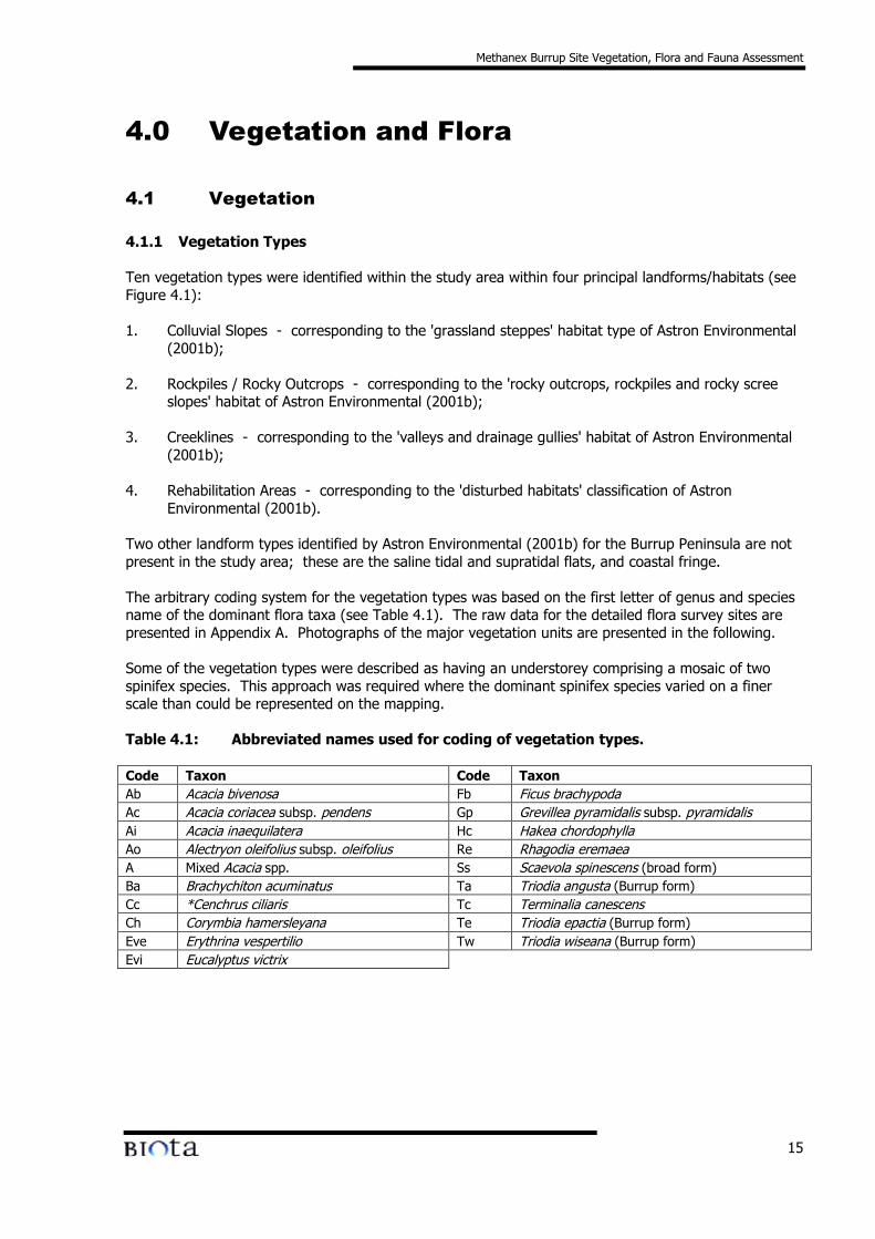
Methanex Burrup Site Vegetation, Flora and Fauna Assessment
15
4.0 Vegetation and Flora
4.1 Vegetation
4.1.1 Vegetation Types
Ten vegetation types were identified within the study area within four principal landforms/habitats (seeFigure 4.1):
1. Colluvial Slopes - corresponding to the 'grassland steppes' habitat type of Astron Environmental(2001b);
2. Rockpiles / Rocky Outcrops - corresponding to the 'rocky outcrops, rockpiles and rocky screeslopes' habitat of Astron Environmental (2001b);
3. Creeklines - corresponding to the 'valleys and drainage gullies' habitat of Astron Environmental(2001b);
4. Rehabilitation Areas - corresponding to the 'disturbed habitats' classification of AstronEnvironmental (2001b).
Two other landform types identified by Astron Environmental (2001b) for the Burrup Peninsula are notpresent in the study area; these are the saline tidal and supratidal flats, and coastal fringe.
The arbitrary coding system for the vegetation types was based on the first letter of genus and speciesname of the dominant flora taxa (see Table 4.1). The raw data for the detailed flora survey sites arepresented in Appendix A. Photographs of the major vegetation units are presented in the following.
Some of the vegetation types were described as having an understorey comprising a mosaic of twospinifex species. This approach was required where the dominant spinifex species varied on a finerscale than could be represented on the mapping.
Table 4.1: Abbreviated names used for coding of vegetation types.
Code Taxon Code TaxonAb Acacia bivenosa Fb Ficus brachypodaAc Acacia coriacea subsp. pendens Gp Grevillea pyramidalis subsp. pyramidalisAi Acacia inaequilatera Hc Hakea chordophyllaAo Alectryon oleifolius subsp. oleifolius Re Rhagodia eremaeaA Mixed Acacia spp. Ss Scaevola spinescens (broad form)Ba Brachychiton acuminatus Ta Triodia angusta (Burrup form)Cc *Cenchrus ciliaris Tc Terminalia canescensCh Corymbia hamersleyana Te Triodia epactia (Burrup form)Eve Erythrina vespertilio Tw Triodia wiseana (Burrup form)Evi Eucalyptus victrix
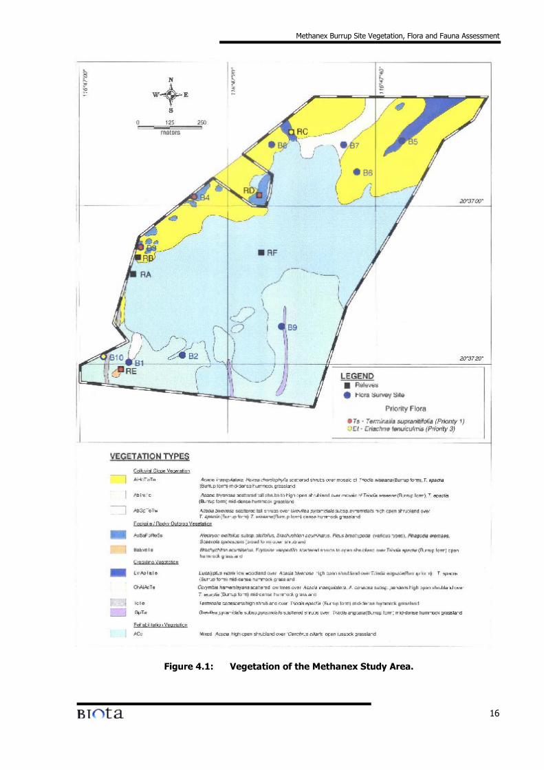
Methanex Burrup Site Vegetation, Flora and Fauna Assessment
16
Figure 4.1: Vegetation of the Methanex Study Area.
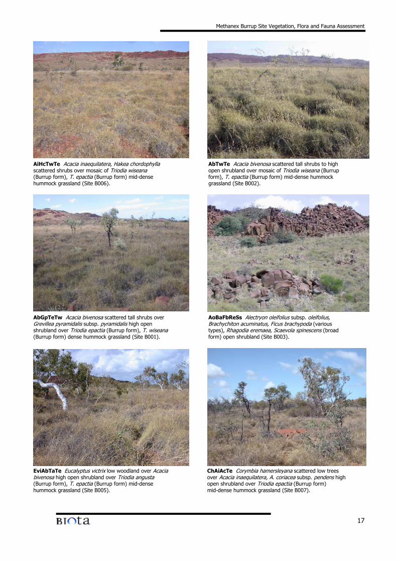
Methanex Burrup Site Vegetation, Flora and Fauna Assessment
17
AiHcTwTe Acacia inaequilatera, Hakea chordophylla AbTwTe Acacia bivenosa scattered tall shrubs to highscattered shrubs over mosaic of Triodia wiseana open shrubland over mosaic of Triodia wiseana (Burrup(Burrup form), T. epactia (Burrup form) mid-dense form), T. epactia (Burrup form) mid-dense hummockhummock grassland (Site B006). grassland (Site B002).
AbGpTeTw Acacia bivenosa scattered tall shrubs over AoBaFbReSs Alectryon oleifolius subsp. oleifolius,Grevillea pyramidalis subsp. pyramidalis high open Brachychiton acuminatus, Ficus brachypoda (variousshrubland over Triodia epactia (Burrup form), T. wiseana types), Rhagodia eremaea, Scaevola spinescens (broad(Burrup form) dense hummock grassland (Site B001). form) open shrubland (Site B003).
EviAbTaTe Eucalyptus victrix low woodland over Acacia ChAiAcTe Corymbia hamersleyana scattered low treesbivenosa high open shrubland over Triodia angusta over Acacia inaequilatera, A. coriacea subsp. pendens high(Burrup form), T. epactia (Burrup form) mid-dense open shrubland over Triodia epactia (Burrup form)hummock grassland (Site B005). mid-dense hummock grassland (Site B007).
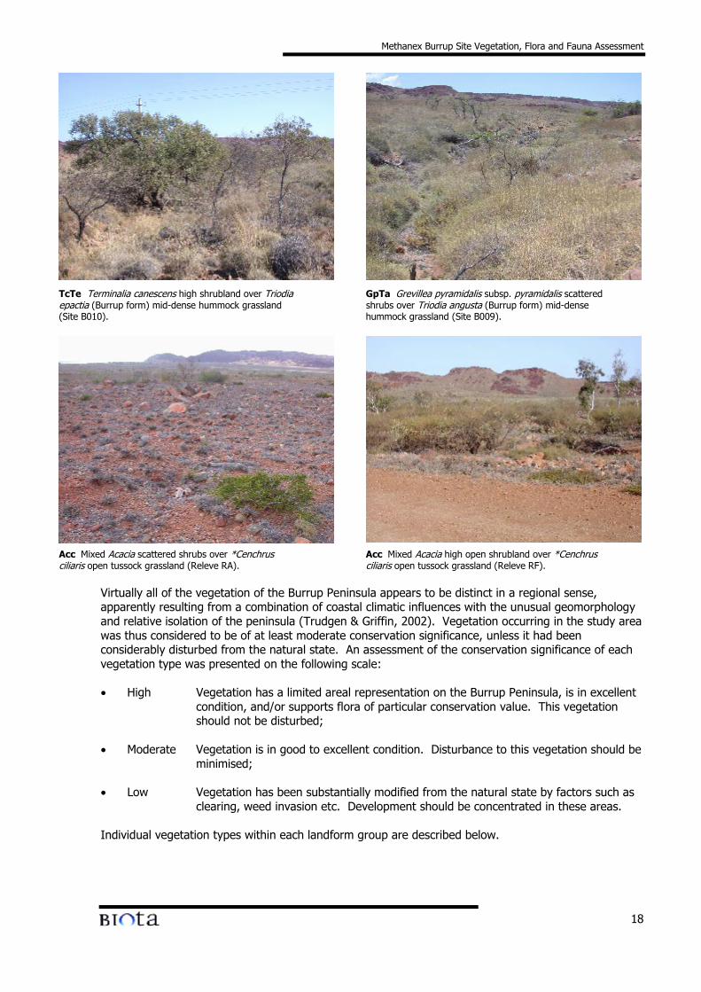
Methanex Burrup Site Vegetation, Flora and Fauna Assessment
18
TcTe Terminalia canescens high shrubland over Triodia GpTa Grevillea pyramidalis subsp. pyramidalis scatteredepactia (Burrup form) mid-dense hummock grassland shrubs over Triodia angusta (Burrup form) mid-dense(Site B010). hummock grassland (Site B009).
Acc Mixed Acacia scattered shrubs over *Cenchrus Acc Mixed Acacia high open shrubland over *Cenchrusciliaris open tussock grassland (Releve RA). ciliaris open tussock grassland (Releve RF).
Virtually all of the vegetation of the Burrup Peninsula appears to be distinct in a regional sense,apparently resulting from a combination of coastal climatic influences with the unusual geomorphologyand relative isolation of the peninsula (Trudgen & Griffin, 2002). Vegetation occurring in the study areawas thus considered to be of at least moderate conservation significance, unless it had beenconsiderably disturbed from the natural state. An assessment of the conservation significance of eachvegetation type was presented on the following scale:
• High Vegetation has a limited areal representation on the Burrup Peninsula, is in excellentcondition, and/or supports flora of particular conservation value. This vegetationshould not be disturbed;
• Moderate Vegetation is in good to excellent condition. Disturbance to this vegetation should beminimised;
• Low Vegetation has been substantially modified from the natural state by factors such asclearing, weed invasion etc. Development should be concentrated in these areas.
Individual vegetation types within each landform group are described below.
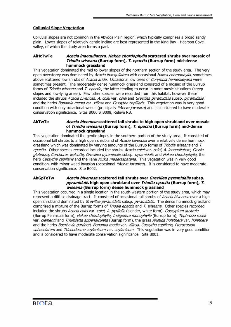
Methanex Burrup Site Vegetation, Flora and Fauna Assessment
19
Colluvial Slope Vegetation
Colluvial slopes are not common in the Abydos Plain region, which typically comprises a broad sandyplain. Lower slopes of relatively gentle incline are best represented in the King Bay - Hearson Covevalley, of which the study area forms a part.
AiHcTwTe Acacia inaequilatera, Hakea chordophylla scattered shrubs over mosaic ofTriodia wiseana (Burrup form), T. epactia (Burrup form) mid-densehummock grassland
This vegetation dominated the mid to lower slopes of the northern section of the study area. The veryopen overstorey was dominated by Acacia inaequilatera with occasional Hakea chordophylla, sometimesabove scattered low shrubs of Acacia arida. Occasional low trees of Corymbia hamersleyana weresometimes present. The moderately dense hummock grassland consisted of a mosaic of the Burrupforms of Triodia wiseana and T. epactia, the latter tending to occur in more mesic situations (steepslopes and low-lying areas). Few other species were recorded from this habitat, however theseincluded the shrubs Acacia bivenosa, A. colei var. colei and Grevillea pyramidalis subsp. pyramidalis,and the herbs Bonamia media var. villosa and Cassytha capillaris. This vegetation was in very goodcondition with only occasional weeds (principally *Aerva javanica) and is considered to have moderateconservation significance. Sites B006 & B008, Releve RB.
AbTwTe Acacia bivenosa scattered tall shrubs to high open shrubland over mosaicof Triodia wiseana (Burrup form), T. epactia (Burrup form) mid-densehummock grassland
This vegetation dominated the gentle slopes in the southern portion of the study area. It consisted ofoccasional tall shrubs to a high open shrubland of Acacia bivenosa over a relatively dense hummockgrassland which was dominated by varying amounts of the Burrup forms of Triodia wiseana and T.epactia. Other species recorded included the shrubs Acacia colei var. colei, A. inaequilatera, Cassiaglutinosa, Corchorus walcottii, Grevillea pyramidalis subsp. pyramidalis and Hakea chordophylla, theherb Cassytha capillaris and the liane Mukia maderaspatana. This vegetation was in very goodcondition, with minor weed invasion (occasional *Aerva javanica). It is considered to have moderateconservation significance. Site B002.
AbGpTeTw Acacia bivenosa scattered tall shrubs over Grevillea pyramidalis subsp.pyramidalis high open shrubland over Triodia epactia (Burrup form), T.wiseana (Burrup form) dense hummock grassland
This vegetation occurred in a single location in the south-western portion of the study area, which mayrepresent a diffuse drainage tract. It consisted of occasional tall shrubs of Acacia bivenosa over a highopen shrubland dominated by Grevillea pyramidalis subsp. pyramidalis. The dense hummock grasslandcomprised a mixture of the Burrup forms of Triodia epactia and T. wiseana. Other species recordedincluded the shrubs Acacia colei var. colei, A. pyrifolia (slender, white form), Gossypium australe(Burrup Peninsula form), Hakea chordophylla, Indigofera monophylla (Burrup form), Tephrosia roseavar. clementii and Triumfetta appendiculata (Burrup form), the grass Aristida holathera var. holatheraand the herbs Boerhavia gardneri, Bonamia media var. villosa, Cassytha capillaris, Pterocaulonsphacelatum and Trichodesma zeylanicum var. zeylanicum. This vegetation was in very good conditionand is considered to have moderate conservation significance. Site B001.
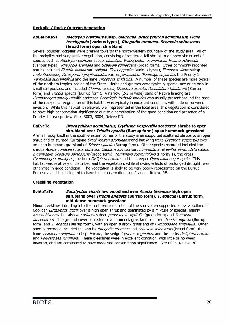
Methanex Burrup Site Vegetation, Flora and Fauna Assessment
20
Rockpile / Rocky Outcrop Vegetation
AoBaFbReSs Alectryon oleifolius subsp. oleifolius, Brachychiton acuminatus, Ficusbrachypoda (various types), Rhagodia eremaea, Scaevola spinescens(broad form) open shrubland
Several boulder rockpiles were present towards the north-western boundary of the study area. All ofthe rockpiles had very similar vegetation, consisting of scattered tall shrubs to an open shrubland ofspecies such as Alectryon oleifolius subsp. oleifolius, Brachychiton acuminatus, Ficus brachypoda(various types), Rhagodia eremaea and Scaevola spinescens (broad form). Other commonly recordedshrubs included Ehretia saligna var. saligna, Ficus opposita (various types), Flueggea virosa subsp.melanthesoides, Pittosporum phylliraeoides var. phylliraeoides, Plumbago zeylanica, the Priority 1Terminalia supranitifolia and the liane Tinospora smilacina. A number of these species are more typicalof the northern tropical region of the State. Herbs and grasses were typically sparse, occurring only insmall soil pockets, and included Cleome viscosa, Dicliptera armata, Paspalidium tabulatum (Burrupform) and Triodia epactia (Burrup form). A narrow (2-3 m wide) band of Native lemongrassCymbopogon ambiguus with scattered Pentalepis trichodesmoides was usually present around the baseof the rockpiles. Vegetation of this habitat was typically in excellent condition, with little or no weedinvasion. While this habitat is relatively well represented in the local area, this vegetation is consideredto have high conservation significance due to a combination of the good condition and presence of aPriority 1 flora species. Sites B003, B004, Releve RD.
BaEveTe Brachychiton acuminatus, Erythrina vespertilio scattered shrubs to openshrubland over Triodia epactia (Burrup form) open hummock grassland
A small rocky knoll in the south-western corner of the study area supported scattered shrubs to an openshrubland of stunted Kurrajong Brachychiton acuminatus and Bat-wing trees Erythrina vespertilio overan open hummock grassland of Triodia epactia (Burrup form). Other species recorded included theshrubs Acacia coriacea subsp. coriacea, Capparis spinosa var. nummularia, Grevillea pyramidalis subsp.pyramidalis, Scaevola spinescens (broad form), Terminalia supranitifolia (Priority 1), the grassCymbopogon ambiguus, the herb Dicliptera armata and the creeper Operculina aequisepala. Thishabitat was relatively undisturbed and the vegetation, while showing effects of prolonged drought, wasotherwise in good condition. The vegetation is likely to be very poorly represented on the BurrupPeninsula and is considered to have high conservation significance. Releve RE.
Creekline Vegetation
EviAbTaTe Eucalyptus victrix low woodland over Acacia bivenosa high openshrubland over Triodia angusta (Burrup form), T. epactia (Burrup form)mid-dense hummock grassland
Minor creeklines intruding into the northeastern portion of the study area supported a low woodland ofCoolibah Eucalyptus victrix over a high open shrubland dominated by a mixture of species, mainlyAcacia bivenosa but also A. coriacea subsp. pendens, A. pyrifolia (green form) and Santalumlanceolatum. The ground cover consisted of a hummock grassland of mixed Triodia angusta (Burrupform) and T. epactia (Burrup form), with an open tussock grassland of Cymbopogon ambiguus. Otherspecies recorded included the shrubs Rhagodia eremaea and Scaevola spinescens (broad form), theliane Jasminum didymum subsp. lineare, the sedge Cyperus vaginatus, and the herbs Dicliptera armataand Polycarpaea longiflora. These creeklines were in excellent condition, with little or no weedinvasion, and are considered to have moderate conservation significance. Site B005, Releve RC.
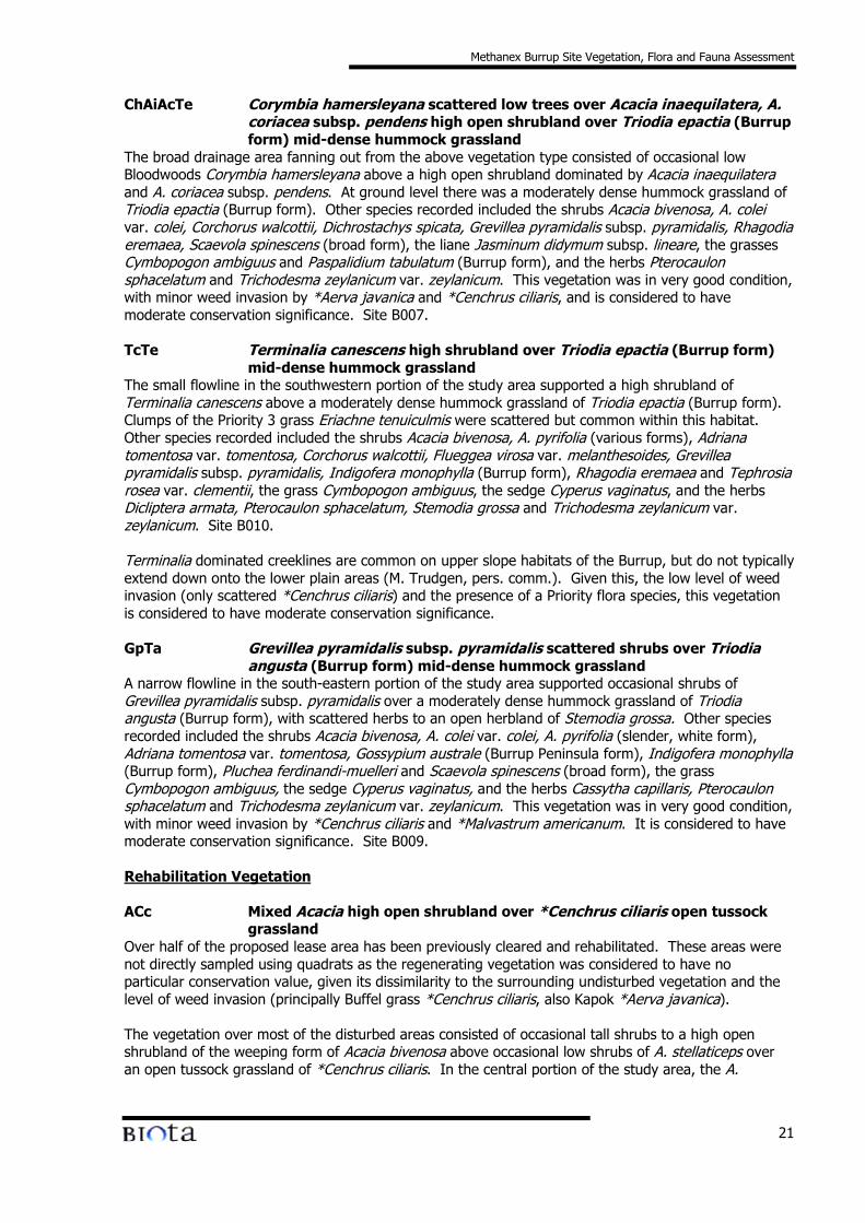
Methanex Burrup Site Vegetation, Flora and Fauna Assessment
21
ChAiAcTe Corymbia hamersleyana scattered low trees over Acacia inaequilatera, A.coriacea subsp. pendens high open shrubland over Triodia epactia (Burrupform) mid-dense hummock grassland
The broad drainage area fanning out from the above vegetation type consisted of occasional lowBloodwoods Corymbia hamersleyana above a high open shrubland dominated by Acacia inaequilateraand A. coriacea subsp. pendens. At ground level there was a moderately dense hummock grassland ofTriodia epactia (Burrup form). Other species recorded included the shrubs Acacia bivenosa, A. coleivar. colei, Corchorus walcottii, Dichrostachys spicata, Grevillea pyramidalis subsp. pyramidalis, Rhagodiaeremaea, Scaevola spinescens (broad form), the liane Jasminum didymum subsp. lineare, the grassesCymbopogon ambiguus and Paspalidium tabulatum (Burrup form), and the herbs Pterocaulonsphacelatum and Trichodesma zeylanicum var. zeylanicum. This vegetation was in very good condition,with minor weed invasion by *Aerva javanica and *Cenchrus ciliaris, and is considered to havemoderate conservation significance. Site B007.
TcTe Terminalia canescens high shrubland over Triodia epactia (Burrup form)mid-dense hummock grassland
The small flowline in the southwestern portion of the study area supported a high shrubland ofTerminalia canescens above a moderately dense hummock grassland of Triodia epactia (Burrup form).Clumps of the Priority 3 grass Eriachne tenuiculmis were scattered but common within this habitat.Other species recorded included the shrubs Acacia bivenosa, A. pyrifolia (various forms), Adrianatomentosa var. tomentosa, Corchorus walcottii, Flueggea virosa var. melanthesoides, Grevilleapyramidalis subsp. pyramidalis, Indigofera monophylla (Burrup form), Rhagodia eremaea and Tephrosiarosea var. clementii, the grass Cymbopogon ambiguus, the sedge Cyperus vaginatus, and the herbsDicliptera armata, Pterocaulon sphacelatum, Stemodia grossa and Trichodesma zeylanicum var.zeylanicum. Site B010.
Terminalia dominated creeklines are common on upper slope habitats of the Burrup, but do not typicallyextend down onto the lower plain areas (M. Trudgen, pers. comm.). Given this, the low level of weedinvasion (only scattered *Cenchrus ciliaris) and the presence of a Priority flora species, this vegetationis considered to have moderate conservation significance.
GpTa Grevillea pyramidalis subsp. pyramidalis scattered shrubs over Triodiaangusta (Burrup form) mid-dense hummock grassland
A narrow flowline in the south-eastern portion of the study area supported occasional shrubs ofGrevillea pyramidalis subsp. pyramidalis over a moderately dense hummock grassland of Triodiaangusta (Burrup form), with scattered herbs to an open herbland of Stemodia grossa. Other speciesrecorded included the shrubs Acacia bivenosa, A. colei var. colei, A. pyrifolia (slender, white form),Adriana tomentosa var. tomentosa, Gossypium australe (Burrup Peninsula form), Indigofera monophylla(Burrup form), Pluchea ferdinandi-muelleri and Scaevola spinescens (broad form), the grassCymbopogon ambiguus, the sedge Cyperus vaginatus, and the herbs Cassytha capillaris, Pterocaulonsphacelatum and Trichodesma zeylanicum var. zeylanicum. This vegetation was in very good condition,with minor weed invasion by *Cenchrus ciliaris and *Malvastrum americanum. It is considered to havemoderate conservation significance. Site B009.
Rehabilitation Vegetation
ACc Mixed Acacia high open shrubland over *Cenchrus ciliaris open tussockgrassland
Over half of the proposed lease area has been previously cleared and rehabilitated. These areas werenot directly sampled using quadrats as the regenerating vegetation was considered to have noparticular conservation value, given its dissimilarity to the surrounding undisturbed vegetation and thelevel of weed invasion (principally Buffel grass *Cenchrus ciliaris, also Kapok *Aerva javanica).
The vegetation over most of the disturbed areas consisted of occasional tall shrubs to a high openshrubland of the weeping form of Acacia bivenosa above occasional low shrubs of A. stellaticeps overan open tussock grassland of *Cenchrus ciliaris. In the central portion of the study area, the A.
Methanex Burrup Site Vegetation, Flora and Fauna Assessment
22
bivenosa overstorey was replaced by a high shrubland to open scrub of Acacia trachycarpa withoccasional individuals of Coolibah Eucalyptus victrix. Other species recorded included the shrubs Acaciainaequilatera, A. pyrifolia and Cassia notabilis, the herbs Rhynchosia sp. Burrup (82-1C) and Swainsonaformosa, and very occasional hummocks of soft spinifex Triodia epactia (Burrup form). Releves RA, RF.
Several species that were recorded from the disturbed areas are common species of the Pilbara region,but do not occur naturally on the Burrup Peninsula (eg. Acacia ancistrocarpa, A. gregorii, A.trachycarpa, A. tumida, Cassia helmsii, C. luerssenii and C. pruinosa). These appear to haveestablished from seeding with a general mixture of coastal Pilbara species, rather than one tailored tothe immediate area in question. While these species are not ‘weeds’ in the traditional sense, they havebeen introduced to the area.
4.1.2 Floristic Analysis
Appendix B contains an extract from the dendrogram showing the results of the PATN analysis on thecombined dataset (the Methanex study area, an area adjoining the southern boundary, and the greaterBurrup Peninsula and surrounds (see Section 3.1.3)). The Methanex sites have a MET prefix (ie. siteB006 appears on the dendrogram as METB006). Sites from the adjoining study area (Morgan &Trudgen, in prep.) have a BMG prefix, while the sites from the broad Burrup study (Trudgen & Griffin,2002) have a prefix of various single letters.
The sites recorded from the colluvial slopes of the study area grouped out in the same general area ofthe dendrogram. These all had a hummock grassland dominated by varying proportions of Triodiawiseana (Burrup form) and T. epactia (Burrup form), with a variable shrub overstorey of mixed Acaciaspecies, Hakea chordophylla and/or Grevillea pyramidalis subsp. pyramidalis. Sites B006 and B008 fromvegetation type AiHcTwTe were clearly very similar to each other floristically (a nearest neighbourdissimilarity coefficient of 0.2821), and relatively similar to site B001 from vegetation type AbGpTeTw (adissimilarity coefficient of 0.3333). These three sites shared a common suite of species including Acaciabivenosa, A. colei var. colei, Grevillea pyramidalis subsp. pyramidalis, Hakea chordophylla, Triodiaepactia (Burrup form) and T. wiseana (Burrup form). The next most similar sites to these in a floristicsense were also from colluvial lower slopes; site BMGC007 located in the adjacent study area, inscattered Acacia bivenosa over Triodia wiseana (Burrup form) (M. Trudgen, pers. comm.) and siteB071, a Triodia wiseana (Burrup form) hummock grassland from elsewhere on the Burrup (Trudgen &Griffin, 2002). Site B002 from vegetation type AbTwTe was relatively similar (a dissimilarity coefficientof 0.3559) to B236 from the greater Burrup Peninsula study, which was another Triodia wiseana(Burrup form) hummock grassland with scattered mixed Acacia species and occasional Corymbiahamersleyana (Trudgen & Griffin, 2002).
The creekline vegetation types occurred in two general areas of the dendrogram. Site B007 fromvegetation type ChAiAcTe was most closely related to site B010 from vegetation type TcTe, howeverthe two sites were only moderately similar floristically (a dissimilarity coefficient of 0.4085). The twovegetation types were very distinct: although both had a hummock grassland understorey of Triodiaepactia (Burrup form), site B007 had an overstorey of Acacia inaequilatera and A. coriacea withoccasional Corymbia hamersleyana, while the overstorey of B010 comprised a shrubland of Terminaliacanescens. The next most similar site was B029 from the greater Burrup Peninsula study, whichcomprised a low open woodland of Corymbia hamersleyana above low shrubs of Indigofera monophylla,Tephrosia rosea var. clementii and Corchorus walcottii over a hummock grassland of Triodia epactia(Burrup form) (Trudgen & Griffin, 2002).
Site B005 from vegetation type EviAbTaTe was most similar to site B009 from vegetation type GpTa,however the level of grouping of these sites again indicated that they were not very similar floristically(a dissimilarity coefficient of 0.4231). The vegetation types were clearly different: although both had ahummock grassland understorey dominated by Triodia angusta (Burrup form), B0005 had an overstoreyof Eucalyptus victrix and Acacia bivenosa, while the overstorey of B009 was dominated by shrubs ofGrevillea pyramidalis subsp. pyramidalis. The other sites within this general grouping were largely

Methanex Burrup Site Vegetation, Flora and Fauna Assessment
23
creeklines from an adjacent study area which similarly had Triodia angusta (Burrup form) as a dominantspinifex species.
The rockpile sites B003 and B004 from vegetation type AoBaFbReSs were most closely related to eachother, however they were not particularly similar floristically (a dissimilarity coefficient of 0.4545). Thismay be a reflection of the nature of the habitat, with different species often being patchily distributedover the rockpiles, and not necessarily recorded by a single 50x50 m quadrat. These sites are mostclosely related to the Burrup rockpile sites of PATN Groups 44_164 or 44_165 (Trudgen & Griffin,2002).
The releve RE recorded in vegetation type BaEveTe was not sufficiently detailed to be included in theanalysis. However, this rocky knoll was also sampled during an adjacent study and was found to linkwith a site on Dolphin Island (M. Trudgen, pers. comm.)
Methanex Burrup Site Vegetation, Flora and Fauna Assessment
24
4.2 Flora
4.2.1 General
A total of 88 native vascular flora species was identified within the study area, belonging to 65 generafrom 35 families (see Appendix C). Thirteen additional taxa (and an additional four genera and onefamily) that were recorded are not native to the Burrup Peninsula (see Section 4.2.3). Note that thesurvey was not conducted at an opportune time for the observation of ephemeral or cryptic species,hence this list should only be regarded as an indication of the flora present within the study area.Further sampling following summer rainfall would undoubtedly yield additional species.
The families represented by the greatest number of native taxa were the Papilionaceae (pea family, 12taxa), Mimosaceae (wattle family, 11 taxa) and Poaceae (grass family, 8 taxa). The remaining familieswere represented by four or less taxa. The only genus represented by more than three native taxa wasAcacia (wattles, 10 taxa).
4.2.2 Flora of Conservation Significance
While all native flora are protected under the Wildlife Conservation Act 1950-1979, a number of plantspecies are assigned an additional level of conservation significance based on the limited number ofknown populations and the perceived threats to these locations (Table 4.1). Species of the highestconservation significance are designated Declared Rare Flora (DRF). Species which appear to be rare orthreatened, but for which there is insufficient information to properly evaluate their conservation status,are assigned to one of four Priority Flora categories. The listing of DRF and Priority species is reviewedon an annual basis by the Department of Conservation and Land Management (CALM).
Table 4.1: Categories of conservation significance for flora species (Atkins, 2001).
Declared Rare Flora - Extant Taxa. Taxa which have been adequately searched for and aredeemed to be in the wild either rare, in danger of extinction or otherwise in need of specialprotection. Declared Rare Flora - Presumed Extinct. Taxa which have not been collected, or otherwiseverified, over the past 50 years despite thorough searching, or of which all known wild populationshave been destroyed more recently. Priority 1 - Poorly Known Taxa. Taxa which are known from one or a few (generally <5)populations which are under threat. Priority 2 - Poorly Known Taxa. Taxa which are known from one or a few (generally <5)populations, at least some of which are not believed to be under threat. Priority 3 - Poorly Known Taxa. Taxa which are known from several populations, at least someof which are not believed to be under threat. Priority 4 - Rare Taxa. Taxa which are considered to have been adequately surveyed and whichwhilst being rare, are not currently threatened by any identifiable factors.
In addition, the presence of some flora species means that it is necessary to refer proposals to theFederal Minister for the Environment under the Environment Protection and Biodiversity ConservationAct 1999. In the Pilbara, only the two Declared Rare Flora species (Lepidium catapycnon andThryptomene wittweri) are currently listed under the EPBC Act. However, the Priority 1 species Alutaquadrata (previously Thryptomene sp. Channar) has been recommended for listing as a DRF (Stephen
Methanex Burrup Site Vegetation, Flora and Fauna Assessment
25
van Leeuwen, CALM Karratha, pers. comm.), and will also presumably be included under the EPBC Actthreatened species listing in future.
No current or proposed Declared Rare Flora were recorded during the field survey, and none areexpected to occur due to the absence of appropriate habitat. There are thus no flora present in thearea that are listed under the EPBC Act 1999.
Two Priority Flora, Terminalia supranitifolia and Eriachne tenuiculmis, were recorded. Rare Flora ReportForms are contained in Appendix D, and the species are discussed individually below.
Terminalia supranitifolia Priority 1This tall shrub species is relatively restricted geographically. It is known from a small number ofpopulations, and is most common on the Burrup Peninsula and adjacent Dolphin Island. T.supranitifolia was recorded four times during the current survey, from sites B003, B004 and releves RDand RE. All of these records were from rockpiles or rocky outcrops.
Eriachne tenuiculmis Priority 3This perennial grass was recorded from two locations within defined creekline habitats (site B010 andan opportunistic collection). It typically occurred as scattered clumps but was not uncommon. E.tenuiculmis is common in creeklines on the Burrup Peninsula and surrounds, where it has beenrecorded over thirty times (M. Trudgen, pers. comm.). This species is also known from severallocations in the Hamersley Range including Serpentine Creek, Yandi and Millstream (see Atkins, 2001),all within large creeklines. It has been collected in a number of creeks in the Newman area (BiotaEnvironmental Sciences, 2001b), was recorded twice from Cape Preston, west of Dampier (see HalpernGlick Maunsell, 2000), and was recorded 69 times during the West Angelas ERMP botanical survey(Trudgen & Casson, 1998). Eriachne tenuiculmis is poorly collected rather than uncommon, and hasbeen recommended for deletion from the Priority list (M. Trudgen, pers. comm.).
Several other flora taxa are of note for various reasons, including restricted geographical range and/orundescribed status. These 'Flora of Interest' are discussed briefly below.
Corchorus walcottiiWhile this name has been misapplied to a wide variety of species, true C. walcottii appears to berelatively restricted geographically, with lodged specimens only from the Burrup Peninsula and fromnear Port Hedland. It is fairly common on the Burrup Peninsula and adjacent islands (M. Trudgen, pers.comm.). It was recorded seven times in various habitats during the current study, from sites B002,B005, B006, B007, B010 and two opportunistic collections.
Indigofera monophylla (Burrup form)This grey form of the common but variable Indigofera monophylla is very common on the BurrupPeninsula and adjacent islands, and has also been recorded from the Abydos Plain (M. Trudgen, pers.comm). It was recorded seven times in various habitats during the current survey, from sites B001,B002, B005, B007, B009, B010 and a single opportunistic collection.
Rhynchosia sp. Burrup (82-1C)This distinct Rhynchosia taxon has leaflets that are resinous and much smaller than the commonRhynchosia cf. minima. It appears restricted to the Burrup Peninsula and at least some of the adjacentislands, but is common in these areas. It was recorded three times during the current survey, fromsites B003, B010 and a single opportunistic collection.
Tephrosia aff. supina (MET 12,357)The genus Tephrosia includes many more taxa than are currently recognised. This undescribed taxon isvery common on the Burrup Peninsula, including in areas zoned for conservation (M. Trudgen, pers.comm.). It seems relatively widespread, having been recorded from localities as distant as WestAngelas (Trudgen & Casson, 1998) and west of Dampier (Halpern Glick Maunsell, 2000). Whileundescribed, this taxon is considered to be common on the coast, less common inland, and not of
Methanex Burrup Site Vegetation, Flora and Fauna Assessment
26
particular concern for conservation. It was recorded twice during the current survey, from the creeklinesites B005 and B007.
Triodia spp. (Burrup forms)The three spinifex taxa recorded represent distinct forms of the type species (Triodia angusta, T.epactia and T. wiseana). T. epactia (Burrup form) appears to be restricted to the Burrup Peninsula andDampier Archipelago, although it may also occur on nearby islands and the mainland, while T. wiseana(Burrup form) and T. angusta (Burrup form) appear to be slightly more widespread (M. Trudgen, pers.comm.).
Triumfetta appendiculata (Burrup form)This taxon was recorded twice from the study area, from sites B001 and B010. It is distinct from thetype of T. appendiculata, although the level of difference (ie. taxonomic status) is uncertain at thisstage. While common on the Burrup Peninsula and Dolphin Island, it was not recorded from otheradjacent islands (M. Trudgen, pers. comm.). There are additional records from Karratha and CapePreston, however the taxon appears very uncommon off the peninsula (M. Trudgen, pers. comm.).
Euphorbia tannensis subsp. eremophila (Burrup form)There was one record of this taxon during the current survey, from site B002. This taxon appears to becommon on the Burrup Peninsula, and has also been recorded from three adjacent islands and fromCape Preston, west of Dampier (M. Trudgen, pers. comm.). It may be quite restricted geographically,however further work would be required to determine this.
Paspalidium tabulatum (Burrup form)This taxon was recorded twice during the current study, from sites B004 (a rockpile) and B007 (aflowline). While common on the Burrup Peninsula and some adjacent islands, it does not appear tooccur on the adjoining mainland (M. Trudgen, pers. comm.).
4.2.3 Introduced Flora
Thirteen introduced species were recorded from the study area (see Appendix C). Four of these(*Cenchrus ciliaris, *Aerva javanica, *Agave americana and *Malvastrum americanum) are species thatare not native to the State. The remainder (all Acacia or Cassia species) are endemic to the Pilbara butdo not occur naturally on the Burrup Peninsula. These appear to have been introduced through seedingof rehabilitation areas.
The introduced flora were as follows:
• Buffel grass *Cenchrus ciliaris was the dominant understorey species in the majority of thedisturbed areas, but has not significantly invaded surrounding intact vegetation.
• Kapok *Aerva javanica was present in the disturbed areas, but was not observed beyond this.

Methanex Burrup Site Vegetation, Flora and Fauna Assessment
27
• A single Century plant *Agave americana was observed in the central portion of the study area,again in a disturbed area (478305 mE, 7720444 mN, AGD 84).
• Spiked malvastrum *Malvastrum americanum was recorded from a drainage line in the southernportion of the study area.
• The following native Pilbara taxa, which do not appear to be endemic to the Burrup Peninsula,were recorded from the rehabilitation areas or surrounds: Acacia ancistrocarpa, A. gregorii, A.trachycarpa, A. tumida, an unidentified Acacia species, Cassia helmsii, C. luerssenii, C. oligophyllax helmsii and C. pruinosa.
Methanex Burrup Site Vegetation, Flora and Fauna Assessment
28
5.0 Fauna
5.1 Land snails
Over 30 sites were examined for snails in the project area (Table 5.1; Figure 5.1). A site was definedas a small area (up to 20m x 20m) that had homogeneous substrate, vegetation and relief.
Solem (1985) states that “most specimens taken by non-malacologically trained collectors will consist ofdead shells found lying upon open ground. Generally these are worn and bleached to the point thatidentification characters cannot be observed.” The collection of live animals is usually more productiveafter rains, however there were no such opportunities within the timeframe of this project. All recordsof snails were from empty shells, which were collected from open ground or declivities between rocks,and were generally quite bleached. Fortunately, the species that were collected can be identified fromold shells. Reference collections held by CALM in Karratha were used as an aid to identification.Published keys (Solem 1986, 1997) were also consulted, although these typically required relativelyfresh adults to be of use for identification purposes (Solem 1997). All snail material was lodged(currently pending collection numbers) with the Western Australian Museum. The identifications madehere were confirmed by expert examination (Slack-Smith 2002).
Two camaenid land snails (Pulmonata: Camaenidae) were collected from the project area:
1. Quistrachia legendrei (Figure 5.2) was found predominantly on or around rockpiles, most oftenwithin the declivities between boulders. Live Q. legendrei are generally found sealed to rocksor other shells (Solem 1997). This species is widespread on the Burrup north of Dampier (P.G.Kendrick unpublished notes). The shells are thin, subdiscoidal with rounded whorls, a narrowumbilicus, a thin, slightly reflected outer lip and subcircular open mouth (Iredale 1939). Theshell is a brownish colour in live individuals. Most Quistrachia are distributed in the Pilbara andsouth to Carnarvon and there are species still awaiting description (Solem 1985, 1997). Nospecies appear to be sympatric in Western Australia (Solem 1997) and the key advises thatreference be made to geographical location. According to this key, Q. legendrei is the onlyrepresentative of this genus occurring near Dampier. Slack-Smith (2001) also found thisspecies in similar habitats on an adjacent lease.
2. Rhagada sp. 12 (G.W. Kendrick and P.G. Kendrick unpublished notes; Figure 5.3) is a largeundescribed species with a low spire. Rhagada sp. 12 was relatively abundant, with emptyshells present in most open areas. It was particularly common in various undisturbed habitatssouth of Village Road, less abundant on colluvial slopes, and was also found in or aroundrockpiles. Rhagada are ‘free sealers’, secreting calcified epiphragms that are shed quickly whenthe snail is exposed to moisture (Solem 1997). This species might have also been collectedfrom the northern part of the Burrup, several islands in the Dampier Archipelago and Millstream– Chichester National Park (G.W. Kendrick and P.G. Kendrick unpublished notes). Shells of thegenus Rhagada are distinguished from Quistrachia by their flattened helicoid aspect, inner baseof the lip with a slight tubercle, curved columella (adpressed, generally closing the umbilicus inthe adult, a narrow perforation always visible in juveniles) sculpture of obscure radials only, andcolouration white with a few coloured bands (Iredale 1939). Adult Rhagada sp. 12 are largerthan both R. angulata and R. convicta, and Rhagada sp. 12 is sympatric with R. convicta insome localities (Slack-Smith 2001).
Slack-Smith (2001) stated that a Rhagada sp. recorded on an adjacent lease (likely to be thesame as Rhagada sp. 12 recorded in the present survey) shelters under rocks, under deep litterand in the soil at the bases of trees on or at the base of rocky slopes. Within the currentsurvey area, Rhagada sp. 12 was recorded in relatively high abundance in the southern portionof the lease on sand/loam associated with Triodia (sites 19-33), and also east of the lease

Methanex Burrup Site Vegetation, Flora and Fauna Assessment
29
boundary on very powdery loam soils with Frankenia and Halosarcia, in addition to the habitatsdescribed above by Slack-Smith (2001).
It is difficult to place the occurrence of Rhagada sp. 12 into a regional context since it has notbeen formally described and compared with specimens from elsewhere in the Pilbara thought tobe the same species. Likewise, any cumulative impact from adjacent leases is difficult to assesswithout knowing how widespread and abundant the taxon is. However, since much of the sitehas already been cleared, the taxon appeared abundant on flat ground adjacent to the lease (tothe east) and since it was also found commonly in rockpiles on the Methanex and the adjacentlease to the west, the proposed developments in the King Bay – Hearson Cove area are notlikely to cause a significant decline. The priority should be placed on a description of the taxonat this stage.
It should be noted that, if this taxon requires management in the future, a plan that involvesthe provision of habitat should be implemented. Occasional fresh empty shells fromrecolonising individuals were observed on the rehabilitated areas, which had probably perisheddue to the lack of appropriate habitat.
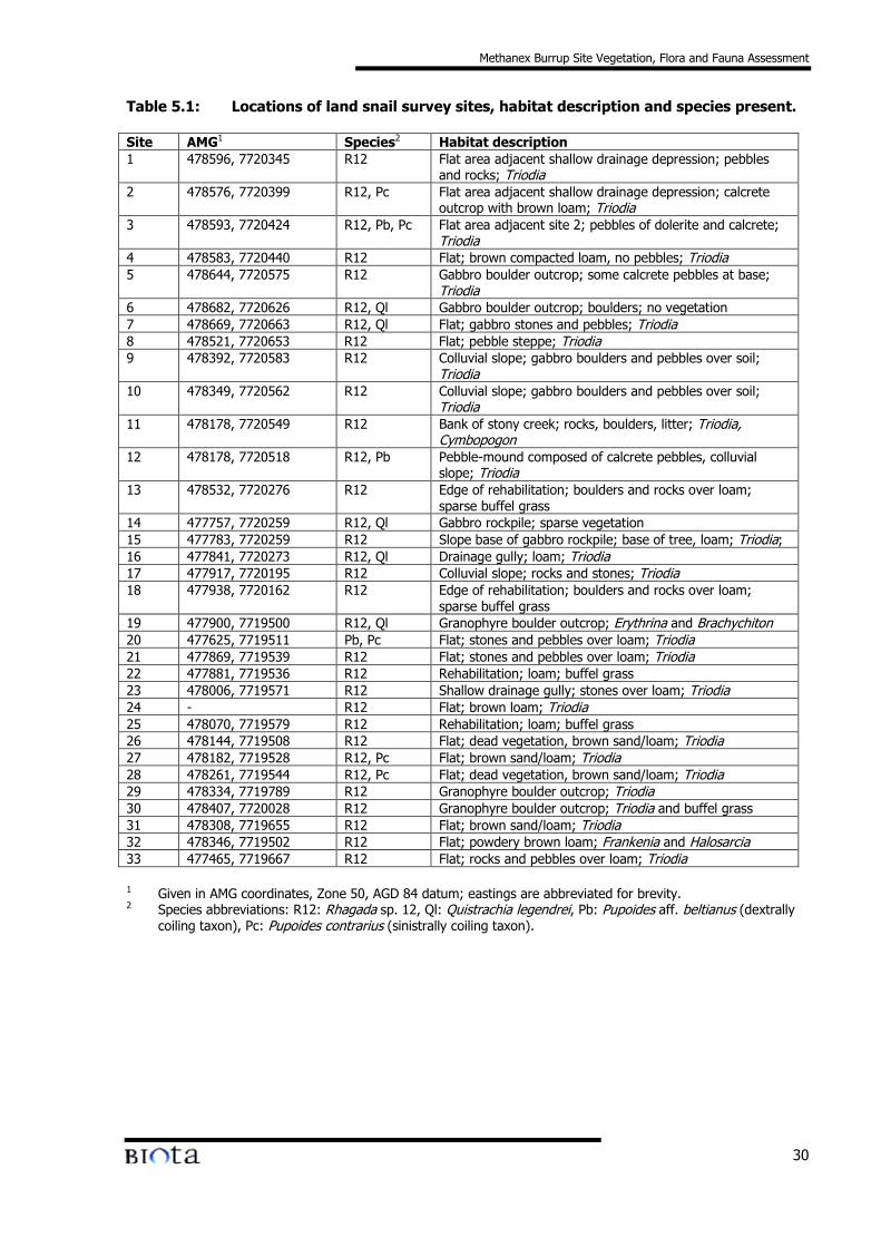
Methanex Burrup Site Vegetation, Flora and Fauna Assessment
30
Table 5.1: Locations of land snail survey sites, habitat description and species present.
Site AMG1 Species2 Habitat description1 478596, 7720345 R12 Flat area adjacent shallow drainage depression; pebbles
and rocks; Triodia2 478576, 7720399 R12, Pc Flat area adjacent shallow drainage depression; calcrete
outcrop with brown loam; Triodia3 478593, 7720424 R12, Pb, Pc Flat area adjacent site 2; pebbles of dolerite and calcrete;
Triodia4 478583, 7720440 R12 Flat; brown compacted loam, no pebbles; Triodia5 478644, 7720575 R12 Gabbro boulder outcrop; some calcrete pebbles at base;
Triodia6 478682, 7720626 R12, Ql Gabbro boulder outcrop; boulders; no vegetation7 478669, 7720663 R12, Ql Flat; gabbro stones and pebbles; Triodia8 478521, 7720653 R12 Flat; pebble steppe; Triodia9 478392, 7720583 R12 Colluvial slope; gabbro boulders and pebbles over soil;
Triodia10 478349, 7720562 R12 Colluvial slope; gabbro boulders and pebbles over soil;
Triodia11 478178, 7720549 R12 Bank of stony creek; rocks, boulders, litter; Triodia,
Cymbopogon12 478178, 7720518 R12, Pb Pebble-mound composed of calcrete pebbles, colluvial
slope; Triodia13 478532, 7720276 R12 Edge of rehabilitation; boulders and rocks over loam;
sparse buffel grass14 477757, 7720259 R12, Ql Gabbro rockpile; sparse vegetation15 477783, 7720259 R12 Slope base of gabbro rockpile; base of tree, loam; Triodia;16 477841, 7720273 R12, Ql Drainage gully; loam; Triodia17 477917, 7720195 R12 Colluvial slope; rocks and stones; Triodia18 477938, 7720162 R12 Edge of rehabilitation; boulders and rocks over loam;
sparse buffel grass19 477900, 7719500 R12, Ql Granophyre boulder outcrop; Erythrina and Brachychiton20 477625, 7719511 Pb, Pc Flat; stones and pebbles over loam; Triodia21 477869, 7719539 R12 Flat; stones and pebbles over loam; Triodia22 477881, 7719536 R12 Rehabilitation; loam; buffel grass23 478006, 7719571 R12 Shallow drainage gully; stones over loam; Triodia24 - R12 Flat; brown loam; Triodia25 478070, 7719579 R12 Rehabilitation; loam; buffel grass26 478144, 7719508 R12 Flat; dead vegetation, brown sand/loam; Triodia27 478182, 7719528 R12, Pc Flat; brown sand/loam; Triodia28 478261, 7719544 R12, Pc Flat; dead vegetation, brown sand/loam; Triodia29 478334, 7719789 R12 Granophyre boulder outcrop; Triodia30 478407, 7720028 R12 Granophyre boulder outcrop; Triodia and buffel grass31 478308, 7719655 R12 Flat; brown sand/loam; Triodia32 478346, 7719502 R12 Flat; powdery brown loam; Frankenia and Halosarcia33 477465, 7719667 R12 Flat; rocks and pebbles over loam; Triodia
1 Given in AMG coordinates, Zone 50, AGD 84 datum; eastings are abbreviated for brevity.2 Species abbreviations: R12: Rhagada sp. 12, Ql: Quistrachia legendrei, Pb: Pupoides aff. beltianus (dextrally
coiling taxon), Pc: Pupoides contrarius (sinistrally coiling taxon).
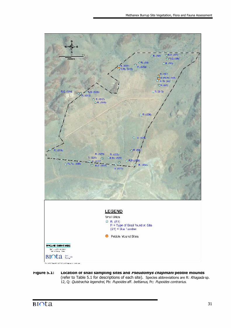
Methanex Burrup Site Vegetation, Flora and Fauna Assessment
31
Figure 5.1: Location of snail sampling sites and Pseudomys chapmani pebble mounds(refer to Table 5.1 for descriptions of each site). Species abbreviations are R: Rhagada sp.12, Q: Quistrachia legendrei, Pb: Pupoides aff. beltianus, Pc: Pupoides contrarius.

Methanex Burrup Site Vegetation, Flora and Fauna Assessment
32
Figure 5.2: The camaenid snail Quistrachia legendrei. These snails are relatively easy toidentify by the wide aperture and their brown colour when fresh.
Figure 5.3: The undescribed camaenid snail Rhagada sp. 12. These snails have a smalleraperture than Q. legendrei and have a striped pattern.
Methanex Burrup Site Vegetation, Flora and Fauna Assessment
33
Small pupilloid gastropods (Pulmonata: Pupillidae) were also collected. Two species were identifiedusing the key of Solem (1986), distinguished by the direction in which the shell coils (Figure 5.4). Theshells with dextral coiling could be one of two species, both of which are found in the Pilbara (Solem1986; Pupoides aff. beltianus and P. lepidulus). Sinistrally coiling shells were keyed to P. contrarius. P.aff. beltianus and P. contrarius have been identified previously by G.W. Kendrick from the Burrup (P.G.Kendrick pers. comm.) and Slack-Smith (2001) recorded both on an adjacent lease.
There are taxonomic issues with both P. aff. beltianus and P. contrarius. Dextrally coiled pupillids thatare distributed between the Pilbara and Shark Bay are similar to Pupoides beltianus that occurs inCentral Australia. The lack of sufficient material prevented a more detailed comparison previously(Solem 1986, 1988). P. contrarius has a wide range along the west of Western Australia betweenBroome, the Monte Bello Islands, Shark Bay and the Houtman Abrolhos. However, two species may bepresent within P. contrarius, distinguished on the basis of size (Solem 1986).
The distribution of Pupoides is widespread, with complexes of species occurring in North America andthe West Indies, India, the Middle East and parts of Africa, and also the semi-arid areas of Australia.Solem (1986) states that
“there has been no agreement as to whether dextral and sinistral populations are geneticvariants or distinct species. The present material suggest that distinct species are involved.Wherever a dextral and sinistral form were microsympatric, there were noticeable size andshape differences between the two morphs. … Thus I am predicting that species leveldifferences are involved.”
Examination of the material collected in the present study found that both dextral and sinistral formsoccurred microsympatrically at several snail sampling sites (Table 5.1). A superficial comparison of bothforms (i.e. side by side) did not reveal any noticeable differences in size or the shape of the shell oraperture. One nodular barrier was present in all cases.
Slack-Smith (2001) found these two pupillids on higher ground including rocky outcrops (P. aff.beltianus), and also on low-lying land, which included brown sandy soils and soils with pebbles (P.contrarius). The present study found both pupillids mainly on pebbly calcrete soils, and on adjacentbrown loams associated with Triodia and thin algal or cyanobacterial mats that commonly form on aridsoils after rain.
A third species of pupillid collected on the adjacent lease (Gastrocopta ?pilbarana; Slack-Smith 2001)may also be present in the proposed site. In that study, G. ?pilbarana was less common and appearedto be restricted to rocky outcrops. Although the amount of rocky outcrop is restricted in the presentstudy site, further intensive searches may record G. ?pilbarana. Specimens recorded from the Burruppreviously show similarities to both G. pilbarana and G. deserti (review in Slack-Smith 2001). Since thecurrent project will avoid rocky areas, a significant impact on Burrup G. ?pilbarana is unlikely.
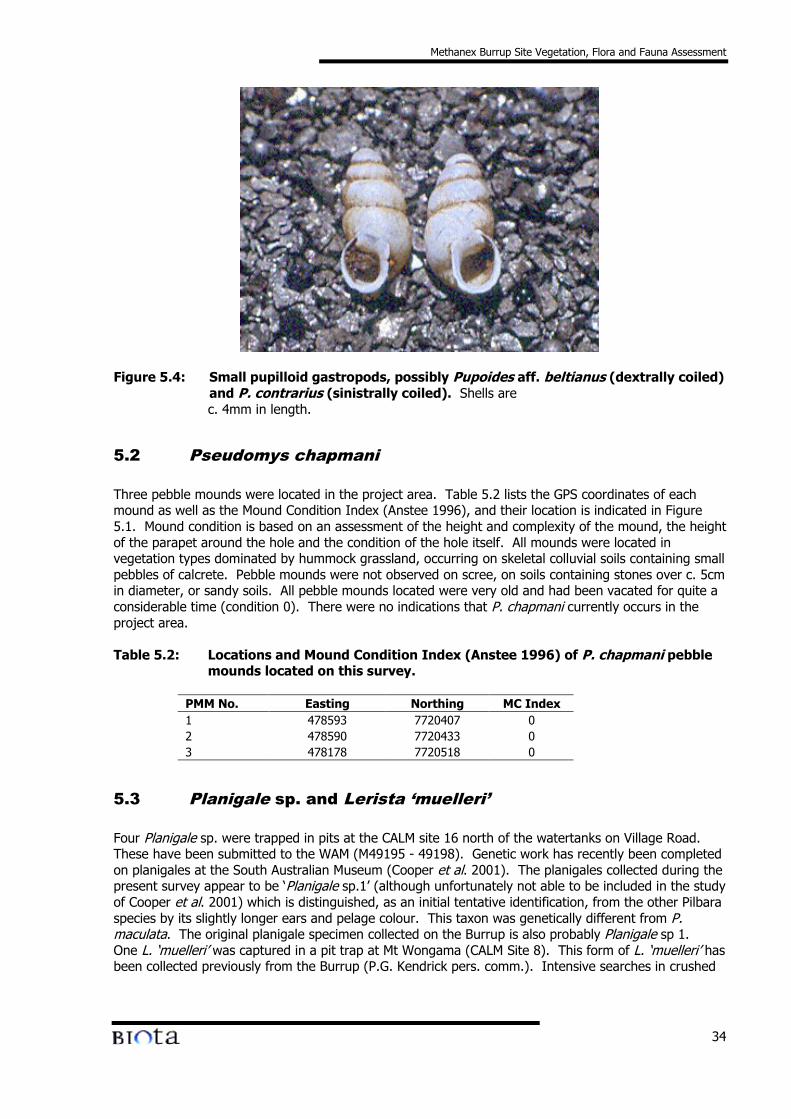
Methanex Burrup Site Vegetation, Flora and Fauna Assessment
34
Figure 5.4: Small pupilloid gastropods, possibly Pupoides aff. beltianus (dextrally coiled)and P. contrarius (sinistrally coiled). Shells arec. 4mm in length.
5.2 Pseudomys chapmani
Three pebble mounds were located in the project area. Table 5.2 lists the GPS coordinates of eachmound as well as the Mound Condition Index (Anstee 1996), and their location is indicated in Figure5.1. Mound condition is based on an assessment of the height and complexity of the mound, the heightof the parapet around the hole and the condition of the hole itself. All mounds were located invegetation types dominated by hummock grassland, occurring on skeletal colluvial soils containing smallpebbles of calcrete. Pebble mounds were not observed on scree, on soils containing stones over c. 5cmin diameter, or sandy soils. All pebble mounds located were very old and had been vacated for quite aconsiderable time (condition 0). There were no indications that P. chapmani currently occurs in theproject area.
Table 5.2: Locations and Mound Condition Index (Anstee 1996) of P. chapmani pebblemounds located on this survey.
PMM No. Easting Northing MC Index1 478593 7720407 02 478590 7720433 03 478178 7720518 0
5.3 Planigale sp. and Lerista ‘muelleri’
Four Planigale sp. were trapped in pits at the CALM site 16 north of the watertanks on Village Road.These have been submitted to the WAM (M49195 - 49198). Genetic work has recently been completedon planigales at the South Australian Museum (Cooper et al. 2001). The planigales collected during thepresent survey appear to be ‘Planigale sp.1’ (although unfortunately not able to be included in the studyof Cooper et al. 2001) which is distinguished, as an initial tentative identification, from the other Pilbaraspecies by its slightly longer ears and pelage colour. This taxon was genetically different from P.maculata. The original planigale specimen collected on the Burrup is also probably Planigale sp 1.One L. ‘muelleri’ was captured in a pit trap at Mt Wongama (CALM Site 8). This form of L. ‘muelleri’ hasbeen collected previously from the Burrup (P.G. Kendrick pers. comm.). Intensive searches in crushed
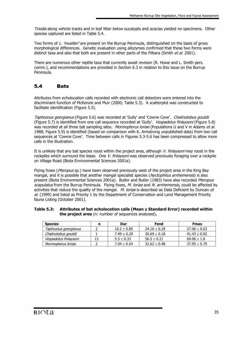
Methanex Burrup Site Vegetation, Flora and Fauna Assessment
35
Triodia along vehicle tracks and in leaf litter below eucalypts and acacias yielded no specimens. Otherspecies captured are listed in Table 5.4.
Two forms of L. ‘muelleri’ are present on the Burrup Peninsula, distinguished on the basis of grossmorphological differences. Genetic evaluation using allozymes confirmed that these two forms weredistinct taxa and also that both are present in other parts of the Pilbara (Smith et al. 2001).
There are numerous other reptile taxa that currently await revision (R. Howe and L. Smith pers.comm.), and recommendations are provided in Section 6.3 in relation to this issue on the BurrupPeninsula.
5.4 Bats
Attributes from echolocation calls recorded with electronic call detectors were entered into thediscriminant function of McKenzie and Muir (2000; Table 5.3). A scatterplot was constructed tofacilitate identification (Figure 5.5).
Taphozous georgianus (Figure 5.6) was recorded at ‘Gully’ and ‘Cowrie Cove’. Chalinolobus gouldii(Figure 5.7) is identified from one call sequence recorded at ‘Gully’. Vespadelus finlaysoni (Figure 5.8)was recorded at all three bat sampling sites. Mormopterus loriae (Populations U and V in Adams et al.1988; Figure 5.9) is identified (based on comparison with K. Armstrong unpublished data) from two callsequences at ‘Cowrie Cove’. Time between calls in Figures 5.3-5.6 has been compressed to allow morecalls in the illustration.
It is unlikely that any bat species roost within the project area, although V. finlaysoni may roost in therockpiles which surround the lease. One V. finlaysoni was observed previously foraging over a rockpileon Village Road (Biota Environmental Sciences 2001a).
Flying foxes (Pteropus sp.) have been observed previously west of the project area in the King Baymangal, and it is possible that another mangal specialist species (Nyctophilus arnhemensis) is alsopresent (Biota Environmental Sciences 2001a). Butler and Butler (1983) have also recorded Pteropusscapulatus from the Burrup Peninsula. Flying foxes, M. loriae and N. arnhemensis, could be affected byactivities that reduce the quality of the mangal. M. loriae is described as Data Deficient by Duncan etal. (1999) and listed as Priority 1 by the Department of Conservation and Land Management Priorityfauna Listing (October 2001).
Table 5.3: Attributes of bat echolocation calls (Mean ±±±± Standard Error) recorded withinthe project area (n: number of sequences analysed).
Species n Dur Fend FmaxTaphozous georgianus 2 10.2 ± 0.85 24.16 ± 0.29 27.06 ± 0.63Chalinolobus gouldii 1 7.49 ± 0.29 30.69 ± 0.18 41.43 ± 0.92Vespadelus finlaysoni 13 5.5 ± 0.33 56.5 ± 0.21 69.06 ± 1.6Mormopterus loriae 2 7.04 ± 0.54 32.62 ± 0.48 37.95 ± 0.79
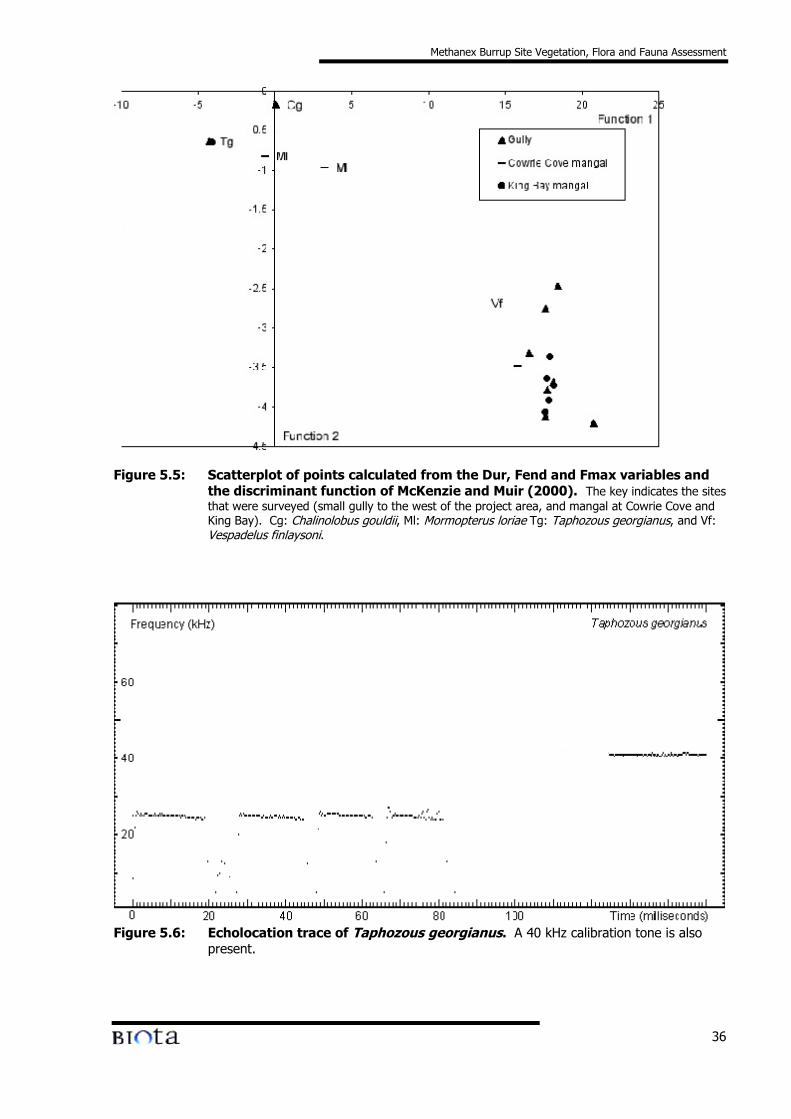
Methanex Burrup Site Vegetation, Flora and Fauna Assessment
36
Figure 5.5: Scatterplot of points calculated from the Dur, Fend and Fmax variables andthe discriminant function of McKenzie and Muir (2000). The key indicates the sitesthat were surveyed (small gully to the west of the project area, and mangal at Cowrie Cove andKing Bay). Cg: Chalinolobus gouldii, Ml: Mormopterus loriae Tg: Taphozous georgianus, and Vf:Vespadelus finlaysoni.
Figure 5.6: Echolocation trace of Taphozous georgianus. A 40 kHz calibration tone is alsopresent.
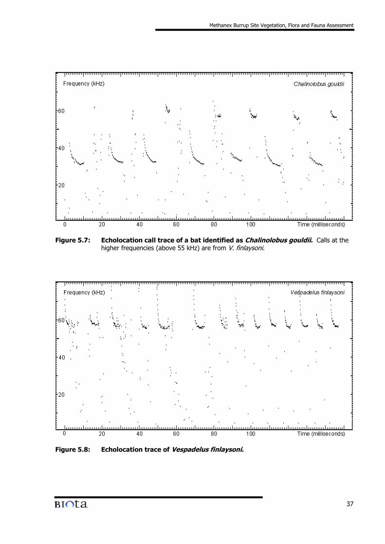
Methanex Burrup Site Vegetation, Flora and Fauna Assessment
37
Figure 5.7: Echolocation call trace of a bat identified as Chalinolobus gouldii. Calls at thehigher frequencies (above 55 kHz) are from V. finlaysoni.
Figure 5.8: Echolocation trace of Vespadelus finlaysoni.
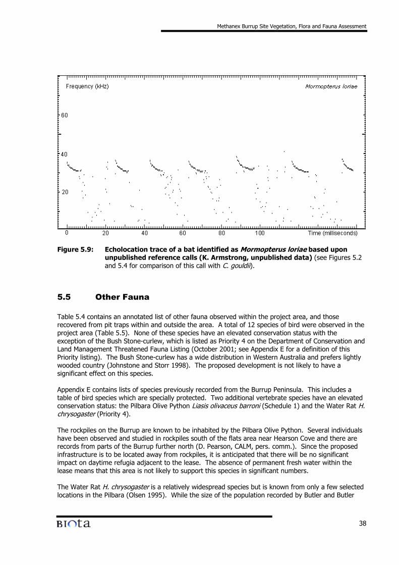
Methanex Burrup Site Vegetation, Flora and Fauna Assessment
38
Figure 5.9: Echolocation trace of a bat identified as Mormopterus loriae based uponunpublished reference calls (K. Armstrong, unpublished data) (see Figures 5.2and 5.4 for comparison of this call with C. gouldii).
5.5 Other Fauna
Table 5.4 contains an annotated list of other fauna observed within the project area, and thoserecovered from pit traps within and outside the area. A total of 12 species of bird were observed in theproject area (Table 5.5). None of these species have an elevated conservation status with theexception of the Bush Stone-curlew, which is listed as Priority 4 on the Department of Conservation andLand Management Threatened Fauna Listing (October 2001; see Appendix E for a definition of thisPriority listing). The Bush Stone-curlew has a wide distribution in Western Australia and prefers lightlywooded country (Johnstone and Storr 1998). The proposed development is not likely to have asignificant effect on this species.
Appendix E contains lists of species previously recorded from the Burrup Peninsula. This includes atable of bird species which are specially protected. Two additional vertebrate species have an elevatedconservation status: the Pilbara Olive Python Liasis olivaceus barroni (Schedule 1) and the Water Rat H.chrysogaster (Priority 4).
The rockpiles on the Burrup are known to be inhabited by the Pilbara Olive Python. Several individualshave been observed and studied in rockpiles south of the flats area near Hearson Cove and there arerecords from parts of the Burrup further north (D. Pearson, CALM, pers. comm.). Since the proposedinfrastructure is to be located away from rockpiles, it is anticipated that there will be no significantimpact on daytime refugia adjacent to the lease. The absence of permanent fresh water within thelease means that this area is not likely to support this species in significant numbers.
The Water Rat H. chrysogaster is a relatively widespread species but is known from only a few selectedlocations in the Pilbara (Olsen 1995). While the size of the population recorded by Butler and Butler
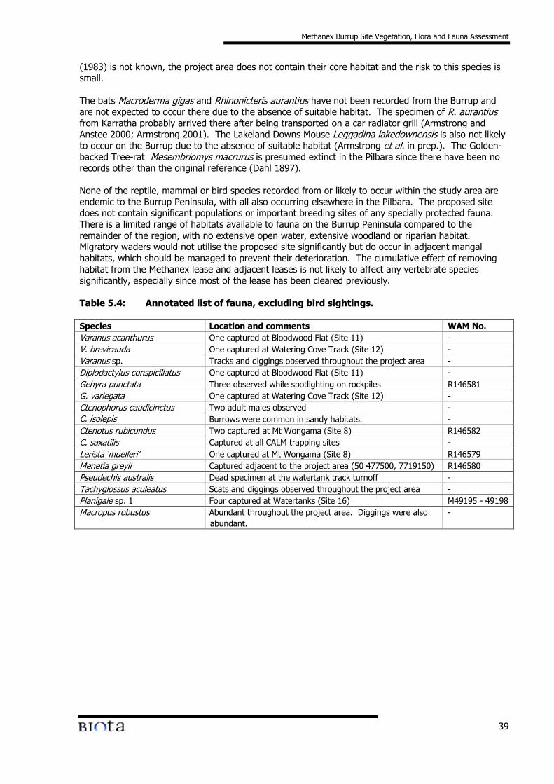
Methanex Burrup Site Vegetation, Flora and Fauna Assessment
39
(1983) is not known, the project area does not contain their core habitat and the risk to this species issmall.
The bats Macroderma gigas and Rhinonicteris aurantius have not been recorded from the Burrup andare not expected to occur there due to the absence of suitable habitat. The specimen of R. aurantiusfrom Karratha probably arrived there after being transported on a car radiator grill (Armstrong andAnstee 2000; Armstrong 2001). The Lakeland Downs Mouse Leggadina lakedownensis is also not likelyto occur on the Burrup due to the absence of suitable habitat (Armstrong et al. in prep.). The Golden-backed Tree-rat Mesembriomys macrurus is presumed extinct in the Pilbara since there have been norecords other than the original reference (Dahl 1897).
None of the reptile, mammal or bird species recorded from or likely to occur within the study area areendemic to the Burrup Peninsula, with all also occurring elsewhere in the Pilbara. The proposed sitedoes not contain significant populations or important breeding sites of any specially protected fauna.There is a limited range of habitats available to fauna on the Burrup Peninsula compared to theremainder of the region, with no extensive open water, extensive woodland or riparian habitat.Migratory waders would not utilise the proposed site significantly but do occur in adjacent mangalhabitats, which should be managed to prevent their deterioration. The cumulative effect of removinghabitat from the Methanex lease and adjacent leases is not likely to affect any vertebrate speciessignificantly, especially since most of the lease has been cleared previously.
Table 5.4: Annotated list of fauna, excluding bird sightings.
Species Location and comments WAM No.Varanus acanthurus One captured at Bloodwood Flat (Site 11) -V. brevicauda One captured at Watering Cove Track (Site 12) -Varanus sp. Tracks and diggings observed throughout the project area -Diplodactylus conspicillatus One captured at Bloodwood Flat (Site 11) -Gehyra punctata Three observed while spotlighting on rockpiles R146581G. variegata One captured at Watering Cove Track (Site 12) -Ctenophorus caudicinctus Two adult males observed -C. isolepis Burrows were common in sandy habitats. -Ctenotus rubicundus Two captured at Mt Wongama (Site 8) R146582C. saxatilis Captured at all CALM trapping sites -Lerista ‘muelleri’ One captured at Mt Wongama (Site 8) R146579Menetia greyii Captured adjacent to the project area (50 477500, 7719150) R146580Pseudechis australis Dead specimen at the watertank track turnoff -Tachyglossus aculeatus Scats and diggings observed throughout the project area -Planigale sp. 1 Four captured at Watertanks (Site 16) M49195 - 49198Macropus robustus Abundant throughout the project area. Diggings were also
abundant.-
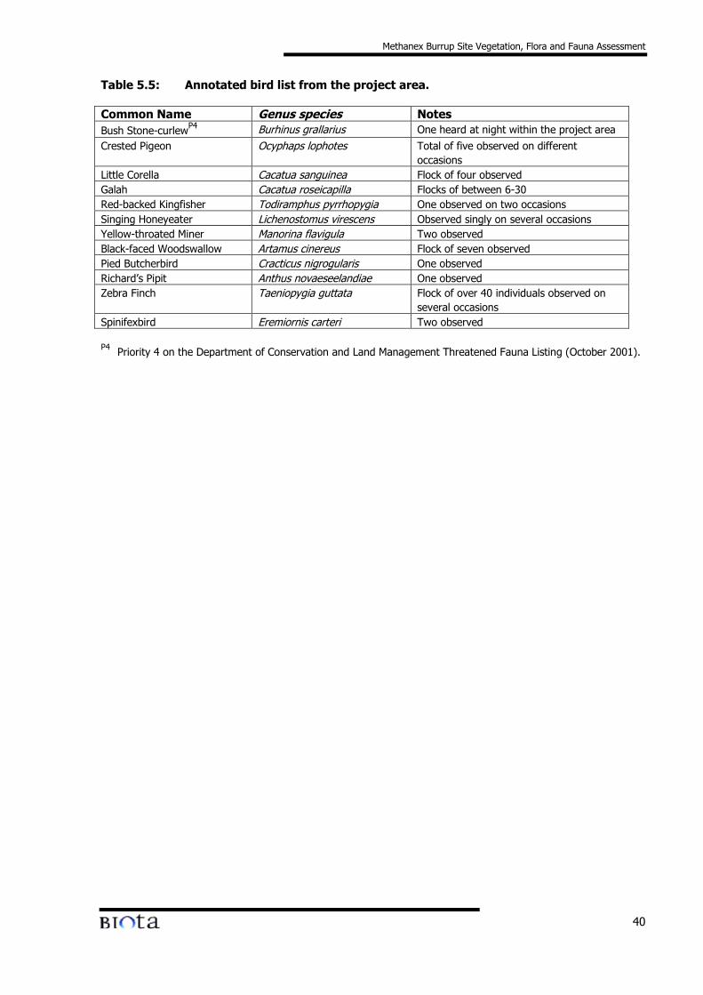
Methanex Burrup Site Vegetation, Flora and Fauna Assessment
40
Table 5.5: Annotated bird list from the project area.
Common Name Genus species NotesBush Stone-curlewP4 Burhinus grallarius One heard at night within the project areaCrested Pigeon Ocyphaps lophotes Total of five observed on different
occasionsLittle Corella Cacatua sanguinea Flock of four observedGalah Cacatua roseicapilla Flocks of between 6-30Red-backed Kingfisher Todiramphus pyrrhopygia One observed on two occasionsSinging Honeyeater Lichenostomus virescens Observed singly on several occasionsYellow-throated Miner Manorina flavigula Two observedBlack-faced Woodswallow Artamus cinereus Flock of seven observedPied Butcherbird Cracticus nigrogularis One observedRichard’s Pipit Anthus novaeseelandiae One observedZebra Finch Taeniopygia guttata Flock of over 40 individuals observed on
several occasionsSpinifexbird Eremiornis carteri Two observed
P4 Priority 4 on the Department of Conservation and Land Management Threatened Fauna Listing (October 2001).
Methanex Burrup Site Vegetation, Flora and Fauna Assessment
41
6.0 Conclusions and Recommendations
6.1 Vegetation and Flora
6.1.1 Conservation Value of the Vegetation
The conservation value of the vegetation of the study area is addressed in the following sections atboth regional and Burrup Peninsula scales.
• Regional ScaleColluvial slopes are relatively rare in the Abydos Plain, which is more generally dominated bysandplains. While rockpiles are common on the Abydos Plain, these make up a small proportion of theoverall land area. In addition, the structure and geology of the rockpiles vary dramatically, influencingthe associated vegetation. Rockpiles of the Burrup have been shown to support very distinct floristiccommunities from those occurring elsewhere along the coast (eg. at Cape Preston) (Trudgen & Griffin,2002). Creekline habitat is widespread on the Abydos Plain but has a small representation in terms ofarea.
All three of these broad habitats on the Burrup Peninsula have been shown to support quite differentvegetation to that occurring on similar landforms in the region (Trudgen & Griffin, 2002). In a generalsense, any given area of vegetation on the Burrup Peninsula is therefore likely to be distinct from thesurrounding areas, and should be assigned at least a moderate conservation value.
• Burrup Peninsula ScaleThe study area lies on one edge of the King Bay to Hearson's Cove valley, which has been highlightedas representing an unusual system within the Burrup Peninsula and thus having a moderate to highconservation value in itself (M. Trudgen, pers. comm.). The Methanex lease does not extendsouthwards to encompass the most restricted vegetation types associated with the valley (specificallythose occurring on the coastal sands and saline tidal flats).
While colluvial slopes are relatively well represented on the Burrup, these are typically of the steeperform as seen in the most northern section of the study area. Gentle colluvial slopes, such as thosecomprising the southern portion of the study area, are less well represented overall. The largest areasof this habitat are found in the King Bay to Hearson's Cove valley (M. Trudgen, pers. comm.).Hummock grassland vegetation of the steeper colluvial slopes of the study area (AiHcTwTe) is thuslikely to have a greater representation on the Burrup Peninsula than that occurring on the lower slopes(AbTwTe, AbGpTeTw). All of the hummock grassland vegetation types were in relatively goodcondition, with limited weed invasion. These vegetation types should be considered to have amoderate conservation significance.
Rockpile and rocky outcrop habitats comprise a smaller proportion of the peninsula than the abovehabitat, and those within the study area were in very good condition, with little or no weed invasion.The vegetation of the small rocky knoll (BaEveTe) would be extremely restricted on the BurrupPeninsula. This was the only location in the study area at which Erythrina vespertilio was observed.This species is uncommon on the Burrup Peninsula, and even in areas of the Pilbara where it is morecommon, typically occurs as scattered trees. Vegetation type BaEveTe is therefore considered to bevery uncommon and is of high conservation significance. The rockpile vegetation type AoBaFbReSs islikely to have a broader distribution, but is still of high conservation significance given the presence ofthe Priority 1 flora species Terminalia supranitifolia.
The creekline vegetation types have a relatively minor distribution on the Burrup compared to thecolluvial slope vegetation types. The creeklines are believed to be of moderate conservationsignificance due to their relatively limited representation. The Terminalia canescens dominated flowline
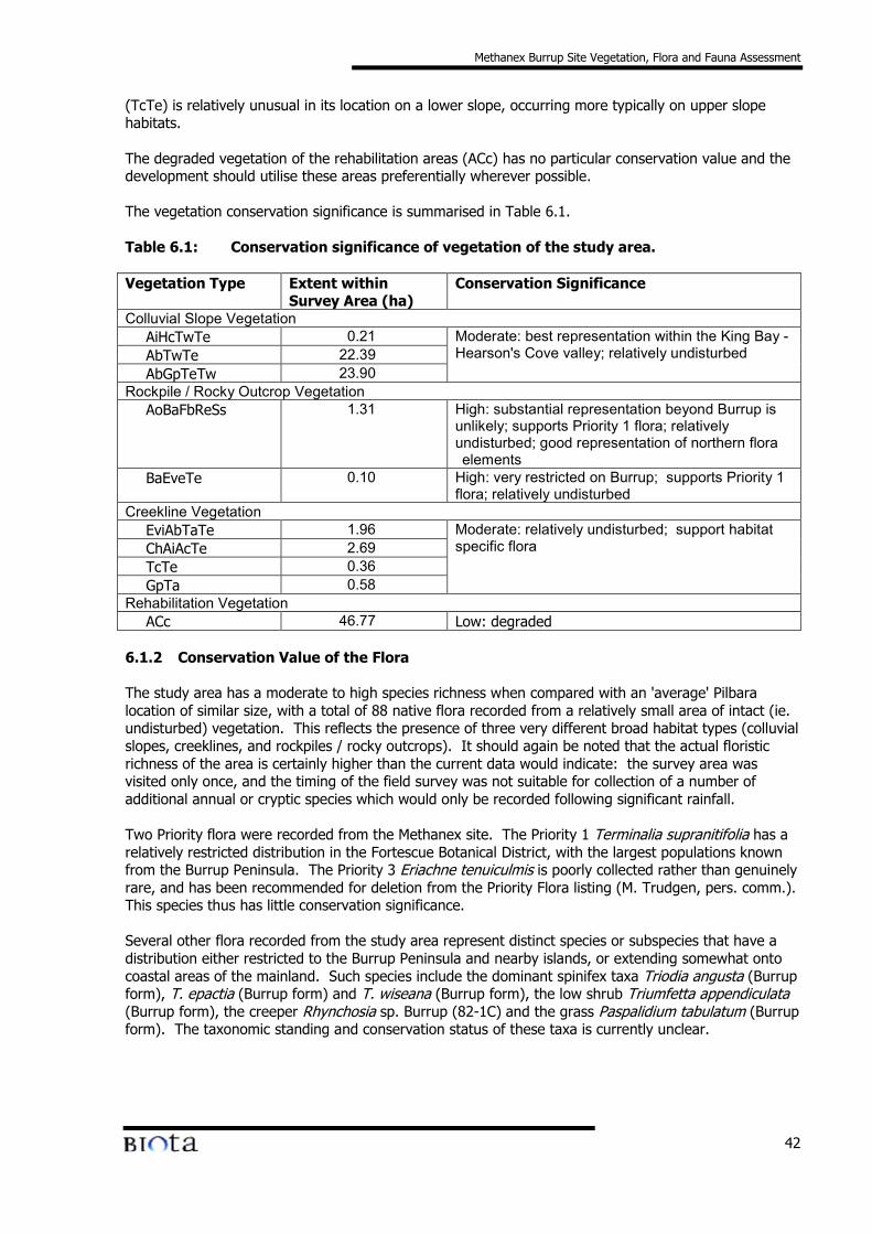
Methanex Burrup Site Vegetation, Flora and Fauna Assessment
42
(TcTe) is relatively unusual in its location on a lower slope, occurring more typically on upper slopehabitats.
The degraded vegetation of the rehabilitation areas (ACc) has no particular conservation value and thedevelopment should utilise these areas preferentially wherever possible.
The vegetation conservation significance is summarised in Table 6.1.
Table 6.1: Conservation significance of vegetation of the study area.
Vegetation Type Extent withinSurvey Area (ha)
Conservation Significance
Colluvial Slope VegetationAiHcTwTe 0.21AbTwTe 22.39AbGpTeTw 23.90
Moderate: best representation within the King Bay -Hearson's Cove valley; relatively undisturbed
Rockpile / Rocky Outcrop VegetationAoBaFbReSs 1.31 High: substantial representation beyond Burrup is
unlikely; supports Priority 1 flora; relativelyundisturbed; good representation of northern floraelements
BaEveTe 0.10 High: very restricted on Burrup; supports Priority 1flora; relatively undisturbed
Creekline VegetationEviAbTaTe 1.96ChAiAcTe 2.69TcTe 0.36GpTa 0.58
Moderate: relatively undisturbed; support habitatspecific flora
Rehabilitation VegetationACc 46.77 Low: degraded
6.1.2 Conservation Value of the Flora
The study area has a moderate to high species richness when compared with an 'average' Pilbaralocation of similar size, with a total of 88 native flora recorded from a relatively small area of intact (ie.undisturbed) vegetation. This reflects the presence of three very different broad habitat types (colluvialslopes, creeklines, and rockpiles / rocky outcrops). It should again be noted that the actual floristicrichness of the area is certainly higher than the current data would indicate: the survey area wasvisited only once, and the timing of the field survey was not suitable for collection of a number ofadditional annual or cryptic species which would only be recorded following significant rainfall.
Two Priority flora were recorded from the Methanex site. The Priority 1 Terminalia supranitifolia has arelatively restricted distribution in the Fortescue Botanical District, with the largest populations knownfrom the Burrup Peninsula. The Priority 3 Eriachne tenuiculmis is poorly collected rather than genuinelyrare, and has been recommended for deletion from the Priority Flora listing (M. Trudgen, pers. comm.).This species thus has little conservation significance.
Several other flora recorded from the study area represent distinct species or subspecies that have adistribution either restricted to the Burrup Peninsula and nearby islands, or extending somewhat ontocoastal areas of the mainland. Such species include the dominant spinifex taxa Triodia angusta (Burrupform), T. epactia (Burrup form) and T. wiseana (Burrup form), the low shrub Triumfetta appendiculata(Burrup form), the creeper Rhynchosia sp. Burrup (82-1C) and the grass Paspalidium tabulatum (Burrupform). The taxonomic standing and conservation status of these taxa is currently unclear.
Methanex Burrup Site Vegetation, Flora and Fauna Assessment
43
Given the moderate to high species richness and the presence of several uncommon and/orgeographically restricted species, the conservation value of flora of the study area is considered to bemoderate to high.
6.2 Fauna
Four species of land snail were identified from the project area using published keys and unpublishednotes. These identifications were confirmed by the Western Australian Museum (WAM). Two of thesesnail taxa currently await further collecting and formal scientific description: Rhagada sp. 12 andPupoides aff. beltianus. It is also possible that this may be complicated by unresolved issues with thetaxonomy of pupilloids that coil in opposite directions. A fifth species of snail, Rhagada sp. HearsonCove, was not found within the project area but has been collected nearby. This taxon has not yetbeen collected beyond Hearson Cove. Rhagada sp. 12 has been collected elsewhere on the BurrupPeninsula.
Three P. chapmani pebble mounds were located in the project area. None of these showed evidence ofrecent use, all having mound activity indices (sensu Anstee 1996) of 0. It is very unlikely that P.chapmani currently exists in the project area or would be likely to recolonise it in the near future.
Four Planigale sp. 1 were collected from pit traps north of the watertanks on Village Road. Previously,only one specimen of Planigale had been collected from the Burrup, despite an intensive trappingprogram by CALM in the mid 1990s. The recent captures have confirmed the presence of this taxon onthe Burrup and provide material for use in future work on Planigale taxonomy (particularlymorphological studies). This taxon is not currently listed as threatened.
One Lerista ‘muelleri’ was collected from nearby Mt Wongama and lodged with the Western AustralianMuseum for use in taxonomic studies (R146579). This form of L. ‘muelleri’ has been collectedpreviously from the Burrup. A number of other Pilbara reptiles that have taxonomic issues are presenton the peninsula but none would be significantly impacted by the proposed activities.
Three bat species were positively identified from echolocation call attributes, either foraging within orover the project area (Chalinolobus gouldii, Vespadelus finlaysoni and Taphozous georgianus). Thesespecies have been recorded previously on the Burrup Peninsula. One additional species, Mormopterusloriae, was identified from mangal habitat using unpublished call data. Further study on the callstructure of M. loriae is required and further surveys for bats need to be conducted on the BurrupPeninsula. Any activity that reduces the quality of the nearby mangal would potentially reduce the sizeof the habitat available for M. loriae (a widespread but Data Deficient species; Duncan et al. 1999;CALM Priority 1) and N. arnhemensis. There are expected to be no significant impacts on bats from thecurrent proposed development.
Fourteen other vertebrate fauna species were recorded opportunistically during the survey, both withinthe project area and at nearby CALM trapping sites. A bird species list compiled for the BurrupPeninsula by R. Johnstone (WAM) identified several species which are either listed as ‘migratory’ underthe Federal Environment Protection and Biodiversity Conservation Act 1999 or listed as Priority 4 on theDepartment of Conservation and Land Management Threatened Fauna Listing (October 2001). One ofthese was recorded during the current survey (Bush Stone-curlew Burhinus grallarius). Other,previously conducted assessments have indicated that adjacent developments are unlikely to impactdirectly on any listed migratory birds that utilise the area (Sinclair Knight Merz, 2001; AstronEnvironmental, 2001b).
Only one specially protected mammal is likely to occur in or near the project area, but is unlikely to besignificantly affected (Water-rat Hydromys chrysogaster; Priority 4).
The Pilbara Olive Python Liasis olivaceus barroni, which is protected under Schedule 1 of the WildlifeConservation (Specially Protected Fauna) Notice 2001, is known to occur on the Burrup Peninsula,
Methanex Burrup Site Vegetation, Flora and Fauna Assessment
44
including near Hearson Cove (S. van Leeuwen, pers. comm.). This species was not specifically targetedduring the present survey (although spotlighting was carried out) and no individuals were detected.The proposed development is not expected to directly impact rocky areas, which form the core habitatof this snake. However, this species may still disperse or forage within the project area.
6.3 Recommendations
In order to protect the biological values of the study area, the following recommendations are made:
1. Further seasonal floristic survey work should be conducted in 2002 following summer rainfall.The outcomes of this study may result in additional recommendations.
2. Given the moderate to high conservation value of the vegetation and flora of the study area,development should be restricted to historically disturbed areas (vegetation type ACc) as far aspossible. These areas are already degraded and have no particular conservation significance.
3. If clearing of additional areas is required, locations of Priority flora must be taken into accountand protected from disturbance. If this is not possible, then liaison should be undertaken withCALM to develop suitable management procedures.
4. Clearing of significant vegetation types (particularly the rocky outcrop and rockpile units BaEveTeand AoBaFbReSs) should be avoided. Disturbance to the remaining vegetation types should beminimised.
5. Disturbed areas remaining after construction of the plant should be rehabilitated. Species used inseed mixes must be appropriate to the area, and seed should be collected locally on the BurrupPeninsula.
6. Since the Burrup Peninsula is regarded as being well surveyed for fauna, the present studyadopted the approach of directing survey effort to poorly known fauna groups together with aprogram of funding research on some of these that occur specifically on the proposed site ornearby on the Burrup. This was considered to be a more appropriate strategy than duplicatinggeneral survey work, and these projects would significantly improve the existing knowledge offauna on the Burrup. It is recommended that the proponent support the following relevantresearch projects:
• Further studies to assist with resolving taxonomic issues of snail taxa. The most obviouscandidate is Rhagada sp. 12, which was the most noticeably abundant gastropod in theproject area and may have a restricted distribution on the Burrup. Taxonomic research onthe second undescribed Rhagada species from Hearson Cove could be conducted for littleadditional cost under the same funding opportunity and would be appropriate given the closeproximity of the proposed infrastructure to its only known habitat.
• Further taxonomic work on Western Australian Planigale species, particularly morphology andupdating museum collections. A genetic comparison has recently been completed, howeverrobust taxonomic work requires that the results of both genetic and morphological studies becorroborated. After the revision of a genus, museum collections need to be updated, whichis time consuming and requires effort over and above normal curatorial work.
• Research on reptile species occurring on the Burrup Peninsula that require further taxonomicwork. An ideal candidate would be the legless lizard Delma pax. This species occurs in thePilbara (including the Burrup) and the Canning Basin, but there are unresolved problems inthis taxon, with variation in specimens keying to D. pax.
Methanex Burrup Site Vegetation, Flora and Fauna Assessment
45
7. In keeping with the spirit of adjacent developers, participate and assist in a collaborative study ofmeasures to minimise bird impacts and encourage their continued use of habitats on the Burrupthrough the development of an industry group for the King Bay - Hearson Cove Industrial Area.
8. The proponent should be aware of the potential for the Pilbara Olive Python Liasis olivaceusbarroni to occur within the plant area. A management plan should be developed andimplemented to reduce potential causes of mortality, and facilitate the removal and translocationof individuals that are found on site.
7.0 Acknowledgements
The following persons are gratefully acknowledged for their assistance with this study:
• Mr Malcolm Trudgen (ME Trudgen & Associates) for assistance with difficult flora identifications,and providing commentary on the conservation status of vegetation types and poorly known floraspecies on the Burrup Peninsula.
• Mr Ted Griffin (Agriculture Western Australia) for running the PATN analysis.
• Dr Peter Kendrick (CALM Karratha) for assistance with snail identification.
• Ms Shirley Slack-Smith (WA Museum) for confirmation of snail identifications.
Methanex Burrup Site Vegetation, Flora and Fauna Assessment
46
8.0 References
Adams, M., Reardon, T.R., Baverstock, P.R. and Watts, C.H.S. (1988). Electrophoretic resolution ofspecies boundaries in Australian Microchiroptera. IV. The Molossidae (Chiroptera). AustralianJournal of Biological Science 41: 315-326.
Anstee, S.D. (1996). Use of external mound structures as indicators of the presence of the pebble-mound mouse, Pseudomys chapmani, in mound systems. Wildlife Research 23: 429-434.
Armstrong, K.N. (2001). The distribution and roost habitat of the orange leaf-nosed bat Rhinonicterisaurantius, in the Pilbara region of Western Australia. Wildlife Research 28: 95-104.
Armstrong, K.N. and Anstee, S.D. (2000). The ghost bat in the Pilbara: 100 years on. AustralianMammalogy 22: 93-101.
Armstrong, K.N., Anstee, S.D et al. (in prep.). The habitat of Leggadina lakedownensis in the mainlandPilbara of WA.
Astron Environmental (1998). Ammonia Urea Plant Service Corridor Fauna Survey. Unpublished reportfor Plenty River Corporation Ltd., August 1998.
Astron Environmental (1999a). Natural Gas to Synthetic Oil Project Product and Feed pipelines,Vegetation, Flora and Fauna Survey. Unpublished report for Syntroleum Corporation, August1999.
Astron Environmental (1999b). Natural Gas to Synthetic Oil Project: Plantsite Vegetation, Flora andFauna Survey. Unpublished report prepared for HLA- Envirosciences Pty Ltd, October, 1999.
Astron Environmental (2000). Natural Gas to Synthetic Oil Project: A Vertebrate Survey of the Plant Siteon the Burrup Peninsula. Unpublished report prepared for HLA- Envirosciences Pty Ltd, June,2000.
Astron Environmental (2001a). Vegetation and Flora of the Proposed Ammonia Plant Site. Unpublishedreport prepared for Sinclair Knight Merz Pty Ltd, April 2001.
Astron Environmental (2001b). Burrup Fertilisers Pty Ltd. Fauna of the Burrup Peninsula and theProposed Ammonia Plant (Revised version). Unpublished report to Sinclair Knight Merz Pty Ltd.
Atkins, K.J. (2001). Declared Rare and Priority Flora List for Western Australia. Prepared by theDepartment of Conservation and Land Management, 23 August 2001.
Beard J.S. (1975). Pilbara. Explanatory notes to Sheet 5, 1:1 000 000 series vegetation survey ofWestern Australia. University of Western Australia Press: Nedlands.
Biota Environmental Sciences Pty Ltd (2001a). Burrup Liquid Ammonia Plant targeted fauna survey.Unpublished report for Sinclair Knight Merz Pty Ltd, October 2001.
Biota Environmental Sciences Pty Ltd (2001b). Baseline Biological & Soil Surveys and Mapping forML244SA West of the Fortescue River. Unpublished report for BHPIO.
Methanex Burrup Site Vegetation, Flora and Fauna Assessment
47
Butler, H. (1994). Fauna and Marine Biota. In: Burrup Peninsula Draft Land Use and Management Plan,Technical Appendices. Unpublished report by O’Brien Planning Consultants.
Butler, W.H. and Butler, M.A. (1983). Burrup Peninsula Fauna Survey. Unpublished report for WoodsideOffshore Petroleum Pty Ltd.
Butler, W.H. and Butler, M.A. (1987). Burrup Peninsula Fauna Survey. Unpublished report for WoodsideOffshore Petroleum Pty Ltd.
Cooper, N.K., Adams, M. and How, R.A. (2001). The identity of Planigale on the Burrup Peninsula.Prepared for Sinclair Knight Merz on behalf of Burrup Fertilisers by the Western AustralianMuseum, November 2001.
Dahl, K. (1897). Biological notes on North Australian Mammalia. Zoologist Series 4 Volume 1: 189-216.
Duncan, A., Baker, G.B., and Montgomery, N. (1999). The Action Plan for Australian Bats. BiodiversityGroup, Environment Australia: Canberra.
Environmental Protection Authority (1995). Burrup Peninsula draft land use and management plan. Asubmission by the EPA on the draft document released for public review by the BurrupPeninsula Management Advisory Board. Bulletin 801, December 1995.
Halpern Glick Maunsell (2000). Austeel Pty Ltd Iron Ore Mine and Downstream Processing, CapePreston, Western Australia: Public Environmental Review. December 2000.
How, R.A., N.K. Cooper and J.L Bannister (2001). Checklist of the mammals of Western Australia.Records of the Western Australian Museum Supplement 63: 91–98.
Iredale, T. (1939). A review of the land Mollusca of Western Australia. Journal of the Royal Society ofWestern Australia 25: 1-88.
Johnstone R.E. and Storr, G.M. (1998). Handbook of Western Australian Birds. Volume 1 – Non-Passerines (Emu to Dollarbird). Western Australian Museum: Perth. 436pp.
Jolly, S. (1996a). Analysis of Anabat files: Bat echolocation call recognition. Australasian Bat SocietyNewsletter 7: 22-28.
Jolly, S. (1996b). Analyze for Windows 95. Download available athttp://members.ozemail.com.au/~jollys/
Jolly, S. (1997). Analysis of Anabat files. Australasian Bat Society Newsletter 9: 25-27.
Kruger, J. and Long, V.L. (1999). A Survey of Vegetation and Fauna in the King Bay Region, BurrupPeninsula, W.A. Unpublished report for Mermaid Marine Australia Pty Ltd.
McKenzie, N.L. and Muir, W.P. (2000). Bats of the southern Carnarvon Basin, Western Australia.Records of the Western Australian Museum Supplement 61: 465-477.
Morgan, B. & Trudgen, M.E. (in prep.). A flora and vegetation survey of a site on the Burrup Peninsulafor a proposed Dimethyl Ether project. Being prepared for PPK Environment and Infrastructure.
Olsen, P.D. (1995). Water-rat Hydromys chryosgaster. In: The mammals of Australia. (R. Strahan ed.).Reed: Chatswood, NSW. 756pp.
Randell, B.R. (1989). Revision of the Cassiinae in Australia. 2. Senna Miller Sect. Psilorhegma (J. Vogel)Irwin and Barneby. Journal of the Adelaide Botanical Gardens 12(2): 165-272.
Methanex Burrup Site Vegetation, Flora and Fauna Assessment
48
Slack-Smith, S.M. (2001). Survey report on the non-marine molluscan fauna of the site proposed for theOswal Ammonia Plant on the Burrup Peninsula, Western Australia. Unpublished report toSinclair Knight Merz by the Western Australian Museum, March 2001.
Slack-Smith, S.M. (2002). Report on a series of land snails collected by K. Armstrong, BiotaEnvironmental Sciences from the proposed site of a methanol plant on the Burrup Peninsula,Western Australia. Unpublished report to Biota Environmental Sciences Pty Ltd from theWestern Australian Museum, January 2002.
Sinclair Knight Merz (2001). Burrup Fertilisers Pty Ltd. Proposed 2,200 tdp Ammonia Plant, BurrupPeninsula Western Australia. Public Environment Review and Response to Submissions. August2001.
Smith, L.A., Adams, M. and How, R.A. (2001). The Lerista muelleri complex on the Burrup Peninsula.Prepared for Sinclair Knight Merz on behalf of Burrup Fertilisers by the Western AustralianMuseum, November 2001.
Solem, A. (1985). Camaenid land snails from Western and Central Australia (Mollusca: Pulmonata:Camaenidae). V. Remaining Kimberley genera and addenda to the Kimberley. Records of theWestern Australian Museum Supplement 20: 707-981.
Solem, A. (1986). Pupilloid land snails from the south and mid-west coasts of Australia Journal of theMalacological Society of Australia 7(3-4): 95-124.
Solem, A. (1988). Non-camaenid land snails of the Kimberley and Northern Territory, Australia. I.Systematics, affinities and ranges. Invertebrate Taxonomy 4: 455-604.
Solem, A. (1990). Camaenid land snails from Western and Central Australia (Mollusca: Pulmonata:Camaenidae). VI. Taxa from the Red Centre. Records of the Western Australian MuseumSupplement 43: 983-1459.
Solem, A. (1997). Camaenid land snails from Western and Central Australia (Mollusca: Pulmonata:Camaenidae). VII. Taxa from Dampierland through the Nullarbor. Records of the WesternAustralian Museum Supplement 50: 1461-1906.
Specht, R.L. (1970). Vegetation. In: The Australian Environment. 4th ed (G.W. Leeper Ed.). Melbourne.
Start, A.N., Anstee, S.D. and Endersby, M. (2000). A review of the biology and conservation status ofthe Ngadji, Pseudomys chapmani Kitchener, 1980 (Rodentia: Muridae). CALMScience 3(2): 125-147.
Symon, D.E. (1966). A revision of the genus Cassia L. Caesalpiniaceae in Australia. Transactions of theRoyal Society of South Australia 90: 73-146.
Tingay, A. and Tingay, S.R. (1979). Technical Report on the Fauna of Burrup Peninsula and DolphinIsland. Unpublished report for Woodside Petroleum Pty Ltd.
Trudgen, M.E. & N. Casson (1998). Flora and vegetation surveys of Orebody A and Orebody B in theWest Angela Hill area, an area surrounding them, and of rail route options considered to linkthem to the existing Robe River Iron Associates rail line. Unpublished report for Robe RiverIron Associates.
Trudgen, M.E. & Griffin, E.A. (2002). A flora, vegetation and floristic survey of the Burrup Peninsula,some adjoining areas and part of the Dampier Archipelago, with comparisons to the floristics ofthree areas of the adjoining mainland. Volume 2. Floristic analysis of vegetation site data from

Methanex Burrup Site Vegetation, Flora and Fauna Assessment
49
the Burrup Peninsula, Dolphin, Angel and Gidley Islands with data from Cape Preston, theChichester Ranges and other localities. Prepared for the Office of Major Projects.
Trudgen, M.E. & Long, V. (in prep.). A flora, vegetation and floristic survey of the Burrup Peninsula,some adjoining areas and part of the Dampier Archipelago, with comparisons to the floristics ofthree areas of the adjoining mainland. Volume 1. Being prepared for the Office of MajorProjects.
Water Corporation of Western Australia (2001). Environmental information for Burrup Peninsuladesalinated and seawater supplies project. Community Consultation document.http://www.watercorporation.com.au/community-consult/images/burrup.pdf
Worley Astron (1999). Dampier Marine Services Facility Environmental referral. Mermaid MarineAustralia Ltd.
Appendix A
Raw Data for Detailed Flora Survey Sites
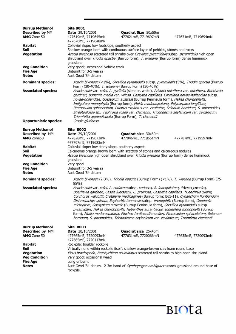
Burrup Methanol Site B001Described by MM Date 29/10/2001 Quadrat Size 50x50mAMG Zone 50 477619mE, 7719645mN 477621mE, 7719697mN 477671mE, 7719694mN
477676mE, 7719648mNHabitat Colluvial slope: low footslope, southerly aspectSoil Shallow orange loam with continuous surface layer of pebbles, stones and rocksVegetation Acacia bivenosa scattered tall shrubs over Grevillea pyramidalis subsp. pyramidalis high open
shrubland over Triodia epactia (Burrup form), T. wiseana (Burrup form) dense hummockgrassland
Veg Condition Very good; occasional vehicle trackFire Age Unburnt for 3-5 years?Notes Aust Geod '84 datum
Dominant species: Acacia bivenosa (<1%), Grevillea pyramidalis subsp. pyramidalis (5%), Triodia epactia (BurrupForm) (30-40%), T. wiseana (Burrup Form) (30-40%)
Associated species: Acacia colei var. colei, A. pyrifolia (slender, white), Aristida holathera var. holathera, Boerhaviagardneri, Bonamia media var. villosa, Cassytha capillaris, Crotalaria novae-hollandiae subsp.novae-hollandiae, Gossypium australe (Burrup Peninsula form), Hakea chordophylla,Indigofera monophylla (Burrup form), Mukia maderaspatana, Polycarpaea longiflora,Pterocaulon sphacelatum, Ptilotus exaltatus var. exaltatus, Solanum horridum, S. phlomoides,Streptoglossa sp., Tephrosia rosea var. clementii, Trichodesma zeylanicum var. zeylanicum,Triumfetta appendiculata (Burrup Form), T. clementii
Opportunistic species: Cassia glutinosa
Burrup Methanol Site B002Described by MM Date 29/10/2001 Quadrat size 30x80mAMG Zone50 477828mE, 7719673mN 477846mE, 7719651mN 477787mE, 7719597mN
477767mE, 7719623mNHabitat Colluvial slope: low stony slope, southerly aspectSoil Calcareous orange-brown loam with scatters of stones and calcareous nodulesVegetation Acacia bivenosa high open shrubland over Triodia wiseana (Burrup form) dense hummock
grasslandVeg Condition Very goodFire Age Unburnt for 3-5 years?Notes Aust Geod '84 datum
Dominant species: Acacia bivenosa (2-3%), Triodia epactia (Burrup Form) (<1%), T. wiseana (Burrup Form) (75-85%)
Associated species: Acacia colei var. colei, A. coriacea subsp. coriacea, A. inaequilatera, *Aerva javanica,Boerhavia gardneri, Cassia luerssenii, C. pruinosa, Cassytha capillaris, *Cenchrus ciliaris,Corchorus walcottii, Crotalaria medicaginea (Burrup form; B65-11), Cynanchum floribundum,Dichrostachys spicata, Euphorbia tannensis subsp. eremophila (Burrup form), Goodeniamicroptera, Gossypium australe (Burrup Peninsula form), Grevillea pyramidalis subsp.pyramidalis, Hakea chordophylla, Hybanthus aurantiacus, Indigofera monophylla (Burrupform), Mukia maderaspatana, Pluchea ferdinandi-muelleri, Pterocaulon sphacelatum, Solanumhorridum, S. phlomoides, Trichodesma zeylanicum var. zeylanicum, Triumfetta clementii
Burrup Methanol Site B003Described by MM Date 30/10/2001 Quadrat size 25x40mAMG Zone 50 477665mE, 7720093mN 477631mE, 7720066mN 477635mE, 7720093mN
477665mE, 7720113mNHabitat Rockpile: boulder rockpileSoil Virtually none within rockpile itself; shallow orange-brown clay loam round baseVegetation Ficus brachypoda, Brachychiton acuminatus scattered tall shrubs to high open shrublandVeg Condition Very good; occasional weedFire Age Long unburntNotes Aust Geod '84 datum. 2-3m band of Cymbopogon ambiguus tussock grassland around base of
rockpile.
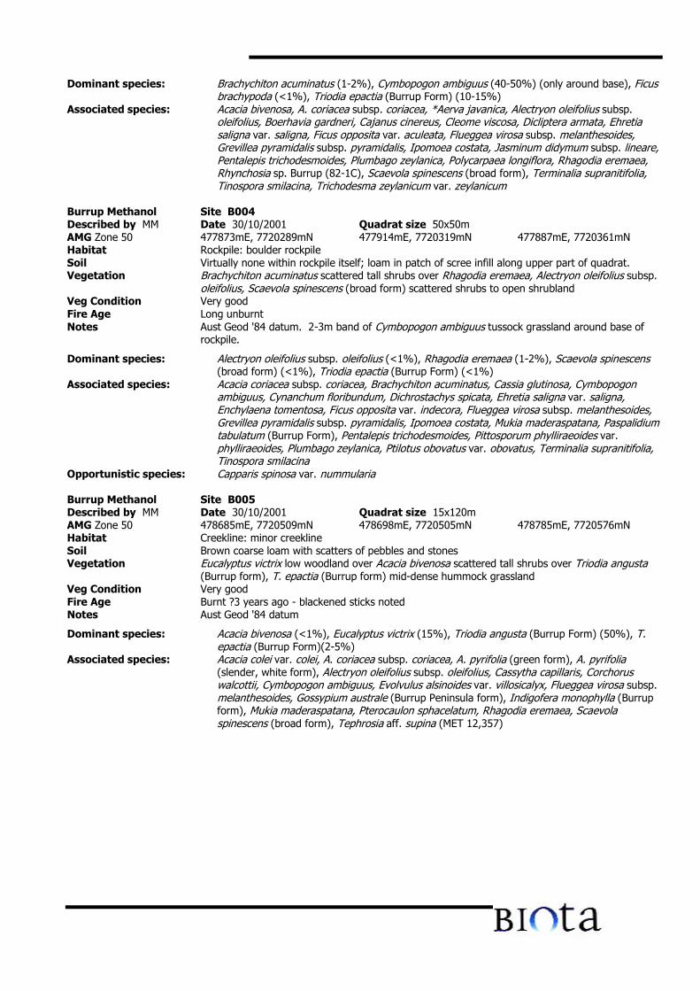
Dominant species: Brachychiton acuminatus (1-2%), Cymbopogon ambiguus (40-50%) (only around base), Ficusbrachypoda (<1%), Triodia epactia (Burrup Form) (10-15%)
Associated species: Acacia bivenosa, A. coriacea subsp. coriacea, *Aerva javanica, Alectryon oleifolius subsp.oleifolius, Boerhavia gardneri, Cajanus cinereus, Cleome viscosa, Dicliptera armata, Ehretiasaligna var. saligna, Ficus opposita var. aculeata, Flueggea virosa subsp. melanthesoides,Grevillea pyramidalis subsp. pyramidalis, Ipomoea costata, Jasminum didymum subsp. lineare,Pentalepis trichodesmoides, Plumbago zeylanica, Polycarpaea longiflora, Rhagodia eremaea,Rhynchosia sp. Burrup (82-1C), Scaevola spinescens (broad form), Terminalia supranitifolia,Tinospora smilacina, Trichodesma zeylanicum var. zeylanicum
Burrup Methanol Site B004Described by MM Date 30/10/2001 Quadrat size 50x50mAMG Zone 50 477873mE, 7720289mN 477914mE, 7720319mN 477887mE, 7720361mNHabitat Rockpile: boulder rockpileSoil Virtually none within rockpile itself; loam in patch of scree infill along upper part of quadrat.Vegetation Brachychiton acuminatus scattered tall shrubs over Rhagodia eremaea, Alectryon oleifolius subsp.
oleifolius, Scaevola spinescens (broad form) scattered shrubs to open shrublandVeg Condition Very goodFire Age Long unburntNotes Aust Geod '84 datum. 2-3m band of Cymbopogon ambiguus tussock grassland around base of
rockpile.
Dominant species: Alectryon oleifolius subsp. oleifolius (<1%), Rhagodia eremaea (1-2%), Scaevola spinescens(broad form) (<1%), Triodia epactia (Burrup Form) (<1%)
Associated species: Acacia coriacea subsp. coriacea, Brachychiton acuminatus, Cassia glutinosa, Cymbopogonambiguus, Cynanchum floribundum, Dichrostachys spicata, Ehretia saligna var. saligna,Enchylaena tomentosa, Ficus opposita var. indecora, Flueggea virosa subsp. melanthesoides,Grevillea pyramidalis subsp. pyramidalis, Ipomoea costata, Mukia maderaspatana, Paspalidiumtabulatum (Burrup Form), Pentalepis trichodesmoides, Pittosporum phylliraeoides var.phylliraeoides, Plumbago zeylanica, Ptilotus obovatus var. obovatus, Terminalia supranitifolia,Tinospora smilacina
Opportunistic species: Capparis spinosa var. nummularia
Burrup Methanol Site B005Described by MM Date 30/10/2001 Quadrat size 15x120mAMG Zone 50 478685mE, 7720509mN 478698mE, 7720505mN 478785mE, 7720576mNHabitat Creekline: minor creeklineSoil Brown coarse loam with scatters of pebbles and stonesVegetation Eucalyptus victrix low woodland over Acacia bivenosa scattered tall shrubs over Triodia angusta
(Burrup form), T. epactia (Burrup form) mid-dense hummock grasslandVeg Condition Very goodFire Age Burnt ?3 years ago - blackened sticks notedNotes Aust Geod '84 datum
Dominant species: Acacia bivenosa (<1%), Eucalyptus victrix (15%), Triodia angusta (Burrup Form) (50%), T.epactia (Burrup Form)(2-5%)
Associated species: Acacia colei var. colei, A. coriacea subsp. coriacea, A. pyrifolia (green form), A. pyrifolia(slender, white form), Alectryon oleifolius subsp. oleifolius, Cassytha capillaris, Corchoruswalcottii, Cymbopogon ambiguus, Evolvulus alsinoides var. villosicalyx, Flueggea virosa subsp.melanthesoides, Gossypium australe (Burrup Peninsula form), Indigofera monophylla (Burrupform), Mukia maderaspatana, Pterocaulon sphacelatum, Rhagodia eremaea, Scaevolaspinescens (broad form), Tephrosia aff. supina (MET 12,357)
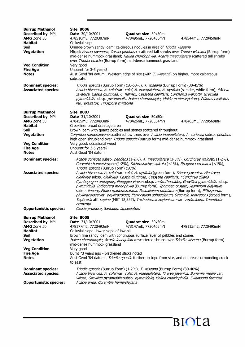
Burrup Methanol Site B006Described by MM Date 30/10/2001 Quadrat size 50x50mAMG Zone 50 478510mE, 7720387mN 478496mE, 7720436mN 478544mE, 7720450mNHabitat Colluvial slopeSoil Orange-brown sandy loam; calcareous nodules in area of Triodia wiseanaVegetation Mixed: Acacia bivenosa, Cassia glutinosa scattered tall shrubs over Triodia wiseana (Burrup form)
mid-dense hummock grassland; Hakea chordophylla, Acacia inaequilatera scattered tall shrubsover Triodia epactia (Burrup form) mid-dense hummock grassland
Veg Condition Very goodFire Age Unburnt for 3-5 years?Notes Aust Geod '84 datum. Western edge of site (with T. wiseana) on higher, more calcareous
substrate.
Dominant species: Triodia epactia (Burrup Form) (50-60%), T. wiseana (Burrup Form) (30-45%)Associated species: Acacia bivenosa, A. colei var. colei, A. inaequilatera, A. pyrifolia (slender, white form), *Aerva
javanica, Cassia glutinosa, C. helmsii, Cassytha capillaris, Corchorus walcottii, Grevilleapyramidalis subsp. pyramidalis, Hakea chordophylla, Mukia maderaspatana, Ptilotus exaltatusvar. exaltatus, Tinospora smilacina
Burrup Methanol Site B007Described by MM Date 31/10/2001 Quadrat size 50x50mAMG Zone 50 478459mE, 7720493mN 478426mE, 7720534mN 478463mE, 7720569mNHabitat Creekline: broad drainage areaSoil Brown loam with quartz pebbles and stones scattered throughoutVegetation Corymbia hamersleyana scattered low trees over Acacia inaequilatera, A. coriacea subsp. pendens
high open shrubland over Triodia epactia (Burrup form) mid-dense hummock grasslandVeg Condition Very good; occasional weedFire Age Unburnt for 3-5 years?Notes Aust Geod '84 datum
Dominant species: Acacia coriacea subsp. pendens (1-2%), A. inaequilatera (3-5%), Corchorus walcottii (1-2%),Corymbia hamersleyana (1-2%), Dichrostachys spicata (<1%), Rhagodia eremaea (<1%),Triodia epactia (Burrup Form) (50%)
Associated species: Acacia bivenosa, A. colei var. colei, A. pyrifolia (green form), *Aerva javanica, Alectryonoleifolius subsp. oleifolius, Cassia glutinosa, Cassytha capillaris, *Cenchrus ciliaris,Cymbopogon ambiguus, Flueggea virosa subsp. melanthesoides, Grevillea pyramidalis subsp.pyramidalis, Indigofera monophylla (Burrup form), Ipomoea costata, Jasminum didymumsubsp. lineare, Mukia maderaspatana, Paspalidium tabulatum (Burrup form), Pittosporumphylliraeoides var. phylliraeoides, Pterocaulon sphacelatum, Scaevola spinescens (broad form),Tephrosia aff. supina (MET 12,357), Trichodesma zeylanicum var. zeylanicum, Triumfettaclementii
Opportunistic species: Cassia pruinosa, Santalum lanceolatum
Burrup Methanol Site B008Described by MM Date 31/10/2001 Quadrat size 50x50mAMG Zone 50 478177mE, 7720493mN 478147mE, 7720453mN 478113mE, 7720495mNHabitat Colluvial slope: lower slope of low hillSoil Brown fine sandy loam with continuous surface layer of pebbles and stonesVegetation Hakea chordophylla, Acacia inaequilatera scattered shrubs over Triodia wiseana (Burrup form)
mid-dense hummock grasslandVeg Condition Very goodFire Age Burnt ?3 years ago - blackened sticks notedNotes Aust Geod '84 datum. Triodia epactia further upslope from site, and on areas surrounding creek
to east
Dominant species: Triodia epactia (Burrup Form) (1-2%), T. wiseana (Burrup Form) (30-40%)Associated species: Acacia bivenosa, A. colei var. colei, A. inaequilatera, *Aerva javanica, Bonamia media var.
villosa, Grevillea pyramidalis subsp. pyramidalis, Hakea chordophylla, Swainsona formosaOpportunistic species: Acacia arida, Corymbia hamersleyana
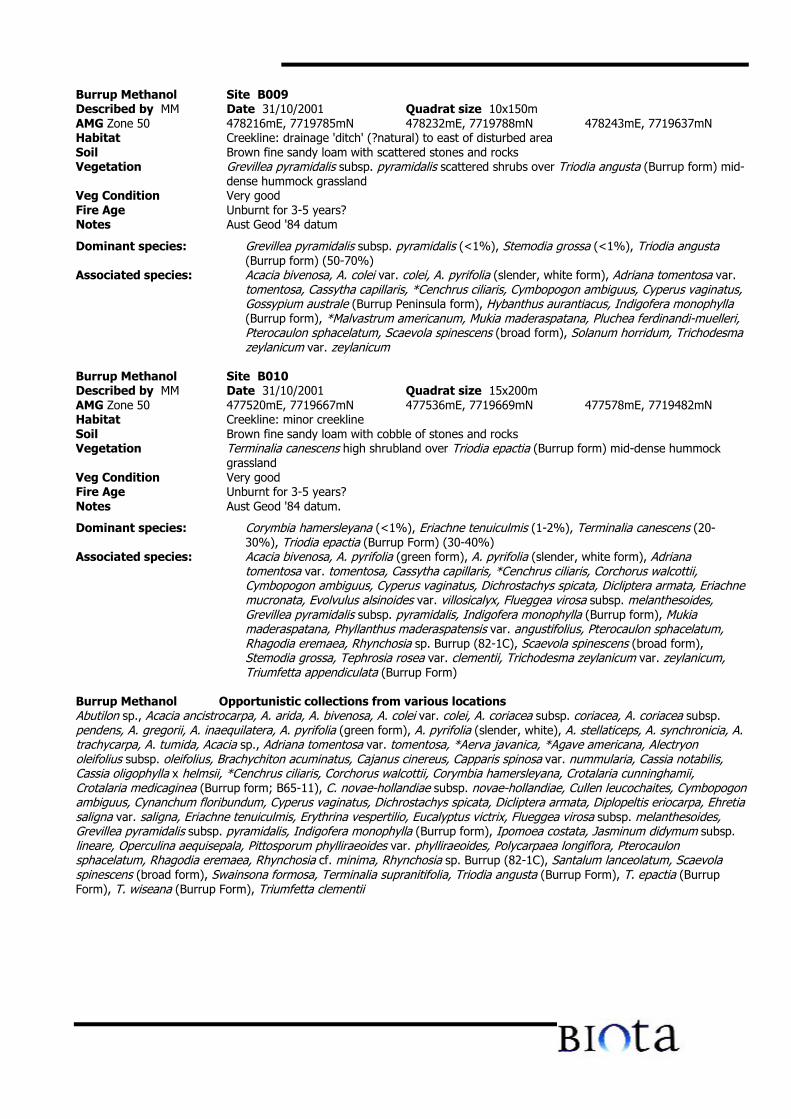
Burrup Methanol Site B009Described by MM Date 31/10/2001 Quadrat size 10x150mAMG Zone 50 478216mE, 7719785mN 478232mE, 7719788mN 478243mE, 7719637mNHabitat Creekline: drainage 'ditch' (?natural) to east of disturbed areaSoil Brown fine sandy loam with scattered stones and rocksVegetation Grevillea pyramidalis subsp. pyramidalis scattered shrubs over Triodia angusta (Burrup form) mid-
dense hummock grasslandVeg Condition Very goodFire Age Unburnt for 3-5 years?Notes Aust Geod '84 datum
Dominant species: Grevillea pyramidalis subsp. pyramidalis (<1%), Stemodia grossa (<1%), Triodia angusta(Burrup form) (50-70%)
Associated species: Acacia bivenosa, A. colei var. colei, A. pyrifolia (slender, white form), Adriana tomentosa var.tomentosa, Cassytha capillaris, *Cenchrus ciliaris, Cymbopogon ambiguus, Cyperus vaginatus,Gossypium australe (Burrup Peninsula form), Hybanthus aurantiacus, Indigofera monophylla(Burrup form), *Malvastrum americanum, Mukia maderaspatana, Pluchea ferdinandi-muelleri,Pterocaulon sphacelatum, Scaevola spinescens (broad form), Solanum horridum, Trichodesmazeylanicum var. zeylanicum
Burrup Methanol Site B010Described by MM Date 31/10/2001 Quadrat size 15x200mAMG Zone 50 477520mE, 7719667mN 477536mE, 7719669mN 477578mE, 7719482mNHabitat Creekline: minor creeklineSoil Brown fine sandy loam with cobble of stones and rocksVegetation Terminalia canescens high shrubland over Triodia epactia (Burrup form) mid-dense hummock
grasslandVeg Condition Very goodFire Age Unburnt for 3-5 years?Notes Aust Geod '84 datum.
Dominant species: Corymbia hamersleyana (<1%), Eriachne tenuiculmis (1-2%), Terminalia canescens (20-30%), Triodia epactia (Burrup Form) (30-40%)
Associated species: Acacia bivenosa, A. pyrifolia (green form), A. pyrifolia (slender, white form), Adrianatomentosa var. tomentosa, Cassytha capillaris, *Cenchrus ciliaris, Corchorus walcottii,Cymbopogon ambiguus, Cyperus vaginatus, Dichrostachys spicata, Dicliptera armata, Eriachnemucronata, Evolvulus alsinoides var. villosicalyx, Flueggea virosa subsp. melanthesoides,Grevillea pyramidalis subsp. pyramidalis, Indigofera monophylla (Burrup form), Mukiamaderaspatana, Phyllanthus maderaspatensis var. angustifolius, Pterocaulon sphacelatum,Rhagodia eremaea, Rhynchosia sp. Burrup (82-1C), Scaevola spinescens (broad form),Stemodia grossa, Tephrosia rosea var. clementii, Trichodesma zeylanicum var. zeylanicum,Triumfetta appendiculata (Burrup Form)
Burrup Methanol Opportunistic collections from various locationsAbutilon sp., Acacia ancistrocarpa, A. arida, A. bivenosa, A. colei var. colei, A. coriacea subsp. coriacea, A. coriacea subsp.pendens, A. gregorii, A. inaequilatera, A. pyrifolia (green form), A. pyrifolia (slender, white), A. stellaticeps, A. synchronicia, A.trachycarpa, A. tumida, Acacia sp., Adriana tomentosa var. tomentosa, *Aerva javanica, *Agave americana, Alectryonoleifolius subsp. oleifolius, Brachychiton acuminatus, Cajanus cinereus, Capparis spinosa var. nummularia, Cassia notabilis,Cassia oligophylla x helmsii, *Cenchrus ciliaris, Corchorus walcottii, Corymbia hamersleyana, Crotalaria cunninghamii,Crotalaria medicaginea (Burrup form; B65-11), C. novae-hollandiae subsp. novae-hollandiae, Cullen leucochaites, Cymbopogonambiguus, Cynanchum floribundum, Cyperus vaginatus, Dichrostachys spicata, Dicliptera armata, Diplopeltis eriocarpa, Ehretiasaligna var. saligna, Eriachne tenuiculmis, Erythrina vespertilio, Eucalyptus victrix, Flueggea virosa subsp. melanthesoides,Grevillea pyramidalis subsp. pyramidalis, Indigofera monophylla (Burrup form), Ipomoea costata, Jasminum didymum subsp.lineare, Operculina aequisepala, Pittosporum phylliraeoides var. phylliraeoides, Polycarpaea longiflora, Pterocaulonsphacelatum, Rhagodia eremaea, Rhynchosia cf. minima, Rhynchosia sp. Burrup (82-1C), Santalum lanceolatum, Scaevolaspinescens (broad form), Swainsona formosa, Terminalia supranitifolia, Triodia angusta (Burrup Form), T. epactia (BurrupForm), T. wiseana (Burrup Form), Triumfetta clementii
Appendix B
Extract of Dendrogram Produced by PATNAnalysis of Data from the Burrup
Peninsula and Surrounds
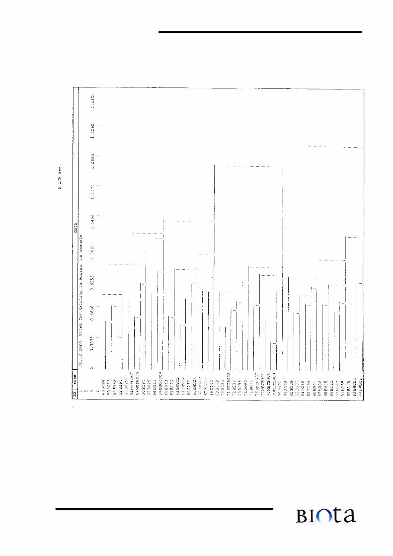
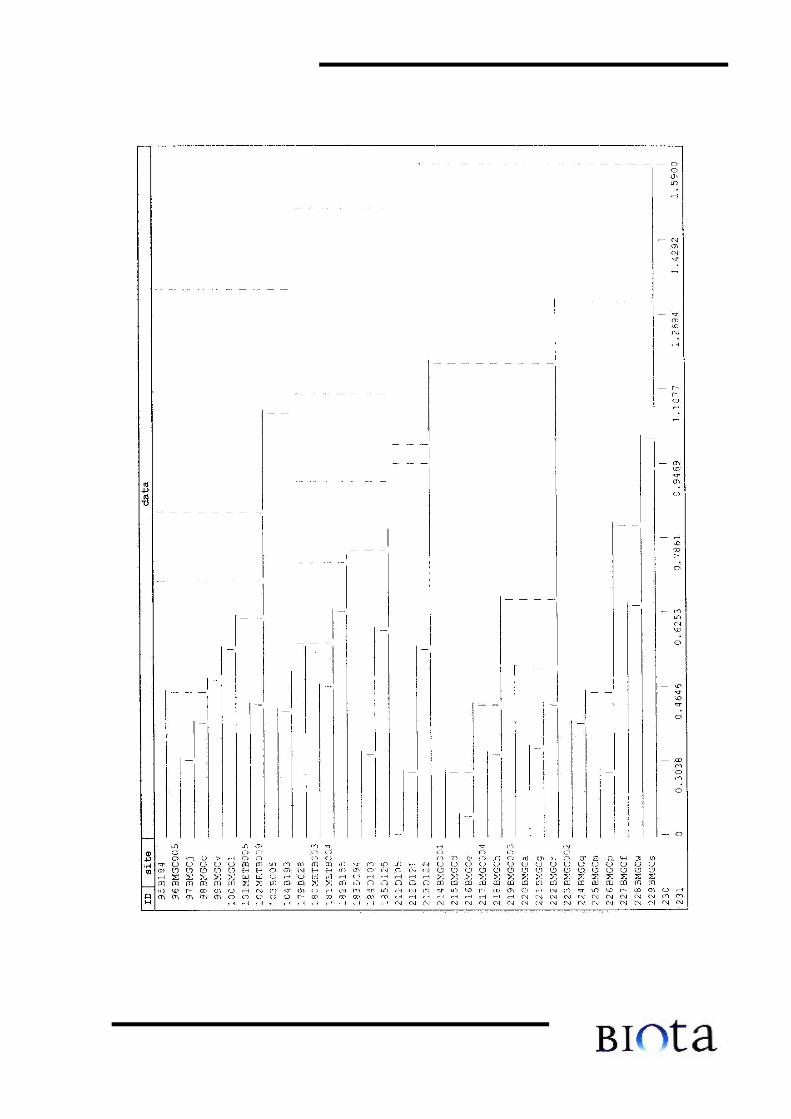
Appendix C
Vascular Flora Recorded from the MethanexStudy Area
NB. * denotes flora introduced to Western Australia† denotes flora that are probably introduced to the Burrup Peninsula
Correspondence of Cassia / Senna nomenclatureCassia glutinosa Senna glutinosa subsp. glutinosaCassia helmsii Senna artemisioides subsp. helmsiiCassia luerssenii Senna glutinosa subsp. x luersseniiCassia notabilis Senna notabilisCassia oligophylla x helmsii Senna artemisioides subsp. oligophylla x helmsiiCassia pruinosa Senna glutinosa subsp. pruinosa
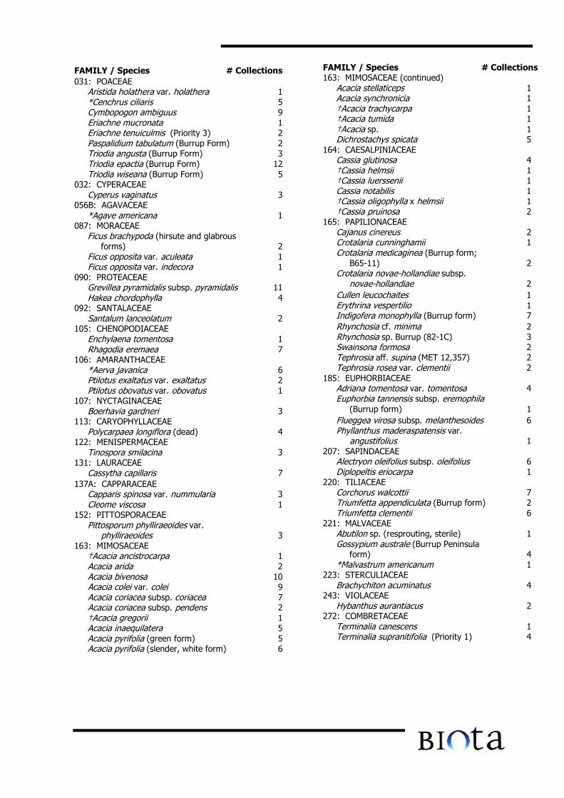
FAMILY / Species # Collections031: POACEAE
Aristida holathera var. holathera 1*Cenchrus ciliaris 5Cymbopogon ambiguus 9Eriachne mucronata 1Eriachne tenuiculmis (Priority 3) 2Paspalidium tabulatum (Burrup Form) 2Triodia angusta (Burrup Form) 3Triodia epactia (Burrup Form) 12Triodia wiseana (Burrup Form) 5
032: CYPERACEAECyperus vaginatus 3
056B: AGAVACEAE*Agave americana 1
087: MORACEAEFicus brachypoda (hirsute and glabrous forms) 2Ficus opposita var. aculeata 1Ficus opposita var. indecora 1
090: PROTEACEAEGrevillea pyramidalis subsp. pyramidalis 11Hakea chordophylla 4
092: SANTALACEAESantalum lanceolatum 2
105: CHENOPODIACEAEEnchylaena tomentosa 1Rhagodia eremaea 7
106: AMARANTHACEAE*Aerva javanica 6Ptilotus exaltatus var. exaltatus 2Ptilotus obovatus var. obovatus 1
107: NYCTAGINACEAEBoerhavia gardneri 3
113: CARYOPHYLLACEAEPolycarpaea longiflora (dead) 4
122: MENISPERMACEAETinospora smilacina 3
131: LAURACEAECassytha capillaris 7
137A: CAPPARACEAECapparis spinosa var. nummularia 3Cleome viscosa 1
152: PITTOSPORACEAEPittosporum phylliraeoides var. phylliraeoides 3
163: MIMOSACEAE†Acacia ancistrocarpa 1Acacia arida 2Acacia bivenosa 10Acacia colei var. colei 9Acacia coriacea subsp. coriacea 7Acacia coriacea subsp. pendens 2†Acacia gregorii 1Acacia inaequilatera 5Acacia pyrifolia (green form) 5Acacia pyrifolia (slender, white form) 6
FAMILY / Species # Collections163: MIMOSACEAE (continued)
Acacia stellaticeps 1Acacia synchronicia 1†Acacia trachycarpa 1†Acacia tumida 1†Acacia sp. 1Dichrostachys spicata 5
164: CAESALPINIACEAECassia glutinosa 4†Cassia helmsii 1†Cassia luerssenii 1Cassia notabilis 1†Cassia oligophylla x helmsii 1†Cassia pruinosa 2
165: PAPILIONACEAECajanus cinereus 2Crotalaria cunninghamii 1Crotalaria medicaginea (Burrup form; B65-11) 2Crotalaria novae-hollandiae subsp. novae-hollandiae 2Cullen leucochaites 1Erythrina vespertilio 1Indigofera monophylla (Burrup form) 7Rhynchosia cf. minima 2Rhynchosia sp. Burrup (82-1C) 3Swainsona formosa 2Tephrosia aff. supina (MET 12,357) 2Tephrosia rosea var. clementii 2
185: EUPHORBIACEAEAdriana tomentosa var. tomentosa 4Euphorbia tannensis subsp. eremophila (Burrup form) 1Flueggea virosa subsp. melanthesoides 6Phyllanthus maderaspatensis var. angustifolius 1
207: SAPINDACEAEAlectryon oleifolius subsp. oleifolius 6Diplopeltis eriocarpa 1
220: TILIACEAECorchorus walcottii 7Triumfetta appendiculata (Burrup form) 2Triumfetta clementii 6
221: MALVACEAEAbutilon sp. (resprouting, sterile) 1Gossypium australe (Burrup Peninsula form) 4*Malvastrum americanum 1
223: STERCULIACEAEBrachychiton acuminatus 4
243: VIOLACEAEHybanthus aurantiacus 2
272: COMBRETACEAETerminalia canescens 1Terminalia supranitifolia (Priority 1) 4
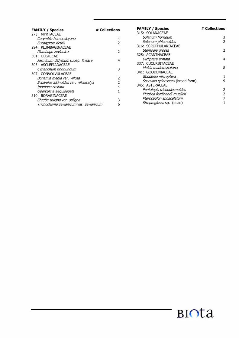
FAMILY / Species # Collections273: MYRTACEAE
Corymbia hamersleyana 4Eucalyptus victrix 2
294: PLUMBAGINACEAEPlumbago zeylanica 2
301: OLEACEAEJasminum didymum subsp. lineare 4
305: ASCLEPIADACEAECynanchum floribundum 3
307: CONVOLVULACEAEBonamia media var. villosa 2Evolvulus alsinoides var. villosicalyx 2Ipomoea costata 4Operculina aequisepala 1
310: BORAGINACEAEEhretia saligna var. saligna 3Trichodesma zeylanicum var. zeylanicum 6
FAMILY / Species # Collections315: SOLANACEAE
Solanum horridum 3Solanum phlomoides 2
316: SCROPHULARIACEAEStemodia grossa 2
325: ACANTHACEAEDicliptera armata 4
337: CUCURBITACEAEMukia maderaspatana 8
341: GOODENIACEAEGoodenia microptera 1Scaevola spinescens (broad form) 9
345: ASTERACEAEPentalepis trichodesmoides 2Pluchea ferdinandi-muelleri 2Pterocaulon sphacelatum 7Streptoglossa sp. (dead) 1
Appendix D
Rare Flora Report Forms


Appendix E
Fauna Recorded Previously from theBurrup Peninsula

Appendix E1: Records of mammals sourced from the Western Australian Museummammal database for the Burrup Peninsula (Latitude: 20°30'0"S to 20°43'0"S,Longitude: 116°36'0"E to 116°55'0"E). Names follow How et al. (2001). Additionalobservations from Butler and Butler (1983) and Butler (1994) are also included(marked with * and # respectively).
Family Genus species Common nameTACHYGLOSSIDAE Tachyglossus aculeatus EchidnaDASYURIDAE Dasykaluta rosamondae Little Red Kaluta
Dasyurus hallucatus Northern Quoll*#Pseudantechinus roryi Rory’s PseudantechinusPlanigale maculata Common PlanigaleNingaui timealyi Pilbara Ningaui
MACROPODIDAE Macropus robustus EuroM. rufus Red Kangaroo#Petrogale rothschildi1 Rothschild’s Rock-wallaby
PTEROPODIDAE Pteropus scapulatus Little Red Flying-fox#EMBALLONURIDAE Taphozous georgianus Common Sheathtail-bat*#VESPERTILIONIDAE Vespadelus finlaysoni2 Finlayson’s Cave BatMURIDAE Pseudomys delicatulus Delicate Mouse
P. hermannsburgensis Sandy Inland MouseZyzomys argurus Common Rock-ratZyzomys argurus Common Rock-ratMus musculus House MouseRattus rattus Black RatR. tunneyi Pale Field-ratHydromys chrysogaster Water-rat*#
CANIDAE Canis familiaris Dog*#Vulpes vulpes Fox*#
FELIDAE Felis catus Cat*#BOVIDAE Ovis aries Sheep
1 Butler (1994) lists Petrogale lateralis.2 As V. pumilis on WAM database.
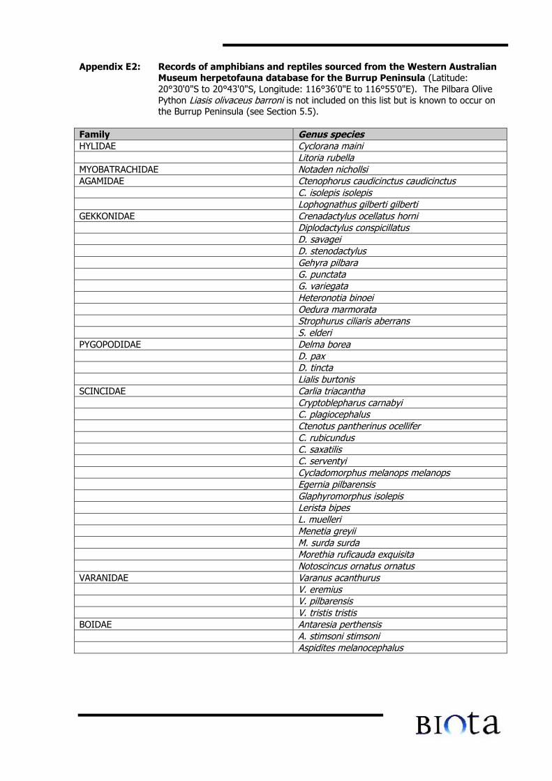
Appendix E2: Records of amphibians and reptiles sourced from the Western AustralianMuseum herpetofauna database for the Burrup Peninsula (Latitude:20°30'0"S to 20°43'0"S, Longitude: 116°36'0"E to 116°55'0"E). The Pilbara OlivePython Liasis olivaceus barroni is not included on this list but is known to occur onthe Burrup Peninsula (see Section 5.5).
Family Genus speciesHYLIDAE Cyclorana maini
Litoria rubellaMYOBATRACHIDAE Notaden nichollsiAGAMIDAE Ctenophorus caudicinctus caudicinctus
C. isolepis isolepisLophognathus gilberti gilberti
GEKKONIDAE Crenadactylus ocellatus horniDiplodactylus conspicillatusD. savageiD. stenodactylusGehyra pilbaraG. punctataG. variegataHeteronotia binoeiOedura marmorataStrophurus ciliaris aberransS. elderi
PYGOPODIDAE Delma boreaD. paxD. tinctaLialis burtonis
SCINCIDAE Carlia triacanthaCryptoblepharus carnabyiC. plagiocephalusCtenotus pantherinus ocelliferC. rubicundusC. saxatilisC. serventyiCycladomorphus melanops melanopsEgernia pilbarensisGlaphyromorphus isolepisLerista bipesL. muelleriMenetia greyiiM. surda surdaMorethia ruficauda exquisitaNotoscincus ornatus ornatus
VARANIDAE Varanus acanthurusV. eremiusV. pilbarensisV. tristis tristis
BOIDAE Antaresia perthensisA. stimsoni stimsoniAspidites melanocephalus
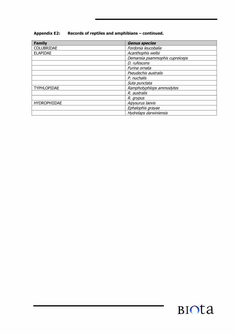
Appendix E2: Records of reptiles and amphibians – continued.
Family Genus speciesCOLUBRIDAE Fordonia leucobaliaELAPIDAE Acanthophis wellsi
Demansia psammophis cupreicepsD. rufescensFurina ornataPseudechis australisP. nuchalisSuta punctata
TYPHLOPIDAE Ramphotyphlops ammodytesR. australisR. grypus
HYDROPHIIDAE Aipysurus laevisEphalophis grayaeHydrelaps darwiniensis
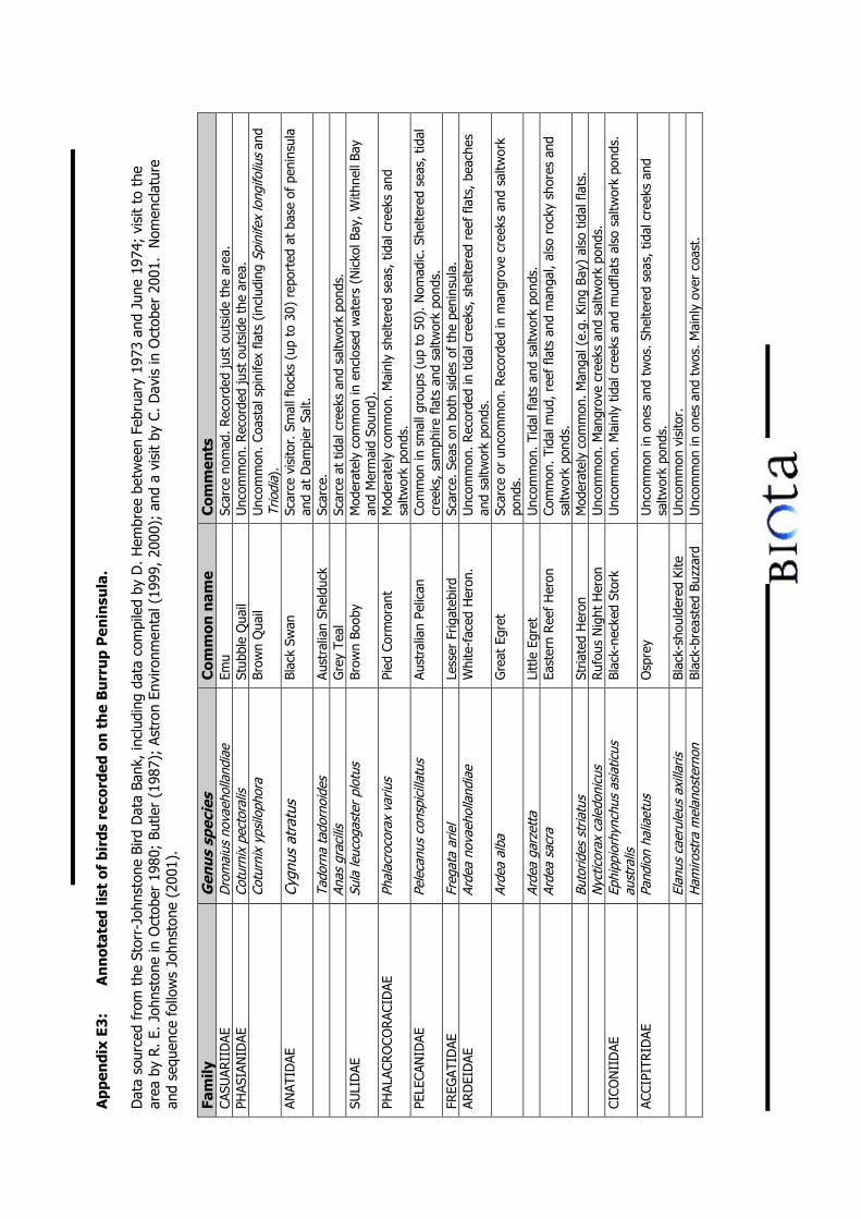
App
endi
x E3
:A
nn
otat
ed li
st o
f bi
rds
reco
rded
on
th
e B
urr
up
Pen
insu
la.
Dat
a so
urce
d fr
om t
he S
torr
-Joh
nsto
ne B
ird D
ata
Bank
, inc
ludi
ng d
ata
com
pile
d by
D. H
embr
ee b
etw
een
Febr
uary
197
3 an
d Ju
ne 1
974;
vis
it to
the
area
by
R. E
. Joh
nsto
ne in
Oct
ober
198
0; B
utle
r (1
987)
; As
tron
Env
ironm
enta
l (19
99, 2
000)
; an
d a
visi
t by
C. D
avis
in O
ctob
er 2
001.
N
omen
clat
ure
and
sequ
ence
fol
low
s Jo
hnst
one
(200
1).
Fam
ilyG
enus
spe
cies
Com
mon
nam
eC
omm
ents
CASU
ARII
DAE
Dro
mai
us n
ovae
holla
ndia
eEm
uSc
arce
nom
ad. R
ecor
ded
just
out
side
the
are
a.PH
ASIA
NID
AECo
turn
ix p
ecto
ralis
Stub
ble
Qua
ilU
ncom
mon
. Rec
orde
d ju
st o
utsi
de t
he a
rea.
Cotu
rnix
yps
iloph
ora
Brow
n Q
uail
Unc
omm
on. C
oast
al s
pini
fex
flats
(in
clud
ing
Spin
ifex
long
ifoliu
s an
dTr
iodi
a).
ANAT
IDAE
Cygn
us a
trat
usBl
ack
Swan
Scar
ce v
isito
r. S
mal
l flo
cks
(up
to 3
0) r
epor
ted
at b
ase
of p
enin
sula
and
at D
ampi
er S
alt.
Tado
rna
tado
rnoi
des
Aust
ralia
n Sh
eldu
ckSc
arce
.An
as g
raci
lisG
rey
Teal
Scar
ce a
t tid
al c
reek
s an
d sa
ltwor
k po
nds.
SULI
DAE
Sula
leuc
ogas
ter
plot
usBr
own
Boob
yM
oder
atel
y co
mm
on in
enc
lose
d w
ater
s (N
icko
l Bay
, W
ithne
ll Ba
yan
d M
erm
aid
Soun
d).
PHAL
ACR
OCO
RAC
IDAE
Phal
acro
cora
x va
rius
Pied
Cor
mor
ant
Mod
erat
ely
com
mon
. Mai
nly
shel
tere
d se
as, t
idal
cre
eks
and
saltw
ork
pond
s.PE
LECA
NID
AEPe
leca
nus
cons
pici
llatu
sAu
stra
lian
Pelic
anCo
mm
on in
sm
all g
roup
s (u
p to
50)
. Nom
adic
. She
ltere
d se
as, t
idal
cree
ks,
sam
phire
fla
ts a
nd s
altw
ork
pond
s.FR
EGAT
IDAE
Freg
ata
arie
lLe
sser
Frig
ateb
irdSc
arce
. Sea
s on
bot
h si
des
of t
he p
enin
sula
.AR
DEI
DAE
Arde
a no
vaeh
olla
ndia
eW
hite
-fac
ed H
eron
.U
ncom
mon
. Rec
orde
d in
tid
al c
reek
s, s
helte
red
reef
fla
ts,
beac
hes
and
saltw
ork
pond
s.Ar
dea
alba
Gre
at E
gret
Scar
ce o
r un
com
mon
. Rec
orde
d in
man
grov
e cr
eeks
and
sal
twor
kpo
nds.
Arde
a ga
rzet
taLi
ttle
Egr
etU
ncom
mon
. Tid
al f
lats
and
sal
twor
k po
nds.
Arde
a sa
cra
East
ern
Ree
f H
eron
Com
mon
. Tid
al m
ud, r
eef
flats
and
man
gal,
also
roc
ky s
hore
s an
dsa
ltwor
k po
nds.
Buto
rides
str
iatu
sSt
riate
d H
eron
Mod
erat
ely
com
mon
. Man
gal (
e.g.
Kin
g Ba
y) a
lso
tidal
fla
ts.
Nyc
ticor
ax c
aled
onic
usRuf
ous
Nig
ht H
eron
Unc
omm
on. M
angr
ove
cree
ks a
nd s
altw
ork
pond
s.CI
CON
IID
AEEp
hipp
iorh
ynch
us a
siat
icus
aust
ralis
Blac
k-ne
cked
Sto
rkU
ncom
mon
. Mai
nly
tidal
cre
eks
and
mud
flats
als
o sa
ltwor
k po
nds.
ACCI
PITR
IDAE
Pand
ion
halia
etus
Osp
rey
Unc
omm
on in
one
s an
d tw
os. S
helte
red
seas
, tid
al c
reek
s an
dsa
ltwor
k po
nds.
Elan
us c
aeru
leus
axi
llaris
Blac
k-sh
ould
ered
Kite
Unc
omm
on v
isito
r.H
amiro
stra
mel
anos
tern
onBl
ack-
brea
sted
Buz
zard
Unc
omm
on in
one
s an
d tw
os. M
ainl
y ov
er c
oast
.
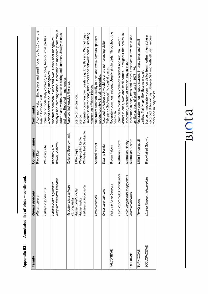
App
endi
x E3
:A
nn
otat
ed li
st o
f bi
rds
– co
nti
nu
ed.
Fam
ilyG
enus
spe
cies
Com
mon
nam
eC
omm
ents
Milv
us m
igra
nsBl
ack
Kite
Unc
omm
on v
isito
r. S
ingl
e bi
rds
and
smal
l flo
cks
(up
to 1
0) o
ver
the
area
in O
ctob
er 1
980.
Hal
iast
ur s
phen
urus
Whi
stlin
g Ki
teCo
mm
on o
r m
oder
atel
y co
mm
on, i
n on
es, t
wos
or
smal
l par
ties.
Woo
ded
habi
tats
incl
udin
g m
angr
oves
.H
alia
stur
indu
s gi
rren
era
Brah
min
y Ki
teM
oder
atel
y co
mm
on in
one
s an
d tw
os. M
ainl
y ne
ar m
angr
oves
.Ac
cipi
ter
fasc
iatu
s fa
scia
tus
Brow
n G
osha
wk
Mai
nly
a no
n-br
eedi
ng v
isito
r. U
ncom
mon
to
mod
erat
ely
com
mon
inau
tum
n an
d w
inte
r, s
carc
e in
spr
ing
and
sum
mer
. Usu
ally
in o
nes
and
twos
. Rep
orte
d in
man
grov
es.
Acci
pite
r ci
rroc
epha
lus
cirr
ocep
halu
sCo
llare
d Sp
arro
wha
wk
Rep
orte
d ju
st o
utsi
de t
he a
rea.
Aqui
la m
orph
noid
esLi
ttle
Eag
leSc
arce
or
unco
mm
on.
Aqui
la a
udax
Wed
ge-t
aile
d Ea
gle
Scar
ce.
Hal
iaee
tus
leuc
ogas
ter
Whi
te-b
ellie
d Se
a-Ea
gle
Mod
erat
ely
com
mon
ove
r co
asts
(e.
g. K
ing
Bay
and
With
nell
Bay)
.Fa
vour
s sh
elte
red
seas
, tid
al c
reek
s an
d sa
ltwor
k po
nds.
Bre
edin
gre
port
ed o
n of
fsho
re is
land
s.Ci
rcus
ass
imili
sSp
otte
d H
arrie
rM
oder
atel
y co
mm
on u
sual
ly in
one
s an
d tw
os. F
avou
rs s
pars
ely
woo
ded
coun
try.
Bre
edin
g re
cord
ed.
Circ
us a
ppro
xim
ans
Swam
p H
arrie
rR
ecor
ded
by A
stro
n bu
t w
ould
be
a ra
re n
on-b
reed
ing
visi
tor
(Feb
ruar
y -
Sept
embe
r) t
o co
asta
l pla
ins.
FALC
ON
IDAE
Falc
o be
rigor
a be
rigor
aBr
own
Falc
onM
oder
atel
y co
mm
on r
esid
ent.
Usu
ally
sin
gle
bird
s. T
hrou
ghou
t th
epe
nins
ula.
Falc
o ce
nchr
oide
s ce
nchr
oide
sAu
stra
lian
Kest
rel
Com
mon
to
mod
erat
ely
com
mon
res
iden
t an
d au
tum
n -
win
ter
visi
tor;
in o
nes,
tw
os a
nd s
mal
l par
ties.
Thr
ough
out
the
peni
nsul
a.Fa
lco
long
ipen
nis
long
ipen
nis
Aust
ralia
n H
obby
Unc
omm
on, r
ecor
ded
at W
ithne
ll Ba
y in
198
7.O
TID
IDAE
Arde
otis
aus
tral
isAu
stra
lian
Bust
ard
Unc
omm
on in
one
s, t
wos
and
thr
ees.
Obs
erve
d in
low
scr
ub a
ndsp
inife
x at
bas
e of
pen
insu
la in
197
3 -
74.
TUR
NIC
IDAE
Turn
ix v
elox
Litt
le B
utto
n-qu
ail
Mod
erat
ely
com
mon
in g
ood
seas
ons
in o
nes,
tw
os a
nd s
mal
lpa
rtie
s. M
ainl
y sp
inife
x fla
ts n
ear
coas
t.SC
OLO
PACI
DAE
Lim
osa
limos
a m
elan
uroi
des
Blac
k-ta
iled
God
wit
Scar
ce t
o m
oder
atel
y co
mm
on v
isito
r fr
om n
orth
ern
hem
isph
ere.
Rec
orde
d at
Nic
kol B
ay, D
ampi
er S
alt
and
With
nell
Bay.
Fav
ours
rock
y an
d m
uddy
coa
sts.
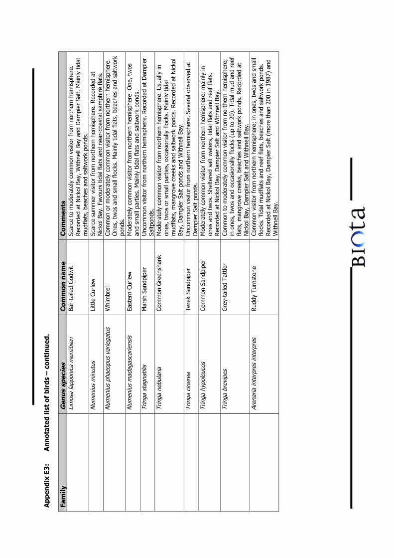
App
endi
x E3
:A
nn
otat
ed li
st o
f bi
rds
– co
nti
nu
ed.
Fam
ilyG
enus
spe
cies
Com
mon
nam
eC
omm
ents
Lim
osa
lapp
onic
a m
enzb
ieri
Bar-
taile
d G
odw
itSc
arce
to
mod
erat
ely
com
mon
vis
itor
from
nor
ther
n he
mis
pher
e.R
ecor
ded
at N
icko
l Bay
, With
nell
Bay
and
Dam
pier
Sal
t. M
ainl
y tid
alm
udfla
ts,
beac
hes
and
saltw
ork
pond
s.N
umen
ius
min
utus
Litt
le C
urle
wSc
arce
sum
mer
vis
itor
from
nor
ther
n he
mis
pher
e. R
ecor
ded
atN
icko
l Bay
. Fa
vour
s tid
al f
lats
and
nea
r-co
asta
l sam
phire
fla
ts.
Num
eniu
s ph
aeop
us v
arie
gatu
sW
him
brel
Com
mon
or
mod
erat
ely
com
mon
vis
itor
from
nor
ther
n he
mis
pher
e.O
nes,
tw
os a
nd s
mal
l flo
cks.
Mai
nly
tidal
fla
ts,
beac
hes
and
saltw
ork
pond
s.N
umen
ius
mad
agas
carie
nsis
East
ern
Curle
wM
oder
atel
y co
mm
on v
isito
r fr
om n
orth
ern
hem
isph
ere.
One
, tw
osan
d sm
all p
artie
s. M
ainl
y tid
al f
lats
and
sal
twor
k po
nds.
Trin
ga s
tagn
atili
sM
arsh
San
dpip
erU
ncom
mon
vis
itor
from
nor
ther
n he
mis
pher
e. R
ecor
ded
at D
ampi
erSa
ltpon
ds.
Trin
ga n
ebul
aria
Com
mon
Gre
ensh
ank
Mod
erat
ely
com
mon
vis
itor
from
nor
ther
n he
mis
pher
e. U
sual
ly in
ones
, tw
os o
r sm
all p
artie
s, o
ccas
iona
lly f
lock
s. M
ainl
y tid
alm
udfla
ts, m
angr
ove
cree
ks a
nd s
altw
ork
pond
s. R
ecor
ded
at N
icko
lBa
y, D
ampi
er S
alt
pond
s an
d W
ithne
ll Ba
y.Tr
inga
cin
erea
Tere
k Sa
ndpi
per
Unc
omm
on v
isito
r fr
om n
orth
ern
hem
isph
ere.
Sev
eral
obs
erve
d at
Dam
pier
Sal
t po
nds.
Trin
ga h
ypol
euco
sCo
mm
on S
andp
iper
Mod
erat
ely
com
mon
vis
itor
from
nor
ther
n he
mis
pher
e; m
ainl
y in
ones
and
tw
os. S
helte
red
salt
wat
ers,
tid
al f
lats
and
ree
f fla
ts.
Rec
orde
d at
Nic
kol B
ay, D
ampi
er S
alt
and
With
nell
Bay.
Trin
ga b
revi
pes
Gre
y-ta
iled
Tatt
ler
Com
mon
to
mod
erat
ely
com
mon
vis
itor
from
nor
ther
n he
mis
pher
e;in
one
s, t
wos
and
occ
asio
nally
flo
cks
(up
to 2
0). T
idal
mud
and
ree
ffla
ts, m
angr
ove
cree
ks,
beac
hes
and
saltw
ork
pond
s. R
ecor
ded
atN
icko
l Bay
, D
ampi
er S
alt
and
With
nell
Bay.
Aren
aria
inte
rpre
s in
terp
res
Rud
dy T
urns
tone
Com
mon
vis
itor
from
nor
ther
n he
mis
pher
e; in
one
s, t
wos
and
sm
all
flock
s. T
idal
mud
flats
and
ree
f fla
ts, b
each
es a
nd s
altw
ork
pond
s.R
ecor
ded
at N
icko
l Bay
, Dam
pier
Sal
t (m
ore
than
200
in 1
987)
and
With
nell
Bay.
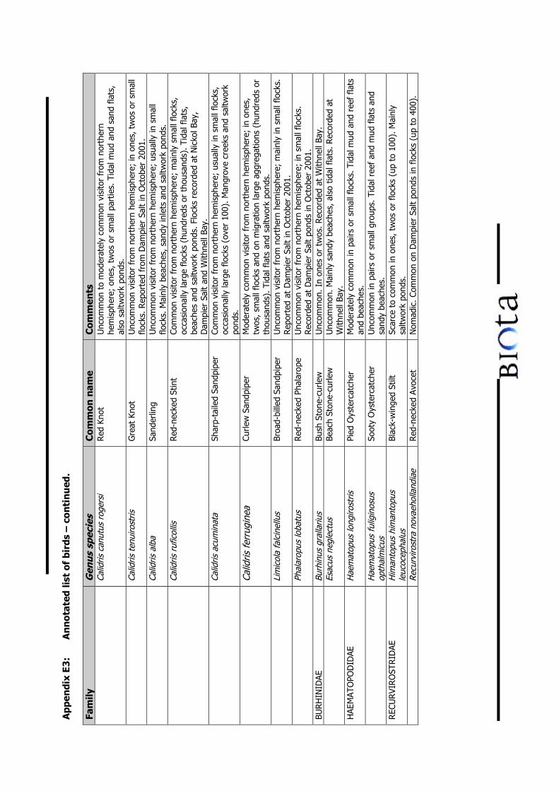
App
endi
x E3
:A
nn
otat
ed li
st o
f bi
rds
– co
nti
nu
ed.
Fam
ilyG
enus
spe
cies
Com
mon
nam
eC
omm
ents
Calid
ris c
anut
us r
oger
siR
ed K
not
Unc
omm
on t
o m
oder
atel
y co
mm
on v
isito
r fr
om n
orth
ern
hem
isph
ere;
one
s, t
wos
or
smal
l par
ties.
Tid
al m
ud a
nd s
and
flats
,al
so s
altw
ork
pond
s.Ca
lidris
ten
uiro
stris
Gre
at K
not
Unc
omm
on v
isito
r fr
om n
orth
ern
hem
isph
ere;
in o
nes,
tw
os o
r sm
all
flock
s. R
epor
ted
from
Dam
pier
Sal
t in
Oct
ober
200
1.Ca
lidris
alb
aSa
nder
ling
Unc
omm
on v
isito
r fr
om n
orth
ern
hem
isph
ere;
usu
ally
in s
mal
lflo
cks.
Mai
nly
beac
hes,
san
dy in
lets
and
sal
twor
k po
nds.
Calid
ris r
ufic
ollis
Red
-nec
ked
Stin
tCo
mm
on v
isito
r fr
om n
orth
ern
hem
isph
ere;
mai
nly
smal
l flo
cks,
occa
sion
ally
larg
e flo
cks
(hun
dred
s or
tho
usan
ds).
Tid
al f
lats
,be
ache
s an
d sa
ltwor
k po
nds.
Flo
cks
reco
rded
at
Nic
kol B
ay,
Dam
pier
Sal
t an
d W
ithne
ll Ba
y.Ca
lidris
acu
min
ata
Shar
p-ta
iled
Sand
pipe
rCo
mm
on v
isito
r fr
om n
orth
ern
hem
isph
ere;
usu
ally
in s
mal
l flo
cks,
occa
sion
ally
larg
e flo
cks
(ove
r 10
0). M
angr
ove
cree
ks a
nd s
altw
ork
pond
s.Ca
lidris
ferr
ugin
eaCu
rlew
San
dpip
erM
oder
atel
y co
mm
on v
isito
r fr
om n
orth
ern
hem
isph
ere;
in o
nes,
twos
, sm
all f
lock
s an
d on
mig
ratio
n la
rge
aggr
egat
ions
(hu
ndre
ds o
rth
ousa
nds)
. Tid
al f
lats
and
sal
twor
k po
nds.
Lim
icol
a fa
lcin
ellu
sBr
oad-
bille
d Sa
ndpi
per
Unc
omm
on v
isito
r fr
om n
orth
ern
hem
isph
ere;
mai
nly
in s
mal
l flo
cks.
Rep
orte
d at
Dam
pier
Sal
t in
Oct
ober
200
1.Ph
alar
opus
loba
tus
Red
-nec
ked
Phal
arop
eU
ncom
mon
vis
itor
from
nor
ther
n he
mis
pher
e; in
sm
all f
lock
s.R
ecor
ded
at D
ampi
er S
alt
pond
s in
Oct
ober
200
1.BU
RH
INID
AEBu
rhin
us g
ralla
rius
Bush
Sto
ne-c
urle
wU
ncom
mon
. In
ones
or
twos
. Rec
orde
d at
With
nell
Bay.
Esac
us n
egle
ctus
Beac
h St
one-
curle
wU
ncom
mon
. Mai
nly
sand
y be
ache
s, a
lso
tidal
fla
ts. R
ecor
ded
atW
ithne
ll Ba
y.H
AEM
ATO
POD
IDAE
Hae
mat
opus
long
irost
risPi
ed O
yste
rcat
cher
Mod
erat
ely
com
mon
in p
airs
or
smal
l flo
cks.
Tid
al m
ud a
nd r
eef
flats
and
beac
hes.
Hae
mat
opus
fulig
inos
usop
thal
mic
usSo
oty
Oys
terc
atch
erU
ncom
mon
in p
airs
or
smal
l gro
ups.
Tid
al r
eef
and
mud
fla
ts a
ndsa
ndy
beac
hes.
REC
UR
VIR
OST
RID
AEH
iman
topu
s hi
man
topu
sle
ucoc
epha
lus
Blac
k-w
inge
d St
iltSc
arce
to
com
mon
in o
nes,
tw
os o
r flo
cks
(up
to 1
00).
Mai
nly
saltw
ork
pond
s.Re
curv
irost
ra n
ovae
holla
ndia
eR
ed-n
ecke
d Av
ocet
Nom
adic
. Com
mon
on
Dam
pier
Sal
t po
nds
in f
lock
s (u
p to
400
).
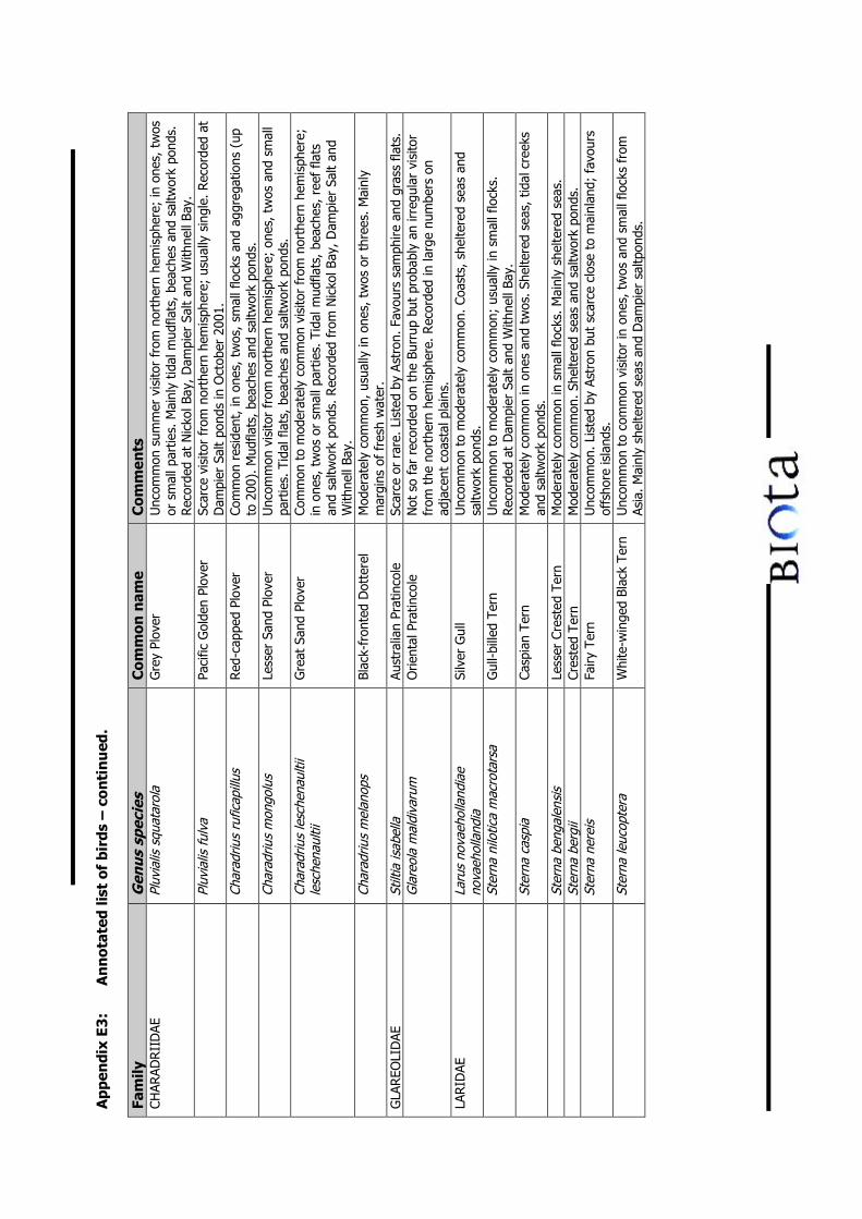
App
endi
x E3
:A
nn
otat
ed li
st o
f bi
rds
– co
nti
nu
ed.
Fam
ilyG
enus
spe
cies
Com
mon
nam
eC
omm
ents
CHAR
ADR
IID
AEPl
uvia
lis s
quat
arol
aG
rey
Plov
erU
ncom
mon
sum
mer
vis
itor
from
nor
ther
n he
mis
pher
e; in
one
s, t
wos
or s
mal
l par
ties.
Mai
nly
tidal
mud
flats
, bea
ches
and
sal
twor
k po
nds.
Rec
orde
d at
Nic
kol B
ay, D
ampi
er S
alt
and
With
nell
Bay.
Pluv
ialis
fulv
aPa
cific
Gol
den
Plov
erSc
arce
vis
itor
from
nor
ther
n he
mis
pher
e; u
sual
ly s
ingl
e. R
ecor
ded
atD
ampi
er S
alt
pond
s in
Oct
ober
200
1.Ch
arad
rius
rufic
apill
usR
ed-c
appe
d Pl
over
Com
mon
res
iden
t, in
one
s, t
wos
, sm
all f
lock
s an
d ag
greg
atio
ns (
upto
200
). M
udfla
ts,
beac
hes
and
saltw
ork
pond
s.Ch
arad
rius
mon
golu
sLe
sser
San
d Pl
over
Unc
omm
on v
isito
r fr
om n
orth
ern
hem
isph
ere;
one
s, t
wos
and
sm
all
part
ies.
Tid
al f
lats
, be
ache
s an
d sa
ltwor
k po
nds.
Char
adriu
s le
sche
naul
tiile
sche
naul
tiiG
reat
San
d Pl
over
Com
mon
to
mod
erat
ely
com
mon
vis
itor
from
nor
ther
n he
mis
pher
e;in
one
s, t
wos
or
smal
l par
ties.
Tid
al m
udfla
ts,
beac
hes,
ree
f fla
tsan
d sa
ltwor
k po
nds.
Rec
orde
d fr
om N
icko
l Bay
, Dam
pier
Sal
t an
dW
ithne
ll Ba
y.Ch
arad
rius
mel
anop
sBl
ack-
fron
ted
Dot
tere
lM
oder
atel
y co
mm
on, u
sual
ly in
one
s, t
wos
or
thre
es. M
ainl
ym
argi
ns o
f fr
esh
wat
er.
GLA
REO
LID
AESt
iltia
isab
ella
Aust
ralia
n Pr
atin
cole
Scar
ce o
r ra
re.
List
ed b
y As
tron
. Fav
ours
sam
phire
and
gra
ss f
lats
.G
lare
ola
mal
diva
rum
Orie
ntal
Pra
tinco
leN
ot s
o fa
r re
cord
ed o
n th
e Bu
rrup
but
pro
babl
y an
irre
gula
r vi
sito
rfr
om t
he n
orth
ern
hem
isph
ere.
Rec
orde
d in
larg
e nu
mbe
rs o
nad
jace
nt c
oast
al p
lain
s.LA
RID
AELa
rus
nova
ehol
land
iae
nova
ehol
land
iaSi
lver
Gul
lU
ncom
mon
to
mod
erat
ely
com
mon
. Coa
sts,
she
ltere
d se
as a
ndsa
ltwor
k po
nds.
Ster
na n
ilotic
a m
acro
tars
aG
ull-b
illed
Ter
nU
ncom
mon
to
mod
erat
ely
com
mon
; us
ually
in s
mal
l flo
cks.
Rec
orde
d at
Dam
pier
Sal
t an
d W
ithne
ll Ba
y.St
erna
cas
pia
Casp
ian
Tern
Mod
erat
ely
com
mon
in o
nes
and
twos
. She
ltere
d se
as, t
idal
cre
eks
and
saltw
ork
pond
s.St
erna
ben
gale
nsis
Less
er C
rest
ed T
ern
Mod
erat
ely
com
mon
in s
mal
l flo
cks.
Mai
nly
shel
tere
d se
as.
Ster
na b
ergi
iCr
este
d Te
rnM
oder
atel
y co
mm
on. S
helte
red
seas
and
sal
twor
k po
nds.
Ster
na n
erei
sFa
iry T
ern
Unc
omm
on. L
iste
d by
Ast
ron
but
scar
ce c
lose
to
mai
nlan
d; f
avou
rsof
fsho
re is
land
s.St
erna
leuc
opte
raW
hite
-win
ged
Blac
k Te
rnU
ncom
mon
to
com
mon
vis
itor
in o
nes,
tw
os a
nd s
mal
l flo
cks
from
Asia
. Mai
nly
shel
tere
d se
as a
nd D
ampi
er s
altp
onds
.
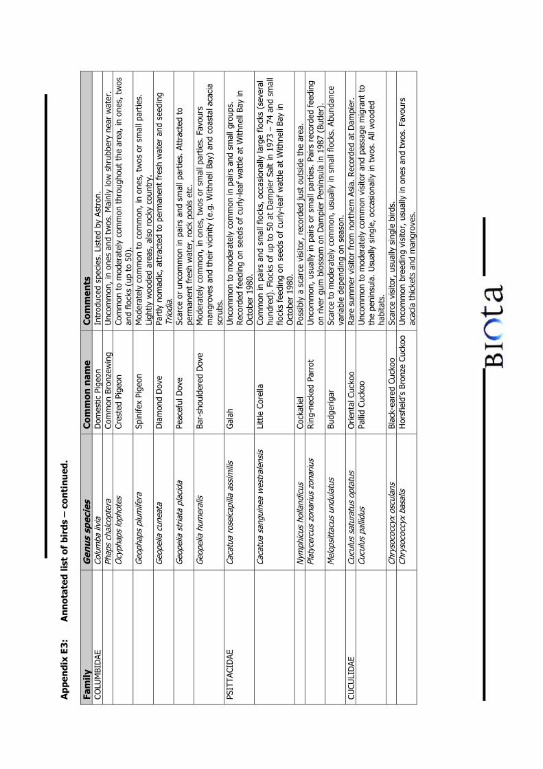
App
endi
x E3
:A
nn
otat
ed li
st o
f bi
rds
– co
nti
nu
ed.
Fam
ilyG
enus
spe
cies
Com
mon
nam
eC
omm
ents
COLU
MBI
DAE
Colu
mba
livi
aD
omes
tic P
igeo
nIn
trod
uced
spe
cies
. Li
sted
by
Astr
on.
Phap
s ch
alco
pter
aCo
mm
on B
ronz
ewin
gU
ncom
mon
, in
ones
and
tw
os. M
ainl
y lo
w s
hrub
bery
nea
r w
ater
.O
cyph
aps
loph
otes
Cres
ted
Pige
onCo
mm
on t
o m
oder
atel
y co
mm
on t
hrou
ghou
t th
e ar
ea, i
n on
es, t
wos
and
flock
s (u
p to
50)
.G
eoph
aps
plum
ifera
Spin
ifex
Pige
onM
oder
atel
y co
mm
on t
o co
mm
on, i
n on
es, t
wos
or
smal
l par
ties.
Ligh
tly w
oode
d ar
eas,
als
o ro
cky
coun
try.
Geo
pelia
cun
eata
Dia
mon
d D
ove
Part
ly n
omad
ic, a
ttra
cted
to
perm
anen
t fr
esh
wat
er a
nd s
eedi
ngTr
iodi
a.G
eope
lia s
tria
ta p
laci
daPe
acef
ul D
ove
Scar
ce o
r un
com
mon
in p
airs
and
sm
all p
artie
s. A
ttra
cted
to
perm
anen
t fr
esh
wat
er, r
ock
pool
s et
c.G
eope
lia h
umer
alis
Bar-
shou
lder
ed D
ove
Mod
erat
ely
com
mon
, in
ones
, tw
os o
r sm
all p
artie
s. F
avou
rsm
angr
oves
and
the
ir vi
cini
ty (
e.g.
With
nell
Bay)
and
coa
stal
aca
cia
scru
bs.
PSIT
TACI
DAE
Caca
tua
rose
icap
illa
assi
mili
sG
alah
Unc
omm
on t
o m
oder
atel
y co
mm
on in
pai
rs a
nd s
mal
l gro
ups.
Rec
orde
d fe
edin
g on
see
ds o
f cu
rly-le
af w
attle
at
With
nell
Bay
inO
ctob
er 1
980.
Caca
tua
sang
uine
a w
estr
alen
sis
Litt
le C
orel
laCo
mm
on in
pai
rs a
nd s
mal
l flo
cks,
occ
asio
nally
larg
e flo
cks
(sev
eral
hund
red)
. Flo
cks
of u
p to
50
at D
ampi
er S
alt
in 1
973
– 74
and
sm
all
flock
s fe
edin
g on
see
ds o
f cu
rly-le
af w
attle
at
With
nell
Bay
inO
ctob
er 1
980.
Nym
phic
us h
olla
ndic
usCo
ckat
iel
Poss
ibly
a s
carc
e vi
sito
r, r
ecor
ded
just
out
side
the
are
a.Pl
atyc
ercu
s zo
nariu
s zo
nariu
sR
ing-
neck
ed P
arro
tU
ncom
mon
, usu
ally
in p
airs
or
smal
l par
ties.
Pai
rs r
ecor
ded
feed
ing
on r
iver
gum
blo
ssom
on
Dam
pier
Pen
insu
la in
198
7 (B
utle
r).
Mel
opsi
ttac
us u
ndul
atus
Budg
erig
arSc
arce
to
mod
erat
ely
com
mon
, usu
ally
in s
mal
l flo
cks.
Abu
ndan
ceva
riabl
e de
pend
ing
on s
easo
n.CU
CULI
DAE
Cucu
lus
satu
ratu
s op
tatu
sO
rient
al C
ucko
oR
are
sum
mer
vis
itor
from
nor
ther
n As
ia. R
ecor
ded
at D
ampi
er.
Cucu
lus
palli
dus
Palli
d Cu
ckoo
Unc
omm
on t
o m
oder
atel
y co
mm
on v
isito
r an
d pa
ssag
e m
igra
nt t
oth
e pe
nins
ula.
Usu
ally
sin
gle,
occ
asio
nally
in t
wos
. All
woo
ded
habi
tats
.Ch
ryso
cocc
yx o
scul
ans
Blac
k-ea
red
Cuck
ooSc
arce
vis
itor,
usu
ally
sin
gle
bird
s.Ch
ryso
cocc
yx b
asal
isH
orsf
ield
’s B
ronz
e Cu
ckoo
Unc
omm
on b
reed
ing
visi
tor,
usu
ally
in o
nes
and
twos
. Fav
ours
acac
ia t
hick
ets
and
man
grov
es.
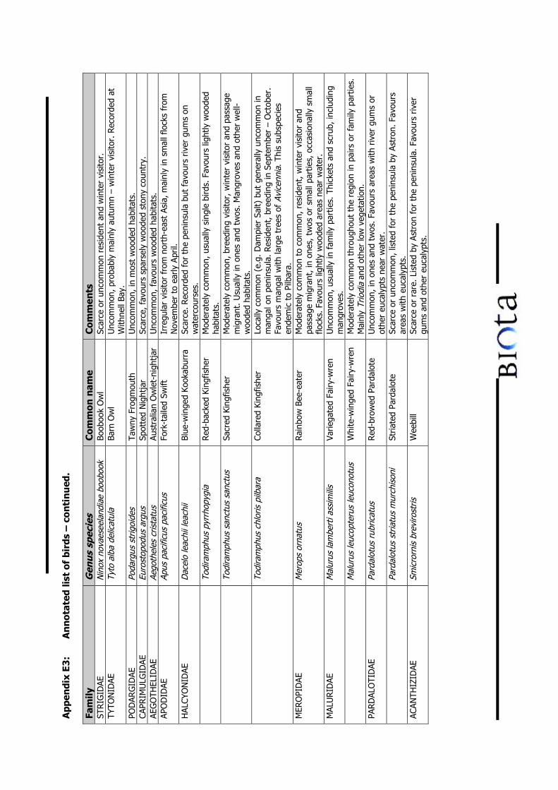
App
endi
x E3
:A
nn
otat
ed li
st o
f bi
rds
– co
nti
nu
ed.
Fam
ilyG
enus
spe
cies
Com
mon
nam
eC
omm
ents
STRIG
IDAE
Nin
ox n
ovae
seel
andi
ae b
oobo
okBo
oboo
k O
wl
Scar
ce o
r un
com
mon
res
iden
t an
d w
inte
r vi
sito
r.TY
TON
IDAE
Tyto
alb
a de
licat
ula
Barn
Ow
lU
ncom
mon
, pro
babl
y m
ainl
y au
tum
n –
win
ter
visi
tor.
Rec
orde
d at
With
nell
Bay.
POD
ARG
IDAE
Poda
rgus
str
igoi
des
Taw
ny F
rogm
outh
Unc
omm
on, i
n m
ost
woo
ded
habi
tats
.CA
PRIM
ULG
IDAE
Euro
stop
odus
arg
usSp
otte
d N
ight
jar
Scar
ce, f
avou
rs s
pars
ely
woo
ded
ston
y co
untr
y.AE
GO
THEL
IDAE
Aego
thel
es c
rista
tus
Aust
ralia
n O
wle
t-ni
ghtja
rU
ncom
mon
, fav
ours
woo
ded
habi
tats
.AP
OD
IDAE
Apus
pac
ificu
s pa
cific
usFo
rk-t
aile
d Sw
iftIr
regu
lar
visi
tor
from
nor
th-e
ast
Asia
, mai
nly
in s
mal
l flo
cks
from
Nov
embe
r to
ear
ly A
pril.
HAL
CYO
NID
AED
acel
o le
achi
i lea
chii
Blue
-win
ged
Kook
abur
raSc
arce
. Rec
orde
d fo
r th
e pe
nins
ula
but
favo
urs
river
gum
s on
wat
erco
urse
s.To
dira
mph
us p
yrrh
opyg
iaRed
-bac
ked
King
fishe
rM
oder
atel
y co
mm
on, u
sual
ly s
ingl
e bi
rds.
Fav
ours
ligh
tly w
oode
dha
bita
ts.
Todi
ram
phus
san
ctus
san
ctus
Sacr
ed K
ingf
ishe
rM
oder
atel
y co
mm
on, b
reed
ing
visi
tor,
win
ter
visi
tor
and
pass
age
mig
rant
. Usu
ally
in o
nes
and
twos
. Man
grov
es a
nd o
ther
wel
l-w
oode
d ha
bita
ts.
Todi
ram
phus
chl
oris
pilb
ara
Colla
red
King
fishe
rLo
cally
com
mon
(e.
g. D
ampi
er S
alt)
but
gen
eral
ly u
ncom
mon
inm
anga
l on
peni
nsul
a. R
esid
ent,
bre
edin
g in
Sep
tem
ber
– O
ctob
er.
Favo
urs
man
gal w
ith la
rge
tree
s of
Avi
cenn
ia. T
his
subs
peci
esen
dem
ic t
o Pi
lbar
a.M
ERO
PID
AEM
erop
s or
natu
sRai
nbow
Bee
-eat
erM
oder
atel
y co
mm
on t
o co
mm
on, r
esid
ent,
win
ter
visi
tor
and
pass
age
mig
rant
, in
ones
, tw
os o
r sm
all p
artie
s, o
ccas
iona
lly s
mal
lflo
cks.
Fav
ours
ligh
tly w
oode
d ar
eas
near
wat
er.
MAL
URID
AEM
alur
us la
mbe
rti a
ssim
ilis
Varie
gate
d Fa
iry-w
ren
Unc
omm
on, u
sual
ly in
fam
ily p
artie
s. T
hick
ets
and
scru
b, in
clud
ing
man
grov
es.
Mal
urus
leuc
opte
rus
leuc
onot
usW
hite
-win
ged
Fairy
-wre
nM
oder
atel
y co
mm
on t
hrou
ghou
t th
e re
gion
in p
airs
or
fam
ily p
artie
s.M
ainl
y Tr
iodi
a an
d ot
her
low
veg
etat
ion.
PAR
DAL
OTI
DAE
Pard
alot
us r
ubric
atus
Red
-bro
wed
Par
dalo
teU
ncom
mon
, in
ones
and
tw
os. F
avou
rs a
reas
with
riv
er g
ums
orot
her
euca
lypt
s ne
ar w
ater
.Pa
rdal
otus
str
iatu
s m
urch
ison
iSt
riate
d Pa
rdal
ote
Scar
ce o
r un
com
mon
, lis
ted
for
the
peni
nsul
a by
Ast
ron.
Fav
ours
area
s w
ith e
ucal
ypts
.AC
ANTH
IZID
AESm
icro
rnis
bre
viro
stris
Wee
bill
Scar
ce o
r ra
re.
List
ed b
y As
tron
for
the
pen
insu
la. F
avou
rs r
iver
gum
s an
d ot
her
euca
lypt
s.
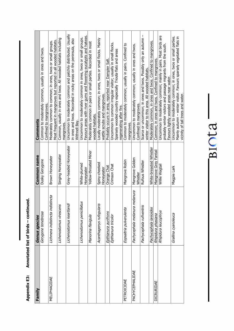
App
endi
x E3
:A
nn
otat
ed li
st o
f bi
rds
– co
nti
nu
ed.
Fam
ilyG
enus
spe
cies
Com
mon
nam
eC
omm
ents
Ger
ygon
e te
nebr
osa
Dus
ky G
eryg
one
Com
mon
to
mod
erat
ely
com
mon
, usu
ally
in o
nes
and
twos
.Co
nfin
ed t
o m
angr
oves
.M
ELIP
HAG
IDAE
Lich
mer
a in
dist
inct
a in
dist
inct
aBr
own
Hon
eyea
ter
Mod
erat
ely
com
mon
to
com
mon
; in
one
s, t
wos
or
smal
l gro
ups.
Mos
t fr
eque
nt in
man
grov
es b
ut r
epor
ted
in a
ll w
oode
d ha
bita
ts.
Lich
enos
tom
us v
iresc
ens
Sing
ing
Hon
eyea
ter
Com
mon
, usu
ally
in o
nes
and
twos
. Al
l woo
ded
habi
tats
incl
udin
gm
angr
oves
.Li
chen
osto
mus
kea
rtla
ndi
Gre
y-he
aded
Hon
eyea
ter
Unc
omm
on t
o m
oder
atel
y co
mm
on a
nd p
atch
ily d
istr
ibut
ed. U
sual
lyin
one
s an
d tw
os. R
ecor
ded
in r
ocky
are
as o
n th
e pe
nins
ula,
als
oW
ithne
ll Ba
y.Li
chen
osto
mus
pen
icill
atus
Whi
te-p
lum
edH
oney
eate
rU
ncom
mon
to
mod
erat
ely
com
mon
in o
nes,
tw
os o
r sm
all g
roup
s.Fa
vour
s ar
eas
with
riv
er g
ums
and
flow
erin
g eu
caly
pts
and
hake
as.
Man
orin
a fla
vigu
laYe
llow
-thr
oate
d M
iner
Mod
erat
ely
com
mon
in p
airs
or
smal
l par
ties.
Rec
orde
d in
mos
tw
oode
d ha
bita
ts.
Acan
thag
enys
ruf
ogul
aris
Spin
y-ch
eeke
dH
oney
eate
rLo
cally
mod
erat
ely
com
mon
; in
one
s, t
wos
or
smal
l flo
cks.
Mai
nly
wat
tle s
crub
s an
d m
angr
oves
.Ep
thia
nura
aur
ifron
sO
rang
e Ch
atPr
obab
ly o
ccur
s in
are
a, r
epor
ted
near
Dam
pier
Sal
t.Ep
thia
nura
tric
olor
Crim
son
Chat
Unc
omm
on t
o co
mm
on ir
regu
lar
visi
tor;
usu
ally
in s
mal
l flo
cks.
Spar
sely
woo
ded
coun
try
espe
cial
ly T
riodi
a fla
ts a
nd a
reas
rege
nera
ting
afte
r fir
e.PE
TRO
ICID
AEEo
psal
tria
pul
veru
lent
aM
angr
ove
Rob
inCo
mm
on t
o m
oder
atel
y co
mm
on;
usua
lly in
pai
rs. C
onfin
ed t
om
angr
oves
.PA
CHYC
EPH
ALID
AEPa
chyc
epha
la m
elan
ura
mel
anur
aM
angr
ove
Gol
den
Whi
stle
rU
ncom
mon
to
mod
erat
ely
com
mon
; us
ually
in o
nes
and
twos
.Co
nfin
ed t
o m
angr
oves
.Pa
chyc
epha
la r
ufiv
entr
isRuf
ous
Whi
stle
rSc
arce
or
unco
mm
on;
in o
nes
and
twos
. Pos
sibl
y on
ly a
n au
tum
n –
win
ter
visi
tor
to t
his
area
. All
woo
ded
habi
tats
.Pa
chyc
epha
la la
nioi
des
Whi
te-b
reas
ted
Whi
stle
rM
oder
atel
y co
mm
on, i
n on
es a
nd t
wos
. Con
fined
to
man
grov
es.
DIC
RU
RID
AERh
ipid
ura
phas
iana
Man
grov
e G
rey
Fant
ail
Com
mon
; in
one
s an
d tw
os. C
onfin
ed t
o m
angr
oves
.Rh
ipid
ura
leuc
ophr
ysW
illie
Wag
tail
Unc
omm
on t
o m
oder
atel
y co
mm
on;
mai
nly
in p
airs
. Mos
t bi
rds
are
prob
ably
win
ter
visi
tors
and
pas
sage
mig
rant
s fr
om t
he s
outh
.Fa
vour
s lig
htly
woo
ded
area
s ne
ar w
ater
.G
ralli
na c
yano
leuc
aM
agpi
e La
rkU
ncom
mon
to
mod
erat
ely
com
mon
; in
one
s, t
wos
or
smal
l par
ties.
Mai
nly
autu
mn
– w
inte
r vi
sito
r. F
avou
rs s
pars
ely
vege
tate
d fla
ts in
vici
nity
of ta
ll tr
ees
and
wat
er.
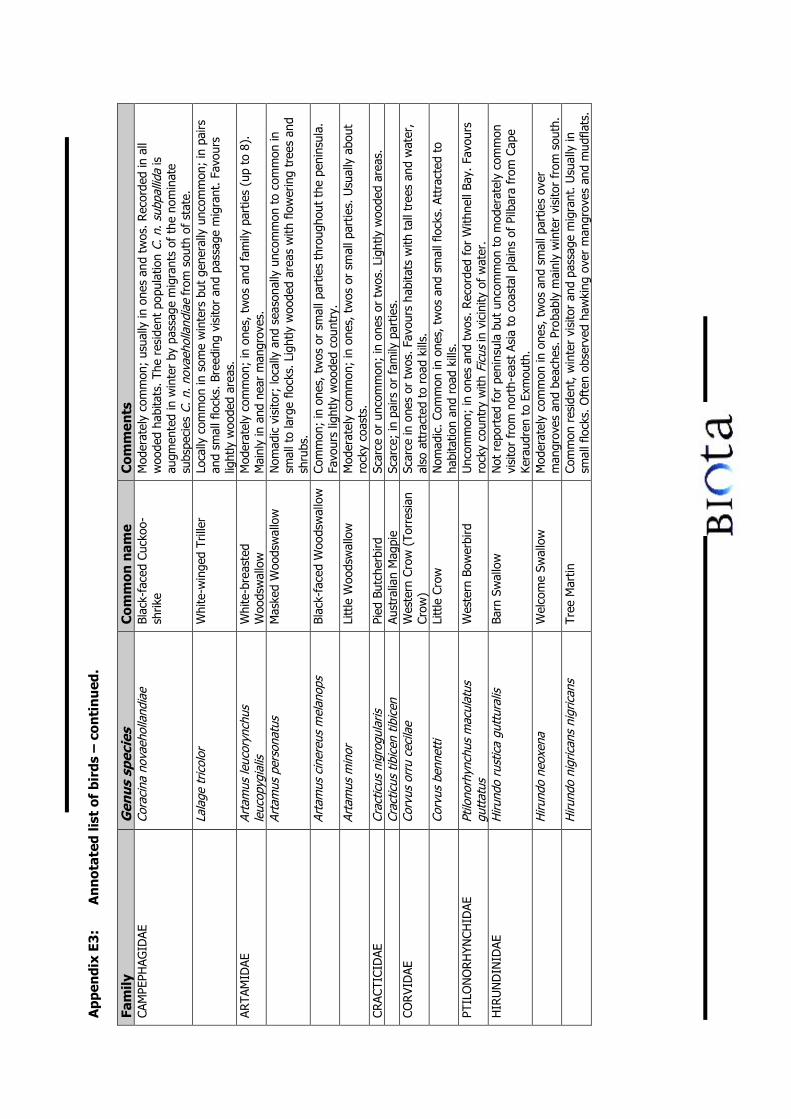
App
endi
x E3
:A
nn
otat
ed li
st o
f bi
rds
– co
nti
nu
ed.
Fam
ilyG
enus
spe
cies
Com
mon
nam
eC
omm
ents
CAM
PEPH
AGID
AECo
raci
na n
ovae
holla
ndia
eBl
ack-
face
d Cu
ckoo
-sh
rike
Mod
erat
ely
com
mon
; us
ually
in o
nes
and
twos
. Rec
orde
d in
all
woo
ded
habi
tats
. The
res
iden
t po
pula
tion
C. n
. sub
palli
da is
augm
ente
d in
win
ter
by p
assa
ge m
igra
nts
of t
he n
omin
ate
subs
peci
es C
. n. n
ovae
holla
ndia
e fr
om s
outh
of
stat
e.La
lage
tric
olor
Whi
te-w
inge
d Tr
iller
Loca
lly c
omm
on in
som
e w
inte
rs b
ut g
ener
ally
unc
omm
on;
in p
airs
and
smal
l flo
cks.
Bre
edin
g vi
sito
r an
d pa
ssag
e m
igra
nt.
Favo
urs
light
ly w
oode
d ar
eas.
ARTA
MID
AEAr
tam
us le
ucor
ynch
usle
ucop
ygia
lisW
hite
-bre
aste
dW
oods
wal
low
Mod
erat
ely
com
mon
; in
one
s, t
wos
and
fam
ily p
artie
s (u
p to
8).
Mai
nly
in a
nd n
ear
man
grov
es.
Arta
mus
per
sona
tus
Mas
ked
Woo
dsw
allo
wN
omad
ic v
isito
r; lo
cally
and
sea
sona
lly u
ncom
mon
to
com
mon
insm
all t
o la
rge
flock
s. L
ight
ly w
oode
d ar
eas
with
flo
wer
ing
tree
s an
dsh
rubs
.Ar
tam
us c
iner
eus
mel
anop
sBl
ack-
face
d W
oods
wal
low
Com
mon
; in
one
s, t
wos
or
smal
l par
ties
thro
ugho
ut t
he p
enin
sula
.Fa
vour
s lig
htly
woo
ded
coun
try.
Arta
mus
min
orLi
ttle
Woo
dsw
allo
wM
oder
atel
y co
mm
on;
in o
nes,
tw
os o
r sm
all p
artie
s. U
sual
ly a
bout
rock
y co
asts
.CR
ACTI
CID
AECr
actic
us n
igro
gula
risPi
ed B
utch
erbi
rdSc
arce
or
unco
mm
on;
in o
nes
or t
wos
. Lig
htly
woo
ded
area
s.Cr
actic
us ti
bice
n tib
icen
Aust
ralia
n M
agpi
eSc
arce
; in
pai
rs o
r fa
mily
par
ties.
COR
VID
AECo
rvus
orr
u ce
cila
eW
este
rn C
row
(To
rres
ian
Crow
)Sc
arce
in o
nes
or t
wos
. Fav
ours
hab
itats
with
tal
l tre
es a
nd w
ater
,al
so a
ttra
cted
to
road
kill
s.Co
rvus
ben
nett
iLi
ttle
Cro
wN
omad
ic. C
omm
on in
one
s, t
wos
and
sm
all f
lock
s. A
ttra
cted
to
habi
tatio
n an
d ro
ad k
ills.
PTIL
ON
OR
HYN
CHID
AEPt
ilono
rhyn
chus
mac
ulat
usgu
ttat
usW
este
rn B
ower
bird
Unc
omm
on;
in o
nes
and
twos
. Rec
orde
d fo
r W
ithne
ll Ba
y. F
avou
rsro
cky
coun
try
with
Fic
us in
vic
inity
of
wat
er.
HIR
UN
DIN
IDAE
Hiru
ndo
rust
ica
gutt
ural
isBa
rn S
wal
low
Not
rep
orte
d fo
r pe
nins
ula
but
unco
mm
on t
o m
oder
atel
y co
mm
onvi
sito
r fr
om n
orth
-eas
t As
ia t
o co
asta
l pla
ins
of P
ilbar
a fr
om C
ape
Kera
udre
n to
Exm
outh
.H
irund
o ne
oxen
aW
elco
me
Swal
low
Mod
erat
ely
com
mon
in o
nes,
tw
os a
nd s
mal
l par
ties
over
man
grov
es a
nd b
each
es. P
roba
bly
mai
nly
win
ter
visi
tor
from
sou
th.
Hiru
ndo
nigr
ican
s ni
gric
ans
Tree
Mar
tinCo
mm
on r
esid
ent,
win
ter
visi
tor
and
pass
age
mig
rant
. Usu
ally
insm
all f
lock
s. O
ften
obs
erve
d ha
wki
ng o
ver
man
grov
es a
nd m
udfla
ts.
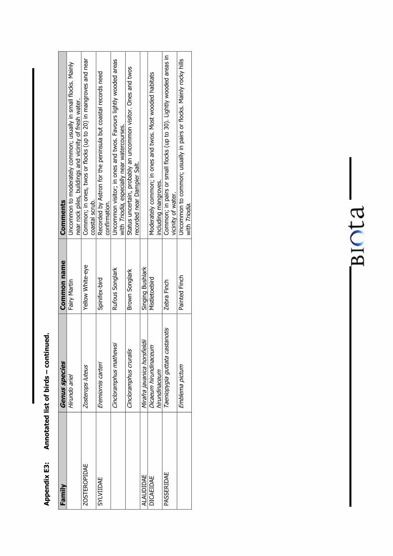
App
endi
x E3
:A
nn
otat
ed li
st o
f bi
rds
– co
nti
nu
ed.
Fam
ilyG
enus
spe
cies
Com
mon
nam
eC
omm
ents
Hiru
ndo
arie
lFa
iry M
artin
Unc
omm
on t
o m
oder
atel
y co
mm
on;
usua
lly in
sm
all f
lock
s. M
ainl
yne
ar r
ock
pile
s, b
uild
ings
and
vic
inity
of
fres
h w
ater
.ZO
STER
OPI
DAE
Zost
erop
s lu
teus
Yello
w W
hite
-eye
Com
mon
; in
one
s, t
wos
or
flock
s (u
p to
20)
in m
angr
oves
and
nea
rco
asta
l scr
ub.
SYLV
IID
AEEr
emio
rnis
car
teri
Spin
ifex-
bird
Rec
orde
d by
Ast
ron
for
the
peni
nsul
a bu
t co
asta
l rec
ords
nee
dco
nfirm
atio
n.Ci
nclo
ram
phus
mat
hew
siRuf
ous
Song
lark
Unc
omm
on v
isito
r; in
one
s an
d tw
os. F
avou
rs li
ghtly
woo
ded
area
sw
ith T
riodi
a, e
spec
ially
nea
r w
ater
cour
ses.
Cinc
lora
mph
us c
rura
lisBr
own
Song
lark
Stat
us u
ncer
tain
, pr
obab
ly a
n un
com
mon
vis
itor.
One
s an
d tw
osre
cord
ed n
ear
Dam
pier
Sal
t.AL
AUD
IDAE
Mira
fra
java
nica
hor
sfie
ldii
Sing
ing
Bush
lark
DIC
AEID
AED
icae
um h
irund
inac
eum
hiru
ndin
aceu
mM
istle
toeb
irdM
oder
atel
y co
mm
on;
in o
nes
and
twos
. Mos
t w
oode
d ha
bita
tsin
clud
ing
man
grov
es.
PASS
ERID
AETa
enio
pygi
a gu
ttat
a ca
stan
otis
Zebr
a Fi
nch
Com
mon
; in
pai
rs o
r sm
all f
lock
s (u
p to
30)
. Lig
htly
woo
ded
area
s in
vici
nity
of
wat
er.
Embl
ema
pict
umPa
inte
d Fi
nch
Unc
omm
on t
o co
mm
on;
usua
lly in
pai
rs o
r flo
cks.
Mai
nly
rock
y hi
llsw
ith T
riodi
a.
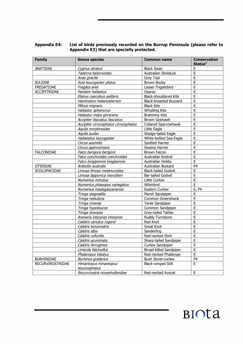
Appendix E4: List of birds previously recorded on the Burrup Peninsula (please refer toAppendix E3) that are specially protected.
Family Genus species Common name ConservationStatus1
ANATIDAE Cygnus atratus Black Swan ETadorna tadornoides Australian Shelduck EAnas gracilis Grey Teal E
SULIDAE Sula leucogaster plotus Brown Booby EFREGATIDAE Fregata ariel Lesser Frigatebird EACCIPITRIDAE Pandion haliaetus Osprey E
Elanus caeruleus axillaris Black-shouldered Kite EHamirostra melanosternon Black-breasted Buzzard EMilvus migrans Black Kite EHaliastur sphenurus Whistling Kite EHaliastur indus girrenera Brahminy Kite EAccipiter fasciatus fasciatus Brown Goshawk EAccipiter cirrocephalus cirrocephalus Collared Sparrowhawk EAquila morphnoides Little Eagle EAquila audax Wedge-tailed Eagle EHaliaeetus leucogaster White-bellied Sea-Eagle ECircus assimilis Spotted Harrier ECircus approximans Swamp Harrier E
FALCONIDAE Falco berigora berigora Brown Falcon EFalco cenchroides cenchroides Australian Kestrel EFalco longipennis longipennis Australian Hobby E
OTIDIDAE Ardeotis australis Australian Bustard P4SCOLOPACIDAE Limosa limosa melanuroides Black-tailed Godwit E
Limosa lapponica menzbieri Bar-tailed Godwit ENumenius minutus Little Curlew ENumenius phaeopus variegatus Whimbrel ENumenius madagascariensis Eastern Curlew E, P4Tringa stagnatilis Marsh Sandpiper ETringa nebularia Common Greenshank ETringa cinerea Terek Sandpiper ETringa hypoleucos Common Sandpiper ETringa brevipes Grey-tailed Tattler EArenaria interpres interpres Ruddy Turnstone ECalidris canutus rogersi Red Knot ECalidris tenuirostris Great Knot ECalidris alba Sanderling ECalidris ruficollis Red-necked Stint ECalidris acuminata Sharp-tailed Sandpiper ECalidris ferruginea Curlew Sandpiper ELimicola falcinellus Broad-billed Sandpiper EPhalaropus lobatus Red-necked Phalarope E
BURHINIDAE Burhinus grallarius Bush Stone-curlew P4RECURVIROSTRIDAE Himantopus himantopus
leucocephalusBlack-winged Stilt E
Recurvirostra novaehollandiae Red-necked Avocet E
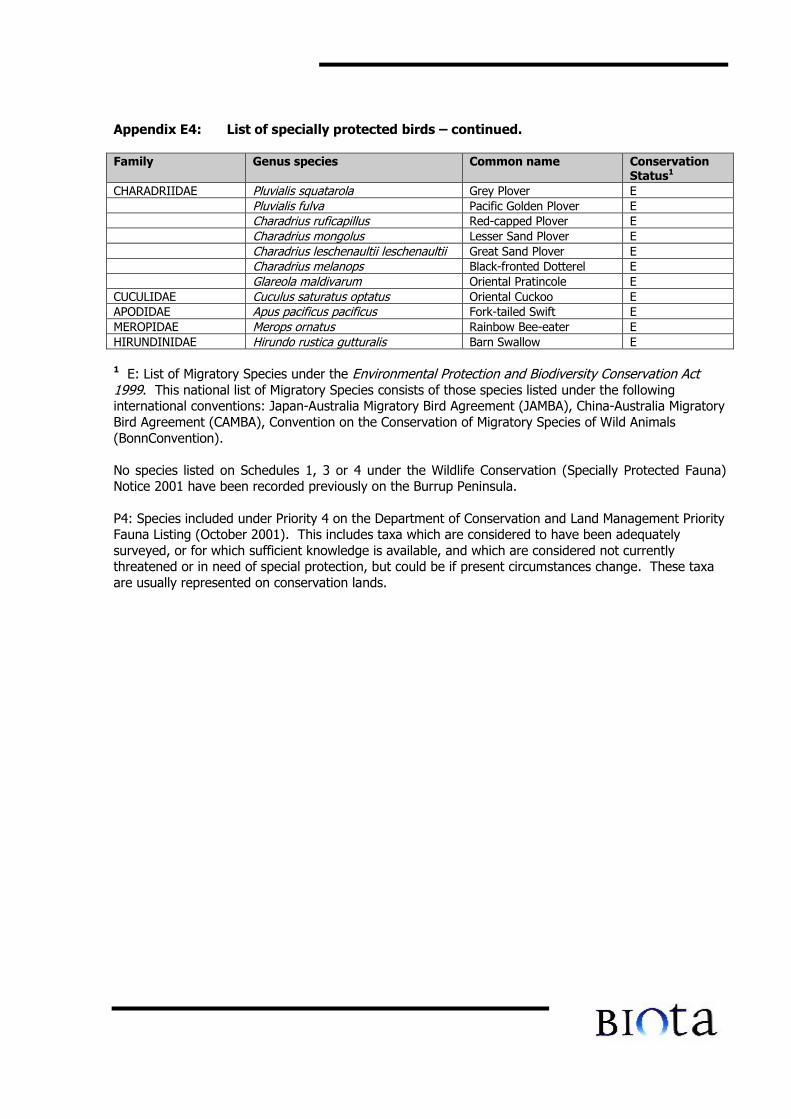
Appendix E4: List of specially protected birds – continued.
Family Genus species Common name ConservationStatus1
CHARADRIIDAE Pluvialis squatarola Grey Plover EPluvialis fulva Pacific Golden Plover ECharadrius ruficapillus Red-capped Plover ECharadrius mongolus Lesser Sand Plover ECharadrius leschenaultii leschenaultii Great Sand Plover ECharadrius melanops Black-fronted Dotterel EGlareola maldivarum Oriental Pratincole E
CUCULIDAE Cuculus saturatus optatus Oriental Cuckoo EAPODIDAE Apus pacificus pacificus Fork-tailed Swift EMEROPIDAE Merops ornatus Rainbow Bee-eater EHIRUNDINIDAE Hirundo rustica gutturalis Barn Swallow E
1 E: List of Migratory Species under the Environmental Protection and Biodiversity Conservation Act1999. This national list of Migratory Species consists of those species listed under the followinginternational conventions: Japan-Australia Migratory Bird Agreement (JAMBA), China-Australia MigratoryBird Agreement (CAMBA), Convention on the Conservation of Migratory Species of Wild Animals(BonnConvention).
No species listed on Schedules 1, 3 or 4 under the Wildlife Conservation (Specially Protected Fauna)Notice 2001 have been recorded previously on the Burrup Peninsula.
P4: Species included under Priority 4 on the Department of Conservation and Land Management PriorityFauna Listing (October 2001). This includes taxa which are considered to have been adequatelysurveyed, or for which sufficient knowledge is available, and which are considered not currentlythreatened or in need of special protection, but could be if present circumstances change. These taxaare usually represented on conservation lands.
Baseline Marine Survey of King Bay
Appendix 4
King Bay BaselineMonitoring Results
MethanexFinal ReportRev 0
March 2002
King Bay Baseline MonitoringResults
Methanex
Final Report
Rev 0
March 2002
Sinclair Knight Merz Pty LimitedACN 001 024 095ABN 37 001 024 0957th Floor, Durack Centre263 Adelaide TerracePO Box H615Perth WAAustralia 6001Telephone: +61 8 9268 4400Facsimile: +61 8 9268 4488
COPYRIGHT: The concepts and information contained in
this document are the property of Sinclair Knight Merz Pty
Ltd. Use or copying of this document in whole or in part
without the written permission of Sinclair Knight Merz
constitutes an infringement of copyright.
WV02214.540:APPENDIX 4 KING BAY BASELINE MONITORING RESULTS.DOC PAGE i
Contents
1. Introduction.................................................................................... 32. Methods .......................................................................................... 4
2.1 Water Quality Sampling ...................................................................42.2 Physico-Chemical Water Column Profiles........................................52.3 Sediment Sampling..........................................................................52.4 Biomonitoring...................................................................................5
2.4.1 Video Survey....................................................................................5
3. Results and Discussion ................................................................ 63.1 Selection of Sites.............................................................................63.2 Water Sampling Results ..................................................................8
3.2.1 Physico-Chemical Water Column Profiles .....................................123.3 Sediment Sampling Results...........................................................17
3.3.1 Metals in sediments .......................................................................173.3.2 Nutrients in sediments ...................................................................18
3.4 Biomonitoring Results....................................................................20
List of Figures
Figure 3-1 Sampling sites in King Bay.......................................................................... 6Figure 3-2 Tides at Dampier during sampling............................................................... 7Figure 3-3 Water nutrients and TSS .............................................................................. 8Figure 3-4 Mean Chlorophyll a, b and c........................................................................ 9Figure 3-5 Dissolved Oxygen / depth profile at site 1 and 2 ....................................... 12Figure 3-6 Salinity / depth profile for site 1 and 2....................................................... 13Figure 3-7 Temperature / depth profile at site 1 and 2 ................................................ 14Figure 3-8 Turbidity / depth profile at site 1 and 2...................................................... 15Figure 3-9 pH / depth profile ....................................................................................... 16Figure 3-10 Metals in sediments.................................................................................. 17Figure 3-11 Nutrients in sediment ............................................................................... 18Figure 3-12 Metals in oysters ...................................................................................... 20
List of Tables
Table 3-1 Sampling site locations.................................................................................. 7Table 3-2 Water Nutrients and chemistry.................................................................... 10Table 3-3 Metals in Water ........................................................................................... 11Table 3-4 Sediment Sampling Results......................................................................... 19
WV02214.540:APPENDIX 4 KING BAY BASELINE MONITORING RESULTS.DOC PAGE ii
Document History and StatusIssue Rev. Issued To Qty Date Reviewed ApprovedDRAFT A Preliminary results
to Water Corporationand Methanex
1 electronic copy 24/01/02
FINAL 0 Methanex 1 electronic copy2. bound copies
7/03/02 J Phillips G Clapin
Printed: 9 April, 2002Last Saved: 5 April, 2002File Name: I:\WVES\02200\WV02214\PER Consolidation And
Reporting\Rep14_11.01\Final\Appendices\Technical Appendices\Appendix 4 King Bay BaselineMonitoring Results.Doc
Project Manager: Geordie ClapinName of Organisation: Water Corporation and MethanexName of Project: King Bay Baseline MonitoringName of Document: King Bay Baseline Monitoring ResultsDocument Version: Final 0Project Number: WV02214.540
WV02214.540:APPENDIX 4 KING BAY BASELINE MONITORING RESULTS.DOC PAGE 3
1. IntroductionThe Water Corporation intends to construct and operate a seawater supply and desalinationsystem on the Burrup Peninsula to service the requirements of new industrial developments inthe area. Methanex would receive water from the Water Corporation supply and returnwastewater to the discharge return line. The proposed desalination system would be located atKing Bay and would include the return of brine and cooling water via a pipeline into the bay.The diffuser would be located in approximately 4 to 8 meters depth of water in an area of mud /sand bottom.
In order to determine the impacts of such a discharge on the marine environment it is importantto establish the present state of the marine environment in the area of the proposed brinedischarge.
This report presents the results of background data collection at the proposed site and areference site in King Bay.
WV02214.540:APPENDIX 4 KING BAY BASELINE MONITORING RESULTS.DOC PAGE 4
2. MethodsThe sites that were sampled for baseline monitoring in King Bay are described in Section 3.1.Water quality and sediment sampling was conducted on 3/12/01 and physico-chemical profilesand the deployment of pearl oysters for biomonitoring were completed on 4/12/01.
2.1 Water Quality SamplingNutrientsThree replicate water samples were collected for nutrient analysis from just below the watersurface at each site. Each replicate consisted of the following:
Two unfiltered samples were placed in clean 125 mL HDPE bottles. Two samples were filteredthrough Whatman GF/C filters followed by 0.45 µm membrane filters (Schelsicher & Schuell).Filtered samples were collected into 10 mL laboratory-grade vials that can be placed directlyinto an auto-analyser to avoid decanting samples. All samples were placed on ice in the darkand frozen at the end of the day for transport to Perth.
Unfiltered samples were analysed for total nitrogen (TN) and total phosphorous (TP). Filteredsamples were analysed for nitrate + nitrite (NO3 + NO2), ammonia nitrogen (NH4) and filterablereactive phosphorous (FRP, or orthophosphate).
Only one each of the unfiltered and filtered samples from each replicate was used for analysis,as the remaining two samples were retained as spares if required.
Total Suspended SolidsTotal suspended solids (TSS) was determined by filtering a known volume of water (normally2 L) and trapping the TSS on to a pre-weighed Whatman GF/C filter. Filtration was done in thefield using a filter tower and vacuum pump. Samples were placed on ice in the dark and frozenat the end of the day. TSS analysis by loss on ignition was conducted on three replicate samplesfor each site.
ChlorophyllThree replicate water samples were collected for chlorophyll analysis from just below the watersurface at each site. Samples were collected by filtering a known volume of water (normally2 L) through a Whatman GF/C filter, which retained any chlorophyll-containing microalgae.Filtration was done in the field using a filter tower and vacuum pump. The filters were thenwrapped in foil and placed on ice in the dark. Chlorophyll a, b and c were determined by theMarine and Freshwater Research Laboratory (MAFRL) at Murdoch University using thetrichromatic method.
MetalsAnalysis of metals dissolved in water was conducted on three replicate samples collected fromjust below the water surface at each site. Samples were filtered through Whatman GF/C filtersfollowed by 0.45µm membrane filters (Schelsicher & Schuell). Filtered water samples werecollected into 10 mL laboratory-grade vials that can be placed directly into an auto-analyser toavoid decanting samples. Samples for mercury (Hg) were collected into 125 mL (HDPE)bottles, as the analysis required a larger volume. All water samples were transported in a darkcontainer, on ice and delivered to the analysis laboratory (MAFRL) within 48 hours ofcollection.
WV02214.540:APPENDIX 4 KING BAY BASELINE MONITORING RESULTS.DOC PAGE 5
2.2 Physico-Chemical Water Column ProfilesProfiles were taken of the water column from the surface to the bottom at the two sampling sitesusing a multi-probe. The parameters measured included turbidity, pH, temperature, salinity,conductivity and dissolved oxygen. Profiles for each site were conducted within <30 minutes ofeach another, during the same stage of an outgoing tide. Unfortunately, because of tide timesand logistics it was not possible to attempt profiles during both the incoming and outgoing tide.
Temperature and Salinity LoggingCombined temperature and salinity loggers for deployment were not available at short noticefrom the manufacturers or for hire and were not deployed at the two locations as had beenintended.
Advice from Mermaid Marine indicated that site 1 may be subject to disturbance from largevessels laying mooring cables across the site, hence there is also the possibility of a logger beinglost or damaged. Note that the oyster mooring at site 1 had been dragged approximately 25 mfrom the deployment location and the surface float had been torn off, possibly by a boatpropeller.
2.3 Sediment SamplingThree replicate sediment core samples were collected for nutrient and metals analysis at eachlocation. Samples were collected by a diver using a polycarbonate tube to extract a core fromthe top 150 mm of sediment, taking care to include the fine surface sediment layer. Replicateswere spaced approximately 1 m apart. Core samples were transferred into sterile 250 mLWhirl-packs (Nasco) taking care not to lose the fine surface sediment. Samples were placed onice in the dark but not frozen.
All sediment samples were transported in a dark container, on ice and delivered to the analysislaboratory (MAFRL) within 24 hours of collection. Sediment samples were analysed for totalKjeldahl nitrogen (TKN) and total phosphorous (TP) and the following metals: Ag, Al, Cd, Co,Cr, Cu, Hg, Ni, Pb, Sn, V and Zn.
2.4 BiomonitoringBiomonitoring using Golden Lip Pearl Oysters (Pinctada maxima) was undertaken at the outletand reference sites. Six oysters were deployed at each site, in a standard six-shell panel heldapproximately 0.5 m above the bottom by a large sub-surface float and heavy mooring anchor.
Oysters were deployed on 4/12/01 and retrieved on 13/01/02. Upon retrieval the shells wereopened and three replicate samples taken for each site, with each sample comprised of the fleshfrom two shells. A background sample of three replicates was also taken from six additionalshells at the time of deployment.
Metals analysis was conducted on each sample and included Ag, Cd, Co, Cr III, Cr VI, Cu, Hg,Ni, Pb, Sn, V and Zn.
2.4.1 Video SurveyVideo transects were planned but could not be conducted due to poor visibility at the site duringboth the deployment and retrieval dives.
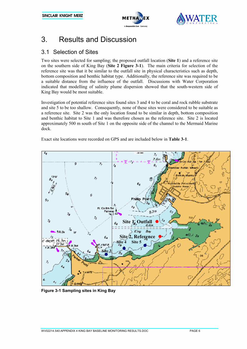
WV02214.540:APPENDIX 4 KING BAY BASELINE MONITORING RESULTS.DOC PAGE 6
3. Results and Discussion3.1 Selection of SitesTwo sites were selected for sampling; the proposed outfall location (Site 1) and a reference siteon the southern side of King Bay (Site 2 Figure 3-1). The main criteria for selection of thereference site was that it be similar to the outfall site in physical characteristics such as depth,bottom composition and benthic habitat type. Additionally, the reference site was required to bea suitable distance from the influence of the outfall. Discussions with Water Corporationindicated that modelling of salinity plume dispersion showed that the south-western side ofKing Bay would be most suitable.
Investigation of potential reference sites found sites 3 and 4 to be coral and rock rubble substrateand site 5 to be too shallow. Consequently, none of these sites were considered to be suitable asa reference site. Site 2 was the only location found to be similar in depth, bottom compositionand benthic habitat to Site 1 and was therefore chosen as the reference site. Site 2 is locatedapproximately 500 m south of Site 1 on the opposite side of the channel to the Mermaid Marinedock.
Exact site locations were recorded on GPS and are included below in Table 3-1.
Figure 3-1 Sampling sites in King Bay
Site 1, Outfall
Site 2, Reference
Site 3
Site 5Site 4
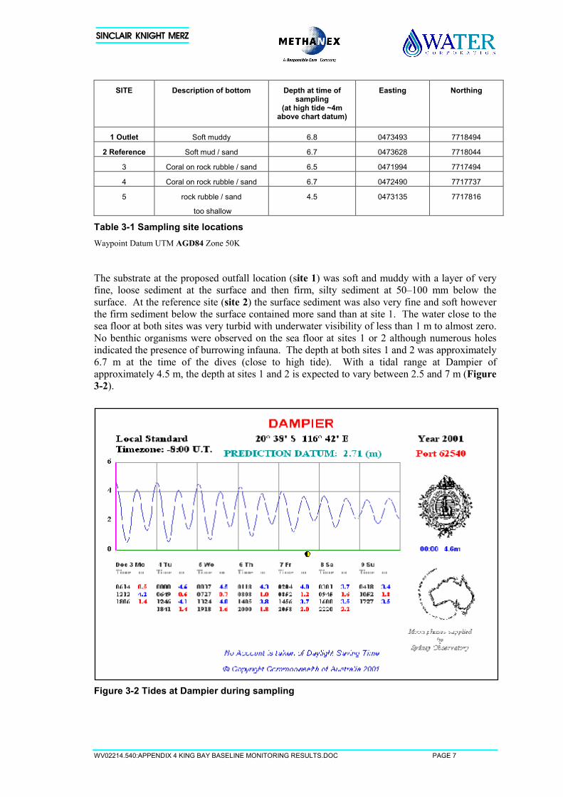
WV02214.540:APPENDIX 4 KING BAY BASELINE MONITORING RESULTS.DOC PAGE 7
SITE Description of bottom Depth at time ofsampling
(at high tide ~4mabove chart datum)
Easting Northing
1 Outlet Soft muddy 6.8 0473493 7718494
2 Reference Soft mud / sand 6.7 0473628 7718044
3 Coral on rock rubble / sand 6.5 0471994 7717494
4 Coral on rock rubble / sand 6.7 0472490 7717737
5 rock rubble / sand
too shallow
4.5 0473135 7717816
Table 3-1 Sampling site locationsWaypoint Datum UTM AGD84 Zone 50K
The substrate at the proposed outfall location (site 1) was soft and muddy with a layer of veryfine, loose sediment at the surface and then firm, silty sediment at 50–100 mm below thesurface. At the reference site (site 2) the surface sediment was also very fine and soft howeverthe firm sediment below the surface contained more sand than at site 1. The water close to thesea floor at both sites was very turbid with underwater visibility of less than 1 m to almost zero.No benthic organisms were observed on the sea floor at sites 1 or 2 although numerous holesindicated the presence of burrowing infauna. The depth at both sites 1 and 2 was approximately6.7 m at the time of the dives (close to high tide). With a tidal range at Dampier ofapproximately 4.5 m, the depth at sites 1 and 2 is expected to vary between 2.5 and 7 m (Figure3-2).
Figure 3-2 Tides at Dampier during sampling
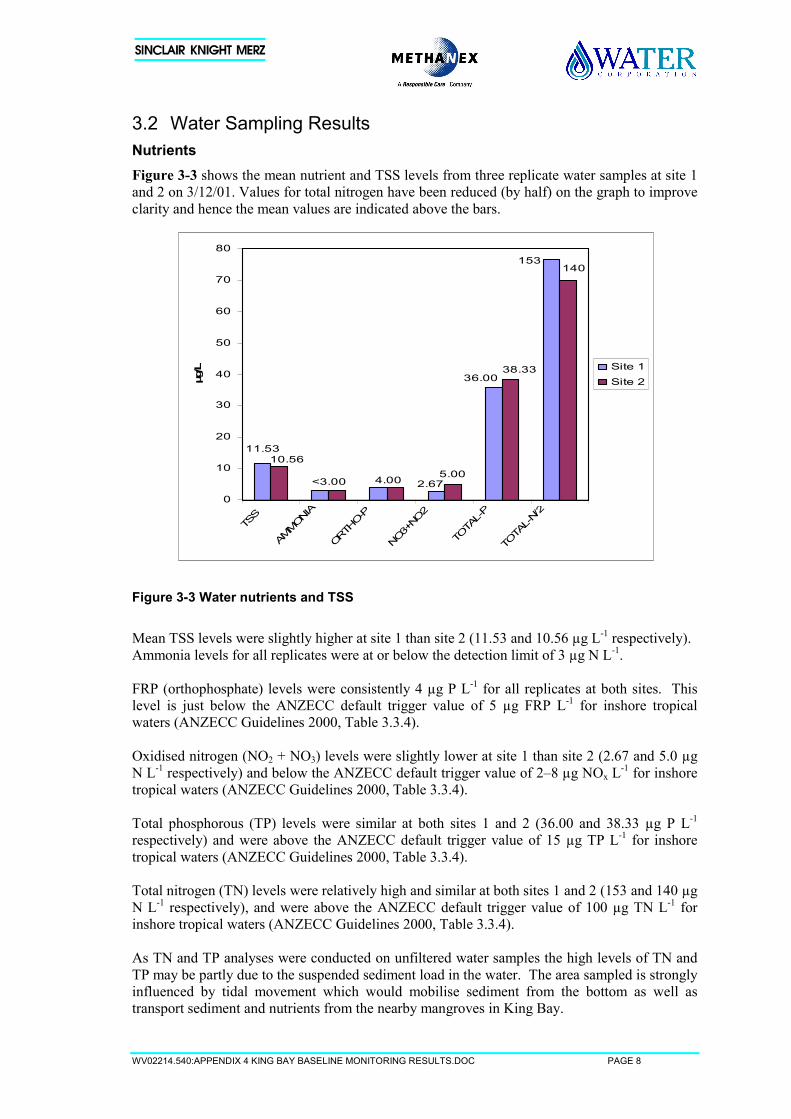
WV02214.540:APPENDIX 4 KING BAY BASELINE MONITORING RESULTS.DOC PAGE 8
3.2 Water Sampling ResultsNutrientsFigure 3-3 shows the mean nutrient and TSS levels from three replicate water samples at site 1and 2 on 3/12/01. Values for total nitrogen have been reduced (by half) on the graph to improveclarity and hence the mean values are indicated above the bars.
Figure 3-3 Water nutrients and TSS
Mean TSS levels were slightly higher at site 1 than site 2 (11.53 and 10.56 µg L-1 respectively).Ammonia levels for all replicates were at or below the detection limit of 3 µg N L-1.
FRP (orthophosphate) levels were consistently 4 µg P L-1 for all replicates at both sites. Thislevel is just below the ANZECC default trigger value of 5 µg FRP L-1 for inshore tropicalwaters (ANZECC Guidelines 2000, Table 3.3.4).
Oxidised nitrogen (NO2 + NO3) levels were slightly lower at site 1 than site 2 (2.67 and 5.0 µgN L-1 respectively) and below the ANZECC default trigger value of 2–8 µg NOx L-1 for inshoretropical waters (ANZECC Guidelines 2000, Table 3.3.4).
Total phosphorous (TP) levels were similar at both sites 1 and 2 (36.00 and 38.33 µg P L-1
respectively) and were above the ANZECC default trigger value of 15 µg TP L-1 for inshoretropical waters (ANZECC Guidelines 2000, Table 3.3.4).
Total nitrogen (TN) levels were relatively high and similar at both sites 1 and 2 (153 and 140 µgN L-1 respectively), and were above the ANZECC default trigger value of 100 µg TN L-1 forinshore tropical waters (ANZECC Guidelines 2000, Table 3.3.4).
As TN and TP analyses were conducted on unfiltered water samples the high levels of TN andTP may be partly due to the suspended sediment load in the water. The area sampled is stronglyinfluenced by tidal movement which would mobilise sediment from the bottom as well astransport sediment and nutrients from the nearby mangroves in King Bay.
5.00<3.00
11.53
153
2.67
36.00
10.56
140
4.00
38.33
0
10
20
30
40
50
60
70
80
TSS
AMMONIA
ORTHO-P
NO3+NO
2
TOTA
L-P
TOTA
L-N/
2
µg/L Site 1
Site 2
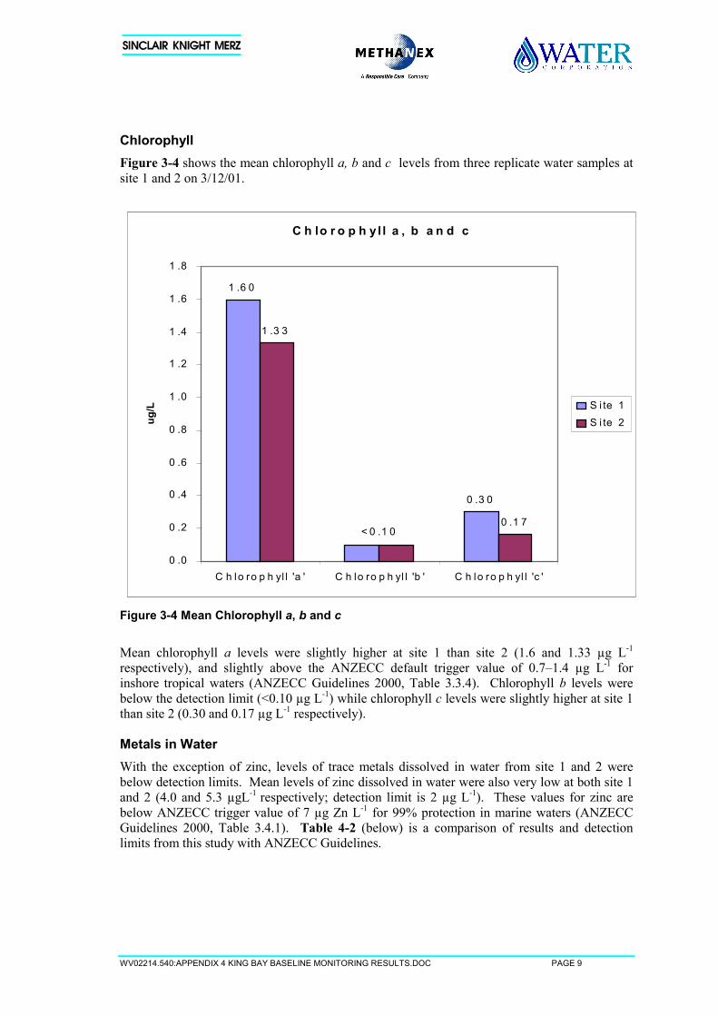
WV02214.540:APPENDIX 4 KING BAY BASELINE MONITORING RESULTS.DOC PAGE 9
ChlorophyllFigure 3-4 shows the mean chlorophyll a, b and c levels from three replicate water samples atsite 1 and 2 on 3/12/01.
Figure 3-4 Mean Chlorophyll a, b and c
Mean chlorophyll a levels were slightly higher at site 1 than site 2 (1.6 and 1.33 µg L-1
respectively), and slightly above the ANZECC default trigger value of 0.7–1.4 µg L-1 forinshore tropical waters (ANZECC Guidelines 2000, Table 3.3.4). Chlorophyll b levels werebelow the detection limit (<0.10 µg L-1) while chlorophyll c levels were slightly higher at site 1than site 2 (0.30 and 0.17 µg L-1 respectively).
Metals in WaterWith the exception of zinc, levels of trace metals dissolved in water from site 1 and 2 werebelow detection limits. Mean levels of zinc dissolved in water were also very low at both site 1and 2 (4.0 and 5.3 µgL-1 respectively; detection limit is 2 µg L-1). These values for zinc arebelow ANZECC trigger value of 7 µg Zn L-1 for 99% protection in marine waters (ANZECCGuidelines 2000, Table 3.4.1). Table 4-2 (below) is a comparison of results and detectionlimits from this study with ANZECC Guidelines.
C h lo r o p h yl l a , b a n d c
1 .6 0
0 .3 0
1 .3 3
0 .1 7< 0 .1 0
0 .0
0 .2
0 .4
0 .6
0 .8
1 .0
1 .2
1 .4
1 .6
1 .8
C h lo ro p h yl l 'a ' C h lo ro p h yl l 'b ' C h lo ro p h yl l 'c '
ug/L S i te 1
S i te 2
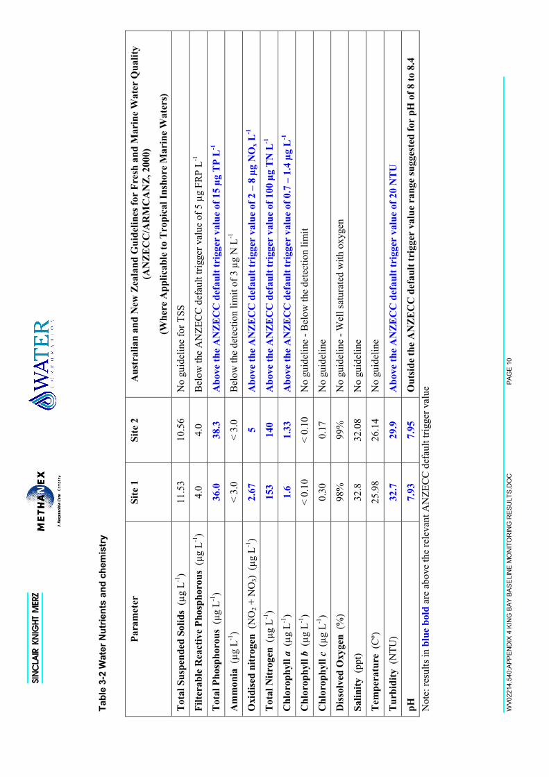
WV0
2214
.540
:APP
END
IX 4
KIN
G B
AY B
ASE
LIN
E M
ON
ITO
RIN
G R
ESU
LTS.
DO
CPA
GE
10
Tabl
e 3-
2 W
ater
Nut
rient
s an
d ch
emis
try
Para
met
erSi
te 1
Site
2A
ustr
alia
n an
d N
ew Z
eala
nd G
uide
lines
for
Fres
h an
d M
arin
e W
ater
Qua
lity
(AN
ZEC
C/A
RM
CA
NZ,
200
0)
(Whe
re A
pplic
able
to T
ropi
cal I
nsho
re M
arin
e W
ater
s)
Tota
l Sus
pend
ed S
olid
s (µ
g L-1
)11
.53
10.5
6N
o gu
idel
ine
for T
SS
Filte
rabl
e R
eact
ive
Phos
phor
ous
(µg
L-1)
4.0
4.0
Bel
ow th
e A
NZE
CC
def
ault
trigg
er v
alue
of 5
µg
FRP
L-1
Tota
l Pho
spho
rous
(µg
L-1
)36
.038
.3A
bove
the
AN
ZEC
C d
efau
lt tr
igge
r va
lue
of 1
5 µg
TP
L-1
Am
mon
ia (
µg L
-1)
< 3.
0<
3.0
Bel
ow th
e de
tect
ion
limit
of 3
µg
N L
-1
Oxi
dise
d ni
trog
en (
NO
2 + N
O3)
(µg
L-1)
2.67
5A
bove
the
AN
ZEC
C d
efau
lt tr
igge
r va
lue
of 2
– 8
µg
NO
x L-1
Tota
l Nitr
ogen
(µg
L-1
)15
314
0A
bove
the
AN
ZEC
C d
efau
lt tr
igge
r va
lue
of 1
00 µ
g T
N L
-1
Chl
orop
hyll
a (µ
g L-1
)1.
61.
33A
bove
the
AN
ZEC
C d
efau
lt tr
igge
r va
lue
of 0
.7 –
1.4
µg
L-1
Chl
orop
hyll
b (µ
g L-1
)<
0.10
< 0.
10N
o gu
idel
ine
- Bel
ow th
e de
tect
ion
limit
Chl
orop
hyll
c (µ
g L-1
)0.
300.
17N
o gu
idel
ine
Dis
solv
ed O
xyge
n (%
)98
%99
%N
o gu
idel
ine
- Wel
l sat
urat
ed w
ith o
xyge
n
Salin
ity (
ppt)
32.8
32.0
8N
o gu
idel
ine
Tem
pera
ture
(Cº
)25
.98
26.1
4N
o gu
idel
ine
Tur
bidi
ty (
NTU
)32
.729
.9A
bove
the
AN
ZEC
C d
efau
lt tr
igge
r va
lue
of 2
0 N
TU
pH7.
937.
95O
utsi
de th
e A
NZE
CC
def
ault
trig
ger
valu
e ra
nge
sugg
este
d fo
r pH
of 8
to 8
.4N
ote:
resu
lts in
blu
e bo
ld a
re a
bove
the
rele
vant
AN
ZEC
C d
efau
lt tri
gger
val
ue
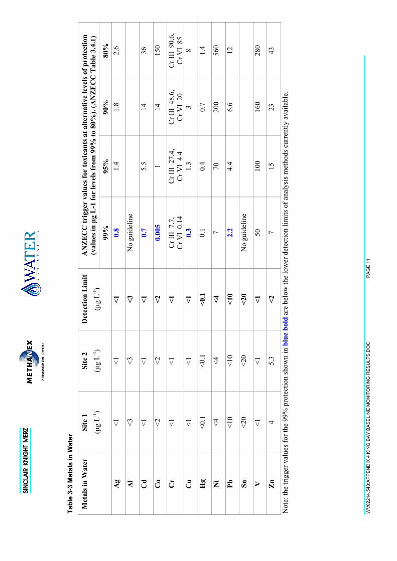
WV0
2214
.540
:APP
END
IX 4
KIN
G B
AY B
ASE
LIN
E M
ON
ITO
RIN
G R
ESU
LTS.
DO
CPA
GE
11
Tabl
e 3-
3 M
etal
s in
Wat
er
AN
ZEC
C tr
igge
r va
lues
for
toxi
cant
s at a
ltern
ativ
e le
vels
of p
rote
ctio
n(v
alue
s in
µg L
-1 fo
r le
vels
from
99%
to 8
0%).
(AN
ZEC
C T
able
3.4
.1)
Met
als i
n W
ater
Site
1
(µg
L-1)
Site
2
(µg
L-1)
Det
ectio
n Li
mit
(µg
L-1)
99%
95%
90%
80%
Ag
<1<1
<10.
81.
41.
82.
6
Al
<3<3
<3N
o gu
idel
ine
Cd
<1<1
<10.
75.
514
36
Co
<2<2
<20.
005
114
150
Cr
<1<1
<1C
r III
7.7
,C
r VI
0.14
Cr I
II 2
7.4,
Cr V
I 4.
4C
r III
48.
6,C
r VI
20C
r III
90.
6,C
r VI
85C
u<1
<1<1
0.3
1.3
38
Hg
<0.1
<0.1
<0.1
0.1
0.4
0.7
1.4
Ni
<4<4
<47
7020
056
0
Pb<1
0<1
0<1
02.
24.
46.
612
Sn<2
0<2
0<2
0N
o gu
idel
ine
V<1
<1<1
5010
016
028
0
Zn4
5.3
<27
1523
43
Not
e: th
e tri
gger
val
ues f
or th
e 99
% p
rote
ctio
n sh
own
in b
lue
bold
are
bel
ow th
e lo
wer
det
ectio
n lim
its o
f ana
lysi
s met
hods
cur
rent
ly a
vaila
ble.
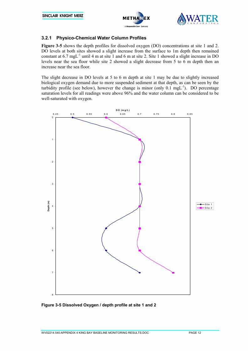
WV02214.540:APPENDIX 4 KING BAY BASELINE MONITORING RESULTS.DOC PAGE 12
3.2.1 Physico-Chemical Water Column ProfilesFigure 3-5 shows the depth profiles for dissolved oxygen (DO) concentrations at site 1 and 2.DO levels at both sites showed a slight increase from the surface to 1m depth then remainedconstant at 6.7 mgL-1 until 4 m at site 1 and 6 m at site 2. Site 1 showed a slight increase in DOlevels near the sea floor while site 2 showed a slight decrease from 5 to 6 m depth then anincrease near the sea floor.
The slight decrease in DO levels at 5 to 6 m depth at site 1 may be due to slightly increasedbiological oxygen demand due to more suspended sediment at that depth, as can be seen by theturbidity profile (see below), however the change is minor (only 0.1 mgL-1). DO percentagesaturation levels for all readings were above 96% and the water column can be considered to bewell-saturated with oxygen.
Figure 3-5 Dissolved Oxygen / depth profile at site 1 and 2
0
1
2
3
4
5
6
7
8
6 .4 5 6 .5 6 .5 5 6 .6 6 .6 5 6 .7 6 .7 5 6 .8 6 .8 5
D O (m g /L )
Dep
th (m
)
S ite 1S ite 2
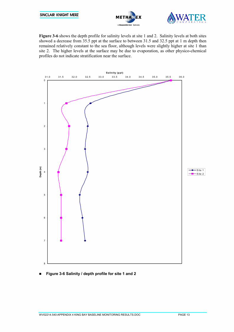
WV02214.540:APPENDIX 4 KING BAY BASELINE MONITORING RESULTS.DOC PAGE 13
Figure 3-6 shows the depth profile for salinity levels at site 1 and 2. Salinity levels at both sitesshowed a decrease from 35.5 ppt at the surface to between 31.5 and 32.5 ppt at 1 m depth thenremained relatively constant to the sea floor, although levels were slightly higher at site 1 thansite 2. The higher levels at the surface may be due to evaporation, as other physico-chemicalprofiles do not indicate stratification near the surface.
� Figure 3-6 Salinity / depth profile for site 1 and 2
0
1
2
3
4
5
6
7
8
31.0 31 .5 32 .0 32.5 33 .0 33.5 34 .0 34 .5 35.0 35 .5 36 .0
S a lin ity (p p t)
Dep
th (m
)
S ite 1S ite 2
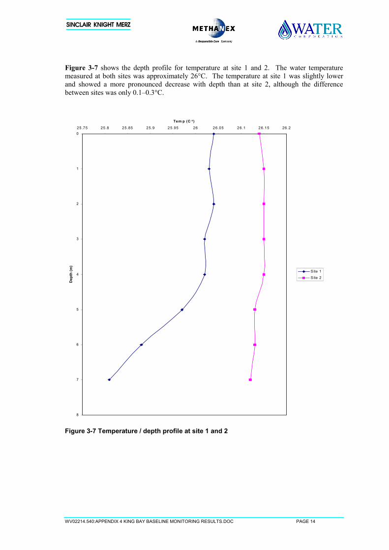
WV02214.540:APPENDIX 4 KING BAY BASELINE MONITORING RESULTS.DOC PAGE 14
Figure 3-7 shows the depth profile for temperature at site 1 and 2. The water temperaturemeasured at both sites was approximately 26°C. The temperature at site 1 was slightly lowerand showed a more pronounced decrease with depth than at site 2, although the differencebetween sites was only 0.1–0.3°C.
Figure 3-7 Temperature / depth profile at site 1 and 2
0
1
2
3
4
5
6
7
8
25 .75 25 .8 25 .85 25 .9 25.95 26 26.05 26.1 26.15 26 .2
Tem p (C o)
Dep
th (m
)
Site 1
S ite 2
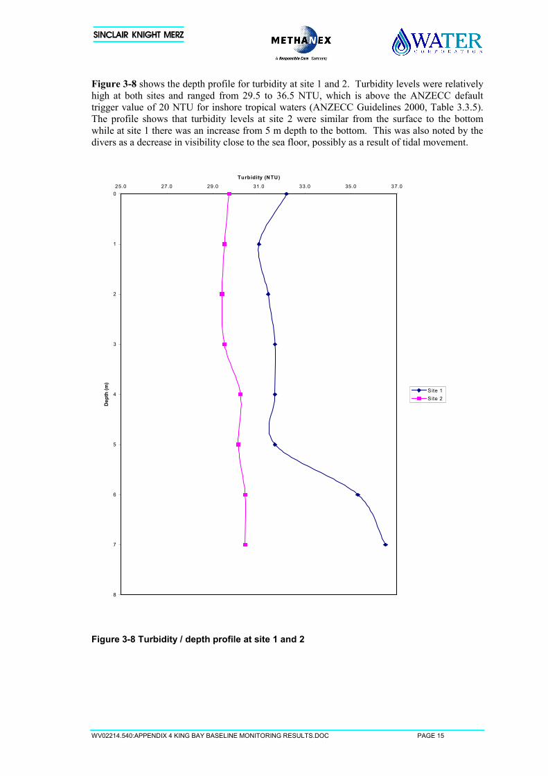
WV02214.540:APPENDIX 4 KING BAY BASELINE MONITORING RESULTS.DOC PAGE 15
Figure 3-8 shows the depth profile for turbidity at site 1 and 2. Turbidity levels were relativelyhigh at both sites and ranged from 29.5 to 36.5 NTU, which is above the ANZECC defaulttrigger value of 20 NTU for inshore tropical waters (ANZECC Guidelines 2000, Table 3.3.5).The profile shows that turbidity levels at site 2 were similar from the surface to the bottomwhile at site 1 there was an increase from 5 m depth to the bottom. This was also noted by thedivers as a decrease in visibility close to the sea floor, possibly as a result of tidal movement.
Figure 3-8 Turbidity / depth profile at site 1 and 2
0
1
2
3
4
5
6
7
8
25.0 27.0 29.0 31.0 33.0 35.0 37.0
Turbidity (NTU)
Dep
th (m
)
Site 1Site 2
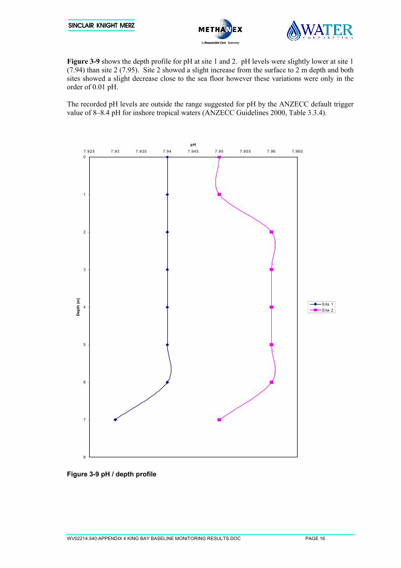
WV02214.540:APPENDIX 4 KING BAY BASELINE MONITORING RESULTS.DOC PAGE 16
Figure 3-9 shows the depth profile for pH at site 1 and 2. pH levels were slightly lower at site 1(7.94) than site 2 (7.95). Site 2 showed a slight increase from the surface to 2 m depth and bothsites showed a slight decrease close to the sea floor however these variations were only in theorder of 0.01 pH.
The recorded pH levels are outside the range suggested for pH by the ANZECC default triggervalue of 8–8.4 pH for inshore tropical waters (ANZECC Guidelines 2000, Table 3.3.4).
Figure 3-9 pH / depth profile
0
1
2
3
4
5
6
7
8
7.925 7.93 7.935 7.94 7.945 7.95 7.955 7.96 7.965
pH
Dep
th (m
)
Site 1S ite 2
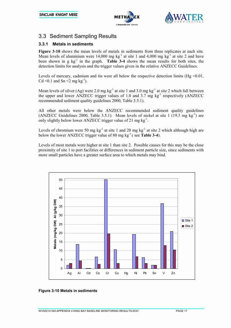
WV02214.540:APPENDIX 4 KING BAY BASELINE MONITORING RESULTS.DOC PAGE 17
3.3 Sediment Sampling Results3.3.1 Metals in sedimentsFigure 3-10 shows the mean levels of metals in sediments from three replicates at each site.Mean levels of aluminium were 14,000 mg kg-1 at site 1 and 4,000 mg kg-1 at site 2 and havebeen shown in g kg-1 in the graph. Table 3-4 shows the mean results for both sites, thedetection limits for analysis and the trigger values given in the relative ANZECC Guidelines.
Levels of mercury, cadmium and tin were all below the respective detection limits (Hg <0.01,Cd <0.1 and Sn <2 mg kg-1).
Mean levels of silver (Ag) were 2.0 mg kg-1 at site 1 and 3.0 mg kg-1 at site 2 which fall betweenthe upper and lower ANZECC trigger values of 1.0 and 3.7 mg kg-1 respectively (ANZECCrecommended sediment quality guidelines 2000, Table 3.5.1).
All other metals were below the ANZECC recommended sediment quality guidelines(ANZECC Guidelines 2000, Table 3.5.1). Mean levels of nickel at site 1 (19.3 mg kg-1) areonly slightly below lower ANZECC trigger value of 21 mg kg-1.
Levels of chromium were 50 mg kg-1 at site 1 and 20 mg kg-1 at site 2 which although high arebelow the lower ANZECC trigger value of 80 mg kg-1 ( see Table 3-4).
Levels of most metals were higher at site 1 than site 2. Possible causes for this may be the closeproximity of site 1 to port facilities or differences in sediment particle size, since sediments withmore small particles have a greater surface area to which metals may bind.
Figure 3-10 Metals in sediments
0
5
10
15
20
25
30
35
40
45
50
Ag Al Cd Co Cr Cu Hg Ni Pb Sn V Zn
Met
als
(mg/
kg D
W)
Al (
g/kg
DW
)
Site 1
Site 2
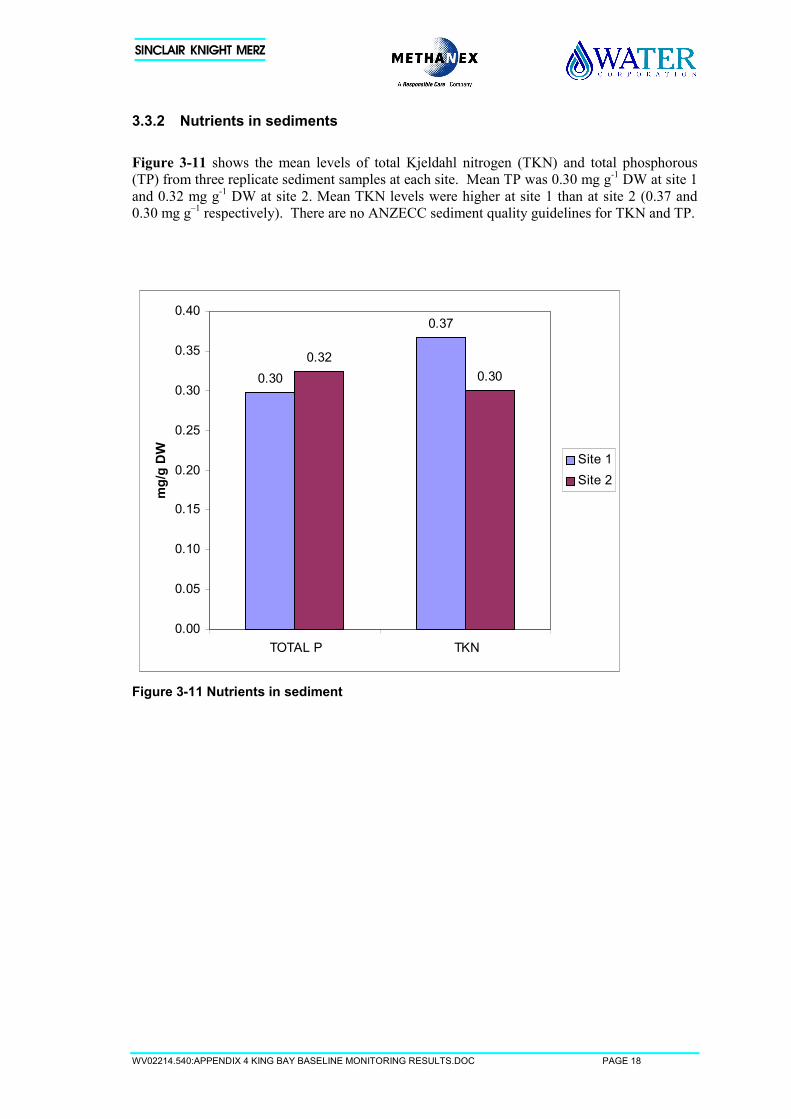
WV02214.540:APPENDIX 4 KING BAY BASELINE MONITORING RESULTS.DOC PAGE 18
3.3.2 Nutrients in sediments
Figure 3-11 shows the mean levels of total Kjeldahl nitrogen (TKN) and total phosphorous(TP) from three replicate sediment samples at each site. Mean TP was 0.30 mg g-1 DW at site 1and 0.32 mg g-1 DW at site 2. Mean TKN levels were higher at site 1 than at site 2 (0.37 and0.30 mg g–1 respectively). There are no ANZECC sediment quality guidelines for TKN and TP.
Figure 3-11 Nutrients in sediment
0.37
0.320.300.30
0.00
0.05
0.10
0.15
0.20
0.25
0.30
0.35
0.40
TOTAL P TKN
mg/
g D
W
Site 1Site 2
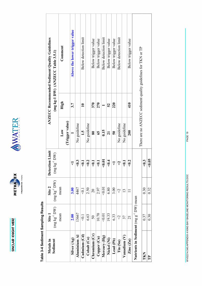
WV0
2214
.540
:APP
END
IX 4
KIN
G B
AY B
ASE
LIN
E M
ON
ITO
RIN
G R
ESU
LTS.
DO
CPA
GE
19
Tabl
e 3-
4 Se
dim
ent S
ampl
ing
Res
ults
AN
ZEC
C R
ecom
men
ded
Sedi
men
t Qua
lity
Gui
delin
es (m
g kg
-1 D
W)
(AN
ZEC
C T
able
3.5
.1)
Met
als i
nSe
dim
ent
Site
1(m
g kg
-1 D
W)
mea
n
Site
2(m
g kg
-1 D
W)
mea
n
Det
ectio
n Li
mit
(mg
kg-1
DW
)
Low
(Tri
gger
val
ue)
Hig
hC
omm
ent
Silv
er (A
g)2.
003.
00<1
13.
7A
bove
the
low
er tr
igge
r va
lue
Alu
min
ium
Al
1366
744
67<0
.3N
o gu
idel
ine
Cad
miu
m (C
d)<0
.1<0
.1<0
.11.
510
Bel
ow d
etec
tion
limit
Cob
alt (
Co)
6.63
2.50
<0.2
No
guid
elin
eC
hrom
ium
(Cr)
5020
<0.1
8037
0B
elow
trig
ger v
alue
Cop
per
(Cu)
10.7
02.
97<0
.165
270
Bel
ow tr
igge
r val
ueM
ercu
ry (H
g)<0
.01
<0.0
1<0
.01
0.15
1B
elow
det
ectio
n lim
itN
icke
l (N
i)19
.33
6.80
<0.4
2152
Bel
ow tr
igge
r val
ueLe
ad (P
b)6.
333.
00<1
5022
0B
elow
trig
ger v
alue
Tin
(Sn)
<2<2
<2N
o gu
idel
ine
Bel
ow d
etec
tion
limit
Van
adiu
m (V
)37
13<0
.1N
o gu
idel
ine
Zinc
(Zn)
2111
<0.2
200
410
Bel
ow tr
igge
r val
ue
Nut
rien
ts in
Sed
imen
t (m
g g-1
DW
) mea
n
TKN
0.37
0.30
<0.3
TP0.
300.
32<0
.05
Ther
e ar
e no
AN
ZEC
C se
dim
ent q
ualit
y gu
idel
ines
for T
KN
or T
P
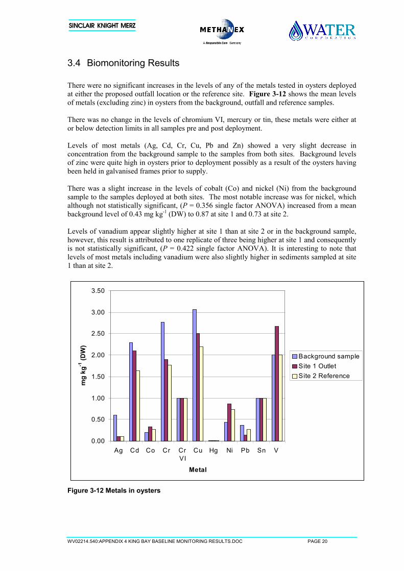
WV02214.540:APPENDIX 4 KING BAY BASELINE MONITORING RESULTS.DOC PAGE 20
3.4 Biomonitoring Results
There were no significant increases in the levels of any of the metals tested in oysters deployedat either the proposed outfall location or the reference site. Figure 3-12 shows the mean levelsof metals (excluding zinc) in oysters from the background, outfall and reference samples.
There was no change in the levels of chromium VI, mercury or tin, these metals were either ator below detection limits in all samples pre and post deployment.
Levels of most metals (Ag, Cd, Cr, Cu, Pb and Zn) showed a very slight decrease inconcentration from the background sample to the samples from both sites. Background levelsof zinc were quite high in oysters prior to deployment possibly as a result of the oysters havingbeen held in galvanised frames prior to supply.
There was a slight increase in the levels of cobalt (Co) and nickel (Ni) from the backgroundsample to the samples deployed at both sites. The most notable increase was for nickel, whichalthough not statistically significant, (P = 0.356 single factor ANOVA) increased from a meanbackground level of 0.43 mg kg-1 (DW) to 0.87 at site 1 and 0.73 at site 2.
Levels of vanadium appear slightly higher at site 1 than at site 2 or in the background sample,however, this result is attributed to one replicate of three being higher at site 1 and consequentlyis not statistically significant, (P = 0.422 single factor ANOVA). It is interesting to note thatlevels of most metals including vanadium were also slightly higher in sediments sampled at site1 than at site 2.
Figure 3-12 Metals in oysters
0.00
0.50
1.00
1.50
2.00
2.50
3.00
3.50
Ag Cd Co Cr CrVI
Cu Hg Ni Pb Sn V
Metal
mg
kg-1
(DW
)
Background sampleSite 1 OutletSite 2 Reference
Air Quality Assessment
Appendix 5
Air Quality AssessmentMethanol Complex
MethanexFinal ReportRev 0
April 2002
Air Quality AssessmentMethanol Complex
Methanex
Final Report
Rev 0
April 2002
Sinclair Knight Merz Pty LimitedACN 001 024 095ABN 37 001 024 0957th Floor, Durack Centre263 Adelaide TerracePO Box H615Perth WAAustralia 6001Telephone: +61 8 9268 4400Facsimile: +61 8 9268 4488
COPYRIGHT: The concepts and information contained in
this document are the property of Sinclair Knight Merz Pty
Ltd. Use or copying of this document in whole or in part
without the written permission of Sinclair Knight Merz
constitutes an infringement of copyright.
WI00294:APPENDIX 5 AIR QUALITY ASSESSMENT.DOC Final PAGE i
Contents
Contents ................................................................................................ iDocument History and Status............................................................. ii1. Introduction.................................................................................... 22. Emissions to Atmosphere............................................................. 3
2.1 Emissions from Normal Operation ...................................................32.1.1 Combustion Products.......................................................................32.1.2 Volatile Organic Compounds ...........................................................4
2.2 Cold Start-Up Operations.................................................................52.3 Combustion Products from Emergency Operations .........................62.4 Existing Emission Sources...............................................................7
2.4.1 Point Sources...................................................................................72.4.2 Area and Biogenic Emissions ..........................................................8
3. Air Quality Criteria ......................................................................... 93.1 Stack Emissions from Gas Turbines ................................................93.2 Ambient Air Quality Standards.........................................................9
4. Existing Air Quality...................................................................... 115. Atmospheric Dispersion Modelling............................................ 12
5.1 DISPMOD......................................................................................125.2 TAPM ............................................................................................125.3 AUSPLUME...................................................................................135.4 Modelling Results ..........................................................................14
5.4.1 DISPMOD ......................................................................................145.4.2 TAPM .............................................................................................185.4.3 AUSPLUME ...................................................................................26
6. References ................................................................................... 27
WI00294:APPENDIX 5 AIR QUALITY ASSESSMENT.DOC Final PAGE ii
Document History and StatusIssue Rev. Issued To Qty Date Reviewed Approved1 0 DEP 1 22 March 2002 BJB BJB
2 1 DEP 1 5 April 2002 BJB OP
Printed: 9 April, 2002Last Saved: 5 April, 2002File Name: I:\WVES\02200\WV02214\PER Consolidation And
Reporting\Rep14_11.01\Final\Appendices\Technical Appendices\Appendix 5 Air QualityAssessment.Doc
Project Manager: Philip MillichampName of Organisation: Methanex AustraliaName of Project: Proposed Methanol Facility
Burrup PeninsulaWestern Australia
Name of Document: Atmospheric EmissionsDocument Version: FinalProject Number: WI00294
WI00294:APPENDIX 5 AIR QUALITY ASSESSMENT.DOC Final PAGE 1
Executive SummaryMethanex Australia proposes to install a methanol manufacturing facility on theBurrup Peninsula, Western Australia. Twin methanol plants are proposed, each with anominal production capacity of 6,000 tonnes per day (tpd).
Atmospheric emissions are estimated to include 359 kg/hr (100 g/s) of oxides ofnitrogen, 1,181 tonnes per year (averaging 39 g/s) of volatile organic compounds(principally methane and methanol) and up to 2.25Mtpa of carbon dioxide.
Three different models were used to assess the impacts. DISPMOD modellednear-field dispersion of oxides of nitrogen, TAPM evaluated photochemical smogimpacts and AUSPLUME was used to assess the potential impact on nearby terrain.
Results indicate that the proposed facility will increase NO2 concentrations but thesewill remain well below the relevant NEPM standard of 120ppb across the entireregion.
Photochemical smog results for existing sources are similar to those from backgroundstudies undertaken by the CSRIO and Department of Environmental Protection, WA(CSIRO, DEP, 2001). Background ozone concentrations are within the NEPMten-year goal across the region (100 ppb for no more than one day a year), while thespatial distribution indicates relatively high concentrations of ozone can occur over thesea to the west, and on the Peninsula to the north east of Dampier.
When the emissions from approved industry and Methanex are modelled, ozone levelsare predicted to remain at similar levels with a slight decrease from background atsome receptors on the land. The slight decrease appears to be due to the high ratio ofoxides of nitrogen to reactive organic compounds in the industrial emissions. This isconsistent with the Perth photochemical smog study, which determined that emissionswith a high ratio of oxides of nitrogen suppress ozone formation (WP/DEP, 1996).Ozone levels increase over the ocean to the west of Dampier, but will remain withinthe NEPM goal.
Because there is a relatively large cumulative emission of oxides of nitrogen, the areais sensitive to organics emissions. Higher ozone concentrations could occur duringdays when there are higher than usual background emissions of reactive organics, suchas wildfire events. The potential effect of wildfires was also noted by the CSIRO andDEP in 2001. The proposed Methanex facility has little impact on this conditionhowever.
WI00294:APPENDIX 5 AIR QUALITY ASSESSMENT.DOC Final PAGE 2
1. IntroductionThe proposed methanol facility will consist of twin plants located on the BurrupPeninsula to the east of King Bay. These will each have a nominal productioncapacity of 6,000 (tpd) tonnes per day of methanol.
Methanex is proposing to employ latest generation methanol production technology.This means reduced emissions and improved energy efficiency over currentconventional technology. The two processes being considered are the LeadingConcept Methanol Process (LCM) and the Lurgi process. The principal emissionsfrom either option are likely to be oxides of nitrogen and volatile organic compounds.These emissions require an assessment of the likely impact on downwind nitrogendioxide concentrations and potential for photochemical smog effects.
This report presents an estimate of emissions based principally on the LCMtechnology, and an assessment of the impact using atmospheric dispersion modelling.It is divided into four sections as follows:
� Section 2 describes the likely emissions from the facility;� Section 3 presents the relevant air quality criteria;� Section 4 describes existing air quality; and� Section 5 presents the atmospheric dispersion modelling results.
As required by the Department of Environment, Water & Catchment Protection(DEWCP), the modelling study predicts concentrations from existing sources in thearea (including those currently approved), the contribution from the proposal on itsown and the combined effect of all sources. Unusual operating conditions are alsoconsidered, including cold start-ups and emergency flaring.
WI00294:APPENDIX 5 AIR QUALITY ASSESSMENT.DOC Final PAGE 3
2. Emissions to AtmosphereEmissions from the proposed methanol plant will vary depending on operatingconditions. These include normal operation, start up and emergency operations. It isexpected however that normal conditions will predominate for the great majority ofthe time. Emissions also fall into two general categories: combustion products andvolatile organic compounds (VOCs), principally methane and methanol vapour fromfugitive emissions.
There is very little difference in emissions from the two most likely technologyoptions. Thus, while the estimates presented later in this report are based on the LCMprocess, emissions from a Lurgi process will be very similar.
Combustion sources from a LCM plant include:
� gas turbine and auxiliary burner� natural gas-fired heater on the desulphurisation plant� flare (principally during start-up and emergencies)� natural gas-fired heater on the primary reformer (start-up only)� natural gas-fired steam boiler (principally for start-up)
The combustion sources from a Lurgi Plant will include:
� primary reformer;� natural gas-fired desulphurisation heater� natural gas-fired utility boiler� flare (principally during start-up and emergencies);� emergency generators.
VOC emissions from either process arise from:
� storage tank vents� fugitive leaks from pipework and fittings� loading product to marine vessels
Products of combustion represent the most significant emissions during any operationscenario and, of these, oxides of nitrogen will be the predominant pollutant (next tocarbon dioxide). VOC emissions are expected to be minor because the process willemploy a high level of fugitive emissions control.
2.1 Emissions from Normal Operation2.1.1 Combustion ProductsAs discussed, for any likely methanol production process, the principal emissions arisefrom combustion of natural gas or other gaseous fuels. The most significant productsof gas combustion include: carbon dioxide (CO2), oxides of nitrogen (NOx) and carbonmonoxide (CO) and unburnt hydrocarbons (VOCs). There may also be traces ofparticulate and sulphur dioxide (SO2) but such emissions are generally considerednegligible.
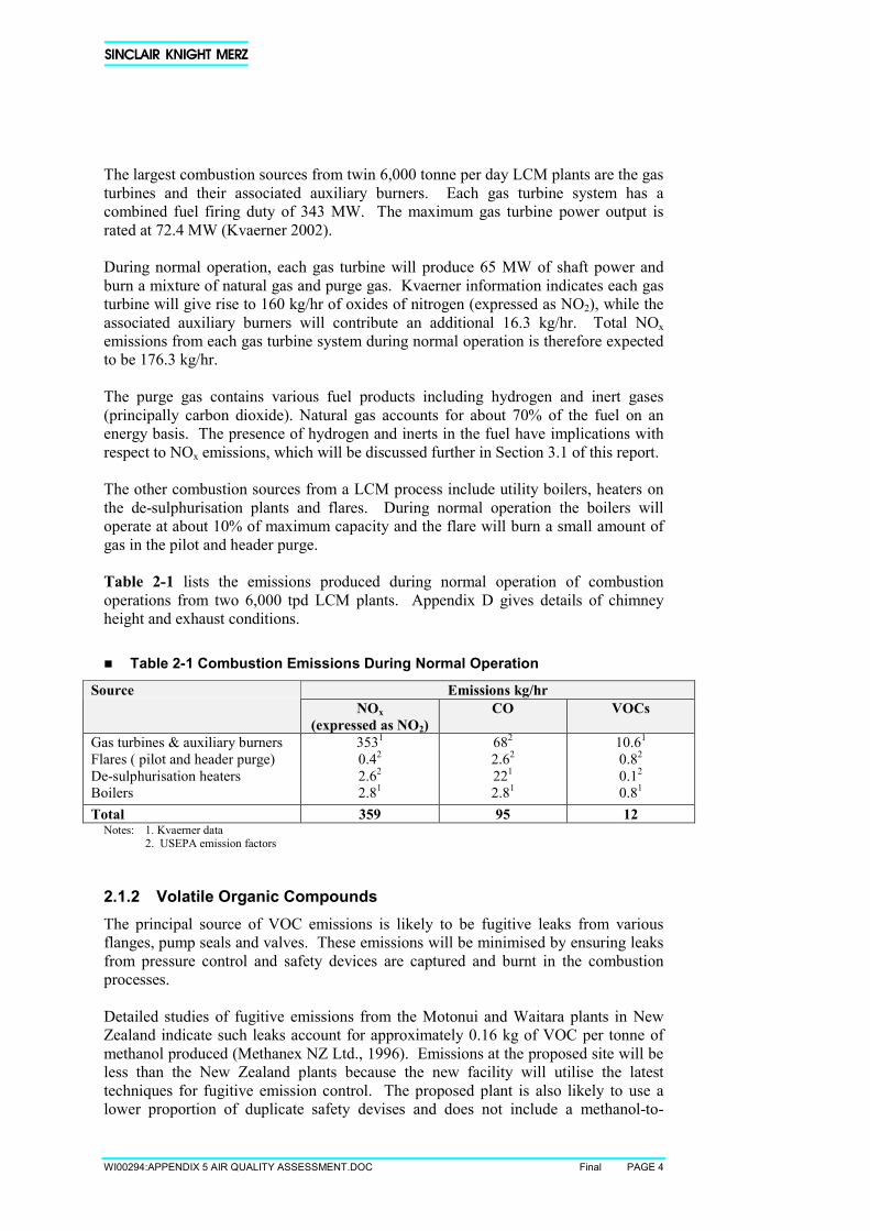
WI00294:APPENDIX 5 AIR QUALITY ASSESSMENT.DOC Final PAGE 4
The largest combustion sources from twin 6,000 tonne per day LCM plants are the gasturbines and their associated auxiliary burners. Each gas turbine system has acombined fuel firing duty of 343 MW. The maximum gas turbine power output israted at 72.4 MW (Kvaerner 2002).
During normal operation, each gas turbine will produce 65 MW of shaft power andburn a mixture of natural gas and purge gas. Kvaerner information indicates each gasturbine will give rise to 160 kg/hr of oxides of nitrogen (expressed as NO2), while theassociated auxiliary burners will contribute an additional 16.3 kg/hr. Total NOxemissions from each gas turbine system during normal operation is therefore expectedto be 176.3 kg/hr.
The purge gas contains various fuel products including hydrogen and inert gases(principally carbon dioxide). Natural gas accounts for about 70% of the fuel on anenergy basis. The presence of hydrogen and inerts in the fuel have implications withrespect to NOx emissions, which will be discussed further in Section 3.1 of this report.
The other combustion sources from a LCM process include utility boilers, heaters onthe de-sulphurisation plants and flares. During normal operation the boilers willoperate at about 10% of maximum capacity and the flare will burn a small amount ofgas in the pilot and header purge.
Table 2-1 lists the emissions produced during normal operation of combustionoperations from two 6,000 tpd LCM plants. Appendix D gives details of chimneyheight and exhaust conditions.
� Table 2-1 Combustion Emissions During Normal Operation
Emissions kg/hrSourceNOx
(expressed as NO2)CO VOCs
Gas turbines & auxiliary burnersFlares ( pilot and header purge)De-sulphurisation heatersBoilers
3531
0.42
2.62
2.81
682
2.62
221
2.81
10.61
0.82
0.12
0.81
Total 359 95 12Notes: 1. Kvaerner data
2. USEPA emission factors
2.1.2 Volatile Organic CompoundsThe principal source of VOC emissions is likely to be fugitive leaks from variousflanges, pump seals and valves. These emissions will be minimised by ensuring leaksfrom pressure control and safety devices are captured and burnt in the combustionprocesses.
Detailed studies of fugitive emissions from the Motonui and Waitara plants in NewZealand indicate such leaks account for approximately 0.16 kg of VOC per tonne ofmethanol produced (Methanex NZ Ltd., 1996). Emissions at the proposed site will beless than the New Zealand plants because the new facility will utilise the latesttechniques for fugitive emission control. The proposed plant is also likely to use alower proportion of duplicate safety devises and does not include a methanol-to-
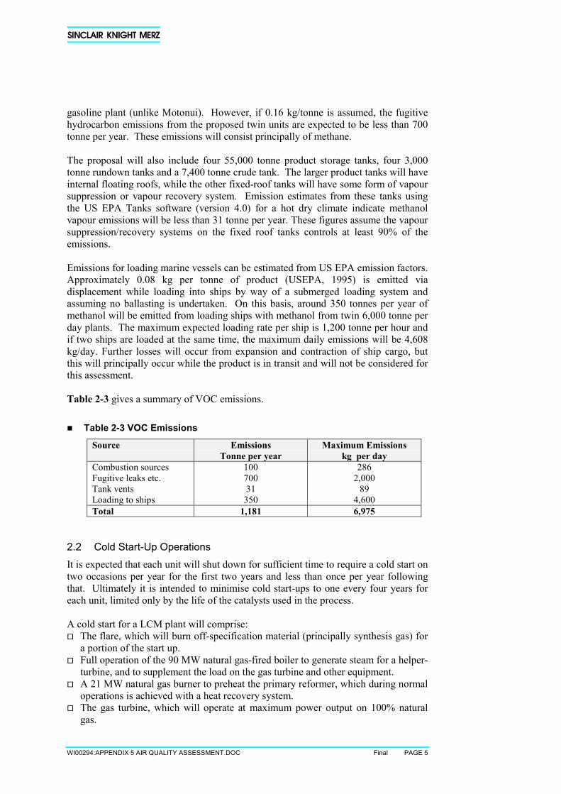
WI00294:APPENDIX 5 AIR QUALITY ASSESSMENT.DOC Final PAGE 5
gasoline plant (unlike Motonui). However, if 0.16 kg/tonne is assumed, the fugitivehydrocarbon emissions from the proposed twin units are expected to be less than 700tonne per year. These emissions will consist principally of methane.
The proposal will also include four 55,000 tonne product storage tanks, four 3,000tonne rundown tanks and a 7,400 tonne crude tank. The larger product tanks will haveinternal floating roofs, while the other fixed-roof tanks will have some form of vapoursuppression or vapour recovery system. Emission estimates from these tanks usingthe US EPA Tanks software (version 4.0) for a hot dry climate indicate methanolvapour emissions will be less than 31 tonne per year. These figures assume the vapoursuppression/recovery systems on the fixed roof tanks controls at least 90% of theemissions.
Emissions for loading marine vessels can be estimated from US EPA emission factors.Approximately 0.08 kg per tonne of product (USEPA, 1995) is emitted viadisplacement while loading into ships by way of a submerged loading system andassuming no ballasting is undertaken. On this basis, around 350 tonnes per year ofmethanol will be emitted from loading ships with methanol from twin 6,000 tonne perday plants. The maximum expected loading rate per ship is 1,200 tonne per hour andif two ships are loaded at the same time, the maximum daily emissions will be 4,608kg/day. Further losses will occur from expansion and contraction of ship cargo, butthis will principally occur while the product is in transit and will not be considered forthis assessment.
Table 2-3 gives a summary of VOC emissions.
� Table 2-3 VOC Emissions
Source EmissionsTonne per year
Maximum Emissionskg per day
Combustion sourcesFugitive leaks etc.Tank ventsLoading to ships
10070031
350
2862,000
894,600
Total 1,181 6,975
2.2 Cold Start-Up OperationsIt is expected that each unit will shut down for sufficient time to require a cold start ontwo occasions per year for the first two years and less than once per year followingthat. Ultimately it is intended to minimise cold start-ups to one every four years foreach unit, limited only by the life of the catalysts used in the process.
A cold start for a LCM plant will comprise:� The flare, which will burn off-specification material (principally synthesis gas) for
a portion of the start up.� Full operation of the 90 MW natural gas-fired boiler to generate steam for a helper-
turbine, and to supplement the load on the gas turbine and other equipment.� A 21 MW natural gas burner to preheat the primary reformer, which during normal
operations is achieved with a heat recovery system.� The gas turbine, which will operate at maximum power output on 100% natural
gas.
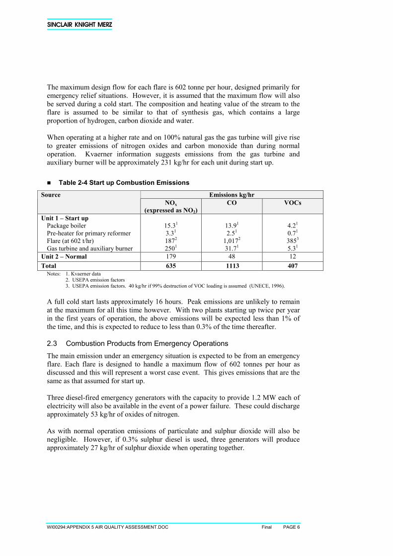
WI00294:APPENDIX 5 AIR QUALITY ASSESSMENT.DOC Final PAGE 6
The maximum design flow for each flare is 602 tonne per hour, designed primarily foremergency relief situations. However, it is assumed that the maximum flow will alsobe served during a cold start. The composition and heating value of the stream to theflare is assumed to be similar to that of synthesis gas, which contains a largeproportion of hydrogen, carbon dioxide and water.
When operating at a higher rate and on 100% natural gas the gas turbine will give riseto greater emissions of nitrogen oxides and carbon monoxide than during normaloperation. Kvaerner information suggests emissions from the gas turbine andauxiliary burner will be approximately 231 kg/hr for each unit during start up.
� Table 2-4 Start up Combustion Emissions
Emissions kg/hrSourceNOx
(expressed as NO2)CO VOCs
Unit 1 – Start upPackage boilerPre-heater for primary reformerFlare (at 602 t/hr)Gas turbine and auxiliary burner
15.31
3.31
1872
2501
13.91
2.51
1,0172
31.71
4.21
0.71
3853
5.31
Unit 2 – Normal 179 48 12Total 635 1113 407
Notes: 1. Kvaerner data2. USEPA emission factors3. USEPA emission factors. 40 kg/hr if 99% destruction of VOC loading is assumed (UNECE, 1996).
A full cold start lasts approximately 16 hours. Peak emissions are unlikely to remainat the maximum for all this time however. With two plants starting up twice per yearin the first years of operation, the above emissions will be expected less than 1% ofthe time, and this is expected to reduce to less than 0.3% of the time thereafter.
2.3 Combustion Products from Emergency OperationsThe main emission under an emergency situation is expected to be from an emergencyflare. Each flare is designed to handle a maximum flow of 602 tonnes per hour asdiscussed and this will represent a worst case event. This gives emissions that are thesame as that assumed for start up.
Three diesel-fired emergency generators with the capacity to provide 1.2 MW each ofelectricity will also be available in the event of a power failure. These could dischargeapproximately 53 kg/hr of oxides of nitrogen.
As with normal operation emissions of particulate and sulphur dioxide will also benegligible. However, if 0.3% sulphur diesel is used, three generators will produceapproximately 27 kg/hr of sulphur dioxide when operating together.
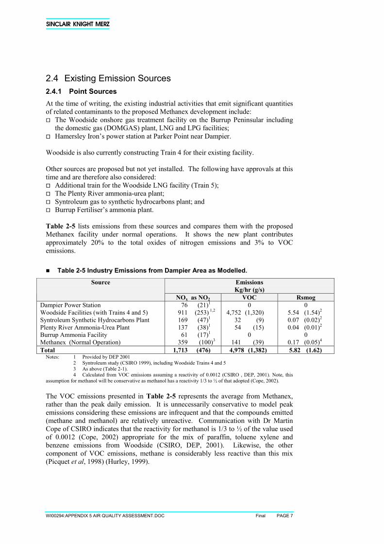
WI00294:APPENDIX 5 AIR QUALITY ASSESSMENT.DOC Final PAGE 7
2.4 Existing Emission Sources2.4.1 Point SourcesAt the time of writing, the existing industrial activities that emit significant quantitiesof related contaminants to the proposed Methanex development include:� The Woodside onshore gas treatment facility on the Burrup Peninsular including
the domestic gas (DOMGAS) plant, LNG and LPG facilities;� Hamersley Iron’s power station at Parker Point near Dampier.
Woodside is also currently constructing Train 4 for their existing facility.
Other sources are proposed but not yet installed. The following have approvals at thistime and are therefore also considered:� Additional train for the Woodside LNG facility (Train 5);� The Plenty River ammonia-urea plant;� Syntroleum gas to synthetic hydrocarbons plant; and� Burrup Fertiliser’s ammonia plant.
Table 2-5 lists emissions from these sources and compares them with the proposedMethanex facility under normal operations. It shows the new plant contributesapproximately 20% to the total oxides of nitrogen emissions and 3% to VOCemissions.
� Table 2-5 Industry Emissions from Dampier Area as Modelled.
EmissionsKg/hr (g/s)
Source
NOx as NO2 VOC RsmogDampier Power StationWoodside Facilities (with Trains 4 and 5)Syntroleum Synthetic Hydrocarbons PlantPlenty River Ammonia-Urea PlantBurrup Ammonia FacilityMethanex (Normal Operation)
76 (21)1
911 (253) 1,2
169 (47)1
137 (38)1
61 (17)1
359 (100)3
04,752 (1,320)
32 (9)54 (15)
0141 (39)
05.54 (1.54)2
0.07 (0.02)2
0.04 (0.01)2
00.17 (0.05)4
Total 1,713 (476) 4,978 (1,382) 5.82 (1.62)Notes: 1 Provided by DEP 2001
2 Syntroleum study (CSIRO 1999), including Woodside Trains 4 and 53 As above (Table 2-1).4 Calculated from VOC emissions assuming a reactivity of 0.0012 (CSIRO , DEP, 2001). Note, this
assumption for methanol will be conservative as methanol has a reactivity 1/3 to ½ of that adopted (Cope, 2002).
The VOC emissions presented in Table 2-5 represents the average from Methanex,rather than the peak daily emission. It is unnecessarily conservative to model peakemissions considering these emissions are infrequent and that the compounds emitted(methane and methanol) are relatively unreactive. Communication with Dr MartinCope of CSIRO indicates that the reactivity for methanol is 1/3 to ½ of the value usedof 0.0012 (Cope, 2002) appropriate for the mix of paraffin, toluene xylene andbenzene emissions from Woodside (CSIRO, DEP, 2001). Likewise, the othercomponent of VOC emissions, methane is considerably less reactive than this mix(Picquet et al, 1998) (Hurley, 1999).
WI00294:APPENDIX 5 AIR QUALITY ASSESSMENT.DOC Final PAGE 8
2.4.2 Area and Biogenic EmissionsAs part of the assessment of photochemical reactions, it is necessary to also accountfor both biogenic and area source emissions from the general area. A recent study ofthe Pilbara region undertaken by CSIRO Atmospheric Research and the Departmentof Environmental Protection (CSIRO, DEP, 2001) has evaluated these emissions withrespect to determining appropriate dispersion models for the region. The relevant datainput files for TAPM used were provided by the CSIRO1.
These data have accounted for NOx and VOC emissions from soils etc. and from theDampier and Karratha townships, significant main roads, and various shippingactivities. Average values were assigned and assumed to remain constant throughoutthe year. The CSIRO/DOE (CSIRO, DEP, 2001) report gives details on theseemissions data.
1 Bill Physick, personal Communications, December 2001.
WI00294:APPENDIX 5 AIR QUALITY ASSESSMENT.DOC Final PAGE 9
3. Air Quality Criteria3.1 Stack Emissions from Gas TurbinesAs discussed in Section 2, if LCM technology is used, the principal emissions sourcefrom the proposed methanol plant will be the gas turbine system. The EnvironmentalProtection Authority (EPA) has developed a guidance statement for oxides of nitrogenemissions from gas turbines, with limits for emissions following the AEC/NHMRCNational Guidelines. These limits are 0.07 g/m3 (STP, dry and 15% O2) for “gaseousfuels” and 0.15 g/m3 for “other fuels”. The Guidance Statement goes on to say thatmodern natural gas-fired systems, employing NOx control technology can be expectedto achieve lower emissions than 0.07 g/m3.
In this case, the presence of hydrogen in the fuel limits the ability to employ NOxcontrol technology. Common methods, such as low- NOx burners or steam injectioncannot be used. Nitrogen injection may be possible but this is unlikely to be aseffective. The ability to recycle purge gas (containing hydrogen) as fuel is animportant part of the overall energy efficiency of the process and helps to minimisecarbon dioxide emissions. Consequently the EPA’s emission criteria for “gaseousfuels” or for natural gas are not appropriate for the proposed plant.
While low NOx burners cannot be employed, the presence of inert gases and therelatively low calorific value of the fuel mix will act to suppress NOx formation byproducing low combustion temperatures. Information from Kvaerner suggests theNOx concentration in the gas turbine flue gases will be approximately 0.24 g/m3
during normal operation.
Therefore, LCM gas turbines are unlikely to meet the EPA guidance criteria but allpracticable steps will be taken to reduce NOx emissions thus satisfying the EPArequirement that “all reasonable and practicable measures should be taken tominimise the discharge...”
3.2 Ambient Air Quality StandardsTable 3-1 lists the National Environmental Protection Measure (NEPM) for therelevant air pollutants.
� Table 3-1 National Environmental Protection Measures for NO2 and Ozone
Pollutant Averaging Period MaximumConcentration ppb (µµµµg/m3)
Goal within 10 years(maximum allowable
exceedences)Nitrogen dioxide
Photochemicaloxidants (as ozone)
1-hourAnnual1-hour4-hours
120 (246)30 (62)
100 (214)80 (171)
1 day a yearnone
1 day a year1 day a year

WI00294:APPENDIX 5 AIR QUALITY ASSESSMENT.DOC Final PAGE 10
These standards have not been implemented in legislation throughout WesternAustralia but the WA DEP intend to implement them through the development of astate wide Environmental Policy.
These standards apply outside industrial areas and residence-free buffer areas aroundindustrial estates. With no formally defined industrial buffer zone applied to theBurrup Peninsula, the standards may be relevant to areas outside those identified forindustrial use in the Burrup Peninsula Land Use Plan and Management Strategy. It isrelevant to note that many of the high model predictions, described in Section 5 of thisreport, occur within industrial areas (shown as purple and orange in Figures 5-1 to5-3).
WI00294:APPENDIX 5 AIR QUALITY ASSESSMENT.DOC Final PAGE 11
4. Existing Air QualityThe DEP have a ambient air monitoring site at Dampier, with measurements of ozone,nitric oxide, nitrogen dioxide, carbon monoxide and particulate (PM10). Monitoringhas also been undertaken at King Bay and Karratha for ozone, nitric oxide, nitrogendioxide and sulphur dioxide.
Monitoring at Dampier shows maximum concentrations of all pollutants remain belowthe relevant NEPM standards, with peak concentrations of ozone and nitrogen dioxidereported as being less than 64 ppb and 21 ppb respectively for 1998 and 1999.Monitoring at the other sites shows similar results.
Studies undertaken in the Pilbara region to date indicate that concentrations ofphotochemical pollutants are generally expected to be low throughout the region.However, background TAPM modelling has predicted relatively high peakconcentrations of ozone over the ocean to the west of Dampier and on the Peninsula tothe east of Dampier. There appears to be evidence of re-circulating flows occurring onoccasions with the potential to return pollutants to the sources and towns. Areasources play an important part and the presence of extensive fires during September toNovember also appears to enhance background ozone levels on some days (CSIRO,2001; CSIRO, DEP, 2001).
WI00294:APPENDIX 5 AIR QUALITY ASSESSMENT.DOC Final PAGE 12
5. Atmospheric Dispersion ModellingThree models were used in this assessment:• DISPMOD, the Western Australian coastal model, specifically designed for
Kwinana;• TAPM, the CSIRO’s prognostic meteorological and air pollution model;• AUSPLUME, the Victorian EPA regulatory model that is commonly used
throughout Australia.
A recent evaluation of models for the Pilbara region undertaken by DEP and CSIROhas shown that DISPMOD and TAPM appear to be suitable for predicting ground-level concentrations in the Burrup Peninsula area.
5.1 DISPMODDISPMOD is primarily suitable for near field predictions, particularly for non-reactivegases and is the recommended model for predictions within 2 to 3 km of a source. Ingeneral, it appears that this model is likely to over-predict concentrations but it haslimitations in areas where fumigation of recirculated emissions are involved, or wherearea sources contribute to background emissions. DISPMOD was used in thisassessment to predict concentrations of NOx and nitrogen dioxide for the proposedplant operating as normal and at start up over a 21 by 14 km receptor grid. Themeteorological data used for this assessment was obtained from the Dampiermeteorological site.
Maximum nitrogen dioxide concentrations were estimated from the DISPMODsimulations by conservatively assuming the following relationship for all parts of thegrid.:
NO2 = 0.3NOx + 14.39 for NOx > 20.56 µg/m3
NO2 = NOx for NOx < 20.56
This is based on monitoring data from Dampier, which shows the ratio of NO2 to NOxto generally remain well below 0.3.
DISPMOD was used to model both normal operation and cold start scenarios. Toassess the potential maximum impacts from the flaring operations during a start, theeffective plume height was determined by using the procedures used in the USEPA’sscreening model, SCREEN3.
Appendix A gives examples of DISPMOD input files. All combustion sources areassumed to have 60m chimneys.
5.2 TAPMTAPM was used to model photochemistry. For this purpose, the model simulationwas set up to follow as closely as practicable that used for the Pilbara modelevaluation in 1999 (CSIRO, DEP, 2001). A coarser nested grid spacing for thepollution simulation was used however, since this provides more efficient run times
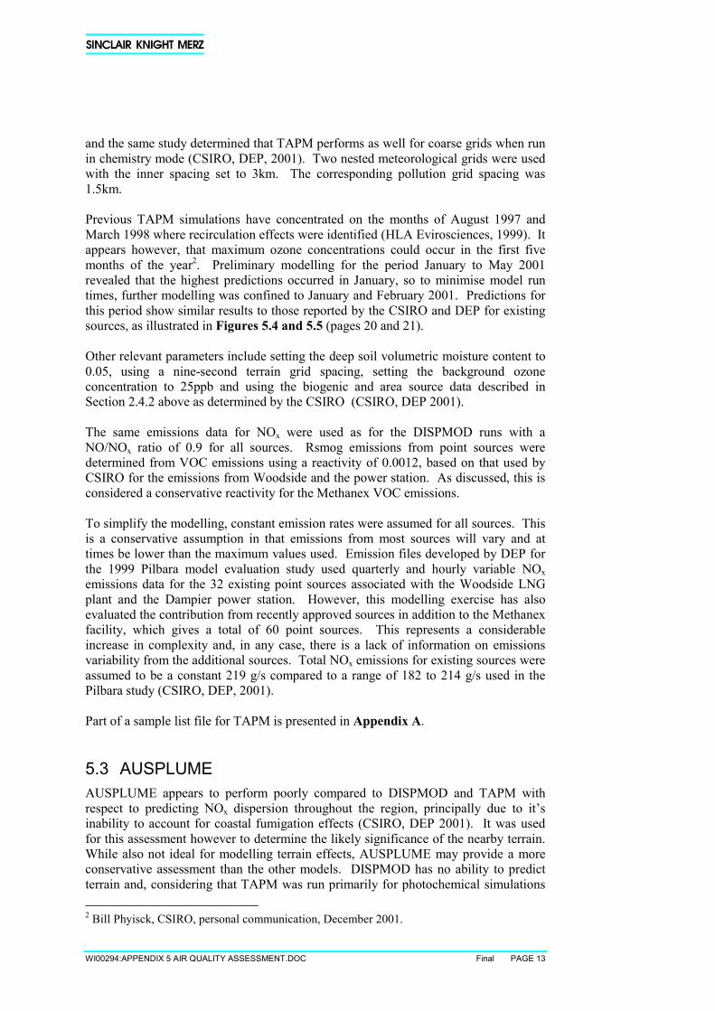
WI00294:APPENDIX 5 AIR QUALITY ASSESSMENT.DOC Final PAGE 13
and the same study determined that TAPM performs as well for coarse grids when runin chemistry mode (CSIRO, DEP, 2001). Two nested meteorological grids were usedwith the inner spacing set to 3km. The corresponding pollution grid spacing was1.5km.
Previous TAPM simulations have concentrated on the months of August 1997 andMarch 1998 where recirculation effects were identified (HLA Evirosciences, 1999). Itappears however, that maximum ozone concentrations could occur in the first fivemonths of the year2. Preliminary modelling for the period January to May 2001revealed that the highest predictions occurred in January, so to minimise model runtimes, further modelling was confined to January and February 2001. Predictions forthis period show similar results to those reported by the CSIRO and DEP for existingsources, as illustrated in Figures 5.4 and 5.5 (pages 20 and 21).
Other relevant parameters include setting the deep soil volumetric moisture content to0.05, using a nine-second terrain grid spacing, setting the background ozoneconcentration to 25ppb and using the biogenic and area source data described inSection 2.4.2 above as determined by the CSIRO (CSIRO, DEP 2001).
The same emissions data for NOx were used as for the DISPMOD runs with aNO/NOx ratio of 0.9 for all sources. Rsmog emissions from point sources weredetermined from VOC emissions using a reactivity of 0.0012, based on that used byCSIRO for the emissions from Woodside and the power station. As discussed, this isconsidered a conservative reactivity for the Methanex VOC emissions.
To simplify the modelling, constant emission rates were assumed for all sources. Thisis a conservative assumption in that emissions from most sources will vary and attimes be lower than the maximum values used. Emission files developed by DEP forthe 1999 Pilbara model evaluation study used quarterly and hourly variable NOxemissions data for the 32 existing point sources associated with the Woodside LNGplant and the Dampier power station. However, this modelling exercise has alsoevaluated the contribution from recently approved sources in addition to the Methanexfacility, which gives a total of 60 point sources. This represents a considerableincrease in complexity and, in any case, there is a lack of information on emissionsvariability from the additional sources. Total NOx emissions for existing sources wereassumed to be a constant 219 g/s compared to a range of 182 to 214 g/s used in thePilbara study (CSIRO, DEP, 2001).
Part of a sample list file for TAPM is presented in Appendix A.
5.3 AUSPLUMEAUSPLUME appears to perform poorly compared to DISPMOD and TAPM withrespect to predicting NOx dispersion throughout the region, principally due to it’sinability to account for coastal fumigation effects (CSIRO, DEP 2001). It was usedfor this assessment however to determine the likely significance of the nearby terrain.While also not ideal for modelling terrain effects, AUSPLUME may provide a moreconservative assessment than the other models. DISPMOD has no ability to predictterrain and, considering that TAPM was run primarily for photochemical simulations 2 Bill Phyisck, CSIRO, personal communication, December 2001.
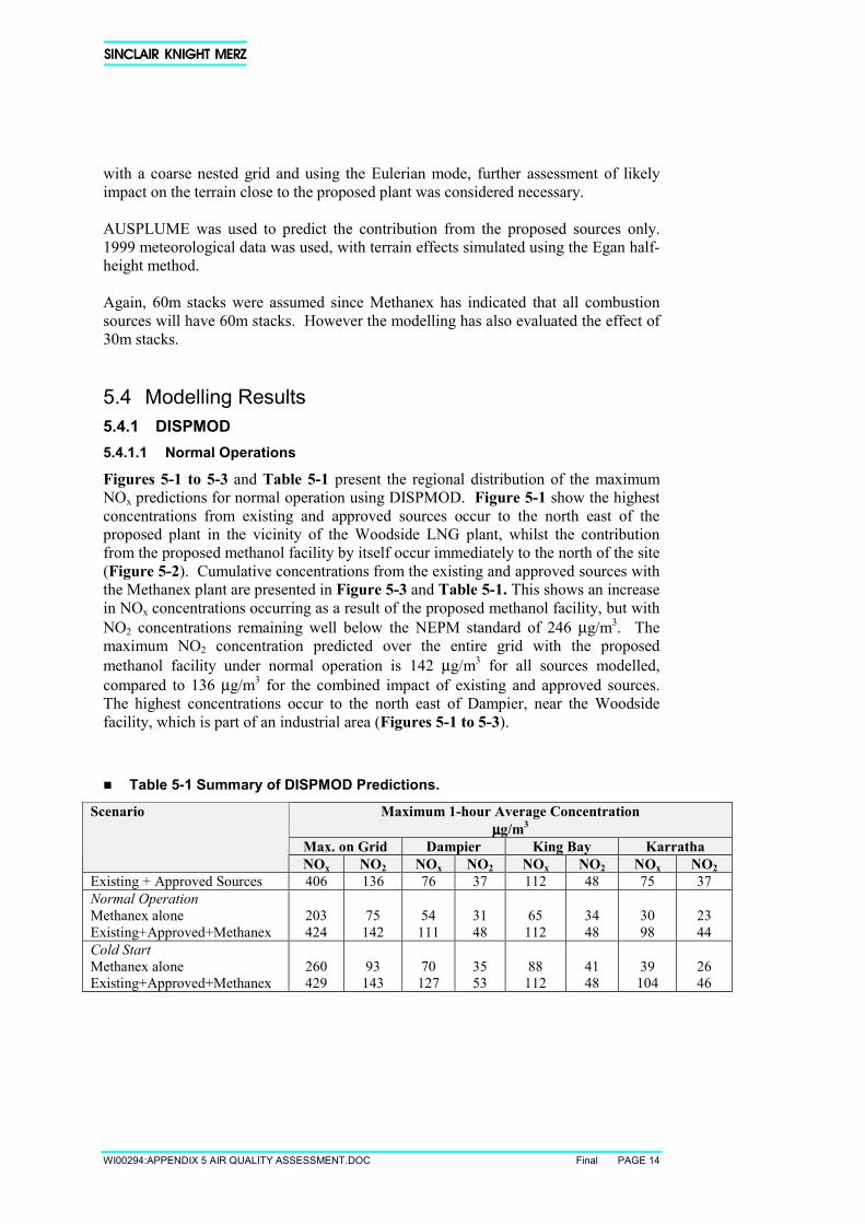
WI00294:APPENDIX 5 AIR QUALITY ASSESSMENT.DOC Final PAGE 14
with a coarse nested grid and using the Eulerian mode, further assessment of likelyimpact on the terrain close to the proposed plant was considered necessary.
AUSPLUME was used to predict the contribution from the proposed sources only.1999 meteorological data was used, with terrain effects simulated using the Egan half-height method.
Again, 60m stacks were assumed since Methanex has indicated that all combustionsources will have 60m stacks. However the modelling has also evaluated the effect of30m stacks.
5.4 Modelling Results5.4.1 DISPMOD5.4.1.1 Normal Operations
Figures 5-1 to 5-3 and Table 5-1 present the regional distribution of the maximumNOx predictions for normal operation using DISPMOD. Figure 5-1 show the highestconcentrations from existing and approved sources occur to the north east of theproposed plant in the vicinity of the Woodside LNG plant, whilst the contributionfrom the proposed methanol facility by itself occur immediately to the north of the site(Figure 5-2). Cumulative concentrations from the existing and approved sources withthe Methanex plant are presented in Figure 5-3 and Table 5-1. This shows an increasein NOx concentrations occurring as a result of the proposed methanol facility, but withNO2 concentrations remaining well below the NEPM standard of 246 µg/m3. Themaximum NO2 concentration predicted over the entire grid with the proposedmethanol facility under normal operation is 142 µg/m3 for all sources modelled,compared to 136 µg/m3 for the combined impact of existing and approved sources.The highest concentrations occur to the north east of Dampier, near the Woodsidefacility, which is part of an industrial area (Figures 5-1 to 5-3).
� Table 5-1 Summary of DISPMOD Predictions.
Maximum 1-hour Average Concentrationµµµµg/m3
Max. on Grid Dampier King Bay Karratha
Scenario
NOx NO2 NOx NO2 NOx NO2 NOx NO2Existing + Approved Sources 406 136 76 37 112 48 75 37Normal OperationMethanex aloneExisting+Approved+Methanex
203424
75142
54111
3148
65112
3448
3098
2344
Cold StartMethanex aloneExisting+Approved+Methanex
260429
93143
70127
3553
88112
4148
39104
2646
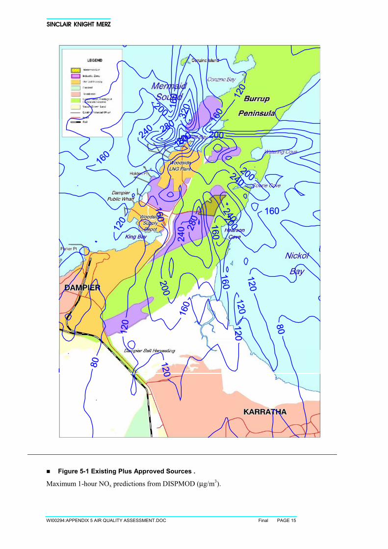
WI00294:APPENDIX 5 AIR QUALITY ASSESSMENT.DOC Final PAGE 15
� Figure 5-1 Existing Plus Approved Sources .
Maximum 1-hour NOx predictions from DISPMOD (µg/m3).
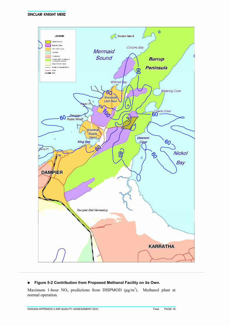
WI00294:APPENDIX 5 AIR QUALITY ASSESSMENT.DOC Final PAGE 16
� Figure 5-2 Contribution from Proposed Methanol Facility on its Own.
Maximum 1-hour NOx predictions from DISPMOD (µg/m3). Methanol plant atnormal operation.
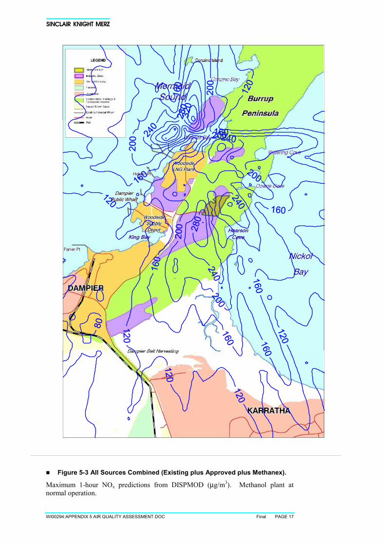
WI00294:APPENDIX 5 AIR QUALITY ASSESSMENT.DOC Final PAGE 17
� Figure 5-3 All Sources Combined (Existing plus Approved plus Methanex).
Maximum 1-hour NOx predictions from DISPMOD (µg/m3). Methanol plant atnormal operation.
WI00294:APPENDIX 5 AIR QUALITY ASSESSMENT.DOC Final PAGE 18
5.4.1.2 Start ups and Upset Conditions
As described in Section 2.2 under cold start ups emissions from the flare and auxiliaryboiler will be much greater than under normal operations and potentially may lead tohigher ground level concentrations. Maximum predicted concentration of NO2 arepresented in Table 5-1 and indicate that the maximum on the modelled grid is143 µg/m3. This is a slight increase over that from normal operations, but still wellbelow the NEPM standards. At Dampier, NO2 concentrations may increase from thatpredicted from the existing and approved sources by approximately 40%. Howeverthe maximum prediction is still low in relation to the NEPM standard. Moreover,these predictions assume a cold start coincides with worst-case meteorology. Giventhat start-up conditions will last no longer than 16 hours per start (0.3% of the time fortwo starts per year), the probability of this occurring is very low. Consequently theimpact of a cold start is likely to be considerably less than predicted.
Emissions from an emergency flare will be similar to that from start up (see Section2.2) and therefore will potentially result in the same ground level concentrations aspresented for the start up case.
5.4.2 TAPMThe peak TAPM predictions for ozone are similar to those reported by CSIRO/DEP in1999, as illustrated in the top contour plots in Figure 5-7 and 5-8 (second highestpredictions). Slight differences can be attributed to the shorter modelling period (twomonths compared to almost year) and that 2001 was used instead of 1999. However,the results confirm the choice of January to February is appropriate for assessingworse case photochemical conditions. Figure 5-8 shows lower existing NO2concentrations than reported for 1999 but this reflects the January-February periodbeing conducive to high ozone concentrations rather than NO2.
Summaries of maximum TAPM predictions for each emission scenario are presentedin Tables 5-2 and 5-3. These results generally show a small incremental decrease inozone concentrations when the combined impact from all sources is compared to theexisting situation. The NO2 concentrations are generally predicted to increase,particularly at Karratha where a 50% increase in peak concentrations over the existingscenario may be observed. The apparent slight decrease in maximum NO2 predictionsat some receptors is related to the non-linearity of the chemistry model and possiblythe effect of modelling inaccuracies associated with using a relatively course Euleriangrid.
Concentrations of NO2 at all receptors remain well below the NEPM standard with amaximum prediction for NO2 of 139 µg/m3 over the grid, similar to the DISPMODprediction of 142 µg/m3 described above (Table 5-1).
� Table 5-2 Summary of Maximum TAPM Predictions – NO2
Maximum 1-hour Concentration (Jan-Feb 2001) ppb (µµµµg/m3 as NO2)
Scenario
Max on Grid Dampier King Bay KarrathaExisting SourcesExisting + ApprovedExisting+Approved+Methanex
47 (97)70 (144)68 (139)
17 (35)17 (35)21 (43)
19 (39)20 (41)19 (39)
13 (27)16 (33)19 (39)
WI00294:APPENDIX 5 AIR QUALITY ASSESSMENT.DOC Final PAGE 19
� Table 5-3 Summary of Maximum TAPM Predictions – O3
Maximum 1-hour Concentration (Jan-Feb 2001) ppb (µµµµg/m3)
Scenario
Max on Grid Dampier King Bay KarrathaExisting SourcesExisting + ApprovedExisting+Approved+Methanex
121 (257)165 (351)105 (224)
38 (81)28 (60)42 (89)
53 (114)30 (64)52 (112)
43 (93)32 (68)39 (83)
The slight decrease in ozone concentrations at some receptors appears to be due to thearea being sensitive to reactive VOC emissions. The high ratio of oxides of nitrogento reactive organic compounds in the industrial emissions tends to suppress ozoneformation. This is consistent with the Perth photochemical smog study (WP/DEP,1996). In this case the increased NOx, from approved sources in particular, appears tohave reduced ozone production.
However, because there is a relatively large cumulative emission of oxides ofnitrogen, higher ozone concentrations could occur during days when there are higherthan usual background emissions of reactive organics, such as wildfire events. Asdiscussed earlier, the CSIRO and DEP also noted the potential effect of wildfires.These events could increase background ozone concentrations by up to 20ppb duringSeptember to November (CSIRO/DEP). The proposed Methanex facility has littleimpact on this condition however, and it appears that wildfires are not as prevalentduring the worse case months for peak ozone concentrations as predicted by themodelling.
Figures 5-4 to 5-6 show cumulative frequency plots for concentrations for both NO2and ozone at Dampier, King Bay and Karratha. Predictions for existing sources atDampier (Figure 5-4) shows a generally similar ozone distribution to that reported forthe Pilbara study undertaken by DEP/CSIRO. Again, slight differences can beattributed to the different modelling periods. The frequency distributions for ozonechange very slightly when all sources are modelled (existing plus approved plusMethanex) as shown at all three receptors. The contribution from approved sourcesappears to suppress some background peaks, possibly due to the additional NOxemissions, while the Methanex contribution appears to return the ozone peaks.
The geographic distribution of pollutants shows the highest peak concentrations ofozone occur over the ocean to the west of Dampier, and on the peninsular to the north-east (Figure 5-7). There is little change over the existing scenario, apart from anincrease over the ocean to the west of Dampier. The highest NO2 predictions occur onthe peninsular to the east of Dampier.
The maximum peak ozone concentration on the grid exceeds 100 ppb on only one dayfor each scenario modelled. Thus, while industrial emissions may give rise torelatively high peak concentrations on rare occasions, the proposed methanol facilitymakes little impact on the frequency of any excursions. Figure 5-9 demonstrates asmall change in the frequency of excursions above 75ppb.
Appendix C gives time series plots for ozone (cumulative sources) and relevantmeteorological conditions for January as modelled by TAPM.
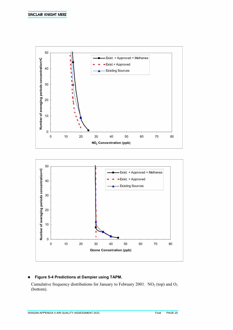
WI00294:APPENDIX 5 AIR QUALITY ASSESSMENT.DOC Final PAGE 20
� Figure 5-4 Predictions at Dampier using TAPM.
Cumulative frequency distributions for January to February 2001. NO2 (top) and O3(bottom).
0
10
20
30
40
50
0 10 20 30 40 50 60 70 80
NO2 Concentration (ppb)
Num
ber o
f ave
ragi
ng p
erio
ds c
once
ntra
tion>
C Exist. + Approved + Methanex
Exist.+ Approved
Existing Sources
0
10
20
30
40
50
0 10 20 30 40 50 60 70 80
Ozone Concetration (ppb)
Num
ber o
f ave
ragi
ng p
erio
ds c
once
ntra
tion>
C
Exist. + Approved + Methanex
Exist. + Approved
Existing Sources
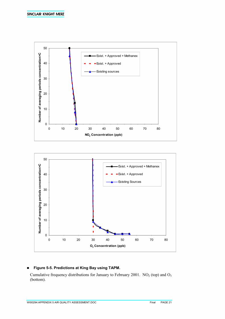
WI00294:APPENDIX 5 AIR QUALITY ASSESSMENT.DOC Final PAGE 21
� Figure 5-5. Predictions at King Bay using TAPM.
Cumulative frequency distributions for January to February 2001. NO2 (top) and O3(bottom).
0
10
20
30
40
50
0 10 20 30 40 50 60 70 80
NO2 Concentration (ppb)
Num
ber o
f ave
ragi
ng p
erio
ds c
once
ntra
tion>
C Exist. + Approved + Methanex
Exist. + Approved
Existing sources
0
10
20
30
40
50
0 10 20 30 40 50 60 70 80
O3 Concentration (ppb)
Num
ber o
f ave
ragi
ng p
erio
ds c
once
ntra
tion>
C Exist. + Approved + Methanex
Exist. + Approved
Existing Sources
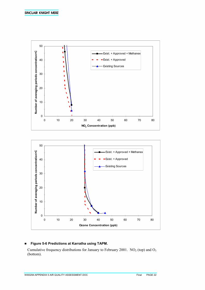
WI00294:APPENDIX 5 AIR QUALITY ASSESSMENT.DOC Final PAGE 22
� Figure 5-6 Predictions at Karratha using TAPM.
Cumulative frequency distributions for January to February 2001. NO2 (top) and O3(bottom).
0
10
20
30
40
50
0 10 20 30 40 50 60 70 80
NO2 Concentration (ppb)
Num
ber o
f ave
ragi
ng p
erio
ds c
once
ntra
tion>
C Exist. + Approved + Methanex
Exist. + Approved
Existing Sources
0
10
20
30
40
50
0 10 20 30 40 50 60 70 80
Ozone Concentration (ppb)
Num
ber o
f ave
ragi
ng p
erio
ds c
once
ntra
tion>
C Exist. + Approved + Methanex
Exist. + Approved
Existing Sources
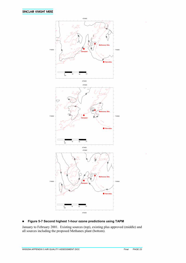
WI00294:APPENDIX 5 AIR QUALITY ASSESSMENT.DOC Final PAGE 23
� Figure 5-7 Second highest 1-hour ozone predictions using TAPM
January to February 2001. Existing sources (top), existing plus approved (middle) andall sources including the proposed Methanex plant (bottom).
6 12 18 21km
716500
470400
716500
470400
Dampier
Karratha
Methanex Site
6 12 18 21km
716500
470400
716500
470400
Dampier
Karratha
Methanex Site
6 12 18 21km
716500
470400
716500
470400
Dampier
Karratha
Methanex Site
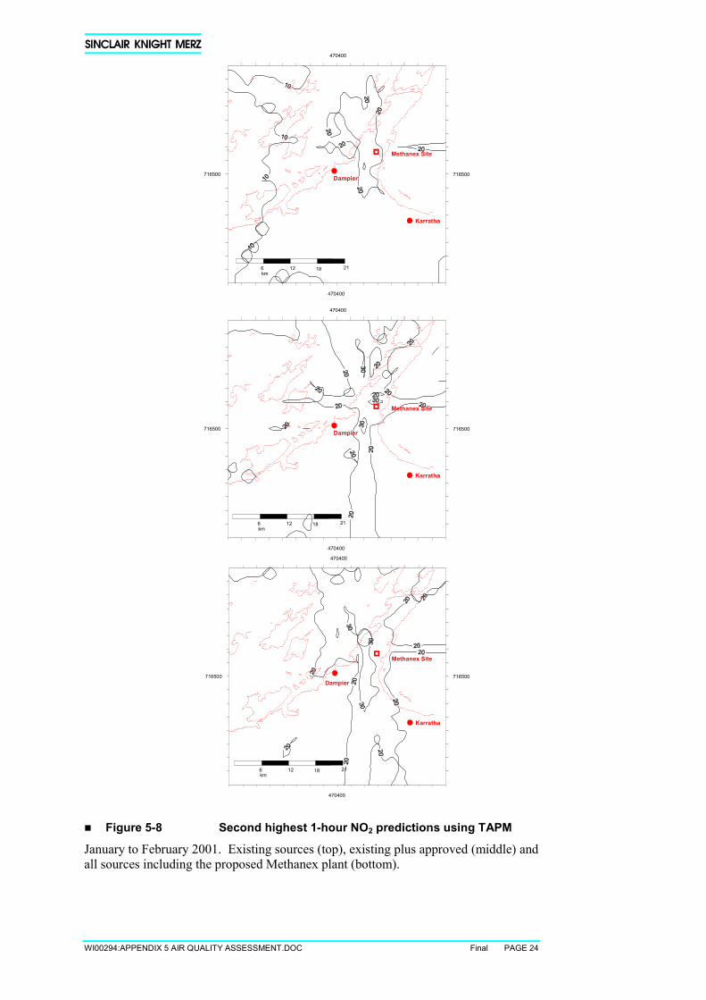
WI00294:APPENDIX 5 AIR QUALITY ASSESSMENT.DOC Final PAGE 24
� Figure 5-8 Second highest 1-hour NO2 predictions using TAPM
January to February 2001. Existing sources (top), existing plus approved (middle) andall sources including the proposed Methanex plant (bottom).
6 12 18 21km
716500
470400
716500
470400
Dampier
Karratha
Methanex Site
6 12 18 21km
716500
470400
716500
470400
Dampier
Karratha
Methanex Site
6 12 18 21km
716500
470400
716500
470400
Dampier
Karratha
Methanex Site
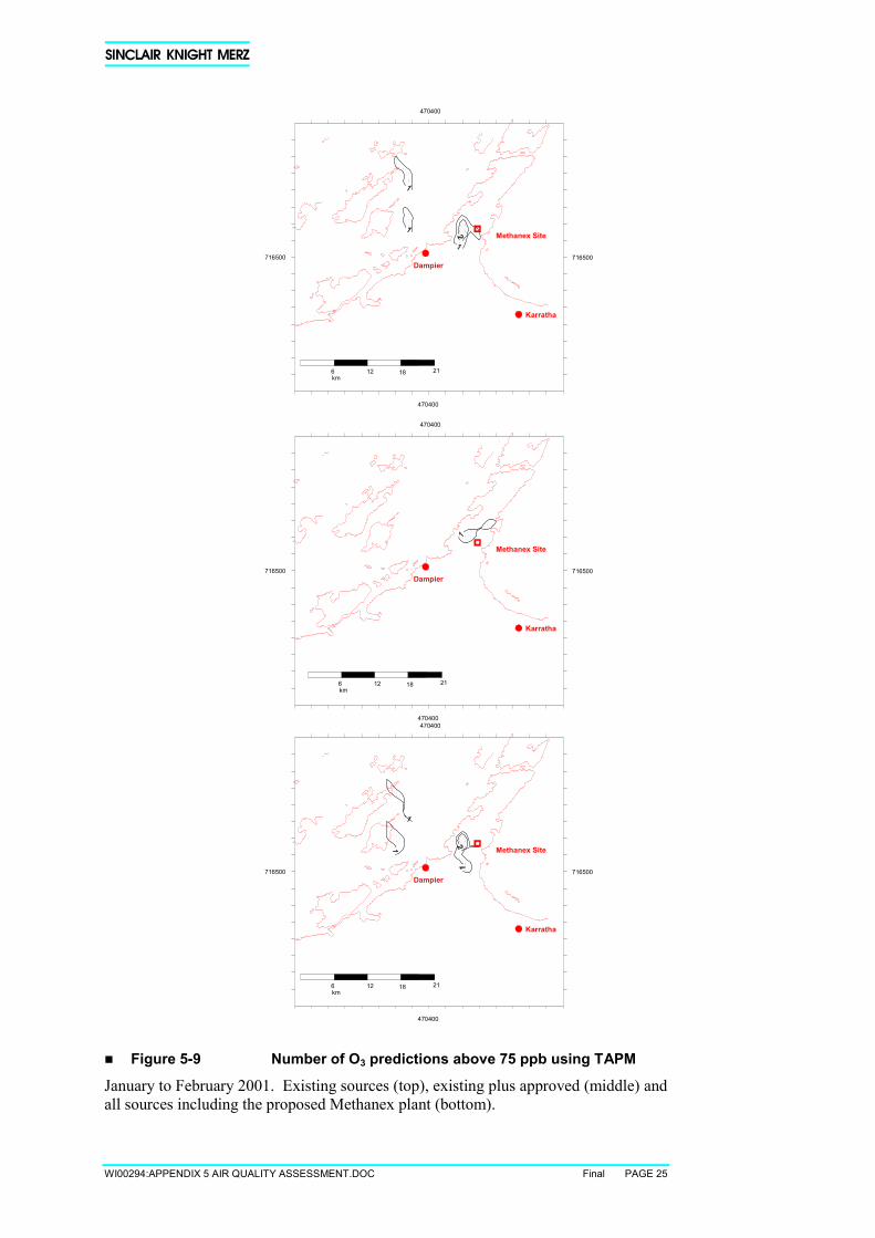
WI00294:APPENDIX 5 AIR QUALITY ASSESSMENT.DOC Final PAGE 25
� Figure 5-9 Number of O3 predictions above 75 ppb using TAPM
January to February 2001. Existing sources (top), existing plus approved (middle) andall sources including the proposed Methanex plant (bottom).
6 12 18 21km
716500
470400
716500
470400
Dampier
Karratha
Methanex Site
6 12 18 21km
716500
470400
716500
470400
Dampier
Karratha
Methanex Site
6 12 18 21km
716500
470400
716500
470400
Dampier
Karratha
Methanex Site
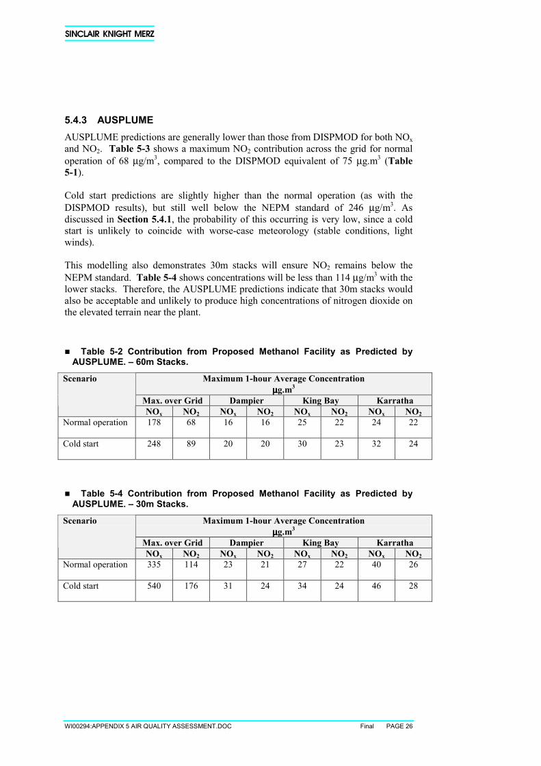
WI00294:APPENDIX 5 AIR QUALITY ASSESSMENT.DOC Final PAGE 26
5.4.3 AUSPLUMEAUSPLUME predictions are generally lower than those from DISPMOD for both NOxand NO2. Table 5-3 shows a maximum NO2 contribution across the grid for normaloperation of 68 µg/m3, compared to the DISPMOD equivalent of 75 µg.m3 (Table5-1).
Cold start predictions are slightly higher than the normal operation (as with theDISPMOD results), but still well below the NEPM standard of 246 µg/m3. Asdiscussed in Section 5.4.1, the probability of this occurring is very low, since a coldstart is unlikely to coincide with worse-case meteorology (stable conditions, lightwinds).
This modelling also demonstrates 30m stacks will ensure NO2 remains below theNEPM standard. Table 5-4 shows concentrations will be less than 114 µg/m3 with thelower stacks. Therefore, the AUSPLUME predictions indicate that 30m stacks wouldalso be acceptable and unlikely to produce high concentrations of nitrogen dioxide onthe elevated terrain near the plant.
� Table 5-2 Contribution from Proposed Methanol Facility as Predicted byAUSPLUME. – 60m Stacks.
Maximum 1-hour Average Concentrationµµµµg.m3
Max. over Grid Dampier King Bay Karratha
Scenario
NOx NO2 NOx NO2 NOx NO2 NOx NO2Normal operation 178 68 16 16 25 22 24 22
Cold start 248 89 20 20 30 23 32 24
� Table 5-4 Contribution from Proposed Methanol Facility as Predicted byAUSPLUME. – 30m Stacks.
Maximum 1-hour Average Concentrationµµµµg.m3
Max. over Grid Dampier King Bay Karratha
Scenario
NOx NO2 NOx NO2 NOx NO2 NOx NO2Normal operation 335 114 23 21 27 22 40 26
Cold start 540 176 31 24 34 24 46 28

WI00294:APPENDIX 5 AIR QUALITY ASSESSMENT.DOC Final PAGE 27
6. ReferencesCSIRO, 1999 Assessment of the Impact on Air Quality of a Proposed Gas- to-OilPlant on the Burrup Peninsula, Western Australia; CSIRO Atmospheric Research,October 1999.
CSIRO, 2001 Meteorology and Air Quality of the Pilbara Region; CSIROAtmospheric Research, May 2001.
CSIRO, DEP, 2001 An Evaluation of Air Quality Models for the Pilbara Region;CSIRO Atmospheric Research, Department of Environmental Protection W.A., June2001.
Hurley P., 1999, The Air Pollution Model (TAPM) Version 1: Technical Descriptionand Examples. CSIRO Atmospheric Research, Technical paper No. 43.
Kvaerner, 2001 2X6000MTPD LCM Methanol Plant – Darwin Process FlowDiagrams. Prepared for Methanex Ltd. KV Nos. 10406-00-F0001 to F0031.
Kvaerner, 2002. NOx Emissions. Email correspondence to Methanex Australia,February 2002.
Methanex NZ Ltd., 1996, Evaluating Methanex NZ’s Air Emissions, October 1996
Picquet B., Heroux S., Chebbi A., Doussin J., Durand-Jolibois R., Monod A., LoiratH., Carlier P., Kinetics of the Reactions of OH Radicals with Some OxygenatedVolatile Organic Compounds Under Simulated Atmospheric Conditions. LaboratoireInteruniversitaire des Systemes Atmospheriques, UMR-CNRS, Universite de Paris,France
US EPA 1995, Compilation of Air Pollution Emission Factors AP-42, Fifth Edition,Volume 1. Chapter 5.2, Transportation and Marketing of Petroleum Products.
UNECE, 1996. Emission Inventory Guidebook. VOC Expert Panel EnvironmentCanada Conservation and Protection Pollution Data Analysis Division, Quebec.
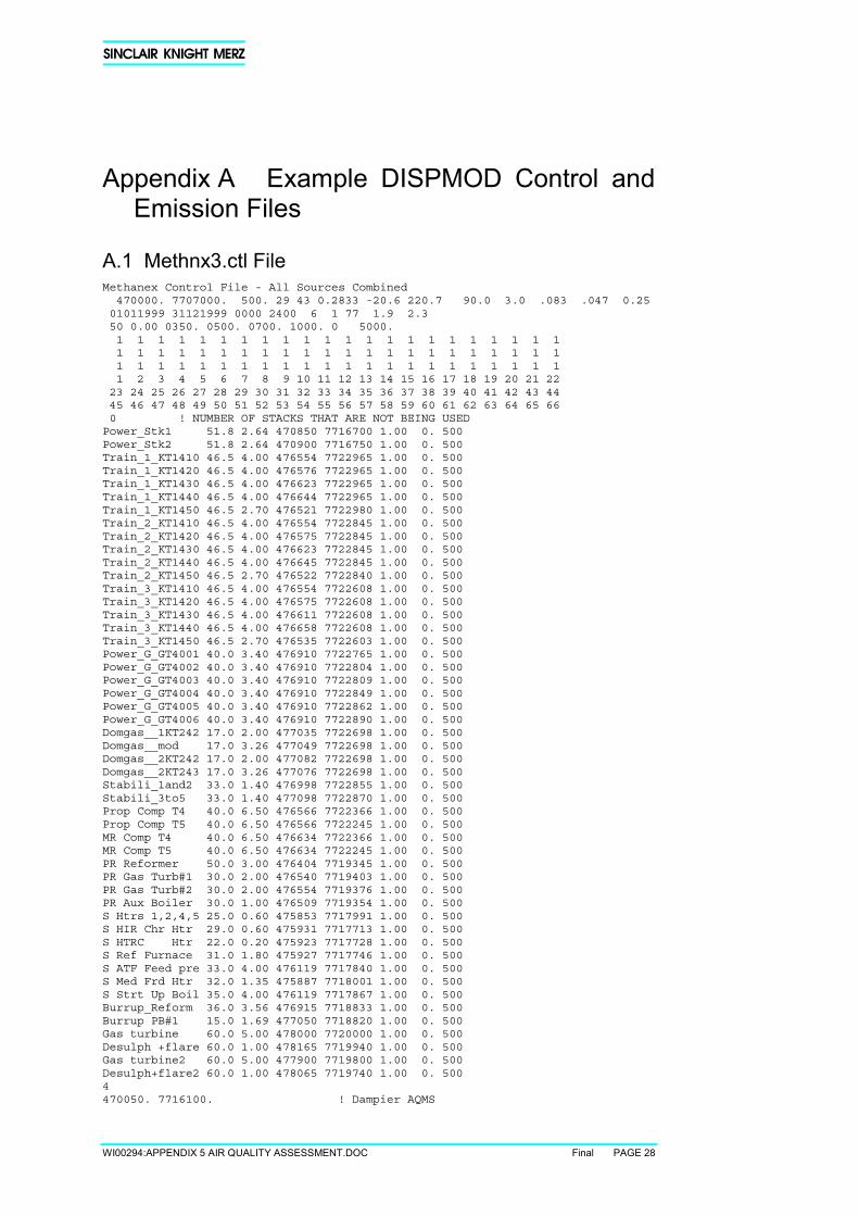
WI00294:APPENDIX 5 AIR QUALITY ASSESSMENT.DOC Final PAGE 28
Appendix A Example DISPMOD Control andEmission Files
A.1 Methnx3.ctl FileMethanex Control File - All Sources Combined470000. 7707000. 500. 29 43 0.2833 -20.6 220.7 90.0 3.0 .083 .047 0.2501011999 31121999 0000 2400 6 1 77 1.9 2.350 0.00 0350. 0500. 0700. 1000. 0 5000.1 1 1 1 1 1 1 1 1 1 1 1 1 1 1 1 1 1 1 1 1 11 1 1 1 1 1 1 1 1 1 1 1 1 1 1 1 1 1 1 1 1 11 1 1 1 1 1 1 1 1 1 1 1 1 1 1 1 1 1 1 1 1 11 2 3 4 5 6 7 8 9 10 11 12 13 14 15 16 17 18 19 20 21 2223 24 25 26 27 28 29 30 31 32 33 34 35 36 37 38 39 40 41 42 43 4445 46 47 48 49 50 51 52 53 54 55 56 57 58 59 60 61 62 63 64 65 660 ! NUMBER OF STACKS THAT ARE NOT BEING USEDPower_Stk1 51.8 2.64 470850 7716700 1.00 0. 500Power_Stk2 51.8 2.64 470900 7716750 1.00 0. 500Train_1_KT1410 46.5 4.00 476554 7722965 1.00 0. 500Train_1_KT1420 46.5 4.00 476576 7722965 1.00 0. 500Train_1_KT1430 46.5 4.00 476623 7722965 1.00 0. 500Train_1_KT1440 46.5 4.00 476644 7722965 1.00 0. 500Train_1_KT1450 46.5 2.70 476521 7722980 1.00 0. 500Train_2_KT1410 46.5 4.00 476554 7722845 1.00 0. 500Train_2_KT1420 46.5 4.00 476575 7722845 1.00 0. 500Train_2_KT1430 46.5 4.00 476623 7722845 1.00 0. 500Train_2_KT1440 46.5 4.00 476645 7722845 1.00 0. 500Train_2_KT1450 46.5 2.70 476522 7722840 1.00 0. 500Train_3_KT1410 46.5 4.00 476554 7722608 1.00 0. 500Train_3_KT1420 46.5 4.00 476575 7722608 1.00 0. 500Train_3_KT1430 46.5 4.00 476611 7722608 1.00 0. 500Train_3_KT1440 46.5 4.00 476658 7722608 1.00 0. 500Train_3_KT1450 46.5 2.70 476535 7722603 1.00 0. 500Power_G_GT4001 40.0 3.40 476910 7722765 1.00 0. 500Power_G_GT4002 40.0 3.40 476910 7722804 1.00 0. 500Power_G_GT4003 40.0 3.40 476910 7722809 1.00 0. 500Power_G_GT4004 40.0 3.40 476910 7722849 1.00 0. 500Power_G_GT4005 40.0 3.40 476910 7722862 1.00 0. 500Power_G_GT4006 40.0 3.40 476910 7722890 1.00 0. 500Domgas__1KT242 17.0 2.00 477035 7722698 1.00 0. 500Domgas__mod 17.0 3.26 477049 7722698 1.00 0. 500Domgas__2KT242 17.0 2.00 477082 7722698 1.00 0. 500Domgas__2KT243 17.0 3.26 477076 7722698 1.00 0. 500Stabili_1and2 33.0 1.40 476998 7722855 1.00 0. 500Stabili_3to5 33.0 1.40 477098 7722870 1.00 0. 500Prop Comp T4 40.0 6.50 476566 7722366 1.00 0. 500Prop Comp T5 40.0 6.50 476566 7722245 1.00 0. 500MR Comp T4 40.0 6.50 476634 7722366 1.00 0. 500MR Comp T5 40.0 6.50 476634 7722245 1.00 0. 500PR Reformer 50.0 3.00 476404 7719345 1.00 0. 500PR Gas Turb#1 30.0 2.00 476540 7719403 1.00 0. 500PR Gas Turb#2 30.0 2.00 476554 7719376 1.00 0. 500PR Aux Boiler 30.0 1.00 476509 7719354 1.00 0. 500S Htrs 1,2,4,5 25.0 0.60 475853 7717991 1.00 0. 500S HIR Chr Htr 29.0 0.60 475931 7717713 1.00 0. 500S HTRC Htr 22.0 0.20 475923 7717728 1.00 0. 500S Ref Furnace 31.0 1.80 475927 7717746 1.00 0. 500S ATF Feed pre 33.0 4.00 476119 7717840 1.00 0. 500S Med Frd Htr 32.0 1.35 475887 7718001 1.00 0. 500S Strt Up Boil 35.0 4.00 476119 7717867 1.00 0. 500Burrup_Reform 36.0 3.56 476915 7718833 1.00 0. 500Burrup PB#1 15.0 1.69 477050 7718820 1.00 0. 500Gas turbine 60.0 5.00 478000 7720000 1.00 0. 500Desulph +flare 60.0 1.00 478165 7719940 1.00 0. 500Gas turbine2 60.0 5.00 477900 7719800 1.00 0. 500Desulph+flare2 60.0 1.00 478065 7719740 1.00 0. 5004470050. 7716100. ! Dampier AQMS
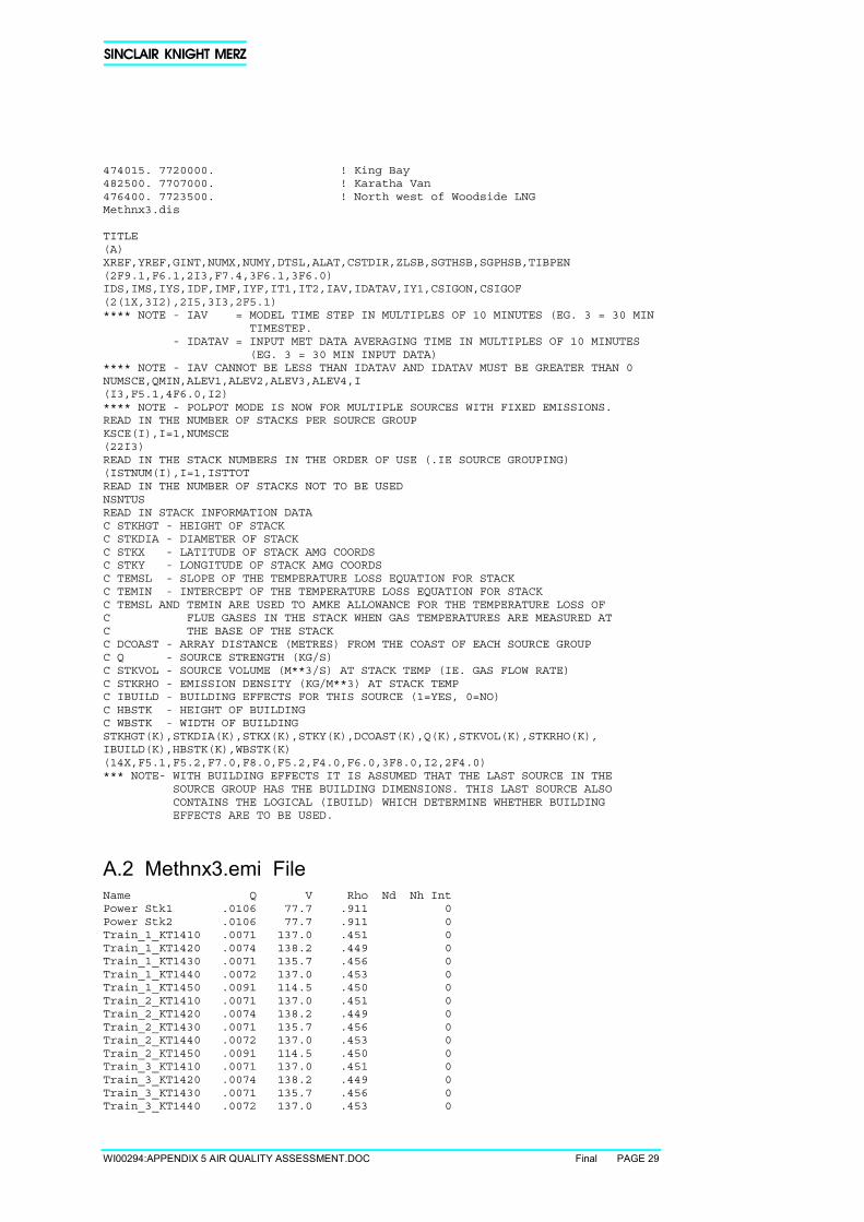
WI00294:APPENDIX 5 AIR QUALITY ASSESSMENT.DOC Final PAGE 29
474015. 7720000. ! King Bay482500. 7707000. ! Karatha Van476400. 7723500. ! North west of Woodside LNGMethnx3.dis
TITLE(A)XREF,YREF,GINT,NUMX,NUMY,DTSL,ALAT,CSTDIR,ZLSB,SGTHSB,SGPHSB,TIBPEN(2F9.1,F6.1,2I3,F7.4,3F6.1,3F6.0)IDS,IMS,IYS,IDF,IMF,IYF,IT1,IT2,IAV,IDATAV,IY1,CSIGON,CSIGOF(2(1X,3I2),2I5,3I3,2F5.1)**** NOTE - IAV = MODEL TIME STEP IN MULTIPLES OF 10 MINUTES (EG. 3 = 30 MIN
TIMESTEP.- IDATAV = INPUT MET DATA AVERAGING TIME IN MULTIPLES OF 10 MINUTES
(EG. 3 = 30 MIN INPUT DATA)**** NOTE - IAV CANNOT BE LESS THAN IDATAV AND IDATAV MUST BE GREATER THAN 0NUMSCE,QMIN,ALEV1,ALEV2,ALEV3,ALEV4,I(I3,F5.1,4F6.0,I2)**** NOTE - POLPOT MODE IS NOW FOR MULTIPLE SOURCES WITH FIXED EMISSIONS.READ IN THE NUMBER OF STACKS PER SOURCE GROUPKSCE(I),I=1,NUMSCE(22I3)READ IN THE STACK NUMBERS IN THE ORDER OF USE (.IE SOURCE GROUPING)(ISTNUM(I),I=1,ISTTOTREAD IN THE NUMBER OF STACKS NOT TO BE USEDNSNTUSREAD IN STACK INFORMATION DATAC STKHGT - HEIGHT OF STACKC STKDIA - DIAMETER OF STACKC STKX - LATITUDE OF STACK AMG COORDSC STKY - LONGITUDE OF STACK AMG COORDSC TEMSL - SLOPE OF THE TEMPERATURE LOSS EQUATION FOR STACKC TEMIN - INTERCEPT OF THE TEMPERATURE LOSS EQUATION FOR STACKC TEMSL AND TEMIN ARE USED TO AMKE ALLOWANCE FOR THE TEMPERATURE LOSS OFC FLUE GASES IN THE STACK WHEN GAS TEMPERATURES ARE MEASURED ATC THE BASE OF THE STACKC DCOAST - ARRAY DISTANCE (METRES) FROM THE COAST OF EACH SOURCE GROUPC Q - SOURCE STRENGTH (KG/S)C STKVOL - SOURCE VOLUME (M**3/S) AT STACK TEMP (IE. GAS FLOW RATE)C STKRHO - EMISSION DENSITY (KG/M**3) AT STACK TEMPC IBUILD - BUILDING EFFECTS FOR THIS SOURCE (1=YES, 0=NO)C HBSTK - HEIGHT OF BUILDINGC WBSTK - WIDTH OF BUILDINGSTKHGT(K),STKDIA(K),STKX(K),STKY(K),DCOAST(K),Q(K),STKVOL(K),STKRHO(K),IBUILD(K),HBSTK(K),WBSTK(K)(14X,F5.1,F5.2,F7.0,F8.0,F5.2,F4.0,F6.0,3F8.0,I2,2F4.0)*** NOTE- WITH BUILDING EFFECTS IT IS ASSUMED THAT THE LAST SOURCE IN THE
SOURCE GROUP HAS THE BUILDING DIMENSIONS. THIS LAST SOURCE ALSOCONTAINS THE LOGICAL (IBUILD) WHICH DETERMINE WHETHER BUILDINGEFFECTS ARE TO BE USED.
A.2 Methnx3.emi FileName Q V Rho Nd Nh IntPower Stk1 .0106 77.7 .911 0Power Stk2 .0106 77.7 .911 0Train_1_KT1410 .0071 137.0 .451 0Train_1_KT1420 .0074 138.2 .449 0Train_1_KT1430 .0071 135.7 .456 0Train_1_KT1440 .0072 137.0 .453 0Train_1_KT1450 .0091 114.5 .450 0Train_2_KT1410 .0071 137.0 .451 0Train_2_KT1420 .0074 138.2 .449 0Train_2_KT1430 .0071 135.7 .456 0Train_2_KT1440 .0072 137.0 .453 0Train_2_KT1450 .0091 114.5 .450 0Train_3_KT1410 .0071 137.0 .451 0Train_3_KT1420 .0074 138.2 .449 0Train_3_KT1430 .0071 135.7 .456 0Train_3_KT1440 .0072 137.0 .453 0
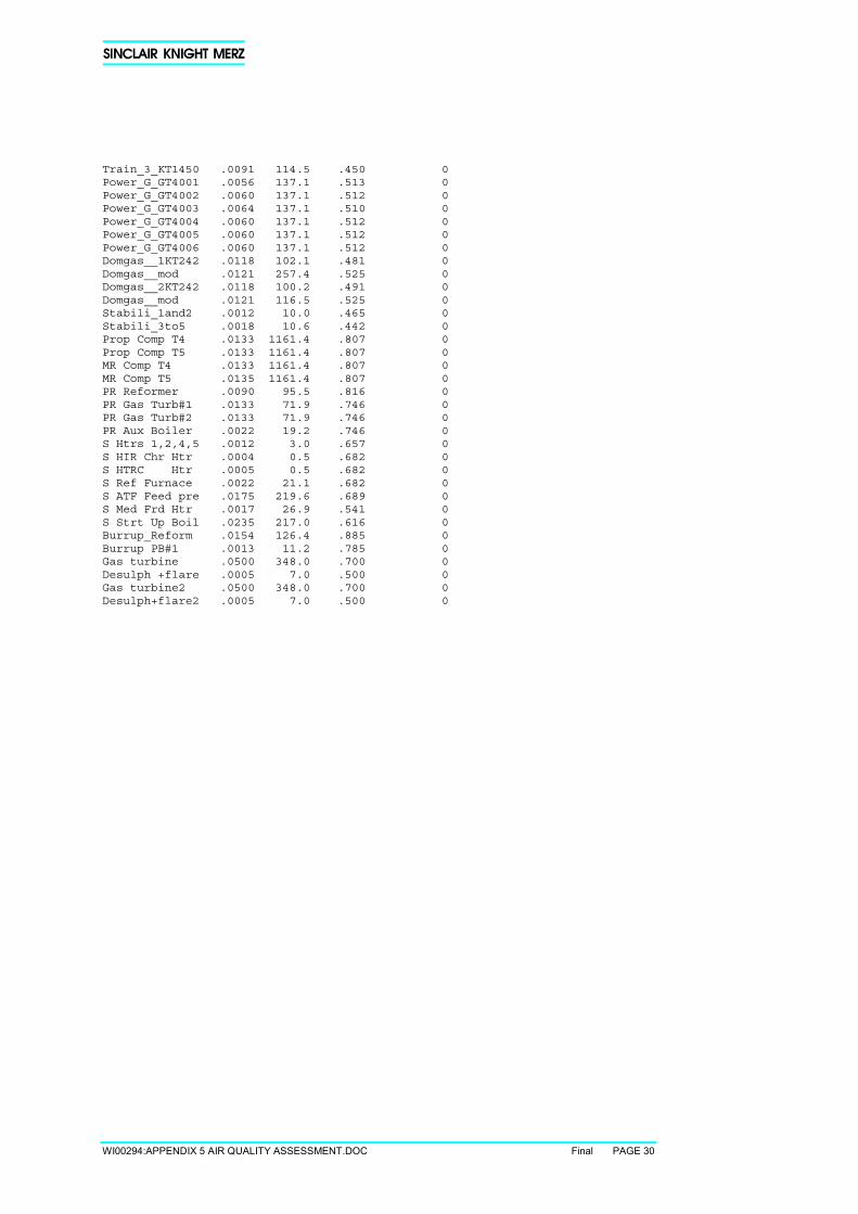
WI00294:APPENDIX 5 AIR QUALITY ASSESSMENT.DOC Final PAGE 30
Train_3_KT1450 .0091 114.5 .450 0Power_G_GT4001 .0056 137.1 .513 0Power_G_GT4002 .0060 137.1 .512 0Power_G_GT4003 .0064 137.1 .510 0Power_G_GT4004 .0060 137.1 .512 0Power_G_GT4005 .0060 137.1 .512 0Power_G_GT4006 .0060 137.1 .512 0Domgas__1KT242 .0118 102.1 .481 0Domgas__mod .0121 257.4 .525 0Domgas__2KT242 .0118 100.2 .491 0Domgas__mod .0121 116.5 .525 0Stabili_1and2 .0012 10.0 .465 0Stabili_3to5 .0018 10.6 .442 0Prop Comp T4 .0133 1161.4 .807 0Prop Comp T5 .0133 1161.4 .807 0MR Comp T4 .0133 1161.4 .807 0MR Comp T5 .0135 1161.4 .807 0PR Reformer .0090 95.5 .816 0PR Gas Turb#1 .0133 71.9 .746 0PR Gas Turb#2 .0133 71.9 .746 0PR Aux Boiler .0022 19.2 .746 0S Htrs 1,2,4,5 .0012 3.0 .657 0S HIR Chr Htr .0004 0.5 .682 0S HTRC Htr .0005 0.5 .682 0S Ref Furnace .0022 21.1 .682 0S ATF Feed pre .0175 219.6 .689 0S Med Frd Htr .0017 26.9 .541 0S Strt Up Boil .0235 217.0 .616 0Burrup_Reform .0154 126.4 .885 0Burrup PB#1 .0013 11.2 .785 0Gas turbine .0500 348.0 .700 0Desulph +flare .0005 7.0 .500 0Gas turbine2 .0500 348.0 .700 0Desulph+flare2 .0005 7.0 .500 0
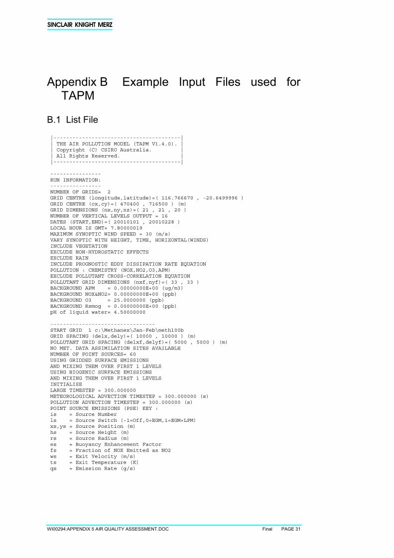
WI00294:APPENDIX 5 AIR QUALITY ASSESSMENT.DOC Final PAGE 31
Appendix B Example Input Files used forTAPM
B.1 List File
|----------------------------------------|| THE AIR POLLUTION MODEL (TAPM V1.4.0). || Copyright (C) CSIRO Australia. || All Rights Reserved. ||----------------------------------------|
----------------RUN INFORMATION:----------------NUMBER OF GRIDS= 2GRID CENTRE (longitude,latitude)=( 116.766670 , -20.6499996 )GRID CENTRE (cx,cy)=( 470400 , 716500 ) (m)GRID DIMENSIONS (nx,ny,nz)=( 21 , 21 , 20 )NUMBER OF VERTICAL LEVELS OUTPUT = 16DATES (START,END)=( 20010101 , 20010228 )LOCAL HOUR IS GMT+ 7.80000019MAXIMUM SYNOPTIC WIND SPEED = 30 (m/s)VARY SYNOPTIC WITH HEIGHT, TIME, HORIZONTAL(WINDS)INCLUDE VEGETATIONEXCLUDE NON-HYDROSTATIC EFFECTSEXCLUDE RAININCLUDE PROGNOSTIC EDDY DISSIPATION RATE EQUATIONPOLLUTION : CHEMISTRY (NOX,NO2,O3,APM)EXCLUDE POLLUTANT CROSS-CORRELATION EQUATIONPOLLUTANT GRID DIMENSIONS (nxf,nyf)=( 33 , 33 )BACKGROUND APM = 0.00000000E+00 (ug/m3)BACKGROUND NOX&NO2= 0.00000000E+00 (ppb)BACKGROUND O3 = 25.0000000 (ppb)BACKGROUND Rsmog = 0.00000000E+00 (ppb)pH of liquid water= 4.50000000
---------------------------------START GRID 1 c:\Methanex\Jan-Feb\meth100bGRID SPACING (delx,dely)=( 10000 , 10000 ) (m)POLLUTANT GRID SPACING (delxf,delyf)=( 5000 , 5000 ) (m)NO MET. DATA ASSIMILATION SITES AVAILABLENUMBER OF POINT SOURCES= 60USING GRIDDED SURFACE EMISSIONSAND MIXING THEM OVER FIRST 1 LEVELSUSING BIOGENIC SURFACE EMISSIONSAND MIXING THEM OVER FIRST 1 LEVELSINITIALISELARGE TIMESTEP = 300.000000METEOROLOGICAL ADVECTION TIMESTEP = 300.000000 (s)POLLUTION ADVECTION TIMESTEP = 300.000000 (s)POINT SOURCE EMISSIONS (PSE) KEY :is = Source Numberls = Source Switch (-1=Off,0=EGM,1=EGM+LPM)xs,ys = Source Position (m)hs = Source Height (m)rs = Source Radius (m)es = Buoyancy Enhancement Factorfs = Fraction of NOX Emitted as NO2ws = Exit Velocity (m/s)ts = Exit Temperature (K)qs = Emission Rate (g/s)
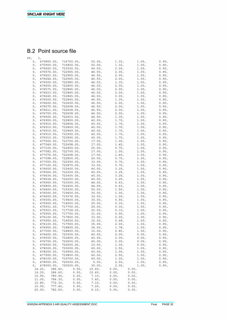
WI00294:APPENDIX 5 AIR QUALITY ASSESSMENT.DOC Final PAGE 32
B.2 Point source file60, 1,
0, 470800.00, 716700.00, 52.00, 1.32, 1.00, 0.90,0, 470900.00, 716800.00, 52.00, 1.32, 1.00, 0.90,0, 476600.00, 723000.00, 46.00, 2.00, 1.00, 0.90,0, 476576.00, 722965.00, 46.50, 2.00, 1.00, 0.90,0, 476623.00, 722965.00, 46.50, 2.00, 1.00, 0.90,0, 476644.00, 722965.00, 46.50, 2.00, 1.00, 0.90,0, 476500.00, 722980.00, 46.50, 1.35, 1.00, 0.90,0, 476600.00, 722800.00, 46.50, 2.00, 1.00, 0.90,0, 476575.00, 722845.00, 46.50, 2.00, 1.00, 0.90,0, 476623.00, 722845.00, 46.50, 2.00, 1.00, 0.90,0, 476645.00, 722845.00, 46.50, 2.00, 1.00, 0.90,0, 476500.00, 722840.00, 46.50, 1.35, 1.00, 0.90,0, 476600.00, 722600.00, 46.50, 2.00, 1.00, 0.90,0, 476575.00, 722608.00, 46.50, 2.00, 1.00, 0.90,0, 476611.00, 722608.00, 46.50, 2.00, 1.00, 0.90,0, 476700.00, 722608.00, 46.50, 2.00, 1.00, 0.90,0, 476500.00, 722603.00, 46.50, 1.35, 1.00, 0.90,0, 476900.00, 722800.00, 40.00, 1.70, 1.00, 0.90,0, 476910.00, 722804.00, 40.00, 1.70, 1.00, 0.90,0, 476910.00, 722809.00, 40.00, 1.70, 1.00, 0.90,0, 476910.00, 722849.00, 40.00, 1.70, 1.00, 0.90,0, 476910.00, 722900.00, 40.00, 1.70, 1.00, 0.90,0, 476910.00, 722890.00, 40.00, 1.70, 1.00, 0.90,0, 477000.00, 722700.00, 17.00, 1.00, 1.00, 0.90,0, 477049.00, 722698.00, 17.00, 1.45, 1.00, 0.90,0, 477100.00, 722800.00, 25.00, 0.75, 1.00, 0.90,0, 477082.00, 722700.00, 17.00, 1.00, 1.00, 0.90,0, 477076.00, 722698.00, 17.00, 1.45, 1.00, 0.90,0, 477098.00, 722800.00, 25.00, 0.75, 1.00, 0.90,0, 477000.00, 722900.00, 33.00, 0.70, 1.00, 0.90,0, 477100.00, 722870.00, 33.00, 0.70, 1.00, 0.90,0, 476600.00, 722400.00, 40.00, 3.25, 1.00, 0.90,0, 476566.00, 722200.00, 40.00, 3.25, 1.00, 0.90,0, 476634.00, 722400.00, 40.00, 3.25, 1.00, 0.90,0, 476634.00, 722200.00, 40.00, 3.25, 1.00, 0.90,0, 476900.00, 723000.00, 44.00, 0.63, 1.00, 0.90,0, 476800.00, 722400.00, 44.00, 0.63, 1.00, 0.90,0, 476400.00, 719300.00, 50.00, 1.50, 1.00, 0.90,0, 476500.00, 719400.00, 30.00, 1.00, 1.00, 0.90,0, 476600.00, 719376.00, 30.00, 1.00, 1.00, 0.90,0, 476500.00, 719400.00, 30.00, 0.50, 1.00, 0.90,0, 475900.00, 718000.00, 25.00, 0.30, 1.00, 0.90,0, 475931.00, 717700.00, 29.00, 0.30, 1.00, 0.90,0, 475923.00, 717728.00, 22.00, 0.10, 1.00, 0.90,0, 475900.00, 717700.00, 31.00, 0.90, 1.00, 0.90,0, 476100.00, 717800.00, 33.00, 2.00, 1.00, 0.90,0, 475900.00, 718000.00, 32.00, 0.68, 1.00, 0.90,0, 476100.00, 717900.00, 35.00, 2.00, 1.00, 0.90,0, 476900.00, 718800.00, 36.00, 1.78, 1.00, 0.90,0, 477000.00, 718800.00, 15.00, 0.85, 1.00, 0.90,0, 476400.00, 723000.00, 40.00, 2.00, 0.00, 0.90,0, 476500.00, 722800.00, 40.00, 2.00, 0.00, 0.90,0, 476700.00, 722600.00, 40.00, 2.00, 0.00, 0.90,0, 476500.00, 722500.00, 10.00, 1.00, 0.00, 0.90,0, 478000.00, 720000.00, 60.00, 2.50, 1.00, 0.90,0, 478200.00, 719900.00, 60.00, 1.00, 1.00, 0.90,0, 477900.00, 719800.00, 60.00, 2.50, 1.00, 0.90,0, 478100.00, 719700.00, 60.00, 1.00, 1.00, 0.90,0, 478000.00, 720000.00, 0.00, 2.50, 1.00, 0.90,0, 478000.00, 720000.00, 35.00, 2.00, 1.00, 0.90,14.20, 386.60, 0.00, 10.60, 0.00, 0.00,14.20, 386.60, 0.00, 10.60, 0.00, 0.00,10.90, 780.90, 0.00, 7.10, 0.00, 0.00,11.00, 784.30, 0.00, 7.40, 0.00, 0.00,10.80, 772.30, 0.00, 7.10, 0.00, 0.00,10.90, 777.40, 0.00, 7.20, 0.00, 0.00,20.00, 782.60, 0.00, 9.10, 0.00, 0.00,
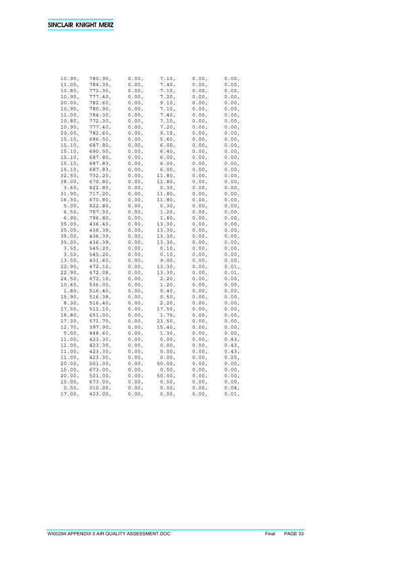
WI00294:APPENDIX 5 AIR QUALITY ASSESSMENT.DOC Final PAGE 33
10.90, 780.90, 0.00, 7.10, 0.00, 0.00,11.00, 784.30, 0.00, 7.40, 0.00, 0.00,10.80, 772.30, 0.00, 7.10, 0.00, 0.00,10.90, 777.40, 0.00, 7.20, 0.00, 0.00,20.00, 782.60, 0.00, 9.10, 0.00, 0.00,10.90, 780.90, 0.00, 7.10, 0.00, 0.00,11.00, 784.30, 0.00, 7.40, 0.00, 0.00,10.80, 772.30, 0.00, 7.10, 0.00, 0.00,10.90, 777.40, 0.00, 7.20, 0.00, 0.00,20.00, 782.60, 0.00, 9.10, 0.00, 0.00,15.10, 686.50, 0.00, 5.60, 0.00, 0.00,15.10, 687.80, 0.00, 6.00, 0.00, 0.00,15.10, 690.50, 0.00, 6.40, 0.00, 0.00,15.10, 687.80, 0.00, 6.00, 0.00, 0.00,15.10, 687.83, 0.00, 6.00, 0.00, 0.00,15.10, 687.83, 0.00, 6.00, 0.00, 0.00,32.50, 732.20, 0.00, 11.80, 0.00, 0.00,38.00, 670.80, 0.00, 11.80, 0.00, 0.00,3.60, 822.80, 0.00, 0.30, 0.00, 0.00,31.90, 717.20, 0.00, 11.80, 0.00, 0.00,16.30, 670.80, 0.00, 11.80, 0.00, 0.00,5.00, 822.80, 0.00, 0.30, 0.00, 0.00,6.50, 757.30, 0.00, 1.20, 0.00, 0.00,6.90, 796.80, 0.00, 1.80, 0.00, 0.00,35.00, 436.40, 0.00, 13.30, 0.00, 0.00,35.00, 436.39, 0.00, 13.30, 0.00, 0.00,35.00, 436.39, 0.00, 13.30, 0.00, 0.00,35.00, 436.39, 0.00, 13.30, 0.00, 0.00,3.50, 545.20, 0.00, 0.10, 0.00, 0.00,3.50, 545.20, 0.00, 0.10, 0.00, 0.00,13.50, 431.60, 0.00, 9.00, 0.00, 0.00,22.90, 472.10, 0.00, 13.30, 0.00, 0.01,22.90, 472.08, 0.00, 13.30, 0.00, 0.01,24.50, 472.10, 0.00, 2.20, 0.00, 0.00,10.60, 536.00, 0.00, 1.20, 0.00, 0.00,1.80, 516.40, 0.00, 0.40, 0.00, 0.00,15.90, 516.38, 0.00, 0.50, 0.00, 0.00,8.30, 516.40, 0.00, 2.20, 0.00, 0.00,17.50, 511.10, 0.00, 17.50, 0.00, 0.00,18.80, 651.00, 0.00, 1.70, 0.00, 0.00,17.30, 571.70, 0.00, 23.50, 0.00, 0.00,12.70, 397.90, 0.00, 15.40, 0.00, 0.00,5.00, 448.60, 0.00, 1.30, 0.00, 0.00,11.00, 423.30, 0.00, 0.00, 0.00, 0.43,11.00, 423.30, 0.00, 0.00, 0.00, 0.43,11.00, 423.30, 0.00, 0.00, 0.00, 0.43,11.00, 423.30, 0.00, 0.00, 0.00, 0.25,20.00, 501.00, 0.00, 50.00, 0.00, 0.00,15.00, 673.00, 0.00, 0.50, 0.00, 0.00,20.00, 501.00, 0.00, 50.00, 0.00, 0.00,15.00, 673.00, 0.00, 0.50, 0.00, 0.00,0.50, 310.00, 0.00, 0.00, 0.00, 0.04,17.00, 423.00, 0.00, 0.00, 0.00, 0.01,
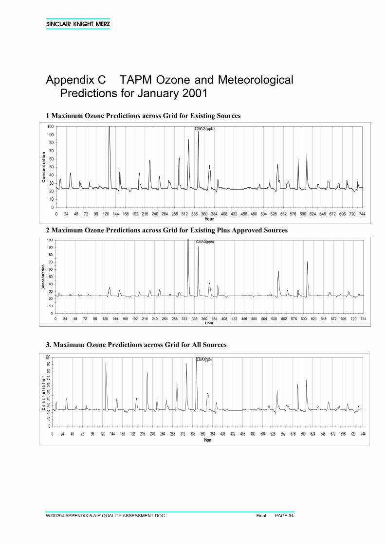
WI00294:APPENDIX 5 AIR QUALITY ASSESSMENT.DOC Final PAGE 34
Appendix C TAPM Ozone and MeteorologicalPredictions for January 2001
1 Maximum Ozone Predictions across Grid for Existing Sources
2 Maximum Ozone Predictions across Grid for Existing Plus Approved Sources
3. Maximum Ozone Predictions across Grid for All Sources
CMAX(ppb)
0102030405060708090
100
0 24 48 72 96 120 144 168 192 216 240 264 288 312 336 360 384 408 432 456 480 504 528 552 576 600 624 648 672 696 720 744Hour
Conc
entra
tion
CMAX(ppb)
0
10
20
30
40
50
60
70
80
90
100
0 24 48 72 96 120 144 168 192 216 240 264 288 312 336 360 384 408 432 456 480 504 528 552 576 600 624 648 672 696 720 744Hour
Conc
entra
tion
CMAX(ppb)
0
10
20
30
40
50
60
70
80
90
100
0 24 48 72 96 120 144 168 192 216 240 264 288 312 336 360 384 408 432 456 480 504 528 552 576 600 624 648 672 696 720 744Hour
Con
cent
ratio
n
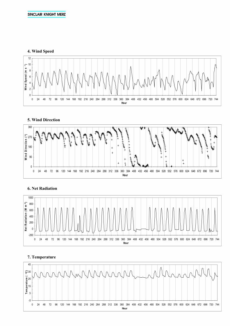
WI00294:APPENDIX 5 AIR QUALITY ASSESSMENT.DOC Final PAGE 35
4. Wind Speed
5. Wind Direction
6. Net Radiation
7. Temperature
0
2
4
6
8
10
12
0 24 48 72 96 120 144 168 192 216 240 264 288 312 336 360 384 408 432 456 480 504 528 552 576 600 624 648 672 696 720 744Hour
Win
d Sp
eed
(m s
-1)
0
90
180
270
360
0 24 48 72 96 120 144 168 192 216 240 264 288 312 336 360 384 408 432 456 480 504 528 552 576 600 624 648 672 696 720 744Hour
Win
d D
irect
ion
(o )
-200
0
200
400
600
800
1000
0 24 48 72 96 120 144 168 192 216 240 264 288 312 336 360 384 408 432 456 480 504 528 552 576 600 624 648 672 696 720 744Hour
Net
Rad
iatio
n (W
m-2
)
-5
5
15
25
35
45
0 24 48 72 96 120 144 168 192 216 240 264 288 312 336 360 384 408 432 456 480 504 528 552 576 600 624 648 672 696 720 744Hour
Tem
pera
ture
(o C
)
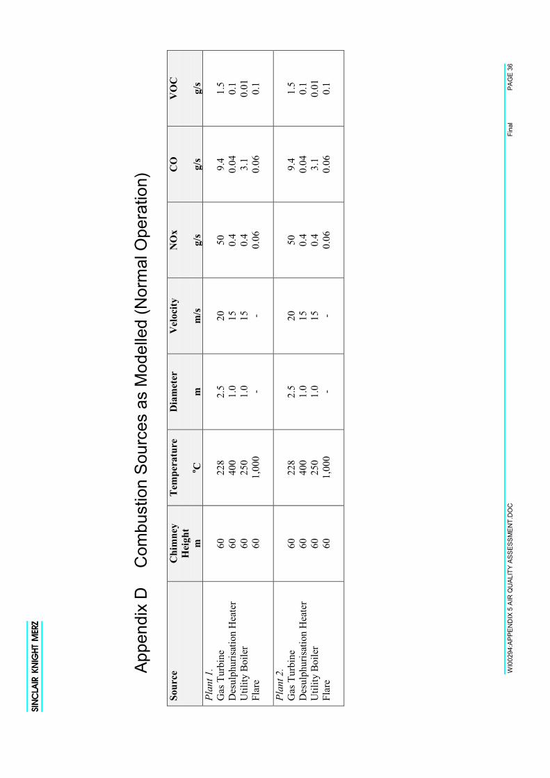
WI0
0294
:APP
END
IX 5
AIR
QU
ALIT
Y AS
SESS
MEN
T.D
OC
Fina
lPA
GE
36
Appe
ndix
D
Com
bust
ion
Sour
ces
as M
odel
led
(Nor
mal
Ope
ratio
n)
Sour
ceC
him
ney
Hei
ght
m
Tem
pera
ture
o C
Dia
met
er
m
Vel
ocity
m/s
NO
x
g/s
CO g/s
VO
C
g/s
Plan
t 1.
Gas
Tur
bine
Des
ulph
uris
atio
n H
eate
rU
tility
Boi
ler
Flar
e
60 60 60 60
228
400
250
1,00
0
2.5
1.0
1.0 -
20 15 15 -
50 0.4
0.4
0.06
9.4
0.04 3.1
0.06
1.5
0.1
0.01 0.1
Plan
t 2.
Gas
Tur
bine
Des
ulph
uris
atio
n H
eate
rU
tility
Boi
ler
Flar
e
60 60 60 60
228
400
250
1,00
0
2.5
1.0
1.0 -
20 15 15 -
50 0.4
0.4
0.06
9.4
0.04 3.1
0.06
1.5
0.1
0.01 0.1
Preliminary Environmental Noise Study
Appendix 6
PRELIMINARY ENVIRONMENTAL NOISE STUDY OFPROPOSED METHANOL PLANT IN KARRATHA
FOR
KVAERNER E&C AUSTRALIA PTY LTD
Date: January 2002Job No: 01072Report No: AV/02/01/002Revision: 0AAuthor: Mr Jim McLoughlin
Client: Kvaerner January 2002Subject: Environmental Noise Study - Karratha Methanol Plant Revision 0A
SVT Engineering Consultants JMc: Kvaerner Karratha methanol plant_rpt_0A.doc Page 2
CONTENTS
1 EXECUTIVE SUMMARY.........................................................................................................................3
2 INTRODUCTION.......................................................................................................................................5
2.1 SCOPE OF WORK .......................................................................................................................................52.2 BRIEF DESCRIPTION OF FACILITY..............................................................................................................5
3 ESTIMATION OF PLANT SOUND POWER LEVELS ........................................................................6
3.1 FIN-FAN COOLERS ....................................................................................................................................63.2 GAS TURBINE ............................................................................................................................................63.3 STEAM TURBINE........................................................................................................................................73.4 AIR COOLED CONDENSER .........................................................................................................................73.5 AIR SEPARATION UNIT ..............................................................................................................................73.6 PIPING NOISE ............................................................................................................................................83.7 BOILER FEED WATER PUMPS ....................................................................................................................8
4 NOISE MODEL ..........................................................................................................................................9
4.1 METHODOLOGY ........................................................................................................................................94.2 INPUT DATA ..............................................................................................................................................9
4.2.1 Source Sound Power Levels ............................................................................................................94.2.2 Topography, Ground Types and Barriers .......................................................................................94.2.3 Receiving Locations ......................................................................................................................104.2.4 Meteorology ..................................................................................................................................10
4.3 NOISE MODELLING RESULTS ..................................................................................................................104.3.1 Noise Contours..............................................................................................................................104.3.2 Point Calculations ........................................................................................................................114.3.3 Summary of Results.......................................................................................................................134.3.4 Source Ranking .............................................................................................................................13
5 NOISE LIMITS.........................................................................................................................................14
5.1 SUMMARY OF LEGISLATION ....................................................................................................................145.2 PLANT BOUNDARY LOCATIONS...............................................................................................................165.3 HEARSON COVE ......................................................................................................................................165.4 DAMPIER .................................................................................................................................................165.5 COMPLIANCE ASSESSMENT .....................................................................................................................16
5.5.1 Impact of Methanol Plant Alone ...................................................................................................165.5.2 Cumulative Impact of Methanol Plant and Other Proposed Industries........................................16
6 RISK ASSESSMENT................................................................................................................................18
6.1 REVIEW OF PREVAILING METEOROLOGICAL CONDITIONS ......................................................................186.2 CORRELATION OF PREVAILING WINDS WITH NOISE IMPACTS .................................................................19
7 NOISE MITIGATION RECOMMENDATIONS ..................................................................................21
7.1 MAIN AIR COOLERS ................................................................................................................................217.2 TURBINE HALLS ......................................................................................................................................217.3 A-FRAME CONDENSERS ..........................................................................................................................227.4 COMPRESSOR SUCTION AND DISCHARGE PIPING.....................................................................................227.5 STEAM TURBINES ....................................................................................................................................227.6 REVISED NOISE LEVEL PREDICTIONS AND NOISE CONTOURS .................................................................22
8 APPENDIX A – LOCATION MAP AND SITE PLAN
9 APPENDIX B – NOISE CONTOURS
10 APPENDIX C – GLOSSARY OF TERMS
Client: Kvaerner January 2002Subject: Environmental Noise Study - Karratha Methanol Plant Revision 0A
SVT Engineering Consultants JMc: Kvaerner Karratha methanol plant_rpt_0A.doc Page 3
1 EXECUTIVE SUMMARY
A preliminary environmental noise assessment has been undertaken of Methanex’s proposedMethanol Production Facility on the Burrup Peninsula in Karratha, Western Australia.
An acoustic model of the proposed methanol plant has been developed and used to providenoise contours for the area surrounding the plant. The noise model has also been used topredict noise levels at two site boundary locations and at two of the nearest noise sensitivelocations to the plant (Hearson Cove and Dampier).
Noise contours and noise level predictions have been undertaken for a range ofmeteorological conditions which include calm conditions and worst-case wind conditions forsound propagation in each of 8 cardinal directions. The effects of temperature inversions havealso been reviewed.
A review of the prevailing meteorology in the Dampier / Karratha area has also beenundertaken so as to determine the percentage occurrence of worst-case conditions for soundpropagation at each of the selected receiving locations.
For Hearson Cove, noise impacts are greatest when winds are from the north west. Duringnight time hours, worst case conditions occur for 2.3 % of the time each year and the worstmonths are March and September.
For residential locations in Dampier, noise impacts are greatest when winds are from northeast. During night time hours, (when noise limits are most stringent), worst-case conditionsoccur for 2.2% of the time each year and the worst months are April to August.
Predicted noise levels have been assessed for compliance with assigned noise level imposedunder the Environmental Protection (Noise) Regulations 1997, both at the site boundary andat the nearest noise sensitive locations. At all locations it has been shown that, unless noisemitigation measures are included in the design of the plant, noise levels will exceedregulatory noise limits.
The following equipment items have been identified as the most significant contributors toexceedances of the noise limits:• Air coolers;• Turbine Halls;• A-frame condensers; and• Compressor suction and discharge piping.• Steam turbines

Client: Kvaerner January 2002Subject: Environmental Noise Study - Karratha Methanol Plant Revision 0A
SVT Engineering Consultants JMc: Kvaerner Karratha methanol plant_rpt_0A.doc Page 4
In order to achieve compliance with the noise limits at all locations, the following noisereductions are required:
• Air coolers – 10 dB(A). This is equivalent to a sound power limit of 115 dB(A) for eachtrain.
• Turbine Halls – 12 dB(A). This is equivalent to a sound pressure level limit of 73 dB(A)at 1m from the walls of each building or a sound power limit of 109 dB(A) for eachbuilding.
• A-frame condensers – 10 dB(A). This is equivalent to a sound power limit of 109 dB(A)for each train.
• Compressor suction and discharge piping – 20 dB(A). This is equivalent to a soundpressure level limit of 80 dB(A) at 1m from the pipe walls.
• Steam turbines – 5 dB(A). This is equivalent to a sound pressure level limit of 80 dB(A)at 1m from the enclosure walls.
The noise model has also been used to demonstrate that compliance with the assigned noiselevels can be achieved under worst-case meteorological conditions if the noise reductionsabove are implemented. It has also been shown that the cumulative impact of noise from themethanol plant and other proposed industries in the area does not cause the assigned levels tobe exceeded.
Client: Kvaerner January 2002Subject: Environmental Noise Study - Karratha Methanol Plant Revision 0A
SVT Engineering Consultants JMc: Kvaerner Karratha methanol plant_rpt_0A.doc Page 5
2 INTRODUCTION
SVT were commissioned by Kvaerner to undertake a preliminary environmental noiseassessment of Methanex’s proposed Methanol Production Facility in Karratha, WesternAustralia. The objectives of the study are to determine the likely noise emissions from themethanol plant, to assess the noise emissions for compliance with noise limits imposed underthe Environmental Protection (Noise) Regulations 1997, and, where appropriate, to suggestmethods to mitigate excessive noise emissions.
2.1 Scope of WorkThe following list outlines the major activities undertaken during the course of the study:• Review of documentation provided by Kvaerner including site plans, equipment lists,
equipment data sheets, meteorological data and topographical data.• Estimation of noise emission levels (sound power levels) for high noise equipment items.• Development of an acoustic model for the plant and surrounding area.• Plotting of noise contours down to 35 dB(A) around the proposed plant for a range of
meteorological conditions.• Calculation of noise levels at the site boundary and at the nearest noise sensitive locations
for a range of meteorological conditions.• Assessment of noise emissions from the plant for compliance with noise limits imposed
under the Environmental Protection (Noise) Regulations 1997, both at the site boundaryand at the nearest noise sensitive locations.
• Determination of the risk of exceeding noise limits based on an analysis of historicalmeteorological data.
• Calculation of the cumulative noise impacts from the Methanol plant and from three otherproposed nearby industries under worst case conditions.
• Identification of high noise equipment items which significantly contribute to excessivenoise levels at the site boundary and at the nearest noise sensitive locations.
• Provision of noise mitigation recommendations to achieve compliance with noise limits.
2.2 Brief Description of FacilityThe proposed methanol production facility is to be located on the Burrup Peninsula, some9km to the north east of Dampier and approximately 1km to the north west of Hearson Cove.The plant comprises two identical production trains, each including the following equipmentitems which have been identified as likely sources of high noise emissions:• Large bank of fin-fan coolers,• Gas turbine exhausting via waste heat recovery unit,• Steam turbine,• A-frame condenser,• Air separation unit,• Compressor suction and discharge piping,• High power pumps.
The plant location and site layout are shown in Figures 1 and 2 in Appendix A.
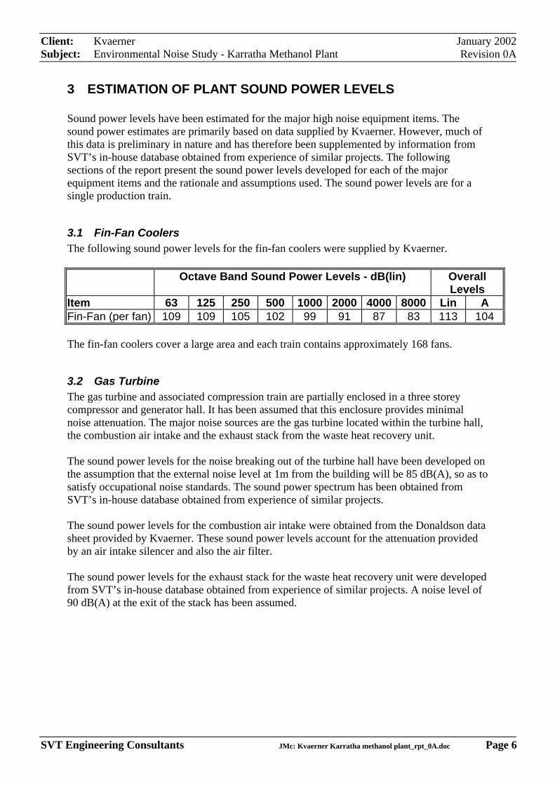
Client: Kvaerner January 2002Subject: Environmental Noise Study - Karratha Methanol Plant Revision 0A
SVT Engineering Consultants JMc: Kvaerner Karratha methanol plant_rpt_0A.doc Page 6
3 ESTIMATION OF PLANT SOUND POWER LEVELS
Sound power levels have been estimated for the major high noise equipment items. Thesound power estimates are primarily based on data supplied by Kvaerner. However, much ofthis data is preliminary in nature and has therefore been supplemented by information fromSVT’s in-house database obtained from experience of similar projects. The followingsections of the report present the sound power levels developed for each of the majorequipment items and the rationale and assumptions used. The sound power levels are for asingle production train.
3.1 Fin-Fan CoolersThe following sound power levels for the fin-fan coolers were supplied by Kvaerner.
Octave Band Sound Power Levels - dB(lin) OverallLevels
Item 63 125 250 500 1000 2000 4000 8000 Lin AFin-Fan (per fan) 109 109 105 102 99 91 87 83 113 104
The fin-fan coolers cover a large area and each train contains approximately 168 fans.
3.2 Gas TurbineThe gas turbine and associated compression train are partially enclosed in a three storeycompressor and generator hall. It has been assumed that this enclosure provides minimalnoise attenuation. The major noise sources are the gas turbine located within the turbine hall,the combustion air intake and the exhaust stack from the waste heat recovery unit.
The sound power levels for the noise breaking out of the turbine hall have been developed onthe assumption that the external noise level at 1m from the building will be 85 dB(A), so as tosatisfy occupational noise standards. The sound power spectrum has been obtained fromSVT’s in-house database obtained from experience of similar projects.
The sound power levels for the combustion air intake were obtained from the Donaldson datasheet provided by Kvaerner. These sound power levels account for the attenuation providedby an air intake silencer and also the air filter.
The sound power levels for the exhaust stack for the waste heat recovery unit were developedfrom SVT’s in-house database obtained from experience of similar projects. A noise level of90 dB(A) at the exit of the stack has been assumed.
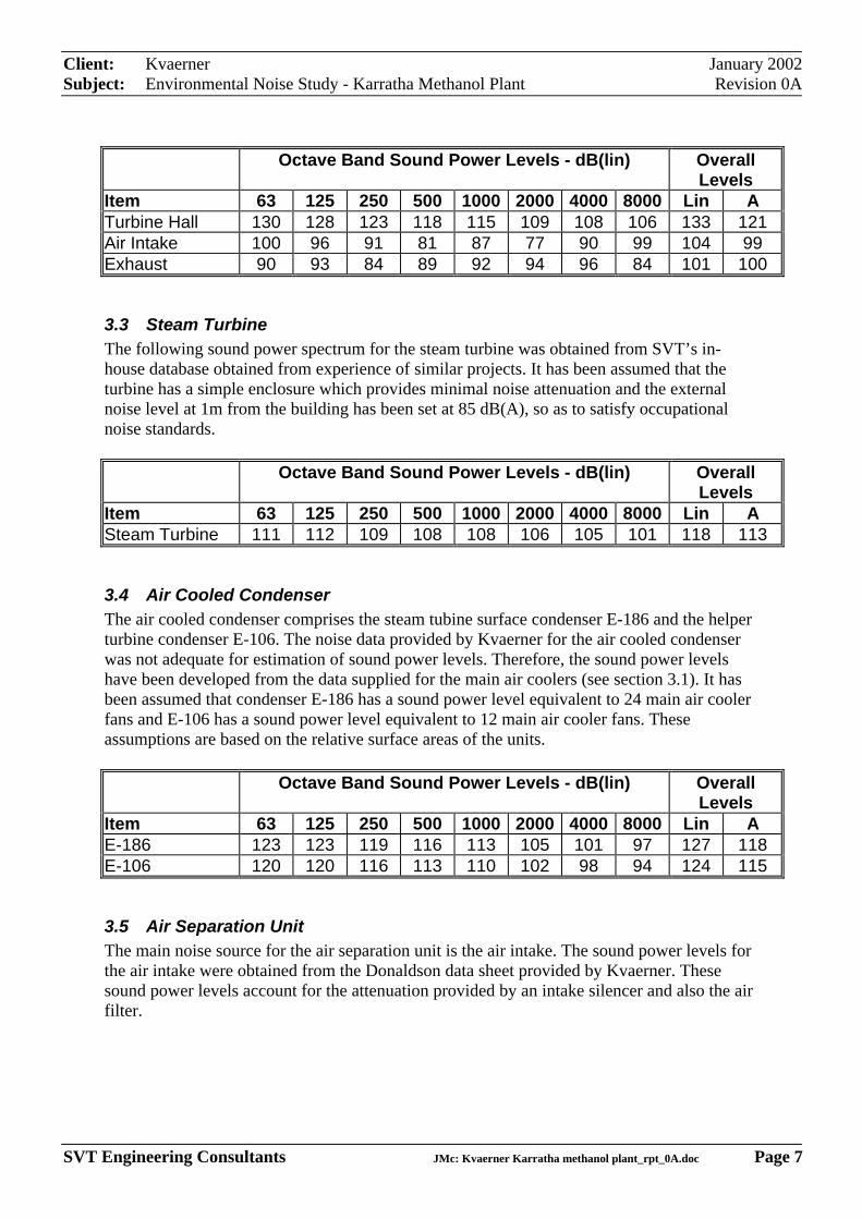
Client: Kvaerner January 2002Subject: Environmental Noise Study - Karratha Methanol Plant Revision 0A
SVT Engineering Consultants JMc: Kvaerner Karratha methanol plant_rpt_0A.doc Page 7
Octave Band Sound Power Levels - dB(lin) OverallLevels
Item 63 125 250 500 1000 2000 4000 8000 Lin ATurbine Hall 130 128 123 118 115 109 108 106 133 121Air Intake 100 96 91 81 87 77 90 99 104 99Exhaust 90 93 84 89 92 94 96 84 101 100
3.3 Steam TurbineThe following sound power spectrum for the steam turbine was obtained from SVT’s in-house database obtained from experience of similar projects. It has been assumed that theturbine has a simple enclosure which provides minimal noise attenuation and the externalnoise level at 1m from the building has been set at 85 dB(A), so as to satisfy occupationalnoise standards.
Octave Band Sound Power Levels - dB(lin) OverallLevels
Item 63 125 250 500 1000 2000 4000 8000 Lin ASteam Turbine 111 112 109 108 108 106 105 101 118 113
3.4 Air Cooled CondenserThe air cooled condenser comprises the steam tubine surface condenser E-186 and the helperturbine condenser E-106. The noise data provided by Kvaerner for the air cooled condenserwas not adequate for estimation of sound power levels. Therefore, the sound power levelshave been developed from the data supplied for the main air coolers (see section 3.1). It hasbeen assumed that condenser E-186 has a sound power level equivalent to 24 main air coolerfans and E-106 has a sound power level equivalent to 12 main air cooler fans. Theseassumptions are based on the relative surface areas of the units.
Octave Band Sound Power Levels - dB(lin) OverallLevels
Item 63 125 250 500 1000 2000 4000 8000 Lin AE-186 123 123 119 116 113 105 101 97 127 118E-106 120 120 116 113 110 102 98 94 124 115
3.5 Air Separation UnitThe main noise source for the air separation unit is the air intake. The sound power levels forthe air intake were obtained from the Donaldson data sheet provided by Kvaerner. Thesesound power levels account for the attenuation provided by an intake silencer and also the airfilter.
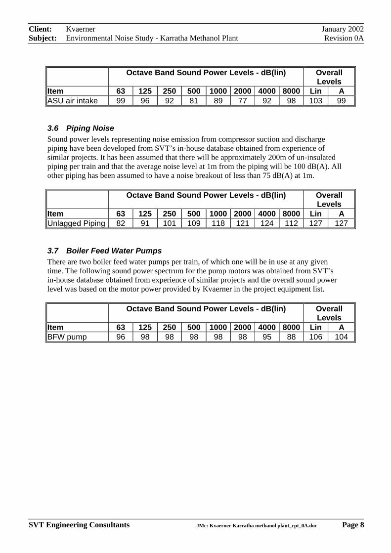
Client: Kvaerner January 2002Subject: Environmental Noise Study - Karratha Methanol Plant Revision 0A
SVT Engineering Consultants JMc: Kvaerner Karratha methanol plant_rpt_0A.doc Page 8
Octave Band Sound Power Levels - dB(lin) OverallLevels
Item 63 125 250 500 1000 2000 4000 8000 Lin AASU air intake 99 96 92 81 89 77 92 98 103 99
3.6 Piping NoiseSound power levels representing noise emission from compressor suction and dischargepiping have been developed from SVT’s in-house database obtained from experience ofsimilar projects. It has been assumed that there will be approximately 200m of un-insulatedpiping per train and that the average noise level at 1m from the piping will be 100 dB(A). Allother piping has been assumed to have a noise breakout of less than 75 dB(A) at 1m.
Octave Band Sound Power Levels - dB(lin) OverallLevels
Item 63 125 250 500 1000 2000 4000 8000 Lin AUnlagged Piping 82 91 101 109 118 121 124 112 127 127
3.7 Boiler Feed Water PumpsThere are two boiler feed water pumps per train, of which one will be in use at any giventime. The following sound power spectrum for the pump motors was obtained from SVT’sin-house database obtained from experience of similar projects and the overall sound powerlevel was based on the motor power provided by Kvaerner in the project equipment list.
Octave Band Sound Power Levels - dB(lin) OverallLevels
Item 63 125 250 500 1000 2000 4000 8000 Lin ABFW pump 96 98 98 98 98 98 95 88 106 104
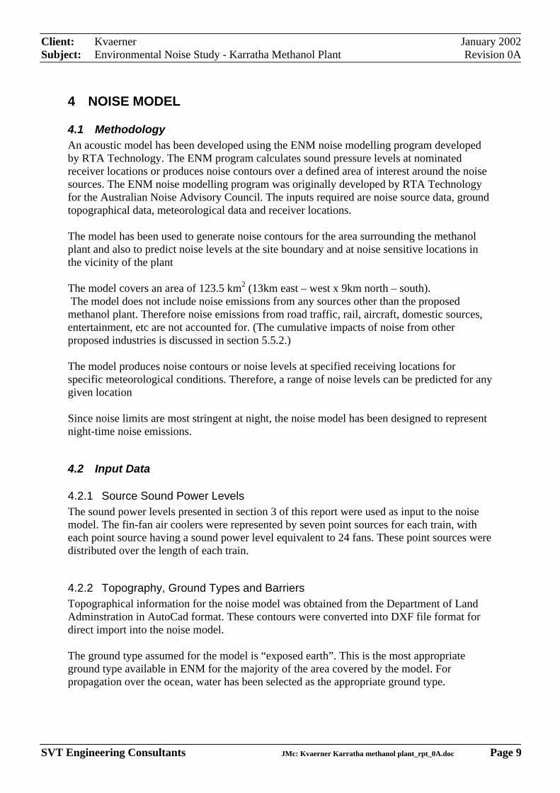
Client: Kvaerner January 2002Subject: Environmental Noise Study - Karratha Methanol Plant Revision 0A
SVT Engineering Consultants JMc: Kvaerner Karratha methanol plant_rpt_0A.doc Page 9
4 NOISE MODEL
4.1 MethodologyAn acoustic model has been developed using the ENM noise modelling program developedby RTA Technology. The ENM program calculates sound pressure levels at nominatedreceiver locations or produces noise contours over a defined area of interest around the noisesources. The ENM noise modelling program was originally developed by RTA Technologyfor the Australian Noise Advisory Council. The inputs required are noise source data, groundtopographical data, meteorological data and receiver locations.
The model has been used to generate noise contours for the area surrounding the methanolplant and also to predict noise levels at the site boundary and at noise sensitive locations inthe vicinity of the plant
The model covers an area of 123.5 km2 (13km east – west x 9km north – south). The model does not include noise emissions from any sources other than the proposedmethanol plant. Therefore noise emissions from road traffic, rail, aircraft, domestic sources,entertainment, etc are not accounted for. (The cumulative impacts of noise from otherproposed industries is discussed in section 5.5.2.)
The model produces noise contours or noise levels at specified receiving locations forspecific meteorological conditions. Therefore, a range of noise levels can be predicted for anygiven location
Since noise limits are most stringent at night, the noise model has been designed to representnight-time noise emissions.
4.2 Input Data
4.2.1 Source Sound Power LevelsThe sound power levels presented in section 3 of this report were used as input to the noisemodel. The fin-fan air coolers were represented by seven point sources for each train, witheach point source having a sound power level equivalent to 24 fans. These point sources weredistributed over the length of each train.
4.2.2 Topography, Ground Types and BarriersTopographical information for the noise model was obtained from the Department of LandAdminstration in AutoCad format. These contours were converted into DXF file format fordirect import into the noise model.
The ground type assumed for the model is “exposed earth”. This is the most appropriateground type available in ENM for the majority of the area covered by the model. Forpropagation over the ocean, water has been selected as the appropriate ground type.
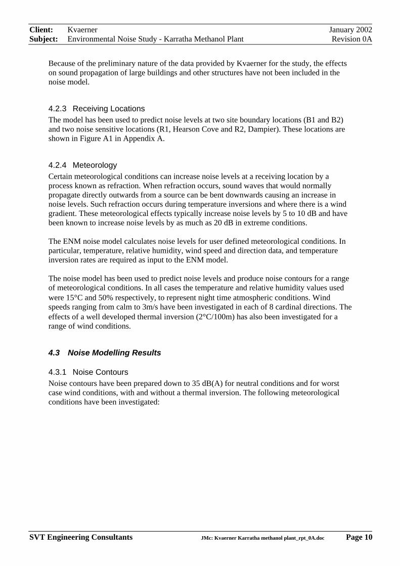
Client: Kvaerner January 2002Subject: Environmental Noise Study - Karratha Methanol Plant Revision 0A
SVT Engineering Consultants JMc: Kvaerner Karratha methanol plant_rpt_0A.doc Page 10
Because of the preliminary nature of the data provided by Kvaerner for the study, the effectson sound propagation of large buildings and other structures have not been included in thenoise model.
4.2.3 Receiving LocationsThe model has been used to predict noise levels at two site boundary locations (B1 and B2)and two noise sensitive locations (R1, Hearson Cove and R2, Dampier). These locations areshown in Figure A1 in Appendix A.
4.2.4 MeteorologyCertain meteorological conditions can increase noise levels at a receiving location by aprocess known as refraction. When refraction occurs, sound waves that would normallypropagate directly outwards from a source can be bent downwards causing an increase innoise levels. Such refraction occurs during temperature inversions and where there is a windgradient. These meteorological effects typically increase noise levels by 5 to 10 dB and havebeen known to increase noise levels by as much as 20 dB in extreme conditions.
The ENM noise model calculates noise levels for user defined meteorological conditions. Inparticular, temperature, relative humidity, wind speed and direction data, and temperatureinversion rates are required as input to the ENM model.
The noise model has been used to predict noise levels and produce noise contours for a rangeof meteorological conditions. In all cases the temperature and relative humidity values usedwere 15°C and 50% respectively, to represent night time atmospheric conditions. Windspeeds ranging from calm to 3m/s have been investigated in each of 8 cardinal directions. Theeffects of a well developed thermal inversion (2°C/100m) has also been investigated for arange of wind conditions.
4.3 Noise Modelling Results
4.3.1 Noise ContoursNoise contours have been prepared down to 35 dB(A) for neutral conditions and for worstcase wind conditions, with and without a thermal inversion. The following meteorologicalconditions have been investigated:
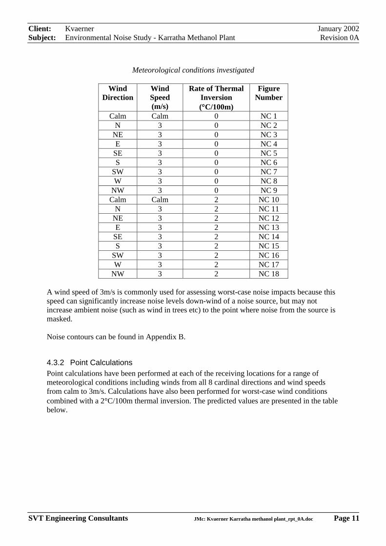
Client: Kvaerner January 2002Subject: Environmental Noise Study - Karratha Methanol Plant Revision 0A
SVT Engineering Consultants JMc: Kvaerner Karratha methanol plant_rpt_0A.doc Page 11
Meteorological conditions investigated
WindDirection
WindSpeed(m/s)
Rate of ThermalInversion(°°C/100m)
FigureNumber
Calm Calm 0 NC 1N 3 0 NC 2
NE 3 0 NC 3E 3 0 NC 4
SE 3 0 NC 5S 3 0 NC 6
SW 3 0 NC 7W 3 0 NC 8
NW 3 0 NC 9Calm Calm 2 NC 10
N 3 2 NC 11NE 3 2 NC 12E 3 2 NC 13
SE 3 2 NC 14S 3 2 NC 15
SW 3 2 NC 16W 3 2 NC 17
NW 3 2 NC 18
A wind speed of 3m/s is commonly used for assessing worst-case noise impacts because thisspeed can significantly increase noise levels down-wind of a noise source, but may notincrease ambient noise (such as wind in trees etc) to the point where noise from the source ismasked.
Noise contours can be found in Appendix B.
4.3.2 Point CalculationsPoint calculations have been performed at each of the receiving locations for a range ofmeteorological conditions including winds from all 8 cardinal directions and wind speedsfrom calm to 3m/s. Calculations have also been performed for worst-case wind conditionscombined with a 2°C/100m thermal inversion. The predicted values are presented in the tablebelow.
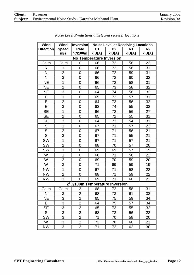
Client: Kvaerner January 2002Subject: Environmental Noise Study - Karratha Methanol Plant Revision 0A
SVT Engineering Consultants JMc: Kvaerner Karratha methanol plant_rpt_0A.doc Page 12
Noise Level Predictions at selected receiver locations
Wind Wind Inversion Noise Level at Receiving LocationsDirection Speed Rate B1 B2 R1 R2
m/s oC/100m dB(A) dB(A) dB(A) dB(A)No Temperature Inversion
Calm Calm 0 66 72 58 23N 1 0 66 72 58 31N 2 0 66 72 59 31N 3 0 66 72 60 32
NE 1 0 66 72 58 31NE 2 0 65 73 58 32NE 3 0 64 74 58 33E 1 0 65 72 57 31E 2 0 64 73 56 32E 3 0 63 74 55 33
SE 1 0 66 72 56 27SE 2 0 65 72 55 31SE 3 0 64 73 54 31S 1 0 67 71 57 22S 2 0 67 71 56 21S 3 0 67 71 55 21
SW 1 0 67 71 57 21SW 2 0 68 70 57 20SW 3 0 69 69 57 19W 1 0 68 71 58 22W 2 0 69 70 59 20W 3 0 71 69 59 19
NW 1 0 67 71 58 22NW 2 0 68 71 59 22NW 3 0 69 71 60 22
2oC/100m Temperature InversionCalm Calm 2 68 72 58 31
N 3 2 68 73 61 33NE 3 2 65 75 59 34E 3 2 64 75 57 34
SE 3 2 65 73 55 32S 3 2 68 72 56 22
SW 3 2 71 70 58 20W 3 2 72 70 60 21
NW 3 2 71 72 62 30
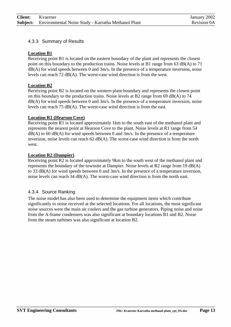
Client: Kvaerner January 2002Subject: Environmental Noise Study - Karratha Methanol Plant Revision 0A
SVT Engineering Consultants JMc: Kvaerner Karratha methanol plant_rpt_0A.doc Page 13
4.3.3 Summary of Results
Location B1Receiving point B1 is located on the eastern boundary of the plant and represents the closestpoint on this boundary to the production trains. Noise levels at B1 range from 63 dB(A) to 71dB(A) for wind speeds between 0 and 3m/s. In the presence of a temperature inversion, noiselevels can reach 72 dB(A). The worst-case wind direction is from the west.
Location B2Receiving point B2 is located on the western plant boundary and represents the closest pointon this boundary to the production trains. Noise levels at B2 range from 69 dB(A) to 74dB(A) for wind speeds between 0 and 3m/s. In the presence of a temperature inversion, noiselevels can reach 75 dB(A). The worst-case wind direction is from the east.
Location R1 (Hearson Cove)Receiving point R1 is located approximately 1km to the south east of the methanol plant andrepresents the nearest point at Hearson Cove to the plant. Noise levels at R1 range from 54dB(A) to 60 dB(A) for wind speeds between 0 and 3m/s. In the presence of a temperatureinversion, noise levels can reach 62 dB(A). The worst-case wind direction is from the northwest.
Location R2 (Dampier)Receiving point R2 is located approximately 9km to the south west of the methanol plant andrepresents the boundary of the townsite at Dampier. Noise levels at R2 range from 19 dB(A)to 33 dB(A) for wind speeds between 0 and 3m/s. In the presence of a temperature inversion,noise levels can reach 34 dB(A). The worst-case wind direction is from the north east.
4.3.4 Source RankingThe noise model has also been used to determine the equipment items which contributesignificantly to noise received at the selected locations. For all locations, the most significantnoise sources were the main air coolers and the gas turbine generators. Piping noise and noisefrom the A-frame condensers was also significant at boundary locations B1 and B2. Noisefrom the steam turbines was also significant at location B2.
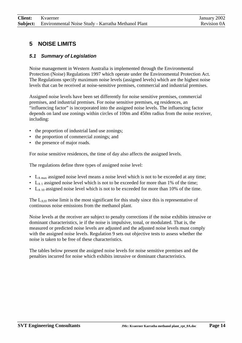
Client: Kvaerner January 2002Subject: Environmental Noise Study - Karratha Methanol Plant Revision 0A
SVT Engineering Consultants JMc: Kvaerner Karratha methanol plant_rpt_0A.doc Page 14
5 NOISE LIMITS
5.1 Summary of Legislation
Noise management in Western Australia is implemented through the EnvironmentalProtection (Noise) Regulations 1997 which operate under the Environmental Protection Act.The Regulations specify maximum noise levels (assigned levels) which are the highest noiselevels that can be received at noise-sensitive premises, commercial and industrial premises.
Assigned noise levels have been set differently for noise sensitive premises, commercialpremises, and industrial premises. For noise sensitive premises, eg residences, an“influencing factor” is incorporated into the assigned noise levels. The influencing factordepends on land use zonings within circles of 100m and 450m radius from the noise receiver,including:
• the proportion of industrial land use zonings;• the proportion of commercial zonings; and• the presence of major roads.
For noise sensitive residences, the time of day also affects the assigned levels.
The regulations define three types of assigned noise level:
• LA max assigned noise level means a noise level which is not to be exceeded at any time;• LA 1 assigned noise level which is not to be exceeded for more than 1% of the time;• LA 10 assigned noise level which is not to be exceeded for more than 10% of the time.
The LA10 noise limit is the most significant for this study since this is representative ofcontinuous noise emissions from the methanol plant.
Noise levels at the receiver are subject to penalty corrections if the noise exhibits intrusive ordominant characteristics, ie if the noise is impulsive, tonal, or modulated. That is, themeasured or predicted noise levels are adjusted and the adjusted noise levels must complywith the assigned noise levels. Regulation 9 sets out objective tests to assess whether thenoise is taken to be free of these characteristics.
The tables below present the assigned noise levels for noise sensitive premises and thepenalties incurred for noise which exhibits intrusive or dominant characteristics.

Client: Kvaerner January 2002Subject: Environmental Noise Study - Karratha Methanol Plant Revision 0A
SVT Engineering Consultants JMc: Kvaerner Karratha methanol plant_rpt_0A.doc Page 15
TABLE OF ASSIGNED NOISE LEVELS
Type of Time of day Assigned level (dB)premisesreceiving noise LA10 LA1 LA max
Noise sensitive 0700 to 1900 hours 45 + 55 + 65 +premises at locations Monday to Saturday influencing influencing influencingwithin 15 metres of a building directly
factor factor factor
associated with a 0900 to 1900 hours 40 + 50 + 65 +noise sensitive Sunday and public influencing influencing influencinguse holidays factor factor factor
1900 to 2200 hours 40 + 50 + 55 +all days influencing influencing influencing
factor factor factor
2200 hours on any 35 + 45 + 55 +day to 0700 hours influencing influencing influencingMonday to Saturday factor factor factorand 0900 hoursSunday and publicholidays
Noise sensitive All hours 60 75 80premises at locationsfurther than 15 metresfrom a building directlyassociated with a noisesensitive use
Commercial premises All hours 60 75 80
Industrial and All hours 65 80 90utility premises
TABLE OF ASSIGNED PENALTIES FOR INTRUSIVE OR DOMINANT NOISE CHARACTERISTICS
Adjustment where noise emission is not music Adjustment where noise emission is musicthese adjustements are cumulative to a maximum of 15 dB
Where tonality Where modulation Where impulsiveness Where impulsiveness Where impulsivenessis present is present is present is not present is present
+5 dB +5 dB +10 dB +10 dB +15 dB
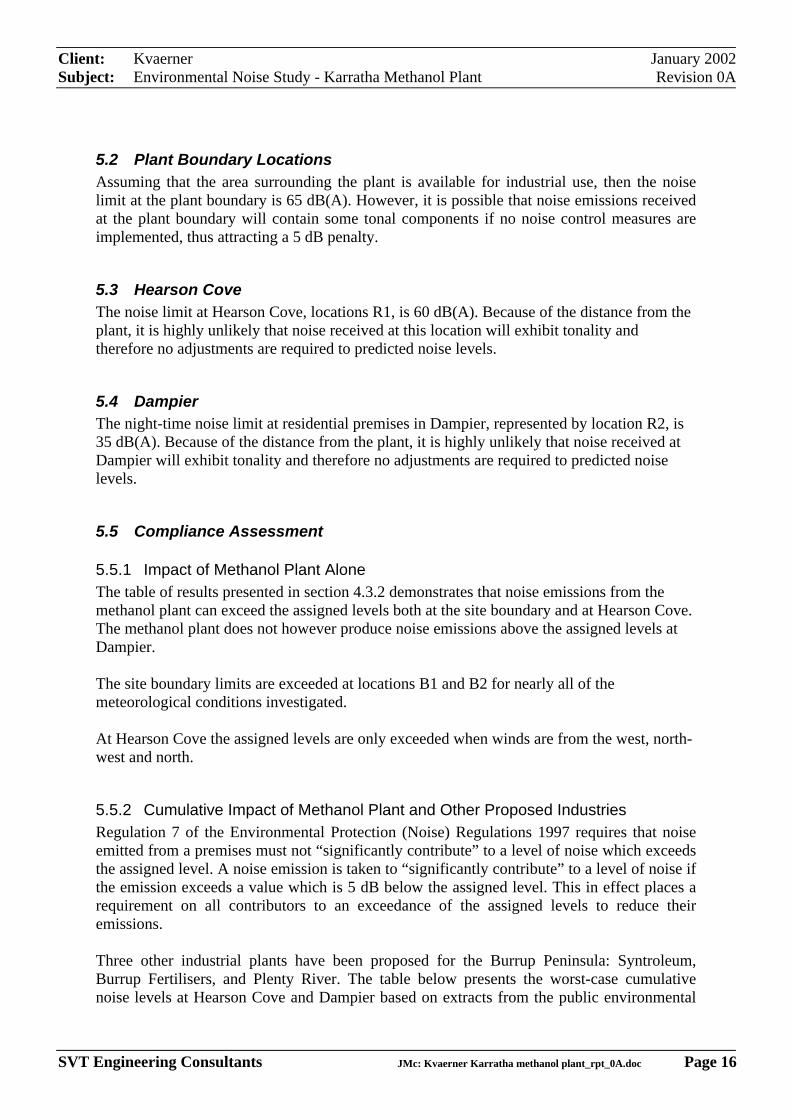
Client: Kvaerner January 2002Subject: Environmental Noise Study - Karratha Methanol Plant Revision 0A
SVT Engineering Consultants JMc: Kvaerner Karratha methanol plant_rpt_0A.doc Page 16
5.2 Plant Boundary LocationsAssuming that the area surrounding the plant is available for industrial use, then the noiselimit at the plant boundary is 65 dB(A). However, it is possible that noise emissions receivedat the plant boundary will contain some tonal components if no noise control measures areimplemented, thus attracting a 5 dB penalty.
5.3 Hearson CoveThe noise limit at Hearson Cove, locations R1, is 60 dB(A). Because of the distance from theplant, it is highly unlikely that noise received at this location will exhibit tonality andtherefore no adjustments are required to predicted noise levels.
5.4 DampierThe night-time noise limit at residential premises in Dampier, represented by location R2, is35 dB(A). Because of the distance from the plant, it is highly unlikely that noise received atDampier will exhibit tonality and therefore no adjustments are required to predicted noiselevels.
5.5 Compliance Assessment
5.5.1 Impact of Methanol Plant AloneThe table of results presented in section 4.3.2 demonstrates that noise emissions from themethanol plant can exceed the assigned levels both at the site boundary and at Hearson Cove.The methanol plant does not however produce noise emissions above the assigned levels atDampier.
The site boundary limits are exceeded at locations B1 and B2 for nearly all of themeteorological conditions investigated.
At Hearson Cove the assigned levels are only exceeded when winds are from the west, north-west and north.
5.5.2 Cumulative Impact of Methanol Plant and Other Proposed IndustriesRegulation 7 of the Environmental Protection (Noise) Regulations 1997 requires that noiseemitted from a premises must not “significantly contribute” to a level of noise which exceedsthe assigned level. A noise emission is taken to “significantly contribute” to a level of noise ifthe emission exceeds a value which is 5 dB below the assigned level. This in effect places arequirement on all contributors to an exceedance of the assigned levels to reduce theiremissions.
Three other industrial plants have been proposed for the Burrup Peninsula: Syntroleum,Burrup Fertilisers, and Plenty River. The table below presents the worst-case cumulativenoise levels at Hearson Cove and Dampier based on extracts from the public environmental
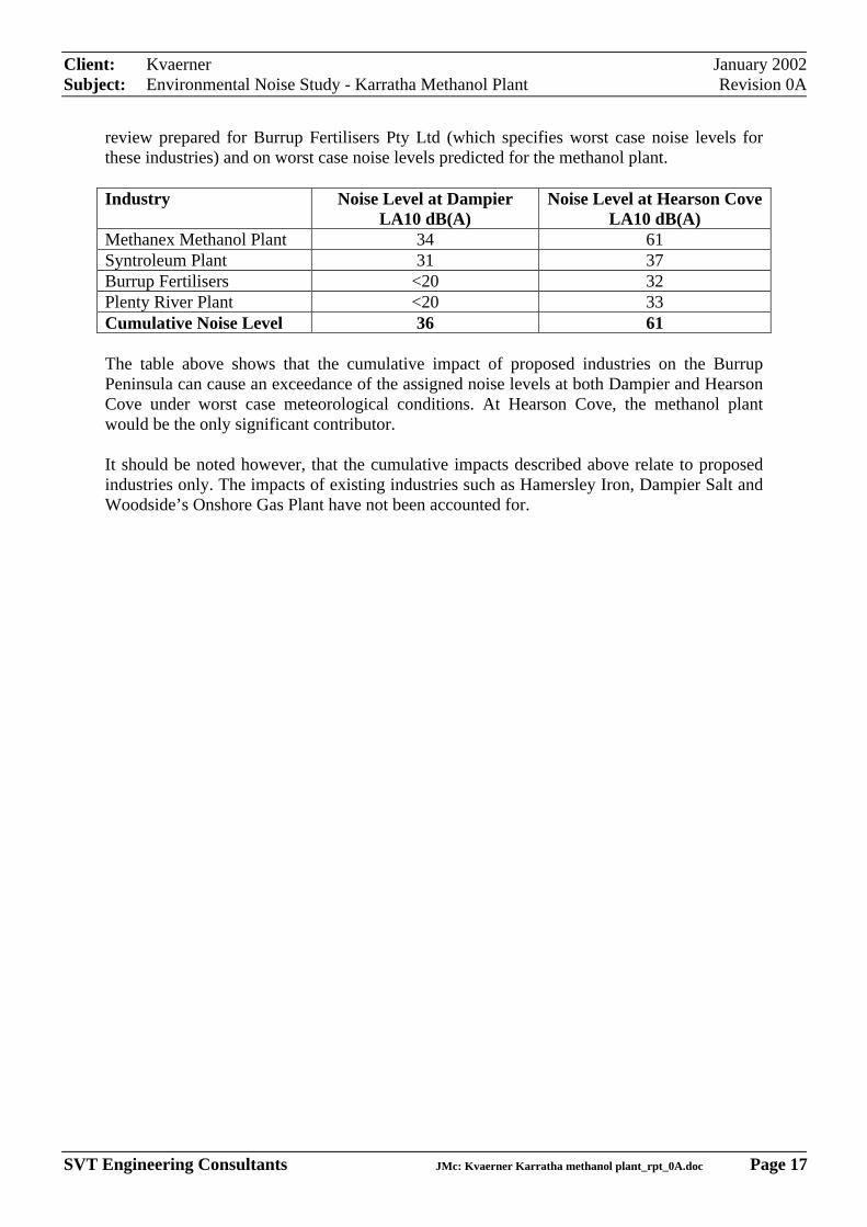
Client: Kvaerner January 2002Subject: Environmental Noise Study - Karratha Methanol Plant Revision 0A
SVT Engineering Consultants JMc: Kvaerner Karratha methanol plant_rpt_0A.doc Page 17
review prepared for Burrup Fertilisers Pty Ltd (which specifies worst case noise levels forthese industries) and on worst case noise levels predicted for the methanol plant.
Industry Noise Level at DampierLA10 dB(A)
Noise Level at Hearson CoveLA10 dB(A)
Methanex Methanol Plant 34 61Syntroleum Plant 31 37Burrup Fertilisers <20 32Plenty River Plant <20 33Cumulative Noise Level 36 61
The table above shows that the cumulative impact of proposed industries on the BurrupPeninsula can cause an exceedance of the assigned noise levels at both Dampier and HearsonCove under worst case meteorological conditions. At Hearson Cove, the methanol plantwould be the only significant contributor.
It should be noted however, that the cumulative impacts described above relate to proposedindustries only. The impacts of existing industries such as Hamersley Iron, Dampier Salt andWoodside’s Onshore Gas Plant have not been accounted for.
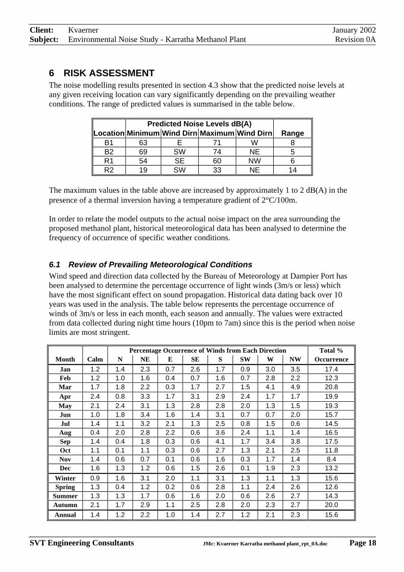
Client: Kvaerner January 2002Subject: Environmental Noise Study - Karratha Methanol Plant Revision 0A
SVT Engineering Consultants JMc: Kvaerner Karratha methanol plant_rpt_0A.doc Page 18
6 RISK ASSESSMENTThe noise modelling results presented in section 4.3 show that the predicted noise levels atany given receiving location can vary significantly depending on the prevailing weatherconditions. The range of predicted values is summarised in the table below.
Predicted Noise Levels dB(A)Location Minimum Wind Dirn Maximum Wind Dirn Range
B1 63 E 71 W 8B2 69 SW 74 NE 5R1 54 SE 60 NW 6R2 19 SW 33 NE 14
The maximum values in the table above are increased by approximately 1 to 2 dB(A) in thepresence of a thermal inversion having a temperature gradient of 2°C/100m.
In order to relate the model outputs to the actual noise impact on the area surrounding theproposed methanol plant, historical meteorological data has been analysed to determine thefrequency of occurrence of specific weather conditions.
6.1 Review of Prevailing Meteorological ConditionsWind speed and direction data collected by the Bureau of Meteorology at Dampier Port hasbeen analysed to determine the percentage occurrence of light winds (3m/s or less) whichhave the most significant effect on sound propagation. Historical data dating back over 10years was used in the analysis. The table below represents the percentage occurrence ofwinds of 3m/s or less in each month, each season and annually. The values were extractedfrom data collected during night time hours (10pm to 7am) since this is the period when noiselimits are most stringent.
Percentage Occurrence of Winds from Each Direction Total %Month Calm N NE E SE S SW W NW Occurrence
Jan 1.2 1.4 2.3 0.7 2.6 1.7 0.9 3.0 3.5 17.4Feb 1.2 1.0 1.6 0.4 0.7 1.6 0.7 2.8 2.2 12.3Mar 1.7 1.8 2.2 0.3 1.7 2.7 1.5 4.1 4.9 20.8Apr 2.4 0.8 3.3 1.7 3.1 2.9 2.4 1.7 1.7 19.9May 2.1 2.4 3.1 1.3 2.8 2.8 2.0 1.3 1.5 19.3Jun 1.0 1.8 3.4 1.6 1.4 3.1 0.7 0.7 2.0 15.7Jul 1.4 1.1 3.2 2.1 1.3 2.5 0.8 1.5 0.6 14.5Aug 0.4 2.0 2.8 2.2 0.6 3.6 2.4 1.1 1.4 16.5Sep 1.4 0.4 1.8 0.3 0.6 4.1 1.7 3.4 3.8 17.5Oct 1.1 0.1 1.1 0.3 0.6 2.7 1.3 2.1 2.5 11.8Nov 1.4 0.6 0.7 0.1 0.6 1.6 0.3 1.7 1.4 8.4Dec 1.6 1.3 1.2 0.6 1.5 2.6 0.1 1.9 2.3 13.2
Winter 0.9 1.6 3.1 2.0 1.1 3.1 1.3 1.1 1.3 15.6Spring 1.3 0.4 1.2 0.2 0.6 2.8 1.1 2.4 2.6 12.6
Summer 1.3 1.3 1.7 0.6 1.6 2.0 0.6 2.6 2.7 14.3Autumn 2.1 1.7 2.9 1.1 2.5 2.8 2.0 2.3 2.7 20.0Annual 1.4 1.2 2.2 1.0 1.4 2.7 1.2 2.1 2.3 15.6
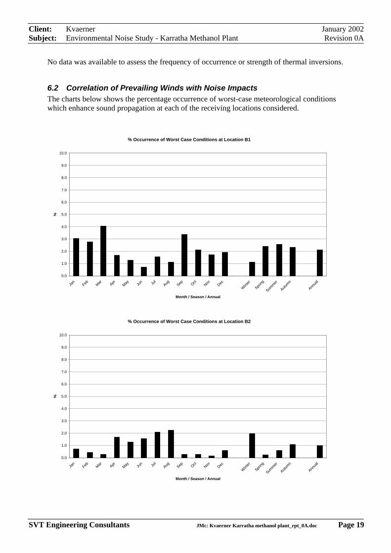
Client: Kvaerner January 2002Subject: Environmental Noise Study - Karratha Methanol Plant Revision 0A
SVT Engineering Consultants JMc: Kvaerner Karratha methanol plant_rpt_0A.doc Page 19
No data was available to assess the frequency of occurrence or strength of thermal inversions.
6.2 Correlation of Prevailing Winds with Noise ImpactsThe charts below shows the percentage occurrence of worst-case meteorological conditionswhich enhance sound propagation at each of the receiving locations considered.
% Occurrence of Worst Case Conditions at Location B1
0.0
1.0
2.0
3.0
4.0
5.0
6.0
7.0
8.0
9.0
10.0
Jan
Feb Mar AprMay Ju
n Jul
Aug Sep OctNov Dec
Wint
er
Spring
Summer
Autumn
Annua
l
Month / Season / Annual
%
% Occurrence of Worst Case Conditions at Location B2
0.0
1.0
2.0
3.0
4.0
5.0
6.0
7.0
8.0
9.0
10.0
Jan
Feb Mar AprMay Ju
n Jul
Aug Sep OctNov Dec
Wint
er
Spring
Summer
Autumn
Annua
l
Month / Season / Annual
%
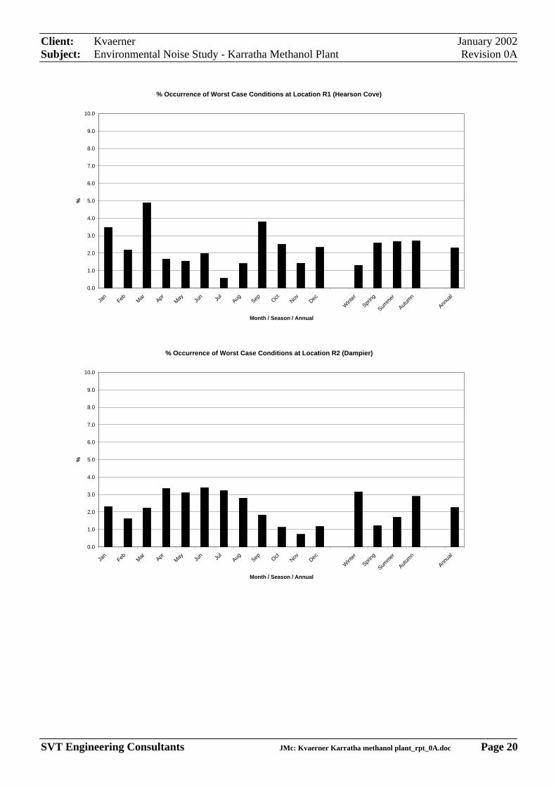
Client: Kvaerner January 2002Subject: Environmental Noise Study - Karratha Methanol Plant Revision 0A
SVT Engineering Consultants JMc: Kvaerner Karratha methanol plant_rpt_0A.doc Page 20
% Occurrence of Worst Case Conditions at Location R1 (Hearson Cove)
0.0
1.0
2.0
3.0
4.0
5.0
6.0
7.0
8.0
9.0
10.0
Jan
Feb Mar AprMay Ju
n Jul
Aug Sep OctNov Dec
Wint
er
Spring
Summer
Autumn
Annua
l
Month / Season / Annual
%
% Occurrence of Worst Case Conditions at Location R2 (Dampier)
0.0
1.0
2.0
3.0
4.0
5.0
6.0
7.0
8.0
9.0
10.0
Jan
Feb Mar AprMay Ju
n Jul
Aug Sep OctNov Dec
Wint
er
Spring
Summer
Autumn
Annua
l
Month / Season / Annual
%
Client: Kvaerner January 2002Subject: Environmental Noise Study - Karratha Methanol Plant Revision 0A
SVT Engineering Consultants JMc: Kvaerner Karratha methanol plant_rpt_0A.doc Page 21
7 NOISE MITIGATION RECOMMENDATIONS
The results presented in section 4 of this report show that under worst-case meteorologicalconditions, noise emissions from the methanol plant can exceed the assigned levels by up to10 dB at the plant boundary and by 1 dB at the Hearson Cove. The cumulative impact ofnoise from the methanol plant and other proposed industries can also cause the assigned levelat Dampier to be exceeded by 1 dB. The major noise sources which contribute to theseexceedances are:
• Main air coolers;• Turbine halls;• A-frame condensers; and• Compressor suction and discharge piping.• Steam turbines
The items from the above list that are most likely to have the greatest cost impacts for theproject are the main air coolers and the A-frame condensers.
Noise mitigation measures for each of these items are discussed in the following sections. Ithas been assumed that the noise mitigation measures will eliminate tonality at the siteboundary.
7.1 Main Air CoolersNoise levels from the air coolers need to reduced by 10 dB. The allowable sound power levelfor individual fans will depend on the configuration of the coolers, particularly the number offans employed. In order to ensure that the required 10 dB reduction is achieved, the overallsound power level for each train should not exceed 115 dB(A). The sound power limit forindividual fans can then be derived from the total number of fans in the train. For example, ifthere are 168 fans in each train (as assumed in the noise model), then the sound power limitfor an individual fan would be 93 dB(A). Noise from air fin coolers is related to the tip speedof the fan blades. Therefore, in order to reduce noise levels it is necessary to reduce the tipspeed. This can be accomplished by reducing the rotational speed of the fans and increasingthe number of blades so as to maintain the required air flow. Alternatively, low noise fans areavailable which have aerodynamic blades and wing tips.
7.2 Turbine HallsNoise radiated from the turbine halls needs to be reduced by 12 dB. This is equivalent to anoise limit of 72 dB(A) at 1m from the walls and roof of the turbine building, or a total soundpower level of 109 dB(A) for each building. In order to achieve this noise reduction, noiseattenuation measures need to be included in the design of the building. Particular attentionshould be given to such items as roof vents, doors, windows, louvres and any coolingmeasures.
Client: Kvaerner January 2002Subject: Environmental Noise Study - Karratha Methanol Plant Revision 0A
SVT Engineering Consultants JMc: Kvaerner Karratha methanol plant_rpt_0A.doc Page 22
7.3 A-Frame CondensersNoise levels from the condensers need to reduced by 10 dB. The allowable sound power levelfor individual fans will depend on the configuration of the condensers, particularly thenumber of fans employed. In order to ensure that the required 10 dB reduction is achieved,the overall sound power level for the condensers in each train should not exceed 109 dB(A).The sound power limit for individual fans can then be derived from the total number of fansin the condenser. The noise reduction methods discussed for the main air coolers also applyto the A-frame condensers.
7.4 Compressor Suction and Discharge PipingNoise emissions from compressor suction and discharge piping are significant at the siteboundaries. However, because of the frequency content of the piping noise, the noise isreadily attenuated during propagation and is not significant at locations R1 and R2. Noiselevels from the piping can be reduced either by lagging the piping or by installing suction anddischarge silencers. A noise reduction of 20 dB is readily achievable using either method.
7.5 Steam TurbinesNoise emissions from the steam turbines significant at the site boundaries and need to bereduced by 5 dB. This is equivalent to a noise limit of 80 dB(A) at 1m from the turbines, or atotal sound power level of 108 dB(A). This can be achieved by upgrading the enclosuressurrounding the turbines.
7.6 Revised Noise Level Predictions and Noise ContoursThe noise model has been used to predict noise levels and produce noise contours based onimplementation of the noise mitigation measures described above. Only worst-casemeteorological conditions have been considered. The noise contours are presented in figuresNC 19 to NC 26 in Appendix B. The predicted noise levels at the site boundary and nearestresidential locations are given in the table below.
Wind Wind Inversion Noise Level at Receiving LocationsDirection Speed Rate B1 B2 R1 R2
m/s oC/100m dB(A) dB(A) dB(A) dB(A)W 3 0 60 58 48 9E 3 0 53 62 45 22
NW 3 0 59 59 50 11NE 3 0 54 62 47 23W 3 2 62 59 50 10E 3 2 54 63 46 23
NW 3 2 60 60 51 19NE 3 2 55 63 48 23
These results demonstrate that compliance with the noise regulations can be achieved underworst-case meteorological conditions if the noise mitigation measures described above areimplemented. The noise mitigation measures also ensure that the cumulative impact of themethanol plant and other proposed industries does not exceed the assigned levels at HearsonCove or Dampier.

Client: Kvaerner January 2002Subject: Environmental Noise Study of Proposed Methanol Plant Revision 0A
SVT Engineering Consultants JMc: Kvaerner Karratha methanol plant_rpt_0A.doc
8 APPENDIX A – LOCATION MAP AND SITE PLAN
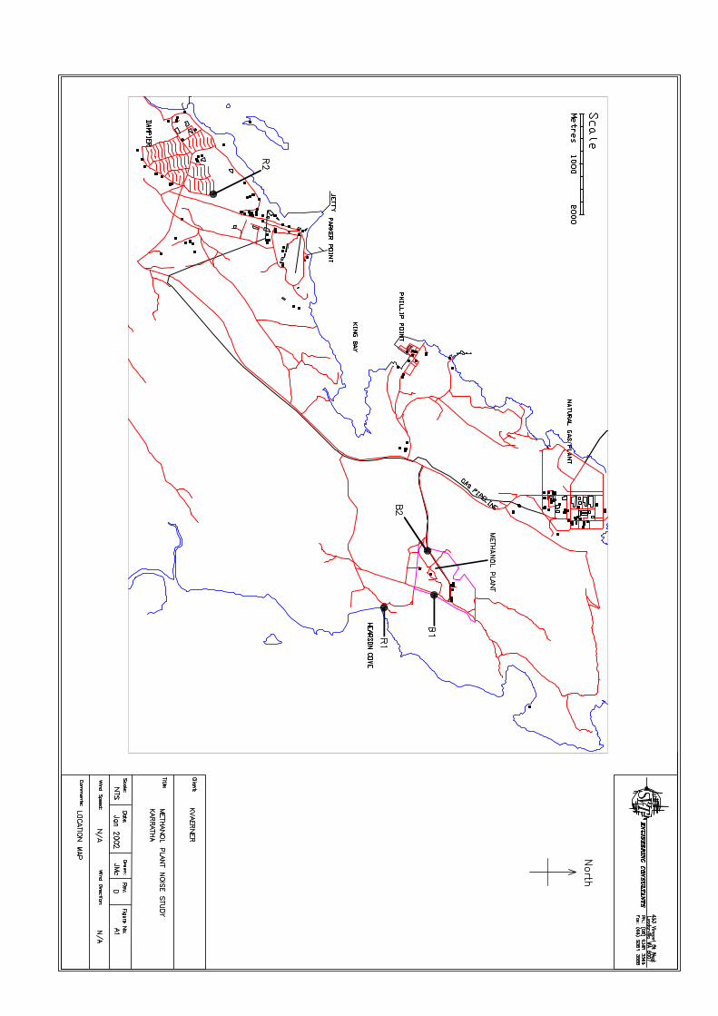

Client: Kvaerner January 2002Subject: Environmental Noise Study - Karratha Methanol Plant Revision 0A
SVT Engineering Consultants JMc: Kvaerner Karratha methanol plant_rpt_0A.doc
9 APPENDIX B – NOISE CONTOURS
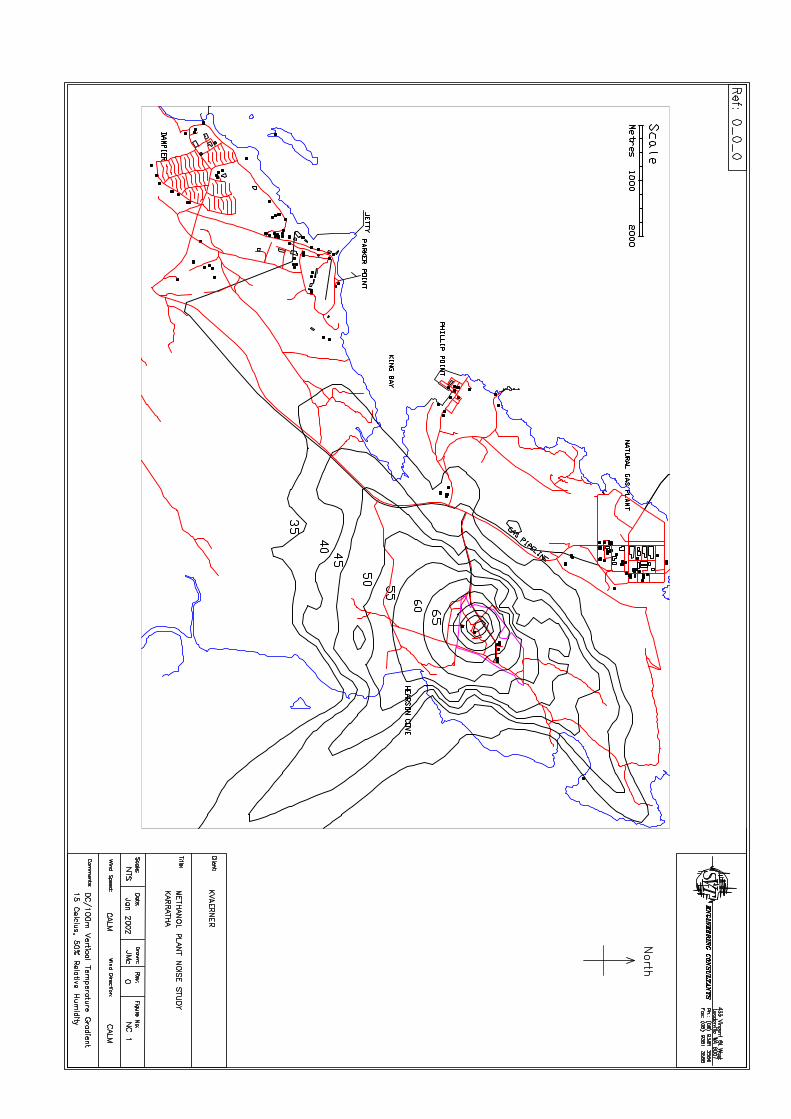
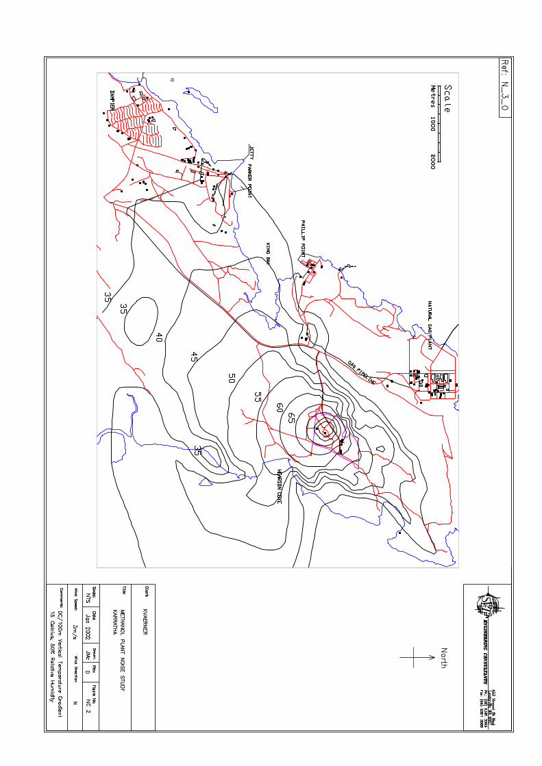
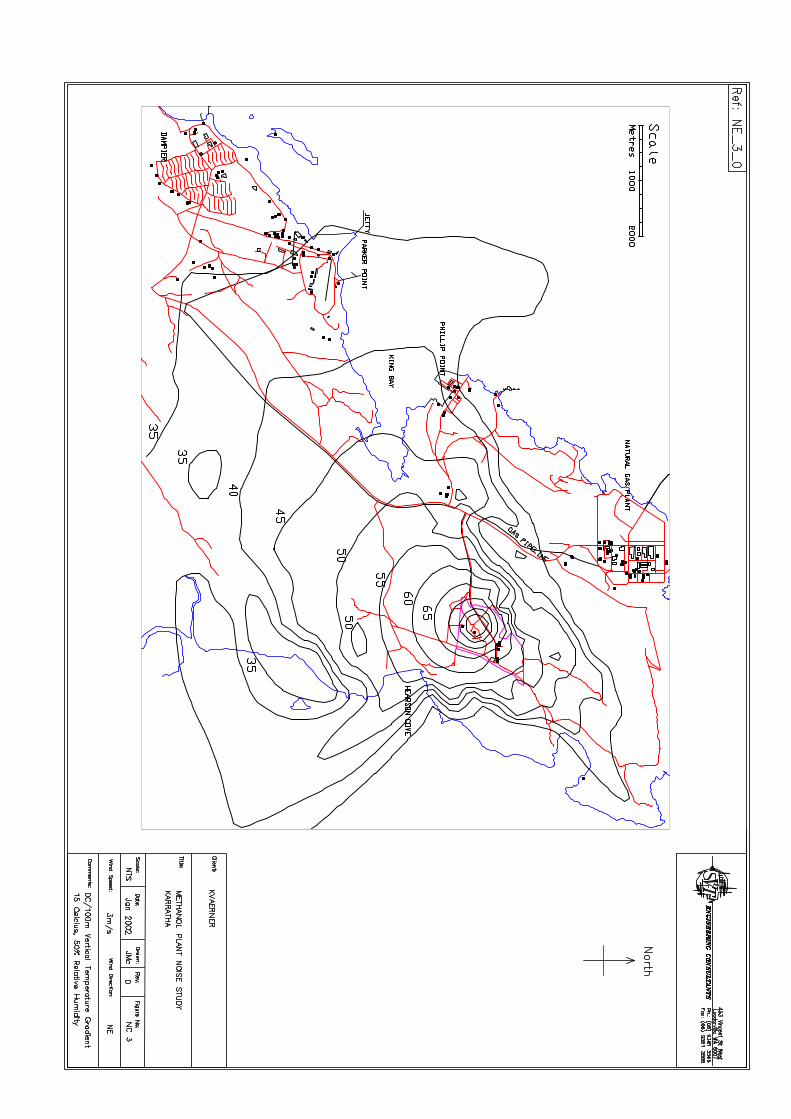
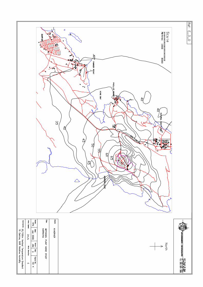
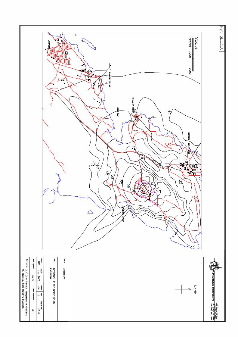
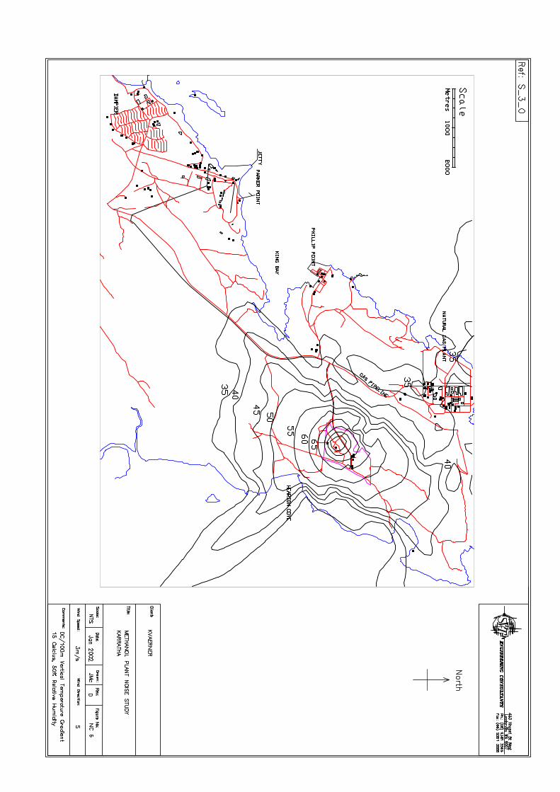
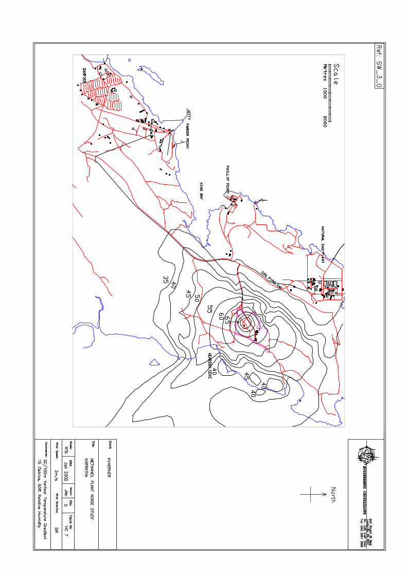
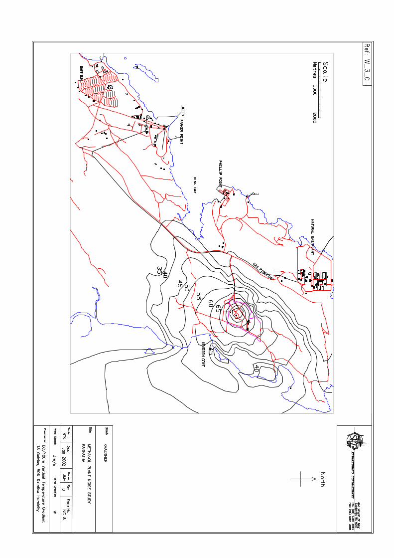
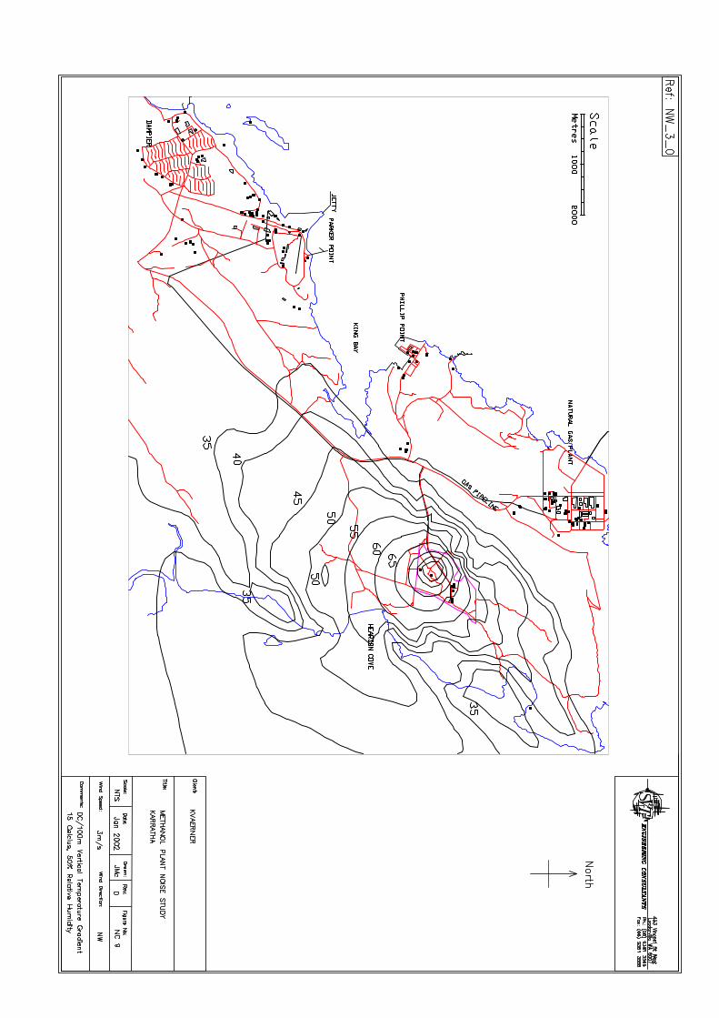
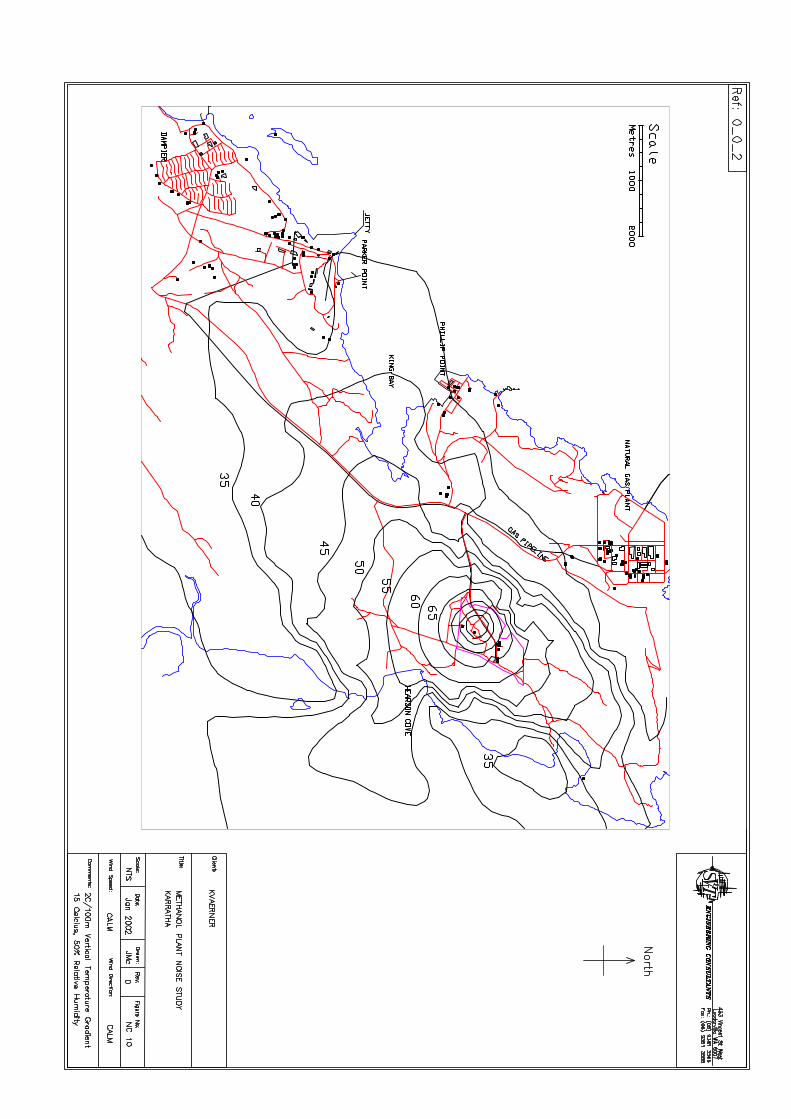
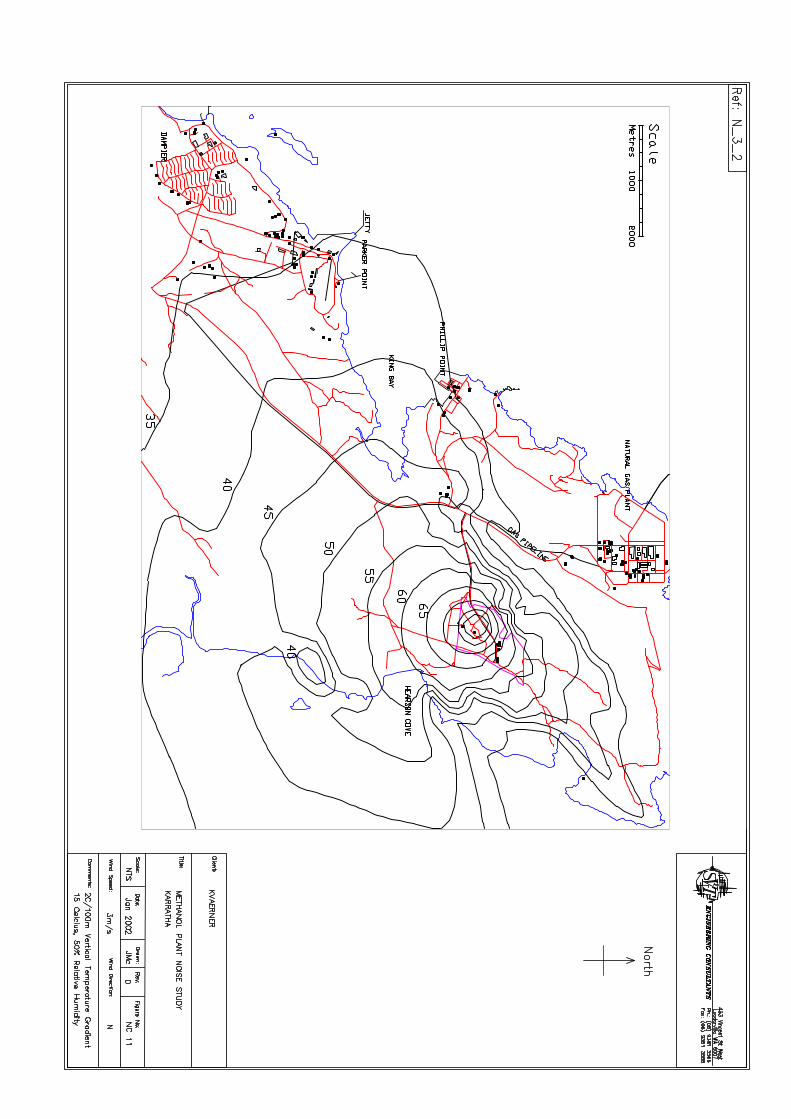
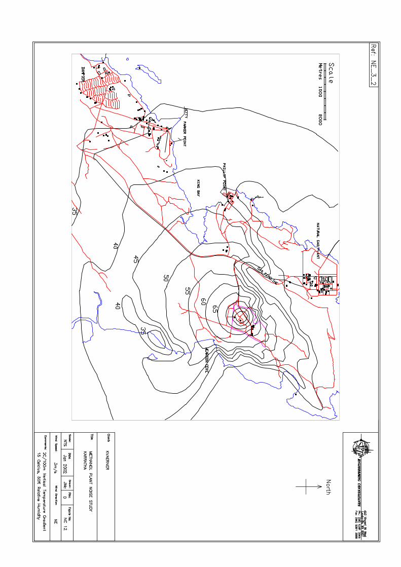
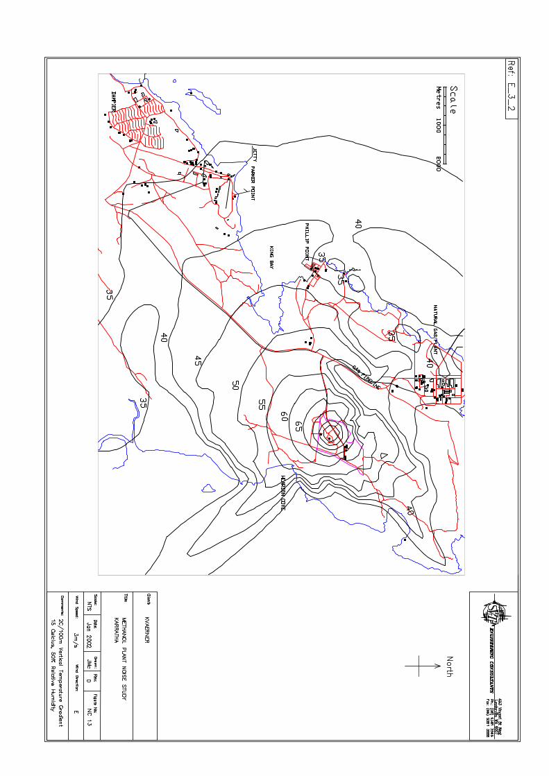
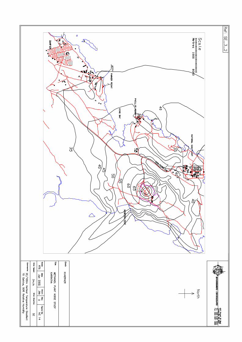

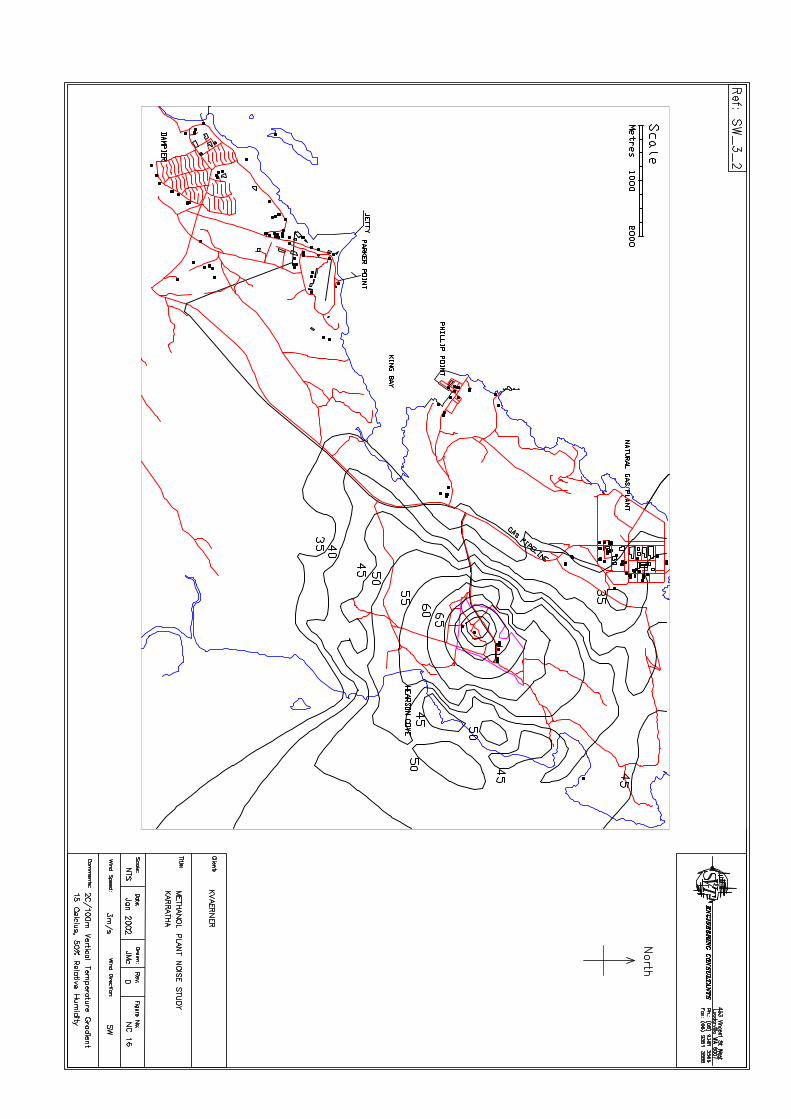
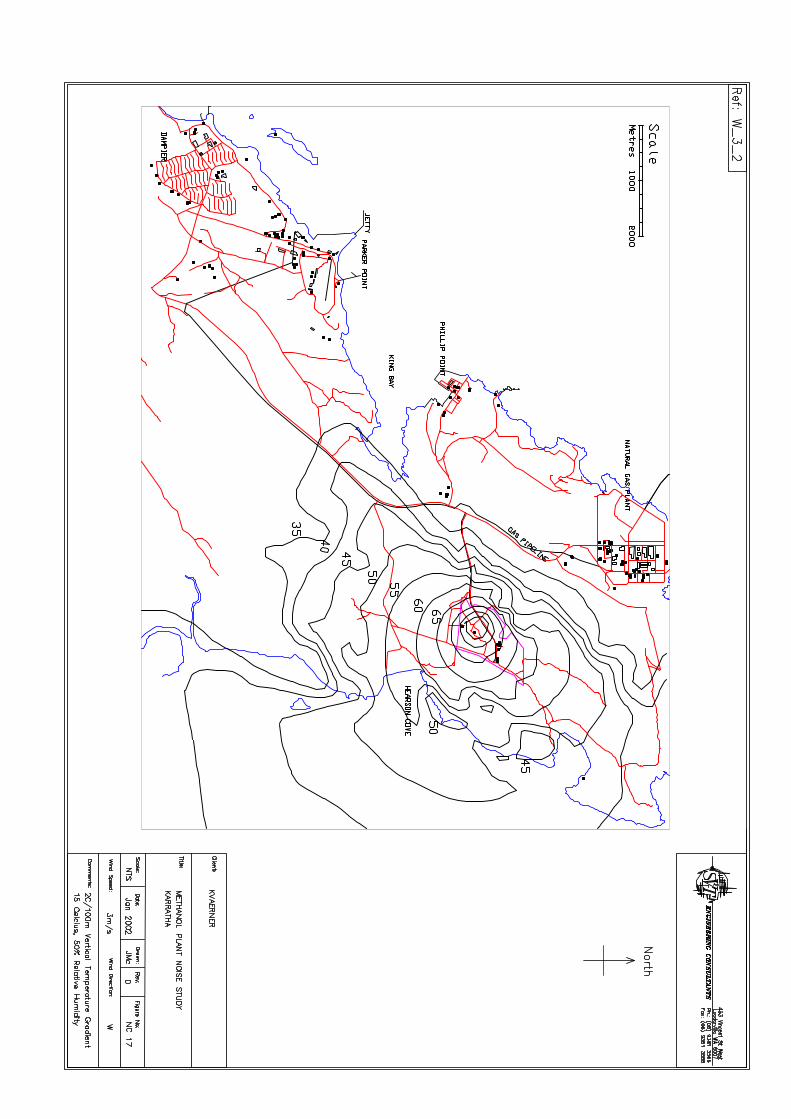
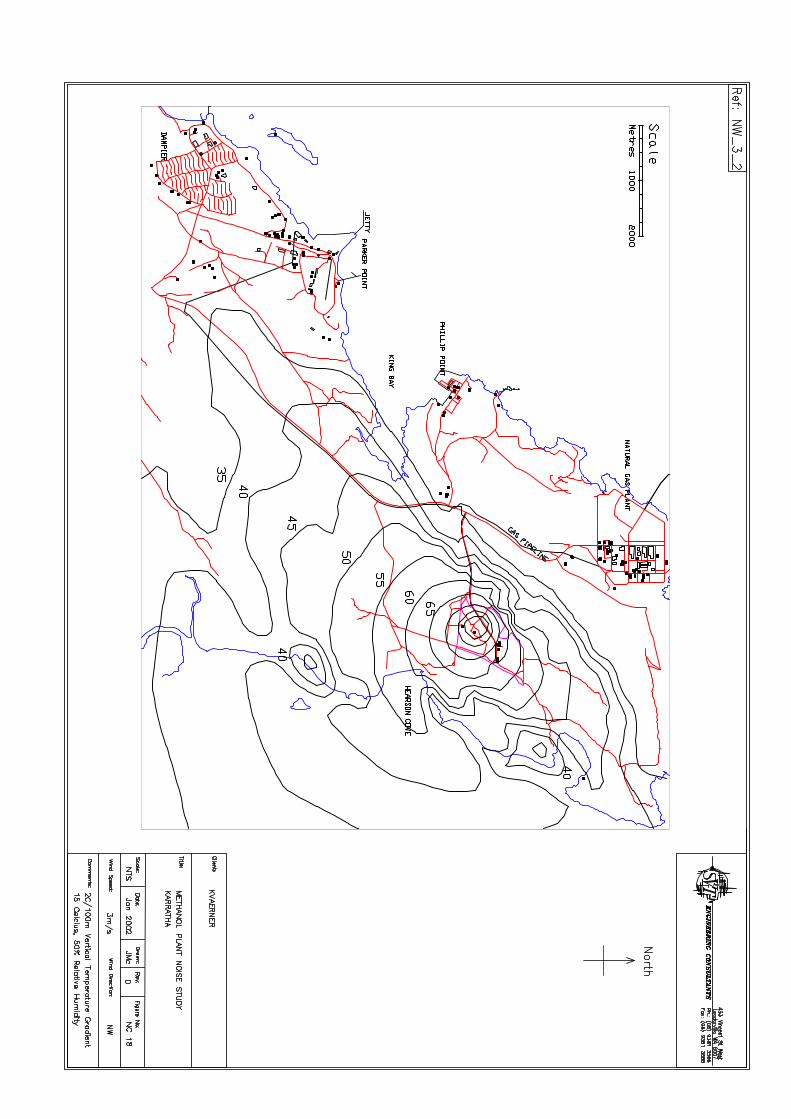
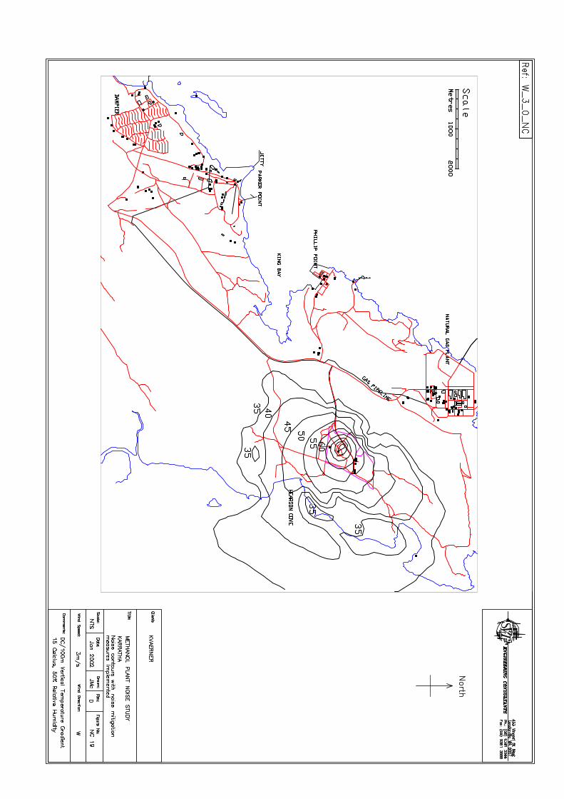
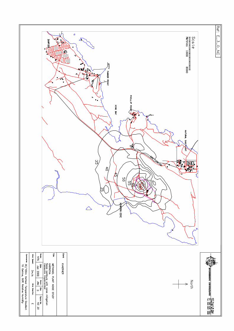
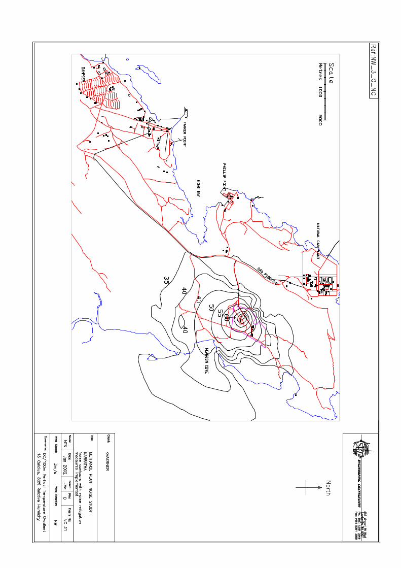
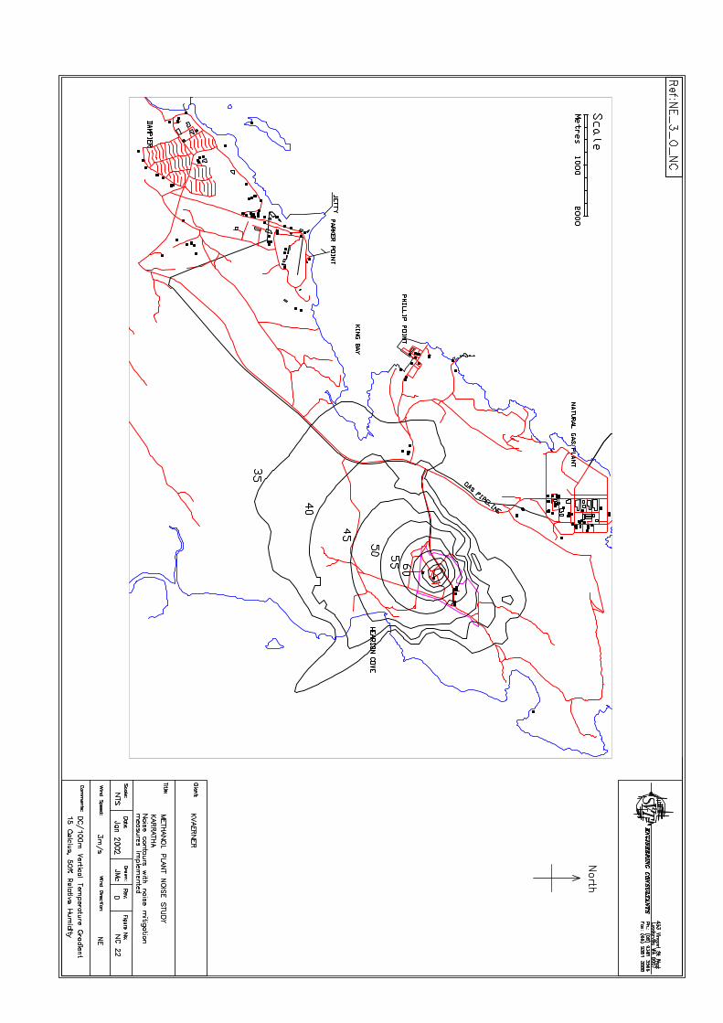

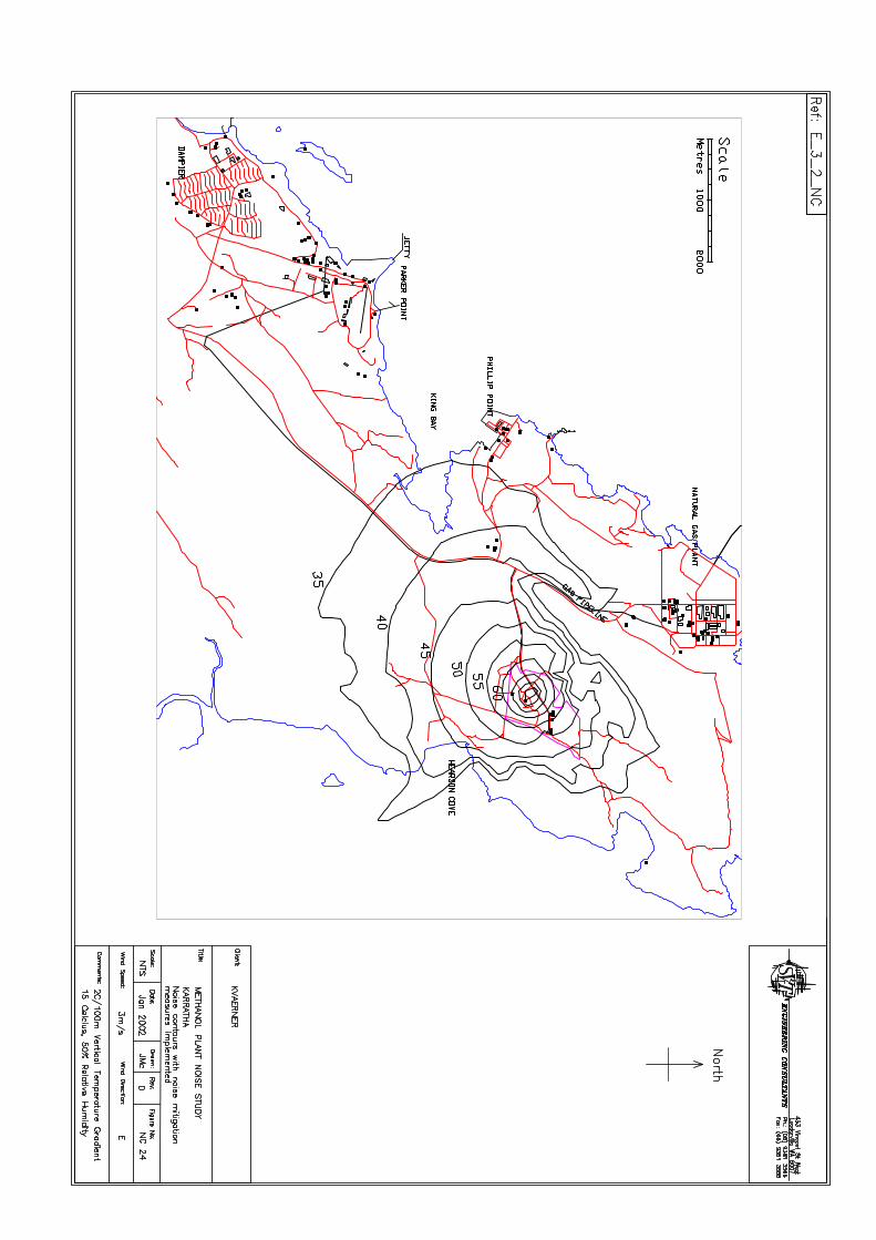

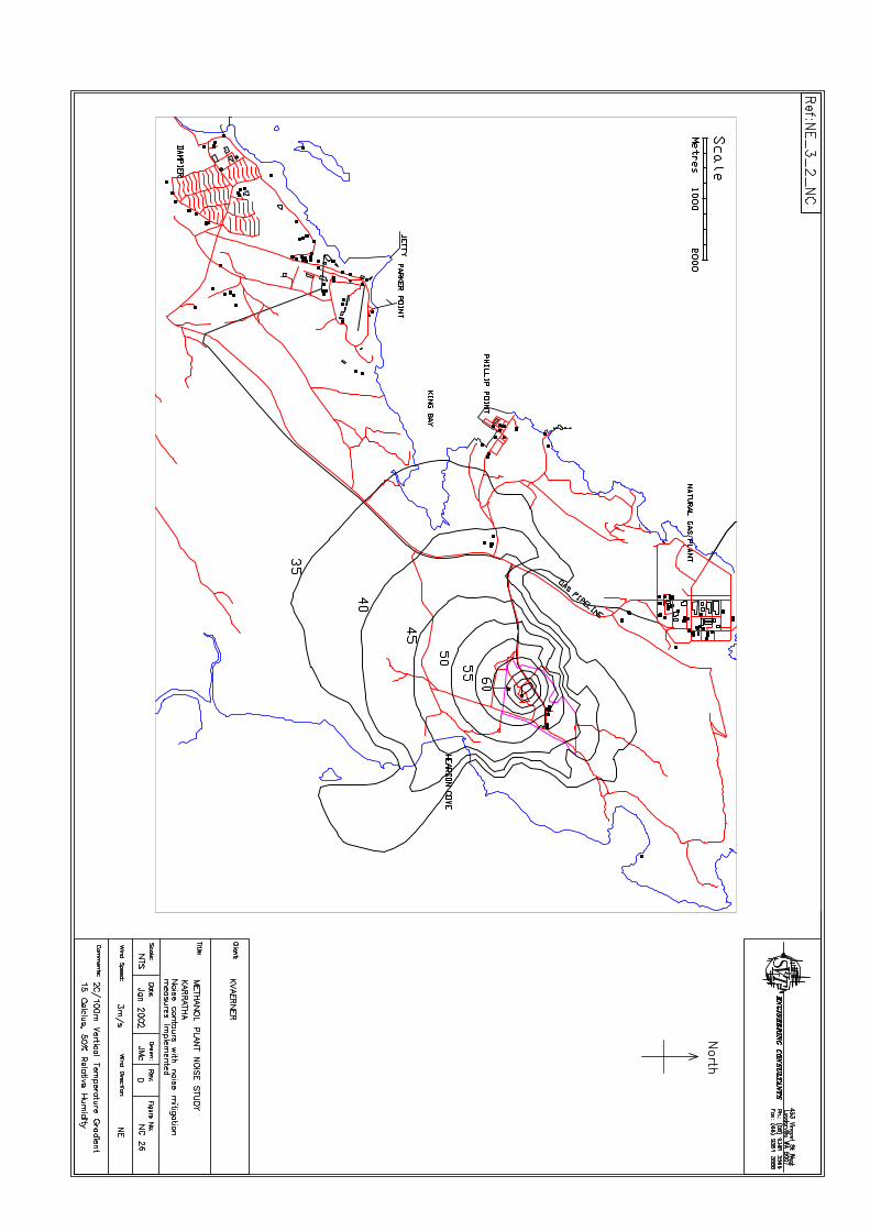
Client: Kvaerner January 2002Subject: Environmental Noise Study - Karratha Methanol Plant Revision 0A
SVT Engineering Consultants JMc: Kvaerner Karratha methanol plant_rpt_0A.doc
10 APPENDIX C – GLOSSARY OF TERMS
Term Definition1/3 Octave Band A range of frequencies where the highest frequency is greater than
the lowest frequency by a factor of 21/3
Amplitude MagnitudeAssigned NoiseLevels
The highest noise levels that can be received at various premisesaccording to the Western Australian Environmental Protection(Noise) Regulations
A-weighting A standardised frequency response used in sound measuringinstruments which approximates the response of the human ear
dB Abbreviation for decibeldB(A) Abbreviation for A-weighted decibeldB(lin) Abbreviation for Un-weighted decibelDecibel A logarithmic unit which represents the ratio of a measured quantity
to a defined reference levelFrequency The rate of vibration in cycles per second (Hertz) commonly
associated with the pitch of a sound - low frequencies produce basssounds and high frequencies produce treble sounds. The frequencyrange of the human ear is nominally 20 Hz to 20,000 Hz
Hertz The unit of frequencyHz Abbreviation for HertzImpulsive Noise Noise containing pronounced peaks in amplitude which last for less
than about 1 second, for example banging and thumpingLA1 The sound pressure level exceeded for 1% of a specified time periodLA10 The sound pressure level exceeded for 10% of a specified time periodLAmax The maximum A-weighted sound pressure level over a specified
period of timeLin Abbreviation for LinearLinear-weighting Description of the weighting used on sound measuring instruments
which respond equally to all frequencies. Also "Un-weighted"Modulating Noise Noise whose amplitude and/or frequency content varies periodically
in time, for example a sirenNoise Unwanted soundNoise Level Sound Pressure LevelOctave Band A range of frequencies were the highest frequency is greater than the
lowest frequency by a factor of 2Sound Power The total sound energy in Watts radiated by a sounce source per unit
timeSound Power Level The magnitude of the sound power expressed in decibels re 1
picowattSound Pressure The variation in ambient pressure caused by a sound wave -
measured in PascalsSound Pressure Level The magnitude of the sound pressure expressed in decibels re 20
micropascalsSpectrum The entire range of sound frequenciesSPL Abbreviation for Sound Pressure Level

Client: Kvaerner January 2002Subject: Environmental Noise Study - Karratha Methanol Plant Revision 0A
SVT Engineering Consultants JMc: Kvaerner Karratha methanol plant_rpt_0A.doc
SWL Abbreviation for Sound Power LevelTonal Noise Noise containing one or more frequencies which dominate the
spectrum. Typically whining or droning noises
Preliminary Risk Analysis of Proposed Methanol Plantand Facilities
Appendix 7
Prepared for:
METHANEX LTD600 St Kilda RoadMelbourne, Victoria 3000
Prepared by:
Halliburton KBR Pty LtdABN 91 007 660 317Level 9, 201 Kent Street, Sydney NSW 2000Telephone 02-9911 0000, Facsimile 02-9241 2900
February 2002
SEH201-001-Rev. 0
PRELIMINARY RISKANALYSIS OF PROPOSEDMETHANOL PLANT ANDFACILITIES
Burrup Peninsula, WesternAustralia
SEH201-001-Rev. AFebruary 2002
Halliburton KBR Pty Ltd, 2002
Halliburton KBR Pty Ltd (formerly Brown & Root)is a member of the Australian Engineering Achievers Group.Members of the Group adhere to best practice in their fieldsof engineering endeavour and are leaders in industry excellence.They demonstrate Australia’s expertise in the field of engineeringand show innovation in the way engineering solutionsare developed and implemented.
Acknowledgments
Limitations Statement
The sole purpose of this report and the associated services performed by Halliburton KBR Pty Ltd (Halliburton KBR)is to prepare a Prelimianry Risk Analysis of the proposed Methanol Plant and facilities in accordance with the scopeof services set out in the contract between Halliburton KBR and Kvaerner Engineering and Construction Pty Ltd(‘the Client’). That scope of services was defined by the requests of the Client, by the time and budgetary constraintsimposed by the Client.
Halliburton KBR derived the data in this report primarily from data provided by the client, previous studiesconducted by Halliburton KBR for the client, and examination of records in the public domain.. The passage of time,changes to design, changes to site and facilities or impacts of future events may require further data analysis, and re-evaluation of the findings, observations and conclusions expressed in this report.
In preparing this report, Halliburton KBR has relied upon and presumed accurate certain information (or absencethereof) relative to the site, and proposd plant and facilities provided by the Client and others identified herein.Except as otherwise stated in the report, Halliburton KBR has not attempted to verify the accuracy or completeness ofany such information.
The findings, observations and conclusions expressed by Halliburton KBR in this report are not, and should not beconsidered, an opinion concerning the validity of the design. No warranty or guarantee, whether express or implied,is made with respect to the data reported or to the findings, observations and conclusions expressed in this report.Further, such data, findings, observations and conclusions are based solely upon the information and drawingssupplied by the Client. in existence at the time of the study.
This report has been prepared on behalf of and for the exclusive use of the Client, and is subject to and issued inconnection with the provisions of the agreement between Halliburton KBR and the Client. Halliburton KBR acceptsno liability or responsibility whatsoever for or in respect of any use of or reliance upon this report by any third party.
SEH201-T1-001 Rev. 0 iiiMarch 2002
CONTENTS
Section Page
1 INTRODUCTION
1.1 Background 1-11.2 Study Objectives 1-11.3 Scope of the Study 1-11.4 Statutory Controls 1-2
2 SUMMARY AND RECOMMENDATIONS
2.1 General 2-12.2 Results 2-12.3 Conclusions 2-52.4 Recommendations 2-5
3 DESCRIPTION OF PROPOSED FACILITY
3.1 Site Location and Surrounding Land Uses 3-13.2 Facility Description 3-13.3 Plant Control System 3-6
4 HAZARD IDENTIFICATION
4.1 General 4-74.2 Hazardous Properties of Materials 4-84.3 Safety Aspects for the Proposed Facility 4-104.4 Hazardous Scenarios and Evaluation of Safeguards 4-124.5 History of Safety Performance of Similar Methanex
Facilities 4-134.6 Hazards Identified 4-13
5 CONSEQUENCE
5.1 Introduction 5-15.2 Scenario Effect Distances 5-15.3 Release Rates 5-15.4 Jet Fires 5-35.5 Vapour Cloud Explosions 5-35.6 Pool Fires 5-45.7 Effects on People 5-45.8 Consequence Analysis Results 5-4
6 FREQUENCY ANALYSIS
6.1 Introduction 6-86.2 Estimation of Leak Frequency 6-8
7 RISK ASSESSMENT
7.1 Introduction 7-17.2 Risk Guidelines 7-1
SEH201-T1-001 Rev. 0 ivMarch 2002
7.3 Risk Assessment Results 7-27.4 Societal Risk 7-77.5 Conclusions 7-7
8 REFERENCES
APPENDICES
A. Hazard Identification Tables
B. Study Assumptions
C. Consequence Analysis (Plant and Pipeline)
D. Frequency Analysis (Plant and Pipeline)
E. Meteorological Data
F. Jetty Analysis
SEH201-T1-001 Rev.0March 2002
v
ABBREVIATIONS
Abbreviation Explanation
AGHR Advanced Gas Heated Reformer
ALARP As Low As Reasonably Practicable
API American Petroleum Institute
ASU Air Separation Unit
BDEP Basic Design and Engineering PackageBFW Boiler Feedwater
CCPS Centre for Chemical Process Safety
CER Consultative Environmental Review
CH4Methane
CO Carbon Monoxide
CO2 Carbon Dioxide
DCS Distributed Control System
DEP Department of Environmental Protection
DG Dangerous Goods
DME Department of Minerals and Energy
DWT Draught Weight Tonnage
EIS Environmental Impact Statement
EPA Environmental Protection Authority (Western Australia)
ERC Emergency Release Coupling
ESD Emergency Shutdown
F Cumulative frequency, pa
FDT Fractional Dead Time
HAZOP Hazard and Operability Study
H2Hydrogen
HDS Hydrosulphurisation
IDLH Immediately Dangerous to Life and Health
IEEE Institute of Electrical and Electronic Engineers
IMO International Maritime Organisation
kg/s kilograms/ second
kl kilolitres

SEH201-T1-001 Rev.0March 2002
vi
Abbreviation Explanation
km kilometres
kPag kilopascals gauge
kW/m2 kilowatts per square metre
LFL Lower Flammable Limit
m metres
M Mass of methanol spill, tonnes
MIIU Marine Incident Investigation Unit
MLA Marine Loading Arm
mm millimetres
m/s metres per second
NFPA National Fire Protection Association
PFD Process Flow Diagram
PHA Preliminary Hazard Analysis
P&ID Piping and Instrumentation Diagram
pmpy per million per year
PRA Preliminary Risk Analysis
PTW Permit to Work
QRA Quantitative Risk Assessment
TCC Tube Cooled Converter
tpd tonnes per day
tph tonnes per hour
UPS Uninterruptible Power Supply
WA Western Australia
WCC Water Cooled Converter
WEL Woodside Energy Limited
SEH201-T1-001 Rev.0 1-1March 2002
1 Introduction
1.1 BACKGROUND
Methanex Australia Ltd is planning to construct a process plant for the manufacture ofmethanol at Burrup Peninsula, Western Australia. The feedstock for methanol isnatural gas, received by pipeline from Woodside Energy Ltd (WEL).
The plant will consist of two identical parallel trains, each train capable of producing anominal 6,000 tonnes per day (tpd) of methanol. The methanol will be stored in aboveground tanks in a tankfarm, and pumped to the jetty for loading into ships.
The Environmental Protection Authority (EPA) of Western Australia has determined,in accordance with the Environmental Protection Act, 1986, that this proposal requiresa Consultative Environmental Review (CER) and a Preliminary Risk Analysis (PRA).
The concept design of the proposed development has been undertaken by KvaernerEngineering and Construction. Methanex has prepared the CER for the project andthis PRA, prepared by Halliburton KBR Pty Ltd, will become part of the CERdocument to be submitted to the EPA.
In this study it has been assumed that the feedstock natural gas will be supplied to themethanol plant site by a dedicated pipeline from the WEL LNG plant site on theBurrup Peninsula, with custody transfer metering at WEL and pressure regulationequipment at the Methanex site.
1.2 STUDY OBJECTIVES
The objectives of this PRA are to:− identify the hazards associated with the proposed facility and operations;− estimate the offsite risk posed by the proposed methanol plant and its associated
facilities including product storage, pipeline transport and ship loading operations;− compare the risks with the risk criteria published by EPA in the Guidance for Risk
Assessment and Management: Offsite Individual Risk from Hazardous IndustrialPlant” (July 2000);
− determine if there is an interaction from the proposed plant with the nearestindustrial facility in terms of overall risk;
− develop risk reduction measures in order to mitigate the risks where appropriate;− prepare a comprehensive report that is auditable and in a form suitable for
submission to the regulatory authorities in Western Australia.
1.3 SCOPE OF THE STUDY
The scope of the study covers all operating facilities associated with the proposeddevelopment including the following:
SEH201-T1-001 Rev.0 1-2March 2002
• Methanol Plant− Natural gas desulphurisation plant− Reformer and synthesis gas production− Methanol converter− Distillation and methanol production− Air separation unit (ASU)− Turbine Drives− Major heat exchangers− Waste heat recovery unit− Methanol tankfarm
• Methanol transfer pipeline
• Ship loading operations.
1.4 STATUTORY CONTROLS
The statutory controls applicable to the proposed development are described in theCER. The main controls relating to the PRA are:
• EPA Guidance for the Assessment of Environmental Factors “Guidance for RiskAssessment and Management: Offsite Individual Risk from Hazardous IndustrialPlant” (Ref 1).
• Worksafe Australia, Control of Major Hazard Facilities.
• Guidelines for a Preliminary Risk Analysis (WA EPA – 1993).
This PRA addresses the requirements of EPA Guidance document and has attemptedto demonstrate that:
• the proposed development meets the EPA criteria for individual risk to public;
• adequate design, operational and organisational safeguards will be incorporated inthe development such that the risk is as low as reasonably practicable (ALARP);and
• existing or proposed industrial developments on the surrounding land would not beadversely affected.
SEH201-T1-001 Rev.0 2-1March 2002
2 Summary and Recommendations
2.1 GENERAL
Methanex Australia Ltd is planning to construct a process plant for the manufacture ofmethanol at Burrup Peninsula, Western Australia. The feedstock for methanol isnatural gas, received by pipeline from Woodside Energy Ltd (WEL). The plant willconsist of two identical parallel trains, each train capable of producing a nominal6,000 tonnes per day (tpd) of methanol. The methanol will be stored in above groundtanks in a tankfarm, and pumped to the jetty for loading into ships.
The Environmental Protection Authority (EPA) of Western Australia has determined,in accordance with the Environmental Protection Act, 1986, that this proposal requiresthe preparation of a Consultative Environmental Review (CER) containing aPreliminary Risk Analysis (PRA) study. This report constitutes the PRA for theproposal and it will be submitted to the EPA for approval, together with the CER.
The primary objective of this high-level hazard analysis study was to estimate theoffsite public risk posed by the Methanex development. The results were then used todetermine the acceptability of the risks in relation to the risk criteria published by theEPA in terms of land use planning for industrial developments.
Established hazard identification techniques were used and the process was reviewedat a preliminary stage by Kvaerner project engineers to ensure that it reflected theplant correctly.
Hazardous incidents that were considered non-credible from an operationalperspective, or had limited localised impact were screened out from further analysis.Only incidents with potential off site consequences or with potential to escalateresulting in off site impact were carried forward and subjected to a more detailed levelof assessment in the consequence analysis.
Following detailed assessment of incident consequence, those events shown to haveoff site impact or potential to escalate and cause off site impact were carried forwardfor frequency analysis and assessment of the risk level to land adjacent to the site.
2.2 RESULTS
2.2.1 Hazard Identification
The incidents identified as having the potential to result in an offsite impact aresummarised in Table 2.1.
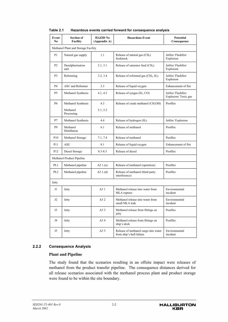
SEH201-T1-001 Rev.0 2-2March 2002
Table 2.1 Hazardous events carried forward for consequence analysis
EventNo
Section ofFacility
HAZID No(Appendix A)
Hazardous Event PotentialConsequence
Methanol Plant and Storage Facility
P1 Natural gas supply 1.1 Release of natural gas (CH4)feedstock.
Jetfire/ Flashfire/Explosion
P2 Desulphurisationunit
2.1, 3.1 Release of saturator feed (CH4) Jetfire/ Flashfire/Explosion
P3 Reforming 3.2, 3.4 Release of reformed gas (CH4, H2) Jetfire/ Flashfire/Explosion
P4 ASU and Reformer 3.3 Release of liquid oxygen Enhancement of fire
P5 Methanol Synthesis 4.1, 4.2 Release of syngas (H2, CO) Jetfire/ Flashfire/Explosion/ Toxic gas
P6 Methanol Synthesis
MethanolProcessing
4.3
5.1, 5.2
Release of crude methanol (CH3OH) Poolfire
P7 Methanol Synthesis 4.4 Release of hydrogen (H2) Jetfire/ Explosion
P9 MethanolDistillation
6.1 Release of methanol Poolfire
P10 Methanol Storage 7.1, 7.4 Release of methanol Poolfire
P11 ASU 8.1 Release of liquid oxygen Enhancement of fire
P12 Diesel Storage 8.3-8.5 Release of diesel Poolfire
Methanol Product Pipeline
PL1 Methanol pipeline A2 1.(a) Release of methanol (operation) Poolfire
PL2 Methanol pipeline A2 1.(d) Release of methanol (third partyinterference)
Poolfire
Jetty
J1 Jetty A3 1 Methanol release into water fromMLA rupture
Environmentalincident
J2 Jetty A3 2 Methanol release into water fromsmall MLA leak
Environmentalincident
J3 Jetty A3 3 Methanol release from fittings onjetty
Poolfire
J4 Jetty A3 4 Methanol release from fittings onship’s deck
Poolfire
J5 Jetty A3 5 Release of methanol cargo into waterfrom ship’s hull failure
Environmentalincident
2.2.2 Consequence Analysis
Plant and Pipeline
The study found that the scenarios resulting in an offsite impact were releases ofmethanol from the product transfer pipeline. The consequence distances derived forall release scenarios associated with the methanol process plant and product storagewere found to be within the site boundary.
SEH201-T1-001 Rev.0 2-3March 2002
The potential for incident escalation was considered low due to the separation distancebetween the various unit operations. These distances had been determined from aprevious safety study on the site layout. However, it was considered that largerreleases (in the order of 100 mm) than considered in the safe layout study would bepossible given the potential size of some of the process pipework and that suchreleases could result in an offsite impact. These larger scenarios were thereforemodelled.
The scenarios that resulted in the most severe impacts in terms of potential for on-siterisk can be identified as:
• release of process vapours, in particular synthesis gas containing high proportionsof carbon monoxide gas, where the release could result in significantconcentrations that might be a threat to life;
• release of feedstock and process vapours containing high proportions of methane,where the release could result in a jet fire (immediate ignition) or flash fire orexplosion (delayed ignition);
• release of hydrogen rich gases (hydrogen gas, synthesis gas) and delayed ignitionleading to an explosion; severity of consequences will be dependent on degree ofconfinement as hydrogen gas clouds have a high probability of detonation in aconfined space.
Jetty
All methanol spillages into water were classified as environmental incidents, withnegligible safety risk, since methanol is fully miscible in water and there would be nofire consequence. For large spillages (eg. structural failure of tanker hull and releaseof cargo), there could be localised toxic effects on marine life.
For methanol pool fires in the bunded area on the jetty, the 4.7 kW/m2 heat radiationcontour extended up to 21 m. It has been recommended that a fire shield be providedat a distance of 30 m from the wharf for personnel to take shelter and operate the firewater monitors.
For a 50 mm leak size on the ship’s deck and a maximum pool diameter of 45 m(width of vessel), the 4.7 kW/m2 heat radiation contour extended up to 40 m.
2.2.3 Frequency Analysis
Plant and Pipeline
Several data bases were used for the development of frequency of incident scenarios.For the pipeline, this involved the determination of pipeline and the associatedequipment's failure rates leading to a release of methanol. Once a release has occurred,it has a probability of ignition. By multiplying the ignition probability by the releasefrequencies, fire frequencies were developed. These were used in the risk assessmentmodel.
The frequency of releases from the process area was not accurately identifiable due tothe limited amount of piping data. Nevertheless, the frequency of releases fromvarious parts of the plant was calculated on the basis of generic data and an assumedquantity of pipework, flanges, valves, vessels and fittings (see Appendix B and D).
SEH201-T1-001 Rev.0 2-4March 2002
Jetty
Frequency values were developed for the various scenarios at the jetty, including thepoolfires and spillages into the water arising from different sized leaks (eg. MLArupture, or flange/ joint leak, tanker cargo tank failure following collision). An F-Mcurve was developed to show the cumulative frequency with which M or more tonnesof methanol could be spilled into the water.
The overall fire frequency for a bund fire on the wharf was calculated to be 5.0 x 10⁻⁵
per annum.
2.2.4 Risk Analysis
Plant and Pipeline
Individual risk can be assessed by combining the consequence and frequency ofevents. TNO RiskCurves was used to generate the isopleths for the methanol processplant and product storage. The resultant risk contour showed that the risk at the plantboundary does not exceed the maximum acceptable criterion of 50 in a million peryear.
In the case of the product transfer line, due to the linear nature of the pipeline, the risklevels were developed as transects, which are levels of risk for a given transversedistance from the pipeline or associated facilities (valve, meter station). Overall, therisk along the entire length of the proposed methanol product pipeline will not exceedthe EPA criterion of 10 x 10-6 for non-industrial activities or active open spaces in abuffer zone between industrial and residential zones. The pipeline will be laid in adedicated pipeline corridor and it is not expected that residential areas or sensitiveland uses (such as hospitals, schools or aged care facilities) will be located within the1 pmpy or 0.5 pmpy contour distances respectively. It is also assumed that there areno commercial activities set within the 5 pmpy distance from the pipeline.
As it is considered non-credible that the consequences of releases from the productpipeline and process plant could result in multiple fatalities offsite, societal risk hasnot been evaluated.
Jetty
There are no established acceptance criteria for the risk of product spills into water.The guiding principle is generally that all product spills should be eliminated, or therisk of a spill reduced to as low as reasonably practicable (ALARP) levels. Theconsequence-frequency curve for the identified scenarios shows that the frequency ofa spill exceeding 100 tonnes is approximately 1 chance in 5,000 per year. This risk islow.
The overall fire frequency for a bund fire on the wharf was calculated to be 5.0 x 10⁻⁵
per annum, which is considered to be low.
Assessment of the ship loading operations at the proposed new wharf indicated thatthe 4.7 kW/m2 heat radiation contour extends approximately 21 m from the centre ofthe pool. Provided that there is a public exclusion zone around the loading point atleast equal to this value, there will be no impact on the public as a result of the loadoutof methanol product.
SEH201-T1-001 Rev.0 2-5March 2002
2.3 CONCLUSIONS
The study found that Kvaerner had adopted a risk-based approach in the design of theMethanex facility. In addition, Methanex had incorporated enhanced design featuresinto the proposed development gathered from past operating experience of similarfacilities.
For the purposes of the hazard analysis, gross assumptions relating to streamcomposition, fire and explosion effects and initiating frequencies were made. Thismade the study findings conservative and was considered appropriate, as the objectivewas to assess the offsite risk levels posed by the development to surrounding landusers.
The following conclusions can be made based on the results of this PRA:
• The methanol production and storage facility has negligible offsite impact withregard to individual risk by virtue of the plot size. The maximum individual risk atthe boundary was well below 1 in a million per year. As such the facility isexpected to have negligible interaction with surrounding industrial developments.This conclusion is based upon the risk contours generated and on the conservativenature of the assumptions that have gone into the contour derivation. The actualrisk contours (that will be defined during detailed design) are unlikely to be largerthan those derived in this study.
• The risk along the entire length of the proposed methanol product pipeline will notexceed the EPA criterion of 10 x 10-6 for non-industrial activities or active openspaces in a buffer zone between industrial and residential zones.
• The proposed Methanex development was found to comply with the EPA riskcriteria in terms of land use planning.
2.4 RECOMMENDATIONS
For the risk analysis study, various assumptions relating to the design of the proposeddevelopment were made. This included Kvaerner providing adequate process safetydetection and protection systems to ensure that there would be negligible risk to thesurrounding environment. In addition, the study has also assumed that Methanex, asthe operator would develop and maintain a comprehensive safety and environmentalmanagement system for the facility, pipeline and jetty operations. This includeswritten procedures, regular audits, training, permit to work system, robust change ofmanagement and emergency planning.
As such the recommendations arising from the PRA relate to the implementation ofthe study assumptions that are outlined in the Hazard Identification tables. This willprovide a basis for the development to reduce risk levels to As Low As ReasonablyPracticable (ALARP).

SEH201-T1-001 Rev.0 2-6March 2002
These recommendations (assumptions) fall under the broad categories of:
• Facility Design.
• Facility Layout.
• Process Safety Control Barriers (ie. gas/fire detection, hazardous areaclassification, pipeline markers).
• Process Safety Recovery Measures (ie. fire protection systems, ESD, emergencypower backup).
• Safety Management Systems (ie. Permit to Work Systems, maintenance schedules,critical alarm testing).
• Provision of fire separation distances and shielding at the wharf.
SEH201-T1-001 Rev.0 3-1March 2002
3 Description of Proposed Facility
The following information is taken from engineering design package (Ref 2).
3.1 SITE LOCATION AND SURROUNDING LAND USES
The proposed location for the methanol plant is a Greenfield site at Burrup Peninsulain Western Australia.
The site lies in a large area zoned industrial, with the majority of the site fallingwithin the Burrup Peninsula Draft Land Use and Management Plan. Currently thearea is mostly undeveloped.
The surrounding land uses of interest to this study are:
• Mitsubishi plant site located on the methanol plant southern boundary.
• Burrup Fertilisers located on the tip of the south western boundary.
• Proposed Plenty River Ammonia/ Urea Plant adjoins the Burrup Fertiliser sitefurther west.
• Dampier public wharf is located west of the site.
3.2 FACILITY DESCRIPTION
3.1.1 General
The proposed facility can be divided into three distinct sections:
• methanol plant and associated tankage and utilities, located at the Hearson Covesite;
• offplot pipeline transferring methanol from the plant tankfarm to the proposed newDampier Wharf; and
• ship loading facilities to be provided at Dampier Wharf.
Each of the two process trains at the methanol plant will produce 6,000 tonnes perday of methanol from natural gas and associated site storage for 18 days production.The plant will operate continuously. An air separation unit on the site will provide theoxygen for the reactor, and nitrogen for inerting utilities.
A steam reforming process is used to produce methanol synthesis gas (syngas) fromnatural gas. This is followed by converting syngas to methanol in a catalyticconverter. The crude methanol is purified by distillation.
SEH201-T1-001 Rev.0 3-2March 2002
3.1.2 Desulphurisation and Saturation
Natural gas enters the plant via a knock out drum to remove entrained hydrocarbonliquids. The natural gas feed is then heated to a temperature suitable forhydrodesulphurisation (HDS) in HDS vessels (R-101A-C) by HDS Heat Exchanger(E-101), with trim heating provided by a fired process heater (E-102). The HDSvessels are arranged such that a vessel containing HDS catalyst precedes two vesselscontaining zinc oxide catalyst for hydrogen sulphide removal. The two vessels withzinc oxide catalyst beds operate in series, in a lead-lag arrangement.
Desulphurised feed gas is then saturated with water by contacting the gas with a largequantity of hot circulating water in a packed column called the Saturator (C-101).
The circulating saturator water is a major heat sink for the process and its re-heatingis achieved by heat integration with reformed gas cooling and the Water CooledConverter (WCC) (R-107). Control of Steam:Carbon upstream of the reformingsection is achieved by injecting intermediate pressure steam underflow control,downstream of the Saturator. During normal operation, the steam injection rate neednot exceed the saturator water make-up rate, nor should there be a need for any utilityheating of the circulating saturator water. However, under abnormal or alternateoperating scenarios, trim heating of saturator water is carried out in the SaturatorWater Steam Heater (E-136), which utilises intermediate pressure extraction steam.
3.1.3 Reforming
The reforming section of the process utilises Synetix proprietary Leading Concept(LC) compact reforming technology. Preheated saturated feed gas passes through thetube side of the Advanced Gas Heated Reformer (AGHR) (R-102), where it is heatedand partially steam reformed. The reformed gas, which still has a high methanecontent, is then passed through an oxygen blown Secondary Reformer (R-109). In thisvessel, the high methane reformed gas is partially combusted with oxygen (98 vol%purity) before passing through the secondary catalyst bed. A dedicated Air SeparationUnit (ASU) supplies oxygen to the Secondary Reformer.
Hot synthesis gas exits the Secondary Reformer and passes through the shell side ofthe AGHR, providing the heat to sustain the endothermic primary reforming reactionsoccurring on the tube side.
A Reformer Start-up Heater (E-104) heats the saturated feed gas upstream of theAGHR tubes, during refractory preheating (in the event of a cold start after aprolonged shutdown) and before the Secondary Reformer oxygen burner can be re-ignited.
Synthesis gas leaving the AGHR shell side is cooled through a heat recovery trainconsisting of a feed/effluent interchanger (E-103), saturator water heaters (E-134/ 139& 140), the methanol Refining Column Reboiler (E-120) and the Topping ColumnReboiler (E-116). An air cooler, the Syngas Cooler (E-105) cools the synthesis gasand process condensate to a suitable catchpot temperature. The Syngas Suction Drum(D-105) separates the synthesis gas from the process condensate, which is returned tothe saturator. Intermediate knockout drums (D-103 & 104) maintain a reformed gasvapour fraction in excess of 90 mol% inlet to any heat recovery heat exchanger, whilealso ensuring that the process condensate temperature remains high.
SEH201-T1-001 Rev.0 3-3March 2002
3.1.4 Methanol Synthesis
The Syngas Compressor (K-103A) compresses synthesis gas to methanol synthesisloop pressure. The make-up to the loop is introduced downstream of the LoopCirculator (K-103B) and the feed/effluent exchanger, the Loop Interchanger (E-151).In the event of a cold start after a prolonged shutdown, a steam heated Start-Up Heater(E-117) provides heat to the system before heat is available from the exothermicsynthesis reactions occurring in the converters.
The synthesis loop is a proprietary Synetix/Methanex design, which utilises two stagesof methanol synthesis. Firstly in a Tube Cooled Converter (TCC) (R-105A/ B) inwhich cold feed entering on the tube side is preheated against the heat of reactionoccurring on the catalyst filled shell side. Secondly in a Water Cooled Converter(WCC) (R-107) where the heat of reaction is removed by heating the circulatingsaturator water. The synthesis reactions are highly exothermic, therefore, good heattransfer is essential between the reaction side and the cooling side of the converter,due to the trade-off between reaction kinetics (enhanced by higher temperature) andreaction equilibrium conversion, which increases as the converter exit temperaturedecreases.
Effluent from the WCC is cooled firstly by heat recovery in the Loop Saturator WaterHeater (E-138), followed by the feed/effluent Loop Interchanger (E-151), the RefiningColumn Feed Preheater (E-135), the Loop Demin Water Heater (E-107), and finallyby air cooling in the Loop Condenser (E-112). The inclusion of a Loop BFWpreheater to heat high pressure BFW, upstream of the Loop Interchanger, offers thepotential to increase the heat recovery efficiency of the gas turbine HRSG if low-pressure steam raising is utilised to improve overall plant efficiency.
Crude methanol is separated at high pressure from recycle gases in the CrudeMethanol Catchpot (D-106). Due to the low conversion per pass in the converterreactors, a gas recycle is both economically viable and necessary to improve operatingefficiency and minimise emissions. The recycle gases are re-circulated by the LoopCirculator (K-103B).
A purge is required to prevent build-up of inert components in the loop. Since themake-up synthesis gas is carbon rich, hydrogen must be recovered from the purge gas,via a membrane/PSA package (X-131). The amount of hydrogen recovered dependson the hydrogen/carbon oxides stoichiometry inlet to the TCC. Recovered hydrogen isreturned to the suction of the make-up gas compressor (K103A). The high pressureresidual purge gas leaving the membrane is utilised as fuel gas for the Gas Turbine(GT) driver (K-104), while the low pressure PSA tail gases are utilised in the HDSHeater (E-102) and as fuel gas for supplementary firing in the HRSG (X-183). A smallportion of the purge gas is also recycled to the front end to provide hydrogen for theHDS section.
3.1.5 Methanol Purification
The high pressure crude methanol from the catchpot (D-106) is first letdown to alower pressure to allow the bulk of the dissolved gases to flash and separate from thecrude methanol liquid in a Letdown Vessel (D-111). The pressure is reduced further ina Low Pressure Letdown Vessel (D-112), to remove more dissolved gases andtherefore minimise the load of non-condensables in the Topping Column (C-104)
SEH201-T1-001 Rev.0 3-4March 2002
overheads. Both letdown vessels utilise water washing for methanol recovery fromflash gases.
Product methanol purification is achieved using a 3-column distillation scheme, inwhich the second and third columns (C-104 and C-105) are double-effect (thermallyintegrated) columns. Light materials and dissolved gases are completely removed inthe Topping Column (C-104) while the purified methanol product is drawn from theoverheads of both the Refining Column (C-105) and the Recovery Column (C-106).Water is separated from the methanol product and removed in Recovery Columnbottoms. The water is returned as make-up to the saturator water circulation systemand as wash water for the letdown vessels. A fusel oil side-draw on the RecoveryColumn limits the concentration of organic material in the column bottoms andtherefore limits the flow rate of organic material entering the saturator water. Byintroducing the fusel separately at the top of the Saturator, organic material can bestripped more effectively and returned to the reforming section.
While operating normally without re-run, no heat is required from utilities. However,the distillation system is designed for up to 10% re-run capacity. Therefore, if thedistillation system is to be operated with re-run or under alternate operating scenarios,then additional heat can be supplied from low-pressure extraction steam via theRefining Column Steam Reboiler (E-164).
Methanol product is pumped to Methanol Rundown Tanks (T-2) before beingtransferred to product storage. A Crude Methanol Tank (T-1) is provided to allowrundown of off-spec product, which can later be returned to the distillation section asre-run.
3.1.6 Air Separation Unit
Atmospheric air is compressed in an air compressor driven by the gas turbine unit, andfed into the air separation unit (ASU). Separation of air into oxygen, nitrogen andother inerts occurs by adiabatic cooling, and separation in a “cold box”, undercryogenic conditions.
Liquid oxygen is removed from the cold box, vapourised by cooling incoming air, andsent to the methanol converter. It is not intended to have liquid oxygen storage on thesite.
Nitrogen produced in the ASU is used as utility gas for inert purging, inert gasblanketing and similar operations.
The location of the air intake to the ASU ensures that even in the event of accidentalreleases of natural gas in the plant, hydrocarbon ingress into the air stream would notoccur, thus eliminating the hazard of hydrocarbon accumulation in the oxygen in thecold box.
3.1.7 Waste Heat Recovery Unit
The gas turbine exhaust gas, and reformer stack gas leave the system at relatively hightemperatures. As a means of energy optimisation, the waste heat is recovered by steamgeneration, and a series of heat exchangers to preheat the feed.
SEH201-T1-001 Rev.0 3-5March 2002
3.1.8 Methanol Tankfarm
The tankfarm consists of four methanol tanks of 50,000 tonnes capacity each, locatedin individually bunded areas. Two tanks will be constructed initially (Phase 1) whenthe plant starts up, and two other tanks will be constructed as part of the plantexpansion to the second train (Phase 2).
The tanks are atmospheric above ground tanks, designed to API 650 standard. Theinstallation will comply with the requirements of AS 1940-1993.
3.1.9 Methanol Transfer Pipeline
Methanol will be pumped from the tankfarm to Dampier Wharf by a single 750 mm(30 inch) diameter pipeline. The line length is approximately 5 km west of themethanol plant.
The pipeline will run above ground for the majority of its length, located in aneasement, with corrosion protection by surface coating, and leak detection installed.The pressure in the pipeline at maximum pumping rates will be about 1,500 kPag(pump discharge).
The pipeline will be rated for 5,000 tonnes per hour (tph) and will be designed andinstalled in full compliance with the requirements of AS 2885.
3.1.10 Ship Loading Operations
Ship loading facilities for methanol will be built at the Dampier Wharf. The facilitywill initially consist of one hydraulic marine loading arm with an emergency releasecoupling to prevent loss of containment in the event of loading arm failures (Phase 1).A second loading arm and associated equipment will be installed in the future Phase 2expansion. Each loading arm will be designed for a rate 2,500 tph of methanol.
The facility will be designed to comply with the requirements of AS-3846.
3.1.11 Utilities
A number of utility systems, typical of petrochemical plant, will be provided in thefacility. These systems are outlined in the following paragraphs.
Steam and Condensate System
The Steam and Condensate system includes the following major equipment: steamgenerator feedwater storage, deaerator, steam generator feedwater pumps, associatedchemical storage, excess steam condenser and steam generator blowdown drum.
Chemicals are injected into the steam generator feed water to minimise corrosion andfouling.
Water Supply System
This area includes the following sub-systems: Fire/ Raw Water Storage, Utility WaterSupply, Raw Water Treating Package, Treated Water Storage, Potable WaterTreatment and Supply, and Fire Water System.
The bulk of process cooling will be achieved through air cooling using fin fan coolersand the cooling water requirement for this purpose is minimal.
SEH201-T1-001 Rev.0 3-6March 2002
Flare System
A flare system is included in the facility to handle planned or emergencydepressurisation and blowdown of hydrocarbon streams and pressure relief valvereleases during emergency situations. The flare system is purged with fuel gas toprevent ingress of air, and a knockout drum is provided to remove liquids prior toentering the flare.
Fuel Gas System
The fuel gas station consists of a pressure regulating station and a knockout drum fornatural gas fuel.
A portion of the feedstock natural gas is reduced in pressure, passed through aknockout drum and fed to a fuel gas header. This fuel gas is used for the gas turbineand the reformer fired heater.
3.3 PLANT CONTROL SYSTEM
3.3.1 Distributed Control System
The principal means of plant control will be by a Distributed Control System (DCS).Plant operating personnel (operators) will be on duty in the control room at all timesand field operators will be on duty in the plant areas and will be in communicationwith the control room operators.
The DCS will perform process and equipment control, equipment interlocks, non-critical process equipment shutdowns, monitoring, alarming, data logging andrecording.
3.3.2 Failure Modes
The plant will have a fail-safe philosophy for protection of personnel and equipmentin the event of equipment and/or process malfunction. Systems will be designed toshutdown in a safe and orderly manner. All remote operated on-off valves and controlvalves will be evaluated for failure mode on loss of power (air or electric). Safedesign practice dictates that solenoids controlling valves will fail-safe by de-energising.
3.3.3 Emergency Shutdown
The emergency shutdown (ESD) system will provide for the shutdown of equipmentand mechanical packages, as well as well as the entire plant. The emergencyshutdown capability provided by the ESD system will be physically separate fromand independent of the DCS. The ESD system will include hardwired signals fromfield instrumentation, a fault tolerant and dedicated field output devices for thehighest possible safety and reliability. The ESD system will be supplemented by ESDpushbuttons and a number of hardwired interlocks throughout the facility.
SEH201-T1-001 Rev.0 4-7March 2002
4 Hazard Identification
4.1 GENERAL
The major hazards in terms of off-site fatality potential associated with the proposeddevelopment relate primarily to ignited events (ie fire/ explosion) and unignitedreleases from certain unit operations (ie carbon monoxide from the Synthesis plant).For the former, the likelihood of such ignition will depend on the flammability of thereleased process stream and the nature and proximity of the ignition source.
This study incorporated an extensive hazard identification that involved a screeningprocess based upon the nature of a hazard and the proposed safeguards. A set ofscenarios that represented the type of hazards associated with the methanol facilitywas developed. Hazardous scenarios were screened out from further analysis if it canbe shown that the scenario (allowing for the safeguards) does not have a potential tocause offsite effects or deemed to be non-credible, either from an operational point ofview or due to the chemical characteristics of the materials.
Those events which had potential off site consequences were carried forward andsubjected to a more detailed level of assessment involving quantifying consequencesand if necessary, the frequency of occurrence for risk quantification. The HazardIdentification (HAZID) table - a summary of the identified hazards, together with theexisting and proposed safeguards is presented in Appendix A.
The proposed Methanex development was divided into a number of sections asoutlined in Section 1.2. Development of credible incidents was based upondiscussions held with Kvaerner design engineers and reviews of previous safetyengineering studies undertaken for similar plant operated by Methanex.
The identification of the hazardous materials was based on a review of the descriptionof the proposed facility and the supporting information, as follows:
• Basic Design and Engineering Package for Outside Fence Facilities;
• Basis of Design documents for control systems;
• general layout drawings;
• process flow diagrams (PFDs); and
• piping and instrumentation diagrams (P&IDs).
In the following sections, the properties of the hazardous materials identified arediscussed and credible hazardous scenarios are postulated for evaluation againstproposed design, hardware and procedural safeguards.
SEH201-T1-001 Rev.0 4-8March 2002
4.2 HAZARDOUS PROPERTIES OF MATERIALS
4.2.1 General
The major hazards identified at the site will be flammable gas and liquids that couldresult in jet, spray or pool fires and vapour cloud explosions following loss ofcontainment.
A release of a flammable gas under pressure may result in a jet fire if ignitedimmediately, or, in the event of delayed ignition, a flash fire followed by jet fire if theleak has not been isolated. A flash fire may result in an explosion if there is asufficient mass of flammable vapour and a degree of confinement for flame frontacceleration. Only the part of the flammable cloud where the concentration is abovethe lower flammability limit will ignite.
The stream properties have been estimated based on the P&IDs/ PFDs and the typicaloperating parameters for similar plant.
Due to the proprietary nature of the Methanex process, the exact compositions andoperating parameters of process streams are considered confidential and have not beenreported. However the study made assumptions on these streams as outlined belowand in Appendix B.
4.2.2 Gas Vapour Streams
Methane
Methane is a major component in the natural gas feedstock and reformed gas.
Natural gas has been assumed to be essentially composed of methane ie. greater than98%. Methane is a Class 2.1 Dangerous Good (flammable gas) that burns with aluminous flame. It has flammability limits of 5-15 vol% in air. Methane is consideredto be an explosion hazard if the gas cloud is confined in significantly congested areas.
The same assumption was also applied to saturator feed and reformed gas.
Hydrogen
Hydrogen is a highly flammable gas that burns with a non-luminous flame. It has wideflammability limits (4 - 75 vol% in air), a very low minimum ignition energy and ahigh burning velocity. It therefore is easily ignited and burns rapidly. Hydrogen gasclouds located in congested and/ or confined locations are considered high explosionhazards. Hydrogen is present as a major component in the Syngas process streamtogether with carbon monoxide.
Carbon Monoxide
The process streams within the syngas plant contain significant amounts of carbonmonoxide (8-21 vol%). Although carbon monoxide is flammable in the range of 12-75vol% in air, the primary hazard arises from toxic gas exposure. Carbon monoxideburns with a luminous flame.
Carbon monoxide is a colourless, odourless gas that has approximately the samedensity as air. It combines with the haemoglobin in the blood to formcarboxyhaemoglobin (COHb), displacing the oxygen, thereby impairing the oxygen
SEH201-T1-001 Rev.0 4-9March 2002
capacity of the blood. The effects are fast acting, with a concentration in air of 1.3vol% causing unconsciousness within a few minutes (Ref. 3).
The concentration of carbon monoxide in air at which 50% of an exposed populationwill be fatally injured (referred to as the LC50) for a 30 minute exposure time is in theorder of 8,000 mg/m3 or 0.7 vol%. A concentration of 1,500 ppm is consideredimmediately dangerous to life and health (IDLH value), ie. potential for irreversibledamage for exposure over 30 minutes.
Oxygen
The hazardous properties of oxygen arise from its ability to enhance the process ofcombustion with oxygen enrichment of air increasing the flammability of materials.
The speed of combustion of common materials increases markedly with an increase inthe oxygen content in the air. For cotton clothing, the burning rate increases by about25% in an oxygen concentration of 40% in air. There is a corresponding increase inthe ease of ignition. Beyond an oxygen concentration of 40% in air, further increasedeffect due to oxygen enrichment is relatively small.
An oxygen concentration of 40% in air was used in the study as the criticalconcentration for enhancement of combustion and ease of ignition.
4.2.3 Liquid Streams
Methanol
Methanol is a liquid hydrocarbon designated as a Class 3 Packing Group II DangerousGood (ie. flammable liquid) with a subsidiary risk of 6.1 (toxic).
Methanol is a colourless, clear and mobile volatile liquid (boiling point of 64.5O C). Ithas a density of 787 kg/ m3 and is miscible with water. It is toxic if swallowed (maycause blindness).
Table 4.1 summarises the proposed volumes of crude and final product methanol to bestored at the site.
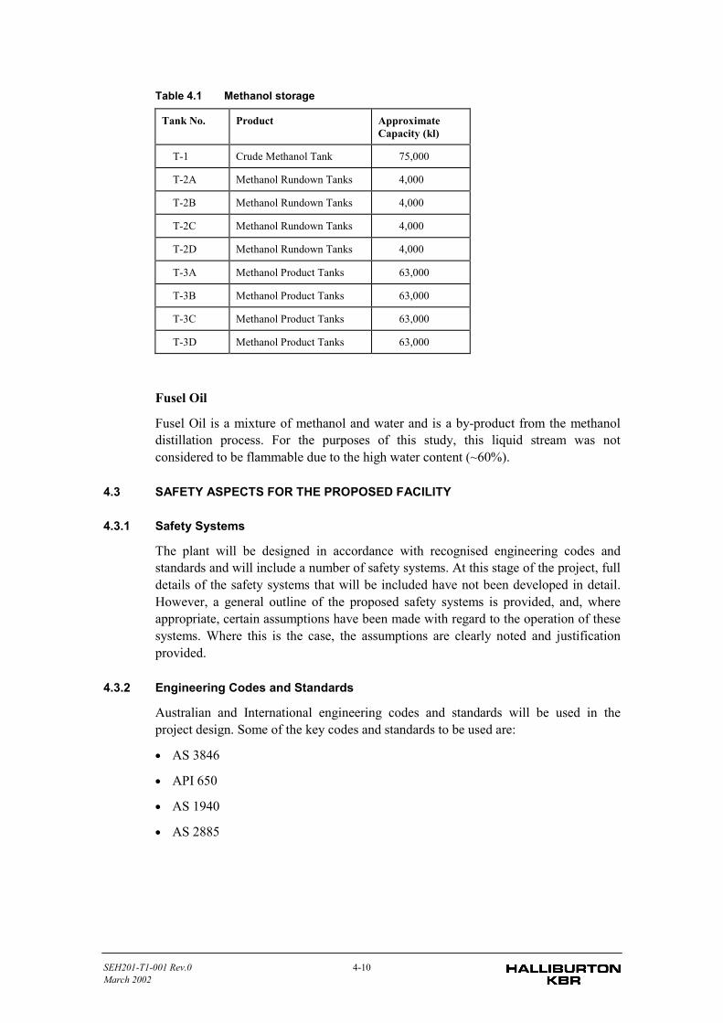
SEH201-T1-001 Rev.0 4-10March 2002
Table 4.1 Methanol storage
Tank No. Product ApproximateCapacity (kl)
T-1 Crude Methanol Tank 75,000
T-2A Methanol Rundown Tanks 4,000
T-2B Methanol Rundown Tanks 4,000
T-2C Methanol Rundown Tanks 4,000
T-2D Methanol Rundown Tanks 4,000
T-3A Methanol Product Tanks 63,000
T-3B Methanol Product Tanks 63,000
T-3C Methanol Product Tanks 63,000
T-3D Methanol Product Tanks 63,000
Fusel Oil
Fusel Oil is a mixture of methanol and water and is a by-product from the methanoldistillation process. For the purposes of this study, this liquid stream was notconsidered to be flammable due to the high water content (~60%).
4.3 SAFETY ASPECTS FOR THE PROPOSED FACILITY
4.3.1 Safety Systems
The plant will be designed in accordance with recognised engineering codes andstandards and will include a number of safety systems. At this stage of the project, fulldetails of the safety systems that will be included have not been developed in detail.However, a general outline of the proposed safety systems is provided, and, whereappropriate, certain assumptions have been made with regard to the operation of thesesystems. Where this is the case, the assumptions are clearly noted and justificationprovided.
4.3.2 Engineering Codes and Standards
Australian and International engineering codes and standards will be used in theproject design. Some of the key codes and standards to be used are:
• AS 3846
• API 650
• AS 1940
• AS 2885
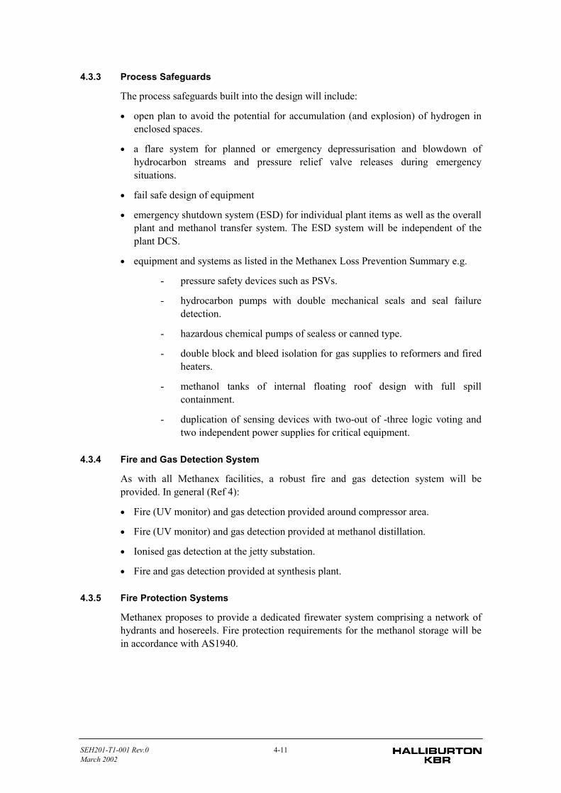
SEH201-T1-001 Rev.0 4-11March 2002
4.3.3 Process Safeguards
The process safeguards built into the design will include:
• open plan to avoid the potential for accumulation (and explosion) of hydrogen inenclosed spaces.
• a flare system for planned or emergency depressurisation and blowdown ofhydrocarbon streams and pressure relief valve releases during emergencysituations.
• fail safe design of equipment
• emergency shutdown system (ESD) for individual plant items as well as the overallplant and methanol transfer system. The ESD system will be independent of theplant DCS.
• equipment and systems as listed in the Methanex Loss Prevention Summary e.g.
- pressure safety devices such as PSVs.
- hydrocarbon pumps with double mechanical seals and seal failuredetection.
- hazardous chemical pumps of sealess or canned type.
- double block and bleed isolation for gas supplies to reformers and firedheaters.
- methanol tanks of internal floating roof design with full spillcontainment.
- duplication of sensing devices with two-out of -three logic voting andtwo independent power supplies for critical equipment.
4.3.4 Fire and Gas Detection System
As with all Methanex facilities, a robust fire and gas detection system will beprovided. In general (Ref 4):
• Fire (UV monitor) and gas detection provided around compressor area.
• Fire (UV monitor) and gas detection provided at methanol distillation.
• Ionised gas detection at the jetty substation.
• Fire and gas detection provided at synthesis plant.
4.3.5 Fire Protection Systems
Methanex proposes to provide a dedicated firewater system comprising a network ofhydrants and hosereels. Fire protection requirements for the methanol storage will bein accordance with AS1940.
SEH201-T1-001 Rev.0 4-12March 2002
4.3.6 Emergency Power
The methanol facility will be provided with a pulse width modulated UninterruptablePower Supply (UPS) system as the primary power supply for all instrumentation andcritical process control equipment.
Emergency power will be supplied by diesel powered engines.
4.3.7 Safety Management System
It is assumed that a comprehensive safety management system will be developed priorto the commencement of operation of the plant. It is expected that this will be similarto safety management systems that are currently in place in other similar installationsin Western Australia and would typically include, but not be limited to, the followingelements:
• safety policy, planning and objectives;
• risk assessment and risk management systems;
• employee training;
• standard and emergency plant operating procedures;
• maintenance management system;
• maintenance procedures and philosophies including standard items such as permitto work (PTW) system, isolations procedures etc;
• incident reporting and investigation procedures;
• management of change procedures; and
• emergency response plan.
4.4 HAZARDOUS SCENARIOS AND EVALUATION OF SAFEGUARDS
4.4.1 Approach
Following the identification of the hazardous materials, inventories and locations foreach section of the facility, hazardous events were identified for each section.
Preliminary hazard identification tables were then developed relating the hazardousevent, the potential causes of the incident, the potential consequences and anyproposed safeguards. The safeguards included consideration of the hardware(equipment), software (management systems) and human factors.
The identified events were then screened to select the incidents with potential to resultin an offsite impact (plant incidents) or produce significant injuries and damage toplant and environment (pipeline and wharf). In conducting this screening process,particular events were eliminated following consideration of hardware andengineering design code requirements or practices that will be adopted in the design ofthe facility. Credit was also given to safety systems proposed for the facility (eg.emergency shutdown and depressurisation systems) and to the safety managementphilosophies, systems and procedures that are likely to be in place for an operating siteof this nature.
SEH201-T1-001 Rev.0 4-13March 2002
The remaining hazardous incidents were carried forward and subjected to a moredetailed level of assessment involving potential consequences, based on the hazardousproperties of the materials, and likelihood of occurrence.
4.5 HISTORY OF SAFETY PERFORMANCE OF SIMILAR METHANEX FACILITIES
Methanex has indicated that it has a very good safety and incident record, with norecorded fatalities.
In general, major incidents can be attributed to inadequacies in plant design, operatingprocedures and maintenance. Given that Methanex will, in-line with current industrypractice, be incorporating risk and hazard studies throughout the design process, andgiven the safety management system that would be expected to be in for a facility ofthis nature, the probability of these incidents occurring at the proposed site isconsidered low.
In addition, Kvaerner will be providing due consideration to the inherent safe featuresof the plant and adopting a risk based design process for the provision of sufficientand adequate safety systems for the prevention, detection and mitigation of potentialincidents.
4.6 HAZARDS IDENTIFIED
The major hazards identified for the Methanex facility were flammable gas and liquidfires and vapour cloud explosions. The material hazard matrix is shown in Table 4.2and the plant area hazard matrix in Table 4.3.
Using the above tables and reviewing the supplied documentation, the HazardIdentification (HAZID) tables for the various sections of the Methanex facility aregiven in Appendix A. The events that were considered to have negligible potential forcausing offsite impact or significant injury/ damage to plant and environment, on thebasis of the screening process described above, are identified within the table.
A summary of the events carried forward for consequence analysis is given inTable 4.4.
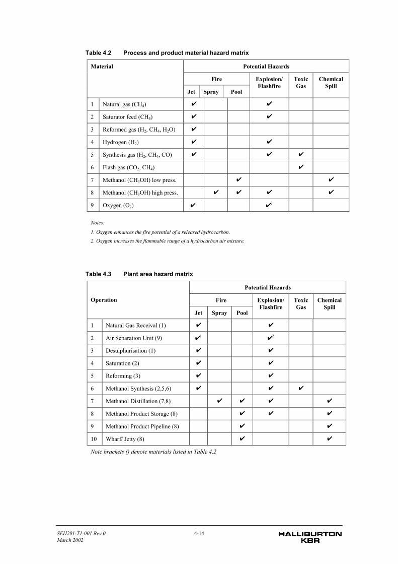
SEH201-T1-001 Rev.0 4-14March 2002
Table 4.2 Process and product material hazard matrix
Potential Hazards
Fire
Material
Jet Spray Pool
Explosion/Flashfire
ToxicGas
ChemicalSpill
1 Natural gas (CH4) ✔ ✔
2 Saturator feed (CH4) ✔ ✔
3 Reformed gas (H2, CH4, H2O) ✔
4 Hydrogen (H2) ✔ ✔
5 Synthesis gas (H2, CH4, CO) ✔ ✔ ✔
6 Flash gas (CO2, CH4) ✔
7 Methanol (CH3OH) low press. ✔ ✔
8 Methanol (CH3OH) high press. ✔ ✔ ✔ ✔
9 Oxygen (O2) ✔1 ✔2
Notes:
1. Oxygen enhances the fire potential of a released hydrocarbon.2. Oxygen increases the flammable range of a hydrocarbon air mixture.
Table 4.3 Plant area hazard matrix
Potential Hazards
FireOperation
Jet Spray Pool
Explosion/Flashfire
ToxicGas
ChemicalSpill
1 Natural Gas Receival (1) ✔ ✔
2 Air Separation Unit (9) ✔1 ✔2
3 Desulphurisation (1) ✔ ✔
4 Saturation (2) ✔ ✔
5 Reforming (3) ✔ ✔
6 Methanol Synthesis (2,5,6) ✔ ✔ ✔
7 Methanol Distillation (7,8) ✔ ✔ ✔ ✔
8 Methanol Product Storage (8) ✔ ✔ ✔
9 Methanol Product Pipeline (8) ✔ ✔
10 Wharf/ Jetty (8) ✔ ✔
Note brackets () denote materials listed in Table 4.2
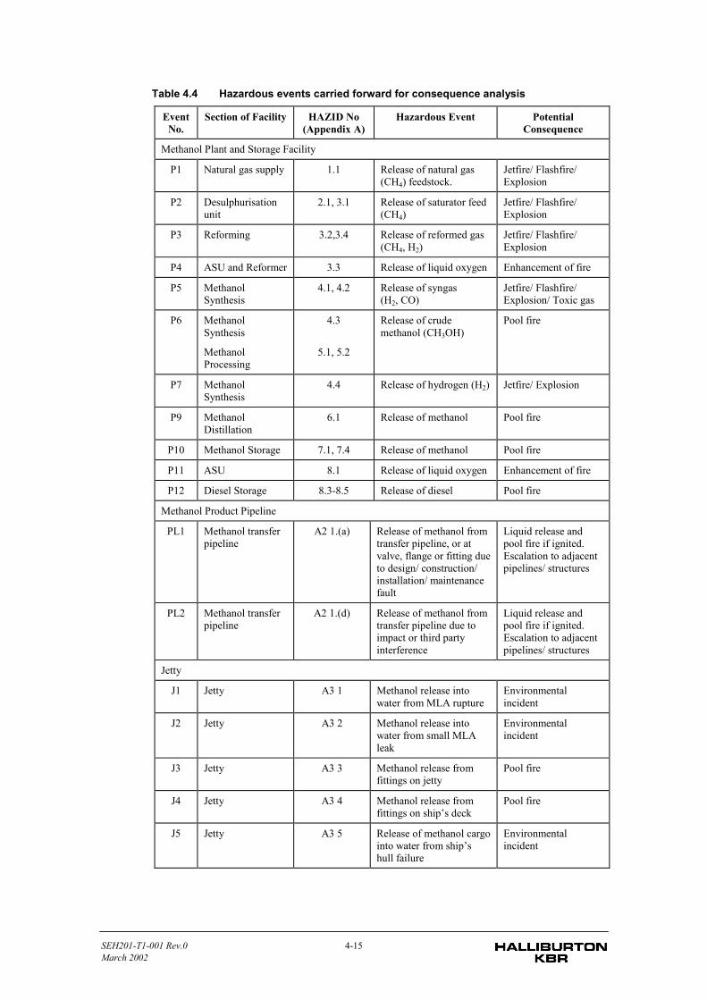
SEH201-T1-001 Rev.0 4-15March 2002
Table 4.4 Hazardous events carried forward for consequence analysis
EventNo.
Section of Facility HAZID No(Appendix A)
Hazardous Event PotentialConsequence
Methanol Plant and Storage Facility
P1 Natural gas supply 1.1 Release of natural gas(CH4) feedstock.
Jetfire/ Flashfire/Explosion
P2 Desulphurisationunit
2.1, 3.1 Release of saturator feed(CH4)
Jetfire/ Flashfire/Explosion
P3 Reforming 3.2,3.4 Release of reformed gas(CH4, H2)
Jetfire/ Flashfire/Explosion
P4 ASU and Reformer 3.3 Release of liquid oxygen Enhancement of fire
P5 MethanolSynthesis
4.1, 4.2 Release of syngas(H2, CO)
Jetfire/ Flashfire/Explosion/ Toxic gas
P6 MethanolSynthesis
MethanolProcessing
4.3
5.1, 5.2
Release of crudemethanol (CH3OH)
Pool fire
P7 MethanolSynthesis
4.4 Release of hydrogen (H2) Jetfire/ Explosion
P9 MethanolDistillation
6.1 Release of methanol Pool fire
P10 Methanol Storage 7.1, 7.4 Release of methanol Pool fire
P11 ASU 8.1 Release of liquid oxygen Enhancement of fire
P12 Diesel Storage 8.3-8.5 Release of diesel Pool fire
Methanol Product Pipeline
PL1 Methanol transferpipeline
A2 1.(a) Release of methanol fromtransfer pipeline, or atvalve, flange or fitting dueto design/ construction/installation/ maintenancefault
Liquid release andpool fire if ignited.Escalation to adjacentpipelines/ structures
PL2 Methanol transferpipeline
A2 1.(d) Release of methanol fromtransfer pipeline due toimpact or third partyinterference
Liquid release andpool fire if ignited.Escalation to adjacentpipelines/ structures
Jetty
J1 Jetty A3 1 Methanol release intowater from MLA rupture
Environmentalincident
J2 Jetty A3 2 Methanol release intowater from small MLAleak
Environmentalincident
J3 Jetty A3 3 Methanol release fromfittings on jetty
Pool fire
J4 Jetty A3 4 Methanol release fromfittings on ship’s deck
Pool fire
J5 Jetty A3 5 Release of methanol cargointo water from ship’shull failure
Environmentalincident
SEH201-T1-001 Rev.0 5-1March 2002
5 Consequence
5.1 INTRODUCTION
The purpose of this section is to outline the consequence models used in the analysis,to reference the assumptions used in the modelling and to discuss the impairmentcriteria to be used in the interpretation of the modelling results.
The consequence modelling has been conducted using the following softwarepackages:
• TNO software package EFFECTS (Ref. 5), which comprises a number of fire,explosion and dispersion models for accidental releases of hazardous materials. Allmodels within EFFECTS are fully detailed in the Yellow Book (Ref 6).
• FRED (Fire Release Explosion and Dispersion), a Proprietary package of ShellGlobal Solutions, with main focus on hydrocarbons (Ref 7).
• In-house developed program for pool fires with built-in experimental burning ratesof flammable liquids (including methanol).
More comprehensive descriptions of the consequence modelling are provided inAppendix C for both the methanol transfer pipeline and the process plant and storagearea. Values of, and references for parameters used in the modelling are also provided.
5.2 SCENARIO EFFECT DISTANCES
The effect distances for each release source have been determined from the site plotplan. Where the effect distance did not extend beyond the property boundary, theevent was screened out from further assessment as it would have not result in anoffsite impact.
5.3 RELEASE RATES
5.3.1 Process Plant
The following scenarios were found to be applicable to the Methanex facility.
1. Small leaks from flange joints. A 10 mm equivalent size was assumed.
2. Leaks from valve glands. The representative hole size was 10 mm. This wasindependent of the valve size.
3. Instrument fittings (20 mm equivalent).
4. Pump seal failures. For calculation purposes, an equivalent hole size of 10 mmdiameter was assumed.
SEH201-T1-001 Rev.0 5-2March 2002
5. Full bore failures of pipework from dropped objects, escalation from flameimpingement from small fires, and pipe failures from ruptures. A hole size of100mm was assumed to be representative of pipe rupture.
Both gas and liquid leak rates were calculated in Effects using the Bernoulli equation.
5.3.2 Methanol Transfer Pipeline
Release rates for liquid releases were calculated using the standard Bernoulli equationfor release from an orifice. To allow for the pressure drop along the pipeline(approximately 4 km from plant boundary to wharf entry), the pipeline length wasdivided into two equal parts and a set pressure was assumed to apply for each part.The upstream section was assumed to be at the maximum pumping rate pressure of1,470 kPag and the downstream section was allocated a pressure of 500 kPag. Thesepressures were taken from the stream data on the PFD for Methanol Metering andLoading.
Based upon past experience in conducting QRA for similar installations and thepotential failure modes of equipment, the following plausible leak scenarios(equivalent hole sizes) were chosen:
1. 13 mm. Small leaks from valve glands and flange gaskets.
2. 20 mm. Rupture of small bore instrument fitting lines.
3. 75 mm. Significant failure of methanol transfer pipeline between plant and wharffrom potential impact/ third party interference.
It is noted that the above approach is conservative as small leaks from flanges andvalves may result in an equivalent hole sizes less than 6 mm.
5.3.3 Jetty
The following scenarios were release identified at the jetty:
1. 10 mm - Small leak from joints or flanges on the MLA/ pipework or ship’stransfer manifold piping
2. 50 mm - Medium leak from joints or flanges on ship’s transfer manifold piping
3. 400 - Full bore rupture of MLA.
4. 300 mm - large leak from failure of ship’s hull
The release rates are shown in Table 5.1.
Table 5.1 Methanol release rates at jetty
Description Hole Size mm Release Rate, kg/s Flow Limiter
Full bore - Loading Arm 400 694.4 Pumping Rateat 2,500 tph
Small leak 10 2.48 Hole Size
Medium leak 50 62.0 Hole Size
Ship’s hull failure 300 617.0 Hole Size
SEH201-T1-001 Rev.0 5-3March 2002
5.4 JET FIRES
Jet fires result when a high pressure leak of gas from a pipe or vessel is ignited duringthe release. Due to the high pressures involved, the exit velocity can be significant.However, the pressure can fall rapidly due to depressuring effect, thus reducing theimpact of jet fires.
The previously completed layout study for the project (Ref 8) showed that jet flamelengths up to approximately 20m could be expected for the scenarios postulated. Heatradiation levels of 15kW/m2 (ie. capable of damaging equipment) could beexperienced up to 25 m from the release point. This effect is well within the siteboundary, as equipment items are located well within the boundary. Assuming that theseparation distances between plant items recommended in the layout study arecomplied with, knock on effects due to jet fires are also regarded as highly unlikely.Jet fire scenarios have therefore not been included in the risk calculations.
5.5 VAPOUR CLOUD EXPLOSIONS
Flammable Cloud Mass
If a release of flammable gas from a pipe or vessel is not ignited immediately, forminga jet fire, then a delayed ignition would result in a flash fire, followed by a jet fire ifthe leak had not been isolated. The flash fire may result in an explosion if there is asufficient mass of flammable vapour and a degree of confinement for flame frontacceleration. Only the part of the flammable cloud where the concentration is abovethe lower flammability limit will ignite.
The flammable gas cloud is defined by the extent of the gas cloud where the gasconcentration is between the upper and lower flammability limits.
Natural Gas
To determine the flammable mass of vapour in the plume from a gas release, and theflammable isopleth, dispersion modelling of the release is performed. The dispersionmodels within TNO EFFECTS were used to model dispersion for releases of naturalgas, and to predict the flammable cloud masses.
Syngas / Hydrogen
For hydrogen rich fires, the Hawksley method was used to predict mass involved in anexplosion. Based on comparisons with a number of models, Hawksley showed that thebest estimate of the size of the flammable cloud involved in the explosion is thequantity of gas discharged from the leak in the first 10 seconds. This reflects the veryshort ignition delays experienced with hydrogen rich gas clouds. For this study, themass was estimated from the leak rate over 20 seconds, to provide a degree ofconservatism. (refer to Appendix C for further detail).
Explosion Overpressure
Only the portion of the flammable cloud that is within a confined area is likely toresult in explosion on ignition; the remainder of the vapour will burn as a flash fire.An explosion model is used to determine the overpressure that results from explosionof the vapour cloud.
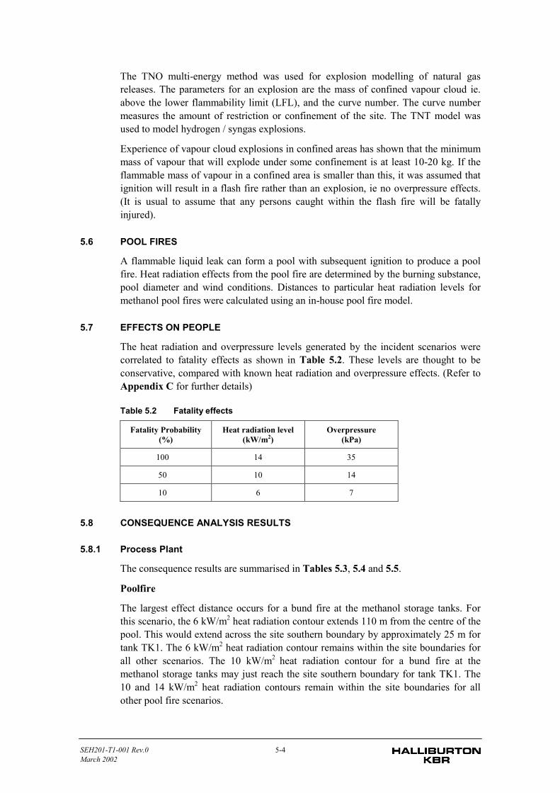
SEH201-T1-001 Rev.0 5-4March 2002
The TNO multi-energy method was used for explosion modelling of natural gasreleases. The parameters for an explosion are the mass of confined vapour cloud ie.above the lower flammability limit (LFL), and the curve number. The curve numbermeasures the amount of restriction or confinement of the site. The TNT model wasused to model hydrogen / syngas explosions.
Experience of vapour cloud explosions in confined areas has shown that the minimummass of vapour that will explode under some confinement is at least 10-20 kg. If theflammable mass of vapour in a confined area is smaller than this, it was assumed thatignition will result in a flash fire rather than an explosion, ie no overpressure effects.(It is usual to assume that any persons caught within the flash fire will be fatallyinjured).
5.6 POOL FIRES
A flammable liquid leak can form a pool with subsequent ignition to produce a poolfire. Heat radiation effects from the pool fire are determined by the burning substance,pool diameter and wind conditions. Distances to particular heat radiation levels formethanol pool fires were calculated using an in-house pool fire model.
5.7 EFFECTS ON PEOPLE
The heat radiation and overpressure levels generated by the incident scenarios werecorrelated to fatality effects as shown in Table 5.2. These levels are thought to beconservative, compared with known heat radiation and overpressure effects. (Refer toAppendix C for further details)
Table 5.2 Fatality effects
Fatality Probability(%)
Heat radiation level(kW/m2)
Overpressure(kPa)
100 14 35
50 10 14
10 6 7
5.8 CONSEQUENCE ANALYSIS RESULTS
5.8.1 Process Plant
The consequence results are summarised in Tables 5.3, 5.4 and 5.5.
Poolfire
The largest effect distance occurs for a bund fire at the methanol storage tanks. Forthis scenario, the 6 kW/m2 heat radiation contour extends 110 m from the centre of thepool. This would extend across the site southern boundary by approximately 25 m fortank TK1. The 6 kW/m2 heat radiation contour remains within the site boundaries forall other scenarios. The 10 kW/m2 heat radiation contour for a bund fire at themethanol storage tanks may just reach the site southern boundary for tank TK1. The10 and 14 kW/m2 heat radiation contours remain within the site boundaries for allother pool fire scenarios.
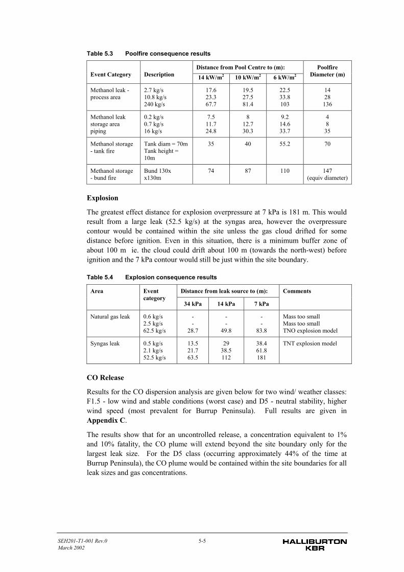
SEH201-T1-001 Rev.0 5-5March 2002
Table 5.3 Poolfire consequence results
Distance from Pool Centre to (m):Event Category Description 14 kW/m2 10 kW/m2 6 kW/m2
PoolfireDiameter (m)
Methanol leak -process area
2.7 kg/s10.8 kg/s240 kg/s
17.623.367.7
19.527.581.4
22.533.8103
1428
136
Methanol leakstorage areapiping
0.2 kg/s0.7 kg/s16 kg/s
7.511.724.8
812.730.3
9.214.633.7
48
35
Methanol storage- tank fire
Tank diam = 70mTank height =10m
35 40 55.2 70
Methanol storage- bund fire
Bund 130xx130m
74 87 110 147(equiv diameter)
Explosion
The greatest effect distance for explosion overpressure at 7 kPa is 181 m. This wouldresult from a large leak (52.5 kg/s) at the syngas area, however the overpressurecontour would be contained within the site unless the gas cloud drifted for somedistance before ignition. Even in this situation, there is a minimum buffer zone ofabout 100 m ie. the cloud could drift about 100 m (towards the north-west) beforeignition and the 7 kPa contour would still be just within the site boundary.
Table 5.4 Explosion consequence results
Distance from leak source to (m):Area Eventcategory
34 kPa 14 kPa 7 kPa
Comments
Natural gas leak 0.6 kg/s2.5 kg/s62.5 kg/s
--
28.7
--
49.8
--
83.8
Mass too smallMass too smallTNO explosion model
Syngas leak 0.5 kg/s2.1 kg/s52.5 kg/s
13.521.763.5
2938.5112
38.461.8181
TNT explosion model
CO Release
Results for the CO dispersion analysis are given below for two wind/ weather classes:F1.5 - low wind and stable conditions (worst case) and D5 - neutral stability, higherwind speed (most prevalent for Burrup Peninsula). Full results are given inAppendix C.
The results show that for an uncontrolled release, a concentration equivalent to 1%and 10% fatality, the CO plume will extend beyond the site boundary only for thelargest leak size. For the D5 class (occurring approximately 44% of the time atBurrup Peninsula), the CO plume would be contained within the site boundaries for allleak sizes and gas concentrations.
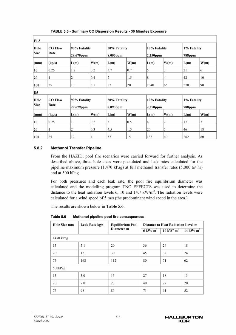
SEH201-T1-001 Rev.0 5-6March 2002
TABLE 5.5 - Summary CO Dispersion Results - 30 Minutes Exposure
F1.5
HoleSize
CO FlowRate
90% Fatality
29,679ppm
50% Fatality
8,093ppm
10% Fatality
2,250ppm
1% Fatality
788ppm
(mm) (kg/s) L(m) W(m) L(m) W(m) L(m) W(m) L(m) W(m)
10 0.25 1.2 0.2 3.7 0.7 5 3 21 6
20 1 2 0.4 7 1.5 8 4 42 10
100 25 13 3.5 87 20 1340 65 2703 90
D5
HoleSize
CO FlowRate
90% Fatality
29,679ppm
50% Fatality
8,093ppm
10% Fatality
2,250ppm
1% Fatality
788ppm
(mm) (kg/s) L(m) W(m) L(m) W(m) L(m) W(m) L(m) W(m)
10 0.25 1 0.2 3 0.5 4 2 17 7
20 1 2 0.3 4.5 1.5 20 5 46 18
100 25 12 4 57 15 138 40 262 80
5.8.2 Methanol Transfer Pipeline
From the HAZID, pool fire scenarios were carried forward for further analysis. Asdescribed above, three hole sizes were postulated and leak rates calculated for thepipeline maximum pressure (1,470 kPag) at full methanol transfer rates (5,000 te/ hr)and at 500 kPag.
For both pressures and each leak rate, the pool fire equilibrium diameter wascalculated and the modelling program TNO EFFECTS was used to determine thedistance to the heat radiation levels 6, 10 and 14.7 kW/m2. The radiation levels werecalculated for a wind speed of 5 m/s (the predominant wind speed in the area.).
The results are shown below in Table 5.6.
Table 5.6 Methanol pipeline pool fire consequences
Distance to Heat Radiation Level mHole Size mm Leak Rate kg/s Equilibrium PoolDiameter m 6 kW/ m2 10 kW/ m2 14 kW/ m2
1470 kPag
13 5.1 20 36 24 18
20 12 30 45 32 24
75 168 112 80 71 62
500kPag
13 3.0 15 27 18 13
20 7.0 23 40 27 20
75 98 86 71 61 52
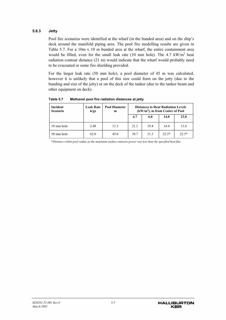
SEH201-T1-001 Rev.0 5-7March 2002
5.8.3 Jetty
Pool fire scenarios were identified at the wharf (in the bunded area) and on the ship’sdeck around the manifold piping area. The pool fire modelling results are given inTable 5.7. For a 10m x 10 m bunded area at the wharf, the entire containment areawould be filled, even for the small leak rate (10 mm hole). The 4.7 kW/m2 heatradiation contour distance (21 m) would indicate that the wharf would probably needto be evacuated or some fire shielding provided.
For the larger leak rate (50 mm hole), a pool diameter of 45 m was calculated,however it is unlikely that a pool of this size could form on the jetty (due to thebunding and size of the jetty) or on the deck of the tanker (due to the tanker beam andother equipment on deck).
Table 5.7 Methanol pool fire radiation distances at jetty
Distances to Heat Radiation Levels(kW/m2), m from Centre of Pool
IncidentScenario
Leak Ratek/gs
Pool Diameterm
4.7 6.0 14.0 23.0
10 mm hole 2.48 11.3 21.1 19.4 14.4 11.6
50 mm hole 62.0 45.0 39.7 31.3 22.5* 22.5*
*Distance within pool radius as the maximum surface emissive power was less than the specified heat flux
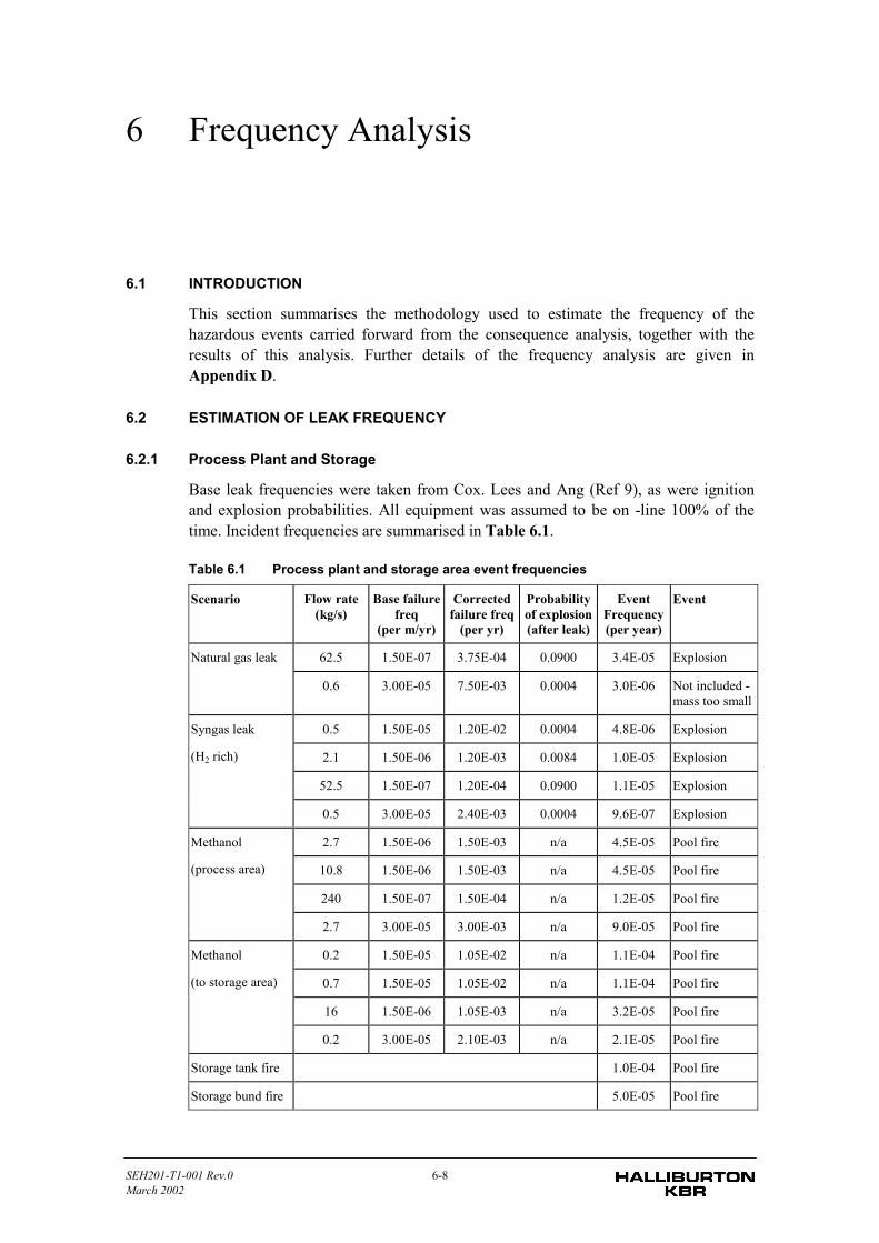
SEH201-T1-001 Rev.0 6-8March 2002
6 Frequency Analysis
6.1 INTRODUCTION
This section summarises the methodology used to estimate the frequency of thehazardous events carried forward from the consequence analysis, together with theresults of this analysis. Further details of the frequency analysis are given inAppendix D.
6.2 ESTIMATION OF LEAK FREQUENCY
6.2.1 Process Plant and Storage
Base leak frequencies were taken from Cox. Lees and Ang (Ref 9), as were ignitionand explosion probabilities. All equipment was assumed to be on -line 100% of thetime. Incident frequencies are summarised in Table 6.1.
Table 6.1 Process plant and storage area event frequencies
Scenario Flow rate(kg/s)
Base failurefreq
(per m/yr)
Correctedfailure freq
(per yr)
Probabilityof explosion(after leak)
EventFrequency(per year)
Event
62.5 1.50E-07 3.75E-04 0.0900 3.4E-05 ExplosionNatural gas leak
0.6 3.00E-05 7.50E-03 0.0004 3.0E-06 Not included -mass too small
0.5 1.50E-05 1.20E-02 0.0004 4.8E-06 Explosion
2.1 1.50E-06 1.20E-03 0.0084 1.0E-05 Explosion
52.5 1.50E-07 1.20E-04 0.0900 1.1E-05 Explosion
Syngas leak
(H2 rich)
0.5 3.00E-05 2.40E-03 0.0004 9.6E-07 Explosion
2.7 1.50E-06 1.50E-03 n/a 4.5E-05 Pool fire
10.8 1.50E-06 1.50E-03 n/a 4.5E-05 Pool fire
240 1.50E-07 1.50E-04 n/a 1.2E-05 Pool fire
Methanol
(process area)
2.7 3.00E-05 3.00E-03 n/a 9.0E-05 Pool fire
0.2 1.50E-05 1.05E-02 n/a 1.1E-04 Pool fire
0.7 1.50E-05 1.05E-02 n/a 1.1E-04 Pool fire
16 1.50E-06 1.05E-03 n/a 3.2E-05 Pool fire
Methanol
(to storage area)
0.2 3.00E-05 2.10E-03 n/a 2.1E-05 Pool fire
Storage tank fire 1.0E-04 Pool fire
Storage bund fire 5.0E-05 Pool fire
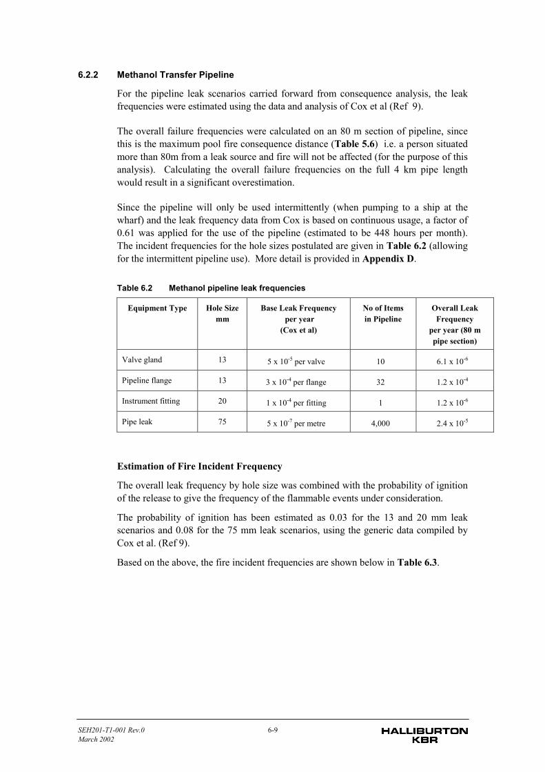
SEH201-T1-001 Rev.0 6-9March 2002
6.2.2 Methanol Transfer Pipeline
For the pipeline leak scenarios carried forward from consequence analysis, the leakfrequencies were estimated using the data and analysis of Cox et al (Ref 9).
The overall failure frequencies were calculated on an 80 m section of pipeline, sincethis is the maximum pool fire consequence distance (Table 5.6) i.e. a person situatedmore than 80m from a leak source and fire will not be affected (for the purpose of thisanalysis). Calculating the overall failure frequencies on the full 4 km pipe lengthwould result in a significant overestimation.
Since the pipeline will only be used intermittently (when pumping to a ship at thewharf) and the leak frequency data from Cox is based on continuous usage, a factor of0.61 was applied for the use of the pipeline (estimated to be 448 hours per month).The incident frequencies for the hole sizes postulated are given in Table 6.2 (allowingfor the intermittent pipeline use). More detail is provided in Appendix D.
Table 6.2 Methanol pipeline leak frequencies
Equipment Type Hole Sizemm
Base Leak Frequency per year
(Cox et al)
No of Itemsin Pipeline
Overall LeakFrequency
per year (80 mpipe section)
Valve gland 13 5 x 10⁻⁵ per valve 10 6.1 x 10⁻⁶
Pipeline flange 13 3 x 10⁻⁴ per flange 32 1.2 x 10⁻⁴
Instrument fitting 20 1 x 10⁻⁴ per fitting 1 1.2 x 10⁻⁶
Pipe leak 75 5 x 10⁻⁷ per metre 4,000 2.4 x 10⁻⁵
Estimation of Fire Incident Frequency
The overall leak frequency by hole size was combined with the probability of ignitionof the release to give the frequency of the flammable events under consideration.
The probability of ignition has been estimated as 0.03 for the 13 and 20 mm leakscenarios and 0.08 for the 75 mm leak scenarios, using the generic data compiled byCox et al. (Ref 9).
Based on the above, the fire incident frequencies are shown below in Table 6.3.
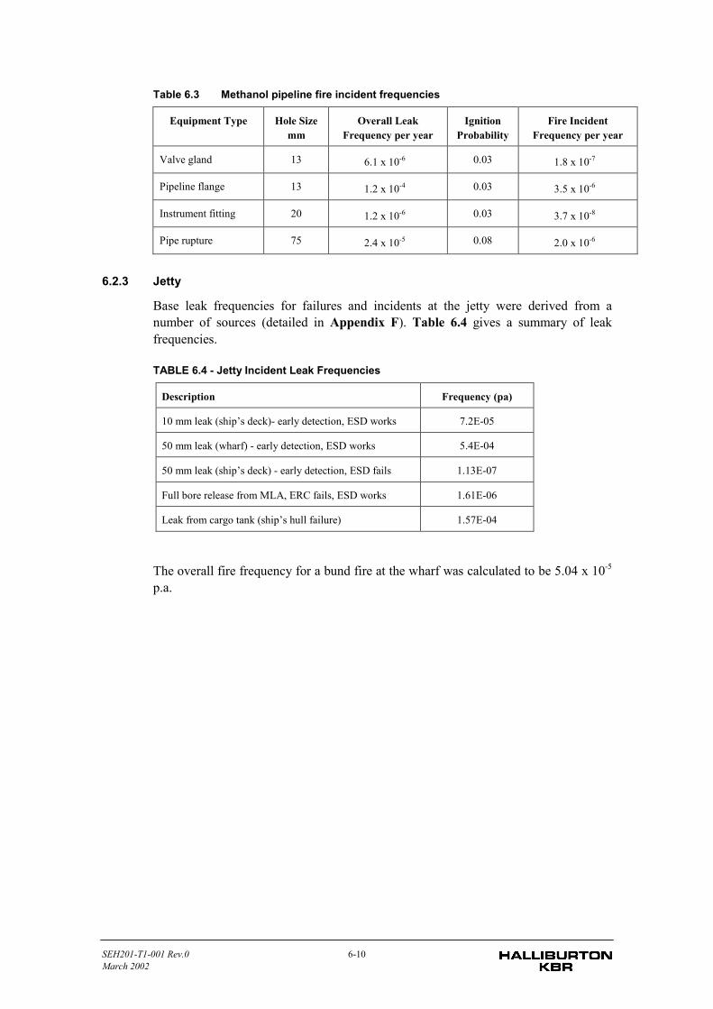
SEH201-T1-001 Rev.0 6-10March 2002
Table 6.3 Methanol pipeline fire incident frequencies
Equipment Type Hole Sizemm
Overall LeakFrequency per year
IgnitionProbability
Fire IncidentFrequency per year
Valve gland 13 6.1 x 10⁻⁶ 0.03 1.8 x 10⁻⁷
Pipeline flange 13 1.2 x 10⁻⁴ 0.03 3.5 x 10⁻⁶
Instrument fitting 20 1.2 x 10⁻⁶ 0.03 3.7 x 10⁻⁸
Pipe rupture 75 2.4 x 10⁻⁵ 0.08 2.0 x 10⁻⁶
6.2.3 Jetty
Base leak frequencies for failures and incidents at the jetty were derived from anumber of sources (detailed in Appendix F). Table 6.4 gives a summary of leakfrequencies.
TABLE 6.4 - Jetty Incident Leak Frequencies
Description Frequency (pa)
10 mm leak (ship’s deck)- early detection, ESD works 7.2E-05
50 mm leak (wharf) - early detection, ESD works 5.4E-04
50 mm leak (ship’s deck) - early detection, ESD fails 1.13E-07
Full bore release from MLA, ERC fails, ESD works 1.61E-06
Leak from cargo tank (ship’s hull failure) 1.57E-04
The overall fire frequency for a bund fire at the wharf was calculated to be 5.04 x 10⁻⁵
p.a.
SEH201-T1-001 Rev.0 7-1March 2002
7 Risk Assessment
7.1 INTRODUCTION
Risk, in the context of this study, refers to the off-site risk to people and propertyarising from the proposal. Risk is a function of the severity of an incident(consequence) and the likelihood of its occurrence (frequency). The level of risk atany particular point is a sum of all risks from causes (scenarios) originating from afacility expressed over a one year period.
The risk from these incidents was analysed using a computer program TNORiskCurves that performs a risk summation for a large number of individual points ona grid pattern around the site. Individual risk contours were then drawn connecting alllocations of equal risk and superimposed on a scale map of the area.
The risk of fatality to an individual was calculated for the following:
• Releases from the methanol process plant and product storage (iso-contours); and
• Release from methanol product pipeline (risk transects).
7.2 RISK GUIDELINES
Individual risk at a given location is generally expressed as the peak individual risk,defined as the risk of fatality to the most exposed individual located at the position for24 hours of the day and 365 days in the year. Since residential areas tend to beoccupied by at least one individual all the time, the above definition would easilyapply to residential areas.
A person indoors would receive natural protection from fire radiation and hence therisk to a person indoors is likely to be lower than to one in open air. In this study, theindividual risk levels have been calculated for a person in open air.
For land uses other than residential areas, (i.e. industrial or commercial) whereoccupancy is not 100% of the time, individual risk is still calculated on the same basis.However, the criteria for acceptability are adjusted for occupancy. Criteria have beenestablished by the Environmental Protection Authority in Western Australia. The riskcriteria are summarised below in Table 7.1.
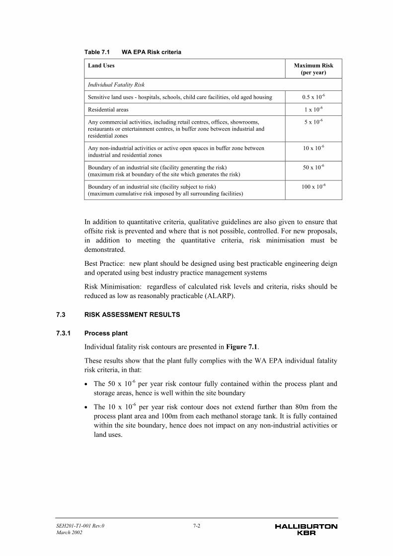
SEH201-T1-001 Rev.0 7-2March 2002
Table 7.1 WA EPA Risk criteria
Land Uses Maximum Risk(per year)
Individual Fatality Risk
Sensitive land uses - hospitals, schools, child care facilities, old aged housing 0.5 x 10⁻⁶
Residential areas 1 x 10⁻⁶
Any commercial activities, including retail centres, offices, showrooms,restaurants or entertainment centres, in buffer zone between industrial andresidential zones
5 x 10⁻⁶
Any non-industrial activities or active open spaces in buffer zone betweenindustrial and residential zones
10 x 10-6
Boundary of an industrial site (facility generating the risk)(maximum risk at boundary of the site which generates the risk)
50 x 10-6
Boundary of an industrial site (facility subject to risk)(maximum cumulative risk imposed by all surrounding facilities)
100 x 10-6
In addition to quantitative criteria, qualitative guidelines are also given to ensure thatoffsite risk is prevented and where that is not possible, controlled. For new proposals,in addition to meeting the quantitative criteria, risk minimisation must bedemonstrated.
Best Practice: new plant should be designed using best practicable engineering deignand operated using best industry practice management systems
Risk Minimisation: regardless of calculated risk levels and criteria, risks should bereduced as low as reasonably practicable (ALARP).
7.3 RISK ASSESSMENT RESULTS
7.3.1 Process plant
Individual fatality risk contours are presented in Figure 7.1.
These results show that the plant fully complies with the WA EPA individual fatalityrisk criteria, in that:
• The 50 x 10-6 per year risk contour fully contained within the process plant andstorage areas, hence is well within the site boundary
• The 10 x 10-6 per year risk contour does not extend further than 80m from theprocess plant area and 100m from each methanol storage tank. It is fully containedwithin the site boundary, hence does not impact on any non-industrial activities orland uses.
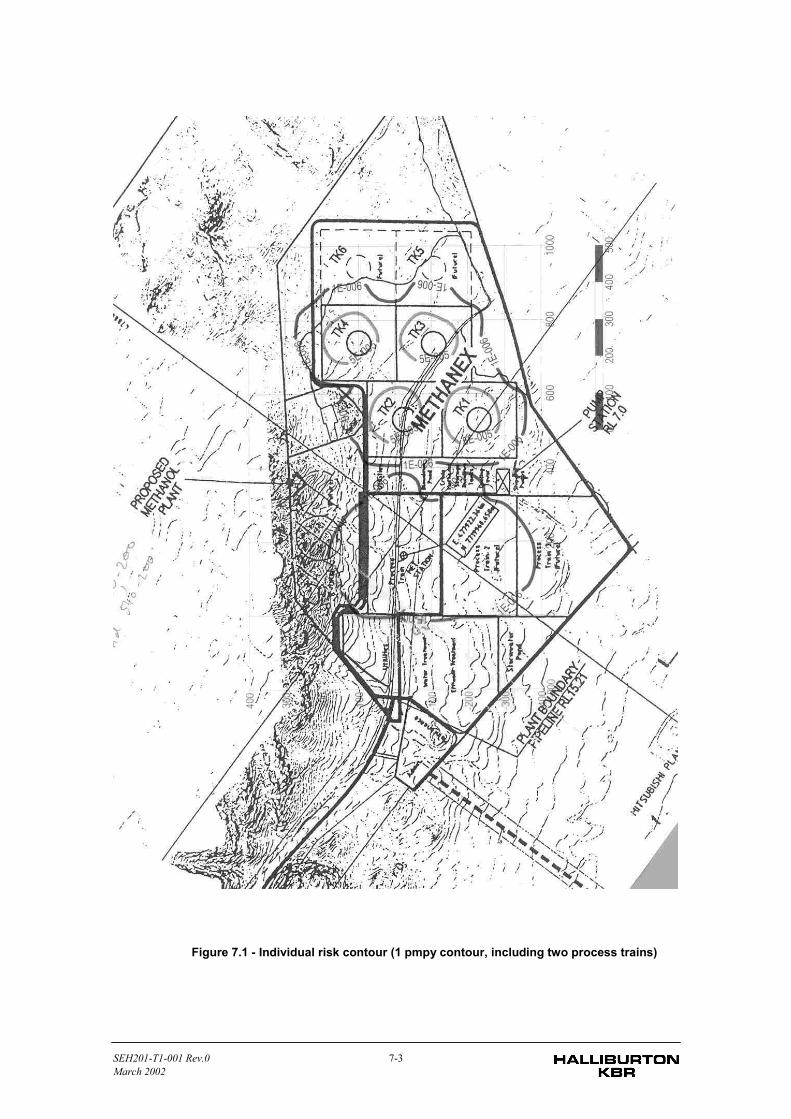
SEH201-T1-001 Rev.0 7-3March 2002
Figure 7.1 - Individual risk contour (1 pmpy contour, including two process trains)
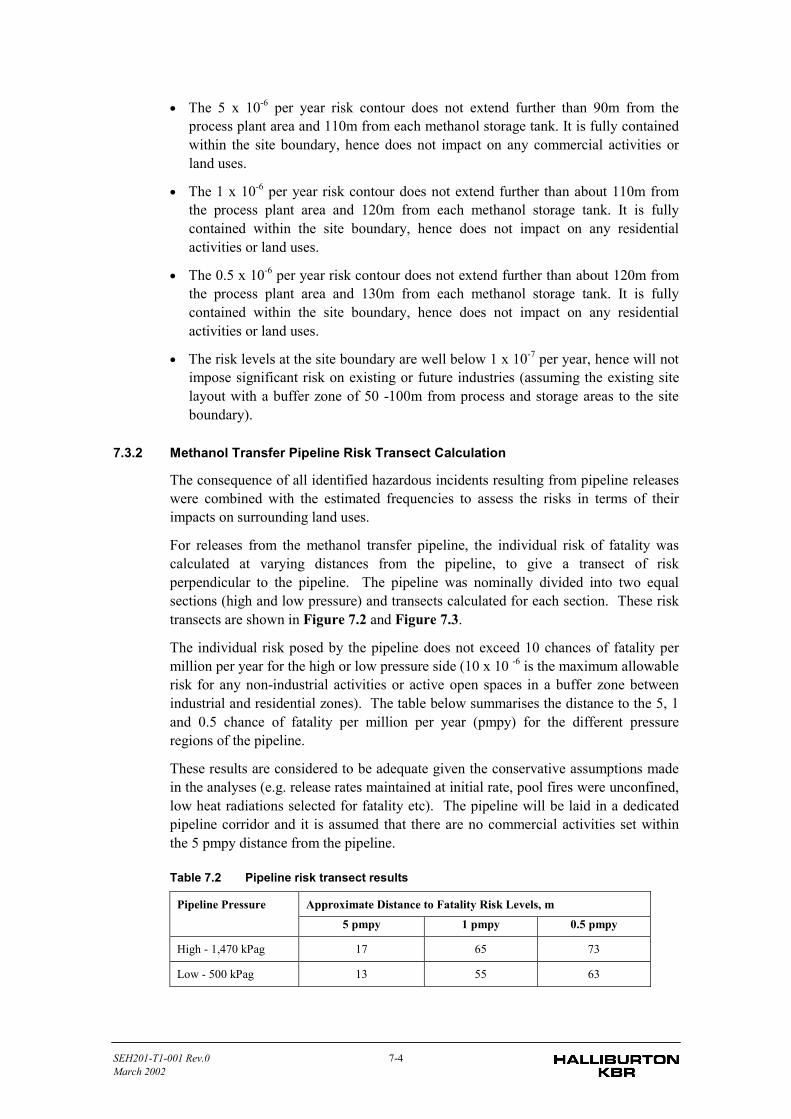
SEH201-T1-001 Rev.0 7-4March 2002
• The 5 x 10⁻⁶ per year risk contour does not extend further than 90m from theprocess plant area and 110m from each methanol storage tank. It is fully containedwithin the site boundary, hence does not impact on any commercial activities orland uses.
• The 1 x 10⁻⁶ per year risk contour does not extend further than about 110m fromthe process plant area and 120m from each methanol storage tank. It is fullycontained within the site boundary, hence does not impact on any residentialactivities or land uses.
• The 0.5 x 10⁻⁶ per year risk contour does not extend further than about 120m fromthe process plant area and 130m from each methanol storage tank. It is fullycontained within the site boundary, hence does not impact on any residentialactivities or land uses.
• The risk levels at the site boundary are well below 1 x 10⁻⁷ per year, hence will notimpose significant risk on existing or future industries (assuming the existing sitelayout with a buffer zone of 50 -100m from process and storage areas to the siteboundary).
7.3.2 Methanol Transfer Pipeline Risk Transect Calculation
The consequence of all identified hazardous incidents resulting from pipeline releaseswere combined with the estimated frequencies to assess the risks in terms of theirimpacts on surrounding land uses.
For releases from the methanol transfer pipeline, the individual risk of fatality wascalculated at varying distances from the pipeline, to give a transect of riskperpendicular to the pipeline. The pipeline was nominally divided into two equalsections (high and low pressure) and transects calculated for each section. These risktransects are shown in Figure 7.2 and Figure 7.3.
The individual risk posed by the pipeline does not exceed 10 chances of fatality permillion per year for the high or low pressure side (10 x 10 -6 is the maximum allowablerisk for any non-industrial activities or active open spaces in a buffer zone betweenindustrial and residential zones). The table below summarises the distance to the 5, 1and 0.5 chance of fatality per million per year (pmpy) for the different pressureregions of the pipeline.
These results are considered to be adequate given the conservative assumptions madein the analyses (e.g. release rates maintained at initial rate, pool fires were unconfined,low heat radiations selected for fatality etc). The pipeline will be laid in a dedicatedpipeline corridor and it is assumed that there are no commercial activities set withinthe 5 pmpy distance from the pipeline.
Table 7.2 Pipeline risk transect results
Approximate Distance to Fatality Risk Levels, mPipeline Pressure5 pmpy 1 pmpy 0.5 pmpy
High - 1,470 kPag 17 65 73
Low - 500 kPag 13 55 63
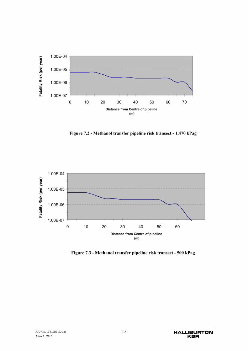
SEH201-T1-001 Rev.0 7-5March 2002
Figure 7.2 - Methanol transfer pipeline risk transect - 1,470 kPag
Figure 7.3 - Methanol transfer pipeline risk transect - 500 kPag
1.00E-07
1.00E-06
1.00E-05
1.00E-04
0 10 20 30 40 50 60 70Distance from Centre of pipeline
(m)
Fata
lity
Ris
k (p
er y
ear)
1.00E-07
1.00E-06
1.00E-05
1.00E-04
0 10 20 30 40 50 60Distance from Centre of pipeline
(m)
Fata
lity
Ris
k (p
er y
ear)
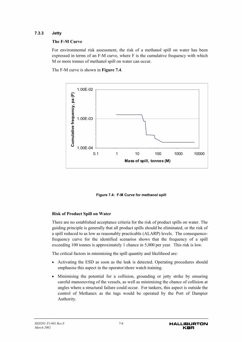
SEH201-T1-001 Rev.0 7-6March 2002
7.3.3 Jetty
The F-M Curve
For environmental risk assessment, the risk of a methanol spill on water has beenexpressed in terms of an F-M curve, where F is the cumulative frequency with whichM or more tonnes of methanol spill on water can occur.
The F-M curve is shown in Figure 7.4.
Figure 7.4: F-M Curve for methanol spill
Risk of Product Spill on Water
There are no established acceptance criteria for the risk of product spills on water. Theguiding principle is generally that all product spills should be eliminated, or the risk ofa spill reduced to as low as reasonably practicable (ALARP) levels. The consequence-frequency curve for the identified scenarios shows that the frequency of a spillexceeding 100 tonnes is approximately 1 chance in 5,000 per year. This risk is low.
The critical factors in minimising the spill quantity and likelihood are:
• Activating the ESD as soon as the leak is detected. Operating procedures shouldemphasise this aspect in the operator/shore watch training.
• Minimising the potential for a collision, grounding or jetty strike by ensuringcareful manoeuvring of the vessels, as well as minimising the chance of collision atangles where a structural failure could occur. For tankers, this aspect is outside thecontrol of Methanex as the tugs would be operated by the Port of DampierAuthority.
1.00E-04
1.00E-03
1.00E-02
0.1 1 10 100 1000 10000
Mass of spill, tonnes (M)
Cum
ulat
ive
freq
uenc
y, p
a (F
)
SEH201-T1-001 Rev.0 7-7March 2002
Fire Risk Assessment
The total fire frequency from a methanol spill on the wharf was calculated as 5 x 10⁻⁵
per annum. This frequency is low.
The emergency procedure should call for taking shelter behind the fire shield andactivating the remote firewater/ foam monitors in the event of a fire. This wouldreduce the heat radiation distances significantly.
The nearest structure is the shore operator’s cabin. This location should be carefullyconsidered to ensure that it is outside the 4.7 kW/m2 heat radiation contour for a fullbund fire. Provided the operator stays in the cabin, at least till fire fightingcommences, when the thermal radiation distances would be attenuated by thewater/foam spray, there would be no injury potential.
7.4 SOCIETAL RISK
Societal risk is a measure of the probability of incidents affecting a human population,and takes into account the number of people exposed to risk. Whereas individual riskis concerned with the risk of fatality to a (notional) person at a particular location,societal risk considers the likelihood of actual fatalities among people exposed to thehazard.
The consequence results presented in Section 5 demonstrate that the effect zones ofthe identified incidents (for both the process plant and methanol pipeline), under worstcase wind weather conditions, do not extend to areas of significant population.
As no significant populations outside the site are within the effect zones, the proposalis not considered to have an impact on societal risk levels.
7.5 CONCLUSIONS
7.5.1 Process Plant and Product Storage
The proposed Methanex site is located in an industrial area well away from residentialareas. The majority of hazardous scenarios are fires or explosions that are essentiallylocalised within the site.
The following conclusions were made as a result of the hazard analysis study for themethanol production facility:
• on a consequence basis alone, heat radiation of 23 kW/m2 was contained whollywithin the site;
• the contour for individual risk of fatality at 50 chances in a million per year wascontained within the site; and
• the contours for individual risk of fatality at 0.5 and 1 chances in a million per yearwere limited to the site and do not reach the nearest residential areas or othersensitive land uses.
It can be seen that the risk resulting from the proposed operation of the site will meetthe risk criteria specified in the EPA Criteria.
SEH201-T1-001 Rev.0 7-8March 2002
7.5.2 Product Pipeline
Overall, the risk along the entire length of the proposed methanol product pipeline willnot exceed the EPA criteria of 10 x 10-6 for non-industrial activities or active openspaces in a buffer zone between industrial and residential zones. The pipeline will belaid in a dedicated pipeline corridor and it is not expected that residential areas orsensitive land uses (such as hospitals, schools or aged care facilities) will be locatedwithin the 1 pmpy or 0.5 pmpy contour distances respectively. It is also assumed thatthere are no commercial activities set within the 5 pmpy distance from the pipeline.
These results are considered to be acceptable given the conservative assumption madein the analyses (e.g. release rates maintained at initial rate, pool fires were unconfined,low heat radiations selected for fatality etc).
7.5.3 Jetty
Fire incidents at the jetty will be localised in their potential impact on people. The fireconsequence distances would not be expected to impact on public areas, given typicalexclusion zones around the wharf.
SEH201-T1-001 Rev.0 8-1March 2002
8 References
1. WA EPA Guidance for the Assessment of Environmental Factors, Guidance forRisk Assessment and Management: Offsite Individual Risk form HazardousIndustrial Plant No 2 July 2000.
2. Clough Engineering and Integrated Solutions: “Methanex Report, Basic Designand Engineering Package for Outside Fence Facilities”, 147-C-7075, REP-00-A-0002 REV 0, Perth, December 2001.
3. Frank Lees “Loss prevention in the Process Industries” 2nd Edition, Butterworth-Heinemann, Oxford 1996.
4. Society of Fire Protection Engineers: “Handbook of Fire ProtectionEngineering”, second edition, 1995, Ma., USA.
5. EFFECTS Version 2.1, Fire, explosion and dispersion models for accidentalreleases for hazardous materials, TNO Department of Industrial Safety,The Netherlands.
6. TNO Department of Industrial Safety, Committee for the Prevention of Disasters,The Netherlands, Methods for the Calculation of Physical Effects “Yellow Book”,CPR 14E, Third Edition 1997, 1997.
7. Shell Global Solutions, Technical Manual Shell FRED, March 2000
8. Granherne, Layout Study
9. A.W. Cox, F.P. Lees, and M. L. Ang: Classification of Hazardous Locations,1991, Rugby, England.
SEH201-T1-001 Rev 0March 2002
Appendix A
HAZARD IDENTIFICATION
PROCESS PLANT
STORAGE
METHANOL TRANSFER PIPELINE
JETTY
SEH201-T1-001 Rev 0 A-1March 2002
A1 Hazard Identification Process Plant
BACKGROUND
This section of the appendix contains the Hazard Identification (HAZID) tables for the proposed LCMMethanol Plant. This aspect of the study was conducted at a high-level to identify incidents that couldhave a potential offsite impact. This was done in consultation with the design engineers (Kvaerner)and with reference to the process flow diagrams.
Hazard identification was undertaken for the following process unit operations:
- Natural gas feedstock to plant.
- Desulphurisation and saturation.
- Reforming and gas heat recovery.
- Methanol synthesis.
- Crude methanol processing.
- Methanol distillation.
- Methanol product storage.
- Flash gas system.
- Air separation unit and oxygen injection.
- Diesel storage.
The HAZID tables for the product export pipeline and wharf operations are reported in separateappendices.
The following Methanex documents were consulted in this review:
- Design document “Power Control Systems”
- Design document “Control Systems Functional Specification”
- Process Flow Diagrams (1046-00-F001 to 1046-00-F031, Issue P3)
RESULTS
Based upon the HAZID, the following incidents were carried forward for further review in theconsequence analyses.

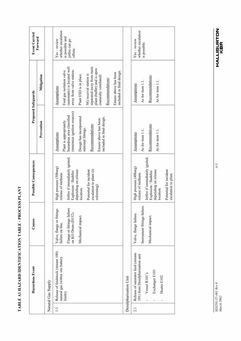
TA
BL
E A
1 H
AZA
RD
IDE
NT
IFIC
AT
ION
TA
BL
E - P
RO
CE
SS P
LAN
T
SEH
201-
T1-0
01 R
ev 0
A-3
Mar
ch 2
002
Prop
osed
Saf
egua
rds
Haz
ardo
us E
vent
Cau
ses
Poss
ible
Con
sequ
ence
s
Prev
entio
nM
itiga
tion
Eve
nt C
arri
edFo
rwar
d
Nat
ural
Gas
Sup
ply
1.1
Rel
ease
of f
eeds
tock
(stre
am 1
00)
natu
ral g
as (w
ithin
site
bat
tery
limits
)
Val
ve, f
lang
e or
fitti
ngs
failu
re o
n lin
e.
Flan
ge o
r fitt
ings
failu
reon
KO
Dru
m (D
152)
.
Mec
hani
cal i
mpa
ct.
Hig
h pr
essu
re (5
0bar
g)re
leas
e of
met
hane
.
Jetfi
re if
imm
edia
tely
igni
ted.
Expl
osio
n / f
lash
fire
depe
ndin
g on
rele
ase
loca
tion.
Pote
ntia
l for
inci
dent
esca
latio
n to
pla
nt (i
ere
form
ing)
.
Ass
umpt
ions
:
Plan
t is a
ppro
pria
tely
haza
rdou
s are
a cl
assi
fied
(min
imiz
e ig
nitio
n so
urce
s)
Des
ign
has i
ncor
pora
ted
min
imal
fitti
ngs.
Rec
omm
enda
tions
:
Ensu
re a
bove
has
bee
nin
clud
ed in
fina
l des
ign.
Ass
umpt
ions
:
Feed
gas
isol
atio
n va
lve
(aut
omat
ic) i
s loc
ated
wel
law
ay fr
om v
alve
stat
ion.
Plan
t ESD
is in
pla
ce.
NG
rece
ival
stat
ion
isse
para
ted
away
from
mai
npl
ant (
buffe
r) a
nd is
ope
n(n
atur
ally
ven
tilat
ed)
Rec
omm
enda
tions
:
Ensu
re a
bove
has
bee
nin
clud
ed in
fina
l des
ign.
Yes
– re
view
whe
ther
esc
alat
ion
is p
ossi
ble
and
jetfi
re c
an g
oof
fsite
.
Des
ulph
uris
atio
n U
nit
2.1
Rel
ease
of s
atur
ator
feed
(stre
am10
1) fr
om D
esul
phur
isat
ion
unit
- V
esse
l R10
1’s
- Ex
chan
ger E
101
- H
eate
r E10
2
Val
ve, f
lang
e fa
ilure
.
Inst
rum
ent f
ittin
gs fa
ilure
.
Mec
hani
cal i
mpa
ct.
Hig
h pr
essu
re (4
8bar
g)re
leas
e of
met
hane
.
Jetfi
re if
imm
edia
tely
igni
ted.
Expl
osio
n / f
lash
fire
depe
ndin
g on
rele
ase
loca
tion.
Pote
ntia
l for
inci
dent
esca
latio
n to
pla
nt.
Ass
umpt
ions
:
As f
or it
em 1
.1.
Rec
omm
enda
tions
:
As f
or it
em 1
.1.
Ass
umpt
ions
:
As f
or it
em 1
.1.
Rec
omm
enda
tions
:
As f
or it
em 1
.1.
Yes
– re
view
whe
ther
esc
alat
ion
is p
ossi
ble.
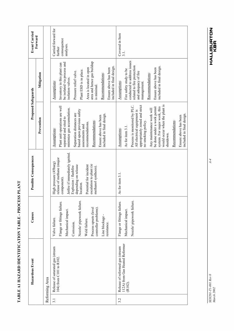
TA
BL
E A
1 H
AZA
RD
IDE
NT
IFIC
AT
ION
TA
BL
E - P
RO
CE
SS P
LAN
T
SEH
201-
T1-0
01 R
ev 0
A-4
Mar
ch 2
002
Prop
osed
Saf
egua
rds
Haz
ardo
us E
vent
Cau
ses
Poss
ible
Con
sequ
ence
s
Prev
entio
nM
itiga
tion
Eve
nt C
arri
edFo
rwar
d
Ref
orm
ing
Are
a
3.1
Rel
ease
of s
atur
ated
gas
(stre
am10
4) fr
om C
101
to R
102.
Val
ve fa
ilure
.
Flan
ge o
r fitt
ings
failu
re.
Mec
hani
cal i
mpa
ct.
Cor
rosi
on.
Noz
zle/
pip
ewor
k fa
ilure
.
Wel
d fa
ilure
.
Proc
ess u
pset
s (le
vel
cont
rolle
r pro
blem
s).
Line
blo
ckag
e -
resi
stan
ce.
Hig
h pr
essu
re (4
5bar
g)re
leas
e of
met
hane
(maj
orco
mpo
nent
).
Jetfi
re if
imm
edia
tely
igni
ted.
Expl
osio
n / f
lash
fire
depe
ndin
g on
rele
ase
loca
tion.
Pote
ntia
l for
inci
dent
esca
latio
n to
pla
nt (i
em
etha
nol s
ynth
esis
).
Ass
umpt
ions
:
Plan
t uni
t ope
ratio
ns a
re w
ell
sepa
rate
d an
d si
ted
tom
inim
ize
gas a
ccum
ulat
ion.
Sepa
ratio
n di
stan
ces a
reba
sed
upon
pre
viou
s saf
ety
asse
ssm
ents
and
reco
mm
enda
tions
.
Rec
omm
enda
tions
:
Ensu
re a
bove
has
bee
nin
clud
ed in
fina
l des
ign.
Ass
umpt
ions
:
Inve
ntor
y in
this
pla
nt c
anbe
isol
ated
via
pro
cess
and
isol
atio
n va
lves
.
Pres
sure
relie
f val
ve.
Plan
t ESD
is in
pla
ce.
Are
a is
loca
ted
in o
pen
area
and
hen
ce g
as b
uild
upis
min
imal
.
Rec
omm
enda
tions
:
Ensu
re a
bove
has
bee
nin
clud
ed in
fina
l des
ign.
Car
ried
forw
ard
for
furth
erco
nseq
uenc
ean
alys
es.
3.2
Rel
ease
of r
efor
med
gas
(stre
am11
2A) f
rom
Gas
Hea
ted
Ref
orm
er(R
102)
.
Flan
ge o
r fitt
ings
failu
re.
Mec
hani
cal i
mpa
ct.
Noz
zle/
pip
ewor
k fa
ilure
.
As f
or it
em 3
.1.
Ass
umpt
ions
:
As f
or it
em 3
.1.
Proc
ess i
s mon
itore
d by
PLC
.A
ll el
ectri
cal e
quip
men
t is
appr
opria
tely
zon
ed a
nd st
rict
no sm
okin
g po
licy.
Any
mai
nten
ance
wor
k w
illbe
don
e un
der a
wor
k pe
rmit
syst
em. F
or m
ajor
wor
k, th
isw
ould
occ
ur w
hen
the
plan
t is
shut
dow
n.
Rec
omm
enda
tions
:
Ensu
re a
bove
has
bee
nin
clud
ed in
fina
l des
ign.
Ass
umpt
ions
:
Fire
safe
ty st
udy
to b
eco
nduc
ted
to a
ddre
ss is
sues
rela
ted
to fi
re p
rote
ctio
nan
d ad
equa
cy o
f fire
man
agem
ent.
Rec
omm
enda
tions
:
Ensu
re a
bove
has
bee
nin
clud
ed in
fina
l des
ign.
Cov
ered
in It
em3.
1.
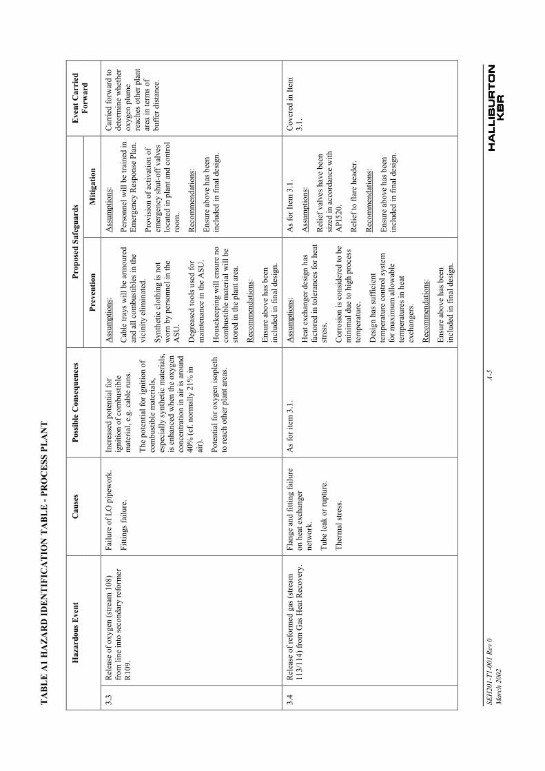
TA
BL
E A
1 H
AZA
RD
IDE
NT
IFIC
AT
ION
TA
BL
E - P
RO
CE
SS P
LAN
T
SEH
201-
T1-0
01 R
ev 0
A-5
Mar
ch 2
002
Prop
osed
Saf
egua
rds
Haz
ardo
us E
vent
Cau
ses
Poss
ible
Con
sequ
ence
s
Prev
entio
nM
itiga
tion
Eve
nt C
arri
edFo
rwar
d
3.3
Rel
ease
of o
xyge
n (s
tream
108
)fro
m li
ne in
to se
cond
ary
refo
rmer
R10
9.
Failu
re o
f LO
pip
ewor
k.
Fitti
ngs f
ailu
re.
Incr
ease
d po
tent
ial f
orig
nitio
n of
com
bust
ible
mat
eria
l, e.
g. c
able
runs
.
The
pote
ntia
l for
igni
tion
ofco
mbu
stib
le m
ater
ials
,es
peci
ally
synt
hetic
mat
eria
ls,
is e
nhan
ced
whe
n th
e ox
ygen
conc
entra
tion
in a
ir is
aro
und
40%
(cf.
norm
ally
21%
inai
r).
Pote
ntia
l for
oxy
gen
isop
leth
to re
ach
othe
r pla
nt a
reas
.
Ass
umpt
ions
:
Cab
le tr
ays w
ill b
e ar
mou
red
and
all c
ombu
stib
les i
n th
evi
cini
ty e
limin
ated
.
Synt
hetic
clo
thin
g is
not
wor
n by
per
sonn
el in
the
ASU
.
Deg
reas
ed to
ols u
sed
for
mai
nten
ance
in th
e A
SU.
Hou
seke
epin
g w
ill e
nsur
e no
com
bust
ible
mat
eria
l will
be
stor
ed in
the
plan
t are
a.
Rec
omm
enda
tions
:
Ensu
re a
bove
has
bee
nin
clud
ed in
fina
l des
ign.
Ass
umpt
ions
:
Pers
onne
l will
be
train
ed in
Emer
genc
y R
espo
nse
Plan
.
Prov
isio
n of
act
ivat
ion
ofem
erge
ncy
shut
-off
valv
eslo
cate
d in
pla
nt a
nd c
ontro
lro
om.
Rec
omm
enda
tions
:
Ensu
re a
bove
has
bee
nin
clud
ed in
fina
l des
ign.
Car
ried
forw
ard
tode
term
ine
whe
ther
oxyg
en p
lum
ere
ache
s oth
er p
lant
area
in te
rms o
fbu
ffer d
ista
nce.
3.4
Rel
ease
of r
efor
med
gas
(stre
am11
3/11
4) fr
om G
as H
eat R
ecov
ery.
Flan
ge a
nd fi
tting
failu
reon
hea
t exc
hang
erne
twor
k.
Tube
leak
or r
uptu
re.
Ther
mal
stre
ss.
As f
or it
em 3
.1.
Ass
umpt
ions
:
Hea
t exc
hang
er d
esig
n ha
sfa
ctor
ed in
tole
ranc
es fo
r hea
tst
ress
.
Cor
rosi
on is
con
sider
ed to
be
min
imal
due
to h
igh
proc
ess
tem
pera
ture
.
Des
ign
has s
uffic
ient
tem
pera
ture
con
trol s
yste
mfo
r max
imum
allo
wab
lete
mpe
ratu
res i
n he
atex
chan
gers
.
Rec
omm
enda
tions
:
Ensu
re a
bove
has
bee
nin
clud
ed in
fina
l des
ign.
As f
or It
em 3
.1.
Ass
umpt
ions
:
Rel
ief v
alve
s hav
e be
ensi
zed
in a
ccor
danc
e w
ithA
PI52
0.
Rel
ief t
o fla
re h
eade
r.
Rec
omm
enda
tions
:
Ensu
re a
bove
has
bee
nin
clud
ed in
fina
l des
ign.
Cov
ered
in It
em3.
1.
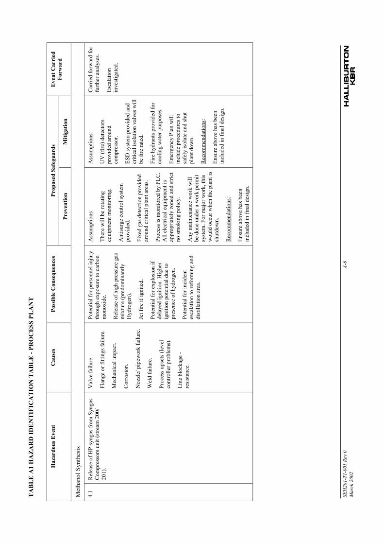
TA
BL
E A
1 H
AZA
RD
IDE
NT
IFIC
AT
ION
TA
BL
E - P
RO
CE
SS P
LAN
T
SEH
201-
T1-0
01 R
ev 0
A-6
Mar
ch 2
002
Prop
osed
Saf
egua
rds
Haz
ardo
us E
vent
Cau
ses
Poss
ible
Con
sequ
ence
s
Prev
entio
nM
itiga
tion
Eve
nt C
arri
edFo
rwar
d
Met
hano
l Syn
thes
is
4.1
Rel
ease
of H
P sy
ngas
from
Syn
gas
Com
pres
sors
uni
t (st
ream
200
/20
1).
Val
ve fa
ilure
.
Flan
ge o
r fitt
ings
failu
re.
Mec
hani
cal i
mpa
ct.
Cor
rosi
on.
Noz
zle/
pip
ewor
k fa
ilure
.
Wel
d fa
ilure
.
Proc
ess u
pset
s (le
vel
cont
rolle
r pro
blem
s).
Line
blo
ckag
e -
resi
stan
ce.
Pote
ntia
l for
per
sonn
el in
jury
thro
ugh
expo
sure
to c
arbo
nm
onox
ide.
Rel
ease
of h
igh
pres
sure
gas
mix
ture
(pre
dom
inan
tlyH
ydro
gen)
.
Jet f
ire if
igni
ted.
Pote
ntia
l for
exp
losi
on if
dela
yed
igni
tion.
Hig
her
igni
tion
pote
ntia
l due
topr
esen
ce o
f hyd
roge
n.
Pote
ntia
l for
inci
dent
esca
latio
n to
refo
rmin
g an
ddi
still
atio
n ar
ea.
Ass
umpt
ions
:
Ther
e w
ill b
e ro
tatin
geq
uipm
ent m
onito
ring.
Ant
isur
ge c
ontro
l sys
tem
prov
ided
.
Fixe
d ga
s det
ectio
n pr
ovid
edar
ound
crit
ical
pla
nt a
reas
.
Proc
ess i
s mon
itore
d by
PLC
.A
ll el
ectri
cal e
quip
men
t is
appr
opria
tely
zon
ed a
nd st
rict
no sm
okin
g po
licy.
Any
mai
nten
ance
wor
k w
illbe
don
e un
der a
wor
k pe
rmit
syst
em. F
or m
ajor
wor
k, th
isw
ould
occ
ur w
hen
the
plan
t is
shut
dow
n.
Rec
omm
enda
tions
:
Ensu
re a
bove
has
bee
nin
clud
ed in
fina
l des
ign.
Ass
umpt
ions
:
UV
(fire
) det
ecto
rspr
ovid
ed a
roun
dco
mpr
esso
r.
ESD
syst
em p
rovi
ded
and
criti
cal i
sola
tion
valv
es w
illbe
fire
rate
d.
Fire
hyd
rant
s pro
vide
d fo
rco
olin
g w
ater
pur
pose
s.
Emer
genc
y Pl
an w
illin
clud
e pr
oced
ures
tosa
fely
isol
ate
and
shut
plan
t dow
n.
Rec
omm
enda
tions
:
Ensu
re a
bove
has
bee
nin
clud
ed in
fina
l des
ign.
Car
ried
forw
ard
for
furth
er a
naly
ses.
Esca
latio
nin
vest
igat
ed.
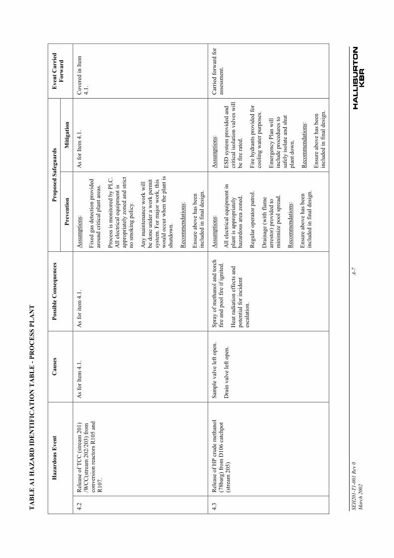
TA
BL
E A
1 H
AZA
RD
IDE
NT
IFIC
AT
ION
TA
BL
E - P
RO
CE
SS P
LAN
T
SEH
201-
T1-0
01 R
ev 0
A-7
Mar
ch 2
002
Prop
osed
Saf
egua
rds
Haz
ardo
us E
vent
Cau
ses
Poss
ible
Con
sequ
ence
s
Prev
entio
nM
itiga
tion
Eve
nt C
arri
edFo
rwar
d
4.2
Rel
ease
of T
CC
(stre
am 2
01)
/WC
C(s
tream
202
/203
) fro
mco
nver
sion
reac
tors
R10
5 an
dR
107.
As f
or It
em 4
.1.
As f
or it
em 4
.1.
Ass
umpt
ions
:
Fixe
d ga
s det
ectio
n pr
ovid
edar
ound
crit
ical
pla
nt a
reas
.
Proc
ess i
s mon
itore
d by
PLC
.A
ll el
ectri
cal e
quip
men
t is
appr
opria
tely
zon
ed a
nd st
rict
no sm
okin
g po
licy.
Any
mai
nten
ance
wor
k w
illbe
don
e un
der a
wor
k pe
rmit
syst
em. F
or m
ajor
wor
k, th
isw
ould
occ
ur w
hen
the
plan
t is
shut
dow
n.
Rec
omm
enda
tions
:
Ensu
re a
bove
has
bee
nin
clud
ed in
fina
l des
ign.
As f
or It
em 4
.1.
Cov
ered
in It
em4.
1.
4.3
Rel
ease
of H
P cr
ude
met
hano
l(7
8bar
g) fr
om D
106
catc
hpot
(stre
am 2
05)
Sam
ple
valv
e le
ft op
en.
Dra
in v
alve
left
open
.
Spra
y of
met
hano
l and
torc
hfir
e an
d po
ol fi
re if
igni
ted.
Hea
t rad
iatio
n ef
fect
s and
pote
ntia
l for
inci
dent
esca
latio
n.
Ass
umpt
ions
:
All
elec
trica
l equ
ipm
ent i
npl
ant i
s app
ropr
iate
lyha
zard
ous a
rea
zone
d.
Reg
ular
ope
rato
r pat
rol.
Dra
inag
e (w
ith fl
ame
arre
stor
) pro
vide
d to
min
imiz
e po
ol sp
read
.
Rec
omm
enda
tions
:
Ensu
re a
bove
has
bee
nin
clud
ed in
fina
l des
ign.
Ass
umpt
ions
:
ESD
syst
em p
rovi
ded
and
criti
cal i
sola
tion
valv
es w
illbe
fire
rate
d.
Fire
hyd
rant
s pro
vide
d fo
rco
olin
g w
ater
pur
pose
s.
Emer
genc
y Pl
an w
illin
clud
e pr
oced
ures
tosa
fely
isol
ate
and
shut
plan
t dow
n.
Rec
omm
enda
tions
:
Ensu
re a
bove
has
bee
nin
clud
ed in
fina
l des
ign.
Car
ried
forw
ard
for
asse
ssm
ent.
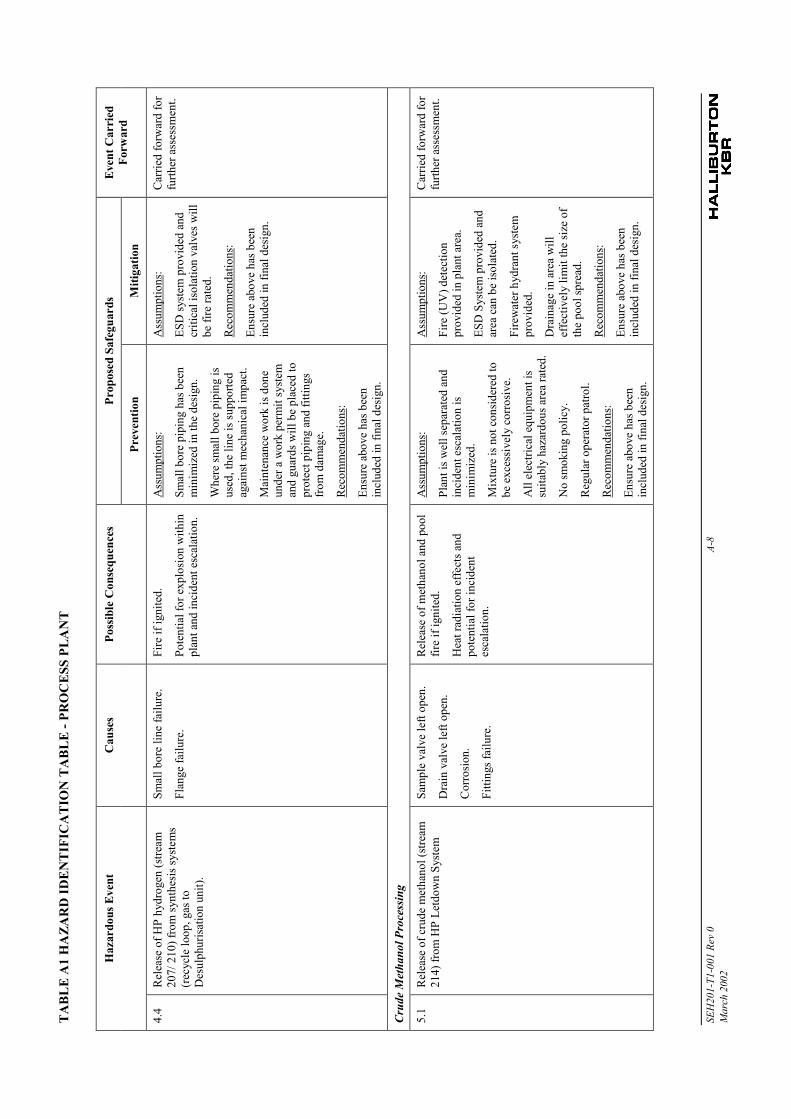
TA
BL
E A
1 H
AZA
RD
IDE
NT
IFIC
AT
ION
TA
BL
E - P
RO
CE
SS P
LAN
T
SEH
201-
T1-0
01 R
ev 0
A-8
Mar
ch 2
002
Prop
osed
Saf
egua
rds
Haz
ardo
us E
vent
Cau
ses
Poss
ible
Con
sequ
ence
s
Prev
entio
nM
itiga
tion
Eve
nt C
arri
edFo
rwar
d
4.4
Rel
ease
of H
P hy
drog
en (s
tream
207/
210
) fro
m sy
nthe
sis s
yste
ms
(rec
ycle
loop
, gas
toD
esul
phur
isat
ion
unit)
.
Smal
l bor
e lin
e fa
ilure
.
Flan
ge fa
ilure
.
Fire
if ig
nite
d.
Pote
ntia
l for
exp
losi
on w
ithin
plan
t and
inci
dent
esc
alat
ion.
Ass
umpt
ions
:
Smal
l bor
e pi
ping
has
bee
nm
inim
ized
in th
e de
sign
.
Whe
re sm
all b
ore
pipi
ng is
used
, the
line
is su
ppor
ted
agai
nst m
echa
nica
l im
pact
.
Mai
nten
ance
wor
k is
don
eun
der a
wor
k pe
rmit
syst
eman
d gu
ards
will
be
plac
ed to
prot
ect p
ipin
g an
d fit
tings
from
dam
age.
Rec
omm
enda
tions
:
Ensu
re a
bove
has
bee
nin
clud
ed in
fina
l des
ign.
Ass
umpt
ions
:
ESD
syst
em p
rovi
ded
and
criti
cal i
sola
tion
valv
es w
illbe
fire
rate
d.
Rec
omm
enda
tions
:
Ensu
re a
bove
has
bee
nin
clud
ed in
fina
l des
ign.
Car
ried
forw
ard
for
furth
er a
sses
smen
t.
Crud
e M
etha
nol P
roce
ssin
g
5.1
Rel
ease
of c
rude
met
hano
l (st
ream
214)
from
HP
Letd
own
Syst
emSa
mpl
e va
lve
left
open
.
Dra
in v
alve
left
open
.
Cor
rosi
on.
Fitti
ngs f
ailu
re.
Rel
ease
of m
etha
nol a
nd p
ool
fire
if ig
nite
d.
Hea
t rad
iatio
n ef
fect
s and
pote
ntia
l for
inci
dent
esca
latio
n.
Ass
umpt
ions
:
Plan
t is w
ell s
epar
ated
and
inci
dent
esc
alat
ion
ism
inim
ized
.
Mix
ture
is n
ot c
onsi
dere
d to
be e
xces
sive
ly c
orro
sive
.
All
elec
trica
l equ
ipm
ent i
ssu
itabl
y ha
zard
ous a
rea
rate
d.
No
smok
ing
polic
y.
Reg
ular
ope
rato
r pat
rol.
Rec
omm
enda
tions
:
Ensu
re a
bove
has
bee
nin
clud
ed in
fina
l des
ign.
Ass
umpt
ions
:
Fire
(UV
) det
ectio
npr
ovid
ed in
pla
nt a
rea.
ESD
Sys
tem
pro
vide
d an
dar
ea c
an b
e is
olat
ed.
Fire
wat
er h
ydra
nt sy
stem
prov
ided
.
Dra
inag
e in
are
a w
illef
fect
ivel
y lim
it th
e si
ze o
fth
e po
ol sp
read
.
Rec
omm
enda
tions
:
Ensu
re a
bove
has
bee
nin
clud
ed in
fina
l des
ign.
Car
ried
forw
ard
for
furth
er a
sses
smen
t.
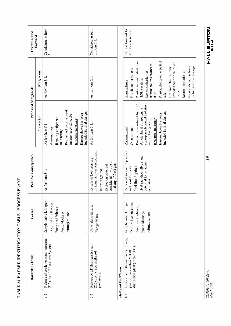
TA
BL
E A
1 H
AZA
RD
IDE
NT
IFIC
AT
ION
TA
BL
E - P
RO
CE
SS P
LAN
T
SEH
201-
T1-0
01 R
ev 0
A-9
Mar
ch 2
002
Prop
osed
Saf
egua
rds
Haz
ardo
us E
vent
Cau
ses
Poss
ible
Con
sequ
ence
s
Prev
entio
nM
itiga
tion
Eve
nt C
arri
edFo
rwar
d
5.2
Rel
ease
of c
rude
met
hano
l (st
ream
217)
from
LP
Letd
own
Syst
emSa
mpl
e va
lve
left
open
.D
rain
val
ve le
ft op
en.
Pum
p se
al fa
ilure
s.Pu
mp
bloc
kage
.Fi
tting
s fai
lure
.
As f
or It
em 5
.1.
As f
or It
em 5
.1A
ssum
ptio
ns:
Rot
atin
g eq
uipm
ent
mon
itorin
g.Pu
mps
will
be
on a
regu
lar
mai
nten
ance
sche
dule
.R
ecom
men
datio
ns:
Ensu
re a
bove
has
bee
nin
clud
ed in
fina
l des
ign.
As f
or It
em 5
.1.
Con
side
red
in It
em5.
1.
5.3
Rel
ease
of L
P fla
sh g
as (s
tream
215)
from
cru
de m
etha
nol
proc
essi
ng.
Val
ve g
land
failu
re.
Flan
ge fa
ilure
.R
elea
se o
f low
-pre
ssur
em
etha
ne a
nd c
arbo
n di
oxid
e.Je
tfire
if ig
nite
d.Ex
plos
ion
pote
ntia
lco
nsid
ered
low
due
tom
akeu
p of
flas
h ga
s.
As f
or it
em 5
.1.
As f
or it
em 5
.1.
Con
side
red
as p
art
of It
em 5
.1.
Met
hano
l Dis
tilla
tion
6.1
Rel
ease
of m
etha
nol f
rom
col
umns
,pu
mps
, lin
es w
ithin
MeO
Hdi
still
atio
n pl
ant (
stre
am 3
03).
Sam
ple
valv
e le
ft op
en.
Dra
in v
alve
left
open
.Pu
mp
seal
failu
res.
Pum
p bl
ocka
ge.
Fitti
ngs f
ailu
re.
Rel
ease
of m
etha
nol p
rodu
ctan
d po
ol fo
rmat
ion.
Pool
fire
if ig
nite
d.H
eat r
adia
tion
effe
cts a
ndpo
tent
ial f
or in
cide
ntes
cala
tion.
Ass
umpt
ions
:O
pera
tor p
atro
l.Pr
oces
s is m
onito
red
by P
LC.
All
elec
trica
l equ
ipm
ent i
sap
prop
riate
ly z
oned
and
stric
tno
smok
ing
polic
y.R
ecom
men
datio
ns:
Ensu
re a
bove
has
bee
nin
clud
ed in
fina
l des
ign.
Ass
umpt
ions
:Fi
re d
etec
tion
syst
em.
Plan
t em
erge
ncy
shut
dow
n(E
SD) s
yste
m.
Dep
ress
uriz
atio
n of
flam
mab
le in
vent
orie
s to
flare
.Pl
ant i
s des
igne
d to
be
fail
safe
.Fi
re p
rote
ctio
n sy
stem
prov
ided
for c
ritic
al p
lant
area
s.R
ecom
men
datio
ns:
Ensu
re a
bove
has
bee
nin
clud
ed in
fina
l des
ign.
Car
ried
forw
ard
for
furth
er a
sses
smen
t.
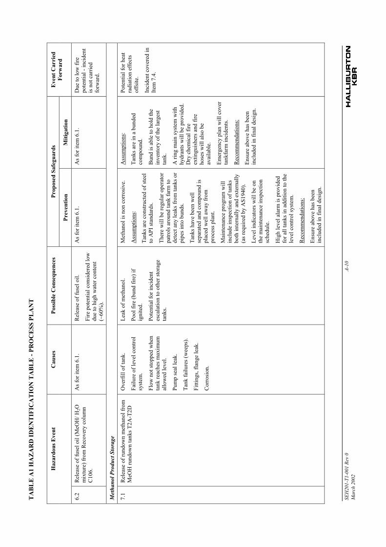
TA
BL
E A
1 H
AZA
RD
IDE
NT
IFIC
AT
ION
TA
BL
E - P
RO
CE
SS P
LAN
T
SEH
201-
T1-0
01 R
ev 0
A-10
Mar
ch 2
002
Prop
osed
Saf
egua
rds
Haz
ardo
us E
vent
Cau
ses
Poss
ible
Con
sequ
ence
s
Prev
entio
nM
itiga
tion
Eve
nt C
arri
edFo
rwar
d
6.2
Rel
ease
of f
usel
oil
(MeO
H/ H
2Om
ixtu
re) f
rom
Rec
over
y co
lum
nC
106.
As f
or it
em 6
.1.
Rel
ease
of f
usel
oil.
Fire
pot
entia
l con
side
red
low
due
to h
igh
wat
er c
onte
nt(~
60%
).
As f
or it
em 6
.1.
As f
or it
em 6
.1.
Due
to lo
w fi
repo
tent
ial -
inci
dent
is n
ot c
arrie
dfo
rwar
d.
Met
hano
l Pro
duct
Sto
rage
7.1
Rel
ease
of r
undo
wn
met
hano
l fro
mM
eOH
rund
own
tank
s T2A
-T2D
Ove
rfill
of t
ank.
Failu
re o
f lev
el c
ontro
lsy
stem
.
Flow
not
stop
ped
whe
nta
nk re
ache
s max
imum
allo
wed
leve
l.
Pum
p se
al le
ak.
Tank
failu
res (
wee
ps).
Fitti
ngs,
flang
e le
ak.
Cor
rosi
on.
Leak
of m
etha
nol.
Pool
fire
(bun
d fir
e) if
igni
ted.
Pote
ntia
l for
inci
dent
esca
latio
n to
oth
er st
orag
eta
nks.
Met
hano
l is n
on c
orro
sive
.
Ass
umpt
ions
:
Tank
s are
con
stru
cted
of s
teel
to A
PI st
anda
rds.
Ther
e w
ill b
e re
gula
r ope
rato
rpa
trols
aro
und
tank
farm
tode
tect
any
leak
s fro
m ta
nks o
rpi
pes i
nto
bund
s.
Tank
s hav
e be
en w
ell
sepa
rate
d an
d co
mpo
und
ispl
aced
wel
l aw
ay fr
ompr
oces
s pla
nt.
Mai
nten
ance
pro
gram
will
incl
ude
insp
ectio
n of
tank
sbo
th in
tern
ally
and
ext
erna
lly(a
s req
uire
d by
AS1
940)
.
Leve
l ind
icat
ors w
ill b
e on
the
mai
nten
ance
insp
ectio
nsc
hedu
le.
Hig
h le
vel a
larm
is p
rovi
ded
for a
ll ta
nks i
n ad
ditio
n to
the
leve
l con
trol s
yste
m.
Rec
omm
enda
tions
:
Ensu
re a
bove
has
bee
nin
clud
ed in
fina
l des
ign.
Ass
umpt
ions
:
Tank
s are
in a
bun
ded
com
poun
d.
Bun
d is
abl
e to
hol
d th
ein
vent
ory
of th
e la
rges
tta
nk.
A ri
ng m
ain
syst
em w
ithhy
dran
ts w
ill b
e pr
ovid
ed.
Dry
che
mic
al fi
reex
tingu
ishe
rs a
nd fi
reho
ses w
ill a
lso
beav
aila
ble.
Emer
genc
y pl
an w
ill c
over
tank
farm
inci
dent
s.
Rec
omm
enda
tions
:
Ensu
re a
bove
has
bee
nin
clud
ed in
fina
l des
ign.
Pote
ntia
l for
hea
tra
diat
ion
effe
cts
offs
ite.
Inci
dent
cov
ered
inIte
m 7
.4.
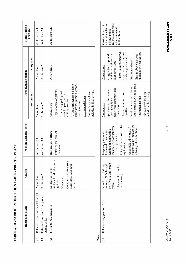
TA
BL
E A
1 H
AZA
RD
IDE
NT
IFIC
AT
ION
TA
BL
E - P
RO
CE
SS P
LAN
T
SEH
201-
T1-0
01 R
ev 0
A-11
Mar
ch 2
002
Prop
osed
Saf
egua
rds
Haz
ardo
us E
vent
Cau
ses
Poss
ible
Con
sequ
ence
s
Prev
entio
nM
itiga
tion
Eve
nt C
arri
edFo
rwar
d
7.2
Rel
ease
of c
rude
met
hano
l fro
m T
1.A
s for
item
7.1
.A
s for
item
7.1
.A
s for
item
7.1
.A
s for
item
7.1
.A
s for
item
7.1
.
7.3
Rel
ease
of m
etha
nol f
rom
pro
duct
stor
age
tank
s.A
s for
item
7.1
As f
or it
em 7
.1.
As f
or it
em 7
.1.
As f
or it
em 7
.1.
As f
or it
em 7
.1.
7.4
Fire
in th
e ta
nkfa
rm a
rea.
Spill
age
or le
ak o
fm
etha
nol a
nd su
bseq
uent
igni
tion.
Hot
wor
k.
Com
bust
ible
deb
ris (o
ilyra
gs) l
eft a
roun
d ta
nkfa
rm.
Hea
t rad
iatio
n ef
fect
s.
Pote
ntia
l for
inci
dent
esca
latio
n.
Ass
umpt
ions
:
Reg
ular
ope
rato
r pat
rols
.
No
smok
ing
polic
y an
dho
usek
eepi
ng w
ill b
een
forc
ed o
n si
te.
All
tank
mai
nten
ance
is d
one
usin
g a
wor
k pe
rmit
hot w
ork
perm
it sy
stem
.
Rec
omm
enda
tions
:
Ensu
re a
bove
has
bee
nin
clud
ed in
fina
l des
ign.
As f
or it
em 7
.1.
As f
or it
em 7
.1.
Oth
ers
8.1
Rel
ease
of o
xyge
n fro
m A
SUV
esse
l ove
rfille
d an
dre
leas
e of
LO
thro
ugh
relie
f val
ve o
n st
orag
eve
ssel
.
Elec
trica
l fire
(mot
or,
switc
hboa
rd).
Larg
e ox
ygen
clo
ud.
Incr
ease
d po
tent
ial f
orig
nitio
n of
com
bust
ible
mat
eria
l. Se
rious
inju
ry to
expo
sed
pers
onne
l.
Pote
ntia
l esc
alat
ion
to p
lant
equi
pmen
t.
An
asso
ciat
ed re
leas
e of
oxyg
en w
ould
incr
ease
the
inte
nsity
of c
ombu
stio
n.
Ass
umpt
ions
:
Spee
d co
ntro
l and
act
ive
rota
ting
equi
pmen
tm
onito
ring
on tu
rbin
e an
dco
mpr
esso
r.
Plan
t is h
azar
dous
are
acl
assi
fied.
Leve
l ind
icat
or p
rovi
ded
onta
nk c
ontro
ls L
O fe
ed to
tank
.
Rec
omm
enda
tions
:
Ensu
re a
bove
has
bee
nin
clud
ed in
fina
l des
ign.
Ass
umpt
ions
:
Oxy
gen
tank
is p
rovi
ded
with
leve
l ind
icat
or a
ndhi
gh le
vel a
larm
.
Ther
e is
a sa
fe sh
utdo
wn
sequ
ence
for t
he tu
rbin
ean
d co
mpr
esso
r tra
in.
Rec
omm
enda
tions
:
Ensu
re a
bove
has
bee
nin
clud
ed in
fina
l des
ign.
Car
ried
forw
ard
tode
term
ine
whe
ther
oxyg
en p
lum
ere
ache
s oth
er p
lant
area
in te
rms o
fbu
ffer d
ista
nce.
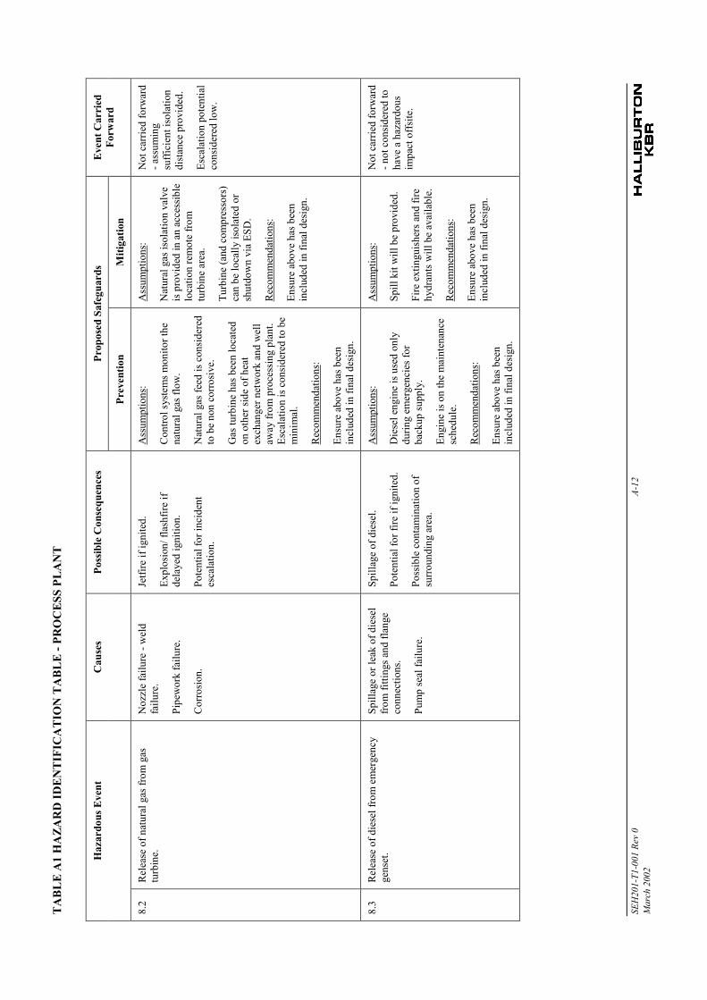
TA
BL
E A
1 H
AZA
RD
IDE
NT
IFIC
AT
ION
TA
BL
E - P
RO
CE
SS P
LAN
T
SEH
201-
T1-0
01 R
ev 0
A-12
Mar
ch 2
002
Prop
osed
Saf
egua
rds
Haz
ardo
us E
vent
Cau
ses
Poss
ible
Con
sequ
ence
s
Prev
entio
nM
itiga
tion
Eve
nt C
arri
edFo
rwar
d
8.2
Rel
ease
of n
atur
al g
as fr
om g
astu
rbin
e.N
ozzl
e fa
ilure
- w
eld
failu
re.
Pipe
wor
k fa
ilure
.
Cor
rosi
on.
Jetfi
re if
igni
ted.
Expl
osio
n/ fl
ashf
ire if
dela
yed
igni
tion.
Pote
ntia
l for
inci
dent
esca
latio
n.
Ass
umpt
ions
:
Con
trol s
yste
ms
mon
itor t
hena
tura
l gas
flow
.
Nat
ural
gas
feed
is c
onsi
dere
dto
be
non
corro
sive
.
Gas
turb
ine
has b
een
loca
ted
on o
ther
side
of h
eat
exch
ange
r net
wor
k an
d w
ell
away
from
pro
cess
ing
plan
t.Es
cala
tion
is c
onsi
dere
d to
be
min
imal
.
Rec
omm
enda
tions
:
Ensu
re a
bove
has
bee
nin
clud
ed in
fina
l des
ign.
Ass
umpt
ions
:
Nat
ural
gas
isol
atio
n va
lve
is p
rovi
ded
in a
n ac
cess
ible
loca
tion
rem
ote
from
turb
ine
area
.
Turb
ine
(and
com
pres
sors
)ca
n be
loca
lly is
olat
ed o
rsh
utdo
wn
via
ESD
.
Rec
omm
enda
tions
:
Ensu
re a
bove
has
bee
nin
clud
ed in
fina
l des
ign.
Not
car
ried
forw
ard
- ass
umin
gsu
ffici
ent i
sola
tion
dist
ance
pro
vide
d.
Esca
latio
n po
tent
ial
cons
ider
ed lo
w.
8.3
Rel
ease
of d
iese
l fro
m e
mer
genc
yge
nset
.Sp
illag
e or
leak
of d
iese
lfro
m fi
tting
s and
flan
geco
nnec
tions
.
Pum
p se
al fa
ilure
.
Spill
age
of d
iese
l.
Pote
ntia
l for
fire
if ig
nite
d.
Poss
ible
con
tam
inat
ion
ofsu
rrou
ndin
g ar
ea.
Ass
umpt
ions
:
Die
sel e
ngin
e is
use
d on
lydu
ring
emer
genc
ies f
orba
ckup
supp
ly.
Engi
ne is
on
the
mai
nten
ance
sche
dule
.
Rec
omm
enda
tions
:
Ensu
re a
bove
has
bee
nin
clud
ed in
fina
l des
ign.
Ass
umpt
ions
:
Spill
kit
will
be
prov
ided
.
Fire
ext
ingu
ishe
rs a
nd fi
rehy
dran
ts w
ill b
e av
aila
ble.
Rec
omm
enda
tions
:
Ensu
re a
bove
has
bee
nin
clud
ed in
fina
l des
ign.
Not
car
ried
forw
ard
- not
con
sider
ed to
have
a h
azar
dous
impa
ct o
ffsi
te.
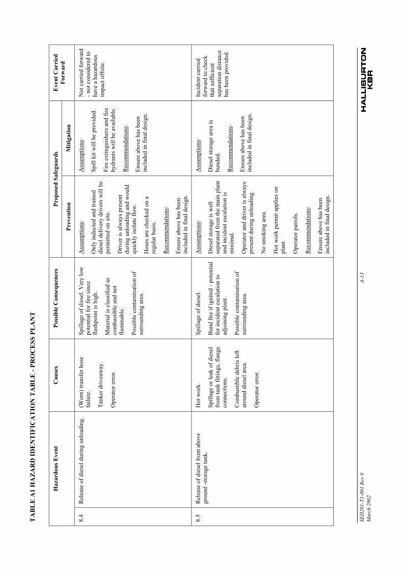
TA
BL
E A
1 H
AZA
RD
IDE
NT
IFIC
AT
ION
TA
BL
E - P
RO
CE
SS P
LAN
T
SEH
201-
T1-0
01 R
ev 0
A-13
Mar
ch 2
002
Prop
osed
Saf
egua
rds
Haz
ardo
us E
vent
Cau
ses
Poss
ible
Con
sequ
ence
s
Prev
entio
nM
itiga
tion
Eve
nt C
arri
edFo
rwar
d
8.4
Rel
ease
of d
iese
l dur
ing
unlo
adin
g.(W
orn)
tran
sfer
hos
efa
ilure
.
Tank
er d
rivea
way
.
Ope
rato
r err
or.
Spill
age
of d
iese
l. V
ery
low
pote
ntia
l for
fire
sinc
efla
shpo
int i
s hig
h.
Mat
eria
l is c
lass
ified
as
com
bust
ible
and
not
flam
mab
le.
Poss
ible
con
tam
inat
ion
ofsu
rrou
ndin
g ar
ea.
Ass
umpt
ions
:
Onl
y in
duct
ed a
nd tr
aine
ddi
esel
del
iver
y dr
iver
s w
ill b
epe
rmitt
ed o
n si
te.
Driv
er is
alw
ays p
rese
ntdu
ring
unlo
adin
g an
d w
ould
quic
kly
isol
ate
flow
.
Hos
es a
re c
heck
ed o
n a
regu
lar b
asis
.
Rec
omm
enda
tions
:
Ensu
re a
bove
has
bee
nin
clud
ed in
fina
l des
ign.
Ass
umpt
ions
:
Spill
kit
will
be
prov
ided
.
Fire
ext
ingu
ishe
rs a
nd fi
rehy
dran
ts w
ill b
e av
aila
ble.
Rec
omm
enda
tions
:
Ensu
re a
bove
has
bee
nin
clud
ed in
fina
l des
ign.
Not
car
ried
forw
ard
- not
con
sider
ed to
have
a h
azar
dous
impa
ct o
ffsi
te.
8.5
Rel
ease
of d
iese
l fro
m a
bove
grou
nd -s
tora
ge ta
nk.
Hot
wor
k.
Spill
age
or le
ak o
f die
sel
from
tank
fitti
ngs,
flang
eco
nnec
tions
.
Com
bust
ible
deb
ris le
ftar
ound
die
sel a
rea.
Ope
rato
r err
or.
Spill
age
of d
iese
l.
Bun
d fir
e if
igni
ted
- pot
entia
lfo
r inc
iden
t esc
alat
ion
toad
join
ing
plan
t.
Poss
ible
con
tam
inat
ion
ofsu
rrou
ndin
g ar
ea.
Ass
umpt
ions
:
Die
sel s
tora
ge is
wel
lse
para
ted
from
the
mai
n pl
ant
and
inci
dent
esc
alat
ion
ism
inim
al.
Ope
rato
r and
driv
er is
alw
ays
pres
ent d
urin
g un
load
ing.
No
smok
ing
area
.
Hot
wor
k pe
rmit
appl
ies o
npl
ant.
Ope
rato
r pat
rols
.
Rec
omm
enda
tions
:
Ensu
re a
bove
has
bee
nin
clud
ed in
fina
l des
ign.
Ass
umpt
ions
:
Die
sel s
tora
ge a
rea
isbu
nded
.
Rec
omm
enda
tions
:
Ensu
re a
bove
has
bee
nin
clud
ed in
fina
l des
ign.
Inci
dent
car
ried
forw
ard
to c
heck
that
suffi
cien
tse
para
tion
dist
ance
has b
een
prov
ided
.
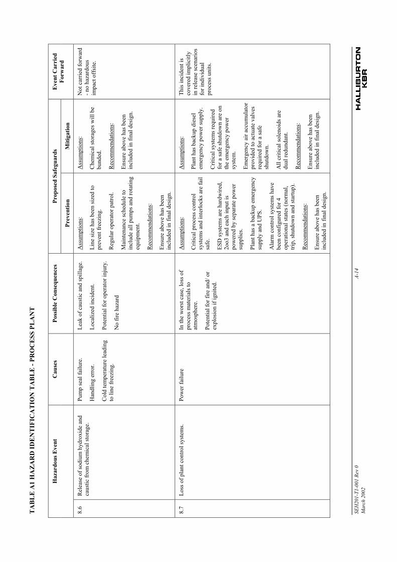
TA
BL
E A
1 H
AZA
RD
IDE
NT
IFIC
AT
ION
TA
BL
E - P
RO
CE
SS P
LAN
T
SEH
201-
T1-0
01 R
ev 0
A-14
Mar
ch 2
002
Prop
osed
Saf
egua
rds
Haz
ardo
us E
vent
Cau
ses
Poss
ible
Con
sequ
ence
s
Prev
entio
nM
itiga
tion
Eve
nt C
arri
edFo
rwar
d
8.6
Rel
ease
of s
odiu
m h
ydro
xide
and
caus
tic fr
om c
hem
ical
stor
age.
Pum
p se
al fa
ilure
.
Han
dlin
g er
ror.
Col
d te
mpe
ratu
re le
adin
gto
line
free
zing
.
Leak
of c
aust
ic a
nd sp
illag
e.
Loca
lized
inci
dent
.
Pote
ntia
l for
ope
rato
r inj
ury.
No
fire
haza
rd
Ass
umpt
ions
:
Line
size
has
bee
n si
zed
topr
even
t fre
ezin
g.
Reg
ular
ope
rato
r pat
rol.
Mai
nten
ance
sche
dule
toin
clud
e al
l pum
ps a
nd ro
tatin
geq
uipm
ent.
Rec
omm
enda
tions
:
Ensu
re a
bove
has
bee
nin
clud
ed in
fina
l des
ign.
Ass
umpt
ions
:
Che
mic
al st
orag
es w
ill b
ebu
nded
.
Rec
omm
enda
tions
:
Ensu
re a
bove
has
bee
nin
clud
ed in
fina
l des
ign.
Not
car
ried
forw
ard
- no
haza
rdou
sim
pact
off
site
.
8.7
Loss
of p
lant
con
trol s
yste
ms.
Pow
er fa
ilure
In th
e w
orst
cas
e, lo
ss o
fpr
oces
s mat
eria
ls to
atm
osph
ere.
Pote
ntia
l for
fire
and
/ or
expl
osio
n if
igni
ted.
Ass
umpt
ions
:
Crit
ical
pro
cess
con
trol
syst
ems a
nd in
terlo
cks a
re fa
ilsa
fe.
ESD
syst
ems a
re h
ardw
ired,
2oo3
and
eac
h in
put i
spo
wer
ed b
y se
para
te p
ower
supp
lies.
Plan
t has
a b
acku
p em
erge
ncy
supp
ly a
nd U
PS.
Ala
rm c
ontro
l sys
tem
s hav
ebe
en c
onfig
ured
for 4
oper
atio
nal s
tate
s (no
rmal
,tri
p, sh
utdo
wn
and
star
tup)
.
Rec
omm
enda
tions
:
Ensu
re a
bove
has
bee
nin
clud
ed in
fina
l des
ign.
Ass
umpt
ions
:
Plan
t has
bac
kup
dies
elem
erge
ncy
pow
er su
pply
.
Crit
ical
syst
ems r
equi
red
for a
safe
shut
dow
n ar
e on
the
emer
genc
y po
wer
syst
em.
Emer
genc
y ai
r acc
umul
ator
prov
ided
to a
ctua
te v
alve
sre
quire
d fo
r a sa
fesh
utdo
wn.
All
criti
cal s
olen
oids
are
dual
redu
ndan
t.
Rec
omm
enda
tions
:
Ensu
re a
bove
has
bee
nin
clud
ed in
fina
l des
ign.
This
inci
dent
isco
vere
d im
plic
itly
in re
leas
e sc
enar
ios
for i
ndiv
idua
lpr
oces
s uni
ts.
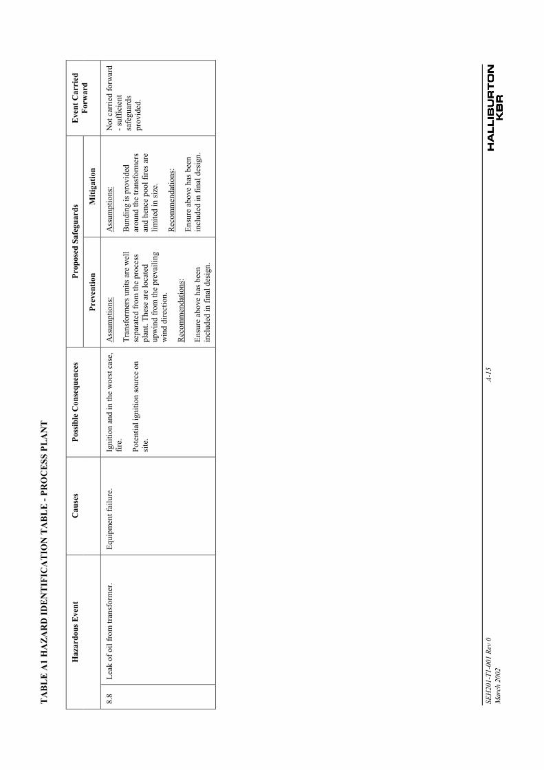
TA
BL
E A
1 H
AZA
RD
IDE
NT
IFIC
AT
ION
TA
BL
E - P
RO
CE
SS P
LAN
T
SEH
201-
T1-0
01 R
ev 0
A-15
Mar
ch 2
002
Prop
osed
Saf
egua
rds
Haz
ardo
us E
vent
Cau
ses
Poss
ible
Con
sequ
ence
s
Prev
entio
nM
itiga
tion
Eve
nt C
arri
edFo
rwar
d
8.8
Leak
of o
il fro
m tr
ansf
orm
er.
Equi
pmen
t fai
lure
.Ig
nitio
n an
d in
the
wor
st c
ase,
fire.
Pote
ntia
l ign
ition
sour
ce o
nsi
te.
Ass
umpt
ions
:
Tran
sfor
mer
s uni
ts a
re w
ell
sepa
rate
d fro
m th
e pr
oces
spl
ant.
Thes
e ar
e lo
cate
dup
win
d fro
m th
e pr
evai
ling
win
d di
rect
ion.
Rec
omm
enda
tions
:
Ensu
re a
bove
has
bee
nin
clud
ed in
fina
l des
ign.
Ass
umpt
ions
:
Bun
ding
is p
rovi
ded
arou
nd th
e tra
nsfo
rmer
san
d he
nce
pool
fire
s are
limite
d in
size
.
Rec
omm
enda
tions
:
Ensu
re a
bove
has
bee
nin
clud
ed in
fina
l des
ign.
Not
car
ried
forw
ard
- suf
ficie
ntsa
fegu
ards
prov
ided
.

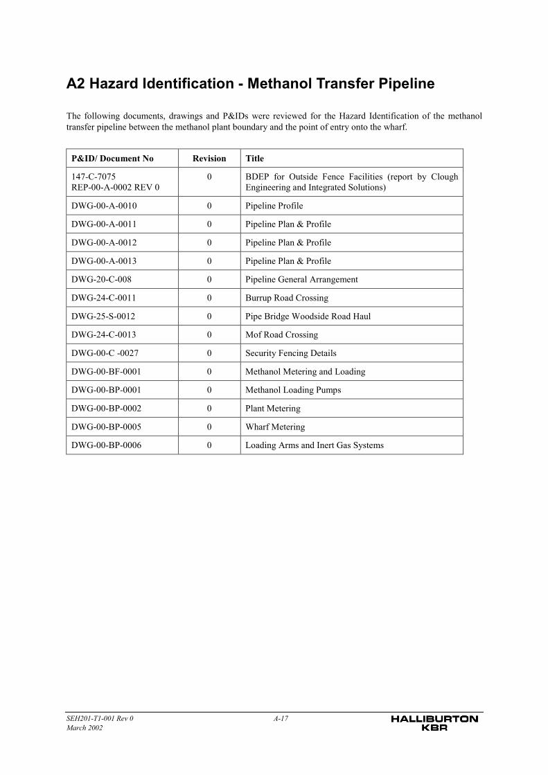
SEH201-T1-001 Rev 0 A-17March 2002
A2 Hazard Identification - Methanol Transfer Pipeline
The following documents, drawings and P&IDs were reviewed for the Hazard Identification of the methanoltransfer pipeline between the methanol plant boundary and the point of entry onto the wharf.
P&ID/ Document No Revision Title
147-C-7075REP-00-A-0002 REV 0
0 BDEP for Outside Fence Facilities (report by CloughEngineering and Integrated Solutions)
DWG-00-A-0010 0 Pipeline Profile
DWG-00-A-0011 0 Pipeline Plan & Profile
DWG-00-A-0012 0 Pipeline Plan & Profile
DWG-00-A-0013 0 Pipeline Plan & Profile
DWG-20-C-008 0 Pipeline General Arrangement
DWG-24-C-0011 0 Burrup Road Crossing
DWG-25-S-0012 0 Pipe Bridge Woodside Road Haul
DWG-24-C-0013 0 Mof Road Crossing
DWG-00-C -0027 0 Security Fencing Details
DWG-00-BF-0001 0 Methanol Metering and Loading
DWG-00-BP-0001 0 Methanol Loading Pumps
DWG-00-BP-0002 0 Plant Metering
DWG-00-BP-0005 0 Wharf Metering
DWG-00-BP-0006 0 Loading Arms and Inert Gas Systems

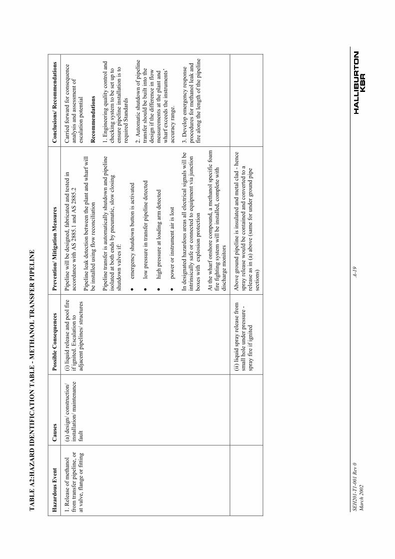
TA
BL
E A
2:H
AZA
RD
IDE
NT
IFIC
AT
ION
TA
BL
E - M
ET
HA
NO
L T
RA
NSF
ER
PIP
EL
INE
SEH
201-
T1-0
01 R
ev 0
A-19
Mar
ch 2
002
Haz
ardo
us E
vent
Cau
ses
Poss
ible
Con
sequ
ence
sPr
even
tion/
Miti
gatio
n M
easu
res
Con
clus
ions
/ Rec
omm
enda
tions
1. R
elea
se o
f met
hano
lfro
m tr
ansf
er p
ipel
ine,
or
at v
alve
, fla
nge
or fi
tting
(a) d
esig
n/ c
onst
ruct
ion/
inst
alla
tion/
mai
nten
ance
faul
t
(i) li
quid
rele
ase
and
pool
fire
if ig
nite
d. E
scal
atio
n to
adja
cent
pip
elin
es/ s
truct
ures
Pipe
line
will
be
desi
gned
, fab
ricat
ed a
nd te
sted
inac
cord
ance
with
AS
2885
.1 a
nd A
S 28
85.2
Pipe
line
leak
det
ectio
n be
twee
n th
e pl
ant a
nd w
harf
will
be in
stal
led
usin
g flo
w re
conc
iliat
ion
Pipe
line
trans
fer i
s aut
omat
ical
ly sh
utdo
wn
and
pipe
line
isol
ated
at b
oth
ends
by
pneu
mat
ic, s
low
clo
sing
shut
dow
n va
lves
if:
• em
erge
ncy
shut
dow
n bu
tton
is a
ctiv
ated
• lo
w p
ress
ure
in tr
ansf
er p
ipel
ine
dete
cted
• hi
gh p
ress
ure
at lo
adin
g ar
m d
etec
ted
• po
wer
or i
nstru
men
t air
is lo
st
In d
esig
nate
d ha
zard
ous a
reas
all
elec
trica
l sig
nals
will
be
intri
nsic
ally
safe
or c
onne
cted
to e
quip
men
t via
junc
tion
boxe
s with
exp
losi
on p
rote
ctio
n
At t
he w
harf
ons
hore
com
poun
d, a
met
hano
l spe
cific
foam
fire
fight
ing
syst
em w
ill b
e in
stal
led,
com
plet
e w
ithdi
scha
rge
mon
itors
Car
ried
forw
ard
for c
onse
quen
cean
alys
is a
nd a
sses
smen
t of
esca
latio
n po
tent
ial
Rec
omm
enda
tions
1. E
ngin
eerin
g qu
ality
con
trol a
ndch
ecki
ng sy
stem
to b
e se
t up
toen
sure
pip
elin
e in
stal
latio
n is
tore
quire
d St
anda
rds
2. A
utom
atic
shut
dow
n of
pip
elin
etra
nsfe
r sho
uld
be b
uilt
into
the
desi
gn if
the
diffe
renc
e in
flow
mea
sure
men
ts a
t the
pla
nt a
ndw
harf
exc
eeds
the
inst
rum
ents
’ac
cura
cy ra
nge.
3. D
evel
op e
mer
genc
y re
spon
sepr
oced
ures
for m
etha
nol l
eak
and
fire
alon
g th
e le
ngth
of t
he p
ipel
ine
(ii) l
iqui
d sp
ray
rele
ase
from
smal
l hol
e un
der p
ress
ure
-sp
ray
fire
if ig
nite
d
Abo
ve g
roun
d pi
pelin
e is
insu
late
d an
d m
etal
cla
d - h
ence
spra
y re
leas
e w
ould
be
cont
aine
d an
d co
nver
ted
to a
rele
ase
as in
(a) a
bove
(sam
e fo
r und
er g
roun
d pi
pese
ctio
ns)
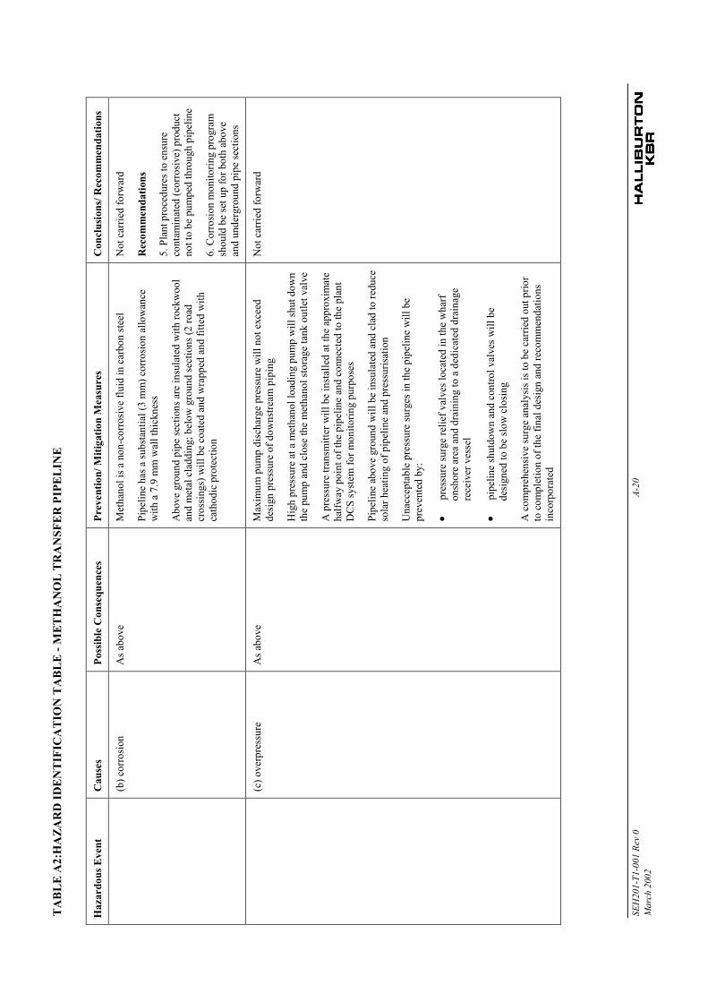
TA
BL
E A
2:H
AZA
RD
IDE
NT
IFIC
AT
ION
TA
BL
E - M
ET
HA
NO
L T
RA
NSF
ER
PIP
EL
INE
SEH
201-
T1-0
01 R
ev 0
A-20
Mar
ch 2
002
Haz
ardo
us E
vent
Cau
ses
Poss
ible
Con
sequ
ence
sPr
even
tion/
Miti
gatio
n M
easu
res
Con
clus
ions
/ Rec
omm
enda
tions
(b) c
orro
sion
As a
bove
Met
hano
l is a
non
-cor
rosi
ve fl
uid
in c
arbo
n st
eel
Pipe
line
has a
subs
tant
ial (
3 m
m) c
orro
sion
allo
wan
cew
ith a
7.9
mm
wal
l thi
ckne
ss
Abo
ve g
roun
d pi
pe se
ctio
ns a
re in
sula
ted
with
rock
woo
lan
d m
etal
cla
ddin
g; b
elow
gro
und
sect
ions
(2 ro
adcr
ossi
ngs)
will
be
coat
ed a
nd w
rapp
ed a
nd fi
tted
with
cath
odic
pro
tect
ion
Not
car
ried
forw
ard
Rec
omm
enda
tions
5. P
lant
pro
cedu
res t
o en
sure
cont
amin
ated
(cor
rosi
ve) p
rodu
ctno
t to
be p
umpe
d th
roug
h pi
pelin
e
6. C
orro
sion
mon
itorin
g pr
ogra
msh
ould
be
set u
p fo
r bot
h ab
ove
and
unde
rgro
und
pipe
sect
ions
(c) o
verp
ress
ure
As a
bove
Max
imum
pum
p di
scha
rge
pres
sure
will
not
exc
eed
desi
gn p
ress
ure
of d
owns
tream
pip
ing
Hig
h pr
essu
re a
t a m
etha
nol l
oadi
ng p
ump
will
shut
dow
nth
e pu
mp
and
clos
e th
e m
etha
nol s
tora
ge ta
nk o
utle
t val
ve
A p
ress
ure
trans
mitt
er w
ill b
e in
stal
led
at th
e ap
prox
imat
eha
lfway
poi
nt o
f the
pip
elin
e an
d co
nnec
ted
to th
e pl
ant
DC
S sy
stem
for m
onito
ring
purp
oses
Pipe
line
abov
e gr
ound
will
be
insu
late
d an
d cl
ad to
redu
ceso
lar h
eatin
g of
pip
elin
e an
d pr
essu
risat
ion
Una
ccep
tabl
e pr
essu
re su
rges
in th
e pi
pelin
e w
ill b
epr
even
ted
by:
• pr
essu
re su
rge
relie
f val
ves l
ocat
ed in
the
wha
rfon
shor
e ar
ea a
nd d
rain
ing
to a
ded
icat
ed d
rain
age
rece
iver
ves
sel
• pi
pelin
e sh
utdo
wn
and
cont
rol v
alve
s will
be
desi
gned
to b
e sl
ow c
losi
ng
A c
ompr
ehen
sive
surg
e an
alys
is is
to b
e ca
rrie
d ou
t prio
rto
com
plet
ion
of th
e fin
al d
esig
n an
d re
com
men
datio
nsin
corp
orat
ed
Not
car
ried
forw
ard
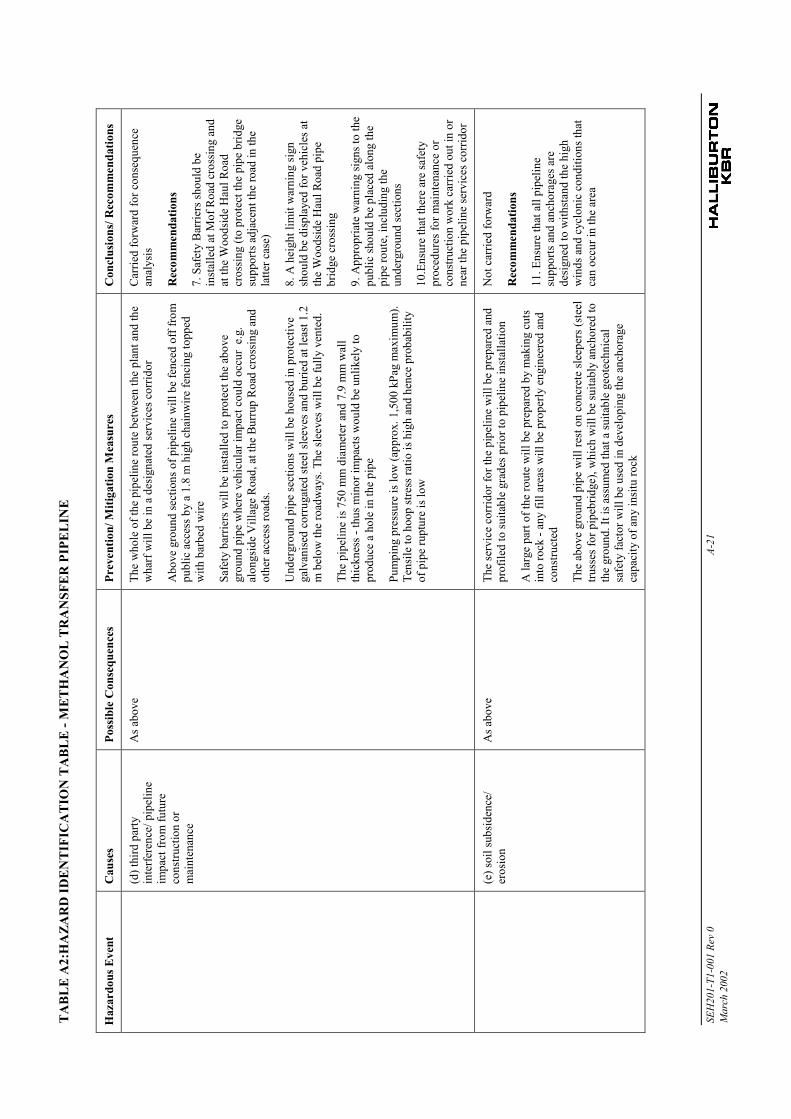
TA
BL
E A
2:H
AZA
RD
IDE
NT
IFIC
AT
ION
TA
BL
E - M
ET
HA
NO
L T
RA
NSF
ER
PIP
EL
INE
SEH
201-
T1-0
01 R
ev 0
A-21
Mar
ch 2
002
Haz
ardo
us E
vent
Cau
ses
Poss
ible
Con
sequ
ence
sPr
even
tion/
Miti
gatio
n M
easu
res
Con
clus
ions
/ Rec
omm
enda
tions
(d) t
hird
par
tyin
terfe
renc
e/ p
ipel
ine
impa
ct fr
om fu
ture
cons
truct
ion
orm
aint
enan
ce
As a
bove
The
who
le o
f the
pip
elin
e ro
ute
betw
een
the
plan
t and
the
wha
rf w
ill b
e in
a d
esig
nate
d se
rvic
es c
orrid
or
Abo
ve g
roun
d se
ctio
ns o
f pip
elin
e w
ill b
e fe
nced
off
from
publ
ic a
cces
s by
a 1.
8 m
hig
h ch
ainw
ire fe
ncin
g to
pped
with
bar
bed
wire
Safe
ty b
arrie
rs w
ill b
e in
stal
led
to p
rote
ct th
e ab
ove
grou
nd p
ipe
whe
re v
ehic
ular
impa
ct c
ould
occ
ur e
.g.
alon
gsid
e V
illag
e R
oad,
at t
he B
urru
p R
oad
cros
sing
and
othe
r acc
ess r
oads
.
Und
ergr
ound
pip
e se
ctio
ns w
ill b
e ho
used
in p
rote
ctiv
ega
lvan
ised
cor
ruga
ted
stee
l sle
eves
and
bur
ied
at le
ast 1
.2m
bel
ow th
e ro
adw
ays.
The
slee
ves
will
be
fully
ven
ted.
The
pipe
line
is 7
50 m
m d
iam
eter
and
7.9
mm
wal
lth
ickn
ess -
thus
min
or im
pact
s wou
ld b
e un
likel
y to
prod
uce
a ho
le in
the
pipe
Pum
ping
pre
ssur
e is
low
(app
rox.
1,5
00 k
Pag
max
imum
).Te
nsile
to h
oop
stre
ss ra
tio is
hig
h an
d he
nce
prob
abili
tyof
pip
e ru
ptur
e is
low
Car
ried
forw
ard
for c
onse
quen
cean
alys
is
Rec
omm
enda
tions
7. S
afet
y B
arrie
rs sh
ould
be
inst
alle
d at
Mof
Roa
d cr
ossin
g an
dat
the
Woo
dsid
e H
aul R
oad
cros
sing
(to
prot
ect t
he p
ipe
brid
gesu
ppor
ts a
djac
ent t
he ro
ad in
the
latte
r cas
e)
8. A
hei
ght l
imit
war
ning
sign
shou
ld b
e di
spla
yed
for v
ehic
les a
tth
e W
oods
ide
Hau
l Roa
d pi
pebr
idge
cro
ssin
g
9. A
ppro
pria
te w
arni
ng si
gns t
o th
epu
blic
shou
ld b
e pl
aced
alo
ng th
epi
pe ro
ute,
incl
udin
g th
eun
derg
roun
d se
ctio
ns
10.E
nsur
e th
at th
ere
are
safe
typr
oced
ures
for m
aint
enan
ce o
rco
nstru
ctio
n w
ork
carr
ied
out i
n or
near
the
pipe
line
serv
ices
cor
ridor
(e) s
oil s
ubsi
denc
e/er
osio
nA
s abo
veTh
e se
rvic
e co
rrid
or fo
r the
pip
elin
e w
ill b
e pr
epar
ed a
ndpr
ofile
d to
suita
ble
grad
es p
rior t
o pi
pelin
e in
stal
latio
n
A la
rge
part
of th
e ro
ute
will
be
prep
ared
by
mak
ing
cuts
into
rock
- an
y fil
l are
as w
ill b
e pr
oper
ly e
ngin
eere
d an
dco
nstru
cted
The
abov
e gr
ound
pip
e w
ill re
st o
n co
ncre
te sl
eepe
rs (s
teel
truss
es fo
r pip
ebrid
ge),
whi
ch w
ill b
e su
itabl
y an
chor
ed to
the
grou
nd. I
t is a
ssum
ed th
at a
suita
ble
geot
echn
ical
safe
ty fa
ctor
will
be
used
in d
evel
opin
g th
e an
chor
age
capa
city
of a
ny in
situ
rock
Not
car
ried
forw
ard
Rec
omm
enda
tions
11. E
nsur
e th
at a
ll pi
pelin
esu
ppor
ts a
nd a
ncho
rage
s are
desi
gned
to w
ithst
and
the
high
win
ds a
nd c
yclo
nic
cond
ition
s tha
tca
n oc
cur i
n th
e ar
ea

SEH201-T1-001 Rev 0 A-22March 2002
A3 Hazard Identification - Jetty
This section of the Appendix contains the Hazard Identification (HAZID) tables for the jettyoperations.
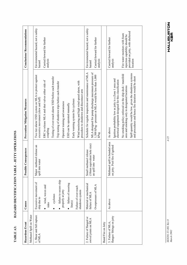
TA
BL
E A
3:H
AZA
RD
IDE
NT
IFIC
AT
ION
TA
BL
E - J
ET
TY
OPE
RA
TIO
NS
SEH
201-
T1-0
01 R
ev 0
A-23
Mar
ch 2
002
Haz
ardo
us E
vent
Cau
ses
Poss
ible
Con
sequ
ence
sPr
even
tion/
Miti
gatio
n M
easu
res
Con
clus
ions
/ Rec
omm
enda
tions
Met
hano
l Spi
ll on
Wat
er
1. S
hear
and
full
rupt
ure
of M
LAEx
cess
ive
mov
emen
t of
ship
due
to
• w
ind,
wav
es a
ndtid
es
• cy
clon
es
• fa
ilure
to se
cure
ship
prop
erly
at j
etty
• fa
ilure
of m
oorin
glin
e(s)
Failu
re o
f ove
r-re
ach
shut
dow
n sy
stem
Maj
or m
etha
nol r
elea
se a
nsp
ill in
to w
ater
Two
tier a
larm
/ ESD
syst
em o
n M
LA to
pro
tect
aga
inst
exce
ssiv
e m
ovem
ent (
slew
and
luff)
ERC
to re
leas
e M
LA a
nd sh
ut v
alve
s eith
er si
de o
fco
uplin
g
Test
ing
of o
ver-
reac
h al
arm
/ ESD
bef
ore
each
tran
sfer
Trip
test
ing
of sh
utdo
wn
trips
bef
ore
each
tran
sfer
Ope
rato
r tra
inin
g an
d aw
aren
ess
ESD
can
be
oper
ated
man
ually
Early
war
ning
syst
em fo
r cyc
lone
s
Win
d m
onito
ring
and
high
win
d sp
eed
alar
m, w
ithpr
oced
ure
to sh
utdo
wn
and
disc
onne
ct a
rm
Envi
ronm
enta
l haz
ard,
not
a sa
fety
haza
rd
Car
ried
forw
ard
for f
urth
eran
alys
is
2. F
ailu
re o
f fla
nged
or
swiv
el jo
ints
on
MLA
Mat
eria
l or m
echa
nica
lfa
ilure
of M
LA
Ove
rpre
ssur
e of
MLA
Smal
l met
hano
l rel
ease
(10m
m e
quiv
alen
t hol
e si
ze)
an sp
ill in
to w
ater
Sche
dule
for r
egul
ar in
spec
tion
and
mai
nten
ance
of M
LA
MLA
des
igne
d fo
r pum
p di
scha
rge
max
imum
pre
ssur
e of
1,50
0 kP
ag -
pres
sure
at M
LA w
ould
be
less
than
1,0
00kP
ag
Envi
ronm
enta
l haz
ard,
not
a sa
fety
haza
rd
Car
ried
forw
ard
for f
urth
eran
alys
is
Bun
d Fi
re o
n Je
tty
3. F
ailu
re o
f MLA
,fla
nges
/ fitt
ings
on
jetty
As a
bove
Met
hano
l spi
ll in
bun
ded
area
on je
tty. P
ool f
ire if
igni
ted
As a
bove
Igni
tion
prob
abili
ty lo
w a
s jet
ty is
a Z
one
1 ar
ea a
ndel
ectri
cal e
quip
men
t des
igne
d fo
r thi
s cla
ssifi
catio
n
No
smok
ing
polic
y en
forc
ed o
n th
e sh
ip d
eck
/ man
ifold
area
and
smok
ing
only
in d
esig
nate
d lo
catio
ns
Spill
qua
ntity
wou
ld b
e lo
w, g
iven
the
shut
dow
n sy
stem
san
d pr
oced
ures
and
hen
ce fi
re d
urat
ion
wou
ld b
e sh
ort
Car
ried
forw
ard
for f
urth
eran
alys
is
Fire
wat
er m
onito
rs w
ith fo
amin
ject
ion
capa
bilit
y sh
ould
be
prov
ided
on
jetty
, with
shel
tere
dlo
catio
n
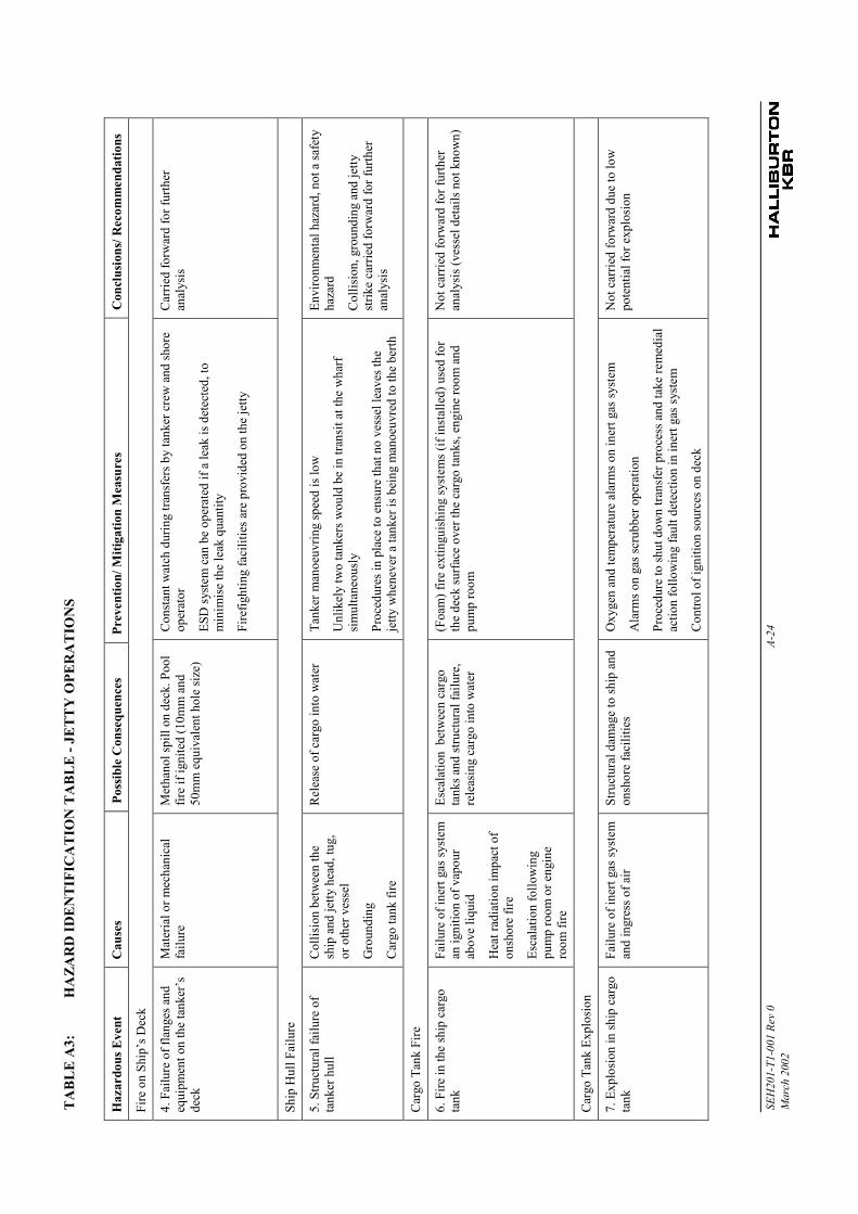
TA
BL
E A
3:H
AZA
RD
IDE
NT
IFIC
AT
ION
TA
BL
E - J
ET
TY
OPE
RA
TIO
NS
SEH
201-
T1-0
01 R
ev 0
A-24
Mar
ch 2
002
Haz
ardo
us E
vent
Cau
ses
Poss
ible
Con
sequ
ence
sPr
even
tion/
Miti
gatio
n M
easu
res
Con
clus
ions
/ Rec
omm
enda
tions
Fire
on
Ship
’s D
eck
4. F
ailu
re o
f fla
nges
and
equi
pmen
t on
the
tank
er’s
deck
Mat
eria
l or m
echa
nica
lfa
ilure
Met
hano
l spi
ll on
dec
k. P
ool
fire
if ig
nite
d (1
0mm
and
50m
m e
quiv
alen
t hol
e si
ze)
Con
stan
t wat
ch d
urin
g tra
nsfe
rs b
y ta
nker
cre
w a
nd sh
ore
oper
ator
ESD
syst
em c
an b
e op
erat
ed if
a le
ak is
det
ecte
d, to
min
imis
e th
e le
ak q
uant
ity
Fire
fight
ing
faci
litie
s are
pro
vide
d on
the
jetty
Car
ried
forw
ard
for f
urth
eran
alys
is
Ship
Hul
l Fai
lure
5. S
truct
ural
failu
re o
fta
nker
hul
lC
ollis
ion
betw
een
the
ship
and
jetty
hea
d, tu
g,or
oth
er v
esse
l
Gro
undi
ng
Car
go ta
nk fi
re
Rel
ease
of c
argo
into
wat
erTa
nker
man
oeuv
ring
spee
d is
low
Unl
ikel
y tw
o ta
nker
s w
ould
be
in tr
ansi
t at t
he w
harf
sim
ulta
neou
sly
Proc
edur
es in
pla
ce to
ens
ure
that
no
vess
el le
aves
the
jetty
whe
neve
r a ta
nker
is b
eing
man
oeuv
red
to th
e be
rth
Envi
ronm
enta
l haz
ard,
not
a sa
fety
haza
rd
Col
lisio
n, g
roun
ding
and
jetty
strik
e ca
rrie
d fo
rwar
d fo
r fur
ther
anal
ysis
Car
go T
ank
Fire
6. F
ire in
the
ship
car
gota
nkFa
ilure
of i
nert
gas s
yste
man
igni
tion
of v
apou
rab
ove
liqui
d
Hea
t rad
iatio
n im
pact
of
onsh
ore
fire
Esca
latio
n fo
llow
ing
pum
p ro
om o
r eng
ine
room
fire
Esca
latio
n b
etw
een
carg
ota
nks a
nd st
ruct
ural
failu
re,
rele
asin
g ca
rgo
into
wat
er
(Foa
m) f
ire e
xtin
guis
hing
syst
ems (
if in
stal
led)
use
d fo
rth
e de
ck su
rface
ove
r the
car
go ta
nks,
engi
ne ro
om a
ndpu
mp
room
Not
car
ried
forw
ard
for f
urth
eran
alys
is (v
esse
l det
ails
not
kno
wn)
Car
go T
ank
Expl
osio
n
7. E
xplo
sion
in sh
ip c
argo
tank
Failu
re o
f ine
rt ga
s sys
tem
and
ingr
ess o
f air
Stru
ctur
al d
amag
e to
ship
and
onsh
ore
faci
litie
sO
xyge
n an
d te
mpe
ratu
re a
larm
s on
iner
t gas
syst
em
Ala
rms o
n ga
s scr
ubbe
r ope
ratio
n
Proc
edur
e to
shut
dow
n tra
nsfe
r pro
cess
and
take
rem
edia
lac
tion
follo
win
g fa
ult d
etec
tion
in in
ert g
as sy
stem
Con
trol o
f ign
ition
sour
ces o
n de
ck
Not
car
ried
forw
ard
due
to lo
wpo
tent
ial f
or e
xplo
sion
SEH201-T1-001 Rev 0March 2002
Appendix B
STUDY ASSUMPTIONS
SEH201-T1-001 Rev 0 B-1March 2002
Study Assumptions
The general assumptions made to prepare the QRA are summarised in this section.
PROCESS PLANT
Plant Layout and Design
1. The separation distances suggested in the Layout Study (Ref ) are complied with. This should reduce thelikelihood of event escalation to very low levels.
2. Hazardous area classifications will apply to reduce likelihood of ignition
Management Systems
1. A Safety Management System (SMS) will exist on the site.
2. The SMS will include key elements such as Control of Modifications / Change Management Procedures, aPermit to Work system, Operator Training, Operating and Maintenance procedures, PreventativeMaintenance Programmes, Emergency Response Procedures
Consequence Assessment
Also refer to Appendix C for further details.
1. All scenarios were consolidated into 4 basic groups:
− natural gas releases
− syngas releases
− methanol releases in process plant area
− methanol releases in storage area
2. Natural gas releases were modelled as 100% methane and syngas release as 100% hydrogen
Failure Frequencies
1. Pipeline and flange failure frequencies were taken from Cox, Lees and Ang (Ref 9)
2. The average pipeline diameter was assumed to be 100mm.
3. Pipeline lengths were estimated by scaling off the layout drawing and multiplying by a factor of 5 toaccount for elevation changes and changes in pipe direction through equipment items etc
4. The number of joints was estimated by assuming 2 joints per section, with a section assumed to be 10m inlength.
5. Ignition probabilities were taken from Cox, Lees and Ang (Ref 9)

SEH201-T1-001 Rev 0 B-2March 2002
METHANOL PIPELINE
Consequence Assessment
Also refer to Appendix G, F for further details.
1. The methanol pool fire burning rate is 0.017 kg/m2.s
2. There are no evaporation or drainage effects associated with the pool fires of methanol
3. 6, 10, 14 kW/m2 correspond to 10%, 50%, 100% fatality probabilities for pool fire exposures.
Failure Frequencies
1. Pipeline, instrument fitting, valve and flange failure frequencies and ignition probabilities were taken fromCox, Lees and Ang (Ref 9).
2. Pipeline failure frequency for a 75 mm hole in a 750 mm diameter pipe is one order of magnitude lowerthan given by Cox et al for a 300 mm pipe.
3. Usage of the pipeline was estimated at 448 hours per month (average) and failure frequencies reducedaccordingly.
4. Overall failure frequencies were assessed for a 80 m length of pipeline (maximum consequence distance).The numbers of valves, flanges etc present in the 80 m length was proportioned from the total number ofitems in the total pipeline length.
SEH201-T1-001 Rev 0March 2002
Appendix C
CONSEQUENCE ANALYSIS(PLANT AND PIPELINE)
SEH201-T1-001 Rev 0 C-1March 2002
Consequence Analysis (Plant and Pipeline)
INTRODUCTION
This appendix outlines the methodology used for hazard consequence analysis, and the software packagesused for the various hazardous scenarios.
Three types of software were used in this study for consequence analysis:
(a) TNO EFFECTS software package (Ref.1) comprises a number of fire, explosion and dispersionmodels for accidental releases of hazardous materials.
(b) FRED (Fire Release Explosion and Dispersion), a Proprietary package of Shell Global Solutions,with main focus on hydrocarbons. This program includes models developed by Shell ThorntonResearch Centre, TNO and others, and the results it produces are comparable to other packages(SAFETI etc.).
(c) In-house developed program for pool fires with built-in experimental burning rates of flammableliquids (including methanol).
All models within EFFECTS are fully detailed in the Yellow Book (Ref.2). Therefore, a brief summary ofthe basis of the models used is provided only, together with the values adopted for any coefficients orspecial input values required.
One of the features of TNO EFFECTS is the ability to link the various models. The automatic transfer ofoutput data from one model to input data for another model is enabled by running the modelsconsecutively.
RELEASE SCENARIOS
Only credible failure scenarios were considered in the Formal Safety Assessment (FSA).
These scenarios also took into consideration the frequency of occurrence (including probability of earlydetection) and the severity of the consequences.
The following scenarios were found to be applicable to the Methanex facility.
(a) Small leaks from flange joints. A 10 mm equivalent size was assumed.
(b) Leaks from valve glands. The representative hole size was 10 mm. This was independent of thevalve size.
(c) Instrument fittings (20 mm equivalent).
(d) Pump seal failures. For calculation purposes, an equivalent hole size of 10 mm diameter wasassumed.
(e) Full bore failures of pipework from dropped objects, escalation from flame impingement fromsmall fires, and pipe failures from ruptures. A hole size of 100mm was assumed to berepresentative of pipe rupture.

SEH201-T1-001 Rev 0 C-2March 2002
RELEASE RATES
Gas Release
The rate of discharge of gas from a pipe or vessel under pressure through an orifice increases as afunction of the pressure gradient until the sonic velocity is reached in the orifice. For ideal gas behaviourand reversible adiabatic expansion, this is described as the critical flow condition. It is noted that as theinventory decreases, so does the pressure and the discharge flow rate. In order to keep the risk analysisconservative, it is usually acceptable to use the initial discharge rate for the duration of the discharge.
The rate of gas discharge through an orifice is calculated using the Bernoulli equation as shown below. .
For ideal gas behaviour and reversible adiabatic expansion, this is described as the critical flow condition.The flow is critical i.e. sonic or choked when:
PP
a
i�
+�
��
�
�� −2
11
γ
γγ
(Typically where P1 > 200 kPa abs)
Where Pa = atmospheric pressure (Pa)
Pi = upstream pressure (Pa)
γ = ratio of specific heats
The following formula is used to calculate the release of gas at sonic velocity:
m YC AP MZRT
D i=+
�
��
�
��
+−γ
γ
γγ
1
112
1
Where m = gas mass flow rate (kg/s)
CD = discharge coefficient A = orifice area (m2)Pi = upstream pressure (Pa)M = molecular weightZ = compressibility factorT1 = gas temperature (K)R = gas constant (8313 J/kmol K)Y = outflow coefficient (for critical flow Y = 1)
For sub-critical discharge, the following equation is used to calculate the outflow coefficient:
Y PP
PP
a a= ���
��� −�
��
�
�� −
�
��
�
��
+���
���
�
�
�
��
−�
�
�������
�
�
�������
+−
i i
11
1 1
1
12
1 21
12
12
γ
γ γγ
γγ
In this analysis, all gas releases have been modelled using the TNO EFFECTS “gas released through holein vessel” Bernoulli model. In order to provide a conservative result, and in the absence of detailedinformation on process inventories, a continuous gas release at the predicted initial discharge rate hasbeen carried forward to the atmospheric dispersion and fire modelling. Therefore, an arbitrary value of100 m3 was assumed for the vessel volume.
A discharge coefficient (CD) of 0.8 was used in these calculations.
Methane was used for the release rate modelling of the natural gas since it is the major component(greater than 98%).

SEH201-T1-001 Rev 0 C-3March 2002
Liquid Release
The rate of liquid discharge through an orifice is calculated using the Bernoulli equation.
A discharge coefficient (CD) of 0.8 was used in these calculations.
m C A PD L
L=
�
��
�
�� + ghρ
ρ2 ∆
Where m = mass liquid flow rate (kg/s)
CD = discharge coefficient (= 0.8)
A = cross section of leak path (m2)
ρL = liquid density (kg/m3)
∆P = pressure difference (Pa)
g = acceleration due to gravity (9.81 m/s2)
h = static head of liquid (m)
The cross-section area of the leak is characterised by an equivalent round hole to calculate thecorresponding leak rate.
JET FIRES
The Shell Company program, FRED 2.3, is based on an extension of the Chamberlain model (Ref.3)developed by Johnson et al (Ref.4) from tests with horizontal jet flames. It includes the effect ofbuoyancy lifting the flame above the horizontal, and the effect of wind momentum. Horizontal jet fireswere modelled since this would provide the largest heat radiation footprint.
None of the computer models available for modelling jet fires are directly suitable for hydrogen rich gasfires, since they have all been based on experiments with natural gas or LPG hydrocarbons.
In this work, methane jet fires have been used to model hydrogen rich gas jet fires, using the same massflow for the release. This will give a conservative result because methane has a higher heat of combustioncompared with synthesis gas.
POOLFIRES
Halliburton KBR (formerly Granherne) has developed an in-house computer program POOLFIRE for usein hazard analysis. The program is able model poolfires, bund fires and tank roof fires. The program iswritten in Microsoft Fortran for PC use.
The main features of the program are:
− it uses a solid flame model and geometric view factors;
− incorporates flame tilt from wind effects;
− contains a wide range of pure substances (flammable and combustible), as well as mixedhydrocarbon fuels (LGO, kerosene, stabilised crude oil);
− incorporates available experimental data on burning rates for the different substances, rather than theassumption of standard rate of loss of pool depth used in simple models;
− accesses a built-in physical property data base to obtain all relevant physical properties of the specificmaterial in question (density, viscosity, flammability limits, heat of combustion etc.);
− accounts for the variation of flame surface emissive power (surface heat flux) as a function of thecombustion characteristic of the fuel, as well as the pool diameter. The larger the diameter, thesmaller the surface emissive power;
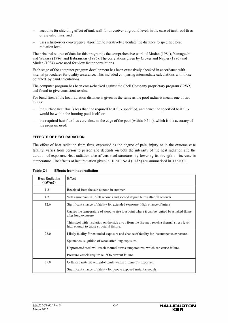
SEH201-T1-001 Rev 0 C-4March 2002
− accounts for shielding effect of tank wall for a receiver at ground level, in the case of tank roof firesor elevated fires; and
− uses a first-order convergence algorithm to iteratively calculate the distance to specified heatradiation level.
The principal source of data for this program is the comprehensive work of Mudan (1984), Yamaguchiand Wakasa (1986) and Babrauskas (1986). The correlations given by Croker and Napier (1986) andMudan (1984) were used for view factor correlations.
Each stage of the computer program development has been extensively checked in accordance withinternal procedures for quality assurance. This included comparing intermediate calculations with thoseobtained by hand calculations.
The computer program has been cross-checked against the Shell Company proprietary program FRED,and found to give consistent results.
For bund fires, if the heat radiation distance is given as the same as the pool radius it means one of twothings:
− the surface heat flux is less than the required heat flux specified, and hence the specified heat fluxwould be within the burning pool itself; or
− the required heat flux lies very close to the edge of the pool (within 0.5 m), which is the accuracy ofthe program used.
EFFECTS OF HEAT RADIATION
The effect of heat radiation from fires, expressed as the degree of pain, injury or in the extreme casefatality, varies from person to person and depends on both the intensity of the heat radiation and theduration of exposure. Heat radiation also affects steel structures by lowering its strength on increase intemperature. The effects of heat radiation given in HIPAP No.4 (Ref.5) are summarised in Table C1.
Table C1 Effects from heat radiation
Heat Radiation(kW/m2)
Effect
1.2 Received from the sun at noon in summer.
4.7 Will cause pain in 15-30 seconds and second degree burns after 30 seconds.
12.6 Significant chance of fatality for extended exposure. High chance of injury.
Causes the temperature of wood to rise to a point where it can be ignited by a naked flameafter long exposure.
Thin steel with insulation on the side away from the fire may reach a thermal stress levelhigh enough to cause structural failure.
23.0 Likely fatality for extended exposure and chance of fatality for instantaneous exposure.
Spontaneous ignition of wood after long exposure.
Unprotected steel will reach thermal stress temperatures, which can cause failure.
Pressure vessels require relief to prevent failure.
35.0 Cellulose material will pilot ignite within 1 minute’s exposure.
Significant chance of fatality for people exposed instantaneously.
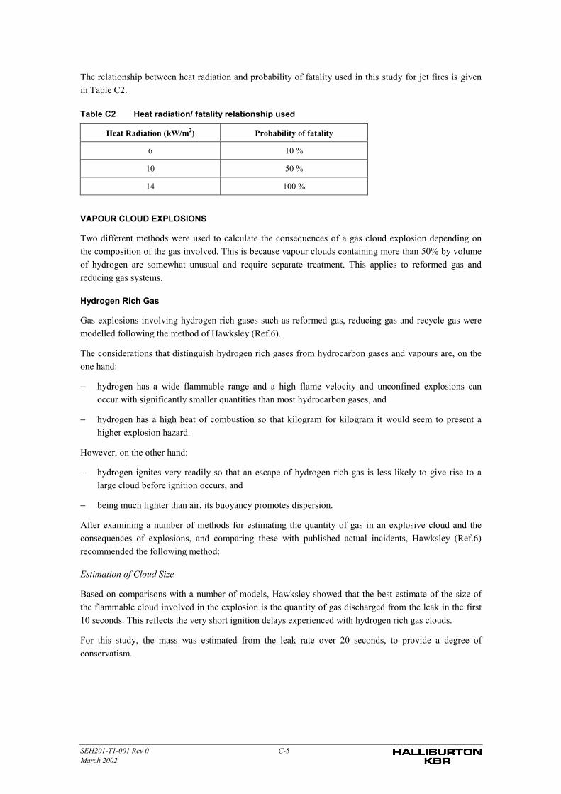
SEH201-T1-001 Rev 0 C-5March 2002
The relationship between heat radiation and probability of fatality used in this study for jet fires is givenin Table C2.
Table C2 Heat radiation/ fatality relationship used
Heat Radiation (kW/m2) Probability of fatality
6 10 %
10 50 %
14 100 %
VAPOUR CLOUD EXPLOSIONS
Two different methods were used to calculate the consequences of a gas cloud explosion depending onthe composition of the gas involved. This is because vapour clouds containing more than 50% by volumeof hydrogen are somewhat unusual and require separate treatment. This applies to reformed gas andreducing gas systems.
Hydrogen Rich Gas
Gas explosions involving hydrogen rich gases such as reformed gas, reducing gas and recycle gas weremodelled following the method of Hawksley (Ref.6).
The considerations that distinguish hydrogen rich gases from hydrocarbon gases and vapours are, on theone hand:
− hydrogen has a wide flammable range and a high flame velocity and unconfined explosions canoccur with significantly smaller quantities than most hydrocarbon gases, and
− hydrogen has a high heat of combustion so that kilogram for kilogram it would seem to present ahigher explosion hazard.
However, on the other hand:
− hydrogen ignites very readily so that an escape of hydrogen rich gas is less likely to give rise to alarge cloud before ignition occurs, and
− being much lighter than air, its buoyancy promotes dispersion.
After examining a number of methods for estimating the quantity of gas in an explosive cloud and theconsequences of explosions, and comparing these with published actual incidents, Hawksley (Ref.6)recommended the following method:
Estimation of Cloud Size
Based on comparisons with a number of models, Hawksley showed that the best estimate of the size ofthe flammable cloud involved in the explosion is the quantity of gas discharged from the leak in the first10 seconds. This reflects the very short ignition delays experienced with hydrogen rich gas clouds.
For this study, the mass was estimated from the leak rate over 20 seconds, to provide a degree ofconservatism.
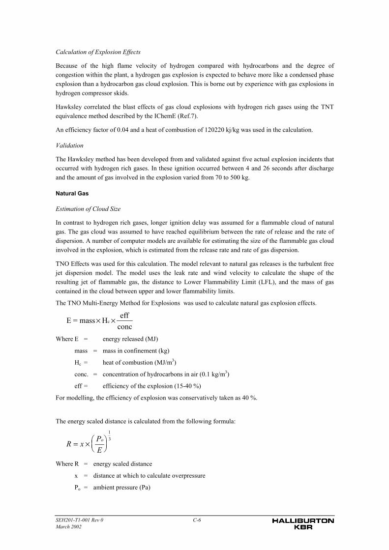
SEH201-T1-001 Rev 0 C-6March 2002
Calculation of Explosion Effects
Because of the high flame velocity of hydrogen compared with hydrocarbons and the degree ofcongestion within the plant, a hydrogen gas explosion is expected to behave more like a condensed phaseexplosion than a hydrocarbon gas cloud explosion. This is borne out by experience with gas explosions inhydrogen compressor skids.
Hawksley correlated the blast effects of gas cloud explosions with hydrogen rich gases using the TNTequivalence method described by the IChemE (Ref.7).
An efficiency factor of 0.04 and a heat of combustion of 120220 kj/kg was used in the calculation.
Validation
The Hawksley method has been developed from and validated against five actual explosion incidents thatoccurred with hydrogen rich gases. In these ignition occurred between 4 and 26 seconds after dischargeand the amount of gas involved in the explosion varied from 70 to 500 kg.
Natural Gas
Estimation of Cloud Size
In contrast to hydrogen rich gases, longer ignition delay was assumed for a flammable cloud of naturalgas. The gas cloud was assumed to have reached equilibrium between the rate of release and the rate ofdispersion. A number of computer models are available for estimating the size of the flammable gas cloudinvolved in the explosion, which is estimated from the release rate and rate of gas dispersion.
TNO Effects was used for this calculation. The model relevant to natural gas releases is the turbulent freejet dispersion model. The model uses the leak rate and wind velocity to calculate the shape of theresulting jet of flammable gas, the distance to Lower Flammability Limit (LFL), and the mass of gascontained in the cloud between upper and lower flammability limits.
The TNO Multi-Energy Method for Explosions was used to calculate natural gas explosion effects.
E = mass H effconc
c× ×
Where E = energy released (MJ)
mass = mass in confinement (kg)
Hc = heat of combustion (MJ/m3)
conc. = concentration of hydrocarbons in air (0.1 kg/m3)
eff = efficiency of the explosion (15-40 %)
For modelling, the efficiency of explosion was conservatively taken as 40 %.
The energy scaled distance is calculated from the following formula:
R x PE
o= × ���
���
13
Where R = energy scaled distance
x = distance at which to calculate overpressure
Po = ambient pressure (Pa)
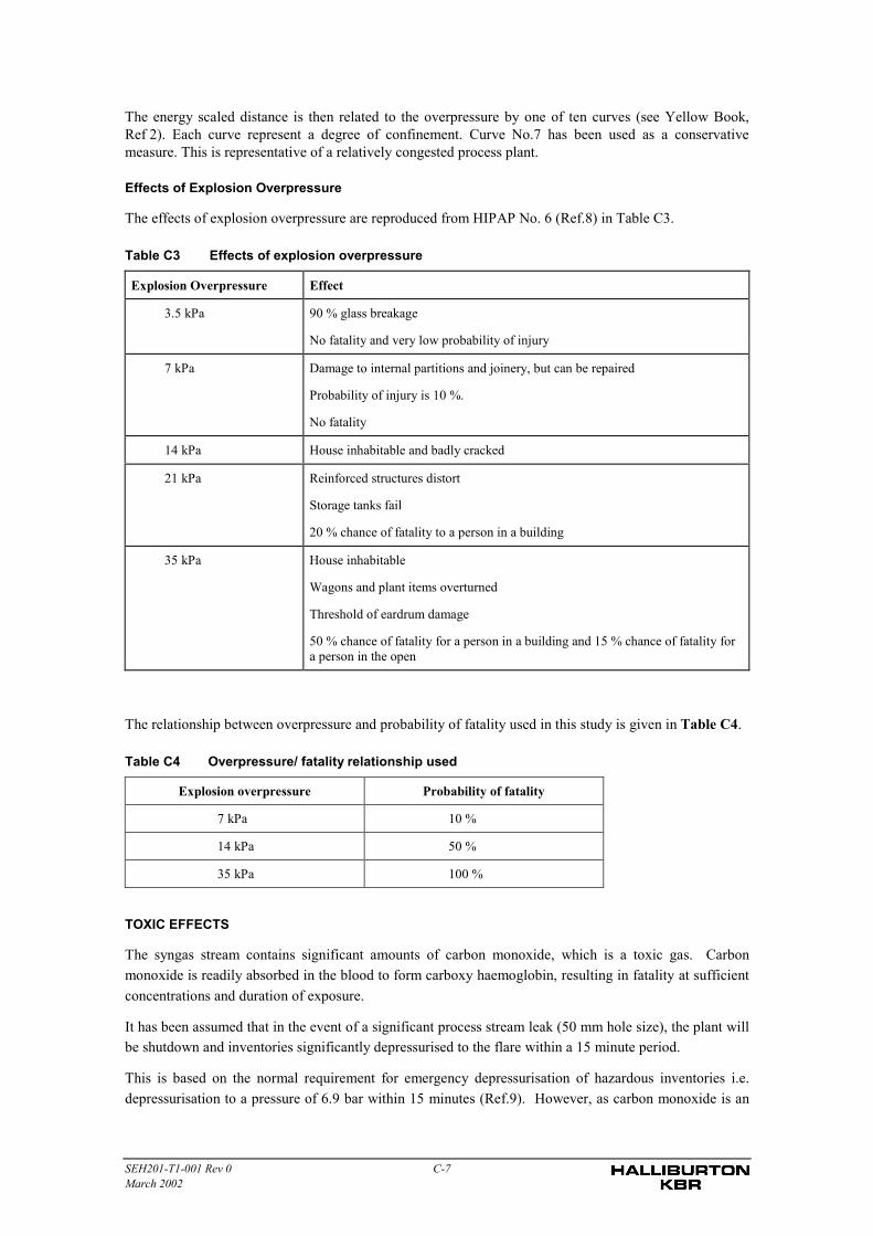
SEH201-T1-001 Rev 0 C-7March 2002
The energy scaled distance is then related to the overpressure by one of ten curves (see Yellow Book,Ref 2). Each curve represent a degree of confinement. Curve No.7 has been used as a conservativemeasure. This is representative of a relatively congested process plant.
Effects of Explosion Overpressure
The effects of explosion overpressure are reproduced from HIPAP No. 6 (Ref.8) in Table C3.
Table C3 Effects of explosion overpressure
Explosion Overpressure Effect
3.5 kPa 90 % glass breakage
No fatality and very low probability of injury
7 kPa Damage to internal partitions and joinery, but can be repaired
Probability of injury is 10 %.
No fatality
14 kPa House inhabitable and badly cracked
21 kPa Reinforced structures distort
Storage tanks fail
20 % chance of fatality to a person in a building
35 kPa House inhabitable
Wagons and plant items overturned
Threshold of eardrum damage
50 % chance of fatality for a person in a building and 15 % chance of fatality fora person in the open
The relationship between overpressure and probability of fatality used in this study is given in Table C4.
Table C4 Overpressure/ fatality relationship used
Explosion overpressure Probability of fatality
7 kPa 10 %
14 kPa 50 %
35 kPa 100 %
TOXIC EFFECTS
The syngas stream contains significant amounts of carbon monoxide, which is a toxic gas. Carbonmonoxide is readily absorbed in the blood to form carboxy haemoglobin, resulting in fatality at sufficientconcentrations and duration of exposure.
It has been assumed that in the event of a significant process stream leak (50 mm hole size), the plant willbe shutdown and inventories significantly depressurised to the flare within a 15 minute period.
This is based on the normal requirement for emergency depressurisation of hazardous inventories i.e.depressurisation to a pressure of 6.9 bar within 15 minutes (Ref.9). However, as carbon monoxide is an
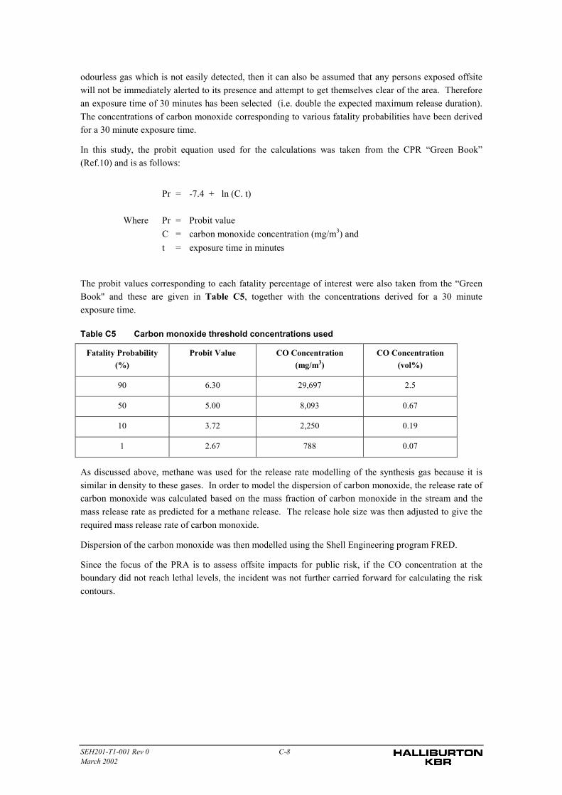
SEH201-T1-001 Rev 0 C-8March 2002
odourless gas which is not easily detected, then it can also be assumed that any persons exposed offsitewill not be immediately alerted to its presence and attempt to get themselves clear of the area. Thereforean exposure time of 30 minutes has been selected (i.e. double the expected maximum release duration).The concentrations of carbon monoxide corresponding to various fatality probabilities have been derivedfor a 30 minute exposure time.
In this study, the probit equation used for the calculations was taken from the CPR “Green Book”(Ref.10) and is as follows:
Pr = -7.4 + ln (C. t)
Where Pr = Probit valueC = carbon monoxide concentration (mg/m3) andt = exposure time in minutes
The probit values corresponding to each fatality percentage of interest were also taken from the “GreenBook" and these are given in Table C5, together with the concentrations derived for a 30 minuteexposure time.
Table C5 Carbon monoxide threshold concentrations used
Fatality Probability(%)
Probit Value CO Concentration(mg/m3)
CO Concentration(vol%)
90 6.30 29,697 2.5
50 5.00 8,093 0.67
10 3.72 2,250 0.19
1 2.67 788 0.07
As discussed above, methane was used for the release rate modelling of the synthesis gas because it issimilar in density to these gases. In order to model the dispersion of carbon monoxide, the release rate ofcarbon monoxide was calculated based on the mass fraction of carbon monoxide in the stream and themass release rate as predicted for a methane release. The release hole size was then adjusted to give therequired mass release rate of carbon monoxide.
Dispersion of the carbon monoxide was then modelled using the Shell Engineering program FRED.
Since the focus of the PRA is to assess offsite impacts for public risk, if the CO concentration at theboundary did not reach lethal levels, the incident was not further carried forward for calculating the riskcontours.
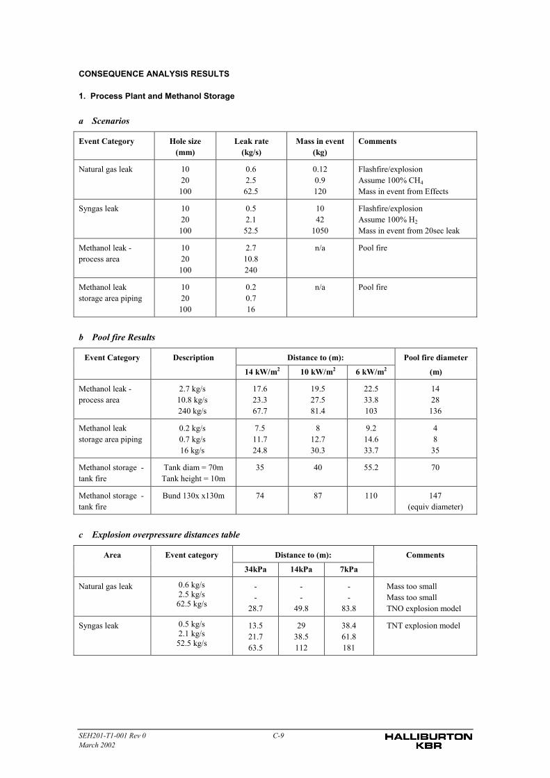
SEH201-T1-001 Rev 0 C-9March 2002
CONSEQUENCE ANALYSIS RESULTS
1. Process Plant and Methanol Storage
a Scenarios
Event Category Hole size(mm)
Leak rate(kg/s)
Mass in event(kg)
Comments
Natural gas leak 1020
100
0.62.5
62.5
0.120.9120
Flashfire/explosionAssume 100% CH4
Mass in event from Effects
Syngas leak 1020
100
0.52.1
52.5
1042
1050
Flashfire/explosionAssume 100% H2
Mass in event from 20sec leak
Methanol leak -process area
1020
100
2.710.8240
n/a Pool fire
Methanol leakstorage area piping
1020
100
0.20.716
n/a Pool fire
b Pool fire Results
Event Category Description Distance to (m): Pool fire diameter
14 kW/m2 10 kW/m2 6 kW/m2 (m)
Methanol leak -process area
2.7 kg/s10.8 kg/s240 kg/s
17.623.367.7
19.527.581.4
22.533.8103
1428
136
Methanol leakstorage area piping
0.2 kg/s0.7 kg/s16 kg/s
7.511.724.8
812.730.3
9.214.633.7
48
35
Methanol storage -tank fire
Tank diam = 70mTank height = 10m
35 40 55.2 70
Methanol storage -tank fire
Bund 130x x130m 74 87 110 147(equiv diameter)
c Explosion overpressure distances table
Area Event category Distance to (m): Comments
34kPa 14kPa 7kPa
Natural gas leak 0.6 kg/s2.5 kg/s62.5 kg/s
--
28.7
--
49.8
--
83.8
Mass too smallMass too smallTNO explosion model
Syngas leak 0.5 kg/s2.1 kg/s52.5 kg/s
13.521.763.5
2938.5112
38.461.8181
TNT explosion model
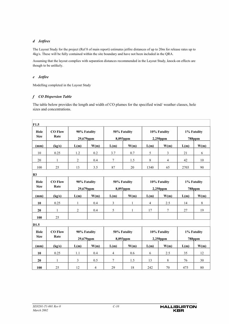
SEH201-T1-001 Rev 0 C-10March 2002
d Jetfires
The Layout Study for the project (Ref 8 of main report) estimates jetfire distances of up to 20m for release rates up to4kg/s. These will be fully contained within the site boundary and have not been included in the QRA.
Assuming that the layout complies with separation distances recommended in the Layout Study, knock-on effects arethough to be unlikely.
e Jetfire
Modelling completed in the Layout Study
f CO Dispersion Table
The table below provides the length and width of CO plumes for the specified wind/ weather classes, holesizes and concentrations.
F1.5
HoleSize
CO FlowRate
90% Fatality
29,679ppm
50% Fatality
8,093ppm
10% Fatality
2,250ppm
1% Fatality
788ppm
(mm) (kg/s) L(m) W(m) L(m) W(m) L(m) W(m) L(m) W(m)
10 0.25 1.2 0.2 3.7 0.7 5 3 21 6
20 1 2 0.4 7 1.5 8 4 42 10
100 25 13 3.5 87 20 1340 65 2703 90
B3
HoleSize
CO FlowRate
90% Fatality
29,679ppm
50% Fatality
8,093ppm
10% Fatality
2,250ppm
1% Fatality
788ppm
(mm) (kg/s) L(m) W(m) L(m) W(m) L(m) W(m) L(m) W(m)
10 0.25 1 0.4 3 1 4 2.5 14 8
20 1 2 0.4 5 1 17 7 27 19
100 25
D1.5
HoleSize
CO FlowRate
90% Fatality
29,679ppm
50% Fatality
8,093ppm
10% Fatality
2,250ppm
1% Fatality
788ppm
(mm) (kg/s) L(m) W(m) L(m) W(m) L(m) W(m) L(m) W(m)
10 0.25 1.1 0.4 4 0.6 6 2.5 35 12
20 1 3 0.5 7 1.5 13 8 76 30
100 25 12 4 29 18 242 70 475 80
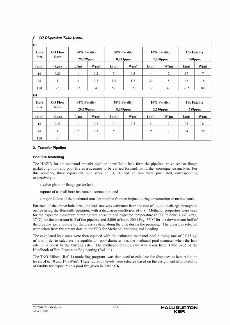
SEH201-T1-001 Rev 0 C-11March 2002
f CO Dispersion Table (cont.)
D5
HoleSize
CO FlowRate
90% Fatality
29,679ppm
50% Fatality
8,093ppm
10% Fatality
2,250ppm
1% Fatality
788ppm
(mm) (kg/s) L(m) W(m) L(m) W(m) L(m) W(m) L(m) W(m)
10 0.25 1 0.2 3 0.5 4 2 17 7
20 1 2 0.3 4.5 1.5 20 5 46 18
100 25 12 4 57 15 138 40 262 80
E4
HoleSize
CO FlowRate
90% Fatality
29,679ppm
50% Fatality
8,093ppm
10% Fatality
2,250ppm
1% Fatality
788ppm
(mm) (kg/s) L(m) W(m) L(m) W(m) L(m) W(m) L(m) W(m)
10 0.25 1 0.2 3 0.5 5 2 25 8
20 1 2 0.3 5 1 25 7 64 20
100 25
2. Transfer Pipeline
Pool fire Modelling
The HAZID for the methanol transfer pipeline identified a leak form the pipeline, valve seal or flangegasket , ignition and pool fire as a scenario to be carried forward for further consequence analysis. Forthis scenario, three equivalent hole sizes of 13, 20 and 75 mm were postulated, correspondingrespectively to
− a valve gland or flange gasket leak;
− rupture of a small bore instrument connection; and
− a major failure of the methanol transfer pipeline from an impact during construction or maintenance.
For each of the above hole sizes, the leak rate was estimated from the rate of liquid discharge through anorifice using the Bernoulli equation, with a discharge coefficient of 0.8. Methanol properties were usedfor the expected maximum pumping rate pressure and expected temperature (5,000 te/hour, 1,470 kPag,37OC) for the upstream half of the pipeline and 5,000 te/hour, 500 kPag, 37OC for the downstream half ofthe pipeline i.e. allowing for the pressure drop along the pipe during the pumping. The pressures selectedwere taken from the stream data on the PFD for Methanol Metering and Loading.
The calculated leak rates were then equated with the estimated methanol pool burning rate of 0.017 kg/m2 s in order to calculate the equilibrium pool diameter i.e. the methanol pool diameter when the leakrate in is equal to the burning rate. The methanol burning rate was taken from Table 3-12 of theHandbook of Fire Protection Engineering (Ref. 11)
The TNO Effects (Ref. 1) modelling program was then used to calculate the distances to heat radiationlevels of 6, 10 and 14 kW/m2. These radiation levels were selected based on the assignment of probabilityof fatality for exposure to a pool fire given in Table C6.
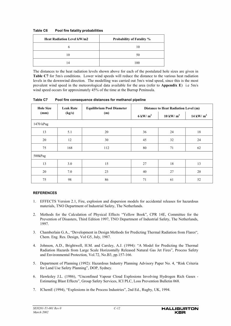
SEH201-T1-001 Rev 0 C-12March 2002
Table C6 Pool fire fatality probabilities
Heat Radiation Level kW/m2 Probability of Fatality %
6 10
10 50
14 100
The distances to the heat radiation levels shown above for each of the postulated hole sizes are given inTable C7 for 5m/s conditions. Lower wind speeds will reduce the distance to the various heat radiationlevels in the downwind direction. The modelling was carried out 5m/s wind speed, since this is the mostprevalent wind speed in the meteorological data available for the area (refer to Appendix E) i.e 5m/swind speed occurs for approximately 45% of the time at the Burrup Peninsula.
Table C7 Pool fire consequence distances for methanol pipeline
Distance to Heat Radiation Level (m)Hole Size(mm)
Leak Rate(kg/s)
Equilibrium Pool Diameter(m)
6 kW/ m2 10 kW/ m2 14 kW/ m2
1470 kPag
13 5.1 20 36 24 18
20 12 30 45 32 24
75 168 112 80 71 62
500kPag
13 3.0 15 27 18 13
20 7.0 23 40 27 20
75 98 86 71 61 52
REFERENCES
1. EFFECTS Version 2.1, Fire, explosion and dispersion models for accidental releases for hazardousmaterials, TNO Department of Industrial Safety, The Netherlands.
2. Methods for the Calculation of Physical Effects “Yellow Book”, CPR 14E, Committee for thePrevention of Disasters, Third Edition 1997, TNO Department of Industrial Safety, The Netherlands,1997.
3. Chamberlain G.A., “Development in Design Methods for Predicting Thermal Radiation from Flares“,Chem. Eng. Res. Design, Vol G5, July, 1987.
4. Johnson, A.D., Brightwell, H.M. and Carsley, A.J. (1994): “A Model for Predicting the ThermalRadiation Hazards from Large Scale Horizontally Released Natural Gas Jet Fires”, Process Safetyand Environmental Protection, Vol.72, No.B3, pp.157-166.
5. Department of Planning (1992): Hazardous Industry Planning Advisory Paper No. 4, “Risk Criteriafor Land Use Safety Planning”, DOP, Sydney.
6. Hawksley J.L. (1986), “Unconfined Vapour Cloud Explosions Involving Hydrogen Rich Gases -Estimating Blast Effects”, Group Safety Services, ICI PLC, Loss Prevention Bulletin 068.
7. IChemE (1994), “Explosions in the Process Industries”, 2nd Ed., Rugby, UK, 1994.

SEH201-T1-001 Rev 0 C-13March 2002
8. Department of Planning (1992): Hazardous Industry Planning Advisory Paper No. 6, “Guidelines forHazard Analysis”, DOP, Sydney.
9. “Guide for Pressure-Relieving and Depressuring Systems”, API Recommended Practice 521 ThirdEdition, November 1990.
10. Methods for Determination of Possible Damage “Green Book”, CPR 16E, Committee for thePrevention of Disasters, First Edition 1992.
11. Society of Fire Protection Engineers: “Handbook of Fire Protection Engineering”, 2nd Edition, 199,Ma, USA.
SEH201-T1-001 Rev 0March 2002
Appendix D
FREQUENCY ANALYSIS(PLANT AND PIPELINE)
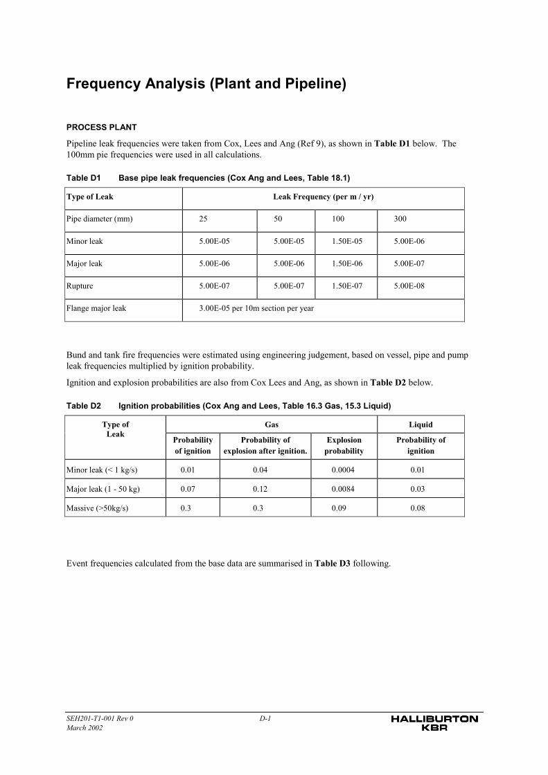
SEH201-T1-001 Rev 0 D-1March 2002
Frequency Analysis (Plant and Pipeline)
PROCESS PLANT
Pipeline leak frequencies were taken from Cox, Lees and Ang (Ref 9), as shown in Table D1 below. The100mm pie frequencies were used in all calculations.
Table D1 Base pipe leak frequencies (Cox Ang and Lees, Table 18.1)
Type of Leak Leak Frequency (per m / yr)
Pipe diameter (mm) 25 50 100 300
Minor leak 5.00E-05 5.00E-05 1.50E-05 5.00E-06
Major leak 5.00E-06 5.00E-06 1.50E-06 5.00E-07
Rupture 5.00E-07 5.00E-07 1.50E-07 5.00E-08
Flange major leak 3.00E-05 per 10m section per year
Bund and tank fire frequencies were estimated using engineering judgement, based on vessel, pipe and pumpleak frequencies multiplied by ignition probability.
Ignition and explosion probabilities are also from Cox Lees and Ang, as shown in Table D2 below.
Table D2 Ignition probabilities (Cox Ang and Lees, Table 16.3 Gas, 15.3 Liquid)
Gas LiquidType ofLeak
Probabilityof ignition
Probability ofexplosion after ignition.
Explosionprobability
Probability ofignition
Minor leak (< 1 kg/s) 0.01 0.04 0.0004 0.01
Major leak (1 - 50 kg) 0.07 0.12 0.0084 0.03
Massive (>50kg/s) 0.3 0.3 0.09 0.08
Event frequencies calculated from the base data are summarised in Table D3 following.
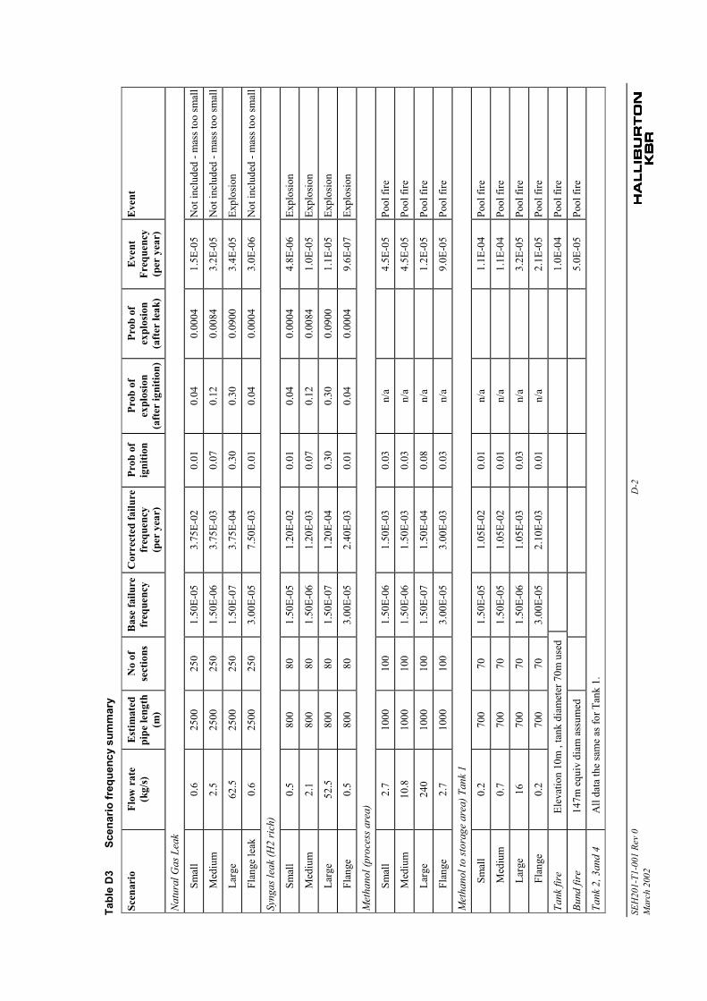
SEH
201-
T1-0
01 R
ev 0
D-2
Mar
ch 2
002
Tabl
e D
3Sc
enar
io fr
eque
ncy
sum
mar
y
Scen
ario
Flow
rat
e(k
g/s)
Est
imat
edpi
pe le
ngth
(m)
No
ofse
ctio
nsB
ase
failu
refr
eque
ncy
Cor
rect
ed fa
ilure
freq
uenc
y(p
er y
ear)
Prob
of
igni
tion
Prob
of
expl
osio
n(a
fter
igni
tion)
Prob
of
expl
osio
n(a
fter
leak
)
Eve
ntFr
eque
ncy
(per
yea
r)
Eve
nt
Nat
ural
Gas
Lea
k
Smal
l0.
625
0025
01.
50E-
053.
75E-
020.
010.
040.
0004
1.5E
-05
Not
incl
uded
- m
ass t
oo sm
all
Med
ium
2.5
2500
250
1.50
E-06
3.75
E-03
0.07
0.12
0.00
843.
2E-0
5N
ot in
clud
ed -
mas
s too
smal
l
Larg
e62
.525
0025
01.
50E-
073.
75E-
040.
300.
300.
0900
3.4E
-05
Expl
osio
n
Flan
ge le
ak0.
625
0025
03.
00E-
057.
50E-
030.
010.
040.
0004
3.0E
-06
Not
incl
uded
- m
ass t
oo sm
all
Syng
as le
ak (H
2 ri
ch)
Smal
l0.
580
080
1.50
E-05
1.20
E-02
0.01
0.04
0.00
044.
8E-0
6Ex
plos
ion
Med
ium
2.1
800
801.
50E-
061.
20E-
030.
070.
120.
0084
1.0E
-05
Expl
osio
n
Larg
e52
.580
080
1.50
E-07
1.20
E-04
0.30
0.30
0.09
001.
1E-0
5Ex
plos
ion
Flan
ge0.
580
080
3.00
E-05
2.40
E-03
0.01
0.04
0.00
049.
6E-0
7Ex
plos
ion
Met
hano
l (pr
oces
s are
a)
Smal
l2.
710
0010
01.
50E-
061.
50E-
030.
03n/
a4.
5E-0
5Po
ol fi
re
Med
ium
10.8
1000
100
1.50
E-06
1.50
E-03
0.03
n/a
4.5E
-05
Pool
fire
Larg
e24
010
0010
01.
50E-
071.
50E-
040.
08n/
a1.
2E-0
5Po
ol fi
re
Flan
ge2.
710
0010
03.
00E-
053.
00E-
030.
03n/
a9.
0E-0
5Po
ol fi
re
Met
hano
l to
stor
age
area
) Tan
k 1
Smal
l0.
270
070
1.50
E-05
1.05
E-02
0.01
n/a
1.1E
-04
Pool
fire
Med
ium
0.7
700
701.
50E-
051.
05E-
020.
01n/
a1.
1E-0
4Po
ol fi
re
Larg
e16
700
701.
50E-
061.
05E-
030.
03n/
a3.
2E-0
5Po
ol fi
re
Flan
ge0.
270
070
3.00
E-05
2.10
E-03
0.01
n/a
2.1E
-05
Pool
fire
Tank
fire
Elev
atio
n 10
m ,
tank
dia
met
er 7
0m u
sed
1.0E
-04
Pool
fire
Bund
fire
147m
equ
iv d
iam
ass
umed
5.0E
-05
Pool
fire
Tank
2, 3
and
4A
ll da
ta th
e sa
me
as fo
r Tan
k 1.
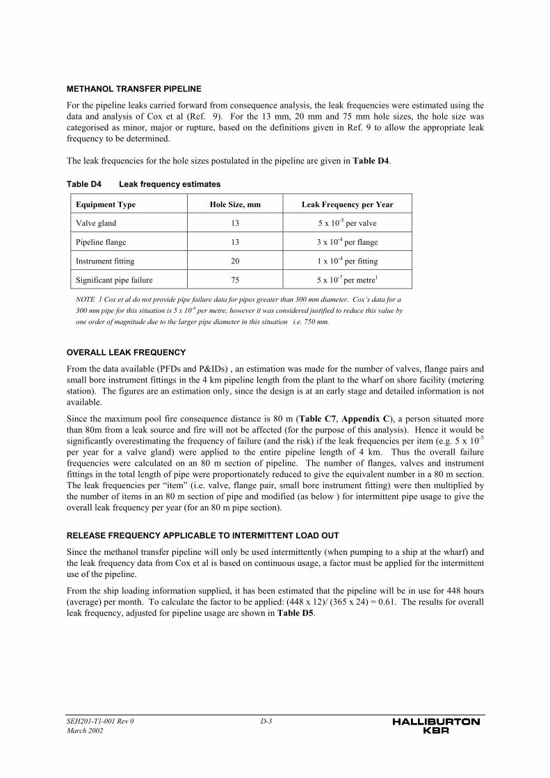
SEH201-T1-001 Rev 0 D-3March 2002
METHANOL TRANSFER PIPELINE
For the pipeline leaks carried forward from consequence analysis, the leak frequencies were estimated using thedata and analysis of Cox et al (Ref. 9). For the 13 mm, 20 mm and 75 mm hole sizes, the hole size wascategorised as minor, major or rupture, based on the definitions given in Ref. 9 to allow the appropriate leakfrequency to be determined.
The leak frequencies for the hole sizes postulated in the pipeline are given in Table D4.
Table D4 Leak frequency estimates
Equipment Type Hole Size, mm Leak Frequency per Year
Valve gland 13 5 x 10⁻⁵ per valve
Pipeline flange 13 3 x 10⁻⁴ per flange
Instrument fitting 20 1 x 10⁻⁴ per fitting
Significant pipe failure 75 5 x 10⁻⁷ per metre1
NOTE 1 Cox et al do not provide pipe failure data for pipes greater than 300 mm diameter. Cox’s data for a300 mm pipe for this situation is 5 x 10⁻⁶ per metre, however it was considered justified to reduce this value byone order of magnitude due to the larger pipe diameter in this situation i.e. 750 mm.
OVERALL LEAK FREQUENCY
From the data available (PFDs and P&IDs) , an estimation was made for the number of valves, flange pairs andsmall bore instrument fittings in the 4 km pipeline length from the plant to the wharf on shore facility (meteringstation). The figures are an estimation only, since the design is at an early stage and detailed information is notavailable.
Since the maximum pool fire consequence distance is 80 m (Table C7, Appendix C), a person situated morethan 80m from a leak source and fire will not be affected (for the purpose of this analysis). Hence it would besignificantly overestimating the frequency of failure (and the risk) if the leak frequencies per item (e.g. 5 x 10⁻⁵
per year for a valve gland) were applied to the entire pipeline length of 4 km. Thus the overall failurefrequencies were calculated on an 80 m section of pipeline. The number of flanges, valves and instrumentfittings in the total length of pipe were proportionately reduced to give the equivalent number in a 80 m section.The leak frequencies per “item” (i.e. valve, flange pair, small bore instrument fitting) were then multiplied bythe number of items in an 80 m section of pipe and modified (as below ) for intermittent pipe usage to give theoverall leak frequency per year (for an 80 m pipe section).
RELEASE FREQUENCY APPLICABLE TO INTERMITTENT LOAD OUT
Since the methanol transfer pipeline will only be used intermittently (when pumping to a ship at the wharf) andthe leak frequency data from Cox et al is based on continuous usage, a factor must be applied for the intermittentuse of the pipeline.
From the ship loading information supplied, it has been estimated that the pipeline will be in use for 448 hours(average) per month. To calculate the factor to be applied: (448 x 12)/ (365 x 24) = 0.61. The results for overallleak frequency, adjusted for pipeline usage are shown in Table D5.
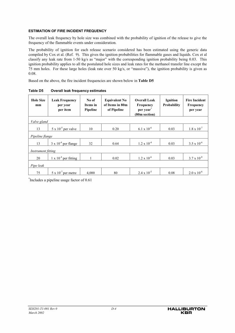
SEH201-T1-001 Rev 0 D-4March 2002
ESTIMATION OF FIRE INCIDENT FREQUENCY
The overall leak frequency by hole size was combined with the probability of ignition of the release to give thefrequency of the flammable events under consideration.
The probability of ignition for each release scenario considered has been estimated using the generic datacompiled by Cox et al. (Ref. 9). This gives the ignition probabilities for flammable gases and liquids. Cox et alclassify any leak rate from 1-50 kg/s as “major” with the corresponding ignition probability being 0.03. Thisignition probability applies to all the postulated hole sizes and leak rates for the methanol transfer line except the75 mm holes. For these large holes (leak rate over 50 kg/s, or “massive”), the ignition probability is given as0.08.
Based on the above, the fire incident frequencies are shown below in Table D5
Table D5 Overall leak frequency estimates
Hole Sizemm
Leak Frequencyper year per item
No ofItems inPipeline
Equivalent Noof Items in 80m
of Pipeline
Overall LeakFrequencyper year*
(80m section)
IgnitionProbability
Fire IncidentFrequencyper year
Valve gland
13 5 x 10⁻⁵ per valve 10 0.20 6.1 x 10⁻⁶ 0.03 1.8 x 10⁻⁷
Pipeline flange
13 3 x 10⁻⁴ per flange 32 0.64 1.2 x 10⁻⁴ 0.03 3.5 x 10⁻⁶
Instrument fitting
20 1 x 10⁻⁴ per fitting 1 0.02 1.2 x 10⁻⁶ 0.03 3.7 x 10⁻⁸
Pipe leak
75 5 x 10⁻⁷ per metre 4,000 80 2.4 x 10⁻⁵ 0.08 2.0 x 10⁻⁶
*Includes a pipeline usage factor of 0.61
SEH201-T1-001 Rev 0March 2002
Appendix E
METEOROLOGICAL DATA
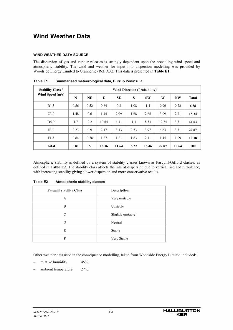
SEH201-001-Rev. 0 E-1March 2002
Wind Weather Data
WIND WEATHER DATA SOURCE
The dispersion of gas and vapour releases is strongly dependent upon the prevailing wind speed andatmospheric stability. The wind and weather for input into dispersion modelling was provided byWoodside Energy Limited to Granherne (Ref. XX). This data is presented in Table E1.
Table E1 Summarised meteorological data, Burrup Peninsula
Wind Direction (Probability)Stability Class /Wind Speed (m/s)
N NE E SE S SW W NW Total
B1.5 0.56 0.52 0.84 0.8 1.08 1.4 0.96 0.72 6.88
C3.0 1.48 0.6 1.44 2.09 1.68 2.65 3.09 2.21 15.24
D5.0 1.7 2.2 10.64 4.41 1.3 8.33 12.74 3.31 44.63
E3.0 2.23 0.9 2.17 3.13 2.53 3.97 4.63 3.31 22.87
F1.5 0.84 0.78 1.27 1.21 1.63 2.11 1.45 1.09 10.38
Total 6.81 5 16.36 11.64 8.22 18.46 22.87 10.64 100
Atmospheric stability is defined by a system of stability classes known as Pasquill-Gifford classes, asdefined in Table E2. The stability class affects the rate of dispersion due to vertical rise and turbulence,with increasing stability giving slower dispersion and more conservative results.
Table E2 Atmospheric stability classes
Pasquill Stability Class Description
A Very unstable
B Unstable
C Slightly unstable
D Neutral
E Stable
F Very Stable
Other weather data used in the consequence modelling, taken from Woodside Energy Limited included:
− relative humidity 45%
− ambient temperature 27°C

SEH201-T1-001 Rev 0March 2002
Appendix F
JETTY ANALYSIS
SEH201-T1-001 Rev 0 F-1March 2002
Jetty Analysis
INTRODUCTION
Product methanol is transported from the tankfarm in the plant at Hearson Cove to Dampier wharf. Ship loadingwill occur via a hydraulic loading arm, at a rate of 2,500 tonnes per hour. A loss of containment incident duringship loading could result in a fire and/ or environmental pollution at the wharf. The hazards associated with theshipping operations and the associated risks are addressed in this Appendix. Information from this appendix hasbeen carried forward into the main report and included in the relevant sections, with appropriate cross-references.
The scope of the study in ship loading operations consists of the following:
− Development of specific hazard scenarios.
− Consequence Analysis of hazard scenarios.
− Frequency assessment of the identified events using generic failure rate data bases. At the PHA stage, onlyconcept design information is available and therefore, a fault tree analysis type of study could not beundertaken.
− Development of F-M curves for product spill for wharf incidents. The F-M curve is similar to the F-N curvefor risk of fatality, but shows the cumulative frequency F with which a product spill of M or more tonnescould occur.
− Evaluate the resultant risk levels and identify risk reduction measures as found appropriate.
DESCRIPTION OF WHARF FACILITIES
Main Features of Design
The wharf facility will consist of a bulk liquids berth for transfer of products to ships. The overall facility willinclude the following:
− A jetty head structure and dolphins with adequate structural integrity for the tidal conditions at Dampierwharf.
− A hydraulic Marine Loading Arm (MLA) system consisting of two 400mm loading arms. One MLA willbe installed as part of Phase 1 of the project (i.e. single methanol train) and the second MLA will beinstalled during Phase 2 expansion (i.e. second methanol train).
− Emergency shutdown system for the loading arms with associated ESD stations and alarms. The ESDsystem will close the wharf ESD valve and raise an audible/visible alarm.
− An Emergency Release Coupling (ERC) on each loading arm to disconnect the arm to stop product spill, inthe event of mooring failure or other unexpected ship movements.
− Wharf fire protection system for fighting fires on the jetty head as well as on ship’s deck, using firewatermonitors.
− Design and construction of the wharf facility in full compliance with AS 3846-1998, “The handling andtransport of dangerous cargoes in port areas”, and relevant IMO requirements.
SEH201-T1-001 Rev 0 F-2March 2002
Safety Systems
The following safety systems are expected to be provided for loading arms and operations at Dampier Wharf.
− Loading arms designed for a pressure of 1,500kPag, which is the maximum discharge head of the pump, sothat loading arm overpressuring can be eliminated.
− Wind speed monitoring system, linked to an alarm if the wind speed exceeds 40 knots. Ship/shore transferoperations would not commence or would be suspended if operations had commenced, during the times ofhigh wind conditions, as indicated by the alarm. It is understood that there is also an early warning systemin place for cyclones - for a severe cyclone threat to the Port of Dampier, loading would be terminated andthe ship would put to sea to avoid the cyclone.
− Overreach Alarm, ESD. This comprises the loading arm range monitoring system. The system monitorsboth the luff and the slew of the loading arm in the event of excessive movement of the ship. There areindependent proximity switches, separately for alarm position and trip position of both luff and slew, for theloading arm. Switches are of fail safe design, so that in the event of a wiring or switch fault on any one ofthe eight, an alarm or ESD condition will occur. Similarly, detection of overreach by the alarm switch willinitiate an alarm and detection of overreach by the trip switch will initiate an ESD.
− An audible ESD alarm is located at the wharf console, outside the operator's cabin at the wharf.
− Ship watch and shore watch during the transfer period, with two-way radio communication between thetwo. The operator can also communicate by radio with the methanol plant control room. Intrinsically saferadios are used.
− Sufficient closure time in the design for the ESD valve on the loading arm to prevent "water hammer" effectwhile the transfer pump is still operating.
− ESD push buttons located at the wharf console, outside the operator's cabin, and at the wharf.
− Fire protection system at the wharf
Ship/ Shore Transfer Operation
The number of tanker movements is expected to be about 183 per year (15 per month, on average), with a totaltransfer duration of between about 21 and 38 hours, varying depending upon the ship size. The maximumnormal transfer rate is 1,200 tonnes per hour (although the MLAs are designed for 2,500tph each), and theparcel size varies from 15,000 tonnes to 45,000 tonnes depending on the tanker.
During transfer, the tanker firewater main is connected to the wharf main by a flexible hose. In the case of a fireon board the tanker, the shore firewater supply can be used to boost the tanker’s firewater.
Transfer operations using the loading arms are suspended in wind speeds in excess of 40 knots or in the event ofnearby lightning strikes.
Methanol tankers typically comprise several individual cargo tanks. The cargo tanks in all tankers have inert gasblanketing systems (usually utilising the exhaust gas from the auxiliary boilers after gas cleaning).
All cargo pump rooms and engine rooms are equipped with fire detection systems. Fire suppression systems areactivated manually upon alarm and once the area has been cleared. Typical systems use a halon substitute orCO2 as an extinguishing medium. Foam systems may also supplement the above and be used on deck abovecargo tanks.
Based on the information supplied to Halliburton KBR, transfer operations would occur for about 448 hours permonth (5,370 hours per year) or 61% of the time. These are actual transfer times, and the connect time of the
SEH201-T1-001 Rev 0 F-3March 2002
loading arms would be longer to allow for preparation before commencing transfer operations and to drain thearms before disconnection.
HAZARD IDENTIFICATION AND EVALUATION OF SAFEGUARDS
General
The hazards associated with ship/shore transfer operations of methanol are:
− A spill on water and mixing with sea water (environmental hazard);
− Product spill in the bunded area of wharf, and a pool fire if ignited;
− Poolfire on deck from product spill on deck;
− Structural failure of hull and release of cargo (environmental hazard); and
− Cargo tank fire/ explosion.
The hazardous incidents considered in this study could occur as a result of:
1. Environmental conditions.
2. Equipment failure.
3. Procedural failure including human error.
The hazardous incidents were evaluated in relation to their potential consequences and the design/operationalsafeguards provided. A detailed discussion on the identified hazards is provided in this section.
Ship/Shore Transfer Operations
The following possible scenarios have been identified for the loading arms:
1. Major methanol release from shearing and full bore rupture of the loading arm.
2. Nominal 10mm diameter equivalent holes from failures of flanged or swivel joints.
A number of factors would contribute to the incident scenarios:
Environmental Wind, waves and tides can cause excessive movement of the vessel being loaded inrelation to the loading arm anchor point, leading to shearing of the arm.
The loading arm is equipped with a two-level alarm/shutdown system to protect againstexcessive movement of the arm. The first level would alarm to alert the operator, and thesecond level would automatically initiate an emergency shutdown. In addition the ERCwould release the loading arm coupling and shut the valves on either side of the coupling.
ProceduralFailure
Human error can negate the effectiveness of procedures; this is particularly relevant for:
- laying of mooring lines;
- load range settings for the loading arm winch too wide. The chance of this happeningis very low as the overreach alarm/ESD is tested each time before a transfer;
- trip testing of shut down trips before commencing transfer;
- operator awareness; and
- operation of manual emergency shutdown and system.
Such procedural failures can also lead to an incident.
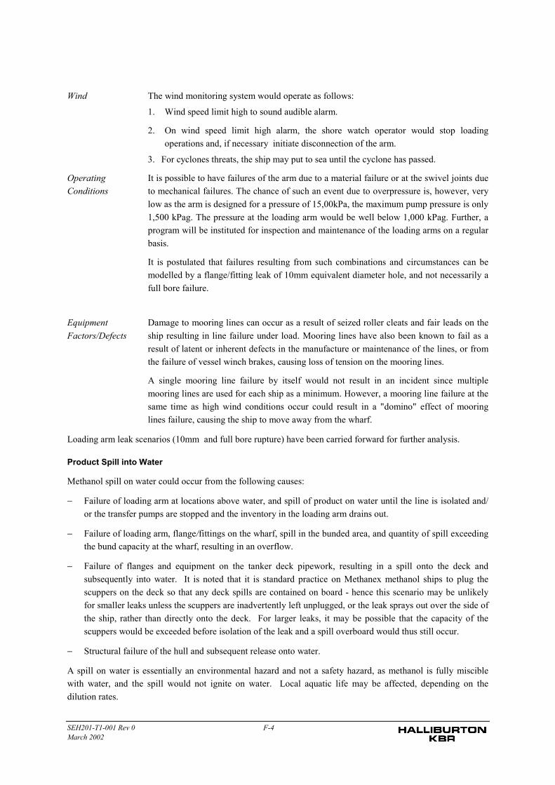
SEH201-T1-001 Rev 0 F-4March 2002
Wind The wind monitoring system would operate as follows:
1. Wind speed limit high to sound audible alarm.
2. On wind speed limit high alarm, the shore watch operator would stop loadingoperations and, if necessary initiate disconnection of the arm.
3. For cyclones threats, the ship may put to sea until the cyclone has passed.
OperatingConditions
It is possible to have failures of the arm due to a material failure or at the swivel joints dueto mechanical failures. The chance of such an event due to overpressure is, however, verylow as the arm is designed for a pressure of 15,00kPa, the maximum pump pressure is only1,500 kPag. The pressure at the loading arm would be well below 1,000 kPag. Further, aprogram will be instituted for inspection and maintenance of the loading arms on a regularbasis.
It is postulated that failures resulting from such combinations and circumstances can bemodelled by a flange/fitting leak of 10mm equivalent diameter hole, and not necessarily afull bore failure.
EquipmentFactors/Defects
Damage to mooring lines can occur as a result of seized roller cleats and fair leads on theship resulting in line failure under load. Mooring lines have also been known to fail as aresult of latent or inherent defects in the manufacture or maintenance of the lines, or fromthe failure of vessel winch brakes, causing loss of tension on the mooring lines.
A single mooring line failure by itself would not result in an incident since multiplemooring lines are used for each ship as a minimum. However, a mooring line failure at thesame time as high wind conditions occur could result in a "domino" effect of mooringlines failure, causing the ship to move away from the wharf.
Loading arm leak scenarios (10mm and full bore rupture) have been carried forward for further analysis.
Product Spill into Water
Methanol spill on water could occur from the following causes:
− Failure of loading arm at locations above water, and spill of product on water until the line is isolated and/or the transfer pumps are stopped and the inventory in the loading arm drains out.
− Failure of loading arm, flange/fittings on the wharf, spill in the bunded area, and quantity of spill exceedingthe bund capacity at the wharf, resulting in an overflow.
− Failure of flanges and equipment on the tanker deck pipework, resulting in a spill onto the deck andsubsequently into water. It is noted that it is standard practice on Methanex methanol ships to plug thescuppers on the deck so that any deck spills are contained on board - hence this scenario may be unlikelyfor smaller leaks unless the scuppers are inadvertently left unplugged, or the leak sprays out over the side ofthe ship, rather than directly onto the deck. For larger leaks, it may be possible that the capacity of thescuppers would be exceeded before isolation of the leak and a spill overboard would thus still occur.
− Structural failure of the hull and subsequent release onto water.
A spill on water is essentially an environmental hazard and not a safety hazard, as methanol is fully misciblewith water, and the spill would not ignite on water. Local aquatic life may be affected, depending on thedilution rates.
SEH201-T1-001 Rev 0 F-5March 2002
Methanol Pool Fires 0n Jetty
Should a spill within the bund on the wharf ignite, a pool fire would result. The chance of ignition is low due tothe following reasons:
− The wharf is given a hazardous area classification of Zone 1 according to AS 2430, and all new electricalequipment and instrumentation will be designed to this standard (ie. intrinsically safe).
− A strict no smoking policy is enforced on the ship deck/manifold area, and smoking is allowed only indesignated locations in the ship.
The quantity of spill would be low, given the shutdown systems in the design and procedures. Therefore, evenin the event of a fire, the duration would be small.
The fire protection systems at the wharf consist of monitors with provision for foam injection (alcoholcompatible foam), and provision for application of fire water from a sheltered location.
This event has been carried forward for further analysis.
Events on Ship
A number of incidents on the tanker have been identified that could have an impact on the onshore terminalfacilities.
Spills on Deck During Unloading
Spills of product may result from leaks on tanker pipework and equipment during transfer or from failures of theloading arm. These may result in releases of cargo to the sea, or if ignited, may cause a pool fire on the deck ofthe tanker. Hole sizes of 10mm and 50mm were identified as potential incidents but full bore losses frompipework on the tanker were not considered credible events.
The likelihood of such spills and fires is reduced by the following:
1. Constant watch during transfers both by tanker crew and by shore operator.
2. In the event of leaks being detected, the ESD will be operated and the pumps will be shutdown, preventingthe spillage of large quantities of methanol.
3. The firefighting facilities on the wharf.
This incident has been carried forward for further analysis.
Cargo Tank Fire
Fires in the storage compartment may occur as a result of:
− Failure of the inert gas system and ignition of vapour above the liquid level;
− Heat radiation impact of onshore fire onto tanker; and
− Escalation following a pump room or engine room fire on the ship.
A fire could escalate between cargo tanks and could cause structural failure and release of cargo onto water. Theconsequences of cargo tank fires may be minimised by the fire extinguishing foam systems (if installed) used forthe deck surface over the cargo tanks, engine room and pump room.
This incident has not been carried forward for further analysis, as details of the vessel are not known at thisstage.
SEH201-T1-001 Rev 0 F-6March 2002
Cargo Tank Explosion
Failure of the inert gas blanket to the cargo tanks and ingress of air into the tanks could result in a flammablemixture which could explode if ignited. The explosion could potentially cause structural damage to the ship andto onshore facilities. However, the inert gas system has alarms on O2 and temperature levels as well as alarmson the gas scrubber operation. Early detection of faults in the inert gas system will allow the ship’s crew to shutdown the transfer process and to take remedial action. In addition, control of ignition sources on the deck wouldreduce the likelihood even further.
This incident has not been carried forward for further analysis, as the potential for explosion is very low, giventhe above safeguards.
Structural Failure and Release of Cargo
Structural failure of the tanker and subsequent release of cargo onto the water may result from:
- Collisions between the tanker and:
- the jetty head;
- a tug; or
- another vessel in Dampier wharf.
The frequency of these incidents will be low because:
- The manoeuvring speed of vessels during berthing is low.
- It is unlikely that two tankers would be in transit at Dampier wharf simultaneously.
- Procedures are in place to ensure that no vessel leaves the wharf whenever a tanker is being manoeuvred tothe berth..
Although these incidents are considered unlikely , they have been carried forward for further analysis because ofthe potential severity of the consequences.
Grounding
Grounding of the ship may occur as a result of human error, engine failure or mooring line failure. Groundingcould result in rupture of the hull and cargo tank and subsequent release of cargo. The risk of grounding isreduced because of the berthing procedures. Again, because of the potential severity of the consequences of thistype of event, it has been carried forward for further analysis.
Summary of Incident Scenarios Carried Forward
The event scenarios which have been carried forward for further discussion or analysis are listed in Table F.1.
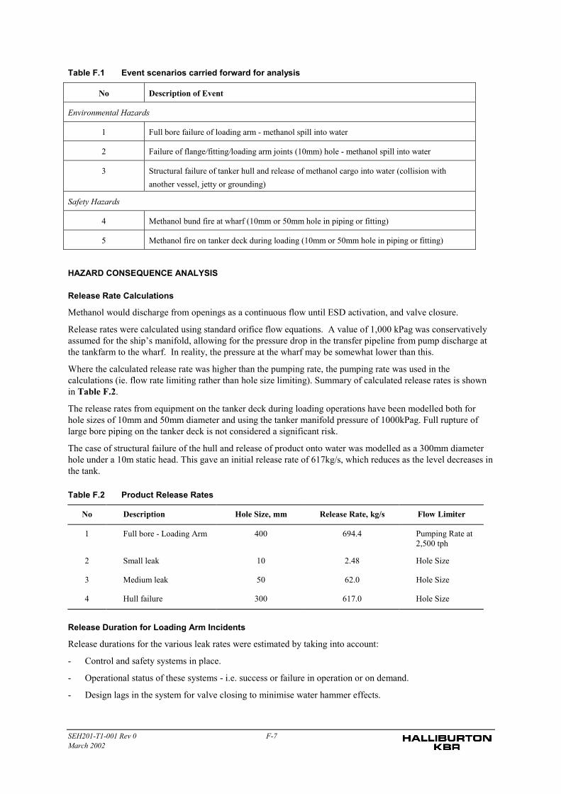
SEH201-T1-001 Rev 0 F-7March 2002
Table F.1 Event scenarios carried forward for analysis
No Description of Event
Environmental Hazards
1 Full bore failure of loading arm - methanol spill into water
2 Failure of flange/fitting/loading arm joints (10mm) hole - methanol spill into water
3 Structural failure of tanker hull and release of methanol cargo into water (collision withanother vessel, jetty or grounding)
Safety Hazards
4 Methanol bund fire at wharf (10mm or 50mm hole in piping or fitting)
5 Methanol fire on tanker deck during loading (10mm or 50mm hole in piping or fitting)
HAZARD CONSEQUENCE ANALYSIS
Release Rate Calculations
Methanol would discharge from openings as a continuous flow until ESD activation, and valve closure.
Release rates were calculated using standard orifice flow equations. A value of 1,000 kPag was conservativelyassumed for the ship’s manifold, allowing for the pressure drop in the transfer pipeline from pump discharge atthe tankfarm to the wharf. In reality, the pressure at the wharf may be somewhat lower than this.
Where the calculated release rate was higher than the pumping rate, the pumping rate was used in thecalculations (ie. flow rate limiting rather than hole size limiting). Summary of calculated release rates is shownin Table F.2.
The release rates from equipment on the tanker deck during loading operations have been modelled both forhole sizes of 10mm and 50mm diameter and using the tanker manifold pressure of 1000kPag. Full rupture oflarge bore piping on the tanker deck is not considered a significant risk.
The case of structural failure of the hull and release of product onto water was modelled as a 300mm diameterhole under a 10m static head. This gave an initial release rate of 617kg/s, which reduces as the level decreases inthe tank.
Table F.2 Product Release Rates
No Description Hole Size, mm Release Rate, kg/s Flow Limiter
1 Full bore - Loading Arm 400 694.4 Pumping Rate at2,500 tph
2 Small leak 10 2.48 Hole Size
3 Medium leak 50 62.0 Hole Size
4 Hull failure 300 617.0 Hole Size
Release Duration for Loading Arm Incidents
Release durations for the various leak rates were estimated by taking into account:
- Control and safety systems in place.
- Operational status of these systems - i.e. success or failure in operation or on demand.
- Design lags in the system for valve closing to minimise water hammer effects.

SEH201-T1-001 Rev 0 F-8March 2002
Small Leaks
For 10mm holes in pipework or loading arms, the system consists of manual detection and operation of theESD, the possibility that the ESD may fail on demand needs to be considered.
The following conservative release durations have been assumed, that include:
− Time for leak to be noticed and acted upon (allowing for poor visibility conditions and minimum manning).
− Time for ESD valve to close.
− Time to inform plant to shut down transfer pumps and time to shut down pumps.
− If ESD fails, time for shore watch operator to attempt manual isolation of the line.
1. Early detection of leak:
Time to detect leak and activate ESD : 3 minutes
Time for ESD valve closure: 0.5 minute
Time for plant pumps to shut down: 3 minutes
Total 6.5 minutes
If ESD fails, manual isolation of line 1 minute
2. Delayed detection of leak:
Leak duration was taken as a total of 20 minutes for all the activities listed in item 1 above.
Release Due to Guillotine Failure of Loading Arm
Guillotine failures of loading arms are relatively rare occurrences. They could happen from excessive shipmovements caused by mooring lines failure, excessive wave action from passing ships etc.
Mooring lines could fail due to excessive wind speeds. They could also fail from defective or incorrectly laidmooring lines. The latter type of failure could occur at any wind speed, but such failures may not always resultin a guillotine failure, unless two or more mooring lines had failed as a result of excessive ship movement.
The range monitoring system would initiate an ESD due to excessive ship movement before the arm failed.Even if the ESD failed, the emergency release coupling would isolate on either side of the failure, stopping aspill.
Control and safety systems for this scenario and release duration are characterised as follows:
1. Emergency release coupling operates: Near instantaneous shutoff
2. Emergency release coupling fails, but automatic shutdown operates
Leak from loading arm until loading arm inventory depleted.
Time for ESD valve activation: 0.5 minute
Time for ESD valve closure: 0.5 minute
Total 1 minute
3. Emergency release coupling fails, and automatic shutdown fails
Time to assess problem and take action 3 minutes
Time to close manual valve 1 minute
Response Times for Tanker Incidents
The response times and incident durations for events occurring on the tanker are described below.
1. Leak on ship pipework
In the event of detection of a leak in pipework on deck, the crew will advise the shore operator to initiatethe ESD. The remaining inventory in the pipework will continue to leak until the line is depressurised.
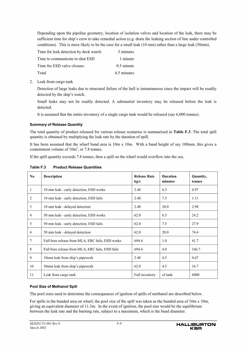
SEH201-T1-001 Rev 0 F-9March 2002
Depending upon the pipeline geometry, location of isolation valves and location of the leak, there may besufficient time for ship’s crew to take remedial action (e.g. drain the leaking section of line under controlledconditions). This is more likely to be the case for a small leak (10 mm) rather than a large leak (50mm).
Time for leak detection by deck watch: 3 minutes
Time to communicate to shut ESD 1 minute
Time for ESD valve closure: 0.5 minute
Total 4.5 minutes
2. Leak from cargo tank
Detection of large leaks due to structural failure of the hull is instantaneous since the impact will be readilydetected by the ship’s watch.
Small leaks may not be readily detected. A substantial inventory may be released before the leak isdetected.
It is assumed that the entire inventory of a single cargo tank would be released (say 6,000 tonnes).
Summary of Release Quantity
The total quantity of product released for various release scenarios is summarised in Table F.3. The total spillquantity is obtained by multiplying the leak rate by the duration of spill.
It has been assumed that the wharf bund area is 10m x 10m. With a bund height of say 100mm, this gives acontainment volume of 10m3, or 7.8 tonnes.
If the spill quantity exceeds 7.8 tonnes, then a spill on the wharf would overflow into the sea.
Table F.3 Product Release Quantities
No Description Release Ratekg/s
Durationminutes
Quantity,tonnes
1 10 mm leak - early detection, ESD works 2.48 6.5 0.97
2 10 mm leak - early detection, ESD fails 2.48 7.5 1.11
3 10 mm leak - delayed detection 2.48 20.0 2.98
4 50 mm leak - early detection, ESD works 62.0 6.5 24.2
5 50 mm leak - early detection, ESD fails 62.0 7.5 27.9
6 50 mm leak - delayed detection 62.0 20.0 74.4
7 Full bore release from MLA, ERC fails, ESD works 694.4 1.0 41.7
8 Full bore release from MLA, ERC fails, ESD fails 694.4 4.0 166.7
9 10mm leak from ship’s pipework 2.48 4.5 0.67
10 50mm leak from ship’s pipework 62.0 4.5 16.7
11 Leak from cargo tank Full inventory of tank 6000
Pool Size of Methanol Spill
The pool sizes used to determine the consequences of ignition of spills of methanol are described below.
For spills in the bunded area on wharf, the pool size of the spill was taken as the bunded area of 10m x 10m,giving an equivalent diameter of 11.3m. In the event of ignition, the pool size would be the equilibriumbetween the leak rate and the burning rate, subject to a maximum, which is the bund diameter.
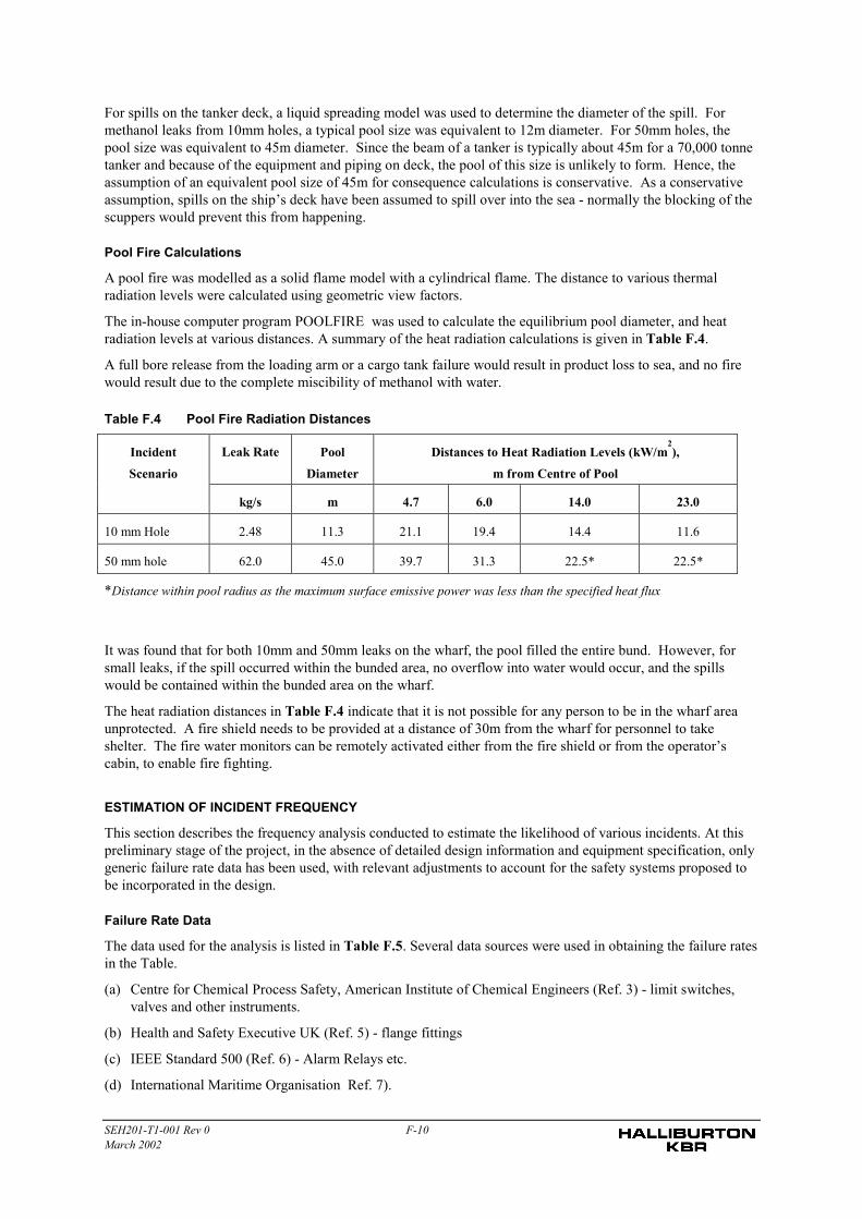
SEH201-T1-001 Rev 0 F-10March 2002
For spills on the tanker deck, a liquid spreading model was used to determine the diameter of the spill. Formethanol leaks from 10mm holes, a typical pool size was equivalent to 12m diameter. For 50mm holes, thepool size was equivalent to 45m diameter. Since the beam of a tanker is typically about 45m for a 70,000 tonnetanker and because of the equipment and piping on deck, the pool of this size is unlikely to form. Hence, theassumption of an equivalent pool size of 45m for consequence calculations is conservative. As a conservativeassumption, spills on the ship’s deck have been assumed to spill over into the sea - normally the blocking of thescuppers would prevent this from happening.
Pool Fire Calculations
A pool fire was modelled as a solid flame model with a cylindrical flame. The distance to various thermalradiation levels were calculated using geometric view factors.
The in-house computer program POOLFIRE was used to calculate the equilibrium pool diameter, and heatradiation levels at various distances. A summary of the heat radiation calculations is given in Table F.4.
A full bore release from the loading arm or a cargo tank failure would result in product loss to sea, and no firewould result due to the complete miscibility of methanol with water.
Table F.4 Pool Fire Radiation Distances
Leak Rate PoolDiameter
Distances to Heat Radiation Levels (kW/m2),
m from Centre of PoolIncidentScenario
kg/s m 4.7 6.0 14.0 23.0
10 mm Hole 2.48 11.3 21.1 19.4 14.4 11.6
50 mm hole 62.0 45.0 39.7 31.3 22.5* 22.5*
*Distance within pool radius as the maximum surface emissive power was less than the specified heat flux
It was found that for both 10mm and 50mm leaks on the wharf, the pool filled the entire bund. However, forsmall leaks, if the spill occurred within the bunded area, no overflow into water would occur, and the spillswould be contained within the bunded area on the wharf.
The heat radiation distances in Table F.4 indicate that it is not possible for any person to be in the wharf areaunprotected. A fire shield needs to be provided at a distance of 30m from the wharf for personnel to takeshelter. The fire water monitors can be remotely activated either from the fire shield or from the operator’scabin, to enable fire fighting.
ESTIMATION OF INCIDENT FREQUENCY
This section describes the frequency analysis conducted to estimate the likelihood of various incidents. At thispreliminary stage of the project, in the absence of detailed design information and equipment specification, onlygeneric failure rate data has been used, with relevant adjustments to account for the safety systems proposed tobe incorporated in the design.
Failure Rate Data
The data used for the analysis is listed in Table F.5. Several data sources were used in obtaining the failure ratesin the Table.
(a) Centre for Chemical Process Safety, American Institute of Chemical Engineers (Ref. 3) - limit switches,valves and other instruments.
(b) Health and Safety Executive UK (Ref. 5) - flange fittings
(c) IEEE Standard 500 (Ref. 6) - Alarm Relays etc.
(d) International Maritime Organisation Ref. 7).
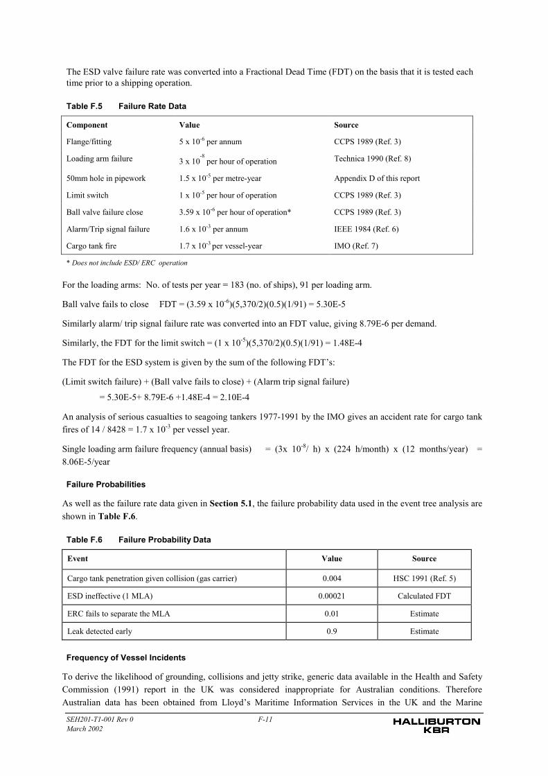
SEH201-T1-001 Rev 0 F-11March 2002
The ESD valve failure rate was converted into a Fractional Dead Time (FDT) on the basis that it is tested eachtime prior to a shipping operation.
Table F.5 Failure Rate Data
Component Value Source
Flange/fitting 5 x 10⁻⁶ per annum CCPS 1989 (Ref. 3)
Loading arm failure 3 x 10⁻⁸ per hour of operation Technica 1990 (Ref. 8)
50mm hole in pipework 1.5 x 10⁻⁵ per metre-year Appendix D of this report
Limit switch 1 x 10⁻⁵ per hour of operation CCPS 1989 (Ref. 3)
Ball valve failure close 3.59 x 10⁻⁶ per hour of operation* CCPS 1989 (Ref. 3)
Alarm/Trip signal failure 1.6 x 10⁻³ per annum IEEE 1984 (Ref. 6)
Cargo tank fire 1.7 x 10⁻³ per vessel-year IMO (Ref. 7)
* Does not include ESD/ ERC operation
For the loading arms: No. of tests per year = 183 (no. of ships), 91 per loading arm.
Ball valve fails to close FDT = (3.59 x 10⁻⁶)(5,370/2)(0.5)(1/91) = 5.30E-5
Similarly alarm/ trip signal failure rate was converted into an FDT value, giving 8.79E-6 per demand.
Similarly, the FDT for the limit switch = (1 x 10⁻⁵)(5,370/2)(0.5)(1/91) = 1.48E-4
The FDT for the ESD system is given by the sum of the following FDT’s:
(Limit switch failure) + (Ball valve fails to close) + (Alarm trip signal failure)
= 5.30E-5+ 8.79E-6 +1.48E-4 = 2.10E-4
An analysis of serious casualties to seagoing tankers 1977-1991 by the IMO gives an accident rate for cargo tankfires of 14 / 8428 = 1.7 x 10⁻³ per vessel year.
Single loading arm failure frequency (annual basis) = (3x 10⁻⁸/ h) x (224 h/month) x (12 months/year) =8.06E-5/year
Failure Probabilities
As well as the failure rate data given in Section 5.1, the failure probability data used in the event tree analysis areshown in Table F.6.
Table F.6 Failure Probability Data
Event Value Source
Cargo tank penetration given collision (gas carrier) 0.004 HSC 1991 (Ref. 5)
ESD ineffective (1 MLA) 0.00021 Calculated FDT
ERC fails to separate the MLA 0.01 Estimate
Leak detected early 0.9 Estimate
Frequency of Vessel Incidents
To derive the likelihood of grounding, collisions and jetty strike, generic data available in the Health and SafetyCommission (1991) report in the UK was considered inappropriate for Australian conditions. ThereforeAustralian data has been obtained from Lloyd’s Maritime Information Services in the UK and the Marine
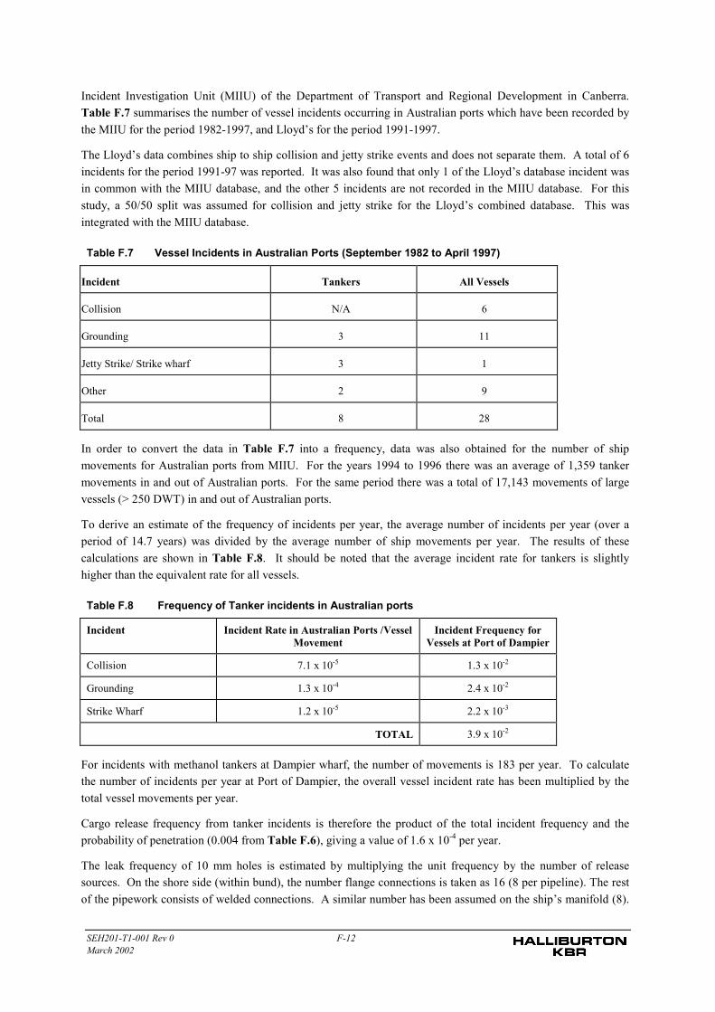
SEH201-T1-001 Rev 0 F-12March 2002
Incident Investigation Unit (MIIU) of the Department of Transport and Regional Development in Canberra.Table F.7 summarises the number of vessel incidents occurring in Australian ports which have been recorded bythe MIIU for the period 1982-1997, and Lloyd’s for the period 1991-1997.
The Lloyd’s data combines ship to ship collision and jetty strike events and does not separate them. A total of 6incidents for the period 1991-97 was reported. It was also found that only 1 of the Lloyd’s database incident wasin common with the MIIU database, and the other 5 incidents are not recorded in the MIIU database. For thisstudy, a 50/50 split was assumed for collision and jetty strike for the Lloyd’s combined database. This wasintegrated with the MIIU database.
Table F.7 Vessel Incidents in Australian Ports (September 1982 to April 1997)
Incident Tankers All Vessels
Collision N/A 6
Grounding 3 11
Jetty Strike/ Strike wharf 3 1
Other 2 9
Total 8 28
In order to convert the data in Table F.7 into a frequency, data was also obtained for the number of shipmovements for Australian ports from MIIU. For the years 1994 to 1996 there was an average of 1,359 tankermovements in and out of Australian ports. For the same period there was a total of 17,143 movements of largevessels (> 250 DWT) in and out of Australian ports.
To derive an estimate of the frequency of incidents per year, the average number of incidents per year (over aperiod of 14.7 years) was divided by the average number of ship movements per year. The results of thesecalculations are shown in Table F.8. It should be noted that the average incident rate for tankers is slightlyhigher than the equivalent rate for all vessels.
Table F.8 Frequency of Tanker incidents in Australian ports
Incident Incident Rate in Australian Ports /VesselMovement
Incident Frequency forVessels at Port of Dampier
Collision 7.1 x 10⁻⁵ 1.3 x 10⁻²
Grounding 1.3 x 10⁻⁴ 2.4 x 10⁻²
Strike Wharf 1.2 x 10⁻⁵ 2.2 x 10⁻³
TOTAL 3.9 x 10⁻²
For incidents with methanol tankers at Dampier wharf, the number of movements is 183 per year. To calculatethe number of incidents per year at Port of Dampier, the overall vessel incident rate has been multiplied by thetotal vessel movements per year.
Cargo release frequency from tanker incidents is therefore the product of the total incident frequency and theprobability of penetration (0.004 from Table F.6), giving a value of 1.6 x 10⁻⁴ per year.
The leak frequency of 10 mm holes is estimated by multiplying the unit frequency by the number of releasesources. On the shore side (within bund), the number flange connections is taken as 16 (8 per pipeline). The restof the pipework consists of welded connections. A similar number has been assumed on the ship’s manifold (8).
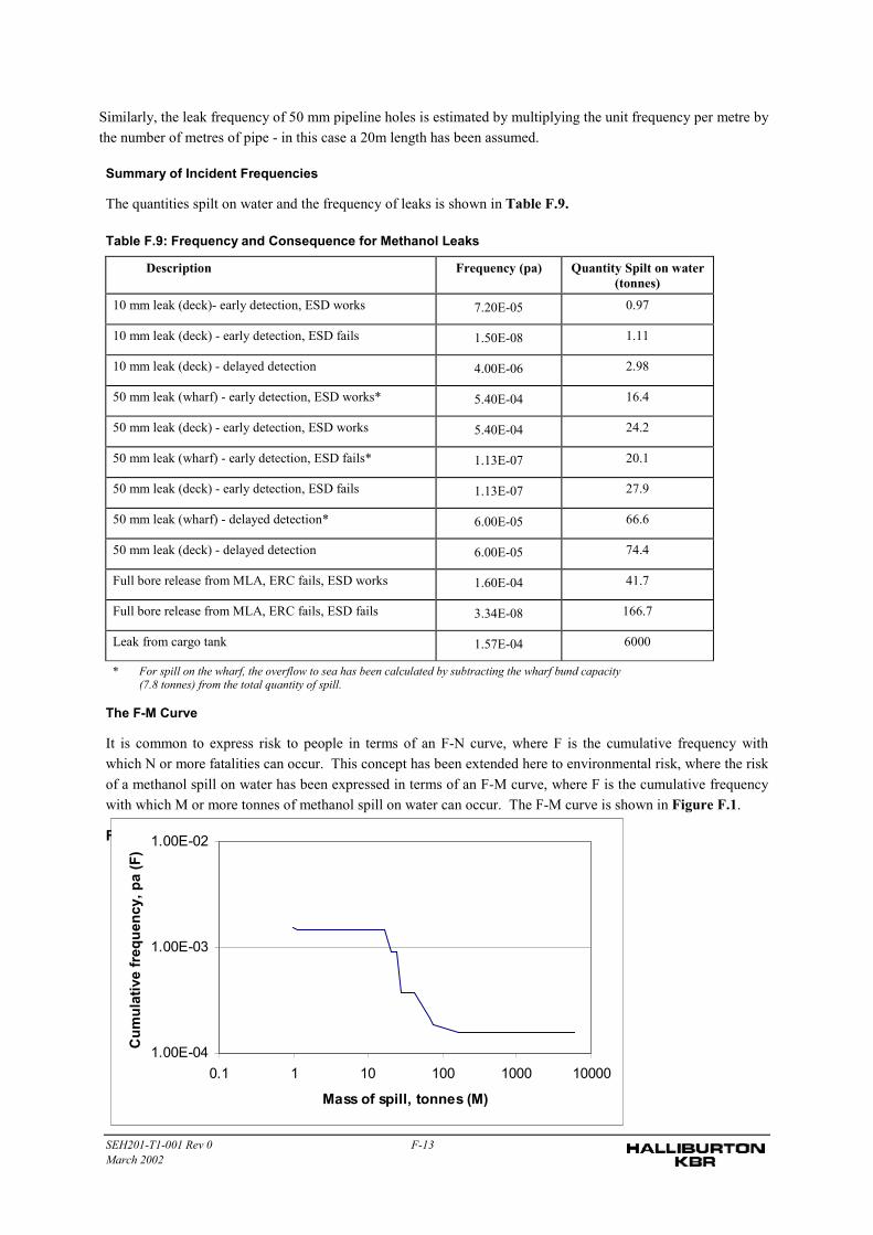
SEH201-T1-001 Rev 0 F-13March 2002
Similarly, the leak frequency of 50 mm pipeline holes is estimated by multiplying the unit frequency per metre bythe number of metres of pipe - in this case a 20m length has been assumed.
Summary of Incident Frequencies
The quantities spilt on water and the frequency of leaks is shown in Table F.9.
Table F.9: Frequency and Consequence for Methanol Leaks
Description Frequency (pa) Quantity Spilt on water(tonnes)
10 mm leak (deck)- early detection, ESD works 7.20E-05 0.97
10 mm leak (deck) - early detection, ESD fails 1.50E-08 1.11
10 mm leak (deck) - delayed detection 4.00E-06 2.98
50 mm leak (wharf) - early detection, ESD works* 5.40E-04 16.4
50 mm leak (deck) - early detection, ESD works 5.40E-04 24.2
50 mm leak (wharf) - early detection, ESD fails* 1.13E-07 20.1
50 mm leak (deck) - early detection, ESD fails 1.13E-07 27.9
50 mm leak (wharf) - delayed detection* 6.00E-05 66.6
50 mm leak (deck) - delayed detection 6.00E-05 74.4
Full bore release from MLA, ERC fails, ESD works 1.60E-04 41.7
Full bore release from MLA, ERC fails, ESD fails 3.34E-08 166.7
Leak from cargo tank 1.57E-04 6000
* For spill on the wharf, the overflow to sea has been calculated by subtracting the wharf bund capacity(7.8 tonnes) from the total quantity of spill.
The F-M Curve
It is common to express risk to people in terms of an F-N curve, where F is the cumulative frequency withwhich N or more fatalities can occur. This concept has been extended here to environmental risk, where the riskof a methanol spill on water has been expressed in terms of an F-M curve, where F is the cumulative frequencywith which M or more tonnes of methanol spill on water can occur. The F-M curve is shown in Figure F.1.
Figure F.1: F-M Curve for Methanol Spill
1.00E-04
1.00E-03
1.00E-02
0.1 1 10 100 1000 10000
Mass of spill, tonnes (M)
Cum
ulat
ive
freq
uenc
y, p
a (F
)
SEH201-T1-001 Rev 0 F-14March 2002
Summary of Fire Frequencies
The probability of ignition of a spill on the wharf is taken from Appendix D. For leak rates of 1-50 kg/s, it is0.03 and for leaks of > 50 kg/s, the value is 0.08.
Therefore, the following fire frequencies were derived, for a bund fire at the wharf.
Overall fire frequency = (frequency of 10mm spill x 0.03 + frequency of 50mm spill x 0.08)
= (5.0E-6 x 8 x 0.03 + 1.5E-5 x20 x 0.08) x 2 loading points pa
= 5.04 x 10⁻⁵ p.a.
RISK ASSESSMENT
Risk of Product Spill on Water
There are no established acceptance criteria for the risk of product spills on water. The guiding principle isgenerally that all product spills should be eliminated, or the risk of a spill reduced to as low as reasonablypracticable (ALARP) levels. The consequence-frequency curve for the identified scenarios shows that thefrequency of a spill exceeding 100 tonnes is approximately 1 chance in a 5,000 per year. This risk is low.Further, significant dilution of the spill would occur because of its miscibility with water, and any toxic impacton the aquatic environment would be localised around the spill area.
The critical factors in minimising the spill quantity and likelihood are:
− Activating the ESD as soon as the leak is detected. Operating procedures should emphasise this aspect inthe operator/shore watch training.
− Minimising the potential for a collision or jetty strike by ensuring careful manoeuvring of the vessels, aswell as minimising the chance of collision at angles where a structural failure could occur. For tankers, thisaspect is outside the control of Methanex as the tugs would be operated by the Port of Dampier Authority.
Fire Risk Assessment
The total fire frequency from a methanol spill on the wharf was calculated as 5.0 x 10⁻⁵ per annum. Thisfrequency is low.
The emergency procedure should call for taking shelter behind the fire shield and activating the remotefirewater/ foam monitors in the event of a fire. This would reduce the heat radiation distances significantly.
The nearest structure is the shore operator’s cabin. This location should be carefully considered to ensure that itis outside the 4.7 kW/m2 heat radiation contour for a full bund fire. Provided the operator stays in the cabin, atleast till fire fighting commences, when the thermal radiation distances would be attenuated by the water/foamspray, there would be no injury potential.
SEH201-T1-001 Rev 0 F-15March 2002
RISK CONTROL MEASURES
There are standard risk control measures as part of the installation design, as required by AS 3846-1998, and theIMO standard. The following measures are recommended in addition to the above.
1. Provide a fire shield at the wharf to provide shelter for fire fighting personnel as the bund fire cannot beapproached without this shield.
2. The operator cabin at the wharf should be located at a distance of at least 30 metres from the bunded area,to provide shelter against fire radiation.
3. The ESD should be tested prior to each ship loading operation. This can form part of the ship/ shorechecklist required by AS 3846-1998.
4. An annual electrical audit of the wharf should be conducted to ensure that the Hazardous Area Zone 1integrity is maintained.
REFERENCES
1. Standards Australia, AS-3846 “The Handling of Hazardous cargo in Ports”, 1998.
2. Blything, K.W. and Reeves, A.B. [1988]: "An Initial Prediction of the BLEVE Frequency of a 100 tonneButane Storage Vessel, SRD/HSE, UK.
3. CCPS [1989]: "Guidelines for Process Equipment Reliability Data", Center for Chemical Process Safety,American Institute of Chemical Engineers, New York.
4. Department Of Transport, Marine Accident Investigation Unit, personal communication with GranhernePty Ltd.
5. Health and Safety Commission [1991], “Major Hazard Aspects of the Transport of Dangerous Substances”,London.
6. IEEE [1984]: "Guide to the Collection and Presentation of Electrical, Electronic, Sensing Component, andMechanical Equipment Reliability Data for Nuclear-Power Generating Stations", Standard 500, New York.
7. International Maritime Organisation, “Analysis of Serious Casualties to Seagoing Tankers 1977-1991 -Analysis of Serious Casualties to Fishing Vessels 1982-1991”
8. Technica Ltd [1990]: "Risk Assessment Study of Hastings Industrial Area", Draft Report. Prepared forDepartment of Labour, Victoria.
Methanol Shipping Hazards Assessment
Appendix 8
Risk, Safety and Health Consultants
MMEETTHHAANNOOLL SSHHIIPPPPIINNGG HHAAZZAARRDDSS
AASSSSEESSSSMMEENNTT
SINCLAIR KNIGHT MERZ
QEST CONSULTING GROUPLEVEL 7, 251 ADELAIDE TERRACEPERTH WA, 6000
Telephone: (08) 9325 3399Facsimile: (08) 9325 3335
Prepared by: Qest Consulting GroupRev 0, April 2002
Qest Consulting GroupMethanol Shipping Hazards Assessment
Sinclair Knight Merz Page iiiAppendix 8 - Shipping Hazard Assessment.doc
for Methanex
Acknowledgment
Qest Consulting Engineers compiled this report, but it is a joint effort between QESTteam members and Sinclair Knight Merz personnel. The author of this report wishesto thank the participants for their diligence during the assessment, and for theirefforts in providing the information required to prepare this report.
Disclaimer
Qest prepared this report as an account of work for Sinclair Knight Merz. Thematerial in it reflects Qest’s best judgement in the light of the information available toit at the time of preparation. However, as Qest cannot control the conditions underwhich this report may be used, Qest and its related companies will not be responsiblefor damages of any nature resulting from use of or reliance upon this report.
Document Revision RecordTitle:Job No: SKM3pRevision: Description: Prepared by: Checked by: Approved by: Date:
A Draft forcomment B. Skinner M. Monaghan 22/3/02
0 Final report B. Skinner M. Monaghan M. Monaghan 2/4/02
Qest Consulting GroupMethanol Shipping Hazards Assessment
Sinclair Knight Merz Page iiiAppendix 8 - Shipping Hazard Assessment.doc
TABLE OF CONTENTS
TABLE OF CONTENTS........................................................................................... III
GLOSSARY .............................................................................................................IV
1 EXECUTIVE SUMMARY.................................................................................... 51.1 Potentially hazardous events ..................................................... 51.2 Recommendations ....................................................................... 5
2 INTRODUCTION ................................................................................................ 62.1 Background .................................................................................. 62.2 Study Aims and Scope of Work .................................................. 6
3 RISK ASSESSMENT METHODOLOGY ............................................................ 7
4 HAZARDS OF SHIPPING METHANOL ............................................................. 84.1 Shipping environment ................................................................. 84.2 Potential Hazards Associated with Methanol Shipping............. 8
4.2.1 Methanol Characteristics................................................................ 84.2.2 Shipping ......................................................................................... 8
5 SEMI QUANTITATIVE RISK ASSESSMENT (SQRA) ..................................... 105.1 Hazard Identification .................................................................. 10
5.1.1 Fire/Explosion .............................................................................. 105.1.2 Shipping Collision......................................................................... 10
6 CONCLUSIONS ............................................................................................... 14
7 RECOMMENDATIONS .................................................................................... 14
8 REFERENCES ................................................................................................. 15
Qest Consulting GroupMethanol Shipping Hazards Assessment
Sinclair Knight Merz Page iiiAppendix 8 - Shipping Hazard Assessment.doc
GLOSSARYDEP Department of Environmental ProtectionDOLA Department of Land AdministrationDPA Dampier Port AuthorityEPA Environmental Protection AuthorityFEA Fire and Explosion AnalysisIMO International Marine OrganisationIRPA Individual Risk Per AnnumPRA Preliminary Risk AssessmentPER Public Environment ReviewSKM Sinclair Knight MerzTLV Threshold Limit ValueWA-DMPR Western Australian Department of Minerals and Petroleum Resources
Qest Consulting GroupMethanol Shipping Hazards Assessment
Sinclair Knight MerzAppendix 8 - Shipping Hazard Assessment.doc
1 EXECUTIVE SUMMARY
Sinclair Knight Merz (SKM) have requested QEST Consulting Engineers prepare areport on the hazards associated with the shipping of methanol by Methanex in theDampier Harbour.
The hazards under consideration in this study are those associated with bulkshipping (range 16 - 45kt) of methanol through the shipping channel heading northwest from the new Dampier Wharf.
The risks were found to be negligible in comparison to those determined from theproduction of methanol.
1.1 Potentially hazardous eventsA summary of the major risk contributors are provided in Table 1.1.1.
Table 1.1.1 Risk Contributions
Internal Event CommentCollision Major cause through engine or steering failure.Grounding Major cause through cyclone, engine or steering failure.Onboard Incident May include fire and explosion.Collision duringberthing anddeparting
Cause through hitting the wharf with sufficient speed to causerupture of methanol storage tank.
The events specified are not considered to be a problem on their own as Methanexhave adequate control measures in place to manage risk.
1.2 RecommendationsThe hazards associated with the shipping of methanol were determined to be lowcompared to those associated with the other facets of methanol production and norisk reduction measures were identified.
However, in preparation of the Safety Report (QRA) Qest recommend that shippinghazards be re-addressed to ensure current shipping data is used.

Qest Consulting GroupMethanol Shipping Hazards Assessment
Sinclair Knight MerzAppendix 8 - Shipping Hazard Assessment.doc
2 INTRODUCTION
2.1 BackgroundMethanex Australia Pty Ltd, the proponent for this project, proposes to construct anexport oriented Methanol complex in the Pilbara region of Western Australia. Thefirst train of the proposed plant will convert natural gas into Methanol at a designcapacity of 2 Mega tonnes per day (mtpd) by 2005 and when the second train is on-line by 2010 5mtpd per day.
A 5km long lagged pipeline will transport the produced methanol from the storagetanks at the methanol facility to the new Dampier Wharf where a loading arm will bepresent for loading onto the ships.
The methanol will then be transported to its international markets via 87 trips perannum for an average methanol load of 23kt. Once the second train is on-line thenumber of trips will increase to 218 with an average load of 23kt.
The new Dampier Wharf will have a dedicated shipping channel which will head northwest from the new wharf for 3.3 nautical miles. It will be dredged to accommodate upto 12m draft (generally 50-60,000 DWT) tankers.
The existing Dampier Public Wharf is located about 5 kilometres to the west of theproposed site. The project will have access to the ship-loading facilities at the newpurpose-built loading wharf (approximately 300m south of the existing DampierPublic Wharf).
The 2 other channels in the harbour will not be connected to the new channel.
2.2 Study Aims and Scope of WorkThe potential for major incident events arising from the shipping of large amounts ofmethanol warrant special measures to ensure the safety of the public, the workforceand the environment.
The aim of this study is to:• Determine the risks of bulk methanol transportation through the shipping channel
from Dampier Wharf for inclusion in the Public Environment Review (PER); and• Make recommendations where applicable.
The Study addresses all major shipping accidents and assesses their risk by:• Determining the potential hazardous events;• Assessing the frequency of such events;• Analysing the potential consequences of hazardous events; and• Reporting any applicable recommendations.
The primary purpose is to ensure that all significant risks are identified and properlyevaluated to enable appropriate action to be taken to eliminate or reduce thepotential for major incident events. These risks can then be reported in terms of theirfrequencies and consequences and analysed further for quantitative risk if deemednecessary.
Qest Consulting GroupMethanol Shipping Hazards Assessment
Sinclair Knight MerzAppendix 8 - Shipping Hazard Assessment.doc
3 RISK ASSESSMENT METHODOLOGY
This report forms part of the PRA for the Methanex project which is part of the PERprocess. The objective of a PRA is to demonstrate that, as far as is reasonablypracticable, all credible accident events that have the potential to cause fatalities offsite have been identified and the EPA Criteria for the assessment of risk fromindustry has been met [11].
The methodology used for this Risk Assessment is based on hazard scenarioidentification, analysis and assessment carried out in well-defined stages. The stagesin the risk assessment methodology are summarised below:
1 Hazard Identification:Identification of credible hazardous events for the shipping operation. This wasdone using the analysts’ experience, the proponents knowledge of theproposed operations, experience and a systematic review of the proposedoperation. This study looks at the shipping operation within the newly proposedchannel and wharf. There was no requirement to include the loading orunloading of cargo in this report.
2 Consequence Analysis:The consequence analysis will consider the various possible release eventsand their potential to cause fatalities and damage to the environment andproperty.
3 Frequency Analysis:To determine the frequency at which the hazardous events may occur whichincludes demonstrating that:• The event development is valid;• The failure data used is valid; and• The frequency of each of the hazardous events has been determined
where applicable.
4 Risk Analysis:Semi quantification of the risk arising from hazardous events was determinedwhere applicable.
5 RecommendationsDuring the process the potential to reduce particular risks through alteration ofoperation, procedures or by other means that may become apparent to theanalyst.
Qest Consulting GroupMethanol Shipping Hazards Assessment
Sinclair Knight MerzAppendix 8 - Shipping Hazard Assessment.doc
4 HAZARDS OF SHIPPING METHANOL
4.1 Shipping environmentThe new Dampier Wharf will have a dedicated shipping channel and will be dredgedto accommodate up to 12m draft (generally 50-60,000 DWT) tankers. Some of thetankers considered for use have a draft of approximately 11.5m and consideration ofthe narrow margin for error has been acknowledged. The new channel will headnorthwest from the new wharf for 3.3 nautical miles.
Two vessels are unlikely to be in the same channel at the same time due to its shortlength. In addition, all non local vessels require a local pilot (methanol tankersincluded) to bring the vessel into the wharf.
Dampier Port Authority monitors vessel movements and ensures that major vesselsin the same area of the port are in communication with each other. All methanoltankers would be under radar surveillance from the Dampier Port Authority.
4.2 Potential Hazards Associated with Methanol ShippingThis analysis is mainly concerned with the impact of the shipping operations on theMethanex employees, surrounding environment and population.
4.2.1 Methanol CharacteristicsMethanol (Methyl Alcohol) is a clear, colourless flammable liquid (and vapour) with afaint characteristic alcohol odour. It is a moderate explosion hazard and dangerousfire hazard when exposed to heat, sparks or flames. It has a boiling point of 65°Cand a flash point of 11°C. Above flash point, vapour/air mixtures are explosive within6 to 36.5% vol. in air. There is potential for rupture of sealed containers whenheated. Methanol is not sensitive to static discharge as it is not a static accumulator.
Methanol is harmful / life-threatening if ingested or absorbed through the skin.Excessive heating and/or incomplete combustion will generate highly poisonous COand CO2.
In the event of an ignited release, a pure methanol fire may not be visible to thenaked eye.
Methanol is completely soluble in water. However if released into water, it will beslightly toxic to aquatic life.
4.2.2 ShippingThe majority of the tankers that will be used for exporting the methanol are operatedunder time charter to Methanex’s own shipping company. They are built toMethanex’ specifications, including double hulls and dedicated for methanol service.The tankers also comply with BCH / ICB codes and IMO standards.
The proposed tanker methanol storage will range between 16 and 45kt and will bemaintained at 25kPa pressure. During loading, vapour is released through high

Qest Consulting GroupMethanol Shipping Hazards Assessment
Sinclair Knight MerzAppendix 8 - Shipping Hazard Assessment.doc
velocity valves/vents that are located about 15m above the deck level as per the IMOstandards.
The tankers do not carry any other hazardous bulk cargo other than methanol.
The hazards associated with the proposed method of shipping methanol from theDampier Wharf through the channel were found to be:• Fire / explosion onboard the tanker;• Collision with another ship;• Grounding;• Collision with the wharf;• Combination of the above events.
Qest Consulting GroupMethanol Shipping Hazards Assessment
Sinclair Knight MerzAppendix 8 - Shipping Hazard Assessment.doc
5 SEMI QUANTITATIVE RISK ASSESSMENT (SQRA)
5.1 Hazard IdentificationThe movement of the tanker to and from the Dampier Wharf through the channel wasanalysed in Section 4. The events considered to be hazardous and consideredfurther are listed in Table 5.1.1.
Table 5.1.1Potential Hazardous Events Examined in Risk AnalysisEvent Release
Ship to ship collision Methanol (l)Grounding Methanol (l)Fire / Explosion onboard Methanol (l)Collision whilst berthing and departing Methanol (l)
5.1.1 Fire/ExplosionA fire or explosion on board the tanker has the potential to escalate to an event thatmay lead to tank rupture whilst a tanker is in passage to and from the loading berth.
Based on the data presented by Brennan and Peachey [9], the potential for a fire orexplosion is estimated here. [9] states that 18 fire/explosion events occurred over19690 ship-years, which equates to 9.1x10⁻⁴ fire/explosion events per year per ship.The tanker enters the harbour only 87 times per year for the first train and 218 timesper year once the second train is on-line. Therefore the annual fire/explosionfrequency is calculated to be 2.2×10⁻⁴
and 5.4x10⁻⁴pa, respectively.
These values incorporate all types of fire and explosion events and are consideredconservative due to the number of safety systems onboard the tanker, which wouldhave to fail to work. Therefore for this event to escalate and result in the release ofmethanol the frequency would be very low as the tanks would have to rupture andthe methanol then find an ignition source. This is not considered further.
The potential for an explosion while entering the port is very low because the vapourin the tanker would be above the level for an explosive fuel / air mixture [11] or wouldnot contain methanol at all [12]. However if the methanol cargo was to ignite it wouldburn itself out. Thermal effects from a fire would be limited to the tanker andimmediate surroundings. If the tanker was to rupture, the methanol would rapidlydiffuse into the water.
Considering the release frequencies are low, and the consequences are very unlikelyto impinge on the wharf, this event is not carried forward for further analysis.
5.1.2 Shipping Collision
5.1.2.1 Collision with the wharfCollisions with the jetty on departure / or arrival are not likely to have significantconsequences, as the tanker would not be moving with sufficient speed to causeserious damage. During their approach and departure they will be assisted bytugboats for such operations.

Qest Consulting GroupMethanol Shipping Hazards Assessment
Sinclair Knight MerzAppendix 8 - Shipping Hazard Assessment.doc
5.1.2.2 Severe weatherThe possibility of a methanol tanker being damaged while in the port from severe orcyclonic weather is extremely unlikely due to the procedures in place at the port.One such procedure includes shutting the port twelve hours prior to gale force windshitting the coast. This gives the tankers sufficient warning to avert any potentialincidents. The port will only be reopened once the seas are determined to be safe.
5.1.2.3 Methanol tanker groundingThe port will be monitored and controlled by the Dampier Port Authority, and all thevessels entering and leaving will be under the control of a local pilot. It is assumedthat the short duration of a ship travelling in the channel greatly reduces the chancesof another vessel being in the channel at the same time.
The only credible scenario in which vessels could come in contact with each otherwould be due to propulsion or steering failure of the methanol tanker at the sametime as being in close proximity to another vessel in the channel or harbour.However, should any of the larger vessels lose steering or power they would be morelikely to run aground prior to colliding with another vessel since their draft precludesmoving out of or turning in the channel.
The grounding of the methanol tanker once propulsion has failed would require theassistance of the tugboat nearby to also fail. The nature of such an incident isunlikely to result in methanol tank rupture because of the low speed at which it wouldbe travelling. This sequence of events resulting in grounding and subsequent releaseof methanol is considered to be so low as to not be analysed further.
5.1.2.4 Passing vessel collisionThe only scenario to be considered, in which the methanol tankers could collide withother vessels is if the steering or propulsion system on either the methanol tanker oranother large vessel fails.
Steering failureThe steering on the methanol tanker has redundancy and since it is standard practicefor ships to have emergency steering backup it will be assumed that the other shipsin the harbour also have redundancy. The redundant steering systems on the shipsmake the probability of steering failure remote.
In the case that there are two vessels in the channel at one time and both steeringsystems fail on one vessel the other vessel should have time to manoeuvre out of thepath of the uncontrolled vessel. In the case that steering failure occurs in bothsystems on both vessels the use of support from tugboats based at the DampierWharf would reduce the frequency of a collision happening. The methanol tanker orany equally large vessel would not be able to drop an anchor in the channel becausethere is not sufficient room for the tanker to swing around on the anchor withoutrunning aground. If steering did fail it would most likely fail during manoeuvring whenarriving at or departing the jetty. During this period a tugboat would be in control ofthe tanker mitigating any possible consequences. Therefore steering failure will notbe considered further.
Propulsion system failureIf the methanol tanker propulsion system failed it could drift on a collision course withany of the vessels in the area. Due to the system of procedures in place requiringtugboats to assist tankers to and from the wharf, a tugboat would be incommunication and nearby if required. However most vessels should be able to
Qest Consulting GroupMethanol Shipping Hazards Assessment
Sinclair Knight MerzAppendix 8 - Shipping Hazard Assessment.doc
avoid the drifting tanker and the tanker may run aground. If any of the smallervessels’ engines fail they could drift out of the channel and in most cases a tankerwould have sufficient time and manoeuvrability to avoid an incident. Also any smallvessel that has lost their engines would be able to manoeuvre until they slowedsufficiently to be able to drop anchor, preventing collision with other vessels. It isassumed the small vessels fail to anchor to 1% of the time and a tugboat isunsuccessful in preventing a collision 1% of the time for larger vessels.
Two scenarios are considered, one is for the first train of production equal to 2mtpaand the second scenario is for 5mtpa. The calculation method is shown for the 1st
train and the same method was used for second phase of production but only theresults are reported. Since the tanker will not contain an explosive fuel / air mixtureon its return to Dampier Wharf, it is not deemed a hazard and only the departingvessel is considered for this event. The results are presented in Table 5.1.2.
Assumptions 2mtpa 5mtpaThe number of methanol exports per year is: 87 218The average tanker payload is: 23,000t 23,000tThe average length is: 186m 186mThe departing tankers are in the harbour for 1 hour.
P Propulsion failure = 11.4 pa [7]P anchor/tug fail = 0.01
Given that the current proposed new wharf is to handle four main exporters, it isassumed that there will be approximately 280 vessels using the new channel eachyear, provided all six projects that have been submitted are approved [10]. It isassumed they will have a manoeuvring time in the harbour for a maximum period of 1hour for arrival and 1 hour for departure. These vessels may be used for the exportof ammonia, urea or DiMethylEther. There will be 87 methanol tankers manoeuvringin the harbour for a maximum of 2 hours.
Therefore the frequency of a methanol tanker visiting or departing the harbour whilea large vessel is travelling through the harbour is:
Fmethanol tanker in harbour = 87paPl non methanol vessel in harbour = (280-87 x 2) / 8760 = 0.044Pmethanol tanker in harbour = 87 / 8760 = 0.0010Pmethanol and non methanol vessel = 0.044 x 0.001 = 4.37E-4fl vessel nearby = 87 × 4.37E-4 = 0.038pa.
Given the probability that the propulsion system fails is 11.4 pa [7], the followingscenarios were considered.
The probability that the methanol tanker propulsion system fails during the 87 hoursper year it is exiting the harbour is:
P propulsion failure 1 = 87 × 11.4 / 8760 = 0.113
The probability that the other vessels’ propulsion system fails during the 386 hoursper year it is in the harbour is:
Ppropulsion failure 2 = 386 × 11.4 / 8760 = 0.50

Qest Consulting GroupMethanol Shipping Hazards Assessment
Sinclair Knight MerzAppendix 8 - Shipping Hazard Assessment.doc
Therefore, total probability of a propulsion failure is:
P total propulsion failure = 0.113 + 0.50= 0.61
This probability is brought forward to assist in determining the risk of methanolrelease due to ship collision.
If the steering fails, the vessel will most likely travel in the direction it was previouslyheading prior to the steering failure. It is assumed that this is the case for a driftingvessel.
If the out of control methanol tanker drifts towards the other vessel the probability ofstriking a nearby vessel is the ratio of the combined length of the two vessels and theperimeter of a circle radius equal to the distance between them.
The vessel separation while in the harbour varies between 1 and 5 N miles. We willconservatively assume 2N miles is the average separation (ie. 3.7km).
The average length of a large vessel is assumed to be 270 m. The average length ofa methanol tanker is assumed to be 186m [12], therefore their combined length is456m.
The perimeter length of a circle of radius 3.7km = 2πr= 23250m
Therefore
Pcollision = 456 / 23250= 0.02
It is assumed that 20% of the collisions are severe enough to penetrate one of theinner methanol tanks resulting in a significant release of methanol. This assumptionis considered conservative due to the double-hulled vessels used for methanoltransportation [12].
Therefore the risk of methanol release due to ship collision is:fmethanol release = flvessel nearby × Ptotal propulsion failure × Panchor/tug fail × Pcollision × Pmethanol release
= 0.038 × 0.61 × 0.01 × 0.02 × 0.2= 9.27 x 10⁻⁷pa
Table 5.1.2 Ship to ship collision frequency2mtpa 5mpta
Frequency 9.27 x 10⁻⁷ 7.49 x 10⁻⁶
This release frequency is very low, coupled with the fact that ignition of a fullmethanol tank is unlikely due to the high miscibility of methanol in water. The IRPAwill be considerably less than 10-6 , hence this event is not considered further.
Qest Consulting GroupMethanol Shipping Hazards Assessment
Sinclair Knight MerzAppendix 8 - Shipping Hazard Assessment.doc
6 CONCLUSIONS
The risk associated with shipping of methanol through the Dampier Harbour wasdetermined to be low in comparison to the risks associated with the other areasinvolved in the PER. The events considered to have a hazardous potential were:
• Tanker / Vessel collision;• Collision with Wharf;• Grounding;• Fire and explosion;• Combination of the above.
All events other than tanker / vessel collision were found to have a negligiblefrequency of occurrence or consequences and were not considered further.
7 RECOMMENDATIONS
No applicable recommendations for reducing the hazard potential of methanolshipping were identified.
However, in preparation of the Safety Report (QRA) Qest recommend that shippinghazards be re-addressed to ensure current shipping data is used.
Qest Consulting GroupMethanol Shipping Hazards Assessment
Sinclair Knight MerzAppendix 8 - Shipping Hazard Assessment.doc
8 REFERENCES
1 Guidelines for the Preparation and Submission of Facility Safety Cases,Department of Industry, Science and Resources (August, 2000).
2 National Standard and Code of Practice for Control of Major Hazard Facilities,Worksafe (September, 1996).
3 CPR 16E 'Methods for the determination of possible damage to people andobjects resulting from releases of hazardous materials', TNO (1989).
4 E&P Forum Report no 11.8/250, Quantitative Risk Assessment DatasheetDirectory (October 1996).
5 TNO Green Book, Methods for the Determination of Possible Damage toPeople and Objects Resulting from Releases of Hazardous Materials,(December 1989).
6 Cox, A.W., Lees, F.P. and Ang, M.L. classification of hazardous Locations,Pub. I. Chem.E. (1990)
7 Lloyds Register. Reliability and Safety Assessment Methods for Ships andOther Installations (May 1983).
8 Kletz (1977) Unconfined vapour cloud explosions. In Loss Prevention, vol II(New York: Am. Inst. Chem. Engrs), p 50
9 Brennan, E. G, and Peachey, J. H., Recent Research into Formal SafetyAssessment for Shipping, Lloyd’s Register Technical Association
10 Telephone conversation between Brad Skinner and Greg Trembarth (DampierPort Authority), 21st March 2002.
11 Telephone conversation between Brad Skinner and Russell Williams(Methanex), 2nd April 2002.
12 Fax from Jenny Lazarov (SKM), Shipping Risk Analysis, 27/3/02.
Related Documents