Predicting System-Scale Impacts of Oyster Clearance on Phytoplankton Productivity in a Small Subtropical Estuary

1 23

Environmental Modeling &Assessment ISSN 1420-2026Volume 18Number 2 Environ Model Assess (2013) 18:185-198DOI 10.1007/s10666-012-9338-y

Predicting System-Scale Impacts of OysterClearance on Phytoplankton Productivityin a Small Subtropical Estuary

Christopher Buzzelli, Melanie Parker,Stephen Geiger, Yongshan Wan, PeterDoering & Daniel Haunert

1 23

Your article is protected by copyright and

all rights are held exclusively by Springer

Science+Business Media B.V.. This e-offprint

is for personal use only and shall not be self-

archived in electronic repositories. If you

wish to self-archive your work, please use the

accepted author’s version for posting to your

own website or your institution’s repository.

You may further deposit the accepted author’s

version on a funder’s repository at a funder’s

request, provided it is not made publicly

available until 12 months after publication.

Predicting System-Scale Impacts of Oyster Clearanceon Phytoplankton Productivity in a SmallSubtropical Estuary

Christopher Buzzelli &Melanie Parker & Stephen Geiger &

Yongshan Wan & Peter Doering & Daniel Haunert

Received: 12 December 2011 /Accepted: 20 August 2012 /Published online: 11 September 2012# Springer Science+Business Media B.V. 2012

Abstract Oyster populations in south Florida estuarieshave declined in part through altered salinity driven byanthropogenic changes in freshwater inputs. In particular,the St. Lucie Estuary (SLE) in southeastern Florida hassuffered widespread loss of oyster habitat. With effortsunderway to improve water quality and oyster habitat inthe SLE, the goal of this study was to develop a model toassess ecosystem level impacts of oyster restoration. Phyto-plankton and oyster biomass modeling targets were estab-lished from observational data collected from 2005 to 2009.Modeled oyster biomass production and filtration fluctuatedwith temperature, salinity, and total suspended solids from acombination of observational and predicted input functionsin 10-year simulations (1998–2007). Model estimates ofoyster biomass fluctuated with salinity from near zero afterextreme freshwater discharge in 2002–2003 and 2004–2005to maximum values near 150.0 and 200.0 gCm−2 in spring1999 and fall 2006. There was potential for algal blooms asturnover time for the phytoplankton standing stock(15.6 days) was faster than water mass turnover (21.0 days).While >1,000 days were required for 50 ha of oyster habitatto filter the entire volume of the estuarine segment, filtertime reduced to <20 days with an estimated fivefold increasein net consumption of phytoplankton if the oyster habitat

was increased to 300 ha. Re-establishment of biologicallydesirable salinity envelopes would stabilize oyster survivalallowing the possibility for successful habitat restoration tobenefit water quality and faunal attributes of the St. LucieEstuary.

Keywords Estuary . Oyster . Phytoplankton . Subtropical .

Modeling

1 Introduction

Oyster bed vitality is a conspicuous indicator of estuarinecondition as the distribution and abundance of the easternoyster (Crassostrea virginica) have ecosystem-scale impli-cations [28, 39, 41]. Oyster beds filter water and suspendedsolids, couple the water column to the benthos, and provideliving aquatic habitat [12, 41, 44]. The widespread declineof oysters over several decades has resulted in increasedefforts to restore the acreage of live oyster bottom in manygeographic areas [12, 34]. An effective management ap-proach is to combine monitoring and modeling at the ap-propriate scale to assess the potential ecosystem scaleimpacts of such restorative actions [8, 57]. Simulation mod-eling offers a mechanism to connect observed abundancesof filter feeders to the environmental factors that regulatesurvival while simultaneously incorporating the effects ofbenthic filtration on the water column processes [19, 22].

Benthic filter feeders have a profound influence on thecomposition of the estuarine water column [21, 42, 56].Studies suggest that potential effects of nutrient loading onphytoplankton production are much more pronounced in theabsence of benthic filter feeders [11, 24, 40]. However,predicting the potential benefits of filtration can be compli-cated by estuarine hydrodynamics. The capacity for both

C. Buzzelli (*) :Y. Wan : P. Doering :D. HaunertCoastal Ecosystems Section,South Florida Water Management District,3301 Gun Club Road,West Palm Beach, FL 33406, USAe-mail: [email protected]

M. Parker : S. GeigerFlorida Fish and Wildlife Conservation Commission,Fish and Wildlife Research Institute,100 8th Avenue S.E.,St. Petersburg, FL 33701, USA

Environ Model Assess (2013) 18:185–198DOI 10.1007/s10666-012-9338-y

Author's personal copy

phytoplankton production and benthic filtration of the watercolumn are dependent upon the hydraulic residence time ofthe basin as rapid physical transport can overwhelm localbiological processes [11, 21, 43].

Filtration by oysters is efficient at very low suspendedsolid concentrations (<1.0 mgL−1) and results in the biode-position of huge amounts of particulate organic matter(POM) [22, 23, 40]. The filtration rate is proportional tothe dry weight of the oyster meat increasing with tempera-ture to a maximum reported value of 0.55 m3gC−1day−1

[19, 29, 38]. Net deposition of POM is significant in thecarbon budget of oyster beds with rates of 6,000 gCm−2

year−1 reported for lower Chesapeake Bay [23]. While indi-vidual oysters effectively filter the water column, impacts onecosystem scale water quality depend upon the relativeabundance of filtering organisms in the estuarine basin [39].

Oyster beds localize heterotrophy in the estuary as respi-ration in the oyster tissue and reef deposits consumes DOand releases excreted/recycled dissolved inorganic nitrogenand phosphorus (DIN and DIP) to the water column [13,39]. Conversely, oyster bed formation represents a net re-moval of total nitrogen (N) from the water column over timethat can augment N removal through denitrification depend-ing upon oxidative conditions at the sediment–water inter-face [41]. The balance between a particular oyster reeffunctioning as a nutrient source or sink is scale dependentas phytoplankton production at the ecosystem scale is large-ly governed by external inputs and not localized efflux fromoyster beds. These trophic attributes are important whenattempting to understand potential positive feedbacks be-tween oyster filtration, water quality patterns, and subma-rine light penetration at the estuarine scale [8, 28, 42, 56].

Clearance rates of individual oysters provided the foun-dation for both estimations and debate about the potentialfor oysters in top–down control of phytoplankton biomassin estuaries [11, 41]. Recent discussion of top–down grazingcontrol of algal blooms emphasizes possible mismatchesbetween the timing and location of phytoplankton produc-tion (channels) relative to the shoal location of oysters [42,45]. These limitations suggest the need for more resolvedmathematical models of estuarine volume, phytoplanktonturnover, and oyster carbon production, which incorporatevariation in multiple, nonlinear, environmental stressors [2,8, 26, 31].

Salinity (S) is the dominant factor affecting the easternoyster in Floridian estuaries [2, 31, 52]. C. virginica is verysensitive to extreme salinities preferring mid-range values of10–30‰ [2, 14, 32, 51]. While the oyster parasite Perkinsusmarinus is found in south Florida, the activity of this marineorganism is reduced through a combination of high fresh-water inflow in the wet season (May–October) and reducedtemperatures in the dry season (November–April [30, 59]).Both short- and long-term changes in salinity influence

oysters in south Florida water bodies because of floodcontrol and watershed development [35, 53]. Specifically,freshwater inflow to and salinity patterns in all the southFlorida estuaries have been altered including the St. LucieEstuary (SLE) on the southeast coast [17].

The goal of this study was to develop a simulation modelthrough which to assess ecosystem-scale benefits of oysterrestoration in the SLE [52, 58]. Phytoplankton and oysterbiomass modeling targets were established through obser-vational data collected in the SLE. The model predicts thebiomasses using a straightforward physical representation offreshwater inputs and tidal exchange for the SLE basin,phytoplankton growth dynamics, and oyster growth andfiltration. It is not an oyster population model but a quanti-tative first attempt to assess both oyster survival and theirinfluence on ecosystem scale processes in a heavily impact-ed estuary [9, 16, 52]. The objectives were to model changesin oyster soft tissue biomass (gCm−2) with daily changes insalinity, temperature, and suspended solids; to predicteffects of oyster habitat coverage on estuarine volume turn-over; and to compare and contrast time scales for estuarineflushing, oyster filtration of the estuary, and phytoplanktonpopulation turnover.

2 Materials and Methods

Background The SLE is located on the southeastern coast ofFlorida and was largely a freshwater system feeding theIndian River Lagoon until the St. Lucie Inlet was createdin 1892. This was followed by the connection of a majordrainage canal from Lake Okeechobee to the South Fork ofthe estuary established in 1937 for flood control [16, 59].The estuary is composed of north and south forks that feed acentral, mid-estuarine segment (Fig. 1). Total surface area ofthe estuary (ASLE) is 29 km2 (2,900 ha) with an averagedepth of 2.4 m [27, 6]. The mid-estuary segment (8.7 km2)between the A1A and Roosevelt Bridges served as thespatial domain for model development and data incorpora-tion (Fig. 1). The average volume of water in this segment is2.1×107 m3 [6].

Connections to and drainage from the watershed have ledto extreme freshwater inflow, phytoplankton blooms, accu-mulation of flocculent muck-like sediments, severe loss ofseagrass habitat, and a dramatic decline in the extent ofoyster beds within the SLE [59]. Information about oystersin the SLE prior to modern water quality and habitat con-cerns initiated in the 1990s is largely anecdotal [61]. Themost recent survey indicated 81 ha of oysters across theentire SLE or approximately 14.3 % of estimated historicallevels (567 ha) [52, 59]. Restoration of the eastern oyster tothe SLE to 365 ha is a key component of the ComprehensiveEverglades Restoration Plan (CERP [47, 52]). Monitoring

186 C. Buzzelli et al.


for oyster abundance, spat fall, and disease prevalence be-gun in 2000 was re-established in 2005. Data collected since2005 were included in this effort.

The model estimated daily changes in phytoplankton andoyster carbon biomass driven by changes in freshwater flow

(F), tidal prism volume (Vprism), temperature (T), depth (h),irradiance (I), salinity (S), and suspended solids (TSS; Fig. 2).Model runs spanned 10 years (3,650 days) mirroring watercolumn data collected from 1998 to 2007. Temperature (°C),photoperiod (h), surface irradiance (I0; μmolm−2s−1), water

Fig. 1 Map of the St. Lucie Estuary (SLE) on the lower southeasterncoast of Florida (inset). The SLE includes North and South Forks thatmerge to feed the Mid-Estuary segment. Indian River Lagoon isadjacent and to the northeast where it connect to St. Lucie Inlet. Watercolumn properties have been monitored at stations SE01 near the inlet,

SE03 in the Mid-Estuary, and HR1 in the North Fork since 1990.Monitoring of juvenile and adult conditions of oysters has occurredat three stations in the Mid-Estuary since 2005. The hatched area of theMid-Estuary between the A1A and Roosevelt Bridges provided thespatial domain of this modeling study

Predicting System-Scale Impacts of Oyster Clearance 187


level (η; m), and depth (m) were modeled hourly using trigo-nometric functions set for 27 °N [4, 5]. Harmonic parametersfor the M2 tide at St. Lucie Inlet were used to model waterlevel (A00.376 m; φ00.191 radians). The sum of F(m3 day−1) from four gauged input canals (C-44, C-23, C-24, and North Fork) is approximately 70 % of the totalfreshwater input to the SLE [27]. Thus, F was introduced tothe basin volume each day as the sum of the four gauged flowsplus an additional 30 % (Fig. 3). Average daily S was derivedfrom continuous monitoring at the Roosevelt Bridge by theUS Geological Survey (Figs. 1 and 3). Salinity and flow wereinversely proportional with salinity varying from a minimum

of <5 ppt in the wet seasons of 1999, 2001, 2003, 2004, and2005. Monthly average TSS concentrations were calculatedfrom biweekly samples taken just below the surface at sam-pling station SE03 on the Roosevelt Bridge. Acceptable targetbiomass ranges for the simulation of phytoplankton and oys-ters were derived from recent monitoring of water quality andoysters in the SLE.

SLE Oyster Monitoring Data This modeling effort reliedupon baseline monitoring of live oyster densities in theSLE from January 2005–2009 as part of CERP [47]. Ob-served oyster densities were converted to biomass solely to

Cphyto(gC m- 3)

Tidal exchange

Respiration

GrazingGPP

ExudationSinking

Coyster(gC m-2)

Respiration

Gresident

Gtransient

BD

FRt

TSSSE03 Sdaily Tmodel

CHLSE01

DNSE03

d-1

ktotal

Pmax

Ik

kDN

ηSLE

VSLE

ASLE

Aoyster Vfilter tfiltertphyto

Clarvae

Fdaily

CHLHR1

FRmax

Rfx

I

Fig. 2 Conceptual model for biomass production by phytoplankton(Cphyto; gCm−3) and oysters (Coyster; gCm−2). Each time step, themodel multiplies water level (η) by the area of the SLE (ASLE) toderive the water volume (VSLE). Phytoplankton gross production(GPP) is driven by the input of chlorophyll a through flow (F) fromthe upstream station (CHLHR1), total light attenuation (ktotal) of surfaceirradiance (I), and two photosynthetic parameters (Ik and Pmax). Dis-solved nitrogen concentrations at station SE03 (DNSE03) were used as alimiting factor depending upon the half-saturation constant for DNuptake (kDN). Phytoplankton turnover time (tphyto; days) was the in-verse of the specific rate of GPP (day−1). Net production of phyto-plankton biomass results from the balance of GPP, respiration, sinking,

grazing, exudation, and tidal exchange. Chlorophyll a concentrationsat station SE01 provided the offshore boundary condition (CHLSE01).Total suspended solids at SE03 (TSSSE03), daily salinity (Sdaily), andtemperature (Tmodel) influenced the gross filtration rate at time “t”(FRt). FRt was combined with the maximum filtration rate (FRmax),biomass from the annual input of new larvae (Clarvae), and a respiratoryfraction (Rfx) as the gross rate of oyster biomass production. Thisprocess was balanced by the respiration, grazing (Gresident andGtransient), and biodeposition (BD). Oyster biomass and FRt wereused to calculate the daily volume filtered by oysters (Vfilter),which was combined with VSLE to estimate the time for oystersto filter the volume (tfilter)



provide data for model calibration. Briefly, sampling ofoysters for counts of live vs. dead (oysters m–2) and wetand dry meat weight (gww and gdw), occurred at threestations in each of the three main SLE segments (NorthFork, South Fork, and Mid-Estuary) from January 2005–2009. At semiannual intervals at each station all the live anddead oysters within each of ten 1 m2 randomly deployedquadrats were sampled. At monthly intervals, five live oys-ters from each station were removed and transported tolaboratory on ice where both the oyster meats were weighed.Data were pooled among the three stations in the Mid-Estuary segment for oyster model development (Fig. 1).Live oyster density ranged from 0 to 1,532 oysters m−2 withan average ± standard deviation of 218±276 oysters m−2

and an average mass of 0.8 gdw oyster−1. A value of 0.5 gCgdw−1 permitted conversion of all values to gram of C persquare meter [19, 41]. These conversions resulted in a liveoyster biomass range of 0.0–612.8 gCm−2 with an average of87.2 gCm−2. The seasonal ranges in live density and con-verted biomass were 0–500 oysters m−2 and 0–200 gCm−2,respectively (Fig. 4a, b).

Oyster and Phytoplankton Formulations The oyster filtra-tion rate (FR; m3 gCoyster−1 day−1) varied continuouslydepending upon dynamic changes in T, TSS, and S. FRwas the product of the maximum rate (FRmax; m3gCoyster−1 day−1) and individual unit-less functions for T,TSS, and S [46]:

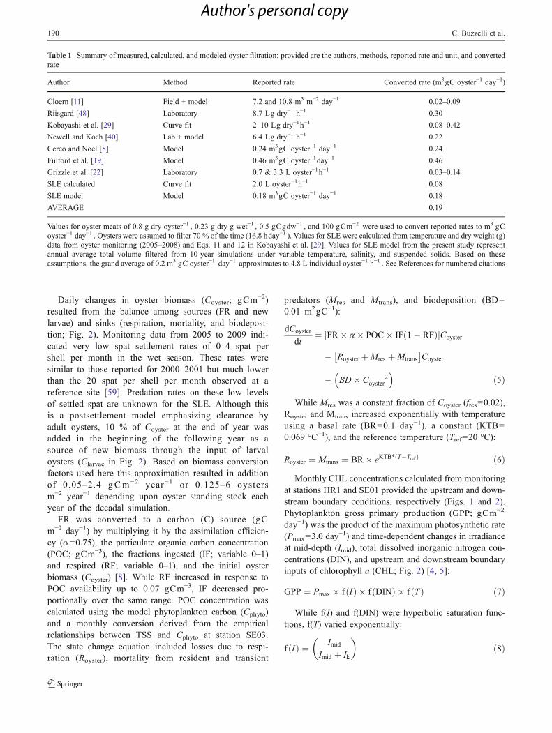
FR ¼ FRmax � f ðTÞ � f TSSð Þ � fðSÞ ð1ÞCompilation and conversion of reported filtration rates

resulted in a range from 0.1 to 0.46 m3gC oyster−1 day−1

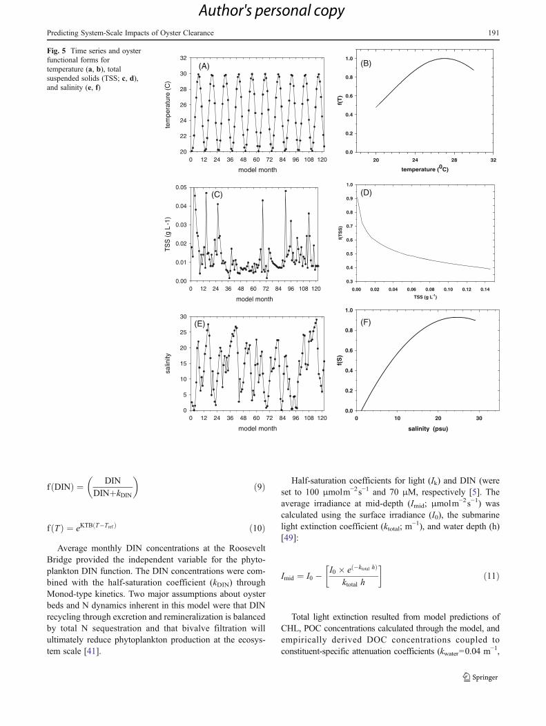
with an average of 0.2 m3gC oyster−1 day−1 (Table 1).Temperature varied between 20 and 30 °C between dryand wet seasons (Fig. 5a). The maximum filtration rate(FRmax; 0.55 m3gC oyster−1 day−1) was greatest at theoptimal temperature (Topt027 °C) before declining at higher

temperatures following an exponential temperature function(Fig. 5b) [8, 19, 29]:

f ðTÞ ¼ e �0:015 T�Toptð Þ2� �

ð2Þ

Monthly average suspended solid concentrations rangedfrom 0.002 to 0.053 and averaged 0.013 gL−1 (Fig. 5c). Thisconcentration range was used to calculate f(TSS) as in [58](Fig. 5d):

f TSSð Þ ¼ 1� 0:01log 10� TSSþ 3:38

0:0418

� �ð3Þ

Salinity was the third factor that influenced oyster FR.Average monthly salinity in the model varied from near0.0 ppt in 1998, 2004, and 2005 to >25 ppt in the dryseasons of 1999, 2001, and 2007 (Fig. 5e). The oystersalinity relationship was assumed to be maximized at themiddle range of salinity values [3, 55]. Oyster growth isgreatly reduced when salinity is <10 ppt, near zero whensalinity is <7.5 ppt, maximized at 20 ppt, and slowly re-duced at higher salinities [32, 58]. While different oyster-salinity functions have been used in modeling [8, 19, 58], anonlinear function was customized for the salinity valuesobserved in SLE monitoring (Fig. 5f):

f ðSÞ ¼ 0:0084S � 0:0017S2 � 0:1002 ð4Þ

Fig. 3 Time series of freshwater inflow (black) into and salinity (gray)for the Mid-Estuary of the SLE from 1 January 1988 to 31 December2007. While flow was the daily sum from four sources salinity atstation SE03 was averaged daily

Fig. 4 Results of oyster density monitoring in the Mid-Estuary of theSLE. Top panel includes gray seasonal bars for live oyster density(number/m2) and average monthly salinity values at the RooseveltBridge. Bottom panel reports oyster biomass (gCm−2) derived fromthe living density values using conversions reported in the text



Daily changes in oyster biomass (Coyster; gCm−2)resulted from the balance among sources (FR and newlarvae) and sinks (respiration, mortality, and biodeposi-tion; Fig. 2). Monitoring data from 2005 to 2009 indi-cated very low spat settlement rates of 0–4 spat pershell per month in the wet season. These rates weresimilar to those reported for 2000–2001 but much lowerthan the 20 spat per shell per month observed at areference site [59]. Predation rates on these low levelsof settled spat are unknown for the SLE. Although thisis a postsettlement model emphasizing clearance byadult oysters, 10 % of Coyster at the end of year wasadded in the beginning of the following year as asource of new biomass through the input of larvaloysters (Clarvae in Fig. 2). Based on biomass conversionfactors used here this approximation resulted in additionof 0.05–2.4 g Cm−2 year−1 or 0.125–6 oystersm−2 year−1 depending upon oyster standing stock eachyear of the decadal simulation.

FR was converted to a carbon (C) source (gCm−2 day−1) by multiplying it by the assimilation efficien-cy (α00.75), the particulate organic carbon concentration(POC; gCm−3), the fractions ingested (IF; variable 0–1)and respired (RF; variable 0–1), and the initial oysterbiomass (Coyster) [8]. While RF increased in response toPOC availability up to 0.07 gCm−3, IF decreased pro-portionally over the same range. POC concentration wascalculated using the model phytoplankton carbon (Cphyto)and a monthly conversion derived from the empiricalrelationships between TSS and Cphyto at station SE03.The state change equation included losses due to respi-ration (Royster), mortality from resident and transient

predators (Mres and Mtrans), and biodeposition (BD00.01 m2gC−1):

dCoyster

dt¼ FR� a � POC� IF 1� RFð Þ½ �Coyster

� Royster þMres þMtrans

� �Coyster

� BD� C 2oyster

� �ð5Þ

While Mres was a constant fraction of Coyster (fres00.02),Royster and Mtrans increased exponentially with temperatureusing a basal rate (BR00.1 day−1), a constant (KTB0

0.069 °C−1), and the reference temperature (Tref020 °C):

Royster ¼ Mtrans ¼ BR� eKTB* T�Trefð Þ ð6ÞMonthly CHL concentrations calculated from monitoring

at stations HR1 and SE01 provided the upstream and down-stream boundary conditions, respectively (Figs. 1 and 2).Phytoplankton gross primary production (GPP; gCm−2

day−1) was the product of the maximum photosynthetic rate(Pmax03.0 day−1) and time-dependent changes in irradianceat mid-depth (Imid), total dissolved inorganic nitrogen con-centrations (DIN), and upstream and downstream boundaryinputs of chlorophyll a (CHL; Fig. 2) [4, 5]:

GPP ¼ Pmax � f ðIÞ � f DINð Þ � f ðTÞ ð7Þ

While f(I) and f(DIN) were hyperbolic saturation func-tions, f(T) varied exponentially:

f ðIÞ ¼ Imid

Imid þ Ik

� �ð8Þ

Table 1 Summary of measured, calculated, and modeled oyster filtration: provided are the authors, methods, reported rate and unit, and convertedrate

Author Method Reported rate Converted rate (m3gC oyster−1 day−1)

Cloern [11] Field + model 7.2 and 10.8 m3 m−2 day−1 0.02–0.09

Riisgard [48] Laboratory 8.7 Lg dry−1 h−1 0.30

Kobayashi et al. [29] Curve fit 2–10 Lg dry−1h−1 0.08–0.42

Newell and Koch [40] Lab + model 6.4 Lg dry−1 h−1 0.22

Cerco and Noel [8] Model 0.24 m3gC oyster−1 day−1 0.24

Fulford et al. [19] Model 0.46 m3gC oyster−1day−1 0.46

Grizzle et al. [22] Laboratory 0.7 & 3.3 L oyster−1h−1 0.03–0.14

SLE calculated Curve fit 2.0 L oyster−1h−1 0.08

SLE model Model 0.18 m3gC oyster−1 day−1 0.18

AVERAGE 0.19

Values for oyster meats of 0.8 g dry oyster−1 , 0.23 g dry g wet−1 , 0.5 gCgdw−1 , and 100 gCm−2 were used to convert reported rates to m3 gCoyster−1 day−1 . Oysters were assumed to filter 70 % of the time (16.8 hday−1 ). Values for SLE were calculated from temperature and dry weight (g)data from oyster monitoring (2005–2008) and Eqs. 11 and 12 in Kobayashi et al. [29]. Values for SLE model from the present study representannual average total volume filtered from 10-year simulations under variable temperature, salinity, and suspended solids. Based on theseassumptions, the grand average of 0.2 m3 gC oyster−1 day−1 approximates to 4.8 L individual oyster−1 h−1 . See References for numbered citations



f DINð Þ ¼ DIN

DINþkDIN

� �ð9Þ

f ðTÞ ¼ eKTB T�Trefð Þ ð10Þ

Average monthly DIN concentrations at the RooseveltBridge provided the independent variable for the phyto-plankton DIN function. The DIN concentrations were com-bined with the half-saturation coefficient (kDIN) throughMonod-type kinetics. Two major assumptions about oysterbeds and N dynamics inherent in this model were that DINrecycling through excretion and remineralization is balancedby total N sequestration and that bivalve filtration willultimately reduce phytoplankton production at the ecosys-tem scale [41].

Half-saturation coefficients for light (Ik) and DIN (wereset to 100 μmolm−2s−1 and 70 μM, respectively [5]. Theaverage irradiance at mid-depth (Imid; μmolm−2s−1) wascalculated using the surface irradiance (I0), the submarinelight extinction coefficient (ktotal; m

−1), and water depth (h)[49]:

Imid ¼ I0 � I0 � e �ktotal hð Þ

ktotal h

� ð11Þ

Total light extinction resulted from model predictions ofCHL, POC concentrations calculated through the model, andempirically derived DOC concentrations coupled toconstituent-specific attenuation coefficients (kwater00.04 m−1,

TSS (g L-1)

0.00 0.02 0.04 0.06 0.08 0.10 0.12 0.14

f(T

SS

)

0.3

0.4

0.5

0.6

0.7

0.8

0.9

1.0

temperature (0C)

20 24 28 32

f(T

)

0.0

0.2

0.4

0.6

0.8

1.0

salinity (psu)

0 10 20 30

f(S

)

0.0

0.2

0.4

0.6

0.8

1.0

model month

0 12 24 36 48 60 72 84 96 108 120

salin

ity

0

5

10

15

20

25

30

model month

0 12 24 36 48 60 72 84 96 108 120te

mpe

ratu

re (

C)

20

22

24

26

28

30

32

model month

0 12 24 36 48 60 72 84 96 108 120

TS

S (

g L

-1)

0.00

0.01

0.02

0.03

0.04

0.05

(A)

(C)

(B)

(D)

(F)(E)

Fig. 5 Time series and oysterfunctional forms fortemperature (a, b), totalsuspended solids (TSS; c, d),and salinity (e, f)



kDOC00.055 m2gC−1, kPOC00.03 m

2gC−1, kCHL00.03 m2mg

CHL−1 [5, 20]):

ktotal ¼ kwater þ kDOC � DOC½ � þ kPOC � POC½ �þ kCHL � CHL½ � ð12Þ

The phytoplankton state change equation connected GPP,resuspension of sediment microalgae (SM), and phytoplank-ton carbon input from the upstream boundary (CHR1) to therespiratory (Rphyto), mortality (Mphyto), exudation (EXphyto),and sinking (Sphyto) loss terms:

dCphyto

dt¼ GPP� Cphyto

� �þ SM� Kresus � ASLEð Þ

þ CHR1 � Rphyto �Mphyto � EXphyto

� Sphyto � Xphyto ð13ÞSM was set to a constant value of 1.0 gCm−2. Respiration

and mortality were modeled similarly as for oysters exceptthat the basal rate was 0.1 day−1 for both loss processes. Thebaseline, temperature-dependent mortality rate for phyto-plankton increased linearly once oyster biomass reached50 gCm−2. Exudation or the dissipation of dissolved organiccarbon from phytoplankton was expressed as 35 % of GPPdaily. The Sphyto term resulted from Cphyto, h, and a sinkingcoefficient (ksink00.35 mday−1):

Sphyto ¼ Cphyto*ksin kh

ð14Þ

The final important process for phytoplankton biomassresulted from tidal exchange at the downstream oceanicboundary (Xphyto). The difference between the variable wa-ter level resulting from the M2 tide and the base elevationfor the SLE (z0−2.0 m) generated a value for depth (h).VSLE was calculated every time step as the product ofestuarine area (ASLE) and h. The difference in volume be-tween successive time steps (dVSLE) permitted calculation offlood vs. ebb tide (Xin vs. Xout) exchanges. The incomingflood tide mass of phytoplankton was the product of dVSLE

and carbon biomass at sampling station SE01 near the St.Lucie inlet (CSE01; Fig. 1). Conversely, the outgoing ebbtide mass of phytoplankton resulted from dVSLE and the insitu Cphyto mass:

Xin ¼ dVSLE � CSE01 ð15Þ

Xout ¼ dVSLE � Cphyto ð16Þ

Simulations and Model Output The model had an integra-tion interval of 6 h (dt00.25 day) generating CHL andCoyster values at daily, monthly, and annual intervals over

10-year simulations (1998–2007). Combining FR, averagebiomass values, and the area of oysters (Aoyster; m

2) provid-ed daily estimates of total volume filtered by oysters (Vfilter;m3day−1):

Vfilter ¼ FR� Coyster � Aoyster ð17Þ

The average daily volume of the middle segment of theSLE (VSLE; m

3) was divided by Vfilter to calculate the timerequired for oysters to filter the entire estuarine volume(Tfilter). Daily values for Tfilter were used to calculate annualaverages over the 10-year simulations. Since the current andprojected areas of oyster habitat are 81 and 567 ha, respec-tively, Aoyster was varied from 250,000 to 4,000,000 m2 (25–400 ha). This simulation series resulted in graphical relation-ships between Aoyster, Tfilter, Tphyto, and CHL used to quan-tify capacity of phytoplankton removal with oysterrestoration. Finally, the times required to replace the estua-rine volume (tidal prism method), the phytoplankton popu-lation (biomass/production or B/P ratio), and Tfilter werecompared and contrasted [33, 50]. Average values for eachof these three time values (days) were generated for eachmonth of the year in order to assess both inter- and intra-annual variations and relationships.

3 Results

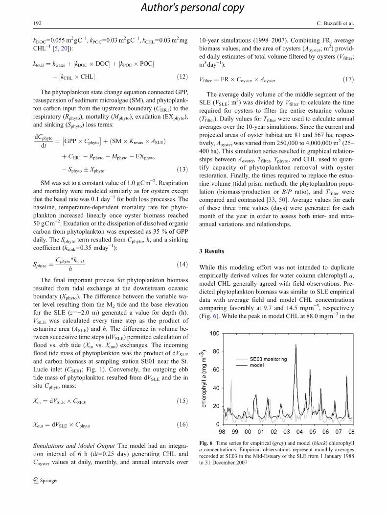
While this modeling effort was not intended to duplicateempirically derived values for water column chlorophyll a,model CHL generally agreed with field observations. Pre-dicted phytoplankton biomass was similar to SLE empiricaldata with average field and model CHL concentrationscomparing favorably at 9.7 and 14.5 mgm−3, respectively(Fig. 6). While the peak in model CHL at 88.0 mgm−3 in the

Fig. 6 Time series for empirical (gray) and model (black) chlorophylla concentrations. Empirical observations represent monthly averagesrecorded at SE03 in the Mid-Estuary of the SLE from 1 January 1988to 31 December 2007



wet season of 2003 was triggered by flow and increasednitrogen concentration, this peak was not evident in themonthly averages derived from the monitoring data.

Oyster biomass varied as a function of temperature andsalinity from near zero values following large freshwaterdischarge coupled with reduced phytoplankton biomass in2002–2003 to maximum values near 150.0 and 200.0 gCm−2 in the spring of 1999 and the fall of 2006, respectively(Fig. 7). There were 2 years of very low oyster biomass(2002–2003) until a modest recovery into early 2004. How-ever, consecutive very wet seasons of 2004 and 2005 re-duced oyster biomass again until 2006 when biomassfluctuated from 10 to 200 gCm−2 before falling to 50 gCm−2 in 2007 (Fig. 7). These fluctuations affected the accu-mulation of living oyster C biomass and thus the capacityfor filtration. The FR of individual oysters (m3gC oyster−1

day−1) was greatly reduced at low salinity values with oysterfiltration near zero during times of freshwater discharge (wetseason 1999, 2001, 2004, and 2005). Total volume filtered(Vfilter) and Tfilter were a function of both the oyster totalbiomass and Aoyster. However, these two indicator variablesare inversely related as Tfilter decreases proportionally to theincrease in Vfilter with increasing oyster biomass. Underbaseline Aoyster conditions of 50 ha, the volume filter rate

ranged from 7,019.6 to 2.4×107m3day−1 when oyster bio-mass was greatest (Table 2). This baseline range translatedto Tfilter00.1–1,428 days in the SLE from 1998 to 2007(Fig. 8).

The simplified physical model had an average tidal prismturnover time (Tprism) of 21.6 days (Table 2; Fig. 9). Tphytoranged from 1.1 to 94.0 days with an average of 15.6 days(Table 2). Phytoplankton turnover time was minimized (e.g.,fastest turnover) from May to November when the combi-nation of temperature, photoperiod, and nutrient availabilitywere optimal. On average, Tfilter (55.8 days) was greaterthan Tprism (21.6 days) or Tphyto (15.6 days), although aver-age Tfilter was similar to the physical and phytoplanktonturnover times from May to July when oyster biomass wasgreatest (Fig. 9).

Increasing Aoyster from 25 to 400 ha (2.5×105–4.0×106m2)had a great effect as Tfilter decreased exponentially (Fig. 10).This result suggested that increasing Aoyster to at least 2.5×10

6

m2 (250 ha) would substantially increase the daily volumefiltered. The Aoyster series provided a platform to link Tfilter toTphyto and calculate potential accommodation of phytoplank-ton productivity by oysters. While the relationship betweenCHL and Tphyto was negatively exponential, that betweenCHL and Tfilter was positively linear (Fig. 11a–e). Since Tfilterdecreased exponentially with Aoyster, the y-axes in Fig. 11 werestructured in order to graphically pinpoint the intersectionbetween Tphyto, Tfilter, and a critical CHL value (CHLcrit).The portion of the curve to the right of CHLcrit indicates thatphytoplankton biomass turnover is faster than consumptionthrough oyster filtration. To the left of CHLcrit suggests thatoyster filtration capacity is greater than phytoplanktonturnover.

Tphyto and Tfilter intersected at decreasing values of 22.0,20.8, 13.8, 10.2, and 9.5 days as Aoyster was increased from50 to 400 ha (Fig. 11). The critical CHL concentrationindicating the balance between phytoplankton productionand oyster consumption increased from 8.2 to 17.0 mgm−3

with Aoyster (Fig. 11 and Table 3). The decrease in Tphyto andincrease in CHLcrit resulted in an increase in the mass ofphytoplankton that oysters could accommodate daily from

Fig. 7 Time series of simulated model oyster biomass (black) andchlorophyll a concentration (gray) from 1 January 1988 to 31 Decem-ber 2007

Table 2 Descriptive statistics for estuarine volume and tidal prism, phytoplankton biomass, and oyster filtration

Vavg(m3)

Vprism

(m3)Tprism(day)

Ofilter (m3gC

oyster−1day−1)Vfilter

(m3day−1)Coyster

(gCm−2)Tfilter(day)

CHL(mgm−3)

Cphyto

(gCm−3)Tphyto(day)

Min 1.87×107 9.61×106 18.0 0.016 7,019.6 0.05 0.1 8.9 0.0 1.1

Max 2.22×107 1.35×107 27.0 0.370 2.4×107 200.0 1,428 136.2 6.8 94.0

Mean +SD

1.94×107±5.75×105

11.5×106±1.4×105

21.6±2.6 0.18±0.1 1.7×107±3.1×107

17.9±58.1 55.8±158.1 14.5±13.1 0.72±0.66 15.6±19.8

Included are average daily minimum, maximum, and mean ± standard deviation for average and tidal prism volumes of the St. Lucie Estuary (Vavgand Vprism), the tidal prism flushing time (Tprism), oyster biomass and filtration time (Coyster and Tfilter), and phytoplankton biomass (chlorophyll a orCHL and carbon or Cphyto) with population turnover time (Tphyto). Sample size for statistics was 3,650 from the 10-year simulation (3,650 Juliandays)



3.9×105 to 1.9×105gCday−1 (Table 3). Therefore, theeightfold increase in oyster area from 50 to 400 ha in theSLE resulted in an estimated five times more phytoplanktoncarbon that could be removed by oysters.

4 Discussion

Unintentional degradation of coastal ecosystems is a com-monly occurring side effect of providing flood control andwater supply for the coastal populace [53]. These socialprovisions historically have been implemented without re-gard for feedback relationships with downstream biota [1,17, 35, 60]. Unfortunately, oyster populations in the St.Lucie Estuary have been degraded by watershed actionsincluding increased impervious cover and management offreshwater supplies for a variety of stakeholders. The cumu-lative effect of this suite of anthropogenic factors is thereplacement of benthic seagrass and oyster habitats withwater column blooms and muck sediments [52].

Efforts are underway to restore some of this oyster habitatrelative to historical levels [47]. Previous studies suggestedthat quantification of filtration is an essential first step tounderstanding possible oyster restoration outcomes [18, 19,22, 25]. Simulation models integrating multiple environ-mental stressors facilitate such efforts in that they linkwatershed drivers to estuarine physical and biotic variablesallowing for feedback [19, 26, 56]. This monitoring andmodeling study illuminated relationships between water-shed inputs, physical transport, phytoplankton, and oysterbiomass relevant for the management of water and bioticresources.

Chlorophyll a concentrations represent the sum of importfrom the upstream river, nutrient loading and availability,residence time, vertical mixing and light penetration, andlosses through respiration, sinking, and grazing [7]. Thebalance between tidal range and river flow establishes thecirculation patterns that largely determine if allochthonousand autochthonous materials will remain in the estuary or beexported [15, 36, 50]. A comparatively long transport timecan enhance the cycling of carbon along the estuarine lengthallowing for biogeochemical cycling in the water columnand benthos [60]. However, the specific relationship be-tween phytoplankton biomass and transport time dependsupon the balance between biological production and con-sumption [33]. In any case, invocation of chlorophyll aconcentrations as an indicator of eutrophication does notalways reflect the rapidity of phytoplankton biomass turn-over. It is important that the time scales for physical trans-port, phytoplankton production, and phytoplanktonconsumption be quantitatively evaluated [33, 42, 43].

Modeling results suggest that carbon production andconsumption could be coupled in the SLE as the times

Fig. 8 Time series of salinity (gray line), simulated model oysterbiomass (black line), and oyster filtration time (Tfilter; filled bars) from1 January 1988 to 31 December 2007

days

0

20

40

60

80

100

120

140

160

180

Tprism

Tphyto

Tfilter

J F M MA J O N DJ A S

Fig. 9 Average monthly times (days) for tidal prism turnover (Tprism),phytoplankton biomass turnover (Tphyto), and oyster filtration (Tfilter)calculated from the 10-year simulations

Aoyster (m2)

0 1e+6 2e+6 3e+6 4e+6

time

to fi

lter

SLE

(d)

0

200

400

600

800

1000

1200

1400

)A*1.7x10(filter

oyster6

e*1887.6t

r2 = 0.93

=

Fig. 10 Relationship between the area of oysters (Aoyster) and the timeto filter (Tfilter) the Mid-Estuary segment of the SLE. The exponentiallydeclining fitted curve explained 93 % of the variance in the Tfilteraveraged over all years for each of the Aoyster simulation trials



required for phytoplankton turnover and oyster filtrationwere similar except in the months of August and Septemberwhen oyster biomass was least. The average water massturnover time (21.6 days) was similar to the 22.8–36.0 daysreported [16]. Doering [16] calculated that the SLE volumecould be replaced 10–16 times annually with similar esti-mates derived more recently using a three-dimensional hy-drodynamic model [27]. Except for times of extremefreshwater discharge (>3,000 ft3 s−107.5×106m3day−1),which can overwhelm biological processes by washing outan estuary [16], oyster restoration offers a renewed capacityto offset excessive phytoplankton production.

Restoration of benthic habitats at the appropriate scaleand location offers new possibilities for water qualityimprovements and estuarine fauna [19, 21, 44]. There are

three primary results of this modeling study relevant to thisstatement. First, given the time-scale similarity betweenphysical transport and biological processing, it is clear thatincreased area of live oysters could provide a sink for watercolumn phytoplankton and particulate matter [33, 43]. Sec-ond, increased area of healthy oysters would greatly reducethe time required to filter the entire estuary. In contrast tovoluminous estuaries such as Chesapeake Bay, small, shal-low estuaries like the SLE with fast water mass turnoverensure connectivity between channel and shoal environments.In fact, the middle segment of the SLE does not possess adistinct central channel but does have a water column contin-ually mixed through tides, wind, and inflow (D. Sun, personalcommunication). Approximately 50 % of the 87×106m2 areaof the middle segment is ≤−2.0 m contributing to an average

5 10 15 20 25 300

50

100

150

200

0

50

100

150

200

5 10 15 20 25 300

10

20

30

40

50

0

10

20

30

40

505 10 15 20 25 30

0

25

50

75

100

0

25

50

75

100

5 10 15 20 25 300

10

20

30

40

50

0

10

20

30

40

50

5 10 15 20 25 300

10

20

30

40

50

0

10

20

30

40

50

Chlorophyll a (mg m 3)-

T phy

to (d

)

T filt

er(d

)

(A) 50 ha oyster beds

(B) 100 ha oyster beds

(C) 200 ha oyster beds

(D) 300 ha oyster beds

Tphyto

Tfilter

(E) 400 ha oyster beds

Fig. 11 Relationships betweenphytoplankton turnover time(Tphyto), oyster filtration time(Tfilter), and water columnchlorophyll a concentrations fora series of oyster areas (Aoyster)ranging from 50 ha (top panel)to 400 ha (bottom panel). Seetext for description andinterpretation of graphicalapproach



depth of −2.7 m for the segment [6]. Assuming muck removalwhere appropriate, the oyster habitat restoration goal for theentire SLE is 980 acres or 24×106 m2, which is 55 % of thearea ≤−2.0 m [47]. Given these attributes of the estuary,increased area of oyster habitat appears to be favorable forwater quality improvements. However, the determination ofthe best distribution and density of restoration has importanttrophic implications.

Oyster bed restoration in excess of optimal levels couldstimulate eutrophication by increasing net remineralizationand oxygen consumption [8, 41]. Oyster beds actively re-lease dissolved N (e.g., NH4

+) through the combination offaunal excretion and microbial recycling [13]. Reduced flowand high biodeposit concentrations enhance microbial oxy-gen and nitrate utilization to release dissolved N and P fromthe benthos [39]. Depending upon the density and distribu-tion of beds, oyster habitat restoration has the potential togreatly influence biogeochemical attributes downstream[19]. However, the influence of oysters upstream couldrange from decreased inputs of phytoplankton and sus-pended solids to the loading of inorganic N and P to thedownstream estuary.

The implications of successful oyster restoration also de-pend upon the factors that limit primary production along theestuarine gradient (light, nutrients, transport, and grazing). Forexample, there is the possibility that successful restoration ofoyster habitat could perpetuate estuarine eutrophication if notexecuted at the appropriate scale and density of organisms.While the present model did not fully account for potentialecosystem level nutrient feedbacks with oyster restoration,results demonstrated that increasing Aoyster beyond 250 hawould not significantly shrink the time to filter the SLE(Fig. 10). This approximation provides a quantitative targetfor the scale of oyster restoration based on oyster survival,growth, and net filtration at the ecosystem scale.

Successful re-establishment of oyster habitats at the ap-propriate scale would lead to the third result as the capacityfor oysters to accommodate phytoplankton derived carbonwould increase several fold [11, 19, 21]. This capacity maybe limited through density dependence given the negativefeedback between the production of new phytoplanktonbiomass and consumption by the existing oyster population[46]. The creation of new estuarine habitat is significant toecosystem trophic structure as the enhanced benthic sub-strate of living oysters and biodeposits offers surface areafor spat fall and reef expansion, secondary production oflocal epibiotic communities, and tertiary production of res-ident and transient fauna [44, 54].

Several caveats must be explored to optimize the model-ing process and its value to oyster restoration in the SLE.The present study developed a postsettlement model ofoysters within a single, spatially aggregated, mid-estuarybasin of homogeneous depth. Future versions will includegrowth cohorts representing larval, juvenile, and adult oys-ters, spatially variable bathymetry, and submodels for eachof the four major segments of the SLE (inlet, mid-estuary,South Forks, and North Forks). Development of a segment-ed estuary model will allow investigations of potential bio-geochemical relationships between segments with andwithout oyster habitat. While inclusion of both disease anddifferent larval stages are desirable to accurately representoyster population dynamics, model uncertainty derives froman overall lack of understanding of larval recruitment anddisease processes in natural populations [34]. This is partic-ularly true given the paucity of historical oyster data in southFlorida and highlights the simplicity and value of the pres-ent model design. Variable basin depth and circulation aresignificant since site location for oyster restoration mustconsider spat fall dynamics as well as potential connectivitywith the location of phytoplankton maxima in the estuary[19, 42].

Finally, given that oysters respond to the concentrationsof total suspended solids (TSS), which are part of watercolumn-sediment N cycling, future versions will includestate variables for TSS and N [5]. Variable turbidity, theimport and redistribution of fine grained sediments, andvariable composition of water column particulate matterare key characteristics of the SLE [9, 16, 52]. Algal produc-tivity in Florida estuaries is generally light and not nutrientlimited [37]. This is significant because light attenuation inthe south Florida estuaries is largely modulated by a com-bination of colored dissolved organic matter from freshwa-ter discharge and turbidity due to suspended inorganicmaterial [9, 10, 16]. Thus, in contrast to Chesapeake Bayand other temperate estuaries, the removal of TSS throughoyster filtration may not necessarily improve light for theexpansion of submersed vegetation and benthic microalgaewith restoration of the St. Lucie Estuary [40].

Table 3 Effects of oyster bed area (Aoyster; ha) on capacity of oysterfiltration to accommodate phytoplankton production

Aoyster Tphyto0Tfilter CHLacc PHYcrit

50 22.0 8.2 3.9×105

100 20.0 11.3 5.9×105

200 13.8 14.1 1.1×106

300 10.2 15.7 1.6×106

400 9.5 17.0 1.9×106

The restoration target for Aoyster in the SLE is 365 ha (902 acres [52]).Summary derived from information in Fig. 10, which provides timeand chlorophyll a critical values (CHLcrit; mgm−3 ) where phytoplank-ton turnover (Tphyto; days) equals time required for oysters to filter theSLE volume (Tfilter; days). Potential phytoplankton mass accommoda-tion rate (PHYcrit; gCday−1 ) was calculated from the CHLcrit, Tphyto,the C/CHL (50:1), and an average SLE volume of 2.1×107 m3 . Theaverage tidal prism flushing time (Tprism) for the SLE was 21.6 days



Acknowledgments This study was supported by the South FloridaWater Management District (SFWMD), Coastal Ecosystems Division.We would like to thank Detong Sun and Chenxia Qiu for discussionsabout circulation processes in Florida estuaries. Roger Newell and CarlCerco provided insight into oyster filtration and modeling approaches,respectively. Amanda MacDonald and Christopher Madden providedassistance in development of the phytoplankton and oyster models.Olga Cruz and Enrique Reyes provided essential literature for modelcalibration. Nenad Irichanin and Vincent Encomio provided SLE waterquality data and information about SLE oyster restoration, respectively.Cecelia Conrad performed the geographic tasks and produced Fig. 1.Finally, we would like to thank Mayra Ashton and Miao-Li Chang atthe SFWMD and two anonymous reviewers for their comments on themanuscript.

References

1. Alber, M. (2002). A conceptual model of estuarine freshwaterinflow management. Estuaries, 25, 1246–1261.

2. Barnes, M., Volety, A., Chartier, K., Mazzotti, F. J., & Pearlstine,L. (2007). A habitat suitability index model for the eastern oyster(Crassostrea virginica) , a tool for restoration of theCaloosahatchee Estuary, Florida. Journal of Shellfish Research,26, 949–959.

3. Buzan, D., Lee, W., Culbertson, J., Kuhn, N., & Robinson, L.(2009). Positive relationship between freshwater inflow and oysterabundance in Galveston Bay, Texas. Estuaries & Coasts, 32, 206–212.

4. Buzzelli, C. P., Childers, D. L., Dong, Q., & Jones, R. D. (2000).Simulation of periphyton phosphorus dynamics in EvergladesNational Park. Ecological Modelling, 134, 103–115.

5. Buzzelli, C. (2008). Development and application of tidal creekecosystem models. Ecological Modelling, 210, 127–143.

6. Buzzelli, C., Chen, Z., Coley, T., Doering, P.., Samimy, R.,Schlezinger, D., Howes, B. (2012). Dry season sediment–waterexchanges of nutrients and oxygen in two Florida estuaries: pat-terns, comparisons, and internal loading. Florida Scientist, in press

7. Cerco, C. F. (2000). Phytoplantkon kinetics in the Chesapeake Bayeutrophication model. Water Quality and Ecosystem Modeling, 1,5–49.

8. Cerco, C. F., & Noel, M. R. (2007). Can oyster restoration reversecultural eutrophication in Chesapeake Bay? Estuaries & Coasts,30, 331–343.

9. Chamberlain, R., & Hayward, D. (1996). Evaluation of waterquality and monitoring in the St. Lucie Estuary, Florida. Journalof the American Water Resources Association, 32, 681–696.

10. Christian, D., & Sheng, Y. P. (2003). Relative influence of variouswater quality parameters on light attenuation in Indian RiverLagoon. Estuarine, Coastal, & Shelf Science, 57, 961–971.

11. Cloern, R. A. (1982). Does the benthos control phytoplanktonbiomass in south San Francisco Bay? Marine Ecology ProgressSeries, 9, 191–202.

12. Coen, L. D., Brumbaugh, R. D., Bushek, D., Grizzle, R. E.,Luckenbach, M. W., Posey, M. H., et al. (2007). Ecosystem serv-ices related to oyster restoration. Marine Ecology Progress Series,341, 303–307.

13. Dame, R. F., Spurrier, J. D., & Wolaver, T. G. (1989). Carbon,nitrogen, and phosphorus processing by an oyster reef. MarineEcology Progress Series, 54, 249–256.

14. Dekshenieks, M. M., Hofmann, E. E., Klinck, J. M., & Powell, E.N. (2000). Quantifying the effects of environmental change on anoyster population: a modeling study. Estuaries, 23, 593–610.

15. Dettmann, E. H. (2001). Effect of water residence time on annualexport and denitrification of nitrogen in estuaries: a model analy-sis. Estuaries, 24, 481–490.

16. Doering, P. H. (1996). Temporal variability of water quality in theSt. Lucie Estuary, South Florida. Water Resources Bulletin, 32,1293–1306.

17. Estevez, E. D. (2002). Review and assessment of biotic variablesand analytical methods used in estuarine inflow studies. Estuaries,25, 1291–1303.

18. French-McCay, D. P., Peterson, C. H., DeAlteris, J. T., & Catena,J. (2003). Restoration that targets function as opposed to structure:replacing lost bivalve filtration ande production. Marine EcologyProgress Series, 264, 197–212.

19. Fulford, R. S., Breitburg, D. L., Newell, R. I. E., Kemp, W. M., &Luckenbach, M. (2007). Effects of oyster population restorationstrategies on phytoplankton biomass in Chesapeake Bay: a flexiblemodeling approach. Marine Ecology Progress Series, 336, 43–61.

20. Gallegos, C. L. (2001). Calculating optical water quality targets torestore and protect submersed aquatic vegetation: overcomingproblems in partitioning the diffuse attenuation coefficient forphotosynthetically active radiation. Estuaries, 24, 381–397.

21. Gerritsen, J., Holland, A. F., & Irvine, D. E. (1994). Suspension-feeding bivalves and the fate of primary production: an estuarinemodel applied to Chesapeake Bay. Estuaries, 17, 403–416.

22. Grizzle, R. E., Greene, J. K., & Coen, L. D. (2008). Sestonremoval by natural and constructed inter-tidal eastern oyster(Crassostrea virginica) reefs: a comparison with previous labora-tory studies and the value of in situ methods. Estuaries & Coasts,31, 1208–1220.

23. Haven, D. S., & Morales-Alamo, R. (1966). Aspects of biodepo-sition by oyster and other invertebrate filter feeders. Limnology &Oceanography, 11, 487–498.

24. Herman, P. M. J., & Scholten, H. 1990. Can suspension feedersstabilize estuarine ecosystems? In: M. Barnes & R.N. Gibson (ed.),24th European Marine Biology Symposium (pp. 104–116).Aberdeen: Aberdeen University Press.

25. Hofmann, E. E., Klinck, J. M., Powell, E. N., Boyles, S., &Ellis, M. S. (1994). Modeling oyster populations. II. Adultsize and reproductive effort. Journal of Shellfish Research, 13,165–182.

26. Hunt, M. J., & Doering, P. H. (2005). Significance of consideringmultiple environmental variables when using habitat as an indica-tor of estuarine condition. In S. Bortone (Ed.), Estuarine indicators(pp. 211–227). Boca Raton: CRC.

27. Ji, Z.-G., Hu, G., Shen, J., & Wan, Y. (2007). Three-dimensionalmodeling of hydrodynamics processes in the St. Lucie Estuary.Estuarine, Coastal, & Shelf Science, 73, 188–200.

28. Kemp, W. M., Boynton, W. R., Adolf, J. E., Boesch, D. F.,Boicourt, W. C., Brush, G., et al. (2005). Eutrophication ofChesapeake Bay: historical trends and ecological interactions.Marine Ecology Progress Series, 303, 1–29.

29. Kobayashi, M., Hofmann, E. E., Powell, E. N., Klinck, J. M., &Kusaka, K. (1997). A population dynamics model for the Japaneseoyster, Crassostrea gigas. Aquaculture, 149, 285–321.

30. LaPeyre, M. K., Nickens, A. D., Volety, A. K., Tolley, S. G., &LaPeyre, J. E. (2003). Environmental significance of freshets inreducing Perkinsus marinus infection in eastern oysters Crassotreavirginia: potential management applications. Marine EcologyProgress Series, 248, 165–176.

31. Livingston, R. J., Lewis, F. G., Woodsum, G. C., Niu, X.-F.,Galperin, B., Huang, W., et al. (2000). Modelling oyster popula-tion response to variation in freshwater input. Estuarine, Coastal,& Shelf Science, 50, 655–672.

32. Loosanoff, V. L. (1953). Behavior of oysters in water of lowsalinities. Proceedings of the National Shellfish Association, 43,135–151.



33. Lucas, L. V., Thompson, J. K., & Brown, L. R. (2009). Why arediverse relationships observed between phytoplankton biomassand transport time? Limnology & Oceanography, 54, 381–390.

34. Mann, R., & Powell, E. N. (2007). Why oyster restoration goals inthe Chesapeake Bay are not and probably cannot be achieved.Journal of Shellfish Research, 26, 905–917.

35. Mattson, R. (2002). A resource-based framework for establishingfreshwater inflow requirements for the Suwannee River Estuary.Estuaries, 25, 1333–1342.

36. Monbet, Y. (1992). Control of phytoplankton biomass in estuaries:a comparative analysis of microtidal and macrotidal estuaries.Estuaries, 15, 563–571.

37. Murrell, M. C., Campbell, J. G., Hagy, J. D., & Caffrey, J. M.(2009). Effects of irradiance on benthic and water column process-es in a Gulf of Mexico estuary: Pensacola Bay, Florida, USA.Estuarine, Coastal, & Shelf Science, 81, 501–512.

38. Newell, R. I. E., & Langdon, C. J. (1996). Mechanisms andphysiology of larval and adult feeding. In V. S. Kennedy, R. I. E.Newell, & A. Eble (Eds.), The eastern oyster (Crassostrea virgin-ica). College Park: Maryland Sea Grant College Program.

39. Newell, R. I. E. (2004). Ecosystem influences of natural andcultivated populations of suspension feeding bivalve molluscs: areview. Journal of Shellfish Research, 23, 51–61.

40. Newell, R. I. E., & Koch, E.W. (2004). Modeling seagrass density anddistribution in response to changes in turbidity stemming from bivalvefiltration and seagrass sediment stabilization. Estuaries, 27, 793–806.

41. Newell, R. I. E., Fisher, T. R., Holyoke, R. R., & Cornwell, J. C.(2005). Influence of eastern oyster on nitrogen and phosphorusregeneration in Chesapeake Bay, USA. In R. Dame & S. Olenin(Eds.), The comparative roles of suspension feeders in ecosystems.Heidelberg: Springer.

42. Newell, R. I. E., Kemp, W. M., Hagy, J. D., Cerco, C. F., Testa, J.M., & Boynton, W. R. (2007). Top–down control of phytoplanktonby oysters in Chesapeake Bay, USA: comment on Pomeroy et al.(2006). Marine Ecology Progress Series, 341, 293–298.

43. Officer, C. B., Smayda, T. J., & Mann, R. (1982). Benthic filterfeeding: a natural eutrophication control.Marine Ecology ProgressSeries, 9, 203–210.

44. Peterson, C. H., Grabowski, J. H., & Powers, S. P. (2003).Estimated enhancement of fish productoin resulting from restoredoyster reef habitat: quantitative valuation. Marine EcologyProgress Series, 264, 249–264.

45. Pomeroy, L. R., D’Elia, C. F., & Schaffner, L. C. (2006). Limits totop-down control of phytoplankton by oysters in Chesapeake Bay.Marine Ecology Progress Series, 325, 301–309.

46. Powell, E. N., Klinck, J. M., Hofmann, E. E., Wilson, E. A., &Ellis, M. S. (1995). Modeling oyster populations. V. Decliningphytoplankton stocks and population dynamics of American oyster(Crassostrea virginica). Fisheries Research, 24, 199–222.

47. RECOVER (2004). Comprehensive Monitoring and AssessmentPlan: Part 1 Monitoring and Supporting Research. RestorationCoordination and Verification Program, c/o United States ArmyCorps of Engineers, Jacksonville, FL, and, South Florida WaterManagement District, West Palm Beach, FL.

48. Riisgard, H. U. (1988). Efficiency of particle retention and filtra-tion rate in 6 species of northeast American bivalves. MarineEcology Progress Series, 45, 217–223.

49. Robson, B. J. (2005). Representing the effects of diurnal variationsin light on primary production on a seasonal time scale. EcologicalModelling, 186, 358–365.

50. Sheldon, J. E., & Alber, M. (2006). The calculation of estuarineturnover times using freshwater fraction and tidal prism methods: acritical evaluatioin. Estuaries and Coasts, 29, 133–146.

51. Shumway, S. E. (1996). Natural environmental factors. In V. S.Kennedy, R. I. E. Newell, & A. Eble (Eds.), The eastern oyster(Crassostrea virginica). College Park: Maryland Sea Grant College.

52. Sime, P. (2005). St. Lucie Estuary and Indian river lagoon concep-tual ecological model. Wetlands, 25, 898–907.

53. Sklar, F. H., & Browder, J. A. (1998). Coastal environmentalimpacts brought about by alterations to freshwater flow in theGulf of Mexico. Environmental Management, 22, 547–562.

54. Tolley, S. G., Volety, A. K., Savarese, M., Walls, L. D., Linardich,C., & Everham, E. M. (2006). Impacts of salinity and freshwaterinflow on oyster-reef communities in Southwest Florida. AquaticLiving Resources, 19, 371–387.

55. Turner, R. E. (2006). Will lowering estuarine salinity increase Gulfof Mexico oyster landings? Estuaries & Coasts, 29, 345–352.

56. Ulanowicz, R. E., & Tuttle, J. H. (1992). The trophic consequences ofoyster stock rehabilitation in Chesapeake Bay. Estuaries, 15, 298–306.

57. Urban, D. L. (2006). A modeling framework for restoration ecol-ogy. In D. A. Falk, M. A. Palmer, & R. J. Hobbs (Eds.),Foundations of restoration ecology. Boca Raton: Island Press.

58. Wang, H., Huang, W., Harwell, M. A., Edmiston, L., Johnson, E.,Hseih, P., et al. (2008). Modeling oyster growth rate by couplingoyster population and hydrodynamic models for Apalachicola Bay.Ecological Modelling, 211, 77–89.

59. Wilson, C., Scotto, L., Scarpa, J., Volety, A., Laramore, S., &Haunert, D. (2005). Survey of water quality, oyster reproduction,and oyster health status in the St. Lucie Estuary. Journal ofShellfish Research, 24, 157–165.

60. Wolanski, E., Boorman, L. A., Chicharo, L., Langlois-Saliou, E.,Lara, R., Plater, A. J., et al. (2004). Ecohydrology as a new tool forsustainable management of estuaries and coastal waters. WetlandEcology & Management, 12, 235–276.

61. Woodward-Clyde International Americas. (1998). St. LucieEstuary Historical SAV and American Oyster Literature. FinalReport, South Florida Water Management District, West PalmBeach, Florida.



Predicting System-Scale Impacts of Oyster Clearance on Phytoplankton Productivity in a Small Subtropical Estuary

Documents