Relationship between photosynthetic parameters and different proxies of phytoplankton biomass in the subtropical ocean

Biogeosciences, 4, 853–868, 2007www.biogeosciences.net/4/853/2007/© Author(s) 2007. This work is licensedunder a Creative Commons License.

Biogeosciences

Relationship between photosynthetic parameters and differentproxies of phytoplankton biomass in the subtropical ocean

Y. Huot1, M. Babin1, F. Bruyant2, C. Grob4, M. S. Twardowski3, and H. Claustre1

1CNRS, Laboratoire d’Oceanographie de Villefranche, 06230 Villefranche-sur-Mer, France; Universite Pierre et MarieCurie-Paris 6, Laboratoire d’Oceanographie de Villefranche, 06230 Villefranche-sur-Mer, France2Dalhousie University, Department of Oceanography, 1355 Oxford Street, Halifax N.S. B3H 4J1, Canada3WET Labs, Inc., Department of Research, 165 Dean Knauss Dr., Narragansett, RI 02882, USA4Graduate Program in Oceanography, Department of Oceanography and Center for Oceanographic Research in the easternSouth Pacific, University of Concepcion, Casilla 160-C, Concepcion, Chile

Received: 20 February 2007 – Published in Biogeosciences Discuss.: 1 March 2007Revised: 7 September 2007 – Accepted: 22 September 2007 – Published: 16 October 2007

Abstract. Probably because it is a readily available oceancolor product, almost all models of primary productivity usechlorophyll as their index of phytoplankton biomass. Asother variables become more readily available, both from re-mote sensing and in situ autonomous platforms, we shouldask if other indices of biomass might be preferable. Herein,we compare the accuracy of different proxies of phytoplank-ton biomass for estimating the maximum photosynthetic rate(Pmax) and the initial slope of the production versus irradi-ance (P vs. E) curve (α). The proxies compared are: the totalchlorophyll a concentration (Tchla, the sum of chlorophylla and divinyl chlorophyll), the phytoplankton absorption co-efficient, the phytoplankton photosynthetic absorption coef-ficient, the active fluorescence in situ, the particulate scat-tering coefficient at 650 nm (bp (650)), and the particulatebackscattering coefficient at 650 nm (bbp (650)). All of thedata (about 170 P vs. E curves) were collected in the SouthPacific Ocean. We find that when only the phytoplanktonicbiomass proxies are available,bp (650) and Tchla are respec-tively the best estimators ofPmax andα. When additionalvariables are available, such as the depth of sampling, theirradiance at depth, or the temperature, Tchla is the best es-timator of bothPmax andα.

Correspondence to:Y. Huot([email protected])

1 Introduction

Photosynthesis (P ) in the ocean can be conveniently de-scribed using two basic quantities: the phytoplanktonbiomass (B), and the photosynthetic rates per unit biomassP B; P=BP B. Both quantities can be measured in situ andare highly variable. To obtain global estimates of productiv-ity, however, these quantities must be estimated for all oceansand with sufficient temporal resolution and this cannot beachieved by shipboard sampling. Because phytoplankton ab-sorption changes the color of the light leaving the ocean,B can be obtained accurately using satellite imagery (usingchlorophylla as a proxy). SinceP B cannot be measured onlarge scales continuously, an alternative method must be usedto estimate it. Finding an appropriate method has proven dif-ficult. Indeed, despite years of research, its estimate remainsthe largest uncertainty in our models of oceanic primary pro-duction.

The main variable influencingP B is the incident irradi-ance. Describing this influence is relatively simple as itcan be mathematically represented by a saturating function(Falkowski and Raven, 1997): the so-called PvsE curve.This function can be parameterized using two parameters:αB [usually mgC (mgChl)−1 h−1 (µmol photon m−2 s−1)−1]which describes the initial slope; andP B

max [usually mgC(mgChl)−1 h−1] which describes the amplitude of the light-saturated plateau. IfP B

max and αB are known, the influ-ence of incident light onP B is known. The most diffi-cult aspect is the prediction of variability inP B

max and αB

that originates from changes in the physiological state (i.e.

Published by Copernicus Publications on behalf of the European Geosciences Union.

854 Y. Huot et al.: Proxies of biomass for primary production

photoacclimation and nutritional status) of phytoplankton orin the species composition of the community.

On the one hand, it has long been observed that ifP Bmax is

normalized to carbon (B=carbon),P Bmax is almost indepen-

dent of the growth irradiance, reflecting a parallel physiolog-ical adjustment of the maximal capacity to fix carbon and thecellular carbon quota. On the other hand, normalization bychlorophyll a shows lower values at low growth irradiancereflecting photoacclimation processes. In an opposite fash-ion, the light limited portion of the curve, when normalizedto chlorophylla, is largely independent of growth irradiance,but varies due to photoacclimation when normalized to car-bon. The ubiquitous nature of these relationships for mostalgal groups has been reviewed by MacIntyre et al. (2002),and several growth and photoacclimation models have beenbuilt to match these observations. It results that, to removean important source of physiological variability, that due tophotoacclimation, and to obtain photosynthetic parametersthat are independent of growth irradiance, carbon is a betterquantity to normalize the light saturated rates and chlorophylla is better to normalize the light limited part of the curve.

Unfortunately, a direct measure of phytoplankton carbonin situ or from remote sensing does not exist, such that allmodels of primary productivity published to date use chloro-phyll a to normalize bothαB andP B

max. Since variability inthe biomass-normalized depth-integrated primary productionis thought to be mostly driven by the light-saturated rate ofphotosynthesis (Behrenfeld and Falkowski, 1997), progressin predictingP B

max is central to estimating oceanic primaryproduction more accurately.

Therefore, if carbon could be measured or estimated ac-curately, phytoplankton carbon might provide a good al-ternative for these models. Recently, Behrenfeld and col-leagues (Behrenfeld et al., 2005; Behrenfeld and Boss, 2003,2006) suggested that light scattering could provide an accu-rate proxy of phytoplankton carbon. These suggestions havebrought to the forefront questions regarding the interpreta-tion of these optical parameters. Though it has long beenknown that the beam attenuation coefficient (cp, m−1) is agood proxy of the total particulate organic carbon (POC) incase 1 waters (Morel, 1988; Gardner et al., 2006, and refer-ences therein), the suggestion of Behrenfeld and Boss (2003)that it represents an accurate proxy of phytoplankton car-bon merits further research. In a similar way, the particu-late backscattering coefficient (bbp, m−1), which can be ob-tained from satellite remote sensing, has been used to esti-mate the concentration of POC (Stramski et al., 1999). Morerecently, Behrenfeld et al. (2005) based on a good correlationbetweenbbp and chlorophylla proposed the utilization of thebackscattering coefficient to estimate the phytoplankton car-bon over large space and time scales. Aware that the sourcesof backscattered light in the ocean remain unknown (Stram-ski et al., 2004), we will examine here bothbbp andcp aspotential alternatives to Tchla for constraining the variabilityof photosynthetic parameters. In this analysis, because mea-

surements of the scattering coefficient (bp, m−1), are avail-able, we will use them instead ofcp, sincecp is generallyused as a surrogate forbp.

Another proxy of biomass examined herein is phytoplank-ton absorption (aphy, m−1). Indeed it has sometimes beenargued thataphy is preferable to Tchla for studies of pri-mary productivity (Perry, 1994; Lee et al., 1996; Marra etal., 2007). The basis for this proposition is thataphy is moredirectly linked both to the remote sensing signal and pho-tosynthetic processes than Tchla (Perry, 1994). The evi-dence for this suggestion is, however, still lacking on largeoceanic scales. Other potentially useful measures exam-ined in this paper are the: photosynthetic absorption (aps ,m−1) which encompasses all and only the photosyntheticpigments; chlorophylla fluorescence, which is due to theabsorption by all photosynthetic pigments and has the ad-vantage of being readily measured in the ocean with hightemporal and spatial resolution but is strongly affected bythe physiological state of the algae; and, finally, picophyto-plankton biovolume obtained by flow cytometry.

After providing some background to give a mechanisticbasis for the interpretation of the photosynthetic parameters,we will use straightforward analyses to verify if any of thesebiomass proxies can be substituted for Tchla to obtain betterpredictions of the phytoplankton photosynthetic parameters.Our study will use a dataset obtained during the BIOSOPEcruise. This cruise encompassed a large range of trophicconditions from the hyperoligotrophic waters of the SouthPacific Gyre to the eutrophic conditions associated with theChile upwelling region, also investigating the mesotrophicHNLC (high nutrient low chlorophyll) waters of the sube-quatorial region and in the vicinity of the Marquesas Islands.We verify that the relationships obtained are applicable toother regions by comparing our results with those obtainedduring the PROSOPE cruise which sampled the Moroccanupwelling and the Mediterranean sea.

2 Background

To quantitatively evaluate potential alternatives to Tchla andinterpret them within a more general and fundamental frame,we use the knowledge from theory and laboratory experi-ments that allows us to describe the photosynthetic param-eters before normalization to biomass, that isPmax and notP B

max andα notαB.ThePmax depends on the concentration (nslowest, m−3) and

the average maximum turnover time (τslowest, s atoms−1) ofthe slowest constituent pool in the photosynthetic reactionchain,

Pmax = 7.174× 10−17nslowest

τslowest, (1)

where 7.174×10−17 mg C atoms−1 s h−1 is the conversionfactor from seconds to hours and mg of carbon to atoms.

Biogeosciences, 4, 853–868, 2007 www.biogeosciences.net/4/853/2007/

Y. Huot et al.: Proxies of biomass for primary production 855

Alternatively,Pmax can also be related to an instantaneousmaximum carbon specific growth rate (µmax, d−1) realizedunder saturating irradiance (neglecting respiration and otherlosses) asPmax=Cphyµmax

/DD, whereD is the daylength

(hours per day) andCphy the phytoplankton carbon (mg Cm−3). This growth rate is an overestimate of the 24-h growthrate since it is valid only under saturating conditions that arenot present throughout the day. To analyze our results we willmostly use the representation given in Eq. (1) as it providesa mechanistic explanation of the processes influencingPmax.

The two formulations are equivalent sinceCphyµmax=cte

(nslowest

/τslowest

), where cte is a pro-

portionality constant.The initial slope of the photosynthesis irradiance curve is

given by the product of the spectrally weighted photosyn-thetic absorption (m−1),

aps =

700∫400

aps (λ)o

E (λ) dλ

/ 700∫400

o

E (λ) dλ, (2)

and the maximum quantum yield of carbon fixation for pho-tons absorbed by photosynthetic pigments (ϕ

ps

C max, mol C[mol photons absorbed]−1) as follows:

α = 43.2apsϕps

C max. (3)

In Eq. (3), the factor 43.2 mg C mol C−1 mol photonsµmolphotons−1 s h−1 accounts for the conversion from seconds tohours,µmol photons to mol photons, and mg C to mol C.

Thusnslowestandaps are measures of biomass (both scalewith the number of cells), the first representing the concen-tration of slowest molecule in water and the second providinga good proxy of the concentration of pigmented molecule.Therefore, bothPmax and α are described by a different“amount” or “biomass” term (nslowest and aps), and a termthat encompasses variability in the physiological or photo-synthetic efficiency (τslowest andϕ

ps

C max). It follows that, intheory, the best index of phytoplankton biomass for the sakeof estimating primary production arenslowest for the light-saturated region of the curve, andaps for the light-limitedregion of the curve. The exact nature ofnslowest, however, re-mains largely unknown in the ocean (though the RUBISCOenzyme is often considered the slowest pool; Sukenic et al.,1987).

To assess the accuracy with which different proxies ofphytoplankton biomass allow us to retrieve the photosyn-thetic parameters, we will use non-linear regression analy-ses where we will compare directlyPmax andα to proxies ofbiomass measured in situ. The trend line will provide theaverage relationship while the variability around the trendline will provide an estimate of the accuracy with which eachproxy of biomass retrieves the “biomass component” ofPmaxandα, namelynslowestandaps . The non-linearity of the re-lationships will allow us to account for second order effects,

which would be not easy using normalized values withoutencountering potential statistical biases (Berges, 1997).

To understand the source of variability around our re-gression line, it is useful to represent equations 1 and3 above in terms of normalized quantities. Essentially,the variability around the mean normalized value willbe similar to the variability around our regression (be-cause we use non-linear regression with an intercept theyare not exactly equivalent). Normalization ofPmax todifferent proxies of phytoplankton biomass (B) leads toP B

max=7.174×10−17[

nslowestB

] 1τslowest

, and the same normal-

ization forα leads toαB=43.2

[aps

B

]ϕ

ps

C max. Since the vari-

ability in ϕps

C max andτslowestshould not be related toB, nor-malization byB removes most of the variability inPmaxandα originating from changes in biomass (i.e. making theterm in the square brackets nearly constant). Any proxy ofbiomass that covaries withaps andnslowestwill remove someof the variability, but proxies that account for a greater frac-tion of the variability will perform best. For example, nor-malizingα by aphy does not account for the variability in theratio of photosynthetic absorption to total phytoplankton ab-sorption, while normalizing by Tchla leaves the variabilityin the photosynthetic absorption to Tchla. Table 1 describesthe different sources of variability that are not accounted forwhen a given biomass proxy is used to normalize the photo-synthetic parameters. To aid in the interpretation of our re-sults, and to elaborate on Table 1, we address in more detailhere the case of the scattering and backscattering coefficients.

The interest of usingbp and bbp as mentioned beforelies in their potential for providing information about thephytoplankton carbon biomass. The particulate scatter-ing coefficient is, however, the sum of scattering by allparticles. The relative contribution of each particle typedepends on their scattering efficiency (which depends ontheir size, shape, structure, and index of refraction) andon their concentration (Morel and Bricaud, 1986; Morel,1973). Given a Junge particle distribution of homogenousspherical particles, those in the size range of 0.5 to 20µm(Morel, 1973) will be the most effective at scattering. Inthe ocean, we can express the particulate scattering coeffi-cient asbp=bphy+bbact+bhet+bvir+bmin+bbub+borg, wherebphy, bbact, bhet, bvir , bmin, bbub, andborg are the contribu-tions from phytoplankton, bacteria, small non-bacterial het-erotrophs, viruses, mineral particles, bubbles, and non-livingorganic matter, respectively. We can thus express the scatter-ing normalizedPmax as:

P bmax = 7.174× 10−17

(nslowest

bphy

) (bphy

bp

)1

τslowest

a similar equation is obtained forα:

αb= 43.2

(aps

bphy

) (bphy

bp

)ϕ

psC max.

www.biogeosciences.net/4/853/2007/ Biogeosciences, 4, 853–868, 2007


Table 1. Summary of sources of variability in the photosynthetic parameters that are not accounted for by the normalization to differentbiomass proxies (always listed as point #1 below), and the principal origin of this variability (presented below as point #2). See Falkowskiand Raven (1997) for details regarding the absorption based proxies; further explanation of the scattering based proxies are developed in thetext.

Absorption-related biomass proxiesTchla aps aphy Fluorescence

Pmax

1) ratio:nslowest/

Tchla.2) Photoacclimation and nutritionalstatus. Expected to increase with in-creasing growth irradiance and nutri-ent availability. Also influenced byspecies composition.

1) ratio:nslowest/aps .

2) The same sources as Tchla,plus packaging effects and pig-ment composition. Expected toincrease with increasing growthirradiance

1) ratio:nslowest

/aphy.

2) The same sourcesasaps .

1) ratio:

nslowest

/(apsϕ

psf

)where ϕ

psf

is thequantum yield offluorescence.2) Same sources as foraps plus variability dueto the quantum yield offluorescence.

α

1) Chlorophyll specific absorptioncoefficient (a∗

ps=apsTchla).2) Pigment composition and packag-ing, and thus the physiological statusand species composition.

1) Physiologically none.2) Methodologically, it may besusceptible to larger variabilitythan expected due to significanterrors in the estimation ofaps .

1) ratio: aps

/aphy

2) Photoacclimata-tion, nutritionalstatus and speciescomposition. Alsoaffected by errorsin the determinationof phytoplanktonabsorption.

1 ratio: aps

/apsϕ

psf

2) Additional variabil-ity in ϕ

psf

and dif-ferent measuring irradi-ance used to “weight”aps , and, hence, on thepigment composition.

Scattering-related biomass proxiesbp (or cp) bbp biovolumes

Pmax

1)(

nslowestbphy

) (bphy

bphy+bbact+bhet+bvir+bmin+bbub+borg

)2) See text for further details.

1) Same equation as forbp (re-placingbp by bbp).2) See text for further details.

1) The intracellularnslowestconcentration.2) Physiological status andspecies composition. Method-ologically limited by the accu-racy in volume determinationand cellular volumes observedby flow cytometry.

α

1)(

aps

bphy

) (bphy

bphy+bbact+bhet+bvir+bmin+bbub+borg

)2) See text for further details.

1) Same equation as forbp (re-placingbp by bbp).2) See text for further details.

The volume specific absorp-tion coefficient.Dependent on physiologicalstatus. Same methodologicalproblems as above.

Therefore, bp provides a good proxy of phytoplanktonbiomass for normalizing the photosynthetic parameters ifbphy is a good proxy fornslowestor aps (i.e. low natural vari-ability within the first parentheses of the equations above)and if, in addition, it meets one of three requirements (lowvariability in the second parentheses of above equations):1) bp must be mostly influenced bybphy and all other con-stituents must represent small or negligible contributions toscattering; 2) all other constituents scattering coefficients

must covary tightly withbphy; or 3) a combination of the firsttwo conditions leading to a reduced variability in thebphy tobp ratio.

From monoculture of phytoplankton, we know thatbphy isa good measure of phytoplankton carbon; while the carbonper cell shows large variability during the day, the carbonspecific attenuation and scattering coefficient remain nearlyconstant (Stramski et al., 1995; Stramski and Reynolds,1993; Claustre et al., 2002). The interspecific variability



seems to remain within a factor of∼5. If bp is found to be agood estimator ofPmax, it is however unlikely that it wouldbe affected mainly by the carbon innslowest, more likely thecovariation ofnslowestwith total phytoplankton carbon wouldbe the cause.

To be a good proxy of phytoplankton biomass, the par-ticulate backscattering coefficient must meet the same threeconditions mentioned above forbp. However, based on Mietheory, particulate backscattering is due to the same con-stituents as scattering, but the efficiency of backscattering ismore strongly weighted towards smaller-size particles (∼0.1to 1µm cf., Morel and Ahn, 1991).

3 Materials and methods

All of the data presented herein were collected duringthe BIOSOPE and PROSOPE cruises. BIOSOPE sam-pled 2 transects from the Marquesas Islands to Easter Is-land, and from Easter Island to Concepcion Chile, throughthe South Pacific Gyre from 26 October to 10 December2004. PROSOPE sampled the Morocco upwelling and theMediterranean Sea from 4 September to 4 October 1999 (seeOubelkheir et al., 2005, for cruise track). Because the datasetfor the BIOSOPE cruise is more complete and allows con-sistent analyses between the parameters studied, we carriedout the statistical analysis on that dataset only, and used thePROSOPE dataset for comparison purposes only. While wewill not discuss the comparison with the PROSOPE datasetfurther, we will mention here that trends and absolute valuescompare well with the BIOSOPE dataset for all variables.All the data shown here are obtained from CTD and rosettecasts made near solar noon. Nine depths were usually sam-pled for the PvsE experiments and all data are matched tothese depths. For discrete samples obtained from Niskin bot-tles (e.g. Tchla, PvsE parameters and absorption), we com-pare data from the same bottle or from duplicate bottles fromthe same depth as the PvsE curve data. The data obtainedfrom profiling instruments (e.g. CTD, fluorescence,bp andbbp), are from the same cast as that of the PvsE sample, andrepresent the average over 2 m centered on the depth of thePvsE bottle.

3.1 Photosynthesis vs. irradiance curves

The PvsE curves of the particulate fraction were determinedby closely following the protocol of Babin et al. (1994). Onemodification was made for the BIOSOPE cruise (but notPROSOPE): we replaced the GFF filters with 0.2µm poresize polycarbonate membrane filters. This modification re-duced the dispersion observed in surface samples (M. Babin,personal observation). Incubations lasted between 2 and

3.5 h. The data were fit to the following equation (Platt etal., 1980; MacIntyre and Cullen, 2005):

P = Ps

[1 − exp

(−

o

E α/Ps

)] [exp

(−β

o

E

/Ps

)]+ Po

wherePs (mgC m−3 h−1) is an hypothetical maximum pho-tosynthetic rate without photoinhibition and an analytic func-tion of β, α and Pmax; β (mg C m−3 h−1 [µmol photonsm−2 s−1]−1) is a parameter describing the reduction of thephotosynthetic rates due to photoinihibition at high irradi-ance; andPo an intercept term. ThePmax reported herein are

equal toPmax+Po wherePmax=Ps

(α/α+β

) (β/α+β

)α/β .The 95% confidence interval (CI) on the parameters was es-timated using the standard MATLAB routinenlpredci.m.Es-timated parameters for which the CI was greater than 50%of the parameter value were discarded. To have a uniformdataset, we also discarded the points for which there wereno concurrent values for all of the following: Tchla, bp,bbp, aphy, aps , and nitrate. This left 159 points forPmaxand 153 points forα from an original dataset of 338 PvsEcurves. Roughly half of the points (77 forPmax and 75 forα were excluded because of the criteria we chose for the CI.Since the number of phytoplankton biovolume estimates wassignificantly smaller, data for missing biovolume estimateswere not excluded.

3.2 Pigments

The concentration of phytoplankton pigments was measuredby HPLC, using a method modified from the protocol of VanHeukelem and Thomas (2001) for the BIOSOPE cruise (Raset al., 2007), and Vidussi et al. (1996) for the PROSOPEcruise.

3.3 Phytoplankton and photosynthetic absorption

The method used for phytoplankton absorption spectra mea-surements is detailed in the works of Bricaud et al. (1998)and Bricaud et al. (2004). Photosynthetic absorption was ob-tained following the procedure of Babin et al. (1996) usingthe individual pigment spectra in solution given by Bricaudet al. (2004). Both were weighted according to the irradianceinside the photosynthetron (see Eq. 4; the same equation wasused foraphy by replacingaps by aphy) to provide an averagevalue for the spectra.

3.4 Fluorescence

Fluorescence was measured in situ using an AquatrackaIII fluorometer (Chelsea Technology Group) placed on thesame rosette as the Niskin bottle for the discrete samples.No correction for the decrease of fluorescence due to non-photochemical quenching was attempted and this is expectedto increase the variability in the comparison with otherbiomass proxies.



3.5 Scattering and backscattering coefficient

The particulate scattering (bp) and backscattering coeffi-cients (bbp) were measured using an AC-9 (WET Labs) andan ECO-BB3 sensor (WET Labs), respectively. AC-9 datawere acquired and processed according to the method ofTwardowski et al. (1999), using the temperature and salin-ity correction coefficients obtained by Sullivan et al. (2006).Scattering errors in the reflective tube absorption measure-ment were corrected using the spectral proportional methodof Zaneveld et al. (1994). Between field calibrations with pu-rified water during the cruise, instrument drift was fine-tunedto independent measurements of absorption in the dissolvedfraction made on discretely collected samples by (Bricaudet al., 2007)1. The ECO-BB3 data were processed accord-ing to Sullivan et al. (2005), using the chi-factors obtainedtherein to convert volume scattering measurements at 117◦

to backscattering coefficients. For optimal accuracy, directmeasurements of in situ dark counts were periodically col-lected by placing black tape over the detectors for an en-tire cast. More details on the processing in Twardowski etal. (2007).

3.6 Diffuse attenuation coefficient

The diffuse attenuation coefficient (Kd , m−1) in the visiblebands was obtained as described in Morel et al. (2007).

3.7 Phytoplankton biovolumes

Prochlorococcus, Synechococcusand picophytoeukaryotebiovolumes were estimated from mean cell size and abun-dance by assuming a spherical shape. See Grob et al. (2007)for details. Cell abundances were directly determined us-ing flow cytometry, except for the weakly fluorescent sur-faceProchlorococcuspopulations whose abundance was es-timated from divinyl chlorophylla concentrations. Mean cellsizes were obtained by establishing a direct relationship be-tween the cytometric forward scatter signal (FSC) normal-ized to reference beads and cell size measured with a Coul-ter Counter for picophytoplanktonic populations isolated insitu and cells from culture (see Sect. 2.1 and Fig. 3a in Grobet al., 2007). Mean cell sizes were then used to calculatecell volumes assuming a spherical shape. Finally, biovol-umes (µm3 ml−1) were obtained by multiplying cell volumeand abundance. Because, as noted above, in surfaces wa-ter at some stations, theProchlorococcuspopulation fluores-cence was undetectable, we discarded allProchlorococcusmeasurements for this study. The biovolumes thus includeonly theSynechococcusand picophytoeukaryotes. The max-imum cell diameter observed with the instrument settingsused during the cruise was 3µm. This included most of the

1Bricaud, A., Babin, M., Claustre, H., Ras, J., and Tieche, F.:The par titioning of light absorption in South Pacific Waters, inpreparation, 2007.

phytoplankton cells in oligotrophic waters but missed a sig-nificant fraction in more eutrophic waters. Similarly, the ab-sence ofProchlorococcusmay miss a significant fraction ofthe biomass in oligotrophic waters.

3.8 Stepwise regression and determining the quality of fits

We use three quantities to assess the quality of fits: the cor-relation coefficient (r), the root mean square error (RMSE),and the mean absolute percent error (MAPE). While the firsttwo are more commonly used statistical measures of fits,the third provides an estimate of variability that is indepen-dent of range or absolute values (relative measure, with-out units) of the data and hence is more easily comparablebetween different estimated variables. The MAPE is ex-pressed as a fraction (instead of a percentage, sometimesabbreviated as MAE in the literature) and is calculated as

MAPE=1n

n∑i=1

(Yi−Yi

)/Yi , whereY is the measured data,

Y is the estimated value andn the total number of points.All stepwise regressions will be conducted with the fol-

lowing constraints: a variable is added if the maximum p-value is 0.05 and removed if the minimum p-value is 0.10.The p-values provided in the text regarding the stepwise re-gression are the probability that the regression coefficient isequal to 0.

4 Results and discussion

4.1 Overview of the dataset

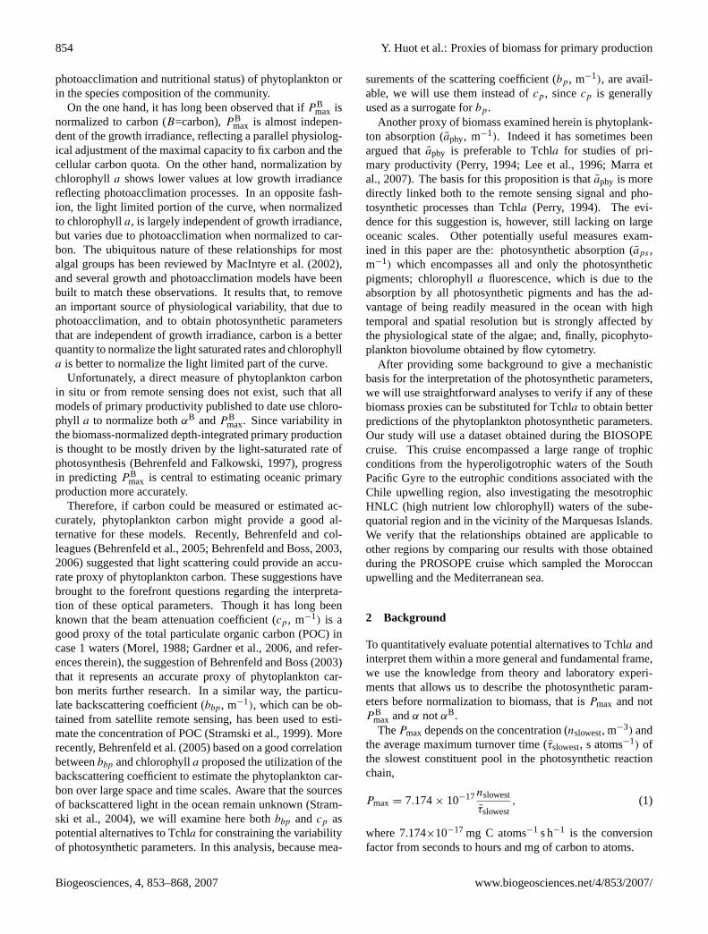
This dataset was collected in case 1 waters. In these waters,away from land influences, all the optical properties covarywith the phytoplanktonic biomass (which spanned roughly 3orders of magnitude) as it underlies the functioning of thewhole ecosystem. Indeed, an overview of the biomass datacollected during the BIOSOPE cruise shows that most vari-ables follow the trends expected as a function of chlorophylla for case 1 waters (Fig. 1); the relationships between sur-face measurements ofbp, bbp, andaphy, and Tchla concen-tration are consistent with statistical relationships previouslyestablished (Bricaud et al., 2004; Loisel and Morel, 1998;Morel and Maritorena, 2001). It is interesting to note theresemblance between panels A and H showing respectivelybp and the phytoplankton biovolume obtained from the flowcytometry measurements as a function of the Tchla concen-tration. Despite (or because of) of the lack ofProchlorococ-cus in the biovolumes dataset and the upper limit of 3µm,and unless strongly covarying particles are present, this sug-gests that variability inbp is in large part influenced by thebiovolume (similar to carbon concentration) of phytoplank-ton. A similar observation can be made with respect toPmaxand biovolumes which both shows patterns that reassemblesstrongly those ofbp and suggest that they are good proxy



Fig. 1. Comparison of different estimators of phytoplankton biomass obtained during the BIOSOPE cruise with published statistics for case1 waters.(A) Particulate scattering coefficient at 650 nm vs. Tchla (sum of chlorophylla and divinyl chlorophyll (A),(B) Backscatteringcoefficient at 470 nm vs. Tchla, (C) Phytoplankton and photosynthetic absorption multiplied by 0.2 (allows it to be discerned from theformer) weighted by the photosynthetron irradiance spectra vs. Tchla, (D) In situ fluorescence vs. Tchla, (E) Pmax vs. Tchla, (F) α vs.Tchla, (G) Pmax vs.α, lines are for two extreme saturation irradiances (Ek) for photosynthesis,(H) Biovolume obtained from a calibratedflow cytometer vs. Tchla. Colorscale represents depth.

of the slowest pool. The decrease ofbp with depth for agiven Tchla concentration (Fig. 1a) is consistent with theoft-reported trends attributed to a “photoacclimation-like”behavior (i.e. an increase in the Tchla per scattering parti-cle, cf. Kitchen et al., 1990). A similar trend is observedin bbp (Fig. 1b). The phytoplankton absorption coefficient(Fig. 1c) generally follows the statistical relationship estab-lished for case 1 waters by Bricaud et al. (2004) but shows aslightly higher slope and lower intercept. A sigmoidal shapeis observed in log space for the fluorescence vs. Tchla re-lationship (Fig. 1d). A clear depth dependence is observedin the Pmax vs. Tchla relationship, while this dependenceis reversed and much less accentuated forα (Figs. 1e andf; see Methods section). The relationship betweenα andPmax (Fig. 1g) also shows a depth dependence which rep-

resents changes inEk with depth (i.e. higher values at thesurface; lower values at depth) consistent with photoadapta-tion (or less-likely photoacclimation). The predominant fac-tor in these changes ofEk are likely photoadaptation ratherthan photoacclimation as there is a layering of species withdepth in these stratified environments (see Ras et al., 2007).

So while all properties covary with one another, there re-mains some variability. This remaining variability, however,is not all random (e.g. depth dependence of thebp vs. Tchlarelationship) and thus contains information about the system.If this information is pertinent to the retrieval of photosyn-thetic parameters some of the measures should provide lessvariability when compared with the photosynthetic parame-ters than other.



Fig. 2. Histograms of the photosynthetic parameters measured during the BIOSOPE cruise.(A) P chlmax, (B) Pmax normalized tobp, (C) αchl,

(D) α normalized tobp. The normalized range was calculated as (min(x)–max(x))/median(x), where x is the normalized photosyntheticparameter. It provides a rough guide to compare the variability between the different panels. For panel (B), two ranges are given, one for thewhole dataset, as in the other panels, and one for normalizedPmax smaller than 7 mg C m−2 h−1 for (focusing on the “normal” region of thedistribution). The abscissas are scaled such that the ratio of the maximum of the axis to the minimum value of the data are equal (for eachrow independently).

Table 2. Statistical difference between the different index ofbiomass used for predictingPmax andα (in Figs. 3 to 6). The es-timator for which the correlation coefficient is not different at the95% confidence level share the same letter. Letters are ordered al-phabetically to the quality of the fits (Figs. 3, 4, 5 and 6), the bestcorrelation have an “a” and the worst a “c”.

bp Biovolume Tchla bbp aphy fluorescence aps

Pmax a a, b b b b b bα c c a c b a, b a, b

A comparison of the distributions of the photosynthetic pa-rameters when they are normalized to Tchla or to the partic-ulate scattering coefficient is provided in Fig. 2. The val-ues obtained forP chl

max [0.26 to 7.2 mg C (mg chl)−1 h−1]andαchl [0.0028 to 0.086 mg C (mg chl)−1 h−1 (µmol pho-tons m−2 s−1)−1] are consistent with values from the liter-ature, but clearly do not cover the full range of variabilityreported. A review of several datasets of photosynthetic pa-rameters by Behrenfeld et al. (2004) gives a range of 0.04 to24.3 (mostly between∼0.5 and∼10) mg C (mg chl)−1 h−1

for P chlmax, and of 0.0004 to∼0.7 (mostly between∼0.005

and∼0.2) mg C (mg chl)−1 h−1 (µmol photons m−2 s−1)−1

for αchl though some variability inαchl originates from thedifferent spectra used for the measurement irradiance. Usinga crude index of dispersion, the normalized range (see Fig. 2caption for details and the values reported on the graphs),shows that normalization of bothPmax andα by Tchla re-duces the variability in the data relative to normalization by

bp (but only slightly in the case ofPmax). The distribution forPmax normalized tobp, however, shows a normal distributionof points below values of 7 mg C m−2 h−1 with a long tailabove. If we consider only the points below that threshold,the variability is much reduced and becomes lower than whenTchla is used as the normalization factor. The higherPmaxnormalized tobp values occur mostly in regions with higherchlorophyll concentrations (coastal upwelling regions, deepchlorophyll maxima, and Marquesas Islands). This couldbe the result of real physiological variability or indicate abias in the normalization bybp with trophic status (e.g. ratioof bphy/bp increasing with increasing chlorophyll concentra-tion, see Table 1 and Background section).

4.2 Determining the best proxy of phytoplankton biomassto predict photosynthetic parameters

Figures 3 and 4 show the comparison betweenPmax and dif-ferent measures of biomass. On both figures, the left panelsshow the scatter plots ofPmax against the different biomassindices measured, and a 2nd order polynomial obtained onthe log-transformed data. The right-hand-side panels showthe values ofPmax predicted by using the polynomial fitagainst the measured values (the statistics of the fits are alsoprovided). As previously mentioned, all fits and statisticsrefer only to the BIOSOPE dataset as it is more completeand allows a consistent comparison of all proxies of biomassfrom an equal number of points taken simultaneously, or nearsimultaneously, while the PROSOPE dataset is superposedfor comparative purposes only. WhilePmax is expected to



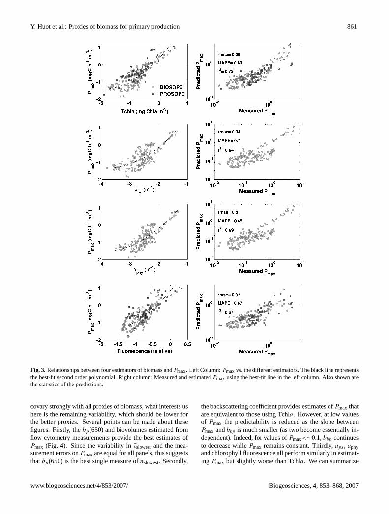
Fig. 3. Relationships between four estimators of biomass andPmax. Left Column:Pmaxvs. the different estimators. The black line representsthe best-fit second order polynomial. Right column: Measured and estimatedPmax using the best-fit line in the left column. Also shown arethe statistics of the predictions.

covary strongly with all proxies of biomass, what interests ushere is the remaining variability, which should be lower forthe better proxies. Several points can be made about thesefigures. Firstly, thebp(650) and biovolumes estimated fromflow cytometry measurements provide the best estimates ofPmax (Fig. 4). Since the variability inτslowestand the mea-surement errors onPmax are equal for all panels, this suggeststhatbp(650) is the best single measure ofnslowest. Secondly,

the backscattering coefficient provides estimates ofPmax thatare equivalent to those using Tchla. However, at low valuesof Pmax the predictability is reduced as the slope betweenPmax andbbp is much smaller (as two become essentially in-dependent). Indeed, for values ofPmax<∼0.1,bbp continuesto decrease whilePmax remains constant. Thirdly,aps , aphyand chlorophyll fluorescence all perform similarly in estimat-ing Pmax but slightly worse than Tchla. We can summarize



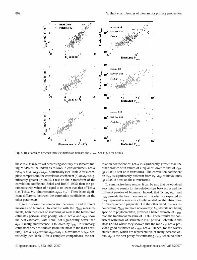
Fig. 4. Relationships between three estimators of biomass andPmax. See Fig. 3 for details.

these results in terms of decreasing accuracy of estimates (us-ing MAPE as the index) as follows:bp≈biovolume>Tchla≈bbp≈ fluo ≈aphy≈aps . Statistically (see Table 2 for a com-plete comparison), the correlation coefficient (r) onbp is sig-nificantly greater (p<0.05, t-test on the z-transform of thecorrelation coefficient, Sokal and Rohlf, 1995) than the pa-rameters with values ofr equal to or lower than that of Tchla

(i.e. Tchla, bbp, fluorescence,aphy, aps). There is no signif-icant difference between the correlation coefficients on theother parameters.

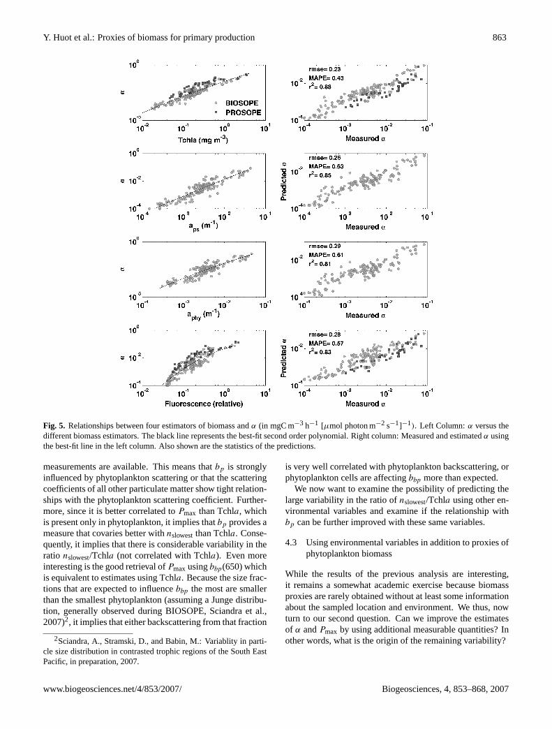
Figure 5 shows the comparison betweenα and differentmeasures of biomass. In contrast with thePmax measure-ments, both measures of scattering as well as the biovolumeestimates perform very poorly, while Tchla and aps showthe best estimates, with Tchla not significantly better thanaps . Finally, fluorescence is followed byaphy. In summary,estimators order as follows (from the most to the least accu-rate): Tchla ≈aps≈fluo>aphy�bp> biovolumes>bbp. Sta-tistically (see Table 2 for a complete comparison), the cor-

relation coefficient of Tchla is significantly greater than theother proxies with values ofr equal or lower to that ofaphy(p<0.05; t-test on z-transform). The correlation coefficienton aphy is significantly different frombp, bbp or biovolumes(p<0.001; t-test on the z-transform).

To summarize these results, it can be said that we obtainedvery intuitive results for the relationships betweenα and thedifferent proxies of biomass. Indeed, that Tchla, aps , andaphy provide the best measures ofα is what we expected asthey represent a measure closely related to the absorptionof photosynthetic pigments. On the other hand, the resultsconcerningPmax are more noteworthy:bp, despite not beingspecific to phytoplankton, provides a better estimate ofPmaxthan the traditional measure of Tchla. These results are con-sistent with those of Behrenfeld et al. (2005); Behrenfeld andBoss (2006) where they showed that the ratiocp/Tchla pro-vided good estimates ofPmax/Tchla. Hence, for the watersstudied here, which are representative of many oceanic wa-ters,bp is the best proxy for estimatingPmax when no other



Fig. 5. Relationships between four estimators of biomass andα (in mgC m−3 h−1 [µmol photon m−2 s−1]−1). Left Column:α versus thedifferent biomass estimators. The black line represents the best-fit second order polynomial. Right column: Measured and estimatedα usingthe best-fit line in the left column. Also shown are the statistics of the predictions.

measurements are available. This means thatbp is stronglyinfluenced by phytoplankton scattering or that the scatteringcoefficients of all other particulate matter show tight relation-ships with the phytoplankton scattering coefficient. Further-more, since it is better correlated toPmax than Tchla, whichis present only in phytoplankton, it implies thatbp provides ameasure that covaries better withnslowestthan Tchla. Conse-quently, it implies that there is considerable variability in theratio nslowest/Tchla (not correlated with Tchla). Even moreinteresting is the good retrieval ofPmax usingbbp(650) whichis equivalent to estimates using Tchla. Because the size frac-tions that are expected to influencebbp the most are smallerthan the smallest phytoplankton (assuming a Junge distribu-tion, generally observed during BIOSOPE, Sciandra et al.,2007)2, it implies that either backscattering from that fraction

2Sciandra, A., Stramski, D., and Babin, M.: Variablity in parti-cle size distribution in contrasted trophic regions of the South EastPacific, in preparation, 2007.

is very well correlated with phytoplankton backscattering, orphytoplankton cells are affectingbbp more than expected.

We now want to examine the possibility of predicting thelarge variability in the ratio ofnslowest/Tchla using other en-vironmental variables and examine if the relationship withbp can be further improved with these same variables.

4.3 Using environmental variables in addition to proxies ofphytoplankton biomass

While the results of the previous analysis are interesting,it remains a somewhat academic exercise because biomassproxies are rarely obtained without at least some informationabout the sampled location and environment. We thus, nowturn to our second question. Can we improve the estimatesof α andPmax by using additional measurable quantities? Inother words, what is the origin of the remaining variability?



Fig. 6. Relationships between three estimators of biomass andα (in mgC m−3 h−1 [µmol photon m−2 s−1]−1). See Fig. 5 for details.

To address this question we used a stepwise regres-sion analysis with the log transform ofα and Pmax asour dependent variable and a series of potentially relevantindependent variables. For each fit, we used only onelog-transformed “biomass proxy” (i.e. whether log(Tchla),log(bp), log(bbp). . . ). The analysis was conducted for alldepths. Table 3 provides all the independent variables testedand a summary of the results. A succinct rationale is givenfor the different variables used (the variables squared allownon-linear relationships to be present). Depth is a generalproxy for growth irradiance (including UV), nutrient avail-ability, and mixing regime (while different types of waterswere encountered, light, UV and diffusivity coefficient al-ways decrease with depth while nutrient always increase).Temperature is expected to have an effect on enzymatic ratesand species composition. The log of the mean PAR irradi-ance at depth over the last three days provides a measure ofirradiance experienced by the cells in their recent past (often

referred to as light history), potentially affecting their pho-toacclimation status. The log of the theoretical PAR irradi-ance at depth provides a measure essentially similar to theoptical depth (except that the surface irradiance is accountedfor) and provides a longer term (∼weeks) proxy of the meanirradiance value at depth; relevant to processes of compet-itive exclusion (by species that have different photoadapta-tion). The nitrate concentration is used as a proxy of nutrientavailability. Figure 7 compares graphically the results forPmax usingbp(650) and Tchla as the independent biomassvariable.

The results are clear (see Table 3, e.g. MAPE row). Us-ing other independent variables beyond biomass, it is pos-sible to significantly improve the relationship betweenPmaxand Tchla (as well asaphy, aps , and fluorescence). How-ever, the same does not occur forbp or bbp, for which therelationships improve only marginally by using several newvariables. Most of the improvements using Tchla arise from



Table 3. Stepwise fit results forPmax vs. different indices of biomass. Values represent the fitted coefficients for each variable. NU is usedfor “Not Used in the fit” (e.g.Pmax(Tchla)=0.236+1.07log10(Tchla)−6.18E−3z+1.35E−5z2+1.55E−2T).

Tchla aps aphy fluo bp(650) bbp(650)

Intercept 0.236 2.42 2.71 0.509 2.05 14.5Log10(Biomass) 1.07 −4.42E−03 −5.39E−3 −6.84E-3 3.21 6.83Log10(Biomass)2 NU 8.32E−06 1.16E−5 1.61E−5 0.677 0.834Depth −6.81E−3 3.34E−2 3.18E−2 NU NU NUDepth2 1.35E−5 NU NU NU NU NUT 1.55E−2 −9.52E−2 NU NU NU −1.95E−1T2 NU 1.34E−02 NU NU 5.36E−3 5.37E−3Log10(Egrowth)

† NU NU NU 5.18E−3 NU NULog10(PARtheo)

§ NU NU NU NU NU NULog10(PARtheo)

2 NU 1.82 1.93 1.21 −5.55E−3 NULog10(NO3) NU 0.143 0.161 NU NU NURMSE 0.15 0.16 0.16 0.18 0.21 0.25MAPE 0.29 0.31 0.30 0.36 0.43 0.54R2 0.93 0.92 0.90 0.90 0.86 0.80

† Egrowth is the mean PAR irradiance during daylight (µmol photon m−2 s−1) at the sampling depth over the three days previous to thesampling day. It is calculated using the incident irradiance measured on the ship and the attenuation coefficient measured at the station.§PARtheo is the mean PAR irradiance calculated using the Gregg and Carder (1990) model at the sampling depth using the attenuationcoefficient measured at the station for the sampling day. Therefore it does not account for cloudiness.

Table 4. Stepwise fit results forα vs. different indices of biomass. Values represent the fitted coefficients for each variable. NU is used for“Not Used in the fit”.

Tchla bp(650) bbp(650) aps aphy fluo

Intercept −1.39 0.63 19.0 1.28 1.36 −1.18Log10(Biomass) 1.36 3.40 767 1.91 1.29 1.47Log10(Biomass)2 NU 0.652 0.96 0.114 NU NUDepth NU NU 7.66E−3 NU −1.12E−2 -3.43E-3Depth2 4.81E−6 2.33E−5 5.48E−5 1.22E−5 4.77E−5 2.71E−5T NU NU −0.642 NU NU −1.24E−2T2 NU 3.00E−4 1.52E−2 4.64E−4 2.94E−4 NULog10(Egrowth) † −3.07E−2 NU NU NU NU NULog10(PARtheo)

§ NU NU 0.155 NU NU NULog10(PARtheo)

2 NU −1.99E−2 −4.09E−2 NU −2.29E−2 NULog10(NO3) NU NU −4.01E−2 NU −1.167E−2 1.43E−2RMSE 0.21 0.30 0.31 0.22 0.23 0.21MAPE 0.40 0.65 0.66 0.44 0.44 0.41R2 0.90 0.80 0.78 0.89 0.88 0.90

† See Table 3§ See Table 3

accounting for the depth effects. This is not unexpected giventhe clear depth dependence ofPmax for a given Tchla con-centration observed in Fig. 1e. The relationships retrievedor the parameters used are not discussed further here, butthe result that interests us is that the pigment or absorptionbased estimates ofPmax can be relatively easily improvedbeyond a simple biomass relationship whereas the same isnot true for the scattering based methods. The latter hence

have lower predictive skill when other sources of variabilityare accounted for. We also note that the errors on the pre-diction of Pmax using this simple regression approach withTchla are very reasonable; the average error (MAPE) is 25%for the BIOSOPE dataset (see Table 3) and 33% for the inde-pendent PROSOPE dataset.

We carried out a similar analysis forα (Table 4 and Fig. 8).In this case, all estimates improved by important margins



Fig. 7. Prediction ofPmax using several variables.(a) Using Tchlaas the biomass index and other variables as given in Table 3.(b)Same as (a) except usingbp as the biomass proxy.

relative to the relationship using only the biomass index.However, the Tchla and absorption based measures remainedsignificantly better than the scattering based methods (Ta-ble 4). In fact, the improvements in the scattering basedmethods are due to the fact that they started off so poorly,and any variable that is somewhat correlated withα or Tchlawill improve the relationships.

4.4 Additional information in scattering beyond Tchla

An important question remains: given the regression usingTchla and environmental variables, can scattering based vari-ables allow us to improve estimates ofPmax andα? In otherwords, is there supplementary information in the scatteringbased proxies? This question can also be addressed by astepwise regression analysis, by verifying if adding scatter-

Fig. 8. Prediction of α (in mgC m−3 h−1 [µmol pho-ton m−2 s−1]−1) using several variables.(a) Using Tchla as thebiomass index and other variables as given in Table 4.(b) Same as(a) except usingbp as the biomass proxy.

ing based measures improves the fit significantly. We testedthe addition of the following variables:bp(650), bp(650)2,and Tchla/bp(650). Only thebp(650) provided a very smallbut significant improvement to the fits forPmax (RMSE de-creased from 0.1488 to 0.1441). None provided signifi-cant improvements in the regression ofα (all had values ofp >0.14). We therefore conclude that, for the waters studied,the bulk scattering measurements adds very little to the esti-mates of photosynthetic parameters, once basic informationregarding chlorophyll concentration and irradiance at depthis available (see Tables 3 and 4).



This conclusion is of course only valid for the environ-ments and the space and time scales that we studied. Scatter-ing based measurements have been proposed to help in theestimation of primary production based on diurnal changesin the cp (e.g. Siegel et al., 1989; Claustre et al., 2007) orof phytoplankton carbon concentration and growth rate fromspace on large spatial scales (Behrenfeld et al., 2005). Theseapplications are beyond the scope of our analysis and our re-sults are difficult to extrapolate to them.

4.5 Estimation of primary productivity using empirical re-lationships

Primary productivity models are generally expressed withthe production (P )-irradiance relationship normalized tobiomass (e.g.P B). This relationship is depth integratedand then multiplied by biomass,P=BP B (the depth in-tegration can occur after the multiplication by biomass ifdepth photosynthetic parameters vary with depth). In or-der to reduce the variability inP B, some authors relate itto its location and time (Platt and Sathyendranath, 1999;Longhurst, 1998), while others describe it in terms of envi-ronmental variables (e.g.P B (T, Salinity, Ed )) (Behrenfeldand Falkowski, 1997). The aim of our study is to identifythe normalization factor (“B”) that reduces as much as pos-sible the variability in the photosynthetic parameters. In do-ing so, we obtain regressions that predictPmax andα fromdifferent biomass proxies and environmental variables (Ta-ble 3 and Table 4). Our relationships can thus be written asP=f (B, T , Salinity, Ed , z. . . ). Therefore, these relation-ships, or extensions of them, could be used in primary pro-duction models using remote sensing data, but without theneed to multiply the resulting primary production by an esti-mate of the phytoplankton biomass. Here, the phytoplanktonbiomass serves directly as a predictive variable.

5 Conclusions

Within the context of evolving ocean observation technology,our analysis consolidates a rationale for the direction takenover the past 50 years or so for estimating primary produc-tivity. Indeed, we find that chlorophylla remains the bestproxy of phytoplankton biomass for studies of primary pro-ductivity. In particular, we find that the scattering coefficient(and other scattering-based variables) did not provide infor-mation about the photosynthetic parameters that could not bemore accurately estimated by a measure of chlorophylla (orfluorescence) and incident irradiance at depth. This is prob-ably due as much to the superior accuracy of the estimationof Tchla compared to other measurements as to its speci-ficity to phytoplankton. There is one main limitation in ourpresent study: most of our dataset originates from subtropi-cal stratified waters (BIOSOPE) and warm temperate waters(PROSOPE). Photosynthetic parameters depend on environ-

mental variables and thus on the regions sampled. While ourmeasurements are representative of a wide range of chloro-phyll concentrations (from∼0.02 to∼3 mg m−3), they arenot representative, for example, of polar or cold temperatewater columns. It is possible that in these waters scattering-based measurement prove to be more robust for the determi-nation of phytoplankton photosynthetic parameters.

Acknowledgements.D. Tailliez and C. Marec are warmly thankedfor their efficient help in CTD rosette management and data process-ing. We also want to thank F. Tieche for processing the phytoplank-ton absorption data, P. Raimbault, J. Ras and A. Morel for provid-ing the nutrient, HPLC and irradiance data. This is a contribution ofthe BIOSOPE project of the LEFE-CYBER French program. Thisresearch was funded by the Centre National de la Recherche Scien-tifique (CNRS), the Institut des Sciences de l’Univers (INSU), theCentre National d’Etudes Spatiales (CNES), the European SpaceAgency (ESA), the National Aeronautics and Space Administration(NASA) and the Natural Sciences and Engineering Research Coun-cil of Canada (NSERC). Y. Huot was funded by postdoctoral schol-arships from NSERC (Canada) and CNES (France). C. Grob wassupported by CONICYT (Chili) through the FONDAP Program anda graduate fellowship, and by the ECOS-CONICYT Program.

Edited by: E. Boss

References

Babin, M. and Morel, A.: An incubator designed for extensive andsensitive measurements of phytoplankton photosynthetic param-eters, Limnol. Oceanogr., 39, 694–702, 1994.

Babin, M., Morel, A., Claustre, H., Bricaud, A., Kolber, Z., andFalkowski, P. G.: Nitrogen- and irradiance-dependent variationsof the maximum quantum yield of carbon fixation in eutrophic,mesotrophic and oligotrophic marine systems, Deep-Sea Res. PtI, 43, 1241–1272, 1996.

Behrenfeld, M. J. and Falkowski, P. G.: A consumer’s guide to phy-toplankton primary productivity models, Limnol. Oceanogr., 42,1479–1491, 1997.

Behrenfeld, M. J. and Boss, E.: The beam attenuation to chloro-phyll ratio: An optical index of phytoplankton physiology in thesurface ocean?, Deep-Sea Res. Pt I, 50, 1537–1549, 2003.

Behrenfeld, M. J., Prasil, O., Babin, M., and Bruyant, F.: In searchof a physiological basis for covariations in light-limited andlight-saturated photosynthesis, J. Phycol., 40, 4–25, 2004.

Behrenfeld, M. J., Boss, E., Siegel, D. A., and Shea, D.M.: Carbon-based ocean productivity and phytoplankton phys-iology from space, Global Biogeochem. Cy., 19, GB1006,doi:1010.1029/2004GB002299, 2005.

Behrenfeld, M. J. and Boss, E.: Beam attenuation and chloro-phyll concentration as alternative optical indices of phytoplank-ton biomass, J. Mar. Res., 64, 431–451, 2006.

Berges, J. A.: Ratios, regression statistics, and “Spurious” Correla-tion, Limnol. Oceanogr., 42, 1006–1007, 1997.

Bricaud, A., Claustre, H., Ras, J., and Oubelkheir, K.: Naturalvariability of phytoplankton absorption in oceanic waters: Influ-ence of the size structure of algal populations, J. Geophys. Res.-Oceans, 109, C11010, doi:11010.11029/12004JC002419, 2004.

Claustre, H., Bricaud, A., Babin, M., Bruyant, F., Guillou, L.,Le Gall, F., Marie, D., and Partensky, F.: Diel variations



in prochlorococcus optical properties, Limnol. Oceanogr., 47,1637–1647, 2002.

Claustre, H., Huot, Y., Obernosterer, I., Gentili, B., Tailliez, D.,Lewis, M.: Gross community production and metabolic bal-ance in the South Pacific Gyre, using a non intrusive bio-opticalmethod, Biogeosciences Discuss., 4, 3089–3121, 2007,http://www.biogeosciences-discuss.net/4/3089/2007/.

Falkowski, P. G. and Raven, J. A.: Aquatic photosynthesis, Firsted., Blackwell Science, Malden, 375 pp., 1997.

Gardner, W. D., Mishonov, A., and Richardson, M. J.: Global pocconcentrations from in-situ and satellite data, Deep-Sea Res. PartII, 53, 718–740, 2006.

Gregg, W. W. and Carder, K. L.: A simple spectral solar irradiancemodel for cloudless maritime atmosphere, Limnol. Oceanogr.,35, 1657–1675, 1990.

Grob, C., Ulloa, O., Claustre, H., Huot, Y., Alarcon, G., andMarie, D.: Contribution of picoplankton to the total particulateorganic carbon concentration in the eastern South Pacific, Bio-geosciences, 4, 837–852, 2007,http://www.biogeosciences.net/4/837/2007/.

Kitchen, J. C., Ronald, J., and Zaneveld, V.: On the noncorrela-tion of the vertical structure of light scattering and chlorophylla in case I waters, J. Geophys. Res.-Oceans, 95, 20 237–20 246,1990.

Lee, Z. P., Carder, K. L., Marra, J., Steward, R. G., and Perry, M.J.: Estimating primary production at depth from remote sensing,Appl. Optics, 35, 463–474, 1996.

Loisel, H. and Morel, A.: Light scattering and chlorophyll concen-tration in case 1 waters: A reexamination, Limnol. Oceanogr.,43, 847–858, 1998.

Longhurst, A. R.: Ecological geography of the sea, Academic Press,San Diego, 398 pp., 1998.

MacIntyre, H. L. and Cullen, J. J.: Using cultures to investigate thephysiological ecology of microalgae, in: Algal culturing tech-niques, edited by: Anderson, R. M., Academic Press, 2005.

Marra, J., Trees, C. C., and O’Reilly, J. E.: Phytoplankton pigmentabsorption: A strong predictor of primary productivity in the sur-face ocean, Deep-Sea Res. Pt I, 54, 155–163, 2007.

Morel, A.: Diffusion de la lumiere par les eaux de mer. Resultatsexperimentaux et approche theorique., AGARD lectures series,3.1.1–3.1.76, 1973.

Morel, A. and Bricaud, A.: Inherent properties of algal cells in-cluding picoplankton: Theoretical and experimental results, in:Photosynthetic picoplankton, edited by: Platt, T. and Li, W. K.W., Canadian bulletin of fisheries and aquatic sciences, 521–559,1986.

Morel, A.: Optical modeling of the upper ocean in relation toits biogenous matter content (case 1 waters), J. Geophys. Res.-Oceans, 93, 10 749–10 768, 1988.

Morel, A. and Ahn, Y.-H.: Optics of heterotrophic nanoflagellatesand ciliates: A tentative assessment of their scattering role inoceanic waters compared to those of bacterial and algal cells, J.Mar. Res., 49, 177–202, 1991.

Morel, A. and Maritorena, S.: Bio-optical properties of oceanic wa-ters: A reappraisal, J. Geophys. Res.-Oceans, 106, 7163–7180,2001.

Morel, A., Gentili, B., Claustre, H., Babin, M., Bricaud, A., Ras,J., and Tieche, F.: Optical properties of the “Clearest” Naturalwaters, Limnol. Oceanogr., 52, 217–229, 2007.

Oubelkheir, K., Claustre, H., Sciandra, A., and Babin, M.:Bio-optical and biogeochemical properties of different trophicregimes in oceanic waters, Limnol. Oceanogr., 50, 1795–1809,2005.

Perry, M. J.: Measurements of phytoplankton absorption other thanper unit of chlorophyll a, in: Ocean optics, edited by: Spinrad, R.W., Carder, K. L., and Perry, M. J., Oxford monographs on ge-ology and geophysics, Oxford University Press, New York, 107–116, 1994.

Platt, T., Gallegos, C. L., and Harrison, W. G.: Photoinhibition ofphotosynthesis in natural assemblages of marine phytoplankton,J. Mar. Res., 38, 687–701, 1980.

Platt, T. and Sathyendranath, S.: Spatial structure of pelagic ecosys-tem processes in the global ocean, Ecosystems, 2, 384–394,1999.

Ras, J., Claustre, H., and Uitz, J.: Spatial variability of phytoplank-ton pigment distributions in the Subtropical South Pacific Ocean:comparison between in situ and predicted data, BiogeosciencesDiscuss., 4, 3409–3451, 2007,http://www.biogeosciences-discuss.net/4/3409/2007/.

Siegel, D. A., Dickey, T. D., Washburn, L., Hamilton, M. K., andMitchell, B. G.: Optical determination of particulate abundanceand production variations in the oligtrophic ocean, Deep-SeaRes., 36, 211–222, 1989.

Sokal, R. R. and Rohlf, F. J.: Biometry the principles and prac-tice of statistics in biological research, 3 ed., W.H. Freeman andCompany, New York, 887 pp., 1995.

Stramski, D. and Reynolds, R. A.: Diel variations in the opticalproperties of a marine diatom, Limnol. Oceanogr., 38, 1347–1364, 1993.

Stramski, D., Shalapyonok, A., and Reynolds, C. S.: Optical char-acterization of the marine oceanic unicellular cyanobacteriumsynechococcus grown under a day-night cycle in natural irradi-ance, J. Geophys. Res.-Oceans, 100, 13 295–13 307, 1995.

Stramski, D., Reynolds, C. S., Kahru, M., and Mitchell, B. G.: Es-timation of particulate organic carbon in the ocean from remotesensing, Science, 285, 239–242, 1999.

Stramski, D., Boss, E., Bogucki, D., and Voss, K. J.: The role ofseawater constituents in light backscattering in the ocean, Prog.Oceanogr., 61, 27–56, 2004.

Sukenic, A., Bennett, J., and Falkowski, P. G.: Light-saturated pho-tosynthesis – limitation by electron transport or carbon fixation,Biochim. Biophys. Acta, 891, 205–215, 1987.

Sullivan, J. M., Twardowski, M. S., Zaneveld, J. R., Moore, C.,Barnard, A., Donaghay, P. L., and Rhoades, B.: The hyperspec-tral temperature and salinity dependencies of absorption by waterand heavy water in the 400–750 nm spectral range, Appl. Optics,45, 5294–5309, 2006.

Twardowski, M. S., Sullivan, J. M., Donaghay, P. L., and Zaneveld,J. R.: Microscale quantification of the absorption by dissolvedand particulate material in coastal waters with an ac-9, J. Atmos.Ocean. Tech., 16, 691–707, 1999.

Twardowski, M. S., Claustre H., Freeman, A., Stramski, D., andHuot, Y.: Optical backscattering properties of the “clearest” nat-ural waters, Biogeosciences Discuss., 4, 2441–2491, 2007,http://www.biogeosciences-discuss.net/4/2441/2007/.

Zaneveld, J. R. V., Kitchen, J. C., and Moore, C. C.: The scatter-ing error correction of reflecting tube absorption meters, OceanOptics XII, 44–55, 1994.


http://www.biogeosciences-discuss.net/4/3089/2007/

http://www.biogeosciences.net/4/837/2007/



Relationship between photosynthetic parameters and different proxies of phytoplankton biomass in the subtropical ocean

Documents