Preconditioning an Artificial Neural Network Using Naive Bayes Nayyar A. Zaidi, Francois Petitjean, Geoffrey I. Webb

Welcome message from author
This document is posted to help you gain knowledge. Please leave a comment to let me know what you think about it! Share it to your friends and learn new things together.
Transcript
Preconditioning an Artificial NeuralNetwork Using Naive Bayes
Nayyar A. Zaidi, Francois Petitjean, Geoffrey I. Webb
Introduction
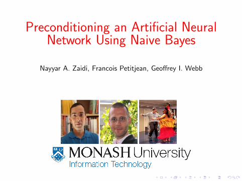
I Maximum likelihood estimates of naive Bayes probabilities canbe used to greatly speed-up logistic regression
I This talk demonstrates that this speed-up can also beattained for Artificial Neural Networks
I Talk outlineI Introduction (2 minutes)I Proposed Approach (6 minutes)I Experimental Analysis (6 minutes)I Future Research, Q & A (3 minutes)
Contributions of the Paper
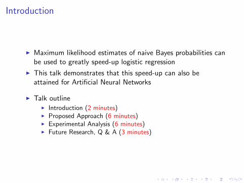
I We show that:
1. Preconditioning based on naive Bayes is applicable and equallyuseful for Artificial Neural Networks (ANN) as it is for LogisticRegression (LR)
2. Optimizing MSE objective function leads to lower bias thanoptimzing CLL, this leads to lower 0-1 Loss and RMSE on bigdatasets
Logistic Regression
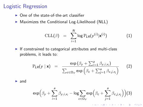
I One of the state-of-the-art classifier
I Maximizes the Conditional Log-Likelihood (NLL)
CLL(β) =N∑i=1
logPLR(y (i)|x(i)) (1)
I If constrained to categorical attributes and multi-classproblems, it leads to:
PLR(y | x) =exp (βy +
∑ai=1 βy ,i ,xi )∑
c∈ΩYexp
(βc +
∑aj=1 βc,j ,xj
) (2)
I and
exp(βy +
a∑i=1
βy ,i ,xi − log∑c∈ΩY
exp(βc +
a∑j=1
βc,j ,xj
))(3)
Naive Bayes and Weighted Naive Bayes
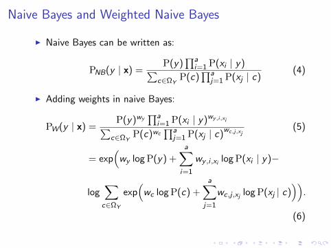
I Naive Bayes can be written as:
PNB(y | x) =P(y)
∏ai=1 P(xi | y)∑
c∈ΩYP(c)
∏aj=1 P(xj | c)
(4)
I Adding weights in naive Bayes:
PW(y | x) =P(y)wy
∏ai=1 P(xi | y)wy,i,xi∑
c∈ΩYP(c)wc
∏aj=1 P(xj | c)
wc,j,xj(5)
= exp(wy logP(y) +
a∑i=1
wy ,i ,xi logP(xi | y)−
log∑c∈ΩY
exp(wc logP(c) +
a∑j=1
wc,j ,xj logP(xj | c))).
(6)
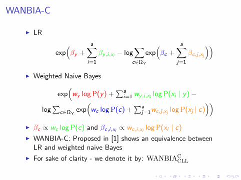
WANBIA-C
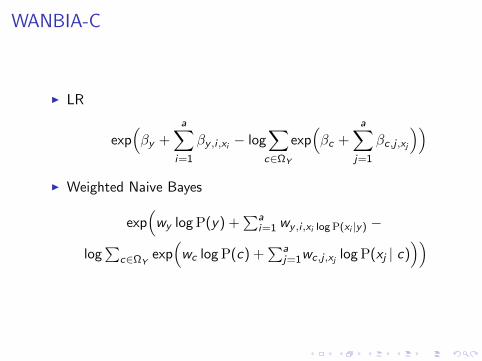
I LR
exp(βy +
a∑i=1
βy ,i ,xi − log∑c∈ΩY
exp(βc +
a∑j=1
βc,j ,xj
))I Weighted Naive Bayes
exp(wy logP(y) +
∑ai=1 wy ,i ,xi log P(xi |y) −
log∑
c∈ΩYexp(wc logP(c) +
∑aj=1wc,j ,xj logP(xj | c)
))
WANBIA-C
I LR
exp(βy +
a∑i=1
βy ,i ,xi − log∑c∈ΩY
exp(βc +
a∑j=1
βc,j ,xj
))I Weighted Naive Bayes
exp(wy logP(y) +
∑ai=1 wy ,i ,xi logP(xi | y)−
log∑
c∈ΩYexp(wc logP(c) +
∑aj=1wc,j ,xj logP(xj | c)
))
WANBIA-C
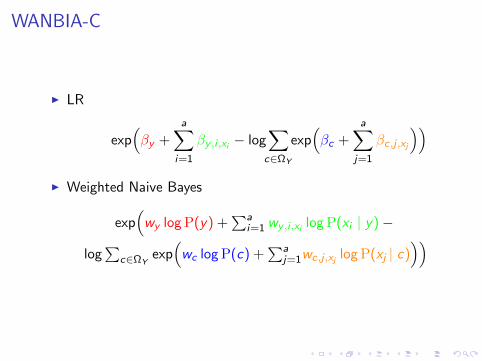
I LR
exp(βy +
a∑i=1
βy ,i ,xi − log∑c∈ΩY
exp(βc +
a∑j=1
βc,j ,xj
))I Weighted Naive Bayes
exp(wy logP(y) +
∑ai=1 wy ,i ,xi logP(xi | y)−
log∑
c∈ΩYexp(wc logP(c) +
∑aj=1wc,j ,xj logP(xj | c)
))I βc ∝ wc logP(c) and βc,i ,xi ∝ wc,i ,xi logP(xi | c)
I WANBIA-C: Proposed in [1] shows an equivalence betweenLR and weighted naive Bayes
I For sake of clarity - we denote it by: WANBIACCLL
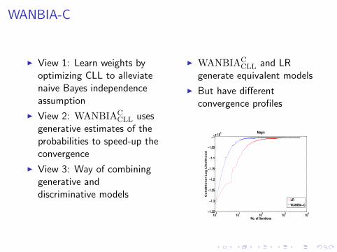
WANBIA-C
I View 1: Learn weights byoptimizing CLL to alleviatenaive Bayes independenceassumption
I View 2: WANBIACCLL uses
generative estimates of theprobabilities to speed-up theconvergence
I View 3: Way of combininggenerative anddiscriminative models
I WANBIACCLL and LR
generate equivalent models
I But have differentconvergence profiles
100
101
102
103
104
−1.35
−1.3
−1.25
−1.2
−1.15
−1.1
−1.05
−1x 10
4
No. of Iterations
Co
nd
itio
nal L
og
Lik
elih
oo
d
Magic
LR
WANBIA−C
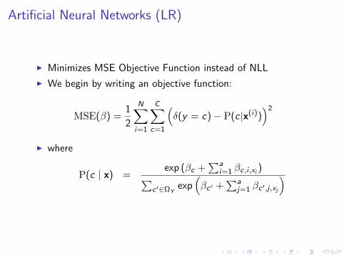
Artificial Neural Networks (LR)
I Minimizes MSE Objective Function instead of NLL
I We begin by writing an objective function:
MSE(β) =1
2
N∑i=1
C∑c=1
(δ(y = c)− P(c |x(i))
)2
I where
P(c | x) =exp (βc +
∑ai=1 βc,i ,xi )∑
c ′∈ΩYexp
(βc ′ +
∑aj=1 βc ′,j ,xj
)
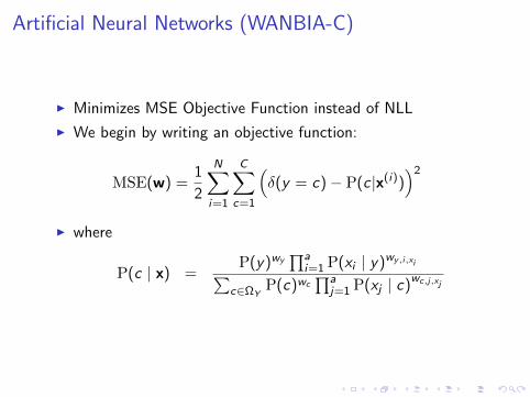
Artificial Neural Networks (WANBIA-C)
I Minimizes MSE Objective Function instead of NLL
I We begin by writing an objective function:
MSE(w) =1
2
N∑i=1
C∑c=1
(δ(y = c)− P(c |x(i))
)2
I where
P(c | x) =P(y)wy
∏ai=1 P(xi | y)wy,i,xi∑
c∈ΩYP(c)wc
∏aj=1 P(xj | c)
wc,j,xj
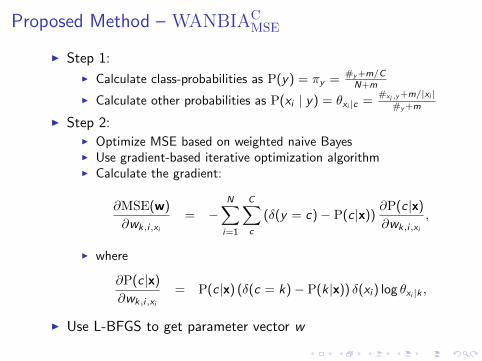
Proposed Method – WANBIACMSE
I Step 1:
I Calculate class-probabilities as P(y) = πy =#y+m/CN+m
I Calculate other probabilities as P(xi | y) = θxi |c =#xi ,y
+m/|xi |#y+m
I Step 2:I Optimize MSE based on weighted naive BayesI Use gradient-based iterative optimization algorithmI Calculate the gradient:
∂MSE(w)
∂wk,i,xi
= −N∑i=1
C∑c
(δ(y = c)− P(c |x))∂P(c |x)
∂wk,i,xi
,
I where
∂P(c |x)
∂wk,i,xi
= P(c |x) (δ(c = k)− P(k |x)) δ(xi ) log θxi |k ,
I Use L-BFGS to get parameter vector w
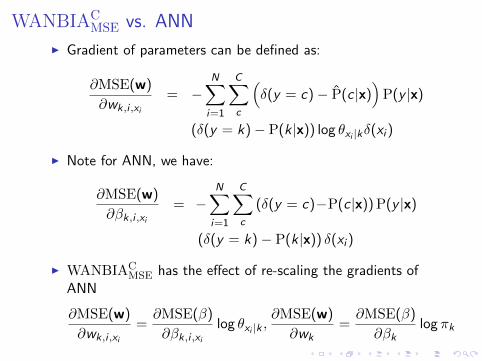
WANBIACMSE vs. ANN
I Gradient of parameters can be defined as:
∂MSE(w)
∂wk,i ,xi
= −N∑i=1
C∑c
(δ(y = c)− P(c |x)
)P(y |x)
(δ(y = k)− P(k|x)) log θxi |kδ(xi )
I Note for ANN, we have:
∂MSE(w)
∂βk,i ,xi= −
N∑i=1
C∑c
(δ(y = c)−P(c |x))P(y |x)
(δ(y = k)− P(k|x)) δ(xi )
I WANBIACMSE has the effect of re-scaling the gradients of
ANN
∂MSE(w)
∂wk,i ,xi
=∂MSE(β)
∂βk,i ,xilog θxi |k ,
∂MSE(w)
∂wk=∂MSE(β)
∂βklog πk
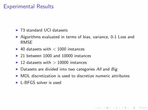
Experimental Results
I 73 standard UCI datasets
I Algorithms evaluated in terms of bias, variance, 0-1 Loss andRMSE
I 40 datasets with < 1000 instances
I 21 between 1000 and 10000 instances
I 12 datasets with > 10000 instances
I Datasets are divided into two categories All and Big
I MDL discretization is used to discretize numeric attributes
I L-BFGS solver is used
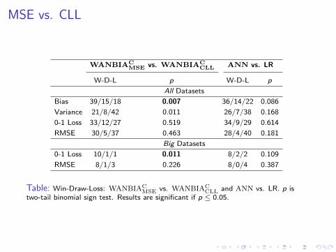
MSE vs. CLL
WANBIACMSE vs. WANBIAC
CLL ANN vs. LR
W-D-L p W-D-L p
All Datasets
Bias 39/15/18 0.007 36/14/22 0.086
Variance 21/8/42 0.011 26/7/38 0.168
0-1 Loss 33/12/27 0.519 34/9/29 0.614
RMSE 30/5/37 0.463 28/4/40 0.181
Big Datasets
0-1 Loss 10/1/1 0.011 8/2/2 0.109
RMSE 8/1/3 0.226 8/0/4 0.387
Table: Win-Draw-Loss: WANBIACMSE vs. WANBIAC
CLL and ANN vs. LR. p istwo-tail binomial sign test. Results are significant if p ≤ 0.05.
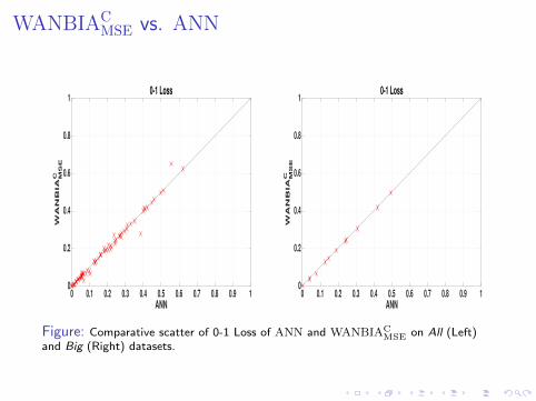
WANBIACMSE vs. ANN
0 0.1 0.2 0.3 0.4 0.5 0.6 0.7 0.8 0.9 1
ANN
0
0.2
0.4
0.6
0.8
1
WA
NB
IA
C MS
E
0-1 Loss
0 0.1 0.2 0.3 0.4 0.5 0.6 0.7 0.8 0.9 1
ANN
0
0.2
0.4
0.6
0.8
1
WA
NB
IA
C MS
E
0-1 Loss
Figure: Comparative scatter of 0-1 Loss of ANN and WANBIACMSE on All (Left)
and Big (Right) datasets.

WANBIACMSE vs. ANN
10-1
100
101
102
103
104
105
ANN
10-1
100
101
102
103
104
105
WA
NB
IA
C MS
E
Training Time
100
101
102
103
104
105
ANN
100
101
102
103
104
105
WA
NB
IA
C MS
E
Training Time
Figure: Comparative scatter of training time of ANN and WANBIACMSE on All
(Left) and Big (Right) datasets.

WANBIACMSE vs. ANN
100
101
102
103
104
105
ANN
100
101
102
103
104
105
WA
NB
IA
C MS
E
Iterations
101
102
103
104
105
ANN
101
102
103
104
105
WA
NB
IA
C MS
E
Iterations
Figure: Comparative scatter of number of iterations to convergence of ANN andWANBIAC
MSE on All (Left) and Big (Right) datasets.
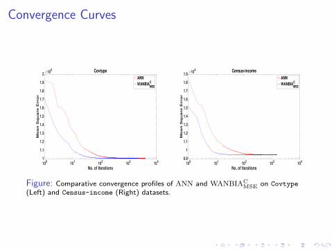
Convergence Curves
100
101
102
103
104
No. of Iterations
1
1.1
1.2
1.3
1.4
1.5
1.6
1.7
1.8
1.9
2
Mean
Sq
uare E
rro
r
×105 Covtype
ANN
WANBIAC
MSE
100
101
102
103
104
No. of Iterations
0.9
1
1.1
1.2
1.3
1.4
1.5
1.6
1.7
1.8
1.9
Mean
Sq
uare E
rro
r
×104 Census-income
ANN
WANBIAC
MSE
Figure: Comparative convergence profiles of ANN and WANBIACMSE on Covtype
(Left) and Census-income (Right) datasets.
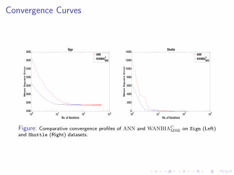
Convergence Curves
100
101
102
103
No. of Iterations
2400
2600
2800
3000
3200
3400
3600
3800
Mean
Sq
uare E
rro
r
Sign
ANN
WANBIAC
MSE
100
101
102
103
No. of Iterations
0
2000
4000
6000
8000
10000
12000
14000
Mean
Sq
uare E
rro
r
Shuttle
ANN
WANBIAC
MSE
Figure: Comparative convergence profiles of ANN and WANBIACMSE on Sign (Left)
and Shuttle (Right) datasets.
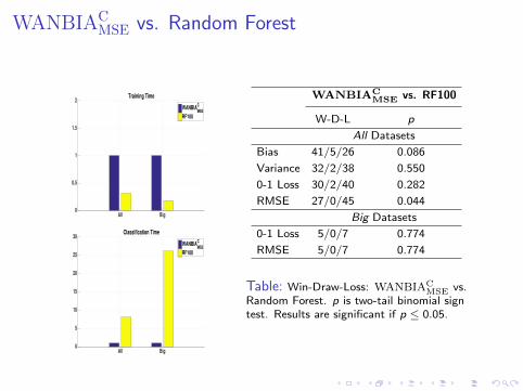
WANBIACMSE vs. Random Forest
All Big0
0.5
1
1.5
2Training Time
WANBIAC
MSE
RF100
All Big0
5
10
15
20
25
30Classification Time
WANBIAC
MSE
RF100
WANBIACMSE vs. RF100
W-D-L p
All Datasets
Bias 41/5/26 0.086
Variance 32/2/38 0.550
0-1 Loss 30/2/40 0.282
RMSE 27/0/45 0.044
Big Datasets
0-1 Loss 5/0/7 0.774
RMSE 5/0/7 0.774
Table: Win-Draw-Loss: WANBIACMSE vs.
Random Forest. p is two-tail binomial signtest. Results are significant if p ≤ 0.05.
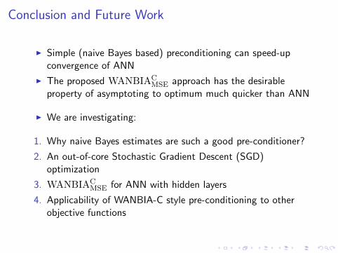
Conclusion and Future Work
I Simple (naive Bayes based) preconditioning can speed-upconvergence of ANN
I The proposed WANBIACMSE approach has the desirable
property of asymptoting to optimum much quicker than ANN
I We are investigating:
1. Why naive Bayes estimates are such a good pre-conditioner?
2. An out-of-core Stochastic Gradient Descent (SGD)optimization
3. WANBIACMSE for ANN with hidden layers
4. Applicability of WANBIA-C style pre-conditioning to otherobjective functions

I Q & A
I Offline Discussions
I @nayyar zaidi
I nayyar zaidi
I http://users.monash.edu.au/~nzaidi
I For further discussions, contact:
N. A. Zaidi, M. J. Carman, J. Cerquides, and G. I. Webb,“Naive-Bayes inspired effective pre-conditioners forspeeding-up logistic regression,” in IEEE InternationalConference on Data Mining, pp. 1097–1102, 2014.
N. A. Zaidi, J. Cerquides, M. J. Carman, and G. I. Webb,“Alleviating naive Bayes attribute independence assumption byattribute weighting,” Journal of Machine Learning Research,vol. 14, pp. 1947–1988, 2013.
Related Documents