Naive Bayes lecture

Naïve Bayes Classification

Material borrowed fromJonathan Huang and

I. H. Witten’s and E. Frank’s “Data Mining”and Jeremy Wyatt and others

Things We’d Like to Do• Spam Classification

– Given an email, predict whether it is spam or not

• Medical Diagnosis– Given a list of symptoms, predict whether a patient has

disease X or not

• Weather– Based on temperature, humidity, etc… predict if it will rain

tomorrow

Bayesian Classification

• Problem statement:– Given features X1,X2,…,Xn

– Predict a label Y

Another Application

• Digit Recognition

• X1,…,Xn {0,1} (Black vs. White pixels)• Y {5,6} (predict whether a digit is a 5 or a 6)

Classifier 5

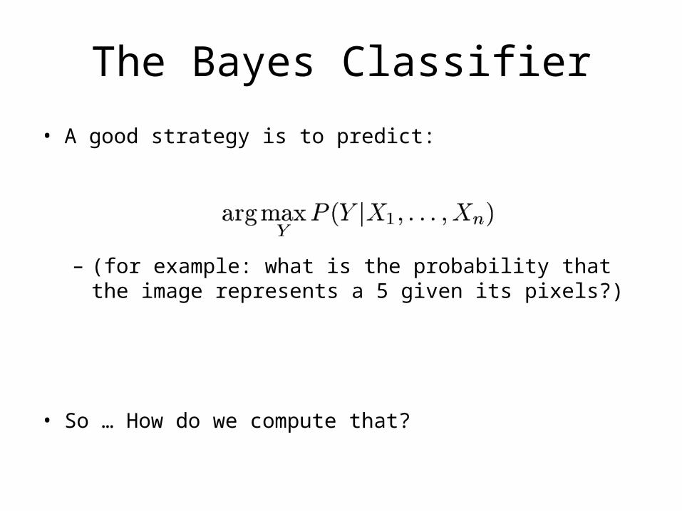
The Bayes Classifier

• A good strategy is to predict:

– (for example: what is the probability that the image represents a 5 given its pixels?)

• So … How do we compute that?

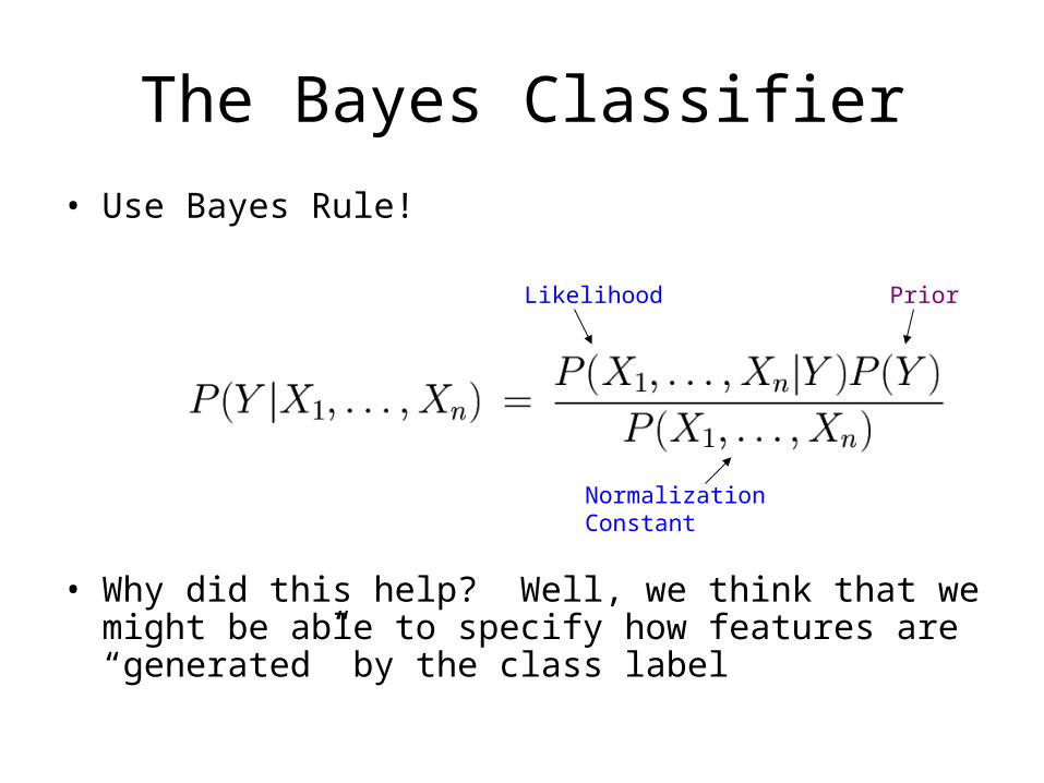
The Bayes Classifier• Use Bayes Rule!

• Why did this help? Well, we think that we might be able to specify how features are “generated” by the class label

Normalization Constant

Likelihood Prior

The Bayes Classifier• Let’s expand this for our digit recognition task:

• To classify, we’ll simply compute these two probabilities and predict based on which one is greater

Model Parameters• For the Bayes classifier, we need to “learn” two functions, the

likelihood and the prior

• How many parameters are required to specify the prior for our digit recognition example?

Model Parameters• How many parameters are required to specify the likelihood?

– (Supposing that each image is 30x30 pixels)

?

Model Parameters

• The problem with explicitly modeling P(X1,…,Xn|Y) is that there are usually way too many parameters:– We’ll run out of space– We’ll run out of time– And we’ll need tons of training data (which is usually not

available)

The Naïve Bayes Model• The Naïve Bayes Assumption: Assume that all features are

independent given the class label Y• Equationally speaking:

• (We will discuss the validity of this assumption later)

Why is this useful?

• # of parameters for modeling P(X1,…,Xn|Y):

2(2n-1)

• # of parameters for modeling P(X1|Y),…,P(Xn|Y)

2n

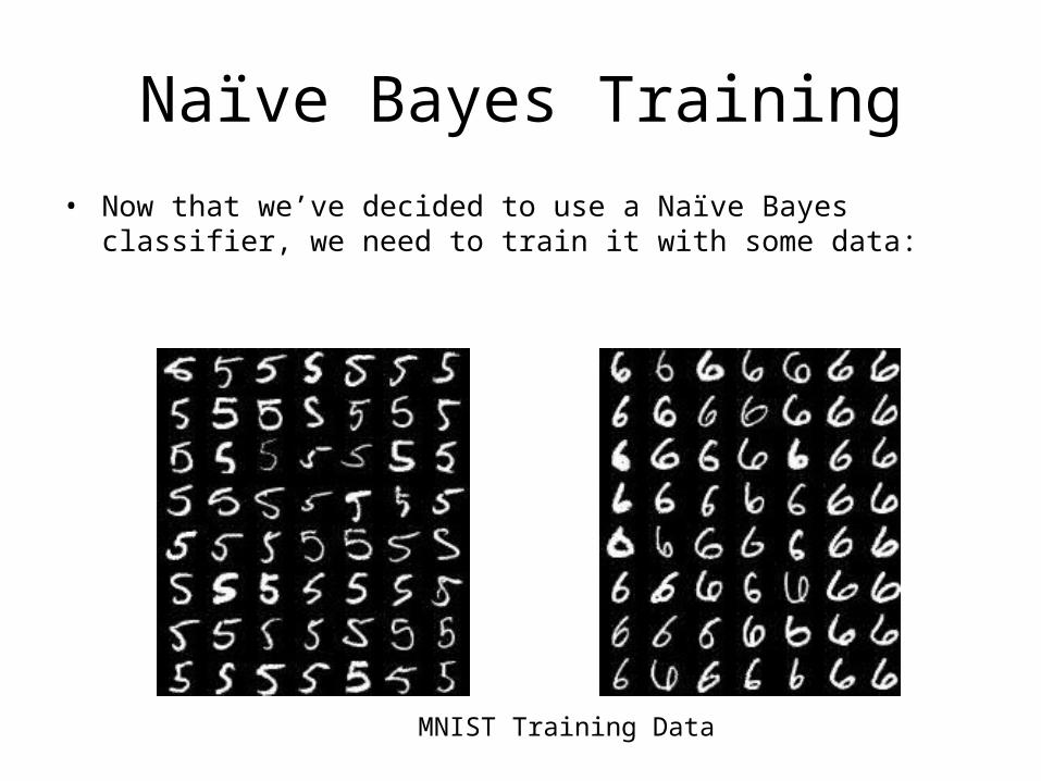
Naïve Bayes Training• Now that we’ve decided to use a Naïve Bayes classifier, we need to train it

with some data:

MNIST Training Data

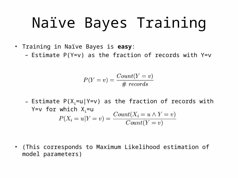
Naïve Bayes Training• Training in Naïve Bayes is easy:

– Estimate P(Y=v) as the fraction of records with Y=v

– Estimate P(Xi=u|Y=v) as the fraction of records with Y=v for which Xi=u

• (This corresponds to Maximum Likelihood estimation of model parameters)

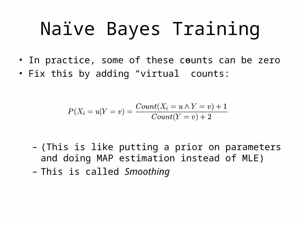
Naïve Bayes Training• In practice, some of these counts can be zero• Fix this by adding “virtual” counts:

– (This is like putting a prior on parameters and doing MAP estimation instead of MLE)

– This is called Smoothing

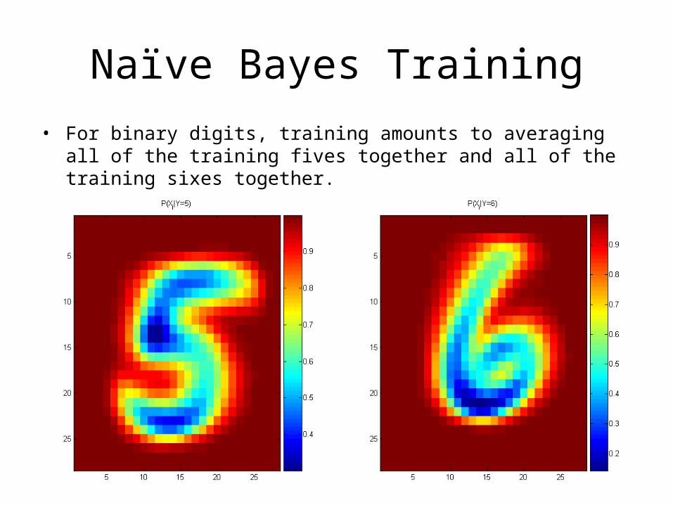
Naïve Bayes Training• For binary digits, training amounts to averaging all of the training fives

together and all of the training sixes together.

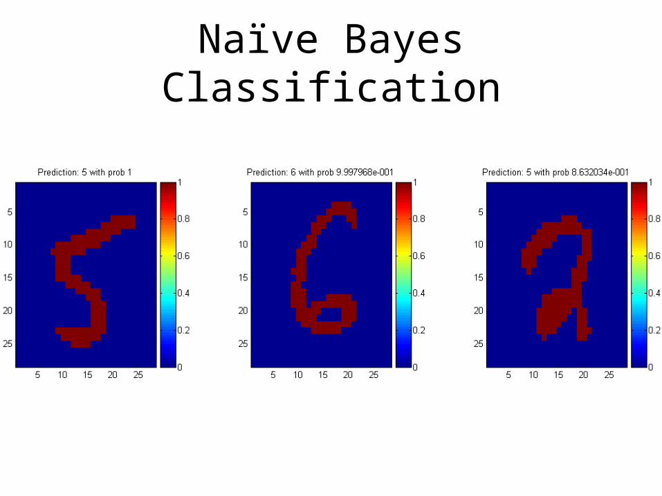
Naïve Bayes Classification

Another Example of the Naïve Bayes Classifier

The weather data, with counts and probabilitiesoutlook temperature humidity windy play

yes no yes no yes no yes no yes no

sunny 2 3 hot 2 2 high 3 4 false 6 2 9 5

overcast 4 0 mild 4 2 normal 6 1 true 3 3

rainy 3 2 cool 3 1

sunny 2/9 3/5 hot 2/9 2/5 high 3/9 4/5 false 6/9 2/5 9/14 5/14

overcast 4/9 0/5 mild 4/9 2/5 normal 6/9 1/5 true 3/9 3/5

rainy 3/9 2/5 cool 3/9 1/5

A new day

outlook temperature humidity windy play

sunny cool high true ?

• Likelihood of yes

• Likelihood of no

• Therefore, the prediction is No

0053.0149

93

93

93

92

0206.0145

53

54

51

53

The Naive Bayes Classifier for Data Sets with Numerical Attribute Values

• One common practice to handle numerical attribute values is to assume normal distributions for numerical attributes.

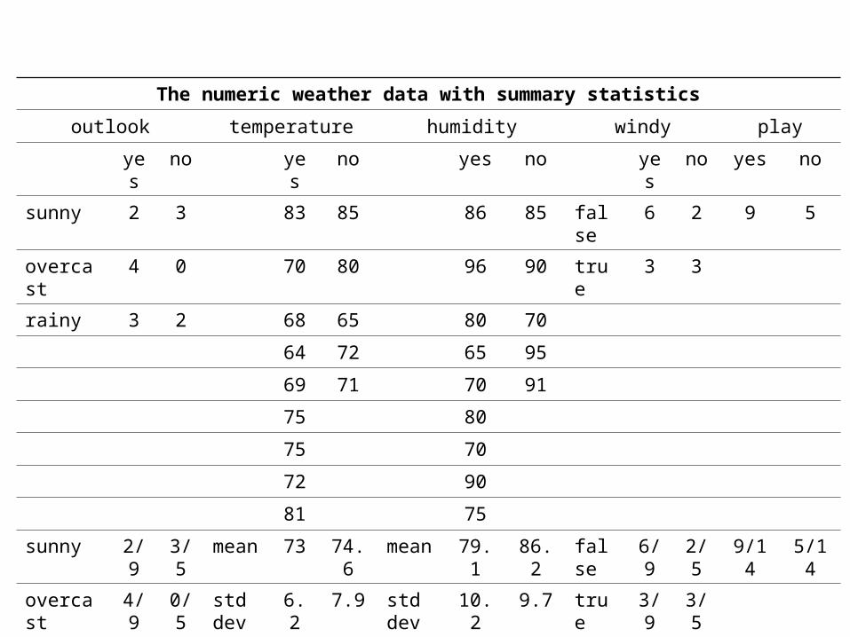
The numeric weather data with summary statisticsoutlook temperature humidity windy play

yes no yes no yes no yes no yes no

sunny 2 3 83 85 86 85 false 6 2 9 5

overcast 4 0 70 80 96 90 true 3 3

rainy 3 2 68 65 80 70

64 72 65 95

69 71 70 91

75 80

75 70

72 90

81 75

sunny 2/9 3/5 mean 73 74.6 mean 79.1 86.2 false 6/9 2/5 9/14 5/14

overcast 4/9 0/5 std dev

6.2 7.9 std dev

10.2 9.7 true 3/9 3/5

rainy 3/9 2/5

• Let x1, x2, …, xn be the values of a numerical attribute in the training data set.

2

2

21)(

11

1

1

2

1

w

ewf

xn

xn

n

ii

n

ii

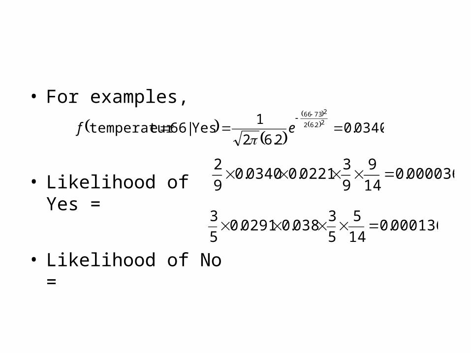
• For examples,

• Likelihood of Yes =

• Likelihood of No =

000036.0149

930221.00340.0

92

000136.0145

53038.00291.0

53

0340.0

2.621Yes|66etemperatur 22.62

27366

ef

Outputting Probabilities• What’s nice about Naïve Bayes (and generative models in

general) is that it returns probabilities– These probabilities can tell us how confident the algorithm

is– So… don’t throw away those probabilities!

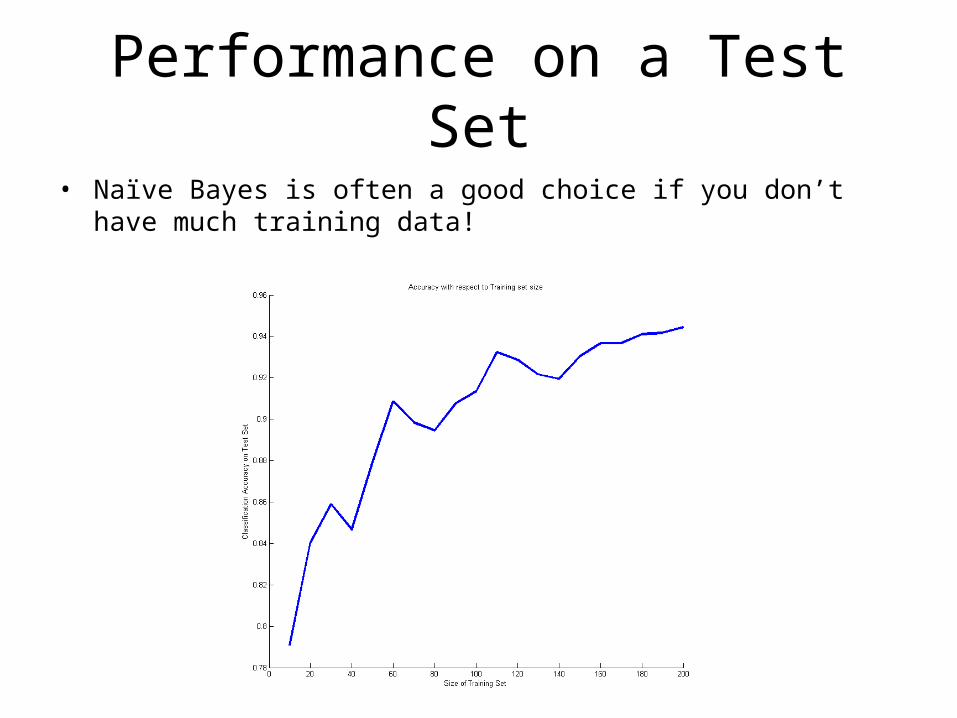
Performance on a Test Set• Naïve Bayes is often a good choice if you don’t have much training data!

Naïve Bayes Assumption• Recall the Naïve Bayes assumption:

– that all features are independent given the class label Y

• Does this hold for the digit recognition problem?

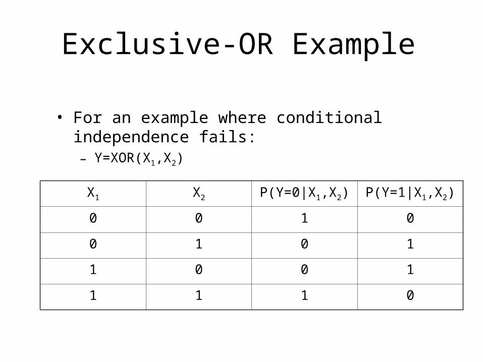
Exclusive-OR Example

• For an example where conditional independence fails:– Y=XOR(X1,X2)

X1 X2 P(Y=0|X1,X2) P(Y=1|X1,X2)

0 0 1 0

0 1 0 1

1 0 0 1

1 1 1 0

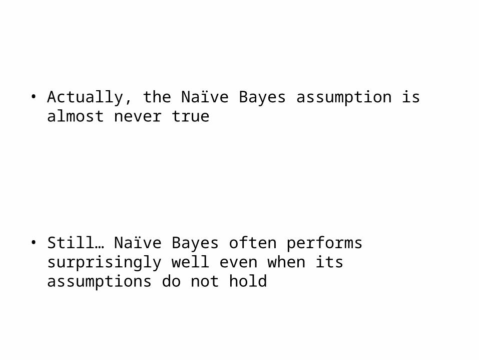
• Actually, the Naïve Bayes assumption is almost never true

• Still… Naïve Bayes often performs surprisingly well even when its assumptions do not hold

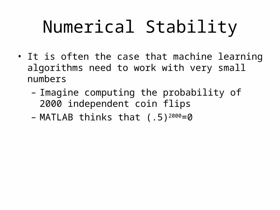
Numerical Stability• It is often the case that machine learning algorithms need to

work with very small numbers– Imagine computing the probability of 2000 independent

coin flips– MATLAB thinks that (.5)2000=0

Underflow Prevention

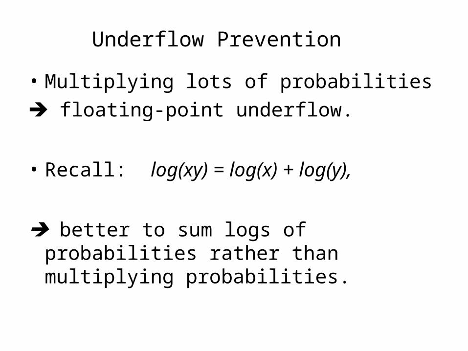
• Multiplying lots of probabilities floating-point underflow.

• Recall: log(xy) = log(x) + log(y),

better to sum logs of probabilities rather than multiplying probabilities.

Underflow Prevention

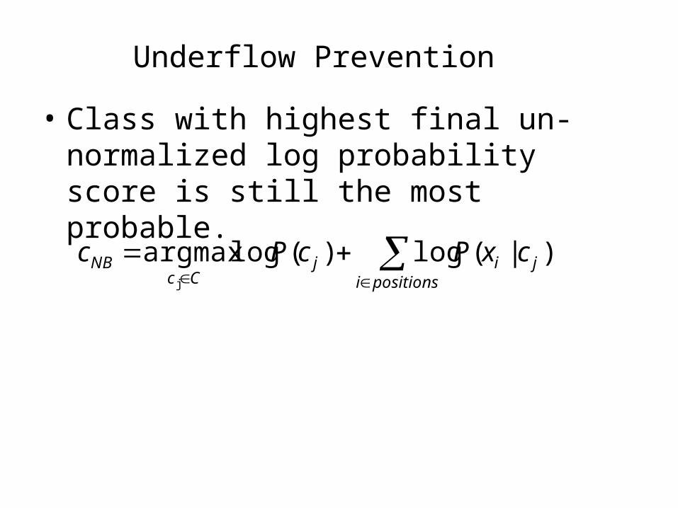
• Class with highest final un-normalized log probability score is still the most probable.

positionsi

jijCc

NB cxPcPc )|(log)(logargmaxj

Numerical Stability

• Instead of comparing P(Y=5|X1,…,Xn) with P(Y=6|X1,…,Xn),– Compare their logarithms

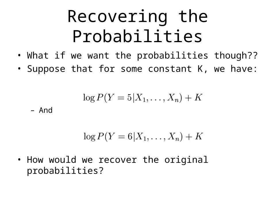
Recovering the Probabilities• What if we want the probabilities though??• Suppose that for some constant K, we have:

– And

• How would we recover the original probabilities?

Recovering the Probabilities• Given:• Then for any constant C:

• One suggestion: set C such that the greatest i is shifted to zero:

See https://stats.stackexchange.com/questions/105602/example-of-how-the-log-sum-exp-trick-works-in-naive-bayes?noredirect=1&lq=1

Recap• We defined a Bayes classifier but saw that it’s intractable to

compute P(X1,…,Xn|Y)• We then used the Naïve Bayes assumption – that everything

is independent given the class label Y

• A natural question: is there some happy compromise where we only assume that some features are conditionally independent?– Stay Tuned…

Conclusions• Naïve Bayes is:

– Really easy to implement and often works well– Often a good first thing to try– Commonly used as a “punching bag” for smarter

algorithms

Evaluating classification algorithms

You have designed a new classifier.

You give it to me, and I try it on my image dataset

Evaluating classification algorithms

I tell you that it achieved 95% accuracy on my data.

Is your technique a success?

Types of errors

• But suppose that– The 95% is the correctly classified pixels– Only 5% of the pixels are actually edges– It misses all the edge pixels

• How do we count the effect of different types of error?

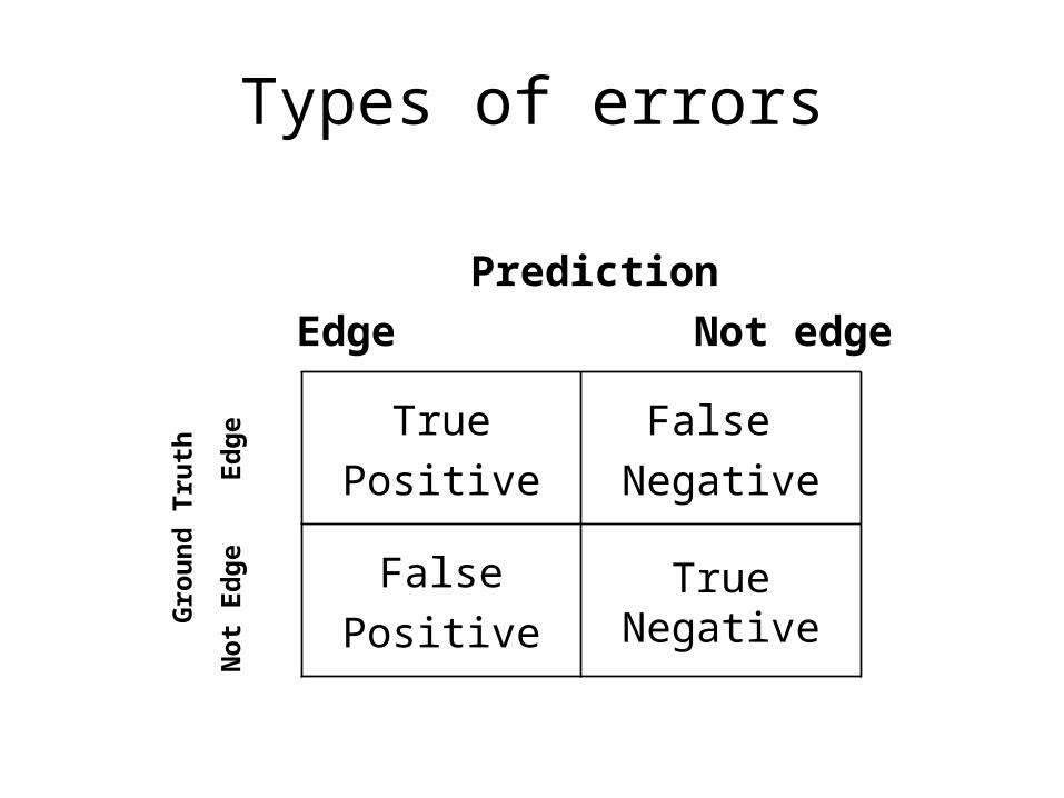
Types of errors

PredictionEdge Not edge

TruePositive

False Negative

FalsePositive

True Negative

Gro

und

Trut

h

Not

Edg

e

Edge

True Positive

Two parts to each: whether you got it correct or not, and what you guessed. For example for a particular pixel, our guess might be labelled…

Did we get it correct? True, we did get it correct.

False NegativeDid we get it correct? False, we did not get it correct.

or maybe it was labelled as one of the others, maybe…

What did we say? We said ‘positive’, i.e. edge.

What did we say? We said ‘negative, i.e. not edge.

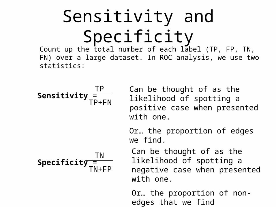
Sensitivity and SpecificityCount up the total number of each label (TP, FP, TN, FN) over a large dataset. In ROC analysis, we use two statistics:

Sensitivity = TP

TP+FN

Specificity = TN

TN+FP

Can be thought of as the likelihood of spotting a positive case when presented with one.

Or… the proportion of edges we find.

Can be thought of as the likelihood of spotting a negative case when presented with one.

Or… the proportion of non-edges that we find

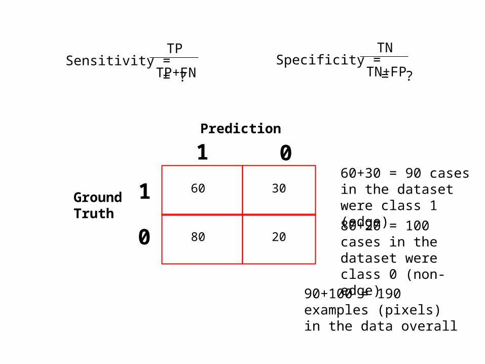
Sensitivity = = ? TP

TP+FNSpecificity = = ?

TN

TN+FP

Prediction

Ground Truth

1

1 0

0

60 30

208080+20 = 100 cases in the dataset were class 0 (non-edge)

60+30 = 90 cases in the dataset were class 1 (edge)

90+100 = 190 examples (pixels) in the data overall

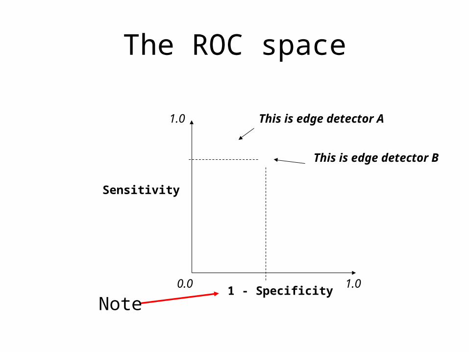
The ROC space

1 - Specificity

Sensitivity

This is edge detector B

This is edge detector A1.0

0.0 1.0

Note

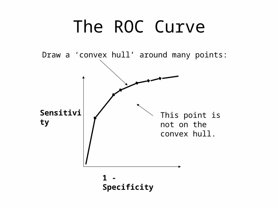
The ROC CurveDraw a ‘convex hull’ around many points:

1 - Specificity

Sensitivity This point is not on the convex hull.

ROC Analysis

1 - specificity

sensitivity

All the optimal detectors lie on the convex hull.

Which of these is best depends on the ratio of edges to non-edges, and the different cost of misclassification

Any detector on this side can lead to a better detector by flipping its output.

Take-home point : You should always quote sensitivity and specificity for your algorithm, if possible plotting an ROC graph. Remember also though,

any statistic you quote should be an average over a suitable range of tests for your algorithm.

Holdout estimation• What to do if the amount of data is limited?

• The holdout method reserves a certain amount for testing and uses the remainder for training

Usually: one third for testing, the rest for training

Holdout estimation• Problem: the samples might not be representative

– Example: class might be missing in the test data

• Advanced version uses stratification– Ensures that each class is represented with

approximately equal proportions in both subsets

Repeated holdout method• Repeat process with different subsamples more reliable

– In each iteration, a certain proportion is randomly selected for training (possibly with stratificiation)

– The error rates on the different iterations are averaged to yield an overall error rate

Repeated holdout method• Still not optimum: the different test sets overlap

– Can we prevent overlapping?

– Of course!

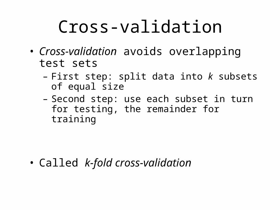
Cross-validation• Cross-validation avoids overlapping test sets

– First step: split data into k subsets of equal size– Second step: use each subset in turn for testing, the

remainder for training

• Called k-fold cross-validation

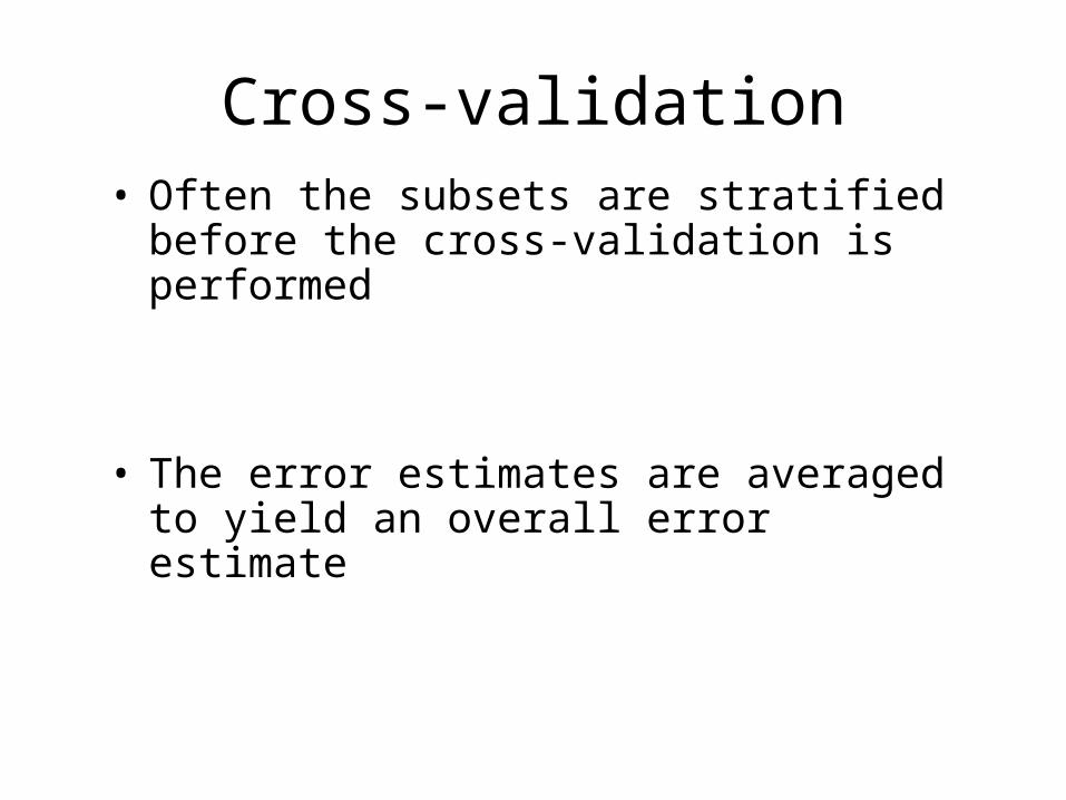
Cross-validation• Often the subsets are stratified before the cross-

validation is performed

• The error estimates are averaged to yield an overall error estimate

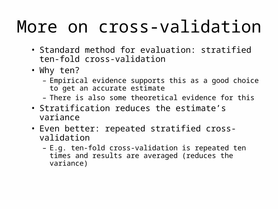
More on cross-validation• Standard method for evaluation: stratified ten-fold

cross-validation• Why ten?

– Empirical evidence supports this as a good choice to get an accurate estimate

– There is also some theoretical evidence for this• Stratification reduces the estimate’s variance• Even better: repeated stratified cross-validation

– E.g. ten-fold cross-validation is repeated ten times and results are averaged (reduces the variance)

Leave-One-Out cross-validation

• Leave-One-Out:a particular form of cross-validation:– Set number of folds to number of training instances– I.e., for n training instances, build classifier n times

• Makes best use of the data• Involves no random subsampling • Very computationally expensive

– (exception: NN)

Leave-One-Out-CV and stratification

• Disadvantage of Leave-One-Out-CV: stratification is not possible– It guarantees a non-stratified sample because there is only

one instance in the test set!

Hands-on Example# Import Bayes.csv from class webpage

# Select training datatraindata <- Bayes[1:14,]

# Select test datatestdata <- Bayes[15,]

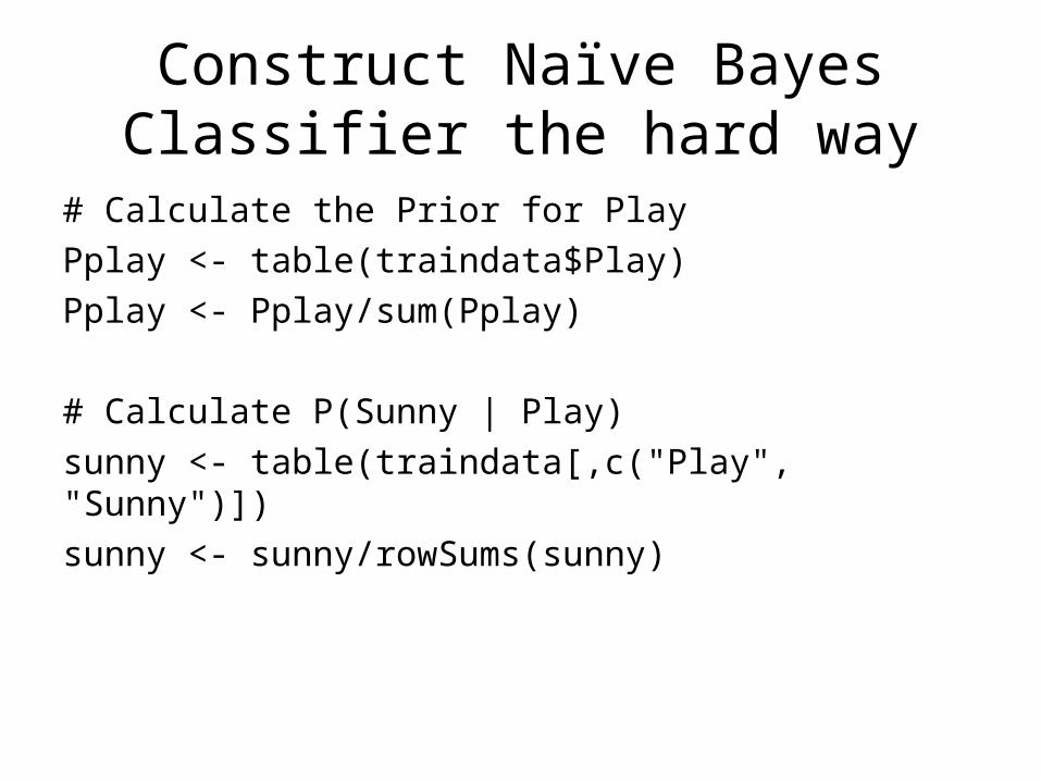
Construct Naïve Bayes Classifier the hard way

# Calculate the Prior for PlayPplay <- table(traindata$Play)Pplay <- Pplay/sum(Pplay)

# Calculate P(Sunny | Play) sunny <- table(traindata[,c("Play", "Sunny")]) sunny <- sunny/rowSums(sunny)

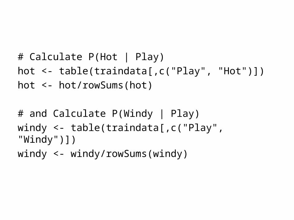
# Calculate P(Hot | Play)hot <- table(traindata[,c("Play", "Hot")]) hot <- hot/rowSums(hot)

# and Calculate P(Windy | Play)windy <- table(traindata[,c("Play", "Windy")])windy <- windy/rowSums(windy)

# Evaluate testdataPyes <- sunny["Yes","Yes"] * hot["Yes","No"] * windy["Yes","Yes"]

Pno <- sunny["No","Yes"] * hot["No","No"] * windy["No","Yes"]

# Do we play or not?Max(Pyes, Pno)

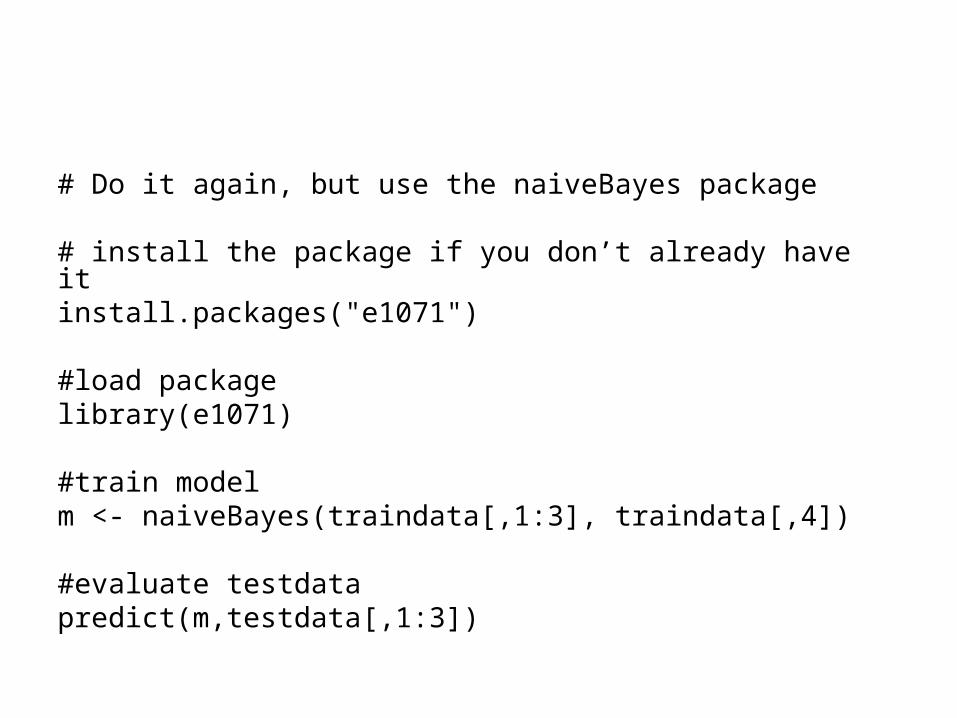
# Do it again, but use the naiveBayes package

# install the package if you don’t already have itinstall.packages("e1071")

#load packagelibrary(e1071)

#train modelm <- naiveBayes(traindata[,1:3], traindata[,4])

#evaluate testdatapredict(m,testdata[,1:3])

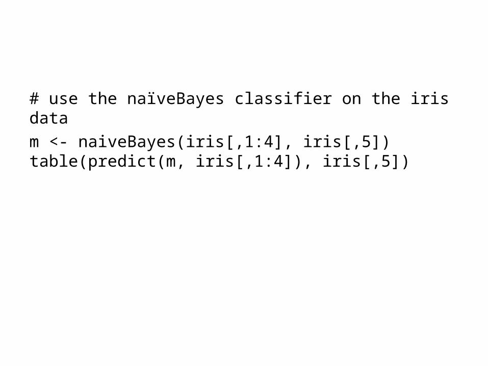
# use the naïveBayes classifier on the iris datam <- naiveBayes(iris[,1:4], iris[,5]) table(predict(m, iris[,1:4]), iris[,5])

Questions?