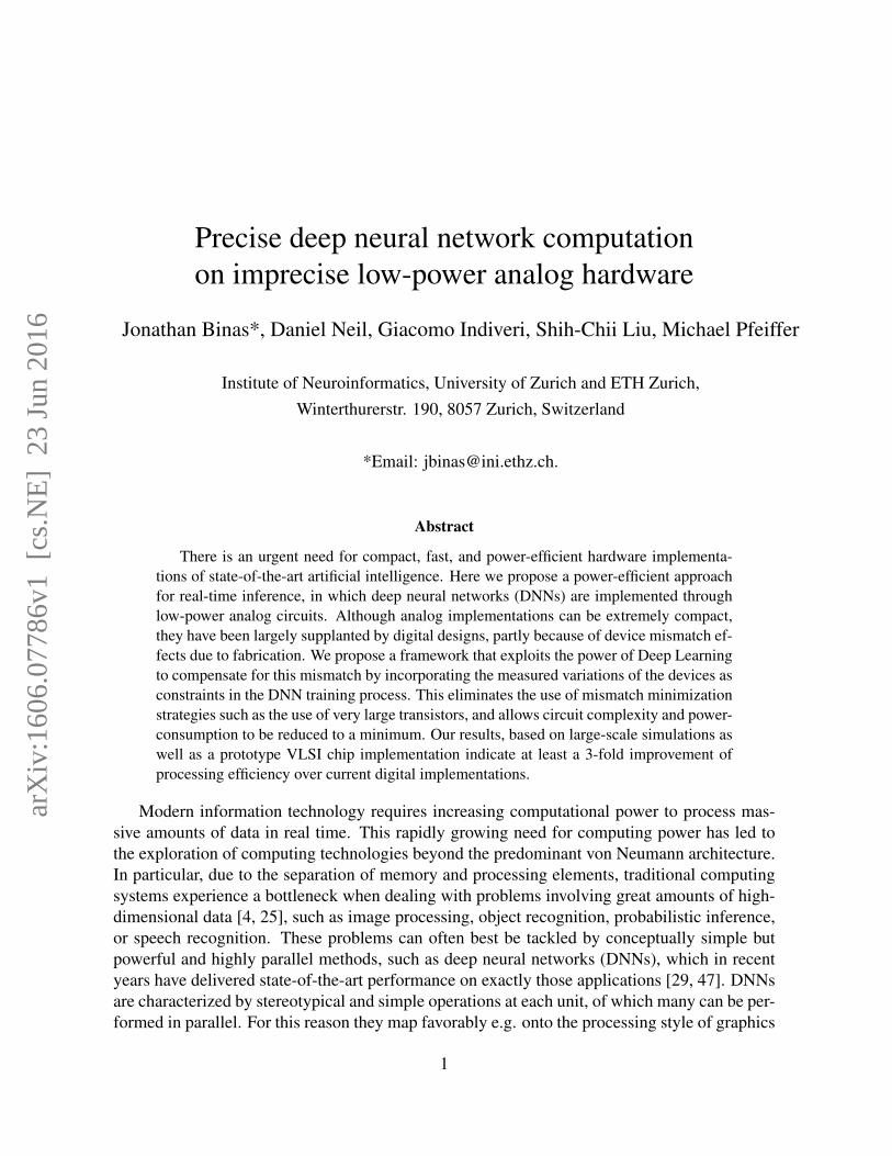
Precise deep neural network computation on imprecise low-power analog · PDF file · 2016-06-27Precise deep neural network computation on imprecise low-power analog hardware Jonathan

Precise deep neural network computationon imprecise low-power analog hardware

Jonathan Binas*, Daniel Neil, Giacomo Indiveri, Shih-Chii Liu, Michael Pfeiffer

Institute of Neuroinformatics, University of Zurich and ETH Zurich,Winterthurerstr. 190, 8057 Zurich, Switzerland

*Email: [email protected].

Abstract

There is an urgent need for compact, fast, and power-efficient hardware implementa-tions of state-of-the-art artificial intelligence. Here we propose a power-efficient approachfor real-time inference, in which deep neural networks (DNNs) are implemented throughlow-power analog circuits. Although analog implementations can be extremely compact,they have been largely supplanted by digital designs, partly because of device mismatch ef-fects due to fabrication. We propose a framework that exploits the power of Deep Learningto compensate for this mismatch by incorporating the measured variations of the devices asconstraints in the DNN training process. This eliminates the use of mismatch minimizationstrategies such as the use of very large transistors, and allows circuit complexity and power-consumption to be reduced to a minimum. Our results, based on large-scale simulations aswell as a prototype VLSI chip implementation indicate at least a 3-fold improvement ofprocessing efficiency over current digital implementations.

Modern information technology requires increasing computational power to process mas-sive amounts of data in real time. This rapidly growing need for computing power has led tothe exploration of computing technologies beyond the predominant von Neumann architecture.In particular, due to the separation of memory and processing elements, traditional computingsystems experience a bottleneck when dealing with problems involving great amounts of high-dimensional data [4, 25], such as image processing, object recognition, probabilistic inference,or speech recognition. These problems can often best be tackled by conceptually simple butpowerful and highly parallel methods, such as deep neural networks (DNNs), which in recentyears have delivered state-of-the-art performance on exactly those applications [29, 47]. DNNsare characterized by stereotypical and simple operations at each unit, of which many can be per-formed in parallel. For this reason they map favorably e.g. onto the processing style of graphics

1

arX

iv:1

606.

0778

6v1

[cs

.NE

] 2

3 Ju

n 20

16

processing units (GPUs) [46]. The large computational demands of DNNs have simultaneouslysparked interest in methods that make neural network inference faster and more power efficient,whether through new algorithmic inventions [19, 21, 11], dedicated digital hardware implemen-tations [6, 17, 8], or by taking inspiration from real nervous systems [14, 37, 33, 23, 34].

With synchronous digital logic being the established standard of the electronics indus-try, first attempts towards hardware deep network accelerators have focused on this approach[6, 18, 7, 38]. However, the massively parallel style of computation of neural networks is notreflected in the mostly serial and time-multiplexed nature of digital systems. An arguably morenatural way of developing a hardware neural network emulator is to implement its computa-tional primitives as multiple physical and parallel instances of analog computing nodes, wherememory and processing elements are co-localized, and state variables are directly representedby analog currents or voltages, rather than being encoded digitally [43, 1, 49, 5, 3, 45]. Bydirectly representing neural network operations in the physical properties of silicon transistors,such analog implementations can outshine their digital counterparts in terms of simplicity, al-lowing for significant advances in speed, size, and power consumption [20, 32]. The mainreason why engineers have been discouraged from following this approach is that the propertiesof analog circuits are affected by the physical imperfections inherent to any chip fabricationprocess, which can lead to significant functional differences between individual devices [40].

In this work we propose a new approach, whereby rather than brute-force engineering morehomogeneous circuits (e.g. by increasing transistor sizes and burning more power), we employneural network training methods as an effective optimization framework to automatically com-pensate for the device mismatch effects of analog VLSI circuits. We use the diverse measuredcharacteristics of individual VLSI devices as constraints in an off-line training process, to yieldnetwork configurations that are tailored to the particular analog device used, thereby compen-sating the inherent variability of chip fabrication. Finally, the network parameters, in particularthe synaptic weights found during the training phase can be programmed in the network, and theanalog circuits can be operated at run-time in the sub-threshold region for significantly lowerpower consumption.

In this article, in addition to introducing a novel training method for both device and net-work, we also propose compact and low-power candidate VLSI circuits. A closed-loop demon-stration of the framework is shown, based on a fabricated prototype chip, as well as detailed,large-scale simulations. The resulting analog electronic neural network performs as well asan ideal network, while offering at least a threefold lower power consumption over its digitalcounterpart.

1 ResultsA deep neural network processes input signals in a number of successive layers of neurons,where each neuron computes a weighted sum of its inputs followed by a non-linearity, such asa sigmoid or rectification. Specifically, the output of a neuron i is given by xi = f

(∑j wijxj

),

2

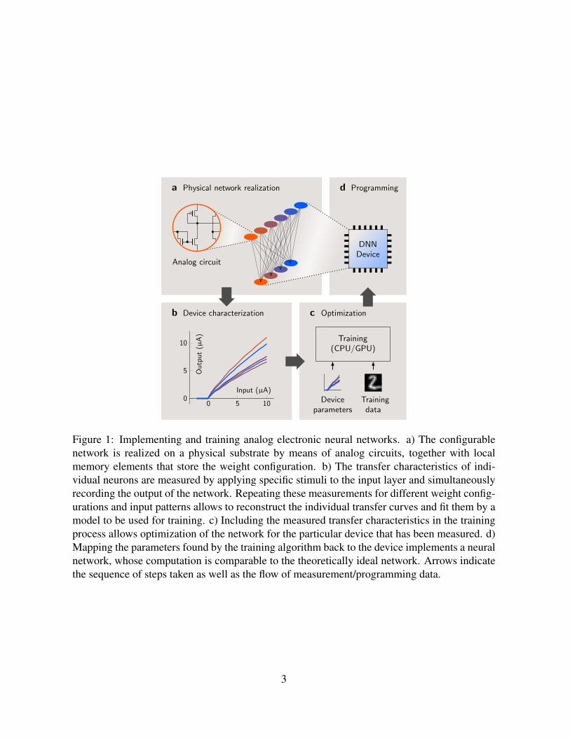
a Physical network realization

b Device characterization c Optimization

d Programming

Analog circuit

0 5 100

5

10

Input (µA)

Output(µ

A)

Training(CPU/GPU)

Deviceparameters

Trainingdata

DNNDevice

Figure 1: Implementing and training analog electronic neural networks. a) The configurablenetwork is realized on a physical substrate by means of analog circuits, together with localmemory elements that store the weight configuration. b) The transfer characteristics of indi-vidual neurons are measured by applying specific stimuli to the input layer and simultaneouslyrecording the output of the network. Repeating these measurements for different weight config-urations and input patterns allows to reconstruct the individual transfer curves and fit them by amodel to be used for training. c) Including the measured transfer characteristics in the trainingprocess allows optimization of the network for the particular device that has been measured. d)Mapping the parameters found by the training algorithm back to the device implements a neuralnetwork, whose computation is comparable to the theoretically ideal network. Arrows indicatethe sequence of steps taken as well as the flow of measurement/programming data.

3

where f is the non-linearity, and wij is the weight of the connection from neuron j to neuroni. Thus, the basic operations comprising a neural network are summation, multiplication byscalars, and simple non-linear transformations. All of these operations can be implemented inanalog electronic circuitry very efficiently, that is with very few transistors, whereby numericvalues are represented by actual voltage or current values, rather than a digital code. Analogcircuits are affected by fabrication mismatch, i.e. small fluctuations in the fabrication processthat lead to fixed distortions of functional properties of elements on the same device, as wellas multiple sources of noise. As a consequence, the response of an analog hardware neuronis slightly different for every instance of the circuit, such that xi = fi

(∑j wijxj

), where fi

approximately corresponds to f , but is slightly different for every neuron i.

1.1 Training with heterogeneous transfer functionsThe weights of multi-layered networks are typically learned from labeled training data usingthe backpropagation algorithm [44], which minimizes the training error by computing errorgradients and passing them backwards through the layers. In order for this to work in practice,the transfer function f needs to be at least piece-wise differentiable, as is the case for the com-monly used rectified linear unit (ReLU) [16]. Although it is common practice in neural networktraining, it is not necessary for all neurons to have identical activation functions f . In fact,having different activation functions makes no difference to backpropagation as long as theirderivatives can be computed. Here this principle is exploited by inserting the heterogeneousbut measured transfer curves fi from a physical analog neural network implementation into thetraining algorithm, with the goal of finding weight parameters that are tailored for a particularheterogeneous system given by f1, . . . , fN .

The process of implementing a target functionality in such a heterogeneous system is illus-trated in Fig. 1. Once a neural network architecture with modifiable weights is implemented insilicon, the transfer characteristics of the different neuron instances can be measured by control-ling the inputs specific cells receive and recording their output at the same time (see Methods). Ifthe transfer curves are sufficiently simple (depending on the actual implemented analog neuroncircuit), a small number of discrete measurements yield sufficient information to fit a contin-uous, (piece-wise) differentiable model to the hardware response. For instance, the rectifiedlinear neuron f(r) = max{0, a · r} is fully described by a single parameter a, which is simplythe ratio of output to input, and therefore can easily be measured. The continuous, parameter-ized description is then used by the training algorithm, which is run on traditional computinghardware, such as CPUs or GPUs, to generate a network configuration that is tailored to theparticular task and the physical device that has been characterized.

1.2 Analog circuit implementationTo achieve a compact and low-power solution, we construct a multilayer network using thecircuits shown in Fig. 2 and operate them in the subthreshold region. The subthreshold current

4

of a transistor is exponential in the gate voltage, rather than polynomial as is the case for abovethreshold operation, and can span many orders of magnitude. Thus, a system based on thistechnology can be operated at orders of magnitude lower currents than a digital one. In turn,this means that the device mismatch arising due to imperfections in the fabrication process canhave an exponentially larger impact. Fortunately, as our method neither depends on the specificform nor the magnitude of the mismatch, it can handle a wide variety of mismatch conditions.

M0

M1

M2

M4

M3

Vp

Vn

Vdd

Iin→

b Soma

M10 M11 M12

M13 M14 M15

M16

M17

M18 M19 M20

Vn

Vp

Vdd

Iout→

w0 w1 w2w±

Weight configurationc Synapse

Lay

erk-

1

Layer k

Soma Synapse

V

I

a

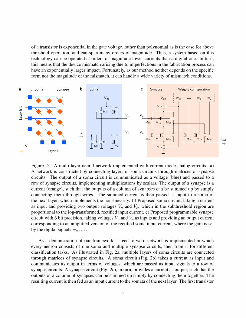
Figure 2: A multi-layer neural network implemented with current-mode analog circuits. a)A network is constructed by connecting layers of soma circuits through matrices of synapsecircuits. The output of a soma circuit is communicated as a voltage (blue) and passed to arow of synapse circuits, implementing multiplications by scalars. The output of a synapse is acurrent (orange), such that the outputs of a column of synapses can be summed up by simplyconnecting them through wires. The summed current is then passed as input to a soma ofthe next layer, which implements the non-linearity. b) Proposed soma circuit, taking a currentas input and providing two output voltages Vn and Vp, which in the subthreshold region areproportional to the log-transformed, rectified input current. c) Proposed programmable synapsecircuit with 3 bit precision, taking voltages Vn and Vp as inputs and providing an output currentcorresponding to an amplified version of the rectified soma input current, where the gain is setby the digital signals w±, wi.

As a demonstration of our framework, a feed-forward network is implemented in whichevery neuron consists of one soma and multiple synapse circuits, then train it for differentclassification tasks. As illustrated in Fig. 2a, multiple layers of soma circuits are connectedthrough matrices of synapse circuits. A soma circuit (Fig. 2b) takes a current as input andcommunicates its output in terms of voltages, which are passed as input signals to a row ofsynapse circuits. A synapse circuit (Fig. 2c), in turn, provides a current as output, such that theoutputs of a column of synapses can be summed up simply by connecting them together. Theresulting current is then fed as an input current to the somata of the next layer. The first transistor

5

of the soma circuit rectifies the input current. The remaining elements of the soma circuit,together with a connected synapse circuit, form a set of scaling current mirrors, i.e. rudimentaryamplifiers, a subset of which can be switched on or off to achieve a particular weight value bysetting the respective synapse configuration bits. Thus, the output of a synapse corresponds to ascaled version of the rectified input current of the soma, similar to the ReLU transfer function.In our proposed example implementation we use signed 3-bit synapses, which are based on2×3 current mirrors of different dimensions (3 for positive and 3 for negative values). One of 24

possible weight values is then selected by switching the respective current mirrors on or off. Thescaling factor of a particular current mirror, and thus its contribution to the total weight value, isproportional to the ratio of the widths of the two transistors forming it. The weight configurationof an individual synapse can be stored digitally in memory elements that are part of the actualsynapse circuit. Thus, in contrast to digital processing systems, our circuit computes in memoryand thereby avoids the bottleneck of expensive data transfer between memory and processingelements.

Although this is just one out of many possible analog circuits implementations, the sim-ple circuits chosen offer several advantages besides the fact that they can be implemented insmall areas: First, numeric values are conveyed only through current mirrors, and therefore aretemperature-independent. Second, most of the fabrication-induced variability is due to the de-vices in the soma with five consecutive transistors, whereas only one layer of transistors affectsthe signal in the synapse. This means that the synapse-induced mismatch can be neglected in afirst order approximation.

Once an analog electronic neural network has been implemented physically as a VLSI de-vice, the transfer characteristics of the individual soma circuits are obtained through measure-ments. The transfer function implemented by our circuits can be well described by a rectifiedlinear curve, where the only free parameter is the slope, and thus can be determined from asingle measurement per neuron. Specifically, the transfer curves of all neurons in a layer k canbe measured through a simple procedure: A single neuron in layer k − 1 is connected, poten-tially through some intermediate neurons, to the input layer and is defined to be the ‘source’.Similarly, a neuron in layer k+1 is connected, potentially through intermediate neurons, to theoutput layer and is called the ‘monitor’. All neurons of layer k can now be probed individu-ally using the source and monitor neurons, whereby the signal to the input layer is held fixedand the signal recorded at the output layer is proportional to the slope of the measured neuron.Note that the absolute scale of the responses is not relevant, i.e. only the relative scale withinone layer matters, as the output of individual layers can be scaled arbitrarily without alteringthe network function. The same procedure can be applied to all layers to obtain a completecharacterization of the network. The measurements can be parallelized by defining multiplesource and monitor neurons per measurement to probe several neurons in one layer simultane-ously, or by introducing additional readout circuitry between layers to measure multiple layerssimultaneously.

6

1.3 Handwritten and spoken digit classificationLarge-scale SPICE simulations of systems consisting of hundreds of thousands of transistors areemployed to assess power consumption, processing speed, and the accuracy of such an analogimplementation.

1414

· · ·

1

50

1

10

0

0.2

0.4

0 5 10 15 200

0.2

0.4

Time (µs)

Current(µ

A)

Inputswitched

Inputswitched

Time tooutput

Time tooutput

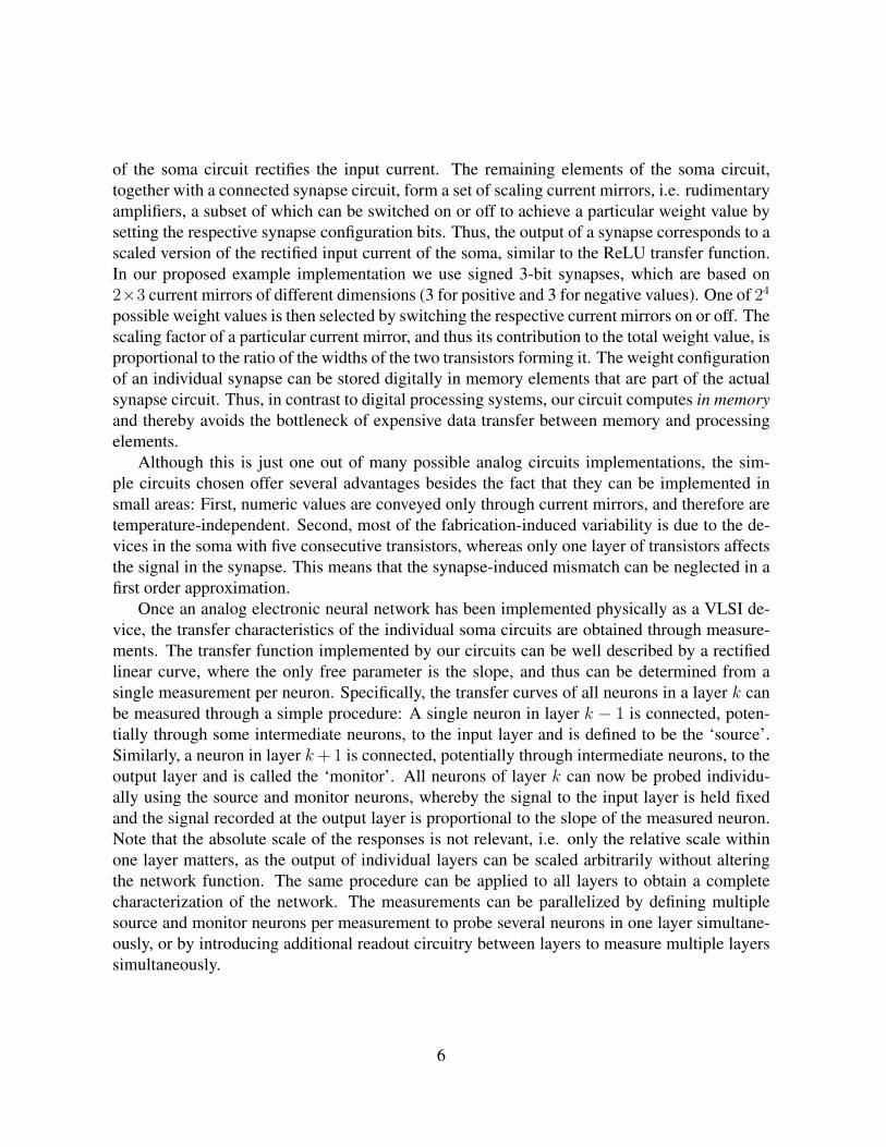
Figure 3: Analog circuit dynamics allow classification within microseconds. The curves rep-resent the activities (currents) of all hidden (top) and output (bottom) units of the 196− 50− 10network shown on the left. When a new input symbol is presented (top), the circuit convergesto its new state within microseconds. Only a few units remain active, while many tend to zero,such that their soma circuits and connected synapses dissipate very little power.

After simulating measurements and parameterizing the transfer characteristics of the circuitsas described previously, software networks were trained on the MNIST dataset of handwrittendigits [30] and the TIDIGITS dataset of spoken digits [31] by means of the ADAM trainingmethod [27]. In order to optimize the network for the use of discrete weights in the synapticcircuits dual-copy rounding [48, 10] was used (see Methods). By evaluating the responses of thesimulated circuit on subsets of the respective test sets, its classification accuracy was found tobe comparable to the abstract software neural network (see Tab. 1 for comparison). Fig. 3 showshow inputs are processed by a small example circuit implementing a 196 − 50 − 10 network,containing around 10k synapses and over 100k transistors. Starting with the presentation of aninput pattern in the top layer, where currents are proportional to input stimulus intensity, thehigher layers react almost instantaneously and provide the correct classification, i.e. the indexof the maximally active output unit, within a few microseconds. After a switch of input patterns,the signals quickly propagate through the network and the outputs of different nodes convergeto their asymptotic values. The time it takes the circuit to converge to its final output defines the

7

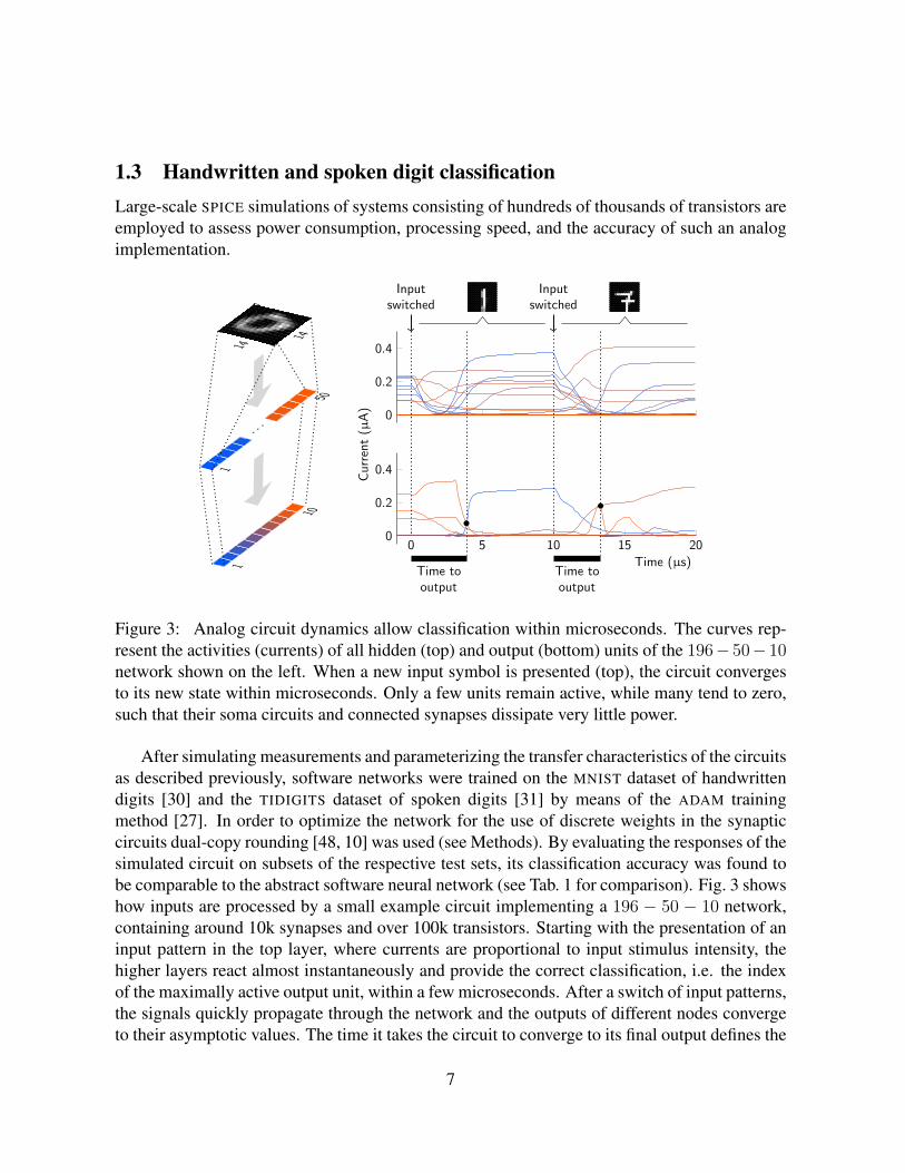
‘time to output’, constraining the maximum frequency at which input patterns can be presentedand evaluated correctly. Measured convergence times are summarized in Fig. 4 for differentpatterns from the MNIST test set, and are found to be in the range of microseconds for a trained196− 100− 50− 10 network, containing over 25k synapses and around 280k transistors. Notethat observed timescale is not fixed as the network can be run faster or slower by changing theinput current, while the average energy dissipated per operation remains roughly constant.

102 103100

1010.1 pJ/Op

0.01 pJ/Op

Average power (µW)

Tim

eto

output(µ

s)

0.01 0.1

50

100

150

0.001

Iavg =45 nA

Energy/op. (pJ)

50

100

150Iavg =15 nA

5 10 15

0.05

0.1

Runtime (µs)

Cou

nt

Energy/o

p.(pJ)

a b

c

Figure 4: Processing performance of a network for handwritten digit classification. All datashown was generated by presenting 500 different input patterns from the MNIST test set toa trained 196 − 100 − 50 − 10 network with the average input current per input neuron setto 15 nA (blue) or 45 nA (orange), respectively. a) The time to output is plotted against theaverage power dissipated over the duration of the transient (from start of the input pattern untiltime to output). The distributions of the data points are indicated by histograms on the sides.Changing the input current causes a shift along the equi-efficiency lines, that is, the networkcan be run slower or faster at the same efficiency (energy per operation). b) Energy dissipatedper operation for different run times, corresponding to different fixed rates at which inputsare presented (mean over 500 samples; standard deviation indicated by shaded areas). c) Theaverage energy consumed per operation was computed from the data shown in a). The datacorresponds to the hypothetical case were the network would be stopped as soon as the correctoutput is reached.

The processing efficiency of the system (energy per operation) was computed for differentinput patterns by integrating the power dissipated between the time at which the input pattern

8

was switched and the time to output. Fig. 4 shows the processing efficiency for the same net-work with different input examples and under different operating currents. With the averageinput currents scaled to either 15 or 45 nA per neuron respectively, the network takes severalmicroseconds to converge and consumes tens or hundreds of microwatts in total, which amountsto a few nanowatts per multiply-accumulate operation. With the supply voltage set to 1.8 V, thiscorresponds to less than 0.1 pJ per operation in most cases. With the average input current setto 15 nA per neuron, the network produces the correct output within 15µs in over 99 % of allcases (mean 8.5µs; std. 2.3µs). Running the circuit for 15µs requires 0.12± 0.01 pJ per oper-ation, such that about 1.7 trillion multiply-accumulate operations can be computed per secondat a power budget of around 200µW if input patterns are presented at a rate of 66 kHz. Withoutmajor optimizations to either process or implementation, this leads to an efficiency of around8 TOp/J, to our knowledge a performance at least four times greater than that achieved by dig-ital single-purpose neural network accelerators in similar scenarios [6, 38]. General purposedigital systems are far behind such specialized systems in terms of efficiency, with the latestGPU generation achieving around 0.05 TOp/J [36].

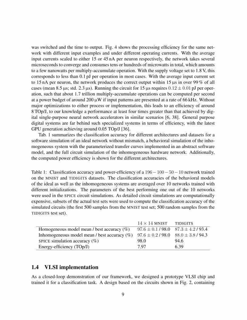
Tab. 1 summarizes the classification accuracy for different architectures and datasets for asoftware simulation of an ideal network without mismatch, a behavioral simulation of the inho-mogeneous system with the parameterized transfer curves implemented in an abstract softwaremodel, and the full circuit simulation of the inhomogeneous hardware network. Additionally,the computed power efficiency is shown for the different architectures.

Table 1: Classification accuracy and power-efficiency of a 196−100−50−10 network trainedon the MNIST and TIDIGITS datasets. The classification accuracies of the behavioral modelsof the ideal as well as the inhomogeneous systems are averaged over 10 networks trained withdifferent initializations. The parameters of the best performing one out of the 10 networkswere used in the SPICE circuit simulations. As detailed circuit simulations are computationallyexpensive, subsets of the actual test sets were used to compute the classification accuracy of thesimulated circuits (the first 500 samples from the MNIST test set; 500 random samples from theTIDIGITS test set).

14× 14 MNIST TIDIGITS

Homogeneous model mean / best accuracy (%) 97.6± 0.1 / 98.0 87.3± 4.2 / 93.4Inhomogeneous model mean / best accuracy (%) 97.6± 0.2 / 98.0 88.0± 3.8 / 94.3SPICE simulation accuracy (%) 98.0 94.6Energy-efficiency (TOp/J) 7.97 6.39

1.4 VLSI implementationAs a closed-loop demonstration of our framework, we designed a prototype VLSI chip andtrained it for a classification task. A design based on the circuits shown in Fig. 2, containing

9

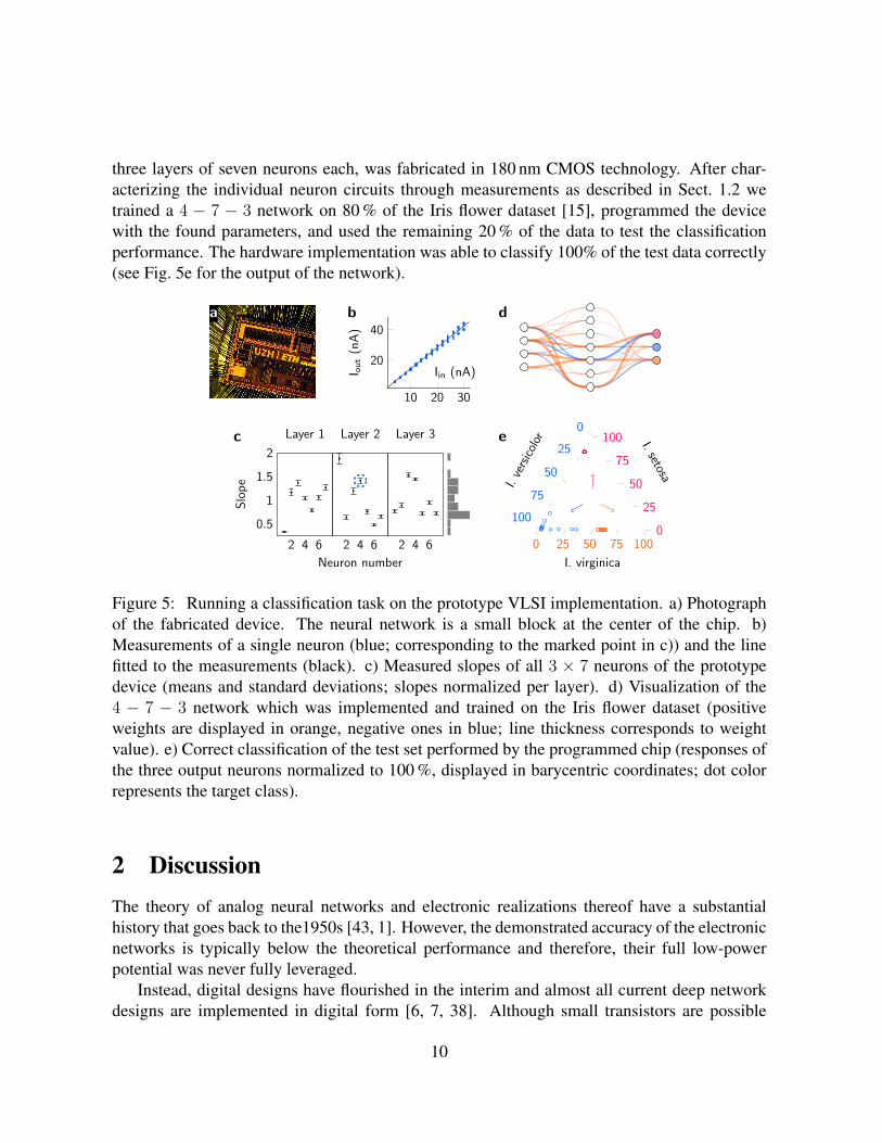
three layers of seven neurons each, was fabricated in 180 nm CMOS technology. After char-acterizing the individual neuron circuits through measurements as described in Sect. 1.2 wetrained a 4 − 7 − 3 network on 80 % of the Iris flower dataset [15], programmed the devicewith the found parameters, and used the remaining 20 % of the data to test the classificationperformance. The hardware implementation was able to classify 100% of the test data correctly(see Fig. 5e for the output of the network).

2 4 6

0.5

1

1.5

2

Slope

Layer 1

2 4 6

Neuron number

Layer 2

2 4 6

Layer 3

10 20 30

20

40

Iin (nA)I out(nA)

0

25

50

75

100

0 25 50 75 1000

25

50

75

100 I.setosa

I.versicolor

I. virginica

c

a b d

e

Figure 5: Running a classification task on the prototype VLSI implementation. a) Photographof the fabricated device. The neural network is a small block at the center of the chip. b)Measurements of a single neuron (blue; corresponding to the marked point in c)) and the linefitted to the measurements (black). c) Measured slopes of all 3 × 7 neurons of the prototypedevice (means and standard deviations; slopes normalized per layer). d) Visualization of the4 − 7 − 3 network which was implemented and trained on the Iris flower dataset (positiveweights are displayed in orange, negative ones in blue; line thickness corresponds to weightvalue). e) Correct classification of the test set performed by the programmed chip (responses ofthe three output neurons normalized to 100 %, displayed in barycentric coordinates; dot colorrepresents the target class).

2 DiscussionThe theory of analog neural networks and electronic realizations thereof have a substantialhistory that goes back to the1950s [43, 1]. However, the demonstrated accuracy of the electronicnetworks is typically below the theoretical performance and therefore, their full low-powerpotential was never fully leveraged.

Instead, digital designs have flourished in the interim and almost all current deep networkdesigns are implemented in digital form [6, 7, 38]. Although small transistors are possible

10

in digital implementations, the typical size of a multiplier-accumulator (MAC) block usuallymeans that these implementations use a smaller subset of functional blocks and therefore theuse of MACs is time-multiplexed by shifting data around accordingly. As a consequence, theprocessing speed of digital implementations is limited by their clock frequency.

The simplicity of the analog VLSI circuits needed for addition - namely connecting togetherwires - allows an explicit implementation of each processing unit or neuron where no element isshared or time-multiplexed within the network implementation. The resulting VLSI network ismaximally parallel and eliminates the bottleneck of transferring data between memory and pro-cessing elements. Using digital technology, such fully parallel implementations would quicklybecome prohibitively large due to the much greater circuit complexity of digital processing el-ements. While the focus in this work has been on an efficient analog VLSI implementation,hardware implementations using new forms of nano devices can also benefit from this trainingmethod. For example, the memristive computing technology which is currently being pursuedfor implementing large-scale cognitive neuromorphic and other technologies still suffers fromthe mismatch of fabricated devices [2, 26, 41]. The proposed training method in this work canbe used to account for device non-idealities in this technology [35].

In fact, any system that can be properly characterized and has configurable elements standsto benefit from this approach. For example, spike-based neuromorphic systems [24] often haveconfigurable weights between neurons. These systems communicate via biologically inspireddigital-like pulses called spikes. Similar to the method outlined in this work, the relationship be-tween an input spike rate and an output spike rate of a neuron can be measured in such a system,and the transfer functions then used as a constraint during the training process so as to achieveaccurate results from the whole network even if the neuron circuits themselves are varied andnon-ideal. In addition to the alternate hardware implementations, other network topologies suchas convolutional networks can be trained using this proposed method. However, as all weightsare implemented explicitly in silicon, the system design here would not benefit from the smallmemory footprint achieved via weight sharing in traditional convolutional network implemen-tations. In principle, even recurrent architectures such as LSTM networks [22] can be trainedusing the same methods, where not only the static properties of the circuit are taken into accountbut also their dynamics.

With every device requiring an individual training procedure, an open question is how theper-device training time can be reduced. Initializing the network to a pre-trained ideal network,which is then fine-tuned for the particular devices is likely to reduce training time.

In the current setting, the efficiency of our system is limited by the worst-case per-exampleruntime, i.e. there may be a few samples where outputs require significantly longer to con-verge to the correct classification result than the majority. This can lead to unnecessarily longpresentation times for many samples, thereby causing unnecessary power consumption. Smartmethods of estimating presentation times from the input data could e.g. accelerate convergencefor slowly converging samples by using higher input currents, and conversely, faster samplescould be slowed down to lower the variability of convergence times and overall reduce energyconsumption. Future research will focus on such estimators, and alternatively explore ways of

11

reducing convergence time variability during network training.This proof-of-principle study is an important step towards the construction of large scale,

possibly ultra-low-power analog VLSI deep neural network processors, paving the way for spe-cialized applications which had not been feasible before due to speed or power constraints.Small, efficient implementations could allow autonomous systems to achieve almost immediatereaction times under strict power limitations. Scaled-up versions can allow for substantiallymore efficient processing in data centers, allowing for a greatly reduced energy footprint orpermitting substantially more data to be effectively processed. Conversely, digital approachesand GPU technology are aiming for general purpose deep network acceleration, and thus natu-rally have an advantage in terms of flexibility compared to the fixed physical implementation ofthe proposed analog devices. However, there is increasing evidence that neural networks pre-trained on large datasets such as ImageNet provide excellent generic feature detectors [13, 42],which means that fast and efficient analog input pre-processors could be used as an importantbuilding blocks for a large variety of applications.

References[1] J. Alspector and R.B. Allen. A neuromorphic VLSI learning system. In P. Losleben, editor,

Proceedings of the 1987 Stanford Conference on Advanced Research in VLSI, pages 313–349, Cambridge, MA, USA, 1987. MIT Press.

[2] S Ambrogio, S Balatti, F Nardi, S Facchinetti, and D Ielmini. Spike-timing depen-dent plasticity in a transistor-selected resistive switching memory. Nanotechnology,24(38):384012, 2013.

[3] Andreas G Andreou, Kwabena Boahen, Philippe O Pouliquen, Aleksandra Pavasovic,Robert E Jenkins, Kim Strohbehn, et al. Current-mode subthreshold MOS circuits foranalog VLSI neural systems. IEEE Transactions on neural networks, 2(2):205–213, 1991.

[4] John Backus. Can programming be liberated from the von neumann style?: A functionalstyle and its algebra of programs. Commun. ACM, 21(8):613–641, 1978.

[5] T.H. Borgstrom, M Ismail, and S.B. Bibyk. Programmable current-mode neural networkfor implementation in analogue MOS VLSI. IEE Proceedings G, 137(2):175–184, 1990.

[6] Lukas Cavigelli, David Gschwend, Christoph Mayer, Samuel Willi, Beat Muheim, andLuca Benini. Origami: A convolutional network accelerator. In Proceedings of the 25thedition on Great Lakes Symposium on VLSI, pages 199–204. ACM, 2015.

[7] Yu-Hsin Chen, Tushar Krishna, Joel Emer, and Vivienne Sze. 14.5 eyeriss: An energy-efficient reconfigurable accelerator for deep convolutional neural networks. In 2016 IEEEInternational Solid-State Circuits Conference (ISSCC), pages 262–263. IEEE, 2016.

12

[8] Yunji Chen, Tao Luo, Shaoli Liu, Shijin Zhang, Liqiang He, Jia Wang, Ling Li, TianshiChen, Zhiwei Xu, Ninghui Sun, et al. Dadiannao: A machine-learning supercomputer.In Microarchitecture, 2014 47th Annual IEEE/ACM International Symposium on, pages609–622. IEEE, 2014.

[9] FranÃgois Chollet. Keras. https://github.com/fchollet/keras, 2015.

[10] Matthieu Courbariaux, Yoshua Bengio, and Jean-Pierre David. Low precision arithmeticfor deep learning. arXiv preprint arXiv:1412.7024, 2014.

[11] Matthieu Courbariaux, Yoshua Bengio, and Jean-Pierre David. Binaryconnect: Trainingdeep neural networks with binary weights during propagations. In Advances in NeuralInformation Processing Systems, pages 3105–3113, 2015.

[12] Tobi Delbruck, Raphael Berner, Patrick Lichtsteiner, and Carlos Dualibe. 32-bit config-urable bias current generator with sub-off-current capability. In Proceedings of 2010 IEEEInternational Symposium on Circuits and Systems, pages 1647–1650. IEEE, 2010.

[13] Jeff Donahue, Yangqing Jia, Oriol Vinyals, Judy Hoffman, Ning Zhang, Eric Tzeng, andTrevor Darrell. DeCAF: A deep convolutional activation feature for generic visual recog-nition. In ICML, pages 647–655, 2014.

[14] Clément Farabet, R Paz-Vicente, JA Pérez-Carrasco, Carlos Zamarreño-Ramos, Alejan-dro Linares-Barranco, Yann LeCun, Eugenio Culurciello, Teresa Serrano-Gotarredona,and Bernabe Linares-Barranco. Comparison between frame-constrained fix-pixel-valueand frame-free spiking-dynamic-pixel convnets for visual processing. Frontiers in Neuro-science, 6:1–12, 2012.

[15] RA Fisher. Iris flower data set, 1936.

[16] Xavier Glorot, Antoine Bordes, and Yoshua Bengio. Deep sparse rectifier neural networks.In International Conference on Artificial Intelligence and Statistics, pages 315–323, 2011.

[17] Vinayak Gokhale, Jonghoon Jin, Aysegul Dundar, Ben Martini, and Eugenio Culurciello.A 240 g-ops/s mobile coprocessor for deep neural networks. In Computer Vision andPattern Recognition Workshops (CVPRW), 2014 IEEE Conference on, pages 696–701.IEEE, 2014.

[18] Matthew Griffin, Gary Tahara, Kurt Knorpp, Ray Pinkham, and Bob Riley. An 11-milliontransistor neural network execution engine. In Solid-State Circuits Conference, 1991.Digest of Technical Papers. 38th ISSCC., 1991 IEEE International, pages 180–313. IEEE,1991.

13

[19] Song Han, Huizi Mao, and William J Dally. Deep compression: Compressing deepneural networks with pruning, trained quantization and huffman coding. arXiv preprintarXiv:1510.00149, 2015.

[20] Jennifer Hasler and Bo Marr. Finding a roadmap to achieve large neuromorphic hardwaresystems. Frontiers in neuroscience, 7, 2013.

[21] Geoffrey Hinton, Oriol Vinyals, and Jeff Dean. Distilling the knowledge in a neural net-work. arXiv preprint arXiv:1503.02531, 2015.

[22] Sepp Hochreiter and Jürgen Schmidhuber. Long short-term memory. Neural computation,9(8):1735–1780, 1997.

[23] Giacomo Indiveri, Federico Corradi, and Ning Qiao. Neuromorphic architectures for spik-ing deep neural networks. In IEEE International Electron Devices Meeting (IEDM), 2015.

[24] Giacomo Indiveri, Bernabe Linares-Barranco, Tara Julia Hamilton, André van Schaik,Ralph Etienne-Cummings, Tobi Delbruck, Shih-Chii Liu, Piotr Dudek, Philipp Häfliger,Sylvie Renaud, Johannes Schemmel, Gert Cauwenberghs, John Arthur, Kai Hynna,Fopefolu Folowosele, Sylvain SAÏGHI, Teresa Serrano-Gotarredona, Jayawan Wijekoon,Yingxue Wang, and Kwabena Boahen. Neuromorphic silicon neuron circuits. Frontiersin Neuroscience, 5(73), 2011.

[25] Giacomo Indiveri and Shih-Chii Liu. Memory and information processing in neuromor-phic systems. Proceedings of the IEEE, 103(8):1379–1397, 2015.

[26] Kuk-Hwan Kim, Siddharth Gaba, Dana Wheeler, Jose M Cruz-Albrecht, Tahir Hussain,Narayan Srinivasa, and Wei Lu. A functional hybrid memristor crossbar-array/CMOSsystem for data storage and neuromorphic applications. Nano letters, 12(1):389–395,2011.

[27] Diederik Kingma and Jimmy Ba. Adam: A method for stochastic optimization. arXivpreprint arXiv:1412.6980, 2014.

[28] Kadaba R Lakshmikumar, Robert Hadaway, and Miles Copeland. Characterisation andmodeling of mismatch in MOS transistors for precision analog design. IEEE Journal ofSolid-State Circuits, 21(6):1057–1066, 1986.

[29] Yann LeCun, Yoshua Bengio, and Geoffrey Hinton. Deep learning. Nature,521(7553):436–444, 2015.

[30] Yann LeCun, Corinna Cortes, and Christopher JC Burges. The MNIST database of hand-written digits, 1998.

14

[31] R Gary Leonard and George Doddington. Tidigits speech corpus. Texas Instruments, Inc,1993.

[32] Peter Masa, Klaas Hoen, and Hans Wallinga. A high-speed analog neural processor. Mi-cro, IEEE, 14(3):40–50, 1994.

[33] Paul A Merolla, John V Arthur, Rodrigo Alvarez-Icaza, Andrew S Cassidy, Jun Sawada,Filipp Akopyan, Bryan L Jackson, Nabil Imam, Chen Guo, Yutaka Nakamura, BernardBrezzo, Ivan Vo, Steven K Esser, Rathinakumar Appuswamy, Brian Taba, Arnon Amir,Myron D Flickner, William P Risk, Rajit Manohar, and Dharmendra S Modha. A millionspiking-neuron integrated circuit with a scalable communication network and interface.Science, 345(6197):668–673, 2014.

[34] Daniel Neil, Michael Pfeiffer, and Shih-Chii Liu. Learning to be efficient: Algorithms fortraining low-latency, low-compute deep spiking neural networks. In ACM Symposium onApplied Computing, 2016.

[35] Dimin Niu, Yiran Chen, Cong Xu, and Yuan Xie. Impact of process variations on emergingmemristor. In Design Automation Conference (DAC), 2010 47th ACM/IEEE, pages 877–882. IEEE, 2010.

[36] NVIDIA. NVIDIA Tesla P100 – the most advanced datacenter accelerator ever built.featuring Pascal GP100, the world’s fastest GPU. NVIDIA Whitepaper, 2016.

[37] Peter O’Connor, Daniel Neil, Shih-Chii Liu, Tobi Delbruck, and Michael Pfeiffer. Real-time classification and sensor fusion with a spiking deep belief network. Frontiers inNeuromorphic Engineering, 7, 2013.

[38] SW Park, J Park, K Bong, D Shin, J Lee, S Choi, and HJ Yoo. An energy-efficient andscalable deep learning/inference processor with tetra-parallel MIMD architecture for bigdata applications. IEEE transactions on biomedical circuits and systems, 2016.

[39] Marcel JM Pelgrom, Hans P Tuinhout, and Maarten Vertregt. Transistor matching inanalog CMOS applications. IEDM Tech. Dig, pages 915–918, 1998.

[40] M.J.M. Pelgrom, Aad C.J. Duinmaijer, and A.P.G. Welbers. Matching properties of MOStransistors. IEEE Journal of Solid-State Circuits, 24(5):1433–1439, Oct 1989.

[41] Mirko Prezioso, Farnood Merrikh-Bayat, BD Hoskins, GC Adam, Konstantin K Likharev,and Dmitri B Strukov. Training and operation of an integrated neuromorphic networkbased on metal-oxide memristors. Nature, 521(7550):61–64, 2015.

[42] Ali Sharif Razavian, Hossein Azizpour, Josephine Sullivan, and Stefan Carlsson. CNNfeatures off-the-shelf: an astounding baseline for recognition. In Proc. of the IEEE Con-ference on Computer Vision and Pattern Recognition (CVPR) Workshops, pages 806–813,2014.

15

[43] F. Rosenblatt. The perceptron: a probabilistic model for information storage and organi-zation in the brain. Psychological review, 65(6):386–408, nov 1958.

[44] D. E. Rumelhart, G. E. Hinton, and R. J. Williams. Parallel distributed processing: Ex-plorations in the microstructure of cognition, vol. 1. chapter Learning Internal Represen-tations by Error Propagation, pages 318–362. MIT Press, Cambridge, MA, USA, 1986.

[45] S. Satyanarayana, Y.P. Tsividis, and H.P. Graf. A reconfigurable VLSI neural network.IEEE Journal of Solid-State Circuits, 27(1):67–81, Jan 1992.

[46] Dominik Scherer, Hannes Schulz, and Sven Behnke. Accelerating large-scale convo-lutional neural networks with parallel graphics multiprocessors. In Artificial NeuralNetworks–ICANN 2010, pages 82–91. Springer, 2010.

[47] J. Schmidhuber. Deep learning in neural networks: An overview. Neural Networks, 61:85–117, January 2015.

[48] Evangelos Stromatias, Daniel Neil, Michael Pfeiffer, Francesco Galluppi, Steve B Furber,and Shih-Chii Liu. Robustness of spiking deep belief networks to noise and reduced bitprecision of neuro-inspired hardware platforms. Frontiers in neuroscience, 9, 2015.

[49] E.A. Vittoz. Analog VLSI implementation of neural networks. In Proc. IEEE Int. Symp.Circuit and Systems, pages 2524–2527, New Orleans, 1990.

Acknowledgments: We are very grateful to Ning Qiao for his help with the VLSI imple-mentation. The work was supported by the Swiss National Science Foundation grant Spike-Comp (200021_146608) and the University of Zurich.

16

3 Methods

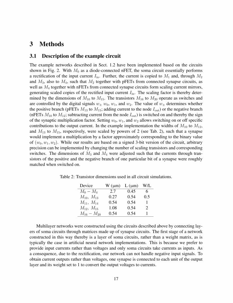
3.1 Description of the example circuitThe example networks described in Sect. 1.2 have been implemented based on the circuitsshown in Fig. 2. With M0 as a diode-connected nFET, the soma circuit essentially performsa rectification of the input current Iin. Further, the current is copied to M1 and, through M2

and M3, also to M4, such that M2 together with pFETs from connected synapse circuits, aswell as M4 together with nFETs from connected synapse circuits form scaling current mirrors,generating scaled copies of the rectified input current Iin. The scaling factor is thereby deter-mined by the dimensions of M10 to M15. The transistors M16 to M20 operate as switches andare controlled by the digital signals w± w0, w1, and w2. The value of w± determines whetherthe positive branch (pFETs M13 to M15; adding current to the node Iout) or the negative branch(nFETs M10 to M12; subtracting current from the node Iout) is switched on and thereby the signof the synaptic multiplication factor. Setting w0, w1, and w2 allows switching on or off specificcontributions to the output current. In the example implementation the widths of M10 to M12,and M13 to M15, respectively, were scaled by powers of 2 (see Tab. 2), such that a synapsewould implement a multiplication by a factor approximately corresponding to the binary valueof (w0, w1, w2). While our results are based on a signed 3-bit version of the circuit, arbitraryprecision can be implemented by changing the number of scaling transistors and correspondingswitches. The dimensions of M3 and M4 were adjusted such that the currents through tran-sistors of the positive and the negative branch of one particular bit of a synapse were roughlymatched when switched on.

Table 2: Transistor dimensions used in all circuit simulations.

Device W (µm) L (µm) W/LM0 −M4 2.7 0.45 6M10, M13 0.27 0.54 0.5M11, M14 0.54 0.54 1M12, M15 1.08 0.54 2M16 −M20 0.54 0.54 1

Multilayer networks were constructed using the circuits described above by connecting lay-ers of soma circuits through matrices made up of synapse circuits. The first stage of a networkconstructed in this way thereby is a layer of soma circuits, rather than a weight matrix, as istypically the case in artificial neural network implementations. This is because we prefer toprovide input currents rather than voltages and only soma circuits take currents as inputs. Asa consequence, due to the rectification, our network can not handle negative input signals. Toobtain current outputs rather than voltages, one synapse is connected to each unit of the outputlayer and its weight set to 1 to convert the output voltages to currents.

17

3.2 Circuit simulation detailsAll circuits were simulated using NGSPICE release 26 and BSIM3 version 3.3.0 models of aTSMC 180 nm process. The SPICE netlist for a particular network was generated using customPython software and then passed to NGSPICE for DC and transient simulations. Input patternswere provided to the input layer by current sources fixed to the respective values. The parame-ters from Tab. 2 were used in all simulations and Vdd was set to 1.8 V. Synapses were configuredby setting their respective configuration bits w±, w0, w1, and w2 to either Vdd or ground, emu-lating a digital memory element. The parasitic capacitances and resistances to be found in animplementation of our circuits were estimated from post-layout simulations of single soma andsynapse cells. The main slowdown of the circuit can be attributed to the parasitic capacitancesof the synapses, which were found to amount to 11 fF per synapse.

Individual hardware instances of our system were simulated by randomly assigning smalldeviations to all transistors of the circuit. Since the exact nature of mismatch is not relevant forour main result (our training method compensates for any kind of deviation, regardless of itscause), the simple but common method of threshold matching was applied to introduce device-to-device deviations [28]. Specifically, for every device, a shift in threshold voltage was drawnfrom a Gaussian distribution with zero mean and standard deviation σ∆V T = AV T/

√W/L,

where the proportionality constant AV T was set to 3.3 mVµm, approximately corresponding tomeasurements from a 180 nm process [39].

3.3 Characterization of the simulated circuit

1

2

3

4

Inputcurrents

1

2

3

1

2

Iin of L1 cell 3

Iin of L2 cell 1

Iout 2

L0L1

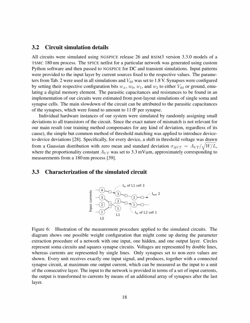
Figure 6: Illustration of the measurement procedure applied to the simulated circuits. Thediagram shows one possible weight configuration that might come up during the parameterextraction procedure of a network with one input, one hidden, and one output layer. Circlesrepresent soma circuits and squares synapse circuits. Voltages are represented by double lines,whereas currents are represented by single lines. Only synapses set to non-zero values areshown. Every unit receives exactly one input signal, and produces, together with a connectedsynapse circuit, at maximum one output current, which can be measured as the input to a unitof the consecutive layer. The input to the network is provided in terms of a set of input currents,the output is transformed to currents by means of an additional array of synapses after the lastlayer.

18

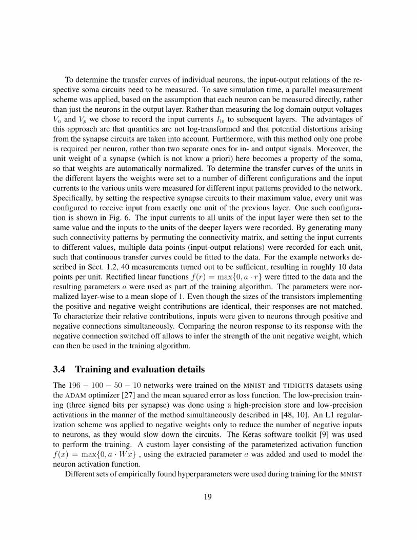
To determine the transfer curves of individual neurons, the input-output relations of the re-spective soma circuits need to be measured. To save simulation time, a parallel measurementscheme was applied, based on the assumption that each neuron can be measured directly, ratherthan just the neurons in the output layer. Rather than measuring the log domain output voltagesVn and Vp we chose to record the input currents Iin to subsequent layers. The advantages ofthis approach are that quantities are not log-transformed and that potential distortions arisingfrom the synapse circuits are taken into account. Furthermore, with this method only one probeis required per neuron, rather than two separate ones for in- and output signals. Moreover, theunit weight of a synapse (which is not know a priori) here becomes a property of the soma,so that weights are automatically normalized. To determine the transfer curves of the units inthe different layers the weights were set to a number of different configurations and the inputcurrents to the various units were measured for different input patterns provided to the network.Specifically, by setting the respective synapse circuits to their maximum value, every unit wasconfigured to receive input from exactly one unit of the previous layer. One such configura-tion is shown in Fig. 6. The input currents to all units of the input layer were then set to thesame value and the inputs to the units of the deeper layers were recorded. By generating manysuch connectivity patterns by permuting the connectivity matrix, and setting the input currentsto different values, multiple data points (input-output relations) were recorded for each unit,such that continuous transfer curves could be fitted to the data. For the example networks de-scribed in Sect. 1.2, 40 measurements turned out to be sufficient, resulting in roughly 10 datapoints per unit. Rectified linear functions f(r) = max{0, a · r} were fitted to the data and theresulting parameters a were used as part of the training algorithm. The parameters were nor-malized layer-wise to a mean slope of 1. Even though the sizes of the transistors implementingthe positive and negative weight contributions are identical, their responses are not matched.To characterize their relative contributions, inputs were given to neurons through positive andnegative connections simultaneously. Comparing the neuron response to its response with thenegative connection switched off allows to infer the strength of the unit negative weight, whichcan then be used in the training algorithm.

3.4 Training and evaluation detailsThe 196 − 100 − 50 − 10 networks were trained on the MNIST and TIDIGITS datasets usingthe ADAM optimizer [27] and the mean squared error as loss function. The low-precision train-ing (three signed bits per synapse) was done using a high-precision store and low-precisionactivations in the manner of the method simultaneously described in [48, 10]. An L1 regular-ization scheme was applied to negative weights only to reduce the number of negative inputsto neurons, as they would slow down the circuits. The Keras software toolkit [9] was usedto perform the training. A custom layer consisting of the parameterized activation functionf(x) = max{0, a ·Wx} , using the extracted parameter a was added and used to model theneuron activation function.

Different sets of empirically found hyperparameters were used during training for the MNIST

19

and TIDIGITS datasets. A reduced resolution version (14× 14 pixels) of the MNIST dataset wasgenerated by identifying the 196 most active pixels (highest average value) in the dataset andonly using those as input to the network. The single images were normalized to a mean pixelvalue of 0.04. The learning rate was set to 0.0065, the L1 penalty for negative weights was setto 10−6, and the networks were trained for 50 epochs with batch sizes of 200.

Each spoken digit of the TIDIGITS dataset was converted to 12 mel-spectrum cepstral coeffi-cients (MFCCs) per time slice, with a maximum frequency of 8 kHz and a minimum frequencyof 0 kHz, using 2048 FFT points and a skip duration of 1536 samples. To convert the variable-length TIDIGITS data to a fixed-size input, the input was padded to a maximum length of 11time slices, forming a 12x11 input for each digit. First derivative and second derivatives ofthe MFCCs were not used. To increase robustness, a stretch factor was applied, changing theskip duration of the MFCCs by a factor of 0.8, 0.9, 1.0, 1.1, and 1.3, allowing fewer or morecolumns of data per example, as this was found to increase accuracy and model robustness. Aselection of hyperparameters for the MFCCs were evaluated, with these as the most successful.The resulting dataset was scaled pixel-wise to values between 0 and 1. Individual samples werethen scaled to yield a mean value of 0.03. The networks were trained for 512 epochs on batchesof size 200 with the learning rate set to 0.0073, and the L1 penalty to 10−6.

3.5 Performance measurementsThe accuracy of the abstract software model was determined after training by running the re-spective test sets through the network. Due to prohibitively long simulation times, only subsetsof the respective test sets were used to determine the accuracy of the SPICE-simulated circuits.Specifically, the first 500 samples of the MNIST test set and 500 randomly picked samples fromthe TIDIGITS test set were used to obtain an estimate of the classification accuracy of the sim-ulated circuits. The data was presented to the networks in terms of currents, by connectingcurrent sources to the Iin nodes of the input layer. Individual samples were scaled to yield meaninput currents of 15 nA or 45 nA per pixel, respectively. The time to output for a particular pat-tern was computed by applying one (random) input pattern from the test set and then, once thecircuit had converged to a steady state, replaced by the input pattern to be tested. In this way, themore realistic scenario of a transition between two patterns is simulated, rather than a ‘switch-ing on’ of the circuit. The transient analysis was run for 7µs and 15µs with the mean inputstrength set to 45 nA and 15 nA, respectively, and a maximum step size of 20 ns. At any point intime, the output class of the network was defined as the index of the output layer unit that wasthe most active. The time to output for each pair of input patterns was determined by checkingat which time the output class of the network corresponded to its asymptotic state (determinedthrough an operating point analysis of the circuit with the input pattern applied) and would notchange anymore. The energy consumed by the network in a period of time was computed byintegrating the current dissipated by the circuit over the decision time and multiplying it by thevalue of Vdd (1.8 V in all simulations).

20

3.6 VLSI prototype implementationA 7−7−7 network, consisting of 21 neurons and 98 synapses was fabricated in 180 nm CMOStechnology (AMS 1P6M). The input currents were provided through custom bias generators,optimized for sub-threshold operation [12]. Custom current-to-frequency converters were usedto read out the outputs of neurons and send them off chip in terms of inter-event intervals. Theweight parameters were stored on the device in latches, directly connected to the configurationlines of the synapse circuits. Custom digital logic was implemented on the chip for program-ming biases, weights, and monitors. Furthermore, the chip was connected to a PC, through aXilinx Spartan 6 FPGA containing custom interfacing logic and a Cypress FX2 device provid-ing a USB interface. Custom software routines were implemented to communicate with the chipand carry out the experiments. The fabricated VLSI chip was characterized through measure-ments as described in Sect. 1.2, by probing individual neurons one by one. The measurementswere repeated several times through different source and monitor neurons for each neuron to becharacterized to average out mismatch effects arising from the synapse or readout circuits. Themean values of the measured slopes were used in a software model to train a network on the Irisflower dataset. The Iris dataset was randomly split into 120 and 30 samples used for trainingand testing, respectively. The resulting weight parameters were programmed into the chip andindividual samples of the dataset were presented to the network in terms of currents scaled tovalues between 0 and 325 nA. The index of the maximally active output unit was used as theoutput label of the network and to compute the classification accuracy.

21