Pp 151184

THE ‘GOLDEN GENERATIONS’ IN HISTORICAL CONTEXT

By Michael Murphy

abstract

Assumptions about future mortality are more important than those for factors such asfertility, migration, disability trends or real interest rates for cost projections of the U.S. OldAge, Survivors, Disability and Health Insurance scheme. Recently, one factor has been assumedto be the key driver of future mortality in both official British population projections andactuarial ones: a ‘cohort effect’ associated with a group who were born in a period centred on theearly 1930s who have been identified as having experienced particularly rapid improvements inmortality rates and are often referred to as the ‘golden generations’ or ‘golden cohorts’. Theconcept of ‘cohort effects’ is discussed; limitations of national-level cohort data considered; andmethods for identifying such effects are reviewed. Particular attention is given to the analysis ofpopulations which have been identified as having clear cut cohort effects; those of Britain andSweden in the later part of the nineteenth century and early twentieth century, as well as thecontemporary British population. The likely magnitude of such effects is discussed using astylised model to assess the extent to which members of the ‘golden generations’ are especiallyprivileged.

keywords

Mortality; Cohort Patterns; Historical Demography; Golden Generations

contact address

Michael Murphy, Department of Social Policy, London School of Economics, Houghton Street,London WC2A 2AE, U.K.Tel: +44-20-7955-7661; Fax: +44-20-7955-7415; E-mail: [email protected]

". Introduction

Pensions liabilities in the OECD countries are estimated as 20 trilliondollars (or 13 trillion pounds); countries such as the United Kingdom, U.S.A.and Switzerland had, in 2005, pensions liabilities larger than their annualGDP (OECD, 2007; SwissRe, 2007, 2008). Sensitivity analysis of costsundertaken for the 2008 OASDI Trustees Report of the U.S. Old Age,Survivors, Disability and Health Insurance scheme found that assumptionsabout future mortality were more important than those for factors such asfertility, migration, disability trends or real interest rates (real earnings over

B.A.J. 15, Supplement, 151-184 (2009)

151

the 50-year period was the only factor that had a larger impact1) (SocialSecurity Administration, 2008; see also Antolin, 2007). Both future levels ofmortality and current forecasts of these will have profound implications forplanning of both public and private institutions and are potential sources offinancial instability.

Official projected increases in life expectancy in Britain between 2005 and2030 of over five years in the 2008-based projections (Office for NationalStatistics, 2009a) are rather higher than values of three to four years byEurostat for Western European EU countries and just over three years by theBureau of the Census for the U.S.2 for the same base year. In the past,projected mortality improvement has usually been assumed to cease or to besubstantially reduced progressively ahead of the period when the projectionswere made (Murphy, 1995). Recently, one factor has been assumed to be thekey driver of future mortality in both official British population projections(e.g. Office for National Statistics, 2008b) and actuarial ones (e.g.Continuous Mortality Investigation, 2007): a ‘cohort effect’ associated with agroup who were born in a period centred on the early 1930s who have beenidentified as having experienced particularly rapid improvements in mortalityrates and are often referred to as the ‘golden generations’ or ‘goldencohorts’ including actuarial discussions, the academic literature (e.g. Cairnset al., 2006), official reports (e.g. The Pensions Regulator, 2008; Office forNational Statistics, 2008b), the financial press (e.g. Euromoney, 2008), andthe informed media.3

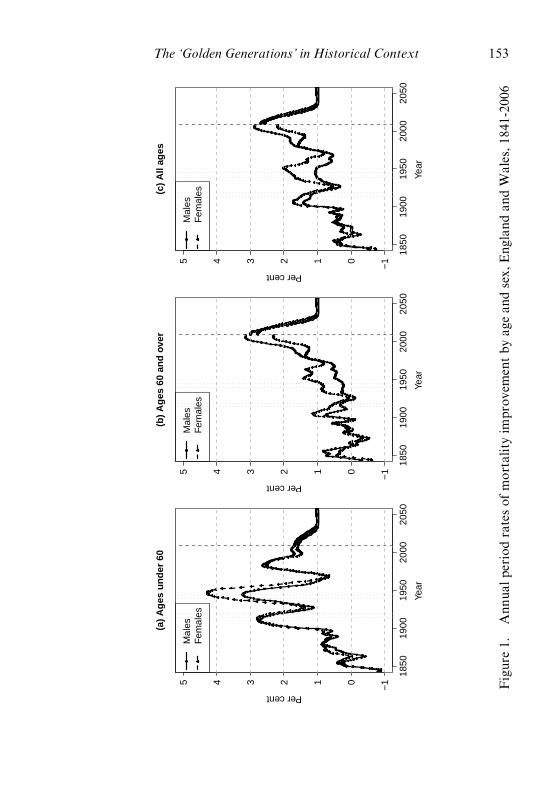
At present, overall age standardised mortality rates (both sexes combined)are improving at about 2.5% per annum in England and Wales with higherrates of improvement at older than at younger ages (Figure 1),4 but currentoverall trends are heavily influenced by patterns at ages where deaths areconcentrated (see Appendix A). In 2005, just over 50% of deaths in Englandand Wales occurred to people born in the period 1925 to 1945, the birthcohorts of the ‘golden generations’ (Office for National Statistics, 2008c).Current British official mortality projections are based on the assumptionthat this group will continue to have higher than average rates of mortalityimprovement in the future so that the differentials in Figure 1 reflectpersistent cohort differences (Office of Population Censuses and Surveys,

1 This may change, but the issue of population ageing will remain important in the long term eventhough the credit crunch is exacerbating the problems of pensions funding. In 2007 de¢ned bene¢t(¢nal salary) schemes in Britain had 2.7 million members in the private sector and 5.2 million inthe public sector (O⁄ce for National Statistics, 2008a), see also Steventon (2008).2 2008-based Eurostat projections available at http://epp.eurostat.ec.europa.eu/portal/page/portal/statistics/search ____ database and U.S. ones at http://www.census.gov/population/www/projections/2008projections.html3 See, for example, http://news.bbc.co.uk/1/hi/business/4295362.stm4 These are based on author’s calculations using the WHO European standard (Doll & Cook,1967) with unpublished Government Actuary’s Department data.

152 The ‘Golden Generations’ in Historical Context

1850

1900

1950

2000

2050

−1012345

(a)

Ag

es u

nd

er 6

0

Year

Per cent

Mal

esF

emal

es

1850

1900

1950

2000

2050

−1012345

(b)

Ag

es 6

0 an

d o

ver

Year

Per cent

Mal

esF

emal

es

1850

1900

1950

2000

2050

−1012345

(c)

All

ages

Year

Per cent

Mal

esF

emal

es

Figure1.

Ann

ualp

eriodratesof

mortalityim

prov

ementby

agean

dsex,

Eng

land

andW

ales,1

841-20

06

The ‘Golden Generations’ in Historical Context 153

1995; Office for National Statistics, 2008b; Willets, 1999, 2004), similarassumptions have come to form the basis of much British actuarial mortalityforecasting as well, but their ‘golden cohorts’ are located slightly earlierreflecting the generally higher financial and social-economic status of thosewho are of particular interest to the financial sector5 (Continuous MortalityInvestigation, 2007). Thus the high levels of mortality improvement observedin recent years are assumed to be a transient phenomenon largelydetermined by those born around the period 1925-45 and that as thesecohorts are replaced in the main mortality age groups by less favouredcohorts, rates of mortality improvement will fall in future. The Britishofficial projections assume that mortality improvement will decline by morethan 60% to a value of 1% per annum in about 25 years’ time after the‘golden generations’ effect has worked itself out of the system. The half-century of accelerating mortality rate improvement for males is projected tobe reversed at a rate not experienced since records started in the 1840s.

The analysis of cohort effects on mortality has been a long-standing areaof interest from the 1920s (Derrick, 1927; Kermack et al., 1934), which hasrecently become renewed largely independently in a number of fields, such asdemography (Preston & Wang, 2006), biology (Finch & Crimmins, 2004),actuarial studies (Willets et al., 2004) and epidemiology (Kuh & Ben-Schlomo, 1997), although developments in other disciplines may beunrecognised: for example, Willets (Willets et al., 2004, p879) points out thatlife course analysis, a major area of epidemiological research, is largelyunfamiliar to actuaries.

The paper is organised as follows. The concept of ‘cohort effects’ isdiscussed; limitations of national-level cohort data considered; and methodsfor identifying such effects are reviewed. Particular attention is given to theanalysis of populations with identified cohort effects; those of Britain andSweden in the later part of the nineteenth century and early twentieth century(Kermack et al., 1934) as well as the contemporary British population. Thelikely magnitude of such effects and potential drivers is discussed using astylised model to assess the extent to which members of the ‘goldengenerations’ are especially privileged. Possible determinants are consideredand the role of the ‘post-golden generations’ for future mortality trends isconsidered.

Æ. Defining Cohort Effects

The term ‘cohort effect’ is widely used but rarely defined. The Handbookof the Life Course (Alwyn & McCammon, 2006, p26) and Susser (2001) do

5 Within the ¢nancial sector, groups with advantaged survivorship are sometimes referred tosomewhat less positively as the ‘toxic tail’ (Blake & Pickles, 2008; Blake et al., 2007).


give similar definitions from sociological and epidemiological backgrounds,respectively, in which a cohort effect is defined as a causal factor acting earlyin life that leads to later identifiable consequences (a more extendeddiscussion is in Murphy, 2010a). Many recent actuarial publications arebased on the influential work of Willets (1999, p5), who defined a ‘cohorteffect’ as a “wave of rapid improvements, rippling upwards throughmortality rates in the United Kingdom’’ and also as “a descriptive term forthe observed trend [of the ‘golden generations’], and does not have a specificstatistical meaning’’, or indeed a causal one, since as Hobcraft et al. (1982,p5) observe: “ages, periods, and cohorts do not have either direct or indirecteffects on demographic or social phenomena’’.

In the first definition above, cohort effects exist only if causalmechanisms that drive the observed regularities can be established, whereasin the second case, cohort effects are usually inferred by examination oftables of age-specific mortality trend data. The latter approach was adoptedby the first study identifying the ‘golden generations’, the Official Report onthe British 1992-based population projections: “a ... higher than average rateof improvement is a special feature of generations born between 1925 and1945 (which more detailed charts show to be centred on the generation bornin 1931). It is not yet understood precisely why the members of thegeneration born about 1931 have been enjoying so much lower death ratesthroughout adult life than the preceding generation ...’’ (Office of PopulationCensuses and Surveys, 1995, p 10). This statement has stood the test of timewell and remains unchanged in official publications until the present day.

A term such as ‘cohort effect’ may be unhelpful and potentially misleading,if it is assumed that it is a causal effect that may be identifiable from analysisof a table of mortality rates cross classified by any two of age, year ofoccurrence, or year of birth. This may be illustrated by an artificial example.One society introduces vaccination of infants, which leads to a reduction insubsequent mortality for all those vaccinated from that age forward. Thesecond introduces an income support scheme that reduces the mortality ofrecipients in the given year, which was originally targeted on young children,but, eligibility was extended over time up the age range by one year in eachsuccessive calendar year. The observed mortality patterns are identical (andwould often be interpreted as a cohort effect), but the future implications arevery different: the vaccinated population will continue to benefit, whereasthe income policy population’s prospects depend on the way in which thepolicy is implemented in future periods. Examination of the mortality surfacewould give no indication as to whether the driving process was a cohort ora period one. The most parsimonious explanation might suggest one relatingto early life conditions, but just analysing the mortality surface, howeverapparently sophisticated the approach, cannot establish the mechanismsinvolved, but only indicate areas where further investigation might takeplace. As Newman (2001, p216) states: “in order to separate out age, period,


and cohort effects ... is necessary to incorporate additional ... substantiveknowledge, and therefore the allocation to age, period or cohort effects is nota statistical issue’’. In practice, of course, such clear-cut alternatives as thecases above are rare, but situations in which mortality improves differentiallyby age, starting first at young ages and moving progressively to older agesover time, would appear to look like a cohort phenomenon, whereas thedriver may be a period factor.

Although apparently very different, neither of the artificial examplesabove requires that cohort effects act similarly over the whole age range.There are plausible causal mechanisms and empirical evidence that suggestthat events around the time of birth (both pre- and post-natal) lead todifferent chances of cardiovascular disease starting at late middle ages(Barker, 1994; Barker et al., 1989), and that inflammation in early childhoodmay influence mortality at even higher ages (Finch & Crimmins, 2004).Other causal factors occurring later in life, such as the well-established effectsof smoking on mortality, especially lung cancer, are largely manifested atolder ages (Charlton & Murphy, 1997).

It is possible to have cohort effects that reverse from some ages; forexample, early adverse circumstances and high mortality at young ages mightlead to proportionately more deaths among the more frail members of thecohort but the surviving and consequently, on average, fitter members of thecohort experience lower mortality at older ages (assuming that frailty isconstant for an individual over the lifetime, e.g. Vaupel et al., 1979; Vaupel &Yashin, 1985). Some theories of ageing argue that some alleles mightprioritise health at younger ages in order to maximise reproductive success atthe expense of long-term survival (‘antagonistic pleiotropy’, Williams, 1957)that could lead to crossovers of different genotypes such as, for example, bydiverting resources from immune function to nutritional status. The existenceof such ‘crossover’ effects has been debated for many years especially in thecontext of racial differences in mortality in the U.S. where reported mortalityrates for Blacks fall below those for Whites at older ages. While it had beenargued that this was due to data errors (Coale & Kisker, 1986), the evidenceis accumulating the crossover is real. In the 2005 U.S. life tables, mortalityrates of Blacks are at least 25% higher than those of Whites at all ages below68, but lower than those of Whites beyond age 86 (Arias et al., 2010).

�. Identifying Cohorts

A cohort usually refers to a group with a common initial characteristic(such as those born in Britain in the same year) followed through time. Aproblem is that the group of people dying in a country such as England andWales at a given age and year of birth is not a well-defined cohort, since itincludes people who were not born in England and Wales but migrated later,


and excludes native-born people who emigrate and subsequently dieelsewhere. The magnitude of migration in Britain has been substantial in thetwentieth century. In 2008, there were an estimated 6.7 million overseas bornpeople in the United Kingdom (Office for National Statistics, 2009b) andover the twentieth century, Britain was a net exporter rather than animporter of people so that the number of British-born people living outsidethe country is also substantial (Coleman & Salt, 1992; Murphy 2009) butwith a very different age structure to that of immigrants to Britain. Unlessthe mortality rates of both immigrants and emigrants are similar to theresident population, the use of such data as an indicator of cohort mortalitychange, which will often be concerned with the difference of a few percentagepoints, is potentially misleading. For example, the immigrant population inthe U.S. grew from 9.6 million in 1970 to 32.5 million in 2002 andimmigrants have very different mortality patterns from their native-borncounterparts. Black immigrant men had 9.4 years longer life expectancy thanblack U.S.-born men and the corresponding figure was 4.3 years forHispanics in the period 1986-94 (Singh and Miller, 2004), with the latterfigure having a substantial impact on overall cohort Hispanic mortality giventhe large numbers of non-native born Hispanics.

This observation is particularly pertinent to the most recent period whenmigration has become much more important. In Britain, for example,considerable attention has been drawn to the relatively poor mortalityperformance of young adults of cohorts born in the 1950s and 1960sfollowing a substantial deterioration in the rate of mortality improvement foryoung adults in the 1980s, which has been used to highlight the apparentlyprivileged position of the ‘golden generations’. A major reason for this wasincreases in mortality from HIV/AIDS, external causes and substance abuse(Aylin et al., 1999). In 1994-6 there were 35,324 deaths among those aged20-39 in England and Wales, but if the 1986-8 rates had applied in 1994-6,there would have been 83 fewer deaths than were actually observed,indicating a slight deterioration in mortality over the period. However, thiswas largely due to an increase of 925 infectious disease deaths, to which HIVinfection was the major contributor (Aylin et al., 1999, p38). Inclusion ofrecent immigrants with high rates of mortality from such causes may lead tomisinterpretation of cohort patterns. Information to calculate values forU.K.-born cohorts in this period is not published, but despite comprising lessthan 1% of the total U.K. population, the number of Black Africans (not allof whom are overseas-born) currently diagnosed with HIV is similar to thatof the white population, who comprise more than 90% of the population.6

The absence of fitter-than-average emigrants from the resident Britishpopulation may also be relevant: Australian age standardised cardiovascular

6 See http://www.avert.org/uk-race-age-gender.htm


disease mortality was 23% lower than that of the U.K. in 2002,7 but even soBritish Isles’ migrants to Australia aged 45 to 64 in 1998-2002 hadcirculatory disease and diabetes mortality 30% lower than native-bornAustralians (Gray et al., 2007), suggesting a substantially lower rate thanthose remaining in the U.K. Thus the distinction between real and pseudo-cohorts should not be ignored when interpreting mortality trends anddifferentials.

ª. Identifying Cohort Effects

The validity of hypothesised mechanisms may be tested empirically in anumber of ‘natural experiments’. Experiences of very adverse conditions at adifferent stage of the life course, such as infancy or pre-natally, that mightbe expected to lead to later poor mortality outcomes have been investigated.Case studies include the severe 1869 famine in Finland which was found laterto have no discernable effect for those born around that time (Kannisto etal., 1997). The effects of extreme hardship suffered by those born around thetime of the 1941-44 siege of Leningrad (where estimated average dailyrations were around 300 calories, containing virtually no protein) and theDutch Hunger Winter of 1944 have been extensively studied for subsequentexcess health risks (Van der Zee, 1998; Lumey et al., 2007; Stein et al., 1975)but Lumey & Van Poppel (1994, p245) conclude that even for such extremeexperiences “the long-term effects are not easily detected’’. Somedisadvantages have been identified for those born around the time of the1918-19 influenza pandemic in the U.S. (Almond, 2006; Mazumder et al.,2009). While inconsistent results have been found, substantial nutritionaldeficits, pre-natally, post-natally, in childhood and in adolescence, appear tobe associated with no excess or only relatively small additional mortality inlater life, which would appear to put a limit on the expected magnitude ofsuch effects in cases where nutritional changes were much smaller over timesuch as in Britain over the twentieth century.

A second way in which cohort patterns have been identified is by fittingstatistical models that incorporate some or all of age, period, and cohortvariables. The appropriate way to model such processes remains an activeresearch area (Carstensen, 2007; Yang et al., 2004) with a substantialstatistical, sociological, demographic and epidemiological literature on thistopic. The model is usually specified as

lnðma;c;tÞ ¼ aa þ bc þ gt þ eact ð1Þ

7 World Health Organisation WHOSIS database http://apps.who.int/whosis/data/Search.jspaccessed 16th November 2009.


wherema;c;t is the mortality rate for age a in year t for cohort c;aa, bc and gt are coefficients, and,eact is a residual term.

or, alternatively,

lnðma;c;tÞ ¼ f ðaÞ þ gðcÞ þ hðtÞ þ eact ð2Þ

wheref ðaÞ, gðcÞ and hðtÞ are functions of age, cohort and period, respectively.

The problem with such models is the identification problem since

t ¼ cþ a ð3Þ

which means that there is no unique solution to equation (1) without somefurther assumption and/or restriction. In particular, if there is a commonlinear change (‘drift’) in mortality, this cannot logically be uniquelyattributed to either period or cohort axes as Preston & Wang (2006, p638)note (see also Murphy, 2010a).8 In practice, it may be difficult to establish ifthe data are free of errors and conform to the model assumptions, such as afixed age pattern. For example, Richards et al. (2007, p498) commented ontheir model results for England and Wales: “One point of particular note isthe result for males in England and Wales [where period effects dominate], asthis flatly contradicts the result in Richards et al. (2006) ... [which]concluded that cohort effects dominated period effects’’. Possibleexplanations for such different interpretations are the use of slightly differentdata sources and/or upper age limits, but such findings emphasise thefrequently found difficulties in drawing definitive conclusions from suchapproaches.

A third way for identifying cohort patterns is use of graphical methods asundertaken by Kermack et al. (1934) (reproduced in Davey Smith & Kuh,2001 and Murphy, 2010b), Office of Population Censuses and Surveys(1995), Willets (1999, 2004), Richards et al. (2006), etc. These range fromstraightforward hand-drawn lines on a mortality table to contour or heatmaps of changing mortality rates using either simple comparisons or variousmodel-based smoothing approaches (see Appendix B). As Preston & Wang(2006, p638) note, graphical methods appear to be considerably more

8 Another general issue is that model-¢tting usually uses data in the form of a rectangularmortality surface of n age groups by m time periods; in such cases the number of cohorts includedis nþ m� 1, but two of the cohorts include only a single observation. It would seem moreappropriate to have symmetric data structures for the two dimensions of period and cohort ifjudgements are to be made about their relative contribution to explanation, but this rarely if everis done.


successful in identifying cohort influences than statistical models. Bothapproaches have advantages and disadvantages � statistical models canproduce goodness of fit indicators but tend to be inflexible so are notnecessarily particularly useful for exploratory analysis. There is the problemof indeterminacy in attributing change unambiguously to the period orcohort dimension. The majority of studies concerned with identifying cohortmortality patterns are confined to certain age groups only, usually older agessince many of these studies involve various forms of cancer. Such modelsusually assume that the effect is manifested as a fixed relative risk onmortality at each age in the age range selected and therefore, for example,would not be able to identity ‘crossover’ effects. Some of the graphicalmethods used make few assumptions about the nature of the underlyingprocess, whereas others may attempt to remove other sources of variabilitysuch as period changes in order to maximise the likelihood that cohortpatterns will become visible. However, given the lack of an agreed way ofpresenting such data, the fact that the analyst can both select the methodof presentation and the section of the mortality surface to be highlighted,the scope for subjectivity in interpretation of results is substantial (seeAppendix C).

�. Historical Discussion

The debate about the relative importance of period and cohort effects onmortality has been a longstanding one. Derrick (1927, p144) presented age-specific mortality rates in the period 1841 to 1925 by year of birth andconcluded that “the parallelism is remarkable’’ and that “nearly the whole ofthe temporal change is due to an entirely independent generation influence,each generation being endowed with a vitality peculiarly its own’’. Otherswere less convinced (see the discussion in Derrick, 1927) including somemembers of the Statistics Committee of the Royal Commission onPopulation, of which Victor Derrick was a member (Kyd, 1953). BothDerrick (1927) and Kermack et al. (1934) argued that cohort approacheswould provide superior forecasts of future mortality than alternativeapproaches. However, such predictions turned out to be poor (Kuh & DaveySmith, 1993) and cohort approaches fell out of favour. For the next half-century, attention was concentrated almost entirely on period ones, to theextent that Hobcraft et al. (1982, p.12) could conclude that: “mostpopulation specialists appear to believe that cohort mortality and effects aresufficiently minor that they need not be incorporated into models ofmortality relations’’.

Kermack et al. (1934) presented data on Scotland and Sweden as well asfor England and Wales, although attention has been concentrated mainly onthe results for England and Wales, and the findings for the other countries


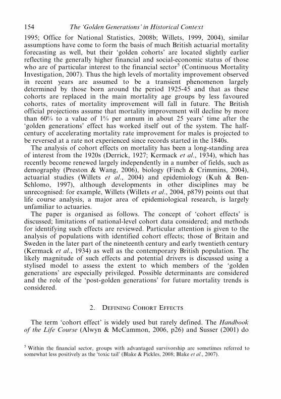
have been largely ignored. Figures 2 to 4 present values using Kermack etal.’s approach with mortality indexed to that of period 1841-50 (1855-64 forScotland since data are only available from 1855) for the three countries bysex updated to 2006 or 2007 with data obtained from the Human MortalityDatabase (2009). Others who have updated these tables include Harris (2001)and Davey Smith & Lynch (2004) but both have used banded data. Thedata presented here use the penalised spline method discussed in Appendix B.While by no means perfect, the data for both men and women up to aboutage 75 for cohorts born in both England and Wales and in Scotland in theperiod 1841 to 1910 show a tendency for isoquants to be at a 45 degreeangle until 1930 for ages 20 to 60 years for males, and somewhat later forwomen. Patterns at other ages and periods are less convincing, althoughinterpretation is inevitably subjective. However, Kermack et al. (1934)acknowledge that their cohort model was not particularly successful inexplaining mortality trends for Sweden, the only non-British country theyinvestigated up to 1926, and the continuing lack of any cohort-like patterns isclear in Figure 4.

There are six potential reservations about Kermack et al.’s (1934) methodof presentation and the extent to which definitive conclusions may be drawnconcerning the pre-eminence of cohort patterns, which are discussed in moredetail in Murphy (2010b). In particular, the results of Table 1 fromKermack et al. (1934), which are among the most widely-cited examples of acohort effect, can arise from a non-cohort mechanism as in the earlierartificial example, as they acknowledge.9 The reasons for the nineteenthcentury mortality decline remain a matter of debate, with the mainarguments centring about the relative contribution of factors such asimproving nutrition (McKeown, 1976, 1988) and public health measures (e.g.Szreter, 1988), but both are considered mainly as period processes. Preston(1996) argues that acceptance of the germ theory of disease had a substantialimpact on infant mortality improvements in the late nineteenth century. Analternative explanation for the later nineteenth century and early twentiethcentury mortality patterns of relatively faster rates of improvement in a givenyear at young, but not at the youngest ages (Woods, 2000; Harris, 2001) isEpidemiological Transition Theory (Omran, 1971, 1998), whereby mortalityinitially starts to improve by reducing communicable diseases and only laterchronic diseases fall substantially. Since communicable diseases formed a

9 Kermack et al. (1934, p700) considered if “the consecutive improvements which have takenplace in succeeding age-groups are the result of a series of independent sets of conditions, orlegislative acts, and that the apparent regularity is largely fortuitous. It might for instance besuggested that early industrial legislation was directed towards the welfare of children, and thatat a later date general industrial and social conditions improved, and that older people were lastin being a¡ected by industrial and housing changes ...’’, but concluded that “it would besomewhat surprising if the quantitative regularity just pointed out should emerge.’’.


(a) England and Wales Males

Year

Age

0

10

20

30

40

50

60

70

80

1860 1880 1900 1920 1940 1960 1980 2000

0.800.80

0.80

0.80

0.80

0.80

0.800.80

0.640.64

0.64

0.51

0.51

0.510.410.41 0.41

0.41

0.410.41

0.410.33

0.33

0.26 0.260.260.26

0.26

0.26

0.0

0.2

0.4

0.6

0.8

1.0

1.2

1.4

1.6

(b) England and Wales Females

Year

Age

0

10

20

30

40

50

60

70

80

1860 1880 1900 1920 1940 1960 1980 2000

0.800.80

0.80

0.80

0.80

0.80

0.80

0.80

0.64

0.64

0.510.510.51

0.51

0.41

0.41

0.33

0.33

0.330.260.26

0.26

0.260.0

0.2

0.4

0.6

0.8

1.0

1.2

Figure 2. Annual period rates of mortality indexed to mid nineteenthcentury values for England and Wales, by sex 1841-2006


(a) Scotland Males

Year

Age

0

10

20

30

40

50

60

70

80

1860 1880 1900 1920 1940 1960 1980 2000

0.80

0.800.800.800.80

0.80

0.80

0.64

0.64

0.640.64

0.640.51

0.51

0.51

0.41

0.41

0.41

0.41

0.33

0.33

0.33

0.260.260.260.26 0.26

0.26

0.2

0.4

0.6

0.8

1.0

1.2

(b) Scotland Females

Year

Age

0

10

20

30

40

50

60

70

80

1860 1880 1900 1920 1940 1960 1980 2000

0.800.80

0.80

0.800.800.800.80

0.64

0.64

0.64

0.51

0.51

0.510.51

0.410.41

0.41

0.41

0.330.330.330.33

0.33

0.33

0.260.26

0.26

0.0

0.2

0.4

0.6

0.8

1.0

1.2

Figure 3. Annual period rates of mortality indexed to mid nineteenthcentury values for Scotland, by sex 1855-2006


(a) Sweden Males

Year

Age

0

10

20

30

40

50

60

70

80

1860 1880 1900 1920 1940 1960 1980 2000

0.80

0.800.80

0.80

0.80

0.80

0.80

0.800.80

0.800.80

0.80

0.800.800.64

0.64

0.640.64

0.64

0.640.64

0.640.64

0.510.51

0.51

0.51

0.51

0.410.410.41

0.41

0.33

0.33

0.33 0.330.330.330.33

0.26

0.260.261

2

3

4

5

(b) Sweden Females

Year

Age

0

10

20

30

40

50

60

70

80

1860 1880 1900 1920 1940 1960 1980 2000

0.800.80

0.80

0.800.80

0.80

0.80

0.80

0.80

0.80

0.800.80

0.800.800.80 0.80 0.800.80

0.800.64

0.640.640.64

0.64

0.640.640.64

0.510.51

0.51

0.51

0.51

0.51

0.410.41

0.41

0.33 0.260.5

1.0

1.5

2.0

2.5

3.0

3.5

4.0

4.5

Figure 4. Annual period rates of mortality indexed to mid nineteenthcentury values for Sweden, by sex 1841-2007


higher proportion of deaths among young people (Preston et al., 1972;Preston, 1976), rates of overall mortality improvement are initially greaterfor younger than for older people.

�. The Role of Infant and Child Mortality

The fact that infant mortality shows very little improvement over thenineteenth century in England and Wales, and Scotland (Figures 2 and 3),whereas toddler mortality starts improving many decades earlier requiresspecific explanations, perhaps related to patterns of urbanisation in Britainand changing disease virulence (e.g. Woods, 2000). Nevertheless, theapproach of Kermack et al. (1934) has been generally endorsed in recenttimes, in part because they anticipate much later work concerned with lifecourse effects, suggesting that pre-natal and infant experiences are likely tohave consequences later in life. They argued that infant mortality improvedonly from the start of the twentieth century after their mothers’ health hadalready improved. They identified cohorts born about 1870 as the first withsubstantially improved mortality (Kermack et al., 1934, p701). However, thelack of empirical justification for the crucial role of early childhoodconditions suggests that it is a post hoc hypothesis. Moreover, this hypothesisfails to explain why Swedish data show a completely reversed pattern: bothinfant and toddler mortality start to improve from the 1860s and showsustained improvement from the 1880s, but mortality of those in their mid-20s shows little improvement until after 1920.

�. Recent Patterns and Methods

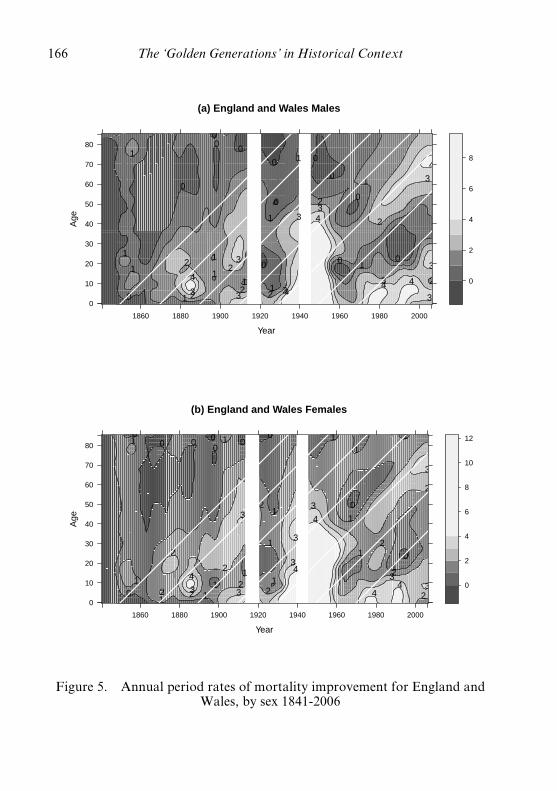
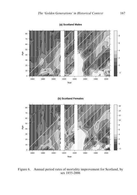
The visual presentation of Figures 2 to 4 has limitations (Murphy,2010b). Recent graphical approaches for identifying cohort effects incontemporary Britain have tended to use estimated rates of age-specificchange in mortality, especially for identifying the ‘golden generations’,including Office of Population Censuses and Surveys (1995), Willets (2004),Willets et al. (2004) and Richards et al. (2006). Figures 5 to 7 show the fullset of values for England and Wales, Scotland and Sweden for all ages andtime periods since the mid-nineteenth century.10 These figures generally

10 The two most substantial period mortality e¡ects, the very sharp £uctuations in the ‘outlier’years 1914-20 (which included the 1919 in£uenza pandemic), and 1939-45 are removed since thereasons for their in£uence are well-de¢ned in Britain. In Sweden only years 1918-20 are excludedas they were not a combatant nation. See Appendix B for a discussion of the approach usedand its rationale. It can be argued that these years should be included, since to exclude the majorperiod factors simply because the underlying cause is well-recognised would tend to downplaythe in£uence of period factors.


(a) England and Wales Males

Year

Age

0

10

20

30

40

50

60

70

80

1860 1880 1900 1920 1940 1960 1980 2000

4

4

4

4 4

4

3 3

3

3

3 3

3

3

3

3

2

2

2

2

2

2

2

2

1

1

1

1

1

1

1 1

1

1

1

1

0

0

0 0 0

0

0

0

0

0

0

0

0

0

2

4

6

8

(b) England and Wales Females

Year

Age

0

10

20

30

40

50

60

70

80

1860 1880 1900 1920 1940 1960 1980 2000

4 4

4

4 4 3 3

3

3

3

3

3

3

3 2

2

2

2

2 2

2

2

2

2

2

1

1

1 1 1

1

1

1

1

1

1

1

1

1

1

1

0

0 0 0

0 0

0 0

0

0

0

2

4

6

8

10

12

Figure 5. Annual period rates of mortality improvement for England andWales, by sex 1841-2006


(a) Scotland Males

Year

Age

0

10

20

30

40

50

60

70

80

1860 1880 1900 1920 1940 1960 1980 2000

4

4

4

4 4

3

3

3

3

3

3 3

3

2

2

2

2

2

2

2

2

2

1

1

1

1

1

1 1

1

1

1

0

0

0

0

0

0

0

0

0

0

0

0

0

0

0

0

−2

0

2

4

6

8

(b) Scotland Females

Year

Age

0

10

20

30

40

50

60

70

80

1860 1880 1900 1920 1940 1960 1980 2000

4

4

4 4 4 3

3

3

3

3

3

3 3

3

3

3

3

3

2

2

2

2

2 2

2 2

2 2

2

2

2 1

1

1

1

1

1

1

1

1

1

1

1

1

1

0

0

0

0

0

0 0

0

0 0

0

0 0

0

0 −2

0

2

4

6

8

10

12

14

16

Figure 6. Annual period rates of mortality improvement for Scotland, bysex 1855-2006


(a) Sweden Males

Year

Age

0

10

20

30

40

50

60

70

80

1860 1880 1900 1920 1940 1960 1980 2000

4 4

4

4 4

4 4

4

4

3

3 3

3 3 3

3

3

3

3

3

3

3 3

3

2

2

2

2

2

2

2

2

2

2

2

2

1

1

1

1

1

1

1

1

1

0

0

0

0 0

0

0 0

0 0

0

0

0

0−2

0

2

4

6

8

(b) Sweden Females

Year

Age

0

10

20

30

40

50

60

70

80

1860 1880 1900 1920 1940 1960 1980 2000

4 4 4 4 4

4

4

3 3

3 3

3

3 3

3

3

3

2

2

2

2

2

2

2

2

2

2

2

2

1

1

1

1

1

1

1

1

1

1

1

1

1

1

1

1

0

0

0

0

0

0

0

0

0

0

0

0

0

0

0

−2

0

2

4

6

8

10

12

Figure 7. Annual period rates of mortality improvement for Sweden, bysex 1841-2006


confirm the findings of Figures 2 to 4 such as that mortality first showssigns of improvement from about age 20 years for both sexes from about1860 in both England and Wales, but that improvements became sustainedand widespread only from about 1880 in both England and Wales andScotland. In contrast, Sweden shows a completely different pattern withmortality improvement occurring largely contemporaneously at all ages,apart from the very marked delay in improvement among young adults notedearlier.

The British ‘golden generations’ are visible as those with higher rates ofmortality improvement than surrounding cohorts for both men and women,with isoquants lying along the 458 diagonal line for those born around 1930for ages above about 40 years, but this pattern is less clear cut for Scotlandand non-existent for Sweden, where, for example, women born about 1960appear to have relatively high rates of improvement, the reverse of the Britishpattern. Little of the patterns identified for earlier cohort in Britain inFigures 2 and 3 are visible in Figures 5 and 6, suggesting that conclusionsabout the existence of cohort patterns arise in part from a particular form ofpresentation. However, the lower quality of data estimates in the nineteenthcentury needs to be acknowledged.

�. A Stylised Model for the ‘Golden Generations’

Two simplified versions of a ‘golden cohorts’ model shown in Figure 8are designed to indicate the orders of magnitude of effects that can beobtained. The first (Model 1) is based on changing trends in a risk factor,which, for concreteness, might be characterised as ‘smoking’. In this example,‘smoking’ moves from a low level to a high-point to and back to a low levelover a period of 40 years; the mortality of both ‘non-smokers’ and ‘smokers’improves by 1% p.a., but smokers have double the mortality of non-smokers at any age (Figures 8(1a) and 8(1b)) � further details are given inAppendix C. In order for the maximum rate of mortality improvement toreach 2% p.a. under this model, the proportion of the cohort who aresmokers would have to reach a maximum of 14% (Figure 8(1c)). With thismodel, the emergence and subsequent disappearance of a risk factor will leadinitially to a lower rate of overall mortality improvement but later to ahigher rate than the baseline level value that would have been experienced ifthe risk had not occurred. In particular, the ‘golden generations’, the groupfor whom mortality improvement is a maximum, experience higher overallrisks than if the mortality had remained at the baseline level.

The alternative scenarios (Model 2) arises from an innovation such as the‘introduction of the Welfare State’ (or of vaccination), during which cohortmortality improves, but as above the rates of improvement in the pre- andpost-transitional phases are 1% p.a. (Figure 8(2a)). In this case, mortality


1890

1900

1910

1920

1930

1940

1950

0.0

0.2

0.4

0.6

0.8

1.0

(1a)

Po

pu

lati

on

s o

f sm

oke

rs&

no

n−s

mo

kers

(M

od

el 1

)

Coh

ort

Proportion

Sm

oker

Non

−sm

oker

1890

1900

1910

1920

1930

1940

1950

1960

0.00

5

0.01

0

0.01

5

0.02

0

0.02

5

(1b

) M

od

el 1

mo

rtal

ity

rate

of

smo

kers

, no

n−s

mo

kers

& o

vera

ll

Coh

ort

Ove

rall

Sm

oker

sN

on−

smok

ers

1890

1900

1910

1920

1930

1940

1950

1960

0.0

0.5

1.0

1.5

2.0

(1c)

Mo

del

1 R

ate

of

over

all

mo

rtal

ity

imp

rove

men

t

Coh

ort

Per cent

1890

1900

1910

1920

1930

1940

1950

1960

0.00

4

0.00

6

0.00

8

0.01

0

0.01

2

(2a)

Mo

del

2 m

ort

alit

y ra

tefo

r in

nov

atio

n m

od

el

Coh

ort

Ove

rall

Initi

alF

inal

1890

1900

1910

1920

1930

1940

1950

1960

1.0

1.2

1.4

1.6

1.8

2.0

(2b

) M

od

el 2

rat

e o

f ov

eral

lm

ort

alit

y im

pro

vem

ent

Coh

ort

Per cent

Figure8.

Stylised

alternativemod

elsfor‘golde

ngene

ration

s’


improvement is never below 1% p.a. With the assumptions of Appendix C,a maximum rate of improvement for the 1930 cohort of 2% (1% abovebaseline) would imply a 23% lower level of mortality in the post-transitionalphase than would have been the case if the innovation had not occurred(Figure 8(2b)).

Temporary high rates of mortality improvement based on transientpatterns due to factors such as reductions in smoking imply the existence ofgroups with corresponding levels of below-baseline mortality improvement(Appendix C) and the underlying change will be over-stated, if comparisonsare made with these groups. (Note that these changes need not be symmetricand different assumptions about the time over which they occur willproduce different results, but the values shown are designed to indicateplausible bounds.) A second point is that for both simplified models, the‘golden generations’ are located at the point of inflexion of the time trend ofprevalence of the risk factor (‘smoking’) or the point at which theproportions benefitting is increasing maximally (“welfare state’’). In bothcases, this is where the values of the second derivative of the aggregatemortality rate is zero and the third derivative is positive. The ‘goldengenerations’ have intermediate mortality levels compared with surroundingcohorts and intermediate exposure to ‘smoking’ or access to welfare stateprovision (compared with surrounding cohorts). Reference to the ‘point ofinflexion generations’ might be a more accurate but less punchy descriptionof the phenomenon, but it might be optimistic to hope that it displaces thenow so widely used phrase ‘golden generations’. Of course, there is no changein the trend in risk over time at the individual level in the ‘smoking’ case foreither smokers or non-smokers, as both groups improve at a constant rate of1% p.a. Therefore neither a smoker nor a non-smoker gains any advantagefrom being a member of the ‘golden generations’ � the changing overallmortality rate is simply due to the changing proportions of smokers and non-smokers in the population. Even in this case, the ‘golden generations’ canonly be considered advantaged in that they are a group in the process ofrecovering from the below-average performance of earlier cohorts. Thewidely-used adjective ‘golden’ may not be the most appropriate in thiscontext.

æ. Explanations for Cohort Effects

As exploratory techniques, graphical and statistical modelling methodsmay suggest the existence of cohort patterns (or indeed period ones, althougha review of the literature suggests that this is rarely if ever done, since theoverwhelming interest is in establishing cohort effects), but they do notelucidate the underlying causes. In an authoritative consensus view of thisarea, the BritishNational Statistician (Dunnell, 2008, p19) accepts the existence


of the ‘golden generations’, but concludes that there are still only a series ofexplanatory hypotheses that include:1. Changing smoking patterns between generations2. Better diet and environmental conditions during and after the Second

World War3. Those born in periods of low fertility facing less competition for

resources as they age4. Benefits from the introduction in the late 1940s of the Welfare State5. Benefits from medical advances.

Singer & Manton (1998) suggest an additional explanation for thesespecific cohorts: that improvement in food preparation and packaging in the1920s and 1930s may have had an influence on later mortality. Therefore,nearly two decades after the phenomenon of the ‘golden generations’ wasidentified, no clear-cut causal mechanisms have been established. The initialand most commonly cited reason for the existence of the ‘golden generations’is changing smoking patterns (Office of Population Censuses and Surveys,1995; Willets, 2004). It is therefore surprising how little attention has beengiven to establishing the validity or otherwise of this hypothesised explanation.At present, there is no definitive evidence for the primacy of the smokingexplanation, although work has been undertaken to examine how farsmoking can account for observed patterns of sex differentials in mortality inUnited States by Preston & Wang (2006). In Britain, mortality trends formales and females are very similar (Figures 5 and 6), although levels andtrends of smoking and the associated variable of lung cancer are verydifferent for men and women (Willets, 2004; Di Cesare & Murphy, 2009).Alternative cohort influences have been suggested: foetal environment andearly life experiences on later cardiovascular mortality (Barker, 1994), andchildhood morbidity, especially inflammation, on old age mortality (Finch& Crimmins, 2004, although they argue that environmental factors andmedical advances mean that such childhood effects would not be expected tobe observed for twentieth century cohorts that are the focus of this paper).Other studies emphasise the role of early patterns of nutrition, as reflected inchildhood height (e.g. Floud et al., 1990; Crimmins & Finch, 2006). Sincethe causal mechanisms involved are unknown, the assumption built intomortality projections that they should continue to act in the same way inyears to come is speculative.

However, understanding the experiences of the ‘golden generations’ maynot be the area of highest priority or interest. More attention should be given tothose born after the ‘golden cohorts’ in the period 1945 to 1965 in Britain11

11 The group born in the period 1945-64 is often but incorrectly referred to as ‘baby-boomers’,which is taken from U.S. fertility patterns. In fact in Britain, there were more births in thequinquennium 1971-75 than in the central period of the nominal British ‘baby boom’ period.


who will dominate mortality trends in the future, since they appear to haveworse mortality than might be expected with little or no mortalityimprovement when compared with their immediate predecessors to date. Thisis particularly anomalous since they were the first products of the WelfareState, including the National Health Service, and brought up in a boomeconomic period with unprecedented family life stability. These post-WorldWar II generations, who start to reach age 65 years only from 2010 onwards,have not yet started to experience especially high mortality rates: indeed, atage 65 years, men and women in Britain today experience far lower mortalityrates than they did in their first year of life.

"�. Conclusions

The analysis presented here suggests that the evidence for the existence ofcohort effects based on an analysis of simple mortality tables usingincreasingly sophisticated computational techniques has sometimes beenover-interpreted, and that there has been a lack of attention to the underlyingmechanisms. If the changes are driven by some as yet unidentified series ofevents that occurred many decades ago, it is unclear whether such effects willcontinue until the highest ages (e.g., HIV/AIDS-related mortality was amajor factor for the apparently poor mortality in the early 1990s for thoseborn around 1960, but deaths from this cause are now negligible for thiscohort). In fact, birth cohort has no particular advantage as a classificatoryvariable, but is simply another variable that provides the option of investigatingdifferences between groups; other and possibly more informative examples ofcharacteristics fixed at birth include sex, ethnic group, duration sinceprevious birth and parental social class at birth.

The recent literature on future British mortality prospects is concernedalmost entirely with the ‘golden generations’. The fact that they appear to dowell compared with preceding ones � people born around the time of theFirst World War, who were brought up in the inter-war depression years �is unsurprising given that rates of mortality improvement have been generallyaccelerating for more than a century (Figure 1). From a forecastingviewpoint, at present mortality rates are improving at about 2.5% p.a. andsimilar rates would be expected to continue in the short term. What doesmatter in forecasting is what happens when the following generations, the‘post-golden generations’, come to dominate mortality trends. It is at thisstage that it becomes important for mortality analysts to know what factorsare driving mortality change.

In 1955, John Hajnal, who together with Bryan Hopkin, was responsiblefor producing the first detailed set of modern population projections as partof the work of the Royal Commission on Population and might be regardedas the father of British population forecasting, reflected on this area of work.


He argued that population projections will continue to be in high demand inthe future as in the past but will often be fairly wide of the mark.Nevertheless the process of making projections can give insight into theunderlying processes, but only if it is approached in the correct way:

“as little forecasting as possible should be done, and ... if a forecast ... is undertaken, itshould involve less computation and more cogitation than has generally been applied.Forecasts should flow from analysis of the past. Anyone who has not bothered withanalysis should not forecast. The labor spent in doing elaborate projections on a variety ofassumptions by a ready-made technique would often be much better-employed in a studyof the past.’’ (Hajnal, 1955, p321)

Such comments appear to be pertinent today, including the issue of thelikely future experiences of the ‘golden generations’ in the light of earlierstudies concerned with establishing cohort patterns.

Acknowledgements

This work was funded by ESRC project Modelling Needs and Resourcesof Older People to 2030 (RES-339-25-0002). Thanks are due to theGovernment Actuary’s Department for access to unpublished mortalityrates.

References

Almond, D.V. (2006). Is the 1918 Influenza Pandemic over? Long-term effects of in uteroinfluenza exposure in the post-1940 U.S. population. Journal of Political Economy, 114,672-712.

Alwyn, D.F. & McCammon, R.J. (2006). Generations, cohorts and social change. In: J.T.

Mortimer and M.J. Shanahan (eds.). Handbook of the Life Course. Springer, NewYork, 23-49.

Antolin, P. (2007). Longevity risk and private pensions: OECD working paper on insurance andprivate pensions No. 3. Financial Affairs Division, Directorate for Financial andEnterprise Affairs Organisation for Economic Co-operation and Development, January2007. Available at www.oecd.org/daf/fin

Arias, E., Rostron, B.L. & Tejada-Vera, B. (2010). United States life tables, 2005. Nationalvital statistics reports; vol. 58 no. 10., MD: National Center for Health Statistics,Hyattsville, MD:. Available at http://www.cdc.gov/nchs/products/nvsr.htm

Aylin, P., Dunnell, K. & Drever, F. (1999). Trends in mortality of young adults aged 15 to44 in England and Wales. Health Statistics Quarterly, 1, 34-39.

Barker, D.J.P. (1994). Mothers, babies and disease in later life. British Medical JournalPublishing Group, London.

Barker, D.J.P., Osmond, C. & Law, C.M. (1989). The intrauterine and early postnatalorigins of cardiovascular disease and chronic bronchitis. Journal of Epidemiology andCommunity Health, 43, 237-240.

Bianchi, M., Boyle, M. & Hollingsworth, D. (1999). A comparison of methods for trendestimation. Applied Economics Letters, 6, 103-109.


Blake, D. & Pickles, J. (2008). Apocalyptic demography? Putting longevity risk in perspective.The Chartered Institute of Management Accountants. Available at www.cimaglobal.com

Blake, D., Cairns, A. & Dowd, K. (2007). Longevity risk and the Grim Reaper’s toxic tail:The survivor fan charts, Pensions Institute Discussion Paper PI-0705. City University: ThePensions Institute.

Cairns, A.J.G., Blake, D. &Dowd, K. (2006). A two-factor model for stochastic mortality withparameter uncertainty: theory and calibration. The Journal of Risk and Insurance, 73(4),687-718.

Carstensen, B. (2007). Age-period-cohort models for the Lexis diagram. Statistics in Medicine,26, 3018-3045.

Charlton, J. & Murphy, M. (eds.) (1997). The health of adult Britain 1841-1994. Office ofpopulation censuses and surveys, Decennial Supplement 12. HMSO, London.

Coale, A.J. & Kisker, E.E. (1986). Mortality crossovers: reality or bad data? Populationstudies, 40, 389-401.

Coleman, D. & Salt, J. (1992). The British population: patterns, trends, and processes. OxfordUniversity Press, Oxford.

Continuous Mortality Investigation (2007). Continuous mortality investigation workingpaper 30. The CMI library of mortality projections, November 2007 (and associatedlibraries). Available at http://www.actuaries.org.uk/knowledge/cmi/cmi ____ wp/wp30.

Crimmins, E.M. & Finch, C.E. (2006). Infection, inflammation, height and longevity.Proceedings of the National Academy of Science USA, 103, 498-503.

Davey Smith, G. & Kuh, D. (2001). Commentary: William Ogilvy Kermack and thechildhood origins of adult health and disease. International Journal of Epidemiology, 30,696-703.

Davey Smith, G. & Lynch, D.J. (2004). Commentary: social capital, social epidemiology, anddisease aetiology. International Journal of Epidemiology, 33, 691-700.

Derrick, V.P.A. (1927). Observation on (1) error on age on the population statistics ofEngland and Wales and (2) the changes of mortality indicated by the national records(with discussion). Journal of the Institute of Actuaries, 58, 117-159.

Di Cesare, M. & Murphy, M. (2009). Forecasting mortality, different approaches for differentcause of deaths? The cases of lung cancer; influenza, pneumonia, and bronchitis; andmotor vehicle accidents. British Actuarial Journal, 15(Supplement), 185-211.

Doll, R. & Cook, P. (1967). Summarizing indices for comparison of cancer incidence data.International Journal of Cancer, 2, 269-279.

Dunnell, K. (2008). Ageing and mortality in the UK � National Statistician’s Annual Articleon the population. Population Trends, 134, 6-23.

Euromoney (2008). Longevity risk debate: How pension schemes cope with an ageingpopulation. Euromoney 7, October 2008, 137-144. Available at http://www.euromoney.com/Print.aspx?ArticleID=2024974

Finch, C.E. & Crimmins, E.M. (2004). Inflammatory exposure and historical changes inhuman life-spans. Science, 305, 1736-1739.

Floud, R., Wachter, K. & Gregory, A. (1990). Height, health and history: nutritional statusin the United Kingdom, 1750-1980. Cambridge University Press, Cambridge.

Gray, L., Harding, S. & Reid, A. (2007). Evidence of divergence with duration of residencein circulatory disease mortality in migrants to Australia. European Journal of PublicHealth, 1-5.

Hajnal, J. (1955). The prospects of population forecasts. Journal of the American StatisticalAssociation, 50, 309-322.

Harris, B. (2001). ‘The child is father of the man’. The relationship between child health andadult mortality in the 19th and 20th centuries. International Journal of Epidemiology, 30,688-696.

Hobcraft, J., Menken, J. & Preston, S.H. (1982). Age, period, and cohort analysis indemography: a review. Population Index, 48(1), 4-43.


Human Mortality Database (2009). University of California, Berkeley (U.S.A.), and MaxPlanck Institute for Demographic Research (Germany). Available at HMD, http://www.mortality.org/

Kannisto, V., Christensen, K. & Vaupel, J.W. (1997). No increased mortality in later lifefor cohorts born during famine. American Journal of Epidemiology, 145(11), 987-994.

Kenny, P.B. & Durbin, J. (1982). Local trend estimation and seasonal adjustment of economicand social time series. Journal of the Royal Statistical Society. Series A (General), 145(1),1-41.

Kermack, W.O., McKendrick, A.G. & McKinlay, P.L. (1934). Death-rates in Great Britainand Sweden. Some general regularities and their significance. Lancet, 223(5770), 698-703.

Kuh, D. & Davey Smith, G. (1993). When is mortality risk determined? Historical insightsinto a current debate. Social History of Medicine, 6, 101-123.

Kuh, D. & Ben-Schlomo, Y. (1997). A life course approach to chronic disease epidemiology.Oxford University Press, Oxford.

Kyd, J.G. (1953). Discussion. Transactions of the Faculty of Actuaries, 21, 45-49.Lumey, L.H. & Van Poppel, F.W. (1994). The Dutch famine of 1944-45: mortality and

morbidity in past and present generations. Social History of Medicine, 7, 229-246.Lumey, L.H., Stein, A.D., Kahn, H.S., van der Pal-de Bruin, K.M., Blauw, G.J.,

Zybert, P.A. & Susser, E.S. (2007). Cohort profile: the Dutch hunger winter familiesstudy. International Journal of Epidemiology, 36(6), 1196-1204.

MacMinn, R. & Weber, F. (2009). Select birth cohorts. Discussion Paper 2009-03. MunichSchool of Management University of Munich Fakulta« t fu« r Betriebswirtschaft Ludwig-Maximilians-Universita« t Mu« nchen. Available at http://epub.ub.uni-muenchen.de/

McKeown, T. (1976). The modern rise of population. Edward Arnold, London.McKeown, T. (1988). The origins of human disease, Blackwell Publishers, Oxford.Mazumder, B., Almond, D., Park, K., Crimmins, E.M. & Finch, C.E. (2009). Lingering

prenatal effects of the 1918 influenza pandemic on cardiovascular disease. Journal ofDevelopmental Origins of Health and Disease. eprint ahead of publication DOI: 10.1017/S2040174409990031.

Ministry of Health, Labour and Welfare (2009). Abridged life tables for Japan 2008.Statistics and Information Department Minister’s Secretariat Ministry of Health, Labourand Welfare Japanese Government. Available at http://www.mhlw.go.jp/

Murphy, M. (1995). The prospect of mortality: England and Wales and the United States ofAmerica 1962-1989. British Actuarial Journal, 1(2), 331-350.

Murphy, M. (2009). Where have all the children gone? Reports of increasing childlessness in alarge-scale continuous household survey. Population Studies, 63(2), 115-133.

Murphy, M. (2010a). Correspondence: detecting year-of-birth mortality patterns with limiteddata. Journal of the Royal Statistical Society Part A, 173(4): 915-920.

Murphy, M. (2010b). Reexamining the dominance of birth cohort effects on mortality.Population and Development Review, 36(2), 365-390.

Newman, S.C. (2001). Biostatistical methods in epidemiology. Wiley-Interscience, New York.OECD (2007). Pensions at a glance: public policies across OECD countries: 2007 Edition. Paris:

OECD Publications.Office for National Statistics (2008a). Occupational pension schemes Annual Report No. 15.

2007 edition. Available at http://www.statistics.gov.uk/statbase/Product.asp?vlnk=1721Office for National Statistics (2008b). National population projections 2006-based. Series

pp2 No 26. Palgrave Macmillan, Basingstoke.Office for National Statistics (2008c). Mortality statistics. Deaths registered in 2007.

Review of the National Statistician on deaths in England and Wales, 2007. Series DRDR ____ 07. Available at http://www.statistics.gov.uk/statbase/Product.asp?vlnk=15096

Office for National Statistics (2009a). Statistical bulletin. National population projections,2008-based 21 October 2009, Available at http://www.statistics.gov.uk/StatBase/Product.asp?vlnk=8519


Office for National Statistics (2009b). Population by country of birth & nationality, Jan2008 to Dec 2008. Available athttp://www.statistics.gov.uk/statbase/Product.asp?vlnk=15147

Office of Population Censuses and Surveys (1995). National population projections 1992-based. Series PP2 no. 18. HMSO, London.

Omran, A.R. (1971). The epidemiologic transition: a theory of the epidemiology of populationchange. The Milbank Memorial Fund Quarterly, 49(4), 509-538.

Omran, A.R. (1998). The epidemiological transition theory revisited thirty years later. WorldHealth Statistics Quarterly, 51, 99-119.

Preston, S.H. (1976). Mortality patterns in national populations: with special reference torecorded causes of death. Academic Press, New York.

Preston, S.H. (1996). American longevity: past, present, and future distinguished lecturer inaging, Series. No. 7/1996. Maxwell School of Citizenship and Public Affairs, Center forPolicy Research, Syracuse University. Available at http://www-cpr.maxwell.syr.edu/pbriefs/pblist.htm

Preston, S.H., Keyfitz, N. & Schoen, R. (1972). Causes of death: life tables for nationalpopulations. Academic Press, New York.

Preston, S.H. & Wang, H. (2006). Sex mortality differences in the United States: the role ofcohort smoking patterns. Demography, 43(4), 631-646.

R Development Core Team (2009). R: a language and environment for statistical computing.R Foundation for Statistical Computing, Vienna, Available at www.r-project.org

Richards, S.J., Ellam, J.R., Hubbard, J., Lu, J.L.C., Makin, S.J. & Miller, K.A. (2007).Two-dimensional mortality data: patterns and projections. British Actuarial Journal, 13,III, 479-555.

Richards, S.J., Kirkby, J.G. & Currie, I.D. (2006). The importance of year of birth in two-dimensional mortality data. British Actuarial Journal, 12, I, 5-61.

Singer, B.H. & Manton, K.G. (1998). The effects of health changes on projections of healthservice needs for the elderly population of the United States. Proceedings of the NationalAcademy of Sciences, 95(26), 15618-15622.

Singh, G.K. & Miller, B.A. (2004). Health, life expectancy, and mortality patterns amongimmigrant populations in the United States. Canadian Journal of Public Health, 95(3),I-14-21.

Social Security Administration (2008). The 2008 Annual Report of the Board of Trustees ofthe Federal Old-Age and Survivors Insurance and Federal Disability Insurance Trust Funds.Available athttps://www.socialsecurity.gov/OACT/TR/TR08/VI ____ LRsensitivity.html#100512

Stein, Z.A., Susser, M., Saenger, G. & Marolla, F. (1975). Famine and Human Development:The Dutch Hunger Winter of 1944-1945. Oxford University Press, New York.

Steventon, A. (2008). An assessment of the Government’s reforms to public sector pensions: aResearch Report by Adam Steventon. Pensions Policy Institute ISBN 978-1-906284-06-0.Available at www.pensionspolicyinstitute.org.uk

Susser, M. (2001). The longitudinal perspective and cohort analysis. International Journal ofEpidemiology, 30, 684-687.

SWISSRE (2007). Annuities: a private solution to longevity risk No. 3/2007. Available athttp://www.swissre.com/pws/research%20publications/sigma%20ins.%20research/annuities%20%20a%20private%20solution%20to%20longevity%20risk%20no%203%202007.html

SWISSRE (2008). Innovative ways of financing retirement. sigma No. 4/2008. Available athttp://www.swissre.com/pws/research%20publications/sigma%20ins.%20research/sigma ____ no ____ 4 ____ 2008.html

Szreter, S. (1988). The importance of social interventions in Britain’s mortality decline c.1850-1914: a re-interpretation of the role of public health. Social History of Medicine,1, 1-37.


The Pensions Regulator (2008). Good practice when choosing assumptions for defined benefitpension schemes with a special focus on mortality. Consultation document February 2008,Available at www.thepensionsregulator.gov.uk

Van der Zee, H.A. (1998). The hunger winter: occupied Holland 1944-1945. University ofNebraska Press, Nebraska.

Vaupel, J.W., Manton, K.G. & Stallard, E. (1979). The impact of heterogeneity inindividual frailty on the dynamics of mortality. Demography, 16, 439-454.

Vaupel, J.W. & Yashin, A.I. (1985). Heterogeneity’s ruses: some surprising effects ofselection on population dynamics. The American Statistician, 39, 176-185.

Willets, R.C. (1999). Mortality in the next millennium. SIAS. Available at http://www.sias.org.uk/siaspapers/listofpapers/view ____ paper?id=MortalityMillennium

Willets, R.C. (2004). The cohort effect: insights and explanations. British Actuarial Journal,10(4), 833-877.

Willets, R.C., Gallop, A.P., Leandro, P.A., Lu, J.L.C., MacDonald, A.S., Miller,

K.A., Richards, S.J., Robjohns, N., Ryan, J.P. & Waters, H.R. (2004). Longevity inthe 21st century (with discussion). British Actuarial Journal, 10(4), 685-832, 878-898.

Williams, G.C. (1957). Pleitropy, natural selection and the evolution of senescence. Evolution,11, 398-411.

Woods, R.I. (2000). The demography of Victorian England and Wales. Cambridge UniversityPress, Cambridge.

Yang, Y., Fu, W.J. & Land, K.C. (2004). A methodological comparison of age-period cohortmodels: intrinsic estimator and conventional generalized linear models, with response ofH.L. Smith. In: R.M. Stolzenberg (ed.). Sociological Methodology. BlackwellPublishing, Boston, MA, 75-110.


APPENDIX A

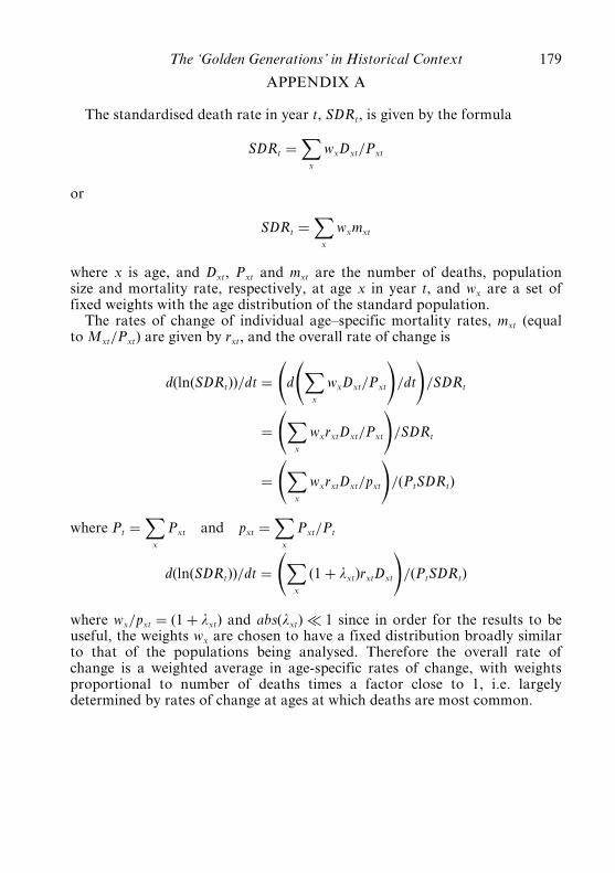
The standardised death rate in year t, SDRt, is given by the formula

SDRt ¼X

x

wxDxt=Pxt

or

SDRt ¼X

x

wxmxt

where x is age, and Dxt, Pxt and mxt are the number of deaths, populationsize and mortality rate, respectively, at age x in year t, and wx are a set offixed weights with the age distribution of the standard population.

The rates of change of individual age^specific mortality rates, mxt (equalto Mxt=Pxt) are given by rxt, and the overall rate of change is

dðlnðSDRtÞÞ=dt ¼ dX

x

wxDxt=Pxt

!=dt

!=SDRt

¼X

x

wxrxtDxt=Pxt

!=SDRt

¼X

x

wxrxtDxt=pxt

!=ðPtSDRtÞ

where Pt ¼X

x

Pxt and pxt ¼X

x

Pxt=Pt

dðlnðSDRtÞÞ=dt ¼X

x

ð1þ lxtÞrxtDxt

!=ðPtSDRtÞ

where wx=pxt ¼ ð1þ lxtÞ and absðlxtÞ � 1 since in order for the results to beuseful, the weights wx are chosen to have a fixed distribution broadly similarto that of the populations being analysed. Therefore the overall rate ofchange is a weighted average in age-specific rates of change, with weightsproportional to number of deaths times a factor close to 1, i.e. largelydetermined by rates of change at ages at which deaths are most common.


APPENDIX B

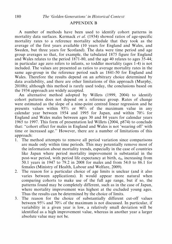
A number of methods have been used to identify cohort patterns inmortality data surfaces. Kermack et al. (1934) showed ratios of age-specificmortality rates to a reference mortality schedule that they took as theaverage of the first years available (10 years for England and Wales, andSweden, but three years for Scotland). The data were time period and agegroup averages so that, for example, the tabulated 1875 figure for Englandand Wales relates to the period 1871-80, and the age 40 relates to ages 35-44;in particular age zero refers to infants, so toddler mortality (ages 1-4) is notincluded. The values are presented as ratios to average mortality rates in thesame age-group in the reference period such as 1841-50 for England andWales. Therefore the results depend on an arbitrary choice determined bydata availability, and there are other limitations of this approach (Murphy,2010b); although this method is rarely used today, the conclusions based onthe 1934 approach are widely accepted.

An alternative method adopted by Willets (1999, 2004) to identifycohort patterns does not depend on a reference group. Rates of changewere estimated as the slope of a nine-point centred linear regression and hepresents values within 95% or 90% of the maximum value in anycalendar year between 1954 and 1995 for Japan, and within 70% forEngland and Wales males between ages 30 and 84 years for calendar years1965 to 1997. This form of presentation led Willets (2004, p874) to concludethat: “cohort effect for males in England and Wales is not ‘wearing off’ withtime or increased age.’’ However, there are a number of limitations of thisapproach:1. The method attempts to remove all period variation since comparisons

are made only within time periods. This may potentially remove most ofthe information about mortality trends, especially in the case of countrieslike Japan where period mortality improvement is substantial in thepost-war period, with period life expectancy at birth, e0, increasing from50.1 years in 1947 to 79.2 in 2008 for males and from 54.0 to 86.1 forfemales (Ministry of Health, Labour and Welfare, 2009).

2. The reason for a particular choice of age limits is unclear (and it alsovaries between applications). It would appear more natural whencomparing cohorts to make use of the full age range, but if so, thepatterns found may be completely different, such as in the case of Japan,where mortality improvement was highest at the excluded young ages.Thus the results can be determined by the choice of limits.

3. The reason for the choice of substantially different cut-off valuesbetween 95% and 70% of the maximum is not discussed. In particular, ifvariability in a given year is low, a relatively small deviation will beidentified as a high improvement value, whereas in another year a largerabsolute value may not be.


More recently, the most common way of identifying patterns in mortalitysurfaces is by showing contour maps of estimated rates of age-specificmortality change. This method does not suffer from the need to choose anarbitrary reference index population and it treats period and cohort largelysymmetrically. The precise method of estimating rates of change varies: theOffice of Population Censuses and Surveys (1995) shows the ratio of 5-yearage-specific rates five years apart, whereas Willets (2004) presented the slopeof a nine point regression of the logarithm of mortality rates to identifyages and periods/cohorts with particularly high relative rates of improvementin England and Wales, and MacMinn & Weber (2009) use 5- and 3-pointregression slopes.

The reasons for such choices are not explicit, but no optimality criteriaare applied, see e.g. Kenny & Durbin (1982). Since the main purpose is toidentify the rate of change (i.e. the first derivative of the logarithm of thetime series of the age-specific series), it is more appropriate to use a methodthat estimates the first derivative directly. There are a number of alternativemethods for estimating trends that will also estimate values at all points ofthe time series and will track non-linear trends more accurately, such alocally fitted regressions and Kalman filters, which tend to provide betterestimates than linear filters (Bianchi et al., 1999). This paper uses analyticfirst derivatives obtained from fitting a smoothing spline, sðxÞ to each singleyear of age data, xi, where i denotes year. The formula for such a model is

Xi

ðyi � sðxiÞÞ2þ l

ðx

dzd2s

dz2

� �2

where l is the smoothing parameter (in the R function smooth.spline, thespar smoothing parameter is a monotonic transformation of l, RDevelopment Core Team, 2009). Such a method allows the user to estimatethe derivative by using some optimality criterion, such as generalised cross-validation where the choice of smoothing is explicitly decided in terms ofa well established method. Unlike linear filters, such methods track non-linear curves and provide estimates for all points of the time series (iffitted to 2nþ 1 values, estimates are not available for the first and last npoints with a centred filter and a missing value would mean that values inthe interval from n years before to n years later would be missing). Whileresults from linears filters and spline-based models are generally similar,the greater coverage, flexibility and optimality properties of model-basedmethods make them preferable. Another advantage of such a method isthat it can include gaps in the data series, such as missing years aroundWorld War I, including the 1918-19 influenza pandemic and the SecondWorld War which have been excluded as extreme values from the fittingprocess (the smoothed spline model estimates values for missing sections of


the time series). If these years were not included on the grounds that theywould distort the underlying trend, with a 9-point moving average,information would be available only for years 1925 to 1934 in the wholeperiod between 1909 and 1950.


APPENDIX C

The population is assumed to comprise two groups. One is at low risk(‘lifetime non-smokers’) and the other is at high risk (‘lifetime smokers’). Inthe case shown here, mortality for both groups declines exponentially at 1%p.a., and so the annual rates of mortality change are constant for bothgroups. However, the level is twice as large for smokers as non-smokers ineach year. This is obviously over-simplified since it does not take account ofcessation of smoking (but it could be reformulated as equivalent numbers oflifetime smokers), but it is made to illustrate the care needed in applyingconclusions from aggregate-level data to individual cases.

The model is as follows:

pðs; xÞ ¼ k½1� cos ðx� 1900Þp=20ð Þ�=2 1900 � x � 1940 ¼ 0 otherwise

wherepðs; xÞ is the proportion of smokers for cohort born in year x, i.e. it risesfrom zero to a maximum of k and then returns to zero.

The proportion of non-smokers in cohort x is

pðn; xÞ ¼ 1� pðs; xÞ:

The mortality rates for non-smokers and smokers, mðn; xÞ and mðs; xÞ,respectively, are given by the formulae

mðn; xÞ ¼ 0:01 exp �0:01ðx� 1900Þð Þ

mðs; xÞ ¼ 0:02 exp �0:01ðx� 1900Þð Þ

so the overall mortality rate is

mðo; xÞ ¼ mðn; xÞð1þ pðs; xÞÞ

and the rate of overall mortality improvement is

rðo; xÞ ¼ 0:01� ðkp=40Þ sinððx� 1900Þp=20Þ=ð1þ pðs; xÞÞ 1900 � x � 1940

¼ 0:01 otherwise:

The maximum rate of improvement occurs around cohort 1930, withapproximate value

0:01þ ðkp=40Þ=ð1þ k=2Þ:

If this is set at 1% over the baseline value, the value of k is 0.14, i.e. the


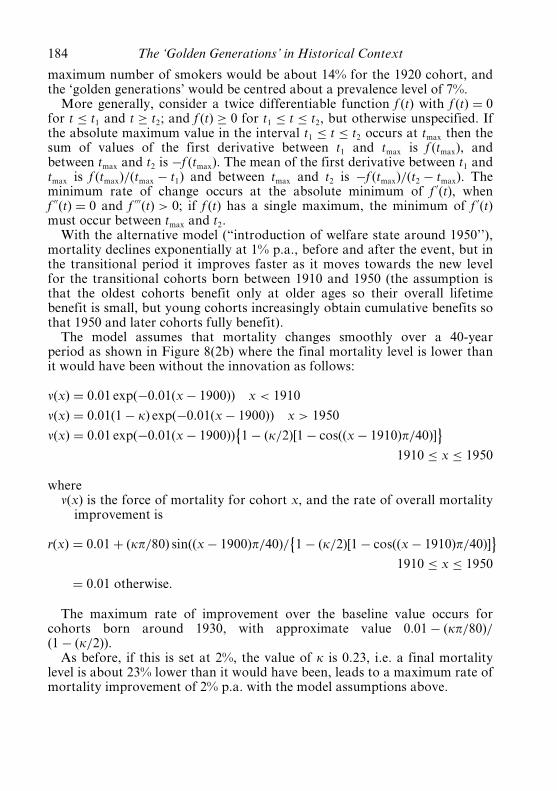
maximum number of smokers would be about 14% for the 1920 cohort, andthe ‘golden generations’ would be centred about a prevalence level of 7%.

More generally, consider a twice differentiable function f ðtÞ with f ðtÞ ¼ 0for t � t1 and t � t2; and f ðtÞ � 0 for t1 � t � t2, but otherwise unspecified. Ifthe absolute maximum value in the interval t1 � t � t2 occurs at tmax then thesum of values of the first derivative between t1 and tmax is f ðtmaxÞ, andbetween tmax and t2 is �f ðtmaxÞ. The mean of the first derivative between t1 andtmax is f ðtmaxÞ=ðtmax � t1Þ and between tmax and t2 is �f ðtmaxÞ=ðt2 � tmaxÞ. Theminimum rate of change occurs at the absolute minimum of f 0ðtÞ, whenf 00ðtÞ ¼ 0 and f 000ðtÞ > 0; if f ðtÞ has a single maximum, the minimum of f 0ðtÞmust occur between tmax and t2.

With the alternative model (“introduction of welfare state around 1950’’),mortality declines exponentially at 1% p.a., before and after the event, but inthe transitional period it improves faster as it moves towards the new levelfor the transitional cohorts born between 1910 and 1950 (the assumption isthat the oldest cohorts benefit only at older ages so their overall lifetimebenefit is small, but young cohorts increasingly obtain cumulative benefits sothat 1950 and later cohorts fully benefit).

The model assumes that mortality changes smoothly over a 40-yearperiod as shown in Figure 8(2b) where the final mortality level is lower thanit would have been without the innovation as follows:

nðxÞ ¼ 0:01 exp �0:01ðx� 1900Þð Þ x < 1910

nðxÞ ¼ 0:01ð1� kÞ exp �0:01ðx� 1900Þð Þ x > 1950

nðxÞ ¼ 0:01 exp �0:01ðx� 1900Þð Þ 1� ðk=2Þ½1� cos ðx� 1910Þp=40ð Þ��

1910 � x � 1950

wherenðxÞ is the force of mortality for cohort x, and the rate of overall mortalityimprovement is

rðxÞ ¼ 0:01þ ðkp=80Þ sin ðx� 1900Þp=40ð Þ= 1� ðk=2Þ½1� cos ðx� 1910Þp=40ð Þ��

1910 � x � 1950

¼ 0:01 otherwise:

The maximum rate of improvement over the baseline value occurs forcohorts born around 1930, with approximate value 0:01� ðkp=80Þ=ð1� ðk=2ÞÞ.

As before, if this is set at 2%, the value of k is 0.23, i.e. a final mortalitylevel is about 23% lower than it would have been, leads to a maximum rate ofmortality improvement of 2% p.a. with the model assumptions above.


Pp 151184

Documents