MARKOV MODELS PERFECT SAMPLING DISCRETE TIME EVENT SIMULATION CASE STUDIES Ψ 3 -SOFTWARE DEMONSTRATION Poisson Systems and Perfect Sampling [email protected] Laboratoire d’Informatique de Grenoble, INRIA Team Polaris École d’été en Recherche Opérationnelle Optimisation et décision en milieu incertain June 4-6, 2016 Work partially supported by ANR Marmote 1 / 105 Poisson Systems and Perfect Sampling

Welcome message from author
This document is posted to help you gain knowledge. Please leave a comment to let me know what you think about it! Share it to your friends and learn new things together.
Transcript

MARKOV MODELS PERFECT SAMPLING DISCRETE TIME EVENT SIMULATION CASE STUDIES Ψ3 -SOFTWARE DEMONSTRATION S
Poisson Systems and Perfect Sampling
Laboratoire d’Informatique de Grenoble, INRIA Team Polaris
École d’été en Recherche OpérationnelleOptimisation et décision en milieu incertain
June 4-6, 2016
Work partially supported by ANR Marmote
1 / 105Poisson Systems and Perfect Sampling

MARKOV MODELS PERFECT SAMPLING DISCRETE TIME EVENT SIMULATION CASE STUDIES Ψ3 -SOFTWARE DEMONSTRATION S
MARKOVIAN WORK
An example of statistical investigation in the text of"Eugene Onegin" illustrating coupling of "tests" inchains.(1913) In Proceedings of Academic Scientific St.Petersburg, VI, pages 153-162.
1856-1922
3 / 105Poisson Systems and Perfect Sampling

MARKOV MODELS PERFECT SAMPLING DISCRETE TIME EVENT SIMULATION CASE STUDIES Ψ3 -SOFTWARE DEMONSTRATION S
GRAPHS AND PATHS
i
1
2
3
4 5
a
bc
d
e f
g
hRandom Walks
Path in a graph :Xn n-th visited nodepath : i0, i1, · · · , innormalized weight : arc (i, j) −→ pi,j
concatenation : . −→ ×P(i0, i1, · · · , in) = pi0,i1 pi1,i2 · · · pin−1,in
disjoint union : ∪ −→ +P(i0 ❀ in) =
∑
i1,··· ,in−1pi0,i1 pi1,i2 · · · pin−1,in
automaton : state/transitions randomized (language)
4 / 105Poisson Systems and Perfect Sampling

MARKOV MODELS PERFECT SAMPLING DISCRETE TIME EVENT SIMULATION CASE STUDIES Ψ3 -SOFTWARE DEMONSTRATION S
MODELING AND ANALYSIS OF COMPUTER SYSTEMS
Complex system
output
Environment
Input of the system
System
System
Basic model assumptions
System :- automaton (discrete state space)- discrete or continuous timeEnvironment : non deterministic- time homogeneous- stochastically regular
Problem
Understand “typical” states- steady-state estimation- ergodic simulation- state space exploring techniques
5 / 105Poisson Systems and Perfect Sampling

MARKOV MODELS PERFECT SAMPLING DISCRETE TIME EVENT SIMULATION CASE STUDIES Ψ3 -SOFTWARE DEMONSTRATION S
QUEUING NETWORKS WITH FINITE CAPACITY
Network model
Finite set of resources :◮ servers
◮ waiting rooms
Routing strategies :◮ state dependent
◮ overflow strategy
◮ blocking strategy
◮ ...
Average performance :◮ load of the system
◮ response time
◮ loss rate
◮ ...
Markov model
1−p
λ
µ
ν
C1
C2 Rejection
Blocking
p
Poisson arrival, exponential services distribution, probabilistic routing⇒ continuous time Markov chain
C1
0
1
2
C2−1
C2
Queue 2
0 2 Queue 11 C1−1
Problem
Computation of steady state distribution⇒ state-space explosion
6 / 105Poisson Systems and Perfect Sampling

MARKOV MODELS PERFECT SAMPLING DISCRETE TIME EVENT SIMULATION CASE STUDIES Ψ3 -SOFTWARE DEMONSTRATION S
INTERCONNEXION NETWORKS
Delta network
8
11
12
13
14
15
16
17
18
19
20
21
22
23
24
25
26
27
28
29
30
31
0
1
2
3
4
5
6
7
10
9
Input ratesService ratesHomogeneous routingOverflow strategy
Problem
Loss probability at each levelAnalysis of hot spot...
7 / 105Poisson Systems and Perfect Sampling

MARKOV MODELS PERFECT SAMPLING DISCRETE TIME EVENT SIMULATION CASE STUDIES Ψ3 -SOFTWARE DEMONSTRATION S
CALL CENTERS
Multilevel Erlang model
Traffic 2
Overflow traffic 2Overflow traffic 1
Type I servers Type II servers
Type III servers
Traffic 1
Types of requestsInput ratesDifferent service ratesOverflow strategy
Problem
Optimization of resourcesQuality of service (waiting time, rejection probability,...)...
8 / 105Poisson Systems and Perfect Sampling

MARKOV MODELS PERFECT SAMPLING DISCRETE TIME EVENT SIMULATION CASE STUDIES Ψ3 -SOFTWARE DEMONSTRATION S
RESOURCE BROKER
Grid model
Q9
Resource Broker
λ
µ2
µ1
µ3
µ4
µ5
µ6
µ7
µ8
µ9
Overflow
Q2
Q3
Q1
Q10
Q11
Q12
Q4
Q6
Q5
Q7
Q8
Input ratesAllocation strategyState dependent allocationIndex based routing : destinationminimize a criteria
Problem
Optimization of throughput, response time,...Comparison of policies, analysis of heuristics...
9 / 105Poisson Systems and Perfect Sampling
MARKOV MODELS PERFECT SAMPLING DISCRETE TIME EVENT SIMULATION CASE STUDIES Ψ3 -SOFTWARE DEMONSTRATION S
FORMAL DEFINITION
Let {Xn}n∈Na random sequence of variables in a discrete state-space X
{Xn}n∈Nis a Markov chain with initial law π(0) iff
◮ X0 ∼ π(0) and
◮ for all n ∈ N and for all (j, i, in−1, · · · , i0) ∈ X n+2
P(Xn+1 = j|Xn = i, Xn−1 = in−1, · · · , X0 = i0) = P(Xn+1 = j|Xn = i).
{Xn}n∈Nis a homogeneous Markov chain iff
◮ for all n ∈ N and for all (j, i) ∈ X 2
P(Xn+1 = j|Xn = i) = P(X1 = j|X0 = i)def= pi,j.
(invariance during time of probability transition)
10 / 105Poisson Systems and Perfect Sampling

MARKOV MODELS PERFECT SAMPLING DISCRETE TIME EVENT SIMULATION CASE STUDIES Ψ3 -SOFTWARE DEMONSTRATION S
ALGEBRAIC REPRESENTATION
P = ((pi,j)) is the transition matrix of the chain
◮ P is a stochastic matrixpi,j > 0;
∑
j
pi,j = 1.
Linear recurrence equation πi(n) = P(Xn = i)
πn = πn−1P.
◮ Equation of Chapman-Kolmogorov (homogeneous) : Pn = ((p(n)i,j
))
p(n)i,j
= P(Xn = j|X0 = i); Pn+m= Pn
.Pm;
P(Xn+m = j|X0 = i) =∑
k
P(Xn+m = j|Xm = k)P(Xm = k|X0 = i);
=∑
k
P(Xn = j|X0 = k)P(Xm = k|X0 = i).
Interpretation : decomposition of the set of paths with length n + m from i to j.
11 / 105Poisson Systems and Perfect Sampling

MARKOV MODELS PERFECT SAMPLING DISCRETE TIME EVENT SIMULATION CASE STUDIES Ψ3 -SOFTWARE DEMONSTRATION S
EVENT MODELLING
Multidimensional state space : X = X1 × · · · × XK with Xi = {0, · · · ,Ci}.Event e :❀ transition function Φ(., e) ; (skip rule)❀ Poisson process λe
States
Events
e1
e2
e3
e4
Time
1781-1840
12 / 105Poisson Systems and Perfect Sampling

MARKOV MODELS PERFECT SAMPLING DISCRETE TIME EVENT SIMULATION CASE STUDIES Ψ3 -SOFTWARE DEMONSTRATION S
EVENT MODELLING : UNIFORMIZATION
Λ =∑
e
λe and P(event e) =λe
Λ;
Trajectory : {en}n∈Zi.i.d. sequence.
⇒ Homogeneous Discrete Time Markov Chain [Bremaud 99]
Xn+1 = Φ(Xn, en+1).
Generation among a small finite space E :O(1)
13 / 105Poisson Systems and Perfect Sampling

MARKOV MODELS PERFECT SAMPLING DISCRETE TIME EVENT SIMULATION CASE STUDIES Ψ3 -SOFTWARE DEMONSTRATION S
EVENTS AND POISSON SYSTEMS
0
Queue
States
2
M/M/1 capacity C = 2
1
Φ(x, d) = max(x − 1, 0)Φ(x, a) = min(x + 1,C)
non effective eventsState
1
2
0
arrivals
departures
time
⇒monotone events
14 / 105Poisson Systems and Perfect Sampling

MARKOV MODELS PERFECT SAMPLING DISCRETE TIME EVENT SIMULATION CASE STUDIES Ψ3 -SOFTWARE DEMONSTRATION S
PROBLEMS
Finite horizon
- Estimation of π(n)- Estimation of stopping times
τA = inf{n > 0; Xn ∈ A}
- · · ·
Infinite horizon
- Convergence properties- Estimation of the asymptotics- Estimation speed of convergence- · · ·
15 / 105Poisson Systems and Perfect Sampling

MARKOV MODELS PERFECT SAMPLING DISCRETE TIME EVENT SIMULATION CASE STUDIES Ψ3 -SOFTWARE DEMONSTRATION S
ASYMPTOTIC BEHAVIOR : LAW CONVERGENCE
Let {Xn}n∈Na homogeneous, irreducible and aperiodic Markov chain taking values in
a discrete state X then◮ The following limits exist (and do not depend on i)
limn→+∞
P(Xn = j|X0 = i) = πj;
◮ π is the unique probability vector invariant by P
πP = π;
◮ The convergence is rapid (geometric) ; there is C > 0 and 0 < α < 1 such that
||P(Xn = j|X0 = i) − πj|| 6 C.αn.
DenoteXn
L−→ X∞;
with X∞ having law ππ is the steady-state probability associated to the chain
16 / 105Poisson Systems and Perfect Sampling

MARKOV MODELS PERFECT SAMPLING DISCRETE TIME EVENT SIMULATION CASE STUDIES Ψ3 -SOFTWARE DEMONSTRATION S
INTERPRETATION
Equilibrium equation
j,j
j
i1
i2
i3
i4
k1
k2
k3
p
p
p
p
p
p
p
p
i1,j
i2,j
i3,j
i4,j
j,k1
j,k2
j,k3
Probability to enter j =probability to exit jbalance equation
∑
i6=j
πipi,j =∑
k 6=j
πjpj,k = πj
∑
k 6=j
pj,k = πj(1− pj,j)
πdef= steady-state.
If π0 = π the process is stationary (πn = π)
17 / 105Poisson Systems and Perfect Sampling

MARKOV MODELS PERFECT SAMPLING DISCRETE TIME EVENT SIMULATION CASE STUDIES Ψ3 -SOFTWARE DEMONSTRATION S
ERGODIC THEOREM
Let {Xn}n∈Na homogeneous aperiodic and irreducible Markov chain on X with
steady-state probability π then- for all function f satisfying Eπ |f | < +∞
1N
N∑
n=1
f (Xn)P−p.s.−→ Eπ f .
generalization of the strong law of large numbers- If Eπ f = 0 then there exist σ such that
1
σ√
N
N∑
n=1
f (Xn)L−→ N (0, 1).
generalization of the central limit theorem
18 / 105Poisson Systems and Perfect Sampling

MARKOV MODELS PERFECT SAMPLING DISCRETE TIME EVENT SIMULATION CASE STUDIES Ψ3 -SOFTWARE DEMONSTRATION S
FUNDAMENTAL QUESTION
Given a function f (cost, reward, performance,...) estimate
Eπf
and provide the quality of this estimation.
19 / 105Poisson Systems and Perfect Sampling
MARKOV MODELS PERFECT SAMPLING DISCRETE TIME EVENT SIMULATION CASE STUDIES Ψ3 -SOFTWARE DEMONSTRATION S
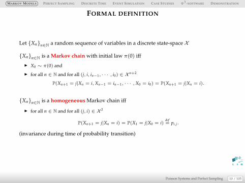
SOLVING METHODS
Solving π = πP
◮ Analytical/approximation methods
◮ Formal methods N 6 80Maple, Sage,...
◮ Direct numerical methods N 6 5000Mathematica, Scilab,...
◮ Iterative methods with preconditioning N 6 500, 000Marca,...
◮ Adapted methods (structured Markov chains) N 6 10, 000, 000PEPS,...
◮ Monte-Carlo simulation N > 108
Postprocessing of the stationary distribution
Computation of rewards (expected stationary functions)Utilization, response time,...
20 / 105Poisson Systems and Perfect Sampling

MARKOV MODELS PERFECT SAMPLING DISCRETE TIME EVENT SIMULATION CASE STUDIES Ψ3 -SOFTWARE DEMONSTRATION S
ERGODIC SAMPLING(1)
Ergodic sampling algorithm
Representation : transition fonction
Xn+1 = Φ(Xn, en+1).
x ← x0{choice of the initial state at time =0}n = 0 ;repeat
n ← n + 1 ;e ← Random_event() ;x ← Φ(x, e) ;Store x{computation of the next state Xn+1}
until some empirical criteriareturn the trajectory
Problem : Stopping criteria
21 / 105Poisson Systems and Perfect Sampling
MARKOV MODELS PERFECT SAMPLING DISCRETE TIME EVENT SIMULATION CASE STUDIES Ψ3 -SOFTWARE DEMONSTRATION S
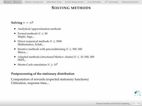
ERGODIC SAMPLING(2)
Start-up
Convergence to stationary behavior
limn→+∞
P(Xn = x) = πx.
Warm-up period : Avoid initial state dependenceEstimation error :
||P(Xn = x)− πx|| 6 Cλn2 .
λ2 second greatest eigenvalue of the transition matrix- bounds on C and λ2 (spectral gap)- cut-off phenomena
λ2 and C non reachable in practice(complexity equivalent to the computation of π)some known results (Birth and Death processes)
22 / 105Poisson Systems and Perfect Sampling

MARKOV MODELS PERFECT SAMPLING DISCRETE TIME EVENT SIMULATION CASE STUDIES Ψ3 -SOFTWARE DEMONSTRATION S
ERGODIC SAMPLING(3)
Estimation quality
Ergodic theorem :
limn→+∞
1n
n∑
i=1
f (Xi) = Eπ f .
Length of the sampling : Error control (CLT theorem)
Complexity
Complexity of the transition function evaluation (computation of Φ(x, .))Related to the stabilization period + Estimation time
23 / 105Poisson Systems and Perfect Sampling

MARKOV MODELS PERFECT SAMPLING DISCRETE TIME EVENT SIMULATION CASE STUDIES Ψ3 -SOFTWARE DEMONSTRATION S
ERGODIC SAMPLING(4)
Typical trajectory
States
0 time
Warm−up period Estimation period
24 / 105Poisson Systems and Perfect Sampling

MARKOV MODELS PERFECT SAMPLING DISCRETE TIME EVENT SIMULATION CASE STUDIES Ψ3 -SOFTWARE DEMONSTRATION S
REPLICATION METHOD
Typical trajectory
States
0 timereplication periods
Sample of independent statesDrawback : length of the replication period (dependence from initial state)
25 / 105Poisson Systems and Perfect Sampling

MARKOV MODELS PERFECT SAMPLING DISCRETE TIME EVENT SIMULATION CASE STUDIES Ψ3 -SOFTWARE DEMONSTRATION S
REGENERATION METHOD
Typical trajectory
States
0 time
start−up period
regeneration period
R1 R2 R3 ....
Sample of independent trajectoriesDrawback : length of the regeneration period (choice of the regenerative state)
26 / 105Poisson Systems and Perfect Sampling
MARKOV MODELS PERFECT SAMPLING DISCRETE TIME EVENT SIMULATION CASE STUDIES Ψ3 -SOFTWARE DEMONSTRATION S
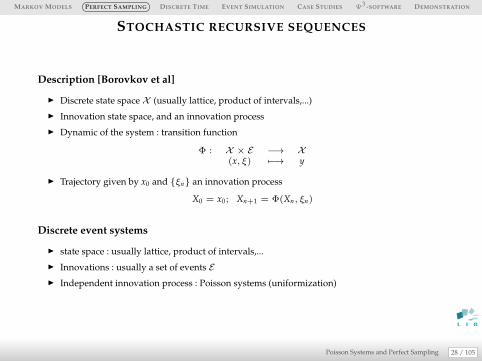
STOCHASTIC RECURSIVE SEQUENCES
Description [Borovkov et al]
◮ Discrete state space X (usually lattice, product of intervals,...)
◮ Innovation state space, and an innovation process
◮ Dynamic of the system : transition function
Φ : X × E −→ X(x, ξ) 7−→ y
◮ Trajectory given by x0 and {ξn} an innovation process
X0 = x0; Xn+1 = Φ(Xn, ξn)
Discrete event systems
◮ state space : usually lattice, product of intervals,...
◮ Innovations : usually a set of events E
◮ Independent innovation process : Poisson systems (uniformization)
28 / 105Poisson Systems and Perfect Sampling

MARKOV MODELS PERFECT SAMPLING DISCRETE TIME EVENT SIMULATION CASE STUDIES Ψ3 -SOFTWARE DEMONSTRATION S
MARKOVIAN MODELLING
Theorem (Markov process)
If {ξn} is a sequence of iid random variables , the process {Xn} is a homogeneous discrete timeMarkov chain.
Random Iterated system of functions
The trajectory Xn is the successive application of random functions taken in the set{Φ(., ξ), ξ ∈ E} according a probability measure on E[Diaconis and Friedman 98]
29 / 105Poisson Systems and Perfect Sampling

MARKOV MODELS PERFECT SAMPLING DISCRETE TIME EVENT SIMULATION CASE STUDIES Ψ3 -SOFTWARE DEMONSTRATION S
COUPLING INEQUALITY
Typical trajectory
Coupling time
Stationary version
τ0 time
States
After τ the two processes are not distinguishable, then stationaryScheme used to prove Markov convergence (coupling inequality)
|P(Xn ∈ A)− πA| 6 P(τ > n)
30 / 105Poisson Systems and Perfect Sampling

MARKOV MODELS PERFECT SAMPLING DISCRETE TIME EVENT SIMULATION CASE STUDIES Ψ3 -SOFTWARE DEMONSTRATION S
FORWARD SAMPLING : AVOID INITIAL STATE DEPENDENCE
Forward coupling
Steady-state ?
f3f4f6f7f3f1Time
State
Example
1
1 − p p
Always couple in the blue stateDoes not guarantee the steady state !
31 / 105Poisson Systems and Perfect Sampling

MARKOV MODELS PERFECT SAMPLING DISCRETE TIME EVENT SIMULATION CASE STUDIES Ψ3 -SOFTWARE DEMONSTRATION S
PERFECT SAMPLING : BACKWARD IDEA
Set dynamic
In what state could I be at time n = 0 ?
X0 ∈ X = Z0
∈ Φ(X , e−1) = Z1
∈ Φ(Φ(X , e−2), e−1) = Z2
......
∈ Φ(Φ(· · ·Φ(X , e−n), · · · ), e−2), e−1) = Zn
32 / 105Poisson Systems and Perfect Sampling

MARKOV MODELS PERFECT SAMPLING DISCRETE TIME EVENT SIMULATION CASE STUDIES Ψ3 -SOFTWARE DEMONSTRATION S
PERFECT SAMPLING : BACKWARD IDEA
All the trajectories
Time
0
−i
−j
−τ ∗
Stationary Process
X
X
X
X
Zi
Zj
Z−τ∗ = {X0}
Z0 = X
collapse
33 / 105Poisson Systems and Perfect Sampling

MARKOV MODELS PERFECT SAMPLING DISCRETE TIME EVENT SIMULATION CASE STUDIES Ψ3 -SOFTWARE DEMONSTRATION S
PERFECT SAMPLING : CONVERGENCE THEOREM
Theorem
Provided some condition on the events the sequence of sets
{Zn}n∈N
is decreasing to a single state, stationary distributed.
τ∗ = inf{n ∈ N; Card(Zn) = 1}.backward coupling time
The set of possible states at time 0 is decreasing with regards to n
34 / 105Poisson Systems and Perfect Sampling

MARKOV MODELS PERFECT SAMPLING DISCRETE TIME EVENT SIMULATION CASE STUDIES Ψ3 -SOFTWARE DEMONSTRATION S
PERFECT SAMPLING : COUPLING CONDITION
Theorem
Suppose that the set of events is finite. Then the two conditions are equivalent :◮ τ∗ < +∞ almost surely ;
◮ There exist a finite sequence of events with positive probability S = {e1, · · · , eM} such that
|Φ(X , e1→M)| = 1.
The sequence S is called a synchronizing pattern(synchronizing word, renovating event,...)
35 / 105Poisson Systems and Perfect Sampling

MARKOV MODELS PERFECT SAMPLING DISCRETE TIME EVENT SIMULATION CASE STUDIES Ψ3 -SOFTWARE DEMONSTRATION S
PERFECT SAMPLING : COUPLING CONDITION (PROOF)
Proof
⇒ If τ∗ < +∞ almost surely there is a trajectory that couples in a finite time. This finitetrajectory is a synchronizing pattern.
⇐ Suppose there is a synchronizing pattern with length M. Because the sequence of events is iid,it occurs almost surely on every trajectory. Applying Borel-Cantelli lemma gives the result.
The forward and backward coupling time have the same distributionτ∗ has an exponentially dominated distribution tail
P(τ∗ > M.n) 6 (1− P(e1→M))n.
Practically efficient
36 / 105Poisson Systems and Perfect Sampling

MARKOV MODELS PERFECT SAMPLING DISCRETE TIME EVENT SIMULATION CASE STUDIES Ψ3 -SOFTWARE DEMONSTRATION S
PERFECT SAMPLING : CONVERGENCE THEOREM (PROOF 1)
Proof based on the shift property
First, because τ < +∞ and the ergodicity of the chain there exists N0 s.t.
|P(Φ(X , e1→n) = {x})− πx| 6 ǫ.
But the sequence of events is iid (stationary) then
P(Φ(X , e1→n) = {x}) = P(Φ(X , e−n+1→0) = {x})
τ∗ < +∞ then there exists N1 such that P(τ∗ > N1) 6 ǫ ; then
P(Φ(X , e−n+1→0) = {x})
= P(Φ(X , e−n+1→0) = {x}, τ∗ < N1) + P(Φ(X , e−n+1→0) = {x}, τ∗ > N1),
= P(Φ(X , e−τ∗→0) = {x}, τ∗ < N1) + ǫ′,
= P(X0 = x, τ∗ < N1) + ǫ′ = P(X0 = x) + ǫ′′.
By the dominated convergence theorem the result follows
37 / 105Poisson Systems and Perfect Sampling

MARKOV MODELS PERFECT SAMPLING DISCRETE TIME EVENT SIMULATION CASE STUDIES Ψ3 -SOFTWARE DEMONSTRATION S
PERFECT SAMPLING : CONVERGENCE THEOREM (PROOF 2)
Proof based on the coupling property [Haggstrom]
Consider N such that P(τ∗ > N) 6 ǫthen consider a process {Xn}with the same events e−N+1→0 but with X−N+1
generated according π. The process {Xn} is stationary.On the event (τ∗ < N) we have X0 = X0 and
P(X0 6= X0) 6 P(τ∗ > N) 6 ǫ (coupling inequality).
FinallyP(X0 = x)− πx = P(X0 = x)− P(X0 = x) 6 P(X0 6= X0) 6 ǫ;
πx − P(X0 = x) = P(X0 = x)− P(X0 = x) 6 P(X0 6= X0) 6 ǫ;
and the result follows.
38 / 105Poisson Systems and Perfect Sampling

MARKOV MODELS PERFECT SAMPLING DISCRETE TIME EVENT SIMULATION CASE STUDIES Ψ3 -SOFTWARE DEMONSTRATION S
PERFECT SAMPLING : ALGORITHM
Backward algorithm
Representation : transition fonction
Xn+1 = Φ(Xn, en+1).
for all x ∈ X doy(x) ← x
end forrepeat
e ← Random_event() ;for all x ∈ X do
z(x) ← y(Φ(x, e)) ;end fory ← z
until All y(x) are equalreturn y(x)
Convergence : If the algorithm stops, the returnedvalue is steady state distributedCoupling time : τ < +∞, properties of Φ
Trajectories
Time
States
0000
0001
0010
0011
0100
0101
0110
1000
1001
1010
1100
−4 −3 −2 −1−5−6−7−8−9−10 0U1U2U3U4U5U6U7U8
τ∗
Mean time complexity
cΦ mean computation cost of Φ(x, e)
C 6 Card(X ).Eτ.cΦ.
39 / 105Poisson Systems and Perfect Sampling

MARKOV MODELS PERFECT SAMPLING DISCRETE TIME EVENT SIMULATION CASE STUDIES Ψ3 -SOFTWARE DEMONSTRATION S
PERFECT REWARD SAMPLING
Backward reward
Representation : transition fonction
Xn+1 = Φ(Xn, en+1).
Arbitrary reward function
for all x ∈ X doy(x) ← x
end forrepeat
e ← Random_event() ;for all x ∈ X do
y(x) ← y(Φ(x, e)) ;end for
until All Reward(y(x)) are equalreturn Reward(y(x))
Convergence : If the algorithm stops, the returnedvalue is steady state reward distributedCoupling time : τr 6 τ < +∞
Trajectories
Time
States
0000
0001
0010
0011
0100
0101
0110
1000
1001
1010
1100
−4 −3 −2 −1−5−6−7−8−9−10 0U1U2U3U4U5U6U7U8
1
0
Cost
Mean time complexity
CReward 6 Card(X ).Eτ.cΦDepends on the reward function.
40 / 105Poisson Systems and Perfect Sampling

MARKOV MODELS PERFECT SAMPLING DISCRETE TIME EVENT SIMULATION CASE STUDIES Ψ3 -SOFTWARE DEMONSTRATION S
INVERSE OF PDF
P(X 6 x)
0
1
1 2 3 K − 1 K
Cumulative distribution function
x
p1
p2
p3
· · ·
Generation
Divide [0, 1[ in intervals with length pk
Find the interval in which Random fallsReturns the index of the intervalComputation cost :O(EX) stepsMemory cost :O(1)
Inverse function algorithm
s=0 ; k=0 ;u=random()while u >s do
k=k+1s=s+pk
end whilereturn k
42 / 105Poisson Systems and Perfect Sampling

MARKOV MODELS PERFECT SAMPLING DISCRETE TIME EVENT SIMULATION CASE STUDIES Ψ3 -SOFTWARE DEMONSTRATION S
SEARCHING OPTIMIZATION
Optimization methods
◮ pre-compute the pdf in a table
◮ rank objects by decreasing probability
◮ use a dichotomy algorithm
◮ use a tree searching algorithm (optimality = Huffmann coding tree)
Comments
- Depends on the usage of the generator (repeated use or not)- pre-computation usuallyO(K) could be huge-
43 / 105Poisson Systems and Perfect Sampling

MARKOV MODELS PERFECT SAMPLING DISCRETE TIME EVENT SIMULATION CASE STUDIES Ψ3 -SOFTWARE DEMONSTRATION S
GENERATION : VISUAL REPRESENTATION
[0, 1] partitionning
10312
112
612
212
712
112
412
312
712
312
1112
f1 f3 f4 f5 f6 f7 f8f2
4 3
21
Random iterated system of functions
Function f1 f2 f3 f4 f5 f6 f7 f8Probability 1
121
121
121
121
124
122
121
12
Stochastic matrix P =⇒ simulation algorithm = RIFS
44 / 105Poisson Systems and Perfect Sampling

MARKOV MODELS PERFECT SAMPLING DISCRETE TIME EVENT SIMULATION CASE STUDIES Ψ3 -SOFTWARE DEMONSTRATION S
THE COUPLING PROBLEM
τ estimation
Eτ = 2
0 1
Couples with probability 12
0 1
Never couples
τ = ∞
10 1
Couples with probability 1
τ = 1
0
12
12
12
12
45 / 105Poisson Systems and Perfect Sampling

MARKOV MODELS PERFECT SAMPLING DISCRETE TIME EVENT SIMULATION CASE STUDIES Ψ3 -SOFTWARE DEMONSTRATION S
GENERAL PROBLEM
Objective
Given a stochastic matrix P = ((pi,j)) build a system of function (fθ, θ ∈ Θ) and a probabilitydistribution (pθ, θ ∈ Θ) such that :
1 the RIFS implements the transition matrix P,
2 ensures coupling in finite time
3 achieve the “best” mean coupling time : tradeoff between- choice of the transition function according to ((pθ)),- computation of the transition
Remarks
Usual method|Θ| = number of non-negative elements of P = O(n2
)
choice inO(log n)
46 / 105Poisson Systems and Perfect Sampling

MARKOV MODELS PERFECT SAMPLING DISCRETE TIME EVENT SIMULATION CASE STUDIES Ψ3 -SOFTWARE DEMONSTRATION S
NON SPARSE MATRICES
Rearranging the system
0 1
"Synchronizing" transformation
0 1
312
112
412
712
312
312
1112
112
612
212
712
f1 f3 f4 f5 f6 f7 f8f2
4 3
21
47 / 105Poisson Systems and Perfect Sampling

MARKOV MODELS PERFECT SAMPLING DISCRETE TIME EVENT SIMULATION CASE STUDIES Ψ3 -SOFTWARE DEMONSTRATION S
NON SPARSE MATRICES
Convergence rate
When at least one column is non-negative⇒ one step coupling.The RIFS ensures coupling and the coupling time τ is upper bounded by a geometricdistribution with rate
∑
j
mini
pi,j
number of transition functions : could be more than the number of non-negativeelementsat most n2
48 / 105Poisson Systems and Perfect Sampling

MARKOV MODELS PERFECT SAMPLING DISCRETE TIME EVENT SIMULATION CASE STUDIES Ψ3 -SOFTWARE DEMONSTRATION S
ALIASING TECHNIQUE
Initialization
K objectslist L=∅,U=∅ ;for k=1 ; k6 K ; k++ do
P[k]=pk
if P[k] > 1K
thenU=U+{k} ;
elseL=L+{k} ;
end ifend for
Alias and threshold tables
while L 6= ∅ doExtract k ∈ LExtract i ∈ US[k]=P[k]A[k]=iP[i] = P[i] - ( 1
K-P[k])
if P[i] > 1K
thenU=U+{i} ;
elseL=L+{i} ;
end ifend while
Combine uniform and alias value when rejection
49 / 105Poisson Systems and Perfect Sampling

MARKOV MODELS PERFECT SAMPLING DISCRETE TIME EVENT SIMULATION CASE STUDIES Ψ3 -SOFTWARE DEMONSTRATION S
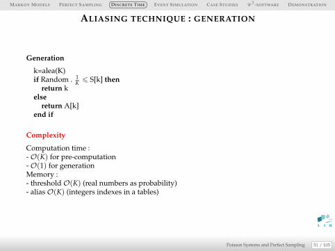
ALIASING TECHNIQUE : GENERATION
1/8
50 / 105Poisson Systems and Perfect Sampling
MARKOV MODELS PERFECT SAMPLING DISCRETE TIME EVENT SIMULATION CASE STUDIES Ψ3 -SOFTWARE DEMONSTRATION S
ALIASING TECHNIQUE : GENERATION
Generation
k=alea(K)if Random . 1
K6 S[k] then
return kelse
return A[k]end if
Complexity
Computation time :-O(K) for pre-computation-O(1) for generationMemory :- thresholdO(K) (real numbers as probability)- aliasO(K) (integers indexes in a tables)
51 / 105Poisson Systems and Perfect Sampling

MARKOV MODELS PERFECT SAMPLING DISCRETE TIME EVENT SIMULATION CASE STUDIES Ψ3 -SOFTWARE DEMONSTRATION S
SPARSE MATRICES
Rearranging the system
10
Aliasing transformation
10
612
1112
312
312
712
412
112
312
712
212
112
f1 f3 f4 f5 f6 f7 f8f2
4 3
21
Complexity
M = maximum out degree of statespθ uniform on {1, · · · , M}, threshold comparisonO(1) to compute one transitionCombination with “Synchronizing” techniques
52 / 105Poisson Systems and Perfect Sampling
MARKOV MODELS PERFECT SAMPLING DISCRETE TIME EVENT SIMULATION CASE STUDIES Ψ3 -SOFTWARE DEMONSTRATION S
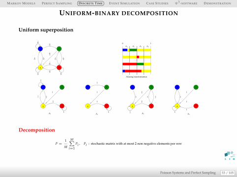
UNIFORM-BINARY DECOMPOSITION
Uniform superposition
1
1
1
1
1
1
34
2
A4
A4
13
1
23
131
22
1 2
34
A3
A3
1
1
1
1
4
A2
A2
21
3
13
23
13
1
1
23
4 3
21
A1
A1
0 1
Aliasing transformation
312
412
112
712
212
612
112
312
1112
312
712
1 2
34
Decomposition
P =1
M
M∑
i=1Pi, Pi : stochastic matrix with at most 2 non negative elements per row
53 / 105Poisson Systems and Perfect Sampling

MARKOV MODELS PERFECT SAMPLING DISCRETE TIME EVENT SIMULATION CASE STUDIES Ψ3 -SOFTWARE DEMONSTRATION S
COUPLING PROPERTY
Exchange of columns or thresholds give an equivalent representative
representation
������������
������������
������������
������������
������������
������������
������������
������������
������������
������������
������������
������������
Equivalent
Spanning tree
Irreducibility =⇒ there is a spanning tree going to a single state where coupling occurs.
P(τ∗ < +∞) = 1.
τ is geometrically bounded, soτ∗ and τ∗C .
54 / 105Poisson Systems and Perfect Sampling

MARKOV MODELS PERFECT SAMPLING DISCRETE TIME EVENT SIMULATION CASE STUDIES Ψ3 -SOFTWARE DEMONSTRATION S
Ψ SOFTWARE
55 / 105Poisson Systems and Perfect Sampling

MARKOV MODELS PERFECT SAMPLING DISCRETE TIME EVENT SIMULATION CASE STUDIES Ψ3 -SOFTWARE DEMONSTRATION S
EXAMPLE
Random transition coefficients :
Number of states 10 100 500 1000 3000Mean coupling time 3.1 4.5 5.3 5.7 6.1Mean execution time µs 3 17 170 360 1100
Pentium III 700MHz and 256Mb memory. Sample size 10000.Remarks :- very small coupling time- Coefficients : same order of magnitude, aliasing enforces coupling
Comparison with birth and death process :
Number of states 10 100 500 1000 3000Mean coupling time 41 557 2850 5680 17000Mean execution time µs 28 1800 88177 366000 3.5s
Remarks :- large coupling time- sparse matrix, large graph diameter
56 / 105Poisson Systems and Perfect Sampling

MARKOV MODELS PERFECT SAMPLING DISCRETE TIME EVENT SIMULATION CASE STUDIES Ψ3 -SOFTWARE DEMONSTRATION S
OVERFLOW MODEL
Model
K
Overflow
rejection
λ µ1
µ2
µ3
µ
Coupling time distribution
Coupling time (iterations)
Den
sity
Sample size : 10000
0
0.05
0.1
0.15
0.2
0 100 200 300 400 500 600 700 800 900 1000 1100 1200 1300 1400 1500 1600 1700 1800 1900 2000
Parameters
K servers,priority on overflowsinput rate λ,different service ratestate (x1, · · · , xK), xi ∈ {0, 1}, size∼ 130000low diameternon product-form structure,
Statistics
Parameter Valueminimum 113maximum 1794median 465mean 498Std 180
exponential tail, low mean value
57 / 105Poisson Systems and Perfect Sampling

MARKOV MODELS PERFECT SAMPLING DISCRETE TIME EVENT SIMULATION CASE STUDIES Ψ3 -SOFTWARE DEMONSTRATION S
OVERFLOW MODEL (2)
Marginal distribution
Index of the server
Util
izat
ion
of s
erve
r
Sample size 10000
0
0.2
0.4
0.6
0.8
1
1 2 3 4 5 6 7 8 9 10 11 12 13 14 15 16 K
Marginal probability estimation
P(Xi = 1)
Occupied servers
Sample size = 10000
Number of occupied servers
Pro
babi
lity
0
0.05
0.1
0.15
0.2
0.25
0.3
0 1 2 3 4 5 6 7 8 9 10 11 12 13 14 15 16
Marginal distribution of the occupiedservers
58 / 105Poisson Systems and Perfect Sampling

MARKOV MODELS PERFECT SAMPLING DISCRETE TIME EVENT SIMULATION CASE STUDIES Ψ3 -SOFTWARE DEMONSTRATION S
OVERFLOW MODEL (3)
Reward coupling
mean value
Cou
plin
g tim
e (it
erat
ions
)
Marginal law (server number)
Sample size 10000 Maximum
Quartile 3Median
Minimum
Quartile 1
1 2 3 4 5 6 7 8 9 10 11 12 13 14 15 16 0
500
1000
1500
2000
2500
loadoc
cupa
tion
stat
e
Reward coupling time- gain 20% for the first marginals- utilization : best reduction
59 / 105Poisson Systems and Perfect Sampling

MARKOV MODELS PERFECT SAMPLING DISCRETE TIME EVENT SIMULATION CASE STUDIES Ψ3 -SOFTWARE DEMONSTRATION S
MONOTONICITY AND PERFECT SAMPLING : IDEA
(X ,≺) partially ordered set (lattice)
Typically componentwise ordering on products of intervals
min = (0, · · · , 0) and Max = (C1, · · · ,Cn).
An event e is monotone if Φ(., e) is monotone on XIf all events are monotone then
X0 ∈ Zn ⊂ [Φ(min, e−n→0),Φ(Max, e−n→0)]
⇒ 2 trajectories
61 / 105Poisson Systems and Perfect Sampling

MARKOV MODELS PERFECT SAMPLING DISCRETE TIME EVENT SIMULATION CASE STUDIES Ψ3 -SOFTWARE DEMONSTRATION S
THE DOUBLING SCHEME
Complexity
◮ Need to store the backward sequence of events
◮ Consider 2 trajectories issued from {min, Max} at time −n and test if couplingOne step backward ⇒
2.(1 + 2 + · · · + τ∗) = τ
∗(τ∗+ 1) = O(τ
∗2)
calls to the transition function.
◮ Consider 2 trajectories issued from {min, Max} at time −2k and test if couplingDoubling step backward ⇒
2.(1 + 2 + · · · + 2k) = 2k+2
− 2
calls to the transition function, with k such that 2k−1 < τ∗ 6 2k ,Number of calls : O(τ∗)
62 / 105Poisson Systems and Perfect Sampling

MARKOV MODELS PERFECT SAMPLING DISCRETE TIME EVENT SIMULATION CASE STUDIES Ψ3 -SOFTWARE DEMONSTRATION S
MONOTONICITY AND PERFECT SAMPLING
Monotone PS
Doubling schemen=1 ;R[1]=Random_event ;repeat
n=2.n ;y(min) ← miny(Max) ← Maxfor i=n downto n/2+1 do
R[i]=Random_event ;end forfor i=n downto 1 do
y(min) ← Φ(y(min), R[i])y(Max) ← Φ(y(Max), R[i])
end foruntil y(min) = y(Max)return y(min)
Trajectories
State
2
1
M
−1−2−4−8−16−32 0
States
: : Maximum
: minimum
Generated
0
Mean time complexity
Cm 6 2.(2.Eτ).cΦ. Reduction factor : 4Card(X )
.
63 / 105Poisson Systems and Perfect Sampling

MARKOV MODELS PERFECT SAMPLING DISCRETE TIME EVENT SIMULATION CASE STUDIES Ψ3 -SOFTWARE DEMONSTRATION S
INDEX ROUTING IN QUEUING NETWORKS
Index functions for event e
For queue i Iei : {0, · · · ,Ci} −→ O (totally ordered set).
Property : ∀xi, xj Iei (xi) 6= Ie
j (xj).
ex : inverse of a priority,...
Routing algorithm :
if xorigin >0 then{ a client is available in the origin queue}xorigin = xorigin − 1 ; { the client is removed from the origin queue}j = argmini Ie
i (xi) ; { computation of the destination}if j 6= -1 then
xj = xj+1 ; { arrival of the client in queue j }{ in the other case, the client goes out of the network}
end ifend if
64 / 105Poisson Systems and Perfect Sampling

MARKOV MODELS PERFECT SAMPLING DISCRETE TIME EVENT SIMULATION CASE STUDIES Ψ3 -SOFTWARE DEMONSTRATION S
MONOTONICITY OF INDEX ROUTING POLICIES
Proposition
If all index functions Iei are monotone then event e is monotone.
Proof :
Let x ≺ y two states and let be an index routing event. Let i be the origin queue for theevent.
jx = argminjIej (xj) and jy = argminjI
ej (yj)
Case 1 xi = yi = 0 nothing happens and Φ(x, e) = x ≺ y = Φ(y, e)
Case 2 xi = 0, yi > 0 then Φ(x, e) = x ≺ y− ei + ejy = Φ(y, e)
Case 3 xi > 0, yi > 0 then
Iejx(xjx ) < Ie
jy(xjy ) 6 Ie
jy(yjy ) < Ie
jx(yjx );
then xjx < yjx and
Φ(x, e) = x− ei + ejx 6 y− ei 6 y− ei + ejy = Φ(y, e)
65 / 105Poisson Systems and Perfect Sampling

MARKOV MODELS PERFECT SAMPLING DISCRETE TIME EVENT SIMULATION CASE STUDIES Ψ3 -SOFTWARE DEMONSTRATION S
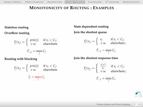
MONOTONICITY OF ROUTING
Examples [Glasserman and Yao]
All of these events could be expressed as index based routing policies :- external arrival with overflow and rejection- routing with overflow and rejection or blocking- routing to the shortest available queue- routing to the shortest mean available response time- general index policies [Palmer-Mitrani]- rerouting inside queues...
66 / 105Poisson Systems and Perfect Sampling
MARKOV MODELS PERFECT SAMPLING DISCRETE TIME EVENT SIMULATION CASE STUDIES Ψ3 -SOFTWARE DEMONSTRATION S
MONOTONICITY OF ROUTING : EXAMPLES
Stateless routing
Overflow routing
Iej (xj) =
{
prio(j) if xj < Cj;+∞ elsewhere
Ie−1 = max
jCj.
Routing with blocking
Iej (xj) =
{
prio(j) if xj < Cj;+∞ elsewhere
Iei = max
jCj.
State dependent routing
Join the shortest queue
Iej (xj) =
{
xj if xj < Cj;+∞ elsewhere ;
Ie−1 = max
jCj.
Join the shortest response time
Iej (xj) =
{
xj+1µj
if xj < Cj;
+∞ elsewhere ;
Ie−1 = max
iCi.
67 / 105Poisson Systems and Perfect Sampling
MARKOV MODELS PERFECT SAMPLING DISCRETE TIME EVENT SIMULATION CASE STUDIES Ψ3 -SOFTWARE DEMONSTRATION S
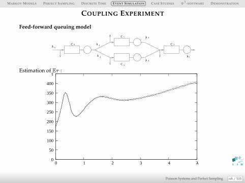
COUPLING EXPERIMENT
Feed-forward queuing model
5
C
C
C
C0
1
2
3λ
λ
λ
λ
λλ
01
2
3
4
Estimation of Eτ :
0
50
100
150
200
250
300
350
400
τ
0 1 2 3 4 λ
68 / 105Poisson Systems and Perfect Sampling

MARKOV MODELS PERFECT SAMPLING DISCRETE TIME EVENT SIMULATION CASE STUDIES Ψ3 -SOFTWARE DEMONSTRATION S
MAIN RESULT
Bound on coupling time
Eτ 6
K∑
i=1
Λ
Λi
Ci + C2i
2,
- Λ : global event rate in the network,
- Λi the rate of events affecting Qi
- Ci is the capacity of Queue i.
Sketch of the proof
- Explicit computation for the M/M/1/C
- Computable bounds for the M/M/1/C
- Bound with isolated queues
69 / 105Poisson Systems and Perfect Sampling

MARKOV MODELS PERFECT SAMPLING DISCRETE TIME EVENT SIMULATION CASE STUDIES Ψ3 -SOFTWARE DEMONSTRATION S
EXPLICIT COMPUTATION FOR THE M/M/1/C
Eτ b = Emin(h0→C, hC→0)Absorbing time in a finite Markov chain ; p = λ
λ+µ= 1− q
1,C
1,C−10,C−2
1,C−2 2,C−1
2,C
3,C
C−2,C−1 C−1,C
C,C0,0
0,1 1,2
0,C
0,C−1
0,C−3
p
p
p
p
p
pp p p p
ppp
p p
pq
q
q
q
q
q q q q q
qqq
q q
qLevel 3
Level 4
Level 5
Level C+1
Level C+2
Level 2
Explicit recurrence equations
Case λ = µ Eτ b = C+C2
2 .
70 / 105Poisson Systems and Perfect Sampling

MARKOV MODELS PERFECT SAMPLING DISCRETE TIME EVENT SIMULATION CASE STUDIES Ψ3 -SOFTWARE DEMONSTRATION S
COMPUTABLE BOUNDS FOR M/M/1/C
If the stationary distribution is concentrated on 0 (λ < µ),
Eτ b6 Eh0→C is an accurate bound.
Theorem
The mean coupling time Eτ b of a M/M/1/C queue with arrival rate λ and service rate µ isbounded using p = λ/(λ+ µ) = 1− q.
Critical bound : ∀p ∈ [0, 1], Eτ b 6C2+C
2 .
Heavy traffic Bound : if p > 12 , Eτ b 6
Cp−q−
q(1−(
qp
)C)
(p−q)2 .
Light traffic bound : if p < 12 , Eτ b 6
Cq−p−
p(1−(
pq
)C)
(q−p)2 .
71 / 105Poisson Systems and Perfect Sampling

MARKOV MODELS PERFECT SAMPLING DISCRETE TIME EVENT SIMULATION CASE STUDIES Ψ3 -SOFTWARE DEMONSTRATION S
COMPUTABLE BOUNDS FOR M/M/1/C
Example with C = 10
0
20
40
60
80
100
120
0 0.2 0.4 0.6 0.8 1
Eτ b
p
heavy trafficLight trafficbound
C+C2
2
C + C2
bound
72 / 105Poisson Systems and Perfect Sampling
MARKOV MODELS PERFECT SAMPLING DISCRETE TIME EVENT SIMULATION CASE STUDIES Ψ3 -SOFTWARE DEMONSTRATION S
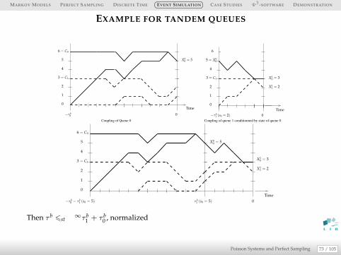
EXAMPLE FOR TANDEM QUEUES
Coupling of Queue 0
Time
0
X00 = 55
4
2
1
3 = C1
6 = C0
0
−τ b0
Coupling of queue 1 conditionned by state of queue 0
4
3 = C1
1
0
−τ b1 (s0 = 2) 0
Time
X11 = 2
X10 = 3
5 = X00
6
2
X11 = 2
5
4
2
1
3 = C1
6 = C0
0
−τ b0 − τ b
1 (s0 = 5)
X00 = 5
τ b1 (s0 = 5) 0
Time
X10 = 3
Then τ b 6st∞τ b
1 + τ b0 , normalized
73 / 105Poisson Systems and Perfect Sampling

MARKOV MODELS PERFECT SAMPLING DISCRETE TIME EVENT SIMULATION CASE STUDIES Ψ3 -SOFTWARE DEMONSTRATION S
BOUND WITH ISOLATED QUEUES
Theorem
In an acyclic stable network of K M/M/1/Ci queues with Bernoulli routing and loss ifoverflow, the coupling time from the past satisfies in expectation,
E[τ b] 6
K−1∑
i=0
Λ
ℓi + µi
Ci
qi − pi−
pi(1−(
piqi
)Ci)
(qi − pi)2
6
K−1∑
i=0
Λ
ℓi + µi(Ci + C2
i ).
74 / 105Poisson Systems and Perfect Sampling

MARKOV MODELS PERFECT SAMPLING DISCRETE TIME EVENT SIMULATION CASE STUDIES Ψ3 -SOFTWARE DEMONSTRATION S
CONJECTURE FOR GENERAL NETWORKS
0
700
800
0 0.5 1 1.5 2 2.5 3 3.5 4
500
400
300
200
100
600
λ5
Eτ b
B1 (proven)
B1 ∧ B2 ∧ B3
B3 (conjecture)
B2 (conjecture)
Extension to cyclic networks,Generalization to several types of eventsApplication : Grid and call centers
75 / 105Poisson Systems and Perfect Sampling

MARKOV MODELS PERFECT SAMPLING DISCRETE TIME EVENT SIMULATION CASE STUDIES Ψ3 -SOFTWARE DEMONSTRATION S
PERFECT SAMPLING PRINCIPLE
All the trajectories
Time
0
−i
−j
−τ ∗
Stationary Process
X
X
X
X
Zi
Zj
Z−τ∗ = {X0}
Z0 = X
collapse
Synchronizing pattern =⇒ finite backward scheme τ∗ <∞[NSMC 2003, LAA 2004]
76 / 105Poisson Systems and Perfect Sampling

MARKOV MODELS PERFECT SAMPLING DISCRETE TIME EVENT SIMULATION CASE STUDIES Ψ3 -SOFTWARE DEMONSTRATION S
MONOTONE PERFECT SAMPLING
−(n + 1)
X
X
time−n
m′M
m
M′
same convergence conditioncomplexity inO(Eτ∗)⇒ polynomial in model dimension
[NSMC 2006,QEST 2008]
77 / 105Poisson Systems and Perfect Sampling

MARKOV MODELS PERFECT SAMPLING DISCRETE TIME EVENT SIMULATION CASE STUDIES Ψ3 -SOFTWARE DEMONSTRATION S
ENVELOPES PERFECT SAMPLING
time
X
X
−(n + 1)
−n
m′
M′
Synchronizing pattern for envelopescomplexity unknown but practically efficient
78 / 105Poisson Systems and Perfect Sampling

MARKOV MODELS PERFECT SAMPLING DISCRETE TIME EVENT SIMULATION CASE STUDIES Ψ3 -SOFTWARE DEMONSTRATION S
ENVELOPES AND SPLITTING PERFECT SAMPLING
Exhaustive state sim
ulation
−i
−j
−τ ∗
Stationary Process
X
X
X
X
Splitting point
Envelope algorithm
Time
0
Guarantees the convergencecomplexity unknown but practically more efficient
[VALUETOOLS 2008]
79 / 105Poisson Systems and Perfect Sampling

MARKOV MODELS PERFECT SAMPLING DISCRETE TIME EVENT SIMULATION CASE STUDIES Ψ3 -SOFTWARE DEMONSTRATION S
PRIORITY SERVERS
Erlang model
Output
ArrivalsServers
Overflow
on next free server
Rejection if all servers
are buzy
X = {0, 1}3
E = {e0, e1, e2, e3}
Card(X ) = 2K
Events
Event type Rate Origin Destination listArrival λ −1 Q1 ; Q2 ; Q3 ; −1Departure µ1 Q1 −1Departure µ2 Q2 −1Departure µ3 Q3 −1
Results
◮ Validation χ2 test
◮ K = 30 µi decreasing
◮ Saturation probability 0.0579 ± 4.710−4
◮ Simulation time 0.4ms
◮ τ = 577
81 / 105Poisson Systems and Perfect Sampling

MARKOV MODELS PERFECT SAMPLING DISCRETE TIME EVENT SIMULATION CASE STUDIES Ψ3 -SOFTWARE DEMONSTRATION S
PRIORITY SERVERS
Erlang model
Output
ArrivalsServers
Overflow
on next free server
Rejection if all servers
are buzy
X = {0, 1}40
µ1 = 1,µ2 = 0.8,µ3 = 0.5Sample size 5.106
Card(X ) = 2K
Saturation probability
Prob
0.1
0.2
0.3
0.4
0.5
0.6
0 10 20 30 40 50 60 70 λ 0
Proba
1e−06
1e−04
0.001
8 8.5 9 9.5 10 10.5 11 11.5 λ
1e−05
Coupling time
s
Reward coupling time
Coupling time
0
200
250
300
350
0 10 20 30 40 50 60 70 λ
100
50
µ
400
150
82 / 105Poisson Systems and Perfect Sampling

MARKOV MODELS PERFECT SAMPLING DISCRETE TIME EVENT SIMULATION CASE STUDIES Ψ3 -SOFTWARE DEMONSTRATION S
LINE OF SERVERS
Tandem queues
reject
µ2C2
C3 µ3
C4 µ4
C5 µ5
C1 µ1
λ
X = {0, · · · , 100}5
E = {e0, · · · , e5}
Card(X ) = CK
Events
Event type Rate Origin Dest. listArrival λ −1 Q1 ; −1Routing/block µ1 Q1 Q2 ; Q1Routing/block µ2 Q2 Q3 ; Q2· · · · · · · · · · · ·Departure µ5 Q5 −1
Results
◮ C = 100 λ = 0.9 ; µ = 1 p = 12
◮ Blocking probability b1 = 0.34, b2 = 0.02 b3 = 0.02, b4,= 0.02.
◮ Simulation time < 1ms
83 / 105Poisson Systems and Perfect Sampling
MARKOV MODELS PERFECT SAMPLING DISCRETE TIME EVENT SIMULATION CASE STUDIES Ψ3 -SOFTWARE DEMONSTRATION S
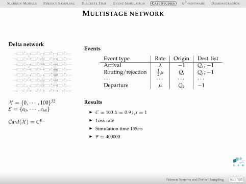
MULTISTAGE NETWORK
Delta network8
11
12
13
14
15
16
17
18
19
20
21
22
23
24
25
26
27
28
29
30
31
0
1
2
3
4
5
6
7
10
9
X = {0, · · · , 100}32
E = {e0, · · · , e64}
Card(X ) = CK
Events
Event type Rate Origin Dest. listArrival λ −1 Qi ; −1Routing/rejection 1
2µ Qi Qj ; −1· · · · · · · · · · · ·Departure µ Qk −1
Results
◮ C = 100 λ = 0.9 ; µ = 1
◮ Loss rate
◮ Simulation time 135ms
◮ τ ≃ 400000
84 / 105Poisson Systems and Perfect Sampling

MARKOV MODELS PERFECT SAMPLING DISCRETE TIME EVENT SIMULATION CASE STUDIES Ψ3 -SOFTWARE DEMONSTRATION S
MULTISTAGE NETWORK
Delta network8
11
12
13
14
15
16
17
18
19
20
21
22
23
24
25
26
27
28
29
30
31
0
1
2
3
4
5
6
7
10
9
X = {0, · · · , 100}32
E = {e0, · · · , e64}
Card(X ) = CK
Sample size 100000
Queue length and saturation proba at level 3
λ
1
2
3
4
5
6
7
E(N_34)
0 0.2 0.4 0.6 0.8 0 λ
0.0002
0.0004
0.0006
0.0008
0.001
0.0012
0.0014
0.58 0.6 0.62 0.64 0.66 0.68 0.7 0.72 0.74 0.76 0.78 0
Coupling time
sGlobal coupling
Reward at least 1 queue saturated (3rd level)
Reward queue 31 saturated
0
10000
12000
14000
16000
18000
0 0.2 0.4 0.6 0.8
6000
4000
2000
λ
µ
8000
85 / 105Poisson Systems and Perfect Sampling

MARKOV MODELS PERFECT SAMPLING DISCRETE TIME EVENT SIMULATION CASE STUDIES Ψ3 -SOFTWARE DEMONSTRATION S
RESOURCE BROKER
Grid model
Q9
Resource Broker
λ
µ2
µ1
µ3
µ4
µ5
µ6
µ7
µ8
µ9
Overflow
Q2
Q3
Q1
Q10
Q11
Q12
Q4
Q6
Q5
Q7
Q8
Input ratesAllocation strategyState dependent allocationIndex based routing : destinationminimize a criteria
Problem
Optimization of throughput, response time,...Comparison of policies, analysis of heuristics...
86 / 105Poisson Systems and Perfect Sampling

MARKOV MODELS PERFECT SAMPLING DISCRETE TIME EVENT SIMULATION CASE STUDIES Ψ3 -SOFTWARE DEMONSTRATION S
ROUTING CUSTOMERS IN PARALLEL QUEUES
The problem :
◮ Find a routing policy maximizing the expected (discounted) throughput of the system.
◮ Several variations on this problem depend on the information available to the controller :current size of all queues (and size of the arriving batch).
The applications :
◮ improve batch schedulers for cluster and grid infrastructures.
◮ Assert the value of information in such cases.
87 / 105Poisson Systems and Perfect Sampling

MARKOV MODELS PERFECT SAMPLING DISCRETE TIME EVENT SIMULATION CASE STUDIES Ψ3 -SOFTWARE DEMONSTRATION S
INDEX POLICIES FOR ROUTING
Optimal routing policy problem is still open for n different M/M/1Heuristic : index policy inspired from the Multi-Armed Bandit⇒ free parameter and compute an equilibrium point.[Mitrani 2005] for routing and repair problems.
µ
S servers
Capacity C
λ
W
b
µ
µ
W is the rejection cost (free parameter).
Theorem
There is an optimal policy of threshold type :there exists θ such that :Reject if x > θ and accept otherwise.- θ does not depend on C as long as C > θ (including if C is infinite).- θ is a non-decreasing function of W.
88 / 105Poisson Systems and Perfect Sampling

MARKOV MODELS PERFECT SAMPLING DISCRETE TIME EVENT SIMULATION CASE STUDIES Ψ3 -SOFTWARE DEMONSTRATION S
INDEX POLICIES FOR ROUTING(II)
Computation of θ(W) linear system of corresponding to Bellman’s equation, afteruniformization.
0
5
10
15
20
25
30
0 2 4 6 8 10 12 14 16 18 20
Bes
tThr
esho
ld(W
)
W
’TW.txt’
Index function I(x) = inf{W | θ(W) = x}.Indifference case : when queue size is x, rejecting or accepting the next batch are bothoptimal choices if the rejection cost is I(x).
89 / 105Poisson Systems and Perfect Sampling
MARKOV MODELS PERFECT SAMPLING DISCRETE TIME EVENT SIMULATION CASE STUDIES Ψ3 -SOFTWARE DEMONSTRATION S
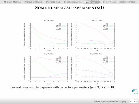
SOME NUMERICAL EXPERIMENTS(I)
0.5
1
1.5
2
2.5
3
3.5
4
4.5
5
1 2 3 4 5 6 7 8 9
Aver
age
wai
ting t
ime
(rat
io w
ith o
pti
m)
Load
1-9_1-9_100.txt
JSQJSQ-mu
JSQ-mu2Seq
*optim*
0.95
1
1.05
1.1
1.15
1.2
1.25
1.3
1.35
1.4
1.45
1.5
8.9 9 9.1 9.2 9.3 9.4 9.5 9.6 9.7 9.8 9.9 10
Aver
age
wai
ting t
ime
(rat
io w
ith o
pti
m)
Load
1-9_9-9.95_100.txt
JSQJSQ-mu
JSQ-mu2Seq
*optim*
0.9
1
1.1
1.2
1.3
1.4
1.5
1.6
1.7
1.8
1 2 3 4 5 6 7 8 9
Aver
age
wai
ting t
ime
(rat
io w
ith o
pti
m)
Load
9-1_1-9_100.txt
JSQJSQ-mu
JSQ-mu2Seq
*optim*
0.95
1
1.05
1.1
1.15
1.2
1.25
1.3
1.35
1.4
8.9 9 9.1 9.2 9.3 9.4 9.5 9.6 9.7 9.8 9.9 10
Aver
age
wai
ting t
ime
(rat
io w
ith o
pti
m)
Load
9-1_9.0-9.95_100.txt
JSQJSQ-mu
JSQ-mu2Seq
*optim*
Several cases with two queues with respective parameters (µ = 9, 1), C = 100
90 / 105Poisson Systems and Perfect Sampling
MARKOV MODELS PERFECT SAMPLING DISCRETE TIME EVENT SIMULATION CASE STUDIES Ψ3 -SOFTWARE DEMONSTRATION S
SOME NUMERICAL EXPERIMENTS(III)
0.98
1
1.02
1.04
1.06
1.08
1.1
1.12
1.14
1.16
1.18
1.2
1 2 3 4 5 6 7 8 9
Aver
age
wai
ting t
ime
(rat
io w
ith o
pti
m)
Load
8-2_1-9_100.txt
JSQJSQ-mu
JSQ-mu2Seq
*optim*
0.98
1
1.02
1.04
1.06
1.08
1.1
1.12
1.14
8.9 9 9.1 9.2 9.3 9.4 9.5 9.6 9.7 9.8 9.9 10
Aver
age
wai
ting t
ime
(rat
io w
ith o
pti
m)
Load
8-2_9.0-9.95_100.txt
JSQJSQ-mu
JSQ-mu2Seq
*optim*
0.98
1
1.02
1.04
1.06
1.08
1.1
1.12
1.14
1.16
1.18
1.2
1 2 3 4 5 6 7 8 9
Aver
age
wai
ting t
ime
(rat
io w
ith o
pti
m)
Load
8-2_1-9_50.txt
JSQJSQ-mu
JSQ-mu2Seq
*optim*
0.98
1
1.02
1.04
1.06
1.08
1.1
1.12
1.14
8.9 9 9.1 9.2 9.3 9.4 9.5 9.6 9.7 9.8 9.9 10
Aver
age
wai
ting t
ime
(rat
io w
ith o
pti
m)
Load
8-2_9.0-9.95_50.txt
JSQJSQ-mu
JSQ-mu2Seq
*optim*
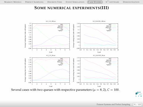
Several cases with two queues with respective parameters (µ = 8, 2), C = 100.
91 / 105Poisson Systems and Perfect Sampling

MARKOV MODELS PERFECT SAMPLING DISCRETE TIME EVENT SIMULATION CASE STUDIES Ψ3 -SOFTWARE DEMONSTRATION S
SOME NUMERICAL EXPERIMENTS(IV)
0.95
1
1.05
1.1
1.15
1.2
1.25
1 2 3 4 5 6 7 8 9
Aver
age
wai
ting t
ime
(rat
io w
ith o
pti
m)
Load
8.1-1.9_1-9_100.txt
JSQJSQ-mu
JSQ-mu2Seq
*optim*
0.98
1
1.02
1.04
1.06
1.08
1.1
1.12
1.14
1.16
8.9 9 9.1 9.2 9.3 9.4 9.5 9.6 9.7 9.8 9.9 10
Aver
age
wai
ting t
ime
(rat
io w
ith o
pti
m)
Load
8.1-1.9_9.0-9.95_100.txt
JSQJSQ-mu
JSQ-mu2Seq
*optim*
0.99
1
1.01
1.02
1.03
1.04
1.05
1 2 3 4 5 6 7 8 9
Aver
age
wai
ting t
ime
(rat
io w
ith o
pti
m)
Load
7-3_1-9_100.txt
JSQJSQ-mu
JSQ-mu2Seq
*optim*
0.995
1
1.005
1.01
1.015
1.02
1.025
1.03
1.035
1.04
1.045
8.9 9 9.1 9.2 9.3 9.4 9.5 9.6 9.7 9.8 9.9 10
Aver
age
wai
ting t
ime
(rat
io w
ith o
pti
m)
Load
7-3_9.0-9.95_100.txt
JSQJSQ-mu
JSQ-mu2Seq
*optim*
Some other cases
92 / 105Poisson Systems and Perfect Sampling
MARKOV MODELS PERFECT SAMPLING DISCRETE TIME EVENT SIMULATION CASE STUDIES Ψ3 -SOFTWARE DEMONSTRATION S
SOME NUMERICAL EXPERIMENTS(V)
0.9
1
1.1
1.2
1.3
1.4
1.5
1.6
1.7
1.8
1.9
1 2 3 4 5 6 7 8 9
Aver
age
wai
ting t
ime
(rat
io w
ith o
pti
m)
Load
8-1-1_1-9_50.txt
JSQJSQ-mu
JSQ-mu2Seq
*optim*
0.95
1
1.05
1.1
1.15
1.2
1.25
1.3
1.35
1.4
1.45
8.9 9 9.1 9.2 9.3 9.4 9.5 9.6 9.7 9.8 9.9 10
Aver
age
wai
ting t
ime
(rat
io w
ith o
pti
m)
Load
8-1-1_9.0-9.95_50.txt
JSQJSQ-mu
JSQ-mu2Seq
*optim*
0.95
1
1.05
1.1
1.15
1.2
1.25
1.3
1 2 3 4 5 6 7 8 9
Aver
age
wai
ting t
ime
(rat
io w
ith o
pti
m)
Load
7-2-1_1-9_50.txt
JSQJSQ-mu
JSQ-mu2Seq
*optim*
0.95
1
1.05
1.1
1.15
1.2
1.25
8.9 9 9.1 9.2 9.3 9.4 9.5 9.6 9.7 9.8 9.9 10
Aver
age
wai
ting t
ime
(rat
io w
ith o
pti
m)
Load
7-2-1_9.0-9.95_50.txt
JSQJSQ-mu
JSQ-mu2Seq
*optim*
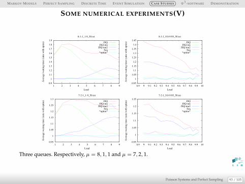
Three queues. Respectively, µ = 8, 1, 1 and µ = 7, 2, 1.
93 / 105Poisson Systems and Perfect Sampling

MARKOV MODELS PERFECT SAMPLING DISCRETE TIME EVENT SIMULATION CASE STUDIES Ψ3 -SOFTWARE DEMONSTRATION S
NUMERICAL EXPERIMENTS(VI)
0.95
1
1.05
1.1
1.15
1.2
1 2 3 4 5 6 7 8 9
Aver
age
wai
ting t
ime
(rat
io w
ith o
pti
m)
Load
6-3-1_1-9_50.txt
JSQJSQ-mu
JSQ-mu2Seq
*optim*
0.98
1
1.02
1.04
1.06
1.08
1.1
1.12
1.14
8.9 9 9.1 9.2 9.3 9.4 9.5 9.6 9.7 9.8 9.9 10
Aver
age
wai
ting t
ime
(rat
io w
ith o
pti
m)
Load
6-3-1_9.0-9.95_50.txt
JSQJSQ-mu
JSQ-mu2Seq
*optim*
0.96
0.98
1
1.02
1.04
1.06
1.08
1.1
1 2 3 4 5 6 7 8 9
Aver
age
wai
ting t
ime
(rat
io w
ith o
pti
m)
Load
6-2-2_1-9_50.txt
JSQJSQ-mu
JSQ-mu2Seq
*optim*
0.97
0.98
0.99
1
1.01
1.02
1.03
1.04
1.05
1.06
1.07
8.9 9 9.1 9.2 9.3 9.4 9.5 9.6 9.7 9.8 9.9 10
Aver
age
wai
ting t
ime
(rat
io w
ith o
pti
m)
Load
6-2-2_9.0-9.95_50.txt
JSQJSQ-mu
JSQ-mu2Seq
*optim*
Now, µ = 6, 3, 1 and µ = 6, 2, 2.
94 / 105Poisson Systems and Perfect Sampling

MARKOV MODELS PERFECT SAMPLING DISCRETE TIME EVENT SIMULATION CASE STUDIES Ψ3 -SOFTWARE DEMONSTRATION S
NUMERICAL EXPERIMENTS(VII)
0.98
1
1.02
1.04
1.06
1.08
1.1
1.12
1.14
1.16
1 2 3 4 5 6 7 8 9
Aver
age
wai
ting t
ime
(rat
io w
ith o
pti
m)
Load
5-4-1_1-9_50.txt
JSQJSQ-mu
JSQ-mu2Seq
*optim*
0.98
1
1.02
1.04
1.06
1.08
1.1
1.12
8.9 9 9.1 9.2 9.3 9.4 9.5 9.6 9.7 9.8 9.9 10
Aver
age
wai
ting t
ime
(rat
io w
ith o
pti
m)
Load
5-4-1_9.0-9.95_50.txt
JSQJSQ-mu
JSQ-mu2Seq
*optim*
0.97
0.975
0.98
0.985
0.99
0.995
1
1.005
1.01
1.015
1.02
1.025
1 2 3 4 5 6 7 8 9
Aver
age
wai
ting t
ime
(rat
io w
ith o
pti
m)
Load
5-3-2_1-9_50.txt
JSQJSQ-mu
JSQ-mu2Seq
*optim*
0.97
0.975
0.98
0.985
0.99
0.995
1
1.005
1.01
1.015
1.02
8.9 9 9.1 9.2 9.3 9.4 9.5 9.6 9.7 9.8 9.9 10
Aver
age
wai
ting t
ime
(rat
io w
ith o
pti
m)
Load
5-3-2_9.0-9.95_50.txt
JSQJSQ-mu
JSQ-mu2Seq
*optim*
Now, µ = 5, 4, 1 and µ = 5, 3, 2.
95 / 105Poisson Systems and Perfect Sampling

MARKOV MODELS PERFECT SAMPLING DISCRETE TIME EVENT SIMULATION CASE STUDIES Ψ3 -SOFTWARE DEMONSTRATION S
ROBUSTNESS OF INDEX POLICIES
The index policy was computed for λ = 5 or 9 and used over the whole range λ = 1 to10.
0.9
1
1.1
1.2
1.3
1.4
1.5
1.6
1.7
1.8
1 2 3 4 5 6 7 8 9
Ave
rage
wai
ting
time
(rat
io w
ith o
ptim
)
Load
9-1_1-9_50.txt.1
mu : 9, 1c : 1, 1Nmax : 50 lambda index : 5
JSQJSQ-mu
JSQ-mu2Seq
*optim*
0.95
1
1.05
1.1
1.15
1.2
1.25
1.3
1.35
1.4
1.45
8.9 9 9.1 9.2 9.3 9.4 9.5 9.6 9.7 9.8 9.9 10
Ave
rage
wai
ting
time
(rat
io w
ith o
ptim
)
Load
9-1_9.0-9.95_50.txt.1
mu : 9, 1c : 1, 1Nmax : 50 lambda index : 5
JSQJSQ-mu
JSQ-mu2Seq
*optim*
0.9
1
1.1
1.2
1.3
1.4
1.5
1.6
1.7
1.8
1 2 3 4 5 6 7 8 9
Ave
rage
wai
ting
time
(rat
io w
ith o
ptim
)
Load
9-1_1-9_50.txt.2
mu : 9, 1c : 1, 1Nmax : 50 lambda index : 9
JSQJSQ-mu
JSQ-mu2Seq
*optim*
0.95
1
1.05
1.1
1.15
1.2
1.25
1.3
1.35
1.4
1.45
8.9 9 9.1 9.2 9.3 9.4 9.5 9.6 9.7 9.8 9.9 10
Ave
rage
wai
ting
time
(rat
io w
ith o
ptim
)
Load
9-1_9.0-9.95_50.txt.2
mu : 9, 1c : 1, 1Nmax : 50 lambda index : 9
JSQJSQ-mu
JSQ-mu2Seq
*optim*
96 / 105Poisson Systems and Perfect Sampling

MARKOV MODELS PERFECT SAMPLING DISCRETE TIME EVENT SIMULATION CASE STUDIES Ψ3 -SOFTWARE DEMONSTRATION S
HTTP://PSI.GFORGE.INRIA.FR
98 / 105Poisson Systems and Perfect Sampling

MARKOV MODELS PERFECT SAMPLING DISCRETE TIME EVENT SIMULATION CASE STUDIES Ψ3 -SOFTWARE DEMONSTRATION S
SIMULATION WORKFLOW
Samples
Coupling timeSample of rewards
Single trajectory
Steady-state independentIndependent trajectories R, S-plus,...
User defined scripts
Statistical analyzer
Simulation kernels
Forward samplingtrajectories
Backward samplingMonotone
Action of the event
Queues descriptionservercs, capacities
Event descriptionRateActivation condition
Model libraries
Samples
Coupling timeSample of rewards
Single trajectory
Steady-state independentIndependent trajectories R, S-plus,...
User defined scripts
Statistical analyzer
99 / 105Poisson Systems and Perfect Sampling

MARKOV MODELS PERFECT SAMPLING DISCRETE TIME EVENT SIMULATION CASE STUDIES Ψ3 -SOFTWARE DEMONSTRATION S
SIMULATION KERNELS
Trajectory Sampling
◮ Initial state
◮ Seed for the random scheme
=⇒ sequence of (time,state)
Set of trajectories
0
10
20
30
40
50
0 200 400 600 800 1000 1200 1400 1600
Traj0Traj1Traj2Traj3Traj4Traj5Traj6Traj7Traj8Traj9
Steady-state Sampling
◮ Monotone events, (envelopes)
◮ Seed for the random scheme
=⇒ sample of steady-state
All the trajectories
Time
0
−i
−j
−τ ∗
Stationary Process
X
X
X
X
Zi
Zj
Z−τ∗ = {X0}
Z0 = X
collapse
100 / 105Poisson Systems and Perfect Sampling

MARKOV MODELS PERFECT SAMPLING DISCRETE TIME EVENT SIMULATION CASE STUDIES Ψ3 -SOFTWARE DEMONSTRATION S
PARALLEL SAMPLING
Computing ressources
◮ Many cores machine (desktop (4), server (16) or parallel (48))
◮ Parallel programing frameworks (OpenMP)
Objective
◮ Evaluate efficiency of parallel implementations on multicore platforms
Forward Simulation
◮ Space parallel approach
Generate a separate Markov chain on each core and combine results [Glynn92]
◮ Time parallel approach
Divide the iteration space and try to precompute parts of the Markov chain [Nicol94]
◮ Space-time parallel approach
Divide the model in several Markov chains [HsiehG09]
Backward Simulation
◮ Generate samples on each core (natural approach)
101 / 105Poisson Systems and Perfect Sampling

MARKOV MODELS PERFECT SAMPLING DISCRETE TIME EVENT SIMULATION CASE STUDIES Ψ3 -SOFTWARE DEMONSTRATION S
DEMONSTRATION
Philosophy
◮ C code
◮ Text files
◮ Models / Kernels / Results
◮ Model generation/ Statistical analysis is out of the software
A simple example
Lambda = 1.6
Capacity: 50
Queue 1 Queue 2
Capacity: 50
Mu = 1.8 Thêta = 2
OverflowOverflow
A more complex example
8
11
12
13
14
15
16
17
18
19
20
21
22
23
24
25
26
27
28
29
30
31
0
1
2
3
4
5
6
7
10
9
103 / 105Poisson Systems and Perfect Sampling

MARKOV MODELS PERFECT SAMPLING DISCRETE TIME EVENT SIMULATION CASE STUDIES Ψ3 -SOFTWARE DEMONSTRATION S
SYNTHESIS
Sampling of Poisson Systems
◮ Several approaches depending on the objective
◮ Common model description : events and distribution
Ψ3 Software
◮ Transient trajectories : Forward methods (Parallel, I/O pipelining, Nicol’s scheme)
◮ Steady-state sampling : Backward methods (Perfect monotone, envelopes)
Future work (practical)
◮ Tuning the sampling methods : adaptive
◮ Impact of I/O : in-situ analysis.
Future work (theoretical)
◮ Coupling time : partial coupling, hitting time,...
◮ Measure transformation : importance sampling, variance reduction
◮ Coupling time, mixing time, spectral gap, entropy
Reproducibility : Everything is on : http://psi.gforge.inria.fr
105 / 105Poisson Systems and Perfect Sampling
Related Documents