Living Rev. Relativity, 12, (2009), 2 http://www.livingreviews.org/lrr-2009-2 LIVING REVIEWS in relativity Physics, Astrophysics and Cosmology with Gravitational Waves B.S. Sathyaprakash School of Physics and Astronomy, Cardiff University, Cardiff, U.K. email: [email protected] Bernard F. Schutz School of Physics and Astronomy, Cardiff University, Cardiff, U.K. and Max Planck Institute for Gravitational Physics (Albert Einstein Institute) Potsdam-Golm, Germany email: [email protected] Living Reviews in Relativity ISSN 1433-8351 Accepted on 29 January 2009 Published on 4 March 2009 Abstract Gravitational wave detectors are already operating at interesting sensitivity levels, and they have an upgrade path that should result in secure detections by 2014. We review the physics of gravitational waves, how they interact with detectors (bars and interferometers), and how these detectors operate. We study the most likely sources of gravitational waves and review the data analysis methods that are used to extract their signals from detector noise. Then we consider the consequences of gravitational wave detections and observations for physics, astrophysics, and cosmology. This review is licensed under a Creative Commons Attribution-Non-Commercial-NoDerivs 3.0 Germany License. http://creativecommons.org/licenses/by-nc-nd/3.0/de/

Welcome message from author
This document is posted to help you gain knowledge. Please leave a comment to let me know what you think about it! Share it to your friends and learn new things together.
Transcript
Living Rev. Relativity, 12, (2009), 2http://www.livingreviews.org/lrr-2009-2
L I V I N G REVIEWS
in relativity
Physics, Astrophysics and Cosmology
with Gravitational Waves
B.S. SathyaprakashSchool of Physics and Astronomy, Cardiff University,
Cardiff, U.K.email: [email protected]
Bernard F. SchutzSchool of Physics and Astronomy, Cardiff University,
Cardiff, U.K.and
Max Planck Institute for Gravitational Physics(Albert Einstein Institute)Potsdam-Golm, Germany
email: [email protected]
Living Reviews in RelativityISSN 1433-8351
Accepted on 29 January 2009Published on 4 March 2009
Abstract
Gravitational wave detectors are already operating at interesting sensitivity levels, andthey have an upgrade path that should result in secure detections by 2014. We review thephysics of gravitational waves, how they interact with detectors (bars and interferometers),and how these detectors operate. We study the most likely sources of gravitational wavesand review the data analysis methods that are used to extract their signals from detectornoise. Then we consider the consequences of gravitational wave detections and observationsfor physics, astrophysics, and cosmology.
This review is licensed under a Creative CommonsAttribution-Non-Commercial-NoDerivs 3.0 Germany License.http://creativecommons.org/licenses/by-nc-nd/3.0/de/
Imprint / Terms of Use
Living Reviews in Relativity is a peer reviewed open access journal published by the Max PlanckInstitute for Gravitational Physics, Am Muhlenberg 1, 14476 Potsdam, Germany. ISSN 1433-8351.
This review is licensed under a Creative Commons Attribution-Non-Commercial-NoDerivs 3.0Germany License: http://creativecommons.org/licenses/by-nc-nd/3.0/de/
Because a Living Reviews article can evolve over time, we recommend to cite the article as follows:
B.S. Sathyaprakash and Bernard F. Schutz,“Physics, Astrophysics and Cosmology with Gravitational Waves”,
Living Rev. Relativity, 12, (2009), 2. [Online Article]: cited [<date>],http://www.livingreviews.org/lrr-2009-2
The date given as <date> then uniquely identifies the version of the article you are referring to.
Article Revisions
Living Reviews supports two different ways to keep its articles up-to-date:
Fast-track revision A fast-track revision provides the author with the opportunity to add shortnotices of current research results, trends and developments, or important publications tothe article. A fast-track revision is refereed by the responsible subject editor. If an articlehas undergone a fast-track revision, a summary of changes will be listed here.
Major update A major update will include substantial changes and additions and is subject tofull external refereeing. It is published with a new publication number.
For detailed documentation of an article’s evolution, please refer always to the history documentof the article’s online version at http://www.livingreviews.org/lrr-2009-2.
Contents
1 A New Window onto the Universe 71.1 Birth of gravitational astronomy . . . . . . . . . . . . . . . . . . . . . . . . . . . . 91.2 What this review is about . . . . . . . . . . . . . . . . . . . . . . . . . . . . . . . . 9
2 Gravitational Wave Observables 112.1 Gravitational field vs gravitational waves . . . . . . . . . . . . . . . . . . . . . . . 112.2 Gravitational wave polarizations . . . . . . . . . . . . . . . . . . . . . . . . . . . . 122.3 Direction to a source . . . . . . . . . . . . . . . . . . . . . . . . . . . . . . . . . . . 122.4 Amplitude of gravitational waves – the quadrupole approximation . . . . . . . . . 13
2.4.1 Wave amplitudes and polarization in TT-gauge . . . . . . . . . . . . . . . . 132.4.2 Simple estimates . . . . . . . . . . . . . . . . . . . . . . . . . . . . . . . . . 14
2.5 Frequency of gravitational waves . . . . . . . . . . . . . . . . . . . . . . . . . . . . 152.6 Luminosity in gravitational waves . . . . . . . . . . . . . . . . . . . . . . . . . . . . 16
3 Sources of Gravitational Waves 183.1 Man-made sources . . . . . . . . . . . . . . . . . . . . . . . . . . . . . . . . . . . . 183.2 Gravitational wave bursts from gravitational collapse . . . . . . . . . . . . . . . . . 183.3 Gravitational wave pulsars . . . . . . . . . . . . . . . . . . . . . . . . . . . . . . . . 193.4 Radiation from a binary star system . . . . . . . . . . . . . . . . . . . . . . . . . . 21
3.4.1 Radiation from a binary system and its backreaction . . . . . . . . . . . . . 213.4.2 Chirping binaries as standard sirens . . . . . . . . . . . . . . . . . . . . . . 223.4.3 Binary pulsar tests of gravitational radiation theory . . . . . . . . . . . . . 233.4.4 White-dwarf binaries . . . . . . . . . . . . . . . . . . . . . . . . . . . . . . . 233.4.5 Supermassive black hole binaries . . . . . . . . . . . . . . . . . . . . . . . . 243.4.6 Extreme and intermediate mass-ratio inspiral sources . . . . . . . . . . . . 24
3.5 Quasi-normal modes of a black hole . . . . . . . . . . . . . . . . . . . . . . . . . . 263.6 Stochastic background . . . . . . . . . . . . . . . . . . . . . . . . . . . . . . . . . . 27
4 Gravitational Wave Detectors and Their Sensitivity 294.1 Principles of the operation of resonant mass detectors . . . . . . . . . . . . . . . . 294.2 Principles of the operation of beam detectors . . . . . . . . . . . . . . . . . . . . . 31
4.2.1 The response of a ground-based interferometer . . . . . . . . . . . . . . . . 324.3 Practical issues of ground-based interferometers . . . . . . . . . . . . . . . . . . . . 36
4.3.1 Interferometers around the globe . . . . . . . . . . . . . . . . . . . . . . . . 384.3.2 Very-high–frequency detectors . . . . . . . . . . . . . . . . . . . . . . . . . 40
4.4 Detection from space . . . . . . . . . . . . . . . . . . . . . . . . . . . . . . . . . . . 404.4.1 Ranging to spacecraft . . . . . . . . . . . . . . . . . . . . . . . . . . . . . . 404.4.2 Pulsar timing . . . . . . . . . . . . . . . . . . . . . . . . . . . . . . . . . . . 414.4.3 Space interferometry . . . . . . . . . . . . . . . . . . . . . . . . . . . . . . . 41
4.5 Characterizing the sensitivity of a gravitational wave antenna . . . . . . . . . . . . 424.5.1 Noise power spectral density in interferometers . . . . . . . . . . . . . . . . 434.5.2 Sensitivity of interferometers in units of energy flux . . . . . . . . . . . . . 45
4.6 Source amplitudes vs sensitivity . . . . . . . . . . . . . . . . . . . . . . . . . . . . . 454.7 Network detection . . . . . . . . . . . . . . . . . . . . . . . . . . . . . . . . . . . . 46
4.7.1 Coherent vs coincidence analysis . . . . . . . . . . . . . . . . . . . . . . . . 474.7.2 Null stream veto . . . . . . . . . . . . . . . . . . . . . . . . . . . . . . . . . 484.7.3 Detection of stochastic signals by cross-correlation . . . . . . . . . . . . . . 48
4.8 False alarms, detection threshold and coincident observation . . . . . . . . . . . . . 49
5 Data Analysis 515.1 Matched filtering and optimal signal-to-noise ratio . . . . . . . . . . . . . . . . . . 52
5.1.1 Optimal filter . . . . . . . . . . . . . . . . . . . . . . . . . . . . . . . . . . . 525.1.2 Optimal signal-to-noise ratio . . . . . . . . . . . . . . . . . . . . . . . . . . 535.1.3 Practical applications of matched filtering . . . . . . . . . . . . . . . . . . . 54
5.2 Suboptimal filtering methods . . . . . . . . . . . . . . . . . . . . . . . . . . . . . . 575.3 Measurement of parameters and source reconstruction . . . . . . . . . . . . . . . . 58
5.3.1 Ambiguity function . . . . . . . . . . . . . . . . . . . . . . . . . . . . . . . . 595.3.2 Metric on the space of waveforms . . . . . . . . . . . . . . . . . . . . . . . . 605.3.3 Covariance matrix . . . . . . . . . . . . . . . . . . . . . . . . . . . . . . . . 615.3.4 Bayesian inference . . . . . . . . . . . . . . . . . . . . . . . . . . . . . . . . 64
6 Physics with Gravitational Waves 676.1 Speed of gravitational waves . . . . . . . . . . . . . . . . . . . . . . . . . . . . . . . 676.2 Polarization of gravitational waves . . . . . . . . . . . . . . . . . . . . . . . . . . . 686.3 Gravitational radiation reaction . . . . . . . . . . . . . . . . . . . . . . . . . . . . . 686.4 Black hole spectroscopy . . . . . . . . . . . . . . . . . . . . . . . . . . . . . . . . . 696.5 The two-body problem in general relativity . . . . . . . . . . . . . . . . . . . . . . 72
6.5.1 Binaries as standard candles: distance estimation . . . . . . . . . . . . . . . 736.5.2 Numerical approaches to the two-body problem . . . . . . . . . . . . . . . . 736.5.3 Post-Newtonian approximation to the two-body problem . . . . . . . . . . . 756.5.4 Measuring the parameters of an inspiraling binary . . . . . . . . . . . . . . 806.5.5 Improvement from higher harmonics . . . . . . . . . . . . . . . . . . . . . . 83
6.6 Tests of general relativity . . . . . . . . . . . . . . . . . . . . . . . . . . . . . . . . 846.6.1 Testing the post-Newtonian approximation . . . . . . . . . . . . . . . . . . 846.6.2 Uniqueness of Kerr geometry . . . . . . . . . . . . . . . . . . . . . . . . . . 876.6.3 Quantum gravity . . . . . . . . . . . . . . . . . . . . . . . . . . . . . . . . . 89
7 Astrophysics with Gravitational Waves 917.1 Interacting compact binaries . . . . . . . . . . . . . . . . . . . . . . . . . . . . . . . 91
7.1.1 Resolving the mass-inclination degeneracy . . . . . . . . . . . . . . . . . . . 927.2 Black hole astrophysics . . . . . . . . . . . . . . . . . . . . . . . . . . . . . . . . . . 93
7.2.1 Gravitational waves from stellar-mass black holes . . . . . . . . . . . . . . . 937.2.2 Stellar-mass black-hole binaries . . . . . . . . . . . . . . . . . . . . . . . . . 937.2.3 Intermediate-mass black holes . . . . . . . . . . . . . . . . . . . . . . . . . . 947.2.4 Supermassive black holes . . . . . . . . . . . . . . . . . . . . . . . . . . . . 95
7.3 Neutron star astrophysics . . . . . . . . . . . . . . . . . . . . . . . . . . . . . . . . 967.3.1 Gravitational collapse and the formation of neutron stars . . . . . . . . . . 967.3.2 Neutron-star–binary mergers . . . . . . . . . . . . . . . . . . . . . . . . . . 967.3.3 Neutron-star normal mode oscillations . . . . . . . . . . . . . . . . . . . . . 977.3.4 Stellar instabilities . . . . . . . . . . . . . . . . . . . . . . . . . . . . . . . . 977.3.5 Low-mass X-ray binaries . . . . . . . . . . . . . . . . . . . . . . . . . . . . . 987.3.6 Galactic population of neutron stars . . . . . . . . . . . . . . . . . . . . . . 98
7.4 Multimessenger gravitational-wave astronomy . . . . . . . . . . . . . . . . . . . . . 99
8 Cosmology with Gravitational Wave Observations 1038.1 Detecting a stochastic gravitational wave background . . . . . . . . . . . . . . . . . 103
8.1.1 Describing a random gravitational wave field . . . . . . . . . . . . . . . . . 1038.1.2 Observations with gravitational wave detectors . . . . . . . . . . . . . . . . 1048.1.3 Observations with pulsar timing . . . . . . . . . . . . . . . . . . . . . . . . 105
8.1.4 Observations using the cosmic microwave background . . . . . . . . . . . . 1068.2 Origin of a random background of gravitational waves . . . . . . . . . . . . . . . . 106
8.2.1 Gravitational waves from the Big Bang . . . . . . . . . . . . . . . . . . . . 1068.2.2 Astrophysical sources of a stochastic background . . . . . . . . . . . . . . . 108
8.3 Cosmography: gravitational wave measurements of cosmological parameters . . . . 108
9 Conclusions and Future Directions 110
10 Acknowledgements 112
References 113
List of Tables
1 Noise power spectral densities Sh(f) of various interferometers in operation andunder construction: GEO600, Initial LIGO (ILIGO), TAMA, VIRGO, AdvancedLIGO (ALIGO), Einstein Telescope (ET) and LISA (instrumental noise only). Foreach detector the noise PSD is given in terms of a dimensionless frequency x = f/f0and rises steeply above a lower cutoff fs. . . . . . . . . . . . . . . . . . . . . . . . . 44
2 The value of the (squared) distance d`2 = r2/ρ2 for several values of P and thecorresponding smallest match that can be expected between templates and the signalat different values of the SNR. . . . . . . . . . . . . . . . . . . . . . . . . . . . . . 64

Physics, Astrophysics and Cosmology with Gravitational Waves 7
1 A New Window onto the Universe
The last six decades have witnessed a great revolution in astronomy, driven by improvements inobserving capabilities across the electromagnetic spectrum: very large optical telescopes, radioantennas and arrays, a host of satellites to explore the infrared, X-ray, and gamma-ray parts of thespectrum, and the development of key new technologies (CCDs, adaptive optics). Each new windowof observation has brought new surprises that have dramatically changed our understanding of theuniverse. These serendipitous discoveries have included:
• the relic cosmic microwave background radiation (Penzias and Wilson [287]), which hasbecome our primary tool for exploring the Big Bang;
• the fact that quasi-stellar objects are at cosmological distances (Maarten Schmidt [323]),which has developed into the understanding that they are powered by supermassive blackholes;
• pulsars (Hewish and Bell [189]), which opened up the study of neutron stars and illuminatedone endpoint for stellar evolution;
• X-ray binary systems (Giacconi and collaborators [326]), which now enable us to make de-tailed studies of black holes and neutron stars;
• gamma-ray bursts coming from immense distances (Klebesadel et al. [216]), which are notfully explained even today;
• the fact that the expansion of the universe is accelerating (two teams [313, 288]), which hasled to the hunt for the nature of dark energy.
None of these discoveries was anticipated by the observing team, and in many cases the instru-ments were built to observe completely different phenomena.
Within a few years another new window on the universe will open up, with the first directdetection of gravitational waves. There is keen interest in observing gravitational waves directly,in order to test Einstein’s theory of general relativity and to observe some of the most exoticobjects in nature, particularly black holes. But, in addition, the potential of gravitational waveobservations to produce more surprises is very high.
The gravitational wave spectrum is completely distinct from, and complementary to, the elec-tromagnetic spectrum. The primary emitters of electromagnetic radiation are charged elementaryparticles, mainly electrons; because of overall charge neutrality, electromagnetic radiation is typi-cally emitted in small regions, with short wavelengths, and conveys direct information about thephysical conditions of small portions of the astronomical sources. By contrast, gravitational wavesare emitted by the cumulative mass and momentum of entire systems, so they have long wave-lengths and convey direct information about large-scale regions. Electromagnetic waves couplestrongly to charges and so are easy to detect but are also easily scattered or absorbed by materialbetween us and the source; gravitational waves couple extremely weakly to matter, making themvery hard to detect but also allowing them to travel to us substantially unaffected by interveningmatter, even from the earliest moments of the Big Bang.
These contrasts, and the history of serendipitous discovery in astronomy, all suggest that elec-tromagnetic observations may be poor predictors of the phenomena that gravitational wave detec-tors will eventually discover. Given that 96% of the mass-energy of the universe carries no charge,gravitational waves provide us with our first opportunity to observe directly a major part of theuniverse. It might turn out to be as complex and interesting as the charged minor component, thepart that we call “normal” matter.
Living Reviews in Relativityhttp://www.livingreviews.org/lrr-2009-2
8 B.S. Sathyaprakash and Bernard F. Schutz
Several long-baseline interferometric gravitational-wave detectors planned over a decade ago[Laser Interferometer Gravitational-Wave Observatory (LIGO) [18], GEO [244], VIRGO [109] andTAMA [363]] have begun initial operations [3, 245, 19] with unprecedented sensitivity levels andwide bandwidths at acoustic frequencies (10 Hz – 10 kHz) [197]. These large interferometers aresuperseding a world-wide network of narrow-band resonant bar antennas that operated for severaldecades at frequencies near 1 kHz. Before 2020 the space-based LISA [71] gravitational wavedetector may begin observations in the low-frequency band from 0.1 mHz to 0.1 Hz. This suite ofdetectors can be expected to open up the gravitational wave window for astronomical exploration,and at the same time perform stringent tests of general relativity in its strong-field dynamic sector.
Gravitational wave antennas are essentially omni-directional, with linearly polarized quadrupo-lar antenna patterns that typically have a response better than 50% of its average over 75% ofthe sky [197]. Their nearly all-sky sensitivity is an important difference from pointed astronomi-cal antennas and telescopes. Gravitational wave antennas operate as a network, with the aim oftaking data continuously. Ground-based interferometers can at present (2008) survey a volumeof order 104 Mpc3 for inspiraling compact star binaries – among the most promising sources forthese detectors – and plan to enhance their range more than tenfold with two major upgrades (toenhanced and then advanced detectors) during the period 2009 – 2014. For the advanced detectors,there is great confidence that the resulting thousandfold volume increase will produce regular de-tections. It is this second phase of operation that will be more interesting from the astrophysicalpoint of view, bringing us physical and astrophysical insights into populations of neutron star andblack hole binaries, supernovae and formation of compact objects, populations of isolated compactobjects in our galaxy, and potentially even completely unexpected systems. Following that, LISA’sability to survey the entire universe for black hole coalescences at milliHertz frequencies will extendgravitational wave astronomy into the cosmological arena.
However, the present initial phase of observation, or observations after the first enhancements,may very well produce the first detections. Potential sources include coalescences of binariesconsisting of black holes at a distance of 100 – 200 Mpc and spinning neutron stars in our galaxywith ellipticities greater than about 10−6. Observations even at this initial level may, of course, alsoreveal new sources not observable in any other way. These initial detections, though not expectedto be frequent, would be important from the fundamental physics point of view and could enableus to directly test general relativity in the strongly nonlinear regime.
Gravitational wave detectors register gravitational waves coherently by following the phase ofthe wave and not just measuring its intensity. Since the phase is determined by large-scale motionsof matter inside the sources, much of the astrophysical information is extracted from the phase.This leads to different kinds of data analysis methods than one normally encounters in astronomy,based on matched filtering and searches over large parameter spaces of potential signals. Thisstyle of data analysis requires the input of pre-calculated template signals, which means thatgravitational wave detection depends more strongly than most other branches of astronomy ontheoretical input. The better the input, the greater the range of the detectors.
The fact that detectors are omni-directional and detect coherently the phase of the incomingwave makes them in many ways more like microphones for sound than like conventional telescopes.The analogy with sound can be helpful, since microphones can be used to monitor environmentsfor disturbances in any location, and since when we listen to sounds our brains do a form ofmatched filtering to allow us to interpret the sounds we want to understand against a backgroundof noise. In a very real sense, gravitational wave detectors will be listening to the sounds of arestless universe. The gravitational wave “window” will actually be a listening post, a monitor forthe most dramatic events that occur in the universe.
Living Reviews in Relativityhttp://www.livingreviews.org/lrr-2009-2
Physics, Astrophysics and Cosmology with Gravitational Waves 9
1.1 Birth of gravitational astronomy
Gravity is the dominant interaction in most astronomical systems. The big surprise of the lastthree decades of the 20th century was that relativistic gravitation is relevant in so many of thesesystems. Strong gravitational fields are Nature’s most efficient converters of mass into energy.Examples where strong-field relativistic gravity is important include the following:
• neutron stars, the residue of supernova explosions, represent up to 0.1% (by number) of theentire stellar population of any galaxy;
• stellar-mass black holes power many binary X-ray sources and tend to concentrate near thecenters of globular clusters;
• massive black holes in the range 106 – 109M seem almost ubiquitous in galaxies that havecentral bulges, and power active galaxies, quasars, and giant radio jets;
• and, of course, the Big Bang is the only naked singularity we expect to be able to see.
Most of these systems are either dynamical or were formed in catastrophic events; many areor were, therefore, strong sources of gravitational radiation. As the 21st century opens, we are onthe threshold of using this radiation to gain a new perspective on the observable universe.
The theory of gravitational radiation already makes an important contribution to the under-standing of a number of astronomical systems, such as neutron star binaries, cataclysmic variables,young neutron stars, low-mass X-ray binaries, and even the anisotropy of the microwave backgroundradiation. As the understanding of relativistic phenomena improves, it can be expected that gravi-tational radiation will play a crucial role as a theoretical tool in modeling relativistic astrophysicalsystems.
1.2 What this review is about
The first three-quarters of the 20th century were required to place the mathematical theory ofgravitational radiation on a sound footing. Many of the most fundamental constructs in generalrelativity, such as null infinity and the theory of conserved quantities, were developed at least inpart to help solve the technical problems of gravitational radiation. We will not cover this historyhere, for which there are excellent reviews [259, 132]. There are still many open questions, sinceit is impossible to construct exact solutions for most interesting situations. For example, we stilllack a full understanding of the two-body problem, and we will review the theoretical work onthis problem below. But the fundamentals of the theory of gravitational radiation are no longerin doubt. Indeed, the observation of the orbital decay in the binary pulsar PSR B1913+16 [388]has lent irrefutable support to the correctness of the theoretical foundations aimed at computinggravitational wave emission, in particular to the energy and angular momentum carried away bythe radiation.
It is, therefore, to be expected that the evolution of astrophysical systems under the influence ofstrong tidal gravitational fields will be associated with the emission of gravitational waves. Conse-quently, these systems are of interest both to a physicist, whose aim is to understand fundamentalinteractions in nature, their inter-relationships and theories describing them, and to an astrophysi-cist, who wants to dig deeper into the environs of dense or nonlinearly gravitating systems insolving the mysteries associated with relativistic phenomena listed in Sections 6, 7 and 8. Indeed,some of the gravitational wave antennas that are being built are capable of observing systems tocosmological distances, and even to the edge of the universe. The new window, therefore, is alsoof interest to cosmologists.
This is a living review of the prospects that lie ahead for gravitational antennas to test thepredictions of general relativity as a fundamental theory, for using relativistic gravitation as a
Living Reviews in Relativityhttp://www.livingreviews.org/lrr-2009-2
10 B.S. Sathyaprakash and Bernard F. Schutz
means to understand highly energetic sources, for interpreting gravitational waves to uncover the(electromagnetically) dark universe, and ultimately for employing networks of gravitational wavedetectors to observe the first fraction of a second of the evolution of the universe.
We begin in Section 2 with a brief review of the physical nature of gravitational waves, giving aheuristic derivation of the formulas involved in the calculation of the gravitational wave observablessuch as the amplitude, frequency and luminosity of gravitational waves. This is followed in Section 3by a discussion of the astronomical sources of gravitational waves, their expected event rates,amplitudes, waveforms and spectra. In Section 4 we then give a detailed description of the existingand upcoming gravitational wave antennas and their sensitivity. Included in Section 4 are barand interferometric antennas covering both ground and space-based experiments. Section 4 alsocompares the sensitivity of the antennas with the strengths of astronomical sources and expectedsignal-to-noise ratios (SNRs). We then turn in Section 5 to data analysis, which is a centralcomponent of gravitational wave astronomy, focusing on those aspects of analysis that are crucialin gleaning physical, astrophysical and cosmological information from gravity wave observations.
Sections 7 – 9 treat in some detail how gravitational wave observations will aid in a betterunderstanding of nonlinear gravity and test some of its fundamental predictions. In Section 6 wereview the physics implications of gravitational wave observations, including new tests of generalrelativity that can be performed via gravitational wave observations, how these observations mayhelp in formulating and gaining insight into the two-body problem in general relativity, and howgravitational wave observations may help to probe the structure of the universe and the nature ofdark energy. In Section 7 we look at the astronomical information returned by gravitational waveobservations, and how these observations will affect our understanding of black holes, neutronstars, supernovae, and other relativistic phenomena. Section 8 is devoted to the cosmologicalimplications of gravitational wave observations, including placing constraints on inflation, earlyphase transitions associated with spontaneous symmetry breaking, and the large-scale structure ofthe universe.
This review is by no means exhaustive. We plan to expand it to include other key topics ingravitational wave astronomy with subsequent revisions.
Unless otherwise specified we shall use a system of units in which c = G = 1, which means1M ' 5× 10⁻⁶ s ' 1.5 km, 1 Mpc ' 1014 s. We shall assume a universe with cold dark-matterdensity of ΩM = 0.3, dark energy of ΩΛ = 0.7, and a Hubble constant of H0 = 70 km s−1 Mpc−1.
Living Reviews in Relativityhttp://www.livingreviews.org/lrr-2009-2
Physics, Astrophysics and Cosmology with Gravitational Waves 11
2 Gravitational Wave Observables
To benefit from gravitational wave observations we must first understand what are the attributesof gravitational waves that we can observe. This section is devoted to a short discussion of thenature of gravitational radiation.
2.1 Gravitational field vs gravitational waves
Gravitational waves are propagating oscillations of the gravitational field, just as light and radiowaves are propagating oscillations of the electromagnetic field. Whereas light and radio waves areemitted by accelerated electrically-charged particles, gravitational waves are emitted by acceleratedmasses. However, since there is only one sign of mass, gravitational waves never exist on their own:they are never more than a small part of the overall external gravitational field of the emitter. Onemay wonder, therefore, how it is possible to infer the presence of an astronomical body by thegravitational waves that it emits, when it is clearly not possible to sense its much larger stationary(essentially Newtonian) gravitational potential. There are, in fact, two reasons:
• In general relativity, the effects of both the stationary field and gravitational radiation aredescribed by the tidal forces they produce on free test masses. In other words, single geodesicsalone cannot detect gravity or gravitational radiation; we need at least a pair of geodesics.While the stationary tidal force due to the Newtonian potential φ of a self-gravitating sourceat a distance r falls off as ∇∇φ ∼ r−3, the tidal force due to the gravitational wave amplitudeh that it emits at wavelength λ decreases as ∇∇h ∼ r−1λ−2. Therefore, the stationarycoulomb gravitational potential is the dominant tidal force close to the gravitating body (inthe near zone, where r ≤ λ). However, in the far zone (r λ) the tidal effect of the wavesis much stronger.
• The stationary part of the tidal field is a DC effect, and simply adds to the stationarytidal forces of all other objects in the universe. It is not possible to discriminate one sourcefrom another. Gravitational waves carry time-dependent tidal forces, and so they can bediscriminated from the stationary field if one knows what kind of time dependence to lookfor. Interferometers are ideal detectors in this respect because they sense only changes in theposition of an interference fringe, which makes them insensitive to the DC part of the tidalfield.
Because gravitational waves couple so weakly to our detectors, those astronomical sources thatwe can detect must be extremely luminous in gravitational radiation. Even at the distance ofthe Virgo cluster of galaxies, a detectable source could be as luminous as the full Moon, if onlyfor a millisecond! Indeed, while radio astronomers deal with flux levels of Jy, mJy and evenµJy, in the case of gravitational wave sources we encounter fluxes that are typically 1020 Jy orlarger. Gravitational wave astronomy therefore is biased toward looking for highly energetic, evencatastrophic, events.
Extracting useful physical, astrophysical and cosmological information from gravitational waveobservations is made possible by measuring a number of gravitational wave attributes that arerelated to the properties of the source. In the rest of this section we discuss those attributes ofgravitational radiation that can be measured via gravitational wave observations. In the process wewill review the basic formulas used in computing the gravitational wave amplitude and luminosityof a source. These will then be used in Section 3 to make an order-of-magnitude estimate of thestrength of astronomical sources of gravitational waves.
Living Reviews in Relativityhttp://www.livingreviews.org/lrr-2009-2
12 B.S. Sathyaprakash and Bernard F. Schutz
2.2 Gravitational wave polarizations
Because of the equivalence principle, single isolated particles cannot be used to measure gravita-tional waves: they fall freely in any gravitational field and experience no effects from the passageof the wave. Instead, one must look for inhomogeneities in the gravitational field, which are thetidal forces carried by the waves, and which can be measured only by comparing the positions orinteractions of two or more particles.
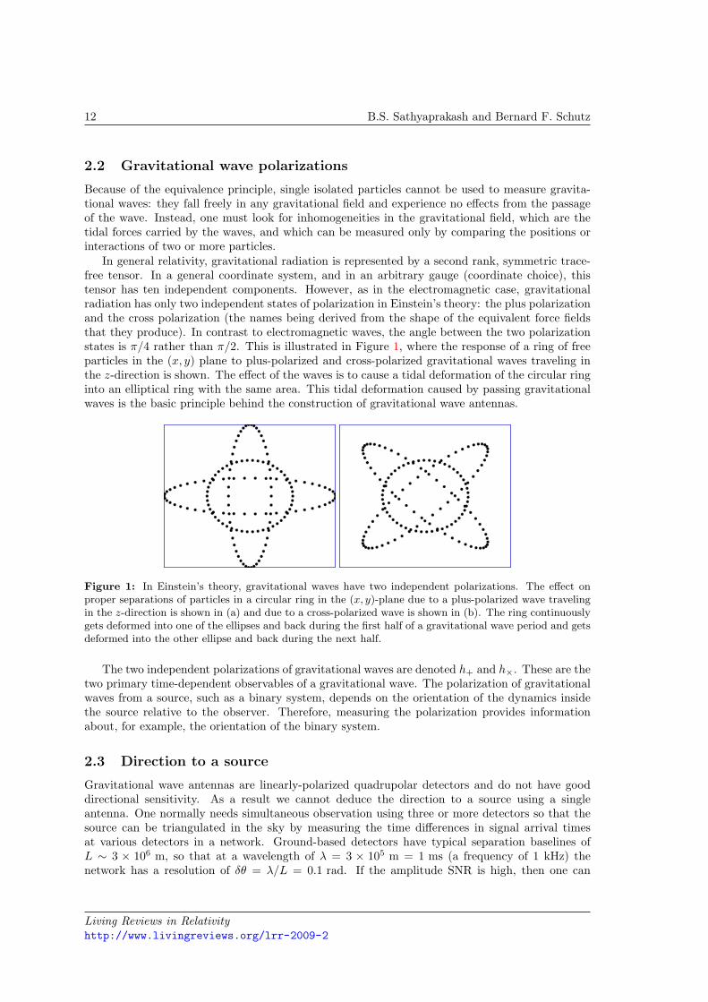
In general relativity, gravitational radiation is represented by a second rank, symmetric trace-free tensor. In a general coordinate system, and in an arbitrary gauge (coordinate choice), thistensor has ten independent components. However, as in the electromagnetic case, gravitationalradiation has only two independent states of polarization in Einstein’s theory: the plus polarizationand the cross polarization (the names being derived from the shape of the equivalent force fieldsthat they produce). In contrast to electromagnetic waves, the angle between the two polarizationstates is π/4 rather than π/2. This is illustrated in Figure 1, where the response of a ring of freeparticles in the (x, y) plane to plus-polarized and cross-polarized gravitational waves traveling inthe z-direction is shown. The effect of the waves is to cause a tidal deformation of the circular ringinto an elliptical ring with the same area. This tidal deformation caused by passing gravitationalwaves is the basic principle behind the construction of gravitational wave antennas.
Figure 1: In Einstein’s theory, gravitational waves have two independent polarizations. The effect onproper separations of particles in a circular ring in the (x, y)-plane due to a plus-polarized wave travelingin the z-direction is shown in (a) and due to a cross-polarized wave is shown in (b). The ring continuouslygets deformed into one of the ellipses and back during the first half of a gravitational wave period and getsdeformed into the other ellipse and back during the next half.
The two independent polarizations of gravitational waves are denoted h+ and h×. These are thetwo primary time-dependent observables of a gravitational wave. The polarization of gravitationalwaves from a source, such as a binary system, depends on the orientation of the dynamics insidethe source relative to the observer. Therefore, measuring the polarization provides informationabout, for example, the orientation of the binary system.
2.3 Direction to a source
Gravitational wave antennas are linearly-polarized quadrupolar detectors and do not have gooddirectional sensitivity. As a result we cannot deduce the direction to a source using a singleantenna. One normally needs simultaneous observation using three or more detectors so that thesource can be triangulated in the sky by measuring the time differences in signal arrival timesat various detectors in a network. Ground-based detectors have typical separation baselines ofL ∼ 3 × 10⁶ m, so that at a wavelength of λ = 3 × 10⁵ m = 1 ms (a frequency of 1 kHz) thenetwork has a resolution of δθ = λ/L = 0.1 rad. If the amplitude SNR is high, then one can
Living Reviews in Relativityhttp://www.livingreviews.org/lrr-2009-2
Physics, Astrophysics and Cosmology with Gravitational Waves 13
localize the source by a factor of 1/SNR better than this.For long-lived sources, however, a single antenna synthesizes many antennas by observing the
source at different points along its orbit around the sun. The baseline for such observations is 2 AU,so that, for a source emitting radiation at 1 kHz, the resolution is as good as ∆θ = 10−6 rad, whichis smaller than an arcsecond.
For space-based detectors orbiting the sun, like LISA, the baseline is again 2 AU, but theobserving frequency is some five or six orders of magnitude lower, so the basic resolution is only oforder 1 radian. However, as we shall see later, some of the sources that a space-based detector willobserve have huge amplitude SNRs in the range of SNR ∼ 103 – 104, which improves the resolutionto arcminute accuracies in the best cases.
2.4 Amplitude of gravitational waves – the quadrupole approximation
The Einstein equations are too difficult to solve analytically in the generic case of a strongly gravi-tating source to compute the luminosity and amplitude of gravitational waves from an astronomicalsource. We will discuss numerical solutions later; the most powerful available analytic approach iscalled the post-Newtonian approximation scheme. This approximation is suited to gravitationally-bound systems, which constitute the majority of expected sources. In this scheme [79, 169], solu-tions are expanded in the small parameter (v/c)2, where v is the typical dynamical speed inside thesystem. Because of the virial theorem, the dimensionless Newtonian gravitational potential φ/c2
is of the same order, so that the expansion scheme links orders in the expanded metric with thosein the expanded source terms. The lowest-order post-Newtonian approximation for the emittedradiation is the quadrupole formula, and it depends only on the density (ρ) and velocity fieldsof the Newtonian system. If we define the spatial tensor Qjk, the second moment of the massdistribution, by the equation
Qjk =∫ρxjxk d3x, (1)
then the amplitude of the emitted gravitational wave is, at lowest order, the three-tensor
hjk =2r
d2Qjk
dt2. (2)
This is to be interpreted as a linearized gravitational wave in the distant almost-flat geometry farfrom the source, in a coordinate system (gauge) called the Lorentz gauge.
2.4.1 Wave amplitudes and polarization in TT-gauge
A useful specialization of the Lorentz gauge is the TT-gauge, which is a comoving coordinatesystem: free particles remain at constant coordinate locations, even as their proper separationschange. To get the TT-amplitude of a wave traveling outwards from its source, project the tensorin Equation (2) perpendicular to its direction of travel and remove the trace of the projectedtensor. The result of doing this to a symmetric tensor is to produce, in the transverse plane, atwo-dimensional matrix with only two independent elements:
hab =(h+ h×h× −h+
). (3)
This is the definition of the wave amplitudes h+ and h× that are illustrated in Figure 1. Theseamplitudes are referred to as the coordinates chosen for that plane. If the coordinate unit basisvectors in this plane are ex and ey, then we can define the basis tensors
e+ = ex ⊗ ex − ey ⊗ ey, (4)e× = ex ⊗ ey + ey ⊗ ex. (5)
Living Reviews in Relativityhttp://www.livingreviews.org/lrr-2009-2
14 B.S. Sathyaprakash and Bernard F. Schutz
In terms of these, the TT-gravitational wave tensor can be written as
h = h+e+ + h×e×. (6)
If the coordinates in the transverse plane are rotated by an angle ψ, then one obtains newamplitudes h′+ and h′× given by
h′+ = cos 2ψ h+ + sin 2ψ h×, (7)h′× = − sin 2ψ h+ + cos 2ψ h×. (8)
This shows the quadrupolar nature of the polarizations, and is consistent with our remark inassociation with Figure 1 that a rotation of π/4 changes one polarization into the other.
It should be clear from the TT projection operation that the emitted radiation is not isotropic:it will be stronger in some directions than in others1. It should also be clear from this thatspherically-symmetric motions do not emit any gravitational radiation: when the trace is removed,nothing remains.
2.4.2 Simple estimates
A typical component of d2Qjk/dt2 will (from Equation (1)) have magnitude (Mv2)nonsph, where
(Mv2)nonsph is twice the nonspherical part of the kinetic energy inside the source. So a bound onany component of Equation (2) is
h .2(Mv2)nonsph
r. (9)
It is interesting to observe that the ratio ε of the wave amplitude to the Newtonian potential φext
of its source at the observer’s distance r is simply bounded by
h/φext < 2v2nonsph,
and this bound is attained if the entire mass of the source is involved in the nonspherical motions,so that (Mv2)nonsph ∼Mv2
nonsph. By the virial theorem for self-gravitating bodies
v2nonsph ≤ φint, (10)
where φint is the maximum value of the Newtonian gravitational potential inside the system. Thisprovides a convenient bound in practice [328]:
h . 2φintφext. (11)
The bound is attained if the system is highly nonspherical. An equal-mass star binary system is agood example of a system that attains this bound.
For a neutron star source, one has φint ∼ 0.2. If the star is in the Virgo cluster (r ∼ 18 Mpc)and has a mass of 1.4M, and if it is formed in a highly-nonspherical gravitational collapse, thenthe upper limit on the amplitude of the radiation from such an event is 1.5 × 10⁻²¹. This is asimple way to get the number that has been the goal of detector development for decades, to makedetectors that can observe waves at or below an amplitude of about 10−21.
1In the case of an inspiraling binary, the root mean square of the two polarization amplitudes in a directionorthogonal to the orbital plane will be a factor 2
√2 larger than in the plane.
Living Reviews in Relativityhttp://www.livingreviews.org/lrr-2009-2
Physics, Astrophysics and Cosmology with Gravitational Waves 15
2.5 Frequency of gravitational waves
The signals for which the best waveform predictions are available have well-defined frequencies. Insome cases the frequency is dominated by an existing motion, such as the spin of a pulsar. Butin most cases the frequency will be related to the natural frequency for a self-gravitating body,defined as
ω0 =√πGρ, or f0 = ω0/2π =
√Gρ/4π, (12)
where ρ is the mean density of mass-energy in the source. This is of the same order as thebinary orbital frequency and the fundamental pulsation frequency of the body. Even though thisis a Newtonian formula, it provides a remarkably good order-of-magnitude prediction of naturalfrequencies, even for highly relativistic systems such as black holes.
The frequency of the emitted gravitational waves need not be the natural frequency, of course,even if the mechanism is an oscillation with that frequency. In many cases, such as binary systems,the radiation comes out at twice the oscillation frequency. But since, at this point, we are nottrying to be more accurate than a few factors, we will ignore this distinction here. In later sections,with specific source models, we will get the factors right.
The mean density and hence the frequency are determined by the size R and mass M ofthe source, taking ρ = 3M/4πR3. For a neutron star of mass 1.4M and radius 10 km, thenatural frequency is f0 = 1.9 kHz. For a black hole of mass 10M and radius 2M = 30 km, itis f0 = 1 kHz. And for a large black hole of mass 2.5 × 10⁶M, such as the one at the centerof our galaxy, this goes down in inverse proportion to the mass to f0 = 4 mHz. In general, thecharacteristic frequency of the radiation of a compact object of mass M and radius R is
f0 =14π
(3MR3
)1/2
' 1 kHz(
10M
M
). (13)
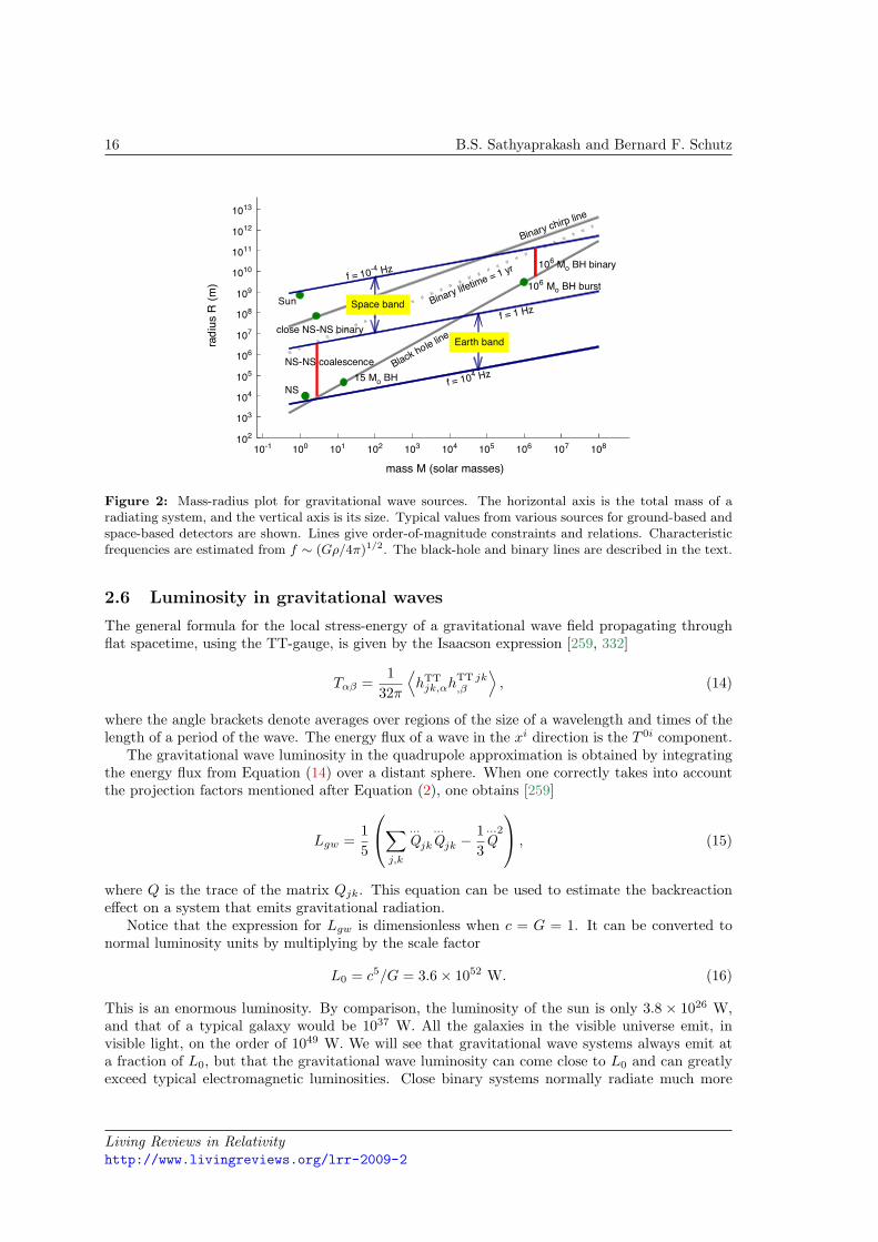
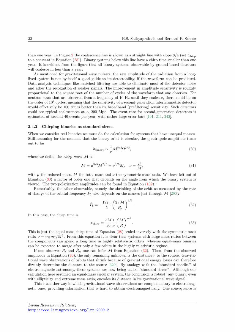
Figure 2 shows the mass-radius diagram for likely sources of gravitational waves. Three linesof constant natural frequency are plotted: f0 = 104 Hz, f0 = 1 Hz, and f0 = 10−4 Hz. Theseare interesting frequencies from the point of view of observing techniques: gravitational wavesbetween 1 and 104 Hz are in principle accessible to ground-based detectors, while lower frequenciesare observable only from space. Also shown is the line marking the black-hole boundary. This hasthe equation R = 2M . There are no objects below this line, because they would be smaller thanthe horizon size for their mass. This line cuts through the ground-based frequency band in such away as to restrict ground-based instruments to looking at stellar-mass objects. No system with amass above about 104M can produce quadrupole radiation in the ground-based frequency band.
A number of typical relativistic objects are placed in the diagram: a neutron star, a pair ofneutron stars that spiral together as they orbit, some black holes. Two other interesting linesare drawn. The lower (dashed) line is the 1-year coalescence line, where the orbital shrinkingtimescale due to gravitational radiation backreaction (cf. Equation (28)) is less than one year. Theupper (solid) line is the 1-year chirp line: if a binary lies below this line, then its orbit will shrinkenough to make its orbital frequency increase by a measurable amount in one year. (In a one-yearobservation one can, in principle, measure changes in frequency of 1 yr−1, or 3× 10⁻⁸ Hz.)
It is clear from the Figure that any binary system that is observed from the ground will coa-lesce within an observing time of one year. Since pulsar binary statistics suggest that neutron-star–binary coalescences happen less often than once every 105 years in our galaxy, ground-baseddetectors must be able to register these events in a volume of space containing at least 106 galaxiesin order to have a hope of seeing occasional coalescences. That corresponds to a volume of radiusroughly 100 Mpc. For comparison, first-generation ground-based interferometric detectors have areach of around 20 Mpc for such binaries, while advanced interferometers should extend that toabout 200 Mpc.
Living Reviews in Relativityhttp://www.livingreviews.org/lrr-2009-2
16 B.S. Sathyaprakash and Bernard F. Schutz
NS
106 Mo BH burst
106 Mo BH binary
Sun
Binary chirp line
10-1 100 101 102 103 104 105 106 107 108
mass M (solar masses)
102
103
104
105
106
107
108
109
1010
1011
1012
1013ra
diu
s R
(m
)
f = 1 Hz
f = 10-4 Hz
Black hole line
close NS-NS binary
Space band Binary lifetim
e = 1 yr
Earth band
f = 104 Hz15 Mo BH
NS-NS coalescence
Figure 2: Mass-radius plot for gravitational wave sources. The horizontal axis is the total mass of aradiating system, and the vertical axis is its size. Typical values from various sources for ground-based andspace-based detectors are shown. Lines give order-of-magnitude constraints and relations. Characteristicfrequencies are estimated from f ∼ (Gρ/4π)1/2. The black-hole and binary lines are described in the text.
2.6 Luminosity in gravitational waves
The general formula for the local stress-energy of a gravitational wave field propagating throughflat spacetime, using the TT-gauge, is given by the Isaacson expression [259, 332]
Tαβ =1
32π
⟨hTT
jk,αhTT jk,β
⟩, (14)
where the angle brackets denote averages over regions of the size of a wavelength and times of thelength of a period of the wave. The energy flux of a wave in the xi direction is the T 0i component.
The gravitational wave luminosity in the quadrupole approximation is obtained by integratingthe energy flux from Equation (14) over a distant sphere. When one correctly takes into accountthe projection factors mentioned after Equation (2), one obtains [259]
Lgw =15
∑j,k
...
Qjk
...
Qjk −13
...
Q2
, (15)
where Q is the trace of the matrix Qjk. This equation can be used to estimate the backreactioneffect on a system that emits gravitational radiation.
Notice that the expression for Lgw is dimensionless when c = G = 1. It can be converted tonormal luminosity units by multiplying by the scale factor
L0 = c5/G = 3.6× 1052 W. (16)
This is an enormous luminosity. By comparison, the luminosity of the sun is only 3.8 × 1026 W,and that of a typical galaxy would be 1037 W. All the galaxies in the visible universe emit, invisible light, on the order of 1049 W. We will see that gravitational wave systems always emit ata fraction of L0, but that the gravitational wave luminosity can come close to L0 and can greatlyexceed typical electromagnetic luminosities. Close binary systems normally radiate much more
Living Reviews in Relativityhttp://www.livingreviews.org/lrr-2009-2
Physics, Astrophysics and Cosmology with Gravitational Waves 17
energy in gravitational waves than in light. Black hole mergers can, during their peak few cycles,compete in luminosity with the steady luminosity of the entire universe!
Combining Equations (2) and (15) one can derive a simple expression for the apparent lu-minosity of radiation F , at great distances from the source, in terms of the gravitational waveamplitude [332]:
F ∼ |h|2
16π. (17)
The above relation can be used to make an order-of-magnitude estimate of the gravitational waveamplitude from a knowledge of the rate at which energy is emitted by a source in the form ofgravitational waves. If a source at a distance r radiates away energy E in a time T , predominantlyat a frequency f , then writing h = 2πfh and noting that F ∼ E/(4πr2T ), the amplitude ofgravitational waves is
h ∼ 1πfr
√E
T. (18)
When the time development of a signal is known, one can filter the detector output through a copyof the expected signal (see Section 5 on matched filtering). This leads to an enhancement in theSNR, as compared to its narrow-band value, by roughly the square root of the number of cyclesthe signal spends in the detector band. It is useful, therefore, to define an effective amplitude of asignal, which is a better measure of its detectability than its raw amplitude:
heff ≡√nh. (19)
Now, a signal lasting for a time T around a frequency f would produce n ' fT cycles. Using thiswe can eliminate T from Equation (18) and get the effective amplitude of the signal in terms ofthe energy, the emitted frequency and the distance to the source:
heff ∼1πr
√E
f. (20)
Notice that this depends on the energy only through the total fluence, or time-integrated fluxE/4πr2 of the wave. As in many other branches of astronomy, the detectability of a source isultimately a function of its apparent luminosity and the observing time. However, one should notignore the dependence on frequency in this formula. Two sources with the same fluence are notequally easy to detect if they are at different frequencies: higher frequency signals have smalleramplitudes.
Living Reviews in Relativityhttp://www.livingreviews.org/lrr-2009-2
18 B.S. Sathyaprakash and Bernard F. Schutz
3 Sources of Gravitational Waves
3.1 Man-made sources
One source can unfortunately be ruled out as undetectable: man-made gravitational radiation.Imagine creating a wave generator with the following extreme properties. It consists of two massesof 103 kg each (a small car) at opposite ends of a beam 10 m long. At its center the beam pivotsabout an axis. This centrifuge rotates 10 times per second. All the velocity is nonspherical, sov2nonsph in Equation (9) is about 105 m2 s−2. The frequency of the waves will actually be 20 Hz,
since the mass distribution of the system is periodic in time with a period of half the rotationperiod. The wavelength of the waves will, therefore, be 1.5 × 10⁷ m, similar to the diameter ofthe earth. In order to detect gravitational waves, not near-zone Newtonian gravity, the detectormust be at least one wavelength from the source, say diametrically opposite the centrifuge on theEarth. Then the amplitude h can be deduced from Equation (9): h ∼ 5 × 10−43. This is far toosmall to contemplate detecting! The story changes, fortunately, when we consider astrophysicalsources of gravitational waves, where nature arranges for masses that are 1027 times larger thanour centrifuge to move at speeds close to the speed of light!
Until observations of gravitational waves are successfully made, one can only make intelligentguesses about most of the sources that will be seen. There are many that could be strong enough tobe seen by the early detectors: star binaries, supernova explosions, neutron stars, the early universe.In this section, we make rough luminosity estimates using the quadrupole formula and otherapproximations, which are usually accurate to within factors of order two, and, very importantly,they show how key observables scale with the properties of the systems. Where appropriate we alsomake use of predictions from the much more accurate modelling that is available for some sources,such as binary systems and black hole mergers. The detectability depends, of course, not only onthe intrinsic luminosity of the source, but on how far away it is. Often the biggest uncertainties inmaking predictions are the spatial density and event rate of any particular class of sources. This isnot surprising, since our information at present comes from electromagnetic observations, and asour earlier remarks about the differences between the mechanisms of emission of gravitational andelectromagnetic radiation make clear, electromagnetic observations may not strongly constrain thesource population.
3.2 Gravitational wave bursts from gravitational collapse
Neutron stars and black holes are formed from the gravitational collapse of a highly evolved staror the core collapse of an accreting white dwarf. In either case, if the collapse is nonspherical,perhaps induced by strong rotation, then gravitational waves could carry away some of the bindingenergy and angular momentum depending on the geometry of the collapse. Collapse events arethought to produce supernovae of various types, and increasingly there is evidence that they alsoproduce most of the observed gamma-ray bursts [191] in hypernovae and collapsars [397, 249].Supernovae of Type II are believed to occur at a rate of between 0.1 and 0.01 per year in a milky-way equivalent galaxy (MWEG); thus, within the Virgo supercluster, we might expect an eventrate of about 30 per year. Hypernova events are considerably rarer and might only contributeobservable gravitational-wave events in current and near-future detectors if they involve so muchrotation that strong non-axisymmetric instabilities are triggered.
Simulating gravitational collapse is a very active area of numerical astrophysics, and most simu-lations also predict the energy and spectral characteristics of the emitted gravitational waves [167].However, it is still beyond the capabilities of computers to simulate a gravitational collapse eventwith all the physics that might be necessary to give reliable predictions: three-dimensional hy-drodynamics, neutrino transport, realistic nuclear physics, magnetic fields, rotation. In fact, it isstill by no means clear why Type II supernovae explode at all: simulations typically have great
Living Reviews in Relativityhttp://www.livingreviews.org/lrr-2009-2
Physics, Astrophysics and Cosmology with Gravitational Waves 19
difficulty reversing the inflow and producing an explosion with the observed light-curves and en-ergetics. It may be that the answer lies in some of the physics that has to be oversimplified inorder to be used in current simulations, or in some neutrino physics that we do not yet know, orin some unexplored hydrodynamic mechanism [276]. In a typical supernova, simulations suggestthat gravitational waves might extract between about 10−7 and 10−5 of the total available mass-energy [264, 147, 148], and the waves could come off in a burst whose frequency might lie in therange of ∼ 200 – 1000 Hz.
We can use Equation (18) to make a rough estimate of the amplitude, if the emitted energy andtimescale are known. Using representative values for a supernova in our galaxy, lying at 10 kpc,emitting the energy equivalent of 10−7M at a frequency of 1 kHz, and lasting for 1 ms, thereceived amplitude would be
h ∼ 6× 10⁻²¹
(E
10−7M
)1/2(1 msT
)1/2(1 kHzf
)(10 kpcr
). (21)
The upper bound in Equation (11) would give the same amplitude for a source 60 times furtheraway, which reflects the fact that simulations find it difficult to put significant energy into gravi-tational waves. This amplitude is large enough for current ground-based detectors to observe witha reasonably high confidence, but of course the event rate within 10 kpc is expected to be far toosmall to make an early detection likely.
3.3 Gravitational wave pulsars
Some likely gravitational wave sources behave like the centrifuge example we used in the firstparagraph of this section, only on a grander scale. Suppose a neutron star of radius R and mass Mspins with a frequency f and has an irregularity, a deformation of its otherwise axially symmetricshape. We idealize this as a “bump” of mass m on its surface, although of course it will really bea distribution of mass leading to an asymmetrical quadrupole tensor. The moment of inertia ofthe bump will be mR2, and it is conventional to parameterize the bump in terms of the fractionalasymmetry it creates in the moment of inertia tensor itself. If we idealize the star as havinguniform density, then the spherical moment of inertia is 2MR2/5, and so the bump has fractionalasymmetry
ε =52m
M, m = 0.4εM. (22)
The bump will emit gravitational radiation at frequency 2f because the star spins about its netcenter of mass, so it effectively has mass excesses on both sides of the star. The nonsphericalvelocity will be just vnonsph = 2πRf . The radiation amplitude will be, from Equation (9),
hbump ∼ (4/5)(2πRf)2εM/r, (23)
and the luminosity, from Equation (15) (assuming that roughly four comparable components ofQjk contribute to the sum),
Lbump ∼ (16/125)(2πf)6ε2M2R4.
The radiated energy would presumably come from the rotational energy of the star Mv2/5. Thiswould lead to a spindown of the star on a timescale
tspindown ∼15Mv2/Lbump ∼
2532π
ε−2f−1
(M
R
)−1
v−3. (24)
It is believed that neutron star crusts are not strong enough to support fractional asymmetrieslarger than about ε ∼ 10−6 [370], and realistic asymmetries may be much smaller.
Living Reviews in Relativityhttp://www.livingreviews.org/lrr-2009-2

20 B.S. Sathyaprakash and Bernard F. Schutz
From these considerations one can estimate the likelihood that the observed spindown timescalesof pulsars are due to gravitational radiation. In most cases, it seems that gravitational wave lossescould account for a substantial amount of the spindown: the required asymmetries are muchsmaller than 10−4, often smaller than 10−7. But an interesting exception is the Crab pulsar,PSR J0534+2200, whose young age and consequently short spindown time (measured to be 8.0×10¹⁰ s, about 2500 yr) would require an exceptionally large asymmetry. If we take the neutronstar’s radius to be 10 km, so that M/R ∼ 0.21 and the speed of any irregularity is v/c ∼ 6.2×10⁻³,then Equation (24) would require an asymmetry of ε ∼ 1.4 × 10⁻³. Of course, we have made alot of approximations to get here, only keeping our estimates of amplitudes and energies correctto within factors of two, but a more careful calculation reduces this only by a factor of two toε ∼ 7 × 10⁻⁴ [12]. What makes this interesting is the fact that an asymmetry this large wouldproduce radiation detectable by first-generation interferometers. Conversely, an upper limit fromfirst-generation interferometers would provide direct observational limits on the asymmetry andon the fraction of energy lost by the Crab pulsar to gravitational waves.
From Equation (23) the Crab pulsar would, if its spindown is dominated by gravitational wavelosses, produce an amplitude at the Earth of h ∼ 1.5 × 10⁻²⁴, if its distance is 2 kpc. Is thisdetectable when present instruments are only capable of seeing millisecond bursts of radiation atlevels of 10−21? The answer is yes, if the observation time is long enough. Indeed, the latestLIGO observations have not detected any gravitational waves from the Crab pulsar, which hasbeen used to set an upper limit on the asymmetry in its mass distribution [12]. The limit dependson the model assumed for the pulsar. If one assumes that gravitational waves are produced atexactly twice the pulsar spin frequency and uses the inferred values of the pulsar orientation andpolarization angle, then for a canonical value of the moment-of-inertia I = 1038 kg m2, one gets anupper limit on the ellipticity of ε ≤ 1.8× 10⁻⁴, assuming the pulsar is at 2 kpc. This is a factor of4.2 below the spindown limit [12]. If, however, one assumes that gravitational waves are emittedat a frequency close, but not exactly equal, to twice the spin frequency and one uses a uniformprior for the orientation and polarization angle, then one gets ε ≤ 9 × 10⁻⁴, which is 0.8 of thelimit derived from the spin-down rate.
Indeed, even signals weaker than the amplitude determined by the Crab spindown rate will beobservable by present detectors, and these may be coming from a larger variety of neutron stars,in particular low-mass X-ray binary systems (LMXBs). The neutron stars in them are accretingmass and angular momentum, so they should be spinning up. Observations suggest that mostneutron stars are spinning at speeds between about 300 and 600 Hz, far below their maximum,which is greater than 1000 Hz. The absence of faster stars suggests that something stops themfrom spinning up beyond this range. Bildsten suggested [77] that the limiting mechanism maybe the re-radiation of the accreted angular momentum in gravitational waves, possibly due to aquadrupole moment created by asymmetrical heating induced by the accreted matter. Anotherpossible mechanism [285] is that a “bump” of the kind we have treated is formed by accretingmatter channeled onto the surface by the star’s magnetic field. It is also possible that accretiondrives an instability in the star that leads to steady emission [308, 270]. In either case, the starscould turn out to be long-lived sources of gravitational waves. This idea, which is a variant of oneproposed long ago by Wagoner [383], is still speculative, but the numbers make a plausible case.We discuss it in more detail in Section 7.3.5.
Living Reviews in Relativityhttp://www.livingreviews.org/lrr-2009-2
Physics, Astrophysics and Cosmology with Gravitational Waves 21
3.4 Radiation from a binary star system
3.4.1 Radiation from a binary system and its backreaction
A binary star system can also be treated as a “centrifuge”. Two stars of the same mass m in acircular orbit of radius R have all their mass in nonspherical motion, so that
(Mv2)nonsph = M(ΩR)2 =M2
R,
where Ω is the orbital angular velocity. The gravitational wave amplitude can then be written
hbinary ∼ 2M
r
M
R. (25)
Since the internal radius R of the orbit is not an observable, it is sometimes convenient to replaceR by the orbital angular frequency Ω using the above orbit equation, giving
hbinary ∼2rM5/3Ω2/3. (26)
The gravitational wave luminosity of such a system is, by a calculation analogous to that forbumps on neutron stars (assuming that four components of Qij to be significant),
Lbinary ∼45
(M
R
)5
, (27)
in units given by the fundamental luminosity L0 in Equation (16). This shows that self-gravitatingsystems always emit at a fraction of L0, since M/R is always smaller than 1, but it can approachL0 for highly-relativistic systems where M/R ∼ 1.
The radiation of energy by the orbital motion causes the orbit to shrink. The shrinking willmake any observed gravitational waves increase in frequency with time. This is called a chirp. Thetimescale2 for this in a binary system with equal masses is
tchirp =Mv2
2/Lbinary ∼
5M8
(M
R
)−4
. (28)
As the binary evolves, the frequency and amplitude of the wave grow and this drives the binaryto evolve even more rapidly. The signal’s frequency, however, will not increase indefinitely; theslow inspiral phase ends either when the stars begin to interact and merge or (if they are verycompact) when the distance between the stars is roughly at the last stable orbit (LSO) R = 6M ,which corresponds to a gravitational wave frequency of
fLSO ∼ 220(
20M
M
)Hz, (29)
where we have normalized this to a binary with M = 20M. This is the last stable orbit (LSO)frequency.
A compact-object binary that coalesces after passing through the last stable orbit is a powerfulsource of gravitational waves, with a luminosity that approaches the limiting luminosity L0. Thisis called a coalescing binary in gravitational wave searches. Since a typical search might last onthe order of one year, a coalescing binary can be defined as a system that has a chirp time smaller
2In Sections 5.1 we will use parameters called chirp times, instead of the masses, to characterize a binary. Thetimescale defined here is closely related to the chirp times.
Living Reviews in Relativityhttp://www.livingreviews.org/lrr-2009-2
22 B.S. Sathyaprakash and Bernard F. Schutz
than one year. In Figure 2 the coalescence line is shown as a straight line with slope 3/4 (set tchirp
to a constant in Equation (28)). Binary systems below this line have a chirp time smaller than oneyear. It is evident from the figure that all binary systems observable by ground-based detectorswill coalesce in less than a year.
As mentioned for gravitational wave pulsars, the raw amplitude of the radiation from a long-lived system is not by itself a good guide to its detectability, if the waveform can be predicted.Data analysis techniques like matched filtering are able to eliminate most of the detector noiseand allow the recognition of weaker signals. The improvement in amplitude sensitivity is roughlyproportional to the square root of the number of cycles of the waveform that one observes. Forneutron stars that are observed from a frequency of 10 Hz until they coalesce, there could be onthe order of 104 cycles, meaning that the sensitivity of a second-generation interferometric detectorwould effectively be 100 times better than its broadband (prefiltering) sensitivity. Such detectorscould see typical coalescences at ∼ 200 Mpc. The event rate for second-generation detectors isestimated at around 40 events per year, with rather large error bars [101, 211, 242].
3.4.2 Chirping binaries as standard sirens
When we consider real binaries we must do the calculation for systems that have unequal masses.Still assuming for the moment that the binary orbit is circular, the quadrupole amplitude turnsout to be
hbinary ∼1rM5/3Ω2/3, (30)
where we define the chirp mass M as
M = µ3/5M2/5 = ν3/5M, ν =µ
M, (31)
with µ the reduced mass, M the total mass and ν the symmetric mass ratio. We have left out ofEquation (30) a factor of order one that depends on the angle from which the binary system isviewed. The two polarization amplitudes can be found in Equation (132).
Remarkably, the other observable, namely the shrinking of the orbit as measured by the rateof change of the orbital frequency Pb also depends on the masses just through M [290]:
Pb = −192π5
(2πMPb
)5/3
. (32)
In this case, the chirp time is
tchirp =5M96
1ν
(M
R
)−4
. (33)
This is just the equal-mass chirp time of Equation (28) scaled inversely with the symmetric massratio ν = m1m2/M
2. From this equation it is clear that systems with large mass ratios betweenthe components can spend a long time in highly relativistic orbits, whereas equal-mass binariescan be expected to merge after only a few orbits in the highly relativistic regime.
If one observes Pb and Pb, one can infer M from Equation (32). Then, from the observedamplitude in Equation (30), the only remaining unknown is the distance r to the source. Gravita-tional wave observations of orbits that shrink because of gravitational energy losses can thereforedirectly determine the distance to the source [329]. By analogy with the “standard candles” ofelectromagnetic astronomy, these systems are now being called “standard sirens”. Although ourcalculation here assumed an equal-mass circular system, the conclusion is robust: any binary, evenwith ellipticity and extreme mass ratio, encodes its distance in its gravitational wave signal.
This is another way in which gravitational wave observations are complementary to electromag-netic ones, providing information that is hard to obtain electromagnetically. One consequence is
Living Reviews in Relativityhttp://www.livingreviews.org/lrr-2009-2
Physics, Astrophysics and Cosmology with Gravitational Waves 23
the possibility that observations of coalescing compact object binaries could allow one to measurethe Hubble constant [329] or other cosmological parameters. This will be particularly interestingfor the LISA project, whose observations of black hole binaries could contribute an independentmeasurement of the acceleration of the universe [195, 131, 48].
Because chirping systems are so interesting we have also drawn, in Figure 2, a line where thechirp time can be measured in one year. This means that the change in frequency due to the chirpmust be larger than the frequency resolution 1 yr−1. A little algebra shows that the condition forthe chirp to be resolved in an observation time T in a binary with period Pb is
Pbtchirp = T 2. (34)
Since Pb ∝ R3/2M−1/2, this condition leads to a line of slope 7/11 in the logarithmic plot inFigure 2. The line drawn there corresponds to a resolution time T of one year. All binaries belowthis line will chirp in a short enough time for their distances to be measured.
3.4.3 Binary pulsar tests of gravitational radiation theory
The most famous example of the effects of gravitational radiation on an orbiting system is theHulse–Taylor Binary Pulsar, PSR B1913+16. In this system, two neutron stars orbit in a closeeccentric orbit. The pulsar provides a regular clock that allows one to deduce, from post-Newtonianeffects, all the relevant orbital parameters and the masses of the stars. The key to the importanceof this binary system is that all of the important parameters of the system can be measured beforeone takes account of the orbital shrinking due to gravitational radiation reaction. This is because anumber of post-Newtonian effects on the arrival time of pulses at the Earth, such as the precessionof the position of the periastron and the time-dependent gravitational redshift of the pulsar periodas it approaches and recedes from its companion, can be measured accurately, and they fullydetermine the masses, the semi-major axis and the eccentricity of their orbit [394, 344].
Equation (28) for the chirp time predicts that this system would change its orbital periodPb = 7.75 hrs on the timescale (taking M = 1.4M and R = 106 km)
tchirp = Pb/Pb ∼ 1.9× 10¹⁸ s.
From this one can infer that Pb ∼ 1.5×10⁻¹⁴. But this has to be corrected for our oversimplificationof the orbit as circular: an eccentric orbit evolves much faster because, during the phase of closestapproach, the velocities are much higher, and the emitted luminosity is a very strong functionof the velocity. Using equations first computed by Peters and Mathews [290], for the actualeccentricity of 0.62, one finds (see Equation (109) below) PT = −(2.40242 ± 0.00002) × 10−12.Observations [394, 388] currently give PO = −(2.4184 ± 0.0009) × 10−12. There is a significantdiscrepancy between these, but it can be removed by realizing that the binary system is acceleratingtoward the center of our galaxy, which produces a small period change. Taking this into accountgives a corrected prediction of −(2.4056 ± 0.0051) × 10−12, and this agrees with the observationwithin the uncertainties [394, 355]. This is the most sensitive test that we have of the correctnessof Einstein’s equations with respect to gravitational radiation, and it leaves little room for doubtin the validity of the quadrupole formula for other systems that may generate detectable radiation.
A number of other binary systems are now known in which such tests are possible [344]. Themost important of the other systems is the “double pulsar” in which both neutron stars are seenas pulsars [246]. This system will soon overtake the Hulse–Taylor binary as the most accurate testof gravitational radiation.
3.4.4 White-dwarf binaries
Binary systems at lower frequencies are much more abundant than coalescing binaries, and theyhave much longer lifetimes. LISA will look for close white-dwarf binaries in our galaxy, and will
Living Reviews in Relativityhttp://www.livingreviews.org/lrr-2009-2
24 B.S. Sathyaprakash and Bernard F. Schutz
probably see thousands of them. White dwarfs are not as compact as black holes or neutron stars.Although their masses can be similar to that of a neutron star their sizes are much larger, typically3,000 km in radius. As a result, white-dwarf binaries never reach the last stable orbit, which wouldoccur at roughly 1.5 kHz for these masses. We will discuss the implications of multi-messengerastronomy for white-dwarf binaries in Section 7.4.
The maximum amplitude of the radiation from a white-dwarf binary will be several ordersof magnitude smaller than that of a neutron star or black hole binary at the same distance butclose to coalescence. However, a binary system with a short period is long lived, so the effectiveamplitude (after matched filtering) improves as the square root of the observing time. Besidesthat, these sources are nearer: there are many thousands of such systems in our galaxy radiatingin the LISA frequency window above about 1 mHz, and LISA should be able to see all of them.Below 1 mHz there are even more sources, so many that LISA will not resolve them individually,but will see them blended together in a stochastic background of radiation, as shown in Figure 5.
3.4.5 Supermassive black hole binaries
Observations indicate that the center of every galaxy probably hosts a black hole whose mass isin the range of 106 – 109M [305], with the black holes mass correlating well with the mass of thegalactic bulge. A black hole whose mass is in the above range is called a supermassive black hole(SMBH). There is now abundant observational evidence that galaxies often collide and merge, andthere are good reasons to believe that when that happens, friction between the SMBHs and thestars and gas of the irregular merged galaxy will lead the SMBHs to spiral into a common nucleusand (on a timescale of some 108 yr) even get close enough to be driven into complete orbital decayby gravitational radiation reaction. In many systems this should lead to a black hole merger withina Hubble time [221]. For a binary with two nonspinning M = 106M black holes, the frequencyof emitted gravitational waves at the last stable orbit is, from Equation (29), fLSO = 4 mHz;during and after the merger the frequency rises from 4 mHz to the quasi-normal-mode frequencyof 24 mHz (if the spin of the final black hole is negligible). (Naturally, all these frequencies simplyscale inversely with the mass for other mass ranges.) This is in the frequency range of LISA, andobserving these mergers is one of the central purposes of the mission.
SMBH mergers are so spectacularly strong that they will be visible in LISA’s data streameven before applying any matched filter, although good models of the inspiral and particularly themerger radiation will be needed to extract source parameters. Because the masses of such blackholes are so large, LISA can see essentially any merger that happens in its frequency band anywherein the universe, even out to extremely high redshifts. It can thereby address astrophysical questionsabout the origin, growth and population of SMBHs. The recent discovery of an SMBH binary [221]and the association of X-shaped radio lobes with the merger of SMBH binaries [254] has furtherraised the optimism concerning SMBH merger rates, as has the suggestion that an SMBH hasbeen observed to have been expelled from the center of its galaxy, an event that could only havehappened as a result of a merger between two SMBHs [222]. The rate at which galaxies merge isabout 1 yr−1 out to a red-shift of z = 5 [185], and LISA’s detection rate for SMBH mergers mightbe roughly the same.
Modelling of the merger of two black holes requires numerical relativity, and the accuracy andreliability of numerical simulations is now becoming good enough that they will soon become anintegral part of gravitational wave searches.
3.4.6 Extreme and intermediate mass-ratio inspiral sources
The SMBH environment of our own galaxy is known to contain a large number of compact objectsand white dwarfs. Near the central SMBH there is a disproportionately large number of stellar-mass black holes, which have sunk there through random gravitational encounters with the normal
Living Reviews in Relativityhttp://www.livingreviews.org/lrr-2009-2
Physics, Astrophysics and Cosmology with Gravitational Waves 25
stellar population (dynamical friction). Three body interaction will occasionally drive one of thesecompact objects into a capture orbit of the central SMBH. The compact object will sometimes becaptured [305, 338, 337] into a highly eccentric trajectory (e > 0.99) with the periastron close tothe last stable orbit of the SMBH. Since the mass of the captured object will be about 1 – 100M,while the SMBH will have a far greater mass, we essentially have a “test mass” falling in thegeometry of a Kerr black hole. By Equation (33) we would expect that the small body wouldspend many orbits in the relativistic regime near the horizon of the large black hole: a 10Mblack hole falling into a 106M black hole would require on the order of 105 orbits. The emittedgravitational radiation [317, 179, 178, 67, 171, 57] would consist of a very long wave train thatcarries information about the nearly geodesic trajectory of the test body, thereby providing a veryclean probe to survey the spacetime geometry of the central object (which could be a Kerr blackhole or some other compact object) and test whether or not this geometry is as predicted by generalrelativity [318, 198, 177, 176, 68].
This kind of event happens occasionally to every SMBH that lives in the center of a galaxy.Indeed, since the SNR from matched filtering builds up in proportion to the square root of theobservation time tchirp ∝ ν−1 = (µ/M)−1 [cf. Equation (33)] and the inherent amplitude of theradiation is linear in ν [cf. Equation (30)], the SNR varies with the symmetric mass ratio as
√ν
and typical SNR will be about ten to a thousand times smaller than an SMBH binary at the samedistance. LISA will, therefore, be able to see such sources only to much smaller distances, saybetween 1 to 10 Gpc depending on the mass ratio. For events at such distances LISA’s SNR aftermatched filtering could be in the range 10 – 100, but matched filtering will be very difficult becauseof the complexity of the orbit, especially of its evolution due to radiation effects. However, thisvolume of space contains a large number of galaxies, and the event rate is expected to be severaltens to hundreds per year [67]. There will be a background from more distant sources that mightin the end set the limit on how much sensitivity LISA has to these events.
Due to relativistic frame dragging, for each passage of the apastron the test body could ex-ecute several nearly circular orbits at its periastron. Therefore, long periods of low-frequency,small-amplitude radiation will be followed by several cycles of high-frequency, large-amplitude ra-diation [317, 179, 178, 67, 171, 57]. The apastron slowly shrinks, while the periastron remains moreor less at the same location, until the final plunge of the compact object before merger. Moreover,if the central black hole has a large spin then spin-orbit coupling leads to precession of the orbitalplane thereby changing the polarization of the wave as seen by LISA.
Thus, there is a lot of structure in the waveforms owing to a number of different physical effects:contribution from higher-order multipoles due to an eccentric orbit, precession of the orbital plane,precession of the periastron, etc., and gravitational radiation backreaction plays a pivotal rolein the dynamics of these systems. If one looks at the time-frequency map of such a signal onenotices that the signal power is greatly smeared across the map [320], as compared to that of asharp chirp from a nonspinning black-hole binary. For this reason, this spin modulated chirp issometimes referred to as a smirch [322]. More commonly, such sources are called extreme massratio inspirals (EMRIs) and represent systems whose mass ratio is in the range of ∼ 10−3 – 10−6.Inspirals of systems with their mass ratio in the range ∼ 10−2 – 10−3 are termed intermediate massratio inspirals or IMRIs. These latter systems correspond to the inspiral of intermediate massblack holes of mass ∼ 103 – 104M and might constitute a prominent source in LISA provided thecentral SMBH grew in mass as a result of a number of mergers of small black holes [30, 31, 32].
While black hole perturbation theory with a careful treatment of radiation reaction is necessaryfor the description of EMRIs, IMRIs may be amenable to a description using a hybrid scheme ofpost-Newtonian approximations and perturbation theory. This is an area that requires more study.
Living Reviews in Relativityhttp://www.livingreviews.org/lrr-2009-2
26 B.S. Sathyaprakash and Bernard F. Schutz
3.5 Quasi-normal modes of a black hole
In 1970, Vishveshwara [381] discussed a gedanken experiment, similar in philosophy to Ruther-ford’s (real) experiment with the atom. In Vishveshwara’s experiment, he scattered gravitationalradiation off a black hole to explore its properties. With the aid of such a gedanken experiment,he demonstrated for the first time that gravitational waves scattered off a black hole will have acharacteristic waveform, when the incident wave has frequencies beyond a certain value, dependingon the size of the black hole. It was soon realized that perturbed black holes have quasi-normalmodes (QNMs) of vibration and in the process emit gravitational radiation, whose amplitude, fre-quency and damping time are characteristic of its mass and angular momentum [296, 220]. We willdiscuss in Section 6.4 how observations of QNMs could be used in testing strong field predictionsof general relativity.
We can easily estimate the amplitude of gravitational waves emitted when a black hole forms ata distance r from Earth as a result of the coalescence of compact objects in a binary. The effectiveamplitude is given by Equation (20), which involves the energy E put into gravitational wavesand the frequency f at which the waves come off. By dimensional arguments E is proportional tothe total mass M of the resulting black hole. The efficiency at which the energy is converted intoradiation depends on the symmetric mass ratio ν of the merging objects. One does not know thefraction of the total mass emitted nor the exact dependence on ν. Flanagan and Hughes [164] arguethat E ∼ 0.03(4ν)2M . The frequency f is inversely proportional to M ; indeed, for Schwarzschildblack holes f = (2πM)−1. Thus, the formula for the effective amplitude takes the form
heff ∼4ανMπr
, (35)
where α is a number that depends on the (dimensionless) angular momentum a of the black holeand has a value between 0.7 (for a = 0, Schwarzschild black hole) and 0.4 (for a = 1, maximallyspinning Kerr black hole). For stellar mass black holes at a distance of 200 Mpc the amplitude is:
heff ' 10−21( ν
0.25
)( M
20M
)(r
200 Mpc
)−1
. (36)
For SMBHs, even at cosmological distances, the amplitude of quasinormal mode signals is prettylarge:
heff ' 3× 10⁻¹⁷( ν
0.25
)( M
2× 10⁶M
)(r
6.5 Gpc
)−1
. (37)
In the first case we have a pair of 10M black holes inspiraling and merging to form a single blackhole. In this case the waves come off at a frequency of around 500 Hz [cf. Equation (13)]. Theinitial ground-based network of detectors might be able to pick these waves up by matched filtering,especially when an inspiral event precedes the ringdown signal. A 100M black hole plunging intoa 106M black hole at a distance of 6.5 Gpc (z ' 1) gives out radiation at a frequency of about15 mHz. Note that in the latter case the radiation is redshifted from 30 mHz to 15 mHz. Suchan event produces an amplitude just large enough to be detected by LISA. At the same distance,a pair of 106M SMBHs spiral in and merge to produce a fantastic amplitude of 3 × 10⁻¹⁷, wayabove the LISA background noise. In this case, the signals would be given off at about 7.5 mHzand will be loud and clear to LISA. It will not only be possible to detect these events, but also toaccurately measure the masses and spins of the objects before and after merger and thereby testthe black hole no-hair theorem and confirm whether the result of the merger is indeed a black holeor some other exotic object (e.g., a boson star or a naked singularity).
Living Reviews in Relativityhttp://www.livingreviews.org/lrr-2009-2
Physics, Astrophysics and Cosmology with Gravitational Waves 27
3.6 Stochastic background
In addition to radiation from discrete sources, the universe should have a random gravitationalwave field that results from a superposition of countless discrete systems and also from funda-mental processes, such as the Big Bang. Observing any of these backgrounds would bring usefulinformation, but the ultimate goal of detector development is the observation of the backgroundradiation from the Big Bang. It is expected to be very weak, but it will come to us unhinderedfrom as early as 10−30 s, and it could illuminate the nature of the laws of physics at energies farhigher than we can hope to reach in the laboratory.
It is usual to characterize the intensity of a random field of gravitational waves by its energydensity as a function of frequency. Since the energy density of a plane wave is the same as its flux(when c = 1), we have from Equation (17)
ρgw =π
4f2h2.
But the wave field in this case is a random variable, so we must replace h2 by a statistical meansquare amplitude per unit frequency (Fourier transform power per unit frequency) called Sgw(f),so that the energy density per unit frequency is proportional to f2Sgw(f). It is then conventional totalk about the energy density per unit logarithm of the frequency, which means multiplying by f .The result, after being careful about averaging over all directions of the waves and all independentpolarization components, is [27, 359]
dρgw
d ln f= 4π2f3Sgw(f).
Finally, what is of most interest is the energy density as a fraction of the closure or criticalcosmological density, given by the Hubble constant H0 as ρc = 3H2
0/8π. The resulting ratio iscalled Ωgw(f):
Ωgw(f) =10π2
3H20
f3Sgw(f).
The only tight constraint on Ωgw from non–gravitational-wave astronomy is that it must besmaller than 10−5, in order not to disturb the agreement between the standard Big Bang modelof nucleosynthesis (of helium and other light elements) and observation. If the universe containsthis much gravitational radiation today, then at the time of nucleosynthesis the (blue-shifted)energy density of this radiation would have been comparable to that of the photons and the threeneutrino species. Although the radiation would not have participated in the nuclear reactions, itsextra energy density would have required that the expansion rate of the universe at that time besignificantly faster, in order to evolve into the universe we see today. In turn, this faster expansionwould have provided less time for the nuclear reactions to “freeze out”, altering the abundancesfrom the values that are observed today [281, 346]. First-generation interferometers should be ableto set direct limits on the cosmological background at around this level. Radiation in the lower-frequency LISA band, from galactic and extra-galactic binaries, is expected to be much smallerthan this bound.
Random radiation is indistinguishable from instrumental noise in a single detector, at leastfor short observing times. If the random field is produced by an anisotropically-distributed set ofastrophysical sources (the binaries in our galaxy, for example) then over a year, as the detectorchanges its orientation, the noise from this background should rise and fall in a systematic way,allowing it to be identified. But this is a rather crude way of detecting the radiation, and a betterway is to perform a cross-correlation between two detectors, if available.
In cross-correlation, which amounts to multiplying the outputs and integrating, the randomsignal in one detector essentially acts as a template for the signal in the other detector. If they
Living Reviews in Relativityhttp://www.livingreviews.org/lrr-2009-2
28 B.S. Sathyaprakash and Bernard F. Schutz
match, then there will be a stronger-than-expected correlation. Notice that they can only matchwell if the wavelength of the gravitational waves is longer than the separation between the detectors:otherwise time delays for waves reaching one detector before the other degrade the match. Theoutcome is not like standard matched filtering, however, since the “filter” of the first detector hasas much noise superimposed on its template as the other detector. As a result, the amplitudeSNR of the correlated field grows only with observing time T as T 1/4, rather than the square rootgrowth that characterizes matched filtering [359].
Living Reviews in Relativityhttp://www.livingreviews.org/lrr-2009-2

Physics, Astrophysics and Cosmology with Gravitational Waves 29
4 Gravitational Wave Detectors and Their Sensitivity
Detectors of gravitational waves generally divide into two classes: beam detectors and resonantmass detectors. In beam detectors, gravitational waves interact with a beam of electromagneticradiation, which is monitored in some way to register the passage of the wave. In resonant massdetectors, the gravitational wave transfers energy to a massive body, from which the resultantoscillations are observed.
Both classes include a variety of systems. The principal beam detectors are the large ground-based laser interferometers currently operating in several locations around the globe, such as theLIGO system in the USA. The ESA–NASA LISA mission aims to put a laser interferometer intospace to detect milliHertz gravitational waves. But beam detectors do not need to involve inter-ferometry: the radio beams transponded to interplanetary spacecraft can carry the signature ofa passing gravitational wave, and this method has been used to search for low-frequency gravita-tional waves. And radio astronomers have for many years monitored the radio beams of distantpulsars for evidence of gravitational waves; new radio instrumentation is turning this into a pow-erful and promising method of looking for stochastic backgrounds and individual sources. And atultra-low frequencies, gravitational waves in the early universe may have left their imprint on thepolarization of the cosmic microwave background.
Resonant mass detectors were the first kind of detector built in the laboratory to detect grav-itational waves: Joseph Weber [387] built two cylindrical aluminum bar detectors and attemptedto find correlated disturbances that might have been caused by a passing impulsive gravitationalwave. His claimed detections led to the construction of many other bar detectors of comparableor better sensitivity, which never verified his claims. Some of those detectors were not developedfurther, but others had their sensitivities improved by making them cryogenic, and today there aretwo ultra-cryogenic detectors in operation (see Section 4.1).
In the following, we will examine the principal detection methods that hold promise today andin the near future.
4.1 Principles of the operation of resonant mass detectors
A typical “bar” detector consists of a cylinder of aluminum with a length ` ∼ 3 m, a very nar-row resonant frequency between f ∼ 500 Hz and 1.5 kHz, and a mass M ∼ 1000 kg. A shortgravitational wave burst with h ∼ 10−21 will make the bar vibrate with an amplitude
δ`gw ∼ h` ∼ 10−21 m. (38)
To measure this, one must fight against three main sources of noise.
1. Thermal noise. The original Weber bar operated at room temperature, but the mostadvanced detectors today, Nautilus [51] and Auriga [227], are ultra-cryogenic, operating atT = 100 mK. At this temperature the root mean square (rms) amplitude of vibration is
〈δ`2〉1/2th =
(kT
4π2Mf2
)1/2
∼ 6× 10⁻¹⁸ m. (39)
This is far larger than the gravitational wave amplitude expected from astrophysical sources.But if the material has a high Q (say, 106) in its fundamental mode, then that changesits thermal amplitude of vibration in a random walk with very small steps, taking a timeQ/f ∼ 1000 s to change by the full amount. However, a gravitational wave burst will causea change in 1 ms. In 1 ms, thermal noise will have random-walked to an expected amplitude
Living Reviews in Relativityhttp://www.livingreviews.org/lrr-2009-2
30 B.S. Sathyaprakash and Bernard F. Schutz
change (1000 s/1 ms)1/2 = Q1/2 times smaller, or (for these numbers)
〈δ`2〉1/2th: 1 ms =
(kT
4π2Mf2Q
)1/2
∼ 6× 10⁻²¹ m. (40)
So ultra-cryogenic bars can approach the goal of detection near h = 10−20 despite thermalnoise.
2. Sensor noise. A transducer converts the bar’s mechanical energy into electrical energy, andan amplifier increases the electrical signal to record it. If sensing of the vibration could bedone perfectly, then the detector would be broadband: both thermal impulses and gravita-tional wave forces are mechanical forces, and the ratio of their induced vibrations would bethe same at all frequencies for a given applied impulsive force.
But sensing is not perfect: amplifiers introduce noise, and this makes small amplitudes harderto measure. The amplitudes of vibration are largest in the resonance band near f , so amplifiernoise limits the detector sensitivity to gravitational wave frequencies near f . But if the noiseis small, then the measurement bandwidth about f can be much larger than the resonantbandwidth f/Q. Typical measurement bandwidths are 10 Hz, about 104 times larger thanthe resonant bandwidths, and 100 Hz is not out of the question [59].
3. Quantum noise. The zero-point vibrations of a bar with a frequency of 1 kHz are
〈δ`2〉1/2quant =
(~
2πMf
)1/2
∼ 4× 10⁻²¹ m. (41)
This is comparable to the thermal limit over 1 ms. So, as detectors improve their thermallimits, they run into the quantum limit, which must be breached before a signal at 10−21 canbe seen with such a detector.
It is not impossible to do better than the quantum limit. The uncertainty principle onlysets the limit above if a measurement tries to determine the excitation energy of the bar, orequivalently the phonon number. But one is not interested in the phonon number, exceptin so far as it allows one to determine the original gravitational wave amplitude. It ispossible to define other observables that also respond to the gravitational wave and can bemeasured more accurately by squeezing their uncertainty at the expense of greater errorsin their conjugate observable [110]. It is not yet clear whether squeezing will be viable forbar detectors, although squeezing is now an established technique in quantum optics and willsoon be implemented in interferometric detectors (see below).
Reliable gravitational wave detection, whether with bars or with other detectors, requires coin-cidence observations, in which two or more detectors confirm each other’s findings. The principalbar detector projects around the world formed the International Gravitational Event Collabora-tion (IGEC) [202] to arrange for long-duration coordinated observations and joint data analysis.A report in 2003 of an analysis of a long period of coincident observing over three years foundno evidence of significant events [50]. The ALLEGRO bar [243] at Louisiana State Universitymade joint data-taking runs with the nearby LIGO interferometer, setting an upper limit on thestochastic gravitational-wave background at around 900 Hz of h2
100Ωgw(f) ≤ 0.53 [17]. More re-cently, because funding for many of the bar detector projects has become more restricted, only twogroups continue to operate bars at present (end of 2008): the Rome [367] and Auriga [227] groups.The latest observational results from IGEC may be found in [54].
It is clear from the above discussion that bars have great difficulty achieving the sensitivitygoal of 10−21. This limitation was apparent even in the 1970s, and that motivated a number
Living Reviews in Relativityhttp://www.livingreviews.org/lrr-2009-2
Physics, Astrophysics and Cosmology with Gravitational Waves 31
of groups to explore the intrinsically wide-band technique of laser interferometry, leading to theprojects described in Section 4.3.1 below. However, the excellent sensitivity of resonant detec-tors within their narrow bandwidths makes them suitable for specialized, high-frequency searches,including cross-correlation searches for stochastic backgrounds [119]. Therefore, novel and imagi-native designs for resonant-mass detectors continue to be proposed. For example, it is possible toconstruct large spheres of a similar size (1 to 3 m diameter) to existing cylinders. This increasesthe mass of the detector and also improves its direction-sensing. One can in principle push tobelow 10−21 with spheres [117]. A spherical prototype called MiniGRAIL[234] has been operatedin the Netherlands[181]. A similar prototype called the Schenberg detector[203] is being built inBrazil [21]. Nested cylinders or spheres, or masses designed to sense multiple modes of vibrationmay also provide a clever way to improve on bar sensitivities [86].
While these ideas have interesting potential, funding for them is at present (2008) very re-stricted, and the two remaining bar detectors are likely to be shut down in the near future, whenthe interferometers begin operating at sensitivities clearly better than 10−21.
4.2 Principles of the operation of beam detectors
Interferometers use laser light to measure changes in the difference between the lengths of twoperpendicular (or nearly perpendicular) arms. Typically, the arm lengths respond differently toa given gravitational wave, so an interferometer is a natural instrument to measure gravitationalwaves. But other detectors also use electromagnetic radiation, for example, ranging to spacecraftin the solar system and even pulsar timing.
The basic equation we need is for the effect of a plane linear gravitational wave on a beamof light. Suppose the angle between the direction of the beam and the direction of the planewave is θ. We imagine a very simple experiment in which the light beam originates at a clock,whose proper time is called t, and is received by a clock, whose proper time is tf . The beam andgravitational-wave travel directions determine a plane, and we denote the polarization componentof the gravitational wave that acts in this plane by h+(t), as measured at the location of theoriginating clock. The proper distance between the clocks, in the absence of the wave, is L. If theoriginating clock puts timestamps onto the light beam, then the receiving clock can measure therate of arrival of the timestamps. If there is no gravitational wave, and if the clocks are ideal, thenthe rate will be constant, which can be normalized to unity. The effect of the gravitational waveis to change the arrival rate as a function of the emission rate by
dtfdt
= 1 +12(1 + cos θ) h+[t+ (1− cos θ)L]− h+(t) . (42)
This is very simple: the beam of light leaves the emitter at the time when the gravitational waveof phase t passes the emitter, and it reaches the receiver at the time when the gravitational waveof phase t+ (1− cos θ)L is passing the receiver. So in the plane wave case, only the amplitudes ofthe wave at the emitting and receiving events affect the time delay.
In order to use such an arrangement to detect gravitational waves, one needs two very stableclocks. The best clocks today are stable to a few parts in 1016 [40], which implies that theminimum amplitude of gravitational waves that could be detected by such a two-clock experimentis h ∼ 10−15. However, this equation is also fundamental to the detection of gravitational wavesby pulsar timing, in which the originating ‘clock’ is a pulsar. By correlating many pulsar signals,one can beat down the single-pulsar noise. This is described below in Section 4.4.2.
An arrangement that uses only one clock is one that sends a beam out to a receiver, whichthen reflects or retransmits (transponds) the beam back to the sender. The sender has the clock,which measures variations in the round-trip time. This method has been used with interplanetaryspacecraft, which has the advantage that the only clock is on the ground, which can be made more
Living Reviews in Relativityhttp://www.livingreviews.org/lrr-2009-2
32 B.S. Sathyaprakash and Bernard F. Schutz
stable than one carried in a spacecraft (see Section 4.4.1). For the same arrangement as above,the return time treturn varies at the rate
dtreturn
dt= 1 +
12(1− cos θ)h+(t+ 2L)− (1 + cos θ)h+(t)
+ 2 cos θ h+[t+ L(1− cos θ)] . (43)
This is known as the three-term relation, the third term being the wave strength at the time thebeam returns back to the sender.
But the sensitivity of such a one-path system as a gravitational wave detector is still limitedby the stability of the clock. For that reason, interferometers have become the most sensitivebeam detectors: effectively one arm of the interferometer becomes the ‘clock’, or at least the timestandard, that variations in the other arm are compared to. Of course, if both arms are affected by agravitational wave in the same way, then the interferometer will not see the wave. But this happensonly in very special geometries. For most wave arrival directions and polarizations, the arms areaffected differently, and a simple interferometer measures the difference between the round-triptravel time variations in the two arms. For the triangular space array LISA, the measured signalis somewhat more complex (see Section 4.4.3 below), but it still preserves the principle that thetime reference for one arm is a combination of the others.
4.2.1 The response of a ground-based interferometer
Ground-based interferometers are the most sensitive detectors operating today, and are likelyto make the first direct detections [197]. The largest detectors operating today are the LIGOdetectors [302], two of which have arm lengths of 4 km. This is much smaller than the wavelengthof the gravitational wave, so the interaction of one arm with a gravitational wave can be wellapproximated by the small-L approximation to Equation (43), namely
dtreturn
dt= 1 + sin2 θLh+(t). (44)
(See [69] for first corrections to the short-arm approximation.) To analyze the full detector, wherethe second arm will normally point out of the plane we have been working in up till now, it ishelpful to go over to a tensorial expression, independent of special coordinate orientations. Thegravitational wave will act in the plane transverse to the propagation direction; let us call thatdirection N and let us set up radiation basis vectors eR
x and eRy in the transverse plane, such that
eRx lies in the plane formed by the wave propagation direction and the arm of our gravitational
wave sensor, which lies along the x-axis of the detector plane, whose unit vector is ex. (For apicture of this geometry, see the left-hand panel of Figure 3, where for the moment we are ignoringthe y-arm of the detector shown there.)
With these definitions, the wave amplitude h+ is the one that has eRx and eR
y as the axes of itsellipse. The full wave amplitude is described, as in Equation (6), by the wave tensor
h(t) = h+(t)e+ + h×(t)e×, (45)
where e+ and e× are the polarization tensors associated with these basis vectors (compare Equa-tion (4)):
e+ = (eRx ⊗ eR
x − eRy ⊗ eR
y ), e× = (eRx ⊗ eR
y + eRy ⊗ eR
x ). (46)
The unique way of expressing Equation (44) in terms of h is(dtreturn
dt
)x−arm
= 1 + Lex · h · ex. (47)
Living Reviews in Relativityhttp://www.livingreviews.org/lrr-2009-2
Physics, Astrophysics and Cosmology with Gravitational Waves 33
This does not depend on any special orientation of the arm relative to the wave direction, anddoes not depend on the basis we chose in the transverse plane, so we can use it as well for thesecond arm of the interferometer, no matter what its orientation. Let us assume it lies along theunit vector by ey. (We do not, in fact, have to assume that the two arms are perpendicular to eachother, but it simplifies the diagram a little.) The return-time derivative along the second arm isthen given by (
dtreturn
dt
)x−arm
= 1 + Ley · h · ey
. The interferometer responds to the difference between these times,(dδtreturn
dt
)=(dtreturn
dt
)x−arm
−(dtreturn
dt
)y−arm
= Lex · h · ex − Ley · h · ey
. By analogy with the wave tensor, we define the detector tensor d by [146]
d = L(ex ⊗ ex − ey ⊗ ey). (48)
(If the arms are not perpendicular this expression would still give the correct tensor if the unitvectors lie along the actual arm directions.) Then we can express the differential return time ratein the simple invariant form (
dδtreturn
dt
)= d : h, (49)
where the notation d : h ≡ dlmhlm denotes the Euclidean scalar product of the tensors d and h.
Equation (49) can be integrated over time to give the instantaneous path-length (or time-delay, orphase) difference between the arms, as measured by the central observer’s proper time clock:
δtreturn(t) = d : h. (50)
This is a robust and compact expression for the response of any interferometer to any wave inthe long-wavelength (short-arm) limit. Its dependence on the wave direction is called its antennapattern.
It is conventional to re-express this measurable in terms of the stretching of the arms of theinterferometer. Within our approximation that the arms are shorter than a wavelength, this makessense: it is possible to define a local inertial coordinate system that covers the entire interferometer,and within this coordinate patch (where light travels at speed 1) time differences measure properlength differences. The differential return time is twice the differential length change of the arms:
δL(t) =12
d : h. (51)
For a bar detector of length L lying along the director a, the detector tensor is
d = La⊗ a, (52)
although one must be careful that the change in proper length of a bar is not simply given byEquation (51), because of the restoring forces in the bar.
When dealing with observations by more than one detector, it is not convenient to tie thealignment of the basis vectors in the sky plane with those in the detector frame, as we have donein the left-hand panel of Figure 3, since the detectors will have different orientations. Instead itwill usually be more convenient to choose polarization tensors in the sky plane according to someuniversal reference, e.g., using a convenient astronomical reference frame. The right-hand panel of
Living Reviews in Relativityhttp://www.livingreviews.org/lrr-2009-2
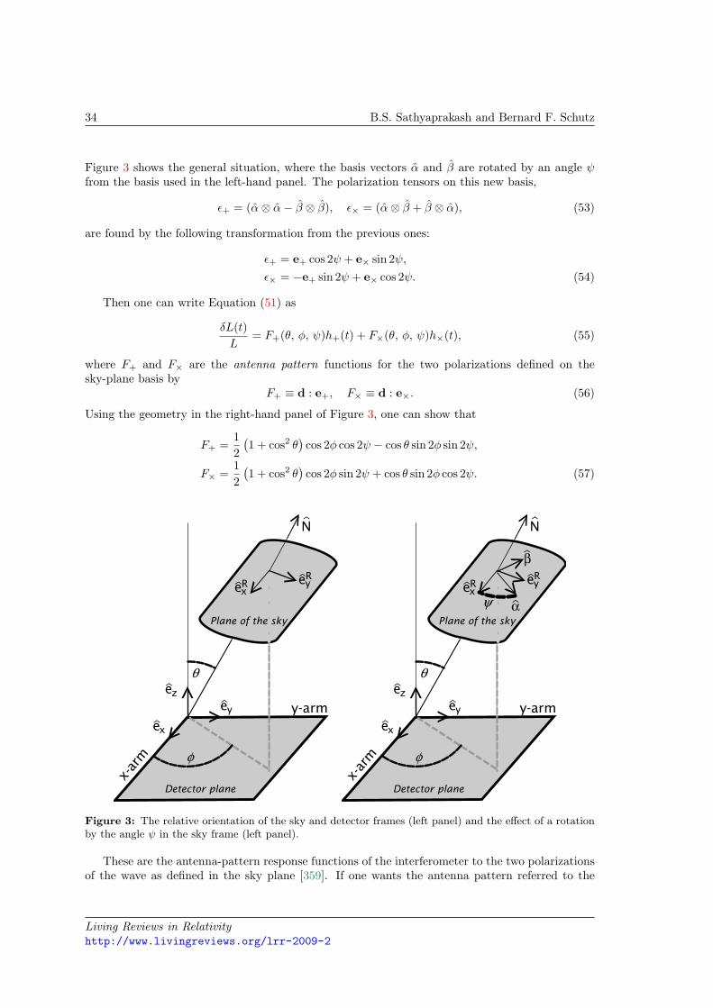
34 B.S. Sathyaprakash and Bernard F. Schutz
Figure 3 shows the general situation, where the basis vectors α and β are rotated by an angle ψfrom the basis used in the left-hand panel. The polarization tensors on this new basis,
ε+ = (α⊗ α− β ⊗ β), ε× = (α⊗ β + β ⊗ α), (53)
are found by the following transformation from the previous ones:
ε+ = e+ cos 2ψ + e× sin 2ψ,ε× = −e+ sin 2ψ + e× cos 2ψ. (54)
Then one can write Equation (51) as
δL(t)L
= F+(θ, φ, ψ)h+(t) + F×(θ, φ, ψ)h×(t), (55)
where F+ and F× are the antenna pattern functions for the two polarizations defined on thesky-plane basis by
F+ ≡ d : e+, F× ≡ d : e×. (56)
Using the geometry in the right-hand panel of Figure 3, one can show that
F+ =12(1 + cos2 θ
)cos 2φ cos 2ψ − cos θ sin 2φ sin 2ψ,
F× =12(1 + cos2 θ
)cos 2φ sin 2ψ + cos θ sin 2φ cos 2ψ. (57)
Figure 3: The relative orientation of the sky and detector frames (left panel) and the effect of a rotationby the angle ψ in the sky frame (left panel).
These are the antenna-pattern response functions of the interferometer to the two polarizationsof the wave as defined in the sky plane [359]. If one wants the antenna pattern referred to the
Living Reviews in Relativityhttp://www.livingreviews.org/lrr-2009-2
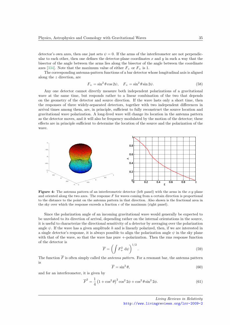
Physics, Astrophysics and Cosmology with Gravitational Waves 35
detector’s own axes, then one just sets ψ = 0. If the arms of the interferometer are not perpendic-ular to each other, then one defines the detector-plane coordinates x and y in such a way that thebisector of the angle between the arms lies along the bisector of the angle between the coordinateaxes [334]. Note that the maximum value of either F+ or F× is 1.
The corresponding antenna-pattern functions of a bar detector whose longitudinal axis is alignedalong the z direction, are
F+ = sin2 θ cos 2ψ, F× = sin2 θ sin 2ψ. (58)
Any one detector cannot directly measure both independent polarizations of a gravitationalwave at the same time, but responds rather to a linear combination of the two that dependson the geometry of the detector and source direction. If the wave lasts only a short time, thenthe responses of three widely-separated detectors, together with two independent differences inarrival times among them, are, in principle, sufficient to fully reconstruct the source location andgravitational wave polarization. A long-lived wave will change its location in the antenna patternas the detector moves, and it will also be frequency modulated by the motion of the detector; theseeffects are in principle sufficient to determine the location of the source and the polarization of thewave.
−1
−0.5
0
0.5
1
−1
−0.5
0
0.5
1−1
−0.5
0
0.5
1
0 0.2 0.4 0.6 0.8 1ε
0
0.2
0.4
0.6
0.8
1
A
0 0.2 0.4 0.6 0.8 10
0.2
0.4
0.6
0.8
1
Figure 4: The antenna pattern of an interferometric detector (left panel) with the arms in the x-y planeand oriented along the two axes. The response F for waves coming from a certain direction is proportionalto the distance to the point on the antenna pattern in that direction. Also shown is the fractional area inthe sky over which the response exceeds a fraction ε of the maximum (right panel).
Since the polarization angle of an incoming gravitational wave would generally be expected tobe unrelated to its direction of arrival, depending rather on the internal orientations in the source,it is useful to characterize the directional sensitivity of a detector by averaging over the polarizationangle ψ. If the wave has a given amplitude h and is linearly polarized, then, if we are interested ina single detector’s response, it is always possible to align the polarization angle ψ in the sky planewith that of the wave, so that the wave has pure +-polarization. Then the rms response functionof the detector is
F =(∫
F 2+ dψ
)1/2
. (59)
The function F is often simply called the antenna pattern. For a resonant bar, the antenna patternis
F = sin2 θ, (60)
and for an interferometer, it is given by
F2
=14(1 + cos2 θ
)2cos2 2φ+ cos2 θ sin2 2φ. (61)
Living Reviews in Relativityhttp://www.livingreviews.org/lrr-2009-2
36 B.S. Sathyaprakash and Bernard F. Schutz
The antenna pattern of an interferometric detector is plotted in the left panel of Figure 4, whichclearly shows the quadrupolar nature of the detector. Note that the response of an interferometeris the best for waves coming from a direction orthogonal to the plane containing the detector, andit is zero for waves in the plane of an interferometer’s arms (i.e., θ = π/2) that arrive from adirection bisecting the two arms (i.e., φ = π/4) or from directions differing from this by a multipleof π/2. What is the response of an antenna to a linearly-polarized source at a random location inthe sky? This is given by the rms value of F over the sky,[
14π
∫F
2sin θ dθ dφ
]1/2
, (62)
which is smaller than the maximum response by a factor of 2/√
15 (52%) for a bar detector andby√
2/5 (63%) for an interferometer.The polarization amplitudes of the radiation from an inspiraling binary, a rotating neutron
star, or a ringing black hole, take a simple form as follows:
h+ =h0
2(1 + cos2 ι
)cos Φ(t), h× = h0 cos ι sinΦ(t),
where h0 is an overall (possibly time-dependent) amplitude, Φ(t) is the signal’s phase and ι isthe angle made by the characteristic direction in the source (e.g., the orbital or the spin angularmomentum) with the line of sight. In this case, the response takes a particularly simple form:
h(t) = F+h+ + F×h× = Ah0 cos(Φ(t)− Φ0), (63)
where
A =(A2
+ +A2×)1/2
, tanΦ0 =A×A+
, A+ =12F+(1 + cos ι2), A× = F× cos ι.
Note that A, just as F , takes values in the range [0, 1]. In this case the average response hasto be worked out by considering all possible sky locations, polarizations (which drops out of thecalculation) and source orientations. More precisely, the rms response is
A =1
8π2
∫ π
0
sin ιdι∫ π
0
sin θ dθ∫ 2π
0
dϕ(A2
+ +A2×). (64)
For an interferometer the above integral gives 2/5. Thus, the rms response is still 40% of the peakresponse.
The right-hand panel of Figure 4 shows the percentage area of the sky over which the antennapattern of an interferometric detector is larger than a certain fraction ε of the peak value. Theresponse is better than the rms value over 40% of the sky, implying that gravitational wave detectorsare fairly omni-directional. In comparison, the sky coverage of most conventional telescopes (radio,infrared, optical, etc.) is a tiny fraction of the area of the sky.
4.3 Practical issues of ground-based interferometers
A detector with an arm length of 4 km responds to a gravitational wave with an amplitude of10−21 with
δlgw ∼ hl ∼ 4× 10⁻¹⁸ m.
Light takes only about 10−5 s to go up and down one arm, much less than the typical period ofgravitational waves of interest. Therefore, it is beneficial to arrange for the light to remain in an
Living Reviews in Relativityhttp://www.livingreviews.org/lrr-2009-2
Physics, Astrophysics and Cosmology with Gravitational Waves 37
arm longer than this, say for 100 round trips. This increases its effective path length by 100 andhence the shift in the position of a given phase of the light beam will be of order 10−16 m. Mostinterferometers keep the light in the arms for this length of time by setting up optical cavities inthe arms with low-transmissivity mirrors; these are called Fabry–Perot cavities.
The main sources of noise against which a measurement must compete are:
1. Ground vibration. External mechanical vibrations must be screened out. These are aproblem for bar detectors, too, but are more serious for interferometers, not least becauseinterferometers bounce light back and forth between the mirrors, and so each reflectionintroduces further vibrational noise. Suspension/isolation systems are based on pendulums.A pendulum is a good mechanical filter for frequencies above its natural frequency. Byhanging the mirrors on pendulums of perhaps 0.5 m length, one achieves filtering above a fewHertz. Since the spectrum of ground noise falls at higher frequencies, this provides suitableisolation. But these systems can be very sophisticated; the GEO600 [143] detector has athree-stage pendulum and other vibration isolation components [291]. The most ambitiousmulti-stage isolation system has been developed for the Virgo detector [175].
2. Thermal noise. Vibrations of the mirrors and of the suspending pendulum can maskgravitational waves. As with vibrational noise, this is increased by the bouncing of the lightbetween the mirrors. Opposite to bars, interferometers perform measurements at frequenciesfar from the resonant frequency, where the amplitude of thermal vibration is largest. Thus,the pendulum suspensions have thermal noise at a few Hertz, so measurements will be madeabove 40 Hz in the first detectors. Internal vibrations of the mirrors have natural frequenciesof several kHz, which sets an effective upper limit to the observing band. By ensuring thatboth kinds of oscillations have very high Q, one can confine most of the vibration energy toa small bandwidth around the resonant frequency, so that at the measurement frequenciesthe vibration amplitudes are extremely small. This allows interferometers to operate atroom temperature. But mechanical Qs of 107 or higher are required, and this is technicallydemanding.
Thermal effects produce other disturbances besides vibration. Some of the mirrors in inter-ferometers are partly transmissive, as is the beam splitter. A small amount of light poweris absorbed during transmission, which raises the temperature of the mirror and changes itsindex of refraction. The resulting “thermal lensing” can ruin the optical properties of thesystem, and random fluctuations in lensing caused by time-dependent thermal fluctuations(thermo-refractive noise) can appear at measurement frequencies. These effects can limitthe amount of laser power that can be used in the detector. Other problems can arise fromheating effects in the multiple-layer coatings that are applied to the reflective surfaces ofmirrors.
3. Shot noise. The photons that are used to do interferometry are quantized, and so theyarrive at random and make random fluctuations in the light intensity that can look like agravitational wave signal. The more photons one uses, the smoother the interference signalwill be. As a random process, the error improves with the square root of the number N ofphotons. Using infrared light with a wavelength λ ∼ 1 µm, one can expect to measure to anaccuracy of
δlshot ∼ λ/(2π√N).
To measure at a frequency f , one has to make at least 2f measurements per second, so onecan accumulate photons for a time 1/2f . With light power P , one gets N = P/(hc/λ)/(2f)photons. In order that δlshot should be below 10−16 m, one needs high light power, farbeyond the output of any continuous laser.
Living Reviews in Relativityhttp://www.livingreviews.org/lrr-2009-2
38 B.S. Sathyaprakash and Bernard F. Schutz
Light-recycling techniques overcome this problem, by using light efficiently. An interferometeractually has two places where light leaves. One is where the interference is measured, thedifference port. The other is the sum of the two return beams on the beam splitter, which goesback towards the input laser. Normally one makes sure that no light hits the interferencesensor, so that only when a gravitational wave passes does a signal register there. Thismeans that all the light normally returns toward the laser input, apart from small losses atthe mirrors. Since mirrors are of good quality, only one part in 103 or less of the light is lostduring a 1 ms storage time. By placing a power-recycling mirror in front of the laser, one canreflect this wasted light back in, allowing power to build up in the arms until the laser merelyresupplies the mirror losses [149]. This can dramatically reduce the power requirement forthe laser. The first interferometers work with laser powers of 5 – 10 W. Upgrades will use tenor more times this input power.
4. Quantum effects. Shot noise is a quantum noise, and like all quantum noises there is acorresponding conjugate noise. As laser power is increased to reduce shot noise, the positionsensing accuracy improves, and one eventually comes up against the Heisenberg uncertaintyprinciple: the momentum transferred to the mirror by the measurement leads to a disturbancethat can mask a gravitational wave. To reduce this backaction pressure fluctuation, scientistsare experimenting with a variety of interferometer configurations that modify the quantumstate of the light, by “squeezing” the Heisenberg uncertainty ellipse, in order to reduce theeffect of this uncertainty on the variable being measured, at the expense of its (unmeasured)conjugate. The key point here is that we are using a quantum field (light) to measurean effectively classical quantity (gravitational wave amplitude), so we do not need to knoweverything about our quantum system: we just need to reduce the uncertainty in that part ofthe quantum field that responds to the gravitational wave at the readout of our interferometer.The best results on squeezing so far [371] have been obtained during preparations for theGEO-HF upgrade of the GEO600 detector [395]. These techniques may be needed for thesecond-generation advanced detectors and will certainly be needed for advances beyond that.
5. Gravity gradient noise. One noise that cannot be screened out is that due to changes inthe local Newtonian gravitational field on the timescale of the measurements. A gravitationalwave detector will respond to tidal forces from local sources just as well as to gravitationalwaves. Environmental noise comes not only from man-made sources, but even more impor-tantly from natural ones: seismic waves are accompanied by changes in the gravitationalfield, and changes in air pressure are accompanied by changes in air density. The spectrumfalls steeply with increasing frequency, so for first-generation interferometers this will not bea problem, but it may limit the performance of more advanced detectors. And it is the pri-mary reason that detecting gravitational waves in the low-frequency band below 1 Hz mustbe done in space.
4.3.1 Interferometers around the globe
The two largest interferometer projects are LIGO [302] and VIRGO [175]. LIGO has built threedetectors at two sites. At Hanford, Washington, there is a 4 km and a 2 km detector in the samevacuum system. At Livingston, Louisiana, there is a single 4 km detector, oriented to be as nearlyparallel to the Hanford detector as possible. After a series of “engineering” runs, which helped todebug the instruments, interspersed with several “science runs”, which helped to test and debugthe data acquisition system and various analysis pipelines, LIGO reached its design sensitivity goalin the final months of 2005. In November 2005, LIGO began a two-year data-taking run, calledS5, which acquired a year’s worth of triple coincidence data among the three LIGO detectors. S5ended on 30 September 2007. Although interferometers are pretty stable detectors, environmental
Living Reviews in Relativityhttp://www.livingreviews.org/lrr-2009-2
Physics, Astrophysics and Cosmology with Gravitational Waves 39
disturbances and instrumental malfunctions can cause them to lose lock during which the dataquality will be either poor or ill defined. The typical duty cycle at one of the LIGO sites is about80%, and hence about two years of operation was required to accumulate a year’s worth of triplecoincident data. Up to date information on LIGO can be found on the project’s website [103]. Arecent review of LIGO’s status is [303].
VIRGO finished commissioning its single 3-km detector at Cascina, near Pisa, in early 2007and began taking data in coincidence with LIGO in May 2007, thus joining for the last part ofS5. VIRGO is a collaboration among research laboratories in Italy and France, and its umbrellaorganization EGO looks after the operation of the site and planning for the future. There arewebsites for both VIRGO [380] and EGO [152]. A recent review of VIRGO’s status is [20].
A smaller 600-m detector, GEO600, has been operational near Hanover, Germany, since 2001[143]. It is a collaboration among research groups principally in Germany and Britain. Althoughsmaller, GEO600 has developed and installed second-generation technology (primarily in its suspen-sions, mirror materials and interferometer configuration) that help it achieve a higher sensitivity.GEO600 technology is being transferred to LIGO and VIRGO as part of their planned upgrades,described below. Full information about GEO can be found on its website [261]. A recent reviewof GEO600’s status is [396].
LIGO and GEO have worked together under the umbrella of the LIGO Scientific Collaboration(LSC) since the beginning of science data runs in 2001. The LSC contains dozens of groups fromuniversities around the world, which contribute to data analysis and technology development. Thetwo detector groups pool their data and analyze it jointly. The LSC has a website containingdetailed information, and providing access to the publications and open-source software of thecollaboration [236].
VIRGO has signed an agreement with the LSC to pool data and analyze it jointly, therebycreating a single worldwide network of long-baseline gravitational wave detectors. VIRGO is not,however, a member of the LSC.
The LSC has already published many papers on the analysis of data acquired during its scienceruns, and many more can be expected. The results from these science runs, which will be discussedlater, are already becoming astrophysically interesting. The LSC maintains a public repository ofits papers and contributions to conference proceedings [237].
For instance, although the search for continuous waves from known pulsars has not found anydefinitive candidates, it has been possible to set stringent upper limits ε ≤ few × 10−6 on themagnitude of the ellipticity of some of these systems [10]. In particular, in the case of the Crabpulsar, gravitational wave observations have begun to improve [12] the upper limit on the strengthof radiation obtained by radio observations of the spin-down rate.
A yet smaller detector in Japan, TAMA300 [362], with 300 m arms, was the first large-scaleinterferometer to achieve continuous operation, at a sensitivity of about 10−19 – 10−20. TAMA isseen as a development prototype, and its sensitivity will be confined to higher frequencies (above∼ 500 Hz). An ambitious follow-on detector called the Large-scale Cryogenic Gravitational-WaveTelescope (LCGT) is being planned in Japan, and, as its name suggests, it will be the first touse cooled mirrors to reduce the effects of thermal noise. TAMA [269] and the LCGT [268] havewebsites where one can get more information. A recent review of TAMA’s status is [130].
There are plans for a detector in Australia, and a small interferometer is operating in WesternAustralia [252]. The Australian Interferometric Gravitational Observatory (AIGO) [368] is a pro-posal of the Australian Consortium for Interferometric Gravitational Astronomy (ACIGA) [56].The ACIGA collaboration is a member of the LSC and assists in mirror and interferometry devel-opment, but it is not yet clear whether and when a larger detector might be funded. From thepoint of view of extracting information from observations, it is very desirable to have large-scaledetectors in Japan and Australia, because of their very long baselines to the USA and Europe.But the future funding of both LCGT and AIGO is not secure as of this writing (2008).
Living Reviews in Relativityhttp://www.livingreviews.org/lrr-2009-2
40 B.S. Sathyaprakash and Bernard F. Schutz
The initial sensitivity levels achieved by LIGO, VIRGO, and GEO are just the starting point.Detailed plans exist for upgrades for all three projects. In October 2007, both LIGO and VIRGObegan upgrading to enhanced detectors, which should improve on LIGO’s S5 sensitivity by a factorof roughly two. These should come online in 2009. After a further observing run, called S6, thedetectors will again shut down for a much more ambitious upgrade to advanced detectors, tooperate around 2014. This will provide a further factor of five in sensitivity, and hence in range.Altogether the two upgrades will extend the volume of space that can be surveyed for gravitationalwaves by a factor of 1000, and this will make regular detections a virtual certainty. AdvancedLIGO has a website giving the plans for the upgrade in the context of development from the initialsensitivity [235].
GEO600 will remain in science mode during the upgrade to enhanced detectors, just in case anearby supernova or equally spectacular event should occur when the larger detectors are down.But, when the enhanced detectors begin operating, GEO will upgrade to GEO-HF [395], a mod-ification designed to improve its sensitivity in the high-frequency region above 1 kHz, where itsshort arm length does not prevent it being competitive with the larger instruments. GEO is alsoa partner in the Advanced LIGO project, contributing high-power lasers and high-Q suspensionsfor controlling thermal noise.
Beyond that, scientists are now studying the technologies that may be needed for a furtherlarge step in sensitivity to third-generation detectors. This may involve cooling mirrors, usingultra-massive substrates of special materials, using purely nontransmissive optics, and even cir-cumventing the quantum limit in interferometers, as has been studied for bars. The goal of third-generation detectors would be to be limited just by gravity-gradient noise and quantum effects. Adesign study for a concept called the “Einstein Telescope” started in Europe in 2008.
4.3.2 Very-high–frequency detectors
The gravitational wave spectrum above the detection band of conventional interferometers, sayabove 10 kHz, may not be empty, and stochastic gravitational waves from the Big Bang may bepresent up to megaHertz frequencies and beyond. It is exceedingly difficult to build sensitive detec-tors at these high frequencies, but two projects have made prototypes: a microwave-based detectorthat senses the change in polarization as the electromagnetic waves follow a waveguide circuit asa gravitational wave passes by [126], and a more conventional light-based interferometer [23].
4.4 Detection from space
Space offers two important ingredients for beam detectors: long arms and a free vacuum. In thissection, we describe the three ways that space has been and will be used for gravitational wavedetection: ranging to spacecraft (Section 4.4.1), pulsar timing (Section 4.4.2), and direct detectionusing space-based interferometers (Section 4.4.3).
4.4.1 Ranging to spacecraft
Both NASA and ESA perform experiments in which they monitor the return time of communi-cation signals with interplanetary spacecraft for the characteristic effect of gravitational waves.For missions to Jupiter and Saturn, for example, the return times are of order 2 – 4 × 10³ s. Anygravitational wave event shorter than this will, by Equation (43), appear three times in the timedelay: once when the wave passes the Earth-based transmitter, once when it passes the spacecraft,and once when it passes the Earth-based receiver. Searches use a form of data analysis usingpattern matching. Using two transmission frequencies and very stable atomic clocks, it is possibleto achieve sensitivities for h of order 10−13, and even 10−15 may soon be reached [40].
Living Reviews in Relativityhttp://www.livingreviews.org/lrr-2009-2
Physics, Astrophysics and Cosmology with Gravitational Waves 41
4.4.2 Pulsar timing
Many pulsars, particularly the old millisecond pulsars, are extraordinarily regular clocks whenaveraged over timescales of a few years, with random timing irregularities too small for the bestatomic clocks to measure. If one assumes that they emit pulses perfectly regularly, then one canuse observations of timing irregularities of single pulsars to set upper limits on the backgroundgravitational-wave field. Here, the one-way formula Equation (42) is appropriate. The transittime of a signal to the Earth from the pulsar may be thousands of years, so we cannot look forcorrelations between the two terms in a given signal. Instead, the delay is a combination of theeffects of waves at the pulsar when the signal was emitted and waves at the Earth when it isreceived. If one observes a single pulsar, then because not enough is known about the intrinsicirregularity in pulse emission, the most one can do is to set upper limits on a background ofgravitational radiation at very low frequencies [242, 344].
If one simultaneously observes two or more pulsars, then the Earth-based part of the delay iscorrelated, and this offers, in addition, a means of actually detecting strong gravitational waveswith periods of several years that pass the Earth (in order to achieve the long-period stabilityof pulse arrival times). Observations are currently underway at a number of observatories. Themost stringent limits to date are from the Parkes Pulsar Timing Array [208], which sets an upperlimit on a stochastic background of Ωgw ≤ 2 × 10⁻⁸. Two further collaborations for timing havebeen formed: the European Pulsar Timing Array (EPTA) [345] and NanoGrav [39]. Astrophysicalbackgrounds in this frequency band are likely (see Section 8.2.2), so these arrays have a goodchance of making early detections. Future timing experiments will be even more powerful, usingnew phased arrays of radio telescopes that can observe many pulsars simultaneously, such as theLow Frequency Array (LOFAR) [156] and the Square Kilometer Array [107].
Pulsar timing can also be used to search for individual events, not just a stochastic signal. Thefirst example of an upper limit from such a search was the exclusion of a black-hole–binary modelfor 3C66B [209].
4.4.3 Space interferometry
Gravity-gradient noise on the Earth is much larger than the amplitude of any expected waves fromastronomical sources at frequencies below about 1 Hz, but this noise falls off rapidly as one movesaway from the Earth. A detector in space would not notice the Earth’s noisy environment. TheLaser Interferometer Space Antenna (LISA) project, currently being developed in collaborationby ESA and NASA with a view toward launching in 2018, would open up the frequency windowbetween 0.1 mHz and 0.1 Hz for the first time [196, 144]. There are several websites that providefull information about this project [24, 153, 266].
We will see below that there are many exciting sources expected in this wave band, for examplethe coalescences of giant black holes in the centers of galaxies. LISA would see such events withextraordinary sensitivity, recording typical SNRs of 1000 or more for events at redshift one.
A space-based interferometer can have arm lengths much greater than a wavelength. LISA, forexample, would have arms 5× 10⁶ km long, and that would be longer than half a wavelength forany gravitational waves above 30 mHz. In this regime, the response of each arm will follow thethree-term formula we encountered earlier. The short-arm approximation we used for ground-basedinterferometers works for LISA only at the lowest frequencies in its observing band.
LISA will consist of three free-flying spacecraft, arranged in an array that orbits the sun at 1 AU,about 20 degrees behind the Earth in its orbit. They form an approximately equilateral trianglein a plane tilted at 60 to the ecliptic, and their simple Newtonian elliptical orbits around the sunpreserve this arrangement, with the array rotating backwards once per year as the spacecraft orbitthe sun. By passing light along each of the arms, one can construct three different Michelson-type interferometers, one for each vertex. With this array one can measure the polarization of
Living Reviews in Relativityhttp://www.livingreviews.org/lrr-2009-2
42 B.S. Sathyaprakash and Bernard F. Schutz
a gravitational wave directly. The spacecraft are too far apart to use simple mirrors to reflectlight back along an arm: the reflected light would be too weak. Instead, LISA will have opticaltransponders: light from one spacecraft’s on-board laser will be received at another, which willthen send back light from its own laser locked exactly to the phase of the incoming signal.
The main environmental disturbances to LISA are forces from the sun: solar radiation pressureand pressure from the solar wind. To minimize these, LISA incorporates drag-free technology.Interferometry is referenced to an internal proof mass that falls freely, unattached to the spacecraft.The job of the spacecraft is to shield this mass from external disturbances. It does this by sensingthe position of the mass and firing its own jets to keep itself (the spacecraft) stationary relativeto the proof mass. To do this, it needs thrusters of very small thrust that have accurate control.The key technologies that have enabled the LISA mission are the availability of such thrusters,accelerometers needed to sense disturbances to the spacecraft, and lasers capable of continuouslyemitting 1 W of infrared light for many years. ESA is planning to launch a satellite called LISAPathfinder to test all of these technologies in 2010 [230].
LISA is not the only proposal for an interferometer in space for gravitational wave detection.The DECIGO proposal is a more ambitious design, positioned at a higher frequency to fill thegap between LISA and ground-based detectors [213]. Even more ambitious, in the same frequencyband, is the Big Bang Observer, a NASA concept study to examine what technology would beneeded to reach the ultimate sensitivity of detecting a gravitational wave background from inflationat these frequencies [267].
4.5 Characterizing the sensitivity of a gravitational wave antenna
The performance of a gravitational wave detector is characterized by the power spectral density(henceforth denoted PSD) of its noise background. One can construct the noise PSD as follows;a gravitational wave detector outputs a dimensionless data train, say x(t), which in the case ofan interferometer is the relative strain in the two arms, scaled to represent the value of h thatwould produce that strain if the wave is optimally oriented with respect to the detector. In theabsence of any gravitational wave signal, the detector output is just an instance of noise n(t), thatis, x(t) = n(t). The noise auto-correlation function κ is defined as
κ ≡ n(t1)n(t2), (65)
where an overline indicates the average over an ensemble of noise realizations. In general, κ dependsboth on t1 and t2. However, if the detector output is a stationary noise process, i.e., its performanceis, statistically speaking, independent of time, then κ depends only on τ ≡ |t1 − t2|.
The assumption of stationarity is not strictly valid in the case of real gravitational-wave detec-tors; however, if their performance doesn’t vary greatly over time scales much larger than typicalobservation time scales, stationarity could be used as a working rule. While this may be goodenough in the case of binary inspiral and coalescence searches, it is a matter of concern for theobservation of continuous and stochastic gravitational waves. In this review, for simplicity, weshall assume that the detector noise is stationary. In this case the one-sided noise PSD, definedonly at positive frequencies, is the Fourier transform of the noise auto-correlation function:
Sh(f) ≡ 12
∫ ∞
−∞κ(τ)e2πifτ dτ, f ≥ 0,
≡ 0, f < 0, (66)
where a factor of 1/2 is included by convention. By using the Fourier transform of n(t), thatis n(f) ≡
∫∞−∞ n(t)e2πift dt, in Equation (65) and substituting the resulting expression in Equa-
Living Reviews in Relativityhttp://www.livingreviews.org/lrr-2009-2
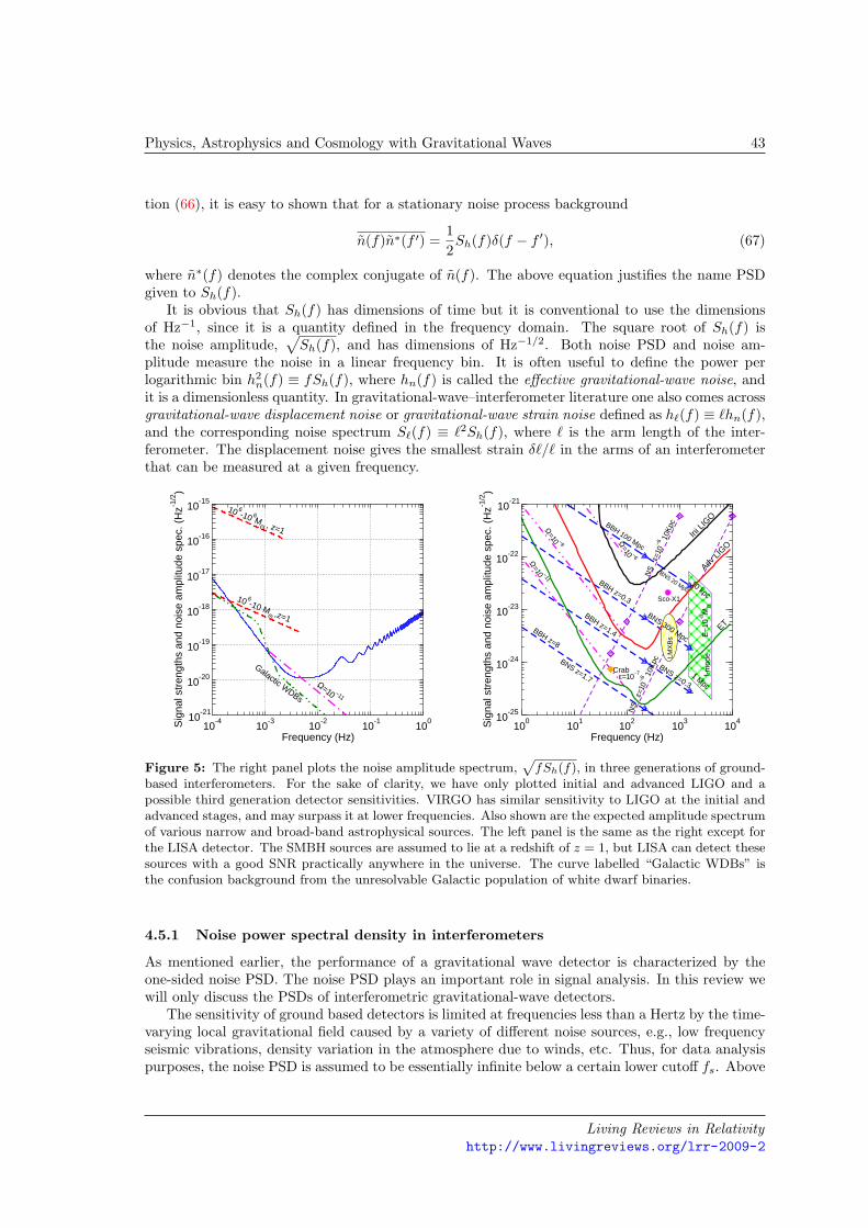
Physics, Astrophysics and Cosmology with Gravitational Waves 43
tion (66), it is easy to shown that for a stationary noise process background
n(f)n∗(f ′) =12Sh(f)δ(f − f ′), (67)
where n∗(f) denotes the complex conjugate of n(f). The above equation justifies the name PSDgiven to Sh(f).
It is obvious that Sh(f) has dimensions of time but it is conventional to use the dimensionsof Hz−1, since it is a quantity defined in the frequency domain. The square root of Sh(f) isthe noise amplitude,
√Sh(f), and has dimensions of Hz−1/2. Both noise PSD and noise am-
plitude measure the noise in a linear frequency bin. It is often useful to define the power perlogarithmic bin h2
n(f) ≡ fSh(f), where hn(f) is called the effective gravitational-wave noise, andit is a dimensionless quantity. In gravitational-wave–interferometer literature one also comes acrossgravitational-wave displacement noise or gravitational-wave strain noise defined as h`(f) ≡ `hn(f),and the corresponding noise spectrum S`(f) ≡ `2Sh(f), where ` is the arm length of the inter-ferometer. The displacement noise gives the smallest strain δ`/` in the arms of an interferometerthat can be measured at a given frequency.
10-4
10-3
10-2
10-1
100
Frequency (Hz)
10-21
10-20
10-19
10-18
10-17
10-16
10-15
Sig
nal s
tren
gths
and
noi
se a
mpl
itude
spe
c. (
Hz-1
/2)
10 6-10 6
MO. , z=1
10 6-10 M
O. ,z=1
Galactic WDBs
Ω=10 −11
100
101
102
103
104
Frequency (Hz)
10-25
10-24
10-23
10-22
10-21
Sig
nal s
tren
gths
and
noi
se a
mpl
itude
spe
c. (
Hz-1
/2)
BBH z=0.3
NS
ε=
10−6 1
0Kpc
Ini L
IGO
Adv L
IGO
Sco-X1
f-m
ode
Ω=10 −11
BBH 100 Mpc
Ω=10 −9
ETBNS 300 Mpc
BBH z=1.4
BNS z=0.3
LMX
Bs
10 kpc
Ω=10 −6
Crabε=10−7
E~
10-8
MO
1 Mpc
BNS 20 Mpc
BBH z=8
BNS z=1.7
NS
ε=
10−8 1
0Kpc
Figure 5: The right panel plots the noise amplitude spectrum,pfSh(f), in three generations of ground-
based interferometers. For the sake of clarity, we have only plotted initial and advanced LIGO and apossible third generation detector sensitivities. VIRGO has similar sensitivity to LIGO at the initial andadvanced stages, and may surpass it at lower frequencies. Also shown are the expected amplitude spectrumof various narrow and broad-band astrophysical sources. The left panel is the same as the right except forthe LISA detector. The SMBH sources are assumed to lie at a redshift of z = 1, but LISA can detect thesesources with a good SNR practically anywhere in the universe. The curve labelled “Galactic WDBs” isthe confusion background from the unresolvable Galactic population of white dwarf binaries.
4.5.1 Noise power spectral density in interferometers
As mentioned earlier, the performance of a gravitational wave detector is characterized by theone-sided noise PSD. The noise PSD plays an important role in signal analysis. In this review wewill only discuss the PSDs of interferometric gravitational-wave detectors.
The sensitivity of ground based detectors is limited at frequencies less than a Hertz by the time-varying local gravitational field caused by a variety of different noise sources, e.g., low frequencyseismic vibrations, density variation in the atmosphere due to winds, etc. Thus, for data analysispurposes, the noise PSD is assumed to be essentially infinite below a certain lower cutoff fs. Above
Living Reviews in Relativityhttp://www.livingreviews.org/lrr-2009-2
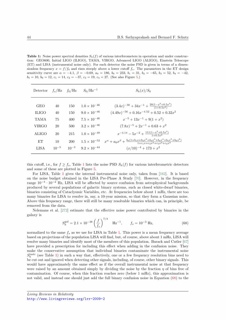
44 B.S. Sathyaprakash and Bernard F. Schutz
Table 1: Noise power spectral densities Sh(f) of various interferometers in operation and under construc-tion: GEO600, Initial LIGO (ILIGO), TAMA, VIRGO, Advanced LIGO (ALIGO), Einstein Telescope(ET) and LISA (instrumental noise only). For each detector the noise PSD is given in terms of a dimen-sionless frequency x = f/f0 and rises steeply above a lower cutoff fs. The parameters in the ET designsensitivity curve are α = −4.1, β = −0.69, a0 = 186, b0 = 233, b1 = 31, b2 = −65, b3 = 52, b4 = −42,b5 = 10, b6 = 12, c1 = 14, c2 = −37, c3 = 19, c4 = 27. (See also Figure 5.)
Detector fs/Hz f0/Hz S0/Hz−1 Sh(x)/S0
GEO 40 150 1.0× 10−46 (3.4x)−30 + 34x−1 + 20(1−x2+0.5x4)(1+0.5x2)
ILIGO 40 150 9.0× 10−46 (4.49x)−56 + 0.16x−4.52 + 0.52 + 0.32x2
TAMA 75 400 7.5× 10−46 x−5 + 13x−1 + 9(1 + x2)
VIRGO 20 500 3.2× 10−46 (7.8x)−5 + 2x−1 + 0.63 + x2
ALIGO 20 215 1.0× 10−49 x−4.14 − 5x−2 + 111(1−x2+0.5x4)1+0.5x2
ET 10 200 1.5× 10−52 xα + a0xβ + b0(1+b1x+b2x2+b3x3+b4x4+b5x5+b6x6)
1+c1x+c2x2+c3x3+c4x4
LISA 10−5 10−3 9.2× 10−44 (x/10)−4 + 173 + x2
this cutoff, i.e., for f ≥ fs, Table 1 lists the noise PSD Sh(f) for various interferometric detectorsand some of these are plotted in Figure 5.
For LISA, Table 1 gives the internal instrumental noise only, taken from [162]. It is basedon the noise budget obtained in the LISA Pre-Phase A Study [70]. However, in the frequencyrange 10−4 – 10−2 Hz, LISA will be affected by source confusion from astrophysical backgroundsproduced by several populations of galactic binary systems, such as closed white-dwarf binaries,binaries consisting of Cataclysmic Variables, etc. At frequencies below about 1 mHz, there are toomany binaries for LISA to resolve in, say, a 10-year mission, so that they form a Gaussian noise.Above this frequency range, there will still be many resolvable binaries which can, in principle, beremoved from the data.
Nelemans et al. [272] estimate that the effective noise power contributed by binaries in thegalaxy is
Sgalh = 2.1× 10−38
(f
fs
)7/3
Hz−1, fs = 10−3 Hz, (68)
normalized to the same fs as we use for LISA in Table 1. This power is a mean frequency averagebased on projections of the population LISA will find, but, of course, above about 1 mHz, LISA willresolve many binaries and identify most of the members of this population. Barack and Cutler [67]have provided a prescription for including this effect when adding in the confusion noise. Theymake the conservative assumption that individual binaries contaminate the instrumental noiseSinstr
h (see Table 1) in such a way that, effectively, one or a few frequency resolution bins need tobe cut out and ignored when detecting other signals, including, of course, other binary signals. Thiswould have approximately the same effect as if the overall instrumental noise at that frequencywere raised by an amount obtained simply by dividing the noise by the fraction η of bins free ofcontamination. Of course, when this fraction reaches zero (below 1 mHz), this approximation isnot valid, and instead one should just add the full binary confusion noise in Equation (68) to the
Living Reviews in Relativityhttp://www.livingreviews.org/lrr-2009-2
Physics, Astrophysics and Cosmology with Gravitational Waves 45
instrumental noise. A smooth way of merging these two regimes is to set
Sfullh = min
(1ηSinstr
h , Sinstrh + Sgal
h
), (69)
where Sinstrh is from Table 1 and Sgal
h is from Equation (68). This prescription uses the contaminatedinstrumental noise, when it is below the total noise power from the binaries, but then uses thetotal binary confusion power when the prescription for allowing for contamination breaks down.
The fraction η of uncontaminated frequency bins as a function of frequency remains to bespecified. Let dN/df be the number of binaries in the galaxy per unit frequency. Since the sizeof the frequency bin for an observation that lasts a time Tobs is 1/Tobs, the expected number ofbinaries per frequency bin is
∆N(f) =1Tobs
dN(f)df
.
Barack and Cutler multiply this by a “fudge factor” κ > 1 to allow for the fact that any binarymay contaminate several bins, so that κ∆N(f) is the expected number of contaminated bins perbinary. If this is small, then it will equal the fractional contamination at frequency f . In that case,the fraction of uncontaminated bins is just 1− κ∆N(f). However, if the expected contaminationper bin approaches or exceeds one, then we have to allow for the fact that the binaries are reallyrandomly distributed in frequency, so that the expected fraction not contaminated comes from thePoisson distribution,
η = exp(−κ∆N). (70)
Inserting this into Equation (69) gives a reasonable approximation to the effective instrumentalnoise if binaries cannot be removed in a clean way from the data stream when looking for othersignals.
Because LISA will observe binaries for several years, the accuracy with which it will know thefrequency, say, of a binary, will be much better than the frequency resolution of LISA during theobservation of a transient source, such as many of the IMBH events considered by Barack andCutler. Therefore, there is a good chance that, in the global LISA data analysis, the effective noisecan be reduced below the one-year noise levels that are normally used in projecting the sensitivityof LISA and the science it can do.
4.5.2 Sensitivity of interferometers in units of energy flux
In radio astronomy one talks about the sensitivity of a telescope in terms of the limiting detectableenergy flux from an astronomical source. We can do the same here too. Given the gravitationalwave amplitude h we can use Equation (17) to compute the flux of gravitational waves. One cantranslate the noise power spectrum Sh(f), given in units of Hz−1 at frequency f , to Jy (Jansky),with the conversion factor 4c3f2/(πG). In Figure 6, the left panel shows the noise power spectrumin astronomical units of Jy and the right panel depicts the noise spectrum in units of Hz−1 togetherwith lines of constant flux.
What is striking in Figure 6 is the magnitude of flux. While modern radio interferometers aresensitive to flux levels of milli and micro-Jy the gravitational wave interferometers need their sourcesto be 24 – 27 orders of magnitude brighter. Turning this argument around, the gravitational wavesources we expect to observe are not really weak, but rather extremely bright sources. The difficultyin detecting them is due to the fact that gravitation is the weakest of all known interactions.
4.6 Source amplitudes vs sensitivity
How does one compare the gravitational wave amplitude of astronomical sources with the instru-mental sensitivity and assess what sort of sources will be observable against noise? Comparisons
Living Reviews in Relativityhttp://www.livingreviews.org/lrr-2009-2
46 B.S. Sathyaprakash and Bernard F. Schutz
101
102
103
Frequency (Hz)
1018
1019
1020
1021
1022
(π/4
) f2 S
h(f)
(Jy)
VIRGOIni. LIGOAdv. LIGO
101
102
103
Frequency (Hz)
10-48
10-47
10-46
10-45
10-44
10-43
10-42
Sh(f
) (H
z-1)
VIRGOIni. LIGOAdv. LIGO
Flux=10 20Jy
Flux=10 22Jy
Flux=10 18Jy
Figure 6: The sensitivity of interferometers in terms of the limiting energy flux they can detect, Jy/Hz,(left panel) and in terms of the gravitational wave amplitude with lines of constant flux levels (right panel).
are almost always made in the frequency domain, since stationary noise is most conveniently char-acterized by its PSD.
The simplest signal to characterize is a long-lasting periodic signal with a given fixed frequencyf0. In an observation time T, all the signal power |h(f0)|2 is concentrated in a single frequency bin ofwidth 1/T . The noise against which it competes is just the noise power in the same bin, Sh(f0)/T .The power SNR is then T |h(f0)|2/Sh(f0), and the amplitude SNR is
√T |h(f0)|/|Sh(f0)|1/2. This
improves with observation time as the square root of the time. The reason for this is that the noiseis stationary, but longer and longer observation times permit the signal to compete only with noisein smaller and smaller frequency windows.
Of course, no expected gravitational-wave signal would have a single fixed frequency in thedetector frame, because the detector is attached to the Earth, whose motion produces frequencymodulations. But the principle of this SNR increase with time can still be maintained if one hasa signal model that allows one to exclude more and more noise from competing with the signalover longer and longer periods of time. This happens with matched filtering, which we return toin Section 5.
Short-lived signals have wider bandwidths, and long observation times are not relevant. To char-acterize their SNR, it is useful to define the dimensionless noise power per logarithmic bandwidth,fSh(f), which we earlier called h2
n(f). The signal Fourier amplitude h(f) ≡∫∞−∞ dt h(t)e2πift has
dimensions of Hz−1 and so the Fourier amplitude per logarithmic frequency, which is called thecharacteristic signal amplitude hc = f |h(f)|, is dimensionless. This quantity should be comparedwith hn(f) to obtain a rough estimate of the SNR of the signal: SNR ∼ hc/hn.
4.7 Network detection
Gravitational wave detectors are almost omni-directional. As discussed in Section 4.2.1, both inter-ferometers and bars have good sensitivity over a large area of the sky. In this regard, gravitationalwave antennas are unlike conventional astronomical telescopes, e.g., optical, radio, or infraredbands, which observe only a very small fraction of the sky at any given time. The good newsis that gravitational wave interferometers will have good sky coverage and therefore only a smallnumber (around six) are enough to survey the sky. The bad news, however, is that gravitationalwave observations will not automatically provide the location of the source in the sky. It will either
Living Reviews in Relativityhttp://www.livingreviews.org/lrr-2009-2

Physics, Astrophysics and Cosmology with Gravitational Waves 47
be necessary to observe the same source in several non–co-located detectors and triangulate theposition of the source using the information from the delay in the arrival times of the signals todifferent detectors, or observe for a long time and use the location-dependent Doppler modulationcaused by the motion of the detector relative to the source to infer the source’s position in the sky.The latter is a well-known technique in radio astronomy of synthesizing a long-baseline observa-tion to gain resolution, and only possible for sources, such as rotating neutron stars or stochasticbackgrounds, that last for a long enough duration.
A network of detectors is, therefore, essential for source reconstruction. Network observationis not only powerful in identifying a source in the sky, but independent observation of the samesource in several detectors adds to the detection confidence, especially since the noise backgroundin the first generation of interferometers is not well understood and is plagued by nonstationarityand non-Gaussianity.
4.7.1 Coherent vs coincidence analysis
The availability of a network of detectors offers two different methods by which the data can becombined. One can either first bring the data sets together, combine them in a certain way, andthen apply the appropriate filter to the network data and integrate the signal coherently, coherentdetection [282, 87, 160, 41], or first analyze the data from each detector separately by applying therelevant filters and then look for coincidences in the multi-dimensional space of intrinsic (massesof the component stars, their spins, . . .) and extrinsic (arrival times, a constant phase, sourcelocation, . . .) parameters, coincidence detection [205, 207, 160, 42, 353, 2, 6, 7, 8].
A recent comparison of coherent analysis vis-a-vis coincidence analysis under the assumptionthat the background noise is Gaussian and stationary has concluded that coherent analysis, as onemight expect, is far better than coincidence analysis [263]. These authors also explore, to a limitedextent, the effect of nonstationary noise and reach essentially the same conclusion.
At the outset, coherent analysis sounds like a good idea, since in a network of ND similardetectors the visibility of a signal improves by a factor of
√ND over that of a single detector. One
can take advantage of this enhancement in SNR to either lower the false alarm rate by increasingthe detection threshold, while maintaining the same detection efficiency, or improve detectionefficiency at a given false alarm rate.
However, there are two reasons that current data-analysis pipelines prefer coincidence anal-ysis over coherent analysis. Firstly, since the detector noise is neither Gaussian nor stationary,coincidence analysis can potentially reduce the background rate far greater than one might thinkotherwise. Secondly, coherent analysis is computationally far more expensive than coincidenceanalysis and it is presently not practicable to employ coherent analysis.
Coincidence analysis is indeed a very powerful method to veto out spurious events. One canassociate with each event in a given detector an ellipsoid, whose location and orientation dependson where in the parameter space and when the event was found, and the SNR can be used tofix the size of the ellipsoid [314]. One is associating with each event a ‘sphere’ of influence in themulti-dimensional space of masses, spins, arrival times, etc., and there is a stringent demand thatthe spheres associated with events from different detectors should overlap each other in order toclaim a detection. Since random triggers from a network of detectors are less likely to be consistentwith one another, this method serves as a very powerful veto.
It is probably not possible to infer beforehand which method might be more effective in detectinga source, as this might depend on the nature of the detector noise, on how the detection statistic isconstructed, etc. An optimal approach might be a suitable combination of both of these methods.For instance, a coherent follow-up of a coincidence analysis (as is currently done by searches forcompact binaries within the LSC) or to use coincidence criteria on candidate events from a coherentsearch.
Living Reviews in Relativityhttp://www.livingreviews.org/lrr-2009-2
48 B.S. Sathyaprakash and Bernard F. Schutz
Coherent addition of data improves the visibility of the signal, but ‘coherent subtraction’ ofthe data in a detector network should lead to data products that are devoid of gravitational wavesignals. This leads us naturally to the introduction of the null stream veto.
4.7.2 Null stream veto
Data from a network of detectors, when suitably shifted in time and combined linearly with co-efficients that depend on the source location, will yield a time series that, in the ideal case, willbe entirely be devoid of the gravitational signal. Such a combination is called a null stream. Forinstance, for a set of three misaligned detectors, each measuring a data stream xk(t), k = 1, 2, 3,the combination x(t) = A23(θ, ϕ)h1(t+τ1)+A31(θ, ϕ)h2(t+τ2)+A12(θ, ϕ)h3(t+τ3), where Aij arefunctions of the responses of the antennas i and j, and τk’s, k = 1, 2, 3, are time delays that dependon the source location and the location of the antenna, is a null stream. If xk(t), k = 1, 2, 3, containa gravitational wave signal from an astronomical source, then x(t) will not contain the signature ofthis source. In contrast, if x(t) and xk(t) both contain the signature of a gravitational wave event,then that is an indication that one of the detectors has a glitch.
The existence and usefulness of a null stream was first pointed out by Gursel and Tinto [184].Wen and Schutz [390] proposed implementing it in LSC data analysis as a veto, and this has beentaken up now by several search groups.
4.7.3 Detection of stochastic signals by cross-correlation
Stochastic background sources and their detection is discussed in more detail in Section 8. Here wewill briefly mention the problem in the context of detector networks. As mentioned in Section 3.6,the universe might be filled with stochastic gravitational waves that were either generated in theprimeval universe or by a population of background sources. For point sources, although eachsource in a population might not be individually detectable, they could collectively produce aconfusion background via a random superposition of the waves from that population. Since thewaves are random in nature, it is not possible to use the techniques described in Sections 4.7.1,4.7.2 and 5.1 to detect a stochastic background. However, we might use the noisy stochastic signalin one of the detectors as a “matched-filter” for the data in another detector [359, 163, 27, 91].In other words, it should be possible to detect a stochastic background by cross-correlating thedata from a pair of detectors; the common gravitational-wave background will grow in time morerapidly than the random backgrounds in the two instruments, thereby facilitating the detection ofthe background.
If two instruments with identical spectral noise density Sh are cross-correlated over a bandwidth∆f for a total time T , the spectral noise density of the output is reduced by a factor of (T∆f)1/2.Since the noise amplitude is proportional to the square root of Sh, the amplitude of a signal thatcan be detected by cross-correlation improves only with the fourth root of the observing time. Thisshould be compared with the square root improvement that matched filtering gives.
The cross-correlation technique works well when the two detectors are situated close to oneanother. When separated, only those waves whose wavelength is larger than or comparable tothe distance between the two detectors, or which arrive from a direction perpendicular to theseparation between the detectors, can contribute coherently to the cross-correlation statistic. Sincethe instrumental noise builds up rapidly at lower frequencies, detectors that are farther apart areless useful in cross-correlation. However, very near-by detectors (as in the case of two LIGOdetectors within the same vacuum tube in Hanford) will suffer from common background noisefrom the control system and the environment, making it rather difficult to ascertain if any excessnoise is due to a stochastic background of gravitational waves.
Living Reviews in Relativityhttp://www.livingreviews.org/lrr-2009-2
Physics, Astrophysics and Cosmology with Gravitational Waves 49
4.8 False alarms, detection threshold and coincident observation
Gravitational-wave event rates in initial interferometers is expected to be rather low: about a fewper year. Therefore, one has to set a high threshold, so that the noise-generated false alarmsmimicking an event are negligible.
For a detector output sampled at 1 kHz and processed through a large number of filters, say103, one has ∼ 3 × 10¹³ instances of noise in a year. If the filtered noise is Gaussian, then theprobability P (x) of observing an amplitude in the range of x to x+ dx is
P (x) dx =1√2πσ
exp(−x2
2σ2
)dx, (71)
where σ is the standard deviation. The above probability-distribution function implies that theprobability that the noise amplitude is greater than a given threshold η is
P (x|x ≥ η) =∫ ∞
η
P (x) dx =1√2πσ
∫ ∞
η
exp(−x2
2σ2
)dx. (72)
Demanding that no more than one noise-generated false alarm occur in a year’s observation meansthat P (x|x ≥ η) = 1/(3 × 1013). Solving this equation for η, one finds that η ' 7.5σ in orderthat false alarms are negligible in a year’s observation. Therefore, a source is detectable only if itsamplitude is significantly larger than the effective noise amplitude, i.e., fh(f) hn(f).
The reason for accepting only such high-sigma events is that the event rate of a transient source,i.e., a source lasting for a few seconds to minutes, such as a binary inspiral, could be as low as a fewper year, and the noise generated false alarms, at low SNRs ∼ 3–4, over a period of a year, tend tobe quite large. Setting higher thresholds for detection helps in removing spurious, noise generatedevents. However, signal enhancement techniques (cf. Section 5) make it possible to detect a signalof relatively low amplitude, provided there are a large number of wave cycles and the shape of thewave is known accurately.
Real detector noise is neither Gaussian nor stationary and therefore the filtered noise cannotbe expected to obey these properties either. One of the most challenging problems is how toremove or veto the false alarm generated by a non-Gaussian and/or nonstationary background.There has been some effort to address the issue of non-Gaussianity [124] and nonstationarity [260];more work is needed in this direction. However, it is expected that the availability of a networkof gravitational wave detectors alleviates the problem to some extent. This is because a highamplitude gravitational wave event will be coincidentally observed in several detectors, althoughnot necessarily with the same SNR, while false alarms are, in general, not coincident, as they arenormally produced by independent sources located close to the detectors.
We have seen that coincident observations help to reduce the false alarm rate significantly. Therate can be further reduced, and possibly even nullified, by subjecting coincident events to furtherconsistency checks in a detector network consisting of four or more detectors. As discussed inSection 2, each gravitational wave event is characterized by five kinematic (or extrinsic) observables:location of the source with respect to the detector (D, θ, ϕ) and the two polarizations (h+, h×).Each detector in a network measures a single number, say the amplitude of the wave. In addition,in a network of N detectors, there are N − 1 independent time delays in the arrival times of thewave at various detector locations, giving a total of 2N − 1 observables. Thus, the minimumnumber of detectors needed to reconstruct the wave and its source is N = 3. More than threedetectors in a network will have redundant information that will be consistent with the quantitiesinferred from any three detectors, provided the event is a true coincident event and not a chancecoincidence, and most likely a true gravitational wave event. In a detector network consisting ofN(≥ 4) detectors, one can perform 2N − 6 consistency checks. Such consistency checks furtherreduce the number of false alarms.
Living Reviews in Relativityhttp://www.livingreviews.org/lrr-2009-2
50 B.S. Sathyaprakash and Bernard F. Schutz
When the shape of a signal is known, matched filtering is the optimal strategy to pull out asignal buried in Gaussian, stationary noise (see Section 5.1). The presence of high-amplitude tran-sients in the data can render the background nonstationary and non-Gaussian, therefore matchedfiltering is not necessarily an optimal strategy. However, the knowledge of a signal’s shape, es-pecially when it has a broad bandwidth, can be used beyond matched filtering to construct aχ2 veto [28] to distinguish between triggers caused by a true signal from those caused by high-amplitude transients or other artifacts. One specific implementation of the χ2 veto compares theexpected signal spectrum with the real spectrum to quantify the confidence with which a triggercan be accepted to be caused by a true gravitational wave signal and has been the most powerfulmethod for greatly reducing the false alarm rate. We shall discuss the χ2 veto in more detail inSection 5.1.
Living Reviews in Relativityhttp://www.livingreviews.org/lrr-2009-2
Physics, Astrophysics and Cosmology with Gravitational Waves 51
5 Data Analysis
Observing gravitational waves requires a data analysis strategy, which is in many ways differentfrom conventional astronomical data analysis. There are several reasons why this is so:
• Gravitational wave antennas are essentially omni-directional, with their response better than50% of the root mean square over 75% of the sky (see Figure 4, right panel, recalling thatthe rms response is 2/5 of the peak). Hence, data analysis systems will have to carry outall-sky searches for sources.
• Interferometers are typically broadband covering three to four orders of magnitude in fre-quency. While this is obviously to our advantage, as it helps to track sources whose frequencymay change rapidly, it calls for searches to be carried out over a wide range of frequencies.
• In Einstein’s theory, gravitational radiation has two independent states of polarization. Mea-suring polarization is of fundamental importance (as there are other theories of gravityin which the number of polarization states is more than two and in some theories evendipolar and scalar waves exist [392]) and has astrophysical implications too (for example,gravitational-wave–polarization measurement is one way to resolve the mass-inclination de-generacy of binary systems observed electromagnetically, as discussed in Section 7.1.1). Po-larization measurements would be possible with a network of detectors, which means analysisalgorithms that work with data from multiple antennas will have to be developed. This shouldalso benefit coincidence analysis and the efficiency of event recognition.
• Unlike typical detection techniques for electromagnetic radiation from astronomical sources,most astrophysical gravitational waves are detected coherently, by following the phase of theradiation, rather than just the energy. That is, the SNR is built up by coherent superpositionof many wave cycles emitted by a source. The phase evolution contains more informationthan the amplitude does and the signal structure is a rich source of the underlying physics.Nevertheless, tracking a signal’s phase means searches will have to be made not only forspecific sources but over a huge region of the parameter space for each source, placing severedemands both on the theoretical understanding of the emitted waveforms as well as on thedata analysis hardware.
• Finally, gravitational wave detection is computationally intensive. Gravitational wave anten-nas acquire data continuously for many years at the rate of several megabytes per second.About 1% of this data is signal data; the rest is housekeeping data that monitors the oper-ation of the detectors. The large parameter space mentioned above requires that the signaldata be filtered many times for different searches, and this puts big demands on computinghardware and algorithms.
Data analysis for broadband detectors has been strongly developed since the mid 1980s [359,331, 330]. The field has a regular series of annual Gravitational Wave Data Analysis Workshops; thepublished proceedings are a good place to find current thinking and challenges. Early coincidenceexperiments with interferometers [273] and bars [29] provided the first opportunities to apply thesetechniques. Although the theory is now fairly well understood [206], strategies for implementingdata analysis depend on available computer resources, data volumes, astrophysical knowledge, andsource modeling, and so are under constant revision.
We will begin with a discussion of the matched filtering algorithm and next use it to estimatethe SNRs for binary coalescences in various detectors. After that, we will develop the theory ofmatched filtering further to work out the computational costs to carry out online searches, that isto search at the same rate as the data is acquired. In the final section, we will use the formalism
Living Reviews in Relativityhttp://www.livingreviews.org/lrr-2009-2
52 B.S. Sathyaprakash and Bernard F. Schutz
developed in earlier sections to discuss parameter estimation. The foundations of signal analysislie in the statistics of making “best estimates” of whether a signal is present in noisy data or not.See the Living Review by Jaranowski and Krolak [206] for a discussion of this in the gravitationalwave context.
5.1 Matched filtering and optimal signal-to-noise ratio
Matched filtering is a data analysis technique that efficiently searches for a signal of known shapeburied in noisy data [186]. The technique consists in correlating the output of a detector with awaveform, variously known as a template or a filter. Given a signal h(t) buried in noise n(t), thetask is to find an ‘optimal’ template q(t) that would produce, on the average, the best possibleSNR. In this review, we shall treat the problem of matched filtering as an operational exercise.However, this intuitive picture has a solid basis in the theory of hypothesis testing. The interestedreader may consult any standard text book on signal analysis, for example Helstrom [186], fordetails.
Let us first fix our notation. We shall use x(t) to denote the detector output, which is assumedto consist of a background noise n(t) and a useful gravitational wave signal h(t). The Fouriertransform of a quantity x(t) will be denoted x(f) and is defined as
x(f) =∫ ∞
−∞x(t)e2πift dt. (73)
5.1.1 Optimal filter
The detector output x(t) is just a realization of noise n(t), i.e., x(t) = n(t), when no signal ispresent. In the presence of a signal h(t) with an arrival time ta, x(t) takes the form,
x(t) = h(t− ta) + n(t). (74)
The correlation c of a template q(t) with the detector output is defined as
c(τ) ≡∫ ∞
−∞x(t)q(t+ τ) dt. (75)
In the above equation, τ is called the lag ; it denotes the duration by which the filter function lagsbehind the detector output. The purpose of the above correlation integral is to concentrate allthe signal energy at one place. The following analysis reveals how this is achieved; we shall workout the optimal filter q(t) that maximizes the correlation c(τ) when a signal h(t) is present in thedetector output. To do this let us first write the correlation integral in the Fourier domain bysubstituting for x(t) and q(t), in the above integral, their Fourier transforms x(f) and q(f), i.e.,x(t) ≡
∫∞−∞ x(f) exp (−2πift) df and q(t) ≡
∫∞−∞ q(t) exp (−2πift) df , respectively. After some
straightforward algebra, one obtains
c(τ) =∫ ∞
−∞x(f)q∗(f)e−2πifτ df, (76)
where q∗(f) denotes the complex conjugate of q(f).Since n is a random process, c is also a random process. Moreover, correlation is a linear
operation and hence c obeys the same probability distribution function as n. In particular, if n isdescribed by a Gaussian random process with zero mean, then c is also described by a Gaussiandistribution function, although its mean and variance will, in general, differ from those of n. The
Living Reviews in Relativityhttp://www.livingreviews.org/lrr-2009-2
Physics, Astrophysics and Cosmology with Gravitational Waves 53
mean value of c, denoted by S ≡ c, is, clearly, the correlation of the template q with the signal h,since the mean value of n is zero:
S ≡ c(τ) =∫ ∞
−∞h(f)q∗(f)e−2πif(τ−ta) df. (77)
The variance of c, denoted N2 ≡ (c− c)2, turns out to be,
N2 = (c− c)2 =∫ ∞
−∞Sh(f) |q(f)|2 df. (78)
Now the SNR ρ is defined by ρ2 ≡ S2/N2.The form of integrals in Equations (77) and (78) leads naturally to the definition of the scalar
product of waveforms. Given two functions, a(t) and b(t), we define their scalar product 〈a, b〉 tobe [159, 161, 114, 128]
〈a, b〉 ≡ 2∫ ∞
0
dfSh(f)
[a(f)b∗(f) + a∗(f)b(f)
]. (79)
Note that Sh(f) ≥ 0 [cf. Equation (67)], consequently, the scalar product is real and positivedefinite.
Noting that the Fourier transform of a real function h(t) obeys h(−f) = h∗(f), we can writedown the SNR in terms of the above scalar product:
ρ2 =
⟨he2πif(τ−ta), Shq
⟩√〈Shq, Shq〉
. (80)
From this it is clear that the template q that obtains the maximum value of ρ is simply
q(f) = γh(f)ei2πf(τ−ta)
Sh(f), (81)
where γ is an arbitrary constant. From the above expression for an optimal filter we note twoimportant things. First, the SNR is maximized when the lag parameter τ is equal to the time ofarrival of the signal ta. Second, the optimal filter is not just a copy of the signal, but rather it isweighted down by the noise PSD. We will see below why this should be so.
5.1.2 Optimal signal-to-noise ratio
We can now work out the optimal SNR by substituting Equation (81) for the optimal template inEquation (80),
ρopt = 〈h, h〉1/2 = 2
∫ ∞
0
df
∣∣∣h(f)∣∣∣2
Sh(f)
1/2
. (82)
We note that the optimal SNR is not just the total energy of the signal (which would be2∫∞0
df |h(f)|2), but rather the integrated signal power weighted down by the noise PSD. This isin accordance with what we would guess intuitively: the contribution to the SNR from a frequencybin where the noise PSD is high is smaller than from a bin where the noise PSD is low. Thus, anoptimal filter automatically takes into account the nature of the noise PSD.
The expression for the optimal SNR Equation (82) suggests how one may compare signalstrengths with the noise performance of a detector. Note that one cannot directly compare h(f)
Living Reviews in Relativityhttp://www.livingreviews.org/lrr-2009-2
54 B.S. Sathyaprakash and Bernard F. Schutz
with Sh(f), as they have different physical dimensions. In gravitational wave literature one writesthe optimal SNR in one of the following equivalent ways
ρopt = 2
∫ ∞
0
dff
∣∣∣√fh(f)∣∣∣2
Sh(f)
1/2
= 2
∫ ∞
0
dff
∣∣∣fh(f)∣∣∣2
fSh(f)
1/2
, (83)
which facilitates the comparison of signal strengths with noise performance. One can compare thedimensionless quantities, f |h(f)| and
√fSh(f), or dimensionful quantities,
√f |h(f)| and
√Sh(f).
Signals of interest to us are characterized by several (a priori unknown) parameters, such as themasses of component stars in a binary, their intrinsic spins, etc., and an optimal filter must agreewith both the signal shape and its parameters. A filter whose parameters are slightly mismatchedwith that of a signal can greatly degrade the SNR. For example, even a mismatch of one cycle in104 cycles can degrade the SNR by a factor two.
When the parameters of a filter and its shape are precisely matched with that of a signal, whatis the improvement brought about, as opposed to the case when no knowledge of the signal isavailable? Matched filtering helps in enhancing the SNR in proportion to the square root of thenumber of signal cycles in the detector band, as opposed to the case in which the signal shape isunknown and all that can be done is to Fourier transform the detector output and compare thesignal energy in a frequency bin to noise energy in that bin. We shall see below that, in initialinterferometers, matched filtering leads to an enhancement of order 30 – 100 for compact binaryinspiral signals.
5.1.3 Practical applications of matched filtering
Matched filtering is currently being applied to mainly two sources: detection of (1) chirping signalsfrom compact binaries consisting of black holes and/or neutron stars and (2) continuous wavesfrom rapidly-spinning neutron stars.
5.1.3.1 Coalescing binaries. In the case of chirping binaries, post-Newtonian theory (a per-turbative approximation to Einstein’s equations in which the relevant quantities are expanded asa power-series in 1/c, where c is the speed of light) has been used to model the dynamics of thesesystems to a very high order in v/c, where v is the relative speeds of the objects in the binary(see also Section 6.5, in which binaries are discussed in more detail). This is an approximationthat can be effectively used to match filter the signal from binaries whose component bodies areof equal, or nearly equal, masses and the system is still “far” from coalescence. In reality, onetakes the waveform to be valid until the last stable circular orbit (LSCO). In the case of bina-ries consisting of two neutron stars, or a neutron star and a black hole, tidal effects might affectthe evolution significantly before reaching the LSCO. However, this is likely to occur at frequen-cies well-above the sensitivity band of the current ground-based detectors, so that for all practicalpurposes post-Newtonian waveforms are a good approximation to low-mass (M < 10M) binaries.
As elucidated in Section 6.5.2, progress in analytical and numerical relativity has made it pos-sible to have a set of waveforms for the merger phase of compact binaries too. The computationalcost in matched filtering the merger phase, however, will not be high, as there will only be onthe order of a few 100 cycles in this phase. But it is important to have the correct waveforms toenhance signal visibility and, more importantly, to enable strong-field tests of general relativity.
In the general case of black-hole–binary inspiral the search space is characterized by 17 differentparameters. These are the two masses of the bodies, their spins, eccentricity of the orbit, itsorientation at some fiducial time, the position of the binary in the sky and its distance from theEarth, the epoch of coalescence and phase of the signal at that epoch, and the polarization angle.
Living Reviews in Relativityhttp://www.livingreviews.org/lrr-2009-2

Physics, Astrophysics and Cosmology with Gravitational Waves 55
However, not all these parameters are important in a matched filter search. Only those parametersthat change the shape of the signal, such as the masses, orbital eccentricity and spins, or causea modulation in the signal due to the motion of the detector relative to the source, such as thedirection to the source, are to be searched for and others, such as the epoch of coalescence and thephase at that epoch, are simply reference points in the signal that can be determined without anysignificant burden on computational power.
For binaries consisting of nonspinning objects that are either observed for a short enoughperiod that the detector motion can be neglected, or last for only a short time in the sensitivepart of a detector’s sensitivity band, there are essentially two search parameters – the componentmasses of the binary. It turns out that the signal manifold in this case is nearly flat, but themasses are curvilinear coordinates and are not good parameters for choosing templates. Chirptimes, which are nonlinear functions of the masses, are very close to being Cartesian coordinatesand template spacing is more or less uniform in terms of these parameters. Chirp times arepost-Newtonian contributions at different orders to the duration of a signal starting from a timewhen the instantaneous gravitational-wave frequency has a fiducial value fL to a time when thegravitational wave frequency formally diverges and system coalesces. For instance, the chirp timesτ0 and τ3 at Newtonian and 1.5 PN orders, respectively, are
τ0 =5
256π ν fL(πMfL)−5/3
, τ3 =1
8 ν fL(πMfL)−2/3
, (84)
where M is the total mass and ν = m1m2/M2 is the symmetric mass ratio. The above relations
can be inverted to obtain M and ν in terms of the chirp times:
M =5
32π2 fL
τ3τ0, ν =
18π fL τ3
(32π τ05 τ3
)2/3
. (85)
There is a significant amount of literature on the computational requirements to search forcompact binaries [321, 145, 277, 279]. The estimates for initial detectors are not alarming andit is possible to search for these systems online. Searches for these systems by the LSC (see, forexample, [8]) employs a hexagonal lattice of templates [118] in the two-dimensional space of chirptimes. For the best LIGO detectors we need several thousand templates to search for componentmasses in the range [mlow,mhigh] = [1, 100]M [279]. Decreasing the lower-end of the mass rangeleads to an increase in the number of templates that goes roughly as m−8/3
low and most currentsearches [2, 6] only begin at mlow = 1M, with the exception of one that looked for black holebinaries of primordial origin [7], in which the lower end of the search was 0.2M.
Inclusion of spins is only important when one or both of the components is rapidly spin-ning [38, 95]. Spins effects are unimportant for neutron star binaries, for which the dimension-less spin parameter q, that is the ratio of its spin magnitude to the square of its mass, is tiny:q = JNS/M
2NS 1. For ground-based detectors, even after including spins, the computational
costs, while high, are not formidable and it should be possible to carry out the search on largecomputational clusters in real time [95]. Recently, the LSC has successfully carried out such asearch [15].
5.1.3.2 Searching for Continuous Wave Signals. In the case of continuous waves (CWs),the signal shape is pretty trivial: a sinusoidal oscillation with small corrections to take accountof the slow spin-down of the neutron star/pulsar to account for the loss of angular momentum togravitational waves and other radiation/particles. However, what leads to an enormous computa-tional cost here is the Doppler modulation of the signal caused by Earth’s rotation, the motion ofthe Earth around the solar system barycenter and the moon. The number of independent patchesthat we have to observe so as not to lose appreciable amounts of SNR can be worked out in the
Living Reviews in Relativityhttp://www.livingreviews.org/lrr-2009-2
56 B.S. Sathyaprakash and Bernard F. Schutz
following manner. The baseline of a gravitational wave detector for CW sources is essentiallyL = 2× 1AU ' 3× 10¹¹ m. For a source that emits gravitational waves at 100 Hz, the wavelengthof the radiation is λ = 3 × 10⁶ m, and the angular resolution ∆θ of the antenna at an SNR of 1is ∆θ ' λ/L = 10−5, or a solid angle of ∆Ω ' (∆θ)2 = 10−10. In other words, the number ofpatches one should search for is Npatches ∼ 4π/∆Ω ' 1011. Moreover, for an observation that lastsfor about a year (T ' 3 × 10⁷ s) the frequency resolution is ∆f = 1/T ' 3 × 10⁻⁸. Searchingover a frequency band of 300 Hz, around the best sensitivity of the detector, gives the numberof frequency bins to be about 1010. Thus, it is necessary to search over roughly 1011 patches inthe sky for each of the 1010 frequency bins. This is a formidable task and one can only performa matched filter search over a short period (days/weeks) of the data or over a restricted region inthe sky, or just perform targeted searches for known objects such as pulsars, the galactic center,etc. [90].
The severe computational burden faced in the case of CW searches has led to the developmentof specialized searches that look for signals from known pulsars [5, 10, 12] using an efficient searchalgorithm that makes use of the known parameters [115, 150] and hierarchical algorithms that addpower incoherently with the minimum possible loss in signal visibility [225, 4, 339, 11]. The mostambitious project in this regard is the Einstein@Home project [369]. The goal here is to carryout coherent searches for CW signals using wasted CPUs on idle computers at homes, offices anduniversity departments around the world. The project has been successful in attracting a largenumber of subscriptions and provides the largest computational infrastructure to the LSC for thespecific search of CW signals and the first scientific results from such are now being published bythe LSC [13].
5.1.3.3 χ2 veto. Towards the end of Section 4.8 we discuss a powerful way of rejecting trig-gers, whose root cause is not gravitational wave signals but false alarms due to instrumental andenvironmental artifacts. In this section we will further quantify the χ2 veto [28] by using the scalarproduct introduced in the context of matched filtering.
The main problem with real data is that it can be glitchy in the form of high amplitude transientsthat might look like damped sinusoids. An inspiral signal and a template employed to detect itare both broadband signals. Therefore, the matched-filter SNR for such signals has contributionsfrom a wide range of frequencies. However, the statistic of matched filtering, namely the SNR, isan integral over frequency and it is not sensitive to contributions from different frequency regions.Imagine dividing the frequency range of integration into a finite number of bins fk ≤ f < fk+1,k = 1, . . . , p, such that their union spans the entire frequency band, f1 = 0 and fp+1 = ∞, andfurther that the contribution to the SNR from each frequency bin is the same, namely,
4∫ fk+1
fk
|h(f)|2
Sh(f)df =
4p
∫ ∞
0
|h(f)|2
Sh(f)df. (86)
Now, define the contribution to the matched filtering statistic coming from the k-th bin by [28]
zk ≡ 〈q, x〉k ≡ 2∫ fk+1
fk
[q∗(f)x(f) + q(f)x∗(f)]df
Sh(f), (87)
where, as before, x(f) and q(f) are the Fourier transforms of the detector output and the template,respectively. Note that the sum z =
∑k zk gives the full matched filtering statistic [28]:
z = 〈q, x〉 ≡ 2∫ ∞
0
[q∗(f)x(f) + q(f)x∗(f)]df
Sh(f). (88)
Having chosen the bins and quantities zk as above, one can construct a statistic based on the
Living Reviews in Relativityhttp://www.livingreviews.org/lrr-2009-2
Physics, Astrophysics and Cosmology with Gravitational Waves 57
measured SNR in each bin as compared to the expected value, namely
χ2 = p
p∑k=1
(zk −
z
p
)2
. (89)
When the background noise is stationary and Gaussian, the quantity χ2 obeys the well-knownchi-square distribution with p − 1 degrees of freedom. Therefore, the statistical properties of theχ2 statistic are known. Imagine two triggers with identical SNRs, but one caused by a true signaland the other caused by a glitch that has power only in a small frequency range. It is easy to seethat the two triggers will have very different χ2 values; in the first case the statistic will be farsmaller than in the second case. This statistic has served as a very powerful veto in the searchfor signals from coalescing compact binaries and it has been instrumental in cleaning up the data(see, e.g., [2, 6]).
5.2 Suboptimal filtering methods
It is not always possible to compute the shape of the signal from a source. For instance, there isno computation, numerical or analytical, that reliably gives us the highly relativistic and nonlineardynamics of gravitational collapse, the supernova that follows it and the emitted gravitationalsignal. The biggest problem here is the unknown physical state of the pre-supernova star and thecomplex physics that is involved in the collapse and explosion. Thus, matched filtering cannot beused to detect signals from supernovae.
Even when the waveform is known, the great variety in the shape of the emitted signals mightrender matched filtering ineffective. In binaries, in which one of the component masses is muchsmaller than the other, the smaller body will evolve on a highly precessing and in some caseseccentric orbit, due to strong spin-orbit coupling. Moreover, the radiation backreaction effects,which in the case of equal mass binaries are computed in an approximate way by averaging over anorbital time scale, should be computed much more accurately. The resulting motion of the smallbody in the Kerr spacetime of the larger body is extremely complicated, leading to a waveformthat is rather complex and matched filtering would not be a practical approach.
Suboptimal methods can be used in such cases and they have a twofold advantage: they areless sensitive to the shape of the signal and are computationally significantly cheaper than matchedfiltering. Of course, the price is a loss in the SNR. The best suboptimal methods are sensitive tosignal amplitudes a factor of two to three larger than that required by matched filtering and afactor of 10 to 30 in volume.
Most suboptimal techniques are one form of time-frequency transform or the other. Theydetermine the presence or absence of a signal by comparing the power over a small volume in thetime-frequency plane in a given segment of data to the average power in the same volume over alarge segment of data. The time-frequency transform q(τ, f) of data x(t) using a window w(t) isdefined as
q(τ, f) =∫ ∞
−∞w(t− τ)x(t)e2πift dt. (90)
The window function w(t − τ) is centered at t = τ , and one obtains a time-frequency map bymoving the window from one end of a data segment to the other. The window is not unique andthe effectiveness of a window depends on the signal one is looking for. Once the time-frequencymap is constructed, one can look for excess power (compared to average) in different regions [33],or look for certain patterns.
The method followed depends on the signal one is looking for. For instance, when looking forunknown signals, all that can be done is to look for a departure from averaged behavior in differentregions of the map [33]. However, when some knowledge of the spectral and temporal content of
Living Reviews in Relativityhttp://www.livingreviews.org/lrr-2009-2
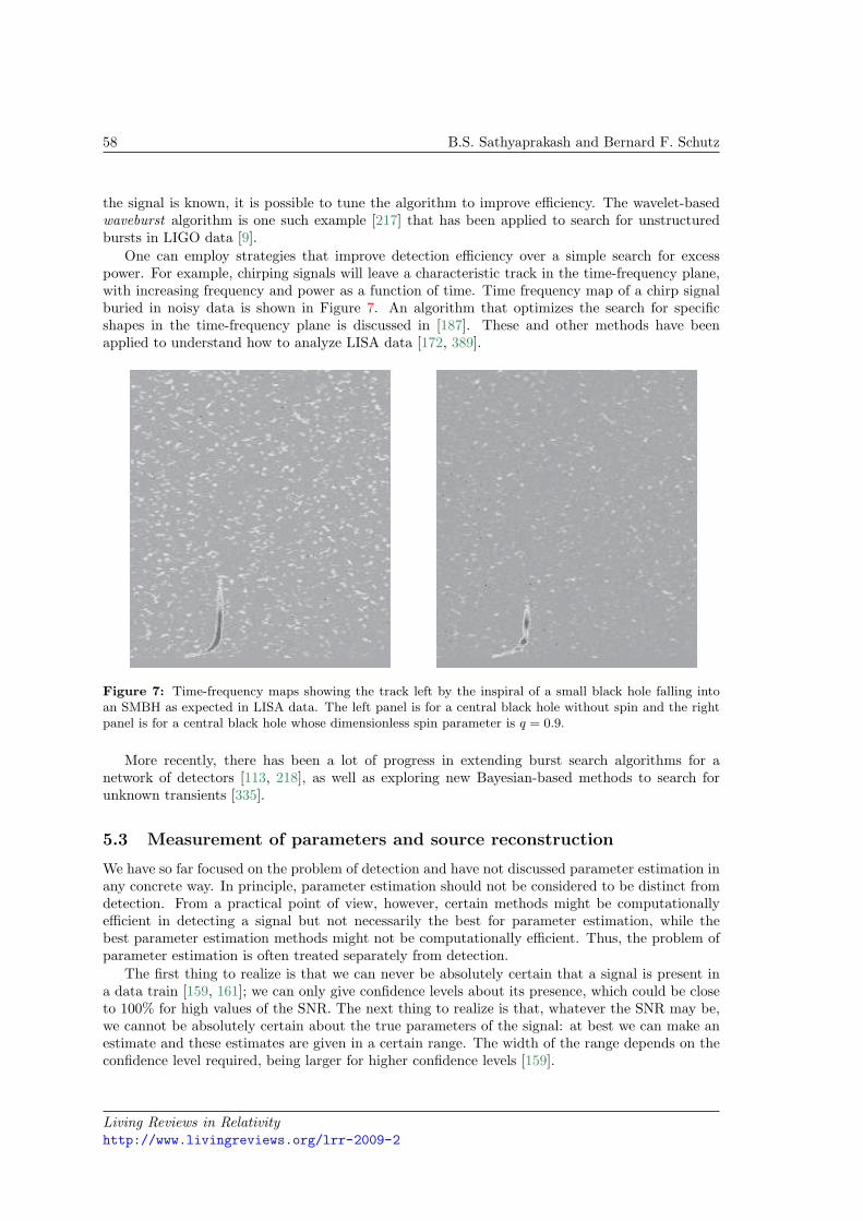
58 B.S. Sathyaprakash and Bernard F. Schutz
the signal is known, it is possible to tune the algorithm to improve efficiency. The wavelet-basedwaveburst algorithm is one such example [217] that has been applied to search for unstructuredbursts in LIGO data [9].
One can employ strategies that improve detection efficiency over a simple search for excesspower. For example, chirping signals will leave a characteristic track in the time-frequency plane,with increasing frequency and power as a function of time. Time frequency map of a chirp signalburied in noisy data is shown in Figure 7. An algorithm that optimizes the search for specificshapes in the time-frequency plane is discussed in [187]. These and other methods have beenapplied to understand how to analyze LISA data [172, 389].
Figure 7: Time-frequency maps showing the track left by the inspiral of a small black hole falling intoan SMBH as expected in LISA data. The left panel is for a central black hole without spin and the rightpanel is for a central black hole whose dimensionless spin parameter is q = 0.9.
More recently, there has been a lot of progress in extending burst search algorithms for anetwork of detectors [113, 218], as well as exploring new Bayesian-based methods to search forunknown transients [335].
5.3 Measurement of parameters and source reconstruction
We have so far focused on the problem of detection and have not discussed parameter estimation inany concrete way. In principle, parameter estimation should not be considered to be distinct fromdetection. From a practical point of view, however, certain methods might be computationallyefficient in detecting a signal but not necessarily the best for parameter estimation, while thebest parameter estimation methods might not be computationally efficient. Thus, the problem ofparameter estimation is often treated separately from detection.
The first thing to realize is that we can never be absolutely certain that a signal is present ina data train [159, 161]; we can only give confidence levels about its presence, which could be closeto 100% for high values of the SNR. The next thing to realize is that, whatever the SNR may be,we cannot be absolutely certain about the true parameters of the signal: at best we can make anestimate and these estimates are given in a certain range. The width of the range depends on theconfidence level required, being larger for higher confidence levels [159].
Living Reviews in Relativityhttp://www.livingreviews.org/lrr-2009-2
Physics, Astrophysics and Cosmology with Gravitational Waves 59
Maximum likelihood estimates have long been used to measure the parameters of a knownsignal buried in noisy data. The method consists in maximizing the likelihood ratio – the ratioof the probability that a given signal is present in the data to the probability that the signal isabsent [186, 159]. Maximum likelihood estimates are not always minimum uncertainty estimates,as has been particularly demonstrated in the case of binary inspiral signals by Balasubramanian,et al. [64, 65]. However, until recently, this is the method that has been very widely followed in thegravitational wave literature. But what is important to note is that maximum likelihood estimatesare unbiased when the SNR is large3, and the mean of the distribution of measured values of theparameters will be centered around the true parameter values. This is an important quality thatwill be useful in our discussion below.
Bayesian estimates, which take into account any prior knowledge that may be available aboutthe distribution of the source parameters, often give much better estimates and do not rely on theavailability of an ensemble of detector outputs [340, 274]. However, they are computationally a lotmore expensive than maximum likelihood estimates.
In any one measurement, any estimated parameters, however efficient, robust and accurate, areunlikely to be the actual parameters of the signal, since, at any finite SNR, noise alters the inputsignal. In the geometric language, the signal vector is being altered by the noise vector and ourmatched filtering aims at computing the projection of this altered vector onto the signal space. Thetrue parameters are expected to lie within an ellipsoid of p dimensions at a certain confidence level– the volume of the ellipsoid increasing with the confidence level at a given SNR but decreasingwith the SNR at a given confidence level.
5.3.1 Ambiguity function
The ambiguity function, well known in the statistical theory of signal detection [186], is a verypowerful tool in signal analysis: it helps one to assess the number of templates required to span theparameter space of the signal [321], to make estimates of variances and covariances involved in themeasurement of various parameters, to compute biases introduced in using a family of templateswhose shape is not the same as that of a family of signals intended to be detected, etc. We willsee below how the ambiguity function can be used to compute the required number of templates.Towards the end of this section we will use the ambiguity function for the estimation of parameters.
The ambiguity function is defined (see Equation (91) below) as the scalar product of twonormalized waveforms maximized over the initial phase of the waveform, in other words, theabsolute value of the scalar product4. A waveform e is said to be normalized if 〈e, e〉1/2 = 1, wherethe inner product is inversely weighted by the PSD, as in Equation (79). Among other things,normalized waveforms help in defining signal strengths: a signal is said to be of strength h0 ifh = h0e. Note that the optimal SNR for such a signal of strength h0 is, 〈h, h〉1/2 = h0.
Let e(t;α), where α = αi|i = 0, . . . , p is the parameter vector comprised of p+ 1 parameters,denote a normalized waveform. It is conventional to choose the parameter α0 to be the lag τ , whichsimply corresponds to a coordinate time when an event occurs and is therefore called an extrinsicparameter, while the rest of the p parameters are called the intrinsic parameters and characterizethe gravitational wave source.
Given two normalized waveforms e(t;α) and e(t;β), whose parameter vectors are not necessarily
3How large the SNR should be to presume that there is no bias in the estimation of parameters depends on thenumber of parameter-space dimensions and strictly speaking the statement is true only in the limit as SNR →∞.
4Working with analytic signals h(t) = a(t)eφ(t)+iφ0 , where a(t) and φ(t) are the time-varying amplitude andphase of the signal, respectively, we see that the initial phase φ0 of the signal simply factors out as a constant phasein the Fourier domain and we can maximize over this initial phase by simply taking the absolute value of the scalarproduct of a template with a signal.
Living Reviews in Relativityhttp://www.livingreviews.org/lrr-2009-2
60 B.S. Sathyaprakash and Bernard F. Schutz
the same, the ambiguity A is defined as
A(α, β) ≡ |〈e(α), e(β)〉| . (91)
Since the waveforms are normalized, A(α, α) = 1 and A(α, β) < 1, if α 6= β. Here, α can bethought of as the parameters of a (normalized) template while β those of a signal. With thetemplate parameters α fixed, the ambiguity function is a function of p signal parameters βi, givingthe SNR obtained by the template for different signals. The region in the signal parameter spacefor which a template obtains SNRs larger than a chosen value (called the minimal match [277])is the span of that template. Template families should be chosen so that altogether they spanthe entire signal parameter space of interest with the least overlap of one other’s spans. One canequally well interpret the ambiguity function as the SNR obtained for a given signal by filters ofdifferent parameter values.
It is clear that the ambiguity function is a local maximum at the “correct” set of parameters,β = α. Search methods that vary β to find the best fit to the parameter values make use of thisproperty in one way or another. But the ambiguity function will usually have secondary maximaas a function of β with fixed α. If these secondaries are only slightly smaller than the primarymaximum, then noise can lead to confusion: it can, at random, sometimes elevate a secondaryand suppress a primary. These can lead to false measurements of the parameters. Search methodsneed to be designed carefully to avoid this as much as possible. One way would be to fit the knownproperties of the ambiguity function to an ensemble of maxima. This would effectively averageover the noise on individual peaks and point more reliably to the correct one.
It is important to note that in the definition of the ambiguity function there is no need for thefunctional forms of the template and signal to be the same; the definition holds true for any signal-template pair of waveforms. Moreover, the number of template parameters need not be identical(and usually aren’t) to the number of parameters characterizing the signal. For instance, a binarycan be characterized by a large number of parameters, such as the masses, spins, eccentricityof the orbit, etc., while we may take as a model waveform the one involving only the masses.In the context of inspiral waves, e(t;β) is the exact general relativistic waveform emitted by abinary, whose form we do not know, while the template family is a post-Newtonian, or some other,approximation to it, that will be used to detect the true waveform. Another example would besignals emitted by spinning neutron stars, isolated or in binaries, whose time evolution is unknown,either because we cannot anticipate all the physical effects that affect their spin, or because theparameter space is so large that we cannot possibly take into account all of them in a realisticsearch.
Of course, in such cases we cannot compute the ambiguity function, since one of the argumentsto the ambiguity function is unknown. These are, indeed, issues where substantial work is calledfor. What are all the physical effects to be considered so as not to miss out a waveform from oursearch? How to make a choice of templates when the functional form of templates is different fromthose of signals? For this review it suffices to assume that the signal and template waveforms areof identical shape and the number of parameters in the two cases is the same.
5.3.2 Metric on the space of waveforms
The computational cost of a search and the estimation of parameters of a signal afford a lucid geo-metrical picture developed by Balasubramanian et al. [65] and Owen [277]. Much of the discussionbelow is borrowed from their work.
Let xk, k = 1, 2, . . . , N , denote the discretely sampled output of a detector. The set of allpossible detector outputs satisfy the usual axioms of a vector space. Therefore, xk can be thoughtof as an N -dimensional vector. It is more convenient to work in the continuum limit, in which casewe have infinite dimensional vectors and the corresponding vector space. However, all the results
Living Reviews in Relativityhttp://www.livingreviews.org/lrr-2009-2
Physics, Astrophysics and Cosmology with Gravitational Waves 61
are applicable to the realistic case in which detector outputs are treated as finite dimensionalvectors.
Amongst all vectors, of particular interest are those corresponding to gravitational waves froma given astronomical source. While every signal can be thought of as a vector in the infinite-dimensional vector space of the detector outputs, the set of all such signal vectors do not, bythemselves, form a vector space. However, the set of all normed signal vectors (i.e., signal vectorsof unit norm) form a manifold, the parameters of the signal serving as a coordinate system [64, 65,277, 279]. Thus, each class of an astronomical source forms an n-dimensional manifold Sn, wheren is the number of independent parameters characterizing the source. For instance, the set of allsignals from a binary on a quasi-circular orbit inclined to the line of sight at an angle ι, consistingof nonspinning black holes of masses m1, and m2, located a distance D from the Earth5 initially inthe direction (θ, ϕ) and expected to merge at a time tC with the phase of the signal at merger ϕC ,forms a nine-dimensional manifold with coordinates D, θ, ϕ, m1, m2, tC , ϕC , ι, ψ, where ψ isthe polarization angle of the signal. In the general case of a signal characterized by n parameterswe shall denote the parameters by pα, where α = 1, . . . , n.
The manifold Sn can be endowed with a metric gαβ that is induced by the scalar productdefined in Equation (79). The components of the metric in a coordinate system pα are defined by6
gαβ ≡⟨∂αh, ∂βh
⟩, ∂αh ≡
∂h
∂pα. (92)
The metric can then be used on the signal manifold as a measure of the proper distance d` betweennearby signals with coordinates pα and pα + dpα, that is signals h(pα) and h(pα + dpα),
d`2 = gαβdpαdpβ . (93)
Now, by Taylor expanding h(pα + dpα) around pα, and keeping only terms to second orderin dpα, it is straightforward to see that the overlap O of two infinitesimally close signals can becomputed using the metric:
O(dpα; pα) ≡⟨h(pα), h(pα + dpα)
⟩= 1− 1
2gαβdpαdpβ . (94)
The metric on the signal manifold is nothing but the well-known Fisher information matrixusually denoted Γαβ , (see, e.g., [186, 283]) but scaled down by the square of the SNR, i.e., gαβ =ρ−2Γαβ . The information matrix is itself the inverse of the covariance matrix Cαβ and is a veryuseful quantity in signal analysis.
5.3.3 Covariance matrix
Having defined the metric, we next consider the application of the geometric formalism in theestimation of statistical errors involved in the measurement of the parameters. We closely followthe notation of Finn and Chernoff [159, 161, 114].
Let us suppose a signal of known shape with parameters pα is buried in background noise thatis Gaussian and stationary. Since the signal shape is known, one can use matched filtering to digthe signal out of the noise. The measured parameters pα will, in general, differ from the true
5Even though we deal with normed signals (which amounts to fixing D), astrophysical gravitational wave signalsare characterized by this additional parameter.
6We have followed the definition of the metric as is conventional in parameter estimation theory (see, e.g.,[159, 161, 114, 65]), which differs from that used in template placement algorithms (see, e.g., [277]) by a factor oftwo. This difference will impact the relationship between the metric and the match, as will be apparent in whatfollows.
Living Reviews in Relativityhttp://www.livingreviews.org/lrr-2009-2
62 B.S. Sathyaprakash and Bernard F. Schutz
parameters of the signal7. Geometrically speaking, the noise vector displaces the signal vector andthe process of matched filtering projects the (noise + signal) vector back on to the signal manifold.Thus, any nonzero noise will make it impossible to measure the true parameters of the signal. Thebest one can hope for is a proper statistical estimation of the influence of noise.
The posterior probability density function P of the parameters pα is given by a multivariateGaussian distribution8:
P(∆pα) dn∆p =dn∆p
(2π)n/2√C
exp[−1
2C−1
αβ ∆pα∆ pβ
], (95)
where n is the number of parameters, ∆pα = pα − pα, and Cαβ is the covariance matrix, C beingits determinant. Noting that C−1
αβ = ρ2gαβ , we can rewrite the above distribution as
P(∆pα) dn∆p =ρn√g dn∆p
(2π)n/2exp
[−ρ
2
2gαβ ∆pα∆ pβ
], (96)
where we have used the fact that C = 1/(ρ2n g), g being the determinant of the metric gαβ . Notethat if we define new parameters p′α = ρpα, then we have exactly the same distribution functionfor all SNRs, except that the deviations ∆pα are scaled by ρ.
Let us first specialize to one dimension to illustrate the region of the parameter space withwhich one should associate an event at a given confidence level. In one dimension the distributionof the deviation from the mean of the measured value of the parameter p is given by
P(∆p)d∆p =d∆p√2πσ
exp(−∆p2
2σ2
)=ρ√gppd∆p√
2πexp
(−ρ
2
2gpp∆p2
), (97)
where, analogous to the n-dimensional case, we have used σ2 = 1/(ρ2gpp). Now, at a given SNR,what is the volume VP in the parameter space, such that the probability of finding the measuredparameters p inside this volume is P? This volume is defined by
P =∫
∆p∈VP
P(∆p)d∆p. (98)
Although VP is not unique, it is customary to choose it to be centered around ∆p = 0:
P =∫
(∆p/σ)2≤r2(P )
d∆p√2πσ
exp(−∆p2
2σ2
)=∫
ρ2gpp∆p2≤r2(P )
ρ√gppd∆p√
2πexp
(−ρ
2 gpp∆p2
2
), (99)
where, given P , the above equation can be used to solve for r(P ) and it determines the range of inte-gration: −rσ ≤ ∆p ≤ rσ. For instance, the volumes VP corresponding to P ' 0.683, 0.954, 0.997, . . .,are the familiar intervals [−σ, σ], [−2σ, 2σ], [−3σ, 3σ], . . ., and the corresponding values of r are1, 2, 3. Since σ = 1/
√ρ2gpp, we see that in terms of gpp the above intervals translate to
1ρ
[− 1√gpp
,1
√gpp
],
1ρ
[− 2√gpp
,2
√gpp
],
1ρ
[− 3√gpp
,3
√gpp
], . . . . (100)
Thus, for a given probability P , the volume VP shrinks as 1/ρ. The maximum distance dmax
within which we can expect to find “triggers” at a given P depends inversely on the SNR ρ:d` =
√gpp∆p2 = r/ρ. Therefore, for P ' 0.954, r = 2 and at an SNR of 5 the maximum distance
7In what follows we shall use an over-line to distinguish the measured parameters from the true parameters pα.8A Bayesian interpretation of P(∆pα) is the probability of having the true signal parameters lie somewhere inside
the ellipsoidal volume centered at the Maximum Likelihood point pα.
Living Reviews in Relativityhttp://www.livingreviews.org/lrr-2009-2
Physics, Astrophysics and Cosmology with Gravitational Waves 63
is 0.4, which corresponds to a match of ε = 1− 12d`
2 = 0.92. In other words, in one dimension 95%of the time we expect our triggers to come from templates that have an overlap greater than orequal to 0.92 with the buried signal when the SNR is five. This interpretation in terms of the matchis a good approximation as long as d` 1, which will be true for large SNR events. However,for weaker signals and/or greater values of P we can’t interpret the results in terms of the match,although Equation (98) can be used to determine r(P ). As an example, at P ' 0.997, r = 3 andat an SNR of ρ = 4, the maximum distance is d` = 0.75 and the match is ε = 23/32 ' 0.72, whichis significantly smaller than one and the quadratic approximation is not good enough to computethe match.
These results generalize to n dimensions. In n-dimensions the volume VP is defined by
P =∫
∆pα∈VP
P(∆pα) dn∆p. (101)
Again, VP is not unique but it is customary to center the volume around the point ∆pα = 0:
P =∫
ρ2gαβ ∆pα∆ pβ≤r2(P,n)
ρn√g dn∆p(2π)n/2
exp[−ρ
2
2gαβ ∆pα∆ pβ
]. (102)
Given P and the parameter space dimension n, one can iteratively solve the above equation forr(P, n). The volume VP is the surface defined by the equation
gαβ∆pα∆pβ =(r
ρ
)2
. (103)
This is the equation of an n-dimensional ellipsoid whose size is defined by r/ρ. For a given r (whichdetermines the confidence level), the size of the ellipsoid is inversely proportional to the SNR, thevolume decreasing as ρn. However, the size is not small enough for all combinations of P and ρto interpret the distance from the center of the ellipsoid to its surface, in terms of the overlap ormatch of the signals at the two locations, except when the distance is close to zero. This is becausethe expression for the match in terms of the metric is based on the quadratic approximation, whichbreaks down when the matches are small. However, the region defined by Equation (103) alwayscorresponds to the probability P and there is no approximation here (except that the detectornoise is Gaussian).
When the SNR ρ is large and 1− P is not close to zero, the triggers are found from the signalwith matches greater than or equal to 1− r2(P,n)
2ρ2 . Table 2 lists the value of r for several values ofP in one, two and three-dimensions and the minimum match εMM for SNRs 5, 10 and 20.
Table 2 should be interpreted in light of the fact that triggers come from an analysis pipeline inwhich the templates are laid out with a certain minimal match and one cannot, therefore, expectthe triggers from different detectors to be matched better than the minimal match.
From Table 2, we see that, when the SNR is large (say greater than about 10), the dependenceof the match εMM on n is very weak; in other words, irrespective of the number of dimensions, weexpect the match between the trigger and the true signal (and for our purposes the match betweentriggers from different instruments) to be pretty close to 1, and mostly larger than a minimalmatch of about 0.95 that is typically used in a search. Even when the SNR is in the region of 5,for low P again there is a weak dependence of εMM on the number of parameters. For large P andlow SNR, however, the dependence of εMM on the number of dimensions becomes important. Atan SNR of 5 and P ' 0.997, εMM = 0.91, 0.87, 0.85 for n = 1, 2, 3 dimensions, respectively.
Bounds on the estimation computed using the covariance matrix are called Cramer–Rao bounds.Cramer–Rao bounds are based on local analysis and do not take into consideration the effectof distant points in the parameter space on the errors computed at a given point, such as the
Living Reviews in Relativityhttp://www.livingreviews.org/lrr-2009-2
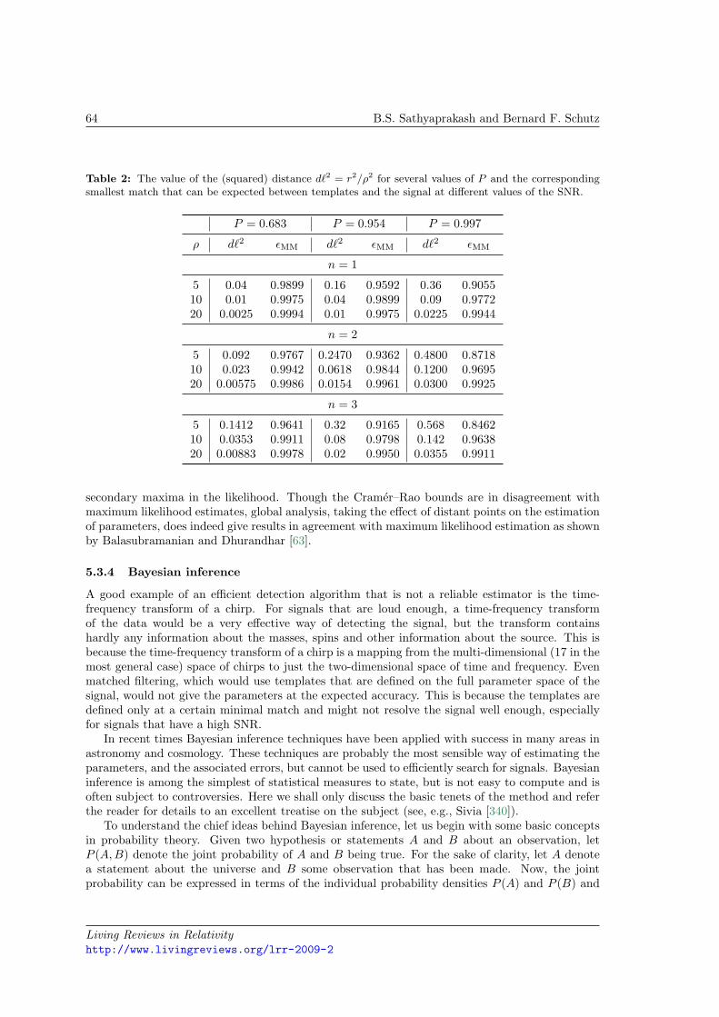
64 B.S. Sathyaprakash and Bernard F. Schutz
Table 2: The value of the (squared) distance d`2 = r2/ρ2 for several values of P and the correspondingsmallest match that can be expected between templates and the signal at different values of the SNR.
P = 0.683 P = 0.954 P = 0.997
ρ d`2 εMM d`2 εMM d`2 εMM
n = 1
5 0.04 0.9899 0.16 0.9592 0.36 0.905510 0.01 0.9975 0.04 0.9899 0.09 0.977220 0.0025 0.9994 0.01 0.9975 0.0225 0.9944
n = 2
5 0.092 0.9767 0.2470 0.9362 0.4800 0.871810 0.023 0.9942 0.0618 0.9844 0.1200 0.969520 0.00575 0.9986 0.0154 0.9961 0.0300 0.9925
n = 3
5 0.1412 0.9641 0.32 0.9165 0.568 0.846210 0.0353 0.9911 0.08 0.9798 0.142 0.963820 0.00883 0.9978 0.02 0.9950 0.0355 0.9911
secondary maxima in the likelihood. Though the Cramer–Rao bounds are in disagreement withmaximum likelihood estimates, global analysis, taking the effect of distant points on the estimationof parameters, does indeed give results in agreement with maximum likelihood estimation as shownby Balasubramanian and Dhurandhar [63].
5.3.4 Bayesian inference
A good example of an efficient detection algorithm that is not a reliable estimator is the time-frequency transform of a chirp. For signals that are loud enough, a time-frequency transformof the data would be a very effective way of detecting the signal, but the transform containshardly any information about the masses, spins and other information about the source. This isbecause the time-frequency transform of a chirp is a mapping from the multi-dimensional (17 in themost general case) space of chirps to just the two-dimensional space of time and frequency. Evenmatched filtering, which would use templates that are defined on the full parameter space of thesignal, would not give the parameters at the expected accuracy. This is because the templates aredefined only at a certain minimal match and might not resolve the signal well enough, especiallyfor signals that have a high SNR.
In recent times Bayesian inference techniques have been applied with success in many areas inastronomy and cosmology. These techniques are probably the most sensible way of estimating theparameters, and the associated errors, but cannot be used to efficiently search for signals. Bayesianinference is among the simplest of statistical measures to state, but is not easy to compute and isoften subject to controversies. Here we shall only discuss the basic tenets of the method and referthe reader for details to an excellent treatise on the subject (see, e.g., Sivia [340]).
To understand the chief ideas behind Bayesian inference, let us begin with some basic conceptsin probability theory. Given two hypothesis or statements A and B about an observation, letP (A,B) denote the joint probability of A and B being true. For the sake of clarity, let A denotea statement about the universe and B some observation that has been made. Now, the jointprobability can be expressed in terms of the individual probability densities P (A) and P (B) and
Living Reviews in Relativityhttp://www.livingreviews.org/lrr-2009-2
Physics, Astrophysics and Cosmology with Gravitational Waves 65
conditional probability densities P (A|B) and P (B|A) as follows:
P (A,B) = P (A)P (B|A) or P (A,B) = P (B)P (A|B). (104)
The first of these equations says the joint probability of A and B both being true is the probabilitythat A is true times the probability that B is true given that A is true and similarly the second.We can use the above equations to arrive at Bayes theorem:
P (B)P (A|B) = P (A)P (B|A) or P (A|B) =P (A)P (B|A)
P (B). (105)
The left-hand side of the above equation can be interpreted as a statement about A (the universe)given B (the data). This is the posterior probability density. The right-hand side contains P (B|A),which is the probability that B is obtained given that A is true and is called the likelihood, P (A),which is the probability of A, called the prior probability of A, and P (B) (the prior of B), whichis simply a normalizing constant often ignored in Bayesian analysis.
For instance, if A denotes the statement it is going to rain and B the amount of humidity in theair then the above equation gives us the posterior probability that it rains when the air containsa certain amount of humidity. Clearly, the posterior depends on what is the likelihood of the airhaving a certain humidity when it rains and the prior probability of rain on a given day. If theprior is very small (as it would be in a desert, for example) then you would need a rather largelikelihood for the posterior to be large. Even when the prior is not so small, say a 50% chanceof rain on any given day (as it would be if you are in Wales), the likelihood has to be large forposterior probability to say something about the relationship between the level of humidity andthe chance of rain.
As another example, and more relevant to the subject of this review, let s be the statementthe data contains a chirp (signal), n the statement the data contains an instrumental transient,(noise), and let t be a test that is performed to infer which of the two statements above are true.Let us suppose t is a very good test, in that it discriminates between s and n very well, and saythe detection probability is as high as P (t|s) = 0.95 with a low false alarm rate P (t|n) = 0.05(note that P (t|s) and P (t|n) need not necessarily add up to 1). Also, the expected event rate of achirp during our observation is low, P (s) = 10−5, but the chance of an instrumental transient isrelatively large, P (n) = 0.01. We are interested in knowing what the posterior probability of thedata containing a chirp is, given that the test has been passed. By Bayes theorem this is
P (s|t) =P (t|s)P (s)
P (t)=
P (t|s)P (s)P (t|s)P (s) + P (t|n)P (n)
, (106)
where P (t) (the probability of the test being positive) is taken to result from either the chirp orthe instrumental transient. Substituting for various quantities in the above equation we find
P (s|t) =0.95× 10⁻⁵
0.95× 10⁻⁵ + 0.05× 0.01' 0.02. (107)
There is only a 2% chance that the data really contains a chirp when the test was taken. On thecontrary, for the same data we find that the chance of an instrumental transient for a positive testresult is P (n|t) ∼ 98%. Thus, though there is a high (low) probability for the test to be positivein the presence of a signal (noise) when the test is indeed positive, we cannot necessarily concludethat a signal is present. This is not surprising since the prior probability of the signal being presentis very low. The situation can be remedied by designing a test that gives a far lower probabilityfor the test to give a positive result in the case of an instrumental transient (i.e., a very low falsealarm rate).
Living Reviews in Relativityhttp://www.livingreviews.org/lrr-2009-2
66 B.S. Sathyaprakash and Bernard F. Schutz
Thus, Bayesian inference neatly folds the prior knowledge about sources in the estimationprocess. One might worry that the outcome of a measurement process would be seriously biasedby our preconception of the prior. To understand this better, let us rewrite Equation (106) asfollows:
P (s|t) =1
1 + P (t|n)P (n)/P (t|s)P (s)=
11 + LNSpSN
, (108)
where LNS = P (t|n)/P (t|s) is the ratio of the two likelihoods and pSN = P (s)/P (n) is the ratio ofthe priors. The latter is not in the hands of a data analyst; it is determined by the nature of thesource being searched for and the property of the instrument. The only way an analyst can makethe posterior probability large is by choosing a test that gives a small value for the ratio of thetwo likelihoods. When LNS pSN (i.e., the likelihood of the test being positive when the signalis present is far larger, depending on the priors, than when the transient is present) the posteriorwill be close to unity.
The above example tells us why we have to work with unusually-small false-alarm probability inthe case of gravitational wave searches. For instance, to search for binary coalescences in ground-based detectors we use a (power) SNR threshold of about 30 to 50. This is because the expectedevent rate is about 0.04 per year.
Computing the posterior involves multi-dimensional integrals and these are highly expensivecomputationally, when the number of parameters involved is large. This is why it is often notpossible to apply Bayesian techniques to continuously streaming data; it would be sensible toreserve the application of Bayesian inference only for candidate events that are selected frominexpensive analysis techniques. Thus, although Bayesian analysis is not used in current detectionpipelines, there has been a lot of effort in evaluating its ability to search for [115, 348, 122, 120]and measure the parameters of [116, 121, 377] a signal and in follow-up analysis [378].
Living Reviews in Relativityhttp://www.livingreviews.org/lrr-2009-2
Physics, Astrophysics and Cosmology with Gravitational Waves 67
6 Physics with Gravitational Waves
Classical general relativity has passed all possible experimental and observational tests so far. Thetheory is elegant, self-consistent and mathematically complete (i.e., its equations are, in principle,solvable). However, theorists are uncomfortable with general relativity because it has so far eludedall efforts of quantization, making it a unique modern theory, whose quantum mechanical analogueis unknown. Although general relativity arises as a by-product in certain string theories, thephysical relevance of such theories is unclear. Therefore, it has been proposed that general relativityis a low-energy limit of a more general theory, which in itself is amenable to both quantizationand unification. There are also other theoretical motivations to look for modifications of generalrelativity or new theories of gravity. While there are some alternative candidates (including theBrans–Dicke theory), none has predictions that contradict general relativistic predictions in linearand mildly nonlinear gravitational fields. More precisely, the extra parameters of these othertheories of gravity are constrained by the present experimental and astronomical observations,however, they are expected to significantly deviate from general relativistic predictions underconditions of strong gravitational fields.
Gravitational wave observations provide a unique opportunity to test strongly nonlinear andhighly relativistic gravity and hence provide an unprecedented testbed for confronting differenttheories of gravity. Every nonlinear gravitational effect in general relativity will have a counterpartin alternative theories and therefore a measurement of such an effect would provide an opportunityto compare the performance of general relativity with its competitors. Indeed, a single measurementof the full polarization of an incident gravitational wave can potentially rule out general relativity.This is a field that would benefit from an in-depth study. What we are lacking is a systematicstudy of higher-order post-Newtonian effects in alternative theories of gravity. For instance, we donot know how tails of gravitational waves or tails of tails would appear in any theory other thangeneral relativity.
In what follows we present strong field tests of general relativity afforded by future gravitationalwave observations. We will begin with observations of single black holes followed by black holebinaries (more generally, coalescing binaries of compact objects).
6.1 Speed of gravitational waves
Association of a gravitational wave event with an electromagnetic event, such as the observationof a gamma or X-ray burst coincidentally with a gravitational wave event, would help to deducethe speed of gravitational waves to a phenomenal accuracy. The best candidate sources for thesimultaneous observations of both are the well-known extra-galactic gamma-ray bursts (GRBs).Depending on the model that produces the GRB, the delay between the emission of a GRB andgravitational waves might be either a fraction of a second (as in GRBs generated by internal shocksin a fireball [306]) or 100’s of seconds (as in GRBs generated when the fireball is incident on anexternal medium [256]). It is unlikely that high-redshift gamma-ray observations will be visiblein the gravitational wave band, since the amplitude of gravitational waves might be rather low.However, advanced detectors might see occasional low-redshift events, especially if the GRB iscaused by black-hole–neutron-star mergers. Third generation detectors would be sensitive to suchevents up to z = 2. A single unambiguous association can verify the speed of gravitational wavesrelative to light to a fantastic precision.
For instance, even a day’s delay in the arrival times of gravitational and electromagnetic ra-diation from a source at a distance of one giga light year (distance to a low-redshift GRB de-tectable by advanced detectors) would determine the relative speeds to better than one part in 1011
(1 day/109 yr ∼ 3× 10⁻¹²). Coincident detection of GRBs and gravitational waves would requiregood timing accuracy to determine the direction of the source so that astronomical observations
Living Reviews in Relativityhttp://www.livingreviews.org/lrr-2009-2
68 B.S. Sathyaprakash and Bernard F. Schutz
of associated gamma rays (and afterglows in other spectral bands) can be made. Consequently,gravitational wave antennas around the globe will have to make a coincident detection of the event.
If the speed of gravitational waves is less than that of light, then this could indicate that thegraviton has an effective nonzero mass.
This would have other observable effects, in particular dispersion; different frequencies shouldmove at different speeds. Will [393] pointed out that LISA’s observations of coalescences of SMBHsat high redshifts will place extremely tight constraints on dispersion, and may, therefore, indirectlyset the best available limits on the speed of gravitational waves. This and other bounds on thegraviton mass are discussed in Section 6.6.1.
6.2 Polarization of gravitational waves
As noted in Section 2, in Einstein’s theory gravitational waves have two independent polarizations,usually denoted h+ and h× [259]. A general wave will be a linear combination of both. Rotatingsources typically emit both polarizations with a phase delay between them, leading to ellipticalpolarization patterns. Depending on the nature of the source such polarizations can be detectedeither with a single detector (in the case of continuous wave sources) or with a network of detectors(in the case of burst sources).
While Einstein’s general relativity predicts only two independent polarizations, there are othertheories of gravitation in which there are additional states of polarization. For instance, in Fierze–Jordan–Brans–Dicke theory [394] there are four polarization degrees of freedom more than inEinstein’s theory. Therefore, an unambiguous determination of the polarization of the waves willbe of fundamental importance.
In the case of a burst source, to determine two polarization states, source direction and am-plitude requires three detectors, observing other polarizations would require the use of more thanthree detectors (see, for example, Will [394]). The scalar polarization mode of Brans–Dicke, forexample, expands a transverse ring of test particles without changing its shape. This is the breath-ing mode, or monopole polarization. If such a wave is incident from above on an interferometer, itwill not register at all. But if it comes in along one of the arms, then, since it acts transversely,it will affect only the other arm and leave a signal. If the wave is seen with enough detectors,then it is possible to determine that it has scalar polarization. Note that a measurement such asthis can make a qualitative change in physics: a single measurement could put general relativity injeopardy.
Polarization measurements have an important application in astronomy. The polarization ofthe waves contains orientation information. For example, a binary system emits purely circularpolarization along the angular momentum axis, but purely linear polarization in its equatorialplane. By measuring the polarization of waves from a binary (or from a spinning neutron star)one can determine the orientation and inclination of its spin axis. This is a piece of informationthat is usually very hard to extract from optical observations. We will return to this discussion inSection 7.1.1.
6.3 Gravitational radiation reaction
In 1974, Hulse and Taylor discovered the first double neutron star binary PSR B1913+16, a sys-tem in which the emission of gravitational radiation has an observable effect [200, 356]. Generalrelativity predicts that the loss of energy and angular momentum due to the emission of gravita-tional waves should cause the period of the system to decrease and, by carefully monitoring theorbital period of the binary, that it would be possible to measure the rate at which the periodchanges. The rate at which the period decays can be computed using the quadrupole formula for
Living Reviews in Relativityhttp://www.livingreviews.org/lrr-2009-2
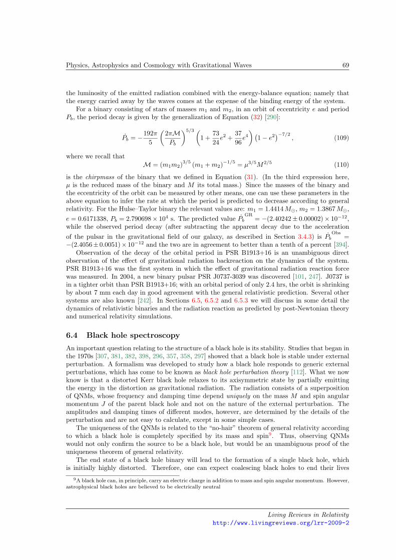
Physics, Astrophysics and Cosmology with Gravitational Waves 69
the luminosity of the emitted radiation combined with the energy-balance equation; namely thatthe energy carried away by the waves comes at the expense of the binding energy of the system.
For a binary consisting of stars of masses m1 and m2, in an orbit of eccentricity e and periodPb, the period decay is given by the generalization of Equation (32) [290]:
Pb = −192π5
(2πMPb
)5/3(1 +
7324e2 +
3796e4)(
1− e2)−7/2
, (109)
where we recall thatM = (m1m2)
3/5 (m1 +m2)−1/5 = µ3/5M2/5 (110)
is the chirpmass of the binary that we defined in Equation (31). (In the third expression here,µ is the reduced mass of the binary and M its total mass.) Since the masses of the binary andthe eccentricity of the orbit can be measured by other means, one can use these parameters in theabove equation to infer the rate at which the period is predicted to decrease according to generalrelativity. For the Hulse–Taylor binary the relevant values are: m1 = 1.4414M, m2 = 1.3867M,e = 0.6171338, Pb = 2.790698× 10⁴ s. The predicted value Pb
GR= −(2.40242± 0.00002)× 10−12,
while the observed period decay (after subtracting the apparent decay due to the accelerationof the pulsar in the gravitational field of our galaxy, as described in Section 3.4.3) is Pb
Obs=
−(2.4056± 0.0051)× 10−12 and the two are in agreement to better than a tenth of a percent [394].Observation of the decay of the orbital period in PSR B1913+16 is an unambiguous direct
observation of the effect of gravitational radiation backreaction on the dynamics of the system.PSR B1913+16 was the first system in which the effect of gravitational radiation reaction forcewas measured. In 2004, a new binary pulsar PSR J0737-3039 was discovered [101, 247]. J0737 isin a tighter orbit than PSR B1913+16; with an orbital period of only 2.4 hrs, the orbit is shrinkingby about 7 mm each day in good agreement with the general relativistic prediction. Several othersystems are also known [242]. In Sections 6.5, 6.5.2 and 6.5.3 we will discuss in some detail thedynamics of relativistic binaries and the radiation reaction as predicted by post-Newtonian theoryand numerical relativity simulations.
6.4 Black hole spectroscopy
An important question relating to the structure of a black hole is its stability. Studies that began inthe 1970s [307, 381, 382, 398, 296, 357, 358, 297] showed that a black hole is stable under externalperturbation. A formalism was developed to study how a black hole responds to generic externalperturbations, which has come to be known as black hole perturbation theory [112]. What we nowknow is that a distorted Kerr black hole relaxes to its axisymmetric state by partially emittingthe energy in the distortion as gravitational radiation. The radiation consists of a superpositionof QNMs, whose frequency and damping time depend uniquely on the mass M and spin angularmomentum J of the parent black hole and not on the nature of the external perturbation. Theamplitudes and damping times of different modes, however, are determined by the details of theperturbation and are not easy to calculate, except in some simple cases.
The uniqueness of the QNMs is related to the “no-hair” theorem of general relativity accordingto which a black hole is completely specified by its mass and spin9. Thus, observing QNMswould not only confirm the source to be a black hole, but would be an unambiguous proof of theuniqueness theorem of general relativity.
The end state of a black hole binary will lead to the formation of a single black hole, whichis initially highly distorted. Therefore, one can expect coalescing black holes to end their lives
9A black hole can, in principle, carry an electric charge in addition to mass and spin angular momentum. However,astrophysical black holes are believed to be electrically neutral
Living Reviews in Relativityhttp://www.livingreviews.org/lrr-2009-2
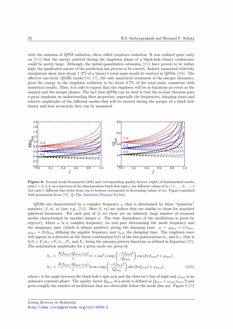
70 B.S. Sathyaprakash and Bernard F. Schutz
with the emission of QNM radiation, often called ringdown radiation. It was realized quite earlyon [164] that the energy emitted during the ringdown phase of a black-hole–binary coalescencecould be pretty large. Although, the initial quantitative estimates [164] have proven to be ratherhigh, the qualitative nature of the prediction has proven to be correct. Indeed, numerical relativitysimulations show that about 1–2% of a binary’s total mass would be emitted in QNMs [298]. Theeffective one-body (EOB) model [96, 97], the only analytical treatment of the merger dynamics,gives the energy in the ringdown radiation to be about 0.7% of the total mass, consistent withnumerical results. Thus, it is safe to expect that the ringdown will be as luminous an event as theinspiral and the merger phases. The fact that QNMs can be used to test the no-hair theorem putsa great emphasis on understanding their properties, especially the frequencies, damping times andrelative amplitudes of the different modes that will be excited during the merger of a black holebinary and how accurately they can be measured.
0.0 0.2 0.4 0.6 0.8 1.0j
0.0
0.2
0.4
0.6
0.8
1.0
1.2
1.4
1.6
1.8
Mω lm
n
l=2
l=3
l=4
0.0 0.2 0.4 0.6 0.8 1.0j
0.0
2.0
4.0
6.0
8.0
Qlm
n
l=2
l=3
l=4
Figure 8: Normal mode frequencies (left) and corresponding quality factors (right) of fundamental modeswith l = 2, 3, 4, as a function of the dimensionless black hole spin j, for different values ofm = l, . . . , 0, . . .−l(for each l, different line styles from top to bottom correspond to decreasing values of m). Figure reprintedwith permission from [76]. c© The American Physical Society.
QNMs are characterized by a complex frequency ω that is determined by three “quantum”numbers, (l, m, n) (see, e.g., [76]). Here (l, m) are indices that are similar to those for standardspherical harmonics. For each pair of (l, m) there are an infinitely large number of resonantmodes characterized by another integer n. The time dependence of the oscillations is given byexp(iωt), where ω is a complex frequency, its real part determining the mode frequency andthe imaginary part (which is always positive) giving the damping time: ω = ωlmn + i/τlmn,ωlmn = 2πflmn defining the angular frequency and τlmn the damping time. The ringdown wavewill appear in a detector as the linear combination h(t) of the two polarizations h+ and h×, that ish(t) = F+h+ +F×h×, F+ and F× being the antenna pattern functions as defined in Equation (57).The polarization amplitudes for a given mode are given by
h+ =A(flmn, Qlmn, εrd)
r(1 + cos2 ι) exp
(−πflmnt
Qlmn
)cos (2πflmnt+ ϕlmn) ,
h× =A(flmn, Qlmn, εrd)
r2 cos ι exp
(−πflmnt
Qlmn
)sin (2πflmnt+ ϕlmn) , (111)
where ι is the angle between the black hole’s spin axis and the observer’s line of sight and ϕlmn is anunknown constant phase. The quality factor Qlmn of a mode is defined as Qlmn = ωlmnτlmn/2 andgives roughly the number of oscillations that are observable before the mode dies out. Figure 8 [76]
Living Reviews in Relativityhttp://www.livingreviews.org/lrr-2009-2
Physics, Astrophysics and Cosmology with Gravitational Waves 71
plots frequencies and quality factors for the first few QNMs as a function of the dimensionless spinparameter j = J/M2. The mode of a Schwarzschild black hole corresponding to l = 2, m = n = 0,is given by
f200 = ±1.207× 10³ 10M
MHz, τ200 = 5.537× 10⁻⁴ M
10Ms. (112)
For stellar-mass–black-hole coalescences expected to be observed in ground-based detectors theringdown signal is a transient that lasts for a very short time. However, for space-based LISAthe signal would last several minutes for a black hole of M = 107M. In the latter case, theringdown waves could carry the energy equivalent of 105M converted to gravitational waves –a phenomenal amount of energy compared even to the brightest quasars and gamma ray bursts.Thus, LISA should be able to see QNMs from black hole coalescences anywhere in the universe,provided the final (redshifted) mass of the black hole is larger than about 106M, as otherwisethe signal lasts for far too short a time for the detector to accumulate the SNR.
Berti et al. [76] have carried out an exhaustive study, in which they find that the LISA obser-vations of SMBH binary mergers could be an excellent testbed for the no-hair theorem. Figure 9(left panel) plots the fractional energy εrd that must be deposited in the ringdown mode so thatthe event is observable at a distance of 3 Gpc. Black holes at 3 Gpc with mass M in the rangeof 106 – 108M would be observable (i.e., will have an SNR of 10 or more) even if a fractionεrd ' 10−7M of energy is in the ringdown phase. Numerical relativity predicts that as much as 1%of the energy could be emitted as QNMs, when two black holes merge, implying that the ringdownphase could be observed with an SNR of 100 or greater all the way up to z ∼ 10, provided theirmass lies in the appropriate range10. Furthermore, they find that at this redshift it should bepossible to resolve the fundamental l = 2, m = 2 mode. Since black holes forming from primordialgas clouds at z = 10 – 15 could well be the seeds of galaxy formation and large-scale structure,LISA could indeed witness their formation through out the cosmic history of the universe.
104
105
106
107
108
M
10-9
10-8
10-7
10-6
10-5
10-4
10-3
10-2
10-1
100
ε rd
l=2, m=2
0.0 0.2 0.4 0.6 0.8 1.0j
10-1
100
101
erro
rs
j
M
l=2, m=2
A
φ
Figure 9: The smallest fraction of black hole mass in ringdown waveforms that is needed to observe thefundamental mode at a distance of 3 Gpc (left) for three values of the black hole spin, j = 0 (solid line)j = 0.80 (dashed line) and j = 0.98 (dot-dashed line) and the error in the measurement of the variousparameters as a function of the black hole spin for the same mode (right). Figure reprinted with permissionfrom [76]. c© The American Physical Society.
Figure 9 (right panel) shows SNR-normalized errors (i.e., one-sigma deviations multiplied by
10Note that a black hole of physical mass M at a redshift of z will appear as a black hole of mass Mz = (1+ z)M .This shifts the frequency of the QNM to the lower end of the spectrum. Assuming a frequency cutoff of 10−4 Hz forLISA, this means that only black holes of intrinsic mass M < 1.2× 10⁸ M/(1 + z) can be observed at a redshift z.
Living Reviews in Relativityhttp://www.livingreviews.org/lrr-2009-2
72 B.S. Sathyaprakash and Bernard F. Schutz
the SNR) in the measurement of the various QNM parameters (the mass of the hole M , its spinj, the QNM amplitude A and phase ϕ) for the fundamental l = m = 2 mode. We see that, forexpected ringdown efficiencies of εrd ' 10−2M into the fundamental mode of an a-million–solar-mass black hole with spin j = 0.8 at 3 Gpc (ρ ∼ 2000), the mass and spin of the black hole canmeasured to an accuracy of a tenth of a percent.
By observing a mode’s frequency and damping time, one can deduce the (redshifted) massand spin of the black hole. However, this is not enough to test the no-hair theorem. It would benecessary, although by no means sufficient, to observe at least one other mode (whose dampingtime and frequency can again be used to find the black hole’s mass and spin) to see if the two areconsistent with each other. Berti et al [76] find that such a measurement should be possible if theevent occurs within a redshift of z ∼ 0.5.
6.5 The two-body problem in general relativity
The largest effort in gravitational radiation theory in recent years has been to study the two-bodyproblem using various approximations. The reason is that gravitationally bound binary systemsare likely to be important gravitational wave sources, and until the evolution of such a system isthoroughly understood, it will not be possible to extract the maximum possible information fromthe observations.
From Figure 2, we see that ground-based detectors will be sensitive to compact binaries withmass in the range of [1, 104]M while LISA will be sensitive to the mass range [104, 108]M. Aswe have seen in Section 3, most classes of binary sources will follow orbits that evolve stronglydue to gravitational radiation reaction. In the case of ground-based detectors, they will all mergewithin a year of entering the observation band. In the case of LISA, we might observe sources(both stellar mass binaries as well as SMBH binaries), whose frequency hardly changes.
In contrast to Newtonian gravity, modeling a bound binary in general relativity is complicatedby the existence of gravitational radiation and the nonlinearity of Einstein’s equations. It musttherefore be done approximately. The three most important approximation methods for solvinggravitational wave problems are:
• The post-Newtonian scheme. This is a combination of a low-velocity expansion (v/csmall) and a weak-field expansion (M/R small), in which the two small parameters arelinked because a gravitationally-bound binary satisfies the virial relation v2 ∼ M/R, evenin relativity. The zero-order solution is the Newtonian binary system. The post-Newtonian(PN) approximation has now been developed to a very high order in v/c because the velocitiesin late-stage binaries, just before coalescence, are very high.
• Perturbation theory. This is an expansion in which the small parameter is the mass-ratio of the binary components. The zero-order solution is the field of the more massivecomponent, and linear field corrections due to the second component determine the binary’sorbital motion and the emitted radiation. This approximation is fully relativistic at all orders.It is being used to study the signals emitted by compact stars and stellar-mass black holesas they fall into SMBHs, an important source for LISA.
• Numerical approaches. With numerical relativity one can in principle simulate any desiredrelativistic system, no matter how strong the fields or high the velocities. It is being used tostudy the final stage of the evolution of binaries, including their coalescence, after the PNapproximation breaks down. Although it deals with fully relativistic and nonlinear generalrelativity, the method needs to be regarded as an approximate one, since spacetime is notresolved to infinite precision. The accuracy of a numerical simulation is normally judged byperforming convergence tests, that is by doing the simulation at a variety of resolutions andshowing that there are no unexpected differences between them.
Living Reviews in Relativityhttp://www.livingreviews.org/lrr-2009-2
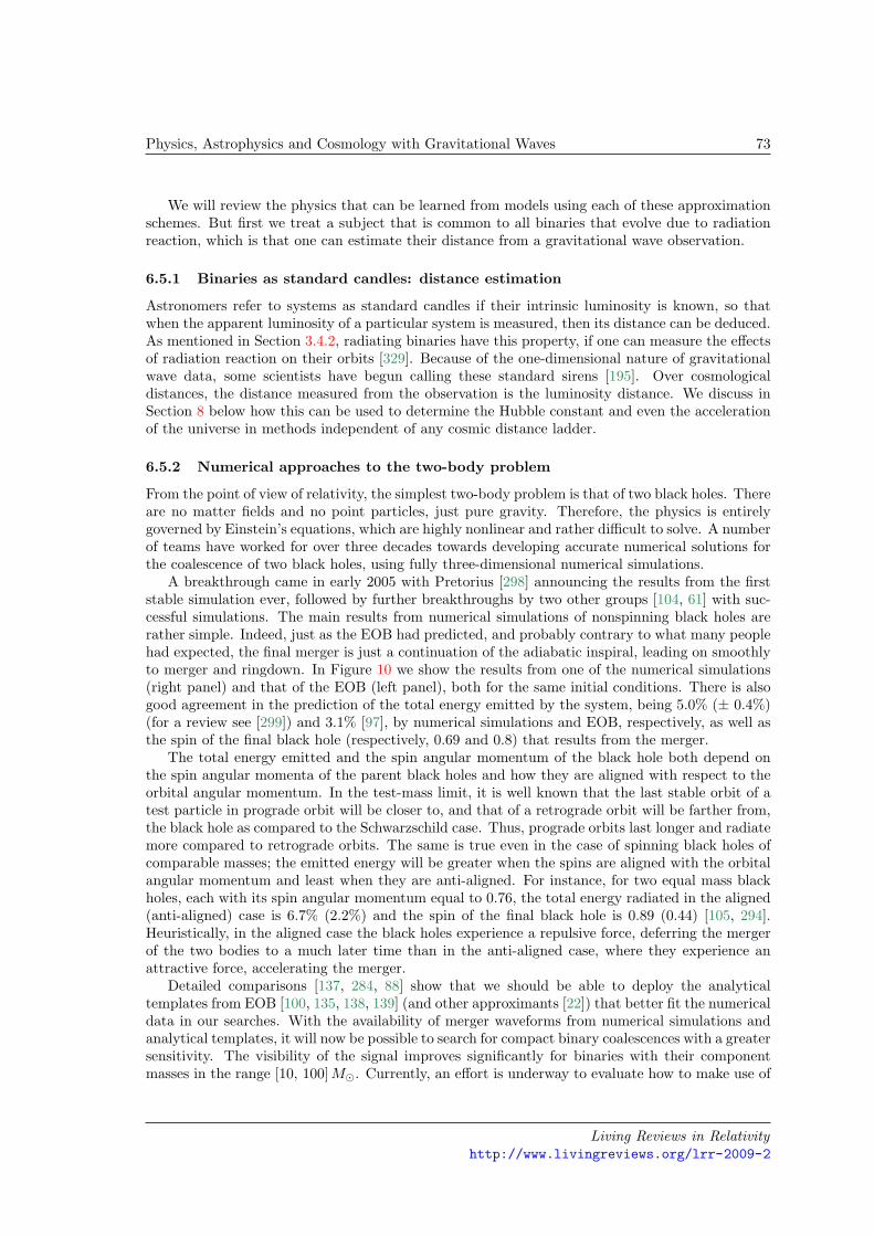
Physics, Astrophysics and Cosmology with Gravitational Waves 73
We will review the physics that can be learned from models using each of these approximationschemes. But first we treat a subject that is common to all binaries that evolve due to radiationreaction, which is that one can estimate their distance from a gravitational wave observation.
6.5.1 Binaries as standard candles: distance estimation
Astronomers refer to systems as standard candles if their intrinsic luminosity is known, so thatwhen the apparent luminosity of a particular system is measured, then its distance can be deduced.As mentioned in Section 3.4.2, radiating binaries have this property, if one can measure the effectsof radiation reaction on their orbits [329]. Because of the one-dimensional nature of gravitationalwave data, some scientists have begun calling these standard sirens [195]. Over cosmologicaldistances, the distance measured from the observation is the luminosity distance. We discuss inSection 8 below how this can be used to determine the Hubble constant and even the accelerationof the universe in methods independent of any cosmic distance ladder.
6.5.2 Numerical approaches to the two-body problem
From the point of view of relativity, the simplest two-body problem is that of two black holes. Thereare no matter fields and no point particles, just pure gravity. Therefore, the physics is entirelygoverned by Einstein’s equations, which are highly nonlinear and rather difficult to solve. A numberof teams have worked for over three decades towards developing accurate numerical solutions forthe coalescence of two black holes, using fully three-dimensional numerical simulations.
A breakthrough came in early 2005 with Pretorius [298] announcing the results from the firststable simulation ever, followed by further breakthroughs by two other groups [104, 61] with suc-cessful simulations. The main results from numerical simulations of nonspinning black holes arerather simple. Indeed, just as the EOB had predicted, and probably contrary to what many peoplehad expected, the final merger is just a continuation of the adiabatic inspiral, leading on smoothlyto merger and ringdown. In Figure 10 we show the results from one of the numerical simulations(right panel) and that of the EOB (left panel), both for the same initial conditions. There is alsogood agreement in the prediction of the total energy emitted by the system, being 5.0% (± 0.4%)(for a review see [299]) and 3.1% [97], by numerical simulations and EOB, respectively, as well asthe spin of the final black hole (respectively, 0.69 and 0.8) that results from the merger.
The total energy emitted and the spin angular momentum of the black hole both depend onthe spin angular momenta of the parent black holes and how they are aligned with respect to theorbital angular momentum. In the test-mass limit, it is well known that the last stable orbit of atest particle in prograde orbit will be closer to, and that of a retrograde orbit will be farther from,the black hole as compared to the Schwarzschild case. Thus, prograde orbits last longer and radiatemore compared to retrograde orbits. The same is true even in the case of spinning black holes ofcomparable masses; the emitted energy will be greater when the spins are aligned with the orbitalangular momentum and least when they are anti-aligned. For instance, for two equal mass blackholes, each with its spin angular momentum equal to 0.76, the total energy radiated in the aligned(anti-aligned) case is 6.7% (2.2%) and the spin of the final black hole is 0.89 (0.44) [105, 294].Heuristically, in the aligned case the black holes experience a repulsive force, deferring the mergerof the two bodies to a much later time than in the anti-aligned case, where they experience anattractive force, accelerating the merger.
Detailed comparisons [137, 284, 88] show that we should be able to deploy the analyticaltemplates from EOB [100, 135, 138, 139] (and other approximants [22]) that better fit the numericaldata in our searches. With the availability of merger waveforms from numerical simulations andanalytical templates, it will now be possible to search for compact binary coalescences with a greatersensitivity. The visibility of the signal improves significantly for binaries with their componentmasses in the range [10, 100]M. Currently, an effort is underway to evaluate how to make use of
Living Reviews in Relativityhttp://www.livingreviews.org/lrr-2009-2
74 B.S. Sathyaprakash and Bernard F. Schutz
numerical relativity simulations in gravitational wave searches [352], which should help to increasethe distance reach of interferometric detectors by a factor of two and correspondingly nearly anorder-of-magnitude increase in event rate.
-200 -100 0 100t/M
-0.2
-0.1
0
0.1
0.2
0.3
h(t)
inspiral-plungemerger-ring-down
-200 -100 0 100t/M
-0.2
-0.1
0
0.1
0.2
0.3
h(t)
numerical relativity
Figure 10: Comparison of waveforms from the analytical EOB approach (left) and numerical relativitysimulations (right) for the same initial conditions. The two approaches predict very similar values for thetotal energy emitted in gravitational waves and the final spin of the black hole. Figure from [94].
Numerical relativity simulations have now greatly matured, allowing a variety of different stud-ies. Some are studying the effect of the spin orientations of the component black holes on the linearmomentum carried away by the final black hole, fancifully called kicks [188, 92, 62, 105, 180, 294];some have focused on the dependence of the emitted waveform phase and energy on the mass ratio;and yet others have strived to evolve the system with high accuracy and for a greater number ofcycles so as to push the techniques of numerical relativity to the limit [89, 88].
Of particular interest are the numerical values of black hole kicks that have been obtained forcertain special configurations of the component spins. Velocities as large as 4000 km s−1 havebeen reported by several groups, but such velocities are only achieved when both black holes havelarge11 spins. Such velocities are in excess of escape velocities typical of normal galaxies andare, therefore, of great astronomical significance. These high velocities, however, are not seen forgeneric geometries of the initial spin orientations; therefore, their astronomical significance is notyet clear.
What is the physics behind kicks? Beamed emission of radiation from a binary could result inimparting a net linear momentum to the final black hole. The radiation could be beamed eitherbecause the masses of the two black holes are not the same (resulting in asymmetric emission inthe orbital plane) or because of the precession of the orbital plane arising from spin-orbit andspin-spin interactions, or both. In the case of black holes with unequal masses, the largest kick onecan get is around 170 km s−1, corresponding to a mass ratio of about 3:1. It was really with theadvent of numerical simulations that superkicks begin to be realized, but only when black holeshad large spins. The spin-orbit configurations that produce large kicks are rather unusual and atfirst sight unexpected. When the component black holes are both of the same mass and have equalbut opposite spin angular momenta that lie in the orbital plane, frame dragging can lead to tiltingand oscillation of the orbital plane, which, in the final phases of the evolution, could result in arather large kick [299]. SMBHs are suspected to have large spins and, therefore, the effect of spin
11By large spins we mean values that are close to the maximum value allowed by general relativity. If J is themagnitude of the spin angular momentum then general relativity requires that |J| ≤ M2
Living Reviews in Relativityhttp://www.livingreviews.org/lrr-2009-2
Physics, Astrophysics and Cosmology with Gravitational Waves 75
on the evolution of a binary and the final spin and kick velocity could be of astrophysical interesttoo.
Curiously, a recent optical observation of a distant quasar, SDSS J0927 12.65+294344.0, couldwell be the first identification of a superkick, causing the SMBH to escape from the parentgalaxy [222]. From a fundamental physics point of view, kicks offer a new way of testing framedragging in the vicinity of black holes, but much work is needed in this direction.
More recently, there has been an effort to understand and predict [98, 309, 136] the spin of thefinal black hole, which should help in further exploring interesting regions of the spin parameterspace. In the relatively simple case of two black holes with equal and aligned spins of magnitudea, but unequal masses, with the symmetric mass ratio being ν = m1m2/(m1 +m2)2, Rezzolla etal. [309] have obtained an excellent fit for the final spin afin of the black hole by enforcing basicconstraints from the test-mass limit:
afin = a+ (2√
3 + t0a+ s4a2)ν + (s5a+ t2)ν2 + t3ν
3,
where t0 = −2.686 ± 0.065, t2 = −3.454 ± 0.132, t3 = 2.353 ± 0.548, s4 = −0.129 ± 0.012, ands5 = −0.384± 0.261. The top and middle panels of Figure 11 compare as functions of black holespin and the symmetric mass ratio the goodness of their fit (blue short-dashed line, top panels)with the predictions of numerical simulations (circles and stars) from different groups (AEI [311],FAU–Jena [251], Jena [75] and Goddard [100]). Their residuals (red dotted lines, bottom panels)are less than a percent over the entire parameter space observed. These figures also show the fitsobtained for the equal-mass but variable-spin case (green long-dashed line, left panel) [98] and forthe nonspinning but unequal-mass case (green long-dashed line, middle panel) [136].
For the simple case of two equal mass black holes with aligned spins, the above analyticalformula predicts that minimal and maximal final spin values of afin = 0.35 ± 0.03 and afin =0.96 ± 0.03, respectively [309]. More interestingly, one can now ask what initial configurationsof the mass ratios and spins would lead to the formation of a Schwarzschild black hole (i.e.,afin(a, ν) = 0) [199], which defines the boundary of the region on one side of which lie systems forwhich the spin of the final black hole flips relative to the initial total angular momentum (bottompanel in Figure 11).
Finally, the evolution of binaries composed of nonspinning bodies is characterized by a singleparameter, namely the ratio of the masses of the two black holes. The study of systems withdifferent mass ratios has allowed relativists to fit numerical waveforms with phenomenologicalwaveforms [22]. The advantage of the latter waveforms is that one is able to more readily carryout data analysis in any part of the parameter space without needing the numerical data over theentire signal manifold.
Numerical relativity is still in its infancy and the parameter space is quite large. In the comingyears more accurate simulations should become available, allowing the computation of waveformswith more cycles and less systematic errors. However, the challenge remains to systematicallyexplore the effect of different spin orientations, mass ratios and eccentricity. One area that hasnot been explored using perturbative methods or post-Newtonian theory is that of intermediate–mass-ratio inspirals. These are systems with moderate mass ratios of order 100:1, where neitherblack-hole perturbation theory nor post-Newtonian approximation might be adequate. Yet, theprospect for detecting such systems in ground and space-based detectors is rather high. Numericalrelativity simulations might be the only way to set up effectual search templates for such systems.
6.5.3 Post-Newtonian approximation to the two-body problem
For the interpretation of observations of neutron-star–binary coalescences, which might be detectedwithin five years by upgraded detectors that are now taking data, it is necessary to understandtheir orbital evolution to a high order in the PN expansion. The first effects of radiation reaction
Living Reviews in Relativityhttp://www.livingreviews.org/lrr-2009-2

76 B.S. Sathyaprakash and Bernard F. Schutz
Figure 11: The final spin of a black hole that results from the merger of two equal mass black holes ofaligned spins (top panel) and nonspinning unequal mass black holes (middle panel). The bottom panelshows the region in the parameter space that results in an overall flip in the spin-orbit orientation of thesystem. Figure reprinted with permission from [310]. See text for details. c© The American AstronomicalSociety.
Living Reviews in Relativityhttp://www.livingreviews.org/lrr-2009-2
Physics, Astrophysics and Cosmology with Gravitational Waves 77
are seen at 2.5 PN order (i.e., at order (v/c)5 beyond Newtonian gravity), but we probably haveto have control in the equations of motion over the expansion at least to 3.5 PN order beyondthe first radiation reaction (i.e., to order (v/c)12 beyond Newtonian dynamics). There are manyapproaches to this, and we can not do justice here to the enormous effort that has gone into thisfield in recent years and refer the reader to the Living Reviews by Blanchet [79] and by Futamase& Itoh [169].
Most work on this problem so far has treated a binary system as if it were composed of twopoint masses. This is, strictly speaking, inconsistent in general relativity, since the masses shouldform black holes of finite size. Blanchet, Damour, Iyer, and collaborators [78] have avoided thisproblem by a method that involves generalized functions. They first expand in the nonlinearityparameter, and, when they have reached sufficiently high order, they obtain the velocity expansionof each order. By ordering terms in the post-Newtonian manner they have developed step-by-stepthe approximations up to 3.5 PN order.
A different team, led by Will, works with a different method of regularizing the point-particlesingularity and compares its results with those of Blanchet et al. at each order [82]. There is noguarantee that either method can be continued successfully to any particular order, but so far theyhave worked well and are in agreement. Their results form the basis of the templates that arebeing designed to search for binary coalescences.
An interesting way of extending the validity of the expansion that is known to any order isto use Pade approximants [133, 134] (rational polynomials) of the fundamental quantities in thetheory, namely the orbital energy and the gravitational wave luminosity. This has worked ratherwell in improving the convergence of PN theory. Buonanno and Damour [96, 97] have proposed anEOB approach to two-body dynamics, which makes it possible to compute the orbit of the binaryand hence the phasing of the gravitational waves emitted beyond the last stable orbit into themerger and ringdown phases in the evolution of the black hole binary. This analytical approachhas been remarkably successful and gained a lot of ground after the recent success in numericalrelativity (see Section 6.5.2).
Other methods have been applied to this problem. Futamase [168] introduced a limit thatcombines the nonlinearity and velocity expansions in different ways in different regions of space,so that the orbiting bodies themselves have a regular (finite relativistic self-gravity) limit, whiletheir orbital motion is treated in a Newtonian limit. This should not fail at any order [169], andhas demonstrated its robustness by arriving at the same results as the other approaches, at leastthrough 3 PN order. But it has a degree of arbitrariness in choosing initial data (see [327]) thatcould cause problems for gravitational wave search templates that integrate orbits for a long periodof time.
Linear calculations of point particles around black holes are of interest in themselves and also forchecking results of the full two-body calculations. These are well-developed for certain situations,e.g., [354, 258]. But the general equation of motion for such a body, taking into account allnongeodesic effects, has not yet been cast into a form suitable for practical calculations [106, 301].This field is reviewed by two separate Living Reviews [292, 319].
Matched filtering, discussed in Section 5.1, is a plausible method of testing the validity ofdifferent approaches to computing the inspiral and merger waveforms from binary systems. Thougha single observation is not likely to settle the question as to which methods are correct, a catalogueof events will help to evaluate the accuracy of different approaches by studying the statistics of theSNRs they measure.
6.5.3.1 Post-Newtonian expansions of energy and luminosity. Post-Newtonian calcu-lations yield the expansion of the gravitational binding energy E and the gravitational wave lu-
Living Reviews in Relativityhttp://www.livingreviews.org/lrr-2009-2
78 B.S. Sathyaprakash and Bernard F. Schutz
minosity F as a function of the post-Newtonian expansion parameter12 v. This is related to thefrequency fgw of the dominant component of gravitational waves emitted by the binary system by
v3 = πMfgw,
where M is the total mass of the system. The expansions for a circular binary are [80, 81, 79]
E = −νMv2
2
1 +
(−9 + ν
12
)v2 +
(−81 + 57ν − ν2
24
)v4
+(−675
64+[34445576
− 205π2
96
]ν − 155
96ν2 − 35
5184ν3
)v6 +O(v8)
, (113)
and
F =32ν2v10
5
1−
(1247336
+3512ν
)v2 + 4πv3 +
(−44711
9072+
9271504
ν +6518ν2
)v5
−(
8191672
+58324
)πv5 +
[664373951969854400
+163π2 − 1712
105(γ + ln(4v))
+(−4709005
272160+
4148π2
)ν − 94403
3024ν2 − 775
324ν3
]v6
+(−16285
504+
2147451728
ν +1933853024
ν2
)πv7 +O(v8)
, (114)
where γ = 0.577 . . . is Euler’s constant.
6.5.3.2 Evolution equation for the orbital phase. Starting from these expressions, onerequires that gravitational radiation comes at the expense of the binding energy of the system(see, e.g., [134]):
F = −dEdt, (115)
the energy balance equation. This can then be used to compute the (adiabatic) evolution of thevarious quantities as a function of time. For instance, the rate of change of the orbital velocityω(t) = v3/M (M being the total mass) can be computed using:
dω(t)dt
=dω
dv
dv
dE
dE
dt=
3v2
M
F(v)E′(v)
,dv
dt=
dv
dE
dE
dt=−F(v)E′(v)
, (116)
where E′(v) = dE/dv. Supplemented with a differential equation for t,
dt =dt
dE
dE
dv= −E
′(v)F
, (117)
one can solve for the evolution of the system’s orbital velocity. Similarly, the evolution of theorbital phase ϕ(t) can be computed using
dϕ(t)dt
=v3
M,
dv
dt=−F(v)E′(v)
. (118)
12In Newton’s theory a two-body problem can be reduced to a one-body problem, in which a body of reducedmass µ moves in an effective potential. The parameter v is the velocity of the reduced mass, if the orbit is circular.In the extreme mass ratio limit ν → 0, v is the velocity of the smaller mass.
Living Reviews in Relativityhttp://www.livingreviews.org/lrr-2009-2
Physics, Astrophysics and Cosmology with Gravitational Waves 79
6.5.3.3 Phasing formulas. The foregoing evolution equations for the orbital phase can besolved in several equivalent ways [134], each correct to the required post-Newtonian order, butnumerically different from one another. For instance, one can retain the rational polynomialF(v)/E(v) in Equation (118) and solve the two differential equations numerically, thereby obtainingthe time evolution of ϕ(t). Alternatively, one might re-expand the rational function F(v)/E(v)as a polynomial in v, truncate it to order vn (where n is the order to which the luminosity isgiven), thereby obtaining a parametric representation of the phasing formula in terms of polynomialexpressions in v:
ϕ(v) = ϕref +n∑
k=0
ϕkvk, t(v) = tref +
n∑k=0
tkvk, (119)
where ϕref and tref are a reference phase and time, respectively. The standard post-Newtonianphasing formula goes one step further and inverts the second of the relations above to express v asa polynomial in t (again truncated to appropriate order), which is then substituted in the first ofthe expressions above to obtain a phasing formula as an explicit function of time:
ϕ(t) =−1ντ5
1 +
(37158064
+5596ν
)τ2 − 3π
4τ3 +
(927549514450688
+284875258048
ν +18552048
ν2
)τ4
+(− 38645
172032+
652048
ν
)πτ5 ln τ +
[83103245074935757682522275840
− 5340π2 − 107
56(γ + ln(2τ))
+(−126510089885
4161798144+
22552048
π2
)ν +
1545651835008
ν2 − 11796251769472
ν3
]τ6
+(
188516689173408256
+488825516096
ν − 141769516096
ν2
)πτ7
, (120)
v2 =τ2
4
1 +
(7434032
+1148ν
)τ2 − π
5τ3 +
(19583254016
+24401193536
ν +31288
ν2
)τ4
+(−11891
53760+
1091920
ν
)πτ5 +
[−10052469856691
6008596070400+π2
6+
107420
(γ + ln 2τ)
+(
3147553127780337152
− 4513072
π2
)ν − 15211
442368ν2 +
25565331776
ν3
]τ6
+(−113868647
433520640− 31821
143360ν +
2949413870720
ν2
)πτ7
. (121)
In the above formulas v = πMfgw and τ = [ν(tC − t)/(5M)]−1/8, tC being the time at which thetwo stars merge together and the gravitational wave frequency fgw formally diverges.
6.5.3.4 Waveform polarizations. The post-Newtonian formalism also gives the two polar-izations h+ and h× as multipole expansions in powers of the parameter v. To lowest order, the twopolarizations of the radiation from a binary with a circular orbit, located at a distance D, withtotal mass M and symmetric mass ratio ν = m1m2/M
2, are given by
h+ =2νMD
v2(1 + cos2 ι) cos[2ϕ(t)], h× =4νMD
v2 cos ι sin[2ϕ(t)], (122)
where ι is the inclination of the orbital plane with the line of sight and v is the velocity parameterintroduced earlier.
An interferometer will record a certain combination of the two polarizations given by
h(t) = F+h+ + F×h×, (123)
Living Reviews in Relativityhttp://www.livingreviews.org/lrr-2009-2
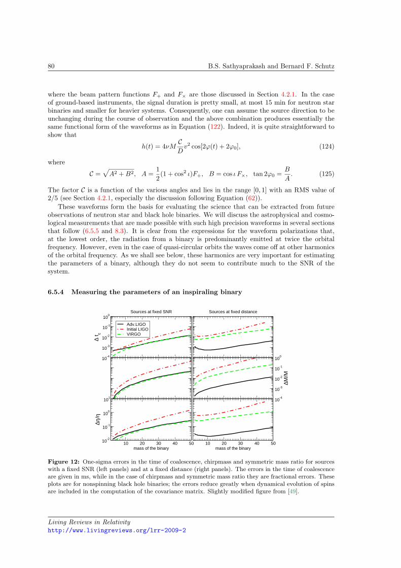
80 B.S. Sathyaprakash and Bernard F. Schutz
where the beam pattern functions F+ and F× are those discussed in Section 4.2.1. In the caseof ground-based instruments, the signal duration is pretty small, at most 15 min for neutron starbinaries and smaller for heavier systems. Consequently, one can assume the source direction to beunchanging during the course of observation and the above combination produces essentially thesame functional form of the waveforms as in Equation (122). Indeed, it is quite straightforward toshow that
h(t) = 4νMCDv2 cos[2ϕ(t) + 2ϕ0], (124)
where
C =√A2 +B2, A =
12(1 + cos2 ι)F+, B = cos ι F×, tan 2ϕ0 =
B
A. (125)
The factor C is a function of the various angles and lies in the range [0, 1] with an RMS value of2/5 (see Section 4.2.1, especially the discussion following Equation (62)).
These waveforms form the basis for evaluating the science that can be extracted from futureobservations of neutron star and black hole binaries. We will discuss the astrophysical and cosmo-logical measurements that are made possible with such high precision waveforms in several sectionsthat follow (6.5.5 and 8.3). It is clear from the expressions for the waveform polarizations that,at the lowest order, the radiation from a binary is predominantly emitted at twice the orbitalfrequency. However, even in the case of quasi-circular orbits the waves come off at other harmonicsof the orbital frequency. As we shall see below, these harmonics are very important for estimatingthe parameters of a binary, although they do not seem to contribute much to the SNR of thesystem.
6.5.4 Measuring the parameters of an inspiraling binary
10-4
10-3
10-2
10-1
100
∆ t c
Adv.LIGOInitial LIGOVIRGO
Sources at fixed SNR Sources at fixed distance
10-4
10-3
10-2
10-1
100
∆M/M
10 20 30 40 50mass of the binary
10-2
10-1
100
101
∆η/η
10 20 30 40 50mass of the binary
Figure 12: One-sigma errors in the time of coalescence, chirpmass and symmetric mass ratio for sourceswith a fixed SNR (left panels) and at a fixed distance (right panels). The errors in the time of coalescenceare given in ms, while in the case of chirpmass and symmetric mass ratio they are fractional errors. Theseplots are for nonspinning black hole binaries; the errors reduce greatly when dynamical evolution of spinsare included in the computation of the covariance matrix. Slightly modified figure from [49].
Living Reviews in Relativityhttp://www.livingreviews.org/lrr-2009-2
Physics, Astrophysics and Cosmology with Gravitational Waves 81
The issue of parameter estimation in the context of black hole binaries has received a lot ofattention [114, 128, 165, 64, 293, 65, 44]. Most authors have used the covariance matrix for thispurpose, although Markov Chain Monte Carlo (MCMC) techniques have also been used occa-sionally [116, 316, 315, 120], especially in the context of LISA [364, 121, 122, 123, 125]. Covari-ance matrix is often the preferred method, as one can explore a large parameter space withouthaving to do expensive Monte Carlo simulations. However, when the parameter space is large,covariance matrix is not a reliable method for estimating parameter accuracies, especially at lowSNRs [63, 64, 372]; but at high SNRs, as in the case of SMBH binaries in LISA, the problem mightbe that our waveforms are not accurate enough to facilitate a reliable extraction of the source pa-rameters [129]. Although MCMC methods can give more reliable estimates, they suffer from beingcomputationally extremely expensive. However, they are important in ascertaining the validityof results based on the covariance matrix, at least in a small subset of the parameter space, andshould probably be employed in assessing parameter accuracies of candidate gravitational waveevents.
In what follows we shall summarize the most recent work on parameter estimation in groundand space-based detectors for binaries with and without spin and the improvements brought aboutby including higher harmonics.
6.5.4.1 Ground-based detectors – nonspinning components. In Figure 12 we have plot-ted the one-sigma uncertainty in the measurement of the time of coalescence, chirpmass and sym-metric mass ratio for initial and advanced LIGO and VIRGO [44]. The plots show errors for sourcesall producing a fixed SNR of 10 (left panels) or all at a fixed distance of 300 Mpc (right panels).The fractional error in chirpmass, even at a modest SNR of 10, can be as low as a few parts in tenthousand for stellar mass binaries, but the error stays around 1%, even for heavier systems thathave only a few cycles in a detector’s sensitivity band. Error in the mass ratio is not as small,increasing to 100% at the higher end of the mass range explored. Thus, although the chirpmasscan be measured to a good accuracy, poor estimation of the mass ratio means that the individualmasses of the binary cannot be measured very well. Note also that the time of coalescence of thesignal is determined pretty well, which means that we would be able to measure the location ofthe system in the sky quite well.
At a given SNR the accuracy is better in the case of low-mass binaries, since they spend alonger duration and a greater number of cycles in the detector band and the chirpmass can bedetermined better than the mass ratio, since to first order the frequency evolution of a binary isdetermined only by the chirpmass.
6.5.4.2 Measuring the parameters of supermassive black hole binaries in LISA. Inthe case of LISA, the merger of SMBHs produces events with extremely large SNRs, even at aredshift of z = 1 (100s to several thousands depending on the chirpmass of the source). Therefore,one expects to measure the parameters of a merger event in LISA to a phenomenal accuracy.Figure 13 depicts the distribution of the errors for a binary consisting of two SMBHs of masses(106, 3 × 10⁵)M at a redshift of z = 1 [232]. The distribution was obtained for ten thousandsamples of the system corresponding to random orientations of the binary at random sky locationswith the starting frequency greater than 3 × 10⁻⁵ Hz and the ending frequency corresponding tothe last stable orbit.
Each plot in Figure 13 shows the results of computations for binaries consisting of black holeswith and without spins. Even in the absence of spin-induced modulations in the waveform, theparameter accuracies are pretty good. Note that spin-induced modulations in the waveform enablea far better estimation of parameters, chirpmass accuracy improving by more than an order ofmagnitude and reduced mass accuracy by two orders of magnitude. It is because of such accurate
Living Reviews in Relativityhttp://www.livingreviews.org/lrr-2009-2
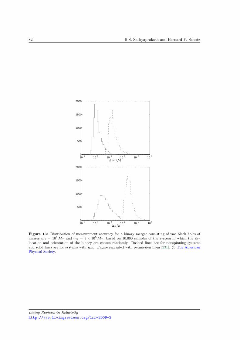
82 B.S. Sathyaprakash and Bernard F. Schutz
10−6
10−5
10−4
10−3
10−2
10−1
0
500
1000
1500
2000
∆M/M
10−5
10−4
10−3
10−2
10−1
100
0
500
1000
1500
2000
∆µ/µ
Figure 13: Distribution of measurement accuracy for a binary merger consisting of two black holes ofmasses m1 = 106M and m2 = 3 × 10⁵M, based on 10,000 samples of the system in which the skylocation and orientation of the binary are chosen randomly. Dashed lines are for nonspinning systemsand solid lines are for systems with spin. Figure reprinted with permission from [231]. c© The AmericanPhysical Society.
Living Reviews in Relativityhttp://www.livingreviews.org/lrr-2009-2
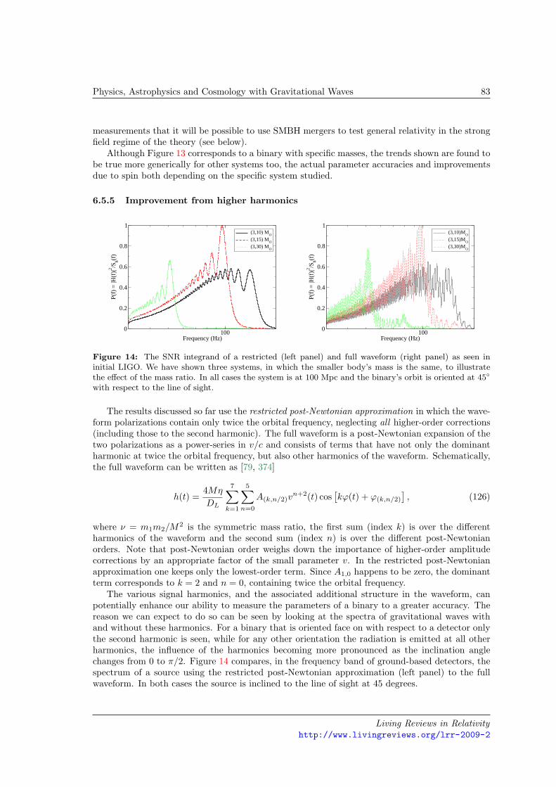
Physics, Astrophysics and Cosmology with Gravitational Waves 83
measurements that it will be possible to use SMBH mergers to test general relativity in the strongfield regime of the theory (see below).
Although Figure 13 corresponds to a binary with specific masses, the trends shown are found tobe true more generically for other systems too, the actual parameter accuracies and improvementsdue to spin both depending on the specific system studied.
6.5.5 Improvement from higher harmonics
100Frequency (Hz)
0
0.2
0.4
0.6
0.8
1
P(f)
= |H
(f)|2 /S
h(f)
(3,10) MO
(3,15) MO
(3,30) MO
100Frequency (Hz)
0
0.2
0.4
0.6
0.8
1
P(f)
= |H
(f)|2 /S
h(f)
(3,10)MO
(3,15)MO
(3,30)MO
Figure 14: The SNR integrand of a restricted (left panel) and full waveform (right panel) as seen ininitial LIGO. We have shown three systems, in which the smaller body’s mass is the same, to illustratethe effect of the mass ratio. In all cases the system is at 100 Mpc and the binary’s orbit is oriented at 45
with respect to the line of sight.
The results discussed so far use the restricted post-Newtonian approximation in which the wave-form polarizations contain only twice the orbital frequency, neglecting all higher-order corrections(including those to the second harmonic). The full waveform is a post-Newtonian expansion of thetwo polarizations as a power-series in v/c and consists of terms that have not only the dominantharmonic at twice the orbital frequency, but also other harmonics of the waveform. Schematically,the full waveform can be written as [79, 374]
h(t) =4Mη
DL
7∑k=1
5∑n=0
A(k,n/2)vn+2(t) cos
[kϕ(t) + ϕ(k,n/2)
], (126)
where ν = m1m2/M2 is the symmetric mass ratio, the first sum (index k) is over the different
harmonics of the waveform and the second sum (index n) is over the different post-Newtonianorders. Note that post-Newtonian order weighs down the importance of higher-order amplitudecorrections by an appropriate factor of the small parameter v. In the restricted post-Newtonianapproximation one keeps only the lowest-order term. Since A1,0 happens to be zero, the dominantterm corresponds to k = 2 and n = 0, containing twice the orbital frequency.
The various signal harmonics, and the associated additional structure in the waveform, canpotentially enhance our ability to measure the parameters of a binary to a greater accuracy. Thereason we can expect to do so can be seen by looking at the spectra of gravitational waves withand without these harmonics. For a binary that is oriented face on with respect to a detector onlythe second harmonic is seen, while for any other orientation the radiation is emitted at all otherharmonics, the influence of the harmonics becoming more pronounced as the inclination anglechanges from 0 to π/2. Figure 14 compares, in the frequency band of ground-based detectors, thespectrum of a source using the restricted post-Newtonian approximation (left panel) to the fullwaveform. In both cases the source is inclined to the line of sight at 45 degrees.
Living Reviews in Relativityhttp://www.livingreviews.org/lrr-2009-2
84 B.S. Sathyaprakash and Bernard F. Schutz
Following is a list of improvements brought about by higher harmonics. In the case of ground-based detectors Van Den Broeck and Sengupta [374, 375] found that, when harmonics are included,the SNR hardly changes, but is always smaller, relative to a restricted waveform. However, thepresence of frequencies higher than twice the orbital frequency means that it will be possible toobserve heavier systems, increasing the mass reach of ground-based detectors by a factor of 2 to3 in advanced LIGO and third generation detectors [374, 375]. The same effect was found inthe case of LISA too, allowing LISA to observe SMBH masses up to a few × 108M [47]. Morethan the increased mass reach, the harmonics reduce the error in the estimation of the chirpmass,symmetric mass ratio and the time of arrival by more than an order of magnitude for stellar-massblack hole binaries. The same is true to a greater extent in the case of SMBH binaries, allowingas well a far greater accuracy in the measurement of the luminosity distance and sky resolutionin LISA’s observation of these sources [48, 361]. For instance, Figure 15 [361] shows the gain inLISA’s angular resolution for two massive black-hole–binary mergers as a consequence of usinghigher harmonics for a specific orientation of the binary. Improvements of order 10 to 100 can beseen over large regions of the sky. This improved performance of LISA makes it a good probe ofdark energy [48] (see Section 8.3).
A word of caution is in order with regard to the improvements brought about by higher har-monics. If the sensitivity of a detector has an abrupt lower frequency cutoff, or falls off rapidlybelow a certain frequency, then the harmonics bring about a more dramatic improvement thanwhen the sensitivity falls off gently. Higher harmonics, nevertheless, always help in reducing therandom errors associated with the measurement of parameters of a coalescing black-hole binary.
6.6 Tests of general relativity
Gravitational wave measurements of black holes automatically test general relativity in its strong-field regime. Observations of the mergers of comparable-mass black holes will be rich in detailsof their strong-field interactions. If measurements can determine the masses and spins of theinitial black holes, as well as the eccentricity and orientation of their inspiral orbit, then one wouldhope to compare the actual observed waveform with the output of a numerical simulation of thesame system. If measurements can also determine the final mass and spin (say from the ringdownradiation) then one can test the Hawking area theorem (the final area must exceed the sum of theareas of the initial holes) and the Penrose cosmic censorship conjecture (the final black hole shouldhave J/M2 < 1).
Observations of stellar mass black holes inspiraling into SMBHs, the extreme mass ratio inspirals(EMRIs), have an even greater potential for testing general relativity. The stellar mass black holespends thousands of precessing (both of periastron and the orbital plane) orbits along highly-eccentric trajectories and slowly inspirals into the larger black hole. The emitted gravitationalradiation literally carries the signature of the spacetime geometry around the central object. Sofitting the orbit to theoretical templates could reveal small deviations of this geometry from thatof Kerr. For example, if we know (from fitting the waveform) the mass and spin of the centralblack hole, then all its higher multipole moments are determined. If we can measure some of theseand they deviate from Kerr, then that would indicate that either the central object is not a blackhole or that general relativity needs to be corrected [177, 68].
6.6.1 Testing the post-Newtonian approximation
Current tests of general relativity rely on experiments in the solar system (using the sun’s gravita-tional field) and observations of binary pulsars. In dimensionless units, the gravitational potentialon the surface of the sun is about one part in a million and even in a binary pulsar the potentialthat each neutron star experiences due to its companion is no more than one part in ten thou-
Living Reviews in Relativityhttp://www.livingreviews.org/lrr-2009-2
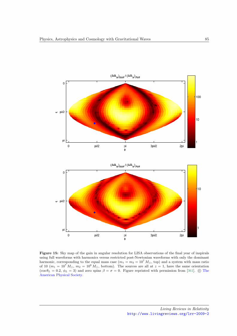
Physics, Astrophysics and Cosmology with Gravitational Waves 85
Figure 15: Sky map of the gain in angular resolution for LISA observations of the final year of inspiralsusing full waveforms with harmonics versus restricted post-Newtonian waveforms with only the dominantharmonic, corresponding to the equal mass case (m1 = m2 = 107M, top) and a system with mass ratioof 10 (m1 = 107M, m2 = 106M, bottom). The sources are all at z = 1, have the same orientation(cos θL = 0.2, φL = 3) and zero spins β = σ = 0. Figure reprinted with permission from [361]. c© TheAmerican Physical Society.
Living Reviews in Relativityhttp://www.livingreviews.org/lrr-2009-2
86 B.S. Sathyaprakash and Bernard F. Schutz
sand. These are mildly relativistic fields, with the corresponding escape velocity being as large asa thousandth and a hundredth that of light, respectively.
Thus, gravitational fields in the solar system or in a binary pulsar are still weak by comparisonto the largest possible values. Indeed, close to the event horizon of a black hole, gravitationalfields can get as strong as they can ever get, with the dimensionless potential being of order unityand the escape velocity equal to that of the speed of light. Although general relativity has beenfound to be consistent with experiments in the solar system and observations of binary pulsars,phenomena close to the event horizons of black holes would be a great challenge to the theory. Itwould be very exciting to test Einstein’s gravity under such circumstances.
The large SNR that is expected from SMBH binaries makes it possible to test Einstein’s theoryunder extreme conditions of gravity [45, 46]. To see how one might test the post-Newtonianstructure of Einstein’s theory, let us consider the waveform from a binary in the frequency domain.Since an inspiral wave’s frequency changes rather slowly (adiabatic evolution) it is possible to applya stationary phase approximation to compute the Fourier transform H(f) of the waveform givenin Equation (124):
H(f) = A f−7/6 exp[iΨ(f) + i
π
4
], (127)
with the Fourier amplitude A and phase Ψ(f) given by
A =C
Dπ2/3
√5ν24M5/6, Ψ(f) = 2πftC + ΦC +
3128 ν
∑k
αk (πMf)(k−5)/3. (128)
Here ν is the symmetric mass ratio defined before (see Equation 31), C is a function of the variousangles, as in Equation (124), and tC and ΦC are the fiducial epoch of merger and the phase of thesignal at that epoch, respectively. The coefficients in the PN expansion of the Fourier phase aregiven by
α0 = 1, α1 = 0, α2 =3715756
+559ν, α3 = −16π,
α4 =15293365508032
+27145504
ν +308572
ν2, α5 = π
(38645756
− 659ν
)[1 + ln
(63/2πM f
)],
α6 =11583231236531
4694215680− 640
3π2 − 6848
21γ +
(−15737765635
3048192+
225512
π2
)ν
+760551728
ν2 − 1278251296
ν3 − 684863
ln (64πM f) ,
α7 = π
(77096675254016
+3785151512
ν − 74045756
ν2
). (129)
These are the PN coefficients in Einstein’s theory; in an alternative theory of gravity they willbe different. In Einstein’s theory the coefficients depend only on the two mass parameters, thetotal mass M and symmetric mass ratio ν. One of the tests we will discuss below concerns theconsistency of the various coefficients. Note, in particular, that in Einstein’s gravity the 0.5 PNterm is absent, i.e., the coefficient of the term v is zero. Even with the very first observations ofinspiral events, it should be possible to test if this is really so.
Figure 16 shows one such test that is possible with SMBH binaries [45, 46]. The observationof these systems in LISA makes it possible to measure the parameters associated with differentphysical effects. For example, the rate at which a signal chirps (i.e., the rate at which its frequencychanges) depends on the binary’s chirpmass. Given the chirpmass, the length of the signal dependson the system’s symmetric mass ratio (the ratio of reduced mass to total mass). Another examplewould be the scattering of gravitational waves off the curved spacetime geometry of the binary,
Living Reviews in Relativityhttp://www.livingreviews.org/lrr-2009-2
Physics, Astrophysics and Cosmology with Gravitational Waves 87
producing the tail effect in the emitted signal, which is determined principally by the system’stotal mass [85, 84]. Similarly, spin-orbit interaction, spin-spin coupling, etc. depend on othercombinations of the masses.
The binary will be seen with a high SNR, which means that we can measure the mass parametersassociated with many of these physical effects. If each parameter is known precisely, we can draw acurve corresponding to it in the space of masses. However, our observations are inevitably subjectto statistical (and possibly systematic) errors. Therefore, each parameter corresponds to a regionin the parameter space (shown in Figure 16 for the statistical errors only). If Einstein’s theoryof gravitation is correct, the regions corresponding to the different parameters must all have atleast one common region, a region that contains the true parameters of the binary. This is becauseEinstein’s theory, or an alternative, has to be used to project the observed data onto the spaceof masses. If the region corresponding to one or more of these parameters does not overlap withthe common region of the rest of the parameters, then Einstein’s theory, or its alternative, is introuble.
In Brans–Dicke theory the system is expected to emit dipole radiation and the PN series wouldbegin an order v−2 earlier than in Einstein’s theory. In the notation introduced above we wouldhave an α−2 term, which has the form [73, 74]
α−2 = − 5S2
84ωBD. (130)
Here S is the the difference in the scalar charges of the two bodies and ωBD is the Brans–Dickeparameter. Although this term is formally two orders lower than the lowest-order quadrupole termof Einstein’s gravity (i.e., it is O(v−2) order smaller), numerically its effect will be far smaller thanthe quadrupole term because of the rather large bound on ωBD 1. Nevertheless, its importancelies in the fact that there is now a new parameter on which the phase depends. Berti, Buonannoand Will conclude that LISA observations of massive black-hole binaries will enable scientists toset limits on ωBD ∼ 104 – 105.
A massive graviton theory would also alter the phase. The dominant effect is at 1 PN orderand would change the coefficient α2 to
α2 → α2 −128ν
3π2DM
λ2g(1 + z)
, (131)
where ν is the symmetric mass ratio. This term alters the time of arrival of waves of differentfrequencies, causing a dispersion, and a corresponding modulation, in the wave’s phase, dependingon the Compton wavelength λg and the distance D to the binary. Hence, by tracking the phaseof the inspiral waves, one can bound the graviton’s mass. Will [393] finds that one can bound themass to 1.7×10¹³ km using ground-based detectors and 1.7×10¹⁷ km using space-based detectors,as also confirmed by more recent and exhaustive calculations [73]. These limits might improve ifone takes into account the modulation of the waveform due to spin-orbit and spin-spin coupling,but the latter authors [73] looked at spinning, but nonprecessing, systems only.
6.6.2 Uniqueness of Kerr geometry
In Section 3 we pointed out that LISA should be able to see many hundreds of signals emittedby compact objects – black holes, neutron stars, even white dwarfs – orbiting around and beingcaptured by massive black holes in the centers of galaxies. But for LISA to reach its full potential,we must model the orbits and their emitted radiation accurately. Since the wave trains maybe many hundreds or thousands of cycles long in the LISA band, the challenge of constructingtemplate waveforms that remain accurate to within about one radian over the whole evolution issignificant.
Living Reviews in Relativityhttp://www.livingreviews.org/lrr-2009-2
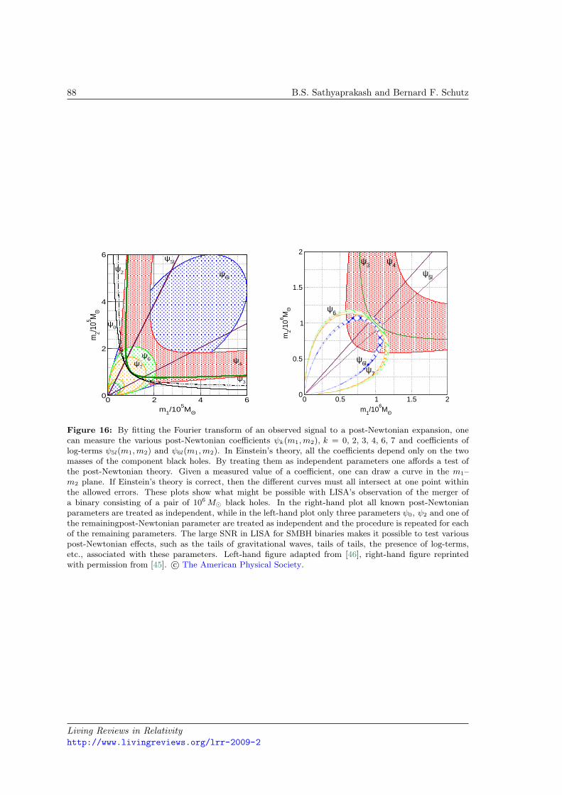
88 B.S. Sathyaprakash and Bernard F. Schutz
0 2 4 6m1/10
5MO.
0
2
4
6
m2/1
05 MO.
ψ6l
ψ3
ψ7
ψ6 ψ
4
ψ2
ψ0
ψ5l
0 0.5 1 1.5 2m1/10
6MO.
0
0.5
1
1.5
2
m2/1
06 MO.
ψ4ψ3
ψ6
ψ7
ψ6l
ψ5l
Figure 16: By fitting the Fourier transform of an observed signal to a post-Newtonian expansion, onecan measure the various post-Newtonian coefficients ψk(m1,m2), k = 0, 2, 3, 4, 6, 7 and coefficients oflog-terms ψ5l(m1,m2) and ψ6l(m1,m2). In Einstein’s theory, all the coefficients depend only on the twomasses of the component black holes. By treating them as independent parameters one affords a test ofthe post-Newtonian theory. Given a measured value of a coefficient, one can draw a curve in the m1–m2 plane. If Einstein’s theory is correct, then the different curves must all intersect at one point withinthe allowed errors. These plots show what might be possible with LISA’s observation of the merger ofa binary consisting of a pair of 106M black holes. In the right-hand plot all known post-Newtonianparameters are treated as independent, while in the left-hand plot only three parameters ψ0, ψ2 and one ofthe remainingpost-Newtonian parameter are treated as independent and the procedure is repeated for eachof the remaining parameters. The large SNR in LISA for SMBH binaries makes it possible to test variouspost-Newtonian effects, such as the tails of gravitational waves, tails of tails, the presence of log-terms,etc., associated with these parameters. Left-hand figure adapted from [46], right-hand figure reprintedwith permission from [45]. c© The American Physical Society.
Living Reviews in Relativityhttp://www.livingreviews.org/lrr-2009-2
Physics, Astrophysics and Cosmology with Gravitational Waves 89
The range of mass ratios is also wide. LISA’s central black holes might have masses between 103
and 107M. Inspiraling neutron stars and white dwarfs might have masses between 0.5 and 2M.Inspiraling stellar-population black holes might be in the range of 7 – 50M, while intermediate-mass black holes formed by the first generation of stars (Population III stars) might have massesaround 300M or even 1000M. So the mass ratios might be anything in the range 10−7 to 1.
The techniques that must be used to compute these signals depend on the mass ratio. Ratiosnear one are treated by post-Newtonian methods until the objects are so close that only numericalrelativity can follow their subsequent evolution. For ratios below 10−4 (a dividing line that is rathervery uncertain and that depends on the bandwidth being used to observe the system, i.e., on howlong the approximation must be valid for), systems are treated by fully-relativistic perturbationtheory, expanding in the mass ratio. Intermediate mass ratios have not been studied in much detailyet; they can probably be treated by post-Newtonian methods up to a certain point, but it is notyet clear whether their final stages can be computed accurately by either numerical relativity orperturbation theory.
Post-Newtonian methods have been extensively discussed above. The basics of perturbationtheory underlying this problem are treated in two Living Reviews [292, 319]. Once one has suf-ficiently good waveform templates, there remain the challenge of finding weak signals in LISA’snoise. This depends on a number of factors, including the rates of sources. A recent study bya number of specialists [170] has concluded that the event rate is high enough and the detectionmethods robust enough for us to be very optimistic that LISA will detect hundreds of these sources.In fact, the opposite problem might materialize: LISA might find it has a confusion problem forthe detection of these sources, as for the galactic binaries. Recent estimates of the magnitude ofthe problem [66] suggest that LISA’s noise may at worst be raised effectively by a factor of two,but in return one gets a large number of sources of this kind.
6.6.3 Quantum gravity
It seems inevitable that general relativity’s description of nature will one day yield to a quantum-based description, involving uncertainties in geometry and probabilities in the outcome of gravita-tional observations. This is one of the most active areas of research in fundamental physics today,and there are many speculations about how quantum effects might show up in gravitational waveobservations.
The simplest idea might be to try to find evidence for “gravitons” directly in gravitational waves,by analogy with the way that astronomers count individual photons from astronomical sources.But this seems doomed to failure. The waves that we can observe have very low frequency, so theenergy of each graviton is extremely small. And the total energy flux of the waves is, as we haveseen, enormous. So the number of gravitons in a detectable gravitational wave is far more thanthe number of photons in the light from a distant quasar.
Quantum gravity might involve new gravity-like fields, whose effects might be seen indirectlyin the inspiral signals of black holes or neutron stars, as we have noted above. String theory mightlead to the production of cosmic strings, which might be observed through their gravitational waveemission [142]. If our universe is just a 4-dimensional subspace of a large-scale 10 or 11-dimensionalspace, then dynamics in the larger space might produce gravitational effects in our space, and inparticular gravitational waves [304].
It might be possible to observe the quantum indeterminacy of geometry directly using grav-itational wave detectors, if Hogan’s principle of holographic indeterminacy is valid [193]. Hoganspeculates that quantum geometry might be manifested by an uncertainty in the position of abeam splitter, and that this could be the explanation for an unexpectedly large amount of noiseat low frequencies in the GEO600 detector. In this connection it is interesting to construct, fromfundamental constants alone, a quantity with the dimensions of amplitude spectral noise density
Living Reviews in Relativityhttp://www.livingreviews.org/lrr-2009-2
90 B.S. Sathyaprakash and Bernard F. Schutz
(Sh)1/2. This has units of s1/2, so one can define the “Planck noise power” SPl = tPl = (G~/c5)1/2.Then the amplitude noise is S1/2
Pl = (G~/c5)1/4 = 2.3 × 10⁻²² Hz−1/2. This is comparable to orlarger than the instrumental noise in current interferometric gravitational wave detectors, as shownin Figure 5. This in itself does not mean that Planckian noise will show up in gravitational wavedetectors, but Hogan argues that the particular design of GEO600 might indeed make it subjectto this noise more strongly than other large interferometers.
Living Reviews in Relativityhttp://www.livingreviews.org/lrr-2009-2
Physics, Astrophysics and Cosmology with Gravitational Waves 91
7 Astrophysics with Gravitational Waves
Gravitational radiation plays an observable role in the dynamics of many known astronomicalsystems. In some, such as cataclysmic variables [157] and neutron-star–binary systems [355], therole of gravitational radiation has been understood for years. In others, such as young neutronstars [34] and low-mass X-ray binaries [77], the potential importance of gravitational radiationhas been understood only recently. As further observations, particularly at X-ray wavelengths,become available, the usefulness of gravitational radiation as a tool for modelling astronomicalsystems should increase [385].
At this point in the progress of gravitational wave detection, the greatest emphasis in cal-culations of sources is on prediction: trying to anticipate what might be seen. Not only is thisimportant in motivating the construction of detectors, but it also guides details of their design and,very importantly, the design of data analysis methods. Historically, many predictions of emissionstrengths and the capability of detectors to extract information from signals have relied on esti-mates using the quadrupole formula. This was justifiable because, given the uncertainties in ourastrophysical understanding of potential sources, more accurate calculations would be unjustifiedin most cases.
But these rough estimates are now being replaced by more and more detailed source modelswhere possible. This applies particularly in two cases. One is binary orbits, where the point-mass approximation is good over a large range of observable frequencies, so that fully relativisticcalculations (using the post-Newtonian methods described above) are not only possible, but arenecessary for the construction of sensitive search templates in the data analysis. The secondexception is the numerical simulations of the merger of black holes and neutron stars, where thedynamics is so complex that none of our analytic approximations offers us reliable guidance. Infact, these two methods are currently being joined to produce uniform models of signal evolutionover as long an observation time as the signal allows. From these models we not only improvedetection algorithms, but we also learn much more about the kinds of information that detectionswill extract from the signals.
Once gravitational waves have been observed, there will of course be a welcome shift of emphasisto include interpretation. The emphasis will be on extracting observable parameters (waveforms,polarizations, source location, etc.) from noisy data or data where (in the case of LISA) there issource confusion. These issues need considerably more attention than they have so far received.
7.1 Interacting compact binaries
The first example of the use of gravitational radiation in modelling an observed astronomicalsystem was the explanation by Faulkner [157] of how the activity of cataclysmic binary systemsis regulated. Such systems, which include many novae, involve accretion by a white dwarf froma companion star. Unlike accretion onto neutron stars, where the accreted hydrogen is normallyprocessed quickly into heavier elements, on a white dwarf the unprocessed material can build upuntil there is a nuclear chain reaction, which results in an outburst of visible radiation from thesystem.
Now, in a circular binary system that conserves total mass and angular momentum, a transferof mass from a more massive to a less massive star will make the orbit shrink, while a transfer inthe opposite direction makes the orbit grow. If accretion onto a white dwarf begins with the dwarfas the less massive star, then the stars will draw together, and the accretion will get stronger.This runaway process stops when the stars are of equal mass, and then accretion begins to drivethem apart again. Astronomers observed that in this phase accretion in certain very close binariescontinued at a more or less steady rate, instead of shutting off as the stars separated more andmore. Faulkner pointed out that gravitational radiation from the orbital motion would carry
Living Reviews in Relativityhttp://www.livingreviews.org/lrr-2009-2
92 B.S. Sathyaprakash and Bernard F. Schutz
away angular momentum and drive the stars together. The two effects together result in steadyaccretion at a rate that can be predicted from the quadrupole formula and simple Newtonianorbital dynamics, and which is in good accord with observations in a number of systems.
Binaries consisting of two white dwarfs in very tight orbits will be direct LISA sources: we won’thave to infer their radiation indirectly, but will actually be able to detect it. Some of them willalso be close enough to tidally interact with one another, leading in some cases to mass transfer.Others will be relatively clean systems in which the dominant effect will be gravitational radiationreaction.
Observations during the last decade have identified a number of such systems with enoughconfidence to predict that LISA should see their gravitational waves. These are called verificationbinaries: if LISA does not see them then either the instrument is not working properly or generalrelativity is wrong! For a review of verification binaries, see [349].
7.1.1 Resolving the mass-inclination degeneracy
Gravitational-wave–polarization measurements can be very helpful in resolving the degeneracythat occurs in the measurement of the mass and inclination of a binary system. As is well known,astronomical observations of binaries cannot yield the total mass but only the combination m sin ι,where ι is the inclination of the binary’s orbit to the line of sight. However, measurement of polar-ization can determine the angle ι since the polarization state depends on the binary’s inclinationwith the line of sight.
For instance, consider a circular binary system with total mass M at a distance D. Suppose itsorbital angular momentum vector makes an angle ι with the line of sight (the standard definitionof the inclination of a binary orbit). The two observed polarizations are given in the quadrupoleapproximation by Equation (122). We can eliminate the distance R between the stars that isimplicit in the velocity v = Rω (where ω is the instantaneous angular velocity of the orbit, thederivative of the orbital phase function ϕ(t)) by using the Newtonian orbital dynamics equationω2 = M/R3. Then we find
h+ =2νMD
[πMf(t)]2/3(1 + cos2 ι) cos[2ϕ(t)], h× =4νMD
[πMf(t)]2/3 cos ι sin[2ϕ(t)], (132)
where M is the total mass of the binary and, as before, ν is the symmetric mass ratio m1m2/M2.
The frequency f = ω/π is the gravitational wave frequency, twice the orbital frequency. Noticethat, consistent with Equation (30), the masses of the stars enter these equations only in thecombination M = ν3/5M .
It is clear that the ratio of the two polarization amplitudes determines the angle ι. In thisconnection it is interesting to relate the polarization to the orientation. When the binary isviewed from a point in its orbital plane, so that ι = π/2, then h× = 0; the radiation has pure+ polarization. From the observer’s point of view, the motion of the binary stars projected ontothe sky is purely linear; the two stars simply go back and forth across the line of sight. This linearprojected motion results in linearly polarized waves. At the other extreme, consider viewing thesystem down its orbital rotation axis, where ι = 0. The stars execute a circular motion in thesky, and the polarization components h+ and h× have equal amplitude and are out of phase byπ/2. This is circularly polarized gravitational radiation. So, when the radiation is produced inthe quadrupole approximation, the polarization has a very direct relationship to the motions ofthe masses when projected on the observer’s sky plane. If the radiation is produced by highermultipoles it becomes more complex to make these relations, but it can be done. For example,see [333] for the case of current quadrupole radiation, which is emitted by the r-mode instabilitydiscussed in Section 7.3.4.2 below.
While a single detector is linearly polarized, it can still measure the two polarizations if thesignal has a long enough duration for the detector to turn (due to the motion of the Earth) and
Living Reviews in Relativityhttp://www.livingreviews.org/lrr-2009-2
Physics, Astrophysics and Cosmology with Gravitational Waves 93
change the polarization component it measures. Alternatively, a network of three detectors candetermine the polarization and location of the source even over short observation times.
Such a measurement would lead to a potentially very interesting interplay between gravitationaland electromagnetic observations, with applications in the observations of isolated neutrons stars,binary systems, etc. And would lead to synergies, for example, between the LISA and Gaia [289]missions.
7.2 Black hole astrophysics
Black holes are the most relativistic systems possible. Observing gravitational waves from them,individually or in binaries, helps to test some of the predictions of general relativity in the stronglynonlinear regime, such as the tails of gravitational waves, spin-orbit coupling induced precession,nonlinear amplitude terms, hereditary effects, etc [360, 84, 83, 322]. They are also good test bedsto constrain other theories of gravity. Gravitational waves – emitted either during the inspiral andmerger of rotating SMBHs or when a stellar-mass compact object falls into a SMBH – can be usedto map the structure of spacetime and test uniqueness theorems on rotating black holes [360]. LISA
will be able to see the formation of massive black holes at cosmological distances by detecting thewaves emitted in the process [360]. We give below a brief discussion of the physics that will followfrom the observation of gravitational waves from black holes.
7.2.1 Gravitational waves from stellar-mass black holes
Astronomers now recognize that there is an abundance of black holes in the universe. Observationsacross the electromagnetic spectrum have located black holes in X-ray binary systems in our galaxyin the centers of star clusters, and in the centers of galaxies.
These three classes of black holes have very different masses. Stellar black holes typically havemasses of around 10M, and are thought to have been formed by the gravitational collapse ofthe center of a large, evolved red giant star, perhaps in a supernova explosion. Black holes inclusters have been found in the range of 104M, and are called intermediate-mass black holes.Black holes in galactic centers have masses between 106 and 1010M, and are called SMBHs. Thehigher masses are found in the centers of active galaxies and quasars. The history and method offormation of intermediate-mass and supermassive black holes are not yet well understood.
All three kinds of black hole can radiate gravitational waves. According to Figure 2, stellarblack-hole radiation will be in the ground-based frequency range, while galactic holes are detectableonly from space. Intermediate-mass black holes may lie at the upper end of the LISA bandor between LISA and ground-based detectors. The radiation from an excited black hole itselfis strongly damped, lasting only a few cycles at its natural frequency [see Equation (12) withR = 2M ]:
fBH ∼ 1000(
M
10M
)−1
Hz
.
7.2.2 Stellar-mass black-hole binaries
Radiation from stellar-mass black holes is expected mainly from coalescing binary systems, whenone or both of the components is a black hole. Although black holes are formed more rarely thanneutron stars, the spatial abundance of binary systems consisting of neutron stars with black holes,or of two black holes, is amplified relative to neutron-star binaries because binary systems are muchmore easily broken up when a neutron star forms than when a black hole forms. When a neutronstar forms, most of the progenitor star’s mass (6M or more) must be expelled from the systemrapidly. This typically unbinds the binary: the companion star has the same speed as before but
Living Reviews in Relativityhttp://www.livingreviews.org/lrr-2009-2
94 B.S. Sathyaprakash and Bernard F. Schutz
is held to the neutron star by only a fraction of the original gravitational attraction. Observedneutron-star binaries are thought to have survived because the neutron star was coincidentally givena kick against its orbital velocity when it formed. When a black hole forms, most of the originalmass may simply go down into the hole, and the binary will have a higher survival probability.However, this argument may not lead to observable black hole binaries; there is a possibility thatsystems that would form black holes close enough to coalesce in a Hubble time do not becomebinaries, but rather the two progenitor stars are so close that they merge before forming blackholes.
On the other hand, double black-hole binaries may in fact be formed abundantly by captureprocesses in globular clusters, which appear to be efficient factories for black-hole binaries [295].Being more massive than the average star in a globular cluster, black holes sink towards the center,where three-body interactions can lead to the formation of binaries. The key point is that thesebinaries are not strongly bound to the cluster, so they can easily be expelled by later encounters.From that point on they evolve in isolation, and typically have a lifetime shorter than 1010 yrs.
The larger mass of stellar black-hole systems makes them visible from a greater distance thanneutron-star binaries. If the abundance of binaries with black holes is comparable to that ofneutron-star binaries, black hole events will be detected much more frequently than those involvingneutron stars. They may even be seen by first-generation detectors in the S5 science run of theLSC (see Section 4.3.1), although that is still not very probable, even with optimistic estimates ofthe black-hole binary population. It seems very possible, however, that the first observations ofbinaries by interferometers will eventually be of black holes.
More speculatively, black hole binaries may even be part of the dark matter of the universe.Observations of Massive Compact Halo Objects (MACHOs) – microlensing of distant stars bycompact objects in the halo of our galaxy – have indicated that up to half of the galactic halocould be made up of dark compact objects of 0.5M [25, 351]. This is difficult to understand interms of stellar evolution, as we understand it today: neutron stars and black holes should be moremassive than this, and white dwarfs of this mass should be bright enough to have been identifiedas the lensing objects. One speculative possibility is that the objects were formed primordially,when conditions may have allowed black holes of this mass to form. If so, there should also bea population of binaries among them, and occasional coalescences should, therefore, be expected.In fact, the abundance would be so high that the coalescence rate might be as large as one every20 years in each galaxy, which is higher than the supernova rate. Since binaries are maximallynon-axisymmetric, these systems could be easily detected by first-generation interferometers outto the distance of the Virgo Cluster [265].
The estimates used here of detectability of black hole systems depend mainly on the radiationemitted as the orbit decays, during which the point-particle post-Newtonian approximation shouldbe adequate. But the inspiral phase will, of course, be followed by a burst of gravitational radiationfrom the merger of the black holes that will depend in detail on the masses and spins of the objects.Numerical simulations of such events will be used to interpret this signal and to provide templatesfor the detection of black holes too massive for their inspiral signals to be seen. There is anabundance of information in these signals: population studies of the masses and spins of blackholes, studies of typical kick velocities for realistic mergers, tests of general relativity.
7.2.3 Intermediate-mass black holes
Intermediate-mass black holes, with masses between 100M and 104M, are expected on generalevolutionary grounds, but have proved hard to identify because of their weaker effect on surroundingstellar motions. Very recently [275] strong evidence has been found for such a black hole in thestar cluster Omega Centauri. If such black holes are reasonably abundant, then they may be LISAsources when they capture a stellar-mass black hole or a neutron star from the surrounding cluster.
Living Reviews in Relativityhttp://www.livingreviews.org/lrr-2009-2
Physics, Astrophysics and Cosmology with Gravitational Waves 95
For these merger events the mass ratio is not as extreme as for EMRIs, and so these are accordinglycalled IMRIs: Intermediate Mass-Ratio Inspirals.
The problem of modelling the signals from these systems has not yet been fully studied. Ifthese signals can be detected, they will tell us how important black holes were in the early stellarpopulation, and whether these black holes have anything to do with the central black holes in thesame galaxies.
7.2.4 Supermassive black holes
Gravitational radiation is expected from SMBHs in two ways. In one scenario, two massive blackholes spiral together in a much more powerful version of the coalescence we have just discussed.The frequency is much lower, in inverse proportion to their masses, and the amplitude is higher.Equation (128) implies that the effective signal amplitude (which is what appears in the expressionfor the SNR) is almost linear in the masses of the black holes, so that a signal from two 106Mblack holes will have an amplitude 105 times bigger than the signal from two 10M holes at thesame distance. Even allowing for differences in technology, this indicates why space-based detectorswill be able to study such events with a very high SNR, no matter where in the universe they occur.Observations of coalescing massive black-hole binaries will therefore provide unique insight intothe behavior of strong gravitational fields in general relativity.
The event rate for such coalescences is not easy to predict, but is likely to be large. It seemsthat the central core of most galaxies may contain a black hole of at least 106M. This is known tobe true for our galaxy [151] and for a very large proportion of other galaxies that are near enoughto be studied in sufficient detail [312]. SMBHs (up to a few times 109M) are believed to powerquasars and active galaxies, and there is a good correlation between the mass of the central blackhole and the velocity dispersion of stars in the core of the host galaxy [174].
If black holes are formed with their galaxies, in a single spherical gravitational collapse event,and if nothing happens to them after that, then coalescences will never be seen. But this is unlikelyfor two reasons. First, it is believed that galaxies may have formed through the merger of smallerunits, sub-galaxies of masses upwards of 106M. If these units had their own black holes, thenthe mergers would have resulted in the coalescences of many of the black holes on a timescaleshorter than the present age of the universe. This would give an event rate of several mergersper year in the universe, most of which would be observable by LISA, if the more massive blackhole is not larger than about 107M. If the 106M black holes were formed from smaller blackholes in a hierarchical merger scenario, then the event rate could be hundreds or thousands peryear. The second reason is that we see large galaxies merging frequently. Interacting galaxies arecommon, and if galaxies come together in such a way that their central black holes both remain inthe central core, then dynamical friction with other stars will bring them close enough together toallow gravitational radiation to bring about a merger on a timescale of less than 1010 yrs. There isconsiderable evidence for black hole binaries in a number of external galaxies [255]. There is evena recent report of an SMBH having been ejected from a galaxy, possibly by the kick following amerger [222] and of an SMBH binary that will coalesce in about 10,000 yrs [373]!
Besides mergers of holes with comparable masses, the capture of a small compact object by amassive black hole can also result in observable radiation. The tidal disruption of main-sequenceor giant stars that stray too close to the black hole is thought to provide the gas that powers thequasar phenomenon. These disruptions are not expected to produce observable radiation. But theclusters will also contain a good number of neutron stars and stellar-mass black holes. They aretoo compact to be disrupted by the black hole, even if they fall directly into it.
Such captures, therefore, emit a gravitational wave signal that will be well approximated asthat from a point mass near the black hole. This will again be a chirp of radiation, but in thiscase the orbit may be highly eccentric. The details of the waveform encode information about the
Living Reviews in Relativityhttp://www.livingreviews.org/lrr-2009-2
96 B.S. Sathyaprakash and Bernard F. Schutz
geometry of spacetime near the black hole. In particular, it may be possible to measure the massand spin of the black hole and thereby to test the uniqueness theorem for black holes. The eventrate is not very dependent on the details of galaxy formation, and is probably high enough formany detections per year from a space-based detector [32], provided that theoretical calculationsgive data analysts accurate predictions of the motion of these point particles over many hundredsof thousands of orbits. These Extreme Mass-Ratio Inspiral sources (EMRIs) are a primary goal ofthe LISA detector. By observing them, LISA will provide information about the stellar populationnear central black holes. When combined with modelling and spectroscopic observations, this willfacilitate a deep view of the centers of galaxies and their evolution.
7.3 Neutron star astrophysics
7.3.1 Gravitational collapse and the formation of neutron stars
The event that forms most neutron stars is the gravitational collapse that results in a supernova.It is difficult to predict the waveform or amplitude expected from this event. Although detectingthis radiation has been a goal of detector development for decades, little more is known aboutwhat to expect than 30 years ago. The burst might be at any frequency between 100 Hz and1 kHz, and it might be a regular chirp (from a rotating deformed core) or a more chaotic signal(from convective motions in the core). Considerable energy is released by a collapse, and on simpleenergetic grounds this source could produce strong radiation: if the emitted energy is more thanabout 0.01M, then second-generation detectors would have no trouble seeing events that occurin the Virgo Cluster. This energetic consideration drove the early development of bar detectors.
But numerical simulations tell a different story, and it seems very likely that radiation am-plitudes will be much smaller, as described in Section 3. Such signals might be detectable bysecond-generation detectors from a supernova in our galaxy, but not from much greater distances.When they are finally detected, the gravitational waves will be extremely interesting, providing ouronly information about the dynamics inside the collapse, and helping to determine the equation ofstate of hot nuclear matter.
If gravitational collapse forms a neutron star spinning very rapidly, then it may be followedby a relatively long period (perhaps a year) of emission of nearly monochromatic gravitationalradiation, as the r-mode instability (Section 7.3.4) forces the star to spin down to speeds of about100 – 200 Hz [278]. If as few as 10% of all the neutron stars formed since star formation began(at a redshift of perhaps four) went through such a spindown, then they may have produced adetectable random background of gravitational radiation at frequencies down to 20 Hz [324].
7.3.2 Neutron-star–binary mergers
When two neutron stars merge, they will almost certainly have too much mass to remain as a star,and will eventually collapse to a black hole, unless they can somehow expel a significant amountof mass. The collision heats up the nuclear matter to a point where, at least initially, thermalpressure becomes significant. Numerical simulations can use theoretical equations of state (suchas that of Lattimer and Swesty [233]) to predict the merger radiation, and observations will thentest the nuclear physics assumptions that go into the equation of state. Simulations show that thechoice of equation of state makes a big difference to the emitted waveform, as do the masses of thestars: there is no mass scaling as there is for black holes [60].
When a neutron star encounters a black hole in a stellar compact binary merger, the star maynot be heated very much by the tidal forces, and the dynamics may be governed by the cold nuclear-matter equation of state, about which there is great uncertainty. Again, comparing observed withpredicted waveforms may provide some insight into this equation of state. Simulations suggestthat these systems may give rise to many of the observed short, hard gamma-ray bursts [155, 336].
Living Reviews in Relativityhttp://www.livingreviews.org/lrr-2009-2
Physics, Astrophysics and Cosmology with Gravitational Waves 97
Simultaneous gravitational wave and gamma ray detections would settle the issue and open theway to more detailed modeling of these systems.
7.3.3 Neutron-star normal mode oscillations
Gravitational wave observations at high frequencies of neutron-star vibrations may also constrainthe cold-matter equation of state. In Figure 2 there is a dot for the typical neutron star. Thecorresponding frequency is the fundamental vibrational frequency of such an object. In fact,neutron stars have a rich spectrum of nonradial normal modes, which fall into several families: f,g, p, w, and r-modes have all been studied. These have been reviewed by Andersson and Comer [35].If their gravitational wave emissions can be detected, then the details of their spectra would be asensitive probe of their structure and of the equation of state of neutron stars, in much the sameway that helioseismology probes the interior of the sun. Even knowing accurately the frequencyand decay time of just the fundamental ` = 2 f-mode would be enough to eliminate most currentequations of state [36].
This is a challenge to ground-based interferometers, which have so far focussed their efforts onfrequencies below 1 kHz. But Advanced LIGO and the upgraded GEO-HF detector (Section 4.3.1)may have the capability to perform narrow-banding and enhance their sensitivity considerably atfrequencies up to perhaps 2 kHz, which could put the f-modes of neutron stars into range.
The f-modes of neutron stars, which could be excited by glitches or by the nuclear explosionson accreting neutron stars that are thought to produce X-ray flares and soft gamma-ray repeaterevents. The rise-time of X-ray emission can be as short as a few milliseconds [173], which mightbe impulsive enough to excite acoustic vibrations. If the rise time of the explosion matches theperiod of the mode well enough, then a substantial fraction of the energy released could go intomechanical vibration, and almost all of this fraction would be carried away by gravitational waves,since other mode-damping mechanisms inside neutron stars are much less efficient.
Radio-pulsar glitches seem to release energies of order 1035 J, and X-ray and gamma ray eventscan be much more energetic. Using Equation (20), we can estimate that the release of that muchenergy into gravitational waves at 2 kHz at a distance of 1 kpc would create a wave of effectiveamplitude around 3× 10⁻²². (The effective amplitude assumes we can do matched filtering, whichin this case is not very difficult.) This kind of amplitude should be within the reach of AdvancedLIGO (Figure 5) and perhaps GEO-HF, provided they implement narrowbanding. This will not beeasy, either scientifically or operationally, but the payoff in terms of our understanding of neutronstar physics could be very substantial.
Observations of these modes would immediately constrain the cold-matter nuclear equation ofstate in significant ways [36, 35].
In fact, modes of neutron stars may have already been observed in X-rays [386]. But theseare likely to be crustal modes, whose restoring force is the shear strength of the crust. While thephysics of the crust is interesting in itself, such observations provide only weak constraints on theinterior physics of the neutron star.
7.3.4 Stellar instabilities
7.3.4.1 The CFS instability. In 1971 Chandrasekhar [111] applied the quadrupole formula tocalculate the corrections to the eignefrequencies of the normal mode vibrations of rotating stars, andhe found to his surprise that some modes were made unstable, i.e., that coupling to gravitationalradiation could destabilize a rotating star. Subsequent work by Friedman and Schutz [166] showedthat there was a key signature for the mode of a Newtonian star that would be unstable in generalrelativity. This was the pattern speed of the mode, i.e., the angular velocity at which the crests ofthe pattern rotated about the rotation axis of the star. If this speed was in the same sense as therotation of the star, but slower than the star, then the mode would be unstable in a perfect-fluid
Living Reviews in Relativityhttp://www.livingreviews.org/lrr-2009-2
98 B.S. Sathyaprakash and Bernard F. Schutz
star. This instability has come to be known as the CFS instability, after the three authors whoexplained it.
The basic theory was developed for perfect-fluid stars. However, Lindblom and Detweiler [238]showed that the effect of viscosity ran counter to that of radiation reaction, so that the instabilitywas strongest in modes with the longest wavelengths, i.e., in the quadrupolar modes. Full numericalcalculations on Newtonian stellar models with realistic viscosity models showed [239] that thestandard fundamental and acoustic modes of rotating neutron stars were not vulnerable to thisinstability. Subsequent work on fully relativistic models [347] has hinted that the instability maybe stronger than the Newtonian models indicate, but it is still at the margins of astrophysicalinterest.
7.3.4.2 The r-mode instability. The situation changed in 1997 when Andersson [34] pointedout that there is another class of modes of Newtonian stars that should be unstable in the sameway, but which had not been studied in this context before, the Rossby or r-modes. Theseare momentum-dominated modes, where the gravitational radiation comes from the current-quadrupole terms, rather than from the mass quadrupole. Investigations by a number of au-thors [241, 37, 278] have shown that this instability could be very strong in hot, rapidly-rotatingstars. This is particularly relevant to young neutron stars, which may well be formed with rapidspin and which will certainly be hot. For their first year, stars spinning faster than about 100 Hzcould spin down to about 100 Hz by losing angular momentum to gravitational radiation. Theinstability might also operate in old accreting neutron stars, such as those in LMXB X-ray binaries(see the next section).
However, the instability is, like other CFS instabilities, sensitive to viscosity, and there is greatuncertainty about the amount of viscosity inside neutron stars [240, 228, 35].
7.3.5 Low-mass X-ray binaries
Observations by the Rossi satellite (RXTE) have given evidence that the class of X-ray sourcescalled Low-Mass X-ray Binaries (LMXB’s) contains neutron stars with a remarkably narrow rangeof spins, between perhaps 250 Hz and 320 Hz [376]. These are systems in which it is believed thatneutron stars are spun up from the low angular velocities they have after their lifetime as normalpulsars to the high spins that millisecond pulsars have. One would expect, therefore, that the spinsof neutron stars in such systems would be spread over a wide range. The fact that they are notrequires an explanation.
The most viable explanation offered so far is the suggestion of Bildsten [77] that gravitationalradiation limits the rotation rate. The proposed mechanism is that anisotropic accretion onto thestar creates a temperature gradient in the crust of the neutron star, which in turn creates a gradientin the mass of the nucleus that is in local equilibrium, and this in turn creates a density gradientthat leads, via the rotation of the star, to the emission of gravitational radiation. This radiationcarries away angular momentum, balancing that which is accreted, so that the star remains at anapproximately constant speed.
According to the model, the gravitational wave luminosity of the star is proportional to themeasured flux of X-rays, since the X-ray flux is itself proportional to the accreted angular mo-mentum that has to be carried away by the gravitational waves. If this model is correct, thenthe X-ray source Sco X-1 might be marginally detectable by advanced interferometers, and othersimilar systems could also be candidates [385].
7.3.6 Galactic population of neutron stars
Neutron stars are known to astronomy through the pulsar phenomenon. As radio surveys improve,the number of known pulsars is pushing up toward 2000. There is a public catalogue on the
Living Reviews in Relativityhttp://www.livingreviews.org/lrr-2009-2
Physics, Astrophysics and Cosmology with Gravitational Waves 99
web [55]. But the galactic population of neutron stars is orders of magnitude larger, perhaps asmany as 108. Most are much older than typical pulsars, which seem to stop emitting after a fewmillion years. X-ray surveys reveal a number of unidentified point sources, which might be hotneutron stars, but older neutron stars are probably not even hot enough to show up in such surveys.
Gravitational wave observations have the potential to discover more neutron stars, but in theforeseeable future the numbers will not be large. Spinning neutron stars can be found in searchesfor continuous-wave signals, but there is no a priori reason to expect significant deformations thatwould lead to large gravitational wave amplitudes. One mechanism, proposed by Cutler [127], isthat a large buried toroidal magnetic field could, by pulling in the waist of a spinning star, turn itinto a prolate spheroid. This is classically unstable and would tip over and spin about a short axis,emitting gravitational waves. Millisecond pulsars could, in principle, be spinning down throughthe emission of gravitational waves in this way. Only deep observations by Advanced LIGO couldbegin to probe this possibility.
In fact, strong emission of gravitational waves is in some sense counterproductive, since it causesa neutron star to spin down and move out of the observing band quickly. This places importantlimits on the likely distribution of observable continuous-wave amplitudes from neutron stars [219].This is important input into the blind searches for such signals being conducted by the LSC.
Radio observations of pulsars have, of course, revealed a fascinating population of binary sys-tems containing neutron stars, including the original Hulse–Taylor pulsar [201] and the doublepulsar PSR J0737-3039 [246]. But radio surveys only cover a small fraction of our galaxy, so theremay be many more interesting and exotic systems waiting to be discovered, including neutron starsorbiting black holes. In fact, not all neutron stars are pulsars, so there are likely to be nearbybinary systems containing neutron stars that are not known as pulsars at all.
LISA has enough sensitivity to detect all such binaries in the galaxy whose gravitational waveemission is above 1 mHz, i.e., with orbital periods shorter than half an hour. Below that frequency,systems may just blend into the confusion noise of the white-dwarf background, unless they areparticularly close. The Hulse–Taylor system is a bit below the LISA band, and even its higherharmonics are likely to be masked by the dense confusion noise of white-dwarf galaxies at lowfrequencies. Double pulsars should be detectable by LISA with low SNR (around five in five years)above the confusion background at a frequency of 0.2 mHz [210]. In all, LISA might detect severaltens or even hundreds of double neutron-star systems, and potentially even a handful of doubleblack hole binaries.
Neutron stars are the fossils of massive stars, and so a population census of binaries can helpnormalize our galaxy’s star-formation rate in the past. The mass distribution of such systems willalso be of interest: do all neutron-star binaries have stars whose masses are near 1.4M, or is thisonly true of systems that become pulsars? LISA observations are likely to illuminate many puzzlesof stellar evolution.
Finally, it is possible to search for gravitational waves from individual spinning neutron starsin binary systems. Although more rare than isolated neutron stars, these systems might have adifferent history and a different distribution of amplitudes. Searches are planned by the LSC, butthey are difficult to do, since the parameter space is even larger than for isolated pulsars.
7.4 Multimessenger gravitational-wave astronomy
Multimessenger gravitational-wave astronomy refers to coordinated observations using differentkinds of radiation and information carriers: electromagnetic, neutrino, cosmic ray, and gravitationalwave. Joint coordinated observing has much to offer gravitational wave detection, by allowing itto target known interesting sources or locations, thereby reducing the parameter space that mustbe searched and improving the confidence of a detection. Even more importantly, the informationobtained from gravitational wave observations is typically complementary to that which one can get
Living Reviews in Relativityhttp://www.livingreviews.org/lrr-2009-2
100 B.S. Sathyaprakash and Bernard F. Schutz
from electromagnetic astronomy, and so there are big science gains to be realized from coordinatedobservations.
One can distinguish three broad classes of coordinated observations: triggered gravitational-wave searches, follow-up electromagnetic observations, and parameter refinement.
• Triggered searches use transient electromagnetic events, such as gamma-ray bursts, to narrowdown the window of time for a search in the gravitational-wave data stream, and possiblyalso to restrict the ranges of various parameters. Since gravitational-wave–signal data isrecorded, it is no problem to go back to data at the time of the triggering event and searchit. This helps to lower the detection threshold, since gravitational wave events need, in thiscase, to be significant over a time scale of a few minutes rather than, say, an entire year.
• Follow-up searches use a, possibly tentative, gravitational-wave detection to mark an area inthe sky and a timeframe for an electromagnetic search. A very interesting example of thiswill occur with LISA, which will be able to predict the location and time of the coalescenceof two SMBHs with reasonable accuracy at least a week in advance. This will allow sufficienttime for telescopes in all the electromagnetic wavelengths to prepare to observe the event.
• Parameter refinement refers to the use of electromagnetic obeservations of potential grav-itational wave sources to improve the values of the parameters that must be used in thegravitational wave search. This has already been used in LSC searches, for example in tryingto detect radiation from known radio pulsars: radio observations during the gravitational-wave observation period were used to track the changing frequency of the pulsar [11].
Finding electromagnetic counterparts to gravitational wave observations is important, of course,for learning about the nature of the events. But it has a more subtle benefit: it generally improvessignificantly the accuracy with which parameters can be estimated from the gravitational waveobservation. The reason is that one of the biggest sources of parameter uncertainty is the sky loca-tion of a gravitational wave source. Interferometers have broad antenna patterns, which is helpfulin that they can monitor essentially the entire sky continuously, but which means that directionalinformation for transient events can come only from time delay information among different detec-tors. The simple Rayleigh limit λgw/D for ground-based interferometers gives angular accuracieson the order of several degrees, divided by the amplitude SNR (never smaller than 5 for any reason-able detection). The covariance of angular errors with uncertainties in other parameters (distance,polarization, stellar masses, etc) is usually significant. Therefore, if a follow-up electromagneticobservation can provide a more accurate position, this can also improve the determination of allthe other parameters measured gravitationally.
Triggered searches are already being performed by the LSC for gravitational waves associatedwith gamma-ray bursts [14]. The nondetection of any gravitational waves associated with thegamma-ray burst GRB 070201 showed that it was not created by the merger of neutron starsin the nearby galaxy M31, despite its positional coincidence on the sky [16]. In addition, thegravitational wave detectors are monitoring the triggers provided by both high-energy and low-energy neutrino detectors in order to get instant warning of a supernova in our galaxy or of somemore exotic event further away. As we have noted above, X-ray flares from neutron stars maysignal normal-mode radiation from acoustic vibrations.
Triggers may also allow the first detection of gravitational waves from the normal modes ofneutron stars, which as mentioned in Section 7.3.3, would provide our first “view” inside theseexotic objects. These triggers could be radio-pulsar glitches, X-ray flares, or even the formationand subsequent ringdown of a neutron star.
Follow-up observations of neutron-star–binary coalescence events are likely to be particularlyinformative. It is possible that these events are associated with short gamma-ray bursts, in which
Living Reviews in Relativityhttp://www.livingreviews.org/lrr-2009-2
Physics, Astrophysics and Cosmology with Gravitational Waves 101
case most events are missed because of the narrow beaming of the gamma rays. Gravitationalwaves, by contrast, are emitted nearly isotropically, so that they will pick out essentially all suchevents within the range of the detectors, and astronomers can subsequently search for afterglowsand prompt X- and gamma-ray emission. The ability to study such events from all aspect angleswill help model them reliably. Even if coalescences are not associated with gamma-ray bursts, it isdifficult to imagine that they will not produce visible afterglows or other transient electromagneticevents that would presumably not have been recognized before. The same considerations apply tocoalescences of neutron stars and black holes.
Gravitational wave events may also provide our first notice of a gravitational collapse event, ifthe event is a strong radiator and is too far away for neutrino detectors to see it. While supernovasimulations generally suggest that the amplitude of emitted gravitational waves is small [147],numerical simulations of the aftermath of neutron-star coalescence suggest the possibility of verypowerful gravitational-wave emission [60]. While this event seems to lead inevitably to a blackhole, because the total mass is too large for a single neutron star, neutron stars might occasionallybe formed in this way by mergers of white dwarfs, again with strong rotation and the possibilityof the emission of strong gravitational radiation. In this connection the suggestion of Arons [43]that at least some magnetars are formed in events of some kind that involve strong magnetic fieldbraking but also strong gravitational wave emission, and that these events are the source of theultra-high–energy cosmic rays whose source, is so far unexplained [384].
LISA offers particularly interesting opportunities for follow-up observations with electromag-netic waves, beyond the direct monitoring of the merger events for SMBHs mentioned above.Because SMBHs often carry accretion disks, the merger event may be followed by the turning onof accretion after a delay of, perhaps, a year or so [257]. The merger may also cause a promptshock in surrounding gas, due to the essentially instantaneous loss of several percent of the gravityof the central mass. These or similar effects may make it possible to identify the galaxies that hostLISA mergers, which in turn will allow one to associate a redshift with the luminosity distance thatthe gravitational wave event provides. This will be important for LISA’s cosmographic capabilities(next section).
LISA will look for close white-dwarf binaries in our galaxy and will probably see thousandsof them. White-dwarf binaries never reach the last stable orbit, which would occur at roughly1.5 kHz for these masses. Instead they undergo a tidal interaction and can either disrupt at muchlower frequency or end up as AM CVns (see, for instance, [341, 271]). In the latter case, we have aclose white-dwarf binary with orbital periods of minutes or hours, wherein the smaller of the twostars transfers mass to the more massive one. This mass loss leads to an increase in the orbitalperiod as a result of redistribution of the angular momentum. So far only a handful of AM CVnsystems are known. LISA could potential discover a lot more of these as their orbital periods areright in the heart of LISA’s sensitivity band and simultaneous observation of these systems in thegravitational and electromagnetic window has huge impacts on the science we can learn aboutthese end products of stellar evolution and their eventual fate.
For each resolved white-dwarf binary LISA can determine the orbital period and the spatialorientation of the orbit, and it can give a relatively crude position. If the orbit is seen to decayduring the observation, LISA can determine the distance to the binary. If the binary is knownfrom optical or X-ray observations, then this can be very valuable additional information aboutthe system, again complementary to that which is normally available from the electromagneticobservation. Even for systems that have not been identified, LISA’s census of white-dwarf binarieswill provide important statistics (on the mass function, distribution of separations, etc) that shouldlead to a better understanding of white-dwarf and binary evolution.
In the near term, one of the most practical applications of multimessenger astronomy is to useelectromagnetic observations to refine the values of key search parameters for the gravitationalwave data analysis. This has been extensively discussed for possible observations of low-mass
Living Reviews in Relativityhttp://www.livingreviews.org/lrr-2009-2
102 B.S. Sathyaprakash and Bernard F. Schutz
X-ray binaries, as described in Section 7.3.5. Watts et al. [385] surveyed the known ranges ofparameters, such as spin rates and orbital parameters, and concluded that they need to be narrowedconsiderably if a practical search were to be possible, not just because of the computer powerrequired, but more importantly because of the loss of significance if too large a parameter spacehas to be searched.
Living Reviews in Relativityhttp://www.livingreviews.org/lrr-2009-2
Physics, Astrophysics and Cosmology with Gravitational Waves 103
8 Cosmology with Gravitational Wave Observations
Gravitational wave observations may inform us about cosmology in at least two ways: by studiesof individual sources at cosmological distances that give information about cosmography (thestructure and kinematics of the universe) and about early structure formation, and by directobservation of a stochastic background of gravitational waves of cosmological origin. In turn, astochastic background could either be astrophysical in origin (generated by any of a myriad ofastrophysical systems that have arisen since cosmological structure formation began, as describedin Section 8.2.2), or it could come from the Big Bang itself (generated by quantum processesassociated with inflation or with spontaneous symmetry breaking in the extremely early universe,as described in Section 8.2.1). The observation of a cosmic gravitational wave background (CGWB)is probably the most fundamentally important observation that gravitational wave detectors canmake. But the astrophysical gravitational wave background (AGWB) also contains importantinformation and may mask the CGWB over much of the accessible spectrum.
The detection of discrete sources at cosmological distances will require high sensitivity. Ad-vanced ground-based detectors should be able to see a few individual sources (mainly stellar-massblack hole binaries) at redshifts approaching 1, with which they may be able to make a good de-termination of the Hubble constant. But LISA’s observations of the coalescences of massive blackhole binaries at all redshifts should make LISA a significant tool for cosmography. We examinecosmography measurements in Section 8.3. These high-z observations may also contain interestinginformation about early structure formation, such as the relationship between SMBH formationand galaxy formation. We have mentioned this already in Section 7.2.4.
Both kinds of detectors will search for a stochastic background in their own wave band. As wehave seen earlier, LISA will almost certainly detect an AGWB from binary systems in our galaxy,and both LISA and advanced ground-based detectors may see a CGWB, if the more optimisticestimates of its strength are correct. But scientists are already sketching designs for a missionto follow LISA with much higher sensitivity, dedicated to observing the CGWB from inflation.Stochastic searches are described in Section 8.1.2.
Other detection methods are also being used to probe the spectrum of the background radiationat longer wavelengths. Pulsar timing observations (Section 8.1.3) are already being used to setlimits on the background at periods of a few years, and they will reach much greater sensitivitywhen coherent antenna arrays (like the Square Kilometer Array [224, 107]) are available. And ob-servations of the temperature fluctuations of the cosmic microwave background (Section 8.1.4) havethe potential to reveal the gravitational wave content of the universe at the redshift of decoupling,which means at wavelength scales comparable to the size of the universe [300, 214].
Before examining the details of detection, we begin by examining the statistics of a randomgravitational wave background. A good introduction to the theory of the CGWB is the set oflectures by Bruce Allen at the 1996 Les Houches summer school [27]. The first paper of the LSCon searches for a stochastic background [1] also contains a brief introduction.
8.1 Detecting a stochastic gravitational wave background
8.1.1 Describing a random gravitational wave field
By definition, a stochastic background of gravitational waves is a superposition of waves arrivingat random times and from random directions, overlapping so much that individual waves arenot identifiable. We assume that there are so many sources (either astrophysical sources or thequantum fluctuations that create the CGWB) that individual ones are not distinguishable. Sucha gravitational wave field will appear in detectors as a time-series noise, which by the centrallimit theorem should have a Gaussian-normal distribution function if there are enough overlappingsources. This kind of background will compete with instrumental noise. It will be detectable by
Living Reviews in Relativityhttp://www.livingreviews.org/lrr-2009-2
104 B.S. Sathyaprakash and Bernard F. Schutz
a single detector, if it is stronger than instrumental noise, but a weaker background could stillbe detected by using a pair of detectors and looking for a correlated component of their “noise”output, on the assumption that their instrumental noise is not correlated.
As a random phenomenon, the gravitational wave fields at two different locations are uncor-related, because gravitational waves arrive from all directions and at all frequencies. It might,therefore, be thought that two detectors’ responses would be correlated only if they were locatedat the same position. But if one considers one component of the wave field with a single frequency,then it is clear that there will be strong correlations between points if they are separated along thewave’s propagation direction by much less than a wavelength. We shall see that these frequency-dependent correlations allow one to detect a background by cross-correlating the output of twoseparated detectors, albeit with less sensitivity than if they were co-located. We shall considercross-correlation as a detection method in Section 8.1.2.
Random gravitational waves are conventionally described in terms of their energy density spec-trum ρgw(f), rather than their mean amplitude. It is convenient to normalize this energy densityto the critical density ρc required to close the universe, which is given in terms of the Hubbleconstant H0 as
ρc = 3H20/8πG.
We then define
Ωgw :=dρgw/ρc
d ln f. (133)
This can be interpreted as the fraction of the closure energy density that is in random gravitationalwaves between the frequency f and e × f . If the source of radiation is scale-free (which meansthat there is no preferred length or time scale in the process), then it will produce a power-lawspectrum, i.e., one in which Ωgw(f) depends on a power of f . Inflation, as we describe below,predicts a flat energy spectrum, one in which Ωgw is essentially independent of frequency [27].
The energy in the cosmological background is, of course, related to the spectral density ofthe noise that the background would produce in a gravitational wave detector. Since we describethe gravitational wave noise in terms of amplitude rather than energy, there are scaling factorsinvolving the frequency between the two. An isotropic gravitational wave background incident onan interferometric detector will induce a strain spectral noise density equal to [359, 27]
Sgw(f) =3H2
0
10π2f−3 Ωgw(f). (134)
Note that the explicit dependence on frequency is f−3: two factors come from the relation ofenergy and squared-strain, and one factor from the fact that Ωgw is an energy distribution per unitlogarithmic frequency. Note also that there are no explicit factors of c or G needed in this formulaif one wants to work in nongeometrized units.
If we scale H0 by h100 = H0/(100 km s−1 Mpc−1), and we note that 100 km s−1 Mpc−1 =3.24× 10⁻¹⁸ s−1, then this equation implies that the strain noise is
S1/2gw = 5.6× 10⁻²² Hz−1/2 Ω1/2
gw
(f
100 Hz
)−3/2
h100. (135)
8.1.2 Observations with gravitational wave detectors
To be observed by a single gravitational wave detector, the gravitational wave noise must be largerthan the instrumental noise. This is a bolometric method of detection of the background, and itrequires great confidence in the understanding of the detector, in order to believe that the observednoise is external. This is how the cosmic microwave background was originally discovered in a radiotelescope by Penzias and Wilson.
Living Reviews in Relativityhttp://www.livingreviews.org/lrr-2009-2

Physics, Astrophysics and Cosmology with Gravitational Waves 105
If there are two detectors, then one may be able to get better sensitivity by cross-correlatingtheir output, as mentioned in Section 4.7.3 above. This works best when the two detectors areclose enough together to respond to the same random wave field. Even when they are separated,however, they are correlated well at lower frequencies.
From Equation 135 and the discussion in Section 4.7.3 it is straightforward to deduce that twoco-located detectors, each with spectral noise density Sh and fully uncorrelated instrumental noise,observing over a bandwidth f at frequency f for a time T , can detect a stochastic backgroundwith energy density
Ω1/2gw h100 =
(S
1/2h
3.1× 10⁻¹⁸ Hz−1/2
)(f
10 Hz
)5/4(T
3 yrs
)−1/4
. (136)
The two LIGO detectors (separated by about 10 ms in light-travel time) are reasonably wellplaced for performing such correlations, particularly when upgrades push their lower frequencylimit to 20 Hz or less. Two co-located first-generation LIGO instruments operating at 100 Hzcould, in a one-year correlation, reach a sensitivity of Ωgw ∼ 1.7× 10⁻⁸. But the separation of theactual detectors takes its toll at this frequency, so that they can actually only reach Ωgw ∼ 10−6.Advanced LIGO may improved this by two or three orders of magnitude, going well below thenucleosynthesis bound. The third-generation instrument ET, with instrumental noise as shownin Figure 5, can go even deeper. Two co-located ETs, observing at 10 Hz for three years, couldreach Ωgw ∼ 10−12. At this frequency the detectors could be as far apart as 5000 km without asubstantial loss in correlation sensitivity. The numbers given here are reflected in the curves inFigure 5.
Correlation searches are also possible between resonant detectors or between one resonant andone interferometric detector [53]. This has been implemented with bar detectors [52] and betweenLIGO and the ALLEGRO bar detector [391].
LISA does not gain by a simple correlation between any two of its independent interferometers,since they share a common arm, which contributes common noise that competes with that ofthe background. A gravitational wave background of Ωgw ∼ 10−10 would compete with LISA’sexpected instrumental noise. However, using all three interferometers together can improve thingsfor LISA at low frequencies, assuming that the LISA instrumental noise is well behaved [194]. Thismight enable LISA to go below 10−11.
8.1.3 Observations with pulsar timing
Other less-direct methods are also being used to search for primordial gravitational waves. As wesaw in Section 4.4.2, pulsar timing can, in principle, detect gravitational-wave–induced fluctuationsin the arrival times of pulses. Millisecond pulsars are such stable clocks when averaged over yearsof observations that they are being used to search for gravitational waves with periods longer thanone year. A single pulsar can set limits on a stochastic background by removing the slow spindownand looking for random timing residuals. Although one would never have enough confidencein the stability of a single pulsar to claim a detection, this sets upper limits in the importantfrequency range below that accessible to man-made instruments. The best such limits are on pulsarPSR B1855+09, with an upper limit (at 90% confidence) of Ωgw < 4.8×10⁻⁹ at f = 4.4 nHz [212].
Arrays of pulsars offer the possibility of cross-correlating their fluctuations, which makes it pos-sible to distinguish between intrinsic variability and gravitational-wave–induced variability. Pulsarsare physically separated by much more than a wavelength of the gravitational waves even withperiods of 10 yrs, so that the correlated fluctuations come from the wave amplitudes at Earth. Itwill soon be possible to monitor many pulsars simultaneously with multibeam instruments, as men-tioned in Section 4.4.2. This method could push the limits on hc ≡ (fSgw)1/2 [cf. Equation (134)]down to 10−16 at 10 nHz [223], which translates into a limit on Ωgw of around 10−12.
Living Reviews in Relativityhttp://www.livingreviews.org/lrr-2009-2
106 B.S. Sathyaprakash and Bernard F. Schutz
8.1.4 Observations using the cosmic microwave background
Observations of the cosmic microwave background (CMB) may in fact make the first detections ofstochastic (or any other!) gravitational waves. The temperature fluctuations first detected by theCosmic Background Explorer (COBE) [342] and more recently measured with great precision by theWilkinson Microwave Anisotropy Probe (WMAP) [72] are produced by both density perturbationsand long-wavelength gravitational waves in the early universe (see the next Section 8.2.1). Inflationsuggests that the gravitational wave component may be almost as large as the density component,but it can only be separated from the density perturbations by looking at the polarization of thecosmic microwave background [215]. WMAP made the first measurements of polarization [280],but it did not have the sensitivity to see the weak imprint of gravitational waves, which appearsin the B-component of the polarization, the part that is divergence-free on the whole sky. Thebest limits on the B-component so far (early 2008) have been made by the QUaD13 detector [300],a cryogenic detector that operated for three seasons in Antarctica. These have not yet shownany evidence for gravitational waves. Results are expected soon from the Background Imaging ofCosmic Extragalactic Polarization (BICEP) detector, also in Antarctica [214]. The next satelliteto study the microwave background will be Planck, due for launch by the European Space Agencyin 2009 [154].
The gravitational waves detectable in the CMB have wavelengths a good fraction of the horizonsize at the time of decoupling, and today they have been redshifted to much longer wavelengths.They are, therefore, much lower frequency than the radiation that would be observed directly byLISA or ground-based detectors, or even by pulsar timing.
8.2 Origin of a random background of gravitational waves
8.2.1 Gravitational waves from the Big Bang
Gravitational waves have traveled almost unimpeded through the universe since they were gener-ated. The cosmic microwave background [72] is a picture of the universe at a time 3 × 10⁵ yrsafter the Big Bang, and studies of nucleosynthesis [346] (how the primordial hydrogen, helium,deuterium, and lithium were created) reveal conditions in the universe a few minutes after theBig Bang. Gravitational waves, on the other hand, were produced at times earlier than 10−24 safter the Big Bang. Observing this background would undoubtedly be one of the most importantmeasurements that gravitational wave astronomy could make. It would provide a test of inflation,and it would have the potential to give information about the fundamental interactions of physicsat energies far higher than we can reach with accelerators.
The most well-defined predictions about the energy in the cosmological gravitational wave back-ground come from inflationary models. Inflation is an attractive scenario for the early universebecause, among other things, it provides a natural mechanism for producing the initial densityperturbations that evolved into galaxies and galaxy clusters as the universe expands. These per-turbations start out as quantum fluctuations in the (hypothetical) scalar inflaton field that isresponsible for the inflationary expansion of the universe. The fluctuations are parametricallyamplified by the expansion [182, 262, 27] and lead to fluctuations in the density of normal matterafter inflation ends.
Several strands of evidence – among them the statistical distribution of density perturbationsseen in the cosmic microwave background (most recently by WMAP [343]), the present distributionof galaxies [229], and numerical simulations of structure formation in the early universe [286] – arefully consistent with the now-standard model of a universe dominated by dark energy and whose
13QUaD stands for QUEST (Q and U Extragalactic Survey Telescope) at DASI (Degree Angular Scale Interfer-ometer).
Living Reviews in Relativityhttp://www.livingreviews.org/lrr-2009-2
Physics, Astrophysics and Cosmology with Gravitational Waves 107
matter density is dominated by some kind of cold (i.e., massive) dark matter particles [350] withdensity perturbations consistent with those that inflation could have produced.
The scalar inflaton fluctuations are accompanied by tensor quantum fluctuations in the grav-itational field that similarly get amplified by inflation and form a random background [26, 27].Different models of inflation make different predictions about the relative strength of the scalarand tensor components.
Although inflation is in excellent agreement with observation, other mechanisms in the earlyuniverse may have led to the additional production of gravitational waves. Defects that arisefrom symmetry breaking as the presumed early unified interactions separate from one another canlead to cosmic strings [379], which can produce both a continuous observable gravitational wavebackground [102] and characteristic isolated bursts of gravitational waves [140, 141, 142]. Stringtheory [93, 99] and brane theory [192, 248] may also provide mechanisms for generating observableradiation.
The various models usually predict significantly different spectra for background radiation.Standard inflationary models predict that the spectrum of Ωgw should be nearly flat, independentof frequency, but variants exist that allow a spectrum that rises with frequency (positive spectralindex) or falls. Symmetry-breaking and brane model cosmologies can make very different predic-tions, even leading to narrow spectral features. It is, therefore, important to measure the spectrumat as many frequencies as possible. Limits on power at one frequency (such as at the very low-frequency end in the cosmic microwave background) do not necessarily predict the power at otherfrequencies (such as at ground-based frequencies, a factor 1020 times higher).
It is even possible that there will be a feature in the spectrum in the observing band of ground-based or space-based detectors. In standard cosmologies, the radiation observable by LISA (1 mHz)had a wavelength comparable to the (then) horizon size at around the time when the temperatureof the universe was equal to the electroweak symmetry-breaking energy. If electroweak symmetrybreaking led to a first-order phase transition, where density fluctuations occurred on the lengthscale of the typical symmetry domain size, then it is likely that these density fluctuations producedgravitational waves with wavelengths of the size of the horizon, which would be in the LISA bandtoday [253]. Detection of this radiation would have deep implications for fundamental physics.
The other expected phase transition is the GUTs (Grand Unified Theory) transition, whoseenergy might have been 1013 times higher. Any gravitational radiation from this transition todaywould then be at a frequency 1013 times that from the electroweak transition, i.e., at centimeterwavelengths. This is one motivation for building microwave-based table-top detectors aimed athigh frequencies [126]. For this radiation to be observable by standard interferometers, the GUTstransition would have to have an energy 107 times smaller than expected, i.e., around 109 GeV.We shall have to wait for observations at these frequencies to tell us if it is there!
In addressing the possibility of new physics, observation of gravitational waves in the cosmicmicrowave background would play a unique role. These waves originated long after nucleosynthesis,at energies where physics is presumably well understood. They would, therefore, normalize theamount of power in the initial tensor perturbations. Then observations at higher frequencies canuse this normalization to measure the excess energy due to any exotic effects due to string theory,phase transitions, or other unknown physics [183, 99].
Pulsar timing arrays (see Section 8.1.3) will also be used to search for a CGWB at frequencies ofa few nanoHertz. As for the microwave background, the physics of the universe when gravitationalwaves at these frequencies originated is well understood, so they could be used to normalize thespectrum. If the power at pulsar frequencies and that in the microwave background are notconsistent, then this could indicate something about the conditions in the universe before inflationbegan.
The predicted spectrum from inflation, strings, and symmetry breakings is highly nonthermal.Any thermal radiation produced in the Big Bang (for example, if, hypothetically, there was some
Living Reviews in Relativityhttp://www.livingreviews.org/lrr-2009-2
108 B.S. Sathyaprakash and Bernard F. Schutz
kind of equipartition between gravitational degrees of freedom and other fields in the initial data atthe singularity, whatever that might mean!) would have been redshifted away to unobservability bythe subsequent inflationary expansion. If inflation did not in fact occur, then this radiation todaywould have a temperature only a little below that of the cosmological microwave background. Sofar no instrument has been proposed that would be sensitive to this radiation, but its detectionwould presumably be inconsistent with inflation.
8.2.2 Astrophysical sources of a stochastic background
After galaxy formation, it is possible that many systems arose that have been radiating gravita-tional waves in the bands observable by pulsar timing, LISA, and ground-based detectors. Thereare likely to be strong extra-galactic backgrounds in the LISA band from compact binary systems,which would limit searches for a CGWB [325] by LISA, even if the sensitivity were better. At lowerfrequencies, even down to pulsar timing frequencies, black hole binaries may make the strongestbackground, while at frequencies above the LISA band (i.e., above 0.1 Hz) the universe should berelatively free of serious backgrounds [158, 365].
In the LISA band our galaxy is a strong source of backgrounds [190]. This presents a seriousconfusion noise in searching for other sources at frequencies below 1 mHz. It should be possible todistinguish this from a CGWB by its intrinsic anisotropy [366].
8.3 Cosmography: gravitational wave measurements of cosmological pa-rameters
Since inspiral signals are standard candles [329], as described in Section 6, observations of massiveblack hole coalescences at cosmological distances by space-based detectors can facilitate an accuratedetermination of the distance to the source. Our earlier expressions for the chirp waveform can begeneralized to the cosmological case (a source at redshift z) by multiplying all masses by 1+ z andby replacing the physical distance D by the cosmological luminosity distance DL [226]. If the waveamplitude, frequency, and chirp rate of the binary can be measured, then its luminosity distancecan be inferred. It is not, however, possible to infer the redshift z from the observed signal: thescale-invariance of black hole solutions means that a signal with a redshift of two and a chirp massM looks identical to a signal with no redshift and a chirp mass of M/3. To use these distancemeasures for cosmography, one has to obtain redshifts of the host galaxies.
Before considering how this might be done, we should ask about the accuracy with which thedistance can be measured. The relative error in the distance is dominated by the relative errorin the measurement of the intrinsic amplitude of the gravitational wave, because the masses willnormally be much more accurately measured (by fitting the evolving phase of the signal) than theamplitude. Several factors contribute to the amplitude uncertainty:
• Signal-to-noise ratio. The intrinsic measurement uncertainty in the amplitude of thedetector’s response is simply the inverse of the SNR. Since LISA can have an SNR of severalthousand when it observes an SMBH coalescence at high redshift, LISA has great potentialfor cosmography.
• Position error. From the detector response one must infer the intrinsic amplitude of thewave, which means projecting it on the antenna pattern of the detectors. This requires aknowledge of the source position, and this will be potentially a bigger source of uncertaintybecause the sensitivity of LISA depends on the location of the source in its antenna pattern.Recent work [232, 58] has shown that LISA may be able to achieve position accuraciesbetween one and ten arcminutes. At, say, three arcminutes error, the amplitude uncertaintywill be of order 0.1%. This error can be reduced to the SNR-limited error if the source can
Living Reviews in Relativityhttp://www.livingreviews.org/lrr-2009-2
Physics, Astrophysics and Cosmology with Gravitational Waves 109
be identified. Although the coalescence of two SMBHs itself may not have an immediateeffect on the visible light from a galaxy, the host galaxy might be identifiable either becauseit shows great irregularity (mergers of black holes follow from mergers of galaxies) or becausesome years after the merger an X-ray source turns on (accretion will be disrupted by thetidal forces of the orbiting black holes, but will start again after they merge) [257]. Othereffects that might lead to an identification include evidence that stars have been expelledfrom the core of a galaxy, fossil radio jets going in more than two directions from a commoncenter, and evidence for accretion having stopped in the recent past.
• Microlensing. If the source is at a redshift larger than one, as we can expect for LISA,then random microlensing can produce a magnification or demagnification on the order of afew percent [195, 131]. The measured intrinsic amplitude then does not match the amplitudethat the signal would have in an ideal smooth cosmology.
The relatively small error boxes within which the LISA coalescences can be localized are promis-ing for identifications, especially if the X-ray indicators mentioned above pick out the host in theerror box. These factors and their impact on cosmography measurements have been examined indetail by Holz and Hughes [195], who coined the term “standard siren” for the chirp sources whosedistance can be determined by gravitational wave measurements. The potential for cosmographicmeasurements by advanced ground-based detectors have been considered in a further paper by thesame authors and collaborators [131]. Nearby coalescences and IMRIs should provide an accuratedetermination of the Hubble Constant [204, 250]. Perhaps the most interesting measurement willbe to characterize the evolution of the dark energy, which is usually characterized by inserting aparameter w in the equation of state of dark energy, p = wρ. If w = −1, then the dark energy isequivalent to a cosmological constant [108] and the energy density will be the same at all epochs.If w > −1, the dark energy is an evolving field whose energy density diminishes in time. Accordingto [131], gravitational wave measurements have the potential to measure w to an accuracy betterthan 10% (for advanced ground-based detectors) and around 4% (for LISA). The accuracy withwhich parameters can be measured improves greatly when one includes in the computation of thecovariance matrix the harmonics of the binary inspiral signal that is normally neglected [374]. Arunet al. [48] have shown that the source location in the sky can be greatly improved when the signalharmonics (up to fifth harmonic) are included, which further helps in measuring the parameter weven better.
Living Reviews in Relativityhttp://www.livingreviews.org/lrr-2009-2
110 B.S. Sathyaprakash and Bernard F. Schutz
9 Conclusions and Future Directions
The development of gravitational wave detectors to their present capability has required patience,ingenuity, and dedication by an entire generation of experimental physicists. No less dedication andvision have been required by scientific funding organizations of a half-dozen nations and two majorspace agencies. The initial data runs of the LIGO and VIRGO detectors at their first sensitivitygoals (bursts with amplitudes of 10−21) have not so far yielded any detections, but this is certainlynot surprising. The operation of these detectors at this sensitivity level has demonstrated that thetechnology is understood, and the analysis of the data has provided important early experience andthe opportunity to organize the efforts into the LSC and VIRGO collaborations. As the detectorsare upgraded during the period 2008 – 2014, the first detection could occur at any time; if theadvanced detectors do not make early detections, then there will inevitably be serious questionsabout general relativity. The field of gravitational wave detection has never before been at thepoint where it could test the fundamental theory.
Once the first detection is made, there will be increasing emphasis on the fundamental physicsand astrophysics that will follow from further detections. As we have discussed in this review,one can look forward soon thereafter to a detailed comparison of black hole mergers with theory,to exploring the relationship between compact-object mergers and gamma-ray bursts, to usingthis association to make a precise and calibration-free measurement of the Hubble constant, andto population studies of neutron stars and black holes. In this early phase of gravitational waveastronomy there are very exciting (but less certain) potential observations: an unexpectedly strongcosmological background, which would revolutionize early-universe physics; the detection of massasymmetry or normal-mode oscillations of rotating neutron stars, either of which would for thefirst time probe the interior physics of these complex objects and would help unravel the mysteryof the pulsar phenomenon; the first studies of the interior core dynamics of a supernova, if onehappens to occur nearby; the detection of populations of compact dark objects, like cosmic stringsor small black holes; the discovery of exceptionally-massive black holes, around 100M; or theassociation of gravitational wave events with transient phenomena other than gamma-ray bursts,such as transient radio bursts.
When LISA is launched, the physics and astrophysics consequences become even richer. LISAwill study black hole mergers during the early phases of galaxy formation, exploring the myste-rious link between the two. It will map in detail black hole spacetimes and verify the black-holeuniqueness and area theorems of general relativity. It is likely to map the history of the expansionof the universe through measuring the distances to massive black hole mergers, and from that lookfor evidence that the dark energy has been evolving with time. It will discover every short-periodbinary system in our galaxy, calibrating white-dwarf masses, mapping their mass distribution,determining the population of neutron stars in binaries. As with ground-based detectors, LISAmight make other discoveries that are harder to predict, such as a cosmological background, cos-mic strings, intermediate-mass black holes, even g-mode oscillations of the sun. LISA has enoughsensitivity to be able to make discoveries even of sources for which there are no signal models toaid data analysis. And if LISA does not see its verification binary sources, that will be fatal forgeneral relativity.
Gravitational wave detections may also come from other technologies, such as pulsar timingsearches or observations of the cosmic microwave background. The spectrum of gravitational wavesis enormous, and present technologies can explore only a tiny fraction of it. Beyond the LISAtimeframe, say after 2020, new technologies may come into the field and make possible detectorsthat extend the ground-based detection band to lower frequencies (such as the Einstein Telescopeproject), observing in space in the 0.1 Hz band, going up to megaHertz frequencies.
The present review has attempted to give a good overview of the science that can be done withgravitational waves, but it is certainly not complete. Future revisions are planned to add more
Living Reviews in Relativityhttp://www.livingreviews.org/lrr-2009-2
Physics, Astrophysics and Cosmology with Gravitational Waves 111
on LISA, more on data analysis issues, and considerably more on detectors that might go beyondAdvanced LIGO and VIRGO. This is a field that is developing rapidly. For example, the launch ofLISA is 10 years away (at the time of writing, 2008), but already the scientific literature containsmany hundreds of refereed papers on LISA science and technology, and every second year thereis a major international symposium on the subject. This is probably unprecedented among spacemissions. Living Reviews in Relativity is planning to release a suite of articles in the near futureon LISA, which will cover cosmology, tests of general relativity, galactic astrophysics, black holeastrophysics, and observations of low-frequency gravitational wave sources with LISA. Until thenext revision, readers interested in keeping up with the field should also consult the proceedingsof the regular conferences on gravitational waves: the Amaldi meetings, GWDAW (GravitationalWave Data Analysis Workshops), GWADW (Gravitational Wave Advanced Detectors Workshops),and the LISA Symposium.
Living Reviews in Relativityhttp://www.livingreviews.org/lrr-2009-2
112 B.S. Sathyaprakash and Bernard F. Schutz
10 Acknowledgements
We would like to thank all authors who granted permission to reproduce their figures. We greatlyacknowledge our GEO colleagues, from whom we have learned so much over the years. Finally,this article would not have seen the light of day without the insistence of Professor Bala Iyer; weare thankful to him for his patience and encouragement.
Living Reviews in Relativityhttp://www.livingreviews.org/lrr-2009-2
Physics, Astrophysics and Cosmology with Gravitational Waves 113
References
[1] Abbott, B. et al. (LIGO Scientific Collaboration), “Analysis of First LIGO Science Data forStochastic Gravitational Waves”, Phys. Rev. D, 69, 122004, (2004). [gr-qc/0312088]. 8
[2] Abbott, B. et al. (LIGO Scientific Collaboration), “Analysis of LIGO data for gravitationalwaves from binary neutron stars”, Phys. Rev. D, 69, 122001, (2004). [gr-qc/0308069]. 4.7.1,5.1.3.1, 5.1.3.3
[3] Abbott, B. et al. (LIGO Scientific Collaboration), “Detector description and performancefor the first coincidence observations between LIGO and GEO”, Nucl. Instrum. Methods A,517, 154–179, (2004). [gr-qc/0308043]. 1
[4] Abbott, B. et al. (LIGO Scientific Collaboration), “First all-sky upper limits from LIGO onthe strength of periodic gravitational waves using the Hough transform”, Phys. Rev. D, 72,102004, (2005). [DOI], [gr-qc/0508065]. 5.1.3.2
[5] Abbott, B. et al. (LIGO Scientific Collaboration), “Limits on gravitational wave emissionfrom selected pulsars using LIGO data”, Phys. Rev. Lett., 94, 181103, (2005). [DOI], [gr-qc/0410007]. 5.1.3.2
[6] Abbott, B. et al. (LIGO Scientific Collaboration), “Search for gravitational waves fromgalactic and extra- galactic binary neutron stars”, Phys. Rev. D, 72, 082001, (2005). [gr-qc/0505041]. 4.7.1, 5.1.3.1, 5.1.3.3
[7] Abbott, B. et al. (LIGO Scientific Collaboration), “Search for gravitational waves from pri-mordial black hole binary coalescences in the galactic halo”, Phys. Rev. D, 72, 082002, (2005).[gr-qc/0505042]. 4.7.1, 5.1.3.1
[8] Abbott, B. et al. (LIGO Scientific Collaboration), “Search for gravitational waves from binaryblack hole inspirals in LIGO data”, Phys. Rev. D, 73, 062001, (2006). [gr-qc/0509129]. 4.7.1,5.1.3.1
[9] Abbott, B. et al. (LIGO Scientific Collaboration), “Search for gravitational-wave bursts inLIGO data from the fourth science run”, Class. Quantum Grav., 24, 5343–5370, (2007).[DOI], [arXiv:0704.0943]. 5.2
[10] Abbott, B. et al. (LIGO Scientific Collaboration), “Upper limits on gravitational wave emis-sion from 78 radio pulsars”, Phys. Rev. D, 76, 042001, (2007). [DOI], [gr-qc/0702039]. 4.3.1,5.1.3.2
[11] Abbott, B. et al. (LIGO Scientific Collaboration), “All-sky search for periodic gravitationalwaves in LIGO S4 data”, Phys. Rev. D, 77, 022001, (2008). [DOI], [arXiv:0708.3818]. 5.1.3.2,7.4
[12] Abbott, B. et al. (LIGO Scientific Collaboration), “Beating the spin-down limit on gravi-tational wave emission from the Crab pulsar”, Astrophys. J. Lett., 683, L45–L49, (2008).[arXiv:0805.4758]. 3.3, 4.3.1, 5.1.3.2
[13] Abbott, B. et al. (LIGO Scientific Collaboration), “The Einstein(AT)Home search forperiodic gravitational waves in LIGO S4 data”, Phys. Rev. D, 79, 022001, (2008).[arXiv:0804.1747]. 5.1.3.2
[14] Abbott, B. et al. (LIGO Scientific Collaboration), “Search for gravitational waves associatedwith 39 gamma-ray bursts using data from the second, third, and fourth LIGO runs”, Phys.Rev. D, 77, 062004, (2008). [arXiv:0709.0766]. 7.4
Living Reviews in Relativityhttp://www.livingreviews.org/lrr-2009-2
114 B.S. Sathyaprakash and Bernard F. Schutz
[15] Abbott, B. et al. (LIGO Scientific Collaboration), “Search of S3 LIGO data for gravitationalwave signals from spinning black hole and neutron star binary inspirals”, Phys. Rev. D, 78,042002, (2008). [DOI], [arXiv:0712.2050]. 5.1.3.1
[16] Abbott, B. et al. (LIGO Scientific Collaboration), and Hurley, K., “Implications for theOrigin of GRB 070201 from LIGO Observations”, Astrophys. J., 681, 1419–1430, (2008).[arXiv:0711.1163]. 7.4
[17] Abbott, B. et al. (LIGO Scientific Collaboration & ALLEGRO Collaboration), “First cross-correlation analysis of interferometric and resonant-bar gravitational-wave data for stochasticbackgrounds”, Phys. Rev. D, 76, 022001, 1–17, (2007). [gr-qc/0703068]. 4.1
[18] Abramovici, A., Althouse, W.E., Drever, R.W.P., Gursel, Y., Kawamura, S., Raab, F.J.,Shoemaker, D.H., Sievers, L., Spero, R.E., Thorne, K.S., Vogt, R.E., Weiss, R., Whitcomb,S.E., and Zucker, M.E., “LIGO: The Laser Interferometer-Gravitational Wave Observatory”,Science, 256, 325–333, (1992). [DOI]. 1
[19] Acernese, F. et al. (Virgo Collaboration), “The Virgo status”, Class. Quantum Grav., 23,S635–S642, (2006). [DOI]. 1
[20] Acernese, F. et al. (Virgo Collaboration), “Status of Virgo detector”, Class. Quantum Grav.,24, S381–S388, (2007). [DOI]. 4.3.1
[21] Aguiar, O.D., Andrade, L.A., Barroso, J.J., Bortoli, F., Carneiro, L.A., Castro, P.J., Costa,C.A., Costa, K.M.F., de Araujo, J.C.N., de Lucena, A.U., de Paula, W., de Rey Neto,E.C., de Souza, S.T., Fauth, A.C., Frajuca, C., Frossati, G., Furtado, S.R., Magalhaes,N.S., Marinho Jr, R.M., Matos, E.S., Melo, J.L., Miranda, O.D., Oliveira Jr, N.F., Paleo,B.W., Remy, M., Ribeiro, K.L., Stellati, C., Velloso Jr, W.F., and Weber, J., “The Braziliangravitational wave detector Mario Schenberg: progress and plans”, Class. Quantum Grav.,22, S209–S214, (2005). [DOI]. 4.1
[22] Ajith, P. et al., “Phenomenological template family for black-hole coalescence waveforms”,Class. Quantum Grav., 24, S689–S700, (2007). [DOI], [arXiv:0704.3764]. 6.5.2, 6.5.2
[23] Akutsu, T., Kawamura, S., Nishizawa, A., Arai, K., Yamamoto, K., Tatsumi, D., Nagano,S., Nishida, E., Chiba, T., Takahashi, R., Sugiyama, N., Fukushima, M., Yamazaki, T., andFujimoto, M., “Search for a stochastic background of 100-MHz gravitational waves with laserinterferometers”, Phys. Rev. Lett., 101, 101101, (2008). [arXiv:0803.4094]. 4.3.2
[24] Albert Einstein Institute, “Laser Interferometer Space Antenna”, project homepage. URL(cited on 08 November 2007):http://www.lisa.aei-hannover.de/. 4.4.3
[25] Alcock, C., Allsman, R.A., Alves, D., Axelrod, T.S., Becker, A.C., Bennett, D.P., Cook,K.H., Freeman, K.C., Griest, K., Guern, J., Lehner, M.J., Marshall, S.L., Peterson, B.A.,Pratt, M.R., Quinn, P.J., Rodgers, A.W., Stubbs, C.W., Sutherland, W., and Welch, D.L.(The MACHO Collaboration), “The MACHO Project: LMC Microlensing Results from theFirst Two Years and the Nature of the Galactic Dark Halo”, Astrophys. J., 486, 697–726,(1997). [astro-ph/9606165]. 7.2.2
[26] Allen, B., “Stochastic gravity-wave background in inflationary-universe models”, Phys. Rev.D, 37, 2078–2085, (1988). [DOI]. 8.2.1
Living Reviews in Relativityhttp://www.livingreviews.org/lrr-2009-2
Physics, Astrophysics and Cosmology with Gravitational Waves 115
[27] Allen, B., “The Stochastic Gravity-Wave Background: Sources and Detection”, in Marck, J.-A., and Lasota, J.-P., eds., Relativistic Gravitation and Gravitational Radiation, Proceedingsof the Les Houches School of Physics, held in Les Houches, Haute Savoie, 26 September – 6October, 1995, Cambridge Contemporary Astrophysics, pp. 373–418, (Cambridge UniversityPress, Cambridge, 1997). 3.6, 4.7.3, 8, 8.1.1, 8.2.1
[28] Allen, B., “χ2 time-frequency discriminator for gravitational wave detection”, Phys. Rev. D,71, 062001, (2005). [DOI], [gr-qc/0405045]. 4.8, 5.1.3.3, 5.1.3.3, 5.1.3.3
[29] Allen, Z.A. et al. (International Gravitational Event Collaboration), “First Search for Gravi-tational Wave Bursts with a Network of Detectors”, Phys. Rev. Lett., 85, 5046–5050, (2000).[astro-ph/0007308]. 5
[30] Amaro-Seoane, P., “Gravitational waves from coalescing massive black holes in young denseclusters”, in Merkowitz, S.M., and Livas, J.C., eds., Laser Interferometer Space Antenna:Sixth International LISA Symposium, Greenbelt, Maryland, U.S.A., 19 – 23 June 2006, AIPConference Proceedings, vol. 873, pp. 250–256, (American Institute of Physics, Melville, NY,2006). [DOI], [astro-ph/0610479]. 3.4.6
[31] Amaro-Seoane, P., and Freitag, M., “Intermediate-mass black holes in colliding clusters:Implications for lower-frequency gravitational-wave astronomy”, Astrophys. J., 653, L53–L56, (2006). [astro-ph/0610478]. 3.4.6
[32] Amaro-Seoane, P., Gair, J.R., Freitag, M., Coleman, M.M., Mandel, I., Cutler, C.J., andBabak, S., “Intermediate and Extreme Mass-Ratio Inspirals – Astrophysics, Science Appli-cations and Detection using LISA”, Class. Quantum Grav., 24, R113–R170, (2007). [astro-ph/0703495]. 3.4.6, 7.2.4
[33] Anderson, W.G., Brady, P.R., Creighton, J.D.E., and Flanagan, E.E., “A power filter forthe detection of burst sources of gravitational radiation in interferometric detectors”, Int. J.Mod. Phys. D, 9, 303–307, (2000). [gr-qc/0001044]. 5.2
[34] Andersson, N., “A new class of unstable modes of rotating relativistic stars”, Astrophys. J.,502, 708–713, (1998). [gr-qc/9706075]. 7, 7.3.4.2
[35] Andersson, N., and Comer, G.L., “Relativistic Fluid Dynamics: Physics for Many DifferentScales”, Living Rev. Relativity, 10, lrr-2007-1, (2007). URL (cited on 03 September 2007):http://www.livingreviews.org/lrr-2007-1. 7.3.3, 7.3.4.2
[36] Andersson, N., and Kokkotas, K.D., “Towards gravitational wave asteroseismology”, Mon.Not. R. Astron. Soc., 299, 1059–1068, (1998). [gr-qc/9711088]. 7.3.3
[37] Andersson, N., Kokkotas, K.D., and Schutz, B.F., “Gravitational radiation limit on the spinof young neutron stars”, Astrophys. J., 510, 846–853, (1999). [astro-ph/9805225]. 7.3.4.2
[38] Apostolatos, T.A., “Search templates for gravitational waves from precessing, inspiralingbinaries”, Phys. Rev. D, 52, 605–620, (1995). [DOI]. 5.1.3.1
[39] Aricebo Observatory, “NanoGrav”, project homepage. URL (cited on 19 May 2008):http://arecibo.cac.cornell.edu/arecibo-staging/nanograv/. 4.4.2
[40] Armstrong, J.W., “Low-Frequency Gravitational Wave Searches Using Spacecraft DopplerTracking”, Living Rev. Relativity, 9, lrr-2006-1, (2006). URL (cited on 03 September 2007):http://www.livingreviews.org/lrr-2006-1. 4.2, 4.4.1
Living Reviews in Relativityhttp://www.livingreviews.org/lrr-2009-2
116 B.S. Sathyaprakash and Bernard F. Schutz
[41] Arnaud, N., Barsuglia, M., Bizouard, M.-A., Brisson, V., Cavalier, F., Davier, M., Hello,P., Kreckelbergh, S., and Porter, E.K., “Coincidence and coherent data analysis methodsfor gravitational wave bursts in a network of interferometric detectors”, Phys. Rev. D, 68,102001, (2003). [gr-qc/0307100]. 4.7.1
[42] Arnaud, N., Barsuglia, M., Bizouard, M.-A., Canitrot, P., Cavalier, F., Davier, M., Hello,P., and Pradier, T., “Detection in coincidence of gravitational wave bursts with a network ofinterferometric detectors. I: Geometric acceptance and timing”, Phys. Rev. D, 65, 042004,(2002). [DOI], [gr-qc/0107081]. 4.7.1
[43] Arons, J., “Magnetars in the Metagalaxy: An Origin for Ultra-High-Energy Cosmic Rays inthe Nearby Universe”, Astrophys. J., 589, 871–892, (2003). [astro-ph/0208444]. 7.4
[44] Arun, K.G., “Parameter estimation of coalescing supermassive black hole binaries withLISA”, Phys. Rev. D, 74, 024025, (2006). [gr-qc/0605021]. 6.5.4, 6.5.4.1
[45] Arun, K.G., Iyer, B.R., Qusailah, M.S.S., and Sathyaprakash, B.S., “Probing the non-linearstructure of general relativity with black hole mergers”, Phys. Rev. D, 74, 024006, (2006).[DOI], [gr-qc/0604067]. 6.6.1, 6.6.1, 16
[46] Arun, K.G., Iyer, B.R., Qusailah, M.S.S., and Sathyaprakash, B.S., “Testing post-Newtoniantheory with gravitational wave observations”, Class. Quantum Grav., 23, L37–L43, (2006).[gr-qc/0604018]. 6.6.1, 6.6.1, 16
[47] Arun, K.G., Iyer, B.R., Sathyaprakash, B.S., and Sinha, S., “Higher harmonics increaseLISA’s mass reach for supermassive black holes”, Phys. Rev. D, 75, 124002, (2007). [DOI],[arXiv:0704.1086]. 6.5.5
[48] Arun, K.G., Iyer, B.R., Sathyaprakash, B.S., Sinha, S., and Van Den Broeck, C., “Highersignal harmonics, LISA’s angular resolution and dark energy”, Phys. Rev. D, 76, 104016,(2007). [DOI], [arXiv:0707.3920]. 3.4.2, 6.5.5, 8.3
[49] Arun, K.G., Iyer, B.R., Sathyaprakash, B.S., and Sundararajan, P.A., “Parameter estimationof inspiralling compact binaries using 3.5 post-Newtonian gravitational wave phasing: Thenonspinning case”, Phys. Rev. D, 71, 084008, 1–16, (2005). [DOI], [gr-qc/0411146]. 12
[50] Astone, P., Babusci, D., Baggio, L., Bassan, M., Blair, D.G., Bonaldi, M., Bonifazi, P., Busby,D., Carelli, P., Cerdonio, M., Coccia, E., Conti, L., Cosmelli, C., D’Antonio, S., Fafone,V., Falferi, P., Fortini, P., Frasca, S., Giordano, G., Hamilton, W.O., Heng, I.S., Ivanov,E.N., Johnson, W.W., Marini, A., Mauceli, E., McHugh, M.P., Mezzena, R., Minenkov, Y.,Modena, I., Modestino, G., Moleti, A., Ortolan, A., Pallottino, G.V., Pizzella, G., Prodi,G.A., Quintieri, L., Rocchi, A., Rocco, E., Ronga, F., Salemi, F., Santostasi, G., Taffarello,L., Terenzi, R., Tobar, M.E., Torrioli, G., Vedovato, G., Vinante, A., Visco, M., Vitale, S.,and Zendri, J.P. (International Gravitational Event Collaboration), “Methods and results ofthe IGEC search for burst gravitational waves in the years 1997–2000”, Phys. Rev. D, 68,022001, 1–33, (2003). [astro-ph/0302482]. 4.1
[51] Astone, P., Babusci, D., Bassan, M., Bonifazi, P., Coccia, E., D’Antonio, S., Fafone, V.,Giordano, G., Marini, A., Minenkov, Y., Modena, I., Modestino, G., Moleti, A., Pallottino,G.V., Pizzella, G., Quintieri, L., Rocchi, A., Ronga, F., Terenzi, R., and Visco, M., “Thenext science run of the gravitational wave detector NAUTILUS”, Class. Quantum Grav., 19,1911–1917, (2002). [DOI]. 1
Living Reviews in Relativityhttp://www.livingreviews.org/lrr-2009-2
Physics, Astrophysics and Cosmology with Gravitational Waves 117
[52] Astone, P., Bassan, M., Bonifazi, P., Carelli, P., Coccia, E., Fafone, V., Frasca, S., Minenkov,Y., Modena, I., Modestino, P., Moleti, A., Pallottino, G.V., Pizzella, G., Terenzi, R., andVisco, M., “Upper limit at 1.8 kHz for a gravitational-wave stochastic background with theALTAIR resonant-mass detector”, Astron. Astrophys., 343, 19, (1999). [ADS]. 8.1.2
[53] Astone, P., Lobo, A., and Schutz, B.F., “Coincidence experiments between interferometricand resonant bar detectors of gravitational waves”, Class. Quantum Grav., 11, 2093–2112,(1994). [DOI]. 8.1.2
[54] Astone, P. et al. (IGEC-2 Collaboration), “Results of the IGEC-2 search for gravitationalwave bursts during 2005”, Phys. Rev. D, 76, 102001, (2007). [arXiv:0705.0688]. 4.1
[55] Australia Telescope National Facility, “ATNF Pulsar Catalogue”, web interface to database.URL (cited on 19 May 2008):http://www.atnf.csiro.au/research/pulsar/psrcat/. 7.3.6
[56] Australian National University, “ACIGA: Australian Consortium for Interferometric Gravi-tational Astronomy”, project homepage. URL (cited on 08 November 2007):http://www.anu.edu.au/Physics/ACIGA/. 4.3.1
[57] Babak, S., Fang, H., Gair, J.R., Glampedakis, K., and Hughes, S.A., “ ‘Kludge’ gravitationalwaveforms for a test-body orbiting a Kerr black hole”, Phys. Rev. D, 75, 024005, (2007).[gr-qc/0607007]. 3.4.6
[58] Babak, S., Hannam, M., Husa, S., and Schutz, B.F., “Resolving Super Massive Black Holeswith LISA”, arXiv e-print, (2008). [arXiv:0806.1591]. 8.3
[59] Baggio, L., Bignotto, M., Bonaldi, M., Cerdonio, M., Conti, L., Falferi, P., Liguori, N., Marin,A., Mezzena, R., Ortolan, A., Poggi, A., Prodi, G.A., Salemi, F., Soranzo, G., Taffarello,L., Vedovato, G., Vinante, A., Vitale, S., and Zendri, J.P., “3-Mode Detection for Wideningthe Bandwidth of Resonant Gravitational Wave Detectors”, Phys. Rev. Lett., 94, 241101,(2005). [gr-qc/0502101]. 2
[60] Baiotti, L., Giacomazzo, B., and Rezzolla, L., “Accurate evolutions of inspiralling neutron-star binaries: prompt and delayed collapse to black hole”, Phys. Rev. D, 78, 084033, (2008).[DOI], [arXiv:0804.0594]. 7.3.2, 7.4
[61] Baker, J.G., Centrella, J., Choi, D.-I., Koppitz, M., and van Meter, J., “Gravitational-waveextraction from an inspiraling configuration of merging black holes”, Phys. Rev. Lett., 96,111102, (2006). [DOI], [gr-qc/0511103]. 6.5.2
[62] Baker, J.G., Centrella, J.M., Choi, D.-I., Koppitz, M., van Meter, J.R., and Miller, M.C.,“Getting a kick out of numerical relativity”, Astrophys. J. Lett., 653, L93–L96, (2006). [DOI],[astro-ph/0603204]. 6.5.2
[63] Balasubramanian, R., and Dhurandhar, S.V., “Estimation of parameters of gravitationalwave signals from coalescing binaries”, Phys. Rev. D, 57, 3408–3422, (1998). [DOI], [gr-qc/9708003]. 5.3.3, 6.5.4
[64] Balasubramanian, R., Sathyaprakash, B.S., and Dhurandhar, S.V., “Estimation of param-eters of gravitational waves from coalescing binaries”, Pramana, 45, L463–L470, (1995).[gr-qc/9508025]. 5.3, 5.3.2, 6.5.4
[65] Balasubramanian, R., Sathyaprakash, B.S., and Dhurandhar, S.V., “Gravitational wavesfrom coalescing binaries: Detection strategies and Monte Carlo estimation of parameters”,Phys. Rev. D, 53, 3033–3055, (1996). [gr-qc/9508011]. 5.3, 5.3.2, 6, 6.5.4
Living Reviews in Relativityhttp://www.livingreviews.org/lrr-2009-2
118 B.S. Sathyaprakash and Bernard F. Schutz
[66] Barack, L., and Cutler, C., “Confusion Noise from LISA Capture Sources”, Phys. Rev. D,70, 122002, (2004). [gr-qc/0409010]. 6.6.2
[67] Barack, L., and Cutler, C., “LISA Capture Sources: Approximate Waveforms, Signal-to-Noise Ratios, and Parameter Estimation Accuracy”, Phys. Rev. D, 69, 082005, (2004). [gr-qc/0310125]. 3.4.6, 4.5.1
[68] Barack, L., and Cutler, C., “Using LISA EMRI sources to test off-Kerr deviations in thegeometry of massive black holes”, Phys. Rev. D, 75, 042003, (2007). [gr-qc/0612029]. 3.4.6,6.6
[69] Baskaran, D., and Grishchuk, L.P., “Components of the gravitational force in the field of agravitational wave”, Class. Quantum Grav., 21, 4041–4061, (2004). [DOI], [gr-qc/0309058].4.2.1
[70] Bender, P.L., Brillet, A., Ciufolini, I., Cruise, A.M., Cutler, C., Danzmann, K., Fidecaro, F.,Folkner, W.M., Hough, J., McNamara, P.W., Peterseim, M., Robertson, D., Rodrigues, M.,Rudiger, A., Sandford, M., Schafer, G., Schilling, R., Schutz, B.F., Speake, C.C., Stebbins,R.T., Sumner, T.J., Touboul, P., Vinet, J.-Y., Vitale, S., Ward, H., and Winkler, W. (LISAStudy Team), LISA. Laser Interferometer Space Antenna for the detection and observationof gravitational waves. An international project in the field of Fundamental Physics in Space.Pre-Phase A report. Second Edition, MPQ Reports, MPQ-233, (Max-Planck-Institut furQuantenoptik, Garching, 1998). Related online version (cited on 27 February 2009):ftp://ftp.ipp-garching.mpg.de/pub/grav/lisa/pdd. 4.5.1
[71] Bender, P.L., Ciufolini, I., Danzmann, K., Folkner, W.M., Hough, J., Robertson, D., Rudiger,A., Sandford, M., Schilling, R., Schutz, B.F., Stebbins, R., Sumner, T., Touboul, P., Vitale,S., Ward, H., Winkler, W., Cornelisse, J., Hechler, F., Jafry, Y., and Reinhard, R., LISA.Laser Interferometer Space Antenna for the detection and observation of gravitational waves.A Cornerstone Project in ESA’s long term space science programme “Horizon 2000 Plus”.Pre-Phase A Report, December 1995, MPQ Reports, MPQ-208, (Max-Planck-Institut furQuantenoptik, Garching, 1996). Related online version (cited on 26 February 2009):ftp://ftp.ipp-garching.mpg.de/pub/grav/lisa/ppa.ps.gz. Also see the Second Edi-tion, MPQ-233. 1
[72] Bennett, C., Hill, R.S., Hinshaw, G., Nolta, M.R., Odegard, N., Page, L., Spergel, D.N.,Weiland, J.L., Wright, E.L., Halpern, M., Jarosik, N., Kogut, A., Limon, M., Meyer, S.S.,Tucker, G.S., and Wollack, E., “First-Year Wilkinson Microwave Anisotropy Probe (WMAP)Observations: Foreground Emission”, Astrophys. J. Suppl. Ser., 148, 97, (2003). [astro-ph/0302208]. 8.1.4, 8.2.1
[73] Berti, E., Buonanno, A., and Will, C.M., “Estimating spinning binary parameters and testingalternative theories of gravity with LISA”, Phys. Rev. D, 71, 084025, (2005). [DOI], [gr-qc/0411129]. 6.6.1, 6.6.1
[74] Berti, E., Buonanno, A., and Will, C.M., “Testing general relativity and probing the mergerhistory of massive black holes with LISA”, Class. Quantum Grav., 22, S943–S954, (2005).[gr-qc/0504017]. 6.6.1
[75] Berti, E., Cardoso, V., Gonzalez, J.A., Sperhake, U., Hannam, M., Husa, S., and Brugmann,B., “Inspiral, merger and ringdown of unequal mass black hole binaries: A multipolar anal-ysis”, Phys. Rev. D, 76, 064034, (2007). [DOI], [gr-qc/0703053]. 6.5.2
Living Reviews in Relativityhttp://www.livingreviews.org/lrr-2009-2
Physics, Astrophysics and Cosmology with Gravitational Waves 119
[76] Berti, E., Cardoso, V., and Will, C.M., “Gravitational-wave spectroscopy of massive blackholes with the space interferometer LISA”, Phys. Rev. D, 73, 064030, (2006). [gr-qc/0512160].8, 6.4, 6.4, 6.4, 9, 6.4
[77] Bildsten, L., “Gravitational radiation and rotation of accreting neutron stars”, Astrophys. J.Lett., 501, L89–L93, (1998). [astro-ph/9804325]. 3.3, 7, 7.3.5
[78] Blanchet, L., “Gravitational Radiation from Relativistic Sources”, in Marck, J.-A., and La-sota, J.P., eds., Relativistic Gravitation and Gravitational Radiation, Proceedings of the LesHouches School of Physics, held in Les Houches, Haute Savoie, 26 September – 6 October,1995, pp. 33–66, (Cambridge University Press, Cambridge, 1997). [gr-qc/9607025]. 6.5.3
[79] Blanchet, L., “Gravitational Radiation from Post-Newtonian Sources and Inspiralling Com-pact Binaries”, Living Rev. Relativity, 9, lrr-2006-4, (2006). URL (cited on 03 September2007):http://www.livingreviews.org/lrr-2006-4. 2.4, 6.5.3, 6.5.3.1, 6.5.5
[80] Blanchet, L., Damour, T., Esposito-Farese, G., and Iyer, B.R., “Gravitational radiation frominspiralling compact binaries completed at the third post-Newtonian order”, Phys. Rev. Lett.,93, 091101, (2004). [DOI], [gr-qc/0406012]. 6.5.3.1
[81] Blanchet, L., Damour, T., Esposito-Farese, G., and Iyer, B.R., “Dimensional regularizationof the third post-Newtonian gravitational wave generation from two point masses”, Phys.Rev. D, 71, 124004, (2005). [DOI], [gr-qc/0503044]. 6.5.3.1
[82] Blanchet, L., Damour, T., Iyer, B.R., Will, C.M., and Wiseman, A.G., “Gravitational-Radiation Damping of Compact Binary Systems to Second Post-Newtonian Order”, Phys.Rev. Lett., 74, 3515–3518, (1995). [gr-qc/9501027]. 6.5.3
[83] Blanchet, L., and Sathyaprakash, B.S., “Signal analysis of gravitational wave tails”, Class.Quantum Grav., 11, 2807–2831, (1994). [DOI]. 7.2
[84] Blanchet, L., and Sathyaprakash, B.S., “Detecting the tail effect in gravitational wave ex-periments”, Phys. Rev. Lett., 74, 1067–1070, (1995). [DOI]. 6.6.1, 7.2
[85] Blanchet, L., and Schafer, G., “Gravitational wave tails and binary star systems”, Class.Quantum Grav., 10, 2699–2721, (1993). [DOI]. 6.6.1
[86] Bonaldi, M., Cerdonio, M., Conti, L., Falferi, P., Leaci, P., Odorizzi, S., Prodi, G.A.,Saraceni, M., Serra, E., and Zendri, J.P., “Principles of wide bandwidth acoustic detec-tors and the single-mass dual detector”, Phys. Rev. D, 74, 022003, (2006). [gr-qc/0605004].4.1
[87] Bose, S., Dhurandhar, S.V., and Pai, A., “Detection of gravitational waves using a networkof detectors”, Pramana, 53, 1125–1136, (1999). [gr-qc/9906064]. 4.7.1
[88] Boyle, M., Brown, D.A., Kidder, L.E., Mroue, A.H., Pfeiffer, H.P., Scheel, M.A., Cook, G.B.,and Teukolsky, S.A., “High-accuracy comparison of numerical relativity simulations withpost-Newtonian expansions”, Phys. Rev. D, 76, 124038, (2007). [DOI], [arXiv:0710.0158].6.5.2, 6.5.2
[89] Boyle, M., Lindblom, L., Pfeiffer, H., Scheel, M., and Kidder, L.E., “Testing the Accuracyand Stability of Spectral Methods in Numerical Relativity”, Phys. Rev. D, 75, 024006, (2007).[DOI], [gr-qc/0609047]. 6.5.2
Living Reviews in Relativityhttp://www.livingreviews.org/lrr-2009-2

120 B.S. Sathyaprakash and Bernard F. Schutz
[90] Brady, P.R., Creighton, T., Cutler, C., and Schutz, B.F., “Searching for periodic sourceswith LIGO”, Phys. Rev. D, 57, 2101–2116, (1998). [gr-qc/9702050]. 5.1.3.2
[91] Bruce, A., and Romano, J.D., “Detecting a stochastic background of gravitational radiation:Signal processing strategies and sensitivities”, Phys. Rev. D, 59, 102001, (1999). [DOI], [gr-qc/9710117]. 4.7.3
[92] Brugmann, B., Gonzalez, J.A., Hannam, M., Husa, S., and Sperhake, U., “Exploring blackhole superkicks”, Phys. Rev. D, 77, 124047, (2008). [DOI], [arXiv:0707.0135]. 6.5.2
[93] Brustein, R., Gasperini, M., Giovannini, M., and Veneziano, G., “Gravitational Radiationfrom String Cosmology”, in Lemonne, J., Van der Velde, C., and Verbeure, F., eds., In-ternational Europhysics Conference on High Energy Physics (HEP95), Brussels, Belgium,July 27 – August 2, 1995, pp. 408–409, (World Scientific, Singapore; River Edge, NJ, 1996).[hep-th/9510081]. 8.2.1
[94] Buonanno, A., “Gravitational waves”, in Bernardeau, F., Grojean, C., and Dalibard, J., eds.,Particle Physics and Cosmology: The Fabric of Spacetime, Proceedings of the Les HouchesSummer School, Session LXXXVI, 31 July – 25 August 2006, pp. 3–52, (Elsevier, Amsterdam;Oxford, 2007). [arXiv:0709.4682]. 10
[95] Buonanno, A., Chen, Y., and Vallisneri, M., “Detection template families for precessingbinaries of spinning compact binaries: Adiabatic limit”, Phys. Rev. D, 67, 104025, (2003).[gr-qc/0211087]. Erratum-ibid. D74, 029904(E) (2006). 5.1.3.1
[96] Buonanno, A., and Damour, T., “Effective one-body approach to general relativistic two-body dynamics”, Phys. Rev. D, 59, 084006, (1999). [gr-qc/9811091]. 6.4, 6.5.3
[97] Buonanno, A., and Damour, T., “Transition from inspiral to plunge in binary black holecoalescences”, Phys. Rev. D, 62, 064015, (2000). [gr-qc/0001013]. 6.4, 6.5.2, 6.5.3
[98] Buonanno, A., Kidder, L.E., and Lehner, L., “Estimating the final spin of a binary blackhole coalescence”, Phys. Rev. D, 77, 026004, (2008). [DOI], [arXiv:0709.3839]. 6.5.2
[99] Buonanno, A., Maggiore, M., and Ungarelli, C., “Spectrum of relic gravitational waves instring cosmology”, Phys. Rev. D, 55, 3330–3336, (1997). [gr-qc/9605072]. 8.2.1
[100] Buonanno, A. et al., “Toward faithful templates for non-spinning binary black holes using theeffective-one-body approach”, Phys. Rev. D, 76, 104049, (2007). [DOI], [arXiv:0706.3732].6.5.2, 6.5.2
[101] Burgay, M., D’Amico, N., Possenti, A., Manchester, R.N., Lyne, A.G., Joshi, B.C., McLaugh-lin, M.A., Kramer, M., Sarkissian, J.M., Camilo, F., Kalogera, V., Kim, C., and Lorimer,D.R., “An increased estimate of the merger rate of double neutron stars from observationsof a highly relativistic system”, Nature, 426, 531–533, (2003). [astro-ph/0312071]. 3.4.1, 6.3
[102] Caldwell, R.R., Battye, R.A., and Shellard, E.P.S., “Relic Gravitational Waves from CosmicStrings: Updated Constraints and Opportunities for Detection”, Phys. Rev. D, 54, 7146–7152, (1996). [astro-ph/9607130]. 8.2.1
[103] California Institute of Technology, “LIGO Laboratory Home Page”, project homepage. URL(cited on 08 November 2007):http://www.ligo.caltech.edu. 4.3.1
Living Reviews in Relativityhttp://www.livingreviews.org/lrr-2009-2
Physics, Astrophysics and Cosmology with Gravitational Waves 121
[104] Campanelli, M., Lousto, C.O., Marronetti, P., and Zlochower, Y., “Accurate evolutions oforbiting black-hole binaries without excision”, Phys. Rev. Lett., 96, 111101, (2006). [DOI],[gr-qc/0511048]. 6.5.2
[105] Campanelli, M., Lousto, C.O., Zlochower, Y., and Merritt, D., “Large Merger Recoils andSpin Flips From Generic Black-Hole Binaries”, Astrophys. J., 659, L5–L8, (2007). [gr-qc/0701164]. 6.5.2, 6.5.2
[106] Capon, R.A., Radiation Reaction Near Black Holes, Ph.D. Thesis, (University of Wales,Cardiff, 1998). Related online version (cited on 26 February 2009):http://www.aei.mpg.de/pdf/doctoral/RCapon 98.pdf. 6.5.3
[107] Carilli, C., and Rawlings, S., eds., Science with the Square Kilometre Array, New Astron.Rev., vol. 48, (Elsevier, Amsterdam, 2004). Related online version (cited on 17 December2008):http://www.skads-eu.org/p/SKA SciBook.php. 4.4.2, 8
[108] Caroll, S.M., “The Cosmological Constant”, Living Rev. Relativity, 4, lrr-2001-1, (2001).URL (cited on 03 September 2007):http://www.livingreviews.org/lrr-2001-1. 8.3
[109] Caron, B. et al. (The VIRGO Collaboration), “The Virgo interferometer”, Class. QuantumGrav., 14, 1461–1469, (1997). 1
[110] Caves, C.M., Thorne, K.S., Drever, R.W.P., Sandberg, V.D., and Zimmerman, M., “On themeasurement of a weak classical force coupled to a quantum-mechanical oscillator. I. Issuesof principle”, Rev. Mod. Phys., 52, 341–392, (1980). [DOI]. 3
[111] Chandrasekhar, S., “Solutions of Two Problems in the Theory of Gravitational Radiation”,Phys. Rev. Lett., 24, 611–615, (1970). [DOI]. 7.3.4.1
[112] Chandrasekhar, S., The Mathematical Theory of Black Holes, International Series of Mono-graphs on Physics, vol. 69, (Oxford University Press, Oxford; New York, 1992). 6.4
[113] Chatterji, S., Lazzarini, A., Stein, L., Sutton, P.J., Searle, A., and Tinto, M., “Coherentnetwork analysis technique for discriminating gravitational-wave bursts from instrumentalnoise”, Phys. Rev. D, 74, 082005, (2006). [DOI], [gr-qc/0605002]. 5.2
[114] Chernoff, D.F., and Finn, L.S., “Gravitational radiation, inspiraling binaries, and cosmol-ogy”, Astrophys. J. Lett., 411, L5–L8, (1993). [DOI], [ADS], [gr-qc/9304020]. 5.1.1, 5.3.3, 6,6.5.4
[115] Christensen, N., Dupuis, R.J., Woan, G., and Meyer, R., “A Metropolis-Hastings algorithmfor extracting periodic gravitational wave signals from laser interferometric detector data”,Phys. Rev. D, 70, 022001, (2004). [DOI], [gr-qc/0402038]. 5.1.3.2, 5.3.4
[116] Christensen, N., and Meyer, R., “Markov chain Monte Carlo methods for Bayesian gravita-tional radiation data analysis”, Phys. Rev. D, 58, 082001, (1998). [DOI]. 5.3.4, 6.5.4
[117] Coccia, E., Fafone, V., and Frossati, G., “On the Design of Ultralow Temperature SphericalGravitational Wave Detectors”, in Coccia, E., Pizzella, G., and Ronga, F., eds., GravitationalWave Experiments, First Edoardo Amaldi Conference, Villa Tuscolana, Frascati, Rome, 14 –17 June 1994, pp. 463–478, (World Scientific, Singapore; River Edge, NJ, 1995). 4.1
Living Reviews in Relativityhttp://www.livingreviews.org/lrr-2009-2

122 B.S. Sathyaprakash and Bernard F. Schutz
[118] Cokelaer, T., “Gravitational waves from inspiralling compact binaries: hexagonal templateplacement and its efficiency in detecting physical signals”, Phys. Rev. D, 76, 102004, (2007).[DOI], [arXiv:0706.4437]. 5.1.3.1
[119] Compton, K.A., and Schutz, B.F., “Bar-Interferometer Observing”, in Ciufolini, I., and Fide-caro, F., eds., Gravitational Waves: Sources and Detectors, Proceedings of the InternationalConference, Cascina, Italy, 19 – 23 March, 1996, Edoardo Amaldi Foundation, vol. 2, pp.173–185, (World Scientific, Singapore; River Edge, NJ, 1997). 4.1
[120] Cornish, N.J., and Littenberg, T.B., “Tests of Bayesian Model Selection Techniques forGravitational Wave Astronomy”, Phys. Rev. D, 76, 083006, (2007). [DOI], [arXiv:0704.1808].5.3.4, 6.5.4
[121] Cornish, N.J., and Porter, E.K., “MCMC Exploration of Supermassive Black Hole BinaryInspirals”, Class. Quantum Grav., 23, S761–S768, (2006). [gr-qc/0605085]. 5.3.4, 6.5.4
[122] Cornish, N.J., and Porter, E.K., “Catching supermassive black hole binaries without a net”,Phys. Rev. D, 75, 021301, (2007). [DOI], [gr-qc/0605135]. 5.3.4, 6.5.4
[123] Cornish, N.J., and Porter, E.K., “Searching for massive black hole binaries in the firstMock LISA Data Challenge”, Class. Quantum Grav., 24, S501–S512, (2007). [DOI], [gr-qc/0701167]. 6.5.4
[124] Creighton, J.D.E., “Data analysis strategies for the detection of gravitational waves in non-Gaussian noise”, Phys. Rev. D, 60, 021101, (1999). [gr-qc/9901075]. 4.8
[125] Crowder, J., and Cornish, N.J., “Extracting galactic binary signals from the first roundof Mock LISA Data Challenges”, Class. Quantum Grav., 24, S575–S586, (2007). [DOI],[arXiv:0704.2917]. 6.5.4
[126] Cruise, A.M., and Ingley, R.M.J., “A prototype gravitational wave detector for 100 MHz”,Class. Quantum Grav., 23, 6185–6193, (2006). [DOI]. 4.3.2, 8.2.1
[127] Cutler, C., “Gravitational waves from neutron stars with large toroidal B fields”, Phys. Rev.D, 66, 084025, (2002). [gr-qc/0206051]. 7.3.6
[128] Cutler, C., and Flanagan, E.E., “Gravitational waves from merging compact binaries: Howaccurately can one extract the binary’s parameters from the inspiral wave form?”, Phys. Rev.D, 49, 2658–2697, (1994). [DOI], [gr-qc/9402014]. 5.1.1, 6.5.4
[129] Cutler, C., and Vallisneri, M., “LISA detections of massive black hole inspirals: parameterextraction errors due to inaccurate template waveforms”, Phys. Rev. D, 76, 104018, (2007).[DOI], [arXiv:0707.2982]. 6.5.4
[130] Daisuke, T., Ryutaro, T., Koji, A., Noriyasu, N., Kazuhiro, A., Toshitaka, Y., Mitsuhiro, F.,Masa-Katsu, F., Akiteru, T., Alessandro, B., Virginio, S., Riccardo, D., Szabolcs, M., Masaki,A., Kimio, T., Tomomi, A., Kazuhiro, Y., Hideki, I., Takashi, U., Shinji, M., Masatake, O.,Kazuaki, K., Norichika, A., Nobuyuki, K., Akito, A., Souichi, T., Takayuki, T., Tomiyoshi,H., Akira, Y., Nobuaki, S., Toshitaka, S., and Takakazu, S., “Current status of Japanesedetectors”, Class. Quantum Grav., 24, S399–S403, (2007). [arXiv:0704.2881]. 4.3.1
[131] Dalal, N., Holz, D.E., Hughes, S.A., and Jain, B., “Short GRB and binary black hole standardsirens as a probe of dark energy”, Phys. Rev. D, 74, 063006, (2006). [DOI], [ADS], [astro-ph/0601275]. 3.4.2, 8.3
Living Reviews in Relativityhttp://www.livingreviews.org/lrr-2009-2
Physics, Astrophysics and Cosmology with Gravitational Waves 123
[132] Damour, T., “The problem of motion in Newtonian and Einsteinian gravity”, in Hawking,S.W., and Israel, W., eds., Three Hundred Years of Gravitation, pp. 128–198, (CambridgeUniversity Press, Cambridge; New York, 1987). 1.2
[133] Damour, T., Iyer, B.R., and Sathyaprakash, B.S., “Improved filters for gravitational wavesfrom inspiraling compact binaries”, Phys. Rev. D, 57, 885–907, (1998). [gr-qc/9708034]. 6.5.3
[134] Damour, T., Iyer, B.R., and Sathyaprakash, B.S., “A comparison of search templates forgravitational waves from binary inspiral”, Phys. Rev. D, 63, 044023, (2001). [gr-qc/0010009].Erratum-ibid. D72 029902 (2005). 6.5.3, 6.5.3.2, 6.5.3.3
[135] Damour, T., and Nagar, A., “Faithful Effective-One-Body waveforms of small-mass-ratiocoalescing black-hole binaries”, Phys. Rev. D, 76, 064028, (2007). [DOI], [arXiv:0705.2519].6.5.2
[136] Damour, T., and Nagar, A., “Final spin of a coalescing black-hole binary: An effective-one-body approach”, Phys. Rev. D, 76, 044003, (2007). [DOI], [arXiv:0704.3550]. 6.5.2
[137] Damour, T., and Nagar, A., “Comparing Effective-One-Body gravitational waveforms toaccurate numerical data”, Phys. Rev. D, 77, 024043, (2008). [DOI], [arXiv:0711.2628]. 6.5.2
[138] Damour, T., Nagar, A., Dorband, E. N., Pollney, D., and Rezzolla, L., “Faithful Effective-One-Body waveforms of equal-mass coalescing black-hole binaries”, Phys. Rev. D, 77, 084017,(2008). [DOI], [arXiv:0712.3003]. 6.5.2
[139] Damour, T., Nagar, A., Hannam, M., Husa, S., and Brugmann, B., “Accurate effective-one-body waveforms of inspiralling and coalescing black-hole binaries”, Phys. Rev. D, 78, 044039,(2008). [DOI], [arXiv:0803.3162]. 6.5.2
[140] Damour, T., and Vilenkin, A., “Gravitational wave bursts from cosmic strings”, Phys. Rev.Lett., 85, 3761–3764, (2000). [DOI], [gr-qc/0004075]. 8.2.1
[141] Damour, T., and Vilenkin, A., “Gravitational wave bursts from cusps and kinks on cosmicstrings”, Phys. Rev. D, 64, 064008, (2001). [DOI], [gr-qc/0104026]. 8.2.1
[142] Damour, T., and Vilenkin, A., “Gravitational radiation from cosmic (super)strings: Bursts,stochastic background, and observational windows”, Phys. Rev. D, 71, 063510, (2005). [DOI],[arXiv:hep-th/0410222]. 6.6.3, 8.2.1
[143] Danzmann, K., Luck, H., Rudiger, A., Schilling, R., Schrempel, M., Winkler, W., Hough, J.,Newton, G.P., Robertson, N.A., Ward, H., Campbell, A.M., Logan, J.E., Robertson, D.I.,Strain, K.A., Bennett, J.R.J., Kose, V., Kuhne, M., Schutz, B.F., Nicholson, D., Shuttle-worth, J., Welling, H., Aufmuth, P., Rinkleff, R., Tunnermann, A., and Willke, B., “GEO600 - A 600-m Laser Interferometric Gravitational Wave Antenna”, in Coccia, E., Pizzella,G., and Ronga, F., eds., Gravitational Wave Experiments, First Edoardo Amaldi Confer-ence, Villa Tuscolana, Frascati, Rome, 14 – 17 June 1994, pp. 100–111, (World Scientific,Singapore; River Edge, NJ, 1995). 1, 4.3.1
[144] Danzmann, K., and Rudiger, A., “LISA technology – concept, status, prospects”, Class.Quantum Grav., 20, S1–S9, (2003). [DOI]. 4.4.3
[145] Dhurandhar, S.V., and Sathyaprakash, B.S., “Choice of filters for the detection of gravi-tational waves from coalescing binaries. II. Detection in colored noise”, Phys. Rev. D, 49,1707–1722, (1994). [DOI]. 5.1.3.1
Living Reviews in Relativityhttp://www.livingreviews.org/lrr-2009-2
124 B.S. Sathyaprakash and Bernard F. Schutz
[146] Dhurandhar, S.V., and Tinto, M., “Astronomical observations with a network of detectors ofgravitational waves – I. Mathematical framework and solution of the five detector problem”,Mon. Not. R. Astron. Soc., 234, 663, (1988). [ADS]. 4.2.1
[147] Dimmelmeier, H., Font, J.A., and Muller, E., “Relativistic simulations of rotational corecollapse. II. Collapse dynamics and gravitational radiation”, Astron. Astrophys., 393, 523–542, (2002). [astro-ph/0204289v1]. 3.2, 7.4
[148] Dimmelmeier, H., Ott, C.D., Janka, H.-T., Marek, A., and Muller, E., “GenericGravitational-Wave Signals from the Collapse of Rotating Stellar Cores”, Phys. Rev. Lett.,98, 251101, (2007). [DOI], [astro-ph/0702305v2]. 3.2
[149] Drever, R.W.P., “Interferometric detectors for gravitational radiation”, in Deruelle, N., andPiran, T., eds., Gravitational Radiation (Rayonnenment Gravitationnel), NATO AdvancedStudy Institute, Centre de physique des Houches, 2 – 21 June 1982, pp. 321–338, (North-Holland; Elsevier, Amsterdam; New York, 1983). 3
[150] Dupuis, R.J., and Woan, G., “Bayesian estimation of pulsar parameters from gravitationalwave data”, Phys. Rev. D, 72, 102002, (2005). [DOI], [gr-qc/0508096]. 5.1.3.2
[151] Eckart, A., and Genzel, R., “Observations of stellar proper motions near the Galactic Centre”,Nature, 383, 415–417, (1996). [DOI]. 7.2.4
[152] EGO, “European Gravitational Observatory Home Page”, project homepage. URL (cited on08 November 2007):http://www.ego-gw.it/. 4.3.1
[153] European Space Agency, “Laser Interferometer Space Antenna”, project homepage. URL(cited on 08 November 2007):http://www.esa.int/esaSC/120376 index 0 m.html. 4.4.3
[154] European Space Agency, “Planck Home Page”, project homepage. URL (cited on 28 August2008):http://www.rssd.esa.int/index.php?project=PLANCK. 8.1.4
[155] Faber, J.A., Baumgarte, T.W., Shapiro, S.L., Taniguchi, K., and Rasio, F.A., “Black Hole-Neutron Star Binary Merger Calculations: GRB Progenitors and the Stability of Mass Trans-fer”, in Alimi, J.-M., and Fuzfa, A., eds., Albert Einstein Century International Conference,Proceedings of the Albert Einstein Century International Conference, 18 – 22 July 2005,Paris, France, AIP Conference Proceedings, vol. 861, pp. 622–629, (American Institute ofPhysics, Melville, NY, 2006). [DOI], [astro-ph/0605512]. 7.3.2
[156] Falcke, H.D., van Haarlem, M.P., de Bruyn, A.G., Braun, R., Rottgering, H.J.A., Stappers,B.W., Boland, W.H.W.M., Butcher, H.R., de Geus, E.J., Koopmans, L.V., Fender, R.P.,Kuijpers, H.J.M.E., Miley, G.K., Schilizzi, R.T., Vogt, C., Wijers, R.A.M.J., Wise, M.W.,Brouw, W.N., Hamaker, J.P., Noordam, J.E., Oosterloo, T., Bahren, L., Brentjens, M.A.,Wijnholds, S.J., Bregman, J.D., van Cappellen, W.A., Gunst, A.W., Kant, G.W., Reitsma,J., van der Schaaf, K., and de Vos, C.M., “A very brief description of LOFAR – the LowFrequency Array”, in van der Hucht, K.A., ed., Highlights of Astronomy 14, Proceedingsof the IAU XXVI General Assembly, 2006, Proceedings of the IAU, vol. 2, pp. 386–387,(Cambridge University Press, Cambridge, 2008). [DOI], [astro-ph/0610652]. 4.4.2
[157] Faulkner, J., “Ultrashort-Period Binaries, Gravitational Radiation, and Mass Transfer. I.The Standard Model, with Applications to WZ Sagittae and Z Camelopardalis”, Astrophys.J., 170, L99–L104, (1971). [DOI], [ADS]. 7, 7.1
Living Reviews in Relativityhttp://www.livingreviews.org/lrr-2009-2
Physics, Astrophysics and Cosmology with Gravitational Waves 125
[158] Ferrari, V., Matarrese, S., and Schneider, R., “Gravitational Wave Background from a Cos-mological Population of Core-Collapse Supernovae”, Mon. Not. R. Astron. Soc., 303, 247–257, (1999). [astro-ph/9804259]. 8.2.2
[159] Finn, L.S., “Detection, measurement and gravitational radiation”, Phys. Rev. D, 46, 5236–5249, (1992). [gr-qc/9209010]. 5.1.1, 5.3, 5.3.3, 6
[160] Finn, L.S., “Aperture synthesis for gravitational-wave data analysis: Deterministic sources”,Phys. Rev. D, 63, 102001, (2001). [gr-qc/0010033]. 4.7.1
[161] Finn, L.S., and Chernoff, D.F., “Observing binary inspiral in gravitational radiation: Oneinterferometer”, Phys. Rev. D, 47, 2198–2219, (1993). [gr-qc/9301003]. 5.1.1, 5.3, 5.3.3, 6
[162] Finn, L.S., and Thorne, K.S., “Gravitational waves from a compact star in a circular, inspiralorbit, in the equatorial plane of a massive, spinning black hole, as observed by LISA”, Phys.Rev. D, 62, 124021, (2000). [gr-qc/0007074]. 4.5.1
[163] Flanagan, E.E., “Sensitivity of the Laser Interferometer Gravitational Wave Observatory toa stochastic background, and its dependence on the detector orientations”, Phys. Rev. D,48, 2389–2407, (1993). [astro-ph/9305029]. 4.7.3
[164] Flanagan, E.E., and Hughes, S.A., “Measuring gravitational waves from binary black holecoalescences. I. Signal to noise for inspiral, merger and ringdown”, Phys. Rev. D, 57, 4535–4565, (1998). [gr-qc/9701039]. 3.5, 6.4
[165] Flanagan, E.E., and Hughes, S.A., “Measuring gravitational waves from binary black holecoalescences. II. The waves’ information and its extraction, with and without templates”,Phys. Rev. D, 57, 4566–4587, (1998). [gr-qc/9710129]. 6.5.4
[166] Friedman, J.L., and Schutz, B.F., “Secular instability of rotating newtonian stars”, Astro-phys. J., 222, 281–296, (1978). [ADS]. 7.3.4.1
[167] Fryer, C.L., and New, K.C.B., “Gravitational Waves from Gravitational Collapse”, LivingRev. Relativity, 6, lrr-2003-2, (2003). URL (cited on 03 September 2007):http://www.livingreviews.org/lrr-2003-2. 3.2
[168] Futamase, T., “Point-particle limit and the far-zone quadrupole formula in general relativ-ity”, Phys. Rev. D, 32, 2566–2574, (1985). [DOI]. 6.5.3
[169] Futamase, T., and Itoh, Y., “The Post-Newtonian Approximation for Relativistic CompactBinaries”, Living Rev. Relativity, 10, lrr-2007-2, (2007). URL (cited on 03 September 2007):http://www.livingreviews.org/lrr-2007-2. 2.4, 6.5.3
[170] Gair, J.R., Barack, L., Creighton, T., Cutler, C., Larson, S.L., Phinney, E.S., and Vallisneri,M., “Event rate estimates for LISA extreme mass ratio capture sources”, Class. QuantumGrav., 21, S1595–S1606, (2004). [gr-qc/0405137]. 6.6.2
[171] Gair, J.R., and Glampedakis, K., “Improved approximate inspirals of test-bodies into Kerrblack holes”, Phys. Rev. D, 73, 064037, (2006). [gr-qc/0510129]. 3.4.6
[172] Gair, J.R, and Jones, G., “Detecting extreme mass ratio inspiral events in LISA data usingthe hierarchical algorithm for clusters and ridges (HACR)”, Class. Quantum Grav., 27,1145–1168, (2007). [DOI], [gr-qc/0610046]. 5.2
Living Reviews in Relativityhttp://www.livingreviews.org/lrr-2009-2
126 B.S. Sathyaprakash and Bernard F. Schutz
[173] Gavriil, F.P., Gonzalez, M.E., Gotthelf, E.V., Kaspi, V.M., Livingstone, M.A., and Woods,P.M., “Magnetar-Like Emission from the Young Pulsar in Kes 75”, Science, 319, 1802–1805,(2008). [DOI], [arXiv:0802.1704]. 7.3.3
[174] Gebhardt, K., Bender, R., Bower, G., Dressler, A., Faber, S.M., Filippenko, A.V., Green, R.,Grillmair, C., Ho, L.C., Kormendy, J., Lauer, T.R., Magorrian, J., Pinkney, J., Richstone,D., and Tremaine, S., “A Relationship between Nuclear Black Hole Mass and Galaxy VelocityDispersion”, Astrophys. J. Lett., 539, L13–L16, (2000). [astro-ph/0006289]. 7.2.4
[175] Giazotto, A. et al., “The VIRGO Experiment: Status of the Art”, in Coccia, E., Pizzella,G., and Ronga, F., eds., Gravitational Wave Experiments, First Edoardo Amaldi Conference,Villa Tuscolana, Frascati, Rome, 14 – 17 June 1994, pp. 86–99, (World Scientific, Singapore;River Edge, NJ, 1995). 1, 4.3.1
[176] Glampedakis, K., “Extreme Mass Ratio Inspirals: LISA’s unique probe of black hole gravity”,Class. Quantum Grav., 22, S605–S659, (2005). [gr-qc/0509024]. 3.4.6
[177] Glampedakis, K., and Babak, S., “Mapping spacetimes with LISA: Inspiral of a test-body ina ‘quasi-Kerr’ field”, Class. Quantum Grav., 23, 4167–4188, (2006). [gr-qc/0510057]. 3.4.6,6.6
[178] Glampedakis, K., Hughes, S.A., and Kennefick, D., “Approximating the inspiral of testbodies into Kerr black holes”, Phys. Rev. D, 66, 064005, (2002). [gr-qc/0205033]. 3.4.6
[179] Glampedakis, K., and Kennefick, D., “Zoom and whirl: Eccentric equatorial orbits aroundspinning black holes and their evolution under gravitational radiation reaction”, Phys. Rev.D, 66, 044002, (2002). [gr-qc/0203086]. 3.4.6
[180] Gonzalez, J.A., Sperhake, U., Brugmann, B., Hannam, M., and Husa, S., “Total recoil: themaximum kick from nonspinning black-hole binary inspiral”, Phys. Rev. Lett., 98, 091101,(2007). [DOI], [gr-qc/0610154]. 6.5.2
[181] Gottardi, L., de Waard, A., Usenko, A., Frossati, G., Podt, M., Flokstra, J., Bassan, M.,Fafone, V., Minenkov, Y., and Rocchi, A., “Sensitivity of the spherical gravitational wavedetector MiniGRAIL operating at 5 K”, Phys. Rev. D, 76, 102005, (2007). [arXiv:0705.0122].4.1
[182] Grishchuk, L.P., “Amplification of gravitational waves in an istropic universe”, Sov. Phys.JETP, 40, 409–415, (1975). 8.2.1
[183] Grishchuk, L.P., “The implications of the microwave background anisotropies for laser-interferometer-tested gravitational waves”, Class. Quantum Grav., 14, 1445–1454, (1997).[DOI], [gr-qc/9609062]. 8.2.1
[184] Gursel, Y., and Tinto, M., “Near optimal solution to the inverse problem for gravitational-wave bursts”, Phys. Rev. D, 40, 3884–3938, (1989). 4.7.2
[185] Haehnelt, M.G., “Supermassive black holes as sources for LISA”, in Folkner, W.M., ed.,Laser Interferometer Space Antenna (LISA), The Second International LISA Symposiumon the Detection and Observation of Gravitational Waves in Space, Pasadena, California,July 1998, AIP Conference Proceedings, vol. 456, pp. 45–49, (American Institute of Physics,Woodbury, NY, 1998). [DOI]. 3.4.5
[186] Helstrom, C.W., Statistical Theory of Signal Detection, International Series of Monographsin Electronics and Instrumentation, vol. 9, (Pergamon Press, Oxford; New York, 1968), 2ndedition. 5.1, 5.3, 5.3.1, 5.3.2
Living Reviews in Relativityhttp://www.livingreviews.org/lrr-2009-2
Physics, Astrophysics and Cosmology with Gravitational Waves 127
[187] Heng, I.S., Balasubramanian, R., Sathyaprakash, B.S., and Schutz, B.F., “First steps towardscharacterizing the hierarchical algorithm for curves and ridges pipeline”, Class. QuantumGrav., 21, S821–S826, (2004). [DOI]. 5.2
[188] Herrmann, F., Hinder, I., Shoemaker, D., Laguna, P., and Matzner, R.A., “Gravitationalrecoil from spinning binary black hole mergers”, Astrophys. J., 661, 430–436, (2007). [DOI],[gr-qc/0701143]. 6.5.2
[189] Hewish, A., Bell, S.J., Pilkington, J.D.H., Scott, P.F., and Collins, R.A., “Observation of aRapidly Pulsating Radio Source”, Nature, 217, 709–713, (1968). [DOI]. 1
[190] Hils, D., Bender, P.L., and Webbink, R.F., “Gravitational radiation from the Galaxy”, As-trophys. J., 360, 75–94, (1990). [DOI]. 8.2.2
[191] Hjorth, J., Sollerman, J., Moller, P., Fynbo, J.P.U., Woosley, S.E., Kouveliotou, C., Tanvir,N.R., Greiner, J., Andersen, M.I., Castro-Tirado, A.J., Castro Ceron, J.M., Fruchter, A.S.,Gorosabel, J., Jakobsson, P., Kaper, L., Klose, S., Masetti, N., Pedersen, H., Pedersen, K.,Pian, E., Palazzi, E., Rhoads, J.E., Rol, E., van den Heuvel, E.P.J., Vreeswijk, P.M., Watson,D., and Wijers, R.A.M.J., “A very energetic supernova associated with the γ-ray burst of 29March 2003”, Nature, 423, 847–850, (2003). [DOI], [astro-ph/0306347]. 3.2
[192] Hogan, C.J., “Cosmological Gravitational Wave Backgrounds”, in Folkner, W.M., ed., LaserInterferometer Space Antenna (LISA), The Second International LISA Symposium on theDetection and Observation of Gravitational Waves in Space, Pasadena, California, July 1998,AIP Conference Proceedings, vol. 456, pp. 79–86, (American Institute of Physics, Woodbury,NY, 1998). [DOI], [astro-ph/9809364]. 8.2.1
[193] Hogan, C.J., “Measurement of quantum fluctuations in geometry”, Phys. Rev. D, 77, 104031,(2008). [DOI], [arXiv:0712.3419]. 6.6.3
[194] Hogan, C.J., and Bender, P.L., “Estimating stochastic gravitational wave backgrounds withthe Sagnac calibration”, Phys. Rev. D, 64, 062002, (2001). [astro-ph/0104266]. 8.1.2
[195] Holz, D.E., and Hughes, S.A., “Using gravitational-wave standard sirens”, Astrophys. J.,629, 15–22, (2005). [astro-ph/0504616]. 3.4.2, 6.5.1, 8.3
[196] Hough, J., “LISA - Laser Interferometer Space Antenna for Gravitational Wave Measure-ments”, in Coccia, E., Pizzella, G., and Ronga, F., eds., Gravitational Wave Experiments,First Edoardo Amaldi Conference, Villa Tuscolana, Frascati, Rome, 14 – 17 June 1994, pp.50–63, (World Scientific, Singapore; River Edge, NJ, 1995). 4.4.3
[197] Hough, J., and Rowan, S., “Gravitational Wave Detection by Interferometry (Ground andSpace)”, Living Rev. Relativity, 3, lrr-2000-3, (2000). URL (cited on 03 September 2007):http://www.livingreviews.org/lrr-2000-3. 1, 4.2.1
[198] Hughes, S.A., “Gravitational waves from extreme mass ratio inspirals: Challenges in mappingthe spacetime of massive, compact objects”, Class. Quantum Grav., 18, 4067–4074, (2001).[gr-qc/0008058]. 3.4.6
[199] Hughes, S.A., and Blandford, R.D., “Black hole mass and spin coevolution by mergers”,Astrophys. J. Lett., 585, L101–L104, (2003). [astro-ph/0208484]. 6.5.2
[200] Hulse, R.A., “Nobel Lecture: The discovery of the binary pulsar”, Rev. Mod. Phys., 66,699–710, (1994). [DOI]. Related online version (cited on 26 February 2009):http://nobelprize.org/nobel prizes/physics/laureates/1993/hulse-lecture.html.6.3
Living Reviews in Relativityhttp://www.livingreviews.org/lrr-2009-2

128 B.S. Sathyaprakash and Bernard F. Schutz
[201] Hulse, R.A., and Taylor, J.H., “Discovery of a pulsar in a binary system”, Astrophys. J.,195, L51–L53, (1975). [ADS]. 7.3.6
[202] INFN, “IGEC: International Gravitational Event Collaboration”, project homepage. URL(cited on 08 November 2007):http://igec.lnl.infn.it/. 4.1
[203] INPE, Brasil, “Gravitational Waves - INPE”, project homepage. URL (cited on 08 November2007):http://www.das.inpe.br/graviton/english.html. 4.1
[204] Jackson, N., “The Hubble Constant”, Living Rev. Relativity, 10, lrr-2007-4, (2007). URL(cited on 01 September 2008):http://www.livingreviews.org/lrr-2007-4. 8.3
[205] Jaranowski, P., and Krolak, A., “Optimal solution to the inverse problem for the gravitationalwave signal of a coalescing compact binary”, Phys. Rev. D, 49, 1723–1739, (1994). [DOI].4.7.1
[206] Jaranowski, P., and Krolak, A., “Gravitational-Wave Data Analysis. Formalism and SampleApplications: The Gaussian Case”, Living Rev. Relativity, 8, lrr-2005-3, (2005). URL (citedon 03 September 2007):http://www.livingreviews.org/lrr-2005-3. 5
[207] Jaranowski, P., Krolak, A., Kokkotas, K. D., and Tsegas, G., “On the estimation of param-eters of the gravitational-wave signal from a coalescing binary by a network of detectors”,Class. Quantum Grav., 13, 1279–1307, (1996). [DOI]. 4.7.1
[208] Jenet, F.A., Hobbs, G.B., van Straten, W., Manchester, R.N., Bailes, M., Verbiest, J.P.W.,Edwards, R.T., Hotan, A.W., Sarkissian, J.M., and Ord, S.M., “Upper bounds on thelow-frequency stochastic gravitational wave background from pulsar timing observations:Current limits and future prospects”, Astrophys. J., 653, 1571–1576, (2006). [DOI], [astro-ph/0609013]. 4.4.2
[209] Jenet, F.A., Lommen, A., Larson, S.L., and Wen, L., “Constraining the Properties of Super-massive Black Hole Systems Using Pulsar Timing: Application to 3C 66B”, Astrophys. J.,606, 799–803, (2004). [astro-ph/0310276]. 4.4.2
[210] Kalogera, V., Kim, C., and Lorimer, D.R., “The Strongly Relativistic Double Pulsar andLISA (Galactic Double Neutron Stars for LISA)”, Invited talk at the 5th InternationalLISA Symposium, ESTEC, Noordwijk, The Netherlands, 12 – 15 July 2004, conference pa-per, (2004). Related online version (cited on 17 December 2008):http://www.astro.northwestern.edu/Vicky/TALKS/LISA 0737.ppt. 7.3.6
[211] Kalogera, V., Kim, C., Lorimer, D.R., Burgay, M., D’Amico, N., Possenti, A., Manchester,R.N., Lyne, A.G., Joshi, B.C., McLaughlin, M.A., Kramer, M., Sarkissian, J.M., and Camilo,F., “The Cosmic Coalescence Rates for Double Neutron Star Binaries”, Astrophys. J. Lett.,601, L179–L182, (2004). [DOI], [astro-ph/0312101]. 3.4.1
[212] Kaspi, V.M., Taylor, J.H., and Ryba, M.F., “High-precision timing of millisecond pulsars.III. Long-term monitoring of PSRs B1855+09 and B1937+21”, Astrophys. J., 428, 713–728,(1994). [ADS]. 8.1.3
Living Reviews in Relativityhttp://www.livingreviews.org/lrr-2009-2
Physics, Astrophysics and Cosmology with Gravitational Waves 129
[213] Kawamura, S., Nakamura, T., Ando, M., Seto, N., and Tsubono, K. et al., “The Japanesespace gravitational wave antenna–DECIGO”, Class. Quantum Grav., 23, S125–S131, (2006).[DOI]. 4.4.3
[214] Keating, B.G., “An ‘Ultrasonic Image’ of the Embryonic Universe: CMB Polarization Testsof the Inflationary Paradigm”, arXiv e-print, (2008). [arXiv:0806.1781]. 8, 8.1.4
[215] Keating, B.G., Polnarev, A.G., Miller, N.J., and Baskaran, D., “The Polarization of theCosmic Microwave Background Due to Primordial Gravitational Waves”, Int. J. Mod. Phys.A, 21, 2459–2479, (2006). [astro-ph/0607208]. 8.1.4
[216] Klebesadel, R.W., Strong, I.B., and Olson, R.A., “Observations of Gamma-Ray Bursts ofCosmic Origin”, Astrophys. J., 182, L85–L88, (1973). 1
[217] Klimenko, S., and Mitselmakher, G., “A wavelet method for detection of gravitational wavebursts”, Class. Quantum Grav., 21, S1819–S1830, (2004). [DOI]. 5.2
[218] Klimenko, S., Yakushin, I., Mercer, A., and Mitselmakher, G., “Coherent method for de-tection of gravitational wave bursts”, Class. Quantum Grav., 25, 114029, (2008). [DOI],[arXiv:0802.3232]. 5.2
[219] Knispel, B., and Allen, B., “Blandford’s Argument: The Strongest Continuous GravitationalWave Signal”, Phys. Rev. D, 78, 044031, (2008). [arXiv:0804.3075]. 7.3.6
[220] Kokkotas, K.D., and Schmidt, B., “Quasi-Normal Modes of Stars and Black Holes”, LivingRev. Relativity, 2, lrr-1999-2, (1999). URL (cited on 03 September 2007):http://www.livingreviews.org/lrr-1999-2. 3.5
[221] Komossa, S., Burwitz, V., Hasinger, G., Predehl, P., Kaastra, J.S., and Ikebe, Y., “Discoveryof a Binary Active Galactic Nucleus in the Ultraluminous Infrared Galaxy NGC 6240 UsingChandra”, Astrophys. J. Lett., 582, L15–L19, (2003). [astro-ph/0212099]. 3.4.5
[222] Komossa, S., Zhou, H., and Lu, H., “A recoiling supermassive black hole in thequasar SDSSJ092712.65+294344.0?”, Astrophys. J. Lett., 678, L81–L84, (2008). [DOI],[arXiv:0804.4585]. 3.4.5, 6.5.2, 7.2.4
[223] Kramer, M., “Pulsars with the SKA”, in Kramer, M., and Rawlings, S., eds., The ScientificPromise of the SKA, Proceedings of a workshop held at Oxford, 7 November 2002, pp. 85–92,(2003). [astro-ph/0306456]. 8.1.3
[224] Kramer, M., “Fundamental Physics with the SKA: Strong-Field Tests of Gravity UsingPulsars and Black Holes”, in Lobanov, A.P., Zensus, J.A., Cesarsyk, C., and Diamond,P., eds., Exploring the Cosmic Frontier: Astrophysical Instruments for the 21st Century,Proceedings of the conference held in Berlin, Germany, 18 – 21 May 2004, ESO AstrophysicsSymposia, pp. 87–90, (Springer, Berlin; New York, 2006). [DOI], [astro-ph/0409020]. 8
[225] Krishnan, B., Sintes, A.M., Papa, M.A., Schutz, B.F., Frasca, S., and Palomba, C., “TheHough transform search for continuous gravitational waves”, Phys. Rev. D, 70, 082001,(2004). [DOI], [gr-qc/0407001]. 5.1.3.2
[226] Krolak, A., and Schutz, B.F., “Coalescing binaries – Probe of the universe”, Gen. Relativ.Gravit., 19, 1163–1171, (1987). [DOI]. 8.3
[227] Laboratori Nationali Legnaro, “AURIGA Bar Detector”, project homepage. URL (cited on08 November 2007):http://www.auriga.lnl.infn.it/. 1, 4.1
Living Reviews in Relativityhttp://www.livingreviews.org/lrr-2009-2

130 B.S. Sathyaprakash and Bernard F. Schutz
[228] Lackey, B.D., Nayyar, M., and Owen, B.J., “Observational constraints on hyperons in neu-tron stars”, Phys. Rev. D, 73, 024021, (2006). [astro-ph/0507312]. 7.3.4.2
[229] Lahav, O., and Suto, Y., “Measuring our Universe from Galaxy Redshift Surveys”, LivingRev. Relativity, 7, lrr-2004-8, (2004). URL (cited on 07 December 2004):http://www.livingreviews.org/lrr-2004-8. 8.2.1
[230] Landgraf, M., Hechler, M., and Kemble, S., “Mission design for LISA Pathfinder”, Class.Quantum Grav., 22, S487–S492, (2005). [gr-qc/0411071]. 4.4.3
[231] Lang, R.N., and Hughes, S.A., “Measuring coalescing massive binary black holes with grav-itational waves: The impact of spin-induced precession”, Phys. Rev. D, 74, 122001, (2006).[DOI], [gr-qc/0608062]. 13
[232] Lang, R.N., and Hughes, S.A., “Localizing coalescing massive black hole binaries with grav-itational waves”, Astrophys. J., 677, 1184–1200, (2008). [arXiv:0710.3795]. 6.5.4.2, 8.3
[233] Lattimer, J.M., and Swesty, F.D., “A generalized equation of state for hot, dense matter”,Nucl. Phys. A, 535, 331–376, (1991). [DOI]. 7.3.2
[234] Leiden University, “MiniGRAIL”, project homepage. URL (cited on 08 November 2007):http://www.minigrail.nl/. 4.1
[235] LIGO Laboratory, “Advanced LIGO”, project homepage. URL (cited on 08 November 2007):http://www.ligo.caltech.edu/advLIGO/scripts/summary.shtml. 4.3.1
[236] LIGO Laboratory, “LIGO Scientific Collaboration”, project homepage. URL (cited on 08November 2007):http://ligo.org/. 4.3.1
[237] LIGO Scientific Collaboration, “LSC Publications”, online resource. URL (cited on 08November 2007):http://www.lsc-group.phys.uwm.edu/ppcomm/Papers.html. 4.3.1
[238] Lindblom, L., and Detweiler, S.L., “On the secular instabilities of the Maclaurin spheroids”,Astrophys. J., 211, 565–567, (1977). [ADS]. 7.3.4.1
[239] Lindblom, L., and Mendell, G., “Does gravitational radiation limit the angular velocities ofsuperfluid neutron stars?”, Astrophys. J., 444, 804–809, (1995). [DOI], [ADS]. 7.3.4.1
[240] Lindblom, L., and Owen, B.J., “Effect of hyperon bulk viscosity on neutron-star r-modes”,Phys. Rev. D, 65, 063006, (2002). [astro-ph/0110558]. 7.3.4.2
[241] Lindblom, L., Owen, B.J., and Morsink, S.M., “Gravitational radiation instability in hotyoung neutron stars”, Phys. Rev. Lett., 80, 4843–4846, (1998). [DOI], [gr-qc/9803053]. 7.3.4.2
[242] Lorimer, D.R., “Binary and Millisecond Pulsars”, Living Rev. Relativity, 8, lrr-2005-7,(2005). URL (cited on 03 September 2007):http://www.livingreviews.org/lrr-2005-7. 3.4.1, 4.4.2, 6.3
[243] Louisiana State University, “ALLEGRO Bar Detector”, project homepage. URL (cited on08 November 2007):http://gravity.phys.lsu.edu/. 4.1
[244] Luck, H., “The GEO600 project”, Class. Quantum Grav., 14, 1471–1476, (1997). [DOI]. 1
Living Reviews in Relativityhttp://www.livingreviews.org/lrr-2009-2
Physics, Astrophysics and Cosmology with Gravitational Waves 131
[245] Luck, H. et al., “Status of the GEO600 detector”, Class. Quantum Grav., 23, S71–S78,(2006). [DOI]. 1
[246] Lyne, A.G., Burgay, M., Kramer, M., Possenti, A., Manchester, R.N., Camilo, F., McLaugh-lin, M.A., Lorimer, D.R., D’Amico, N., Joshi, B.C., Reynolds, J., and Freire, P.C.C., “ADouble-Pulsar System: A Rare Laboratory for Relativistic Gravity and Plasma Physics”,Science, 303, 1153–1157, (2004). [DOI], [astro-ph/0401086]. 3.4.3, 7.3.6
[247] Lyne, A.G., Burgay, M., Kramer, M., Possenti, A., Manchester, R.N., Camilo, F., McLaugh-lin, M.A., Lorimer, D.R., D’Amico, N., Joshi, B.C., Reynolds, J., and Freire, P.C.C., “ADouble-Pulsar System: A Rare Laboratory for Relativistic Gravity and Plasma Physics”,Science, 303, 1153–1157, (2004). [astro-ph/0401086]. 6.3
[248] Maartens, R., “Brane-World Gravity”, Living Rev. Relativity, 7, lrr-2004-7, (2004). URL(cited on 07 December 2004):http://www.livingreviews.org/lrr-2004-7. 8.2.1
[249] MacFadyen, A.I., and Woosley, S.E., “Collapsars: Gamma-ray bursts and explosions in ‘failedsupernovae”’, Astrophys. J., 524, 262–289, (1999). [DOI], [astro-ph/9810274]. 3.2
[250] MacLeod, C.L., and Hogan, C.J., “Precision of Hubble constant derived using black holebinary absolute distances and statistical redshift information”, Phys. Rev. D, 77, 043512,(2008). [DOI], [arXiv:0712.0618]. 8.3
[251] Marronetti, P., Tichy, W., Brugmann, B., Gonzalez, J., and Sperhake, U., “High-spin binaryblack hole mergers”, Phys. Rev. D, 77, 064010, (2008). [DOI], [arXiv:0709.2160]. 6.5.2
[252] McClelland, D.E., and Bachor, H.-A., eds., Gravitational Astronomy: Instrument Designand Astrophysical Prospects, Proceedings of the Elizabeth and Frederick White ResearchConference, Canberra, Australia, September 24 – 26, 1990, (World Scientific, Singapore; RiverEdge, NJ, 1991). 4.3.1
[253] Megevand, A., and Astorga, F., “Generation of baryon inhomogeneities in the electroweakphase transition”, Phys. Rev. D, 71, 023502, (2005). [hep-ph/0409321]. 8.2.1
[254] Merritt, D., and Ekers, R.D., “Tracing black hole mergers through radio lobe morphology”,Science, 297, 1310–1313, (2002). [DOI], [astro-ph/0208001]. 3.4.5
[255] Merritt, D., and Milosavljevic, M., “Massive Black Hole Binary Evolution”, Living Rev.Relativity, 8, lrr-2005-8, (2005). URL (cited on 03 September 2007):http://www.livingreviews.org/lrr-2005-8. 7.2.4
[256] Meszaros, P., and Rees, M.J., “Relativistic fireballs and their impact on external matter- Models for cosmological gamma-ray bursts”, Astrophys. J., 405, 278–284, (1993). [DOI],[ADS]. 6.1
[257] Milosavljevic, M., and Phinney, E.S., “The Afterglow of Massive Black Hole Coalescence”,Astrophys. J. Lett., 622, L93–L96, (2005). [astro-ph/0410343]. 7.4, 8.3
[258] Mino, Y., Shibata, M., and Tanaka, T., “Gravitational waves induced by a spinning particlefalling into a rotating black hole”, Phys. Rev. D, 53, 622–634, (1996). [DOI]. 6.5.3
[259] Misner, C.W., Thorne, K.S., and Wheeler, J.A., Gravitation, (W.H. Freeman, San Francisco,1973). 1.2, 2.6, 2.6, 6.2
Living Reviews in Relativityhttp://www.livingreviews.org/lrr-2009-2
132 B.S. Sathyaprakash and Bernard F. Schutz
[260] Mohanty, S.D., “A robust test for detecting non-stationarity in data from gravitational wavedetectors”, Phys. Rev. D, 61, 122002, (2000). [gr-qc/9910027]. 4.8
[261] MPI for Gravitational Physics (Albert Einstein Institute), “GEO600: The German-BritishGravitational Wave Detector”, project homepage. URL (cited on 08 November 2007):http://geo600.aei.mpg.de. 4.3.1
[262] Mukhanov, V.F., Feldman, H.A., and Brandenberger, R.H., “Theory of cosmological pertur-bations”, Phys. Rep., 215, 203–333, (1992). [DOI]. 8.2.1
[263] Mukhopadhyay, H., Sago, N., Tagoshi, H., Dhurandhar, S., Takahashi, H., and Kanda, N.,“Detecting gravitational waves from inspiraling binaries with a network of detectors: coherentversus coincident strategies”, Phys. Rev. D, 74, 083005, (2006). [gr-qc/0608103]. 4.7.1
[264] Muller, E., “Gravitational Waves from Core Collapse Supernovae”, in Marck, J.-A., andLasota, J.-P., eds., Relativistic Gravitation and Gravitational Radiation, Proceedings of theLes Houches School of Physics, held in Les Houches, Haute Savoie, 26 September – 6 October,1995, Cambridge Contemporary Astrophysics, pp. 273–308, (Cambridge University Press,Cambridge, 1997). 3.2
[265] Nakamura, T., Sasaki, M., Tanaka, T., and Thorne, K.S., “Gravitational waves from coa-lescing black hole MACHO binaries”, Astrophys. J. Lett., 487, L139–L142, (1997). [astro-ph/9708060]. 7.2.2
[266] NASA, “Laser Interferometer Space Antenna”, project homepage. URL (cited on 08 Novem-ber 2007):http://lisa.nasa.gov/. 4.4.3
[267] NASA, “NASA Vision Missions”, project homepage. URL (cited on 08 November 2007):http://universe.nasa.gov/program/vision.html. 4.4.3
[268] National Astronomical Observatory, Japan, “Large-Scale Cryogenic Gravitational-WaveTelescope Project”, project homepage. URL (cited on 28 August 2008):http://www.icrr.u-tokyo.ac.jp/gr/LCGT.html. 4.3.1
[269] National Astronomical Observatory, Japan, “TAMA300 Project”, project homepage. URL(cited on 08 November 2007):http://tamago.mtk.nao.ac.jp/. 4.3.1
[270] Nayyar, M., and Owen, B.J., “R-modes of accreting hyperon stars as persistent sources ofgravitational waves”, Phys. Rev. D, 73, 084001, (2006). [DOI], [astro-ph/0512041]. 3.3
[271] Nelemans, G., “AM CVn stars”, in Hameury, J.-M., and Lasota, J.-P., eds., The Astrophysicsof Cataclysmic Variables and Related Objects, Proceedings of a meeting held in Strasbourg,France, 11 – 16 July 2004, ASP Conference Series, vol. 330, pp. 27–40, (Astronomical Societyof the Pacific, San Francisco, 2005). [ADS], [astro-ph/0409676]. 7.4
[272] Nelemans, G., Yungelson, L.R., and Portegies Zwart, S.F., “The gravitational wave signalfrom the Galactic disk population of binaries containing two compact objects”, Astron. As-trophys., 375, 890–898, (2001). [DOI], [astro-ph/0105221]. 4.5.1
[273] Nicholson, D., Dickson, C.A., Watkins, W.J., Schutz, B.F., Shuttleworth, J., Jones, G.S.,Robertson, D.I., MacKenzie, N.L., Strain, K.A., Meers, B.J., Newton, G.P., Ward, H.,Cantley, C.A., Robertson, N.A., Hough, J., Danzmann, K., Niebauer, T.M., Ruediger, A.,Schilling, R., Schnupp, L., and Winkler, W., “Results of the first coincident observations by
Living Reviews in Relativityhttp://www.livingreviews.org/lrr-2009-2
Physics, Astrophysics and Cosmology with Gravitational Waves 133
two laser-interferometric gravitational wave detectors”, Phys. Lett. A, 218, 175–180, (1996).[gr-qc/9605048]. 5
[274] Nicholson, D., and Vecchio, A., “Bayesian bounds on parameter estimation accuracy forcompact coalescing binary gravitational wave signals”, Phys. Rev. D, 57, 4588–4599, (1998).[DOI], [gr-qc/9705064]. 5.3
[275] Noyola, E., Gebhardt, K., and Bergmann, M., “Gemini and Hubble Space Telescope Evidencefor an Intermediate Mass Black Hole in ω Centauri”, Astrophys. J., 676, 1008–1015, (2008).[DOI], [arXiv:0801.2782]. 7.2.3
[276] Ott, C.D., Burrows, A., Dessart, L., and Livne, E., “A New Mechanism for GravitationalWave Emission in Core-Collapse Supernovae”, Phys. Rev. Lett., 96, 201102, (2006). [astro-ph/0605493v1]. 3.2
[277] Owen, B.J., “Search templates for gravitational waves from inspiralling binaries: Choise oftemplate spacing”, Phys. Rev. D, 53, 6749–6761, (1996). [gr-qc/9511032]. 5.1.3.1, 5.3.1, 5.3.2,6
[278] Owen, B.J., Lindblom, L., Cutler, C., Schutz, B.F., Vecchio, A., and Andersson, N., “Grav-itational waves from hot young rapidly rotating neutron stars”, Phys. Rev. D, 58, 084020,(1998). [gr-qc/9804044]. 7.3.1, 7.3.4.2
[279] Owen, B.J., and Sathyaprakash, B.S., “Matched filtering of gravitational waves from inspi-raling compact binaries: Computational cost and template placement”, Phys. Rev. D, 60,022002, (1999). [DOI], [gr-qc/9808076]. 5.1.3.1, 5.3.2
[280] Page, L., Hinshaw, G., Komatsu, E., Nolta, M.R., Spergel, D.N., Bennett, C.L., Barnes, C.,Bean, R., Dore, O., Dunkley, J., Halpern, M., Hill, R. S., Jarosik, N., Kogut, A., Limon,M., Meyer, S.S., Odegard, N., Peiris, H.V., Tucker, G.S., Verde, L., Weiland, J.L., Wollack,E., and Wright, E.L., “Three Year Wilkinson Microwave Anisotropy Probe (WMAP) Ob-servations: Polarization Analysis”, Astrophys. J. Suppl. Ser., 170, 335–376, (2007). [DOI],[astro-ph/0603450]. 8.1.4
[281] Pagel, B.E.J., “Helium and Big Bang nucleosynthesis”, Phys. Rep., 333, 433–447, (2000).[DOI]. 3.6
[282] Pai, A., Dhurandhar, S., and Bose, S., “A data-analysis strategy for detecting gravitational-wave signals from inspiraling compact binaries with a network of laser-interferometric detec-tors”, Phys. Rev. D, 64, 042004, (2001). [gr-qc/0009078]. 4.7.1
[283] Pan, Y., Buonanno, A., Chen, Y., and Vallisneri, M., “Physical template family for gravita-tional waves from precessing binaries of spinning compact objects: Application to single-spinbinaries”, Phys. Rev. D, 69, 104017, (2004). [gr-qc/0310034]. Erratum-ibid. D74, 029905(E)(2006). 5.3.2
[284] Pan, Y. et al., “A data-analysis driven comparison of analytic and numerical coalescing binarywaveforms: Nonspinning case”, Phys. Rev. D, 77, 024014, (2008). [DOI], [arXiv:0704.1964].6.5.2
[285] Payne, D.J.B., Melatos, A., and Phinney, E.S., “Gravitational waves from an accretingneutron star with a magnetic mountain”, in Centrella, J.M., ed., Astrophysics of GravitationalWave Sources, College Park, Maryland, April 24 – 26, 2003, AIP Conference Proceedings, vol.686, pp. 92–95, (American Institute of Physics, Melville, NY, 2003). [DOI]. 3.3
Living Reviews in Relativityhttp://www.livingreviews.org/lrr-2009-2
134 B.S. Sathyaprakash and Bernard F. Schutz
[286] Pearce, F.R., Jenkins, A., Frenk, C.S., White, S.D.M., Thomas, P.A., Couchman, H.M.P.,Peacock, J.A., and Efstathiou, G., “Simulations of galaxy formation in a cosmological vol-ume”, Mon. Not. R. Astron. Soc., 326, 649, (2001). [astro-ph/0010587]. 8.2.1
[287] Penzias, A.A., and Wilson, R.W., “A Measurement of Excess Antenna Temperature at 4080Mc/s”, Astrophys. J., 142, 419–421, (1965). [ADS]. 1
[288] Perlmutter, S. et al. (The Supernova Cosmology Project), “Measurements of Ω and Λ from 42High-Redshift Supernovae”, Astrophys. J., 517, 565–586, (1999). [DOI], [astro-ph/9812133].1
[289] Perryman, M.A.C., Turon, C., and O’Flaherty, K.S., eds., The Three-Dimensional Universewith Gaia, Proceedings of the Symposium held at the Observatoire de Paris-Meudon, 4 – 7October 2004, ESA Conference Proceedings, vol. SP-576, (ESA Publications Division,Noordwijk, 2005). Related online version (cited on 05 September 2008):http://www.rssd.esa.int/index.php?project=Gaia&page=Gaia 2004 Proceedings.7.1.1
[290] Peters, P.C., and Mathews, J., “Gravitational radiation from point masses in a Keplerianorbit”, Phys. Rev., 131, 435–440, (1963). [DOI]. 3.4.2, 3.4.3, 6.3
[291] Plissi, M.V., Strain, K.A., Torrie, C.I., Robertson, N.A., Killbourn, S., Rowan, S., Twyford,S., Ward, H., Skeldon, K.D., and Hough, J., “Aspects of the suspension system for GEO600”,Rev. Sci. Instrum., 69, 3055–3061, (1998). [DOI]. 1
[292] Poisson, E., “The Motion of Point Particles in Curved Spacetime”, Living Rev. Relativity, 7,lrr-2004-6, (2004). URL (cited on 03 September 2007):http://www.livingreviews.org/lrr-2004-6. 6.5.3, 6.6.2
[293] Poisson, E., and Will, C.M., “Gravitational waves from inspiraling compact binaries: Pa-rameter estimation using second-post-Newtonian wave forms”, Phys. Rev. D, 52, 848–855,(1995). [DOI], [gr-qc/9502040]. 6.5.4
[294] Pollney, D., Reisswig, C., Rezzolla, L., Szilagyi, B., Ansorg, M., Deris, B., Diener, P., Dor-band, E.N., Koppitz, M., Nagar, A., and Schnetter, E., “Recoil velocities from equal-massbinary black-hole mergers: a systematic investigation of spin-orbit aligned configurations”,Phys. Rev. D, 76, 124002, (2007). [DOI], [arXiv:0707.2559]. 6.5.2, 6.5.2
[295] Portegies Zwart, S.F., and McMillan, S.L.W., “Black hole mergers in the universe”, Astro-phys. J. Lett., 528, L17–L20, (2000). [gr-qc/9910061]. 7.2.2
[296] Press, W.H., “Long Wave Trains of Gravitational Waves from a Vibrating Black Hole”,Astrophys. J. Lett., 170, L105–L108, (1971). [ADS]. 3.5, 6.4
[297] Press, W.H., and Teukolsky, S.A., “Perturbations of a Rotating Black Hole. II. DynamicalStability of the Kerr Metric”, Astrophys. J., 185, 649–673, (1973). [ADS]. 6.4
[298] Pretorius, F., “Evolution of binary black-hole spacetimes”, Phys. Rev. Lett., 95, 121101,(2005). [DOI], [gr-qc/0507014]. 6.4, 6.5.2
[299] Pretorius, F., “Binary Black Hole Coalescence”, in Colpi, M., Casella, P., Gorini, V.,Moschella, U., and Possenti, A., eds., Physics of Relativistic Objects in Compact Binaries:From Birth to Coalescence, Astrophysics and Space Science Library, vol. 359, (Springer,Berlin; New York, 2009). [arXiv:0710.1338]. 6.5.2, 6.5.2
Living Reviews in Relativityhttp://www.livingreviews.org/lrr-2009-2
Physics, Astrophysics and Cosmology with Gravitational Waves 135
[300] Pryke, C., Ade, P., Bock, J., Bowden, M., Brown, M.L., Cahill, G., Castro, P.G., Church,S., Culverhouse, T., Friedman, R., Ganga, K., Gear, W.K., Gupta, S., Hinderks, J., Kovac,J., Lange, A.E., Leitch, E., Melhuish, S.J., Memari, Y., Murphy, J.A., Orlando, A., Schwarz,R., O’Sullivan, C., Piccirillo, L., Rajguru, N., Rusholme, B., Taylor, A.N., Thompson, K.L.,Turner, A.H., Wu, E.Y.S., and Zemcov, M. (QUaD collboration), “Second and third seasonQUaD CMB temperature and polarization power spectra”, Astrophys. J., submitted, (2008).[arXiv:0805.1944]. 8, 8.1.4
[301] Quinn, T.C., and Wald, R.M., “An axiomatic approach to electromagnetic and gravitationalradiation reaction of particles in curved spacetime”, Phys. Rev. D, 56, 3381–3394, (1997).[gr-qc/9610053]. 6.5.3
[302] Raab, F.J., “The LIGO Project: Progress and Prospects”, in Coccia, E., Pizzella, G., andRonga, F., eds., Gravitational Wave Experiments, First Edoardo Amaldi Conference, VillaTuscolana, Frascati, Rome, 14 – 17 June 1994, (World Scientific, Singapore; River Edge, NJ,1995). 4.2.1, 4.3.1
[303] Raab, F.J. (for the LIGO Scientific Collaboration), “The status of laser interferometergravitational-wave detectors”, J. Phys.: Conf. Ser., 39, 25–31, (2006). [DOI]. 4.3.1
[304] Randall, L., and Servant, G., “Gravitational waves from warped spacetime”, J. High EnergyPhys., 2007(05), 054, (2007). [DOI], [hep-ph/0607158]. 6.6.3
[305] Rees, M.J., “Gravitational waves from galactic centres?”, Class. Quantum Grav., 14, 1411–1415, (1997). [DOI]. 3.4.5, 3.4.6
[306] Rees, M.J., and Meszaros, P., “Unsteady outflow models for cosmological gamma-ray bursts”,Astrophys. J., 430, L93–L96, (1994). [astro-ph/9404038]. 6.1
[307] Regge, T., and Wheeler, J.A., “Stability of a Schwarzschild singularity”, Phys. Rev., 108,1063–1069, (1957). [DOI]. 6.4
[308] Reisenegger, A., and Bonacic, A.A., “Millisecond pulsars with r-modes as steady gravitationalradiators”, Phys. Rev. Lett., 91, 201103, (2003). [DOI], [astro-ph/0303375]. 3.3
[309] Rezzolla, L., Barausse, E., Dorband, E.N., Pollney, D., Reisswig, C., Seiler, J., and Husa,S., “On the final spin from the coalescence of two black holes”, Phys. Rev. D, 78, 044002,(2007). [DOI], [arXiv:0712.3541]. 6.5.2
[310] Rezzolla, L., Diener, P., Dorband, E.N., Pollney, D., Reisswig, C., Schnetter, E., and Seiler,J., “The final spin from the coalescence of aligned-spin black hole binaries”, Astrophys. J.Lett., 674, L29–L32, (2008). [DOI], [arXiv:0710.3345]. 11
[311] Rezzolla, L., Dorband, E.N., Reisswig, C., Diener, P., Pollney, D., Schnetter, E., and Szilagyi,B., “Spin Diagrams for Equal-Mass Black-Hole Binaries with Aligned Spins”, Astrophys. J.,679, 1422–1426, (2007). [arXiv:0708.3999]. 6.5.2
[312] Richstone, D., “Supermassive Black Holes Then and Now”, in Folkner, W.M., ed., LaserInterferometer Space Antenna (LISA), The Second International LISA Symposium on theDetection and Observation of Gravitational Waves in Space, Pasadena, California, July 1998,AIP Conference Proceedings, vol. 456, (American Institute of Physics, Woodbury, NY, 1998).[astro-ph/9810379]. 7.2.4
Living Reviews in Relativityhttp://www.livingreviews.org/lrr-2009-2
136 B.S. Sathyaprakash and Bernard F. Schutz
[313] Riess, A.G., Filippenko, A.V., Challis, P., Clocchiatti, A., Diercks, A., Garnavich, P.M.,Gilliland, R.L., Hogan, C.J., Jha, S., Kirshner, R.P., Leibundgut, B., Phillips, M.M., Reiss,D., Schmidt, B.P., Schommer, R.A., Smith, R.C., Spyromilio, J., Stubbs, C., Suntzeff, N.B.,and Tonry, J., “Observational Evidence from Supernovae for an Accelerating Universe and aCosmological Constant”, Astrophys. J., 116, 1009–1038, (1998). [ADS], [astro-ph/9805201].1
[314] Robinson, C.A.K., Sathyaprakash, B.S., and Sengupta, A.S., “A geometric algorithm forefficient coincident detection of gravitational waves”, Phys. Rev. D, 78, 062002, (2008).[arXiv:0804.4816]. 4.7.1
[315] Rover, C., Meyer, R., and Christensen, N., “Bayesian inference on compact binary inspiralgravitational radiation signals in interferometric data”, Class. Quantum Grav., 23, 4895–4906, (2006). [gr-qc/0602067]. 6.5.4
[316] Rover, C., Meyer, R., and Christensen, N., “Coherent Bayesian inference on compact binaryinspirals using a network of interferometric gravitational wave detectors”, Phys. Rev. D, 75,062004, (2007). [DOI], [gr-qc/0609131]. 6.5.4
[317] Ryan, F.D., “Gravitational waves from the inspiral of a compact object into a massive,axisymmetric body with arbitrary multipole moments”, Phys. Rev. D, 52, 5707–5718, (1995).[DOI]. 3.4.6
[318] Ryan, F.D., “Accuracy of estimating the multipole moments of a massive body from thegravitational waves of a binary inspiral”, Phys. Rev. D, 56, 1845–1855, (1997). [DOI]. 3.4.6
[319] Sasaki, M., and Tagoshi, H., “Analytic Black Hole Perturbation Approach to GravitationalRadiation”, Living Rev. Relativity, 6, lrr-2003-6, (2003). URL (cited on 03 September 2007):http://www.livingreviews.org/lrr-2003-6. 6.5.3, 6.6.2
[320] Sathyaprakash, B.S., “Problem of searching for spinning black hole binaries”, in Dumarchez,J., and Tran Than Van, J., eds., Gravitational Waves and Experimental Gravity, Proceedingsof the XXXVIII Rencontres de Moriond, Les Arcs, France, March 22 – 29, 2003, (The GioiPublishers, Hanoi, Vietnam, 2004). Related online version (cited on 17 December 2008):http://moriond.in2p3.fr/J03/transparencies/6 friday/2 afternoon/sathyaprakash.pdf. 3.4.6
[321] Sathyaprakash, B.S., and Dhurandhar, S.V., “Choice of filters for the detection of gravita-tional waves from coalescing binaries”, Phys. Rev. D, 44, 3819–3834, (1991). [DOI]. 5.1.3.1,5.3.1
[322] Sathyaprakash, B.S., and Schutz, B.F., “Templates for stellar mass black holes fallinginto supermassive black holes”, Class. Quantum Grav., 20, S209–S218, (2003). [DOI], [gr-qc/0301049]. 3.4.6, 7.2
[323] Schmidt, M., “Spectrum of a Stellar Object Identified with the Radio Source 3C 286”,Astrophys. J., 136, 684, (1962). [ADS]. 1
[324] Schneider, R., Ferrari, V., and Matarrese, S., “Stochastic backgrounds of gravitational wavesfrom cosmological populations of astrophysical sources”, Nucl. Phys. B (Proc. Suppl.), 80,C722, (2000). [astro-ph/9903470]. 7.3.1
[325] Schneider, R., Ferrari, V., Matarrese, S., and Portegies Zwart, S.F., “Gravitational wavesfrom cosmological compact binaries”, Mon. Not. R. Astron. Soc., 324, 797, (2001). [DOI],[astro-ph/0002055]. 8.2.2
Living Reviews in Relativityhttp://www.livingreviews.org/lrr-2009-2
Physics, Astrophysics and Cosmology with Gravitational Waves 137
[326] Schreier, E., Levinson, R., Gursky, H., Kellogg, E., Tananbaum, H., and Giacconi, R., “Ev-idence for the Binary Nature of Centaurus X-3 from UHURU X-Ray Observations”, Astro-phys. J., 172, L79–L89, (1972). [DOI], [ADS]. 1
[327] Schutz, B.F., “Statistical formulation of gravitational radiation reaction”, Phys. Rev. D, 22,249–259, (1980). [DOI]. 6.5.3
[328] Schutz, B.F., “Gravitational Waves on the Back of an Envelope”, Am. J. Phys., 52, 412–419,(1984). [DOI]. 2.4.2
[329] Schutz, B.F., “Determining the Hubble Constant from Gravitational Wave Observations”,Nature, 323, 310–311, (1986). [DOI]. 3.4.2, 6.5.1, 8.3
[330] Schutz, B.F., ed., Gravitational Wave Data Analysis, Proceedings of the NATO AdvancedResearch Workshop held at Dyffryn House, St. Nichols, Cardiff, Wales, 6 – 9 July 1987, NATOASI Series C, vol. 253, (Kluwer, Dordrecht; Boston, 1989). 5
[331] Schutz, B.F., “Data Processing, Analysis and Storage for Interferometric Antennas”, in Blair,D.G., ed., The Detection of Gravitational Waves, pp. 406–452, (Cambridge University Press,Cambridge; New York, 1991). 5
[332] Schutz, B.F., A First Course in General Relativity, (Cambridge University Press, Cambridge;New York, 2009), 2nd edition. 2.6, 2.6
[333] Schutz, B.F., and Ricci, F., “Gravitational Waves, Sources and Detectors”, in Ciufolini, I.,Gorini, V., Moschella, U., and Fre, P., eds., Gravitational Waves, Lectures given at a schoolon ‘Gravitational Waves in Astrophysics, Cosmology and String Theory’, held in Como, Italy,1999, Series in High Energy Physics, Cosmology and Gravitation, pp. 11–83, (Institute ofPhysics, Bristol, 2001). 7.1.1
[334] Schutz, B.F., and Tinto, M., “Antenna patterns of interferometric detectors of gravitationalwaves – I. Linearly polarized waves”, Mon. Not. R. Astron. Soc., 224, 131–154, (1987).[ADS]. 4.2.1
[335] Searle, A.C., Sutton, P.J., Tinto, M., and Woan, G., “Robust Bayesian detection of unmod-elled bursts”, Class. Quantum Grav., 25, 114038, (2008). [DOI], [arXiv:0712.0196]. 5.2
[336] Shibata, M., and Uryu, K., “Merger of black hole-neutron star binaries in full general rela-tivity”, Class. Quantum Grav., 24, S125–S137, (2007). [DOI]. 7.3.2
[337] Sigurdsson, S., “Estimating the detectable rate of capture of stellar mass black holes by mas-sive central black holes in normal galaxies”, Class. Quantum Grav., 14, 1425–1429, (1997).[DOI], [astro-ph/9701079]. 3.4.6
[338] Sigurdsson, S., and Rees, M.J., “Capture of stellar–mass compact objects by massive blackholes in galactic cusps”, Mon. Not. R. Astron. Soc., 284, 318, (1996). [astro-ph/9608093].3.4.6
[339] Sintes, A.M., and Krishnan, B., “Improved Hough search for gravitational wave pulsars”, J.Phys.: Conf. Ser., 32, 206–211, (2006). [gr-qc/0601081]. 5.1.3.2
[340] Sivia, D.S., Data Analysis: A Bayesian Tutorial, (Oxford University Press, Oxford; NewYork, 1996). 5.3, 5.3.4
[341] Smak, J., “Light Variability of HZ 29”, Acta Astron., 17, 255–270, (1967). [ADS]. 7.4
Living Reviews in Relativityhttp://www.livingreviews.org/lrr-2009-2
138 B.S. Sathyaprakash and Bernard F. Schutz
[342] Smoot, G.F., Bennett, C.L., Kogut, A., Wright, E.L., Aymon, J., Boggess, N.W., Cheng,E.S., de Amici, G., Gulkis, S., Hauser, M.G., Hinshaw, G., Jackson, P.D., Janssen, M., Kaita,E., Kelsall, T., Keegstra, P., Lineweaver, C., Loewenstein, K., Lubin, P., Mather, J., Meyer,S.S., Moseley, S.H., Murdock, T., Rokke, L., Silverberg, R.F., Tenorio, L., and Weiss, R.,“Structure in the COBE DMR First Year Maps”, Astrophys. J. Lett., 396, L1–L5, (1992).[DOI], [ADS]. 8.1.4
[343] Spergel, D.N., Bean, R., Dore, O., Nolta, M.R., Bennett, C.L., Dunkley, J., Hinshaw, G.,Jarosik, N., Komatsu, E., Page, L., Peiris, H.V., Verde, L., Halpern, M., Hill, R.S., Kogut, A.,Limon, M., Meyer, S.S., Odegard, N., Tucker, G.S., Weiland, J.L., Wollack, E., and Wright,E.L., “Wilkinson Microwave Anisotropy Probe (WMAP) Three Year Results: Implicationsfor Cosmology”, Astrophys. J. Suppl. Ser., 170, 377–408, (2007). [astro-ph/0603449]. 8.2.1
[344] Stairs, I.H., “Testing General Relativity with Pulsar Timing”, Living Rev. Relativity, 6, lrr-2003-5, (2003). URL (cited on 03 September 2007):http://www.livingreviews.org/lrr-2003-5. 3.4.3, 4.4.2
[345] Stappers, B.W., Kramer, M., Lyne, A.G., D’Amico, N., and Jessner, A., “The EuropeanPulsar Timing Array”, Chin. J. Astron. Astrophys. Suppl., 6, 298–303, (2006). [ADS]. 4.4.2
[346] Steigman, G., “Primordial Nucleosynthesis in the Precision Cosmology Era”, Annu. Rev.Nucl. Part. Sci., 57, 463–491, (2007). [DOI], [arXiv:0712.1100]. 3.6, 8.2.1
[347] Stergioulas, N., and Friedman, J.L., “Nonaxisymmetric Neutral Modes in Rotating Rela-tivistic Stars”, Astrophys. J., 492, 301–322, (1998). [DOI], [gr-qc/9705056]. 7.3.4.1
[348] Stroeer, A., Gair, J.R., and Vecchio, A., “Automatic Bayesian inference for LISA data analy-sis strategies”, in Merkowitz, S.M., and Livas, J.C., eds., Laser Interferometer Space Antenna,6th International LISA Symposium, Greenbelt, Maryland, 19 – 23 June 2006, AIP Confer-ence Proceedings, vol. 873, pp. 444–451, (American Institute of Physics, Melville, NY, 2006).[gr-qc/0609010]. 5.3.4
[349] Stroeer, A., and Vecchio, A., “The LISA verification binaries”, Class. Quantum Grav., 23,S809–S818, (2006). [astro-ph/0605227]. 7.1
[350] Sumner, T.J., “Experimental Searches for Dark Matter”, Living Rev. Relativity, 5, lrr-2002-4, (2002). URL (cited on 07 December 2004):http://www.livingreviews.org/lrr-2002-4. 8.2.1
[351] Sutherland, W., “Gravitational Microlensing - A Report on the MACHO Project”, Rev. Mod.Phys., 71, 421–434, (1999). [astro-ph/9811185]. 7.2.2
[352] Syracuse University Gravitational Wave Group, “Numerical Injection Analysis Project HomePage”, project homepage. URL (cited on 28 August 2008):https://www.gravity.phy.syr.edu/dokuwiki/doku.php?id=ninja:home. 6.5.2
[353] Tagoshi, H., Mukhopadhyay, H., Dhurandhar, S., Sago, N., Takahashi, H., and Kanda,N., “Detecting gravitational waves from inspiraling binaries with a network of detectors:Coherent strategies by correlated detectors”, Phys. Rev. D, 75, 087306, (2007). [DOI], [gr-qc/0702019]. 4.7.1
[354] Tagoshi, H., Shibata, M., Tanaka, T., and Sasaki, M., “Post-Newtonian expansion of gravi-tational waves from a particle in circular orbits around a rotating black hole: Up to O(v8)beyond the quadrupole formula”, Phys. Rev. D, 54, 1439–1459, (1996). [gr-qc/9603028]. 6.5.3
Living Reviews in Relativityhttp://www.livingreviews.org/lrr-2009-2
Physics, Astrophysics and Cosmology with Gravitational Waves 139
[355] Taylor, J.H., and Weisberg, J.M., “Further experimental tests of relativistic gravity usingthe binary pulsar PSR 1913+16”, Astrophys. J., 345, 434–450, (1989). [ADS]. 3.4.3, 7
[356] Taylor Jr, J.H., “Nobel Lecture: Binary pulsars and relativistic gravity”, Rev. Mod. Phys.,66, 711–719, (1994). [DOI]. Related online version (cited on 26 February 2009):http://nobelprize.org/nobel prizes/physics/laureates/1993/taylor-lecture.html. 6.3
[357] Teukolsky, S.A., “Rotating black holes: Separable wave equations for gravitational and elec-tromagnetic perturbations”, Phys. Rev. Lett., 29, 1114–1118, (1972). [DOI]. 6.4
[358] Teukolsky, S.A., “Perturbations of a rotating black hole. I. Fundamental equations for grav-itational electromagnetic and neutrino-field perturbations”, Astrophys. J., 185, 635–647,(1973). [DOI]. 6.4
[359] Thorne, K.S., “Gravitational radiation”, in Hawking, S.W., and Israel, W., eds., Three Hun-dred Years of Gravitation, pp. 330–458, (Cambridge University Press, Cambridge; New York,1987). 3.6, 4.2.1, 4.7.3, 5, 8.1.1
[360] Thorne, K.S., “Gravitational waves”, in Kolb, E.W., and Peccei, R., eds., Particle and Nu-clear Astrophysics and Cosmology in the Next Millennium, Proceedings of the 1994 SnowmassSummer Study, Snowmass, Colorado, June 29 – July 14, 1994, pp. 160–184, (World Scientific,Singapore; River Edge, NJ, 1995). 7.2
[361] Trias, M., and Sintes, A.M., “LISA observations of supermassive black holes: parameterestimation using full post-Newtonian inspiral waveforms”, Phys. Rev. D, 77, 024030, (2008).[DOI], [arXiv:0707.4434]. 6.5.5, 15
[362] Tsubono, K., “300-m Laser Interferometer Gravitational Wave Detector (TAMA300) inJapan”, in Coccia, E., Pizzella, G., and Ronga, F., eds., Gravitational Wave Experiments,First Edoardo Amaldi Conference, Villa Tuscolana, Frascati, Rome, 14 – 17 June 1994, pp.112–114, (World Scientific, Singapore; River Edge, NJ, 1995). 4.3.1
[363] Tsubono, K. et al. (The TAMA Collaboration), “TAMA Project”, in Tsubono, K., Fujimoto,M.-K., and Kuroda, K., eds., Gravitational Wave Detection, Proceedings of the TAMAInternational Workshop held at Saitama, Japan, November 12 – 14, 1996), Frontiers ScienceSeries, vol. 20, pp. 183–191, (Universal Academy Press, Tokyo, 1997). [ADS]. 1
[364] Umstatter, R. et al., “Bayesian modeling of source confusion in LISA data”, Phys. Rev. D,72, 022001, (2005). [DOI], [gr-qc/0506055]. 6.5.4
[365] Ungarelli, C., and Vecchio, A., “High energy physics and the very early universe with LISA”,Phys. Rev. D, 63, 064030, 1–14, (2001). [DOI]. 8.2.2
[366] Ungarelli, C., and Vecchio, A., “Studying the anisotropy of the gravitational wave stochasticbackground with LISA”, Phys. Rev. D, 64, 121501, (2001). [astro-ph/0106538]. 8.2.2
[367] University of Rome ‘La Sapienza’, “Rome Gravitational Wave Group”, project homepage.URL (cited on 08 November 2007):http://www.roma1.infn.it/rog/. 4.1
[368] University of Western Australia, “AIGRC”, project homepage. URL (cited on 08 November2007):http://www.gravity.uwa.edu.au/. 4.3.1
Living Reviews in Relativityhttp://www.livingreviews.org/lrr-2009-2
140 B.S. Sathyaprakash and Bernard F. Schutz
[369] University of Wisconsin at Milwaukee, “EinsteinATHome Project Home Page”, project home-page. URL (cited on 08 November 2007):http://einstein.phys.uwm.edu/. 5.1.3.2
[370] Ushomirsky, G., Cutler, C., and Bildsten, L., “Deformations of accreting neutron star crustsand gravitational wave emission”, Mon. Not. R. Astron. Soc., 319, 902–932, (2000). [DOI],[astro-ph/0001136]. 3.3
[371] Vahlbruch, H., Mehmet, M., Chelkowski, S., Hage, B., Franzen, A., Lastzka, N., Gossler,S., Danzmann, K., and Schnabel, R., “Observation of Squeezed Light with 10-dB Quantum-Noise Reduction”, Phys. Rev. Lett., 100, 033602, (2008). [DOI], [arXiv:0706.1431]. 4
[372] Vallisneri, M., “Use and abuse of the Fisher information matrix in the assessment ofgravitational-wave parameter-estimation prospects”, Phys. Rev. D, 77, 042001, (2008).[DOI], [gr-qc/0703086]. 6.5.4
[373] Valtonen, M.J., Lehto, H.J., Nilsson, K., Heidt, J., Takalo, L.O., Sillanpaa, A., Villforth, C.,Kidger, M., Poyner, G., Pursimo, T., Zola, S., Wu, J.-H., Zhou, X., Sadakane, K., Drozdz,M., Koziel, D., Marchev, D., Ogloza, W., Porowski, C., Siwak, M., Stachowski, G., Winiarski,M., Hentunen, V.-P., Nissinen, M., Liakos, A., and Dogru, S., “A massive binary black-holesystem in OJ 287 and a test of general relativity”, Nature, 452, 851–853, (2008). [DOI]. 7.2.4
[374] Van Den Broeck, C., and Sengupta, A.S., “Binary black hole spectroscopy”, Class. QuantumGrav., 24, 1089–1114, (2007). [DOI], [gr-qc/0610126]. 6.5.5, 6.5.5, 8.3
[375] Van Den Broeck, C., and Sengupta, A.S., “Phenomenology of amplitude-corrected post-Newtonian gravitational waveforms for compact binary inspiral. I. Signal-to-noise ratios”,Class. Quantum Grav., 24, 155–176, (2007). [gr-qc/0607092]. 6.5.5
[376] van der Klis, M., “Kilohertz quasi-periodic oscillations in low-mass X-ray binaries”, in Buc-cheri, R., van Paradijs, J., and Alpar, M.A., eds., The Many Faces of Neutron Stars, Pro-ceedings of the NATO Advanced Study Institute, Lipary, Italy, September 30 – October 11,1996, NATO ASI Series, vol. 515, pp. 337–368, (Kluwer Academic Publishers, Dordrecht,1998). 7.3.5
[377] Veitch, J., and Vecchio, A., “Assigning confidence to inspiral gravitational wave candi-dates with Bayesian model selection”, Class. Quantum Grav., 25, 184010, (2008). [DOI],[arXiv:0807.4483]. 5.3.4
[378] Veitch, J., and Vecchio, A., “A Bayesian approach to the follow-up of candidate gravitationalwave signals”, Phys. Rev. D, 78, 022001, (2008). [DOI], [arXiv:0801.4313]. 5.3.4
[379] Vilenkin, A., and Shellard, E.P.S., Cosmic Strings and Other Topological Defects, CambridgeMonographs on Mathematical Physics, (Cambridge University Press, Cambridge, 1994). 8.2.1
[380] VIRGO Project, “VIRGO Project Home Page”, project homepage. URL (cited on 08 Novem-ber 2007):http://wwwcascina.virgo.infn.it/. 4.3.1
[381] Vishveshwara, C.V., “Scattering of gravitational radiation by a Schwarzschild black-hole”,Nature, 227, 936–938, (1970). [DOI]. 3.5, 6.4
[382] Vishveshwara, C.V., “Stability of the Schwarzschild metric”, Phys. Rev. D, 1, 2870–2879,(1970). 6.4
Living Reviews in Relativityhttp://www.livingreviews.org/lrr-2009-2
Physics, Astrophysics and Cosmology with Gravitational Waves 141
[383] Wagoner, R.V., “Gravitational radiation from accreting neutron stars”, Astrophys. J., 278,345–348, (1984). [DOI], [ADS]. 3.3
[384] Watson, A.A., “Observations of ultra-high energy cosmic rays”, J. Phys.: Conf. Ser., 39,365–371, (2006). [astro-ph/0511800]. 7.4
[385] Watts, A., Krishnan, B., Bildsten, L., and Schutz, B.F., “Detecting gravitational wave emis-sion from the known accreting neutron stars”, Mon. Not. R. Astron. Soc., accepted, (2008).[arXiv:0803.4097]. 7, 7.3.5, 7.4
[386] Watts, A.L., and Strohmayer, T.E., “High frequency oscillations during magnetar flares”,Astrophys. Space Sci., 308, 625–629, (2007). [astro-ph/0608476]. 7.3.3
[387] Weber, J., “Gravitational radiation”, Phys. Rev. Lett., 18, 498–501, (1967). [DOI]. 4
[388] Weisberg, J.M., and Taylor, J.H., “The Relativistic Binary Pulsar B1913+16: Thirty Yearsof Observations and Analysis”, in Rasio, F.A., and Stairs, I.H., eds., Binary Radio Pul-sars, Proceedings of a meeting held at the Aspen Center for Physics, USA, 12 – 16 January2004, ASP Conference Series, vol. 328, pp. 25–32, (Astronomical Society of the Pacific, SanFrancisco, 2005). [astro-ph/0407149]. 1.2, 3.4.3
[389] Wen, L., and Gair, J.R, “Detecting extreme mass ratio inspirals with LISA using time-frequency methods”, Class. Quantum Grav., 22, S445–S452, (2005). [DOI], [gr-qc/0502100].5.2
[390] Wen, L., and Schutz, B.F., “Coherent network detection of gravitational waves: the redun-dancy veto”, Class. Quantum Grav., 22, S1321–S1336, (2005). [gr-qc/0508042]. 4.7.2
[391] Whelan, J.T., Daw, E., Heng, I.S., McHugh, M.P., and Lazzarini, A., “Phenomenologicaltemplate family for black-hole coalescence waveforms”, Class. Quantum Grav., 20, S689,(2003). [gr-qc/0308045]. 8.1.2
[392] Will, C.M., Theory and Experiment in Gravitational Physics, (Cambridge University Press,Cambridge; New York, 1993), 2nd edition. 5
[393] Will, C.M., “Bounding the mass of the graviton using gravitional-wave observations of inspi-ralling compact binaries”, Phys. Rev. D, 57, 2061–2068, (1998). [DOI], [gr-qc/9709011]. 6.1,6.6.1
[394] Will, C.M., “The Confrontation between General Relativity and Experiment”, Living Rev.Relativity, 9, lrr-2006-3, (2006). URL (cited on 03 September 2007):http://www.livingreviews.org/lrr-2006-3. 3.4.3, 6.2, 6.3
[395] Willke, B., Ajith, P., Allen, B., Aufmuth, P., and Aulbert, C. et al., “The GEO-HF project”,Class. Quantum Grav., 23, S207–S214, (2006). [DOI]. 4, 4.3.1
[396] Willke, B. (for the LIGO Scientific Collaboration), “GEO600: status and plans”, Class.Quantum Grav., 24, S389–S397, (2007). 4.3.1
[397] Woosley, S.E., “Gamma-ray bursts from stellar mass accretion disks around black holes”,Astrophys. J., 405, 273–277, (1993). [DOI], [ADS]. 3.2
[398] Zerilli, F.J., “Gravitational Field of a Particle Falling in a Schwarzschild Geometry Analyzedin Tensor Harmonics”, Phys. Rev. D, 2, 2141–2160, (1970). [DOI]. 6.4
Living Reviews in Relativityhttp://www.livingreviews.org/lrr-2009-2
Related Documents