MASARYK UNIVERSITY F S D M S Ph.D. Dissertation B V H ´

Welcome message from author
This document is posted to help you gain knowledge. Please leave a comment to let me know what you think about it! Share it to your friends and learn new things together.
Transcript

MASARYK UNIVERSITYFaculty of Science
Department of Mathematics and Statistics
Ph.D. Dissertation
Brno 2019 Veronika Hajnova

Faculty of ScienceDepartment of Mathematics and Statistics
Bifurcation theory andcomputational methods forbifurcation manifoldsPh.D. DissertationVeronika Hajnova
Supervisor: RNDr. Lenka Pribylova, Ph.D. Brno 2019

Bibliograficky zaznam
Autor: RNDr. Veronika HajnovaPrırodovedecka fakulta, Masarykova univerzitaUstav Matematiky a Statistiky
Nazev prace: Teorie bifurkacı a metody vypoctu bifurkacnıch variet
Studijnı program: Pravdepodobnost, statistika a matematicke modelovanı
Vedoucı prace: RNDr. Lenka Pribylova, Ph.D.
Akademicky rok: 2019/2020
Pocet stran: ix + 131
Klıcova slova: bifurkace, Fold, Hopfova; Flip; Neimarkova-Sackerova;Grobnerovy baze; Groebnerovy baze; bialternativnı maticovysoucin, Matcont; Auto; XPPAut; LPA model; Selkovuv model;model predator korist; FitzHughuv-Nagumuv model, Henonovozobrazenı

Bibliographic Entry
Author: RNDr. Veronika HajnovaFaculty of Science, Masaryk UniversityDepartment of Mathematics and Statistics
Title of Thesis: Bifurcation theory and computational methods for bifurcationmanifolds
Degree Programme: Probability, Statistics and Mathematical Modelling
Supervisor: RNDr. Lenka Pribylova, Ph.D.
Academic Year: 2019/2020
Number of Pages: ix + 131
Keywords: bifurcation; Fold; Hopf; Flip; Neimark-Sacker; Grobner ba-sis; Groebner basis; bialternate matrix product; Matcont, Auto,XPPaut, LPA model, Selkov model, predator-prey model,FitzHugh-Nagumo model, Henon map
Abstrakt
Ustrednım tematem modernı analyzy dynamickych systemu je popis bifurkacnıch va-riet v prostoru parametru. Problem hledanı bifurkacnıch variet dynamickych systemus diskretnım i spojitym casem obecne vede na resenı systemu nelinearnıch rovnic. Cılemteto dizertacnı prace je navrhnout a demonstrovat na vhodnych prıkladech algebraickemetody k hledanı bifurkacnıch variet a srovnat tyto metody s bezne uzıvanymi numer-icky metodami. Vetsina modelovych prıkladu je resena s pouzitım Grobnerovych bazı.Nejvetsım prınosem teto zvolene metody je moznost zıskat implicitnı popis bifurkacnıchvariet v prostoru vsech parametru bez nutnosti vypoctu stacionarnıch bodu.
Abstract
The primary topic of modern analysis of dynamical systems is bifurcation manifoldsdescription in parameter space. The problem of finding bifurcation manifolds of a discrete-time or a continuous-time dynamical system leads to a solution of a system of generallynon-linear equations. The aim of the dissertation is to describe a method to find bifurcationmanifolds using an algebraic approach, and to compare this approach with commonly-usednumerical methods. For most of the case studies in the dissertation, we use a method basedon the Grobner basis. The most significant advantage of this approach is the possibilityto obtain an implicit formula for bifurcation manifolds in full parameter space withoutthe necessity of computing steady states.

Acknowledgements
I am grateful to my brother, mother, father, and boyfriend, Jan, Anna, Pavel, and Jakubrespectively, who have provided me with moral and emotional support throughout my life.I am also grateful to my other family members and friends who have supported me alongthe way. Exceptional gratitude goes out to Dr. Lenka Pribylova. She was always interested,encouraging, and always enthusiastic. Therefore she is the best supervisor I could havehad. I want to thank also to members of the Department of Mathematics and Statistics,Faculty of Science, Masaryk University, with a special mention to doc. Lukas Vokrınek,prof. Zdenek Pospısil and prof. Ivanka Horova for their unfailing support and assistance.
Thanks for all your encouragement!

Original publications and author’s partin research
This dissertation was created based on the following author’s (Veronika Hajnova, VH)manuscripts.
Research paper 1: Two parametric bifurcations in LPA model
HAJNOVA, Veronika and PRIBYLOVA, Lenka. Two parametric bifurcations in LPAmodel. Journal of Mathematical Biology, Heidelberg: Springer Heidelberg, 2017. [45]
VH made all computations in the research paper under the supervision of Dr. Pribylova,prepared a draft of the paper, and finalized it with Dr. Pribylova.
Research paper 2: Bifurcation manifolds in predator-prey modelscomputed by Grobner basis method
HAJNOVA, Veronika and PRIBYLOVA, Lenka. Bifurcation manifolds in predator-preymodels computed by Grobner basis method. Mathematical Biosciences, Amsterdam:Elsevier, 2019. [41]
VH proposed a method for computations used in the research paper. VH madeall calculations for the first model, and assisted with calculations for the second model inthe research paper, prepared a draft of the paper, and finalized it with Dr. Pribylova.
Proceedings 1: Two parametric bifurcations in LPA model
HAJNOVA, Veronika a Lenka PRIBYLOVA. Two parametric bifurcation in LPA model.In Christos H. Skiadas. Proceedings of CHAOS 2015 International Conference. Crete,Greece: Technical University of Crete, 2016. [44]
VH performed all computations in the research paper under the supervision ofDr. Pribylova, prepared a draft of the paper, and finalised it with Dr. Pribylova.
Proceedings 2: Grobner Basis Method in FitzHugh-Nagumo Model
HAJNOVA, Veronika. Grobner Basis Method in FitzHugh-Nagumo Model. In ChristosH. Skiadas and I. Lubashevsky. 11th Chaotic Modeling and Simulation InternationalConference. Springer Proceedings in Complexity: Springer International Publishing,2019. [39]
VH is the sole author of the following piece of work.
Conference abstracts
HAJNOVA, Veronika and PRIBYLOVA, Lenka. Two parametric bifurcation in LPAmodel. In The 8th CHAOS 2015 International Conference. 2015. [43]
VH attended The 8th CHAOS 2015 International Conference with talk Two parametricbifurcation in LPA model.
HAJNOVA, Veronika. Grobner Basis Method in Bifurcation Analysis. InThe 10th CHAOS 2017 International Conference. 2017. [38]
VH attended The 10th CHAOS 2017 International Conference with talk GrobnerBasis Method in Bifurcation Analysis.
HAJNOVA, Veronika. Grobner Basis Method in the FitzHugh-Nagumo Model.In The 11th Chaotic Modeling and Simulation International Conference. 2018. [40]
VH attended The 11th CHAOS 2018 International Conference with talk GrobnerBasis Method in the FitzHugh-Nagumo Model.
Posters
HAJNOVA, Veronika and PRIBYLOVA, Lenka. Biological and physiologicalphenomena in view of applied bifurcation theory. At the 16th International Conferenceon Computational Methods in Systems Biology. 2018. [42]
VH attended the 16th International Conference on Computational Methods inSystems Biology with poster Biological and physiological phenomena in view of appliedbifurcation theory.

Contents
Introduction . . . . . . . . . . . . . . . . . . . . . . . . . . . . . . . . . . . . . . . . . . . . . . . . . . . . . . . . . . . . . . . . 1
Chapter 1. Introduction to dynamical systems and bifurcation theory . . . . . . . . 21.1 Dynamical systems and evolutionary operators . . . . . . . . . . . . . . . . . . . . 21.2 Invariant sets of dynamical systems and topological equivalency . . . . . . . . 31.3 Introduction to bifurcation theory . . . . . . . . . . . . . . . . . . . . . . . . . . . . . 51.4 One-parameter bifurcations for continuous dynamical systems . . . . . . . . . 6
1.4.1 Fold bifurcation . . . . . . . . . . . . . . . . . . . . . . . . . . . . . . . . . . . . . 71.4.2 Hopf bifurcation . . . . . . . . . . . . . . . . . . . . . . . . . . . . . . . . . . . . 10
1.5 One-parameter bifurcations for discrete dynamical systems . . . . . . . . . . . 121.5.1 Fold bifurcation . . . . . . . . . . . . . . . . . . . . . . . . . . . . . . . . . . . . . 121.5.2 Flip bifurcation . . . . . . . . . . . . . . . . . . . . . . . . . . . . . . . . . . . . . 131.5.3 Neimark-Sacker bifurcation . . . . . . . . . . . . . . . . . . . . . . . . . . . . . 13
1.6 Center manifold . . . . . . . . . . . . . . . . . . . . . . . . . . . . . . . . . . . . . . . . . 141.7 Two-parameter bifurcations . . . . . . . . . . . . . . . . . . . . . . . . . . . . . . . . . 16
1.7.1 Two-parameter bifurcations for differential equations . . . . . . . . . . . 161.7.2 Two-parameter bifurcations for difference equations . . . . . . . . . . . . 17
Chapter 2. Bifurcation manifold detection and continuation . . . . . . . . . . . . . . . . . . 192.1 Equilibria/fixed points detection and continuation . . . . . . . . . . . . . . . . . . 202.2 Bialternate matrix product . . . . . . . . . . . . . . . . . . . . . . . . . . . . . . . . . . 222.3 One-parameter bifurcation detection and continuation for differential equa-
tions . . . . . . . . . . . . . . . . . . . . . . . . . . . . . . . . . . . . . . . . . . . . . . . . 232.4 One-parameter bifurcation detection and continuation for difference equations 252.5 Bifurcation manifold continuation using continuation software . . . . . . . . . 27
2.5.1 Example of continuation process in MATCONT . . . . . . . . . . . . . . . . 272.5.2 Example of continuation process in XPPAUT . . . . . . . . . . . . . . . . . 32
2.6 Analytic method for bifurcation manifold detection . . . . . . . . . . . . . . . . . 352.6.1 Basic background about Grobner bases . . . . . . . . . . . . . . . . . . . . . 362.6.2 Buchberger algorithm . . . . . . . . . . . . . . . . . . . . . . . . . . . . . . . . . 37
Chapter 3. Case studies . . . . . . . . . . . . . . . . . . . . . . . . . . . . . . . . . . . . . . . . . . . . . . . . . . . . 383.1 Two-parameter bifurcations in LPA model . . . . . . . . . . . . . . . . . . . . . . . 383.2 Basic examples of usage of the Grobner basis method in bifurcation analysis 44
3.2.1 Selkov model of glycolysis . . . . . . . . . . . . . . . . . . . . . . . . . . . . . 443.2.2 Spruce Budworm model . . . . . . . . . . . . . . . . . . . . . . . . . . . . . . . 453.2.3 The Rosenzweig–MacArthur model with Holling type III functional
response . . . . . . . . . . . . . . . . . . . . . . . . . . . . . . . . . . . . . . . . . . 483.3 Bifurcation manifolds in predator-prey models computed by the Grobner
basis method . . . . . . . . . . . . . . . . . . . . . . . . . . . . . . . . . . . . . . . . . . . 523.4 Bifurcation manifolds in FitzHugh-Nagumo model computed by the
Grobner basis method . . . . . . . . . . . . . . . . . . . . . . . . . . . . . . . . . . . . . 573.5 Bifurcation manifolds in Henon map computed by the Grobner basis method 63
Conclusion . . . . . . . . . . . . . . . . . . . . . . . . . . . . . . . . . . . . . . . . . . . . . . . . . . . . . . . . . . . . . . . . . 67
Appendix 1 . . . . . . . . . . . . . . . . . . . . . . . . . . . . . . . . . . . . . . . . . . . . . . . . . . . . . . . . . . . . . . . . . 69
Appendix 2 . . . . . . . . . . . . . . . . . . . . . . . . . . . . . . . . . . . . . . . . . . . . . . . . . . . . . . . . . . . . . . . . . 71
Bibliography . . . . . . . . . . . . . . . . . . . . . . . . . . . . . . . . . . . . . . . . . . . . . . . . . . . . . . . . . . . . . . . 73
Attachment 1: Maple worksheets . . . . . . . . . . . . . . . . . . . . . . . . . . . . . . . . . . . . . . . . . . . . 79
Attachment 2: Original publications . . . . . . . . . . . . . . . . . . . . . . . . . . . . . . . . . . . . . . . . . 81Researcher identifiers . . . . . . . . . . . . . . . . . . . . . . . . . . . . . . . . . . . . . . . . 81Research paper 1: Two parametric bifurcations in LPA model . . . . . . . . . . . . . 82Research paper 2: Bifurcation manifolds in predator-prey models computed by
Grobner basis method . . . . . . . . . . . . . . . . . . . . . . . . . . . . . . . . . . . . . 100Proceedings 1: Two parametric bifurcations in LPA model . . . . . . . . . . . . . . . 108Proceedings 2: Grobner Basis Method in FitzHugh-Nagumo Model . . . . . . . . . 120Poster 1: Biological and physiological phenomena in view of applied bifurcation
theory . . . . . . . . . . . . . . . . . . . . . . . . . . . . . . . . . . . . . . . . . . . . . . . 129
Introduction
Modern methods of analysis of dynamical systems started with Poicare [66] andBirkhoff [8], at the end of the 19th century and the beginning of the 20th century.In the 20th century, the theory was rapidly developed mainly because by the workof Andronov [1], Arnold [2, 3, 4, 5] and Takens [79, 80]. In the past decades, chaostheory was developed mainly by the work of Smale [75], Ruelle [71, 72], Lorenz [55],Golubitstky [28], and others.
The principle aim of dynamical systems analysis is bifurcation manifolds detectionand continuation. The analysis leads to a problem of finding solutions to a system of non-linear algebraic equations. This approach often fails since it is not possible to expressequilibria explicitly. Therefore, simultaneously with the development of a quantitativeanalysis of dynamical systems, the methods for numerical analysis starts developing sincethe late 1960s. To provide numerical analysis of dynamical systems, the community com-monly uses continuation software with a graphical interface, e.g., MATCONT [21, 23], andAUTO [26, 48, 65].
Dynamical systems with polynomial or rational right-hand sides in state and parame-ter variables model many natural processes studied in population biology, systems biol-ogy, biochemistry, chemistry, or physics. This dissertation focuses mainly on the analyticcomputation of bifurcation manifolds. We will describe an algebraic procedure basedon the Grobner basis computation, which finds bifurcation manifolds without computingequilibria. We will demonstrate this procedure using well-known examples, see chapter 3.A similar approach was used in several isolated examples, in the steady-state analysis [74],in explicit computation of bifurcation points in a logistic map [6, 49], and Hopf bifurcationpoints detection [62, 63].
This dissertation consists of three chapters. In the first chapter, we introduce modernmethods of quantitative analysis of dynamical systems. The second chapter is focusedon both numerical and algebraic methods used in bifurcation detection and continuation.The third chapter consists of several case studies.
– 1 –
Chapter 1
Introduction to dynamical systems andbifurcation theory
In this chapter, we shortly introduce the essential foundations of the classical theory ofdynamical systems and bifurcation theory, see [25, 32, 53, 77, 81]. All proofs can be foundin the referenced books.
1.1 Dynamical systems and evolutionary operatorsLet us denote a set of all possible states xxx of the dynamical system by Ω. This set iscalled the state space. The evolution of a dynamical system means changes the states ofthe system with time t ∈ T . We will focus on dynamical systems with T = Z (discrete-timedynamical systems), or with T = R (continuous-time dynamical systems). Let us considera family of operators ϕt : Ω→Ω, parametrised by t ∈ T . The operator ϕt transforms initialstate xxx0 ∈Ω to xxxt = ϕtxxx0 ∈Ω. Assuming the following properties hold
1. ϕ0 = id
2. ϕt+s = ϕt ϕs,
operator ϕt is called the evolutionary operator.
Definition 1.1. A tripleT,Ω,ϕt, where T is a time set, Ω is a state space and ϕt : Ω→Ω
is a family of evolutionary operators parametrised by t ∈ T , is called a dynamical system.
A discrete-time dynamical system is fully defined by a time-one map ϕ1 = ggg. In-deed ϕ2 = ϕ1 ϕ1 = ggg ggg = ggg2 and similarly for all k > 0. If ggg is invertible, the dyna-mical system is also defined for k < 0. Finally ϕ0 = id. The most common way to definea continuous-time dynamical system is by an autonomous system of differential equations.The function xxx (xxx0, t) =ϕtxxx0, considered as a function of time, is called a solution of the dy-namical system starting at xxx0. A solution curve is a set (t, xxx) : t ∈ T, xxx = xxx (xxx0, t) ⊆ T ×Ω.An orbit is a set xxx : t ∈ T, xxx = xxx (xxx0, t) ⊆Ω. Therefore, an orbit is a projection of a solutioncurve into state space.
– 2 –
Chapter 1. Introduction to dynamical systems and bifurcation theory 3
1.2 Invariant sets of dynamical systems and topologicalequivalency
Definition 1.2. An invariant set of a dynamical systemT,Ω,ϕt is a subset S ⊂ Ω such
that xxx0 ∈ S implies for all t ∈ T ϕtxxx0 ∈Ω.
Similarly, an invariant set S is called positively (or negatively) invariant if the pro-perty from Definition 1.2 holds for t ≥ 0 (or t ≤ 0). Basic examples of invariant sets ofcontinuous-time dynamical systems are equilibria and periodic orbits (cycles). Similarly,for discrete-time dynamical systems, basic invariant sets are, for instance, fixed points, pe-riodic orbits (two-cycles, three-cycles) and invariant loops. More complex invariant setscan exist, for example, with topological Cantor structure.
Definition 1.3. An invariant set S is called stable (unstable) if
1. Lyapunov stability: for any sufficiently small neighbourhood U ⊃ S there existsa neighbourhood V ⊃ S such that ϕtxxx ∈ U for all xxx ∈ V and all t > 0 (t < 0)
2. asymptotic stability: there exists a neighbourhood U ⊃ S such that ϕtxxx → Sfor all xxx ∈ U, as t→∞ (t→−∞).
Terminology in stability theory is not unified. We used terminology from [53]. Otherauthors use different terminology, see [25, 81]. One have to be also aware of distinguishingthe concept of structural stability, which means preserving of the flow of the perturbedsystem.
Theorem 1.1. Consider a dynamical system
dxxxdt
= fff (xxx) , xxx ∈ Rn, (1.1)
where fff is smooth. Suppose xxx∗ = fff (xxx∗) is an equilibrium. Moreover for eigenvalues ofa Jacobi matrix J (xxx∗) = D fff (xxx∗) the following holds
a) all have a negative real parts. Then the equilibrium xxx∗ of system (1.1) is stable -an attractor.
b) at least one has a positive real part. Then the equilibrium xxx∗ of system (1.1) isunstable.
c) all have a positive real part. Then the equilibrium xxx∗ of system (1.1) is a repeller.
Theorem 1.2. Consider a dynamical system
xxx (n + 1) = ggg (xxx (n)) , xxx ∈ Rn, (1.2)
where ggg is smooth. Suppose xxx∗ = ggg (xxx∗) is a fixed point. Moreover for eigenvalues ofa Jacobi matrix J (xxx∗) = Dggg (xxx∗) the following holds
a) all have an absolute value smaller than one. Then the fixed point xxx∗ of system (1.2)is stable - an attractor.
Chapter 1. Introduction to dynamical systems and bifurcation theory 4
b) at least one has an absolute value larger than one. Then the fixed point xxx∗ ofsystem (1.2) is unstable.
c) all have an absolute value larger than one. Then the fixed point xxx∗ of system (1.2)is unstable - a repeller.
In spite of Theorems 1.1, 1.2, let us denote n− for arbitrary equilibria (fixed points) xxx∗
the number of eigenvalues of a matrix J (xxx∗) with negative real parts for continuous-timedynamical systems (or with absolute values smaller than one for discrete-time dynamicalsystems), n+ number of eigenvalues of a matrix J (xxx∗) with positive real parts (or withabsolute values greater than one), and n0 number of eigenvalues of matrix J (xxx∗) with zeroreal parts (or with absolute values equal to one).
Definition 1.4. An equilibrium (fixed point) is called hyperbolic if n0 = 0. If the conditiondoes not hold, an equilibrium (fixed point) is called non-hyperbolic.
Definition 1.5. An equilibrium (fixed point) is called a saddle if n+n− , 0.
Definition 1.6. A dynamical systemT,Ω,ϕt near xxx∗ is called locally topologically
equivalent to a dynamical systemT,Ω,ψt near yyy∗ if there is a homeomorphism h : Ω→Ω
such that:
1. it is defined in a small neighbourhood U ⊂Ω of xxx∗;
2. satisfies yyy∗ = h (xxx∗);
3. maps orbits of the systemT,Ω,ϕt in U onto orbits of the system
T,Ω,ψt in
h (U) ⊂Ω, preserving the direction of time.
Theorem 1.3. SystemsT,Ω,ϕt and
T,Ω,ψt with Ω =R (or Ω =Z) in a sufficiently small
neighbourhood of hyperbolic equilibria (fixed points) xxx∗ and yyy∗, are locally topologicallyequivalent if and only if these equilibria (fixed points) have the same number n− and n+,and number.
According to Hartman-Grobman theorem [32], systemT,Ω,ϕt with Ω =R (or Ω = Z)
near xxx∗ is locally topologically equivalent with its linearisation.
Theorem 1.4 (Reduction principle). There exists a smooth invariant manifold WS in theneighbourhood of hyperbolic equilibrium (fixed point) xxx∗. A dimension of manifold WS isthe same as geometric multiplicity of eigenvalues with negative real parts (or with absolutevalues smaller than one) of a Jacobi matrix J (xxx∗). The manifold is tangent to space T S ,where T S is the generalised eigenspace corresponding to the union of all eigenvalues withnegative real parts (or with absolute values smaller than one).
A similar statement holds for eigenvalues with positive real parts (or with an absolutevalues larger than one). Let us denote the corresponding smooth invariant manifolds WU .A polynomial approximation of manifolds WS (or WU), is computed using the Taylorpolynomial. Let us assume a continuous-time dynamical a system described by a systemof differential equations
dxxxdt
= fff (xxx)
Chapter 1. Introduction to dynamical systems and bifurcation theory 5
with a Jacobi matrix J (000) ∈ Rn×n in Jordan canonical form. Otherwise, using a change ofcoordinates, one can achieve J (000) to be in the canonical form:
J (000) =
(J1 (000) 000
000 J2 (000)
).
Block J1 (000) ∈ Rn−×n− consists of blocks corresponding to eigenvalues with negative realparts, and block J2 (000) ∈ Rn+×n+ consists of blocks corresponding to eigenvalues with po-sitive real parts. Let xxx = (uuu,www)T , and uuu ∈ Rn− , www ∈ Rn+ . Then
duuudt
= J1 (000)uuu + ggg (uuu,www) (1.3)
dwwwdt
= J2 (000)www + hhh (uuu,www) (1.4)
where ggg (xxx) = O(||xxx||2), hhh (xxx) = O(||xxx||2). Then
WS = (uuu,www) : www = v1 (uuu)
WU = (uuu,www) : uuu = v2 (www) .
We can then substitute www = v1 (uuu) into (1.4), or uuu = v2 (www) into (1.3). Using the Taylorexpansion of the function v1, or v2, and comparing of coefficients for equation (1.4), orequation (1.3), we obtain an approximation of the function v1 (uuu) (or v2 (www)). The reductionis performed similarly for discrete time dynamical systems. The technique to computean approximation of the invariant manifolds WS (or WU) was programmed in the Maplesoftware [57] and can be found in [35, 36].
Previous theorems provide sufficient background for the classification of phase por-traits in the neighbourhood of a hyperbolic equilibrium (fixed point). In the followingsection, we will focus on the case of a non-hyperbolic equilibrium (fixed point).
1.3 Introduction to bifurcation theory
This section is devoted to dynamical systems depending on parameters εεε ∈ Rl, l ∈ N.Let
T,Rn,ϕt
εεε
be a dynamical system, where ϕt
εεε is a family of evolutionary operatorsparametrised by t ∈ T and εεε ∈ Rl.
Definition 1.7. Consider a dynamical systemT,Rn,ϕt
εεε
. The appearance of topologically
non-equivalent phase portraits in the neighbourhood (xxx∗, εεε0) transversally crossing the cri-tical parameter value εεε = εεε0
1 is called a local bifurcation of equilibrium (fixed point) xxx∗.The parameters εεε are called bifurcation parameters.
1This means there is no neighbourhood of εεε0, in which phase portraits near equilibria (fixed point) xxx∗
are topologically equivalent. Therefore there is no neighbourhood of εεε0, in which for arbitrary values ofparameters εεε1 and εεε2 exists smooth invertible transformation (homeomorphism) of trajectories of
T,Rn,ϕt
εεε
in the neighbourhood of xxx∗ with parameters εεε1 on trajectories of
T,Rn,ϕt
εεε
in the neighbourhood of xxx∗ with
parameters εεε2.
Chapter 1. Introduction to dynamical systems and bifurcation theory 6
Local bifurcations occur in a dynamical systemT,Rn,ϕt
ε
if the system has a non-
hyperbolic equilibrium (fixed point) xxx∗ for a critical value of parameter εεε = εεε0.In sections 1.4, 1.5, 1.7 normal forms for fundamental one-parameter and two-
parameter bifurcation of both differential and difference equations are listed. We considerthem as special cases of a dynamical system
T,Rn,ϕt
εεε
. Bifurcation analysis is done in
the lowest possible dimension, in which the bifurcation can occur. For a fold, a flip,a pitchfork, and a transcritical bifurcation, we will study a one-dimensional system withone parameter. For Neimark-Sacker and Hopf bifurcation, we study a two-dimensionalsystem with one parameter. A similar list of two-parameter bifurcations is given insection 1.7. We state that an arbitrary system, for which non-degeneracy and transversalityconditions hold, is locally topologically equivalent to its normal form. Therefore thereexists a continuous invertible map (homeomorphism) that transforms trajectories ofthe system to trajectories of its normal form. Assume the system dimension is the same asthe dimension of the normal form, then topologically, the system is identical to its normalform. Proofs of all theorems in this section can be found in [5, 53]. The center manifoldtheorem can be used to generalise theorems about normal forms to systems of higherdimensions, see section 1.6. Let us also recall a branch of bifurcation theory; catastrophetheory. It is also a particularly special case of a more general singularity theory ingeometry [2, 76]. The most elementary catastrophe is one-parameter a fold bifurcation.Elementary two-parameter catastrophe is a cusp, three-parameter is a swallowtail,four-parameter is a butterfly and five-parameter a wigwam. Full classification ofelementary catastrophes for less than five parameters is given by the Thom classificationtheorem [76]. For more than five parameters, the classification is infinite [76]. Therefore,for more than five parameters, it is not possible to formulate normal form theorems.
1.4 One-parameter bifurcations for continuous dynami-cal systems
Letdxxxdt
= fff (xxx, εεε) (1.5)
be a system of differential equations xxx ∈ Rn, n ∈ N is a vector of state variables andεεε ∈ Rl, l = 1 is a parameter. Local one-parameter bifurcations occur in system (1.5), whileeigenvalues of the a Jacobi matrix of system (1.5) cross transversally the real axis due toa change of one parameter εεε ∈ Rl, l = 1. The eigenvalue is either λ = 0 or there are twocomplex conjugate pure imaginary eigenvalues λ1,2. In the case l = 1 we use ε ∈ R insteadof εεε. Generic one-parameter bifurcation associated with
1. an eigenvalue λ = 0 is called a fold (denoted by LP).
2. two complex conjugate pure imaginary eigenvalues λ1,2 is called a Hopf (denotedby H).
Chapter 1. Introduction to dynamical systems and bifurcation theory 7
1.4.1 Fold bifurcationTheorem 1.5 (Normal form of the fold bifurcation). Let
dxdt
= f (x, ε) , x ∈ R, ε ∈ R (1.6)
be a one-dimensional system of differential equations, where f is sufficiently smooth, it hasfor ε = 0 an equilibrium x∗ = 0, and λ = fx (0,0) = 0. Assuming the following conditionshold
1. fxx (0,0) , 0 (non-degeneracy condition)
2. fε (0,0) , 0 (transversality condition),
system (1.6) is topologically equivalent to the system
dηdt
= α+ sη2, s = ±1 (1.7)
Definition 1.8. Generic one-parameter bifurcation originated in system (1.7) for α = 0 iscalled a fold bifurcation. Based on Theorem 1.5, it occurs in an arbitrary system (1.6) forε = 0 and for which the theorem conditions hold.
Violating genericity conditions 1, 2 different types of bifurcations may occur. The aimof the following definitions is to present the two possible cases. Table 1.1 depicts associ-ated bifurcation diagrams.
Definition 1.9 (Transcritical bifurcation). Let x ∈ R, ε ∈ R and there exists a puncturedneighbourhood U of the parameter ε0 of system (1.5) so that system (1.5) has in this neigh-bourhood two fixed points x∗1 (ε), x∗2 (ε). x∗1 (ε) is stable, x∗2 (ε) is unstable for ε < ε0 andx∗1 (ε) is unstable, x∗2 (ε) is stable for ε > ε0 and x∗1 (ε) = x∗2 (ε) for ε = ε0. Then transcriticalbifurcation occurs in system (1.5) for parameter ε0.
Similarly, to the case of fold bifurcation, it is possible to formulate a normal formtheorem for transcritical bifurcation.
Theorem 1.6 (Normal form of the transcritical bifurcation). Let
dxdt
= f (x, ε) , x ∈ R, ε ∈ R (1.8)
be a one-dimensional system of differential equations, where f is sufficiently smooth, andit has for ε = 0 an equilibrium x∗ = 0. Let λ = fx (0,0) = 0 and fε (0,0) = 0. Assumingthe following conditions hold
1. fxx (0,0) , 0 (non-degeneracy condition)
2. fεx (0,0) , 0 (transversality condition),
Chapter 1. Introduction to dynamical systems and bifurcation theory 8
system (1.8) is topologically equivalent to the system
dηdt
= αη+ sη2, s = ±1.
Definition 1.10 (Pitchfork bifurcation). Let x ∈ R, ε ∈ R and there exists a left neigh-bourhood U1 of parameter value ε0 of system (1.5) so that system (1.5) has one equilib-rium x∗1 (ε) in this neighbourhood. Moreover, there exists a right neighbourhood U2 ofparameter value ε0 of system (1.5) so that system (1.5) has three equilibria x∗1 (ε), x∗2 (ε),x∗3 (ε) in this neighbourhood. Then a pitchfork bifurcation occurs in system (1.5) for para-meter value ε0.
Again, it is possible to formulate a normal form theorem for a pitchfork bifurcation.
Theorem 1.7 (Normal form of the pitchfork bifurcation). Let
dxdt
= f (x, ε) , x ∈ R, ε ∈ R, (1.9)
be a one-dimensional system of differential equations, where f is sufficiently smooth, andit has for ε = 0 equilibrium x∗ = 0. Let λ = fx (0,0) = 0, fε (0,0) = 0 and fxx (0,0) = 0.Assuming the following conditions hold
1. fxxx (0,0) , 0 (non-degeneracy condition)
2. fεx (0,0) , 0 (transversality condition),
system (1.9) is topologically equivalent to the system
dηdt
= αη+ sη3, s = ±1.
In contrast to the fold bifurcation, we require additional equality conditions in the caseof the transcritical or the pitchfork bifurcations. Therefore, neither transcritical nor pitch-fork bifurcations are generic. By extending the requirements on system (1.5), we canensure that transcritical or the pitchfork bifurcation becomes generic. For example, forZ2-symmetric systems of differential equations, there exist two generic one-parameter bi-furcations (the fold and the pitchfork) with eigenvalue λ = 0, see [53].
Chapter 1. Introduction to dynamical systems and bifurcation theory 9
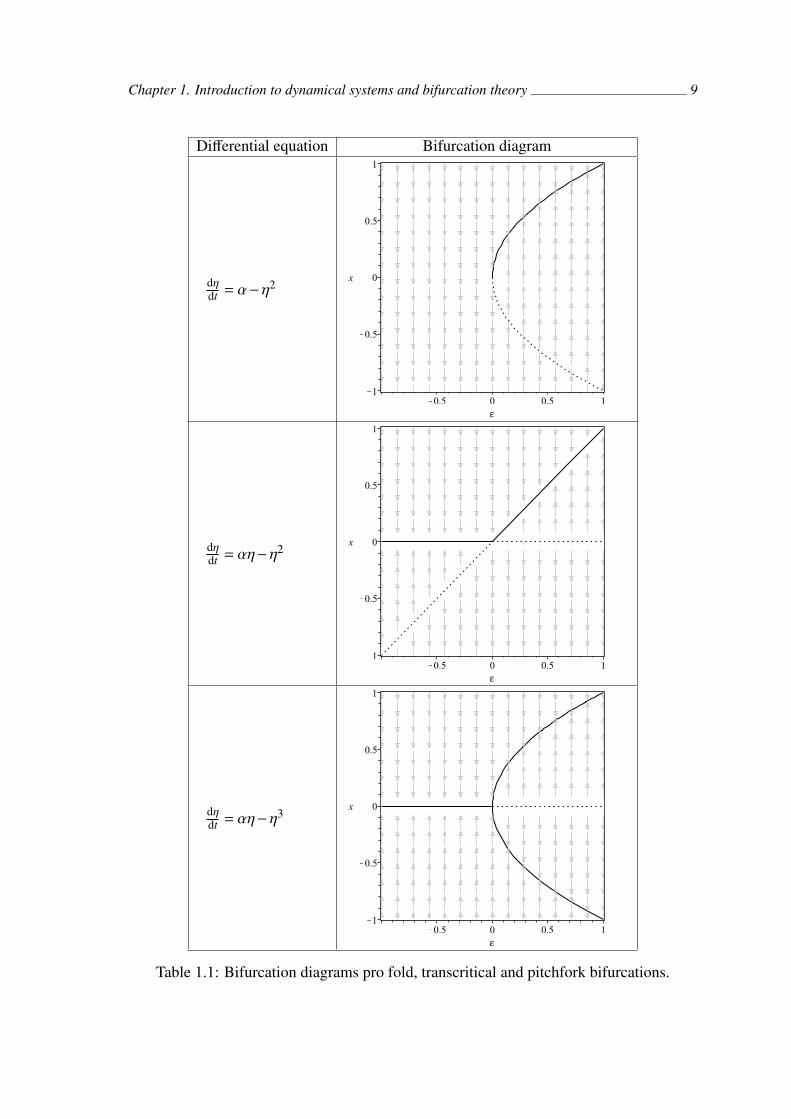
Differential equation Bifurcation diagram
dηdt = α−η2
dηdt = αη−η2
dηdt = αη−η3
Table 1.1: Bifurcation diagrams pro fold, transcritical and pitchfork bifurcations.

Chapter 1. Introduction to dynamical systems and bifurcation theory 10
1.4.2 Hopf bifurcationTheorem 1.8 (Normal form of the Hopf bifurcation). Let
dxxxdt
= fff (xxx, ε) , xxx (k) ∈ R2, ε ∈ R, (1.10)
be a two-dimensional system of differential equations, where fff is sufficiently smooth,and it has an equilibrium xxx∗ (ε) for sufficiently small |ε|. Moreover, the Jacobi mat-rix J (xxx, ε) of system (1.10) has two complex conjugate eigenvalues λ1,2 = µ (ε)± iω (ε),where µ (0) = 0, φ (0) = ω0 > 0. Assuming the following conditions hold
1. l1 , 0, where l1 is the first Lyapunov coefficient (non-degeneracy condition),see equation (1.12)
2. µε , 0 (transversality condition),
system (1.10) is topologically equivalent to the system
ddt
(y1y2
)=
(β −11 β
)(y1y2
)+ s
(y2
1 + y22
) (y1y2
), (1.11)
where s = ±1.
Definition 1.11. Generic one-parameter bifurcation associated with β = 0 originated insystem (1.11) is called a Hopf bifurcation. According to Theorem 1.8, it occurs in an ar-bitrary system (1.10) for ε = 0 and for which the theorem conditions hold.
Definition 1.12 (Topological types of the Hopf bifurcation). If s = −1, Hopf bifurcation iscalled a supercritical. If s = 1, Hopf bifurcation is called a subcritical.
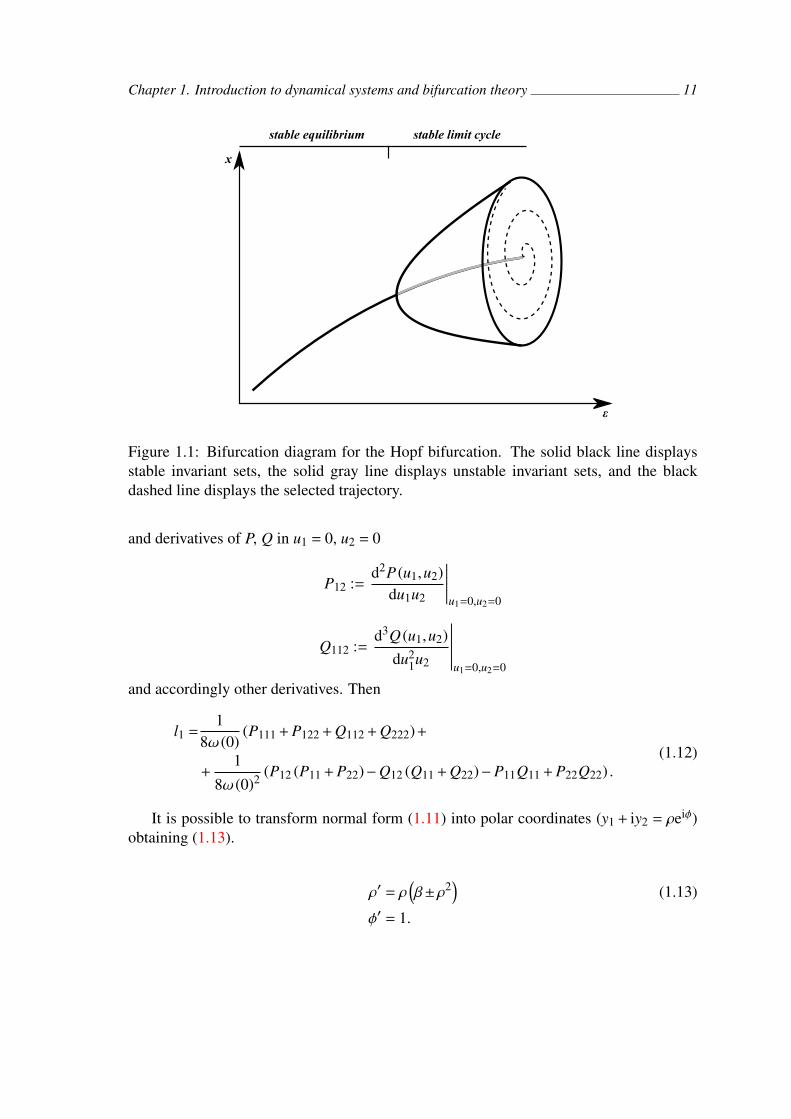
The supercritical Hopf bifurcation gives birth to a stable limit cycle. An unstablelimit cycle arises as a consequence of the subcritical Hopf bifurcation. Figure 1.1 depictsthe origin of a stable limit cycle through the supercritical Hopf bifurcation.
The following computation shows a way to compute the first Lyapunov coefficient l1.The Jacobi matrix J (000,0) has, according to Theorem 1.8, two purely imaginary eigen-values λ1,2 = ±iω (0) and corresponding eigenvectors v, v are complex conjugate. LetT = (Re v Im v). Mapping xxx = Tuuu transforms system
dxxxdt
= fff (xxx,0) = J (000,0) xxx + FFF (xxx)
toduuudt
= fff (xxx,0) = T−1J (000,0)Tuuu + T−1FFF (Tuuu) .
Denote (P (u1,u2)Q (u1,u2)
):= T−1FFF (Tuuu) ,
Chapter 1. Introduction to dynamical systems and bifurcation theory 11
stable equilibrium
ε
x
stable limit cycle
Figure 1.1: Bifurcation diagram for the Hopf bifurcation. The solid black line displaysstable invariant sets, the solid gray line displays unstable invariant sets, and the blackdashed line displays the selected trajectory.
and derivatives of P, Q in u1 = 0, u2 = 0
P12 :=d2P (u1,u2)
du1u2
∣∣∣∣∣∣u1=0,u2=0
Q112 :=d3Q (u1,u2)
du21u2
∣∣∣∣∣∣∣u1=0,u2=0
and accordingly other derivatives. Then
l1 =1
8ω (0)(P111 + P122 + Q112 + Q222)+
+1
8ω (0)2(P12 (P11 + P22)−Q12 (Q11 + Q22)−P11Q11 + P22Q22) .
(1.12)
It is possible to transform normal form (1.11) into polar coordinates (y1 + iy2 = ρeiφ)obtaining (1.13).
ρ′ = ρ(β±ρ2
)(1.13)
φ′ = 1.

Chapter 1. Introduction to dynamical systems and bifurcation theory 12
1.5 One-parameter bifurcations for discrete dynamicalsystems
Similarly to the previous section, in this section, we focus on parameter-dependent sys-tems. Let
xxx (k + 1) = ggg (xxx (k) , εεε) (1.14)
be a system of difference equations, where xxx ∈ Rn is a vector of state variables and εεε ∈ Rl,l = 1 is a parameter.
Local one-parameter bifurcations occur in system (1.14), where one or more eigenva-lues of (1.14) reaches a unit circle in a complex plane due to a change of parameter εεε ∈ Rl,l = 1. The eigenvalue is either λ = 1, λ = −1, or there are two complex conjugate eigen-values λ1,2 of size one. In case l = 1 we use ε ∈ R instead of εεε. Generic one-parameterbifurcation associated with
1. an eigenvalue λ = 1 is called fold (denoted by LP).
2. an eigenvalue λ = −1 is called flip (denoted by PD).
3. two complex conjugate eigenvalues λ1,2 of size one is called Neimark-Sacker (de-noted by NS).
1.5.1 Fold bifurcationTheorem 1.9 (Normal form of the fold bifurcation). Let
x (k + 1) = g (x (k) , ε) , x (k) ∈ R, ε ∈ R (1.15)
be a one-dimensional system of difference equations, where g is sufficiently smooth, it hasfor ε = 0 a fixed point x∗ = 0 and λ = gx (0,0) = 1. Assuming the following conditions hold
1. gxx (0,0) , 0 (non-degeneracy condition)
2. gε (0,0) , 0 (transversality condition),
system (1.15) is topologically equivalent to the system
η (k + 1) = α+η (k) . (1.16)
Definition 1.13. Generic one-parameter bifurcation originated in system (1.16) for α = 0is called a fold bifurcation. Based on Theorem 1.9, it occurs in an arbitrary system (1.15)for ε = 0 and for which the theorem the conditions hold.
Chapter 1. Introduction to dynamical systems and bifurcation theory 13
1.5.2 Flip bifurcationTheorem 1.10 (Normal form of the flip bifurcation). Let
x (k + 1) = g (x (k) , ε) , x (k) ∈ R, ε ∈ R (1.17)
be a one-dimensional system of difference equations, where g is sufficiently smooth, it hasfor ε = 0 a fixed point x∗ = 0 and λ = gx (0,0) = −1. Assuming the following conditionshold
1. 12 (gxx (0,0))2 + 1
3gxxx (0,0) , 0 (non-degeneracy condition)
2. gxε (0,0) , 0 (transversality condition)
system (1.17) is topologically equivalent to the system
η (k + 1) = − (1 +α)η (k) + sη3 (k) , s = ±1 (1.18)
Definition 1.14. Generic one-parameter bifurcation originated in system (1.18) for α = 0is called a flip bifurcation. Based on Theorem 1.10, it occurs in an arbitrary system (1.17)for ε = 0 and for which the theorem conditions hold.
There exist two topological types of the flip bifurcation. If s = −1, a stable two-cycleoriginates, and a stable equilibrium becomes unstable. If s = 1, an unstable two-cycleoriginates, and an unstable equilibrium becomes stable.
1.5.3 Neimark-Sacker bifurcationTheorem 1.11 (“Normal form” of the Neimark-Sacker bifurcation). Let
xxx (k + 1) = ggg (xxx (k) , ε) , xxx (k) ∈ R2, ε ∈ R, (1.19)
be a two-dimensional system of difference equations, where ggg is sufficiently smooth, it hasfor small |ε| a fixed point xxx∗ (ε). Moreover, a Jacobi matrix J (xxx, ε) of system (1.19) hastwo complex conjugate eigenvalues λ1,2 = r (ε)e±iφ(ε), where r (0) = 1,φ(0) = θ0. Assumingthe following conditions holds
1. eimθ0 , 1 for m = 1,2,3,4 (non-degeneracy condition)
2. rε , 0 (transversality condition),
system (1.19) is topologically equivalent to the system(y1 (k + 1)y2 (k + 1)
)= (1 +α)
(cos(θ) −sin(θ)sin(θ) cos(θ)
)(y1 (k)y2 (k)
)+
+(y2
1 (k) + y22 (k)
) (cos(θ) −sin(θ)sin(θ) cos(θ)
)(a −bb a
)(y1 (k)y2 (k)
)+ O(||yyy (k) ||4) (1.20)
where α is a parameter, a = a (α), b = b (α) and θ = θ (α) is smooth function, θ (0) = θ0,0 < θ (α) < π.
Chapter 1. Introduction to dynamical systems and bifurcation theory 14
Definition 1.15. Generic one-parameter bifurcation originated in system (1.20) for α = 0,a (0) , 0 is called a Neimark-Sacker bifurcation. Based on Theorem 1.11 it occurs inarbitrary system (1.19) for εεε = 000 and for which the theorem conditions hold.
Condition 1 is sometimes called the absence of strong resonances. By violatingthe condition, strong resonances occur. We can consider a (0) , 0 to be another non-degeneracy condition. By violating the condition, a Chenciner bifurcation occurs.
Definition 1.16 (Topological types of the Neimark-Sacker bifurcation). If a (0) < 0a Neimark-Sacker bifurcation is called a supercritical. If a (0) > 0 a Neimark-Sackerbifurcation is called a subcritical.
The supercritical Neimark-Sacker bifurcation gives a birth to a stable invariant loop.An unstable invariant loop arises as a consequence of the subcritical Neimark-Sacker bi-furcation.
The O(||yyy (k) ||4)-terms in the normal form cannot be truncated. The orbit structure onthe closed invariant curve and the variation of this structure, when the parameter changes,are generically different in systems (1.20) and the truncated system. A complete classi-fication of an orbit structure on the closed invariant curve remains unknown [53]. Thisproblem was studied by Arnold [4], or Smale [75].
One can transform the normal form of the Neimark-Sacker bifurcation (1.19), usingthe polar coordinates transformation (y1 + iy2 = ρeiφ), onto (1.21), where R (ρ (k) ,α) andQ (ρ (k) ,α) are smooth functions of α and ρ.
ρ (k + 1) = ρ (k)(1 +α+ aρ2 (k)
)+ρ4 (k)R (ρ (k) ,α) (1.21)
φ (k + 1) = φ (k) + θ+ρ2 (k) Q (ρ (k) ,α) ,
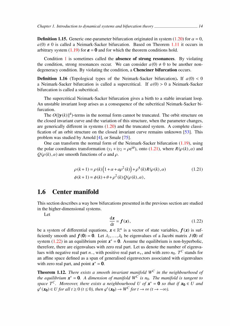
1.6 Center manifoldThis section describes a way how bifurcations presented in the previous section are studiedin the higher-dimensional systems.
Letdxxxdt
= fff (xxx) , (1.22)
be a system of differential equations, xxx ∈ Rn is a vector of state variables, fff (xxx) is suf-ficiently smooth and fff (000) = 000. Let λ1, . . . ,λk be eigenvalues of a Jacobi matrix J (000) ofsystem (1.22) in an equilibrium point xxx∗ = 000. Assume the equilibrium is non-hyperbolic,therefore, there are eigenvalues with zero real part. Let us denote the number of eigenva-lues with negative real part n−, with positive real part n+, and with zero n0. TC stands foran affine space defined as a span of generalised eigenvectors associated with eigenvalueswith zero real part, and point xxx∗ = 000.
Theorem 1.12. There exists a smooth invariant manifold WC in the neighbourhood ofthe equilibrium xxx∗ = 000. A dimension of manifold WC is n0. The manifold is tangent tospace TC . Moreover, there exists a neighbourhood U of xxx∗ = 000 so that if xxx000 ∈ U andϕt (xxx000) ∈ U for all t ≥ 0 (t ≤ 0), then ϕt (xxx000)→WC for t→∞ (t→−∞).

Chapter 1. Introduction to dynamical systems and bifurcation theory 15
Definition 1.17. Manifold WC is called a center manifold at xxx∗ = 000.
Note (Parameter-dependent systems). Let us assume the system (1.5) smoothly dependson one parameter εεε ∈ Rl, l = 1. We use ε ∈ R instead of εεε. For ε = 0 system (1.5) hasa non-hyperbolic equilibrium xxx∗ = 000. Theorem 1.12 proves existence of n+1-dimensionalcenter manifold WC for an extended system
dxxxdt
= fff (xxx, ε)
dεdt
= 0.
Furthermore hyperplanes Πε0 = (xxx, ε) , ε = ε0 are invariant too. Consequently, manifoldWCε = WC ∩Πε0 is called a center manifold of parameter-dependent system (1.5).
For a numerical approximation of the center manifold, we use similar techniques as forreduction principle, Theorem 1.4. The reduction principle was programmed in the Maplesoftware [57], and used to demonstrate the center manifold theorem. Worksheets can befound in [35, 36].
As an analogy to Theorem 1.12 for system (1.22) we can formulate center manifoldtheorem for difference equations.
Letxxx (k + 1) = ggg (xxx (k)) , (1.23)
be a system of difference equations, xxx ∈Rn is a vector of state variables, ggg (xxx) is sufficientlysmooth and ggg (000) = 000. Let λ1, . . . ,λk be eigenvalues of Jacobi matrix J (000) of system (1.23)in a fixed point xxx∗ = 000. Assume the fixed point is non-hyperbolic. Therefore the absolutevalues of one or more eigenvalues is equal to one. Let us denote the number of those eigen-values n0. Consequently, let us denote the number of eigenvalues outside the unit circlein the complex plane n+, and the number of eigenvalues inside the unit circle in the com-plex plane n−. TC stands for affine space defined as a span of generalised eigenvectorsassociated with eigenvalues with absolute values equal to one, and point xxx∗ = 000.
Theorem 1.13. There exists a smooth invariant manifold WC in the neighbourhood of thefixed point xxx∗ = 000. A dimension of manifold WC is n0. The manifold is tangent to space TC .Moreover, there exists a neighbourhood U of xxx∗ = 000 so that if xxx000 ∈ U and gggk (xxx000) ∈ U forall k ≥ 0 (k ≤ 0), then gggk (xxx000)→WC for k→∞ (k→−∞).
Definition 1.18. Manifold WC is called a center manifold at xxx∗ = 000.
Note (Parameter-dependent systems). Let us assume (1.14) smoothly depending on oneparameter εεε ∈ Rl, l = 1. We use ε ∈ R instead of εεε. For ε = 0 has system (1.14) a non-hyperbolic fixed point xxx∗ = 000. Theorem 1.13 proves existence of n + 1-dimensional centermanifold WC for an extended system
xxx (k + 1) = ggg (xxx (k) , ε (k))ε (k + 1) = ε (k) .
Furthermore hyperplanes Πε0 = (xxx, ε) , ε = ε0 are invariant too. Consequently, manifoldWCε = WC ∩Πε0 is called a center manifold of parameter-dependent system (1.14).
Chapter 1. Introduction to dynamical systems and bifurcation theory 16
1.7 Two-parameter bifurcationsThis section is devoted to systems of differential and difference equations with two pa-rameters εεε ∈ R2. Let
T,Rn,ϕt
εεε
be a dynamical system, where ϕt
εεε is a class of evolu-tionary operator parametrised by t ∈ T and εεε ∈ R2. Similar to one-parameter bifurcation,two-parameter bifurcations are defined in Definition 1.7 for l = 2. There are two possi-ble two-parameter bifurcations origin scenarios in dynamical systems. The first scenariois through violating non-degeneracy conditions. In this case, a dimension of a centermanifold remains the same as for corresponding one-parameter bifurcation. In anotherscenario, the additional eigenvalue of the Jacobi matrix of our dynamical system reachesthe imaginary axis (the unit circle). This causes a change in dimension of the center ma-nifold, which is in both cases equal to the number of eigenvalues with zero real part fora continuous-time dynamical system (with absolute value one for a discrete-time dynami-cal system). Important two-parameter bifurcations were named after the mathematicians,who studied them. Other two-parameter bifurcations are addressed by the name of corre-sponding one-parameter bifurcations.
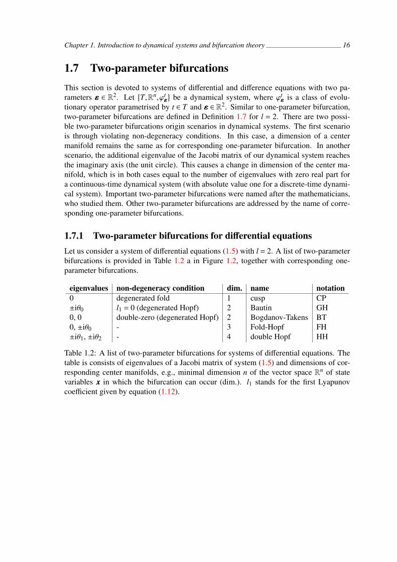
1.7.1 Two-parameter bifurcations for differential equationsLet us consider a system of differential equations (1.5) with l = 2. A list of two-parameterbifurcations is provided in Table 1.2 a in Figure 1.2, together with corresponding one-parameter bifurcations.
eigenvalues non-degeneracy condition dim. name notation0 degenerated fold 1 cusp CP±iθ0 l1 = 0 (degenerated Hopf) 2 Bautin GH0, 0 double-zero (degenerated Hopf) 2 Bogdanov-Takens BT0, ±iθ0 - 3 Fold-Hopf FH±iθ1, ±iθ2 - 4 double Hopf HH
Table 1.2: A list of two-parameter bifurcations for systems of differential equations. Thetable is consists of eigenvalues of a Jacobi matrix of system (1.5) and dimensions of cor-responding center manifolds, e.g., minimal dimension n of the vector space Rn of statevariables xxx in which the bifurcation can occur (dim.). l1 stands for the first Lyapunovcoefficient given by equation (1.12).
Chapter 1. Introduction to dynamical systems and bifurcation theory 17
Fold
Hopf
Cusp
Bautin
Bogdanov-Takens
Fold-Hopf
Hopf-Hopf
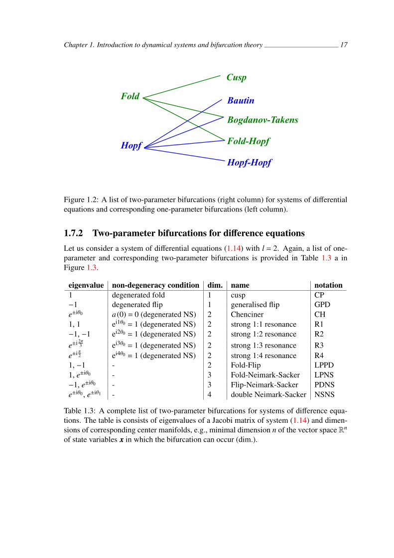
Figure 1.2: A list of two-parameter bifurcations (right column) for systems of differentialequations and corresponding one-parameter bifurcations (left column).
1.7.2 Two-parameter bifurcations for difference equationsLet us consider a system of differential equations (1.14) with l = 2. Again, a list of one-parameter and corresponding two-parameter bifurcations is provided in Table 1.3 a inFigure 1.3.
eigenvalue non-degeneracy condition dim. name notation1 degenerated fold 1 cusp CP−1 degenerated flip 1 generalised flip GPDe±iθ0 a (0) = 0 (degenerated NS) 2 Chenciner CH1, 1 ei1θ0 = 1 (degenerated NS) 2 strong 1:1 resonance R1−1, −1 ei2θ0 = 1 (degenerated NS) 2 strong 1:2 resonance R2e±i 2π
3 ei3θ0 = 1 (degenerated NS) 2 strong 1:3 resonance R3e±i π2 ei4θ0 = 1 (degenerated NS) 2 strong 1:4 resonance R41, −1 - 2 Fold-Flip LPPD1, e±iθ0 - 3 Fold-Neimark-Sacker LPNS−1, e±iθ0 - 3 Flip-Neimark-Sacker PDNSe±iθ0 , e±iθ1 - 4 double Neimark-Sacker NSNS
Table 1.3: A complete list of two-parameter bifurcations for systems of difference equa-tions. The table is consists of eigenvalues of a Jacobi matrix of system (1.14) and dimen-sions of corresponding center manifolds, e.g., minimal dimension n of the vector space Rn
of state variables xxx in which the bifurcation can occur (dim.).
Chapter 1. Introduction to dynamical systems and bifurcation theory 18
Fold
CuspChencinerova
Strong 1:2 resonance
LP-NSNS-NS
Flip
Generalized flipStrong 1:1 resonance
Strong 1:4 resonanceStrong 1:3 resonance
PD-NS
LP-PDNeimark-Sacker
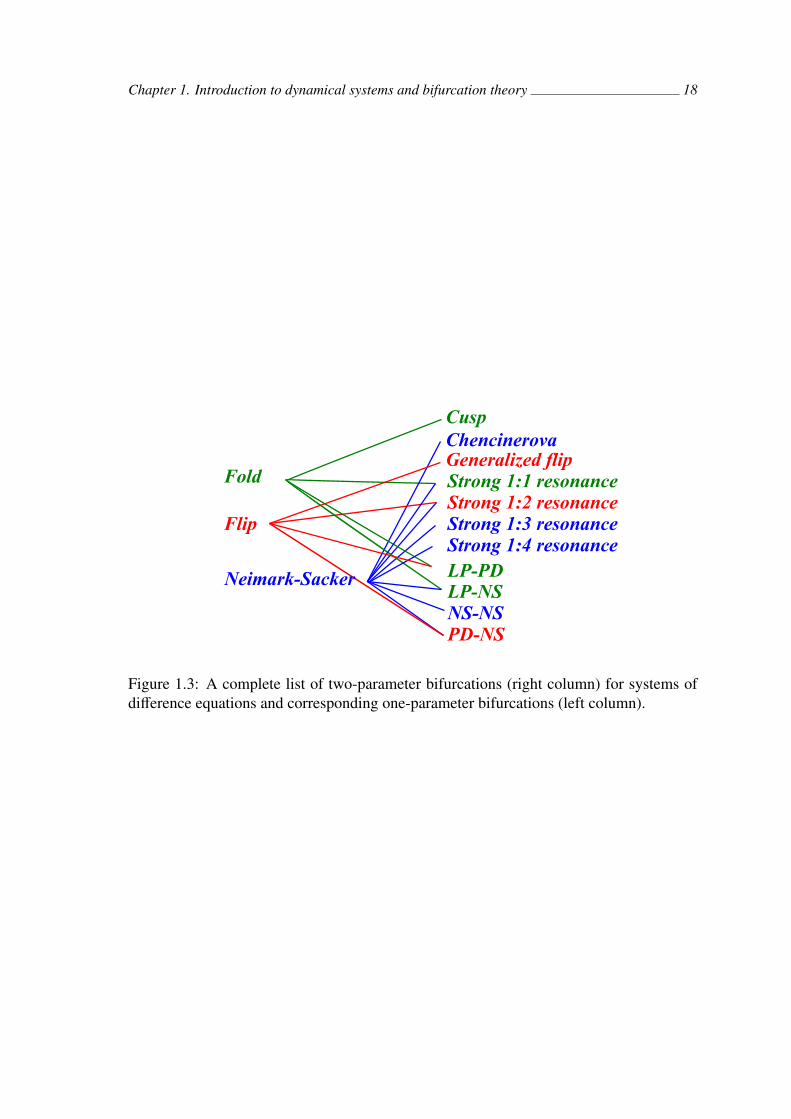
Figure 1.3: A complete list of two-parameter bifurcations (right column) for systems ofdifference equations and corresponding one-parameter bifurcations (left column).
Chapter 2
Bifurcation manifold detection andcontinuation
A standard approach for the analysis of dynamical systems is to use numerical methodsimplemented in continuation software. Firstly, we will focus on those numerical tech-niques. We will also describe the continuation process. Due to the rapid development ofboth mathematical software and hardware, it is possible today to use sophisticated analyti-cal algorithms for bifurcation analysis, because the computational time of such algorithmsis reduced. In the last section of this chapter, we propose a method to compute bifurcationmanifolds analytically using the Grobner basis. Although it might seem that the use ofthe Grobner basis method is simply a different approach for the analysis, it is not the case.This method enables the computation of the bifurcation manifolds without the need tocalculate equilibria explicitly, as opposed to the commonly used analysis of dynamicalsystems.
History of continuation software starts with developing a numerical technique calledthe pseudo-inverse continuation in the late 1960s and 1970s. Later on, this techniqueand its generalisation, the Moore-Penrose continuation, allows us to continue equilib-ria and bifurcation branches. The first generation of continuation software consists ofcodes without a graphical interface, like AUTO86, LINLBF, BIFOR2. This generationof software was developed in the 1980s and early 1990s. Later on, interactive programs(AUTO97, LOCBIF, AUTO07-p), closed environments (DsTool, CONTENT), and openenvironments (MATCONT) started being developed [78].
Currently, both MATCONT and AUTO are widely used in the dynamical systems com-munity. MATCONT software development started in 2000, and the first publication ap-peared in 2003 [21, 22]. New features came out in 2008 [23]. Since 2008, MATCONT isstill being updated. The leaders of the project are Govaerts, Kuznetsov and Meijer. Theycame out with a new version at least once every year [59]. Also, since 2014, MATCONTM,an equivalent of MATCONT for mapping, is available [51]. AUTO is a publicly availablepiece of software distributed since 1980 [48]. The software was developed with major con-tributions by Champneys, Fairgrieve, Kuznetsov, Oldeman, Paffenroth, Sandstede, Wang,and Zhang. Its latest version AUTO07-p was released in 2007, and until 2012 it wasundated on yearly basis [26, 48, 65].
– 19 –

Chapter 2. Bifurcation manifold detection and continuation 20
2.1 Equilibria/fixed points detection and continuationWe shortly introduce numerical techniques implemented in commonly used continuationsoftware like MATCONT, toolbox for Matlab [21, 23], AUTO, which is distributed as partof the Linux version of XPP [26, 48], MATCONTM, which is an equivalent of MATCONTfor mapping [51], and LOCBIF, which is distributed as part of the Windows version ofXPP [27]. Examples of a step-by-step bifurcation analysis in MATCONT and AUTO arepresented in the next two subsections. Handling other continuation software is similar.
Let us recall system of differential equations (1.5), where xxx ∈ Rn is a vector of statevariables and εεε ∈ Rl, l = 1 is a parameter. Let us use ε ∈ R instead of εεε. Let xxx = [xxx, ε] and
FFF (xxx) := fff (xxx) = fff (xxx, ε) .
Equilibria of (1.5) are solutions of system of equations
FFF (xxx) = 0. (2.1)
Moreover, let (1.14) be a system of difference equations, where xxx ∈ Rn is a vector of statevariables and εεε ∈Rl, l = 1 is a parameter. Again, let us use ε ∈R instead of εεε. Let xxx = [xxx, ε]and
GGG (xxx) := ggg (xxx)− xxx = ggg (xxx, ε)− xxx = 0.
Fixed points of (1.14) are solutions of system of equations
GGG (xxx) = 0. (2.2)
Assuming fff ,ggg are smooth functions in both their arguments. FFF, GGG are smooth functionsFFF : Rn+1 → Rn, and GGG : Rn+1 → Rn. A numerical technique for solving those equations,implemented in commonly used continuation software like MATCONT, or AUTO, is calleda continuation. The numerical continuation computes a sequence of points which approxi-mate the desired branch of equilibria (fixed points for discrete dynamical systems), usuallyusing a predictor-corrector method. Suppose we have found a point xxxi = [xxxi, εi] which lieson the desired branch of equilibria. Then establishing the next point xxxi+1 = [xxxi+1, εi+1]consists of two steps:
1. Prediction: Suppose h > 0 is a stepsize. Then
XXX0 = xxxi + hvvvi .
Vector vvvi is a vector tangent to the equilibrium curve at xxxi. The process iscalled a tangent prediction. Vector vvvi can be found as a solution of the systemDFFF (xxxi)vvvi = 0 (or DGGG (xxxi)vvvi = 0), together with a normalisation condition. HereDFFF (xxxi) (or DGGG (xxxi)) is a Jacobi matrix of FFF (or GGG) evaluated at xxxi. As a normal-isation condition we can use ||vvvi|| = 1 or 〈vvvi−1,vvvi〉 = 1. For each starting point xxxithere exists two possible starting directions. The implementation needs to preservethe proper direction along the curve. Another popular prediction process is calleda secant prediction [53]. Stepsize control algorithms are used to determine stepsizeh. Minimum and maximum stepsize are usually defined. For more informationabout stepsize control algorithms see MATCONT [22].

Chapter 2. Bifurcation manifold detection and continuation 21
2. Correction: Assuming XXX0 is closed to the desired branch, we use a Newton-likeprocedure to establish xxxi+1. Since the Newton method is applicable only to systems,where a number of equations and variables are equal, we need to use one extra scalarcondition:
FFF (xxx) = 0
f (xxx) = 0
or
GGG (xxx) = 0g (xxx) = 0.
In continuation software, there exist two common possibilities to choose functionsf , and g. One option is called a pseudo-arclength continuation, see Figure 2.1a,where
f (xxx) = 〈xxx−XXX0,vvvi〉
org (xxx) = 〈xxx−XXX0,vvvi〉 .
The other way is called a Moore-Penrose continuation, see Figure 2.1b. Let usset VVV0 = vvvi. The basic principal of the method is to seek for XXXk in a hyperplaneperpendicular previous tangent vector. Therefore
fk (xxx) = 〈xxx−XXXk,VVVk〉 ,
andgk (xxx) = 〈xxx−XXXk,VVVk〉 ,
where DFFF (XXXk−1)VVVk = 0, and DGGG (XXXk−1)VVVk = 0.
To compute the initial point xxxi for the chosen εi, we can use standard techniques forsolving equation (1.5) numerically, like Runge-Kutta methods. Similarly, we can iteratemap (1.14). Alternatively, we can solve equations (2.1), or (2.2), analytically or numeri-cally.
Chapter 2. Bifurcation manifold detection and continuation 22
X0
Predition
hvi
x~i
Correction
x~i+1
(a) Pseudo-arclength continuation
X0
Predition
hvi
x~i
Correction
x~i+1
X1
V1
V2X2
(b) Moore-Penrose continuation
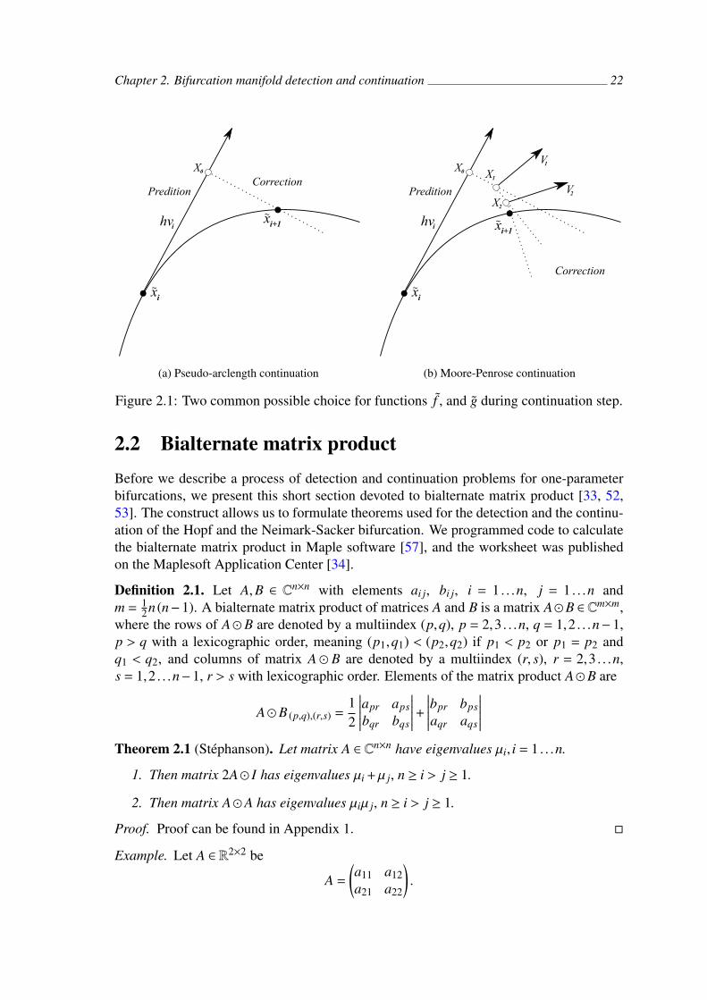
Figure 2.1: Two common possible choice for functions f , and g during continuation step.
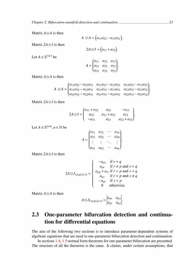
2.2 Bialternate matrix productBefore we describe a process of detection and continuation problems for one-parameterbifurcations, we present this short section devoted to bialternate matrix product [33, 52,53]. The construct allows us to formulate theorems used for the detection and the continu-ation of the Hopf and the Neimark-Sacker bifurcation. We programmed code to calculatethe bialternate matrix product in Maple software [57], and the worksheet was publishedon the Maplesoft Application Center [34].
Definition 2.1. Let A,B ∈ Cn×n with elements ai j, bi j, i = 1 . . .n, j = 1 . . .n andm = 1
2n (n−1). A bialternate matrix product of matrices A and B is a matrix AB ∈ Cm×m,where the rows of A B are denoted by a multiindex (p,q), p = 2,3 . . .n, q = 1,2 . . .n−1,p > q with a lexicographic order, meaning (p1,q1) < (p2,q2) if p1 < p2 or p1 = p2 andq1 < q2, and columns of matrix A B are denoted by a multiindex (r, s), r = 2,3 . . .n,s = 1,2 . . .n−1, r > s with lexicographic order. Elements of the matrix product AB are
AB (p,q),(r,s) =12
∣∣∣∣∣∣apr apsbqr bqs
∣∣∣∣∣∣+∣∣∣∣∣∣bpr bpsaqr aqs
∣∣∣∣∣∣Theorem 2.1 (Stephanson). Let matrix A ∈ Cn×n have eigenvalues µi, i = 1 . . .n.
1. Then matrix 2A I has eigenvalues µi +µ j, n ≥ i > j ≥ 1.
2. Then matrix AA has eigenvalues µiµ j, n ≥ i > j ≥ 1.
Proof. Proof can be found in Appendix 1.
Example. Let A ∈ R2×2 be
A =
(a11 a12a21 a22
).
Chapter 2. Bifurcation manifold detection and continuation 23
Matrix AA is thenA A =
(a11a22−a12a21
).
Matrix 2A I is then2A I =
(a11 + a22
).
Let A ∈ R3×3 be
A =
a11 a12 a13a21 a22 a23a31 a32 a33
.Matrix AA is then
A A =
a11a22−a12a21 a11a23−a13a21 a12a23−a13a22a11a32−a12a31 a11a33−a13a31 a12a33−a13a32a21a32−a22a31 a21a33−a23a31 a22a33−a23a32
.Matrix 2A I is then
2A I =
a11 + a22 a23 −a13a32 a11 + a33 a12−a31 a21 a22 + a33
.Let A ∈ Rn×n,n ∈ N be
A =
a11 a12 · · · a1na21 a22 · · · a24...
.... . .
...an1 an2 · · · ann
.Matrix 2A I is then
2A I (p,q),(r,s) =
−aps if r = qapr if r , p and s = q
app + arr if r = p and s = qaqs if r = p and s , q−aqr if s = p
0 otherwise.
Matrix AA is then
AA (p,q),(r,s) =
∣∣∣∣∣∣apr apsaqr aqs
∣∣∣∣∣∣ .2.3 One-parameter bifurcation detection and continua-
tion for differential equationsThe aim of the following two sections is to introduce parameter-dependent systems ofalgebraic equations that are used in one-parameter bifurcation detection and continuation.
In sections 1.4, 1.5 normal form theorems for one-parameter bifurcation are presented.The structure of all the theorems is the same. It claims, under certain assumptions, that

Chapter 2. Bifurcation manifold detection and continuation 24
an arbitrary system of differential, or difference, equations is locally topologically equiva-lent to the normal form. The structure of assumptions is the following. We always assumeright-hand sides of equations (1.5), or (1.14), to be sufficiently smooth and to have a tri-vial equilibrium (or fixed point) x∗ = 0 for a trivial parameter value ε = 0. The other typeof assumptions can be formulated as equalities. For generic one-parameter bifurcations,there is always only one equality assumption. It stands a condition for the eigenvalues ofa Jacobi matrix J (xxx, εεε) of (1.5), or (1.14). The last type of assumptions are formulatedas inequalities and are usually called non-degeneracy conditions and transversality condi-tions. We formulate a system of algebraic equations taking into account the first two typesof assumptions. The system of algebraic equations obtained describes a one-parameter bi-furcation manifold implicitly in the space of both state-variables and parameters. Our goalis to eliminate state variables for the system to obtain an implicit description of the one-parameter bifurcation manifold in the space of parameters. Since we do not take intoaccount non-degeneracy and transversality conditions, the obtained one-parameter bifur-cation manifold may consist of sub-manifolds containing degenerated points (e.g., neutralsaddles), degenerated bifurcations (e.g., transcritical or pitchfork), or two-parameter bi-furcations.
In this section, we focus on equation (1.5) with a Jacobi matrix J (xxx, εεε). In ∈ Rn×n
stands for the identity matrix.
Theorem 2.2. Let us assume system of differential equations (1.5), then a solution ofthe system of equations
fff (xxx, εεε) = 000 (2.3)det (J (xxx, εεε)) = 0 (2.4)
contains all fold bifurcation points of (1.5).
Proof. Equation (2.3) formulates a condition on a solution to be an equilibrium. Moreover,we seek for a point xxx, in which the Jacobi matrix J (xxx, εεε) has at least one eigenvalue equal tozero. From equation det (J (xxx, εεε)−λIn) = 0 for λ= 0 we obtain (2.4). Finally, equilibrium xxx,together with a critical value of parameters εεε for which the fold bifurcation of equilibriumxxx originates, are solutions of system of equations (2.3), (2.4).
Now let us formulate a system of equations whose solution contains Hopf bifurcationpoints of (1.5). Let us assume the following example first.
Example. Let us assume system of differential equations (1.5) with n = 2. Let us denotexxx = (x,y). Let
[x∗,y∗
]be an equilibrium of system (1.5). Therefore
dxdt
= f1 (x,y, εεε)
dydt
= f2 (x,y, εεε) .
Moreover, we assume that the Jacobi matrix
J(x∗,y∗
)=
dg1(x,y)dx
dg1(x,y)dy
dg2(x,y)dx
dg2(x,y)dy
x=x∗,y=y∗
Chapter 2. Bifurcation manifold detection and continuation 25
has two complex eigenvalues with zero real parts. A characteristic polynomial of the Ja-cobi matrix J is λ2− trJ (x∗,y∗)λ+ det J (x∗,y∗). Consequently a solution of
f1 (x,y, εεε) = 0f2 (x,y, εεε) = 0
trJ (x,y, εεε) = 0
contains all Hopf bifurcation points. This came about from Vieta’s formulae.
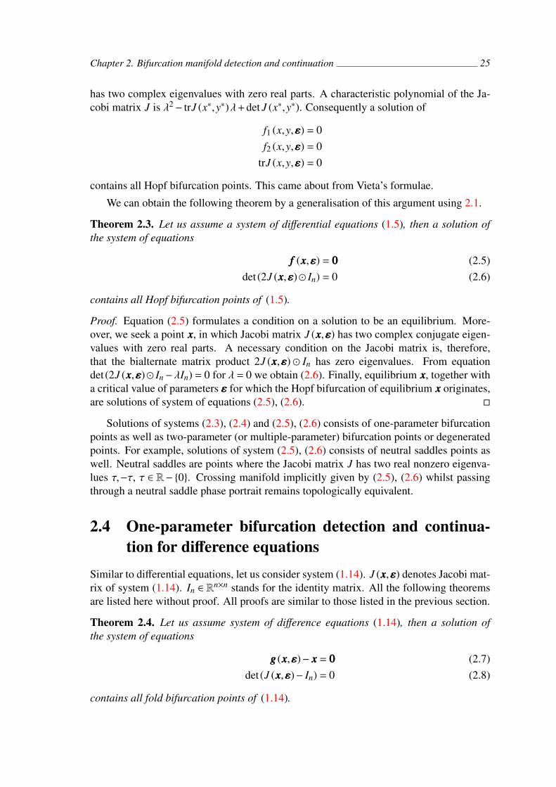
We can obtain the following theorem by a generalisation of this argument using 2.1.
Theorem 2.3. Let us assume a system of differential equations (1.5), then a solution ofthe system of equations
fff (xxx, εεε) = 000 (2.5)det (2J (xxx, εεε) In) = 0 (2.6)
contains all Hopf bifurcation points of (1.5).
Proof. Equation (2.5) formulates a condition on a solution to be an equilibrium. More-over, we seek a point xxx, in which Jacobi matrix J (xxx, εεε) has two complex conjugate eigen-values with zero real parts. A necessary condition on the Jacobi matrix is, therefore,that the bialternate matrix product 2J (xxx, εεε) In has zero eigenvalues. From equationdet (2J (xxx, εεε) In−λIn) = 0 for λ = 0 we obtain (2.6). Finally, equilibrium xxx, together witha critical value of parameters εεε for which the Hopf bifurcation of equilibrium xxx originates,are solutions of system of equations (2.5), (2.6).
Solutions of systems (2.3), (2.4) and (2.5), (2.6) consists of one-parameter bifurcationpoints as well as two-parameter (or multiple-parameter) bifurcation points or degeneratedpoints. For example, solutions of system (2.5), (2.6) consists of neutral saddles points aswell. Neutral saddles are points where the Jacobi matrix J has two real nonzero eigenva-lues τ,−τ, τ ∈ R− 0. Crossing manifold implicitly given by (2.5), (2.6) whilst passingthrough a neutral saddle phase portrait remains topologically equivalent.
2.4 One-parameter bifurcation detection and continua-tion for difference equations
Similar to differential equations, let us consider system (1.14). J (xxx, εεε) denotes Jacobi mat-rix of system (1.14). In ∈ R
n×n stands for the identity matrix. All the following theoremsare listed here without proof. All proofs are similar to those listed in the previous section.
Theorem 2.4. Let us assume system of difference equations (1.14), then a solution ofthe system of equations
ggg (xxx, εεε)− xxx = 000 (2.7)det (J (xxx, εεε)− In) = 0 (2.8)
contains all fold bifurcation points of (1.14).

Chapter 2. Bifurcation manifold detection and continuation 26
Theorem 2.5. Let us assume system of difference equations (1.14), then a solution ofthe system of equations
ggg (xxx, εεε)− xxx = 000 (2.9)det (J (xxx, εεε) + In) = 0 (2.10)
contains all flip bifurcation points of (1.14).
Theorem 2.6. Let us assume system of difference equations (1.14), then a solution ofthe system of equations
ggg (xxx, εεε)− xxx = 000 (2.11)det (J (xxx, εεε) J (xxx, εεε)− In) = 0. (2.12)
contains all Neimark-Sacker bifurcation points of (1.14).
Example. Similar to the Hopf bifurcation case for differential equations, we can simplifythe previous theorem for system of difference equations (1.14) for n = 2. Let us denotexxx = (x,y). Therefore
x (k + 1) = g1 (x (k) ,y (k) , εεε)y (k + 1) = g2 (x (k) ,y (k) , εεε)
Moreover, the Jacobi matrix
J(x∗,y∗
)=
dg1(x,y)dx
dg1(x,y)dy
dg2(x,y)dx
dg2(x,y)dy
x=x∗,y=y∗
has two complex conjugate eigenvalues of size one. The characteristic polynomial ofJacobi matrix J is λ2− trJ (x∗,y∗)λ+ det J (x∗,y∗). Consequently, from Theorem 2.6, a so-lution of
g1 (x,y, εεε)− x = 0g2 (x,y, εεε)− y = 0
det J (x,y, εεε)−1 = 0
contains all Neimark-Sacker bifurcation points.
Again, solutions of systems (2.7), (2.8); (2.9), (2.10); and (2.11), (2.12) consist of one-parameter bifurcation points as well as two-parameter bifurcation points or degeneratedpoints. Similar to the case of differential equations, solutions of system (2.11), (2.12)consist of, for instance, neutral saddles points. Neutral saddles are points where the Jacobimatrix J has two real nonzero eigenvalues τ,−1
τ , τ ∈ R−0. Crossing manifold implicitlygiven by (2.11), (2.12) whilst passing through a neutral saddle phase portrait remainstopologically equivalent.

Chapter 2. Bifurcation manifold detection and continuation 27
2.5 Bifurcation manifold continuation using continuationsoftware
This section aims to present methods for detection and continuation commonly used inthe bifurcation analysis. One-parameter bifurcation detection is carried out during equi-libria continuation, described in section 2.1. For each point xxxi, we compute the value ofa test function. If the value of the test function in xxxi has the opposite sign than the value ofthe test function in xxxi+1, then a bifurcation point occurs for ε in interval (εi, εi+1). The testfunctions are defined based on the theorems in sections 2.3 and 2.4.
Continuation techniques for one-parameter bifurcation manifolds in the space of twoparameters and state variables are similar to continuation techniques for equilibria, seesection 2.1. Finally, the detection of two-parameter bifurcation is similar to one-parameterbifurcation detection. While using continuation software we usually follow this procedure:
1. detect equilibrium (fixed point)
2. perform equilibria (fixed points) continuation
3. detect one-parameter bifurcation points
4. perform one-parameter bifurcation continuation
5. detect two-parameter bifurcation points
2.5.1 Example of continuation process in MATCONT
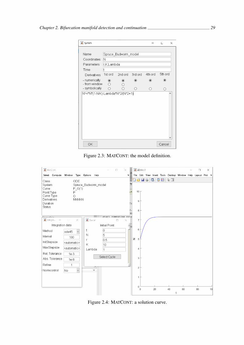
The demonstration of a continuation process will be done using a well-known Spruce Bud-worm model [56]. The model is precisely described and repeatedly solved by a differentmethod in case studies in section 3.2.2. The demonstration was performed in MATCONT,a toolbox in Matlab for bifurcation analysis of differential equations. This demonstrationwas done in version matcont6p10, released on 26th February 2018. The MATCONT inter-face consists of the main window, see Figure 2.2, and other contextual windows, such asIntegrator, Starter, Continuer, 2Dplot, 3Dplot, and Numeric. All computationalcommands can be started from the main window. Firstly you need to define the systemuse Select→System→New, see Figure 2.3.
The first step of the bifurcation analysis of equilibria is to detect an equilibrium. Onepossible way to detect a stable equilibrium is by solving equation (1.5) numerically, using,for example, the Runge-Kutta method. Let us set the last point of the numerically com-puted solution of the trajectory with respect to time to be an approximation of a stable equi-librium. In Figure 2.4, you can see the computation setting in MATCONT. Firstly the userselects Type→Initial point→Point. This opens the additional context windows anIntegrator and a Starter. The Integrator allows specification of the numericalmethod for solving equation (1.5), the time interval for the numerical solution, the stepsize, and tolerance. The Starter is used to set the initial point and parameters of the sys-tem. One can also open a Numeric, a 2DPlot, or a 3DPlot window to show the con-tinuation process using the Window tab. To initialize the computational process, click onCompute→Forward. To find a solution for t→−∞ click on Compute→Backward.

Chapter 2. Bifurcation manifold detection and continuation 28
Figure 2.2: MATCONT: the main window.
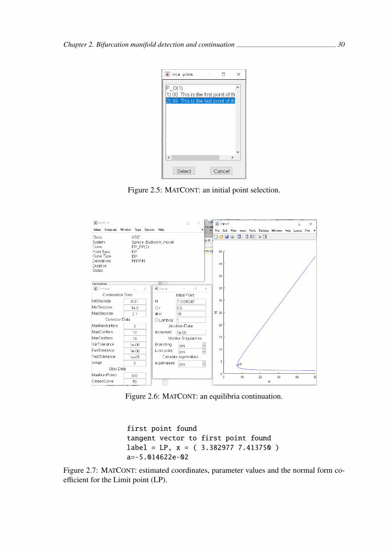
The second step is to do the equilibria continuation. First of all, one needs to selectan initial point using Select→Initial point, see Figure 2.5. Then it is necessaryto change the type of computation in tab Type→Initial point→Equilibrium.Again two contextual windows open, a Starter and a Continuer, see Figure 2.6.In the Continuer window, one can set parameters related to the Moore-Penrosecontinuation. In the Starter window as an addition to previously listed items, one cansee the radio button to select the desired parameter for continuation, which needs to beset to at least one value, the Jacobian data increment option, the monitor singularitiesoptions, and the calculate eigenvalues option. To initialize the computational process,click on Compute→Forward. To find the other part of the equilibrium branch, click onCompute→Backward. If monitor singularity is set to “yes”, the program detects oneparameter bifurcations. In our example, a LP singularity has been detected. LP refersto the fold bifurcation, and in the Matlab command window, one can find estimatedcoordinates and parameter values of the point and an estimated normal form coefficient.The sign of the normal form coefficient distinguishes between the topological type ofthe bifurcation [53]. In our case, see Figure 2.7, the coefficient a is negative, whichcorresponds to s = −1 in normal form (1.7).
The next step is the one-parameter bifurcation continuation. Before performingthe computation, it is necessary to select the limit point (LP) using Select→Initialpoint, see Figure 2.8. The next step is again to choose the right type of computation in thetab Type→Initial point→Limit point. The contextual windows remain the sameas for equilibria continuation, see 2.9. To perform a one-parameter bifurcation continua-tion, one needs to select two free parameters using the radio button in the Starter win-dow. The computation initialisation process and monitor the singularity process remainthe same, see Figures 2.9, 2.10.
Chapter 2. Bifurcation manifold detection and continuation 29
Figure 2.3: MATCONT: the model definition.
Figure 2.4: MATCONT: a solution curve.
Chapter 2. Bifurcation manifold detection and continuation 30
Figure 2.5: MATCONT: an initial point selection.
Figure 2.6: MATCONT: an equilibria continuation.
first point found
tangent vector to first point found
label = LP, x = ( 3.382977 7.413750 )
a=-5.014622e-02
Figure 2.7: MATCONT: estimated coordinates, parameter values and the normal form co-efficient for the Limit point (LP).

Chapter 2. Bifurcation manifold detection and continuation 31
Figure 2.8: MATCONT: an initial point selection.
Figure 2.9: MATCONT: a limit point continuation.
first point found
tangent vector to first point found
label = CP, x = ( 1.732048 0.649519 5.196152 )
c=-5.412674e-02
Figure 2.10: MATCONT: estimated coordinates, parameter values and the normal formcoefficient for the Cusp point (CP).

Chapter 2. Bifurcation manifold detection and continuation 32
2.5.2 Example of continuation process in XPPAUTXPPAUT, or XPP, is a program for solving differential equations, difference equations,delay equations, functional equations, boundary value problems, and stochastic equations.Its Linux distribution contains a tool for bifurcation analysis AUTO. AUTO can performa continuation of bifurcation branches of algebraic systems, continuation of systems ofordinary differential equations, and certain continuation and evolution computations forparabolic PDEs [48]. Here we will focus on bifurcation analysis of systems of ordinarydifferential equations. The same Spruce Budworm model, as in the previous example, isused in this example [56]. The analysis was done in version XPPAUT 8.0, released inJanuary 2016. To use XPPAUT, one needs to create an xpp input file. The obligatorypart of the XPPAUT file is a definition of initial conditions (keyword init), parameters(keyword par), and equations. Other XPPAUT settings can be made using either the inputfile or in the XPPAUT app. This setting line starts with a symbol @. The symbol #denotes user notes. See an example of code below. For more information, see XPPAUTdocumentation [26].
#Spruce budworm
dN/dt = r*N*(1-N/K)-Lambda*Nˆ2/(Nˆ2+1)
init N=5
par r=0.5, K=10, Lambda=1
@ XP=t, YP=N, XLO=0, XHI=100, YLO=0, YHI=10
@ total=100
done
After opening the input file in XPPAUT, the first step is again the stable equilib-rium detection. The detection can be done by numerically integrating a solution fora sufficiently large time interval, using command Initial conditions → Go, and thenInitial conditions → Last, to expand the time interval, see Figure 2.11. To detecta repeller, one needs to set reverse time direction by setting Dt property in the Numericwindow to a negative value.

Chapter 2. Bifurcation manifold detection and continuation 33
Figure 2.11: XPPAUT: integral curve.
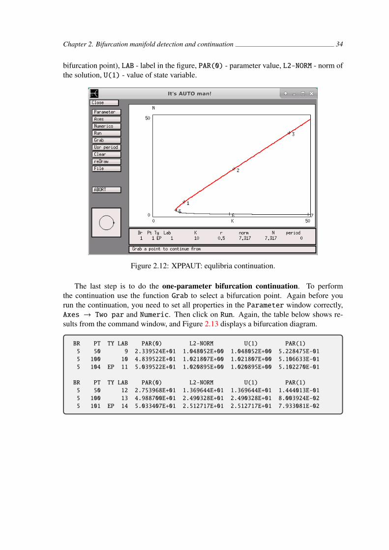
The next step is to do the equilibria continuation. The continuation is perform inthe AUTO software, which is executable from the XPPAUT menu using File→Auto.Before you run the continuation, you need to set all properties in the Parameter win-dow correctly, Axes → Hi-lo and Numeric. Then click on Run → Steady state.To compute the other part of the equilibrium branch, one needs to set Ds property inthe Numeric window to a negative value. Results of the continuation are displayed in Fig-ure 2.12. XPPAUT also prints details of the result into the command window, as shownbelow.
BR PT TY LAB PAR(0) L2-NORM U(1)
1 1 EP 1 1.000000E+01 7.316625E+00 7.316625E+00
1 50 2 2.575441E+01 2.357329E+01 2.357329E+01
1 100 3 4.339173E+01 4.129122E+01 4.129122E+01
1 119 EP 4 5.010197E+01 4.801599E+01 4.801599E+01
BR PT TY LAB PAR(0) L2-NORM U(1)
1 15 LP 5 7.413750E+00 3.382976E+00 3.382976E+00
1 50 6 2.432254E+01 1.419461E+00 1.419461E+00
1 100 7 4.932192E+01 1.256257E+00 1.256257E+00
1 102 EP 8 5.032192E+01 1.252958E+00 1.252958E+00
The output table columns have the following meanings: BR - branch of the bifurcation,PT - number of a point, TY - type of a point (bifurcation: EP - equilibrium, LP - fold
Chapter 2. Bifurcation manifold detection and continuation 34
bifurcation point), LAB - label in the figure, PAR(0) - parameter value, L2-NORM - norm ofthe solution, U(1) - value of state variable.
Figure 2.12: XPPAUT: equlibria continuation.
The last step is to do the one-parameter bifurcation continuation. To performthe continuation use the function Grab to select a bifurcation point. Again before yourun the continuation, you need to set all properties in the Parameter window correctly,Axes → Two par and Numeric. Then click on Run. Again, the table below shows re-sults from the command window, and Figure 2.13 displays a bifurcation diagram.
BR PT TY LAB PAR(0) L2-NORM U(1) PAR(1)
5 50 9 2.339524E+01 1.048052E+00 1.048052E+00 5.228475E-01
5 100 10 4.839522E+01 1.021807E+00 1.021807E+00 5.106633E-01
5 104 EP 11 5.039522E+01 1.020895E+00 1.020895E+00 5.102270E-01
BR PT TY LAB PAR(0) L2-NORM U(1) PAR(1)
5 50 12 2.753968E+01 1.369644E+01 1.369644E+01 1.444013E-01
5 100 13 4.988700E+01 2.490328E+01 2.490328E+01 8.003924E-02
5 101 EP 14 5.033407E+01 2.512717E+01 2.512717E+01 7.933081E-02

Chapter 2. Bifurcation manifold detection and continuation 35
Figure 2.13: XPPAUT: one-parameter bifurcation continuation.
2.6 Analytic method for bifurcation manifold detectionThe problem of finding bifurcation manifolds leads to a problem of solving a system ofnonlinear equations. Often the system is polynomial or can be reduced to a polynomialform, see sections 2.3, 2.4. In such cases, we can avoid numerical continuation and de-rive the results analytically [9]. This section describes a different method to analyse one-parameter bifurcations of equilibria in the case of a differential/difference system withpolynomial or rational right-hand sides using the Grobner basis computation. In the dis-sertation, we present an approach that allows us to analyse the system algorithmically andcompute bifurcation manifolds as implicit or parametric functions in full parameter spaceusing known algorithms to compute the Grobner basis of the polynomial system. Op-posed to the commonly used analysis of dynamical systems, described in section 2.5, thismethod enables the computation of the bifurcation manifolds without the need to calculateequilibria explicitly.
Firstly, let us recall the concept of an affine algebraic variety, the central objects ofstudy in algebraic geometry. An affine algebraic variety V is defined as the set of solutionsof a system of polynomial equations over complex numbers. Affine algebraic varietiescan be characterised by their dimensions. The dimension of affine algebraic variety V isthe maximal dimension of the tangent vector spaces at non-singular points of V . Affinealgebraic varieties of dimension one are called algebraic curves, and affine varieties of di-mension two are called algebraic surfaces. Generally, an algebraic hypersurface is an affinealgebraic variety of dimension n−1 in n-dimensional space, n ∈N,n> 1. An algebraic ma-

Chapter 2. Bifurcation manifold detection and continuation 36
nifold is an algebraic variety which is also a manifold1.
2.6.1 Basic background about Grobner basesIn this section, the essential background about Grobner bases is provided. Notation anddefinitions are taken from [14]. Bruno Buchberger initiated the theory of Grobner basisin his Ph.D. dissertation in 1965 and has developed this theory throughout his career.The theory is named after Bruno Buchberger’s supervisor Wolfgang Grobner.
We work with polynomials p ∈ R[x1, . . . , xm] with real coefficients and variablesx1, . . . , xm. For a set S ⊆ R[x1, . . . , xm] of such polynomials, we denote by Z(S )the so-called zero set
Z(S ) = (x1, . . . , xm) ∈ Rm | ∀p ∈ S : p(x1, . . . , xm) = 0.
It is easy to see that, for ideal I = (S ) generated by S , we obtain the same zero set, i.e.,Z(I) = Z(S ), so that we may restrict to zero sets of ideals. A subset V ∈ Rm is calledan affine algebraic variety2, if V = Z (S ) for some S .
In order to define a Grobner basis of an ideal, we need to set up a monomial order, inthe other words, an ordering of the monomials with certain properties. In this dissertation,we will use exclusively the lexicographical order that depends only on a linear ordering ofvariables. In chapter 3, we specify the ordering of variables explicitly; here, for simplicity,we assume x1 · · · xm. Then we define
xα11 · · · x
αmm xβ1
1 · · · xβmm
to mean that there exists an index i such that α1 = β1, . . . , αi−1 = βi−1, αi > βi.We will abbreviate xα1
1 · · · xαmm to xα, where α stands for the m-tuple (α1, . . . ,αm). Since
the monomial ordering is linear, each non-zero polynomial p ∈R[x1, . . . , xm] can be writtenuniquely as
p = aαxα+∑
xα>xβaβxβ
with aα , 0. In such a case, aα is called the leading coefficient, xα the leading monomialand aαxα the leading term of p. They are denoted LCp, LMp and LTp, respectively.
For an ideal I, we denote by LTI the ideal generated by the leading terms (or, equiva-lently, leading monomials) of the elements of I. Polynomials p1, . . . , pn ∈ I are a Grobnerbasis of I if their leading terms generate LTI. It is well known that any Grobner basisgenerates an ideal I. Importantly, a Grobner basis exists for any ideal I (and if one possesan additional condition on such a basis – namely that it is reduced – then it is even unique).
For more information about Grobner basis see [54]. The advantage of Grobner ba-sis method is that it can be found algorithmically by the Buchberger algorithm [11]. Bychoosing the correct lexicographic order of variables, it is possible to eliminate some vari-ables (especially state variables) for a system of polynomial equations. This enables to
1Many affine algebraic varieties are manifolds, but an affine algebraic variety may have singular pointswhile a manifold cannot. Note in chapter 3 we sometimes use notion manifolds instead of variety, despitethe variety has singular points. This denomination is usual in bifurcation theory.
2In algebradic geometry affine algebraic varieties are more often defined over an algebraically closedfield Cm. Note some results for algebraic varieties hold only for Cm.
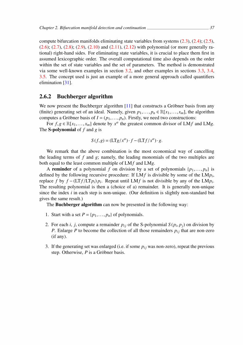
Chapter 2. Bifurcation manifold detection and continuation 37
compute bifurcation manifolds eliminating state variables from systems (2.3), (2.4); (2.5),(2.6); (2.7), (2.8); (2.9), (2.10) and (2.11), (2.12) with polynomial (or more generally ra-tional) right-hand sides. For eliminating state variables, it is crucial to place them first inassumed lexicographic order. The overall computational time also depends on the orderwithin the set of state variables and the set of parameters. The method is demonstratedvia some well-known examples in section 3.2, and other examples in sections 3.3, 3.4,3.5. The concept used is just an example of a more general approach called quantifierselimination [31].
2.6.2 Buchberger algorithmWe now present the Buchberger algorithm [11] that constructs a Grobner basis from any(finite) generating set of an ideal. Namely, given p1, . . . , pn ∈ R[x1, . . . , xm], the algorithmcomputes a Grobner basis of I = (p1, . . . , pn). Firstly, we need two constructions:
For f ,g ∈ R[x1, . . . , xm] denote by xα the greatest common divisor of LM f and LMg.The S-polynomial of f and g is
S ( f ,g) = (LTg/xα) · f − (LT f /xα) ·g.
We remark that the above combination is the most economical way of cancellingthe leading terms of f and g; namely, the leading monomials of the two multiples areboth equal to the least common multiple of LM f and LMg.
A reminder of a polynomial f on division by a set of polynomials p1, . . . , pn isdefined by the following recursive procedure: If LM f is divisible by some of the LMpi,replace f by f − (LT f /LTpi) pi. Repeat until LM f is not divisible by any of the LMpi.The resulting polynomial is then a (choice of a) remainder. It is generally non-uniquesince the index i in each step is non-unique. (Our definition is slightly non-standard butgives the same result.)
The Buchberger algorithm can now be presented in the following way:
1. Start with a set P = p1, . . . , pn of polynomials.
2. For each i, j, compute a remainder pi j of the S-polynomial S (pi, p j) on division byP. Enlarge P to become the collection of all those remainders pi j that are non-zero(if any).
3. If the generating set was enlarged (i.e. if some pi j was non-zero), repeat the previousstep. Otherwise, P is a Grobner basis.
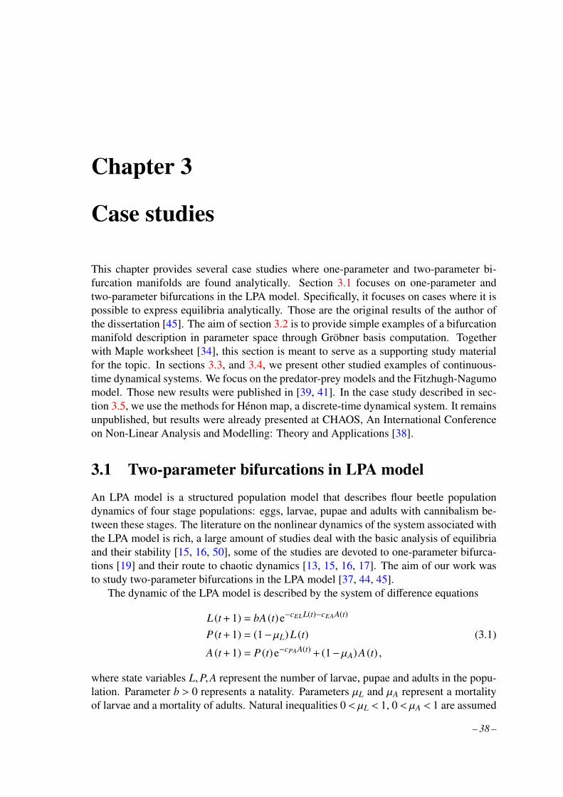
Chapter 3
Case studies
This chapter provides several case studies where one-parameter and two-parameter bi-furcation manifolds are found analytically. Section 3.1 focuses on one-parameter andtwo-parameter bifurcations in the LPA model. Specifically, it focuses on cases where it ispossible to express equilibria analytically. Those are the original results of the author ofthe dissertation [45]. The aim of section 3.2 is to provide simple examples of a bifurcationmanifold description in parameter space through Grobner basis computation. Togetherwith Maple worksheet [34], this section is meant to serve as a supporting study materialfor the topic. In sections 3.3, and 3.4, we present other studied examples of continuous-time dynamical systems. We focus on the predator-prey models and the Fitzhugh-Nagumomodel. Those new results were published in [39, 41]. In the case study described in sec-tion 3.5, we use the methods for Henon map, a discrete-time dynamical system. It remainsunpublished, but results were already presented at CHAOS, An International Conferenceon Non-Linear Analysis and Modelling: Theory and Applications [38].
3.1 Two-parameter bifurcations in LPA modelAn LPA model is a structured population model that describes flour beetle populationdynamics of four stage populations: eggs, larvae, pupae and adults with cannibalism be-tween these stages. The literature on the nonlinear dynamics of the system associated withthe LPA model is rich, a large amount of studies deal with the basic analysis of equilibriaand their stability [15, 16, 50], some of the studies are devoted to one-parameter bifurca-tions [19] and their route to chaotic dynamics [13, 15, 16, 17]. The aim of our work wasto study two-parameter bifurcations in the LPA model [37, 44, 45].
The dynamic of the LPA model is described by the system of difference equations
L (t + 1) = bA (t)e−cELL(t)−cEAA(t)
P (t + 1) = (1−µL) L (t) (3.1)
A (t + 1) = P (t)e−cPAA(t) + (1−µA) A (t) ,
where state variables L,P,A represent the number of larvae, pupae and adults in the popu-lation. Parameter b > 0 represents a natality. Parameters µL and µA represent a mortalityof larvae and a mortality of adults. Natural inequalities 0 < µL < 1, 0 < µA < 1 are assumed
– 38 –

Chapter 3. Case studies 39
to be satisfied. Parameters cEL,cEA,cPA denote cannibalism rates. Namely, cEL is the can-nibalism rate of larvae on eggs, cEA is the cannibalism rate of adults on eggs and cPA isthe cannibalism rate of adults on pupae. We assume cEA ≥ 0,cPA ≥ 0 and cEL = 0.
Bifurcation Implicit description of bifurcation manifolds in the parameter space
transcriticalb (1−µL)
µA= 1 (3.2)
flip b =µAe
2µA
1−µL(3.3)
Neimark-Sacker
1(cEA + cPA)2
−µ2AcEAcPA ln
(b (1−µL)
µA
)2
+µ2Ac2
EA ln(b (1−µL)
µA
)2
+
+µAc2EA ln
(b (1−µL)
µA
)−2µ2
AcPAcEA ln(b (1−µL)
µA
)+µ2
Ac2PA ln
(b (1−µL)
µA
)+
+µAcEAcPA ln(b (1−µL)
µA
)−3µ2
Ac2EA ln
(b (1−µL)
µA
)− c2
PA−µAc2PA + 2µ2
Ac2EA−
−2µAcEAcPA + 4µ2AcEAcPA−2cPAcEA−µAc2
EA− c2EA + 2µ2
Ac2PA
)= 0. (3.4)
Table 3.1: One-parameter bifurcation manifolds given implicitly in the parameterspace.
There are at most two fixed points of system (3.1). The trivial fixed point [0,0,0] and[L∗,P∗,A∗]. In the case cEL = 0, it is possible to express the fixed point analytically [15].Let us recall the main results of a one-parameter bifurcation analysis [19], see table 3.1.We perform a two-parameter bifurcation analysis [37, 44, 45]. As was already discussedin section 1.7, there are two possible origins of two parameter bifurcations. For the sit-uation, where two eigenvalues of the Jacobi matrix of (3.1) reach the unit circle, we candescribe two-parameter bifurcation manifolds as sub-manifolds of the intersection of one-parameter bifurcation manifolds. In table 3.2, two-parameter bifurcation manifolds arelisted. A manifold, implicitly defined by (3.6) corresponds to the strong 1:2 resonancewith associated eigenvalues −1,−1, 1
2 . The strong 1:2 resonance lies in the intersection ofthe Neimark-Sacker bifurcation manifold (3.4) and the flip bifurcation manifold (3.3). Wefocus on the strong 1:2 resonance and accompanying bifurcation manifolds. We createa complete bifurcation diagram near the strong 1:2 resonance, see Figures 3.1, 3.2 and3.3. The necessary condition for existence of the strong 1:2 resonance is µA >
12 . For µA
sufficiently close to 12 the supercritical strong 1:2 resonance occurs in LPA model, see Fig-
ure 3.1. Both the Chenciner bifurcation and the subcritical strong 1:2 resonance occurin LPA model for µA sufficiently close to 1, see Figure 3.2 and 3.3. Attractors and re-
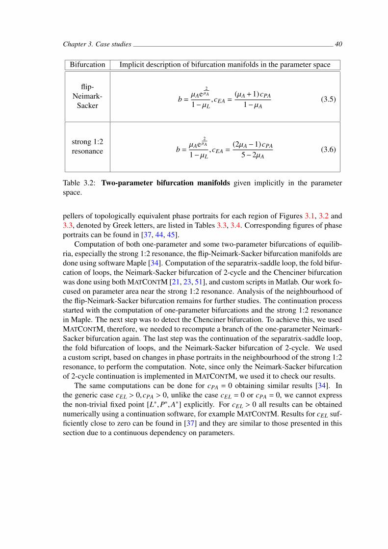
Chapter 3. Case studies 40
Bifurcation Implicit description of bifurcation manifolds in the parameter space
flip-Neimark-
Sackerb =
µAe2µA
1−µL,cEA =
(µA + 1)cPA
1−µA(3.5)
strong 1:2resonance b =
µAe2µA
1−µL,cEA =
(2µA−1)cPA
5−2µA(3.6)
Table 3.2: Two-parameter bifurcation manifolds given implicitly in the parameterspace.
pellers of topologically equivalent phase portraits for each region of Figures 3.1, 3.2 and3.3, denoted by Greek letters, are listed in Tables 3.3, 3.4. Corresponding figures of phaseportraits can be found in [37, 44, 45].
Computation of both one-parameter and some two-parameter bifurcations of equilib-ria, especially the strong 1:2 resonance, the flip-Neimark-Sacker bifurcation manifolds aredone using software Maple [34]. Computation of the separatrix-saddle loop, the fold bifur-cation of loops, the Neimark-Sacker bifurcation of 2-cycle and the Chenciner bifurcationwas done using both MATCONTM [21, 23, 51], and custom scripts in Matlab. Our work fo-cused on parameter area near the strong 1:2 resonance. Analysis of the neighbourhood ofthe flip-Neimark-Sacker bifurcation remains for further studies. The continuation processstarted with the computation of one-parameter bifurcations and the strong 1:2 resonancein Maple. The next step was to detect the Chenciner bifurcation. To achieve this, we usedMATCONTM, therefore, we needed to recompute a branch of the one-parameter Neimark-Sacker bifurcation again. The last step was the continuation of the separatrix-saddle loop,the fold bifurcation of loops, and the Neimark-Sacker bifurcation of 2-cycle. We useda custom script, based on changes in phase portraits in the neighbourhood of the strong 1:2resonance, to perform the computation. Note, since only the Neimark-Sacker bifurcationof 2-cycle continuation is implemented in MATCONTM, we used it to check our results.
The same computations can be done for cPA = 0 obtaining similar results [34]. Inthe generic case cEL > 0,cPA > 0, unlike the case cEL = 0 or cPA = 0, we cannot expressthe non-trivial fixed point [L∗,P∗,A∗] explicitly. For cEL > 0 all results can be obtainednumerically using a continuation software, for example MATCONTM. Results for cEL suf-ficiently close to zero can be found in [37] and they are similar to those presented in thissection due to a continuous dependency on parameters.
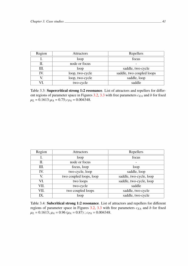
Chapter 3. Case studies 41
Region Attractors RepellersI. loop focusII. node or focus -III. loop saddle, two-cycleIV. loop, two-cycle saddle, two coupled loopsV. loop, two-cycle saddle, loopVI. two-cycle saddle
Table 3.3: Supercritical strong 1:2 resonance. List of attractors and repellers for differ-ent regions of parameter space in Figures 3.2, 3.3 with free parameters cEA and b for fixedµL = 0.1613;µA = 0.75;cPA = 0.004348.
Region Attractors RepellersI. loop focusII. node or focus -III. focus, loop loopIV. two-cycle, loop saddle, loopV. two coupled loops, loop saddle, two-cycle, loopVI. two loops saddle, two-cycle, loopVII. two-cycle saddleVII. two coupled loops saddle, two-cycleIX. loop saddle, two-cycle
Table 3.4: Subcritical strong 1:2 resonance. List of attractors and repellers for differentregions of parameter space in Figures 3.2, 3.3 with free parameters cEA and b for fixedµL = 0.1613; µA = 0.96 (µA = 0.87) ; cPA = 0.004348.
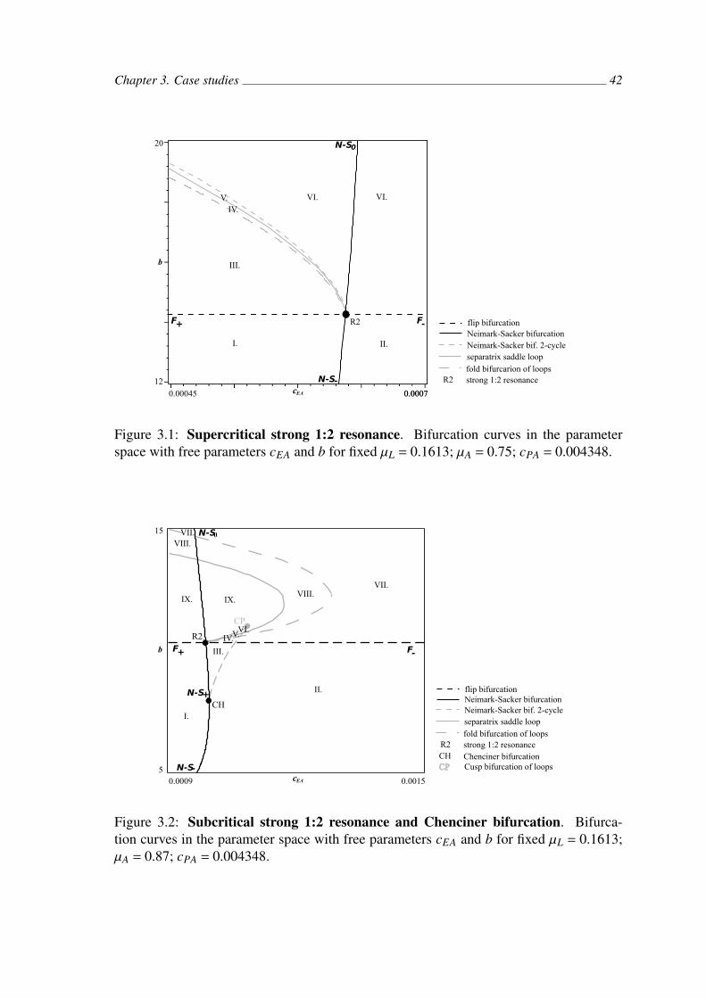
Chapter 3. Case studies 42
0.00045 0.0007
12
20
flip bifurcationNeimark-Sacker bifurcationNeimark-Sacker bif. 2-cycleseparatrix saddle loop
fold bifurcarion of loopsR2 strong 1:2 resonance
cEA
b
N-S-
N-S0
F+ F-R2
I. II.
III.
IV.V. VI. VI.
0.0007
Figure 3.1: Supercritical strong 1:2 resonance. Bifurcation curves in the parameterspace with free parameters cEA and b for fixed µL = 0.1613; µA = 0.75; cPA = 0.004348.
I.
II.
III.
cEA
b
VII.VIII.
0.0009 0.00155
15
N-S-
N-S
F+ F-
flip bifurcationNeimark-Sacker bifurcationNeimark-Sacker bif. 2-cycleseparatrix saddle loop
fold bifurcation of loopsR2 strong 1:2 resonanceCH Chenciner bifurcationCP Cusp bifurcation of loops
CH
R2
CP
N-S+
IV.V.VI.
0
IX. IX.
VIII.VII.
Figure 3.2: Subcritical strong 1:2 resonance and Chenciner bifurcation. Bifurca-tion curves in the parameter space with free parameters cEA and b for fixed µL = 0.1613;µA = 0.87; cPA = 0.004348.
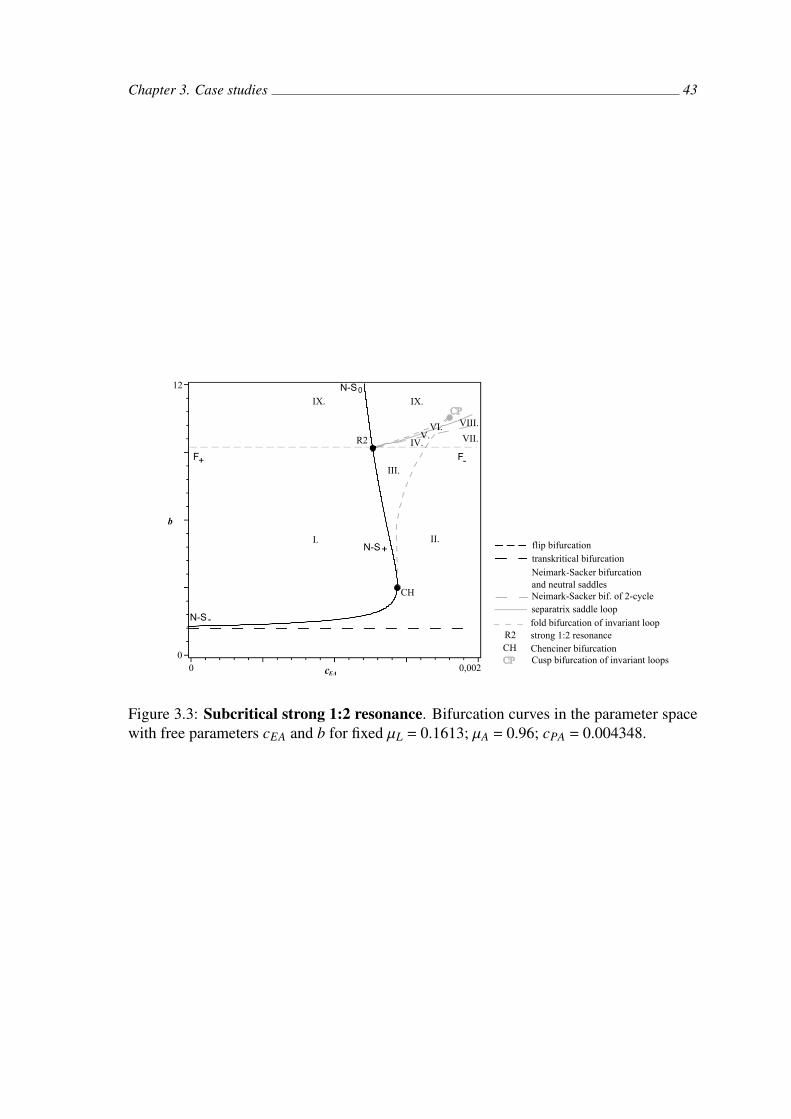
Chapter 3. Case studies 43
R2
CH
I. II.
III.
flip bifurcation
transkritical bifurcation
Neimark-Sacker bifurcation
and neutral saddles
cEA
b
IV. VII.
VIII.
V.VI.
IX.IX.
Neimark-Sacker bif. of 2-cycle
separatrix saddle loop
fold bifurcation of invariant loop
R2 strong 1:2 resonance
CH Chenciner bifurcation
0 0,002
0
12
CP
CP Cusp bifurcation of invariant loops
N-S-
N-S0
F+
F-
Figure 3.3: Subcritical strong 1:2 resonance. Bifurcation curves in the parameter spacewith free parameters cEA and b for fixed µL = 0.1613; µA = 0.96; cPA = 0.004348.

Chapter 3. Case studies 44
3.2 Basic examples of usage of the Grobner basis methodin bifurcation analysis
In this section, we present essential examples of continuous dynamical systems. Thissection aims to compare the commonly used approach in bifurcation analysis of the dyna-mical systems with the analysis using the Grobner basis. Another goal is to present a stepby step computation of the Grobner basis for those who are not familiar with the concept.Examples presented in sections 3.2.1, 3.2.2, 3.2.3 were also programmed in Maple soft-ware and can be found in [34]. The section is meant to be a supporting study material forthe Grobner basis method in bifurcation analysis.
3.2.1 Selkov model of glycolysisIn this well-known model, we use the Grobner basis method to compute a Hopf bifurcationmanifold. We demonstrate the Buchberger algorithm step by step, see Appendix 2. How-ever, usually the calculation is very complex, and it is necessary to use a computationalsoftware.
Model is studied in form
dxdt
= x2y + ay− x
dydt
= x2y−ay + b,(3.7)
where state variables x,y are concentrations of ADP molecules and a,b > 0 are kineticparameters [77].
A Hopf bifurcation manifold is implicitly defined by the following system of nonlinearequations:
p1 := x2y− x + ay = 0
p2 := −x2y−ay + b = 0
p3 := −x2 + 2xy−a−1 = 0,
(3.8)
where polynomials p1, p2 are given by equation (2.5), and p3 is given by equation (2.6).Let us compute the Grobner basis of the ideal of polynomials I = (p1, p2, p3) with lex-icographic order x y a b. The Grobner basis of ideal I is a set of polynomialsp4, p9, p10, p11:
p4 := −x + b = 0
p9 := −2by + b2 + a + 1 = 0
p10 := 2ay + ab + b3−b = 0
p11 := a2 + 2ab2 + a + b4−b2 = 0,
for more details of the calculation, see Appendix 2. Polynomial p11 does not containvariables x,y. The Hopf bifurcation curve is implicitly given by polynomial p11.
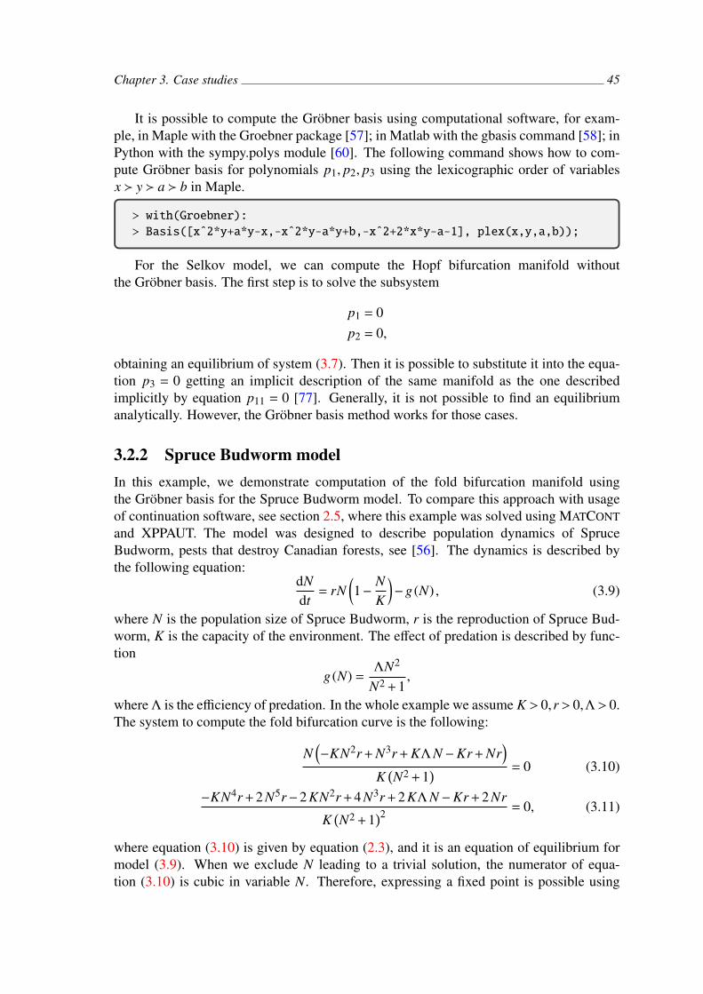
Chapter 3. Case studies 45
It is possible to compute the Grobner basis using computational software, for exam-ple, in Maple with the Groebner package [57]; in Matlab with the gbasis command [58]; inPython with the sympy.polys module [60]. The following command shows how to com-pute Grobner basis for polynomials p1, p2, p3 using the lexicographic order of variablesx y a b in Maple.
> with(Groebner):
> Basis([xˆ2*y+a*y-x,-xˆ2*y-a*y+b,-xˆ2+2*x*y-a-1], plex(x,y,a,b));
For the Selkov model, we can compute the Hopf bifurcation manifold withoutthe Grobner basis. The first step is to solve the subsystem
p1 = 0p2 = 0,
obtaining an equilibrium of system (3.7). Then it is possible to substitute it into the equa-tion p3 = 0 getting an implicit description of the same manifold as the one describedimplicitly by equation p11 = 0 [77]. Generally, it is not possible to find an equilibriumanalytically. However, the Grobner basis method works for those cases.
3.2.2 Spruce Budworm modelIn this example, we demonstrate computation of the fold bifurcation manifold usingthe Grobner basis for the Spruce Budworm model. To compare this approach with usageof continuation software, see section 2.5, where this example was solved using MATCONTand XPPAUT. The model was designed to describe population dynamics of SpruceBudworm, pests that destroy Canadian forests, see [56]. The dynamics is described bythe following equation:
dNdt
= rN(1−
NK
)−g (N) , (3.9)
where N is the population size of Spruce Budworm, r is the reproduction of Spruce Bud-worm, K is the capacity of the environment. The effect of predation is described by func-tion
g (N) =ΛN2
N2 + 1,
where Λ is the efficiency of predation. In the whole example we assume K > 0,r > 0,Λ> 0.The system to compute the fold bifurcation curve is the following:
N(−KN2r + N3r + KΛ N −Kr + Nr
)K
(N2 + 1
) = 0 (3.10)
−KN4r + 2 N5r−2 KN2r + 4 N3r + 2 KΛ N −Kr + 2 Nr
K(N2 + 1
)2 = 0, (3.11)
where equation (3.10) is given by equation (2.3), and it is an equation of equilibrium formodel (3.9). When we exclude N leading to a trivial solution, the numerator of equa-tion (3.10) is cubic in variable N. Therefore, expressing a fixed point is possible using
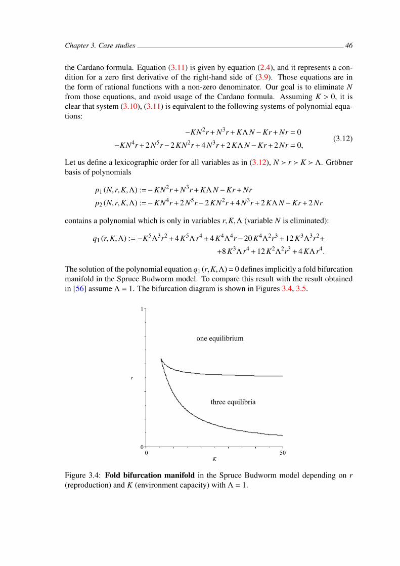
Chapter 3. Case studies 46
the Cardano formula. Equation (3.11) is given by equation (2.4), and it represents a con-dition for a zero first derivative of the right-hand side of (3.9). Those equations are inthe form of rational functions with a non-zero denominator. Our goal is to eliminate Nfrom those equations, and avoid usage of the Cardano formula. Assuming K > 0, it isclear that system (3.10), (3.11) is equivalent to the following systems of polynomial equa-tions:
−KN2r + N3r + KΛ N −Kr + Nr = 0
−KN4r + 2 N5r−2 KN2r + 4 N3r + 2 KΛ N −Kr + 2 Nr = 0,(3.12)
Let us define a lexicographic order for all variables as in (3.12), N r K Λ. Grobnerbasis of polynomials
p1 (N,r,K,Λ) :=−KN2r + N3r + KΛ N −Kr + Nr
p2 (N,r,K,Λ) :=−KN4r + 2 N5r−2 KN2r + 4 N3r + 2 KΛ N −Kr + 2 Nr
contains a polynomial which is only in variables r,K,Λ (variable N is eliminated):
q1 (r,K,Λ) := −K5Λ3r2 + 4 K5Λr4 + 4 K4Λ4r−20 K4Λ2r3 + 12 K3Λ3r2+
+8 K3Λr4 + 12 K2Λ2r3 + 4 KΛr4.
The solution of the polynomial equation q1 (r,K,Λ) = 0 defines implicitly a fold bifurcationmanifold in the Spruce Budworm model. To compare this result with the result obtainedin [56] assume Λ = 1. The bifurcation diagram is shown in Figures 3.4, 3.5.
one equilibrium
three equilibria
Figure 3.4: Fold bifurcation manifold in the Spruce Budworm model depending on r(reproduction) and K (environment capacity) with Λ = 1.
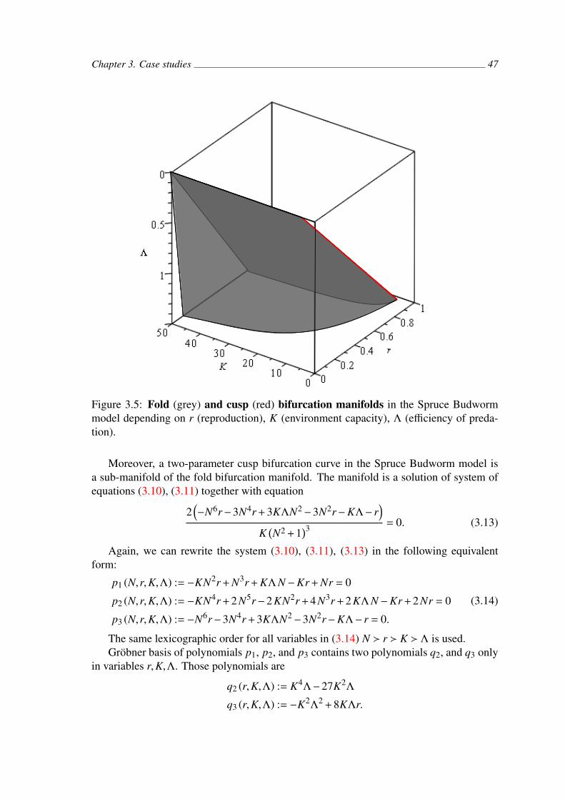
Chapter 3. Case studies 47
Figure 3.5: Fold (grey) and cusp (red) bifurcation manifolds in the Spruce Budwormmodel depending on r (reproduction), K (environment capacity), Λ (efficiency of preda-tion).
Moreover, a two-parameter cusp bifurcation curve in the Spruce Budworm model isa sub-manifold of the fold bifurcation manifold. The manifold is a solution of system ofequations (3.10), (3.11) together with equation
2(−N6r−3N4r + 3KΛN2−3N2r−KΛ− r
)K
(N2 + 1
)3 = 0. (3.13)
Again, we can rewrite the system (3.10), (3.11), (3.13) in the following equivalentform:
p1 (N,r,K,Λ) := −KN2r + N3r + KΛ N −Kr + Nr = 0
p2 (N,r,K,Λ) := −KN4r + 2 N5r−2 KN2r + 4 N3r + 2 KΛ N −Kr + 2 Nr = 0
p3 (N,r,K,Λ) := −N6r−3N4r + 3KΛN2−3N2r−KΛ− r = 0.
(3.14)
The same lexicographic order for all variables in (3.14) N r K Λ is used.Grobner basis of polynomials p1, p2, and p3 contains two polynomials q2, and q3 only
in variables r,K,Λ. Those polynomials are
q2 (r,K,Λ) := K4Λ−27K2Λ
q3 (r,K,Λ) := −K2Λ2 + 8KΛr.
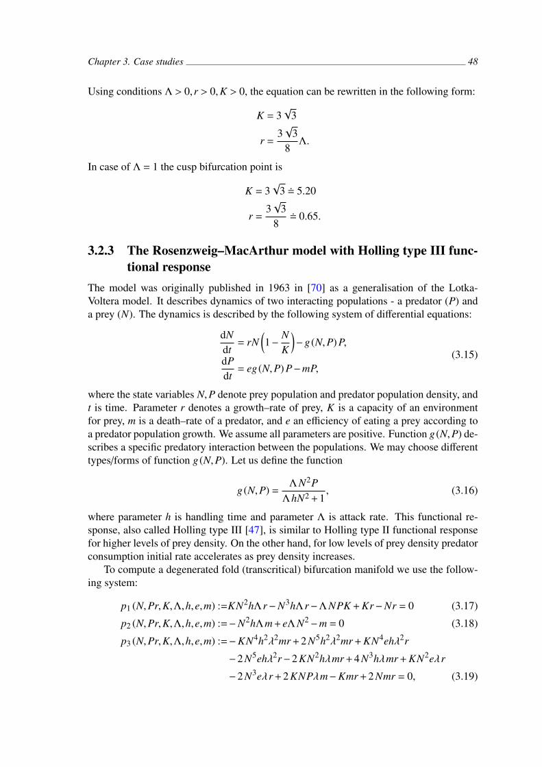
Chapter 3. Case studies 48
Using conditions Λ > 0,r > 0,K > 0, the equation can be rewritten in the following form:
K = 3√
3
r =3√
38
Λ.
In case of Λ = 1 the cusp bifurcation point is
K = 3√
3 5.20
r =3√
38
0.65.
3.2.3 The Rosenzweig–MacArthur model with Holling type III func-tional response
The model was originally published in 1963 in [70] as a generalisation of the Lotka-Voltera model. It describes dynamics of two interacting populations - a predator (P) anda prey (N). The dynamics is described by the following system of differential equations:
dNdt
= rN(1−
NK
)−g (N,P) P,
dPdt
= eg (N,P) P−mP,(3.15)
where the state variables N,P denote prey population and predator population density, andt is time. Parameter r denotes a growth–rate of prey, K is a capacity of an environmentfor prey, m is a death–rate of a predator, and e an efficiency of eating a prey according toa predator population growth. We assume all parameters are positive. Function g (N,P) de-scribes a specific predatory interaction between the populations. We may choose differenttypes/forms of function g (N,P). Let us define the function
g (N,P) =Λ N2P
ΛhN2 + 1, (3.16)
where parameter h is handling time and parameter Λ is attack rate. This functional re-sponse, also called Holling type III [47], is similar to Holling type II functional responsefor higher levels of prey density. On the other hand, for low levels of prey density predatorconsumption initial rate accelerates as prey density increases.
To compute a degenerated fold (transcritical) bifurcation manifold we use the follow-ing system:
p1 (N,Pr,K,Λ,h,e,m) :=KN2hΛr−N3hΛr−Λ NPK + Kr−Nr = 0 (3.17)
p2 (N,Pr,K,Λ,h,e,m) :=−N2hΛm + eΛ N2−m = 0 (3.18)
p3 (N,Pr,K,Λ,h,e,m) :=−KN4h2λ2mr + 2 N5h2λ2mr + KN4ehλ2r
−2 N5ehλ2r−2 KN2hλmr + 4 N3hλmr + KN2eλr
−2 N3eλr + 2 KNPλm−Kmr + 2 Nmr = 0, (3.19)
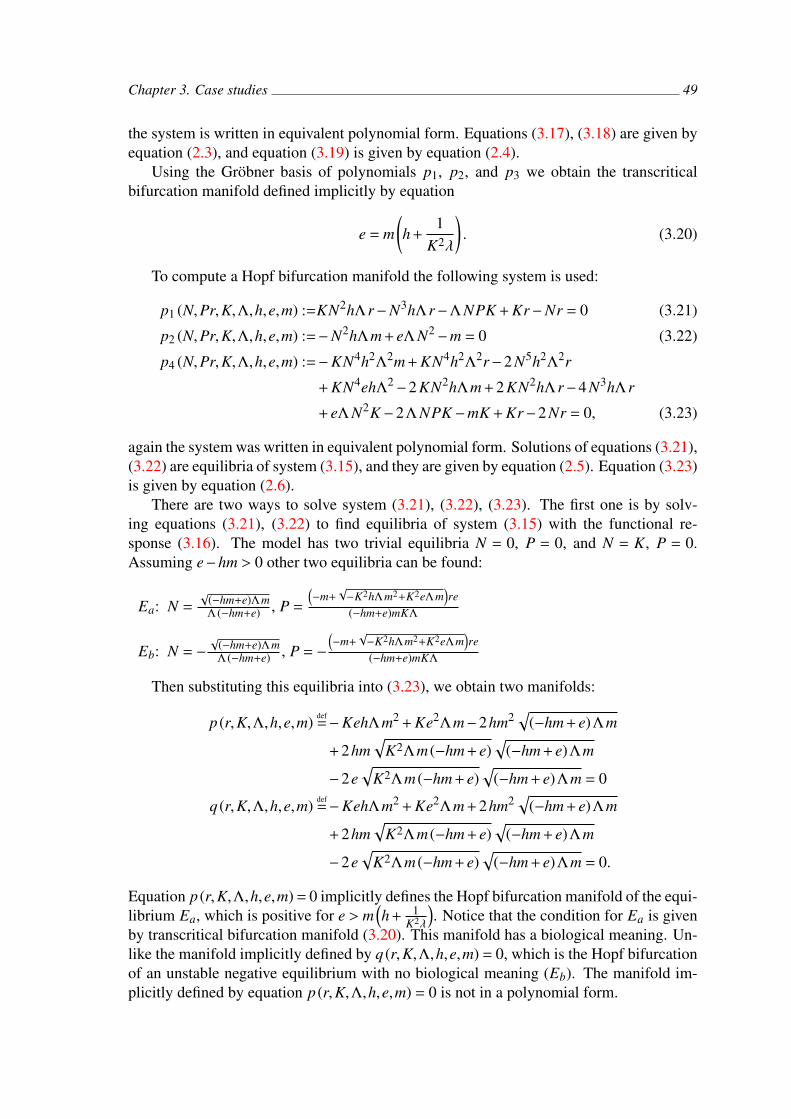
Chapter 3. Case studies 49
the system is written in equivalent polynomial form. Equations (3.17), (3.18) are given byequation (2.3), and equation (3.19) is given by equation (2.4).
Using the Grobner basis of polynomials p1, p2, and p3 we obtain the transcriticalbifurcation manifold defined implicitly by equation
e = m(h +
1K2λ
). (3.20)
To compute a Hopf bifurcation manifold the following system is used:
p1 (N,Pr,K,Λ,h,e,m) :=KN2hΛr−N3hΛr−Λ NPK + Kr−Nr = 0 (3.21)
p2 (N,Pr,K,Λ,h,e,m) :=−N2hΛm + eΛ N2−m = 0 (3.22)
p4 (N,Pr,K,Λ,h,e,m) :=−KN4h2Λ2m + KN4h2Λ2r−2 N5h2Λ2r
+ KN4ehΛ2−2 KN2hΛm + 2 KN2hΛr−4 N3hΛr
+ eΛ N2K −2Λ NPK −mK + Kr−2 Nr = 0, (3.23)
again the system was written in equivalent polynomial form. Solutions of equations (3.21),(3.22) are equilibria of system (3.15), and they are given by equation (2.5). Equation (3.23)is given by equation (2.6).
There are two ways to solve system (3.21), (3.22), (3.23). The first one is by solv-ing equations (3.21), (3.22) to find equilibria of system (3.15) with the functional re-sponse (3.16). The model has two trivial equilibria N = 0, P = 0, and N = K, P = 0.Assuming e−hm > 0 other two equilibria can be found:
Ea: N =√
(−hm+e)ΛmΛ (−hm+e) , P =
(−m+
√−K2hΛm2+K2eΛm
)re
(−hm+e)mKΛ
Eb: N = −√
(−hm+e)ΛmΛ (−hm+e) , P = −
(−m+
√−K2hΛm2+K2eΛm
)re
(−hm+e)mKΛ
Then substituting this equilibria into (3.23), we obtain two manifolds:
p (r,K,Λ,h,e,m) def=−KehΛm2 + Ke2Λm−2hm2
√(−hm + e)Λm
+ 2hm√
K2Λm (−hm + e)√
(−hm + e)Λm
−2e√
K2Λm (−hm + e)√
(−hm + e)Λm = 0
q (r,K,Λ,h,e,m) def=−KehΛm2 + Ke2Λm + 2hm2
√(−hm + e)Λm
+ 2hm√
K2Λm (−hm + e)√
(−hm + e)Λm
−2e√
K2Λm (−hm + e)√
(−hm + e)Λm = 0.
Equation p (r,K,Λ,h,e,m) = 0 implicitly defines the Hopf bifurcation manifold of the equi-librium Ea, which is positive for e > m
(h + 1
K2λ
). Notice that the condition for Ea is given
by transcritical bifurcation manifold (3.20). This manifold has a biological meaning. Un-like the manifold implicitly defined by q (r,K,Λ,h,e,m) = 0, which is the Hopf bifurcationof an unstable negative equilibrium with no biological meaning (Eb). The manifold im-plicitly defined by equation p (r,K,Λ,h,e,m) = 0 is not in a polynomial form.
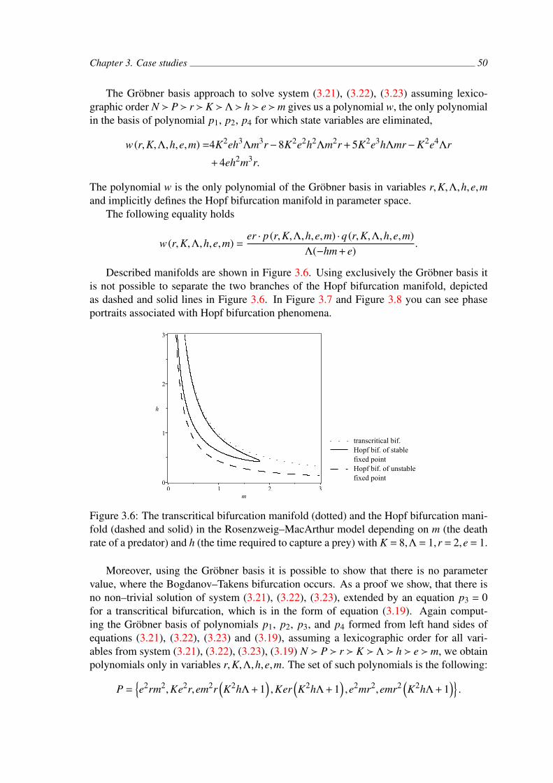
Chapter 3. Case studies 50
The Grobner basis approach to solve system (3.21), (3.22), (3.23) assuming lexico-graphic order N P r K Λ h e m gives us a polynomial w, the only polynomialin the basis of polynomial p1, p2, p4 for which state variables are eliminated,
w (r,K,Λ,h,e,m) =4K2eh3Λm3r−8K2e2h2Λm2r + 5K2e3hΛmr−K2e4Λr
+ 4eh2m3r.
The polynomial w is the only polynomial of the Grobner basis in variables r,K,Λ,h,e,mand implicitly defines the Hopf bifurcation manifold in parameter space.
The following equality holds
w (r,K,Λ,h,e,m) =er · p (r,K,Λ,h,e,m) ·q (r,K,Λ,h,e,m)
Λ(−hm + e).
Described manifolds are shown in Figure 3.6. Using exclusively the Grobner basis itis not possible to separate the two branches of the Hopf bifurcation manifold, depictedas dashed and solid lines in Figure 3.6. In Figure 3.7 and Figure 3.8 you can see phaseportraits associated with Hopf bifurcation phenomena.
transcritical bif.Hopf bif. of stablefixed pointHopf bif. of unstablefixed point
Figure 3.6: The transcritical bifurcation manifold (dotted) and the Hopf bifurcation mani-fold (dashed and solid) in the Rosenzweig–MacArthur model depending on m (the deathrate of a predator) and h (the time required to capture a prey) with K = 8,Λ = 1,r = 2,e = 1.
Moreover, using the Grobner basis it is possible to show that there is no parametervalue, where the Bogdanov–Takens bifurcation occurs. As a proof we show, that there isno non–trivial solution of system (3.21), (3.22), (3.23), extended by an equation p3 = 0for a transcritical bifurcation, which is in the form of equation (3.19). Again comput-ing the Grobner basis of polynomials p1, p2, p3, and p4 formed from left hand sides ofequations (3.21), (3.22), (3.23) and (3.19), assuming a lexicographic order for all vari-ables from system (3.21), (3.22), (3.23), (3.19) N P r K Λ h e m, we obtainpolynomials only in variables r,K,Λ,h,e,m. The set of such polynomials is the following:
P =e2rm2,Ke2r,em2r
(K2hΛ+ 1
),Ker
(K2hΛ+ 1
),e2mr2,emr2
(K2hΛ+ 1
).
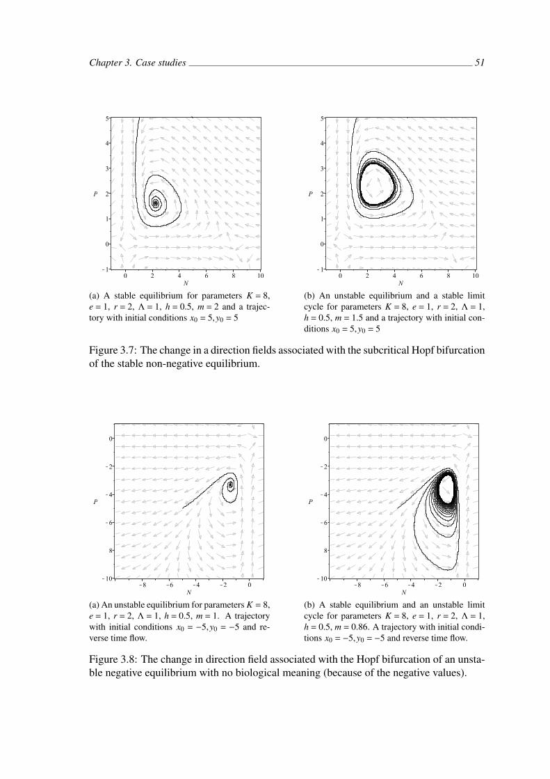
Chapter 3. Case studies 51
(a) A stable equilibrium for parameters K = 8,e = 1, r = 2, Λ = 1, h = 0.5, m = 2 and a trajec-tory with initial conditions x0 = 5,y0 = 5
(b) An unstable equilibrium and a stable limitcycle for parameters K = 8, e = 1, r = 2, Λ = 1,h = 0.5, m = 1.5 and a trajectory with initial con-ditions x0 = 5,y0 = 5
Figure 3.7: The change in a direction fields associated with the subcritical Hopf bifurcationof the stable non-negative equilibrium.
(a) An unstable equilibrium for parameters K = 8,e = 1, r = 2, Λ = 1, h = 0.5, m = 1. A trajectorywith initial conditions x0 = −5,y0 = −5 and re-verse time flow.
(b) A stable equilibrium and an unstable limitcycle for parameters K = 8, e = 1, r = 2, Λ = 1,h = 0.5, m = 0.86. A trajectory with initial condi-tions x0 = −5,y0 = −5 and reverse time flow.
Figure 3.8: The change in direction field associated with the Hopf bifurcation of an unsta-ble negative equilibrium with no biological meaning (because of the negative values).

Chapter 3. Case studies 52
If we set all polynomials from set P equals zero, it is easy to see, that for all solutions ofsuch a system at least one parameter r,K,Λ,h,e or m have to be zero. Therefore there doesnot exist a Bogdanov–Takens bifurcation point for non-zero parameters r,K,Λ,h,e,m.
The computations in this section were performed by using Maple [57].
3.3 Bifurcation manifolds in predator-prey models com-puted by the Grobner basis method
Current research models (3.15) with different types of functional responses g (N,P) [7, 67,68, 73]. The aim of the first part of this section is to show new results in the model stu-died in [7], and [67], obtained using Grobner basis method [41]. The functional responseg (N,P) is considered in the following form:
g (N,P) =Λ (P) N
Λ (P) hN + 1,
Λ (P) =Λ0
(b + P)2
(3.24)
where parameter h > 0 is a handling time and function Λ (P) is an attack rate with Λ0 > 0,b > 0. Functional response g (N,P) is a generalisation of Holling type II functional re-sponse [47]. Function Λ (P) is a decreasing function, therefore function g (N,P) is de-creasing in P for any fixed N, and it represents interference among predators.
Assuming a lexicographic order N P r K h e m b Λ0 , it is possible tofind the Grobner basis for the set of polynomials S 1.
S 1 =
numerator ( f1 (N,P)) ,numerator ( f2 (N,P)) ,numeratordet
d f1(P,N)dN
d f1(P,N)dP
d f2(P,N)dN
d f2(P,N)dP
By factorisation of the first polynomial in the basis we obtain polynomials
p1 (N,P,r,K,h,e,m,b,Λ0) =16r3K2e3b + 4r2K2he2mΛ0−4r2K2e3Λ0
+ 128r2Ke2mb2 + 144rKhem2bΛ0−144rKe2mbΛ0
+ 256rem2b3 + 27 Kh2m3Λ02−54 Khem2Λ0
2
+ 27 Ke2mΛ02,
p2 (N,P,r,K,h,e,m,b,Λ0) =−KhmΛ0 + KeΛ0−mb2,
p3 (N,P,r,K,h,e,m,b,Λ0) =−hm + e.
The polynomials vanish at fold or transcritical bifurcation points and so we get animplicit description of the corresponding bifurcation manifolds. The case whene = hm is not biologically relevant. The transcritical bifurcation in the intersection ofcoexistence equilibrium branch and prey equilibrium [K,0] without predator branch [67],is described by p2 = 0. On the other hand p1 = 0 implicitly defines the fold manifoldthat is derived in full parameter space. Similarly assuming lexicographic order

Chapter 3. Case studies 53
N P r K h e m b Λ0, it is possible to find the Grobner basis for the set ofpolynomial S 2 to obtain the Hopf bifurcation manifold.
S 2 =
numerator ( f1 (N,P)) ,numerator ( f2 (N,P)) ,numeratortrace
d f1(P,N)dN
d f1(P,N)dP
d f2(P,N)dN
d f2(P,N)dP
Factorisation of the first polynomial in the basis implies that polynomial
q (N,P,r,K,h,e,m,b,Λ0) =r3K2h2e4l2−4r2K2h3e3m2l2 + 6r2K2h2e4ml2
−4r2K2he5mbl−2r2K2he5Λ02 + 4r2K2e6bΛ0
+ 2r2Kh3e2m2bΛ02 + 4r2Kh2e3mbΛ0
2 + 2r2Khe4bΛ02
+ 4rK2h4e2m4Λ02−16rK2h3e3m3Λ0
2 + 16rK2h2e4m3bΛ0
+ 20rK2h2e4m2Λ02−32rK2he5m2bΛ0−8rK2he5mΛ0
2
+ 16rK2e6mbΛ0 + rKh5m4Λ03 + 2rKh4em3Λ0
3
+ 4rKh3e2m4b2Λ0−2rKh3e2m3bΛ02−12rKh2e3m3b2Λ0
−2rKh2e3m2bΛ02−2rKh2e3mΛ0
3−4rKhe4m2b2Λ0
+ 2rKhe4mbΛ02− rKhe4Λ0
3 + 12rKe5mb2Λ0 + 2rKe5bΛ02
+ rh4m4b2Λ02 + 4rh3em3b2Λ0
2 + 6rh2e2m2b2Λ02
+ 4rhe3mb2Λ02 + re4b2Λ0
2 + 8 K2h4e2m5Λ02
−16 K2h3e3m5bΛ0−24 K2h3e3m4Λ02 + 48 K2h2e4m4bΛ0
+ 24 K2h2e4m3Λ02−48 K2he5m3bΛ0−8 K2he5m2Λ0
2
+ 16 K2e6m2bΛ0 + 8 Kh3e2m5b2Λ0−16 Kh2e3m5b3
−8 Kh2e3m4b2Λ0 + 32 Khe4m4b3−8 Khe4m3b2Λ0
−16 Ke5m3b3 + 8 Ke5m2b2Λ0
vanishes at Hopf bifurcation points. Figures 3.9, 3.10 depict the fold bifurcation manifoldimplicitly defined by p1 = 0 and the Hopf bifurcation manifold implicitly defined by q = 0.It is crucial to point out that the vanishing ideal of (3.3) does not account for the scenario,where the Jacobi matrix determinant is positive. Therefore the expressed manifold consistsof Hopf bifurcation points as well as neutral saddle points. Additional analysis of the ma-nifold subset that satisfies det J > 0 is necessary to avoid spurious results. This couldbe done numerically, analytically or using the Grobner basis with an additional parame-ter delta = det J and an additional polynomial δ−det J. The Hopf bifurcation manifold inparametric space border is the contour δ= 0, so the border is usually the Bogdanov-Takensbifurcation manifold (see the next example below).
A cusp bifurcation, denoted by CP in Figure 3.9, is a two-parameter bifurcation ofequilibria. For the normal form of this bifurcation see [53]. A cusp bifurcation manifoldis a co-dimension two manifold, sub-manifold of the fold bifurcation manifold. At cusppoints, two branches of fold bifurcation manifolds of co-dimension 1 meet tangentiallyin a typical V-shape, see Figure 3.9. Let us assume that we are interested in analysis ofparameters m and h, and we seek hysteresis or transient dynamics. Because generally,

Chapter 3. Case studies 54
as well as in this example, cusp bifurcation points can be found as points where the im-plicitly defined function has no derivative, according to the implicit function theorem, cusppoints are solutions of a set of polynomial equations ∂p1
∂h = 0 and ∂p1∂m = 0. Eliminating h
and m respectively using the Grobner basis method again, we get the cusp bifurcationpoints explicitly as
m =112
Kerb,
h =43
(9Λ0−32br)bKrΛ0
.
The bifurcation analysis provided in this paper is not complete, for more see [67].Dynamical model in form (3.15) with functional response (3.24) is in fact a special case ofmodel studied in [67]. In [67] function Λ (P) is considered in form Λ (P) =
Λ0(b+P)w . Here,
parameter w is set to critical value 2. The Hopf curve passes directly through the cuspbifurcation point (CP), which is a degenerate situation, see Figure 3.9.
fold bifurcationHopf bifurcationcusp bifurcationCP
CP
Figure 3.9: The fold bifurcation manifold, implicitly defined by equation p1 = 0, andthe Hopf bifurcation manifold, implicitly defined by equation q = 0, in the generalisedRosenzweig–MacArthur model depending on m (the death rate of a predator) and h(the handling time) with K = 5,Λ0 = 28,r = 3.5,e = 1,b = 1.3. Note that the solid bi-furcation manifold consists of both neutral saddle points and Hopf bifurcation points.
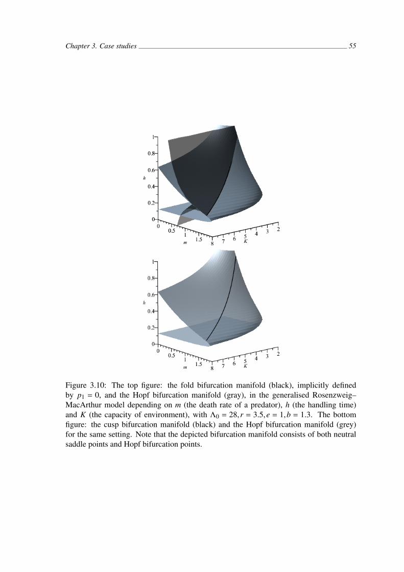
Chapter 3. Case studies 55
Figure 3.10: The top figure: the fold bifurcation manifold (black), implicitly definedby p1 = 0, and the Hopf bifurcation manifold (gray), in the generalised Rosenzweig–MacArthur model depending on m (the death rate of a predator), h (the handling time)and K (the capacity of environment), with Λ0 = 28,r = 3.5,e = 1,b = 1.3. The bottomfigure: the cusp bifurcation manifold (black) and the Hopf bifurcation manifold (grey)for the same setting. Note that the depicted bifurcation manifold consists of both neutralsaddle points and Hopf bifurcation points.
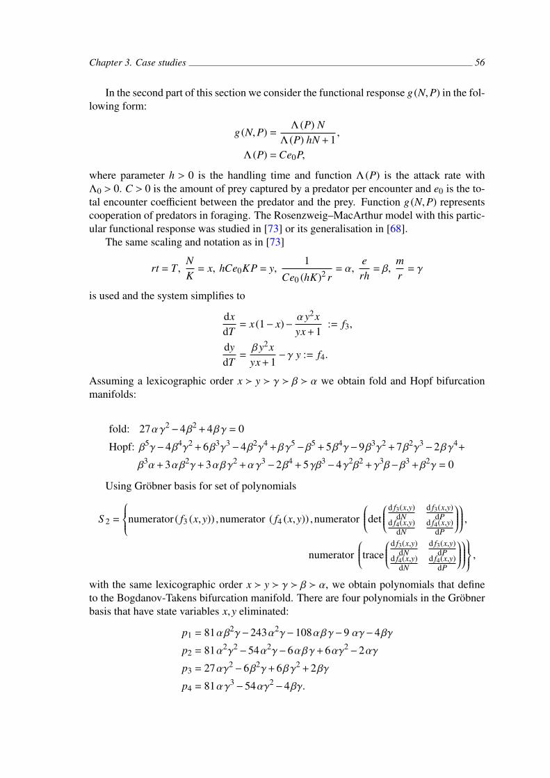
Chapter 3. Case studies 56
In the second part of this section we consider the functional response g (N,P) in the fol-lowing form:
g (N,P) =Λ (P) N
Λ (P) hN + 1,
Λ (P) = Ce0P,
where parameter h > 0 is the handling time and function Λ (P) is the attack rate withΛ0 > 0. C > 0 is the amount of prey captured by a predator per encounter and e0 is the to-tal encounter coefficient between the predator and the prey. Function g (N,P) representscooperation of predators in foraging. The Rosenzweig–MacArthur model with this partic-ular functional response was studied in [73] or its generalisation in [68].
The same scaling and notation as in [73]
rt = T,NK
= x, hCe0KP = y,1
Ce0 (hK)2 r= α,
erh
= β,mr
= γ
is used and the system simplifies to
dxdT
= x (1− x)−αy2xyx + 1
:= f3,
dydT
=βy2xyx + 1
−γ y := f4.
Assuming a lexicographic order x y γ β α we obtain fold and Hopf bifurcationmanifolds:
fold: 27αγ2−4β2 + 4βγ = 0
Hopf: β5γ−4β4γ2 + 6β3γ3−4β2γ4 +βγ5−β5 + 5β4γ−9β3γ2 + 7β2γ3−2βγ4+
β3α+ 3αβ2γ+ 3αβγ2 +αγ3−2β4 + 5γβ3−4γ2β2 +γ3β−β3 +β2γ = 0
Using Grobner basis for set of polynomials
S 2 =
numerator ( f3 (x,y)) ,numerator ( f4 (x,y)) ,numeratordet
d f3(x,y)dN
d f3(x,y)dP
d f4(x,y)dN
d f4(x,y)dP
,numerator
traced f3(x,y)
dNd f3(x,y)
dPd f4(x,y)
dNd f4(x,y)
dP
,with the same lexicographic order x y γ β α, we obtain polynomials that defineto the Bogdanov-Takens bifurcation manifold. There are four polynomials in the Grobnerbasis that have state variables x,y eliminated:
p1 = 81αβ2γ−243α2γ−108αβγ−9 αγ−4βγ
p2 = 81α2γ2−54α2γ−6αβγ+ 6αγ2−2αγ
p3 = 27αγ2−6β2γ+ 6βγ2 + 2βγ
p4 = 81αγ3−54αγ2−4βγ.
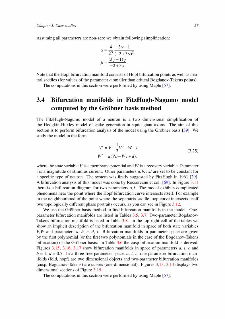
Chapter 3. Case studies 57
Assuming all parameters are non-zero we obtain following simplification:
α =4
273γ−1
(−2 + 3γ)2
β =(3γ−1)γ−2 + 3γ
.
Note that the Hopf bifurcation manifold consists of Hopf bifurcation points as well as neu-tral saddles (for values of the parameter α smaller than critical Bogdanov-Takens points).
The computations in this section were performed by using Maple [57].
3.4 Bifurcation manifolds in FitzHugh-Nagumo modelcomputed by the Grobner basis method
The FitzHugh-Nagumo model of a neuron is a two dimensional simplification ofthe Hodgkin-Huxley model of spike generation in squid giant axons. The aim of thissection is to perform bifurcation analysis of the model using the Grobner basis [39]. Westudy the model in the form
V′ = V −13
V3−W + i
W′ = a (Vb−Wc + d) ,(3.25)
where the state variable V is a membrane potential and W is a recovery variable. Parameteri is a magnitude of stimulus current. Other parameters a,b,c,d are set to be constant fora specific type of neuron. The system was firstly suggested by FitzHugh in 1961 [29].A bifurcation analysis of this model was done by Rocsoreanu et col. [69]. In Figure 3.11there is a bifurcation diagram for two parameters a, i. The model exhibits complicatedphenomena near the point where the Hopf bifurcation curve intersects itself. For examplein the neighbourhood of the point where the separatrix saddle loop curve intersects itselftwo topologically different phase portraits occurs, as you can see in Figure 3.12.
We use the Grobner basis method to find bifurcation manifolds in the model. One-parameter bifurcation manifolds are listed in Tables 3.5, 3.7. Two-parameter Bogdanov-Takens bifurcation manifold is listed in Table 3.8. In the top right cell of the tables weshow an implicit description of the bifurcation manifold in space of both state variablesV,W and parameters a, b, c, d, i. Bifurcation manifolds in parameter space are givenby the first polynomial (or the first two polynomials in the case of the Bogdanov-Takensbifurcation) of the Grobner basis. In Table 3.6 the cusp bifurcation manifold is derived.Figures 3.15, 3.16, 3.17 show bifurcation manifolds in space of parameters a, i, c andb = 1, d = 0.7. In a three free parameter space, a, i, c, one-parameter bifurcation man-ifolds (fold, hopf) are two dimensional objects and two-parameter bifurcation manifolds(cusp, Bogdanov-Takens) are curves (one-dimensional). Figures 3.13, 3.14 displays twodimensional sections of Figure 3.15.
The computations in this section were performed by using Maple [57].

Chapter 3. Case studies 58
0.2 1
0.4
0.8
a
i
Figure 3.11: Bifurcation diagram of the FitzHugh-Nagumo model forb = 1,c = 1.2,d = 0.7. Bifurcation manifolds: Hopf (red), fold (black), LPC (blackdashed), separatrix-saddle loop (grey).
foldg1 =V −1/3V3−W + ig2 =Vab−Wac + ad
g3 =V2ac + ab−ac
Grobner basis
ppp111 =999aaaccc333iii222−−−111888ccc222dddiii +++ 444aaabbb333−−−111222cccbbb222aaa +++ 111222aaabbbccc222−−−444aaaccc333 +++ 999aaacccddd222
p2 =6Wac2i−9ac2i2−6Wacd + 12acdi + 4b2a−8cba + 4ac2−3d2a
p3 =2cbWa−2Wac2−3icba + abd + 2acd
p4 =6W2acd−15Wacdi + 9acdi2−4Wab2 + 4Wac2 + 3d2Wa+
+ 6ib2a + 6icba−3d2ia−4abd−8acd
p5 =4W2ac2−9ac2
p6 =i2−8Wacd + 18acdi + 8b2a−12cba + 4ac2−5d2a
p7 =4W2ac−12Waci + 9aci2 + 2daV + 2dWa−3dia + 4ab−4ac
p8 =2caV −2Wac + 3ica−ad,Vab−Wac + ad
p9 =V3−3V + 3W −3i
Table 3.5: Fold bifurcation manifold. Equations g1 = 0, g2 = 0 are given by equa-tion (2.3), and g3 = 0 is given by equation (2.4).
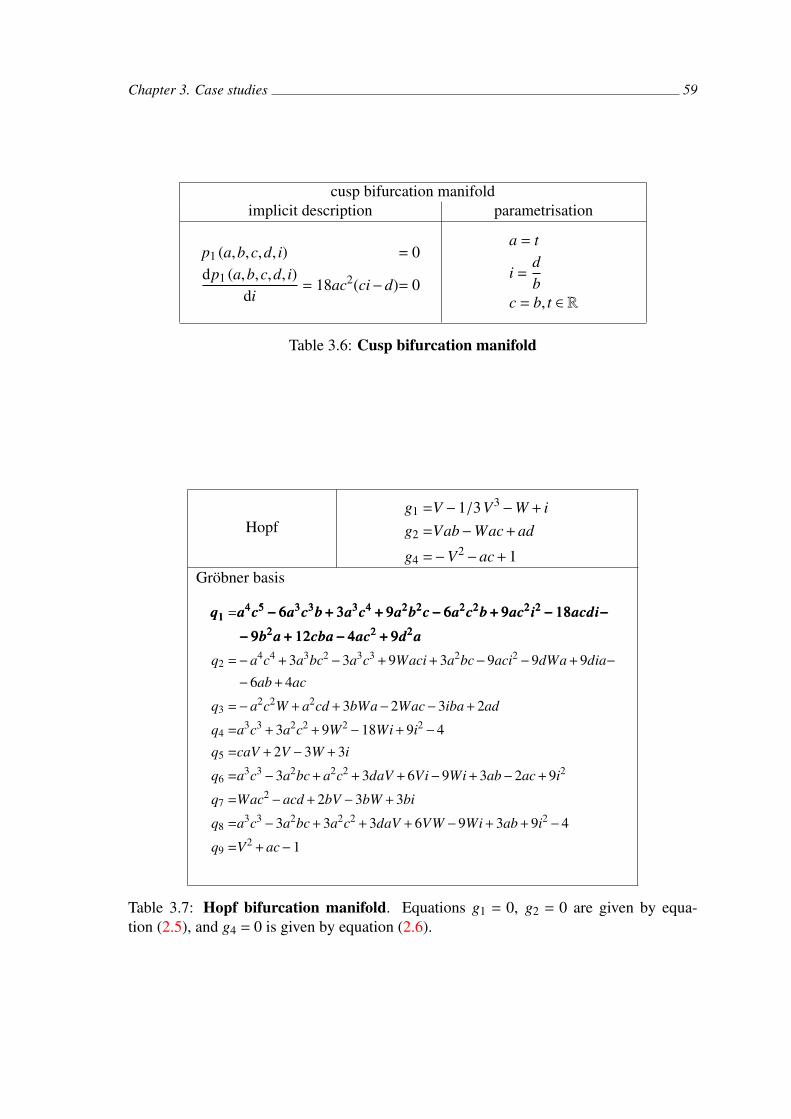
Chapter 3. Case studies 59
cusp bifurcation manifoldimplicit description parametrisation
p1 (a,b,c,d, i) = 0dp1 (a,b,c,d, i)
di= 18ac2(ci−d)= 0
a = t
i =db
c = b, t ∈ R
Table 3.6: Cusp bifurcation manifold
Hopfg1 =V −1/3V3−W + ig2 =Vab−Wac + ad
g4 =−V2−ac + 1Grobner basis
qqq111 =aaa444ccc555−−−666aaa333ccc333bbb +++ 333aaa333ccc444 +++ 999aaa222bbb222ccc−−−666aaa222ccc222bbb +++ 999aaaccc222iii222−−−111888aaacccdddiii−−−
−−−999bbb222aaa +++ 111222cccbbbaaa−−−444aaaccc222 +++ 999ddd222aaa
q2 =−a4c4 + 3a3bc2−3a3c3 + 9Waci + 3a2bc−9aci2−9dWa + 9dia−
−6ab + 4ac
q3 =−a2c2W + a2cd + 3bWa−2Wac−3iba + 2ad
q4 =a3c3 + 3a2c2 + 9W2−18Wi + 9i2−4
q5 =caV + 2V −3W + 3i
q6 =a3c3−3a2bc + a2c2 + 3daV + 6Vi−9Wi + 3ab−2ac + 9i2
q7 =Wac2−acd + 2bV −3bW + 3bi
q8 =a3c3−3a2bc + 3a2c2 + 3daV + 6VW −9Wi + 3ab + 9i2−4
q9 =V2 + ac−1
Table 3.7: Hopf bifurcation manifold. Equations g1 = 0, g2 = 0 are given by equa-tion (2.5), and g4 = 0 is given by equation (2.6).
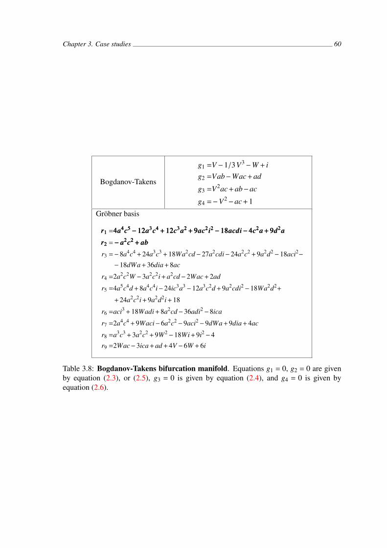
Chapter 3. Case studies 60
Bogdanov-Takens
g1 =V −1/3V3−W + ig2 =Vab−Wac + ad
g3 =V2ac + ab−ac
g4 =−V2−ac + 1
Grobner basis
rrr111 =444aaa444ccc555−−−111222aaa333ccc444 +++ 111222ccc333aaa222 +++ 999aaaccc222iii222−−−111888aaacccdddiii−−−444ccc222aaa +++ 999ddd222aaa
rrr222 =−−−aaa222ccc222 +++ aaabbb
r3 =−8a4c4 + 24a3c3 + 18Wa2cd−27a2cdi−24a2c2 + 9a2d2−18aci2−
−18dWa + 36dia + 8ac
r4 =2a2c2W −3a2c2i + a2cd−2Wac + 2ad
r5 =4a5c4d + 8a4c4i−24ic3a3−12a3c2d + 9a2cdi2−18Wa2d2+
+ 24a2c2i + 9a2d2i + 18
r6 =aci3 + 18Wadi + 8a2cd−36adi2−8ica
r7 =2a4c4 + 9Waci−6a2c2−9aci2−9dWa + 9dia + 4ac
r8 =a3c3 + 3a2c2 + 9W2−18Wi + 9i2−4
r9 =2Wac−3ica + ad + 4V −6W + 6i
Table 3.8: Bogdanov-Takens bifurcation manifold. Equations g1 = 0, g2 = 0 are givenby equation (2.3), or (2.5), g3 = 0 is given by equation (2.4), and g4 = 0 is given byequation (2.6).
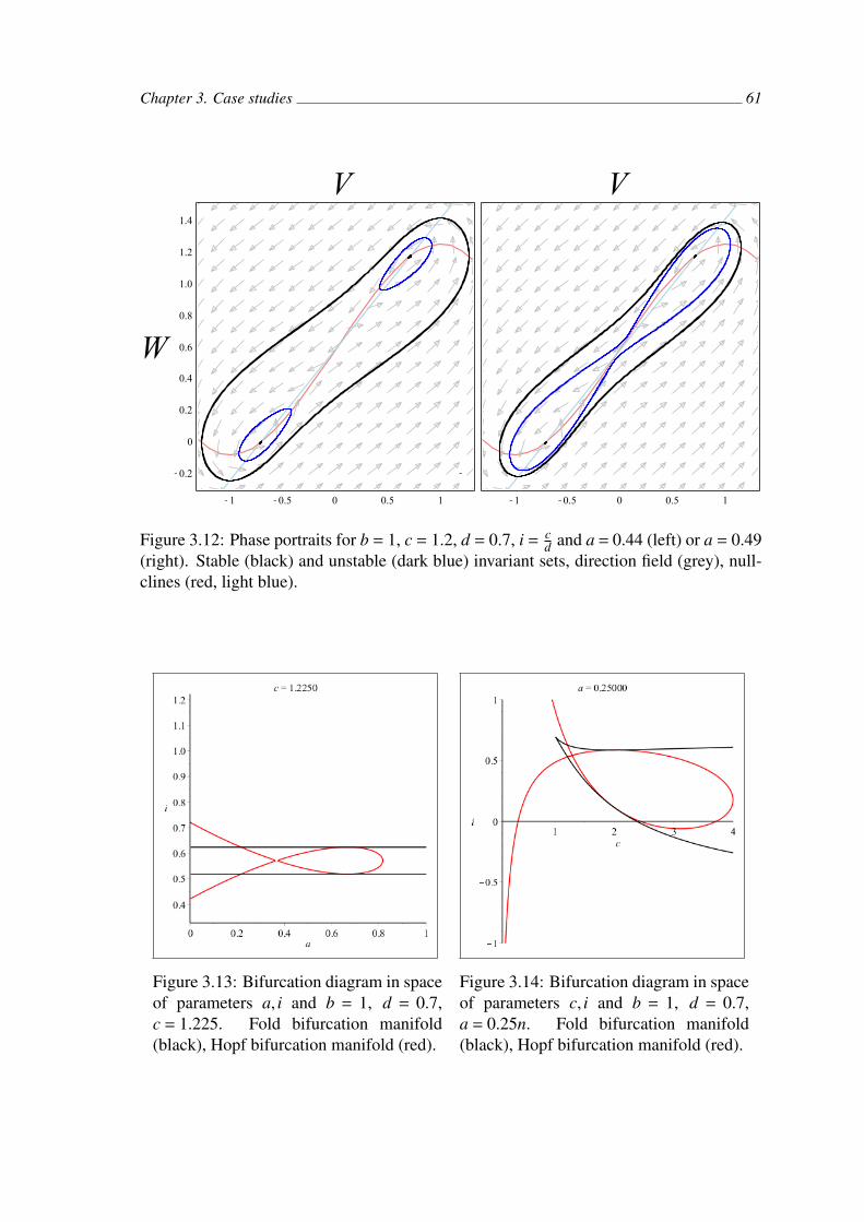
Chapter 3. Case studies 61
V V
W
Figure 3.12: Phase portraits for b = 1, c = 1.2, d = 0.7, i = cd and a = 0.44 (left) or a = 0.49
(right). Stable (black) and unstable (dark blue) invariant sets, direction field (grey), null-clines (red, light blue).
Figure 3.13: Bifurcation diagram in spaceof parameters a, i and b = 1, d = 0.7,c = 1.225. Fold bifurcation manifold(black), Hopf bifurcation manifold (red).
Figure 3.14: Bifurcation diagram in spaceof parameters c, i and b = 1, d = 0.7,a = 0.25n. Fold bifurcation manifold(black), Hopf bifurcation manifold (red).
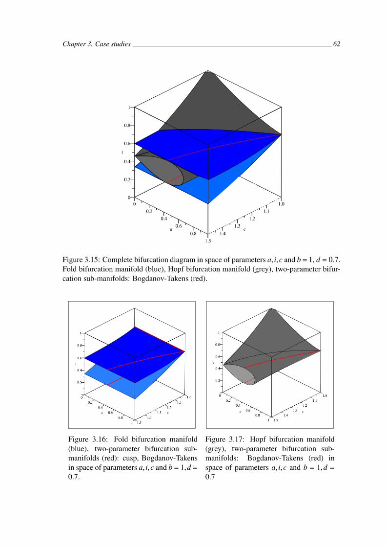
Chapter 3. Case studies 62
Figure 3.15: Complete bifurcation diagram in space of parameters a, i,c and b = 1, d = 0.7.Fold bifurcation manifold (blue), Hopf bifurcation manifold (grey), two-parameter bifur-cation sub-manifolds: Bogdanov-Takens (red).
Figure 3.16: Fold bifurcation manifold(blue), two-parameter bifurcation sub-manifolds (red): cusp, Bogdanov-Takensin space of parameters a, i,c and b = 1,d =
0.7.
Figure 3.17: Hopf bifurcation manifold(grey), two-parameter bifurcation sub-manifolds: Bogdanov-Takens (red) inspace of parameters a, i,c and b = 1,d =
0.7
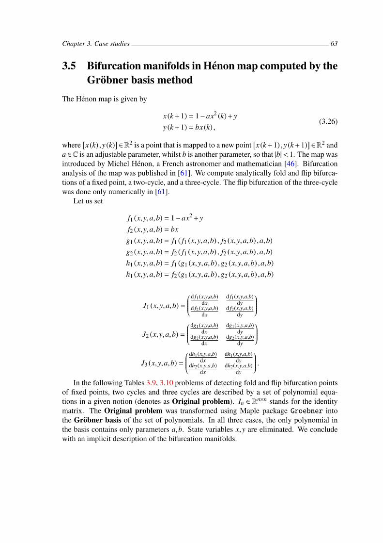
Chapter 3. Case studies 63
3.5 Bifurcation manifolds in Henon map computed by theGrobner basis method
The Henon map is given by
x (k + 1) = 1−ax2 (k) + yy (k + 1) = bx (k) ,
(3.26)
where[x (k) ,y (k)
]∈R2 is a point that is mapped to a new point
[x (k + 1) ,y (k + 1)
]∈R2 and
a ∈C is an adjustable parameter, whilst b is another parameter, so that |b|< 1. The map wasintroduced by Michel Henon, a French astronomer and mathematician [46]. Bifurcationanalysis of the map was published in [61]. We compute analytically fold and flip bifurca-tions of a fixed point, a two-cycle, and a three-cycle. The flip bifurcation of the three-cyclewas done only numerically in [61].
Let us set
f1 (x,y,a,b) = 1−ax2 + yf2 (x,y,a,b) = bxg1 (x,y,a,b) = f1 ( f1 (x,y,a,b) , f2 (x,y,a,b) ,a,b)g2 (x,y,a,b) = f2 ( f1 (x,y,a,b) , f2 (x,y,a,b) ,a,b)h1 (x,y,a,b) = f1 (g1 (x,y,a,b) ,g2 (x,y,a,b) ,a,b)h1 (x,y,a,b) = f2 (g1 (x,y,a,b) ,g2 (x,y,a,b) ,a,b)
J1 (x,y,a,b) =
d f1(x,y,a,b)dx
d f1(x,y,a,b)dy
d f2(x,y,a,b)dx
d f2(x,y,a,b)dy
J2 (x,y,a,b) =
dg1(x,y,a,b)dx
dg1(x,y,a,b)dy
dg2(x,y,a,b)dx
dg2(x,y,a,b)dy
J3 (x,y,a,b) =
dh1(x,y,a,b)dx
dh1(x,y,a,b)dy
dh2(x,y,a,b)dx
dh2(x,y,a,b)dy
.In the following Tables 3.9, 3.10 problems of detecting fold and flip bifurcation points
of fixed points, two cycles and three cycles are described by a set of polynomial equa-tions in a given notion (denotes as Original problem). In ∈ R
n×n stands for the identitymatrix. The Original problem was transformed using Maple package Groebner intothe Grobner basis of the set of polynomials. In all three cases, the only polynomial inthe basis contains only parameters a,b. State variables x,y are eliminated. We concludewith an implicit description of the bifurcation manifolds.

Chapter 3. Case studies 64
Original problem Grobner basis
fixedpoint
f1 (x,y,a,b)− x = 0f2 (x,y,a,b)− y = 0
det (J1 (x,y,a,b)− I2) = 0
p1def= b2 + 4a−2b + 1 = 0
by + 2b− y = 0−y−2 + x = 0
twocycle
g1 (x,y,a,b)− x = 0g2 (x,y,a,b)− y = 0
det (J2 (x,y,a,b)− I2) = 0
p2def=
(b2 + 4a−2b + 1
)(−3b2 + 4a + 6b−3
)2= 03
threecycle
h1 (x,y,a,b)− x = 0h2 (x,y,a,b)− y = 0
det (J3 (x,y,a,b)− I2) = 0
p3def=
(b2 + 4a−2b + 1
)(−7b2 + 4a−10b−7
)(7b4−4ab2−4b3 + 16a2+
+ 32ab + 3b2−4a−4b+
+ 7)2
= 03
3 Polynomials of the Grobner basis which contain state variables x,y are omitted here.
Table 3.9: Fold and transcritical bifurcation points are given implicitly in parameterspace by polynomials in the Grobner basis contain only parameters a,b.
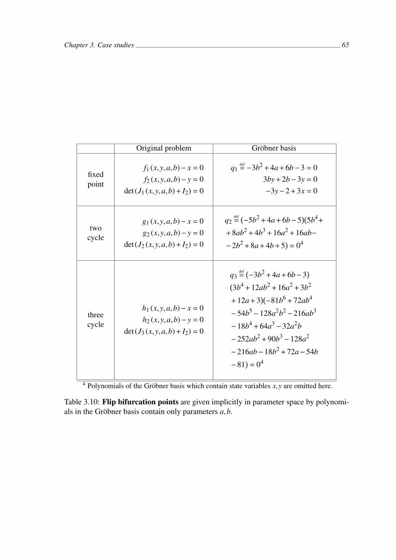
Chapter 3. Case studies 65
Original problem Grobner basis
fixedpoint
f1 (x,y,a,b)− x = 0f2 (x,y,a,b)− y = 0
det (J1 (x,y,a,b) + I2) = 0
q1def= −3b2 + 4a + 6b−3 = 0
3by + 2b−3y = 0−3y−2 + 3x = 0
twocycle
g1 (x,y,a,b)− x = 0g2 (x,y,a,b)− y = 0
det (J2 (x,y,a,b) + I2) = 0
q2def=
(−5b2 + 4a + 6b−5
)(5b4+
+ 8ab2 + 4b3 + 16a2 + 16ab−
−2b2 + 8a + 4b + 5)
= 04
threecycle
h1 (x,y,a,b)− x = 0h2 (x,y,a,b)− y = 0
det (J3 (x,y,a,b) + I2) = 0
q3def=
(−3b2 + 4a + 6b−3
)(3b4 + 12ab2 + 16a2 + 3b2
+ 12a + 3)(−81b6 + 72ab4
−54b5−128a2b2−216ab3
−18b4 + 64a3−32a2b
−252ab2 + 90b3−128a2
−216ab−18b2 + 72a−54b
−81)
= 04
4 Polynomials of the Grobner basis which contain state variables x,y are omitted here.
Table 3.10: Flip bifurcation points are given implicitly in parameter space by polynomi-als in the Grobner basis contain only parameters a,b.
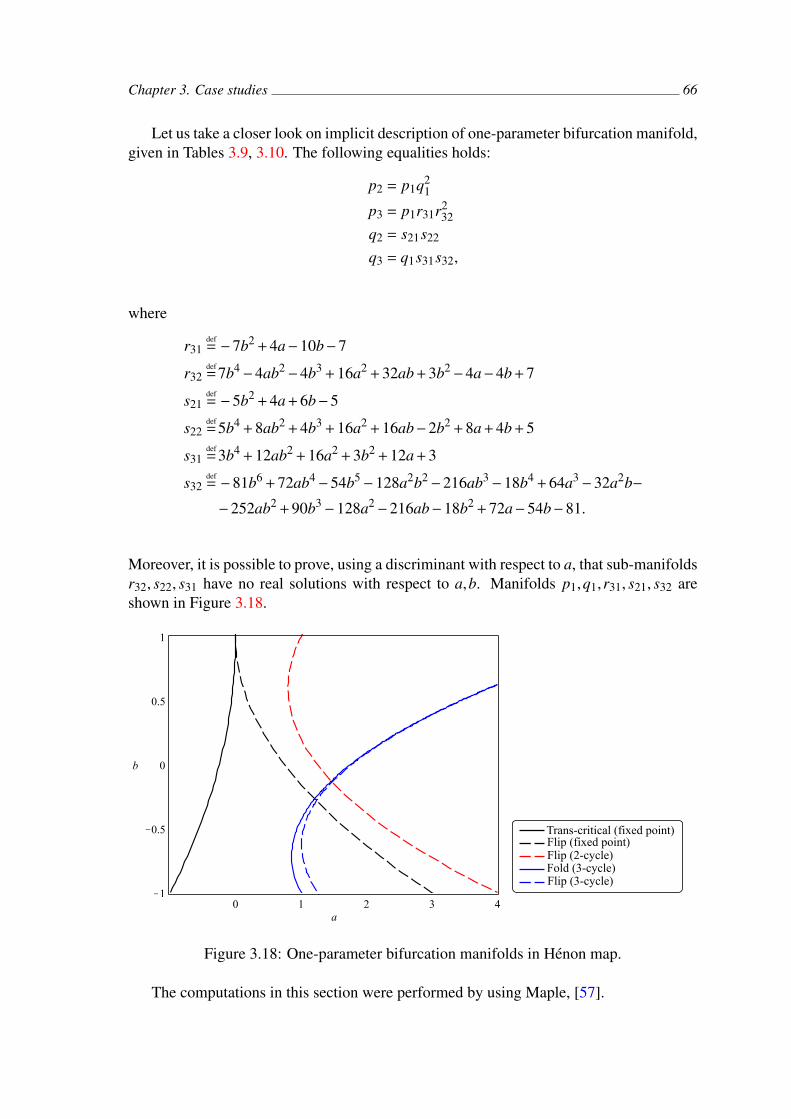
Chapter 3. Case studies 66
Let us take a closer look on implicit description of one-parameter bifurcation manifold,given in Tables 3.9, 3.10. The following equalities holds:
p2 = p1q21
p3 = p1r31r232
q2 = s21s22
q3 = q1s31s32,
where
r31def= −7b2 + 4a−10b−7
r32def=7b4−4ab2−4b3 + 16a2 + 32ab + 3b2−4a−4b + 7
s21def= −5b2 + 4a + 6b−5
s22def=5b4 + 8ab2 + 4b3 + 16a2 + 16ab−2b2 + 8a + 4b + 5
s31def=3b4 + 12ab2 + 16a2 + 3b2 + 12a + 3
s32def= −81b6 + 72ab4−54b5−128a2b2−216ab3−18b4 + 64a3−32a2b−
−252ab2 + 90b3−128a2−216ab−18b2 + 72a−54b−81.
Moreover, it is possible to prove, using a discriminant with respect to a, that sub-manifoldsr32, s22, s31 have no real solutions with respect to a,b. Manifolds p1,q1,r31, s21, s32 areshown in Figure 3.18.
Trans-critical (fixed point) Flip (fixed point)Flip (2-cycle)Fold (3-cycle)Flip (3-cycle)
Figure 3.18: One-parameter bifurcation manifolds in Henon map.
The computations in this section were performed by using Maple, [57].
Conclusion
One of the crucial issues of modern analysis of dynamical systems is the bifurcation mani-fold description in parameter space. Presently, the community often uses processes of de-tection and continuation implemented in continuation software Matcont [23], or Auto [26].In a limited number of cases where it is possible to express equilibrium explicitly, we canalways express one-parameter bifurcation manifolds of the equilibrium analytically andimplicitly. An example of the process is provided in section 3.1. As an alternative tocommonly used methods, we proposed a different approach through Grobner basis com-putation. Our goal is also to provide a comparison with the numerical methods imple-mented in continuation software. The main advantage of the method is the full-parameterspace representation of bifurcation manifolds. Continuation algorithms allow the com-putation of the bifurcation points on the manifold only depending on one parameter, oronly detect two-parameter bifurcations. An algorithm described in the dissertation allowsfinding bifurcation manifolds analytically in full parameter space without the necessity ofexpressing equilibria explicitly. The approach was used to obtain new results for predator-prey models (section 3.3), the FitzHugh-Nagumo model (section 3.4), and the Henon map(section 3.5).
The originally proposed Buchberger algorithm for Grobner basis computation is ofhuge complexity. Therefore it can be used only for a limited number of cases. Sincethe discovery of the Grobner basis in the 1960s, information technology is undergoingconsiderable development. Together with many variants of Buchberger’s algorithm, whichimproved its efficiency, it now allows us to find bifurcation manifolds analytically even forcases where it was not possible before. Faugere’s F4 and F5 algorithms are the mostefficient algorithms for computing Grobner bases, and both of them are implemented, forinstance, in the computer algebra system Maple [57], and they were used in case studiesfor this dissertation. Due to their implementation, it is simple to use the proposed approachto study dynamical systems even for non-experts in the field. We proposed basic examplesin section 3.2, and we prepared Maple Worksheet [34] solving those examples.
The suggested method brings several related issues, which need to be considered. Wecannot easily distinguish between computed bifurcation manifold parts that belong to dif-ferent equilibria or different domains of topological equivalence since we get manifold ex-pression in parameter space without the direct equilibria correspondence, see section 3.2.3.Also, it is not possible to directly assume additional properties of state variables such aspositivity. We use the proposed method only for dynamical systems described by an au-tonomous polynomial, or rational, systems of differential, or difference equations. Suchsystems are typical for population biology [7, 67, 68, 73], biochemistry [24, 64] and neu-roscience [29]. The usage can be extended for some problems described by goniometric
– 67 –

Conclusion 68
systems of dynamic equations, or irrational function systems of dynamic equations [12].An example of such systems is the Kuramoto model and its generalisations [42], andthe predator-prey model with square root functional responses [10]. Systems of exponen-tial equations also describe many dynamical systems. Generally, quantifier eliminationis not possible for exponential expression [30]. Several results similar to the Buchbergeralgorithm were proposed [82], and it would be interesting to investigate their potential forbifurcation theory.
Appendix 1: Bialternate matrix productand wedge product
To prove Stephanson theorem we define bialternate matrix product using a wedge prod-uct [52]. We show that this definition is equivalent to the definition used in chapter 2.
Definition 3.1. A wedge product of vectors v = (v1,v2, . . . ,vn)T ∈ Cn,w = (w1,w2, . . . ,wn)T ∈ Cn is a vector v ∧ w ∈ Cm, m = 1
2n (n−1), whose compo-nents are (v∧w)(i, j) = viw j − v jwi, n ≥ i > j ≥ 1 with lexicographic order, therefore(i1, j1) < (i2, j2), when i1 < i2 or i1 = i2 and j1 < j2.
Definition 3.2. Let v,w ∈ Cn a v∧w ∈ Cm, m = 12n (n−1). Transformation
AB (v∧w) =12
(Av∧Bw−Aw∧Bv) (3.27)
is called bialternate matrix product.
Theorem 3.1. Bialternate matrix product is a linear mapping in Cm. Matrix A B inthe basis ei∧ e j, n ≥ i > j ≥ 1, where ei, i ∈ 1,∈,n, of Cm is
AB(p,q),(r,s) =12
∣∣∣∣∣∣apr apsbqr bqs
∣∣∣∣∣∣+∣∣∣∣∣∣bpr bpsaqr aqs
∣∣∣∣∣∣ ,where n ≥ p > q ≥ 1 a n ≥ r > s ≥ 1.
– 69 –

Appendix 70
Proof.
(AB) (er ∧ es) =12
(Aer ∧Bes−Aes∧Ber)
=12
∑p
aprep∧∑
qbqseq−
∑p
apsep∧∑
qbqreq
=
12
∑p,q
aprbqs(ep∧ eq
)−
∑p,q
apsbqr(ep∧ eq
)=
12
∑p>q
aprbqs(ep∧ eq
)+
∑p<q
aprbqs(ep∧ eq
)−
−∑p>q
apsbqr(ep∧ eq
)−
∑p<q
apsbqr(ep∧ eq
)=
12
∑p>q
aprbqs(ep∧ eq
)−
∑p>q
aqrbps(ep∧ eq
)−
−∑p>q
apsbqr(ep∧ eq
)+
∑p>q
aqsbpr(ep∧ eq
)=
12
∑p>q
(aprbqs−apsbqr + aqsbpr −aqrbps
) (ep∧ eq
)= (AB)(p,q)(r,s) (er ∧ es)
Theorem 3.2 (Stephanson). Let A ∈ Cn×n with eigenvalues µi, i = 1 . . .n. Then matrix
1. 2A I has eigenvalues µi +µ j, n ≥ i > j ≥ 1.
2. AA has eigenvalues µiµ j, n ≥ i > j ≥ 1.
Proof. Firstly, let us assume all eigenvalues µi, i ∈ 1,∈,n of matrix A are simple. Thentheir eigenvalues vi, i ∈ 1,∈,n define the basis of Cn and vectors vi ∧ v j, n ≥ i > j ≥ 1defines the basis of Cm, m = 1
2n (n−1).
(2A I)(vi∧ v j
)= Avi∧ v j + vi∧Av j = µivi∧ v j + vi∧µ jv j =
(µi +µ j
) (vi∧ v j
)(AA)
(vi∧ v j
)= Avi∧Av j = µivi∧µ jv j = µiµ j
(vi∧ v j
)Consequently, if we assume the eigenvalues are functions of the matrix elements,
the theorem follows for non-simple eigenvalues from the continuity.

Appendix 2: Step by step computationof Grobner basis for Hopf bifurcationmanifold in Selkov model of glycolisis
According to section 3.2.1 a system to compute a fold bifurcation manifold is the follow-ing:
p1 := x2y− x + ay = 0
p2 := −x2y−ay + b = 0
p3 := −x2 + 2xy−a−1 = 0
To find an implicit formula for the manifold in parameter space, let us computethe Grobner basis of the ideal of polynomials I = (p1, p2, p3) with lexicographicorder x y a b. Firstly we will start by computing S-polynomial of p1, p2:
S (p1, p2) = p1 + p2 = −x + b := p4
Following equality holds I = (p1, p2, p3) = (p1, p2, p3, p4) = (p2, p3, p4). It is possible toavoid polynomial p1, because
p1 = p4− p2.
Next step is to compute S-polynomial of p2, p3:
S (p2, p3) = p2− xyp3 = −bxy−ay + b := p5.
Therefore I = (p3, p4, p5) holds. Then S-polynomial of p4, p5:
S (p4, p5) = byp4− p5 = b2y + ay−b := p6.
Therefore I = (p3, p4, p6) holds and S-polynomial of p3, p4:
S (p3, p4) = p3− xp4 = 2xy−bx−a−1 := p7.
That causes I = (p4, p6, p7). Then S-polynomial of p4, p7:
S (p4, p7) = −2yp4− p7 = bx−2by + a + 1 := p8.
Ideal I is possible to define as I = (p4, p6, p8). Then it is necessary to computeS-polynomial of p4, p8:
S (p4, p8) = bp4− p8 = −2by + b2 + a + 1 := p9
– 71 –
Appendix 72
and ideal I can be written in the form I = (p4, p6, p9). The next step is to compute the S-polynomial of p6, p9:
S (p6, p9) = 2p6 + bp9 = 2ay + ab + b3−b := p10.
Finally S-polynomial of p9, p10:
S (p9, p10) = ap9 + bp10 = a2 + 2ab2 + a + b4−b2 := p11.
Therefore I = (p4, p9, p10, p11) holds. It is possible to show that all S-polynomialsS (p4, p9), S (p4, p10), S (p4, p11) and S (p9, p11) can be reduced to zero, because theirleading monomials are relatively prime. Computation of S (p10, p11) leads to polynomialand again it is possible to reduce it to zero. This part of the computation is omitted. Thatmeans the Grobner basis of ideal I is the set of polynomials p4, p9, p10, p11. Polyno-mial p11 does not contain variables x,y. The fold bifurcation curve is implicitly given bypolynomial p11.
Bibliography
[1] A. A. Andronov et al. Theory of bifurcations of dynamic systems on a plane. 2nd ed.Jerusalem: The Israel Program for Scientific Translations, 1971.
[2] V. I. Arnold. Catastrophe Theory. 1st ed. Berlin Heidelberg: Springer-Verlag, 1984.isbn: 978-3-642-96799-3.
[3] V. I. Arnold. Collected works. Representations of Functions, Celestial Mechanicsand KAM Theory, 1957-1965. 1st ed. New York: Springer, 2009. isbn: 978-3-642-01741-4.
[4] V. I. Arnold. Geometrical Methods in the Theory of Ordinary Differential Equa-tions. 2nd ed. New York: Springer-Verlag, 1988. isbn: 978-0-387-96649-6.
[5] V. I. Arnold. Vladimir I. Arnold - collected works. hydrodynamics, bifurcation the-ory, and algebraic geometry, 1965-1972. 2nd ed. New York: Springer, 2013. isbn:978-3-642-31030-0.
[6] D. H. Bailey et al. “Ten Problems in Experimental Mathematics”. In: The AmericanMathematical Monthly 113.6 (2006), pp. 481–509. issn: 00029890. doi: 10.2307/27641975.
[7] L. Berec. “Impacts of Foraging Facilitation Among Predators on Predator-prey Dy-namics”. In: Bulletin of Mathematical Biology 72.1 (2010), pp. 94–121. issn: 0092-8240. doi: 10.1007/s11538-009-9439-1.
[8] G. D. Birkhoff. Dynamical systems. 10th ed. New York: American MathematicalSociety, 1927.
[9] W. Boege, R. Gebauer, and H. Kredel. “Some examples for solving systems ofalgebraic equations by calculating groebner bases”. In: Journal of Symbolic Com-putation 2.1 (1986), pp. 83–98. issn: 07477171. doi: 10.1016/S0747-7171(86)80014-1.
[10] P. A. Braza. “Predator-prey dynamics with square root functional responses”. In:Nonlinear Analysis: Real World Applications 13.4 (2012), pp. 1837–1843. issn:14681218. doi: 10.1016/j.nonrwa.2011.12.014.
[11] B. Buchberger. “Grobner Bases. An Algorithmic Method in Polynomial Ideal The-ory”. In: Multidimensional Systems Theory. 1st ed. Dordrecht: Springer Nether-lands, 1985, p. 184. isbn: 978-1-4020-0328-8. doi: 10.1007/978-94-009-5225-6_6.
[12] B. Buchberger and M. Kauers. “Groebner basis”. In: Scholarpedia 51.10 (2010),p. 7763. doi: doi:10.4249/scholarpedia.7763.
– 73 –

Bibliography 74
[13] R. F. Costantino and T. D. Schowalter. “Chaotic Dynamics in an Insect Population”.In: Science 275.5298 (1997), pp. 153–177. doi: 10.1016/b978- 012088772-9/50030-3.
[14] D. A. Cox, J. B. Little, and D. O’Shea. Ideals, varieties, and algorithms. an in-troduction to computational algebraic geometry and commutative algebra. 3rd ed.New York: Springer, 2007. isbn: 03-873-5651-7.
[15] J. Cushing. Chaos in ecology. experimental nonlinear dynamics. 1st ed. Amster-dam: Academic Press, 2003. isbn: 01-219-8876-7.
[16] J. M. Cushing. An introduction to structured population dynamics. 1st ed. Philadel-phia: Society Industrial and Applied Mathematics, 1998. isbn: 08-987-1417-6.
[17] J. M. Cushing et al. “A chaotic attractor in ecology. theory and experimental data”.In: Chaos, Solitons 12.2 (2001), pp. 219–234. issn: 09600779. doi: 10 . 1016 /S0960-0779(00)00109-0.
[18] J. M. Cushing et al. “Nonlinear Population Dynamics. Models, Experiments andData”. In: Journal of Theoretical Biology 194.1 (1998), pp. 1–9. issn: 00225193.doi: 10.1006/jtbi.1998.0736.
[19] B. Dennis et al. “Nonlinear Demographic Dynamics. Mathematical Models, Sta-tistical Methods, and Biological Experiments”. In: Ecological Monographs 65.3(1995), pp. 261–281. issn: 00129615. doi: 10.2307/2937060.
[20] B. Dennis et al. “Transitions in Population Dynamics. Equilibria to Periodic Cyclesto Aperiodic Cycles”. In: The Journal of Animal Ecology 66.5 (1997), pp. 225–268.doi: 10.1007/978-94-011-0715-0_10.
[21] A. Dhooge, W. Govaerts, and Yu. A. Kuznetsov. “MatCont: A MATLAB packagefor numerical bifurcation analysis of ODEs”. In: ACM Transactions on Mathemat-ical Software 29.2 (2003), pp. 141–164. issn: 00983500. doi: 10.1145/779359.779362.
[22] A. Dhooge et al. MATCONT and CL MATCONT: Continuation toolboxes in matlab.Tutorial. Utrecht, Belgium, 2006.
[23] A. Dhooge et al. “New features of the software MatCont for bifurcationanalysis of dynamical systems”. In: Mathematical and Computer Modellingof Dynamical Systems 14.2 (2008), pp. 147–175. issn: 1387-3954. doi:10.1080/13873950701742754.
[24] O. Dıaz-Hernandez and M. Santillan. “Bistable behavior of the lac operon in E. coliwhen induced with a mixture of lactose and TMG”. In: Front Physiol. 22.1 (2010).issn: 16640640. doi: 10.3389/fphys.2010.00022.
[25] S. Elaydi. An introduction to difference equations. 3rd. ed. New York: Springer,2005. isbn: 03-872-3059-9.
[26] G. B. Ermentrout. Bifurcation Calculations with AUTO. Tutorial. Pittsburgh, 1995.
[27] G. B. Ermentrout. Brief Intro to LOCBIF. Tutorial. Pittsburgh, 1999. url: http://www.math.pitt.edu/˜bard/classes/wppdoc/locbif.html.
Bibliography 75
[28] M Field and M Golubitsky. Symmetry in chaos. a search for pattern in mathemat-ics, art, and nature. 2nd ed. Philadelphia, PA: Society for Industrial and AppliedMathematics, 2009. isbn: 978-0-898716-72-6.
[29] R. FitzHugh. “Impulses and Physiological States in Theoretical Models of NerveMembrane”. In: Biophysical Journal 1.6 (1961), pp. 445–466. issn: 00063495. doi:10.1016/S0006-3495(61)86902-6.
[30] A. Gabrielov. “Counterexamples to Quantifier Elimination for Fewnomial and Ex-ponential Expressions”. In: Moscow Mathematical Journal 7.3 (2007), pp. 453–460. issn: 16093321. doi: 10.17323/1609-4514-2007-7-3-453-460.
[31] S. Gao, A. Platzer, and E. M. Clarke. “Quantifier Elimination over Finite Fields Us-ing Grobner Bases”. In: Winkler F. (eds) Algebraic Informatics. CAI 2011. LectureNotes in Computer Science 6742 (2011), pp. 140–157. doi: 10.1007/978-3-642-21493-6_9.
[32] J. Guckenheimer and P. Holmes. Nonlinear oscillations, dynamical systems, andbifurcations of vector fields. 5th ed. New York: Springer, 1997. isbn: 978-0-387-90819-9.
[33] J. Guckenheimer, M. Myers, and B. Sturmfels. “Computing Hopf Bifurcations I”.In: SIAM Journal on Numerical Analysis 34.1 (1997), pp. 1–21. issn: 0036-1429.doi: 10.1137/S0036142993253461.
[34] V. Hajnova. “Bialternate matrix products and its application in bifurcation the-ory”. In: Application Center (2019). url: https : / / www . maplesoft . com /applications/view.aspx?SID=154567.
[35] V. Hajnova. “Center manifolds for three-dimensional systems of differential equa-tions”. In: Application Center (2019). url: https://www.maplesoft.com/applications/view.aspx?SID=154575.
[36] V. Hajnova. “Center manifolds for two-dimensional systems of differential equa-tions”. In: Application Center (2019). url: https://www.maplesoft.com/applications/view.aspx?SID=154568.
[37] V. Hajnova. “Dvouparametricke bifurkace v LPA modelu”. Rigorous thesis. Brno:Masaryk university, 2015.
[38] V. Hajnova. “Grobner Basis Method in Bifurcation Analysis”. In: Book of Abstractsof the 10th CHAOS 2017 International Conference. 1st ed. Technical University ofCrete, Greece: ISAST: International Society for the Advancement of Science andTechnology, 2017, p. 55. isbn: 978-618-5180-21-8.
[39] V. Hajnova. “Grobner Basis Method in FitzHugh-Nagumo Model”. In: 11th ChaoticModeling and Simulation International Conference. Cham: Springer InternationalPublishing, 2019, pp. 77–84. isbn: 978-3-030-15296-3. doi: 10.1007/978- 3-030-15297-0_8.
[40] V. Hajnova. “Grobner Basis Method in the FitzHugh-Nagumo Model”. In: Bookof Abstracts of the 11th CHAOS 2018 International Conference. 1st ed. TechnicalUniversity of Crete, Greece: ISAST: International Society for the Advancement ofScience and Technology, 2018, p. 47. isbn: 978-618-5180-28-7.
Bibliography 76
[41] V. Hajnova and L. Pribylova. “Bifurcation manifolds in predator-prey models com-puted by Grobner basis method”. In: Mathematical Biosciences 312 (2019), pp. 1–7. issn: 00255564. doi: 10.1016/j.mbs.2019.03.008.
[42] V. Hajnova and L. Pribylova. “Biological and physiological phenomena in viewof applied bifurcation theory”. In 16th International Conference on ComputationalMethods in Systems Biology. 2018.
[43] V. Hajnova and L. Pribylova. “Two parametric bifurcation in LPA model”. In: Bookof Abstracts of the 8th CHAOS 2015 International Conference. 1st ed. TechnicalUniversity of Crete, Greece: ISAST: International Society for the Advancement ofScience and Technology, 2015, p. 46. isbn: 978-618-5180-00-3.
[44] V. Hajnova and L. Pribylova. “Two parametric bifurcation in LPA model”. In: Pro-ceedings of CHAOS 2015 International Conference. Technical University of Crete,2016, pp. 325–335.
[45] V. Hajnova and L. Pribylova. “Two-parameter bifurcations in LPA model”. In: Jour-nal of Mathematical Biology 75.5 (2017), pp. 1235–1251. issn: 0303-6812. doi:10.1007/s00285-017-1115-8.
[46] M. Henon. “A two-dimensional mapping with a strange attractor”. In: Commu-nications in Mathematical Physics 50.1 (1976), pp. 69–77. issn: 0010-3616. doi:10.1007/BF01608556.
[47] C. S. Holling. “The Components of Predation as Revealed by a Study of Small-Mammal Predation of the European Pine Sawfly”. In: The Canadian Entomologist91.05 (1959), pp. 293–320. issn: 0008-347x. doi: 10.4039/Ent91293-5.
[48] P. Kamthan. AUTO. software for continuation and bifurcation problems in ordinarydifferential equations. Canada: Concordia University in Montreal, 1996. url: http://indy.cs.concordia.ca/auto/.
[49] I. S. Kotsireas and K. Karamanos. “Exact computation of the bifurcation point B4 ofthe logistic map and the Bailey-Broadhurst conjectures”. In: International Journalof Bifurcation and Chaos 14.07 (2004), pp. 2417–2423. issn: 0218-1274. doi: 10.1142/S0218127404010709.
[50] Y. Kuang and J. M. Cushing. “Global stability in a nonlinear difference-delay equa-tion model of flour beetle population growth”. In: Journal of Difference Equa-tions and Applications 2.1 (1996), pp. 31–37. issn: 1023-6198. doi: 10 . 1080 /10236199608808040.
[51] Y. A. Kuznetsov. A Tutorial for MatcontM GUI. 2013.
[52] Y. A. Kuznetsov. “Bialternate matrix product. Lecture notes for Introduction to Nu-merical Bifurcation Analysis of ODEs and Maps”. Lecture Notes. Twente, 2000.
[53] Y. A. Kuznetsov. Elements of Applied Bifurcation Theory. 2nd ed. New York:Springer, 1998. isbn: 03-879-8382-1.
[54] D. Lazard. “Grobner bases, Gaussian elimination and resolution of systems of alge-braic equations”. In: Computer Algebra 162 (1983), pp. 146–156. doi: 10.1007/3-540-12868-9_99.
Bibliography 77
[55] E. N. Lorenz. “Deterministic Nonperiodic Flow”. In: Journal of the AtmosphericSciences 20 (1963), pp. 130–141.
[56] D. Ludwig, D. D. Jones, and C. S. Holling. “Qualitative Analysis of Insect OutbreakSystems. The Spruce Budworm and Forest”. In: The Journal of Animal Ecology47.1 (1978), pp. 315–332. issn: 00218790. doi: 10.2307/3939.
[57] Maple 18. Waterloo, Ontario, United States: Maplesoft, a division of WaterlooMaple Inc.
[58] MATLAB and Statistics Toolbox Release 2018b. Natick, Massachusetts, UnitedStates: The MathWorks, Inc.
[59] H. G. E Meijer and W. Govaerts. MatCont. Numerical Bifurcation Analysis Toolboxin Matlab. SourceForge: Slashdot Media, 2007. url: https://sourceforge.net/projects/matcont/.
[60] A. Meurer et al. “SymPy: symbolic computing in Python”. In: PeerJ ComputerScience 3 (2017), e103. issn: 2376-5992. doi: 10.7717/peerj-cs.103.
[61] E. Mosekilde et al. “Bifurcation analysis of the Henon map”. In: Dis-crete Dynamics in Nature and Society 5.3 (2000), pp. 203–221. doi:10.1155/S1026022600000534.
[62] W. Niu and D. Wang. “Algebraic Analysis of Bifurcation and Limit Cycles for Bio-logical Systems”. In: Algebraic Biology: Third International Conference, AB 2008,Castle of Hagenberg, Austria, July 31-August 2, 2008 Proceedings 5147 (2008),pp. 156–171. doi: 10.1007/978-3-540-85101-1_12.
[63] W. Niu and D. Wang. “Algebraic Approaches to Stability Analysis of BiologicalSystems”. In: Mathematics in Computer Science 1.3 (2008), pp. 507–539. issn:1661-8270. doi: 10.1007/s11786-007-0039-x.
[64] B. Novak and J. J. Tyson. “Design principles of biochemical oscillators”. In: NatureReviews Molecular Cell Biology 9.12 (2008), pp. 981–991. issn: 1471-0072. doi:10.1038/nrm2530.
[65] B. Oldeman, E. Doedel, and R. Paffenroth. AUTO-07P. SourceForge: Slashdot Me-dia, 2001. url: https://sourceforge.net/projects/auto-07p/.
[66] H. Poincaree. New methods of celestial mechanics. Woodbury, NY: American In-stitute of Physics, 1993. isbn: 978-1-56396-117-5.
[67] L. Pribylova and L. Berec. “Predator interference and stability of predator-prey dy-namics”. In: Journal of Mathematical Biology 71.2 (2015), pp. 301–323. issn: 0303-6812. doi: 10.1007/s00285-014-0820-9.
[68] L. Pribylova and A. Peniaskova. “Foraging facilitation among predators and itsimpact on the stability of predator-prey dynamics”. In: Ecological Complexity 29(2017), pp. 30–39. issn: 1476945X. doi: 10.1016/j.ecocom.2016.11.006.
[69] C. Rocsoreanu, A. Georgescu, and N. Giurgiteanu. The FitzHugh-Nagumo model.bifurcation and dynamics. 1st ed. Boston: Kluwer Academic Publishers, 2000. isbn:978-0-7923-6427-6.
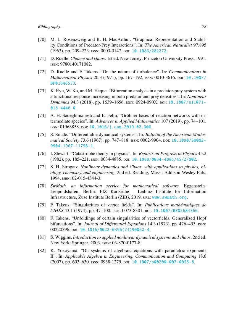
Bibliography 78
[70] M. L. Rosenzweig and R. H. MacArthur. “Graphical Representation and Stabil-ity Conditions of Predator-Prey Interactions”. In: The American Naturalist 97.895(1963), pp. 209–223. issn: 0003-0147. doi: 10.1086/282272.
[71] D. Ruelle. Chance and chaos. 1st ed. New Jersey: Princeton University Press, 1991.isbn: 9780140171082.
[72] D. Ruelle and F. Takens. “On the nature of turbulence”. In: Communications inMathematical Physics 20.3 (1971), pp. 167–192. issn: 0010-3616. doi: 10.1007/BF01646553.
[73] K. Ryu, W. Ko, and M. Haque. “Bifurcation analysis in a predator-prey system witha functional response increasing in both predator and prey densities”. In: NonlinearDynamics 94.3 (2018), pp. 1639–1656. issn: 0924-090X. doi: 10.1007/s11071-018-4446-0.
[74] A. H. Sadeghimanesh and E. Feliu. “Grobner bases of reaction networks with in-termediate species”. In: Advances in Applied Mathematics 107 (2019), pp. 74–101.issn: 01968858. doi: 10.1016/j.aam.2019.02.006.
[75] S. Smale. “Differentiable dynamical systems”. In: Bulletin of the American Mathe-matical Society 73.6 (1967), pp. 747–818. issn: 0002-9904. doi: 10.1090/S0002-9904-1967-11798-1.
[76] I. Stewart. “Catastrophe theory in physics”. In: Reports on Progress in Physics 45.2(1982), pp. 185–221. issn: 0034-4885. doi: 10.1088/0034-4885/45/2/002.
[77] S. H. Strogatz. Nonlinear dynamics and Chaos. with applications to physics, bi-ology, chemistry, and engineering. 2nd ed. Reading, Mass.: Addison-Wesley Pub.,1994. isbn: 02-015-4344-3.
[78] SwMath. an information service for mathematical software. Eggenstein-Leopoldshafen, Berlin: FIZ Karlsruhe - Leibniz Institute for InformationInfrastructure, Zuse Institute Berlin (ZIB), 2019. url: www.swmath.org.
[79] F. Takens. “Singularities of vector fields”. In: Publications mathematiques del’IHES 43.1 (1974), pp. 47–100. issn: 0073-8301. doi: 10.1007/BF02684366.
[80] F. Takens. “Unfoldings of certain singularities of vectorfields. Generalized Hopfbifurcations”. In: Journal of Differential Equations 14.3 (1973), pp. 476–493. issn:00220396. doi: 10.1016/0022-0396(73)90062-4.
[81] S. Wiggins. Introduction to applied nonlinear dynamical systems and chaos. 2nd ed.New York: Springer, 2003. isbn: 03-870-0177-8.
[82] K. Yokoyama. “On systems of algebraic equations with parametric exponentsII”. In: Applicable Algebra in Engineering, Communication and Computing 18.6(2007), pp. 603–630. issn: 0938-1279. doi: 10.1007/s00200-007-0055-8.
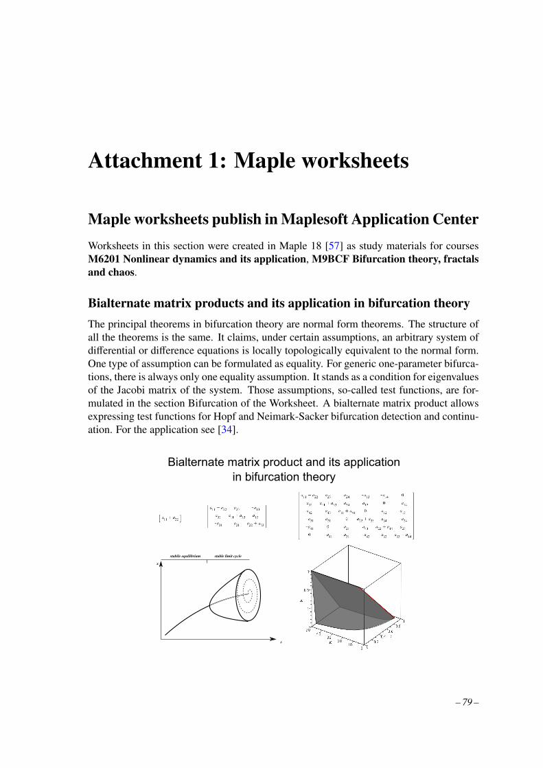
Attachment 1: Maple worksheets
Maple worksheets publish in Maplesoft Application CenterWorksheets in this section were created in Maple 18 [57] as study materials for coursesM6201 Nonlinear dynamics and its application, M9BCF Bifurcation theory, fractalsand chaos.
Bialternate matrix products and its application in bifurcation theoryThe principal theorems in bifurcation theory are normal form theorems. The structure ofall the theorems is the same. It claims, under certain assumptions, an arbitrary system ofdifferential or difference equations is locally topologically equivalent to the normal form.One type of assumption can be formulated as equality. For generic one-parameter bifurca-tions, there is always only one equality assumption. It stands as a condition for eigenvaluesof the Jacobi matrix of the system. Those assumptions, so-called test functions, are for-mulated in the section Bifurcation of the Worksheet. A bialternate matrix product allowsexpressing test functions for Hopf and Neimark-Sacker bifurcation detection and continu-ation. For the application see [34].
stabile equilibrium
ε
x
stable limit cycle
Bialternate matrix product and its applicationin bifurcation theory
– 79 –
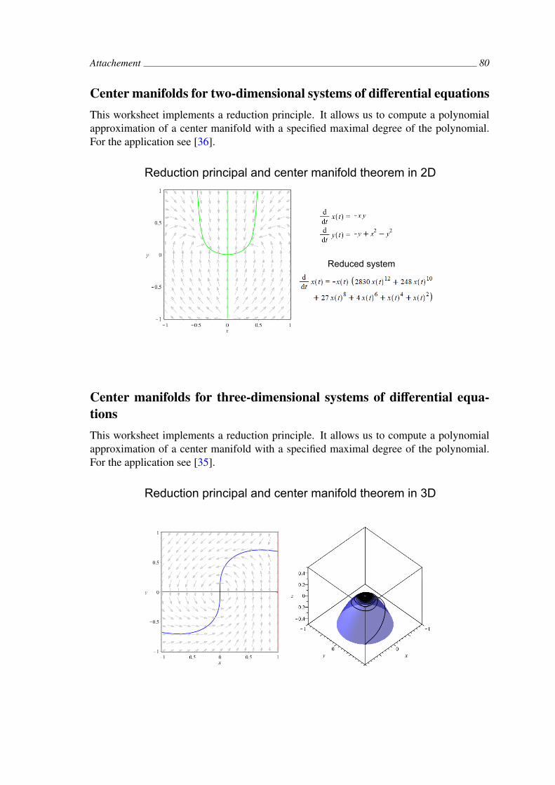
Attachement 80
Center manifolds for two-dimensional systems of differential equationsThis worksheet implements a reduction principle. It allows us to compute a polynomialapproximation of a center manifold with a specified maximal degree of the polynomial.For the application see [36].
Reduction principal and center manifold theorem in 2D
Reduced system
Center manifolds for three-dimensional systems of differential equa-tionsThis worksheet implements a reduction principle. It allows us to compute a polynomialapproximation of a center manifold with a specified maximal degree of the polynomial.For the application see [35].
Reduction principal and center manifold theorem in 3D
Attachment 2: Original publications
Researcher identifiers:Web of Science ResearcherID: AAF-2643-2019ORCID: 0000-0001-8476-7740Scopus Author ID: 57193545592
Research paper 1:Two parametric bifurcation in LPA model
HAJNOVA, Veronika and PRIBYLOVA, Lenka
Journal ofMathematical Biology,
Heidelberg: Springer Heidelberg, 2017.
Impact factor: 1.786Web of Science: UT WOS: 000409891600007, 3 citationsScopus: EID Scopus: 85014751704, 1 citation

J. Math. Biol. (2017) 75:1235–1251DOI 10.1007/s00285-017-1115-8 Mathematical Biology
Two-parameter bifurcations in LPA model
Veronika Hajnová1 · Lenka Pribylová1
Received: 29 September 2014 / Revised: 21 February 2017 / Published online: 10 March 2017© Springer-Verlag Berlin Heidelberg 2017
Abstract The structured population LPAmodel is studied. The model describes flourbeetle (Tribolium) population dynamics of four stage populations: eggs, larvae, pupaeand adults with cannibalism between these stages. We concentrate on the case of non-zero cannibalistic rates of adults on eggs and adults on pupae and no cannibalism oflarvae on eggs, but the results can be numerically continued to non-zero cannibalism oflarvae on eggs. In this article two-parameter bifurcations in LPA model are analysed.Various stable and unstable invariant sets are found, different types of hysteresis arepresented and abrupt changes in dynamics are simulated to explain the complicatedway the system behaves near two-parameter bifurcation manifolds. The connectionsbetween strong 1:2 resonance and Chenciner bifurcations are presented as well astheir very significant consequences to the dynamics of the Tribolium population. Thehysteresis phenomena described is a generic phenomenon nearby the Chenciner bifur-cation or the cusp bifurcation of the loop.
Keywords Population dynamics · Two-parameter bifurcations · LPA model · Strong1:2 resonance · Chenciner bifurcation
Mathematics Subject Classification 92D25 · 37N25 · 37G10 · 37G15 · 34C23
B Lenka Pribylová[email protected]
1 Section of Applied Mathematics, Department of Mathematics and Statistics, Faculty of Science,Masaryk University, Kotlárská 2, 611 37 Brno, Czech Republic
123
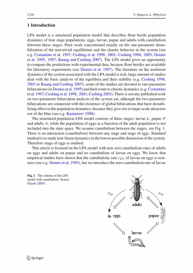
1236 V. Hajnová, L. Pribylová
1 Introduction
LPA model is a structured population model that describes flour beetle populationdynamics of four stage populations: eggs, larvae, pupae and adults with cannibalismbetween these stages. Prior work concentrated mainly on the one-parameter desta-bilization of the non-trivial equilibrium and the chaotic behavior in the system (seee.g. Costantino et al. 1997; Cushing et al. 1998, 2001; Cushing 1998, 2003; Denniset al. 1995, 1997; Kuang and Cushing 2007). The LPA model gives an opportunityto compare the predictions with experimental data, because flour beetles are availablefor laboratory experiments (see Dennis et al. 1997). The literature on the nonlineardynamics of the system associated with the LPAmodel is rich, large amount of studiesdeal with the basic analysis of the equilibria and their stability (e.g. Cushing 1998,2003 or Kuang and Cushing 2007), some of the studies are devoted to one-parameterbifurcations (asDennis et al. 1995) and their route to chaotic dynamics (e.g. Costantinoet al. 1997; Cushing et al. 1998, 2001; Cushing 2003). There is not any publishedworkon two-parameter bifurcation analysis of the system yet, although the two-parameterbifurcations are connected with the existence of global bifurcations that have destabi-lizing effect to the population dynamics, because they give rise to large-scale attractorsout of the blue (see e.g. Kuznetsov 1998).
The structured population LPA model consists of three stages: larvae L , pupae Pand adults A, while the population of eggs as a function of the adult population is notincluded into the state space. We assume cannibalism between the stages, see Fig. 1.There is no interaction (cannibalism) between any stage and stage of eggs. Standardmethod is to study non-linear dynamics in the lowest possible dimension of the system.Therefore stage of eggs is omitted.
This article is focused on the LPA model with non-zero cannibalism rates of adultson eggs and adults on pupae and no cannibalism of larvae on eggs. We know thatempirical studies have shown that the cannibalistic rate cEL of larvae on eggs is non-zero (see e.g. Dennis et al. 1995), but we introduce the zero-cannibalism rate of larvae
Fig. 1 The schema of the LPAmodel with cannibalism SourceElaydi (2005)
123
Two-parameter bifurcations in LPA model 1237
on eggs assumption in order to simplify the calculations. In the “zero case” a lot ofcomputations may be done analytically and that gives muchmore clear insight into theanalysis. Computed manifold can be numerically continued to cEL > 0 and resultsare analogous for positive values of cEL .
Paper is focused on two-parameter bifurcations, because they are present in LPAmodel and cause large destabilization (see Sect. 7). The strong 1:2 resonance andthe Chenciner bifurcations are studied. The mathematical background of these bifur-cations, their normal forms and their analysis can be found in Kuznetsov (1998). Atwo-parameter bifurcation diagram is presented to demonstrate the origin of stable(and unstable) manifolds and their dependence on parameters. In this paper the two-parameter bifurcations are described in parameter space with free parameters cE A andb, but it may be done for other pair of parameters as well. Other parameters werefixed μL = 0.1613;μA = 0.96; cPA = 0.004348 to values used for specific exper-imental manipulation according to Cushing (2003). It’s important to understand thatthe topological structure nearby the described strong 1:2 resonance and the Chencinerbifurcation manifolds connection is typical (generic) and a parameter shift does notchange the topology in quite a big parameter domain. In other words, birth or death ofinvariant stable sets is a common dynamic behaviour that is implied by the vicinity ofthe strong 1:2 resonance and the Chenciner bifurcation manifolds. It is very similar totypical generic phenomenon of hysteresis nearby a cusp manifold that is widely usedin literature (the best known example is the spruce budworm population model, seeLudwig et al. 1978), but the dynamic changes are much more complicated. Knowl-edge of the strong 1:2 resonance and the Chenciner bifurcation manifolds location inthe parameter space and their connections by one-parameter manifolds is crucial forunderstanding newly described phenomena in behaviour of the LPA model near thosemanifolds. Our goal is to complete the bifurcation diagram to understand the qualita-tive changes in the population of Tribolium caused by these connected two-parameterbifurcations. Moreover, the diagram may be used for other at least two-parameter dis-crete models with at least two state variables, where these two-parameter bifurcationmanifolds exist together.
2 Model description, basic analysis and one-parameter bifurcation
The dynamic of the LPA model is described by the system of difference equations(see e.g. Cushing 2003 or 1998)
L (t + 1) = bA (t) e−cEL L(t)−cE A A(t)
P (t + 1) = (1 − μL) L (t)
A (t + 1) = P (t) e−cP A A(t) + (1 − μA) A (t) , (1)
where state variables L , P, A represent the number of larvae, pupae and adults in thepopulation. Parameter b > 0 represents natality. Parameters μL and μA representmortality of larvae and mortality of adults. Natural inequalities 0 < μL < 1, 0 <
μA < 1 are assumed to be satisfied. Parameters cEL , cE A, cPA denote cannibalismrates. Namely, cEL is the cannibalism rate of larvae on eggs, cE A is the cannibalism
123

1238 V. Hajnová, L. Pribylová
rate of adults on eggs and cPA is the cannibalism rate of adults on pupae. We alsoassume cE A ≥ 0, cPA ≥ 0 and cEL ≥ 0, in this article cEL = 0 is mostly considered,unless stated otherwise.
There are at most two fixed points of the system (1). The trivial fixed point [0, 0, 0]corresponds to extinction of the population. The non-trivial fixed point [L∗, P∗, A∗]can be found analytically, see e.g. Cushing (2003).
Let us denote the basic reproduction number by R0 = b(1−μL )μA
and the manifoldR0 = 1 is the transcritical bifurcation manifold that divides the parameter space intovalues of survival and extinction of the population.
The analysis of one-parameter bifurcations is already known (see e.g. Dennis et al.1995). In Dennis et al. (1995), authors examined one-parameter bifurcations in two-parameter spaces μA, b for various ratios of cannibalism rates cE A, cPA and detecteda flip and a Neimark–Sacker bifurcations.
The flip bifurcation (2-cycle bifurcation) is responsible for period doubling andcorresponds to an eigenvalue−1. The flip bifurcation manifold of the non-trivial fixedpoint is
b = μAe2
μA
1 − μL(2)
and similarly to the transcritical bifurcation it does not depend on cannibalism rates1.The Neimark–Sacker bifurcation is characterized by two complex eigenvalues with
unitmodulus. It is an analogy of theHopf bifurcation in continuous dynamical systems.An invariant loop exists in the neighborhood of the fixed point (the orbits on theinvariant loop can either be all everywhere dense or there exists only a finite number ofperiodic orbits, see e.g. Kuznetsov 1998). The Neimark–Sacker bifurcation manifoldof the non-trivial fixed point of the system (1)
1
(cE A + cPA)2
(−μ2
AcE AcPA ln
(b (1 − μL)
μA
)2
+ μ2Ac
2E A ln
(b (1 − μL)
μA
)2
+μAc2E A ln
(b (1 − μL)
μA
)− 2μ2
AcPAcE A ln
(b (1 − μL)
μA
)
+μ2Ac
2PA ln
(b (1 − μL)
μA
)+ μAcE AcPA ln
(b (1 − μL)
μA
)
− 3μ2Ac
2E A ln
(b (1 − μL)
μA
)− c2PA − μAc
2PA − 2μAcE AcPA + 4μ2
AcE AcPA
− 2cPAcE A − μAc2E A − c2E A + 2μ2
Ac2PA + 2μ2
Ac2E A
)= 0. (3)
was derived in a different form already in Dennis et al. (1995). The Neimark–Sackerbifurcation manifold depends on cannibalism rates.
The flip bifurcationmanifold (named 2-cycles) and theNeimark–Sacker bifurcationmanifold (named loops) can intersect (see figure 1 in Dennis et al. 1995). There are
1 In the case where cEL = 0 the flip bifurcation manifold depends on cannibalism rates.
123

Two-parameter bifurcations in LPA model 1239
two possible two-parameter bifurcations that are presented near the intersection. Theone we are interested in this paper is the strong 1:2 resonance. All our results arein agreement with the results presented in Dennis et al. (1995) as well as with thesufficient conditions for global stability of the non-trivial fixed point that is presentedin Kuang and Cushing (2007).
3 Routes to two-parameter bifurcations
In this section the local two-parameter bifurcations of fixed points are summarized.Readers familiar with the concept of the two-parameter bifurcations can skip thissection.
Two-parameter bifurcations lie on manifolds of one-parameter bifurcations. Thesituation in discrete systems is slightly more complicated than in continuous systems.We distinguish between three basic local one-parameter bifurcations of fixed points:the Neimark–Sacker bifurcation (denoted by N–S), the flip bifurcation (denoted byPD) and the fold bifurcation (denoted by LP).
Two-parameter local bifurcations of fixed points can be obtained by two differentways. Firstly, it is the violation of the non-degeneracy conditions of the one-parameterbifurcations. For example, the Neimark–Sacker bifurcation non-degeneracy conditionis violated in the Chenciner critical points. The following table summarizes two-parameter bifurcations obtained by the violation of non-degeneracy conditions ofone-parameter bifurcations (for more details see e.g. Kuznetsov 1998).
Corresponding one-parameter bifurcation Eigenvalues Name Label
Fold 1 Cusp CPFlip −1 Generalized flip GPDNeimark–Sacker e±iθ0 Chenciner CHNeimark–Sacker 1, 1 Strong 1:1 resonance R1Neimark–Sacker −1,−1 Strong 1:2 resonance R2Neimark–Sacker e±iθ0 , θ0 = 2π
3 Strong 1:3 resonance R3Neimark–Sacker e±iθ0 , θ0 = π
2 Strong 1:4 resonance R4
Secondly, another eigenvalue can reach the unit circle. Obviously it is the casewhen the two-parameter bifurcationmanifold covers the intersection of one-parameterbifurcation manifolds. The following table summarizes two-parameter bifurcationsobtained in this way (for more details see e.g. Kuznetsov 1998).
Eigenvalues Dimension Name Label
1 −1 2 – LPPD1 1 2 1:1 resonance R1−1 −1 2 1:2 resonance R21 e±iθ0 3 – LPNS−1 e±iθ0 3 – PDNSe±iθ0 e±iθ1 4 - NSNS
123
1240 V. Hajnová, L. Pribylová
The detection of two-parameter bifurcations is crucial for population dynamics.The most important consequence of many two-parameter bifurcations is the existenceofmore than one attracting invariant set in a phase portrait. Then a long term behaviourof the system depends on parameters as well as on initial conditions very significantly.
4 Two-parameter bifurcations in LPA model
Main results of the paper are based on two-parameter bifurcations described in thissection.We concentrate on the casewhen the population survives (R0 > 1 is assumed).There are two types of intersections of the flip (2) and the Neimark–Sacker bifurcation(3) manifolds:
(i) b = μAe2
μA
1−μL, cE A = (μA+1)cP A
1−μAflip-Neimark–Sacker
(ii) b = μAe2
μA
1−μL, cE A = (2μA−1)cP A
5−2μAstrong 1:2 resonance.
The manifold (i) exists for all allowed values of parameters. On the other hand,manifold (ii) exists for μA > 1
2 only.The manifold (i) corresponds to the flip-Neimark–Sacker bifurcation with eigen-
values −1, 12 +
√32 i, 1
2 +√32 i. This bifurcation is connected with period doubling and
a route to chaos and we will not focus on this case in this paper, but it was not studiedin LPA model yet as well as other two-parameter bifurcations.
The manifold (ii) corresponds to the strong 1:2 resonance with associated eigenval-ues −1,−1, 1
2 .2 A complete bifurcation diagram in the neighborhood of the strong
1:2 resonance is presented in the Sect. 6. The parameters μL , μA, cPA are fixed tovalues μL = 0.1613;μA = 0.96; cPA = 0.004348 used for specific experimentalmanipulation according to Cushing (2003) and only cE A and b are varied. The movingparameters may be arbitrarily chosen in the parameter domain, where two-parameterbifurcation manifold (ii) exist. The dynamic changes in LPA model are generic.
4.1 Chenciner bifurcation
Chenciner bifurcation is a two-parameter bifurcation of a fixed point included inthe Neimark–Sacker bifurcation manifold. There are two topological types of theNeimark–Sacker bifurcation: supercritical and subcritical. The supercritical type givesrise to a stable invariant loop, reversely, the subcritical brings about an unstable loop.The Chenciner bifurcation is a critical change of these two types3. This implies that forsome parameter value near to the Chenciner manifold there is a stable invariant looparound the fixed point and for some other parameter values near themanifold there is anunstable loop. A transversal section at a point of the Chencinermanifold has the typical
2 Non-degeneracy and transversality conditions should be involved for each bifurcation for correct analysis.It can be done analytically using the reduction to the center manifold. We used program MactontM (seee.g. Kuznetsov 2013) to get numerical results, because we do not continue with any further analysis ofcodimension 3 bifurcations.3 The Chenciner bifurcation is an analogy of continuous Bautin (or generalized Hopf) bifurcation.
123

Two-parameter bifurcations in LPA model 1241
1
Fig. 2 TheChenciner bifurcation diagram in a two-parameter space. N–S− denotes the supercritical branchof the Neimark–Sacker curve, N–S+ denotes the subcritical branch of the Neimark–Sacker curve, LPCdenotes the fold bifurcation of the invariant loop curve. The phase portraits within each domain 1© , 2©and 3© bordered by the bifurcation curves are topologically equivalent. The semi-stable invariant loop(LPC-curve) has a special heteroclinic structure of orbits that appears even in the neighborhood of LPC .For more details see Kuznetsov (1998) or Chenciner (1987), but the complete analysis of the LPC-curveneighborhood seems to be unknown yet
form displayed at Fig. 2 (for more details see Kuznetsov 1998). Bifurcation theoryproves the existence of another non-local one-parameter bifurcation manifold nearby,namely the fold bifurcation of the invariant loop (named sometimes also the limit pointbifurcation of the invariant loop). In continuous casewe refer to this phenomenon as thefold bifurcation of limit cycles4 (or sometimes the limit point bifurcation of the limitcycle, LPC). The common abbreviation LPC for the fold bifurcation of the invariantloop is taken from the continuous case. It is worth to notice that the diagram V-shapeis similar to cusp diagram, and it give rise to a phenomenon similar to hysteresisconnected with the cusp bifurcation, only the attracting sets are not two fixed points,but a fixed point and a loop. The hysteresis phenomenon is discussed later in theSect. 7. In the continuous case for the analogous Bautin bifurcation, this hysteresisphenomenon is used for description of the fold/fold cycle bursting in a neural systemmodelling (see Izhikevich 2007). The hysteresis associated with a stable periodicorbit and a stable equilibrium has been already studied in ecological literature (seee.g. Schreiber and Rudolf 2008).
The expression for the Chenciner bifurcation manifold in LPA model (1) can beobtained analytically using the reduction to the center manifold (see e.g. Kuznetsov1998), but we preferred the numerical approach using MatcontM. The Chenciner
4 Fold bifurcation of a fixed point gives rise to two fixed points with opposite stability, fold bifurcation ofa cycle gives rise to two cycles with opposite stability, for more details see Kuznetsov (1998).
123

1242 V. Hajnová, L. Pribylová
bifurcation occurs only on one branch of the Neimark–Sacker bifurcation, near to thestrong 1:2 resonance. We found also parameter values for which the Chenciner andthe strong 1:2 resonance bifurcations collide, but we did not investigate this three-parameter bifurcation. This bifurcation manifold neighborhood is not covered in anyavailable bifurcation theory yet. This can be a possible extension of our study. Itis certainly true, that together, the strong 1:2 resonance and Chenciner bifurcationinfluence the dynamics of the parameter dependent system (1) enormously.
4.2 Strong 1:2 resonance
Strong 1:2 resonance has four topological types: a subcritical bifurcation of a saddle,a supercritical bifurcation of a saddle, a subcritical bifurcation of a node or a focus anda supercritical bifurcation of a node or a focus. Here, the generic topological structureof the state space in the neighborhood of the subcritical strong 1:2 resonance of a nodeor a focus is described (for more information see e.g. Kuznetsov 1998).
Strong 1:2 resonance points lie in the intersection of the Neimark–Sacker bifur-cation manifold and the flip bifurcation manifold, therefore we expect a birth of thelimit loop from a fixed point due to the Neimark–Sacker bifurcation and the split ofthe fixed point into a 2-cycle nearby the strong 1:2 resonance point. Figure 3 displaysthe generic transversal two-parameter space section of a canonic strong 1:2 resonancebifurcation manifold at zero with one-parameter Neimark–Sacker and flip manifoldsat the horizontal and the vertical axes.
Moving around the strong 1:2 resonance point, the topological structure of thestate space change in the way that is presented for the canonic form at Fig. 3. In thedomain 1©, the state space contains an unstable fixed point (node or focus). Crossingthe Neimark–Sacker manifold N–S+ gives rise to the unstable loop around a stablefixed point that loses stability at N–S+. Here the the domain 2© is reached. Crossingthe F− manifold, the flip bifurcation of the stable fixed point originates a saddle anda stable 2-cycle. The domain 3© is reached. At some close neighborhood, the saddleand the 2-cycle are surrounded by the unstable invariant loop that continues from theN–S bifurcation loop birth. The topological structure of the upcoming domains is notcommon, however the bifurcation manifold sequence is typical for the neighborhoodof a generic case of strong 1:2 resonance neighborhood (see Kuznetsov 1998). Man-ifold N–S2− that follows is a supercritical Neimark–Sacker bifurcation of a 2-cycle.Crossing this manifold gives rise to two small stable symmetric coupled loops aroundthe unstable 2-cycle. If we stay close enough to the strong 1:2 resonance point, thestable twin-loop is still surrounded by the unstable invariant loop (domain 4©). As wemove around through domain 4© and get away from N–S2− manifold, the twin-loopsincrease and go extinct at the saddle separatrix. This non-local bifurcation, denotedby P , is called the saddle separatrix loop. It causes the origin of a stable invariant loopinside an unstable loop with an unstable 2-cycle and a saddle inside, see domain 5©.These two stable and unstable loops collide and disappear while crossing the bifur-cation manifold marked LPC (the fold bifurcation of the invariant loop). Domain 6©bounded by LPC manifold and the flip F+ manifold corresponds to a state space witha saddle and an unstable 2-cycle that collide to an unstable fixed point at the flip F+
123
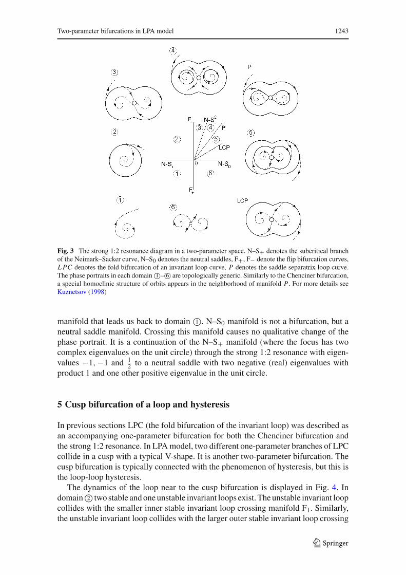
Two-parameter bifurcations in LPA model 1243
Fig. 3 The strong 1:2 resonance diagram in a two-parameter space. N–S+ denotes the subcritical branchof the Neimark–Sacker curve, N–S0 denotes the neutral saddles, F+, F− denote the flip bifurcation curves,LPC denotes the fold bifurcation of an invariant loop curve, P denotes the saddle separatrix loop curve.The phase portraits in each domain 1©– 6© are topologically generic. Similarly to the Chenciner bifurcation,a special homoclinic structure of orbits appears in the neighborhood of manifold P . For more details seeKuznetsov (1998)
manifold that leads us back to domain 1©. N–S0 manifold is not a bifurcation, but aneutral saddle manifold. Crossing this manifold causes no qualitative change of thephase portrait. It is a continuation of the N–S+ manifold (where the focus has twocomplex eigenvalues on the unit circle) through the strong 1:2 resonance with eigen-values −1,−1 and 1
2 to a neutral saddle with two negative (real) eigenvalues withproduct 1 and one other positive eigenvalue in the unit circle.
5 Cusp bifurcation of a loop and hysteresis
In previous sections LPC (the fold bifurcation of the invariant loop) was described asan accompanying one-parameter bifurcation for both the Chenciner bifurcation andthe strong 1:2 resonance. In LPAmodel, two different one-parameter branches of LPCcollide in a cusp with a typical V-shape. It is another two-parameter bifurcation. Thecusp bifurcation is typically connected with the phenomenon of hysteresis, but this isthe loop-loop hysteresis.
The dynamics of the loop near to the cusp bifurcation is displayed in Fig. 4. Indomain 2© two stable andoneunstable invariant loops exist. The unstable invariant loopcollides with the smaller inner stable invariant loop crossing manifold F1. Similarly,the unstable invariant loop collides with the larger outer stable invariant loop crossing
123

1244 V. Hajnová, L. Pribylová
Fig. 4 Stable sets for the cusp bifurcation of a loop and a schematic phase portrait for parameters μL =0.1613;μA = 0.96; cP A = 0.004348; cE A = 0.00182 and different values of parameter b. Stable sets aredisplayed in two-dimensional projection of a three-dimensional space
manifold F2. Therefore in domain 1© only one stable invariant loop exists. In previoustwo two-parametric bifurcations we presented a schematic phase portraits, here in theFig. 4 we present loops simulated for different parameter values in LPA model. Let usnote that we see a two-dimensional projection of a three-dimensional loop, the loopsdoes not intersect in the 3D space.
The fixed point-loop hysteresis mentioned in the Sect. 5 near Chenciner bifurcationand loop-loop hysteresis here are analogous to hysteresis driven by normal cusp inthe intersection of two branches of fold bifurcations of fixed points. Let us imagine asection of the V-shape. One invariant set (a fixed point for Chenciner bifurcation, seeFig. 2 domain 1©, or a loop here, see Fig. 4 domain 1©) is attracting for low valuesof parameter b. The system (1) get stabilized and as the parameter b increases, thesystem is still stabilized on the stable loop that continues to the domain 2© in Fig. 4(for Chenciner bifurcation it is analogous for a fixed point, see Fig. 2 and imaginetransversal crossing of the V-shape from domain 1© to domain 3©). Crossing manifoldF2 (or N–S+ for the Chenciner bifurcation) destabilizes the system abruptly and givesrise to large oscillations. The system (1) stabilizes at the bigger attracting loop. Ifthe parameter decreases back again, the system remains at the large oscillation mode.
123
Two-parameter bifurcations in LPA model 1245
Stabilization to smaller invariant loop (or fixed point for Chenciner bifurcation case)is provided for much lower value than destabilization came. This is hysteresis.
6 Connection between Chenciner bifurcation and strong 1:2 resonancein LPA model
Both theChenciner bifurcation and the strong1:2 resonanceoccur inLPAmodel forμA
sufficiently close to 1 (the necessary condition for the strong 1:2 resonance isμA > 12 ).
The topological structure of the parameter space near theChenciner bifurcation and thestrong 1:2 resonance gives rise to a complicated state space dynamics with coexistenceof different types of invariant sets. Fixed points that globally attract orbits can be easilydestabilized within the described parameter area. The destabilization may be weak(oscillating behavior tending to a 2-cycle or almost 2-cycle behavior near a twin-loop)or strong (large oscillations tending to a globally attractive stable invariant big loop).Different types of orbit behavior are obtained even for very close parameter valuesand very close initial conditions that corresponds to more or less stabilized populationstructure. For the dynamics of a Tribolium population weak destabilization is not sodestructive, however large oscillations that are getting close to zero values may causeeven an extinction of the population. In next section we discuss this phenomenon indetails.
A complete bifurcation diagram of this phenomenon appearing in the LPA modelfor case cEL = 0 is presented in Fig. 55. Similarly as in the previous section, wedescribe the structure through equivalence classes of structurally stable domains withtopologically equivalent state spaces. The borders of these domains are one-parameterbifurcation manifolds. The transversal two-dimensional section b versus cE A of bothtwo-parameter manifolds (the Chenciner and the strong 1:2 resonance) is taken forfixed parameters μL = 0.1613;μA = 0.96; cPA = 0.004348 again (see Cushing2003 for more details about parameter estimation).
Figure 5 corresponds locally to Figs. 2 and 3. The parameter space is divided intonine domains where the state spaces stay topologically equivalent. All dynamic classesI.–IX. are displayed in the Fig. 6. Some of those dynamic classes are related directlyto Figs. 2 and 3. Specially classes I., II. and III. are related to classes 2©, 1© and 3© inFig. 2. Classes I., III., IV., V., VI. and IX. are related to classes 1©, 2©, 3©, 4©, 5© and6© in Fig. 3. The case with low reproduction number, R0 ∈ (0, 1) is omitted, becausethe trivial fixed point is globally stable in this case and so the population goes extinct.
Domains I. and II. are separated by the Neimark–Sacker manifold. The only fixedpoint in II. changes its stability at the border N–S and is surrounded by an invariantloop in I. The lower part of the N–S curve is supercritical (a stable point, a stable loop),the upper part is subcritical (an unstable point, an unstable loop). The loop changesits stability because of the Chenciner bifurcation at point CH. Therefore, crossing theNeimark–Sacker bifurcation manifold N–S+ stable and unstable invariant loops anda stable fixed point exist at region III.. Stable and unstable invariant loops go extinctat the parameter manifold LCP (fold bifurcation of invariant loop). This is exactly
5 Topologically equivalent diagram is obtained for small cEL > 0.
123
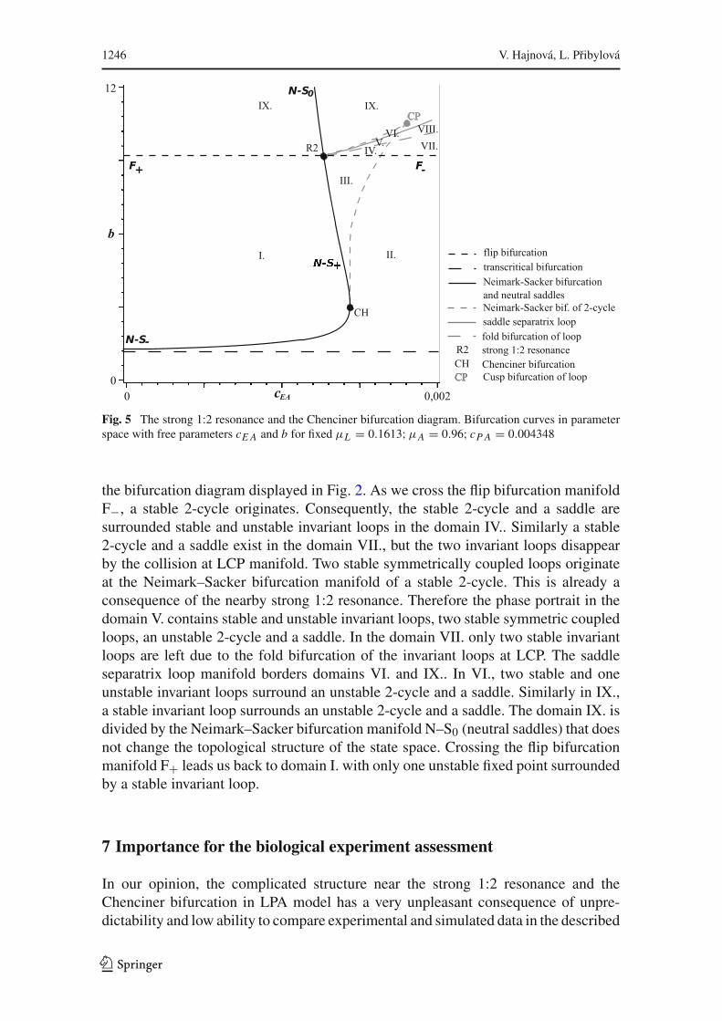
1246 V. Hajnová, L. Pribylová
Fig. 5 The strong 1:2 resonance and the Chenciner bifurcation diagram. Bifurcation curves in parameterspace with free parameters cE A and b for fixed μL = 0.1613;μA = 0.96; cP A = 0.004348
the bifurcation diagram displayed in Fig. 2. As we cross the flip bifurcation manifoldF−, a stable 2-cycle originates. Consequently, the stable 2-cycle and a saddle aresurrounded stable and unstable invariant loops in the domain IV.. Similarly a stable2-cycle and a saddle exist in the domain VII., but the two invariant loops disappearby the collision at LCP manifold. Two stable symmetrically coupled loops originateat the Neimark–Sacker bifurcation manifold of a stable 2-cycle. This is already aconsequence of the nearby strong 1:2 resonance. Therefore the phase portrait in thedomain V. contains stable and unstable invariant loops, two stable symmetric coupledloops, an unstable 2-cycle and a saddle. In the domain VII. only two stable invariantloops are left due to the fold bifurcation of the invariant loops at LCP. The saddleseparatrix loop manifold borders domains VI. and IX.. In VI., two stable and oneunstable invariant loops surround an unstable 2-cycle and a saddle. Similarly in IX.,a stable invariant loop surrounds an unstable 2-cycle and a saddle. The domain IX. isdivided by the Neimark–Sacker bifurcation manifold N–S0 (neutral saddles) that doesnot change the topological structure of the state space. Crossing the flip bifurcationmanifold F+ leads us back to domain I. with only one unstable fixed point surroundedby a stable invariant loop.
7 Importance for the biological experiment assessment
In our opinion, the complicated structure near the strong 1:2 resonance and theChenciner bifurcation in LPA model has a very unpleasant consequence of unpre-dictability and low ability to compare experimental and simulated data in the described
123
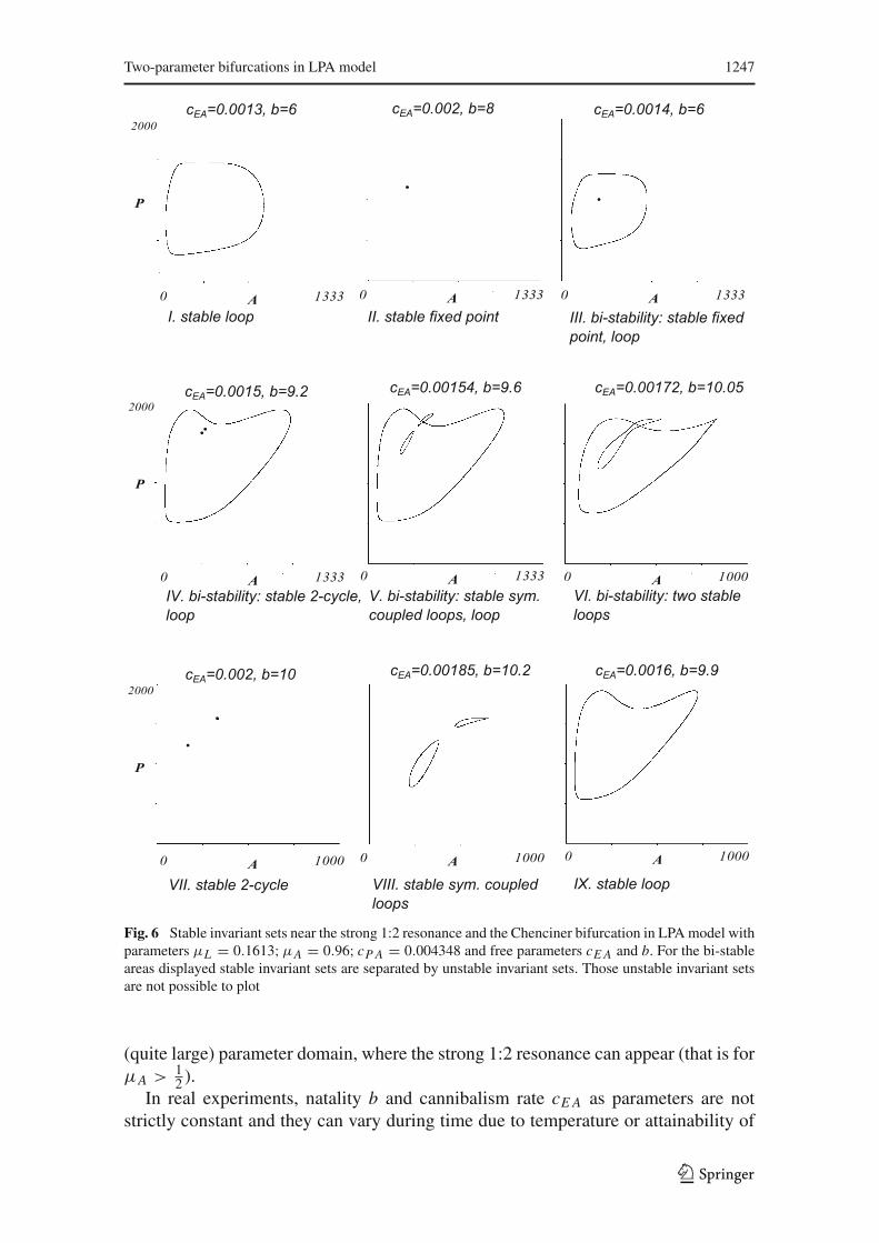
Two-parameter bifurcations in LPA model 1247
Fig. 6 Stable invariant sets near the strong 1:2 resonance and the Chenciner bifurcation in LPAmodel withparameters μL = 0.1613;μA = 0.96; cP A = 0.004348 and free parameters cE A and b. For the bi-stableareas displayed stable invariant sets are separated by unstable invariant sets. Those unstable invariant setsare not possible to plot
(quite large) parameter domain, where the strong 1:2 resonance can appear (that is forμA > 1
2 ).In real experiments, natality b and cannibalism rate cE A as parameters are not
strictly constant and they can vary during time due to temperature or attainability of
123
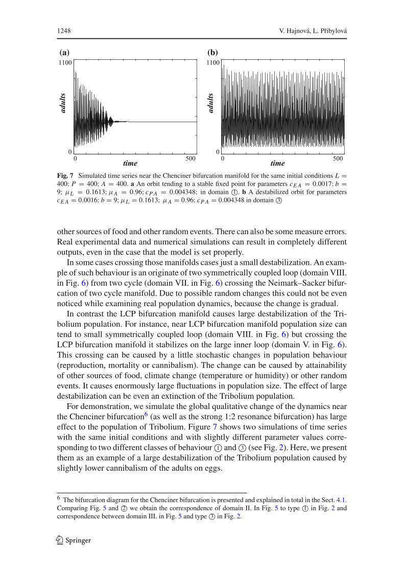
1248 V. Hajnová, L. Pribylová
(a) (b)
Fig. 7 Simulated time series near the Chenciner bifurcation manifold for the same initial conditions L =400; P = 400; A = 400. a An orbit tending to a stable fixed point for parameters cE A = 0.0017; b =9; μL = 0.1613;μA = 0.96; cP A = 0.004348; in domain 1©. b A destabilized orbit for parameterscE A = 0.0016; b = 9;μL = 0.1613; μA = 0.96; cP A = 0.004348 in domain 3©
other sources of food and other random events. There can also be somemeasure errors.Real experimental data and numerical simulations can result in completely differentoutputs, even in the case that the model is set properly.
In some cases crossing those manifolds cases just a small destabilization. An exam-ple of such behaviour is an originate of two symmetrically coupled loop (domain VIII.in Fig. 6) from two cycle (domain VII. in Fig. 6) crossing the Neimark–Sacker bifur-cation of two cycle manifold. Due to possible random changes this could not be evennoticed while examining real population dynamics, because the change is gradual.
In contrast the LCP bifurcation manifold causes large destabilization of the Tri-bolium population. For instance, near LCP bifurcation manifold population size cantend to small symmetrically coupled loop (domain VIII. in Fig. 6) but crossing theLCP bifurcation manifold it stabilizes on the large inner loop (domain V. in Fig. 6).This crossing can be caused by a little stochastic changes in population behaviour(reproduction, mortality or cannibalism). The change can be caused by attainabilityof other sources of food, climate change (temperature or humidity) or other randomevents. It causes enormously large fluctuations in population size. The effect of largedestabilization can be even an extinction of the Tribolium population.
For demonstration, we simulate the global qualitative change of the dynamics nearthe Chenciner bifurcation6 (as well as the strong 1:2 resonance bifurcation) has largeeffect to the population of Tribolium. Figure 7 shows two simulations of time serieswith the same initial conditions and with slightly different parameter values corre-sponding to two different classes of behaviour 1© and 3© (see Fig. 2). Here, we presentthem as an example of a large destabilization of the Tribolium population caused byslightly lower cannibalism of the adults on eggs.
6 The bifurcation diagram for the Chenciner bifurcation is presented and explained in total in the Sect. 4.1.Comparing Fig. 5 and 2© we obtain the correspondence of domain II. In Fig. 5 to type 1© in Fig. 2 andcorrespondence between domain III. in Fig. 5 and type 3© in Fig. 2.
123
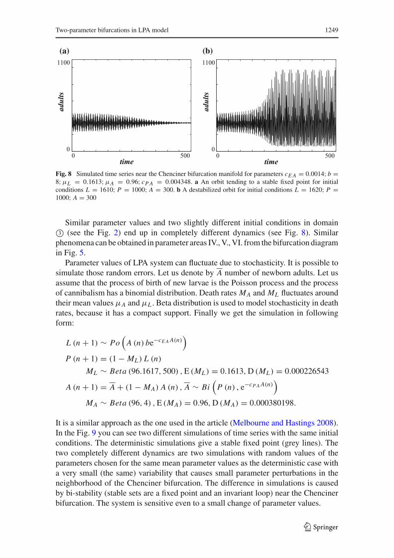
Two-parameter bifurcations in LPA model 1249
(a) (b)
Fig. 8 Simulated time series near the Chenciner bifurcation manifold for parameters cE A = 0.0014; b =8;μL = 0.1613;μA = 0.96; cP A = 0.004348. a An orbit tending to a stable fixed point for initialconditions L = 1610; P = 1000; A = 300. b A destabilized orbit for initial conditions L = 1620; P =1000; A = 300
Similar parameter values and two slightly different initial conditions in domain3© (see the Fig. 2) end up in completely different dynamics (see Fig. 8). Similarphenomena can be obtained in parameter areas IV.,V.,VI. from the bifurcation diagramin Fig. 5.
Parameter values of LPA system can fluctuate due to stochasticity. It is possible tosimulate those random errors. Let us denote by A number of newborn adults. Let usassume that the process of birth of new larvae is the Poisson process and the processof cannibalism has a binomial distribution. Death rates MA and ML fluctuates aroundtheir mean values μA and μL . Beta distribution is used to model stochasticity in deathrates, because it has a compact support. Finally we get the simulation in followingform:
L (n + 1) ∼ Po(A (n) be−cE A A(n)
)P (n + 1) = (1 − ML) L (n)
ML ∼ Beta (96.1617, 500) ,E (ML) = 0.1613,D (ML) = 0.000226543
A (n + 1) = A + (1 − MA) A (n) , A ∼ Bi(P (n) , e−cP A A(n)
)MA ∼ Beta (96, 4) ,E (MA) = 0.96,D (MA) = 0.000380198.
It is a similar approach as the one used in the article (Melbourne and Hastings 2008).In the Fig. 9 you can see two different simulations of time series with the same initialconditions. The deterministic simulations give a stable fixed point (grey lines). Thetwo completely different dynamics are two simulations with random values of theparameters chosen for the same mean parameter values as the deterministic case witha very small (the same) variability that causes small parameter perturbations in theneighborhood of the Chenciner bifurcation. The difference in simulations is causedby bi-stability (stable sets are a fixed point and an invariant loop) near the Chencinerbifurcation. The system is sensitive even to a small change of parameter values.
123

1250 V. Hajnová, L. Pribylová
Fig. 9 time series simulating the number of adults for initial parameters cE A = 0.00165; cP A =0.004348; b = 9; μL = 0.1613;μA = 0.96 and initial conditions L = 1750; P = 1472; A = 344
Unpredictable random (even small) perturbations near those two-parameter bifur-cation manifolds cause impossibility to predict the population size and structure.
8 Conclusion
We presented a two-parameter bifurcation analysis of LPA model (for parameterscEL and b) for zero or small cEL cannibalism rate to show the complexity of thedynamics in the model of the Tribolium population. Here we mention that we are notconcerned in period doubling and chaos, because there are a lot of papers devoted tothis topic. Instead of that, we focus on bifurcations that were overlooked so far, andtheir destabilization effect were not described yet. We presented also two types ofhysteresis: fixed point-loop and loop-loop hysteresis.
We explained the importance of the bifurcation type, because both of the types (sub-critical and supercritical) are present.We are the firstwhohave described theChencinerbifurcation with its large consequences to the model dynamics. We showed two typesof destabilizing effects to the Tribolium population model due to the Chencinerbifurcation (connected to the perturbations in initial conditions and the parameterperturbations). We found the strong 1:2 resonance in LPA model and we explained itstopological structure. In the case of zero cEL , both of these two-parameter bifurcationmanifolds are analytically formulated and therefore it is possible to compute the crit-ical parameters easily. The continuation software MatcontM yields analogous resultsfor the non-zero cEL .
As the most important part of our paper we consider the finding of the connectionbetween the Chenciner bifurcation and the strong 1:2 resonance and setting of thecomplete two-parameter bifurcation diagram of these manifolds connection (together
123

Two-parameter bifurcations in LPA model 1251
with the nearby non-local bifurcation manifolds). The two-parameter bifurcation dia-gram is presented for three other parameters fixed in common values, but the analyticexpression of themainmanifolds and the genericity of the bifurcationmanifolds neigh-borhood permits to base topologically equivalent diagrams for other parameters in thearea of the Chenciner bifurcation and the strong 1:2 resonance.
Both strong 1:2 resonance and Chenciner bifurcations can occur in discrete dynam-ical systems with at least two state variables and two parameters, which means thatsimilar mechanism can be possibly found in other population models.
References
Chenciner A (1987) Bifurcations de points fixes elliptiques. III. Orbites périodiques de “petites” périodes etélimination résonnante des couples de courbes invariantes, Inst. Hautes Études Sci. PublMath 66:5–91
Costantino RF, Desharnais RA, Cushing JM, Dennis B (1997) Chaotic dynamics in an insect population.Science 275(5298):389–391
Cushing JM (1998) An introduction to structured population dynamics. Society for Industrial and AppliedMathematics, Philadelphia
Cushing JM (2003) Chaos in ecology: experimental nonlinear dynamics. Academic Press, AmsterdamCushing JM,ConstantinoRF,DennisB,DesharnaisRA,HensonSM(1998)Nonlinear population dynamics:
models, experiments and data. J Theor Biol 194(1):1–9Cushing JM, Henson SM, Desharnais RA, Dennis B, Costantino RF, King A (2001) A chaotic attractor in
ecology: theory and experimental data. Chaos Solitons Fractals 12(2):219–234Dennis B, Desharnais RA, Cushing JM, Constantino RF (1995) Nonlinear demographic dynamics: mathe-
matical models, statistical methods, and biological experiments. Ecol Monogr 65(3):261–282DennisB,DesharnaisRA,Cushing JM,CostantinoRF (1997)Transitions in population dynamics: equilibria
to periodic cycles to aperiodic cycles. J Anim Ecol 66(5):704–729Elaydi S (2005) An introduction to difference equations, 3rd edn. Springer, New YorkIzhikevich EM (2007) Dynamical systems in neuroscience. MIT press, CambridgeKuang Y, Cushing JM (2007) Global stability in a nonlinear difference-delay equation model of flour beetle
population growth. J Differ Equ Appl 2(1):31–37Kuznetsov YA (1998) Elements of applied bifurcation theory, 2nd edn. Springer, New YorkKuznetsov YA (2013) A Tutorial for MatcontM GUI. Utretcht University, UtrechtLudwig D, Jones DD, Holling CS (1978) Qualitative analysis of insect outbreak systems: the spruce bud-
worm and forest. J Anim Ecol 47:315–332Melbourne BA, Hastings A (2008) Extinction risk depends strongly on factors contributing to stochasticity.
Nature 454(7200):100–103Schreiber S, Rudolf VHW (2008) Crossing habitat boundaries: coupling dynamics of ecosystems through
complex life cycles. Ecol Lett 11(6):576–587
123
Research paper 2:Bifurcation manifolds in predator-prey
models computed by Grobner basismethod
HAJNOVA, Veronika and PRIBYLOVA, Lenka
Mathematical Biosciences, Amsterdam: Elsevier, 2019.
Impact factor: 1.680 in 2018Web of Science: UT WOS: 000469895200001Scopus: EID Scopus: 85063868259
Contents lists available at ScienceDirect
Mathematical Biosciences
journal homepage: www.elsevier.com/locate/mbs
Bifurcation manifolds in predator–prey models computed by Gröbner basismethodVeronika Hajnová⁎, Lenka PřibylováDepartment of Mathematics and Statistics, Section of Applied Mathematics, Faculty of Science, Masaryk University, Kotlářská 2, Brno, 611 37, Czechia
A R T I C L E I N F O
Keywords:Rosenzweig–MacArthur modelBifurcation manifoldsGröbner basisHopf bifurcationFold bifurcationPredator–prey model
2010 MSC:13P1037M2037G1065P30
A B S T R A C T
Many natural processes studied in population biology, systems biology, biochemistry, chemistry or physics aremodeled by dynamical systems with polynomial or rational right-hand sides in state and parameter variables.The problem of finding bifurcation manifolds of such discrete or continuous dynamical systems leads to aproblem of finding solutions to a system of non-linear algebraic equations. This approach often fails since it is notpossible to express equilibria explicitly. Here we describe an algebraic procedure based on the Gröbner basiscomputation that finds bifurcation manifolds without computing equilibria. Our method provides formulas forbifurcation manifolds in commonly studied cases in applied research – for the fold, transcritical, cusp, Hopf andBogdanov–Takens bifurcations. The method returns bifurcation manifolds as implicitly defined functions orparametric functions in full parameter space. The approach can be implemented in any computer algebra system;therefore it can be used in applied research as a supporting autonomous computation even by non-experts inbifurcation theory. This paper demonstrates our new approach on the recently publishedRosenzweig–MacArthur predator–prey model generalizations in order to highlight the simplicity of our methodcompared to the published analysis.
1. Introduction
The aim of this paper is to describe a method of finding bifurcationmanifolds using the Gröbner basis computation. The approach is pre-sented on the Rosenzweig–MacArthur model generalizations. The ori-ginal model was published in 1963 in [21] as a generalization of Lot-ka–Voltera model. Dynamics of two interacting populations is describedby the following system of differential equations:
= =
= =
Nt
rN NK
g N P P f N P
Pt
eg N P P mP f N P
dd
1 ( , ) : ( , ),
dd
( , ) : ( , ),
1
2 (1)
where the state variables N, P denote prey population and predatorpopulation density and t is time. A common notation is used - parameterr denotes the growth rate of the prey, K is carrying capacity of the prey,m is the death rate of the predator and e is the conversion efficiency ofthe predator. We assume that all parameters are positive. Function g(N,P) is a specific functional response. Models with number of differenttypes of functional responses g(N, P) are studied in current research, seefor example [3,19,20,22] or others.
All parameters of a dynamical system such as (1) can fluctuate overtime. External factors typically cause these fluctuations. Bifurcation theory
provides a background to describe the consequences of those fluctuations.More precisely, bifurcation theory brings in tools to analyze qualitativechanges in dynamics of a given family of differential equations. The to-pological structure of the state–parameter space is described by a bi-furcation diagram, usually presented in parameter space as a partition ofthe parameter space to structurally stable domains with topologicallyequivalent dynamics, while their boundaries are given by the bifurcationmanifolds. That is why the computation of bifurcation manifolds is crucialin applied research. Let us recall that biochemical switches and bistabilityare related to fold or cusp bifurcations, see e.g. [7,11,17,23]. Chemicaloscillations and current research of network phenomena such as syn-chronization or chimera states are related to Hopf bifurcation, see e.g.[1,18,24]. Control methods of harvesting or preserving populations,sudden population extinction explanation are related to fold or Bogda-nov–Takens bifurcations, see [8,9,13] or [19]. However, the analysis itselfis often very complicated and usually requires numerical continuationmethods and software, for example, Matcont [14] or Auto [25]. In case ofa differential system with polynomial or rational right-hand sides, wherethe problem of finding bifurcation manifolds leads to a problem of solvinga system of polynomial equations, see [12], we can avoid numericalcontinuation and derive the results analytically. We present our approachthat allows us to analyse the system algorithmically and compute
https://doi.org/10.1016/j.mbs.2019.03.008Received 26 October 2018; Received in revised form 30 March 2019; Accepted 31 March 2019
⁎ Corresponding author.E-mail address: [email protected] (V. Hajnová).
Mathematical Biosciences 312 (2019) 1–7
Available online 01 April 20190025-5564/ © 2019 Elsevier Inc. All rights reserved.
T
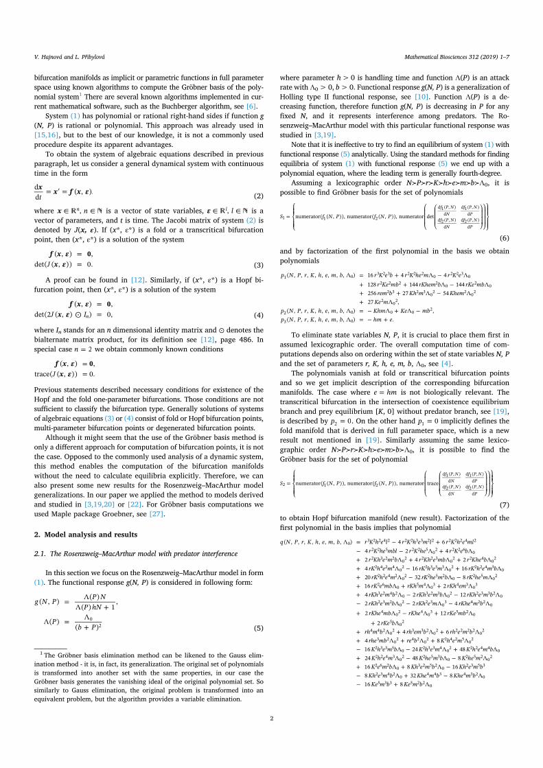
bifurcation manifolds as implicit or parametric functions in full parameterspace using known algorithms to compute the Gröbner basis of the poly-nomial system1 There are several known algorithms implemented in cur-rent mathematical software, such as the Buchberger algorithm, see [6].
System (1) has polynomial or rational right-hand sides if function g(N, P) is rational or polynomial. This approach was already used in[15,16], but to the best of our knowledge, it is not a commonly usedprocedure despite its apparent advantages.
To obtain the system of algebraic equations described in previousparagraph, let us consider a general dynamical system with continuoustime in the form
= =x x f xt
dd
( , ). (2)
where x n,n is a vector of state variables, l,l is avector of parameters, and t is time. The Jacobi matrix of system (2) isdenoted by J(x, ε). If (x*, ε*) is a fold or a transcritical bifurcationpoint, then (x*, ε*) is a solution of the system
==
f xxJ
0( , ) ,det( ( , )) 0. (3)
A proof can be found in [12]. Similarly, if (x*, ε*) is a Hopf bi-furcation point, then (x*, ε*) is a solution of the system
==
f xxJ I
0( , ) ,det(2 ( , ) ) 0,n (4)
where In stands for an n dimensional identity matrix and ⊙ denotes thebialternate matrix product, for its definition see [12], page 486. Inspecial case =n 2 we obtain commonly known conditions
==
f xxJ
0( , ) ,trace( ( , )) 0.
Previous statements described necessary conditions for existence of theHopf and the fold one-parameter bifurcations. Those conditions are notsufficient to classify the bifurcation type. Generally solutions of systemsof algebraic equations (3) or (4) consist of fold or Hopf bifurcation points,multi-parameter bifurcation points or degenerated bifurcation points.
Although it might seem that the use of the Gröbner basis method isonly a different approach for computation of bifurcation points, it is notthe case. Opposed to the commonly used analysis of a dynamic system,this method enables the computation of the bifurcation manifoldswithout the need to calculate equilibria explicitly. Therefore, we canalso present some new results for the Rosenzweig–MacArthur modelgeneralizations. In our paper we applied the method to models derivedand studied in [3,19,20] or [22]. For Gröbner basis computations weused Maple package Groebner, see [27].
2. Model analysis and results
2.1. The Rosenzweig–MacArthur model with predator interference
In this section we focus on the Rosenzweig–MacArthur model in form(1). The functional response g(N, P) is considered in following form:
=+
=+
g N P P NP hN
Pb P
( , ) ( )( ) 1
,
( )( )
02 (5)
where parameter h>0 is handling time and function Λ(P) is an attackrate with Λ0>0, b>0. Functional response g(N, P) is a generalization ofHolling type II functional response, see [10]. Function Λ(P) is a de-creasing function, therefore function g(N, P) is decreasing in P for anyfixed N, and it represents interference among predators. The Ro-senzweig–MacArthur model with this particular functional response wasstudied in [3,19].
Note that it is ineffective to try to find an equilibrium of system (1) withfunctional response (5) analytically. Using the standard methods for findingequilibria of system (1) with functional response (5) we end up with apolynomial equation, where the leading term is generally fourth-degree.
Assuming a lexicographic order N≻P≻r≻K≻h≻e≻m≻b≻Λ0, it ispossible to find Gröbner basis for the set of polynomials
=S f N P f N Pnumerator( ( , )), numerator( ( , )), numerator detf P N
Nf P N
Pf P N
Nf P N
P
1 1 2
d 1 ( , )d
d 1 ( , )d
d 2 ( , )d
d 2 ( , )d
(6)
and by factorization of the first polynomial in the basis we obtainpolynomials
= ++ ++ ++= += +
p N P r K h e m b r K e b r K he m r K er Ke mb rKhem b rKe mbrem b Kh m Khem
Ke mp N P r K h e m b Khm Ke mbp N P r K h e m b hm e
( , , , , , , , , ) 16 4 4128 144 144256 27 5427 ,
( , , , , , , , , ) ,( , , , , , , , , ) .
1 0 3 2 3 2 2 2 0 2 2 3 02 2 2 2 0 2 0
2 3 2 3 02 2 02
2 02
2 0 0 0 2
3 0
To eliminate state variables N, P, it is crucial to place them first inassumed lexicographic order. The overall computation time of com-putations depends also on ordering within the set of state variables N, Pand the set of parameters r, K, h, e, m, b, Λ0, see [4].
The polynomials vanish at fold or transcritical bifurcation pointsand so we get implicit description of the corresponding bifurcationmanifolds. The case where =e hm is not biologically relevant. Thetranscritical bifurcation in the intersection of coexistence equilibriumbranch and prey equilibrium [K, 0] without predator branch, see [19],is described by =p 02 . On the other hand =p 01 implicitly defines thefold manifold that is derived in full parameter space, which is a newresult not mentioned in [19]. Similarly assuming the same lexico-graphic order N≻P≻r≻K≻h≻e≻m≻b≻Λ0, it is possible to find theGröbner basis for the set of polynomial
=S f N P f N Pnumerator( ( , )), numerator( ( , )), numerator tracef P N
Nf P N
Pf P N
Nf P N
P
2 1 2
d 1 ( , )d
d 1( , )d
d 2 ( , )d
d 2 ( , )d
(7)
to obtain Hopf bifurcation manifold (new result). Factorization of thefirst polynomial in the basis implies that polynomial
= ++
+ + ++ +++ + ++
+ ++
+ + ++ + +
+++ +
++
q N P r K h e m b r K h e l r K h e m l r K h e mlr K he mbl r K he r K e br Kh e m b r Kh e mb r Khe brK h e m rK h e m rK h e m b
rK h e m rK he m b rK he mrK e mb rKh m rKh em
rKh e m b rKh e m b rKh e m brKh e m b rKh e m rKhe m brKhe mb rKhe rKe mb
rKe brh m b rh em b rh e m b
rhe mb re b K h e mK h e m b K h e m K h e m bK h e m K he m b K he mK e m b Kh e m b Kh e m b
Kh e m b Khe m b Khe m bKe m b Ke m b
( , , , , , , , , ) 4 64 2 42 4 24 16 1620 32 816 24 2 122 2 42 12
24 6
4 816 24 4824 48 816 8 168 32 816 8
0 3 2 2 4 2 2 2 3 3 2 2 2 2 2 4 2
2 2 5 2 2 5 02 2 2 6 02 3 2 2 02 2 2 3 02 2 4 02
2 4 2 4 02 2 3 3 3 02 2 2 4 3 02 2 4 2 02 2 5 2 0 2 5 02
2 6 0 5 4 03 4 3 03
3 2 4 2 0 3 2 3 02 2 3 3 2 02 3 2 02 2 3 03 4 2 2 0
4 02 4 03 5 2 05 02
4 4 2 02 3 3 2 02 2 2 2 2 02
3 2 02 4 2 02 2 4 2 5 02
2 3 3 5 0 2 3 3 4 02 2 2 4 4 02 2 4 3 02 2 5 3 0 2 5 2 02
2 6 2 0 3 2 5 2 0 2 3 5 3
2 3 4 2 0 4 4 3 4 3 2 05 3 3 5 2 2 0
1 The Gröbner basis elimination method can be likened to the Gauss elim-ination method - it is, in fact, its generalization. The original set of polynomialsis transformed into another set with the same properties, in our case theGröbner basis generates the vanishing ideal of the original polynomial set. Sosimilarly to Gauss elimination, the original problem is transformed into anequivalent problem, but the algorithm provides a variable elimination.
V. Hajnová and L. Přibylová Mathematical Biosciences 312 (2019) 1–7
2

vanishes at Hopf bifurcation points. Figs. 1 and 2 depict the foldbifurcation manifold implicitly defined by =p 01 and the Hopf bi-furcation manifold implicitly defined by =q 0. It is crucial to point outthat the vanishing ideal of (7) does not account for the scenario, wherethe Jacobi matrix determinant is positive. Therefore the expressedmanifold consists of Hopf bifurcation points as well as neutral saddlepoints. Additional analysis of the manifold subset that satisfies det J>0is necessary to avoid spurious results. This could be done numerically,analytically or using Gröbner basis with an additional parameter
= Jdet and an additional polynomial Jdet . The Hopf bifurcationmanifold in parametric space border is the contour = 0, so the borderis usually the Bogdanov–Takens bifurcation manifold (see the next ex-ample below).
A cusp bifurcation, denoted by CP in Fig. 1, is a two-parameter bi-furcation of equilibria. For the normal form of this bifurcation see [12].A cusp bifurcation manifold is a co-dimension two manifold, sub-manifold of the fold bifurcation manifold. At cusp points, two branchesof fold bifurcation manifolds of co-dimension 1 meet tangentially in atypical V-shape, see Fig. 1. Let us assume that we are interested inparameter m and h analysis and we seek hysteresis or transient
dynamics. Because generally, as well as in this example, cusp bifurca-tion points can be found as points where the implicitly defined functionhas no derivative, according to the implicit function theorem, cusppoints are solutions of a set of polynomial equations = 0p
h1 and
= 0pm
1 . Eliminating h and m respectively using the Gröbner basismethod again, we get the cusp bifurcation points explicitly as
=
=
m Kerb
h br bKr
112
,
43
(9 32 ) .0
0
The bifurcation analysis provided in this paper is not complete, formore see [19]. Dynamical model in form (1) with functional response(8) is in fact a special case of model studied in [19]. In [19] functionΛ(P) is considered in form = +P( ) b P( )w
0 . In our paper parameter w isset to critical value 2. The Hopf curve passes directly through the cuspbifurcation point (CP), which is a degenerate situation, see Fig. 1.
Such computations, made for example in Maple, may serve as quicksupport to more in-depth analysis or simulations. Following code showsall necessary computations in Maple.
fold bifurcationHopf bifurcationcusp bifurcationCP
CP
Fig. 1. The fold bifurcation manifold, implicitly defined by equation =p 0,1 and the Hopf bifurcation manifold, implicitly defined by equation =q 0, in thegeneralized Rosenzweig–MacArthur model depending on m (a death rate of a predator) and h (handling time) with = = = = =K r e b5, 28, 3.5, 1, 1.30 . Note thatthe solid bifurcation manifold consists of both neutral saddle points and Hopf bifurcation points.
V. Hajnová and L. Přibylová Mathematical Biosciences 312 (2019) 1–7
3
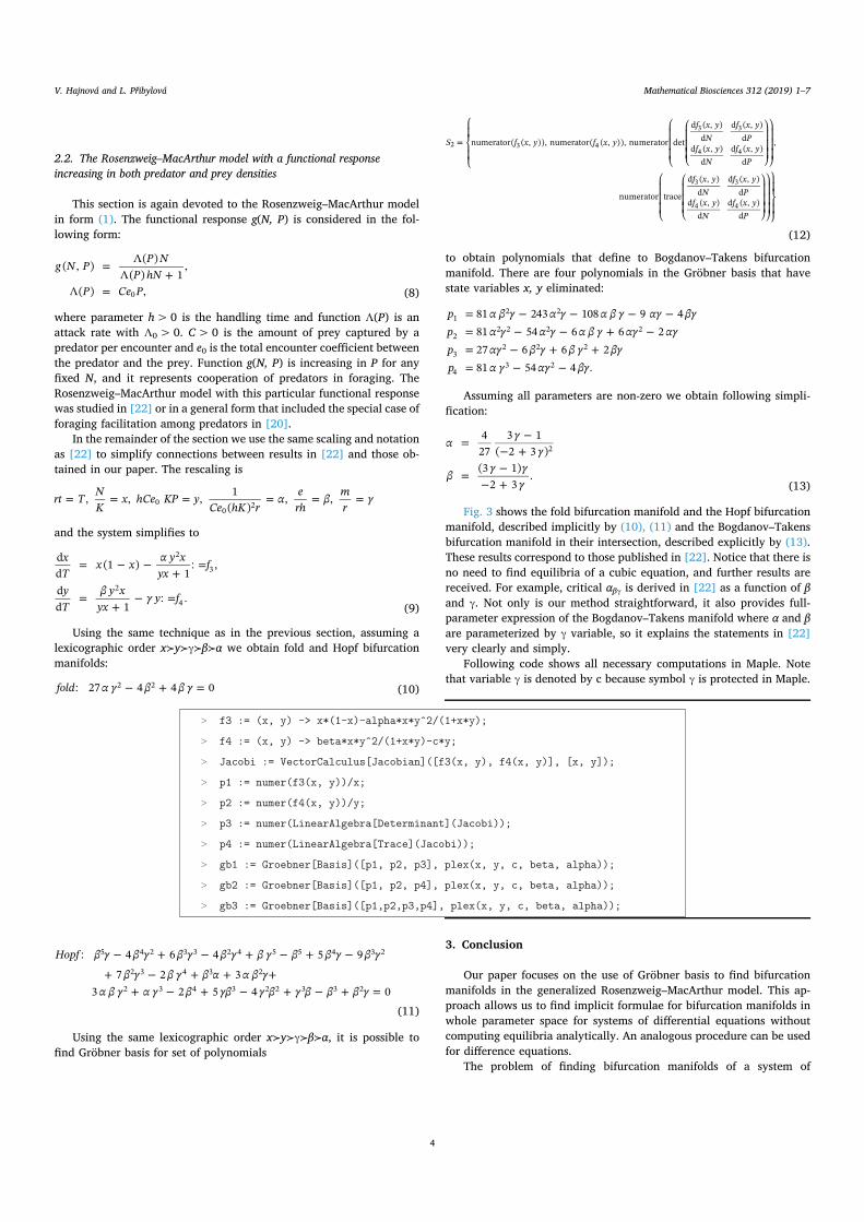
2.2. The Rosenzweig–MacArthur model with a functional responseincreasing in both predator and prey densities
This section is again devoted to the Rosenzweig–MacArthur modelin form (1). The functional response g(N, P) is considered in the fol-lowing form:
=+
=
g N P P NP hN
P Ce P
( , ) ( )( ) 1
,
( ) ,0 (8)
where parameter h>0 is the handling time and function Λ(P) is anattack rate with Λ0> 0. C>0 is the amount of prey captured by apredator per encounter and e0 is the total encounter coefficient betweenthe predator and the prey. Function g(N, P) is increasing in P for anyfixed N, and it represents cooperation of predators in foraging. TheRosenzweig–MacArthur model with this particular functional responsewas studied in [22] or in a general form that included the special case offoraging facilitation among predators in [20].
In the remainder of the section we use the same scaling and notationas [22] to simplify connections between results in [22] and those ob-tained in our paper. The rescaling is
= = = = = =rt T NK
x hCe KP yCe hK r
erh
mr
, , , 1( )
, ,00
2
and the system simplifies to
=+
=
=+
=
xT
x x y xyx
f
yT
y xyx
y f
dd
(1 )1
: ,
dd 1
: .
2
3
2
4 (9)
Using the same technique as in the previous section, assuming alexicographic order x≻y≻γ≻β≻α we obtain fold and Hopf bifurcationmanifolds:
+ =fold: 27 4 4 02 2 (10)
+ + ++ + + +
+ + + + =
Hopf : 4 6 4 5 97 2 3
3 2 5 4 0
5 4 2 3 3 2 4 5 5 4 3 2
2 3 4 3 2
2 3 4 3 2 2 3 3 2
(11)
Using the same lexicographic order x≻y≻γ≻β≻α, it is possible tofind Gröbner basis for set of polynomials
=S f x y f x y
f x yN
f x yP
f x yN
f x yP
f x yN
f x yP
f x yN
f x yP
numerator( ( , )), numerator( ( , )), numerator det
d ( , )d
d ( , )d
d ( , )d
d ( , )d
,
numerator trace
d ( , )d
d ( , )d
d ( , )d
d ( , )d
2 3 4
3 3
4 4
3 3
4 4
(12)
to obtain polynomials that define to Bogdanov–Takens bifurcationmanifold. There are four polynomials in the Gröbner basis that havestate variables x, y eliminated:
== += + +=
pppp
81 243 108 9 481 54 6 6 227 6 6 281 54 4 .
12 2
22 2 2 2
32 2 2
43 2
Assuming all parameters are non-zero we obtain following simpli-fication:
=+
=+
427
3 1( 2 3 )
(3 1)2 3
.
2
(13)
Fig. 3 shows the fold bifurcation manifold and the Hopf bifurcationmanifold, described implicitly by (10), (11) and the Bogdanov–Takensbifurcation manifold in their intersection, described explicitly by (13).These results correspond to those published in [22]. Notice that there isno need to find equilibria of a cubic equation, and further results arereceived. For example, critical αβγ is derived in [22] as a function of βand γ. Not only is our method straightforward, it also provides full-parameter expression of the Bogdanov–Takens manifold where α and βare parameterized by γ variable, so it explains the statements in [22]very clearly and simply.
Following code shows all necessary computations in Maple. Notethat variable γ is denoted by c because symbol γ is protected in Maple.
3. Conclusion
Our paper focuses on the use of Gröbner basis to find bifurcationmanifolds in the generalized Rosenzweig–MacArthur model. This ap-proach allows us to find implicit formulae for bifurcation manifolds inwhole parameter space for systems of differential equations withoutcomputing equilibria analytically. An analogous procedure can be usedfor difference equations.
The problem of finding bifurcation manifolds of a system of
V. Hajnová and L. Přibylová Mathematical Biosciences 312 (2019) 1–7
4
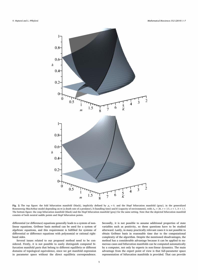
differential (or difference) equations generally leads to a system of non-linear equations. Gröbner basis method can be used for a system ofalgebraic equations, and this requirement is fulfilled for systems ofdifferential or difference equations with polynomial or rational right-hand sides.
Several issues related to our proposed method need to be con-sidered. Firstly, it is not possible to easily distinguish computed bi-furcation manifold parts that belong to different equilibria or differentdomains of topological equivalence, since we get manifold expressionin parameter space without the direct equilibria correspondence.
Secondly, it is not possible to assume additional properties of statevariables such as positivity, so these questions have to be studiedafterward. Lastly, in many practically relevant cases it is not possible toobtain Gröbner basis in reasonable time due to the computationalcomplexity of the algorithm. Despite the mentioned disadvantages, themethod has a considerable advantage because it can be applied to nu-merous cases and bifurcation manifolds can be computed automaticallyby a computer, not only by experts in non-linear dynamics. The mainadvantage from the expert point of view is that full-parameter spacerepresentation of bifurcation manifolds is provided. That can provide
Fig. 2. The top figure: the fold bifurcation manifold (black), implicitly defined by =p 0,1 and the Hopf bifurcation manifold (gray), in the generalizedRosenzweig–MacArthur model depending on m (a death rate of a predator), h (handling time) and K (capacity of environment), with = = = =r e b28, 3.5, 1, 1.30 .The bottom figure: the cusp bifurcation manifold (black) and the Hopf bifurcation manifold (gray) for the same setting. Note that the depicted bifurcation manifoldconsists of both neutral saddle points and Hopf bifurcation points.
V. Hajnová and L. Přibylová Mathematical Biosciences 312 (2019) 1–7
5
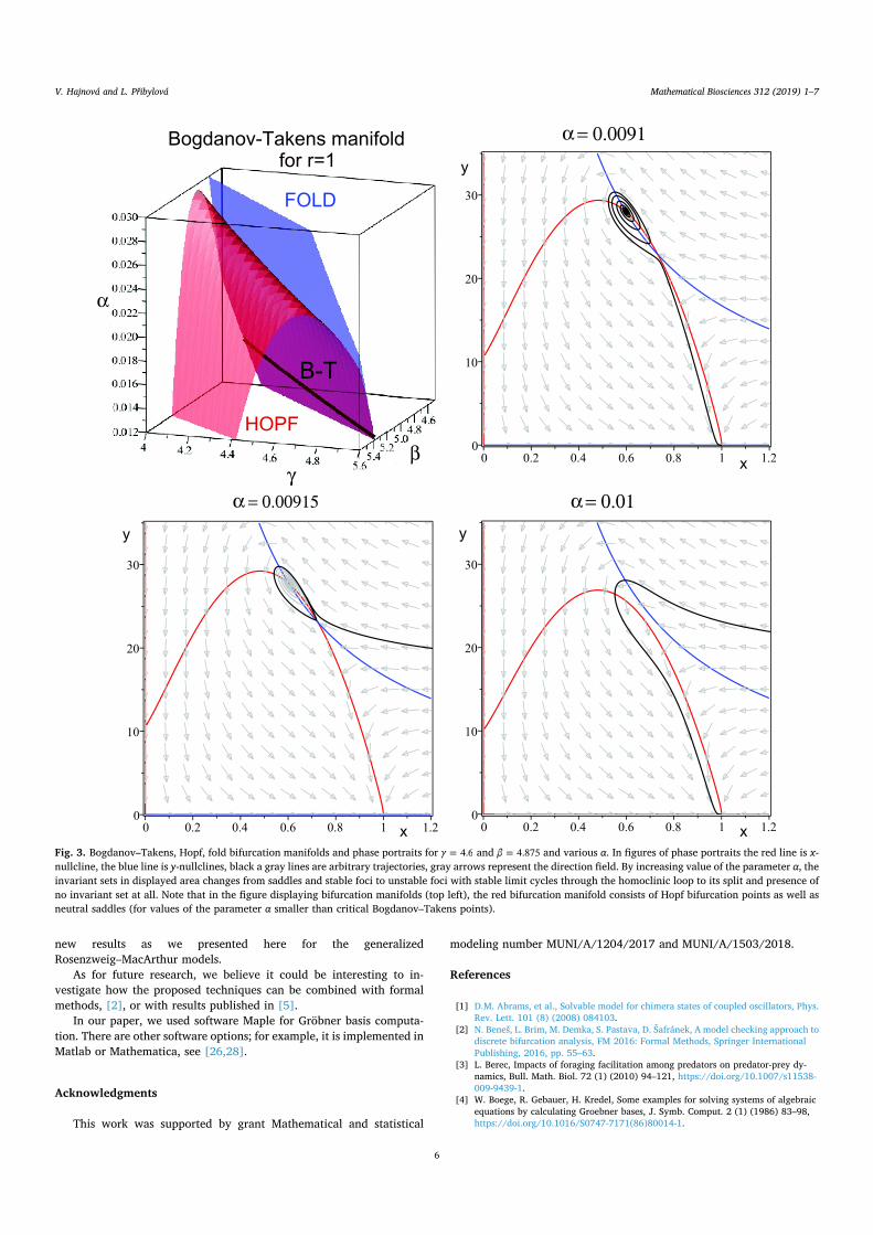
new results as we presented here for the generalizedRosenzweig–MacArthur models.
As for future research, we believe it could be interesting to in-vestigate how the proposed techniques can be combined with formalmethods, [2], or with results published in [5].
In our paper, we used software Maple for Gröbner basis computa-tion. There are other software options; for example, it is implemented inMatlab or Mathematica, see [26,28].
Acknowledgments
This work was supported by grant Mathematical and statistical
modeling number MUNI/A/1204/2017 and MUNI/A/1503/2018.
References
[1] D.M. Abrams, et al., Solvable model for chimera states of coupled oscillators, Phys.Rev. Lett. 101 (8) (2008) 084103.
[2] N. Beneš, L. Brim, M. Demka, S. Pastava, D. Šafránek, A model checking approach todiscrete bifurcation analysis, FM 2016: Formal Methods, Springer InternationalPublishing, 2016, pp. 55–63.
[3] L. Berec, Impacts of foraging facilitation among predators on predator-prey dy-namics, Bull. Math. Biol. 72 (1) (2010) 94–121, https://doi.org/10.1007/s11538-009-9439-1.
[4] W. Boege, R. Gebauer, H. Kredel, Some examples for solving systems of algebraicequations by calculating Groebner bases, J. Symb. Comput. 2 (1) (1986) 83–98,https://doi.org/10.1016/S0747-7171(86)80014-1.
Fig. 3. Bogdanov–Takens, Hopf, fold bifurcation manifolds and phase portraits for = 4.6 and = 4.875 and various α. In figures of phase portraits the red line is x-nullcline, the blue line is y-nullclines, black a gray lines are arbitrary trajectories, gray arrows represent the direction field. By increasing value of the parameter α, theinvariant sets in displayed area changes from saddles and stable foci to unstable foci with stable limit cycles through the homoclinic loop to its split and presence ofno invariant set at all. Note that in the figure displaying bifurcation manifolds (top left), the red bifurcation manifold consists of Hopf bifurcation points as well asneutral saddles (for values of the parameter α smaller than critical Bogdanov–Takens points).
V. Hajnová and L. Přibylová Mathematical Biosciences 312 (2019) 1–7
6
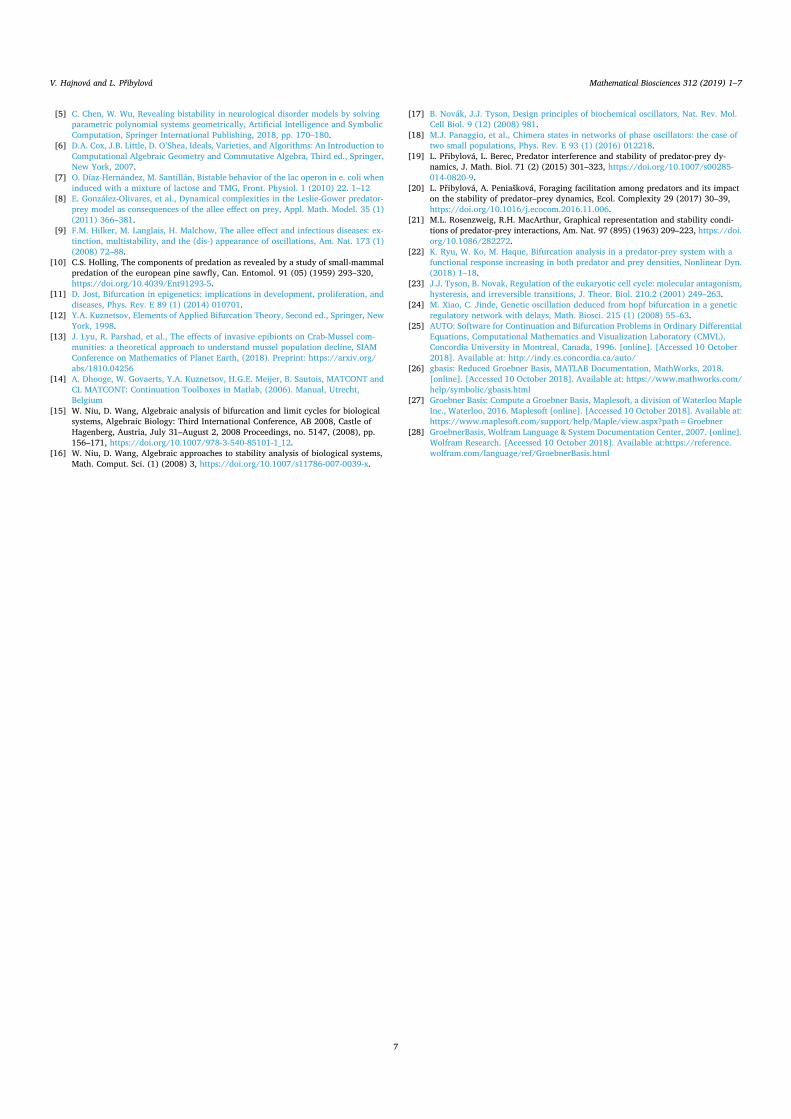
[5] C. Chen, W. Wu, Revealing bistability in neurological disorder models by solvingparametric polynomial systems geometrically, Artificial Intelligence and SymbolicComputation, Springer International Publishing, 2018, pp. 170–180.
[6] D.A. Cox, J.B. Little, D. O’Shea, Ideals, Varieties, and Algorithms: An Introduction toComputational Algebraic Geometry and Commutative Algebra, Third ed., Springer,New York, 2007.
[7] O. Díaz-Hernández, M. Santillán, Bistable behavior of the lac operon in e. coli wheninduced with a mixture of lactose and TMG, Front. Physiol. 1 (2010) 22. 1–12
[8] E. González-Olivares, et al., Dynamical complexities in the Leslie-Gower predator-prey model as consequences of the allee effect on prey, Appl. Math. Model. 35 (1)(2011) 366–381.
[9] F.M. Hilker, M. Langlais, H. Malchow, The allee effect and infectious diseases: ex-tinction, multistability, and the (dis-) appearance of oscillations, Am. Nat. 173 (1)(2008) 72–88.
[10] C.S. Holling, The components of predation as revealed by a study of small-mammalpredation of the european pine sawfly, Can. Entomol. 91 (05) (1959) 293–320,https://doi.org/10.4039/Ent91293-5.
[11] D. Jost, Bifurcation in epigenetics: implications in development, proliferation, anddiseases, Phys. Rev. E 89 (1) (2014) 010701.
[12] Y.A. Kuznetsov, Elements of Applied Bifurcation Theory, Second ed., Springer, NewYork, 1998.
[13] J. Lyu, R. Parshad, et al., The effects of invasive epibionts on Crab-Mussel com-munities: a theoretical approach to understand mussel population decline, SIAMConference on Mathematics of Planet Earth, (2018). Preprint: https://arxiv.org/abs/1810.04256
[14] A. Dhooge, W. Govaerts, Y.A. Kuznetsov, H.G.E. Meijer, B. Sautois, MATCONT andCL MATCONT: Continuation Toolboxes in Matlab, (2006). Manual, Utrecht,Belgium
[15] W. Niu, D. Wang, Algebraic analysis of bifurcation and limit cycles for biologicalsystems, Algebraic Biology: Third International Conference, AB 2008, Castle ofHagenberg, Austria, July 31–August 2, 2008 Proceedings, no. 5147, (2008), pp.156–171, https://doi.org/10.1007/978-3-540-85101-1_12.
[16] W. Niu, D. Wang, Algebraic approaches to stability analysis of biological systems,Math. Comput. Sci. (1) (2008) 3, https://doi.org/10.1007/s11786-007-0039-x.
[17] B. Novák, J.J. Tyson, Design principles of biochemical oscillators, Nat. Rev. Mol.Cell Biol. 9 (12) (2008) 981.
[18] M.J. Panaggio, et al., Chimera states in networks of phase oscillators: the case oftwo small populations, Phys. Rev. E 93 (1) (2016) 012218.
[19] L. Přibylová, L. Berec, Predator interference and stability of predator-prey dy-namics, J. Math. Biol. 71 (2) (2015) 301–323, https://doi.org/10.1007/s00285-014-0820-9.
[20] L. Přibylová, A. Peniašková, Foraging facilitation among predators and its impacton the stability of predator–prey dynamics, Ecol. Complexity 29 (2017) 30–39,https://doi.org/10.1016/j.ecocom.2016.11.006.
[21] M.L. Rosenzweig, R.H. MacArthur, Graphical representation and stability condi-tions of predator-prey interactions, Am. Nat. 97 (895) (1963) 209–223, https://doi.org/10.1086/282272.
[22] K. Ryu, W. Ko, M. Haque, Bifurcation analysis in a predator-prey system with afunctional response increasing in both predator and prey densities, Nonlinear Dyn.(2018) 1–18.
[23] J.J. Tyson, B. Novak, Regulation of the eukaryotic cell cycle: molecular antagonism,hysteresis, and irreversible transitions, J. Theor. Biol. 210.2 (2001) 249–263.
[24] M. Xiao, C. Jinde, Genetic oscillation deduced from hopf bifurcation in a geneticregulatory network with delays, Math. Biosci. 215 (1) (2008) 55–63.
[25] AUTO: Software for Continuation and Bifurcation Problems in Ordinary DifferentialEquations, Computational Mathematics and Visualization Laboratory (CMVL),Concordia University in Montreal, Canada, 1996. [online]. [Accessed 10 October2018]. Available at: http://indy.cs.concordia.ca/auto/
[26] gbasis: Reduced Groebner Basis, MATLAB Documentation, MathWorks, 2018.[online]. [Accessed 10 October 2018]. Available at: https://www.mathworks.com/help/symbolic/gbasis.html
[27] Groebner Basis: Compute a Groebner Basis, Maplesoft, a division of Waterloo MapleInc., Waterloo, 2016. Maplesoft [online]. [Accessed 10 October 2018]. Available at:https://www.maplesoft.com/support/help/Maple/view.aspx?path=Groebner
[28] GroebnerBasis, Wolfram Language & System Documentation Center, 2007. [online].Wolfram Research. [Accessed 10 October 2018]. Available at:https://reference.wolfram.com/language/ref/GroebnerBasis.html
V. Hajnová and L. Přibylová Mathematical Biosciences 312 (2019) 1–7
7
Proceedings 1:Two parametric bifurcation in LPA model
HAJNOVA, Veronika and PRIBYLOVA, Lenka
Proceedings of CHAOS 2015 International Conference.
Technical University of Crete, 2016.
Scopus: EID Scopus: 85072398707
Two-parameter bifurcation in LPA model
Veronika Hajnova1 and Lenka Pribylova2
1 Department of Mathematics and Statistics, Masaryk University, Brno, CzechRepublic(E-mail: [email protected])
2 Department of Mathematics and Statistics, Masaryk University, Brno, CzechRepublic(E-mail: [email protected])
Abstract. The structured population LPA model describes flour beetle populationdynamics of four stage populations: eggs, larvae, pupae, and adults with cannibalismbetween these stages. The case of non-zero cannibalistic rates of adults on eggs andadults on pupae and no cannibalism of larvae on eggs is study. This assumption isnecessary to make at least some calculations analytically. It is shown that the behav-ior can be continued to the generic model with non-zero cannibalistic rate of larvaeon eggs. In the model both supercritical and subcritical strong 1:2 resonance arepresent. The bifurcation responsible for the change of topological type of the strong1:2 resonance is study. This bifurcation is accompanied by the origination of theChenciner bifurcation. The destabilization of the system, caused by two parametricbifurcation, is studied in this paper and its biological consequences are discussed.
Keywords: two-parameter bifurcation; LPA model; Tribolium model; strong 1:2resonance; Chenciner bifurcation.
1 Introduction
This article is based on the original work of Robert F. Costantino, Ph.D., JimCushing, Ph.D., Brian Dennis, Ph.D., Robert A. Desharnais, Ph.D. and Shan-delle Henson, Ph.D. about LPA model (Tribolium model). LPA model is astructured population model that describes flour beetle population dynamicsof four stage populations: eggs, larvae, pupae, adults with cannibalism betweenthese stages. Main results of the research have been published from the year1995 to nowadays. In the published articles authors concentrate mainly onchaotic behavior in the system. The literature on nonlinear dynamics of thesystem associated with the LPA model is rich, there is a lot of studies that dealwith basic analysis of equilibria and their stability (e.g. Cushing[6], Cushing[4]or Kuang and Cushing[10]), some works are devoted to one-parameter bifurca-tions (as Dennis et al.[7]) and their route to chaotic dynamics (e.g. Cushing[6],Constantino et al.[2], Cushing et al.[5], Cushing et al.[3]). To our best knowl-edge, there is not any published work about two-parameter bifurcation analysis
8thCHAOS Conference Proceedings, 26-29 May 2015, Henri Poicare Institute,Paris France
c© 2014 ISAST

by far. The original detailed analysis of the Chenciner bifurcation and the sub-critical strong 1:2 resonance was done in our article which is under review inJournal of Mathematical Biology. Here we present both the supercritical andthe subcritical strong 1:2 resonances and their connection.
In this article we concentrate on both the supercritical and the subcriticalstrong resonance 1:2 and the bifurcation responsible for the change of topolog-ical type of the strong 1:2 resonance, which is accompanied with the Chencinerbifurcations. The mathematical background for these bifurcations, their nor-mal forms and analysis can be found in Kuznetsov[11].
The structured population LPA model consists of three stages: larvae L,pupae P and adults A, while the population of eggs as a function of the adultpopulation is not included into the state space. We assume cannibalism betweenthe stages. We have to point out that we concentrate on LPA model withnon-zero cannibalistic rates of adults on eggs and adults on pupae and nocannibalism of larvae on eggs. Here this assumption of no cannibalism of larvaeon eggs is used only to make the mathematical calculations more easy and clear(a lot of them may be done analytically in this case) and this case was alsoexamined in e.g. Dennis et al.[7].
2 Model description and basic analysis
The dynamic of LPA model is (see e.g. Cushing[6] or Cushing[4]):
L (t+ 1) = bA (t) e−cELL(t)−cEAA(t)
P (t+ 1) = (1− µL)L (t) (1)
A (t+ 1) = P (t) e−cPAA(t) + (1− µA)A (t) ,
where state variables L,P,A represent number of larvae, pupae and adultsin the population. Parameter b > 0 represents natality. Parameters µL andµA represent mortality of larvae and adults. We assume natural inequalities0 < µL < 1, 0 < µA < 1 to be satisfied. Parameters cEL, cEA, cPA denotecannibalistic rates. Namely, cEL is the cannibalistic rate of larvae on eggs, cEAis the cannibalistic rate of adults on eggs and cPA is the cannibalistic rate ofadults on pupae. We assume cEA ≥ 0, cPA ≥ 0 and cEL ≥ 0, in this article weconsider a special case cEL = 0.
There can be two fixed points of the system (1). The trivial fixed point cor-responds to extinction of the population, the non-trivial fixed point [L∗, P ∗, A∗]
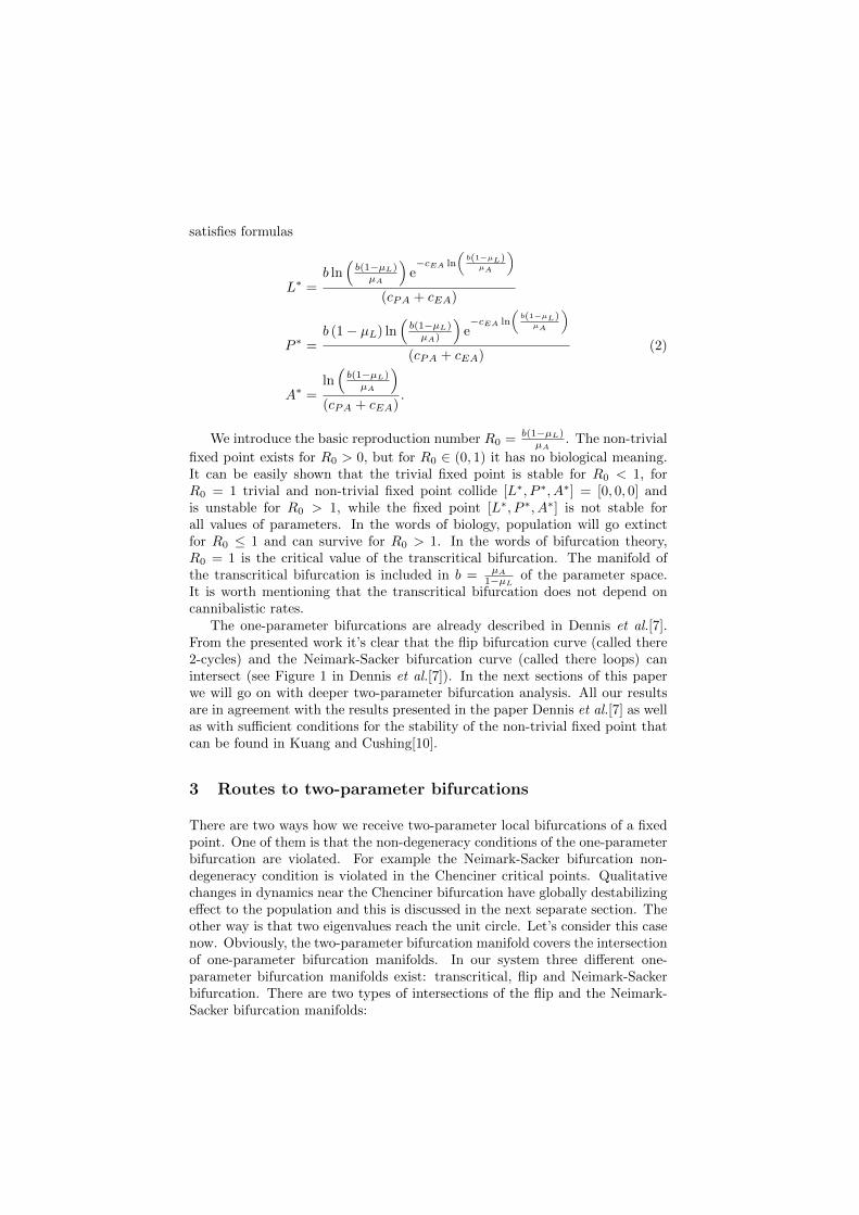
satisfies formulas
L∗ =b ln
(b(1−µL)µA
)e−cEA ln
(b(1−µL)µA
)
(cPA + cEA)
P ∗ =b (1− µL) ln
(b(1−µL)µA)
)e−cEA ln
(b(1−µL)µA
)
(cPA + cEA)(2)
A∗ =ln(b(1−µL)µA
)
(cPA + cEA).
We introduce the basic reproduction number R0 = b(1−µL)µA
. The non-trivial
fixed point exists for R0 > 0, but for R0 ∈ (0, 1) it has no biological meaning.It can be easily shown that the trivial fixed point is stable for R0 < 1, forR0 = 1 trivial and non-trivial fixed point collide [L∗, P ∗, A∗] = [0, 0, 0] andis unstable for R0 > 1, while the fixed point [L∗, P ∗, A∗] is not stable forall values of parameters. In the words of biology, population will go extinctfor R0 ≤ 1 and can survive for R0 > 1. In the words of bifurcation theory,R0 = 1 is the critical value of the transcritical bifurcation. The manifold ofthe transcritical bifurcation is included in b = µA
1−µL of the parameter space.It is worth mentioning that the transcritical bifurcation does not depend oncannibalistic rates.
The one-parameter bifurcations are already described in Dennis et al.[7].From the presented work it’s clear that the flip bifurcation curve (called there2-cycles) and the Neimark-Sacker bifurcation curve (called there loops) canintersect (see Figure 1 in Dennis et al.[7]). In the next sections of this paperwe will go on with deeper two-parameter bifurcation analysis. All our resultsare in agreement with the results presented in the paper Dennis et al.[7] as wellas with sufficient conditions for the stability of the non-trivial fixed point thatcan be found in Kuang and Cushing[10].
3 Routes to two-parameter bifurcations
There are two ways how we receive two-parameter local bifurcations of a fixedpoint. One of them is that the non-degeneracy conditions of the one-parameterbifurcation are violated. For example the Neimark-Sacker bifurcation non-degeneracy condition is violated in the Chenciner critical points. Qualitativechanges in dynamics near the Chenciner bifurcation have globally destabilizingeffect to the population and this is discussed in the next separate section. Theother way is that two eigenvalues reach the unit circle. Let’s consider this casenow. Obviously, the two-parameter bifurcation manifold covers the intersectionof one-parameter bifurcation manifolds. In our system three different one-parameter bifurcation manifolds exist: transcritical, flip and Neimark-Sackerbifurcation. There are two types of intersections of the flip and the Neimark-Sacker bifurcation manifolds:

(i) b = µAe2µA
1−µL , cEA = (µA+1)cPA1−µA and
(ii) b = µAe2µA
1−µL , cEA = (2µA−1)cPA5−2µA
.
The manifold (i) exists for all allowed values of parameters. On the otherhand, the manifold (ii) exists for µA >
12 only.
In this paper we focus on manifold (ii). The manifold (ii) corresponds withthe strong 1:2 resonance with associated eigenvalues −1,−1, 12 .
For arbitrarily fixed parameters µL, µA, cPA, the two-parameter bifurcationmanifolds correspond to points of intersection of one-parameter bifurcationcurves in a two-parameter space cEA versus b. The parameters µL, µA, cPAare fixed to common values (see e.g. Dennis et al.[8]).
4 Strong 1:2 resonance in LPA model
Strong 1:2 resonance is a two-parameter bifurcation that lies in the intersectionof the flip bifurcation manifold and the Neimark-Sacker bifurcation manifold.In our model two topological types of the strong 1:2 resonance exists: subcriticalbifurcation of a node or a focus and supercritical bifurcation of a node or a focus.The normal form for the supercritical bifurcation is similar to the subcritical,but the time variable has an opposite sign (see e.g. Kuznetsov[11]). Thereforethe phase portraits of subcritical and supercritical bifurcations have oppositestability.
Strong 1:2 resonance points lie in the intersection of Neimark-Sacker and flipmanifolds, therefore we expect birth of the limit loop from a fixed point due toN-S bifurcation and split of the fixed point into a 2-cycle nearby the strong 1:2resonance point. The Figure 1 displays the generic transversal two-parameterspace section of a canonical subcritical strong 1:2 resonance bifurcation man-ifold at zero with one-parameter N-S and flip manifolds at the horizontal andvertical axes.
As we move around the strong 1:2 resonance point, the topological structureof the state space the structure changes in the way that is presented for thecanonical form in Figure 1.
5 Chenciner bifurcation in LPA model
Transversal crossing of the Neimark-Sacker bifurcation manifold gives rise toan invariant loop around a fixed point that changes its stability. There are twotopological types of the Neimark-Sacker bifurcation: supercritical and subcrit-ical. The supercritical type gives rise to a stable invariant loop, reversely, thesubcritical brings about an unstable loop. The Chenciner bifurcation is a crit-ical change of these two types. An accompanying bifurcation manifold of theChenciner bifurcation exists. It is called the fold bifurcation of an invariantloop or the limit point bifurcation of an invariant loop and it gives birth to thestable and unstable invariant loop around.
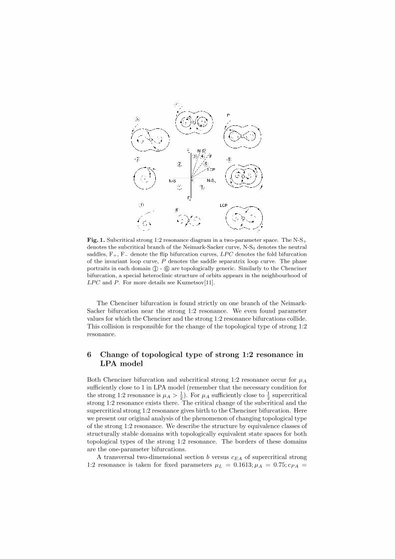
0
1
2
3 4
5
6
N-S+
F
F+
N-S-
2
P
LCP
N-S0
1
2
3
Fig. 1. Subcritical strong 1:2 resonance diagram in a two-parameter space. The N-S+
denotes the subcritical branch of the Neimark-Sacker curve, N-S0 denotes the neutralsaddles, F+, F− denote the flip bifurcation curves, LPC denotes the fold bifurcationof the invariant loop curve, P denotes the saddle separatrix loop curve. The phaseportraits in each domain 1© - 6© are topologically generic. Similarly to the Chencinerbifurcation, a special heteroclinic structure of orbits appears in the neighbourhood ofLPC and P . For more details see Kuznetsov[11].
The Chenciner bifurcation is found strictly on one branch of the Neimark-Sacker bifurcation near the strong 1:2 resonance. We even found parametervalues for which the Chenciner and the strong 1:2 resonance bifurcations collide.This collision is responsible for the change of the topological type of strong 1:2resonance.
6 Change of topological type of strong 1:2 resonance inLPA model
Both Chenciner bifurcation and subcritical strong 1:2 resonance occur for µAsufficiently close to 1 in LPA model (remember that the necessary condition forthe strong 1:2 resonance is µA >
12 ). For µA sufficiently close to 1
2 supercriticalstrong 1:2 resonance exists there. The critical change of the subcritical and thesupercritical strong 1:2 resonance gives birth to the Chenciner bifurcation. Herewe present our original analysis of the phenomenon of changing topological typeof the strong 1:2 resonance. We describe the structure by equivalence classes ofstructurally stable domains with topologically equivalent state spaces for bothtopological types of the strong 1:2 resonance. The borders of these domainsare the one-parameter bifurcations.
A transversal two-dimensional section b versus cEA of supercritical strong1:2 resonance is taken for fixed parameters µL = 0.1613;µA = 0.75; cPA =

0.004348 (which is shown in Figure 2). The dynamic classes I. - VI. are dis-played in Figure 3.
0.00045 0.0007
12
20
flip bifurcationNeimark-Sacker bifurcationNeimark-Sacker bif. 2-cycleseparatrix saddle loop
fold bifurcarion of loopsR2 strong 1:2 resonance
cEA
b
N-S-
N-S0
F+ F-R2
I. II.
III.
IV.V. VI. VI.
0.0007
Fig. 2. Strong 1:2 resonance and Chenciner bifurcation diagram. Bifurcation curvesin parametric space with free parameters cEA and b for fixed µL = 0.1613;µA =0.75; cPA = 0.004348.
The topological structure of the parameter space near the Chenciner bi-furcation and the subcritical strong 1:2 resonance gives rise to a complicatedstate space dynamics with coexistence of different types of invariant sets. Thetransversal two-dimensional section b versus cEA of both two-parameter mani-folds (Chenciner and subcritical strong 1:2 resonance) is taken for fixed param-eters µL = 0.1613;µA = 0.96; cPA = 0.004348. Striped and shadowed domainsbelong to basins of attraction corresponding to weak and huge oscillations re-spectively. White domains belong to a stable fixed point basins of attraction.The two different branches of LPC (fold bifurcation of the invariant loop) col-lide in a typical V-shape in a cusp point, that is a two-parameter bifurcationpoint. The cusp point is typically connected with the phenomenon of hysteresis.The parameter space is divided into nine domains where the state spaces staytopologically equivalent. All dynamic classes I. - IX. are displayed in Figures6. We omit the stripe underneath the transcritical bifurcation curve, wherethe population is dying out. Here the only fixed point is the trivial equilibriumthat is globally stable and so the population goes extinct. For values of b abovethe transcritical bifurcation curve, the trivial equilibrium is unstable and theorbits can tend to another attractors.
For parameter values near the change of the topological type of strong 1:2resonance the system is locally topologically equivalent to the system displayedin Figure 4. The global behavior is shown in Figure 5.

10 000
1 0000
P
A
(a) I: stable invariant loop, e.g. cEA =0.0013, b = 6
10 000
1 0000
P
A
(b) II: stable fixed point, e.g. cEA =0.002, b = 8
10 000
1 0000
P
A
(c) III: stable fixed point, stable invari-ant loop, e.g. cEA = 0.0014, b = 6
10 000
1 0000
P
A
(d) IV: stable 2-cycle, stable invariantloop, e.g. cEA = 0.0015, b = 9.2
10 000
1 0000
P
A
(e) V: two stable symmetric coupledloops, stable invariant loop, e.g. cEA =0.00154, b = 9.6
10 000
1 0000
P
A
(f) VI: two stable invariant loops, e.g.cEA = 0.00172, b = 10.05
Fig. 3. Phase portraits near the strong resonance 1:2 and the Chenciner bifurcationin LPA model with parameters µL = 0.1613;µA = 0.96; cPA = 0.004348 and freeparameters cEA a b. In the left column, there are schematic phase portraits for eachdomain according to Figure 2. In the right column, there are computed stable setsat adults and pupae state variables.
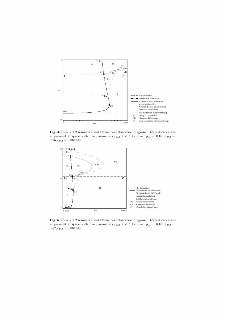
R2
CH
I. II.
III.
flip bifurcation
transkritical bifurcation
Neimark-Sacker bifurcation
and neutral saddles
cEA
b
IV. VII.
VIII.
V.VI.
IX.IX.
Neimark-Sacker bif. of 2-cycle
separatrix saddle loop
fold bifurcation of invariant loop
R2 strong 1:2 resonance
CH Chenciner bifurcation
0 0,002
0
12
CP
CP Cusp bifurcation of invariant loops
N-S-
N-S0
F+
F-
Fig. 4. Strong 1:2 resonance and Chenciner bifurcation diagram. Bifurcation curvesin parametric space with free parameters cEA and b for fixed µL = 0.1613;µA =0.96; cPA = 0.004348.
I.
II.
III.
cEA
b
VII.VIII.
0.0009 0.00155
15
N-S-
N-S
F+ F-
flip bifurcationNeimark-Sacker bifurcationNeimark-Sacker bif. 2-cycleseparatrix saddle loop
fold bifurcation of loopsR2 strong 1:2 resonanceCH Chenciner bifurcationCP Cusp bifurcation of loops
CH
R2
CP
N-S+
IV.V.VI.
0
IX. IX.
VIII.VII.
Fig. 5. Strong 1:2 resonance and Chenciner bifurcation diagram. Bifurcation curvesin parametric space with free parameters cEA and b for fixed µL = 0.1613;µA =0.87; cPA = 0.004348.
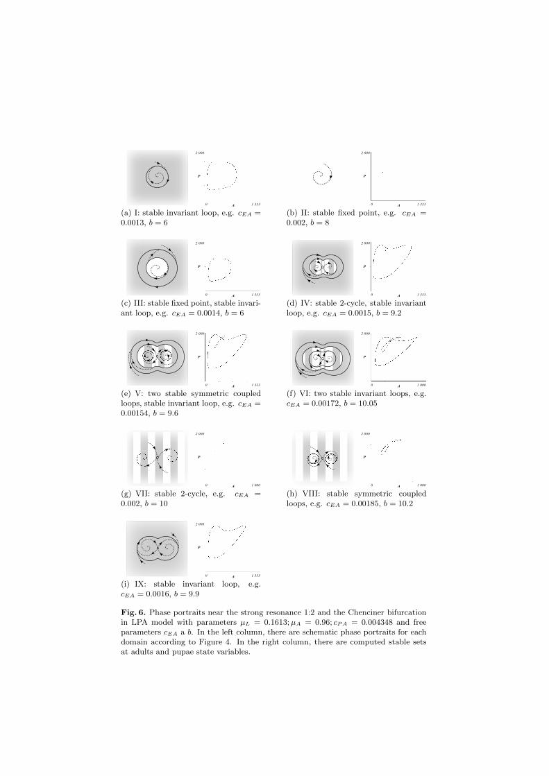
2 000
1 3330
P
A
(a) I: stable invariant loop, e.g. cEA =0.0013, b = 6
2 000
1 3330
P
A
(b) II: stable fixed point, e.g. cEA =0.002, b = 8
2 000
1 3330
P
A
(c) III: stable fixed point, stable invari-ant loop, e.g. cEA = 0.0014, b = 6
2 000
1 3330
P
A
(d) IV: stable 2-cycle, stable invariantloop, e.g. cEA = 0.0015, b = 9.2
2 000
1 3330
P
A
(e) V: two stable symmetric coupledloops, stable invariant loop, e.g. cEA =0.00154, b = 9.6
2 000
1 0000
P
A
(f) VI: two stable invariant loops, e.g.cEA = 0.00172, b = 10.05
2 000
1 0000
P
A
(g) VII: stable 2-cycle, e.g. cEA =0.002, b = 10
2 000
1 0000
P
A
(h) VIII: stable symmetric coupledloops, e.g. cEA = 0.00185, b = 10.2
2 000
1 3330
P
A
(i) IX: stable invariant loop, e.g.cEA = 0.0016, b = 9.9
Fig. 6. Phase portraits near the strong resonance 1:2 and the Chenciner bifurcationin LPA model with parameters µL = 0.1613;µA = 0.96; cPA = 0.004348 and freeparameters cEA a b. In the left column, there are schematic phase portraits for eachdomain according to Figure 4. In the right column, there are computed stable setsat adults and pupae state variables.
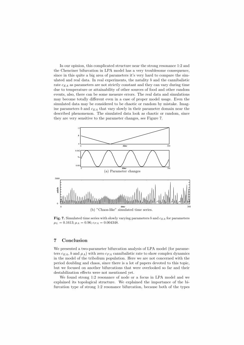
In our opinion, this complicated structure near the strong resonance 1:2 andthe Chenciner bifurcation in LPA model has a very troublesome consequence,since in this quite a big area of parameters it’s very hard to compare the sim-ulated and real data. In real experiments, the natality b and the cannibalisticrate cEA as parameters are not strictly constant and they can vary during timedue to temperature or attainability of other sources of food and other randomevents, also, there can be some measure errors. The real data and simulationsmay become totally different even in a case of proper model usage. Even thesimulated data may be considered to be chaotic or random by mistake. Imag-ine parameters b and cEA that vary slowly in their parameter domain near thedescribed phenomenon. The simulated data look as chaotic or random, sincethey are very sensitive to the parameter changes, see Figure 7.
0 300
8
13
time
b
300
0.001
0.002
time
c
0
EA
(a) Parameter changes
300
0
5000
time
adults
0
(b) ”Chaos-like” simulated time series.
Fig. 7. Simulated time series with slowly varying parameters b and cEA for parametersµL = 0.1613;µA = 0.96; cPA = 0.004348.
7 Conclusion
We presented a two-parameter bifurcation analysis of LPA model (for parame-ters cEA, b and µA) with zero cPA cannibalistic rate to show complex dynamicsin the model of the tribolium population. Here we are not concerned with theperiod doubling and chaos, since there is a lot of papers devoted to this topic,but we focused on another bifurcations that were overlooked so far and theirdestabilization effects were not mentioned yet.
We found strong 1:2 resonance of node or a focus in LPA model and weexplained its topological structure. We explained the importance of the bi-furcation type of strong 1:2 resonance bifurcation, because both of the types
(subcritical and supercritical) are present. The topological change of the strong1:2 resonance gives birth to the Chenciner bifurcation.
As the most important part of our paper we consider to be the finding ofa connection between the Chenciner bifurcation and strong 1:2 resonance andsetting of the complete two-parameter bifurcation diagram of these manifoldsconnection (together with the nearby non-local bifurcation manifolds).
References
1. A. Chenciner, Bifurcations de points fixes elliptiques. III. Orbites periodiques depetites periodes et elimination resonnante des couples de courbes invariantes,Inst. Hautes Etudes Sci. Publ. Math. 66 (1987), pp. 5-91.
2. R.F. Costantino, R.A. Desharnais, J.M. Cushing, B. Dennis, Chaotic dynamics inan insect population, Science, Vol. 275, Issue 5298 (1997), pp. 389–391.
3. J.M. Cushing,, R.F. Constantino, B. Dennis, R.A. Desharnais, and S.M. Henson,Nonlinear population dynamics: models, experiments and data, Journal of Theo-retical Biology, Vol. 194, Issue 1 (1998), pp. 1–9.
4. J.M. Cushing, An Introduction to Structured Population Dynamics, Society forIndustrial and Applied Mathematics, Philadelphia, 1998.
5. J.M. Cushing, S.M. Henson, R.A. Desharnais, B. Dennis, R.F. Costantino, andA. King, A chaotic attractor in ecology: theory and experimental data, Chaos,Solitons & Fractals, Vol. 12, Issue 2, (2001), pp. 219–234.
6. J.M. Cushing, Chaos in Ecology: Experimental Nonlinear Dynamics, AcademicPress, Amsterdam, 2003
7. B. Dennis, R.A. Desharnais, J.M. Cushing, and R.F. Constantino, Nonlinear de-mographic dynamics: mathematical models, statistical methods, and biologicalexperiments, Ecological Monographs, Vol. 65, Issue 3 (1995), pp. 261–282
8. B. Dennis, R.A. Desharnais, J.M. Cushing, and R.F. Costantino, Transitions inpopulation dynamics: equilibria to periodic cycles to aperiodic cycles, The Journalof Animal Ecology, Vol. 66, Issue 5 (1997), pp. 704–729.
9. S. Elaydi, An Introduction to Difference Equations, 3rd ed., Springer, New York,2005.
10. Y. Kuang, and J.M. Cushing, Global stability in a nonlinear difference-delay equa-tion model of flour beetle population growth, Journal of Difference Equations andApplications, Vol. 2, Issue 1 (2007), pp. 31–37.
11. Y.A. Kuznetsov, Elements of Applied Bifurcation Theory, 2nd ed., Springer, NewYork, 1998.

Proceedings 2:Grobner Basis Method inFitzHugh-Nagumo Model
HAJNOVA, Veronika
11th ChaoticModeling and Simulation International Conference.
Springer Proceedings in Complexity: Springer International Publishing,2019.
Scopus: EID Scopus: 85067248827


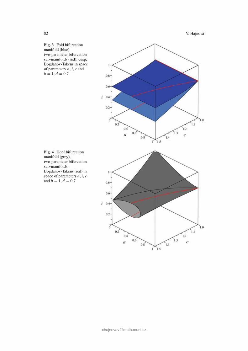
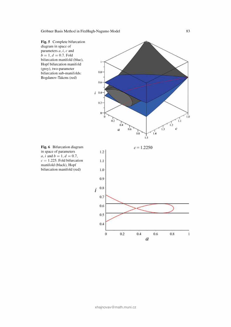


Poster 1:Biological and physiological phenomena
in view of applied bifurcation theory
HAJNOVA, Veronika and PRIBYLOVA, Lenka
In 16th International Conference on ComputationalMethods in SystemsBiology. 2018.
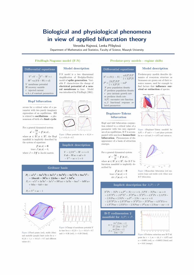
Biological and physiological phenomenain view of applied bifurcation theory
Veronika Hajnová, Lenka PřibylováDepartment of Mathematics and Statistics, Faculty of Science, Masaryk University
FitzHugh-Nagumo model (F-N)
Differential equations
V ′ =V − 13V
3 −W + i
W ′ =a (V b−Wc + d)V membrane potentialW recovery variablei injected currenta, b, c, d constant parameters
Hopf bifurcation
occurs for a critical value of a pa-rameter with two purely imaginaryeigenvalues of an equilibrium. HBis related to oscillations – a phe-nomenon of birth of a limit cycle.
For a general dynamical system
x′ = dx
dt = f (x, ε) ,
where x ∈ R2, ε ∈ Rk, the Hopfmanifold is implicitly described bythe system of equations
f (x, ε) = 0trace J (x, ε) = 0,
where J = Df is Jacobi matrix.
Model description
F-N model is a two dimensionalsimplification of Hodgkin-Huxleymodel of spike generation. Vari-able V characterizes the change ofelectrical potential of a neu-ral membrane in time. Modelwas introduced by FitzHugh (1961).
Figure 1:Phase portraits for a = 0.2, b =1, c = 0.8, d = 0.7.
Implicit description
V − 1/3V 3 −W + i = 0V ab−Wac + ad = 0− V 2 − ac + 1 = 0
Gröbner basis
P1 = a4c5 − 6a3c3b + 3a3c4 + 9a2b2c − 6a2c2b + 9ac2i2−− 18acdi − 9b2a + 12cba − 4ac2 + 9d2a
P2 = −a4c4 + 3a3bc2 − 3a3c3 + 9Waci + 3a2bc− 9aci2 − 9dWa++ 9dia− 6ab + 4ac...
P9 = V 2 + ac− 1
0
0.5
1
1.5 −2
−1.5
−1
−0.5
0
0.5
1
1.5
2
−0.5
0
0.5
1
1.5
2
V
Wi
Figure 2:Fixed points (red), stable (blue)and unstable (purple) limit cycles for a =0.2, b = 1, c = 0.8, d = 0.7 and differentvalues of i.
-2
-1.5
-1
-0.5
0
0.5
1
1.5
2
0 50 100 150 200
V
t
Figure 3:Change of membrane potential Vin time for a = 0.2, b = 1, c = 0.8, d = 0.7and i = 0.36 (red), i = 0.38 (black).
Predator-prey models - regime shifts
Differential equations
N ′ = rN(1−N)− αλ(P )NP1 + λ(P )N
P ′ = βλ(P )NP1 + λ(P )N −mP
N prey population densityP predator population densityr prey intrinsic growth ratem predator death rateλ(P ) encounter rate functionα, β functional response re-lated parameters
Bogdanov-Takensbifurcation
Hopf and fold bifurcation conjunc-tion related to a critical value of aparameter with two zero eigenval-ues of an equilibrium, B-T is accom-panied with non-local homoclinicbifurcation. Phenomenon of dis-appearance of a basin of attractionemerges.
For a general dynamical system
x′ = dx
dt = f (x, ε) ,
where x ∈ R2, ε ∈ Rk, the B-T bi-furcation manifold is implicitly de-scribed by
f (x, ε) = 0trace J (x, ε) = 0det J (x, ε) = 0.
Model description
Predator-prey models describe dy-namics of ecosystem structure asbiomasses are grown out of their re-source masses, used for example tofind factors that influence sur-vival or extinction of species.
Figure 4:Bogdanov-Takens manifold forλ(P ) = P and r = 1 and phase portraitsfor m = 4.6 and β = 4.875 and various α.
Figure 5:Homoclinic bifurcation (red sep-aratrix loop) and stable cycle (blue) nearB-T bifurcation.
Implicit description for λ(P ) = P
N 2Pr −NPr + αP 2 + Nr + r = 0, β PN −NPm−m = 0− 2N 3P 2r + β P 2N 2 −N 2P 2m + N 2P 2r − 4N 2Pr + 2 β PN−− 2NPm + 2NPr − αP 2 − 2Nr −m + r = 0− 2N 3P 2β r + 2N 3P 2mr + N 2P 2β r −N 2P 2mr − 4N 2Pβ r++ 4N 2Pmr + 2NPβ r − 2NPmr + P 2αm + 2Nmr −mr = 0
B-T codimension 2manifold for λ(P ) = P .
α = 4 r2 (3m− r)27 (3m− 2 r)2
β =m (3m− r)3m− 2 r
Figure 6:Predator extinction near B-T bif.point for r = 1,m = 4.6, β = 4.875 andα = 0.0091 (red), α = 0.00915 (black) andα = 0.01 (orange).
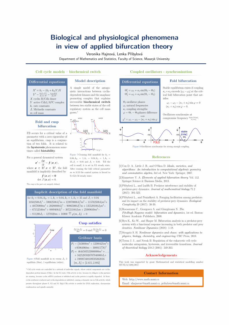
Biological and physiological phenomenain view of applied bifurcation theory
Veronika Hajnová, Lenka PřibylováDepartment of Mathematics and Statistics, Faculty of Science, Masaryk University
Cell cycle models – biochemical switch
Differential equations
X ′ = k1 − (k2 + k2rY )XY ′ = k3(1−Y )
J1+1−Y − k4mXYJ2+Y
X cyclin B/Cdk dimerY active Cdh1/APC complexki rate constantsJi Michaelis constantsm cell mass
Fold and cuspbifurcation
FB occurs for a critical value of aparameter with a zero eigenvalue ofan equilibrium, cusp is a conjunc-tion of two folds. It is related tothe hysteresis phenomenon some-times called bistability.
For a general dynamical system
x′ = dx
dt = f (x, ε) ,
where x ∈ R2, ε ∈ Rk, the foldmanifold is implicitly described by
f (x, ε) = 0det J (x, ε) = 0.
The cusp is the part not uniquely defined.
Model description
A simple model of the antago-nistic interactions between cyclin-dependent kinases and the anaphasepromoting complex that explainsirreversible biochemical switchbetween two stable states of the cellregulatory system as the cell massgrows.∗
Figure 7:Crossing fold manifold for k2 =0.04, k2r = 1, k1 = 0.04, k3 = 1, k4 =35, J1 = 0.04 and J2 = 0.04. Till thecell is small, it is set in G1 steady state.After crossing the fold critical parameterm ≈ 0.53 the control system is forced toS+G2+M steady state.
Implicit description of the fold manifoldfor k2 = 0.04, k2r = 1, k1 = 0.04, k3 = 1, k4 = 35 and J1 = 0.0410562500J2
4 − 59062500J23m + 123970000J2
2m2 − 115762500J2m3+
+ 40576900m4 + 20280000J23 − 90965000J2
2m + 135529100J2m2−
− 67152540m3 + 8889400J22 − 30721180J2m + 25989649m2−
− 811200J2 − 1279320m + 16900 def= ϕ(m, J2) = 0
Figure 8:Fold manifold in m versus J2, 3equilibria (blue), 1 equilibrium (white).
Cusp satisfies∂ϕ (m,J2)
∂m = 0 and ∂ϕ (m,J2)∂J2
= 0
Gröbner basisP1 =
(343000m3 + 12388425m2+
+95964960m− 308915776)2
P2 = 4644503523800000m5 + . . .
+ 3425285926707840000J2++ 198987408109595862016[m, J2] = [2.415, 2.882]
* Cell cycle events are controlled by a network of molecular signals, whose central components are cyclin-
dependent protein kinases (Cdks). In the G1 state, Cdk activity is low, because its obligate cyclin partners
are missing, because cyclin mRNA synthesis is inhibited and cyclin protein is rapidly degraded. At Start,
cyclin synthesis is induced and cyclin degradation is inhibited, causing a dramatic rise in Cdk activity, which
persists throughout phases S, G2 and M. High Cdk activity is needed for DNA replication, chromosome
condensation and spindle assembly.
Coupled oscillators - synchronization
Differential equations
Θ′1 = ω1 + κ1 sin(Θ2 − Θ1)Θ′2 = ω2 + κ2 sin(Θ1 − Θ2)
Θi oscillator phasesωi natural frequenciesκi coupling strengthsϕ = Θ1 − Θ2phases difference
=⇒ϕ′ = ω1 − ω2 − (κ1 + κ2) sinϕ
Fold bifurcation
Stable equilibrium exists if couplingκ1 +κ2 exceeds |ω1−ω2| at the crit-ical fold bifurcation point that sat-isfies
ω1 − ω2 − (κ1 + κ2) sinϕ = 0(κ1 + κ2) cosϕ = 0.
Oscillators synchronize atcompromise frequency κ2ω1+κ1ω2
κ1+κ2.
Figure 9:Oscillators synchronize for strong enough coupling.
References
[1] Cox D. A., Little J. B., and O’Shea D. Ideals, varieties, andalgorithms: An introduction to computational algebraic geometryand commutative algebra, 3rd ed. New York: Springer, 2007.
[2]Kuznetsov Y. A. Elements of applied bifurcation theory. Vol. 112.Springer Science & Business Media, 2013.
[3] Přibylová L., and Luděk B. Predator interference and stability ofpredator-prey dynamics. Journal of mathematical biology 71.2(2015): 301-323.
[4] Přibylová L., and Peniašková A. Foraging facilitation among predatorsand its impact on the stability of predator-prey dynamics. EcologicalComplexity 29 (2017): 30-39.
[5]Rocsoreanu C., Georgescu A. and Giurgiteanu N. TheFitzHugh-Nagumo model: bifurcation and dynamics, 1st ed. Boston:Kluwer Academic Publishers, 2000.
[6]Ryu K., Ko W., and Haque M. Bifurcation analysis in a predator-preysystem with a functional response increasing in both predator and preydensities. Nonlinear Dynamics (2018): 1-18.
[7] Strogatz S. H. Nonlinear dynamics and chaos: with applications tophysics, biology, chemistry, and engineering. CRC Press, 2018.
[8] Tyson J. J., and Novak B. Regulation of the eukaryotic cell cycle:molecular antagonism, hysteresis, and irreversible transitions. Journalof theoretical biology 210.2 (2001): 249-263.
Acknowledgements
This work was supported by grant Mathematical and statistical modelling numberMUNI/A/1204/2017.
Contact InformationWeb: http://www.math.muni.czEmail: [email protected], [email protected]

Related Documents