POLITECNICO DI MILANO Scuola di Ingegneria Industriale e dell’Informazione Corso di Laurea Magistrale in Ingegneria Elettrica PHASOR MEASUREMENT UNITS AND DISTRIBUTION SMART GRIDS: APPLICATIONS AND BENEFITS Relatore: Prof. Alberto Berizzi Correlatore: Dott. Ing. Simone Cuni Tesi di Laurea Magistrale di: Giuseppe Torregrossa Matr. 10517751 Anno accademico 2016/2017

Welcome message from author
This document is posted to help you gain knowledge. Please leave a comment to let me know what you think about it! Share it to your friends and learn new things together.
Transcript
POLITECNICO DI MILANO
Scuola di Ingegneria Industriale e dell’Informazione Corso di Laurea Magistrale in Ingegneria Elettrica
PHASOR MEASUREMENT UNITS AND DISTRIBUTION SMART GRIDS: APPLICATIONS AND BENEFITS
Relatore: Prof. Alberto Berizzi
Correlatore: Dott. Ing. Simone Cuni
Tesi di Laurea Magistrale di:
Giuseppe Torregrossa
Matr. 10517751
Anno accademico 2016/2017


Acknowledgements
This thesis would not have been possible without the support of many people. Many
thanks to my supervisor, Professor Alberto Berizzi, who gave me the opportunity to work on
an experimental project in e-distribuzione and helped make some sense of the confusion that
sometimes happened to arise.
Also thanks to the Smart Grid Lab team, and in particular Gianluca Sapienza, Giovanni
Valvo, and Carla Marino, who offered guidance and support. A special mention goes to Simone
Cuni, for not only being my main source of advice, positive criticism and suggestions, but also
providing me with all the means to complete this project with ease and keeping up the mood
with his optimistic and charismatic personality. A note of appreciation to my colleagues Flavia
and Mattia too, for the hand they lent me in the reviewing phase.
I am grateful to my parents Arturo e Rosaria and my sister Giorgia, whose love and
care reaches me every day even from the distance that keeps us apart; to my cousins Giulio
and Silvia, without whom I would have missed this great opportunity and to whom I truly owe
a lot; to my grandmother Mela, a strong role-model that even now misses no opportunity to
teach me rules of the world and how to survive it.
Last but not least, I want to thank the friends I met during this two-year academic
adventure: Quanti (Isacco), Disagea (Davide), Foppa (Massimo), Fero (Federico) and all the
people I met and learned to trust and respect living in the “Casa dello Studente” students’
residence.
Thank you all for your precious help and, most importantly, for gifting me with an
existence that would not be as worth without even just one of you.
I

II

Abstract
This thesis’ objective is to research the many potential applications for the PMU
technologies when installed on the Italian distribution grid, with attention to the benefits
DSOs could gain as a consequence.
After a brief introduction explaining the reasons why the MV and LV networks would
nowadays require the use of real time monitoring and control more than ever before, the
phasor theory is reviewed and the PMU technology is presented in detail. A list of potential
distribution applications is then offered and its elements are presented one by one.
Only one of them, however, is chosen as the subject of an intensive experimental research:
the validation of MV network parameters by a PMU-enabled real time system. This is studied
in depth thanks to the help of the Real Time Digital Simulator (RDTS). Models and algorithms
are created and implemented in a long series of tests, whose results are then collected and
commented thoroughly.
Finally, the work ends with some considerations regarding the economic feasibility of a
future potential network upgrade to implement these devices and benefit from their
applications.
III
Astratto
L’obiettivo di questa tesi è studiare le potenziali applicazioni delle tecnologie PMU sulla
rete di distribuzione Italiana, con particolare attenzione ai benefici che i DSO potrebbero trarre
dal loro utilizzo.
Dopo una breve introduzione, utile a capire le ragioni per le quali le reti MT e BT al giorno
d’oggi necessitino più che mai di monitoraggio e controllo in tempo reale, viene riportato un
sunto della teoria dei fasori e presentata in dettaglio la tecnologia PMU. Una lista di potenziali
applicazioni di tale tecnologia per le reti di distribuzione è quindi proposta, ed i punti che la
compongono analizzati singolarmente.
Tuttavia uno solo fra essi viene scelto come soggetto dell’analisi sperimentale condotta: la
validazione in tempo reale dei parametri di una rete MT effettuata per mezzo di un sistema
automatico basato sulle PMU. Tale studio è condotto per mezzo del Real Time Digital
Simulator (RTDS). Modelli ed algoritmi vengono creati ed implementati in una lunga serie di
test, i cui risultati sono infine raccolti ordinatamente e commentati.
Infine, il lavoro si conclude con la presentazione di alcune considerazioni sulla praticabilità
economica di un futuro miglioramento degli assetti di rete, finalizzato all’implementazione di
questi dispositivi in funzione dei benefici e vantaggi che essi potrebbero portare.
IV

Index of contents
PHASOR MEASUREMENT UNITS AND DISTRIBUTION SMART GRIDS:
APPLICATIONS AND BENEFITS .............................................................................................. I
ACKNOWLEDGEMENTS ............................................................................................................. I
ABSTRACT ...................................................................................................................................... III
ASTRATTO ...................................................................................................................................... IV
INDEX OF CONTENTS ................................................................................................................. V
INDEX OF FIGURES ................................................................................................................ VIII
INTRODUCTION ............................................................................................................................. 1
CHAPTER 1 DG PENETRATION AND PMUS ....................................................................... 3
1.1 HISTORICAL BACKGROUND ........................................................................................................... 3 1.1.1 Italian electricity market liberalization process ............................................................ 3 1.1.2 Network evolution .............................................................................................................. 5
1.2 THEORETICAL PREMISE ................................................................................................................ 9 1.2.1 Phasor theory outlines ....................................................................................................... 9 1.2.2 Phasor Measurement Units ............................................................................................ 13
CHAPTER 2 POTENTIAL PMU APPLICATIONS ON DISTRIBUTION
NETWORKS..................................................................................................................................... 19
2.1 ANTI-ISLANDING ......................................................................................................................... 19 2.1.1 Unintentional islands detection ...................................................................................... 20 2.1.2 Island management ......................................................................................................... 21
2.2 PHASE IDENTIFICATION.............................................................................................................. 22 2.3 MODEL VALIDATION ................................................................................................................... 23 2.4 LOW FREQUENCY OSCILLATIONS DETECTION ............................................................................. 25 2.5 PARALLEL BUS VOLTAGE MONITORING ...................................................................................... 26 2.6 STATE ESTIMATION (SE) ............................................................................................................ 27 2.7 REAL TIME MONITORING AND REMEDIAL ACTION SCHEMES (RAS) ......................................... 30
V

2.8 POST-EVENT ANALYSIS ............................................................................................................... 32 2.9 FAULT MANAGEMENT................................................................................................................. 32
2.9.1 Fault prevention ............................................................................................................... 32 2.9.2 Fault detection ................................................................................................................. 33 2.9.3 Fault localization ............................................................................................................. 35 2.9.4 Fault resolution ................................................................................................................ 37
2.10 UNMASKING LOAD BEHIND NET-METERED DG ....................................................................... 38 2.11 REVERSE POWER FLOW (RPF) DETECTION ............................................................................. 38
CHAPTER 3 PMU-BASED NETWORK MODEL VALIDATOR ...................................... 41
3.1 REAL TIME DIGITAL SIMULATOR ............................................................................................... 41 3.1.1 General premises .............................................................................................................. 41 3.1.2 Hardware description ..................................................................................................... 42 3.1.3 Software description ....................................................................................................... 44 3.1.4 Interface with external devices ...................................................................................... 48 3.1.5 Signal amplification ........................................................................................................ 50
3.2 NETWORK MODELING AND VALIDATOR DEVELOPMENT ............................................................ 51 3.3 VALIDATOR TESTING IN A REALISTIC DISTRIBUTION NETWORK ................................................ 60
3.3.1 Short linear unloaded feeder .......................................................................................... 63 3.3.2 Long linear unloaded feeder .......................................................................................... 67 3.3.3 Long branched unloaded feeder .................................................................................... 71 3.3.4 Long branched loaded feeder ........................................................................................ 74
3.4 VALIDATOR TESTING WITH REAL PMUS .................................................................................... 80 3.5 CLOCK ACCURACY REQUIREMENTS FOR PMUS’ DISTRIBUTION APPLICATIONS ......................... 82
CONCLUSION................................................................................................................................. 86
BIBLIOGRAPHY ............................................................................................................................ 87
APPENDICES .................................................................................................................................. 89
A.1 PI-MODEL DISTRIBUTION LINE’S SEQUENCE PARAMETERS CALCULATION ................................ 89 A.2 EQ.34 AND EQ.37 VALIDATION TEST ......................................................................................... 90 A.3 PMU-BASED MODEL VALIDATOR CODE VERSION 1.0 ................................................................ 92 A.4 SYMMETRICAL COMPONENTS AND FORTESCUE MATRIX ........................................................... 96 A.5 PMU-BASED MODEL VALIDATOR CODE VERSION 2.0 ............................................................... 96 A.6 SINGLE PI-MODEL EQUIVALENCE TO A CASCADE OF PI-MODELS: EQUATIONS AND MATLAB
ALGORITHM .................................................................................................................................... 101 A.7 BRANCHING LINE SECTION CIRCUITAL EQUIVALENT AND MATLAB MODEL ......................... 108 A.8 PARALLEL THREE-PHASE DELTA LOAD CIRCUITAL SEQUENCE EQUIVALENT .......................... 113
VI

A.1 IEEE C37.118 VALIDATOR’S ALGORITHM ............................................................................... 116
VII
Index of figures
Figure 1 Italian electric power system representation. 5 Figure 2 Photovoltaic annual installed capacity and incentives digression. 6 Figure 3 Phasor-wave relationship explained by graphical means. 10 Figure 4 Example of two waveforms shifted by an angle equal to Φ. 10 Figure 5 Phasorial representation of the two waveforms seen in Figure 4. 11 Figure 6 Example of two voltage phasors and their sum. 12 Figure 7 Example of an asynchronous scan routinely run by traditional SCADA systems.
15 Figure 8 Communication network for PMU-based applications. 16 Figure 9 PDC data bundling example, with six PMUs forwarding synchrophasor packets
every 100 ms to form a single time-stamped sample. 16 Figure 10 A simple example of islanding event for a two-bus system. 20 Figure 11 Frequency difference method block scheme. 21 Figure 12 Change of angle difference method block scheme. 21 Figure 13 Dual feed and underground transition on distribution feeder. 22 Figure 14 Simplified distribution line model. 24 Figure 15 Two-bus distribution system example. 26 Figure 16 Bus voltage monitoring system. 27 Figure 17 SCADA and SVP direct state measurements. 28 Figure 18 SVP peer-to-peer communication. 29 Figure 19 SVP local-area state estimation. 30 Figure 20 Voltage oscillations detected by a PMU and ignored by older equipment. 31 Figure 21 MV conductor break event example. 35 Figure 22 Two-ends synchronized fault-location arrangement. 36 Figure 23 Reverse power flow detection on an MV feeder. 40 Figure 24 Real Time Digital Simulator (RTDS). 43 Figure 25 Small network represented through the use of the Draft functionality. 45 Figure 26 Separate Subsystem connected via transmission lines. 46 Figure 27 Separate Subsystem connected via decoupling transformers. 47 Figure 28 Digital channels input and output connections. 49 Figure 29 High Voltage Digital Interface Panel. 49
VIII
Figure 30 Input/output cards cascade connection. 50 Figure 31 Omicron power amplifier. 51 Figure 32 Simple test circuit built in the Draft section of the RSCAD software. 52 Figure 33 RTDS PMU-network simulator. 53 Figure 34 Runtime section monitoring system. 53 Figure 35 Design phase for the PMU-based model validator v. 1.0. 57 Figure 36 Two DV7203 components simulating two real PMUs placed on the grid. 58 Figure 37 the PMU-based model validator v. 2.0. (final) 59 Figure 38 Realistic distribution grid model’s portion as represented in the Draft section.
61 Figure 39 Three-phase pi line model. 62 Figure 40 Single-phase symmetrical pi line model. (for positive and zero sequence only)
62 Figure 41 Line sequence parameters’ configuration window example. 62 Figure 42 “Feeder 3” partial view as represented in the Draft section. 63 Figure 43 “Feeder 1” partial view as represented in the Draft section. 67 Figure 44 “Feeder 2” partial view as represented in the Draft section. 71 Figure 45 “Feeder 1” partial view as represented in the Draft section with load. 75 Figure 46 Distribution line pi model, with two different shunt impedances. 78 Figure 47 Block scheme of the used communication network setup. 80 Figure 48 From the top: the AXION PMU model, the SEL 2407 clock, the SEL 411L PMU
model. 81 Figure 49 Simplified distribution line model. 89 Figure 50 Circuital representation of a branching section of a feeder. 108 Figure 51 Delta-connection of a load onto a three-phase distribution line section. 113 Figure 52 Delta-connected three-phase load. 114 Figure 53 Delta-connected three-phase load sequence equivalent circuits. 115
IX

X

INTRODUCTION
The Italian electricity market liberalization process, started in 1999 and still ongoing,
brought many changes in the grid management approach. One of the most influential factors
is without a doubt the massive penetration of Distributed Energy Sources (DER). In fact, the
liberalized market allowed a great number of new participant, individuals that were eager to
invest their however small capitals into the newly opened market. This caused a fast and
radical change in the national generation assets: big and centralized conventional power plants
(such as coal-fired and gas powered ones) were joined, and sometimes even substituted, by a
multitude of small generators distributed all over the grid. If the former systems often required
energy to be transmitted over long distances, the latter could by contrast be installed close to
the load they served, thanks to their low capacities (10 megawatts or less), modularity and
flexibility.
This revolution brought many benefits with it, but also a number of issues: Distribution
System Operators (DSOs) had to deal with new challenges, due to the penetration of such an
amount of DG plants in a portion of the network that was not originally designed to
accommodate as much. The existing literature is more than exhaustive about such problems,
and some of them will be described in more detail in the following chapters. The focus of this
work, however, will not be on the already well-known complications, but on the possible
solutions.
Among the many proposed technical alternatives, the one that this thesis focused on is the
implementation of Phasor Measurement Units (PMUs, from now on) on a portion of the
distribution grid under the responsibility of e-distribuzione. PMUs are measurement devices
whose readings could, as will be shown, prove to be fundamental for the implementation of
innovative monitoring and control techniques developed in order to solve DG-related issues
and, more in general, improve system efficiency.
This work is composed by three distinct chapters. The first one goes in-depth with the
description of the grid criticalities that the DSOs, and e-distribuzione in particular, must face
in the new liberalized environment, as well as the theoretical and mathematical tools used for
1

0Introduction
their analysis. Particular focus will be put on the definition of Phasor Measurement Units
(PMU) and on the explanation of their purpose and role in said analysis.
The second chapter is dedicated to the study of the potential benefits of PMUs’ installation
on the national distribution grid, with emphasis on their impact on the DG-related issues
previously mentioned. Several hypothetical applications will be presented and described in
detail.
The third and last portion of this endeavor will illustrate the implementation of one
specific PMU application to a portion of the grid managed by e-distribuzione. The experiment
is conducted by means of a simulation of the actual network, run by the Real Time Digital
Simulator (RTDS) and set up through the use of the RSCAD software.
2

CHAPTER 1
DG PENETRATION AND PMUS
As already mentioned, the focus of this work is the analysis of the impact of Phasor
Measurement Units’ (PMUs) implementation on a number of issues affecting the distribution
network, whose prime cause is Distributed Generation (DG) penetration, and Renewable
Energy Sources (RES) in particular. In order to understand the benefits the PMUs could bring
to the system, first a preliminary study of the new problems plaguing it is necessary.
The following sub-chapters contain an historical overview of the Italian regulatory
framework, and an explanation about how it has been the main driver for the rise of said new
problems; these criticalities will then be listed and explained in detail. Additionally, this
section contains specific descriptions of the theoretical assumptions and mathematical tools
used to conduct the study discussed in the successive chapters.
1.1 Historical background
1.1.1 Italian electricity market liberalization process
By “regulatory framework” we refer to a system which allows governments to formalize
and institutionalize its commitments to protect consumers and investors in a certain market.
For what concerns the electric power industry, two main regulatory models can be identified:
• A traditional one, in which the electric power industry is managed by a vertically
integrated monopolistic company, which is the only one in charge of providing
electrical supply as a public service. According to this regulation philosophy, the
chosen firm benefits from an exclusive franchise agreement with the public
administration, which can last indeterminately. The lack of any form of
3

0Chapter 1 DG penetration and PMUs
competition in this environment calls for strict monitoring and control actions
operated by an appointed regulatory body: the Regulator; this entity has many
role, for example price definition based on the firm’s expenses.
This regulatory approach was in force in Italy between 1962 and 1999. During
this period, every aspect of the Italian electric power industry, ranging from
generation to distribution to retailing, was in the hands of the Enel company.
• An innovative one, based on competition, that only appeared on the scenes in
recent years. The first attempt was made in Chile in 1982 and it involved the
separation – the so-called “unbundling” – of every activity related to the electric
power provision, as a result of which most of these activities were privatized and
had to be re-organized. Furthermore, a competitive pool market was created:
here different generation companies (GENCOs) competed for the right of
supplying a specific service by means of auction bids. This pool market
mechanism serves as a non-discriminatory tool, in which each player is paid the
very same quantity of money.
In Italy, the transition to this new regulatory model occurred after the enactment
of the legislative decree n.79 of March the 16th 1999, also known as “Bersani
decree” by the name of its inspirer.
This normative act of the Italian Republic, transposition of the European directive
96/92/CE, determined the shift from the traditional vertically integrated structure managed
by Enel as a public monopolistic company to an open market structure where a plurality of
players were allowed to participate. Additionally, Enel was privatized and forced to sell a great
amount of its generation capacity and, later on, also lost the ownership of the transmission
network (high/very high voltage lines).
This process limited the influence of the Enel company on the pool and dispatching
market, but changed almost nothing relatively to its role as a power distributor. In fact, even
if the distribution business was partially opened to competition, Enel managed to prevail and
assure for itself a great share of it all (as of today, it manages 85% of the national distribution
network). However the transition brought new challenges, linked to an intrinsic lack of
coordination in the system (one of the downsides of activities unbundling) and to the drastic
increase of distributed generation.
4
1.1 Historical background
1.1.2 Network evolution
Distribution System Operators’ role
Distribution activities consist of transporting and delivering – wanting to use an analogy
with material goods – electric energy to medium and low voltage customers. The decree made
the former fully monopolistic distribution business into a local monopoly, meaning that inside
a certain geographic enclosure defined by the territory of a municipality there must be only
one distributor chosen to carry out such a service.
Enel and all the other firms operating in more than one sector of the power supply chain
were forced to carry out an unbundling of their activities for the sake of transparency. This is
why, as of today, business branches formerly named after their main company had to be re-
named and re-organized as separate societies: for instance, the former “Enel Distribuzione” is
now known as “e-distribuzione”.
Distribution network structure
The Italian distribution network is a fraction of a much bigger system, one that can be
synthetized as shown in Figure 1.
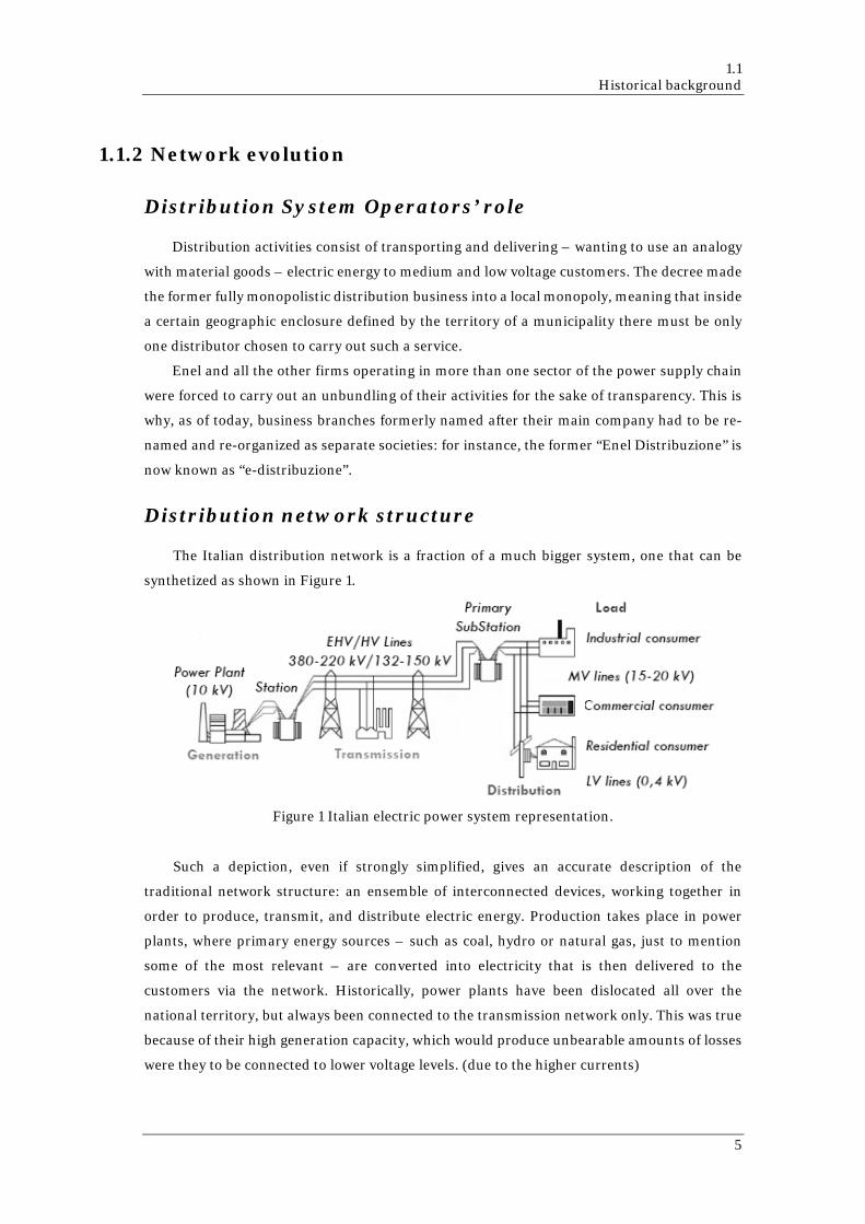
Figure 1 Italian electric power system representation.
Such a depiction, even if strongly simplified, gives an accurate description of the
traditional network structure: an ensemble of interconnected devices, working together in
order to produce, transmit, and distribute electric energy. Production takes place in power
plants, where primary energy sources – such as coal, hydro or natural gas, just to mention
some of the most relevant – are converted into electricity that is then delivered to the
customers via the network. Historically, power plants have been dislocated all over the
national territory, but always been connected to the transmission network only. This was true
because of their high generation capacity, which would produce unbearable amounts of losses
were they to be connected to lower voltage levels. (due to the higher currents)
5
0Chapter 1 DG penetration and PMUs
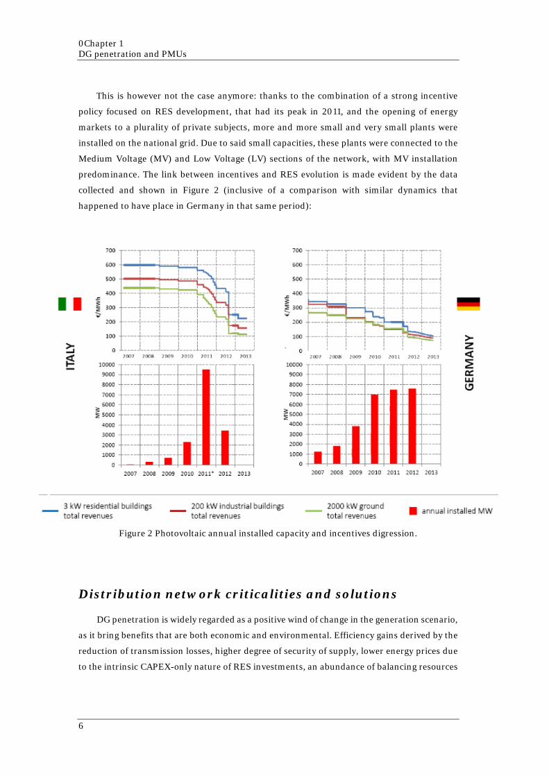
This is however not the case anymore: thanks to the combination of a strong incentive
policy focused on RES development, that had its peak in 2011, and the opening of energy
markets to a plurality of private subjects, more and more small and very small plants were
installed on the national grid. Due to said small capacities, these plants were connected to the
Medium Voltage (MV) and Low Voltage (LV) sections of the network, with MV installation
predominance. The link between incentives and RES evolution is made evident by the data
collected and shown in Figure 2 (inclusive of a comparison with similar dynamics that
happened to have place in Germany in that same period):
Figure 2 Photovoltaic annual installed capacity and incentives digression.
Distribution network criticalities and solutions
DG penetration is widely regarded as a positive wind of change in the generation scenario,
as it bring benefits that are both economic and environmental. Efficiency gains derived by the
reduction of transmission losses, higher degree of security of supply, lower energy prices due
to the intrinsic CAPEX-only nature of RES investments, an abundance of balancing resources
6

1.1 Historical background
from a new category of ancillary services providers (the prosumers) can be considered
economic benefits, while CO2 emissions reduction – whether it is from the generation process
(less burnt coal or natural gas), the transportation industry (electrical vehicles spread) or the
domestic environment (self-consumption for house heating/cooling) – are the environmental
benefits.
Unfortunately, benefits do not come alone in this case. Distributed generation brought
new problems with it, or worsened old ones. The following is a list of such known matters, to
underline their link to the DG penetration issue:
• Reverse Power Flow (RPF);
• Unwanted islanding;
• Instability due to RES volatility;
• Network saturation (lines+transformers);
• Selectivity issues (line protection devices);
• Voltage regulation issues (slow/fast);
• Frequency regulation issues;
• Higher degree of complexity and management/reinforcement costs (telecoms/hosting
capacity);
• Regulatory framework adaptation.
In simple terms, the public electrical grid was originally designed to deliver power in a
uni-directional fashion: from a few big plants, into the grid and then to the final customer to
consume. Nowadays, however, more and more customers are operating power generating
devices – such as solar panels, windmills, etc. – for self-consumption and/or to generate
income by feeding power into the grid from their end. As the electric utility cannot deny by law
the this energy injection, that is on the contrary incentivized, system operators need to make
sure that it does not damage the network or prejudice its good functioning.
On-field technicians and experts alike provided numerous possible solutions to every
problem on the previously mentioned list, each one with its pros and cons. Just to clarify the
amount of proposed viable actions to solve a single issue, voltage regulation ones are taken in
consideration as an example and their solving measures are shown in the following: (a
distinction is made between slow and fast variations)
• Network reconfiguration: (slow and fast)
o Pros: cheap, easy, fast, dynamic;
o Cons: only in MV, only for low penetration of DGs.
• Network reinforcement: (slow and fast)
7

0Chapter 1 DG penetration and PMUs
o Pros: always an option, both for LV and MV, simple;
o Cons: expensive, slow permission/construction iter, static.
• On-load tap changer: (slow)
o Pros: simple, dynamic, relatively cheap;
o Cons: problems with increasing penetration.
• Booster transformers: (slow)
o Pros: simple, both for MV and LV, relatively cheap;
o Cons: static, slow installation.
• Reactive compensation: (slow)
o Pros: simple, both for MV and LV;
o Cons: must be coordinated with OLTC and load/generation;
• Storage systems: (slow and fast)
o Pros: both for MV and LV, dynamic, allows advanced management;
o Cons: expensive and space consuming.
• Advanced voltage control: (slow and fast)
o Pros: highly dynamic and adaptive, it’s a set of different tools;
o Cons: costs, TLC, complex, Smart architecture/regulation needed.
• Advanced closed-loop operation: (slow and fast)
o Pros: those of loop configurations; (e.g. power/voltage stability)
o Cons: Smart architecture/regulation needed, rarely seen in MV.
As it can be seen, there are both simple but scarcely efficient measures and effective but
complex ones. Proposals from the two categories can be combined in order to obtain a good
final result, however both their advantages and disadvantages will overlap. Any mixed solution
would then be quite complex to manage, both in terms of needed starting data collection and
delivery. This is the reason why modern management and control systems rely more and more
on telecommunications and distributed intelligence, hence the development of Smart Grids
and companion devices capable of providing the data that said Smart Grid would help to
collect, transmit and elaborate on.
Among those many devices, there is one believed to be able to exponentially increase the
efficiency of monitoring and control system if properly used. This instrument and its possible
applications are the subject of the present study: it is the “Phasor Measurement Unit”.
8
1.2 Theoretical premise
1.2 Theoretical premise
In order to understand the full extension of PMUs’ potential in system management and
control applications, the first thing needed is an in-depth understanding of the theoretical
basis upon which these devices are built.
1.2.1 Phasor theory outlines
Electrical data analysis often requires comparisons between time-variant quantities in
order to extract meaningful results from raw data. An example of such need is the case in which
the voltage of an impedance must be compared to the current flowing through it in order to
compute energy consumption or define the nature of the load. A common way to differentiate
between capacitive and inductive load is, in fact, checking the angular difference between its
measured voltage and current waveforms, given that they are at the same frequency. Once a
zero-angle reference is set, then the two quantities can be compared graphically or by analyzing
their expressions in the time domain (Eq. 1 shows the generic form for a sine wave), and in
particular the phase parameter φ:
𝐴𝐴(𝑡𝑡) = 𝐴𝐴𝑚𝑚 sin(𝜔𝜔𝑡𝑡 ± 𝜑𝜑) Eq. 1
This comparison is however not very intuitive, and mathematical operations turn out to
be quite difficult to conduct in the time domain. One way to overcome these problems is to
represent the sinusoids graphically within the phasor-domain form by using phasor diagrams,
and this is achieved by the rotating vector method.
Basically, a “phasor” is a rotating vector whose length represents an AC quantity’s
magnitude and whose direction represents, with respect to a reference angle, its phase. While
the AC quantity is time-variant, the phasor representation is instead static, as if frozen at some
point in time. Normally, phasors are assumed to pivot at one end around a fixed point known
as “the point of origin”, freely rotating in anti-clockwise direction at an angular velocity ω=2πf,
where f is the frequency of the waveform.
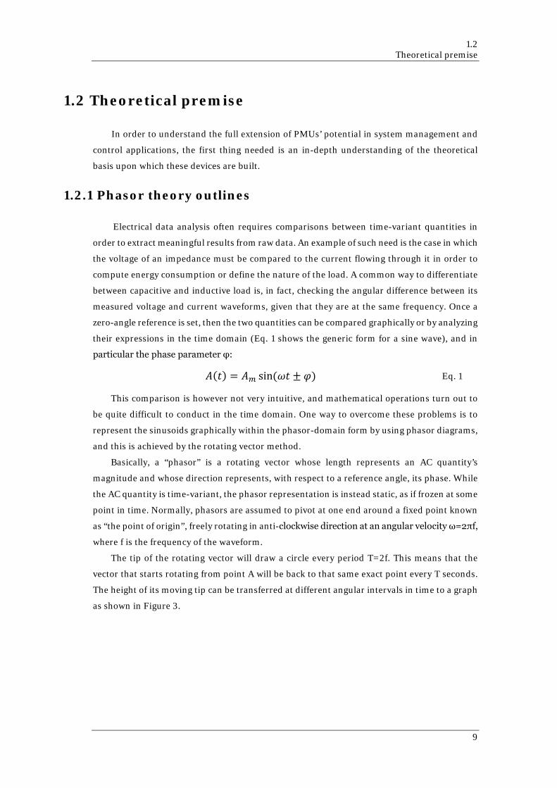
The tip of the rotating vector will draw a circle every period T=2f. This means that the
vector that starts rotating from point A will be back to that same exact point every T seconds.
The height of its moving tip can be transferred at different angular intervals in time to a graph
as shown in Figure 3.
9
0Chapter 1 DG penetration and PMUs
Figure 3 Phasor-wave relationship explained by graphical means.
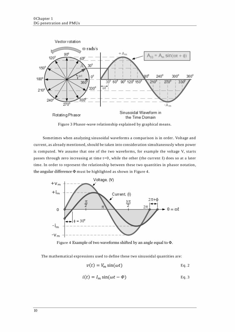
Sometimes when analyzing sinusoidal waveforms a comparison is in order. Voltage and
current, as already mentioned, should be taken into consideration simultaneously when power
is computed. We assume that one of the two waveforms, for example the voltage V, starts
passes through zero increasing at time t=0, while the other (the current I) does so at a later
time. In order to represent the relationship between these two quantities in phasor notation,
the angular difference Φ must be highlighted as shown in Figure 4.
Figure 4 Example of two waveforms shifted by an angle equal to Φ.
The mathematical expressions used to define these two sinusoidal quantities are:
𝑣𝑣(𝑡𝑡) = 𝑉𝑉𝑚𝑚 sin(𝜔𝜔𝑡𝑡) Eq. 2
𝑖𝑖(𝑡𝑡) = 𝐼𝐼𝑚𝑚 sin(𝜔𝜔𝑡𝑡 − 𝛷𝛷) Eq. 3
10

1.2 Theoretical premise
The current is lagging with respect to the voltage by an angle Φ=30. This same angle will
be the phase difference between the two corresponding phasors, that can be represented
together as in Figure 5.
Figure 5 Phasorial representation of the two waveforms seen in Figure 4.
The phasor diagram – this is the name of such a depiction – is drawn as if the two rotating
vectors were frozen at time t=o. Since the rotation’s direction is anti-clockwise, the phase
difference Φ is measured in that same direction.
To understand why phasors are considered to be essential tools in the study of electric
phenomena, a simple applicative example is in order.
Circuital analysis often leads to the need to sum two sine waveforms. If they are in phase,
that is if their phase difference Φ=0, then they can be combined as it happens with DC
quantities through an algebraic sum of the respective waveforms or vectors at any given
moment in time. For example, if two voltages of 50 V and 25 V of magnitude respectively are
in phase, the resultant vector that will be formed by their combinations is going to be one with
a 75 V of magnitude.
If however the two waveforms are not in phase, this simple computational procedure
cannot and be followed. Phase difference must be taken into account, and this is much easier
analyzing the problem with phasorial representation. The method applied in this case is the
vector sum, carried out graphically using the parallelogram law as shown in Figure 6.
11
0Chapter 1 DG penetration and PMUs
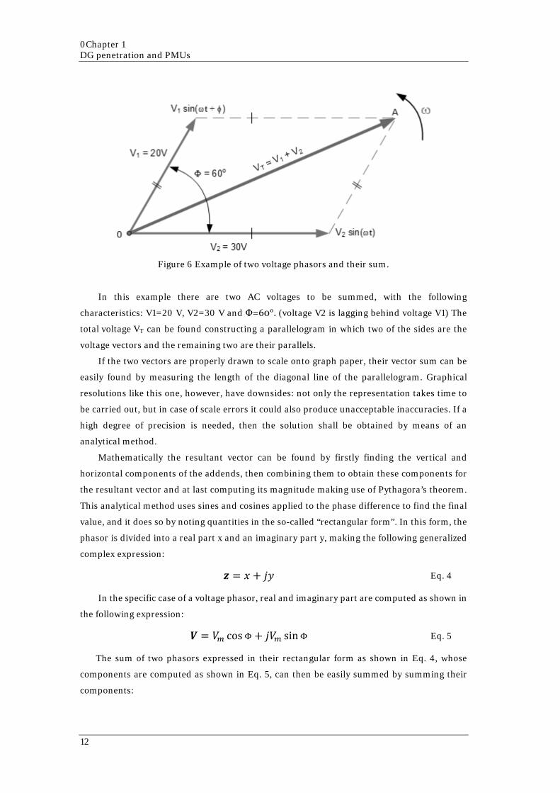
Figure 6 Example of two voltage phasors and their sum.
In this example there are two AC voltages to be summed, with the following
characteristics: V1=20 V, V2=30 V and Φ=60°. (voltage V2 is lagging behind voltage V1) The
total voltage VT can be found constructing a parallelogram in which two of the sides are the
voltage vectors and the remaining two are their parallels.
If the two vectors are properly drawn to scale onto graph paper, their vector sum can be
easily found by measuring the length of the diagonal line of the parallelogram. Graphical
resolutions like this one, however, have downsides: not only the representation takes time to
be carried out, but in case of scale errors it could also produce unacceptable inaccuracies. If a
high degree of precision is needed, then the solution shall be obtained by means of an
analytical method.
Mathematically the resultant vector can be found by firstly finding the vertical and
horizontal components of the addends, then combining them to obtain these components for
the resultant vector and at last computing its magnitude making use of Pythagora’s theorem.
This analytical method uses sines and cosines applied to the phase difference to find the final
value, and it does so by noting quantities in the so-called “rectangular form”. In this form, the
phasor is divided into a real part x and an imaginary part y, making the following generalized
complex expression:
𝒛𝒛 = 𝑥𝑥 + 𝑗𝑗𝑗𝑗 Eq. 4
In the specific case of a voltage phasor, real and imaginary part are computed as shown in
the following expression:
𝑽𝑽 = 𝑉𝑉𝑚𝑚 cosΦ + 𝑗𝑗𝑉𝑉𝑚𝑚 sinΦ Eq. 5
The sum of two phasors expressed in their rectangular form as shown in Eq. 4, whose
components are computed as shown in Eq. 5, can then be easily summed by summing their
components:
12
1.2 Theoretical premise
𝑨𝑨 = 𝑥𝑥 + 𝑗𝑗𝑗𝑗 Eq. 6
𝑩𝑩 = 𝑤𝑤 + 𝑗𝑗𝑗𝑗 Eq. 7
𝑨𝑨 + 𝑩𝑩 = (𝑥𝑥 + 𝑤𝑤) + 𝑗𝑗(𝑗𝑗 + 𝑗𝑗) Eq. 8
The example of Figure 6 and its data are taken into consideration and a computational
example is made. Voltage V2 lays on the zero-angle reference, so its vertical component is null.
Hence, using Eq. 5 we obtain the following rectangular expression:
𝑽𝑽𝟐𝟐 = 30 cos(0°) + 𝑗𝑗30 sin(0) = (30 + 𝑗𝑗0) 𝑉𝑉 Eq. 9
The same computation can be made for voltage V1, which leads V2 by 60°:
𝑽𝑽𝟏𝟏 = 20 cos(60°) + 𝑗𝑗20 sin(60°) = (10 + 𝑗𝑗17.32) 𝑉𝑉 Eq. 10
Now, as explained, in order to obtain the resultant voltage VT a vector sum is made, that is
adding component by component the two vectors:
𝑽𝑽𝑻𝑻 = 𝑽𝑽𝟏𝟏 + 𝑽𝑽𝟐𝟐 = (30 + 𝑗𝑗0) + (10 + 𝑗𝑗17.32) = (40 + 𝑗𝑗17.32) 𝑉𝑉 Eq. 11
Now that both the real and imaginary values have been found, the magnitude of voltage
VT is determined by simply using Pythagora’s Theorem as follows:
𝑉𝑉𝑇𝑇 = �402 + 17.322 = 43.6 𝑉𝑉 Eq. 12
Similar is the procedure for vector subtractions, while other operations – such as
multiplication or exponentiation – is a little more complex.
1.2.2 Phasor Measurement Units
Phasor Measurement Units (PMU), sometimes wrongly addressed as “Synchrophasors”,
are power system measuring devices capable of collecting data from the electricity grid in a far
more precise and fast fashion when compared to traditional equipment. This is possible thanks
to the use of a common time source for data synchronization, meaning that every measurement
made by PMUs spread all over the network will be provided of an accurate time-stamp which
allows to exploit the potential of big data time correlation.
Phasors had been known and used for almost an entire century before the invention of
Phasor Measurement Units, since Charles Proteus Steinmetz developed the already discussed
phasor theory in 1893, while Dr. Arun G. Phadke and Dr. James S. Thorp designed the first
PMU in 1988 and built the first prototype in 1992. This device had already most of the basic
features modern models have, including of course the calculation of real-time phasors
synchronized to an absolute time reference provided by the Global Positioning System. (GPS)
13
0Chapter 1 DG penetration and PMUs
Historically, however, the absence of a proper telecommunication infrastructure, capable
of managing the massive amount of data produced and exchanged by PMUs times short
enough to be acceptable, prevented the growth of this technology. Another reason for its slow
development was the general lack of need for it: up until twenty years ago, in fact, power was
being delivered in a uni-lateral fashion through passive components to customers, so there
was no interest in collecting great amounts of real-time data for monitoring and control
purposes since passive grids’ management is relatively simple. However, in more recent years,
the exponential growth of distributed generation resources on the peripheral parts of electric
networks all over the world changed the scenario. This newly emerged condition made it
imperative to continuously observe both transmission and distribution networks through
advanced sensor technology, namely the PMUs.
From a technical point of view, the following are the most noteworthy characteristics of a
modern PMU system:
• High speed GPS-synchronized waveforms sampling – up to 50 samples per cycle – for
50/60 Hz three-phase voltages and currents, with subsequent signal digitalization;
• Top notch clock accuracy, down to one microsecond, that can be provided by
alternative/additional sources other than GPS if reliable enough;
• High rate time-stamped phasors transmission from widely dispersed locations to local
receivers, up to 30 observations per second; (compared to one every four seconds
using conventional technology)
• Collection of a wide range of data, including three-phase voltage magnitudes and
phases, three-phase current magnitudes and phases, frequency and Rate Of Change
Of Frequency (ROCOF) with respect to time.
Phasor measurements that occur at the same time are called “synchrophasors”. While it is
commonplace for the terms “PMU” and “synchrophasor” to be used interchangeably, they
actually represent two separate technical meanings: the latter is the metered value, whereas
the former is the metering device.
Thanks to the high degree of synchronization, collected data can be put in a meaningful
comparison in order to assess system conditions via parameters that would be otherwise
impossible (if not harmful) to use together, such as voltage magnitude differences and phase
shifts. The system operators can monitor the grid with any number of PMUs, but their number
and positioning are important parameters: few well-placed devices can provide good results if
used in small networks or assisted by very efficient state estimators to fill the data-gaps in non-
monitored nodes. Experience has however proved that, even in case of good positioning, the
use of PMUs from multiple vendors could yield inaccurate results due to the immaturity of the
relative standardization framework.
14
1.2 Theoretical premise
Telecommunication infrastructure
Traditional power system network monitoring tools use data coming from Remote
Terminal Units (RTUs), protective relays and transducers to provide useful information to
system operators. This information often proves to be vital for the operation of the power
system, both under normal and contingency conditions. However, the mechanism most
commonly used to obtain said data from the measuring devices – the Supervisory Control And
Data Acquisition (SCADA) system – is asynchronous and relatively slow, implying that the
obtained system representation is accurate enough during normal steady-conditions but lacks
in reliability when fast dynamics are to be taken into account.
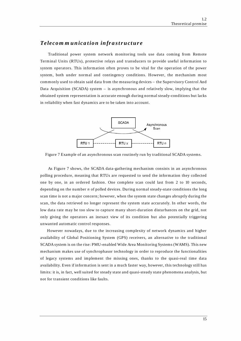
Figure 7 Example of an asynchronous scan routinely run by traditional SCADA systems.
As Figure 7 shows, the SCADA data-gathering mechanism consists in an asynchronous
polling procedure, meaning that RTUs are requested to send the information they collected
one by one, in an ordered fashion. One complete scan could last from 2 to 10 seconds,
depending on the number n of polled devices. During normal steady-state conditions the long
scan time is not a major concern; however, when the system state changes abruptly during the
scan, the data retrieved no longer represent the system state accurately. In other words, the
low data rate may be too slow to capture many short-duration disturbances on the grid, not
only giving the operators an inexact view of its condition but also potentially triggering
unwanted automatic control responses.
However nowadays, due to the increasing complexity of network dynamics and higher
availability of Global Positioning System (GPS) receivers, an alternative to the traditional
SCADA system is on the rise: PMU-enabled Wide Area Monitoring Systems (WAMS). This new
mechanism makes use of synchrophasor technology in order to reproduce the functionalities
of legacy systems and implement the missing ones, thanks to the quasi-real time data
availability. Even if information is sent in a much faster way, however, this technology still has
limits: it is, in fact, well suited for steady state and quasi-steady state phenomena analysis, but
not for transient conditions like faults.
15
0Chapter 1 DG penetration and PMUs
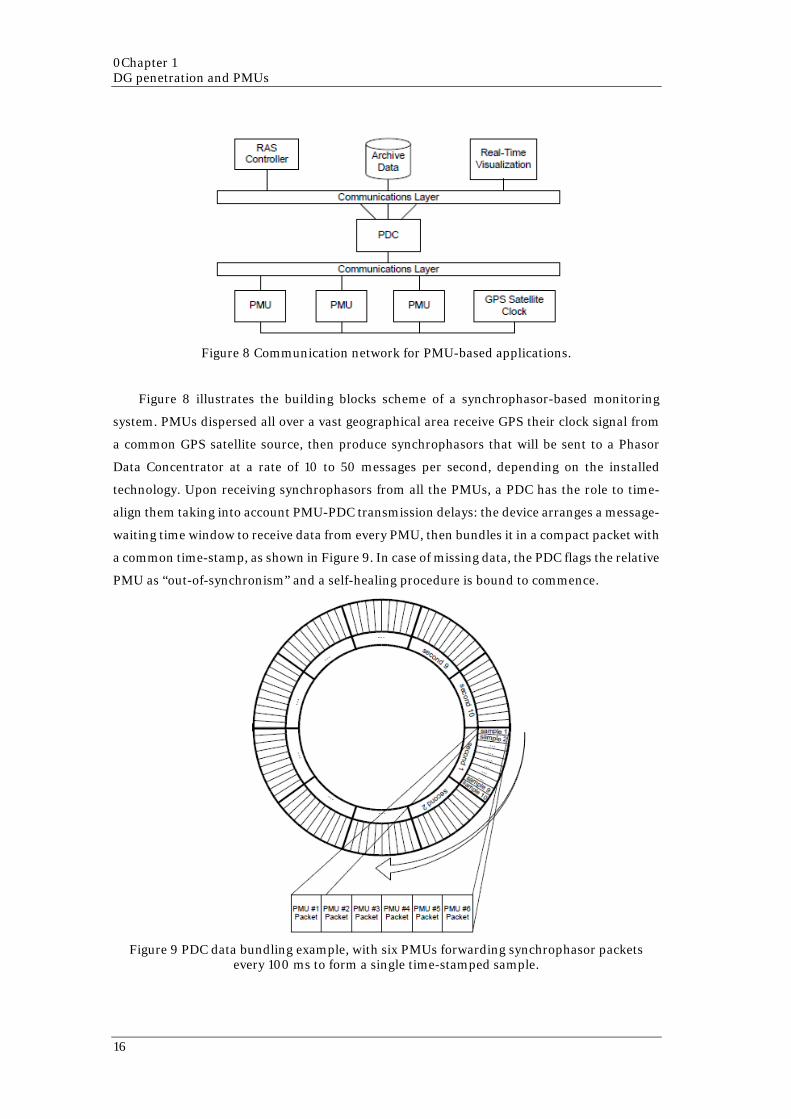
Figure 8 Communication network for PMU-based applications.
Figure 8 illustrates the building blocks scheme of a synchrophasor-based monitoring
system. PMUs dispersed all over a vast geographical area receive GPS their clock signal from
a common GPS satellite source, then produce synchrophasors that will be sent to a Phasor
Data Concentrator at a rate of 10 to 50 messages per second, depending on the installed
technology. Upon receiving synchrophasors from all the PMUs, a PDC has the role to time-
align them taking into account PMU-PDC transmission delays: the device arranges a message-
waiting time window to receive data from every PMU, then bundles it in a compact packet with
a common time-stamp, as shown in Figure 9. In case of missing data, the PDC flags the relative
PMU as “out-of-synchronism” and a self-healing procedure is bound to commence.
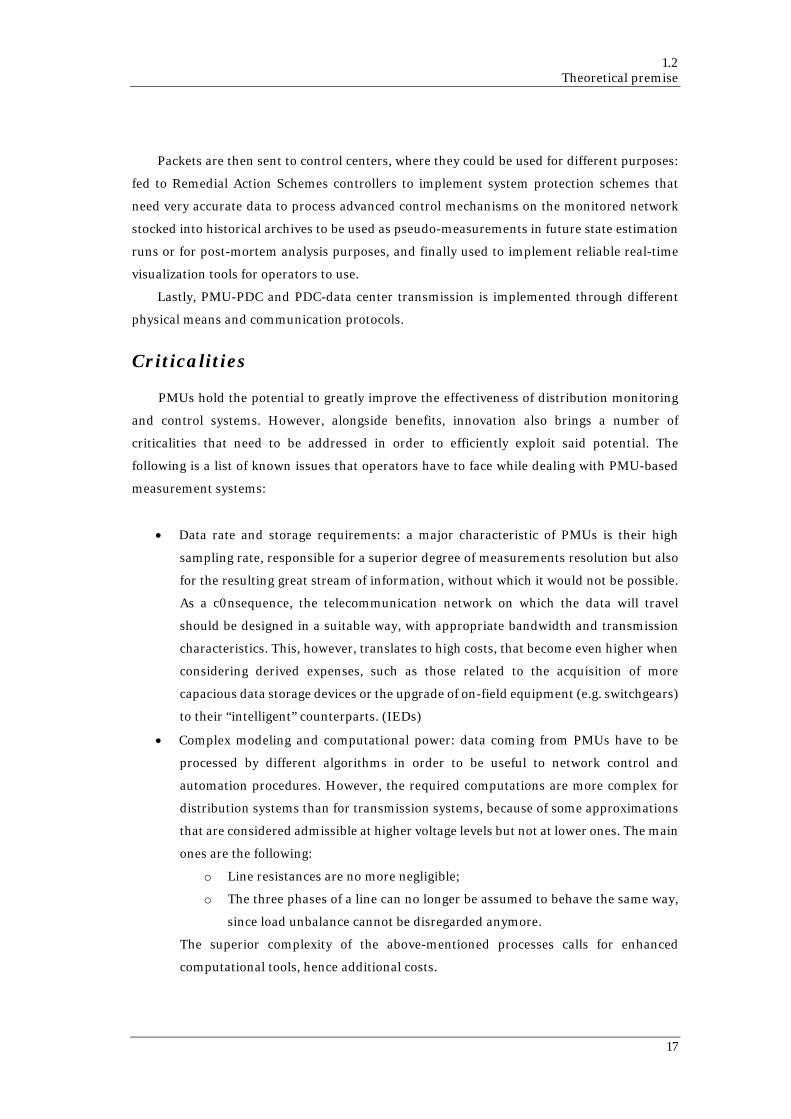
Figure 9 PDC data bundling example, with six PMUs forwarding synchrophasor packets
every 100 ms to form a single time-stamped sample.
16
1.2 Theoretical premise
Packets are then sent to control centers, where they could be used for different purposes:
fed to Remedial Action Schemes controllers to implement system protection schemes that
need very accurate data to process advanced control mechanisms on the monitored network
stocked into historical archives to be used as pseudo-measurements in future state estimation
runs or for post-mortem analysis purposes, and finally used to implement reliable real-time
visualization tools for operators to use.
Lastly, PMU-PDC and PDC-data center transmission is implemented through different
physical means and communication protocols.
Criticalities
PMUs hold the potential to greatly improve the effectiveness of distribution monitoring
and control systems. However, alongside benefits, innovation also brings a number of
criticalities that need to be addressed in order to efficiently exploit said potential. The
following is a list of known issues that operators have to face while dealing with PMU-based
measurement systems:
• Data rate and storage requirements: a major characteristic of PMUs is their high
sampling rate, responsible for a superior degree of measurements resolution but also
for the resulting great stream of information, without which it would not be possible.
As a c0nsequence, the telecommunication network on which the data will travel
should be designed in a suitable way, with appropriate bandwidth and transmission
characteristics. This, however, translates to high costs, that become even higher when
considering derived expenses, such as those related to the acquisition of more
capacious data storage devices or the upgrade of on-field equipment (e.g. switchgears)
to their “intelligent” counterparts. (IEDs)
• Complex modeling and computational power: data coming from PMUs have to be
processed by different algorithms in order to be useful to network control and
automation procedures. However, the required computations are more complex for
distribution systems than for transmission systems, because of some approximations
that are considered admissible at higher voltage levels but not at lower ones. The main
ones are the following:
o Line resistances are no more negligible;
o The three phases of a line can no longer be assumed to behave the same way,
since load unbalance cannot be disregarded anymore.
The superior complexity of the above-mentioned processes calls for enhanced
computational tools, hence additional costs.
17
0Chapter 1 DG penetration and PMUs
• Cyber-security risk: the more information travels along a communication line, the
more it is susceptible to intentional external influences or theft. The data-flow must
be protected from such dangers, in order to preserve own or customers’ sensible data
from industrial espionage or sabotage attempts. This is not, however, a costless effort
since it requires technical expertise that was not needed with legacy system.
• Optimized device placement: a PMU network is no different from a traditional
measurement system under the device-positioning point of view. State estimators, in
fact, are known to produce more accurate results when measurement are provided by
specific nodes. In order to pinpoint such optimal installation points for PMUs,
however, it is impossible to use the same algorithms used the SCADA system so new
ones need to be developed.
• Physical differences with respect to the transmission network: most of the available
knowledge about PMUs and their use nowadays comes from experience matured
through applications on the high voltage networks, where they were first introduced.
This experience, however, cannot be fully exploited for MV installations, due to the
differences between the two grid typologies. Higher degree of measurement accuracy
is required for lower voltage installations, for example, since shorter distances
between distribution networks’ nodes imply smaller amplitude and phase differences
between the respective synchrophasors: in order to properly compare them, μPMUs
need to be accurate to the tenth of a degree.
Another aspect to take into consideration is the faster dynamics that are to be expected
when dealing with Smart Grids (e.g. the intermittent behavior of generators, loads and
storage devices), which may require time responsiveness beyond the limits defined by
the current standards, since those refer to PMUs used in HV.
18
CHAPTER 2
POTENTIAL PMU APPLICATIONS ON
DISTRIBUTION NETWORKS
So far, synchrophasors have been considered “a solution waiting for a problem”. Their
undeniable theoretical potential has been in fact mostly ignored due to economic reasons and
limitations derived from the luck of a suitable telecommunication infrastructure, but also by a
lack of need for such advanced measurement tools. Historically, in fact, passive networks did
not require real-time monitoring and control. However, as already mentioned, in time the
evolution of distributed energy resources gave birth to new problems that could be addressed
by the implementation of PMU systems. The truth is, however, that synchrophasors are a tool
that may or may not be appropriate to solve said problems. This is where research and
experimentation come in, and this chapter’s aim in particular is to verify the feasibility of a
number of possible PMUs’ applications on the Italian distribution grid, evaluate their
advantages and disadvantages and compare them to alternative solutions already in place
(both from a technical and an financial standpoint).
2.1 Anti-islanding
Islanding is a condition where a part of the power system, consisting of both loads and
generation, becomes isolated from the rest of the power grid, and generators continue to
energize the isolated network. [1] Two types of islanding can occur in a power system:
intentional islanding or unintentional islanding. The former is performed for either
maintenance or load-shedding purposes to protect the rest of the power grid and avoid a
blackout, with the isolated generators operating in voltage and frequency control mode to
provide constant voltage to local loads while maintaining the isolated grid frequency; the
19
0CHAPTER 2 Potential pmu applications on distribution networks
latter, instead, occurs due to equipment failure or severe faults resulting in the opening of
circuit breakers that interconnect the island with the rest of the power system. Unintentional
islanding may result in hazards in power system operation and may lead to safety risks for
maintenance staff. In addition, during unintentional islanding, the isolated network suffers
from significant voltage and frequency variations that can damage both loads and generators
within the island. Furthermore, the autoreclosure of the tie line, which is a standard and
automated procedure followed in case of temporary faults, results in out-of-phase and
unsynchronized reclosing when the system is subject to unintentional islanding.
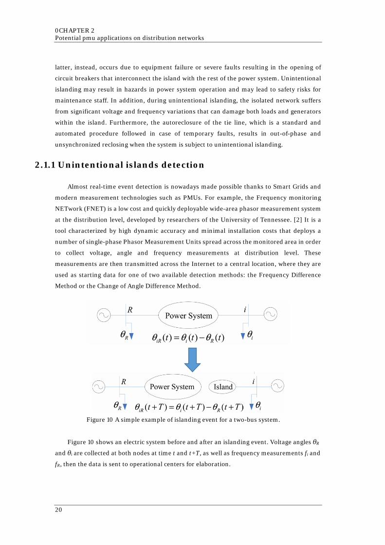
2.1.1 Unintentional islands detection
Almost real-time event detection is nowadays made possible thanks to Smart Grids and
modern measurement technologies such as PMUs. For example, the Frequency monitoring
NETwork (FNET) is a low cost and quickly deployable wide-area phasor measurement system
at the distribution level, developed by researchers of the University of Tennessee. [2] It is a
tool characterized by high dynamic accuracy and minimal installation costs that deploys a
number of single-phase Phasor Measurement Units spread across the monitored area in order
to collect voltage, angle and frequency measurements at distribution level. These
measurements are then transmitted across the Internet to a central location, where they are
used as starting data for one of two available detection methods: the Frequency Difference
Method or the Change of Angle Difference Method.
Figure 10 A simple example of islanding event for a two-bus system.
Figure 10 shows an electric system before and after an islanding event. Voltage angles θR
and θi are collected at both nodes at time t and t+T, as well as frequency measurements fi and
fR, then the data is sent to operational centers for elaboration.
20
2.1 Anti-islanding
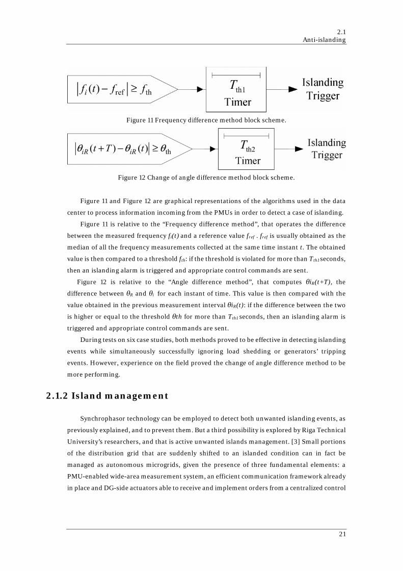
Figure 11 Frequency difference method block scheme.
Figure 12 Change of angle difference method block scheme.
Figure 11 and Figure 12 are graphical representations of the algorithms used in the data
center to process information incoming from the PMUs in order to detect a case of islanding.
Figure 11 is relative to the “Frequency difference method”, that operates the difference
between the measured frequency fi(t) and a reference value fref . fref is usually obtained as the
median of all the frequency measurements collected at the same time instant t. The obtained
value is then compared to a threshold fth: if the threshold is violated for more than Tth1 seconds,
then an islanding alarm is triggered and appropriate control commands are sent.
Figure 12 is relative to the “Angle difference method”, that computes θiR(t+T), the
difference between θR and θi for each instant of time. This value is then compared with the
value obtained in the previous measurement interval θiR(t): if the difference between the two
is higher or equal to the threshold θth for more than Tth1 seconds, then an islanding alarm is
triggered and appropriate control commands are sent.
During tests on six case studies, both methods proved to be effective in detecting islanding
events while simultaneously successfully ignoring load shedding or generators’ tripping
events. However, experience on the field proved the change of angle difference method to be
more performing.
2.1.2 Island management
Synchrophasor technology can be employed to detect both unwanted islanding events, as
previously explained, and to prevent them. But a third possibility is explored by Riga Technical
University’s researchers, and that is active unwanted islands management. [3] Small portions
of the distribution grid that are suddenly shifted to an islanded condition can in fact be
managed as autonomous microgrids, given the presence of three fundamental elements: a
PMU-enabled wide-area measurement system, an efficient communication framework already
in place and DG-side actuators able to receive and implement orders from a centralized control
21

0CHAPTER 2 Potential pmu applications on distribution networks
room. Distributed generators whose communications are not cut off by the islanding
phenomenon can in fact balance their output in response to the sudden event that caused it,
thanks to the very fast readings of PMUs placed in the island itself. If suitably placed, the
measurements of these devices can be elaborated by a remote control system that
automatically computes the new production profiles that generators have to follow in order to
maintain balance, or by a local intelligent device able to at least implement pre-determined
algorithms selected as a function of the specific scenario.
Furthermore, these very same devices could be useful during the restoration phase. When
the criticality that caused the creation of the island in the first place is solved, the open breaker
must be closed with great caution since the island is still energized. This means that the voltage
phasors may not be synchronized with those of the main grid and a sudden reclosure could
lead to a plethora of negative consequences, ranging from temporary voltage instability to
dangerous high currents. All this is made possible only thanks to the quick response of PMUs,
that provide data at a rate high enough to react to fast dynamic events such as the creation of
an unwanted island.
2.2 Phase identification
As service quality becomes a more important issue to engineers and regulators, the simple
matter of phase identification becomes more important than it was decades ago. Having
improper phase identification can lead to issues with load balance, fault location, metering and
other reliability issues. However, even in case of relatively simple distribution junction – such
as the one shown in Figure 13 –, it is clear that phase identification is not a trivial matter.
Figure 13 Dual feed and underground transition on distribution feeder.
22
2.3 Model validation
While it is true that phase identification tools are already available to operators to use on
the field, it is also true that employing a team of technicians every time phase information is
needed often proves to be a waste of both time and money. PMUs could solve the problem,
thanks to their unique angle measurement feature, but devices should be installed on a huge
number of nodes and the cost/benefit ratio is definitely too high to justify such an investment.
[4] However, if PMUs were to be deployed for different purposes, then the phase identification
capability would be a very well welcomed side effect. Its advent would not only bring
improvements to load balancing and fault detection, as already mentioned, but also be useful
in the future when advanced tripping techniques – such as the adaptive multi-phase tripping
or the single-phase tripping – will be implemented in the network control systems.
Backfeeding automation schemes would also greatly benefit from this data, since to backfeed
any portion of the distribution grid a well-timed closure of the end-switch is needed in order
to avoid damages to the system.
2.3 Model validation
Network topology, that is the ensemble of data regarding lines and devices belonging to a
portion of the distribution grid and their connection, is a fundamental piece of information for
system operators. Not only grid management systems are easier to program and utilize when
technicians have a clear and user-friendly virtual representation of the physical grid thanks to
the information stored in dedicated databases, but also the automation itself would be
impossible to be effectively implemented without a precise knowledge of every part of the
system under control. Operators rely on system models to know how power flows will change
as a result of manual or relay-initiated changes to topology – such as line tripping, capacitor
bank insertion or generator starting. Accurate knowledge of the response of the grid in terms
of energy flows as a result of topology variations is vital to both economic optimization and
security of system assets.
Network characteristics, however, change with time. And if it is true that databases are
periodically updated in order to provide the most accurate picture of the current status, it is
also true that traditional inspection methods are not always reliable: assets aging, unrecorded
switching and undetected capacitive insertions are only some of the elements that may turn an
otherwise trustworthy network depiction into an unreliable, and therefore unusable,
representation. Hence, a model validation tool would be needed in order to guarantee optimal
and secure network management.
One way to guarantee the validity of a database-stored model is to frequently update its
data with new information coming from the grid, but this is not always possible. Measurement
23
0CHAPTER 2 Potential pmu applications on distribution networks
of lines’ impedances, for example, are not operated frequently; on the contrary, sometimes
their virtual values are set when they are constructed and never changed thereafter. And even
when changes are recorded with appropriate regularity, the scan output could still suffer from
inaccuracies due to the slowness of legacy methods. To cope with these issues, a PMU-based
wide area measurement system would be extremely useful, as will be proved by the following
example of a fast line impedance value’s update method. [5]
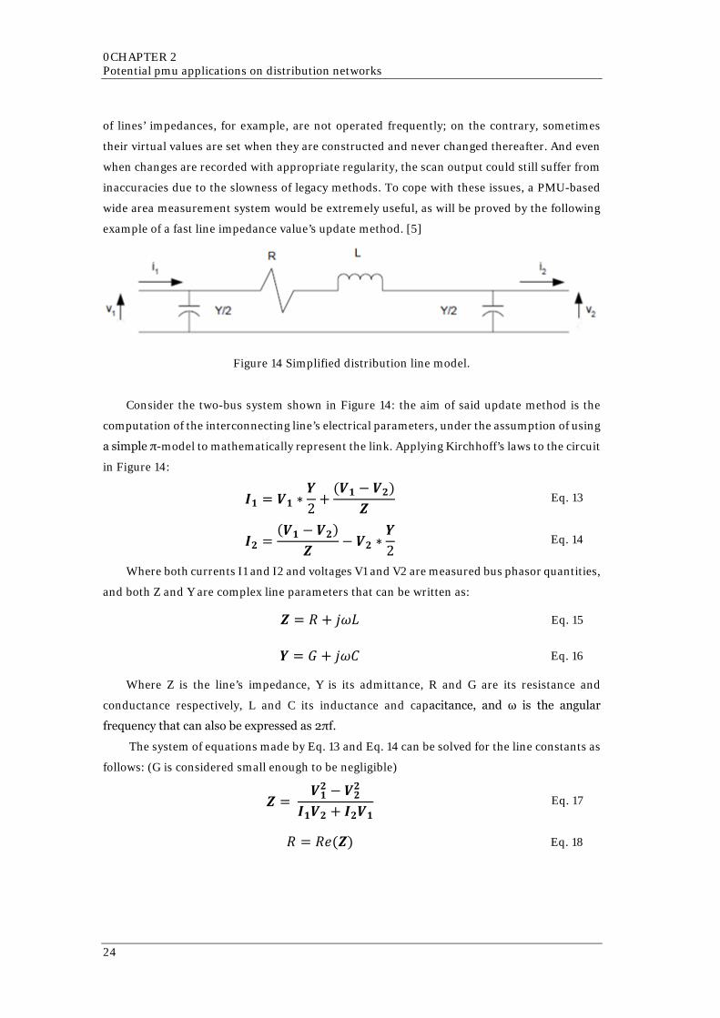
Figure 14 Simplified distribution line model.
Consider the two-bus system shown in Figure 14: the aim of said update method is the
computation of the interconnecting line’s electrical parameters, under the assumption of using
a simple π-model to mathematically represent the link. Applying Kirchhoff’s laws to the circuit
in Figure 14:
𝑰𝑰𝟏𝟏 = 𝑽𝑽𝟏𝟏 ∗𝒀𝒀2
+(𝑽𝑽𝟏𝟏 − 𝑽𝑽𝟐𝟐)
𝒁𝒁 Eq. 13
𝑰𝑰𝟐𝟐 =(𝑽𝑽𝟏𝟏 − 𝑽𝑽𝟐𝟐)
𝒁𝒁− 𝑽𝑽𝟐𝟐 ∗
𝒀𝒀2
Eq. 14
Where both currents I1 and I2 and voltages V1 and V2 are measured bus phasor quantities,
and both Z and Y are complex line parameters that can be written as:
𝒁𝒁 = 𝑅𝑅 + 𝑗𝑗𝜔𝜔𝑗𝑗 Eq. 15
𝒀𝒀 = 𝐺𝐺 + 𝑗𝑗𝜔𝜔𝑗𝑗 Eq. 16
Where Z is the line’s impedance, Y is its admittance, R and G are its resistance and
conductance respectively, L and C its inductance and capacitance, and ω is the angular
frequency that can also be expressed as 2πf.
The system of equations made by Eq. 13 and Eq. 14 can be solved for the line constants as
follows: (G is considered small enough to be negligible)
𝒁𝒁 = 𝑽𝑽𝟏𝟏𝟐𝟐 − 𝑽𝑽𝟐𝟐𝟐𝟐
𝑰𝑰𝟏𝟏𝑽𝑽𝟐𝟐 + 𝑰𝑰𝟐𝟐𝑽𝑽𝟏𝟏 Eq. 17
𝑅𝑅 = 𝑅𝑅𝑅𝑅(𝒁𝒁) Eq. 18
24
2.4 Low frequency oscillations detection
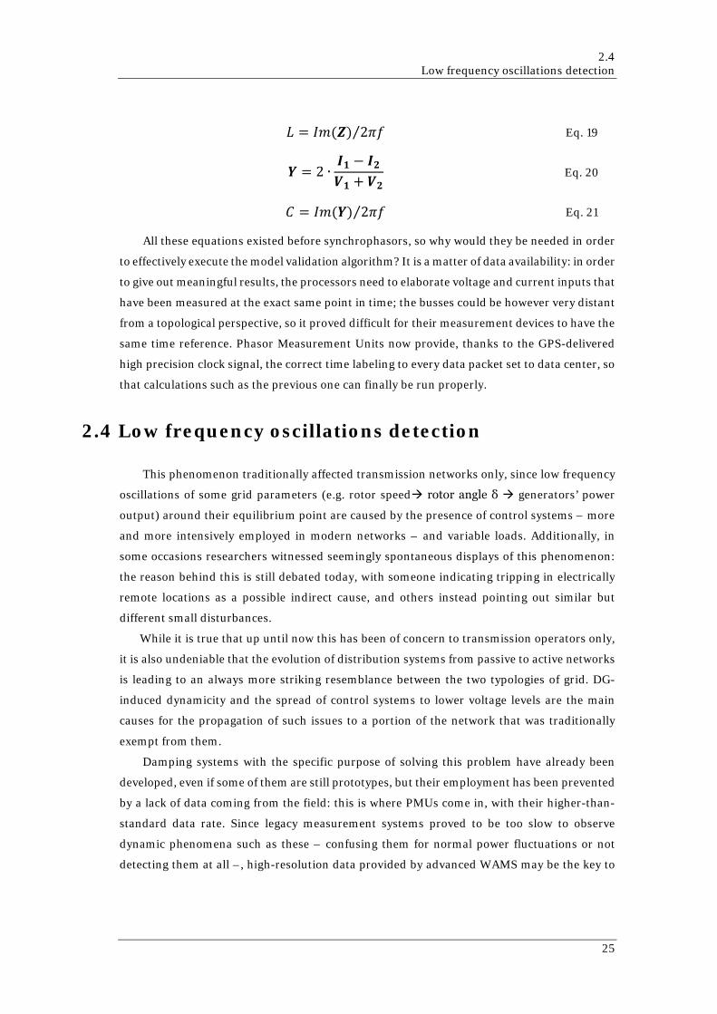
𝑗𝑗 = 𝐼𝐼𝐼𝐼(𝒁𝒁) 2𝜋𝜋𝜋𝜋⁄ Eq. 19
𝒀𝒀 = 2 ∙𝑰𝑰𝟏𝟏 − 𝑰𝑰𝟐𝟐𝑽𝑽𝟏𝟏 + 𝑽𝑽𝟐𝟐
Eq. 20
𝑗𝑗 = 𝐼𝐼𝐼𝐼(𝒀𝒀) 2𝜋𝜋𝜋𝜋⁄ Eq. 21
All these equations existed before synchrophasors, so why would they be needed in order
to effectively execute the model validation algorithm? It is a matter of data availability: in order
to give out meaningful results, the processors need to elaborate voltage and current inputs that
have been measured at the exact same point in time; the busses could be however very distant
from a topological perspective, so it proved difficult for their measurement devices to have the
same time reference. Phasor Measurement Units now provide, thanks to the GPS-delivered
high precision clock signal, the correct time labeling to every data packet set to data center, so
that calculations such as the previous one can finally be run properly.
2.4 Low frequency oscillations detection
This phenomenon traditionally affected transmission networks only, since low frequency
oscillations of some grid parameters (e.g. rotor speed rotor angle δ generators’ power
output) around their equilibrium point are caused by the presence of control systems – more
and more intensively employed in modern networks – and variable loads. Additionally, in
some occasions researchers witnessed seemingly spontaneous displays of this phenomenon:
the reason behind this is still debated today, with someone indicating tripping in electrically
remote locations as a possible indirect cause, and others instead pointing out similar but
different small disturbances.
While it is true that up until now this has been of concern to transmission operators only,
it is also undeniable that the evolution of distribution systems from passive to active networks
is leading to an always more striking resemblance between the two typologies of grid. DG-
induced dynamicity and the spread of control systems to lower voltage levels are the main
causes for the propagation of such issues to a portion of the network that was traditionally
exempt from them.
Damping systems with the specific purpose of solving this problem have already been
developed, even if some of them are still prototypes, but their employment has been prevented
by a lack of data coming from the field: this is where PMUs come in, with their higher-than-
standard data rate. Since legacy measurement systems proved to be too slow to observe
dynamic phenomena such as these – confusing them for normal power fluctuations or not
detecting them at all –, high-resolution data provided by advanced WAMS may be the key to
25
0CHAPTER 2 Potential pmu applications on distribution networks
improvement in this field. The use of control solutions to avoid instability issues, since
underdamped oscillations could lead to system collapse, will finally be possible.
2.5 Parallel bus voltage monitoring
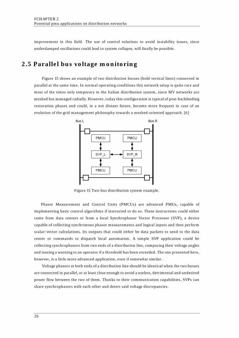
Figure 15 shows an example of two distribution busses (bold vertical lines) connected in
parallel at the same time. In normal operating conditions this network setup is quite rare and
most of the times only temporary in the Italian distribution system, since MV networks are
meshed but managed radially. However, today this configuration is typical of post-backfeeding
restoration phases and could, in a not distant future, become more frequent in case of an
evolution of the grid management philosophy towards a meshed-oriented approach. [6]
Figure 15 Two-bus distribution system example.
Phasor Measurement and Control Units (PMCUs) are advanced PMUs, capable of
implementing basic control algorithms if instructed to do so. These instructions could either
come from data centers or from a local Synchrophasor Vector Processor (SVP), a device
capable of collecting synchronous phasor measurements and logical inputs and then perform
scalar/vector calculations. Its outputs that could either be data packets to send to the data
center or commands to dispatch local automation. A simple SVP application could be
collecting synchrophasors from two ends of a distribution line, comparing their voltage angles
and issuing a warning to an operator if a threshold has been exceeded. The one presented here,
however, is a little more advanced application, even if somewhat similar.
Voltage phasors at both ends of a distribution line should be identical when the two busses
are connected in parallel, or at least close enough to avoid a useless, detrimental and undesired
power flow between the two of them. Thanks to their communication capabilities, SVPs can
share synchrophasors with each other and detect said voltage discrepancies.
26
2.6 State Estimation (SE)
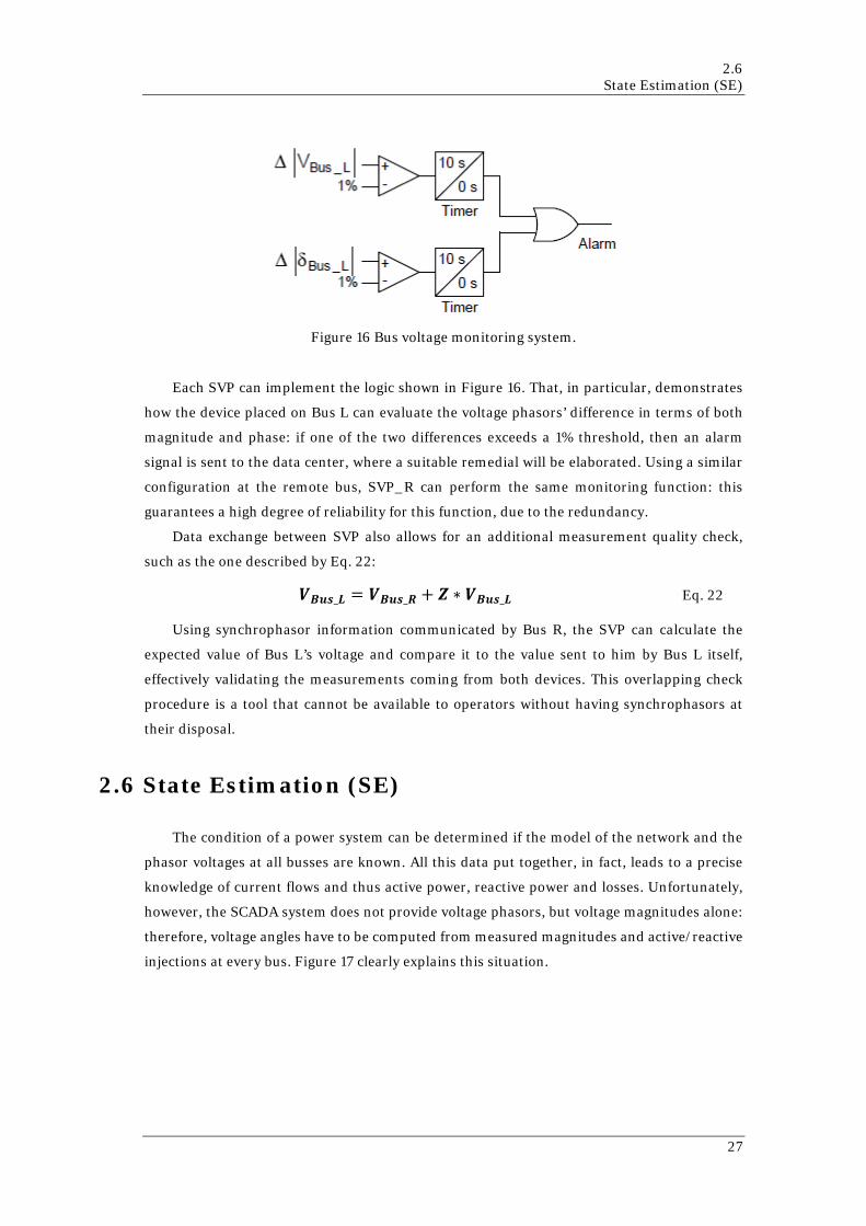
Figure 16 Bus voltage monitoring system.
Each SVP can implement the logic shown in Figure 16. That, in particular, demonstrates
how the device placed on Bus L can evaluate the voltage phasors’ difference in terms of both
magnitude and phase: if one of the two differences exceeds a 1% threshold, then an alarm
signal is sent to the data center, where a suitable remedial will be elaborated. Using a similar
configuration at the remote bus, SVP_R can perform the same monitoring function: this
guarantees a high degree of reliability for this function, due to the redundancy.
Data exchange between SVP also allows for an additional measurement quality check,
such as the one described by Eq. 22:
𝑽𝑽𝑩𝑩𝑩𝑩𝑩𝑩_𝑳𝑳 = 𝑽𝑽𝑩𝑩𝑩𝑩𝑩𝑩_𝑹𝑹 + 𝒁𝒁 ∗ 𝑽𝑽𝑩𝑩𝑩𝑩𝑩𝑩_𝑳𝑳 Eq. 22
Using synchrophasor information communicated by Bus R, the SVP can calculate the
expected value of Bus L’s voltage and compare it to the value sent to him by Bus L itself,
effectively validating the measurements coming from both devices. This overlapping check
procedure is a tool that cannot be available to operators without having synchrophasors at
their disposal.
2.6 State Estimation (SE)
The condition of a power system can be determined if the model of the network and the
phasor voltages at all busses are known. All this data put together, in fact, leads to a precise
knowledge of current flows and thus active power, reactive power and losses. Unfortunately,
however, the SCADA system does not provide voltage phasors, but voltage magnitudes alone:
therefore, voltage angles have to be computed from measured magnitudes and active/reactive
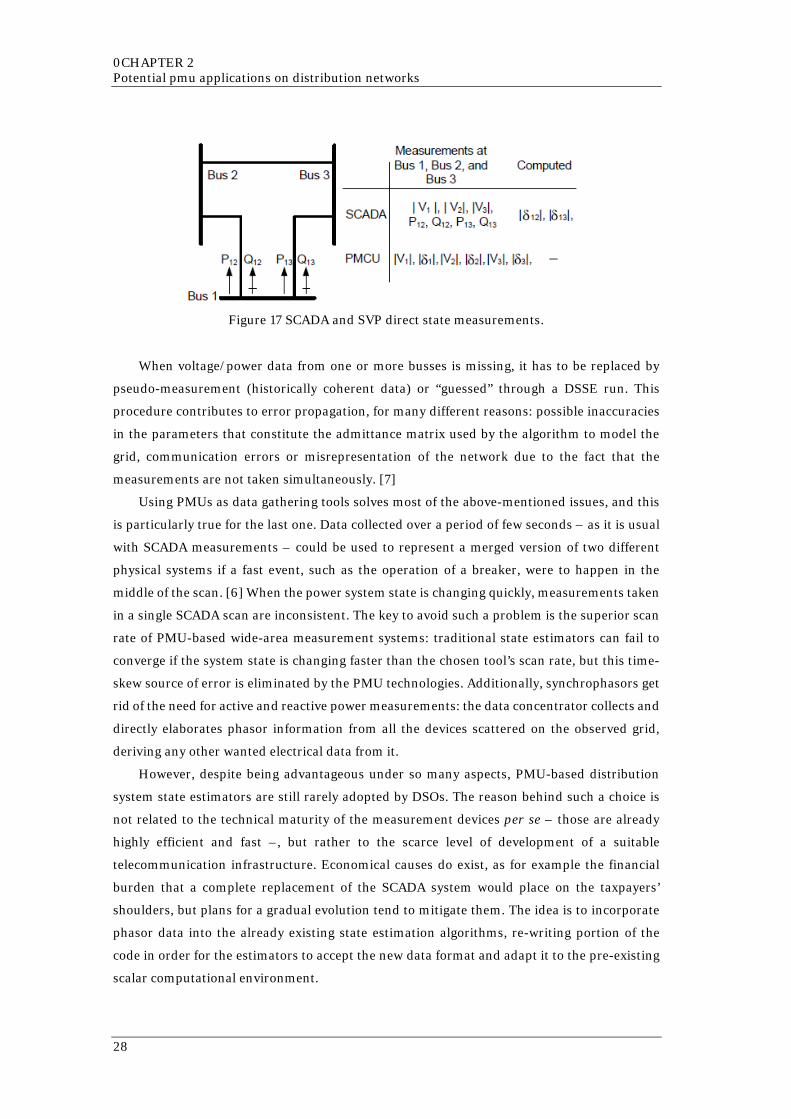
injections at every bus. Figure 17 clearly explains this situation.
27
0CHAPTER 2 Potential pmu applications on distribution networks
Figure 17 SCADA and SVP direct state measurements.
When voltage/power data from one or more busses is missing, it has to be replaced by
pseudo-measurement (historically coherent data) or “guessed” through a DSSE run. This
procedure contributes to error propagation, for many different reasons: possible inaccuracies
in the parameters that constitute the admittance matrix used by the algorithm to model the
grid, communication errors or misrepresentation of the network due to the fact that the
measurements are not taken simultaneously. [7]
Using PMUs as data gathering tools solves most of the above-mentioned issues, and this
is particularly true for the last one. Data collected over a period of few seconds – as it is usual
with SCADA measurements – could be used to represent a merged version of two different
physical systems if a fast event, such as the operation of a breaker, were to happen in the
middle of the scan. [6] When the power system state is changing quickly, measurements taken
in a single SCADA scan are inconsistent. The key to avoid such a problem is the superior scan
rate of PMU-based wide-area measurement systems: traditional state estimators can fail to
converge if the system state is changing faster than the chosen tool’s scan rate, but this time-
skew source of error is eliminated by the PMU technologies. Additionally, synchrophasors get
rid of the need for active and reactive power measurements: the data concentrator collects and
directly elaborates phasor information from all the devices scattered on the observed grid,
deriving any other wanted electrical data from it.
However, despite being advantageous under so many aspects, PMU-based distribution
system state estimators are still rarely adopted by DSOs. The reason behind such a choice is
not related to the technical maturity of the measurement devices per se – those are already
highly efficient and fast –, but rather to the scarce level of development of a suitable
telecommunication infrastructure. Economical causes do exist, as for example the financial
burden that a complete replacement of the SCADA system would place on the taxpayers’
shoulders, but plans for a gradual evolution tend to mitigate them. The idea is to incorporate
phasor data into the already existing state estimation algorithms, re-writing portion of the
code in order for the estimators to accept the new data format and adapt it to the pre-existing
scalar computational environment.
28
2.6 State Estimation (SE)
This is called “single-stage SE approach”, as opposed to the “two-stage SE approach” that
instead has two separated calculation steps to keep the different data sets apart. The first one
is more difficult to design (i.e. more expensive) but more performing, while the second one is
less effective – since phasor data is only used to validate the results obtained through the use
of SCADA measurements in the first step – but definitely cheaper. Both solutions, however,
have common advantages with respect to the plain old SCADA state estimator in terms of
resolution, redundancy, precision and the possibility of real-time monitoring. These benefits
come with downsides: the cost of a significantly increased computational burden, the need to
deal with the so-called “data tsunami” issue (i.e. both hardware and software portions of the
state estimator need to be able to manage the increased data rate of PMU systems) and the
necessity to somehow synchronize time-stamped and not-time-stamped data for it to be
meaningful.
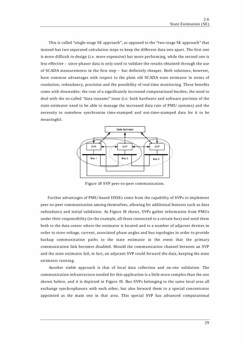
Figure 18 SVP peer-to-peer communication.
Further advantages of PMU-based DSSEs come from the capability of SVPs to implement
peer-to-peer communication among themselves, allowing for additional features such as data
redundancy and initial validation. As Figure 18 shows, SVPs gather information from PMUs
under their responsibility (in the example, all those connected to a certain bus) and send them
both to the data center where the estimator is located and to a number of adjacent devices in
order to store voltage, current, associated phase angles and bus topologies in order to provide
backup communication paths to the state estimator in the event that the primary
communication link becomes disabled. Should the communication channel between an SVP
and the state estimator fail, in fact, an adjacent SVP could forward the data, keeping the state
estimator running.
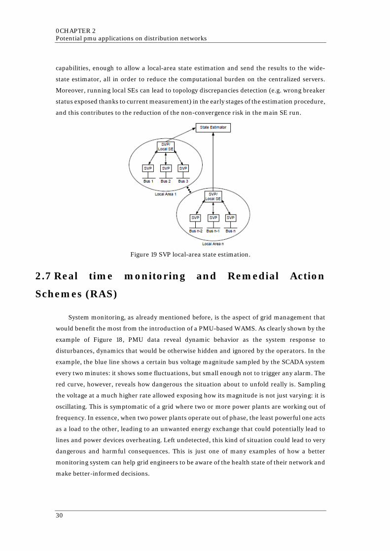
Another viable approach is that of local data collection and on-site validation. The
communication infrastructure needed for this application is a little more complex than the one
shown before, and it is depicted in Figure 19. Bus SVPs belonging to the same local area all
exchange synchrophasors with each other, but also forward them to a special concentrator
appointed as the main one in that area. This special SVP has advanced computational
29
0CHAPTER 2 Potential pmu applications on distribution networks
capabilities, enough to allow a local-area state estimation and send the results to the wide-
state estimator, all in order to reduce the computational burden on the centralized servers.
Moreover, running local SEs can lead to topology discrepancies detection (e.g. wrong breaker
status exposed thanks to current measurement) in the early stages of the estimation procedure,
and this contributes to the reduction of the non-convergence risk in the main SE run.
Figure 19 SVP local-area state estimation.
2.7 Real time monitoring and Remedial Action
Schemes (RAS)
System monitoring, as already mentioned before, is the aspect of grid management that
would benefit the most from the introduction of a PMU-based WAMS. As clearly shown by the
example of Figure 18, PMU data reveal dynamic behavior as the system response to
disturbances, dynamics that would be otherwise hidden and ignored by the operators. In the
example, the blue line shows a certain bus voltage magnitude sampled by the SCADA system
every two minutes: it shows some fluctuations, but small enough not to trigger any alarm. The
red curve, however, reveals how dangerous the situation about to unfold really is. Sampling
the voltage at a much higher rate allowed exposing how its magnitude is not just varying: it is
oscillating. This is symptomatic of a grid where two or more power plants are working out of
frequency. In essence, when two power plants operate out of phase, the least powerful one acts
as a load to the other, leading to an unwanted energy exchange that could potentially lead to
lines and power devices overheating. Left undetected, this kind of situation could lead to very
dangerous and harmful consequences. This is just one of many examples of how a better
monitoring system can help grid engineers to be aware of the health state of their network and
make better-informed decisions.
30
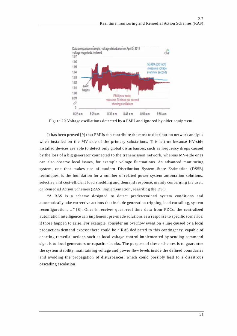
2.7 Real time monitoring and Remedial Action Schemes (RAS)
Figure 20 Voltage oscillations detected by a PMU and ignored by older equipment.
It has been proved [9] that PMUs can contribute the most to distribution network analysis
when installed on the MV side of the primary substations. This is true because HV-side
installed devices are able to detect only global disturbances, such as frequency drops caused
by the loss of a big generator connected to the transmission network, whereas MV-side ones
can also observe local issues, for example voltage fluctuations. An advanced monitoring
system, one that makes use of modern Distribution System State Estimation (DSSE)
techniques, is the foundation for a number of related power system automation solutions:
selective and cost-efficient load shedding and demand response, mainly concerning the user,
or Remedial Action Schemes (RAS) implementation, regarding the DSO.
“A RAS is a scheme designed to detect predetermined system conditions and
automatically take corrective actions that include generation tripping, load curtailing, system
reconfiguration, …” [8]. Once it receives quasi-real time data from PDCs, the centralized
automation intelligence can implement pre-made solutions as a response to specific scenarios,
if those happen to arise. For example, consider an overflow event on a line caused by a local
production/demand excess: there could be a RAS dedicated to this contingency, capable of
enacting remedial actions such as local voltage control implemented by sending command
signals to local generators or capacitor banks. The purpose of these schemes is to guarantee
the system stability, maintaining voltage and power flow levels inside the defined boundaries
and avoiding the propagation of disturbances, which could possibly lead to a disastrous
cascading escalation.
31
0CHAPTER 2 Potential pmu applications on distribution networks
2.8 Post-event analysis
Network condition’s analysis post relevant events (e.g. a fault) is a procedure traditionally
run via SCADA system to assess the causes and the consequences of such an accident, in order
to elaborate appropriate strategies for system restoration and prevent it from happening again
in the future. Legacy method are already quite effective, however the introduction of PMUs
could boost post-event analysis efficiency thanks to synchrophasors’ superior data resolution:
a more accurate post-mortem analysis is very likely to lead to a more specific and fast
resolution of the original issue. However, while it is true that having a great amount of
information available is often a positive news for operator, it also brings two negative
consequences: the need for both a suitable data storage system and a fast and efficient data-
mining algorithm. Both this conditions mean additional costs for the grid operator.
A fast and detailed analysis can help, for example, ensuring a safe system restoration to
its pre-event status, thanks to the possibility to assess the network parameters immediately
after the destructive occurrence. Continuous monitoring allows for the detection of abnormal
system conditions that would prevent a correct restoration by regular means: the presence of
power oscillations after a fault, for example, would go undetected by the SCADA system; this
could lead to instability and, in extreme cases, to grid collapse after incautious breaker
reclosure. Knowledge about the real state of the network post-event will then be vital to
elaborate alternative restoration procedures to solve the issue.
2.9 Fault management
Phasor measurement units can enhance the effectiveness of many fault-related automated
operations, dedicated to both network and users’ protection. In particular, there are four
categories in which the topic can be subdivided: fault prevention, fault detection, fault
localization and fault resolution. For each of them an application example will be described,
among many possible ones that are currently under research.
2.9.1 Fault prevention
On August 14th 2003, 50 million people across Ontario and eight northeastern U.S. states
lost electric power. [9] The combination of a hot afternoon and an unexpected breakdown of a
coal-fired generating station near Cleveland set off a chain reaction that within 94 minutes left
most of northeastern America in the dark. It took more than 24 hours to get power restored to
most parts of the power grid, and fully restoring production capacity to meet demand in the
region took almost two weeks. It will be remembered as The Great Blackout of 2003.
32

2.9 Fault management
It came as a surprise to most grid operators that a seemingly innocent event far away could
cause the entire power grid to collapse. A situation in Cleveland was allowed to go undetected
for just over 90 minutes when transmission lines were operating close to maximum capacity.
The hot summer air was generating high demand for electric energy to power air conditioners
across the region. When a coal-fired generating station went offline, a local transmission line
overloaded, causing the wires of the line to extend and sink towards the ground. When the line
touched a tree that had been allowed to grow below the transmission line, the line short-
circuited to ground, causing the automatic circuit protection to break. This put more stress on
the remaining lines. One hour later, three other lines failed, and a catastrophic surge of electric
power rushed in through the remaining lines in Ohio, triggering several other circuit breakers.
As the remaining transmission lines had insufficient capacity to carry the required energy
across the region, the entire grid collapsed within 90 seconds. This left consumers without
electrical energy. Unable to deliver the energy they were generating, several nuclear power
plants were forced to follow emergency procedures and shut down their nuclear reactors,
causing harm to the nuclear reactors. It took almost four days to restore power on the grid,
and nearly two weeks to bring all reactors back up to full capacity.
An investigation of The Great Blackout revealed that the power grid control systems were
outdated and largely unable to monitor and protect the health of the grid. Time was never an
issue. It took 31 minutes from the moment the Cleveland power station failed until the first
transmission line collapsed. The situation looked manageable for another 61 minutes, until
more transmission lines started burning out. The men and women controlling the grid were
caught completely off guard because they had no means to detect warning signals from the
power grid. Without access to real time information, the power grid control rooms were unable
to predict where the next error would occur and plan corrective actions. The investigation
concluded that the disaster could have been avoided if the power grid had been equipped with
better monitoring systems. The U.S. Department of Energy considers the US-Canada blackout
in 2003 to be the single most important motivator behind the Smart Grid initiative.
2.9.2 Fault detection
It is fairly easy to detect fault events most of the times, since the majority of them is
characterized by high values of current magnitudes. The detection method, in these cases, is
both effective and straightforward: overcurrent relays are triggered by these exceptionally
abundant flows and are disposed of when protections trip, after a suitably short set time. There
are occasions, however, in which this simple system cannot guarantee timely response to a
fault event, thus potentially leading to harmful consequences for both people and equipment’s
safety. One of such cases is, for example, a high impedance fault. (HIF)
33

0CHAPTER 2 Potential pmu applications on distribution networks
Table 1 Typical current levels for MV HIFs.
Surface Current (A) Dry asphalt 0 Dry sand 0
Concrete (non-reinforced) 0 Wet sand 15 Dry sod 20
Dry grass 25 Wet sod 40
Wet grass 50 Concrete (reinforced) 75
High impedance faults usually happen when an energized conductor comes in contact
with a quasi-insulating object such as a tree, structure or equipment, or falls to the ground
(typical current values relative to a number of these cases are shown above in Table 1). The
significance of these previously undetectable faults is that they represent a serious public
hazard as well as a risk of arcing ignition of fires. This occurrence is rare but very dangerous,
so the operators have to resort to alternative detection methods in order to assure well-timed
resolutive actions. Mechanical HIF detection methods have been tested for decades now and
proved to be relatively effective, but their susceptibility to adverse weather conditions (ice,
wind, tree growth) and installation costs prevented their employment. A simple example is
that of a pole-mounted device placed below the line to protect and connected to ground
through a low impedance: in case of conductor downing, a spring inside the device is released
and it ejects a bus bar that makes contact with the conductor and allows the flow of a current
high enough for the relays to detect the fault and act on the breakers. Electrical HIF detection
methods have been object of study, but none succeeded in becoming widely spread among grid
operators.
Recent advances in PMU technologies have enabled alternative solutions that are not only
capable of detecting these faults, but that can also trip the affected circuit section in the narrow
time window between the moment of the break and the time the conductor hits the ground.
The affected circuit section is de-energized while the conductor is still falling, eliminating the
risk of an arcing ground fault or energized circuits on the ground. Three different methods
have been developed to achieve this goal: the dV/dt detection method, the Inverse and Zero
Sequence Voltage Magnitude detection method and the Inverse and Zero Sequence Voltage
Phase detection method. [10]
34
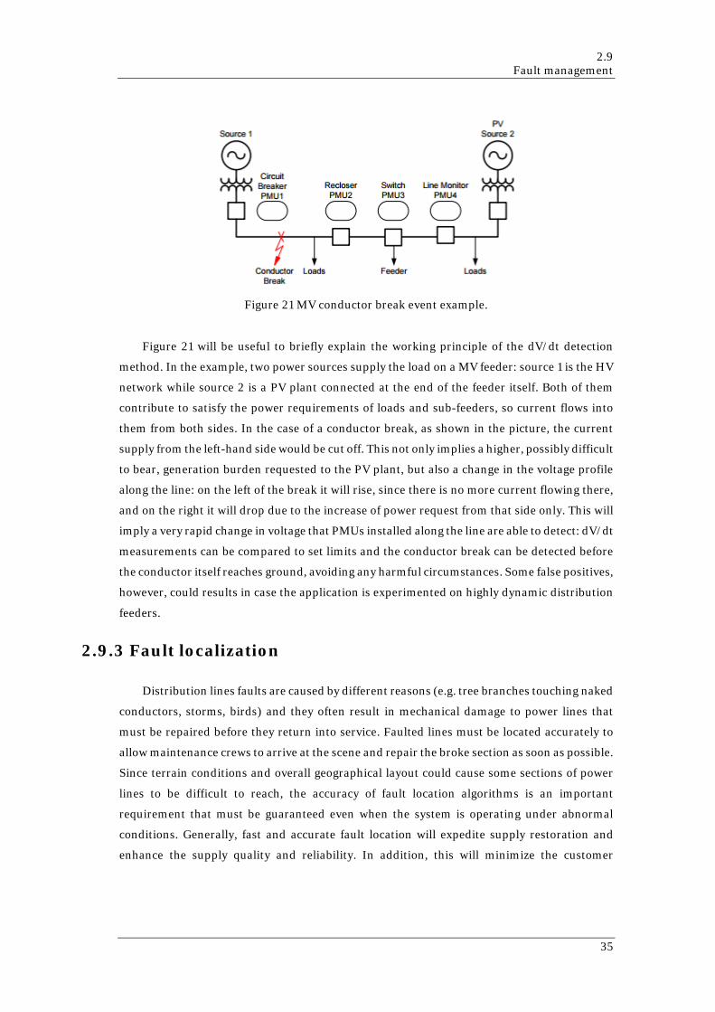
2.9 Fault management
Figure 21 MV conductor break event example.
Figure 21 will be useful to briefly explain the working principle of the dV/dt detection
method. In the example, two power sources supply the load on a MV feeder: source 1 is the HV
network while source 2 is a PV plant connected at the end of the feeder itself. Both of them
contribute to satisfy the power requirements of loads and sub-feeders, so current flows into
them from both sides. In the case of a conductor break, as shown in the picture, the current
supply from the left-hand side would be cut off. This not only implies a higher, possibly difficult
to bear, generation burden requested to the PV plant, but also a change in the voltage profile
along the line: on the left of the break it will rise, since there is no more current flowing there,
and on the right it will drop due to the increase of power request from that side only. This will
imply a very rapid change in voltage that PMUs installed along the line are able to detect: dV/dt
measurements can be compared to set limits and the conductor break can be detected before
the conductor itself reaches ground, avoiding any harmful circumstances. Some false positives,
however, could results in case the application is experimented on highly dynamic distribution
feeders.
2.9.3 Fault localization
Distribution lines faults are caused by different reasons (e.g. tree branches touching naked
conductors, storms, birds) and they often result in mechanical damage to power lines that
must be repaired before they return into service. Faulted lines must be located accurately to
allow maintenance crews to arrive at the scene and repair the broke section as soon as possible.
Since terrain conditions and overall geographical layout could cause some sections of power
lines to be difficult to reach, the accuracy of fault location algorithms is an important
requirement that must be guaranteed even when the system is operating under abnormal
conditions. Generally, fast and accurate fault location will expedite supply restoration and
enhance the supply quality and reliability. In addition, this will minimize the customer
35
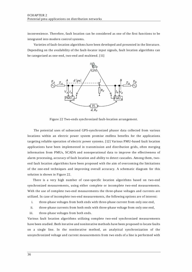
0CHAPTER 2 Potential pmu applications on distribution networks
inconvenience. Therefore, fault location can be considered as one of the first functions to be
integrated into modern control systems.
Varieties of fault-location algorithms have been developed and presented in the literature.
Depending on the availability of the fault-locator input signals, fault location algorithms can
be categorized as one-end, two-end and multiend. [11]
Figure 22 Two-ends synchronized fault-location arrangement.
The potential uses of subsecond GPS-synchronized phasor data collected from various
locations within an electric power system promise endless benefits for the applications
targeting reliable operation of electric power systems. [12] Various PMU-based fault location
applications have been implemented in transmission and distribution grids, often merging
information from PMUs, SCADA and nonoperational data to improve the effectiveness of
alarm processing, accuracy of fault location and ability to detect cascades. Among them, two-
end fault location algorithms have been proposed with the aim of overcoming the limitations
of the one-end techniques and improving overall accuracy. A schematic diagram for this
solution is shown in Figure 22.
There is a very high number of case-specific location algorithms based on two-end
synchronized measurements, using either complete or incomplete two-end measurements.
With the use of complete two-end measurements the three-phase voltages and currents are
utilized. In case of incomplete two-end measurements, the following options are of interest:
i. three-phase voltages from both ends with three-phase current from only one end,
ii. three-phase currents from both ends with three-phase voltage from only one end,
iii. three-phase voltages from both ends.
Various fault location algorithms utilizing complete two-end synchronized measurements
have been studied. Both iterative and noniterative methods have been proposed to locate faults
on a single line. In the noniterative method, an analytical synchronization of the
unsynchronized voltage and current measurements from two ends of a line is performed with
36
2.9 Fault management
use of the determined synchronization operator. Then, the synchronized measurements are
used to calculate the distance to fault. Simultaneous usage of two kinds of symmetrical
components for determining the synchronization operator makes the calculations simple and
highly accurate.
2.9.4 Fault resolution
Once a fault has occurred and its location has been pinpointed, it needs to be extinguished
in due time. Network protection systems effectively do so most of the times, but they can lack
responsiveness during particular and rare events. Relay settings are, in fact, calibrated to trip
the breakers under normal grid conditions and may prove to be inefficient in case of anomalies.
Adaptive relaying is a philosophy of protection design that provides for adjustments in
protection settings and/or functions automatically, as grid conditions change. (e.g. Interface
Protection Systems after Annex 70) The adoption of this kind of relaying is needed to ensure
timely breaker operations not only under normal circumstances but also in case of those
abnormalities (e.g. cascade tripping) to face which they lack proper regulation, all leading to
malfunction. Adaptive relays are already a reality, but in order to operate they need a high data
rate stream coming from the network, a quasi-real-time information input that can only be
supplied by special sensors placed on the observed grid, and PMUs for sure are suitable
candidates.
The following list contains examples of grid operations enabled by the adaptive approach,
which is not only exclusive to breakers tripping but also to more complex functionalities: [13]
• Intelligent load shedding: adoption of a smart management of load dropping schemes
in emergencies, that allows to locate with precision which users to cut out in order to
solve an unbalance instead of blindingly shedding pre-set blocks (or “aggregates”) of
them without exactly knowing how power consumption is reduced by doing so. This
approach avoids long load shed/generation trip iterative procedures to achieve
balance, thus improving service power quality;
• Adaptive loss-of-field relaying: automatic setting correction for generators excitation
current relays, that in unstable working conditions could happen to trip even when
not supposed to;
• Oscillation damping controller: dynamic adjustments for oscillation damping
systems’ (those already mentioned in section 2.4) parameters. These systems cannot,
in fact, be rigid but need to adapt to different kinds of oscillation singularities that
could occur.
37
0CHAPTER 2 Potential pmu applications on distribution networks
2.10 Unmasking load behind net-metered DG
Measurements made at the customers’ point of connection onto the grid can only be this
useful, since they monitor a prosumer’s net injection/withdrawal only. Separate data
regarding load and production profiles would be of much more interest for system operators,
since having it at their disposal would imply being able to prepare remedial actions for possible
DG loss or rapid ramps, but also facilitate forecasting of net load by understanding its
composition even when “masked” by generation.
In this predicament, PMU measurements might allow remote inference of load /DG ratio
[14] without the need for customer-side access (which could be impossible or undesired for
legal, technical or economic reasons), combining time series net load data with power quality
measurements, that is an harmonic content analysis capable of obtaining a “fingerprint”
typical of generation or load. (i.e. the load gives its specific harmonic contribution to the
spectrum profile, in a way that – if properly analyzed – can unveil its hidden presence)
2.11 Reverse Power Flow (RPF) detection
Electrical networks are complex dynamic systems that need to be studied with specific
tools. When an operator is interested in knowing magnitude and direction of power flows, the
mathematical instruments to be used are called load flow equations. They can be written as
follows:
𝑃𝑃𝑖𝑖 = 𝑉𝑉𝑖𝑖2𝑌𝑌𝑖𝑖𝑖𝑖 cos 𝜃𝜃𝑖𝑖𝑖𝑖 + �𝑉𝑉𝑖𝑖𝑉𝑉𝑗𝑗𝑌𝑌𝑖𝑖𝑗𝑗 cos(𝛿𝛿𝑗𝑗 − 𝛿𝛿𝑖𝑖 + 𝜃𝜃𝑖𝑖𝑗𝑗)𝑛𝑛
𝑗𝑗≠𝑖𝑖
Eq. 23
𝑄𝑄𝑖𝑖 = 𝑉𝑉𝑖𝑖2𝑌𝑌𝑖𝑖𝑖𝑖 sin 𝜃𝜃𝑖𝑖𝑖𝑖 + �𝑉𝑉𝑖𝑖𝑉𝑉𝑗𝑗𝑌𝑌𝑖𝑖𝑗𝑗 sin(𝛿𝛿𝑗𝑗 − 𝛿𝛿𝑖𝑖 + 𝜃𝜃𝑖𝑖𝑗𝑗)𝑛𝑛
𝑗𝑗≠𝑖𝑖
Eq. 24
where:
• Pi is the net active power injection at the i-eth node of the network;
• Qi is the net reactive power injection at the i-eth node of the network;
• Vi is the voltage magnitude of the i-eth node of the network;
• Yii is the magnitude of the element found at the intersection of the i-eth row and
i-eth column in the network’s bus admittance matrix;
• 𝜃𝜃𝑖𝑖𝑖𝑖 is the angle of the the element found at the intersection of the i-eth row and i-
eth column in the network’s bus admittance matrix;
• Vj is the voltage magnitude of the j-eth node of the network;
38

2.11 Reverse Power Flow (RPF) detection
• Yij is the magnitude of the element found at the intersection of the i-eth row and
j-eth column in the network’s bus admittance matrix;
• 𝛿𝛿𝑗𝑗 is the voltage angle of the j-eth node of the network;
• 𝛿𝛿𝑖𝑖 is the voltage angle of the i-eth node of the network.
When complex voltages for each node are not known variables, multiple iterative
computational methods must be used in order to estimate them (since the power equations
are not linear): the Gauss method and the Newton-Rhapson method are suitable examples.
However, if node voltages are already known – as in the case shown in Figure 23, where real-
time complex measurements are constantly taken by μPMUs –, then the apparent power
flowing between two adjacent nodes can be directly computed:
𝑺𝑺𝟏𝟏𝟐𝟐 = 𝑽𝑽𝟏𝟏(𝒀𝒀𝟏𝟏𝟏𝟏𝑽𝑽𝟏𝟏 + 𝒀𝒀𝟏𝟏𝟐𝟐𝑽𝑽𝟐𝟐) Eq. 25
where:
• S12 is the complex power flowing from node 1 to node 2;
• V1 is the complex voltage of node 1;
• V2 is the complex voltage of node 2;
• Y11 is the element found at the intersection of the first row and first column in the
network’s bus admittance matrix;
• Y12 is the element found at the intersection of the first row and second column in
the network’s bus admittance matrix.
However, under some simplifying assumptions (all bus voltages equal to 1 p.u., negligible
shunt parameters for lines and transformers and no losses), the active power flowing between
two adjacent busses can be expressed as:
𝑃𝑃12 =𝑉𝑉1𝑉𝑉2𝑋𝑋12
sin(𝛿𝛿1 − 𝛿𝛿2) Eq. 26
where:
• P12 is the complex power flowing from node 1 to node 2;
• V1 is the voltage magnitude of node 1;
• V2 is the voltage magnitude of node 2;
• X12 is the reactance of the line connecting the two nodes;
• 𝛿𝛿1 is the voltage angle of node 1;
• 𝛿𝛿2 is the voltage angle of node 2.
39
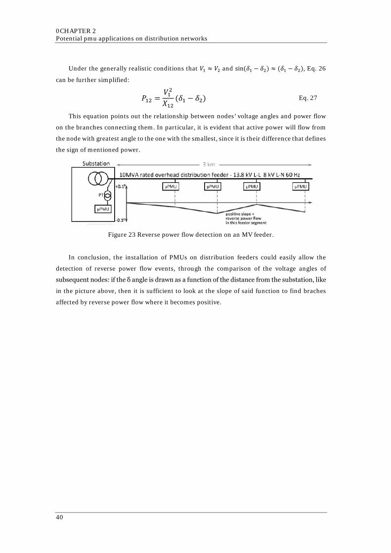
0CHAPTER 2 Potential pmu applications on distribution networks
Under the generally realistic conditions that 𝑉𝑉1 ≈ 𝑉𝑉2 and sin(𝛿𝛿1 − 𝛿𝛿2) ≈ (𝛿𝛿1 − 𝛿𝛿2), Eq. 26
can be further simplified:
𝑃𝑃12 =𝑉𝑉12
𝑋𝑋12(𝛿𝛿1 − 𝛿𝛿2) Eq. 27
This equation points out the relationship between nodes’ voltage angles and power flow
on the branches connecting them. In particular, it is evident that active power will flow from
the node with greatest angle to the one with the smallest, since it is their difference that defines
the sign of mentioned power.
Figure 23 Reverse power flow detection on an MV feeder.
In conclusion, the installation of PMUs on distribution feeders could easily allow the
detection of reverse power flow events, through the comparison of the voltage angles of
subsequent nodes: if the δ angle is drawn as a function of the distance from the substation, like
in the picture above, then it is sufficient to look at the slope of said function to find braches
affected by reverse power flow where it becomes positive.
40
3.1 Real Time Digital Simulator
CHAPTER 3
PMU-BASED NETWORK MODEL
VALIDATOR
After holding an exhaustive presentation on the above-mentioned PMU applications for
the Italian MV grid at e-distribuzione’s Smart Grid Lab sited in Milan, in agreement with the
local decisional board, one of the many proposed alternatives was selected to be studied more
in depth. To be more specific, the choice fell on the development of a synchrophasor-based
network model validator (as briefly described in section 2.3), its optimization in a simulated
yet realistic medium voltage grid and subsequent testing with real equipment.
This study was carried out thanks to the availability of the Real Time Digital Simulator
(RTDS), a powerful instrument at the Lab’s disposal capable of modeling the electric systems
and its components and mimic its dynamics in real-time. The tool can in fact simulate complex
networks’ responses in multiple scenarios, with both digital inputs coming from programmed
elements and analog inputs from external devices. It can also elaborate said responses for
analysis purposes or use them as output to be delivered to real devices, connected through
suitable amplifiers, in order to test them as if they were actually placed on the field.
3.1 Real Time Digital Simulator
3.1.1 General premises
The following section is dedicated to the detailed description of the simulation tool used
to perform the experiments described in the next paragraphs: the Real Time Digital Simulator.
(RTDS)
41
0CHAPTER 3 PMU-based network model validator
“To simulate” means to develop a mathematical model that represents a physical existing
system with the aid of modern informatics, and then analyze its behavior over time. During a
simulation, time is intended as a variable that grows following a linear ramp. This ramp
represents the time base to which any model implemented in the simulator will refer.
In general, the duration of a simulation depends on the computational power of the used
calculator’s processor. For instance, a very complex model in terms of number and intricacy of
its defining equations will need a longer elaboration time with respect to a simpler model. In
order to perform a real time simulation, therefore, the computer needs to be able to elaborate
all the inputs and obtain the outputs as fast as the analyzed event evolves. This calls for very
powerful processors, if the desired performance is meant to be optimal even when dealing with
very fast transients occurring in complex models.
The main characteristic of the RTDS is that the simulator is able to work in real time,
thanks to the extreme computational capability provided by its advanced hardware. It can in
fact rapidly elaborate the mathematical models describing power systems up to a certain
extension, giving outputs that realistically represent the real grid’s conditions. Additionally,
since the solution is in real time, the simulator can be directly connect to power and control
system devices in order to study their interaction with the network where they are going to be
installed even before the real installation. (very useful practice when, for example, protection
equipment prototypes need to be tested in close-to-real scenarios, without neither risking
damages to the grid nor lowering quality of service levels)
3.1.2 Hardware description
The Real Time Digital Simulator is a modular system produced by the homonymous
Canadian company “RTDS Technologies®”. It is composed of many units installed on a cabinet
called “racks”. The one present in the Smart Grid Lab is equipped with four of those racks, as
can be seen in Figure 24.
42
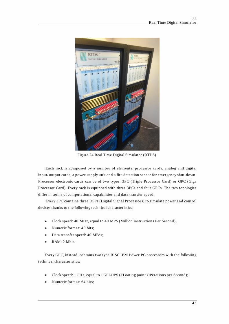
3.1 Real Time Digital Simulator
Figure 24 Real Time Digital Simulator (RTDS).
Each rack is composed by a number of elements: processor cards, analog and digital
input/output cards, a power supply unit and a fire detection sensor for emergency shut-down.
Processor electronic cards can be of two types: 3PC (Triple Processor Card) or GPC (Giga
Processor Card). Every rack is equipped with three 3PCs and four GPCs. The two topologies
differ in terms of computational capabilities and data transfer speed.
Every 3PC contains three DSPs (Digital Signal Processors) to simulate power and control
devices thanks to the following technical characteristics:
• Clock speed: 40 MHz, equal to 40 MPS (Million instructions Per Second);
• Numeric format: 40 bits;
• Data transfer speed: 40 MB/s;
• RAM: 2 Mbit.
Every GPC, instead, contains two type RISC IBM Power PC processors with the following
technical characteristics:
• Clock speed: 1 GHz, equal to 1 GFLOPS (FLoating point OPerations per Second);
• Numeric format: 64 bits;
43
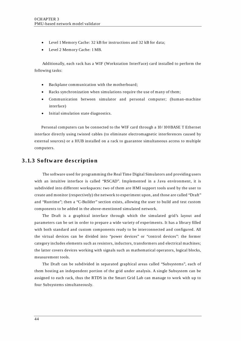
0CHAPTER 3 PMU-based network model validator
• Level 1 Memory Cache: 32 kB for instructions and 32 kB for data;
• Level 2 Memory Cache: 1 MB.
Additionally, each rack has a WIF (Workstation InterFace) card installed to perform the
following tasks:
• Backplane communication with the motherboard;
• Racks synchronization when simulations require the use of many of them;
• Communication between simulator and personal computer; (human-machine
interface)
• Initial simulation state diagnostics.
Personal computers can be connected to the WIF card through a 10/100BASE T Ethernet
interface directly using twisted cables (to eliminate electromagnetic interferences caused by
external sources) or a HUB installed on a rack to guarantee simultaneous access to multiple
computers.
3.1.3 Software description
The software used for programming the Real Time Digital Simulators and providing users
with an intuitive interface is called “RSCAD”. Implemented in a Java environment, it is
subdivided into different workspaces: two of them are HMI support tools used by the user to
create and monitor (respectively) the network to experiment upon, and those are called “Draft”
and “Runtime”; then a “C-Builder” section exists, allowing the user to build and test custom
components to be added in the above-mentioned simulated network.
The Draft is a graphical interface through which the simulated grid’s layout and
parameters can be set in order to prepare a wide variety of experiments. It has a library filled
with both standard and custom components ready to be interconnected and configured. All
the virtual devices can be divided into “power devices” or “control devices”: the former
category includes elements such as resistors, inductors, transformers and electrical machines;
the latter covers devices working with signals such as mathematical operators, logical blocks,
measurement tools.
The Draft can be subdivided in separated graphical areas called “Subsystems”, each of
them hosting an independent portion of the grid under analysis. A single Subsystem can be
assigned to each rack, thus the RTDS in the Smart Grid Lab can manage to work with up to
four Subsystems simultaneously.
44
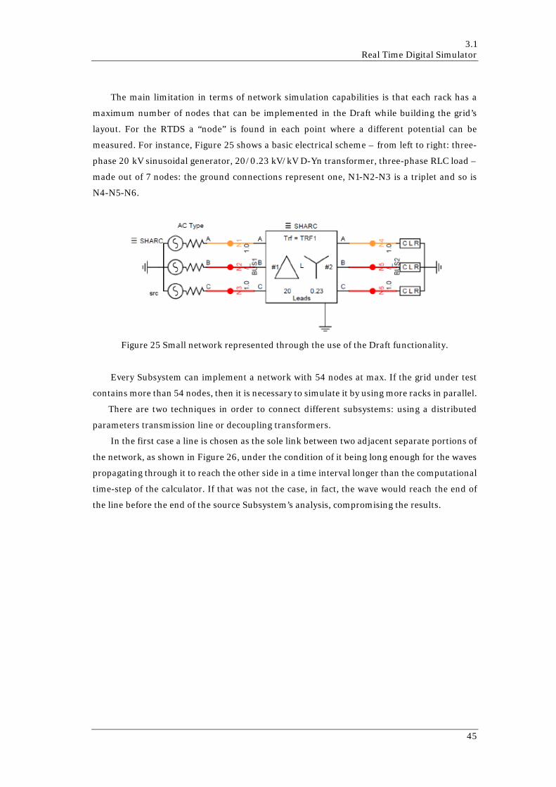
3.1 Real Time Digital Simulator
The main limitation in terms of network simulation capabilities is that each rack has a
maximum number of nodes that can be implemented in the Draft while building the grid’s
layout. For the RTDS a “node” is found in each point where a different potential can be
measured. For instance, Figure 25 shows a basic electrical scheme – from left to right: three-
phase 20 kV sinusoidal generator, 20/0.23 kV/kV D-Yn transformer, three-phase RLC load –
made out of 7 nodes: the ground connections represent one, N1-N2-N3 is a triplet and so is
N4-N5-N6.
Figure 25 Small network represented through the use of the Draft functionality.
Every Subsystem can implement a network with 54 nodes at max. If the grid under test
contains more than 54 nodes, then it is necessary to simulate it by using more racks in parallel.
There are two techniques in order to connect different subsystems: using a distributed
parameters transmission line or decoupling transformers.
In the first case a line is chosen as the sole link between two adjacent separate portions of
the network, as shown in Figure 26, under the condition of it being long enough for the waves
propagating through it to reach the other side in a time interval longer than the computational
time-step of the calculator. If that was not the case, in fact, the wave would reach the end of
the line before the end of the source Subsystem’s analysis, compromising the results.
45
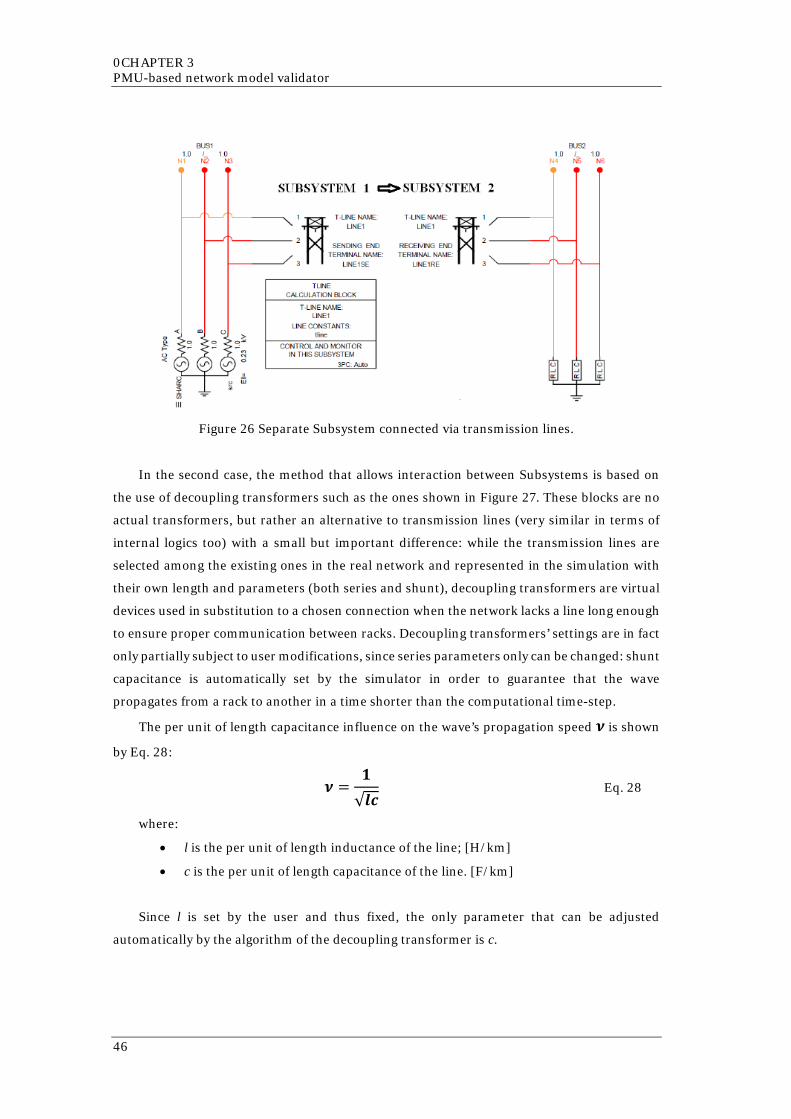
0CHAPTER 3 PMU-based network model validator
Figure 26 Separate Subsystem connected via transmission lines.
In the second case, the method that allows interaction between Subsystems is based on
the use of decoupling transformers such as the ones shown in Figure 27. These blocks are no
actual transformers, but rather an alternative to transmission lines (very similar in terms of
internal logics too) with a small but important difference: while the transmission lines are
selected among the existing ones in the real network and represented in the simulation with
their own length and parameters (both series and shunt), decoupling transformers are virtual
devices used in substitution to a chosen connection when the network lacks a line long enough
to ensure proper communication between racks. Decoupling transformers’ settings are in fact
only partially subject to user modifications, since series parameters only can be changed: shunt
capacitance is automatically set by the simulator in order to guarantee that the wave
propagates from a rack to another in a time shorter than the computational time-step.
The per unit of length capacitance influence on the wave’s propagation speed 𝝂𝝂 is shown
by Eq. 28:
𝝂𝝂 =𝟏𝟏√𝒍𝒍𝒍𝒍
Eq. 28
where:
• l is the per unit of length inductance of the line; [H/km]
• c is the per unit of length capacitance of the line. [F/km]
Since l is set by the user and thus fixed, the only parameter that can be adjusted
automatically by the algorithm of the decoupling transformer is c.
46
3.1 Real Time Digital Simulator
Figure 27 Separate Subsystem connected via decoupling transformers.
This is, of course, a solution that can negatively influence the accuracy of the final results.
In order to avoid errors due to a wrong “propagation duration/time-step” ratio, in fact, a
different kind of error is intentionally introduced: a difference between real and virtual shunt
capacitance for the chosen connection line. Most of the times, however, the difference is so
small that it fails to influence the final results, thus why this second solution is deemed
acceptable.
The other two sections the RSCAD software is composed by are the Runtime and the C-
Builder.
The Runtime is an interface that allows interactions during a simulation run between the
user and the network drawn on the Draft, both in terms of inputs (e.g. breakers and sliders can
be freely manipulated here) and outputs (e.g. any consequence of said manipulation can be
monitored in real-time through a wide variety of meters and displays).
The C-Builder is a tool that gives the user the ability to modify any of the components’
models in the pre-loaded library and even create new ones. Many functions can thus be freely
implemented in a project, and that is particularly needed in the case of this thesis since the
RTDS’ library is mainly intended for HV networks. This lead to the creation of new
components, fit for the MV environment: some of them for general purposes, some for this
specific work.
Any element, created or modified, needs to be defined in terms of: expected
inputs/outputs, block graphical form and code written in C language defining the role and
function of that specific component.
47
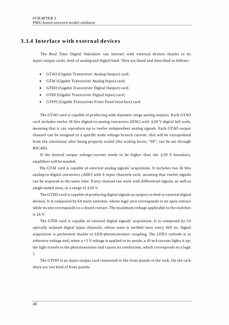
0CHAPTER 3 PMU-based network model validator
3.1.4 Interface with external devices
The Real Time Digital Simulator can interact with external devices thanks to its
input/output cards, both of analog and digital kind. They are listed and described as follows:
• GTAO (Gigabit Transceiver Analog Output) card;
• GTAI (Gigabit Transceiver Analog Input) card;
• GTDO (Gigabit Transceiver Digital Output) card;
• GTDI (Gigabit Transceiver Digital input) card;
• GTFPI (Gigabit Transceiver Front Panel Interface) card.
The GTAO card is capable of producing wide dynamic range analog outputs. Each GTAO
card includes twelve 16 bits digital-to-analog converters (DAC) with ±10 V digital full scale,
meaning that it can reproduce up to twelve independent analog signals. Each GTAO output
channel can be assigned to a specific node voltage/branch current, that will be extrapolated
from the simulation after being properly scaled (the scaling factor, “SF”, can be set through
RSCAD).
If the desired output voltage/current needs to be higher than the ±10 V boundary,
amplifiers will be needed.
The GTAI card is capable of external analog signals’ acquisition. It includes two 16 bits
analog-to-digital converters (ADC) with 6 input channels each, meaning that twelve signals
can be acquired at the same time. Every channel can work with differential signals, as well as
single ended ones, in a range of ±10 V.
The GTDO card is capable of producing digital signals as outputs to feed to external digital
devices. It is composed by 64 static switches, whose logic zero corresponds to an open contact
while its one corresponds to a closed contact. The maximum voltage applicable to the switches
is 24 V.
The GTDI card is capable of external digital signals’ acquisition. It is composed by 24
optically isolated digital input channels, whose state is verified once every 300 ns. Signal
acquisition is performed thanks to LED-phototransistor coupling. The LED’s cathode is at
reference voltage and, when a +5 V voltage is applied to its anode, a 10 mA current lights it up;
the light travels to the phototransistor and causes its conduction, which corresponds to a logic
1.
The GTFPI is an input-output card connected to the front panels of the rack. On the rack
there are two kind of front panels:
48
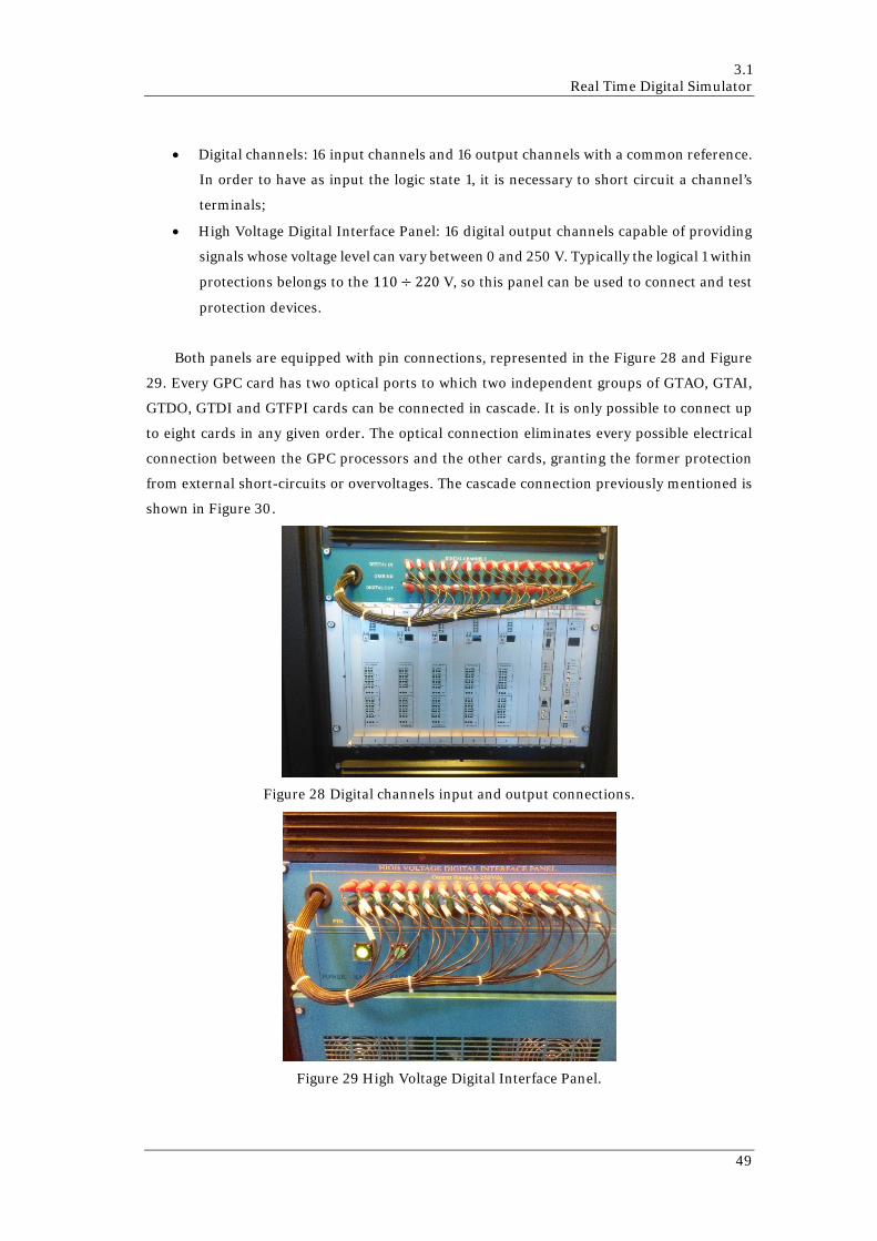
3.1 Real Time Digital Simulator
• Digital channels: 16 input channels and 16 output channels with a common reference.
In order to have as input the logic state 1, it is necessary to short circuit a channel’s
terminals;
• High Voltage Digital Interface Panel: 16 digital output channels capable of providing
signals whose voltage level can vary between 0 and 250 V. Typically the logical 1 within
protections belongs to the 110 ÷ 220 V, so this panel can be used to connect and test
protection devices.
Both panels are equipped with pin connections, represented in the Figure 28 and Figure
29. Every GPC card has two optical ports to which two independent groups of GTAO, GTAI,
GTDO, GTDI and GTFPI cards can be connected in cascade. It is only possible to connect up
to eight cards in any given order. The optical connection eliminates every possible electrical
connection between the GPC processors and the other cards, granting the former protection
from external short-circuits or overvoltages. The cascade connection previously mentioned is
shown in Figure 30.
Figure 28 Digital channels input and output connections.
Figure 29 High Voltage Digital Interface Panel.
49
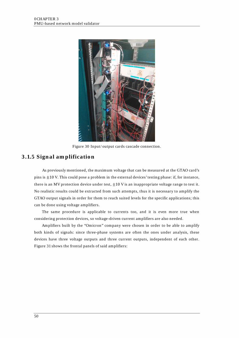
0CHAPTER 3 PMU-based network model validator
Figure 30 Input/output cards cascade connection.
3.1.5 Signal amplification
As previously mentioned, the maximum voltage that can be measured at the GTAO card’s
pins is ±10 V. This could pose a problem in the external devices’ testing phase: if, for instance,
there is an MV protection device under test, ±10 V is an inappropriate voltage range to test it.
No realistic results could be extracted from such attempts, thus it is necessary to amplify the
GTAO output signals in order for them to reach suited levels for the specific applications; this
can be done using voltage amplifiers.
The same procedure is applicable to currents too, and it is even more true when
considering protection devices, so voltage-driven current amplifiers are also needed.
Amplifiers built by the “Omicron” company were chosen in order to be able to amplify
both kinds of signals: since three-phase systems are often the ones under analysis, these
devices have three voltage outputs and three current outputs, independent of each other.
Figure 31 shows the frontal panels of said amplifiers:
50
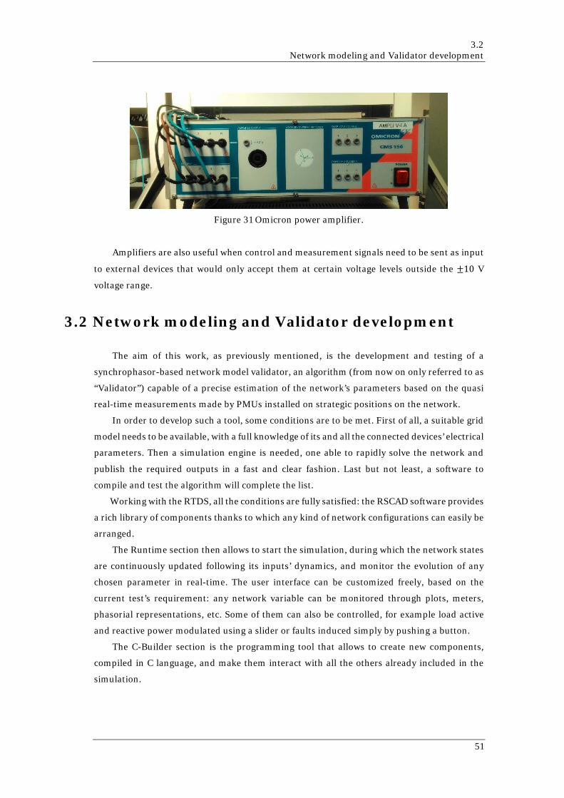
3.2 Network modeling and Validator development
Figure 31 Omicron power amplifier.
Amplifiers are also useful when control and measurement signals need to be sent as input
to external devices that would only accept them at certain voltage levels outside the ±10 V
voltage range.
3.2 Network modeling and Validator development
The aim of this work, as previously mentioned, is the development and testing of a
synchrophasor-based network model validator, an algorithm (from now on only referred to as
“Validator”) capable of a precise estimation of the network’s parameters based on the quasi
real-time measurements made by PMUs installed on strategic positions on the network.
In order to develop such a tool, some conditions are to be met. First of all, a suitable grid
model needs to be available, with a full knowledge of its and all the connected devices’ electrical
parameters. Then a simulation engine is needed, one able to rapidly solve the network and
publish the required outputs in a fast and clear fashion. Last but not least, a software to
compile and test the algorithm will complete the list.
Working with the RTDS, all the conditions are fully satisfied: the RSCAD software provides
a rich library of components thanks to which any kind of network configurations can easily be
arranged.
The Runtime section then allows to start the simulation, during which the network states
are continuously updated following its inputs’ dynamics, and monitor the evolution of any
chosen parameter in real-time. The user interface can be customized freely, based on the
current test’s requirement: any network variable can be monitored through plots, meters,
phasorial representations, etc. Some of them can also be controlled, for example load active
and reactive power modulated using a slider or faults induced simply by pushing a button.
The C-Builder section is the programming tool that allows to create new components,
compiled in C language, and make them interact with all the others already included in the
simulation.
51

0CHAPTER 3 PMU-based network model validator
The first step in this experiment was the creation of a small MV network, far from being
realistic in terms of extension but as similar as possible to real installations under any other
aspect. The electrical scheme used is the one shown in Figure 32:
Figure 32 Simple test circuit built in the Draft section of the RSCAD software.
This simple circuit is composed by the following elements:
• An ideal 20 kV three-phase 50 Hz voltage generator, with three 0.1 ohm resistors
in series to represent its internal resistance and no ground connection to follow e-
distribuzione’s policy on MV-side transformer grounding;
• A “PI Section” black box to a short distribution line with a condensed parameters
sequence pi model, with the following known characteristics:
o Positive sequence series resistance Rd=10.8420 Ω;
o Positive sequence series inductive reactance X_Ld=2.5874 Ω;
o Positive sequence shunt capacitive reactance X_Cd=75.224 kΩ;
o Zero sequence series resistance Ro=28.2320 Ω;
o Zero sequence series inductive reactance X_Lo=17.2920 Ω;
o Zero sequence shunt capacitive reactance X_Co=75.224 kΩ.
• A three-phase balance delta load, with real-time controllable absorbed active and
reactive power via the sliders placed below the block and in the Runtime section.
After a preliminary verification of the correct placement and parametrization of each of
the installed elements, the Phasor Measurement Units were implemented. The presence of the
ready-to-use component shown in Figure 33 in the pre-loaded library made easy this first
approach, but in a more advanced stage it was eventually replaced for a more performing
custom element.
52
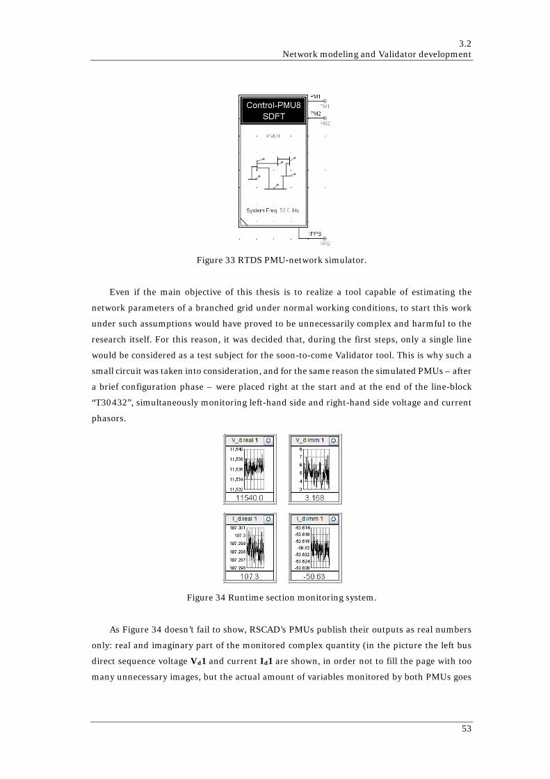
3.2 Network modeling and Validator development
Figure 33 RTDS PMU-network simulator.
Even if the main objective of this thesis is to realize a tool capable of estimating the
network parameters of a branched grid under normal working conditions, to start this work
under such assumptions would have proved to be unnecessarily complex and harmful to the
research itself. For this reason, it was decided that, during the first steps, only a single line
would be considered as a test subject for the soon-to-come Validator tool. This is why such a
small circuit was taken into consideration, and for the same reason the simulated PMUs – after
a brief configuration phase – were placed right at the start and at the end of the line-block
“T30432”, simultaneously monitoring left-hand side and right-hand side voltage and current
phasors.
Figure 34 Runtime section monitoring system.
As Figure 34 doesn’t fail to show, RSCAD’s PMUs publish their outputs as real numbers
only: real and imaginary part of the monitored complex quantity (in the picture the left bus
direct sequence voltage Vd1 and current Id1 are shown, in order not to fill the page with too
many unnecessary images, but the actual amount of variables monitored by both PMUs goes
53
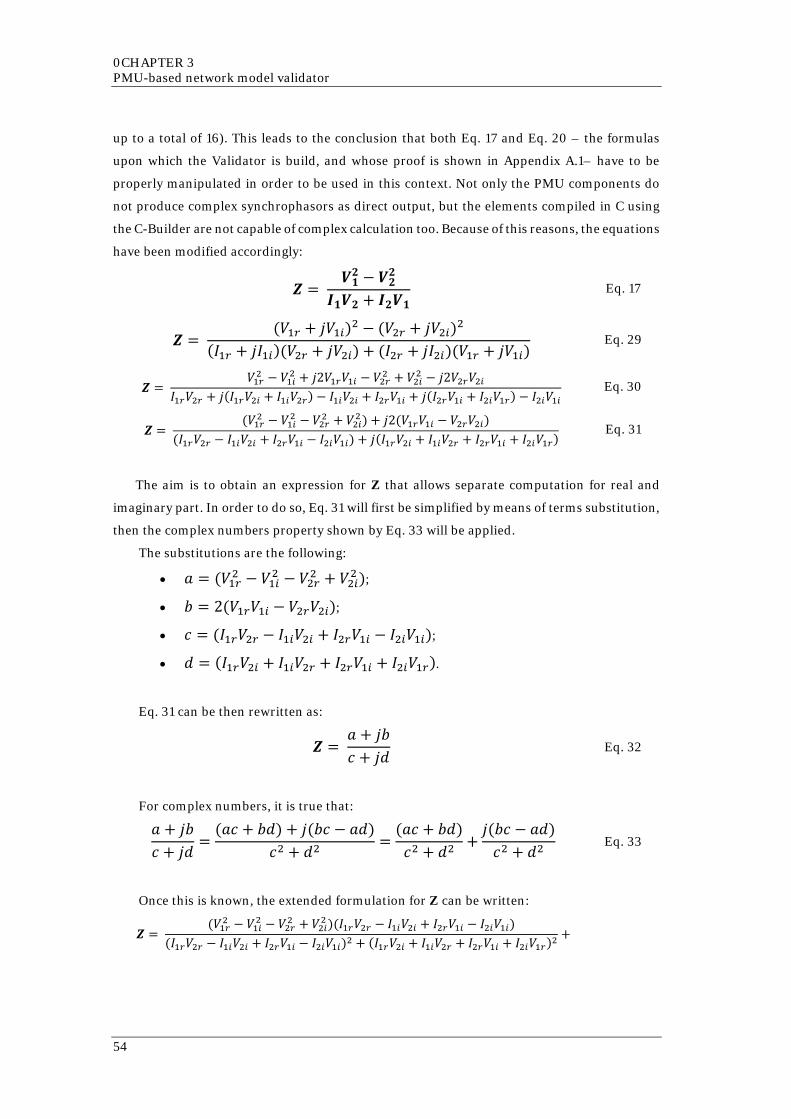
0CHAPTER 3 PMU-based network model validator
up to a total of 16). This leads to the conclusion that both Eq. 17 and Eq. 20 – the formulas
upon which the Validator is build, and whose proof is shown in Appendix A.1– have to be
properly manipulated in order to be used in this context. Not only the PMU components do
not produce complex synchrophasors as direct output, but the elements compiled in C using
the C-Builder are not capable of complex calculation too. Because of this reasons, the equations
have been modified accordingly:
𝒁𝒁 = 𝑽𝑽𝟏𝟏𝟐𝟐 − 𝑽𝑽𝟐𝟐𝟐𝟐
𝑰𝑰𝟏𝟏𝑽𝑽𝟐𝟐 + 𝑰𝑰𝟐𝟐𝑽𝑽𝟏𝟏 Eq. 17
𝒁𝒁 = (𝑉𝑉1𝑟𝑟 + 𝑗𝑗𝑉𝑉1𝑖𝑖)2 − (𝑉𝑉2𝑟𝑟 + 𝑗𝑗𝑉𝑉2𝑖𝑖)2
(𝐼𝐼1𝑟𝑟 + 𝑗𝑗𝐼𝐼1𝑖𝑖)(𝑉𝑉2𝑟𝑟 + 𝑗𝑗𝑉𝑉2𝑖𝑖) + (𝐼𝐼2𝑟𝑟 + 𝑗𝑗𝐼𝐼2𝑖𝑖)(𝑉𝑉1𝑟𝑟 + 𝑗𝑗𝑉𝑉1𝑖𝑖) Eq. 29
𝒁𝒁 = 𝑉𝑉1𝑟𝑟2 − 𝑉𝑉1𝑖𝑖2 + 𝑗𝑗2𝑉𝑉1𝑟𝑟𝑉𝑉1𝑖𝑖 − 𝑉𝑉2𝑟𝑟2 + 𝑉𝑉2𝑖𝑖2 − 𝑗𝑗2𝑉𝑉2𝑟𝑟𝑉𝑉2𝑖𝑖
𝐼𝐼1𝑟𝑟𝑉𝑉2𝑟𝑟 + 𝑗𝑗(𝐼𝐼1𝑟𝑟𝑉𝑉2𝑖𝑖 + 𝐼𝐼1𝑖𝑖𝑉𝑉2𝑟𝑟) − 𝐼𝐼1𝑖𝑖𝑉𝑉2𝑖𝑖 + 𝐼𝐼2𝑟𝑟𝑉𝑉1𝑖𝑖 + 𝑗𝑗(𝐼𝐼2𝑟𝑟𝑉𝑉1𝑖𝑖 + 𝐼𝐼2𝑖𝑖𝑉𝑉1𝑟𝑟) − 𝐼𝐼2𝑖𝑖𝑉𝑉1𝑖𝑖 Eq. 30
𝒁𝒁 = (𝑉𝑉1𝑟𝑟2 − 𝑉𝑉1𝑖𝑖2 − 𝑉𝑉2𝑟𝑟2 + 𝑉𝑉2𝑖𝑖2) + 𝑗𝑗2(𝑉𝑉1𝑟𝑟𝑉𝑉1𝑖𝑖 − 𝑉𝑉2𝑟𝑟𝑉𝑉2𝑖𝑖)
(𝐼𝐼1𝑟𝑟𝑉𝑉2𝑟𝑟 − 𝐼𝐼1𝑖𝑖𝑉𝑉2𝑖𝑖 + 𝐼𝐼2𝑟𝑟𝑉𝑉1𝑖𝑖 − 𝐼𝐼2𝑖𝑖𝑉𝑉1𝑖𝑖) + 𝑗𝑗(𝐼𝐼1𝑟𝑟𝑉𝑉2𝑖𝑖 + 𝐼𝐼1𝑖𝑖𝑉𝑉2𝑟𝑟 + 𝐼𝐼2𝑟𝑟𝑉𝑉1𝑖𝑖 + 𝐼𝐼2𝑖𝑖𝑉𝑉1𝑟𝑟) Eq. 31
The aim is to obtain an expression for Z that allows separate computation for real and
imaginary part. In order to do so, Eq. 31 will first be simplified by means of terms substitution,
then the complex numbers property shown by Eq. 33 will be applied.
The substitutions are the following:
• 𝑎𝑎 = (𝑉𝑉1𝑟𝑟2 − 𝑉𝑉1𝑖𝑖2 − 𝑉𝑉2𝑟𝑟2 + 𝑉𝑉2𝑖𝑖2 );
• 𝑏𝑏 = 2(𝑉𝑉1𝑟𝑟𝑉𝑉1𝑖𝑖 − 𝑉𝑉2𝑟𝑟𝑉𝑉2𝑖𝑖);
• 𝑐𝑐 = (𝐼𝐼1𝑟𝑟𝑉𝑉2𝑟𝑟 − 𝐼𝐼1𝑖𝑖𝑉𝑉2𝑖𝑖 + 𝐼𝐼2𝑟𝑟𝑉𝑉1𝑖𝑖 − 𝐼𝐼2𝑖𝑖𝑉𝑉1𝑖𝑖);
• 𝑑𝑑 = (𝐼𝐼1𝑟𝑟𝑉𝑉2𝑖𝑖 + 𝐼𝐼1𝑖𝑖𝑉𝑉2𝑟𝑟 + 𝐼𝐼2𝑟𝑟𝑉𝑉1𝑖𝑖 + 𝐼𝐼2𝑖𝑖𝑉𝑉1𝑟𝑟).
Eq. 31 can be then rewritten as:
𝒁𝒁 = 𝑎𝑎 + 𝑗𝑗𝑏𝑏𝑐𝑐 + 𝑗𝑗𝑑𝑑
Eq. 32
For complex numbers, it is true that:
𝑎𝑎 + 𝑗𝑗𝑏𝑏𝑐𝑐 + 𝑗𝑗𝑑𝑑
=(𝑎𝑎𝑐𝑐 + 𝑏𝑏𝑑𝑑) + 𝑗𝑗(𝑏𝑏𝑐𝑐 − 𝑎𝑎𝑑𝑑)
𝑐𝑐2 + 𝑑𝑑2=
(𝑎𝑎𝑐𝑐 + 𝑏𝑏𝑑𝑑)𝑐𝑐2 + 𝑑𝑑2
+𝑗𝑗(𝑏𝑏𝑐𝑐 − 𝑎𝑎𝑑𝑑)𝑐𝑐2 + 𝑑𝑑2
Eq. 33
Once this is known, the extended formulation for Z can be written:
𝒁𝒁 = (𝑉𝑉1𝑟𝑟2 − 𝑉𝑉1𝑖𝑖2 − 𝑉𝑉2𝑟𝑟2 + 𝑉𝑉2𝑖𝑖2 )(𝐼𝐼1𝑟𝑟𝑉𝑉2𝑟𝑟 − 𝐼𝐼1𝑖𝑖𝑉𝑉2𝑖𝑖 + 𝐼𝐼2𝑟𝑟𝑉𝑉1𝑖𝑖 − 𝐼𝐼2𝑖𝑖𝑉𝑉1𝑖𝑖)
(𝐼𝐼1𝑟𝑟𝑉𝑉2𝑟𝑟 − 𝐼𝐼1𝑖𝑖𝑉𝑉2𝑖𝑖 + 𝐼𝐼2𝑟𝑟𝑉𝑉1𝑖𝑖 − 𝐼𝐼2𝑖𝑖𝑉𝑉1𝑖𝑖)2 + (𝐼𝐼1𝑟𝑟𝑉𝑉2𝑖𝑖 + 𝐼𝐼1𝑖𝑖𝑉𝑉2𝑟𝑟 + 𝐼𝐼2𝑟𝑟𝑉𝑉1𝑖𝑖 + 𝐼𝐼2𝑖𝑖𝑉𝑉1𝑟𝑟)2 +
54
3.2 Network modeling and Validator development
+2(𝑉𝑉1𝑟𝑟𝑉𝑉1𝑖𝑖 − 𝑉𝑉2𝑟𝑟𝑉𝑉2𝑖𝑖)(𝐼𝐼1𝑟𝑟𝑉𝑉2𝑖𝑖 + 𝐼𝐼1𝑖𝑖𝑉𝑉2𝑟𝑟 + 𝐼𝐼2𝑟𝑟𝑉𝑉1𝑖𝑖 + 𝐼𝐼2𝑖𝑖𝑉𝑉1𝑟𝑟)
(𝐼𝐼1𝑟𝑟𝑉𝑉2𝑟𝑟 − 𝐼𝐼1𝑖𝑖𝑉𝑉2𝑖𝑖 + 𝐼𝐼2𝑟𝑟𝑉𝑉1𝑖𝑖 − 𝐼𝐼2𝑖𝑖𝑉𝑉1𝑖𝑖)2 + (𝐼𝐼1𝑟𝑟𝑉𝑉2𝑖𝑖 + 𝐼𝐼1𝑖𝑖𝑉𝑉2𝑟𝑟 + 𝐼𝐼2𝑟𝑟𝑉𝑉1𝑖𝑖 + 𝐼𝐼2𝑖𝑖𝑉𝑉1𝑟𝑟)2 + Eq. 34
+𝒋𝒋(2(𝑉𝑉1𝑟𝑟𝑉𝑉1𝑖𝑖 − 𝑉𝑉2𝑟𝑟𝑉𝑉2𝑖𝑖)(𝐼𝐼1𝑟𝑟𝑉𝑉2𝑟𝑟 − 𝐼𝐼1𝑖𝑖𝑉𝑉2𝑖𝑖 + 𝐼𝐼2𝑟𝑟𝑉𝑉1𝑖𝑖 − 𝐼𝐼2𝑖𝑖𝑉𝑉1𝑖𝑖)
(𝐼𝐼1𝑟𝑟𝑉𝑉2𝑟𝑟 − 𝐼𝐼1𝑖𝑖𝑉𝑉2𝑖𝑖 + 𝐼𝐼2𝑟𝑟𝑉𝑉1𝑖𝑖 − 𝐼𝐼2𝑖𝑖𝑉𝑉1𝑖𝑖)2 + (𝐼𝐼1𝑟𝑟𝑉𝑉2𝑖𝑖 + 𝐼𝐼1𝑖𝑖𝑉𝑉2𝑟𝑟 + 𝐼𝐼2𝑟𝑟𝑉𝑉1𝑖𝑖 + 𝐼𝐼2𝑖𝑖𝑉𝑉1𝑟𝑟)2 +
−(𝑉𝑉1𝑟𝑟2 − 𝑉𝑉1𝑖𝑖2 − 𝑉𝑉2𝑟𝑟2 + 𝑉𝑉2𝑖𝑖2)(𝐼𝐼1𝑟𝑟𝑉𝑉2𝑖𝑖 + 𝐼𝐼1𝑖𝑖𝑉𝑉2𝑟𝑟 + 𝐼𝐼2𝑟𝑟𝑉𝑉1𝑖𝑖 + 𝐼𝐼2𝑖𝑖𝑉𝑉1𝑟𝑟)
(𝐼𝐼1𝑟𝑟𝑉𝑉2𝑟𝑟 − 𝐼𝐼1𝑖𝑖𝑉𝑉2𝑖𝑖 + 𝐼𝐼2𝑟𝑟𝑉𝑉1𝑖𝑖 − 𝐼𝐼2𝑖𝑖𝑉𝑉1𝑖𝑖)2 + (𝐼𝐼1𝑟𝑟𝑉𝑉2𝑖𝑖 + 𝐼𝐼1𝑖𝑖𝑉𝑉2𝑟𝑟 + 𝐼𝐼2𝑟𝑟𝑉𝑉1𝑖𝑖 + 𝐼𝐼2𝑖𝑖𝑉𝑉1𝑟𝑟)2)
The exact same reasoning can be applied to Eq. 20, leading to the following result:
𝒀𝒀 = 2 ∙𝑰𝑰𝟏𝟏 − 𝑰𝑰𝟐𝟐𝑽𝑽𝟏𝟏 + 𝑽𝑽𝟐𝟐
Eq. 20
𝒀𝒀 = 2 ∙(𝐼𝐼1𝑟𝑟 + 𝑗𝑗𝐼𝐼1𝑖𝑖) − (𝐼𝐼2𝑟𝑟 + 𝑗𝑗𝐼𝐼2𝑖𝑖)
(𝑉𝑉1𝑟𝑟 + 𝑗𝑗𝑉𝑉1𝑖𝑖) + (𝑉𝑉2𝑟𝑟 + 𝑗𝑗𝑉𝑉2𝑖𝑖) Eq. 35
𝒀𝒀 = 2 ∙(𝐼𝐼1𝑟𝑟 − 𝐼𝐼2𝑟𝑟) + 𝑗𝑗(𝐼𝐼1𝑖𝑖 − 𝐼𝐼2𝑖𝑖)
(𝑉𝑉1𝑟𝑟 + 𝑉𝑉2𝑟𝑟) + 𝑗𝑗(𝑉𝑉1𝑖𝑖 + 𝑉𝑉2𝑖𝑖) Eq. 36
Defining the new substitution terms:
• 𝑎𝑎′ = (𝐼𝐼1𝑟𝑟 − 𝐼𝐼2𝑟𝑟);
• 𝑏𝑏′ = (𝐼𝐼1𝑖𝑖 − 𝐼𝐼2𝑖𝑖);
• 𝑐𝑐′ = (𝑉𝑉1𝑟𝑟 + 𝑉𝑉2𝑟𝑟);
• 𝑑𝑑′ = (𝑉𝑉1𝑖𝑖 + 𝑉𝑉2𝑖𝑖).
Using these new parameters in Eq. 33, we finally obtain:
𝒀𝒀 = 2(𝐼𝐼1𝑟𝑟 − 𝐼𝐼2𝑟𝑟)(𝑉𝑉1𝑟𝑟 + 𝑉𝑉2𝑟𝑟) + (𝐼𝐼1𝑖𝑖 − 𝐼𝐼2𝑖𝑖)(𝑉𝑉1𝑖𝑖 + 𝑉𝑉2𝑖𝑖)
(𝑉𝑉1𝑟𝑟 + 𝑉𝑉2𝑟𝑟)2 + (𝑉𝑉1𝑖𝑖 + 𝑉𝑉2𝑖𝑖)2+
Eq. 37
+2𝑗𝑗(𝐼𝐼1𝑖𝑖 − 𝐼𝐼2𝑖𝑖)(𝑉𝑉1𝑟𝑟 + 𝑉𝑉2𝑟𝑟) − (𝐼𝐼1𝑟𝑟 − 𝐼𝐼2𝑟𝑟)(𝑉𝑉1𝑖𝑖 + 𝑉𝑉2𝑖𝑖)
(𝑉𝑉1𝑟𝑟 + 𝑉𝑉2𝑟𝑟)2 + (𝑉𝑉1𝑖𝑖 + 𝑉𝑉2𝑖𝑖)2
Both Eq. 34 and Eq. 37, written in a generic fashion, can be used to calculate the
impedance/admittance of any of the sequences (positive, negative, zero), given the proper
voltage and current measurements. Once applied, series resistance and inductive reactance
and shunt capacitive reactance can be derived simply by isolation of the real/imaginary portion
of the calculated impedance Z and admittance Y. Both equations were tested in MATLAB,
comparing their results with the ones produced by Eq. 17 and Eq. 20 using the same inputs
(see Appendix A.2 for the source code).
The results produced by both sets of equations, however, were interesting yet problematic:
• Positive sequence series resistance Rd= 10.7938 Ω; (-0.4% error)
55
0CHAPTER 3 PMU-based network model validator
• Positive sequence series inductive reactance X_Ld= 2.5664 Ω; (-0.8% error)
• Positive sequence shunt capacitive reactance X_Cd= 72.6130 kΩ; (-3.5% error)
• Zero sequence series resistance Ro= 6.481 kΩ; (+22856.2% error)
• Zero sequence series inductive reactance X_Lo= -1.5850 kΩ; (-9266.1% error)
• Zero sequence shunt capacitive reactance X_Co= -7.1810 kΩ. (-109.5% error)
While the positive sequence parameters were calculated with a high degree of precision,
the same could not be said for the zero sequence ones. They were in fact clearly affected by
some kind of issues that prevented the algorithm to obtain the correct values. After some in-
depth analysis and tests involving simulated single-phase faults, it was concluded that the
gross errors obtained were caused by a lack of zero sequence current, unable to circulate in
such a small network. PMU measurements were, in particular, strongly affected by errors due
to the currents’ proximity to zero, and their oscillation around that same value. Simulating a
single-line-to-ground fault, that is allowing zero sequence current to flow on the line, solved
the issue:
• Positive sequence series resistance Rd= 10.8400 Ω; (-0.02% error)
• Positive sequence series inductive reactance X_Ld= 2.5880 Ω; (+0.02% error)
• Positive sequence shunt capacitive reactance X_Cd= 72.2200 kΩ; (-4.0% error)
• Zero sequence series resistance Ro= 28.2514 Ω; (+0.07% error)
• Zero sequence series inductive reactance X_Lo= 17.3125 Ω; (+0.12% error)
• Zero sequence shunt capacitive reactance X_Co= 75.2110 Ω. (-0.02% error)
Note that, in order to make the current flow during the fault simulation, a return path had
to be created. This was done by connecting the generator’s neutral point to ground. Even
though this is no usual practice for a real MV distribution grid, it was needed for this specific
test’s sake. The ground connection was then removed.
The outcome of this last experiment revealed the need to carry out new ones in a different
environment, a network model far more extensive and realistic. This evolution will be seen in
sub-chapter 3.3, while this one will be instead closed with the description of another part of
the development process, with a higher degree of priority: the creation of the first version of
the Validator component (both in terms of aesthetic design and code creation in C language).
The creative process starts in the C-Builder section of RSCAD. Here, as shown in Figure
35, the user is first given the opportunity to decide the shape of the component (even though
this will have no consequences on its performance whatsoever), the number and position of its
input/output ports (respectively on the left/right) and the possible presence of any writings on
it. In this case, the Validator assumed a rectangular shape in order to accommodate the high
number of needed ports. In the simple case of two PMUs monitoring both sides of a line in
order to calculate its positive and zero sequence parameters (the negative ones are of no
interest for e-distribuzione), four synchrophasors will have to be collected from each of them
56
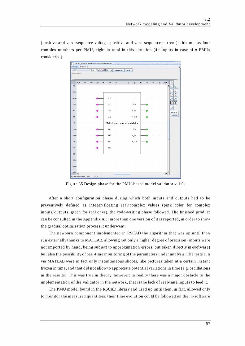
3.2 Network modeling and Validator development
(positive and zero sequence voltage, positive and zero sequence current); this means four
complex numbers per PMU, eight in total in this situation (4n inputs in case of n PMUs
considered).
Figure 35 Design phase for the PMU-based model validator v. 1.0.
After a short configuration phase during which both inputs and outputs had to be
preventively defined as integer/floating real/complex values (pink color for complex
inputs/outputs, green for real ones), the code-writing phase followed. The finished product
can be consulted in the Appendix A.3: more than one version of it is reported, in order to show
the gradual optimization process it underwent.
The newborn component implemented in RSCAD the algorithm that was up until then
run externally thanks to MATLAB, allowing not only a higher degree of precision (inputs were
not imported by hand, being subject to approximation errors, but taken directly in-software)
but also the possibility of real-time monitoring of the parameters under analysis. The tests run
via MATLAB were in fact only instantaneous shoots, like pictures taken at a certain instant
frozen in time, and that did not allow to appreciate potential variations in time (e.g. oscillations
in the results). This was true in theory, however: in reality there was a major obstacle to the
implementation of the Validator in the network, that is the lack of real-time inputs to feed it.
The PMU model found in the RSCAD library and used up until then, in fact, allowed only
to monitor the measured quantities: their time evolution could be followed on the in-software
57
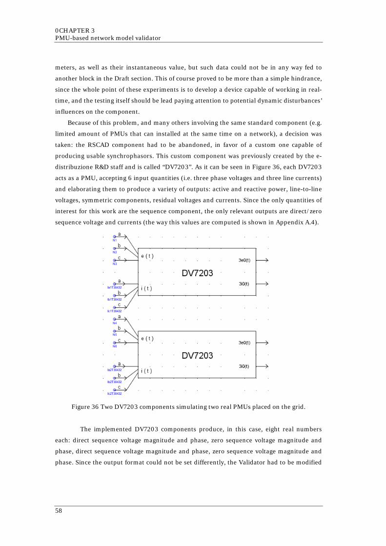
0CHAPTER 3 PMU-based network model validator
meters, as well as their instantaneous value, but such data could not be in any way fed to
another block in the Draft section. This of course proved to be more than a simple hindrance,
since the whole point of these experiments is to develop a device capable of working in real-
time, and the testing itself should be lead paying attention to potential dynamic disturbances’
influences on the component.
Because of this problem, and many others involving the same standard component (e.g.
limited amount of PMUs that can installed at the same time on a network), a decision was
taken: the RSCAD component had to be abandoned, in favor of a custom one capable of
producing usable synchrophasors. This custom component was previously created by the e-
distribuzione R&D staff and is called “DV7203”. As it can be seen in Figure 36, each DV7203
acts as a PMU, accepting 6 input quantities (i.e. three phase voltages and three line currents)
and elaborating them to produce a variety of outputs: active and reactive power, line-to-line
voltages, symmetric components, residual voltages and currents. Since the only quantities of
interest for this work are the sequence component, the only relevant outputs are direct/zero
sequence voltage and currents (the way this values are computed is shown in Appendix A.4).
Figure 36 Two DV7203 components simulating two real PMUs placed on the grid.
The implemented DV7203 components produce, in this case, eight real numbers
each: direct sequence voltage magnitude and phase, zero sequence voltage magnitude and
phase, direct sequence voltage magnitude and phase, zero sequence voltage magnitude and
phase. Since the output format could not be set differently, the Validator had to be modified
58
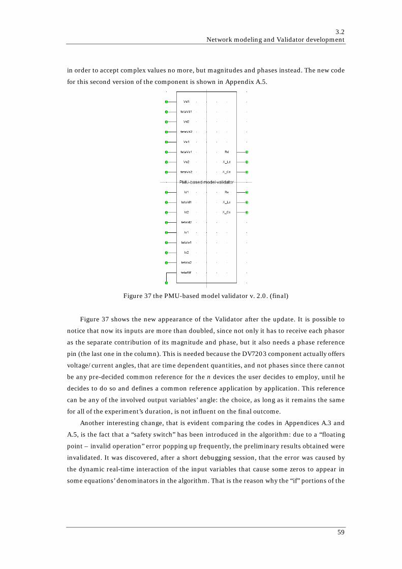
3.2 Network modeling and Validator development
in order to accept complex values no more, but magnitudes and phases instead. The new code
for this second version of the component is shown in Appendix A.5.
Figure 37 the PMU-based model validator v. 2.0. (final)
Figure 37 shows the new appearance of the Validator after the update. It is possible to
notice that now its inputs are more than doubled, since not only it has to receive each phasor
as the separate contribution of its magnitude and phase, but it also needs a phase reference
pin (the last one in the column). This is needed because the DV7203 component actually offers
voltage/current angles, that are time dependent quantities, and not phases since there cannot
be any pre-decided common reference for the n devices the user decides to employ, until he
decides to do so and defines a common reference application by application. This reference
can be any of the involved output variables’ angle: the choice, as long as it remains the same
for all of the experiment’s duration, is not influent on the final outcome.
Another interesting change, that is evident comparing the codes in Appendices A.3 and
A.5, is the fact that a “safety switch” has been introduced in the algorithm: due to a “floating
point – invalid operation” error popping up frequently, the preliminary results obtained were
invalidated. It was discovered, after a short debugging session, that the error was caused by
the dynamic real-time interaction of the input variables that cause some zeros to appear in
some equations’ denominators in the algorithm. That is the reason why the “if” portions of the
59
0CHAPTER 3 PMU-based network model validator
code were added: they act as a protection, avoiding the zeros to influence the calculation by
substituting them with a very small yet non-null constant.
After the Validator 2.0 was introduced, new tests were run. The results were positive, with
small errors: this was the confirmation that the component was still working well even after
the upgrade. However it proved, again, to be able to accurately compute zero sequence
parameters only while simulating a single-phase-to-ground fault. This condition, completely
unacceptable, needed to be studied more in depth and, if possible, overcome. In order to do
so, as anticipated, another network model (that pre-existed in e-distribuzione’s database) was
taken into consideration, one where zero sequence currents naturally flow – even if small in
magnitude – due to its size. In that new context, the Validator was expected to produce
positive results even without the necessity to simulate ground faults. This hypothesis is
validated in the following sub-chapter 3.3.
3.3 Validator testing in a realistic distribution
network
The new network model the following tests were run in is, by e-distribuzione’s will, to be
kept as anonymous as possible. Due to this internal policy, no real names can be mentioned
and the grid itself cannot be fully shown (also because of its sheer size, too big to be properly
presented in its entirety on A4 pages). However this proves to be not a problem: only portions
of said grid were interested by the research activities, and those will be described as precisely
as possible.
Figure 38, in the following page, shows a small but important part of the network: on the
left the HV grid’s equivalent is simulated by means of a couple of three-phase 150 kV real
sinusoidal voltage generators. At the top of the picture there is the 156 kV/20.8 kV HV/MV
Y/Yn transformer from which a number of MV feeders depart. The vertical three-phase MV
line the feeders are connected to simulates the low voltage-side busbar. The visible
transformer, the only one of interest in this context, is the red one in the primary substation:
five feeders are found here. The vertical three-phase HV line is connected to the green
transformer, that will remain hidden since it is not needed to consider it in this study.
It is not possible to show the feeders in all their length, since they are very long and/or
branch out so much that it would be too encumbering on the document’s layout to show them
all. However some of them, the ones that are going to be studied in depth, will be described
with words and partial graphical representation, as needed case by case.
60
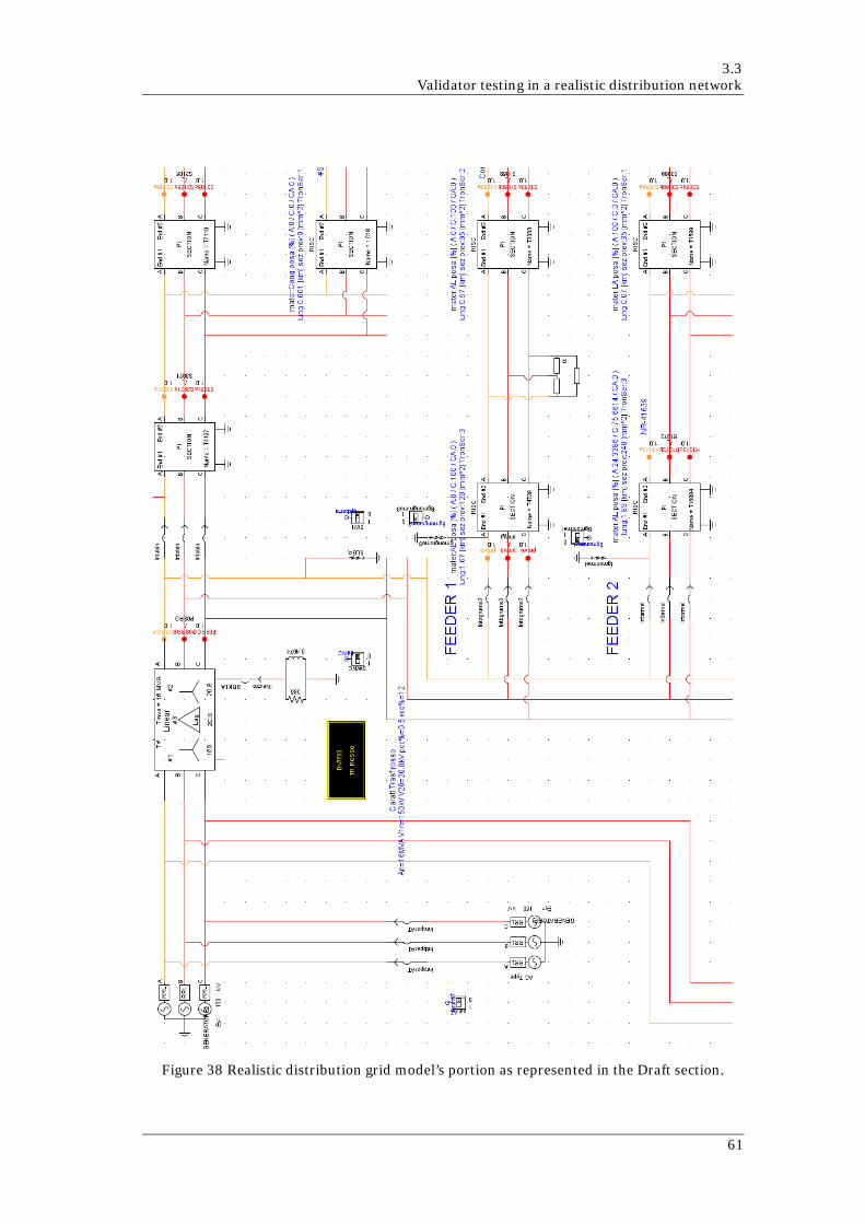
3.3 Validator testing in a realistic distribution network
Figure 38 Realistic distribution grid model’s portion as represented in the Draft section.
61
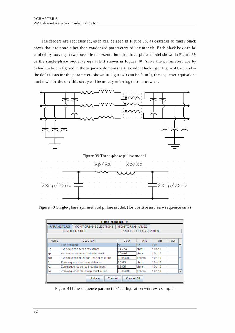
0CHAPTER 3 PMU-based network model validator
The feeders are represented, as in can be seen in Figure 38, as cascades of many black
boxes that are none other than condensed parameters pi line models. Each black box can be
studied by looking at two possible representation: the three-phase model shown in Figure 39
or the single-phase sequence equivalent shown in Figure 40. Since the parameters are by
default to be configured in the sequence domain (as it is evident looking at Figure 41, were also
the definitions for the parameters shown in Figure 40 can be found), the sequence equivalent
model will be the one this study will be mostly referring to from now on.
Figure 39 Three-phase pi line model.
Figure 40 Single-phase symmetrical pi line model. (for positive and zero sequence only)
Figure 41 Line sequence parameters’ configuration window example.
62

3.3 Validator testing in a realistic distribution network
The first experiments were carried out in a no-load condition: all the lines were
interested only by a current flow caused by the presence of shunt capacitances, and nothing
else. It was decided to proceed like this, at least at first, in order to simplify the Validator’s
effectiveness preliminary testing phase: loads were added in a second phase, following a
progressive increase in complexity plan for the network that the component had to work in.
To be more precise, the plan was the following these steps:
1. Verifying the Validator’s effectiveness/efficiency when used on a short linear
unloaded feeder;
2. Verifying the Validator’s effectiveness/efficiency when used on a long linear
unloaded feeder;
3. Verifying the Validator’s effectiveness/efficiency when used on a long branched
unloaded feeder;
4. Verifying the Validator’s effectiveness/efficiency when used on a long branched
loaded feeder.
The chosen distribution network luckily offers lines that fit all four possible scenarios,
that will now be analyzed one by one.
3.3.1 Short linear unloaded feeder
The line chosen to conduct these tests is “Feeder 3”, a relatively short one (4.6 km)
fragmented into eight portions. (the first three of them are shown in Figure 42)
Figure 42 “Feeder 3” partial view as represented in the Draft section.
This test aims to prove that the Validator is able to correctly compute the cumulative
symmetrical line parameters (positive and zero sequence) not only when applied to a single pi-
model, but also when their number increases and the total considered length with it. (in order
to understand if there is any precision drop working with longer lines) To validate the test
results however, that is to understand if the outputs of the Validator are correct or not, a
MATLAB model of the line needs to be built. The objective of this model is to elaborate, starting
63

0CHAPTER 3 PMU-based network model validator
from the data from each of the eight sections the line is split in, an equivalent pi-model (one
for each sequence) whose parameters must coincide to the ones computed by the Validator.
Before showing the MATLAB code that was created with this specific intent, it is necessary
to explain the theoretical basis on which it was built. The core concept is that to each pi-model
corresponds a transmission matrix: once the eight transmission matrices are calculated, the
black boxes’ cascade can be analytically translated into the ordered multiplication of said
matrices, until a single one is obtained. This single transmission matrix represents the
equivalent of the entire line (in terms of symmetrical variables) and can finally be transformed
back into a pi-model, ready to be compared with the Validator’s results.
The rigorous step-by-step mathematical demonstration of what has been stated here can
be found in Appendix 101A.6, together with the MATLAB algorithm that implements this
procedure for Feeder 3.
The eight sections of the line under analysis are called, from left (busbar) to right (end
switch): T3016, T3641, T3642, T3017, T3650, T3649, T3009 and T3647. The following list
compares the line parameters of interest – positive sequence series resistance Rd, series
inductive reactance X_Ld, shunt capacitive reactance X_Cd and zero sequence series
resistance Ro, series inductive reactance X_Lo, shunt capacitive reactance X_Co – as obtained
from the MATLAB algorithm (on the left) and from the Validator in the simulation (on the
right), underlining in brackets the percent difference between the two measurements.
One branch section at a time, all of them will be included in the analysis by moving the
second PMU toward the right:
T3016
• Rd=0.4585 Ω, while the Validator’s output is 0.4809 Ω; (+0.05%)
• X_Ld=0.2050 Ω, while the Validator’s output is 0.2051 Ω; (+0.05%)
• X_Cd=6409.3 Ω, while the Validator’s output is 6406 Ω; (-0.05%)
• Ro=2.0679 Ω, while the Validator’s output is 2.090 Ω; (+1.1)
• X_Lo=1.5525 Ω, while the Validator’s output is 1.553 Ω; (0.03%)
• X_Co=6409.3 Ω, while the Validator’s output is 6406 Ω; (-0.05%)
T3016 and T3641
• Rd=0.5833 Ω, while the Validator’s output is 0.5893 Ω; (+1.03%)
• X_Ld=0.2549 Ω, while the Validator’s output is 0.2539 Ω; (-0.39%)
• X_Cd=5220 Ω, while the Validator’s output is 5218 Ω; (-0.04%)
64

3.3 Validator testing in a realistic distribution network
• Ro=2.5360 Ω, while the Validator’s output is 2.5470 Ω; (-0.43%)
• X_Lo=1.9425 Ω, while the Validator’s output is 1.9350 Ω; (-0.39%)
• X_Co=5221 Ω, while the Validator’s output is 5218 Ω; (-0.06%)
T3016, T3641 and T3642
• Rd=0.6761 Ω, while the Validator’s output is 0.6869 Ω; (+1.60%)
• X_Ld=0.2920 Ω, while the Validator’s output is 0.2905 Ω; (-0.51%)
• X_Cd=4588 Ω, while the Validator’s output is 4585 Ω; (-0.07%)
• Ro=2.8842 Ω, while the Validator’s output is 2.9040 Ω; (+0.69%)
• X_Lo=2.2324 Ω, while the Validator’s output is 2.2180 Ω; (-0.65%)
• X_Co=4588 Ω, while the Validator’s output is 4585 Ω; (-0.07%)
T3016, T3641, T3642 and T3017
• Rd=0.8272 Ω, while the Validator’s output is 0.8470 Ω; (+2.39%)
• X_Ld=0.3524 Ω, while the Validator’s output is 0.3500 Ω; (-0.68%)
• X_Cd=3832 Ω, while the Validator’s output is 3830 Ω; (-0.05%)
• Ro=3.4509 Ω, while the Validator’s output is 3.4870 Ω; (+1.05%)
• X_Lo=2.7044 Ω, while the Validator’s output is 2.6780 Ω; (-0.98%)
• X_Co=3832 Ω, while the Validator’s output is 3830 Ω; (-0.05%)
T3016, T3641, T3642, T3017 and T3650
• Rd=0.9631 Ω, while the Validator’s output is 0.9530 Ω; (-1.05%)
• X_Ld=0.4073 Ω, while the Validator’s output is 0.4033 Ω; (-0.98%)
• X_Cd=3329 Ω, while the Validator’s output is 3328 Ω; (-0.03%)
• Ro=3.9683 Ω, while the Validator’s output is 3.9820 Ω; (+0.35%)
• X_Lo=3.1325 Ω, while the Validator’s output is 3.0950 Ω; (-1.20%)
• X_Co=3330 Ω, while the Validator’s output is 3327 Ω; (-0.09%)
T3016, T3641, T3642, T3017, T3650 and T3649
• Rd=1.2399 Ω, while the Validator’s output is 1.2160 Ω; (-1.93%)
• X_Ld=0.5180 Ω, while the Validator’s output is 0.5108 Ω; (-1.39%)
65

0CHAPTER 3 PMU-based network model validator
• X_Cd=2637 Ω, while the Validator’s output is 2636 Ω; (-0.04%)
• Ro=5.0075 Ω, while the Validator’s output is 5.0270 Ω; (0.39%)
• X_Lo=3.9972 Ω, while the Validator’s output is 3.9270 Ω; (-1.76%)
• X_Co=2638 Ω, while the Validator’s output is 2636 Ω; (-0.08%)
T3016, T3641, T3642, T3017, T3650, T3649 and T3009
• Rd=1.2639 Ω, while the Validator’s output is 1.2440 Ω; (-1.57%)
• X_Ld=0.5276 Ω, while the Validator’s output is 0.5202 Ω; (-1.4%)
• X_Cd=2591 Ω, while the Validator’s output is 2589 Ω; (-0.08%)
• Ro=5.0977 Ω, while the Validator’s output is 5.1230 Ω; (0.4%)
• X_Lo=4.0722 Ω, while the Validator’s output is 3.9999 Ω; (-1.8%)
• X_Co=2591 Ω, while the Validator’s output is 2589 Ω; (-0.08%)
T3016, T3641, T3642, T3017, T3650, T3649, T3009 and T3647
• Rd=1.4099 Ω, while the Validator’s output is 1.3380 Ω; (-4.49%)
• X_Ld=0.5859 Ω, while the Validator’s output is 0.5776 Ω; (-1.4%)
• X_Cd=2339 Ω, while the Validator’s output is 2338 Ω; (-0.04%)
• Ro=5.6458 Ω, while the Validator’s output is 5.7310 Ω; (+1.51%)
• X_Lo=4.5279 Ω, while the Validator’s output is 4.4320 Ω; (-2.12%)
• X_Co=2339 Ω, while the Validator’s output is 2337 Ω; (-0.09%)
The test results in a success, since very small errors are met in the process. Small enough
to be considered negligible: the error threshold imposed by e-distribuzione’s technician was
+/-5%, so the Validator’s measurements successfully passed this first exam. However, even if
already considered acceptable, this errors can be further reduced taking into consideration
their causes: parallax errors in the readings, influence of circuital components not taken in
consideration in the MATLAB model (e.g. breakers resistance) on the measurements and error
propagation during the calculations. With those considered, the difference between the two
algorithms tends to zero.
66

3.3 Validator testing in a realistic distribution network
3.3.2 Long linear unloaded feeder
The line chosen to conduct these tests is “Feeder 1”, a relatively long one (9.048 km)
fragmented into fifteen portions. (the first three of them are shown in Figure 43)
Figure 43 “Feeder 1” partial view as represented in the Draft section.
This test aims to prove that the Validator is able to correctly compute the cumulative
symmetrical line parameters (positive and zero sequence) also in case of very long lines. This
experiment was conducted as the previous one was, with the gradual addition of the line
sections and step-by-step parameters’ reading from both the simulation and MATLAB:
(starting from the first couple of branch portions on the left, since the effectiveness of the
method on the single segment has been already proved)
T4739 and T3003
• Rd=0.6530 Ω, while the Validator’s output is 0.6486 Ω; (-0.67%)
• X_Ld=0.2859 Ω, while the Validator’s output is 0.2848 Ω; (-0.38%)
• X_Cd=4781 Ω, while the Validator’s output is 4779 Ω; (-0.04%)
• Ro=2.8572 Ω, while the Validator’s output is 2.8570 Ω; (-0.01%)
• X_Lo=2.1710 Ω, while the Validator’s output is 2.1540 Ω; (-0.78%)
• X_Co=4853 Ω, while the Validator’s output is 4850 Ω; (-0.06%)
T4739, T3003 and T23081
• Rd=0.8210 Ω, while the Validator’s output is 0.8062 Ω; (-1.80%)
• X_Ld=0.3399 Ω, while the Validator’s output is 0.3373 Ω; (-0.76%)
• X_Cd=4135 Ω, while the Validator’s output is 4133 Ω; (-0.05%)
• Ro=3.3951 Ω, while the Validator’s output is 3.3600 Ω; (-1.03%)
• X_Lo=2.5621 Ω, while the Validator’s output is 2.526 Ω; (-1.41%)
67

0CHAPTER 3 PMU-based network model validator
• X_Co=4189 Ω, while the Validator’s output is 4186; (-0.07%)
T4739, T3003, T23081 and T19459
• Rd=0.9429 Ω, while the Validator’s output is 0.9203 Ω; (-2.40%)
• X_Ld=0.3790 Ω, while the Validator’s output is 0.3752 Ω; (-1.00%)
• X_Cd=3776 Ω, while the Validator’s output is 3764 Ω; (-0.32%)
• Ro=3.7851 Ω, while the Validator’s output is 3.761 Ω; (-0.7%)
• X_Lo=2.8456 Ω, while the Validator’s output is 2.827 Ω; (-0.6%)
• X_Co=3811 Ω, while the Validator’s output is 3809 Ω; (-3.3%)
T4739, T3003, T23081, T19459 and T3656
• Rd=1.3415 Ω, while the Validator’s output is 1.2990 Ω; (-3.17%)
• X_Ld=0.5225 Ω, while the Validator’s output is 0.5151 Ω; (-1.42%)
• X_Cd=2822 Ω, while the Validator’s output is 2821 Ω; (-0.04%)
• Ro=5.1833 Ω, while the Validator’s output is 5.1300 Ω; (-1.03%)
• X_Lo=3.9197 Ω, while the Validator’s output is 3.878 Ω; (-1.06%)
• X_Co=2847 Ω, while the Validator’s output is 2845 Ω; (-0.07%)
T4739, T3003, T23081, T19459, T3656 and T12820
• Rd=1.4893 Ω, while the Validator’s output is 1.4420 Ω; (-3.18%)
• X_Ld=0.5761 Ω, while the Validator’s output is 0.5683 Ω; (-1.35%)
• X_Cd=2563 Ω, while the Validator’s output is 2562 Ω; (-0.04%)
• Ro=5.6998 Ω, while the Validator’s output is 5.6470 Ω; (-0.93%)
• X_Lo=4.3259 Ω, while the Validator’s output is 4.2810 Ω; (-1.04%)
• X_Co=2584 Ω, while the Validator’s output is 2582 Ω; (-0.08%)
T4739, T3003, T23081, T19459, T3656, T12820 and T3600
• Rd=1.6200 Ω, while the Validator’s output is 1.5690 Ω; (-3.15%)
• X_Ld=0.6236 Ω, while the Validator’s output is 0.6151 Ω; (-1.36%)
• X_Cd=2371 Ω, while the Validator’s output is 2369 Ω; (-0.08%)
• Ro=6.1671 Ω, while the Validator’s output is 6.1050 Ω; (-1.01%)
68

3.3 Validator testing in a realistic distribution network
• X_Lo=4.6855 Ω, while the Validator’s output is 4.638 Ω; (-1.99%)
• X_Co=2388 Ω, while the Validator’s output is 2386 Ω; (-0.08%)
T4739, T3003, T23081, T19459, T3656, T12820, T3600 and T7013
• Rd=1.6914 Ω, while the Validator’s output is 1.633 Ω; (-3.45%)
• X_Ld=0.6465 Ω, while the Validator’s output is 0.6371 Ω; (-1.45%)
• X_Cd=2295 Ω, while the Validator’s output is 2294 Ω; (-0.04%)
• Ro=6.3860 Ω, while the Validator’s output is 6.324 Ω; (-0.97%)
• X_Lo=4.8516 Ω, while the Validator’s output is 4.800 Ω; (-1.06%)
• X_Co=2312 Ω, while the Validator’s output is 2310 Ω; (-0.09%)
T4739, T3003, T23081, T19459, T3656, T12820, T3600, T7013 and T12247
• Rd=1.8775 Ω, while the Validator’s output is 1.805 Ω; (-3.86%)
• X_Ld=0.7101 Ω, while the Validator’s output is 0.6993 Ω; (-1.52%)
• X_Cd=2099 Ω, while the Validator’s output is 2098 Ω; (-0.05%)
• Ro=7.0088 Ω, while the Validator’s output is 6.9340 Ω; (-1.07%)
• X_Lo=5.3243 Ω, while the Validator’s output is 5.2660 Ω; (-1.09%)
• X_Co=2113 Ω, while the Validator’s output is 2111 Ω; (-0.09%)
T4739, T3003, T23081, T19459, T3656, T12820, T3600, T7013, T12247 and T6824
• Rd=2.0343 Ω, while the Validator’s output is 1.968 Ω; (-3.26%)
• X_Ld=0.7731 Ω, while the Validator’s output is 0.7639 Ω; (-1.19%)
• X_Cd=1918 Ω, while the Validator’s output is 1917 Ω; (-0.05 %)
• Ro=7.6021 Ω, while the Validator’s output is 7.5540 Ω; (-0.63%)
• X_Lo=5.8169 Ω, while the Validator’s output is 5.7620 Ω; (-0.94%)
• X_Co=1930 Ω, while the Validator’s output is 1928 Ω; (-0.10%)
T4739, T3003, T23081, T19459, T3656, T12820, T3600, T7013, T12247, T6824 and T3661
• Rd=2.1317 Ω, while the Validator’s output is 2.0690 Ω; (-2.94%)
• X_Ld=0.8120 Ω, while the Validator’s output is 0.8037 Ω; (-1.02%)
69

0CHAPTER 3 PMU-based network model validator
• X_Cd=1821 Ω, while the Validator’s output is 1820 Ω; (-0.05%)
• Ro=7.9681 Ω, while the Validator’s output is 7.9370 Ω; (-0.39%)
• X_Lo=6.1206 Ω, while the Validator’s output is 6.0680 Ω; (-0.86%)
• X_Co=1832 Ω, while the Validator’s output is 1830 Ω; (-0.11%)
T4739, T3003, T23081, T19459, T3656, T12820, T3600, T7013, T12247, T6824, T3661 and T3665
• Rd=2.4006 Ω, while the Validator’s output is 2.2980 Ω; (-4.27%)
• X_Ld=0.8983 Ω, while the Validator’s output is 0.8849 Ω; (-1.49%)
• X_Cd=1663 Ω, while the Validator’s output is 1662 Ω; (-0.06%)
• Ro=8.8312 Ω, while the Validator’s output is 8.7390 Ω; (-1.04%)
• X_Lo=6.7456 Ω, while the Validator’s output is 6.6700 Ω; (-1.12%)
• X_Co=1672 Ω, while the Validator’s output is 1670 Ω; (-0.12%)
T4739, T3003, T23081, T19459, T3656, T12820, T3600, T7013, T12247, T6824, T3661, T3665 and T3004
• Rd=2.6537 Ω, while the Validator’s output is 2.5390 Ω; (-4.32%)
• X_Ld=0.9897Ω, while the Validator’s output is 0.9749 Ω; (-1.50%)
• X_Cd=1510 Ω, while the Validator’s output is 1509 Ω; (-0.07%)
• Ro=9.7169 Ω, while the Validator’s output is 9.6240 Ω; (-0.96%)
• X_Lo=7.4382 Ω, while the Validator’s output is 7.3570 Ω; (-1.09%)
• X_Co=1517 Ω, while the Validator’s output is 1515 Ω; (-0.13%)
T4739, T3003, T23081, T19459, T3656, T12820, T3600, T7013, T12247, T6824, T3661, T3665, T3004 and T16518
• Rd=2.9664 Ω, while the Validator’s output is 2.8550 Ω; (-3.76%)
• X_Ld=1.1084 Ω, while the Validator’s output is 1.0970 Ω; (-1.03%)
• X_Cd=1342 Ω, while the Validator’s output is 1341 Ω; (-0.07%)
• Ro=10.8951 Ω, while the Validator’s output is 10.8200 Ω; (-0.69%)
• X_Lo=8.3286 Ω, while the Validator’s output is 8.2760 Ω; (-0.63%)
• X_Co=1348 Ω, while the Validator’s output is 1346 Ω; (-0.15%)
70
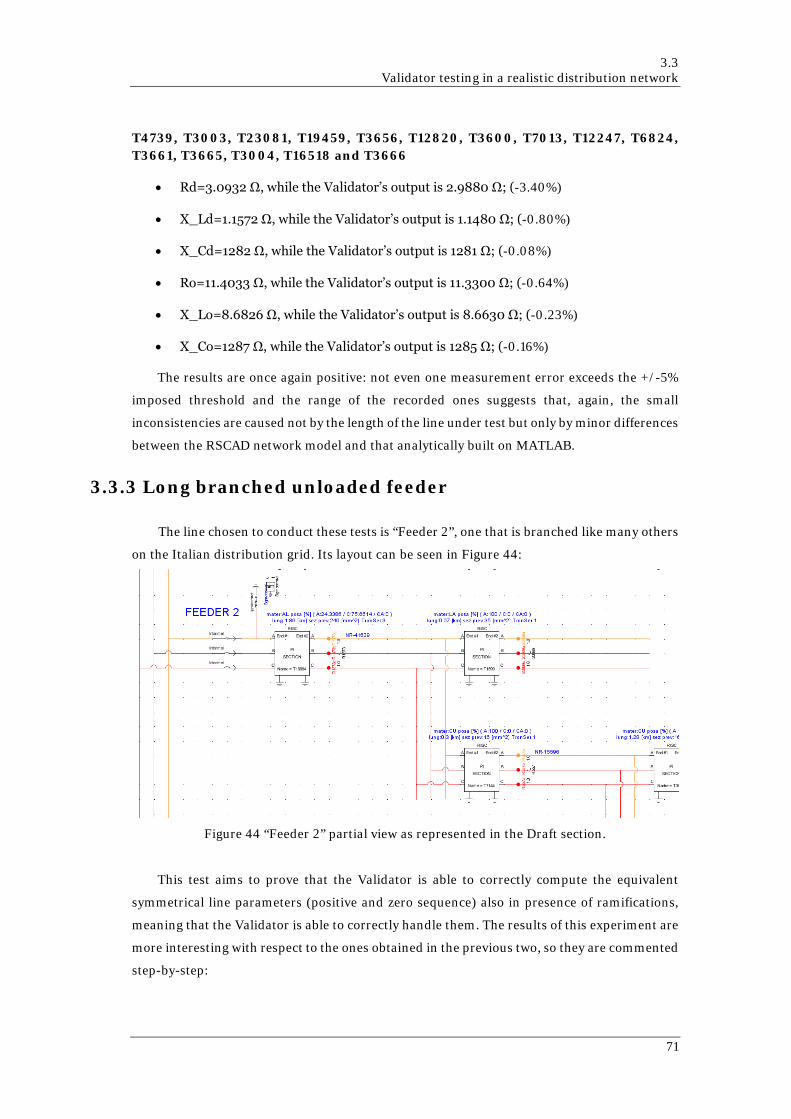
3.3 Validator testing in a realistic distribution network
T4739, T3003, T23081, T19459, T3656, T12820, T3600, T7013, T12247, T6824, T3661, T3665, T3004, T16518 and T3666
• Rd=3.0932 Ω, while the Validator’s output is 2.9880 Ω; (-3.40%)
• X_Ld=1.1572 Ω, while the Validator’s output is 1.1480 Ω; (-0.80%)
• X_Cd=1282 Ω, while the Validator’s output is 1281 Ω; (-0.08%)
• Ro=11.4033 Ω, while the Validator’s output is 11.3300 Ω; (-0.64%)
• X_Lo=8.6826 Ω, while the Validator’s output is 8.6630 Ω; (-0.23%)
• X_Co=1287 Ω, while the Validator’s output is 1285 Ω; (-0.16%)
The results are once again positive: not even one measurement error exceeds the +/-5%
imposed threshold and the range of the recorded ones suggests that, again, the small
inconsistencies are caused not by the length of the line under test but only by minor differences
between the RSCAD network model and that analytically built on MATLAB.
3.3.3 Long branched unloaded feeder
The line chosen to conduct these tests is “Feeder 2”, one that is branched like many others
on the Italian distribution grid. Its layout can be seen in Figure 44:
Figure 44 “Feeder 2” partial view as represented in the Draft section.
This test aims to prove that the Validator is able to correctly compute the equivalent
symmetrical line parameters (positive and zero sequence) also in presence of ramifications,
meaning that the Validator is able to correctly handle them. The results of this experiment are
more interesting with respect to the ones obtained in the previous two, so they are commented
step-by-step:
71
0CHAPTER 3 PMU-based network model validator
T16884
• Rd= 0.7011 Ω, while the Validator’s output is 0.7107 Ω; (-1.40%)
• X_Ld= 0.3519 Ω, while the Validator’s output is 0.3522 Ω; (+0.08%)
• X_Cd=5612 Ω, while the Validator’s output is 5609 Ω; (-0.05%)
• Ro=2.1838 Ω, while the Validator’s output is 2.1500 Ω; (-1.5%)
• X_Lo=1.8791 Ω, while the Validator’s output is 1.8800 Ω; (+0.05%)
• X_Co=5635 Ω, while the Validator’s output is 5632 Ω; (-0.05%)
The presence of a successive ramification has no effect on the measurements made on a
single line section. This could be easily imagined, but it was worth verifying. The small errors
are, once again, due to slight discrepancies in MATLAB’s and RSCAD’s grid models.
T16884 and T1599 (with T7144 as a branch in the middle)
• Rd= 0.7664 Ω, while the Validator’s output is 1.3790 Ω; (+77.61%)
• X_Ld= 0.3789 Ω, while the Validator’s output is 0.6420 Ω; (+69.44%)
• X_Cd=5606 Ω, while the Validator’s output is 983 Ω; (-82.47%)
• Ro=2.2595 Ω, while the Validator’s output is 2.5800 Ω; (+14.18%)
• X_Lo=1.9927 Ω, while the Validator’s output is 2.3250 Ω; (+16.68%)
• X_Co=5632 Ω, while the Validator’s output is 4449 Ω; (-21.00%)
This is where problems start to arise: as it can be easily inferred by the huge difference
between the measurements, the Validator is influenced by the branching of the line. The same
happens when the PMU is moved to the other branch, even if with smaller consequences:
T16884 and T7144 (with T1599 as a branch in the middle)
• Rd=1.0321 Ω, while the Validator’s output is 1.0100 Ω; (-2.14%)
• X_Ld=0.4776 Ω, while the Validator’s output is 0.4658 Ω; (-2.47%)
• X_Cd=5589 Ω, while the Validator’s output is 5580 Ω; (-0.16%)
• Ro=2.5594 Ω, while the Validator’s output is 2.5200 Ω; (-1.54%)
• X_Lo=2.3747 Ω, while the Validator’s output is 2.3230 Ω; (-2.18%)
• X_Co=5626 Ω, while the Validator’s output is 5621 Ω; (-0.09%)
72

3.3 Validator testing in a realistic distribution network
The errors are low, but still higher than the average with respect to the previous
experiments. This is true because most of the energy flows in the direction of branch T7144
(from which the rest of the feeder develops), thus the role of T1599 as a “disturbing element”
is limited by its small current withdrawal. (since there is no network development from there
on)
The question here was: does the Validator correctly measure the equivalent parameters,
taking in proper consideration the ramification? Or are its outputs inconsistent with the true
network parameters? In order to answer to these questions, the MATLAB model needs to be
modified accordingly, including the branched section as it is shown in Appendix A.7. The
following are the results obtained from the new model compared to the same Validator’s
outputs seen in the previous step.
T16884 and T7144 (with T1599 as a branch in the middle)
• Rd=1.0321 Ω, while the Validator’s output is 1.0100 Ω; (-2.14%)
• X_Ld=0.4776 Ω, while the Validator’s output is 0.4658 Ω; (-2.47%)
• X_Cd=5582 Ω, while the Validator’s output is 5580 Ω; (-0.04%)
• Ro=2.5594 Ω, while the Validator’s output is 2.5200 Ω; (-1.54%)
• X_Lo=2.3747 Ω, while the Validator’s output is 2.3230 Ω; (-2.18%)
• X_Co=5623 Ω, while the Validator’s output is 5621 Ω; (-0.05%)
The only difference here is a reduction of the shunt parameters (both positive and zero
sequence), and that seems reasonable considering that the model has to take into
consideration the shunt capacitances of the branch section and this contributes to the overall
reduction of the equivalent shunt reactance that can be witnessed above. In order to be sure of
the correct modeling, a branch derivation (T1599) is added to Feeder 1, just to experiment the
consequences of such an addition in terms of algorithm coherence. What follows is a
comparison between two experiments, with and without addition:
T4739 and T3003
• Rd=0.6530 Ω, while the Validator’s output is 0.6486 Ω; (-0.67%)
• X_Ld=0.2859 Ω, while the Validator’s output is 0.2848 Ω; (-0.38%)
• X_Cd=4781 Ω, while the Validator’s output is 4779 Ω; (-0.04%)
• Ro=2.8572 Ω, while the Validator’s output is 2.8570 Ω; (-0.01%)
• X_Lo=2.1710 Ω, while the Validator’s output is 2.1650 Ω; (-0.28%)
73
0CHAPTER 3 PMU-based network model validator
• X_Co=4853 Ω, while the Validator’s output is 4850 Ω; (-0.06%)
T4739 and T3003 (with T1599 as a branch in the middle)
• Rd=0.6530 Ω, while the Validator’s output is 0.6486 Ω; (-0.67%)
• X_Ld=0.2859 Ω, while the Validator’s output is 0.2848 Ω; (-0.38%)
• X_Cd=4777 Ω, while the Validator’s output is 4774 Ω; (-0.06%)
• Ro=2.8573 Ω, while the Validator’s output is 2.8570 Ω; (-0.01%)
• X_Lo=2.1709 Ω, while the Validator’s output is 2.1650 Ω; (-0.28%)
• X_Co=4851 Ω, while the Validator’s output is 4848 Ω; (-0.06%)
As can be clearly seen from the data above, the insertion of a branch changes shunt
parameters only, and the errors remain almost perfectly constant in the two cases, meaning
that the Validator reacts to the new element as the MATLAB model does. This is the desired
result, that is confirmed by a last experiment conducted on Feeder 1 with the exact same
condition as the last one, but one thing: the branching section had its parameters modified by
a great deal (series/shunt components multiplied/divided by ten) to confirm that the Validator
correctly works even with different kind of branches. (longer ones, in this case)
T4739 and T3003 (with a modified T1599 as a branch in the middle)
• Rd=0.6530 Ω, while the Validator’s output is 0.6486 Ω; (-0.67%)
• X_Ld=0.2859 Ω, while the Validator’s output is 0.2848 Ω; (-0.38%)
• X_Cd=4737 Ω, while the Validator’s output is 4734 Ω; (-0.06%)
• Ro=2.8572 Ω, while the Validator’s output is 2.8570 Ω; (-0.01%)
• X_Lo=2.1710 Ω, while the Validator’s output is 2.1650 Ω; (-0.78%)
• X_Co=4832 Ω, while the Validator’s output is 4830 Ω; (-0.04%)
Despite the alteration, errors are still very low. This result lead to optimistic hopes regarding
the Validator’s ability to take into account correctly the line parameters’ variation also in
normal working conditions. (presence of load)
3.3.4 Long branched loaded feeder
This last experiment had place on Feeder 1, with a particular focus on its first and second
line sections. As Figure 45 clearly shows, a three-phase load is placed between them as a
74
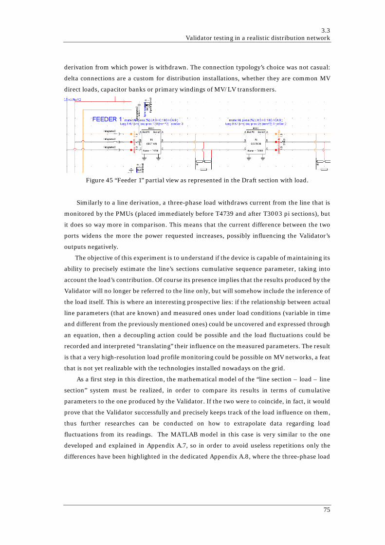
3.3 Validator testing in a realistic distribution network
derivation from which power is withdrawn. The connection typology’s choice was not casual:
delta connections are a custom for distribution installations, whether they are common MV
direct loads, capacitor banks or primary windings of MV/LV transformers.
Figure 45 “Feeder 1” partial view as represented in the Draft section with load.
Similarly to a line derivation, a three-phase load withdraws current from the line that is
monitored by the PMUs (placed immediately before T4739 and after T3003 pi sections), but
it does so way more in comparison. This means that the current difference between the two
ports widens the more the power requested increases, possibly influencing the Validator’s
outputs negatively.
The objective of this experiment is to understand if the device is capable of maintaining its
ability to precisely estimate the line’s sections cumulative sequence parameter, taking into
account the load’s contribution. Of course its presence implies that the results produced by the
Validator will no longer be referred to the line only, but will somehow include the inference of
the load itself. This is where an interesting prospective lies: if the relationship between actual
line parameters (that are known) and measured ones under load conditions (variable in time
and different from the previously mentioned ones) could be uncovered and expressed through
an equation, then a decoupling action could be possible and the load fluctuations could be
recorded and interpreted “translating” their influence on the measured parameters. The result
is that a very high-resolution load profile monitoring could be possible on MV networks, a feat
that is not yet realizable with the technologies installed nowadays on the grid.
As a first step in this direction, the mathematical model of the “line section – load – line
section” system must be realized, in order to compare its results in terms of cumulative
parameters to the one produced by the Validator. If the two were to coincide, in fact, it would
prove that the Validator successfully and precisely keeps track of the load influence on them,
thus further researches can be conducted on how to extrapolate data regarding load
fluctuations from its readings. The MATLAB model in this case is very similar to the one
developed and explained in Appendix A.7, so in order to avoid useless repetitions only the
differences have been highlighted in the dedicated Appendix A.8, where the three-phase load
75

0CHAPTER 3 PMU-based network model validator
model for a symmetrical components’ circuit is created. Once this is done, the equivalent load
can be introduced in the algorithm and the reference cumulative parameters calculated.
Once the reference parameters are available, the next step is creating a number of load
scenarios and collect the parameters produced by the Validator in each of it in order to
compare them with the firsts. The cases will be differentiated by load total impedance and
power factor:
Z=500 Ω and 𝐜𝐜𝐜𝐜𝐜𝐜𝝋𝝋=1:
• Rd=0.6535 Ω, while the Validator’s output is 0.6941 Ω; (+6.21%)
• X_Ld=0.2864 Ω, while the Validator’s output is 0.3041 Ω; (+6.18%)
• X_Cd=5 Ω, while the Validator’s output is 5053 Ω; (+86074%)
• Ro=2.8572 Ω, while the Validator’s output is 2.8565 Ω; (-0.02%)
• X_Lo=2.1710 Ω, while the Validator’s output is 2.1479 Ω; (-1.06%)
• X_Co=4853 Ω, while the Validator’s output is 4851 Ω; (-0.04%)
Z=1000 Ω and 𝐜𝐜𝐜𝐜𝐜𝐜𝝋𝝋=1:
• Rd=0.6533 Ω, while the Validator’s output is 0.6751 Ω; (+3.34%)
• X_Ld=0.2861 Ω, while the Validator’s output is 0.2956 Ω; (+3.32%)
• X_Cd=23 Ω, while the Validator’s output is 4889 Ω; (+20980%)
• Ro=2.8572 Ω, while the Validator’s output is 2.8550 Ω; (-0.08%)
• X_Lo=2.1710 Ω, while the Validator’s output is 2.1430 Ω; (-1.29%)
• X_Co=4853 Ω, while the Validator’s output is 4851 Ω; (-0.04%)
Z=5000 Ω and 𝐜𝐜𝐜𝐜𝐜𝐜𝝋𝝋=1:
• Rd=0.6531 Ω, while the Validator’s output is 0.6578 Ω; (+0.72%)
• X_Ld=0.2860 Ω, while the Validator’s output is 0.2879 Ω; (+0.66%)
• X_Cd=518 Ω, while the Validator’s output is 4796 Ω; (+826%)
• Ro=2.8572 Ω, while the Validator’s output is 2.8550 Ω; (-0.08%)
• X_Lo=2.1710 Ω, while the Validator’s output is 2.1480 Ω; (-1.06%)
• X_Co=4853 Ω, while the Validator’s output is 4848 Ω; (-0.10%)
Z=8000 Ω and 𝐜𝐜𝐜𝐜𝐜𝐜𝝋𝝋=1:
76

3.3 Validator testing in a realistic distribution network
• Rd=0.6531 Ω, while the Validator’s output is 0.6560 Ω; (+0.44%)
• X_Ld=0.2859 Ω, while the Validator’s output is 0.2872 Ω; (+0.45%)
• X_Cd=1135 Ω, while the Validator’s output is 4789 Ω; (-322%)
• Ro=2.8572 Ω, while the Validator’s output is 2.8530 Ω; (-0.15%)
• X_Lo=2.1710 Ω, while the Validator’s output is 2.1410 Ω; (-1.38%)
• X_Co=4853 Ω, while the Validator’s output is 4850 Ω; (-0.06%)
Z=590.5 Ω and 𝐜𝐜𝐜𝐜𝐜𝐜𝝋𝝋=0.85: (inductive)
• Rd=0.6535 Ω, while the Validator’s output is 0.6925 Ω; (+5.97%)
• X_Ld=0.2860 Ω, while the Validator’s output is 0.2827 Ω; (-1.15%)
• X_Cd=107 Ω, while the Validator’s output is -401.8 Ω; (-472%)
• Ro=2.8572 Ω, while the Validator’s output is 2.8500 Ω; (-0.25%)
• X_Lo=2.1710 Ω, while the Validator’s output is 2.1420 Ω; (-1.34%)
• X_Co=4853 Ω, while the Validator’s output is 4848 Ω; (-0.10%)
Z=1048 Ω and 𝐜𝐜𝐜𝐜𝐜𝐜𝝋𝝋=0.95: (inductive)
• Rd=0.6533 Ω, while the Validator’s output is 0.6760 Ω; (+3.47%)
• X_Ld=0.2861 Ω, while the Validator’s output is 0.2889 Ω; (+0.98%)
• X_Cd=124 Ω, while the Validator’s output is -1539 Ω; (-1341%)
• Ro=2.8572 Ω, while the Validator’s output is 2.8610 Ω; (+0.13%)
• X_Lo=2.1710 Ω, while the Validator’s output is 2.1470 Ω; (-1.11%)
• X_Co=4853 Ω, while the Validator’s output is 4849 Ω; (-0.08%)
Z=1181 Ω and 𝐜𝐜𝐜𝐜𝐜𝐜𝝋𝝋=0.85: (inductive)
• Rd=0.6533 Ω, while the Validator’s output is 0.6738 Ω; (+3.47%)
• X_Ld=0.2860 Ω, while the Validator’s output is 0.2835 Ω; (-0.87%)
• X_Cd=221 Ω, while the Validator’s output is -877 Ω; (-497%)
• Ro=2.8572 Ω, while the Validator’s output is 2.8440 Ω; (-0.46%)
• X_Lo=2.1710 Ω, while the Validator’s output is 2.1400 Ω; (-1.43%)
• X_Co=4853 Ω, while the Validator’s output is 4850 Ω; (-0.06%)
77
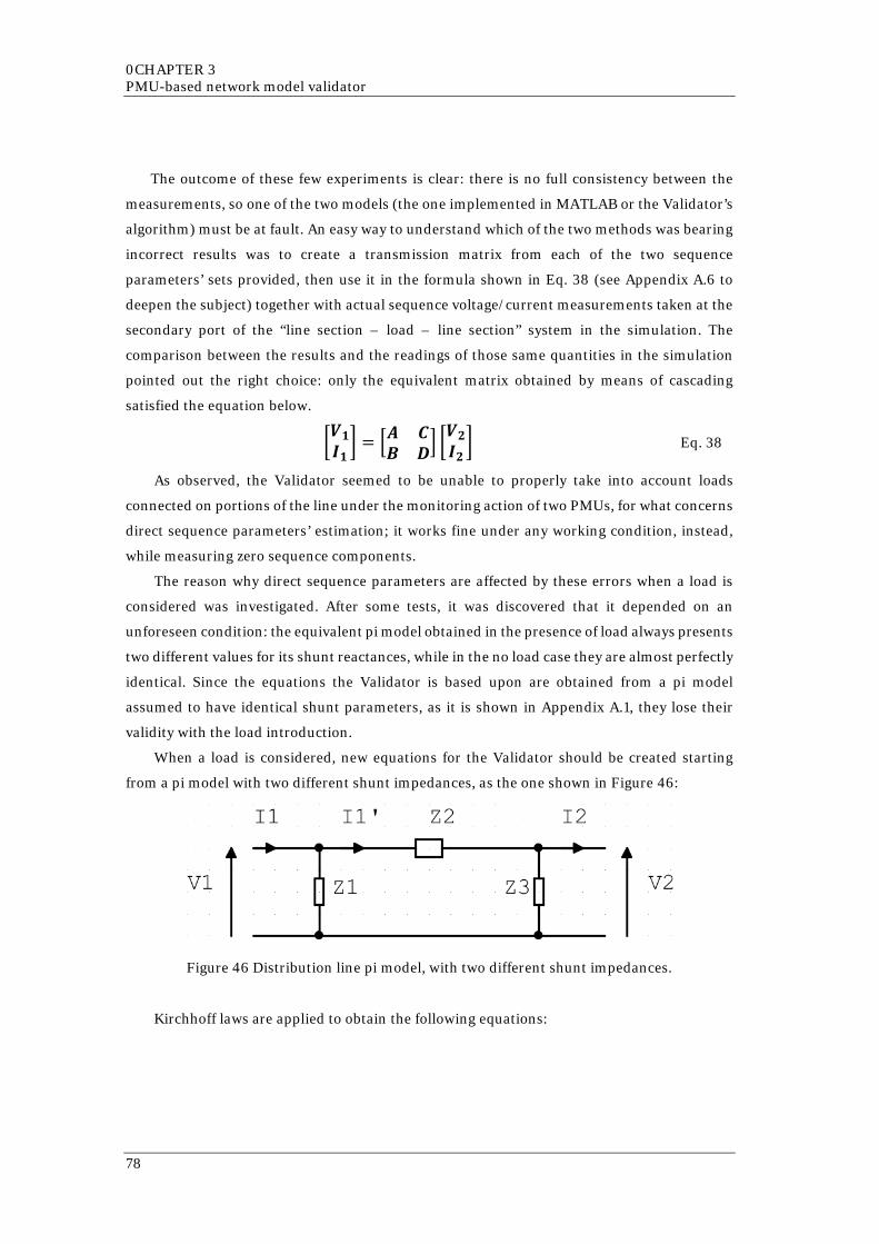
0CHAPTER 3 PMU-based network model validator
The outcome of these few experiments is clear: there is no full consistency between the
measurements, so one of the two models (the one implemented in MATLAB or the Validator’s
algorithm) must be at fault. An easy way to understand which of the two methods was bearing
incorrect results was to create a transmission matrix from each of the two sequence
parameters’ sets provided, then use it in the formula shown in Eq. 38 (see Appendix A.6 to
deepen the subject) together with actual sequence voltage/current measurements taken at the
secondary port of the “line section – load – line section” system in the simulation. The
comparison between the results and the readings of those same quantities in the simulation
pointed out the right choice: only the equivalent matrix obtained by means of cascading
satisfied the equation below.
�𝑽𝑽𝟏𝟏𝑰𝑰𝟏𝟏� = �𝑨𝑨 𝑪𝑪
𝑩𝑩 𝑫𝑫� �𝑽𝑽𝟐𝟐𝑰𝑰𝟐𝟐� Eq. 38
As observed, the Validator seemed to be unable to properly take into account loads
connected on portions of the line under the monitoring action of two PMUs, for what concerns
direct sequence parameters’ estimation; it works fine under any working condition, instead,
while measuring zero sequence components.
The reason why direct sequence parameters are affected by these errors when a load is
considered was investigated. After some tests, it was discovered that it depended on an
unforeseen condition: the equivalent pi model obtained in the presence of load always presents
two different values for its shunt reactances, while in the no load case they are almost perfectly
identical. Since the equations the Validator is based upon are obtained from a pi model
assumed to have identical shunt parameters, as it is shown in Appendix A.1, they lose their
validity with the load introduction.
When a load is considered, new equations for the Validator should be created starting
from a pi model with two different shunt impedances, as the one shown in Figure 46:
Figure 46 Distribution line pi model, with two different shunt impedances.
Kirchhoff laws are applied to obtain the following equations:
78
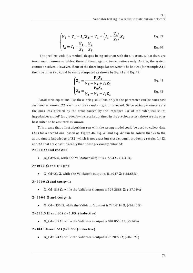
3.3 Validator testing in a realistic distribution network
⎩⎨
⎧𝑽𝑽𝟐𝟐 = 𝑽𝑽𝟏𝟏 − 𝑰𝑰𝟏𝟏′𝒁𝒁𝟐𝟐 = 𝑽𝑽𝟏𝟏 − �𝑰𝑰𝟏𝟏 −𝑽𝑽𝟏𝟏𝒁𝒁𝟏𝟏�𝒁𝒁𝟐𝟐
𝑰𝑰𝟐𝟐 = 𝑰𝑰𝟏𝟏 −𝑽𝑽𝟏𝟏𝒁𝒁𝟏𝟏
−𝑽𝑽𝟐𝟐𝒁𝒁𝟑𝟑
Eq. 39
Eq. 40
The problem with this method, despite being coherent with the situation, is that there are
too many unknown variables: three of them, against two equations only. As it is, the system
cannot be solved. However, if one of the three impedances were to be known (for example Z2),
then the other two could be easily computed as shown by Eq. 41 and Eq. 42:
⎩⎨
⎧𝒁𝒁𝟏𝟏 =𝑽𝑽𝟏𝟏𝒁𝒁𝟐𝟐
𝑽𝑽𝟐𝟐 − 𝑽𝑽𝟏𝟏 + 𝑰𝑰𝟏𝟏𝒁𝒁𝟐𝟐
𝒁𝒁𝟑𝟑 =𝑽𝑽𝟐𝟐𝒁𝒁𝟐𝟐
𝑽𝑽𝟏𝟏 − 𝑽𝑽𝟐𝟐 − 𝑰𝑰𝟐𝟐𝒁𝒁𝟐𝟐
Eq. 41
Eq. 42
Parametric equations like these bring solutions only if the parameter can be somehow
assumed as known. Z2 was not chosen randomly, in this regard. Since series parameters are
the ones less affected by the error caused by the improper use of the “identical shunt
impedances model” (as proved by the results obtained in the previous tests), those are the ones
best suited to be assumed as known.
This means that a first algorithm run with the wrong model could be used to collect data
(Z2) for a second one, based on Figure 46. Eq. 41 and Eq. 42 can be solved thanks to the
approximate knowledge of Z2, which is not exact but close enough, producing results for Z1
and Z3 that are closer to reality than those previously obtained:
Z=500 Ω and 𝐜𝐜𝐜𝐜𝐜𝐜𝝋𝝋=1:
• X_Cd=5 Ω, while the Validator’s output is 4.7794 Ω; (-4.41%)
Z=1000 Ω and 𝐜𝐜𝐜𝐜𝐜𝐜𝝋𝝋=1:
• X_Cd=23 Ω, while the Validator’s output is 16.4047 Ω; (-28.68%)
Z=5000 Ω and 𝐜𝐜𝐜𝐜𝐜𝐜𝝋𝝋=1:
• X_Cd=518 Ω, while the Validator’s output is 326.2888 Ω; (-37.01%)
Z=8000 Ω and 𝐜𝐜𝐜𝐜𝐜𝐜𝝋𝝋=1:
• X_Cd=1135 Ω, while the Validator’s output is 744.6114 Ω; (-34.40%)
Z=590.5 Ω and 𝐜𝐜𝐜𝐜𝐜𝐜𝝋𝝋=0.85: (inductive)
• X_Cd=107 Ω, while the Validator’s output is 100.8556 Ω; (-5.74%)
Z=1048 Ω and 𝐜𝐜𝐜𝐜𝐜𝐜𝝋𝝋=0.95: (inductive)
• X_Cd=124 Ω, while the Validator’s output is 78.2072 Ω; (-36.93%)
79
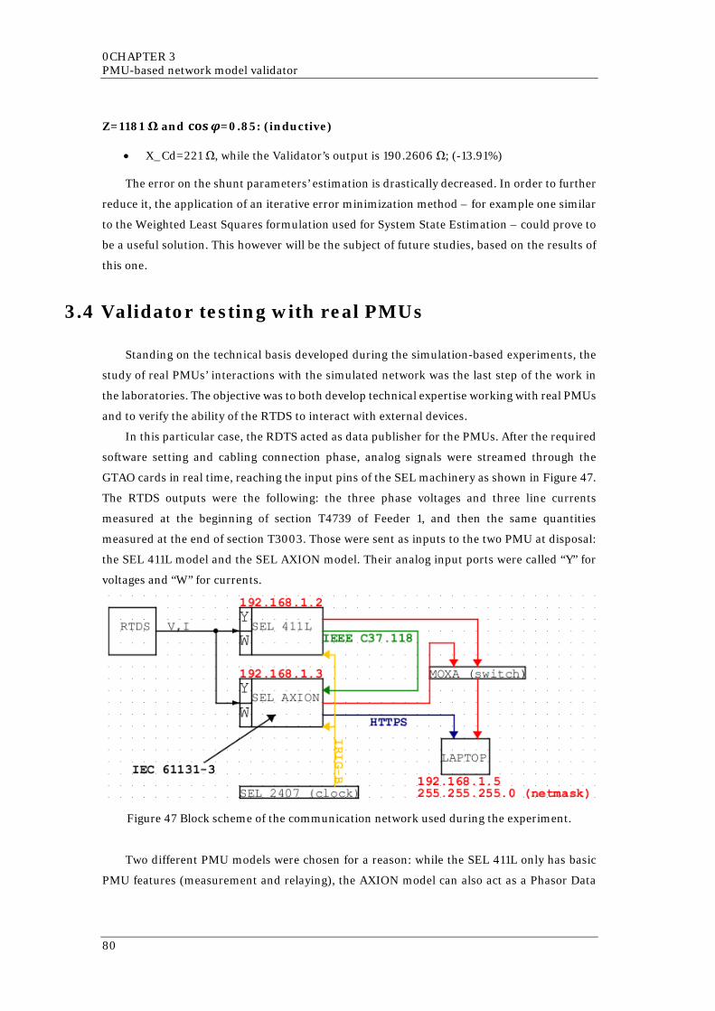
0CHAPTER 3 PMU-based network model validator
Z=1181 Ω and 𝐜𝐜𝐜𝐜𝐜𝐜𝝋𝝋=0.85: (inductive)
• X_Cd=221 Ω, while the Validator’s output is 190.2606 Ω; (-13.91%)
The error on the shunt parameters’ estimation is drastically decreased. In order to further
reduce it, the application of an iterative error minimization method – for example one similar
to the Weighted Least Squares formulation used for System State Estimation – could prove to
be a useful solution. This however will be the subject of future studies, based on the results of
this one.
3.4 Validator testing with real PMUs
Standing on the technical basis developed during the simulation-based experiments, the
study of real PMUs’ interactions with the simulated network was the last step of the work in
the laboratories. The objective was to both develop technical expertise working with real PMUs
and to verify the ability of the RTDS to interact with external devices.
In this particular case, the RDTS acted as data publisher for the PMUs. After the required
software setting and cabling connection phase, analog signals were streamed through the
GTAO cards in real time, reaching the input pins of the SEL machinery as shown in Figure 47.
The RTDS outputs were the following: the three phase voltages and three line currents
measured at the beginning of section T4739 of Feeder 1, and then the same quantities
measured at the end of section T3003. Those were sent as inputs to the two PMU at disposal:
the SEL 411L model and the SEL AXION model. Their analog input ports were called “Y” for
voltages and “W” for currents.
Figure 47 Block scheme of the communication network used during the experiment.
Two different PMU models were chosen for a reason: while the SEL 411L only has basic
PMU features (measurement and relaying), the AXION model can also act as a Phasor Data
80

3.4 Validator testing with real PMUs
Collector (PDC) and possesses computational capabilities. After analog input elaboration
(sampling and data digitalization), the two machines communicate using the IEEE C37.118
protocol (also called “synchrophasors protocol”, since it is considered the best for phasor data
communication as of now). The simpler PMU (SEL 411L) publishes the phasors it created after
their elaboration. Then the AXION receives them as well as creating its own ones
simultaneously. Further calculations take place in the latter, producing sequence phasor
quantities but also running the Validator’s algorithm. The code was in fact implemented in this
device through the programming protocol IEC 61131-3, a C-like language, taking the form
shown in Appendix A.9.
Since no synchrophasor would have meaning without precise synchronization, a SEL 2407
clock was also installed on the rack with the other devices. Thanks to the IRIG-B protocol,
widely used by electric utilities to ensure precise time synchronization of power system
devices, both PMUs were able to assure high quality for their outputs. These data, including
the network parameters calculated by the AXION, were then made available to the operator
via a Human-Machine Interface (HMI). The HMI was both easy to consult and safe thanks to
the HTTPS protocol.
As for the transport layer, the communication between devices is enstablished by a
dedicated small private network. The IPv4 addresses were assigned as shown in Figure 47.
The complete installation on the rack is shown in Figure 48.
Figure 48 From the top: the AXION PMU model, the SEL 2407 clock, the SEL 411L PMU
model.
81
0CHAPTER 3 PMU-based network model validator
Due to unforeseen technical issues with the equipment, the experiments could not
produce the expected results in due time. However, the work is still in progress and will be
subject to further analysis in the near future.
3.5 Clock accuracy requirements for PMUs’
distribution applications
Phasor Measurement Units, as shown by this thesis work, have much potential in terms
of future applications on the Italian distribution network. The validation – or even from
scratch creation – of network parameters’ databases is but one of the possible ways their
installation could benefit a DSO, as it has been clearly shown in the second chapter of this
endeavor. However, from a grid manager point of view, any potential network upgrade must
always be evaluated in relationship not only to the technical improvements it could bring, but
also to its economic implications. PMUs are, in fact, no cheap devices and because of their
intrinsic network-based nature they need to be acquired in vast stocks in order to be employed
effectively. The investment could easily become unacceptably high, especially considering the
extension of the distribution grid and consequently the number of nodes to be monitored with
a PMU.
Since an accurate evaluation of the actual cost/benefit ratio of such an installation would
be a matter far too complex and long to be properly analyzed in this paper, a different – and
possibly more achievable – alternative is taken in consideration. That is the possibility to
upgrade already in place RGDM (Rilevatore di Guasto Direzionale e Misure) devices to
transform them into proprietary PMUs. Making use of already existing machinery could, in
fact, imply a reduction of the initial investment big enough to justify it. Still, in order to get a
general idea of the feasibility of such a project, the components needed for the upgrade must
be investigated and their costs evaluated. After a consultation meeting with e-distribuzione’s
experts on the matter, it emerged that there is only one missing component to proceed in that
direction: a clock precise enough to guarantee accuracy levels for the phasor measurements
high enough to make any of the mentioned applications viable.
The clock accuracy requirements for PMUs’ distribution applications not necessarily
coincide with the standards used for transmission applications (±500 ns, with a normal
distribution), since the angle differences measured in those cases are far greater and suffer less
from a lack of synchronization errors. Therefore, a custom study of the matter was needed. It
was based on the equation that links time accuracy σT (expressed in seconds) and the resulting
angle measurement errors σA (expressed in degrees or radians). Both of these values are
82
3.5 Clock accuracy requirements for PMUs’ distribution applications
standard deviations, quantities used to describe the degree of dispersion of a set of data values
from its expected value.
𝜎𝜎𝐴𝐴 =𝜎𝜎𝑇𝑇
𝑠𝑠𝑅𝑅𝑐𝑐𝑠𝑠𝑠𝑠𝑑𝑑𝑠𝑠 𝑝𝑝𝑅𝑅𝑝𝑝 𝑐𝑐𝑗𝑗𝑐𝑐𝑐𝑐𝑅𝑅∙ 𝑑𝑑𝑅𝑅𝑑𝑑𝑝𝑝𝑅𝑅𝑅𝑅𝑠𝑠 𝑝𝑝𝑅𝑅𝑝𝑝 𝑐𝑐𝑗𝑗𝑐𝑐𝑐𝑐𝑅𝑅 =
𝜎𝜎𝑇𝑇0.02
∙ 360° Eq. 43
Eq. 43 has a general validity, but here it had to be adapted to the Italian grid
characteristics. (50 Hz 0.02 seconds per cycle) If, for example, σT=±10 𝜇𝜇s was taken into
consideration, then it would imply that the PMU measurements angle accuracy would be equal
to σA=±0.18˚. Is it good enough for distribution applications? If not, what value should be
chosen for σT in order for it to be considered acceptable? It all depends on the angle differences
∆𝜃𝜃 between neighboring Secondary Substations: phasor angle accuracy should be at most
±10% of the smallest measurable angle difference.
Experiments conducted with the assistance of the RTDS proved that the smallest angle
differences are attested when analyzing voltages. (in the order of the thousandth of degree,
while for currents it is always at least some degrees) Therefore, a number of tests were run in
order to obtain both said difference (easy to find, since it was obviously measured between the
two substations connected by the shorter link) and an average value for the grid used as an
example. (the same one examined in the third chapter of this work) The results were the
following:
∆𝜗𝜗𝑎𝑎𝑎𝑎𝑎𝑎𝑟𝑟𝑎𝑎𝑎𝑎𝑎𝑎 = 0.0313° → 𝜎𝜎𝐴𝐴 = ±0.1 ∙ ∆𝜗𝜗𝑚𝑚𝑖𝑖𝑛𝑛𝑖𝑖𝑚𝑚𝑚𝑚𝑚𝑚 = ±0.00313° → 𝜎𝜎𝑇𝑇 = ±173ns Eq. 44
∆𝜗𝜗𝑚𝑚𝑖𝑖𝑛𝑛𝑖𝑖𝑚𝑚𝑚𝑚𝑚𝑚 = 0.0011° → 𝜎𝜎𝐴𝐴 = ±0.1 ∙ ∆𝜗𝜗𝑎𝑎𝑎𝑎𝑎𝑎𝑟𝑟𝑎𝑎𝑎𝑎𝑎𝑎 = ±0.00011° → 𝜎𝜎𝑇𝑇 = ±6.1ns Eq. 45
As it can be immediately noticed, the required time accuracy is considerably lower than
the standard for transmission lines. This is of course understandable, since longer distances
between Substations imply bigger angle differences between the voltage phasors. However,
these levels of average time accuracy requirements are nothing that cannot be handled by
modern synchronization devices: as for the suggestion of a SEL (Schweitzer Engineering
Laboratories) technician, a good choice for this kind of upgrade would be the SEL-2401
satellite-synchronized clock. With its ±100 ns time accuracy, intentionally designed to provide
timing signals for IEEE C37.118 (“synchrophasors protocol”) control applications – such as
the ones studied by this paper –, this device is guaranteed to commit errors almost two times
lower than the limit calculated through Eq. 44. This is, of course, a very positive result: it
means that there is already existing technology that can support the potential RGDMPMU
transition without problematic technical constraints. The same cannot be said, of course,
looking at Eq. 45, but here is the kicker: that particular measurement was taken where two
Secondary Substations were divided by a very short distance, and connected by a very short
link; this situation is extremely rare and unlikely, in this case probably dictated by special
needs, thus it cannot be taken as an example of a possible obstacle to the aforementioned
83
0CHAPTER 3 PMU-based network model validator
transition. In cases like this, in fact, it would be sufficient to just skip one of the Substation (as
if it did not exist at all) and base any estimation on the measurements obtained by the next
one, which for sure would be far enough to grant an appropriate degree of accuracy.
All of these observations are even more true when the grid is considered unloaded no more
and a realistic load scenario is simulated: the differences between the angles widens, and
therefore also the tolerated error margins increase accordingly. This further proves the
technical feasibility of the RGDM upgrade project, but tells nothing more in terms of financial
feasibility.
The economic impact of such an installment, in fact, is very difficult to properly evaluate.
However, assuming to be allowed to simplify the matter to a certain degree, a rough estimation
can be done. Assuming a cost of 1000 USD for each synchronization device, that is the price of
the SEL-2401 unit, and considering all the Secondary Substations spread across the county
(around 400000 in total), then the expected CAPEX for the operation would be around 400
million dollars. (more or less 340 million euros) This figure is likely to increase considering
all the related operative costs, but it is also presumable it could decrease because of stock
discounts or a smaller number of units bought in order to by-pass, as explained before, some
Secondary Substations when too close to another one.
In conclusion, whatever the actual amount may be, the GPS clocks’ installation has to be
valued in relationship to the long time horizon benefits their symbiosis with the RGDMs could
produce: if the overall increase in Quality of Service (QoS) is high enough to justify it, then it
could prove to be a good investment. (QoS improvements are in fact rewarded with monetary
benefits granted to the virtuous DSOs ) However, there is another important variable to keep
under control: the cost of a μPMU. If this new device, nowadays still under development, in
the near future happened to undergo a fast technical and commercial maturation, then it
would prove to be a cheaper and more effective alternative to buy and install. It would not be
wise, in fact, to disregard the evolution competitive solutions while working on a proprietary
one.
84

3.5 Clock accuracy requirements for PMUs’ distribution applications
85
0Conclusion
CONCLUSION
Phasor Measurement Units technology, thanks to the fast and yet still accelerating growth
of telecommunication assets employed in the electrical field, could prove to be a precious asset
in a not far future.
The wide range of synchrophasors applications for distribution utilities, both in terms of
radical innovation and improvement of already existing control techniques, has an untapped
potential that nowadays is yet to be disclosed – or even fully understood. However researches
like the one described in this work clearly show that there is much to be learned, and even
more to be gained: the creation of the network model Validator, which was the main focus of
the thesis, is an example of this. Such an application, as experimented through the use of a
complex but powerful MV grid simulator, could in fact grant the DSO the chance not only to
update its already existing network parameters’ databases, but it could also create new ones
from scratches where they are most needed. (e.g. South American networks, after their
acquisition, are still in need of an accurate mapping and overall review) This is particularly
important while speaking of zero sequence parameters, whose precise estimation has always
been a problem for system operators.
The research, however, also offers hints for future development: if the issues with direct
sequence parameters’ estimation in normal load conditions were to be solved, then their link
with load fluctuations could be exploited to develop a real-time high-resolution load profile
monitoring system, capable of precisely tracking power flow trends on a small scale. The
information produced by such a system could be useful in many different ways: dispatching
services planning, more accurate and fast voltage and frequency regulation, strategic network
development, etc.
In conclusion, in a world where information is becoming more and more a key-factor for
innovation and success, where Smart devices are steadily replacing traditional ones and Big
Data production and management is the next big thing, PMUs have the potential to become
part of the next generation equipment that will define the shape of the electrical industry’s
future.
86
Bibliography
[1] F. Katiraei, M. R. Iravani, P. F. W. P. Lehn, "Micro-grid autonomous operation during and subsequent to islanding process", IEEE Trans. Power Del., vol. 20, no. 1, pp. 248-257, Jan. 2005.
[2] Yingchen Zhang, P. Markham, Tao Xia, Lang Chen, Yanzhu Ye, Zhongyu Wu, Zhiyong Yuan, Lei Wang, J. Bank, J. Burgett, R. W. Conners, Yilu Liu, "Wide-area frequency monitoring network (FNET) architecture and applications", IEEE Trans. on Smart Grid, vol. 1, no. 2, pp. 159-167, Sept. 2010.
[3] A. Riepnieks, H. Kirkham, L. Ribickis, “Considerations for phasor measurement unit introduction in distribution systems”, Power and Electrical Engineering of Riga Technical University Conference (RTUCON), pp. 1-6, Oct. 2015.
[4] G. Hataway, B. Flerchinger, R. Moxley, “Synchrophasors for Distribution Applications”, Power and Energy Automation Conference, pp.4-5, Mar. 2013.
[5] R. Moxley, “Synchrophasors in the Real World”, 7th Annual Western Power Delivery Automation Conference, May 2005
[6] E. O. Schweitzer III, D. E. Whithead, “Real-Time Power System Control Using Synchrophasors”, 62nd Annual Georgia Tech Protective Relaying Conference, May 2008
[7] C. Muscas, M. Pau, P.A. Pegoraro, S. Sulis, J. Liu, F. Ponci, A. Monti, “Stima dello stato e della pianificazione ottima di un sistema di misura distribuito robusto per reti elettriche di distribuzione”, XXX Congresso GMEE, Sep. 2013
[8] “Remedial Action Scheme” Definition Development: Background and Frequently Asked Questions, NERC, June 2014
[9] J. Spears, “Blackout 2003: How Ontario went dark”, The Star, August 2013
[10] W. O’Brien, E. Udren, K. Garg, D. Haes, B. Sridharan, “Catching Falling Conductors in Midair – Detecting and Tripping Broken Distribution Circuit Conductors at Protection Speeds”, 69th Annual Conference for Protective Relay Engineers, Apr. 2016
[11] A. H. Al-Mohammed, M. A. Abido, “Fault Location Based on Synchronized Measurements: A Comprehensive Survey”, The Scientific World Journal, vol. 2014, Feb. 2014
[12] Saha M, Izykowski J, Rosolowski E. Fault Location on Power Network. New York, NY, USA: Springer; 2010
87

Bibliography
[13] L. Cibulka, “Synchrophasors: How Are They Making the Electric Grid Smarte”, The i4Energy Seminar Series, Feb. 2011
[14] R. Arghandeh, “Towards Micro-synchrophasors (μPMUs) for Distribution Networks”, IEEE Power Engineering Society Dissertation, Oct. 2013
88
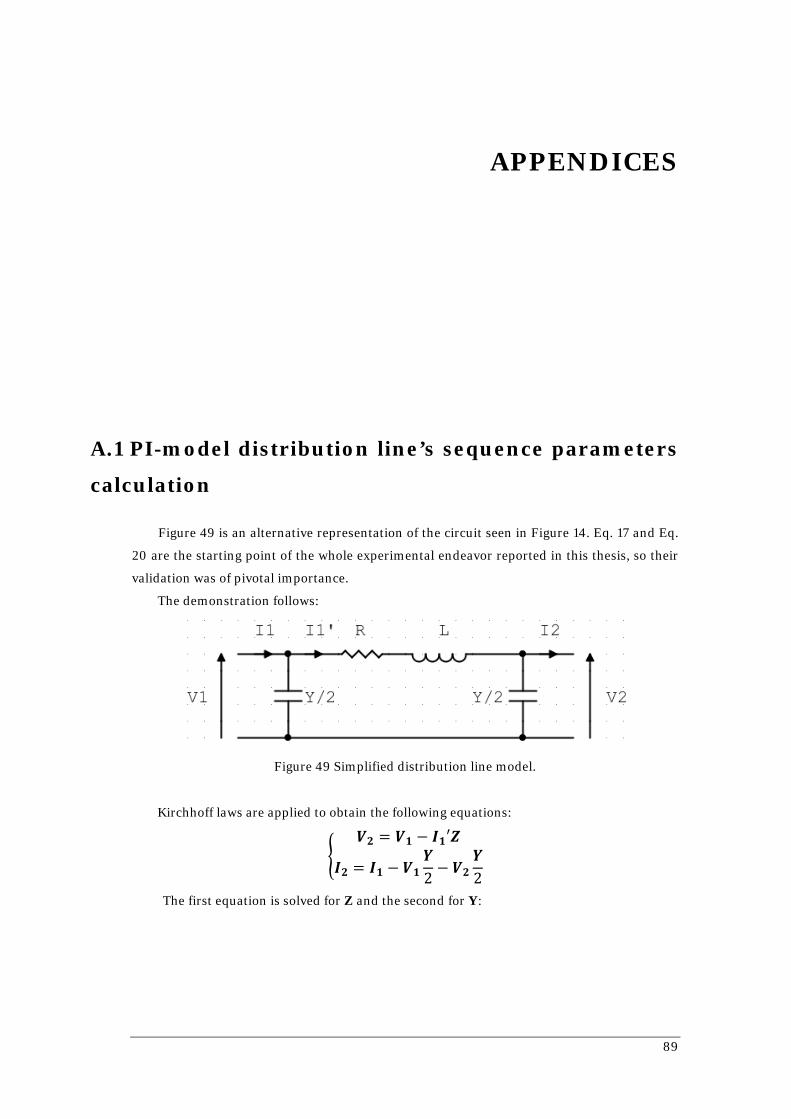
APPENDICES
A.1 PI-model distribution line’s sequence parameters
calculation
Figure 49 is an alternative representation of the circuit seen in Figure 14. Eq. 17 and Eq.
20 are the starting point of the whole experimental endeavor reported in this thesis, so their
validation was of pivotal importance.
The demonstration follows:
Figure 49 Simplified distribution line model.
Kirchhoff laws are applied to obtain the following equations:
�𝑽𝑽𝟐𝟐 = 𝑽𝑽𝟏𝟏 − 𝑰𝑰𝟏𝟏′𝒁𝒁
𝑰𝑰𝟐𝟐 = 𝑰𝑰𝟏𝟏 − 𝑽𝑽𝟏𝟏𝒀𝒀2− 𝑽𝑽𝟐𝟐
𝒀𝒀2
The first equation is solved for Z and the second for Y:
89
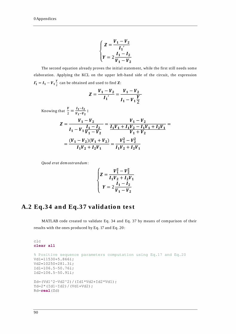
0Appendices
⎩⎨
⎧ 𝒁𝒁 =𝑽𝑽𝟏𝟏 − 𝑽𝑽𝟐𝟐𝑰𝑰𝟏𝟏′
𝒀𝒀 = 2𝑰𝑰𝟏𝟏 − 𝑰𝑰𝟐𝟐𝑽𝑽𝟏𝟏 − 𝑽𝑽𝟐𝟐
The second equation already proves the initial statement, while the first still needs some
elaboration. Applying the KCL on the upper left-hand side of the circuit, the expression 𝑰𝑰𝟏𝟏′ = 𝑰𝑰𝟏𝟏 − 𝑽𝑽𝟏𝟏
𝒀𝒀2 can be obtained and used to find Z:
𝒁𝒁 =𝑽𝑽𝟏𝟏 − 𝑽𝑽𝟐𝟐𝑰𝑰𝟏𝟏′
=𝑽𝑽𝟏𝟏 − 𝑽𝑽𝟐𝟐
𝑰𝑰𝟏𝟏 − 𝑽𝑽𝟏𝟏𝒀𝒀2
Knowing that 𝒀𝒀2
= 𝑰𝑰𝟏𝟏−𝑰𝑰𝟐𝟐𝑽𝑽𝟏𝟏−𝑽𝑽𝟐𝟐
:
𝒁𝒁 =𝑽𝑽𝟏𝟏 − 𝑽𝑽𝟐𝟐
𝑰𝑰𝟏𝟏 − 𝑽𝑽𝟏𝟏𝑰𝑰𝟏𝟏 − 𝑰𝑰𝟐𝟐𝑽𝑽𝟏𝟏 − 𝑽𝑽𝟐𝟐
=
𝑽𝑽𝟏𝟏 − 𝑽𝑽𝟐𝟐𝑰𝑰𝟏𝟏𝑽𝑽𝟏𝟏 + 𝑰𝑰𝟏𝟏𝑽𝑽𝟐𝟐 − 𝑰𝑰𝟏𝟏𝑽𝑽𝟏𝟏 + 𝑰𝑰𝟐𝟐𝑽𝑽𝟏𝟏
𝑽𝑽𝟏𝟏 + 𝑽𝑽𝟐𝟐
=
=(𝑽𝑽𝟏𝟏 − 𝑽𝑽𝟐𝟐)(𝑽𝑽𝟏𝟏 + 𝑽𝑽𝟐𝟐)
𝑰𝑰𝟏𝟏𝑽𝑽𝟐𝟐 + 𝑰𝑰𝟐𝟐𝑽𝑽𝟏𝟏=
𝑽𝑽𝟏𝟏𝟐𝟐 − 𝑽𝑽𝟐𝟐𝟐𝟐
𝑰𝑰𝟏𝟏𝑽𝑽𝟐𝟐 + 𝑰𝑰𝟐𝟐𝑽𝑽𝟏𝟏
Quod erat demostrandum:
⎩⎪⎨
⎪⎧𝒁𝒁 =
𝑽𝑽𝟏𝟏𝟐𝟐 − 𝑽𝑽𝟐𝟐𝟐𝟐
𝑰𝑰𝟏𝟏𝑽𝑽𝟐𝟐 + 𝑰𝑰𝟐𝟐𝑽𝑽𝟏𝟏
𝒀𝒀 = 2𝑰𝑰𝟏𝟏 − 𝑰𝑰𝟐𝟐𝑽𝑽𝟏𝟏 − 𝑽𝑽𝟐𝟐
A.2 Eq.34 and Eq.37 validation test
MATLAB code created to validate Eq. 34 and Eq. 37 by means of comparison of their
results with the ones produced by Eq. 17 and Eq. 20:
clc clear all % Positive sequence parameters computation using Eq.17 and Eq.20 Vd1=11530+5.866i; Vd2=10250+281.3i; Id1=106.5-50.76i; Id2=106.5-50.91i; Zd=(Vd1^2-Vd2^2)/(Id1*Vd2+Id2*Vd1); Yd=2*(Id1-Id2)/(Vd1+Vd2); Rd=real(Zd)
90
Xd_L=imag(Zd) Bd=imag(Yd); Xd_C=1/Bd % Zero sequence parameters computation using Eq.17 and Eq.20 Vo1=-163.8+162.8i; Vo2=-151.1+183.4i; Io1=0.007981+0.01018i; Io2=-0.01182-0.01648i; Zo=(Vo1^2-Vo2^2)/(Io1*Vo2+Io2*Vo1); Yo=2*(Io1-Io2)/(Vo1+Vo2); Ro=real(Zo) Xo_L=imag(Zo) Bo=imag(Yo); Xo_C=1/Bo % Eq.34 and Eq.37 validation test Vd1r=real(Vd1); Vd1i=imag(Vd1); Vd2r=real(Vd2); Vd2i=imag(Vd2); Id1r=real(Id1); Id1i=imag(Id1); Id2r=real(Id2); Id2i=imag(Id2); Vo1r=real(Vo1); Vo1i=imag(Vo1); Vo2r=real(Vo2); Vo2i=imag(Vo2); Io1r=real(Io1); Io1i=imag(Io1); Io2r=real(Io2); Io2i=imag(Io2); Rdnew=((Vd1r^2-Vd1i^2-Vd2r^2+Vd2i^2)*(Id1r*Vd2r-Id1i*Vd2i+Id2r*Vd1r-Id2i*Vd1i)+2*(Vd1r*Vd1i-Vd2r*Vd2i)*(Id1r*Vd2i+Id1i*Vd2r+Id2r*Vd1i+Id2i*Vd1r))/((Id1r*Vd2r-Id1i*Vd2i+Id2r*Vd1r-Id2i*Vd1i)^2+(Id1r*Vd2i+Id1i*Vd2r+Id2r*Vd1i+Id2i*Vd1r)^2) Xd_Lnew=(2*(Vd1r*Vd1i-Vd2r*Vd2i)*(Id1r*Vd2r-Id1i*Vd2i+Id2r*Vd1r-Id2i*Vd1i)-(Vd1r^2-Vd1i^2-Vd2r^2+Vd2i^2)*(Id1r*Vd2i+Id1i*Vd2r+Id2r*Vd1i+Id2i*Vd1r))/((Id1r*Vd2r-Id1i*Vd2i+Id2r*Vd1r-Id2i*Vd1i)^2+(Id1r*Vd2i+Id1i*Vd2r+Id2r*Vd1i+Id2i*Vd1r)^2) Bdnew=2*((Id1i-Id2i)*(Vd1r+Vd2r)-(Id1r-Id2r)*(Vd1i+Vd2i))/((Vd1r+Vd2r)^2+(Vd1i+Vd2i)^2); Xd_Cnew=1/Bdnew Ronew=((Vo1r^2-Vo1i^2-Vo2r^2+Vo2i^2)*(Io1r*Vo2r-Io1i*Vo2i+Io2r*Vo1r-Io2i*Vo1i)+2*(Vo1r*Vo1i-Vo2r*Vo2i)*(Io1r*Vo2i+Io1i*Vo2r+Io2r*Vo1i+Io2i*Vo1r))/((Io1r*Vo2r-Io1i*Vo2i+Io2r*Vo1r-Io2i*Vo1i)^2+(Io1r*Vo2i+Io1i*Vo2r+Io2r*Vo1i+Io2i*Vo1r)^2)
91
0Appendices
Xo_Lnew=(2*(Vo1r*Vo1i-Vo2r*Vo2i)*(Io1r*Vo2r-Io1i*Vo2i+Io2r*Vo1r-Io2i*Vo1i)-(Vo1r^2-Vo1i^2-Vo2r^2+Vo2i^2)*(Io1r*Vo2i+Io1i*Vo2r+Io2r*Vo1i+Io2i*Vo1r))/((Io1r*Vo2r-Io1i*Vo2i+Io2r*Vo1r-Io2i*Vo1i)^2+(Io1r*Vo2i+Io1i*Vo2r+Io2r*Vo1i+Io2i*Vo1r)^2) Bonew=2*((Io1i-Io2i)*(Vo1r+Vo2r)-(Io1r-Io2r)*(Vo1i+Vo2i))/((Vo1r+Vo2r)^2+(Vo1i+Vo2i)^2); Xo_Cnew=1/Bonew
A.3 PMU-based model validator code version 1.0
The following is the code written for the first version of the Validator, the one made to
receive synchrophasors directly (as complex numbers):
VERSION: 3.001 // Include file below is generated by C-Builder // and contains the variables declared as - // PARAMETERS, INPUTS, OUTPUTS . . . #include "Validator.h" STATIC: // ----------------------------------------------- // Variables declared here may be used in both the // RAM: and CODE: sections below. // ----------------------------------------------- // double dt; double Vd1r; double Vd1i; double Vd2r; double Vd2i; double Id1r; double Id1i; double Id2r; double Id2i; double Vo1r; double Vo1i; double Vo2r; double Vo2i; double Io1r; double Io1i; double Io2r; double Io2i; double Bd; double Bo; double a,b,c,d,e,f,g,h,i,l,m,n; double sqVd1r; double sqVd1i; double sqVd2r; double sqVd2i; double sqVo1r;
92
double sqVo1i; double sqVo2r; double sqVo2i; // - E n d o f S T A T I C : S e c t i o n - RAM_FUNCTIONS: // ----------------------------------------------- // This section should contain any 'c' functions // to be called from the RAM section (either // RAM_PASS1 or RAM_PASS2). Example: // // static double myFunction(double v1, double v2) // { // return(v1*v2); // } // ----------------------------------------------- RAM: // ----------------------------------------------- // Place C code here which computes constants // required for the CODE: section below. The C // code here is executed once, prior to the start // of the simulation case. // ----------------------------------------------- // dt= getTimeStep(); sqVd1r=Vd1r*Vd1r; sqVd1i=Vd1i*Vd1i; sqVd2r=Vd2r*Vd2r; sqVd2i=Vd2i*Vd2i; a=(Id1r*Vd2r-Id1i*Vd2i+Id2r*Vd1r-Id2i*Vd1i); b=(Id1r*Vd2i+Id1i*Vd2r+Id2r*Vd1i+Id2i*Vd1r); c=1/(a*a+b*b); d=(Vd1r+Vd2r)*(Vd1r+Vd2r); e=(Vd1i+Vd2i)*(Vd1i+Vd2i); f=1/(d+e); sqVo1r=Vo1r*Vo1r; sqVo1i=Vo1i*Vo1i; sqVo2r=Vo2r*Vo2r; sqVo2i=Vo2i*Vo2i; g=(Io1r*Vo2r-Io1i*Vo2i+Io2r*Vo1r-Io2i*Vo1i); h=(Io1r*Vo2i+Io1i*Vo2r+Io2r*Vo1i+Io2i*Vo1r); i=1/(g*g+h*h); l=(Vo1r+Vo2r)*(Vo1r+Vo2r); m=(Vo1i+Vo2i)*(Vo1i+Vo2i); n=1/(l+m); // ------------- End of RAM: Section ------------- CODE:
93
0Appendices
// ----------------------------------------------- // Place C code here which runs on the RTDS. The // code below is entered once each simulation // step. // ----------------------------------------------- Vd1r=Vd1[0]; Vd1i=Vd1[1]; Vd2r=Vd2[0]; Vd2i=Vd2[1]; Id1r=Id1[0]; Id1i=Id1[1]; Id2r=Id2[0]; Id2i=Id2[1]; Vo1r=Vo1[0]; Vo1i=Vo1[1]; Vo2r=Vo2[0]; Vo2i=Vo2[1]; Io1r=Io1[0]; Io1i=Io1[1]; Io2r=Io2[0]; Io2i=Io2[1]; //Code containing squares expressed as "^2" //Rd=((Vd1r^2-Vd1i^2-Vd2r^2+Vd2i^2)*(Id1r*Vd2r-Id1i*Vd2i+Id2r*Vd1r-Id2i*Vd1i)+2*(Vd1r*Vd1i-Vd2r*Vd2i)*(Id1r*Vd2i+Id1i*Vd2r+Id2r*Vd1i+Id2i*Vd1r))/((Id1r*Vd2r-Id1i*Vd2i+Id2r*Vd1r-Id2i*Vd1i)^2+(Id1r*Vd2i+Id1i*Vd2r+Id2r*Vd1i+Id2i*Vd1r)^2); //X_Ld=(2*(Vd1r*Vd1i-Vd2r*Vd2i)*(Id1r*Vd2r-Id1i*Vd2i+Id2r*Vd1r-Id2i*Vd1i)-(Vd1r^2-Vd1i^2-Vd2r^2+Vd2i^2)*(Id1r*Vd2i+Id1i*Vd2r+Id2r*Vd1i+Id2i*Vd1r))/((Id1r*Vd2r-Id1i*Vd2i+Id2r*Vd1r-Id2i*Vd1i)^2+(Id1r*Vd2i+Id1i*Vd2r+Id2r*Vd1i+Id2i*Vd1r)^2); //Bd=2*((Id1i-Id2i)*(Vd1r+Vd2r)-(Id1r-Id2r)*(Vd1i+Vd2i))/((Vd1r+Vd2r)^2+(Vd1i+Vd2i)^2); //X_Cd=1/Bd; //Ro=((Vo1r^2-Vo1i^2-Vo2r^2+Vo2i^2)*(Io1r*Vo2r-Io1i*Vo2i+Io2r*Vo1r-Io2i*Vo1i)+2*(Vo1r*Vo1i-Vo2r*Vo2i)*(Io1r*Vo2i+Io1i*Vo2r+Io2r*Vo1i+Io2i*Vo1r))/((Io1r*Vo2r-Io1i*Vo2i+Io2r*Vo1r-Io2i*Vo1i)^2+(Io1r*Vo2i+Io1i*Vo2r+Io2r*Vo1i+Io2i*Vo1r)^2); //X_Lo=(2*(Vo1r*Vo1i-Vo2r*Vo2i)*(Io1r*Vo2r-Io1i*Vo2i+Io2r*Vo1r-Io2i*Vo1i)-(Vo1r^2-Vo1i^2-Vo2r^2+Vo2i^2)*(Io1r*Vo2i+Io1i*Vo2r+Io2r*Vo1i+Io2i*Vo1r))/((Io1r*Vo2r-Io1i*Vo2i+Io2r*Vo1r-Io2i*Vo1i)^2+(Io1r*Vo2i+Io1i*Vo2r+Io2r*Vo1i+Io2i*Vo1r)^2); //Bo=2*((Io1i-Io2i)*(Vo1r+Vo2r)-(Io1r-Io2r)*(Vo1i+Vo2i))/((Vo1r+Vo2r)^2+(Vo1i+Vo2i)^2); //X_Co=1/Bo; //Code with explicitated squares of two //Rd=((Vd1r*Vd1r-Vd1i*Vd1i-Vd2r*Vd2r+Vd2i*Vd2i)*(Id1r*Vd2r-Id1i*Vd2i+Id2r*Vd1r-Id2i*Vd1i)+2*(Vd1r*Vd1i-Vd2r*Vd2i)*(Id1r*Vd2i+Id1i*Vd2r+Id2r*Vd1i+Id2i*Vd1r))/((Id1r*Vd2r-
94
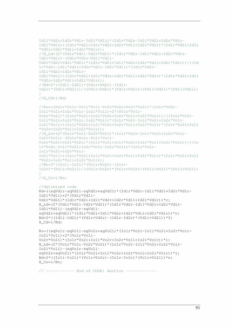
Id1i*Vd2i+Id2r*Vd1r-Id2i*Vd1i)*(Id1r*Vd2r-Id1i*Vd2i+Id2r*Vd1r-Id2i*Vd1i)+(Id1r*Vd2i+Id1i*Vd2r+Id2r*Vd1i+Id2i*Vd1r)*(Id1r*Vd2i+Id1i*Vd2r+Id2r*Vd1i+Id2i*Vd1r)); //X_Ld=(2*(Vd1r*Vd1i-Vd2r*Vd2i)*(Id1r*Vd2r-Id1i*Vd2i+Id2r*Vd1r-Id2i*Vd1i)-(Vd1r*Vd1r-Vd1i*Vd1i-Vd2r*Vd2r+Vd2i*Vd2i)*(Id1r*Vd2i+Id1i*Vd2r+Id2r*Vd1i+Id2i*Vd1r))/((Id1r*Vd2r-Id1i*Vd2i+Id2r*Vd1r-Id2i*Vd1i)*(Id1r*Vd2r-Id1i*Vd2i+Id2r*Vd1r-Id2i*Vd1i)+(Id1r*Vd2i+Id1i*Vd2r+Id2r*Vd1i+Id2i*Vd1r)*(Id1r*Vd2i+Id1i*Vd2r+Id2r*Vd1i+Id2i*Vd1r)); //Bd=2*((Id1i-Id2i)*(Vd1r+Vd2r)-(Id1r-Id2r)*(Vd1i+Vd2i))/((Vd1r+Vd2r)*(Vd1r+Vd2r)+(Vd1i+Vd2i)*(Vd1i+Vd2i)); //X_Cd=1/Bd; //Ro=((Vo1r*Vo1r-Vo1i*Vo1i-Vo2r*Vo2r+Vo2i*Vo2i)*(Io1r*Vo2r-Io1i*Vo2i+Io2r*Vo1r-Io2i*Vo1i)+2*(Vo1r*Vo1i-Vo2r*Vo2i)*(Io1r*Vo2i+Io1i*Vo2r+Io2r*Vo1i+Io2i*Vo1r))/((Io1r*Vo2r-Io1i*Vo2i+Io2r*Vo1r-Io2i*Vo1i)*(Io1r*Vo2r-Io1i*Vo2i+Io2r*Vo1r-Io2i*Vo1i)+(Io1r*Vo2i+Io1i*Vo2r+Io2r*Vo1i+Io2i*Vo1r)*(Io1r*Vo2i+Io1i*Vo2r+Io2r*Vo1i+Io2i*Vo1r)); //X_Lo=(2*(Vo1r*Vo1i-Vo2r*Vo2i)*(Io1r*Vo2r-Io1i*Vo2i+Io2r*Vo1r-Io2i*Vo1i)-(Vo1r*Vo1r-Vo1i*Vo1i-Vo2r*Vo2r+Vo2i*Vo2i)*(Io1r*Vo2i+Io1i*Vo2r+Io2r*Vo1i+Io2i*Vo1r))/((Io1r*Vo2r-Io1i*Vo2i+Io2r*Vo1r-Io2i*Vo1i)*(Io1r*Vo2r-Io1i*Vo2i+Io2r*Vo1r-Io2i*Vo1i)+(Io1r*Vo2i+Io1i*Vo2r+Io2r*Vo1i+Io2i*Vo1r)*(Io1r*Vo2i+Io1i*Vo2r+Io2r*Vo1i+Io2i*Vo1r)); //Bo=2*((Io1i-Io2i)*(Vo1r+Vo2r)-(Io1r-Io2r)*(Vo1i+Vo2i))/((Vo1r+Vo2r)*(Vo1r+Vo2r)+(Vo1i+Vo2i)*(Vo1i+Vo2i)); //X_Co=1/Bo; //Optimized code Rd=((sqVd1r-sqVd1i-sqVd2r+sqVd2i)*(Id1r*Vd2r-Id1i*Vd2i+Id2r*Vd1r-Id2i*Vd1i)+2*(Vd1r*Vd1i-Vd2r*Vd2i)*(Id1r*Vd2i+Id1i*Vd2r+Id2r*Vd1i+Id2i*Vd1r))*c; X_Ld=(2*(Vd1r*Vd1i-Vd2r*Vd2i)*(Id1r*Vd2r-Id1i*Vd2i+Id2r*Vd1r-Id2i*Vd1i)-(sqVd1r-sqVd1i-sqVd2r+sqVd2i)*(Id1r*Vd2i+Id1i*Vd2r+Id2r*Vd1i+Id2i*Vd1r))*c; Bd=2*((Id1i-Id2i)*(Vd1r+Vd2r)-(Id1r-Id2r)*(Vd1i+Vd2i))*f; X_Cd=1/Bd; Ro=((sqVo1r-sqVo1i-sqVo2r+sqVo2i)*(Io1r*Vo2r-Io1i*Vo2i+Io2r*Vo1r-Io2i*Vo1i)+2*(Vo1r*Vo1i-Vo2r*Vo2i)*(Io1r*Vo2i+Io1i*Vo2r+Io2r*Vo1i+Io2i*Vo1r))*i; X_Ld=(2*(Vo1r*Vo1i-Vo2r*Vo2i)*(Io1r*Vo2r-Io1i*Vo2i+Io2r*Vo1r-Io2i*Vo1i)-(sqVo1r-sqVo1i-sqVo2r+sqVo2i)*(Io1r*Vo2i+Io1i*Vo2r+Io2r*Vo1i+Io2i*Vo1r))*i; Bd=2*((Io1i-Io2i)*(Vo1r+Vo2r)-(Io1r-Io2r)*(Vo1i+Vo2i))*n; X_Co=1/Bo; // ------------ End of CODE: Section -------------
95
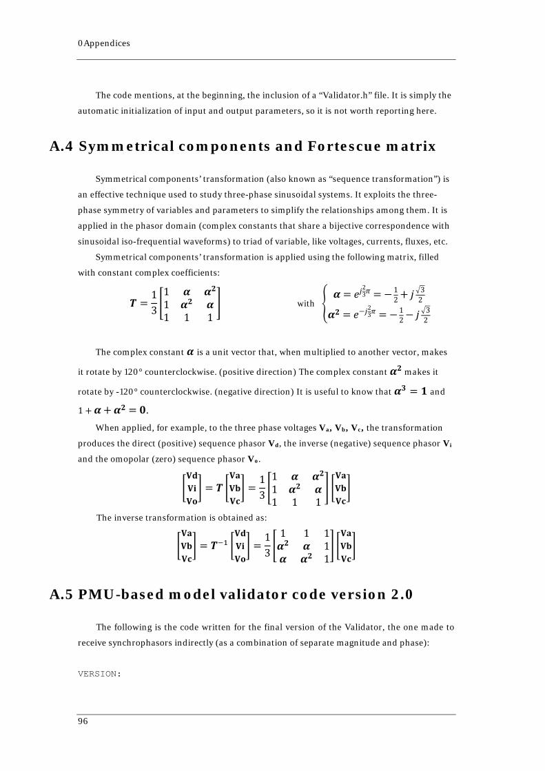
0Appendices
The code mentions, at the beginning, the inclusion of a “Validator.h” file. It is simply the
automatic initialization of input and output parameters, so it is not worth reporting here.
A.4 Symmetrical components and Fortescue matrix
Symmetrical components’ transformation (also known as “sequence transformation”) is
an effective technique used to study three-phase sinusoidal systems. It exploits the three-
phase symmetry of variables and parameters to simplify the relationships among them. It is
applied in the phasor domain (complex constants that share a bijective correspondence with
sinusoidal iso-frequential waveforms) to triad of variable, like voltages, currents, fluxes, etc.
Symmetrical components’ transformation is applied using the following matrix, filled
with constant complex coefficients:
𝑻𝑻 =13�1 𝜶𝜶 𝜶𝜶𝟐𝟐1 𝜶𝜶𝟐𝟐 𝜶𝜶1 1 1
� with �𝜶𝜶 = 𝑅𝑅𝑗𝑗
23𝜋𝜋 = − 1
2 + 𝑗𝑗 �32
𝜶𝜶𝟐𝟐 = 𝑅𝑅−𝑗𝑗23𝜋𝜋 = − 1
2− 𝑗𝑗�32
The complex constant 𝜶𝜶 is a unit vector that, when multiplied to another vector, makes
it rotate by 120° counterclockwise. (positive direction) The complex constant 𝜶𝜶𝟐𝟐 makes it
rotate by -120° counterclockwise. (negative direction) It is useful to know that 𝜶𝜶𝟑𝟑 = 𝟏𝟏 and
1 +𝜶𝜶+𝜶𝜶𝟐𝟐 = 𝟎𝟎. When applied, for example, to the three phase voltages Va, Vb, Vc, the transformation
produces the direct (positive) sequence phasor Vd, the inverse (negative) sequence phasor Vi
and the omopolar (zero) sequence phasor Vo.
�𝐕𝐕𝐝𝐝𝐕𝐕𝐢𝐢𝐕𝐕𝐜𝐜� = 𝑻𝑻 �
𝐕𝐕𝐚𝐚𝐕𝐕𝐛𝐛𝐕𝐕𝐜𝐜� =
13�1 𝜶𝜶 𝜶𝜶𝟐𝟐1 𝜶𝜶𝟐𝟐 𝜶𝜶1 1 1
� �𝐕𝐕𝐚𝐚𝐕𝐕𝐛𝐛𝐕𝐕𝐜𝐜�
The inverse transformation is obtained as:
�𝐕𝐕𝐚𝐚𝐕𝐕𝐛𝐛𝐕𝐕𝐜𝐜� = 𝑻𝑻−1 �
𝐕𝐕𝐝𝐝𝐕𝐕𝐢𝐢𝐕𝐕𝐜𝐜� =
13�
1 1 1𝜶𝜶𝟐𝟐 𝜶𝜶 1𝜶𝜶 𝜶𝜶𝟐𝟐 1
� �𝐕𝐕𝐚𝐚𝐕𝐕𝐛𝐛𝐕𝐕𝐜𝐜�
A.5 PMU-based model validator code version 2.0
The following is the code written for the final version of the Validator, the one made to
receive synchrophasors indirectly (as a combination of separate magnitude and phase):
VERSION:
96
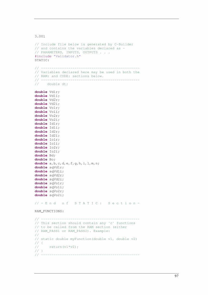
3.001 // Include file below is generated by C-Builder // and contains the variables declared as - // PARAMETERS, INPUTS, OUTPUTS . . . #include "Validator.h" STATIC: // ----------------------------------------------- // Variables declared here may be used in both the // RAM: and CODE: sections below. // ----------------------------------------------- // double dt; double Vd1r; double Vd1i; double Vd2r; double Vd2i; double Vo1r; double Vo1i; double Vo2r; double Vo2i; double Id1r; double Id1i; double Id2r; double Id2i; double Io1r; double Io1i; double Io2r; double Io2i; double Bd; double Bo; double a,b,c,d,e,f,g,h,i,l,m,n; double sqVd1r; double sqVd1i; double sqVd2r; double sqVd2i; double sqVo1r; double sqVo1i; double sqVo2r; double sqVo2i; // - E n d o f S T A T I C : S e c t i o n - RAM_FUNCTIONS: // ----------------------------------------------- // This section should contain any 'c' functions // to be called from the RAM section (either // RAM_PASS1 or RAM_PASS2). Example: // // static double myFunction(double v1, double v2) // { // return(v1*v2); // } // -----------------------------------------------
97
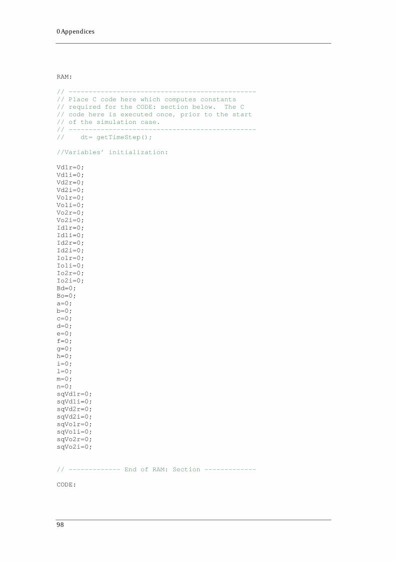
0Appendices
RAM: // ----------------------------------------------- // Place C code here which computes constants // required for the CODE: section below. The C // code here is executed once, prior to the start // of the simulation case. // ----------------------------------------------- // dt= getTimeStep(); //Variables’ initialization: Vd1r=0; Vd1i=0; Vd2r=0; Vd2i=0; Vo1r=0; Vo1i=0; Vo2r=0; Vo2i=0; Id1r=0; Id1i=0; Id2r=0; Id2i=0; Io1r=0; Io1i=0; Io2r=0; Io2i=0; Bd=0; Bo=0; a=0; b=0; c=0; d=0; e=0; f=0; g=0; h=0; i=0; l=0; m=0; n=0; sqVd1r=0; sqVd1i=0; sqVd2r=0; sqVd2i=0; sqVo1r=0; sqVo1i=0; sqVo2r=0; sqVo2i=0; // ------------- End of RAM: Section ------------- CODE:
98
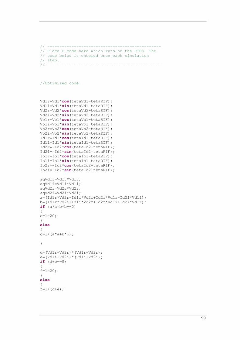
// ----------------------------------------------- // Place C code here which runs on the RTDS. The // code below is entered once each simulation // step. // ----------------------------------------------- //Optimized code: Vd1r=Vd1*cos(tetaVd1-tetaRIF); Vd1i=Vd1*sin(tetaVd1-tetaRIF); Vd2r=Vd2*cos(tetaVd2-tetaRIF); Vd2i=Vd2*sin(tetaVd2-tetaRIF); Vo1r=Vo1*cos(tetaVo1-tetaRIF); Vo1i=Vo1*sin(tetaVo1-tetaRIF); Vo2r=Vo2*cos(tetaVo2-tetaRIF); Vo2i=Vo2*sin(tetaVo2-tetaRIF); Id1r=Id1*cos(tetaId1-tetaRIF); Id1i=Id1*sin(tetaId1-tetaRIF); Id2r=-Id2*cos(tetaId2-tetaRIF); Id2i=-Id2*sin(tetaId2-tetaRIF); Io1r=Io1*cos(tetaIo1-tetaRIF); Io1i=Io1*sin(tetaIo1-tetaRIF); Io2r=-Io2*cos(tetaIo2-tetaRIF); Io2i=-Io2*sin(tetaIo2-tetaRIF); sqVd1r=Vd1r*Vd1r; sqVd1i=Vd1i*Vd1i; sqVd2r=Vd2r*Vd2r; sqVd2i=Vd2i*Vd2i; a=(Id1r*Vd2r-Id1i*Vd2i+Id2r*Vd1r-Id2i*Vd1i); b=(Id1r*Vd2i+Id1i*Vd2r+Id2r*Vd1i+Id2i*Vd1r); if (a*a+b*b==0) { c=1e20; } else { c=1/(a*a+b*b); } d=(Vd1r+Vd2r)*(Vd1r+Vd2r); e=(Vd1i+Vd2i)*(Vd1i+Vd2i); if (d+e==0) { f=1e20; } else { f=1/(d+e);
99
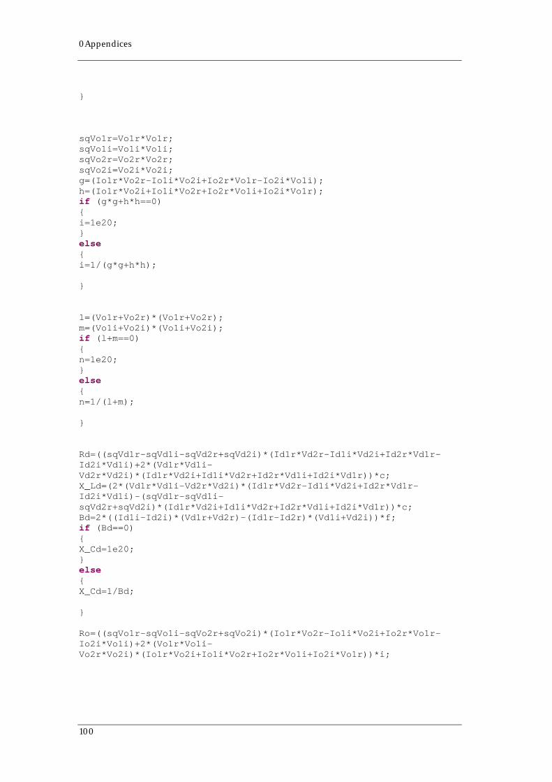
0Appendices
} sqVo1r=Vo1r*Vo1r; sqVo1i=Vo1i*Vo1i; sqVo2r=Vo2r*Vo2r; sqVo2i=Vo2i*Vo2i; g=(Io1r*Vo2r-Io1i*Vo2i+Io2r*Vo1r-Io2i*Vo1i); h=(Io1r*Vo2i+Io1i*Vo2r+Io2r*Vo1i+Io2i*Vo1r); if (g*g+h*h==0) { i=1e20; } else { i=1/(g*g+h*h); } l=(Vo1r+Vo2r)*(Vo1r+Vo2r); m=(Vo1i+Vo2i)*(Vo1i+Vo2i); if (l+m==0) { n=1e20; } else { n=1/(l+m); } Rd=((sqVd1r-sqVd1i-sqVd2r+sqVd2i)*(Id1r*Vd2r-Id1i*Vd2i+Id2r*Vd1r-Id2i*Vd1i)+2*(Vd1r*Vd1i-Vd2r*Vd2i)*(Id1r*Vd2i+Id1i*Vd2r+Id2r*Vd1i+Id2i*Vd1r))*c; X_Ld=(2*(Vd1r*Vd1i-Vd2r*Vd2i)*(Id1r*Vd2r-Id1i*Vd2i+Id2r*Vd1r-Id2i*Vd1i)-(sqVd1r-sqVd1i-sqVd2r+sqVd2i)*(Id1r*Vd2i+Id1i*Vd2r+Id2r*Vd1i+Id2i*Vd1r))*c; Bd=2*((Id1i-Id2i)*(Vd1r+Vd2r)-(Id1r-Id2r)*(Vd1i+Vd2i))*f; if (Bd==0) { X_Cd=1e20; } else { X_Cd=1/Bd; } Ro=((sqVo1r-sqVo1i-sqVo2r+sqVo2i)*(Io1r*Vo2r-Io1i*Vo2i+Io2r*Vo1r-Io2i*Vo1i)+2*(Vo1r*Vo1i-Vo2r*Vo2i)*(Io1r*Vo2i+Io1i*Vo2r+Io2r*Vo1i+Io2i*Vo1r))*i;
100
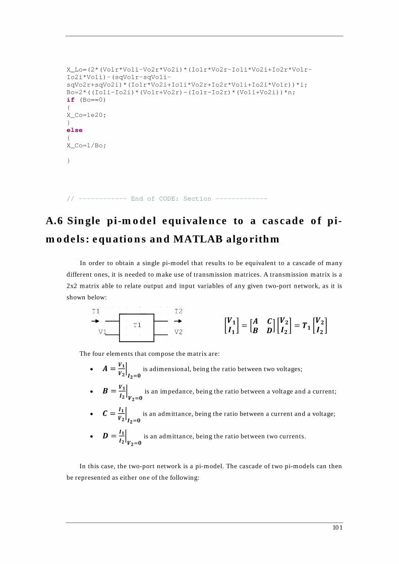
X_Lo=(2*(Vo1r*Vo1i-Vo2r*Vo2i)*(Io1r*Vo2r-Io1i*Vo2i+Io2r*Vo1r-Io2i*Vo1i)-(sqVo1r-sqVo1i-sqVo2r+sqVo2i)*(Io1r*Vo2i+Io1i*Vo2r+Io2r*Vo1i+Io2i*Vo1r))*i; Bo=2*((Io1i-Io2i)*(Vo1r+Vo2r)-(Io1r-Io2r)*(Vo1i+Vo2i))*n; if (Bo==0) { X_Co=1e20; } else { X_Co=1/Bo; } // ------------ End of CODE: Section -------------
A.6 Single pi-model equivalence to a cascade of pi-
models: equations and MATLAB algorithm
In order to obtain a single pi-model that results to be equivalent to a cascade of many
different ones, it is needed to make use of transmission matrices. A transmission matrix is a
2x2 matrix able to relate output and input variables of any given two-port network, as it is
shown below:
�𝑽𝑽𝟏𝟏𝑰𝑰𝟏𝟏� = �𝑨𝑨 𝑪𝑪
𝑩𝑩 𝑫𝑫� �𝑽𝑽𝟐𝟐𝑰𝑰𝟐𝟐� = 𝑻𝑻𝟏𝟏 �
𝑽𝑽𝟐𝟐𝑰𝑰𝟐𝟐�
The four elements that compose the matrix are:
• 𝑨𝑨 = 𝑽𝑽𝟏𝟏𝑽𝑽𝟐𝟐�𝑰𝑰𝟐𝟐=𝟎𝟎
is adimensional, being the ratio between two voltages;
• 𝑩𝑩 = 𝑽𝑽𝟏𝟏𝑰𝑰𝟐𝟐�𝑽𝑽𝟐𝟐=𝟎𝟎
is an impedance, being the ratio between a voltage and a current;
• 𝑪𝑪 = 𝑰𝑰𝟏𝟏𝑽𝑽𝟐𝟐�𝑰𝑰𝟐𝟐=𝟎𝟎
is an admittance, being the ratio between a current and a voltage;
• 𝑫𝑫 = 𝑰𝑰𝟏𝟏𝑰𝑰𝟐𝟐�𝑽𝑽𝟐𝟐=𝟎𝟎
is an admittance, being the ratio between two currents.
In this case, the two-port network is a pi-model. The cascade of two pi-models can then
be represented as either one of the following:
101
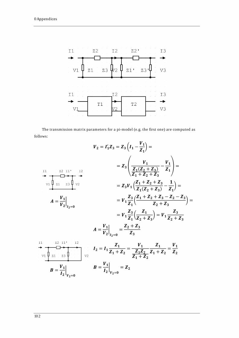
0Appendices
The transmission matrix parameters for a pi-model (e.g. the first one) are computed as
follows:
𝑨𝑨 =𝑽𝑽𝟏𝟏𝑽𝑽𝟐𝟐�𝑰𝑰𝟐𝟐=𝟎𝟎
𝑽𝑽𝟐𝟐 = 𝑰𝑰𝟏𝟏′ 𝒁𝒁𝟑𝟑 = 𝒁𝒁𝟑𝟑 �𝑰𝑰𝟏𝟏 −𝑽𝑽𝟏𝟏𝒁𝒁𝟏𝟏� =
= 𝒁𝒁𝟑𝟑 �𝑽𝑽𝟏𝟏
𝒁𝒁𝟏𝟏(𝒁𝒁𝟐𝟐 + 𝒁𝒁𝟑𝟑)𝒁𝒁𝟏𝟏 + 𝒁𝒁𝟐𝟐 + 𝒁𝒁𝟑𝟑
−𝑽𝑽𝟏𝟏𝒁𝒁𝟏𝟏� =
= 𝒁𝒁𝟑𝟑𝑽𝑽𝟏𝟏 �𝒁𝒁𝟏𝟏 + 𝒁𝒁𝟐𝟐 + 𝒁𝒁𝟑𝟑𝒁𝒁𝟏𝟏(𝒁𝒁𝟐𝟐 + 𝒁𝒁𝟑𝟑) −
𝟏𝟏𝒁𝒁𝟏𝟏� =
= 𝑽𝑽𝟏𝟏𝒁𝒁𝟑𝟑𝒁𝒁𝟏𝟏
�𝒁𝒁𝟏𝟏 + 𝒁𝒁𝟐𝟐 + 𝒁𝒁𝟑𝟑 − 𝒁𝒁𝟐𝟐 − 𝒁𝒁𝟑𝟑
𝒁𝒁𝟐𝟐 + 𝒁𝒁𝟑𝟑� =
= 𝑽𝑽𝟏𝟏𝒁𝒁𝟑𝟑𝒁𝒁𝟏𝟏
�𝒁𝒁𝟏𝟏
𝒁𝒁𝟐𝟐 + 𝒁𝒁𝟑𝟑� = 𝑽𝑽𝟏𝟏
𝒁𝒁𝟑𝟑𝒁𝒁𝟐𝟐 + 𝒁𝒁𝟑𝟑
𝑨𝑨 =𝑽𝑽𝟏𝟏𝑽𝑽𝟐𝟐�𝑰𝑰𝟐𝟐=𝟎𝟎
=𝒁𝒁𝟐𝟐 + 𝒁𝒁𝟑𝟑𝒁𝒁𝟑𝟑
𝑩𝑩 =𝑽𝑽𝟏𝟏𝑰𝑰𝟐𝟐�𝑽𝑽𝟐𝟐=𝟎𝟎
𝑰𝑰𝟐𝟐 = 𝑰𝑰𝟏𝟏𝒁𝒁𝟏𝟏
𝒁𝒁𝟏𝟏 + 𝒁𝒁𝟐𝟐=
𝑽𝑽𝟏𝟏𝒁𝒁𝟏𝟏𝒁𝒁𝟐𝟐𝒁𝒁𝟏𝟏 + 𝒁𝒁𝟐𝟐
𝒁𝒁𝟏𝟏𝒁𝒁𝟏𝟏 + 𝒁𝒁𝟐𝟐
=𝑽𝑽𝟏𝟏𝒁𝒁𝟐𝟐
𝑩𝑩 =𝑽𝑽𝟏𝟏𝑰𝑰𝟐𝟐�𝑽𝑽𝟐𝟐=𝟎𝟎
= 𝒁𝒁𝟐𝟐
102
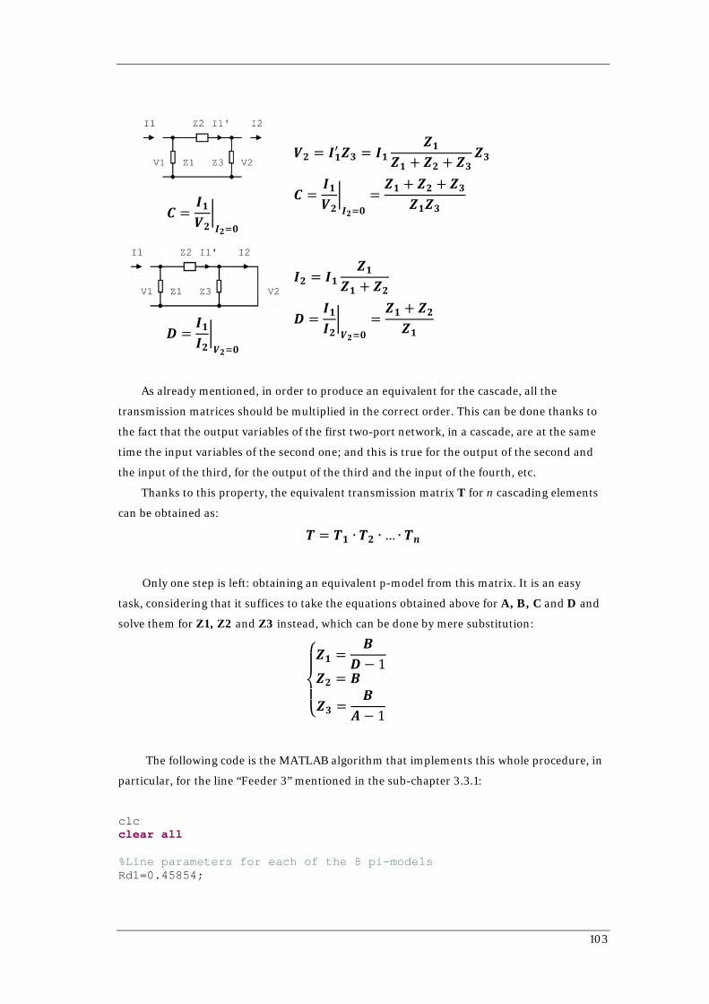
𝑪𝑪 =𝑰𝑰𝟏𝟏𝑽𝑽𝟐𝟐�𝑰𝑰𝟐𝟐=𝟎𝟎
𝑽𝑽𝟐𝟐 = 𝑰𝑰𝟏𝟏′ 𝒁𝒁𝟑𝟑 = 𝑰𝑰𝟏𝟏𝒁𝒁𝟏𝟏
𝒁𝒁𝟏𝟏 + 𝒁𝒁𝟐𝟐 + 𝒁𝒁𝟑𝟑𝒁𝒁𝟑𝟑
𝑪𝑪 =𝑰𝑰𝟏𝟏𝑽𝑽𝟐𝟐�𝑰𝑰𝟐𝟐=𝟎𝟎
=𝒁𝒁𝟏𝟏 + 𝒁𝒁𝟐𝟐 + 𝒁𝒁𝟑𝟑
𝒁𝒁𝟏𝟏𝒁𝒁𝟑𝟑
𝑫𝑫 =𝑰𝑰𝟏𝟏𝑰𝑰𝟐𝟐�𝑽𝑽𝟐𝟐=𝟎𝟎
𝑰𝑰𝟐𝟐 = 𝑰𝑰𝟏𝟏𝒁𝒁𝟏𝟏
𝒁𝒁𝟏𝟏 + 𝒁𝒁𝟐𝟐
𝑫𝑫 =𝑰𝑰𝟏𝟏𝑰𝑰𝟐𝟐�𝑽𝑽𝟐𝟐=𝟎𝟎
=𝒁𝒁𝟏𝟏 + 𝒁𝒁𝟐𝟐𝒁𝒁𝟏𝟏
As already mentioned, in order to produce an equivalent for the cascade, all the
transmission matrices should be multiplied in the correct order. This can be done thanks to
the fact that the output variables of the first two-port network, in a cascade, are at the same
time the input variables of the second one; and this is true for the output of the second and
the input of the third, for the output of the third and the input of the fourth, etc.
Thanks to this property, the equivalent transmission matrix T for n cascading elements
can be obtained as:
𝑻𝑻 = 𝑻𝑻𝟏𝟏 ∙ 𝑻𝑻𝟐𝟐 ∙ … ∙ 𝑻𝑻𝒏𝒏
Only one step is left: obtaining an equivalent p-model from this matrix. It is an easy
task, considering that it suffices to take the equations obtained above for A, B, C and D and
solve them for Z1, Z2 and Z3 instead, which can be done by mere substitution:
⎩⎪⎨
⎪⎧𝒁𝒁𝟏𝟏 =
𝑩𝑩𝑫𝑫− 1
𝒁𝒁𝟐𝟐 = 𝑩𝑩
𝒁𝒁𝟑𝟑 =𝑩𝑩
𝑨𝑨 − 1
The following code is the MATLAB algorithm that implements this whole procedure, in
particular, for the line “Feeder 3” mentioned in the sub-chapter 3.3.1:
clc clear all %Line parameters for each of the 8 pi-models Rd1=0.45854;
103

0Appendices
X_Ld1=0.20498; X_Cd1=0.0064093e+006; X_Cd1t=2*X_Cd1; Zsd1=Rd1+X_Ld1*1i; Ztd1=X_Cd1t*1i; Ro1=2.0679; X_Lo1=1.5525; X_Co1=0.0064093e+006; X_Co1t=2*X_Co1; Zso1=Ro1+X_Lo1*1i; Zto1=X_Co1t*1i; Rd2=0.1248; X_Ld2=0.04992; X_Cd2=0.028144e+006; X_Cd2t=2*X_Cd2; Zsd2=Rd2+X_Ld2*1i; Ztd2=X_Cd2t*1i; Ro2=0.468; X_Lo2=0.39; X_Co2=0.028144e+006; X_Co2t=2*X_Co2; Zso2=Ro2+X_Lo2*1i; Zto2=X_Co2t*1i; Rd3=0.0928; X_Ld3=0.03712; X_Cd3=0.037849e+006; X_Cd3t=2*X_Cd3; Zsd3=Rd3+X_Ld3*1i; Ztd3=X_Cd3t*1i; Ro3=0.348; X_Lo3=0.29; X_Co3=0.037849e+006; X_Co3t=2*X_Co3; Zso3=Ro3+X_Lo3*1i; Zto3=X_Co3t*1i; Rd4=0.15104; X_Ld4=0.060416; X_Cd4=0.023255e+006; X_Cd4t=2*X_Cd4; Zsd4=Rd4+X_Ld4*1i; Ztd4=X_Cd4t*1i; Ro4=0.5664; X_Lo4=0.472; X_Co4=0.023255e+006; X_Co4t=2*X_Co4; Zso4=Ro4+X_Lo4*1i; Zto4=X_Co4t*1i; Rd5=0.13588; X_Ld5=0.054897; X_Cd5=0.025392e+006; X_Cd5t=2*X_Cd5; Zsd5=Rd5+X_Ld5*1i;
104
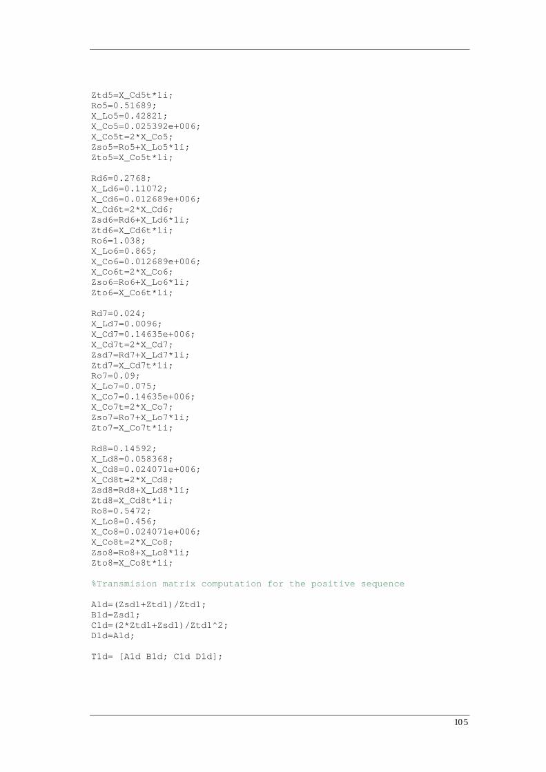
Ztd5=X_Cd5t*1i; Ro5=0.51689; X_Lo5=0.42821; X_Co5=0.025392e+006; X_Co5t=2*X_Co5; Zso5=Ro5+X_Lo5*1i; Zto5=X_Co5t*1i; Rd6=0.2768; X_Ld6=0.11072; X_Cd6=0.012689e+006; X_Cd6t=2*X_Cd6; Zsd6=Rd6+X_Ld6*1i; Ztd6=X_Cd6t*1i; Ro6=1.038; X_Lo6=0.865; X_Co6=0.012689e+006; X_Co6t=2*X_Co6; Zso6=Ro6+X_Lo6*1i; Zto6=X_Co6t*1i; Rd7=0.024; X_Ld7=0.0096; X_Cd7=0.14635e+006; X_Cd7t=2*X_Cd7; Zsd7=Rd7+X_Ld7*1i; Ztd7=X_Cd7t*1i; Ro7=0.09; X_Lo7=0.075; X_Co7=0.14635e+006; X_Co7t=2*X_Co7; Zso7=Ro7+X_Lo7*1i; Zto7=X_Co7t*1i; Rd8=0.14592; X_Ld8=0.058368; X_Cd8=0.024071e+006; X_Cd8t=2*X_Cd8; Zsd8=Rd8+X_Ld8*1i; Ztd8=X_Cd8t*1i; Ro8=0.5472; X_Lo8=0.456; X_Co8=0.024071e+006; X_Co8t=2*X_Co8; Zso8=Ro8+X_Lo8*1i; Zto8=X_Co8t*1i; %Transmision matrix computation for the positive sequence A1d=(Zsd1+Ztd1)/Ztd1; B1d=Zsd1; C1d=(2*Ztd1+Zsd1)/Ztd1^2; D1d=A1d; T1d= [A1d B1d; C1d D1d];
105
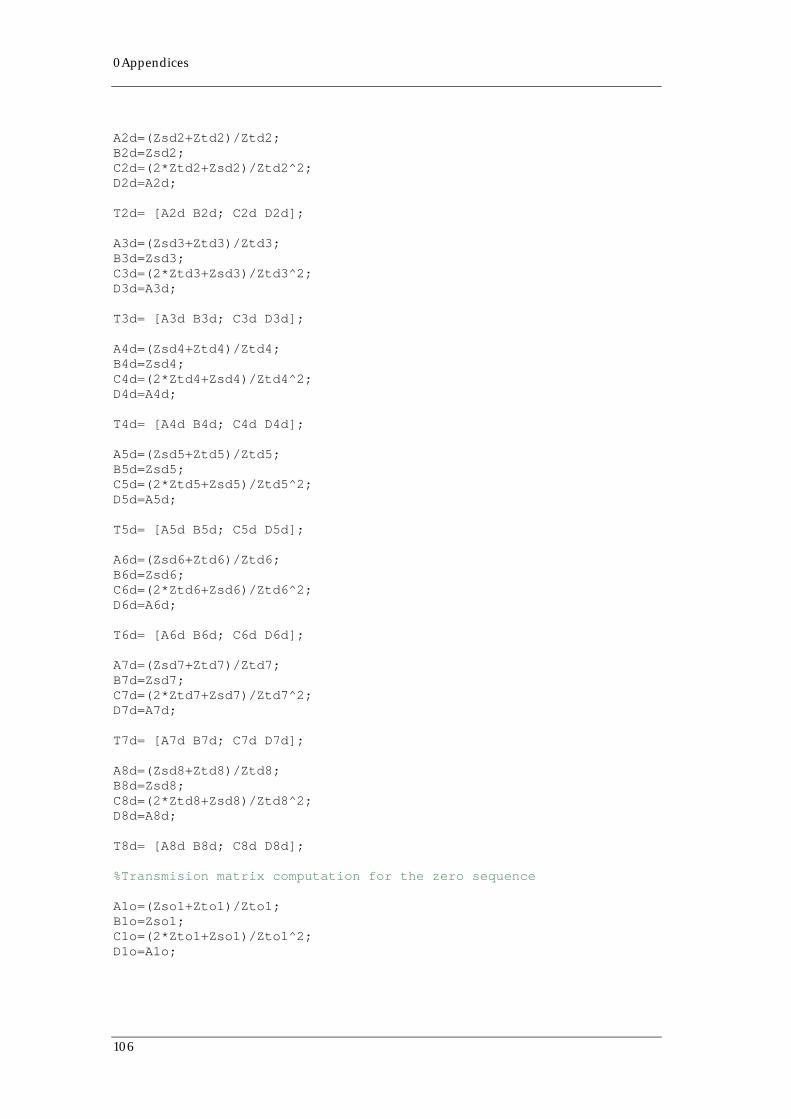
0Appendices
A2d=(Zsd2+Ztd2)/Ztd2; B2d=Zsd2; C2d=(2*Ztd2+Zsd2)/Ztd2^2; D2d=A2d; T2d= [A2d B2d; C2d D2d]; A3d=(Zsd3+Ztd3)/Ztd3; B3d=Zsd3; C3d=(2*Ztd3+Zsd3)/Ztd3^2; D3d=A3d; T3d= [A3d B3d; C3d D3d]; A4d=(Zsd4+Ztd4)/Ztd4; B4d=Zsd4; C4d=(2*Ztd4+Zsd4)/Ztd4^2; D4d=A4d; T4d= [A4d B4d; C4d D4d]; A5d=(Zsd5+Ztd5)/Ztd5; B5d=Zsd5; C5d=(2*Ztd5+Zsd5)/Ztd5^2; D5d=A5d; T5d= [A5d B5d; C5d D5d]; A6d=(Zsd6+Ztd6)/Ztd6; B6d=Zsd6; C6d=(2*Ztd6+Zsd6)/Ztd6^2; D6d=A6d; T6d= [A6d B6d; C6d D6d]; A7d=(Zsd7+Ztd7)/Ztd7; B7d=Zsd7; C7d=(2*Ztd7+Zsd7)/Ztd7^2; D7d=A7d; T7d= [A7d B7d; C7d D7d]; A8d=(Zsd8+Ztd8)/Ztd8; B8d=Zsd8; C8d=(2*Ztd8+Zsd8)/Ztd8^2; D8d=A8d; T8d= [A8d B8d; C8d D8d]; %Transmision matrix computation for the zero sequence A1o=(Zso1+Zto1)/Zto1; B1o=Zso1; C1o=(2*Zto1+Zso1)/Zto1^2; D1o=A1o;
106
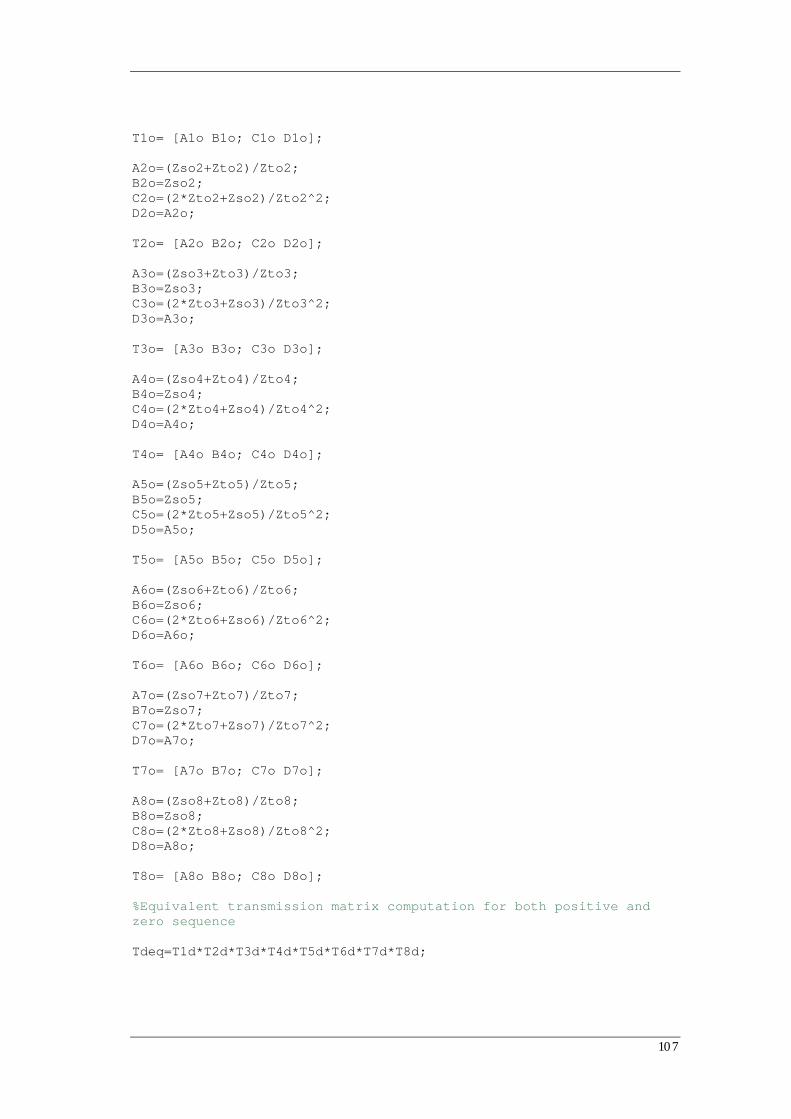
T1o= [A1o B1o; C1o D1o]; A2o=(Zso2+Zto2)/Zto2; B2o=Zso2; C2o=(2*Zto2+Zso2)/Zto2^2; D2o=A2o; T2o= [A2o B2o; C2o D2o]; A3o=(Zso3+Zto3)/Zto3; B3o=Zso3; C3o=(2*Zto3+Zso3)/Zto3^2; D3o=A3o; T3o= [A3o B3o; C3o D3o]; A4o=(Zso4+Zto4)/Zto4; B4o=Zso4; C4o=(2*Zto4+Zso4)/Zto4^2; D4o=A4o; T4o= [A4o B4o; C4o D4o]; A5o=(Zso5+Zto5)/Zto5; B5o=Zso5; C5o=(2*Zto5+Zso5)/Zto5^2; D5o=A5o; T5o= [A5o B5o; C5o D5o]; A6o=(Zso6+Zto6)/Zto6; B6o=Zso6; C6o=(2*Zto6+Zso6)/Zto6^2; D6o=A6o; T6o= [A6o B6o; C6o D6o]; A7o=(Zso7+Zto7)/Zto7; B7o=Zso7; C7o=(2*Zto7+Zso7)/Zto7^2; D7o=A7o; T7o= [A7o B7o; C7o D7o]; A8o=(Zso8+Zto8)/Zto8; B8o=Zso8; C8o=(2*Zto8+Zso8)/Zto8^2; D8o=A8o; T8o= [A8o B8o; C8o D8o]; %Equivalent transmission matrix computation for both positive and zero sequence Tdeq=T1d*T2d*T3d*T4d*T5d*T6d*T7d*T8d;
107

0Appendices
Adeq=Tdeq(1,1); Bdeq=Tdeq(1,2); Cdeq=Tdeq(2,1); Ddeq=Tdeq(2,2); Toeq=T1o*T2o*T3o*T4o*T5o*T6o*T7o*T8o; Aoeq=Toeq(1,1); Boeq=Toeq(1,2); Coeq=Toeq(2,1); Doeq=Toeq(2,2); %Equivalent p-model computation for both positive and zero sequence Ztdeq_sx=Bdeq/(Ddeq-1); Zsdeq=Bdeq; Ztdeq_dx=Bdeq*Ddeq/(Bdeq*Cdeq-Ddeq+1); Ztdeq=Ztdeq_sx*Ztdeq_dx/(Ztdeq_dx+Ztdeq_sx); Rdeq=real(Zsdeq) X_Ldeq=imag(Zsdeq) X_Cdeq=imag(Ztdeq) Ztoeq_sx=Boeq/(Doeq-1); Zsoeq=Boeq; Ztoeq_ox=Boeq*Doeq/(Boeq*Coeq-Doeq+1); Ztoeq=Ztoeq_sx*Ztoeq_ox/(Ztoeq_ox+Ztoeq_sx); Roeq=real(Zsoeq) X_Loeq=imag(Zsoeq) X_Coeq=imag(Ztoeq)
A.7 Branching line section circuital equivalent and
MATLAB model
Figure 50 Circuital representation of a branching section of a feeder.
108

In order to include in the MATLAB model already developed in Appendix A.6 the
branching section shown in the equivalent of Figure 50, some circuital elaborations were in
order. The following equivalent is elaborated under the assumptions of no loads connected to
any of the ports and for any of the three sequences, just to keep the process as general as
possible.
𝒁𝒁𝑩𝑩𝒔𝒔𝑩𝑩𝒏𝒏𝒔𝒔 = 𝑗𝑗𝑋𝑋𝐶𝐶3
𝒁𝒁𝑩𝑩𝒔𝒔𝒔𝒔𝒔𝒔𝒔𝒔𝑩𝑩 = 𝒁𝒁𝟑𝟑 + 𝒁𝒁𝑩𝑩𝒔𝒔𝑩𝑩𝒏𝒏𝒔𝒔
𝒁𝒁𝒔𝒔𝒆𝒆 =𝒁𝒁𝑩𝑩𝒔𝒔𝒔𝒔𝒔𝒔𝒔𝒔𝑩𝑩𝒁𝒁𝑩𝑩𝒔𝒔𝑩𝑩𝒏𝒏𝒔𝒔𝒁𝒁𝑩𝑩𝒔𝒔𝒔𝒔𝒔𝒔𝒔𝒔𝑩𝑩𝒁𝒁𝑩𝑩𝒔𝒔𝑩𝑩𝒏𝒏𝒔𝒔
Once Zeq is computed, the element can be implemented in the two-ports cascade by
simply calculating its transformation matrix and including it in the ordered multiplication
already shown in Appendix A.6. It’s transformation matrix can be easily found as show
below:
𝑨𝑨 =𝑽𝑽𝟏𝟏𝑽𝑽𝟐𝟐�𝑰𝑰𝟐𝟐=𝟎𝟎
𝑽𝑽𝟐𝟐 = 𝑽𝑽𝟏𝟏
𝑨𝑨 =𝑽𝑽𝟏𝟏𝑽𝑽𝟐𝟐�𝑰𝑰𝟐𝟐=𝟎𝟎
= 1
109
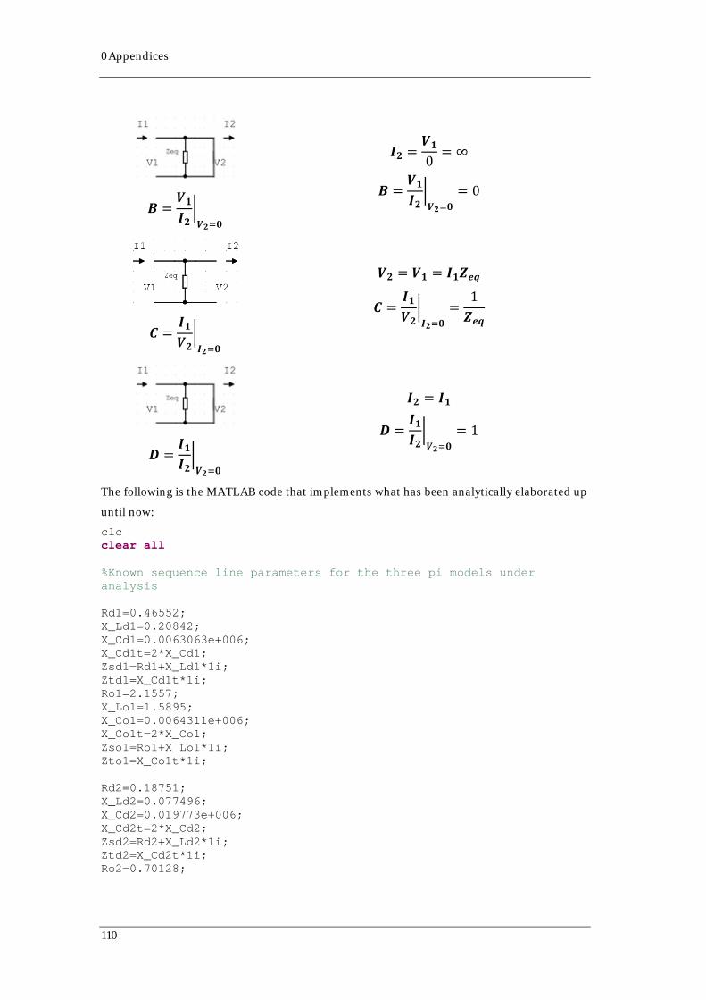
0Appendices
𝑩𝑩 =𝑽𝑽𝟏𝟏𝑰𝑰𝟐𝟐�𝑽𝑽𝟐𝟐=𝟎𝟎
𝑰𝑰𝟐𝟐 =𝑽𝑽𝟏𝟏0
= ∞
𝑩𝑩 =𝑽𝑽𝟏𝟏𝑰𝑰𝟐𝟐�𝑽𝑽𝟐𝟐=𝟎𝟎
= 0
𝑪𝑪 =𝑰𝑰𝟏𝟏𝑽𝑽𝟐𝟐�𝑰𝑰𝟐𝟐=𝟎𝟎
𝑽𝑽𝟐𝟐 = 𝑽𝑽𝟏𝟏 = 𝑰𝑰𝟏𝟏𝒁𝒁𝒔𝒔𝒆𝒆
𝑪𝑪 =𝑰𝑰𝟏𝟏𝑽𝑽𝟐𝟐�𝑰𝑰𝟐𝟐=𝟎𝟎
=1𝒁𝒁𝒔𝒔𝒆𝒆
𝑫𝑫 =𝑰𝑰𝟏𝟏𝑰𝑰𝟐𝟐�𝑽𝑽𝟐𝟐=𝟎𝟎
𝑰𝑰𝟐𝟐 = 𝑰𝑰𝟏𝟏
𝑫𝑫 =𝑰𝑰𝟏𝟏𝑰𝑰𝟐𝟐�𝑽𝑽𝟐𝟐=𝟎𝟎
= 1
The following is the MATLAB code that implements what has been analytically elaborated up
until now:
clc clear all %Known sequence line parameters for the three pi models under analysis Rd1=0.46552; X_Ld1=0.20842; X_Cd1=0.0063063e+006; X_Cd1t=2*X_Cd1; Zsd1=Rd1+X_Ld1*1i; Ztd1=X_Cd1t*1i; Ro1=2.1557; X_Lo1=1.5895; X_Co1=0.0064311e+006; X_Co1t=2*X_Co1; Zso1=Ro1+X_Lo1*1i; Zto1=X_Co1t*1i; Rd2=0.18751; X_Ld2=0.077496; X_Cd2=0.019773e+006; X_Cd2t=2*X_Cd2; Zsd2=Rd2+X_Ld2*1i; Ztd2=X_Cd2t*1i; Ro2=0.70128;
110
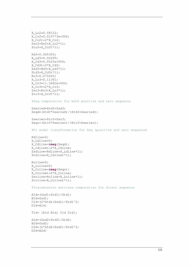
X_Lo2=0.58152; X_Co2=0.019773e+006; X_Co2t=2*X_Co2; Zso2=Ro2+X_Lo2*1i; Zto2=X_Co2t*1i; Rd3=0.065305; X_Ld3=0.02695; X_Cd3=5.0525e+006; X_Cd3t=2*X_Cd3; Zsd3=Rd3+X_Ld3*1i; Ztd3=X_Cd3t*1i; Ro3=0.075665; X_Lo3=0.11361; X_Co3=11.3682e+006; X_Co3t=2*X_Co3; Zso3=Ro3+X_Lo3*1i; Zto3=X_Co3t*1i; %Zeq computation for both positive and zero sequence Zseried=Ztd3+Zsd3; Zeqd=(Ztd3*Zseried)/(Ztd3+Zseried); Zserieo=Zto3+Zso3; Zeqo=(Zto3*Zserieo)/(Zto3+Zserieo); %Pi model transformation for Zeq (positive and zero sequence) Rdline=0; X_Ldline=0; X_Cdline=imag(Zeqd); X_Cdlinet=2*X_Cdline; Zsdline=Rdline+X_Ldline*1i; Ztdline=X_Cdlinet*1i; Roline=0; X_Loline=0; X_Coline=imag(Zeqo); X_Colinet=2*X_Coline; Zsoline=Roline+X_Loline*1i; Ztoline=X_Colinet*1i; %Transmission matrices computation for direct sequence A1d=(Zsd1+Ztd1)/Ztd1; B1d=Zsd1; C1d=(2*Ztd1+Zsd1)/Ztd1^2; D1d=A1d; T1d= [A1d B1d; C1d D1d]; A2d=(Zsd2+Ztd2)/Ztd2; B2d=Zsd2; C2d=(2*Ztd2+Zsd2)/Ztd2^2; D2d=A2d;
111
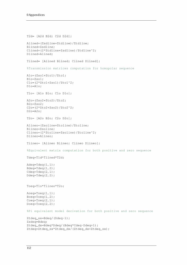
0Appendices
T2d= [A2d B2d; C2d D2d]; Alined=(Zsdline+Ztdline)/Ztdline; Blined=Zsdline; Clined=(2*Ztdline+Zsdline)/Ztdline^2; Dlined=Alined; Tlined= [Alined Blined; Clined Dlined]; %Transmission matrices computation for homopolar sequence A1o=(Zso1+Zto1)/Zto1; B1o=Zso1; C1o=(2*Zto1+Zso1)/Zto1^2; D1o=A1o; T1o= [A1o B1o; C1o D1o]; A2o=(Zso2+Zto2)/Zto2; B2o=Zso2; C2o=(2*Zto2+Zso2)/Zto2^2; D2o=A2o; T2o= [A2o B2o; C2o D2o]; Alineo=(Zsoline+Ztoline)/Ztoline; Blineo=Zsoline; Clineo=(2*Ztoline+Zsoline)/Ztoline^2; Dlineo=Alineo; Tlineo= [Alineo Blineo; Clineo Dlineo]; %Equivalent matrix computation for both positive and zero sequence Tdeq=T1d*Tlined*T2d; Adeq=Tdeq(1,1); Bdeq=Tdeq(1,2); Cdeq=Tdeq(2,1); Ddeq=Tdeq(2,2); Toeq=T1o*Tlineo*T2o; Aoeq=Toeq(1,1); Boeq=Toeq(1,2); Coeq=Toeq(2,1); Doeq=Toeq(2,2); %Pi equivalent model derivation for both positive and zero sequence Ztdeq_sx=Bdeq/(Ddeq-1); Zsdeq=Bdeq; Ztdeq_dx=Bdeq*Ddeq/(Bdeq*Cdeq-Ddeq+1); Ztdeq=Ztdeq_sx*Ztdeq_dx/(Ztdeq_dx+Ztdeq_sx);
112
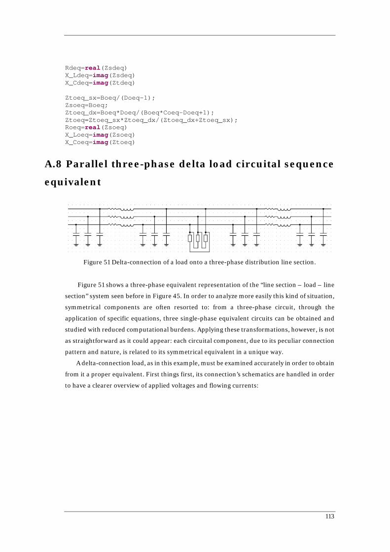
Rdeq=real(Zsdeq) X_Ldeq=imag(Zsdeq) X_Cdeq=imag(Ztdeq) Ztoeq_sx=Boeq/(Doeq-1); Zsoeq=Boeq; Ztoeq_dx=Boeq*Doeq/(Boeq*Coeq-Doeq+1); Ztoeq=Ztoeq_sx*Ztoeq_dx/(Ztoeq_dx+Ztoeq_sx); Roeq=real(Zsoeq) X_Loeq=imag(Zsoeq) X_Coeq=imag(Ztoeq)
A.8 Parallel three-phase delta load circuital sequence
equivalent
Figure 51 Delta-connection of a load onto a three-phase distribution line section.
Figure 51 shows a three-phase equivalent representation of the “line section – load – line
section” system seen before in Figure 45. In order to analyze more easily this kind of situation,
symmetrical components are often resorted to: from a three-phase circuit, through the
application of specific equations, three single-phase equivalent circuits can be obtained and
studied with reduced computational burdens. Applying these transformations, however, is not
as straightforward as it could appear: each circuital component, due to its peculiar connection
pattern and nature, is related to its symmetrical equivalent in a unique way.
A delta-connection load, as in this example, must be examined accurately in order to obtain
from it a proper equivalent. First things first, its connection’s schematics are handled in order
to have a clearer overview of applied voltages and flowing currents:
113
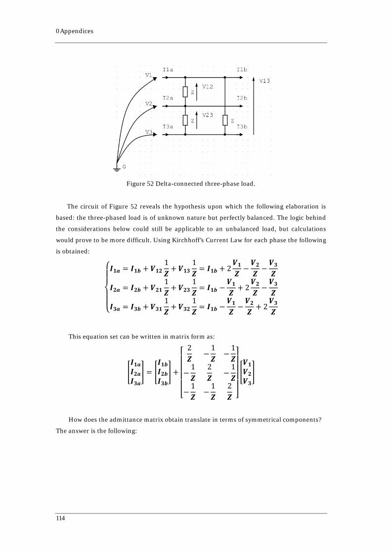
0Appendices
Figure 52 Delta-connected three-phase load.
The circuit of Figure 52 reveals the hypothesis upon which the following elaboration is
based: the three-phased load is of unknown nature but perfectly balanced. The logic behind
the considerations below could still be applicable to an unbalanced load, but calculations
would prove to be more difficult. Using Kirchhoff’s Current Law for each phase the following
is obtained:
⎩⎪⎨
⎪⎧𝑰𝑰𝟏𝟏𝟏𝟏 = 𝑰𝑰𝟏𝟏𝟏𝟏 + 𝑽𝑽𝟏𝟏𝟐𝟐
1𝒁𝒁
+ 𝑽𝑽𝟏𝟏𝟑𝟑1𝒁𝒁
= 𝑰𝑰𝟏𝟏𝟏𝟏 + 2𝑽𝑽𝟏𝟏𝒁𝒁−𝑽𝑽𝟐𝟐𝒁𝒁−𝑽𝑽𝟑𝟑𝒁𝒁
𝑰𝑰𝟐𝟐𝟏𝟏 = 𝑰𝑰𝟐𝟐𝟏𝟏 + 𝑽𝑽𝟐𝟐𝟏𝟏1𝒁𝒁
+ 𝑽𝑽𝟐𝟐𝟑𝟑1𝒁𝒁
= 𝑰𝑰𝟏𝟏𝟏𝟏 −𝑽𝑽𝟏𝟏𝒁𝒁
+ 2𝑽𝑽𝟐𝟐𝒁𝒁−𝑽𝑽𝟑𝟑𝒁𝒁
𝑰𝑰𝟑𝟑𝟏𝟏 = 𝑰𝑰𝟑𝟑𝟏𝟏 + 𝑽𝑽𝟑𝟑𝟏𝟏1𝒁𝒁
+ 𝑽𝑽𝟑𝟑𝟐𝟐1𝒁𝒁
= 𝑰𝑰𝟏𝟏𝟏𝟏 −𝑽𝑽𝟏𝟏𝒁𝒁−𝑽𝑽𝟐𝟐𝒁𝒁
+ 2𝑽𝑽𝟑𝟑𝒁𝒁
This equation set can be written in matrix form as:
�𝑰𝑰𝟏𝟏𝟏𝟏𝑰𝑰𝟐𝟐𝟏𝟏𝑰𝑰𝟑𝟑𝟏𝟏
� = �𝑰𝑰𝟏𝟏𝟏𝟏𝑰𝑰𝟐𝟐𝟏𝟏𝑰𝑰𝟑𝟑𝟏𝟏
� +
⎣⎢⎢⎢⎢⎡
2𝒁𝒁
−1𝒁𝒁
−1𝒁𝒁
−1𝒁𝒁
2𝒁𝒁
−1𝒁𝒁
−1𝒁𝒁
−1𝒁𝒁
2𝒁𝒁 ⎦⎥⎥⎥⎥⎤
�𝑽𝑽𝟏𝟏𝑽𝑽𝟐𝟐𝑽𝑽𝟑𝟑�
How does the admittance matrix obtain translate in terms of symmetrical components?
The answer is the following:
114
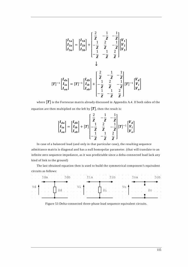
�𝑰𝑰𝟏𝟏𝟏𝟏𝑰𝑰𝟐𝟐𝟏𝟏𝑰𝑰𝟑𝟑𝟏𝟏
� = �𝑰𝑰𝟏𝟏𝟏𝟏𝑰𝑰𝟐𝟐𝟏𝟏𝑰𝑰𝟑𝟑𝟏𝟏
� +
⎣⎢⎢⎢⎢⎡
2𝒁𝒁
−1𝒁𝒁
−1𝒁𝒁
−1𝒁𝒁
2𝒁𝒁
−1𝒁𝒁
−1𝒁𝒁
−1𝒁𝒁
2𝒁𝒁 ⎦⎥⎥⎥⎥⎤
�𝑽𝑽𝟏𝟏𝑽𝑽𝟐𝟐𝑽𝑽𝟑𝟑�
↓
[𝑻𝑻]−1 �𝑰𝑰𝒅𝒅𝟏𝟏𝑰𝑰𝒔𝒔𝟏𝟏𝑰𝑰𝒐𝒐𝟏𝟏
� = [𝑻𝑻]−1 �𝑰𝑰𝒅𝒅𝟏𝟏𝑰𝑰𝒔𝒔𝟏𝟏𝑰𝑰𝒐𝒐𝟏𝟏
� +
⎣⎢⎢⎢⎢⎡
2𝒁𝒁
−1𝒁𝒁
−1𝒁𝒁
−1𝒁𝒁
2𝒁𝒁
−1𝒁𝒁
−1𝒁𝒁
−1𝒁𝒁
2𝒁𝒁 ⎦⎥⎥⎥⎥⎤
[𝑻𝑻]−1 �𝑽𝑽𝒅𝒅𝑽𝑽𝒔𝒔𝑽𝑽𝒐𝒐�
where [𝑻𝑻] is the Fortescue matrix already discussed in Appendix A.4. If both sides of the
equation are then multiplied on the left by [𝑻𝑻], then the result is:
�𝑰𝑰𝒅𝒅𝟏𝟏𝑰𝑰𝒔𝒔𝟏𝟏𝑰𝑰𝒐𝒐𝟏𝟏
� = �𝑰𝑰𝒅𝒅𝟏𝟏𝑰𝑰𝒔𝒔𝟏𝟏𝑰𝑰𝒐𝒐𝟏𝟏
� + [𝑻𝑻]
⎣⎢⎢⎢⎢⎡
2𝒁𝒁
−1𝒁𝒁
−1𝒁𝒁
−1𝒁𝒁
2𝒁𝒁
−1𝒁𝒁
−1𝒁𝒁
−1𝒁𝒁
2𝒁𝒁 ⎦⎥⎥⎥⎥⎤
[𝑻𝑻]−1 �𝑽𝑽𝒅𝒅𝑽𝑽𝒔𝒔𝑽𝑽𝒐𝒐�
In case of a balanced load (and only in that particular case), the resulting sequence
admittance matrix is diagonal and has a null homopolar parameter. (that will translate to an
infinite zero sequence impedance, as it was predictable since a delta-connected load lack any
kind of link to the ground)
The last obtained equation then is used to build the symmetrical component’s equivalent
circuits as follows:
Figure 53 Delta-connected three-phase load sequence equivalent circuits.
115

0Appendices
A.9 IEEE C37.118 Validator’s algorithm
The code, originally written on RSCAD in C, has been translated into the IEEE C37.118
synchrophasor-specific language in order to be run on the AXION SEL device working as a
PDC.
The algorithm is the following:
PROGRAM Validator’s Algorithm
VAR
Vd1r : REAL;
Vd1i : REAL;
Vd2r : REAL;
Vd2i : REAL;
Vo1r : REAL;
Vo1i : REAL;
Vo2r : REAL;
Vo2i : REAL;
Id1r : REAL;
Id1i : REAL;
Id2r : REAL;
Id2i : REAL;
Io1r : REAL;
Io1i : REAL;
Io2r : REAL;
Io2i : REAL;
Bd : REAL;
Bo : REAL;
a,b,c,d,e,f,g,h,i,l,m,n : REAL;
sqVd1r : REAL;
sqVd1i : REAL;
116

sqVd2r : REAL;
sqVd2i : REAL;
sqVo1r : REAL;
sqVo1i : REAL;
sqVo2r : REAL;
sqVo2i : REAL;
xcd : REAL;
Rd : REAL;
X_Ld : REAL;
Ro : REAL;
X_Lo : REAL;
X_Co : REAL;
IA_R, IA_I : REAL;
IB_R, IB_I : REAL;
IC_R, IC_I : REAL;
I0_R, I0_I : REAL;
VA_R, VA_I : REAL;
VB_R, VB_I : REAL;
VC_R, VC_I : REAL;
V0_R, V0_I : REAL;
I0_MAG, I0_ANG : REAL;
END_VAR
117
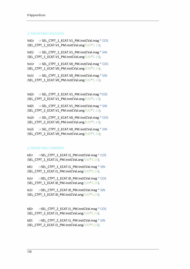
0Appendices
// AXION PMU VOLTAGES
Vd1r := SEL_CTPT_1_ECAT.V1_PM.instCVal.mag * COS (SEL_CTPT_1_ECAT.V1_PM.instCVal.ang/180*3.14);
Vd1i := SEL_CTPT_1_ECAT.V1_PM.instCVal.mag * SIN (SEL_CTPT_1_ECAT.V1_PM.instCVal.ang/180*3.14);
Vo1r := SEL_CTPT_1_ECAT.V0_PM.instCVal.mag * COS (SEL_CTPT_1_ECAT.V0_PM.instCVal.ang/180*3.14);
Vo1i := SEL_CTPT_1_ECAT.V0_PM.instCVal.mag * SIN (SEL_CTPT_1_ECAT.V0_PM.instCVal.ang/180*3.14);
Vd2r := SEL_CTPT_2_ECAT.V1_PM.instCVal.mag *COS (SEL_CTPT_2_ECAT.V1_PM.instCVal.ang/180*3.14);
Vd2i := SEL_CTPT_2_ECAT.V1_PM.instCVal.mag * SIN (SEL_CTPT_2_ECAT.V1_PM.instCVal.ang/180*3.14);
Vo2r := SEL_CTPT_2_ECAT.V0_PM.instCVal.mag * COS (SEL_CTPT_2_ECAT.V0_PM.instCVal.ang/180*3.14);
Vo2i := SEL_CTPT_2_ECAT.V0_PM.instCVal.mag * SIN (SEL_CTPT_2_ECAT.V0_PM.instCVal.ang/180*3.14);
// AXION PMU CURRENTS
Id1r :=SEL_CTPT_1_ECAT.I1_PM.instCVal.mag * COS (SEL_CTPT_1_ECAT.I1_PM.instCVal.ang/180*3.14);
Id1i :=SEL_CTPT_1_ECAT.I1_PM.instCVal.mag * SIN (SEL_CTPT_1_ECAT.I1_PM.instCVal.ang/180*3.14);
Io1r :=SEL_CTPT_1_ECAT.I0_PM.instCVal.mag * COS (SEL_CTPT_1_ECAT.I0_PM.instCVal.ang/180*3.14);
Io1i :=SEL_CTPT_1_ECAT.I0_PM.instCVal.mag * SIN (SEL_CTPT_1_ECAT.I0_PM.instCVal.ang/180*3.14);
Id2r :=SEL_CTPT_2_ECAT.I1_PM.instCVal.mag * COS (SEL_CTPT_2_ECAT.I1_PM.instCVal.ang/180*3.14);
Id2i :=SEL_CTPT_2_ECAT.I1_PM.instCVal.mag * SIN (SEL_CTPT_2_ECAT.I1_PM.instCVal.ang/180*3.14);
118

Io2r :=SEL_CTPT_2_ECAT.I0_PM.instCVal.mag * COS (SEL_CTPT_2_ECAT.I0_PM.instCVal.ang/180*3.14);
Io2i :=SEL_CTPT_2_ECAT.I0_PM.instCVal.mag * SIN (SEL_CTPT_2_ECAT.I0_PM.instCVal.ang/180*3.14);
Bd :=0;
Bo :=0;
a :=0;
b :=0;
c :=0;
d :=0;
e :=0;
f :=0;
g :=0;
h :=0;
i :=0;
l :=0;
m :=0;
n :=0;
sqVd1r :=0;
sqVd1i :=0;
sqVd2r :=0;
sqVd2i :=0;
sqVo1r :=0;
sqVo1i :=0;
sqVo2r :=0;
sqVo2i :=0;
119
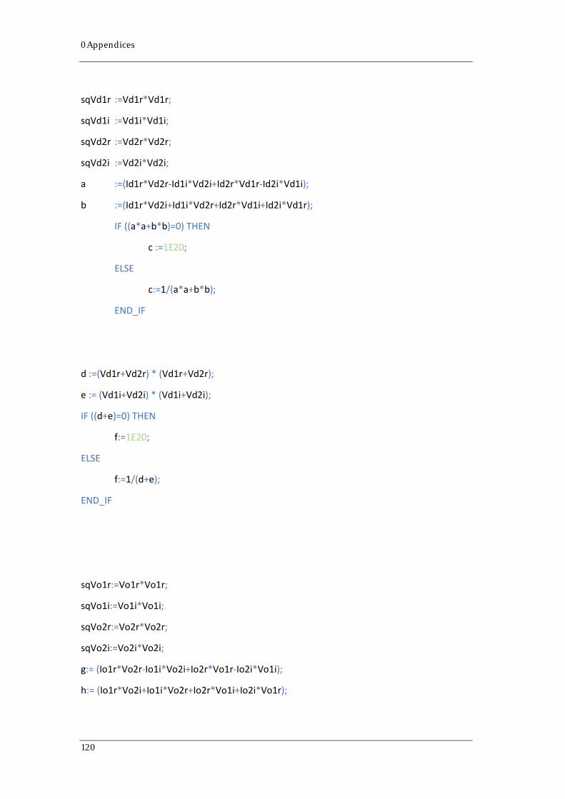
0Appendices
sqVd1r :=Vd1r*Vd1r;
sqVd1i :=Vd1i*Vd1i;
sqVd2r :=Vd2r*Vd2r;
sqVd2i :=Vd2i*Vd2i;
a :=(Id1r*Vd2r-Id1i*Vd2i+Id2r*Vd1r-Id2i*Vd1i);
b :=(Id1r*Vd2i+Id1i*Vd2r+Id2r*Vd1i+Id2i*Vd1r);
IF ((a*a+b*b)=0) THEN
c :=1E20;
ELSE
c:=1/(a*a+b*b);
END_IF
d :=(Vd1r+Vd2r) * (Vd1r+Vd2r);
e := (Vd1i+Vd2i) * (Vd1i+Vd2i);
IF ((d+e)=0) THEN
f:=1E20;
ELSE
f:=1/(d+e);
END_IF
sqVo1r:=Vo1r*Vo1r;
sqVo1i:=Vo1i*Vo1i;
sqVo2r:=Vo2r*Vo2r;
sqVo2i:=Vo2i*Vo2i;
g:= (Io1r*Vo2r-Io1i*Vo2i+Io2r*Vo1r-Io2i*Vo1i);
h:= (Io1r*Vo2i+Io1i*Vo2r+Io2r*Vo1i+Io2i*Vo1r);
120

IF ((g*g+h*h)=0) THEN
i:=1E20;
ELSE
i:=1/(g*g+h*h);
END_IF
l:= (Vo1r+Vo2r) * (Vo1r+Vo2r);
m:= (Vo1i+Vo2i) * (Vo1i+Vo2i);
IF ((l+m)=0) THEN
n:=1E20;
ELSE
n:=1/(l+m);
END_IF
Rd := ((sqVd1r-sqVd1i-sqVd2r+sqVd2i) * (Id1r*Vd2r-Id1i*Vd2i+Id2r*Vd1r-Id2i*Vd1i)+2*(Vd1r*Vd1i-Vd2r*Vd2i) * (Id1r*Vd2i+Id1i*Vd2r+Id2r*Vd1i+Id2i*Vd1r))*c;
X_Ld:= (2*(Vd1r*Vd1i-Vd2r*Vd2i) * (Id1r*Vd2r-Id1i*Vd2i+Id2r*Vd1r-Id2i*Vd1i)-(sqVd1r-sqVd1i-sqVd2r+sqVd2i) * (Id1r*Vd2i+Id1i*Vd2r+Id2r*Vd1i+Id2i*Vd1r))*c;
Bd:=2*((Id1i-Id2i) * (Vd1r+Vd2r)-(Id1r-Id2r) * (Vd1i+Vd2i))*f;
IF (Bd=0) THEN
xcd := 1E20;
ELSE
xcd := 1/Bd;
END_IF
121

0Appendices
Ro:= ((sqVo1r-sqVo1i-sqVo2r+sqVo2i) * (Io1r*Vo2r-Io1i*Vo2i+Io2r*Vo1r-Io2i*Vo1i)+2*(Vo1r*Vo1i-Vo2r*Vo2i) * (Io1r*Vo2i+Io1i*Vo2r+Io2r*Vo1i+Io2i*Vo1r))*i;
X_Lo:= (2*(Vo1r*Vo1i-Vo2r*Vo2i) * (Io1r*Vo2r-Io1i*Vo2i+Io2r*Vo1r-Io2i*Vo1i)-(sqVo1r-sqVo1i-sqVo2r+sqVo2i) * (Io1r*Vo2i+Io1i*Vo2r+Io2r*Vo1i+Io2i*Vo1r))*i;
Bo:=2*((Io1i-Io2i) * (Vo1r+Vo2r)-(Io1r-Io2r) * (Vo1i+Vo2i))*n;
IF (Bo=0) THEN
X_Co:=1E20;
ELSE
X_Co:=1/Bo;
END_IF
122
Related Documents