Application of phasor measurements in distribution grids Citation for published version (APA): Singh, R. S. (2021). Application of phasor measurements in distribution grids: assessment of flexible cable loading limits and aggregated harmonic impedance models. Technische Universiteit Eindhoven. Document status and date: Published: 23/03/2021 Document Version: Publisher’s PDF, also known as Version of Record (includes final page, issue and volume numbers) Please check the document version of this publication: • A submitted manuscript is the version of the article upon submission and before peer-review. There can be important differences between the submitted version and the official published version of record. People interested in the research are advised to contact the author for the final version of the publication, or visit the DOI to the publisher's website. • The final author version and the galley proof are versions of the publication after peer review. • The final published version features the final layout of the paper including the volume, issue and page numbers. Link to publication General rights Copyright and moral rights for the publications made accessible in the public portal are retained by the authors and/or other copyright owners and it is a condition of accessing publications that users recognise and abide by the legal requirements associated with these rights. • Users may download and print one copy of any publication from the public portal for the purpose of private study or research. • You may not further distribute the material or use it for any profit-making activity or commercial gain • You may freely distribute the URL identifying the publication in the public portal. If the publication is distributed under the terms of Article 25fa of the Dutch Copyright Act, indicated by the “Taverne” license above, please follow below link for the End User Agreement: www.tue.nl/taverne Take down policy If you believe that this document breaches copyright please contact us at: [email protected] providing details and we will investigate your claim. Download date: 06. Jul. 2022

Welcome message from author
This document is posted to help you gain knowledge. Please leave a comment to let me know what you think about it! Share it to your friends and learn new things together.
Transcript

Application of phasor measurements in distribution grids
Citation for published version (APA):Singh, R. S. (2021). Application of phasor measurements in distribution grids: assessment of flexible cableloading limits and aggregated harmonic impedance models. Technische Universiteit Eindhoven.
Document status and date:Published: 23/03/2021
Document Version:Publisher’s PDF, also known as Version of Record (includes final page, issue and volume numbers)
Please check the document version of this publication:
• A submitted manuscript is the version of the article upon submission and before peer-review. There can beimportant differences between the submitted version and the official published version of record. Peopleinterested in the research are advised to contact the author for the final version of the publication, or visit theDOI to the publisher's website.• The final author version and the galley proof are versions of the publication after peer review.• The final published version features the final layout of the paper including the volume, issue and pagenumbers.Link to publication
General rightsCopyright and moral rights for the publications made accessible in the public portal are retained by the authors and/or other copyright ownersand it is a condition of accessing publications that users recognise and abide by the legal requirements associated with these rights.
• Users may download and print one copy of any publication from the public portal for the purpose of private study or research. • You may not further distribute the material or use it for any profit-making activity or commercial gain • You may freely distribute the URL identifying the publication in the public portal.
If the publication is distributed under the terms of Article 25fa of the Dutch Copyright Act, indicated by the “Taverne” license above, pleasefollow below link for the End User Agreement:www.tue.nl/taverne
Take down policyIf you believe that this document breaches copyright please contact us at:[email protected] details and we will investigate your claim.
Download date: 06. Jul. 2022
Doctoral Thesis
Application of Phasor Measurementsin Distribution Grids
Assessment of Flexible Cable Loading Limits andAggregated Harmonic Impedance Models
Ravi Shankar Singh
2021

© Ravi Shankar Singh, Utrecht 2021.
All rights reserved. No part of this publication may be reproduced, stored in a re-
trieval system or transmitted in any form or by any means, electronic, mechanical,
photocopying, recording or otherwise, without prior written permission of the author.
Printed by Ipskamp Enschede
ISBN 978-94-6421-263-1
Application of Phasor Measurementsin Distribution Grids
Assessment of Flexible Cable Loading Limits andAggregated Harmonic Impedance Models
PROEFSCHRIFT
ter verkrijging van de graad van doctor aan
de Technische Universiteit Eindhoven, op gezag van de rector magnificus, prof.dr.ir.
F.P.T Baaijens, voor een commissie aangewezen door het College voor Promoties in
het openbaar te verdedigen op dinsdag 23 maart 2021, om 16:00 uur
door
Ravi Shankar Singh
geboren te Patna, India

Dit proefschrift is goedgekeurd door de promotoren en de samenstelling van de pro-
motiecommissie is als volgt:
Voorzitter: Prof. dr. ir. P.M.J. van den Hof
Promotor: Prof. dr. ir. J.F.G. Cobben
Copromotor : Dr. V. Cuk
Leden: Prof. dr. ir. J. Desmet (Universiteit Gent)
Prof. dr. M. Gibescu (Universiteit Utrecht)
Prof. dr. ir. P.C.J.M. van der Wielen
Prof. dr. ing. A.J.M. Pemen
Adviseur: Dr. H.E. van den Brom (VSL)
Het onderzoek of ontwerp dat in dit proefschrift wordt beschreven is uitgevoerd in
overeenstemming met de TU/e Gedragscode Wetenschapsbeoefening.

Summary
The focus of the modern electricity grid is towards achieving cost-effective generation
and delivery of electric power with minimum impact on the environment. The evolu-
tion of modern distribution grids is marked by a rapid increase in renewable energy
sources (RES) such as wind parks (WPs) and photovoltaic (PV) systems. Simultane-
ously, electrification of the end uses is driving the electric power demand high. New
types of non-linear loads such as electrical vehicles (EVs), battery energy storage
system (BESS) and heat-pumps are also being integrated in the distribution grid.
Proliferation of intermittent RES and non-linear loads bring technical challenges in
terms of optimal grid asset utilization and safe grid operation while providing high
quality power to the costumers.
Increased power-flow during increased generation periods or power rerouting oper-
ations may saturate the loading capacity of certain sections of the grid leading to
congestion problems. Much of the medium voltage (MV) distribution grid in Nether-
lands is operated between 10 and 50 kV levels and is composed entirely of under-
ground power cables. Loading limits of such cable networks are constrained by the
thermal limits of the cable insulation and play a crucial role in regulating the power-
flows. Conventional ratings of the power cables have a fixed (steady) rating which
limits the flow of current above a certain value. Such ratings also limit the rerouting
of power even for short periods and cause under-utilization of the cables. Emergency
ratings could be used to temporarily increase the loading limits of the cables to al-
low a temporary increase in the power-flow through the cable. A Flexible (dynamic)
loading scheme based emergency ratings could be used to accommodate intermit-
tent peaks of power-flow caused by rerouting operations or a temporary ramp-up in
generation. This would increase the overall loading capacity of the grid and in some
cases may also delay the urgent need for grid reinforcements. However, knowledge of
the initial thermal states of the cable conductors is required to calculate the flexible
emergency ratings. For such an application, a cable temperature monitoring tool is
required to facilitate the calculations of flexible loading limits.
On the other hand, proliferation of non-linear loads impacts the overall quality of
power supplied to the consumers. Grid utilities are curious to access the impact
of the evolution of the distribution grids on various power quality (PQ) indices in-
cluding harmonic pollution. Methods such as harmonic state estimation, harmonic
source localization and calculation of harmonic contribution by large customers re-
quire harmonic impedance models of the utility and customer side of the grid. It
is challenging for the grid operator to accurately model the distribution side of the
grid. For harmonic studies, electricity grids are normally represented using Norton’s
Summary
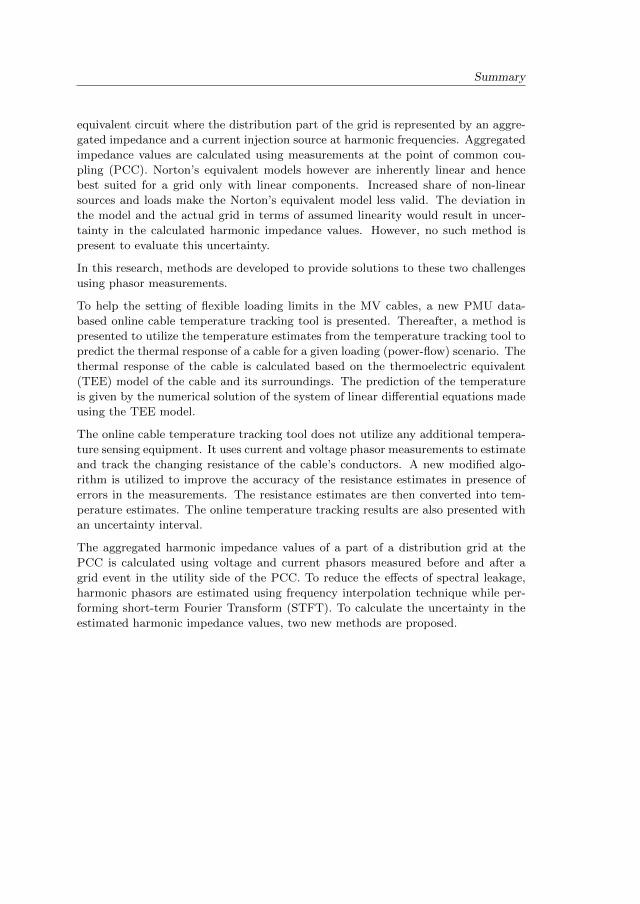
equivalent circuit where the distribution part of the grid is represented by an aggre-
gated impedance and a current injection source at harmonic frequencies. Aggregated
impedance values are calculated using measurements at the point of common cou-
pling (PCC). Norton’s equivalent models however are inherently linear and hence
best suited for a grid only with linear components. Increased share of non-linear
sources and loads make the Norton’s equivalent model less valid. The deviation in
the model and the actual grid in terms of assumed linearity would result in uncer-
tainty in the calculated harmonic impedance values. However, no such method is
present to evaluate this uncertainty.
In this research, methods are developed to provide solutions to these two challenges
using phasor measurements.
To help the setting of flexible loading limits in the MV cables, a new PMU data-
based online cable temperature tracking tool is presented. Thereafter, a method is
presented to utilize the temperature estimates from the temperature tracking tool to
predict the thermal response of a cable for a given loading (power-flow) scenario. The
thermal response of the cable is calculated based on the thermoelectric equivalent
(TEE) model of the cable and its surroundings. The prediction of the temperature
is given by the numerical solution of the system of linear differential equations made
using the TEE model.
The online cable temperature tracking tool does not utilize any additional tempera-
ture sensing equipment. It uses current and voltage phasor measurements to estimate
and track the changing resistance of the cable’s conductors. A new modified algo-
rithm is utilized to improve the accuracy of the resistance estimates in presence of
errors in the measurements. The resistance estimates are then converted into tem-
perature estimates. The online temperature tracking results are also presented with
an uncertainty interval.
The aggregated harmonic impedance values of a part of a distribution grid at the
PCC is calculated using voltage and current phasors measured before and after a
grid event in the utility side of the PCC. To reduce the effects of spectral leakage,
harmonic phasors are estimated using frequency interpolation technique while per-
forming short-term Fourier Transform (STFT). To calculate the uncertainty in the
estimated harmonic impedance values, two new methods are proposed.
Contents
Summary v
1 Introduction 1
1.1 Energy transition and the electricity distribution grid . . . . . . . . 1
1.2 Challenges of evolving distribution grid . . . . . . . . . . . . . . . . 2
1.3 Measurement-based solutions . . . . . . . . . . . . . . . . . . . . . . 4
1.4 Research objectives and questions . . . . . . . . . . . . . . . . . . . 6
1.5 Research approach . . . . . . . . . . . . . . . . . . . . . . . . . . . . 6
1.6 Thesis outline . . . . . . . . . . . . . . . . . . . . . . . . . . . . . . 7
2 Phasor Measurements in the Distribution Grid 9
2.1 Phasor measurement process . . . . . . . . . . . . . . . . . . . . . . 10
2.2 Interpolated DFT for harmonic phasors . . . . . . . . . . . . . . . . 15
2.3 Application of phasors . . . . . . . . . . . . . . . . . . . . . . . . . . 19
2.4 Conclusion . . . . . . . . . . . . . . . . . . . . . . . . . . . . . . . . 20
3 Measurement Chain and Error Propagation 23
3.1 Errors in phasor measurement chain . . . . . . . . . . . . . . . . . . 24
3.2 Uncertainty estimation and propagation . . . . . . . . . . . . . . . . 28
3.3 Conclusion . . . . . . . . . . . . . . . . . . . . . . . . . . . . . . . . 34
4 Online Cable Temperature Tracking 35
4.1 Introduction . . . . . . . . . . . . . . . . . . . . . . . . . . . . . . . 36
4.2 Required accuracy in resistance estimates . . . . . . . . . . . . . . . 37
4.3 Parameter estimation model . . . . . . . . . . . . . . . . . . . . . . 38
4.4 Review of existing line parameter estimation methods . . . . . . . . 40
4.5 Existing estimation algorithm . . . . . . . . . . . . . . . . . . . . . . 42
4.6 New proposed method . . . . . . . . . . . . . . . . . . . . . . . . . . 47
4.7 Data pre-processing . . . . . . . . . . . . . . . . . . . . . . . . . . . 52
4.8 Estimation of uncertainty . . . . . . . . . . . . . . . . . . . . . . . . 53
4.9 Results and comparison . . . . . . . . . . . . . . . . . . . . . . . . . 55
4.10 Laboratory test . . . . . . . . . . . . . . . . . . . . . . . . . . . . . . 65
4.11 Results from grid PMU data . . . . . . . . . . . . . . . . . . . . . . 72
4.12 Temperature estimation . . . . . . . . . . . . . . . . . . . . . . . . . 78
4.13 Conclusion . . . . . . . . . . . . . . . . . . . . . . . . . . . . . . . . 80
5 Cable Thermal Assessment for Flexible Loading 81
5.1 Introduction . . . . . . . . . . . . . . . . . . . . . . . . . . . . . . . 82
Contents
5.2 Construction of TEE model . . . . . . . . . . . . . . . . . . . . . . . 83
5.3 Conclusion . . . . . . . . . . . . . . . . . . . . . . . . . . . . . . . . 91
6 Aggregated Harmonic model of Sub-grids. 93
6.1 Introduction . . . . . . . . . . . . . . . . . . . . . . . . . . . . . . . 94
6.2 Impedance estimation . . . . . . . . . . . . . . . . . . . . . . . . . . 95
6.3 Proposed uncertainty estimation methods . . . . . . . . . . . . . . . 97
6.4 Distribution grid model . . . . . . . . . . . . . . . . . . . . . . . . . 100
6.5 Results . . . . . . . . . . . . . . . . . . . . . . . . . . . . . . . . . . 107
6.6 Discussion . . . . . . . . . . . . . . . . . . . . . . . . . . . . . . . . 110
6.7 Conclusion . . . . . . . . . . . . . . . . . . . . . . . . . . . . . . . . 111
7 Conclusions, Contributions and Recommendations 113
7.1 Conclusions . . . . . . . . . . . . . . . . . . . . . . . . . . . . . . . . 114
7.2 Contributions . . . . . . . . . . . . . . . . . . . . . . . . . . . . . . . 117
7.3 Recommendations . . . . . . . . . . . . . . . . . . . . . . . . . . . . 118
A Measurement Models for Ordinary Least Square 121
A.1 Existing method . . . . . . . . . . . . . . . . . . . . . . . . . . . . . 121
A.2 Proposed method . . . . . . . . . . . . . . . . . . . . . . . . . . . . 122
B Ordinary Least Square Diagnosis 125
C Adaptive Kalman Filter 127
Bibliography 133
Nomenclature 147
Published work 149
Acknowledgments 151
About the author 153

1Introduction
1.1 Energy transition and the electricitydistribution grid
In 2015, the world came together under the Paris Agreement on climate change to
work together towards limiting the global temperature change to 1.5 to 2 C [1].
In the view of the agreement, the European Commission set an ambitious target
to reduce the European Union’s domestic greenhouse emissions by at least 40%
compared to 1990 by the year 2030 [2]. However looking beyond 2030, to limit
the climate change to 1.5 C it was recommended that EU achieves greenhouse gas
emission neutrality by the year 2050 [3]. Renewable energy sources, energy efficient
systems and electrification of the end uses such as transport sector and buildings are
identified as the key factors for a successful energy transition resulting in a reduction
in energy-related greenhouse gas emissions [4].
A world-wide effort to de-carbonize the electricity supply is driving a rapid evolution
of the distribution grids. The modern distribution grid is being developed to facili-
tate minimization of both cost and the environmental impact of the electrical energy
production and its delivery to the customers. Pushed by the increase in power gener-
ation from wind parks (WPs) and photovaltic (PV) systems, the share of electricity
generation from the renewable sources is continuously increasing [5]. WPs and PV
generators are connected to the grid via power electronics (PE)-based inverters [6].

Chapter 1. Introduction
These sources are variable or intermittent in nature as the energy they produce is
less predictable compared to conventional technologies. To optimize the operation of
such a distribution system with significant intermittent sources, technical procedures
such as import and export of power for balancing services and increased harness are
necessary. At the same time, driven by the electrification of end uses, costumer
electric power demand is also increasing. With the advancement of technology, in-
creasing number of variable loads like electric vehicles (EVs), battery energy storage
system (BESS) and heat-pumps are being integrated in the distribution grid. These
loads are also connected to the power grid via PE based converters [6] and interaction
of such devices with the grid can affect the quality of power in the grid. Increasing
proliferation of intermittent generation sources and PE connected loads bring tech-
nical challenges in terms of optimal asset utilization and safe grid operation while
providing high quality to the costumers.
1.2 Challenges of evolving distribution grid
1.2.1 Flexible delivery infrastructure
Operation of a distribution grid with increased deployment of renewable energy
sources (RES) would require frequent rerouting of aggregated power for balancing
and smoothing the affects of their intermittent nature. Such operations may satu-
rate the loadability margins of critical power delivery lines or cables. Saturation of
delivery assets limits the possibility of further installation of “green” power sources
[7], [8]. Thus as increasing generation and demand of electrical energy puts growing
stress on the power distribution lines and cables, the distribution grids must have a
flexible delivery infrastructure to transport the intermittently generated clean energy
to the loads to maximize the harnessing of clean energy from the integrated RES.
Flexibility by means of temporary increase in the loading limits of the cables to max-
imize the accommodation of the intermittent peaks of power flows would help acquire
more clean energy and deliver more power to load centers using the existing cable
infrastructure. Schemes like dynamic line rating (DLR) and dynamic hosting capac-
ity can be utilized to increase the loading of the power cables. DLR models calculate
the temporary loading capacity of the cables as a function of thermal state of the
cable and the ambient conditions. DLR calculates flexible loading limits which are
less conservative than the traditional steady-state ratings which are oriented towards
the worst-case scenarios. This would facilitate more accommodation of intermittent
peaks of power by the RES and deliver the peak demands of an urban load center
by setting temporary flexible loading limits for the overhead lines or cables transfer-
ring power. Smart applications build to facilitate DLR could not only increase the
loading capacity of the network but also improve the safety of operation [9].
1.2 Challenges of evolving distribution grid
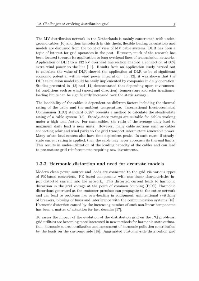
The MV distribution network in the Netherlands is mainly constructed with under-
ground cables [10] and thus henceforth in this thesis, flexible loading calculations and
models are discussed from the point of view of MV cable systems. DLR has been a
topic of interest for grid operators in the past. However, much of the research has
been focused towards its application to long overhead lines of transmission networks.
Application of DLR to a 132 kV overhead line section enabled a connection of 50%
extra wind power to the line [11]. Results from an application study carried out
to calculate the value of DLR showed the application of DLR to be of significant
economic potential within wind power integration. In [12], it was shown that the
DLR calculation model could be easily implemented by companies in daily operation.
Studies presented in [13] and [14] demonstrated that depending upon environmen-
tal conditions such as wind (speed and direction), temperature and solar irradiance,
loading limits can be significantly increased over the static ratings.
The loadability of the cables is dependent on different factors including the thermal
rating of the cable and the ambient temperature. International Electrotechnical
Commission (IEC) standard 60287 presents a method to calculate the steady-state
rating of a cable system [15]. Steady-state ratings are suitable for cables working
under a high load factor. For such cables, the ratio of the average daily load to
maximum daily load is near unity. However, many cable sections such as cables
connecting solar and wind parks to the grid transport intermittent renewable power.
Many urban load centers also have time-dependent peaks. In such cases, if steady-
state current rating is applied, then the cable may never approach its thermal limits.
This results in under-utilization of the loading capacity of the cables and can lead
to pre-mature grid reinforcements requiring new investments.
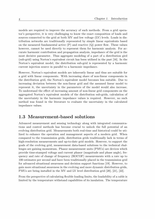
1.2.2 Harmonic distortion and need for accurate models
Modern clean power sources and loads are connected to the grid via various types
of PE-based converters. PE based components with non-linear characteristics in-
ject distorted current into the network. This distorted current leads to harmonic
distortion in the grid voltage at the point of common coupling (PCC). Harmonic
distortions generated at the customer premises can propagate to the entire network
and can lead to problems like over-heating in equipment, unintentional switching
of breakers, blowing of fuses and interference with the communication systems [16].
Harmonic distortion caused by the increasing number of such non-linear components
has been a matter of attention for last decades [17].
To assess the impact of the evolution of the distribution grid on the PQ problems,
grid utilities are becoming more interested in new methods for harmonic state estima-
tion, harmonic source localization and assessment of harmonic pollution contribution
by the loads on the customer side [18]. Aggregated customer-side distribution grid
Chapter 1. Introduction
models are required to improve the accuracy of such methods. From a grid opera-
tor’s perspective, it is very challenging to know the exact composition of loads and
sources connected to the grid at both MV and low voltage (LV) levels. Loads in dis-
tribution networks are traditionally represented by simple linear equivalents based
on the measured fundamental active (P) and reactive (Q) power flow. These values
however, cannot be used directly to represent them for harmonic analysis. For ac-
curate harmonic contribution and propagation analysis, impedance of the grid is the
most decisive parameter. Thus aggregate modeling of a part of a distribution gird
(sub-grid) using Norton’s equivalent circuit has been utilized in the past [16]. In the
Norton’s equivalent model, the distribution sub-grid is represented by a harmonic
current injection source in parallel to a harmonic impedance.
However, Norton’s equivalent models are inherently linear and thus are suitable for
a grid with linear components. With increasing share of non-linear components in
the distribution grid, the Norton’s equivalent model becomes less suitable. Due to
increasing deviation between the non-linear grid and the assumed linear model to
represent it, the uncertainty in the parameters of the model would also increase.
To understand the effect of increasing amount of non-linear grid components on the
aggregated Norton’s equivalent models of the distribution sub-grids, calculation of
the uncertainty in the harmonic impedance values is required. However, no such
method was found in the literature to evaluate the uncertainty in the calculated
impedance values.
1.3 Measurement-based solutions
Advanced measurement and sensing technology along with integrated communica-
tions and control methods has become crucial to unlock the full potential of an
evolving distribution grid. Measurements both real-time and historical could be uti-
lized to enhance the operation and management aspects of a modern grid. When
compared to the transmission grids, distribution grids traditionally lack in terms of
high-resolution measurements and up-to-date grid models. However, to support the
goals of the evolving grid, measurement data-based solutions to the technical chal-
lenges are gaining momentum. Phasor measurement units (PMUs) are devices which
provide time-stamped voltage and current phasor (magnitude and phase angle), fre-
quency and rate of change of frequency (ROCOF) measurements with a rate up to
100 estimates per second and have been traditionally placed in the transmission grid
for advanced situational awareness and decision support functions [19]. However, to
gain more situational awareness in the evolving and more dynamic distribution grids,
PMUs are being installed in the MV and LV level distribution grid [20], [21], [22].
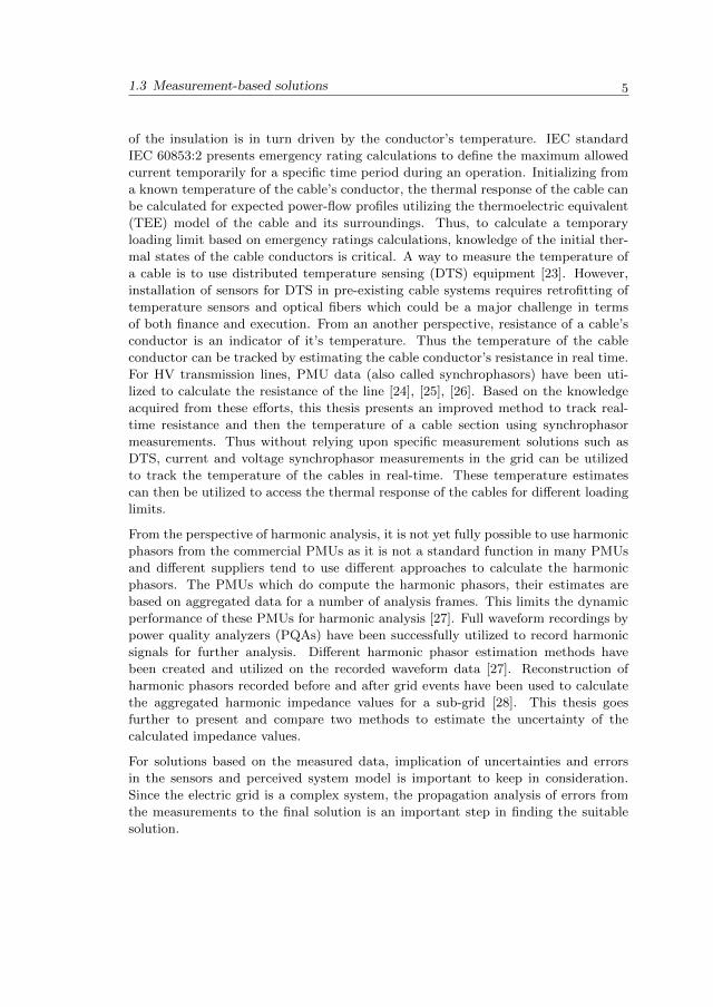
From the perspective of calculating flexible loading limits, the loadability of a cable is
limited by the temperature withstand capabilities of its insulation. The temperature
1.3 Measurement-based solutions
of the insulation is in turn driven by the conductor’s temperature. IEC standard
IEC 60853:2 presents emergency rating calculations to define the maximum allowed
current temporarily for a specific time period during an operation. Initializing from
a known temperature of the cable’s conductor, the thermal response of the cable can
be calculated for expected power-flow profiles utilizing the thermoelectric equivalent
(TEE) model of the cable and its surroundings. Thus, to calculate a temporary
loading limit based on emergency ratings calculations, knowledge of the initial ther-
mal states of the cable conductors is critical. A way to measure the temperature of
a cable is to use distributed temperature sensing (DTS) equipment [23]. However,
installation of sensors for DTS in pre-existing cable systems requires retrofitting of
temperature sensors and optical fibers which could be a major challenge in terms
of both finance and execution. From an another perspective, resistance of a cable’s
conductor is an indicator of it’s temperature. Thus the temperature of the cable
conductor can be tracked by estimating the cable conductor’s resistance in real time.
For HV transmission lines, PMU data (also called synchrophasors) have been uti-
lized to calculate the resistance of the line [24], [25], [26]. Based on the knowledge
acquired from these efforts, this thesis presents an improved method to track real-
time resistance and then the temperature of a cable section using synchrophasor
measurements. Thus without relying upon specific measurement solutions such as
DTS, current and voltage synchrophasor measurements in the grid can be utilized
to track the temperature of the cables in real-time. These temperature estimates
can then be utilized to access the thermal response of the cables for different loading
limits.
From the perspective of harmonic analysis, it is not yet fully possible to use harmonic
phasors from the commercial PMUs as it is not a standard function in many PMUs
and different suppliers tend to use different approaches to calculate the harmonic
phasors. The PMUs which do compute the harmonic phasors, their estimates are
based on aggregated data for a number of analysis frames. This limits the dynamic
performance of these PMUs for harmonic analysis [27]. Full waveform recordings by
power quality analyzers (PQAs) have been successfully utilized to record harmonic
signals for further analysis. Different harmonic phasor estimation methods have
been created and utilized on the recorded waveform data [27]. Reconstruction of
harmonic phasors recorded before and after grid events have been used to calculate
the aggregated harmonic impedance values for a sub-grid [28]. This thesis goes
further to present and compare two methods to estimate the uncertainty of the
calculated impedance values.
For solutions based on the measured data, implication of uncertainties and errors
in the sensors and perceived system model is important to keep in consideration.
Since the electric grid is a complex system, the propagation analysis of errors from
the measurements to the final solution is an important step in finding the suitable
solution.
Chapter 1. Introduction
1.4 Research objectives and questionsThermal assessment of cables participating in flexible power delivery schemes is es-
sential to ensure safe operation. On the other hand access to detailed and reliable
harmonic models of the grid is necessary to provide high-quality power to the cus-
tomers. This research is focused on providing solutions to these two technical chal-
lenges and proposes solutions utilizing phasor estimates from PMUs and other high
precision acquisition devices like PQAs.
The two main research objectives and the associated research questions investigated
in the thesis are:
1. To assess the flexible loading limits of cables, first devise a method to utilize
PMU data to track the temperature of a cable section in real-time. Subse-
quently, utilize the real-time temperature estimates to predict the dynamic
thermal response of the cable for a given loading profile using the TEE model
of the cable. This objective leads to the following research questions:
• How to accurately track the temperature of a 3-phase cable segment using
PMU data?
• How to estimate the effect of measurement uncertainties in the sensors on
the temperature estimates?
• How to utilize the real-time temperature estimates to predict the thermal
response of the cable for predicted loading scenarios?
2. Assess the impact of the non-linear components on the accuracy of the aggre-
gated harmonic impedance values of a linear distribution sub-grid model. To do
so, formulate a method to estimate the uncertainty in the calculated harmonic
impedance values. This objective leads to the following research questions:
• How to estimate the aggregated sub-grid harmonic impedance model?
• How to estimate the uncertainty in the harmonic impedance values of the
aggregated sub-grid model?
1.5 Research approach
1.5.1 Assessment of flexible loading limits
For flexible cable loading limits, the aim of the proposed solution is to predict and
assess the thermal response of the cables for a given power-flow profile. The thermal
response is calculated based on the TEE model of the cable system (including the
ground characteristics). Temperature of the cable conductors, insulation and other
components are the state of the TEE model. However to predict the response to a
1.6 Thesis outline
power-flow profile, states of the model need to be initialized by their current (real-
time) temperatures. Resistance of a conductor is an indicator of its temperature and
tracking the resistance of the conductor can lead to the temperature information
about the conductor and all the other components. The developed online cable
tracking tool forms the core of the presented method.
Thus firstly, an in-depth investigation of cable resistance estimation process is done.
Using the relationship between the resistivity of the conductor material and the tem-
perature, the required accuracy of the resistance estimation algorithm is calculated.
After that an improved least-square-based method is formulated to get accurate re-
sistance in the presence of bias errors in the measurement sensors. This model is
an extension of a model used for HV overhead lines, with improvements done to
reduce the uncertainty in the resistance estimates in caused by bias present in the
measurement sensors. The resistance estimates are then converted into temperature
estimates and uncertainty in the final temperature estimates is calculated. The per-
formance of the temperature estimation tool is then demonstrated using PMU data
from an MV Grid in the Netherlands. In the end, the dynamic thermal response of
an MV cable for a given loading scenario is calculated utilizing given temperature
estimates and the TEE model of the cable.
1.5.2 Sub-grid modelling
Calculation of harmonic phasors from recorded waveform data is a challenge due to
spectral leakage caused by a lack of synchronization between varying grid frequency
and constant sampling frequency. Reliable phasor estimation is realized by estimating
correct frequency using frequency interpolation technique while performing short-
term Fourier Transform (STFT). Then the Norton’s equivalent model of a sub-grid
is estimated using pre and post event data measured data. Utilizing the proposed
methods, the uncertainty in the estimated model is calculated and presented.
1.6 Thesis outline
The rest of the thesis is presented in the following chapters as:
Chapter 2: Phasor Measurements in a grid. This chapter presents an overview
of phasor measurement process in a power grid. First, an introduction about pha-
sors and a basic phasor estimation algorithm is presented. After that a method of
harmonic phasor estimation in case of varying gird frequency is presented.
Chapter 3: Measurement Chain and Error Propagation. This chapter
presents the complete measurement chain required for phasor estimation and dis-
cusses the impact of errors in the measurement chain on the phasor estimates. The
Chapter 1. Introduction
theory of measurement error propagation in final measured quantities is also pre-
sented.
Chapter 4: Online Cable Temperature Tracking. This chapter presents the
first part of the DLR, that is the tracking of cable conductor temperature in real-time.
First, it discusses the required accuracy in the resistance estimates to track the cable
temperature. Thereafter, it presents and compares cable temperature estimating
methods available in the literature. Next, a new PMU data-based method to estimate
cable resistance and subsequently the cable temperature is presented. In the end
application of the new method in tracking the temperature is demonstrated using
field experiment results.
Chapter 5: Cable Thermal Assessment for Flexible Loading. The second
part of the DLR is presented in this chapter. It presents the method to utilize the
real-time temperature estimates to predict the thermal response of the cables. To
simulate the thermal response of the cable a TEE model of the cable was built whose
state variables could be initialized using the real-time temperature estimates. In the
end, to show the validity of such thermal assessment scheme, the thermal response
of the TEE model of a cable was compared to the thermal response of the finite
element method (FEM) based model of the same cable.
Chapter 6: Aggregated harmonic impedance model of Sub-grids. This
chapter presents a harmonic phasor based-method to estimate the Norton’s equiv-
alent model of a part of distribution grid (a sub-grid). At first, it presents and
compares invasive and non-invasive measurement methods present in the literature
to estimate such models. Next, it presents two methods to estimate the uncertainty
in such models caused by the inherent non-linear character of the grid. Results from
simulation experiments are presented in the end.
Chapter 7: Discussion and Conclusions. This chapter concludes with the main
results and findings of this thesis. In the end several recommendations for the future
work are presented.
2Phasor Measurements in
the Distribution Grid
Distribution grids are in the process of evolution to facilitate a greener and smarter
energy supply. Evolving distribution grids have become more dynamic, complex and
vulnerable to breach stability and power quality requirements. This has created a
need for an improved monitoring capability for safe and efficient grid operation. Tra-
ditionally, distribution grid operators have relied on data from supervisory control
and data acquisition (SCADA) systems to monitor and operate the grid. However
SCADA systems sample the grid signals asynchronously and report only once every
few seconds. Such a reporting rate is insufficient to capture the dynamics of the
power systems states in case of events [22], [29]. On the other hand, HV transmis-
sion grids have utilized Phasor Measurement Units (PMUs) for their synchronized
high sampling rate and frequent phasor estimates. Synchronized sampling makes it
possible to compare the phasors measured at any given time instant across multiple
locations and frequent reporting rates are suitable for monitoring of dynamic states
of the distribution grid. PMUs are becoming available at MV and LV level distribu-
tion grids and numerous applications are being explored by the researchers and the
grid utilities [20], [22], [29]. Owing to advanced sensors and data acquisition devices,
it has also become possible to calculate high accuracy harmonic phasors for study-
ing power quality related problems. This chapter presents background information
on the concept of phasor measurement process and their role in aiding DLR and
sub-grid modelling applications.
Chapter 2. Phasor Measurements in the Distribution Grid
2.1 Phasor measurement process
2.1.1 Phasor
Transforming alternating sinusoidal electrical signals into phasor representations has
been used historically as an analysis tool. Phasor transformation allows a stationary
sinusoidal signal in time domain of form:
xa(t) = Acos(ωt+ φ) (2.1)
to be represented as [30]:
X =A√2ejφ (2.2)
where, xa(t) is the instantaneous value of function at time t, A is the magnitude,
φ is the phase angle and ω is the frequency of the signal in rad/s . The magnitude
of the phasor is given by the root-mean-square (RMS) value of the waveform ( A√2
).
The time dependency of the signal is removed due to its stationary nature. Using
the Euler’s identity, equation 2.2 can be written in rectangular form as:
X =A√2
(cos(φ) + jsin(φ)) (2.3)
= Are + jAim (2.4)
where, subscripts re and im denote the real and imaginary parts of the complex
value.
Fourier series and transforms are the basic tools used to analyze signals with multiple
harmonic content. Using Fourier series, a periodic signal consisting of the fundamen-
tal frequency component and its harmonic multiples (h) up to order H can be written
as:
xa(t) =
H∑h=0
ahcos(hω1t) + bhsin(hω1t) (2.5)
=
H∑h=0
Ahcos(hω1t+ φh) (2.6)
where, Ah =√a2h + b2hand φh = arctan(−bhah ), ω1 is the fundamental frequency, Ah
and φh are the respective magnitude and phase of the harmonic order h. Harmonic
order h=0 corresponds to the DC component. Phasors at harmonic frequencies h
are then given by:
2.1 Phasor measurement process
Xh =Ah√
2ejφh (2.7)
Extraction of phasor magnitude and phase components is done often using the Fourier
transform (FT). FTs transform both periodic and non-periodic signals from time
domain to frequency domain using the analysis equation:
X(ω) =
∫ ∞−∞
x(t)e−jωtdt (2.8)
For finite length discretely sampled xa(t), such that
x[n] = xa(nTs) (2.9)
where, n is the sample number and Ts is the sampling time interval, discrete Fourier
transform (DFT) is applied. The fact that ‘n’ is always an integer leads to some
important differences between the properties of discrete-time and continuous-time
sinusoidal sequences. An importance difference is seen when we consider a frequency
ω1 + 2πh. As shown in equation 2.10, signals with frequencies ω1 + 2πh are indistin-
guishable from each other when h is an integer.
x[n] = Aej(ω1+2π)h = Aejω1hej2π = Aejω1h (2.10)
Another important difference is in the periodicity. In continuous signals the period
is calculated by 2πωh
. However in discrete signals the period is defined by N samples
such that x[n] = x[n+N ]. The frequency resolution (ωr) of the discrete sampling is
given by:
ωr = ω1 =2π
N(2.11)
For N equally spaced samples of a signal, it’s DFT can be written as:
X[k] =
N−1∑n=0
x[n]e−jkω1n for k = 0 to N − 1, (2.12)
where k is the frequency bin. According to the Nyquist sampling theorem, to avoid
spectrum overlap (also known as aliasing), the signal sampling frequency must be at
least double the highest frequency component in the signal [31]. In case of Spectrum
overlapping, the original signal cannot be recovered using a low-pass filter. Since the
harmonic content is not known in advance, to avoid spectrum overlapping, before
the sampling process, the analog signal is first filtered using a low-pass filter [31].
Chapter 2. Phasor Measurements in the Distribution Grid
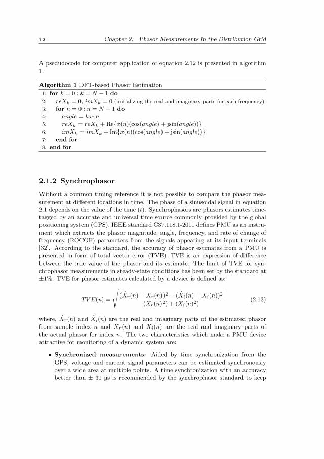
A psedudocode for computer application of equation 2.12 is presented in algorithm
1.
Algorithm 1 DFT-based Phasor Estimation
1: for k = 0 : k = N − 1 do
2: reXk = 0, imXk = 0 (initializing the real and imaginary parts for each frequency)
3: for n = 0 : n = N − 1 do
4: angle = kω1n
5: reXk = reXk + Rex(n)(cos(angle) + jsin(angle))6: imXk = imXk + Imx(n)(cos(angle) + jsin(angle))7: end for
8: end for
2.1.2 Synchrophasor
Without a common timing reference it is not possible to compare the phasor mea-
surement at different locations in time. The phase of a sinusoidal signal in equation
2.1 depends on the value of the time (t). Synchrophasors are phasors estimates time-
tagged by an accurate and universal time source commonly provided by the global
positioning system (GPS). IEEE standard C37.118.1-2011 defines PMU as an instru-
ment which extracts the phasor magnitude, angle, frequency, and rate of change of
frequency (ROCOF) parameters from the signals appearing at its input terminals
[32]. According to the standard, the accuracy of phasor estimates from a PMU is
presented in form of total vector error (TVE). TVE is an expression of difference
between the true value of the phasor and its estimate. The limit of TVE for syn-
chrophasor measurements in steady-state conditions has been set by the standard at
±1%. TVE for phasor estimates calculated by a device is defined as:
TV E(n) =
√(Xr(n)−Xr(n))2 + (Xi(n)−Xi(n))2
(Xr(n)2) + (Xi(n)2)(2.13)
where, Xr(n) and Xi(n) are the real and imaginary parts of the estimated phasor
from sample index n and Xr(n) and Xi(n) are the real and imaginary parts of
the actual phasor for index n. The two characteristics which make a PMU device
attractive for monitoring of a dynamic system are:
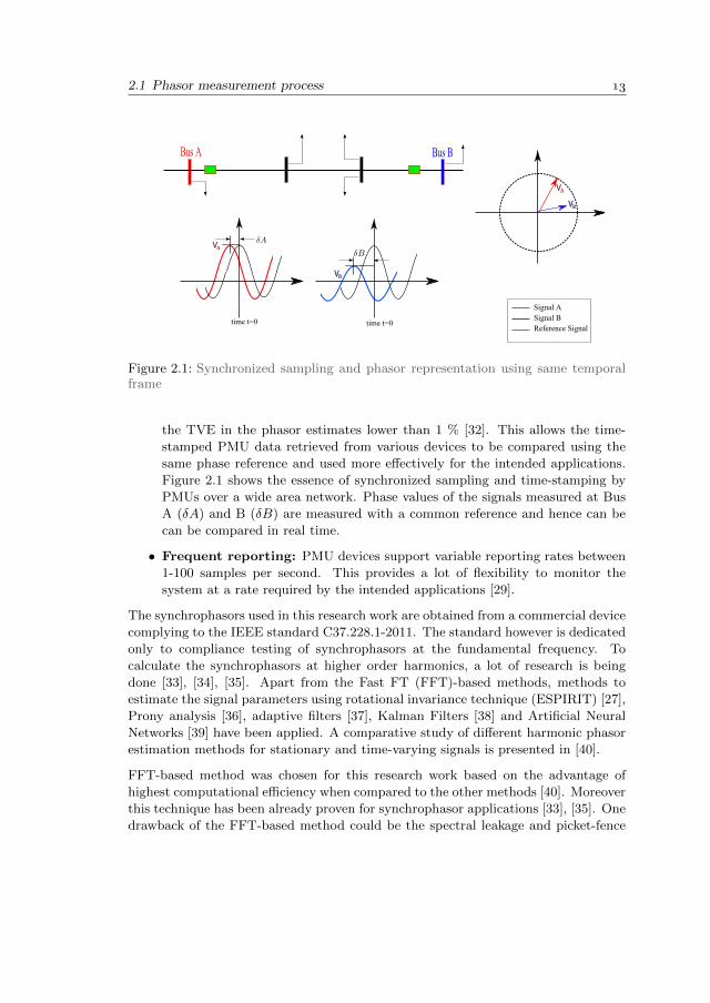
• Synchronized measurements: Aided by time synchronization from the
GPS, voltage and current signal parameters can be estimated synchronously
over a wide area at multiple points. A time synchronization with an accuracy
better than ± 31 µs is recommended by the synchrophasor standard to keep
2.1 Phasor measurement process
Bus A Bus B
VA
VB
time t=0 time t=0
Signal ASignal BReference Signal
VA
VB
Figure 2.1: Synchronized sampling and phasor representation using same temporalframe
the TVE in the phasor estimates lower than 1 % [32]. This allows the time-
stamped PMU data retrieved from various devices to be compared using the
same phase reference and used more effectively for the intended applications.
Figure 2.1 shows the essence of synchronized sampling and time-stamping by
PMUs over a wide area network. Phase values of the signals measured at Bus
A (δA) and B (δB) are measured with a common reference and hence can be
can be compared in real time.
• Frequent reporting: PMU devices support variable reporting rates between
1-100 samples per second. This provides a lot of flexibility to monitor the
system at a rate required by the intended applications [29].
The synchrophasors used in this research work are obtained from a commercial device
complying to the IEEE standard C37.228.1-2011. The standard however is dedicated
only to compliance testing of synchrophasors at the fundamental frequency. To
calculate the synchrophasors at higher order harmonics, a lot of research is being
done [33], [34], [35]. Apart from the Fast FT (FFT)-based methods, methods to
estimate the signal parameters using rotational invariance technique (ESPIRIT) [27],
Prony analysis [36], adaptive filters [37], Kalman Filters [38] and Artificial Neural
Networks [39] have been applied. A comparative study of different harmonic phasor
estimation methods for stationary and time-varying signals is presented in [40].
FFT-based method was chosen for this research work based on the advantage of
highest computational efficiency when compared to the other methods [40]. Moreover
this technique has been already proven for synchrophasor applications [33], [35]. One
drawback of the FFT-based method could be the spectral leakage and picket-fence
Chapter 2. Phasor Measurements in the Distribution Grid
effects when the frequency of the signal varies with time and the available frequency
resolution is insufficient. Varying grid frequency makes the signal sampling process
asynchronous and this leads to spectral leakage. Spectral leakage causes errors in
the magnitude and phase of the estimated harmonic phasors. To reduce the spec-
tral leakage, synchronization is achieved using two different categories of methods:
resampling and interpolation. For resampling, the frequency of the fundamental
component of the power grid signal is estimated first and then the sampling rate
of the analog to digital converter (ADC) is adjusted. The fundamental frequency
is estimated by tracking zero-crossings [41], Phase-locked loops (PLL)-based tech-
niques [42], [43] and nonlinear Newton-type algorithm [44]. Interpolation technique
is used to estimate the fundamental frequency by comparing the components of the
adjacent frequency bins and interpolate to estimate the frequency [45]. Interpolated
DFT (IDFT) technique has been utilized successfully to reduce the effects of spectral
leakage while estimating harmonic phasors in non-synchronous sampling conditions
[35], [46], [47], [48]. IDFT method presented in [31] was used in this thesis to esti-
mate the correct power-grid frequency and then calculate the corrected magnitude
and phase of the harmonic phasors.
The interpolated DFT 1 method employed in this thesis is a batch processing method
where a block of data is analysed to estimate the phasor parameters. The analysis is
performed under the assumption that the signal is stationary for the duration of the
block. This method is able to capture the time-varying nature of the signal’s spectral
properties. This kind of batch processing technique on a block of data collected
at progressing time-instances is called short-time Fourier transform (STFT). For
discrete-time STFT, the signal x[n] is multiplied by a window w[n] to get a block of
data and DFT is computed for the resulting windowed signal given as:
xw[n] = x[n]w[n]. (2.14)
Windowing techniques using Hann, Hamming, Blackman and Gaussian windows are
also used to reduce the spectral leakage [31]. A Hann window has been utilized in
this thesis for this purpose. If m is the center of the window, then time-frequency
representation of the measured signal using STFT is written as [31]:
XSTFT(ejω,m) =
∞∑n=−∞
x[n]w[n−m]e−jωn. (2.15)
1The Interpolated DFT method and its application on field data in based on results pre-sented in S. Babaev, R. S. Singh, J. F. G. Cobben, et al., “Multi-Point Time-SynchronizedWaveform Recording for the Analysis of Wide-Area Harmonic Propagation”, AppliedSciences, vol. 10, no. 11, 2020, issn: 2076-3417. doi: 10.3390/app10113869. [Online].Available: https://www.mdpi.com/2076-3417/10/11/3869.
2.2 Interpolated DFT for harmonic phasors
The window is then shifted by a fixed amount in time depending on the desired over-
lap length. Along with the frequency resolution, the quality of the spectral analysis
of time-varying signals is defined by the temporal-resolution. Selecting the length
of the data block requires a trade-off between the temporal resolution and the fre-
quency resolution. IEC standard 61000-4-7 suggests a 10 cycle (200 ms) long analysis
window to obtain a 5 Hz FFT fundamental frequency [50]. However depending upon
the requirements, data-blocks of 5 cycle lengths have also been utilized to estimate
harmonic phasors of time-varying signals [35].
2.2 Interpolated DFT for harmonic phasors
Using batch processing technique, STFT can be implemented as calculating DFT
of overlapping blocks of windowed signals. A multi-tone windowed signal consist-
ing several harmonics (ωh) of the fundamental frequency (ω1) and sampled with a
frequency Fs can be represented as:
xw[n] =
(∑h
Ahcos(ωhn
Fs+ φh)
)w[n], (2.16)
The discrete-time FT (DTFT) of the windowed signal xw[n] is obtained by the
convolution of their FTs [31] and is given as:
Xw(ejω) = X(ejω) ∗W (ejω)
=∑h
(X(ejωh)W (ej(ω+ωh)) +X(ejωh)W (ej(ω−ωh))
).
(2.17)
where, X(ejω) and W (ejω) are the FTs of x[n] and w[n] respectively. Since DFT is
the sampled version of DTFT and is obtained at discrete frequencies, the result for
frequency ωk can be written as:
Xw(ejω)|ωk =∑h
(X(ejωh)W (ej(ω+ωh)) +X(ejωh)W (ej(ω−ωh))
)∣∣∣∣ω=ωk
Xw[k] =∑h
(Ah2
ejφhW (ej(ωk+ωh)) +Ah2
ejφhW (ej(ωk−ωh))
),
(2.18)
where, the frequency of the bins for N number of samples are
ωk = 2πk/N for k = 0, 1, 2, ..., N − 1. (2.19)
Chapter 2. Phasor Measurements in the Distribution Grid
The positive half of the spectrum can be written as:
X+w [k] =
∑h
(Ah2
ejφhW (ej(ωk−ωh))
), k ≤ N
2− 1. (2.20)
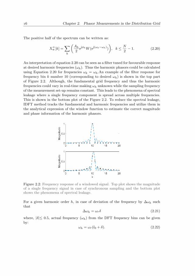
An interpretation of equation 2.20 can be seen as a filter tuned for favourable response
at desired harmonic frequencies (ωh). Thus the harmonic phasors could be calculated
using Equation 2.20 for frequencies ωk = ωh.An example of the filter response for
frequency bin k number 10 (corresponding to desired ωh) is shown in the top part
of Figure 2.2. Although, the fundamental grid frequency and thus the harmonic
frequencies could vary in real-time making ωh unknown while the sampling frequency
of the measurement set-up remains constant. This leads to the phenomena of spectral
leakage where a single frequency component is spread across multiple frequencies.
This is shown in the bottom plot of the Figure 2.2. To reduce the spectral leakage,
IDFT method tracks the fundamental and harmonic frequencies and utilize them in
the analytical expression of the window function to estimate the correct magnitude
and phase information of the harmonic phasors.
Figure 2.2: Frequency response of a windowed signal. Top plot shows the magnitudeof a single frequency signal in case of synchronous sampling and the bottom plotshows the phenomena of spectral leakage.
For a given harmonic order h, in case of deviation of the frequency by ∆ωh such
that
∆ωh = ωrδ (2.21)
where, |δ|≤ 0.5, actual frequency (ωh) from the DFT frequency bins can be given
by:
ωh = ωr(l0 + δ). (2.22)

2.2 Interpolated DFT for harmonic phasors
where, l0 is the index of the frequency bin with highest magnitude and ωk = l0ωr.
The deviation in the frequency is determined using the ratio between the two highest
DFT components given by:
α =|X+
w [l0 + ε]||X+
w [l0]|(2.23)
where, ε could be either 1 or -1 depending on the position of the second highest DFT
bin compared with respect to l0. It can be shown that for k = l0 + ε,
ωk − ωh = (1− δ)ωr. (2.24)
Similarly, for k = l0,
ωk − ωh = −δωr. (2.25)
Utilizing equations 2.20, 2.24 and 2.25, equation 2.23 can be written as:
α =|W (ej(ε−δ)ωr )||W (e−jδωr )|
. (2.26)
where the frequency response of the window function is dependent on the type of
window used.
The frequency response of a rectangular window of length N samples is given by:
Wrec(ejω) = e−jω(N−1)/2 sin(ωN/2)
sin(ω/2). (2.27)
A δ-α look-up table was created using equation 2.26 for uniformly spread out values
of δ. A Hann window was used in the process whose frequency frequency response
is given by:
Whann(ejω) = 0.5Wrec(ejω)− 0.25Wrec(ej(ω−ω1))− 0.25Wrec(ej(ω+ω1)), (2.28)
where ω is (ε− δ)ωr and ω1 is ωr.
In the look-up table, the values of calculated α was paired with the closest value of δ
to determine the deviation in the frequency. The actual frequency (ωh) is calculated
as:
ωh = ωk ± δωr. (2.29)
From equation 2.20 the ratio of magnitudes for one half of the spectrum can be
written as:|Xωh ||Xωk |
=|W (ejωh)||W (ejωk )|
. (2.30)
Chapter 2. Phasor Measurements in the Distribution Grid
Using the relationship between ωh and ωk from Equation 2.29, the corrected phasor
magnitude at harmonic frequency ωh is calculated using equation 2.30 as:
|Xωh |= |Xωk ||W (e0)||W (ejδωr )|
. (2.31)
Similarly the phase information at harmonic frequency ωh is calculated using the
phase relationship between the two frequencies given by:
argXωh = argXωk )± argW (ejδωr ), (2.32)
where,
argW (ejδωr ) = arge−jδπ(N−1)/N,= δπ(N − 1)/N.
(2.33)
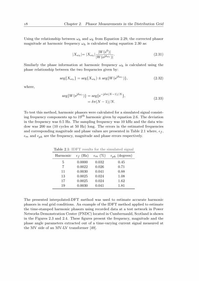
To test this method, harmonic phasors were calculated for a simulated signal consist-
ing frequency components up to 19th harmonic given by equation 2.6. The deviation
in the frequency was 0.5 Hz. The sampling frequency was 10 kHz and the data win-
dow was 200 ms (10 cycles at 50 Hz) long. The errors in the estimated frequencies
and corresponding magnitude and phase values are presented in Table 2.1 where, εf ,
εm and εph are the frequency, magnitude and phase errors respectively.
Table 2.1: IDFT results for the simulated signal
Harmonic εf (Hz) εm (%) εph (degrees)
5 0.0000 0.032 0.45
7 0.0022 0.026 0.71
11 0.0030 0.041 0.88
13 0.0025 0.024 1.08
17 0.0025 0.024 1.62
19 0.0030 0.041 1.81
The presented interpolated-DFT method was used to estimate accurate harmonic
phasors in real grid conditions. An example of the IDFT method applied to estimate
the time-stamped harmonic phasors using recorded data at a test network in Power
Networks Demonstration Center (PNDC) located in Cumbernauld, Scotland is shown
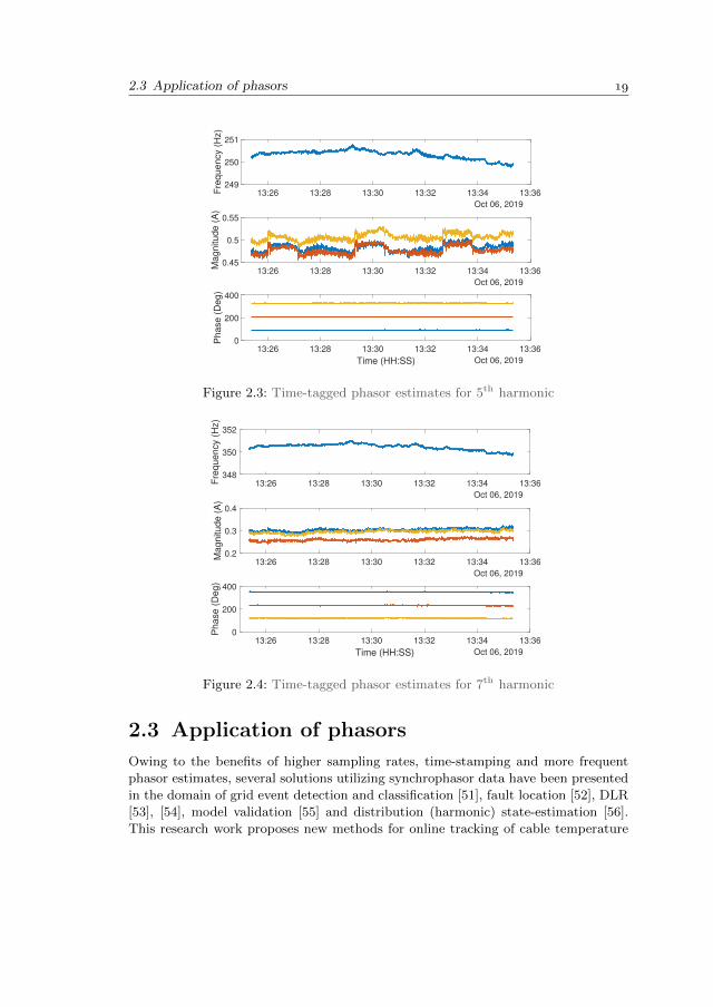
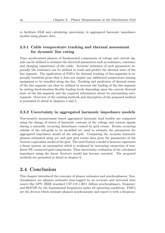
in the Figures 2.3 and 2.4. These figures present the frequency, magnitude and the
phase angle parameters extracted out of a time-varying current signal measured at
the MV side of an MV-LV transformer [49].
2.3 Application of phasors
13:26 13:28 13:30 13:32 13:34 13:36
Oct 06, 2019
249
250
251
Fre
quency (
Hz)
13:26 13:28 13:30 13:32 13:34 13:36
Oct 06, 2019
0.45
0.5
0.55M
agnitude (
A)
13:26 13:28 13:30 13:32 13:34 13:36
Time (HH:SS) Oct 06, 2019
0
200
400
Phase (
Deg)
Figure 2.3: Time-tagged phasor estimates for 5th harmonic
13:26 13:28 13:30 13:32 13:34 13:36
Oct 06, 2019
348
350
352
Fre
qu
en
cy (
Hz)
13:26 13:28 13:30 13:32 13:34 13:36
Oct 06, 2019
0.2
0.3
0.4
Ma
gn
itu
de
(A
)
13:26 13:28 13:30 13:32 13:34 13:36
Time (HH:SS) Oct 06, 2019
0
200
400
Ph
ase
(D
eg
)
Figure 2.4: Time-tagged phasor estimates for 7th harmonic
2.3 Application of phasors
Owing to the benefits of higher sampling rates, time-stamping and more frequent
phasor estimates, several solutions utilizing synchrophasor data have been presented
in the domain of grid event detection and classification [51], fault location [52], DLR
[53], [54], model validation [55] and distribution (harmonic) state-estimation [56].
This research work proposes new methods for online tracking of cable temperature
Chapter 2. Phasor Measurements in the Distribution Grid
to facilitate DLR and calculating uncertainty in aggregated harmonic impedance
models using phasor data.
2.3.1 Cable temperature tracking and thermal assessmentfor dynamic line rating
Time synchronized phasors of fundamental components of voltage and current sig-
nals can be utilized to estimate the electrical parameters such as resistance, reactance
and charging capacitance of the cable. Accurate estimates of such parameters es-
pecially the resistance can be utilized to track and predict the thermal state of the
line segment. The application of PMUs for thermal tracking of line-segments is es-
pecially beneficial given that it does not require any additional temperature sensing
equipment to be installed along the line. Tracking and prediction of thermal states
of the line segment can then be utilized to increase the loading of the line segment
by setting fixed-duration flexible loading levels depending upon the current thermal
state of the line-segment and the required information about its surrounding envi-
ronment. Overview of the existing methods and description of the proposed method
is presented in detail in chapters 4 and 5.
2.3.2 Uncertainty in aggregated harmonic impedance models
Non-invasive measurement based aggregated harmonic load models are computed
using the change of states of harmonic contents of the voltage and current signals
during a naturally occurring disturbance caused by grid events. Events occurring
outside of the sub-grids to be modelled are used to estimate the parameters for
aggregated impedance model of the sub-grid. Comparing the accurate harmonic
phasors estimated using pre and post grid events data gives the parameters of the
Norton’s equivalent model of the grid. The used Norton’s model is however represents
a linear system; an assumption which is weakened by increasing connection of non-
linear PE connected grid components. Thus uncertainty evaluation of the calculated
impedance using the linear Norton’s model has become essential. The proposed
methods are presented in detail in chapter 6.
2.4 Conclusion
This chapter introduced the concepts of phasor estimates and synchrophasors. Syn-
chrophasors are phasors estimates time-tagged by an accurate and universal time
source like GPS. IEEE standard C37.118.1-2011 defines synchrophasors, frequency
and ROCOF for the fundamental frequencies under all operating conditions. PMUs
are the devices which estimate phasors synchronously and report it with a frequency

2.4 Conclusion
range of 1-100 phasor estimates per second. Time-tagged estimates and frequent
reporting make PMU devices attractive for monitoring of a dynamic system. To
calculate synchrophasors at higher order harmonics, new methods are being devel-
oped. This thesis uses the FFT-based IDFT technique to estimate the harmonic
phasors due to its advantage of high computational efficiency and already proven
track-record for harmonic synchrophasor applications. Chapters 4, 5 and 6 present
the application of phasor measurements in DLR and harmonic modelling process.

3Measurement Chain and
Error Propagation
No measurement ever made is exact. Imperfection in measurements give rise to errors
which are composed of two components: random noise and systematic bias. The goal
of a measurement is to estimate the values of the parameters of the mathematical
model of the measurand (the quantity being measured). However, the measurand
may be altered by an error changing it’s inherent mathematical model [57]. Such
an error can also be termed as systematic bias. Random noise components cause
repeated measurements of the same measurand to give different results. Phasor
estimates can have errors in both magnitude and phase values. Phase and magni-
tude errors in estimated phasors are caused by errors in the instrumentation chain
feeding the phasor estimation device and phasor estimation process of the device
itself. These errors propagate into the various application processes which use the
estimated phasors and worsen their performance. This chapter presents the mea-
surement chain required for phasor estimation. The theory of measurement errors
and their propagation in calculated quantities is also presented.

Chapter 3. Measurement Chain and Error Propagation
3.1 Errors in phasor measurement chain
According to the guide to the expression of uncertainty in measurements (GUM), any
error in measurement is composed of two components: a random and a systematic
component [58]. Random errors are caused by stochastic variations in the influencing
factors and have an expected value of zero. On the other hand bias errors are caused
by lack of calibration or non-linearity and has a non-zero expected value. In reality,
the true value of the measurand is never known and an index of uncertainty is used
to reflect this lack of knowledge of true value and give an estimate of the error in
the measurement. Uncertainty of a measurement is specified in terms of a range
or spread between the highest and lowest possible values. Uncertainty is usually
quantified by standard deviation (SD), where a lower SD signifies a lower spread in
expected values. Although error and uncertainty have been utilized in this thesis
interchangeably, it is important to realize that they are not synonyms and represent
different concepts. Uncertainty for a measurement can be quantified whereas the
error in the measurement can only be quantified if the true value of the measurand
is known.
The errors in the phasors given by PMUs and other devices are a result of the esti-
mation device itself and the instrumentation channel feeding signals to them. Instru-
mentation channel is a group of devices that feed scaled replicas of high-magnitude
voltage or current signals to the phasor measurement devices. The most important
components in the instrumentation channel are the instrument transformers: current
and voltage transformers (CTs and VTs). Control cables connecting the instrument
transformers to one or multiple burdens (end devices such as relays, PMUs etc.) form
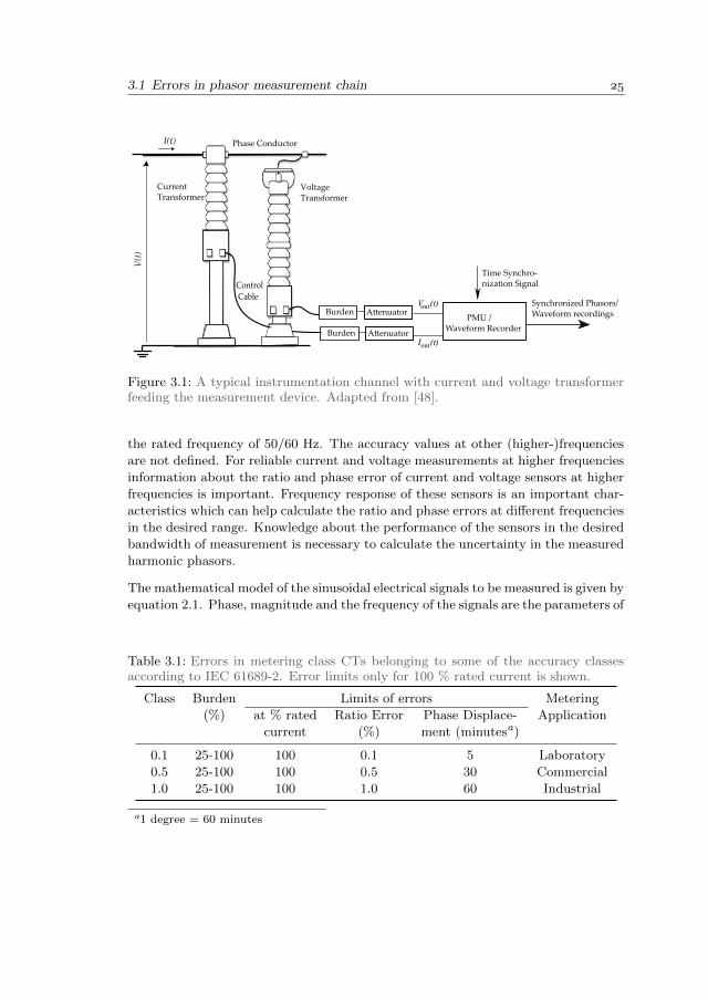
the other part of the instrumentation channel. A typical instrumentation channel
feeding current and voltage signals is shown in Figure 3.1.
Instrument transformers act as sensors and transform high current and voltage sig-
nals from the grid to lower levels for feeding devices like relays, fault-recorders and
PMUs. The transformation happens according to the same principle as by power
transformers. As a result of the transformation process, phase and magnitude of the
sinusoidal signals are prone to errors in their magnitude and phase values.
Instrument transformers are classified into two classes: metering (M) class and pro-
tection (P) class. For metering applications, accuracy of the output is the key.
According to IEC 61689-2, metering CTs and VTs operate in the range of 5-120 %
of their rated values with different accuracy classes. Limits of magnitude and phase
displacement errors for each accuracy class can be found in the standard document.
Protection CTs and VTs feed the protective relays and speed is the desired quality
over accuracy. Examples of error limits in some of the metering class CTs according
to IEC 61689-2 and for metering class VTs according to IEC 61689-3 is presented in
Tables 3.1 and 3.2. It is to be noted that these accuracy values are defined only for
3.1 Errors in phasor measurement chain
Control Cable
Burden Aenuator
PMU /Waveform Recorder
Time Synchro-nization Signal
V(t)
I(t)
I (t)out
V (t)out Synchronized Phasors/Waveform recordings Burden Aenuator
Voltage Transformer
Current Transformer
Phase Conductor
Figure 3.1: A typical instrumentation channel with current and voltage transformerfeeding the measurement device. Adapted from [48].
the rated frequency of 50/60 Hz. The accuracy values at other (higher-)frequencies
are not defined. For reliable current and voltage measurements at higher frequencies
information about the ratio and phase error of current and voltage sensors at higher
frequencies is important. Frequency response of these sensors is an important char-
acteristics which can help calculate the ratio and phase errors at different frequencies
in the desired range. Knowledge about the performance of the sensors in the desired
bandwidth of measurement is necessary to calculate the uncertainty in the measured
harmonic phasors.
The mathematical model of the sinusoidal electrical signals to be measured is given by
equation 2.1. Phase, magnitude and the frequency of the signals are the parameters of
Table 3.1: Errors in metering class CTs belonging to some of the accuracy classesaccording to IEC 61689-2. Error limits only for 100 % rated current is shown.
Class Burden Limits of errors Metering
(%) at % rated Ratio Error Phase Displace- Application
current (%) ment (minutesa)
0.1 25-100 100 0.1 5 Laboratory
0.5 25-100 100 0.5 30 Commercial
1.0 25-100 100 1.0 60 Industrial
a1 degree = 60 minutes
Chapter 3. Measurement Chain and Error Propagation
Table 3.2: Errors in metering class VTs belonging to some of the accuracy classesaccording to IEC 61689-3.
Class Burden Limits of errors Metering
(%) at % rated Ratio Error Phase Displace- Application
voltage (%) ment (minutes)
0.1 25-100 80-120 0.1 5 Laboratory
0.5 25-100 80-120 0.5 20 Commercial
1.0 25-100 80-120 1.0 40 Industrial
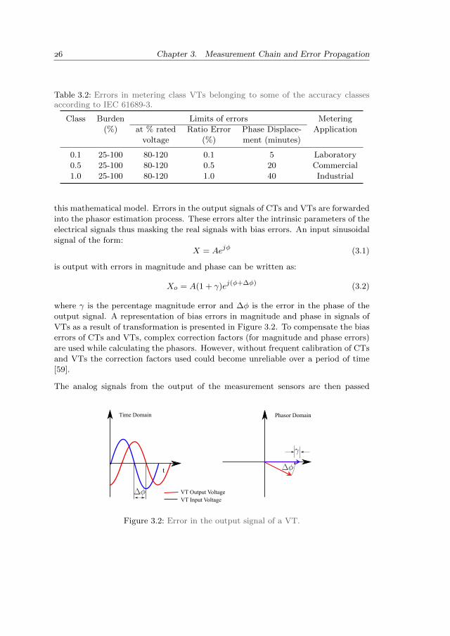
this mathematical model. Errors in the output signals of CTs and VTs are forwarded
into the phasor estimation process. These errors alter the intrinsic parameters of the
electrical signals thus masking the real signals with bias errors. An input sinusoidal
signal of the form:
X = Aejφ (3.1)
is output with errors in magnitude and phase can be written as:
Xo = A(1 + γ)ej(φ+∆φ) (3.2)
where γ is the percentage magnitude error and ∆φ is the error in the phase of the
output signal. A representation of bias errors in magnitude and phase in signals of
VTs as a result of transformation is presented in Figure 3.2. To compensate the bias
errors of CTs and VTs, complex correction factors (for magnitude and phase errors)
are used while calculating the phasors. However, without frequent calibration of CTs
and VTs the correction factors used could become unreliable over a period of time
[59].
The analog signals from the output of the measurement sensors are then passed
t
VT Output VoltageVT Input Voltage
Time Domain Phasor Domain
Figure 3.2: Error in the output signal of a VT.
3.1 Errors in phasor measurement chain
though a low pass (anti-aliasing) filter and acquired by the phasor estimation de-
vices using an analog to digital converter (ADC). The ADC samples the signals with
a uniform sampling rate with the help of a time source. The sampling rate is de-
pendent on the application and the range of frequency spectrum. According to the
Nyquist’s sampling theorem, the sampling rate should be greater than twice of the
bandwidth of the sampled signal [60]. Ideally, without any bias in the signals fed
to the phasor estimation devices, the error in the phasor estimates in presence of
white noise would be zero [61]. However, due to uncertainties from sources such
as ADC and time synchronisation, the phasor estimates have a certain associated
uncertainty. Such errors are treated in this thesis as random errors in the phasor es-
timates. Incorporating both random and systematic bias errors in the measurement,
a composite model with both kind of uncertainties can be presented for the signal of
equation 3.1 in the form:
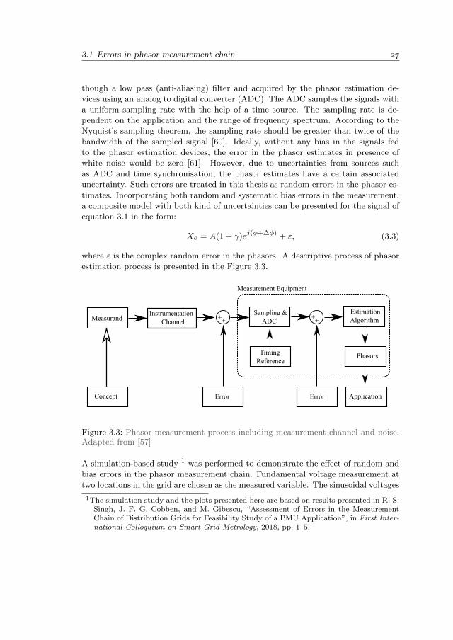
Xo = A(1 + γ)ej(φ+∆φ) + ε, (3.3)
where ε is the complex random error in the phasors. A descriptive process of phasor
estimation process is presented in the Figure 3.3.
Concept
Measurand
Error
Instrumentation Channel
Sampling & ADC
Estimation Algorithm
Phasors
Application
TimingReference
Error
Measurement Equipment
++ ++
Figure 3.3: Phasor measurement process including measurement channel and noise.Adapted from [57]
A simulation-based study 1 was performed to demonstrate the effect of random and
bias errors in the phasor measurement chain. Fundamental voltage measurement at
two locations in the grid are chosen as the measured variable. The sinusoidal voltages
1The simulation study and the plots presented here are based on results presented in R. S.Singh, J. F. G. Cobben, and M. Gibescu, “Assessment of Errors in the MeasurementChain of Distribution Grids for Feasibility Study of a PMU Application”, in First Inter-national Colloquium on Smart Grid Metrology, 2018, pp. 1–5.
Chapter 3. Measurement Chain and Error Propagation
-5 0 5
real axis (p.u.) 10-3
-6
-4
-2
0
2
4
6
ima
gin
ary
axis
(p
.u.)
10-3
V
Vm
-5 0 5
real axis (p.u.) 10-3
-8
-6
-4
-2
0
2
4
6
10-3
V
Vm
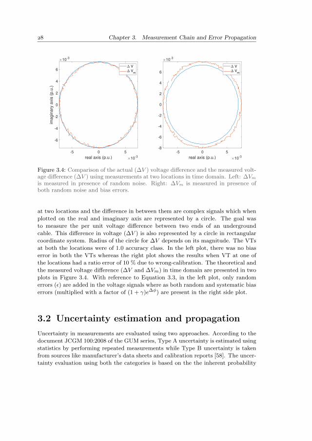
Figure 3.4: Comparison of the actual (∆V ) voltage difference and the measured volt-age difference (∆V ) using measurements at two locations in time domain. Left: ∆Vm
is measured in presence of random noise. Right: ∆Vm is measured in presence ofboth random noise and bias errors.
at two locations and the difference in between them are complex signals which when
plotted on the real and imaginary axis are represented by a circle. The goal was
to measure the per unit voltage difference between two ends of an underground
cable. This difference in voltage (∆V ) is also represented by a circle in rectangular
coordinate system. Radius of the circle for ∆V depends on its magnitude. The VTs
at both the locations were of 1.0 accuracy class. In the left plot, there was no bias
error in both the VTs whereas the right plot shows the results when VT at one of
the locations had a ratio error of 10 % due to wrong-calibration. The theoretical and
the measured voltage difference (∆V and ∆Vm) in time domain are presented in two
plots in Figure 3.4. With reference to Equation 3.3, in the left plot, only random
errors (ε) are added in the voltage signals where as both random and systematic bias
errors (multiplied with a factor of (1 + γ)e∆φ) are present in the right side plot.
3.2 Uncertainty estimation and propagation
Uncertainty in measurements are evaluated using two approaches. According to the
document JCGM 100:2008 of the GUM series, Type A uncertainty is estimated using
statistics by performing repeated measurements while Type B uncertainty is taken
from sources like manufacturer’s data sheets and calibration reports [58]. The uncer-
tainty evaluation using both the categories is based on the the inherent probability
3.2 Uncertainty estimation and propagation
distribution of the variables and is quantified by SD (σ) and variance (σ2). Proba-
bility distribution for a random variable is a function giving the probability that the
variable takes a certain values and is calculated based on observed data for Type A
estimation while it is assumed for the Type B uncertainty. Further to provide an
interval about the result, an expanded uncertainty (U) is obtained by multiplying a
coverage factor to the calculated uncertainty [58].
3.2.1 Uncertainty evaluation
For Type A uncertainty calculations, for a random variable with n independent
observations of variable xi, the variance (u2(xi)) and standard uncertainty (u(xi))
of the distribution are given by:
u2(xi) =1
n− 1
n∑i=1
(xi − x)2 (3.4)
and
u(xi) =√u2(xi) (3.5)
where, x is the mean of the n observations.
For Type B uncertainty, the variance and standard uncertainty is estimated based
on the available data. If the quoted uncertainty (uq(xi)) is given along the coverage
factor, then the standard uncertainty is calculated by dividing the coverage factor
from the given uncertainty. Thus:
u(xi) =uq(xi)
kf, (3.6)
where kf the coverage factor. In several cases, uncertainty u(xi) is not mentioned
as a multiple of SD and is defined using an interval having 90, 95 or 99 percent level
of confidence. Unless stated otherwise, it is assumed that the quoted uncertainty
region was calculated using a normal distribution. The probability density function
(PDF) for a normal distribution is given by
p = f(xi|µ, σ) =1
σ√
2πe−
12 ( x−µσ )2 (3.7)
where µ is the mean of the distribution. In that case, the standard uncertainty is
calculated by dividing the quoted uncertainty by selecting an appropriate factor for
the normal distribution. Coverage factors corresponding to the stated percentage
level of confidence are 1.62, 1.96 and 2.58 respectively [58]. In cases where only
upper and lower bounds of the uncertainty region are mentioned, then it is assumed
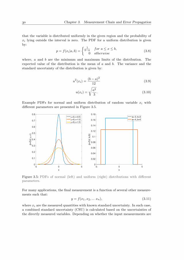
Chapter 3. Measurement Chain and Error Propagation
that the variable is distributed uniformly in the given region and the probability of
xi lying outside the interval is zero. The PDF for a uniform distribution is given
by:
p = f(xi|a, b) =
1b−a for a ≤ x ≤ b,
0 otherwise(3.8)
where, a and b are the minimum and maximum limits of the distribution. The
expected value of the distribution is the mean of a and b. The variance and the
standard uncertainty of the distribution is given by:
u2(xi) =(b− a)2
12(3.9)
u(xi) =
√a2
3. (3.10)
Example PDFs for normal and uniform distribution of random variable xi with
different parameters are presented in Figure 3.5.
-5 0 5
x
0
0.1
0.2
0.3
0.4
0.5
0.6
0.7
0.8
p=
f(x|
,)
=0, =0.5
=0, =1.0
=0, =1.5
-5 0 5
x
0
0.02
0.04
0.06
0.08
0.1
0.12
0.14
0.16
0.18
p=
f(x| a
,b)
a=-3, b=3
a=-4, b=4
Figure 3.5: PDFs of normal (left) and uniform (right) distributions with differentparameters.
For many applications, the final measurement is a function of several other measure-
ments such that:
y = f(x1, x2, ... xn), (3.11)
where xi are the measured quantities with known standard uncertainty. In such case,
a combined standard uncertainty (CSU) is calculated based on the uncertainties of
the directly measured variables. Depending on whether the input measurements are

3.2 Uncertainty estimation and propagation
correlated or not, the CSU can be calculated in two ways. If the measured input
quantities are uncorrelated of each other, then the CSU is given by the positive
square-root of the combined variance which is given by:
u2(y) =
N∑i=1
(∂f
∂xi
)2u2(xi) (3.12)
where, f is the function described in equation 3.12, N is the total number of mea-
sured quantities used in f and each u(xi) is calculated either by Type A or Type B
uncertainty evaluation. The partial derivative ( δfδxi ) is evaluated at each xi and are
called as sensitivity coefficients.
For correlated measured quantities, the combined variance is then given by:
u2(y) =
N∑i=1
N∑j=1
∂f
∂xi
∂f
∂xju(xi)(xj). (3.13)
3.2.2 Multivariate measurement model
In reality, many measurement models are actually multivariate. A multivariate mea-
surement model is one which specifies the relationship between multiple measured
inputs and multiple final outputs. For M number of input measurements given by
X = (x1, x2, ... xM )>, > denoting “transpose” and m output quantities given by
Y = (y1, y2, ... ym)>, the measurement model takes the form:
Y = f(X), f = (f1, f2, ... fm)>, (3.14)
where f denotes the multivariate measurement function and fi is a function as shown
in Equation 3.11 which could depend on any subset of X. A representation of such
multivariate measurement model is presented in Figure 3.6.
For m functions, the covariance matrix UY for final output measurements of dimen-
sion [m×m] is of form:
UY =
u(y1, y1) u(y1, y2) · · · u(y1, ym)
u(y2, y1) u(y2, y2) · · · u(y2, ym)...
. . ....
...
u(ym, y1) u(ym, y2) · · · u(ym, ym)
(3.15)
and is given by:
UY = CXUXC>X (3.16)
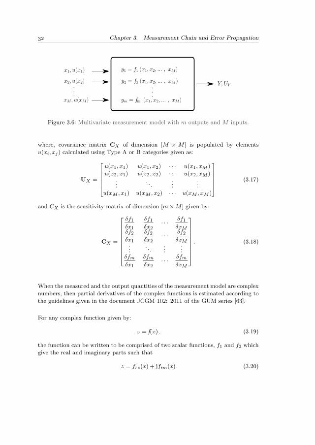
Chapter 3. Measurement Chain and Error Propagation
Figure 3.6: Multivariate measurement model with m outputs and M inputs.
where, covariance matrix CX of dimension [M × M ] is populated by elements
u(xi, xj) calculated using Type A or B categories given as:
UX =
u(x1, x1) u(x1, x2) · · · u(x1, xM )
u(x2, x1) u(x2, x2) · · · u(x2, xM )...
. . ....
...
u(xM , x1) u(xM , x2) · · · u(xM , xM )
(3.17)
and CX is the sensitivity matrix of dimension [m×M ] given by:
CX =
δf1
δx1
δf1
δx2· · · δf1
δxMδf2
δx1
δf2
δx2· · · δf2
δxM...
. . ....
...δfmδx1
δfmδx2
· · · δfmδxM
. (3.18)
When the measured and the output quantities of the measurement model are complex
numbers, then partial derivatives of the complex functions is estimated according to
the guidelines given in the document JCGM 102: 2011 of the GUM series [63].
For any complex function given by:
z = f(x), (3.19)
the function can be written to be comprised of two scalar functions, f1 and f2 which
give the real and imaginary parts such that
z = fre(x) + jfim(x) (3.20)
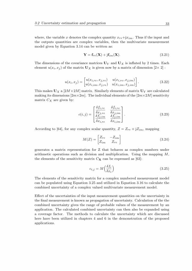
3.2 Uncertainty estimation and propagation
where, the variable x denotes the complex quantity xre+jxim. Thus if the input and
the outputs quantities are complex variables, then the multivariate measurement
model given by Equation 3.14 can be written as:
Y = fre(X) + jfim(X). (3.21)
The dimensions of the covariance matrices UY and UX is inflated by 2 times. Each
element u(xi, xj) of the matrix UX is given now by a matrix of dimension [2× 2] :
u(xi, xj) =
[u(xi,re, xj,re) u(xi,re, xj,im)
u(xi,im, xj,re) u(xi,im, xj,im)
]. (3.22)
This makes UX a [2M×2M ] matrix. Similarly elements of matrix UY are calculated
making its dimensions [2m×2m]. The individual elements of the [2m×2M ] sensitivity
matrix CX are given by:
c(i, j) =
δfi,reδxj,re
δfi,reδxj,im
δfj,imδxi,re
δfj,imδxi,im
. (3.23)
According to [64], for any complex scalar quantity, Z = Zre + jZim, mapping
M(Z) =
[Zre −ZimZim Zre
](3.24)
generates a matrix representation for Z that behaves as complex numbers under
arithmetic operations such as division and multiplication. Using the mapping M ,
the elements of the sensitivity matrix CX can be expressed as [63]:
ci,j = M(δfiδxi
)(3.25)
The elements of the sensitivity matrix for a complex numbered measurement model
can be populated using Equation 3.25 and utilized in Equation 3.16 to calculate the
combined uncertainty of a complex valued multivariate measurement model.
Effect of the uncertainties of the input measurement quantities on the uncertainty in
the final measurement is known as propagation of uncertainty. Calculation of the the
combined uncertainty gives the range of probable values of the measurement by an
application. The calculated combined uncertainty can then also be expanded using
a coverage factor. The methods to calculate the uncertainty which are discussed
here have been utilized in chapters 4 and 6 in the demonstration of the proposed
applications.

Chapter 3. Measurement Chain and Error Propagation
3.3 ConclusionThis chapter presented the measurement chain and the sources of error in a pha-
sor estimation process. Systematic bias and random errors and their effect on the
phasor estimates were discussed. Process to calculate the uncertainty of measure-
ments using Type A and B methods was presented. Propagation of uncertainty in
a measurement chain was discussed along with methods to calculate the combined
uncertainty of such measurements which are dependent on multiple individual mea-
surements. Propagation of uncertainty in multivariate measurement models for real
and complex valued quantities was presented in detail. The concepts presented in
this chapter are used in the the following chapters to analyse the measurement data
and formulate the results.
4Online Cable Temperature
Tracking
Dynamic line rating is a concept to calculate flexible loading limits of a cable as a
function of thermal state of the cable and its surroundings. The relationship between
the cable’s conductor’s resistance and it’s temperature can be utilized to estimate
it’s thermal state. However, estimating the resistance with an accuracy so that it
can be effectively used to track temperature with an accuracy of about to 5 to 10 Cis a challenging task. This chapter presents an improved method to accurately track
the resistance and temperature of the cable using real-time PMU measurements.
The focus is on a relatively new domain, the MV distribution grids where more
decentralized renewable sources like wind and solar parks are being integrated.
Parts of this chapter are based on:
R. S. Singh, H. van den Brom, S. Babaev, et al., “Estimation of impedance and sus-
ceptance parameters of a 3-phase cable system using PMU data”, Energies, vol. 12,
no. 23, 2019, issn: 1996-1073. doi: 10.3390/en12234573. [Online]. Available: https:
//www.mdpi.com/1996-1073/12/23/4573
R. S. Singh, J. F. G. Cobben, and V. Cuk, “PMU-based Cable Temperature Mon-
itoring and Thermal Assessment for Dynamic Line Rating”, IEEE Transactions on
Power Delivery, pp. 1–1, 2020.
Chapter 4. Online Cable Temperature Tracking
4.1 Introduction
Line rating or loading limits define the maximum current a cable system can carry
for a specified period of time. Loading limits of cable systems are dependent on
the physical thermal properties of the cables and their surroundings and are limited
by the temperature withstand capabilities of the cable insulation. For example,
the thermal limit of the cross-linked poly-ethylene (XLPE) insulation which is a
common insulating materials used in power cables is 90 C. Thus, for a cable with
XLPE insulation, the line rating for a given duration would be given by the current
which would result in a conductor temperature of 90 C.
Depending on the duration of the specified time period (infinite or finite), these
limits are categorized as steady state or dynamic loading limit. IEC standard 60853:2
presents two ways to determine the dynamic loading limits for cable systems: cyclic
rating and the emergency rating. Cyclic ratings define maximum current allowed in
a cable system during a load cycle (often 24 hours) for which the cable system does
not breach it’s thermal limits. Cyclic ratings are of merit when cables are exposed to
cyclic loading patterns. On the other hand, emergency rating define the maximum
allowed current for a specific time period during an operation. No fixed loading
patterns are required to calculate the emergency rating. However, knowledge about
the thermal state of cable’s conductor and other cable parts is essential to calculate
the emergency rating of the cable from that starting point. From the starting point,
the emergency rating is determined by calculating the thermal response of the cable
to a load step.
In this research, the concept of DLR has been presented as the process of calculating
the emergency rating of a cable(system) by forecasting the thermal states of the ca-
ble conductors in response to a given dynamic loading profile. A method to estimate
time-dependent thermal state of power-cables using the TEE model is presented in
[67]. A finite element model (FEM) based method-based dynamic rating was calcu-
lated in [68]. However, to initialize the models, both the methods require knowledge
about the initial temperatures of the cable’s components such as conductor, insula-
tion and jacket. Without utilizing any dedicated temperature sensing infrastructure,
tracking resistance of the cable utilizing PMU measurements presents a viable solu-
tion to gain real-time information about the cable’s conductor’s temperature. The
idea is inspired from the physical property of the conductors that it’s resistance is
proportional to the its temperature. Accurate estimates of the conductor resistance
in real-time can then be utilized to find the conductor temperature in real-time.
Work has been presented in the past to show the feasibility of this idea albeit mostly
in a simulation environment and only for high-voltage (HV) long-distance overhead
lines. Accurate and reliable resistance and hence temperature estimates for shorter
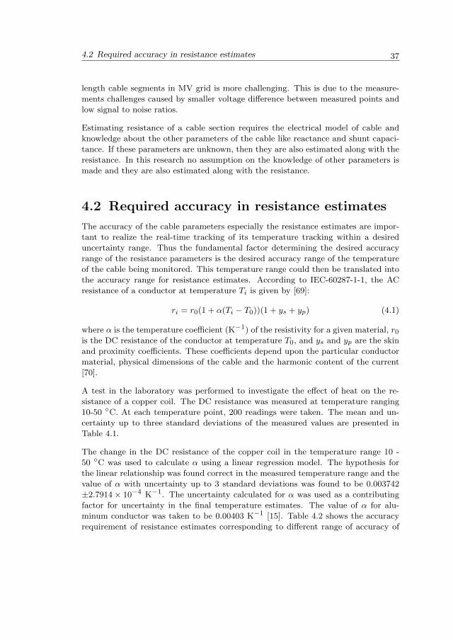
4.2 Required accuracy in resistance estimates
length cable segments in MV grid is more challenging. This is due to the measure-
ments challenges caused by smaller voltage difference between measured points and
low signal to noise ratios.
Estimating resistance of a cable section requires the electrical model of cable and
knowledge about the other parameters of the cable like reactance and shunt capaci-
tance. If these parameters are unknown, then they are also estimated along with the
resistance. In this research no assumption on the knowledge of other parameters is
made and they are also estimated along with the resistance.
4.2 Required accuracy in resistance estimates
The accuracy of the cable parameters especially the resistance estimates are impor-
tant to realize the real-time tracking of its temperature tracking within a desired
uncertainty range. Thus the fundamental factor determining the desired accuracy
range of the resistance parameters is the desired accuracy range of the temperature
of the cable being monitored. This temperature range could then be translated into
the accuracy range for resistance estimates. According to IEC-60287-1-1, the AC
resistance of a conductor at temperature Ti is given by [69]:
ri = r0(1 + α(Ti − T0))(1 + ys + yp) (4.1)
where α is the temperature coefficient (K−1) of the resistivity for a given material, r0is the DC resistance of the conductor at temperature T0, and ys and yp are the skin
and proximity coefficients. These coefficients depend upon the particular conductor
material, physical dimensions of the cable and the harmonic content of the current
[70].
A test in the laboratory was performed to investigate the effect of heat on the re-
sistance of a copper coil. The DC resistance was measured at temperature ranging
10-50 C. At each temperature point, 200 readings were taken. The mean and un-
certainty up to three standard deviations of the measured values are presented in
Table 4.1.
The change in the DC resistance of the copper coil in the temperature range 10 -
50 C was used to calculate α using a linear regression model. The hypothesis for
the linear relationship was found correct in the measured temperature range and the
value of α with uncertainty up to 3 standard deviations was found to be 0.003742
±2.7914× 10⁻⁴ K−1. The uncertainty calculated for α was used as a contributing
factor for uncertainty in the final temperature estimates. The value of α for alu-
minum conductor was taken to be 0.00403 K−1 [15]. Table 4.2 shows the accuracy
requirement of resistance estimates corresponding to different range of accuracy of
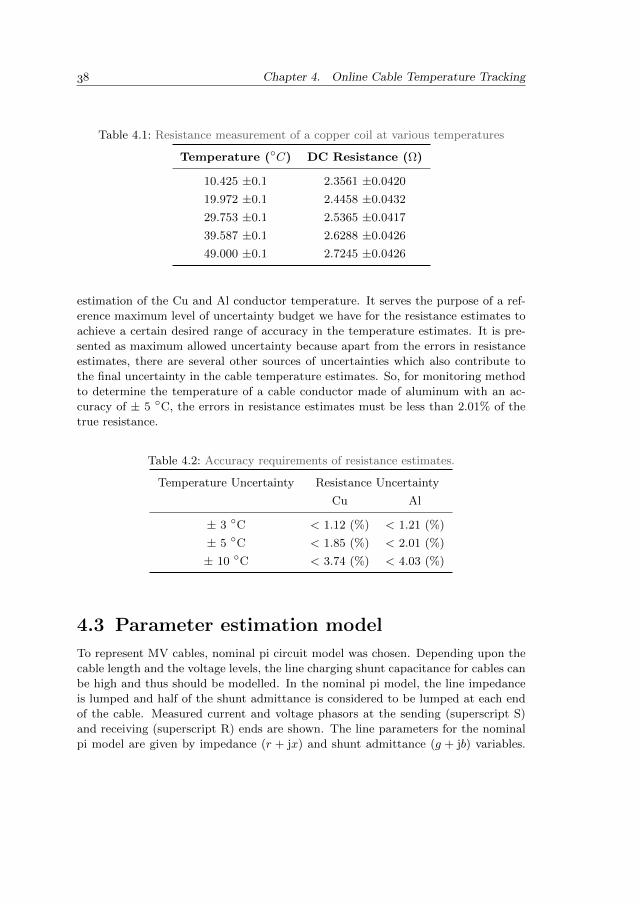
Chapter 4. Online Cable Temperature Tracking
Table 4.1: Resistance measurement of a copper coil at various temperatures
Temperature (C) DC Resistance (Ω)
10.425 ±0.1 2.3561 ±0.0420
19.972 ±0.1 2.4458 ±0.0432
29.753 ±0.1 2.5365 ±0.0417
39.587 ±0.1 2.6288 ±0.0426
49.000 ±0.1 2.7245 ±0.0426
estimation of the Cu and Al conductor temperature. It serves the purpose of a ref-
erence maximum level of uncertainty budget we have for the resistance estimates to
achieve a certain desired range of accuracy in the temperature estimates. It is pre-
sented as maximum allowed uncertainty because apart from the errors in resistance
estimates, there are several other sources of uncertainties which also contribute to
the final uncertainty in the cable temperature estimates. So, for monitoring method
to determine the temperature of a cable conductor made of aluminum with an ac-
curacy of ± 5 C, the errors in resistance estimates must be less than 2.01% of the
true resistance.
Table 4.2: Accuracy requirements of resistance estimates.
Temperature Uncertainty Resistance Uncertainty
Cu Al
± 3 C < 1.12 (%) < 1.21 (%)
± 5 C < 1.85 (%) < 2.01 (%)
± 10 C < 3.74 (%) < 4.03 (%)
4.3 Parameter estimation model
To represent MV cables, nominal pi circuit model was chosen. Depending upon the
cable length and the voltage levels, the line charging shunt capacitance for cables can
be high and thus should be modelled. In the nominal pi model, the line impedance
is lumped and half of the shunt admittance is considered to be lumped at each end
of the cable. Measured current and voltage phasors at the sending (superscript S)
and receiving (superscript R) ends are shown. The line parameters for the nominal
pi model are given by impedance (r + jx) and shunt admittance (g + jb) variables.
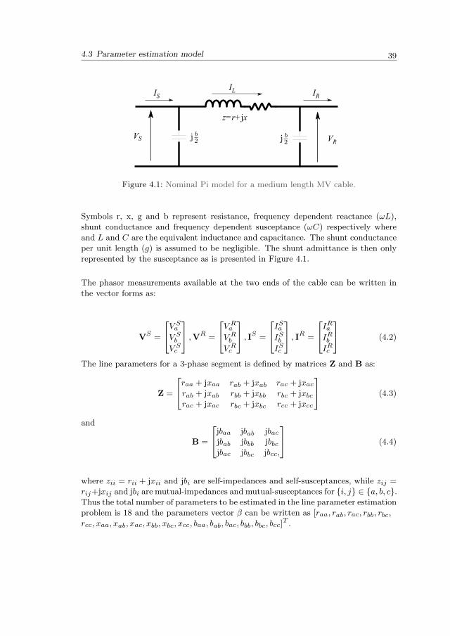
4.3 Parameter estimation model
VS VR
ILIS IR
z=r+jx
Figure 4.1: Nominal Pi model for a medium length MV cable.
Symbols r, x, g and b represent resistance, frequency dependent reactance (ωL),
shunt conductance and frequency dependent susceptance (ωC) respectively where
and L and C are the equivalent inductance and capacitance. The shunt conductance
per unit length (g) is assumed to be negligible. The shunt admittance is then only
represented by the susceptance as is presented in Figure 4.1.
The phasor measurements available at the two ends of the cable can be written in
the vector forms as:
VS =
V SaV SbV Sc
,VR =
V RaV RbV Rc
, IS =
ISaISbISc
, IR =
IRaIRbIRc
(4.2)
The line parameters for a 3-phase segment is defined by matrices Z and B as:
Z =
raa + jxaa rab + jxab rac + jxacrab + jxab rbb + jxbb rbc + jxbcrac + jxac rbc + jxbc rcc + jxcc
(4.3)
and
B =
jbaa jbab jbacjbab jbbb jbbcjbac jbbc jbcc,
(4.4)
where zii = rii + jxii and jbi are self-impedances and self-susceptances, while zij =
rij+jxij and jbi are mutual-impedances and mutual-susceptances for i, j ∈ a, b, c.Thus the total number of parameters to be estimated in the line parameter estimation
problem is 18 and the parameters vector β can be written as [raa, rab, rac, rbb, rbc,
rcc, xaa, xab, xac, xbb, xbc, xcc, baa, bab, bac, bbb, bbc, bcc]T .
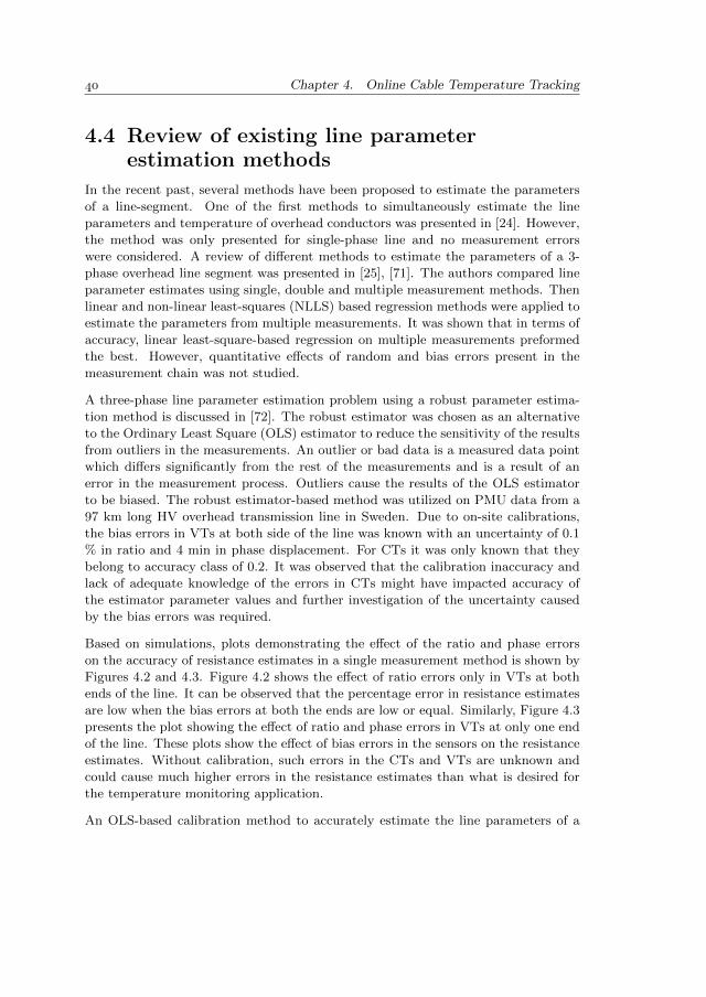
Chapter 4. Online Cable Temperature Tracking
4.4 Review of existing line parameterestimation methods
In the recent past, several methods have been proposed to estimate the parameters
of a line-segment. One of the first methods to simultaneously estimate the line
parameters and temperature of overhead conductors was presented in [24]. However,
the method was only presented for single-phase line and no measurement errors
were considered. A review of different methods to estimate the parameters of a 3-
phase overhead line segment was presented in [25], [71]. The authors compared line
parameter estimates using single, double and multiple measurement methods. Then
linear and non-linear least-squares (NLLS) based regression methods were applied to
estimate the parameters from multiple measurements. It was shown that in terms of
accuracy, linear least-square-based regression on multiple measurements preformed
the best. However, quantitative effects of random and bias errors present in the
measurement chain was not studied.
A three-phase line parameter estimation problem using a robust parameter estima-
tion method is discussed in [72]. The robust estimator was chosen as an alternative
to the Ordinary Least Square (OLS) estimator to reduce the sensitivity of the results
from outliers in the measurements. An outlier or bad data is a measured data point
which differs significantly from the rest of the measurements and is a result of an
error in the measurement process. Outliers cause the results of the OLS estimator
to be biased. The robust estimator-based method was utilized on PMU data from a
97 km long HV overhead transmission line in Sweden. Due to on-site calibrations,
the bias errors in VTs at both side of the line was known with an uncertainty of 0.1
% in ratio and 4 min in phase displacement. For CTs it was only known that they
belong to accuracy class of 0.2. It was observed that the calibration inaccuracy and
lack of adequate knowledge of the errors in CTs might have impacted accuracy of
the estimator parameter values and further investigation of the uncertainty caused
by the bias errors was required.
Based on simulations, plots demonstrating the effect of the ratio and phase errors
on the accuracy of resistance estimates in a single measurement method is shown by
Figures 4.2 and 4.3. Figure 4.2 shows the effect of ratio errors only in VTs at both
ends of the line. It can be observed that the percentage error in resistance estimates
are low when the bias errors at both the ends are low or equal. Similarly, Figure 4.3
presents the plot showing the effect of ratio and phase errors in VTs at only one end
of the line. These plots show the effect of bias errors in the sensors on the resistance
estimates. Without calibration, such errors in the CTs and VTs are unknown and
could cause much higher errors in the resistance estimates than what is desired for
the temperature monitoring application.
An OLS-based calibration method to accurately estimate the line parameters of a
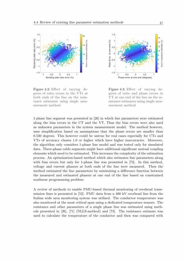
4.4 Review of existing line parameter estimation methods
-1 -0.5 0 0.5 1
Sending side ratio error (%)
-1.5
-1
-0.5
0
0.5
1
1.5R
eceiv
ing s
ide r
atio e
rror
(%)
5
10
15
20
Err
or
in r
esis
tan
ce
estim
ate
s (
%)
Figure 4.2: Effect of varying de-grees of ratio errors in the VTs atboth ends of the line on the resis-tance estimates using single mea-surement method.
-1 -0.5 0 0.5 1
Phase error at one end (degrees)
-1.5
-1
-0.5
0
0.5
1
1.5
Ratio E
rror
at one e
nd (
%)
2
4
6
8
10
12
14
16
Err
or
in r
esis
tan
ce
estim
ate
s (
%)
Figure 4.3: Effect of varying de-grees of ratio and phase errors inVT at one end of the line on the re-sistance estimates using single mea-surement method.
1-phase line segment was presented in [26] in which line parameters were estimated
along the bias errors in the CT and the VT. Thus the bias errors were also used
as unknown parameters in the system measurement model. The method however,
uses simplification based on assumptions that the phase errors are smaller than
0.530 degrees. This however could be untrue for real cases especially for CTs and
VTs of accuracy classes 1.0 or higher which have higher inaccuracies. Moreover,
the algorithm only considers 1-phase line model and was tested only for simulated
data. Three-phase cable segments might have additional significant mutual coupling
elements which need to be estimated. This increases the complexity of the estimation
process. An optimization-based method which also estimates line parameters along
with bias errors but only for 1-phase line was presented in [73]. In this method,
voltage and current phasors at both ends of the line were measured. Then the
method estimated the line parameters by minimizing a difference function between
the measured and estimated phasors at one end of the line based on constrained
nonlinear programming problem.
A review of methods to enable PMU-based thermal monitoring of overhead trans-
mission lines is presented in [53]. PMU data from a 400 kV overhead line from the
Italian wide area monitoring system was utilized. The conductor temperature was
also monitored at the most critical span using a dedicated temperature sensors. The
resistance and other parameters of a single phase line was estimated using meth-
ods presented in [26], [71] (NLLS-method) and [73]. The resistance estimate was
used to calculate the temperature of the conductor and then was compared with
Chapter 4. Online Cable Temperature Tracking
the measured temperature. Even though no quantification of error or uncertainty in
the estimated temperature values was presented, the figures presented showed that
the optimization method presented in [26] performed the worst of all. There was no
significant difference between the results from the other two methods even though
the NLLS method did not account for possible bias errors in the measurements.
There are two major drawbacks of the reviewed methods present in the literature.
First of all, the methods which include bias error in their models are developed only
for a single-phase of the line. Their impedance model did not include any mutual
impedance or susceptance parameters which might have a significant presence in a
3-phase cable segment. Adding extra parameters for 3-phase cable and the correction
coefficients for CTs and VTs of all the phases is a challenging task.
The second drawback is that none of the discussed methods provide any uncertainty
range for the calculated line parameters and temperature values. The metrics for
the evaluation of the results were based on the knowledge of the actual parameter
values. However the reference values of conductor resistance is more likely to be a
steady-state value which cannot be utilized as a reference while tracking the dynamic
resistance and hence the temperature in the real-time. Thus, without an uncertainty
range, it is impossible to quantify the level of trust in the estimated parameters.
This makes this type of validation process less suitable for application using real-
field data, since the reference parameters might have changed depending on the
ambient environmental and power system operating conditions.
To overcome these drawbacks this thesis presents a new improved method which
is capable of giving accurate and reliable resistance and temperature estimates in
real-time for a 3-phase line segments in presence of random and bias errors in the
measurements. The presented method is based on the OLS based multivariate re-
gression method presented in [71]. This method was chosen because unlike other
methods, the presented method uses a complete 3-phase cable model and gives accu-
rate resistance estimates of all the conductors using measurements that do not have
bias errors. This thesis also presents, correct modelling of the cable impedance ma-
trix based upon the geometry and operating condition of the grid which is important
to select the significant parameters that need to be estimated. In the end uncer-
tainty spread around the resistance and temperature estimates are also evaluated
and presented using expanded uncertainty (U).
4.5 Existing estimation algorithm
This section presents the existing 3-phase line parameter estimation algorithm pre-
sented in [71]. The performance of the algorithm in presence of random and bias
errors is presented and analysed. According to the nominal pi model shown in Figure
4.5 Existing estimation algorithm
4.1, the voltage and current phasors at the two ends of the cable can be related using
the line impedance and susceptance parameters as:
IS − IR =1
2B(VS + VR
), (4.5)
VS −VR = Z(
1
2BVR + IR
). (4.6)
In equations 4.5 and 4.6, the current and voltage phasors are represented as complex
numbers in Cartesian coordinates and are written in matrix form as:
∆Ia∆Ib∆Ic
= j1
2
baa bab bacbab bbb bbcbac bbc bcc
ΣVaΣVbΣVc
(4.7)
IRaIRbIRc
=
yaa yab yacyab ybb ybcyac ybc ycc
∆Va∆Vb∆Vc
−j1
2
baa bab bacbab bbb bbcbac bbc bcc
V RaV RbV Rc
, (4.8)
where the elements yij are from the admittance matrix Y such that Y = Z−1,
ΣVi = V Si + V Ri and ∆Ii = ISi − IRi . Equations 4.7 and 4.8 can be expanded to
form 6 equations with variables in complex form:
∆Ia = j12 (baaΣVa + babΣVb + bacΣVc)
∆Ib = j12 (babΣVa + bbbΣVb + bbcΣVc)
∆Ic = j 12 (bacΣVa + bbcΣVb + bccΣVc)
IRa = yaa∆Va + yab∆Vb + yac∆Vc − j 12 (baaVa + babVb + bacVc)
IRb = yab∆Va + ybb∆Vb + ybc∆Vc − j 12 (babVa + babVb + bbcVc)
IRc = yac∆Va + ybc∆Vb + ycc∆Vc − j 12 (bacVa + bbcVb + bccVc)
(4.9)
Set of equations in 4.9 can then be separated into real and imaginary terms, giving a
set of 12 equations (A.1)-(A.12) shown in Appendix A. The unknown line parameters
(yij) of Y matrix were also separated in the real and imaginary terms (tij and
gij). These equations present the different outputs (dependent variables) in a linear
combination of the unknown parameters (coefficients) and predictors (independent
variables). The unbiased linear equations for n parameters can be written as:
zi = ηi1β1 + ηi2β2 + ...+ ηinβn + εi, (4.10)
where, according to equations (4.5) and (4.6), zi is made up of real or imaginary parts
of ∆I or IR. Coefficients ηij are the contribution of the parameters in the output
Chapter 4. Online Cable Temperature Tracking
zi. and is either real or imaginary elements of IS , VS or VR vectors. Unknown
parameters to be estimated are denoted by βj and εi is the error term calculated as
the difference between the measured quantity and the result of the linear equation
formed by the expected parameter values and the independent variables. For n
parameters (18 in this case) and m sets of observations, the whole system of linear
equations is represented in matrix form as:
z = Hβ + ε, (4.11)
where z ∈ R12m is the measurement vector for m number of observations for 12
equations and β ∈ Rn is the parameter vector of length n. H ∈ R12m×n is the
relation matrix formed of variables which are real or imaginary components of the
measured voltage and current phasors and ε ∈ R12n is the error of the measurement
model. A more detailed description about putting the unknown and unknown vari-
ables from the model and available measurements in the form of (4.11) is presented
in Appendix A. The estimates for parameter β are given by:
β =covariance(z,H)
variance(H), (4.12)
where β is the estimate of parameter vector β. In matrix form, the analytical solution
could be found out by solving the OLS problem:
minβ||z−Hβ||2. (4.13)
The analytical solution is given as:
β = (H>H)−1H>z. (4.14)
Matrix Y is formed using the estimated tij and gij parameters and then the resistance
(rij) and reactance (xij) parameters were calculated by inverting the matrix Y .
4.5.1 OLS characteristics and drawbacks of existing method
The solution to the OLS problem (equation 4.11) is given by equation 4.14 which
gives us the estimates of the ‘true’ parameters. Since the values of ‘true’ parame-
ters is unknown in most-real time applications, estimation of the uncertainty of the
estimated parameters is an important as well as challenging part of validating the
results. The solution given by the OLS estimator is ‘unbiased’ and have the min-
imum variance of all the unbiased estimators when certain assumptions about the
estimator are true. These assumptions are mentioned in the Table 4.3.
Assumption A1 is dependent on the measurement models (shown by equations 4.5
4.5 Existing estimation algorithm
Table 4.3: Assumptions of the Ordinary Least Square Estimator
A1 Linearity zi = ηi1β1 + ηi2β2 + ...+ ηinβn + εi.
A2 Full rank rank(H) = n.
A3 Independent Variables E[εi|ηj1, ηj2, ..., ηjn] = 0, i, j ∈ 1, 2, ..., n.
A4 Homoscedasticity Var[εi|H] = σ2 and Cov[εi, εj |H] = 0
A5 Normality ε|H ∼ N (0, σ2I)
and 4.6) which portrays a linear relationship between dependent and independent
variables. Assumption A2 says that the 12m × n matrix is full rank and there is
no linear relationship between any of the independent variables. Assumption A3
states that the expected errors εi value of the ith observations is zero and is not a
function of the independent variables. Assumption A4 states that the errors have a
constant variance (homoscedasticity). Each error has the same finite variance and is
uncorrelated to other errors. The two parts of assumption A4 imply that:
E[εε>|H] =
E[ε1ε1|H] E[ε1ε2|H] · · · E[ε1ε12m|H]
E[ε2ε1|H] E[ε2ε2|H] · · · E[ε2ε12m|H]...
. . ....
...
E[ε12ε1|H] E[ε12mε2|H] · · · E[ε12mε12m|H]
(4.15)
=
σ2 0 · · · 0
0 σ2 · · · 0...
. . ....
...
0 0 · · · σ2
(4.16)
and can be summarized as :
E[εε>|H] = σ2I. (4.17)
Based on the assumptions A1-A4, assumption A5 is easy to make which is that the
error vector as a normal distribution with zero mean and a constant variance given
by σ2I. These assumptions are the cornerstone of the OLS method and an analysis
of these assumptions can help diagnose the errors in the linear model (equation 4.10)
used to measure and describe the system. Regression analysis is performed to check
the validity of the regression model [74].
Using the solution vector β we get the fitted model as:
zi = ηi1β1 + ηi2β2 + ...+ ηinβn + ei, (4.18)
Chapter 4. Online Cable Temperature Tracking
The residual vector can be calculated as:
e = z−Hβ (4.19)
Residuals ei are the difference between the observed measurements and predicted
values according to the fitted regression model (4.18). As shown in Appendix B, the
expected value of the residuals is zero and they can be considered as the ‘observed
errors’ given the model given by equation 4.18 is correct. Thus if the fitted model
is correct then the residuals should validate the assumptions made about the errors
[74].
The Shapiro-Wilk test [75] is way to test the normality of the given errors samples.
However, the test is only reliable for relatively smaller sample size. One way to
still use this test to analyse the residuals is re-sampling the measurements into sets
of smaller sample lengths and select the results from the set whose residuals have
the highest possibility of being normally distributed. One drawback of reducing the
number of samples is that when random measurements errors are present, OLS gives
more accurate results when number of samples are increased. Thus reducing the
number of samples will worsen the quality of results.
Another method, a visual one is to plot the residuals of the estimator in form of a
QQ-plot [74]. A QQ-plot displays the quantiles 1 of the sample under test verses the
expected quantile values of a sample with normal distribution [76]. The QQ-plot does
not test the hypothesis of normality but gives a visual indication about normality of
the residual samples. If the distribution of the residuals under test is normal, then
the plotted residuals in the QQ-plot appear linear. The benefit of using a QQ-plot
is that it’s performance does not depend on the size of the data sample and hence
was chosen to analyze the residuals.
In field measurements, some of these assumptions (A1-A4) might not hold true.
Apart from the random measurement errors, field CTs and VTs might have a sys-
tematic bias error in their measurement due to the unknown magnitude and phase
errors of different magnitudes. Due to lack of frequent calibration of CTs and VTs,
the known correction coefficients to cancel those errors might not be correct. As
shown in Appendix A, elements of the matrix H and vector z are real and imagi-
nary parts of measured current and voltage phasors. The presence of any magnitude
and phase errors in the measurement chain would cause a fixed bias error in those
elements. Use of the same regression model as in the existing method will result
in residuals whose expected value might be non-zero and have a non-normal dis-
tribution. This indicates a mismatch between the linear regression model and the
measurements acquired from the system and the estimated model parameters will
1Quantiles divide a probability distribution into several equal intervals of equal probability
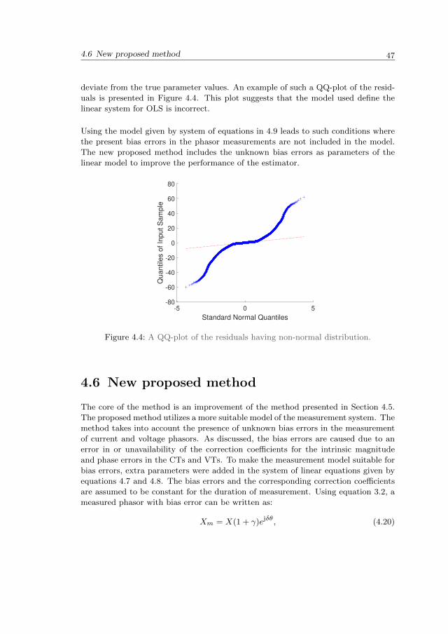
4.6 New proposed method
deviate from the true parameter values. An example of such a QQ-plot of the resid-
uals is presented in Figure 4.4. This plot suggests that the model used define the
linear system for OLS is incorrect.
Using the model given by system of equations in 4.9 leads to such conditions where
the present bias errors in the phasor measurements are not included in the model.
The new proposed method includes the unknown bias errors as parameters of the
linear model to improve the performance of the estimator.
-5 0 5
Standard Normal Quantiles
-80
-60
-40
-20
0
20
40
60
80
Qu
an
tile
s o
f In
pu
t S
am
ple
Figure 4.4: A QQ-plot of the residuals having non-normal distribution.
4.6 New proposed method
The core of the method is an improvement of the method presented in Section 4.5.
The proposed method utilizes a more suitable model of the measurement system. The
method takes into account the presence of unknown bias errors in the measurement
of current and voltage phasors. As discussed, the bias errors are caused due to an
error in or unavailability of the correction coefficients for the intrinsic magnitude
and phase errors in the CTs and VTs. To make the measurement model suitable for
bias errors, extra parameters were added in the system of linear equations given by
equations 4.7 and 4.8. The bias errors and the corresponding correction coefficients
are assumed to be constant for the duration of measurement. Using equation 3.2, a
measured phasor with bias error can be written as:
Xm = X(1 + γ)ejδθ, (4.20)
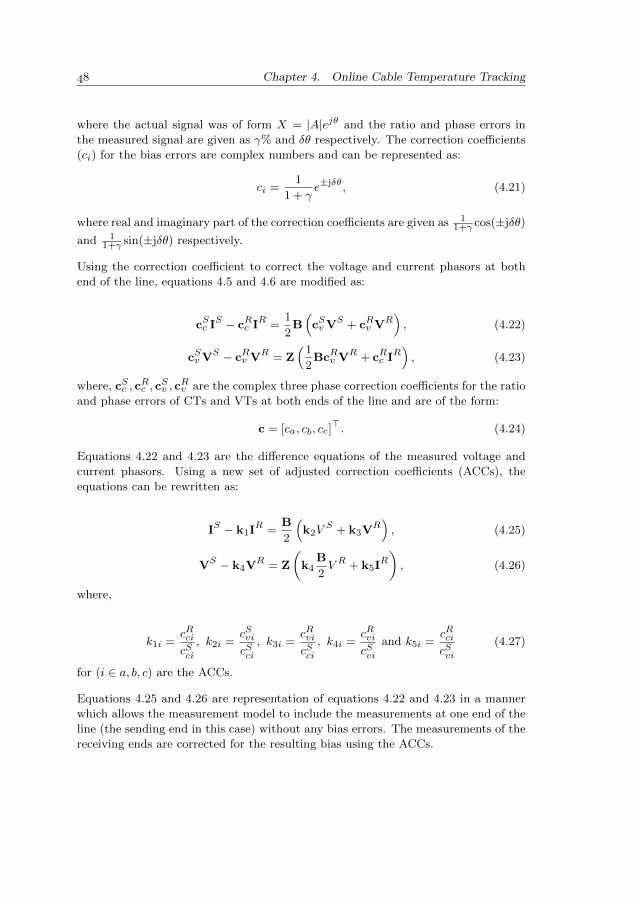
Chapter 4. Online Cable Temperature Tracking
where the actual signal was of form X = |A|ejθ and the ratio and phase errors in
the measured signal are given as γ% and δθ respectively. The correction coefficients
(ci) for the bias errors are complex numbers and can be represented as:
ci =1
1 + γe±jδθ, (4.21)
where real and imaginary part of the correction coefficients are given as 11+γ cos(±jδθ)
and 11+γ sin(±jδθ) respectively.
Using the correction coefficient to correct the voltage and current phasors at both
end of the line, equations 4.5 and 4.6 are modified as:
cSc IS − cRc IR =1
2B(cSvVS + cRv VR
), (4.22)
cSvVS − cRv VR = Z(
1
2BcRv VR + cRc IR
), (4.23)
where, cSc , cRc , c
Sv , c
Rv are the complex three phase correction coefficients for the ratio
and phase errors of CTs and VTs at both ends of the line and are of the form:
c = [ca, cb, cc]>. (4.24)
Equations 4.22 and 4.23 are the difference equations of the measured voltage and
current phasors. Using a new set of adjusted correction coefficients (ACCs), the
equations can be rewritten as:
IS − k1IR =B
2
(k2V
S + k3VR), (4.25)
VS − k4VR = Z
(k4
B
2V R + k5IR
), (4.26)
where,
k1i =cRcicSci
, k2i =cSvicSci
, k3i =cRvicSci
, k4i =cRvicSvi
and k5i =cRcicSvi
(4.27)
for (i ∈ a, b, c) are the ACCs.
Equations 4.25 and 4.26 are representation of equations 4.22 and 4.23 in a manner
which allows the measurement model to include the measurements at one end of the
line (the sending end in this case) without any bias errors. The measurements of the
receiving ends are corrected for the resulting bias using the ACCs.
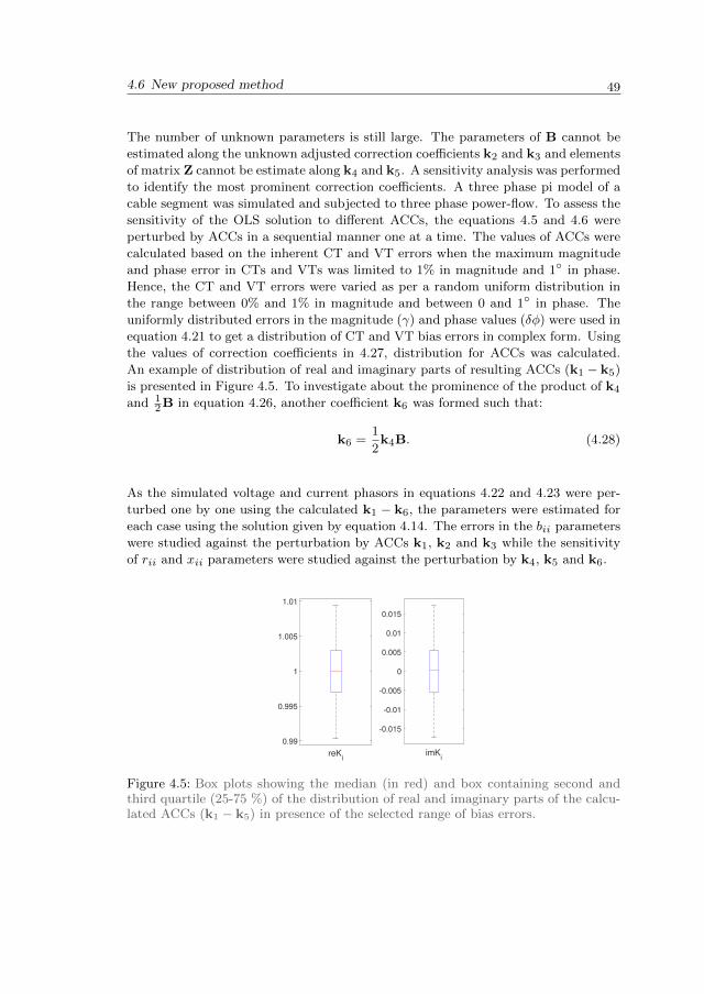
4.6 New proposed method
The number of unknown parameters is still large. The parameters of B cannot be
estimated along the unknown adjusted correction coefficients k2 and k3 and elements
of matrix Z cannot be estimate along k4 and k5. A sensitivity analysis was performed
to identify the most prominent correction coefficients. A three phase pi model of a
cable segment was simulated and subjected to three phase power-flow. To assess the
sensitivity of the OLS solution to different ACCs, the equations 4.5 and 4.6 were
perturbed by ACCs in a sequential manner one at a time. The values of ACCs were
calculated based on the inherent CT and VT errors when the maximum magnitude
and phase error in CTs and VTs was limited to 1% in magnitude and 1 in phase.
Hence, the CT and VT errors were varied as per a random uniform distribution in
the range between 0% and 1% in magnitude and between 0 and 1 in phase. The
uniformly distributed errors in the magnitude (γ) and phase values (δφ) were used in
equation 4.21 to get a distribution of CT and VT bias errors in complex form. Using
the values of correction coefficients in 4.27, distribution for ACCs was calculated.
An example of distribution of real and imaginary parts of resulting ACCs (k1 − k5)
is presented in Figure 4.5. To investigate about the prominence of the product of k4
and 12B in equation 4.26, another coefficient k6 was formed such that:
k6 =1
2k4B. (4.28)
As the simulated voltage and current phasors in equations 4.22 and 4.23 were per-
turbed one by one using the calculated k1 − k6, the parameters were estimated for
each case using the solution given by equation 4.14. The errors in the bii parameters
were studied against the perturbation by ACCs k1, k2 and k3 while the sensitivity
of rii and xii parameters were studied against the perturbation by k4, k5 and k6.
reKi
0.99
0.995
1
1.005
1.01
imKi
-0.015
-0.01
-0.005
0
0.005
0.01
0.015
Figure 4.5: Box plots showing the median (in red) and box containing second andthird quartile (25-75 %) of the distribution of real and imaginary parts of the calcu-lated ACCs (k1 − k5) in presence of the selected range of bias errors.
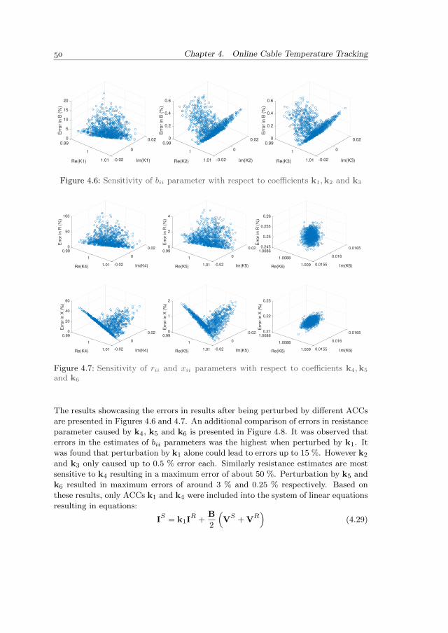
Chapter 4. Online Cable Temperature Tracking
0.0200.99
5
Im(K1)
0
10
Re(K1)
Err
or
in B
(%
)
1
15
20
-0.021.01
0.0200.99
0.2
Im(K2)
0
Re(K2)E
rror
in B
(%
)
1
0.4
0.6
-0.021.01
0.0200.99
0.2
Im(K3)
0
Re(K3)
Err
or
in B
(%
)
1
0.4
0.6
-0.021.01
Figure 4.6: Sensitivity of bii parameter with respect to coefficients k1,k2 and k3
0.0200.99
Im(K4)
0
50
Re(K4)
Err
or
in R
(%
)
1
100
-0.021.01
0.0200.99
20
Im(K4)
0
Re(K4)
Err
or
in X
(%
)
1
40
60
-0.021.01
0.0200.99
Im(K5)
0
2
Re(K5)
Err
or
in R
(%
)
1
4
-0.021.01
0.0200.99
Im(K5)
0
1
Re(K5)
Err
or
in X
(%
)
1
2
-0.021.01
0.01650.2451.0086
0.25
Im(K6)
0.016
Re(K6)
Err
or
in R
(%
)1.0088
0.255
0.26
0.01551.009
0.01650.211.0086
Im(K6)
0.016
0.22
Re(K6)
Err
or
in X
(%
)
1.0088
0.23
0.01551.009
Figure 4.7: Sensitivity of rii and xii parameters with respect to coefficients k4,k5
and k6
The results showcasing the errors in results after being perturbed by different ACCs
are presented in Figures 4.6 and 4.7. An additional comparison of errors in resistance
parameter caused by k4, k5 and k6 is presented in Figure 4.8. It was observed that
errors in the estimates of bii parameters was the highest when perturbed by k1. It
was found that perturbation by k1 alone could lead to errors up to 15 %. However k2
and k3 only caused up to 0.5 % error each. Similarly resistance estimates are most
sensitive to k4 resulting in a maximum error of about 50 %. Perturbation by k5 and
k6 resulted in maximum errors of around 3 % and 0.25 % respectively. Based on
these results, only ACCs k1 and k4 were included into the system of linear equations
resulting in equations:
IS = k1IR +B
2
(VS + VR
)(4.29)
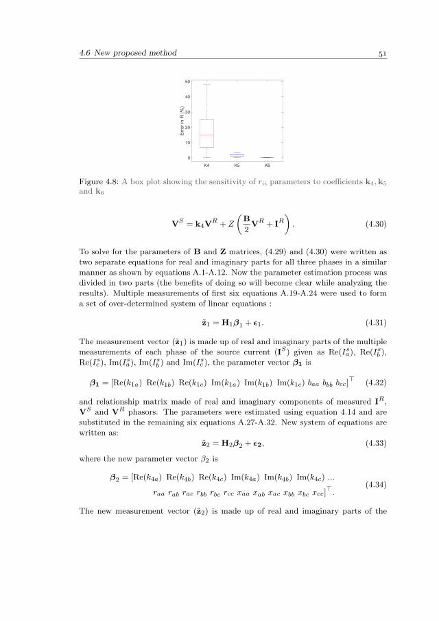
4.6 New proposed method
K4 K5 K6
0
10
20
30
40
50
Err
or
in R
(%
)Figure 4.8: A box plot showing the sensitivity of rii parameters to coefficients k4,k5
and k6
VS = k4VR + Z
(B
2VR + IR
). (4.30)
To solve for the parameters of B and Z matrices, (4.29) and (4.30) were written as
two separate equations for real and imaginary parts for all three phases in a similar
manner as shown by equations A.1-A.12. Now the parameter estimation process was
divided in two parts (the benefits of doing so will become clear while analyzing the
results). Multiple measurements of first six equations A.19-A.24 were used to form
a set of over-determined system of linear equations :
z1 = H1β1 + ε1. (4.31)
The measurement vector (z1) is made up of real and imaginary parts of the multiple
measurements of each phase of the source current (IS) given as Re(Isa), Re(Isb ),
Re(Isc ), Im(Isa), Im(Isb ) and Im(Isc ), the parameter vector β1 is
β1 = [Re(k1a) Re(k1b) Re(k1c) Im(k1a) Im(k1b) Im(k1c) baa bbb bcc]> (4.32)
and relationship matrix made of real and imaginary components of measured IR,
VS and VR phasors. The parameters were estimated using equation 4.14 and are
substituted in the remaining six equations A.27-A.32. New system of equations are
written as:
z2 = H2β2 + ε2, (4.33)
where the new parameter vector β2 is
β2 = [Re(k4a) Re(k4b) Re(k4c) Im(k4a) Im(k4b) Im(k4c) ...
raa rab rac rbb rbc rcc xaa xab xac xbb xbc xcc]>.
(4.34)
The new measurement vector (z2) is made up of real and imaginary parts of the
Chapter 4. Online Cable Temperature Tracking
multiple measurements of each phase of the source Voltage (VS) given as Re(V sa ),
Re(V sb ), Re(V sc ), Im(V sa ), Im(V sb ) and Im(V sc ). The new relationship matrix H2
matrix made of real and imaginary components of measured IR, VS and VR phasors
is formulated and estimate for parameter vector β2 is calculated.
4.7 Data pre-processingSection 4.6 presented a new improved method to estimate line parameters in presence
of bias errors. However, real-time PMU measurements could also be corrupted with
high amplitude random noise and outliers. Utilizing highly corrupted PMU measure-
ments directly in the OLS regression-based method would reduce the accuracy of the
method. Pre-processing is the step of curating the data to make it more suitable for
the application. In this work, linear Kalman filter (KF) based on the static state
estimation method presented in [77] and [78] was used to process the signals to filter
out the excessive random noise and outliers. The linear KF was chosen because the
output states of the KF are relatively steady sate voltage and current values. The
system does not include dynamic states such as generator rotor angles and speed.
The KF is a blend of prediction and measurement [79] and consists of two steps:
prediction and update. The first step gives the prior which is the probability distri-
bution of the state without using the measurements. For each data point, during the
first step, a prediction is calculated using the initial conditions and a process model.
The process model is mathematical representation of the system. The process model
is not perfect and the error in process model is known as process error. The update
step, also known as measurement update, gives the state of the model using the
results of the process step and the available measurement data. The result is called
posterior which gives a probability distribution after including the measurements.
More details about the implementation of the KF is presented in Appendix C.
The KF was used to pre-process the PMU data before utilizing in the algorithm to
smooth the effects of the random noise errors, data outliers and missing data. Figure
4.9 shows the results of applying the KF on voltage magnitude data which had a
maximum random error of 1%. Some bad data points were also added to the voltage
magnitude values. It is seen from the figure that, the KF has a smoothing effect on
the random noise and removes the bad data points.
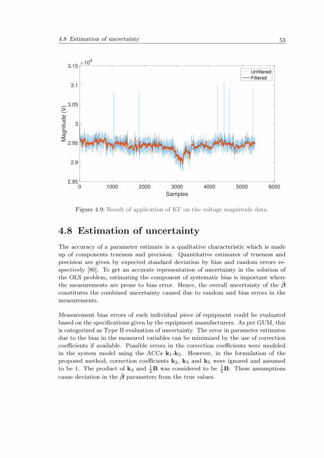
4.8 Estimation of uncertainty
0 1000 2000 3000 4000 5000 6000
Samples
2.85
2.9
2.95
3
3.05
3.1
3.15M
agnitude (
V)
104
Unfiltered
Filtered
Figure 4.9: Result of application of KF on the voltage magnitude data.
4.8 Estimation of uncertainty
The accuracy of a parameter estimate is a qualitative characteristic which is made
up of components trueness and precision. Quantitative estimates of trueness and
precision are given by expected standard deviation by bias and random errors re-
spectively [80]. To get an accurate representation of uncertainty in the solution of
the OLS problem, estimating the component of systematic bias is important where
the measurements are prone to bias error. Hence, the overall uncertainty of the β
constitutes the combined uncertainty caused due to random and bias errors in the
measurements.
Measurement bias errors of each individual piece of equipment could be evaluated
based on the specifications given by the equipment manufacturers. As per GUM, this
is categorized as Type B evaluation of uncertainty. The error in parameter estimates
due to the bias in the measured variables can be minimized by the use of correction
coefficients if available. Possible errors in the correction coefficients were modeled
in the system model using the ACCs k1-k5. However, in the formulation of the
proposed method, correction coefficients k2, k3 and k5 were ignored and assumed
to be 1. The product of k4 and 12B was considered to be 1
2B. These assumptions
cause deviation in the β parameters from the true values.
Chapter 4. Online Cable Temperature Tracking
4.8.1 Uncertainty caused by bias in measurements
The deviations in the estimated parameters caused by the assumptions can be cal-
culated using two methods: propagation of uncertainty using the GUM framework
and Monte Carlo-based simulations. Following sub-sections present the two methods
evaluated to estimate the uncertainty in the parameters due to bias errors in the
phasors.
Propagation of uncertainty as per GUM
In this method, the deviation in the impedance parameters caused by the bias errors
in measurements is estimated by calculating the combined uncertainty calculation as
specified in the GUM [63]. The magnitude and phase errors were assumed to vary
normally with a standard deviation of σe. The standard uncertainty in a parameter
estimate due to believed bias in the measurements (ub(βi)) was quantified by the
combined uncertainty given in equation 3.12:
ub(βi) =
N∑j=1
(∂f
∂xj
)2u2(xj), (4.35)
where f is the analytical function to calculate the susceptance, resistance and reac-
tance given equations 4.25 and 4.26 and xj ∈ rek2, imk2, rek3, imk3, rek5, imk5
rek6, imk6 Each u(xi) is the believed standard deviation in real and imaginary
parts of coefficients k2, k3, k5 and k6. This method however, uses an analytical
function f from equations 4.25 and 4.26 which is only possible for single-phase sys-
tem or a 3-phase system with no mutual coupling elements in the B and Z matrices.
Next, a Monte Carlo simulation based approach is presented which could be applied
to other cases.
Monte Carlo simulations
Equations 4.25 and 4.26 were expanded into complex forms and the real and imagi-
nary parts were separated. The magnitude and phase errors were varied normally in
a believed range with the mean given by last calibrated values and an uncertainty up
to 3σe, where σe is the believed standard deviation in phase and magnitude values.
Instances of relationship matrix (Hj) and output vector (zj) were were formed using
all possible values for the coefficients k2, k3 and k5. For each set of Hj and zjparameter vector βj was estimated. The distribution of the errors was found to be
4.9 Results and comparison
normal and the maximum deviation in each of the elements of the parameters vector
due to bias errors in the measurement was given by:
∆βi ≤ max
|βji − βi||βi|
, (4.36)
where j is the instance and βi is the true parameter value. Since the distribution
of errors for each element was found to be normal, the standard uncertainty in each
estimated parameter caused by the bias errors was written as:
ub =1
3∆β, (4.37)
where the maximum error was represented by a coverage factor of 3 SDs.
4.8.2 Uncertainty caused by random errors in measurements
Given that assumptions A1-A4 are satisfied, the standard deviation in the solution
of the OLS problem is given by the diagonal elements of the covariance matrix of
the estimates. As shown in Appendix B, this is written as:
Cov[β|H] = σ2I(H>H)−1 (4.38)
and
urnd = diag(Cov[β|H]), (4.39)
where σ2 is the estimate of the variance given by
σ2 =1
m− ne>e, (4.40)
where n is the number of unknown parameters and m is the length of the measure-
ment vector (z). The combined standard deviation in the parameter estimate βi is
then given by:
u(βi) =√u2rnd(βi) + u2
b(βi). (4.41)
A coverage factor of three was multiplied to calculate the expanded uncertainty
around the parameter estimates.
4.9 Results and comparison
To demonstrate the performance of the new proposed model and compare it with
the existing method the accuracy of the estimates is evaluated using simulations
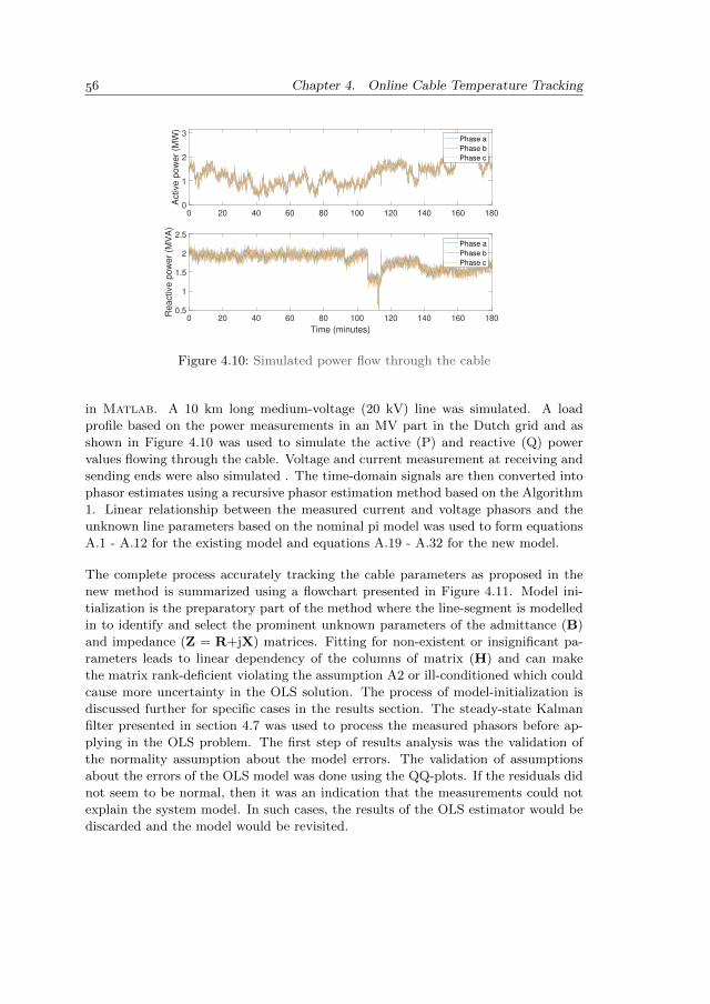
Chapter 4. Online Cable Temperature Tracking
0 20 40 60 80 100 120 140 160 1800
1
2
3
Active
po
we
r (M
W)
Phase a
Phase b
Phase c
0 20 40 60 80 100 120 140 160 180
Time (minutes)
0.5
1
1.5
2
2.5
Re
active
po
we
r (M
VA
)
Phase a
Phase b
Phase c
Figure 4.10: Simulated power flow through the cable
in Matlab. A 10 km long medium-voltage (20 kV) line was simulated. A load
profile based on the power measurements in an MV part in the Dutch grid and as
shown in Figure 4.10 was used to simulate the active (P) and reactive (Q) power
values flowing through the cable. Voltage and current measurement at receiving and
sending ends were also simulated . The time-domain signals are then converted into
phasor estimates using a recursive phasor estimation method based on the Algorithm
1. Linear relationship between the measured current and voltage phasors and the
unknown line parameters based on the nominal pi model was used to form equations
A.1 - A.12 for the existing model and equations A.19 - A.32 for the new model.
The complete process accurately tracking the cable parameters as proposed in the
new method is summarized using a flowchart presented in Figure 4.11. Model ini-
tialization is the preparatory part of the method where the line-segment is modelled
in to identify and select the prominent unknown parameters of the admittance (B)
and impedance (Z = R+jX) matrices. Fitting for non-existent or insignificant pa-
rameters leads to linear dependency of the columns of matrix (H) and can make
the matrix rank-deficient violating the assumption A2 or ill-conditioned which could
cause more uncertainty in the OLS solution. The process of model-initialization is
discussed further for specific cases in the results section. The steady-state Kalman
filter presented in section 4.7 was used to process the measured phasors before ap-
plying in the OLS problem. The first step of results analysis was the validation of
the normality assumption about the model errors. The validation of assumptions
about the errors of the OLS model was done using the QQ-plots. If the residuals did
not seem to be normal, then it was an indication that the measurements could not
explain the system model. In such cases, the results of the OLS estimator would be
discarded and the model would be revisited.
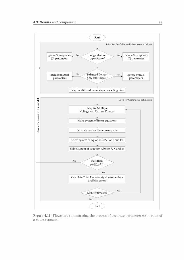
4.9 Results and comparison
Start
Separate real and imaginary parts
Make system of linear equations
Select additional parameters modelling bias
Solve system of equation 4.29 for B and k1
Balanced Power-flow and Trefoil?
Include Susceptance (B) parameter
Ignore Susceptance (B) parameter
Acquire Multiple Voltage and Current Phasors
Solve system of equation 4.30 for R, X and k4
Long cable forcapacitance?
Include mutual parameters
Ignore mutual parameters
Calculate Total Uncertainty due to random and bias errors
Residuals
ε=N(0,σ I)?
Residuals
ε=N(0,σ I)?
Initialize the Cable and Measurement Model
No
Yes
Yes
Yes
No
No
Ch
eck
for
err
ors
in t
he
mo
del
More Estimates?More Estimates?
End
Loop for Continuous Estimation
2
No
Yes
Figure 4.11: Flowchart summarizing the process of accurate parameter estimation ofa cable segment.
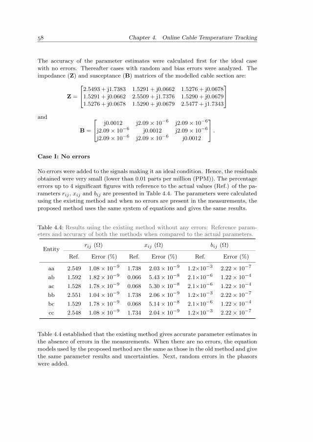
Chapter 4. Online Cable Temperature Tracking
The accuracy of the parameter estimates were calculated first for the ideal case
with no errors. Thereafter cases with random and bias errors were analyzed. The
impedance (Z) and susceptance (B) matrices of the modelled cable section are:
Z =
2.5493 + j1.7383 1.5291 + j0.0662 1.5276 + j0.0678
1.5291 + j0.0662 2.5509 + j1.7376 1.5290 + j0.0679
1.5276 + j0.0678 1.5290 + j0.0679 2.5477 + j1.7343
and
B =
j0.0012 j2.09× 10−6 j2.09× 10−6
j2.09× 10−6 j0.0012 j2.09× 10−6
j2.09× 10−6 j2.09× 10−6 j0.0012
.Case I: No errors
No errors were added to the signals making it an ideal condition. Hence, the residuals
obtained were very small (lower than 0.01 parts per million (PPM)). The percentage
errors up to 4 significant figures with reference to the actual values (Ref.) of the pa-
rameters rij , xij and bij are presented in Table 4.4. The parameters were calculated
using the existing method and when no errors are present in the measurements, the
proposed method uses the same system of equations and gives the same results.
Table 4.4: Results using the existing method without any errors: Reference param-eters and accuracy of both the methods when compared to the actual parameters.
Entityrij (Ω) xij (Ω) bij (Ω)
Ref. Error (%) Ref. Error (%) Ref. Error (%)
aa 2.549 1.08× 10⁻⁹ 1.738 2.03× 10⁻⁹ 1.2×10⁻³ 2.22× 10⁻⁷
ab 1.592 1.82× 10⁻⁹ 0.066 5.43× 10⁻⁸ 2.1×10⁻⁶ 1.22× 10⁻⁴
ac 1.528 1.78× 10⁻⁹ 0.068 5.30× 10⁻⁸ 2.1×10⁻⁶ 1.22× 10⁻⁴
bb 2.551 1.04× 10⁻⁹ 1.738 2.06× 10⁻⁹ 1.2×10⁻³ 2.22× 10⁻⁷
bc 1.529 1.78× 10⁻⁹ 0.068 5.14× 10⁻⁸ 2.1×10⁻⁶ 1.22× 10⁻⁴
cc 2.548 1.08× 10⁻⁹ 1.734 2.04× 10⁻⁹ 1.2×10⁻³ 2.22× 10⁻⁷
Table 4.4 established that the existing method gives accurate parameter estimates in
the absence of errors in the measurements. When there are no errors, the equation
models used by the proposed method are the same as those in the old method and give
the same parameter results and uncertainties. Next, random errors in the phasors
were added.
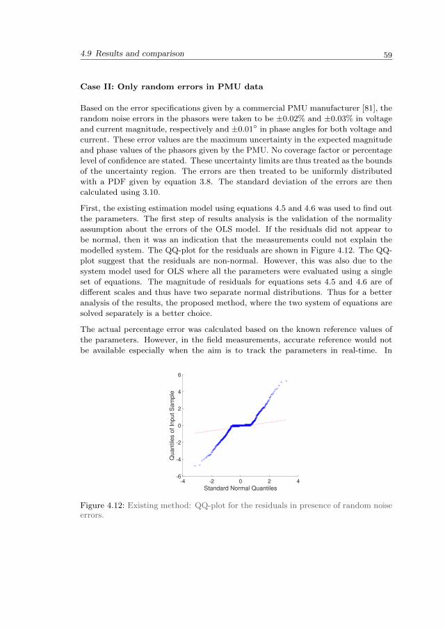
4.9 Results and comparison
Case II: Only random errors in PMU data
Based on the error specifications given by a commercial PMU manufacturer [81], the
random noise errors in the phasors were taken to be ±0.02% and ±0.03% in voltage
and current magnitude, respectively and ±0.01 in phase angles for both voltage and
current. These error values are the maximum uncertainty in the expected magnitude
and phase values of the phasors given by the PMU. No coverage factor or percentage
level of confidence are stated. These uncertainty limits are thus treated as the bounds
of the uncertainty region. The errors are then treated to be uniformly distributed
with a PDF given by equation 3.8. The standard deviation of the errors are then
calculated using 3.10.
First, the existing estimation model using equations 4.5 and 4.6 was used to find out
the parameters. The first step of results analysis is the validation of the normality
assumption about the errors of the OLS model. If the residuals did not appear to
be normal, then it was an indication that the measurements could not explain the
modelled system. The QQ-plot for the residuals are shown in Figure 4.12. The QQ-
plot suggest that the residuals are non-normal. However, this was also due to the
system model used for OLS where all the parameters were evaluated using a single
set of equations. The magnitude of residuals for equations sets 4.5 and 4.6 are of
different scales and thus have two separate normal distributions. Thus for a better
analysis of the results, the proposed method, where the two system of equations are
solved separately is a better choice.
The actual percentage error was calculated based on the known reference values of
the parameters. However, in the field measurements, accurate reference would not
be available especially when the aim is to track the parameters in real-time. In
-4 -2 0 2 4
Standard Normal Quantiles
-6
-4
-2
0
2
4
6
Qu
an
tile
s o
f In
pu
t S
am
ple
Figure 4.12: Existing method: QQ-plot for the residuals in presence of random noiseerrors.
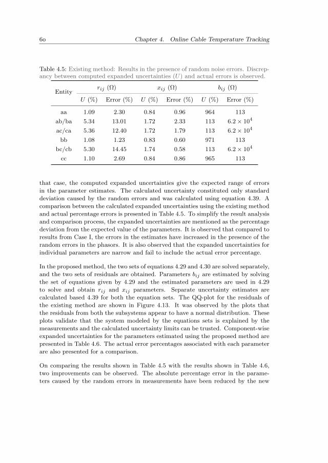
Chapter 4. Online Cable Temperature Tracking
Table 4.5: Existing method: Results in the presence of random noise errors. Discrep-ancy between computed expanded uncertainties (U) and actual errors is observed.
Entityrij (Ω) xij (Ω) bij (Ω)
U (%) Error (%) U (%) Error (%) U (%) Error (%)
aa 1.09 2.30 0.84 0.96 964 113
ab/ba 5.34 13.01 1.72 2.33 113 6.2× 10⁴
ac/ca 5.36 12.40 1.72 1.79 113 6.2× 10⁴
bb 1.08 1.23 0.83 0.60 971 113
bc/cb 5.30 14.45 1.74 0.58 113 6.2× 10⁴
cc 1.10 2.69 0.84 0.86 965 113
that case, the computed expanded uncertainties give the expected range of errors
in the parameter estimates. The calculated uncertainty constituted only standard
deviation caused by the random errors and was calculated using equation 4.39. A
comparison between the calculated expanded uncertainties using the existing method
and actual percentage errors is presented in Table 4.5. To simplify the result analysis
and comparison process, the expanded uncertainties are mentioned as the percentage
deviation from the expected value of the parameters. It is observed that compared to
results from Case I, the errors in the estimates have increased in the presence of the
random errors in the phasors. It is also observed that the expanded uncertainties for
individual parameters are narrow and fail to include the actual error percentage.
In the proposed method, the two sets of equations 4.29 and 4.30 are solved separately,
and the two sets of residuals are obtained. Parameters bij are estimated by solving
the set of equations given by 4.29 and the estimated parameters are used in 4.29
to solve and obtain rij and xij parameters. Separate uncertainty estimates are
calculated based 4.39 for both the equation sets. The QQ-plot for the residuals of
the existing method are shown in Figure 4.13. It was observed by the plots that
the residuals from both the subsystems appear to have a normal distribution. These
plots validate that the system modeled by the equations sets is explained by the
measurements and the calculated uncertainty limits can be trusted. Component-wise
expanded uncertainties for the parameters estimated using the proposed method are
presented in Table 4.6. The actual error percentages associated with each parameter
are also presented for a comparison.
On comparing the results shown in Table 4.5 with the results shown in Table 4.6,
two improvements can be observed. The absolute percentage error in the parame-
ters caused by the random errors in measurements have been reduced by the new
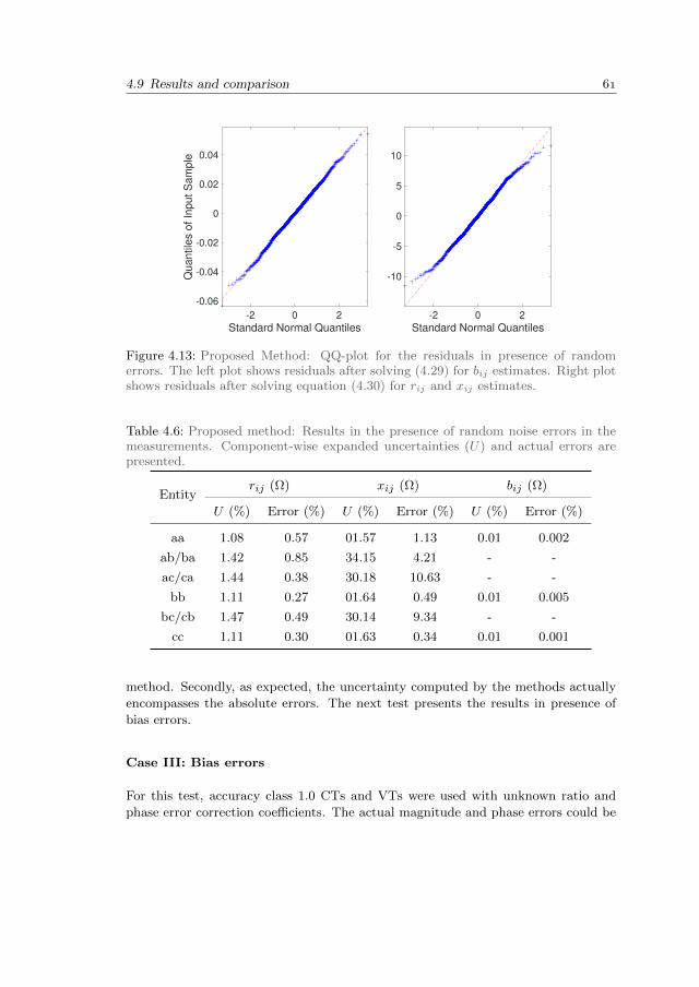
4.9 Results and comparison
-2 0 2
Standard Normal Quantiles
-0.06
-0.04
-0.02
0
0.02
0.04
Quantile
s o
f In
put S
am
ple
-2 0 2
Standard Normal Quantiles
-10
-5
0
5
10
Figure 4.13: Proposed Method: QQ-plot for the residuals in presence of randomerrors. The left plot shows residuals after solving (4.29) for bij estimates. Right plotshows residuals after solving equation (4.30) for rij and xij estimates.
Table 4.6: Proposed method: Results in the presence of random noise errors in themeasurements. Component-wise expanded uncertainties (U) and actual errors arepresented.
Entityrij (Ω) xij (Ω) bij (Ω)
U (%) Error (%) U (%) Error (%) U (%) Error (%)
aa 1.08 0.57 01.57 1.13 0.01 0.002
ab/ba 1.42 0.85 34.15 4.21 - -
ac/ca 1.44 0.38 30.18 10.63 - -
bb 1.11 0.27 01.64 0.49 0.01 0.005
bc/cb 1.47 0.49 30.14 9.34 - -
cc 1.11 0.30 01.63 0.34 0.01 0.001
method. Secondly, as expected, the uncertainty computed by the methods actually
encompasses the absolute errors. The next test presents the results in presence of
bias errors.
Case III: Bias errors
For this test, accuracy class 1.0 CTs and VTs were used with unknown ratio and
phase error correction coefficients. The actual magnitude and phase errors could be
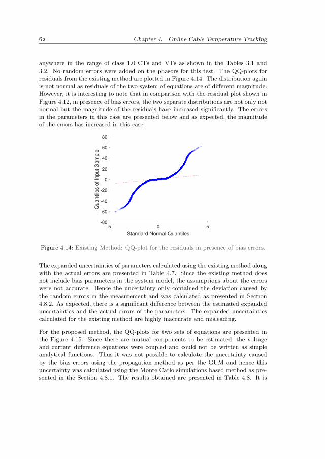
Chapter 4. Online Cable Temperature Tracking
anywhere in the range of class 1.0 CTs and VTs as shown in the Tables 3.1 and
3.2. No random errors were added on the phasors for this test. The QQ-plots for
residuals from the existing method are plotted in Figure 4.14. The distribution again
is not normal as residuals of the two system of equations are of different magnitude.
However, it is interesting to note that in comparison with the residual plot shown in
Figure 4.12, in presence of bias errors, the two separate distributions are not only not
normal but the magnitude of the residuals have increased significantly. The errors
in the parameters in this case are presented below and as expected, the magnitude
of the errors has increased in this case.
-5 0 5
Standard Normal Quantiles
-80
-60
-40
-20
0
20
40
60
80
Qu
an
tile
s o
f In
pu
t S
am
ple
Figure 4.14: Existing Method: QQ-plot for the residuals in presence of bias errors.
The expanded uncertainties of parameters calculated using the existing method along
with the actual errors are presented in Table 4.7. Since the existing method does
not include bias parameters in the system model, the assumptions about the errors
were not accurate. Hence the uncertainty only contained the deviation caused by
the random errors in the measurement and was calculated as presented in Section
4.8.2. As expected, there is a significant difference between the estimated expanded
uncertainties and the actual errors of the parameters. The expanded uncertainties
calculated for the existing method are highly inaccurate and misleading.
For the proposed method, the QQ-plots for two sets of equations are presented in
the Figure 4.15. Since there are mutual components to be estimated, the voltage
and current difference equations were coupled and could not be written as simple
analytical functions. Thus it was not possible to calculate the uncertainty caused
by the bias errors using the propagation method as per the GUM and hence this
uncertainty was calculated using the Monte Carlo simulations based method as pre-
sented in the Section 4.8.1. The results obtained are presented in Table 4.8. It is
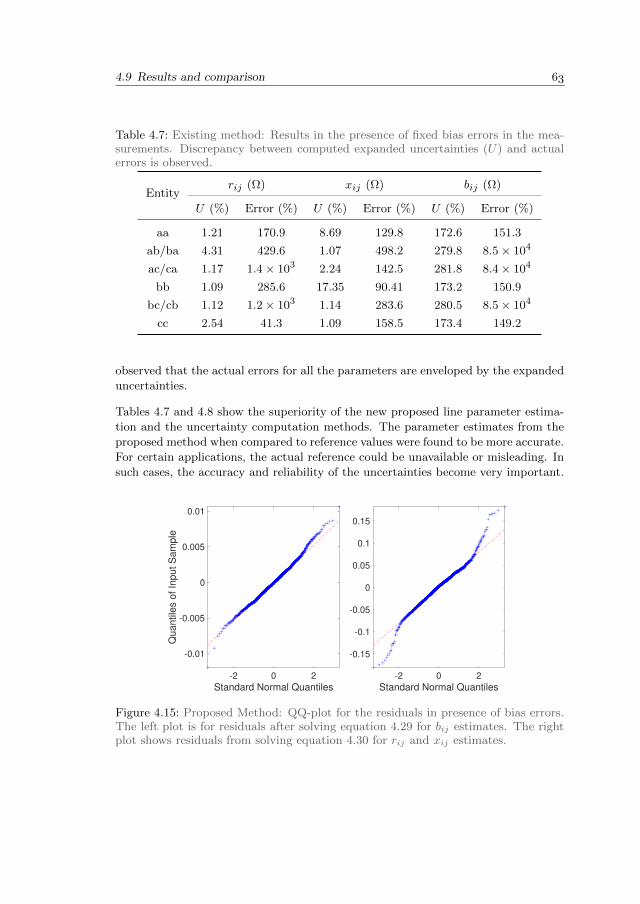
4.9 Results and comparison
Table 4.7: Existing method: Results in the presence of fixed bias errors in the mea-surements. Discrepancy between computed expanded uncertainties (U) and actualerrors is observed.
Entityrij (Ω) xij (Ω) bij (Ω)
U (%) Error (%) U (%) Error (%) U (%) Error (%)
aa 1.21 170.9 8.69 129.8 172.6 151.3
ab/ba 4.31 429.6 1.07 498.2 279.8 8.5× 10⁴
ac/ca 1.17 1.4× 10³ 2.24 142.5 281.8 8.4× 10⁴
bb 1.09 285.6 17.35 90.41 173.2 150.9
bc/cb 1.12 1.2× 10³ 1.14 283.6 280.5 8.5× 10⁴
cc 2.54 41.3 1.09 158.5 173.4 149.2
observed that the actual errors for all the parameters are enveloped by the expanded
uncertainties.
Tables 4.7 and 4.8 show the superiority of the new proposed line parameter estima-
tion and the uncertainty computation methods. The parameter estimates from the
proposed method when compared to reference values were found to be more accurate.
For certain applications, the actual reference could be unavailable or misleading. In
such cases, the accuracy and reliability of the uncertainties become very important.
-2 0 2
Standard Normal Quantiles
-0.01
-0.005
0
0.005
0.01
Qu
an
tile
s o
f In
pu
t S
am
ple
-2 0 2
Standard Normal Quantiles
-0.15
-0.1
-0.05
0
0.05
0.1
0.15
Figure 4.15: Proposed Method: QQ-plot for the residuals in presence of bias errors.The left plot is for residuals after solving equation 4.29 for bij estimates. The rightplot shows residuals from solving equation 4.30 for rij and xij estimates.
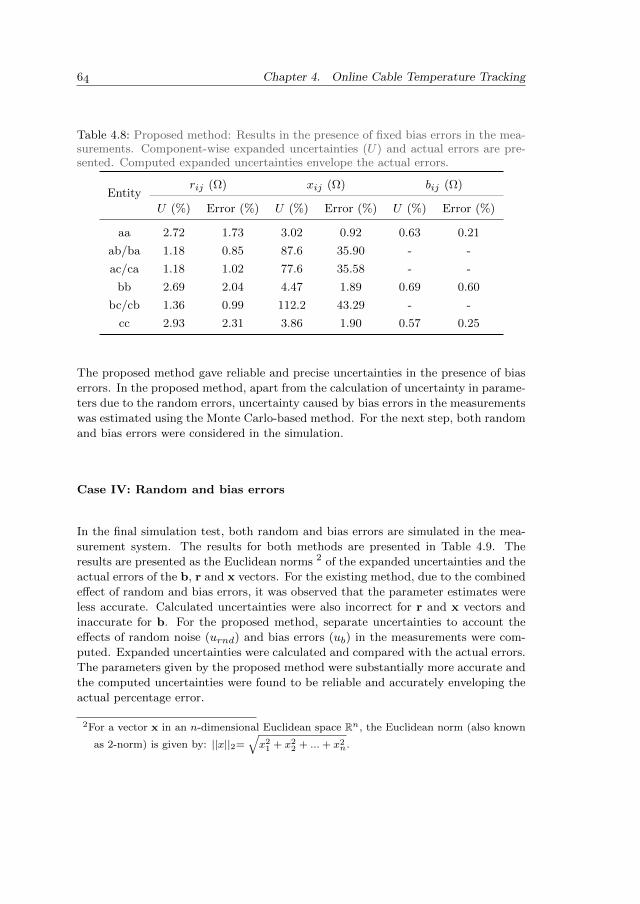
Chapter 4. Online Cable Temperature Tracking
Table 4.8: Proposed method: Results in the presence of fixed bias errors in the mea-surements. Component-wise expanded uncertainties (U) and actual errors are pre-sented. Computed expanded uncertainties envelope the actual errors.
Entityrij (Ω) xij (Ω) bij (Ω)
U (%) Error (%) U (%) Error (%) U (%) Error (%)
aa 2.72 1.73 3.02 0.92 0.63 0.21
ab/ba 1.18 0.85 87.6 35.90 - -
ac/ca 1.18 1.02 77.6 35.58 - -
bb 2.69 2.04 4.47 1.89 0.69 0.60
bc/cb 1.36 0.99 112.2 43.29 - -
cc 2.93 2.31 3.86 1.90 0.57 0.25
The proposed method gave reliable and precise uncertainties in the presence of bias
errors. In the proposed method, apart from the calculation of uncertainty in parame-
ters due to the random errors, uncertainty caused by bias errors in the measurements
was estimated using the Monte Carlo-based method. For the next step, both random
and bias errors were considered in the simulation.
Case IV: Random and bias errors
In the final simulation test, both random and bias errors are simulated in the mea-
surement system. The results for both methods are presented in Table 4.9. The
results are presented as the Euclidean norms 2 of the expanded uncertainties and the
actual errors of the b, r and x vectors. For the existing method, due to the combined
effect of random and bias errors, it was observed that the parameter estimates were
less accurate. Calculated uncertainties were also incorrect for r and x vectors and
inaccurate for b. For the proposed method, separate uncertainties to account the
effects of random noise (urnd) and bias errors (ub) in the measurements were com-
puted. Expanded uncertainties were calculated and compared with the actual errors.
The parameters given by the proposed method were substantially more accurate and
the computed uncertainties were found to be reliable and accurately enveloping the
actual percentage error.
2For a vector x in an n-dimensional Euclidean space Rn, the Euclidean norm (also known
as 2-norm) is given by: ||x||2=√x2
1 + x22 + ...+ x2
n.
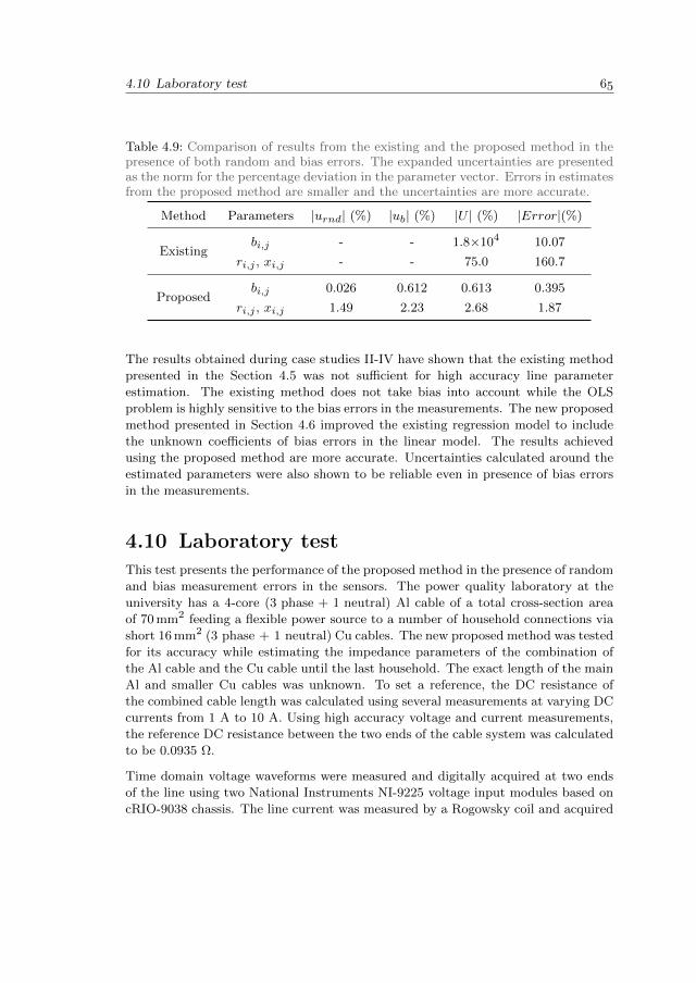
4.10 Laboratory test
Table 4.9: Comparison of results from the existing and the proposed method in thepresence of both random and bias errors. The expanded uncertainties are presentedas the norm for the percentage deviation in the parameter vector. Errors in estimatesfrom the proposed method are smaller and the uncertainties are more accurate.
Method Parameters |urnd| (%) |ub| (%) |U | (%) |Error|(%)
Existingbi,j - - 1.8×10⁴ 10.07
ri,j , xi,j - - 75.0 160.7
Proposedbi,j 0.026 0.612 0.613 0.395
ri,j , xi,j 1.49 2.23 2.68 1.87
The results obtained during case studies II-IV have shown that the existing method
presented in the Section 4.5 was not sufficient for high accuracy line parameter
estimation. The existing method does not take bias into account while the OLS
problem is highly sensitive to the bias errors in the measurements. The new proposed
method presented in Section 4.6 improved the existing regression model to include
the unknown coefficients of bias errors in the linear model. The results achieved
using the proposed method are more accurate. Uncertainties calculated around the
estimated parameters were also shown to be reliable even in presence of bias errors
in the measurements.
4.10 Laboratory test
This test presents the performance of the proposed method in the presence of random
and bias measurement errors in the sensors. The power quality laboratory at the
university has a 4-core (3 phase + 1 neutral) Al cable of a total cross-section area
of 70 mm2 feeding a flexible power source to a number of household connections via
short 16 mm2 (3 phase + 1 neutral) Cu cables. The new proposed method was tested
for its accuracy while estimating the impedance parameters of the combination of
the Al cable and the Cu cable until the last household. The exact length of the main
Al and smaller Cu cables was unknown. To set a reference, the DC resistance of
the combined cable length was calculated using several measurements at varying DC
currents from 1 A to 10 A. Using high accuracy voltage and current measurements,
the reference DC resistance between the two ends of the cable system was calculated
to be 0.0935 Ω.
Time domain voltage waveforms were measured and digitally acquired at two ends
of the line using two National Instruments NI-9225 voltage input modules based on
cRIO-9038 chassis. The line current was measured by a Rogowsky coil and acquired
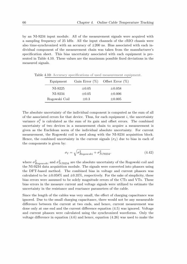
Chapter 4. Online Cable Temperature Tracking
by an NI-9234 input module. All of the measurement signals were acquired with
a sampling frequency of 25 kHz. All the input channels of the cRIO chassis were
also time-synchronized with an accuracy of ±200 ns. Bias associated with each in-
dividual component of the measurement chain was taken from the manufacturer’s
specification sheet. This bias uncertainty associated with each equipment is pre-
sented in Table 4.10. These values are the maximum possible fixed deviations in the
measured signals.
Table 4.10: Accuracy specifications of used measurement equipment.
Equipment Gain Error (%) Offset Error (%)
NI-9225 ±0.05 ±0.058
NI-9234 ±0.05 ±0.006
Rogowski Coil ±0.3 ±0.005
The absolute uncertainty of the individual component is computed as the sum of all
of the associated errors for that device. Thus, for each equipment i, the uncertainty
variance σ2i is calculated as the sum of its gain and offset errors. The combined
uncertainty of two devices in a measurement chain to acquire a measurement is
given as the Euclidean norm of the individual absolute uncertainty. For current
measurement, the Rogowski coil is used along with the NI-9234 acquisition block.
Hence, the combined uncertainty in the current signals (σI) due to bias in each of
the components is given by:
σI =√σ2Rogowski + σ2
NI9234, (4.42)
where σ2Rogowski and σ2
NI9234 are the absolute uncertainty of the Rogowski coil and
the NI-9234 data acquisition module. The signals were converted into phasors using
the DFT-based method. The combined bias in voltage and current phasors was
calculated to be ±0.058% and ±0.35%, respectively. For the sake of simplicity, these
bias errors were assumed to be solely magnitude errors of the CTs and VTs. These
bias errors in the measure current and voltage signals were utilized to estimate the
uncertainty in the resistance and reactance parameters of the cable.
Since the length of the cables was very small, the effect of charging capacitance was
ignored. Due to the small charging capacitance, there would not be any measurable
difference between the current at two ends, and hence, current measurement was
done only at one end and the current difference equation (4.5) was ignored. Voltage
and current phasors were calculated using the synchronized waveforms. Only the
voltage difference in equation (4.6) and hence, equation (4.26) was used to make the
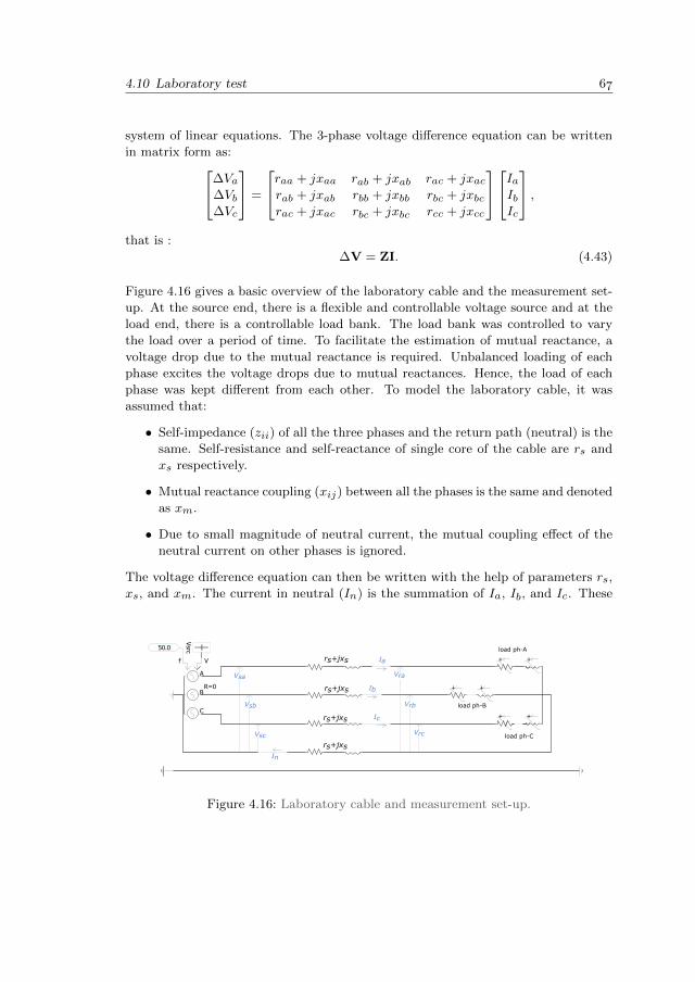
4.10 Laboratory test
system of linear equations. The 3-phase voltage difference equation can be written
in matrix form as:∆Va∆Vb∆Vc
=
raa + jxaa rab + jxab rac + jxacrab + jxab rbb + jxbb rbc + jxbcrac + jxac rbc + jxbc rcc + jxcc
IaIbIc
,that is :
∆V = ZI. (4.43)
Figure 4.16 gives a basic overview of the laboratory cable and the measurement set-
up. At the source end, there is a flexible and controllable voltage source and at the
load end, there is a controllable load bank. The load bank was controlled to vary
the load over a period of time. To facilitate the estimation of mutual reactance, a
voltage drop due to the mutual reactance is required. Unbalanced loading of each
phase excites the voltage drops due to mutual reactances. Hence, the load of each
phase was kept different from each other. To model the laboratory cable, it was
assumed that:
• Self-impedance (zii) of all the three phases and the return path (neutral) is the
same. Self-resistance and self-reactance of single core of the cable are rs and
xs respectively.
• Mutual reactance coupling (xij) between all the phases is the same and denoted
as xm.
• Due to small magnitude of neutral current, the mutual coupling effect of the
neutral current on other phases is ignored.
The voltage difference equation can then be written with the help of parameters rs,
xs, and xm. The current in neutral (In) is the summation of Ia, Ib, and Ic. These
++
+ +
+ +
A
B
C
Vf
R=0
50.0
Vsrc load ph-A
load ph-C
load ph-B
rs+jxs
rs+jxs
rs+jxs
rs+jxs
Vsa
Vsb
Vsc
Vra
Vrb
Vrc
In
Ia
Ib
Ic
Figure 4.16: Laboratory cable and measurement set-up.
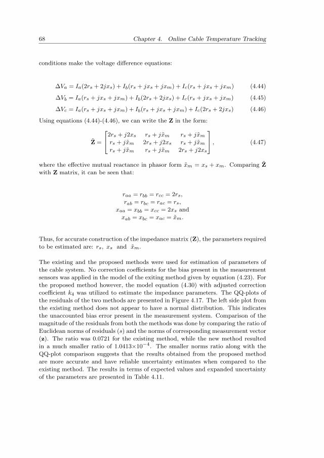
Chapter 4. Online Cable Temperature Tracking
conditions make the voltage difference equations:
∆Va = Ia(2rs + 2jxs) + Ib(rs + jxs + jxm) + Ic(rs + jxs + jxm) (4.44)
∆Vb = Ia(rs + jxs + jxm) + Ib(2rs + 2jxs) + Ic(rs + jxs + jxm) (4.45)
∆Vc = Ia(rs + jxs + jxm) + Ib(rs + jxs + jxm) + Ic(2rs + 2jxs) (4.46)
Using equations (4.44)-(4.46), we can write the Z in the form:
Z =
2rs + j2xs rs + jxm rs + jxmrs + jxm 2rs + j2xs rs + jxmrs + jxm rs + jxm 2rs + j2xs
, (4.47)
where the effective mutual reactance in phasor form xm = xs + xm. Comparing Z
with Z matrix, it can be seen that:
raa = rbb = rcc = 2rs,
rab = rbc = rac = rs,
xaa = xbb = xcc = 2xs and
xab = xbc = xac = xm.
Thus, for accurate construction of the impedance matrix (Z), the parameters required
to be estimated are: rs, xs and xm.
The existing and the proposed methods were used for estimation of parameters of
the cable system. No correction coefficients for the bias present in the measurement
sensors was applied in the model of the exiting method given by equation (4.23). For
the proposed method however, the model equation (4.30) with adjusted correction
coefficient k4 was utilized to estimate the impedance parameters. The QQ-plots of
the residuals of the two methods are presented in Figure 4.17. The left side plot from
the existing method does not appear to have a normal distribution. This indicates
the unaccounted bias error present in the measurement system. Comparison of the
magnitude of the residuals from both the methods was done by comparing the ratio of
Euclidean norms of residuals (s) and the norms of corresponding measurement vector
(z). The ratio was 0.0721 for the existing method, while the new method resulted
in a much smaller ratio of 1.0413×10⁻⁴. The smaller norms ratio along with the
QQ-plot comparison suggests that the results obtained from the proposed method
are more accurate and have reliable uncertainty estimates when compared to the
existing method. The results in terms of expected values and expanded uncertainty
of the parameters are presented in Table 4.11.
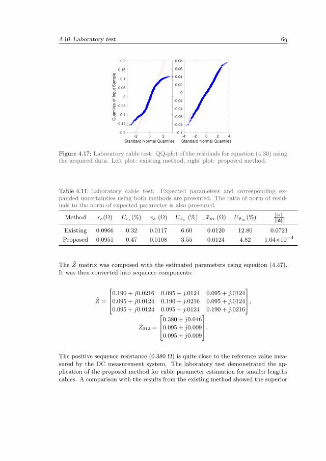
4.10 Laboratory test
-2 0 2
Standard Normal Quantiles
-0.2
-0.15
-0.1
-0.05
0
0.05
0.1
0.15
0.2
Qu
an
tile
s o
f In
pu
t S
am
ple
-4 -2 0 2 4
Standard Normal Quantiles
-0.1
-0.08
-0.06
-0.04
-0.02
0
0.02
0.04
0.06
0.08
Figure 4.17: Laboratory cable test: QQ-plot of the residuals for equation (4.30) usingthe acquired data. Left plot: existing method, right plot: proposed method.
Table 4.11: Laboratory cable test: Expected parameters and corresponding ex-panded uncertainties using both methods are presented. The ratio of norm of resid-uals to the norm of expected parameter is also presented.
Method rs(Ω) Urs(%) xs (Ω) Uxs (%) xm (Ω) Uxm(%)||s||||z||
Existing 0.0966 0.32 0.0117 6.60 0.0120 12.80 0.0721
Proposed 0.0951 0.47 0.0108 3.55 0.0124 4.82 1.04×10⁻⁴
The Z matrix was composed with the estimated parameters using equation (4.47).
It was then converted into sequence components:
Z =
0.190 + j0.0216 0.095 + j.0124 0.095 + j.0124
0.095 + j0.0124 0.190 + j.0216 0.095 + j.0124
0.095 + j0.0124 0.095 + j.0124 0.190 + j.0216
,
Z012 =
0.380 + j0.046
0.095 + j0.009
0.095 + j0.009
.
The positive sequence resistance (0.380 Ω) is quite close to the reference value mea-
sured by the DC measurement system. The laboratory test demonstrated the ap-
plication of the proposed method for cable parameter estimation for smaller lengths
cables. A comparison with the results from the existing method showed the superior
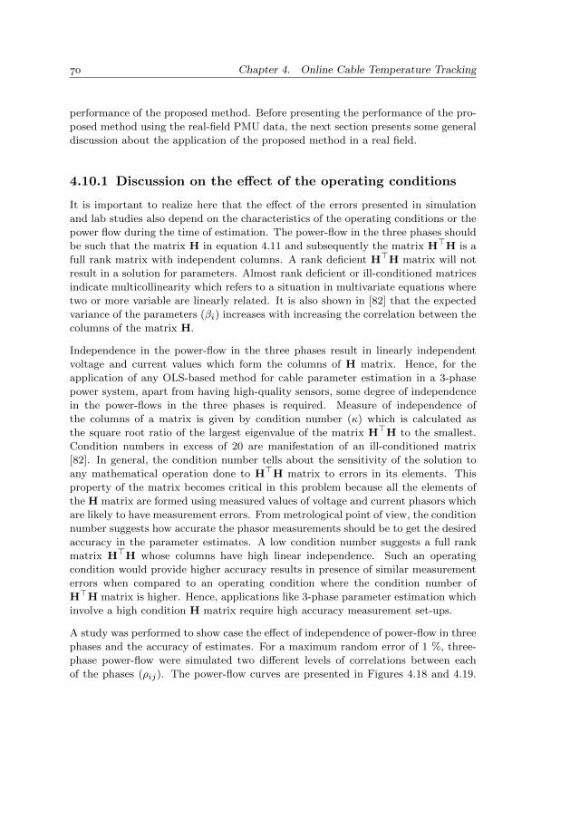
Chapter 4. Online Cable Temperature Tracking
performance of the proposed method. Before presenting the performance of the pro-
posed method using the real-field PMU data, the next section presents some general
discussion about the application of the proposed method in a real field.
4.10.1 Discussion on the effect of the operating conditions
It is important to realize here that the effect of the errors presented in simulation
and lab studies also depend on the characteristics of the operating conditions or the
power flow during the time of estimation. The power-flow in the three phases should
be such that the matrix H in equation 4.11 and subsequently the matrix H>H is a
full rank matrix with independent columns. A rank deficient H>H matrix will not
result in a solution for parameters. Almost rank deficient or ill-conditioned matrices
indicate multicollinearity which refers to a situation in multivariate equations where
two or more variable are linearly related. It is also shown in [82] that the expected
variance of the parameters (βi) increases with increasing the correlation between the
columns of the matrix H.
Independence in the power-flow in the three phases result in linearly independent
voltage and current values which form the columns of H matrix. Hence, for the
application of any OLS-based method for cable parameter estimation in a 3-phase
power system, apart from having high-quality sensors, some degree of independence
in the power-flows in the three phases is required. Measure of independence of
the columns of a matrix is given by condition number (κ) which is calculated as
the square root ratio of the largest eigenvalue of the matrix H>H to the smallest.
Condition numbers in excess of 20 are manifestation of an ill-conditioned matrix
[82]. In general, the condition number tells about the sensitivity of the solution to
any mathematical operation done to H>H matrix to errors in its elements. This
property of the matrix becomes critical in this problem because all the elements of
the H matrix are formed using measured values of voltage and current phasors which
are likely to have measurement errors. From metrological point of view, the condition
number suggests how accurate the phasor measurements should be to get the desired
accuracy in the parameter estimates. A low condition number suggests a full rank
matrix H>H whose columns have high linear independence. Such an operating
condition would provide higher accuracy results in presence of similar measurement
errors when compared to an operating condition where the condition number of
H>H matrix is higher. Hence, applications like 3-phase parameter estimation which
involve a high condition H matrix require high accuracy measurement set-ups.
A study was performed to show case the effect of independence of power-flow in three
phases and the accuracy of estimates. For a maximum random error of 1 %, three-
phase power-flow were simulated two different levels of correlations between each
of the phases (ρij). The power-flow curves are presented in Figures 4.18 and 4.19.
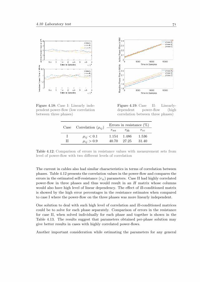
4.10 Laboratory test
Figure 4.18: Case I: Linearly inde-pendent power-flow (low correlationbetween three phases)
Figure 4.19: Case II: Linearly-dependent power-flow (highcorrelation between three phases)
Case Correlation (ρij)Errors in resistance (%)
raa rbb rcc
I ρij < 0.1 1.154 1.486 1.536
II ρij > 0.9 40.70 27.25 31.40
Table 4.12: Comparison of errors in resistance values with measurement sets fromlevel of power-flow with two different levels of correlation
The current in cables also had similar characteristics in terms of correlation between
phases. Table 4.12 presents the correlation values in the power-flow and compares the
errors in the estimated self-resistance (rii) parameters. Case II had highly correlated
power-flow in three phases and thus would result in an H matrix whose columns
would also have high level of linear dependency. The effect of ill-conditioned matrix
is showed by the high error percentages in the resistance estimates when compared
to case I where the power-flow on the three phases was more linearly independent.
One solution to deal with such high level of correlation and ill-conditioned matrices
could be to solve for each phase separately. Comparison of errors in the resistance
for case II, when solved individually for each phase and together is shown in the
Table 4.13. The results suggest that parameters obtained per-phase solution may
give better results in cases with highly correlated power-flows.
Another important consideration while estimating the parameters for any general
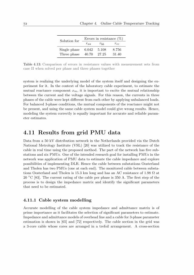
Chapter 4. Online Cable Temperature Tracking
Solution forErrors in resistance (%)
raa rbb rcc
Single phase 6.042 5.108 8.756
Three phase 40.70 27.25 31.40
Table 4.13: Comparison of errors in resistance values with measurement sets fromcase II when solved per phase and three phases together
system is realizing the underlying model of the system itself and designing the ex-
periment for it. In the context of the laboratory cable experiment, to estimate the
mutual reactance component xm, it is important to excite the mutual relationship
between the current and the voltage signals. For this reason, the currents in three
phases of the cable were kept different from each other by applying unbalanced loads.
For balanced 3-phase conditions, the mutual components of the reactance might not
be present, and using the same cable system model could give wrong results. Hence,
modeling the system correctly is equally important for accurate and reliable param-
eter estimates.
4.11 Results from grid PMU data
Data from a 50 kV distribution network in the Netherlands provided via the Dutch
National Metrology Institute (VSL) [20] was utilized to track the resistance of the
cable in real time using the proposed method. The part of the network has five sub-
stations and six PMUs. One of the intended research goal for installing PMUs in the
network was application of PMU data to estimate the cable impedance and explore
possibilities of implementing DLR. Hence the cable between substations Oosterland
and Tholen has two PMUs (one at each end). The monitored cable between substa-
tions Oosterland and Tholen is 15.3 km long and has an AC resistance of 1.98 Ω at
20 C [83]. The current rating of the cable per phase is 350 A. The first step of the
process is to design the impedance matrix and identify the significant parameters
that need to be estimated.
4.11.1 Cable system modelling
Accurate modelling of the cable system impedance and admittance matrix is of
prime importance as it facilitates the selection of significant parameters to estimate.
Impedance and admittance models of overhead line and a cable for 3-phase parameter
estimation is shown in [65] and [72] respectively. The cable section in the grid was
a 3-core cable whose cores are arranged in a trefoil arrangement. A cross-section
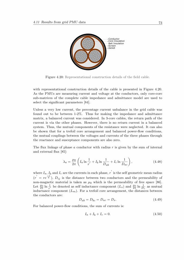
4.11 Results from grid PMU data
ConductorCore InsulationBelt InsulationScreenJacket
Figure 4.20: Representational construction details of the field cable.
with representational construction details of the cable is presented in Figure 4.20.
As the PMUs are measuring current and voltage at the conductors, only core-core
sub-matrices of the complete cable impedance and admittance model are used to
select the significant parameters [84].
Unless a very low current, the percentage current unbalance in the grid cable was
found out to be between 1-2%. Thus for making the impedance and admittance
matrix, a balanced current was considered. In 3-core cables, the return path of the
current is via the other phases. However, there is no return current in a balanced
system. Thus, the mutual components of the resistance were neglected. It can also
be shown that for a trefoil core arrangement and balanced power-flow conditions,
the mutual couplings between the voltages and currents of the three phases through
the reactance and susceptance components are also zero.
The flux linkage of phase a conductor with radius r is given by the sum of internal
and external flux [85]:
λa =µ0
2π
(Ia ln
1
r′ + Ib ln
1
Dab+ Ic ln
1
Dac
), (4.48)
where Ia, Ib and Ic are the currents in each phase, r′
is the self geometric mean radius
(r′
= re−14 ), Dij is the distance between two conductors and the permeability of
non-magnetic material is taken as µ0 which is the permeability of free space [86].
Let µ02π ln 1
r′be denoted as self inductance component (Ls) and µ0
2π ln 1Ds
as mutual
inductance component (Lm). For a trefoil core arrangement, the distances between
the conductors are:
Dab = Dbc = Dac = Ds. (4.49)
For balanced power-flow conditions, the sum of currents is:
Ia + Ib + Ic = 0. (4.50)

Chapter 4. Online Cable Temperature Tracking
Using equations 4.48, 4.49 and 4.50, it can be shown that:λaλbλc
=
Ls − Lm 0 0
0 Ls − Lm 0
0 0 Ls − Lm
IaIbIc
, (4.51)
where
Ls − Lm =µ0
2πlnDs
r′ . (4.52)
Thus there is no off-diagonal element in the inductance matrix for a trefoil cable
in the condition of balanced power-flow. Thus the impedance matrix of the cable
system does not have any off-diagonal elements.
Similarly it can be shown that the off-diagonal elements of the admittance matrix
are also zero for a trefoil cable carrying balanced current. For a system of three
conductors carrying charge q coulombs/meter each, the relationship between the
charge and the voltages can be written in form [85]:
Vab =1
2πεi
(qa ln
Dabr
+ qb lnr
Dab+ qc ln
DbcDab
)(4.53)
where εi is the effective electric permittivity insulation between the core and jacket
[84]. The conductivity of the insulation is very small and is considered zero [87].
Considering Dab = Dbc = Dac = Ds:
Vab =1
2πεi
(qa ln
Dsr
+ qb lnr
Ds
). (4.54)
Similarly,
Vac =1
2πεi
(qa ln
Dsr
+ qc lnr
Ds
). (4.55)
Using the balanced power-flow condition, qa + qb + qc = 0,
Vab + Vac =1
2πεi
(2qa ln
Dsr− qa ln
r
Ds
). (4.56)
For a three phase network it can be shown that, Vab + Vac = 3Van, where Van is the
voltage of phase a with respect to the neutral. Further simplification of (4.56) leads
to the result for phase a:
3Van =1
2πεi3qa ln
Dsr
(4.57)
and the charge and voltage relation using the capacitance matrix can be written
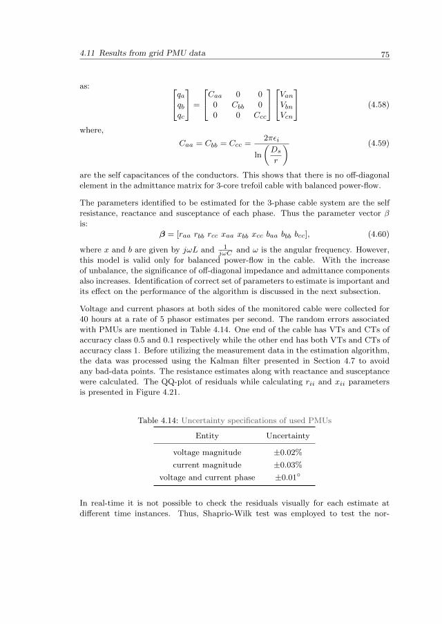
4.11 Results from grid PMU data
as: qaqbqc
=
Caa 0 0
0 Cbb 0
0 0 Ccc
VanVbnVcn
(4.58)
where,
Caa = Cbb = Ccc =2πεi
ln
(Dsr
) (4.59)
are the self capacitances of the conductors. This shows that there is no off-diagonal
element in the admittance matrix for 3-core trefoil cable with balanced power-flow.
The parameters identified to be estimated for the 3-phase cable system are the self
resistance, reactance and susceptance of each phase. Thus the parameter vector β
is:
β = [raa rbb rcc xaa xbb xcc baa bbb bcc], (4.60)
where x and b are given by jωL and 1jωC and ω is the angular frequency. However,
this model is valid only for balanced power-flow in the cable. With the increase
of unbalance, the significance of off-diagonal impedance and admittance components
also increases. Identification of correct set of parameters to estimate is important and
its effect on the performance of the algorithm is discussed in the next subsection.
Voltage and current phasors at both sides of the monitored cable were collected for
40 hours at a rate of 5 phasor estimates per second. The random errors associated
with PMUs are mentioned in Table 4.14. One end of the cable has VTs and CTs of
accuracy class 0.5 and 0.1 respectively while the other end has both VTs and CTs of
accuracy class 1. Before utilizing the measurement data in the estimation algorithm,
the data was processed using the Kalman filter presented in Section 4.7 to avoid
any bad-data points. The resistance estimates along with reactance and susceptance
were calculated. The QQ-plot of residuals while calculating rii and xii parameters
is presented in Figure 4.21.
Table 4.14: Uncertainty specifications of used PMUs
Entity Uncertainty
voltage magnitude ±0.02%
current magnitude ±0.03%
voltage and current phase ±0.01
In real-time it is not possible to check the residuals visually for each estimate at
different time instances. Thus, Shaprio-Wilk test was employed to test the nor-
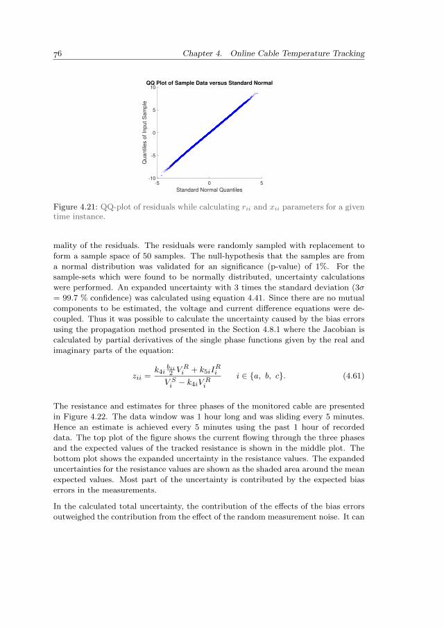
Chapter 4. Online Cable Temperature Tracking
-5 0 5
Standard Normal Quantiles
-10
-5
0
5
10
Quantile
s o
f In
put S
am
ple
QQ Plot of Sample Data versus Standard Normal
Figure 4.21: QQ-plot of residuals while calculating rii and xii parameters for a giventime instance.
mality of the residuals. The residuals were randomly sampled with replacement to
form a sample space of 50 samples. The null-hypothesis that the samples are from
a normal distribution was validated for an significance (p-value) of 1%. For the
sample-sets which were found to be normally distributed, uncertainty calculations
were performed. An expanded uncertainty with 3 times the standard deviation (3σ
= 99.7 % confidence) was calculated using equation 4.41. Since there are no mutual
components to be estimated, the voltage and current difference equations were de-
coupled. Thus it was possible to calculate the uncertainty caused by the bias errors
using the propagation method presented in the Section 4.8.1 where the Jacobian is
calculated by partial derivatives of the single phase functions given by the real and
imaginary parts of the equation:
zii =k4i
bii2 V
Ri + k5iI
Ri
V Si − k4iVRi
i ∈ a, b, c. (4.61)
The resistance and estimates for three phases of the monitored cable are presented
in Figure 4.22. The data window was 1 hour long and was sliding every 5 minutes.
Hence an estimate is achieved every 5 minutes using the past 1 hour of recorded
data. The top plot of the figure shows the current flowing through the three phases
and the expected values of the tracked resistance is shown in the middle plot. The
bottom plot shows the expanded uncertainty in the resistance values. The expanded
uncertainties for the resistance values are shown as the shaded area around the mean
expected values. Most part of the uncertainty is contributed by the expected bias
errors in the measurements.
In the calculated total uncertainty, the contribution of the effects of the bias errors
outweighed the contribution from the effect of the random measurement noise. It can
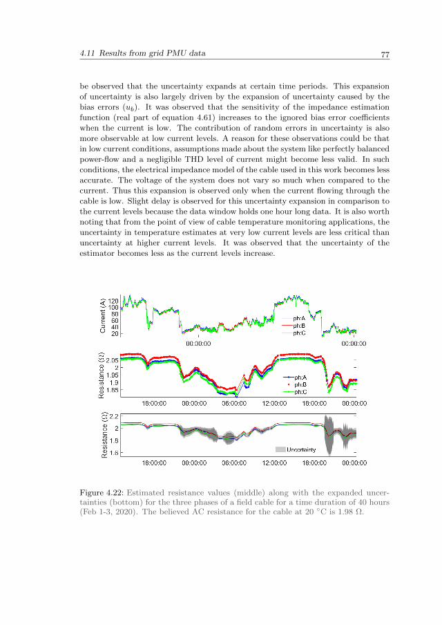
4.11 Results from grid PMU data
be observed that the uncertainty expands at certain time periods. This expansion
of uncertainty is also largely driven by the expansion of uncertainty caused by the
bias errors (ub). It was observed that the sensitivity of the impedance estimation
function (real part of equation 4.61) increases to the ignored bias error coefficients
when the current is low. The contribution of random errors in uncertainty is also
more observable at low current levels. A reason for these observations could be that
in low current conditions, assumptions made about the system like perfectly balanced
power-flow and a negligible THD level of current might become less valid. In such
conditions, the electrical impedance model of the cable used in this work becomes less
accurate. The voltage of the system does not vary so much when compared to the
current. Thus this expansion is observed only when the current flowing through the
cable is low. Slight delay is observed for this uncertainty expansion in comparison to
the current levels because the data window holds one hour long data. It is also worth
noting that from the point of view of cable temperature monitoring applications, the
uncertainty in temperature estimates at very low current levels are less critical than
uncertainty at higher current levels. It was observed that the uncertainty of the
estimator becomes less as the current levels increase.
Figure 4.22: Estimated resistance values (middle) along with the expanded uncer-tainties (bottom) for the three phases of a field cable for a time duration of 40 hours(Feb 1-3, 2020). The believed AC resistance for the cable at 20 C is 1.98 Ω.
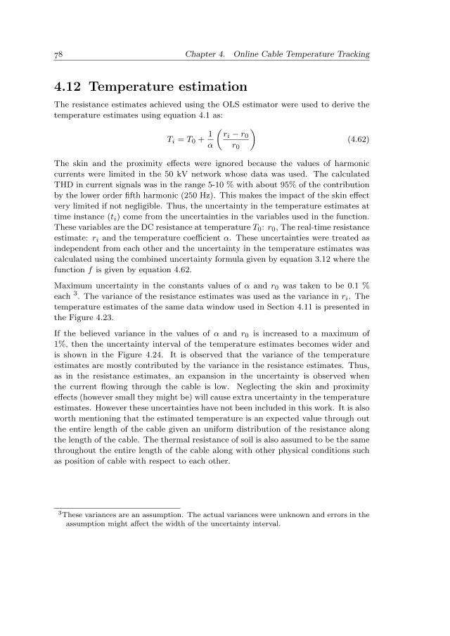
Chapter 4. Online Cable Temperature Tracking
4.12 Temperature estimationThe resistance estimates achieved using the OLS estimator were used to derive the
temperature estimates using equation 4.1 as:
Ti = T0 +1
α
(ri − r0r0
)(4.62)
The skin and the proximity effects were ignored because the values of harmonic
currents were limited in the 50 kV network whose data was used. The calculated
THD in current signals was in the range 5-10 % with about 95% of the contribution
by the lower order fifth harmonic (250 Hz). This makes the impact of the skin effect
very limited if not negligible. Thus, the uncertainty in the temperature estimates at
time instance (ti) come from the uncertainties in the variables used in the function.
These variables are the DC resistance at temperature T0: r0, The real-time resistance
estimate: ri and the temperature coefficient α. These uncertainties were treated as
independent from each other and the uncertainty in the temperature estimates was
calculated using the combined uncertainty formula given by equation 3.12 where the
function f is given by equation 4.62.
Maximum uncertainty in the constants values of α and r0 was taken to be 0.1 %
each 3. The variance of the resistance estimates was used as the variance in ri. The
temperature estimates of the same data window used in Section 4.11 is presented in
the Figure 4.23.
If the believed variance in the values of α and r0 is increased to a maximum of
1%, then the uncertainty interval of the temperature estimates becomes wider and
is shown in the Figure 4.24. It is observed that the variance of the temperature
estimates are mostly contributed by the variance in the resistance estimates. Thus,
as in the resistance estimates, an expansion in the uncertainty is observed when
the current flowing through the cable is low. Neglecting the skin and proximity
effects (however small they might be) will cause extra uncertainty in the temperature
estimates. However these uncertainties have not been included in this work. It is also
worth mentioning that the estimated temperature is an expected value through out
the entire length of the cable given an uniform distribution of the resistance along
the length of the cable. The thermal resistance of soil is also assumed to be the same
throughout the entire length of the cable along with other physical conditions such
as position of cable with respect to each other.
3These variances are an assumption. The actual variances were unknown and errors in theassumption might affect the width of the uncertainty interval.
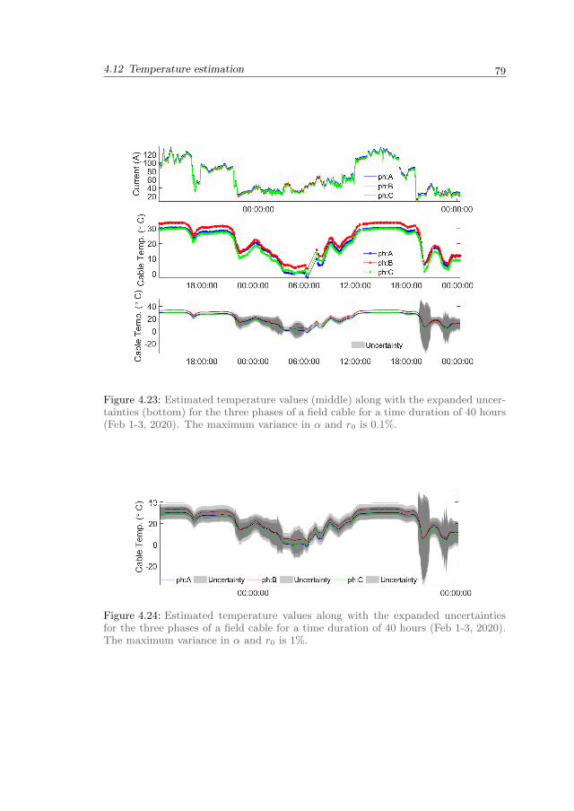
4.12 Temperature estimation
Figure 4.23: Estimated temperature values (middle) along with the expanded uncer-tainties (bottom) for the three phases of a field cable for a time duration of 40 hours(Feb 1-3, 2020). The maximum variance in α and r0 is 0.1%.
Figure 4.24: Estimated temperature values along with the expanded uncertaintiesfor the three phases of a field cable for a time duration of 40 hours (Feb 1-3, 2020).The maximum variance in α and r0 is 1%.

Chapter 4. Online Cable Temperature Tracking
4.13 ConclusionResistance of the cable is the most important parameter for tracking the cable tem-
perature in real-time. This chapter presented an improved method proposed to track
cable resistance accurately along with other line parameters in real-time. A review
about the drawbacks of the existing estimators was presented in the beginning. It
was then shown that the proposed estimator gives accurate estimates even in the
presence of bias errors in the measurements and is suitable for 3-phase applications.
Methods to estimate the total uncertainty in the resistance estimates considering
both random and bias errors were presented. Importance about modelling of the
system and choice of significant parameters was also discussed. The performance of
the proposed estimator was first presented for simulated data. A discussion about
the effect of operating conditions on the accuracy of the results was presented before
moving on to a laboratory test and application on data from the field PMUs. In the
end, temperature tracking was presented using the estimated resistance values.

5Cable Thermal Assessment
for Flexible Loading
Increasing the loadability of the cables while ensuring that the thermal limits are
not breached is key to implementing DLR. Cable thermal models give the system
equations to solve and predict the thermal response of the cables for different loading
scenario. Real-time cable temperature is necessary to initialize such system of equa-
tions. This chapter presents the TEE model and its application in cable’s thermal
assessment for flexible loading limits utilizing the real-time temperature values.
Parts of this chapter are based on:
R. S. Singh, J. F. G. Cobben, and V. Cuk, “PMU-based Cable Temperature Mon-
itoring and Thermal Assessment for Dynamic Line Rating”, IEEE Transactions on
Power Delivery, pp. 1–1, 2020.
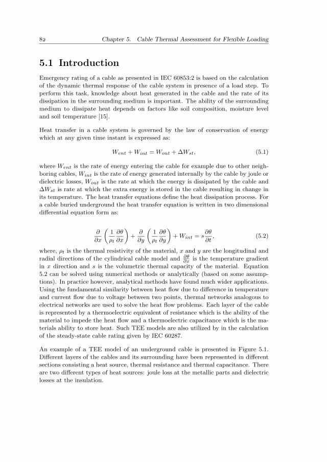
Chapter 5. Cable Thermal Assessment for Flexible Loading
5.1 Introduction
Emergency rating of a cable as presented in IEC 60853:2 is based on the calculation
of the dynamic thermal response of the cable system in presence of a load step. To
perform this task, knowledge about heat generated in the cable and the rate of its
dissipation in the surrounding medium is important. The ability of the surrounding
medium to dissipate heat depends on factors like soil composition, moisture level
and soil temperature [15].
Heat transfer in a cable system is governed by the law of conservation of energy
which at any given time instant is expressed as:
Went +Wint = Wout + ∆Wst, (5.1)
where Went is the rate of energy entering the cable for example due to other neigh-
boring cables, Wint is the rate of energy generated internally by the cable by joule or
dielectric losses, Wout is the rate at which the energy is dissipated by the cable and
∆Wst is rate at which the extra energy is stored in the cable resulting in change in
its temperature. The heat transfer equations define the heat dissipation process. For
a cable buried underground the heat transfer equation is written in two dimensional
differential equation form as:
∂
∂x
(1
ρt
∂θ
∂x
)+
∂
∂y
(1
ρt
∂θ
∂y
)+Wint = s
∂θ
∂t, (5.2)
where, ρt is the thermal resistivity of the material, x and y are the longitudinal and
radial directions of the cylindrical cable model and ∂θ∂x is the temperature gradient
in x direction and s is the volumetric thermal capacity of the material. Equation
5.2 can be solved using numerical methods or analytically (based on some assump-
tions). In practice however, analytical methods have found much wider applications.
Using the fundamental similarity between heat flow due to difference in temperature
and current flow due to voltage between two points, thermal networks analogous to
electrical networks are used to solve the heat flow problems. Each layer of the cable
is represented by a thermoelectric equivalent of resistance which is the ability of the
material to impede the heat flow and a thermoelectric capacitance which is the ma-
terials ability to store heat. Such TEE models are also utilized by in the calculation
of the steady-state cable rating given by IEC 60287.
An example of a TEE model of an underground cable is presented in Figure 5.1.
Different layers of the cables and its surrounding have been represented in different
sections consisting a heat source, thermal resistance and thermal capacitance. There
are two different types of heat sources: joule loss at the metallic parts and dielectric
losses at the insulation.
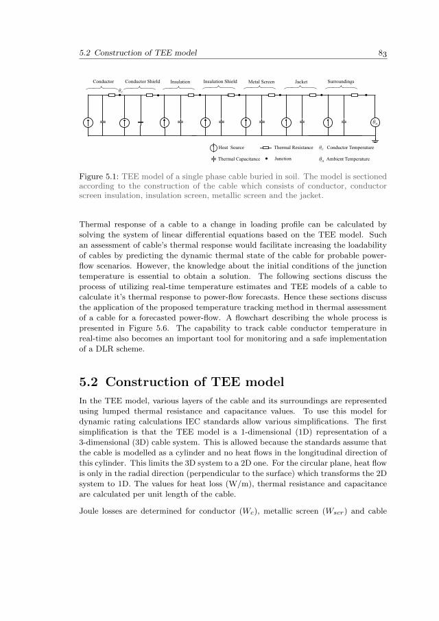
5.2 Construction of TEE model
Conductor Conductor Shield Insulation Insulation Shield Metal Screen Jacket Surroundings
Heat Source
Thermal Capacitance
Thermal Resistance
Junction
Conductor Temperature
Ambient Temperature
Figure 5.1: TEE model of a single phase cable buried in soil. The model is sectionedaccording to the construction of the cable which consists of conductor, conductorscreen insulation, insulation screen, metallic screen and the jacket.
Thermal response of a cable to a change in loading profile can be calculated by
solving the system of linear differential equations based on the TEE model. Such
an assessment of cable’s thermal response would facilitate increasing the loadability
of cables by predicting the dynamic thermal state of the cable for probable power-
flow scenarios. However, the knowledge about the initial conditions of the junction
temperature is essential to obtain a solution. The following sections discuss the
process of utilizing real-time temperature estimates and TEE models of a cable to
calculate it’s thermal response to power-flow forecasts. Hence these sections discuss
the application of the proposed temperature tracking method in thermal assessment
of a cable for a forecasted power-flow. A flowchart describing the whole process is
presented in Figure 5.6. The capability to track cable conductor temperature in
real-time also becomes an important tool for monitoring and a safe implementation
of a DLR scheme.
5.2 Construction of TEE model
In the TEE model, various layers of the cable and its surroundings are represented
using lumped thermal resistance and capacitance values. To use this model for
dynamic rating calculations IEC standards allow various simplifications. The first
simplification is that the TEE model is a 1-dimensional (1D) representation of a
3-dimensional (3D) cable system. This is allowed because the standards assume that
the cable is modelled as a cylinder and no heat flows in the longitudinal direction of
this cylinder. This limits the 3D system to a 2D one. For the circular plane, heat flow
is only in the radial direction (perpendicular to the surface) which transforms the 2D
system to 1D. The values for heat loss (W/m), thermal resistance and capacitance
are calculated per unit length of the cable.
Joule losses are determined for conductor (Wc), metallic screen (Wscr) and cable
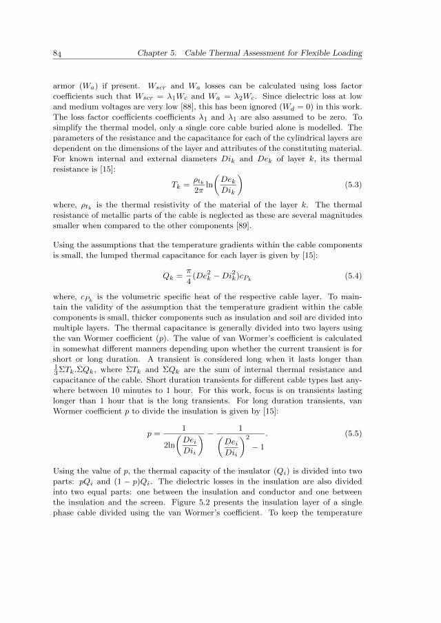
Chapter 5. Cable Thermal Assessment for Flexible Loading
armor (Wa) if present. Wscr and Wa losses can be calculated using loss factor
coefficients such that Wscr = λ1Wc and Wa = λ2Wc. Since dielectric loss at low
and medium voltages are very low [88], this has been ignored (Wd = 0) in this work.
The loss factor coefficients coefficients λ1 and λ1 are also assumed to be zero. To
simplify the thermal model, only a single core cable buried alone is modelled. The
parameters of the resistance and the capacitance for each of the cylindrical layers are
dependent on the dimensions of the layer and attributes of the constituting material.
For known internal and external diameters Dik and Dek of layer k, its thermal
resistance is [15]:
Tk =ρtk2π
ln
(DekDik
)(5.3)
where, ρtk is the thermal resistivity of the material of the layer k. The thermal
resistance of metallic parts of the cable is neglected as these are several magnitudes
smaller when compared to the other components [89].
Using the assumptions that the temperature gradients within the cable components
is small, the lumped thermal capacitance for each layer is given by [15]:
Qk =π
4(De2k −Di
2k)cPk (5.4)
where, cPk is the volumetric specific heat of the respective cable layer. To main-
tain the validity of the assumption that the temperature gradient within the cable
components is small, thicker components such as insulation and soil are divided into
multiple layers. The thermal capacitance is generally divided into two layers using
the van Wormer coefficient (p). The value of van Wormer’s coefficient is calculated
in somewhat different manners depending upon whether the current transient is for
short or long duration. A transient is considered long when it lasts longer than13ΣTk.ΣQk, where ΣTk and ΣQk are the sum of internal thermal resistance and
capacitance of the cable. Short duration transients for different cable types last any-
where between 10 minutes to 1 hour. For this work, focus is on transients lasting
longer than 1 hour that is the long transients. For long duration transients, van
Wormer coefficient p to divide the insulation is given by [15]:
p =1
2ln
(DeiDii
) − 1(DeiDii
)2
− 1
. (5.5)
Using the value of p, the thermal capacity of the insulator (Qi) is divided into two
parts: pQi and (1 − p)Qi. The dielectric losses in the insulation are also divided
into two equal parts: one between the insulation and conductor and one between
the insulation and the screen. Figure 5.2 presents the insulation layer of a single
phase cable divided using the van Wormer’s coefficient. To keep the temperature
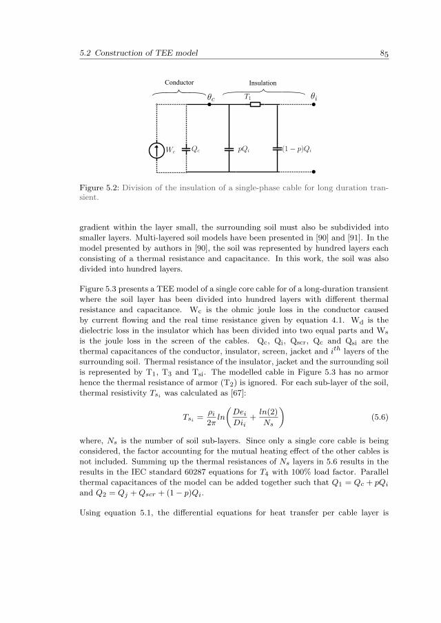
5.2 Construction of TEE model
Conductor Insulation
Figure 5.2: Division of the insulation of a single-phase cable for long duration tran-sient.
gradient within the layer small, the surrounding soil must also be subdivided into
smaller layers. Multi-layered soil models have been presented in [90] and [91]. In the
model presented by authors in [90], the soil was represented by hundred layers each
consisting of a thermal resistance and capacitance. In this work, the soil was also
divided into hundred layers.
Figure 5.3 presents a TEE model of a single core cable for of a long-duration transient
where the soil layer has been divided into hundred layers with different thermal
resistance and capacitance. Wc is the ohmic joule loss in the conductor caused
by current flowing and the real time resistance given by equation 4.1. Wd is the
dielectric loss in the insulator which has been divided into two equal parts and Ws
is the joule loss in the screen of the cables. Qc, Qi, Qscr, Qc and Qsi are the
thermal capacitances of the conductor, insulator, screen, jacket and ith layers of the
surrounding soil. Thermal resistance of the insulator, jacket and the surrounding soil
is represented by T1, T3 and Tsi. The modelled cable in Figure 5.3 has no armor
hence the thermal resistance of armor (T2) is ignored. For each sub-layer of the soil,
thermal resistivity Tsi was calculated as [67]:
Tsi =ρi2πln
(DeiDii
+ln(2)
Ns
)(5.6)
where, Ns is the number of soil sub-layers. Since only a single core cable is being
considered, the factor accounting for the mutual heating effect of the other cables is
not included. Summing up the thermal resistances of Ns layers in 5.6 results in the
results in the IEC standard 60287 equations for T4 with 100% load factor. Parallel
thermal capacitances of the model can be added together such that Q1 = Qc + pQiand Q2 = Qj +Qscr + (1− p)Qi.
Using equation 5.1, the differential equations for heat transfer per cable layer is
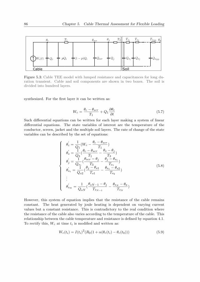
Chapter 5. Cable Thermal Assessment for Flexible Loading
Cable Soil
Figure 5.3: Cable TEE model with lumped resistance and capacitances for long du-ration transient. Cable and soil components are shown in two boxes. The soil isdivided into hundred layers.
synthesized. For the first layer it can be written as:
Wc =θc − θscr
T1+Q1
∂θc∂t
(5.7)
Such differential equations can be written for each layer making a system of linear
differential equations. The state variables of interest are the temperature of the
conductor, screen, jacket and the multiple soil layers. The rate of change of the state
variables can be described by the set of equations:
θ′c =
1
Q1(Wc −
θc − θscrT1
)
θ′s =
1
Q3(θc − θscr
T1−θs − θjT3
)
θ′
j =1
Qs1(θscr − θj
T3−θj − θs1Ts1
)
θ′s1 =
1
Qs2(θj − θs1Ts1
− θs1 − θs2Ts2
)
...
θ′sN =
1
QsN(θsN−1 − θjTsN−1
− θsN − θaTsN
)
(5.8)
However, this system of equation implies that the resistance of the cable remains
constant. The heat generated by joule heating is dependent on varying current
values but a constant resistance. This is contradictory to the real condition where
the resistance of the cable also varies according to the temperature of the cable. This
relationship between the cable temperature and resistance is defined by equation 4.1.
To rectify this, Wc at time ti is modified and written as:
Wc(ti) = I(ti)2(R0(1 + α(θc(ti)− θc(t0))) (5.9)
5.2 Construction of TEE model
where r0 and θc0 are the cable conductor resistance and temperature estimated by
the temperature monitoring method and used as the initial conditions for (5.8) at
time t0.
5.2.1 Transient thermal analysis
The modified system (equation 5.8) can be written using the state-space notation:
x′
s = Asxs + Bsus (5.10)
where the state vector xs is [θc θscr θj θs1 ... θsN ]T and conductor and ambient
temperatures (θc and θa) are known. The driving function (Bs) for a given time
period can be determined using the forecasts of the generation and load units. The
thermal response of the cable over the given period of time can be obtained by solving
the system of differential equations. The time domain solution of system given by
equation 5.10 is the superposition of natural and forced response of the system and
for a given period (t0-t1) can be given as:
xs(t) = PeΛtP−1xs(t0) + PeΛtBs
∫ t1
t0
e−Λtdt, (5.11)
where Λ is the diagonal matrix made of the eigenvalues of the matrix A and P is the
left eigenvector.
The initial value of the state vector (xs(t0)) can be calculated during the steady-state
conditions using the available real-time estimates of the conductor temperature. The
steady state condition of the system is reached when the junction temperatures are
not varying (x′s = 0). For practical applications a threshold of maximum rate of
variation can be utilized to define a pseudo steady-state condition. The steady-state
condition of the system can be represented as:
Wc −θc − θscr
T1= 0
θc − θscrT1
−θs − θjT3
= 0
θscr − θjT3
−θj − θs1Ts1
= 0
θj − θs1Ts1
− θs1 − θs2Ts2
= 0
...θsN−1 − θjTsN−1
− θsN − θaTsN
= 0
(5.12)
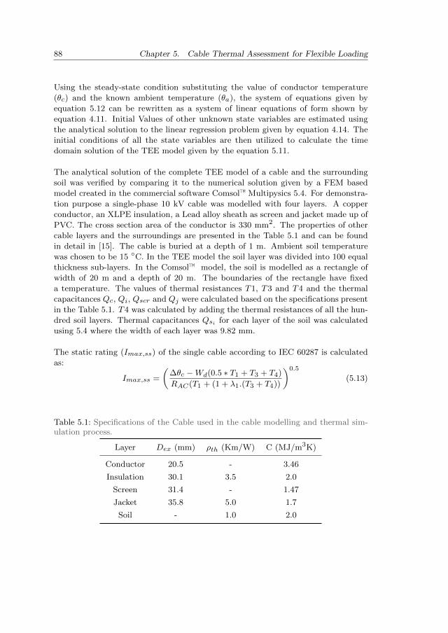
Chapter 5. Cable Thermal Assessment for Flexible Loading
Using the steady-state condition substituting the value of conductor temperature
(θc) and the known ambient temperature (θa), the system of equations given by
equation 5.12 can be rewritten as a system of linear equations of form shown by
equation 4.11. Initial Values of other unknown state variables are estimated using
the analytical solution to the linear regression problem given by equation 4.14. The
initial conditions of all the state variables are then utilized to calculate the time
domain solution of the TEE model given by the equation 5.11.
The analytical solution of the complete TEE model of a cable and the surrounding
soil was verified by comparing it to the numerical solution given by a FEM based
model created in the commercial software Comsol™ Multipysics 5.4. For demonstra-
tion purpose a single-phase 10 kV cable was modelled with four layers. A copper
conductor, an XLPE insulation, a Lead alloy sheath as screen and jacket made up of
PVC. The cross section area of the conductor is 330 mm2. The properties of other
cable layers and the surroundings are presented in the Table 5.1 and can be found
in detail in [15]. The cable is buried at a depth of 1 m. Ambient soil temperature
was chosen to be 15 C. In the TEE model the soil layer was divided into 100 equal
thickness sub-layers. In the Comsol™ model, the soil is modelled as a rectangle of
width of 20 m and a depth of 20 m. The boundaries of the rectangle have fixed
a temperature. The values of thermal resistances T1, T3 and T4 and the thermal
capacitances Qc, Qi, Qscr and Qj were calculated based on the specifications present
in the Table 5.1. T4 was calculated by adding the thermal resistances of all the hun-
dred soil layers. Thermal capacitances Qsi for each layer of the soil was calculated
using 5.4 where the width of each layer was 9.82 mm.
The static rating (Imax,ss) of the single cable according to IEC 60287 is calculated
as:
Imax,ss =
(∆θc −Wd(0.5 ∗ T1 + T3 + T4)
RAC(T1 + (1 + λ1.(T3 + T4))
)0.5
(5.13)
Table 5.1: Specifications of the Cable used in the cable modelling and thermal sim-ulation process.
Layer Dex (mm) ρth (Km/W) C (MJ/m3K)
Conductor 20.5 - 3.46
Insulation 30.1 3.5 2.0
Screen 31.4 - 1.47
Jacket 35.8 5.0 1.7
Soil - 1.0 2.0
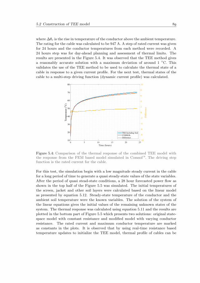
5.2 Construction of TEE model
where ∆θc is the rise in temperature of the conductor above the ambient temperature.
The rating for the cable was calculated to be 947 A. A step of rated current was given
for 24 hours and the conductor temperatures from each method were recorded. A
24 hours step was for day-ahead planning and assessment of thermal limits. The
results are presented in the Figure 5.4. It was observed that the TEE method gives
a reasonably accurate solution with a maximum deviation of around 1 C. This
validates the use of the TEE method to be used to calculate the thermal state of a
cable in response to a given current profile. For the next test, thermal states of the
cable to a multi-step driving function (dynamic current profile) was calculated.
0 5 10 15 20 25
Time (hours)
10
20
30
40
50
60
70
80
Tem
per
atu
re (
oC
)
-10
-8
-6
-4
-2
0
2
4
6
8
10
Dif
fere
nce
TEE Including Soil
COMSOL
Difference
Figure 5.4: Comparison of the thermal response of the combined TEE model withthe response from the FEM based model simulated in Comsol™. The driving stepfunction is the rated current for the cable.
For this test, the simulation begin with a low magnitude steady current in the cable
for a long period of time to generate a quasi steady-state values of the state variables.
After the period of quasi stead-state conditions, a 28 hour forecasted power flow as
shown in the top half of the Figure 5.5 was simulated. The initial temperatures of
the screen, jacket and other soil layers were calculated based on the linear model
as presented by equation 5.12. Steady-state temperature of the conductor and the
ambient soil temperature were the known variables. The solution of the system of
the linear equations gives the initial values of the remaining unknown states of the
system. The thermal response was calculated using equation 5.11 and the results are
plotted in the bottom part of Figure 5.5 which presents two solutions: original state-
space model with constant resistance and modified model with varying conductor
resistance. The rated current and maximum conductor temperature are marked
as constants in the plots. It is observed that by using real-time resistance based
temperature updates to initialize the TEE model, thermal profile of cables can be
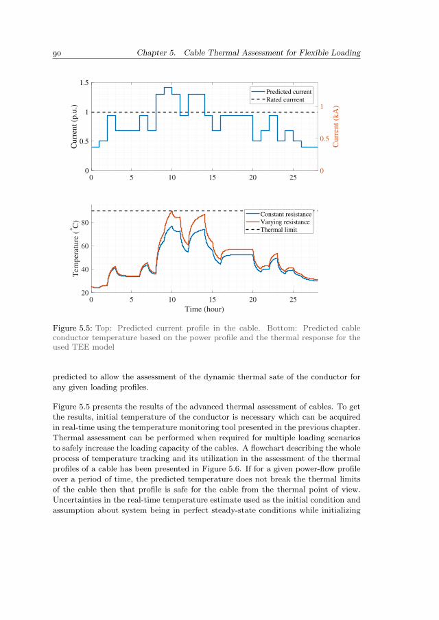
Chapter 5. Cable Thermal Assessment for Flexible Loading
0 5 10 15 20 250
0.5
1
1.5
Curr
ent
(p.u
.)
0
0.5
1
Curr
ent
(kA
)
Predicted current
Rated currrent
0 5 10 15 20 25
Time (hour)
20
40
60
80
Tem
per
ature
(°C
)
Constant resistance
Varying resistance
Thermal limit
Figure 5.5: Top: Predicted current profile in the cable. Bottom: Predicted cableconductor temperature based on the power profile and the thermal response for theused TEE model
predicted to allow the assessment of the dynamic thermal sate of the conductor for
any given loading profiles.
Figure 5.5 presents the results of the advanced thermal assessment of cables. To get
the results, initial temperature of the conductor is necessary which can be acquired
in real-time using the temperature monitoring tool presented in the previous chapter.
Thermal assessment can be performed when required for multiple loading scenarios
to safely increase the loading capacity of the cables. A flowchart describing the whole
process of temperature tracking and its utilization in the assessment of the thermal
profiles of a cable has been presented in Figure 5.6. If for a given power-flow profile
over a period of time, the predicted temperature does not break the thermal limits
of the cable then that profile is safe for the cable from the thermal point of view.
Uncertainties in the real-time temperature estimate used as the initial condition and
assumption about system being in perfect steady-state conditions while initializing
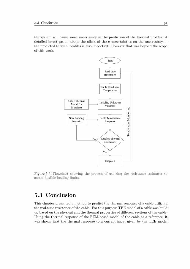
5.3 Conclusion
the system will cause some uncertainty in the prediction of the thermal profiles. A
detailed investigation about the affect of those uncertainties on the uncertainty in
the predicted thermal profiles is also important. However that was beyond the scope
of this work.
Start
Real-time
Resistance
Cable Conductor
Temperature
Initialize Unknown
Variables
Cable Temperature
Response
New Loading
Scenario
Cable Thermal
Model for
Transients
Tem
per
atu
re M
on
ito
rin
g
Satisfies Thermal
Constraint?
Dispatch
No
Yes
Figure 5.6: Flowchart showing the process of utilizing the resistance estimates toassess flexible loading limits.
5.3 Conclusion
This chapter presented a method to predict the thermal response of a cable utilizing
the real-time resistance of the cable. For this purpose TEE model of a cable was build
up based on the physical and the thermal properties of different sections of the cable.
Using the thermal response of the FEM-based model of the cable as a reference, it
was shown that the thermal response to a current input given by the TEE model

Chapter 5. Cable Thermal Assessment for Flexible Loading
is highly accurate and comparable to the response given by the FEM-based model.
The TEE model can be initialized in real-time using the temperature estimates given
by the PMU-based online temperature tracking tool allowing thermal assessment of
cables for dynamic loading forecasts.
Uncertainties in the temperature estimates and the assumption of the steady-state
conditions while initializing the system of equations however have not been con-
sidered while calculating the thermal response. The cable system chosen for the
demonstration purpose was a single core cable without any influence from the other
faces. Adding more phases in different geometric configurations will alter the TEE
model and its parameters and may add more uncertainties in the results. Thermal
resistivity of the soil was assumed to be same all along the length of the cable. A
more detailed investigation of the performance of the TEE model with different cable
systems without such assumptions could be a task for future.

6Aggregated Harmonic
model of Sub-grids.
Aggregated Norton’s equivalent models with parallel impedance and current injec-
tion at different harmonic frequencies are used to model the distribution grid and
connected installations in harmonic studies. Linear Norton’s equivalent models have
been adopted to represent the aggregated network and loads. However, due to the
increasing non-linear components in and connected to the grid, the uncertainty in pa-
rameters of such equivalent models becomes higher. This chapter presents two novel
methods to calculate the uncertainty of the measurement-based Norton’s equivalent
harmonic model of the distribution sub-grids as seen from the utility side at the
Point of Common Coupling (PCC).
Parts of this chapter are based on:
R. S. Singh, V. Cuk, and S. Cobben, “Measurement-based distribution grid harmonic
impedance models and their uncertainties”, Energies, vol. 13, no. 16, 2020, issn:
1996-1073. doi: 10.3390/en13164259. [Online]. Available: https://www.mdpi.com/
1996-1073/13/16/4259.
Chapter 6. Aggregated Harmonic model of Sub-grids.
6.1 Introduction
Inclusion of non-linear power electronics connected sources and loads along with
increasing amount of cables in medium and low voltage networks are causing a change
in the impedance of the distribution grids [93]. As more overhead lines are being
replaced by cables, the resonance frequency of the grid decreases due to the capacitive
effects of the cables. Increasing number of generation source and loads connected
via power electronics-based converters add capacitance to the network decreasing
it’s resonance frequency [93]. Harmonic current injections due to such sources and
loads result in voltage distortion at the PCC which propagates into the grid. For
analysis of harmonic distortion propagation and emissions, grid utilities are becoming
more interested in new methods for harmonic state estimation, harmonic source
localization and assessment of harmonic pollution contribution by the loads on the
customer side [18]. Aggregated sub-grid models are required to perform and improve
the accuracy of such investigations.
The impact of models of the loads in the distribution grid on harmonic impedance
seen by the transmission network was studied in [94]. The study showed that the MV
cables have a major influence on the harmonic impedance. It was concluded that it
is important to model the transformers and cables of the MV network. Harmonic
interaction between a large number of distributed power inverters in distribution
network was studied in [95]. The authors of [96] investigated in detail the effect of
modeling MV and LV network and components on the resonant frequencies and cor-
responding peaks. The effect of various load types on the relationship between grid
frequency and impedance values was presented. It was shown that the impedance
parameters should not be calculated from the power measurements at the fundamen-
tal frequency. A simulation study performed by authors in [97] showed a resonance
located at a very low frequency (500 Hz) in a residential grid which is caused by the
power-electronics equipment used in the households. The most prominent effect in
the impedance is due to the equivalent capacitance of the household appliances and
the PV inverters [95].
It is very challenging for a network operator to know the exact composition of loads
and sources connected to the grid at both MV and LV levels. Hence aggregated
harmonic load and the network impedance models are utilized in system studies.
These models are derived based on measurements and/or prior knowledge about the
grid. Loads in distribution grids are traditionally represented by the resistance and
the reactance values calculated based on the measured active (P) and reactive (Q)
power. These values however, cannot be used directly to represent them for harmonic
analysis.
Using a measurement-based method, harmonic grid impedance can be calculated
using voltage and current measurements at the PCC. Typically a measurement-based
6.2 Impedance estimation
distribution grid impedance estimation method uses harmonic phasors of current and
voltage signals to capture the response of the distribution grid before and after an
event. The measurement based methods are categorized into two types. Invasive
methods are the ones where disturbances are deliberately injected into grids to excite
current and voltage states at the PCC [98], [99], [100], [101] and [102]. Such methods
are mostly utilized to calculate the impedance seen by the PE connected source for
stability analysis and control purposes. In such cases, the source can inject desired
signals into the grid.
Non-invasive methods are those where naturally occurring grid events have been
used as sources of excitation in at the PCC to determine the grid impedance [28],
[72], [103], [104], [105], [106], [107]. These methods utilize events happening in
the region outside the sub-grid to be modelled as a source of perturbation in har-
monic voltages and measure the sub-grid’s response in terms of harmonic currents.
Non-invasive measurements are preferred for grid impedance estimation because in
invasive methods additional perturbation needs to be artificially injected into the
system to perform such analysis. Opportunities to artificially perturb the grid at
will and with desired magnitude and frequency spectrum could be rare or impossi-
ble. As suggested in [108], switching operations of transformers and capacitor banks
could result in rich voltage spectra which would cause a current response from the
sub-grid to be modelled. By measuring the change in the state of voltage at different
harmonics and the response in terms of change in the current harmonics, a simpli-
fied impedance based on the linear Norton’s or Thevenin’s equivalent model of the
distribution grid is achieved.
What is still missing in the measurement-based impedance estimation methods pre-
sented in the literature is the lack of the information over the uncertainty of the
estimated impedance values. As the modern distribution becomes more complex and
non-linear, uncertainty associated with the impedance parameters of the used linear
models must be evaluated. Authors in [109] presented a Monte Carlo simulation-
based method to determine the uncertainty of the impedance using probability dis-
tribution for resistive, inductive and capacitive parameters of various loads. How-
ever, these parameters were varied based on the prior knowledge of the customer
load profiles. Measurement-based methods do not need such prior knowledge and
assumptions and give results treating the unknown grid as a black-box. This chapter
presents two new methods to evaluate the uncertainty of the measurement-based
impedance parameters for a section of the distribution grid.
6.2 Impedance estimation
Norton’s equivalent circuit as shown by the Figure 6.1 is used to model the dis-
tribution grid which is modelled as an linear time invariant (LTI) system using a
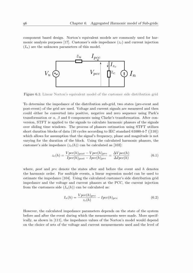
Chapter 6. Aggregated Harmonic model of Sub-grids.
component based design. Norton’s equivalent models are commonly used for har-
monic analysis purposes [17]. Customer’s side impedance (zc) and current injection
(In) are the unknown parameters of this model.
Figure 6.1: Linear Norton’s equivalent model of the customer side distribution grid
To determine the impedance of the distribution sub-grid, two states (pre-event and
post-event) of the grid are used. Voltage and current signals are measured and then
could either be converted into positive, negative and zero sequence using Park’s
transformation or α, β and 0 components using Clarke’s transformation. After con-
version, STFT is applied to the signals to calculate harmonic phasors of the signals
over sliding time windows. The process of phasors estimation using STFT utilizes
short duration blocks of data (10 cycles according to IEC standard 61000-4-7 ([110])
which allows for assumption that the signal’s frequency, phase and magnitude is not
varying for the duration of the block. Using the calculated harmonic phasors, the
customer’s side impedance (zc(h)) can be calculated as [103]:
zc(h) =V pcc(h)post − V pcc(h)pre
Ipcc(h)post − Ipcc(h)pre=
∆V pcc(h)
∆Ipcc(h)(6.1)
where, post and pre denote the states after and before the event and h denotes
the harmonic order. For multiple events, a linear regression model can be used to
estimate the impedance [104]. Using the calculated customer’s side distribution grid
impedance and the voltage and current phasors at the PCC, the current injection
from the customers side (In(h)) can be calculated as:
In(h) =V pcc(h)prezc(h)
− Ipcc(h)pre (6.2)
However, the calculated impedance parameters depends on the state of the system
before and after the event during which the measurements were made. More specif-
ically, as shown in [111], the impedance values of the Norton’s model would depend
on the choice of sets of the voltage and current measurements used and the level of
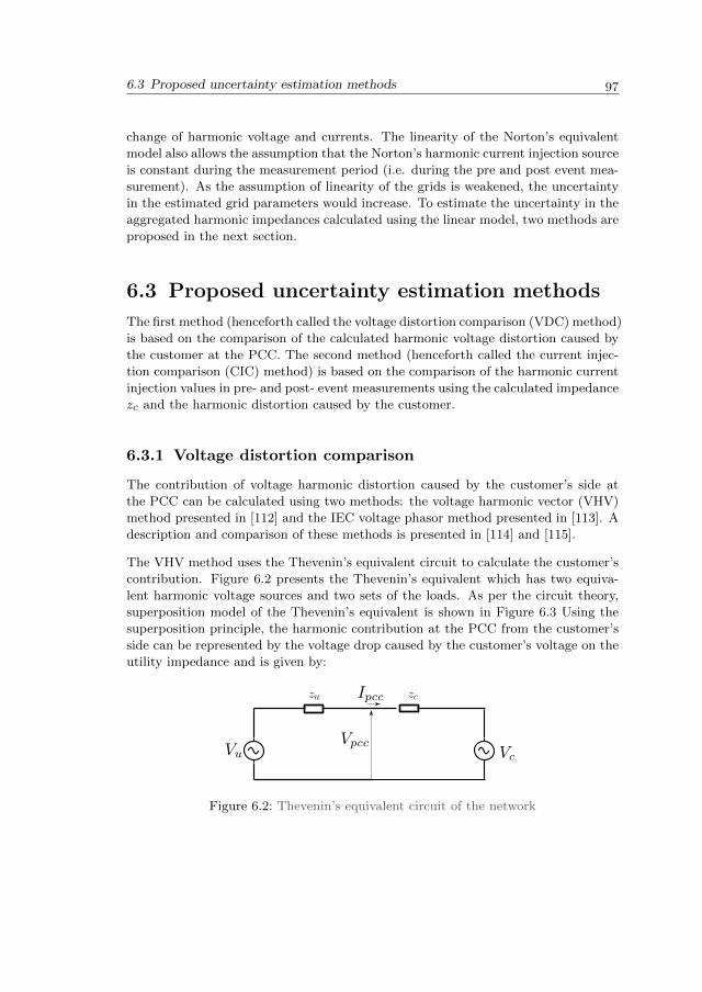
6.3 Proposed uncertainty estimation methods
change of harmonic voltage and currents. The linearity of the Norton’s equivalent
model also allows the assumption that the Norton’s harmonic current injection source
is constant during the measurement period (i.e. during the pre and post event mea-
surement). As the assumption of linearity of the grids is weakened, the uncertainty
in the estimated grid parameters would increase. To estimate the uncertainty in the
aggregated harmonic impedances calculated using the linear model, two methods are
proposed in the next section.
6.3 Proposed uncertainty estimation methods
The first method (henceforth called the voltage distortion comparison (VDC) method)
is based on the comparison of the calculated harmonic voltage distortion caused by
the customer at the PCC. The second method (henceforth called the current injec-
tion comparison (CIC) method) is based on the comparison of the harmonic current
injection values in pre- and post- event measurements using the calculated impedance
zc and the harmonic distortion caused by the customer.
6.3.1 Voltage distortion comparison
The contribution of voltage harmonic distortion caused by the customer’s side at
the PCC can be calculated using two methods: the voltage harmonic vector (VHV)
method presented in [112] and the IEC voltage phasor method presented in [113]. A
description and comparison of these methods is presented in [114] and [115].
The VHV method uses the Thevenin’s equivalent circuit to calculate the customer’s
contribution. Figure 6.2 presents the Thevenin’s equivalent which has two equiva-
lent harmonic voltage sources and two sets of the loads. As per the circuit theory,
superposition model of the Thevenin’s equivalent is shown in Figure 6.3 Using the
superposition principle, the harmonic contribution at the PCC from the customer’s
side can be represented by the voltage drop caused by the customer’s voltage on the
utility impedance and is given by:
Figure 6.2: Thevenin’s equivalent circuit of the network
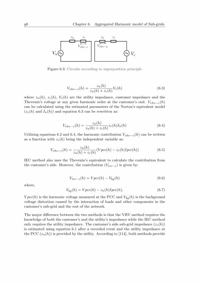
Chapter 6. Aggregated Harmonic model of Sub-grids.
Figure 6.3: Circuits according to superposition principle
Vvhv−c(h) =zu(h)
zu(h) + zc(h)Vc(h) (6.3)
where zu(h), zc(h), Vc(h) are the utility impedance, customer impedance and the
Thevenin’s voltage at any given harmonic order at the customer’s end. Vvhv−c(h)
can be calculated using the estimated parameters of the Norton’s equivalent model
(zc(h) and In(h)) and equation 6.3 can be rewritten as:
Vvhv−c(h) =zu(h)
zu(h) + zc(h)zc(h)In(h) (6.4)
Utilizing equations 6.2 and 6.4, the harmonic contribution Vvhv−c(h) can be written
as a function with zc(h) being the independent variable as:
Vvhv−c(h) =zu(h)
zu(h) + zc(h)(V pcc(h)− zc(h)Ipcc(h)) (6.5)
IEC method also uses the Thevenin’s equivalent to calculate the contribution from
the customer’s side. However, the contribution (Viec−c) is given by:
Viec−c(h) = V pcc(h)− Vbg(h) (6.6)
where,
Vbg(h) = V pcc(h)− zu(h)Ipcc(h), (6.7)
V pcc(h) is the harmonic voltage measured at the PCC and Vbg(h) is the background
voltage distortion caused by the interaction of loads and other components in the
customer’s sub-grid and the rest of the network.
The major difference between the two methods is that the VHV method requires the
knowledge of both the customer’s and the utility’s impedance while the IEC method
only requires the utility impedance. The customer’s side sub-grid impedance (zc(h))
is estimated using equation 6.1 after a recorded event and the utility impedance at
the PCC (zu(h)) is provided by the utility. According to [114], both methods provide

6.3 Proposed uncertainty estimation methods
qualitatively correct emission contribution while the authors in [115] propose that
for valid circuit model assumptions, the VHV method would give true harmonic
emission contribution.
The proposed method to find the uncertainty in the estimates zc(h) is based on
comparing the difference in the distortion contribution (emission) calculated by the
VHV and IEC methods. The difference (∆Vc(h)) calculated using the available zc(h)
and zu(h) values in equations 6.5 and 6.6 is given by:
∆Vc(h) = |Vvhv−c(h)− Viec−c(h)| (6.8)
∆Vc(h) is taken as the maximum error in the Vvhv−c(h) values (2 SDs from the cal-
culated Vvhv−c(h) values) given by equation 6.4 . It was also taken that the source
of this error is the uncertainty in the variable zc(h). The expected variance in zc(h)
is then calculated using the error propagation theory of complex numbers and func-
tions presented in the Section 3.2.2.
For any complex function
Y = f(X), (6.9)
the covariance matrix for the output (UY ) is calculated using the generalized law of
propagation of uncertainty and is given as:
UY = CXUXC>X , (6.10)
where, CX is the sensitivity matrix.
Using equation 6.10, the diagonal elements of the UY covariance matrix is populated
by the elements ∆Vc(h) for different harmonic frequencies. For each harmonic order,
the ∆Vc(h) value was taken as the maximum error in the Vvhv−c(h) value for a
normal distribution. The expected variance in the zc(h) is then calculated using
equation 6.10 as:
UX = C−1X UY (C>X)−1. (6.11)
Equation 6.11 gives the expected variance in the real and imaginary components of
the customer impedance. An expansion factor of 2 was multiplied to the standard
deviation (√
UX) to calculate the total uncertainty envelope in real and imaginary
parts of the calculated zc(h).
6.3.2 Current injection comparison
This method compares the harmonic current injection values calculated from pre-
and post-event voltage and current measurements at the PCC using the estimated
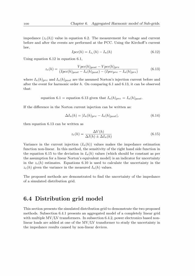
Chapter 6. Aggregated Harmonic model of Sub-grids.
impedance (zc(h)) value in equation 6.2. The measurement for voltage and current
before and after the events are performed at the PCC. Using the Kirchoff’s current
law,
Ipcc(h) = Izc(h)− In(h) (6.12)
Using equation 6.12 in equation 6.1,
zc(h) =V pcc(h)post − V pcc(h)pre
(Ipcc(h)post − In(h)post)− (Ipccpre − In(h)pre)(6.13)
where In(h)pre and In(h)post are the assumed Norton’s injection current before and
after the event for harmonic order h. On comparing 6.1 and 6.13, it can be observed
that:
equation 6.1 = equation 6.13 given that In(h)pre = In(h)post.
If the difference in the Norton current injection can be written as:
∆In(h) = |In(h)pre − In(h)post|, (6.14)
then equation 6.13 can be written as
zc(h) =∆V (h)
∆I(h)±∆In(h)(6.15)
Variance in the current injection (In(h)) values makes the impedance estimation
function non-linear. In this method, the sensitivity of the right hand side function in
the equation 6.15 to the deviation in In(h) values (which should be constant as per
the assumption for a linear Norton’s equivalent model) is an indicator for uncertainty
in the zc(h) estimates. Equations 6.10 is used to calculate the uncertainty in the
zc(h) given the variance in the measured In(h) values.
The proposed methods are demonstrated to find the uncertainty of the impedance
of a simulated distribution grid.
6.4 Distribution grid model
This section presents the simulated distribution grid to demonstrate the two proposed
methods. Subsection 6.4.1 presents an aggregated model of a completely linear grid
with multiple MV/LV transformers. In subsection 6.4.2, power electronics based non-
linear loads are added at one of the MV/LV transformer to study the uncertainty in
the impedance results caused by non-linear devices.
6.4 Distribution grid model
+
L_mot
+
R_LV2
+
C_LV2
+
C_MV
BRK_Trf2b
BRK_Trf1b
BRK_Trf2a
BRK_Trf1a
#1 #2
RLC
#1 #2
HV110kV
+
L_MV
HV MV
I_HV_Trf1
I_HV_Trf2
I_MV
Closed
Open
110/10 kV
110/10 kV
Figure 6.4: Distribution grid seen from the HV side
6.4.1 Aggregated linear model
To estimate the impedance of the distribution grid, a component-based system model
of the network was selected and modeled in PSCAD. Examples for modelling of dis-
tribution grid for harmonic analysis are presented in [116], [117]. Similar aggregated
models have been used by other researchers to represent the distribution grid for
harmonic studies [94], [118]. The distribution network was modeled as per the rec-
ommendations in [117]. The network specifications were based on a typical Dutch
MV-LV distribution grid [119]. The aggregated distribution grid model along with
two parallel transformers at the primary substation is shown in the Figure 6.4. L MV
and C MV are the inductance and capacitance of the MV/LV transformers and MV
cables. L mot is the aggregated inductance of motors in the LV grid, C LV2 is the
aggregated capacitance of the household devices and R LV2 is the resistance compo-
nents of the loads.
The voltage level of the HV grid was 110 kV and the primary substation has two 110-
10 kV transformers with nominal power rating (Snom) of 66 MVA. The upstream
grid was modelled as a voltage source. The short circuit level of the grid at the
110 kV side of the transformers was 3000 MVA thus making it a strong grid. The
transformers were modeled identically using the classical approach as described in
[120]. The positive sequence leakage reactance (XL) was set to be 0.1 p.u. and the
air core reactance was set twice of XL at 0.2 p.u. Magnetizing current (Im) was set
to be 2% of the nominal current. Copper loss (Pcu) and iron loss (Pfe) were set to be
0.01 and 0.002 p.u. respectively. Saturation curve of the transformer is dependent
on air core reactance, magnetizing current and the knee point voltage which was
set at 1.2 p.u of the base voltage. The complete set of parameters for the modelled
transformers are mentioned in the Table 6.1.
The aggregate load models of the network were modeled based on types mentioned in
[108] and [117]. The resistive part of the load was aggregated as constant impedance
load and the effective resistance was calculated based on the power consumption.
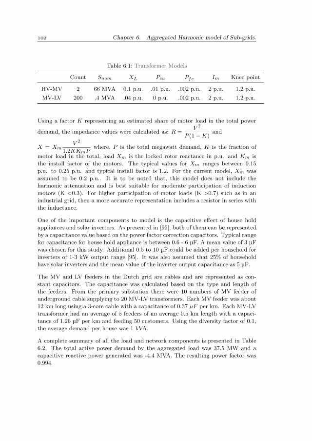
Chapter 6. Aggregated Harmonic model of Sub-grids.
Table 6.1: Transformer Models
Count Snom XL Pcu Pfe Im Knee point
HV-MV 2 66 MVA 0.1 p.u. .01 p.u. .002 p.u. 2 p.u. 1.2 p.u.
MV-LV 200 .4 MVA .04 p.u. 0 p.u. .002 p.u. 2 p.u. 1.2 p.u.
Using a factor K representing an estimated share of motor load in the total power
demand, the impedance values were calculated as: R =V 2
P (1−K)and
X = XmV 2
1.2KKmPwhere, P is the total megawatt demand, K is the fraction of
motor load in the total, load Xm is the locked rotor reactance in p.u. and Km is
the install factor of the motors. The typical values for Xm ranges between 0.15
p.u. to 0.25 p.u. and typical install factor is 1.2. For the current model, Xm was
assumed to be 0.2 p.u.. It is to be noted that, this model does not include the
harmonic attenuation and is best suitable for moderate participation of induction
motors (K <0.3). For higher participation of motor loads (K >0.7) such as in an
industrial grid, then a more accurate representation includes a resistor in series with
the inductance.
One of the important components to model is the capacitive effect of house hold
appliances and solar inverters. As presented in [95], both of them can be represented
by a capacitance value based on the power factor correction capacitors. Typical range
for capacitance for house hold appliance is between 0.6 - 6 µF. A mean value of 3 µF
was chosen for this study. Additional 0.5 to 10 µF could be added per household for
inverters of 1-3 kW output range [95]. It was also assumed that 25% of household
have solar inverters and the mean value of the inverter output capacitance as 5 µF.
The MV and LV feeders in the Dutch grid are cables and are represented as con-
stant capacitors. The capacitance was calculated based on the type and length of
the feeders. From the primary substation there were 10 numbers of MV feeder of
underground cable supplying to 20 MV-LV transformers. Each MV feeder was about
12 km long using a 3-core cable with a capacitance of 0.37 µF per km. Each MV-LV
transformer had an average of 5 feeders of an average 0.5 km length with a capaci-
tance of 1.26 µF per km and feeding 50 customers. Using the diversity factor of 0.1,
the average demand per house was 1 kVA.
A complete summary of all the load and network components is presented in Table
6.2. The total active power demand by the aggregated load was 37.5 MW and a
capacitive reactive power generated was -4.4 MVA. The resulting power factor was
0.994.
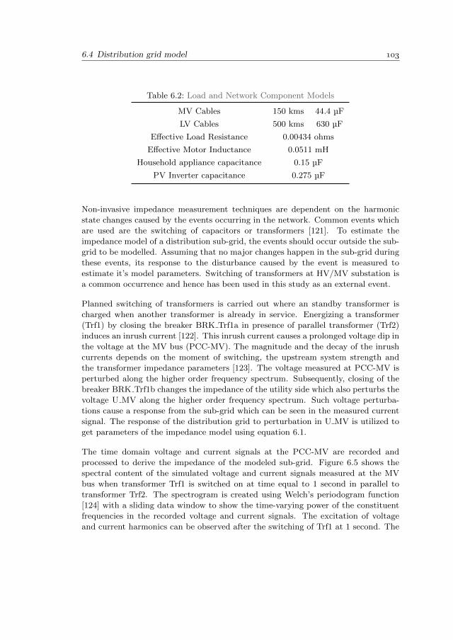
6.4 Distribution grid model
Table 6.2: Load and Network Component Models
MV Cables 150 kms 44.4 µF
LV Cables 500 kms 630 µF
Effective Load Resistance 0.00434 ohms
Effective Motor Inductance 0.0511 mH
Household appliance capacitance 0.15 µF
PV Inverter capacitance 0.275 µF
Non-invasive impedance measurement techniques are dependent on the harmonic
state changes caused by the events occurring in the network. Common events which
are used are the switching of capacitors or transformers [121]. To estimate the
impedance model of a distribution sub-grid, the events should occur outside the sub-
grid to be modelled. Assuming that no major changes happen in the sub-grid during
these events, its response to the disturbance caused by the event is measured to
estimate it’s model parameters. Switching of transformers at HV/MV substation is
a common occurrence and hence has been used in this study as an external event.
Planned switching of transformers is carried out where an standby transformer is
charged when another transformer is already in service. Energizing a transformer
(Trf1) by closing the breaker BRK Trf1a in presence of parallel transformer (Trf2)
induces an inrush current [122]. This inrush current causes a prolonged voltage dip in
the voltage at the MV bus (PCC-MV). The magnitude and the decay of the inrush
currents depends on the moment of switching, the upstream system strength and
the transformer impedance parameters [123]. The voltage measured at PCC-MV is
perturbed along the higher order frequency spectrum. Subsequently, closing of the
breaker BRK Trf1b changes the impedance of the utility side which also perturbs the
voltage U MV along the higher order frequency spectrum. Such voltage perturba-
tions cause a response from the sub-grid which can be seen in the measured current
signal. The response of the distribution grid to perturbation in U MV is utilized to
get parameters of the impedance model using equation 6.1.
The time domain voltage and current signals at the PCC-MV are recorded and
processed to derive the impedance of the modeled sub-grid. Figure 6.5 shows the
spectral content of the simulated voltage and current signals measured at the MV
bus when transformer Trf1 is switched on at time equal to 1 second in parallel to
transformer Trf2. The spectrogram is created using Welch’s periodogram function
[124] with a sliding data window to show the time-varying power of the constituent
frequencies in the recorded voltage and current signals. The excitation of voltage
and current harmonics can be observed after the switching of Trf1 at 1 second. The
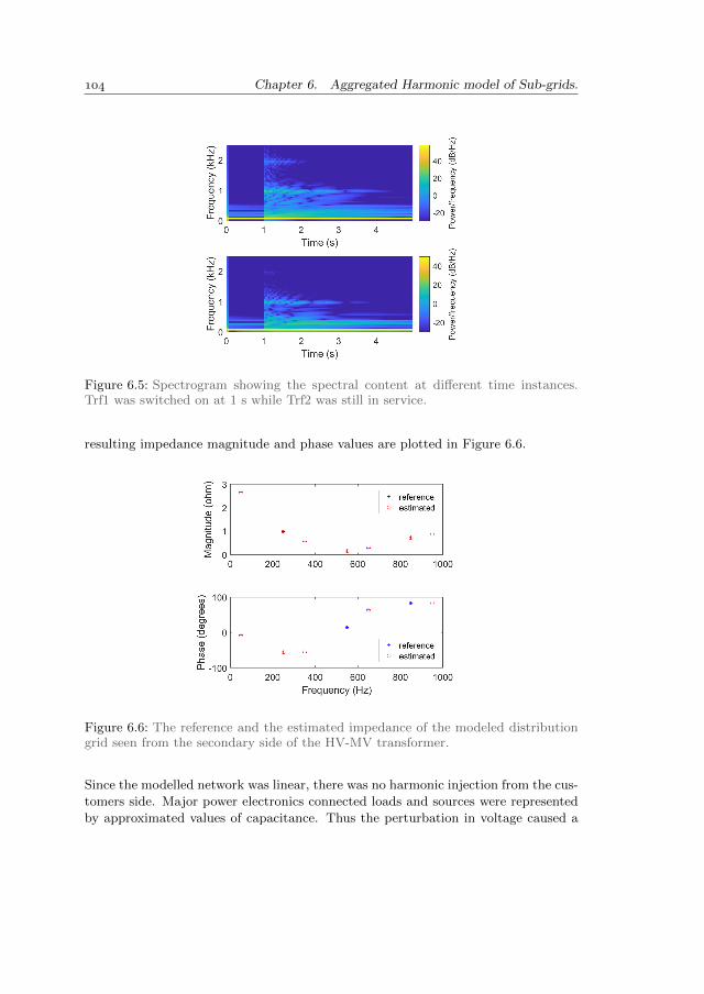
Chapter 6. Aggregated Harmonic model of Sub-grids.
Figure 6.5: Spectrogram showing the spectral content at different time instances.Trf1 was switched on at 1 s while Trf2 was still in service.
resulting impedance magnitude and phase values are plotted in Figure 6.6.
Figure 6.6: The reference and the estimated impedance of the modeled distributiongrid seen from the secondary side of the HV-MV transformer.
Since the modelled network was linear, there was no harmonic injection from the cus-
tomers side. Major power electronics connected loads and sources were represented
by approximated values of capacitance. Thus the perturbation in voltage caused a
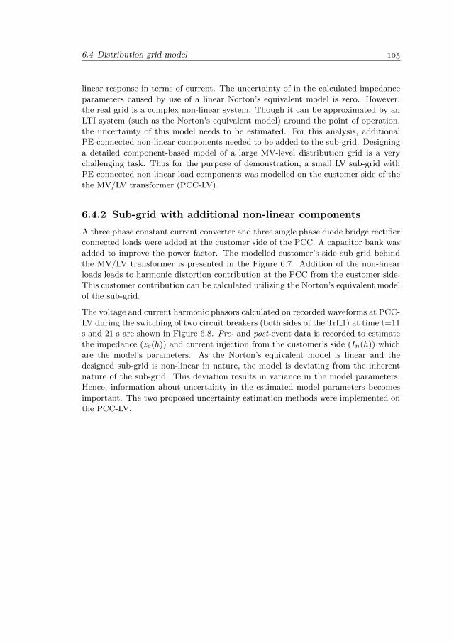
6.4 Distribution grid model
linear response in terms of current. The uncertainty of in the calculated impedance
parameters caused by use of a linear Norton’s equivalent model is zero. However,
the real grid is a complex non-linear system. Though it can be approximated by an
LTI system (such as the Norton’s equivalent model) around the point of operation,
the uncertainty of this model needs to be estimated. For this analysis, additional
PE-connected non-linear components needed to be added to the sub-grid. Designing
a detailed component-based model of a large MV-level distribution grid is a very
challenging task. Thus for the purpose of demonstration, a small LV sub-grid with
PE-connected non-linear load components was modelled on the customer side of the
the MV/LV transformer (PCC-LV).
6.4.2 Sub-grid with additional non-linear components
A three phase constant current converter and three single phase diode bridge rectifier
connected loads were added at the customer side of the PCC. A capacitor bank was
added to improve the power factor. The modelled customer’s side sub-grid behind
the MV/LV transformer is presented in the Figure 6.7. Addition of the non-linear
loads leads to harmonic distortion contribution at the PCC from the customer side.
This customer contribution can be calculated utilizing the Norton’s equivalent model
of the sub-grid.
The voltage and current harmonic phasors calculated on recorded waveforms at PCC-
LV during the switching of two circuit breakers (both sides of the Trf 1) at time t=11
s and 21 s are shown in Figure 6.8. Pre- and post-event data is recorded to estimate
the impedance (zc(h)) and current injection from the customer’s side (In(h)) which
are the model’s parameters. As the Norton’s equivalent model is linear and the
designed sub-grid is non-linear in nature, the model is deviating from the inherent
nature of the sub-grid. This deviation results in variance in the model parameters.
Hence, information about uncertainty in the estimated model parameters becomes
important. The two proposed uncertainty estimation methods were implemented on
the PCC-LV.
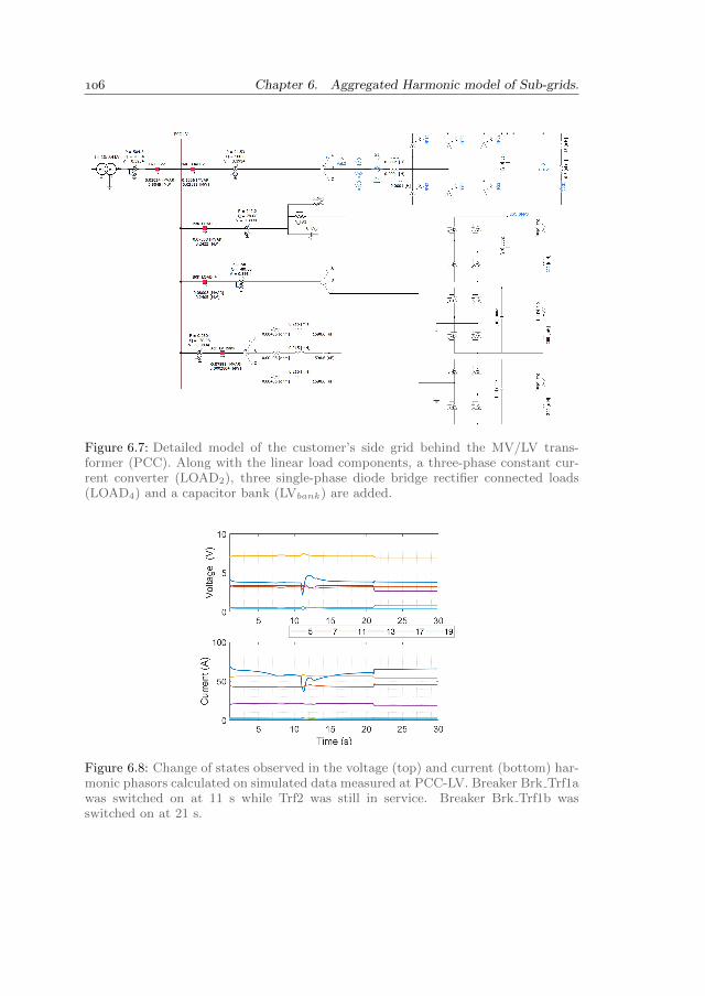
Chapter 6. Aggregated Harmonic model of Sub-grids.
Figure 6.7: Detailed model of the customer’s side grid behind the MV/LV trans-former (PCC). Along with the linear load components, a three-phase constant cur-rent converter (LOAD2), three single-phase diode bridge rectifier connected loads(LOAD4) and a capacitor bank (LVbank) are added.
Figure 6.8: Change of states observed in the voltage (top) and current (bottom) har-monic phasors calculated on simulated data measured at PCC-LV. Breaker Brk Trf1awas switched on at 11 s while Trf2 was still in service. Breaker Brk Trf1b wasswitched on at 21 s.
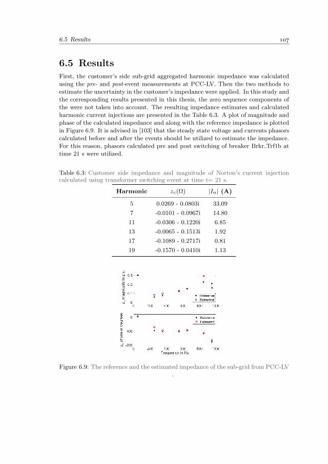
6.5 Results
6.5 ResultsFirst, the customer’s side sub-grid aggregated harmonic impedance was calculated
using the pre- and post-event measurements at PCC-LV. Then the two methods to
estimate the uncertainty in the customer’s impedance were applied. In this study and
the corresponding results presented in this thesis, the zero sequence components of
the were not taken into account. The resulting impedance estimates and calculated
harmonic current injections are presented in the Table 6.3. A plot of magnitude and
phase of the calculated impedance and along with the reference impedance is plotted
in Figure 6.9. It is advised in [103] that the steady state voltage and currents phasors
calculated before and after the events should be utilized to estimate the impedance.
For this reason, phasors calculated pre and post switching of breaker Brkr Trf1b at
time 21 s were utilized.
Table 6.3: Customer side impedance and magnitude of Norton’s current injectioncalculated using transformer switching event at time t= 21 s.
Harmonic zc(Ω) |In| (A)
5 0.0269 - 0.0803i 33.09
7 -0.0101 - 0.0967i 14.80
11 -0.0306 - 0.1220i 6.85
13 -0.0065 - 0.1513i 1.92
17 -0.1089 - 0.2717i 0.81
19 -0.1570 - 0.0410i 1.13
Figure 6.9: The reference and the estimated impedance of the sub-grid from PCC-LV.
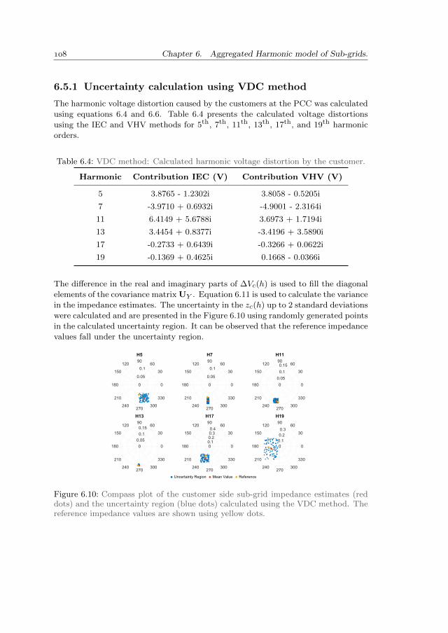
Chapter 6. Aggregated Harmonic model of Sub-grids.
6.5.1 Uncertainty calculation using VDC method
The harmonic voltage distortion caused by the customers at the PCC was calculated
using equations 6.4 and 6.6. Table 6.4 presents the calculated voltage distortions
using the IEC and VHV methods for 5th, 7th, 11th, 13th, 17th, and 19th harmonic
orders.
Table 6.4: VDC method: Calculated harmonic voltage distortion by the customer.
Harmonic Contribution IEC (V) Contribution VHV (V)
5 3.8765 - 1.2302i 3.8058 - 0.5205i
7 -3.9710 + 0.6932i -4.9001 - 2.3164i
11 6.4149 + 5.6788i 3.6973 + 1.7194i
13 3.4454 + 0.8377i -3.4196 + 3.5890i
17 -0.2733 + 0.6439i -0.3266 + 0.0622i
19 -0.1369 + 0.4625i 0.1668 - 0.0366i
The difference in the real and imaginary parts of ∆Vc(h) is used to fill the diagonal
elements of the covariance matrix UY . Equation 6.11 is used to calculate the variance
in the impedance estimates. The uncertainty in the zc(h) up to 2 standard deviations
were calculated and are presented in the Figure 6.10 using randomly generated points
in the calculated uncertainty region. It can be observed that the reference impedance
values fall under the uncertainty region.
0
30
6090
120
150
180
210
240270
300
330
0
0.05
0.1
H5
0
30
6090
120
150
180
210
240270
300
330
0
0.05
0.1
H7
0
30
6090
120
150
180
210
240270
300
330
0
0.05
0.1
0.15
H11
0
30
6090
120
150
180
210
240270
300
330
0
0.05
0.1
0.15
H13
0
30
6090
120
150
180
210
240270
300
330
00.10.20.30.4
H17
0
30
6090
120
150
180
210
240270
300
330
0
0.1
0.2
0.3
H19
Uncertainty Region Mean Value Reference
Figure 6.10: Compass plot of the customer side sub-grid impedance estimates (reddots) and the uncertainty region (blue dots) calculated using the VDC method. Thereference impedance values are shown using yellow dots.
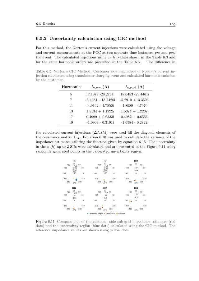
6.5 Results
6.5.2 Uncertainty calculation using CIC method
For this method, the Norton’s current injections were calculated using the voltage
and current measurements at the PCC at two separate time instance: pre and post
the event. The calculated injections using zc(h) values shown in the Table 6.3 and
for the same harmonic orders are presented in the Table 6.5. The difference in
Table 6.5: Norton’s CIC Method: Customer side magnitude of Norton’s current in-jection calculated using transformer charging event and calculated harmonic emissionby the customer.
Harmonic In,pre (A) In,post (A)
5 17.1979 -28.2764i 18.0453 -29.4461i
7 -5.4984 +13.7428i -5.2910 +13.3593i
11 -4.9142 - 4.7850i -4.8989 - 4.7976i
13 1.5134 + 1.1922i 1.5374 + 1.2237i
17 0.4999 + 0.6333i 0.4982 + 0.6556i
19 -1.0903 - 0.3191i -1.0584 - 0.2822i
the calculated current injections (∆In(h)) were used fill the diagonal elements of
the covariance matrix UX . Equation 6.10 was used to calculate the variance of the
impedance estimates utilizing the function given by equation 6.15. The uncertainty
in the zc(h) up to 2 SDs were calculated and are presented in the Figure 6.11 using
randomly generated points in the calculated uncertainty region.
0
30
6090
120
150
180
210
240270
300
330
00.020.040.060.080.1
H5
0
30
6090
120
150
180
210
240270
300
330
00.020.040.060.080.1
H7
0
30
6090
120
150
180
210
240270
300
330
0
0.05
0.1
H11
0
30
6090
120
150
180
210
240270
300
330
0
0.05
0.1
0.15
H13
0
30
6090
120
150
180
210
240270
300
330
0
0.1
0.2
0.3
H17
0
30
6090
120
150
180
210
240270
300
330
0
0.1
0.2
H19
Uncertainty Region Mean Value Reference
Figure 6.11: Compass plot of the customer side sub-grid impedance estimates (reddots) and the uncertainty region (blue dots) calculated using the CIC method. Thereference impedance values are shown using yellow dots.
Chapter 6. Aggregated Harmonic model of Sub-grids.
It was observed that the CIC method gives very narrow range of uncertainty when
compared to the VDC method. However, the uncertainty range given by the VDC
method includes the reference impedance at all frequencies. Another difference be-
tween the two methods is that the VDC method requires the knowledge of the util-
ity impedance at the PCC. The importance of the accuracy of the known utility
impedance was realized when both of the methods were applied to a transformers-
switching event data while diode rectifier and the converter were switched off (a linear
load condition). The CIC method gave zero variance. This was expected because for
a linear load, the current injection before and after the event was zero. The VDC
method however, gave a certain variance because of the difference in the harmonic
emission calculated by the IEC and VHV methods caused by the error in the known
utility impedance. Thus it can be said that the VDC method gives a more con-
servative (broad) uncertainty range while the CIC method gives a more optimistic
(narrow) uncertainty range around the estimated impedance results. Based on the
results it was observed that although being conservative, the VDC method performs
better for the uncertainty analysis of the aggregated harmonic impedance.
6.6 DiscussionThe presented simulation study is an ideal case scenario with no measurement errors.
In handling field data, it becomes critical to set a minimum threshold for event
detection at the harmonic frequencies. The bigger the threshold the less is the effect
of noise errors. As shown in [28], relative change in the harmonic current phasor
to the change in fundamental current phasor∆I(h)∆I1
can be used to set a minimum
threshold for an event to be considered suitable for data acquisition. The accuracy
of the sensors used for data acquisition is also crucial in determining the accuracy
of the estimates. However, the aim of this thesis was only to propose methods to
calculate the uncertainty of the impedance estimates in presence of non-linear grid
components.
The sub-grid impedance will vary as the loads vary. One of the limitations of the
measurement-based methods is that the calculated impedance using data from a sin-
gle event will only give a snapshot of the grid impedance for a particular set of loading
conditions and background harmonics. Several such measurement-based snapshots
may be required to get impedance results during different loading conditions of the
(sub)-grid. Another drawback is that the impedance values can only be calculated
up to the frequencies which are perturbed by the event. So impedance calculation
over a broad range of frequencies (especially for the higher frequencies) may not be
possible for some events.
Validation of the estimated impedance parameters of the Norton’s equivalent model
of a physical grid is a very challenging task. Actual impedance of the sub-grid is
6.7 Conclusion
unknown and the distortions in the voltage and current signals measured at the
PCC are a superimposed effect of emission from the customer’s side sub-grid and the
background distortion from the utility’s side grid. This is why the proposed methods
to estimate the uncertainty range of the calculated impedance values are important
for generating reliable models of the grid.
6.7 ConclusionThis chapter presented two methods to compute the uncertainty of the harmonic
impedance parameters in presence of non-linear loads. The voltage distortion com-
parison method compares the customer emissions (voltage distortion at PCC caused
by the customer’s side) calculated by the VHV and IEC methods. The IEC method
method uses only the utility impedance at harmonic frequencies to estimate the cus-
tomer’s emission whereas the VHV method utilized both utility’s and the customer’s
side impedance. As both the method should give quantitatively similar emission val-
ues, the difference in the emissions calculated using the two methods was believed to
caused by the variance in the utilized customer impedance. This uncertainty in the
customer impedance is then back-calculated using the theory of error propagation.
This method however, requires the knowledge of the utility harmonic impedance at
the PCC.
The current injection comparison method does not require the knowledge of the util-
ity side impedance and compares the value of calculated harmonic injection at times
before and after an event. For the used linear Norton’s equivalent model, harmonic
current injection should remain constant before and after the event. However due to
the non-linear characteristics of the grid, there is a difference in the injection currents
at time instants before and after the events. This deviation is considered as a source
of variance in the customer’s harmonic impedance values. This variance is calculated
utilizing the principles of error propagation.
It was found that the VDC method gives a more conservative yet reliable uncertainty
range, that is more likely to envelope the actual impedance values whereas the CIC
method gives very narrow uncertainty range that is less likely to envelope the ac-
tual impedance value. Thus the VDC method was found to perform better for the
uncertainty analysis of aggregated harmonic load impedance. This method could
be utilized to provide additional information about the uncertainty in the results
obtained while making aggregated Norton’s equivalent models of the distribution
(sub) grids. More information about the uncertainty in the grid model in presence of
non-linear devices would help understand the intrinsic nature of the aggregated load.
Multiple results resulting from measurements during different events and operating
conditions could be compared to select the result with least uncertainty.

7Conclusions, Contributions
and Recommendations
The objective of this thesis was to develop phasor measurement-based methods for
applications in assessment of flexible loading limits of cables and uncertainty calcu-
lations in aggregated harmonic grid-impedance values. To facilitate flexible loading
of the power cables, this thesis presented a method to estimate and track the tem-
perature of a cable section in real-time using PMU data. Then a method to utilize
the estimated temperature to predict the thermal response of a cable for a dynamic
power-flow profile was presented. In this way, real-time temperature estimates could
be utilized to calculate and assess the emergency rating of a cable section for a limited
period of time.
To achieve accurate and reliable aggregated harmonic impedance models of a dis-
tribution grid, this thesis presented two new methods to determine the uncertainty
in the harmonic impedance parameters that are calculated using the measurements.
In this way, the effect of non-linearity of the grid components on the traditional
Norton’s equivalent model could be evaluated.
This chapter presents the conclusions regarding the proposed methods followed by
contributions of the thesis and some recommendations.
Chapter 7. Conclusions, Contributions and Recommendations
7.1 Conclusions
7.1.1 Online cable temperature tracking
A new improved method was developed to track the resistance and thereafter the
temperature of a three-phase cable section using real-time synchronized phasor data
from PMUs. The tracker was so designed that it could provide highly-accurate
results for a three phase cable section even in the presence of bias errors in the
measurements.
The permissible error percentage in the resistance estimates required to estimate the
cable temperature in desired range is extremely low. For an uncertainty of 5 C in
temperature, the margin of uncertainty in the resistance estimates is about 2 % for
a cable with aluminium conductor. On the other hand, the presence of random and
bias errors in the measurements substantially increase the uncertainty in the results.
To reduce the impact of outliers in the measurements, an adaptive Kalman filter can
be used to detect and fill for outliers. A new system of multiple linear equations was
formulated using the measured current and voltage phasor data and significant cable
parameters. To reduce the effect of the bias errors in the measurements, additional
parameters were used in the equations to model the effect of bias errors. Investigation
for significant parameters allows us to remove insignificant parameters making the
solution of the system of equations more robust to random measurement errors.
Extra insignificant parameters result in ill condition matrices while solving the system
of equations. The system of linear equations was solved in a least-square sense to
achieve the cable resistance parameters. It was then observed that the operating
conditions during which the grid measurements were performed also influence the
uncertainty in the estimates of resistance parameters. For instance, independence
in power-flow in the three phases is required to estimate the mutual components
of the cable impedance and admittance matrix. It was observed that higher level
of independence in the power-flow, results in better parameter estimates for a 3-
phase cable section. Knowledge about such factors while modelling the system and
selecting the data can help in achieving more reliable results.
Resistance and temperature of a cable are dynamic parameters changing in real-time.
A rolling-window of measured data was used to continuously track the resistance
and give continuous temperature estimates. The true values of these parameters at
a particular time instant are unknown. Thus validating the achieved parameters and
calculating the estimation uncertainty is important.
In order to validate the requirements for an unbiased solution in a least-square sense,
normality of the residuals can be verified. A visual QQ-plot for a large sample size
and Shapiro–Wilk test for smaller data sets can be used to check the normality of the
residuals. A new method was presented to calculate the uncertainty of the estimated
resistance and temperature parameters. The principles of error propagation in a
7.1 Conclusions
multivariate function were used to calculate the variance and an extended uncertainty
interval. The calculated variance consisted of uncertainty caused by both random
and bias errors in the measurements.
A demonstration of the developed algorithm was presented using the PMU data from
a 50 kV section of a distribution grid. It was observed that the uncertainty in the
resistance and temperature estimates were of varying nature. The uncertainty was
higher at time periods with lower currents in the cable. This was due to an increase
in the uncertainty contribution from both random and bias errors is higher at low
currents. It is believed that, at low currents, the assumptions like perfect balanced
power flow and negligible THD level in the current which were made while building
the cable impedance matrix and hence used in the system of equations become less
valid. Thus at low current the model of the cable system used becomes inherently
less accurate. This however is not critical from this application’s point of view as
we need the highest accuracy in the estimates when the cable is operating at high
loading levels. During time periods with higher current levels, the uncertainty in the
estimated temperature values of a three-phase section of a cable was calculated to
be within 5 C with 99.7 % confidence (3 standard deviations).
7.1.2 Dynamic thermal assessment of cables
This thesis presented a method to utilize the real-time cable temperature values in
calculating the emergency rating of the cable by estimating its thermal response to a
specified dynamic load profile under certain ambient conditions for a limited period of
time. For this purpose, TEE model based on the physical and thermal properties of
various cable sections and the surrounding soil was built. The TEE model can also be
represented as a system of linear differential equations with the junction temperatures
of all the layers as the state variables. To maintain the validity of the assumption that
the thermal gradient within the cable sections remain small, thicker components such
as insulation and soil were divided into multiple sections. The surrounding soil for
example was divided into 100 sections. During a steady-state condition, the known
values of real-time conductor temperature estimates and ambient temperature can
be used to determine other unknown state variables (junction temperatures) of the
TEE model by solving the system of linear equations. Using the known state-variable
values as an initial-state, the system of linear differential equations can then be solved
for any predicted dynamic power-flow scenario.
The results achieved by solving the system of differential equations were compared
to the the thermal response of an FEM-based model of the same cable as a reference.
The solution of the TEE model was found to be accurate with a maximum deviation
of less than 2 C. Apart from this, variance in the tracked real-time cable conductor
temperature estimates which are used as the initial condition and variance in the
Chapter 7. Conclusions, Contributions and Recommendations
assumed (quasi)-steady state initial conditions will also contribute in the uncertainty
in the prediction of the thermal response. These calculations are not presented in
this thesis and should be investigated further. In addition to that, the cable system
used in this work had only of a single core cable for the purpose of demonstration. A
system with multi-core cable or multiple cables will also have multiple heat sources
(self and mutual). In such cases, a more complex TEE model would be required to
represent the three-phase cable system in different geometrical arrangements.
7.1.3 Aggregated harmonic impedance model of sub-grids
This thesis presented two novel methods to calculate the uncertainty in impedance
parameters of a distribution sub-grid seen from the utility side at the PCC.
The first method is based on voltage distortion comparison. The sub-grid’s contri-
bution in the voltage distortion at the PCC is calculated using two different meth-
ods (voltage harmonic vector (VHV) method and IEC recommended method). The
VHV method utilizes the known utility impedance and the estimated customer’s
impedance to calculate the customer’s contribution in voltage distortion. The IEC
method utilizes only the known utility side impedance to calculate the voltage distor-
tion at the PCC. Both methods provide qualitatively correct emission contributions.
The parameters used in both methods are same except the estimated value of the
customer harmonic impedance used only in the VHV method. The difference in the
voltage distortions calculated by the two methods is considered to be due to uncer-
tainty in the customer impedance. This uncertainty in the customer impedance is
then back-calculated using the principles of error propagation. A drawback of this
method is that it requires the knowledge of the utility impedance at the PCC.
The second method to calculate the uncertainty in impedance parameters is the
current injection comparison method which does not need the knowledge of the utility
side impedance. It is based on the condition that in linear Norton’s equivalent model,
the harmonic injection current at the PCC is unchanged before and after the events.
However, in presence of non-linear grid components, a variance in the harmonic
current injection values is observed after an event. This variance suggests an error
in the linear model and is utilized to calculate the uncertainty in the harmonic
impedance values using the principles of error propagation.
It was observed that the uncertainty calculated by the voltage distortion comparison
method is more reliable than the current injection comparison method. Utilizing this
method, uncertainty in the harmonic impedance parameters the Norton’s equivalent
models can be calculated. However, it is to be noted that no-measurement noise
were considered for this study. Presence of noise in the measurements would impose
additional challenge in terms of detection of the events. In such a case, the accuracy
of the sensors used for data acquisition is also critical in determining the accuracy of
7.2 Contributions
the estimates. The customer’s side sub-grid impedance will vary as the load varies
and the measurement-based impedance using data from a single event would only
give a snapshot of the grid impedance for a particular profile of loads in the sub-
grid and background harmonics at the PCC. Thus several such measurement-based
snapshots at various operating conditions would be required to get impedance values
during those conditions.
7.2 Contributions
The main contributions of this thesis are presented below:
• A new three-phase cable temperature tracking method. This method
does not employ any dedicated temperature sensor and uses current and voltage
phasors to track the temperature of a cable section in real-time. The improved
method takes into account the possible presence of bias errors in the phasor
measurements and reduces their impact on the accuracy of estimation results.
• A new method for uncertainty calculation in the cable resistance
parameters. For the first time, uncertainty was calculated for a three-phase
line parameter estimator. The contribution of the bias errors were included in
the uncertainty calculations.
• Guidelines for model validation and estimation result analysis. To
verify the various assumptions made during the modelling of the cable-system
and validate the system of equations used in the estimation process, various
guidelines were presented. For example the use of QQ-plot or Shapiro-Wilk
test to check the normality of the residuals of the least-square problem and the
sensitivity analysis to find the least significant parameters of the cable model.
• Assessment of thermal response of the cable. A method was presented
to utilize the real-time cable conductor temperature estimates to initialize a
system of linear differential equations given by the TEE model. After initial-
ization, it was shown that the thermal response of the cable can be calculated
for any dynamic power-flow forecast.
• Two new methods proposed to estimate the uncertainty in the cus-
tomer side sub-grid harmonic impedance. The methods were used to cal-
culate the uncertainty of the impedance-estimates which are calculated using
measurements from the grid. The methods could be utilized while calculating
the aggregated harmonic impedance to realize the uncertainty in the results.
Calculated impedance values with high uncertainty can then be discarded.
This can be helpful in maintaining reliable harmonic impedance models of the
modern grid with increasing share of non-linear components.
Chapter 7. Conclusions, Contributions and Recommendations
7.3 Recommendations
The work presented in this thesis can be improved and further research in these
areas can be performed in future based on the recommendations presented in this
section.
Cable temperature tracking and thermal assessment
• Validation using dedicated temperature sensors. Temperature estimates
achieved using the proposed method using the PMU-data could be compared
with real temperature measurements on the cable using dedicated temperature
sensors.
• Implementation of skin end proximity effect in the cable tempera-
ture model. Skin and proximity coefficients were assumed to be insignificant
and ignored while converting the real-time resistance estimates into temper-
ature values in equation 4.62. However further investigations could be done
to validate this claim. For this purpose, the effect of ignoring these coeffi-
cients on the uncertainty in the temperature estimates needs to be evaluated.
These evaluations can be carried our for various operating conditions in terms
of harmonic content in the current and physical dimensions of the cable. If
the uncertainty caused by ignoring these coefficients under certain operating
and physical conditions is higher than a minimum threshold, then it would be
recommended to include these coefficients in the model under those conditions.
• Effect of changing surroundings and cable conditions. In this thesis, the
soil surrounding the cable is considered to have the same physical and thermal
attributes across the length of the cable. Further research is recommended to
accommodate the changing effects of cable surroundings or localized conditions.
For example, a local section of the cable crossing riverbeds or other cables might
have a different thermal profile. Similarly cable conditions like joints with a
hot-spot would also significantly alter the thermal state of the cable at a local
level. The presented method uses the total resistance of the cable to calculate
the temperature of its conductor. However, hot-spots due to various reasons
could have a high regional resistance and hence can become the bottleneck while
deciding the loading limits. More knowledge about such bottlenecks could be
used to estimate the temperature of the critical hot-spots.
• TEE models for more complex 3-phase cable system. In this thesis the
thermal profile of the cables was simulated and validated using the TEE model
of a single-phase cable. Three-phase cable segments in different geometrical
arrangements would require a more complex TEE model. Thus, validation of
7.3 Recommendations
TEE models for three-phase cable-sections with different arrangements is also
important and needs to be investigated further.
• Uncertainty due to error in TEE model initialization. For initializa-
tion of the TEE model, during steady-state conditions, the system of linear
equations (5.12) is solved to get the initial values of all the state variables.
However, in practice such conditions are more likely to be quasi steady-state
and this could cause error in the initial states of the system. The propagation
of errors in the initial temperature of various layers of the cable to the final so-
lution could also be investigated. A maximum threshold to identify a suitable
steady-state condition could also be established for more accurate calculation
of the thermal response of the cables.
Aggregated harmonic impedance model
• The effect of the measurements errors. None of the literature reviewed
presented the uncertainty in the estimated impedance values. This thesis pre-
sented methods to estimate the uncertainty in the harmonic impedance values
caused by the non-linear nature of the loads. However, the effect of measure-
ment errors could increase these uncertainty limits. A practical measurement
experiment imposing grid events to a sub-grid with non-linear loads could give
more insights on the effect of such measurement errors on the overall uncer-
tainty in the impedance values.


AMeasurement Models for
Ordinary Least Square
A.1 Existing method
The complex equations 4.7 and 4.8 describing the nominal pi model and the phasormeasurements at two ends can be separated into real and imaginary components toform a set of 12 linear equations:
Re(∆Ia) = −1
2(baa Im(ΣVa) + bab Im(ΣVb) + bac Im(ΣVc)) (A.1)
Re(∆Ib) = −1
2(bab Im(ΣVa) + bbb Im(ΣVb) + bbc Im(ΣVc)) (A.2)
Re(∆Ic) = −1
2(bac Im(ΣVa) + bbc Im(ΣVb) + bcc Im(ΣVc)) (A.3)
Im(∆Ia) =1
2(baa Re(ΣVa) + bab Re(ΣVb) + bac Re(ΣVc)) (A.4)
Im(∆Ib) =1
2(bab Re(ΣVa) + bbb Re(ΣVb) + bbc Re(ΣVc)) (A.5)
Im(∆Ic) =1
2(bac Re(ΣVa) + bbc Re(ΣVb) + bcc Re(ΣVc)) (A.6)
Re(IRa ) = gaa Re(∆Va)− taa Im(∆Va) + gab Re(∆Vb)− tab Im(∆Vb) + gac Re(∆Vc)
−tac Im(∆Vc) +1
2(baa Im(V
Ra ) + bab Im(V
Rb ) + bac Im(V
Rc ))
(A.7)
Re(IRb ) = gab Re(∆Va)− tab Im(∆Va) + gbb Re(∆Vb)− tbb Im(∆Vb) + gbc Re(∆Vc)
−tbc Im(∆Vc) +1
2(bab Im(V
Ra ) + bbb Im(V
Rb ) + bbc Im(V
Rc ))
(A.8)
Re(IRc ) = gac Re(∆Va)− tac Im(∆Va) + gbc Re(∆Vb)− tbc Im(∆Vb) + gcc Re(∆Vc)
−tcc Im(∆Vc) +1
2(bac Im(V
Ra ) + bbc Im(V
Rb ) + bcc Im(V
Rc ))
(A.9)
Im(IRa ) = taa Re(∆Va) + gaa Im(∆Va) + tab Re(∆Vb)− gab Im(∆Vb) + tac Re(∆Vc)
−gac Im(∆Vc)−1
2(baa Re(V
Ra ) + bab Re(V
Rb ) + bac Re(V
Rc ))
(A.10)
Im(IRb ) = tab Re(∆Va) + gab Im(∆Va) + tbb Re(∆Vb)− gbb Im(∆Vb) + tbc Re(∆Vc)
−gbc Im(∆Vc)−1
2(bab Re(V
Ra ) + bbb Re(V
Rb ) + bbc Re(V
Rc ))
(A.11)
Chapter A. Measurement Models for Ordinary Least Square
Im(IRc ) = tac Re(∆Va) + gac Im(∆Va) + tbc Re(∆Vb)− gbc Im(∆Vb) + tcc Re(∆Vc)
−gcc Im(∆Vc)−1
2(bac Re(V
Ra ) + bbc Re(V
Rb ) + bcc Re(V
Rc ))
(A.12)
The unknown parameters vector β is written as:
β = [baa bbb bcc bab bac bbc gaa taa gbb tbb gcc tcc gab tab gac tac gbc tbc]> (A.13)
and the measurement vector (z) is given as:
z = [Re(∆Ib) Re(∆Ib) Re(∆Ib) Im(∆Ia) Im(∆Ib) Im(∆Ic) Re(IRa ) Re(I
Rb ) ...
Re(IRc ) Im(I
Ra ) Im(I
Rb ) Im(I
Rc )]>.
(A.14)
The measurement vector (z) and the parameters are linearly related using the rela-
tionship matrix H such that z = Hβ. Element of z during ith measurement (zi) canbe written as:
zi = ηi1β1 + ηi2β2 + ...+ ηi18β18 + εi, (A.15)
where ηij is an element of the matrix H. Since the system is made up of 12 separatelinear equations, the dimension of the relationship matrix H is 12m × n, where mis the total number of observation points and n is the number of parameters to beestimated. Matrix H is constructed using individual equations as sub-matrices Hi(i ∈ 1 : 12) such as:
H = [H1; H2; H3; H4; H5; H6; H7; H8; H9; H10; H11; H12], (A.16)
where each row Hi is written based on the equations A.1-A.12. For example:
H1 = [0, 0, 0, 0, 0, 0, 0, 0, 0, 0, 0, 0, −1
2Im(ΣV
Ra ), 0, 0, −
1
2Im(ΣV
Rb ), −
1
2Im(ΣV
Rc ), 0] (A.17)
H7 = [Re(∆Va), − Im(∆Va), 0, 0, 0, 0, Re(∆Vb), − Im(∆Vb), Re(∆Vc), − Im(∆Vc), 0, 0,
1
2Im(V
Ra ), 0, 0,
1
2Im(V
Rb ),
1
2Im(V
Rc ), 0]
(A.18)
A.2 Proposed method
The complex equations 4.29 and 4.30 describing the nominal pi model using thephasor measurements at two ends along with the ACCs can be separated into realand imaginary components to form two sets of six linear equations each. The fist setof linear equations is given as:
Re(ISa ) = Re(k1a) Re(I
Ra )− Im(k1a) Im(I
Ra )−
1
2(baa(Im(V
Sa − Im(V
Ra )) (A.19)
Re(ISb ) = Re(k1b) Re(I
Rb )− Im(k1b) Im(I
Rb )−
1
2(bbb(Im(V
Sb − Im(V
Rb )) (A.20)
Re(ISc ) = Re(k1c) Re(I
Rc )− Im(k1c) Im(I
Rc )−
1
2(bcc(Im(V
Sc − Im(V
Rc )) (A.21)

A.2 Proposed method
Im(ISa ) = Re(k1a) Im(I
Ra )− Im(k1a) Re(I
Ra ) +
1
2(baa(Im(V
Sa − Im(V
Ra )) (A.22)
Im(ISb ) = Re(k1b) Im(I
Rb )− Im(k1b) Re(I
Rb ) +
1
2(bbb(Im(V
Sb − Im(V
Rb )) (A.23)
Im(ISc ) = Re(k1c) Im(I
Rc )− Im(k1c) Re(I
Rc ) +
1
2(bcc(Im(V
Sc − Im(V
Rc )). (A.24)
The unknown parameters β1 and measurement vector (z1) are written as:
β1 = [Re(k1a) Re(k1b) Re(k1c) Im(k1a) Im(k1b) Im(k1c) baa bbb bcc]> (A.25)
andz1 = [Re(I
Sa ) Re(I
Sb ) Re(I
Sc ) Im(I
Sa ) Im(I
Sb ) Im(I
Sc )]>. (A.26)
The values of estimated parameters baa, bbb and bcc are now utilized in forming thesecond set of linear equations to estimate the remaining parameters. The second setof linear equations for the proposed method is written as:
Re(VSa ) = Re(k4a) Re(V
Ra )− Im(k4c) Im(V
Ra ) + raa(Re(I
Ra )−
1
2baa Im(V
Ra ))) + rab(Re(I
Rb )
−1
2bbb Im(V
Rb ))) + rac(Re(I
Rc )−
1
2bcc Im(V
Rc )))− xaa(Im(I
Ra ) +
1
2baa Re(V
Ra )))−
xab(Im(IRb ) +
1
2bbb Re(V
Rb )))− xac(Im(I
Rc ) +
1
2bcc Re(V
Rc )))
(A.27)
Re(VSb ) = Re(k4b) Re(V
Rb )− Im(k4b) Im(V
Rb ) + rab(Re(I
Ra )−
1
2baa Im(V
Ra ))) + rbb(Re(I
Rb )
−1
2bbb Im(V
Rb ))) + rbc(Re(I
Rc )−
1
2bcc Im(V
Rc )))− xab(Im(I
Ra ) +
1
2baa Re(V
Ra )))−
xbb(Im(IRb ) +
1
2bbb Re(V
Rb )))− xbc(Im(I
Rc ) +
1
2bcc Re(V
Rc )))
(A.28)
Re(VSc ) = Re(k4c) Re(V
Rc )− Im(k4c) Im(V
Rc ) + rac(Re(I
Ra )−
1
2baa Im(V
Ra ))) + rbc(Re(I
Rb )
−1
2bbb Im(V
Rb ))) + rcc(Re(I
Rc )−
1
2bcc Im(V
Rc )))− xac(Im(I
Ra ) +
1
2baa Re(V
Ra )))−
xbc(Im(IRb ) +
1
2bbb Re(V
Rb )))− xcc(Im(I
Rc ) +
1
2bcc Re(V
Rc )))
(A.29)
Im(VSa ) = Re(k4a) Im(V
Ra ) + Im(k4c) Re(V
Ra ) + raa(Im(I
Ra ) +
1
2baa Re(V
Ra ))) + rab(Im(I
Rb )
+1
2bbb Re(V
Rb ))) + rac(Im(I
Rc ) +
1
2bcc Re(V
Rc ))) + xaa(Re(I
Ra )−
1
2baa Im(V
Ra )))+
xab(Re(IRb )−
1
2bbb Im(V
Rb ))) + xac(Re(I
Rc )−
1
2bcc Im(V
Rc )))
(A.30)
Im(VSb ) = Re(k4b) Im(V
Rb ) + Im(k4b) Re(V
Rb ) + rab(Im(I
Ra ) +
1
2baa Re(V
Ra ))) + rbb(Im(I
Rb )
+1
2bbb Re(V
Rb ))) + rbc(Im(I
Rc ) +
1
2bcc Re(V
Rc ))) + xab(Re(I
Ra )−
1
2baa Im(V
Ra )))+
xbb(Re(IRb )−
1
2bbb Im(V
Rb ))) + xbc(Re(I
Rc )−
1
2bcc Im(V
Rc )))
(A.31)

Chapter A. Measurement Models for Ordinary Least Square
Im(VSc ) = Re(k4c) Im(V
Rc ) + Im(k4c) Re(V
Rc ) + rac(Im(I
Ra ) +
1
2baa Re(V
Ra ))) + rbc(Im(I
Rb )
+1
2bbb Re(V
Rb ))) + rcc(Im(I
Rc ) +
1
2bcc Re(V
Rc ))) + xac(Re(I
Ra )−
1
2baa Im(V
Ra )))+
xbc(Re(IRb )−
1
2bbb Im(V
Rb ))) + xcc(Re(I
Rc )−
1
2bcc Im(V
Rc )))
(A.32)
The unknown parameters β2 and measurement vector (z2) are written as:
β2 = [Re(k4a) Re(k4b) Re(k4c) Im(k4a) Im(k4b) Im(k4c) raa rab rac rbb rbc rcc...
xaa xab xac xbb xbc xcc]>.
(A.33)
z2 = [Re(VSa ) Re(V
Sb ) Re(V
Sc ) Im(V
Sa ) Im(V
Sb ) Im(V
Sc )]> (A.34)

BOrdinary Least Square
DiagnosisSuppose a linear system of equations with n number of unknown parameters and m
number of measurement points:
zi = ηi1β1 + ηi2β2 + ...+ ηinβn + εi, (B.1)
where zi is the ith element of the measurement vector z and coefficients ηij are the
elements of the relationship matrix H. True values of the unknown parameters to
be estimated are denoted by βi and εi is the error term. The least square solution
vector minimizes the sum of squared residuals:
m∑i=1
e2i =
m∑i=1
(zi −n∑j=1
ηij βj)2, (B.2)
where βj is the jth element of the solution vector β and ei is the residual. In matrix
terms the minimization function minβ is written as
e>e = (z−Hβ)>(z−Hβ) (B.3)
= z>z− 2z>Hβ + βH>Hβ. (B.4)
The necessary condition for a minimum is:
∂e>e
∂β= −2H>z + 2H>Hβ = 0. (B.5)
If the inverse of H>H exists, which follows from the assumption A2 in Table 4.3,
then the solution is
β = (H>H)−1H>z. (B.6)
Using equations B.6, and B.1, we can write:
β = (H>H)−1H>(Hβ + ε), (B.7)
where β is vector of the true values of the parameters. The expectation of the second
term is zero according to the assumption A3 making it an unbiased estimator. The
Chapter B. Ordinary Least Square Diagnosis
covariance matrix of the estimator is given by:
V ar[β|H] = E[(β − β)(β − β)>|H] (B.8)
= E[(H>H)−1H>εε>H(H>H)−1|H] (B.9)
= (H>H)−1H[εε>|H]H(H>H)−1 (B.10)
= (H>H)−1H>(σ2I)H(H>H)−1 (B.11)
= σ2I(H>H)−1. (B.12)
Since, σ2 is the expected value of the ε2i and ei is an estimate of εi, so by analogy
the variance estimate would be
σ2 =1
m
m∑i=1
e2i , (B.13)
where m is the length of the measurement vector (z). However, this estimate is
biased and the unbiased estimate of σ2 is given by [82]
σ2 =1
m− n
m∑i=1
e2i =1
m− ne>e. (B.14)
Thus the variance of the estimator is given by:
V ar[β|H] = σ2I(H>H)−1. (B.15)
The standard deviations of the elements βi is given by the the square root of the ith
diagonal elements of matrix V ar[β|H]. The residual vector can be calculated as:
e = z−Hβ (B.16)
= z−H(H>H)−1H>z (B.17)
= (I−P)z (B.18)
= (I−P)(Hβ + ε) (B.19)
= (I−P)Hβ + (I−P)ε, (B.20)
where P = H(H>H)−1H>. Now taking expectation iterating over H:
E(e|H) = (I−P)E(ε|H). (B.21)
By assumption A3, E(ε|H) = 0. Therefore, the expected value of the residual vector
is zero.
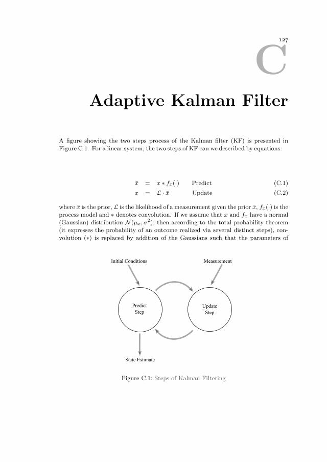
CAdaptive Kalman Filter
A figure showing the two steps process of the Kalman filter (KF) is presented in
Figure C.1. For a linear system, the two steps of KF can we described by equations:
x = x ∗ fx(·) Predict (C.1)
x = L · x Update (C.2)
where x is the prior, L is the likelihood of a measurement given the prior x, fx(·) is the
process model and ∗ denotes convolution. If we assume that x and fx have a normal
(Gaussian) distribution N (µx, σ2), then according to the total probability theorem
(it expresses the probability of an outcome realized via several distinct steps), con-
volution (∗) is replaced by addition of the Gaussians such that the parameters of
PredictStep
UpdateStep
State Estimate
Initial Conditions Measurement
Figure C.1: Steps of Kalman Filtering
Chapter C. Adaptive Kalman Filter
distribution of the predicted x:
µx = µx + µfx (C.3)
σ2x = σ2
x + σ2fx . (C.4)
For the update state, it is shown that the prior (x) can be represented by a Gaussian.
The remaining term of likelihood is a probability of getting the measurement given
the current state. As shown in Chapter 2, the measurements can be represented
as Gaussian with a mean (µ) and standard uncertainty (σ). This allows us to to
treat the likelihood of measurements as Gaussian :z = N (µx, σ2). The product of
two Gaussians is proportional to another Gaussian [79] where the mean is a scaled
sum of the prior (x) and the measurement (z). The variance is a combination of the
variances of the prior and the measurement. The updated Gaussian for x can be
written as:
N (µx, σ2) = N (µx, σ
2x) · N (µz , σ
2z) (C.5)
= N(σ2xµz + σ2
zµx
σ2x + σ2
z,σ2xσ
2z
σ2x + σ2
z
). (C.6)
Equations C.1-C.3 define the two steps of the Kalman filters and the calculated µxin the update step is known as the Kalman Gain.
For multivariate linear systems written as:
xk = Axk−1 + Buk−1 + wk−1 (C.7)
zk = Hxk + vk. (C.8)
where x ∈ Rn is the state vector, z ∈ Rm is the measurement vector A ∈ Rn×nis the state transition matrix relating the new state vector xk to the previous state
xk−1 vector. B ∈ Rn×n matrix the contribution of the input vector u ∈ Rn. and
H ∈ Rm×n is the relationship matrix between the measurements and the system
states. The process noise (error) wk and measurement noise (error) vector vk are
assumed to be mutually independent random variables with Gaussian probability
distributions:
p(w) = N (0,Q) (C.9)
p(v) = N (0,R), (C.10)
where Q is the process noise covariance and R is the measurement noise covariance.
R can obtained either by Type A or Type B type uncertainty estimation category
mentioned in the GUM [58] while estimating Q for various processes van be a chal-
lenging task.
Using the equations C.3 and C.4, the prediction step of the multivariate Kalman
filter is given as:
x−k = Axk−1 + Buk−1 (C.11)
P−k = AP−k−1A> + Q, (C.12)
where x−k ∈ Rn is the a priori state estimate at time step k and P−k ≡ E[e−k ]e−Tk ] is
the a priori state error covariance. The linear transformation of the error covariance
matrix casued by the process function is given by AP−k−1A>. The update step is
carried out by utilizing the measurements and calculated Kalman gain based on the
equation C.6:
I−k = zk −Hx−k (C.13)
Kk = P−k H>(HP−k H> + R)−1 (C.14)
xk = x−k + KkI−k (C.15)
= x−k + Kk(zk −Hx−k ) (C.16)
Pk = (I−KkH)P−k , (C.17)
where I−k is the innovation vector, Kk is the Kalman gain, xk is the updated
a posteriory state estimate at time instant k and Pk is the updated state vector
error covariance matrix. Innovation vector (I−k ) is distinguished from the residual
vector (Ik) which is defined as:
Ik = zk −Hxk. (C.18)
The state vector and variance was initialized based on the recent historic values.
The phase and magnitude of the voltage and current phasors were assumed to be
in quasi-steady state condition. The state transition matrix A is thus assumed
to be an identity matrix. Since all the state variables are directly measured, the
measurement relationship matrix H is also an identity matrix. The errors in the
phasor measurements of voltage and currents of different phases are considered to
be independent of each other and the measurement noise covariance matrix (R) is
populated using the uncertainty values given by the manufacturer. Any variance in
the state variables is considered to be process error and is quantified by the process
error covariance matrix Q.
To improve the performance of the filter, R and Q matrices can be update in real-
time. R is updated depending upon the quality of measurements to filter out bad
Chapter C. Adaptive Kalman Filter
data and Q is updated to treat the un-modeled process noise. To assess the perfor-
mance of the filer, innovation (I−k ) is analysed to confirm a normal distribution with
zero mean and a covariance (Sk)given by:
Sk = HPk −H>. (C.19)
Innovation covariance (Sk) is a quantification of the system uncertainty which accord-
ing to equation C.4 is the sum of a priori state error covariance and the measurement
noise covariance. When the used process model does not match the process in re-
ality, the mean of the innovation shifts suggesting a mismatch. A threshold is used
to compare with the normalized innovation vector (normalized by Sk) to identify
such a misfit. However, as Sk is made up of Q and R, their role in the mismatch is
indistinguishable. To further identify the reason of the mismatch, residual Ik is also
analyzed. Ideally Ik is normally distributed with zero mean and its covariance Tk
given by [77]:
Tk = RS−1k R. (C.20)
To distinguish the source of errors between Q and R, the following three-step ap-
proach was used.
1. For each data point, after the prediction step, innovation covariance matrix (Sk)
and normalized innovation vector I−k were calculated where,
I−i =
|I−i |√Sii
, i = 1, 2, ...n (C.21)
and the step count (k) is omitted for simplification. If for some threshold τQ:
I−i > τQ → i ∈ OP (C.22)
where OP is the vector of the indices of outliers caused by the process noise. First
the outlier is assumed to be caused by unknown process noise. To solve this, the
process noise covariance matrix Q is inflated by diagonal matrix ∆Q. This causes
inflation in P− by ∆Q and in S by ∆S by H(∆Q)H>. This causes the elements of
the new normalized innovation vector given by:
I−i =
|I−i |√Sii + ∆Sii
, i = 1, 2, ...n (C.23)
lower than the threshold τQ.
2. The inflated Q is the utilized in the update step. After the update step, the

residual covariance (T) and normalized residual vector (I) were calculated where
Ii =|Ii|√Tii
, i = 1, 2, ...n (C.24)
If for some threshold τR:
I−i > τR → i ∈ OR & i /∈ OP , (C.25)
where OR is the vector of the indices of outliers caused by measurement noise. In
this case, the inflated Q is deflated again and measurement error covariance matrix
R is inflated by ∆R such that ∆Rii = λiRii where
λi =|Ii|
τR√
Tii, i ∈ OR. (C.26)
3. The update step is carried out using the inflated Q or R matrices. If neither
of conditions shown in equations C.22 and C.25 are true then the method uses the
initial Q or R matrices.


Bibliography
[1] United Nations, “Paris Agreement”, 2015.
[2] European Commission, “The road from paris: Assessing the implications of
the paris agreement and accompanying the proposal for a council decision on
the signing, on behalf of the european union, of the paris agreement adopted
under the united nations framework convention on climate change”, 2016.
[3] ——, “A european strategic long-term vision for a prosperous, modern, com-
petitive and climate neutral economy”, 2018.
[4] United Nations, “Emissions gap report 2019”, 2019.
[5] U. S. Energy Information Administration, “Annual Energy Outlook 2019 with
projections to 2050”, Tech. Rep., 2018.
[6] Y. Sun, “The impact of voltage-source-converters’ control on the power sys-
tem : The stability analysis of a power electronics dominant grid”, PhD thesis,
Eindhoven University of Technology, Eindhoven, Dec. 2018. [Online]. Avail-
able: https : / / research . tue . nl / en / publications / the - impact - of -
voltage-source-converters-control-on-the-power-syst.
[7] C. Pisani, D. Lauria, D. Villacci, and E. M. Carlini, “An integrated approach
to improve the networks security in presence of high penetration of res”,
in 2014 International Symposium on Power Electronics, Electrical Drives,
Automation and Motion, 2014, pp. 1110–1115.
[8] E. M. Carlini, C. Pisani, A. Vaccaro, and D. Villacci, “Dynamic line rating
monitoring in wams: Challenges and practical solutions”, in 2015 IEEE 1st
International Forum on Research and Technologies for Society and Industry
Leveraging a better tomorrow (RTSI), 2015, pp. 359–364.
[9] Entso-E, “Dynamic line rating for overhead lines”, Tech. Rep., 2015. [Online].
Available: https://docs.entsoe.eu/dataset/dynamic-line-rating-for-
overhead-lines-continential-europe.
[10] F. Provoost, “Intelligent distribution network design”, PhD thesis, Eindhoven
University of Technology, Eindhoven, Jan. 2009. [Online]. Available: https://
research.tue.nl/en/publications/intelligent-distribution-network-
design.
[11] T. Yip, C. An, G. Lloyd, M. Aten, and B. Ferri, “Dynamic line rating protec-
tion for wind farm connections”, in 2009 CIGRE/IEEE PES Joint Symposium
Integration of Wide-Scale Renewable Resources Into the Power Delivery Sys-
tem, Jul. 2009, pp. 1–5.
Bibliography
[12] C. J. Wallnerstrom, Y. Huang, and L. Soder, “Impact from dynamic line rating
on wind power integration”, IEEE Transactions on Smart Grid, vol. 6, no. 1,
pp. 343–350, Jan. 2015, issn: 1949-3061. doi: 10.1109/TSG.2014.2341353.
[13] L. Dawson and A. M. Knight, “Applicability of dynamic thermal line rating
for long lines”, IEEE Transactions on Power Delivery, vol. 33, no. 2, pp. 719–
727, 2018.
[14] B. P. Bhattarai, J. P. Gentle, T. McJunkin, P. J. Hill, K. S. Myers, A. W.
Abboud, R. Renwick, and D. Hengst, “Improvement of transmission line am-
pacity utilization by weather-based dynamic line rating”, IEEE Transactions
on Power Delivery, vol. 33, no. 4, pp. 1853–1863, 2018.
[15] G. J. Anders, “Rating of electric power cables in unfavorable thermal envi-
ronment”, in. Wiley-IEEE Press, 2005, isbn: 978-0-471-67909-7.
[16] E. Thunberg and L. Soder, “A norton approach to distribution network mod-
eling for harmonic studies”, IEEE Transactions on Power Delivery, vol. 14,
no. 1, pp. 272–277, 1999.
[17] T. Busatto, V. Ravindran, A. Larsson, S. K. Ronnberg, M. H. Bollen, and
J. Meyer, “Deviations between the commonly-used model and measurements
of harmonic distortion in low-voltage installations”, Electric Power Systems
Research, vol. 180, p. 106 166, 2020, issn: 0378-7796. doi: https://doi.
org / 10 . 1016 / j . epsr . 2019 . 106166. [Online]. Available: http : / / www .
sciencedirect.com/science/article/pii/S0378779619304857.
[18] G. D’Antona, C. Muscas, and S. Sulis, “State estimation for the localization
of harmonic sources in electric distribution systems”, IEEE Transactions on
Instrumentation and Measurement, vol. 58, no. 5, pp. 1462–1470, 2009.
[19] NERC, “Real-time application of synchrophasors for improving reliability”,
Tech. Rep., 2010. [Online]. Available: https : / / www . naspi . org / sites /
default/files/reference_documents/rapir_final_20101017.pdf?fileID=
519.
[20] G. Rietveld, A. Jongepier, J. van Seters, M. Visser, P. Liu, M. Acanski, D.
Hoogenboom, and H. van den Brom, “Application of PMUs for monitoring a
50 kv distribution grid”, in Proceedings of the 23rd International Conference
on Electricity Distribution (CIRED 2015), Jun. 2015, p. 1046.
[21] C- DAX. Consortium, “Test Results of Field Trial with C-DAX Compatible
Grid Devices”, Tech. Rep., 2018. [Online]. Available: http://cdax.ilabt.
imec.be/sites/default/C-DAX-D5.2.pdf.
[22] A. Von Meier, E. Stewart, A. McEachern, M. Andersen, and L. Mehrmanesh,
“Precision Micro-Synchrophasors for Distribution Systems: A Summary of
Applications”, IEEE Transactions on Smart Grid, vol. 8, no. 6, pp. 2926–
2936, 2017, issn: 19493053. doi: 10.1109/TSG.2017.2720543.
Bibliography
[23] A. Ukil, H. Braendle, and P. Krippner, “Distributed temperature sensing:
Review of technology and applications”, IEEE Sensors Journal, vol. 12, no. 5,
pp. 885–892, May 2012, issn: 2379-9153. doi: 10.1109/JSEN.2011.2162060.
[24] Yan Du and Y. Liao, “Online estimation of power transmission line parame-
ters, temperature and sag”, in 2011 North American Power Symposium, 2011,
pp. 1–6.
[25] D. Shi, D. J. Tylavsky, N. Logic, and K. M. Koellner, “Identification of
short transmission-line parameters from synchrophasor measurements”, in
2008 40th North American Power Symposium, IEEE, Sep. 2008, pp. 1–8, isbn:
978-1-4244-4283-6. doi: 10.1109/NAPS.2008.5307354. [Online]. Available:
http://ieeexplore.ieee.org/document/5307354/.
[26] D. Ritzmann, P. S. Wright, W. Holderbaum, and B. Potter, “A method for
accurate transmission line impedance parameter estimation”, IEEE Transac-
tions on Instrumentation and Measurement, vol. 65, no. 10, pp. 2204–2213,
Oct. 2016, issn: 0018-9456. doi: 10.1109/TIM.2016.2556920.
[27] S. K. Jain, P. Jain, and S. N. Singh, “A fast harmonic phasor measure-
ment method for smart grid applications”, IEEE Transactions on Smart Grid,
vol. 8, no. 1, pp. 493–502, 2017.
[28] D. Serfontein, J. Rens, G. Botha, and J. Desmet, “Continuous event-based
harmonic impedance assessment using online measurements”, IEEE Transac-
tions on Instrumentation and Measurement, vol. 65, no. 10, pp. 2214–2220,
2016.
[29] H. Lee, Tushar, B. Cui, A. Mallikeswaran, P. Banerjee, and A. K. Srivastava,
“A review of synchrophasor applications in smart electric grid”, WIREs En-
ergy and Environment, vol. 6, no. 3, e223, 2017. doi: 10.1002/wene.223.
[Online]. Available: https://onlinelibrary.wiley.com/doi/abs/10.1002/
wene.223.
[30] A. Phadke and J. Thorp, “High frequency grid impedance analysis by cur-
rent injection”, in Synchronized Phasor Measurements and Their Applica-
tions, 2009, pp. 536–541. doi: 10.1109/IECON.2009.5414978.
[31] P. F. Ribeiro, C. Duque, P. M. Silveria, and A. Cerqueira, Power System
Signal Processing for Smart Grids. 2014, isbn: 978-1-119-99150-2.
[32] IEEE standard for synchrophasor measurements for power systems, IEEE Std
C37.118.1-2011 (Revision of IEEE Std C37.118-2005), Dec. 2011. doi: 10.
1109/IEEESTD.2011.6111222.
[33] M. Chakir, I. Kamwa, and H. Le Huy, “Extended c37.118.1 PMU algorithms
for joint tracking of fundamental and harmonic phasors in stressed power
systems and microgrids”, IEEE Transactions on Power Delivery, vol. 29, no. 3,
pp. 1465–1480, 2014.
Bibliography
[34] S. R. Samantaray, I. Kamwa, and G. Joos, “Phasor measurement unit based
wide-area monitoring and information sharing between micro-grids”, IET
Generation, Transmission Distribution, vol. 11, no. 5, pp. 1293–1302, 2017.
[35] A. Carta, N. Locci, and C. Muscas, “A PMU for the measurement of synchro-
nized harmonic phasors in three-phase distribution networks”, IEEE Trans-
actions on Instrumentation and Measurement, vol. 58, no. 10, pp. 3723–3730,
2009.
[36] G. W. Chang and C. Chen, “An accurate time-domain procedure for harmon-
ics and interharmonics detection”, IEEE Transactions on Power Delivery,
vol. 25, no. 3, pp. 1787–1795, 2010.
[37] C. Chen and Y. Chen, “Application of adaptive model-based scheme for
harmonic diagnosis and compensation of grid-connected converters”, IEEE
Transactions on Industrial Electronics, vol. 65, no. 1, pp. 770–777, 2018.
[38] J. Enayati and Z. Moravej, “Real-time harmonics estimation in power systems
using a novel hybrid algorithm”, IET Generation, Transmission Distribution,
vol. 11, no. 14, pp. 3532–3538, 2017.
[39] G. W. Chang, C. Chen, and Y. Teng, “Radial-basis-function-based neural net-
work for harmonic detection”, IEEE Transactions on Industrial Electronics,
vol. 57, no. 6, pp. 2171–2179, 2010.
[40] C. Chen and Y. Chen, “Comparative study of harmonic and interharmonic
estimation methods for stationary and time-varying signals”, IEEE Transac-
tions on Industrial Electronics, vol. 61, no. 1, pp. 397–404, 2014.
[41] V. Friedman, “A zero crossing algorithm for the estimation of the frequency
of a single sinusoid in white noise”, IEEE Transactions on Signal Processing,
vol. 42, no. 6, pp. 1565–1569, 1994.
[42] F. Cupertino, E. Lavopa, P. Zanchetta, M. Sumner, and L. Salvatore, “Run-
ning dft-based pll algorithm for frequency, phase, and amplitude tracking
in aircraft electrical systems”, IEEE Transactions on Industrial Electronics,
vol. 58, no. 3, pp. 1027–1035, 2011.
[43] M. Aiello, A. Cataliotti, V. Cosentino, and S. Nuccio, “Synchronization tech-
niques for power quality instruments”, IEEE Transactions on Instrumentation
and Measurement, vol. 56, no. 5, pp. 1511–1519, 2007.
[44] M. S. Reza, M. Ciobotaru, and V. G. Agelidis, “Power system frequency
estimation by using a newton-type technique for smart meters”, IEEE Trans-
actions on Instrumentation and Measurement, vol. 64, no. 3, pp. 615–624,
2015.
[45] V. K. Jain, W. L. Collins, and D. C. Davis, “High-accuracy analog mea-
surements via interpolated fft”, IEEE Transactions on Instrumentation and
Measurement, vol. 28, no. 2, pp. 113–122, 1979.
Bibliography
[46] D. Agrez, “Improving phase estimation with leakage minimization”, IEEE
Transactions on Instrumentation and Measurement, vol. 54, no. 4, pp. 1347–
1353, 2005.
[47] D. Gallo, R. Langella, and A. Testa, “Desynchronized processing technique
for harmonic and interharmonic analysis”, IEEE Transactions on Power De-
livery, vol. 19, no. 3, pp. 993–1001, 2004.
[48] P. Romano, “DFT-based synchrophasor estimation algorithms and their in-
tegration in advanced phasor measurement units for the real-time monitoring
of active distribution networks”, PhD thesis, EPFL, Lausane, Feb. 2016. [On-
line]. Available: https://infoscience.epfl.ch/record/215321?ln=en.
[49] S. Babaev, R. S. Singh, J. F. G. Cobben, V. Cuk, and A. Downie, “Multi-
Point Time-Synchronized Waveform Recording for the Analysis of Wide-Area
Harmonic Propagation”, Applied Sciences, vol. 10, no. 11, 2020, issn: 2076-
3417. doi: 10.3390/app10113869. [Online]. Available: https://www.mdpi.
com/2076-3417/10/11/3869.
[50] Testing and measurement techniques—general guide on harmonics and in-
terharmonics measurements and instrumentation, for power supply systems
and equipment connected thereto, IEC Std 61000-4-7 (Revision of IEEE Std
C37.118-2005), 2009.
[51] Y. Zhou, R. Arghandeh, H. Zou, and C. J. Spanos, “Nonparametric event de-
tection in multiple time series for power distribution networks”, IEEE Trans-
actions on Industrial Electronics, vol. 66, no. 2, pp. 1619–1628, 2019.
[52] M. Pignati, L. Zanni, P. Romano, R. Cherkaoui, and M. Paolone, “Fault
detection and faulted line identification in active distribution networks us-
ing synchrophasors-based real-time state estimation”, IEEE Transactions on
Power Delivery, vol. 32, no. 1, pp. 381–392, 2017.
[53] G. Coletta, A. Vaccaro, and D. Villacci, “A review of the enabling method-
ologies for PMUs-based dynamic thermal rating of power transmission lines”,
Electric Power Systems Research, vol. 152, pp. 257–270, 2017, issn: 0378-
7796. doi: https : / / doi . org / 10 . 1016 / j . epsr . 2017 . 07 . 016. [On-
line]. Available: http://www.sciencedirect.com/science/article/pii/
S0378779617303012.
[54] D. L. Alvarez, J. A. Rosero, F. Faria da Silva, C. L. Bak, and E. E. Mombello,
“Dynamic line rating — technologies and challenges of PMU on overhead
lines: A survey”, in 2016 51st International Universities Power Engineering
Conference (UPEC), 2016, pp. 1–6.
Bibliography
[55] E. M. Stewart, S. Kiliccote, D. Arnold, A. von Meier, and R. Arghandeh,
“Accuracy and validation of measured and modeled data for distributed pv
interconnection and control”, in 2015 IEEE Power Energy Society General
Meeting, 2015, pp. 1–5.
[56] I. D. Melo, J. L. Pereira, A. M. Variz, and P. A. Garcia, “Harmonic state es-
timation for distribution networks using phasor measurement units”, Electric
Power Systems Research, vol. 147, pp. 133–144, 2017, issn: 0378-7796. doi:
https://doi.org/10.1016/j.epsr.2017.02.027. [Online]. Available: http:
//www.sciencedirect.com/science/article/pii/S0378779617300858.
[57] H. Kirkham, “A Conceptual Framework for Measurement (with emphasis on
phasor measurement)”, Tech. Rep., 2015.
[58] JCGM 100:2008, Evaluation of measurement data – Guide to the expression
of uncertainty in measurement.
[59] K. V. Khandeparkar, S. A. Soman, and G. Gajjar, “Detection and correction
of systematic errors in instrument transformers along with line parameter
estimation using pmu data”, IEEE Transactions on Power Systems, vol. 32,
no. 4, pp. 3089–3098, 2017. doi: 10.1109/TPWRS.2016.2620990.
[60] A. V. Oppenheim, R. W. Schaffer, and J. R. Buck, Discrete-Time Signal
Processing, 2nd ed. 1998, isbn: 0-13-754920-2.
[61] K. V. Khandeparkar, S. A. Soman, and G. Gajjar, “Detection and correction
of systematic errors in instrument transformers along with line parameter
estimation using PMU data”, IEEE Transactions on Power Systems, vol. 32,
no. 4, pp. 3089–3098, Jul. 2017, issn: 0885-8950. doi: 10.1109/TPWRS.2016.
2620990.
[62] R. S. Singh, J. F. G. Cobben, and M. Gibescu, “Assessment of Errors in the
Measurement Chain of Distribution Grids for Feasibility Study of a PMU
Application”, in First International Colloquium on Smart Grid Metrology,
2018, pp. 1–5.
[63] JCGM 102:2011, Evaluation of measurement data – Supplement 2 to the
“Guide to the expression of uncertainty in measurement”.
[64] B. D. Hall, “On the propagation of uncertainty in complex-valued quantities”,
Metrologia, vol. 41, no. 3, pp. 173–177, Apr. 2004. doi: 10.1088/0026-1394/
41/3/010. [Online]. Available: https://doi.org/10.1088%2F0026-1394%
2F41%2F3%2F010.
[65] R. S. Singh, H. van den Brom, S. Babaev, J. F. G. Cobben, and V. Cuk,
“Estimation of impedance and susceptance parameters of a 3-phase cable
system using PMU data”, Energies, vol. 12, no. 23, 2019, issn: 1996-1073. doi:
10.3390/en12234573. [Online]. Available: https://www.mdpi.com/1996-
1073/12/23/4573.
Bibliography
[66] R. S. Singh, J. F. G. Cobben, and V. Cuk, “PMU-based Cable Tempera-
ture Monitoring and Thermal Assessment for Dynamic Line Rating”, IEEE
Transactions on Power Delivery, pp. 1–1, 2020.
[67] R. Olsen, G. J. Anders, J. Holboell, and U. S. Gudmundsdottir, “Modelling of
dynamic transmission cable temperature considering soil-specific heat, ther-
mal resistivity, and precipitation”, IEEE Transactions on Power Delivery,
vol. 28, no. 3, pp. 1909–1917, Jul. 2013, issn: 1937-4208. doi: 10.1109/TPWRD.
2013.2263300.
[68] R. Huang, J. A. Pilgrim, P. L. Lewin, and D. Payne, “Dynamic cable ratings
for smarter grids”, in IEEE PES ISGT Europe 2013, Oct. 2013, pp. 1–5. doi:
10.1109/ISGTEurope.2013.6695230.
[69] L. Lindstrom, “Evaluating impact on ampacity according to IEC-60287 re-
garding thermally unfavourable placement of power cables”, Master’s thesis,
KTH, Stockholm, 2011.
[70] C. Bates, “Underground cable ampacity: A fresh look at addressing the future
electric grid”, PhD thesis, Colorado School of Mines, Colorado, USA, 2018.
[Online]. Available: https://mountainscholar.org/handle/11124/172806.
[71] D. Shi, D. J. Tylavsky, K. M. Koellner, N. Logic, and D. E. Wheeler, “Trans-
mission line parameter identification using PMU measurements”, European
Transactions on Electrical Power, vol. 21, no. 4, pp. 1574–1588, May 2011,
issn: 1430144X. doi: 10.1002/etep.522. [Online]. Available: http://doi.
wiley.com/10.1002/etep.522.
[72] V. Milojevic, S. Calija, G. Rietveld, M. V. Acanski, and D. Colangelo, “Uti-
lization of PMU measurements for three-phase line parameter estimation in
power systems”, IEEE Transactions on Instrumentation and Measurement,
vol. 67, no. 10, pp. 2453–2462, Oct. 2018, issn: 0018-9456. doi: 10.1109/TIM.
2018.2843098.
[73] C. Pisani, A. Vaccaro, and D. Villacci, “Conceptualization and experimental
deployment of an adaptive synchronized sensing system for power line thermal
monitoring”, IEEE Transactions on Industrial Informatics, vol. 12, no. 6,
pp. 2158–2165, 2016.
[74] S. H. Draper Norman R., Applied Regression Analysis, Third. Wiley-Interscience,
1998, isbn: 0-471-17082-8. [Online]. Available: http://pages.stern.nyu.
edu/~wgreene/Text/econometricanalysis.htm.
[75] S. S. Shapiro and M. B. Wilk, “An analysis of variance test for normality
(complete samples)”, Biometrika, vol. 52, no. 3/4, pp. 591–611, 1965, issn:
00063444. [Online]. Available: http://www.jstor.org/stable/2333709.
Bibliography
[76] D. J. Olive, Linear regression. Cham: Springer International Publishing, 2017,
p. 254, isbn: 9783319552521. doi: 10.1007/978- 3- 319- 55252- 1. arXiv:
1512.00567. [Online]. Available: http://link.springer.com/10.1007/978-
3-319-55252-1.
[77] J. Zhang, G. Welch, G. Bishop, and Z. Huang, “A two-stage kalman filter ap-
proach for robust and real-time power system state estimation”, IEEE Trans-
actions on Sustainable Energy, vol. 5, no. 2, pp. 629–636, 2014.
[78] F. Mahmood, H. Hooshyar, J. Lavenius, A. Bidadfar, P. Lund, and L. Van-
fretti, “Real-time reduced steady-state model synthesis of active distribution
networks using pmu measurements”, IEEE Transactions on Power Delivery,
vol. 32, no. 1, pp. 546–555, 2017.
[79] R. R. Labbe Jr, Kalman and Bayesian Filters in Python. 2018. [Online]. Avail-
able: https://elec3004.uqcloud.net/2015/tutes/Kalman_and_Bayesian_
Filters_in_Python.pdf.
[80] A. Menditto, M. Patriarca, and B. Magnusson, “Understanding the meaning
of accuracy, trueness and precision”, Accreditation and Quality Assurance,
vol. 12, pp. 45–47, Oct. 2007. doi: 10.1007/s00769-006-0191-z.
[81] Model 1133a Power Sentinel Power Quality Revenue Standard Operation Man-
ual, Arbiter Systems, Inc. [Online]. Available: https://www.arbiter.com/
files/product-attachments/1133a_manual.pdf.
[82] W. H. Greene, Econometric Analysis, Fifth. Pearson Education, 2003, isbn:
0-13-066189-9. [Online]. Available: http://pages.stern.nyu.edu/~wgreene/
Text/econometricanalysis.htm.
[83] N. Save, “Phasor Measurement Unit (PMU) based power system analysis of
mv distribution grid”, Master’s thesis, Delft University of Technology, Delft,
Netherlands, 2016.
[84] A. A. Hafner, M. V. Ferreira da Luz, and W. P. Carpes Jr., “Impedance
and admittance calculations of a three-core power cable by the finite element
method”, in 2015 IPST -International Conference on Power Systems Tran-
sients, 2015, pp. 1–8.
[85] H. Saadat, “Power system analysis”, in. McGraw-Hill, 1999, isbn: 0-07-561634-
3.
[86] L. L. Grigsby, “Electric power generation, transmission, and distribution”, in.
Taylor & Francis Group, 2012, isbn: 9781315222424.
[87] A. Rakowska and K. Hajdrowski, “Influence of different test conditions on
volume resistivity of polymeric insulated cables and polyethylene samples”, in
2000 Eighth International Conference on Dielectric Materials, Measurements
and Applications (IEE Conf. Publ. No. 473), 2000, pp. 281–284.
Bibliography
[88] T. V. M. Nielsen, S. Jakobsen, and M. Savaghebi, “Dynamic rating of three-
core xlpe submarine cables for offshore wind farms”, Applied Sciences, vol. 9,
no. 4, 2019, issn: 2076-3417. doi: 10.3390/app9040800. [Online]. Available:
https://www.mdpi.com/2076-3417/9/4/800.
[89] R. Olsen, “The impact of dynamic loadability of cable based transmission
grids”, PhD thesis, Technical University of Denmark, Lyngby, Aug. 2013.
[Online]. Available: https://orbit.dtu.dk/en/publications/dynamic-
loadability-of-cable-based-transmission-grids.
[90] R. Olsen, J. Holboell, and U. S. Gudmundsdottir, “Electrothermal coordi-
nation in cable based transmission grids”, IEEE Transactions on Power Sys-
tems, vol. 28, no. 4, pp. 4867–4874, Nov. 2013, issn: 1558-0679. doi: 10.1109/
TPWRS.2013.2278040.
[91] M. Diaz-Aguilo, F. De Leon, S. Jazebi, and M. Terracciano, “Ladder-type
soil model for dynamic thermal rating of underground power cables”, IEEE
Power and Energy Technology Systems Journal, vol. 1, pp. 21–30, 2014.
[92] R. S. Singh, V. Cuk, and S. Cobben, “Measurement-based distribution grid
harmonic impedance models and their uncertainties”, Energies, vol. 13, no. 16,
2020, issn: 1996-1073. doi: 10.3390/en13164259. [Online]. Available: https:
//www.mdpi.com/1996-1073/13/16/4259.
[93] O. Lennerhag and M. H. J. Bollen, “Power system impacts of decreasing
resonance frequencies”, in 2018 18th International Conference on Harmonics
and Quality of Power (ICHQP), 2018, pp. 1–6. doi: 10.1109/ICHQP.2018.
8378880.
[94] F. Barakou, M. H. J. Bollen, S. Mousavi-Gargari, O. Lennerhag, P. A. A. F.
Wouters, and E. F. Steennis, “Impact of load modeling on the harmonic
impedance seen from the transmission network”, in 2016 17th International
Conference on Harmonics and Quality of Power (ICHQP), Oct. 2016, pp. 283–
288. doi: 10.1109/ICHQP.2016.7783466.
[95] J. H. R. Enslin and P. J. M. Heskes, “Harmonic interaction between a large
number of distributed power inverters and the distribution network”, in IEEE
34th Annual Conference on Power Electronics Specialist, 2003. PESC ’03.,
vol. 4, Jun. 2003, 1742–1747 vol.4. doi: 10.1109/PESC.2003.1217719.
[96] V. Cuk, J. F. G. Cobben, W. L. Kling, and P. F. Ribeiro, “Considerations on
harmonic impedance estimation in low voltage networks”, in 2012 IEEE 15th
International Conference on Harmonics and Quality of Power, Jun. 2012,
pp. 358–363. doi: 10.1109/ICHQP.2012.6381250.
Bibliography
[97] J. Meyer, R. Stiegler, P. Schegner, I. Roder, and A. Belger, “Harmonic res-
onances in residential low-voltage networks caused by consumer electronics”,
CIRED - Open Access Proceedings Journal, vol. 2017, no. 1, pp. 672–676,
2017.
[98] M. Sumner, B. Palethorpe, and D. W. P. Thomas, “Impedance measure-
ment for improved power quality-part 1: The measurement technique”, IEEE
Transactions on Power Delivery, vol. 19, no. 3, pp. 1442–1448, 2004. doi:
10.1109/TPWRD.2004.829873.
[99] A. Knop and F. W. Fuchs, “High frequency grid impedance analysis by current
injection”, in 2009 35th Annual Conference of IEEE Industrial Electronics,
2009, pp. 536–541. doi: 10.1109/IECON.2009.5414978.
[100] T. T. Do, M. Jordan, H. Langkowski, and D. Schulz, “Novel grid impedance
measurement setups in electrical power systems”, in 2016 IEEE International
Workshop on Applied Measurements for Power Systems (AMPS), 2016, pp. 1–
6. doi: 10.1109/AMPS.2016.7602808.
[101] H. L. Monteiro, C. A. Duque, L. R. Silva, J. Meyer, R. Stiegler, A. Testa,
and P. F. Ribeiro, “Harmonic impedance measurement based on short time
current injections”, Electric Power Systems Research, vol. 148, pp. 108–116,
2017, issn: 0378-7796. doi: https://doi.org/10.1016/j.epsr.2017.03.031.
[Online]. Available: http://www.sciencedirect.com/science/article/pii/
S0378779617301311.
[102] A. Riccobono, E. Liegmann, M. Pau, F. Ponci, and A. Monti, “Online para-
metric identification of power impedances to improve stability and accuracy of
power hardware-in-the-loop simulations”, IEEE Transactions on Instrumen-
tation and Measurement, vol. 66, no. 9, pp. 2247–2257, 2017.
[103] Wilsun Xu, E. E. Ahmed, Xiqin Zhang, and Xian Liu, “Measurement of net-
work harmonic impedances: Practical implementation issues and their solu-
tions”, IEEE Transactions on Power Delivery, vol. 17, no. 1, pp. 210–216,
2002.
[104] J. Hui, W. Freitas, J. C. M. Vieira, H. Yang, and Y. Liu, “Utility harmonic
impedance measurement based on data selection”, IEEE Transactions on
Power Delivery, vol. 27, no. 4, pp. 2193–2202, 2012. doi: 10.1109/TPWRD.
2012.2207969.
[105] A. A. Girgis and R. B. McManis, “Frequency domain techniques for modeling
distribution or transmission networks using capacitor switching induced tran-
sients”, IEEE Transactions on Power Delivery, vol. 4, no. 3, pp. 1882–1890,
1989.
Bibliography
[106] D. Borkowski, A. Wetula, and A. Bien, “New method for noninvasive mea-
surement of utility harmonic impedance”, in 2012 IEEE Power and Energy
Society General Meeting, 2012, pp. 1–8.
[107] M. Nagpal, W. Xu, and J. Sawada, “Harmonic impedance measurement using
three-phase transients”, IEEE Transactions on Power Delivery, vol. 13, no. 1,
pp. 272–277, 1998.
[108] Joint CIGRE/CIRED Working Group CC02, “Guide for assessing the network
harmonic impedance”, in 14th International Conference and Exhibition on
Electricity Distribution. Part 1. Contributions (IEE Conf. Publ. No. 438),
vol. 2, Jun. 1997, 3/1–310 vol.2. doi: 10.1049/cp:19970473.
[109] T. Busatto, A. Larsson, S. K. Ronnberg, and M. H. J. Bollen, “Including
uncertainties from customer connections in calculating low-voltage harmonic
impedance”, IEEE Transactions on Power Delivery, vol. 34, no. 2, pp. 606–
615, 2019.
[110] “IEC Std 61000-4-7 (Revision of IEEE Std C37.118-2005): Testing and Mea-
surement Techniques—General Guide on Harmonics and Interharmonics Mea-
surements and Instrumentation, for Power Supply Systems and Equipment
Connected Thereto”, Tech. Rep. February, 2009, pp. 1–58.
[111] M. Rylander and W. M. Grady, “Problems in the use of norton equivalent
models for single-phase nonlinear loads”, in IEEE PES General Meeting, 2010,
pp. 1–7. doi: 10.1109/PES.2010.5589732.
[112] Wilsun Xu and Yilu Liu, “A method for determining customer and utility
harmonic contributions at the point of common coupling”, IEEE Transactions
on Power Delivery, vol. 15, no. 2, pp. 804–811, 2000.
[113] “Electromagnetic compatibility (EMC) - Part 3-6: Limits - Assessment of
emission limits for the connection of distorting installations to MV, HV and
EHV power systems”, Tech. Rep. February, 2008, pp. 1–58.
[114] A. Spelko, B. Blazic, I. Papic, M. Pourarab, J. Meyer, X. Xu, and S. Z. Djokic,
“CIGRE/CIRED JWG C4.42: Overview of common methods for assessment
of harmonic contribution from customer installation”, in 2017 IEEE Manch-
ester PowerTech, 2017, pp. 1–6.
[115] I. Papic, D. Matvoz, A. Spelko, W. Xu, Y. Wang, D. Mueller, C. Miller,
P. F. Ribeiro, R. Langella, and A. Testa, “A benchmark test system to eval-
uate methods of harmonic contribution determination”, IEEE Transactions
on Power Delivery, vol. 34, no. 1, pp. 23–31, 2019.
[116] P. F. Ribeiro, “Guidelines on distribution system and load representation for
harmonic studies”, in ICHPS V International Conference on Harmonics in
Power Systems., Sep. 1992, pp. 272–280. doi: 10.1109/ICHPS.1992.559090.
Bibliography
[117] Task Force on Harmonic Modeling and Simulation, “Impact of aggregate lin-
ear load modeling on harmonic analysis: A comparison of common practice
and analytical models”, IEEE Transactions on Power Delivery, vol. 18, no. 2,
pp. 625–630, Apr. 2003, issn: 0885-8977. doi: 10.1109/TPWRD.2003.810492.
[118] G. Ye, A. Sans, V. Cuk, J. van Waes, and J. F. G. Cobben, “Impact of
distribution network modelling on harmonic impedance in the HV grid”, in
CIRED 2019, Madrid, June 2019, Jun. 2019.
[119] S. Bhattacharyya, Z. Wang, J. F. G. Cobben, J. M. A. Myrzik, and W. L.
Kling, “Analysis of power quality performance of the dutch medium and low
voltage grids”, in 2008 13th International Conference on Harmonics and Qual-
ity of Power, Sep. 2008, pp. 1–6. doi: 10.1109/ICHQP.2008.4668800.
[120] EMTDC User’s Guide,vol. 4.7, fifth printing, February 2010, Manitoba Hydro
International, Ltd., p. 97.
[121] D. Serfontein, J. Rens, G. Botha, and J. Desmet, “Improved event based
method for harmonic impedance assessment”, in 2016 IEEE International
Workshop on Applied Measurements for Power Systems (AMPS), Sep. 2016,
pp. 1–6. doi: 10.1109/AMPS.2016.7602807.
[122] J. Peng, H. Li, Z. Wang, F. Ghassemi, and P. Jarman, “Influence of sympa-
thetic inrush on voltage dips caused by transformer energisation”, IET Gen-
eration, Transmission Distribution, vol. 7, no. 11, pp. 1173–1184, Nov. 2013,
issn: 1751-8687. doi: 10.1049/iet-gtd.2012.0166.
[123] M. Nagpal, T. G. Martinich, A. Moshref, K. Morison, and P. Kundur, “As-
sessing and limiting impact of transformer inrush current on power quality”,
IEEE Transactions on Power Delivery, vol. 21, no. 2, pp. 890–896, 2006. doi:
10.1109/TPWRD.2005.858782.
[124] P. Welch, “The use of fast fourier transform for the estimation of power spec-
tra: A method based on time averaging over short, modified periodograms”,
IEEE Transactions on Audio and Electroacoustics, vol. 15, no. 2, pp. 70–73,
1967.
[125] R. S. Singh, V. Cuk, and J. F. G. Cobben, “Measurement-based distribution
grid harmonic impedance models and their uncertainties”, Energies, vol. 13,
no. 16, 2020, issn: 1996-1073. doi: 10.3390/en13164259. [Online]. Available:
https://www.mdpi.com/1996-1073/12/23/4573.
[126] S. Babaev, R. S. Singh, J. F. G. Cobben, V. Cuk, and J. Desmet, “Circular
regression models of modern harmonic producing sources”, IET Generation,
Transmission Distribution, vol. 14, 3826–3836(10), 18 Sep. 2020, issn: 1751-
8687.
Bibliography
[127] R. S. Singh, J. F. G. Cobben, H. van den Brom, and G. Rietveld, “Pmu data-
based temperature monitoring of a power cable”, in 2020 IEEE Power Energy
Society General Meeting (PESGM), 2020, pp. 1–5.
[128] R. S. Singh, S. Babaev, V. Cuk, J. F. G. Cobben, and H. van den Brom,
“Line parameters estimation in presence of uncalibrated instrument trans-
formers”, in 2019 2nd International Colloquium on Smart Grid Metrology
(SMAGRIMET), Apr. 2019, pp. 1–8. doi: 10 . 23919 / SMAGRIMET . 2019 .
8720376.
[129] R. S. Singh, J. F. G. Cobben, M. Gibescu, H. van den Brom, D. Colangelo, and
G. Rietveld, “Medium voltage line parameter estimation using synchrophasor
data: A step towards dynamic line rating”, in 2018 IEEE Power Energy So-
ciety General Meeting (PESGM), Aug. 2018, pp. 1–5. doi: 10.1109/PESGM.
2018.8586111.
[130] S. Babaev, R. S. Singh, J. F. G. Cobben, V. Cuk, and H. Van Den Brom,
“Considerations on the performance of multi-point synchronized harmonic
measurement system”, in 2018 IEEE 9th International Workshop on Applied
Measurements for Power Systems (AMPS), 2018, pp. 1–5.


Nomenclature
ACC: Adjusted Correction Coefficients
ADC: Analog to Digital Converter
BESS: Battery Energy Storage System
CIC: Current Injection Comparison
CSU: Combined Standard Uncertainty
DFT: Discrete Fourier Transform
DTFT: Discrete Time Fourier Transform
DLR: Dynamic Line Rating
EV: Electric Vehicle
FEM: Finite Element Method
FFT: Fast Fourier Transform
FT: Fourier Transform
GPS: Global Positioning System
IDFT: Interpolated Discrete Fourier Transform
IEC: International Electrotechnical Commission
KF: Kalman Filter
LTI: Linear Time Invariant
OLS: Ordinary Least Squares
PCC: Point of Common Coupling
PDF:Probability Density Function
PE: Power Electronics
PMU: Phasor Measurement Unit
PQA: Power Quality Analyzer
PV: Photo-voltaic
RES: Renewable Energy Sources
RMS: Root Mean Square
SCADA: Supervisory Control and Data Acquisition
SD: Standard Deviation
STFT: Short-Time Fourier Transform
TEE: Thermoelectric Equivalent
THD: Total Harmonic Distortion
TVE: Total Vector Error
VDC: Voltage Distortion Comparison
VHV:Voltage Harmonic Vector
WP: Wind Park
XLPE: Cross-Linked Poly-Ethylene

Published work
Journal Publications
2020
R. S. Singh, V. Cuk, and J. F. G. Cobben, “Measurement-based distribution grid
harmonic impedance models and their uncertainties”, Energies, vol. 13, no. 16, 2020,
issn: 1996-1073. doi: 10.3390/en13164259. [Online]. Available: https://www.
mdpi.com/1996-1073/12/23/4573.
R. S. Singh, J. F. G. Cobben, and V. Cuk, “PMU-based Cable Temperature Mon-
itoring and Thermal Assessment for Dynamic Line Rating”, IEEE Transactions on
Power Delivery, pp. 1–1, 2020.
S. Babaev, R. S. Singh, J. F. G. Cobben, et al., “Circular regression models of modern
harmonic producing sources”, IET Generation, Transmission Distribution, vol. 14,
3826–3836(10), 18 Sep. 2020, issn: 1751-8687.
S. Babaev, R. S. Singh, J. F. G. Cobben, et al., “Multi-Point Time-Synchronized
Waveform Recording for the Analysis of Wide-Area Harmonic Propagation”, Ap-
plied Sciences, vol. 10, no. 11, 2020, issn: 2076-3417. doi: 10.3390/app10113869.
[Online]. Available: https://www.mdpi.com/2076-3417/10/11/3869.
2019
R. S. Singh, H. van den Brom, S. Babaev, et al., “Estimation of impedance and sus-
ceptance parameters of a 3-phase cable system using PMU data”, Energies, vol. 12,
no. 23, 2019, issn: 1996-1073. doi: 10.3390/en12234573. [Online]. Available: https:
//www.mdpi.com/1996-1073/12/23/4573.
Published work
Conference Publications
2020
R. S. Singh, J. F. G. Cobben, H. van den Brom, et al., “Pmu data-based temperature
monitoring of a power cable”, in 2020 IEEE Power Energy Society General Meeting
(PESGM), 2020, pp. 1–5.
2019
R. S. Singh, S. Babaev, V. Cuk, et al., “Line parameters estimation in presence of un-
calibrated instrument transformers”, in 2019 2nd International Colloquium on Smart
Grid Metrology (SMAGRIMET), Apr. 2019, pp. 1–8. doi: 10.23919/SMAGRIMET.
2019.8720376.
2018
R. S. Singh, J. F. G. Cobben, and M. Gibescu, “Assessment of Errors in the Mea-
surement Chain of Distribution Grids for Feasibility Study of a PMU Application”,
in First International Colloquium on Smart Grid Metrology, 2018, pp. 1–5.
R. S. Singh, J. F. G. Cobben, M. Gibescu, et al., “Medium voltage line parameter
estimation using synchrophasor data: A step towards dynamic line rating”, in 2018
IEEE Power Energy Society General Meeting (PESGM), Aug. 2018, pp. 1–5. doi:
10.1109/PESGM.2018.8586111.
S. Babaev, R. S. Singh, J. F. G. Cobben, et al., “Considerations on the performance
of multi-point synchronized harmonic measurement system”, in 2018 IEEE 9th In-
ternational Workshop on Applied Measurements for Power Systems (AMPS), 2018,
pp. 1–5.

Acknowledgments
As my journey as a Ph.D. candidate at Eindhoven University of Technology comes
to an end, I would like to thank some people who have supported and helped me
throughout this period.
First of all, I would like to thank my promotor prof. Sjef Cobben from the Electri-
cal Energy Systems group for showing trust in me and giving me the opportunity
to embark on this journey into the academic world. Sjef, thank you very much
for your constant guidance and support. Your comments on my work were always
thought provoking. I would also like to thank my copromotor and daily supervisor
Dr. Vladimir Cuk who took this role midway and was a constant source of support
till the end. From the same group, I would like to thank prof. Guus Pemen for the
encouragement and feedback that I received from him.
I give thanks to Dr. Helko van den Brom of VSL with whom I had many technical
discussions especially during the first two years. I learnt a great deal about metrology
during those discussions. From VSL I would also like to thank Dr. Gert Rietveld
and Dr. Daniele Colangelo who helped me during the initial phase of the project.
I thank prof. Madeleine Gibescu, prof. Peter van der Wielen and prof. Jan Desmet
for their roles as committee members in my Ph.D. defense. Your comments and
feedback helped to improve my work.
I would like to thank all of my colleagues in the Electrical Energy Systems group
who made the everyday working environment both fun and inspiring. Especially, I
would like to thank my office-mates Stanislav, Jeroen, Gu, Irina and Martijn. I will
look back and fondly remember the great atmosphere of our room and the time we
spent discussing everything under the sun.
Last but no the least, I would like to take this opportunity to say thanks to my wife
Shailaja, my parents Sunil and Kanchan and my brother Shashi for their uncondi-
tional love and support that I have been receiving over the years. None of this would
have been possible without you. Thank you for everything!
Ravi Shankar Singh
Utrecht
2021-03-23


About the author
Ravi Shankar Singh received his B.Tech degree in electrical engineering from National
Institute of Technology Rourkela in India in 2009 and M.Sc. in electrical engineering
from Aalto University in Finland in 2016. From 2009 to 2012 he worked as an Electri-
cal engineer in Alstom T&D India. From 2014 to 2016, he was a Research Engineer
with the Department of Electrical Power System, KTH, Stockholm. From October
2016, he is a Ph.D. candidate at Eindhoven University of Technology, The Nether-
lands. His Ph.D. research is focused on applications based on phasor measurements
for application in cable temperature monitoring and grid harmonic modelling. His
interests lie in the fields of Power Systems Monitoring, Power Quality and Renewable
Integration.
Related Documents