Reference NATL INST. OF STAND & TECH NBS Publi- -"•a* *ons AlllDS TbflTfib •"•CAU 0» " NBS TECHNICAL NOTE 1061 U.S. DEPARTMENT OF COMMERCE / National Bureau of Standards Phase Equilibria: An Informal Symposium — QC

Welcome message from author
This document is posted to help you gain knowledge. Please leave a comment to let me know what you think about it! Share it to your friends and learn new things together.
Transcript
ReferenceNATL INST. OF STAND & TECH
NBSPubli--"•a**ons
AlllDS TbflTfib
•"•CAU 0» " NBS TECHNICAL NOTE 1061
U.S. DEPARTMENT OF COMMERCE / National Bureau of Standards
Phase Equilibria:
An Informal Symposium
— QC
NATIONAL BUREAU OF STANDARDS
The National Bureau of Standards' was established by an act of Congress on March 3, 1901.
The Bureau's overall goal is to strengthen and advance the Nation's science and technology
and facilitate their effective application for public benefit. To this end, the Bureau conducts
research and provides: (1) a basis for the Nation's physical measurement system, (2) scientific
and technological services for industry and government, (3) a technical basis for equity in
trade, and (4) technical services to promote public safety. The Bureau's technical work is per-
formed by the National Measurement Laboratory, the National Engineering Laboratory, and
the Institute for Computer Sciences and Technology.
THE NATIONAL MEASUREMENT LABORATORY provides the national system of
physical and chemical and materials measurement; coordinates the system with measurement
systems of other nations and furnishes essential services leading to accurate and uniform
physical and chemical measurement throughout the Nation's scientific community, industry,
and commerce; conducts materials research leading to improved methods of measurement,
standards, and data on the properties of materials needed by industry, commerce, educational
institutions, and Government; provides advisory and research services to other Government
agencies; develops, produces, and distributes Standard Reference Materials; and provides
calibration services. The Laboratory consists of the following centers:
Absolute Physical Quantities^ — Radiation Research — Chemical Physics —Analytical Chemistry — Materials Science
THE NATIONAL ENGINEERING LABORATORY provides technology and technical ser-
vices to the public and private sectors to address national needs and to solve national
problems; conducts research in engineering and applied science in support of these efforts;
builds and maintains competence in the necessary disciplines required to carry out this
research and technical service; develops engineering data and measurement capabilities;
provides engineering measurement traceability services; develops test methods and proposes
engineering standards and code changes; develops and proposes new engineering practices;
and develops and improves mechanisms to transfer results of its research to the ultimate user.
The Laboratory consists of the following centers:
Applied Mathematics — Electronics and Electrical Engineering^ — Manufacturing
Engineering — Building Technology — Fire Research — Chemical Engineering^
THE INSTITUTE FOR COMPUTER SCIENCES AND TECHNOLOGY conducts
research and provides scientific and technical services to aid Federal agencies in the selection,
acquisition, application, and use of computer technology to improve effectiveness and
economy in Government operations in accordance with Public Law 89-306 (40 U.S.C. 759),
relevant Executive Orders, and other directives; carries out this mission by managing the
Federal Information Processing Standards Program, developing Federal ADP standards
guidelines, and managing Federal participation in ADP voluntary standardization activities;
provides scientific and technological advisory services and assistance to Federal agencies; and
provides the technical foundation for computer-related policies of the Federal Government.
The Institute consists of the following centers:
Programming Science and Technology — Computer Systems Engineering.
'Headquarters and Laboratories at Gaithersburg, MD, unless otherwise noted;
mailing address Washington, DC 20234.
'Some divisions within the center are located at Boulder, CO 80303.
^
Phase Equilibria:
An Informal Symposium
NATIONAL BUHEAa.OF STANDAHOS
UBRAHT
WAR "7 TQB3
B. E. Eaton *tJ. F. Ely
H. J. M. HanleytR. D. McCartyJ. C. Rainwater
Thermophysical Properties Division
National Engineering LaboratoryNational Bureau of StandardsBoulder, Colorado 80303
* Department of Chennical Engineering, University of Colorado, Boulder, CO 80307
tin collaboration with J. Stecki and P. Wielopolski, Institute of Physical Chennistry, Polish
Acadenny of Sciences, Warsaw, Poland.
e
'^^ATESO^"^
U.S. DEPARTMENT OF COMMERCE, Malcolm Baldrige, Secretary
NATIONAL BUREAU OF STANDARDS, Ernest Annbler, Director
Issued January 1983
National Bureau of Standards Technical Note 1061
Nat. Bur. Stand. (U.S.), Tech Note 1061, 156 pages (Jan. 1983)
CODEN: NBTNAE
U.S. GOVERNMENT PRINTING OFFICEWASHINGTON: 1983
For sale by the Superintendent of Documents, U.S. Government Printing Office, Washington, DC 20402
Price $6.50
(Add 25 percent for other than U.S. mailing)
PHASE EQUILIBRIA: AN INFOkHAL SYMPOoIUM
B. £. Eaton*"'', J. F. Ely, H. J. M. Hdnley''",
R. D. hlcCcirty and d. C. Rainwater
Therrnopiiysical Properties DivisionNational Engineering LaboratoryNational Bureau of StandardsBoulder, Colorado 80303
PREFACE
Phase equilibria in fluid mixtures is a classical problem in the theory of
liquids v/fiich is not properly resolved, even today. The problem is of special
relevance because of current emphasis on synthetic fuels, the use of new
feedstocks, and the need to conserve and increase productivity with existing
fluid technology. Hov^ever, the data base required for these new developments is
deficient and, in any case, the tasK of measuring all data that might be required
is prohibitive. One needs predictive procedures which can only be based on an
understanding of fluid behavior backed up by the results of controlled
experiments on well-defined systems.
One of the tasks of the Boulder Fluid Properties Group, National Engineering
Laboratory, is to undertake such a program: namely, a study of mixtures via
theory, experiment and data correlation. We felt tnat some of our theoretical
ideas and approaches should be discussed and coordinated so an informal symposium
v/as held in October 1980 to do this. This Technical Note reproduces the main
presentations and is organized as follows: First, Ely reviews the state-of-the-
art of phase equilibria of nonelectrolyte systems, McCarty then reports on his
study of the procedure knov;n as extended corresponding states with special
emphasis on the nitrogen/methane system. This followed by a discussion by
Rainwater on an alternative attack based on the approach of Griffith and Wheeler
which addresses the prediction of VLE (vapor, liquid equilibrium) of mixtures
near the critical locus. Finally, Eaton and coworkers discuss the calculation of
the critical line itself and possible implications of the calculation to VLE in
general
.
* Department of Chemical Engineering, University of Colorado, boulder, CO
80307.
"*"
In collaboration with J. Stecki and P. Wielopolski, Institute of Physical
Chemistry, Polish Acadeniy of Sciences, Warsaw, Poland.
m
Uo claim is made that the symposium covered other than a limited segment of
the total phase equilibria problem, but soi.ie themes and difficulties did emerge
which are general. Perhaps the most important of these is the well-known dilemma
between the strickly programmatic seiiii-empirical viewpoint, and the more
systematic, more academic counterpart. In the long run, of course, the latter
viev;point is preferable, but one has to be realistic and appreciate the need for
procedures which v/ork for the systems of interest today. It was felt that the
technique of extended corresponding states is an attractive coi.ipromise: it v/orks
well for nonpolar mixtures and is a systematic, soundly based, theory which can
still be developed; it applies to the v/hole of the liquid phase diagram without
parameter adjustment while most other techniques do not. However, the method is
based on the concept that a mixture can be replicated by a hypothetical pure
substance, and McCarty points out soi.ie subtle differences in mixture versus pure
behavior which need to bo discussed further. Clearly, too, the critical region
has to be included in a systematic manner, and we are studying combining the
extended corresponding states theory with that proposed by Rainwater. With
respect to this. Rainwater points out that the logical variables for a phase
equilibria study are the intensive set of pressure, temperature and chemical
potential. The engineer, of course, prefers, say, pressure, temperature and mole
fraction. It would bo interesting and important to try to resolve this
fundamental disagreement.
The probleiii of mixing rules and interaction parameters was discussed. The
latter difficulty is serious. As pointed out by Eaton, even interaction
parameters obtained by fitting the critical line, which is a sensitive task
involving second and third derivatives of the chemical potential, have no
significance away from the critical region. As of today, the parameters tend to
obscure any unambiguous assessment of how well a theory can represent data.
This is one more reason why it is important to understand the assumptions which
go into a theory before the theory is developed and broadened.
Much of the work reported here was supported by the Office of Standard
Reference Data, and we thank Dr. Howard White, who attended the meeting, for his
interest and support. We also thank Mrs. Karen Bowie for typing and for other
help in preparing this Technical Note.
H. J. M. Hanley
IV
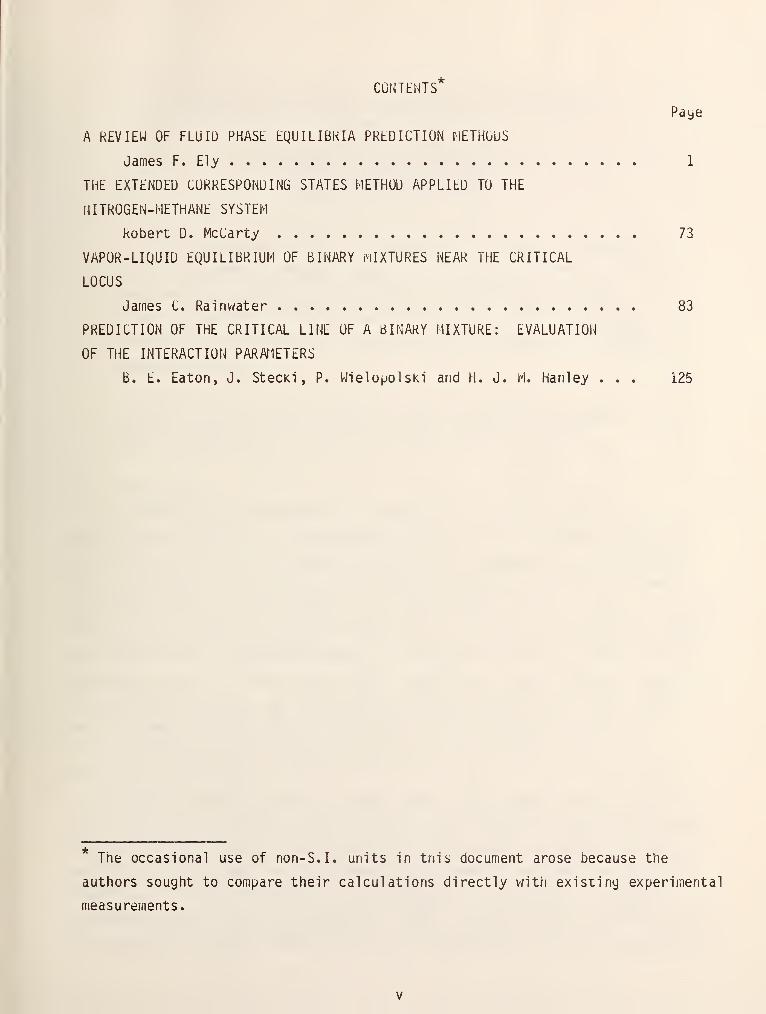
CONTENTS*
A REVIEW OF FLUID PHASE EQUILIBKIA PREDICTION METHODS
James F. Ely 1
THE EXTENDED CORRESPONDING STATES METHOD APPLIED TO THE
NITROGEN-METHANE SYSTEM
Robert D. McCarty 73
VAPOR-LIQUID EQUILIBRIUM OF BINARY MIXTURES NEAR THE CRITICAL
LOCUS
James C. Rainwater 83
PREDICTION OF THE CRITICAL LINE OF A BINARY MIXTURE: EVALUATION
OF THE INTERACTION PARAMETERS
B. E. Eaton, J. StecKi , P. Wielopolski and H. J. M. Hanley ... 125
Tne occasional use of non-S.I. units in tnis document arose because the
authors sought to compare their calculations directly with existing experimental
measurements.

A REVIEW OF FLUID PHASE EQUILIBRIA PREDICTION METHODS
James F. Ely
Thermophysical Properties Division
National Engineering LaboratoryNational Bureau of Standards
Boulder, Colorado 80303
The accurate prediction of phase equilibria plays an important
role in the chemical process industries. A brief overview of fluid
phase equilibria predictive techniques is presented with special
emphasis on methods in current use in industry. Areas where better
fundamental understanding will lead to improved models are discussed
whenever possible.
Key words: activity coefficients; chemical potential; equations of
state; fugacity; group contribution models; phase equilibria.
1. Introduction
The prediction of thermophysical properties of mixtures presents
complications which are not encountered with pure fluids -- namely, that the
composition as well as the temperature and pressure dependence of the property
must be considered. This composition dependence introduces size and polarity
difference effects in the properties of single phase mixtures. From a predictive
point of view, hov/ever, the most difficult task is that of predicting the number
and compositions of coexisting phases at a known temperature, pressure and bulk
composition, e.g., the phase equilibria. Note that in predicting the properties
of single phase mixtures we are concerned with the properties of the fluid as a
whole. However, in the case of the phase equilibrium prediction, we are
interested in the partial properties of the individual components which
constitute the mixture.
Generally speaking, there is a vast base of experimental data for fluid
phase equilibria, especially when compared to the available experimental mixture
PVT, enthalpy and transport data. Partially due to this vast arnount of phase
equilibrium data, many simple, phenomenological models have been developed to
predict and correlate the observed phase behavior. Frequently, the simple
predictive models fail in a quantitative sense, especially when they are applied
to systems which contain species which differ substantially in size and polarity.
1
In order to make accurate predictions on these systems, statistical mechanical
models which can explicitly account for size and polarity effects must be used.
Unfortunately, the potential of the molecular models to predict complex fluid
phase equilibria has not been fully realized due to the mathematical complexity
of the problem and, to some degree, ignorance concerning the interactions of
chemically dissimilar molecules. For this reason, the engineering community is
forced to use simple models to make predictions, regardless of the accuracy
achieved.
The purpose of this chapter is to review the methods which are commonly used
to predict fluid phase equilibria for engineering applications. Areas where
fundamental research and further molecular understanding will improve our
predictive models or perhaps lead to new models will be identified. Techniques
which have a more fundamental basis and those which have been developed to deal
with large size and polarity difference effects will be emphasized whenever
possible. The review will be limited to nonelectrolyte systems with the
exception being water-common inorganic (COp, HpS,..) systems. Solid-liquid
and sol id- vapor systems will also be excluded.
The structure of this article is as follows: section 2 examines some binary
mixture phase diagrams to illustrate some of the common types of fluid phase
equilibria. In section 3, the thermodynamic criteria for phase equilibrium and
mathematical methods for predicting the component equilibrium concentrations are
discussed. Section 4 reviews mixture equation of state methods for predicting
chemical potentials and section 5 reviews the liquid phase activity-vapor phase
fugacity approach to phase equilibria, including the group solution methods.
2. Qualitative Phase Behavior in Mixtures
Phase diagrams for mixtures are considerably more difficult to visualize
than those for pure components due to the fact that the composition must be
considered. In addition to this added dimension, a casual inspection of
different phase diagrams shows great disparity in behavior from one binary system
to another. For example, some systems have azeotropes, isolated regions of
immiscibility and three phase lines. Von Konynenburg and Scott [1,2] have
proposed a convenient classification scheme which accounts for most of the
possible types of behavior. Their method is based on the existence or absence of
three phase lines, the number of critical lines and the manner in which the
critical lines connect with the pure component critical points and three phase
2
lines. Azeotropy gives rise to subclasses but does not change the qualitative
structure of the classification scheme.
In this system there are six basic types of phase diagrams which are
illustrated as p-T projections of their corresponding three dimensional space
models in figure 1 [3]. In this diagram the dashed lines are critical loci and
solid lines are either pure component vapor pressure curves, three phase lines or
azeotrope lines. Type I systems are the simplest of those encountered and
typically have a continuous critical locus which connects the critical points of
the two pure fluids, a common example of which is methane/propane. As is shown
in figure 1, the critical locus can be monotonically increasing or can have a
maximum or minimum value. Figure 2 shows the three dimensional space model which
is typical of a type I system and an isoplethal (constant composition) of the
space model
.
Phase behavior in the region of a mixture critical point is usually more
complex than in a pure fluid because the two phase region can extend to pressures
and temperatures which are higher than the critical values. This type of
phenomenon is known as retrograde behavior and is very common in mixtures. It
was first discovered and investigated by Kuenen in 1893 [4]. Figure 3 shows this
behavior more clearly. In this figure the highest temperature and pressure at
which the two phase exists (the maxcondentherm and maxcondenbar, respectively) do
not correspond with the critical point. Moving in the direction of increasing
temperature along the isobar AB in figure 3a, we see that we intersect the two
phase region at the point B, , where a less dense phase appears. Continuing along
this line more and more of this phae forms until we reach a point where it begins
to disappear and we emerge from the two phase region at B^ into a single,
dense liquid like phase. This process is called retrograde vaporization .
Similar behavior is observed along the line isotherm oB in figure 3b which is
called retrograde condensation .
If this behavior is not complicated enough, figure 4 shows a relatively
unknown type of behavior called double retrograde vaporization. This behavior
has been seldom discussed in the literature [5,6] even though it has been
experimentally observed in hydrogen/n-hexane mixtures [7]. In light of current
technological interest in hydrogen mixtures (e.g., coal liquefaction) further
experimental studies in this area seem warranted.
Figure 5 shows some isobaric cross sections of the type I space model
projected on the T-X plane. The upper curves are called the dew point
3
tei.iperature curve which gives the temperatures as a function of composition at
which liquid will condense at a fixed pressure. The lower curves are called
bubble point curves and give the temperatures at which the liquids begin to
vaporize. The sections at ^^ ^"*^ P4 ^^ow the mixture critical points which Are
extrema on these projections. Note that in the cross section at p, there are
tvw critical points. This corresponds to a critical locus which has an extremum
between tho critical points of the two pure fluids. Similar projections can be
made at constant temperature to obtain p-x curves as shown in figure 6.
In figures 5 and 6 the dew and bubble points were shown to be monotonic
functions of composition. In reality, this is frequently not the case. It is
SQr^ coi.imon to encounter chemical systems in which the pressure for an isothermal
cross section or the temperature for an isobaric section attains a minimum or
maximum value and the dew and bubble points become identical. These systems are
called azeotropic mixtures and the different possibilities are shown in figure 7.
At the azeotropic point, the liquid and vapor phase compositions become identical
as is shown by the vertical, dashed line. From an industrial point of view this
means that the components cannot be separated by simple distillation. There are
occasions where the formation of an azeotrope is desired, e.g., azeotropic
distillation in a multi component mixture, so that an otherwise difficult
secondary separation may be made. It is also relatively common for the
azeotropic line in a binary mixture to intersect the critical locus thereby
giving rise to a critical azeotrope as is shown in figure 8.
Another variation in the behavior of mixtures is that of a miscibility gap .
Usually this type of behavior is only observed for liquid or solid phases, but it
can also occur in the high pressure vapor phase giving rise to the so-called
gas-gas or fluid-fluid equilibria. This type of behavior is shown in the
types II-VI exai.iples in figure 1. Usually the components are partially miscible
as is shown in figure 9. Within the closed loop shov/n in figure 9, two liquid
phases exist with compositions being given by the ends of the tie lines. The
temperatures and pressures labeled T , T. , P and P. are called the upper
and lower critical solution or consolute temperatures and pressures ,
respectively. Above or below these points the coiaponents are completely miscible
and form a single liquid phase.
Many systems only exhibit an upper or lov/er consolute point in which case
the miscibility gap can intersect a two phase liquid-vapor region. This is shown
in figure 10. To further complicate matters azeotropic systems can also exhibit
partial miscibility as is shown in figure 11.
This brief description of qualitative fluid phase behavior has been included
to present a picture of the vast possibilities. For a more complete qualitative
discussion of different types of phase behavior see references [8-10].
3. Prediction of Phase Equilibria
The basic problem that we are faced with in mixture thermodynamics is to
predict the composition of the various phases which are in equilibrium. Once we
have obtained the compositions of these phases v/e are then faced with the
secondary problem of predicting the thermophysical properties (e.g., entropy,
viscosity, enthalpy, etc.) of those phases. Normally the temperature and
pressure are specified along with the total, bulk composition of the system, but
frequently we must also calculate the dew or bubble point temperature or pressure
given only the overall composition and another variable. Certainly part of this
general problem is to be able to know how many and what types of phases coexist
at certain conditions. Even though this problem is quite complex, both
mathematically and conceptually, thermodynamics gives us some extremely powerful
tools for tackl ing it.
From thermodynamics we know that the condition for equilibrium in a closed
system is that at constant entropy and volume, for any infintesimal change in
state
dU^^, =0 (1)
Since we can always consider a multiphase system to be one large closed system we
are thereby led to the conclusion that for equilibrium to exist v/e must have the
conditions
,(1) = p(2) ^ ^ p(ir)(3)
yP^ = \l\^^ = . . . = u\'^ i = 1, N (4)
where T^^ ,p^"^^ and u- ^ are the temperature, pressure and chemical potential
of the i component in the j phase. The super "^" denotes a property of a
component in solution. Physically these equations mean that there is no heat
transfer between phases, no boundary expansion and no potential for mass
transfer. The chemical potential is an intensive parameter v/hich, in general, a
function of temperature, pressure and composition. From a predictive viewpoint
we can assume that the temperature and pressure of the coexisting phases are
equal, so the prediction of phase equilibrium reduces to the problaa of
predicting the chemical potential at some specified temperature and pressure and
(to be determined) composition.
Most engineers do not, however, work directly with the chemical potential
but rather with a related quantity, the fugacity . The fugacity was defined by
G. N. Lewis [11] by the differential relation
du^. = RT d £n f^ (5)
and has the units of pressure. Mathematically the. fugacity is easier to work
with than the chemical potential for two reasons: (1) it approaches the pressure
as the fluid approaches the ideal gas state whereas the chemical potential
approaches minus infinity and (2) unlike the chemical potential it can be
calculated without a knowledge of thermal properties of the component, e.g.,
ideal gas heat capacities. The use of fugacity does not affect the criteria for
equilibrium -- eq (4) is merely transformed to be
fP = fj2^ = . . . = f^) i = 1, N (6)
e.g., the fugacity merely replaces the chemical potential.
Fugacity is frequently referred to as the escaping tendency and in order to
get a better feel for eq (6), it is appropriate to consider some qualitative
molecular aspects of phase equilibrium. In a system which is capable of existing
in two phases at some pressure and temperature, the molecules will have a
tendency to "escape" from the phases in which they exist to another phase because
of their thermal energy. Unless this escaping tendency is exactly balanced by
the tendency of molecules to return to the given phase by escaping from another
coexisting phase [e.g., no potential for mass transfer], the phase in which the
escaping tendency is greater will disappear in favor of the phase of smaller
escaping tendency. The fugacity (and chemical potential) is a measure of this
escaping tendency and thus v/e can grasp the meaning of the criteria that
As was mentioned previously, the prediction of phase equilibrium reduces to
the prediction of fugacity. There are basically two ways of achieving this
goal: (1) equations of state v/hich incorporate a corresponding states principle
and (2) specific correlations or models for fugacity.
3.1 Mathematical Considerations for Calculating Phase Equilibria
Before proceeding to discuss specific means of calculating phase equilibria,
let's briefly consider the philosophy of how one actually performs the
calculations. From thermodynamics we know that at equilibrium the Gibbs energy
of the entire system is at a minimum, i.e., at constant temperature and pressure
dG^^p < (7)
Since for a composite system comprised of several phases in equilibrium we have
titG. = L n|^'^G^J) (8)
' ' j=l '
and for every phase in equilibrium
G^J) = E np^ yjJ'^(9)
i = l ^ ^
we can use a non-linear minimization routine to find the absolute minimum of the
Gibbs energy of the system, subject to the material balance constraints that
nx = E nV^ and n. = L n^^ (10)' j=l '
'' j=l '
i.e., material balance. In these equations G^"^' is the molar Gibbs energy of
the i phase, jj|^ is the chemical potential of the j component in the i
phase and r\\'^' is the number of moles of the i component in the j phase and
the subscript "T" denotes the total, composite system.
This procedure, which is conceptually simple, is time consuming from a
numerical point of view and is susceptible to the usual problems of non-linear
optimization, i.e., local minima. In addition, in order for the procedure to be
perfectly general it requires a "phase splitting" algorithm which is capable of
deciding when another phase will form and what its major components will be.
This is obviously a yery difficult task and only recently has there been an
algorithm proposed which shows promise of being successful. This method was
developed by Guatam and Seider L12,13J and has been included in the project ASPEN
7
simulation program. Several other Gibbs energy minimization algorithms have also
been proposed [14-16].
Because of the difficulties with direct minimization, most investigators use
what is called a multiphase flash algorithm for phase equilibria calculations.
The basic limitation of this type of calculation is that it is not easily
expanded to more than three phases and can be unstable near a critical point,
nonetheless this method is applicable to a wide range of phase behavior and is
probably used in 99 percent of all phase equilibrium calculations.
A flash calculation is essentially a direct solution of the material balance
eq (10) for the coexisting phases. Its name is derived from what is called a
flash separator or single stage distillation in chemical engineering. The
general scheme of a 2-phase flash calculation is as follows. If there are n.
moles of a component in a mixture which potentially could be two-phased, we can
write without loss of generality a material balance equation
xf + y^V = Z.F = n. i=l, N (11)
where L, V and F are the total number of moles in the liquid, vapor and bulk
mixture phases and x. , y. and Z. are the mole fractions of component i in the
liquid, vapor and feed phases respectively. By overall material balance for the
mixture
and we may write
and
F = L + V (12)
Z. = [(1 - R) K. + R] X. (13)
Z^ = L(l - R) + R/K^] y^ (14)
where R is the so-called liquid to feed distribution ratio, L/F, and k. is the
equilibrium K-value y./x.. The K-value is yery common in engineering distilla-
tion calculations and gives the equilibrium distribution of a component between
coexisting phases (in this case liquid and vapor). By rearranging these
equations and summing over all components we find that
E Zi L(l - R)K. + R]-' = E Z.K. [(1 - R)K. + R]-' = 1 (15)i=l ^ ^ i=l ^ ^ ^
Subtracting, v/e find that our material balance equation takes the form
8
Z^. (1 - K.)L(1 - R)K. + R]""" = (16)
The method of calculating phase compositions is then to make an initial guess at
the K-values (typically Raoult's law) for e'^ery component in the system and then
numerically solving the material balance equation for R. Then, new phase
compositions are calculated using the relations
X. = Z./[(l - R)K. + R] (17)
y^ = Z.k./[(1 - R)K. + R] . (18)
These new compositions are then used in the calculation of the component
fugacities. If the fugacities of the components do not match, new K values
are calculated from the expression K. = (i>\ ' /<^\ ' where (t)J'' = fj /x.p and/\/\ 111 111
^y) = fvVy-p, i.e., the fugacity coefficients in each phase, and a new
and set of compositions are calculated. The iteration stops when two successive
values of R match and the fugacities of all components satisfy the criteria
del ineated earl ier.
There are also some variations of this procedure, namely dew and bubble
point calculations which are performed by forcing R to be either or 1
,
respectively, and searching for the temperature and pressure that make the
fugacities match. For extensions of this method to three phases see [17-20].
4. Mixture Equations of State
As mentioned previously, the first method of calculating fugacities for
phase equilibrium uses an equation of state. Given an equation of state and the
ideal gas heat capacities for the mixture, it is possible via straightforward
thermodynamics to calculate all of the thermophysical properties of interest,
e.g., enthalpy, entropy, energy, etc. In order to calculate the fugacity, one
uses the relationship
f.
RT £n""
X.P
K
X3P or -^ - KT iln Z (19)
As of today, no investigator has reported a perfectly general equation of state
which can be applied to a wide spectrum of mixtures whose components differ
greatly in polarity and size. Instead, specialized equations have been developed
v/hich apply to limited ranges of niixtures, for example, natural gases and gas
liquids, and perhaps mixtures of aliphatic alcohols. The primary hinderance to
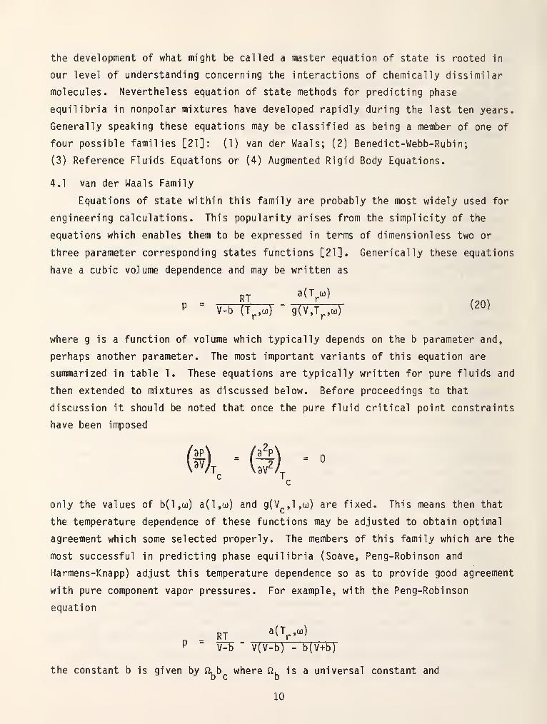
the development of what might be called a master equation of state is rooted in
our level of understanding concerning the interactions of chemically dissimilar
molecules. Nevertheless equation of state methods for predicting phase
equilibria in nonpolar mixtures have developed rapidly during the last ten years.
Generally speaking these equations may be classified as being a member of one of
four possible families [21]: (1) van der Waals; (2) Benedict-Webb-Rubin;
(3) Reference Fluids Equations or (4) Augmented Rigid Body Equations.
4.1 van der Waals Family
Equations of state within this family are probably the most widely used for
engineering calculations. This popularity arises from the simplicity of the
equations which enables them to be expressed in terms of dimensionless two or
three parameter corresponding states functions [21]. Generically these equations
have a cubic volume dependence and may be written as
RTaCT^u))
P = V-b (1^,0))-
g(V,T^,a,)(20)
where g is a function of volume which typically depends on the b parameter and,
perhaps another parameter. The most important variants of this equation are
summarized in table 1. These equations are typically written for pure fluids and
then extended to mixtures as discussed below. Before proceedings to that
discussion it should be noted that once the pure fluid critical point constraints
have been imposed
=(s), iV)
only the values of b{l,a)) a(l,a)) and g(V ,l,a)) are fixed. This means then that
the temperature dependence of these functions may be adjusted to obtain optimal
agreement which some selected properly. The members of this family which are the
most successful in predicting phase equilibria (Soave, Peng-Robinson and
Harmens-Knapp) adjust this temperature dependence so as to provide good agreement
with pure component vapor pressures. For example, with the Peng-Robinson
equation
R]L_ '(V*"^^P v-b " V(V-b) - b(V+b)
the constant b is given by Q,b where ^, is a universal constant andbe b
10
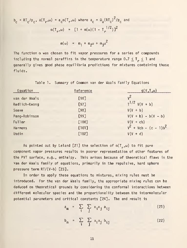
2b^ = RT^/Pc» a(Tp,tD) = a^a(T^,a)) where a^ = ^g{RT^) /p^ and
a(T^,a)) = [1 + m((.)(l - 1^^'^)^
m((jo) = m-, + mM + mva)
The function a was chosen to fit vapor pressures for a series of compounds
including the normal paraffins in the temperature range 0.7 <. T < 1 and
generally gives good phase equilibria predictions for mixtures containing those
fluids.
Table 1. Summary of Common v
Equation Reference
van der Waals [96]
Redl ich-Kwong [97]
Soave [98]
Peng-Robinson [99]
Fuller [100]
Harmens [101]
Usdin [102]
g(V.T.a))
T^/^ V(V + b)
V(V + b)
V(V + b) - b(V - b)
V(V + cb)
V^ + Vcb - (c - l)b^
V(V + d)
As pointed out by Lei and [21] the selection of a(T ,0)) to fit pure
component vapor pressures results in poorer representation of other features of
the PVT surface, e.g., enthalpy. This arises because of theoretical flaws in the
Van der Waals family of equations, primarily in the repulsive, hard sphere
pressure term RT/(V-b) [23].
In order to apply these equations to mixtures, mixing rules must be
introduced. For the van der Waals family, the appropriate mixing rules can be
deduced on theoretical grounds by considering the conformal interactions between
different molecular species and the proportionality between the intermolecular
potential parameters and critical constants [24]. The end result is
a, = E E x.xj a.j (21)
". =
^ ^Vi "ij(22)
11
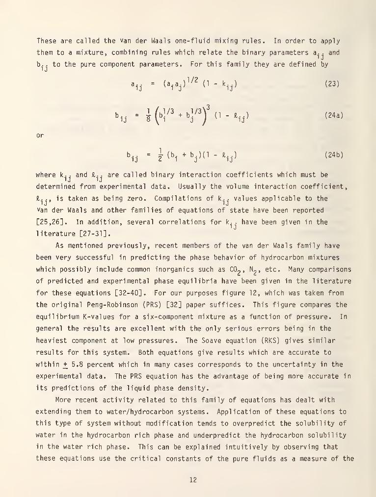
These are called the van der Waals one-fluid mixing rules. In order to apply
them to a mixture, combining rules which relate the binary parameters a. . and
b. . to the pure component parameters. For this family they are defined by
a,.j = (a^aj)l/2 (1 - k.^) (23)
,3
.. = l(b]/3^b]/3) (1.,..) (24a)
or
b.j = 1 (b. . bj)(l - £.j) (24b)
where k.. and £. . are called binary interaction coefficients which must be
determined from experimental data. Usually the volume interaction coefficient,
£.., is taken as being zero. Compilations of k.. values applicable to the
Van der Waals and other families of equations of state have been reported
[25,26]. In addition, several correlations for k. . have been given in the
literature [27-31].
As mentioned previously, recent members of the van der Waals family have
been very successful in predicting the phase behavior of hydrocarbon mixtures
which possibly include common inorganics such as CO2 , Np, etc. Many comparisons
of predicted and experimental phase equilibria have been given in the literature
for these equations [32-40]. For our purposes figure 12, which was taken from
the original Peng-Robinson (PRS) [32] paper suffices. This figure compares the
equilibrium K-values for a six-component mixture as a function of pressure. In
general the results are excellent with the only serious errors being in the
heaviest component at low pressures. The Soave equation (RKS) gives similar
results for this system. Both equations give results which are accurate to
within +5.8 percent which in many cases corresponds to the uncertainty in the
experimental data. The PRS equation has the advantage of being more accurate in
its predictions of the liquid phase density.
More recent activity related to this family of equations has dealt with
extending them to water/hydrocarbon systems. Application of these equations to
this type of system without modification tends to overpredict the solubility of
water in the hydrocarbon rich phase and underpredict the hydrocarbon solubility
in the water rich phase. This can be explained intuitively by observing that
these equations use the critical constants of the pure fluids as a measure of the
12
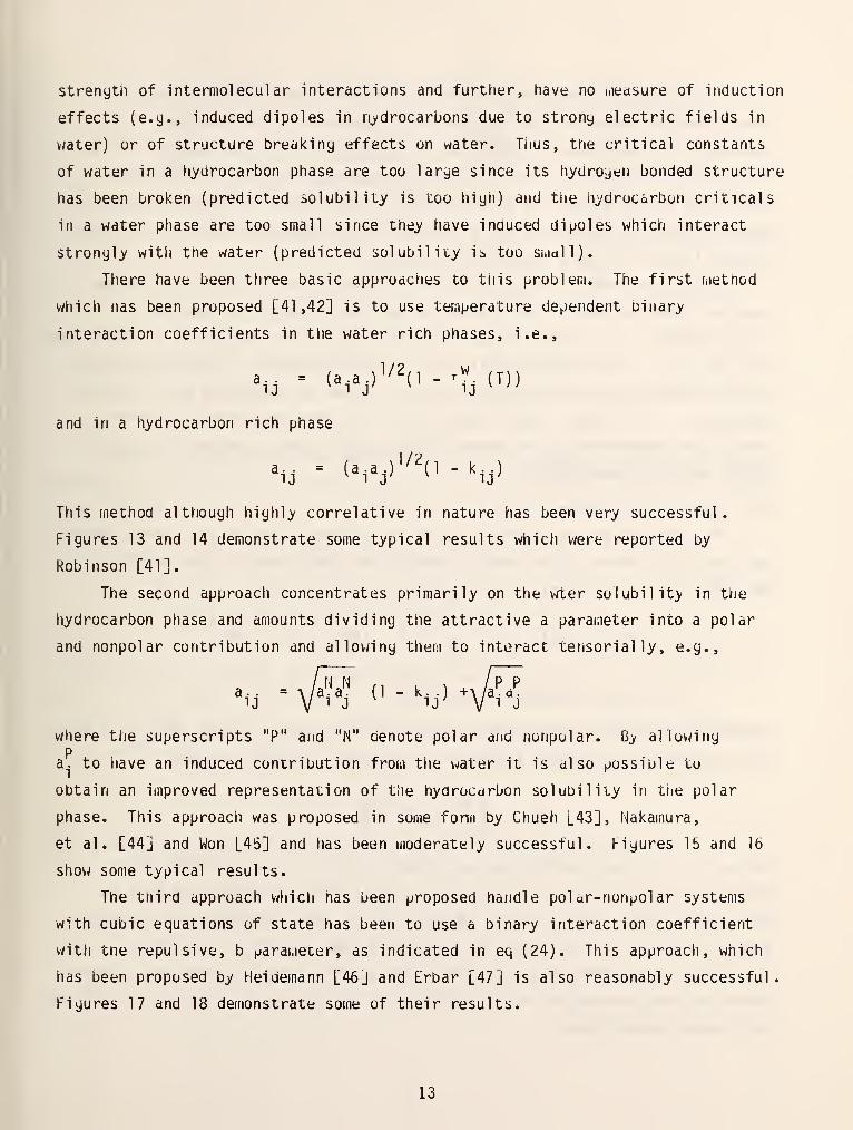
strength of intermolecular interactions and further, have no nieasure of induction
effects (e.g., induced dipoles in nj^drocarbons due to strong electric fields in
water) or of structure breaking effects on water. Thus, the critical constants
of water in a fiydrocarbon phase are too large since its hydrovjen bonded structure
has been broken (predicted solubility is too hign) and the hydrocarbon critical s
in a water phase are too small since they have induced dipoles which interact
strongly with the water (predicted solubility ii too Sinall).
There have been three basic approaches to this problem. The first raethod
which nas been proposed [41,42] is to use temperature dependent binary
interaction coefficients in the water rich phases, i.e..
a,, = {a,.a,)-(1-Ij(T))
and in a hydrocarbon rich phase
a, . = (a,a.)'/'^(l - k..)
This method although highly correlative in nature has been yery successful.
Figures 13 and 14 demonstrate some typical results which were reported by
Robinson [41].
The second approach concentrates primarily on the wter solubility in the
hydrocarbon phase and amounts dividing the attractive a parameter into a polar
and nonpolar contribution and allowing them to interact tensorial ly , e.g..
^ - s,) ^^^where the superscripts "P" and "N" denote polar and nonpolar. B> allowingp
a. to nave an induced contribution from the water it is also possible to
obtain an improved representation of the hydrocarbon solubility in ttie polar
phase. This approach was proposed in some fonn by Chueh [43], Nakamura,
et al . [44] and Won [45] and has been moderately successful. Figures 15 and 16
show some typical results.
The third approach which has been proposed handle polar-nonpol ar systems
with cubic equations of state has been to use a binary interaction coefficient
with tne repulsive, b jjarai.ieter, as indicated in eq (24). This approach, which
has been proposed by Heidemann [46] and Erbar [47] is also reasonably successful.
Figures 17 and 18 demonstrate some of their results.
13
In spite of the relative success of these modifications in correlating
polar/nonpolar phase equilibria, they still leave much to be desired. For
example, it is not generally possible to a priori predict the required binary
interaction coefficients nor is it possible to determine the polar/nonpolar
separation of the attractive coefficients. In addition, this type of model is
merely correcting a model which is basically too simple and incorrect in detail
to make it work for more complicated systems.
Another approach to the correlation and prediction of phase equilibrium
based on a van der Waals family equation has been proposed by several
investigators. It is based on modifying the composition dependence of the mixing
rule, eq (21). This method enables one to correlate data for complex mixtures
but the equation of state parameters can no longer be identified with critical
constants. In addition, these models do not give the theoretically correct
composition dependence of the second virial coefficient. For details of this
method see references [48-51].
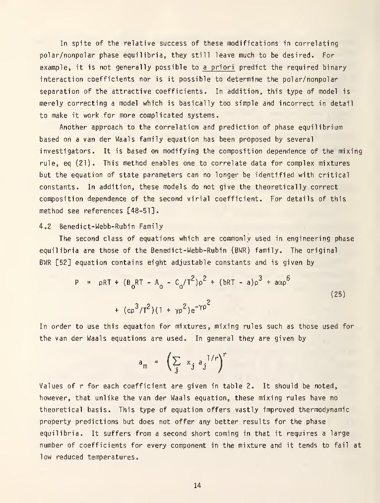
4.2 Benedict-Webb-Rubin Family
The second class of equations which are commonly used in engineering phase
equilibria are those of the Benedict-Webb-Rubin (BWR) family. The original
BWR [52] equation contains eight adjustable constants and is given by
P = pRT + (BqRT - Aq - Cq/T^)p^ + (bRT - a)p^ + aap^
(25)
2
+ (cp^/t2)(1 + YP^)e-^P
In order to use this equation for mixtures, mixing rules such as those used for
the van der Waals equations are used. In general they are given by
^m (? > :"1
Values of r for each coefficient are given in table 2. It should be noted,
however, that unlike the van der Waals equation, these mixing rules have no
theoretical basis. This type of equation offers vastly improved thermodynamic
property predictions but does not offer any better results for the phase
equilibria. It suffers from a second short coming in that it requires a large
number of coefficients for eyery component in the mixture and it tends to fail at
low reduced temperatures.
14
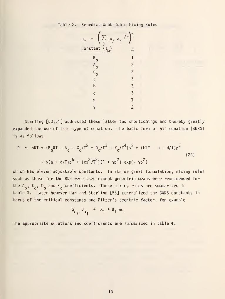
Table l. Benedict-Webb-Rubin Mixing Rules
n \ . J J /
Constant (a^^) £
«0 1
^ 2
^0 2
a 3
b 3
c 3
a 3
Y 2
Starling [53,54] addressed these latter two shortcomings and thereby greatly
expanded the use of this type of equation. The basic form of his equation (BURS)
is as follows
P = pRT + (BqRT - A^ - Cq/T^ + Dq/T^ - Eq/t'^)p^ + (bRT - a - d/T)p^
+ a(a + d/T)p^ + (cp'^/T^)(l + yp^) exp(- yp^)
(26)
which has eleven adjustable constants. In its original formulation, mixing rules
such as those for the BUR were used except geometric means were recommended for
the A^, C , D and E coefficients. These mixing rules are summarized ino' ^
table 3. Later hov/ever Han and Starling L55] generalized the BWRS constants in
terms of the critical constants and Pitzer's acentric factor, for example
The appropriate equations and coefficients are summarized in table 4.
15
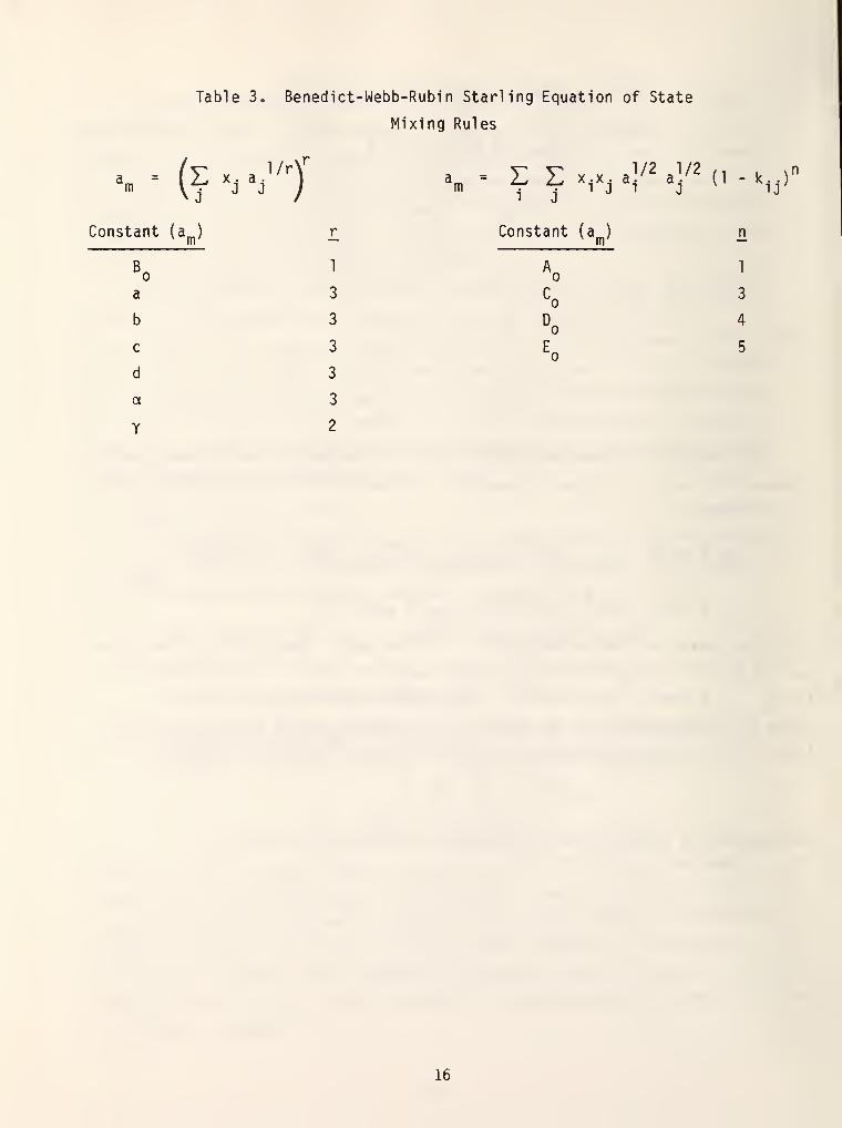
Table 3. Benedict-Webb-Rubin Starling Equation of State
Mixing Rules
^m =It "j^j
;
Constant(^n,)
r
^ 1
a 3
b 3
c 3
d 3
a 3
Y 2
a„ = E E x,x. a|/^ a]/^ (I - .,.,"1 J
Constant (a„)m
16
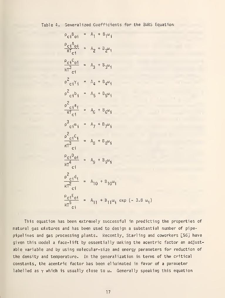
Table 4. Generalized Coefficients for the BURS Equation
p .B . = A, + B,(jo.^Cl 01 111p .A .
^Cl 01 ^ ^ •)
ci
p .C .
Cl 01 A . D
^' ci
P^i^i = ^4 ^ ^4'^i
p2^.b. = A5.B3C..
P^i^
p^^.a. = A^ + B^a..
p -C •
^ Cl 1 „ ^ D
'^'ci
p .D .
Cl 01 A J. D-1 = ^9 ^ S^iRT^ .
J y 1
ci
p2 .d.^Cl 1 _ „
, R;Z2— - ^0 ^ ^10^-^' Ci
^^ = A^^ +B^^u3. exp(- 3.8..)'^'
ci
This equation has been extremely successful in predicting the properties of
natural gas mixtures and has been used to design a substantial number of pipe-
pipelines and gas processing plants. Recently, Starling and coworkers [56j have
given this model a face-lift by essentially making the acentric factor an adjust-
able variable and by using molecular-size and energy parameters for reduction of
the density and temperature. In the generalization in terms of the critical
constants, the acentric factor has been eliminated in favor of a parai;ieter
labelled as y which is usually close to w. Generally speaking this equation
17
offers only marginal ii,iproveinent over the original BWRS. Other modifications of
the BWR equation have been proposed and the interested reader should consult
references [57-60].
The BWR family of equations has not been successfully extended to mixtures
containing highly polar components such as water. The primary problem in this
area lies in the large number of parameters used in this equation and the lack of
any theoretical guidelines. In fact, the BWRS has never been successfully fitted
to pure water so the parameters required for the mixing rules are not available.
This problem is under current investigation by Starling and his coworkers L61j.
4.3 Reference Fluid Equations of State
During the past 15 years large quantities of highly precise (and accurate)
PVT and thermodynamic property data have been measured by various laboratories.
With the advent of these data, complex equations of state have been developed to
represent these data without regard to mathematica-1 simplicity or eventual
generalization to other fluids. Notable examples of this class of equations are
the 32 term BWR proposed by Stewart and Jacobsen L62] and the nonanalytic
equation developed by Goodwin [63].
In order to apply this type of equation of state to other pure fluids or
mixtures, conformal solution theory must be used. This theory is based on the
assumption that within classes (e.g., homologous series) of fluids the
intermolecular potentials are given by
Uj (r) = ej f{r/o.)
for a pure fluid and
u^j (r) = e,j f(r/o.j)
for an unlike binary pair. This leads to the conclusion [64,65] for this class
of fluids that
and
Z^.(V,T) = ZQ(V/h., T/f.) (27a)
A^ =-^i
Ao(V/h.. T/f.) (27b)
18
D
where Z is the compressibility factor, A is the residual Helmholtz free energy
and f. and h. are called equivalent substance reducing ratios which are defined
by
h. = v^/V^^ and f. = T^/T^^ .
The subscript "o" denotes the reference fluid. Lei and and coworkers [66,67]
further extended this two parameter corresponding states model to fluids having
assymetric, but not dipolar interactions by introducing shape factors in the
equivalent substance reducing ratios, viz.
h. = (V^/V^) *. (T^ , V^ , 0).) (28)
fi = (^/^o) S- ^V.'V.'^') (29)1 1
The shape factors have been fit to a generalized mathematical form and are given
in reference [67]. Given eqs (27-29) it is possible to calculate all of the
thermodynamic properties of a pure fluid belonging to the same conformal class.
In order to extend this method to mixtures, mixing and combining rules must be
introduced for the parameters f and h. Usually they are chosen in accordance
with the van der Waals one-fluid theory [68]
a 3
and
Ot p
although other choices are possible. The combining rules used with this model
are
f o = (^ ^o)^^^ (1 - k J (32)ag ^ a 3 a3
and
\e ' I ^^'l" ' ^^r^'^' - ^cb'(33^)
or
19
Using eqs (30-33) in conjunction with (27-29) enables one to calculate any
mixture property of interest. For example, for the fugacity of a component in
solution
U*^ 9f 3h
X a X a
where Uq and Zq are the residual internal energy and coinpressibil ity factor of
the reference fluid. Several authors [69-72] have explored the predictions of
this method using a methane reference and figures 19 and 20 show some typical
results. In general, results obtained with this i.iethod using a methane reference
are yery accurate if the system doesn't contain components with molecular weights
greater than Cy or associating components [69]. Furthermore, the method suffers
from being mathematically coniplex which historically hinders industrial
acceptance.
A second reference fluid equation of state method has been proposed by
several authors [73-76]. It is based on the original Pitzer corresponding states
i.iodel [75], but uses more than one reference fluid. For a two-fluid model [74]
it takes the form
Z(P,,T^) Z^(2) _ Jl)
LZ Z ]
where the superscripts (1) and (2) denote the reference fluid values. In order
to apply this method to i^iixtures, pseudocritical parameters must be defined via
mixing rules such as
^n^cm = ^ ^ ^i^j 'c. ^c,.
03 2-, X. CO. , etc,111 . 1 1
most applications of this method have dealt with prediction of mixture density
and enthalpy and the results are very good [75]. Current work with this approach
deals with phase equilibria and critical lines [77j.
4.4 Augmented Rigid Body Equations of State
The final category of equations of state is similar in some respects to the
van der kJaals family, but is set apart because of the abandonment of the van der
20
Waals repulsion term RT/(V-b) . These equations start with theoretically based
rigid body equations of state and add terms to account for the effect of
molecular attraction. The rigid body terms are the Wertheim-Thiele [82],
Carnahan-Starl ing equation of state for hard spheres [78] and the equations of
Gibbons [79], Boublik [80] or Nezbeda and Lei and [81] for rigid nonspherical
bodies. Examples of this class of equations are the perturbed hard chain theory
[83,84], augmented van der Waals theory [85-87] and the Hlavaty equation of state
[88,89] among others [99-94].
Of particular interest in this class are the augmented van der Waals
equation developed by Kregleski and cov/orkers [85-87] and the perturbed hard
chain theory of Prausnitz, et al . [83,84]. These two models have been applied to
polar/nonpolar systems with moderate success. Recently [95] the Prausnitz model
has been successfully applied to water and water/alcohol /hydrocarbon containing
mixtures. Generally speaking, this family of equations of state is in a
developmental stage and has not yet found widespread industrial use. They
appear, however, to offer the most economical route to phase equilibria in
polar/nonpolar systems.
4.5 Critical Loci From Cubic Equations of State
Latter portions of this report deal with the prediction of critical loci
using the reference fluid equation of state approach and the Leung-Griffiths
model [103-105]. It should be pointed out in passing that a considerable amount
of effort has been made in predicting these loci using members of the van der
Waals (cubic) family of equations of state. Scott and von Konynenburg [1,2] have
shown that with the appropriate choice of parameters in the original van der
Waals equation, all known types of critical lines in binary mixtures may be
qualitatively predicted. More recently, Peng and Robinson [106] have developed a
numerical method for predicting critical lines in multicomponent mixtures. They
applied this method using their equation of state to both binary and
multicomponent liquid-vapor mixtures having up to 12 components. Their
comparisons showed prediction of the mixture critical temperature to within an
average absolute error of 4 K (% 1 .3 percent) and pressures to within 173 kPa
(>. 2.3 percent). Predictions of the critical volumes were substantially worse
(x 12 percent error) which is not surprising since cubic equations of state are
not very accurate for density prediction.
21
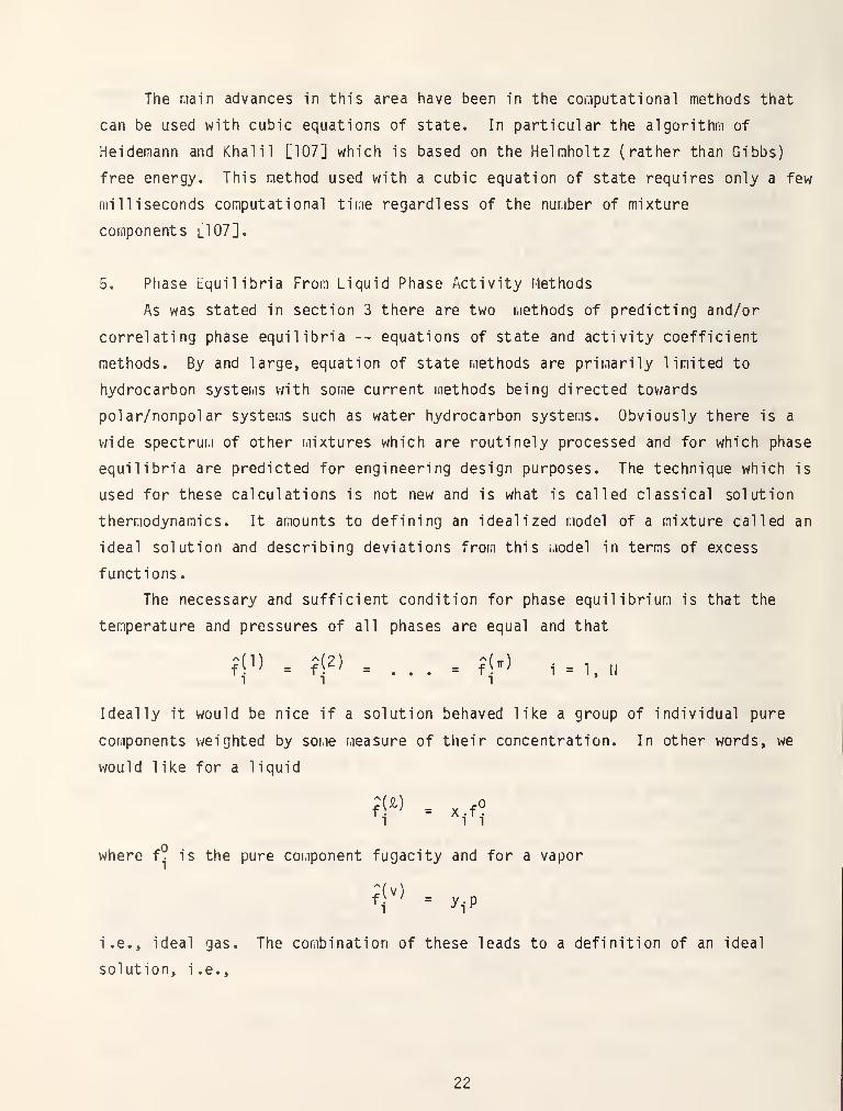
The main advances in this area have been in the coiTiputational methods that
can be used with cubic equations of state. In particular the algorithm of
Heidemann and Khalil [107] which is based on the Helmholtz (rather than Gibbs)
free energy. This method used with a cubic equation of state requires only a few
milliseconds computational time regardless of the number of mixture
components l107].
5. Phase Equilibria From Liquid Phase Activity Methods
As was stated in section 3 there are two methods of predicting and/or
correlating phase equilibria -- equations of state and activity coefficient
methods. By and large, equation of state methods are primarily limited to
hydrocarbon systems with some current methods being directed tov/ards
polar/nonpolar systems such as water hydrocarbon systems. Obviously there is a
wide spectrum of other iiiixtures which are routinely processed and for which phase
equilibria are predicted for engineering design purposes. The technique which is
used for these calculations is not new and is what is called classical solution
thermodynamics. It amounts to defining an idealized model of a mixture called an
ideal solution and describing deviations from this model in terns of excess
functions.
The necessary and sufficient condition for phase equilibrium is that the
temperature and pressures of all phases are equal and that
f,P) = ff = . . . = f(") i = 1. N
Ideally it would be nice if a solution behaved like a group of individual pure
components weighted by some measure of their concentration. In other words, we
would like for a liquid
where f. is the pure component fugacity and for a vapor
i.e., ideal gas. The combination of these leads to a definition of an ideal
solution, i.e..
22
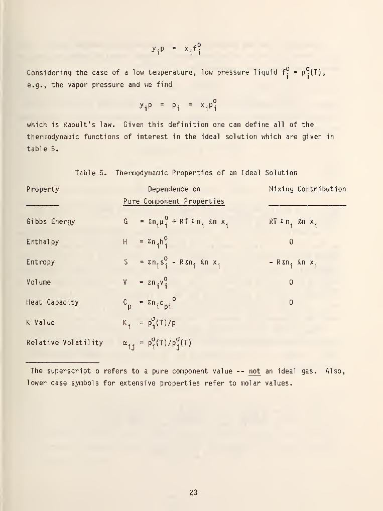
y^.p = x.f.
Considering the case of a low temperature, low pressure liquid f? = p^(T),
e.g., the vapor pressure and we find
y^P = Pi = x.p^
which is Raoult's law. Given this definition one can define all of the
thermodynai.iic functions of interest in the ideal solution which are given in
table 5.
Table 5. Thermodynamic Properties of an Ideal Solution
Property Dependence on Mixing Contribution
Pure Component Properties
Gibbs Energy G = zn.u° + RT 2 n . £n x. RT 2n. iln x.^•^ 11 11 11Enthalpy H = 2n.h°
Entropy S = ^n.s^ - Rzn. in x. - Rzn. £n x.
Volume V = J:n.v^
Heat Capacity C = zn.c .°
K Value K. = p*^(T)/p
Relative Volatility a.. = p?{T)/p^(T)
The superscript refers to a pure component value -- not an ideal gas. Also,
lower case symbols for extensive properties refer to molar values.
23
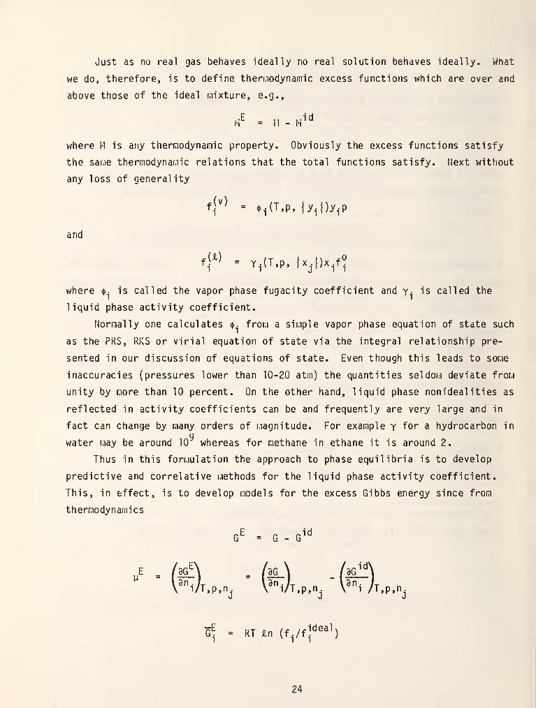
Just as no real gas behaves ideally no real solution behaves ideally. What
we do, therefore, is to define theri.iodynamic excess functions which are over and
above those of the ideal mixture, e.g.,
M^ = M - M^^
where M is any thermodynamic property. Obviously the excess functions satisfy
the same thermodynamic relations that the total functions satisfy. Next without
any loss of generality
and
where ({>. is called the vapor phase fugacity coefficient and y. is called the
liquid phase activity coefficient.
Normally one calculates (j). from a simple vapor phase equation of state such
as the PRS, RKS or virial equation of state via the integral relationship pre-
sented in our discussion of equations of state. Even though this leads to some
inaccuracies (pressures lov^er than 10-20 atm) the quantities seldom deviate from
unity by more than 10 percent. On the other hand, liquid phase nonideal ities as
reflected in activity coefficients can be and frequently are VQry large and in
fact can change by many orders of magnitude. For example y ^or a hydrocarbon in
9water may be around 10 whereas for methane in ethane it is around 2.
Thus in this formulation the approach to phase equilibria is to develop
predictive and correlative methods for the liquid phase activity coefficient.
This, in effect, is to develop models for the excess Gibbs energy since from
thermodynamics
G^ = G - G^^
E /3g!\ U\ (^\V'"l/T.p.n, V"lA.p,n, V"lA.p,n.
G^ = RT tn (f^/fj''^'^
24
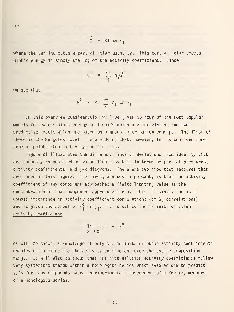
or
G^ = RT in Y^
where the bar indicates a partial molar quantity. This partial molar excess
Gibb's energy is simply the log of the activity coefficient. Since
G^ = S n.G^
we see that
G^ = RT E n. £n y.
In this overview consideration will be given to four of the most popular
models for excess Gibbs energy in liquids which are correlative and two
predictive models which are based on a group contribution concept. The first of
these is the Margules model. Before doing that, however, let us consider some
general points about activity coefficients.
Figure 21 illustrates the different kinds of deviations from ideality that
are commonly encountered in vapor-liquid systems in terms of partial pressures,
activity coefficients, and y-x diagrams. There are two important features that
are shown in this figure. The first, and most important, is that the activity
coefficient of any component approaches a finite limiting value as the
concentration of that component approaches zero. This limiting value is of
upmost importance in activity coefficient correlations (or Gp correlations)
and is given the symt
activity coefficient
and is given the symbol of y^ ory.. It is called the infinite dilution
lim y. = y°
X. -^0
As will be shown, a knowledge of only the infinite dilution activity coefficients
enables us to calculate the activity coefficient over the entire composition
range. It will also be shown that infinite dilution activity coefficients follow
very systematic trends within a homologous series which enables one to predict
y.'s for many compounds based on experimental measurement of a few key members
of a homologous series.
25
The second point which is of interest with regard to figure 21 has to do
with azeotrope formation and miscibility gaps. In the case labeled "large
positive deviations" we see in the y-x diagram the vapor and liquid compositions
actually become identical at x = .85. This corresponds to azeotrope formation,
which as you can see by comparison is not possible in an ideal solution. In the
system with \/ery large positive deviations, the dotted lines indicate a
miscibility gap, which also is not possible in an ideal mixture. Thus, it would
not be possible to do azeotropic distillation or liquid-liquid extractions if it
were not for liquid phase non- idealities.
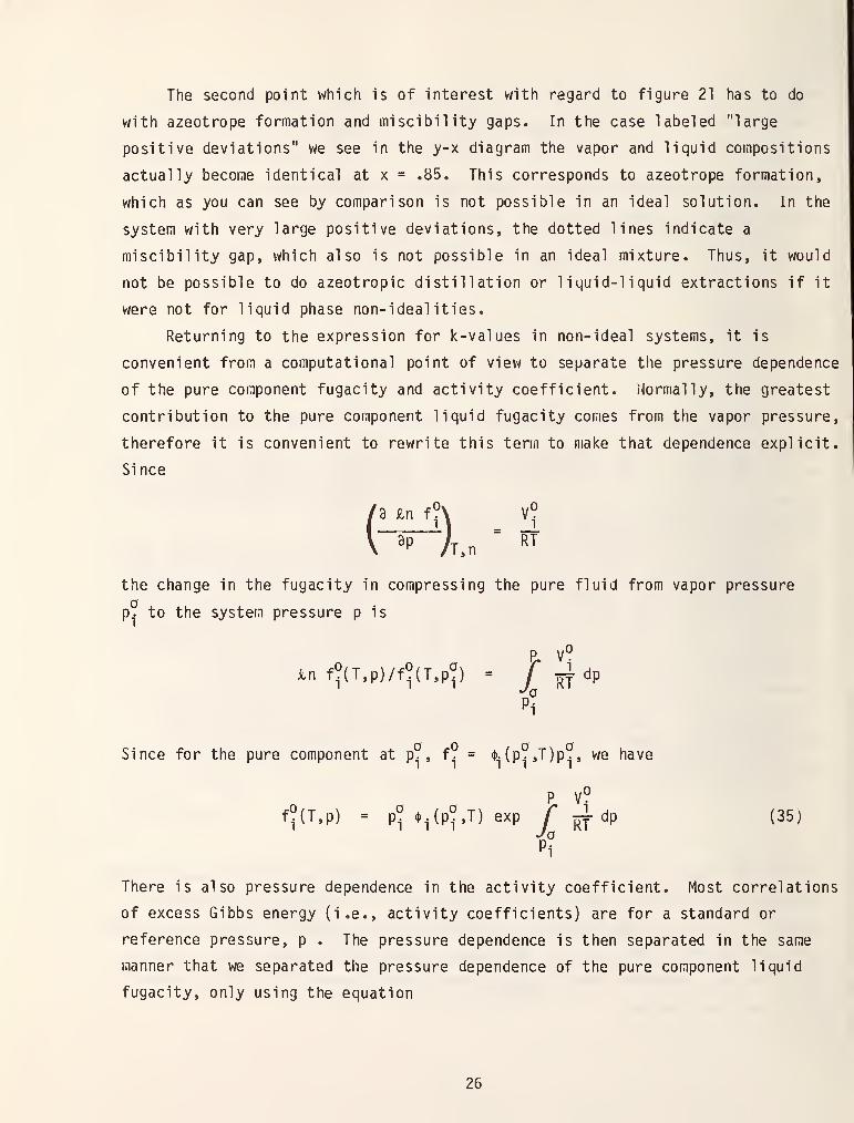
Returning to the expression for k-values in non-ideal systems, it is
convenient from a computational point of view to separate the pressure dependence
of the pure component fugacity and activity coefficient, formally, the greatest
contribution to the pure component liquid fugacity comes from the vapor pressure,
therefore it is convenient to rewrite this term to make that dependence explicit.
Since
\ ^P A.n " «T
the change in the fugacity in compressing the pure fluid from vapor pressure
p. to the system pressure p is
e, v°
ion f°(T,p)/f°(T,p^) = / rT ^P•10
Pi
Since for the pure component at p?, f. = 4!:{p^,T)p^, we have
P V?
•/o
f?(T,p) = P^ l-^-lp^.T) exp r ^dp (35j
Pi
There is also pressure dependence in the activity coefficient. Most correlations
of excess Gibbs energy (i.e., activity coefficients) are for a standard or
reference pressure, p . The pressure dependence is then separated in the same
manner that we separated the pressure dependence of the pure component liquid
fugacity, only using the equation
26
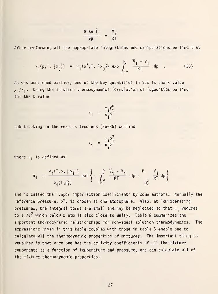
3 £n f^. V.
3p RT
After performing all the appropriate integrations and Manipulations we find that
P V. - V.
Yi{p,T, \x.\) = Y^(p*,T, \x.\) exp T \j dp . (36)
As was mentioned earlier, one of the key quantities in VLE is the k value
y./x.. Using the solution thermodynamics formulation of fugacities we find
for the k value
^i <^.P
substituting in the results from eqs (35-36) we find
ki e^p
where e^ is defined as
^(T^p.iyil) (
9^. = exp < -
^{T.p") '
and is called (the "vapor imperfection coefficient" by some authors. Nori.ial ly the
reference pressure, p*, is chosen as one atmosphere. Also, at low operating
pressures, the integral terms are small and may be neglected so that e. reduces
to 4»^/<t)^ which below 2 atm is also close to unity. Table 6 summarizes the
important thermodynamic relationships for non-ideal solution theriiiodynamics. The
expressions given in this table coupled with those in table 5 enable one to
calculate all the thermodynamic properties of mixtures. The important thing to
remember is that once one has the activity coefficients of all the mixture
coinponents as a function of temperature and pressure, one can calculate all of
the mixture thermodynamic properties.
27
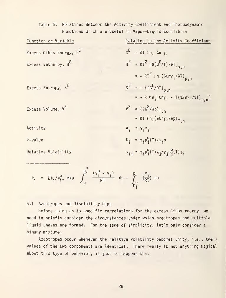
Table 6, Relations Between the Activity Coefficient and Thermodynamic
Functions Which are Useful in Vapor-Liquid Equilibria
Function or Variable Relation to the Activity Coefficient
Excess Gibbs Energy, G G = RT z n . i2,n y^
Excess Enthalpy, H^ H^ = RT^ [3(G^/T)/3Tj ^
= - RT^ £n.0£nY/3T)p^^
Excess Entropy, S*" S^ = - (9G^/3T) ^
= - R Zn.L^ny^ - T(3£nY ./3T)p^^j
Excess Volume, V^ V^ = (3G^/3p)-p^
= RTZn.{3£nY./3p)^^^
Activity a. = y,-x.
k-value K. = y.p^.{l)/<^.p
Relative Volatility a.^ = Y^.p°(T) ^yYjPj(T) 4.^.
^i (v° - V.) p V.
e. = [*./.°] exp / -^^^ dp - jr (^) dp
Pi
5.1 Azeotropes and Miscibility Gaps
Before going on to specific correlations for the excess Gibbs energy, we
need to briefly consider the circumstances under which azeotropes and multiple
liquid phases are formed. For the sake of simplicity, let's only consider a
binary mixture.
Azeotropes occur whenever the relative volatility becomes unity, i.e., the k
values of the two components are identical. There really is not anything magical
about this type of behavior, it just so happens that
28
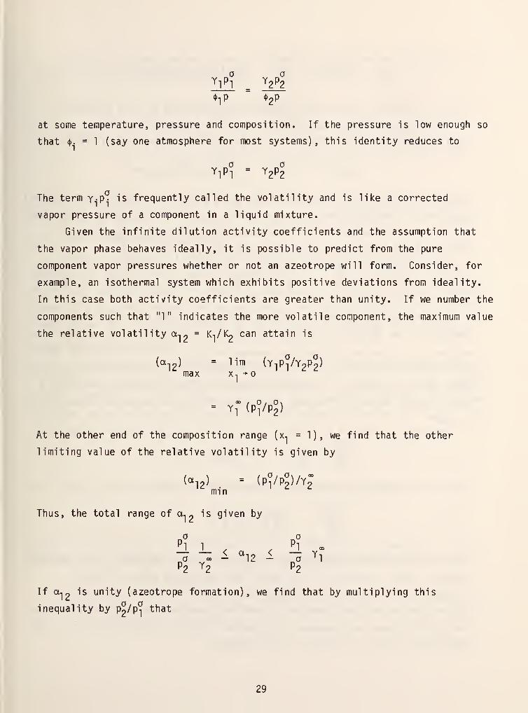
o o
4>-|P '^2^
at some temperature, pressure and composition. If the pressure is low enough so
that (f>.= 1 (say one atmosphere for most systems), this identity reduces to
a aYiPi = Y2P2
The term y.p? is frequently called the volatility and is like a corrected
vapor pressure of a component in a liquid mixture.
Given the infinite dilution activity coefficients and the assumption that
the vapor phase behaves ideally, it is possible to predict from the pure
component vapor pressures whether or not an azeotrope will form. Consider, for
example, an isothermal system which exhibits positive deviations from ideality.
In this case both activity coefficients are greater than unity. If we number the
components such that "1" indicates the more volatile component, the maximum value
the relative volatility a-.^ = K-i/Ko can attain is
(a^2) = li"! (y-|P^/Y2P2)max x-, -^0
" /_0 ,_0\= Yf(Pi/P2)
At the other end of the composition range (x-. = 1 ) , we find that the other
limiting value of the relative volatility is given by
O /_0\ / 00
(^12) . = (Pi/P2)/Y2min
Thus, the total range of a, « is given by
a ah 1 Pi oc
a 00_< "12 <
a ^1
h ^2 P2
If a,2 is unity (azeotrope formation), we find that by multiplying thiso ,_a
inequality by p^/Pi that
29
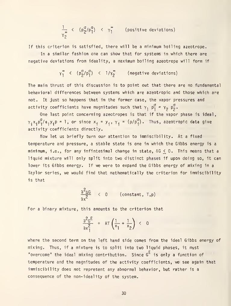
— < (pp/p?) < Yr (positive deviations)
If this criterion is satisfied, there will be a minimum boiling azeotrope.
In a similar fashion one can show that for systems in which there are
negative deviations from ideality, a maximum boiling azeotrope will form if
yT < (Pp/P-i) ^ I/Yo (negative deviations)
The main thrust of this discussion is to point out that there are no fundamental
behavioral differences between systems which are azeotropic and those which are
not. It just so happens that in the former case, the vapor pressures and
activity coefficients have magnitudes such that y-i P? = Yp P?*
One last point concerning azeotropes is that if the vapor phase is ideal,
Y^-x^.p'^/^^.y^p = 1 , or since x^ =y^. , y^- = (p/p^) • Thus, azeotropic data give
activity coefficients directly.
Now let us briefly turn our attention to immiscibility. At a fixed
temperature and pressure, a stable state is one in which the Gibbs energy is a
minimum, i.e., for any infintesimal change in state, 5G _< 0. This means that a
liquid mixture will only split into two distinct phases if upon doing so, it can
lower its Gibbs energy. If we were to expand the Gibbs energy of mixing in a
Taylor series, we would find that mathematically the criterion for immiscibility
is that
2
^-^ < (constant, T,p)
9x^
For a binary mixture, this amounts to the criterion that
9x^ \^1 ^ ^2/
where the second term on the left hand side comes from the ideal Gibbs energy of
mixing. Thus, if a mixture is to split into two liquid phases, it must
"overcome" the ideal mixing contribution. Since G is only a function of
temperature and the magnitudes of the activity coefficients, we see again that
immiscibility does not represent any abnormal behavior, but rather is a
consequence of the non-ideality of the system.
30
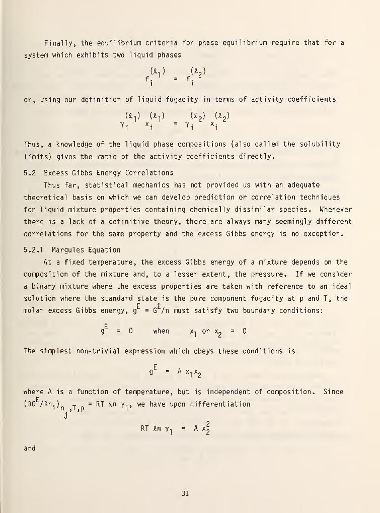
Finally, the equilibrium criteria for phase equilibrium require that for a
system which exhibits two liquid phases
or, using our definition of liquid fugacity in terms of activity coefficients
Yi X. = Yi X.
Thus, a knowledge of the liquid phase compositions (also called the solubility
limits) gives the ratio of the activity coefficients directly.
5.2 Excess Gibbs Energy Correlations
Thus far, statistical mechanics has not provided us with an adequate
theoretical basis on which we can develop prediction or correlation techniques
for liquid mixture properties containing chemically dissimilar species. Whenever
there is a lack of a definitive theory, there are always many seemingly different
correlations for the same property and the excess Gibbs energy is no exception.
5.2.1 Margules Equation
At a fixed temperature, the excess Gibbs energy of a mixture depends on the
composition of the mixture and, to a lesser extent, the pressure. If we consider
a binary mixture where the excess properties are taken with reference to an ideal
solution where the standard state is the pure component fugacity at p and T, the
molar excess Gibbs energy, g = G /n must satisfy two boundary conditions:
g = when x-, or Xp =
The simplest non-trivial expression which obeys these conditions is
g = A x^Xg
where A is a function of temperature, but is independent of composition. Since
(9G /9n,-)pT D
~ '^^ ^"'''i'
^^ ^^^^ ^^^^ differentiation
2RT £n Y-i = A Xp
and
31
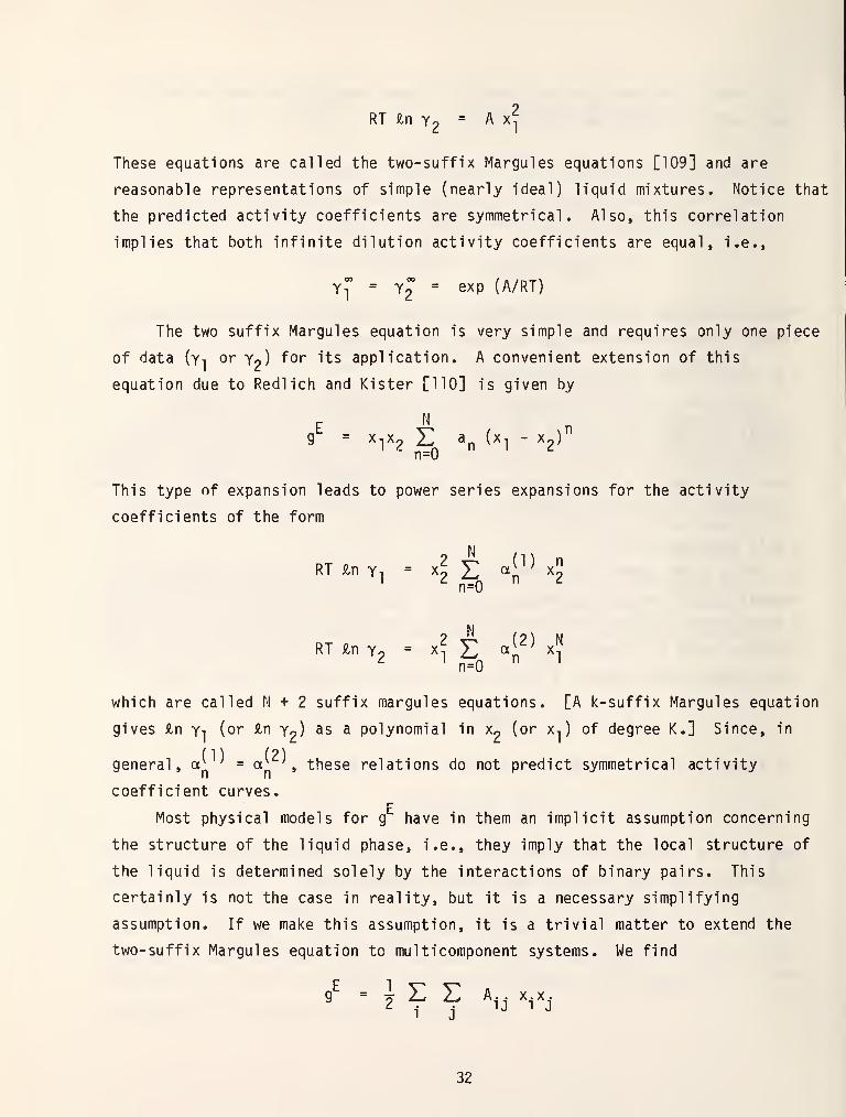
2RT £n Y2 = A x^
These equations are called the two-suffix Margules equations [109] and are
reasonable representations of simple (nearly ideal) liquid mixtures. Notice that
the predicted activity coefficients are symmetrical. Also, this correlation
implies that both infinite dilution activity coefficients are equal, i.e.,
Yf = Y2 = exp (A/RT)
The two suffix Margules equation is yery simple and requires only one piece
of data (y-i or Yo) ^^^ its application. A convenient extension of this
equation due to Redlich and Kister [110] is given by
E ^g = x-jXp E a (x, - Xp)
' '^ n=0 " '
'^
This type of expansion leads to power series expansions for the activity
coefficients of the form
RT £n Yi = 4 ^ ""n^""
' "^ n=0 "X,
RT iln Yo = x^ E a[^^ x^"^
' n=0 " '
which are called M + 2 suffix margules equations. [A k-suffix Margules equation
gives £n y-i (or iln Yo) ^s a polynomial in Xp (or x-, ) of degree K.] Since, in
general, aj^ ' = aj^ ' , these relations do not predict symmetrical activity
coefficient curves.
Most physical models for g have in them an implicit assumption concerning
the structure of the liquid phase, i.e., they imply that the local structure of
the liquid is determined solely by the interactions of binary pairs. This
certainly is not the case in reality, but it is a necessary simplifying
assumption. If we make this assumption, it is a trivial matter to extend the
two-suffix Margules equation to multicomponent systems. We find
32
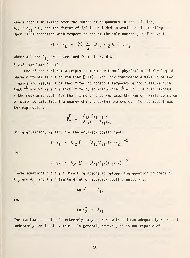
where both sums extend over the number of components in the solution,
A.. = A.. =0, and the factor of 1/2 is included to avoid double counting.
Upon differentiation with respect to one of the mole numbers, we find that
RT Hn Y,, = E E (A,^ - -1 A.j) x.Xj
where all the A. . are determined from binary data.
5.2.2 van Laar Equation
One of the earliest attempts to form a rational physical model for liquid
phase mixtures is due to van Laar [111], van Laar considered a mixture of two
liquids and assumed that they mixed at constant temperature and pressure suchE E E E
that V and S were identically zero, in which case G = .He then devised
a thermodynamic cycle for the mixing process and used the van der Waals equation
of state to calculate the energy changes during the cycle. The net result was
the expression:
Sl. = /l2 ^21 ^1^2
RT (A^2^l ^ ^21^2^
Differentiating, we find for the activity coefficients
iln Y^ = A^2 ^^ ^ (A^2/^21^^^l/^2^^"^
and
^n Y2 = A2^ [1 + (A2^/A^2)(^2'^^l^^"^
These equations provide a direct relationship between the equation parameters
Ai2 and A21 and the infinite dilution activity coefficients, viz.
and
In Y^ = A^2
^nY2 = A21
The van Laar equation is extremely easy to work with and can adequately represent
moderately non-ideal systems. In general, however, it is not capable of
33
representing strongly non-ideal systems, especially those which exhibit
association or strong physical interactions.
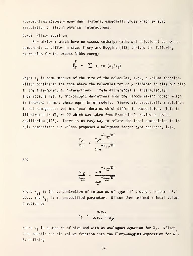
5.2.3 Wilson Equation
For mixtures which have no excess enthalpy (athermal solutions) but whose
components do differ in size, Flory and Huggins [112] derived the following
expression for the excess Gibbs energy
^ = E X. £n (X./x.)
where X. is some ineasure of the size of the molecules, e.g., a volume fraction.
Wilson considered the case where the molecules not only differed in size but also
in the intermolecular interactions. These differences in intermolecular
interactions lead to microscopic deviations from the random mixing notion which
is inherent in many phase equilibrium models. Viewed microscopically a solution
is not homogeneous but has local domains which differ in composition. This is
illustrated in figure 22 which was taken from Prausnitz's review on phase
equilibrium [113]. There is no easy way to relate the local composition to the
bulk composition but Wilson proposed a Boltzmann factor type approach, i.e..
A/^ T AntyKZ
-Ajj/RT
X„ -X„/RTx-je
and
A T rt At"-X^2^RT
Xrt^ —A^^/K
1
Xj,e
where Xp-i is the concentration of molecules of type "1" around a central "2,"
etc., and \.. is an unspecified parameter. Wilson then defined a local volume
fraction by
1 v,x,i +V2,
where v. is a measure of size and with an analogous equation for X . Wilson
then substituted his volume fraction into the Flory-Huggins expression for G .
By defining
34
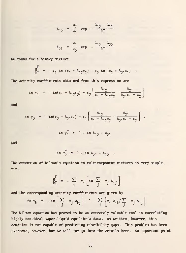
^ = !i exp .^]1_L^^21 V2 ^ RT
he found for a binary mixture
%f = - x-| £n (x, + A-ipXp) - Xp an (x^ + Ap-iX,)
The activity coefficients obtained from this expression are
A,« A,
£n Y^ = - £n(x^ ^ A-igX^) ^ X3[^^ ^^^^^^^
-^^^^^\ ^j
and
£n Yo = " ^"(Xo •" ^21^1^ ^ ^112
A,21
X-i » '^ 1Q '^o 01 1 O
£n Yi = 1 - iln A12 - A^i
and
00
iln Yo - 1 - ^n Api - A-.^ .
The extension of Wilson's equation to multicomponent mixtures is very simple,
viz.
^ = - E XRT Y i
£n E X. A. .
and the corresponding activity coefficients are given by
An Yi. = - ^n.? ''o^o
.1 - Ei
X, A.,/E Xj A..
The Wilson equation has proved to be an extremely valuable tool in correlatTng
highly non-ideal vapor-liquid equilibria data. As written, however, this
equation is not capable of predicting miscibility gaps. This problem has been
overcome, however, but we will not go into the details here. An important point
35
relating to this equation is that it forms the basis for a predictive method of
calculating vapor-liquid equilibria knov/n as ASOG (Analytical Solution of Groups)
which has been developed by E. L. Derr. This method along with another
predictive method for activity coefficients will be discussed in section 5.3.
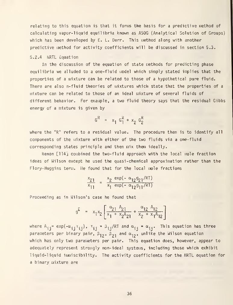
5.2.4 NRTL Equation
In the discussion of the equation of state methods for predicting phase
equilibria we alluded to a one-fluid i,x)del which simply stated implies that the
properties of a mixture can be related to those of a hypothetical pure fluid.
There are also n-fluid theories of mixtures which state that the properties of a
mixture can be related to those of an ideal mixture of several fluids of
different behavior. For example, a two fluid theory says that the residual Gibbs
energy of a mixture is given by
= X, G, + x^ G2
where the "R" refers to a residual value. The procedure then is to identify all
components of the mixture with either of the two fluids via a one-fluid
corresponding states principle and then mix them ideally.
Renon [114] combined the two-fluid approach with the local mole fraction
ideas of Wilson except he used the quasi-chemical approximation rather than the
Flory-Huggins term. He found that for the local mole fractions
X21 X2 exp(- a^^^g^^^/RJ)
T^ ~ x^ exp(- a^29ll/^^^
Proceeding as in Wilson's case he found that
g = x^x^^21 ^21 ^ ^^12^2
X-i ' '^o'*oi o 110
where A. .= exp(-a .
.
t. .) , t.. = 3../RT and a.. = a... This equation has three
parameters per binary pair, C-io* Boi and a,^, unlike the Wilson equation
which has only two parameters per pair. This equation does, however, appear to
adequately represent strongly non-ideal systems, including those which exhibit
liquid-liquid immiscibil ity. The activity coefficients for the MRTL equation for
a binary mixture are
36
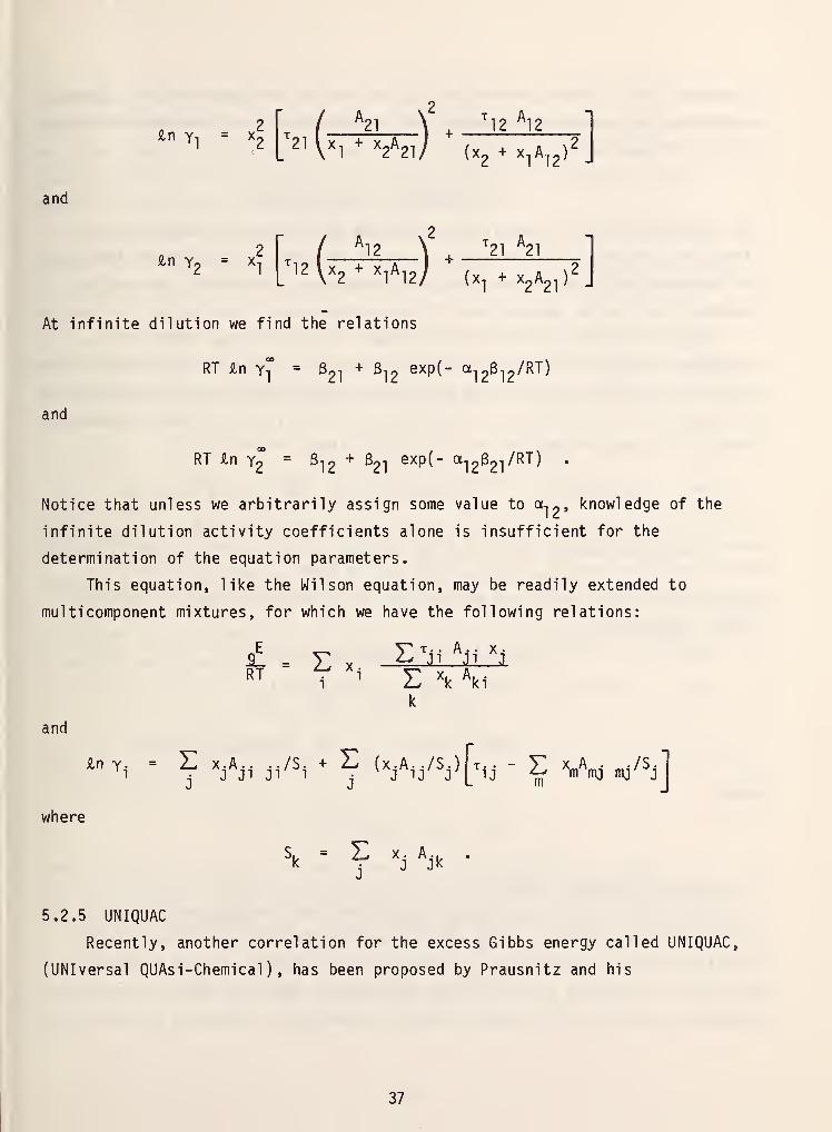
£n Y"! = x^ T^^
V^l "^21/ (X, .x,A,,)2j
and
2 r / ^12 \ ^ ^21 ^21
1p2\^X2 + x^A^2>/
(X, +x,A,in Yp = X
At infinite dilution we find the relations
1 "2"21A,i)'J
RT iln Y^ = ^2]"^ ^12 ®^P^' °'l2^12^'^^^
and
RT In Y2 = Bi2 + B21 exp(- a^2^21^'^"'^^ '
Notice that unless we arbitrarily assign some value to a, ^j knowledge of the
infinite dilution activity coefficients alone is insufficient for the
determination of the equation parameters.
This equation, like the Wilson equation, may be readily extended to
multicomponent mixtures, for which we have the following relations:
' - E^ii^i^^ = E XRT . ^i E \ \i
k
and
£n Y^ = E x.Aj, ../S. . E (x/,j/Sj)[,,j - E x,A^- „,-/Sjj
where
^k = ^ ^j ^•k•
5.2.5 UNIQUAC
Recently, another correlation for the excess Gibbs energy called UNIQUAC,
(UNIversal QUAsi-Chemical) , has been proposed by Prausnitz and his
37
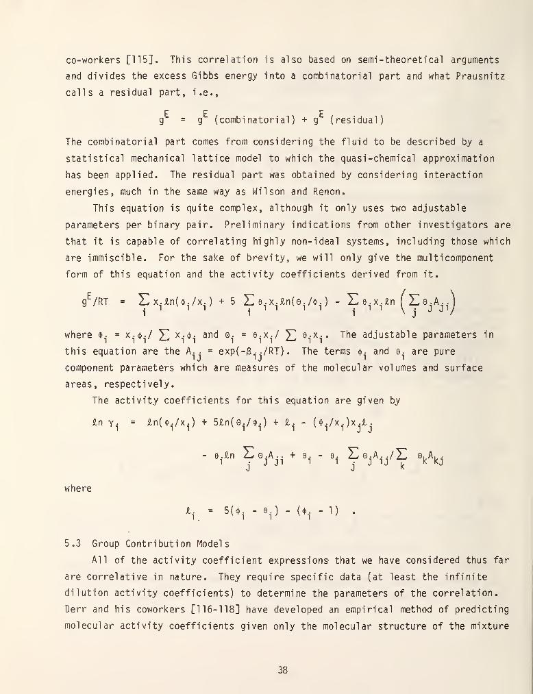
co-workers [115]. This correlation is also based on semi-theoretical arguments
and divides the excess Gibbs energy into a combinatorial part and what Prausnitz
calls a residual part, i.e.,
E E Eg = 9 (combinatorial) + g (residual)
The combinatorial part comes from considering the fluid to be described by a
statistical mechanical lattice model to which the quasi-chemical approximation
has been applied. The residual part was obtained by considering interaction
energies, much in the same way as Wilson and Renon.
This equation is quite complex, although it only uses two adjustable
parameters per binary pair. Preliminary indications from other investigators are
that it is capable of correlating highly non-ideal systems, including those which
are immiscible. For the sake of brevity, we will only give the multicomponent
form of this equation and the activity coefficients derived from it.
g^/RT = Ex.£n($^./x.) + 5 E e^.x^.£n(e./$^.) - L e^.x^.£n ( E e.A. .
j
where $. = x.ct)./ ^ x.(i). and e. = 9,-x./ ^ ^i^i*"^^^ adjustable parameters in
this equation are the A.. = exp(-B. ./RT) . The terms 4). and e. are pure
component parameters which are measures of the molecular volumes and surface
areas, respectively.
The activity coefficients for this equation are given by
£n Y^- = ini^./x.) + 5£n(e^./$^) + £^. - ($^./x.)x.£.
- ^-^^f Vji" ^• - ^ f Vij/? 'k\j
where
i. = 5(*. - e. )-(*.- 1)
5.3 Group Contribution Models
All of the activity coefficient expressions- that we have considered thus far
are correlative in nature. They require specific data (at least the infinite
dilution activity coefficients) to determine the parameters of the correlation.
Derr and his coworkers [116-118] have developed an empirical method of predicting
molecular activity coefficients given only the molecular structure of the mixture
38
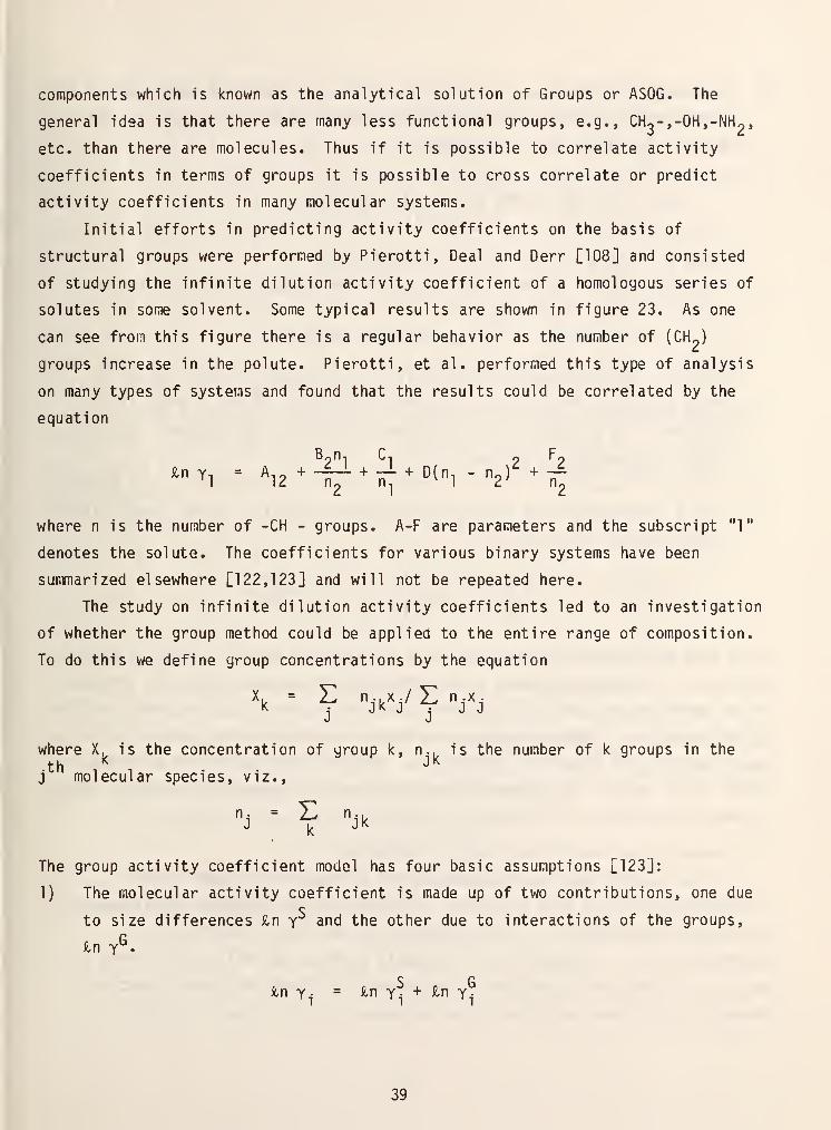
components which is known as the analytical solution of Groups or ASOG. The
general idea is that there are many less functional groups, e.g., CHo-j-OH.-NHp,
etc. than there are molecules. Thus if it is possible to correlate activity
coefficients in terms of groups it is possible to cross correlate or predict
activity coefficients in many molecular systems.
Initial efforts in predicting activity coefficients on the basis of
structural groups were performed by Pierotti, Deal and Derr [108] and consisted
of studying the infinite dilution activity coefficient of a homologous series of
solutes in some solvent. Some typical results are shown in figure 23. As one
can see from this figure there is a regular behavior as the number of (CH„)
groups increase in the polute. Pierotti, et al. performed this type of analysis
on many types of systems and found that the results could be correlated by the
equation
^"^1 = ^2^-H^ ^ ij ^ °'"l -"2)^-4
where n is the number of -CH - groups. A-F are parameters and the subscript "1"
denotes the solute. The coefficients for various binary systems have been
sunmarized elsewhere [122,123] and will not be repeated here.
The study on infinite dilution activity coefficients led to an investigation
of whether the group method could be applied to the entire range of composition.
To do this we define group concentrations by the equation
where X. is the concentration of group k, n.. is the number of k groups in the
th "^
j molecular species, viz..
The group activity coefficient model has four basic assumptions [123]:
1) The molecular activity coefficient is made up of two contributions, one due
to size differences £n y and the other due to interactions of the groups.
in Y^.
c pin Y,- = ^n Y,- + ^n y^
39
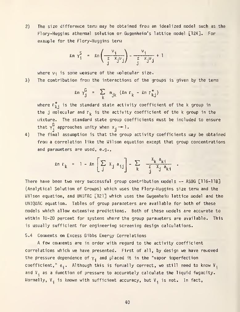
2) The size difference term may be obtained from an idealized model such as the
Flory-Huggins athermal solution or Gugenheim's lattice model [124]. For
example for the Flory-Huggins term
-v^ = ^"(tV])-ty]+
1
where vj is some measure of the molecular size,
3) The contribution from the interactions of the groups is given by the term
where r^^- is the standard state activity coefficient of the k group in
the j molecular and r|^ is the activity coefficient of the k group in the
i.iixture. The standard state group coefficients must be included to ensure
that y. approaches unity when x.-^l.J J
4) The final assumption is that the group activity coefficients may be obtained
from a correlation like the Wilson equation except that group concentrations
and parameters are used, e.g..
£n r. = 1 - £n
f h ^u. E '^
"'''
k] h ^i
There have been two very successful group contribution models -- ASOG [116-118]
(Analytical Solution of Groups) which uses the Flory-Huggins size term and the
Wilson equation, and UNIFAC [121] which uses the Gugenheim lattice model and the
UNIQUAC equation. Tables of group parameters are available for both of these
models which allow extensive predictions. Both of these models are accurate to
within 10-20 percent for systems wheref the group parameters are available. This
is usually sufficient for engineering screening design calculations.
5.4 Corarnents on Excess Gibbs Energy Correlations
A few coLiments are in order with regard to the activity coefficient
correlations which vie have presented. First of all, by design we have removed
the pressure dependence of y- ^nd placed it in the "vapor imperfection
coefficient," e . Although this is formally correct, we still need to know V.
and V. as a function of pressure to accurately calculate the liquid fugacity.
Normally, V. is known with sufficient accuracy, but V- is not. In fact.
40
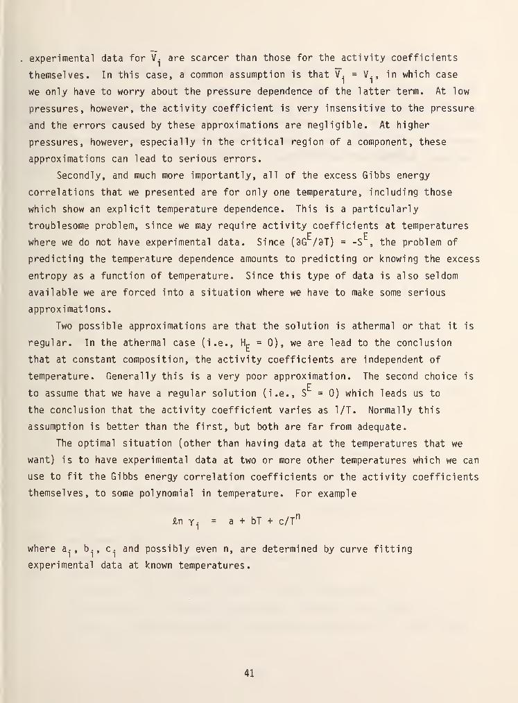
experimental data for V. are scarcer than those for the activity coefficients
themselves. In this case, a common assumption is that V. = V., in which case
we only have to worry about the pressure dependence of the latter term. At low
pressures, however, the activity coefficient is very insensitive to the pressure
and the errors caused by these approximations are negligible. At higher
pressures, however, especially in the critical region of a component, these
approximations can lead to serious errors.
Secondly, and much more importantly, all of the excess Gibbs energy
correlations that we presented are for only one temperature, including those
which show an explicit temperature dependence. This is a particularly
troublesome problem, since we may require activity coefficients at temperatures
where we do not have experimental data. Since (9G /9T) = -S , the problem of
predicting the temperature dependence amounts to predicting or knowing the excess
entropy as a function of temperature. Since this type of data is also seldom
available we are forced into a situation where we have to make some serious
approximations.
Two possible approximations are that the solution is athermal or that it is
regular. In the athermal case (i.e., H^ = 0), we are lead to the conclusion
that at constant composition, the activity coefficients are independent of
temperature. Generally this is a very poor approximation. The second choice is
to assume that we have a regular solution (i.e., S = 0) which leads us to
the conclusion that the activity coefficient varies as 1/T. Normally this
assumption is better than the first, but both are far from adequate.
The optimal situation (other than having data at the temperatures that we
want) is to have experimental data at two or more other temperatures which we can
use to fit the Gibbs energy correlation coefficients or the activity coefficients
themselves, to some polynomial in temperature. For example
£n y^. = a + bT + c/t"
where a., b., c. and possibly even n, are determined by curve fitting
experimental data at known temperatures.
41
6. Conclusions
This completes our brief overview of phase equilibria prediction methods.
Although equation of state methods have developed rapidly during the past few
years, there is still a definite need for models which represent systems which
have large size and polarity differences. Activity coefficient methods which are
predictive, e.g., ASOG, lack a sound theoretical basis upon which they may be
improved. Further work in this area is needed.
42
7. References
[I] Scott, R. L. and von Konynenburg, P. H., Discuss. Farad. Soc. 49, 87
(1970).
[2] Von Konynenburg, P. H. and Scott, R. L., Phil. Trans. Roy. Soc. London
298 , 495 (1980).
[3] Gubbins, K. E. and Twu, C. H., Chem. Eng. Sci . 33, 863 (1978).
[4] Kuenen, J. P., Communs. Phys. Lab. Univ. Leiden, No. 4 (1892).
[5] Adler, S. B., Spencer, C. F., Ozkardesh, H. and Kuo, C. M., "Industrial
Uses of Equations of State: A State-of-the-Art Review," in "Phase
Equilibria and Fluid Properties in the Chemical Industry," Storvick, T. S.
and Sandler, S. I., eds., ACS Symposium Series No. 60, American Chemical
Society, Washington, D.C., 1977.
[6] Kobayashi, R. and Carnahan, N. F., Proceedings of the Van der Waals
Centenial Conf., 1973.
[7] Nichols, W. B., Reamer, H. H. and Sage, B. H., A.I.Ch.E. J. 3, 262
(1957).
[8] Model 1, M. and Reid, R. C, "Thermodynamics and Its Applications in
Chemical Engineering," Prentice-Hall, Englewood Cliffs, N. J., 1974.
[9] Rowlinson, J. S., "Liquids and Liquid Mixtures," 2nd ed.. Plenum Press,
New York, N. Y., 1969.
[10] King, M. B., "Phase Equilibrium in Mixtures," Pergamon Press, New York,
N. Y., 1969.
[II] Lewis, G. N., Proc. Am. Acad. 37, 49 (1901).
[12] Gautam, R. and Seider, W. 0., A.I.Ch.E. J. 25, 991 (1979).
[13] Gautam, R. and Seider, W. D., A.I.Ch.E. J. 25, 999 (1979).
[14] George, B., Brown, L. P., Farmer, C. H., Buthod, P. and Manning, F. S.,
Ind. Eng. Chem., Process Des. Dev. ]_5, 372 (1976).
[15] Asselineau, L., Bogdanic, G. and Vidal, J., Fluid Phase Equil. 2» 273
(1979).
[16] Heidemann, R. A., A.I.Ch.E. J. 20, 847 (1974).
[17] Fussell, L. T., Soc. Pet. Eng. paper No. 6722, 1977.
[18] Heidemann, R. A., Hydro. Processing, 167 (1974).
[19] Heidemann, R. A., "Critical Points in Reacting Mixtures," in
"Thermodynamics of Aqueous Systems with Industrial Applications," S. A,
Newman, ed., American Chemical Society Symposium Series 133, Washington,
D.C., 1980.
43
[20] Deam, J. R. and Maddox, R. N., Hydrocarbon Processing, 163 (1969).
[21] Leland, T. W., "Equations of State for Dense Fluid Phase Equilibrium
Computations," Proc. 2nd International Conference on Phase Equilibria and
Fluid Properties in the Chemical Industry," DECHEMA, 1980.
[22] Abbott, M. M., "Cubic Equations of State: An Interpretive Review," in
"Equations of State in Engineering and Research," Chao, K. C. and
Robinson, R. L., eds. ACS Symposium Series, No. 182, American Chemical
Society, Washington, D.C., 1979.
[23] Henderson, D., "Practical Calculations of the Equation of State of Fluids
and Fluid Mixtures Using Perburbation Theory and Related Theories," in
"Equations of State in Engineering and Research," Chao, K. C. and
Robinson, R L., eds., ACS Symposium Series, No. 182, American Chemical
Society, Washington, D.C., 1979.
[24] Reid, R. C. and Leland, T. W., A.I.Ch.E. J. ]]_, 228 (1965).
[25] Chueh, P. L. and Prausnitz, J. M., Ind. Eng. Chem. 6, 492 (1967);
A.I.Ch.E. J. 13, 1099, 1107 (1967).
[26] Oellrich, L., Plocker, U., Prausnitz, J. M., Knapp, H., Int. Chem. Eng.
21, 1 (1981).
[27] Hiza, M. J. and Duncan, A. G., A.I.Ch.E. J. J6_, 733 (1970).
[28] Hudson, G. H. and McCoubrey, J. C, Trans. Farad. Soc. 56, 761 (1960).
[29] Kramer, H. L. and Herschbach, D. R., J. Chem. Phys. 53, 2792 (1970).
[30] Chueh, P. L. and Ely, J. F., unpublished.
[31] Graboski, M. S. and Daubert, M. S., Ind. Eng. Chem. Process Des. Dev. 17,
448 (1978).
[32] Graboski, M. S. and Daubert, T. E., Ind. Eng. Chem. Process Des. Dev. VT.,
443 (1978).
[33] Martin, J. J., Ind. Eng. Chem. Fundam. J8, 81 (1979).
[34] Zudkevitch, D., Joffe, J. and Schroeder, G. M., I. Chem. Eng. Symp. Series
32, p 21, 1969.
[35] Firoozabadi, A., Hekim, Y. and Katz, D. L., Can. J. Chem. Eng. 56^, 610
(1978).
[36] Kato, M., Chung, W. K., Lu , B. C.-Y., Can. J. Chem. Eng. 5^, 701 (1977).
[37] Graboski, M. S. and Daubert, T. E., Ind. Eng. Chem. Process Des. Dev. 28,
300 (1979).
[38] Shah, M. K. and Bishnoi, P. R., Can. J. Chem. Eng. 56, 478 (1978).
44
[39] Asselineau, L., Bogdanic, G. and Vidal, J., Chem. Eng. Sci. 33., 1269
(1978).
[40] Erbar, J. H., Jagota, A. K., Muthswamy, S. and Moshfeghian, M.,
"Predicting Synthetic Gas and Natural Gas Properties Using a Modified
Soave Redlich Kwong Equation of State," Gas Processors Assn. Research
Report No. 43, 1980.
[41] Peng, D.-Y. and Robinson, D. B., "Two- and Three-Phase Equilibrium
Calculations for Coal Gasification and Related Processes," in
"Thermodynamics of Aqueous Systems with Industrial Applications," Newman,
S. A., ed,, ACS Symposium Series No. 133, American Chemical Society,
Washington, D.C., 1980.
[42] Peng, D.-Y. and Robinson, D. B., Can. J. Chem. Eng. 54, 595 (1976).
[43] Chueh, P. L., private communcation.
[44] Nakamura, R., Breedveld, G. J. F. and Prausnitz, J. M., Ind. Eng. Chem.
Process Des. Dev. 25, 557 (1976).
[45] Won, K. W., Advan. Cryo. Eng. 23, 544 (1977).
[46] Evelein, K. A., Moore, R. G. and Heidemann, R. A., Ind. Eng. Chem. Process
Des. Dev. J5, 423 (1976).
[47] See reference [40].
[48] Cunningham, J. and Wilson, G. M., Proc. 54th Annual GPA Meeting, Denver,
CO, 1974.
[49] Vidal, J.. Chem. Eng. Sci. 33, 787 (1978).
[50] Huron, M.-J. and Vidal, J., Fluid Phase Equil. 3, 255 (1979).
[51] Moshfeghian, M., Shariat, A. and Erbar, J. H., "Application of the
PFGC-MES Equation of State to Synthetic and Natural Gas Systems," in
"Thermodynamics of Aqueous Systems with Industrial Importance," Newman,
S. A., ed., ACS Symposium Series No. 133, American Chemical Society,
Washington, D.C., 1980.
[52] Benedict, M., Webb, G. B., Rubin, L. C, J. Chem. Phys. 8, 334 (1940);
JO, 747 (1942).
[53] Starling, K. E. and Powers, J. E., Ind. Eng. Chem. Fundam. £, 531 (1970).
[54] Lin, C. J., Kwok, Y. C. and Starling, K. E., Can. J. Chem. Eng. 50, 644
(1972).
[55] Starling, K. E., "Fluid Thermodynamic Properties for Light Petroleum
Systems," Gulf Publishing Co., Houston, TX, 1973.
[56] Brule, M. R., Lee, L. L. and Starling, K. E., Chem. Eng. 86, 155 (1979).
45
[57] Nishiumi, H. and Saito, S., J. Chem. Eng. Japan 8, 356 (1975).
[58] Yamada, T., A.I.Ch.E. J. 29, 286 (1973).
[59] Hansen, R. E., Proc. 48th Natural Gas Processors Association, p 52, 1969.
[60] Lin, M. S. and Naphtali, L. M., A.I.Ch.E. J. 9, 580 (1963).
[61] Lee, L. L. and Starling, K. E., GRI Contractors Report, March, 1980.
[62] Jacobsen, R. T. and Stewart, R. B., J. Phys. Chem. Ref. Data ^, 757
(1973).
[63] Goodwin, R. D., Nat. Bur. Stand. (U.S.), Tech. Note 653 (1974).
[64] Rowlinson, J. S., "Prediction of Thermodynamic Properties" in "Phase
Equilibria and Fluid Properties in the Chemical Industry," Storvich, T. S.
and Sandler, S. I., eds., ACS Symposium Series No. 60, American Chemical
Society, Washington, D.C., 1977.
[65] Rowlinson, J. S. and Watson, I. D., Chem. Eng. Sci. 24, 1565 (1969).
[66] Leach, J. W., Chappelear, P. S. and Leland, T. W., A.I.Ch.E. J. J4, 568
(1968).
[67] Fisher, G. D. and Leland, T. W., Ind. Eng. Chem. Fundam. 9, 537 (1970).
[68] Leland, T. M. and Mueller, W. H., Ind. Eng. Chem. 51, 597 (1959).
[69] Mentzer, R. A., Greenkorn, R. A. and Chao, K. C, Sep. Sci. Tech. 25, 1613
(1980).
[70] Mollerup, J., Adv. Cryo. Eng. 20, 172 (1975).
[71] Mollerup, J., Adv. Cryo. Eng. 23, 550 (1978).
[72] Leland, T. W. and Chappelear, P. S., Ind. Eng. Chem. 60, 15 (1968).
[73] Lee, B. I. and Kessler, M. G., A.I.Ch.E. J. 21, 510 (1975).
[74] Teja, A. S., Sandler, S. I. and Patel , N. C, Chem. Eng. J. _21, 21
(1981).
[75] Teja, A. S. and Rice, P., Chem. Eng. Sci. 36, 1 (1981).
[76] Pitzer, K. S., Lippmann, D. Z., Curl, R. F., Huggins, C. M. and Peterson,
D. E., J. Am. Chem. Soc. 77, 3433 (1955).
[77] Genco, J. M., Teja, A. S. and Kay, W. B., J. Chem. Eng. Data 25, 350
(1980).
[78] Carnahan, N. F. and Starling, K. E., J. Chem. Phys. 5^, 600 (1970).
[79] Gibbons. R. M., Mol . Phys. U., 81 (1969).
[80] Boublik, T., Mol. Phys. 42, 209 (1981).
[81] Nezbeda, I. and Leland, T. W., J. Chem. Soc, Faraday Trans. II 75., 193
(1979).
46
[82] Wertheim, M. S., Phys. Rev. Lett. 10, 321 (1963); Thiele, E., J. Chem.
Phys. 39, 474 (1963).
[83] Beret, S. and Prausnitz, J. M., A.I.Ch.E. J. 21, 1123 (1975).
[84] Donohue, M. D. and Prausnitz, J. M., A.I.Ch.E. J. 24, 849 (1978).
[85] Kegleski, A., Wihoit, R. C. and Zwolinski, B. J., J. Phys. Chem. 77_, 2212
(1973).
[86] Kregleski, A. and Chen, S. S., J. Chim. Phys. 15, 347 (1978).
[87] Kregleski, A. and Wihoit, R. C, J. Phys. Chem. 78, 1961 (1974); 19, 449
(1975).
[88] Hlavaty, K., Coll. Czech. Chem. Commun. 39, 2927 (1974).
[89] Drahos, J., Wichterle, I. and Hala, E., Fluid Phase Equil. 1, 173 (1977).
[90] De Santis, R., Gironi, F. and Marrelli, L., Ind. Eng. Chem. Fundam. 15,
183 (1976).
[91] Oellrich, L. R., Knapp, H. and Prausnitz, J. M., Fluid Phase Equil. ^,
1963 (1978).
[92] Carnahan, N. F. and Starling, K. E., A.I.Ch.E. J. 18, 1184 (1972).
[93] Haar, L. and Shenker, S. H., Proc. 5th Symp. Thermophysical Properties,
p 223, 1970.
[94] Bienkowski, P. R., Denenholz, H. S. and Chao, K. C, A.I.Ch.E. J. 19, 167
(1973).
[95] Whiting, W. B. and Prausnitz, J. M., "A New Equation of State for Fluid
Water Based on Hard-Sphere Perturbation Theory and Dimerization
Equilibria," 9th Int. Conf. on Properties of Steam, Munich, 1979.
[96] See, Threlfall, R. and Adair, J. F., "Physical Memoirs," Vol. 1, part 3,
Phys. Soc, London, 1890.
[97] Redlich, 0. and Kwong, J. N. S., Chem. Rev. 44, 233 (1949).
[98] Soave, G., Chem. Eng. Sci . 27, 1197 (1972).
[99] Peng, D.-Y. and Robinson, D. B., Ind. Eng. Chem. Fundam. 15, 59 (1976).
[100] Fuller, G. G., Ind. Eng. Chem. Fundam. 15, 254 (1976).
[101] Harmens, A. and Knapp, H., Ind. Eng. Chem. Fundam. 19, 291 (1980).
[102] IJsdin, E. and McAuliffe, J. C, Chem. Eng. Sci. H, 1077 (1976).
[103] Leung, S. S. and Griffiths, R. B., Phys. Rev. A8, 2670 (1973).
[104] d'Arrigo, L. M. and Tartaglia, P., Phys. Rev. A12, 2587 (1975).
[105] Moldover, M. R. and Gallagher, J. S., A.I.Ch.E. J. 24, 267 (1978).
[106] Peng, D.-Y. and Robinson, D. B., A.I.Ch.E. J. 23, 137 (1977).
[107] Michelson, M. L. and Heidemann, R. A., A.I.Ch.E. J. 27, 521 (1981).
47
[108] Pierotti, G. J. and Derr, E. L., Ind. Eng. Chem. 51, 95 (1959).
[109] Margules, M., Sitzber. Akad. Wiss. Math. Naturwiss. Klasse II 104 , 1243
(1895).
[110] Redlich, 0. and Kister, A. T., Ind. Eng. Chem. 40, 345 (1948).
[Ill] van Laar, J. J., Z. Phys. Chem. 72, 723 (1929).
[112] Flory, P. J., J. Chem. Phys. 9, 660 (1941); JO, 51 (1942); Huggins,
M. L., J. Chem. Phys. 9, 440 (1941).
[113] Prausnitz, J. M. "State-of-the-Art Review of Phase Equilibria," in "Phase
Equilibria and Fluid Properties in the Chemical Industry," Storvich, T. S.
and Sandler, S. I., eds., ACS Symposium Series No. 60, American Chemical
Society, Washington, D.C., 1977.
[114] Renon, H. and Prausnitz, J. M., A.I.Ch.E. J. 24, 135 (1968).
[115] Abrams, D. S. and Prausnitz, J. M., A.I.Ch.E. J. H, 116 (1975).
[116] Derr, E. L. and Deal, C. H., I. Chem. E. Symp. Ser. 32, 40 (1969).
[117] Deal, C. H. and Derr, E. L., Ind. Eng. Chem. 60, 28 (1968).
[118] Derr, E. L. and Deal, C. H., Adv. Chem. Series 124, p 11 (1973).
[119] Wilson, G. M. and Deal, C. H., Ind. Eng. Chem. Fundam. J_, 20 (1962).
[120] Gugenheim, E. A., "Mixtures," Oxford University Press, Oxford, 1952.
[121] Fredenslund, A. A., Jones, R. L. and Prausnitz, J. M., A.I.Ch.E. J. 2J[,
1086 (1975).
[122] Chao, K. C. and Greenkorn, R. A., "Thermodynamics of Fluids," Marcel
Dekker, New York, New York (1975).
[123] Reid, R. C, Prausnitz, J. M. and Sherwood, T. K., "The Properties of
Gases and Liquids," McGraw-Hill, New York, New York (1977).
48
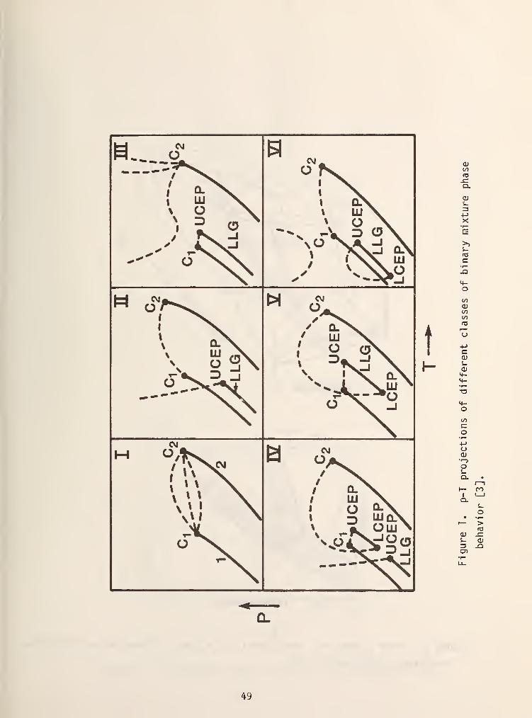
H->._o
1=1
$1
X
t
a
(U
3
>>
000)«/)
V)ITS
U4-»
(US-
0)
oCO
+->
oQi<-5
Os-
Q.
OO
or— >
49
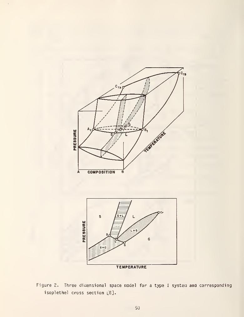
COMPOSITION B
u3COm111
aea.
s #^CrM
LMM.>^J^L*^"P^
Sii^/^^ Hf^^ G
prr
TEMPERATURE
Figure 2. Three dii.iensional space model for a type I system and corresponding
isoplethel cross section l8].
50
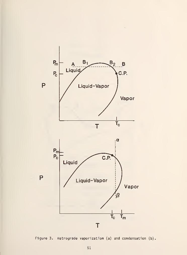
Pm A ^^ J^2 B
Pc- Liquip" "V^
p
/ Liquid-Vapor
/ / Vapor
m
Liquid
Vapor
J L
"'c "^m
Figure 3. Retrograde vaporization (a) and condensation (b)
51
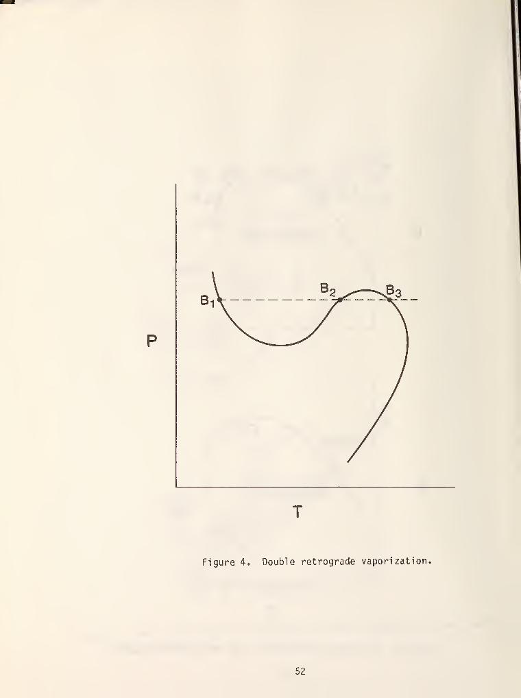
Figure 4. Double retrograde vaporization.
52
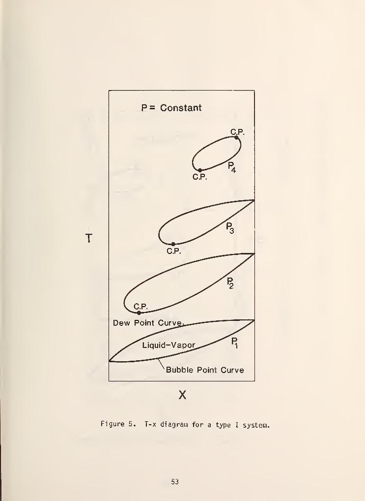
P = Constant
C.P
cC.P.
/^
C.P.
^(
Dew Point Curvgi^- ^/''^LiqLjid-Vapor,^.-.-'''^ ^1
^Bubble Point Curve
X
Figure 5. T-x diagram for a type I system,
53
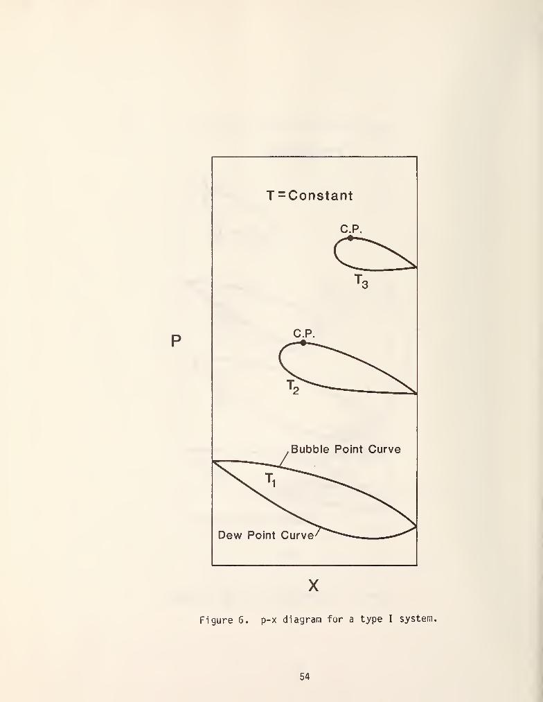
T = Constant
C.P.
T3
C.P.
V_\^
, Bubble Point Curve
^\V ^^^^^Dew Point Curve^-—
^
X
Figure 6. p-x diagram for a type I system.
54
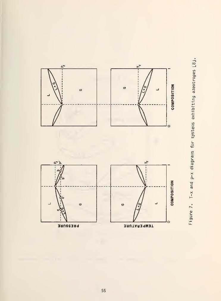
00cL"^ »-"
Vf
V\o o
1 / V-i
l\.
/ \
Q.NOl
ll
(/)
a;Q.o5-+->
X Oo 0)
M1- fO
oQ.
c"r-4->o
u -Q•r"
x:Xa»
00GO)+->
en>»CO
s_
o"+-
COr:
fOs_
CDfO*r*-a
XCL
zo a
c1- (T3
co Xo 1
CL 1—soo •
r^
cuS-
CD
3UnS83tid 3tiniVtJ3dlfl31
55
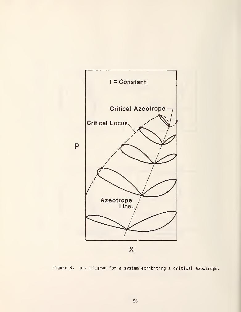
T= Constant
Critical Azeotrope
Critical LocuSv ^
Figure 8. p-x diagram for a system exhibiting a critical azeotrope,
56
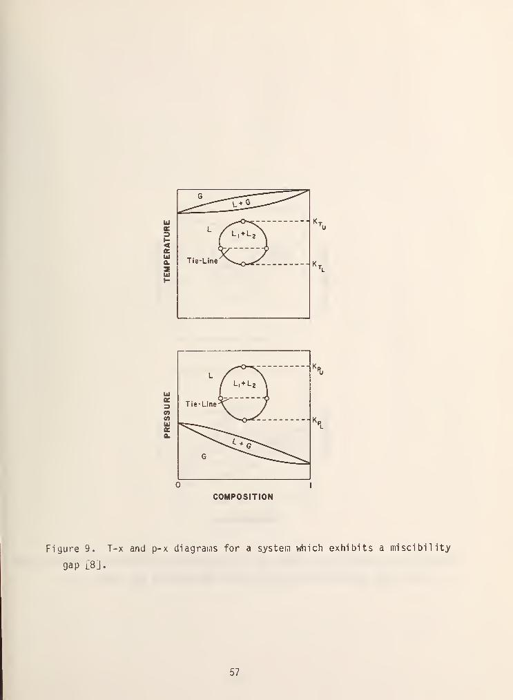
COMPOSITION
Figure 9. T-x and p-x diagrams for a system which exhibits a miscibility
gap [8].
57
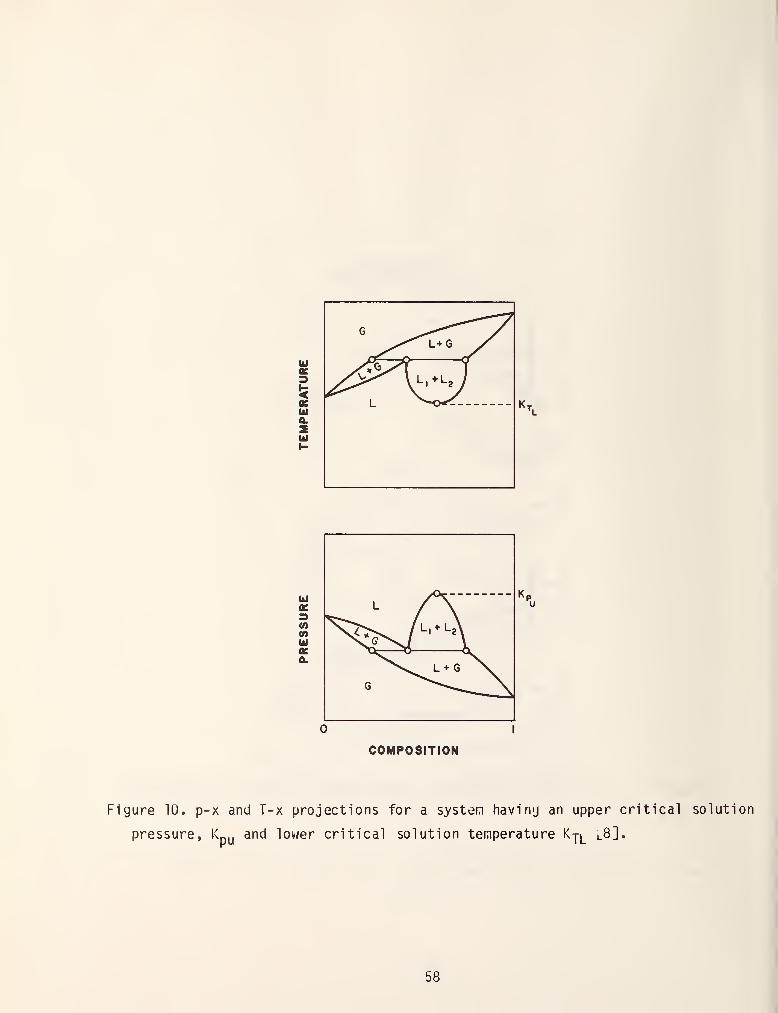
llJ
<KbiQ.SUJ
kJK3COCOllJ
a:a.
COMPOSITION
Figure 10. p-x and T-x projections for a system havimj an upper critical solution
pressure, li^^ and lov/er critical solution temperature Kj|_ l8].
58
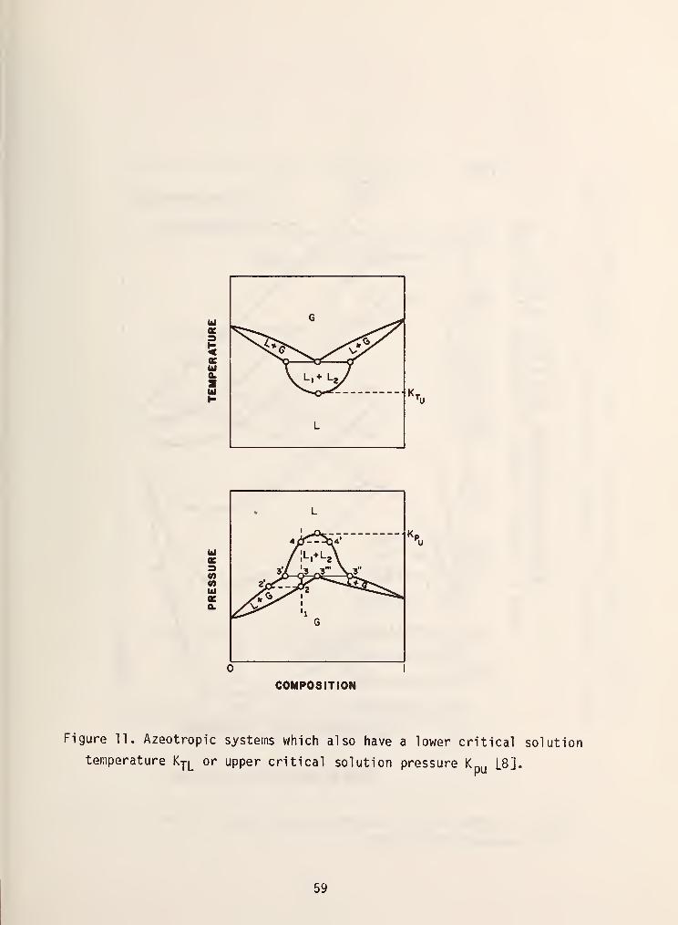
Ill
oe
oeUJa.
111
uic3COmuQCa.
COMPOSITION
Figure 11. Azeotropic systems which also have a lower critical solution
temperature Kjl or upper critical solution pressure K L8].
59
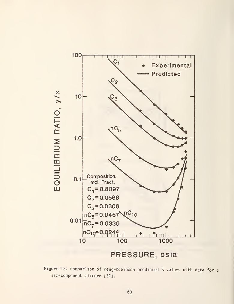
100
X
<CO
CO
oLU
10
1.0
0.1
0.01
I I I I I I
ll1 TT
Composition,
mol. Fract.
C^ = 0.8097
C2 = 0.0566
63 = 0.0306
nC5=0.0457
nC7. = 0.0330
nCi 0=0.0244, •, • ,
L^I I I I I I III 1*1I
I L_L
10 100 1000
PRESSURE, psia
Figure 12. Comparison of Peng-Robinson predicted K values with data for a
six-component mixture [32],
60
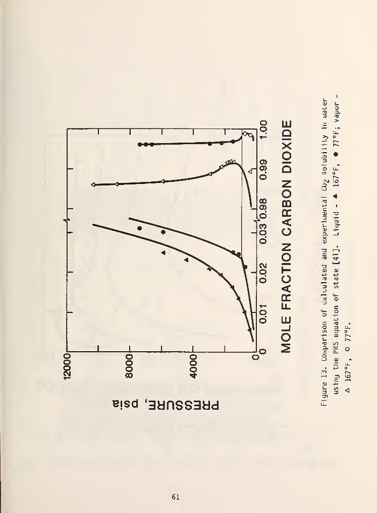
LU
9XoQzoDC<O
O<ccLi.
Ill
-J
o
^isd '3anss3dd
s_cu t-+-> o2 3.-> •a
>r—
>» o+J r^•1— r-^r^
5 •a— Ao u_LO o
ro ^o I—
1
i-3
^ 4(XS
+f 1
u.0) T3^ •r—
•r— 3i- cr0) •f—:^ —IX0)
•
-o 1—
1
^ r—fO
1 1oOJ u-!-> +J•a
3 tou
M-a oJ
c1+- oo
t->
c <n •
o zs LUI/) o- O*r— 0) r^1- r>^(O 00a. 2i O
Ci_
5:_) O) A
j^ '_l_
• +->
ro r^1—1 :d lO
c I—
1
OJ •n-
3co3 <
31
61
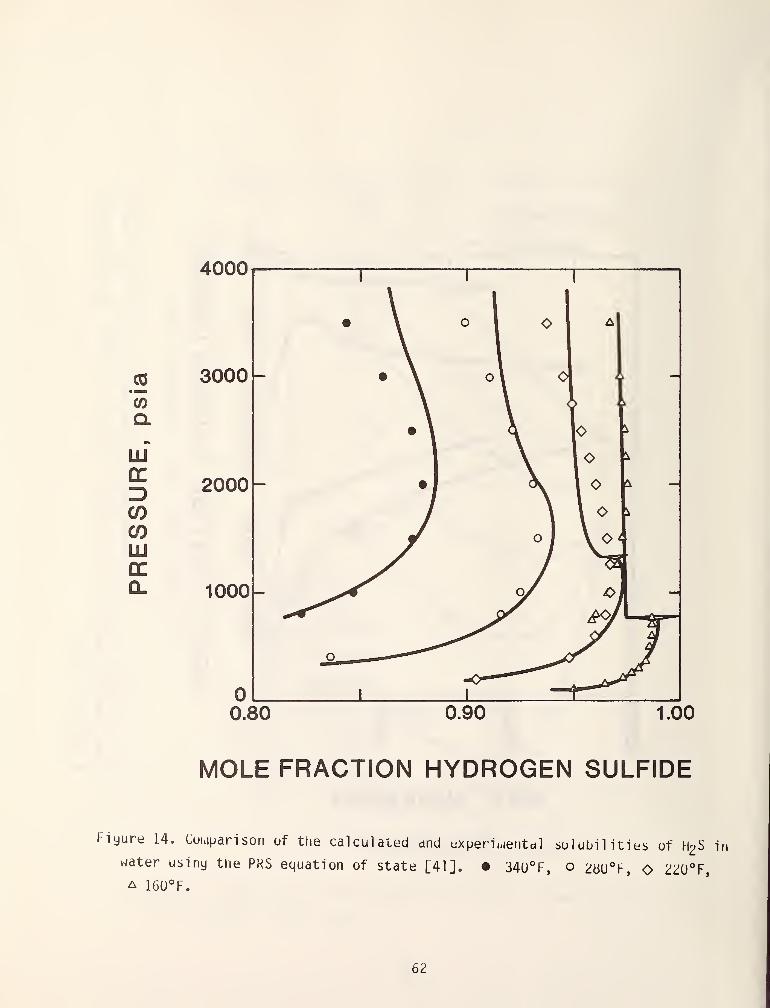
4000
.5CO
aLIl
cc
COCOHIocQ-
3000-
2000-
1000-
0.80 0.90 1.00
MOLE FRACTION HYDROGEN SULFIDE
Fiyure 14. Cohiparison uf the calculdted dnd experimentdl solubilities of H2S in
water usiny the PKS equation of state [41]. • 34U°F, o 28U°H, O 2:20°F,
A 160°F.
62
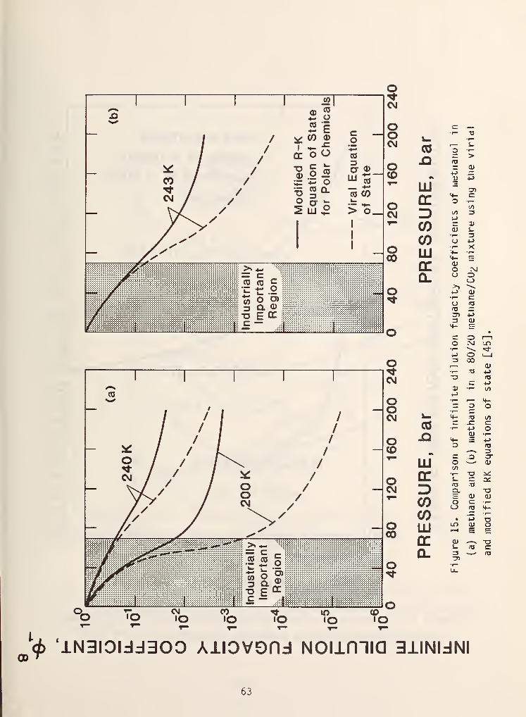
°o
^X1 1 1 i2| CM
n—
^
/
21/ i^CO o
/ ccoo
c —o
(0•!3
OOCM
CQ
c•r—
5
•r—
>
"CO
CVJ/ , O o- >:
iral
Eqi
f
State
1 OCOT-
oCM
LlT4-O
+3
c
—
y^^' 2m o > o_
1 CO
to
53
— /y 1
1 _ O00
COLU 4-
4-
3l->
X
:/ S: (0 ca C llllllllOC0.
O
//
r
\ 1
Industri
Importi Regio
"""'''''''''"'"'
\^
O >>4->
•p—
Ocuc
430)rr
OO
o
1—
1
•^1—
1
O 3 00
-a(U
1 1^ 4->
1 1 CM -a -/-s a; •t— l/l
CO t->
«M^
1/ ,
•_ OO •r—
'o4-O
/ / / / CM ^ 4- "^t/>
/ / / / CO •r- 4->co
m^mm ^ // /
/ L/
/
OCO
JQ 4-gj
4->
3oCM /
//
/ /^\ /^ / O
CM
LUQC
Oa
3-
//
/ o /"""
COQ.
I
5cuc
-a
4-
/ \,^/ CO • 4J•1—
— // / ^ -^ O LU .—10)
^f >r ^ 00
oCL
cu.tJ
"
lip
^' -n****^«--^^
ustrialiy
portant
tegion lllli
-ac
#1 T3 E "•m 1£-
i r olO
CMlO
COlO To
inlO
^<i> 'lN3IOIJd300 AilOVOnd NOIimiQ 3ilNldNI00 '
63
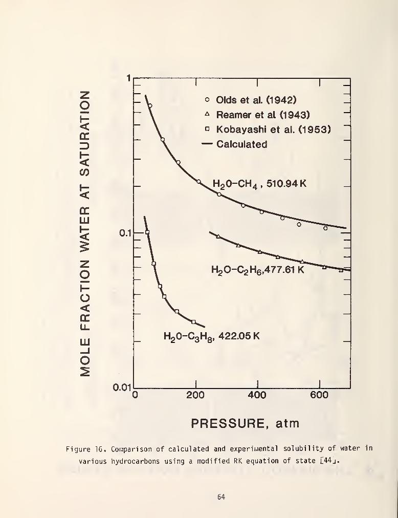
<a:
!^
CO
trLU
oh-o<LU
LU
0.1
0.01
o Oldset al. (1942)
^ Reamer et aL (1943)
D Kobayashi et al. (1963)
— Calculated
H2O-CH4, 510.94 K
H20-C2H6,477.61 K
H2O-C3H8, 422.05 K
200 400 600
PRESSURE, atm
Figure IG. Comparison of calculated and experii.iental solubility of water in
various hydrocarbons using a modified RK equation of state l44j.
64
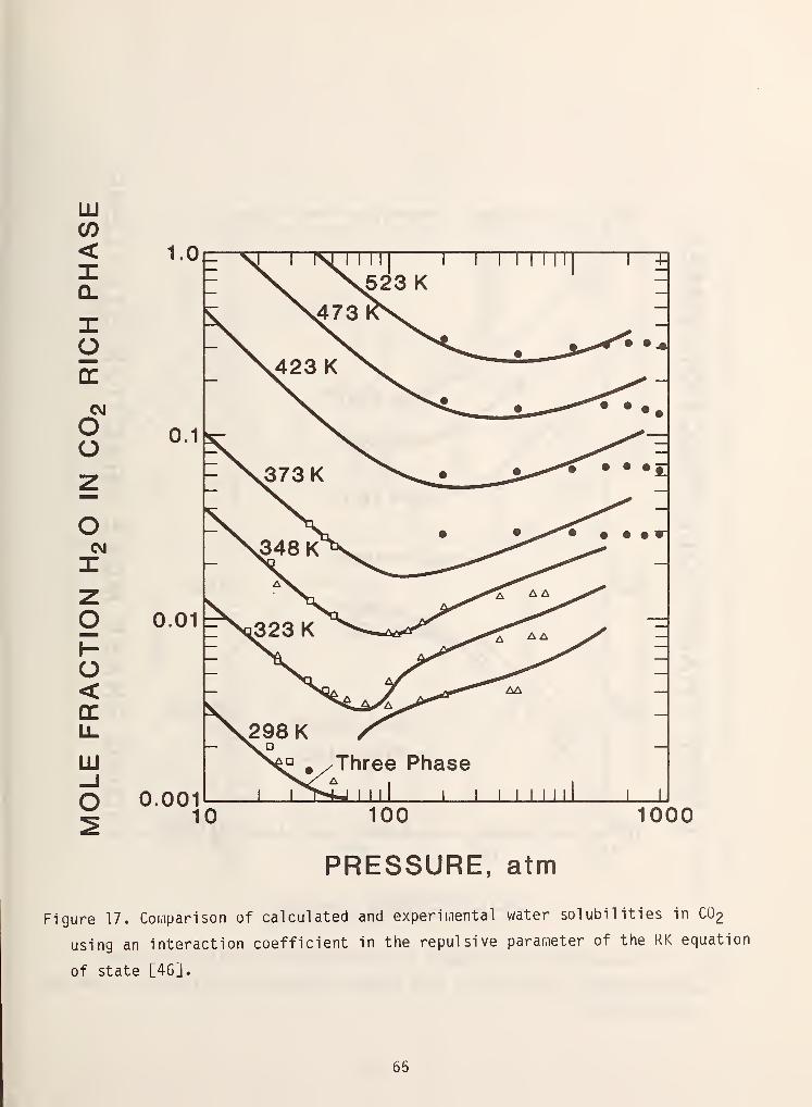
LJJ
CO<
o
CNJ
oo
oCM
o<U.
LU-I
o
0.01 f
0.00110 100
PRESSURE, atm
1000
Figure 17. Comparison of calculated and experimental water solubilities in CO2
using an interaction coefficient in the repulsive parameter of the RK equation
of state [4G].
65
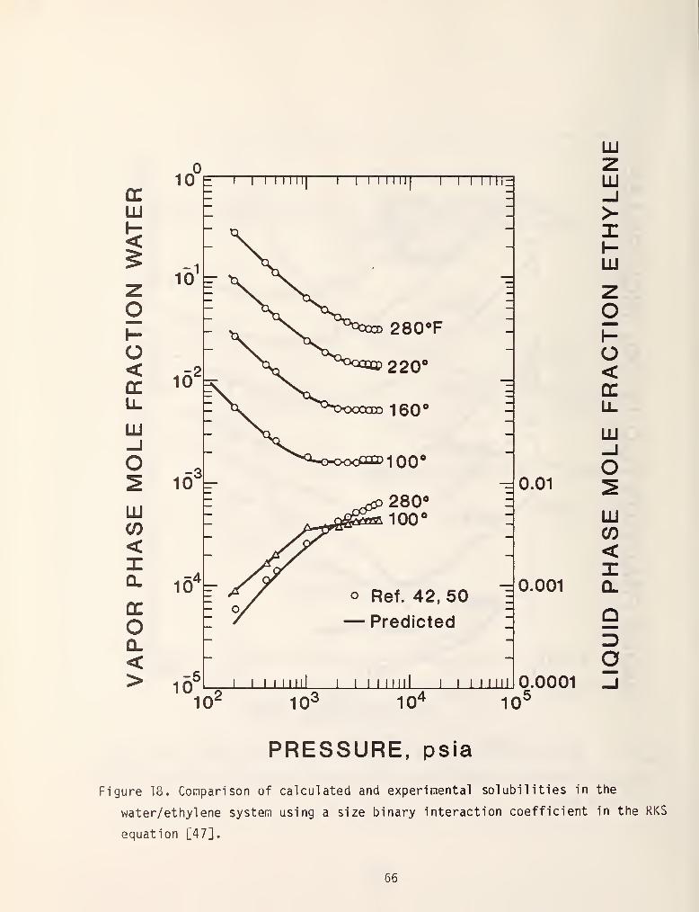
LU
<
O<
LU
LUCO
<IQ.
OC
OQ.
<>
10 =—\—I I 1 1 iii| \—I I I iiii| \—I I I II
10^
280«100**
o Ref. 42, 50— Predicted
I iiiil 11
0.01
0.001
10- 10' 10^ 10
0.00015
LUzLU—I>-
ILU
O<ccLJ-
LU
o
LUCO
<IQ.
9
o
PRESSURE, psia
Figure 18. Comparison of calculated and experimental solubilities in the
water/ethyl ene system using a size binary interaction coefficient in the RKS
equation [47].
66
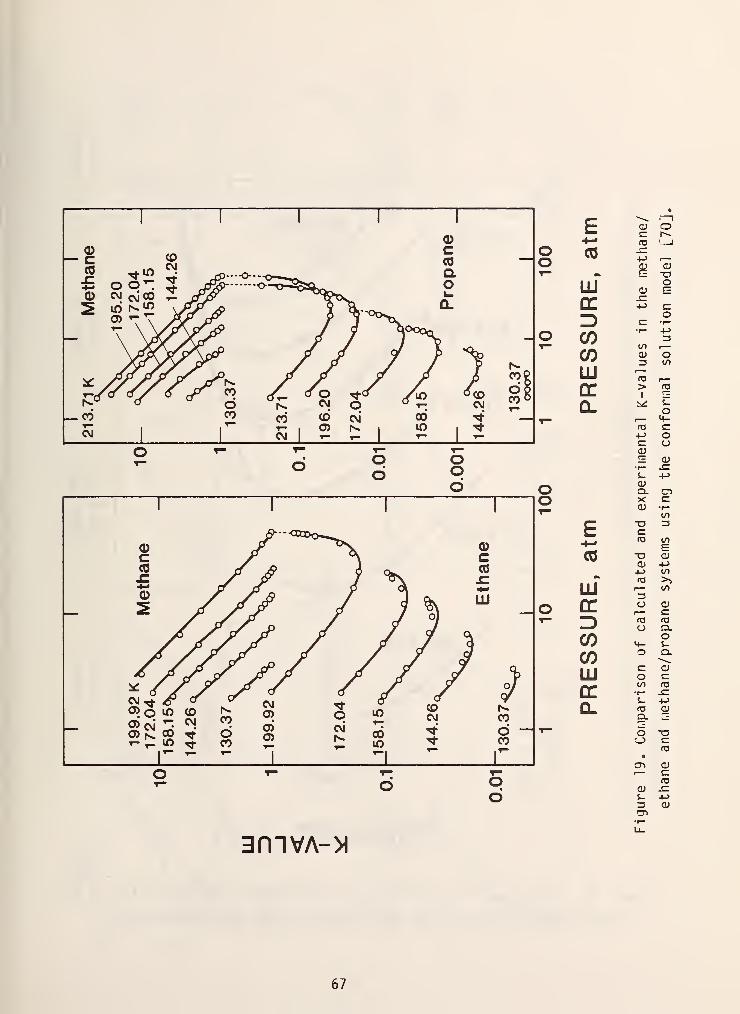
<D0)r (0
CO ^lO ^—o— -co or ^ o<N cvi® y
5 in r^*^ \>i^ /S>o) tT >V^iV
fc- <u okv c: r^*- fOoo CO 43'aJ
^" k oLU a
oG
OC E3 c
O•r-
o CO•r-
13T- 00 ^^
CO 3ot/5
LIJ "to ^GC >
1
Q. i»iO
^m 1
—
<4-
(T3 C+J oC oOJc= O)•r- -cr
S- +->
o Q. CDo X C0) •r-
E -o rs
"-• "3 oo
CO -o <uCD +->
4-> oo•*
(tJ >>
tu 3oo
o cc O CDc
T— ID Q.
CO M-O
COO Q.
LU o
OC00
£LS-
Q.
1— O -aO c:fO
CT> O)'
<U x:s_ 4->
3 <uCD
3mVA->t
67
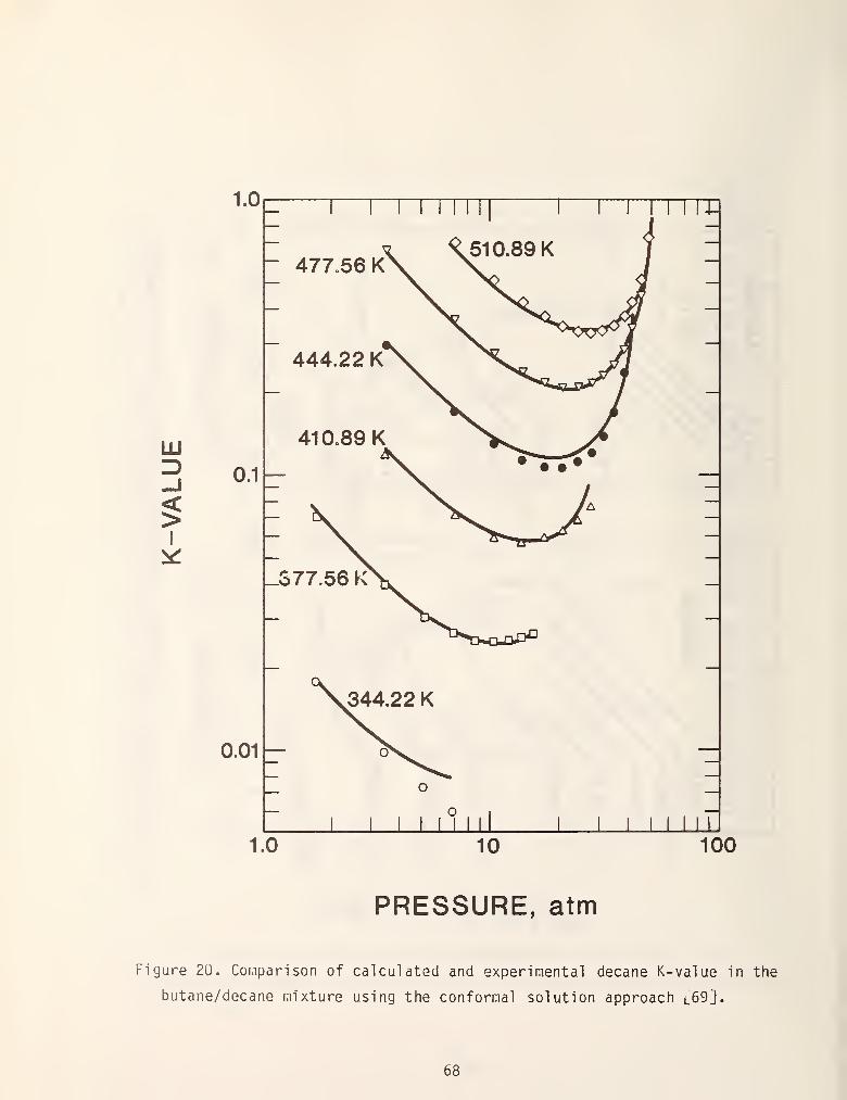
LU
I
1.0
0.1
0.01
477.56 K
444.22 K
410.89 K
_377.56 K
344.22 K
Tl
1.0 10 100
PRESSURE, atm
Figure 20. Comparison of calculated and experimental decane K-value in the
butane/decane mixture using the conformal solution approach l69].
68
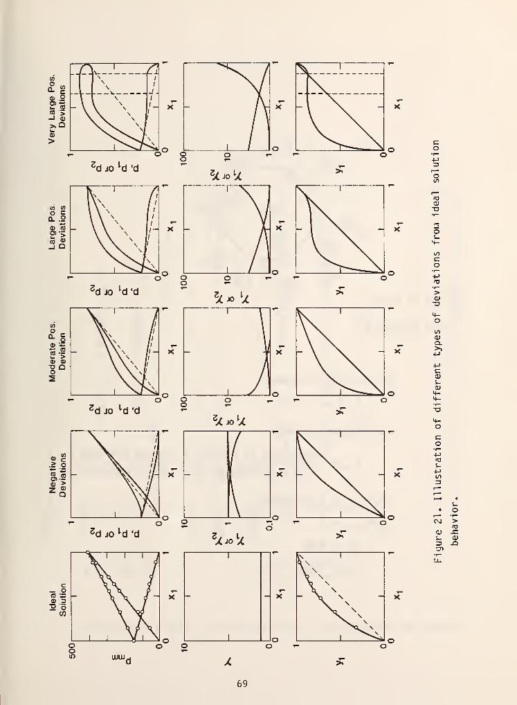
0)
<D Ou. (0
« •>_i a>
>
Y r \ /
\K/\I^
l\><.4->
3o
O)o
oi-M-
w»cO•r—4->
to•r—
>-a
CO
Q.
•(-J
(U
0)
•->
s_+->
3
CM >
69
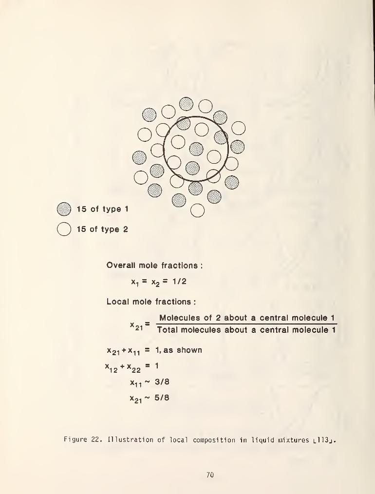
o©p
15 of type 1
Q 16 of type 2
Overall mole fractions :
x^ = Xg = 1/2
Local mole fractions
:
Molecules of 2 about a central molecule 1
Xo4 =2^ Total molecules about a central molecule 1
^21 •^11 "
X^ 2+^22
^11
'21
1,as shown
1
3/8
5/8
Figure 22. Illustration of local composition in liquid mixtures l113j
70
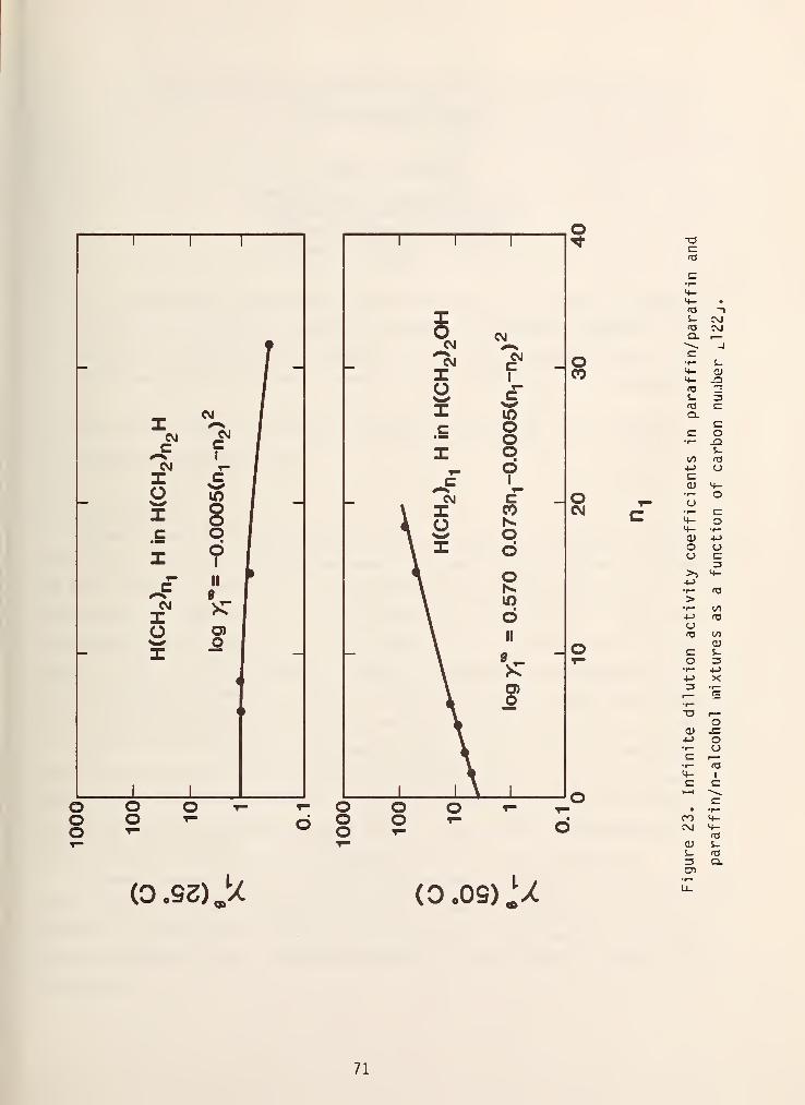
-
1 V
/-X ^ f
C\iCVJ /
c c/^^ 1 /
CVJ ^ fX c1o
X s"
c oX d
1
c" II
t
/-^ 9
X )C
o O)>1^ oX
\
( 1
1 1
X
1
O CMCM <H
- CNJ
X r -
oXc ooX o
t— dc 1
^-N ^"CNJ c
\ X CO
i o 1^1 '**' o\ X d
oLO
dII
1 1 )
s
^ 1
ooooo O 1- T- O
d <=>O 1-
o oO T-
(0.92)> (0.09)iX
o-ocra
c
4- •
(O —
1
s- ?JfO CVJQ.
-1
co S_
CO <4- J303 "^
S- 3(O CQ.
CC O" J2
(/) fO-!-> oCOJ 4-
o ^ oo
CVJ c- •-- co
4-0) +->
o ou>> 4--M•r— fO>•r— I/)M «oCJ03 (/J
o £Z^~ o 3
•n- +J•l-> X3 •r—
E•r—
-o'o
O) -C-M o•r— aC 1—•1— (O4-c c=
o 1—
1
c• .^.
en <+-
C\S
<u s_s- fO3 a.CT»
Ll-
71
THE EXTENDED CORRESPONDING STATES METHOD APPLIED TO THE
NITROGEN-METHANE SYSTEM
Robert D. McCarty
Thermophysical Properties DivisionNational Engineering LaboratoryNational Bureau of StandardsBoulder, Colorado 30303
An extended corresponding states method of predicting the equation
of state for the N2-CH4 system is reviewed. Comparisons between the
predictive method and experimental PVTx data have revealed basic
problems with the method. A review of this ongoing work is presented.
Key words: equation of state; extended corresponding states; mixtures;
predictive methods; PVTx.
1. Introduction
Several years ago the properties of fluids group at NBS-Boulder, undertook a
long range project to develop a mathematical model of the equation of state of
LNG which would be capable of predicting densities given the pressure,
temperature and composition of a LNG mixture. Several different models were
investigated during the course of that project, each of whicM proved to be
adequate under the limited scope of pressure, temperature and components of
LNG [1]. One of the methods, the "extended corresponding states" method proved
to be the most versatile and suggested the possibility of describing the equation
of state of a mixture over a much broader range of pressure and temperature in a
truly predictive sense. The purpose of the present v/ork is to explore that
possibility. The binary system of CH.-N^ was chosen as a test case because of
the availability of good experimental data for that system and because the
CH^-N^ system is one of the binary systems studied in the LNG project.
Although the work on this system is by no means complete, this paper reports
the progress in that investigation to date. In order to better understand the
principle of corresponding states and its evolution to the modifications being
used here (there are many other modifications) a short history is given in the
next section.
73
2. Background
Before the metriod can be applied to mixtures, one must understand the
application of the method to |jure fluids.
Van der Waals proposed the original law of corresponding states in 1881.
Noticing a similarity in the shape of the PVT surfaces of many different fluids,
van der Waals proposed the following:
f(Pp, V^, T^j = fur all gases (i)
where
[Juw introduce fluid U and fluid 1 so that
P, P^ P P, P^^
p^ = P^ = p^ or /- = p^ and P = P p^ (3)
^cl^
'^co ^co ^cl " ^ '^cl
and it follows that
cl cl
therefore if we have an equation of state for fluid 0, i.e.,
Po = f'^C To)
tnen to use this equation of state for fluid 1 via the van der Waals
corresp(
3 and 4
corresponding states we may substitute into f for V ana T tne equations in
it follows then that
P / V T \
' ^cl V^ ^cl' 1 \J ^ ^
-/ -7 CO \
cl
74
but as p -^ 0, Z-,-^ 1 and Z * j
— which is only 1 if Z = Z , therefore to
insure correct ideal gas behavior one of the three original reducing parameters
is el iiiiinai:ed by equating Z = Z , , i.e.,
-, _ CO CO ^ cl cl ,-,x
CO " RT RTT
^'^CO cl
which then may be solved for any one of the critical parameter ratios in (3) and
(4).
Since critical volumes were typically the most uncertain of the critical
P T Vcl CO C
parameters the j— p— was usually substituted [2j for
y— which achieved the
'cl ^co \l
correct ideal gas limit at the expense of the critical point inaccuracy (unless
Z happened to equal Z -,) and reduces the number of reducing parameters
required from three to two. Although this iiiodifi cation of the original principle
improved the performance of corresponding states, significant deviations between
predicted and actual PVT surfaces was observed especially between fluids with
dissimilar molecular structure. The extended corresponding states principle
proposed by Rowlinson and Watson [3] is an extension of the above tv^o parameter
version except that instead of eliminating tfie V ^/V ,, P ,/P^i is eliminated,*^-* CO cl CO cl
i .e. , from (3)
P. - P. 1!^ ^ (8)CO cl
which corresponds to
where
h
^.0
'o ("l.o/^l.o) (3)
T^ 9(T V ) (10)
CO
and
CO
75
if 9 and <J>= 1. Tnen if the 9 and <i> (shape factors) are defined by the
equations
and
where Z is the compressibility factor and A is the helinholtz free energy one has
two equations with two unknowns which means that an exact correspondence between
two fluids (for those two properties) exists providing one knows the correct f
and h.
It is interesting to note that in the early 60' s a variation of this idea
was used by McCarty, et al . [4] to generate PVT data for neon. In that
application only one shape factor was useu to modify the density so that
• (•'»-• ^)P. = Y^ = p. lV,/h, ^, ^-^J (14)
CO
in that case models of the equation of state for nitrogen and argon were used to
determine the h, which was then used to transform the nitrogen surface to
the neon surface. Figure 1 illustrates that transformation function which in
this case is called density ratio. The validity of the assumption that the shape
factors are general between similar fluids is the key to v/hether or not the
extended corresponding states method is truly a predictive method or not and is
equally crucial to the Rowlinson definition.
The stage is now set to apply the extended corresponding states method to
mixtures. If one assumes that the equation of state of a mixture of fixed
composition behaves the same as that of a pure fluid then eqs (12) and (13)
apply, i.e..
and
\ - \ ^v^,o> y^,o) (^^)
A„ = f A (V /h , T /f ) (16)X X,0 ^ X x,o' X x,o^ ^ '
where the subscript x denotes the mixture and the o subscript denotes "base"
fluid, and the f and h dire defined by
76
^ij.o = ^1o '^11.0' fjj.o)'^' (20)
"1J.0 ^: (^K!o 4 ^^.^!oy (-)
The C. and n.. are binary interaction parameters and functions of a particular
binary system and the f- and h. are functions of the pure fluids only.
3. Nitrogen-Methane
As was stated earlier the iiiain purpose of this work is to explore the
possibility of using the extended corresponding states method to describe the
properties of mixtures over a much broader range of pressure and temperature than
was the case in the LNG project.
The starting point of this study was the extended corresponding states
results of the LNG project and the PVTx experimental data by Straty and
Diller [5]. Figure 1 shows the most serious deviations between calculated and
experimental densities at the starting point. Even though these deviations d^r^
irtuch greater tlian the accuracy of the experimental data, the comparison does
produce further encouragement of eventual success of the method. The extended
corresponding states equation of state for the nitrogen-methane system resulting
from the LNG project, except for the methane equation of state which is a wide
range equation of state for the base fluid, is based entirely on low temperature
saturated liquid PVTx data. The comparison of the mixture equation of state with
the Straty and Uiller experimental Np-CH^ data then constitutes an
extrapolation of the mixture parameter to much higtier temperatures and lower
densities.
Since there br^ manj' more variables involved in an equation of state for
mixtures than there d.r^ for a pure fluid, a plan was developed to proceed from
this point which would systematically investigate the effects of each variable.
77
step 1. A 32 tenn MBWR v/as fit to the 50-50 composition data of Strat> and
Oilier. This step provided a sort of yard stick for the development of the
mixtures equation of state as v/ell as a means of comparison at arbitraty P and
and T.
Step 2. The Dinary interaction parameters ^ and v in eqs (19) and (20) were
re-estimated using the Straty/Dil ler data. The new parameters frum a least
squares fit improved the performance only slightly, indicating further work.
Step 3. The e(V^, T^) and 4)(V^, T^) (eqs (10) and (lljj from the LNG
project was eliminated by a direct solution of eqs (12:) and (13) using the
equation of state for N^ ^^^ ^^a' This proved to be a difficult task and a
completely satisfactory solution is still not in hand. A good deal of time v^as
spent trying to find a fail safe method of solving for e and ({> without success.
A method was found hov/ever which v/orks enough of trie time to allow a comparison
to a sufficient nuiiiber of experimental points to detennine that s/ery little
improvement over tne e and 4) from the LNG project was achieved.
Step 4. Step 2 was repeated using the results of step 3. The results of
this exercise could be predicted to be not much different tnan trie results of the
original step 2 but the procedure was carried out anyway out of the interest of
being thorougn.
At this point one can conclude that the failure of the method must be a
consequence of one of two things or perhaps a comoination thereof. Eitiier the
theory is wrong or one or both of trie equations of state used for N^ and CH-
are wrong. A third possibility that the experimental PVTx data are wrong is
highly unlikely since the fit of the 50-50 data to the MBWR was satisfactory.
Step 5. In an attempt to discover where the method breaks down, step 4 was
repeated using data of various comoinations of restricted ranges of density,
temperature and cohiposition to try to detennine if the binary interaction
parameters exhibited a dependence of any kind. The results of this procedure are
quite interesting. If one leaves all of the ddta below 11 mol/L at temperatures
below 164 K out of the fit, tne rest of the data can oe represented adequately
and the resulting binary interaction parameters are yery nearly the sauie as those
determined in the LNG project. This has only been observed for the 50-50
composition and further experimentation using data from the other two
compositions is yet to be accomplished.
78
This is about where the work stands at present except for one other
calculation which has been made which is of interest. Using experimental PVTx
data from the region of failure as input, the mixture equation of state was
solved first for a 9 of CH- to N^ holding <}> constant such that the equation of
state predicted the experimental PVTx exactly and then the same calculation was
made with the roles of 9 and * reversed. The results of this calculation
indicated that an error in 9 is much more important than an error in 4.. When the
4) is held constant, a small change in ({> (1 or 2 percent) produces an 8 percent
change in density but over a 100 percent change in 9 is required to achieve the
same results when holding 9 constant. This would indicate that the reason the
method fails is a result of the theory being wrong rather than the Np or CH.
equation of state because while the equations of state may easily be wrong by
several percent density in the region of failure, it is highly unlikely that they
are wrong in temperature by 1 or 2 percent.
79
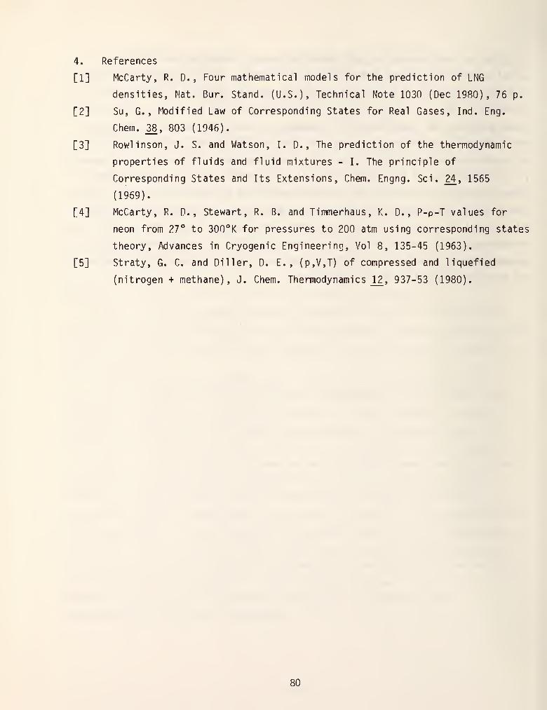
4. References
[1] McCarty, R. D. , Four mathematical models for the prediction of LNG
densities, Nat. Bur. Stand. (U.S.), Technical Note 1030 (Dec 1980), 76 p.
[2] Su, G. , Modified Law of Corresponding States for Real Gases, Ind. Eng.
Chem. 38, 803 (1946).
[3] Rowlinson, J. S. and Watson, I. D. , The prediction of the thermodynamic
properties of fluids and fluid mixtures - I. The principle of
Corresponding States and Its Extensions, Chem. Engng. Sci. 24, 1565
(1969).
[4] McCarty, R. D. , Stewart, R. B. and Timmerhaus, K. D. , P-p-T values for
neon from 27° to 300°K for pressures to 200 atm using corresponding states
theory. Advances in Cryogenic Engineering, Vol 8, 135-45 (1963).
[5] Straty, G. C. and Diller, D. E. , (p,V,T) of compressed and liquefied
(nitrogen + methane), J. Chem. Thermodynamics 12, 937-53 (1980).
80
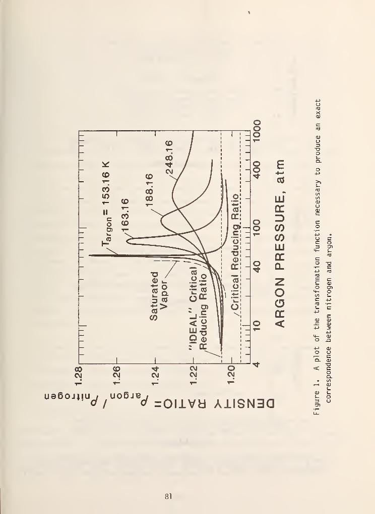
00^ '^
CD COCM
" r-CO 00 /lO
(0T-
00\
II
c CO\r"o CO V.
O) ^ \.CO
00CM
COCM
OO
oHO
oo
o
CO
LJJ
ccZ>COCOLUCCa.
O(DCC
<
ua6oj;|uo / d =OllVa AilSNBQ
-t-i
ofOX(U
£=to
(Uo3-aos_Q.
O-!->
>>S-03{/)
(/>
a>o<ucco•^4-> •
o cc: o=3 cr>tf- S-
<tJ
co T3•r- C+-> 03fO
cIT CUo CDM- Oco s_c 4->
03i. C4->
cCU <u_C CU-!-> s
+->
4- a»O JD
-!-> d)O o^~ cQ. CU
T3<: c
oa.
• (/I
.—
1
CUS-
CU S-S- o^ acr>
81
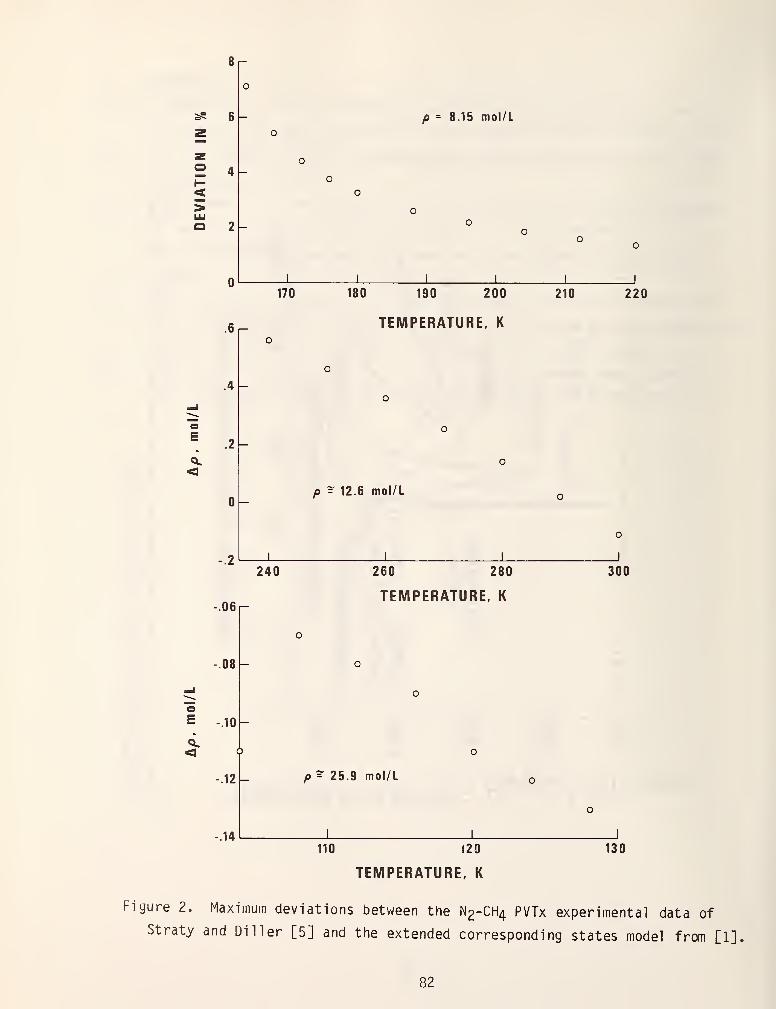
p = 8.15 mol/L
° 4
<>
170
_J \ L_180 190 200
TEMPERATURE. K
p = 12.6 mol/L
240
-.08^
.08-
260 280
TEMPERATURE, K
E -.10^
-.12
.14
p = 25.9 mol/L
210 220
110 120
TEMPERATURE, K
300
130
Figure 2. Maximum deviations between the N2-CH4 PVTx experimental data of
Straty and Diller [5] and the extended corresponding states model from [1],
82
VAPOR-LIQUIO EQUILIBRIUM OF BINARY MIXTURES
NEAR THE CRITICAL LOCUS
James C. Rainwater
Thermophysical Properties DivisionNational Engineering LaboratoryNational bureau of StandardsBoulder, Colorado 80303
A new method is presented for the prediction and correlation of
vapor-liquid equilibrium of binary mixtures in the critical region. The
basic Ljual ita'ci ve features of the problan are first reviewed, as well as
the e>revious theories of Griffiths and Wheeler, Leung and Griffiths, and
Holdover and Gallagher, and the concepts of field and density variables,
corresponding states, and scaliiig-law equations of state. The
Moldover-Gallagher recipe is i.iodified by making the dependent variable
of corresponding states a quadratic combination of density change and
composition change across the phase boundary, rather than density change
alone. The revised i.iethod is applied to the nitrogen-methane data of
Bloomer and Parent. Along the locus of points twelve percent below the
mixture critical temperature in suitably reduced units, the prediction
of composition difference across the phase boundary is greatly improved.
Tne revised procedure is shown not to be significantly different from
that of Moldover and Gallagher for mixtures where the latter has been
successful
.
Key words: binary mixtures; corresponding states; critical exponents;
critical line; dew-bubble curves; field variables; Leung-Griffiths
procedure; nitrogen-methane VLE; quadratic coupling; scaling-law
equation of state; vapor-liquid equilibrium.
1. Introduction
In the previous talk by Jim Ely [1], a wide variety of equations and
techniques used in industry to predict vapor-liquid equilibriuni (VLE) of luixtures
was described. As Jim pointed out, these methods are not as accurate near the
critical locus, i.e., witnin about 10 percent of the critical temperature, as
they are farther away. In fact, modern theories of phase transitions predict
83
that the "classical" equations of state commonly used in industry give incorrect
critical exponents and thus have fundamental limitations in predicting
thermophysical behavior near the critical locus. The talk following mine, by
Brian Eaton [2], will describe methods for predicting the critical locus of a
binary mixture.
My talk is intennediate in range of temperature as well as order of
presentation. In the present lecture, we will not be concerned with VLE at
temperatures less than about o5 percent of the critical temperature. Nor will we
be concerned with prediction of the critical line itself, which we take as given.
Rather, we pose the following question: Given the vapor pressure curves of the
pure components and the critical line of a binary mixture, can we quantitatively
predict VLE behavior over the region near tne critical line, where the
industrially oriented methods tend to break down?
This lecture will concentrate on a line of research, more academically
oriented and less industrially oriented than the methods described in Jim Ely's
lecture, which has made significant progress in answering the above question over
the past decade. The research essentially began with the classification by
Griffiths and Wheeler [3], in 1970, of thermodynamic variables into two kinds,
density and field variables. It continued in 1973 with the prediction by Leung3 4
and Griffiths [4] of VLE of a simply behaved binary mixture, namely He- He.
Later, Moldover and Gallagher [5] modified the Leung-Griffiths method so that it
could be applicable to mixtures with more complicated VLE behavior (e.g.,
azeotropy). The Moldover-Gallagher recipe was remarkably successful for several
binary mixtures, but tended to break down for systems with large composition
differences between liquid and vapor.
Most recently, I have proposed a modification of the Moldover-Gallagher
method, tentatively named the "quadratic coupling recipe," to account for
mixtures with large composition differences. Although the results are admittedly
preliminary at present, the modified recipe appears quite promising so far. It
yields significantly improved agreement between theory and experiment for the
liquid-vapor composition difference of nitrogen-methane, and is rooted in
plausible theoretical assumptions.
This line of research, at least since Moldover and Gallagher [5J, has been
intimately connected with the law of corresponding states. The lectures by Brian
Eaton [2] and Bob McCarty [6] will describe the law of corresponding states in
more sopnistication; here we consider only its most basic form. In essence, the
84
law characterizes an intermolecular potential by two parameters, a length scale
and an energy scale. Then, so long as the potentials for different fluids have
basically the sanie shape, the thermophysical properties of those fluids are
predicted (in appropriately reduced units) to obey universal behavior. The
principle is general in that it is independent of the particular shape of the
potential
.
Furthermore, the law of corresponding states is an essential tool for the
understanding of fluid mixtures [7]. At least sufficiently far from the
two-phase region, a mixture may be represented as a hypotnetical pure fluid.
With the appropriate mixing rules (i.e., weighted averages over the length and
energy scales of the pure cohiponents) , and application of tne law of
corresponding states, PVT properties of mixtures may be predicted accurately over
a wide range of thermodynamic variables [7].
Here we consider the question of whether the law of corresponding states is
useful in understanding and predicting the VLE behavior of fluid mixtures. For
the sake of simplicity, we restrict the discussion to binary mixtures which are
miscible in both the liquid and gaseous pnases. Specifically, we ask the
questions:
(1) In terms of the most commonly used physical variables, is the VLE behavior
of binary mixtures even qualitatively similar to VLE of pure fluids?
(2) If the answer to (1) is negative, can a transformation of variables be made
such that the VLE properties of mixtures and pure fluids are qualitatively
similar?
(3) Can such a transformation be found with no appreciable difficulty in
performing both the direct and inverse transformations?
(4) Can we predict which variables, both dependent and independent, "obey
corresponding states" in the transformed spaces?
Our answers will be negative to (1) and positive, in a qualified and
tentative way, to (2), (3) and (4).
2. VLE of Pure Fluids: Scaling Laws
We first review the basic VLE properties of pure fluids. These may be
characterized by coexistence curves in the T (temperature) - p (density) plane as
shown in figure 1, and the P (pressure) - T plane as shown in figure 2. The
first figure shows the "coexistence dome" with the critical point at the point of
highest temperature. The curve may be represented by [5]
85
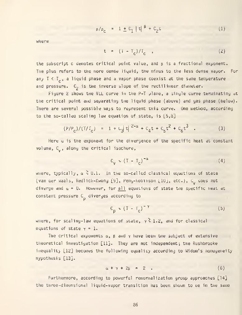
p/Pc = 1 ± 4 hi ^ + c^t (1)
where
t = (T - TJ/T^ , U)
the subscript c denotes critical point value, and a is a fractional exponent.
The plus refers to tha more dense liquid, the minus to the less dense vapor. For
an^ T < T , a liquid phase and a vapor phase coexist at the same temperature
and pressure. C^ is the inverse slope of the rectilinear diafiieter.
Fiyure Z shows trie VLL curve in trie P-T plane, a siriyle curve teruiinatiny at
tne critical point and separatiri'j tne liquid phase (above) and yas phase (below).
There are several possible wa>s to represent triis curve. Une uiethoa, according
to the so-calleu scaling law equation of state, is [5,8]
(P/P^)/(T/r^) = 1 + L3I t|^"°'
+ C^t + C^t^ + C^t^ . (3)
Here u is the exponent for the divergence of the specific heat at constant
volume, C , along the critical isochore,
Cy - (T - TJ-^ (4)
where, typically, a -t 0.1. In the so-called classical equations of state
(van aer Waals, Redl ich-Kwong [^Js Peng-KoDi nson lIUj, etc.), C does not
diverge and a = 0. However, tor al
1
equations of state tne specific heat at
constant pressure C diverges according to
CpMT-T,)-^ (b)
Where, for scaling-! aw equations of state, y^ l-Z, and for classical
equations of state y = 1.
The critical exponents a, 3 and y licive been tne subject of extensive
theoretical investigation [11]. They are not independent; tne Rushbrooke
inequality [IZ] becomes the following equalicy according to Widom's homogeneity
hypothesi s [13].
u + Y + 2(5 = 2 . (6)
Furthermore, according to powerful renormal ization group approaches [14]
the three-dimensional liquid-vapor transition has been shovni to ue in the saine
86
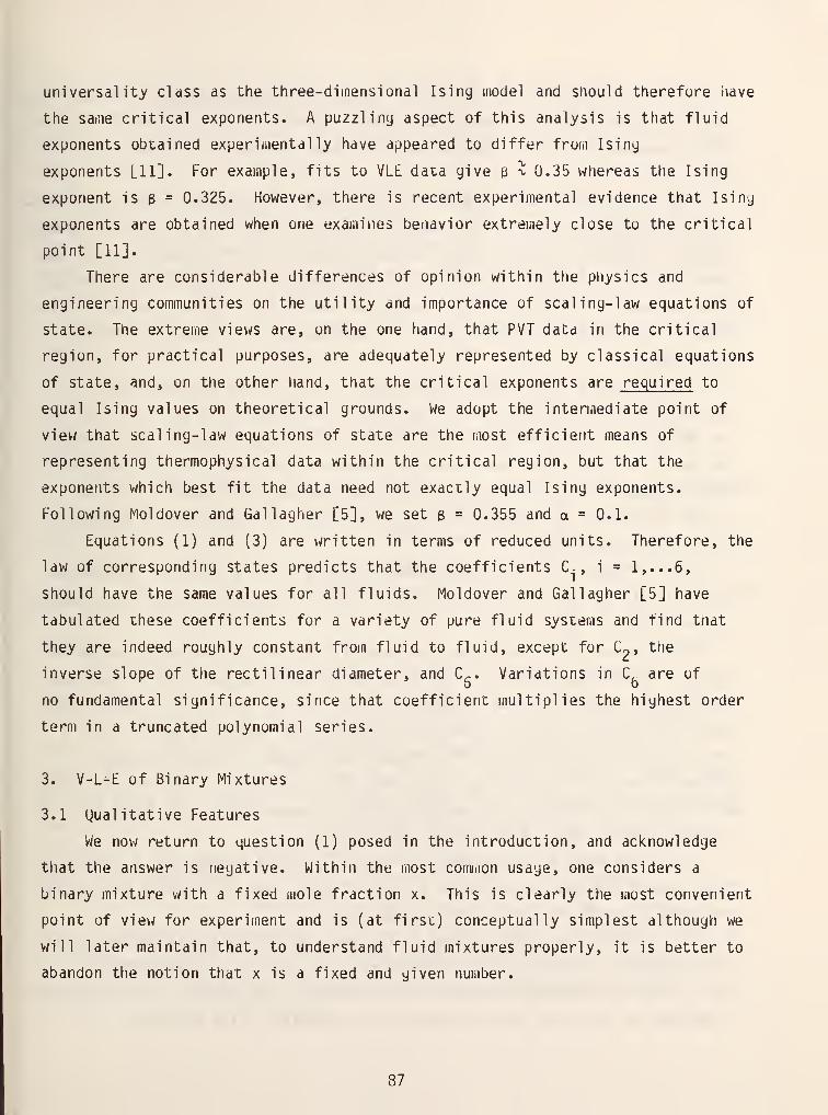
universality class as the three-dimensional Ising model and should therefore have
the same critical exponents. A puzzling aspect of this analysis is that fluid
exponents obtained experimentally have appeared to differ from Ising
exponents Lll]« For example, fits to VLt data give b x 0.35 whereas the Ising
exponent is g = 0.325. However, there is recent experimental evidence that Ising
exponents are obtained when one examines benavior extremely close to the critical
point [11].
There are considerable differences of opinion within the physics and
engineering communities on the utility and importance of scaling-law equations of
state. The extreme views are^ on the one hand, that PVT data in the critical
region, for practical purposes, are adequately represented by classical equations
of state, and, on the other hand, that the critical exponents are required to
equal Ising values on theoretical grounds. We adopt the intermediate point of
view that scaling-law equations of state are the most efficient means of
representing thermophysical data within the critical region, but that the
exponents which best fit the data need not exactly equal Ising exponents.
Following Moldover and Gallagher [5], we set 3 = 0.355 and a = 0.1.
Equations (1) and (3) are v/ritten in terms of reduced units. Therefore, tne
law of corresponding states predicts that the coefficients C. , i = 1,...6,
should have the same values for all fluids. Moldover and Gallagher [5] have
tabulated these coefficients for a variety of pure fluid systems and find that
they are indeed roughly constant from fluid to fluid, except for C^, the
inverse slope of the rectilinear diameter, and C^. Variations in C^ are of
no fundamental significance, since that coefficient multiplies the highest order
term in a truncated polynomial series.
3. V-L-E of Binary Mixtures
3.1 Qualitative Features
We now return to question (1) posed in the introduction, and acknowledge
that the answer is negative. Within the most comiiion usage, one considers a
binary mixture with a fixed mole fraction x. This is clearly the most convenient
point of view for experiment and is (at first) conceptually simplest although we
will later maintain that, to understand fluid mixtures properly, it is better to
abandon the notion that x is a fixed and given number.
87
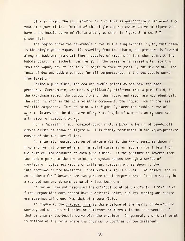
If X is fixed, the VLE behavior of a mixture is qual itatively different from
that of a pure fluid. Instead of the single vapor-pressure curve of figure 2 we
have a dew-bubble curve of finite width, as shown in figure 3 in the P-T
plane [15].
The region above tiie dew-bubble curve is tiie single-phase liquid; that below
is the single-pnase vapor. If, starting from the liquid, the pressure is lowered
along an isotherm (vertical line), bubbles of vapor will form when point A, the
bubble point, is reached. Similarly, if the pressure is raised after starting
from the vapor, dew or liquid will begin to form at point B, the dew point. The
locus of dew and bubble points, for all temperatures, is the dew-bubble curve
(for fixed x)
.
Unlike a pure fluid, the dew and bubble points do not have the same
pressure. Furthermore, and most significantly different frotn a pure fluid, in
the two-phase region the compositions of the liquid and vapor are not identical.
The vapor is rich in the more volatile component, the liquid rich in the less
volatile component. Thus at point C in figure 3, where the buuble curve of
X-, < X intersects the dew curve of x^, > x, liquid of composition x, coexists
with vapor of composition x„.
For a "nortiial " u'.e., nonazeotropic) mixture [15], a family of dew-bubble
curves exists as shov;n in figure 4. This family tenni nates in the vapor-pressure
curves of the two pure fluids.
An alternate representation of mixture VLE is the P-x diagram as shown in
figure 5 for nitrogen-methane. The solid curve is an isotiienn for T less than
the critical temperatures of both pure fluids. As the pressure is lowered from
the bubble point to the dew point, the system passes through a series of
coexisting liquids and vapors of different composition, as shown by the
intersections of the horizontal lines with the solid curves. The dashed line is
an isotherm for T uetween the two pure critical temperatures. It terminates, in
a rounded manner, at sodie value of x less than one.
So far v/e have not discussed the critical point of a mixture. A mixture of
fixed composition does indeed have a critical point, but its meaning and nature
are somewhat different from that of a pure fluid.
In figure 4, the critical line is the envelope of the family of dew-bubble
curves, and the critical point of a mixture of fixed x is tne intersection of
that particular dew-bubble curve witfi the envelope. In general, a critical point
is defined as the point wtiere tne pnysical properties of two different.
88
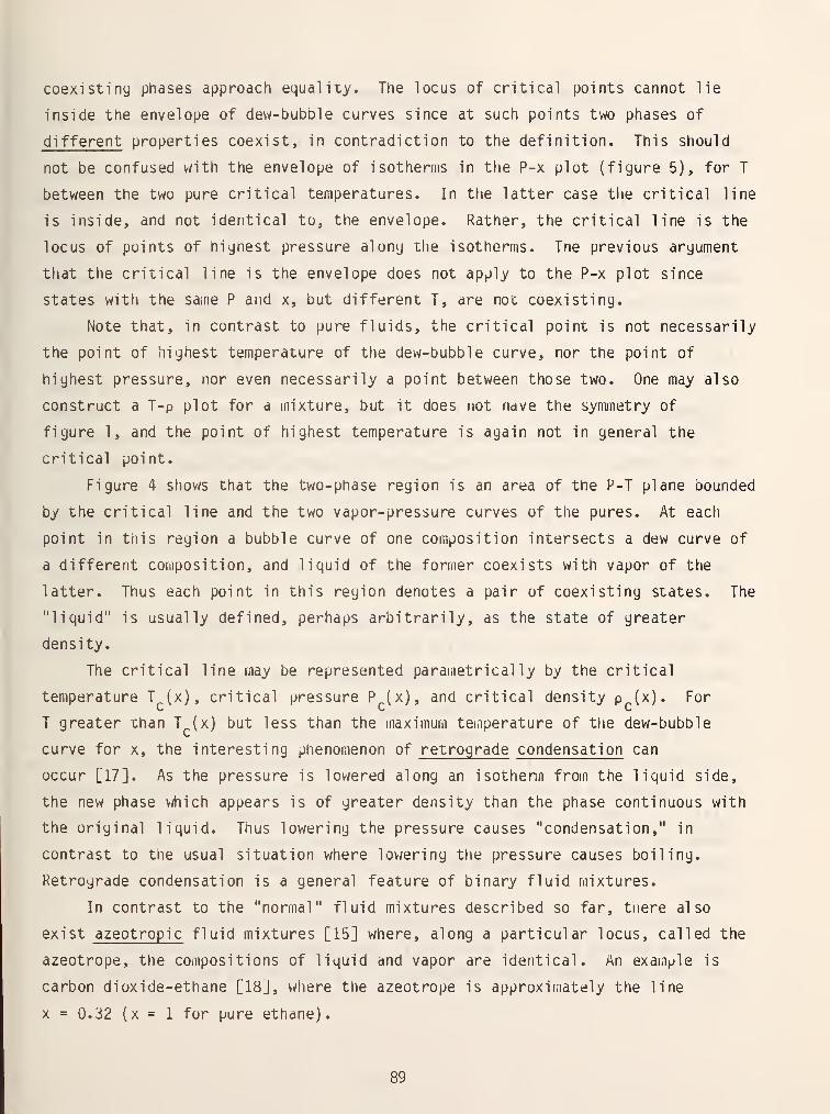
coexisting phases approach equality. The locus of critical points cannot lie
inside the envelope of dew-bubble curves since at such points two phases of
different properties coexist, in contradiction to the definition. This should
not be confused with the envelope of isotherms in the P-x plot (figure 5), for T
between the two pure critical temperatures. In the latter case tlie critical line
is inside, and not identical to, the envelope. Rather, the critical line is the
locus of points of highest pressure along the isotherms. Tne previous argument
that the critical line is the envelope does not apply to the P-x plot since
states with the same P and x, but different T, are not coexisting.
Note that, in contrast to pure fluids, the critical point is not necessarily
the point of highest temperature of the dew-bubble curve, nor the point of
highest pressure, nor even necessarily a point between those two. One may also
construct a T-p plot for a mixture, but it does not naye the symmetry of
figure 1, and the point of highest temperature is again not in general the
critical point.
Figure 4 shows that the two-phase region is an area of the P-T plane bounded
by the critical line and the two vapor-pressure curves of the pures. At each
point in this region a bubble curve of one composition intersects a dew curve of
a different composition, and liquid of the former coexists with vapor of the
latter. Thus each point in this region denotes a pair of coexisting states. The
"liquid" is usually defined, perhaps arbitrarily, as the state of greater
density.
The critical line may be represented parametrically by the critical
temperature T (x), critical pressure Pj,(x), and critical density p (x). For
T greater chan T (x) but less than the maximum teinperature of the dew-bubble
curve for x, the interesting phenomenon of retrograde condensation can
occur [17]. As the pressure is lowered along an isotherm from the liquid side,
the new phase vAiich appears is of greater density than the phase continuous with
the original liquid. Thus lowering the pressure causes "condensation," in
contrast to the usual situation where lov/ering the pressure causes boiling.
Retrograde condensation is a general feature of binary fluid mixtures.
In contrast to the "normal" fluid mixtures described so far, there also
exist azeotropic fluid mixtures [15] where, along a particular locus, called the
azeotrope, the compositions of liquid and vapor are identical. An exam^^le is
carbon dioxide-ethane [18], where the azeotrope is approximately the line
X = 0.32 (x = 1 for pure ethane).
89
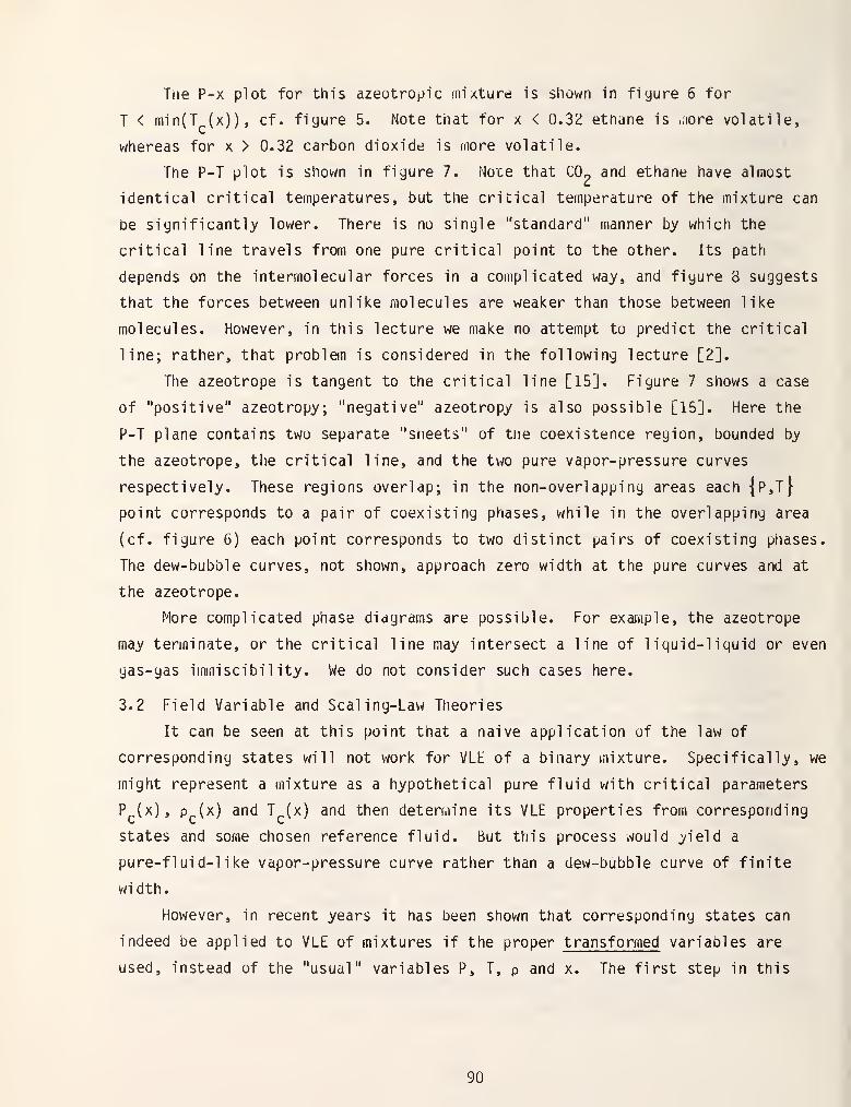
Tiie P-x plot for this azeotropic mixture is shov/n in figure 6 for
T < min(T (x)), cf. figure 5. Note that for x < 0.3^ ethane is r.iore volatile,
whereas for x > 0.32 carbon dioxide is more volatile.
The P-T plot is shown in figure 7. Note that CO^ and ethane have almost
identical critical temperatures, but the critical temperature of the mixture can
be significantly lower. There is no single "standard" manner by which the
critical line travels from one pure critical point to the other. Its path
depends on the intermolecul ar forces in a complicated way, and figure 8 suggests
that the forces between unlike molecules are weaker than those between like
molecules. However, in this lecture v;e make no attempt to predict the critical
line; rather, that problem is considered in the following lecture [2].
The azeotrope is tangent to the critical line [15]. Figure 7 shows a case
of "positive" azeotropy; "negative" azeotropy is also possible [15]. Here the
P-T plane contains two separate "sheets" of tne coexistence region, bounded by
the azeotrope, the critical line, and the two pure vapor-pressure curves
respectively. These regions overlap; in the non-overlapping areas each {P,Tf
point corresponds to a pair of coexisting phases, while in the overlapping area
(cf. figure 6) each point corresponds to two distinct pairs of coexisting phases.
The dew-bubble curves, not shown, approach zero width at the pure curves and at
the azeotrope.
More complicated phase diagrams are possible. For exarnple, the azeotrope
may terminate, or the critical line may intersect a line of liquid-liquid or even
gas-gas iminiscibil ity. We do not consider such cases here.
3.2 Field Variable and Scaling-Law Theories
It can be seen at this point that a naive application of the law of
corresponding states will not work for VLE of a binary mixture. Specifically, we
might represent a mixture as a hypothetical pure fluid with critical parameters
P (x), pp(x) and T (x) and then determine its VLE properties from corresponding
states and some chosen reference fluid. But this process would yield a
pure-fluid-like vapor-pressure curve rather than a dew-bubble curve of finite
width.
However, in recent years it has been shown that corresponding states can
indeed be applied to VLE of mixtures if the proper transformed variables are
used, instead of the "usual" variables P, T, p and x. The first step in this
90
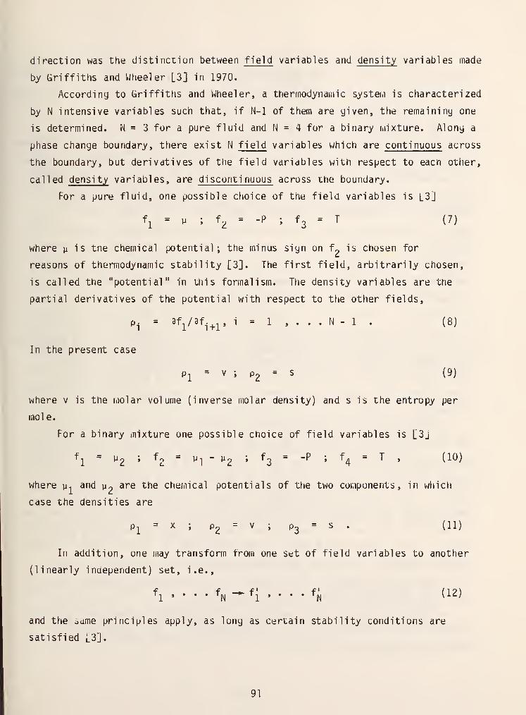
direction was the distinction between field variables and density variables made
by Griffiths and Wheeler [3] in 1970.
According to Griffiths and Wheeler, a thermodynamic system is characterized
by N intensive variables such that, if N-1 of them are given, the remaining one
is determined. N = 3 for a pure fluid and N = 4 for a binary i.iixture. Along a
phase change boundary, there exist N field variables which are continuous across
the boundary, but derivatives of the field variables with respect to eacn other,
called density variables, are discontinuous across the boundary.
For a pure fluid, one possible choice of the field variables is L3]
fl = y ; f^ = -P ; f3 = T (7)
where y is tne chemical potential; the minus sign on f^ is chosen for
reasons of thermodynamic stability [3]. The first field, arbitrarily chosen,
is called the "potential" in Uiis formalism. The density variables are the
partial derivatives of the potential with respect to the other fields,
Pi =^^l/^^i+1'
i = 1 » • • • N - 1 • (8)
In the present case
p^ = V ; P2 = s (9)
where v is the molar volume (inverse molar density) and s is the entropy per
mole.
For a binary mixture one possible choice of field variables is [SJ
f], = ^2 »fo = V] - ^2 » ^3 "" "'^ i ^4 = T
, (10)
where u, and m^ are the chemical potentials of the two components, in which
case the densities are
p^ = X ; p^ = V ; p^ = s . (11)
In addition, one may transform from one set of field variables to another
(linearly independent) set, i.e.,
t^ , . . . tj^ -*"1 ' * * *
N \^^J
and the ^ume principles apply, as long as certain stability conditions are
satisfied [3].
91
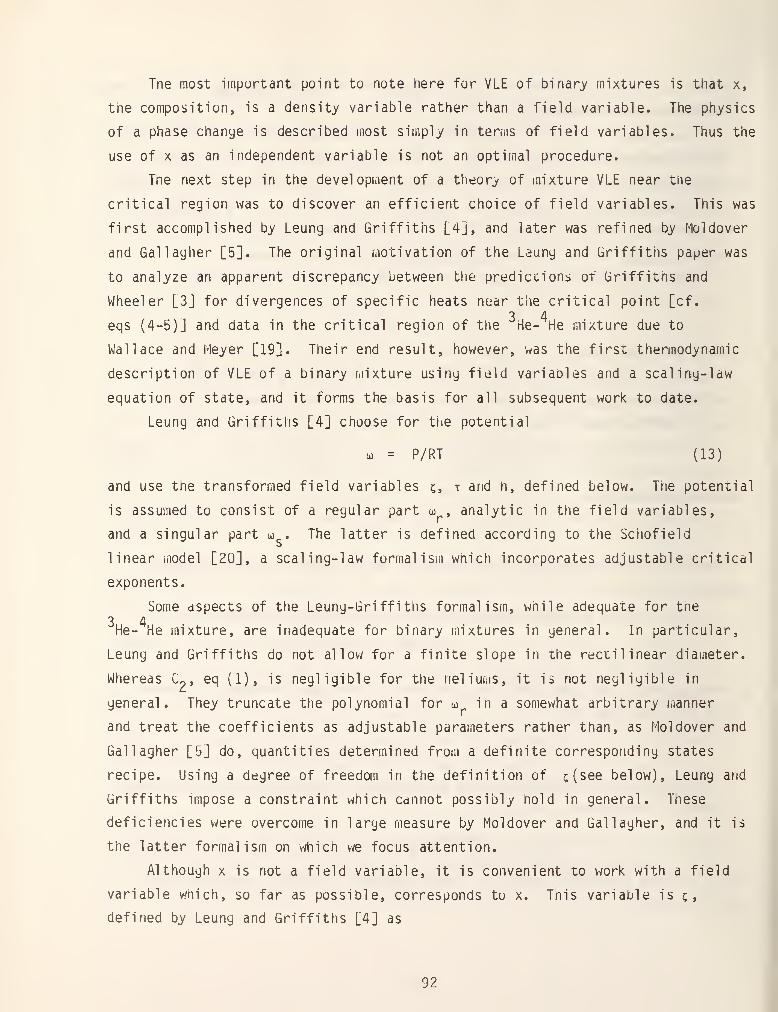
Tne most important point to note here for VLE of binary mixtures is that x,
the composition, is a density variable rather than a field variable. The physics
of a phase change is described most simply in terms of field variables. Thus the
use of X as an independent variable is not an optimal procedure.
The next step in tne development of a theory of mixture VLE near the
critical region was to discover an efficient choice of field variables. This was
first accomplished by Leung and Griffiths [4], and later was refined by Moldover
and Gallagher [5]. The original motivation of the Leung and Griffiths paper was
to analyze an apparent discrepancy between the predictions of Griffiths and
Wheeler [3] for divergences of specific heats near the critical point [cf.
3 4eqs (4-5)] and data in the critical region of the He- He mixture due to
Wallace and Meyer [19]. Their end result, however, was the first thermodynamic
description of VLE of a binary r.iixture using field variaoles and a scaling-law
equation of state, and it forms the basis for all subsequent work to date.
Leung and Griffiths [4] choose for tlie potential
0) = P/RT (13)
and use the transformed field variables c, t and h, defined below. The potential
is assumed to consist of a regular part w , analytic in the field variables,
and a singular part to . The latter is defined according to the Sciiofield
linear model [20], a scaling-law formalism which incorporates adjustable critical
exponents.
Some aspects of the Leung-Griffiths formalism, while adequate for the3 4He- He mixture, are inadequate for binary mixtures in general. In particular,
Leung and Griffiths do not allow for a finite slope in the rectilinear diameter.
Whereas C^, eq (1), is negligible for the iieliums, it is not negligible in
general. They truncate the polynomial for oj in a somewhat arbitrary (nanner
and treat the coefficients as adjustable parameters rather than, as Moldover and
Gallagher [5] do, quantities determined from a definite corresponding states
recipe. Using a degree of freedom in the definition of ^(see below), Leung and
Griffiths impose a constraint which cannot possibly hold in general. These
deficiencies were overcome in large measure by Moldover and Gallagher, and it is
the latter formalism on which we focus attention.
Although x is not a field variable, it is convenient to work with a field
variable which, so far as possible, corresponds to x. Tnis variable is 5,
defined by Leung and Griffiths [4] as
92
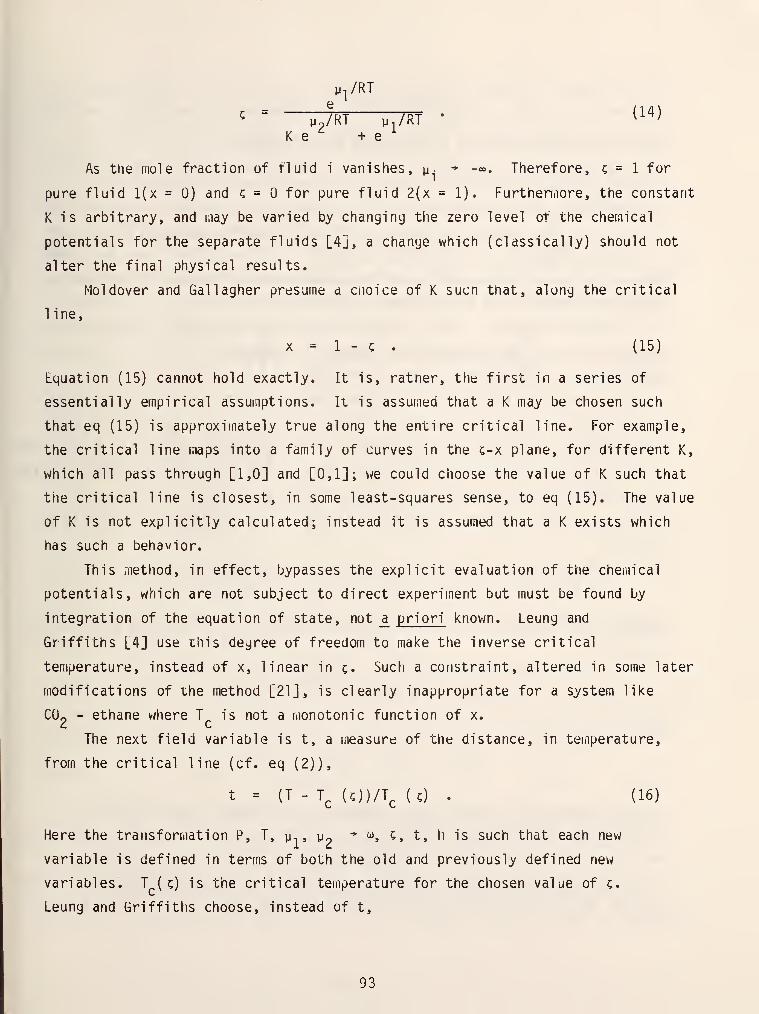
K e ^ + e
As the mole fraction of fluid i vanishes, y. - -<». Therefore, c = 1 for
pure fluid l(x = 0) and c = for pure fluid 2(x = 1). Furthennore, the constant
K is arbitrary, and may be varied by changing the zero level of the chemical
potentials for the separate fluids [4], a change which (classically) should not
alter the final physical results.
Holdover and Gallagher presume a choice of K sucn that, along the critical
1 ine,
X = 1 - c . (15)
Equation (15) cannot hold exactly. It is, rather, the first in a series of
essentially empirical assumptions. It is assumed that a K may be chosen such
that eq (15) is approximately true along the entire critical line. For example,
the critical line maps into a family of curves in the c-x plane, for different K,
which all pass through [1,0] and [0,1]; we could choose the value of K such that
the critical line is closest, in some least-squares sense, to eq (15). The value
of K is not explicitly calculated; instead it is assumed that a K exists which
has such a behavior.
This method, in effect, bypasses the explicit evaluation of the chemical
potentials, which are not subject to direct experiment but must be found by
integration of the equation of state, not a^ priori known. Leung and
Griffiths [4] use this degree of freedom to make the inverse critical
temperature, instead of x, linear in c. Such a constraint, altered in some later
modifications of the method [21], is clearly inappropriate for a system like
COo - ethane where T is not a monotonic function of x.2 c
The next field variable is t, a measure of the distance, in temperature,
from the critical line (cf. eq (2)),
t = (T - T^ (0)/T^ (c) . (16)
Here the transformation P, T, y, , y^ -^ i^, ^, t, h is such that each new
variable is defined in terms of both the old and previously defined new
variables. Tp( ^) is the critical temperature for the chosen value of ^.
Leung and Griffiths choose, instead of t.
93
X = (RT^ (0)'^ - (KT)-^ (17)
which has the disadvantage of not being diinensionless.
The last field variable is h, which measures the distance away from the
coexistence surface.
/ u^/RT y,/RT\ / v.^°(^,t)/RT yl'lcTJ/kTXh = jin{Ke^ +e^ 1-iinfKe'^ +e^ ) (18)
where y-(i;,T) is the value of y- on the coexistence surface, or its extension
above the critical line [4], for tlie given (c,t).
In the transformed space, the phase transition region has a particularly
simple geometry. The critical line is the line segment t = 0, h = 0, <^ c <. 1>
and the coexistence surface is the plane region t < 0, h = 0, _< ^ <. 1.
The essential feature of the Holdover-Gallagher formalism [5] is to make a
correspondence, for each value of c between and 1, with a hypothetical pure
fluid, and to assume the VLE properties of this hypothetical pure fluid are given
by the law of corresponding states and a dual system of reference fluids (the tvw
pure fluids) with a linear interpolation "mixing rule." In particular, the
"vapor pressure" curve for a locus of fixed r, on the coexistence surface is [of.
eq (3)],
PT^(0/TP^(0 = 1 + C3(c)|t| ^-^ + C^iOt + C5(0t^ + C.(c)t^ (19)
and this hypothetical fluid has a coexistence dome in the T-p plane given b^ [cf.
eq (1)]
p/p^(c) = 1 ± C^(c)|t|-^^^
+ C2(c)t (20)
where, i = 1,...6,
Ci(d = c|2) + (cP-cj2)),= c|2)+crc , (21)
and the superscripts refer to the respective pure fluids. Note that the
superscripts were incorrectly reversed in reference [5], eq (8). This error did
not affect the final results of reference [5].
Figure 8 shows lines of constant c in the P-T plane for the nitrogen-methane
system. Equations (19) and (21) predict that these lines form a nearly parallel
94
curvilinear grid, which is an additional empirical assumption. Note that, if
the two fluids obey corresponding states exactly, cj. ^ = c|| - C.{^) for all
5. In general, C. (;;) is never expected to be \iery far from either pure fluid
value.
As explained previously, each (P,T) point within the coexistence region
corresponds to two coexisting phases of different densities and compositions.
Thus, given c and t, our goal is to predict p^,. p„^^, x-,. and x,,^^ . The1 1 Cj vap 1 1 c{ vap
densities are given by eq (20). Leung and Griffiths, in a lengthy analysis, have
worked out the inverse transformation from the field variables to the
composition. In the Holdover-Gallagher formalism [5], this transformation is
= (1 - c) jl. ,[^.M.H(c,t)]| (22)
where
Q(c,t) =RTP,
K
1^41t|^-^ + C^t + C^t2+ C^t^j (23)
and T , P and C are functions of c. Substitution of p = p,. and p = p
in eq (22) yields, respectively, x,. and x^ ' _ "^
1 1 q vapThe function H(c,t) has an explicit and rather complicated definition
(eqs (A3) and (A7) of reference [5]) in terms of thermodynamic derivatives. For
our applications, it is assumed to be a smooth function with adjustable fitting
parameters. Note that, for eq (15) to hold on the critical line,
H(c,0) = . (24)
In their first recipe, Moldover and Gallagher make the additional empirical
assumption that IT = over the entire coexistence surface, thus completing
the construction of a closed recipe to predict x.
In practice, given the vapor pressure curves of the pure fluids and the
mixture critical line, we seek to construct isotherms in the P-x plane, figure 5,
95
and dew-bubble curves for fixed x, figure 3. For the former, we merely choose
successive values of c from to 1. Then, for a fixed T, the variables t, P,
X, . and X are determined algebrdically, yielding a series of points whichliq vap ^ J i J J V
describes the isotherm. Construction of dew-bubble curves is more complicated.
The bubble curves are loci of constant x, . , the dew curves of constant xliq' vap
To find points on these curves, we must perform a numerical root-finding search
on eq (22), since direct algebraic inversion is not possible. Alternately, we
could calculate x-,. and x on a sufficiently fine grid of (^,t) points as
in figure 8, and construct a coniplete family of dev.'-bubble curves by
interpolation.
There diVQ at present only a limited number of binary mixtures with accurate
experimental data for the critical line; particularly scarce are those with
accurate measurements of p (x). Moldover and Gallagher [5,22] tested their3 4
method on four binary mixtures: He- He (with results [22] essentially
equivalent to those of Leung and Griffiths), carbon dioxide-ethane, sulfur
hexafluoride-metiiane, and propane-octane. Tiie method yields excellent agreement
between theory and experiment for all but tne last inixture. Of particular
interest is the excellent VLE predictions for the azeotropic mixtures
CUp-CpH^ and SF^-CH.. As functions of commonly used thermodynamic variables
the VLE surfaces of these mixtures appear to have a ^ery complicated topological
structure. However, upon transformation to field variables, application of the
Moldover-Gallagher formalism, and performance of the inverse transformation, the
apparently complex VLE surfaces diVQ predicted to high accuracy (see, for example,
figures 3, 4 and 6 of reference [5]).
For the normal mixture C^Hq-Cc^H,^, Moldover and Gallagher found
significant discrepancies between theory and experiment, particularly for
propane-rich mixtures. In an attempt to correct this, they proposed a second
recipe where, instead of setting H = for all {^,t}, they assumed that
-1 '^cH(c.T) = C^ T^ ^ t , (25)
with Tq evaluated at c = 1 - x.
Note that eq (24), and hence eq (15), are still valid. Moldover and
Gallagher give some theoretical justification for this form in their Appendix B.
The constant C^ is, in effect, an adjustable parameter and the choice Cm = -25
96
provides d best fit to the propane-octane VLE data. However, for propane-rich
mixtures such a fit is still not entirely satisfactory.
3.3 The Quadratic Coupling Recipe
At this point, v;e seek a revised version of the Moldover-Gallagher [5]
technique that incorporates the appropriate modifications for mixtures on which
their methods break down, but which reduces to their methods for those mixtures
where it does currently work. To do this, we first must try to decide, with the
available clues, what features are held in common by mixtures on which the
Moldover-Gallayher recipe does or aoes not work. We mention here that their
methods appear also not to predict properly VLE behavior of the normal system
nitroyen-methane [figure 4].
The feature most immediately evident is that systems with small composition
difference betv^een liquids and vapor phases are described accurately by the
Moldover-Gallagher formalism, whereas systems with large composition differences
are not. Comparing figures 5 and 6, we see that the presence of an azeotrope
tends to "pinch" the VLE curves in the P-x plane, and hence makes the vapor-
liquid composition difference in general smaller than that of a normal mixture.
In addition, the composition difference generally becomes larger with wider
dew-bubble curves. Propane-octane and nitrogen-methane both have wide dew-bubble3 4
curves, whereas those of the normal mixture He- He happen to be ^jery narrow.
It is illuminating to rewrite eqs (20) and (22) in terms of averages and
differences of properties in the vapor and liquid phases.
p avg= Pcd + C2(c)t) (26)
1.355
>^avg = (1 - 0<1 - ^
Ap = 2p^ C^(0|tl*-"^^ (27)
(l . J|Li^ , kl^ . klM . H(c,t)l j (28)
( L ^liq ^vap ^c J)
ix = C(l - ,,[iiLMi . ali^ 1 . (29)
L ^vap ^liq J
97
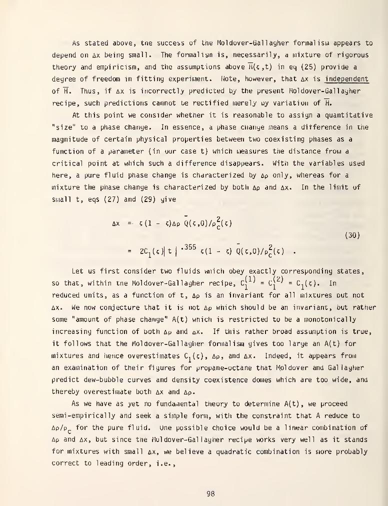
As stated above, tne success of tne Moldover-Gallagher formalism appears to
depend on ax being small. The formalism is, necessarily, a mixture of rigorous
theory and empiricism, and the assumptions above H(5 ,t) in eq (25) provide a
degree of freedom in fitting experiment. Note, however, that ax is independent
of TT. Thus, if AX is incorrectly predicted by the present Moldover-Gallagher
recipe, such predictions cannot be rectified merely oy variation of H.
At this point we consider whether it is reasonable to assign a quantitative
"size" to a phase change. In essence, a phase change means a difference in tne
magnitude of certain physical properties between tv/o coexisting phases as a
function of a parameter (in our case t) which measures the distance from a
critical point at which such a difference disappears. With the variables used
here, a pure fluid phase change is characterized by Ap only, whereas for a
mixture the phase change is characterized by both Ap and ax. In the limit of
small t, eqs (27) and (29) give
AX = 5(1 - C)Ap Q(?,0)/p^(O
= 2C^(0|tI
-^^^c(l - Q(c,0)/p^(O
(30)
Let us first consider two fluids wnich obey exactly corresponding states,
so that, within tne Moldover-Gallagher recipe, Cj ^ = c| ^ = CJ^). In
reduced units, as a function of t, Ap is an invariant for all mixtures out not
AX. We now conjecture that it is not Ap which should be an invariant, but rather
some "amount of phase change" A(t) wnich is restricted to be a monotonically
increasing function of both Ap and nx. If this rather broad assumption is true,
it follows that the Moldover-Gallagher formalism gives too large an A(t) for
mixtures and hence overestimates C, (c), Ap, and ax. Indeed, it appears from
an examination of their figures for propane-octane that Holdover and Gallagher
predict dew-bubble curves and density coexistence domes which are too wide, and
thereby overestimate both ax and Ap.
As we have as yet no fundaniental theory to determine A(t) , we proceed
semi-empirical ly and seek a simple form, with the constraint that A reduce to
Ap/p for the pure fluid. Une possible choice vwuld be a linear combination of
Ap and AX, but since the Moldover-Gallagher recipe works very well as it stands
for mixtures with small ax, v;e believe a quadratic combination is more probably
correct to leading order, i.e..
98
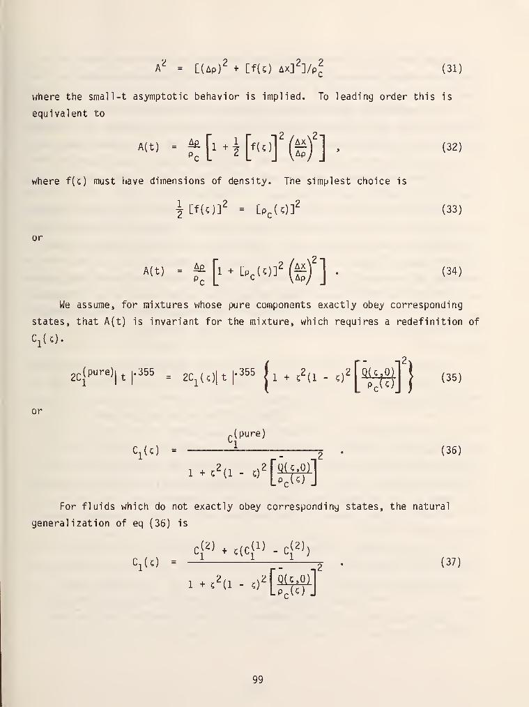
a'^ = [(Ap)^ + [f(0 Ax]2]/p^ (31)
where the small-t asymptotic behavior is implied. To leading order this is
equivalent to
A(t) = J [14 [no]' (f^)'] . (32)
where f(?) must liave dimensions of density. The simplest choice is
J \.fU)f = [P^IO]^ (33)
or
A(t) = M [i . t,^(„]2 (Mj]
. (34)
We assume, for mixtures whose pure components exactly obey corresponding
states, that A(t) is invariant for the mixture, which requires a redefinition of
Ci(c).
2c(pure)|^ |.355 ^ 2C^^0|tl'^^^ jl + c^d - o4^^1 j
(35)
or
^(pure)
C^(0 =^-
: 2 • ^^^^
1 + c^(l - 0^
For fluids which do not exactly obey corresponding states, the natural
generalization of eq (36) is
Ci^) . ,(c(l) - c(2))
4(0 = — ^ 2 • '3^'
I.c^a-,^[W]
99
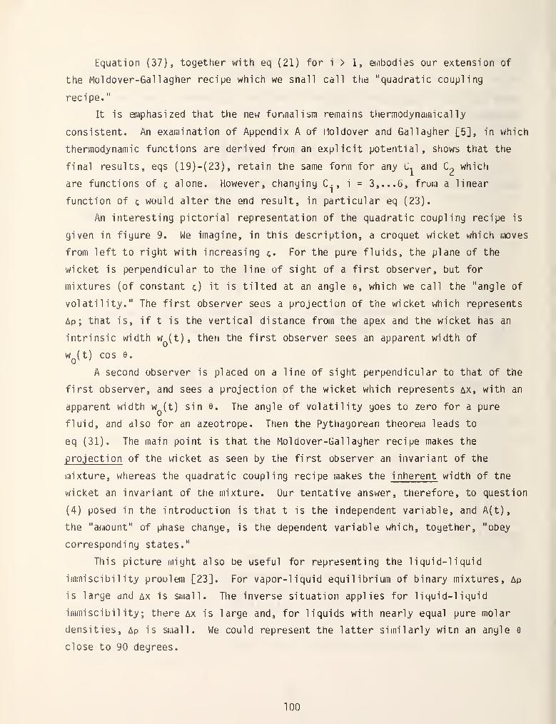
Equation (37), together with eq (21) for i > 1, Qiibodies our extension of
the Moldover-Gallagher recipe which we shall call the "quadratic coupling
recipe."
It is emphasized that the new fonnalism remains thermodynainical ly
consistent. An examination of Appendix A of Holdover and Gallagher [5], in which
thermodynamic functions are derived from an explicit potential, shows that the
final results, eqs (19)-(23), retain the same form for any C, and C.-, which
are functions of ^ alone. However, changing C.
, i = 3,... 6, fruin a linear
function of c would alter the end result, in particular eq (23).
An interesting pictorial representation of the quadratic coupling recipe is
given in figure 9. We imagine, in this description, a croquet wicket which moves
from left to right with increasing c« For the pure fluids, the plane of the
wicket is perpendicular to the line of sight of a first observer, but for
mixtures (of constant c) it is tilted at an angle e, which we call the "angle of
volatility." The first observer sees a projection of the wicket which represents
Ap; that is, if t is the vertical distance from the apex and the wicket has an
intrinsic width w (t), then the first observer sees an apparent width of
W (t) cos 6.
A second observer is placed on a line of sight perpendicular to that of the
first observer, and sees a projection of the wicket which represents ax, with an
apparent width w (t) sin e. The angle of volatility goes to zero for a pure
fluid, and also for an azeotrope. Then the Pytiiagorean theorem leads to
eq (31). The main point is that the Moldover-Gallagher recipe makes the
projection of the wicket as seen by the first observer an invariant of the
mixture, whereas the quadratic coupling recipe makes the inherent width of tne
wicket an invariant of the mixture. Our tentative answer, therefore, to question
(4) posed in the introduction is that t is the independent variable, and A(t),
the "amount" of phase change, is the dependent variable which, together, "obey
corresponding states."
This picture might also be useful for representing the liquid-liquid
immiscibil ity problem [23]. For vapor-liquid equilibrium of binary mixtures, Ap
is large and ax is small. The inverse situation applies for liquid-liquid
immiscibil ity; there ax is large and, for liquids with nearly equal pure molar
densities, Ap is small. We could represent the latter similarly witn an angle e
close to 90 degrees.
100
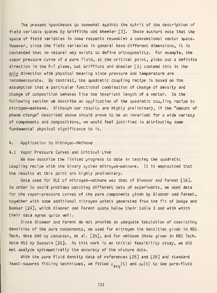
The present hypotheses go somewhat ayainst the spirit of the description of
field variable spaces by Griffiths and Wheeler [3]. Those authors note that the
space of field variables in some respects resembles a conventional vector space.
However, since the field variables in general have different dimensions, it is
contended that no natural way exists to define orthogonality. For example, the
vapor pressure curve of a pure fluid, at the critical point, picks out a definite
direction in the P-T plane, but Griffiths and Wheeler [3j contend this is the
only direction with physical meaning since pressure and temperature are
incommensurate. By contrast, the quadratic coupling recipe is based on the
assumption that a particular functional combination of change of density and
change of composition behaves like the invariant length of a vector. In the
following section \^e describe an application of the quadratic cou^^ling recipe to
nitrogen-methane. Although our results are highly preliminary, if the "amount of
phase change" described above should prove to be an invariant for a wide variety
of components and compositions, we would feel justified in attributing some
fundamental physical significance to it.
4. Application to Nitrogen-Methane
4.1 Vapor Pressure Curves and Critical Line
We now describe the limited progress to date in testing the quadratic
coupling recipe with the binary system nitrogen-methane. It is emphasized that
the results at this point are highly preliminary.
Data used for VLE of nitrogen-methane was that of Bloomer and Parent [16].
In order to avoid problems matching different sets of experiments, we used data
for the vapor-pressure curves of the pure components given by Bloomer and Parent,
together with some additional nitrogen points generated from the fit of Dodge and
Dunbar [24], which Bloomer and Parent quote below their table 3 and with which
their data agree quite well.
Since Bloomer and Parent do not provide an adequate tabulation of coexisting
densities of the pure components, we used for nitrogen the densities given in NBS
Tech. Note 648 by Jacobsen, et al . [25], and for methane those given in NBS Tech.
Note 653 by Goodwin [26]. As this work is an initial feasibility study, we did
not analyze systematically the accuracy of the mixture data.
With the pure fluid density data of references [25] and [26] and standard
least-squares fitting techniques, we fitted p^, (t) and Ap(t) to the pure-fluidavg
101
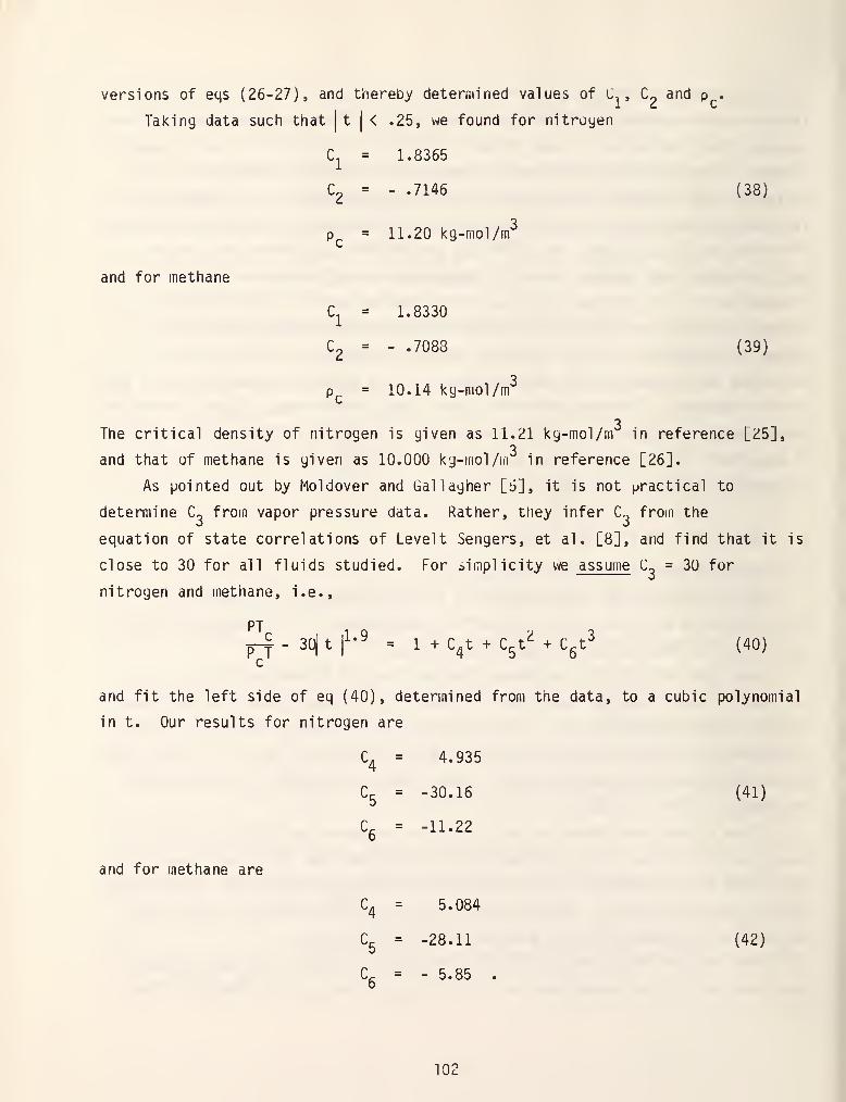
versions of eqs (26-27), and thereby determined values of C, , C^ and p ,
Taking data such that|t
|< .25, we found for nitroyen
C^ = 1.8365
C2 = - .7146 (38)
p^ = 11.20 kg-mol/m^
and for methane
C^ = 1.8330
C2 = - .7088 (39)
p^ = 10.14 kg-mol/m^
3The critical density of nitrogen is given as 11.21 kg-mol/m in reference [25],
3and that of methane is given as 10.000 ky-mol/in in reference [26].
As pointed out by Holdover and Gallagher [5], it is not practical to
determine C^ from vapor pressure data. Rather, they infer C, from the
equation of state correlations of Level t Sengers, et al . [8], and find that it is
close to 30 for all fluids studied. For simplicity we assume C^ = 30 for
nitrogen and methane, i.e.,
PT
p-^ - 30| t 1^-^ = 1 + C^t + C^t^ + Cgt^ (40)
and fit the left side of eq (40), determined from the data, to a cubic polynomial
in t. Our results for nitrogen are
C^ = 4.935
C^ = -30.16 (41)
Cg = -11.22
and for methane are
s = 5.084
s = -28.11
s = - 5.85
(42)
102
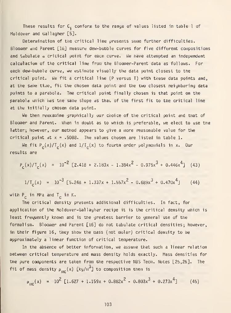
These results for C conform to the range of values listed in table 1 of
Moldover and Gallagher [5].
Determination of tiie critical line presents some further difficulties.
Bloomer and Parent [Ibj measure dew-bubble curves for five different compositions
and tdbulate a critical point for eacn curve. We riave attempted an independent
calculation of the critical line from the Bloomer-Parent data as follows. For
each dew-bubble curve, we estimate visually the data point closest to the
critical point. We fit a critical line (P versus T) with tliese data points and,
at the same tiiiie, fie the chosen data point and the two closest neighboring data
points to a parabola. Tne critical point finally chosen is that point on the
parabola v^nich has tne same slope as thai of the first fit to the critical line
at the initially chosen data point.
We then reexamine graphically our clioice of the critical point and that of
Bloomer and Parent. When in doubt as to which is preferable, we elect to use the
latter; however, our metiiod appears to give a more reasonable value for ttie
critical point at x = .5088. The values chosen are listed in table 1.
We fit Pr{x)/Tp(x) and 1/T (x) to fourtn order polynomials in x. Our
results are
P^(x)/T^(x) = 10"^ [2.418 + 2.183X - 1.384x^ - 0.975x^ + 0.446x^] (43)
1/T (x) = 10"^ [5.248 + 1.337X + 1.557x^ - 0.689x^ + 0.470x^] (44)
with P in MPa and T in K.c c
The critical density presents additional difficulties. In fact, for
application of the Moldover-Gallagher recipe it is the critical density which is
least frequently known and is the greatest barrier to general use of tne
formalism. Bloomer and Parent [16] do not tabulate critical densities; hov/ever,
in their figure 16, they show the mass (not molar) critical density to be
approximately a linear function of critical temperature.
In the absence of better information, we assume that such a linear relation
between critical temperature and mass density holds exactly. Mass densities for
tne pure components are taken from the respective NBS Tech. Notes [26,26]. The3
fit of mass densityp,
-(x) [kg/m ] to composition then is
Pi^^(x) = 10^ [1.627 + 1.159X + 0.882x^ - 0.803x^ + 0.273x^] (45)
103
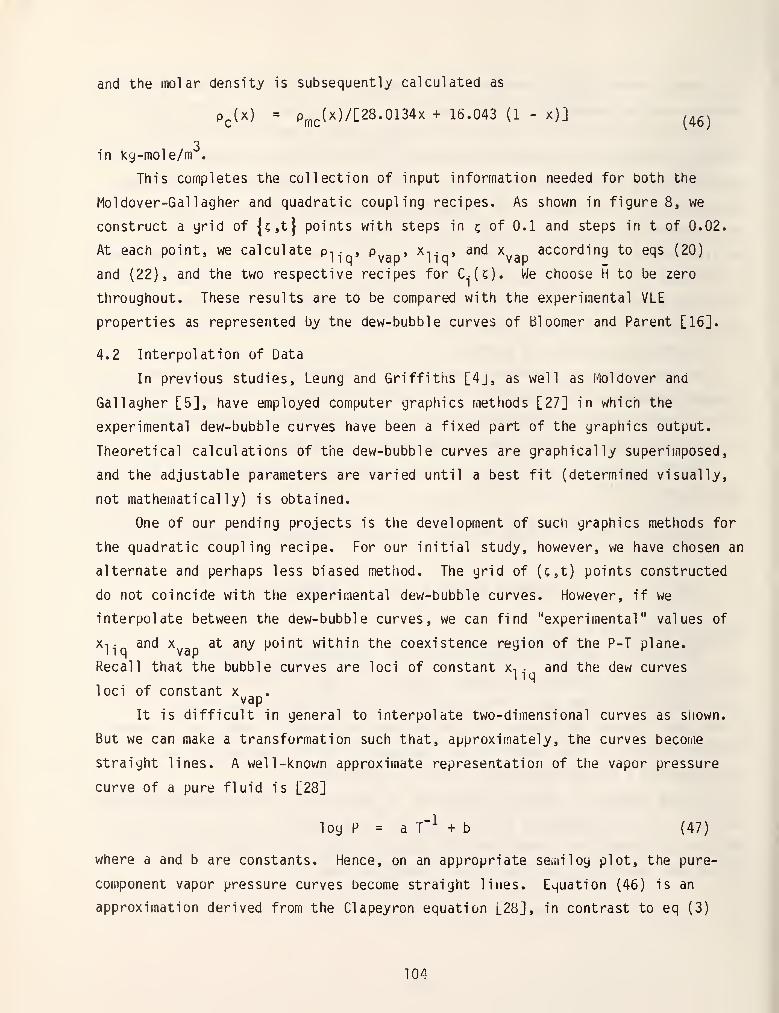
and the molar density is subsequently calculated as
Pc(x) = p^^(x)/[28.0134x + 16.043 (1 - x)]^^^^
3in kg-mole/m .
This completes the collection of input information needed for both the
Holdover-Gallagher and quadratic coupling recipes. As shown in figure 8, we
construct a grid of |c,t} points with steps in c of 0.1 and steps in t of 0.02.
At each point, we calculate p-i^ , ^vaD* ^lia' ^"^ ^vau^^^^'^^i'^Q ^o ^^^ (20)
and (22), and the two respective recipes for C.(i;). We choose H to be zero
throughout. These results are to be compared with the experimental VLE
properties as represented by tne dew-bubble curves of Bloomer and Parent [16].
4.2 Interpolation of Data
In previous studies, Leung and Griffiths [4j, as well as Holdover and
Gallagher [5], have employed computer graphics methods [27] in which the
experimental dew-bubble curves have been a fixed part of the graphics output.
Theoretical calculations of the dew-bubble curves are graphically superimposed,
and the adjustable parameters are varied until a best fit (determined visually,
not mathematically) is obtained.
One of our pending projects is the development of such graphics methods for
the quadratic coupling recipe. For our initial study, however, v/e have chosen an
alternate and perhaps less biased method. The grid of (c,t) points constructed
do not coincide with the experimental dew-bubble curves. However, if we
interpolate between the dew-bubble curves, we can find "experimental" values of
Xi- and x,,^^ at any point within the coexistence region of the P-T plane.1 1 q vap
Recall that the bubble curves are loci of constant Xn • and the dew curvesliq
loci of constant x ^ .
vapIt is difficult in general to interpolate two-dimensional curves as snown.
But we can make a transformation such that, approximately, the curves become
straight lines. A well-known approximate representation of the vapor pressure
curve of a pure fluid is [28]
log P = a T"-^ + b (47)
where a and b are constants. Hence, on an appropriate semilog plot, the pure-
component vapor pressure curves become straight lines. Equation (46) is an
approximation derived from the Clapeyron equation [28], in contrast to eq (3)
104
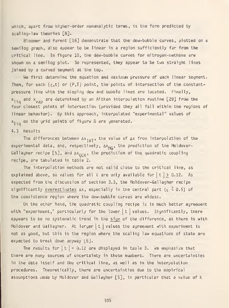
which, apart from higher-order nonanalytic terms, is the form predicted by
scaling- law theories [8].
Bloomer and Parent [16] demonstrate that the dew-bubble curves, plotted on a
semilog graph, also appear to be linear in a region sufficiently far from the
critical line. In figure 10, the dew-bubble curves for nitrogen-methane are
shown on a semilog plot. So represented, they appear to be two straight lines
joined by a curved segment at the top.
We first determine the equation and maximum pressure of each linear segment.
Then, for each (^,t) or (P,T) point, the points of intersection of the constant-
pressure line v/ith the sloping dew and bubble lines are located. Finally,
Xt . and X are detennined by an Aitken interpolation routine [29] from theliq vap -^ ^
four closest points of intersection (provided they all fall within the regions of
linear behavior). By this approach, interpolated "experimental" values of
X-, . on the grid points of figure 8 are generated.
4.3 Results
The differences between AXyj.j, the value of ax from interpolation of the
experimental data, and, respectively, AXj^p, the prediction of the Moldover-
Gallagher recipe [5], and Ax^,^d, the prediction of the quadratic coupling
recipe, are tabulated in table 2.
The interpolation methods are not valid close to the critical line, as
explained above, so values for all c are only available for |t|_> 0.12. As
expected from the discussion of section 3.3, the Moldover-Gallagher recipe
significantly overestimates ax, especially in the central part {c, % 0.5) of
the coexistence region where the dew-bubble curves are widest.
On the other hand, the quadratic coupling recipe is in much better agreement
with "experiment," particularly for the lower |tjvalues. Significantly, tnere
appears to be no systematic trend in the sign of the difference, as there is with
Moldover and Gallagher. At larger jtj
values the agreement with experiment is
not as good, but this is the region where the scaling law equations of state are
expected to break down anyway [5].
The results forjt
j
= 0.12 are displayed in taDle 3. We aiiphasize that
there are many sources of uncertainty in these numbers. There are uncertainties
in the data itself and the critical line, as well as in the interpolation
procedures. Theoretically, there are uncertainties due to the empirical
assumptions inade by Moldover and Gallagher [5], in particular that a value of K
105
exists [eq (14)] such that eq (15) holds accurately, and that, with this value,
lines of constant c are yiven by eq (19) or the curvilinear grid of figure 8.
Therefore, an overall uncertainty of at least 0.01 in ax is to be expected, and
the agreement at this level is most satisfactory.
A similar interpolation scheme could be tried on the densities, to test the
predictions of Ap. However, this would require a double interpolation of the
experimental data, and density predictions depend yery sensitively on the
critical density [27] which is not accurately known here. Hence such a density
analysis has not been attempted at this time.
5. Summary and Future Projects
We have described in this lecture a line of tneoretical research into the
VLE behavior of binary mixtures near the critical locus wnich is based on
scaling-law equations of states and field (rather than density) variables as
defined by Griffiths and Wheeler [3].
The first explicit recipe created for such prediction of VLE behavior, given
the critical line and the vapor pressure equation of the pures, was that of Leung
and Griffiths [4]. Their iTiethod, the foundation uf subsequent work, was limited3 4
in many respects to \/ery simply behaving binary mixtures like He- He. It was
significantly extended in range (although some empirical assumptions were
incorporated) by Moldover and Gallagher [5], who were successful particularly in
predicting VLE of azeotropic mixtures. Finally, \^e have proposed an extension of
the Moldover-Gallagner recipe v/hich shows promise of working for mixtures with
large composition difference betv^een coexisting phases, yet which alters only
minutely the l^loldover-Gallagner predictions for those cases where tneir recipe is
successful.
We conclude the lecture by listing some unanswered questions and some
projects for the future.
1) Although we have found \fery good agreement using the quadratic coupling
recipe for ax of nitrogen-methane at|t
|
= 0.12, roughly the limit of the range
where scaling laws are expected to hold, we have not demonstrated comparable
agreement for values of|t
|between 0.12 and the critical line. This is probably
best verified by a computer graphics method as described in section 4.2, and may
require minor adjustments in the critical line, particularly p-(x). Checks of
coexisting density predictions should be made by the same method.
106
2) The formalism incorporates certain empirical assumptions about c, which is a
function of the chemical potentials, and bypasses explicit calculation of those
chemical potentials. Certain classical equations of state described in Jim Ely's
lecture [1], while yielding incorrect critical exponents, show a certain limited
degree of quantitative success in predicting VLE near tlie critical line, and one
of these, the Peng-Robinson equation [10], provides an explicit algebraic fonn
for the chemical potential. Thus it would be instructive to use the
Peng-Robinson equation in conjunction with the present methods. Explicit
variation of the parameter K in the definition of i, can be used to test the
self-consistency of our empirical assumptions.
3) While our method predicts ax well, it fails rather poorly in the prediction
of X (for H = 0). As explained in section 3.3, this can be remedied by
changing H; however, the second Holdover-Gallagher recipe [eq (25)] might
not, at this stage, remain optimal. As recommended in Appendix B of Holdover and
Gallagher, classical equations of state can also oe studied to help select an
appropriate general model for R(c,t).
4) To demonstrate the general validity of our recipe we must, of course, test
it on a variety of different mixtures, not only nitrogen-methane. The logical
choice of a second system is propane-octane. Good data is available and that
mixture is an example which is of particular present interest to our group, as it
contains molecules of widely disparate sizes.
The most frequent limitation to use of the method is the absence of accurate
data for Pp(x). In this context, we expect that the techniques described by
Brian Eaton [2] in the following lecture should prove helpful. If T (x) and
P (x), but not p„(x) , are known accurately, it may be possible to determine
p (x) theoretically from the equation of state with parameters which best fit
T and P , and use the theoretically calculated p (x) as input,
5) Although we have restricted our discussion to prediction of the coexistence
surface, the Leung-Griffiths formalism, in principle, predicts an equation of
state for the entire region (one-phase and two-phase) around the critical line.
In fact, such predictions have been used and compared with experiment for
He- He by Doiron, Behringer and Meyer [30].
It is of interest to predict similarly an equation of state for the entire
critical region according to the Moldover-Gallagher and quadratic coupling
recipes. A note of caution must be made, hov^ever [27]. For C^ ^ in eq (1),
107
the Moldover-Gallagher formalism singles out the supercritical extension of the
rectilinear diameter as a special direction. It appears more appropriate to
single out the critical isochore as a special direction, so the formalism should
by some means be revised accordl ingly. Some ideas for doing this are suggested
in the recent review by Moldover [31J.
6) An important unresolved problem in the theory of fluids is the proper
matching of equations of state valid inside the critical region with those
outside it. For pure fluids, Goodwin's equation of state [32] is designed to
predict PVT properties both within and outside the critical region. Hov/ever,
Goodwin's method has thus far never been applied to mixtures. It would be
interesting to reformulate the Goodwin equation of state in tenns of field
variables and perhaps thereby obtain an equation of state for mixtures valid over
the entire range of fluid thermodynamic variables.
7) Finally, fundamental theories of phase changes should be examined with the
hope of shedding light on the "amount of phase change" A(t) defined in
section 3.3. As stated earlier, use of this function appears to violate the
"orthodox" view of field variable vector spaces, namely that field on density
variables of differing dimensions cannot be added in a meaningful way. But if
A(t) is seen empirically to be an invariant for a wide variety of mixtures, this
will be sufficient motivation to search for its fundamental significance, and
hopefully thereby add to our basic understanding of phase transitions.
Note added March 1982 : Since the original presentation of this lecture in
October 1980, the author and Mike Moldover have made significant progress in
achieving some of the goals listed above. This progress [33] is briefly
summarized:
We have developed an efficient minicomputer program and graphics routine
which calculates and plots several dew-bubble curves or constant-composition
temperature-density curves per minute, over the range -0.1 <. t <^ 0. When our
method is applied to the nitrogen-methane data of Bloomer and Parent [16],
excellent agreement is obtained between experiment and tlieory with C,, = -8
[eq (25)] for the dew-bubble curves. The temperature-density curves do not fit
well if we retain the previous assumption that the mass density is linear in
temperature along the critical line. Hov;ever, variation of the T-p critical
line, in the direction of higher critical densities, leads to excellent agreement
with experiment in the T-p plane without degrading the fit in the P-T plane. We
108
believe that, by analoyy with pure fluids, such a fitting procedure may prove to
be a superior means of determining p (x) than direct experimental measurement
(cf. eq (39) and p from reference [26]).
We find also that a linear coupling recipe works as well as, and perhaps
better than, the present quadratic coupling recipe. The linear coupling method
replaces eq (34) is by
A =I
Ap |/p^ + C^l AXI
(48)
and modifies eqs (36)-(37) accordingly, where Cw is an adjustable parameter.
The best fit to nitrogen-methane VLE data in the linear coupling model occurs for
Cii = -6, Cy = 0.3.
We also have constructed a very good fit to the n-butane-octane data of Kay,
et al. [34] with the additional feature that Cn can depend linearly on c. The
optimal fitting parameters for n-butane-octane are C„ = 0.3 and Cu = -12
(1 - 1.3c). At present it is not clear whether the linear or quadratic coupling
model is superior in general.
The present (quadratic) theory has also been applied by Al-Sahhaf [35] to a
variety of binary mixtures and with a mixed record of success. Al-Sahhaf has
analyzed the same systems with the Peng-Robinson equation [10] and has compared
our method with that of Peng and Robinson. The author thanks Dendy Sloan and
Taher Al-Sahhaf for many nelpful discussions concerning their work.
6. Acknowledgments
This work would not have been possible without the research and guidance of
Mike Holdover, with whom the author acknowledges an ongoing collaboration. The
author thanks Mike for his encouragement and patient elucidation of the
principles of phase transitions. He thanks Hal Raveche and the staff of the
Thermophysics Division, National Bureau of Standards, Washington, DC for their
hospitality during the author's visit in 1979, when this work was conmenced.
Finally, he thanks Howard Hanley and the staff of the Thermophysical Properties
Division for numerous valuable suggestions.
109
7. HEFEREIMCES
[I] Ely, J. F., "A review of fluid phase equilibria prediction methods," this
volume.
[2] Eaton, b. E., Stecki , J., Wielopolski, P., and Hanley, ri. J. M.
,
"Prediction of the critical line of a binary mixture: evaluation of tne
interaction parameters," this volume.
[3] Griffiths, R. 6. and Wheeler, J. C, Phys. Rev. A2, 1047 (1970).
[4] Leung, S. S. and Griffiths, R. B. , Phys. Rev. A8, 2670 (1973).
[5] Holdover, M. R. and Gallagher, J. S., AIChE J. 24, 267 (1978).
[6] McCarty, R. U., "The extended corresponding states method applied to the
nitrogen-methane system," this volume.
[7] Rowlinson, J. S. and Watson, I. L)., Chem. Eng. Sci. 24, 1565 (1969).
[8] Level t Sengers, J. H. H., Greer, W. L. and Sengers, J. V., J. Phys. Chem.
Ref. Data 5^, 1 (1976).
[9] Redlich, 0. and Kwong, J. H. S., Chem. Rev. 44, 233 (1949).
[10] Peng, D. Y. and Robinson, D. B., Ind. Eng. Chem. Fund. J_5, 59 (1976).
[II] Sengers, A. L. , Hocken, R. and Sengers, J. V., Physics Today 3_0, 42 (Dec
1977).
[12] Rushbrooke, G. S., J. Chem. Phys. 39, 842 (1963).
[13] Widom, B., J. Chem. Phys. 43, 3898 (1965).
[14] Fisher, M. E., Rev. Mod. Phys. 46, 597 (1974).
[15] Rowlinson, J. S., Liquids and Liquid Mixtures, (Plenum Press, New York,
1969), Chap. 6.
[16] Bloomer, 0. T. and Parent, J. D. , Chem. Eng. Progr. Symp. Ser. 49, No. 6,
11 (1953).
[17] Himmelblau, D.H. , Basic Principles and Calculations In Chemical
Engineering (Prentice-Hall, Englewood Cliffs, N. J., 1967), p. 204.
[18] Khazanova, N. E. , Lesnevskaya, L. S. and Zaknarova, A. V., Khimsch.
Promph. 44, 364 (1966).
[19] Wallace, B. , Jr. and lAeyer, H. , Phys. Rev. A2, 1563 (1970); 5, 953
(1972).
[20] Schofield, P., Pnys. Rev. Lect. 22, 606 (1969).
[21] D'Arrigo, G., Mistura, L. and Tartaglia, P., Phys. Rev. A ]_2, 2587
(1975); Doiron, F. , Bull. Ai.i. Pnys. Soc. 26, 1217 (1981).
[22] Moldover, M. R. and Gallagher, J. S., in Phase Equilibria and Fluid
Properties in the Chemical Industry , ACS Symposium Series No. 60, S. I.
Sandler and T. J. Sturvick, Eds., American Chemical Society, Washington,
1977, p. 498.110
[23] Model 1, M. and Reid, R. C. , Thermodynamics and its Applications in
Chemical Engineering (Prentice-Hall, Englewood Cliffs, N. J., 1974).
[24] Dodge, B. J. and Dunbar, A. K. , J. Am. Chem. Soc. 49, 591 (1927).
[25] Jacobsen, R. T., Stewart, R. B., McCarty, R. D. and Hanley, H. J. M.,
"Thermophysical properties of nitrogen from the fusion line to 3500 R for
pressures to 1500 psia," Nat. Bur. Stand. (U.S.), Tech. Note No. 648
(1973).
[26] Goodwin, R. D., "The thermophysical properties of methane, from 90 to 500
K at pressures to 700 bar," Nat. Bur. Stand. (U.S.), Tech. Note No. 653
(1974).
[27] Moldover, M. R. , private communication.
[28] Himrnelblau, D. M., Basic Principles and Calculations in Chemical
Engineering (Prentice-Hall, Englewood Cliffs, N. J., 1967), p. 176 and
p. 257.
[29] Kopal, Z., Numerical Analysis (Wiley, New York, 1955), p. 36.
[30] Dorion, T., Behringer, R. P. and Meyer, H., J. Low Temp. Phys. 24, 345
(1976).
[31] Moldover, M. R., Theriiiodynainic anomalies near the liquid-vapor critical
point: A review of experiments, to be published.
[32] Goodwin, R. D. , in Equations of State in Engineering and Research ,
Advances in Chemistry Series, No. 182, K. C. Chao and R. L. Robinson, Eds.
American Chemical Society, Washington, 1979, Chap. 19.
[33] Rainwater, J. C. and Moldover, M. R., Thermodynamic models for fluid
mixtures near critical conditions, paper 33d presented at AIChE 1981
Annual Meeting, New Orleans; to be published in Chemical Engineering at
Supercritical -Fluid Conditions , Ann Arbor Science Publishers, 1982.
[34] Kay, W. B., Genco, J. and Fichtner, D. A., Vapor-liquid equilibrium
relationships of binary systems propane-n-octane and n-butane-n-octane, J.
Chem. Eng. Data 19, 275 (1974).
[35] Al-Sahhaf, T. A., Measurement and prediction of vapor-liquid equilibria
for the nitrogen-methane-carbon dioxide system, Ph.D. Thesis, Colorado
School of Mines, Golden, Colo., 1981.
in
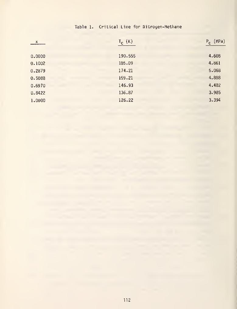
Table 1. Critical Line for Nitrogen-Methane
X Tc (K) Pc (MPa)
0.0000 190.555 4.608
0.1002 185.09 4.861
0.2879 174.21 5.068
0.5088 159.21 4.888
0.6970 146.93 4.482
0.8422 136.87 3.985
1.0000 126.22 3.394
112
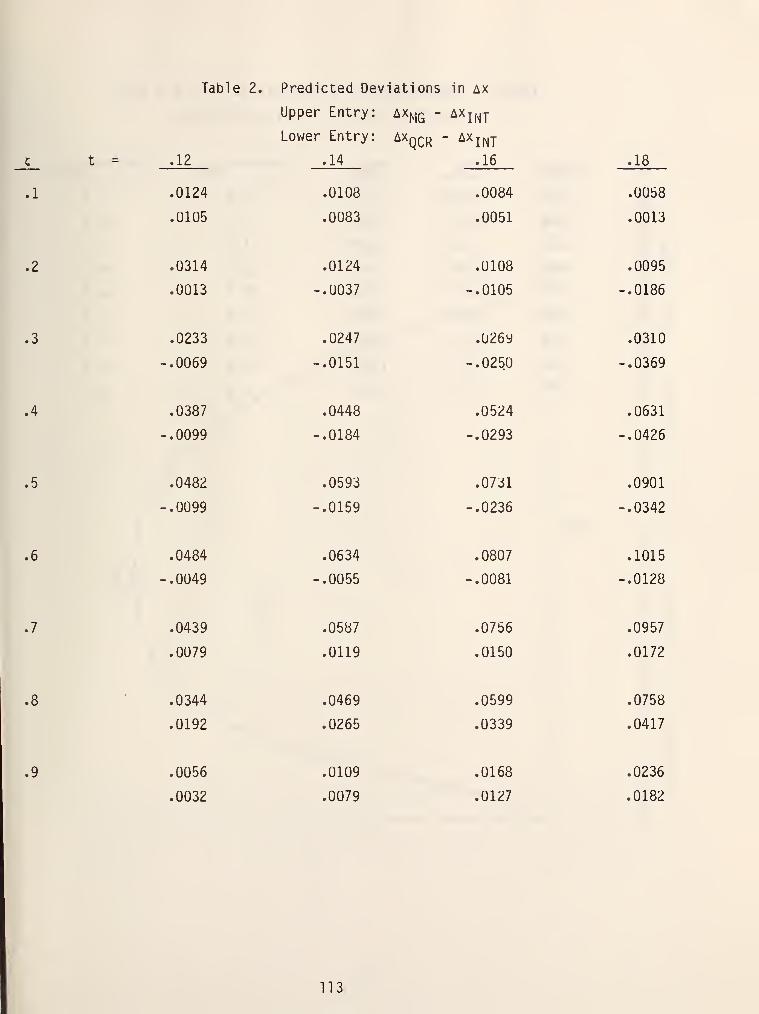
Table 2. Predicted Deviations in ax
Upper Entry: axj^iq " ^^INT
Lov/er Entry: axqqj^ - AXj,^j
c t .12 .14 .16 .18
.1 .0124 .0108 .0084 .0068
.0105 .0083 .0051 .0013
.2 .0314 .0124 .0108 .0095
,0013 -.0037 -.0105 -.0186
.3 .0233 .0247 .0269 .0310
-.0069 -.0151 -.0250 -.0369
.4 .0387 .0448 .0524 .0631
-.0099 -.0184 -.0293 -.0426
.5 .0482 .0593 .0731 .0901
-.0099 -.0159 -.0236 -.0342
.6 .0484 .0634 .0807 .1015
-.0049 -.0055 -.0081 -.0128
.7 .0439 .0587 .0756 .0957
.0079 .0119 .0150 .0172
.8 .0344 .0469 .0599 .0758
.0192 .0265 .0339 .0417
.9 .0056 .0109 .0168 .0236
.0032 .0079 .0127 .0182
113
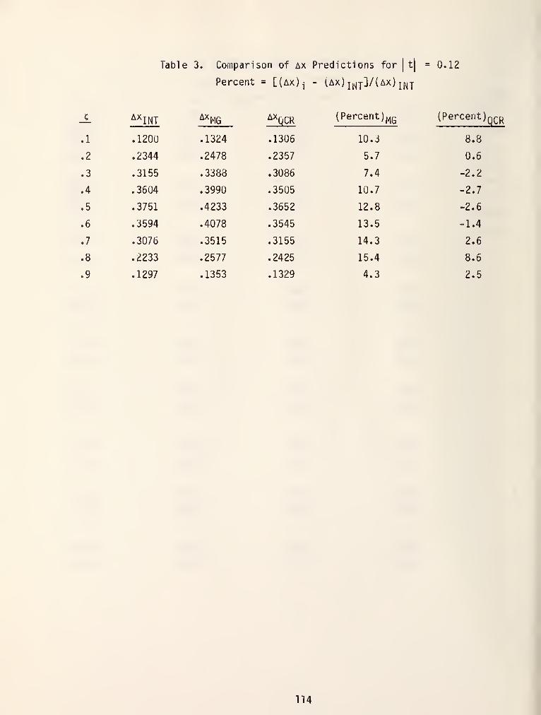
Table 3. Comparison of ax Predictions for|
t| = 0.12
Percent = [(ax)^ - (ax) j,^j]/(ax)jj^y
AXi^ Ax^,^Q Ax^(^^ (Percent)f^G (PercentJQ^R
1 .1200 .1324 .1306 10.3 8.8
2 .2344 .2478 .2357 5.7 0.6
3 .3155 .3388 .3086 7.4 -2.2
4 .3604 .3990 .3505 10.7 -2.7
5 .3751 .4233 .3652 12.8 -2.6
6 .3594 .4078 .3545 13.5 -1.4
7 .3076 .3515 .3155 14.3 2.6
8 .2233 .2577 .2425 15.4 8.6
9 .1297 .1353 .1329 4.3 2.5
114\
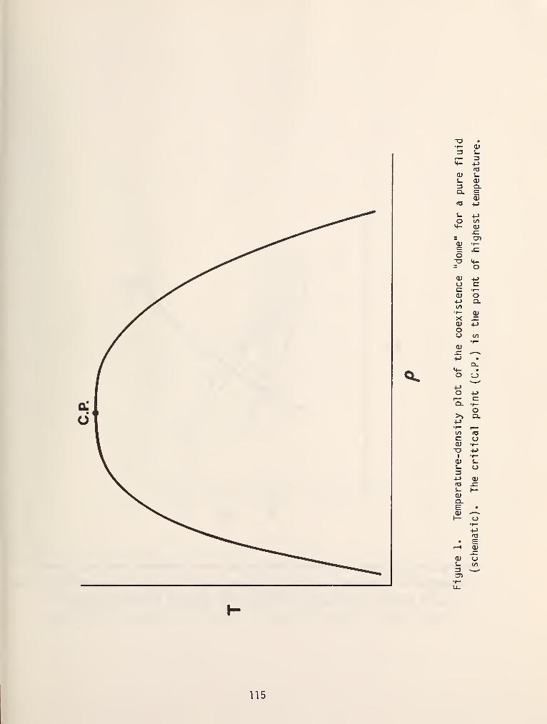
T3 ••r- a>3 S-r— 3M- +->
(Oo; s_s_ O)3 Q.Q. (=
33fO +->
J- +jo CO<+- O)
-C-
:t)
O) •r—c= -Coo M-= OO) 4->
a cc r-
<u o+-> Q.to•r— QiXO) +Joo 1/1
p—(V^ ,.—
X
+-> •
ex.
H- •
O os.._^
+->
O 4->^~ CQ. •r—
o>> Q.l->•r— ^~to (X3
c O(Ua -l->
1•^
0) t.S- o3+J cufO -Cs_ h-O)Q.E •
0) ^—
^
1— tjr*4->
(O• E
1—
1
O)-C
cu uS- to
Ol
115
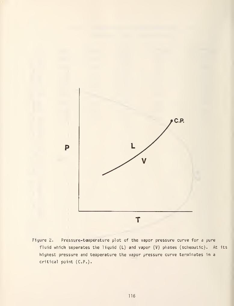
Figure 1. Pressure-temperature plot of the vapor pressure curve for a pure
fluid which separates the liquid (L) and vapor (V) phases (schematic). At its
highest pressure and temperature the vapor pressure curve terminates in a
critical point (C.P.)«
116
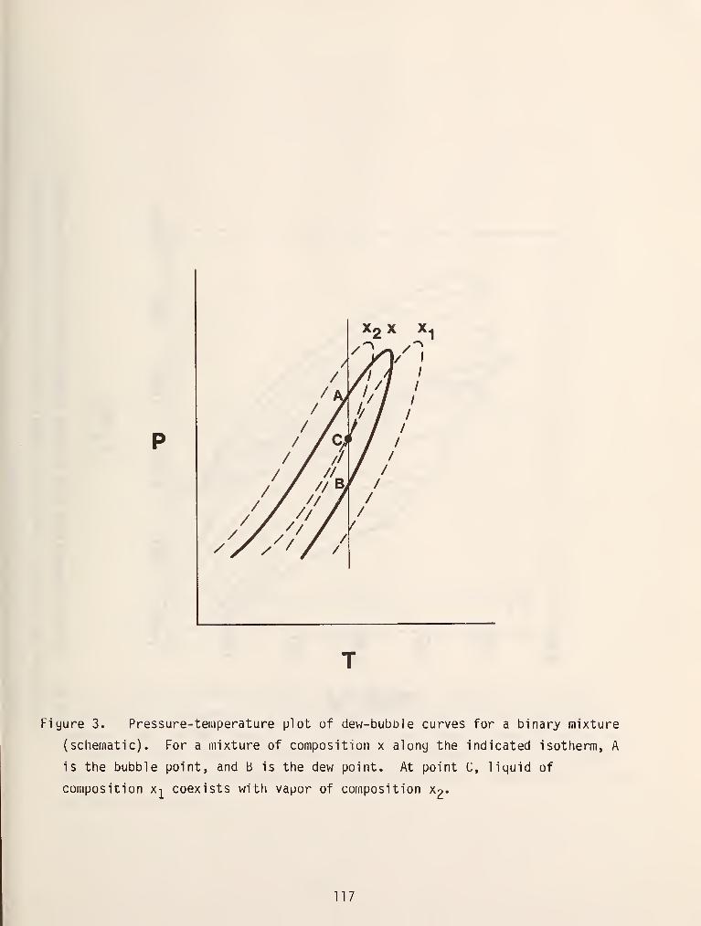
Figure 3. Pressure-temperature plot of dew-bubble curves for a binary mixture
(schematic). For a mixture of composition x along the indicated isotherm, A
is the bubble point, and B is the dew point. At point C, liquid of
composition x-|^ coexists with vapor of composition X2.
117
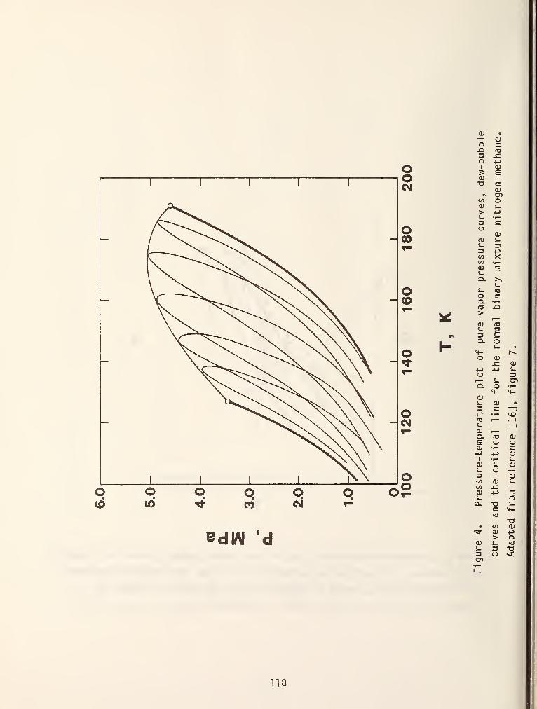
I— O)
edV\l 'd
jd cja fOu -CJ2
1 Ols EO) 1
T3a;
A CDCO o<U s>> +->
s_ •r-3 Ca
OJ
OJ S-&. 33 4->
CO Xw •^0) =s-3.
S_ (T3
o Ca. -r—ITS -Q> ^0) 'Oi. (=
3 5-a. Oc •
i+- r^o 0)
JZ O)M -l-> i.
O 31
—
s- O^Cl o •r—
<+- M-<vJ- O) #1
3 c 1—
1
-f-> •r- <^fO ^^ 1—1
S- 1 1
OJ ,
—
Q. 13 <U1= U u(U ^ c
-»-> 4-> O)1 t-OJ Z 0)1- O 4-3 a>l/l OJ S-CO J=0) +-> =s_ oo. "O s-
c <4-
fO
T3• CO <V
«* a) 4->
> Q.0) s_ (Ot. 3 -o3 O <a>
118
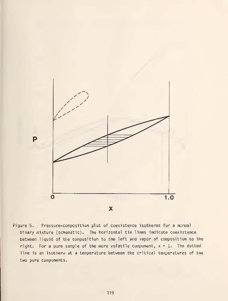
/
/
//
// /
^ )/
y
1.0
Figure 5. Pressure-composition plot of coexistence isotherms for a normal
binary mixture (schematic). The horizontal tie lines indicate coexistence
between liquid of the composition to the left and vapor of composition to the
right. For a pure sample of the more volatile component, x = 1. The dotted
line is an isotherm at a temperature between the critical temperatures of the
two pure components.
119
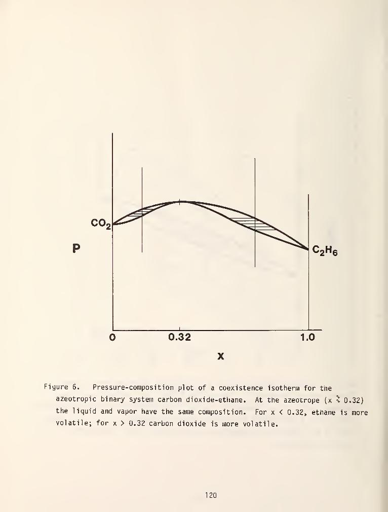
CoHi
Figure 6. Pressure-composition plot of a coexistence isotherm for the
azeotropic binary system carbon dioxide-ethane. At the azeotrope (x I 0.32)
the liquid and vapor have the same composition. For x < 0.32, ethane is more
volatile; for x > 0.32 carbon dioxide is more volatile.
120
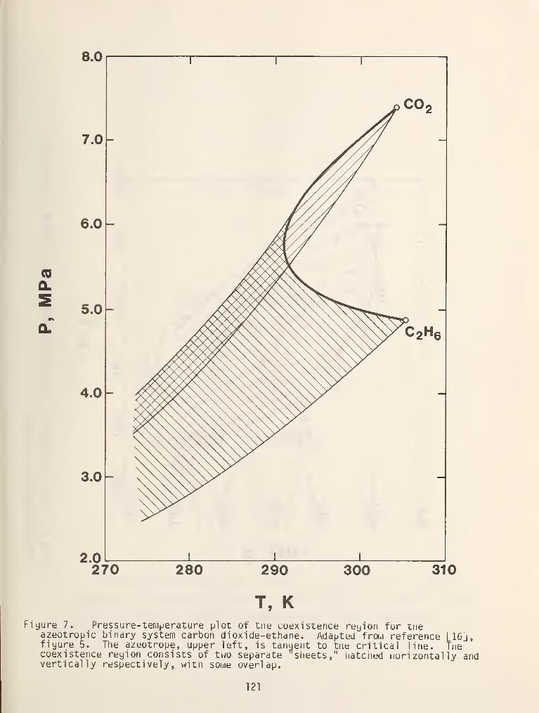
(0
270 280 290 300 310
T, KFigure 7. Pressure-temperature plot of the coexistence reyion for the
azeotropic binary system carbon dioxide-ethane. Adapted from reference [16],fiyure 5. The azeotrope, upper left, is tangent to tiie critical line. Thecoexistence reyion consists of tv;o separate "sheets," hatched horizontally andvertically respectively, with some overlap.
121
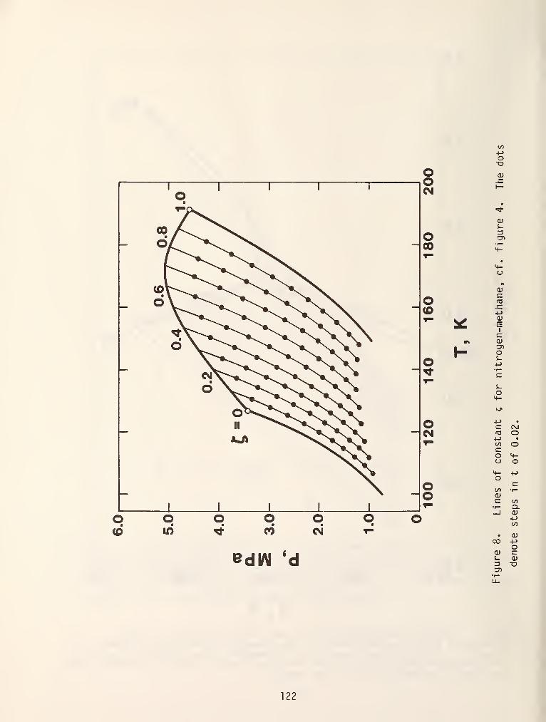
ooCM
O00
O
O
4->
Oo
J-
cn
o
O)
+->
O)
EcOJ:^Os_4->
o4-
oCM ro
+->T- CO
coa<^-
oo COo <U
edI/V 'd
CO
a;
oi
o
o
«/)
a.<u+->
CO
-t->
O
-a
122
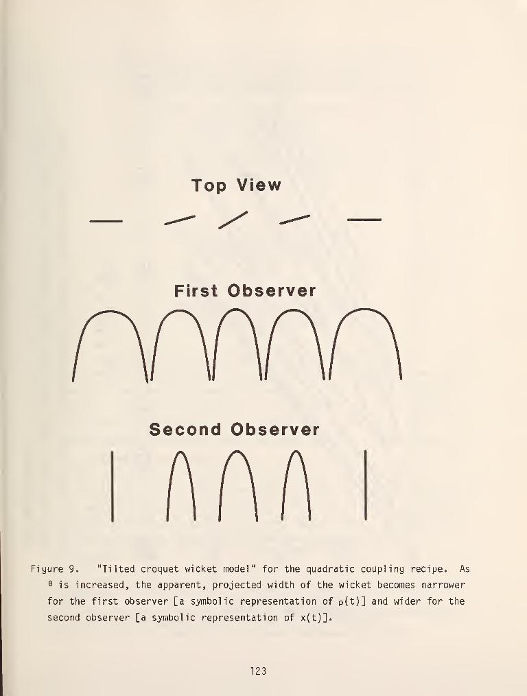
Top View
First Observer
Second Observer
Fiyure 9. "Tilted croquet wicket model" for the quadratic coupling recipe. As
9 is increased, the apparent, projected width of the wicket becomes narrower
for the first observer [a symbolic representation of p(t)] and wider for the
second observer [a symbolic representation of x(t)].
123
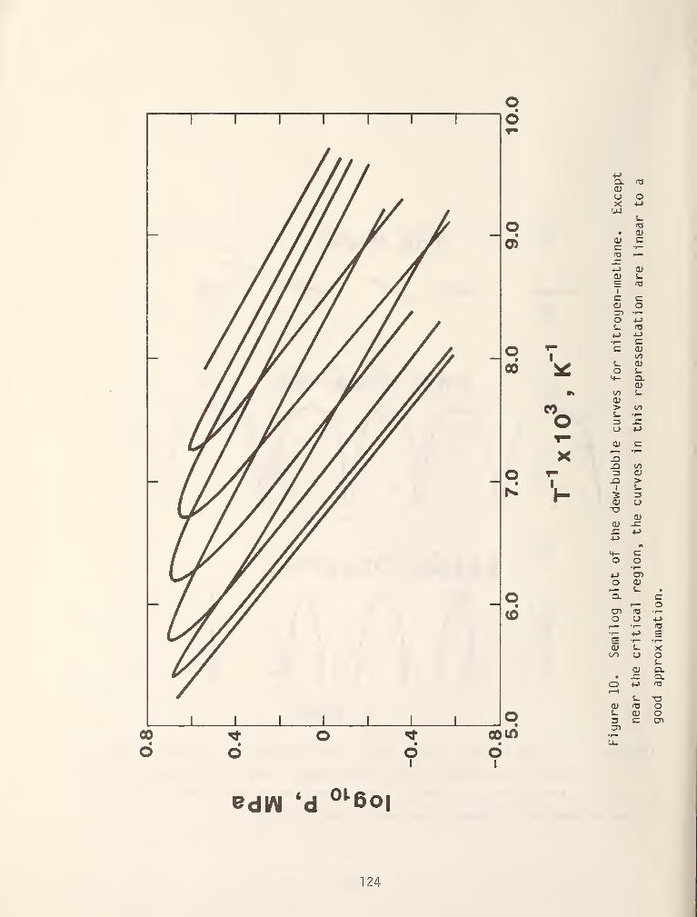
oo
coin
o
+->
Q. TJO)O OX +->
LUi_o •
0>
O)
1
os-4->
o•->
o1
E 0)CO
00 ^ s-o4-
(U5-
M t-
n > i/)
oT-
<u CK
J3
•f—
oW
3-Q
O)-o
(U
-!->
4-O+->
O
cu>S-
oa;-C
cz
oa>
s- •o 'q. c^^ o
(0 o -(->
r^ •r— TJ•1— +-> cE •r— • 1—
a; S- XOO u o
S-
• c~ Q.o +J 03r-H
S- -a(1) fO o
o :3cu o
enZT1
edlAI 'd ^^6o|
124
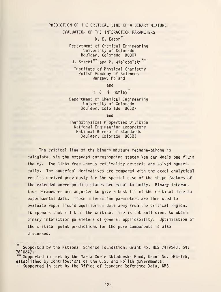
PREDICTION OF THE CRITICAL LINE OF A BINARY MIXTURE:
EVALUATION OF THE INTERACTION PARAMETERS
B. E. Eaton
Department of Chemical EngineeringUniversity of Colorado
Boulder, Colorado 80307
J. Stecki and P. Wielopolski
Institute of Physical ChemistryPolish Academy of Sciences
Warsaw, Poland
and
H. J. M. Hanley"*"
Department of Chemical EngineeringUniversity of Colorado
Boulder, Colorado 80307
and
Thermophysical Properties DivisionNational Engineering LaboratoryNational Bureau of Standards
Boulder, Colorado 80303
The critical line of the binary mixture methane-ethane is
calculate'^ via the extended corresponding states Van der Waals one fluid
theory. The Gibbs free energy critical ity criteria are solved numeri-
cally. The numerical derivatives are compared with the exact analytical
results derived previously for the special case of the shape factors of
the extended corresponding states set equal to unity. Binary interac-
tion parameters are adjusted to give a best fit of the critical line to
experimental data. These interaction parameters are then used to
evaluate vapor liquid equilibrium data av/ay from the critical region.
It appears that a fit of the critical line is not sufficient to obtain
binary interaction parameters of general applicability. Optimization of
the critical point predictions for the pure components is also
discussed.
Supported by the National Science Foundation, Grant No. HES 7419548, SMI
7610647.** Supported in part by the Maria Curie Sklodowska Fund, Grant No. NBS-196,established by contributions of the U.S. and Polish governments."*" Supported in part by the Office of Standard Reference Data, NBS.
125
Key words: binary interaction parameters; critical ity criteria;
extended corresponding states; gas-liquid critical line; one fluid
theory; van der Waal s theory; VLE prediction.
1 . Introduction
The prediction of phase equilibria is both a classical problem of the theory
of liquids and a problem of engineering concern. Today the chemical and fuel
industries have to increase productivity and conservation and have to transfer to
nev/ feedstocks; phase equilibria is a major factor. But it is well-known that
the prediction, even the correlation, of the properties of the appropriate
systems can be exceptionally difficult if the results are required to any
reasonable accuracy. Prediction techniques are needed especially because the
number of possible systems makes measurement an overwhelming task. Prediction
requires an understanding of theory but, unfortunately, theory cannot yet always
handle adequately the complex systems encountered: the gap between a systematic
practical theory and reality is large. One technique, however, has been applied
successfully to simple systems and does show promise in that the assumptions can
be identified clearly. This method is extended corresponding states. Here we
apply it to a system of methane and ethane. A specific objective is to calculate
the gas/liquid critical line and to observe the effect of the binary interaction
parameters on the calculation. It is then interesting to see how these
parameters, optimized for the critical line, represent vapor liquid equilibrium
(VLE) data.
The critical line in a binary mixture may be calculated by solving the
equations
= ; ^ =
for a temperature (T) and pressure (p) with the mole fraction (x) specified. G
is the molar configurational Gibbs free energy of the mixture. In this v/ork
these second and third order derivatives were evaluated numerically, but have
been compared with the analytical results of Wielopolski [1] in the special case
when the extended corresponding states shape factors are unity. The accuracy of
the approach has thus been evaluated.
126
The system methane/ethane was selected for comparison with experiment since
the VLE data have been evaluated for thermodynamic consistency by Hiza,
et al . [2]. The procedure is quite general, however, and we have applied it to
several mixtures. Variations have been reported extensively by Watson and
Rowlinson [3], Gunning and Rowlinson [4], Teja and Rowlinson [5], Mollerup and
Rowlinson [6], and Mollerup [7,8]. The overall objective is to develop a general
technique for calculating the critical line of a binary mixture and to see if the
binary interaction parameters can be reliably evaluated by adjusting them to give
the best least squares fit of the critical line data.
2. Corresponding States and Equations
The basic postulate of the theory used here -- the van der Waals one fluid
theory -- is that if the components a (a = 1 ,n where n is the total number of
species) of a mixture separately obey classical corresponding states, then their
mixture will also obey corresponding states as if it were a single substance.
The components can be represented by selected parameters, e.g., critical
temperature (T ) and critical molar volume (V ) , and the hypothetical equivalent
substance, designed by subscript x^ can be characterized by some suitable
composition dependent averaged parameters T^ and V^. The method then assumes
that the properties of a pure substance at p and T, or V and T, can be evaluated
with respect to those of a reference fluid, designated by subscript £, via
T = T/f ^ and V„ = V/h_ ^ (1)aa,o aa,o ^ '
where the scaling ratios h and f are defined respectively by
h = V^/V^ and f = T^/t'^ (2)aa,o a' o aa,o a' o ^
'
For a mixture the most natural definition of h and f follows from the workA A
of Henderson and Leonard [9] to give the van der Waals one fluid mixing rules:
\o - £ ^ V& '^06. (*'
The cross coefficients f „ and h „ are left unspecified until further
combination rules are defined, e.g..
127
^a3,o ~ ^a3,o ^^aa,o ^B6,o^ ^^^
"^aBjO '\q
where C „ and iin q ^re the binary interaction coefficients which, although
formally close to unity, can play a major role in the calculation of phase
equil ibria.
2.1 One Fluid Mixture Equations
The properties of a mixture can be evaluated in terms of the reference
substance and the ratios of eq (2). The basic equations are:
Compressibility factor, Z
Z (T,V,x) = Z^(T,V,x) (7)
= Z (T/f , V/h ) (8)0^ x,o* x,o' ^'
Molar configurational Helmholtz free energy, A
A (V,T,x) E y V,T,x) + RJ Z \ ^n^a
^^^
a
where
A (V,T,x) = f A (V/h , T/f ) - RT £n h (10)x^ ' ' ' x,o 0^ x,o' x,o' x,o ^ '
or the molar configurational Gibbs free energy, G
G (p,T,x) E G^(p,T,x) + RT X; ^a^"
"^a^^^^
a
where
G„(p,T,x) = f G (ph /f , T/f ) - RT -in h ^ (12)x^^* * ' X,0 0^^ x,o x,o' x,o' x,o ^ '
The symbol ^ refers to the koI ar quantity. Equations (7)- (12) which define the
properties of an n-component mixture, can also be used for pure component
properties if all subscript x's are replaced with a's.
128
2.2 VL£ Equations
For pure component VLE, equating the molar Gibbs free energy of each phase
results in the following expression:
[A«"/RT„ - in Z^ - 1 + Z„] = CA^"/RT„ - <.n Z^ - 1 + Z^] (13)vap liq
where
In eq (13) superscript Res refers to the residual value defined by eq (14)
with A^ the value of the equivalent perfect gas. Equation (13) is expressed
in terms of the residual Helmholtz free energy rather than Gibbs since the
reference equation of state has T and V (not T and p) as the independent
variables.
For mixture VLE one can calculate the K-value for, say, species a at T and
P:
K = y /x (15)
where one can derive
with p the residual chemical potential. Further manipulations give y in
terms of G and, for a binary mixture.
/ a(VRT)\
^3 V-9V~/t,C - ^ - «T X3 -97—1 - «T £n ^ (17)
P
where
•v.
G.. A'Res
129
2.3 Critical Criteria
The conditions for a critical point at T,p for a mixture are
0^G/9X^)-P^p = (3^G/3x^)^^p = (19)
Substitution of the one fluid equations gives
0^ (G /RT)/3x^) +J_ = (20)T,p a Q,
and
"v X ~ X
0^ (G /RT)/3xb *— 1 = (21)T.p (x^Xg)2
which can thus be evaluated using eq (18).
The above equations and others have been discussed in full and derived by
Rowlinson and Watson [3], by Eaton [10] and by other authors so it has been
sufficient to be ^ery brief. The equations form the basics of the evaluation of
phase equilibria for a pure fluid or mixture, given the reference equation of
state and the reference Gg or Aq.
2.4 Extended Corresponding States
In general, since classical corresponding states is not obeyed, eqs (8) and
(10) or (8) and (12) are not satisfied with the scaling ratios of eq (2). It is
possible, however, to define a corresponding states so that eqs (8) and (10) are
satisfied exactly . To do this we define shape factors 6 and <)> so that (for a
pure, for example)
aa,o
hence the ratios f and h become
Vq = Vl^lx-^ (22)
aa= C—)e • h = C-^]^ (23)
The point about this redefinition, i.e., the basis of extended corresponding
states theory, is that the corresponding states equations can be used formally
130
with the provision that the scaling ratios are given by eq (23). It should be
stressed that the ratios could be solved for either a pure or a mixture via
eqs (8) and (10) but to do this would require a complete description of the
fluids in question: essentially an impossibility. It is convenient to have some
generalized analytical relation for 9 and <^, Leach and Leland proposed the
following [11]:
e (T* V*. oj ) = 1 + (o) - 0) ) F(T* V*) (24)aa,o ^ a* a' a^ ^ a o^ ^ a* a^ ^ '
k * Z^
(T. V^. caj = {1 + (o) - u)J G(T , VJM (25)aa,o a' a' a'|
'a o a' a' i ^ca
where
* *
^i^r.» ^J = a, + b, £n T + (c, + dJJ ) (V - 0.5) (26)
and
* *G(T^. V^) = a^ (V^ + bj) * Cj (V^ + CI2) S.n T^ (27)
Here o) is the pitzer acentric factor or some chosen parameter and a, b, c, d are
constants:
a^ = 0.0892, 32 = 0.3903
b^ = -0.8493, b2 = -1.0177
c^ = 0.3063, C2 = -0.9462
d^ = -0.4506, d2 = -0.7663
The asterisk denotes the value reduced by the critical value. The equations are•k -k
constrained in that V is set equal to 2.0 for al 1 V > 2.0 and to 0.5 forot ct
V* < 0.5: T* is set to 2.0 i f T * > 2.0.a a a
We [12] have recently tested the Leach-Leland equations for the hydrocarbons
C, - C2n over an extensive range of experimental conditions and revised
coefficients are reported in the reference. We also verified that the original
equations were satisfactory for reduced temperatures greater than 0.5.
3. Calculation and Numerical Methods
The objective is to solve the critical criteria eqs (20) and (21) for the
methane/ethane system and in so doing, observe the effects of the interaction
131
parameters and n of eqs (5) and (6) on the results. Having these values, we
then evaluate some K-values for selected temperatures using eqs (15)-(18). We
chose methane as the reference fluid, the equation of state for which is the 32
term BWR of McCarty [13]. Critical parameters and Leach-Lei and acentric factors
for methane and ethane are given in table 1.
Table 1. Parameters for Methane and Ethane
0)T^ P^
(K) (cm /mole) (Bar)
CH4 190.555 97.75 44.793
^2^6 305.33 147.06 47.448 .105
3.1 Analytical and Numerical Evaluation of the Derivatives
The numerical techniques used in this v/ork are standard. We use the central
difference formulas [14] for which the first two terms in the infinite power
series expansions are given here. For the derivatives of a function f evaluated
at a point x, one has
f, - f., f^ - 2f, . 2f., - f.2
2h 12h
fl - ^fp * f-1 ^2 - ^^1 ' '^^0 - ^^-1 ' ^-2
2 " 2
rf\ . h - 2^1 * 2f.i - f.2 f3 - 4f2 . 5f, - 5f., + 4f_2 - f.3"U
(28)
(29)
(30)
9x"/^ 2h^ Hi?
where
fo = f(x) . f^ = f(x+ nh) (31)
The difficulty is to choose a value of h which is not too small (otherwise
significant figures will be lost in evaluating the numerators of eqs (28)-(30)
but not too large (otherwise the truncation error, which can be estimated by the
second term of eqs (28)- (30), will be large). One also has to consider the word
length of the computer and the convenience of using single versus double
132
precision. In this work we calculated on a CDC 6400 and a CDC 6600 machine with
a 60 bit word length (13 significant figures).
We were able to observe definitely the effect of varying h for the special
case 9 = * = 1, i.e., for classical corresponding states. Equations (19) and
(20) have been solved analytically by Wielopolski (1980) and the lengthy
expressions are reported in an NBS publication [1] and will not be repeated here.
For example, table 2 lists the number of figures in the numerical results which
were in agreement with the analytical results for the first, second, and third-u
derivatives of G /RT for a particular test case. The number of figures inX
-V,
agreement for the function value of G /RT itself was 10-12.A
Table 2. Comparison of Numerical and Analytical Resulto for
Derivative Calculations Using Single Precision
Arithmetic.
h (G /RT) (G /RT) (G /RT)^ X ^ 2x ^ 3x
10"^ 6 5 4
10"^ 7 5 3
10"^ 7 3
Table 2 indicates that the first order derivative is truncation error
controlled, since its value becomes more accurate as h is decreased. The second
and third derivatives are, on the other hand, controlled by the loss of
significant figures since as h is decreased, they lose accuracy. Since the third
order derivative is the least accurate, we chose the value of h for which it is
calculated most accurately.
We now consider what the smallest values of the second and third order_3
derivatives are which can be calculated with h = 10 , since our eventual goal
is to solve the equations for the critical point by driving the values of those
derivatives to zero. The derivatives go to zero by a cancellation of the two
terms in eqs (20) and (21), that is, the contribution from the hypothetical
substance is cancelled by the ideal mixture contribution. For this reason, the
values of the derivatives cannot be made arbitrarily small. The ideal mixture
contribution (which can be computed with negligible error) can only cancel as
133
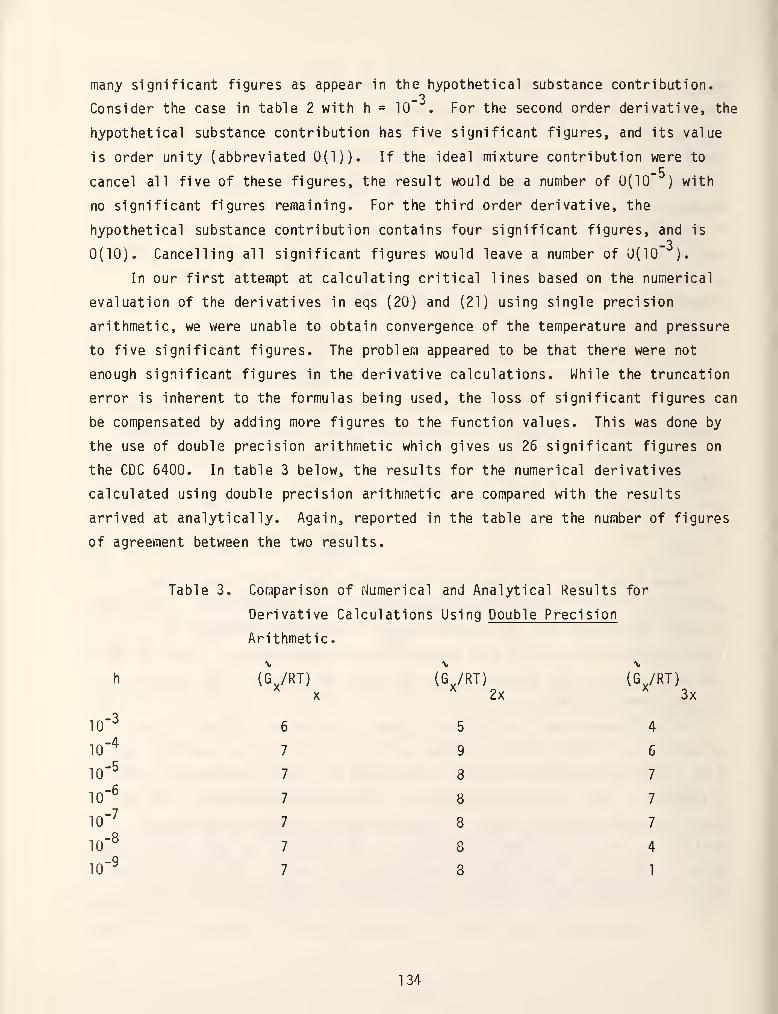
many significant figures as appear in the hypothetical substance contribution.
Consider the case in table 2 with h = 10 . For the second order derivative, the
hypothetical substance contribution has five significant figures, and its value
is order unity (abbreviated 0(1)). If the ideal mixture contribution were to
cancel all five of these figures, the result would be a number of 0(10 ) with
no significant figures remaining. For the third order derivative, the
hypothetical substance contribution contains four significant figures, and is
0(10). Cancelling all significant figures would leave a number of 0(10 ).
In our first attempt at calculating critical lines based on the numerical
evaluation of the derivatives in eqs (20) and (21) using single precision
arithmetic, we were unable to obtain convergence of the temperature and pressure
to five significant figures. The problem appeared to be that there were not
enough significant figures in the derivative calculations. While the truncation
error is inherent to the formulas being used, the loss of significant figures can
be compensated by adding more figures to the function values. This was done by
the use of double precision arithmetic which gives us 26 significant figures on
the CDC 6400. In table 3 below, the results for the numerical derivatives
calculated using double precision arithmetic are compared with the results
arrived at analytically. Again, reported in the table are the number of figures
of agreement between the two results.
Table 3. Comparison of Numerical and Analytical Results for
Derivative Calculations Using Double Precision
Arithmetic.
h (G /RT) (G /RT) (6 /RT)^ X ^ 2x ^ 3x
10"^ 6 5 4
10"^ 7 9 6
10"^ 7 8 7
10'^7 8 7
10"'^7 8 7
10"^7 8 4
10"^7 8 1
134
_3For h = 10 , the single and double precision results are the same, which
indicates that truncation error is controlling. Looking at the double precision
results, the third derivative shows an increase in accuracy as h is decreased to-5
10 ; clearly indicating that the truncation error is decreasing to this
point. As h is decreased past 10", accuracy is lost due to loss of
significant figures.
Based on these results, a value of h = 10' is chosen to compute the
derivatives in double precision. Given this value for h, the smallest value of
the second derivative which may be calculated (containing no significant figures)_o a
is 0(10" ), and that for the third derivative is 0(10" ). The calculations of
the binary critical line were subsequently made to converge to five significant
figures for both temperature and pressure.
4. Results
It must again be stressed that the general procedure for calculating the
critical line or VLE is predictive and requires only the critical constants and
an acentric factor for the fluid of interest, or of the components in a mixture.
For a relatively simple system the results will be reasonable without optimiza-
tion of any parameters. Since, however, we are concerned only with VLE and the
critical point we considered two straightforward optimization procedures
involving the factor w. The first was to adjust oj to give ttie best representa-
tion of the pure component vapor pressure curve, the second was to force the
critical temperature and pressure of the pure fluids to correspond exactly with
those of the reference substance. This second variation is simply to set
0) = 03 : hence by eqs (24) and (25) 9 = 1 and (}>= L^Jl^ — a form of classical
corresponding states. One should note that the two procedures are not the same
because the Leach-Lei and equations are not constrained at the critical point.
4.1 Ethane: Pure Component Results
We first considered the ethane vapor pressure curve v/hich was obtained
using Leach's expression for the shape factors. The value of the acentric factor
for the Leach equations was determined by optimizing agreement with the vapor
pressure data by a trial and error procedure in which the sum of the average
absolute deviations, for the vapor pressure, and saturated vapor and liquid
densities, were minimized; temperature being chosen as the independent
variable. The temperature range over which the results were optimized was 180 K
135
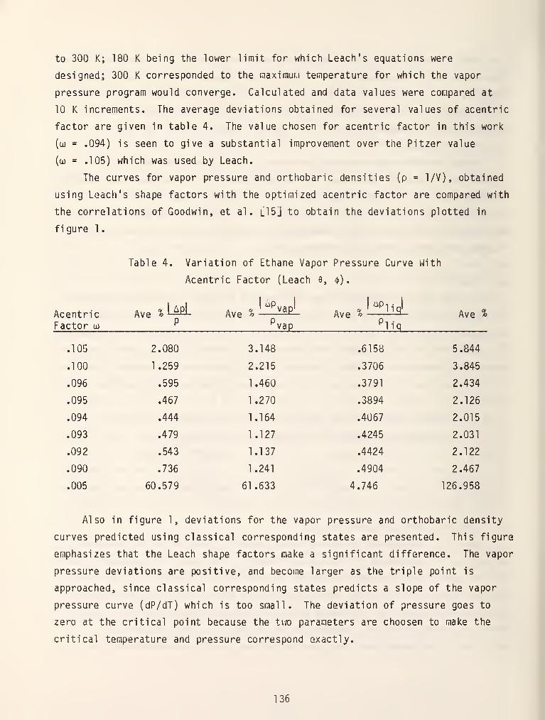
to 300 K; 180 K being the lower limit for which Leach's equations were
designed; 300 K corresponded to the maximum temperature for which the vapor
pressure program would converge. Calculated and data values were compared at
10 K increments. The average deviations obtained for several values of acentric
factor are given in table 4. The value chosen for acentric factor in this work
(oj = .094) is seen to give a substantial improvement over the Pitzer value
(u) = .105) which was used by Leach.
The curves for vapor pressure and orthobaric densities (p = 1/V), obtained
using Leach's shape factors with the optimized acentric factor are compared with
the correlations of Goodwin, et al . l15J to obtain the deviations plotted in
figure 1
.
AcentricFactor w
Table 4. Variation of Ethane Vapor Pressure Curve With
Acentric Factor (Leach Q, <^)
.
Ave % apIAve %L^^^ Ave %
Apliq'
vap UiAve %
.100
.096
.095
.094
.093
.092
.090
.005
2.080
1.259
.595
.467
.444
.479
.543
.736
60.579
3.148
2.215
1.460
1.270
1.164
1.127
1.137
1.241
61.633
.6158
.3706
.3791
.3894
.4067
.4245
.4424
.4904
4.746
5.844
3.845
2.434
2.126
2.015
2.031
2.122
2.467
126.958
Also in figure 1, deviations for the vapor pressure and orthobaric density
curves predicted using classical corresponding states are presented. This figure
emphasizes that the Leach shape factors make a significant difference. The vapor
pressure deviations are positive, and become larger as the triple point is
approached, since classical corresponding states predicts a slope of the vapor
pressure curve (dP/dT) which is too small. The deviation of pressure goes to
zero at the critical point because the two parameters are choosen to make the
critical temperature and pressure correspond exactly.
136
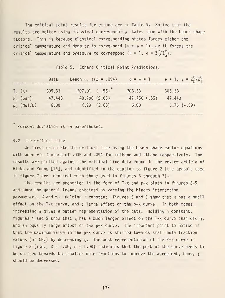
T^ (K) 305.33 307.01 ( .55)*
P^ (bar) 47.448 48.790 (2.83)
P^ (mol/L) 6.80 6.98 (2.65)
The critical point results for ethane are in Table 5. Notice that the
results are better using classical corresponding states than with the Leach shape
factors. This is because classical corresponding states forces either the
critical temperature and density to correspond (e =<t>
= 1), or it forces thec c
critical temperature and pressure to correspond (e = 1, 4) = 1/1),
Table 5. Ethane Critical Point Predictions.
Data Leach e, $(aj = .094) e =(j)
= 1 e = 1 ,<t)
= Z^/Z^
305.33 305.33
47.750 (.55) 47.448
6.80 6.76 (-.59)
Percent deviation is in parentheses.
4.2 The Critical Line
We first calculate the critical line using the Leach shape factor equations
with acentric factors of .005 and .094 for methane and ethane respectively. The
results are plotted against the critical line data found in the review article of
Hicks and Young [16], and identified in the caption to figure 2 (the symbols used
in figure 2 are identical with those used in figures 3 through 7).
The results are presented in the form of T-x and p-x plots in figures 2-5
and show the general trends obtained by varying the binary interaction
parameters, 5 and n. Holding C constant, figures 2 and 3 show that n has a small
effect on the T-x curve, and a large effect on the p-x curve. In both cases,
increasing n gives a better representation of the data. Holding n constant,
figures 4 and 5 show that ^ has a much larger effect on the T-x curve than did n*
and an equally large effect on the p-x curve. The important point to notice is
that the maximum value in the p-x curve is shifted towards small mole fraction
values (of CH,) by decreasing 5. The best representation of the P-x curve in
figure 3 (i.e., K = 1.00, r\ = 1.08) indicates that the peak of the curve needs to
be shifted towards the smaller mole fractions to improve the agreement, thus, 5
should be decreased.
137
To achieve the goal of obtaining the interaction parameters by fitting the
critical line data, a manual search technique was initiated. The "best fit" was
defined in the least squares sense. The results of this search were that
K = .97, and n = 1^13 were chosen as the "best" values for the interaction
parameters. The "best fit" T-x and p-x curves are presented in figures 6 and 7
respectively.
The fit of the T-x curve is good, v/ith only one data point which seems
astray. The p-x curve, however, does not have the right shape to fit the data
well. Part of the fitting problem is due to the bad prediction which is made for
the critical point of pure ethane. This led us to try the second approach of
setting w = oj . Hence, the critical endpoints in the T-x, and p-x curves are
exact. A new optimization led to the parameter values c = '97, r\ = 1.07. While
the fit of the T-x curve was not significantly improved that for the p-x curve
was. These results are shown in figures 6 and 7.
4.3 Vapor-Liquid Equilibria Results
Of the VLE data judged to be thermodynamically consistent by Hiza,
et al . [2J, three representative isotherms were chosen to test the predictions
made using the binary interaction parameters determined in the previous section.
Two of the isotherms are supercritical (250 K and 199.92 K) , and one is
subcritical (144.26 K) . The sources of the data are: 250 K isotherm, Davalos,
et al. [17]; 199.92 K and 144.26 K isotherms, Wichterle and Kobayashi [18].
The VLE calculations used the Leach shape factors with the acentric factors
.005 and .094 for methane and ethane respectively. The results are presented as
K-value deviation plots for both the methane and the ethane K-value predictions.
Figures 8, 9, and 10 contain these curves with the interaction parameters
obtained from the critical line fit (i.e., C = .97, n = 1.07), These figures
also show that setting the interaction parameters to unity gives much better VLE
predictions than do the parameters obtained from the best fit of the critical
line data.
5. Summary and Conclusions
The proposed technique of calculating binary critical lines by numerically
evaluating the second and third order derivatives of the Gibbs free energy has
been checked with an analytical solution for the special case of classical
corresponding states, and has proven successful. The best least squares fit of
138
the critical line data of the system methane-ethane was then shown to be poor
(particularly the p-x curve) if the Leach shape factors are used with an acentric
factor optimized for pure component vapor pressure predictions. This is due to a
bad prediction of the critical endpoint for ethane. To improve this fit, we use
classical corresponding states to force correspondence of the temperature and
pressure at the critical line endpoints. However we also show that the pure
component vapor pressure predictions are not satisfactory if this is done.
Finally, VLE predictions are made using Leach shape factors with the acentric
factor optimized for vapor pressure predictions, and the binary interaction i
parameters obtained from the best fit of the critical line data (i.e., withc c
e = 1, <t)= Z /Z ). The results are not as good in general as those which are
obtained by setting c = n = 1. Hence we conclude that a fit of the binary
critical line does not yield binary interaction parameters of any general
significance.
139
6. References
[1] Wielopolski, P., On the calculation of critical liquid-vapor lines of
binary mixtures, J. Res. Nat. Bur. Stand. (U.S.) 8^, No. 6, 441-449
(Nov-Dec 1980).
[2] Hiza, M. J., Miller, R. C. and Kiunay, A. J., A review, evaluation, and
correlation of the phase equilibria, heat of mixing and change in volume
on nixing for liquid mixtures of methane plus ethane, o. Phys. Cher.i. Ref.
Data 8, No. 3, 799-316 (1979).
[3] Watson, I. D. and Rowlinson, J. S., The prediction of the thermodynamic
properties of fluids and fluid mixtures. II. Liquid-vapor equilibrium in
the system argon + nitrogen + oxygen, Chein. Eng. Sci. 24_, 1575-1580
(19G9).
[4] Gunning, A. J. and Rov/linson, J. S., The prediction of the thermodynamic
properties of fluids and fluid mixtures. III. Applications, Chem. Eng.
Sci. 23, 521-527 (1973).
[5] Teja, A. S. and Rowlinson, J. S., The prediction of the thermodynamic
properties of fluids and fluid mixtures. IV. Critical and azeotropic
states, Chem. Eng. Sci. 28_, 529-538 (1974).
[6] Mollerup, J. and Rowlinson, J. S., The prediction of the densities of
liquefied natural gas and of lov/er molecular weight hydrocarbons, Chem.
Eng. Sci. 29, 1373-1381 (1974).
l7] Mollerup, J., Correlated and predicted thermodynamic properties of LUG and
related mixtures in the normal and critical regions. Paper E-2 in
Advances in Cryogenic Engineering, Vol. 20, K. D. Timr.ierhaus, ed.,
(Plenum Publishing Corp., New York, NY, 1975) pp. 172-194.
[8] Mollerup, J., Thermodynamic properties of natural gas, petroleum gas, and
related mixtures: enthalpy predictions. Paper M-l in Advances in
Cryogenic Engineering, Vol. 23, K. D. Timmerhaus, ed. (Plenum Pub! ishing
Corp., New York, NY, 1973), pp. 550-560.
[9] Henderson, D. and Leonard, P. J., Physical Chemistry, Eyring, H.,
Henderson, D., and Jost, W., ed. (Academic Press, Hew York, 1971)
Chapter 7, "Liquid Mixtures."
LlO] Eaton, B. E., Prediction of the critical line of binary mixtures:
Determination of binary interaction parameters, M.S. Thesis, University of
Colorado, 1980, 151 pp.
140
[11] Leach, J. W., Chappelear, P. S. and Leland, T, W., Use of molecular shape
factors in vapor-liquid equilibrium calculations with the corresponding
states principle, A.I.Ch.E. J. 14, No. 4, 568-576 (1968).
[12] Ely, J. F. and Hanley, H. J. M., Prediction of Transport Properties.
I. Viscosity of Fluids and Mixtures, Ind. Eng. Chem. Fund. 20, No. 4,
323-32 (Nov 1981).
[13] McCarty, R. D., A modified Benedict-Webb-Rubin equation of state for
methane using recent experimental data. Cryogenics J£, No. 5, 276-280
(1974).
[14] Hildebrand, F. B., Introduction to Numerical Analysis, 2nd ed.
(McGraw-Hill, New York, NY, 1974), 669 pp.
[15] Goodwin, R. D., Roder, H. M. and Straty, G. C, Thermophysical properties
of ethane, from 90 to 600 K at pressures to 700 bar, Nat. Bur. Stand.
(U.S.), Tech. Note 684 (Aug 1976), 320 pp.
[16] Hicks, C. P. and Young, C. L., The gas-liquid critical properties of
binary mixtures. Chemical Reviews 75., No. 2, 139-175 (Apr 1975).
[17] Davalos, J., Anderson, W. R., Phelps, R. E. and Kidnay, A. J, Liquid-vapor
equilibria at 250.00 K for systems containing methane, ethane, and carbon
dioxide, J. Chem. Eng. Data 2_1, No. 1, 81-84 (1976).
[18] Wichterle, I. and Kobayashi, R., Vapor-liquid equilibrium of methane-
ethane system at low temperatures and high pressures, J. Chem. Eng. Data
J2. No. 1, 9-12 (1972).
[19] Goodwin, R. D., The thermophysical properties of methane, from 90 to 500 K
at pressures to 700 bar, Nat. Bur. Stand. (U.S.), Tech. Note 653 (Apr
1974), 274 pp.
141
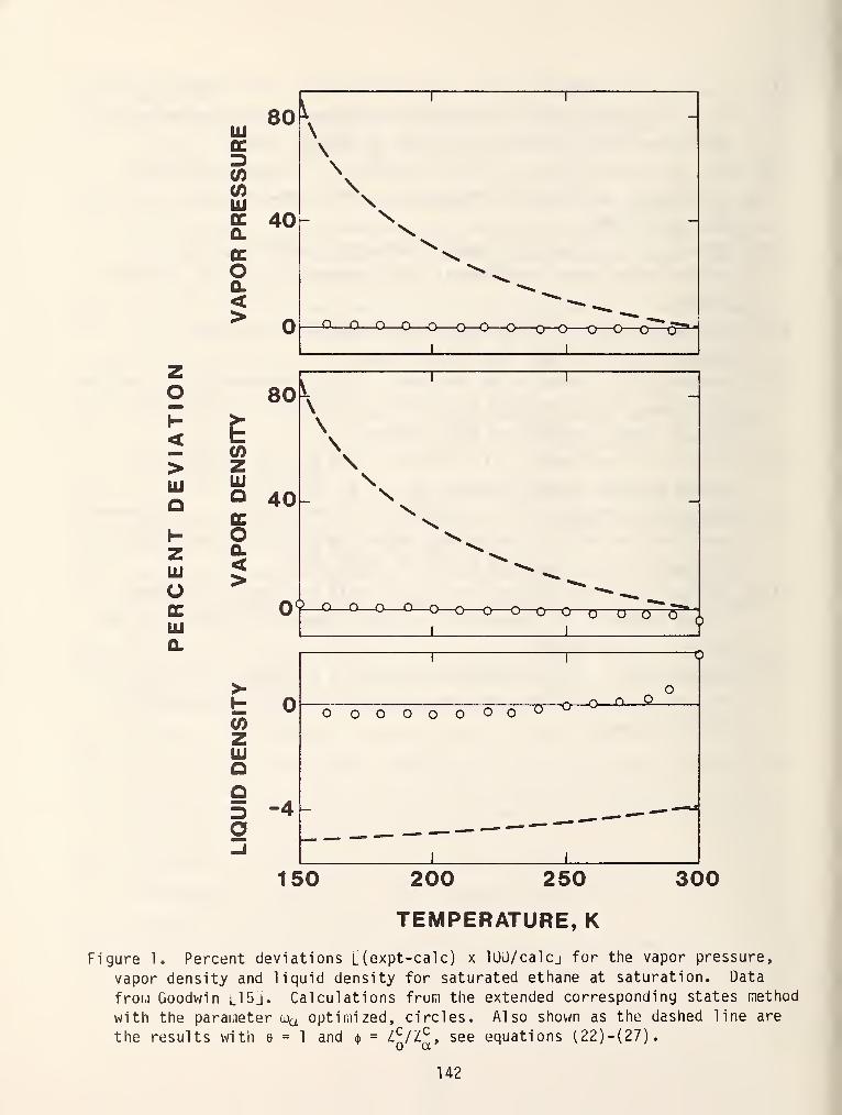
<>lU
O
LU
OliJ
0.
80 ^ ' ' .
UJ \OC \Dif)
\\
HI \cc 40 r \Q. \ \CC ^Oa.<> c>r^r^i~\r\i~^/-\/~^ ^ ^ _^_ J ^ -ufu (JUL) OO O ^ O ^
1 1
1
150 200 250
TEMPERATURE, K
300J
Figure 1. Percent deviations [(expt-calc) x lUO/calcj for the vapor pressure,
vapor density and liquid density for saturated ethane at saturation. Data
froM Goodwin l15j. Calculations from the extended corresponding states method
with the parai.ieter(jjtt
optimized, circles. Also shown as the dashed line are
the results with 8=1 and ({>= ^q/^^» see equations (22)-(27).
142
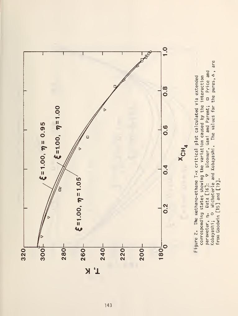
—
1
=
1.00
1 1 1 /
^ 0) i> /f —
.
o 6 // °
II o Ml^
•
II
/// >
6 ^/j'//
o ^'
II
/o
II
L 1 1
wo.
OOII
1 1 1 1
00
o
o
oX
o
CM
o
o o o O O O O OCM o CO <D Tf CM O COCO CO CM CM CM CM CM T-
-a cCD o"O <-
n3
-M fO 1-
CD O)+J
fo c D
Q.
>CD ••« S_
"O -C 4-> OdJ 4-> C ^--M (Ufa >^ s- toI— -Q 03 O)3 Q. 3U T3 ,—>— O "O fO<0 CO C >CJ 3 (O
+j a •!- x:o c I—1— C fOQ. o ^
CJ •>-
•I- s_+j ro•r- >
s cS <ao >io <o<— J233 O
I— CTC
<U -r-
fO O I
a CUC +J
-c +->
+J CO
CU
I—
I
•• <U (Ttr—I I— I
—
r— CUI I 4-> -Q
<u cfO x: ro+-> o(tJ •!- I
1
Q 3 LO
0)
(— coQ.
s- o3 oen
c cr
5- -r- -OOJ ^ O4-J 00 OCU 03 OE >, „03 (O ES Q O03 O S-Q. i^ M-
>l'l
143
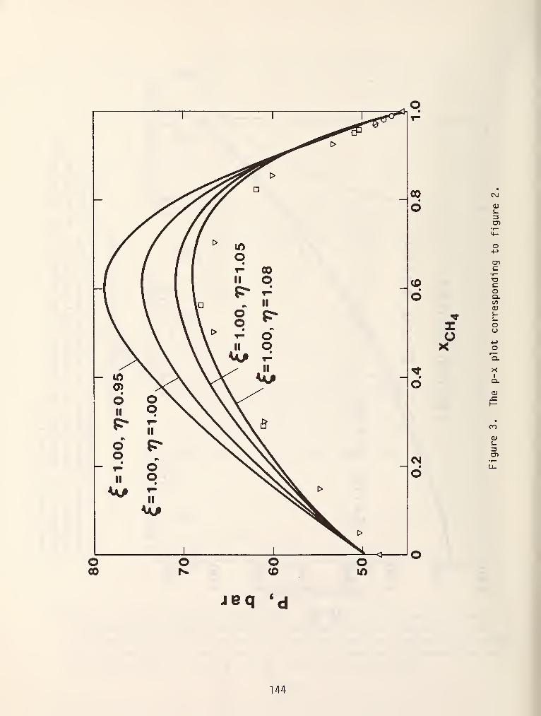
1 1
^<-^^^
^x^^ >
/^fino
II
00o-
I 1 p~• —
\\ \\ o
oII
\A\ II
oo
•
II
- in ^v^V V(^<JJ^
—0) >^ \ \ \ ^o o \\ \\^II o ^\\ \\J>
II \NvV.fi
o t> NS^O\o •s NXvVV~ T- o NSv\ —
II o Ns\U/
II
11
V
00 C\J
oen
o»->
(D-ac
m
o oQ.CO
^z o
ooX o
'q.
^ X
o Q.
0)
CM
O
CO
cn
o00
o O Oin
I
jeq 'd
114
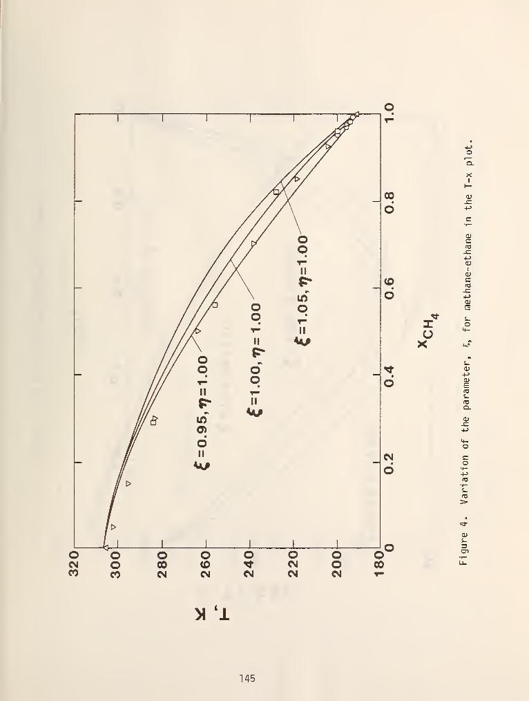
^
^// o// oV ^X II
///^ «>
// \ in
// o o/ o
•
a
( T- II
\ II AM\
oo or^ oII
{> IT^ Am
in
o>
6II
00
o
o
o
o
o
o o o o o O O OCM o 00 (0 ^ CM O 00CO CO CM CM CM CM CM y-
o
XI
(1)c«osz4->
<uI
O)
-C4->
O)ES-o<+-
O)4-'
OJ
EfOS-fOQ.
O)
+->
4-o
OJ5-
en
>l'i
145
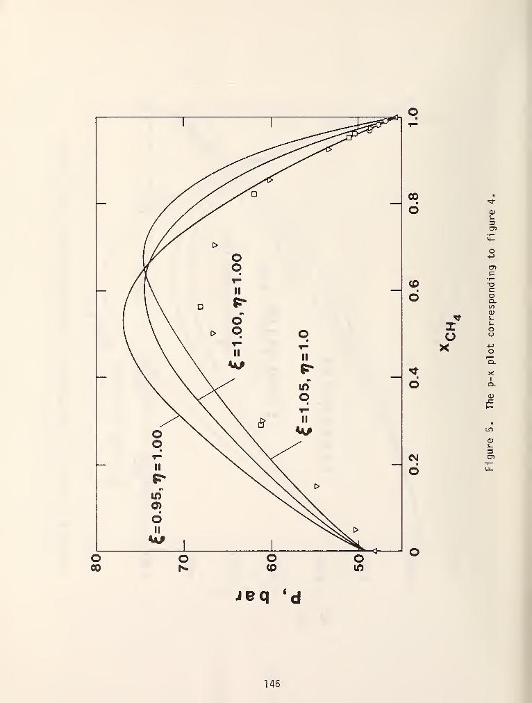
00•
•
o os-
o4->
c(D
•I—
-ac:
o oa.
^ s_
X oo o
X 4Jo'q.
'^ Xo Q.
o
(U
LO
0)
jeq 'd
i
146
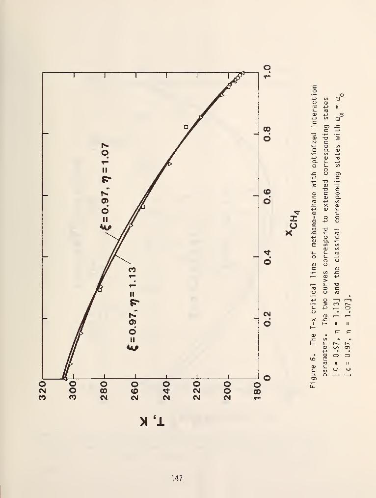
00
o
o
o
o
CM
o
o
OS-O)+->
c
T3OJN•r~
+->
Q.O
GJCn3-C4JO)I
.C+->
O)
O
<U
to
OJS-
O)
fO
CD
oa.to<uS-
ouT3O)T3c:cu+->
XO)
o+->
-a
oQ.00OJi.s_
oo
•I- 00I— O)
>r— S-
u o•r—
+-> O•r- 2S- •4->
Ocu
I I—
oos_
QJ-MOJE(tJ
s_
3
+->
oo(U-MfO
OO
c-o
oQ.00CUs_S-o
O•^-
ooU)fO
oO)
->
-oc
CO o
CTi
o O o o O O O oCM O 00 <0 ^ CM O 00CO CO CM CM CM CM CM
>l'±
H7
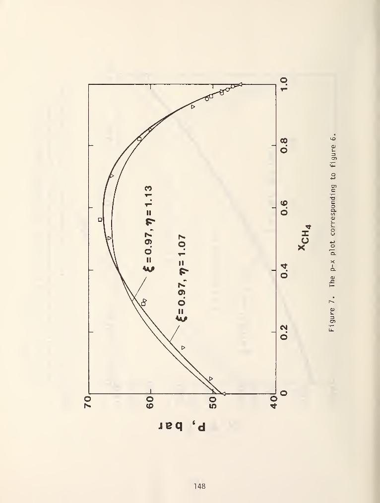
o
U3
o
oQ.to<uS-S-oa+->
oQ.
XQ.
0)
(U
a>
jeq 'd
148
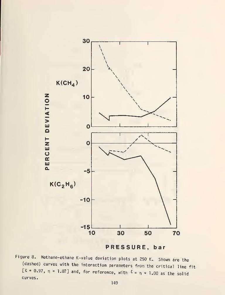
K(CH4)
>LU
O
LU
ODC
UJ
CL
KCCgHg)
-10-
PRESSURE, bar
Figure 8. Methane-ethane K-value deviation plots at 250 K. Shown are the(dashed) curves with the interaction parameters from the critical line fit
[5 = 0.97, n = 1.07] and, for reference, with ^ = n = 1.00 as the solidcurves.
149
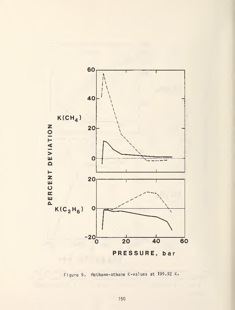
K(CH4)
I-
<>UJ
o
UJ
o
LU
0.
20
KCCgHg)
-20
1
y
1
y \y y \
y \\
V \
1
-
1
"^\
1
20 40 60
PRESSURE, bar
Figure 9. Methane-ethane K-values at 199.92 K.
150
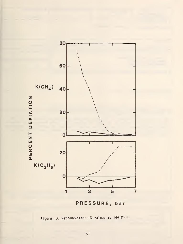
80
60-
KCCH^) 4o_
<>
QI-
ZLU
oLU
CL
20-
20
KCCgHg)
PRESSURE, bar
Figure 10. Methane-ethane K-values at 144.26 K.
151
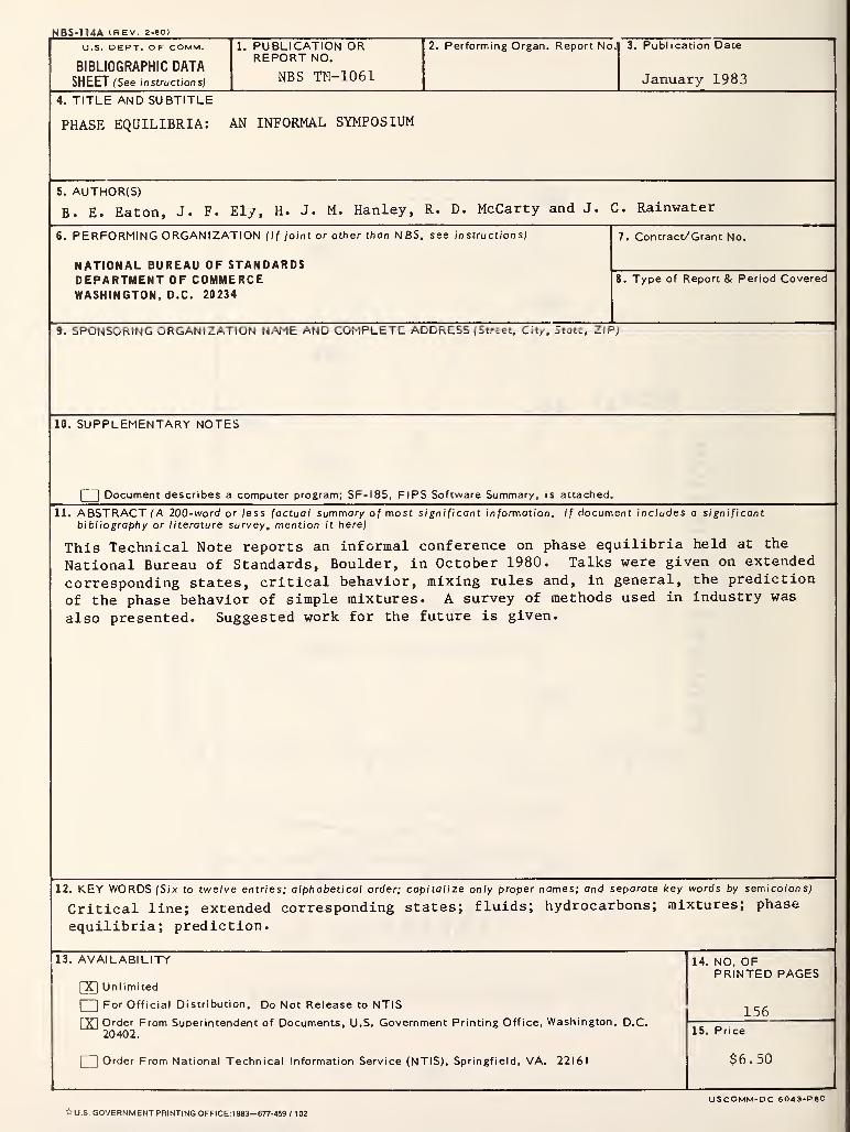
NBS-n4A (REV. 2-8C
U.S. DEPT. OF COMM.
BIBLIOGRAPHIC DATASHEET (See instructions)
1. PUBLICATION ORREPORT NO.
NBs "ra-ioei
2. Performing Organ. Report No, 3. Publication Date
January 1983
4. TITLE AND SUBTITLE
PHASE EQUILIBRIA: AN INFORMAL SYMPOSIUM
5. AUTHOR(S)
B. E. Eaton, J. F. Ely, H. J. M. Hanley, R. D. McCarty and J. C Rainwater
6, PERFORMING ORGANIZATION (If joint or other than NBS. see instructions)
NATIONAL BUREAU OF STANDARDSDEPARTMENT OF COMMERCEWASHINGTON, D.C. 20234
7. Contract/Grant No.
8. Type of Report & Period Covered
9. SPONSORING ORGANIZATION NAME AND COMPLETE ADDRESS (Street. City. State, ZIP)
10. SUPPLEMENTARY NOTES
\2^ Document describes a computer program; SF-185, FlPS Software Summary, is attached.
11. ABSTRACT (A 200-word or less factual summary of most significant information. If document includes a significantbibliography or literature survey, mention it here)
This Technical Note reports an informal conference on phase equilibria held at the
National Bureau of Standards, Boulder, in October 1980. Talks were given on extended
corresponding states, critical behavior, mixing rules and, in general, the prediction
of the phase behavior of simple mixtures. A survey of methods used in industry was
also presented. Suggested work for the future is given.
12. KEY WORDS (S/x to twelve entries; alphabetical order; capitalize only proper names; and separate key words by semicolons)
Critical line; extended corresponding states; fluids; hydrocarbons; mixtures; phase
equilibria; prediction.
13. AVAILABILITY
[X| Unlimited
|~~| For Official Distribution. Do Not Release to NTIS
rXI Order From Superintendent of Documents, U.S. Government Printing Office, Washington, D.C.20402.
031 Order From National Technical Information Service (NTIS), Springfield, VA. 22161
14. NO. OFPRINTED PAGES
156
15. Price
$6.50
USCOMM-DC 6043-P8C
^?U.S. GOVERNMENT PRINTING 0FFICE:1983— 677-459 / 102


NBS TECHNICAL PUBLICATIONS
PERIODICALS
JOURNAL OF RESEARCH—The Journal of Research of the
National Bureau of Standards reports NBS research and develop-
ment in those disciplines of the physical and engineering sciences in
which the Bureau is active. These include physics, chemistry,
engineering, mathematics, and computer sciences. Papers cover a
broad range of subjects, with major emphasis on measurement
methodology and the basic technology underlying standardization.
Also included from time to time are survey articles on topics
closely related to the Bureau's technical and scientific programs.
As a special service to subscribers each issue contains complete
citations to all recent Bureau publications in both NBS and non-
NBS media. Issued six times a year. Annual subscription: domestic
$18; foreign $22.50. Single copy, $4.25 domestic; $5.35 foreign.
NONPERIODICALS
Monographs— Major contributions to the technical literature on
various subjects related to the Bureau's scientific and technical ac-
tivities.
Handbooks— Recommended codes of engineering and industrial
practice (including safety codes) developed in cooperation with in-
terested industries, professional organizations, and regulatory
bodies.
Special Publications— include proceedings of conferences spon-
sored by NBS, NBS annual reports, and other special publications
appropriate to this grouping such as wall charts, pocket cards, andbibliographies.
Applied Mathematics Series— Mathematical tables, manuals, andstudies of special interest to physicists, engineers, chemists,
biologists, mathematicians, computer programmers, and others
engaged in scientific and technical work.
National Standard Reference Data Series— Provides quantitative
data on the physical and chemical properties of materials, com-piled from the world's literature and critically evaluated.
Developed under a worldwide program coordinated by NBS under
the authorits of the National Standard Data .Act (Public Law90-396).
NOTE: The principal publication outlet for the foregoing data is
the Journal of Physical and Chemical Reference Data (JPCRD)published quarterly for NBS by the American Chemical Society
(ACS) and the American Institute of Physics (AlP). Subscriptions,
reprints, and supplements available from ACS. 1 155 Sixteenth St.,
NW, Washington, DC 20056.
Building Science Series— Disseminates technical information
developed at the Bureau on building materials, components,
systems, and whole structures. The series presents research results,
test methods, and performance criteria related to the structural andenvironmental functions and the durability and safety charac-
teristics of building elements and systems.
Technical Notes—Studies or reports which are complete in them-
selves but restrictive in their treatment of a subject. Analogous to
monographs but not so comprehensive in scope or definitive in
treatment of the subject area. Often serve as a vehicle for final
reports of work performed at NBS under the sponsorship of other
government agencies.
Voluntary Product Standards— Developed under procedures
published by the Department o'' Commerce in Part 10, Title 15, of
the Code of Federal Regulations. The standards establish
nationally recognized requirements for products, and provide all
concerned interests with a basis for common understanding of the
characteristics of the products. NBS administers this program as a
supplement to the activities of the private sector standardizing
organizations.
Consumer Information Series— Practical information, based onNBS research and experience, covering areas of interest to the con-
sumer. Easily understandable language and illustrations provide
useful background knowledge for shopping in today's tech-
nological marketplace.
Order the above NBS publications from: Superintendenl of Docu-
menls. Government Printing Of/ice, Washington. DC 20402.
Order the following NBS publications—FIPS and NBSIR's—fromthe National Technical Information Services. Springfield. VA 22161
.
Federal Information Processing Standards Publications (FIPS
PUB)— Publications in this series collectively constitute the
Federal Information Processing Standards Register. The Register
serves as the official source of information in the Federal Govern-
ment regarding standards issued by NBS pursuant to the Federal
Property and Administrative Services Act of 1949 as amended.
Public Law 89-306 (79 Stat. 1127), and as implemented by Ex-
ecutive Order 11717(38 FR 12315, dated May II, 1973) and Part 6
of Title 15 CFR (Code of Federal Regulations).
NBS Interagency Reports (NBSIR)- ' necial series of interim or
final reports on work performed h .BS for outside sponsors
(both government and non-government). In general, initial dis-
tribution is handled by the sponsor; public distribution is by the
National Technical Information Services, Springfield, VA 22161,
in paper copy or microfiche form.

U.S. Department of CommerceNational Bureau of Standards
Washington. DC. 20234Official Business
Penalty for Private Use S300
POSTAGE AND FEES PAIDU S DEPARTMENT OF COMMERCE
COM-215
SPECIAL FOURTH-CLASS RATEBOOK
Related Documents