Phase coherence among the Fourier modes and non ...

Prog. Theor. Exp. Phys. 2017, 033J01 (14 pages)DOI: 10.1093/ptep/ptx016

Phase coherence among the Fourier modes andnon-Gaussian characteristics in the Alfvén chaossystem

Yasuhiro Nariyuki1,∗, Makoto Sasaki2, Naohiro Kasuya2, Tohru Hada3, and Masatoshi Yagi4

1Faculty of Human Development, University of Toyama, 3190, Gofuku, Toyama City, Toyama 930-8555, Japan2Research Institute for Applied Mechanics, Kyushu University, 6-1, Kasugakoen, Kasuga City, Fukuoka816-8580, Japan3Faculty of Engineering Sciences, Kyushu University, 6-1, Kasugakoen, Kasuga City, Fukuoka 816-8580, Japan4National Institutes for Quantum and Radiological Science and Technology, 2-166, Omotedate, Obuchi,Rokkasho, Aomori 039-3212, Japan∗E-mail: [email protected]

Received June 29, 2016; Revised January 27, 2017; Accepted January 30, 2017; Published March 30, 2017

... . . . . . . . . . . . . . . . . . . . . . . . . . . . . . . . . . . . . . . . . . . . . . . . . . . . . . . . . . . . . . . . . . . . . . . . . . . . . . . . . . . . . . . . . . . . . . . . . . . . . . . . . . . . . . . . .Non-Gaussian characteristics in time series of the Alfvén chaos system are discussed. The phasecoherence index, a measure defined by using the surrogate data method and the structure func-tion, is used to evaluate the phase coherence among the Fourier modes. Through Monte Carlosignificance testing, it is found that the phase coherence decays monotonically with increasingdissipative parameter and time scale. By applying the Mori projection operator method assum-ing the Markov process, a model equation for the time correlation function is derived from thegeneralized Langevin equation. As opposed to the result of the phase coherence analysis, itis concluded that the difference between the direct numerical simulation and the model equa-tion becomes pronounced as the dissipative parameters are increased. This suggests that, evenwhen the phase coherence index is not significant, the underlying physical system may be anon-Gaussian process... . . . . . . . . . . . . . . . . . . . . . . . . . . . . . . . . . . . . . . . . . . . . . . . . . . . . . . . . . . . . . . . . . . . . . . . . . . . . . . . . . . . . . . . . . . . . . . . . . . . . . . . . . . . . . . . . .

Subject Index A33, J21, J24

1. Introduction

It is well known that finite amplitude Alfvénic fluctuations are frequently observed in the solarwind plasma (Refs. [1–4]). Since these fluctuations disappear with increasing heliocentric dis-tances (Refs. [5,6]), their damping processes possibly play important roles in the generation ofmagnetic turbulence and/or in plasma heating. Damping of such finite amplitude Alfvén waves hasbeen intensively discussed in terms of parametric decay (Refs. [7,8]) and modulational instabilities(Refs. [9,10]). When the system concerned contains the source of Alfvén waves and dissipationterms (sinks of energy), the statistical stationary Alfvénic states can be achieved approximately(Refs. [11,12]). Such a situation can be realized in space plasma, e.g., in the earth-foreshock region(Refs. [13,14]) and in the solar atmosphere (Ref. [15]), in which some sources of Alfvén waves mayexist. It should also be noted that the magnetic fluctuations observed in the earth’s foreshock regionexhibit finite phase coherence among the Fourier modes (Refs. [16,17]). The result is in contrast tothe often used ansatz of the “phase random approximation”, which is assumed to be held in weakturbulence theories.

In the present study, we discuss the generation of non-Gaussian characteristics in nonlinear evo-lution of Alfvén waves by using the Alfvén chaos system proposed by Hada et al. (Ref. [11]). The

© The Author(s) 2017. Published by Oxford University Press on behalf of the Physical Society of Japan.This is an Open Access article distributed under the terms of the Creative Commons Attribution License (http://creativecommons.org/licenses/by/4.0/),which permits unrestricted reuse, distribution, and reproduction in any medium, provided the original work is properly cited.

Dow

nloaded from https://academ

ic.oup.com/ptep/article/2017/3/033J01/3096140 by guest on 21 August 2022

PTEP 2017, 033J01 Y. Nariyuki et al.

Alfvén chaos system is derived from the driven-damped derivative nonlinear Schrodinger equation(DNLS) (Ref. [18]) with traveling wave solution. In Sect. 2, the phase coherence among the Fouriermodes in the chaotic time series of the Alfvén chaos system is discussed. In Sect. 3, we discuss alinear Markovian equation by using the Mori projection operator method (Refs. [19,20]). The resultsare summarized and future issues are discussed in Sect. 4.

2. Phase coherence of Alfvén chaos

Let us first define the Alfvén chaos system (Refs. [11,21,22]). By incorporating the monochromaticgrowth term and the dissipation term into the DNLS with traveling wave ansatz, Hada et al. (Ref. [11])obtained the ordinary differential equation set

by − νbz = bz(b2y + b2

z − 1) − λbz + a cos θ , (1)

bz − νby = −by(b2y + b2

z − 1) − λ(by − 1) + a sin θ , (2)

θ = �. (3)

The ordinary differential equation set (1), (2) is derived by using the coordinate transformationξ = X − VT , where X and T are spatial coordinate and time respectively, and V is a constant.If there is no driving force, Eqs. (1), (2) describe the stationary solutions of the DNLS system(Ref. [11]). In accordance with the past study in Ref. [21], here we use the variable t = ξ as theconventional time variable. The terms by and bz are the transverse magnetic field, ν corresponds tothe coefficient of the Burgers-type dissipation term, λ indicates the velocity V normalized to theambient magnetic field, and a and � are the intensity and frequency of the driving term, respectively.The ambient magnetic field is assumed to be in the x–y plane.

Past studies (Refs. [11,21]) carried out direct numerical simulations of the system (1)–(3) anddiscussed the bifurcation diagram of the Alfvén chaos. In the present study, we also carry out directnumerical simulation of the Alfvén chaos system (1)–(3) with the parameters that lead to the chaotictime series observed by Chian et al. (Ref. [21]). The runs are presented in Table 1. In a similar wayto Chian et al. (Ref. [21]), we vary only the dissipative parameter ν and fix the other parametersas λ = 0.25, � = −1, and a = 0.3. The hodogram (by − bz) is shown in Fig. 1. The reasonfor the gap between runs 1–6 and runs 7–10 is a window in the bifurcation diagram (Ref. [21]),in which period-doubling bifurcation of the stable periodic orbit with decreasing ν is observed.At the end of the bifurcation (ν = 0.06212), an interior crisis is observed, which occurs due tothe collision between the unstable orbit from the saddle-node bifurcation and the bounded chaoticattractor (Ref. [21]). Detailed discussion on the bifurcation was given in the past study in Ref. [21].As for numerical integration, a fourth-order Runge–Kutta scheme is used for the time integration,with �t = 5 × 10−4.

To check the statistical stability, runs are repeated fifty times using different initial conditions eachtime, i.e., by giving by(t = 0) = bz(t = 0) = c0, where c0 is a uniform random number within the

Table 1. The parameter (ν) used in simulation runs. The other parameters are fixed as λ = 0.25, � = −1,and a = 0.3 so that the system shows the chaotic behavior (Ref. [21]).

Run 1 2 3 4 5 6 7 8 9 10ν 0.02 0.05 0.0616 0.06212 0.078 0.08 0.175 0.1775 0.1995 0.2

2/14

Dow

nloaded from https://academ

ic.oup.com/ptep/article/2017/3/033J01/3096140 by guest on 21 August 2022

PTEP 2017, 033J01 Y. Nariyuki et al.

Fig. 1. The hodogram of bz and by for 3000 ≤ t ≤ 5000, with (a) ν = 0.02 (run 1), (b) ν = 0.0616 (run 3),(c) ν = 0.06212 (run 4), (d) ν = 0.08 (run 6), (e) ν = 0.1775 (run 8), and (f) ν = 0.2 (run 10).

range [0, 1]. The mean values (indicated by 〈·〉) shown in Figs. 2(a),(b) are calculated by using thetime average from t = 1 to t = 106 for each initial condition. As shown in Figs. 2(a),(b), exceptfor the case where the averaged values themselves are small (absolute values less than 0.01), thestandard error during the runs using different initial conditions is less than 1 percent of the averagedvalue.

To examine the non-Gaussian characteristics in Alfvén chaos, we use the phase coherence index(Refs. [16,26]) as a measure for evaluating the phase coherence among the Fourier modes containedin a given time series (Ref. [23]). Here we use the modified version of the phase coherence index(Ref. [26])

Cφ = |Lrs − Lor||Lrs − Lor| + |Lor − Lcs| , (4)

where Li(α, τ) = �t|f (t + τ) − f (t)|α is the structure function, f = by, bz, i = or (original data), rs(randomized surrogate data), and cs (coherent surrogate data). The value α = 1 is used in the presentstudy. Figure 3 shows the time series of (a) the original data of by, (b) the randomized surrogate

3/14

Dow

nloaded from https://academ

ic.oup.com/ptep/article/2017/3/033J01/3096140 by guest on 21 August 2022

PTEP 2017, 033J01 Y. Nariyuki et al.

Fig. 2. The dependence of the time-averaged values on ν (simulation runs tabulated in Table 1): (a) ◦ 〈by〉, •〈bz〉, � 〈b2

y〉, � 〈b2z 〉, + 〈bybz〉, � 〈b2

y bz〉, and � 〈byb2z 〉; (b) ◦ 〈b3

y〉, • 〈b3z 〉, � 〈b4

y〉, � 〈b4z 〉, � 〈b3

y bz〉, � 〈b3z by〉,

and + 〈b2y b2

z 〉. The hat symbol is defined in Eq. (6).

data, and (c) the coherent surrogate data in run 3. As seen in Fig. 3(c), the wave form of the coherentsurrogate (randomized surrogate) becomes localized and the variance measured by the structurefunction becomes smaller (larger) than the one for the original data. Here we use one time seriesfor each run, since the dependence of the statistical properties of the runs on the initial conditions isalmost negligible, as mentioned above.

In the present study, the phase shuffle surrogate data (Refs. [16,17,23,25,26]), in which the correla-tion function (power spectrum) of the original data is conserved, is used as the randomized surrogatedata. This can be done by first discrete Fourier transforming (DFT) the target time series to obtainthe complex DFT spectra, and then by rewriting its phase part by random numbers within the range[0, 2π ]. To evaluate the significance, multiple surrogate data are generated by using different sets ofrandom numbers. In the present study, the number of random surrogate data for each window (oneDFT window) is 100. The number of windows is 5, so we have 5 windows to check the variance ofCφ . As shown in Fig. 5, the error bar is negligibly small. The coherent surrogate data are obtainedby substituting a uniform number for the original phase.

When we apply the phase shuffle surrogate to the Monte Carlo significance testing, the null hypoth-esis is the linear Gaussian process (color noise) (Refs. [23,25]). While the histogram of the originaldata of by (Fig. 4(a)) is far from the Gaussian distribution, one of the surrogate data sets (Fig. 4(b))becomes close to the Gaussian distribution (Ref. [25]). Here we use 16 384 data points (data fromt = 100.1 to ∼ 1738.4 with interval of 0.1) for the DFT with box windows similar to the paststudies in Refs. [17,27]. The histograms are also calculated by using the same time series (16 834data points). As mentioned above, the number of random surrogate data for each window is 100 andthe number of windows is 5. The level of significance for the one-sided rank-order test is definedas (Ref. [23]) (1 − β) × 100 percent, where β = 1/(1 + N ), and N (= 100) is the number of

4/14

Dow

nloaded from https://academ

ic.oup.com/ptep/article/2017/3/033J01/3096140 by guest on 21 August 2022

PTEP 2017, 033J01 Y. Nariyuki et al.

Fig. 3. The time series of (a) the original data of by, (b) the randomized surrogate data, and (c) the coherentsurrogate data derived from run 3.

Fig. 4. The histogram of (a) the original data of by and (b) its random surrogate data for the data shown inFigs. 3(a),(b).

5/14

Dow

nloaded from https://academ

ic.oup.com/ptep/article/2017/3/033J01/3096140 by guest on 21 August 2022

PTEP 2017, 033J01 Y. Nariyuki et al.

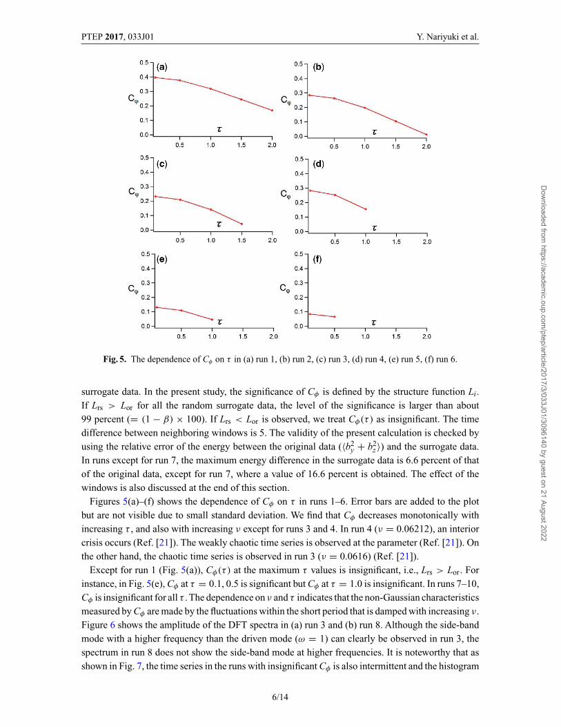
Fig. 5. The dependence of Cφ on τ in (a) run 1, (b) run 2, (c) run 3, (d) run 4, (e) run 5, (f) run 6.

surrogate data. In the present study, the significance of Cφ is defined by the structure function Li.If Lrs > Lor for all the random surrogate data, the level of the significance is larger than about99 percent (= (1 − β) × 100). If Lrs < Lor is observed, we treat Cφ(τ ) as insignificant. The timedifference between neighboring windows is 5. The validity of the present calculation is checked byusing the relative error of the energy between the original data (〈b2

y + b2z 〉) and the surrogate data.

In runs except for run 7, the maximum energy difference in the surrogate data is 6.6 percent of thatof the original data, except for run 7, where a value of 16.6 percent is obtained. The effect of thewindows is also discussed at the end of this section.

Figures 5(a)–(f) shows the dependence of Cφ on τ in runs 1–6. Error bars are added to the plotbut are not visible due to small standard deviation. We find that Cφ decreases monotonically withincreasing τ , and also with increasing ν except for runs 3 and 4. In run 4 (ν = 0.06212), an interiorcrisis occurs (Ref. [21]). The weakly chaotic time series is observed at the parameter (Ref. [21]). Onthe other hand, the chaotic time series is observed in run 3 (ν = 0.0616) (Ref. [21]).

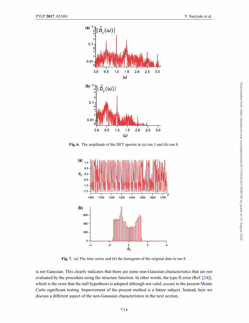
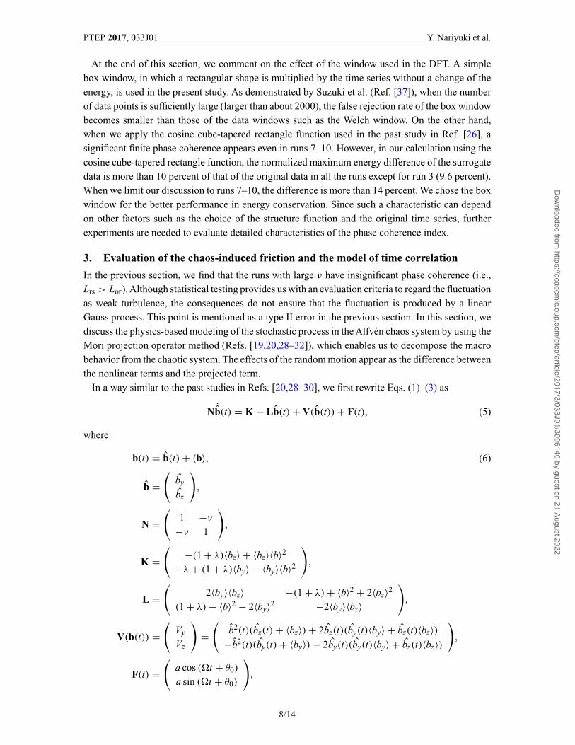
Except for run 1 (Fig. 5(a)), Cφ(τ ) at the maximum τ values is insignificant, i.e., Lrs > Lor. Forinstance, in Fig. 5(e), Cφ at τ = 0.1, 0.5 is significant but Cφ at τ = 1.0 is insignificant. In runs 7–10,Cφ is insignificant for all τ . The dependence on ν and τ indicates that the non-Gaussian characteristicsmeasured by Cφ are made by the fluctuations within the short period that is damped with increasing ν.Figure 6 shows the amplitude of the DFT spectra in (a) run 3 and (b) run 8. Although the side-bandmode with a higher frequency than the driven mode (ω = 1) can clearly be observed in run 3, thespectrum in run 8 does not show the side-band mode at higher frequencies. It is noteworthy that asshown in Fig. 7, the time series in the runs with insignificant Cφ is also intermittent and the histogram

6/14

Dow

nloaded from https://academ

ic.oup.com/ptep/article/2017/3/033J01/3096140 by guest on 21 August 2022

PTEP 2017, 033J01 Y. Nariyuki et al.

Fig. 6. The amplitude of the DFT spectra in (a) run 3 and (b) run 8.

Fig. 7. (a) The time series and (b) the histogram of the original data in run 8.

is not Gaussian. This clearly indicates that there are some non-Gaussian characteristics that are notevaluated by the procedure using the structure function. In other words, the type II error (Ref. [24]),which is the error that the null hypothesis is adopted although not valid, occurs in the present MonteCarlo significant testing. Improvement of the present method is a future subject. Instead, here wediscuss a different aspect of the non-Gaussian characteristics in the next section.

7/14

Dow

nloaded from https://academ

ic.oup.com/ptep/article/2017/3/033J01/3096140 by guest on 21 August 2022

PTEP 2017, 033J01 Y. Nariyuki et al.

At the end of this section, we comment on the effect of the window used in the DFT. A simplebox window, in which a rectangular shape is multiplied by the time series without a change of theenergy, is used in the present study. As demonstrated by Suzuki et al. (Ref. [37]), when the numberof data points is sufficiently large (larger than about 2000), the false rejection rate of the box windowbecomes smaller than those of the data windows such as the Welch window. On the other hand,when we apply the cosine cube-tapered rectangle function used in the past study in Ref. [26], asignificant finite phase coherence appears even in runs 7–10. However, in our calculation using thecosine cube-tapered rectangle function, the normalized maximum energy difference of the surrogatedata is more than 10 percent of that of the original data in all the runs except for run 3 (9.6 percent).When we limit our discussion to runs 7–10, the difference is more than 14 percent. We chose the boxwindow for the better performance in energy conservation. Since such a characteristic can dependon other factors such as the choice of the structure function and the original time series, furtherexperiments are needed to evaluate detailed characteristics of the phase coherence index.

3. Evaluation of the chaos-induced friction and the model of time correlation

In the previous section, we find that the runs with large ν have insignificant phase coherence (i.e.,Lrs > Lor).Although statistical testing provides us with an evaluation criteria to regard the fluctuationas weak turbulence, the consequences do not ensure that the fluctuation is produced by a linearGauss process. This point is mentioned as a type II error in the previous section. In this section, wediscuss the physics-based modeling of the stochastic process in the Alfvén chaos system by using theMori projection operator method (Refs. [19,20,28–32]), which enables us to decompose the macrobehavior from the chaotic system. The effects of the random motion appear as the difference betweenthe nonlinear terms and the projected term.

In a way similar to the past studies in Refs. [20,28–30], we first rewrite Eqs. (1)–(3) as

N ˙b(t) = K + Lb(t) + V(b(t)) + F(t), (5)

where

b(t) = b(t) + 〈b〉, (6)

b =(

by

bz

),

N =(

1 −ν

−ν 1

),

K =(

−(1 + λ)〈bz〉 + 〈bz〉〈b〉2

−λ + (1 + λ)〈by〉 − 〈by〉〈b〉2

),

L =(

2〈by〉〈bz〉 −(1 + λ) + 〈b〉2 + 2〈bz〉2

(1 + λ) − 〈b〉2 − 2〈by〉2 −2〈by〉〈bz〉

),

V(b(t)) =(

Vy

Vz

)=(

b2(t)(bz(t) + 〈bz〉) + 2bz(t)(by(t)〈by〉 + bz(t)〈bz〉)−b2(t)(by(t) + 〈by〉) − 2by(t)(by(t)〈by〉 + bz(t)〈bz〉)

),

F(t) =(

a cos (�t + θ0)

a sin (�t + θ0)

),

8/14

Dow

nloaded from https://academ

ic.oup.com/ptep/article/2017/3/033J01/3096140 by guest on 21 August 2022

PTEP 2017, 033J01 Y. Nariyuki et al.

and θ0 = 0. Then, the projection of the nonlinear term V(b(t)) is discussed by using the Moriprojection operator method (Refs. [20,28–30]). The projection of a variable H (X (t)) on the macrovariable A ≡ A(t = 0) is defined as (Ref. [28])

P(H (A(t))) = 〈H (A(t))A†〉〈AA†〉−1A, (7)

where 〈·〉 is the long-time average, and the symbol † denotes the Hermitian conjugate. In the samemanner as the past studies in Refs. [20,28,30],

V(b(t)) = e�t(P + Q)V(b), (8)

where � is the evolution operator (Refs. [20,28,30]), Q = 1 − P, and

e�tPV (b) = LPb(t), (9)

e�tQV (b) = −∫ t

0�(s)b(t − s) ds + r, (10)

LP ≡⎛⎜⎝

〈Vyby〉〈by

2〉〈Vybz〉〈bz

2〉〈Vzby〉〈by

2〉〈Vzbz〉〈bz

2〉

⎞⎟⎠,

r = etQ�QV (b) is the fluctuating force, and �(t) = 〈r(t)r†〉〈bb†〉−1 is the memory function that isassumed to be a diagonal matrix in the present study. Equation (5) can be rewritten as

N ˙b(t) = K + (L + LP)b(t) −∫ t

0�(τ)b(t − τ) dτ + r(t) + F(t). (11)

From Eq. (11), we can obtain an evolution equation for the time correlation function

C = 〈b(t)b†〉 = limτ→∞

1

τ

∫ τ

0ds b(t + s)b†(s)

as (Refs. [20,28,30])

˙Cyy(t) − ν ˙Czy(t) = LtyyCyy + LtyzCzy −∫ t

0�yy(τ )Cyy(t − τ) dτ + CFyy, (12)

˙Czy(t) − ν ˙Cyy(t) = LtzyCyy + LtzzCzy + CFzy, (13)

where CF = 〈F(t)b†〉, Lt = L+LP. By performing the Laplace transformation, the relation betweenthe time correlation spectrum and the memory spectrum can be obtained (Refs. [29,30]). Here weconsider the linear Markovian stochastic equation as (Refs. [20,28,29])

∫ t0 �(s)C(t − s) ds ≈ γ C(t),

where γ = diag(γyy, γzz) is the chaos-induced friction coefficient (Refs. [20,29]).From Eqs. (12) and (13), we obtain

¨Cyy(t) + κ ˙Cyy(t) + �20Cyy(t) = Ftyy(t), (14)

where κ = (γyy − ν(Ltyz + Ltzy) − (Ltyy + Ltzz))/(1 − ν2), �20 = (|Lt| − γyyLtzz)/(1 − ν2), and

Ftyy = ˙CFyy(t) + ν ˙CFzy(t) + LtyzCFzy(t) − LtzzCFyy(t). (15)

Direct numerical simulations indicate that Ftyy becomes the sinusoidal function

Ftyy = f0 sin(t + �). (16)

9/14

Dow

nloaded from https://academ

ic.oup.com/ptep/article/2017/3/033J01/3096140 by guest on 21 August 2022

PTEP 2017, 033J01 Y. Nariyuki et al.

Table 2. The coefficients in Eqs. (14), (16).

Run 1 2 3 4 5 6 7 8 9 10

ν 0.02 0.05 0.0616 0.06212 0.078 0.08 0.175 0.1775 0.1995 0.2γyy −0.3085 −0.0242 1.321 1.960 0.9091 0.3685 −0.8284 −1.519 −1.508 −1.508κ −0.2741 0.0311 1.381 2.022 0.9735 0.4308 −0.9328 −1.585 −1.547 −1.547�2

0 22.77 24.04 27.34 30.02 28.89 28.60 9.941 12.62 7.968 7.967f0 0.4230 0.5921 0.6421 0.8694 0.8572 0.8405 0.3978 0.3702 0.2531 0.2505� 2.130 2.612 2.606 2.678 2.879 2.933 −2.636 −2.563 −2.575 −2.562

Numerically evaluated coefficients are presented in Table 2. Thus, Eq. (14) models a simple force-damped oscillator with a special solution

Cyy,s = I1 cos(t + �) + I2 sin(t + �), (17)

where

I1 = − κf0(�2

0 − 1)2 + κ2, (18)

I2 = (�20 − 1)f0

(�20 − 1)2 + κ2

(19)

or

Cyy,s = E0 sin(t + � + �0), (20)

where

E0 = f0((�2

0 − 1)2 + κ2)1/2 , (21)

tan �0 = κ

�20 − 1

. (22)

From Eq. (21), we can have the quadratic equation for γyy,

k2γ2yy + k1γyy + k0 = 0, (23)

where

k0 = G22 + (|Lt| − G1)

2 −(

G1f0E0

)2

, (24)

k1 = 2G2 − 2G3(|Lt| − G1), (25)

k2 = 1 + G23, (26)

G1 = 1 − ν2, (27)

G2 = −ν(Ltzy + Ltyz) − (Ltyy + Ltzz), (28)

G3 = Ltzz. (29)

10/14

Dow

nloaded from https://academ

ic.oup.com/ptep/article/2017/3/033J01/3096140 by guest on 21 August 2022

PTEP 2017, 033J01 Y. Nariyuki et al.

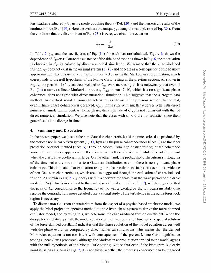
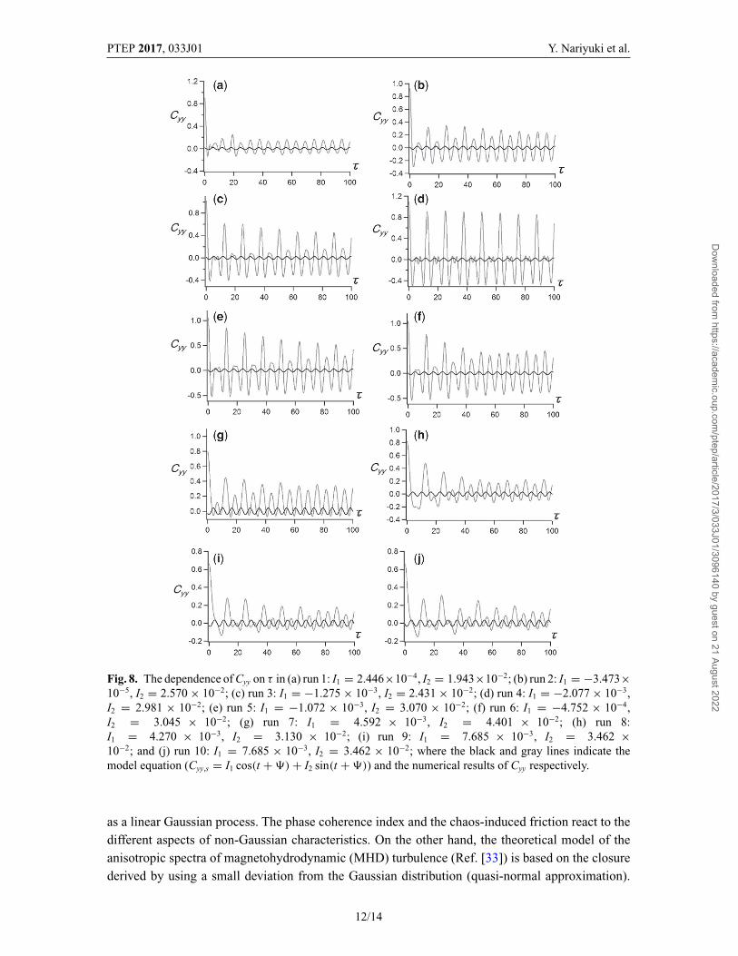
Past studies evaluated γ by using mode-coupling theory (Ref. [20]) and the numerical results of thenonlinear force (Ref. [29]). Here we evaluate the unique γyy using the multiple root of Eq. (23). Fromthe condition that the discriminant of Eq. (23)) is zero, we obtain the equation

γyy = − k1

2k2. (30)

In Table 2, γyy and the coefficients of Eq. (14) for each run are tabulated. Figure 8 shows thedependence of Cyy on τ . Due to the existence of the side-band mode as shown in Fig. 6, the modulationis observed in Cyy calculated by direct numerical simulation. We remark that the chaos-inducedfriction γyy does not exist in the original system (1)–(3) and appears as a consequence of the Markovapproximation. The chaos-induced friction is derived by using the Markovian approximation, whichcorresponds to the null hypothesis of the Monte Carlo testing in the previous section. As shown inFig. 9, the phases of Cyy,s are decorrelated to Cyy with increasing ν. It is noteworthy that even ifEq. (14) assumes a linear Markovian process, Cyy,s in runs 7–10, which has no significant phasecoherence, does not agree with direct numerical simulation. This suggests that the surrogate datamethod can overlook non-Gaussian characteristics, as shown in the previous section. In contrast,even if finite phase coherence is observed, Cyy,s in the runs with smaller ν agrees well with directnumerical simulation. In contrast to the phase, the amplitude of Cyy,s is not consistent with that ofdirect numerical simulation. We also note that the cases with κ < 0 are not realistic, since theirgeneral solutions diverge in time.

4. Summary and Discussion

In the present paper, we discuss the non-Gaussian characteristics of the time series data produced bythe reduced nonlinearAlfvén system (1)–(3) by using the phase coherence index (Sect. 2) and the Moriprojection operator method (Sect. 3). Through Monte Carlo significance testing, phase coherenceamong Fourier modes appears when the dissipative coefficient ν is small, while it is not significantwhen the dissipative coefficient is large. On the other hand, the probability distributions (histogram)of the time series are not similar to a Gaussian distribution even if there is no significant phasecoherence. This indicates that evaluation using the phase coherence index can overlook evidenceof non-Gaussian characteristics, which are also suggested through the evaluation of chaos-inducedfriction. As shown in Fig. 5, Cφ decays within a shorter time scale than the wave period of the drivemode (= 2π ). This is in contrast to the past observational study in Ref. [17], which suggested thatthe peak of Cφ corresponds to the frequency of the waves excited by the ion beam instability. Toresolve the contradiction, more detailed observational study of the turbulence in the earth-foreshockregion is necessary.

To discuss non-Gaussian characteristics from the aspect of a physics-based stochastic model, weapply the Mori projection operator method to the Alfvén chaos system to derive the force-dampedoscillator model, and by using this, we determine the chaos-induced friction coefficient. When thedissipation is relatively small, the model equation of the time correlation function (the special solutionof the force-damped oscillator) indicates that the phase evolution of the model equation agrees wellwith the phase evolution computed by direct numerical simulations. This means that the derivedMarkovian equation is not consistent with consequences of the present Monte Carlo significancetesting (linear Gauss processes), although the Markovian approximation applied to the model agreeswith the null hypothesis of the Monte Carlo testing. Notice that even if the histogram is clearlynon-Gaussian as shown in Fig. 7, it is not trivial whether the processes concerned can be regarded

11/14

Dow

nloaded from https://academ

ic.oup.com/ptep/article/2017/3/033J01/3096140 by guest on 21 August 2022

PTEP 2017, 033J01 Y. Nariyuki et al.

Fig. 8. The dependence of Cyy on τ in (a) run 1: I1 = 2.446×10−4, I2 = 1.943×10−2; (b) run 2: I1 = −3.473×10−5, I2 = 2.570 × 10−2; (c) run 3: I1 = −1.275 × 10−3, I2 = 2.431 × 10−2; (d) run 4: I1 = −2.077 × 10−3,I2 = 2.981 × 10−2; (e) run 5: I1 = −1.072 × 10−3, I2 = 3.070 × 10−2; (f) run 6: I1 = −4.752 × 10−4,I2 = 3.045 × 10−2; (g) run 7: I1 = 4.592 × 10−3, I2 = 4.401 × 10−2; (h) run 8:I1 = 4.270 × 10−3, I2 = 3.130 × 10−2; (i) run 9: I1 = 7.685 × 10−3, I2 = 3.462 ×10−2; and (j) run 10: I1 = 7.685 × 10−3, I2 = 3.462 × 10−2; where the black and gray lines indicate themodel equation (Cyy,s = I1 cos(t + �) + I2 sin(t + �)) and the numerical results of Cyy respectively.

as a linear Gaussian process. The phase coherence index and the chaos-induced friction react to thedifferent aspects of non-Gaussian characteristics. On the other hand, the theoretical model of theanisotropic spectra of magnetohydrodynamic (MHD) turbulence (Ref. [33]) is based on the closurederived by using a small deviation from the Gaussian distribution (quasi-normal approximation).

12/14

Dow

nloaded from https://academ

ic.oup.com/ptep/article/2017/3/033J01/3096140 by guest on 21 August 2022

PTEP 2017, 033J01 Y. Nariyuki et al.

Fig. 9. The dependence of Pearson’s correlation coefficient between Cyy and Cyy,s on ν.

Practically, the applicability condition of the Gaussian distribution is significant in understandingMHD turbulence in the solar wind. Such an applicability condition should be justified from a pluralityof viewpoints. As a result, the present result suggests that even if the phase coherence is significantlylow, the physics-based model derived by using the Mori-projection operator method declines to applythe Gaussian distribution to the Alfvén chaos system. When we discuss turbulence observed by thespacecraft, a lesson from the present analysis should be absorbed.

Some recent studies also discussed random (thermal) fluctuations in the solar wind plasma by usingthe fluctuation–dissipation theorem (Refs. [34–36]), while the physical origin of the fluctuations isunclear at the present time, since the collisional effects of the solar wind plasma are usually believedto be negligible. As discussed in the present study, even if the time series is non-Gaussian, theMarkov approximation can partially come into effect in one aspect. From this point of view, therandomization due to non-Gaussian processes can become one origin of the random fluctuation inthe solar wind plasma.

Acknowledgements

This work was supported in part by the Collaborative Research Program of the Research Institute for AppliedMechanics, Kyushu University, and MEXT/JSPS under Grant-in-Aid for Young Scientists (B) No. 15K17770and Grant-in-Aid for Scientific Research (B) No. 26287119. Y.N. acknowledges Makoto Okamura, HoriaComisel, Shinji Saito, Yasuhito Narita, and Jungjoon Seough for their useful comments and discussions.

References[1] R. Bruno and V. Carbone, Living Rev. Solar Phys. 10, 2 (2013).[2] T. W. J. Unti and M. Neugebauer, Phys. Fluids 11, 563 (1968).[3] J. W. Belcher and L. Davis Jr, J. Geophys. Res. 76, 3534 (1971).[4] B. Bavassano, E. Pietropaolo, and R. Bruno, J. Geophys. Res. 105, 15959 (2000).[5] S. Dasso, L. J. Milano, W. H. Mattheus, and C. W. Smith, Astrophys. J. 635, L181 (2005).[6] M. E. Ruiz, S. Dasso, W. H. Matthaeus, E. Marsch, and J. M. Weygand, J. Geophys. Res.

116, A10102 (2011).[7] N, F. Derby, Astrophys. J. 224, 1013 (1978).[8] M. L. Goldstein, Astrophys. J. 219, 700 (1978).[9] K. Mio, T. Ogino, K. Minami, and S. Takeda, J. Phys. Soc. Jpn 41, 265 (1976).

[10] E. Mjølhus, J. Plasma. Phys. 16, 321 (1976).[11] T. Hada, C. F. Kennel, B. Buti, and E. Mjolhus, Phys. Fluid B 2, 2581 (1990).[12] J. C. Perez and S. Boldyrec, Phys. Plasmas 17, 055903 (2010).[13] C. Mazelle et al., Planetary and Space Sci. 51, 785 (2003).

13/14

Dow

nloaded from https://academ

ic.oup.com/ptep/article/2017/3/033J01/3096140 by guest on 21 August 2022

PTEP 2017, 033J01 Y. Nariyuki et al.

[14] Y. Narita, K.-H. Glassmeier, M. Franz, Y. Nariyuki, and T. Hada, Nonlin. Processes Geophys.14, 361 (2007).

[15] T. J. Okamoto et al., Science 318, 1577 (2007).[16] T. Hada, D. Koga, and E. Yamamoto, Space Sci. Rev. 107, 463 (2003).[17] D. Koga, A. C.-L. Chian, and R. A. Miranda, Phys. Rev. E 75, 046401 (2007).[18] S. R. Spangler, Phys. Fluids 29, 2535 (1986).[19] H. Mori, Prog. Theor. Phys. 33, 423 (1965).[20] H. Mori, S. Kuroki, H. Tominaga, R. Ishizaki, and N. Mori, Prog. Theor. Phys. 111, 635 (2004).[21] A. C.-L. Chian, Y. Kamide, E. L. Rempel, and W. M. Santana, J. Geophys. Res. 111, A07S03 (2006).[22] A. C.-L. Chian, W. M. Santana, E. L. Rempel, F. A. Borotto, T. Hada, and Y. Kamide, Nonlin.

Processes Geophys. 14, 17 (2007).[23] T. Schreiber and A. Schmitz, Physica D 142, 346 (2000).[24] E. Kreyszig, Advanced Engineering Mathematics (John Wiley, New York, 1967), 2nd ed.[25] T. Ikeguchi and K. Aihara, IEICE Trans. Fundamentals E80-A, 859 (1997).[26] F. Sahraoui, Phys. Rev. E 78, 026402 (2008).[27] T. Dudok de Wit, Phys. Rev. E 70, 055302(R) (2004).[28] R. Ishizaki, S. Kuroki, H. Tominaga, N. Mori, and H. Mori, Prog. Theor. Phys. 109, 169 (2003).[29] R. Ishizaki, H. Mori, H. Tominaga, S. Kuroki, and N. Mori, Prog. Theor. Phys. 116, 1051 (2006).[30] D. Hamada, Master’s Thesis, Interdisciplinary Graduate school of Engineering Science, Kyushu

University (2007).[31] H. Mori and M. Okamura, Phys. Rev. E 76, 061104 (2007).[32] M. Okamura and H. Mori, Phys. Rev. E 79, 056312 (2009).[33] P. Goldreich and S. Sridhar, Astrophys. J. 438 763 (1995).[34] R. E. Navarro, P. S. Moya, V. Munoz, J. A. Araneda, A. F.-Vinas, and J. A. Valdivia, Phys. Rev. Lett.

112, 245001 (2014).[35] R. E. Navarro, J. A. Araneda, V. Munoz, P. S. Moya, A. F.-Vinas, and J. A. Valdivia, Phys. Plasmas

21, 092902 (2014).[36] R. E. Navarro, V. Munoz, J. A. Araneda, A. F.-Vinas, P. S. Moya, and J. A. Valdivia, J. Geophys. Res.

120, 2382 (2015).[37] T. Suzuki, T. Ikeguchi, and M. Suzuki, Phys. Rev. E 71, 056708 (2005).

14/14

Dow

nloaded from https://academ

ic.oup.com/ptep/article/2017/3/033J01/3096140 by guest on 21 August 2022