Welcome message from author
This document is posted to help you gain knowledge. Please leave a comment to let me know what you think about it! Share it to your friends and learn new things together.
Transcript


ABSTRACT
Title of Thesis: HARDWARE SUPPORT FOR REAL-TIME
OPERATING SYSTEMS
Degree candidate: Paul Kohout
Degree and year: Master of Science, 2002
Thesis directed by: Professor Bruce L. JacobDepartment of Electrical and Computer Engineering
As semiconductor prices drop and their performance improves, there is a
rapid increase in the complexity of embedded applications. Embedded
devices are getting smarter, which means that they are becoming more dif-
ficult to develop. This has resulted in the more frequent use of several tech-
niques designed to reduce their development time. One such technique is
the use of embedded operating systems. Those operating systems used in
real-time systems—real-time operating systems (RTOSes)—have the addi-
tional burden of complying with timing constraints. Unfortunately, RTOSes
can introduce a significant amount of performance degradation. The perfor-
mance loss comes in the form of increased processor utilization, response
time, and real-time jitter. This is a major limitation of RTOSes.
This thesis presents the Real-Time Task Manager (RTM)—a processor
extension intended to minimize the performance drawbacks associated
with RTOSes. The RTM accomplishes this by implementing, in hardware,
a few of the common RTOS operations that are performance bottlenecks:
task scheduling, time management, and event management. By performing
these operations in hardware, their inherent parallelism can be exploited
more efficiently. Thus, the RTM is able to complete these RTOS operations
in a trivial amount of time.
Through extensive analysis of several realistic models of real-time sys-
tems, the RTM is shown to be highly effective at minimizing RTOS perfor-
mance loss. It decreases the processing time used by the RTOS by up to
90%. It decreases the maximum response time by up to 81%. And it
decreases the maximum real-time jitter by up to 66%. Therefore, the RTM
drastically reduces the effects of the RTOS performance bottlenecks.

HARDWARE SUPPORT FOR
REAL-TIME OPERATING SYSTEMS
by
Paul James Kohout
Thesis submitted to the Faculty of the Graduate School of theUniversity of Maryland, College Park in partial fulfillment
of the requirements for the degree ofMaster of Science
2002
Advisory Committee:
Professor Bruce L. Jacob, ChairProfessor Gang QuProfessor David B. Stewart

©Copyright by
Paul James Kohout
2002

ii
ACKNOWLEDGEMENTS
I would like to thank my advisor, Dr. Bruce Jacob, for offering his guid-
ance and sharing his knowledge over the past couple years. He has helped
me develop several ideas and sort out some stumbling blocks along the
way. He has always been very dedicated to his graduate students and I
appreciate that very much.
I would also like to thank all my fellow graduate students that helped me
with studying for classes, developing my research, and writing my thesis. I
would like to send a special thanks to Brinda, Aamer, Dave, Lei, Vinodh,
and Tiebing for their constant advice and assistance. Without their help, I
would never have come close to finishing.
Finally, I would like to thank all of my family and friends for putting up
with me over the years; especially my Mom and Dad, my brother Nick, my
sister Stephanie, my brother Andrew, and my girlfriend Jessica. Thanks for
all your support.
iii
TABLE OF CONTENTS
List of Tables. . . . . . . . . . . . . . . . . . . . . . . . . . . . . . . . . . . . . . . . . . v
List of Figures. . . . . . . . . . . . . . . . . . . . . . . . . . . . . . . . . . . . . . . . vi
List of Abbreviations . . . . . . . . . . . . . . . . . . . . . . . . . . . . . . . . . viii
1 Introduction. . . . . . . . . . . . . . . . . . . . . . . . . . . . . . . . . . . . . . . . . . . 11.1 Modern Embedded Systems . . . . . . . . . . . . . . . . . . . . . . . . . 11.2 Real-Time Operating Systems . . . . . . . . . . . . . . . . . . . . . . . . 5
1.2.1 Development . . . . . . . . . . . . . . . . . . . . . . . . . . . . . . . 61.2.2 Performance . . . . . . . . . . . . . . . . . . . . . . . . . . . . . . . . 8
1.3 Addressing the Performance Problem . . . . . . . . . . . . . . . . . 111.3.1 Bottlenecks within RTOSes . . . . . . . . . . . . . . . . . . . 121.3.2 Real-Time Task Manager . . . . . . . . . . . . . . . . . . . . . 13
1.4 Overview . . . . . . . . . . . . . . . . . . . . . . . . . . . . . . . . . . . . . . . 16
2 Bottlenecks in Real-Time Operating Systems . . . . . . . . . . . . . . . 182.1 Task Scheduling . . . . . . . . . . . . . . . . . . . . . . . . . . . . . . . . . . 202.2 Time Management . . . . . . . . . . . . . . . . . . . . . . . . . . . . . . . . 272.3 Event Management . . . . . . . . . . . . . . . . . . . . . . . . . . . . . . . 34
3 Real-Time Task Manager . . . . . . . . . . . . . . . . . . . . . . . . . . . . . . . 413.1 Design . . . . . . . . . . . . . . . . . . . . . . . . . . . . . . . . . . . . . . . . . 433.2 Architecture . . . . . . . . . . . . . . . . . . . . . . . . . . . . . . . . . . . . . 47
4 Experimental Method . . . . . . . . . . . . . . . . . . . . . . . . . . . . . . . . . . 554.1 Processor . . . . . . . . . . . . . . . . . . . . . . . . . . . . . . . . . . . . . . . 574.2 Real-Time Operating Systems . . . . . . . . . . . . . . . . . . . . . . . 59
4.2.1 µC/OS-II . . . . . . . . . . . . . . . . . . . . . . . . . . . . . . . . . 604.2.2 NOS . . . . . . . . . . . . . . . . . . . . . . . . . . . . . . . . . . . . . 62
4.3 Benchmarks . . . . . . . . . . . . . . . . . . . . . . . . . . . . . . . . . . . . . 664.3.1 GSM. . . . . . . . . . . . . . . . . . . . . . . . . . . . . . . . . . . . . 664.3.2 G.723 . . . . . . . . . . . . . . . . . . . . . . . . . . . . . . . . . . . . 674.3.3 ADPCM . . . . . . . . . . . . . . . . . . . . . . . . . . . . . . . . . . 674.3.4 Pegwit . . . . . . . . . . . . . . . . . . . . . . . . . . . . . . . . . . . 67
iv
4.4 Tasks . . . . . . . . . . . . . . . . . . . . . . . . . . . . . . . . . . . . . . . . . . 684.5 Measurements . . . . . . . . . . . . . . . . . . . . . . . . . . . . . . . . . . . 72
5 Results & Analysis . . . . . . . . . . . . . . . . . . . . . . . . . . . . . . . . . . . . 755.1 Real-Time Jitter . . . . . . . . . . . . . . . . . . . . . . . . . . . . . . . . . . 75
5.1.1 µC/OS-II . . . . . . . . . . . . . . . . . . . . . . . . . . . . . . . . . 765.1.2 NOS . . . . . . . . . . . . . . . . . . . . . . . . . . . . . . . . . . . . . 82
5.2 Response Time. . . . . . . . . . . . . . . . . . . . . . . . . . . . . . . . . . . 885.2.1 µC/OS-II . . . . . . . . . . . . . . . . . . . . . . . . . . . . . . . . . 885.2.2 NOS . . . . . . . . . . . . . . . . . . . . . . . . . . . . . . . . . . . . . 94
5.3 Processor Utilization . . . . . . . . . . . . . . . . . . . . . . . . . . . . . . 985.3.1 µC/OS-II . . . . . . . . . . . . . . . . . . . . . . . . . . . . . . . . . 995.3.2 NOS . . . . . . . . . . . . . . . . . . . . . . . . . . . . . . . . . . . . 103
6 Related Work . . . . . . . . . . . . . . . . . . . . . . . . . . . . . . . . . . . . . . . 1116.1 Modeling of Real-Time Systems with RTOSes . . . . . . . . . 1116.2 Hardware Support for RTOSes . . . . . . . . . . . . . . . . . . . . . 113
7 Conclusion . . . . . . . . . . . . . . . . . . . . . . . . . . . . . . . . . . . . . . . . . 1157.1 Summary . . . . . . . . . . . . . . . . . . . . . . . . . . . . . . . . . . . . . . 1157.2 Future Work . . . . . . . . . . . . . . . . . . . . . . . . . . . . . . . . . . . . 118
Bibliography . . . . . . . . . . . . . . . . . . . . . . . . . . . . . . . . . . . . . . . . 120

v
LIST OF TABLES
4.1 Summary of Tested System Configurations. . . . . . . . . . . . . . . . 73
vi
LIST OF FIGURES
1.1 RTOS Shipments Forecast ($ million) . . . . . . . . . . . . . . . . . . . . . 5
1.2 Multitasking . . . . . . . . . . . . . . . . . . . . . . . . . . . . . . . . . . . . . . . . . 7
1.3 Model of a Real-Time System With an RTOS. . . . . . . . . . . . . . . 7
1.4 Real-Time Jitter . . . . . . . . . . . . . . . . . . . . . . . . . . . . . . . . . . . . . . 9
1.5 Response Time. . . . . . . . . . . . . . . . . . . . . . . . . . . . . . . . . . . . . . 10
2.1 Bit-Vector Scheduling Example. . . . . . . . . . . . . . . . . . . . . . . . . 22
2.2 Software Timer Queue Example . . . . . . . . . . . . . . . . . . . . . . . . 30
3.1 General RTM Data Structure . . . . . . . . . . . . . . . . . . . . . . . . . . . 44
3.2 Reference RTM Data Structure . . . . . . . . . . . . . . . . . . . . . . . . . 48
3.3 Reference RTM Task Scheduling Architecture . . . . . . . . . . . . . 50
3.4 Reference RTM Time Management Architecture . . . . . . . . . . . 51
3.5 Reference RTM Event Management Architecture. . . . . . . . . . . 52
4.1 Structure of Real-Time System Models. . . . . . . . . . . . . . . . . . . 56
4.2 µC/OS-II Task Scheduling Pseudocode. . . . . . . . . . . . . . . . . . . 60
4.3 µC/OS-II Time Management Pseudocode . . . . . . . . . . . . . . . . . 61
4.4 NOS Task Scheduling Pseudocode . . . . . . . . . . . . . . . . . . . . . . 64
4.5 NOS Time Management Pseudocode . . . . . . . . . . . . . . . . . . . . 65
4.6 Task Structure . . . . . . . . . . . . . . . . . . . . . . . . . . . . . . . . . . . . . . 69

vii
5.1 Real-Time Jitter Using µC/OS-II. . . . . . . . . . . . . . . . . . . . . . . . 77
5.2 Real-Time Jitter Using µC/OS-II (continued) . . . . . . . . . . . . . . 78
5.3 Real-Time Jitter Using NOS . . . . . . . . . . . . . . . . . . . . . . . . . . . 83
5.4 Real-Time Jitter Using NOS (continued). . . . . . . . . . . . . . . . . . 84
5.5 Response Time Using µC/OS-II . . . . . . . . . . . . . . . . . . . . . . . . 89
5.6 Response Time Using µC/OS-II (continued). . . . . . . . . . . . . . . 90
5.7 Response Time Using NOS . . . . . . . . . . . . . . . . . . . . . . . . . . . . 95
5.8 Response Time Using NOS (continued) . . . . . . . . . . . . . . . . . . 96
5.9 Processor Utilization Using µC/OS-II . . . . . . . . . . . . . . . . . . . 100
5.10 Processor Utilization Using µC/OS-II (continued) . . . . . . . . . 101
5.11 Processor Utilization Using NOS . . . . . . . . . . . . . . . . . . . . . . 104
5.12 Processor Utilization Using NOS (continued). . . . . . . . . . . . . 105

viii
LIST OF ABBREVIATIONS
ADPCM Adaptive Differential Pulse Code Modulation
API Application Programming Interface
ASIC Application Specific Integrated Circuit
CCITT International Telegraph and Telephone Consultative Committee
CODEC Coder/Decoder
DSL Digital Subscriber Loop
DSP Digital Signal Processor
DVD Digital Versatile Disc
EDF Earliest Deadline First
ETSI European Telecommunications Standard Institute
GPS Global Positioning Satellite
GSM Global Systems for Mobile Communications
IDE Integrated Development Environment
IP Intellectual Property
IPC Interprocess Communication
ISA Instruction Set Architecture
ISR Interrupt Service Routine
ITU International Telecommunications Union
ix
LCD Liquid Crystal Display
MAC Multiply and Accumulate
MP3 MPEG Audio Layer 3
MPEG Moving Picture Experts Group
RBE Register-Bit Equivalent
RMA Rate-Monotonic Algorithm
RTM Real-Time Task Manager
RTOS Real-Time Operating System
RTU Real-Time Unit
SPARC Scalable Processor Architecture
TCB Task Control Block
VLIW Very Long Instruction Word
VME VersaModule Eurocard
1
CHAPTER 1
INTRODUCTION
1.1 Modern Embedded Systems
Embedded devices are often designed to serve their purpose while bring-
ing as little attention to their presence as possible, however, their effect on
society can hardly go unnoticed. From cell phones and MP3 players to
microwave ovens and television remote controls, almost everyone interacts
with embedded systems on an every day basis. This influence has been on
the increase in recent years and the trend is not slowing down. On the hori-
zon are several devices that are far more interactive, such as electronic
clothing [14, 16], and implantable artificial hearts [8]. This rapid evolution
of the embedded system industry is largely due to numerous advances in
technology and ever changing market conditions.
An embedded system is a computing system that is designed to solve a
specific problem. These systems usually include one or more microproces-
sors, some I/O devices, and some memory—both RAM and ROM. As
opposed to general-purpose computers, the software that embedded sys-
tems run is static, and it is sometimes referred to as firmware. The embed-
2
ded system, including the firmware, must be carefully designed, because
any mistake may require a recall. It is also important to minimize both the
manufacturing and the operating costs of the system. This is achieved by
minimizing several aspects of the design, such as the die area, the amount
of memory, and the power consumption. These are the defining characteris-
tics of an embedded system.
As microcontroller and DSP processing power have increased exponen-
tially, so have the demands of the average application [11]. Embedded
devices have been heading in the directions of greater algorithm intricacy,
higher data volume, and increased overall functionality. This trend has
resulted in the industry producing more complicated systems that meet
these growing requirements. This complexity occurs at the chip-level hard-
ware, the board-level hardware, and the embedded software as well.
Today’s embedded market place is booming, due to less expensive elec-
tronic components and new technologies. The prices of processors, memo-
ries, and other devices have been dropping, while their performance has
been on the rise [5]. This has made the implementation of many applica-
tions possible, when only a few years ago they were not. Several key tech-
nologies—the Internet, MPEG audio and video, GPS, DVD, DSL, and
many more—have further expanded the realm of possibility and created
new market sectors. These lucrative new opportunities have caught the
3
attention of countless corporations and entrepreneurs, creating competition
and innovation. This is good for the consumer, because the industry is
under a great deal of pressure to develop products with quick time-to-mar-
ket turnaround and to sell them as inexpensively as possible.
The increased complexity of embedded applications and the intensified
market pressure to rapidly develop cheaper products have caused the indus-
try to streamline software development. Logically, embedded software
engineers have looked at how this problem has already been addressed in
other areas of software development. One obvious solution has been the
increased use of high-level languages, such as C, C++, and Java. Surpris-
ingly, low-level assembly is still heavily used today, mostly because of sim-
plistic applications, compiler inefficiency, and poor compiler targetability,
due to complicated memory models and application specific instructions,
such as the multiply-and-accumulate (MAC) instruction. However, these
factors are no longer holding back high-level languages as applications
become more complex, compiler technology evolves, and processor archi-
tects eliminate poor compiler targetability. The emergence of powerful
integrated development environments (IDEs) for embedded software has
significantly contributed to making software development faster, simpler,
and more efficient [19]. Software development has been further stream-
lined with the advent of purchasing third party software modules, or intel-

4
lectual property (IP), to perform independent functions required of the
application, thereby shortening time-to-market. Finally, software develop-
ment has been made simpler, quicker, and even cheaper with the incorpora-
tion of embedded operating systems. Unfortunately, operating systems do
introduce several forms of overhead that must be minimized. This overhead
will be discussed in Section 1.2.
Real-time systems are embedded systems in which the correctness of an
application implementation is not only dependent upon the logical accu-
racy of its computations, but its ability to meet its timing constraints as
well. Simply put, a system that produces a late result is just as bad as a sys-
tem that produces an incorrect result [21]. Because of this need to meet
timing requirements, implementations of real-time systems must behave as
predictably as possible. Thus, their supporting software must be written to
take this into account. The operating systems used in real-time systems—
real-time operating systems (RTOSes)—are no exception. Therefore, in
addition to their need to minimize overhead, RTOSes also have the goal of
maximizing their predictability. Whether or not an RTOS can be used for a
particular application depends upon its ability to optimize these constraints
to within specified tolerance levels. This can prove to be quite difficult with
modern embedded processor and RTOS designs.

5
1.2 Real-Time Operating Systems
RTOSes have become extremely important to the development of real-
time systems. It has been projected that over half a billion dollars in ship-
ments of RTOSes will be sold in 2002 and this number is on the rise. Figure
1.1 illustrates this point. This has been increasing the pressure to optimize
the efficiency of RTOSes by maximizing their strengths and minimizing
their weaknesses. A closer look at their advantages and disadvantages, both
with the development and the performance of real-time systems, will help
to illustrate these issues.
Figure 1.1: RTOS Shipments Forecast ($ million). The annual trend for the millions of dollars spent on RTOSes.
6
1.2.1 Development
RTOSes affect the real-time system development process in numerous
ways. Some of the effects include hardware abstraction, multitasking, code
size, learning curves, and the initial investment in the RTOS. None of these
factors should be taken lightly.
Hardware abstraction, or the mapping of processor dependent interfaces
to processor independent interfaces is one advantage of RTOSes. For exam-
ple, most processors include hardware timers. Each processor may have a
completely different interface for communicating with their timers. Hard-
ware abstraction will include functions in the RTOS that interface with the
hardware timers and provide a standard API for the application-level code.
This reduces the need to learn many of the details of how to interface with
the various peripherals attached to a processor, thereby reducing develop-
ment time. Hardware abstraction makes application code more portable.
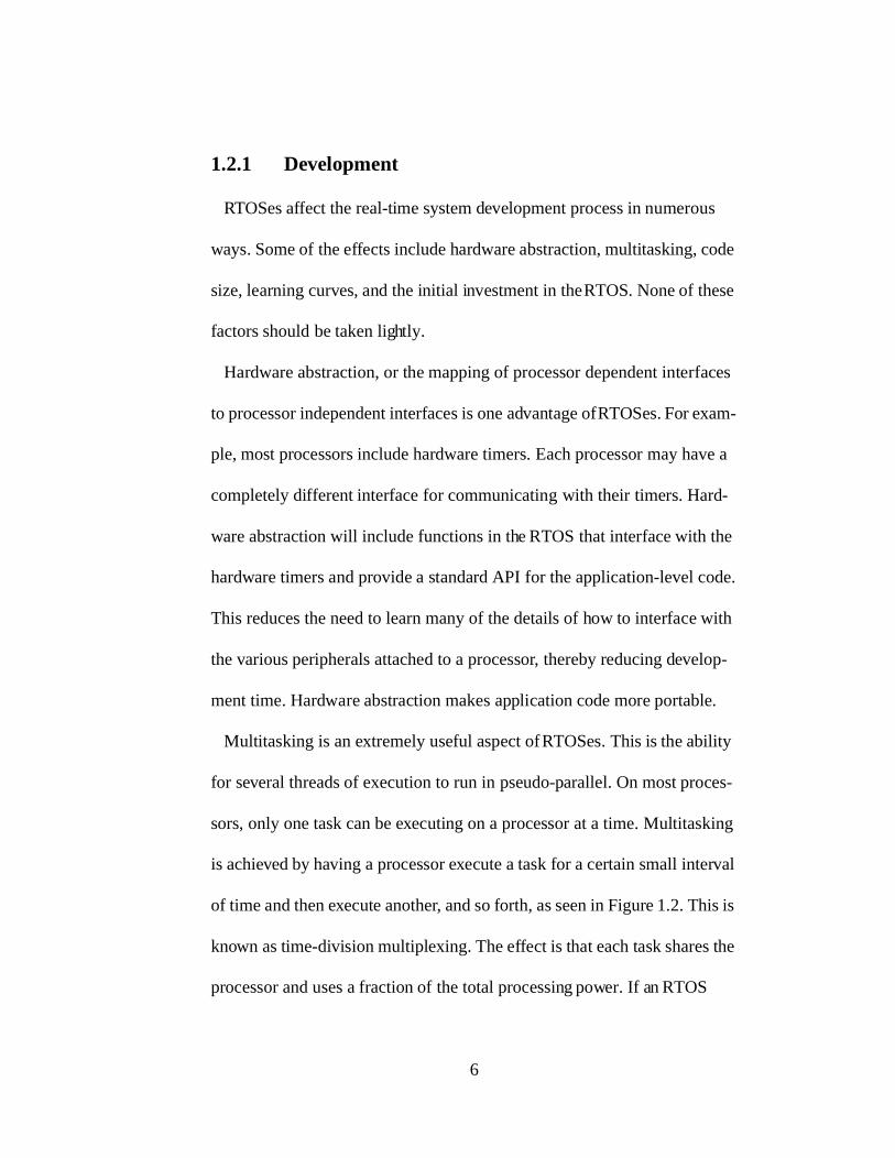
Multitasking is an extremely useful aspect of RTOSes. This is the ability
for several threads of execution to run in pseudo-parallel. On most proces-
sors, only one task can be executing on a processor at a time. Multitasking
is achieved by having a processor execute a task for a certain small interval
of time and then execute another, and so forth, as seen in Figure 1.2. This is
known as time-division multiplexing. The effect is that each task shares the
processor and uses a fraction of the total processing power. If an RTOS
7
supports preemption, then it will be able to stop or preempt a task in the
middle of its execution and begin executing another. Whether or not an
RTOS is preemptive has a large influence on the behavior of the real-time
system. However, in some systems, preemption may cause problems
known as race-conditions, which can lead to data corruption and deadlock.
Fortunately, these problems can be solved with careful software develop-
ment, so they are not a focus of this study. Whether preemption is sup-
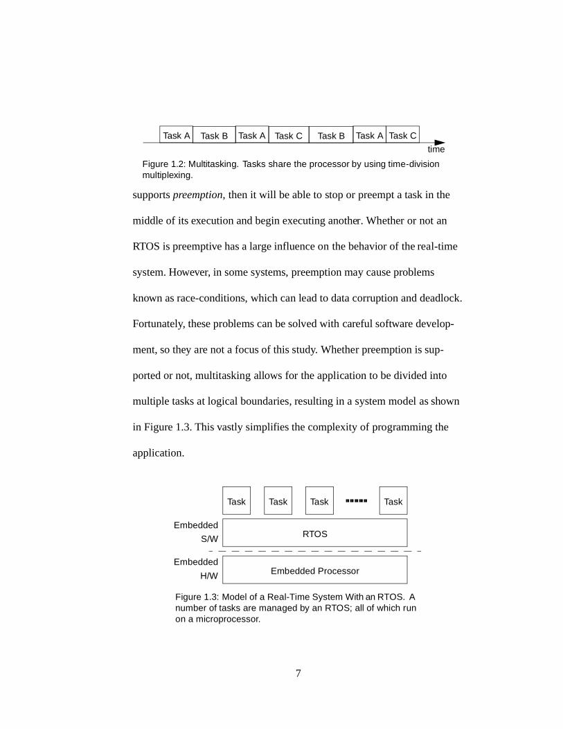
ported or not, multitasking allows for the application to be divided into
multiple tasks at logical boundaries, resulting in a system model as shown
in Figure 1.3. This vastly simplifies the complexity of programming the
application.
Figure 1.2: Multitasking. Tasks share the processor by using time-division multiplexing.
Task A Task CTask ATask A
time
Task BTask B Task C
Task Task Task Task
RTOS
Embedded Processor
Embedded
S/W
Embedded
H/W
Figure 1.3: Model of a Real-Time System With an RTOS. A number of tasks are managed by an RTOS; all of which run on a microprocessor.

8
The code size must be taken into account when developing real-time sys-
tems. RTOSes often introduce quite a bit of code overhead to the system.
Fortunately there are several different RTOSes available with many differ-
ent footprint sizes. Also, there are many RTOSes that are scalable, creating
a variable sized footprint, depending on the amount of functionality
desired.
Unfortunately, there are other overheads associated with RTOSes. There
are several different operating systems, each supporting a limited number
of processors and each with its own API to learn. The learning curve will
increase development time whenever an RTOS is used that the developers
are unfamiliar with. Also, if a proprietary one is used, it must be initially
developed. If it is developed by a third party, it must be paid for, either on a
one-time or per-unit basis.
These factors must each be taken into consideration when choosing an
appropriate RTOS for a given design. Any one of them can have an
extremely significant effect on the development process.
1.2.2 Performance
The use of RTOSes has several drastic effects on the performance of real-
time systems. Namely, they have great influence upon processor utilization,
9
response time, and real-time jitter. All of these issues must be taken into
consideration, before an RTOS is chosen.
The processor utilization refers to the fraction of available processing
power that an application is able to make use of. RTOSes often increase
this fraction by taking advantage of the otherwise wasted time while a task
is waiting for an external event and running other tasks. However, in order
to provide the services available to a particular RTOS, including multitask-
ing, preemption, and numerous others, a processing overhead is introduced.
It is important to note that although this processing overhead may be signif-
icant, the services provided by the RTOS will simplify the application-level
code and reduce the processing power required by the application. This
will make up for some of the RTOS overhead. Also, many RTOSes are
scalable, but they cannot be perfectly optimized for every application with-
out devoting a significant amount of development time to them. In other
words, since most RTOSes are designed to be general-purpose to at least
some degree, they will introduce a processing overhead due to the func-
tions they perform that are suboptimal or unnecessary for the given appli-
cation. This is an unavoidable performance hit.
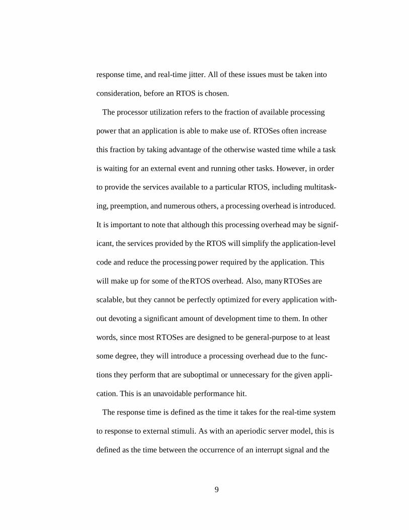
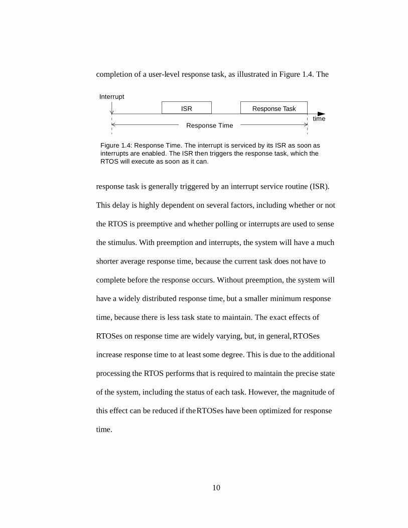
The response time is defined as the time it takes for the real-time system
to response to external stimuli. As with an aperiodic server model, this is
defined as the time between the occurrence of an interrupt signal and the
10
completion of a user-level response task, as illustrated in Figure 1.4. The
response task is generally triggered by an interrupt service routine (ISR).
This delay is highly dependent on several factors, including whether or not
the RTOS is preemptive and whether polling or interrupts are used to sense
the stimulus. With preemption and interrupts, the system will have a much
shorter average response time, because the current task does not have to
complete before the response occurs. Without preemption, the system will
have a widely distributed response time, but a smaller minimum response
time, because there is less task state to maintain. The exact effects of
RTOSes on response time are widely varying, but, in general, RTOSes
increase response time to at least some degree. This is due to the additional
processing the RTOS performs that is required to maintain the precise state
of the system, including the status of each task. However, the magnitude of
this effect can be reduced if the RTOSes have been optimized for response
time.
Interrupt
ISR Response Task
Figure 1.4: Response Time. The interrupt is serviced by its ISR as soon as interrupts are enabled. The ISR then triggers the response task, which the RTOS will execute as soon as it can.
Response Timetime
11
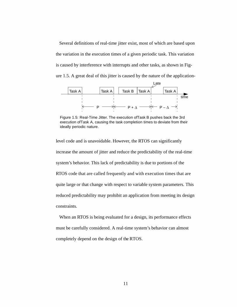
Several definitions of real-time jitter exist, most of which are based upon
the variation in the execution times of a given periodic task. This variation
is caused by interference with interrupts and other tasks, as shown in Fig-
ure 1.5. A great deal of this jitter is caused by the nature of the application-
level code and is unavoidable. However, the RTOS can significantly
increase the amount of jitter and reduce the predictability of the real-time
system’s behavior. This lack of predictability is due to portions of the
RTOS code that are called frequently and with execution times that are
quite large or that change with respect to variable system parameters. This
reduced predictability may prohibit an application from meeting its design
constraints.
When an RTOS is being evaluated for a design, its performance effects
must be carefully considered. A real-time system’s behavior can almost
completely depend on the design of the RTOS.
P P – ∆P + ∆
Task A
Figure 1.5: Real-Time Jitter. The execution of Task B pushes back the 3rd execution of Task A, causing the task completion times to deviate from their ideally periodic nature.
Task ATask ATask A
Late
time
Task B
12
1.3 Addressing the Performance Problem
The negative effects of RTOSes on the performance of real-time systems
can be, in some cases, unacceptable. The drawbacks affecting the develop-
ment process can be quite serious as well. However, they are not absolutely
prohibitive. They can be compensated for in several ways, such as provid-
ing training for the software developers or by increasing the amount of
memory in the hardware design itself. In order to decrease processor over-
head, response time, and real-time jitter, much more significant design
modifications are required. The most straightforward solution would be to
increase the processing power of the system by using a faster processor.
Unfortunately, this may be cost prohibitive or even impossible with the pro-
cessor currently available. Therefore, it would be highly advantageous to
analyze the sources of the decreased performance and formulate a possible
solution.
1.3.1 Bottlenecks within RTOSes
In order to propose a solution to the problem of decreased performance
when using RTOSes, it is necessary to analyze the problem at a finer level
of detail, identify the root of the problem, and characterize its nature. This
analysis has been accomplished in this study by using several techniques,
including: (1) examining traces of the execution of various real-time appli-

13
cations using a sample set of RTOSes, (2) from these traces, observing
which RTOS functions are causing the performance of the system to
degrade, and (3) for each of these functions, determining how often it is
called and for how long it executes. Through this analysis, it has become
apparent that the source of much of the decreased performance can be
traced to a small subset of functions. These functions happen to execute
most of the core operations of RTOSes, namely task scheduling, time man-
agement, and event management. A further analysis of these functions
reveals that they are executed very frequently, that many of them perform
highly inter-related actions, and that these actions exhibit a fundamental
parallelism. However, this parallelism has not been exploited, due to the
inherent limitations associated with implementing the functions completely
in software. This underlying parallelism is the key to solving the problem
of the decreased performance associated with RTOSes. More details on
these bottlenecks can be found in Chapter 2.
1.3.2 Real-Time Task Manager
Using hardware to optimize embedded processors for a specific purpose
is a growing trend for several reasons. Although adding extra hardware
does not come for free, it is becoming less costly. Also, software suffers
from several design constraints, such as the inability to perform a simple

14
operation on an array of data in a constant amount of time. The implemen-
tation of a hardware solution allows for these sometimes severe design con-
straints to be circumvented. By taking advantage of the benefits of a
hardware solution, the RTOS performance problem can be reduced.
Adding hardware has some drawbacks. Not only will it increase the cost
of the initial investment into the design, it, more importantly, leads to
increasing the die area on every processor, thereby increasing the cost for
every unit shipped. And the more complex the hardware is, the more the
cost will be. This increased cost could prevent the manufacturer from keep-
ing up with its competitors. Fortunately, the cost of logic has been dropping
at the fast rate of approximately 25-30% per year [7]. This has significantly
influenced the trend to put more custom hardware on embedded proces-
sors.
The performance improvements of a hardware implementation comes not
only from the optimized logic, but from the elimination of the fundamental
limitations of sequential programming. While software is very efficient at
performing intrinsically sequential operations, it is not able to quickly carry
out many naturally parallel actions. Hardware, however, has almost no lim-
itation on the amount of available parallelism that can be taken advantage
of. For instance, a hardware implementation could determine the maximum
value from a set of N integers in a relatively small constant time. On the
15
other hand, a software implementation would have to serialize this process
by using a loop to compare each value to a running maximum, resulting in
a slow O(N) execution time. This is a limitation of the architecture of mod-
ern microprocessors, which are merely machines that execute lists of rela-
tively simple commands. This makes them highly flexible, but not always
efficient for every task. This software limitation has contributed to the
move towards custom hardware.
One must also consider how often these operations are going to be per-
formed. The performance gain that can occur from moving an operation
from software to hardware is directly dependent upon the frequency at
which the operation is performed. Many of today’s embedded processors
are designed for embedded applications in general. Each application that
uses such a processor may perform a particular operation at completely dif-
ferent frequency. This makes it very difficult to optimize the performance
of a processor for every application. However, there is a trend to build more
application specific processors [23]. These processors are customized for
various application areas, such as video processing, telecommunications,
and encryption. Processor manufacturers can estimate, with more certainty,
the types of operations that applications will be performing on them. This
allows for frequently used functionality to be put in hardware, which is
16
another reason why it is more common to see custom hardware in modern
processors.
These factors and the nature of the causes of RTOS performance loss sug-
gest that RTOSes would greatly benefit from a custom hardware solution.
This is the motivation for the Real-Time Task Manager (RTM), a hardware
module designed to optimize task scheduling, time management, and event
management—the main sources of performance loss in real-time operating
systems. The RTM is designed to be an extension to the processor that
makes several common functions available in more efficient hardware
implementations, for an RTOS to take advantage of. The RTM is also
designed to be compatible with as many RTOSes as possible, not with just
a select few. It is intended to reduce the common problems associated with
RTOSes—increased processor overhead, response-time, and real-time jit-
ter. The details of the RTM are located in Chapter 3.
The effectiveness of the RTM has been determined in a formal manner.
Measurements have been taken of the performance impact of the RTM, by
analyzing accurate models of realistic real-time systems. These measure-
ments show that processor utilization is reduced by up to 90%, maximum
response time by up to 81%, and maximum real-time jitter by up to 66%.
17
1.4 Overview
The remainder of this thesis is organized into several chapters. In Chapter
2, an analysis of the performance bottlenecks for real-time operating sys-
tems is presented. In Chapter 3, the behavior and architecture of the Real-
Time Task Manager is described. In Chapter 4, the experimental method is
fully detailed. In Chapter 5, the experimental results are presented and ana-
lyzed. In Chapter 6, related work is explained. Finally, in Chapter 7, the
RTM is summarized and future work is highlighted.

18
CHAPTER 2
BOTTLENECKS IN REAL-TIME OPERATING SYSTEMS
Real-time operating systems do have several advantages, but they can
also have significant negative effects on sensitive performance issues,
including processor utilization, response time, and real-time jitter. These
weaknesses may lead to serious problems in the design of real-time sys-
tems. Therefore, it would be beneficial to reduce or eliminate them. In
order to accomplish this, a complete analysis of the causes of these weak-
nesses is necessary. It has been determined that these causes are primarily
isolated to three key areas: task scheduling, time management, and event
management.
To better understand what these bottlenecks are, it is necessary to intro-
duce a few key concepts. Every RTOS maintains a list in some sort of data
structure, with one task per entry, known as the task control block (TCB)
list. Most or all of the information that an RTOS has about each task is
located in this list. For the most part, each task is in one of a few different
states at any given time: ready, waiting for time to elapse, or waiting for
interprocess communication. On a uniprocessor system, only one task can

19
be executing at any given time. One of the core components of an RTOS is
the task scheduler, whose purpose is to determine which of the ready tasks
should be executing. If there are no ready tasks at a given time, then no task
can be executed, and the system must remain idle until a task becomes
ready. Another central part of an RTOS is keeping track of time. Time man-
agement is the part of the RTOS that precisely determines when those tasks
waiting for time to elapse have finished waiting, therefore becoming ready
tasks. Precise and accurate timing is crucial to the most common type of
task in real-time systems—periodic tasks. Finally, interprocess communi-
cation is a powerful capability present in every true RTOS. IPC allows for
the details of communication amongst tasks to be passed to the scheduler.
This provides a clean interface between tasks that allows them to effec-
tively sleep until their desired synchronization events or data arrive. With-
out IPC, the software development required to guarantee logical accuracy
in an application implementation would be far more difficult, if not impos-
sible. A necessary part of IPC, called event management, can be a severe
performance hindrance. All three of these major components of RTOSes
cause performance limitations.
The remainder of this chapter will present analyses of these bottlenecks.
The RTOS components, along with any necessary background information,
will be described in detail. Then they will be characterized in terms of the
20
complexity of the operations that implement them and the frequency at
which these operations are performed. Finally, the effects of these charac-
teristics on the processor utilization, response time, and real-time jitter will
be presented.
2.1 Task Scheduling
One of the most highly researched topics in RTOS design is task schedul-
ing [17]. This is defined as the assignment of tasks to the available proces-
sors in a system [13]. In other words, it is the process of determining which
task should be running on each processor at any given time. In general, a
real-time system may include several microprocessors, however, the
remainder of this analysis will assume a uniprocessor system. Scheduling
is a very broad subject that needs to be described in detail.
There are many different types of task scheduling. The three most com-
mon types are clock-driven, round-robin, and priority-driven. Clock-driven
schedulers use precomputed static schedules indicating which tasks to run
at specific predetermined time instants. This scheduling algorithm mini-
mizes run-time overhead. Round-robin schedulers continuously cycle
through all ready tasks, executing each one for a predetermined amount of
time. This basic algorithm is easy to implement and fair, in terms of the
amount of processing time allotted to each task. Priority-driven schedulers

21
require that each task has an associated priority level. The scheduler always
executes a ready-to-run task with the highest priority. This is the most com-
mon form of task scheduling in real-time systems and will be the scheme
targeted for the remainder of this analysis.
Priority-driven scheduling can be further sub-classified into static and
dynamic priority categories. Static priority scheduling means that the prior-
ity of each task is assigned at designed time and remains constant. The
most common method of determining the static priority to assign to each
task is the rate-monotonic algorithm (RMA) [12], in which a periodic
task’s priority is proportional to the rate at which it is executed. Conversely,
dynamic priority schedulers are those that change the priorities of tasks
during run-time. A well-known dynamic-priority scheduling scheme is the
earliest deadline first (EDF) algorithm [12], in which task priorities are
proportional to the proximity of their deadlines. Dynamic priority schedul-
ing can result in a greater utilization of the processor; however, it intro-
duces a larger computational overhead and less predictable results. In fact,
many of the most popular commercial RTOSes use static-priority schedul-
ing and do not provide sufficient support for dynamic priority scheduling
[13]. The remainder of this study only deals with systems that use static
priority scheduling.

22
The complexity of static priority scheduling, as with many operations,
varies widely with the exact implementation. There are many possible
implementations for this type of task scheduling. The brute force way is to
walk through the TCB list and find the task with the highest priority that is
ready-to-run. The complexity of this method scales linearly with the num-
ber of tasks. An obvious improvement would be to keep a separate list of
just the tasks that are ready-to-run, sorted by their priorities. However, this
improvement just moves the complexity of walking through the list to
inserting tasks into the sorted list. In the case where all tasks have a unique
priority, an innovative optimization is to maintain a bit-vector in which
each bit indicates whether the task with a specific priority is ready or not,
as illustrated in Figure 2.1. By associating the bit position with the priority,
the highest priority ready task can be determined by calculating the least
Figure 2.1: Bit-Vector Scheduling Example. Each bit indicates whether or not the task with that priority is ready, where a 1 means ready and a 0 means not ready. In this example of an 8-bit bit-vector, the tasks with priorities 1, 3, 4, and 7 are ready. By determining the least significant bit that is set to one in the bit-vector, the highest priority ready task will be found, which, in this case, is the task with priority 1.
0101 1001
0124 3567

23
significant bit that is set high [9]. This can be done in constant time, if the
processor has a count-leading-zeros instruction, or by using a lookup table.
However, the size of a lookup table scales exponentially with the maximum
number of tasks allowed in the system. Static priority task scheduling may
be simpler than dynamic priority scheduling, but it is still a non-trivial task.
The frequency that the task scheduler is invoked can be quite high. The
scheduler is initiated when the application makes various system calls that
change the status of a task, such as creating and deleting tasks, changing
task priorities, delaying a task, and initiating interprocess communication.
Nothing can be said in general about the rate at which these calls occur,
except that it depends only upon how much the application uses them.
Other situations in which the scheduler is initiated depend upon whether or
not the RTOS supports preemption. For a preemptive RTOS, after every
interrupt, including the timer tick interrupt, the scheduler is initiated. This
allows for a newly readied task to preempt the currently executing one.
This component of the scheduling frequency scales linearly with the fre-
quency of the timer tick interrupt, as well as with that of all other inter-
rupts. For non-preemptive RTOSes, scheduling occurs at specified
scheduling points within the task, as well as after every interrupt that
occurs during time intervals when the processor is idle. Because the sched-
uling behavior of non-preemptive systems depends on whether or not the

24
system is idle, this component of the scheduling frequency scales partially
with the frequency of the interrupts and partially with the frequency at
which scheduling points are reached. The frequency that task scheduling is
performed can become quite large.
The scheduling functions performed by an RTOS cause the real-time jit-
ter of the system to be increased in all but the simplest applications. The
more frequently the scheduler is invoked, the more frequently real-time jit-
ter will be higher. So as any of the previously mentioned factors increase
the scheduling frequency, the average jitter will increase too. Any differ-
ences in the processing time required to perform scheduling will add to the
real-time jitter that the tasks will experience. This processing time may
increase linearly with the number of tasks, causing the real-time jitter to do
the same. If the number of tasks in the system is not known ahead of time,
this will amplify the problem by adding uncertainty to what one can say
about how much jitter the real-time system will exhibit. This increased and
less predictable jitter may be unacceptable for a given real-time applica-
tion.
The effects of scheduling on response time depend heavily upon whether
or not the RTOS is preemptive. When an aperiodic interrupt occurs and
schedules a task, a portion of the response time is equal to the time it takes
to schedule the task. Again, this may vary with the number of tasks, possi-
25
bly adding to the lack of predictability of the response time of the system.
However, this is only a portion of the response time. When an aperiodic
interrupt occurs during the execution of a critical section of code, interrupts
will be disabled and it will not be serviced right away, thus adding to
response time. Most of the core functions of the RTOS, including task
scheduling, require interrupts to be disabled, so as to prevent the system
from entering an invalid state. Therefore, the longest time that it takes to
perform task scheduling or any other critical section of code adds to the
maximum response time; and the longer and more frequent that they take in
general, the greater the average response times will be. For preemptive sys-
tems, these are the only effects of scheduling on the response time. There-
fore, because the time it takes to perform task scheduling may scale
linearly with the number of tasks, the response time may do the same for
preemptive systems.
For non-preemptive systems, there may be another component to the
response time. This additional component is not present when the proces-
sor is idle. It is only encountered when the processor is executing a task. It
is a result of the fact that the system must reach a scheduling point before
the response task can run. So the length of the periods in between schedul-
ing points greatly influence the response time for the non-preemptive case.
Because these periods between scheduling points are usually much longer

26
than the duration of critical sections and much longer than the time it takes
to perform task scheduling, they dominate the response time when they are
encountered. Thus the response time for interrupts that occur when the pro-
cessor is executing a task in a non-preemptive system is generally not
affected by task scheduling. When the processor is idle, however, the
response time of a non-preemptive system has the same characteristics as a
preemptive one. Overall, the increase and lack of predictability in the
response time can exceed the tolerance of the application.
Additionally, an overall performance hit is incurred simply because per-
forming task scheduling consumes processing time. The processor utiliza-
tion of the RTOS due to task scheduling is proportional to both the
frequency and complexity of the scheduling. Since both of these compo-
nents may increase linearly with the number of tasks, there may be a qua-
dratic relationship between the number of tasks in the system and the
processor utilization due to task scheduling. This overhead can quickly get
out of hand and cause the system to slow down significantly.
It is quite clear that task scheduling is a bottleneck to the performance of
RTOSes. The potentially high complexity and frequency of task scheduling
are the underlying causes of the bottleneck. The result is reduced predict-
ability, in terms of real-time jitter and response time, as well as increased

27
processing overhead. It is for these reasons that task scheduling is an
important factor in RTOS design.
2.2 Time Management
One of the defining characteristics of an RTOS is its ability to accurately
and precisely keep track of time. For the remainder of this analysis, time
management will be used to refer to the RTOS’s ability to allow tasks to be
scheduled at specific times. This is achieved by having the tasks block for a
specific amount of time, after which they will become ready-to-run. The
issues involved with time management must be described in detail in order
to understand why it is a bottleneck.
The need for timing services comes from the fundamental nature of real-
time systems. As previously mentioned, the success or failure of a real-time
system is not only based on the logical correctness of its output, but its abil-
ity to satisfy its predetermined timing requirements. To elaborate, the basic
model for a real-time system includes a collection of tasks, each of which is
assigned pairs of release times and deadlines [13]. A release time denotes
the earliest moment at which a task is allowed to start a calculation. Like-
wise, a deadline is the latest time at which a task is allowed to finish the
calculation. Each release time is associated with a deadline, the two of
which denote a timing constraint. Tasks may have several pairs of release
28
times and deadlines, as in the case of periodic tasks. In all cases, it is the
job of the RTOS’s time manager to ensure that all timing constraints are
met. This is not always a simple undertaking.
There are several requirements for an RTOS to implement time manage-
ment. First of all, there needs to be some sort of hardware that provides a
means to accurately keep track of time. This could be in the form of an
external real-time clock that interfaces with the processor. The most com-
mon scenario is that the processor has one or more internal hardware tim-
ers. Whatever the case, the timing device needs to provide some way of
communicating to the software how much time has elapsed. This may be
done by allowing the RTOS to read a counter register from the device.
More commonly, the timer can be programmed to trigger precise periodic
interrupts. These interrupts let the RTOS know that one clock tick (not to be
confused with the CPU’s clock) has elapsed. Timer interrupts are necessary
for preemptive RTOSes, because there needs to be some way of stopping a
task from running in the middle of its execution. It would be impossible to
service a clock tick interrupt every clock cycle, so the timer is programmed
with a much larger period, on the order of hundreds of microseconds to
milliseconds [13]. The period of the clock tick is an RTOS parameter that
determines the resolution or granularity at which it has a sense of time. If
the granularity is increased, the application will have more flexibility with
29
the scheduling patterns of its tasks. Most real-time applications require a
high level of clock tick resolution. All modern methods of implementing
time management are based upon this basic model.
Like task scheduling, the complexity of the time manager also depends
upon how it is implemented. One method that is used is to maintain a
counter for each entry in the TCB list that indicates the number of timer
interrupts to wait until that task should become ready-to-run. Whenever a
clock tick is processed, the TCB list must be traversed and the counter for
each task that is waiting for its next release time must be decremented.
When a counter reaches zero, then the task status is set to ready-to-run. The
complexity of this method scales linearly with the number of tasks and can
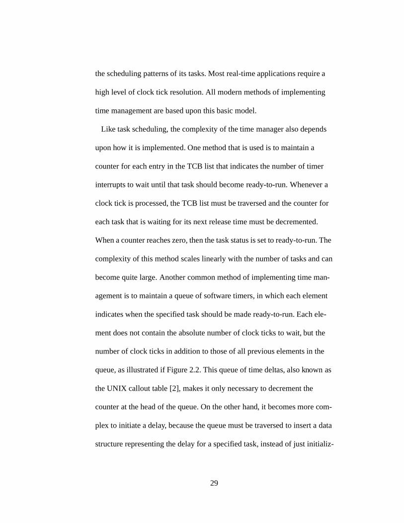
become quite large. Another common method of implementing time man-
agement is to maintain a queue of software timers, in which each element
indicates when the specified task should be made ready-to-run. Each ele-
ment does not contain the absolute number of clock ticks to wait, but the
number of clock ticks in addition to those of all previous elements in the
queue, as illustrated if Figure 2.2. This queue of time deltas, also known as
the UNIX callout table [2], makes it only necessary to decrement the
counter at the head of the queue. On the other hand, it becomes more com-
plex to initiate a delay, because the queue must be traversed to insert a data
structure representing the delay for a specified task, instead of just initializ-

30
ing a counter. Also, the maximum amount of time that it takes to process a
clock tick is not constant, because there may be entries in the queue with a
time delta of zero, meaning that they should be made ready-to-run at the
same clock tick as the previous task in the queue. This results in a nonde-
terministic amount of time to complete this operation. Unfortunately, there
is no great way to implement time management in software alone.
The rate at which RTOS time-keeping operations are performed can
become extremely high. Exactly when they are performed depends entirely
upon whether or not the RTOS supports preemption. By definition, pre-
emptive systems allow for higher priority tasks that become ready to pre-
empt or stop the execution of lower priority tasks. Consider a scenario in
which a low priority task is running when a high priority task is waiting for
one clock tick to elapse. When the next clock tick interrupt occurs, a pre-
A3
B
0
C
1
D
2
(a)time
A, B C D
(b)
now
Figure 2.2: Software Timer Queue Example. a) In this example, tasks A and B will be released after three clock ticks, task C will be released after four clock ticks, and task D will be released after six clock ticks. b) Each queue entry indicates the task to release and the number of additional clock ticks to wait.

31
emptive RTOS should be able to perform a context switch and execute the
high priority task. Therefore, preemptive RTOSes must perform all time
management operations in the clock tick interrupt handler. So the fre-
quency that the time management operations are executed is equal to the
granularity of the clock tick. This can become extremely expensive,
because many real-time applications require a very high level of granular-
ity. Alternatively, a non-preemptive RTOS does not need to determine
which task to run next until the currently executing task reaches a task
scheduling point. Therefore, the clock tick interrupt handler for non-pre-
emptive RTOSes only needs to increment a counter. The RTOS must then
process all the new clock ticks that have elapsed when a task scheduling
point is reached. An exception to this rule is when the processor is idle,
during which the RTOS needs to process every clock tick interrupt immedi-
ately. In the non-preemptive case, the frequency of the time management
operations scales with both the frequency of the interrupts and the fre-
quency at which scheduling points are reached. Although the time monu-
ment operations are less frequent for non-preemptive RTOSes, they still
occur quite often.
The time management operations that RTOSes need to execute in the
background negatively affect the real-time jitter of the system. Increased
jitter is inevitable due to the fact that the amount of time that it takes to per-

32
form any software implementation of the time-keeping operations varies
with the system state. If, for example, a software timer queue is used, the
amount of time that it takes to insert an entry into the queue depends upon
how many tasks have entries already in the queue, and what their time del-
tas are. Also, whether software timers are used or not, the time it takes to
process a clock tick is nondeterministic because the number of tasks that
will become ready-to-run due to each clock tick depends upon the number
of tasks to schedule each tick. Unfortunately, this type of information is
generally not predetermined, so few guarantees can be made about the
amount of real-time jitter a system will experience. The nature of the afore-
mentioned complexity of the time management operations cause the mag-
nitude of the real-time jitter to increase linearly with the number of tasks in
the system when time-keeping operations interrupt task executions. Simi-
larly, the frequency of this increased real-time jitter increase linearly with
the frequency of the time management operations, mentioned above. These
effects may cause the system to fail to meet the timing constraints of the
application.
Like task scheduling, the effects of time management on response time
depend heavily on whether or not the RTOS is preemptive. As described in
section 2.1, the response time for non-preemptive systems when the pro-
cessor is executing a task is dominated by the lengths of the intervals

33
between scheduling points. Thus, as with scheduling, time management
generally does not significantly affect the response time for interrupts that
occur during the execution of a task in non-preemptive systems. For the
preemptive case, however, time management operations do have a consid-
erable effect. There are only two scenarios in which time-keeping opera-
tions affect the response time in preemptive systems: (1) responses to
interrupts that occur during the execution of these operations are delayed,
because interrupts are disabled throughout their execution; and (2) clock
tick interrupts that occur just after the occurrence of another interrupt delay
the corresponding response, because clock tick interrupts have higher pri-
ority. In either case, the response time is increased by part or all of the time
taken to perform the time-keeping operation. Because the time needed to
perform this operation increases linearly with the number of tasks in the
system, so does the response time, for preemptive RTOSes. Also with a
preemptive system, the higher the clock tick granularity, the more often
these cases will occur. In fact, time management is often the dominant fac-
tor in response time delay for such systems.
As with all RTOS operations, a performance overhead is introduced
because of the processing time used to execute time-keeping operations.
The processor utilization of the RTOS due to time management is propor-
tional to both the frequency and complexity of the operations that imple-
34
ment it. Because all implementations of time management operations
traverse a list, the complexity always increases linearly with the number of
tasks. Furthermore, increasing the clock tick granularity increases the fre-
quency. These factors can easily cause the overhead to become too much
for the system to handle.
Time management is definitely a bottleneck to the performance of
RTOSes. The particularly high frequency and complexity of time-keeping
operations are the underlying causes of the bottleneck. As with task sched-
uling, time management results in reduced predictability, in terms of real-
time jitter and response time, as well as increased processing overhead.
Therefore, the efficiency of the time management implementation is a key
element of every RTOS’s performance.
2.3 Event Management
Most real-time operating systems today integrate communication and
synchronization between tasks—known as interprocess communication
(IPC)—into the RTOS itself. Such services often include support for sema-
phores, message queues, and shared memory. This allows for the applica-
tion development to be simplified and for the scheduler to make better
decisions about which task to run. Applications access these integrated ser-
vices through the RTOS’s API. A major component of IPC involves keep-

35
ing track of which tasks are waiting for IPC and determining which tasks
should accept IPC. This component of IPC is referred to in this analysis as
event management. Although RTOS support for IPC has numerous advan-
tages, event management may become a hindrance to the performance of
the system. The factors which cause this performance loss must be charac-
terized, if a solution is to be proposed.
Most services categorized as IPC perform event management. This RTOS
operation is what mediates access to resources. This is done when tasks
make requests for access to resources and, conversely, when tasks release
access to resources. The request may not be fulfilled immediately, in which
case the task is said to block, or wait for the requested resource to become
available. The scheduler has knowledge of which tasks are blocked and
does not consider those tasks for execution; when a task blocks, another
task will be executed. When a resource does become available, it is
released, or made accessible to any tasks that may be blocking on it. If
tasks were blocked while waiting for this particular resource, the one such
task with the highest priority is unblocked and will again be considered for
execution by the scheduler. If the priority of the recently unblocked task is
higher than the priority of the currently executing task, a context switch
will occur, and the unblocked task will resume execution. Most RTOSes
use this model of event management.

36
Again, the complexity of the event management operations depends com-
pletely upon the implementation. One approach is to include an event iden-
tifier field in the TCB of each task that indicates what specific resource the
task is blocking on, if any. When a task blocks, this field is simply written
with the appropriate identifier, and the task status is set to indicate that the
task is pending on IPC. This operation can be performed in a relatively
small constant time. However, when the resource is released, the entire
TCB list must be traversed to find the task with the highest priority that is
pending on IPC and has the corresponding event identifier in its TCB. This
operation scales linearly with the number of tasks in the system. Another
method is to maintain a data structure for each resource that requires IPC
services, and include in this data structure a list of all tasks pending on the
corresponding resource, sorted by task priorities. This would eliminate the
need to traverse the list on a release, since the task at the head of the list
will always be the one chosen to be unblocked. However, this just moves
the complexity from unblocking a task to blocking it, because the task list
would still have to be traversed during a block to keep it sorted by priority.
Also like with task scheduling, the task list could be implemented as a bit
vector. This optimization makes the operation take a constant amount of
time to complete, however, it may still be large enough to cause significant

37
performance loss. Whatever the implementation, the complexity may make
event management too much for the system to handle.
These event management operations may occur very frequently in some
applications. However, the only times that they actually do occur are when
a task explicitly calls an IPC function. The frequency at which tasks make
these function calls depends completely upon the application. Therefore,
the only general statement that can be made about the frequency of event
management operations is that the rate at which application makes use of
IPC completely determines the frequency of event management operations.
Some applications may use none, while others may use so much IPC that
event management becomes the major source of RTOS performance loss.
Because IPC can become used often in some cases, it is important to ana-
lyze the effects of event management.
Real-time jitter may be considerably increased because of the event man-
agement operations. Since the amount that IPC is used depends completely
upon the application, the extent to which event management contributes to
jitter is heavily reliant upon the application as well. However, the relation-
ship between the complexity of event management operations and the num-
ber of tasks in the system also influences this source of jitter. In the case of
this relationship being linear, the amount of jitter due to event management
will also increase linearly with the number of tasks. Therefore, the
38
increased real-time jitter due to event management may also cause the tim-
ing constraints not to be met.
As with the previous bottlenecks, whether or not the RTOS is preemptive
drastically changes the effects of event management on response time. As
with task scheduling and time management, event management generally
does not affect the response time for non-preemptive systems when the pro-
cessor is executing a task. Again, this is because the lengths of the intervals
between task scheduling points dominate the response time. However,
assuming the application makes use of IPC, event management will affect
the response time for preemptive systems. In such systems, event manage-
ment operations affect response time when an interrupts occurs and these
operations are executing. This is because event management operations are
critical sections; so they disable interrupts and there is no response until
interrupts are re-enabled. Therefore, the average response time is increased
by a fraction of the time taken to perform the event management operation.
The time it takes to complete this operation may increase linearly with the
number of tasks in the system, so the response time may as well. If this
operation is constant, the response time will be more predictable, but it will
still be increased. The response time may become unacceptable in systems
that heavily use IPC.
39
Once again, a performance overhead is introduced because of the pro-
cessing time used to perform event management operations. The processor
utilization of the RTOS due to event management is proportional to both
the frequency and complexity of the operations that implement it. The
complexity may increase linearly with the number of tasks. More impor-
tantly, the processor utilization is extremely dependent upon the extent to
which the application uses IPC. Therefore, depending on how event man-
agement is implemented and how much the application uses IPC, the pro-
cessor utilization due to event management can become quite high.
Event management may definitely be an RTOS performance bottleneck.
This is because many applications use a great deal of IPC, and event man-
agement can be a costly operation. The effects are, again, reduced predict-
ability, in terms of real-time jitter and response time, as well as increased
processing overhead. Consequently, quick and efficient event management
mechanisms are necessary to minimize performance loss due to the RTOS.
Task scheduling, time management, and event management are all
sources of performance loss due to RTOSes. Reducing the effects of these
bottlenecks would increase the determinism and processing power of the
real-time system. This would allow developers to benefit from the advan-

40
tages inherent in using a real-time operating system, such as reduced devel-
opment time, without suffering from too great a performance loss.
41
CHAPTER 3
REAL-TIME TASK MANAGER
The performance loss associated with using an RTOS in a real-time sys-
tem is unacceptable. What is needed is a new approach that would drasti-
cally reduce these negative performance side effects. This is the purpose of
the Real-Time Task Manager (RTM). In order to achieve its goal, the RTM
must increase the predictability and usable processing power of systems
using RTOSes. As is described in Section 3.1, the RTM is able to do this by
adding architectural support for some of the RTOS functionality to the pro-
cessor. There are, however, other factors that need to be taken into consid-
eration before the exact design is finalized.
There are numerous RTOSes available in today’s embedded market, each
of which has widely varying characteristics and implementations. If the
RTM is to be successful, it must be compatible with most, if not all of
them. Otherwise, processor manufacturers would be limiting the amount of
interest in the RTM; and it would not be worth their time and money to
integrate it into their products. This imposes the requirement that the RTM
must be robust enough to be beneficial to as many RTOSes as possible.
42
Also, if the RTM requires too much change to the real-time system, it
will not be useful. This is due to the costs associated with the initial proces-
sor and RTOS development, as well as the increased die area. Also, an
excessively sophisticated design may require so much logic that it would be
impractical to implement. Although the RTM requires some additions to
the processor architecture and some changes to the RTOS software, they
must be kept as minimal as possible.
Unfortunately, the performance loss problem cannot be completely
solved. As described in Chapter 2, the bottlenecks are caused by both the
complexity of a few basic RTOS operations and the frequency at which
they are executed. The complexity may be optimized, however, the fre-
quency cannot be reduced at all. To do so would mean significantly chang-
ing the RTOS. Therefore, the RTM must be completely focused on
minimizing the processing time of each basic RTOS operation.
Taking these issues into consideration, the RTM intends to reduce the
performance loss associated with using an RTOS. This would remove a
major limitation associated with RTOSes, allowing more real-time systems
to take advantage of their benefits. The remainder of this chapter will
describe the design and architecture of the RTM.

43
3.1 Design
The RTM is a hardware module that implements the key RTOS opera-
tions that are performance bottlenecks: task scheduling, time management,
and event management. Because it is not restricted by the processor’s
instruction set, as with software algorithms, it is able to exploit the intrinsic
parallelism in these RTOS operations with custom hardware. This allows
for the RTM to perform these operations in a trivial and constant amount of
time. Because these operations are underlying causes of RTOS perfor-
mance loss, the RTM will significantly reduce this problem.
Before the details of the functions performed by the RTM are described,
it is important to understand its software interface. Not unlike an L1 cache,
the RTM resides in the same chip as the processor and interfaces directly
with the processor core. The RTM communicates with the core with a
memory-mapped interface using the address and data buses. In fact, the
RTM is an internal peripheral, like an internal hardware timer, so its inter-
face is the same as other internal devices. The purpose of this is to help
keep the development cost down, which is necessary for the RTM to be
successful.
To perform its functions, the RTM needs to maintain its own internal data
structure. This data structure, illustrated in Figure 3.1, contains all the
information it needs to perform the RTOS operations. It consists of a small
44
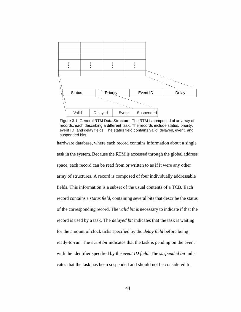
hardware database, where each record contains information about a single
task in the system. Because the RTM is accessed through the global address
space, each record can be read from or written to as if it were any other
array of structures. A record is composed of four individually addressable
fields. This information is a subset of the usual contents of a TCB. Each
record contains a status field, containing several bits that describe the status
of the corresponding record. The valid bit is necessary to indicate if that the
record is used by a task. The delayed bit indicates that the task is waiting
for the amount of clock ticks specified by the delay field before being
ready-to-run. The event bit indicates that the task is pending on the event
with the identifier specified by the event ID field. The suspended bit indi-
cates that the task has been suspended and should not be considered for
Status Priority Event ID Delay
Valid Delayed Event Suspended
Figure 3.1: General RTM Data Structure. The RTM is composed of an array of records, each describing a different task. The records include status, priority, event ID, and delay fields. The status field contains valid, delayed, event, and suspended bits.

45
scheduling until this bit is cleared. If the valid bit is set, but the delayed,
event, and suspended bits are clear, then the task is ready-to-run. Finally,
the priority field indicates the task’s priority. Also, the maximum number
of records is some fixed constant, such as 64 or 256. Therefore, this is the
maximum number of tasks that the RTM can handle. This maximum
should be set high enough to accommodate any practical number of tasks
for a given processor, or the RTM will not be useful. This data structure
allows the RTM to easily implement the RTOS operations.
The RTM implements priority-driven scheduling by performing a calcu-
lation on its internal data structure. Although the priorities of each task can
be changed by the software, it is not done automatically by the RTM.
Therefore, the RTM fully implements static-priority scheduling, but it does
not determine the priority to assign to each task for dynamic-priority
scheduling. The RTM is able to query its data for the highest priority ready
task. The result is returned to the RTOS when it reads a memory-mapped
register from the RTM. This calculation is completed by comparing, in par-
allel, the priority fields of every record for which the status field indicates
that the task is ready-to-run; and, in doing so, determining which has the
highest priority. This calculation can be done when the RTOS requests the
index of the highest priority ready task. However, if this query takes several
cycles to compute, the RTOS would have to remain idle while it waits for

46
the result. On the other hand, it can also be done whenever a change is
made to the task status or priority; and the result can be stored for any
future queries. This would allow the query to take several cycles without
stalling the RTOS, unless a query is made before the result is ready. So long
as the delay is not too great, most RTOSes can easily be written to avoid
this situation.
Time management is somewhat similar to implement, because there are
no interdependencies amongst records. It is performed when the RTOS
processes clock ticks. The RTOS may process multiple clock ticks that
have accumulated over a period of time, as is the case with non-preemptive
systems. Therefore, the RTOS must write to a control register that indicates
the number of ticks. The RTM then decrements the delay fields of all
records by the given number of ticks. For every record in which the delay
field is then less than or equal to zero, its delayed bit is cleared. This rela-
tively simple operation takes much longer to perform in a software.
Event management is very similar to static-priority scheduling. Instead of
querying its data structure for the highest priority ready task, it queries for
the highest priority task that is pending on a given event identifier. In other
words, the calculation is made by comparing, in parallel, the priority fields
of every record for which the status field indicates that the task is pending
on an event and that the event identifier matches the given one; and, in

47
doing so, determining which has the highest priority. This operation
requires that the event identifier is written to a control register before the
calculation can be made. Therefore, before the index of the unblocked task
is read back from the RTM, the RTOS has to remain idle for however many
cycles it takes to perform the calculation. Fortunately this delay will be
small or zero if the limit on the number of tasks is reasonable.
The RTM is designed to reduce the performance loss associated with
using an RTOS. Because it is not affected by the restrictions of software,
the RTM is able to perform each of task scheduling, time management, and
event management in a small constant time. Because these operations are
the main sources of RTOS performance loss, the RTM will achieve its goal.
3.2 Architecture
It is of fundamental importance that the RTM is not so complicated that it
is impractical or impossible to implement in real hardware. For this reason,
a reference architecture is presented here. It should be noted that this refer-
ence design has not been optimized. It is merely presented to illustrate the
complexity and scalability of implementing the hardware architecture of
the RTM. Estimations are given of the amount of hardware components
necessary for the storage elements themselves, as well as the combinational
logic that implements the RTOS operations.
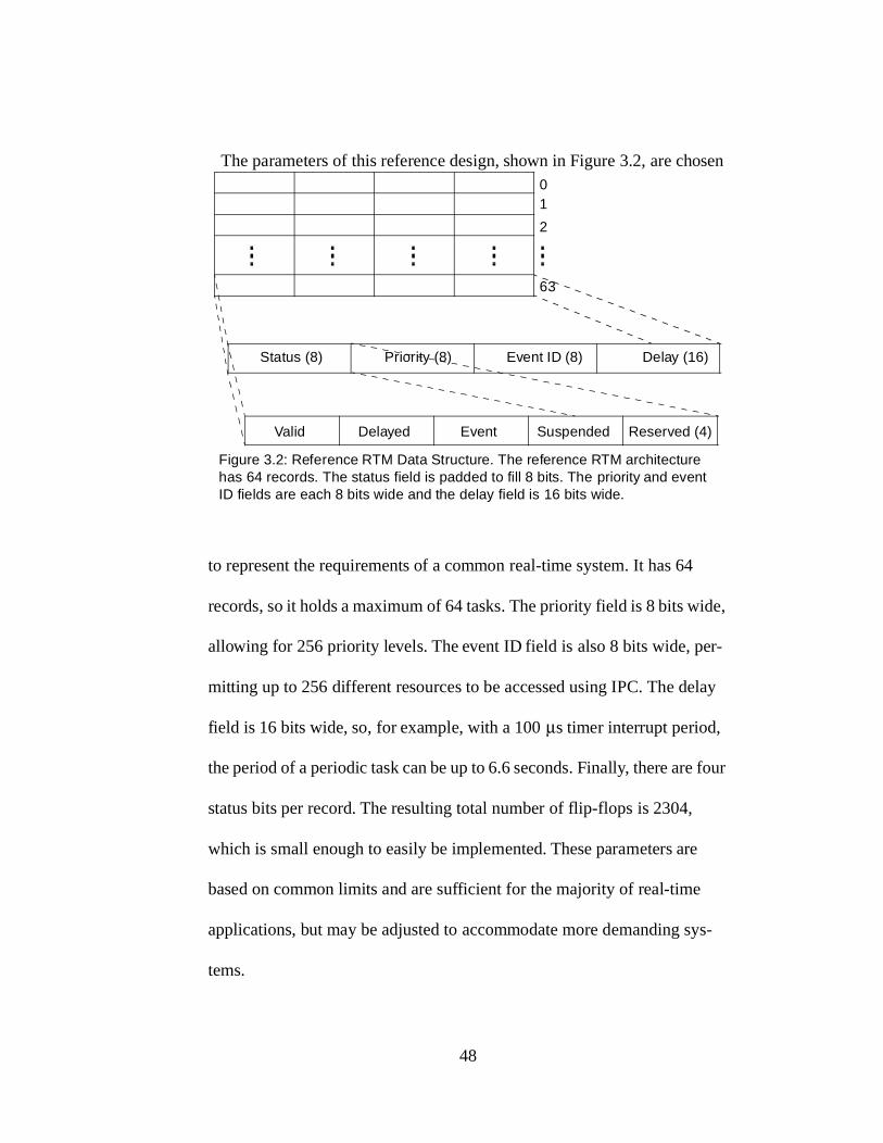
48
The parameters of this reference design, shown in Figure 3.2, are chosen
to represent the requirements of a common real-time system. It has 64
records, so it holds a maximum of 64 tasks. The priority field is 8 bits wide,
allowing for 256 priority levels. The event ID field is also 8 bits wide, per-
mitting up to 256 different resources to be accessed using IPC. The delay
field is 16 bits wide, so, for example, with a 100 µs timer interrupt period,
the period of a periodic task can be up to 6.6 seconds. Finally, there are four
status bits per record. The resulting total number of flip-flops is 2304,
which is small enough to easily be implemented. These parameters are
based on common limits and are sufficient for the majority of real-time
applications, but may be adjusted to accommodate more demanding sys-
tems.
Status (8) Priority (8) Event ID (8) Delay (16)
Valid Delayed Event Suspended
Figure 3.2: Reference RTM Data Structure. The reference RTM architecture has 64 records. The status field is padded to fill 8 bits. The priority and event ID fields are each 8 bits wide and the delay field is 16 bits wide.
Reserved (4)
01
2
63

49
Task scheduling is somewhat more complicated. It is performed using 64
ready-test cells and a binary tree of 63 priority-test cells, as shown in Fig-
ure 3.3. The ready-test cells simply determine which tasks are ready-to-run
with three inverters and an AND gate. Each priority-test cell determines the
highest priority ready task, based upon the two task priority and ready
inputs. Each priority-test cell also indicates whether or not either of the two
input tasks are ready. These cells then output the priority and index of the
highest priority ready task, if any, as well as whether or not there is such a
task. The first order priority-test cells compare the priorities of adjacent
pairs of records, using the result of the ready-test cells. The second order
cells use only the output of the first order cells, the third order cells use
only the output of the second order cells, and so on, until the single sixth
order cell outputs the index of the overall highest priority ready task, if any.
Because the number of bits required to store the index increases by one
after each stage of the binary tree, the complexity of these cells slightly
increases from one stage to the next. Each Nth order priority-test cell con-
tains an 8-bit comparator, an 8-bit 2:1 MUX, an (N-1)-bit 2:1 MUX, an OR
gate, an AND gate, and a NAND gate. The amount of logic required for
this method of implementing task scheduling scales more or less linearly
with the number of records in the RTM (e.g. for a 16 entry RTM, 16 ready-
test cells are required and 15 priority-test cells are required; for a 32 entry

50
RT
RT
RT
RT
RT
RT
RT
RT
RT
RT
RT
RT
RT
RT
RT
RT
RT
RT
RT
RT
RT
RT
RT
RT
RT
RT
RT
RT
RT
RT
RT
RT
RT
RT
RT
RT
RT
RT
RT
RT
RT
RT
RT
RT
RT
RT
RT
RT
RT
RT
RT
RT
RT
RT
RT
RT
RT
RT
RT
RT
RT
RT
RT
RT
PT1
PT1
PT1
PT1
PT1
PT1
PT1
PT1
PT1
PT1
PT1
PT1
PT1
PT1
PT1
PT1
PT1
PT1
PT1
PT1
PT1
PT1
PT1
PT1
PT1
PT1
PT1
PT1
PT1
PT1
PT1
PT1
PT2
PT2
PT2
PT2
PT2
PT2
PT2
PT2
PT2
PT2
PT2
PT2
PT2
PT2
PT2
PT2
PT3
PT3
PT3
PT3
PT3
PT3
PT3
PT3
PT4
PT4
PT4
PT4
PT5
PT5
PT6
(a)
(b)
validsuspended
delayedevent
enable
Figure 3.3: Reference RTM Task Scheduling Architecture. a) Topology (note: for clarity, not all interconnects are shown). b) Ready-Test Cell. c) Nth Order Priority-Test Cell.
>
enable1index1
priority1
enable2index2
priority2
(c)
enable
index
priority
N –1 N
8
8
8
N –1
N –1

51
RTM, 32 ready-test cells are required and 31 priority-test cells are required,
etc.). The computational delay, however, is proportional to the logarithm of
the number of records. So long as the number of records is reasonable, as
with this reference design, this implementation of task scheduling will be
fast enough and small enough to use in a real system.
Time management, on the other hand, is far less involved. In order to
implement this, 64 delay decrement cells are all that is required, as shown
in Figure 3.4. Delay decrement cells consists of a simplified 16-bit ALU
and an AND gate. The ALUs must simultaneously perform a subtraction
and a greater-than comparison. This allows the delay field to be decre-
mented and the delay bit to be cleared when necessary. In this implementa-
tion, the amount of logic scales linearly with the number of records;
however, the computational delay is a constant.
The event management is almost exactly the same as task scheduling.
The only difference is that instead of ready-test cells, it has event-test cells,
as seen in Figure 3.5. This allows the binary tree of priority-test cells to be
Figure 3.4: Reference RTM Time Management Architecture. a) Topology (note: for clarity, not all interconnects are shown). b) Delay Decrement Cell.
DD
DD
DD
DD
(a)
012
63
(b)
16
16
16
current delay field
# clock ticks
current delayed bit
next delayed bit
next delay field
A
B
A > B
A – B
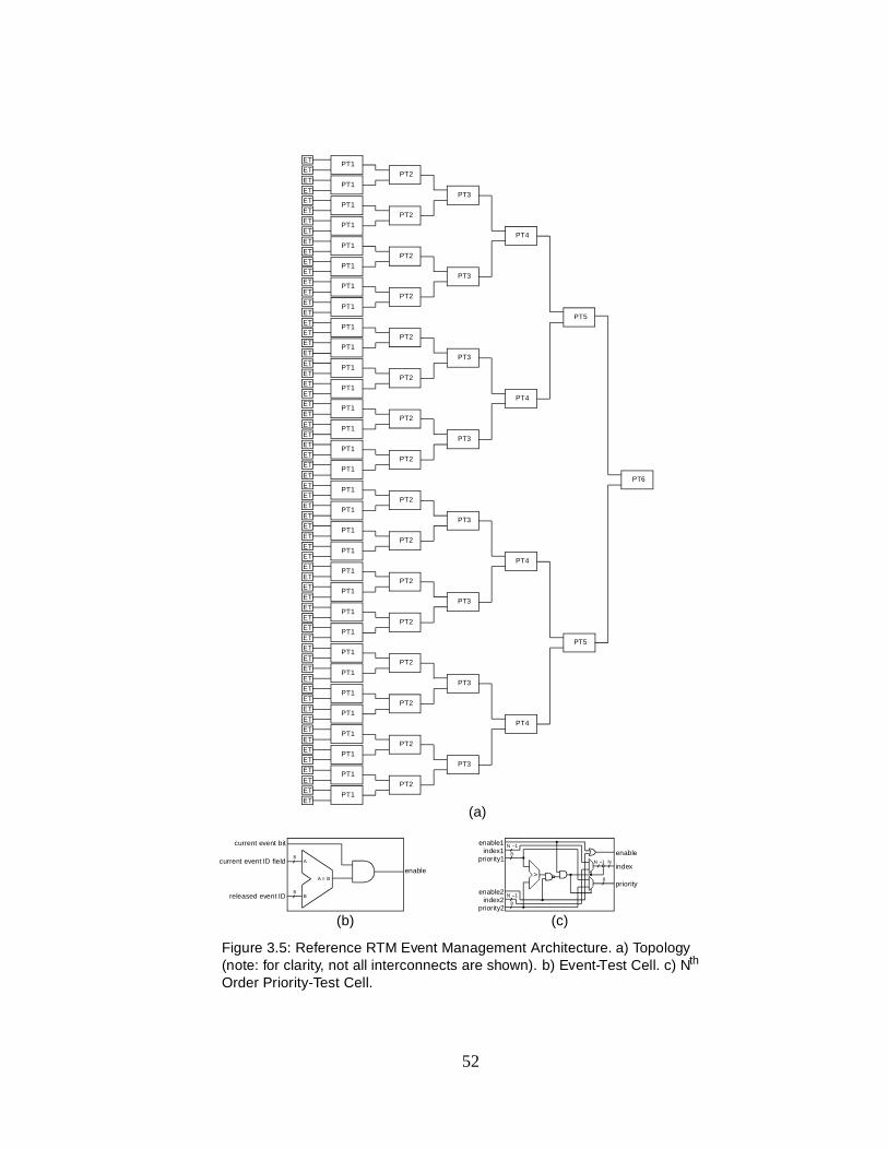
52
Figure 3.5: Reference RTM Event Management Architecture. a) Topology (note: for clarity, not all interconnects are shown). b) Event-Test Cell. c) Nth Order Priority-Test Cell.
ET
ET
ET
ET
ET
ET
ET
ET
ET
ET
ET
ET
ET
ET
ET
ET
ET
ET
ET
ET
ET
ET
ET
ET
ET
ET
ET
ET
ET
ET
ET
ET
ET
ET
ET
ET
ET
ET
ET
ET
ET
ET
ET
ET
ET
ET
ET
ET
ET
ET
ET
ET
ET
ET
ET
ET
ET
ET
ET
ET
ET
ET
ET
ET
PT1
PT1
PT1
PT1
PT1
PT1
PT1
PT1
PT1
PT1
PT1
PT1
PT1
PT1
PT1
PT1
PT1
PT1
PT1
PT1
PT1
PT1
PT1
PT1
PT1
PT1
PT1
PT1
PT1
PT1
PT1
PT1
PT2
PT2
PT2
PT2
PT2
PT2
PT2
PT2
PT2
PT2
PT2
PT2
PT2
PT2
PT2
PT2
PT3
PT3
PT3
PT3
PT3
PT3
PT3
PT3
PT4
PT4
PT4
PT4
PT5
PT5
PT6
(a)
(b)
>
enable1index1
priority1
enable2index2
priority2
(c)
enable
index
priority
N –1 N
8
8
8
N –1
N –1
8
8
A
B
A = B
enable
current event bit
current event ID field
released event ID

53
used for both scheduling and event management. The event-test cells just
check if the event bit is set and if the event ID of the resource being
released matches the event ID in a specific record. They each use an 8-bit
equality comparator and an AND gate. The amount of combinational logic
required for event management scales linearly, except that the majority can
be shared with the task scheduler. Also, the computational delay is
O(log(n)), as it is with scheduling.
The amount of die area that the RTM needs is important in determining
its feasibility. Based on existing area models for register files and caches
[15], the RTM reference architecture requires approximately 2600 register-
bit equivalents (RBEs). This is roughly equivalent to the amount of die area
used by a 32-bit by 64-word register file. Therefore, the RTM can easily be
implemented in hardware.
Both the amount of logic and the latency of this reference architecture are
acceptable. Neither the storage elements nor the RTOS operations impose
requirements that would make the RTM impossible or undesirable to
include in the design of a processor intended for real-time systems. This
reference model demonstrates that the RTM is well suited for hardware
implementation.

54
The Real-Time Task Manager is a valid solution to the problem of perfor-
mance loss due to real-time operating systems. By implementing task
scheduling, time management, and event management in hardware, the
RTM is able to eliminate much of the major performance bottlenecks in
RTOSes. The RTM is easily integrated into most processors and RTOSes
without having to invest an excessive amount of resources into the develop-
ment process. Also, the RTM is simple enough for its architecture to be
easily implemented without drastically increasing the amount of logic.
Clearly, the RTM can be very beneficial to real-time systems.
55
CHAPTER 4
EXPERIMENTAL METHOD
In order to formally justify the use of the Real-Time Task Manager in
actual real-time systems, an accurate quantification of the effects that it has
on performance is necessary. This is achieved by analyzing models of real-
time systems that use RTOSes. These modeled systems are configured so
that they represent as large a percentage of those found in industry as possi-
ble. Performance measurements are then taken from the models both with
and without the use of the RTM. These measurements allow its perfor-
mance effects to be accurately characterized.
The real-time system models all adhere to the same hierarchical struc-
ture, shown if Figure 4.1. At the lowest level, there is a powerful host work-
station, upon which the software that actually does the modeling runs. The
next level up is a cycle-accurate RTL-level simulator of the embedded pro-
cessor used in the modeled real-time system. The simulator is capable of
loading the same executable binary files that run in actual systems and exe-
cuting them exactly as they would on a real processor. This simulator
allows changes to be easily made to the behavior of the processor being
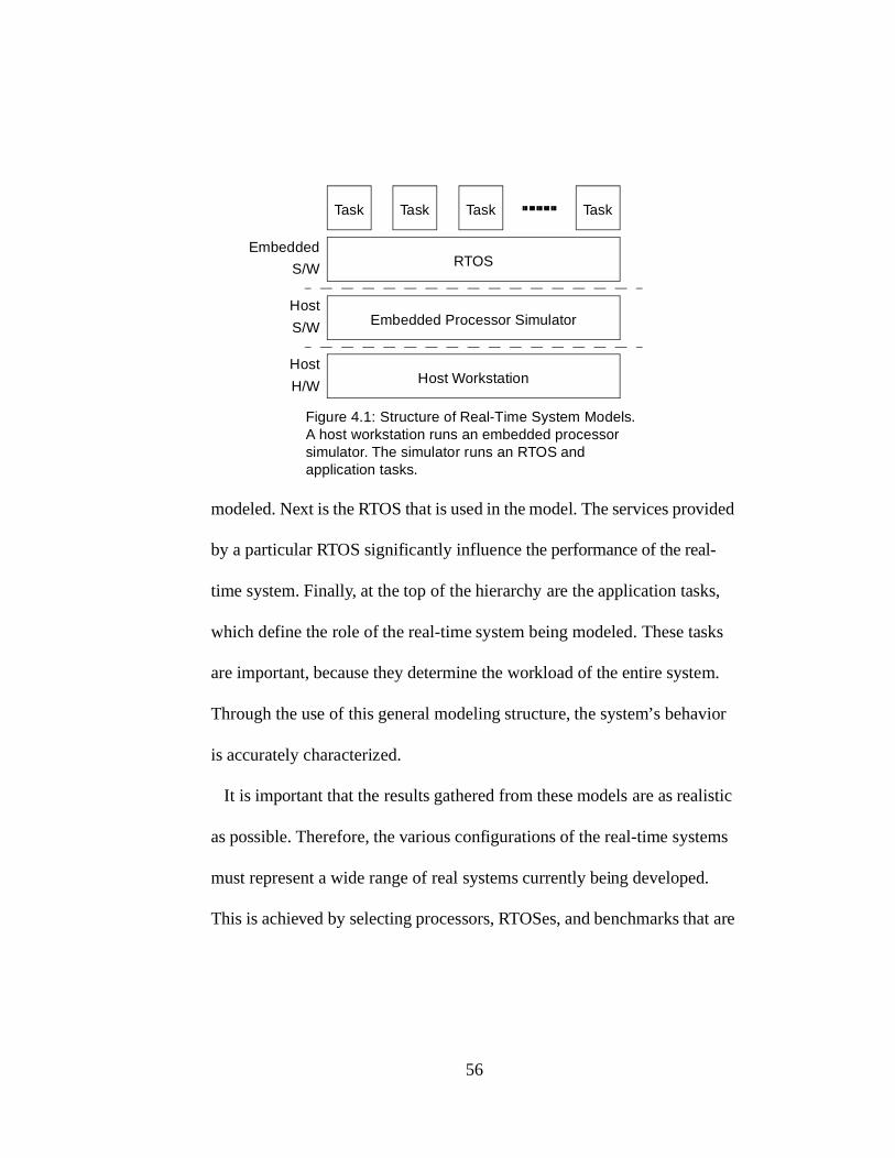
56
modeled. Next is the RTOS that is used in the model. The services provided
by a particular RTOS significantly influence the performance of the real-
time system. Finally, at the top of the hierarchy are the application tasks,
which define the role of the real-time system being modeled. These tasks
are important, because they determine the workload of the entire system.
Through the use of this general modeling structure, the system’s behavior
is accurately characterized.
It is important that the results gathered from these models are as realistic
as possible. Therefore, the various configurations of the real-time systems
must represent a wide range of real systems currently being developed.
This is achieved by selecting processors, RTOSes, and benchmarks that are
Task Task Task Task
RTOS
Embedded Processor Simulator
Embedded
S/W
Host
S/W
Figure 4.1: Structure of Real-Time System Models. A host workstation runs an embedded processor simulator. The simulator runs an RTOS and application tasks.
Host WorkstationHost
H/W

57
as similar as possible to those used in industry. This ensures that the results
are representative of a wide range of realistic scenarios.
In order for this model to be useful, measurements are taken of the per-
formance of the system. These measurements are carried out by the simula-
tor. Specifically, the simulator takes measurements of the aspects of the
system’s performance that are affected by RTOSes: real-time jitter,
response time, and processor utilization. These measurements are the nec-
essary pieces of information required to accurately describe the perfor-
mance of real-time systems.
By comparing the performance measurements of systems both with and
without using the RTM, its effects are clearly illustrated. For this reason
and because these systems are representative of actual modern real-time
systems, the RTM’s ability to solve the performance loss problem caused
by RTOSes is accurately quantified.
4.1 Processor
Just as the processor that is chosen for a real system design greatly influ-
ences its performance, the processor that is simulated significantly affects
the performance of a modeled system. Due to the difficulty of creating an
accurate simulator, the same processor simulator is used for every sample
real-time system in this analysis. To maintain as fair a representation of

58
actual systems as possible, a very commonly used processor has been cho-
sen. The Texas Instruments TMS320C6201 is a high-performance 32-bit
VLIW fixed-point DSP with a 200 MHz clock that can issue eight 32-bit
instructions per cycle [22]. The C6201’s substantial processing power
makes it ideal for high-bandwidth processing, commonly found in telecom-
munications, video processing, and encryption applications. This DSP is
used in many modern commercial applications. Therefore, it is the proces-
sor that is used for the real-time system models in this study.
The simulator is an efficient program that correctly implements the
C6201 ISA and provides precise and detailed measurements of the execu-
tion of the embedded software. The simulator is written in the C program-
ming language, allowing for very fast simulations. It accurately simulates
the pipeline, register files, interrupts, and timers; all of which are necessary
to execute an RTOS [4]. Numerous options make the simulator a flexible
tool, capable of producing information such as cycle-by-cycle pipeline reg-
ister dumps and individual function execution details. In fact, the simulator
provides enough information to make almost any type of performance mea-
surement. Also, an implementation of the RTM is built in to the simulator
so that its effects on the performance of the real-time system can be
observed.
59
There is one obvious simplification in the simulator’s behavior, which is
that memory latencies are not simulated accurately. All memory accesses
have been simulated as if they are as fast as accesses to the internal pro-
gram and data memories without any bank conflicts. This is a reasonable
estimate. However, the effects of the memory system are not the focus of
this research, so this inaccuracy is acceptable.
Overall, the simulator is a powerful tool that is used to assess the perfor-
mance of real-time systems that use the high-performance C6201 DSP. It
allows for the effects of the RTM to be formally characterized.
4.2 Real-Time Operating Systems
The RTOSes used in this analysis are definitely major influences on the
performance of the real-time system. Some RTOS design choices that have
a large effect on performance are whether or not the RTOS supports pre-
emption. If it does not, then the location of the scheduling points within the
application tasks will have a sizable impact. Also, the way that the func-
tions performed by the RTOS have been implemented will significantly
influence the performance. Thus, in order to come to a general conclusion
about the success of the RTM, it is necessary to model systems with widely
varying RTOS behavior. Therefore, two vastly differing RTOSes have been
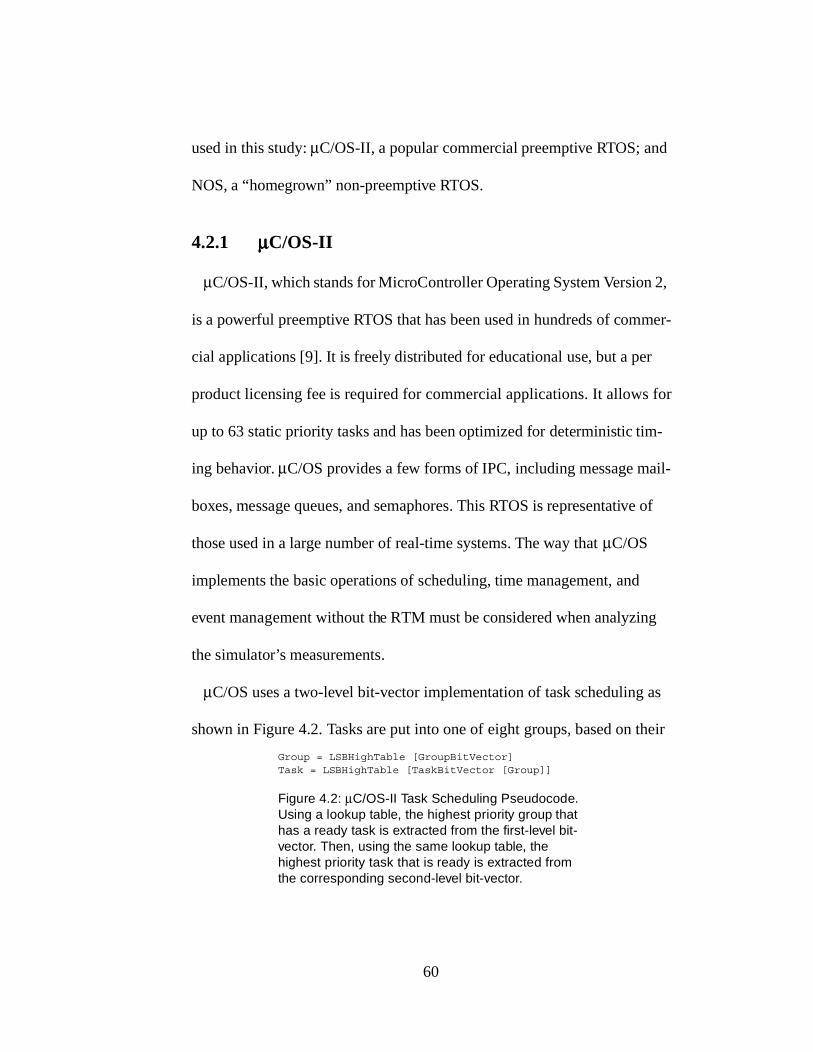
60
used in this study: µC/OS-II, a popular commercial preemptive RTOS; and
NOS, a “homegrown” non-preemptive RTOS.
4.2.1 µµµµC/OS-II
µC/OS-II, which stands for MicroController Operating System Version 2,
is a powerful preemptive RTOS that has been used in hundreds of commer-
cial applications [9]. It is freely distributed for educational use, but a per
product licensing fee is required for commercial applications. It allows for
up to 63 static priority tasks and has been optimized for deterministic tim-
ing behavior. µC/OS provides a few forms of IPC, including message mail-
boxes, message queues, and semaphores. This RTOS is representative of
those used in a large number of real-time systems. The way that µC/OS
implements the basic operations of scheduling, time management, and
event management without the RTM must be considered when analyzing
the simulator’s measurements.
µC/OS uses a two-level bit-vector implementation of task scheduling as
shown in Figure 4.2. Tasks are put into one of eight groups, based on their
Group = LSBHighTable [GroupBitVector]Task = LSBHighTable [TaskBitVector [Group]]
Figure 4.2: µC/OS-II Task Scheduling Pseudocode. Using a lookup table, the highest priority group that has a ready task is extracted from the first-level bit-vector. Then, using the same lookup table, the highest priority task that is ready is extracted from the corresponding second-level bit-vector.

61
priorities. There is an 8-bit first-level bit-vector that indicates which of
these priority groups contains a task that is ready-to run. µC/OS uses a 256
entry lookup table to determine the highest priority ready group that has
ready tasks. There is also one 8-bit second-level bit-vector for each priority
group, which indicates the tasks within that group that are ready-to-run.
µC/OS uses the same 256 entry lookup table to determine the highest prior-
ity ready task within each ready group. This implementation has the advan-
tage of executing in a deterministic amount of time, however, the amount of
memory required for the lookup tables may be too large for some real-time
systems.
The time management operation is performed the brute-force way, as
illustrated in Figure 4.3. On every clock tick, the entire list of TCBs is tra-
versed and a counter is decremented for each task that is waiting for its next
release time. This is an extremely time consuming operation that scales
with the number of tasks and is the largest performance bottleneck for this
RTOS.
for each taskif TCB[task].Status == DELAYED
TCB[task].DelayCounter = TCB[task].DelayCounter - 1if TCB[task].DelayCounter == 0
TCB[task].Status = READYend if
end ifend if
Figure 4.3: µC/OS-II Time Management Pseudocode. The TCB list is traversed and the delay counter is decremented for all tasks waiting on clock ticks. When a counter reaches zero, that task is ready-to-run.

62
The task unblocking operation of event management is similar to task
scheduling. Each resource that is accessed using IPC maintains its own set
of two-level bit vectors. However, the bits indicate the highest priority
group or task that is waiting for the resource to be released. Again, the 256
entry lookup table is used to determine which task to unblock when the
resource is released. Again, this implementation has the advantage that it is
performed in a deterministic amount of time, but, the amount of memory
required for the lookup tables may be too large for some real-time systems.
In order to test the effects of the RTM, it must be integrated into µC/OS.
Thus, modifications have been made to µC/OS so that it uses the RTM for
task scheduling, time management, and event management, instead of the
software implementations described above. The performance of real-time
systems using the modified version of the RTOS is then compared to the
performance of those using the unmodified version.
4.2.2 NOS
The next RTOS analyzed in this study is NOS, which is an acronym of
Not an Operating System. The reason for its name is that it only provides a
subset of the services provided by a complete RTOS. For example, there is
no support for IPC. It is non-preemptive and does not perform context
switches in the traditional sense. In fact, NOS is more of just a real-time
63
scheduler than an RTOS. However, for the purposes of this analysis, it is
referred to as an RTOS. NOS is not used in any commercial applications
and was developed entirely for the purposes of this study. The reason that it
is used in this analysis is that over 25% of RTOSes, like NOS, are merely
subsets of complete RTOSes [5]. An RTOS such as this is usually devel-
oped only by the company which intends on using it, and is sometimes
referred to as homegrown. These RTOSes may not be full-featured, but
they should not be ignored. It is important that they be represented in this
analysis.
NOS does nothing more than execute function calls after their specified
release times. This imposes the requirement that periodic tasks are com-
posed of a function that executes one iteration and then reschedules itself
for the next iteration. For example, if a task is to perform a computation
every millisecond, then the task will consist of a function that performs just
one computation. This function must re-schedule itself for execution one
millisecond later. NOS has no way of stopping a function once it starts.
Each function must run to completion before any other is called. Thus, the
scheduling points occur when these functions return. In fact, the core of
NOS is merely an infinite loop that executes the highest priority ready
task’s function, if any, and then processes any clock ticks that may have
occurred during that time. This loop is referred to as the polling loop.
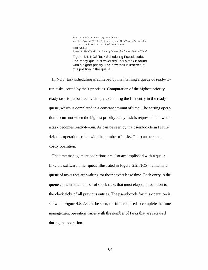
64
In NOS, task scheduling is achieved by maintaining a queue of ready-to-
run tasks, sorted by their priorities. Computation of the highest priority
ready task is performed by simply examining the first entry in the ready
queue, which is completed in a constant amount of time. The sorting opera-
tion occurs not when the highest priority ready task is requested, but when
a task becomes ready-to-run. As can be seen by the pseudocode in Figure
4.4, this operation scales with the number of tasks. This can become a
costly operation.
The time management operations are also accomplished with a queue.
Like the software timer queue illustrated in Figure 2.2, NOS maintains a
queue of tasks that are waiting for their next release time. Each entry in the
queue contains the number of clock ticks that must elapse, in addition to
the clock ticks of all previous entries. The pseudocode for this operation is
shown in Figure 4.5. As can be seen, the time required to complete the time
management operation varies with the number of tasks that are released
during the operation.
SortedTask = ReadyQueue.Headwhile SortedTask.Priority <= NewTask.Priority
SortedTask = SortedTask.Nextend whileInsert NewTask in ReadyQueue before SortedTask
Figure 4.4: NOS Task Scheduling Pseudocode. The ready queue is traversed until a task is found with a higher priority. The new task is inserted at this position in the queue.

65
As previously mentioned, NOS does not have any support for IPC. One
of the biggest advantages of IPC is that it can be used to eliminate race-
conditions, which are situations in which data can be corrupted or deadlock
can occur. Race-conditions are a much bigger problem for preemptive
RTOSes. Since NOS is a non-preemptive RTOS, IPC does not have as
many advantages. Because event management is only used for IPC, it is not
present in NOS either. Therefore, a portion of the RTM goes unused for
systems using NOS. This is perfectly acceptable because one of the goals
of the RTM is to be compatible with as many RTOSes as possible, regard-
less of what services they provide.
The RTM must be integrated into NOS so that its effects on performance
can be quantified. Therefore, a modified version of NOS has been created
in which the software task scheduling and time management implementa-
tions described above have been replaced with the RTM’s implementations.
This allows for the two versions of NOS to be compared to each other, thus
characterizing the effects of the RTM.
while DelayQueue.Head.Delay <= TicksEllapsedTicksEllapsed = TicksEllapsed - DelayQueue.Head.DelayDequeue from DelayQueueCall scheduler for dequeued task
end whileDelayQueue.Head.Delay = DelayQueue.Head.Delay - TicksEllapsed
Figure 4.5: NOS Time Management Pseudocode. Tasks are dequeued from the delay queue repeatedly until all the clock ticks have been accounted for. The dequeued tasks are scheduled as in Figure 4.4, but scheduling is not part of the time management operation.
66
4.3 Benchmarks
The systems that are modeled in this study must have workloads similar
to those of systems commonly developed by the real-time system industry.
This is achieved with the use of standard benchmarks consisting of applica-
tions common to real-time systems. Several applications from the Media-
Bench suite [10] are used in this analysis. These benchmarks have widely
varying workload characteristics and are all representative of common real-
time system applications. Descriptions of the benchmarks used in this
study are presented below.
4.3.1 GSM
GSM 06.10 is the standard for full-rate speech transcoding for European
mobile telephone networks, as defined by the European Telecommunica-
tion Standard Institute (ETSI). GSM originally stood for Groupe Spécial
Mobil, but it now stands for Global Systems for Mobile Communications.
It uses residual pulse excitation and long term prediction algorithms to
transcode between a raw 128 kbps (8 kHz stream of 16-bit audio samples)
and a compressed 13 kbps (50 Hz stream of 260-bit frames). Both the com-
pression and decompression algorithms are used as benchmarks for this
study.

67
4.3.2 G.723
G.723 is an international telecommunications standard for digital coding
of analog signals. The standard was defined by the International Telegraph
and Telephone Consultative Committee (CCITT), which is now part of the
International Telecommunications Union (ITU). It uses adaptive differen-
tial pulse code modulation (ADPCM) to compress a 128 kbps raw audio
stream to a 24 kbps or 40 kbps stream. The 24 kbps compression and
decompression algorithms are used in this study.
4.3.3 ADPCM
ADPCM is another benchmark from MediaBench similar to G.723,
except that it is much simpler, and faster. This coder/decoder (CODEC)
compresses audio to 32 kbps. This algorithm is not an industry standard,
but it is similar to the processing done on many common formats of audio
files used in personal computers. Again, both the compression and decom-
pression algorithms are used in this study.
4.3.4 Pegwit
Pegwit is a benchmark capable of public key encryption and authentica-
tion. It has many advanced cryptographic capabilities, such as elliptic
curves over GF(2255), SHA1 for hashing, and the symmetric block cipher

68
square for encryption [20]. In this study, the encryption and decryption
algorithms are used to process data at a rate of 1.6 Mbps.
4.4 Tasks
All real-time applications that make use of RTOSes consist of a number
of tasks, each of which is intended to accomplish a subset of the objectives
of the entire system. In general, each task has its own thread of control and
it is the RTOS’s job to determine which task runs when. This allows the
duties of an application to be divided up at logical boundaries and assigned
to tasks, which may execute independently from each other. Unfortunately,
this is not how the benchmarks in the MediaBench suite have been written.
The algorithms in these benchmarks are used to provide the real-time sys-
tem models with realistic workload characteristics. However, a task struc-
ture for their use in real-time applications is required.
In this study, the task structures used in all system configurations being
tested are based on the same model. This is possible because all the bench-
marks used in this analysis are similar, in that they process streams of data.
Each system configuration will process a specific number of these data
streams. In other words, the applications will process multiple channels of
data. Two tasks are assigned to each data channel. One task is the process-
ing task, shown in Figure 4.6 (a), which reads from the input stream and
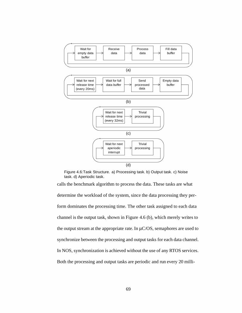
69
calls the benchmark algorithm to process the data. These tasks are what
determine the workload of the system, since the data processing they per-
form dominates the processing time. The other task assigned to each data
channel is the output task, shown in Figure 4.6 (b), which merely writes to
the output stream at the appropriate rate. In µC/OS, semaphores are used to
synchronize between the processing and output tasks for each data channel.
In NOS, synchronization is achieved without the use of any RTOS services.
Both the processing and output tasks are periodic and run every 20 milli-
Figure 4.6: Task Structure. a) Processing task. b) Output task. c) Noise task. d) Aperiodic task.
Wait for nextrelease time(every 32ms)
Trivialprocessing
Wait for nextaperiodicinterrupt
Trivialprocessing
Wait for nextrelease time(every 20ms)
Wait for fulldata buffer
Sendprocessed
Empty databuffer
data
Wait forempty data
buffer
Receivedata
Processdata
Fill databuffer
(a)
(b)
(c)
(d)
70
seconds. A constant-size block or frame of data is read from the input
stream and processed during each iteration. The output of the algorithm
results in a frame of data of a constant-size as well. These frame sizes
determines the data rates of the input and output streams, respectively. The
key benefit of this model is that it allows for a different number of data
channels in each system configuration.
At this point, the model is somewhat too simple. All task iterations will
execute at exactly 20 millisecond intervals, because there is nothing to per-
turb them. However, in real systems, there are other periodic tasks running
in the background with different frequencies, causing interference which
leads to real-time jitter. For example, many systems have LCD displays
which have to be periodically refreshed. This is often performed with a
dedicated task, running at a frequency that differs from that of the other
tasks in the system. Therefore, each system configuration that is modeled
in this study also includes an additional periodic task referred to as the
noise task. The noise task, shown in Figure 4.6 (c), has a period of 32 milli-
seconds and each iteration lasts only a few microseconds. Its purpose is to
insert the type of background noise commonly present in real-time applica-
tions.
The task structure is now more realistic, but it is not yet complete. There
may be task interference in the system, but it is not complex enough. Real

71
systems generally have not only periodic tasks, but aperiodic ones as well.
These tasks might be used to respond to external stimuli, such as input
from a keypad or packets arriving through a communications port. Typi-
cally, this sort of event has to be detected either by polling for the status of
the corresponding device or by receiving an interrupt from it. In either case,
the event would cause the performance of the system, in terms of real-time
jitter and response time, to be non-deterministic. In many systems, the pre-
dictability is very important and must be within a given range in order to be
a successful design. Therefore, in these models, aperiodic interrupts with
geometrically distributed inter-arrival times are used to simulate this type
of interference. The interrupts occur, on average, every 10 milliseconds,
and are representative of any relatively high-speed asynchronous process-
ing, such as what would occur when external devices send packets of data
to the DSP to be processed. The ISR responds by releasing a task, shown in
Figure 4.6 (d), to deal with the event. This task, referred to as the aperiodic
task, completes in a few microseconds. With the addition of the aperiodic
task to all the models in this study, their behavior is representative of real-
time systems commonly being developed today.

72
4.5 Measurements
For each one of the system configurations used in this analysis, detailed
measurements of the performance must be made. This is easily achieved
using some of the options of the C6201 processor simulator since it was
designed specifically for this research. To summarize, the system configu-
rations tested for this study have been outlined in Table 4.1. Each configu-
ration is simulated with different numbers of data channels, ranging from
one to as many as can be handled by the simulated processor and RTOS.
Thus, a range of workload characteristics are analyzed. They are also simu-
lated with forty different random number seeds used by the simulator, so
that the aperiodic interrupts occur at different times and their effects can be
more accurately described. Each simulation runs for one second of simu-
lated time, which requires approximately fifteen minutes to run on a 750
MHz Pentium III workstation. It takes ten such processors running simula-
tions continuously for about a month to get all the measurements used in
this study.
Measurements have been taken to quantify the effects of RTOS perfor-
mance loss. Real-time jitter is measured by recording the amount of time
that has elapsed between successive writes to the output stream of each
data channel. Next, the intended period of twenty milliseconds is sub-
tracted from these numbers. Finally, their absolute values are taken. The

73
larger the values, the more the real-time jitter. If the results are all zeros,
then no jitter has occurred in the system. Response time is easily measured
by recording the amount of time that elapses between the occurrence of
aperiodic interrupts and the beginning of the execution of their correspond-
ing aperiodic tasks. The processor utilization is measured by recording the
amount of time that is spent executing RTOS functions out of the one sec-
ond that is simulated. This is then further subdivided into several main
areas of RTOS functionality, such as scheduling, time management, IPC,
and context switching, so that the bottlenecks can be clearly identified.
Finally, certain key RTOS functions are analyzed in greater detail by mea-
suring and recording both the number of times it is executed and the dura-
tion of each execution. All of these measurements allow for the
performance of the systems to be precisely characterized.
Processor RTOS
Implementation of Bottleneck
RTOS Operations
Benchmarks
C6201 µC/OS-IINOS
StandardRTM
GSM encodeGSM decode
G.723 (24 kbps) encodeG.723 (24 kbps) decode
ADPCM encodeADPCM decodePegwit encryptPegwit decrypt
Table 4.1: Summary of Tested System Configurations. A configuration is defined by the selection of a processor, an RTOS, an implementation of bottleneck RTOS operations, and a benchmark; as well as the number of data channels in the system (not shown).

74
By using accurate models of modern real-time systems that use RTOSes,
the performance of actual systems that use the Real-Time Task Manager is
estimated. The RTM’s effects are accurately quantified by comparing these
estimates with those of systems that use the standard software implementa-
tions of the core RTOS operations. From this analysis, the overall effective-
ness of the RTM is determined.

75
CHAPTER 5
RESULTS & ANALYSIS
The goal of the Real-Time Task Manager is to reduce the performance
loss problem associated with RTOSes. In order to validate the success of
the RTM, characterizations of its effects on processor utilization, response
time, and real-time jitter are necessary. This has been achieved by taking
accurate measurements of models of several configurations of realistic real-
time systems, both with and without using the RTM.
For the remainder of this chapter, the effects of the RTM on the perfor-
mance of real-time systems will be presented and analyzed in detail. Its
effects on processor utilization, response time, and real-time jitter are
treated individually and discussed in separate sections for clarity. Through
this analysis, the effectiveness of the RTM will be formally established.
5.1 Processor Utilization
The processor utilization is also significantly affected by the use of the
RTM. This is illustrated by the measurements of the real-time system mod-
els using both µC/OS-II and NOS. The effects of the RTM using each of
these RTOSes and several benchmarks are analyzed in detail.
76
5.1.1 µµµµC/OS-II
The RTOS processor utilization has been divided into five categories for
system configurations that use µC/OS. Each of these categories represents
the processing time spent executing a different RTOS operation. Figures
5.1 and 5.2 show the percent of the total processing time spent executing
the operations in each of these categories and how they vary with system
load, for every benchmark tested, both with and without using the RTM.
System load refers to the amount of processing power used by the applica-
tion, which, in this case, is determined by the number of data channels pro-
cessed in the application. Also, each value measured is represented by a
circle, the area of which indicates the fraction of the jitter measurements
that are equal to that value. As seen in the graphs, the RTOS processor uti-
lization can be quite significant. By analyzing the overhead from each cate-
gory separately, the effects of the RTM can be described in more detail.
The RTOS operations in the miscellaneous category account for an insig-
nificant fraction of the processing time—less than a tenth of a percent—
and are barely visible on the graphs. The RTM is not used to optimize any
of these operations, so there is no change in performance. Therefore, this
category is not analyzed any further.
The RTOS operations that implement IPC consume a nontrivial fraction
of the processing time. This category includes the event management oper-
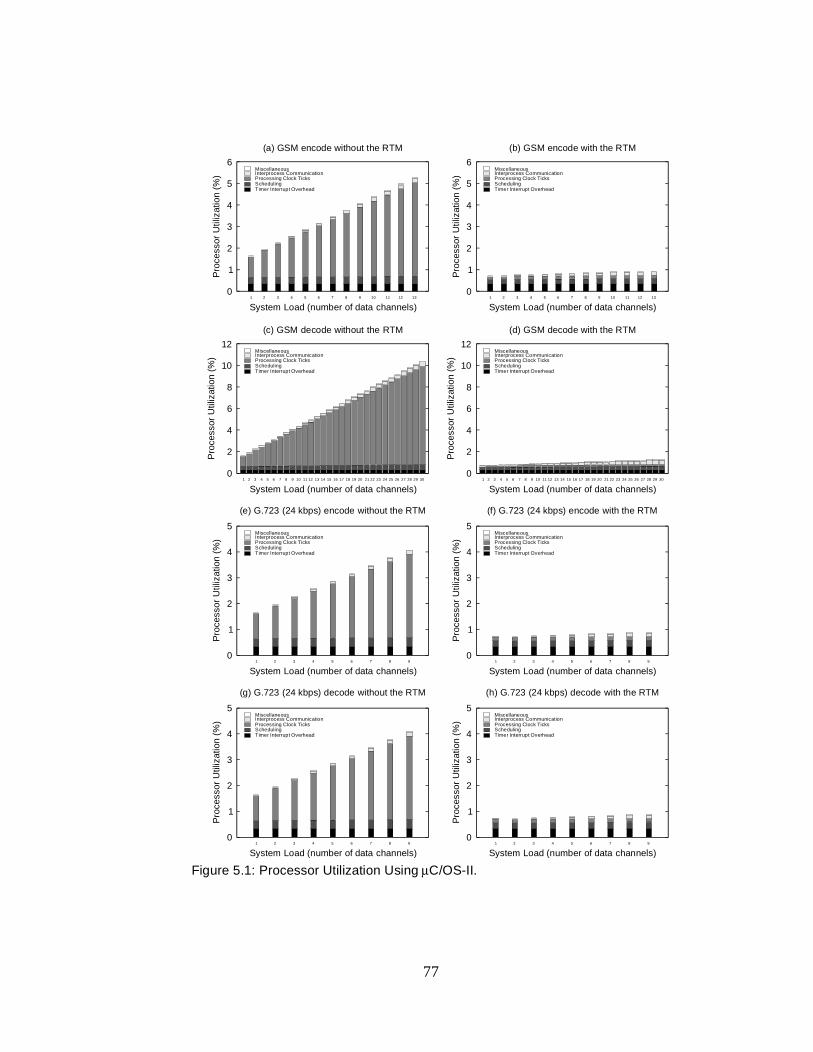
77
Figure 5.1: Processor Utilization Using µC/OS-II.
1 2 3 4 5 6 7 8 9 10 11 12 13
System Load (number of data channels)
0
1
2
3
4
5
6
Pro
cess
or U
tiliz
atio
n (%
)
MiscellaneousInterprocess CommunicationProcessing Clock TicksSchedulingTimer Interrupt Overhead
(a) GSM encode without the RTM
1 2 3 4 5 6 7 8 9 10 11 12 13
System Load (number of data channels)
0
1
2
3
4
5
6
Pro
cess
or U
tiliz
atio
n (%
)
MiscellaneousInterprocess CommunicationProcessing Clock TicksSchedulingTimer Interrupt Overhead
(b) GSM encode with the RTM
1 2 3 4 5 6 7 8 9 10 11 12 13 14 15 16 17 18 19 20 21 22 23 24 25 26 27 28 29 30
System Load (number of data channels)
0
2
4
6
8
10
12
Pro
cess
or U
tiliz
atio
n (%
)
MiscellaneousInterprocess CommunicationProcessing Clock TicksSchedulingTimer Interrupt Overhead
(c) GSM decode without the RTM
1 2 3 4 5 6 7 8 9 10 11 12 13 14 15 16 17 18 19 20 21 22 23 24 25 26 27 28 29 30
System Load (number of data channels)
0
2
4
6
8
10
12
Pro
cess
or U
tiliz
atio
n (%
)
MiscellaneousInterprocess CommunicationProcessing Clock TicksSchedulingTimer Interrupt Overhead
(d) GSM decode with the RTM
1 2 3 4 5 6 7 8 9
System Load (number of data channels)
0
1
2
3
4
5
Pro
cess
or U
tiliz
atio
n (%
)
MiscellaneousInterprocess CommunicationProcessing Clock TicksSchedulingTimer Interrupt Overhead
(e) G.723 (24 kbps) encode without the RTM
1 2 3 4 5 6 7 8 9
System Load (number of data channels)
0
1
2
3
4
5
Pro
cess
or U
tiliz
atio
n (%
)
MiscellaneousInterprocess CommunicationProcessing Clock TicksSchedulingTimer Interrupt Overhead
(f) G.723 (24 kbps) encode with the RTM
1 2 3 4 5 6 7 8 9
System Load (number of data channels)
0
1
2
3
4
5
Pro
cess
or U
tiliz
atio
n (%
)
MiscellaneousInterprocess CommunicationProcessing Clock TicksSchedulingTimer Interrupt Overhead
(g) G.723 (24 kbps) decode without the RTM
1 2 3 4 5 6 7 8 9
System Load (number of data channels)
0
1
2
3
4
5
Pro
cess
or U
tiliz
atio
n (%
)
MiscellaneousInterprocess CommunicationProcessing Clock TicksSchedulingTimer Interrupt Overhead
(h) G.723 (24 kbps) decode with the RTM
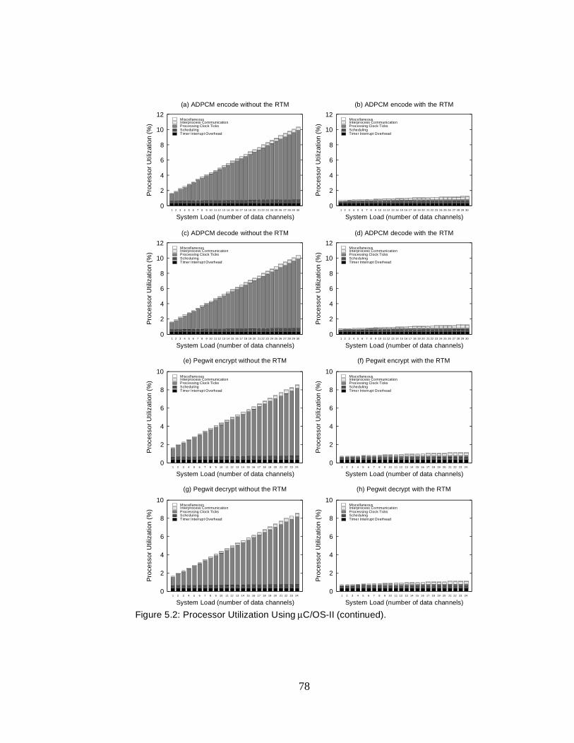
78
Figure 5.2: Processor Utilization Using µC/OS-II (continued).
1 2 3 4 5 6 7 8 9 10 11 12 13 14 15 16 17 18 19 20 21 22 23 24 25 26 27 28 29 30
System Load (number of data channels)
0
2
4
6
8
10
12
Pro
cess
or U
tiliz
atio
n (%
)
MiscellaneousInterprocess CommunicationProcessing Clock TicksSchedulingTimer Interrupt Overhead
(a) ADPCM encode without the RTM
1 2 3 4 5 6 7 8 9 10 11 12 13 14 15 16 17 18 19 20 21 22 23 24 25 26 27 28 29 30
System Load (number of data channels)
0
2
4
6
8
10
12
Pro
cess
or U
tiliz
atio
n (%
)
MiscellaneousInterprocess CommunicationProcessing Clock TicksSchedulingTimer Interrupt Overhead
(b) ADPCM encode with the RTM
1 2 3 4 5 6 7 8 9 10 11 12 13 14 15 16 17 18 19 20 21 22 23 24 25 26 27 28 29 30
System Load (number of data channels)
0
2
4
6
8
10
12
Pro
cess
or U
tiliz
atio
n (%
)
MiscellaneousInterprocess CommunicationProcessing Clock TicksSchedulingTimer Interrupt Overhead
(c) ADPCM decode without the RTM
1 2 3 4 5 6 7 8 9 10 11 12 13 14 15 16 17 18 19 20 21 22 23 24 25 26 27 28 29 30
System Load (number of data channels)
0
2
4
6
8
10
12
Pro
cess
or U
tiliz
atio
n (%
)
MiscellaneousInterprocess CommunicationProcessing Clock TicksSchedulingTimer Interrupt Overhead
(d) ADPCM decode with the RTM
1 2 3 4 5 6 7 8 9 10 11 12 13 14 15 16 17 18 19 20 21 22 23 24
System Load (number of data channels)
0
2
4
6
8
10
Pro
cess
or U
tiliz
atio
n (%
)
MiscellaneousInterprocess CommunicationProcessing Clock TicksSchedulingTimer Interrupt Overhead
(e) Pegwit encrypt without the RTM
1 2 3 4 5 6 7 8 9 10 11 12 13 14 15 16 17 18 19 20 21 22 23 24
System Load (number of data channels)
0
2
4
6
8
10
Pro
cess
or U
tiliz
atio
n (%
)
MiscellaneousInterprocess CommunicationProcessing Clock TicksSchedulingTimer Interrupt Overhead
(f) Pegwit encrypt with the RTM
1 2 3 4 5 6 7 8 9 10 11 12 13 14 15 16 17 18 19 20 21 22 23 24
System Load (number of data channels)
0
2
4
6
8
10
Pro
cess
or U
tiliz
atio
n (%
)
MiscellaneousInterprocess CommunicationProcessing Clock TicksSchedulingTimer Interrupt Overhead
(g) Pegwit decrypt without the RTM
1 2 3 4 5 6 7 8 9 10 11 12 13 14 15 16 17 18 19 20 21 22 23 24
System Load (number of data channels)
0
2
4
6
8
10
Pro
cess
or U
tiliz
atio
n (%
)
MiscellaneousInterprocess CommunicationProcessing Clock TicksSchedulingTimer Interrupt Overhead
(h) Pegwit decrypt with the RTM

79
ations, as well as all others needed to fully implement IPC. As can be seen
in the graphs, without the RTM, the processor utilization of these opera-
tions increases linearly with system load at 0.014% per data channel. How-
ever, with the RTM, the processor utilization increases at 0.012% per data
channel, for a 14% improvement. This is an improvement, however, it is
small, because µC/OS already performs event management operations in a
constant amount of time. Although this performance enhancement is small,
it may become more important for applications that make heavy use of
IPC.
Processing clock ticks uses a very large percentage of the processing time
in µC/OS. This category includes the time management operations used to
ready those tasks that reach their release times whenever a clock tick
occurs. Systems that do not use the RTM suffer from a huge processing
overhead in this category. The processor utilization increases linearly with
system load at 0.28% per data channel. This drastically affects the amount
of processing power available to the application. However, with the RTM,
the processor utilization for time management is a constant 0.14%, for up
to a 98% improvement. This is a large performance increase that is seen for
every benchmark tested.
The RTOS operations in the scheduling category use a small, yet signifi-
cant portion of the available processing power. Without the RTM, the pro-
80
cessing time consumed by these operations increases slightly with system
load, by 0.0059% per data channel. Also, the scheduling operations per-
formed by timer interrupts contribute 0.29% to this of overhead. However,
the scheduling operations for those systems that use the RTM increases at
only 0.0042% per data channel, with an additional 0.20% coming from
timer interrupts. The result is approximately a 31% improvement. This is a
small decrease in overhead that would be larger in more complicated appli-
cations in which the tasks experience more interference with each other or
use more IPC.
Finally, the timer interrupt overhead accounts for another nontrivial frac-
tion of the processing time. This category includes the time spent branch-
ing to the ISR and preserving the context of the interrupted task.
Unfortunately, the RTM is not capable of optimizing these operations, so
this category accounts for a constant 0.34% of the processor utilization,
both with and without the RTM.
The basic RTOS operations that the RTM implements result in the pro-
cessing overhead required by µC/OS to be reduced by 60% to 90%. These
operations, especially clock tick processing, are performed quickly enough
by the RTM that the processor utilization becomes much less of a problem.
81
5.1.2 NOS
For NOS, the processor utilization has been divided into six categories.
Figures 5.3 and 5.4 show the percent of the total processing time spent exe-
cuting the operations in each of these categories and how they vary with
system load, for every benchmark tested, both with and without using the
RTM. As seen in the graphs, the RTOS processor utilization is not quite as
large as it is for µC/OS, however, it is still enough so that it is worth opti-
mizing. Again, the overhead within each category is discussed separately,
so that the effects of the RTM can be presented in more clearly.
The RTOS operations in the miscellaneous category account for an insig-
nificant fraction of the processing time—less than a hundredth of a per-
cent—and are not even visible on the graphs. The RTM is not used to
optimize any of these operations, so there is no change in performance.
This category is not analyzed any further.
Polling accounts for a large portion of the processing overhead in NOS.
This is the processing done in the main loop that repeatedly calls the high-
est priority task’s function, if there is one, or enters the processor into idle
mode, if there is not. When the processor is idle, polling operations occur
periodically, whenever timer interrupts occurs. This ensures that the highest
priority ready task is run as soon as possible. So when the processor is idle,
a certain fraction of the processing time is still devoted to polling opera-

82
Figure 5.3: Processor Utilization Using NOS.
1 2 3 4 5 6 7 8 9 10 11 12 13
System Load (number of data channels)
0.00
0.15
0.30
0.45
0.60
0.75
Pro
cess
or U
tiliz
atio
n (%
)
MiscellaneousPollingProcessing Clock TicksProcessing Release TimesSchedulingTimer Interrupt Overhead
(a) GSM encode without the RTM
1 2 3 4 5 6 7 8 9 10 11 12 13
System Load (number of data channels)
0.00
0.15
0.30
0.45
0.60
0.75
Pro
cess
or U
tiliz
atio
n (%
)
MiscellaneousPollingProcessing Clock TicksProcessing Release TimesSchedulingTimer Interrupt Overhead
(b) GSM encode with the RTM
1 2 3 4 5 6 7 8 9 10 11 12 13 14 15 16 17 18 19 20 21 22 23 24 25 26 27 28 29 30
System Load (number of data channels)
0.00
0.25
0.50
0.75
1.00
1.25
Pro
cess
or U
tiliz
atio
n (%
)
MiscellaneousPollingProcessing Clock TicksProcessing Release TimesSchedulingTimer Interrupt Overhead
(c) GSM decode without the RTM
1 2 3 4 5 6 7 8 9 10 11 12 13 14 15 16 17 18 19 20 21 22 23 24 25 26 27 28 29 30
System Load (number of data channels)
0.00
0.25
0.50
0.75
1.00
1.25
Pro
cess
or U
tiliz
atio
n (%
)
MiscellaneousPollingProcessing Clock TicksProcessing Release TimesSchedulingTimer Interrupt Overhead
(d) GSM decode with the RTM
1 2 3 4 5 6 7 8 9
System Load (number of data channels)
0.00
0.15
0.30
0.45
0.60
0.75
Pro
cess
or U
tiliz
atio
n (%
)
MiscellaneousPollingProcessing Clock TicksProcessing Release TimesSchedulingTimer Interrupt Overhead
(e) G.723 (24 kbps) encode without the RTM
1 2 3 4 5 6 7 8 9
System Load (number of data channels)
0.00
0.15
0.30
0.45
0.60
0.75
Pro
cess
or U
tiliz
atio
n (%
)
MiscellaneousPollingProcessing Clock TicksProcessing Release TimesSchedulingTimer Interrupt Overhead
(f) G.723 (24 kbps) encode with the RTM
1 2 3 4 5 6 7 8 9
System Load (number of data channels)
0.00
0.15
0.30
0.45
0.60
0.75
Pro
cess
or U
tiliz
atio
n (%
)
MiscellaneousPollingProcessing Clock TicksProcessing Release TimesSchedulingTimer Interrupt Overhead
(g) G.723 (24 kbps) decode without the RTM
1 2 3 4 5 6 7 8 9
System Load (number of data channels)
0.00
0.15
0.30
0.45
0.60
0.75
Pro
cess
or U
tiliz
atio
n (%
)
MiscellaneousPollingProcessing Clock TicksProcessing Release TimesSchedulingTimer Interrupt Overhead
(h) G.723 (24 kbps) decode with the RTM

83
Figure 5.4: Processor Utilization Using NOS (continued).
1 2 3 4 5 6 7 8 9 10 11 12 13 14 15 16 17 18 19 20 21 22 23 24 25 26 27 28 29 30
System Load (number of data channels)
0.00
0.25
0.50
0.75
1.00
1.25
1.50
Pro
cess
or U
tiliz
atio
n (%
)
MiscellaneousPollingProcessing Clock TicksProcessing Release TimesSchedulingTimer Interrupt Overhead
(a) ADPCM encode without the RTM
1 2 3 4 5 6 7 8 9 10 11 12 13 14 15 16 17 18 19 20 21 22 23 24 25 26 27 28 29 30
System Load (number of data channels)
0.00
0.25
0.50
0.75
1.00
1.25
1.50
Pro
cess
or U
tiliz
atio
n (%
)
MiscellaneousPollingProcessing Clock TicksProcessing Release TimesSchedulingTimer Interrupt Overhead
(b) ADPCM encode with the RTM
1 2 3 4 5 6 7 8 9 10 11 12 13 14 15 16 17 18 19 20 21 22 23 24 25 26 27 28 29 30
System Load (number of data channels)
0.00
0.25
0.50
0.75
1.00
1.25
1.50
Pro
cess
or U
tiliz
atio
n (%
)
MiscellaneousPollingProcessing Clock TicksProcessing Release TimesSchedulingTimer Interrupt Overhead
(c) ADPCM decode without the RTM
1 2 3 4 5 6 7 8 9 10 11 12 13 14 15 16 17 18 19 20 21 22 23 24 25 26 27 28 29 30
System Load (number of data channels)
0.00
0.25
0.50
0.75
1.00
1.25
1.50
Pro
cess
or U
tiliz
atio
n (%
)
MiscellaneousPollingProcessing Clock TicksProcessing Release TimesSchedulingTimer Interrupt Overhead
(d) ADPCM decode with the RTM
1 2 3 4 5 6 7 8 9 10 11 12 13 14 15 16 17 18 19 20 21 22 23 24
System Load (number of data channels)
0.0
0.2
0.4
0.6
0.8
1.0
Pro
cess
or U
tiliz
atio
n (%
)
MiscellaneousPollingProcessing Clock TicksProcessing Release TimesSchedulingTimer Interrupt Overhead
(e) Pegwit encrypt without the RTM
1 2 3 4 5 6 7 8 9 10 11 12 13 14 15 16 17 18 19 20 21 22 23 24
System Load (number of data channels)
0.0
0.2
0.4
0.6
0.8
1.0
Pro
cess
or U
tiliz
atio
n (%
)
MiscellaneousPollingProcessing Clock TicksProcessing Release TimesSchedulingTimer Interrupt Overhead
(f) Pegwit encrypt with the RTM
1 2 3 4 5 6 7 8 9 10 11 12 13 14 15 16 17 18 19 20 21 22 23 24
System Load (number of data channels)
0.0
0.2
0.4
0.6
0.8
1.0
Pro
cess
or U
tiliz
atio
n (%
)
MiscellaneousPollingProcessing Clock TicksProcessing Release TimesSchedulingTimer Interrupt Overhead
(g) Pegwit decrypt without the RTM
1 2 3 4 5 6 7 8 9 10 11 12 13 14 15 16 17 18 19 20 21 22 23 24
System Load (number of data channels)
0.0
0.2
0.4
0.6
0.8
1.0
Pro
cess
or U
tiliz
atio
n (%
)
MiscellaneousPollingProcessing Clock TicksProcessing Release TimesSchedulingTimer Interrupt Overhead
(h) Pegwit decrypt with the RTM

84
tions. This fraction is the same for every benchmark. Polling operations
also occur after the completion of each task’s function, so that the next one
can be executed. Thus, a fraction of time is also spent executing polling
operations during periods when the processor is not idle. For more compli-
cated benchmarks, the processing tasks take longer to execute, and the frac-
tion of time spent executing polling operations when the processor is not
idle is lower. This is because polling operations will occur less frequently
when executing tasks than when idling. If the fraction of time spent execut-
ing polling operations is lower when the processor is not idle than when it
is idle, then the processor utilization of polling operations decreases lin-
early with increases in system load. This is the case for most of the bench-
marks, as seen in the graphs, because most of them require enough
processing time to keep the time spent polling during non-idle periods rela-
tively low. Conversely, if the fraction of time spent executing polling opera-
tions is higher when the processor is not idle than when it is idle, then the
processor utilization of polling operations increases linearly with increases
in system load. This occurs when the duration of the average task execution
is lower than the time between timer interrupts. This is illustrated by the
ADPCM encode and decode benchmarks, as seen in Figures 5.4 (a), (b),
(c), and (d). The effects of the RTM on this category of the processor utili-
zation can be deceiving. Unfortunately, the RTM can increase the amount
85
of processing time consumed by the polling operations by up to 25%. This
is because, without the RTM, polling is as simple as looking at the head of
the ready queue, but with the RTM, most of communication with the RTM
is performed while polling. This slight performance loss in terms of the
polling overhead is compensated for in other categories, in which processor
utilization is decreased.
The category of processing clock ticks consumes a sizeable fraction of
the available processing power. There is no need to process a clock tick that
occurs while a task is executing, since the task cannot be preempted. Thus,
as with the polling overhead, this operation is only performed when tasks
complete and after interrupts that occur during idle mode. Therefore, the
same behavior is seen as is with polling. The processor utilization for pro-
cessing clock ticks either increases or decreases linearly with the system
load, depending on the duration of the processing tasks in that system.
However, in this case, the RTM is quite effective at reducing the magnitude
of this overhead. As seen in the graphs, the RTM reduces this category’s
processor utilization by over 85%. This performance enhancement is seen
for every benchmark tested.
The percent of the time devoted to processing the release times can be
quite significant in NOS. This operation records the next release time of a
task in the RTOS’s internal data structure. Without the RTM, this operation
86
increases linearly with the number of tasks, because the software timer
queue must be traversed. Also, this operation occurs more frequently as the
number of data channels increases. Therefore, the processing time used by
this operation increases quadratically with the system load for systems that
do not use the RTM. However, the RTM performs this operation in a trivial
and constant amount of time. Therefore, when the RTM is used, the pro-
cessing time consumed by processing release times increases linearly at
only 0.00037% per data channel for up to a 95% decrease. This processor
utilization is not even visible on some graphs.
The scheduling operation in NOS can easily consume a great deal of pro-
cessing power. As with processing release times, this operation increases
linearly with system load in both complexity and frequency when the RTM
is not used. However, when the RTM is used, the complexity of this opera-
tion becomes small and constant. As seen in the graphs, the scheduling pro-
cessor utilization for those systems not using the RTM increases
quadratically with system load, and becomes a major component of the
processing overhead for large numbers of data channels. On the other hand,
the scheduling overhead for those systems that do use the RTM also scales
linearly at only 0.00037% per data channel for up to a 98% decrease, and is
almost nonexistent. The processing overhead is drastically reduced because
of this improvement.

87
Lastly, a lot of the processing time is devoted to the timer interrupt over-
head. This category includes the time spent branching to the ISR and pre-
serving the context of the interrupted task. Unfortunately, the RTM is not
capable of optimizing these operations, so this category accounts for a con-
stant 0.13% of the processor utilization, both with and without the RTM.
The basic RTOS operations that the RTM implements result in the pro-
cessing overhead required by ΝΟS to be reduced by 20% to 65%. These
operations are performed quickly enough by the RTM that the processor
utilization becomes much less of a problem.
5.2 Response Time
The RTM has a large influence on response time. This is apparent from
the measurements taken of models of real-time systems using both µC/OS-
II and NOS. The effects of the RTM using each of these RTOSes and sev-
eral benchmarks are analyzed in detail.
5.2.1 µµµµC/OS-II
For the system configurations that use µC/OS, the response time is deter-
mined by several factors. Each of these factors contributes to the response
time in varying ways. Figures 5.5 and 5.6 show the different values of
response time measured and how they vary with system load, for every

88
Figure 5.5: Response Time Using µC/OS-II.
1 2 3 4 5 6 7 8 9 10 11 12 13
System Load (number of data channels)
0
2
4
6
8
Res
pons
e T
ime
(µs)
(a) GSM encode without the RTM
1 2 3 4 5 6 7 8 9 10 11 12 13
System Load (number of data channels)
0
2
4
6
8
Res
pons
e T
ime
(µs)
(b) GSM encode with the RTM
1 2 3 4 5 6 7 8 9 10 11 12 13 14 15 16 17 18 19 20 21 22 23 24 25 26 27 28 29 30
System Load (number of data channels)
0
2
4
6
8
10
12
Res
pons
e T
ime
(µs)
(c) GSM decode without the RTM
1 2 3 4 5 6 7 8 9 10 11 12 13 14 15 16 17 18 19 20 21 22 23 24 25 26 27 28 29 30
System Load (number of data channels)
0
2
4
6
8
10
12
Res
pons
e T
ime
(µs)
(d) GSM decode with the RTM
1 2 3 4 5 6 7 8 9
System Load (number of data channels)
0
1
2
3
4
5
6
7
Res
pons
e T
ime
(µs)
(e) G.723 (24 kbps) encode without the RTM
1 2 3 4 5 6 7 8 9
System Load (number of data channels)
0
1
2
3
4
5
6
7
Res
pons
e T
ime
(µs)
(f) G.723 (24 kbps) encode with the RTM
1 2 3 4 5 6 7 8 9
System Load (number of data channels)
0
1
2
3
4
5
6
7
Res
pons
e T
ime
(µs)
(g) G.723 (24 kbps) decode without the RTM
1 2 3 4 5 6 7 8 9
System Load (number of data channels)
0
1
2
3
4
5
6
7
Res
pons
e T
ime
(µs)
(h) G.723 (24 kbps) decode with the RTM

89
Figure 5.6: Response Time Using µC/OS-II (continued).
1 2 3 4 5 6 7 8 9 10 11 12 13 14 15 16 17 18 19 20 21 22 23 24 25 26 27 28 29 30
System Load (number of data channels)
0
2
4
6
8
10
12
Res
pons
e T
ime
(µs)
(a) ADPCM encode without the RTM
1 2 3 4 5 6 7 8 9 10 11 12 13 14 15 16 17 18 19 20 21 22 23 24 25 26 27 28 29 30
System Load (number of data channels)
0
2
4
6
8
10
12
Res
pons
e T
ime
(µs)
(b) ADPCM encode with the RTM
1 2 3 4 5 6 7 8 9 10 11 12 13 14 15 16 17 18 19 20 21 22 23 24 25 26 27 28 29 30
System Load (number of data channels)
0
2
4
6
8
10
12
Res
pons
e T
ime
(µs)
(c) ADPCM decode without the RTM
1 2 3 4 5 6 7 8 9 10 11 12 13 14 15 16 17 18 19 20 21 22 23 24 25 26 27 28 29 30
System Load (number of data channels)
0
2
4
6
8
10
12
Res
pons
e T
ime
(µs)
(d) ADPCM decode with the RTM
1 2 3 4 5 6 7 8 9 10 11 12 13 14 15 16 17 18 19 20 21 22 23 24
System Load (number of data channels)
0
2
4
6
8
10
Res
pons
e T
ime
(µs)
(e) Pegwit encrypt without the RTM
1 2 3 4 5 6 7 8 9 10 11 12 13 14 15 16 17 18 19 20 21 22 23 24
System Load (number of data channels)
0
2
4
6
8
10
Res
pons
e T
ime
(µs)
(f) Pegwit encrypt with the RTM
1 2 3 4 5 6 7 8 9 10 11 12 13 14 15 16 17 18 19 20 21 22 23 24
System Load (number of data channels)
0
2
4
6
8
10
Res
pons
e T
ime
(µs)
(g) Pegwit decrypt without the RTM
1 2 3 4 5 6 7 8 9 10 11 12 13 14 15 16 17 18 19 20 21 22 23 24
System Load (number of data channels)
0
2
4
6
8
10
Res
pons
e T
ime
(µs)
(h) Pegwit decrypt with the RTM
90
benchmark tested, both with and without using the RTM. As seen in the
graphs, the majority of the response time measurements are a constant
value of 1.8 microseconds without the RTM and 1.4 microseconds with the
RTM. This is because µC/OS is a preemptive RTOS. However, many of
these measurements are not equal to this constant value. These deviations
are due to the effects of interference with the timer interrupts and aperiodic
interrupts, as well as the limitations of the C6201 processor itself.
The timer interrupts play the biggest role in causing increased response
time. During the execution of the timer interrupt’s ISR, interrupts are dis-
abled, thus delaying the response to any aperiodic interrupt that may occur
during this time. In fact, this does not just occur with the timer interrupt
ISR, but any critical section of code in which interrupts are disabled. How-
ever, the timer interrupt ISRs are, by far, the longest and most frequent peri-
ods during which interrupt are disabled; and they dominate this type of
increased response time. Because aperiodic interrupts occur at random,
they occur at uniformly distributed random times during the execution of
the timer interrupt ISRs. This leads to a uniform distribution of time, rang-
ing from zero to the execution time of the ISR, to be added to the response
time measurements. When the RTM is not used, the execution time of the
ISR is dominated by the time management operation, which scales linearly
with the number of tasks. The effect on the response time, as seen in the
91
graphs, is a uniform distribution of values, ranging from the common 1.8
microsecond value to an upper limit, which increases with system load, for
up to 11.8 microseconds. However, by using the RTM, the time manage-
ment operation is always performed in a trivial amount of time. The effect
of the timer interrupt on response time when using the RTM is a uniform
distribution of measurements, ranging from 1.4 microseconds to 2.2 micro-
seconds, an 83% decrease. The timer interrupt can be an enormous
response time bottleneck, but the RTM provides a huge improvement.
Other aperiodic interrupts can also influence response time. This happens
when a second aperiodic interrupt occurs before the response is made to the
first one. This adds to the response time of the first interrupt by the time it
takes to execute the aperiodic interrupt ISR. Also, this situation actually
decreases the response time of the second interrupt. This is because the sec-
ond interrupt’s ISR does not have to perform a context switch, since the
response task is already running. This results in response time values occa-
sionally appearing about a microsecond above or below the range of the
uniform distribution that was previously described. Unfortunately, the
RTM does nothing to solve this problem.
The last factor that influences response time is a result of the way that the
C6201 processor handles branch instructions. The C6201 is a VLIW pro-
cessor and, unlike superscalar processors, it does not perform any dynamic
92
instruction re-ordering. All instruction scheduling is done at compile time.
Because the first execute stage of the pipeline is six stages away from the
first execute stage, it takes six cycles for a branch instruction to complete.
In order to optimize instruction throughput, after every branch instruction
there are five delay slots. As opposed to just stalling the pipeline, this
allows for the compiler to schedule instructions after the execution of a
branch instruction, but before the branch target executes. The problem is
that only the program counter of the first execute stage is saved, so if an
interrupt is handled before a branch delay slot, then the address of the
branch target would be lost. This could be avoided by saving the program
counter of every stage of the pipeline up to and including the first execute
stage, but this would be very expensive. The C6201 solves this problem by
automatically disabling all interrupts during branch delay slots. However,
this leads to increased response time for every interrupt that occurs during
branch delay slots. All the embedded software used in this study’s simula-
tions have been compiled so that there are never any overlapping branch
delay slots. Therefore, up to five cycles, or 25 nanoseconds, of the response
time may be due to branch delay slots. Benchmarks like Pegwit encrypt
and decrypt, that have lots of branches in their instruction mix, will experi-
ence this slightly increased response time more often. As seen by the
graphs for these benchmarks in Figure 5.5 (e), (f), (g), and (h), the constant

93
common case values of tends to slightly diverge into six values, each sepa-
rated by 5 nanoseconds higher than the previous. Again, the RTM can do
nothing for this source of increased response time. Fortunately, it is such a
small difference that it is virtually insignificant.
The timer interrupt, aperiodic interrupts, and branch delay slots can all
increase the response time with µC/OS. Some affect it more than others.
The RTM is able to reduce the effects of the largest source of increased
response time—timer interrupts—and results in an 81% decrease in
response time. This makes the response time bottleneck much less of a
problem.
5.2.2 NOS
Unlike with µC/OS, the response time with NOS has little to do with the
effects of the RTOS. Instead, the biggest determining factor has to do with
the application code. Again, Figures 5.7 and 5.8 illustrate the different val-
ues of response time measured and how they vary with system load, for
every benchmark tested, both with and without using the RTM. These
graphs indicate a concentration of values close to zero and a uniform distri-
bution of values from this point to some limit that is only dependent upon
the benchmark. The response time for systems using NOS is mostly depen-
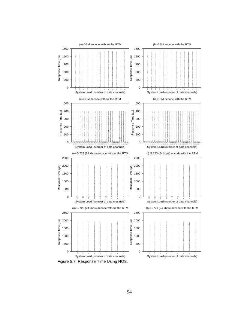
94
Figure 5.7: Response Time Using NOS.
1 2 3 4 5 6 7 8 9 10 11 12 13
System Load (number of data channels)
0
300
600
900
1200
1500
Res
pons
e T
ime
(µs)
(a) GSM encode without the RTM
1 2 3 4 5 6 7 8 9 10 11 12 13
System Load (number of data channels)
0
300
600
900
1200
1500
Res
pons
e T
ime
(µs)
(b) GSM encode with the RTM
1 2 3 4 5 6 7 8 9 10 11 12 13 14 15 16 17 18 19 20 21 22 23 24 25 26 27 28 29 30
System Load (number of data channels)
0
100
200
300
400
500
Res
pons
e T
ime
(µs)
(c) GSM decode without the RTM
1 2 3 4 5 6 7 8 9 10 11 12 13 14 15 16 17 18 19 20 21 22 23 24 25 26 27 28 29 30
System Load (number of data channels)
0
100
200
300
400
500
Res
pons
e T
ime
(µs)
(d) GSM decode with the RTM
1 2 3 4 5 6 7 8 9
System Load (number of data channels)
0
500
1000
1500
2000
2500
Res
pons
e T
ime
(µs)
(e) G.723 (24 kbps) encode without the RTM
1 2 3 4 5 6 7 8 9
System Load (number of data channels)
0
500
1000
1500
2000
2500
Res
pons
e T
ime
(µs)
(f) G.723 (24 kbps) encode with the RTM
1 2 3 4 5 6 7 8 9
System Load (number of data channels)
0
500
1000
1500
2000
2500
Res
pons
e T
ime
(µs)
(g) G.723 (24 kbps) decode without the RTM
1 2 3 4 5 6 7 8 9
System Load (number of data channels)
0
500
1000
1500
2000
2500
Res
pons
e T
ime
(µs)
(h) G.723 (24 kbps) decode with the RTM

95
Figure 5.8: Response Time Using NOS (continued).
1 2 3 4 5 6 7 8 9 10 11 12 13 14 15 16 17 18 19 20 21 22 23 24 25 26 27 28 29 30
System Load (number of data channels)
0
10
20
30
40
50
Res
pons
e T
ime
(µs)
(a) ADPCM encode without the RTM
1 2 3 4 5 6 7 8 9 10 11 12 13 14 15 16 17 18 19 20 21 22 23 24 25 26 27 28 29 30
System Load (number of data channels)
0
10
20
30
40
50
Res
pons
e T
ime
(µs)
(b) ADPCM encode with the RTM
1 2 3 4 5 6 7 8 9 10 11 12 13 14 15 16 17 18 19 20 21 22 23 24 25 26 27 28 29 30
System Load (number of data channels)
0
10
20
30
40
50
Res
pons
e T
ime
(µs)
(c) ADPCM decode without the RTM
1 2 3 4 5 6 7 8 9 10 11 12 13 14 15 16 17 18 19 20 21 22 23 24 25 26 27 28 29 30
System Load (number of data channels)
0
10
20
30
40
50
Res
pons
e T
ime
(µs)
(d) ADPCM decode with the RTM
1 2 3 4 5 6 7 8 9 10 11 12 13 14 15 16 17 18 19 20 21 22 23 24
System Load (number of data channels)
0
200
400
600
800
Res
pons
e T
ime
(µs)
(e) Pegwit encrypt without the RTM
1 2 3 4 5 6 7 8 9 10 11 12 13 14 15 16 17 18 19 20 21 22 23 24
System Load (number of data channels)
0
200
400
600
800
Res
pons
e T
ime
(µs)
(f) Pegwit encrypt with the RTM
1 2 3 4 5 6 7 8 9 10 11 12 13 14 15 16 17 18 19 20 21 22 23 24
System Load (number of data channels)
0
200
400
600
800
Res
pons
e T
ime
(µs)
(g) Pegwit decrypt without the RTM
1 2 3 4 5 6 7 8 9 10 11 12 13 14 15 16 17 18 19 20 21 22 23 24
System Load (number of data channels)
0
200
400
600
800
Res
pons
e T
ime
(µs)
(h) Pegwit decrypt with the RTM

96
dent upon the application, but there are a few cases in which the RTOS has
some influence.
Because NOS is a non-preemptive RTOS, the response time depends
heavily on whether or not the system is idle. When the system is idle, the
interrupt wakes the processor up out of idle mode and immediately exe-
cutes the ISR, followed by the response task. This is indicated on the
graphs as the large concentration of values near zero, which is actually 1.4
microseconds. The fraction of interrupts that occur when the system is idle
decreases as the system load increases. Thus, the fraction of response time
measurements at this value decreases with system load as well. Conversely,
during the execution of a task, responses to interrupts cannot occur until
that task reaches a scheduling point. In NOS, scheduling points are simply
the return of a task’s main function. Therefore, an aperiodic interrupt that
occurs during the execution of a task is not responded to until the current
task completes its main function. The time spent executing tasks is domi-
nated by the processing tasks. Therefore, the response times for interrupts
that occur during the execution of a task are distributed more or less uni-
formly from 1.4 microseconds, to the amount of time necessary to execute
the processing task. This can be up to several hundreds of microseconds or
more, depending on the application. Also, as the system load increases, the
concentration of points within this region becomes more dense, because
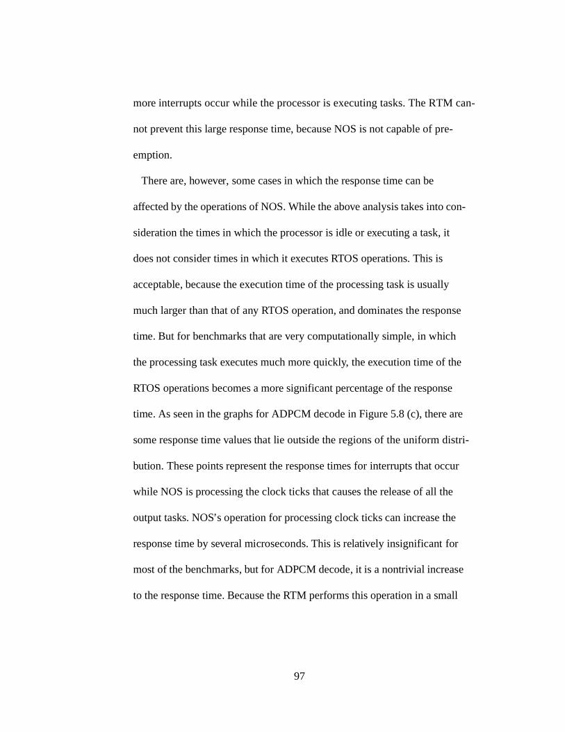
97
more interrupts occur while the processor is executing tasks. The RTM can-
not prevent this large response time, because NOS is not capable of pre-
emption.
There are, however, some cases in which the response time can be
affected by the operations of NOS. While the above analysis takes into con-
sideration the times in which the processor is idle or executing a task, it
does not consider times in which it executes RTOS operations. This is
acceptable, because the execution time of the processing task is usually
much larger than that of any RTOS operation, and dominates the response
time. But for benchmarks that are very computationally simple, in which
the processing task executes much more quickly, the execution time of the
RTOS operations becomes a more significant percentage of the response
time. As seen in the graphs for ADPCM decode in Figure 5.8 (c), there are
some response time values that lie outside the regions of the uniform distri-
bution. These points represent the response times for interrupts that occur
while NOS is processing the clock ticks that causes the release of all the
output tasks. NOS’s operation for processing clock ticks can increase the
response time by several microseconds. This is relatively insignificant for
most of the benchmarks, but for ADPCM decode, it is a nontrivial increase
to the response time. Because the RTM performs this operation in a small
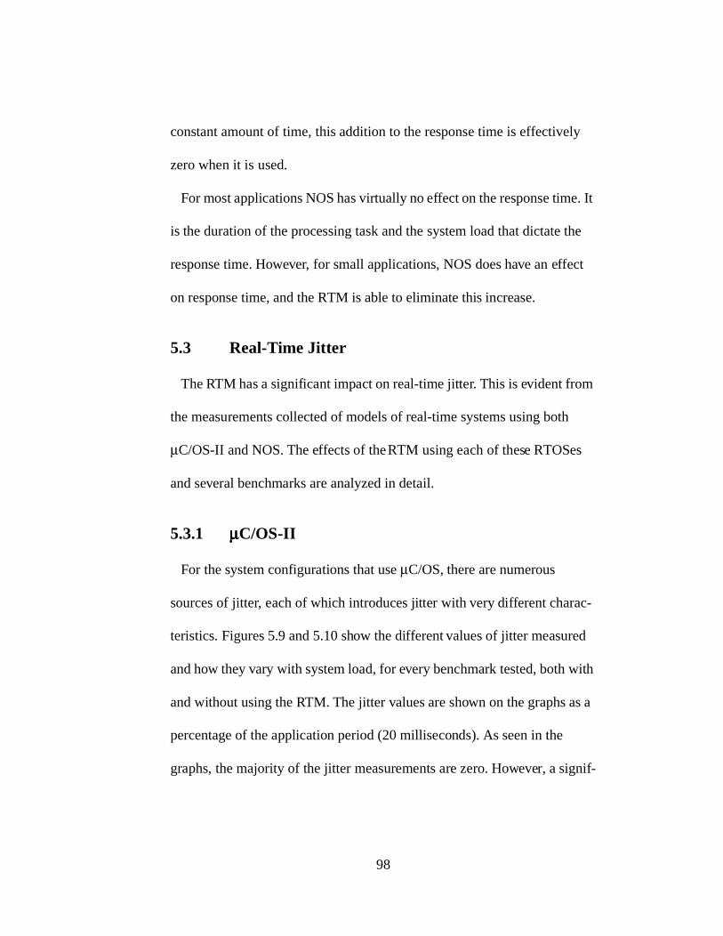
98
constant amount of time, this addition to the response time is effectively
zero when it is used.
For most applications NOS has virtually no effect on the response time. It
is the duration of the processing task and the system load that dictate the
response time. However, for small applications, NOS does have an effect
on response time, and the RTM is able to eliminate this increase.
5.3 Real-Time Jitter
The RTM has a significant impact on real-time jitter. This is evident from
the measurements collected of models of real-time systems using both
µC/OS-II and NOS. The effects of the RTM using each of these RTOSes
and several benchmarks are analyzed in detail.
5.3.1 µµµµC/OS-II
For the system configurations that use µC/OS, there are numerous
sources of jitter, each of which introduces jitter with very different charac-
teristics. Figures 5.9 and 5.10 show the different values of jitter measured
and how they vary with system load, for every benchmark tested, both with
and without using the RTM. The jitter values are shown on the graphs as a
percentage of the application period (20 milliseconds). As seen in the
graphs, the majority of the jitter measurements are zero. However, a signif-
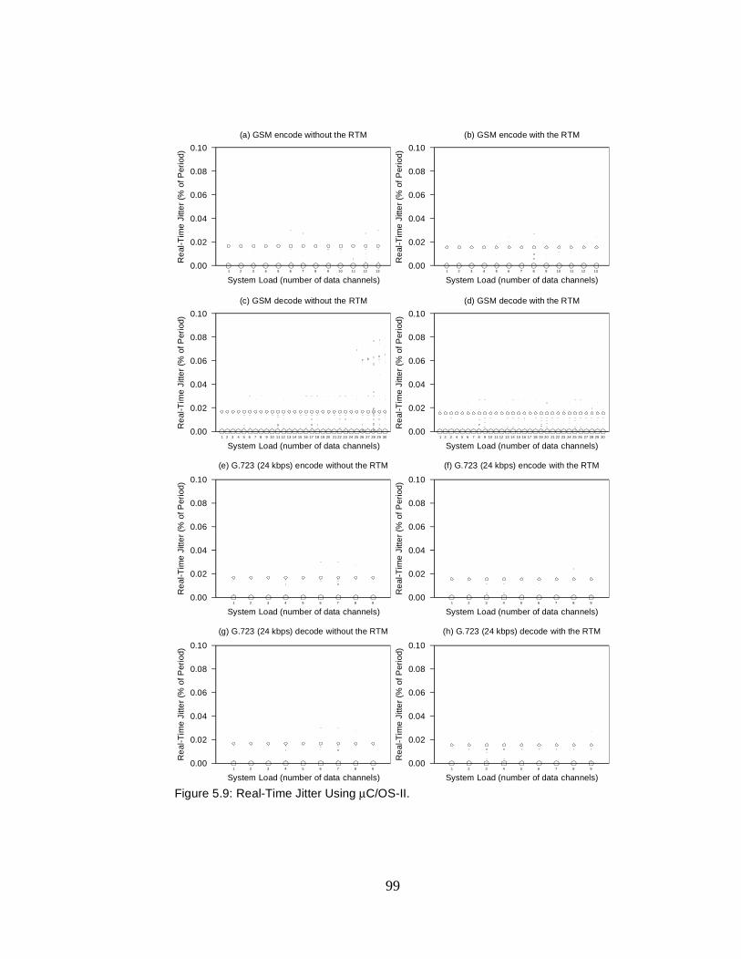
99
Figure 5.9: Real-Time Jitter Using µC/OS-II.
1 2 3 4 5 6 7 8 9 10 11 12 13
System Load (number of data channels)
0.00
0.02
0.04
0.06
0.08
0.10
Re
al-T
ime
Jitt
er
(% o
f Per
iod)
(a) GSM encode without the RTM
1 2 3 4 5 6 7 8 9 10 11 12 13
System Load (number of data channels)
0.00
0.02
0.04
0.06
0.08
0.10
Re
al-T
ime
Jitt
er
(% o
f Per
iod)
(b) GSM encode with the RTM
1 2 3 4 5 6 7 8 9 10 11 12 13 14 15 16 17 18 19 20 21 22 23 24 25 26 27 28 29 30
System Load (number of data channels)
0.00
0.02
0.04
0.06
0.08
0.10
Re
al-T
ime
Jitt
er
(% o
f Per
iod)
(c) GSM decode without the RTM
1 2 3 4 5 6 7 8 9 10 11 12 13 14 15 16 17 18 19 20 21 22 23 24 25 26 27 28 29 30
System Load (number of data channels)
0.00
0.02
0.04
0.06
0.08
0.10
Re
al-T
ime
Jitt
er
(% o
f Per
iod)
(d) GSM decode with the RTM
1 2 3 4 5 6 7 8 9
System Load (number of data channels)
0.00
0.02
0.04
0.06
0.08
0.10
Re
al-T
ime
Jitt
er
(% o
f Per
iod)
(e) G.723 (24 kbps) encode without the RTM
1 2 3 4 5 6 7 8 9
System Load (number of data channels)
0.00
0.02
0.04
0.06
0.08
0.10
Re
al-T
ime
Jitt
er
(% o
f Per
iod)
(f) G.723 (24 kbps) encode with the RTM
1 2 3 4 5 6 7 8 9
System Load (number of data channels)
0.00
0.02
0.04
0.06
0.08
0.10
Re
al-T
ime
Jitt
er
(% o
f Per
iod)
(g) G.723 (24 kbps) decode without the RTM
1 2 3 4 5 6 7 8 9
System Load (number of data channels)
0.00
0.02
0.04
0.06
0.08
0.10
Re
al-T
ime
Jitt
er
(% o
f Per
iod)
(h) G.723 (24 kbps) decode with the RTM

100
Figure 5.10: Real-Time Jitter Using µC/OS-II (continued).
1 2 3 4 5 6 7 8 9 10 11 12 13 14 15 16 17 18 19 20 21 22 23 24 25 26 27 28 29 30
System Load (number of data channels)
0.00
0.02
0.04
0.06
0.08
0.10
Re
al-T
ime
Jitt
er
(% o
f Per
iod)
(a) ADPCM encode without the RTM
1 2 3 4 5 6 7 8 9 10 11 12 13 14 15 16 17 18 19 20 21 22 23 24 25 26 27 28 29 30
System Load (number of data channels)
0.00
0.02
0.04
0.06
0.08
0.10
Re
al-T
ime
Jitt
er
(% o
f Per
iod)
(b) ADPCM encode with the RTM
1 2 3 4 5 6 7 8 9 10 11 12 13 14 15 16 17 18 19 20 21 22 23 24 25 26 27 28 29 30
System Load (number of data channels)
0.00
0.02
0.04
0.06
0.08
0.10
Re
al-T
ime
Jitt
er
(% o
f Per
iod)
(c) ADPCM decode without the RTM
1 2 3 4 5 6 7 8 9 10 11 12 13 14 15 16 17 18 19 20 21 22 23 24 25 26 27 28 29 30
System Load (number of data channels)
0.00
0.02
0.04
0.06
0.08
0.10
Re
al-T
ime
Jitt
er
(% o
f Per
iod)
(d) ADPCM decode with the RTM
1 2 3 4 5 6 7 8 9 10 11 12 13 14 15 16 17 18 19 20 21 22 23 24
System Load (number of data channels)
0.00
0.02
0.04
0.06
0.08
0.10
Re
al-T
ime
Jitt
er
(% o
f Per
iod)
(e) Pegwit encrypt without the RTM
1 2 3 4 5 6 7 8 9 10 11 12 13 14 15 16 17 18 19 20 21 22 23 24
System Load (number of data channels)
0.00
0.02
0.04
0.06
0.08
0.10
Re
al-T
ime
Jitt
er
(% o
f Per
iod)
(f) Pegwit encrypt with the RTM
1 2 3 4 5 6 7 8 9 10 11 12 13 14 15 16 17 18 19 20 21 22 23 24
System Load (number of data channels)
0.00
0.02
0.04
0.06
0.08
0.10
Re
al-T
ime
Jitt
er
(% o
f Per
iod)
(g) Pegwit decrypt without the RTM
1 2 3 4 5 6 7 8 9 10 11 12 13 14 15 16 17 18 19 20 21 22 23 24
System Load (number of data channels)
0.00
0.02
0.04
0.06
0.08
0.10
Re
al-T
ime
Jitt
er
(% o
f Per
iod)
(h) Pegwit decrypt with the RTM
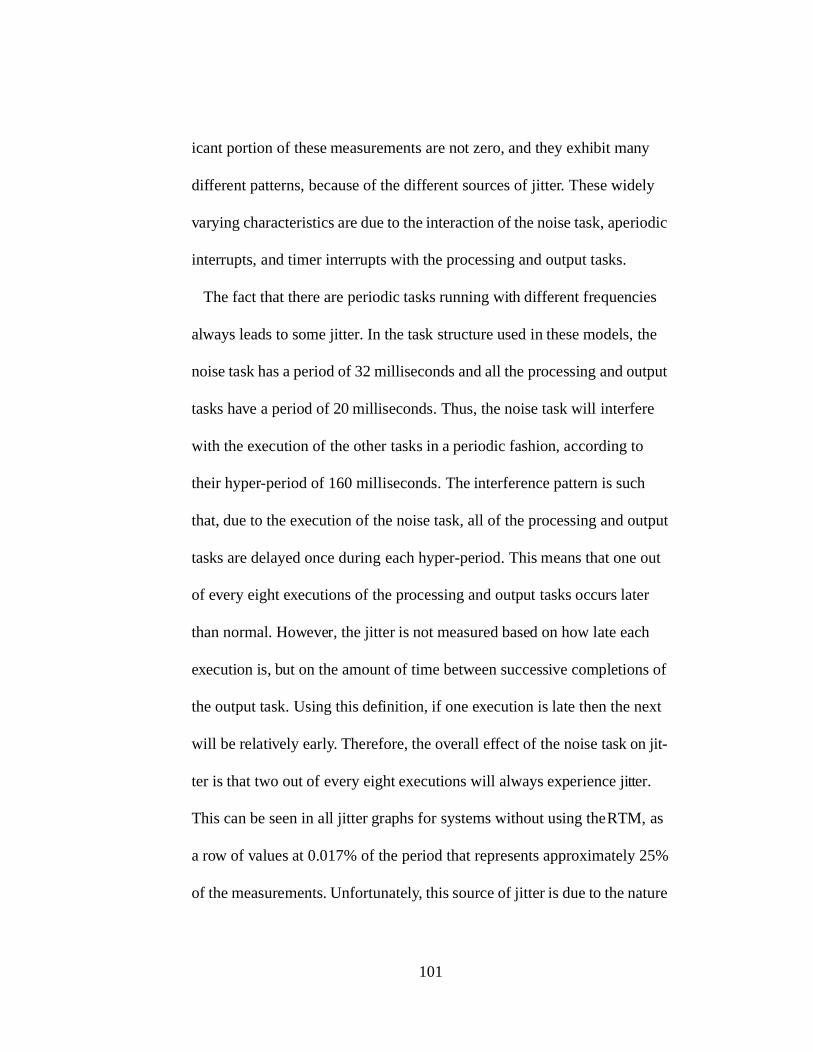
101
icant portion of these measurements are not zero, and they exhibit many
different patterns, because of the different sources of jitter. These widely
varying characteristics are due to the interaction of the noise task, aperiodic
interrupts, and timer interrupts with the processing and output tasks.
The fact that there are periodic tasks running with different frequencies
always leads to some jitter. In the task structure used in these models, the
noise task has a period of 32 milliseconds and all the processing and output
tasks have a period of 20 milliseconds. Thus, the noise task will interfere
with the execution of the other tasks in a periodic fashion, according to
their hyper-period of 160 milliseconds. The interference pattern is such
that, due to the execution of the noise task, all of the processing and output
tasks are delayed once during each hyper-period. This means that one out
of every eight executions of the processing and output tasks occurs later
than normal. However, the jitter is not measured based on how late each
execution is, but on the amount of time between successive completions of
the output task. Using this definition, if one execution is late then the next
will be relatively early. Therefore, the overall effect of the noise task on jit-
ter is that two out of every eight executions will always experience jitter.
This can be seen in all jitter graphs for systems without using the RTM, as
a row of values at 0.017% of the period that represents approximately 25%
of the measurements. Unfortunately, this source of jitter is due to the nature
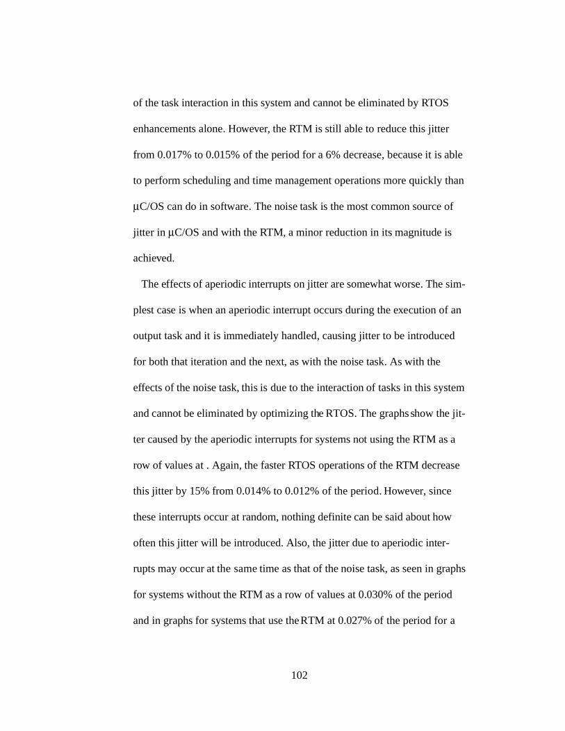
102
of the task interaction in this system and cannot be eliminated by RTOS
enhancements alone. However, the RTM is still able to reduce this jitter
from 0.017% to 0.015% of the period for a 6% decrease, because it is able
to perform scheduling and time management operations more quickly than
µC/OS can do in software. The noise task is the most common source of
jitter in µC/OS and with the RTM, a minor reduction in its magnitude is
achieved.
The effects of aperiodic interrupts on jitter are somewhat worse. The sim-
plest case is when an aperiodic interrupt occurs during the execution of an
output task and it is immediately handled, causing jitter to be introduced
for both that iteration and the next, as with the noise task. As with the
effects of the noise task, this is due to the interaction of tasks in this system
and cannot be eliminated by optimizing the RTOS. The graphs show the jit-
ter caused by the aperiodic interrupts for systems not using the RTM as a
row of values at . Again, the faster RTOS operations of the RTM decrease
this jitter by 15% from 0.014% to 0.012% of the period. However, since
these interrupts occur at random, nothing definite can be said about how
often this jitter will be introduced. Also, the jitter due to aperiodic inter-
rupts may occur at the same time as that of the noise task, as seen in graphs
for systems without the RTM as a row of values at 0.030% of the period
and in graphs for systems that use the RTM at 0.027% of the period for a

103
10% decrease. Furthermore, an aperiodic interrupt could occur just before
the release time of an output task, thereby delaying its execution by a frac-
tion of the processing time required to handle the interrupt. Because aperi-
odic interrupts can occur at any time, this can introduce jitter of any value
less than the aperiodic interrupt processing time. The aperiodic interrupts
are the source of the least predictable form of real-time jitter and can be
slightly lessened with the RTM.
Finally, the timer interrupt may be the most harmful source of jitter. With
this task model, when the number of data channels processed in each appli-
cation exceeds about 25, the processing time required to execute the output
tasks for every channel approaches the 100 microsecond timer interrupt
period. In other words, the next clock tick after the output tasks are released
will occur while one of the output tasks is still executing. The timer inter-
rupt alone is not the problem, because if the interrupt always occurs at the
same point during the execution of the output tasks, there will be no jitter.
However, its interaction with existing sources of jitter is a problem. When
the noise task or aperiodic interrupts push the completion of the output task
of one of the data channels past the occurrence of the timer interrupt, the
task must wait until the interrupt handler completes before resuming execu-
tion. Therefore, the jitter due to the noise task and aperiodic interrupts can
effectively be amplified by the timer interrupt. Also, the timer interrupt in
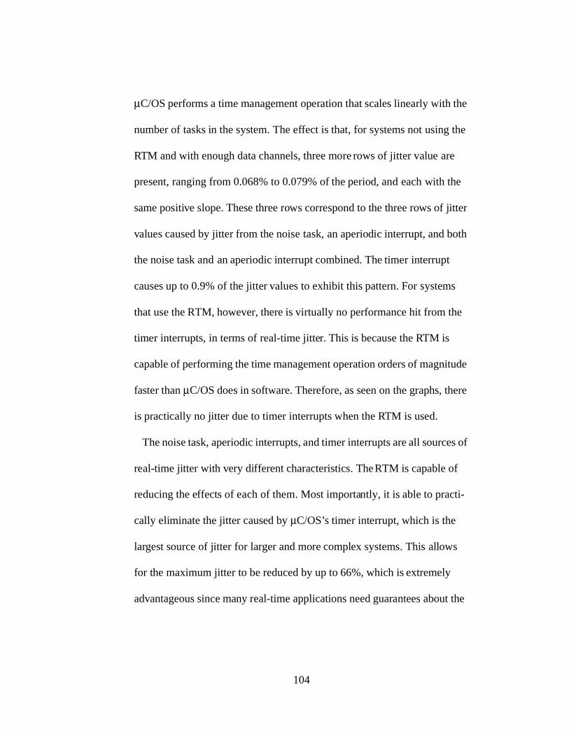
104
µC/OS performs a time management operation that scales linearly with the
number of tasks in the system. The effect is that, for systems not using the
RTM and with enough data channels, three more rows of jitter value are
present, ranging from 0.068% to 0.079% of the period, and each with the
same positive slope. These three rows correspond to the three rows of jitter
values caused by jitter from the noise task, an aperiodic interrupt, and both
the noise task and an aperiodic interrupt combined. The timer interrupt
causes up to 0.9% of the jitter values to exhibit this pattern. For systems
that use the RTM, however, there is virtually no performance hit from the
timer interrupts, in terms of real-time jitter. This is because the RTM is
capable of performing the time management operation orders of magnitude
faster than µC/OS does in software. Therefore, as seen on the graphs, there
is practically no jitter due to timer interrupts when the RTM is used.
The noise task, aperiodic interrupts, and timer interrupts are all sources of
real-time jitter with very different characteristics. The RTM is capable of
reducing the effects of each of them. Most importantly, it is able to practi-
cally eliminate the jitter caused by µC/OS’s timer interrupt, which is the
largest source of jitter for larger and more complex systems. This allows
for the maximum jitter to be reduced by up to 66%, which is extremely
advantageous since many real-time applications need guarantees about the
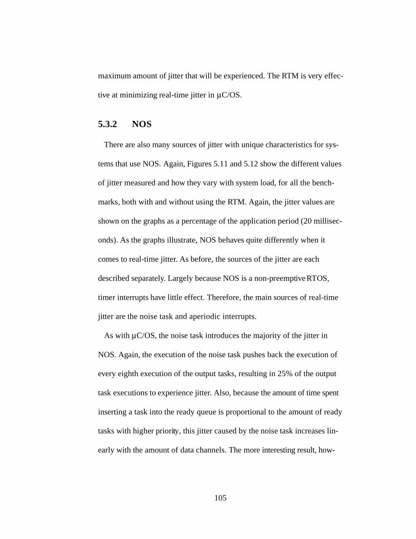
105
maximum amount of jitter that will be experienced. The RTM is very effec-
tive at minimizing real-time jitter in µC/OS.
5.3.2 NOS
There are also many sources of jitter with unique characteristics for sys-
tems that use NOS. Again, Figures 5.11 and 5.12 show the different values
of jitter measured and how they vary with system load, for all the bench-
marks, both with and without using the RTM. Again, the jitter values are
shown on the graphs as a percentage of the application period (20 millisec-
onds). As the graphs illustrate, NOS behaves quite differently when it
comes to real-time jitter. As before, the sources of the jitter are each
described separately. Largely because NOS is a non-preemptive RTOS,
timer interrupts have little effect. Therefore, the main sources of real-time
jitter are the noise task and aperiodic interrupts.
As with µC/OS, the noise task introduces the majority of the jitter in
NOS. Again, the execution of the noise task pushes back the execution of
every eighth execution of the output tasks, resulting in 25% of the output
task executions to experience jitter. Also, because the amount of time spent
inserting a task into the ready queue is proportional to the amount of ready
tasks with higher priority, this jitter caused by the noise task increases lin-
early with the amount of data channels. The more interesting result, how-

106
Figure 5.11: Real-Time Jitter Using NOS.
1 2 3 4 5 6 7 8 9 10 11 12 13
System Load (number of data channels)
0.000
0.005
0.010
0.015
0.020
0.025
Re
al-T
ime
Jitt
er
(% o
f Per
iod)
(a) GSM encode without the RTM
1 2 3 4 5 6 7 8 9 10 11 12 13
System Load (number of data channels)
0.000
0.005
0.010
0.015
0.020
0.025
Re
al-T
ime
Jitt
er
(% o
f Per
iod)
(b) GSM encode with the RTM
1 2 3 4 5 6 7 8 9 10 11 12 13 14 15 16 17 18 19 20 21 22 23 24 25 26 27 28 29 30
System Load (number of data channels)
0.000
0.005
0.010
0.015
0.020
0.025
0.030
Re
al-T
ime
Jitt
er
(% o
f Per
iod)
(c) GSM decode without the RTM
1 2 3 4 5 6 7 8 9 10 11 12 13 14 15 16 17 18 19 20 21 22 23 24 25 26 27 28 29 30
System Load (number of data channels)
0.000
0.005
0.010
0.015
0.020
0.025
0.030
Re
al-T
ime
Jitt
er
(% o
f Per
iod)
(d) GSM decode with the RTM
1 2 3 4 5 6 7 8 9
System Load (number of data channels)
0.000
0.005
0.010
0.015
0.020
Re
al-T
ime
Jitt
er
(% o
f Per
iod)
(e) G.723 (24 kbps) encode without the RTM
1 2 3 4 5 6 7 8 9
System Load (number of data channels)
0.000
0.005
0.010
0.015
0.020
Re
al-T
ime
Jitt
er
(% o
f Per
iod)
(f) G.723 (24 kbps) encode with the RTM
1 2 3 4 5 6 7 8 9
System Load (number of data channels)
0.000
0.005
0.010
0.015
0.020
Re
al-T
ime
Jitt
er
(% o
f Per
iod)
(g) G.723 (24 kbps) decode without the RTM
1 2 3 4 5 6 7 8 9
System Load (number of data channels)
0.000
0.005
0.010
0.015
0.020
Re
al-T
ime
Jitt
er
(% o
f Per
iod)
(h) G.723 (24 kbps) decode with the RTM

107
Figure 5.12: Real-Time Jitter Using NOS (continued).
1 2 3 4 5 6 7 8 9 10 11 12 13 14 15 16 17 18 19 20 21 22 23 24 25 26 27 28 29 30
System Load (number of data channels)
0.000
0.005
0.010
0.015
0.020
0.025
0.030
Re
al-T
ime
Jitt
er
(% o
f Per
iod)
(a) ADPCM encode without the RTM
1 2 3 4 5 6 7 8 9 10 11 12 13 14 15 16 17 18 19 20 21 22 23 24 25 26 27 28 29 30
System Load (number of data channels)
0.000
0.005
0.010
0.015
0.020
0.025
0.030
Re
al-T
ime
Jitt
er
(% o
f Per
iod)
(b) ADPCM encode with the RTM
1 2 3 4 5 6 7 8 9 10 11 12 13 14 15 16 17 18 19 20 21 22 23 24 25 26 27 28 29 30
System Load (number of data channels)
0.000
0.005
0.010
0.015
0.020
0.025
0.030
Re
al-T
ime
Jitt
er
(% o
f Per
iod)
(c) ADPCM decode without the RTM
1 2 3 4 5 6 7 8 9 10 11 12 13 14 15 16 17 18 19 20 21 22 23 24 25 26 27 28 29 30
System Load (number of data channels)
0.000
0.005
0.010
0.015
0.020
0.025
0.030
Re
al-T
ime
Jitt
er
(% o
f Per
iod)
(d) ADPCM decode with the RTM
1 2 3 4 5 6 7 8 9 10 11 12 13 14 15 16 17 18 19 20 21 22 23 24
System Load (number of data channels)
0.000
0.005
0.010
0.015
0.020
0.025
0.030
Re
al-T
ime
Jitt
er
(% o
f Per
iod)
(e) Pegwit encrypt without the RTM
1 2 3 4 5 6 7 8 9 10 11 12 13 14 15 16 17 18 19 20 21 22 23 24
System Load (number of data channels)
0.000
0.005
0.010
0.015
0.020
0.025
0.030
Re
al-T
ime
Jitt
er
(% o
f Per
iod)
(f) Pegwit encrypt with the RTM
1 2 3 4 5 6 7 8 9 10 11 12 13 14 15 16 17 18 19 20 21 22 23 24
System Load (number of data channels)
0.000
0.005
0.010
0.015
0.020
0.025
0.030
Re
al-T
ime
Jitt
er
(% o
f Per
iod)
(g) Pegwit decrypt without the RTM
1 2 3 4 5 6 7 8 9 10 11 12 13 14 15 16 17 18 19 20 21 22 23 24
System Load (number of data channels)
0.000
0.005
0.010
0.015
0.020
0.025
0.030
Re
al-T
ime
Jitt
er
(% o
f Per
iod)
(h) Pegwit decrypt with the RTM
108
ever, is that the jitter values diverge in all cases, as the number of data
channels increases. This is due to the fact that the time that it takes to insert
a task into the software timer queue is proportional to the number of tasks
that have release times less than or equal to that of the task being inserted.
This causes variations in the time required to insert a task in the queue,
which results in the divergence of jitter values. The jitter caused by the
noise task in systems without the RTM is visible on the respective graphs
as two dark bands of values. As can be seen, the lower band is bounded on
the bottom by zero and on the top by a linearly increasing limit, whereas
the upper band originates at 0.0084% of the period and is bounded on the
top and bottom by linearly increasing limits, resulting in jitter up to 0.018%
of the period. The RTM is able to significantly reduce the effects of the
noise task on real-time jitter. By performing task scheduling and time man-
agement operations in a small constant amount of time, there is no relation-
ship between the jitter caused by the noise task and the system load. The
divergence of values disappears completely, and the upper band is reduced
to a constant row of jitter values at 0.0037% of the period, which is up to a
79% decrease. The noise task will always introduce jitter, but the RTM is
able to minimize it effectively.
Aperiodic interrupts are sources of jitter in NOS as well. Since NOS is
non-preemptive, if an interrupt occurs during the middle of the execution of
109
a task, the response does not occur until the current task completes. The
interrupt just inserts a response task at the head of the ready queue. This
may occur during the execution of an output task, which introduces a con-
stant amount of jitter equal to 0.0045% of the period. The response task
executes after the current task completes, thereby delaying the rest of the
output tasks by an additional 0.0038% of the period, for a total of 0.0083%
of the period. However, because the noise task causes jitter from the varia-
tion in time it takes to insert tasks into the software timer queue, the jitter
caused by the aperiodic interrupts appears as a spectrum of values between
the two dark bands mentioned above. Also, the aperiodic interrupts and
noise task can both occur during the same cycle of output task executions.
This results in all the jitter values above the upper band, which look like its
shadow. In fact, these values exhibit the same properties as the upper band,
namely the divergence and linear increase, except 0.0083% of the period
larger in magnitude, resulting in jitter up to 0.0026% of the period. Aperi-
odic interrupts can also cause real-time jitter of any value less than the time
required to process an interrupt, if it overlaps with the release times of the
output tasks. The RTM, however, radically decreases the side-effects that
aperiodic interrupts have on real-time jitter. The fast, constant-time RTOS
operations that it implements have a direct effect on the jitter. Particularly,
the response task only introduces jitter equal to 0.0063% of the period for a

110
21% decrease; and when the effects of the aperiodic interrupts combine
with those of the noise task, jitter of only 0.010% of the period occurs for
up to a 61% decrease. As seen in the graphs, the aperiodic interrupt intro-
duces several patterns of real-time jitter, all of which are reduced by the
RTM.
The noise task and aperiodic interrupts are both sources of real-time jitter
in NOS. Each of which exhibits very different attributes. However, the
RTM reduces the jitter caused by both of them. The RTM reduces the max-
imum jitter experienced by 61%. With the use of the RTM, real-time jitter
in NOS becomes much less of a problem.

111
CHAPTER 6
RELATED WORK
6.1 Modeling of Real-Time Systems with RTOSes
There has been extensive research dealing with the modeling of real-time
systems. However, there has been limited modeling of those that use real-
time operating systems.
The work of Dick, Lakshminarayana, Raghunathan, and Jha is the first
published study of the power consumption of RTOSes in embedded sys-
tems [6]. They have achieved this by using an instruction-level simulator of
the Fujitsu SPARClite processor, developed at Princeton. The embedded
software that they analyze includes a few example embedded applications
running µC/OS. With this testbed, they have taken measurements of the
energy and processing time consumed by various categories of RTOS func-
tions. From these measurements, they have suggested ways in which to
design application software so that the power consumption is minimized.
They believe that their research will lead to formal power-aware system-
level design.
112
Although the focus of this paper is on the power consumption of the
RTOS and this thesis is focused on the performance effects of the RTOS,
there are several similarities between the two. The likenesses are with the
testbeds used in these two studies. Their simulator closely resembles the
C6201 simulator used in this thesis, in terms of input, output, and detail.
The benchmarks used in their study are indicative of the types of applica-
tions that run on the SPARClite, whereas the MediaBench suite used in this
thesis represents a broad range of applications common to high-perfor-
mance DSPs. Finally, the manner in which they analyze the RTOS power
consumption by breaking it down into categories very closely resembles
the analysis of processor utilization in this thesis. These similarities dem-
onstrate that the method used to model real-time systems in this thesis has
been well established.
Studies of the characteristics of RTOSes are becoming increasingly
important. The complexity of real-time applications has been intensifying,
causing more embedded system developers to turn to RTOSes. Through the
work of Dick, et. al. and others, future real-time systems will be faster and
more energy efficient.

113
6.2 Hardware Support for RTOSes
There has been extensive research dealing with the hardware support for
operating systems in desktop processors, but not for RTOSes in embedded
real-time systems. However, there have been some studies focused on
RTOSes in real-time systems.
Adomat, Furunäs, Lindh, and Stärner describes the Real-Time Unit
(RTU)—a hardware module designed to perform RTOS functions [1]. The
RTU is designed for single or multiprocessor systems. It has been imple-
mented as an external ASIC that interfaces with the processors via a VME
bus. The RTU supports 64 tasks with 8 priority levels, as well as sema-
phores, watch dog timers, event flags, external interrupts, periodic release
times, relative time delays, and task scheduling. It informs processors that
they need to switch tasks by sending them interrupts. The processors com-
municate with the RTU by accessing registers through the shared bus. Their
goal is to improve performance and predictability.
The RTU has lots of similarities with the RTM. Both are hardware mod-
ules designed to perform RTOS functions in order to increase performance
and predictability. Both perform task scheduling, time management, and
event management operations. There are, however, many differences. The
main difference is that the RTU is a system-level module and the RTM is
on the processor chip. Because the RTU is external to the processor, it has
114
several advantages and disadvantages. It is capable of supporting multiple
processors and the same RTU can be used for different kinds of processors,
without their modification. However, there is a communication overhead in
arbitrating the bus and sending interrupts, which can actually decrease per-
formance. Also, the RTU will cost more, because of the significant increase
in required hardware. The RTU implements closer to a complete RTOS
than just the bottleneck operations. This may slightly increase perfor-
mance, but it does not allow for existing RTOSes to easily take advantage
of its offerings. These differences illustrate that the RTU and RTM are two
distinct solutions to just about the same problem.
It is becoming more and more apparent that hardware support for
RTOSes is necessary. As application complexity increases, more real-time
systems require the use of an RTOS without the usual performance hit.
Through the efforts of Adomat, et. al. and others, future real-time systems
will be faster and more predictable.
115
CHAPTER 7
CONCLUSION
7.1 Summary
The goal of real-time system designers, like all engineers, is to build an
inexpensive, marketable product that will not take too long to develop and
that performs well enough to satisfy the consumers. This is a delicate bal-
ance and improving one area may be to the detriment of another. Real-time
operating systems happen to allow for faster, cheaper development, but
come at the price of increased real-time jitter, response time, and processor
utilization. This performance decrease can be severe enough to rule out the
use of RTOSes in many real-time systems.
The Real-Time Task Manager helps to solve this problem by consider-
ably reducing the performance loss associated with RTOSes. The RTM
achieves this by implementing three common RTOS operations that are
often major performance bottlenecks in hardware. These RTOS operations
are task scheduling, time management, and event management. By imple-
menting them in hardware, the RTM can extract much more of their intrin-
sic parallelism. Thus, the RTM is able to perform the operations far more
116
quickly, resulting in significant improvements in the performance of the
system.
A reference RTM architecture has been proposed that would be able to
support practically every real-time application. The hardware implementa-
tion of the reference design has been described in detailed schematics. A
die area estimation indicates that it would be feasible to implement the
RTM. This reference architecture demonstrates that it is practical to use the
RTM in real embedded processors.
The effects of the RTM have been estimated through the analysis of sev-
eral models of realistic real-time systems. Each model includes a processor
simulator, an RTOS, and application tasks. The Texas Instruments
TMS320C6201 DSP has been simulated and is used for all systems being
modeled. This processor is commonly used in modern commercial applica-
tions. Two different RTOSes are used in these models: µC/OS-II and NOS.
They are used to demonstrate of the effects of the RTM with two drastically
different RTOSes. Several benchmarks from the MediaBench suite have
been ported to a multitasking environment. These benchmarks define the
function of the application tasks and provide realistic workload characteris-
tics. The models have been thoroughly analyzed with varying amounts of
system load, both with and without the use of the RTM. This analysis
117
allows for the accurate characterization of the RTM’s effects on perfor-
mance.
The RTM drastically improves the performance of real-time systems.
This improvement is due to the fact that, in software, the time it takes to
execute a few key RTOS operations is quite large and may scale linearly
with the number of tasks. However, the RTM performs these operations in a
trivial amount of time. The results of the analysis clearly demonstrate the
RTM’s effects. It reduces the maximum real-time jitter by up to 66% for
µC/OS and up to 61% for NOS. It reduces the maximum response time by
up to 81% for µC/OS, but not significantly for NOS because the applica-
tion, not NOS, determines its maximum response time. Lastly, it reduces
the RTOS processor utilization by up to 90% for µC/OS and up to 65% for
NOS. The RTM is highly effective at reducing the performance loss usually
associated with using an RTOS.
The Real-Time Task Manager is a practical and effective solution to the
RTOS performance loss problem. It is designed to be compatible with as
many systems as possible and is feasible to implement in hardware. Using
extensive formal analysis, the RTM has been shown to significantly reduce
the performance degradation caused by the RTOS. Therefore, the RTM
would allow more real-time systems to take advantage of RTOSes, making
new systems less expensive and decreasing their development time.
118
7.2 Future Work
As with all research, the analysis presented in this thesis can be extend
and improve upon. There are three general areas that should be concen-
trated on to enhance this work: modeling the real-time system more accu-
rately; making the real-time system models more representative of modern
real-time applications; and increasing the performance benefit of the RTM.
Each of these enhancements would benefit this research.
The models are very accurate, however, they are not perfect. Most nota-
bly, the memory system could be fully simulated. Also, formal hardware
verification of the simulator’s accuracy would be desirable. These improve-
ments would contribute to the significance of this research.
Although the models represent a wide range of modern real-time sys-
tems, they do not represent as many systems as they could. For instance,
more processors should be simulated and more RTOSes should be tested.
Also, benchmarks that were designed specifically to test embedded sys-
tems would better represent actual real-time systems. These enhancements
would make the results of this research applicable to a broader range of
real-time systems.
The RTM is very effective at improving the performance of RTOSes, but
it could do more. Particularly, it could easily be modified to fully imple-
ment a dynamic priority scheduling algorithm, such as EDF. This algorithm
119
is used in some RTOSes today. While one of the goals of the RTM is to be
compatible with as many RTOSes as possible, there is some RTOS specific
functionality that could be included in the RTM that would significantly
increase performance. For instance, the effects of the timer interrupt could
be almost eliminated if the RTM was directly connected to a hardware
timer. This would make it only necessary to service an interrupt in response
to a clock tick when a context switch should occur, drastically reducing the
performance effects of the RTOS. Furthermore, advanced features such as
priority inheritance and deadlock detection would be advantageous. All of
these capabilities would make the RTM more robust.
This research can be enhanced through more accurate modeling, more
representative models, and more RTM functionality. These improvements
are the future directions of the work presented in this thesis.

120
BIBLIOGRAPHY
[1] J. Adomat, J. Furunäs, L. Lindh, and J. Stärner. “Real-Time Kernel in
Hardware RTU: A step towards deterministic and high performance
real-time systems.” In Proceedings of Eighth Euromicro Workshop on
Real-Time Systems, L'Aquila, Italy, June 1996, pp. 164-168.
[2] M. Bach. The Design of the UNIX Operating System. Prentice-Hall,
Englewood Cliffs, NJ, 1986.
[3] M. Barr. Programming Embedded Systems in C and C++. O’Reilly &
Associates, CA, January 1999.
[4] K. Baynes, C. Collins, E. Fiterman, B. Ganesh, P. Kohout, C. Smit, T.
Zhang, and B. Jacob. “The Performance and ENergy Consumption of
Three Embedded Real-Time Operating Systems.” In Proceedings of
the 2001 International Conference on Compilers, Architecture, and
Synthesis for Embedded Systems (CASES ’01), Atlanta, GA, Novem-
ber 2001, pp. 203-210.
[5] T. Coopee. “Embedded Intelligence.” InfoWorld, November 17, 2000.

121
[6] R. Dick, G. Lakshminarayana, A. Raghunathan, and N. Jha. “Power
Analysis of Embedded Operating Systems.” In Proceedings of the
37th Design Automation Conference, Los Angeles, CA, June 2000.
[7] International Technology Working Group. International Technology
Roadmap for Semiconductors 2001 Edition: Executive Summary.
Semiconductor Industry Association, 2001.
[8] Jewish Hospital, University of Louisville Health Sciences Center, and
ABIOMED, Inc. “The Implantable Artificial Heart Project.” <ht-
tp://www.heartpioneers.com>, 2001.
[9] J. Labrosse. MicroC/OS-II: The Real-Time Kernel. R & D Books,
Lawrence, KS, 1999.
[10] C. Lee, M. Potkonjak, and W. Mangione-Smith. “MediaBench: A
Tool for Evaluating and Synthesizing Multimedia and Communica-
tions Systems.” In Proceedings of the 30th Annual International Sym-
posium on Microarchitecture (MICRO ‘97), Research Triangle Park,
NC, December 1997.
[11] Y. Li, M. Potkonjak, and W. Wolf. “Real-Time Operating Systems for
Embedded Computing.” In Proceedings of the 1997 International
Conference on Computer Design (ICCD ’97), Austin, TX, October
1997.

122
[12] C. Liu and J. Layland. “Scheduling Algorithms for Multiprogram-
ming in a Hard-Real-Time Environment.” Journal of the Association
for Computing Machinery (JACM), Vol. 20, No. 1, January 1973, pp.
46-61.
[13] J. Liu. Real-Time Systems. Prentice Hall, Upper Saddle River, NJ,
2000.
[14] K. Mackenzie, E. Hudson, D. Maule, S. Jayaraman, and S. Park. “A
Prototype Network Embedded in Textile Fabric.” In Proceedings of
the 2001 International Conference on Compilers, Architecture, and
Synthesis for Embedded Systems (CASES ’01), Atlanta, GA, Novem-
ber 2001, pp. 188-194.
[15] J. Mulder, N. Quach, and M. Flynn. “An Area Model for On-Chip
Memories and its Application.” IEEE Journal of SOLID-STATE Cir-
cuits, Vol. 26, No. 2, February 1991, pp. 98-106.
[16] S. Park and S. Jayaraman. “Textiles and Computing: Background and
Opportunities for Convergence.” In Proceedings of the 2001 Interna-
tional Conference on Compilers, Architecture, and Synthesis for Em-
bedded Systems (CASES ’01), Atlanta, GA, November 2001, pp. 186-
187.

123
[17] K. Shin. “Current Status and Future Directions of Real-Time Comput-
ing.”
[18] A. Tannenbaum. Modern Operating Systems. Prentice Hall, Engle-
wood Cliffs, NJ, 1992.
[19] Texas Instruments. Code Composer Studio User’s Guide. February
2000.
[20] B. Schneier. Applied Cryptography: Protocols, Algorithms, and
Source Code in C. John Wiley & Sons, NY, 1996.
[21] D. Stewart. “Introduction to Real Time.” Embedded Systems Pro-
gramming, CMP Media, November 2001.
[22] J. Turley and H. Hakkarainen. “TI’s New ‘C6x DSP Screams at 1,600
MIPS.” The Microprocessor Report, Vol. 11, 1997, pp. 14-17.
[23] C. Weaver, R. Krishna, L. Wu, T. Austin. “Application Specific Archi-
tectures: A Recipe for Fast, Flexible and Power Efficient Designs.” In
Proceedings of the 2001 International Conference on Compilers, Ar-
chitecture, and Synthesis for Embedded Systems (CASES ’01), Atlan-
ta, GA, November 2001, pp. 181-185.

Related Documents