Performance Enhancement in Heterogeneous Wireless Networks: Channel Assignment considering Switching Overhead, Query Processing using Event Signatures, and Uplink Traffic Analysis by Mira Yun B.S. February 2002, Pukyong National University, South Korea M.S. February 2004, Pukyong National University, South Korea A Dissertation submitted to The Faculty of The School of Engineering and Applied Science of The George Washington University in partial fulfillment of the requirements for the degree of Doctor of Philosophy May 15, 2011 Dissertation directed by Hyeong-Ah Choi Professor of Computer Science

Welcome message from author
This document is posted to help you gain knowledge. Please leave a comment to let me know what you think about it! Share it to your friends and learn new things together.
Transcript

Performance Enhancementin Heterogeneous Wireless Networks:
Channel Assignment considering Switching Overhead,Query Processing using Event Signatures,
and Uplink Traffic Analysis
by Mira YunB.S. February 2002, Pukyong National University, South KoreaM.S. February 2004, Pukyong National University, South Korea
A Dissertation submitted to
The Faculty ofThe School of Engineering and Applied Science
of The George Washington Universityin partial fulfillment of the requirementsfor the degree of Doctor of Philosophy
May 15, 2011
Dissertation directed by
Hyeong-Ah ChoiProfessor of Computer Science

The School of Engineering and Applied Science of The George Washington University
certifies that Mira Yun has passed the Final Examination for the degree of Doctor of
Philosophy as of March 28, 2011. This is the final and approved form of the dissertation.
Performance Enhancementin Heterogeneous Wireless Networks:
Channel Assignment considering Switching Overhead,Query Processing using Event Signatures,
and Uplink Traffic Analysis
Mira Yun
Dissertation Research Committee:
Hyeong-Ah Choi, Professor of Computer Science, Dissertation Director
Xiuzhen Cheng, Associate Professor of Computer Science, Committee Member
Mohamed Tamer Refaei, Senior Infosec Scientist, MITRE Corporation, CommitteeMember
Suresh Subramaniam, Professor of Electrical and Computer Engineering, CommitteeMember
Abdou Youssef, Professor of Computer Science, Committee Member
ii

Abstract
Performance Enhancement in Heterogeneous Wireless Networks:Channel Assignment considering Switching Overhead,
Query Processing using Event Signatures, and Uplink Traffic Analysis
As new Radio Access Technologies have been constantly developed and deployed with
various emerging multimedia applications and multi-radio portable devices, the level of
heterogeneity in wireless networks has been increasing. Since current wireless network
technologies have their own unique characteristics and capabilities, radio resource sharing
and information processing in heterogeneous environments is widely considered to be
crucial in optimizing the network throughput and capacity. Furthermore, new trends in the
use of the Internet due to the emergence of new services and changes in the propensity of
mobile users make heterogeneous resource management problems increasingly difficult.
In this dissertation, these three concerns are addressed in order to achieve significant
performance enhancement in terms of network management and user satisfaction.
First, resource allocation and scheduling problems in multi-radio multi-channel Wireless
Mesh Networks are addressed by considering the switching overhead incurred from
switching radios dynamically from one channel to another. We explicitly model the
switching delay that is incurred during channel switching and use that delay in the design
of channel assignment algorithms. Both centralized and distributed channel assignment
algorithms are provided. Performance of the developed channel assignment algorithms is
analyzed through discrete-event simulations.
Second, the problem of information processing in Heterogeneous Wireless Sensor Net-
works is considered. As a powerful application domain of information processing, we
iii

consider the problem of identifying significant events using diverse sensors deployed in
the area. We provide a mechanism by which sensors can exchange information using
signatures of events instead of raw data to save on transmission costs. Further, we present
an algorithm that dynamically generates phases of information exchange based on the cost
and selectivity of each sensor filter. Simulation results show that the proposed algorithm
detects events while minimizing the transmission and processing costs at sensors.
The new trend in wireless services is shifting from downlink-centric services to bidirec-
tional and uplink centric services. Through the popularity of social networking services
(e.g. Facebook, YouTube, and Flickr), we are observing an ever-increasing amount of user-
generated content, also known as user-created content. This recent uplink traffic pattern
is considered as a final problem in this dissertation. Live uplink traffic traces obtained by
monitoring 3G networks of a mobile data service provider are analyzed. The results using
six different self-similarity analysis algorithms suggest that this uplink traffic is self-similar.
The impact of analyzed traffic characteristics on mobile data networks is evaluated in the
WiMAX module available in OPNET software.
The contributions of this dissertation research lie in the area of radio resource management,
distributed information processing, and new traffic pattern analysis in heterogeneous
wireless networks. This work is the first to investigate the three crucial factors that limit
network throughput and capacity, and analyze their impact on network performance in
heterogeneous environments. Our consideration of switching overhead and use of sensory
signatures are novel contributions and achieve significant performance enhancement in
heterogeneous wireless networks.
iv

Contents
Abstract iii
List of Figures ix
List of Tables xi
1 Introduction 1
1.1 Motivation . . . . . . . . . . . . . . . . . . . . . . . . . . . . . . . . . . . 1
1.2 Heterogeneous Wireless Networks . . . . . . . . . . . . . . . . . . . . . . 3
1.2.1 Heterogeneous Wireless Mesh Networks . . . . . . . . . . . . . . 7
1.2.2 Heterogeneous Wireless Sensor Networks . . . . . . . . . . . . . . 8
1.3 Scope of Research . . . . . . . . . . . . . . . . . . . . . . . . . . . . . . . 9
1.4 Dissertation Outline . . . . . . . . . . . . . . . . . . . . . . . . . . . . . . 11
2 Literature Survey 13
2.1 Channel Assignment in Heterogeneous Wireless Mesh Networks . . . . . . 13
v

2.2 Event Detection in Heterogeneous Wireless Sensor Networks . . . . . . . . 15
2.3 UGC Traffic and Mobile Data Networks . . . . . . . . . . . . . . . . . . . 17
2.3.1 User-Generated Content . . . . . . . . . . . . . . . . . . . . . . . 17
2.3.2 Mobile Network Evolution: Towards Uplink Enhancement . . . . . 17
3 Channel Assignment considering Switching Overhead in HWMNs 20
3.1 Channel Assignment and Switching Overhead . . . . . . . . . . . . . . . . 20
3.1.1 Related Work . . . . . . . . . . . . . . . . . . . . . . . . . . . . . 20
3.1.2 Switching Overhead - Negligible or not? . . . . . . . . . . . . . . 22
3.1.3 Shortcomings of GMS with Switching Overhead . . . . . . . . . . 23
3.2 System Model and Problem Statement . . . . . . . . . . . . . . . . . . . . 25
3.2.1 System Model . . . . . . . . . . . . . . . . . . . . . . . . . . . . 25
3.2.2 Problem Statement . . . . . . . . . . . . . . . . . . . . . . . . . . 26
3.3 Scheduling considering Switching Overhead . . . . . . . . . . . . . . . . . 27
3.3.1 Centralized Scheduling with Switching Overhead . . . . . . . . . . 28
3.3.2 Distributed Scheduling with Switching Overhead . . . . . . . . . . 31
3.3.3 Stability Analysis . . . . . . . . . . . . . . . . . . . . . . . . . . . 35
3.4 Simulation Results . . . . . . . . . . . . . . . . . . . . . . . . . . . . . . 36
3.4.1 Simulation Scenarios . . . . . . . . . . . . . . . . . . . . . . . . . 36
3.4.2 Simulation Results . . . . . . . . . . . . . . . . . . . . . . . . . . 37
4 Distributed Query Processing using Event Signatures in HWSNs 41
vi

4.1 System Model and Problem Formulation . . . . . . . . . . . . . . . . . . . 41
4.1.1 Area as a Grid . . . . . . . . . . . . . . . . . . . . . . . . . . . . 41
4.1.2 Sensor Nodes . . . . . . . . . . . . . . . . . . . . . . . . . . . . . 42
4.1.3 Cell Status as a Sensory Signature . . . . . . . . . . . . . . . . . . 43
4.1.4 Query Protocol . . . . . . . . . . . . . . . . . . . . . . . . . . . . 44
4.1.5 Problem Formulation . . . . . . . . . . . . . . . . . . . . . . . . . 45
4.1.6 Cost Model . . . . . . . . . . . . . . . . . . . . . . . . . . . . . . 45
4.2 Distributed Query Processing using Signatures . . . . . . . . . . . . . . . 46
4.2.1 Distributed Query Processing Protocol . . . . . . . . . . . . . . . . 49
4.3 Localized Query Processing Protocol . . . . . . . . . . . . . . . . . . . . . 52
4.4 Simulation Results . . . . . . . . . . . . . . . . . . . . . . . . . . . . . . 52
4.4.1 Protocol Effects on Total Power . . . . . . . . . . . . . . . . . . . 54
4.4.2 Protocol Effects on Computational Power . . . . . . . . . . . . . . 56
5 Uplink Traffic Pattern in Mobile Data Network 58
5.1 Traffic Measurement and Self-Similarity Analysis . . . . . . . . . . . . . . 59
5.1.1 Heavy-tailedness . . . . . . . . . . . . . . . . . . . . . . . . . . . 61
5.2 Impact on Network Performance . . . . . . . . . . . . . . . . . . . . . . . 63
5.2.1 Delay Analysis with Low Load Delay-Sensitive Traffic . . . . . . . 64
5.2.2 Delay Analysis with High Load Delay-Sensitive Traffic . . . . . . . 65
6 Conclusion and Future Directions 70
vii

6.1 Contributions . . . . . . . . . . . . . . . . . . . . . . . . . . . . . . . . . 70
6.1.1 Channel Assignment considering Switching Overhead in HWMNs . 70
6.1.2 Distributed Query Processing using Event Signatures in HWSNs . . 71
6.1.3 Uplink Traffic Pattern in Mobile Data Network . . . . . . . . . . . 71
6.2 Future Directions . . . . . . . . . . . . . . . . . . . . . . . . . . . . . . . 72
Bibliography 74
viii

List of Figures
1.1 Heterogeneous Wireless Networks . . . . . . . . . . . . . . . . . . . . . . 6
1.2 Heterogeneous Wireless Mesh Networks . . . . . . . . . . . . . . . . . . . 7
2.1 Channel Assignment in Wireless Mesh Networks . . . . . . . . . . . . . . 14
3.1 Example topology and schedule with GMS . . . . . . . . . . . . . . . . . 24
3.2 The average throughput of scheduling algorithms . . . . . . . . . . . . . . 37
3.3 The average end-to-end delay of scheduling algorithms . . . . . . . . . . . 38
3.4 The average backlog with δ = 0.1and 0.3 . . . . . . . . . . . . . . . . . . 38
4.1 Grid representing battleground with deployed sensors . . . . . . . . . . . . 42
4.2 Overlapping detection areas without communication . . . . . . . . . . . . 47
4.3 Distribution of sensors . . . . . . . . . . . . . . . . . . . . . . . . . . . . 54
4.4 Total Power Used by 3 protocols, as a function of network size. . . . . . . . 55
4.5 Protocol Effects on Computational Power . . . . . . . . . . . . . . . . . . 56
5.1 Log-log plot of MMS object size . . . . . . . . . . . . . . . . . . . . . . . 62
ix

5.2 Aggregate traffic with 64 MMS and 64 video-telephny services . . . . . . . 64
5.3 Packet delay of video-telephony with 64 MMS and 64 video-telephony SS . 67
5.4 Aggregate traffic with 108 MMS and 108 video-conferencing. . . . . . . . 68
5.5 Packet delay of video-telephony with 108 MMS and 108 video-telephony SS 69
x

List of Tables
1.1 WPAN Standards . . . . . . . . . . . . . . . . . . . . . . . . . . . . . . . 4
1.2 WLAN Standards . . . . . . . . . . . . . . . . . . . . . . . . . . . . . . . 5
1.3 WMAN Standards . . . . . . . . . . . . . . . . . . . . . . . . . . . . . . 5
1.4 Wireless Multimedia Motes . . . . . . . . . . . . . . . . . . . . . . . . . . 9
3.1 Average Backlog Improvement: Centralized Algorithm . . . . . . . . . . . 37
3.2 Average Backlog Improvement: Distributed Algorithm . . . . . . . . . . . 39
3.3 Throughput Improvement-Centralized Algorithm . . . . . . . . . . . . . . 39
3.4 Throughput Improvement-Distributed Algorithm . . . . . . . . . . . . . . 40
4.1 Combining bits in sensory signatures . . . . . . . . . . . . . . . . . . . . . 48
4.2 Sensor filter capabilities . . . . . . . . . . . . . . . . . . . . . . . . . . . . 53
5.1 Hurst Parameter . . . . . . . . . . . . . . . . . . . . . . . . . . . . . . . . 61
5.2 Summary of parameters . . . . . . . . . . . . . . . . . . . . . . . . . . . . 64
xi

Chapter 1
Introduction
1.1 Motivation
As new Radio Access Technologies (RATs) have been constantly developed and deployed
with various emerging multimedia applications and multi-radio portable devices, the level
of heterogeneity in wireless networks has been increasing. Since current wireless network
technologies have their own unique characteristics and capabilities, radio resource sharing
and information processing in heterogeneous environments is widely considered to be
crucial in optimizing the network throughput and capacity. Furthermore, new trends in the
use of the Internet due to the emergence of new services and changes in the propensity of
mobile users make heterogeneous resource management problems increasingly difficult.
In this dissertation, these three concerns are addressed in order to achieve significant
performance enhancement in terms of network management and user satisfaction.
In heterogeneous networks, transmitting huge volumes of data efficiently is a major prob-
lem in terms of resource sharing over different frequency bands and networks. More and
1

more users are generating and publishing their own real-time multimedia data, and various
emerging devices are collecting and distributing real-time physical data. Consequently,
delivering large amounts of real-time data successfully throughout heterogeneous wireless
networks is a critical and difficult problem in optimizing the network throughput and
interference. As Heterogeneous Wireless Mesh Networks (HWMNs) are envisioned as
one of the key infrastructures in the next generation of wireless networks [RDV+05], we
consider channel assignment and scheduling in multi-radio multi-channel HWMNs.
When we consider highly resource-constrained heterogeneous environments, information
processing is another critical problem in terms of minimizing the transmission and
processing costs, thereby extending the life of the network. As a powerful application
domain of information processing, event detection in sensor networks has received much
attention in the wireless research community. Detecting an event using distributed query
processing in a strictly constrained and highly heterogeneous sensor network is a significant
challenge. This event detection scheme can be applied in a broad spectrum of application
domains such as health care systems and battlefields. For these reasons, we consider
the problem of identifying significant events in Heterogeneous Wireless Sensor Networks
(HWSNs).
The new trend in wireless services is shifting from downlink-centric services to bidirec-
tional and uplink centric services. Through the popularity of social networking services
(e.g. Facebook, YouTube, and Flickr), we are observing an ever-increasing amount of user-
generated content (UGC), also known as user created content (UCC) [fECoO]. These new
uplink traffic patterns should be considered as a crucial problem for achieving significant
performance enhancement in emerging heterogeneous environments.
Motivated by the above issues, this research investigates major factors that limit network
2

throughput and capacity, develops new schemes with the aforementioned factors explicitly
considered, and analyzes their impact on network performance in heterogeneous wireless
networks.
1.2 Heterogeneous Wireless Networks
Today’s advanced portable devices including smartphone are popularized with multiple
wireless interfaces such as 3G, 802.11 WiFi, Bluetooth, 802.16 WiMAX etc. Before
we discuss the challenging issues in heterogeneous wireless netwoeks, we briefly give an
overview of current wireless technologies.
• Wireless PAN
Wireless Personal Area Networks (WPANs) interconnect devices around an individ-
ual person’s workspace. Typically the maximum communication ranges of WPAN is
about 10 meters. IEEE 802.15.1 (Bluetooth), 802.15.3 (Ultra Wide Band (UWB)),
and 802.15.4 (ZigBee) support WPAN applications. Table 1.1 shows the main
characteristics of the WPAN technologies as specified in the IEEE 802.15.
• Wireless LAN
Wireless Local Area Networks (WLANs) interconnect devices in local area within
about 100meters. The IEEE 802.11 group of standards specifies the technologies for
WLANs. Table 1.2 shows the main characteristics of the WLAN technologies as
specified in the IEEE 802.11.
3

Table 1.1: WPAN Standards
StandardFrequencyBand
MaximumRange
Maximumdata rate
AccessMethod
ModulationMethod
802.15.1(Bluetooth)
2.4GHz 10meters 3Mbps FHSSGFSK, 2PSK,DQSP, 8PSK
802.15.3(UWB)
3.1-10.6GHz
10meters55Mbps -1Gbps
DS-UWB,OFDM
OPSK, BPSK,OOK, PAM,PPM, BiPhase
802.15.4(ZigBee)
868MHz,902-928MHz,2.4GHz
100meters 250Kbps DSSS
BPSK(868/928MHz)OPSK(2.4GHz)
• Wireless MAN
Wireless Metropolitan Area Networks (WMANs) are wireless networks that typ-
ically cover a metropolitan area or campus. IEEE 802.16 defines the WMAN
technology which is called as WiMAX. Table 1.3 shows the main characteristics
of the WMAN technologies as specified in the IEEE 802.16.
• Wireless WAN
Wireless Wide Area Networks (WWANs) provide regional, nationwide and global
wireless coverage. WWAN can achieve Internet connectivity through using cellular
tower technology or satellite technology.
In this heterogeneous environment, interworking between different network types is
inevitable. Various interworking strategies are reported in the literature [FSA10], [Sal04],
[AHP03], [ZGLC03]. In [FSA10], authors identified the four interworking levels based
on the level of service integration among networks and provided interworking mechanisms
that constitute the basic building blocks in each level. More specifically, [Sal04] proposed
4
Table 1.2: WLAN Standards
StandardFrequencyBand
MaximumRange
Maximumdata rate
AccessMethod
ModulationMethod
802.11a 5.8GHz 100meters 54Mbps OFDMBPSK, QPSK,16-QAM,64-QAM
802.11b 2.4GHz 100meters 11MbpsDSSS,CCK
DPSK,DBPSK,DQPSK
802.11g 2.4GHz 110meters 54Mbps OFDM
BPSK, QPSK,16-QAM, 64-QAM, DBPSK,DQPSK
802.11n2.4-5.8GHz
160meters 248Mbps MIMOBPSK, QPSK,16-QAM,64-QAM
Table 1.3: WMAN Standards
StandardFrequencyBand
MaximumRange
Maximumdata rate
AccessMethod
ModulationMethod
802.16d(FixedWiMAX)
2-66GHz 31miles 134MbpsMIMO-SOFDMA
QPSK, QAM
802.16e(MobileWiMAX)
2-11GHz 31miles 15MbpsMIMO-SOFDMA
QPSK, QAM
some techniques and architectures for IEEE 802.11 WLANs and 3G cellular network
integration. As the development of interworking solutions for heterogeneous wireless
networks has been spurred, IEEE 802.21 working group has started work from March
2004 to enable seamless Media Independent Handover (MIH) and interoperability between
heterogeneous network types including both 802 and non 802 networks [TOF+09].
Within these interworking architectures, multi-access management is a key issue to provide
seamless connectivity and efficient radio resource utilization in Always-Best-Connected
5

Figure 1.1: Heterogeneous Wireless Networks
paradigm [GJ03]. Sachs et al. [SPG09] proposed a general multi-access management
framework which includes the different multi-access functions such as access detection,
access selection and access handover. In the literature [OK10], [KMR+01], [YMM09],
access selection or RAT selection problem including vertical handover has been considered
as a fundamental problem. In [GPRSA08], authors proposed a Markovian approach based
analytical model for RAT selection policies, and showed the validation and suitability
of the proposed model with 3GPP standardized technologies GSM/EDGE [HMG02] and
UMTS [HT02]. With considering initial RAT selection at a call or session establishment,
Gelabert et al. [GSPRA09] considered potential QoS failure due to intrinsic dynamics of
the network, called radio access congestion.
In the following subsections, various types of heterogeneous wireless networks are
introduced.
6

Figure 1.2: Heterogeneous Wireless Mesh Networks
1.2.1 Heterogeneous Wireless Mesh Networks
Heterogeneous Wireless Mesh Networks (HWMNs), envisioned as one of the key in-
frastructures in the next generation wireless networks. As shown in Fig. 1.2, HWMNs
consist of gateways, mesh routers, and mesh clients. Heterogeneous Mesh Routers (HMRs)
connect to each other and forward packets to the destination using multi-hop routing, and
provide network access service to mobile mesh clients. Some HMRs which connect the
Internet with wired connection will serve as gateways. Since HWMNs can be deployed
quickly with low initial capital expense and provide highly flexible and reconfigurable
wireless links over large areas, HWMNs are considered as a promising wireless broadband
networks for various applications such as Public Safety Networks, Municipal Broadband
7

Internet Access, and Mobile Telephony Backhaul Networks.
According to Muniwireless [Bro], there are more than hundreds metro-scale WiFi mesh
projects currently underway or in the planning stage, and we expect this number to grow
dramatically over the next few years. Furthermore, current telecommunication service
providers have deployed 4G (WiMAX and LTE) technologies already, and there are
numerous industry-projects and academic-studies on their interworking architectures and
mechanisms [Com],[FDAI+10],[LLCM08],[CMGK08].
1.2.2 Heterogeneous Wireless Sensor Networks
Wireless Sensor Networks (WSNs) consist of a large number of small devices with
various sensing capabilities. Typically wireless sensors monitor physical or environmental
conditions including temperature, light, sound, or motion, and transmit monitored physical
data through the wireless networks. As the technology of microelectronics and wireless
communications is rapidly developing, WSNs have been considered as a promising
wireless infrastructure for various application domains. Examples of such applications
range from a controlled domain such as homes, hospitals, or offices to an uncontrolled
domain such as battlefield or disaster areas.
Current available multimedia wireless motes are shown in Table 1.4 [AGZAKMP10].
As advanced multimedia sensors and wireless technologies are developing, the level of
heterogeneity of WSNs is rapidly increasing. In Heterogeneous WSNs (HWSNs), sensor
nodes have different capabilities on power, computation, and communication. Because of
this heterogeneity, diverse data processing and efficient transmission schemes should be
designed carefully in HWSNs.
8

Table 1.4: Wireless Multimedia Motes
Platform ProcessorMemoryRAM
Camera Radio Power
Cyclops8-bitATMEI
64KB Agilent compact CIF 802.15.4110mW-0.76mW
Imote2+Cam
32-nitPXA271
256KB IBM400 camera 802.15.4322mW-1.8mW
MeshEye55MHz32-bitARM7TDMI
64KB Agilent ADNS-3060 802.15.4175.9mW-1.78mW
Panoptes400MHz32-bitPXA255
64MB Logitech 3000USB 802.115.3W-58mW
MicrelEye8-bitATMEL
36KB+1MBSRAM
Omnivision OV7640 Bluetooth 500mW
CITRIC624MHz32-bitPXA270
64MB Omnivision OV9655 802.15.4 1W
Fox+Cam
100MHzLX416
16KB Labtec Webcam bro Bluetooth 1.5W
1.3 Scope of Research
In this dissertation research, we focus on three problems that can impact network
performance in heterogeneous wireless networks.
First, the problem of resource allocation and scheduling in multi-radio multi-channel mesh
environment are considered. The switching overhead is explicitly modeled and channel
assignment algorithms are designed by considering that switching overhead.
Second, the problem of information processing in heterogeneous sensor networks is
considered. We provide an event detection mechanism by which sensors can exchange
information using signatures of events instead of raw data to save transmission costs.
9

Last, a recent uplink traffic pattern is considered. Live uplink traffic traces obtained
by monitoring 3G networks are analyzed, and their impact on network performance is
evaluated.
The scope of this research is outlined as follows.
1. Channel Assignment considering Switching Overhead in HWMNs
• The switching overhead that is incurred during channel switching is modeled ,
channel assignment algorithms are designed by using that delay.
• We extend existing algorithms in the literature, namely Greedy Maximal Scheduling
(GMS) and Distributed Maximal Scheduling (DMS) [LR07], taking the switching
delay into account in the channel assignment.
• Performance of the developed algorithms is analyzed through discrete-event simula-
tions.
2. Event Detection using Sensory Signatures in HWSNs.
• We consider the problem of identifying significant events using sensors deployed in
the area.
• We provide two protocols that can reduce the computation cost and the communi-
cation cost for the sensor network, thereby extending the life of the network. The
suggested protocols employ three main techniques to reduce these costs:
(i) use of sensory signature to avoid sending raw or processed data
(ii) use of phases to avoid unnecessary computations
10

(iii) use of leader nodes to avoid unnecessary communications.
• Performance of the developed protocols is analyzed through discrete-event simula-
tions.
3. Uplink Traffic Pattern in Mobile Data Networks.
• We analyze uplink traffic collected from MMS services in WCDMA networks of SK
Telecom, Korea.
• Six different self-similarity analysis algorithms are used.
• The impact of this characteristics on mobile data networks is evaluated through the
WiMAX module available in OPNET software.
1.4 Dissertation Outline
This dissertation document is organized as follows: Chapter 2 presents key issues in
various heterogeneous environments and the relevant literatures. Chapter 3 presents
channel assignment algorithms considering switching overhead in multi-radio multi-
channel HWMNs. After discussing the role of switching overhead and showing why it is
necessary to consider the effects, we extend existing algorithms taking the switching delay
into account in the channel assignment. At last, performance analysis through discrete-
event simulations is given. Chapter 4 presents event detection protocols using sensory
signatures and distributed query processing in HWSNs. By using sensory signatures
and phases, the communication cost and the computation cost are significantly reduced.
In chapter 5, we analyze live traffic traces of uplink traffic and discuss its self-similar
11

characteristics. As the simulation results, we present the impact of the data burst on
the network performance through trace-driven OPNET simulation. Finally in chapter 6,
concluding remarks are made and future directions are pointed out.
12

Chapter 2
Literature Survey
2.1 Channel Assignment in Heterogeneous Wireless Mesh
Networks
In Wireless Mesh Networks (WMNs), channel assignment problem can be defined as
finding a proper mapping between the available channels and the radios at each node
such that the network performance is optimized. Thus channel assignment and scheduling
methods are widely considered to be crucial in optimizing the network interference and
throughput.
As shown in Fig. 2.1, mesh routers can be equipped with multiple radios operating in
multiple non-overlapping channels. By assigning different channels to radio interfaces
in the interference range, multiple channel-interface pairs can be served simultaneously,
and this leads to higher network capacity. In this multi-radio multi-channel environment,
a proper assignment of channels to interfaces is a critical factor of resource allocation
13

Figure 2.1: Channel Assignment in Wireless Mesh Networks
problem [RDV+05].
Channel assignment schemes can be divided into three categorizes: fixed, dynamic, and
hybrid assignment [SGD+07]. Fixed schemes assign channels to radio interfaces statically
[RGcC04], [KV05], [MD05] and are adequate for use when the network condition is
stable. In order to consider significant changes to traffic load or network topology in
fixed schemes, quasi-static channel assignments are proposed in [JZ08] and [SGDC08].
Quasi-static schemes allow the channel assignment changes, but infrequently, resulting
in negligible traffic measurement overheads and switching delays. Dynamic assignment
schemes change the assignment as needed, per packet or time slot [RC05]. Since radio
interfaces can frequently switch from one channel to another, dynamic schemes can
accommodate the changes in network conditions. However channel switching delays
(typically 802.11 card has a few hundreds of microseconds to a few milliseconds) can be
a challenging problem [SGD+07], [VKLS06], [FLW08]. Hybrid strategies combine static
and dynamic assignment concepts by using static assignment for certain nodes/radios, and
using a dynamic assignment approach for the other nodes [KV05], [KV06], [RBAB06].
14

2.2 Event Detection in Heterogeneous Wireless Sensor
Networks
In Wireless Sensor Networks (WSNs), information processing is a critical problem due to
the huge volume of real-time physical data collected through many diverse sensors [ZG04].
As a powerful application domain of information processing, event detection in sensor
networks has received much attention in the wireless research community. The literature
provides various event detection schemes, as in [LWHS02], [KI04], and [BRS03]. In these
event detection projects, events are typically categorized into two groups: atomic events
and compound events defined by [PKRVJ05] and [LLS+04]. An atomic event is an event
characterized by a single type of physical data, while a compound event is one characterized
by multiple types of physical data. Even detecting an atomic event in a constrained
network is a significant challenge. Marticic et al. in [MS06] present a distributed event
representation paradigm. This paradigm divides the detection area into cells, gathers data
from all nodes in each cell, and computes a weighted average of all data gathered within
the cell. Sensor nodes store copies of adjacent cell averages, and can detect an event
by matching this submatrix of cell averages to an event signature. Hu et al. in [HY07]
present a sleeping schedule to reduce communication and computation overhead, improve
energy efficiency and prolong the life of the network. By deploying multiple sensors to
monitor the same area and electing a single node to monitor the area, a large fraction of
nodes can remain asleep while still ensuring that the area is monitored. For compound
events, Abadi et al. extend the TinyDB query processor in [MFHH05] to produce an event
detection system for sensor networks called REED, presented in [AML05]. The system
supports in-network joins between sensory data and static tables built outside the sensor
15

network. Kumar et al. in [PKRVJ05] propose a distributed event detection framework
by considering collaboration among sensor nodes. The framework forms a group of sensor
nodes gathering all data types necessary to detect a compound event, and each group reports
to the centralized headquarters if the aggregated data satisfies the given conditions.
Previous work considering sensor networks in battle environments include [OUS+08],
[SML+04], and [WSS03]. Especially the Battle of the Water Sensor Networks (BWSN)
was held in August 2006. After the events of September 11, 2001, in the United
States, more practical research and performance analysis on water distribution systems
are demanded against possible chemical attacks, so that fifteen sensor network designs
considering the following four design objectives are proposed in BWSN [OUS+08]: 1)
minimization of the expected time of event detection, 2) minimization of the expected
population affected prior to event detection, 3) minimization of the expected demand
of contaminated water prior to event detection, and 4) maximazation of the detection
likelihood.
In the case of battle event detection, sensors can be deployed in a battlefield, gathering
several types of data. The sensors can take the form of smoke-detectors, noise-detectors,
motion-detectors, as well as cameras. We would like to match data gathered around the
same time and location to identify significant events that are characterized by specific
sensory data and to alert a centralized headquarters about the occurrence of the significant
events so that they can respond appropriately to the events. The type of events that we
would like to identify can vary; for example, a significant event might be the explosion of
a bomb or the deployment of a chemical agent. Each event is characterized by a particular
set of sensory data, or “sensory signature”. For example, an exploding bomb might be
characterized by a bright light, loud sound, and hot temperature, and its sensory signature
16
would reflect these properties.
2.3 UGC Traffic and Mobile Data Networks
2.3.1 User-Generated Content
Web 2.0 does not refer to a new technology or technical specification, but to changes
in web-based environment which software developers and end-users use as a platform.
The basic idea of this Web 2.0 is empowering computer end-users to contribute to
develop, share, and evaluate information efficiently in Internet. As a part of Web 2.0
concept, user-generated content (UGC), also known as user-created content (UCC) or
consumer generated media (CGM), is growing rapidly and making a new producing trend
of media content [fECoO]. In other words, as opposes to traditional media producers,
end-users are generating multi-media contents and uploading them to websites such as
YouTube, Facebook, Wikipedia, MySpace, Flickr, and so on. These changes in web-based
communities are emerging not only in wired networks, but also in wireless networks. In
cellular networks, especially, as being upgraded to 3G technologies the study on modeling
and analysis of new traffic pattern of UCC is required.
2.3.2 Mobile Network Evolution: Towards Uplink Enhancement
Fast growth in cellular usage with emerging multimedia applications have led to the
requirement for new 3G cellular telecommunication networks. To deal this requirement,
two new partnership projects, 3rd Generation Partnership Project (3GPP) and 3GPP2,
were established in 1998 [3GPa][3GPb]. 3GPP is developing 3G standard for Global
17

System for Mobile (GSM) based system such as General Packet Radio Service (GPRS)
and Universal Mobile Telecommunications System (UMTS)( or Wideband Code Division
Multiple Access (WCDMA)) and 3GPP2 is focusing on Interim Standard (IS)-95 based
CDMA system such as CDMA2000. As high data rate services such as video transmission
and other data services became popular, both 3GPP and 3GPP2 introduced downlink
enhancement technologies of each 3G system (WCDMA, CDMA2000), which are High
Speed Downlink Packet Access (HSDPA)(up to 10Mbps) and CDMA 1x Evolution Data
Only (EvDO) (up to 2.4 Mbps in Rev. 0) respectively [HT06][FGB+05].
Initially most of 3G applications were considered to have much heavier traffic in the
downlink direction than in the uplink direction. However, as new services such as video
telephony and FTP upload are introduced and a new uploading pattern such as UCC
emerged, uplink enhancements have also received great attention making High Speed
Uplink Packet Access (HSUPA) and CDMA 1x EvDO Rev. A system considered in 3.5G
systems [SK05][EVD06].
The CDMA 1x EvDO Rev. A system was standardized in March 2004. The peak
rate can achieve up to 3.1Mbps for the downlink and 1.8Mbps for the uplink. A novel
flow-centric protocol design is adopted to enhance the system’s capability for satisfying
different flow QoS requirements. Improvement has been observed in supporting delay-
sensitive applications and providing tradeoff in delay, capacity and physical-layer error-rate
[FGB+05].
HSUPA was introduced to improve the capacity of WCDMA uplink in 3GPP Release 6
with the first specification version in December 2004. Although HSUPA is the commonly
used terminology, Enhanced-Dedicated Channel (E-DCH) is the official term used by 3GPP
to describe the new uplink transport channel [HT06]. The E-DCH supports fast Node B
18

based uplink scheduling, fast physical layer hybrid ARQ (HARQ) retransmission schemes
and, optionally, a shorter transmission time interval (TTI) (2ms) to reduce delays, increase
the data rate (up to 5Mbps) and improve the capacity of the uplink [PEHS04].
WiMAX 802.16 has become the most promising broadband wireless access technology. In
Oct 2007, WiMAX is officially accepted as the one of the 3G standards by International
Telecommunication Union (ITU). The standard of WiMAX evolved from the original
802.16 to the latest 802.16e which supports full mobility. When the Orthogonal Frequency-
Division Multiple Access (OFDMA) physical layer is employed, the theoretical uplink or
downlink raw bitrate could achieve 70Mbps [Nua].
19

Chapter 3
Channel Assignment considering
Switching Overhead in HWMNs
3.1 Channel Assignment and Switching Overhead
3.1.1 Related Work
A vast amount of research has been conducted to exploit multiple channels for performance
improvement. Ramachandran et al. [RBAB06] proposed a centralized channel assignment
algorithm which has a Channel Assignment Server (CAS). CAS allocates channels to radio
interfaces while minimizing interference in multi-radio multi-channel WMNs. Among the
centralized algorithms, an optimum scheduling policy was given by Tassiulas et al. in
their seminal paper [TE92]. This scheduling policy, commonly referred to as Maximum
Weighted Scheduling, is computationally prohibitive for general interference models (such
as 2-hop interference model), and a simpler but suboptimal strategy called GMS is well
20

established as a scheduling algorithm for single channel multi-hop wireless networks. GMS
has been known to have an efficiency ratio of 1/κ in single-channel networks [LS06] and
1/(κ + 2) in multiple-channel networks [LR07], where κ is the interference degree of the
network [CKS05], [Cha06]. Very recently, insights into the true efficiency ratio of GMS
have been presented in [JLS09], where authors showed that the efficiency ratio of GMS
is equal to a network property (pooling factor). They also showed that the worst-case
efficiency ratio of GMS in geometric network graphs is between 16
and 13.
In distributed algorithms, Joo [Joo08] proposed a simple distributed scheduling algorithm
for single channel wireless networks, which achieves an efficiency ratio no smaller than
GMS. In [LR07], Lin et al. suggested a distributed algorithm for multi-channel network
with low-complexity that has the same level of efficiency ratio as GMS. Ko et al. [KMPR07]
also proposed a distributed channel assignment algorithm with channel interference cost
function which indicates the spectral overlapping level between channels. Generally,
distributed algorithms can only achieve a fraction of the maximum possible throughput
due to the lack of complete information. To provide the higher throughput in distributed
schemes, Brzezinski et al. [BZM08] proposed algorithms for pre-partitioning a mesh
network into smaller subnetworks in which simple distributed scheduling algorithms can
achieve the maximum capacity.
In addition, much of the recent research on multi-radio multi-channel WMNs has dealt
the channel assignment and routing problem jointly as a challenging cross-layer problem
[LR07], [NGES07], [TT07]. Raniwala et al. [RGcC04] showed significant improvement
of the overall network goodput in 802.11 based multi-channel WMN architecture by
considering channel assignment and routing jointly. In [LR07], authors proposed a
distributed channel scheduling algorithm that guarantees the efficiency ratio to be same
21

as the centralized GMS algorithm in multi-channel wireless networks.
Recently switching overhead has been acknowledged as a factor for channel assignment
and routing problems in multi-radio WMNs. However, none of existing schemes considers
the switching overhead in channel assignment algorithm itself. In [FLW08], Feng et al.
suggested a hybrid channel assignment protocol (HCAP) to find out a reasonable tradeoff
between flexibility and switching overheads. In order to avoid frequent interface switching,
HCAP adopts static assignment for nodes that have the heaviest loads. In [FLW09], authors
considered switching overhead as a key factor to estimate interference level of a node/link.
3.1.2 Switching Overhead - Negligible or not?
In multi-radio multi-channel environment, many channel assignment algorithms need
frequent channel switching to optimize the efficiency of WMNs. However channel
switching incurs some non-negligible delay, which leads to accumulation of switching
delays between end to end nodes.
In a 802.11 card, the hardware switching delay is typically in the order of a few hundreds
of microseconds to a few milliseconds [RC05], [VKLS06]. When a packet of 1024 bytes
is transmitted through 802.11a/b network where the typical transmission rate is about
25Mbps/6Mbps, it takes 1024 × 8/(25 × 106) = 328µs or 1024 × 8/(6 × 106) = 1.3ms,
which are in the same range of 802.11a/b switching delay. Furthermore when switching
occurs across different frequency bands (e.g., 5GHz for 802.11a and 2.4GHz for 802.11b/g)
the impact of switching delay on the overall network performance becomes even more
significant. In [KV05], Kyasanur and Vaidya showed that the switching delay degrades
the network capacity as a function of SS+T
(where S is switch delay and T is transmission
22

time). As in the example above, the value of S can approach the value of T . This causes a
significant degradation in network capacity.
With technology advancements, it is expected that the switching delay will become smaller
overtime [BCD04]. However, the switching delay can be expressed in terms of packet
duration as dt × L/P , where dt is the hardware switching delay, and P and L are the
packet size and transmission speed respectively. While the hardware switching delay
can be expected to progressively get smaller, the transmission speeds can be expected
to progressively get larger. Thus, the trend on the overall loss of bandwidth due to
the switching delay is difficult to predict due to this “push-pull” effect of technology.
This highlights the need to design channel assignment schemes that consider the delay
induced due to the switching overhead, and to model their performance as a function of the
switching overhead.
3.1.3 Shortcomings of GMS with Switching Overhead
It has been shown in [JLS09] that the worst-case efficiency ratio of GMS in geometric
network graphs is between 16
and 13. In our earlier work [YZAC09], however, we indicated
that when switching overhead is considered, GMS algorithm may have no provable
efficiency ratio. Next, we present a counterexample which shows that the efficiency ratio
of GMS algorithm can be arbitrarily close to 0 when switching overhead δ is considered in
a network with 2-hop interference model.
Consider the network topology as shown in Figure 3.1. We assume that the traffic moves
in clockwise direction, all link capacities are 4 and the initial queue size is χ + 3 at nodes
A, E and I , χ + 2 at nodes B, F and J , χ + 1 at nodes C, G and K, and χ, at nodes D,
23

(a) Topology (b) Initial schedule
Figure 3.1: Example topology and schedule with GMS
H and L, where χ is a large number. Consider that all nodes have a constant arrival rate of
1 − δ + ε, where ε is a small number. GMS initially serves links 0, 4 and 8, as the queues
at the origin nodes of those links are the highest and all link capacities are equal. In the
next timeslot, GMS serves nodes 1, 5 and 9. In the following timeslot, GMS serves nodes
2, 6 and 10. followed by nodes 3, 7 and 11. Then, the entire cycle repeats. During these 4
timeslots, each node receives service over one timeslot, and is able to send 4(1 − δ) bits.
During the same 4 timeslots, it receives a total of 4(1 − δ + ε) new bits from its arrival
process, and thus its queue is not stable under GMS.
However, the following schedule can serve the same system with an arrival rate of 4/3− δ:
Consider three link assignments: 0, 3, 6, 9, 1, 4, 7, 10 or 2, 5, 8, 11. We observe that
considering the 2-hop interference model, these link assignments are valid. Start with the
first one, and switch to the next one after χ/3 timeslots. Thus, over χ timeslots, each node
can send (χ/3 − 1)4 + (1 − δ)4 bits. During the same χ timeslots, it receives a total of
χ(4/3− δ) new bits from its arrival process, and thus its queue is stable under this channel
24

assignment scheme.
Therefore, the efficiency ratio of GMS over this schedule is no better than 1−δ+ε4/3−δ
. Since δ
can be vary between 0 and 1, the efficiency ratio can be arbitrarily close to 0.
3.2 System Model and Problem Statement
In this section, we first describe the network model considered in this paper. Then, we
present a formulation of our problem for channel assignment and scheduling.
3.2.1 System Model
We consider a time slotted multi-hop network modeled by an undirected graph G = (V,E)
where V denotes the set of nodes and E denotes the set of edges. For a link l ∈ E when
used in a transmission, the transmitter and the receiver nodes are denoted by b(l) and e(l),
respectively. For a node v ∈ V , the set E(v) denotes the set of edges incident on node
v. Let C denote the set of channels available in the system. Time is slotted into a unit
length. Each node is equipped with at least one radio and can dynamically switch radios
from one channel to another with additional overhead δ represented as a fraction of the
time slot duration, i.e., δ = switching time/time slot duration. It is assumed that each
node v is equipped with α(v) radios such that at any time, v can be involved in up to α(v)
transmissions as either transmitters or receivers.
Let Il denote the set of links that interfere with link l. It is assumed that during the
scheduling period (i.e., over a certain period of time), the network topology is fixed; hence,
the interfering set Il of link l is also fixed. We assume that the interference relation is
25

symmetrical. We denote the queue length of link l in time slot t by q(l, t) where the queue
is assumed to be corresponding to b(l), that is, the transmitter node of link l. The rate at
which link l can transmit on channel c is denoted by r(l, c).
3.2.2 Problem Statement
There are S users in the system. We assume that user s injects packets into the system with
a rate λs and traffic from s follows a fixed path during the scheduling period. (The routing
table is assumed to be fixed during the scheduling period). Let h(l, s) = 1 if user s’s traffic
traverses over link l, and 0 otherwise. The evolution of q(l, t) is then:
q(l, t + 1) = [q(l, t) +S∑
s=1
h(l, s)λs −D(l, t)]+ (3.1)
where D(l, t) denotes the number of packets that link l can serve in time t and [·]+ denotes
the projection to [0,∞). We say the system is stable if the queue length of each link in any
time slot remains finite.
Let ~λ = [λ1, · · · , λS] denote the traffic injected by the S users into the system. The capacity
region under a particular channel assignment and scheduling algorithm is the set of ~λ such
that the system remains stable. The optimal capacity region Ω is defined to be the union
of capacity regions of all algorithms. An algorithm is called throughput-optimal if it can
achieve the optimal capacity region Ω. The efficiency ratio of an algorithm is the largest
number γ ≤ 1 such that for any load ~λ ∈ Ω, γ~λ is in capacity region of the algorithm.
A major component of any throughput-optimal scheduling problem is to solve an optimiza-
tion problem in each time slot t that maximizes∑
l∈E
∑c∈C q(l, c, t)r(l, c, t) satisfying the
26

given constraints. With the switching delay δ as an additional constraint, we formulate
the scheduling problem as follows where z(l, c, t) ∈ 0, 1 is a decision variable such that
z(l, c, t) = 1 means that channel c ∈ C is assigned to link l ∈ E in time slot t.
Scheduling with δ:
Input: Z(t−1) = [ z(l, c, t−1) ] for all l ∈ E and c ∈ C; q(l, t) for all l ∈ E; and r(l, c, t)
for all l ∈ E and c ∈ C.
Output: Z(t) = [ z(l, c, t) ] where (i) z(i, c, t) ∈ 0, 1, (ii) for any l, l′ ∈ E such that
l′ ∈ Il and c ∈ C, z(l, c, t) + z(l′, c, t) ≤ 1, (iii) for any l ∈ E,∑
c∈C z(l, c, t) ≤minα(b(l)), α(e(l)), and satisfying (i-iii), the objective is to maximize
∑
l∈E,c∈C
z(l, c, t)q(l, t)r(l, c, t) | z(l, c, t− 1) = 1
+∑
l∈E,c∈C
z(l, c, t)(1− δ)q(l, t)r(l, c, t) | z(l, c, t− 1) = 0
Note that if z(l, c, t − 1) = 1 and z(l, c, t) = 1, the channel c can be fully utilized on link
l during the time slot t. But if z(l, c, t− 1) = 0, the channel c when assigned to l in time t
can be utilized for only a fraction 1− δ of the time slot.
3.3 Scheduling considering Switching Overhead
In this section, we extend the existing algorithms taking the switching delay into account
in the channel assignment. The basic idea is to define different weight functions depending
on the necessity of switching. In the following subsections, we present our centralized and
distributed control algorithms beginning with the existing algorithms.
27

3.3.1 Centralized Scheduling with Switching Overhead
Greedy Maximal Scheduling (GMS) has considered as the efficient and low-complexity
scheduling algorithm for both single-channel and multi-channel wireless networks [JLS09].
In this subsection, we will show the extension of GMS algorithm that considers switching
overhead for multi-channel multi-radio wireless networks. In multi-channel multi-radio
environment, GMS schedules link-channel pairs in decreasing order of the queue-weighted
rate conforming to interference constraints. Let F denote the set of all link-channel pairs
in a network graph G, i.e., F = (l, c)|l ∈ E, c ∈ C. For all link-channel pairs (l, c),
w(l, c, t) is defined as the queue-weighted rate q(l, t)r(l, c). After finding the largest weight
w(l, c, t), it removes all link-channel pairs that cannot be scheduled due to (l, c) being
scheduled. In other words, remove from F all ink-channel pairs (k, c) with k ∈ Il. And if
α(l) = 0, which means link l already uses up all available radio interfaces, remove from Fall link-channel pairs (k, c′) with k ∈ E(b(l)) ∪ E(e(l)). With the remaining pairs in F ,
continue to find the largest weight until no link-channel pairs are left in F . The detailed
GMS algorithm is shown in Algorithm 1.
Considering switching overhead, the algorithm CSSO is summarized in Algorithm 2.
Our centralized algorithm considering switching overhead defines two different weight
functions depending on whether or not the switching is needed. For a set of all scheduled
link-channel pairs in time slot t − 1, i.e. Z = (l, c)|z(l, c, t − 1) = 1, we define
w(l, c, t) = q(l, t)r(l, c). For a set F − Z, define w(l, c, t) = (1 − δ)q(l, t)r(l, c). In
other words, we consider the switching delay factor δ as an additional factor of the weight
function if the channel switching is needed when channel c ∈ C is assigned to link l ∈ E
in time slot t. With different weight functions we use above GMS algorithm to get Z(t).
28

Algorithm 1 Greedy Maximal Scheduling (GMS)1: β(v) ← α(v) for all nodes v2: while size(F) > 0 do3: In F , find (l, c) with the largest weight w(l, c, t)4: z(l, c, t) ← 15: β(b(l)) ← β(b(l))− 16: β(e(l)) ← β(e(l))− 17: for k ∈ Il do8: remove (k, c) from F9: end for
10: if β(b(l)) = 0 then11: for k ∈ E(b(l)) do12: Remove (k, c′) from F for all channels c′
13: end for14: end if15: if β(e(l)) = 0 then16: for k ∈ E(e(l)) do17: Remove (k, c′) from F for all channels c′
18: end for19: end if20: end while
29

Algorithm 2 Centralized Scheduling with Switching Overhead (CSSO)1: For each time-slot t:
Let F = (l, c)|l ∈ E, c ∈ C, Z = (l, c)|z(l, c, t− 1) = 1Initialize β(v) ← α(v) for all nodes vFor Z , define w(l, c, t) = q(l, t)r(l, c).For F − Z, define w(l, c, t) = (1− δ)q(l, t)r(l, c)
2: while size(F) > 0 do3: In F , find (l, c) with the largest weight w(l, c, t)
z(l, c, t) ← 1β(b(l)) ← β(b(l))− 1β(e(l)) ← β(e(l))− 1
4: for k ∈ Il do5: remove (k, c) from F6: end for7: if β(b(l)) = 0 then8: for k ∈ E(b(l)) do9: Remove (k, c′) from F for all channels c′
10: end for11: end if12: if β(e(l)) = 0 then13: for k ∈ E(e(l)) do14: Remove (k, c′) from F for all channels c′
15: end for16: end if17: end while
30

3.3.2 Distributed Scheduling with Switching Overhead
In [LR07], a distributed joint channel-assignment, scheduling, and routing algorithm
(referred here as Distributed Maximal Scheduling (DMS) is proposed. They developed
a distribute scheduling algorithm for multi-channel network that can guarantee the same
efficiency ratio as the centralized GMS. The main idea is to use two queueing steps to
handle channel diversity. In the first step, packets arriving to each link l are assigned to
each channel queue (logically) to prevent links from using ”weak” channels. By using
the queue length information DMS logically define the number of packets that link l can
assign to channel c. In the second step, actual channels are assigned to radios according to
multi-channel maximal scheduling algorithm.
In order to show the impact of switching overhead on the WMN throughput we extend their
algorithm by considering switching overhead. We describe the single-path case (SP) only,
but our switching overhead concept can be extended to the multi-path case.
Without the switching overhead, DMS can be summarized as follows. For each time t,
1. Define x(l, c, t) to be the number of packets that link l can assign to channel c at time
t.
For each link l, x(l, c, t) can be assigned as follows.
x(l, c, t) =
r(l, c), if q(l)ζl≥ 1
r(l,c)[∑
k∈Il
η(k,c,t)r(k,c,t)
+ 1α(b(l))
∑k∈E(b(l))
∑Cd=1
η(k,d,t)r(k,d,t)
+ 1α(e(l))
∑k∈E(e(l))
∑Cd=1
η(k,d,t)r(k,d,t)
]
0, otherwise(3.2)
ζl is an arbitrary positive constant chosen for link l. The per-channel queue η(l, c, t)
31

represents the backlog of packets assigned to channel c by link l. From q(l), the
number of packets assigned to each channel queue is y(l, c, t) ∈ [0, x(l, c, t)], where∑C
c=1 y(l, c, t) = minq(l, t),∑Cc=1 x(l, c, t).
2. Based on the channel queues (η(l, c, t)+ y(l, c, t)), Multi-channel Maximal Schedul-
ing (We use LubyMIS algorithm [Lub85]) is carried out. We define Zc(t) as the set
of non-interfering links that are chosen to transmit data at channel c at time t, i.e.
Z(t) = [Zc(t)]. For each channel c, Zc(t) consists of links l that are backloged in
channel c, i.e. η(l, c, t) + y(l, c, t) ≥ r(l, c). Further, for any backloged link-channel
pairs (l, c), at least one of the following is true.
(a) Either link l is scheduled in channel c, i.e., l ∈ Zc(t), or
(b) Either link k is scheduled in channel c, i.e., k ∈ Zc(t)for some backloged
k ∈ Il, or
(c) Either the transmitter or the receiver of link l has used up all the radios.
Considering switching overhead, the proposed algorithm (DSSO) is summarized in
Algorithm 3.
Algorithm 3 Distribute Scheduling with Switching Overhead (DSSO) Algorithm1: For Z , x(l, c, t) = r(l, c) or 02: For F − Z, x(l, c, t) = (1− δ)r(l, c) or 03: for each link l and channel c do4: Assign y(l, c, t) ∈ [0, x(l, c, t)]
where∑C
c=1 y(l, c, t) = minq(l, t),∑Cc=1 x(l, c, t)
5: end for6: for each channel c do7: find Zc(t) by calling LubyMIS(G, c);8: end for
32

For each time t, we have known the set Z of all scheduled link-channel pairs (l, c) at time
t− 1
1. Define x(l, c, t) to be the number of packets that link l can assign to channel c at time
t.
For the set Z , x(l, c, t) can be assigned as follows.
x(l, c, t) =
r(l, c), if q(l)ζl≥ 1
r(l,c)[∑
k∈Il
η(k,c,t)r(k,c,t)
+ 1α(b(l))
∑k∈E(b(l))
∑Cd=1
η(k,d,t)r(k,d,t)
+ 1α(e(l))
∑k∈E(e(l))
∑Cd=1
η(k,d,t)r(k,d,t)
]
0, otherwise(3.3)
For the set F − Z, x(l, c, t) can be assigned as follows.
x(l, c, t) =
(1− δ)r(l, c), if q(l)ξl≥ 1
r(l,c)[∑
k∈Il
η(k,c,t)r(k,c)
+ 1α(b(l))
∑k∈E(b(l))
∑Cd=1
η(k,d,t)r(k,d)
+ 1α(e(l))
∑k∈E(e(l))
∑Cd=1
η(k,d,t)r(k,d)
]
0, otherwise(3.4)
ζl and ξl are the arbitrary positive constants chosen for link l. From q(l), the number
of packets assigned to each channel queue ηcl is y(l, c, t) ∈ [0, x(l, c, t)], where
∑Cc=1 y(l, c, t) = minq(l, t),∑C
c=1 x(l, c, t).
2. Based on the channel queues (η(l, c, t)+ y(l, c, t)), Multi-channel Maximal Schedul-
ing is carried out. We define Zc(t) as the set of non-interfering links that are chosen
to transmit data at channel c at time t, i.e. Z(t) = [Zc(t)]. For each channel c, Zc(t)
33

consists of links l that are backloged in channel c, i.e., η(l, c, t) + y(l, c, t) ≥ r(l, c).
And we give higher priority to the set Z backloged again. For any remaining
backloged link-channel pairs (l, c), at least one of the following is true.
(a) Either link l is scheduled in channel c, i.e., l ∈ Zc(t), or
(b) Either link k is scheduled in channel c, i.e., k ∈ Zc(t) for some backloged
k ∈ Il, or
(c) Either the transmitter or the receiver of link l has used up all the radios.
In order to implement Multi-channel Maximal Scheduling Algorithm, we use the Luby
Maximal Independent Set (LubyMIS) algorithm for each channel c [Lub85]. The algorithm
consists of three rounds. In the first round, each link updates their weight w(l, c, t) and
send to interference neighbors. If (l, c) ∈ Z , w(l, c, t) = (η(l, c, t) + y(l, c, t))r(l, c).
Otherwise w(l, c, t) = (1 − δ)(η(l, c, t) + y(l, c, t))r(l, c). By the end of the first round,
links with highest weight are marked as the winner. In the second round, each winner notify
their interference neighbors the fact that they have won. Thus at the end of second round,
the interference neighbors knows that they are the losers. In the third round, each loser
notifies its neighbors. Then all the winners, the losers, and the loser’s neighbors remove
the appropriate nodes and links from the graph G. After the third round, the algorithm
repeats from the first round to find the winners, the losers, and the loser’s neighbors with
remaining nodes and links. This process is repeated until no links are left in G. Finally,
LubyMIS provides Zc(t), consisting of the winners.
34

3.3.3 Stability Analysis
We prove in this section that the efficiency ratio of the proposed DSSO algorithm is (1 −δ)/(κ + 2), where κ is the interference degree of the network.
Proof: We show that for any−→λ , such that
−→λ (κ + 2)/(1 − δ) can be served by a
scheduling algorithm, then−→λ can be served by DSSO.
As outlined in [LR07], one key to observing this is first note that there must exist some
x(l, c) ∈ [0, r(l, c)] such that:
(1 + ε)2(κ + 2)
1− δ
S∑s=1
H lsλs ≤
C∑c=1
x(l, c), ∀ links l (3.5)
∑
k∈Il
x(k, c)
r(k, c)≤ κ (3.6)
∑
k∈E(i)
C∑c=1
x(k, c)
r(k, c)≤ α(i) (3.7)
These 3 equations come from the long term average service x(l, c) that a link l can
receive on channel c under the stability requirement (3.5), interference constraint (3.6)
and constraint on the number of radios (3.7). Using the same Lyapunov function and the
techniques outlined in [LR07], we observe that the results follow as in [LR07].
We also observe that the proven efficiency ratio of the proposed DSSO algorithm is by
definition less than the frequency ratio of the DMS algorithm, that is due to the fact that the
switching delay has not been taken into account in case of the optimal algorithm. In fact,
when we do compare the simulation results of DSSO and DMS algorithms, it is clear that
DSSO algorithm outperforms DMS significantly.
35

3.4 Simulation Results
In this section, we use simulation to evaluate the performance of the channel assignment
algorithms. We first compare their system throughput and end-to-end delay with varying
switching overhead δ. Then we show the average backlog under different packet arrival
rate.
3.4.1 Simulation Scenarios
We consider two different network scenarios under 2-hop interference models. In the
first scenario, we consider an 8 × 8 grid topology where each node could potentially
communicate with up to four neighbors. Schedule occurs at every time-slot during
simulation time (1000 time-slots). To consider the switching delay, each time-slot is
divided into ten mini-time-slots (total of 10000 mini-time-slots). The number of radios
on each node varies from 2 to 4, which includes one default radio to maintain the topology.
We assume each radio has 7 non-overlapping channels, of which one of those channels is
used as the default for the default radio. We randomly selected capacity for each channel
for each link from [10, 14] (uniformly distributed), which means the number of unit packet
per mini-time-slot. Then we randomly pick fifteen source-destination pairs for each of the
packet arrival rate λ which follows the Poisson distribution.
For the second scenario, we consider 5 randomly generated mesh networks with 25 nodes
in a square of 300 × 300 meters. Two nodes are connected by a link if they are within
transmission range (100 meters). Each node has 4 radios and each radio has 7 channels
which has a capacity between [10, 14] (uniformly distributed). Then we randomly pick
ten source-destination pairs having 5 hops each. We assume a Poisson process with packet
36

Figure 3.2: The average throughput of scheduling algorithms
generation rate λ = 3 for packet arrivals. During simulation time (1000 time-slots), the
routing table is fixed. Any routing algorithm can be used to create the routing table. Our
work focuses on the channel assignment and scheduling aspect only.
3.4.2 Simulation Results
Table 3.1: Average Backlog Improvement: Centralized AlgorithmNetwork δ = 0.2 δ = 0.3 δ = 0.4
1 23.71 63.12 76.172 19.26 54.63 73.443 23.02 40.55 53.174 20.04 59.76 74.995 29.25 49.68 63.23
In the first scenario, we show the average backlog packets under different scheduling
algorithm and switching overhead pairs. And we also show the system throughput and
end-to-end delay with varying switching overhead with λ = 2. Fig. 3.2 compares the
37

Figure 3.3: The average end-to-end delay of scheduling algorithms
Figure 3.4: The average backlog with δ = 0.1and 0.3
38

Table 3.2: Average Backlog Improvement: Distributed AlgorithmNetwork δ = 0.2 δ = 0.3 δ = 0.4
1 8.68 30.88 46.782 4.19 26.31 41.873 7.84 24.68 41.244 11.16 28.16 48.645 7.29 20.15 33.98
Table 3.3: Throughput Improvement-Centralized AlgorithmNetwork δ = 0.2 δ = 0.3 δ = 0.4
1 100.94 110.76 126.972 100.78 110.70 133.503 107.52 124.75 154.344 101.45 111.83 134.615 105.05 119.09 146.88
throughput for different algorithms varying switching overhead δ. We define the throughput
as the ratio of the total received packets to the total sent packets. As shown in Fig. 3.2, the
throughput of GMS and DMS which implemented without considering switching overhead
has decreased dramatically when δ is larger than 0.2 and 0.1 respectively. However
proposed algorithms (CSSO and DSSO) have almost the same performance with varying
δ. Fig. 3.3 presents the end-to-end delay (time-slots) with varying δ switching overhead.
As expected proposed algorithms show a vast improvement over GMS and DMS.
Fig. 3.4 plots the average backlog (queue length) versus the packet arrival rate under
four different scheduling algorithms with δ = 0.1 and 0.3. When the packet arrival
rate (packets/mini-time-slot) approaches a certain limit, the average backlog increase
dramatically. When δ = 0.1, newly proposed algorithms have a slightly improved
performance than others. However, when δ = 0.3, the throughput performance of proposed
algorithms is significantly improved. For example, GMS has more than double of the
39

Table 3.4: Throughput Improvement-Distributed AlgorithmNetwork δ = 0.2 δ = 0.3 δ = 0.4
1 102.70 115.40 132.982 101.88 114.82 135.563 106.74 130.72 175.194 104.30 117.92 145.795 104.31 119.51 146.32
average backlog than our CSSO when the packet arrival rate is 2. Thus, by considering
switching overhead, we can significantly improve network throughput and capacity.
In the second scenario, we considered 5 different random topologies. Table 3.1 and 3.2
show average backlog improvement of different δ values in each network. The average
backlog improvement is defined as ExistingAlgo backlog−ProposedAlgo backlogExistingAlgo backlog
× 100, where
ExistingAlgo backlog is the average backlog of GMS and DMS and ProposedAlgo backlog
is the average backlog of the proposed algorithms (CSSO and DSSO). Overall, the
proposed algorithms outperform in every case consistently with improvements from 7%
to 70%.
Table 3.3 and 3.4 show the improvement of throughput with varying δ in each network. The
proposed algorithms can achieve up to 146% of throughput improvement. By presenting the
results in 5 different random topologies, we showed that our proposed algorithms always
outperform the existing algorithms and the improvements become more pronounced as the
switching overhead increase.
40
Chapter 4
Distributed Query Processing using
Event Signatures in HWSNs
In this chapter, we consider highly resource-constrained Heterogeneous Wireless Sensor
Networks (HWSNs). Two event detection protocols are proposed in Section 4.2 and
Section 4.3.
4.1 System Model and Problem Formulation
4.1.1 Area as a Grid
We model the area that we would like to monitor as a grid of cells. Each cell encompasses
a contiguous subsection of the area, every point in the area belongs to exactly one cell. We
assume that sensor nodes are deployed throughout the area, and may be located anywhere
within the grid. We also assume that each cell is monitored sufficiently by sensors to allow
41

Figure 4.1: Grid representing battleground with deployed sensors
for event detection.
4.1.2 Sensor Nodes
We assume that each node deployed in our grid is equipped with specific sensor capabilities.
In our work, we assume that each node is “homogeneous,” having a single sensing
capability, as in [AGZAKMP10]. Each type of sensor has a particular radius of detection.
We also assume that each node has a particular radius of communication determined by the
broadcasting power of the node. When the sensing radii of two sensor nodes overlaps, both
nodes can capture data on events that occur in the overlapping area. More formally, each
sensor node vi is associated with the following information:
42

• location: the location within the area grid.
• detection capability: the sensor type located at the node.
• detection radii: the radii within which each sensor can detect data. For example, a
temperature sensor is likely to have a much smaller radius of detection than a camera,
since temperature is very localized whereas a picture can encapsulate data over a
larger area.
• communication radius: the radius within which each sensor can broadcast data.
We assume that sensor nodes only capture data when they are triggered by a relevant
stimulus. For example, a motion detector will only capture data when movement is
observed within a certain proximity.
4.1.3 Cell Status as a Sensory Signature
The status of each cell in the grid is modeled by a “sensory signature” of bits, similar to the
event hierarchy paradigm presented in [LLS+04]. Each bit indicates the data that sensors
have gathered about a specific sensory property. For example, the first bit might indicate
the presence of smoke.
Each type of battle event corresponds to a signature. These bits are relevant because the
value of these bits determine whether or not the event has been perceived. For example, the
bits in a sensory signature that corresponds to the explosion of a bomb might indicate the
presence of smoke and noise above a particular decibel.
The bits in a sensory signature can take one of the following four values: Y, N, X, and
?. “Y” means that data has been collected indicating that the corresponding property
43

is present. Conversely, “N” means that data has been collected indicating that the
corresponding property is not present. “X” means that contradictory data has been
collected, some of which indicate that the corresponding property is present and some
of which indicate that the property is not present. Finally, “?” means that no data has yet
been collected.
Caveat on the use of signature: While our idea of using signature bits is quite effective,
and saves significant amounts of transmission power, it suffers from one drawback - we
cannot distinguish between two sets of events in the same battle cell, if the two sets of
events lead to the same composite signature. As an example, consider one set of two
events with bit signatures “???YYY” and “YYY???”, and another set with a single event
with individual bit signature “YYYYYY”. Both of these sets are recognized as a single
compound event with bit signature “YYYYYY” using our signature based protocols. This
drawback is not a limitation in the business problem being considered as multiple events
are also of significant interest to a battlefield commander. However, we recognize that such
signature based protocols may not be applicable in all scenarios.
4.1.4 Query Protocol
We assume that all event queries originate from a centralized headquarters node. This
headquarters “asks” the network to look out for the occurrence of a particular event by
specifying the corresponding sensory signature. For example, suppose the headquarters
wishes to know if a bomb has exploded in the network area, and an explosion is
characterized by smoke, noise above a particular decibel, and a flash of light. The
headquarters specifies a signature with three bits set indicating sufficient presence of
44

smoke, noise, and light, respectively. It then sends its query out to the network.
Sensor nodes continue to monitor the landscape until a new query is received from the
headquarters.
4.1.5 Problem Formulation
Given:
• an area grid with a set of sensor nodes v1, ..., vn
• set of filters k, where each sensor node can have one of these k filters
• the query signature of k 0/1 bits which corresponds to significant event
• the maximum latency for an event detection
Find: all events in the area grid that satisfy the sensory signature of the significant event
within the maximum latency time. As we discuss in later sections, the event query and the
latency can change dynamically at the discretion of the headquarters node.
4.1.6 Cost Model
We assume that the sensor nodes are equipped with the capacity to filter the data they
collect. More specifically, a filter takes the data that has been captured in its original form,
and converts it to a true or false value based on a test. For example, a filter for pictures of
smoke would reduce a picture of the ashy air around a burning building to a true value, and
a picture of a river to a false value. These true and false values correspond to the “Y” and
“N” values that can be placed in the sensory signature.
45

The performance of these filters is one factor that impacts the total cost of query processing
in the network. So to evaluate the cost of our proposed solutions, we define the following
terms:
• filter cost ci: the computation cost of executing filter Fi. We normalize these costs to
account for differences in the nodes’ total power by dividing the computational power
required to run the filter by the total power of the node to find ci. We expect some
filters to have a higher computation cost than others, depending on the complexity
of the captured data. For example, a filter acting on a picture will typically be more
expensive than another acting on a temperature reading.
• filter selectivity si: the fraction of sensory data that can be expected to pass the
criteria of filter Fi [SMW05]. For example, if we expect 2 out of 10 sound readings
to measure sounds above 60 dB, a filter for sounds above 60 dB will have a selectivity
of 20%. We assume that filters are independent, so that the selectivity of any given
filter is not affected by the prior execution of other filters.
• global broadcasting cost BG: the cost of broadcasting data records to all other nodes
in the network. We assume a standard broadcasting protocol, where the time and cost
of transmitting data throughout the network is a function of the network.
4.2 Distributed Query Processing using Signatures
To improve overall network performance, we would like to discard data that is determined
to be irrelevant to avoid unnecessary broadcasting and processing. However, it is difficult
to ensure that we can discard data safely. If the detection radius of a node is larger than its
46
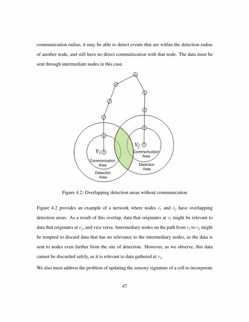
communication radius, it may be able to detect events that are within the detection radius
of another node, and still have no direct communication with that node. The data must be
sent through intermediate nodes in this case.
Figure 4.2: Overlapping detection areas without communication
Figure 4.2 provides an example of a network where nodes vi and vj have overlapping
detection areas. As a result of this overlap, data that originates at vi might be relevant to
data that originates at vj , and vice versa. Intermediary nodes on the path from vi to vj might
be tempted to discard data that has no relevance to the intermediary nodes, as the data is
sent to nodes even further from the site of detection. However, as we observe, this data
cannot be discarded safely, as it is relevant to data gathered at vj .
We also must address the problem of updating the sensory signature of a cell to incorporate
47

data gathered by several sensor nodes. Given two input signatures, we combine each bit
using the ⊕ operator, defined as follows:
Table 4.1: Combining bits in sensory signatures⊕ Y N ? XY Y X Y XN X N N X? Y N ? XX X X X X
In addition to handling the “joining” of two individual signatures, we must also handle
joining streams of sensory signatures. When sensory nodes gather data, the time of data
collection is recorded. To facilitate keeping track of the time and location of data collection,
we define a data structure, which is a tuple consisting of the following information: ¿timestamp, location, sensory signature À.
A primary advantage of using such a data structure is the pairing of time with the gathered
sensory data. In order to detect an event, we would intuitively like to consolidate records
with the same time and location that provide data gathered at different nodes. However, we
note that it can be difficult to pair sensory data with the appropriate time.
One possibility is to match sensory data with the time at which the data was gathered.
However, such a pairing might be rendered ineffective when we combine data gathered
at different locations and by different types of sensors. For example, if one sensor node is
twice as close to an event as another sensor node, the data gathered at each note will possess
different time stamps, even though they correspond to the same event. This problem is
further complicated by the fact that different physical properties travel at varying speeds.
For example, sound waves travel more slowly than light. As a result, even when sensors
at the same sensory node gather data on sound and light pertaining to the same event, the
48
time stamps will be different.
Furthermore, because time is a continuous variable, there are an infinite number of possible
time values. For example, two data records that correspond to the same event might display
times t and t + ε. Yet they might not be consolidated because their times are different. One
potential solution to this problem of continuity would be to create data records with only
standardized times. The set of potential times would be of the form t + aεtime, where t
is the time when the system is put in place, a is an integer from 0 to ∞, and εtime is a
predetermined constant specifying the interval between consecutive potential times. Then
each data record would be assigned the time of form t + aεtime that is closest to the actual
detection time.
One practical solution to this problem of consolidating sensory data by time is to make use
of the nodes’ memory. If a node receives a sensory signature, and has its own sensory data
stored in recent memory, we can assume that these pieces of data match.
4.2.1 Distributed Query Processing Protocol
In this subsection, we present an innovative battle event detection protocol using distributed
query processing with sensory signature.
We assume that the sensor nodes are aware of the query signature that is of interest to the
head quarters. The algorithm divides the filters into several phases which depend on the
cost and the selectivity of various filters as well as the query signature. In each phase,
only a set of filters is active. The filters belonging to the first phase are active at all times.
The filters belonging to the subsequent phases are active only when an event matching
the signature of the previous filters has been received. As the sensors receive the event
49

messages from their neighbors, they consolidate and maintain a partial signature for each
event received. When the partial signature of some events in their sensing radius matches
the signature of the prior phases, the sensor becomes active. The sensors that have filters
belonging to the first phase do not perform the consolidation and maintenance steps. The
steps of the algorithm are shown in Algorithm 4.
Algorithm 4 Distributed Query Processing ProtocolCompute and Broadcast Stepfor each phase i distributed with the query do
- Run the ith class of filters on data pertaining to cells with partial sensory signaturessatisfying the query specifications.- Update the partial sensory signature for the monitored cells with the filter results.- Broadcast updated signature records to all neighbors.- Update signature records based on received records.
end forAction Step The headquarters node receives all complete sensory signatures satisfyingthe query specifications, and takes appropriate action.
4.2.1.1 Algorithm for computing phases
In order to optimize the performance of Algorithm 4 in terms of total cost, the optimal
number of phases must be found. This equates to determining the number of filter classes
and which filters belong to each class. Since the central headquarter node generates event
queries, it naturally follows that the headquarters should determine the grouping of filters
into phases, and distribute this information along with the query.
In order to do this, we provide a dynamic programming algorithm. We first order the
n filters necessary to process the meaningful bits specified by the event query, so that
F1, ..., Fn where c11−s1
≤ c21−s2
≤ ... ≤ cn
1−sn. This ranking is derived from the work done
in [SMW05]. We also define the cost function c(Fx, Fy, k) to be the cost of running filters
50

Fx through Fy using at most k phases.
In the following algorithm, k∗ is the maximum number of phases possible that satisfy the
maximum allowed latency for an event detection. For example, suppose it takes tbroadcast
time to broadcast data to all nodes in the network, tfilters time to run all filters, and we
want the headquarters to be alerted about events with a maximum latency of tlatency time.
Then the maximum number of phases possible is k∗ = b tlatency−tfilters
tbroadcastc + 1, since (k∗ −
1)tbroadcast + tfilters ≤ tlatency. We further observe that k∗ cannot exceed k, as there must
be at least one filter in each phase.
Algorithm 5 Dynamic Programming Algorithm to Determine the Optimal Number ofPhases.
for x = 1 to n, and y = x to n do
c(Fx, Fy, 0) =
y∑i=x
ci since this is simply the sum cost of running filters Fx through
Fy.end forfor k1 = 1 to k∗ do
for x = 1 to n, and y = x to n doc(Fx, Fy, k1) =
y
minz=x
c(Fx, Fz, k1 − 1) + tbroadcast +
z∏i=x
sic(Fz+1, Fy, 0))
end forend forreturn
k∗
mink1=1
c(F1, Fn, k1)
Time Analysis: Algorithm 5 runs in O(n4k) time where n is the number of sensor nodes,
and k is the number of filter types, since the second loop runs at most O(n2k) times, the
min function inside must compare at most n values, and the inner product must multiply
at most n elements. However, we can reduce this run time to O(n3k) by computing the
possible product values∏z
i=x si for all values of x and z in O(n2) time once before entering
51

the loop.
4.3 Localized Query Processing Protocol
Depending on the landscape and sensor types, the relation between the computation cost
and communication cost can be different. The Distributed Query Processing Protocol
presented in Section 4.2 focuses on minimizing the computation cost. However, if the
communication cost dominates computation cost, then a different approach can be helpful.
In this section, we present a leader based protocol which focuses on reduce communication
cost. Each cell has a leader node that gathers the partial sensory signatures from all cell
members. In this localized protocol, all filters are active at all times. When a node runs a
filter, it transmits the updated records to the local leader node. Nodes receive, process and
forward the event signatures based on following two rules:
• A leader node only processes information from its local nodes or other leader nodes
• Non-leader nodes do not process or forward any information.
The steps of this algorithm are shown in Algorithm 6.
4.4 Simulation Results
In our simulation, we deploy nodes with varying sensing capabilities and detection radii.
Sensing capabilities of the nodes are coupled with filtering capabilities, which have
associated costs. We assume that we have 10 basic types of data. The costs and detection
52

Algorithm 6 Localized Query Processing ProtocolCompute and Broadcast Step
1. Nodes process events that trigger their corresponding filters.
2. Nodes transmit the event signatures to their local leader nodes.
3. Leader nodes update signature records based on received records and transmitupdated signature records to the other leader nodes.
Action Step The headquarters node receives all complete sensory signatures satisfyingthe query specifications, and takes appropriate action.
radii of the corresponding filters are shown in Table 4.2. Table 4.2 provides a mapping
of these capabilities to real sensor node classifications, extrapolated from the sensor
capabilities presented in [AGZAKMP10]. We normalize the distribution of these sensor
nodes so that the area is monitored by the same number of each type of sensor, as shown in
Figure 4.3. Accordingly, the number of sensors deployed with a given detection radius is
inversely proportional to the square of the radius. The communication radius of each sensor
node is randomly selected from [10, 100]. In each simulation, we introduce 10 events, and
a random number of these 10 have the matching event signature for our query.
Table 4.2: Sensor filter capabilitiesFilter Sample Processor Cost Detection RadiusPicture (low res) Cyclops-ATmega128L MCU+CPLD 100 20Picture (high res) MeshEye-ARM7TDMI based on ATMEL 600 50Temperature Mica2Dot-ATmega128L 4MHz 1 10Light Mica2Dot-ATmega128L 4MHz 1 10Sound FireFly-ATmega128L 8MHz 5 10Motion Imote2-PXA271 XScale 13MHz 20 10Chemical (simple) MeshEye-ARM7TDMI based on ATMEL 600 50Chemical (complex) CITRIC-Intel XScale PXA270 CPU 3000 100Video (low res) MeshEye-ARM7TDMI based on ATMEL 600 50Video (high res) CITRIC-Intel XScale PXA270 CPU 3000 100
53

Figure 4.3: Distribution of sensors
In each of our simulations, we compare three protocols: the distributed protocol and
localized protocol described in this work, as well as a naive protocol. This naive protocol
consists of filtering and broadcasting all data as soon as it is gathered at the sensors.
These protocols are compared in terms of cost. Since power resources are limited and
crucial for sensor networks, we model our cost function to represent power. This includes
computational power to run filters and gather data, and communication power to transmit
and receive data.
4.4.1 Protocol Effects on Total Power
First, we analyzed the effect of the environment size on the total power cost of our
algorithms. Figure 4.4 presents the simulation results reflecting the impact of the
54

environment size, in terms of number of sensors, on the total cost, which includes the cost
of transmission, reception, and computation. We see that both our distributed and localized
protocols present significant improvements over the naive protocol. As the environment
area grows, our protocols are increasingly beneficial, because they avoid processing and
transmitting increasingly large amounts of data through an increasingly large area.
More specifically, the naive protocol transmits the original gathered data to the headquarters
whenever that data satisfies the corresponding filter. We assume that the size of this original
sensory data is proportional to the cost of the filter. Because our protocols reduce the
original data to a single sensory signature, the amount of data that passes through the
network is greatly reduced. Figure 4.4 demonstrates the scalability of our solutions, in
comparison to the naive solution.
Figure 4.4: Total Power Used by 3 protocols, as a function of network size.
We note that the total power cost includes the cost of both computation and communication.
Because communication costs contribute a large fraction of the total cost in sensor
55
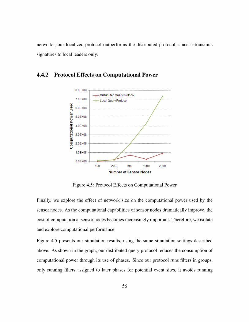
networks, our localized protocol outperforms the distributed protocol, since it transmits
signatures to local leaders only.
4.4.2 Protocol Effects on Computational Power
Figure 4.5: Protocol Effects on Computational Power
Finally, we explore the effect of network size on the computational power used by the
sensor nodes. As the computational capabilities of sensor nodes dramatically improve, the
cost of computation at sensor nodes becomes increasingly important. Therefore, we isolate
and explore computational performance.
Figure 4.5 presents our simulation results, using the same simulation settings described
above. As shown in the graph, our distributed query protocol reduces the consumption of
computational power through its use of phases. Since our protocol runs filters in groups,
only running filters assigned to later phases for potential event sites, it avoids running
56

these filters excessively. In our simulation settings, our protocol was optimized with two
phases. Our results thus demonstrate that even dividing the filters into two phases saves a
considerable amount of computational power.
57

Chapter 5
Uplink Traffic Pattern in Mobile Data
Network
User-generated content (UGC) also known as user-created content (UCC) refers to various
kinds of media contents that are produced by end users. A recent trend in the use of the
Internet exhibits that data traffic from UGC is rapidly growing with the potential to create
a huge amount of uplink traffic for wireless operators [fECoO]. As the reality of UGC’s
scope and power is becoming crystalized (e.g., YouTube, Facebook, Wikipedia, MySpace,
and Flickr), modeling and analysis of uplink traffic has just begun to receive attention
in the wireless research community [PCJ+05]. As the third factor that limits network
performance, we consider this new traffic pattern.
58

5.1 Traffic Measurement and Self-Similarity Analysis
Recent empirical studies of traffic measurements from a variety of different packet
networks have demonstrated that the self-similarity or burstiness over a wide range of time
scales is a prevalent phenomenon [LTWW94][CB96][JNHT01]. Most of network traffic
measurements have been performed on wired networks with some performed on wireless
downlink data networks. Little attention has been paid to uplink traffic until recently. We
were only able to find one report [PCJ+05] in the literature that deals with real uplink traffic
obtained from WAP services in a CDMA1x network. As a growing number of end users
are embracing the full potential of mobile technologies to create and share multimedia
contents, most of wireless mobile operators are providing multimedia services commonly
called multimedia messaging (MMS) services to support uploading of multimedia files
such as pictures, video files, and music files. We have analyzed live traffic traces of MMS
services collected from WCDMA networks of SK Telecom.
Currently SK Telecom has over 1,000 base stations for each network, two Serving GPRS
Supporting Nodes (SGSNs) covering WCDMA networks and two Packet Data Serving
Nodes (PSDNs) serving CDMA networks. Two traffic collectors are located at one SGSN
and one PDSN, respectively. MMS traffic data were collected from WCDMA network for
every 24 hours from August 10 to 15, 2007. In the following, we proceed to discuss the
self-similarity and our analysis of this traffic trace.
There are many different definitions of self-similarity. One common definition is for
continuous time processes, which states that Y (t) is self-similar with self-similarity
59
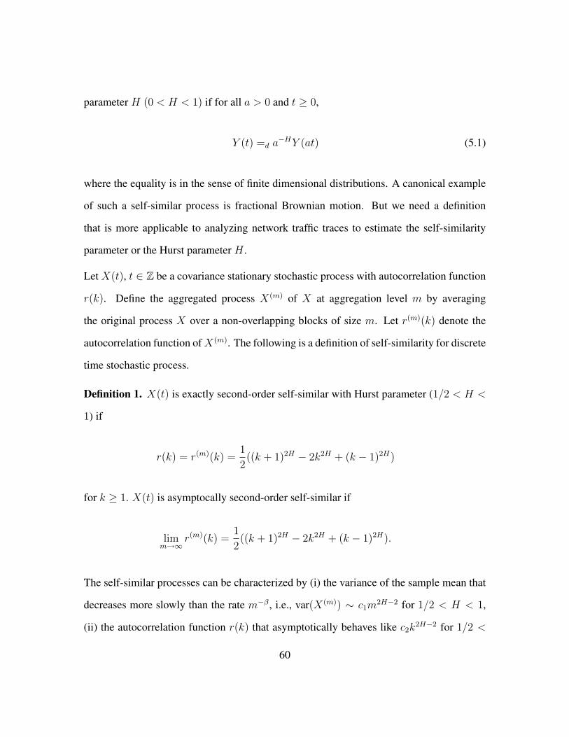
parameter H (0 < H < 1) if for all a > 0 and t ≥ 0,
Y (t) =d a−HY (at) (5.1)
where the equality is in the sense of finite dimensional distributions. A canonical example
of such a self-similar process is fractional Brownian motion. But we need a definition
that is more applicable to analyzing network traffic traces to estimate the self-similarity
parameter or the Hurst parameter H .
Let X(t), t ∈ Z be a covariance stationary stochastic process with autocorrelation function
r(k). Define the aggregated process X(m) of X at aggregation level m by averaging
the original process X over a non-overlapping blocks of size m. Let r(m)(k) denote the
autocorrelation function of X(m). The following is a definition of self-similarity for discrete
time stochastic process.
Definition 1. X(t) is exactly second-order self-similar with Hurst parameter (1/2 < H <
1) if
r(k) = r(m)(k) =1
2((k + 1)2H − 2k2H + (k − 1)2H)
for k ≥ 1. X(t) is asymptocally second-order self-similar if
limm→∞
r(m)(k) =1
2((k + 1)2H − 2k2H + (k − 1)2H).
The self-similar processes can be characterized by (i) the variance of the sample mean that
decreases more slowly than the rate m−β , i.e., var(X(m)) ∼ c1m2H−2 for 1/2 < H < 1,
(ii) the autocorrelation function r(k) that asymptotically behaves like c2k2H−2 for 1/2 <
60

H < 1, and thus∑
k r(k) = ∞ (long range dependence), and (iii) the spectral density f(·)that obeys a power law near the origin, i.e., f(λ) ∼ c3λ
1−2H for 1/2 < H < 1.
These properties of self-similar processes lead to various methods for estimating the Hurst
parameter H (see [Pop91]). We estimated the Hurst parameter for MMS traffic using an
analysis tool SELFIS [Kar02]. Table 5.1 shows the results for estimated Hurst values
obtained using six different methods: Aggregate variance,R/S, Periodogram, Absolute
moment, Whittle estimator, and Abry-Veitch. The results demonstrate that the Hurst values
are between 0.5 and 1 indicating the self-similarity.
Table 5.1: Hurst ParameterEstimation method MMS (Hurst parameter)Aggregate variance 0.920R/S 0.739Periodogram 0.785Absolute moment 0.766Whittle estimator 0.845Abry-veitch estimator 0.745
5.1.1 Heavy-tailedness
The heavy-tailedness is roughly said to cause a network traffic to possess the self-similar
property. A random variable Z is said to obey a heavy-tailed distribution if
P (Z > x) ∼ cx−α, x →∞ (5.2)
where 0 < α < 2 is the tail index and c is a positive constant. The variable Z could
represent a session size, or inter-session time between two successive sessions. In order
to check for the heavy-tailedness of the distribution of a given variable, we make use of
61

0 2 4 6−5
−4
−3
−2
−1
0
log (x)
log(
P(Z
>x)
)
Distribution of MMS object size (kbytes)
raw dataLognormal fit
Figure 5.1: Log-log plot of MMS object size
complementary distribution plots. Indeed, if we take logarithms of both sides of Eq. (5.2),
we obtain
log(P (Z > x)) ∼ −α log(x) + log(c), x →∞.
This relation says that if a variable obeyed the heavy-tailed distribution, the log-log plot of
the complementary distribution of the variable would be a straight line for large x-values,
with a slope −α.
In Fig. 5.1, we show the log-log plot of the complementary distribution of the MMS raw
data. This figure suggests a strong empirical evidence of the heavy-tailed property of the
file size distribution for MMS services.
62
5.2 Impact on Network Performance
In this section, we analyze the impact of uplink traffic characteristics on the network
performance using the WiMAX module available by OPNET 12.0 developed based on
IEEE 802.16e. In our simulations, we use the MMS uplink traces collected from the SK
Telecom network to model best-effort multi-media uplink traffic. Video-telephony traffic
modeled in OPNET 12.0 is used to model delay-sensitive uplink traffic. The topology of
a simple network is used where subscriber stations are connected to a single base station.
We only model the wireless connection between BS and SSs, i.e., the radio layer in the
access network, and a round-robin scheduling QoS algorithm for WiMAX available in the
OPNET 12.0 is applied. The round-robin WiMAX QoS scheduling algorithm implemented
in OPNET is briefly described next.
The latest IEEE 802.16e supports five scheduling service types:
• Unsolicited Grant Service (UGS)
• Extended Real-time Polling Service (ertPS)
• Real-time Polling Service (rtPS)
• Non Real-time Polling Service (nrtPS)
• Best Effort (BE)
UGS and ertPS have the highest scheduling priority, and packets from SSs with these
services are periodically inform their queue status information to the scheduler which
resides in the base station. rtPS and nrtPS have the middle priority, and packets from SSs
with these services are scheduled for transmission after clearing packets in the buffer with
63

(a) 300s period (b) 60s period (c) 10s period
Figure 5.2: Aggregate traffic with 64 MMS and 64 video-telephny services
UGS and ertPS services. BE has the lowest priority and all connections from SSs share
a same scheduling queue by first-come-first-served. In our simulations, video-telephony
is categorized as rtPS, and MMS is categorized as BE, and only traffic video-telephony
services is considered delay-sensitive.
5.2.1 Delay Analysis with Low Load Delay-Sensitive Traffic
We first consider a scenario in which both MMS and video-telephony traffic loads are low.
The parameters used for traffic generation are summarized in Table 5.2.
Table 5.2: Summary of parametersParameters ValuesSimulation Time 300 secondsNumber of video-telephony SS 64Number of MMS SS 64video-telephony packet size (bytes) Lognormal(6.0, 1.0)video-telephony packet interarrival time (seconds) Constant(0.1)MMS packet size (kbytes) Lognormal(1.2, 1.5)MMS packet interarrival time (seconds) Exponential(2.88)
64

Figure 5.2 (a) shows the total amount of aggregate traffic (in bytes/sec), over the entire
simulation time, received at the server. This figure is then zoomed into 60 seconds (b)
and 10 seconds (c) of simulation periods. The traffic burstiness is observed across all time
scales. This scale-invariant burstiness shows the self-similarity property. Similar results
are also discovered for MMS traffic and video-telephony traffic at each SS.
Since video-telephony is delay-sensitive, a major QoS requirement should be the delay.
We assume that the delay requirement for this service is to have at least 99% of packets
experience delays less than 0.03 seconds, and services meeting this requirement are
considered satisfiable.
Packet delays of video-telephony service at a single SS is shown in Fig. 5.3(a). The QoS
requirement of the video-telephony is fulfilled as shown, and it can be also clearly verified
by the cumulative density function CDF of the delay shown in Fig. 5.3(b).
5.2.2 Delay Analysis with High Load Delay-Sensitive Traffic
In this scenario, we increase the traffic loads from both MMS and video-telephony services
by injecting 108 SSs with MMS services and 108 SSs with video-telephony services.
The aggregate traffic received at the BS is shown in Figure 5.4. We note here that the
burstiness is also observed and the total traffic received at the BS (in the range of 40 to 60
bytes/sec) is much lower than the network capacity (theoretical max capacity of WiMAX
is 70 Mbps).
As the total number of SSs is increased to have 108 MMS SSs and 108 video-telephony
SSs, the delay of video-telephony packets is largely affected even though they are served
under the rtPS category with the higher scheduling priority. From the Fig.5.5(a), it is
65

clear that the delays are much larger in this case than those in the previous scenario with
64 MMS SSs and 64 video-telephony SSs. A closer look at the CDF plot of the packet
delay shown in Figigure 5.5(b) reveals that at least 5% packets have delays larger than 0.03
seconds. Here we should note that the aggregated traffic load in any moment is much less
than 250 kbytes, which is far less than the network capacity. This observation depicts that
the network resource has not been fully utilized. Better scheduling algorithms and access
control schemes should be developed to improve the network’s performance in supporting
QoS requirements.
66

(a) Packet delay
(b) CDF of packet delay
Figure 5.3: Packet delay of video-telephony with 64 MMS and 64 video-telephony SS
67

Figure 5.4: Aggregate traffic with 108 MMS and 108 video-conferencing.
68

(a) Packet delay
(b) CDF of packet delay
Figure 5.5: Packet delay of video-telephony with 108 MMS and 108 video-telephony SS
69
Chapter 6
Conclusion and Future Directions
This dissertation research investigated major factors that limit network throughput and
capacity, and developed new schemes with aforementioned factors explicitly considered
in heterogeneous wireless networks.
6.1 Contributions
The contributions of this dissertation are in three different areas: resource sharing in
HWMNs, information processing in HWSNs, and new traffic pattern in 3G/4G networks.
6.1.1 Channel Assignment considering Switching Overhead in HWMNs
1. The switching overhead that is incurred during channel switching is explicitly
modeled, and channel assignment algorithms are designed by using that delay.
2. We showed that the well known GMS dose not achieve any provable efficiency ratio
70

when the switching overhead is considered.
3. We extended two well known algorithms, centralized and distributed, taking the
switching overhead into account in the channel assignment.
4. Performance of the developed algorithms is analyzed through discrete-event simula-
tions.
6.1.2 Distributed Query Processing using Event Signatures in HWSNs
1. The problem of identifying significant events is addressed with the objective of
minimizing the total power cost in HWSNs.
2. We proposed two protocols that can reduce the computation cost and the communi-
cation cost for the sensor network, thereby extending the life of the network. The
suggested protocols employ three main techniques to reduce these costs:
(i) use of sensory signature to avoid sending raw or processed data
(ii) use of phases to avoid unnecessary computations
(iii) use of leader nodes to avoid unnecessary communications.
3. Performance of the developed protocols is analyzed through discrete-event simula-
tions.
6.1.3 Uplink Traffic Pattern in Mobile Data Network
1. We analyzed live uplink traffic traces obtained by monitoring 3G networks of a
mobile data service provider (SK Telecom in Korea).
71

2. Our statistical analysis showed the self-similarity in this traffic trace. Six different
self-similarity analysis algorithms are used.
3. The impact of this traffic characteristics on mobile data networks is evaluated through
the WiMAX module available in OPNET software.
6.2 Future Directions
Our research can be further extended in the following avenues:
1. Switching Overhead: Current switching overhead δ model does not include
switching type information. As mentioned in Section 3.1.2, when switching occurs
across different frequency bands (e.g., 5GHz for 802.11a and 2.4GHz for 802.11b/g),
the impact of switching delay on the overall network performance becomes even
more significant. Thus, radio switching across different frequency bands can be
modeled separately from in-band channel switching.
2. Event Detection: In addition to the single type of event detection, further research
can consist of using sensor network to detect multiple types of events simultaneously.
For example, we may want to detect bomb explosions, gunfire and chemical
agent deployment simultaneously. Future work can also consist of combining
the helpful attributes of the two protocols suggested in this research. Distributed
query processing protocol reduces computation cost, and localized query processing
protocol reduces communication cost. A protocol that combines aspects of these two
protocols could possibly reduce both, and still detect events correctly.
72

3. Traffic Pattern: Our observation suggests that call admission control should be
carefully monitored for delay-sensitive uplink services as most of admission control
algorithms only focus on the available network capacity. Further research on
developing uplink scheduling algorithms integrated with call admission control is
also required to deal with the new uplink traffic patterns.
73

Bibliography
[3GPa] The 3rd Generation Partnership Project 3GPP. http://www.3gpp.org.
[3GPb] The 3rd Generation Partnership Project 2 3GPP2. http://www.3gpp2.org.
[AGZAKMP10] Islam T. Almalkawi, Manel Guerrero Zapata, Jamal N. Al-Karaki, and
Julian Morillo-Pozo. Wireless multimedia sensor networks: Current
trends and future directions. Sensors, 10(7):6662–6717, 2010.
[AHP03] K. Ahmavaara, H. Haverinen, and R. Pichna. Interworking architecture
between 3gpp and wlan systems. Communications Magazine, IEEE,
41(11):74 – 81, nov. 2003.
[AML05] Daniel J. Abadi, Samuel Madden, and Wolfgang Lindner. Reed: robust,
efficient filtering and event detection in sensor networks. In Proceedings
of the 31st international conference on Very large data bases, VLDB ’05,
pages 769–780. VLDB Endowment, 2005.
[BCD04] Paramvir Bahl, Ranveer Chandra, and John Dunagan. SSCH: slotted
seeded channel hopping for capacity improvement in IEEE 802.11 ad-
hoc wireless networks. In MobiCom ’04: Proceedings of the 10th annual
74
international conference on Mobile computing and networking, pages
216–230, New York, NY, USA, 2004. ACM.
[Bro] Muni Wireless Broadband. http://muniwireless.com.
[BRS03] R.R. Brooks, P. Ramanathan, and A.M. Sayeed. Distributed target
classification and tracking in sensor networks. Proceedings of the IEEE,
91(8):1163 – 1171, 2003.
[BZM08] A. Brzezinski, G. Zussman, and E. Modiano. Distributed throughput
maximization in wireless mesh networks via pre-partitioning. Network-
ing, IEEE/ACM Transactions on, 16(6):1406–1419, Dec. 2008.
[CB96] Mark Crovella and Azer Bestavros. Self-similarity in world wide
web traffic evidence and possible causes. IEEE/ACM Transactions on
Networking, 5:835–846, 1996.
[Cha06] Prasanna Chaporkar. Achieving queue length stability through maximal
scheduling in wireless networks. In University of California, 2006.
[CKS05] Prasanna Chaporkar, Koushik Kar, and Saswati Sarkar. Throughput
guarantees through maximal scheduling in wireless networks. In In
Proceedings of 43d Annual Allerton Conference on Communication,
Control and Computing, pages 28–30, 2005.
[CMGK08] J. Camp, V. Mancuso, O. Gurewitz, and E.W. Knightly. A measurement
study of multiplicative overhead effects in wireless networks. In
INFOCOM 2008. The 27th Conference on Computer Communications.
IEEE, pages 76 –80, 2008.
75

[Com] Sprint Community. http://community.sprint.com/baw/message/191672.
[EVD06] cdma2000 high rate packet data air interface specification, 2006.
[FDAI+10] L.S. Ferreira, M.D. De Amorim, L. Iannone, L. Berlemann, and L.M.
Correia. Opportunistic management of spontaneous and heterogeneous
wireless mesh networks [accepted from open call]. Wireless
Communications, IEEE, 17(2):41 –46, 2010.
[fECoO] Organisation for Economic Co-operation and Development (OECD).
Participative Web and User-created Content: Wbe 2.0, Wikis and Social
Networking, [Online] Available: http://www.oecd.org, 2007.
[FGB+05] Mingxi Fan, D. Ghosh, N. Bhushan, R. Attar, C. Lott, and J. Au. On the
reverse link performance of cdma2000 1 times;ev do revision a system. In
Communications, 2005. ICC 2005. 2005 IEEE International Conference
on, volume 4, pages 2244 – 2250 Vol. 4, 16-20 2005.
[FLW08] Yunxia Feng, Minglu Li, and Min-You Wu. Improving capacity
and flexibility of wireless mesh networks by interface switching. In
Communications, 2008. ICC ’08. IEEE International Conference on,
pages 4729–4733, May 2008.
[FLW09] Yunxia Feng, Minglu Li, and Min-You Wu. A weighted interference
estimation scheme for interface-switching wireless mesh networks.
Wirel. Commun. Mob. Comput., 9(6):773–784, 2009.
76

[FSA10] R. Ferrus, O. Sallent, and R. Agusti. Interworking in heterogeneous
wireless networks: Comprehensive framework and future trends.
Wireless Communications, IEEE, 17(2):22 –31, april 2010.
[GJ03] E. Gustafsson and A. Jonsson. Always best connected. IEEE Wireless
Communications, 10:49–55, Febrary 2003.
[GPRSA08] X. Gelabert, J. Perez-Romero, O. Sallent, and R. Agusti. A markovian
approach to radio access technology selection in heterogeneous
multiaccess/multiservice wireless networks. Mobile Computing, IEEE
Transactions on, 7(10):1257 –1270, oct. 2008.
[GSPRA09] X. Gelabert, O. Sallent, J. Perez-Romero, and R. Agusti. Radio access
congestion in multiaccess/multiservice wireless networks. Vehicular
Technology, IEEE Transactions on, 58(8):4462 –4475, oct. 2009.
[HMG02] Timo Halonen, Juan Melero, and Javier Romero Garcia. GSM, GPRS and
EDGE Performance: Evolution Toward 3G/UMTS. Halsted Press, New
York, NY, USA, 2002.
[HT02] Harri Holma and Antti Toskala, editors. Wcdma for Umts. John Wiley &
Sons, Inc., New York, NY, USA, 2002.
[HT06] Harri Holma and Antti Toskala. HSDPA/HSUPA for UMTS: High Speed
Radio Access for Mobile Communications. John Wiley & Sons, 2006.
[HY07] Xianghua Hu and Xuejun Yang. Grid-based sense schedule for event
detection in wireless sensor networks. In Jadwiga Indulska, Jianhua Ma,
77

Laurence Yang, Theo Ungerer, and Jiannong Cao, editors, Ubiquitous
Intelligence and Computing, volume 4611 of Lecture Notes in Computer
Science, pages 557–566. Springer Berlin / Heidelberg, 2007.
[JLS09] Changhee Joo, Xiaojun Lin, and N.B. Shroff. Understanding the capacity
region of the greedy maximal scheduling algorithm in multihop wireless
networks. Networking, IEEE/ACM Transactions on, 17(4):1132 –1145,
aug. 2009.
[JNHT01] M. Jiang, M. Nikolic, S. Hardy, and L. Trajkovic. Impact of self-
similarity on wireless data network performance. In Communications,
2001. ICC 2001. IEEE International Conference on, volume 2, pages
477 –481 vol.2, 2001.
[Joo08] Changhee Joo. A local greedy scheduling scheme with provable
performance guarantee. In MobiHoc ’08: Proceedings of the 9th ACM
international symposium on Mobile ad hoc networking and computing,
pages 111–120, New York, NY, USA, 2008. ACM.
[JZ08] Ren Juan and Qiu Zhengding. Centralized quasi-static channel assign-
ment in multi-radio wireless mesh networks. In Communication Systems,
2008. ICCS 2008. 11th IEEE Singapore International Conference on,
pages 1149–1154, Nov. 2008.
[Kar02] Thomas Karagiannis. Selfis: A tool for self-similarity and long-range
dependence analysis. In In 1st Workshop on Fractals and Self-Similarity
in Data Mining: Issues and Approaches (in KDD, 2002.
78

[KI04] Bhaskar Krishnamachari and Sitharama Iyengar. Distributed bayesian
algorithms for fault-tolerant event region detection in wireless sensor
networks. IEEE Transactions on Computers, 53:241–250, 2004.
[KMPR07] Bong-Jun Ko, V. Misra, J. Padhye, and D. Rubenstein. Distributed
channel assignment in multi-radio 802.11 mesh networks. In Wireless
Communications and Networking Conference, IEEE, pages 3978–3983,
2007.
[KMR+01] J. Kalliokulju, P. Meche, M.J. Rinne, J. Vallstrom, P. Varshney, and
S.-G. Haggman. Radio access selection for multistandard terminals.
Communications Magazine, IEEE, 39(10):116 –124, oct 2001.
[KV05] P. Kyasanur and N. H. Vaidya. Capacity of multi-channel wireless
networks: Impact of number of channels and interfaces. In Proceedings
of the 11th annual ACM/IEEE international conference on Mobile
computing and networking, August 2005.
[KV06] Pradeep Kyasanur and Nitin H. Vaidya. Routing and link-layer protocols
for multi-channel multi-interface ad hoc wireless networks. SIGMOBILE
Mob. Comput. Commun. Rev., 10(1):31–43, 2006.
[LLCM08] Haiping Liu, Xin Liu, Chen-Nee Chuah, and P. Mohapatra. Heteroge-
neous wireless access in large mesh networks. In Mobile Ad Hoc and
Sensor Systems, 2008. MASS 2008. 5th IEEE International Conference
on, 29 2008.
79

[LLS+04] Shuoqi Li, Ying Lin, Sang H. Son, John A. Stankovic, and Yuan Wei.
Event detection services using data service middleware in distributed
sensor networks. Telecommunication Systems, 26:351–368, 2004.
10.1023/B:TELS.0000029046.79337.8f.
[LR07] Xiaojun Lin and Shahzada Rasool. A distributed joint channel-
assignment, scheduling and routing algorithm for multi-channel ad hoc
wireless networks. In Proceedings of the IEEE INFOCOM, 2007.
[LS06] Xiaojun Lin and Ness B. Shroff. The impact of imperfect scheduling on
cross-layer congestion control in wireless networks. IEEE/ACM Trans.
Netw., 14(2):302–315, 2006.
[LTWW94] Will E. Leland, Murad S. Taqqu, Walter Willinger, and Daniel V.
Wilson. On the self-similar nature of ethernet traffic (extended version).
IEEE/ACM Trans. Netw., 2(1):1–15, 1994.
[Lub85] M Luby. A simple parallel algorithm for the maximal independent set
problem. In STOC ’85: Proceedings of the seventeenth annual ACM
symposium on Theory of computing, pages 1–10, New York, NY, USA,
1985. ACM.
[LWHS02] Dan Li, K.D. Wong, Yu Hen Hu, and A.M. Sayeed. Detection,
classification, and tracking of targets. Signal Processing Magazine, IEEE,
19(2):17 –29, March 2002.
[MD05] M. Marina and S. Das. A topology control approach for utilizing
multiple channels in multi-radio wireless mesh networks. In Broadband
80

Networks, 2005 2nd International Conference on, volume 1, pages 381–
390, October 2005.
[MFHH05] Samuel R. Madden, Michael J. Franklin, Joseph M. Hellerstein, and
Wei Hong. Tinydb: an acquisitional query processing system for sensor
networks. ACM Trans. Database Syst., 30:122–173, March 2005.
[MS06] Fernando Martincic and Loren Schwiebert. Distributed event detection in
sensor networks. Systems and Networks Communication, International
Conference on, 0:43, 2006.
[NGES07] M. Nekoui, A. Ghiamatyoun, S.N. Esfahani, and M. Soltan. Iterative
cross layer schemes for throughput maximization in multi-channel
wireless mesh networks. Computer Communications and Networks,
2007. ICCCN 2007. Proceedings of 16th International Conference on,
pages 1088–1092, Aug. 2007.
[Nua] Loutfi Nuaymi. WiMAX: Technology for Broadband Wireless Access.
[OK10] Eng Hwee Ong and J.Y. Khan. On optimal network selection in
a dynamic multi-rat environment. Communications Letters, IEEE,
14(3):217 –219, march 2010.
[OUS+08] Avi Ostfeld, James G Uber, Elad Salomons, Jonathan W Berry, William E
Hart, Cindy A Phillips, Jean-Paul Watson, Gianluca Dorini, Philip
Jonkergouw, Zoran Kapelan, and et al. The battle of the water sensor
networks (bwsn): A design challenge for engineers and algorithms.
81

Journal of Water Resources Planning and Management, 134(6):556,
2008.
[PCJ+05] Liang Peng, Tang Cailin, Ma Jie, Chang Yongyu, and Yang Dacheng.
Experimental study on traffic model of wireless internet services in cdma
network. In Vehicular Technology Conference, 2005. VTC 2005-Spring.
2005 IEEE 61st, volume 4, pages 2137 – 2141 Vol. 4, 30 2005.
[PEHS04] S. Parkvall, E. Englund, K.W. Helmersson, and M. Samuelsson. Wcdma
uplink enhancements for high-speed data access. In Vehicular Technology
Conference, 2004. VTC2004-Fall. 2004 IEEE 60th, volume 7, pages 5204
– 5208 Vol. 7, 26-29 2004.
[PKRVJ05] A V U Phani Kumar, Adi Mallikarjuna Reddy V, and D. Janakiram.
Distributed collaboration for event detection in wireless sensor networks.
In Proceedings of the 3rd international workshop on Middleware for
pervasive and ad-hoc computing, MPAC ’05, pages 1–8, New York, NY,
USA, 2005. ACM.
[Pop91] Adrian Popescu. Traffic self-similarity, 1991.
[RBAB06] K. N. Ramachandran, E. M. Belding, K. C. Almeroth, and M. M.
Buddhikot. Interference-aware channel assignment in multi-radio
wireless mesh networks. In INFOCOM 2006. 25th IEEE International
Conference on Computer Communications. Proceedings, pages 1–12,
April 2006.
82

[RC05] Ashish Raniwala and T.-C. Chiueh. Architecture and algorithms for
an IEEE 802.11-based multi-channel wireless mesh network. In IEEE
INFOCOM, 2005.
[RDV+05] S. Roy, A. Das, R. Vijaykumar, H. Alazemi, E. Alotaibi, and H. Ma.
Capacity scaling with multiple radios and multiple channels in wireless
mesh networks. In IEEE Wireless MESH Network Workshop, September
2005.
[RGcC04] Ashish Raniwala, Kartik Gopalan, and Tzi cker Chiueh. Centralized
channel assignment and routing algorithms for multi-channel wireless
mesh networks. SIGMOBILE Mob. Comput. Commun. Rev., 8(2):50–65,
2004.
[Sal04] A.K. Salkintzis. Interworking techniques and architectures for wlan/3g
integration toward 4g mobile data networks. Wireless Communications,
IEEE, 11(3):50 – 61, june 2004.
[SGD+07] H. Skalli, S. Ghosh, S.K. Das, L. Lenzini, and M. Conti. Channel
assignment strategies for multiradio wireless mesh networks: Issues and
solutions. Communications Magazine, IEEE, 45(11):86–95, November
2007.
[SGDC08] A.P. Subramanian, H. Gupta, S.R. Das, and Jing Cao. Minimum
interference channel assignment in multiradio wireless mesh networks.
Mobile Computing, IEEE Transactions on, 7(12):1459–1473, Dec. 2008.
83

[SK05] G. Sharma and G.S. Kumar. Moving towards hsupa (high speed
uplink packet access): a complete 3.5g wireless system. In Personal
Wireless Communications, 2005. ICPWC 2005. 2005 IEEE International
Conference on, pages 174 – 177, 23-25 2005.
[SML+04] Gyula Simon, Miklos Maroti, Akos Ledeczi, Gyorgy Balogh, Branislav
Kusy, Andras Nadas, Gabor Pap, Janos Sallai, and Ken Frampton.
Sensor network-based countersniper system. In Proceedings of the
2nd international conference on Embedded networked sensor systems,
SenSys ’04, pages 1–12, New York, NY, USA, 2004. ACM.
[SMW05] U. Srivastava, K. Munagala, and J. Widom. Operator placement for in-
network stream query processing. In Proceedings of the twenty-fourth
ACM SIGMOD-SIGACT-SIGART symposium on Principles of database
systems, pages 250–258. ACM, 2005.
[SPG09] Joachim Sachs, Mikael Prytz, and Jens Gebert. Multi-access management
in heterogeneous networks. Wirel. Pers. Commun., 48(1):7–32, 2009.
[TE92] L. Tassiulas and A. Ephremides. Stability properties of constrained
queueing systems and scheduling policies for maximum throughput in
multihop radio networks. Automatic Control, IEEE Transactions on,
37(12):1936–1948, Dec 1992.
[TOF+09] K. Taniuchi, Y. Ohba, V. Fajardo, S. Das, M. Tauil, Yuu-Heng Cheng,
A. Dutta, D. Baker, M. Yajnik, and D. Famolari. Ieee 802.21:
84

Media independent handover: Features, applicability, and realization.
Communications Magazine, IEEE, 47(1):112 –120, january 2009.
[TT07] Wai-Hong Tarn and Yu-Chee Tseng. Joint multi-channel link layer and
multi-path routing design for wireless mesh networks. INFOCOM 2007.
26th IEEE International Conference on Computer Communications.
IEEE, pages 2081–2089, May 2007.
[VKLS06] Ramanuja Vedantham, Sandeep Kakumanu, Sriram Lakshmanan, and
Raghupathy Sivakumar. Component based channel assignment in single
radio, multi-channel ad hoc networks. In MobiCom ’06: Proceedings
of the 12th annual international conference on Mobile computing and
networking, pages 378–389, New York, NY, USA, 2006. ACM.
[WSS03] Anthony D. Wood, John A. Stankovic, and Sang H. Son. Jam: A
jammed-area mapping service for sensor networks. Real-Time Systems
Symposium, IEEE International, 0:286, 2003.
[YMM09] R. Yim, N.B. Mehta, and A.F. Molisch. Fast multiple access selection
through variable power transmissions. Wireless Communications, IEEE
Transactions on, 8(4):1962 –1973, april 2009.
[YZAC09] Mira Yun, Yu Zhou, Amrinder Arora, and Hyeong-Ah Choi. Channel-
assignment and scheduling in wireless mesh networks considering
switching overhead. In Communications, 2009. ICC ’09. IEEE
International Conference on, June 2009.
85

[ZG04] F. Zhao and L. Guibas. Wireless Sensor Networks: An Information
Processing Approach. Morgan Kaufman, 2004.
[ZGLC03] Wei Zhuang, Yung-Sze Gan, Kok-Jeng Loh, and Kee-Chaing Chua.
Policy-based qos-management architecture in an integrated umts and
wlan environment. Communications Magazine, IEEE, 41(11):118 – 125,
nov. 2003.
86
Related Documents