Understanding VNA Calibration - Steven M. Anlage …anlage.umd.edu/Anritsu_understanding-vna-calibration.pdf3 | Understanding VNA calibration Table 1 - This table summarizes the various

www.anritsu.com

Understanding VNA Calibration

1 | Understanding VNA calibration

Table of Contents

Calibration Overview ................................................................................................................................. 2Calibration Summary ................................................................................................................................... 2Calibration Algorithms ................................................................................................................................ 3Configuring the VNA ................................................................................................................................ 4 Frequency Start, Stop and Number of Points ............................................................................. 4IF Bandwidth and Averaging ............................................................................................................ 4Point-by-point versus sweep-by-sweep Averaging ........................................................................ 4Power ...................................................................................................................................................... 4Types of Calibration .................................................................................................................................... 5Full 2-port ............................................................................................................................................... 5Full 1-port ............................................................................................................................................... 51-path 2-port (forward or reverse) ..................................................................................................... 5Frequency Response (reflection response and transmission-frequency response) ................... 5Line Types ...................................................................................................................................................... 7Calibration Kits ........................................................................................................................................... 9SOLT Kits ............................................................................................................................................... 9Kits with Triple-Offset Shorts ............................................................................................................. 10LRL Kits ................................................................................................................................................. 10Microstrip & Coplanar Waveguide Kits for the Universal Test Fixture ........................................ 11On Wafer Calibration Kits ......................................................................................................... 11Automatic Calibration (AutoCal) ...................................................................................................................... 12Precision AutoCal Calibration Module .......................................................................................................... 12Physical Setup ..................................................................................................................................................... 14Other AutoCal Topics ..................................................................................................................................... 14Thru Type ....................................................................................................................................................... 14AutoCal Assurance ............................................................................................................................ 14Test Port Converters .......................................................................................................................... 14Chartacterization ................................................................................................................................. 15Nojn-insertable Measurements ................................................................................................................. 15SOLT ................................................................................................................................................... 16Calibration Model Accuracy ............................................................................................................. 16Triple Offset Short .............................................................................................................................. 19Offset Short .......................................................................................................................................... 19SOLR (Unknown Thru Approach) ......................................................................................................... 21LRL/LRM/ALRM ............................................................................................................................... 23Isolation ................................................................................................................................................... 28Adapter Removal ................................................................................................................................... 29Thru Update ............................................................................................................................................. 31Interpolation .............................................................................................................................................. 31Calibration Merge ............................................................................................................................................ 32Network Extraction ............................................................................................................................................ 32Summary .............................................................................................................................................................. 34

2w w w . a n r i t s u . c o m

In this guide, the concept of calibration is presented and discussed in detail. Specific topicsto be covered include how to configure the VNA for calibration, types of calibration andcalibration kits. A minimal amount of calibration mathematics and theory will also be covered.

Calibration Overview

Calibration is critical to making good VNA S-parameter measurements. While the VNA is ahighly-linear receiver and has sufficient spectral purity in its sources to make goodmeasurements, there are a number of imperfections that limit measurements done withoutcalibrations. These imperfections include:

1. Match—Because the VNA is such a broadband instrument, the raw match is decent butnot excellent. Even a 20-dB match, which is physically very good, can lead to errors ofgreater than 1 dB. Correcting for this raw match greatly reduces the potential error.

2. Directivity—A key component of a VNA is a directional coupler. This device allows theinstrument to separate the signal incident on the DUT from the signal reflected back fromthe DUT. While the couplers used in the VNA are of very high quality, there is a certainamount of coupled signal, even when a perfect termination is connected. This is related todirectivity and can impact measurements of very small reflection coefficients.

3. Frequency Response—While the internal frequency response of the VNA could becalibrated at the factory, any cables connected externally will have some frequencyresponse that must be calibrated out for high-quality measurements.

Calibration Summary

Calibration is a tool for correcting for these imperfections, as well as other defects. There arean enormous number of possible calibration algorithms and many of them are implementedwithin VNAs. The choice between them is largely determined by the media the engineer isworking in, the calibration standards available and the desired accuracy/ effort trade off.While these choices will be discussed in detail later in this chapter, they can be categorizedaccording to two distinctions: calibration type (e.g., which ports are being corrected and towhat level they are being corrected) and calibration algorithm (e.g., how the correction isbeing accomplished). A summary of calibration types is provided in Table 1.


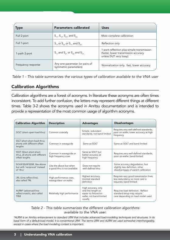
Table 1 - This table summarizes the various types of calibration available to the VNA user

Calibration Algorithms

Calibration algorithms are a forest of acronyms. In literature these acronyms are often timesinconsistent. To add further confusion, the letters may represent different things at differenttimes. Table 3-2 shows the acronyms used in Anritsu documentation and is intended toprovide a representation of the most common usage of algorithm acronyms.

Table 2 - This table summarizes the different calibration algorithms available to the VNA user.

Type Parameters calibrated Uses

Full 2-port

Full 1-port

S11, S12, S21, and S22

S11 or S22 or S11 and S22

Most complete calibration

Reflection only

1-port reflection plus simple transmission(faster, lower transmission accuracyunless DUT very lossy)

Frequency response

1-path 2-port S11 and S21 or S22 and S12

Normalization only. fast, lower accuracyAny one parameter (or pairs ofsymmetric parameters)

Calibration Algorithm Description

SOLT (short-open-load-thru) Common coaxially

Common in waveguide

Simple, redundantstandards; not band limited

Same as SOLT

Same as SOLT but better accuracy athigh frequency

SSLT (short-short-load-thru), shorts with different offset lengths

Common in waveguide or high frequency coax

Does not requirewell-defined thru

Like the above but whena good thru is not available

SSST (Short-short-short-thru), all shorts with differentoffset lengths

SOLR/SSLR/SSSR, like abovebut with ‘reciprocal’ insteadof ‘thru’

LRL (Line-reflect-line),also called TRL

ALRM* (advanced line-reflect-match), also called TRM

Relatively high performance

High performance coax,waveguideor on-wafer

Advantages

Highest accuracy,minimal standarddefinition

High accuracy, only one line length so easier to fixture/on-wafer, not band-limitedusually

Disadvantages

Requires very well-defined standards,poor on-wafer, lower accuracy at highfrequency

Same as SOLT and band-limited

Requires very well-defined standards,poor on-wafer, band-limited

Some accuracy degradation, but slightly less definition, other disadvantages of parent calibration

Requires very good transmission lines,less redundancy so more care isrequired, band-limited

Requires load definition. Reflectstandard setup may requirecare depending on load model used

*ALRM is an Anritsu enhancement to standard LRM that includes advanced load-modeling techniques and structures. In itsbasal form of a default-load model, it is conventional LRM. The terms LRM and ALRM are used somewhat interchangeably,except in cases where the load modeling context is important.


Configuring The VNA

Before discussing calibration further, and some of the alternatives available, it is important tofirst gain a clear understanding of any VNA setup issues as they will affect calibrationperformance. In almost all cases, the VNA settings are used during calibration. Therefore,setting up the VNA as desired beforehand can be especially helpful. The settings of interestare:

1. Frequency Start, Stop and Number of Points - These settings are obvious. Segmentedsweep must also be setup in advance if a more custom frequency list is desired.

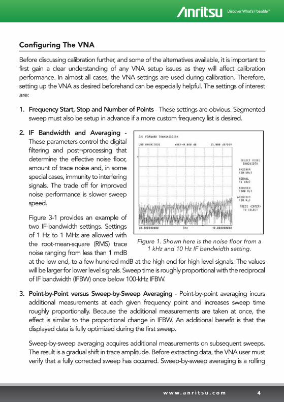
2. IF Bandwidth and Averaging -These parameters control the digitalfiltering and post¬processing thatdetermine the effective noise floor,amount of trace noise and, in somespecial cases, immunity to interferingsignals. The trade off for improvednoise performance is slower sweepspeed.

Figure 3-1 provides an example oftwo IF-bandwidth settings. Settingsof 1 Hz to 1 MHz are allowed withthe root-mean-square (RMS) tracenoise ranging from less than 1 mdBat the low end, to a few hundred mdB at the high end for high level signals. The valueswill be larger for lower level signals. Sweep time is roughly proportional with the reciprocalof IF bandwidth (IFBW) once below 100-kHz IFBW.

3. Point-by-Point versus Sweep-by-Sweep Averaging - Point-by-point averaging incursadditional measurements at each given frequency point and increases sweep timeroughly proportionally. Because the additional measurements are taken at once, theeffect is similar to the proportional change in IFBW. An additional benefit is that thedisplayed data is fully optimized during the first sweep.

Sweep-by-sweep averaging acquires additional measurements on subsequent sweeps.The result is a gradual shift in trace amplitude. Before extracting data, the VNA user mustverify that a fully corrected sweep has occurred. Sweep-by-sweep averaging is a rolling

Figure 1. Shown here is the noise floor from a 1 kHz and 10 Hz IF bandwidth setting.


average, so the time it takes to fully stabilize from a sudden DUT change is roughlyproportional to the average count. Consequently, it offers an alternate way to improvelower-frequency variations.

4. Power - Port power in the MS4640A VectorStar VNA is somewhat less critical due to theexcellent linearity of the receivers, but any step-attenuator settings must be selectedbefore calibration. Changing the step-attenuator settings alters the RF match in themeasurement paths as well as in the insertion loss thus. Therefore, changing them willinvalidate the calibration.

An important aspect of test-set power level is the consideration of dynamic range. Settingthe port power to the maximum level before receiver compression provides the widestpossible signal-to-noise floor ratio and thus dynamic range. Be sure to perform this settingbefore beginning calibration.

Types of Calibrations

There are several types of calibrations, defined by what ports are involved and what level ofcorrection is accomplished. These calibration types include:

• Full 2-Port - This is the most commonly used and most complete calibration involving twoports. All four S-parameters (S

11, S

12, S

21, and S

22) are fully corrected.

• Full 1-Port - In this case, a single reflection parameter is fully corrected (either S11

or S22).

Both ports can be covered but only reflection measurements will be corrected. Thiscalibration type is useful for reflection-only measurements, including the possibility ofdoing two reflection-only measurements at the same time.

• 1-Path 2-Port (forward or reverse) - In this case, reflection measurements on one portare corrected and one transmission path is partially corrected, but load match is not. Hereforward means that S

11and S

21are covered, while reverse means that S

12and S

22are

covered. This technique may be used when speed is at a premium, only 2 S-parametersare needed and either the accuracy requirements on the transmission parameter are lowor the DUT is very lossy (approximately greater than 10 to 20 dB insertion loss).

• Frequency Response (reflection response and transmission-frequency response) - Thiscalibration is essentially a normalization and partially corrects one parameter, althoughtwo can be covered within the calibration menus. Only the frequency response, ortracking slope, of the parameter is corrected. Directivity and match behaviors are nottaken into account. This technique is valuable when accuracy requirements are not at apremium and all that is needed is a quick measurement.


Each of these calibrations has an associated error model that describes what is beingcorrected. These error models are briefly covered in this chapter. For more detailedinformation, refer to Anritsu’s available application notes on the subject matter.

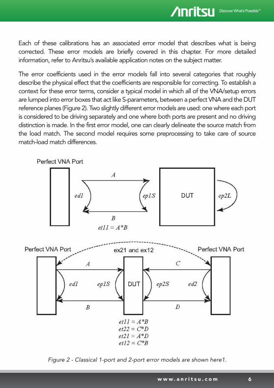
The error coefficients used in the error models fall into several categories that roughlydescribe the physical effect that the coefficients are responsible for correcting. To establish acontext for these error terms, consider a typical model in which all of the VNA/setup errorsare lumped into error boxes that act like S-parameters, between a perfect VNA and the DUTreference planes (Figure 2). Two slightly different error models are used: one where each portis considered to be driving separately and one where both ports are present and no drivingdistinction is made. In the first error model, one can clearly delineate the source match fromthe load match. The second model requires some preprocessing to take care of sourcematch-load match differences.

Figure 2 - Classical 1-port and 2-port error models are shown here1.


Using Figure 2 as a reference, the error terms can be defined as follows:

1. Directivity (ed1 and ed2) - Describes the finite directivity of the bridges or directionalcouplers in the system. Partially includes some internal mismatch mechanisms thatcontribute to effective directivity.

2. Source Match (ep1S and ep2S) - Describes the return loss of a driving port.

3. Load Match (ep1L and ep2L) - Describes the return loss of a terminating port. In the 8-term error models used as a basis for the LRL/ALRM and other calibration families, loadmatch is treated the same as source match, but the incoming data is pre-corrected to takeinto account the measured difference in match between driving and terminating states.

4. Reflection Tracking (et11 and et22) - Describes the frequency response of a reflectmeasurement, including loss behaviors due to the couplers, transmission lines, converters,and other components.

5. Transmission Tracking (et12 and et21) - Same as above, but for the transmission paths.The tracking terms are not entirely independent and this fact is used in some of thecalibration algorithms.

6. Isolation (ex12 and ex21) - This term takes into account certain types of internal (e.g., non-DUT dependent) leakages that may be present in hardware. It is largely present for legacyreasons and is rarely used in practice since this type of leakage is typically very small inmodern VNAs. These terms are handled somewhat differently from the others and will becovered later in this guide.

Line Types

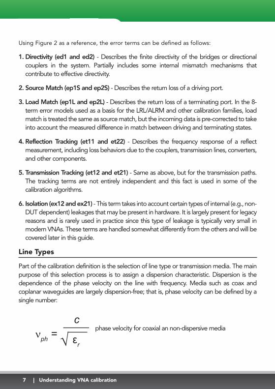
Part of the calibration definition is the selection of line type or transmission media. The mainpurpose of this selection process is to assign a dispersion characteristic. Dispersion is thedependence of the phase velocity on the line with frequency. Media such as coax andcoplanar waveguides are largely dispersion-free; that is, phase velocity can be defined by asingle number:

phase velocity for coaxial an non-dispersive media νph =

с

√ εr


Here c is the speed of light in a vacuum (~2.9978 108 m/s) and εris the relative permittivity of

the medium involved. Coax has its own selection since it is intrinsic to the instrument, whileother non-dispersive media can be selected separately.

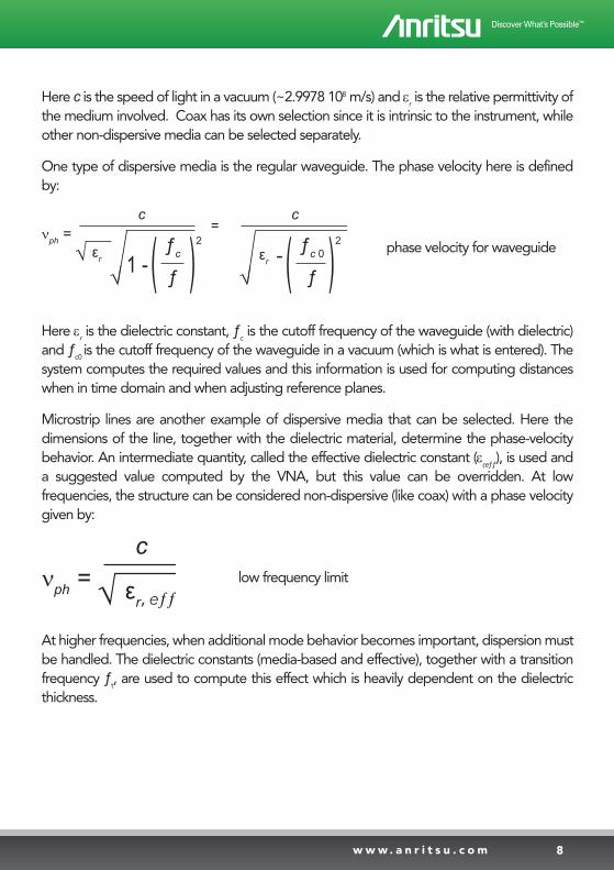
One type of dispersive media is the regular waveguide. The phase velocity here is definedby:

Here εris the dielectric constant, ƒ

cis the cutoff frequency of the waveguide (with dielectric)

and ƒc0

is the cutoff frequency of the waveguide in a vacuum (which is what is entered). Thesystem computes the required values and this information is used for computing distanceswhen in time domain and when adjusting reference planes.

Microstrip lines are another example of dispersive media that can be selected. Here thedimensions of the line, together with the dielectric material, determine the phase-velocitybehavior. An intermediate quantity, called the effective dielectric constant (ε

r,eƒƒ), is used anda suggested value computed by the VNA, but this value can be overridden. At lowfrequencies, the structure can be considered non-dispersive (like coax) with a phase velocitygiven by:

low frequency limit

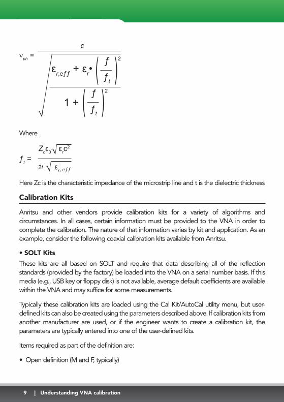
At higher frequencies, when additional mode behavior becomes important, dispersion mustbe handled. The dielectric constants (media-based and effective), together with a transitionfrequency ƒ

t, are used to compute this effect which is heavily dependent on the dielectric

thickness.

νph = с

√ εr

√ (1 - (ƒc

ƒ

2

с

√ ( (ƒc 0

ƒ

2=

εr - phase velocity for waveguide

νph = с

√ εr, eƒƒ


Where

Here Zc is the characteristic impedance of the microstrip line and t is the dielectric thickness

Calibration Kits

Anritsu and other vendors provide calibration kits for a variety of algorithms andcircumstances. In all cases, certain information must be provided to the VNA in order tocomplete the calibration. The nature of that information varies by kit and application. As anexample, consider the following coaxial calibration kits available from Anritsu.

• SOLT Kits

These kits are all based on SOLT and require that data describing all of the reflectionstandards (provided by the factory) be loaded into the VNA on a serial number basis. If thismedia (e.g., USB key or floppy disk) is not available, average default coefficients are availablewithin the VNA and may suffice for some measurements.

Typically these calibration kits are loaded using the Cal Kit/AutoCal utility menu, but user-defined kits can also be created using the parameters described above. If calibration kits fromanother manufacturer are used, or if the engineer wants to create a calibration kit, theparameters are typically entered into one of the user-defined kits.

Items required as part of the definition are:

• Open definition (M and F, typically)

νph = с

√

( (ƒ

ƒt

2

εr,eƒƒ + εr•

( (ƒ

ƒt

2

1 +

ƒt = Zсε0

√ εr, eƒƒ

√ εrc2

2t


• Short definition (M and F, typically) • Load definition (M and F, typically)

• Kits With Triple-Offset Shorts

Some kits employ multiple algorithms to cover larger frequency ranges. The Anritsu 36_6 110 GHz Calibration Kit uses a triple-offset short scheme for frequencies up to 110 GHz,where it is more difficult to characterize opens and loads. At lower frequencies, an SOLTcalibration is used in a banded approach, since the SSST is fundamentally band-limited. Oftena merge calibration method is used to combine the triple-offset short and SOLT calibrations.Some additional standards definitions are therefore required, but the general procedure isthe same as for an SOLT kit. User-defined kits can be generated for custom kits or for thosefrom another manufacturer.


• Open definition (for low frequency, M and F) • Load definition (for low frequency, M and F) • Short 1 definition (M and F) • Short 2 definition (M and F) • Short 3 definition (M and F)

• LRL Kits

These airline-based kits use the LRL algorithm so much less definition of components isrequired. Reflects may be part of the kit, but the only piece of information necessary is anoffset length which is used to help with root selection and is hence somewhat non-critical.Line lengths are the other parameters and are mainly used for reference plane placement. Allof these parameters must be entered manually since there are a large number of lines in thekit and usually only 2 or 3 will be used per calibration. Details on line selection and the tradeoffs involved are discussed in the LRL/LRM section later in this chapter.


• Line lengths (at least 2) • Reflect offset length • Offset-Short Waveguide Kits

Waveguide calibration kits based on offset-short calibrations are also provided for differentwaveguide bands. Here two different offset-length shorts (sometimes accomplished withflush shorts and two different insert lengths), loads and a thru must be specified. Some of the


standard kits are pre-defined and user-defined kits are possible as usual. Additional pieces ofinformation needed here due to line type are the cutoff frequency and dielectric constant.


• Load definition • Short 1 definition • Short 2 definition • Waveguide cutoff frequency

• Microstrip and Coplanar Waveguide Kits for the Universal Test Fixture

For certain microstrip and coplanar waveguide measurements, the Universal Test Fixture(Anritsu model 3680 Series) can be used as it accommodates a range of substrate sizes andthicknesses. The supplied calibration kits provide opens, shorts, loads, and a variety oftransmission-line lengths on alumina that can be used for different calibration algorithms.User-defined kits must be generated based on the information provided with the kits.

• On-Wafer Calibration Kits

A variety of calibration-standard substrates or impedance-standard substrates are availablefrom other vendors that contain opens, shorts, loads, and transmission lines for on-wafercalibrations. A variety of calibration algorithms may be used depending on the application.For the defined-standards calibrations, a user-defined kit will have to be generated.


Automatic Calibration (AutoCal)

In contrast to the mechanical standards approach to calibration, automatic calibrationmodules can be used to simplify the calibration method. Automatic calibration techniques,such as those performed by the AutoCal modules available from Anritsu, are often thepreferred method for calibrating VNAs. AutoCal provides VNA users with the ability toquickly calibrate the network analyzer with the simple push of a button. The AutoCal moduleincorporates extremely accurate, repeatable solid-state switches to select a variety ofimpedance standards from just one connection between the VNA and a calibrator module.

Precision AutoCal Calibration Module

Calibrations employing AutoCal modules are consistent, repeatable and provide betteraccuracy than traditional broadband-termination, 12-term calibrations. In addition, automaticcalibrations are much faster than with traditional calibration kits. For example, a 401-point,12-term AutoCal takes typically 30 seconds when using the VectorStar VNA, as compared tothe 10 to 1_ minutes it takes with a traditional calibration kit. In addition, calibrating with thePrecision AutoCal module requires only two connections, while a mechanical calibration kitrequires 7 to 9 connections for a typical calibration. Note that test-port characteristicspecifications require a sliding load-termination calibration, thereby further escalating thecomplexity of the calibration. Sliding-load terminations require a high level of expertise andcare due to their mechanical complexity. If broadband terminations are used, the resultantdirectivity and port-match performance will suffer.

A further benefit of the Precision AutoCal process stems from the flexibility of the PrecisionAutoCal characterization process which allows users to measure:

• Non-insertable devices. • Devices with different connector types on each port. • Devices with waveguide or coaxial connectors, as well as several other combinations.

The automatic calibrator module also saves wear and tear on traditional calibrationcomponents and eliminates operator mistakes, such as incorrect use of calibrationcoefficients. In addition, it still maintains the accuracy required for critical measurements.

The basic concept in Precision AutoCal is the transfer of known calibration parameters froma traceable VNA to measure the calibration standards within the Precision AutoCal module—a process referred to as Precision AutoCal characterization. A calibrated VNA (using atraceable calibration kit) measures the S-parameter data of each impedance standardthroughout the calibrator module’s frequency range. The accuracy of the calibrated VNA is


thereby transferred to the Precision AutoCal module. The stability and repeatability of thePrecision AutoCal impedance standards provides excellent automatic calibrations over adefined time frame. This method of impedance transfer typically results in limited sacrifice ofaccuracy for simplicity, speed and convenience. But, by combining the Precision AutoCalcalibrator with the MS4640A VectorStar VNA, the resulting overall measurement accuracy isbetter than a mechanical standards calibration, including sliding-load terminations. Thisaccomplishment is reached through the use of ultra-precision LRL/LRM calibration and over-determined algorithms.

The following discussion includes both types of AutoCal modules. In the areas that are uniqueto the newer AutoCal technology, the term Precision AutoCal will be used.

The AutoCal calibration process represents both a calibration device and an algorithm thatcan be used to speed up the calibration process with extremely high accuracy and a minimalnumber of manual connections. Anritsu offers two types of AutoCal modules; the 36_8_XSeries Precision AutoCal and the 36_81X Series Standard AutoCal. Both AutoCal seriescalibrate the VNA by a process known as ‘transfer calibration.’ There are a number ofimpedance and transmission states in the module designed to be extremely stable in timeand these states are carefully ‘characterized,’ generally by the Anritsu factory. In certain cases,this characterization can also take place in a customer laboratory. When the same states arere-measured during an actual calibration and the results compared to the characterizationdata, an accurate picture is generated of the behaviors and error terms of the VNA and setupbeing calibrated.

Very high calibration accuracy is maintained through the use of certain principles:

• The use of many impedance and transmission states covering as wide a range as possibleacross the Smith chart.

• The creation of very stable states that are further enhanced with a constant-temperaturethermal platform inside the module.

• The use of very reliable and repeatable solid-state switching constructed to provide a greatvariety of state impedances for better calibration stability.

The resulting accuracy can exceed the performance obtained using a common SOLTmechanical calibration with sliding loads—a process generally performed in a laboratory.


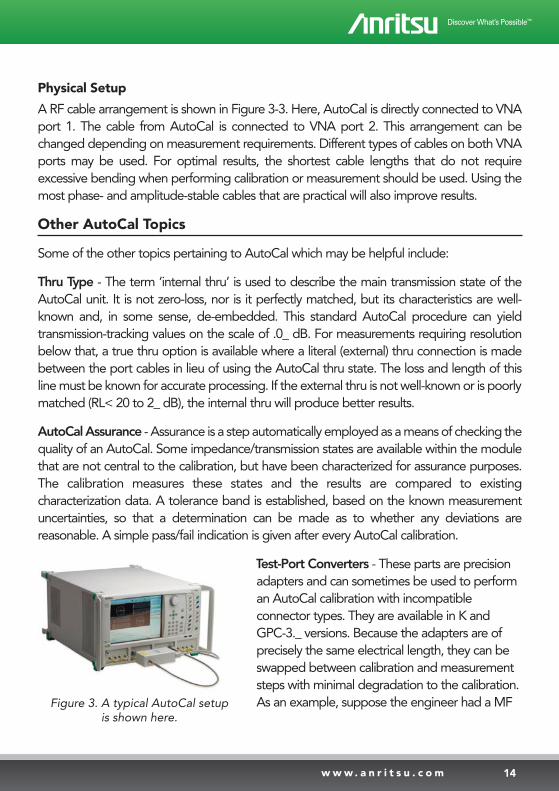
Physical Setup

A RF cable arrangement is shown in Figure 3-3. Here, AutoCal is directly connected to VNAport 1. The cable from AutoCal is connected to VNA port 2. This arrangement can bechanged depending on measurement requirements. Different types of cables on both VNAports may be used. For optimal results, the shortest cable lengths that do not requireexcessive bending when performing calibration or measurement should be used. Using themost phase- and amplitude-stable cables that are practical will also improve results.

Other AutoCal Topics

Some of the other topics pertaining to AutoCal which may be helpful include:

Thru Type - The term ‘internal thru’ is used to describe the main transmission state of theAutoCal unit. It is not zero-loss, nor is it perfectly matched, but its characteristics are well-known and, in some sense, de-embedded. This standard AutoCal procedure can yieldtransmission-tracking values on the scale of .0_ dB. For measurements requiring resolutionbelow that, a true thru option is available where a literal (external) thru connection is madebetween the port cables in lieu of using the AutoCal thru state. The loss and length of thisline must be known for accurate processing. If the external thru is not well-known or is poorlymatched (RL< 20 to 2_ dB), the internal thru will produce better results.

AutoCal Assurance - Assurance is a step automatically employed as a means of checking thequality of an AutoCal. Some impedance/transmission states are available within the modulethat are not central to the calibration, but have been characterized for assurance purposes.The calibration measures these states and the results are compared to existingcharacterization data. A tolerance band is established, based on the known measurementuncertainties, so that a determination can be made as to whether any deviations arereasonable. A simple pass/fail indication is given after every AutoCal calibration.

Test-Port Converters - These parts are precisionadapters and can sometimes be used to performan AutoCal calibration with incompatibleconnector types. They are available in K andGPC-3._ versions. Because the adapters are ofprecisely the same electrical length, they can beswapped between calibration and measurementsteps with minimal degradation to the calibration.As an example, suppose the engineer had a MFFigure 3. A typical AutoCal setup

is shown here.


K AutoCal unit, but wanted to have reference planes established at a MM interface. Toaccomplish this, the engineer could place a FF test-port converter on one of the MM test-port cable connectors, making a MF interface available for the AutoCal. After calibration,the FF converter could then be removed and a MF converter installed so that the MMplanes would be established. The typical uncertainty penalty is less than 0.1 dB to 40 GHz,although the residual directivity may be degraded to about 30 dB. If this is unacceptable,consider the adapter removal or related techniques to be discussed later in this chapter.

Characterization

Typically, characterization of auto-calibrators is performed at the factory since the process canbe very carefully controlled to achieve maximum accuracy. In certain cases, the customer maywish to perform the characterization themselves. In this case, the customer takes fullresponsibility for performing an adequate quality characterization.

If re-characterizing the AutoCal module is a necessity, there are procedures available toensure the characterization process is as accurate as possible. The process involvesperformance of a calibration check after the VNA is calibrated and requires the use of Anritsuairlines and 20-dB return loss terminations and shorts. Using the components provides amethod for measuring the resultant test-port characteristics after a calibration.

After measurement of the actual performance of the corrected VNA, the transfer of accuracyto the AutoCal module is precisely known and therefore can be considered a traceable path.The path is traceable because of the National Institute of Standards and Technology (NIST)-traceable mechanical standards that were used to verify the impedance accuracy of thereference airlines. Thus, re-characterization of the module can be performed without theaccuracy of a LRL calibration kit (as performed at the Anritsu factory), and still provide a highlevel of confidence in the characterization procedure.

Non-Insertable Measurements

Many VNA users have devices which are non-insertable and/or have alternative connectortypes to the standard K or V connectors used on each AutoCal module. The characterizationsoftware built into Anritsu’s VNAs allows users to characterize the AutoCal modules withadapters installed specific to their calibration needs. As is the case with a standardcharacterization, the user must first calibrate the VNA prior to performing thecharacterization. In this situation, the specific connector type should be calibrated using atraditional calibration kit. In the event of a non-insertable calibration, all Anritsu VNA’s offer(as standard) the Adapter Removal calibration feature which utilizes two calibrations toremove the effects of the adapter.


SOLT

One of the more common calibration algorithms is based on SOLT.[1] This is a defined-standards calibration, meaning that each component behavior is specified in advance usingdata or models. Since the behaviors of all standards are known, measuring them with theVNA provides the opportunity to define all of the error terms. The load behavior largely setsthe directivity terms. Together, the short and open largely determine source match andreflection tracking. The thru largely determines transmission tracking and load match.

Shorts - Defined by an S-parameter file or a model consisting of a transmission line lengthand a frequency-dependent inductance. The inductance is defined as

L = L0+ L

1• f + L

2 • f 2 + L

3• f 3

Opens - Defined by an S-parameter file or a model consisting of a transmission line lengthand a frequency-dependent capacitance. The capacitance is defined as

C = C0+ C

1• f + C

2• f 2 + C

3• f 3

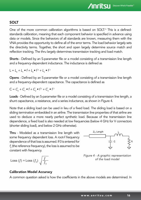
Loads - Defined by an S-parameter file or a model consisting of a transmission line length, ashunt capacitance, a resistance, and a series inductance, as shown in Figure 4.

Note that a sliding load can be used in lieu of a fixed load. The sliding load is based on asliding termination embedded in an airline. The transmission line properties of that airline areused to deduce a more nearly perfect synthetic load. Because of the transmission linedependence, a fixed load is also needed at low frequencies (below 4 GHz for V connectors(shorter sliding load), and below 2 GHz otherwise).

Thru - Modeled as a transmission line length withsome frequency dependent loss. A root-f frequencydependence of that loss is assumed. If 0 is entered forf0(the reference frequency), the loss is assumed to be

constant with frequency.

Calibration Model Accuracy

A common question asked is how the coefficients in the above models are determined. In

Loss (ƒ) = Loss (ƒ0) √ƒƒ0

Figure 4 - A graphic representationof the load model


some custom structures (e.g., fixtured), the VNA user could perform electromagneticmodeling of the structures and then use simulation tools to determine the best fit circuitmodels. For coaxial components, however, the structures are usually sufficiently complex thatthis process is too difficult. Instead the measurement of an airline, the key to most impedancetraceability, is often used to determine the models. A calibration is generated using thecomponents in question and then the models are iterated in a nonlinear least squares fashion.This produces the calibrated result for the airline most closely matching the expectedbehavior, based on the tight dimensional control of the airline. By using different terminationson the airline, the effects of the various models can be separated, making the problem moresoluble. A low-reflectance termination causes the load model to dominate the calibration,while a high-reflectance termination causes the short and open models to dominate. At lowfrequencies, when an airline may become unfeasibly large to be electrically long, precision-lumped components are used instead. These components can be characterized by othertraceable paths including DC and other low-frequency measurements.

For 1-port calibrations, only one of the port definitions (unless reflection-only calibrations arebeing performed for both ports 1 and 2) will be present. The through line section will not bepresent. For a 1-path, 2-port calibration, one of the port definition sections will not bepresent.

For waveguide and microstrip, a few things change:

• Fewer calibration kits are factory-defined and more are user-defined.

• The media must be part of the definition (e.g., cutoff frequency and dielectric constant forwaveguide; line width, substrate height, and substrate dielectric constant for microstrip).

• SOLT is not recommended for waveguide due to the difficulty in modeling open standards.

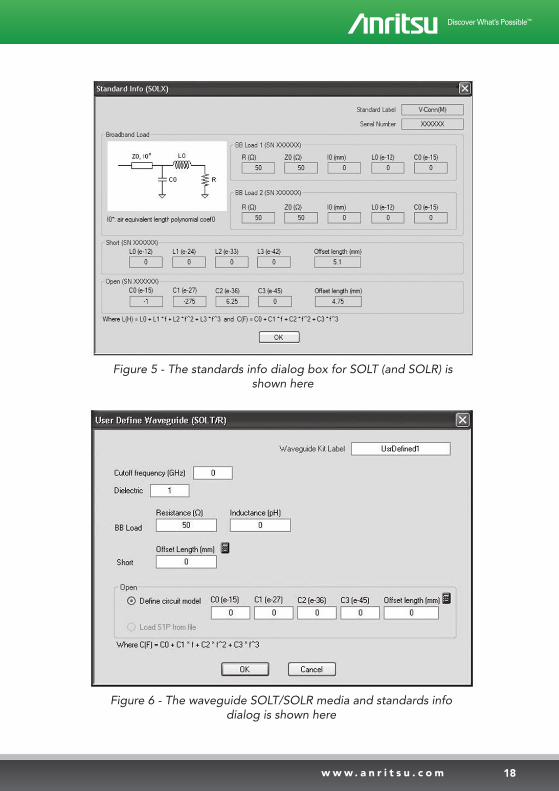
The standards information dialog for SOLT (and SOLR) is shown in Figure 5 using a V-connector as an example.

The standards information for microstrip does not change, but the microstrip mediainformation must be provided either in a user-defined fashion or from selecting theappropriate microstrip calibration kit (Figure 6).


Figure 5 - The standards info dialog box for SOLT (and SOLR) isshown here

Figure 6 - The waveguide SOLT/SOLR media and standards info dialog is shown here


Offset Short

The prime difference between SSLT and SOLT is that differing offset lengths between twoshorts are used to help define reflection behavior instead of an open and short.[2] Thefrequency range is limited since at DC and higher frequencies, these reflect standards lookthe same. This method is most commonly used for waveguide problems and in certain coaxand board- or wafer-level situations where creating a stable, high-reflection open standard isdifficult. The modeling constructs for SSLT are about the same as for SOLT. From an error-term perspective, the only difference is that the two shorts together now largely determinesource match and reflection tracking behavior.

Generally, the electrical length difference between the shorts should be between 20 and 160degrees, over the frequency range of interest. Mathematically, this is stated as:

The top calibration-kit definition dialog for SSLT is identical to the one for SOLT. The standardsinformation dialog is somewhat different and is shown in Figure 7.

Triple Offset Short

The next step in this progression is to remove the load so that the entire reflection space isdefined by three shorts of varying offset lengths. The individual short definitions are the sameas for SOLT. Together, the three shorts determine all of the reflectometer error terms(directivity, source match and reflection tracking). This calibration is even somewhat moreband-limited than the double-offset short method.

20 < 720 • ƒ • | Loffset_short1 - Loffset_short2 |

νph

<160


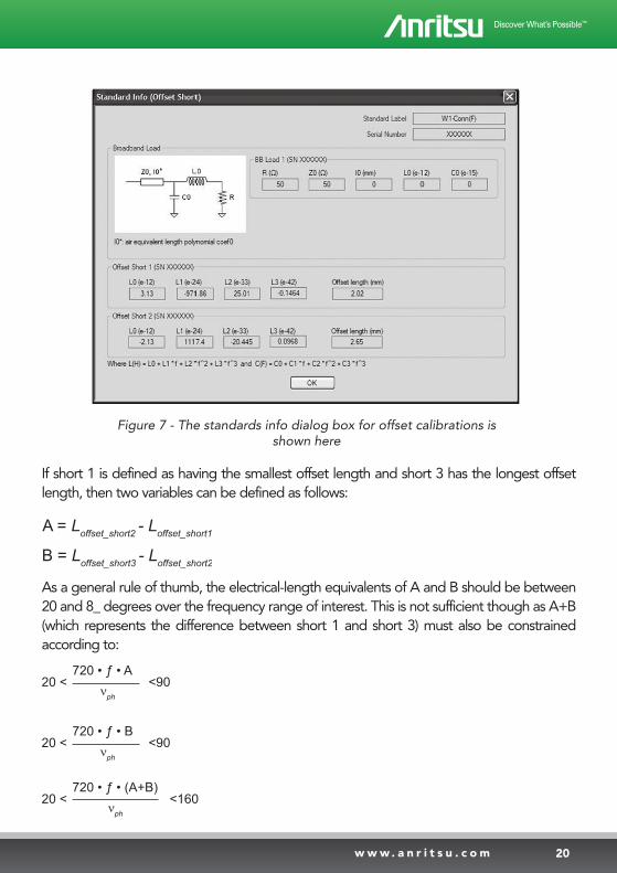
If short 1 is defined as having the smallest offset length and short 3 has the longest offsetlength, then two variables can be defined as follows:

As a general rule of thumb, the electrical-length equivalents of A and B should be between20 and 8_ degrees over the frequency range of interest. This is not sufficient though as A+B(which represents the difference between short 1 and short 3) must also be constrainedaccording to:

Figure 7 - The standards info dialog box for offset calibrations isshown here

20 < 720 • ƒ • A

νph

<90

20 < 720 • ƒ • B

νph

<90

20 < 720 • ƒ • (A+B)

νph

<160

B = Loffset_short3 - Loffset_short2

A = Loffset_short2 - Loffset_short1


Since the only standards needed are shorts, this method is attractive for millimeter wave (mm-wave) applications, as well as for certain board and wafer-level calibrations where other typesof standards are difficult to manufacture. It should be noted, however, that the impact ofinaccuracies in the short offset lengths are more elevated in this calibration since they are usedto map the entire reflection space. A good residual directivity (which results from the abilityto map the center of the Smith chart accurately) requires very accurate offset-lengthknowledge. Also, note that the qualities of the connections are critical. With the inclusion ofadditional short standards, connection quality becomes an even larger issue.

SOLR (Unknown Thru Approach)

The three previous calibration techniques all require a known ‘thru’ as part of the full 2¬portor 1-path 2-port calibration. The ‘thru’ is a defined transmission line having known length,known loss and an assumed perfect match (under most conditions). There are certain caseswhen this is not possible (Figure 3-8). Some examples include:

• Coaxial calibration, when the two ports are different connector types.

• On-wafer, when the ‘thru’ is a meandering transmission line of imperfect match.

• A calibration that must take place through a test set (e.g., coax or waveguide) withunknown, and highly frequency-dependent, loss and match.

For these cases, and others when the ‘thru’ is not well-known, there is the reciprocal option,also known as the unknown thru.[3] In this case, the same reflect standards are used, but noassumption is made about the ‘thru’ except that it is reciprocal (e.g., S

21=S

12; no assumption

made about S11

and S22). In practice, there are some limits to this that will be addressed later

in the chapter.

The SOLR technique borrows from the LRL family and uses some of the redundancy availablewith the fully-defined families to reduce the amount of knowledge needed about something;in this case, the thru. The resulting calibration is generally not quite as accurate as the regularthru version, assuming the thru met the conditions described above. Although it is betterthan using the regular thru version when the thru has unknown loss or match.

A line length estimate (e.g., electrical delay or free-space equivalent length) is needed to helpwith root choice, but this is not a critical parameter. Typically, the VNA user need only bewithin a half-wavelength of the correct length at the maximum desired calibration frequency.

If the match of the reciprocal network gets worse than about –8 dB, or the loss exceeds ~20


dB, even the reciprocal treatment will start to degrade slightly, but a calibration will still bepossible. Since such a network is at the limits of de-embedding capability, there are fewchoices except to consider 1-path 2-port processing with scalar de-embedding.

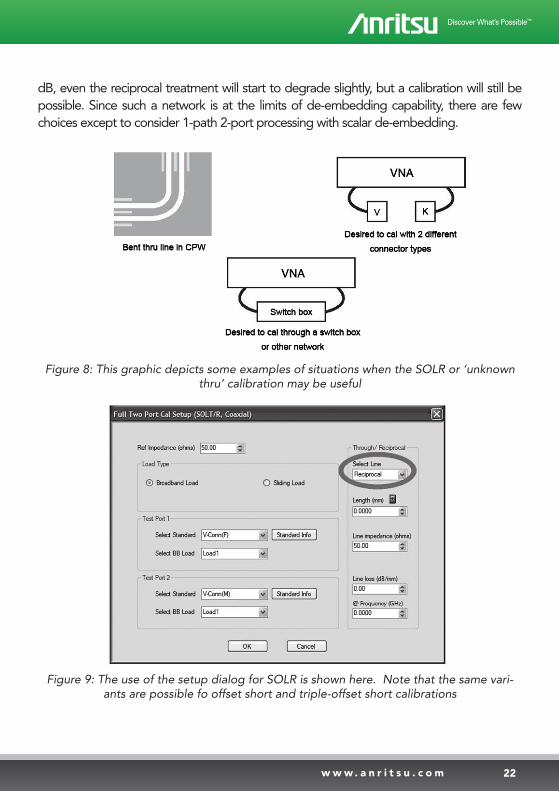
Figure 8: This graphic depicts some examples of situations when the SOLR or ‘unknownthru’ calibration may be useful

Figure 9: The use of the setup dialog for SOLR is shown here. Note that the same vari-ants are possible fo offset short and triple-offset short calibrations


For SOLR, the ‘select line’ field is chosen as ‘reciprocal’ instead of ‘through.’ The length fieldis the estimate of length for root choice that was previously discussed (Figure 9).

LRL/LRM/ALRM

The LRL/LRM/ALRM family of calibrations is somewhat different from the previous families. Itrelies more on the intrinsic behavior of certain components, primarily transmission lines, thanit does on characterized/modeled behaviors of components.[4] [_] It also makes less use ofredundancy so fewer measurements are needed to complete a calibration. In return though,it is somewhat less tolerant of poor or non-repeatable measurements. Included in thiscalibration family is:

• ALRM - An extension of the LRM algorithm that provides improved performance for on-wafer applications where load symmetry is not ideal. The examples shown apply to theMS4640A series of VectorStar VNAs.

• LRL - Uses two or more transmission lines and a reflect standard for each port. The linelengths are important since the lines are required to look electrically distinct at all times. LRLwill not work at DC or at a frequency where the difference in length is an integral numberof half wavelengths. The reflect standard is not that important as it is only assumed to besymmetric and with not too high of a return loss. Practically speaking, even a 20-dB returnloss will usually work. The lines are assumed perfect (e.g., no mismatch) which usuallymeans airlines for coaxial calibrations, although other structures can be used. On-wafertransmission lines are usually very good and therefore, this calibration approach will workwell if the required probe movement can be effectively handled.

• LRM/ALRM - Here one of the lines above is replaced with a match or load. The load ismodeled/characterized (or assumed perfect), so in some sense this calibration drifts backto the concept of the defined standards. Since only one line is involved, it can work downto DC and up to very high frequencies (practically limited by the matchknowledge/characterization). Some variations allow one of the match measurements to betraded for a pair of additional reflect measurements, although a second reflect standard isneeded. In this case, the requirement that the reflect standards be distinct may force thecalibration to become band limited.

In the limiting case of a match that is assumed perfect, or at least assumed symmetric, thiscalibration reduces to the classical LRM. The added flexibility in the ALRM case is in the abilityto define asymmetric load models and to use multiple reflect standards as discussed above.Other extensions are possible elsewhere.[6] [7] [8] The double-reflect methodology allows the

user to feed into a load modeling utility where the load model can be further optimized.

Some parameters to keep in mind include:

Line Lengths - In addition to the LRL frequency limits, the line length is used in all cases forsome reference-plane tasks. The fundamental reference plane of an LRL/ALRM calibration isin the middle of the first line. Sometimes it is desirable to have the reference plane at the endsof this line so that the line length (and loss which can also be entered) can be used to rotatethe reference planes to the desired place. The line-length delta is also used for some root-choice tasks, although the accuracy required on this entry is less.

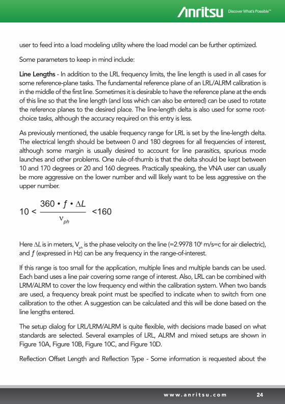
As previously mentioned, the usable frequency range for LRL is set by the line-length delta.The electrical length should be between 0 and 180 degrees for all frequencies of interest,although some margin is usually desired to account for line parasitics, spurious modelaunches and other problems. One rule-of-thumb is that the delta should be kept between10 and 170 degrees or 20 and 160 degrees. Practically speaking, the VNA user can usuallybe more aggressive on the lower number and will likely want to be less aggressive on theupper number.

Here ∆L is in meters, Vph

is the phase velocity on the line (=2.9978 108 m/s=c for air dielectric),and ƒ (expressed in Hz) can be any frequency in the range-of-interest.

If this range is too small for the application, multiple lines and multiple bands can be used.Each band uses a line pair covering some range of interest. Also, LRL can be combined withLRM/ALRM to cover the low frequency end within the calibration system. When two bandsare used, a frequency break point must be specified to indicate when to switch from onecalibration to the other. A suggestion can be calculated and this will be done based on theline lengths entered.

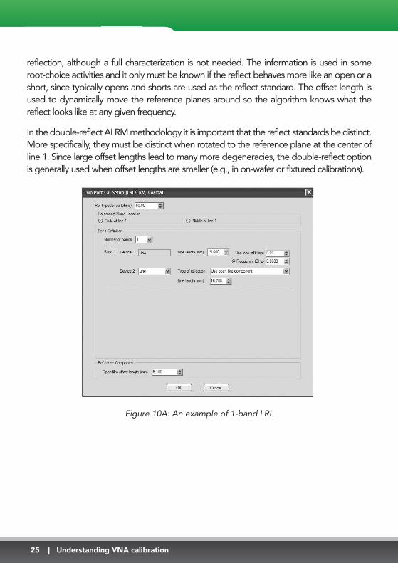
The setup dialog for LRL/LRM/ALRM is quite flexible, with decisions made based on whatstandards are selected. Several examples of LRL, ALRM and mixed setups are shown inFigure 10A, Figure 10B, Figure 10C, and Figure 10D.

Reflection Offset Length and Reflection Type - Some information is requested about the

10 < 360 • ƒ • ∆L

νph

<160



reflection, although a full characterization is not needed. The information is used in someroot-choice activities and it only must be known if the reflect behaves more like an open or ashort, since typically opens and shorts are used as the reflect standard. The offset length isused to dynamically move the reference planes around so the algorithm knows what thereflect looks like at any given frequency.

In the double-reflect ALRM methodology it is important that the reflect standards be distinct.More specifically, they must be distinct when rotated to the reference plane at the center ofline 1. Since large offset lengths lead to many more degeneracies, the double-reflect optionis generally used when offset lengths are smaller (e.g., in on-wafer or fixtured calibrations).

Figure 10A: An example of 1-band LRL


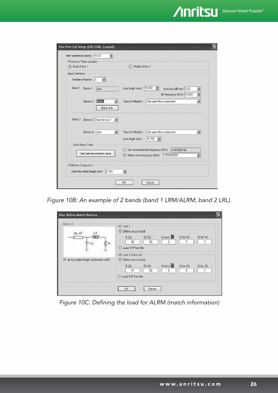
Figure 10B: An example of 2 bands (band 1 LRM/ALRM, band 2 LRL).

Figure 10C: Defining the load for ALRM (match information)


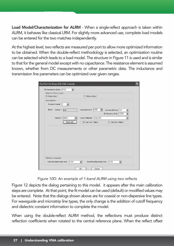
Load Model/Characterization for ALRM - When a single-reflect approach is taken withinALRM, it behaves like classical LRM. For slightly more advanced use, complete load modelscan be entered for the two matches independently.

At the highest level, two reflects are measured per port to allow more optimized informationto be obtained. When the double-reflect methodology is selected, an optimization routinecan be selected which leads to a load model. The structure in Figure 11 is used and is similarto that for the general model except with no capacitance. The resistance element is assumedknown, whether from DC measurements or other parametric data. The inductance andtransmission line parameters can be optimized over given ranges.

Figure 10D: An example of 1-band ALRM using two reflects

Figure 12 depicts the dialog pertaining to this model. it appears after the main calibrationsteps are complete. At that point, the fit model can be used (default) or modified values maybe entered. Note that the dialogs shown above are for coaxial or non-dispersive line types.For waveguide and microstrip line types, the only change is the addition of cutoff frequencyand dielectric constant information to complete the model.

When using the double-reflect ALRM method, the reflections must produce distinctreflection coefficients when rotated to the central reference plane. When the reflect offset


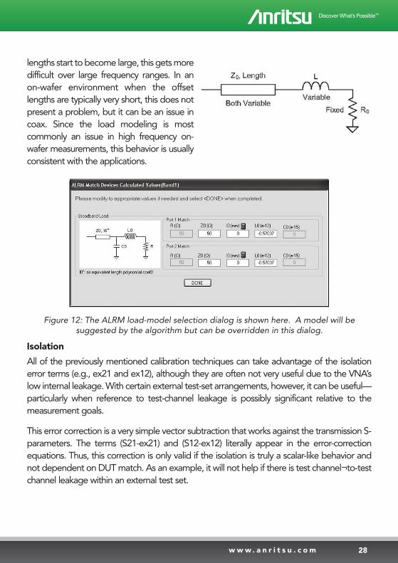
lengths start to become large, this gets moredifficult over large frequency ranges. In anon-wafer environment when the offsetlengths are typically very short, this does notpresent a problem, but it can be an issue incoax. Since the load modeling is mostcommonly an issue in high frequency on-wafer measurements, this behavior is usuallyconsistent with the applications.

Figure 12: The ALRM load-model selection dialog is shown here. A model will be suggested by the algorithm but can be overridden in this dialog.

Isolation

All of the previously mentioned calibration techniques can take advantage of the isolationerror terms (e.g., ex21 and ex12), although they are often not very useful due to the VNA’slow internal leakage. With certain external test-set arrangements, however, it can be useful—particularly when reference to test-channel leakage is possibly significant relative to themeasurement goals.

This error correction is a very simple vector subtraction that works against the transmission S-parameters. The terms (S21-ex21) and (S12-ex12) literally appear in the error-correctionequations. Thus, this correction is only valid if the isolation is truly a scalar-like behavior andnot dependent on DUT match. As an example, it will not help if there is test channel¬to-testchannel leakage within an external test set.


Adapter Removal

There are a number of situations where the DUT configuration is not entirely compatible withcommon calibration procedures, such as when:

• The DUT has one connector of some coaxial type and another connector of a coaxial type froma different family (e.g., K and V).

• One port of the DUT is coaxial and the other is waveguide.

• One port of the DUT is coaxial and the other is fixtured (e.g., a transmission line on a board or onwafer)

• The DUT is coaxial with both ports of the same type, but also the same sex and there is aproblem creating the thru.

All of these cases share a common problem - it is difficult to generate the thru, or a goodtransmission line, for the calibration. A number of options exist to address this problem,including:

• Use the SOLR calibration discussed previously. This will work assuming that the VNA user iswilling to perform a semi-defined-standards calibration.

• Enter the length and loss of what can be constructed as a thru. Use that information in thecalibrations. This can work if the loss is not too great, is well-behaved and the match is still good.

• Use the Phase-Equal-Insertable method (for the case listed above). Here one adapter is usedduring the calibration and a different adapter of the same electrical length and loss is substitutedfor the measurement. Note that this is the same as the Test-Port Converter method discussed inthe AutoCal section.

• De-embed an adapter. If the VNA user knows enough about the adapting structure (either agood model or .s2p data), the adapter can be de-embedded separately. Acquiring thisinformation is usually the hard part.

• Use the concept of adapter removal.

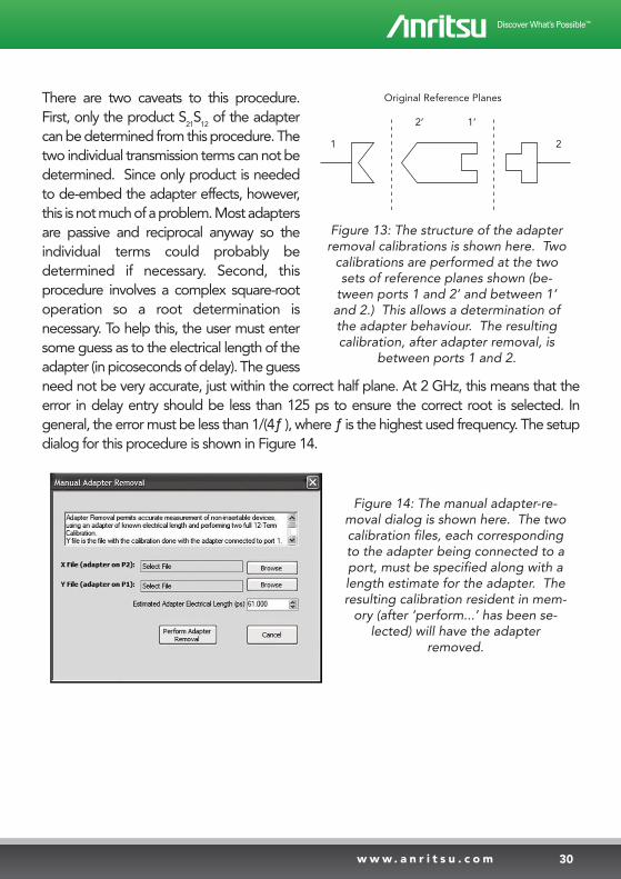
The concept of adapter removal relies on the existence of two related sets of referenceplanes: one set on either side of the adapter (Figure 13). Assuming a full calibration isperformed at each set of reference planes, there is enough information to extract thebehavior of the adapter itself. When the calibration is being performed at the referenceplanes on the left (between ports 1 and 2’), the adapter behavior is embedded in thecharacteristics of port 2’. Similarly, when the calibration is being performed between ports 1’and 2, the adapter behavior is embedded in the characteristics of port 1’. Since each of thesetwo calibrations involve mating connector types, they are far easier to perform than the direct1-2 calibration. The use of the two calibrations provides nearly enough information to extractthe parameters of the adapter itself.


There are two caveats to this procedure.First, only the product S

21S

12of the adapter

can be determined from this procedure. Thetwo individual transmission terms can not bedetermined. Since only product is neededto de-embed the adapter effects, however,this is not much of a problem. Most adaptersare passive and reciprocal anyway so theindividual terms could probably bedetermined if necessary. Second, thisprocedure involves a complex square-rootoperation so a root determination isnecessary. To help this, the user must entersome guess as to the electrical length of theadapter (in picoseconds of delay). The guessneed not be very accurate, just within the correct half plane. At 2 GHz, this means that theerror in delay entry should be less than 125 ps to ensure the correct root is selected. Ingeneral, the error must be less than 1/(4ƒ ), where ƒ is the highest used frequency. The setupdialog for this procedure is shown in Figure 14.

1

2’ 1’

2

Original Reference Planes

Figure 13: The structure of the adapterremoval calibrations is shown here. Two

calibrations are performed at the twosets of reference planes shown (be-

tween ports 1 and 2’ and between 1’and 2.) This allows a determination ofthe adapter behaviour. The resultingcalibration, after adapter removal, is

between ports 1 and 2.

Figure 14: The manual adapter-re-moval dialog is shown here. The twocalibration files, each correspondingto the adapter being connected to aport, must be specified along with alength estimate for the adapter. Theresulting calibration resident in mem-

ory (after ‘perform...’ has been se-lected) will have the adapter

removed.


Now consider the special case of adapter removal with AutoCal. In the AutoCal-specializedversion, adapter removal primarily refers to the case of a sex incompatibility when the userdoes not want to use test-port converters (e.g., the user has a MF AutoCal unit and wants toestablish MM reference planes). A separate menu item is provided for AutoCal adapterremoval. This speeds up the process since fewer manual steps are needed. In this calibrationsequence, an adapter that can mate the desired reference-plane connectors is used as partof the calibration. As an example, for the MF AutoCal scenario, the adapter is placed on thedesired port and the system is calibrated as before. Then, the AutoCal and adapter pair isrotated between the VNA test ports and the calibration is repeated. The process of reversingthe AutoCal provides all the information needed for the internal algorithm to remove theadapter from calibration.

Thru Update

A common question related to calibrations is: How often is it necessary to redo thecalibration? The answer depends heavily on the environment, both in terms of temperaturestability and in terms of the cabling/fixturing construct that is being used. A recurring theme,however, is that this calibration lifetime is often limited by the stability of the test-port cablesthrough drift or motion. These drift defects directly affect transmission tracking and loadmatch. Therefore, the user might be able to lengthen the time between recalibrations byemploying a simple means of refreshing these terms.

The idea is that it is relatively simple to connect just a thru/line and quickly refresh thetransmission-tracking and load-match terms without great effort. In a sense, thru update is aone-step calibration that can be used to refresh a current, full 2-port or 1-path 2-portcalibration.

Interpolation

Typically, the user calibrates at a specific list of frequencies and then performs measurementsover that same list of frequencies. While this is an accurate process, it is not necessarilyconvenient. If, for example, a variety of narrow-bandpass filters of different center frequenciesare being measured, it would be useful to zoom in to look at the passband of each filter,without having to recalibrate. Interpolated calibrations can be useful in these types ofsituations.

Care must be used when interpolating error coefficients between calibration points tominimize possible error. For the cause of interpolation error, note that the cable running withinthe instrument and those provided by the user typically result in a large electrical length. Asa result, the error coefficient magnitude versus frequency is often periodic in shape. If the


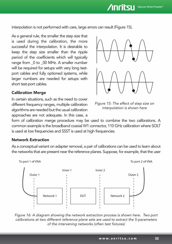
interpolation is not performed with care, large errors can result (Figure 15).

As a general rule, the smaller the step size thatis used during the calibration, the moresuccessful the interpolation. It is desirable tokeep the step size smaller than the rippleperiod of the coefficients which will typicallyrange from _0 to _00 MHz. A smaller numberwill be required for setups with very long test-port cables and fully optioned systems, whilelarger numbers are needed for setups withshort test-port cables.

Calibration Merge

In certain situations, such as the need to coverdifferent frequency ranges, multiple calibrationalgorithms are needed but the usual calibrationapproaches are not adequate. In this case, aform of calibration merge procedure may be used to combine the two calibrations. Acommon example is the broadband coaxial W1 connector, 110 GHz calibration where SOLTis used at low frequencies and SSST is used at high frequencies.

Network Extraction

As a conceptual variant on adapter removal, a pair of calibrations can be used to learn aboutthe networks that are present near the reference planes. Suppose, for example, that the user

Figure 15: The effect of step size oninterpolation is shown here

Network 1 Network 2DUT

Inner 1 Inner 2Outer 1 Outer 2

To port 1 of VNA To port 2 of VNA

Figure 16: A diagram showing the network extraction process is shown here. Two portcalibrations at two different reference plane sets are used to extract the S-parameters

of the intervening networks (often test fixtures)


has networks that attach to the ports, the most common of which is a fixture. If a calibrationcan be performed both inside and outside of those networks, then there is enoughinformation to extract the networks’ S-parameters.

Consider the diagram in Figure 16. A calibration is required at the outer reference-plane setand the inner reference-plane set. The outer calibration is usually done coaxially, or with someother well-defined media, depending on the networks involved. The inner calibration is oftenmore complicated and may be board- or wafer-level. Also, it may require the user to createcalibration standards. Assuming these calibrations are possible, then the S-parameters ofNetwork 1 and Network 2 can be found.

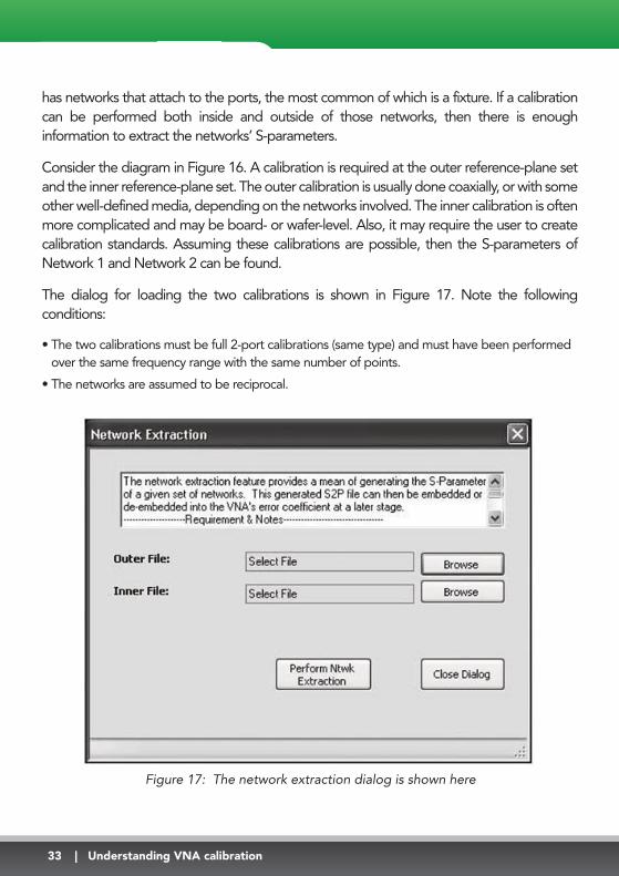
The dialog for loading the two calibrations is shown in Figure 17. Note the followingconditions:

• The two calibrations must be full 2-port calibrations (same type) and must have been performedover the same frequency range with the same number of points.

• The networks are assumed to be reciprocal.

Figure 17: The network extraction dialog is shown here


Summary

The guide introduces the concept of calibration. The various calibration types and calibrationalgorithms where defined, along with the associated error models that describe what is beingcorrected.

This chapter also provided details on the selection of line type or transmission media andAutoCal—automatic calibration modules that are used to simplify the calibration method.The concept of adapter removal was also presented as a way to deal with situations wherethe DUT configuration is not entirely compatible with common calibration procedures. Whilea minimal amount of calibration mathematics and theory were covered in this chapter, moreinformation is available in Anritsu Application Notes and in readily-available referenceliterature.[1]-[11]

References 1. W. Kruppa, “An explicit solution for the scattering parameters of a linear two-port measured with an imperfect

test set,” IEEE Trans. On Micr. Theory and Tech., vol. 19, pp. 122-123, Jan. 1971.

2. G. J. Scalzi, A. J. Slobodnik, and G. A. Roberts, “Network analyzer calibration using offset shorts,” IEEE Trans. OnMicr. Theory and Tech., vol. 36, pp. 1097-1100, June 1988.

3. A. Ferrero and U. Pisani, “Two-port network analyzer calibration using and unknown ‘thru’,” IEEE Micr. AndGuided Wave Lett., vol. 2, pp. _0_-_07, Dec. 1992.

4. G. F. Engen and C. A. Hoer, “‘Thru-Reflect-Line’: An improved technique for calibrating the dual six-port automaticnetwork analyzer,” IEEE Trans. On Micr. Theory and Tech., vol. 27, pp. 987-993, Dec. 1979.

5. H. Eul and B. Schiek, “A generalized theory and new calibration procedures for network analyzer self-calibration,”IEEE Trans. On Micr. Theory and Tech., vol. 39, pp. 724-731, Apr. 1991.

6. A. Davidson, K. Jones, and E. Strid, “LRM and LRRM calibrations with automatic determination of loadinductance,” 36th ARFTG Conf. Dig., pp. _7-63, Dec. 1990.

7. L. Hayden, “An Enhanced Line-Reflect-Reflect-Match Calibration,” 67th ARFTG Conf. Digest, pp. 143-149, June2006.

8. R. Doerner and A. Rumiantsev, “Verification of the wafer-level LRM+ calibration technique for GaAs applicationsup to 110 GHz,” 6_th ARFTG Conf. Dig., pp. 1_-19, June 200_.

9. R. B. Marks, “A multiline method of network analyzer calibration,” IEEE Trans. On Micr. Theory and Tech., vol. 39,pp. 120_-121_, Jul. 1991.

10. D. F. William, C. M. Wang, and U. Arz, “An optimal multiline TRL calibration algorithm,” 2003 IEEE MTT-S Digest,pp. 1819-1822, June 2003.

11. U. Stemper, “Uncertainty of VNA S-parameter measurement due to nonideal TRL calibration items,” IEEE Trans.

Instr. and Meas., vol. _4, pp. 676-679, Apr. 2005.

• United StatesAnritsu Company1155 East Collins Blvd., Suite 100, Richardson, TX 75081, U.S.A.Toll Free: 1-800-267-4878Phone: +1-972-644-1777Fax: +1-972-671-1877

• CanadaAnritsu Electronics Ltd.700 Silver Seven Road, Suite 120, Kanata, Ontario K2V 1C3, CanadaPhone: +1-613-591-2003 Fax: +1-613-591-1006

• Brazil Anritsu Eletrônica Ltda.Praça Amadeu Amaral, 27 - 1 Andar01327-010 - Bela Vista - São Paulo - SP - BrazilPhone: +55-11-3283-2511Fax: +55-11-3288-6940

• MexicoAnritsu Company, S.A. de C.V.Av. Ejército Nacional No. 579 Piso 9, Col. Granada11520 México, D.F., MéxicoPhone: +52-55-1101-2370Fax: +52-55-5254-3147

• United KingdomAnritsu EMEA Ltd.200 Capability Green, Luton, Bedfordshire, LU1 3LU, U.K.Phone: +44-1582-433200 Fax: +44-1582-731303

• FranceAnritsu S.A.12 avenue du Québec, Bâtiment Iris 1- Silic 612,91140 VILLEBON SUR YVETTE, FrancePhone: +33-1-60-92-15-50Fax: +33-1-64-46-10-65

• GermanyAnritsu GmbHNemetschek Haus, Konrad-Zuse-Platz 1 81829 München, Germany Phone: +49-89-442308-0 Fax: +49-89-442308-55

• ItalyAnritsu S.r.l.Via Elio Vittorini 129, 00144 Roma, ItalyPhone: +39-6-509-9711 Fax: +39-6-502-2425

• SwedenAnritsu ABBorgarfjordsgatan 13A, 164 40 KISTA, SwedenPhone: +46-8-534-707-00 Fax: +46-8-534-707-30

• FinlandAnritsu ABTeknobulevardi 3-5, FI-01530 VANTAA, FinlandPhone: +358-20-741-8100Fax: +358-20-741-8111

• DenmarkAnritsu A/S (Service Assurance)Anritsu AB (Test & Measurement)Kay Fiskers Plads 9, 2300 Copenhagen S, DenmarkPhone: +45-7211-2200Fax: +45-7211-2210

• RussiaAnritsu EMEA Ltd. Representation Office in RussiaTverskaya str. 16/2, bld. 1, 7th floor.Russia, 125009, MoscowPhone: +7-495-363-1694Fax: +7-495-935-8962

• United Arab EmiratesAnritsu EMEA Ltd.Dubai Liaison OfficeP O Box 500413 - Dubai Internet CityAl Thuraya Building, Tower 1, Suit 701, 7th FloorDubai, United Arab EmiratesPhone: +971-4-3670352Fax: +971-4-3688460

• SingaporeAnritsu Pte. Ltd.60 Alexandra Terrace, #02-08, The Comtech (Lobby A)Singapore 118502Phone: +65-6282-2400Fax: +65-6282-2533

• IndiaAnritsu Pte. Ltd. India Branch Office3rd Floor, Shri Lakshminarayan Niwas, #2726, 80 ft Road, HAL 3rd Stage, Bangalore - 560 075, IndiaPhone: +91-80-4058-1300Fax: +91-80-4058-1301

• P.R. China (Shanghai)Anritsu (China) Co., Ltd.Room 1715, Tower A CITY CENTER of Shanghai, No.100 Zunyi Road Chang Ning District, Shanghai 200051, P.R. ChinaPhone: +86-21-6237-0898Fax: +86-21-6237-0899

• P.R. China (Hong Kong)Anritsu Company Ltd.Units 4 & 5, 28th Floor, Greenfield Tower, Concordia Plaza, No. 1 Science Museum Road, Tsim Sha Tsui East, Kowloon, Hong Kong, P.R. ChinaPhone: +852-2301-4980Fax: +852-2301-3545

• JapanAnritsu Corporation8-5, Tamura-cho, Atsugi-shi, Kanagawa, 243-0016 JapanPhone: +81-46-296-1221Fax: +81-46-296-1238

• KoreaAnritsu Corporation, Ltd.502, 5FL H-Square N B/D, 681Sampyeong-dong, Bundang-gu, Seongnam-si, Gyeonggi-do, 463-400 KoreaPhone: +82-31-696-7750Fax: +82-31-696-7751

• AustraliaAnritsu Pty. Ltd.Unit 21/270 Ferntree Gully Road, Notting Hill, Victoria 3168, AustraliaPhone: +61-3-9558-8177Fax: +61-3-9558-8255

• TaiwanAnritsu Company Inc.7F, No. 316, Sec. 1, NeiHu Rd., Taipei 114, TaiwanPhone: +886-2-8751-1816Fax: +886-2-8751-1817

Specifications are subject to change without notice.

03/2011

1005

Please contact:

Part No 111410-00673A, Rev A, 06/2012

©2012 Anritsu Company. All rights reserved.

35

®Anritsu All trademarks are registered trademarks of their

respective companies. Data subject to change without notice.

For the most recent specifications visit: www.anritsu.com

Understanding VNA Calibration - Steven M. Anlage …anlage.umd.edu/Anritsu_understanding-vna-calibration.pdf3 | Understanding VNA calibration Table 1 - This table summarizes the various

Documents