PDF (1.319 MB)

A&A 561, A61 (2014)DOI: 10.1051/0004-6361/201322428c© ESO 2013

Astronomy&

Astrophysics

Radial velocity variations in the young eruptive star EX Lupi�,��

Á. Kóspál1,���, M. Mohler-Fischer2, A. Sicilia-Aguilar3, P. Ábrahám4, M. Curé5, Th. Henning2, Cs. Kiss4,R. Launhardt2, A. Moór4, and A. Müller6

1 European Space Agency (ESA-ESTEC, SRE-S), PO Box 299, 2200 AG Noordwijk, The Netherlandse-mail: [email protected]

2 Max-Planck-Institut für Astronomie, Königstuhl 17, 69117 Heidelberg, Germany3 Departamento de Física Teórica, Facultad de Ciencias, Universidad Autónoma de Madrid, 28049 Cantoblanco, Madrid, Spain4 Konkoly Observatory, Research Centre for Astronomy and Earth Sciences, Hungarian Academy of Sciences, PO Box 67,

1525 Budapest, Hungary5 Departamento de Física y Astronomía, Facultad de Ciencias, Universidad de Valparaíso, Av. Gran Bretaña 1111, 5030 Casilla,

Valparaíso, Chile6 European Southern Observatory, Alonso de Córdova 3107, Vitacura, Santiago, Chile

Received 1 August 2013 / Accepted 21 October 2013

ABSTRACT

Context. EX Lup-type objects (EXors) are low-mass pre-main sequence objects characterized by optical and near-infrared outburstsattributed to highly enhanced accretion from the circumstellar disk onto the star.Aims. The trigger mechanism of EXor outbursts is still debated. One type of theory requires a close (sub)stellar companion thatperturbs the inner part of the disk and triggers the onset of the enhanced accretion. Here, we study the radial velocity (RV) variationsof EX Lup, the prototype of the EXor class, and test whether they can be related to a close companion.Methods. We conducted a five-year RV survey, collecting 54 observations with HARPS and FEROS. We analyzed the activity ofEX Lup by checking the bisector, the equivalent width of the Ca 8662 Å line, the asymmetry of the Ca II K line, the activity indicatorSFEROS, the asymmetry of the cross-correlation function, the line depth ratio of the VI/FeI lines, and the TiO, CaH 2, CaH 3, CaOH,and Hα indices. We complemented the RV measurements with a 14-day optical/infrared photometric monitoring to look for signaturesof activity or varying accretion.Results. We found that the RV of EX Lup is periodic (P = 7.417 d), with stable period, semi-amplitude (2.2 km s−1), and phase overat least four years of observations. This period is not present in any of the above-mentioned activity indicators. However, the RVs ofnarrow metallic emission lines suggest the same period, but with an anti-correlating phase. The observed absorption line RVs can befitted with a Keplerian solution around a 0.6 M� central star with m sin i = (14.7±0.7) MJup and eccentricity of e = 0.24. Alternatively,we attempted to model the observations with a cold or hot stellar spot as well. We found that in our simple model, the spot parametersneeded to reproduce the RV semi-amplitude are in contradiction with the photometric variability, making the spot scenario unlikely.Conclusions. We qualitatively discuss two possibilities to explain the RV data: a geometry with two accretion columns rotating withthe star, and a single accretion flow synchronized with the orbital motion of the hypothetical companion; the second scenario is moreconsistent with the observed properties of EX Lup. In this scenario, the companion’s mass would fall into the brown dwarf desert,which, together with the unusually small separation of 0.06 au would make EX Lup a unique binary system. The companion also hasinteresting implications on the physical mechanisms responsible for triggering the outburst.

Key words. stars: formation – circumstellar matter – infrared: stars – techniques: radial velocities – stars: individual: EX Lupi

1. Introduction

EX Lup-type objects (EXors) form a spectacular group of low-mass pre-main sequence (PMS) objects, characterized by repet-itive optical outbursts of 1–5 mag, lasting from a few monthsto a few years. The outburst is usually attributed to enhancedaccretion from the inner circumstellar disk (within ∼0.1 au) tothe stellar surface, caused by an instability in the disk (Herbig1977, 2008). In quiescence, EXors typically accrete at a rateof 10−10 to 10−7 M� yr−1, while in outburst, accretion rates are

� This work is based in part on observations made with ESOTelescopes at the La Silla Paranal Observatory under programIDs 079.A-9017, 081.A-9005, 081.A-9023, 081.C-0779, 082.C-0390,082.C-0427, 083.A-9011, 083.A-9017, 084.A-9011, 085.A-9027,086.A-9006, 086.A-9012, 087.A-9013, 087.A-9029, and 089.A-9007.�� Tables 2 and 3 are available in electronic form athttp://www.aanda.org��� ESA Fellow.

about an order of magnitude higher (Lorenzetti et al. 2012). Thebrief episodes of highly increased accretion may significantlycontribute to the build-up of the final stellar mass. Moreover,the outbursts have a substantial effect on the circumstellar ma-terial. The importance of the outburst phase on early stellar/diskevolution was demonstrated by Ábrahám et al. (2009), for exam-ple, who discovered episodic crystallization of silicate grains inthe disk surface due to the increased luminosity and temperatureduring the 2008 outburst of EX Lup, resulting in material thatforms the building blocks of primitive comets.

The origin of these accretion outbursts is still highly de-bated. One type of explanation includes viscous-thermal in-stabilities in the disk (Bell & Lin 1994), a combination ofgravitational and magneto-rotational instability (Armitage et al.2001), or accretion of clumps in a gravitationally unstabledisk (Vorobyov & Basu 2005, 2006). Another model proposesthat accretion onto a strongly magnetic protostar is inherentlyepisodic if the disk is truncated close to the corotation radius

Article published by EDP Sciences A61, page 1 of 12

A&A 561, A61 (2014)

(D’Angelo & Spruit 2010). Yet another type of theory involvesa close stellar or sub-stellar companion that perturbs the disk andtriggers the onset of the enhanced accretion. The actual physicalprocess could be thermal instability induced by density perturba-tions due to a massive planet in the disk (Lodato & Clarke 2004),for example, or tidal effects from close companions (Bonnell &Bastien 1992). Such explanations are especially favored in caseswhere the accretion rate increases by several orders of magni-tude in just a few weeks or few months, because these rapid risetimes are difficult to explain without external perturbations.

It is an open question whether all young eruptive stars havecompanions. Among the FU Orionis-type objects, which areyoung stars producing even more powerful and longer lastingoutbursts than EXors, binarity is not unheard of. For instance,a companion to the prototype object FU Ori was found with thedirect imaging technique at a projected distance of 225 au (Wanget al. 2004). Some EXors are also in binaries, such as the spectro-scopic binary system UZ Tau E (Jensen et al. 2007), or the visualbinaries V1118 Ori (separation 0.′′18; Reipurth et al. 2007) andVY Tau (separation 0.′′66; Leinert et al. 1993). Since the trigger-ing mechanism requires a companion that perturbs the inner partof the disk, typically at a few tenths of an au, radial velocity (RV)methods could be suitable to find such companions. However,many of the young eruptive stars have never been searched forclose companions with RV methods, mostly because of the dif-ficulty of measuring the RV in young, chromospherically activeand/or actively accreting stars.

In this paper we present a spectroscopic and photometricmonitoring of EX Lup, the prototypical EXor object, focusingon the possible existence of a close companion and on the ac-cretion process. EX Lup is an M0.5-type young star situatednot far from the Lupus 3 star-forming region, at a distance of155 pc (Lombardi et al. 2008). Over the last six decades, EX Luphas exhibited two large eruptions (ΔV >∼ 5 mag), and severalsmaller (ΔV = 1−3 mag) outbursts. The latest outburst hap-pened in 2008. Since then, the system has been mostly quiescent,with minor fluctuations around V = 12−13 mag. Several authorshave searched for a companion to EX Lup with different meth-ods without any success. Ghez et al. (1997) used K-band directimaging and were able to exclude the presence of a companionbetween about 150 au and 1800 au. Bailey (1998) used spectro-astrometry, but found no companion down to 15 au. A few spo-radic RV measurements with different instruments (two values inMelo 2003, three values in Guenther et al. 2007, and four valuesin Herbig 2007) were inconclusive in terms of a companion.

This study is the continuation of a series of papers by ourgroup investigating the quiescent state and the extreme outburstof EX Lup in 2008 (Sipos et al. 2009; Ábrahám et al. 2009; Gotoet al. 2011; Kóspál et al. 2011; Juhász et al. 2012; Sicilia-Aguilaret al. 2012). In Sect. 2 we summarize the observations and de-scribe the steps of data reduction. In Sect. 3 we analyze theRV data and different stellar activity indicators, present our spotmodel, and study the photometric light curves. In Sect. 4 wediscuss the implications of our results in the broader context ofyoung eruptive stars.

2. Observations and data reduction2.1. Radial velocity measurements

FEROS. We obtained 57 spectra of EX Lup between 2007 Julyand 2012 July with FEROS, the Fiber-fed Extended RangeOptical Spectrograph (Kaufer et al. 1999), which is an échellespectrograph mounted at the MPG/ESO 2.2 m telescope atLa Silla Observatory, Chile. The spectra cover the 3500–9200Å

wavelength range with high resolution (R = 48 000), distributedin 39 different échelle orders. The wavelength calibration wasdone with a thorium-argon (ThAr) lamp and spectra were ob-tained in object-cal (simultaneous exposure to the ThAr lampduring the target observation) and in object-sky mode (simul-taneous sky exposure). Exposure times were typically 1200–1500 s, but in some cases were increased to 3000 s because ofbad weather conditions. The spectra were reduced using the on-line Data Reduction System (DRS) on site, which included thefollowing steps: detection of spectral orders, wavelength cali-bration, background subtraction, flatfield correction, and orderextraction. Finally, the DRS rebinned the reduced spectra toconstant wavelength steps and merged the individual orders.The signal-to-noise ratio in the final spectra is between 5 and80. Given the known problem with the barycentric correctionprovided by the FEROS pipeline (Müller et al. 2013), we re-calculated the barycentric correction by using the IDL routinebaryvel.pro1. The necessary corrections were in the range of 0–70 m/s, with a seasonal variation.

HARPS. We obtained ten spectra of EX Lup between 2008 Mayand 2009 March with HARPS, the High Accuracy Radial ve-locity Planet Searcher (Mayor et al. 2003), which is a fiber-fed high-resolution (R = 115 000) spectrograph mounted at the3.6 m telescope at La Silla Observatory, Chile. The instrumentis able to obtain target and ThAr calibration spectra simultane-ously, as well as target and sky spectra at once. The spectra coverthe 3780–6910Å wavelength range, distributed over the échelleorders 89–161. Exposure times were between 600 s and 1200 s.The reduced data were obtained from the ESO archive pipelineprocessed data query2. The spectra have similar signal-to-noiseratios to the FEROS spectra.

RV determination. Because EX Lup is a highly active star, spe-cial care had to be taken when determining its RV. During the2008 outburst, except for a very veiled Li 6708 Å line, no pho-tospheric absorption lines were visible in the optical and near-infrared spectra of EX Lup (Sicilia-Aguilar et al. 2012; Kóspálet al. 2011). Thus RV determination was not possible fromthose spectra. Before the outburst in 2007, and after the out-burst in 2009–2012, however, several photospheric absorptionlines were present. We used the list of emission lines detectedby Sicilia-Aguilar et al. (2012, see their Table 2), and checkedwhether we see emission at these wavelengths, either as pureemission lines, or as little narrow emission peaks superimposedon broader absorption lines. The affected absorption lines werediscarded from the RV analysis.

To obtain RV from the absorption lines (i.e., the RV ofthe central star), we cross-correlated the object spectra witha synthetic template spectrum. We chose a synthetic templatewith an effective temperature of Teff = 3750 K, surface grav-ity of log g = 4.0, and solar metallicity, because EX Lupis an M0.5-type star with an estimated stellar mass of M∗ =0.6 M� and stellar radius of R∗ = 1.6 R� (Gras-Velázquez &Ray 2005; Sipos et al. 2009; Aspin et al. 2010). We synthe-sized the template spectrum using the SPECTRUM software3 by

1 The barycentric correction in the FEROS pipeline was found to beinaccurate, which introduces an artificial one-year period with a semi-amplitude of 62 m s−1. The algorithm used in baryvel.pro is accurate to∼1 m s−1. For details, see Müller et al. (2013).2 archive.eso.org/wdb/wdb/eso/repro/form3 http://www1.appstate.edu/dept/physics/spectrum/spectrum.html

A61, page 2 of 12

Á. Kóspál et al.: RV variations in EX Lup

Gray & Corbally (1994). Following the method of Reiners et al.(2012), we broadened the synthetic spectrum to account for theline broadening due to the stellar rotation in the object spectrum.Owing to the finite spectral resolution of FEROS (and the re-sulting instrumental broadening of about 2−3 km s−1), we couldonly determine an upper limit of v sin i < 3 km s−1 for EX Lup.We obtained the same upper limit for v sin i from the HARPSspectra, which is consistent with the detection limit of HARPSwithout observing a large sample of M dwarfs (cf. Houdebine2010; Reiners et al. 2012).

We used similar RV determination procedures for bothFEROS and HARPS. In the case of FEROS, we used 10 échelleorders between 5580 Å and 7875 Å, and discarded shorter wave-lengths because the signal-to-noise ratio was too low. Weavoided regions contaminated by telluric absorption features. Wecalculated the cross-correlation function (CCF) of the observedand the synthetic spectrum for each individual order separately.By fitting a Gaussian to the CCF, we determined the RV shiftfor each order. We checked whether there is any systematic dif-ference in the RV values obtained for bluer or redder orders,but detected no difference. Thus, we calculated a weighted aver-age of the RVs from all orders. The errors for the average val-ues were calculated using the relation derived in Setiawan et al.(2003). In the case of HARPS, we used nine different ordersbetween 5450 Å and 6865 Å, again avoiding telluric absorptionlines, and determined the RV and its uncertainty the same way asfor FEROS, using the same CCF template. In total we obtained45 FEROS and 9 HARPS RV values. Five FEROS spectra wereunusable because of very low signal-to-noise ratio caused by badweather or high airmass, while seven FEROS spectra and oneHARPS spectrum had to be discarded because they were takenin 2008 when EX Lup was in outburst. The results are listed inTable 2.

The quiescence spectra of EX Lup are very rich in emissionlines. Such lines are assumed to form in the hot gas within theaccretion columns (e.g., Beristain et al. 1998), and given thatthey appear at near-zero velocity, they probably originate fromhot gas not far from the stellar photosphere. To understand thecauses of the EX Lup RV variations, we also measured separateRVs for the emission lines. For this purpose, we selected a num-ber of strong, narrow (FWHM typically around 10−20 km s−1)emission lines in the quiescent spectra of EX Lup. We testedthree different sets of lines: (a) 60 emission lines identified inthe one quiescent spectrum with the best signal-to-noise ratio;(b) 133 emission lines identified by Sicilia-Aguilar et al. (2012)in the outburst spectra; and (c) 25 Fe II lines, the strongest onesamong the emission lines visible in the quiescent spectra (a sub-set of the 133 lines in point b). We used the RVSAO/EMSAOpackage in IRAF to determine RV from the emission lines by fit-ting Gaussians to the detected narrow emission lines. We foundthat the RVs obtained with the different sets of lines were con-sistent within the measurement uncertainties, although there isa hint of small systematic differences between the ionized andthe neutral lines. In the following, we will use the emission lineRVs detemined in point (b) because these have the smallest un-certainties. These results are also listed in Table 2.

2.2. Optical and infrared light curves

Spitzer. We obtained 3.6 μm and 4.5 μm observations ofEX Lup with IRAC, the infrared camera on-board the SpitzerSpace Telescope, as part of a post-He program aimed at mon-itoring low- and intermediate-mass young stellar objects (PID:60167, PI: P. Ábrahám). Observations were taken between

2010 April 24 and May 7 with an approximately one-day ca-dence. On each day, images were taken in full array mode, usingan exposure time of 0.2 s and a 5-point dithering. We down-loaded corrected basic calibrated data (CBCD) produced by thepipeline version S18.18 from the Spitzer Archive. Photometrywas made on individual CBCD frames that were corrected forarray location dependence. We performed aperture photometrywith an aperture radius of 2.′′4 (2 pixels), and sky annulus be-tween 14.′′4 and 24′′ (12 and 20 pixels). For the sky estimates, weused an iterative sigma-clipping method with a clipping thresh-old of 3σ. We applied pixel phase correction to the 3.6 μm data.Aperture corrections were 1.205 at 3.6 μm and 1.221 at 4.5 μm(IRAC Instrument Handbook v2.0). Finally, we computed theaverage and rms of the individual flux values measured in thedifferent dither positions (at each band). The obtained fluxes andtheir uncertainties can be found in Table 3.

REM. Ground-based optical and near-infrared observationswere obtained with the 60 cm diameter Rapid Eye Mount (REM)telescope located in La Silla, Chile (Covino et al. 2004). Thetelescope is equipped with two cameras that are operated si-multaneously. Optical images using the V filter were taken withthe ROSS instrument, while infrared images using the J, H, andK′ filters were taken with the REMIR instrument: ROSS has an1024× 1024 pixel Apogee Alta CCD camera with a pixel scaleof 0.′′575 and REMIR has a 512 × 512 Rockwell Hawaii detec-tor with a pixel scale of 1.′′2. Both cameras have a field of viewof about 10′ × 10′. Observations were executed in service modeduring 14 nights between 2010 April 24 and May 9, in mostcases simultaneously with the Spitzer observations.

Nine V-band images were obtained on each night with anexposure time of 60 s. We corrected the images for bias, dark,and flatfield in the usual way. Then, we shifted and co-addedthe nine frames in order to increase the signal-to-noise ratio.We obtained aperture photometry on the co-added frames us-ing an aperture radius of 4.′′6 (8 pixels) and a sky annulus be-tween 17.′′25 and 23′′ (30 and 40 pixels). We calculated instru-mental magnitudes for the science target and four other stars inthe field, to be used as comparison stars in differential photom-etry. For absolute calibration of the magnitude scale, V magni-tudes of four comparison stars (NOMAD 0496-0417325, 0496-0417355, 0496-0417185, and 0496-0417090) were taken fromthe NOMAD catalog (Zacharias et al. 2005).

The near-infrared images were obtained with exposure timeof 5 s (in the H and K′ filters) or 10 s (in the J filter). Each ob-servation was taken at five dither positions, which were com-bined to eliminate the sky signal and correct for flatfield dif-ferences. We performed aperture photometry on the individualdither frames, with a radius of 3.′′6 (3 pixels) and a sky annulusbetween 12′′ and 16′′ (10 and 13 pixels). For the photometriccalibration, we used the Two Micron All Sky Survey (2MASS)catalog (Cutri et al. 2003). To avoid any remaining flatfieldinhomogeneities within the image, we used the two closestbright 2MASS stars with AAA quality flag (2MASS16031144-4018178, and 2MASS 16030056-4018290) as comparison stars.We determined the offset between the instrumental and the2MASS magnitudes by combining the five dither measurementsof both comparison stars using an outlier-resistant algorithm.No color term was needed in this transformation. The uncer-tainty of the final photometry is the quadratic sum of the formaluncertainty of the aperture photometry, the scatter of the pho-tometry of the individual dither frames, and photometric cali-bration. The resulting photometry is listed in Table 3.

A61, page 3 of 12

A&A 561, A61 (2014)

0.0

0.2

0.4

0.6

0.8

1.0

GLS

Pow

er

1 10 100 1000Period / d

0.0

0.1

0.2

0.3

0.4

0.5

Win

dow

pow

er

10−4

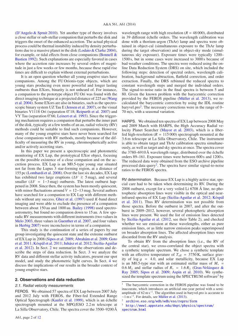
Fig. 1. Top: GLS periodogram of the FEROS RV values, showing thebest period of 7.417 days. The horizontal dashed line indicates theFAP level of 10−4. Bottom: window function.

3. Results and analysis

3.1. Period analysis of the RV data and orbital solution

To search for periodicities in the RV values measured fromthe absorption lines, we used the generalized Lomb-Scargle(GLS) method (Zechmeister & Kürster 2009). Since the num-ber of available HARPS points is not sufficient to carry outan independent RV period determination, we first consideredthe FEROS data only, and afterwards we combined the FEROSand HARPS data points, and repeated our analysis. The datapoints were weighted with the inverse square of their uncertain-ties. Figure 1 shows the GLS periodogram calculated for the 45FEROS points. Two significant periods with false alarm proba-bility (FAP) of <10−4 are visible, one at around 1 day, which isan alias caused by the sampling (see the window function in thebottom panel of Fig. 1), and another one at 7.417 days. The RVcurve phase-folded with the 7.417 day period is plotted in Fig. 2.

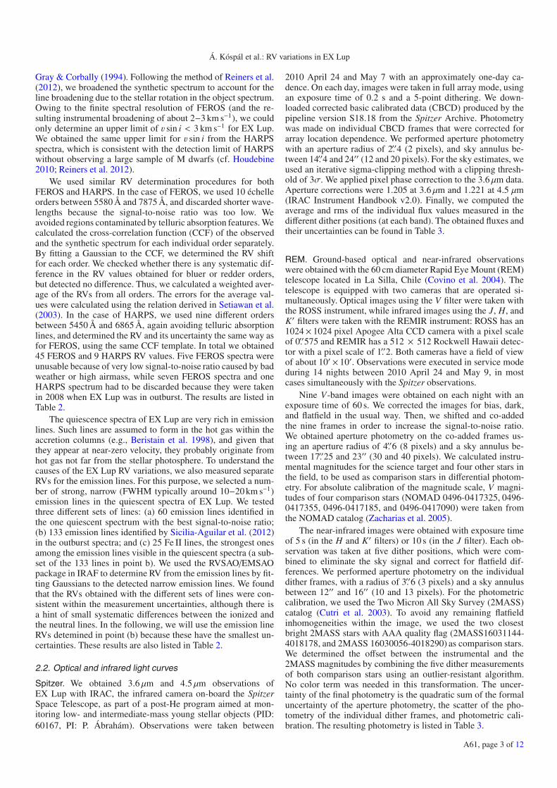
Figure 2 exhibits a clear periodic signal with an RV semi-amplitude of ≈2.2 km s−1. The shape of the curve is asymmetric,with the increasing part approximately 1.7 times longer than thedecreasing part. In the figure, we color-coded the different ob-serving seasons during our five-year monitoring program. Nosystematic differences can be seen between the different sea-sons, which suggests that the period, phase, and amplitude ofthe RV variations were stable for at least four years, between2009 and 2012. The three data points from 2007 are also consis-tent with the later observations, implying that the RV variationswere largely unaffected by the largest outburst of EX Lup everobserved which occurred in 2008.

The shape of the phase-folded RV curve suggests the pos-sible existence of a companion on an eccentric orbit aroundEX Lup. We fitted a Keplerian solution to the FEROS RVs usingboth GLS and the idl code RVlin4 (Wright & Howard 2009). TheRVlin code can handle data from different instruments by fittingparameters to correct for the relative offset between them, thus,we used it to fit the combined FEROS+HARPS data sets, and de-termined an offset of 0.291 km s−1 between the two instruments.The code also calculates uncertainties for the fitted parametersusing a bootstrapping algorithm (Xuesong Wang et al. 2012).

4 http://exoplanets.org/code/

-4

-2

0

2

4

6

RV

[km

s-1]

2007-22009-12009-22010-12010-22011-12012-2

HARPS

FEROS

(absorption lines)

-101

O-C

[km

s-1]

0.0 0.5 1.0 1.5 2.0Phase

-2

0

2

RV e

m [

kms-1

]

(emission lines)

Fig. 2. Top: best Keplerian fit to the absorption line RVs for the com-bined FEROS and HARPS RV data set (with RVlin). The different col-ors indicate different observing seasons (-1 stands for the first half ofthe year, -2 for the second half). Circles represent FEROS and squaresHARPS data points. Middle: residua with the same color and shape cod-ing. Bottom: emission line RVs with the same color and shape coding.

Table 1. Best-fitting parameters of the Keplerian solution fitted to theRV measurements of EX Lup (with RVlin, using the combined FEROSand HARPS dataset).

Parameter Unit ValuePeriod day 7.417 ± 0.001RV semi-amplitude km s−1 2.18 ± 0.10Eccentricity . . . 0.23 ± 0.05Longitude of periastron ◦ 96.8 ± 11.4Epoch of periastron passage JD 2 455 405.112 ± 0.224RV offset km s−1 –0.52 ± 0.07FAPa . . . 6.7×10−27

m sin ib MJupiter 14.7 ± 0.7semi-major axisb au 0.063 ± 0.005

Notes. (a) False alarm probability of the Keplerian fit as defined byCumming (2004). (b) Assuming a stellar mass of 0.6 M�.

The orbital parameters determined from the fit for the combineddata sets are listed in Table 1. The values derived for the differ-ent data sets using different methods are all consistent within theuncertainties.

To calculate m sin i and the semi-major axis a, we assumeda stellar mass of M∗ = 0.6 M� for EX Lup (Gras-Velázquez &Ray 2005). Figure 2 shows the best fit for the combined data set,which has a FAP of 6.7× 10−27. After subtracting the 7.417 dayperiod Keplerian fit from the RV data, we searched for sine pe-riodicities in the RV residuals, but found no significant periodswith FAP < 10−4.

As described in Sect. 2.1, we calculated RVs from those nar-row emission lines that are isolated and not superimposed onbroader absorption features. Similar but weaker emission linesmay distort the absorption lines and might introduce artificialRV signals, despite our best efforts to discard the affected ab-sorption lines from our analysis. To make sure that this is not thecase, we performed a period analysis on the RVs of the emis-sion lines. The algorithm found no significant periods, although

A61, page 4 of 12

Á. Kóspál et al.: RV variations in EX Lup

a small peak is present at about 7 days with FAP of 10−2. InFig. 2, we plotted the RVs of the emission lines phase foldedwith the 7.417 d period. The data points have a large scattercompared to the RVs determined from the absorption lines, andthey show instead a sinusoidal variation with a semi-amplitudeof about 0.8 km s−1. From this exercise, it is clear that emissioncomponents moving at this velocity cannot cause the RV signalobserved in the absorption lines.

3.2. Analysis of the stellar activity

The presence of a companion is not the only possible explana-tion for periodic RV changes. Photospheric stellar activity, i.e.,dark (cold) or bright (hot) spots, are known to result in periodicRV variations (e.g., Lanza et al. 2011, and references therein).For instance, a cool spot on the stellar surface would produce adeficit of emission at the spot’s velocity within the line profile,and the rotation of the star then leads to an RV signal which isperiodic with the rotational period. Additionally, RV measure-ments from lines with different temperature sensitivities wouldyield different RV amplitudes (e.g., Hatzes 1999). Thus, by an-alyzing the distortion of the spectral lines and their correlationwith the RV, or by analyzing line ratios sensitive to the effectivetemperature, it is possible to verify the presence of stellar spots.In addition to the photospheric spots, cool stars, especially therapidly rotating younger ones, have very active chromospheres(Montes et al. 2004). The chromospheric spectrum is dominatedby emission lines, which again can distort the photospheric ab-sorption line profiles, or in extreme cases can even fill them upor turn them into emission lines. Chromospheric activity mayincrease the noise of RV measurements, but it may also pro-duce periodic RV signals over a few rotational periods (Santoset al. 2003). In the following, we check whether the RV varia-tions and their periodicity observed for EX Lup can be due tostellar activity.

Bisector analysis. The CCF represents the mean absorptionline profile of the star. We computed the CCF for each spec-trum by combining the individual CCFs of the different ordersinto a master CCF using a robust averaging method that as-signs less weight to the deviating orders. One way to analyzeits distortion is to compute the bisector (e.g., Queloz et al. 2001;Gray 2005), as illustrated in Fig. 3. Following Dall et al. (2006),we computed the mean bisector velocities for different regionsin the CCF, and estimated the formal uncertainty of the meanvalues from the dispersion of the bisector points within that re-gion. Following Povich et al. (2001), we defined three regions:v1 for 0.4 ≤ CCF ≤ 0.55, v2 for 0.55 ≤ CCF ≤ 0.7, and v3 for0.7 ≤ CCF ≤ 0.9 (Fig. 3). These CCF ranges were suitable formost spectra; however, in a few cases the continuum level washigh and affected the lowest bisector points in the v1 range. Thesemeasurements were discarded from further analysis. In the nextstep, we calculated the bisector velocity span (BVS= v3−v1), thebisector curvature (BC = (v3 − v2) − (v2 − v1)), and the bisectorvelocity displacement (BVD = (v1 + v2 + v3)/3 − λc, where λc isthe observed central wavelength).

We checked whether the BVSs correlate with the RV, whichis expected if the RV variations are caused by rotational modu-lation due to starspots (e.g., Queloz et al. 2001). Figure 4 showsthe BVS plotted as a function of the RV and the RV residua (af-ter the subtraction of the Keplerian solution). The linear Pearsoncorrelation coefficients (Pearson 1920) for the two graphs are0.08 and 0.27, respectively, indicating no correlation betweenthe quantities. As an independent check, we also performed

-20 -10 0 10 20Velocity [km/s]

0.2

0.4

0.6

0.8

1.0

CCF

ν1

ν2

ν3

-1.8 -1.6 -1.4

ν1

ν2

ν3

Magnification

Fig. 3. Bisector of the CCF computed from the FEROS spectrum ofEX Lup observed on 2010 July 23.

-4 -2 0 2 4RV [km/s]

-1.0

-0.5

0.0

0.5

1.0

BVS

[km

/s]

-1.5 -1.0 -0.5 0.0 0.5 1.0RV residua [km/s]

Fig. 4. BVS values plotted against the RV (left) and against the RVresidua (right).

a bisector analysis on carefully selected individual absorptionlines in the FEROS spectra. Similarly to our previous results, nocorrelation between the BVS and the RV was found. We calcu-lated GLS periodograms for the BVS, BC, and BVD (Fig. 5), butfound no significant period with FAP smaller than 10−4. As in-dicated by the arrows in the figure, no peak is present at a periodof 7.417 days.

Asymmetry of the CCF. Distortions of the CCF profile can alsobe analyzed by first plotting the slope of the CCF at each ve-locity, then by integrating over the velocity axis with positiveand negative slopes, respectively, and calculating the ratio of thepositive and negative areas. For a perfectly symmetric Gaussian,this ratio would be 1, while for a distorted Gaussian, it wouldbe below or over 1. We determined this measure of the CCFasymmetry for each order separately, then took their weightedaverage. Finally, we calculated the GLS periodogram (Fig. 5),but again found no significant periods, and no peak at a periodof 7.417 days.

Temperature-sensitive spectral features. A cool spot on thestellar surface, rotating in and out of view, changes the effectivetemperature of the visible stellar hemisphere. This has an influ-ence on the strength of temperature-sensitive absorption lines orbands. For instance, Catalano et al. (2002) showed that both the6268.87 Å V I line and the 6270.23 Å Fe I line become strongerwith decreasing temperature, but the variation of the line depthof the low-excitation V I line is more pronounced than that of

A61, page 5 of 12

A&A 561, A61 (2014)

0.00.20.40.60.81.0

1 10 100 1000

0.00.20.40.60.8

0.00.20.40.60.8

0.00.20.40.60.8

1 10 100 1000Period / d

0.00.20.40.60.8

GLS

pow

er

BVS

BC

BVD

CCF asym.

LDR

10−4

10−4

10−4

10−4

10−4

Fig. 5. GLS periodograms of the BVS, BC, BVD, CCF asymmetry, andthe LDR of V I and F I. The arrows mark the 7.417 day RV period. Thehorizontal dashed lines indicate a FAP level of 10−4.

0.0

0.2

0.4

0.6

0.8

1.0

1.2

CC

F

−20 −10 0 10 20Velocity

−0.10

−0.05

0.00

0.05

Slo

pe

in e

ach

poi

nt

Fig. 6. Illustration of the calculation method of the CCF asymmetry.The quantity of asymmetry is determined by obtaining the quotient ofthe area of positive slope (red) and of negative slope (blue). The CCFdisplayed here was computed from the FEROS spectrum of EX Lupobserved on 2010 July 23.

Fe I. For this reason, the line depth ratio (LDR) is a good tracerof changes in the effective surface temperature. We calculatedthe GLS periodogram of the LDR of V I and Fe I (Fig. 5), butfound no significant period, and no peak at 7.417 days.

In the presence of a cool spot, bands like TiO, CaH, andCaOH may appear or strengthen (see Reid et al. 1995, who mea-sured these bands in a large number of M dwarfs). Using ourFEROS spectra, we determined the TiO 1, TiO 2, TiO 3, TiO 4,TiO 5, CaH 2, CaH 3, CaOH, and Hα indices as defined by Reidet al. (1995), and looked for periodic changes due to spots onthe stellar surface. Similarly to the other stellar spot indicatorsdiscussed above, we found no significant period in the GLS pe-riodograms of these spectral indices, and no peak at a periodof 7.417 days.

Analysis of the Ca lines. Larson et al. (1993) have shown thatcalcium lines in the stellar spectrum, such as the Ca II H andK lines at 3968 Å and 3933 Å and the Ca II infrared triplet at8498 Å, 8542 Å, and 8662 Å are good indicators of stellar chro-mospheric activity. Since the Ca II H line is possibly blendedwith Hε , and the Ca II 8498 Å and 8542 Å lines are contami-nated by terrestrial water vapor lines, we discarded them fromfurther analysis and concentrated on the Ca II K line at 3933 Åand on the Ca II line at 8662 Å. For Caλ3933 Å we calculated thechromospheric activity index S FEROS and monitored its variationover time. S FEROS is defined as follows:

S FEROS =Fe

Fb + Fr=

F3933 Å −3935 Å

F3930 Å −3933 Å + F3935 Å −3938 Å, (1)

where Fe, Fb, and Fr are the fluxes integrated over the wave-length ranges indicated in the equation above. These S-indicesfor the Ca II H and K lines were first defined by Vaughan et al.(1978), and they measure the strength of the line emission rel-ative to the adjacent continuum, an established chromosphericactivity indicator (e.g., Mittag et al. 2013). Additionally we cal-culated the equivalent width (EW) of Caλ8662 Å, and appliedthe method of the asymmetry analysis of the CCF to the emissioncore of the Ca II K line. We calculated GLS periodograms for allthree indicators, but found no significant peak at the RV periodof 7.417 d. The S FEROS index and the Caλ8662 Å line EW show apeak around 1.0 d with a FAP smaller than 10−5, which we inter-pret as a feature of the sampling effect. The Caλ8662 Å line EWreveals a strong peak at a FAP smaller than 10−5 at about 25 d.However, by looking at the window function of the EW values,it is apparent that this is a result of the sampling as well. TheCa II K asymmetry does not exhibit any significant peaks be-tween 1 and 1000 d. We note that the Ca II infrared triplet is oftenconsidered a good accretion tracer (e.g., Muzerolle et al. 1998).EX Lup has a non-negligible accretion rate even in quiescence,and the broad wings of the Ca II lines (Fig. 3 in Sicilia-Aguilaret al. 2012) suggest that part of the line flux is related to accretionrather than to chromospheric activity.

3.3. Spot model

In all our previous analyses we found no evidence of periodicstellar activity. Nevertheless, in the following we will assumethat the 7.417 d period we found in the RVs is in fact due to stel-lar rotation, and we will try to find a spot model that can repro-duce the observed ≈2.2 km s−1 semi-amplitude of the RV curve.Since there is no flat section in the RV curve, the spot shouldpractically always be visible to a certain extent. Given the largeRV semi-amplitude compared to the small v sin i < 3 km s−1, weexpect spots with large filling factors. We constructed a simplespot model and simulated a grid of single spots with differenttemperatures, sizes, and latitudes on the photosphere of EX Lupwith different stellar inclinations. The results showed that typicalcold or hot spots, covering a few per cent of the stellar surfaceand having a temperature difference of a few hundred K, are un-able to reproduce the measured RV semi-amplitude. Thus, wehad to explore more extreme parameters in our modeling. Wefound that a large cold spot covering practically a whole hemi-sphere, with a filling factor between 80% and 100%, with a tem-perature of 1500−2500 K cooler than the stellar photosphere atlow latitudes (within 30◦ of the equator), and with low stellarinclinations (the angle between the line of sight and the stellarequator being between 0 and 30◦) reproduced the observed RVsemi-amplitude. Similarly, even if it is unrealistic, the only hot

A61, page 6 of 12

Á. Kóspál et al.: RV variations in EX Lup

9.6

9.4

9.2

9.0

8.8

8.6

8.4

Mag

nitu

de

310 315 320 325MJD - 55000

V-3.6

J-0.5

H

K+0.2

[3.6]+0.7

[4.5]+1

-4-2024

RV

[km

s-1]

-4-2024

RV e

m [

kms-1

]

-0.5 0 0.5 1 1.5Phase

Fig. 7. Light curves and RV curves of EX Lup. For clarity, the lightcurves were shifted along the y-axis by the amounts indicated on theright side. Dashed and dotted lines mark when the RV equals the sys-temic velocity.

spot that produced an adequate fit to the RV semi-amplitude cov-ered a whole hemisphere with a temperature of 10 500 K hotterthan the photosphere at a latitude of 0◦, and an inclination of 0◦.

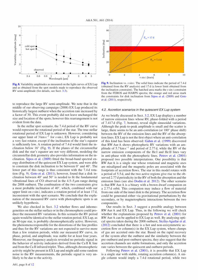
To test if any of these spot models could reproduce the ob-served photometric behavior, we plotted in Fig. 7 the light curvesof EX Lup between 0.55 and 4.5 μm covering about two weeksin 2010 with an approximately daily cadence. We observed sig-nificant brightness changes in this period at all wavelengths. Thecurves between V and H exhibit similar shapes with a decreasingamplitude towards longer wavelengths. The peak-to-peak ampli-tude of the variability is ΔV = 0.33 mag, ΔJ = 0.18 mag, andΔH = 0.14 mag. The curves seem to be periodic with minimaaround MJD = 55 316 and MJD = 55 323, which is consistentwith the rotation period of our spot model. This periodicity is ob-servable also between K and [4.5], but superimposed on a risingtrend. There is a hint of a phase lag in the maxima towards longerwavelengths. The peak-to-peak variability amplitudes here areΔK = 0.16 mag, Δ[3.6] = 0.24 mag, and Δ[4.5] = 0.25 mag,as measured directly on the light curves, and ΔK = 0.14 mag,Δ[3.6] = 0.17 mag, and Δ[4.5] = 0.13 mag if we subtract a lin-early increasing trend.

We calculated the photometric variability amplitudes fromour spot models using the limb darkening coefficients from JohnSouthworth’s JKTLD code5 (0.787 for the V band, 0.470 for theJ band, 0.439 for the H band, 0.366 for the K band, 0.190 at3.550 μm, and 0.142 at 4.493 μm). The obtained values (the me-dian of several models that were all consistent with the observed

5 http://www.astro.keele.ac.uk/jkt/codes/jktld.html

RV amplitude, with the standard deviation as error bars) are plot-ted in Fig. 8. It is evident that the amplitudes for the spot modelsexceed the observed ones by several magnitudes. In the case ofa cold spot, the phase when the spot faces towards the observercorresponds to the lowest photometric brightness and the pointin the RV curve when it becomes smaller than the systemic ve-locity (dotted lines in Fig. 7). Conversely, in the case of a hotspot, the phase when the spot faces towards the observer cor-responds to the highest photometric brightness and the point inthe RV curve when it becomes larger than the systemic velocity(dashed lines in Fig. 7). While this is approximately consistentwith our observations, the extremely large variability amplitudespredicted by the spot models still make it improbable that spotsare wholly responsible for the observed RV variations.

In case spots cause the RV variations of EX Lup, the ob-served RV semi-amplitude should depend on the wavelength. Asthe contrast between the spot and the unspotted stellar photo-sphere decreases with increasing wavelength, we expect grad-ually smaller RV amplitudes. For our large cold spot model,the difference between 5580 Å and 7875 Å (roughly correspond-ing to the bluest and reddest FEROS orders we used) would be0.05 km s−1 in the RV semi-amplitude. For our large hot spotmodel, the value would be 0.28 km s−1. As we briefly mentionedin Sect. 2.1, we found no significant difference in the RVs ob-tained from bluer or redder orders. Our RV data allowed us to de-termine the RV semi-amplitude to a precision of about 0.1 km s−1

(Table 1). Thus, while we cannot exclude the cold spot scenariobased on these arguments alone, the hot spot scenario seems tobe unlikely.

Finally, we checked whether we can find a spot model (ei-ther cold or hot) that would reproduce the observed photomet-ric variability amplitudes and calculated the expected RV semi-amplitudes. We found that a cold spot with a temperature of1500 K cooler than the photosphere and covering 11% of a hemi-sphere would give ΔV = 0.33 mag (both the latitude of the spotand the inclination of the star was taken to be 0◦). The same ΔVcan also be the result of a hot spot with a temperature of 525 Khotter than the photosphere (covering factor, latitude, and incli-nation are the same as before). However, these relatively smallspots would only cause an approximately 0.3 km s−1 RV semi-amplitude, much smaller than the observed 2.2 km s−1. Thus, wecan conclude that the observed photometric and RV variationscannot be reproduced at the same time with cold or hot spots onthe stellar surface.

4. Discussion

4.1. EX Lup: a spotted or an active star?

In Sects. 3.2 and 3.3 we investigated in detail whether the ob-served RV signal could be caused by cold or hot spots on thestellar surface. We verified that spot indicators like the BVS, BC,and CCF asymmetry do not exhibit any periodicity. Nor do wesee any dependence of the observed RV on wavelength withinthe range covered by the FEROS spectra. We constructed a sim-ple spot model to reproduce the observed RV semi-amplitude.Our modeling suggests that the spot would have to cover a com-plete hemisphere, which is an extreme and atypical solution.Moreover, the temperature of this extended spot deviates fromthat of the photosphere by several thousand K. Thus, unless itcools mainly through line emission (c.f. Dodin & Lamzin 2013),it would cause periodic photometric changes of 4−8 mag in theV band, which is not seen in our observations. A spot modelthat reproduces the observed V band variability amplitude fails

A61, page 7 of 12

A&A 561, A61 (2014)

Wavelength [μm]

0

2

4

6

8

10

Vari

abili

ty a

mpl

itude

[mag

]

0.4 0.6 0.8 1 2 3 4 5

cold spothot spot

observed

Fig. 8. Variability amplitudes as measured on the light curves of EX Lupand as obtained from the spot models made to reproduce the observedRV semi-amplitude (for details, see Sect. 3.3).

to reproduce the large RV semi-amplitude. We note that in themiddle of our observing campaign (2008) EX Lup produced itshistorically largest outburst when the accretion rate increased bya factor of 30. This event probably did not leave unchanged thesize and location of the spots; however this rearrangement is notevident from the data.

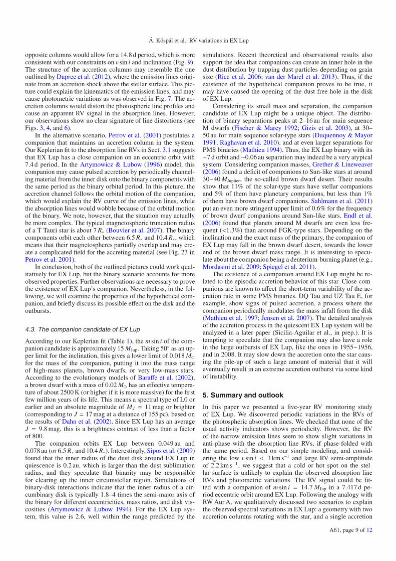
In the stellar spot scenario, the 7.4 d period of the RV curvewould represent the rotational period of the star. The true stellarrotational period of EX Lup is unknown. However, consideringour upper limit of 3 km s−1 for v sin i, EX Lup is probably nota very fast rotator, except if the inclination of the star’s equatoris sufficiently low. A rotation period of 7.4 d would limit the in-clination below 16◦ (Fig. 9). If the planes of the circumstellardisk and the star’s equator are not very different, modeling thecircumstellar disk geometry also provides information on the in-clination. Sipos et al. (2009) fitted the broad-band spectral en-ergy distribution of the quiescent EX Lup system, and were ableto constrain the disk inclination to be between 0◦ and 40◦. Thelower part of this range is thus consistent with the 7.4 d rota-tion (Fig. 9). Goto et al. (2011), however, found that a disk in-clination between 40◦ and 50◦ is needed to fit the fundamentalvibrational lines of CO observed in the 4.5–5 μm range duringthe 2008 outburst. The combination of the two constraints givea most probable inclination of 40◦, which, combined with ourupper limit on v sin i, indicates a rotation period of at least 17 d,inconsistent with the spot scenario. We conclude that the expla-nation of the measured RV curve with photospheric spots is anunlikely hypothesis.

We also checked in Sect. 3.2 whether flows and inhomo-geneities on the stellar surface or in the chromosphere could pro-duce the measured RV variations. In this scenario the RV periodagain would be identical to the stellar rotation period. EX Lup, asan M-type star, is probably chromospherically active. However,the phenomena responsible for the distortions of the line profilesand thus for the RV variations are not expected to survive morethan a few rotation periods, while our measured RV curve, itsphase, period, and amplitude, was stable for at least four years.Moreover, our frequency analysis revealed no periodic signal inthe behavior of activity indicators derived from the Ca II K lineand from the Ca II infrared triplet. Thus, although chromosphericactivity might be present in EX Lup and might add some randomnoise to the RV measurements, the periodic signal is very un-likely to be due to the activity.

0 2 4 6 8 10v sin i [km/s]

0

20

40

60

80

Incl

inat

ion

[deg

]

Prot = 7.4 d

Prot = 17 d

Fig. 9. Inclination vs. v sin i. The solid lines indicate the period of 7.4 d(obtained from the RV analysis) and 17 d (a lower limit obtained fromthe inclination constraint). The hatched area marks the v sin i constraintfrom the FEROS and HARPS spectra; the orange and red areas markthe constraints for disk inclination from Sipos et al. (2009) and Gotoet al. (2011), respectively.

4.2. Accretion scenarios in the quiescent EX Lup system

As we briefly discussed in Sect. 3.2, EX Lup displays a numberof narrow emission lines whose RV, phase-folded with a periodof 7.417 d (Fig. 7, bottom), reveal slight sinusoidal variations.Although the peak-to-peak amplitude is small and the scatter islarge, there seems to be an anti-correlation (or 180◦ phase shift)between the RV of the emission lines and the RV of the absorp-tion lines. EX Lup is not the first object where an anti-correlationof this kind has been observed: Gahm et al. (1999) discoveredthat RW Aur A shows photospheric RV variations with an am-plitude of 5.7 km s−1 and period of 2.77 d, while the RV of thenarrow emission components of the He I and He II lines varyin anti-phase with the photospheric lines. Petrov et al. (2001)proposed two possible interpretations. One possibility is thatRW Aur A is a single star whose rotational and magnetic axesare misaligned and the magnetic poles are associated with thefootprints of accretion flows. The star in this model rotates witha period of 5.5 d, and the two active regions give rise to the ob-served 2.77 d periodicity in the RV of both the absorption and theemission lines (see also Dodin et al. 2012). The other scenariois that RW Aur A is a binary with a brown dwarf companion ona 2.77 d orbit. This companion may induce a flow of materialfrom one side of the inner disk to the primary. The accretion flowcould be generated either via gravitational perturbations by thesecondary, or by magnetospheric interactions between the twocomponents.

Our results in Sect. 3 suggest a possible analogy betweenRW Aur A and EX Lup. Thus, in the following we will checkwhether the explanations proposed by Petrov et al. (2001) forRW Aur A can be applied to EX Lup as well. By analysing opti-cal spectra taken during the 2008 outburst, Sicilia-Aguilar et al.(2012) concluded that there is a hot and non-axisymmetric ac-cretion flow or column(s) in the EX Lup system, where clumpsof gas are accreted onto the star. Based on the rapid recoveryof the system after the outburst and the similarity between thepre-outburst and post-outburst spectra, they also suggest that theaccretion channels are stable formations, and only the accretionrate varies between the quiescent and outburst periods.

Following Petrov et al. (2001), it is possible that EX Lupis a single star with stable, rotating accretion column(s). A sin-gle column would imply a 7.4 d rotational period, while two

A61, page 8 of 12

Á. Kóspál et al.: RV variations in EX Lup

opposite columns would allow for a 14.8 d period, which is moreconsistent with our constraints on v sin i and inclination (Fig. 9).The structure of the accretion columns may resemble the oneoutlined by Dupree et al. (2012), where the emission lines origi-nate from an accretion shock above the stellar surface. This pic-ture could explain the kinematics of the emission lines, and maycause photometric variations as was observed in Fig. 7. The ac-cretion columns would distort the photospheric line profiles andcause an apparent RV signal in the absorption lines. However,our observations show no clear signature of line distortions (seeFigs. 3, 4, and 6).

In the alternative scenario, Petrov et al. (2001) postulates acompanion that maintains an accretion column in the system.Our Keplerian fit to the absorption line RVs in Sect. 3.1 suggeststhat EX Lup has a close companion on an eccentric orbit with7.4 d period. In the Artymowicz & Lubow (1996) model, thiscompanion may cause pulsed accretion by periodically channel-ing material from the inner disk onto the binary components withthe same period as the binary orbital period. In this picture, theaccretion channel follows the orbital motion of the companion,which would explain the RV curve of the emission lines, whilethe absorption lines would wobble because of the orbital motionof the binary. We note, however, that the situation may actuallybe more complex. The typical magnetospheric truncation radiusof a T Tauri star is about 7 R∗ (Bouvier et al. 2007). The binarycomponents orbit each other between 6.5 R∗ and 10.4 R∗, whichmeans that their magnetospheres partially overlap and may cre-ate a complicated field for the accreting material (see Fig. 23 inPetrov et al. 2001).

In conclusion, both of the outlined pictures could work qual-itatively for EX Lup, but the binary scenario accounts for moreobserved properties. Further observations are necessary to provethe existence of EX Lup’s companion. Nevertheless, in the fol-lowing, we will examine the properties of the hypothetical com-panion, and briefly discuss its possible effect on the disk and theoutbursts.

4.3. The companion candidate of EX Lup

According to our Keplerian fit (Table 1), the m sin i of the com-panion candidate is approximately 15 MJup. Taking 50◦ as an up-per limit for the inclination, this gives a lower limit of 0.018 M�for the mass of the companion, putting it into the mass rangeof high-mass planets, brown dwarfs, or very low-mass stars.According to the evolutionary models of Baraffe et al. (2002),a brown dwarf with a mass of 0.02 M� has an effective tempera-ture of about 2500 K (or higher if it is more massive) for the firstfew million years of its life. This means a spectral type of L0 orearlier and an absolute magnitude of MJ = 11 mag or brighter(corresponding to J = 17 mag at a distance of 155 pc), based onthe results of Dahn et al. (2002). Since EX Lup has an averageJ = 9.8 mag, this is a brightness contrast of less than a factorof 800.

The companion orbits EX Lup between 0.049 au and0.078 au (or 6.5 R∗ and 10.4 R∗). Interestingly, Sipos et al. (2009)found that the inner radius of the dust disk around EX Lup inquiescence is 0.2 au, which is larger than the dust sublimationradius, and they speculate that binarity may be responsiblefor clearing up the inner circumstellar region. Simulations ofbinary-disk interactions indicate that the inner radius of a cir-cumbinary disk is typically 1.8–4 times the semi-major axis ofthe binary for different eccentricities, mass ratios, and disk vis-cosities (Artymowicz & Lubow 1994). For the EX Lup sys-tem, this value is 2.6, well within the range predicted by the

simulations. Recent theoretical and observational results alsosupport the idea that companions can create an inner hole in thedust distribution by trapping dust particles depending on grainsize (Rice et al. 2006; van der Marel et al. 2013). Thus, if theexistence of the hypothetical companion proves to be true, itmay have caused the opening of the dust-free hole in the diskof EX Lup.

Considering its small mass and separation, the companioncandidate of EX Lup might be a unique object. The distribu-tion of binary separations peaks at 2–16 au for main sequenceM dwarfs (Fischer & Marcy 1992; Gizis et al. 2003), at 30–50 au for main sequence solar-type stars (Duquennoy & Mayor1991; Raghavan et al. 2010), and at even larger separations forPMS binaries (Mathieu 1994). Thus, the EX Lup binary with its∼7 d orbit and ∼0.06 au separation may indeed be a very atypicalsystem. Considering companion masses, Grether & Lineweaver(2006) found a deficit of companions to Sun-like stars at around30−40 MJupiter, the so-called brown dwarf desert. Their resultsshow that 11% of the solar-type stars have stellar companionsand 5% of them have planetary companions, but less than 1%of them have brown dwarf companions. Sahlmann et al. (2011)put an even more stringent upper limit of 0.6% for the frequencyof brown dwarf companions around Sun-like stars. Endl et al.(2006) found that planets around M dwarfs are even less fre-quent (<1.3%) than around FGK-type stars. Depending on theinclination and the exact mass of the primary, the companion ofEX Lup may fall in the brown dwarf desert, towards the lowerend of the brown dwarf mass range. It is interesting to specu-late about the companion being a deuterium-burning planet (e.g.,Mordasini et al. 2009; Spiegel et al. 2011).

The existence of a companion around EX Lup might be re-lated to the episodic accretion behavior of this star. Close com-panions are known to affect the short-term variability of the ac-cretion rate in some PMS binaries. DQ Tau and UZ Tau E, forexample, show signs of pulsed accretion, a process where thecompanion periodically modulates the mass infall from the disk(Mathieu et al. 1997; Jensen et al. 2007). The detailed analysisof the accretion process in the quiescent EX Lup system will beanalyzed in a later paper (Sicilia-Aguilar et al., in prep.). It istempting to speculate that the companion may also have a rolein the large outbursts of EX Lup, like the ones in 1955−1956,and in 2008. It may slow down the accretion onto the star caus-ing the pile-up of such a large amount of material that it willeventually result in an extreme accretion outburst via some kindof instability.

5. Summary and outlook

In this paper we presented a five-year RV monitoring studyof EX Lup. We discovered periodic variations in the RVs ofthe photospheric absorption lines. We checked that none of theusual activity indicators shows periodicity. However, the RVof the narrow emission lines seem to show slight variations inanti-phase with the absorption line RVs, if phase-folded withthe same period. Based on our simple modeling, and consid-ering the low v sin i < 3 km s−1 and large RV semi-amplitudeof 2.2 km s−1, we suggest that a cold or hot spot on the stel-lar surface is unlikely to explain the observed absorption lineRVs and photometric variations. The RV signal could be fit-ted with a companion of m sin i = 14.7 MJup in a 7.417 d pe-riod eccentric orbit around EX Lup. Following the analogy withRW Aur A, we qualitatively discussed two scenarios to explainthe observed spectral variations in EX Lup: a geometry with twoaccretion columns rotating with the star, and a single accretion

A61, page 9 of 12

A&A 561, A61 (2014)

flow synchronized with the orbital motion of the hypotheticalcompanion. Taking 40–50◦ as the most likely value for the incli-nation, the mass of this hypothetical companion is probably inthe brown dwarf range. The small separation and large mass ra-tio make EX Lup a very atypical binary system. The companioncandidate may be responsible for the smaller or larger accretionoutbursts of EX Lup, supporting those theories that assume acompanion as the triggering mechanism for the eruptions of cer-tain EXors.

Acknowledgements. The authors thank the referee, D. Lorenzetti, for hiscomments that helped to improve the manuscript. The authors also thankV. Roccatagliata, and M. Fang for their help with the FEROS barycentric cor-rection and A. Simon for his help with the bisector analysis. This work isbased in part on observations made with the Spitzer Space Telescope, which isoperated by the Jet Propulsion Laboratory, California Institute of Technology,under a contract with NASA. A.S.A. acknowledges support of the SpanishMICINN/MINECO “Ramón y Cajal” program, grant number RYC-2010-06164,and the action “Proyectos de Investigación fundamental no orientada”, grantnumber AYA2012-35008. This work was partly supported by the grant OTKAK101393 of the Hungarian Scientific Research Fund.

ReferencesÁbrahám, P., Juhász, A., Dullemond, C. P., et al. 2009, Nature, 459, 224Armitage, P. J., Livio, M., & Pringle, J. E. 2001, MNRAS, 324, 705Artymowicz, P., & Lubow, S. H. 1994, ApJ, 421, 651Artymowicz, P., & Lubow, S. H. 1996, ApJ, 467, L77Aspin, C., Reipurth, B., Herczeg, G. J., & Capak, P. 2010, ApJ, 719, L50Bailey, J. 1998, MNRAS, 301, 161Baraffe, I., Chabrier, G., Allard, F., & Hauschildt, P. H. 2002, A&A, 382, 563Bell, K. R., & Lin, D. N. C. 1994, ApJ, 427, 987Beristain, G., Edwards, S., & Kwan, J. 1998, ApJ, 499, 828Bonnell, I., & Bastien, P. 1992, ApJ, 401, L31Bouvier, J., Alencar, S. H. P., Harries, T. J., Johns-Krull, C. M., & Romanova,

M. M. 2007, Protostars and Planets V (Tucson: Unitersity of Arizona Press),479

Catalano, S., Biazzo, K., Frasca, A., & Marilli, E. 2002, A&A, 394, 1009Covino, S., Zerbi, F. M., Chincarini, G., et al. 2004, Astron. Nachr., 325, 543Cumming, A. 2004, MNRAS, 354, 1165Cutri, R. M., Skrutskie, M. F., van Dyk, S., et al. 2003, 2MASS All Sky Catalog

of point sources, Vizier online Data Catalog: II/246D’Angelo, C. R., & Spruit, H. C. 2010, MNRAS, 406, 1208Dahn, C. C., Harris, H. C., Vrba, F. J., et al. 2002, AJ, 124, 1170Dall, T. H., Santos, N. C., Arentoft, T., Bedding, T. R., & Kjeldsen, H. 2006,

A&A, 454, 341Dodin, A. V., & Lamzin, S. A. 2013, Astron. Lett., 39, 389Dodin, A. V., Lamzin, S. A., & Chuntonov, G. A. 2012, Astron. Lett., 38, 167Dupree, A. K., Brickhouse, N. S., Cranmer, S. R., et al. 2012, ApJ, 750, 73Duquennoy, A., & Mayor, M. 1991, A&A, 248, 485Endl, M., Cochran, W. D., Kürster, M., et al. 2006, ApJ, 649, 436Fischer, D. A., & Marcy, G. W. 1992, ApJ, 396, 178Gahm, G. F., Petrov, P. P., Duemmler, R., Gameiro, J. F., & Lago, M. T. V. T.

1999, A&A, 352, L95Ghez, A. M., McCarthy, D. W., Patience, J. L., & Beck, T. L. 1997, ApJ, 481,

378Gizis, J. E., Reid, I. N., Knapp, G. R., et al. 2003, AJ, 125, 3302Goto, M., Regály, Z., Dullemond, C. P., et al. 2011, ApJ, 728, 5

Gras-Velázquez, À., & Ray, T. P. 2005, A&A, 443, 541Gray, D. F. 2005, PASP, 117, 711Gray, R. O., & Corbally, C. J. 1994, AJ, 107, 742Grether, D., & Lineweaver, C. H. 2006, ApJ, 640, 1051Guenther, E. W., Esposito, M., Mundt, R., et al. 2007, A&A, 467, 1147Hatzes, A. P. 1999, in IAU Colloq. 170: Precise Stellar Radial Velocities, eds.

J. B. Hearnshaw, & C. D. Scarfe, ASP Conf. Ser., 185, 259Herbig, G. H. 1977, ApJ, 217, 693Herbig, G. H. 2007, AJ, 133, 2679Herbig, G. H. 2008, AJ, 135, 637Houdebine, E. R. 2010, MNRAS, 407, 1657Jensen, E. L. N., Dhital, S., Stassun, K. G., et al. 2007, AJ, 134, 241Juhász, A., Dullemond, C. P., van Boekel, R., et al. 2012, ApJ, 744, 118Kaufer, A., Stahl, O., Tubbesing, S., et al. 1999, The Messenger, 95, 8Kóspál, Á., Ábrahám, P., Goto, M., et al. 2011, ApJ, 736, 72Lanza, A. F., Boisse, I., Bouchy, F., Bonomo, A. S., & Moutou, C. 2011, A&A,

533, A44Larson, A. M., Irwin, A. W., Yang, S. L. S., et al. 1993, PASP, 105, 332Leinert, C., Zinnecker, H., Weitzel, N., et al. 1993, A&A, 278, 129Lodato, G., & Clarke, C. J. 2004, MNRAS, 353, 841Lombardi, M., Lada, C. J., & Alves, J. 2008, A&A, 480, 785Lorenzetti, D., Antoniucci, S., Giannini, T., et al. 2012, ApJ, 749, 188Mathieu, R. D. 1994, ARA&A, 32, 465Mathieu, R. D., Stassun, K., Basri, G., et al. 1997, AJ, 113, 1841Mayor, M., Pepe, F., Queloz, D., et al. 2003, The Messenger, 114, 20Melo, C. H. F. 2003, A&A, 410, 269Mittag, M., Schmitt, J. H. M. M., & Schröder, K.-P. 2013, A&A, 549, A117Montes, D., Crespo-Chacón, I., Gálvez, M. C., et al. 2004, Lecture Notes and

Essays in Astrophysics, 1, 119Mordasini, C., Alibert, Y., Benz, W., & Naef, D. 2009, A&A, 501, 1161Müller, A., Roccatagliata, V., Henning, T., et al. 2013, A&A, 556, A3Muzerolle, J., Hartmann, L., & Calvet, N. 1998, AJ, 116, 455Pearson, K. 1920, Biometrica Trust, 13, 25Petrov, P. P., Gahm, G. F., Gameiro, J. F., et al. 2001, A&A, 369, 993Queloz, D., Henry, G. W., Sivan, J. P., et al. 2001, A&A, 379, 279Raghavan, D., McAlister, H. A., Henry, T. J., et al. 2010, ApJS, 190, 1Reid, I. N., Hawley, S. L., & Gizis, J. E. 1995, AJ, 110, 1838Reiners, A., Joshi, N., & Goldman, B. 2012, AJ, 143, 93Reipurth, B., Guimarães, M. M., Connelley, M. S., & Bally, J. 2007, AJ, 134,

2272Rice, W. K. M., Armitage, P. J., Wood, K., & Lodato, G. 2006, MNRAS, 373,

1619Sahlmann, J., Ségransan, D., Queloz, D., et al. 2011, A&A, 525, A95Santos, N. C., Udry, S., Mayor, M., et al. 2003, A&A, 406, 373Setiawan, J., Pasquini, L., da Silva, L., von der Lühe, O., & Hatzes, A. 2003,

A&A, 397, 1151Sicilia-Aguilar, A., Kóspál, Á., Setiawan, J., et al. 2012, A&A, 544, A93Sipos, N., Ábrahám, P., Acosta-Pulido, J., et al. 2009, A&A, 507, 881Spiegel, D. S., Burrows, A., & Milsom, J. A. 2011, ApJ, 727, 57van der Marel, N., van Dishoeck, E. F., Bruderer, S., et al. 2013, Science, 340,

1199Vaughan, A. H., Preston, G. W., & Wilson, O. C. 1978, PASP, 90, 267Vorobyov, E. I., & Basu, S. 2005, ApJ, 633, L137Vorobyov, E. I., & Basu, S. 2006, ApJ, 650, 956Wang, H., Apai, D., Henning, T., & Pascucci, I. 2004, ApJ, 601, L83Wright, J. T., & Howard, A. W. 2009, ApJS, 182, 205Xuesong Wang, S., Wright, J. T., Cochran, W., et al. 2012, ApJ, 761, 46Zacharias, N., Monet, D. G., Levine, S. E., et al. 2005, VizieR Online Data

Catalog: I/297Zechmeister, M., & Kürster, M. 2009, A&A, 496, 577

Pages 11 to 12 are available in the electronic edition of the journal at http://www.aanda.org

A61, page 10 of 12

Á. Kóspál et al.: RV variations in EX Lup

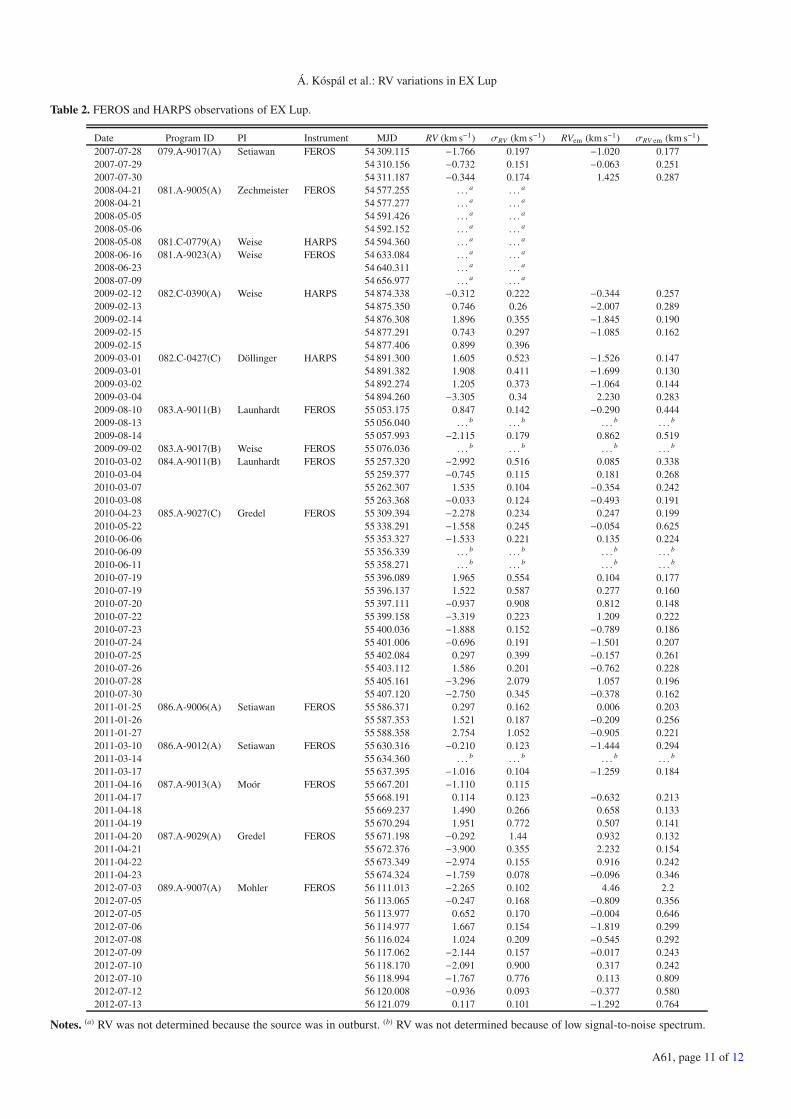
Table 2. FEROS and HARPS observations of EX Lup.

Date Program ID PI Instrument MJD RV (km s−1) σRV (km s−1) RVem (km s−1) σRV em (km s−1)2007-07-28 079.A-9017(A) Setiawan FEROS 54 309.115 −1.766 0.197 −1.020 0.1772007-07-29 54 310.156 −0.732 0.151 −0.063 0.2512007-07-30 54 311.187 −0.344 0.174 1.425 0.2872008-04-21 081.A-9005(A) Zechmeister FEROS 54 577.255 . . . a . . . a

2008-04-21 54 577.277 . . . a . . . a

2008-05-05 54 591.426 . . . a . . . a

2008-05-06 54 592.152 . . . a . . . a

2008-05-08 081.C-0779(A) Weise HARPS 54 594.360 . . . a . . . a

2008-06-16 081.A-9023(A) Weise FEROS 54 633.084 . . . a . . . a

2008-06-23 54 640.311 . . . a . . . a

2008-07-09 54 656.977 . . . a . . . a

2009-02-12 082.C-0390(A) Weise HARPS 54 874.338 −0.312 0.222 −0.344 0.2572009-02-13 54 875.350 0.746 0.26 −2.007 0.2892009-02-14 54 876.308 1.896 0.355 −1.845 0.1902009-02-15 54 877.291 0.743 0.297 −1.085 0.1622009-02-15 54 877.406 0.899 0.3962009-03-01 082.C-0427(C) Döllinger HARPS 54 891.300 1.605 0.523 −1.526 0.1472009-03-01 54 891.382 1.908 0.411 −1.699 0.1302009-03-02 54 892.274 1.205 0.373 −1.064 0.1442009-03-04 54 894.260 −3.305 0.34 2.230 0.2832009-08-10 083.A-9011(B) Launhardt FEROS 55 053.175 0.847 0.142 −0.290 0.4442009-08-13 55 056.040 . . . b . . . b . . . b . . . b

2009-08-14 55 057.993 −2.115 0.179 0.862 0.5192009-09-02 083.A-9017(B) Weise FEROS 55 076.036 . . . b . . . b . . . b . . . b

2010-03-02 084.A-9011(B) Launhardt FEROS 55 257.320 −2.992 0.516 0.085 0.3382010-03-04 55 259.377 −0.745 0.115 0.181 0.2682010-03-07 55 262.307 1.535 0.104 −0.354 0.2422010-03-08 55 263.368 −0.033 0.124 −0.493 0.1912010-04-23 085.A-9027(C) Gredel FEROS 55 309.394 −2.278 0.234 0.247 0.1992010-05-22 55 338.291 −1.558 0.245 −0.054 0.6252010-06-06 55 353.327 −1.533 0.221 0.135 0.2242010-06-09 55 356.339 . . . b . . . b . . . b . . . b

2010-06-11 55 358.271 . . . b . . . b . . . b . . . b

2010-07-19 55 396.089 1.965 0.554 0.104 0.1772010-07-19 55 396.137 1.522 0.587 0.277 0.1602010-07-20 55 397.111 −0.937 0.908 0.812 0.1482010-07-22 55 399.158 −3.319 0.223 1.209 0.2222010-07-23 55 400.036 −1.888 0.152 −0.789 0.1862010-07-24 55 401.006 −0.696 0.191 −1.501 0.2072010-07-25 55 402.084 0.297 0.399 −0.157 0.2612010-07-26 55 403.112 1.586 0.201 −0.762 0.2282010-07-28 55 405.161 −3.296 2.079 1.057 0.1962010-07-30 55 407.120 −2.750 0.345 −0.378 0.1622011-01-25 086.A-9006(A) Setiawan FEROS 55 586.371 0.297 0.162 0.006 0.2032011-01-26 55 587.353 1.521 0.187 −0.209 0.2562011-01-27 55 588.358 2.754 1.052 −0.905 0.2212011-03-10 086.A-9012(A) Setiawan FEROS 55 630.316 −0.210 0.123 −1.444 0.2942011-03-14 55 634.360 . . . b . . . b . . . b . . . b

2011-03-17 55 637.395 −1.016 0.104 −1.259 0.1842011-04-16 087.A-9013(A) Moór FEROS 55 667.201 −1.110 0.1152011-04-17 55 668.191 0.114 0.123 −0.632 0.2132011-04-18 55 669.237 1.490 0.266 0.658 0.1332011-04-19 55 670.294 1.951 0.772 0.507 0.1412011-04-20 087.A-9029(A) Gredel FEROS 55 671.198 −0.292 1.44 0.932 0.1322011-04-21 55 672.376 −3.900 0.355 2.232 0.1542011-04-22 55 673.349 −2.974 0.155 0.916 0.2422011-04-23 55 674.324 −1.759 0.078 −0.096 0.3462012-07-03 089.A-9007(A) Mohler FEROS 56 111.013 −2.265 0.102 4.46 2.22012-07-05 56 113.065 −0.247 0.168 −0.809 0.3562012-07-05 56 113.977 0.652 0.170 −0.004 0.6462012-07-06 56 114.977 1.667 0.154 −1.819 0.2992012-07-08 56 116.024 1.024 0.209 −0.545 0.2922012-07-09 56 117.062 −2.144 0.157 −0.017 0.2432012-07-10 56 118.170 −2.091 0.900 0.317 0.2422012-07-10 56 118.994 −1.767 0.776 0.113 0.8092012-07-12 56 120.008 −0.936 0.093 −0.377 0.5802012-07-13 56 121.079 0.117 0.101 −1.292 0.764

Notes. (a) RV was not determined because the source was in outburst. (b) RV was not determined because of low signal-to-noise spectrum.

A61, page 11 of 12

A&A 561, A61 (2014)

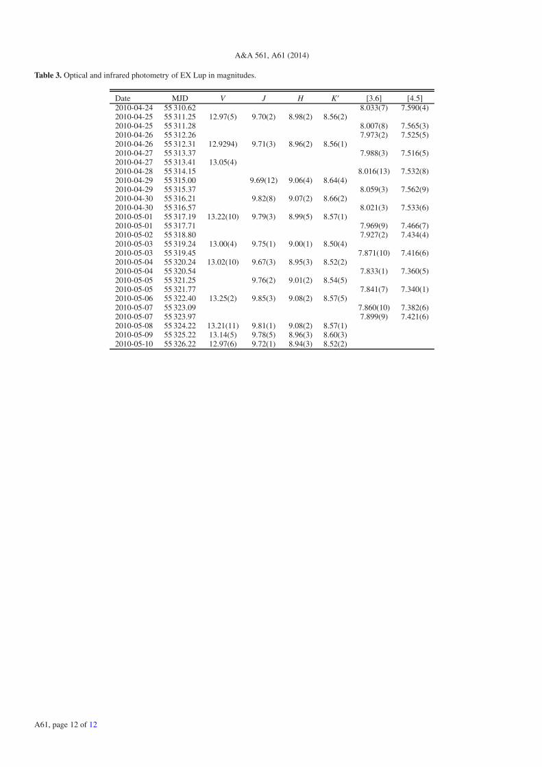
Table 3. Optical and infrared photometry of EX Lup in magnitudes.

Date MJD V J H K′ [3.6] [4.5]2010-04-24 55 310.62 8.033(7) 7.590(4)2010-04-25 55 311.25 12.97(5) 9.70(2) 8.98(2) 8.56(2)2010-04-25 55 311.28 8.007(8) 7.565(3)2010-04-26 55 312.26 7.973(2) 7.525(5)2010-04-26 55 312.31 12.9294) 9.71(3) 8.96(2) 8.56(1)2010-04-27 55 313.37 7.988(3) 7.516(5)2010-04-27 55 313.41 13.05(4)2010-04-28 55 314.15 8.016(13) 7.532(8)2010-04-29 55 315.00 9.69(12) 9.06(4) 8.64(4)2010-04-29 55 315.37 8.059(3) 7.562(9)2010-04-30 55 316.21 9.82(8) 9.07(2) 8.66(2)2010-04-30 55 316.57 8.021(3) 7.533(6)2010-05-01 55 317.19 13.22(10) 9.79(3) 8.99(5) 8.57(1)2010-05-01 55 317.71 7.969(9) 7.466(7)2010-05-02 55 318.80 7.927(2) 7.434(4)2010-05-03 55 319.24 13.00(4) 9.75(1) 9.00(1) 8.50(4)2010-05-03 55 319.45 7.871(10) 7.416(6)2010-05-04 55 320.24 13.02(10) 9.67(3) 8.95(3) 8.52(2)2010-05-04 55 320.54 7.833(1) 7.360(5)2010-05-05 55 321.25 9.76(2) 9.01(2) 8.54(5)2010-05-05 55 321.77 7.841(7) 7.340(1)2010-05-06 55 322.40 13.25(2) 9.85(3) 9.08(2) 8.57(5)2010-05-07 55 323.09 7.860(10) 7.382(6)2010-05-07 55 323.97 7.899(9) 7.421(6)2010-05-08 55 324.22 13.21(11) 9.81(1) 9.08(2) 8.57(1)2010-05-09 55 325.22 13.14(5) 9.78(5) 8.96(3) 8.60(3)2010-05-10 55 326.22 12.97(6) 9.72(1) 8.94(3) 8.52(2)

A61, page 12 of 12