Paul C. Bressloff and Matthew A. Webber- Neural field model of binocular rivalry waves

8/3/2019 Paul C. Bressloff and Matthew A. Webber- Neural field model of binocular rivalry waves

http://slidepdf.com/reader/full/paul-c-bressloff-and-matthew-a-webber-neural-field-model-of-binocular-rivalry 1/22

13

Journal of ComputationalNeuroscience ISSN 0929-5313 J Comput NeurosciDOI 10.1007/s10827-011-0351-y

Neural field model of binocular rivalry

waves

Paul C. Bressloff & Matthew A. Webber



13

Your article is protected by copyright and

all rights are held exclusively by Springer

Science+Business Media, LLC. This e-offprint

is for personal use only and shall not be self-

archived in electronic repositories. If youwish to self-archive your work, please use the

accepted author’s version for posting to your

own website or your institution’s repository.

You may further deposit the accepted author’s

version on a funder’s repository at a funder’s

request, provided it is not made publicly

available until 12 months after publication.



J Comput Neurosci

DOI 10.1007/s10827-011-0351-y

Neural field model of binocular rivalry waves

Paul C. Bressloff ·

Matthew A. Webber

Received: 28 April 2011 / Revised: 20 June 2011 / Accepted: 22 June 2011© Springer Science+Business Media, LLC 2011

Abstract We present a neural field model of binocular

rivalry waves in visual cortex. For each eye we considera one-dimensional network of neurons that respond

maximally to a particular feature of the corresponding

image such as the orientation of a grating stimulus.

Recurrent connections within each one-dimensionalnetwork are assumed to be excitatory, whereas connec-

tions between the two networks are inhibitory (cross-

inhibition). Slow adaptation is incorporated into themodel by taking the network connections to exhibit

synaptic depression. We derive an analytical expression

for the speed of a binocular rivalry wave as a function of various neurophysiological parameters, and show how

properties of the wave are consistent with the wave-like propagation of perceptual dominance observed

in recent psychophysical experiments. In addition toproviding an analytical framework for studying binoc-

ular rivalry waves, we show how neural field methods

provide insights into the mechanisms underlying thegeneration of the waves. In particular, we highlight

the important role of slow adaptation in providing a

“symmetry breaking mechanism” that allows waves topropagate.

Action Editor: Carson C. Chow

P. C. Bressloff · M. A. WebberMathematical Institute, University of Oxford,24-29 St. Giles’, Oxford, OX1 3LB, UK

P. C. Bressloff (B)Department of Mathematics, University of Utah,Salt Lake City, UT 84112-0090, USAe-mail: [email protected]

Keywords Binocular rivalry · Neural fields ·

Synaptic depression · Cortical waves · Oscillations

1 Introduction

A number of phenomena in visual perception involve

wave-like propagation dynamics. Examples include

perceptual filling-in (De et al. 1998), migraine aura(Hadjikhani et al. 2001), expansion of illusory contours

(Gold and Shubel 2006) and the line–motion illusion

(Jancke et al. 2004). Another important example, whichis the focus of this paper, is the wave-like propaga-

tion of perceptual dominance during binocular rivalry

(Wilson et al. 2001; Lee et al. 2005; Kang et al.2009, 2010). Binocular rivalry is the phenomenon

where perception switches back and forth between

different images presented to the two eyes. The re-

sulting fluctuations in perceptual dominance and sup-pression provide a basis for non-invasive studies of the

human visual system and the identification of possible

neural mechanisms underlying conscious visual aware-ness (Blake 2001; Blake and Logothetis 2002). One way

to observe and measure the speed of perceptual waves

in psychophysical experiments (Wilson et al. 2001; Leeet al. 2005) is to take the rival images to be a low-

contrast radial grating presented to one eye and a high-

contrast spiral grating presented to the other eye. Each

image is restricted to an annular region of the visualfield centered on the fixation point of the observer,

thus effectively restricting wave propagation to the one

dimension around the annulus. Switches in perceptualdominance can then be triggered using a brief rapid

increase in stimulus contrast within a small region of

the suppressed low-contrast grating. This induces a



J Comput Neurosci

perceptual traveling wave in which the observer per-

ceives the local dominance of the low-contrast image

spreading around the annulus. The observer presses akey when the perceptual wave reaches a target area

at a fixed distance from the trigger zone, and this

determines the wave speed (Wilson et al. 2001; Leeet al. 2005). Since the rival images consist of oriented

gratings, one might expect that primary visual cortex(V1) plays some role in the generation of binocular ri-

valry waves. Indeed, it has been shown using functionalmagnetic resonance imaging that there is a systematic

correspondence between the spatiotemporal dynamics

of activity in V1 and the time course of perceptualwaves (Lee et al. 2005). However, it has not been

established whether the waves originate in V1 or are

evoked by feedback from extrastriate cortex.Recently Kang et al. (2009, 2010) have developed

a new psychophysical method for studying binocular

rivalry waves that involves periodic perturbations of the

rival images. An observer tracks rivalry within a small,

central region of spatially extended rectangular grating

patterns, while alternating contrast triggers are pre-

sented repetitively in the periphery of the rival patterns.The basic experimental set up is illustrated in Fig. 1.

A number of interesting results have been obtained

from these studies. First, over a range of trigger fre-quencies, the switching between rival percepts within

the central regions is entrained to the triggering events.Moreover, the optimal triggering frequency dependson the natural frequency of spontaneous switching (in

the absence of triggers). Second, the latency between

triggering event and perceptual switching increases ap-

proximately linearly with the distance between the trig-gering site and the central region being tracked by the

observer, consistent with the propagation of a traveling

front. Third, the speed of the traveling wave acrossobservers covaries with the spontaneous switching

rate.

In this paper we analyze the existence and stability

of binocular rivalry waves in a continuum neural field

Fig. 1 Schematic diagramillustrating experimentalprotocol used to studybinocular rivalry waves (Kanget al. 2009). High contrasttriggers are presentedperiodically in antiphasewithin the upper extendedregion of one grating patternand within the lower regionof the rival pattern. Subject

simply reports perceptualalternations in rivaldominance within the centralmonitoring region indicatedby the horizontal black lineson each pattern. Themonitoring region is adistance d from the triggerregion, which can beadjusted. If t is the latencybetween the triggering eventand the subsequentobservation of a perceptualswitch, then the speed c of thewave is given by the slope of

the plot d = ct



J Comput Neurosci

model of visual cortex. We derive an analytical expres-

sion for the wave speed as a function of neurophysio-

logical parameters, and use this to show how our modelreproduces various experimental results found by Kang

et al. (2009, 2010), in particular, the observation that

wave speed covaries with the natural alternation rate.Our model is essentially a continuum version of a pre-

vious computational model of rivalry waves based ona discrete two layer neural network (Wilson et al. 2001;

Kang et al. 2010). The two layers represent cortical neu-rons responsive to one or more features of the image

presented to the left and right eye respectively. Such

features could include the orientation of a spatiallyextended grating stimulus or distinguish between spiral

and radial annulus patterns. In the discrete computa-

tional model, connections within a layer were taken tobe excitatory, whereas between layers, neurons mutu-

ally inhibited each other via a set of local interneurons.

Moreover, in order to allow switching between the

dominant and suppressed populations, the excitatoryneurons were assumed to exhibit some form of slow

spike frequency adaptation. In our neural field version

of this model, we consider an alternative form of slowadaptation based on depressing synapses. In addition to

providing an analytical framework for studying binoc-

ular rivalry waves, we show how neural field methodsprovide insights into the mechanisms underlying the

generation of the waves. In particular, we highlight

the important role of slow adaptation in providing a

“symmetry breaking mechanism” that allows fronts topropagate.

2 The model

In order to model binocular rivalry waves in the pres-ence of oriented grating stimuli (Wilson et al. 2001;

Kang et al. 2009, 2010), it is useful to review some of

the stimulus response properties of neurons in the pri-

mary visual cortex (V1) (Hubel and Wiesel 1962, 1977).First, each neuron in V1 responds to light stimuli in a

restricted region of the visual field called its classical

receptive f ield; stimuli outside a neuron’s receptive fielddo not directly affect its activity. Second, most neurons

in V1 respond preferentially to stimuli targeting either

the left or right eye, which is known as ocular domi-

nance. It has been suggested that neurons with different

ocular dominance may inhibit one another if they have

nearby receptive fields (Katz et al. 1989). Third, most

neurons in V1 are tuned to respond maximally when astimulus of a particular orientation is in their receptive

field (Hubel and Wiesel 1962; Blasdel 1992). This is

known as a neuron’s orientation preference, and the

neuron will not respond if a stimulus is sufficiently

different from its preferred orientation. Finally, mul-tielectrode recordings and optical imaging have estab-

lished that at each point in the visual field there exists

a corresponding set of neurons spanning the entirespectrum of orientation preferences that are packed to-

gether as a unit in V1, known as a hypercolumn (Hubel

and Wiesel 1977; Tootell et al. 1998; Blasdel 1992).Within each hypercolumn, neurons with sufficientlysimilar orientations tend to excite each other whereas

those with sufficiently different orientations inhibit

each other, and this serves to sharpen a particular neu-ron’s orientation preference (Ben-Yishai et al. 1995;

Ferster and Miller 2000). Moreover, anatomical evi-

dence suggests that inter-hypercolumn connections linkneurons with similar orientation preferences (Sincich

and Blasdel 2001; Angelucci et al. 2002). The functional

relationship between stimulus feature preferences andsynaptic connections within V1 thus suggests that V1

is a likely substrate of simple examples of binocularrivalry such as those involving sinusoidal grating stimuli

(Sterzer et al. 2009).Binocular rivalry waves consist of two basic com-

ponents: the switching between rivalrous left/right eye

states and the propagation of the switched state acrossa region of cortex. Let us first focus on the switching

mechanism by neglecting spatial effects. Suppose that

distinct oriented grating patterns are presented to thetwo eyes such as those shown in Fig. 1. This induces

rivalry due to the combination of orientation specific

and ocular dominant cross-inhibition in V1 (Ben-

Yishai et al. 1995; Sincich and Blasdel 2001; Blake andLogothetis 2002). During left eye stimulus dominance,

it is assumed that a group of the left eye neurons

that respond to 135 degree orientations, say, are firingpersistently, while right eye neurons are suppressed by

cross-inhibitory connections. Following this, some slow

adaptive process such as synaptic depression or spike

frequency adaptation causes a switch so that right eye

neurons tuned to 45 degree orientations fire persis-

tently, suppressing the left eye neurons. The cycle of left eye neural dominance along with right eye neural

suppression followed by right eye neural dominance

along with left eye neural suppression can then repeatitself in the form of rivalrous oscillations. This basic

model of reciprocal inhibition paired with a slow adap-

tive process has often been used to phenomenologicallymodel the neural substrate of binocular rivalry oscilla-

tions (Fox and Rasche 1969; Skinner et al. 1994; Wilson

et al. 2001; Laing and Chow 2002; Taylor et al. 2002;Shpiro et al. 2007, 2009; Kilpatrick and Bressloff 2010).

In order to take into account the propagation of

activity seen in binocular rivalry waves (Wilson et al.



J Comput Neurosci

2001; Kang et al. 2009, 2010), we will consider a contin-

uum neural field model. Several previous studies have

modeled the spontaneous switching between rivalrousoriented stimuli in terms of a pair of ring networks

(neural fields on a periodic domain) with slow adapta-

tion and cross-inhibition, representing a pair of hyper-columns for the left and right eyes, respectively (Laing

and Chow 2002; Kilpatrick and Bressloff 2010). In thesemodels, the rivalrous states consist of stationary activity

bumps coding for either the left or right eye stimuli.(Rivalry effects in a spatially extended model have

also been examined in a prior study by Loxley and

Robinson (Loxley and Robinson 2009), in which rival-rous stimuli are presented to a single one-dimensional

network). However, these models were not used to

study binocular rivalry waves and, as formulated, wereon the wrong spatial scale since they only considered

short-range spatial scales comparable to a single hy-

percolumn. One way to proceed would be to construct

a more general coupled ring model along the lines of Bressloff et al. (2001) and Bressloff and Cowan (2002),

in which two sets of hypercolumns (ring networks) are

distributed along a pair of lines corresponding to theleft and right eyes, respectively, such that along each

line the synaptic weights can be decomposed into short-

range intra-columnar interactions and long-range inter-columnar interactions, together with cross-inhibitory

connections between the left and right eye networks.

In this paper, we will consider a simpler network ar-

chitecture in which we neglect the internal structureof a hypercolumn. That is, for each eye we consider

a one-dimensional network of neurons whose orienta-

tion preference coincides with the orientation of the

corresponding grating stimulus, which is a reasonablefirst approximation from the perspective of the experi-

ments conducted by Kang et al. (2009, 2010). Recurrent

connections within each one-dimensional network areassumed to be excitatory, whereas connections between

the two networks are inhibitory (cross-inhibition). Slowadaptation is incorporated into the model by takingthe network connections to exhibit synaptic depression

along the lines of Kilpatrick and Bressloff (2010). The

basic architecture is shown schematically in Fig. 2. Notethat a similar network architecture was previously con-

sidered in a computational model of binocular rivalry

waves (Wilson et al. 2001; Kang et al. 2010), in which

cross inhibition was mediated explicitly by interneu-rons and, rather than including depressing synapses,

the excitatory neurons were taken to exhibit spike

frequency adaptation. The most significant difference

between our approach and the previous computationalapproaches (besides considering synaptic depression

rather than spike frequency adaptation) is that thelatter considers a discrete neural network rather than

a continuum neural field. As we will establish in this

paper, one advantage of neural field theory is thatanalytical methods can be used to derive conditions

for the existence and stability of traveling waves, and

to derive formulae relating the wave speed to various

neurophysiological parameters.Let u( x, t ) and v( x, t ) denote the activity of the left

and right eye networks at position x∈R at time t . The

Fig. 2 Schematic diagram of network architecture consisting of two one-dimensional neural fields. Suppose that the left eye isshown a 135 degree grating and the right eye is shown a 45

degree grating. Then one of the neural fields represents theactivity of neurons tuned to 135 degree orientations in the lefteye, whilst the other neural field represents the activity of neu-rons tuned to 45 degree orientations in the right eye. Recurrent

connections within each one-dimensional network are assumedto be excitatory, whereas connections between the two networksare inhibitory (cross-inhibition). The excitatory and inhibitoryweight distributions are taken to be Gaussians. Slow adaptationis incorporated into the model by taking the network connectionsto exhibit synaptic depression



J Comput Neurosci

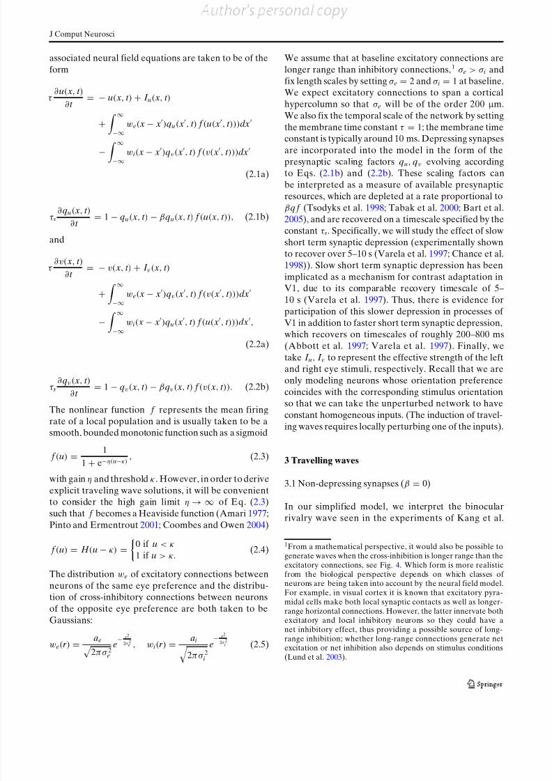
associated neural field equations are taken to be of the

form

τ ∂u( x, t )

∂t = − u( x, t ) + I u( x, t )

+

∞

−∞

we( x − x)qu( x, t ) f (u( x, t )))dx

− ∞

−∞wi( x − x)qv( x, t ) f (v( x, t )))dx

(2.1a)

τ s∂qu( x, t )

∂t = 1 − qu( x, t ) − βqu( x, t ) f (u( x, t )), (2.1b)

and

τ ∂v( x, t )

∂t = −v( x, t )

+ I v( x, t )

+ ∞

−∞we( x − x)qv( x, t ) f (v( x, t )))dx

− ∞

−∞wi( x − x)qu( x, t ) f (u( x, t )))dx,

(2.2a)

τ s∂qv( x, t )

∂t = 1 − qv( x, t ) − βqv( x, t ) f (v( x, t )). (2.2b)

The nonlinear function f represents the mean firingrate of a local population and is usually taken to be asmooth, bounded monotonic function such as a sigmoid

f (u) = 1

1 + e−η(u−κ), (2.3)

with gain η and threshold κ . However, in order to derive

explicit traveling wave solutions, it will be convenientto consider the high gain limit η → ∞ of Eq. (2.3)

such that f becomes a Heaviside function (Amari 1977;

Pinto and Ermentrout 2001; Coombes and Owen 2004)

f (u) = H (u − κ) = 0 if u < κ1 if u > κ. (2.4)

The distribution we of excitatory connections between

neurons of the same eye preference and the distribu-tion of cross-inhibitory connections between neurons

of the opposite eye preference are both taken to be

Gaussians:

we(r ) = ae2π σ 2e

e− r 2

2σ 2e , wi(r ) = ai2π σ 2i

e− r 2

2σ 2i (2.5)

We assume that at baseline excitatory connections are

longer range than inhibitory connections,1 σ e > σ i and

fix length scales by setting σ e = 2 and σ i = 1 at baseline.We expect excitatory connections to span a cortical

hypercolumn so that σ e will be of the order 200 μ m.

We also fix the temporal scale of the network by setting

the membrane time constant τ

=1; the membrane time

constant is typically around 10 ms. Depressing synapsesare incorporated into the model in the form of the

presynaptic scaling factors qu, qv evolving accordingto Eqs. (2.1b) and (2.2b). These scaling factors can

be interpreted as a measure of available presynaptic

resources, which are depleted at a rate proportional toβq f (Tsodyks et al. 1998; Tabak et al. 2000; Bart et al.2005), and are recovered on a timescale specified by the

constant τ s. Specifically, we will study the effect of slow

short term synaptic depression (experimentally shownto recover over 5–10 s (Varela et al. 1997; Chance et al.

1998)). Slow short term synaptic depression has been

implicated as a mechanism for contrast adaptation inV1, due to its comparable recovery timescale of 5–

10 s (Varela et al. 1997). Thus, there is evidence for

participation of this slower depression in processes of

V1 in addition to faster short term synaptic depression,which recovers on timescales of roughly 200–800 ms

(Abbott et al. 1997; Varela et al. 1997). Finally, we

take I u, I v to represent the effective strength of the leftand right eye stimuli, respectively. Recall that we are

only modeling neurons whose orientation preference

coincides with the corresponding stimulus orientationso that we can take the unperturbed network to have

constant homogeneous inputs. (The induction of travel-

ing waves requires locally perturbing one of the inputs).

3 Travelling waves

3.1 Non-depressing synapses (β = 0)

In our simplified model, we interpret the binocularrivalry wave seen in the experiments of Kang et al.

1From a mathematical perspective, it would also be possible togenerate waves when the cross-inhibition is longer range than theexcitatory connections, see Fig. 4. Which form is more realisticfrom the biological perspective depends on which classes of neurons are being taken into account by the neural field model.For example, in visual cortex it is known that excitatory pyra-midal cells make both local synaptic contacts as well as longer-range horizontal connections. However, the latter innervate bothexcitatory and local inhibitory neurons so they could have anet inhibitory effect, thus providing a possible source of long-range inhibition; whether long-range connections generate netexcitation or net inhibition also depends on stimulus conditions(Lund et al. 2003).



J Comput Neurosci

(2009, 2010) as a traveling wave front solution of the

neural field equations (2.1) and (2.2), in which a high

activity state invades the suppressed left eye network,say, whilst retreating from the dominant right eye net-

work. Let us begin by ignoring the effects of synaptic

depression, that is, we set β = 0 and qu = qv ≡ 1. We

also assume that both inputs have the same strength

or contrast so that I u = I v = I . We then obtain thereduced system of equations (for τ = 1 and f given by

the Heaviside (2.4))

∂u

∂t + u =

∞

−∞we( x − x)H (u( x, t ) − κ)dx

− ∞

−∞wi( x − x)H (v( x, t ) − κ)dx + I ,

(3.1)

and

∂v

∂t + v = ∞

−∞ we( x − x)H (v( x, t ) − κ)dx

− ∞

−∞wi( x − x)H (u( x, t ) − κ)dx + I .

(3.2)

Given that the differential operator D = ∂∂t

+ 1 has a

Green’s function given by G(t , s) = η(t − s) with

η(t ) =0 t < 0

e−t t > 0,

we can re-write the above equations in purely integral

form:

u( x, t ) = I + ∞

0

η( s)Ge[u]( x, t − s)ds

− ∞

0

η( s)Gi[v]( x, t − s)ds (3.3)

v( x, t ) = I + ∞

0

η( s)Ge[v]( x, t − s)ds

− ∞0

η( s)Gi[u]( x, t − s)ds (3.4)

where

G p[u]( x, t ) = ∞

−∞w p( y)H (u( x − y, t ) − κ)dy (3.5)

for p = e, i.

Homogeneous fixed point solutions (U ∗, V ∗) of

Eqs. (3.3) and (3.4) satisfy the pair of equations

U ∗ = ae H (U ∗ − κ) − ai H (V ∗ − κ) + I

V ∗ = ae H (V ∗ − κ) − ai H (U ∗ − κ) + I ,

where we have used the normalization of the Gaussians

(2.5) ∞

−∞we( x)dx = ae,

∞

−∞wi( x)dx = ai. (3.6)

There are a maximum of four possible fixed point

solutions, all of which are stable. First, there is the off

state U ∗ = V ∗ = I , which occurs when I < κ , that is,the input is not strong enough to directly activate either

population. Second there is the on-state or fusion stateU ∗ = V ∗ = ae − ai + I , which occurs when I > κ + ai −ae. This case is more likely when recurrent excitation

is strong or cross-inhibition is weak. Finally, there are

two winner-take-all (WTA) states in which one pop-ulation dominates the other: the left eye dominant

state (U ∗, V ∗) = XL ≡ (ae + I , I − ai) and the right eye

dominant state (U ∗, V ∗) = XR ≡ ( I − ai, ae + I ). These

states exist when I > κ − ae and I < κ + ai.Let us now consider a traveling wave front solution

of the form

u( x, t ) = U ( x − ct ), v( x, t ) = V ( x − ct )

where c is the wave speed and ξ = x − ct is a traveling

wave coordinate. We assume that

(U (ξ), V (ξ)) → XL as ξ → −∞,

(U (ξ), V (ξ)) → XR as ξ → ∞

with U (ξ ) a monotonically decreasing function of ξ

and V (ξ ) a monotonically increasing function of ξ .

It follows that if c > 0 then the wavefront representsa solution in which activity invades a supressed lefteye network and retreats from a dominant right eye

network. Substituting the traveling front solution into

Eqs. (3.3) and (3.4) gives

U (ξ ) = I + ∞

0

η( s)Ge[U ](ξ + cs)ds

− ∞

0

η( s)Gi[V ](ξ + cs)ds

V (ξ ) = I + ∞

0η( s)Ge[V ](ξ + cs)ds

− ∞

0

η( s)Gi[U ](ξ + cs)ds.

where

G p[U ](ξ ) = ∞

−∞w p( y)H (U (ξ − y) − κ)dy, p = e, i

Given the asymptotic behavior of the solution and

the requirements of monotonicity, we see that U (ξ )



J Comput Neurosci

and V (ξ) each cross threshold at a single location,

which may be different for the two eyes. Exploiting

translation invariance we take U (0) = κ and V (ξ0) =κ . These threshold crossing conditions imply that the

above equations simplify further according to

U (ξ )

= ∞

0

η( s) ∞

ξ+cs

we( y)dy

− ξ−ξ0+cs

−∞wi( y)dyds

+ I

(3.7)

V (ξ )= ∞

0

η( s)

ξ−ξ0+cs

−∞we( y)dy −

∞

ξ+cs

wi( y)dy

ds + I .

(3.8)

It is convenient to introduce the function

ξ0(z) = ∞

z

we( y)dy − z−ξ0

−∞wi( y)dy. (3.9)

Exploiting the fact that the Gaussian weight distribu-

tions we( y) and wi( y) are even functions of y, it can beseen that

ξ0(ξ0 − z) = z−ξ0

−∞we( y)dy −

∞z

wi( y)dy,

so that Eqs. (3.7) and (3.8) can be rewritten in the morecompact form

U (ξ ) = ∞0

η( s)ξ0 (ξ + cs)ds + I (3.10)

V (ξ ) =

∞

0

η( s)ξ0 (ξ0 − ξ − cs) + I . (3.11)

Finally, imposing the threshold conditions U (0) =V (ξ0) = κ gives

κ = ∞0

η( s)ξ0(cs)ds + I , (3.12)

κ = ∞0

η( s)ξ0(−cs)ds + I . (3.13)

It is now straightforward to show that a travelingfront solution cannot exist for the neural field model

without adaptation given by Eqs. (3.1) and (3.2). For

subtracting Eq. (3.13) from Eq. (3.12) implies that ∞

0

η( s)

ξ0(cs) − ξ0 (−cs)

ds = 0, (3.14)

which does not have a solution for any c, ξ0 such thatc = 0. The latter follows from Eq. (3.9), which shows

that for c = 0,

c

ξ0(cs) − ξ0 (−cs)

= −c

cs

−cs

we( y)dy − c

cs−ξ0

−cs−ξ0

wi( y)dy < 0

whereas η( s) > 0 for all s ∈ [0, ∞). The non-existence

of traveling fronts is consistent with the observation

that in the absence of any cross inhibition (wi ≡ 0), thesystem reduces to two independent one-dimensional

neural fields with excitatory connections. In order to

construct a front solution that simultaneously invades

one network whilst retreating from the other we would

require a one dimensional excitatory neural field tobe able to support a pair of counter-propagating front

solutions with speeds ±c, which is not possible (Amari1977). Therefore, some mechanism must be introduced

that breaks the exchange symmetry of the two one-

dimensional networks. One way to break the symmetrywould be to take the input strengths of the left and

right eye stimuli to be sufficiently different, I u = I v.

However, this case can be excluded, since rivalry waves

are still observed experimentally when both inputs areof equal strength. Moreover, a traveling front could

only travel in one direction, depending on the sign of

I L − I R. Therefore, we consider an alternative mecha-nism based on slow synaptic depression.

3.2 Slow synaptic depression (β > 0, τ s 1)

Let us now consider the full neural field model withdepressing synaptic connections given by Eqs. (2.1)

and (2.2) with f (u) = H (u − κ). As in the case β = 0,

there are four possible homogeneous fixed points cor-responding to an off-state, a fusion state and two WTA

states, and all are stable. Denoting a homogeneous

fixed point by (U ∗, V ∗, Q∗u, Q∗v), we have

U ∗ = Q∗uae H (U ∗ − κ) − Q∗

vai H (V ∗ − κ) + I

Q∗u = 1

1 + β H (U ∗ − κ)

V ∗ = Q∗vae H (V ∗ − κ) − Q∗

uai H (U ∗ − κ) + I

Q∗v = 1

1 + β H (V ∗ − κ)

with ae, ai given by Eq. (3.6). Hence, the fusion state is

now

(U ∗, V ∗) =

ae − ai

1 + β+ I ,

ae − ai

1 + β+ I

,

(Q∗u, Q∗

v) =

1

1 + β,

1

1 + β

, (3.15)

and occurs when I > κ − (ae − ai)/(1 + β). This caseis more likely for very strong depression (β large),

since cross inhibition will be weak, or when the local



J Comput Neurosci

connections are strong and excitation-dominated. The

left eye dominant WTA state now takes the form

(U ∗, V ∗) =

ae

1 + β+ I , I − ai

1 + β

,

(Q∗u, Q∗

v) =

1

1

+β

, 1

(3.16)

whereas the right eye dominant WTA state becomes

(U ∗, V ∗) =

I − ai

1 + β,

ae

1 + β+ I

,

(Q∗u, Q∗

v) =1,

1

1 + β

(3.17)

The WTA states exist provided that

I > κ − ae

1 + β, I < κ + ai

1 + β

This will occur in the presence of weak depression (βsmall) and strong cross-inhibition such that depression

cannot exhaust the dominant hold one population has

on the other. Previously, we have shown that Eqs.

(2.1) and (2.2) also support homogeneous limit cycleoscillations in which there is periodic switching between

left and right eye dominance consistent with binocular

rivalry (Kilpatrick and Bressloff 2010). Since all thefixed points are stable, it follows that such oscillations

cannot arise via a standard Hopf bifurcation. Indeed,

we find bistable regimes where a rivalry state coexistswith a fusion state as illustrated in Fig. 3. (Such behav-

ior persists in the case of smooth sigmoid firing rate

0.1 0.2 0.3-0.4

-0.2

0

0.2

0.4

input I

u

WTA

fusion

rivalry

Off

Fig. 3 Bifurcation diagram showing homogeneous solutions forthe left population activity u as a function of the input amplitude I . Solid lines represent stable states, whereas circles representthe maximum and minimum of rivalrous oscillations. It can beseen that there are regions of off/WTA bistability, WTA/fusionbistability, and fusion/rivalry bistability. Parameters are τ s = 500,κ = 0.05, β = 5, ae = 0.4 and ai = 1

functions, at least for sufficiently high gain (Kilpatrick

and Bresslof f 2010)).

Suppose that the full system given by Eqs. (2.1) and(2.2) is initially in a stable right eye dominated WTA

state, and is then perturbed away from this state by

introducing a propagating front that generates a switchfrom right to left eye dominance. We further assume

that over a finite spatial domain of interest the timetaken for the wave front to propagate is much smaller

than the relaxation time τ s of synaptic depression. Thus,to a first approximation we can ignore the dynamics of

the depression variables and assume that they are con-

stant, that is, (qu( x, t ), qv( x, t )) = (Qu, Qv) with Qu = 1

and Qv = (1 + β)−1. A similar adiabatic approximationcan also be made if the network is in a binocular rivalry

state, provided that (a) the duration of wave propaga-

tion is short compared to the natural switching periodand (b) the induction of the wave does not occur close

to the point at which spontaneous switching occurs. In

this case Qu and Qv will not be given by the WTAsolution, but we can assume that Qu = Qv. Under the

adiabatic approximation, we obtain a slightly modified

version of Eqs. (3.3) and (3.4) given by

u( x, t ) = I + Qu

∞

0

η( s)Ge[u]( x, t − s)ds

− Qv

∞0

η( s)Gi[v]( x, t − s)ds (3.18)

v( x, t ) = I + Qv ∞0

η( s)Ge[v]( x, t − s)ds

− Qu

∞

0

η( s)Gi[u]( x, t − s)ds. (3.19)

with Ge,i given by Eq. (3.5). The analysis of the ex-

istence of a traveling wave front solution proceeds

along identical lines to Section 3.1, except that now theasymptotic states take the form

XL = (Quae + I , I − Qvai),

XR = ( I − Quai, Qvae + I ).

We thus obtain the following modified threshold

conditions:

κ = ∞0

η( s)ξ0 (cs)ds + I , (3.20)

κ = ∞0

η( s)ξ0 (−cs)ds + I , (3.21)



J Comput Neurosci

with and defined by

ξ0(z) = Qu

∞z

we( y)dy − Qv

z−ξ0

−∞wi( y)dy. (3.22)

ξ0(z)

=Qv

∞

z

we( y)dy

−Qu

z−ξ0

−∞wi( y)dy. (3.23)

It can be seen that synaptic depression breaks the

symmetry of the consistency equations, and this will

allow us to find solutions for c, ξ0 and thus establish the

existence of traveling front solutions.

3.3 Calculation of wave speed

In order to establish the existence of a wave speed c anda threshold crossing point ξ0, define the functions

F 1(c, ξ0) = ∞0 η( s)ξ0(cs)ds (3.24)

and

F 2(c, ξ0) = ∞0

η( s)ξ0(−cs)ds. (3.25)

Evaluating the integrals using Eqs. (2.5), (3.22), (3.23)

and η( s) = e− s gives (for c > 0)

F 1(c, ξ0) = ae Qu

2

1 − e

σ 2e

2τ 2 f

c2

Erfc

σ e√ 2τ f c

−ai Qv

2

⎛⎝Erfc ξ0√ 2σ i

− e

σ 2

i −2τ

f

cξ0

2τ 2 f

c2

× Erfc

σ 2i − τ f cξ0√

2σ iτ f c

⎞⎠ (3.26)

F 2(c, ξ0) = ae Qv

2

1 + e

σ 2e

2τ 2 f

c2

Erfc

σ e√ 2τ f c

−ai Qu

2 ⎛⎝Erfc ξ0

√ 2σ i −e

σ 2i

+2ξ0τ f c

2τ 2 f

c2

× Erfc

σ 2i + ξ0τ f c√

2σ iτ f c

⎞⎠ (3.27)

where

Erfc( x) = 2√ π

∞ x

e−t 2dt

is the complementary error function. Subtracting Eq.

(3.21) from Eq. (3.20), we then have the implicit

equation

G(c, ξ0) ≡ F 1(c, ξ0) − F 2(c, ξ0) = 0. (3.28)

It is straightforward to show that for fixed ξ0,

limc→∞

G(c, ξ0) > 0, limc→−∞

G(c, ξ0) < 0.

Hence, the intermediate value theorem guarantees at

least one solution c = c(ξ0), which is differentiable

by the implicit function theorem. If Qu = Qv, thenF 1(0, ξ0) = F 2(0, ξ0) and the only point where G van-

ishes is at c = 0. On the other hand, if Qv = Qu thenG(0, ξ0) = 0 for all finite ξ0 so that c(ξ0) = 0. Given asolution c = c(ξ0) of Eq. (3.28), the existence of a trav-

eling wavefront solution reduces to the single threshold

condition

κ = F 1(c(ξ0), ξ0) + I . (3.29)

We find that there exists a unique traveling front solu-tion for a range of values of κ .

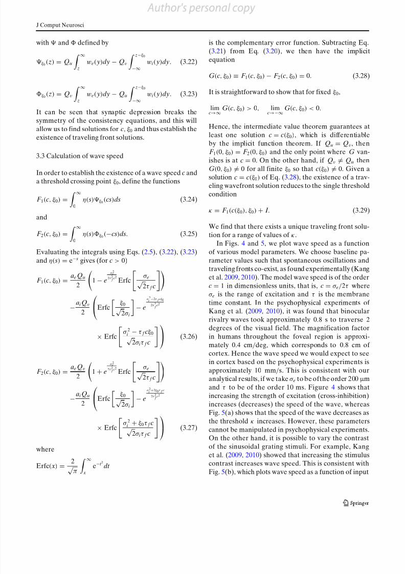
In Figs. 4 and 5, we plot wave speed as a function

of various model parameters. We choose baseline pa-

rameter values such that spontaneous oscillations andtraveling fronts co-exist, as found experimentally (Kang

et al. 2009, 2010). The model wave speed is of the orderc = 1 in dimensionless units, that is, c = σ e/2τ whereσ e is the range of excitation and τ is the membrane

time constant. In the psychophysical experiments of Kang et al. (2009, 2010), it was found that binocularrivalry waves took approximately 0.8 s to traverse 2

degrees of the visual field. The magnification factor

in humans throughout the foveal region is approxi-

mately 0.4 cm/deg, which corresponds to 0.8 cm of cortex. Hence the wave speed we would expect to see

in cortex based on the psychophysical experiments is

approximately 10 mm/s. This is consistent with ouranalytical results, if we take σ e to be ofthe order 200 μ m

and τ to be of the order 10 ms. Figure 4 shows that

increasing the strength of excitation (cross-inhibition)

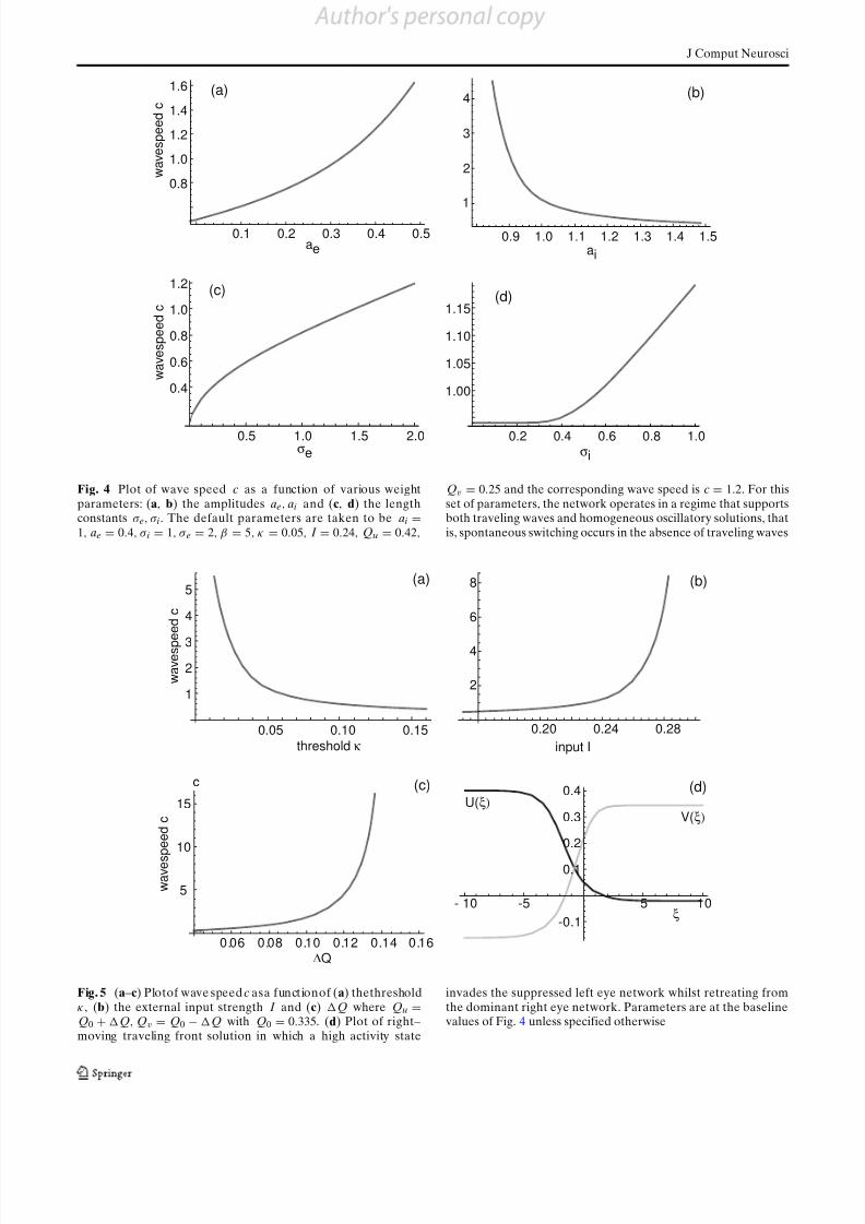
increases (decreases) the speed of the wave, whereasFig. 5(a) shows that the speed of the wave decreases as

the threshold κ increases. However, these parameters

cannot be manipulated in psychophysical experiments.On the other hand, it is possible to vary the contrast

of the sinusoidal grating stimuli. For example, Kang

et al. (2009, 2010) showed that increasing the stimuluscontrast increases wave speed. This is consistent with

Fig. 5(b), which plots wave speed as a function of input



J Comput Neurosci

0.1 0.2 0.3 0.4 0.5

0.8

1.0

1.2

1.4

1.6

ae0.9 1.0 1.1 1.2 1.3 1.4 1.5

2

3

4

1

ai

w a v e s p e e d c

0.5 1.0 1.5 2.0

0.4

0.6

0.8

1.0

1.2

w a v e s p e e d c

σe

0.2 0.4 0.6 0.8 1.0

1.00

1.05

1.10

1.15

σi

(a) (b)

(c) (d)

Fig. 4 Plot of wave speed c as a function of various weightparameters: (a, b) the amplitudes ae, ai and (c, d) the lengthconstants σ e, σ i. The default parameters are taken to be ai =1, ae = 0.4, σ i = 1, σ e = 2, β = 5, κ = 0.05, I = 0.24, Qu = 0.42,

Qv = 0.25 and the corresponding wave speed is c = 1.2. For thisset of parameters, the network operates in a regime that supportsboth traveling waves and homogeneous oscillatory solutions, thatis, spontaneous switching occurs in the absence of traveling waves

0.05 0.10 0.15

1

2

3

4

5

w a v e s p

e e d c

threshold κ

(a)

0.20 0.24 0.28

2

4

6

8 (b)

input I

ΔQ

w a v e s

p e e d c

(c)

0.06 0.08 0.10 0.12 0.14 0.16

5

10

15

c

- 10 -5 5 10

-0.1

0.1

0.2

0.3

0.4

ξ

U(ξ)V(ξ)

(d)

Fig. 5 (a–c) Plotof wave speed c asa functionof (a) thethresholdκ , (b) the external input strength I and (c) Q where Qu =Q0 + Q, Qv = Q0 − Q with Q0 = 0.335. (d) Plot of right–moving traveling front solution in which a high activity state

invades the suppressed left eye network whilst retreating fromthe dominant right eye network. Parameters are at the baselinevalues of Fig. 4 unless specified otherwise



J Comput Neurosci

amplitude I . Another variable that could be manipu-

lated is the time at which a rivalry wave is induced

relative to the phase of the limit cycle representingspontaneous rivalry oscillations. In our model, under

the adiabatic approximation, this would correspond to

changing the values of Qu and Qv. In Fig. 5(c) we plot

wave speed as a function of Q

=(Qu

−Qv)/2 with

Qu + Qv fixed. It can be seen that c increases with Q,which is analogous to inducing a wave closer to the

point at which spontaneous switching would occur (seealso Section 4). Note that in the experimental protocol

of Kang et al. (2009, 2010), see Fig. 1, the wave speed is

determined after averaging with respect to the switch-ing events induced by a sequence of periodic trigger

stimuli rather than a single triggering event. In terms

of our model, this would correspond to averaging the

wave speed with respect to a range of values of Qu andQv, since spontaneous binocular rivalry oscillations are

actually noisy. Hence, the dependence of wave speed

on the timing of the inducing stimuli relative to thephase of spontaneous oscillations is effectively reduced.

However, Kang et al. did find that there is an optimal

trigger period for inducing reliable switching that de-

pends on the natural period of spontaneous oscillations.It is likely that this phase-locking phenomenon reflects

some residual dependence of wave propagation on the

relative timing of the trigger stimuli. Finally, a typicalexample of a wavefront profile is shown in Fig. 5(d).

Note that the symmetry breaking mechanism necessary

to support wave propagation is reflected by the fact thatlimξ

→−∞U (ξ) > limξ

→∞V (ξ). That is, the initial activ-

ity in the dominant right eye is depressed compared to

the final activity in the dominant left eye (under the

adiabatic approximation).

3.4 Wave stability

In order to determine wave stability, we linearizeEqs. (3.18) and (3.19) around the traveling wave solu-

tion (U (ξ), V (ξ)) with Qu, Qv fixed. Writing u( x, t ) =U (ξ ) + r (ξ )eλt and v( x, t ) = V (ξ ) + p(ξ )eλt , we obtain

the linear system

r (ξ ) = Qu

∞

0

η( s)

∞

−∞we( y)r (ξ + cs − y)e−λ s

× δ(U (ξ + cs − y) − κ)dyds

− Qv

∞

0

η( s)

∞

−∞wi( y) p(ξ + cs − y)e−λ s

× δ(V (ξ + cs − y) − κ)dyds

p(ξ ) = Qv

∞

0

η( s)

∞

−∞we( y) p(ξ + cs − y)e−λ s

× δ(V (ξ + cs − y) − κ)dyds

− Qu ∞

0

η( s) ∞

−∞

wi( y)r (ξ + cs − y)e−λ s

× δ(U (ξ + cs − y) − κ)dyds,

where δ(U − κ) denotes the Dirac delta function. Usingthe threshold conditions U (0) = κ, V (ξ0) = κ and a

property of Dirac delta functions, we have

δ(U (ξ ) − κ) = δ(ξ)

|U (0)| ,

δ(V (ξ ) − κ) = δ(ξ − ξ0)

|V (ξ0)| (3.30)

Hence,

r (ξ ) = Qu

∞

0

η( s)we(ξ + cs)r (0)

|U (0)|e−λ sds

−Qv

∞0

η( s)wi(ξ + cs − ξ0) p(ξ0)

|V (ξ0)|e−λ sds

(3.31)

p(ξ ) = Qv

∞

0

η( s)we(ξ + cs − ξ0) p(ξ0)

|V (ξ0)

|

e−λ sds

−Qu

∞

0

η( s)wi(ξ + cs)r (0)

|U (0)|e−λ sds.

(3.32)

Introducing an appropriate norm on the space of func-

tions (r (ξ), p(ξ)), the linear equations (3.31) and (3.32)generate a well defined spectral problem. In particular,

the discrete spectrum of eigenvalues λ is obtained by

finding solutions r (ξ) and p(ξ ) that decay sufficiently

fast as |ξ | → ∞—the rate of decay is determined bythe weight functions we, wi. These eigensolutions can

be found by setting ξ = 0 in Eq. (3.31) and ξ = ξ0 inEq. (3.32), and solving the resulting self-consistencyequations for r (0) and p(ξ0):

r (0)

p(ξ0)

=

QuW e(λ,0)

|U (0)| − QvW i(λ,−ξ0)

|V (ξ0)|− Qu

W i (λ,ξ0)

|U (0)|Qv

W e(λ,0)

|V (ξ0)|

r (0)

p(ξ0)

where

W p(λ,ξ) = ∞

0

η( s)w p(cs + ξ )e−λ sds



J Comput Neurosci

for p = e, i. The self-consistency equation has a non-

trivial solution provided that λ is a zero of the function

E(λ) = det

Qu

W e(λ,0)

|U (0)| − 1 − QvW i (λ,−ξ0)

|V (ξ0)|− Qu

W i(λ,ξ0)

|U (0)|Qv

W e(λ,0)

|V (ξ0)| − 1

We identify E(λ) with the so-called Evans function of the traveling wave solution (Zhang 2003; Coombes andOwen 2004; Sandstede 2007). That is, the complex num-

ber λ is an eigenvalue of the linear system if and only if E(λ) = 0. Moreover, the algebraic multiplicity of each

eigenvalue is equal to the order of the corresponding

zero of the Evans function. It can be shown that E(λ)

is analytic in λ and thus normal numeric root findingmay be used to find λ. The wave will be linearly stable

if all non-zero eigenvalues λ have negative real part

and λ = 0 is a simple eigenvalue. The existence of a

zero eigenvalue reflects translation invariance of the

dynamical system given by Eqs. (3.18) and (3.19). (Notethat there is also a continuous part of the spectrum, but

this always lies in the left-half complex λ-plane and thusdoes not contribute to any wave instabilities (Coombes

and Owen 2004; Sandstede 2007)). Numerically plotting

100 200 300 400 500 600

-0.2

-0.1

0.1

0.2

0.3

0.4

time t

v

u

qvqu

(a)

(b) (c)10

5

-5

-10

0

10

5

-5

-10

0

300 302 304 306 308 310 312 314time t

s p a c e x

300 302 304 306 308 310 312 314time t

s p a c e x

Fig. 6 Induction of a solitary binocular rivalry wave. Pa-rameter values are τ s = 800, ai = 1, ae = 0.4, σ i = 1, σ e = 2, β =5, κ = 0.05, I = 0.24. (a) Homogeneous oscillatory solution inwhich there is spontaneous periodic switching between left andright eye dominance. Plot against time of the left eye neuralactivity u ( solid red), the right eye neural activity v ( solid blue)together with the corresponding depression variables qu (dashedred) and qv (dashed blue). (b, c) Space–time plots of u( x, t ) andv( x, t ) following onset of the trigger stimulus to the left eye at

time t 0 = 300, which involves a temporary increase in the inputstrength I u from 0.24 to 0.74 within the domain −2 ≤ x ≤ 2.(The duration of the trigger stimulus is also indicated by the grey bar in the unperturbed trace of part (a)). Lighter (darker )colors indicate higher (lower) activity values. The mean wavespeed of the front (calculated numerically)) is c ∼ 2. This is ingood agreement with our analytical results based on taking fixeddepression variables Qu = qu(t 0), Qv = qv (t 0)



J Comput Neurosci

100 200 300 400 500 600

-0.2

-0.1

0.1

0.2

0.3

0.4

time t

v

u

qvqu

(a)

(b) (c)10

5

-5

-10

0

10

5

-5

-10

0

200 205 210 215 220time t

s p a c e x

s p a c e x

200 205 210 215 220time t

Fig. 7 Same as Fig. 6 except that τ s = 500. Onset of trigger stimulus is at t 0 = 200. Both the frequency of spontaneous oscillations andthe speed of the wave are higher with c ∼ 3

the zero sets Re[E[λ]] and Im[E[λ]] for the baseline

parameter values, we find that there exists only a single

eigenvalue (at λ = 0), indicating that the traveling frontis linearly stable. This result persists for other choices of

parameters for which a traveling front exists.

4 Numerical simulations

In our analysis of binocular rivalry waves (Section 3),

we neglected the dynamics of the depression variablesby making an adiabatic approximation. In this section

we numerically solve the full system of Eqs. (2.1) and

(2.2) and show that traveling fronts persist when the

dynamics of the depression variables is included. Webegin by considering a single trigger stimulus in the

form of a temporary, spatially localized increase in the

303 304 305 306 307 308

2

4

6

8

10

x

302

t

Fig. 8 Plot of the spatial location x vs. time t of the point atwhich u( x, t ) = 0.3 ( solid curve). Same parameter values as Fig. 6with onset of trigger stimulus at t 0 = 300. There is a latencyperiod before the wave front reaches the initial location of thepoint u = 0.3. The wave front moves with approximately constantspeed that is consistent with the theoretical value as indicated bythe dashed line of constant slope



J Comput Neurosci

-5

5

10

15

c

θ0

qvqu

1 2 3 4 5 6

cL cR

Fig. 9 Wavespeed vs phase ( solid curve) along one cycle of spon-taneous oscillations. Here cL (cR) denotes the speed of a waveinduced in the suppressed left (right) eye network. Also shownare the temporal profiles of the depression variables (dashedcurves). Same parameter values as Fig. 7

input strength to the suppressed eye network, which for

concreteness we take to be the left eye. Thus,

I u

( x, t )=

H (t −

t 0)H (t +

t 0−

t )H ( x− |

x|) I

+ I ,

I v( x, t ) = I

where H is again the Heaviside function. The trigger

stimulus is switched on at t = t 0 and switched off at

0. 24 0. 25 0. 26 0.27 0. 28

input I

5

6

7

8

9

0.24 0.25 0.26 0.27

0.9

1.0

1.1

1.2

1.3

c

T-1

input I

(a)

(b)

Fig. 10 Wavespeed and frequency of spontaneous oscillationscovary. Plot of (a) wavespeed c and (b) alternation rate 1

T as

a function of stimulus contrast I . The depression parametersQu, Qv are determined by taking the phase θ of stimulus onsetto be θ = 3π/2. All other parameters are given by the baselinevalues of Fig. 4

time t = t 0 + t , and consists of an increase in input

strength I in a region of width 2 x centered about x = 0. In order for traveling waves to be induced in ourmodel, the size x of the excited region has to be of the

order of σ e, otherwise the effects of the perturbation

simply die away. This is consistent with the size of per-

turbation used in the experiments by Kang et al. (2009,

2010), which was of size 0.2 degrees, correspondingto 0.8 mm of cortical tissue. Their perturbations were

shown for200 ms, similar to the time interval of t = 10

used in our simulations. Two examples of induced

binocular rivalry waves are shown in Figs. 6 and 7. In

these examples, the wave speed is fast relative to thefrequency of spontaneous oscillations so the depression

variables change very little over the time during which

the wave is traveling. Hence, there is a good matchbetween properties of the numerically simulated wave

and our analytical results of Section 3. In Fig. 8 we

further illustrate the good agreement between theory

100 200 300 400 500 600

-0.2

-0.1

0.1

0.2

0.3

0.4

100 200 300 400 500 600

-0.2

-0.1

0.1

0.2

0.3

0.4

0.5

time t

time tvu

qv qu(a)

(b)

Fig. 11 Comparison of spontaneous and periodically forcedbinocular rivalry oscillations in the presence of noise. The timeevolution of the activity and depression variables are shownat a fixed spatial location ( x = 7). Noise strength σ = 1 andall other parameter values are as in Fig. 7. Left (right) eyevariables are shown in red (blue) with noise in the depressionvariables. (a) Homogeneous oscillatory solution, which showssome irregularity due to noise in the depression variables.(b) Periodically triggered alternations in dominance. Onset of each trigger stimulus is indicated by an arrow. Initial triggeroccurs at t 0 = 150 and time between triggers is T 0 = 100



J Comput Neurosci

and numerics by plotting the location x vs. time t of

a fixed point in traveling wave coordinates given byu( x, t ) = 0.3. As expected, there is a small variationin wave speed due to the dynamics of the depression

variables but the mean speed is consistent with theory.

Since the network operates in a regime where spon-taneous rivalry oscillations occur in the absence of any

trigger stimuli, it follows from our analytical results(Section 3) that the speed of the induced wave will de-

pend on which phase of the limit cycle the trigger stim-

ulus is initiated. That is, let the time of stimulus onset

be t 0 = nT + θ T /(2π ), where T is the period of spon-

taneous oscillations, n is an integer and 0 ≤ θ < 2π .Denoting the oscillatory solution of the depression vari-

ables on the limit cycle by {q∗u(φ), q∗

v(φ)|0 ≤ φ < 2π},

we set Qu = q∗u(θ), Qv = q∗

v(θ) where Qu, Qv are the

fixed values appearing in Eqs. (3.18) and (3.19) under

the adiabatic approximation. It follows that the wavespeed calculated from Eq. (3.29) is phase-dependent:c = c(Qu, Qv) = c(θ ). An example plot of wave speed

100 200 300 400 500 600

-0.2

-0.1

0.1

0.2

0.3

0.4

100 200 300 400 500 600

0.2

0.4

0.6

-0.4 -0.2 0.0 0.2 0.4

10

20

30

40

-0.4 -0.2 0.0 0.2 0.4

5

10

15

20

-0.4 -0.2 0.0 0.2 0.4

5

10

15

20

25

30

time t

time t

(a)

(b)

time t

100 200 300 400 500 600

-2.0

0.2

0.4

0.6(c)

(d)

(e)

(f)

activity Δu

# o f t r i a l s

# o f t r i a l s

# o f t r i a l s

activity Δu

activity Δu

0

0

0

Fig. 12 Breakdown of mode-locking as noise strength increases.(a–c) The time evolution of the activity and depression variablesare shown at a fixed spatial location ( x = 7) for various noisestrengths: (a) σ = 1, (b) σ = 2, (c) σ = 3. All other parametervalues are as in Fig. 11. Onset of each trigger stimulus is in-dicated by an arrow. Initial trigger occurs at t 0 = 150 and time

between triggers is T 0 = 100. (d–f ) Corresponding histogramsshowing how the change in activity u = u( x0, t 1) − u( x0, t 2) at afixed location x0 = 7 and two different times (t 1 = 450, t 2 = 470)is distributed over multiple trials. Pink ( purple) bars indicatedistribution in the presence (absence) of periodic trigger stimuli



J Comput Neurosci

vs phase θ is shown in Fig. 9. We see that a rivalry wave

only exists if the trigger stimulus occurs in the latter∼ 2

3of the half-cycle, with faster waves induced closer

to the point of spontaneous switching. Now suppose

that we keep the phase of the trigger stimulus fixed

and determine how both the natural frequency 1/ T and

wave speed c vary with stimulus contrast I . The results

are presented in Fig. 10. The wave speed is determinedfrom Eq. (3.29), whereas the period T is calculated

using the analytical results of Kilpatrick and Bressloff (2010). It can be seen that faster natural alternation

0.01 0.02 0.03

P(ω )

(a)

(b)

(c)

ω/2π

P(ω )

P(ω )

200

400

600

800

5

10

15

20

25

30

1

2

3

4

5

6

0.01 0.02 0.03

0.01 0.02 0.03

ω/2π

ω/2π

Fig. 13 Power spectrum P (ω) = |u(ω)|2 where u(ω) is theFourier transform of time varying signal u( x0, t ) for x0 = 7: (a)σ = 1, (b) σ = 2, (c) σ = 3. All other parameters as in Fig. 12

rates lead to faster wave speeds. (Wavespeed and fre-

quency also covary with changes in the depression rate

constant β, for example). Interestingly, an analogousresult was obtained by Kang et al. (2009, 2010), who

found experimentally that traveling waves were faster

for subjects whose natural rate of binocular rivalryoscillations was higher. However, as noted in Section 3,

the wave speed was averaged over several cycles of trig-ger stimuli in the psychophysical experiments. Given

the stochastic nature of spontaneous oscillations, weexpect such averaging to reduce the dependence on the

phase θ .

In order to relate our model more closely with theexperimental protocol of Kang et al. (2009, 2010), we

have also carried out simulations of the full model (2.1)

and (2.2) in the presence of additive noise and periodictrigger stimuli. For the sake of illustration, we introduce

spatially uncorrelated additive white noise terms to the

the dynamical equations for the depression variables

according to

τ s∂qu( x, t )

∂t = 1 − qu( x, t ) − βqu( x, t ) f (u( x, t ))

+ σ ξu( x, t ) (4.1)

τ s∂qv( x, t )

∂t = 1 − qv( x, t ) − βqv( x, t ) f (v( x, t ))

+ σ ξv( x, t ) (4.2)

with

ξu( x, t ) = ξv( x, t ) = 0

time t

s p a c e x

s p a c e x

s p a c e x

(a)

(b)

(c)

0 600300

10

-10

10

-10

10

-10

0

0

0

Fig. 14 Space–time plots of periodically triggered binocular ri-valry waves in left eye network for increasing levels of noise: (a)σ = 1, (b) σ = 2, (c) σ = 3. Red rectangles indicate duration andspatial extent of trigger stimuli. All other parameters as in Fig. 12



J Comput Neurosci

100 200 300 400 500 600

-1.0

0.1

0.2

0.3

0.4

time t

v u

qv qu

(a)

(b) (c)10

5

-5

-10

0

10

5

-5

-10

0

290 295 300 305 310time t

s p a c e

x

s p a c e

x

290 295 300 305 310time t

304 306 308

4

6

8

x

302t

(d)

298 300

0

Fig. 15 Induction of a solitary binocular rivalry wave in thecase of a smooth sigmoidal firing rate function. Gain of sig-moid is η = 80. Other parameter values are as in Fig. 6. (a)Homogeneous oscillatory solution in which there is spontaneousperiodic switching between left and right eye dominance. Plotagainst time of the left eye neural activity u ( solid red), the righteye neural activity v ( solid blue) together with the correspond-ing depression variables qu (dashed red) and qv (dashed blue).

(b, c) Space–time plots of u( x, t ) and v( x, t ) following onset of thetrigger stimulus to the left eye at time t 0

=290, which involves

a temporary increase in the input strength I u from 0.24 to 0.74

within the domain −2 ≤ x ≤ 2. Lighter (darker) colors indicatehigher (lower) activity values. (d) Plot of the spatial location xvs. time t of the point at which u( x, t ) = 0.2 (black curve). Thespeed calculated for the Heaviside case is given by the slope of the straight line ( grey curve)

and

ξu( x, t )ξu( x, t ) = δ( x − x)δ(t − t ),

ξv( x, t )ξv( x, t ) = δ( x − x)δ(t − t )

ξu( x, t )ξv( x, t )

=0.

Furthermore, the inputs I u and I v in Eqs. (2.1a) and(2.2a) take the form

I u( x, t ) = I +

m=0,2,4,...

H (t − t 0 − mT 0)

× H (t + t 0 + mT 0 − t )H ( x − | x|) I ,

I v( x, t ) = I +

m=1,3,5,...

H (t − t 0 − mT 0)

× H (t + t 0 + mT 0 − t )H ( x − | x|) I

That is, starting at time t = t 0, the left and right eye

networks receive a T 0-periodic alternating sequence of

trigger stimuli, each of which consists of an enhance-ment of input strength in the domain | x| < x that has

duration t .

Results from numerical simulations of the full modelgiven by Eqs. (2.1a), (2.2a), (4.1) and (4.2) are shown in

Figs. 11 and 12. It can be seen that if the noise strengthσ is not too large then there is reliable switching be-

tween left and right eye dominance that phase locksto the periodic trigger stimuli. However, as σ increases

to a value of around σ ≈ 2, phase locking starts to

break down. As a further illustration of how mode-locking depends on the level of noise, we also plot in

Fig. 12 histograms comparing the spontaneous and

forced distributions of activity u = u( x0, t 1) − u( x0, t 2)



J Comput Neurosci

at a fixed location x = x0 and fixed times time t 1, t 2 over

multiple trials (simulation runs). For a noise strengthσ = 1 it can be seen that mode locking causes a verystrong tendency to be in the completely opposite state

to that without mode locking, whereas for higher noise

strengths σ = 2, 3 the distribution is much wider andin some situations the forcing did not change the state

from the unforced case (breakdown of mode-locking).The corresponding power spectrum of the time varying

signal u( x0, t ) is plotted in Fig. 13, which shows a broad-ening of the peak at the forcing frequency ω/2π =1/ T 0 = 0.01 as the noise strength increases. Finally, the

disruption of binocular rivalry waves with increasing

noise is illustrated by the space–time plots of the leftnetwork activity variable u( x, t ) in Fig. 14.

So far we have taken the firing rate function to be

the Heaviside function (2.4) in order to compare ournumerics with the analysis of Section 3. As in many

previous studies of neural field equations dating back

to Amari (1977), the use of Heavisides allowed us toconstruct explicit traveling wave solutions and to derive

an explicit formula for the speed of the wave. However,

it is important to check that the same basic mecha-nism of wave induction and propagation carries over to

more realistic sigmoidal rate functions. This is indeed

found to be the case, as is illustrated in Fig. 15. The

speed of the wave is more variable than the Heavisidecase but is still comparable in magnitude to theoretical

predictions.

Note on simulations All deterministic simulations

were carried out by discretizing space and solving theresulting system of ODEs with Mathematica 8.0’s ODE

solver (NDSolve). Discretization of the neural fieldmodel with additive noise generated a system of sto-

chastic ODEs, which were then simulated in C++ code

(with boost and Intel TBB) using the Euler–Maruyamamethod.

5 Discussion

In this paper we analyzed a neural field model of binoc-ular rivalry waves in primary visual cortex. Formulat-

ing the problem in terms of continuum neural field

equations allowed us to study the short time behavior

associated with the propagation of eye dominance froman analytical perspective. In particular, we established

that in order for traveling waves to exist, a symmetry

breaking mechanism needs to be present. That is, theequations for the left and right eye networks have to

be different on the time scales during which traveling

waves propagate. We identified one possible mecha-

nism for providing the necessary symmetry breaking,

namely, synaptic depression. However, we expect thatother forms of slow adaptation such as spike frequency

adaptation would also work. We then showed analyti-

cally that for plausible values of biological parameters

such as the range of synaptic interactions and the mem-brane time constant, we could recover wave speeds

similar to those seen in experiments (Wilson et al. 2001;Kang et al. 2009, 2010). Moreover, our model exhibitedthe expected dependence of wave speed on parameters

that can be experimentally varied, such as stimulus

contrast. It also replicated the experimental findingthat wave speed covaries with the natural frequency

of spontaneous rivalry oscillations. Finally, numerical

simulations of the full system were in good agreementwith our analytical short time scale results in the case

of a Heaviside firing rate function. We also found that

binocular rivalry waves persisted in the case of smooth

sigmoid firing rate functions and in the presence of

additive white noise in the depression variable dynam-ics. However, mode-locking to periodic trigger stimuli

broke down when the noise strength became too large.In future work it would be interesting to extend

our neural field model to a more realistic network

topology. Instead of considering one line of neuronsfor each eye, we could consider a circle of neurons

for each point in the visual field—this would allow us

to take orientation information into account using an

extension of the coupled ring model (Bressloff et al.2001; Bressloff and Cowan 2002). We could then in-

vestigate the experimental observation that the speed

of binocular rivalry waves depends on the orientationof the left and right eye grating stimuli (Wilson et al.

2001). Another important issue that we only partially

addressed in this paper is the role of noise. A numberof recent studies have considered stochastic models

of binocular rivalry and the statistics of dominance

times, but have neglected spatial effects (Moreno-Bote

et al. 2007; Shpiro et al. 2009; Braun and Mattia 2010).One particularly interesting implication of our work is

that purely noise-driven switching between rivalrous

states in the absence of adaptation cannot by itself generate rivalry waves. That is, if we were to include

zero mean, spatially uncorrelated additive noise in the

activity equations (3.1) and (3.2) without any adapta-tion, then this would not be sufficient to break the

exchange symmetry of the left and right eye networks.

Hence, if noise is inadequate as a symmetry-breakingmechanism, this would argue against studies that favor

a noise-only (or at least noise-dominated) approach

to modeling rivalry (Moreno-Bote et al. 2007; Gigante

et al. 2009). Developing a further understanding of the combined effects of adaptation, noise and wave



J Comput Neurosci

propagation on periodically triggered switching would

allow us to address relevant issues such as determin-

ing the stimulus trigger period in a noisy system thatgives the highest probability of a dominance switch.

This would add to the results already found in this

paper (such as wave speed variation with phase angle)that could be experimentally tested and lead to further

refinements of the neural field model.

References

Abbott, L. F., Varela, J. A., Sen, K., & Nelson, S. B. (1997).Synaptic depression and cortical gain control. Science, 275,220–224.

Amari, S. (1977). Dynamics of pattern formation in lateral-inhibition type neural fields. Biological Cybernetics, 27 , 77–87.

Angelucci, A., Levitt, J. B., Walton, E. J. S., Hupe, J.-M., Bullier,J., & Lund, J. S. (2002). Circuits for local and global signal

integration in primary visual cortex. Journal of Neuroscience, 22, 8633–8646.Bart, E., Bao, S., & Holcman, D. (2005). Modeling the sponta-

neous activity of the auditory cortex.. Journal of Computa-tional Neuroscience, 19, 357–378.

Ben-Yishai, R., Bar-Or, R. L., & Sompolinsky, H. (1995). Theoryof orientation tuning in visual cortex. Proceedings of the Na-tional Academy of Sciences of the United States of America,92, 3844–3848.

Blake, R. (2001). A primer on binocular rivalry, including currentcontroversies. Brain and Mind, 2, 5–38.

Blake, R., & Logothetis, N. (2002). Visual competition. NatureReviews Neuroscience, 3, 1–11.

Blasdel, G. G. (1992). Orientation selectivity, preference, andcontinuity in monkey striate cortex. Journal of Neuroscience,

12, 3139–3161.Braun, J. C., & Mattia, M. (2010). Attractors and noise: Twindrivers of decisions and multistability. Neuroimage, 52, 740–751.

Bressloff, P. C., & Cowan, J. D. (2002). An amplitude equa-tion approach to contextual effects in visual cortex. Neural Computation, 14, 493–525.

Bressloff, P. C., Cowan, J. D., Golubitsky, M., Thomas, P. J., &Wiener, M. (2001). Geometric visual hallucinations, Euclid-ean symmetry and the functional architecture of striatecortex. Philosophical Transactions of the Royal Society B:Biological Sciences, 40, 299–330.

Chance, F. S., Nelson, S. B., & Abbott, L. F. (1998). Synapticdepression and the temporal response characteristics of V1cells. Journal of Neuroscience, 18, 4785–4799.

Coombes, S., & Owen, M. R. (2004). Evans functions for integralneural field equations with Heaviside firing rate function.SIAM Journal on Applied Dynamical Systems, 3, 574–600.

De Weerd, P., Desimone, R., & Ungerleider, L. G. (1998). Per-ceptual filling in: A parametric study. Vision Research, 38,2721–2734.

Ferster, D., & Miller, K. D. (2000). Neural mechanisms of ori-entation selectivity in the visual cortex. Annual Review of Neuroscience, 23, 441–471.

Fox, R., & Rasche, F. (1969). Binocular rivalry and reciprocalinhibition. Perception & Psychophysics, 5, 215–217.

Gigante, G., Mattia, M., Braun, J., & Del Giudice, P. (2009).Bistable perception modeled as competing stochastic inte-

grations at two levels. PLoS Computational Biological 5(7),e1000430.

Gold, J. M., & Shubel, E. (2006). The spatiotemporal propertiesof visual completion measured by response classification. Journal of Vision, 6, 356–365.

Hadjikhani, N., Sanchez Del Rio, M., Wu, O., Schwartz, D.,Bakker, D., et al. (2001). Mechanisms of migraine aura re-vealed by functional MRI in human visual cortex. Proceed-ings of the National Academy of Sciences of the United Statesof America, 98, 4687–4692.

Hubel, D. H., & Wiesel, T. N. (1962). Receptive fields, binocu-lar interaction and functional architecture in the cat’s visualcortex. Journal of Physiology, 160, 106–154.

Hubel, D. H., & Wiesel, T. N. (1977). Functional architectureof macaque monkey visual cortex. Proceedings of the Royal Society of London. Series B, Biological Sciences, 198, 1–59.

Jancke, D., Chavane, F., Maaman, S., & Grinvald, A. (2004).Imaging cortical correlates of illusion in early visual cortex.Nature, 428, 423–426.

Kang, M., Heeger, D. J., & Blake, R. (2009). Periodic perturba-tions producing phase-locked fluctuations in visual percep-tion. Journal of Vision, 9(2:8), 1–12.

Kang, M., Lee, S.-H., Kim, J., Heeger, D. J., & Blake, R. (2010).

Modulation of spatiotemporal dynamics of binocular rivalryby collinear facilitation and pattern-dependent adaptation. Journal of Vision, 10(11:3), 1–15.

Katz, L. C., Gilbert, C. D., & Wiesel, T. N. (1989). Local circuitsand ocular dominance columns in monkey striate cortex. Journal of Neuroscience, 9, 1389–1399.

Kilpatrick, Z. P., & Bressloff, P. C. (2010). Binocular rivalry in acompetitive neural network with synaptic depression. SIAM Journal of Applied Dynamical Systems, 9, 1303–1347.

Laing, C. R., & Chow, C. C. (2002). A spiking neuron model forbinocular rivalry. Journal of Computational Neuroscience,12, 39–53.

Lee, S.-H., Blake, R., & and Heeger, D. J. (2005). Travelingwaves of activity in primary visual cortex during binocularrivalry. Nature Neuroscience, 8, 22–23.

Loxley, P. N., & Robinson, P. A. (2009). Soliton model of com-petitive neural dynamics during binocular rivalry. Physical Review Letters, 102, 258701.

Lund, J. S., Angelucci, A., & Bressloff, P. C. (2003). Anatomicalsubstrates for functional columns in macaque monkey pri-mary visual cortex. Cerebral Cortex, 12, 15–24.

Moreno-Bote, R., Rinzel, J., & Rubin, N. (2007). Noise-inducedalternations in an attractor network model of perceptualbistability. Journal of Neurophysiology, 98, 1125–1139.

Pinto, D. J., & Ermentrout, G. B. (2001). Spatially structured ac-tivity in synaptically coupled neuronal networks: I. Travelingfronts and pulses. SIAM Journal of Applied Mathematics, 62,206–228.

Sandstede, B. (2007). Evans functions and nonlinear stability of traveling waves in neuronal network models. International

Journal of Bifurcation and Chaos in Applied Sciences andEngineering, 17 , 2693–2704.

Shpiro, A., Curtu, R., Rinzel, J., & Rubin, N. (2007). Dynami-cal characteristics common to neuronal competition models. Journal of Neurophysiology, 97 , 462–473.

Shpiro, A., Moreno-Bote, R., Rubin, N. R., & Rinzel, J. (2009).Balance between noise and adaptation in competition mod-els of perceptual bistability. Journal of Computational Neuroscience, 27 , 37–54.

Skinner, F. K., Kopell, N., & Marder, E. (1994). Mechanisms foroscillation and frequency control in reciprocally inhibitorymodel neural networks. Journal of Computational Neuro- science, 1, 69–87.



J Comput Neurosci

Sincich, L., & Blasdel, G. G. (2001). Oriented axon projec-tions in primary visual cortex of the monkey. Journal of Neuroscience, 21, 4416–4426.

Sterzer, P., Kleinschmidt, A., & Rees, G. (2009). The neural basesof multistable perception. Trends in Cognitive Sciences, 13,310–318.

Tabak, J., Senn, W., O’Donovan, M. J., & Rinzel, J. (2000). Mod-eling of spontaneous activity in developing spinal cord us-ing activity-dependent depression in an excitatory network. Journal of Neuroscience, 20, 3041–3056.

Taylor, A. L., Cottrell, G. W., & Kristan, W. B. (2002). Analy-sis of oscillations in a reciprocally inhibitory network withsynaptic depression. Neural Computation, 14, 561–581.

Tootell, R. B., Switkes, E., Silverman, M. S., & Hamilton, S. L.(1988). Functional anatomy of macaque striate cortex. II.

Retinotopic organization. Journal of Neuroscience, 8, 1531–1568.

Tsodyks, M., Pawelzik, K., & Markram, H. (1998). Neural net-works with dynamic synapses. Neural Computation, 10, 821–835.

Varela, J. A., Sen, K., Gibson, J., Fost, J., Abbott, L. F., &Nelson, S. B. (1997). A quantitative description of short-term plasticity at excitatory synapses in layer 2/3 of ratprimary visual cortex. Journal of Neuroscience, 17 , 7926–7940.

Wilson, H. R., Blake, R., & Lee, S. H. (2001). Dynamics of trav-eling waves in visual perception. Nature, 412, 907–910.

Zhang, L. (2003). On stability of traveling wave solutions insynaptically coupled neuronal networks. Differential and Integral Equations, 16, 513–536.

Paul C. Bressloff and Matthew A. Webber- Neural field model of binocular rivalry waves

Documents