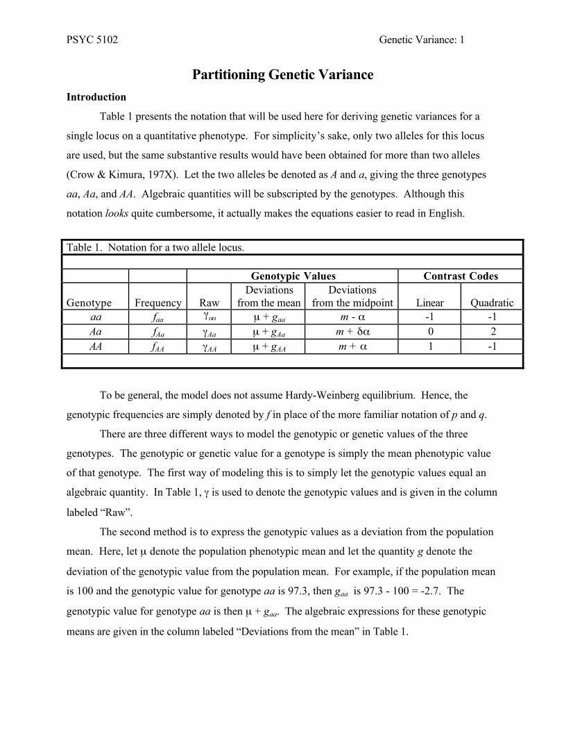
PSYC 5102 Genetic Variance: 1 Partitioning Genetic Variance Introduction Table 1 presents the notation that will be used here for deriving genetic variances for a single locus on a quantitative phenotype. For simplicity’s sake, only two alleles for this locus are used, but the same substantive results would have been obtained for more than two alleles (Crow & Kimura, 197X). Let the two alleles be denoted as A and a, giving the three genotypes aa, Aa, and AA. Algebraic quantities will be subscripted by the genotypes. Although this notation looks quite cumbersome, it actually makes the equations easier to read in English. Table 1. Notation for a two allele locus. Genotypic Values Contrast Codes Genotype Frequency Raw Deviations from the mean Deviations from the midpoint Linear Quadratic aa f aa γ αα μ + g aa m - α -1 -1 Aa f Aa γ Aa μ + g Aa m + δα 0 2 AA f AA γ AA μ + g AA m + α 1 -1 To be general, the model does not assume Hardy-Weinberg equilibrium. Hence, the genotypic frequencies are simply denoted by f in place of the more familiar notation of p and q. There are three different ways to model the genotypic or genetic values of the three genotypes. The genotypic or genetic value for a genotype is simply the mean phenotypic value of that genotype. The first way of modeling this is to simply let the genotypic values equal an algebraic quantity. In Table 1, γ is used to denote the genotypic values and is given in the column labeled “Raw”. The second method is to express the genotypic values as a deviation from the population mean. Here, let μ denote the population phenotypic mean and let the quantity g denote the deviation of the genotypic value from the population mean. For example, if the population mean is 100 and the genotypic value for genotype aa is 97.3, then g aa is 97.3 - 100 = -2.7. The genotypic value for genotype aa is then μ + g aa . The algebraic expressions for these genotypic means are given in the column labeled “Deviations from the mean” in Table 1.

Welcome message from author
This document is posted to help you gain knowledge. Please leave a comment to let me know what you think about it! Share it to your friends and learn new things together.
Transcript
PSYC 5102 Genetic Variance: 1
Partitioning Genetic Variance
Introduction
Table 1 presents the notation that will be used here for deriving genetic variances for a
single locus on a quantitative phenotype. For simplicity’s sake, only two alleles for this locus
are used, but the same substantive results would have been obtained for more than two alleles
(Crow & Kimura, 197X). Let the two alleles be denoted as A and a, giving the three genotypes
aa, Aa, and AA. Algebraic quantities will be subscripted by the genotypes. Although this
notation looks quite cumbersome, it actually makes the equations easier to read in English.
Table 1. Notation for a two allele locus.
Genotypic Values Contrast Codes
Genotype Frequency RawDeviations
from the meanDeviations
from the midpoint Linear Quadraticaa faa
γαα µ + gaa m - α -1 -1Aa fAa γAa µ + gAa m + δα 0 2AA fAA γAA µ + gAA m + α 1 -1
To be general, the model does not assume Hardy-Weinberg equilibrium. Hence, the
genotypic frequencies are simply denoted by f in place of the more familiar notation of p and q.
There are three different ways to model the genotypic or genetic values of the three
genotypes. The genotypic or genetic value for a genotype is simply the mean phenotypic value
of that genotype. The first way of modeling this is to simply let the genotypic values equal an
algebraic quantity. In Table 1, γ is used to denote the genotypic values and is given in the column
labeled “Raw”.
The second method is to express the genotypic values as a deviation from the population
mean. Here, let µ denote the population phenotypic mean and let the quantity g denote the
deviation of the genotypic value from the population mean. For example, if the population mean
is 100 and the genotypic value for genotype aa is 97.3, then gaa is 97.3 - 100 = -2.7. The
genotypic value for genotype aa is then µ + gaa. The algebraic expressions for these genotypic
means are given in the column labeled “Deviations from the mean” in Table 1.
PSYC 5102 Genetic Variance: 2
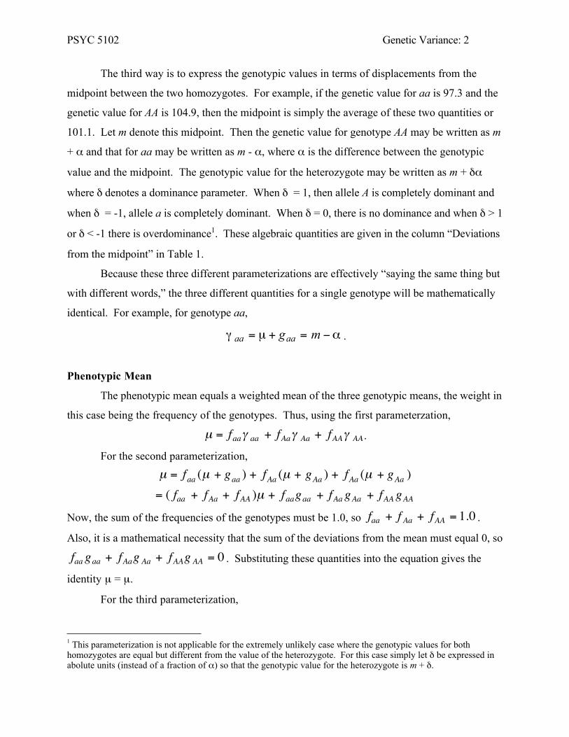
The third way is to express the genotypic values in terms of displacements from the
midpoint between the two homozygotes. For example, if the genetic value for aa is 97.3 and the
genetic value for AA is 104.9, then the midpoint is simply the average of these two quantities or
101.1. Let m denote this midpoint. Then the genetic value for genotype AA may be written as m
+ α and that for aa may be written as m - α, where α is the difference between the genotypic
value and the midpoint. The genotypic value for the heterozygote may be written as m + δα
where δ denotes a dominance parameter. When δ = 1, then allele A is completely dominant and
when δ = -1, allele a is completely dominant. When δ = 0, there is no dominance and when δ > 1
or δ < -1 there is overdominance1. These algebraic quantities are given in the column “Deviations
from the midpoint” in Table 1.
Because these three different parameterizations are effectively “saying the same thing but
with different words,” the three different quantities for a single genotype will be mathematically
identical. For example, for genotype aa,
γ aa = µ + gaa = m −α .
Phenotypic Mean
The phenotypic mean equals a weighted mean of the three genotypic means, the weight in
this case being the frequency of the genotypes. Thus, using the first parameterzation,
µ = faaγ aa + fAaγ Aa + fAAγ AA .
For the second parameterization,
µ = faa (µ + gaa ) + fAa (µ + gAa ) + fAa (µ + gAa )= ( faa + fAa + fAA )µ + faagaa + fAa gAa + fAA gAA
Now, the sum of the frequencies of the genotypes must be 1.0, so faa + f Aa + fAA = 1.0 .
Also, it is a mathematical necessity that the sum of the deviations from the mean must equal 0, so
faa gaa + fAag Aa + fAAg AA = 0 . Substituting these quantities into the equation gives the
identity µ = µ.
For the third parameterization,
1 This parameterization is not applicable for the extremely unlikely case where the genotypic values for bothhomozygotes are equal but different from the value of the heterozygote. For this case simply let δ be expressed inabolute units (instead of a fraction of α) so that the genotypic value for the heterozygote is m + δ.

PSYC 5102 Genetic Variance: 3
µ = faa (m −α ) + fAa (m + δα) + f AA (m + α)which reduces to
µ = m +α( fAA − faa + fAaδ ).
Phenotypic Variance
The equation for the phenotypic value for the ith person with the jth genotype (or Pij)
may be written in a general form as
Pij = γ j + Rij .
where Rij denotes a residual deviation from the population mean. This residual value will include
all environmental factors as well as the influence of all loci other than the A locus. For example,
the phenotypic value for the ith person with genotype aa will be
Pi.aa = γ aa + Ri.aa = µ + gaa + Ri.aa = m −α + Ri.aa .
In English, this equation states that that an individual’s phenotypic value equals the genotypic
mean for his/hers genotype plus the effects of “all other genetic and environmental factors.” At
this point, we note that this model assumes no gene-gene interaction (aka epistasis) involving the
A locus and no gene-environment interaction involving the A locus. (There may indeed be
epistasis and/or gene-environment interaction involving other loci; this assumption applies only
to the A locus.) We also introduce a second assumption of no covariance between the genotypic
values at the A locus and any other genes and environments. Because of this assumption, the
mean value for R for each of the three genotypes will be 0.
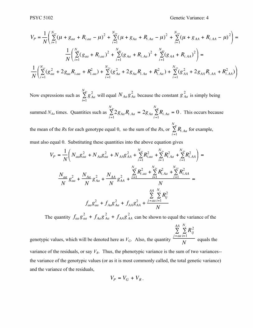
Just as the phenotypic mean was the weighted sum of the genotypic means, the
phenotypic variance will equal the weighted squared deviations from the mean. To see how this
is so, we first write the phenotypic variance in summation notation,
PSYC 5102 Genetic Variance: 4
VP =1N
(µ + gaa + Ri.aa − µ)2i= 1
Naa
∑ + (µ + gAa + Ri.Aa − µ)2i =1
NAa
∑ + (µ + gAA + Ri.AA − µ)2i=1
NAA
∑
=
1N
(gaa + Ri.aa )2
i=1
Naa
∑ + (gAa + Ri.Aa )2
i =1
NAa
∑ + (gAA + Ri.AA)2
i =1
NAA
∑
=
1N
(gaa2 + 2gaaRi.aa + Ri.aa
2 )i =1
Naa
∑ + (gAa2 + 2gAaRi.Aa + Ri.Aa
2 )i =1
NAa
∑ + (gAA2 + 2gAARi.AA + Ri.AA
2 )i =1
NAA
∑
Now expressions such as gAa2
i=1
NAa
∑ will equal NAa gAa2
because the constant g Aa2
is simply being
summed NAa times. Quantities such as 2gAaRi.Aai =1
NAa
∑ = 2gAa Ri.Aai =1
NAa
∑ = 0 . This occurs because
the mean of the Rs for each genotype equal 0, so the sum of the Rs, or Ri.Aai =1
NAa
∑ for example,
must also equal 0. Substituting these quantities into the above equation gives
VP =1N
Naagaa2 + NAagaa2 + NAAgAA2 + Ri.aa2 +i =1
Naa
∑ Ri.Aa2 +i= 1
NAa
∑ Ri.AA2
i =1
NAA
∑
=
Naa
Ngaa2 +
NAa
NgAa2 +
NAA
NgAA2 +
Ri.aa2 +
i =1
Naa
∑ Ri.Aa2 +
i=1
NAa
∑ Ri.AA2
i =1
NAA
∑
N=
faagaa2 + fAagAa
2 + fAAgAA2 +
Rij2
i=1
Nj
∑j =aa
AA∑
NThe quantity faa gaa
2 + fAag Aa2 + fAAg AA
2 can be shown to equal the variance of the
genotypic values, which will be denoted here as VG. Also, the quantity
Rij2
i=1
Nj
∑j =aa
AA∑
N equals the
variance of the residuals, or say VR. Thus, the phenotypic variance is the sum of two variances--
the variance of the genotypic values (or as it is most commonly called, the total genetic variance)
and the variance of the residuals,
VP = VG + VR .

PSYC 5102 Genetic Variance: 5
This result is almost intuitive to those who have had quantitative genetics. The purpose
of this exercise was not to demonstrate the obvious, but to demonstrate the techniques whereby
many further equations may be derived.2
Additive genetic variance
For a single locus, the total genetic variance is partitioned into two types of variance, the
additive genetic variance and dominance variance. Here we give the derivation for additive genetic
variance. We begin by noting the orthogonal contrast codes for the three genotypes at the right
hand side of table 1. There are two of these, a linear contrast code of -1, 0, and 1 for genotypes
aa, Aa, and AA, respectively, and a quadratic contrast code of -1, 2, and -1. The variance
associated with the linear contrast code is the additive genetic variance. To find out the algebraic
formula for this variance, we use a simple linear regression to regress the phenotypic values on
the contrast codes. The general equation for this is
Pij = a + bXlj + Uij
where Pij, as before, is the phenotypic value for the ith person with the jth genotype, X l jis the
value of the contrast code for the jth genotype, Uij is a residual, and a and b are respectively the
intercept and slope for the regression line. The equations for the two regression parameters are
b =cov(P,Xl )
VXl
and
a = µ − bX l .
The additive genetic variance is the variance associated with the slope of the regression line or
VA = b2VXl
=cov(P, Xl )2
VXl
.
To derive this quantity, it is necessary first to obtain expressions for the mean and
variance of variance Xl, the linear contrast codes. As before, we find the mean as a weighted sum
of the genotypic means, or
2 The summation notation will always give the correct result, but it is much more cumbersome than usingmathematical expectations. Students who wish to pursue this topic are urged to express the algebra in terms ofexpectaions.
PSYC 5102 Genetic Variance: 6
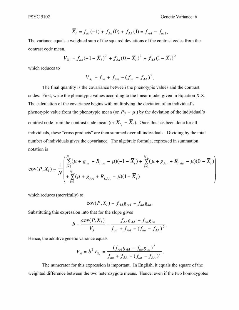
X l = faa (−1) + fAa (0) + fAA (1) = f AA − faa1 .
The variance equals a weighted sum of the squared deviations of the contrast codes from the
contrast code mean,
VXl= faa (−1− X l )
2 + fAa (0 − X l )2 + fAA (1− X l )
2
which reduces to
VXl = faa + fAA − ( faa − fAA )2.
The final quantity is the covariance between the phenotypic values and the contrast
codes. First, write the phenotypic values according to the linear model given in Equation X.X.
The calculation of the covariance begins with multiplying the deviation of an individual’s
phenotypic value from the phenotypic mean (or Pij − µ ) by the deviation of the individual’s
contrast code from the contrast code mean (or Xl j− X l ). Once this has been done for all
individuals, these “cross products” are then summed over all individuals. Dividing by the total
number of individuals gives the covariance. The algebraic formula, expressed in summation
notation is
cov(P, Xl ) =1N
(µ + gaa + Ri.aa − µ)(−1 − X l )i=1
Naa
∑ + (µ + gAa + Ri.Aa − µ)(0 − X l )i =1
N Aa
∑
+ (µ + gAA + Ri.AA − µ)(1− X l )i=1
N AA
∑
which reduces (mercifully) to
cov(P, Xl ) = fAAgAA − faa gaa .
Substituting this expression into that for the slope gives
b =cov(P,Xl )
VXl
=fAAgAA − faagaa
faa + fAA − ( faa − fAA )2.
Hence, the additive genetic variance equals
VA = b2VXl
=( fAA gAA − faa gaa )2
faa + fAA − ( faa − fAA )2.
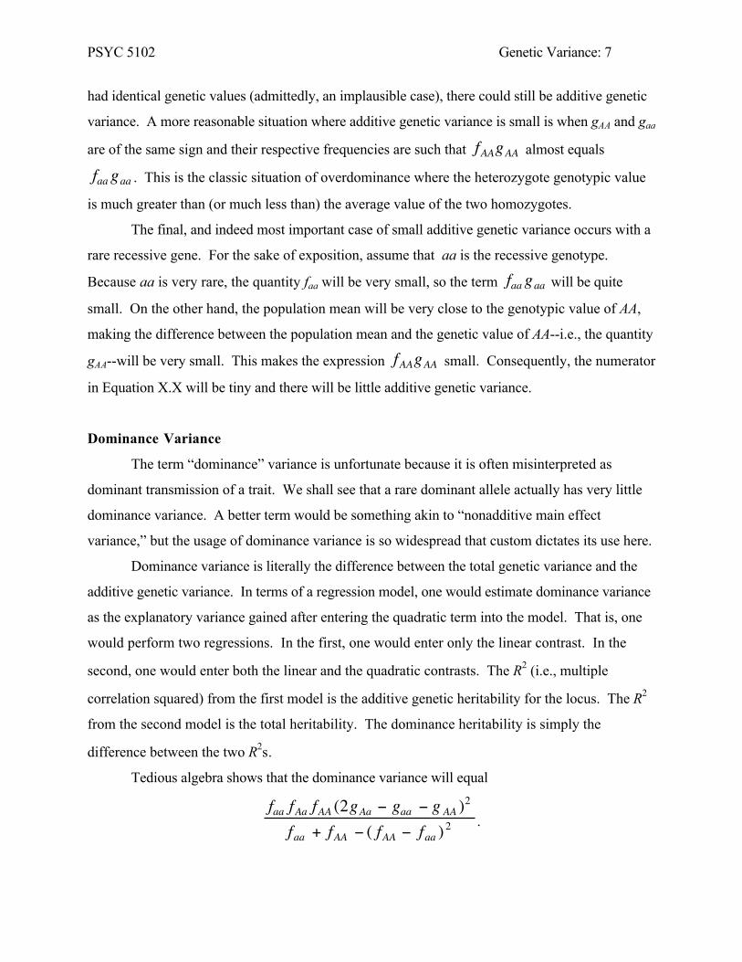
The numerator for this expression is important. In English, it equals the square of the
weighted difference between the two heterozygote means. Hence, even if the two homozygotes
PSYC 5102 Genetic Variance: 7
had identical genetic values (admittedly, an implausible case), there could still be additive genetic
variance. A more reasonable situation where additive genetic variance is small is when gAA and gaa
are of the same sign and their respective frequencies are such that fAAgAA almost equals
faa gaa . This is the classic situation of overdominance where the heterozygote genotypic value
is much greater than (or much less than) the average value of the two homozygotes.
The final, and indeed most important case of small additive genetic variance occurs with a
rare recessive gene. For the sake of exposition, assume that aa is the recessive genotype.
Because aa is very rare, the quantity faa will be very small, so the term faa gaa will be quite
small. On the other hand, the population mean will be very close to the genotypic value of AA,
making the difference between the population mean and the genetic value of AA--i.e., the quantity
gAA--will be very small. This makes the expression fAAgAA small. Consequently, the numerator
in Equation X.X will be tiny and there will be little additive genetic variance.
Dominance Variance
The term “dominance” variance is unfortunate because it is often misinterpreted as
dominant transmission of a trait. We shall see that a rare dominant allele actually has very little
dominance variance. A better term would be something akin to “nonadditive main effect
variance,” but the usage of dominance variance is so widespread that custom dictates its use here.
Dominance variance is literally the difference between the total genetic variance and the
additive genetic variance. In terms of a regression model, one would estimate dominance variance
as the explanatory variance gained after entering the quadratic term into the model. That is, one
would perform two regressions. In the first, one would enter only the linear contrast. In the
second, one would enter both the linear and the quadratic contrasts. The R2 (i.e., multiple
correlation squared) from the first model is the additive genetic heritability for the locus. The R2
from the second model is the total heritability. The dominance heritability is simply the
difference between the two R2s.
Tedious algebra shows that the dominance variance will equal
faa fAa fAA (2gAa − gaa − g AA )2
faa + fAA − ( fAA − faa )2.
PSYC 5102 Genetic Variance: 8
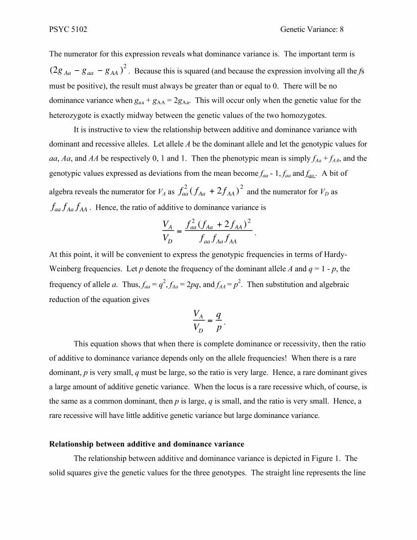
The numerator for this expression reveals what dominance variance is. The important term is
(2g Aa − gaa − gAA )2
. Because this is squared (and because the expression involving all the fs
must be positive), the result must always be greater than or equal to 0. There will be no
dominance variance when gaa + gAA = 2gAa. This will occur only when the genetic value for the
heterozygote is exactly midway between the genetic values of the two homozygotes.
It is instructive to view the relationship between additive and dominance variance with
dominant and recessive alleles. Let allele A be the dominant allele and let the genotypic values for
aa, Aa, and AA be respectively 0, 1 and 1. Then the phenotypic mean is simply fAa + fAA, and the
genotypic values expressed as deviations from the mean become faa - 1, faa and f aa . A bit of
algebra reveals the numerator for VA as faa2 ( fAa + 2 f AA )
2 and the numerator for VD as
faa fAa fAA . Hence, the ratio of additive to dominance variance is
VAVD
=faa2 ( fAa + 2 fAA )2
faa fAa fAA.
At this point, it will be convenient to express the genotypic frequencies in terms of Hardy-
Weinberg frequencies. Let p denote the frequency of the dominant allele A and q = 1 - p, the
frequency of allele a. Thus, faa = q2, fAa = 2pq, and fAA = p2. Then substitution and algebraic
reduction of the equation gives
VAVD
=qp .
This equation shows that when there is complete dominance or recessivity, then the ratio
of additive to dominance variance depends only on the allele frequencies! When there is a rare
dominant, p is very small, q must be large, so the ratio is very large. Hence, a rare dominant gives
a large amount of additive genetic variance. When the locus is a rare recessive which, of course, is
the same as a common dominant, then p is large, q is small, and the ratio is very small. Hence, a
rare recessive will have little additive genetic variance but large dominance variance.
Relationship between additive and dominance variance
The relationship between additive and dominance variance is depicted in Figure 1. The
solid squares give the genetic values for the three genotypes. The straight line represents the line

PSYC 5102 Genetic Variance: 9
of best fit when regressing these genotypic values upon the linear contrast codes. The variance
associated with this straight line is the additive genetic variance.
The deviations of the actual genotypic values from their values predicted on the values of
the regression line are depicted by the double headed arrows. These are prediction errors from
the simple additive model. The variance associated with these prediction errors are the
dominance variance. Literally, computation of dominance variance would begin by measuring the
length of a double headed arrow. Then square that length and then multiply this squared length
by the frequency of the genotype. Summing these “weighted square lengths” over the three
genotypes gives the dominance variance.
Figure 1: Additivity and Dominance
aa Aa AA
Genotype
Genotypic
Value
Epistasis
Epistasis occurs when genes and/or gene products interact and epistatic variance is the
statistical interaction variance. It is important to emphasis the term statistical in this definition.
It is entirely possible for biochemical products of loci to physically interact but this does not
necessarily lead to a statistical interaction3. Classic examples of epistasis for behavior can be
seen in many rare genetic disorders. A Tay-Sachs genotype, for example, interacts with those
loci that contribute to individual differences in normal cognitive development during infancy. If
an infant has Tay-Sachs disease, the expression of these normal loci is inhibited. For those
without Tay-Sachs disease, the other loci will be expressed. However, epistatic variance for the
Tay-Sachs locus will be very small because the disorder is very rare.
3 The same must be said of the gene-environment interaction. In casual discourse, this term often implies that bothgenes and environment are important for behavior. In quantitative genetics, however, the term implies a statisticalinteraction. Hence, when heritability is less than 1.0, there is always gene-environment interaction in the loosesense, but there may be no gene-environment interaction in the strict sense.
PSYC 5102 Genetic Variance: 10
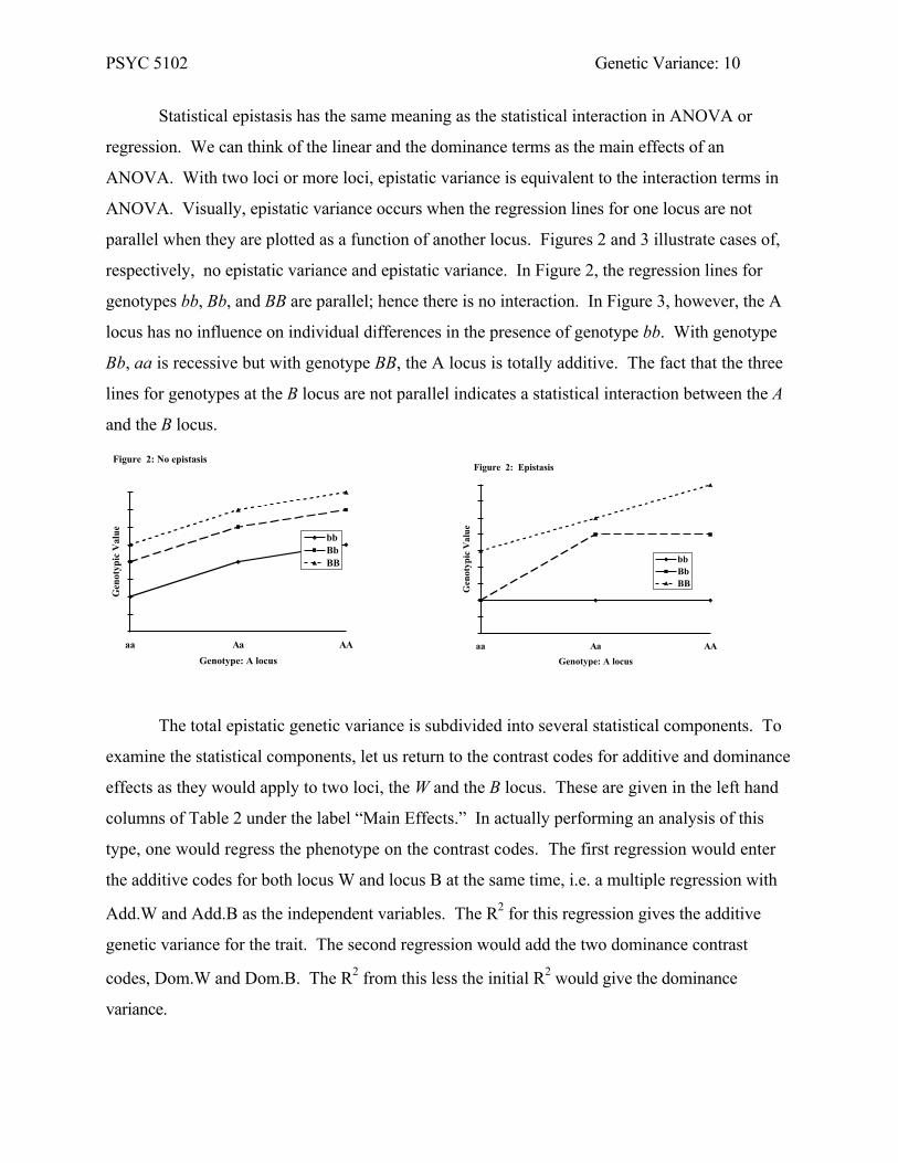
Statistical epistasis has the same meaning as the statistical interaction in ANOVA or
regression. We can think of the linear and the dominance terms as the main effects of an
ANOVA. With two loci or more loci, epistatic variance is equivalent to the interaction terms in
ANOVA. Visually, epistatic variance occurs when the regression lines for one locus are not
parallel when they are plotted as a function of another locus. Figures 2 and 3 illustrate cases of,
respectively, no epistatic variance and epistatic variance. In Figure 2, the regression lines for
genotypes bb, Bb, and BB are parallel; hence there is no interaction. In Figure 3, however, the A
locus has no influence on individual differences in the presence of genotype bb. With genotype
Bb, aa is recessive but with genotype BB, the A locus is totally additive. The fact that the three
lines for genotypes at the B locus are not parallel indicates a statistical interaction between the A
and the B locus.
Figure 2: No epistasis
aa Aa AA
Genotype: A locus
Gen
otyp
ic V
alue bb
BbBB
Figure 2: Epistasis
aa Aa AA
Genotype: A locus
Gen
otyp
ic V
alue
bbBbBB
The total epistatic genetic variance is subdivided into several statistical components. To
examine the statistical components, let us return to the contrast codes for additive and dominance
effects as they would apply to two loci, the W and the B locus. These are given in the left hand
columns of Table 2 under the label “Main Effects.” In actually performing an analysis of this
type, one would regress the phenotype on the contrast codes. The first regression would enter
the additive codes for both locus W and locus B at the same time, i.e. a multiple regression with
Add.W and Add.B as the independent variables. The R2 for this regression gives the additive
genetic variance for the trait. The second regression would add the two dominance contrast
codes, Dom.W and Dom.B. The R2 from this less the initial R2 would give the dominance
variance.

PSYC 5102 Genetic Variance: 11
Table 2. Contrast codes for two loci.
Main Effects Interactions
Additive DominanceAdditive*Additive
Additive*Domiance
Dominance*Dominance
Geno-type
Add.W
Add.B
DomW
DomB
Add.W*Add.B
Add.W*Dom.B
Dom.W*Add.B
Dom.W*Dom.B
WWBB 1 1 -1 -1 1 -1 -1 1WWBb 1 0 -1 2 0 2 0 -2WWbb 1 -1 -1 -1 -1 -1 1 1WwBB 0 1 2 -1 0 0 2 -2WwBb 0 0 2 2 0 0 0 4Wwbb 0 -1 2 -1 0 0 -2 -2wwBB -1 1 -1 -1 -1 1 -1 1wwBb -1 0 -1 2 0 -2 0 -2wwbb -1 -1 -1 -1 1 1 1 1
The epistatic or interaction variance is literally the results of multiplying the additive and
dominance contrast codes for the W locus with those for the B locus. Multiplying the additive
code for W (Add.W) with that for B (Add.B) gives the contrast code for the first epistatic
component, additive by additive epistasis. The variance associated with this contrast code is
called additive by additive epistatic variance and is usually abbreviated as VAA. On would
estimate this component by entering the contrast code into the regression equation. There are
now five independent variables (Add.W, Add.B, Dom.W, Dom.B, and Add.W*Add.B). The R2
for this less the R2 for the model containing dominance gives the estimate of VAA.
The second epistatic component involves multiplying the additive contrast codes for one
locus and the dominance codes for the other locus. There are two ways of doing this. The first
way is to multiply Add.W with Dom.B, and the second is to multiply Dom.W with Add.B.
Entering both of these contrast codes into the last regression equation and subtracting the R2 from
the previous R2 gives what is called the additive by dominance epistatic variance, or VAD.
The final epistatic component is VDD or dominance by dominance epistasis. This is
estimated by multiplying the two dominance contrast codes together, entering the resulting
contrast code into the last regression equation, and subtracting the R2s.
PSYC 5102 Genetic Variance: 12
Epistatic components for additional loci will be formed in a similar way, but there will be
more epistatic components. For example, let us add the C locus to the above problem. There
would now be three additive by additive contrast codes, Add.W*Add.B, Add.W*Add.C, and
Add.B*Add.C. Entering these three contrast codes simultaneously into the regression and
subtracting the R2s would now give the estimate of VAA, the additive by additive epistatic
variance. Following this logic would give 6 contrast codes for estimating VAD (or all the two way
interactions between the additive and dominance contrast codes), and 3 for VD (or all the two way
interactions among the dominance contrast codes.
With the three locus case, however, there is also the possibility of three way interactions
among the loci. Just as the two way interactions were subdivided into components, so are the
three way epistatic interactions subdivided into individual components that reflect the products
of the additive and dominance contrast codes. The first of these would be VAAA or the additive by
additive by additive epistatic variance. The contrast code for this is simply
Add.W*Add.B*Add.C, or the product of the three additive contrast codes. The second
component would be VAAD (additive by additive by dominance epistatic variance), the next
component would be VADD (additive by dominance by dominance epistatic variance), and the final
three way interaction would be VDDD (the dominance by dominance by dominance epistatic
variance). Once again the contrast codes may be found by multiply all the relevant additive and
dominance main effects contrast codes, and the variance components would be estimated by
hierarchical multiple regression.
The total epistatic variance for the three locus case is simply the addition of all the
individual components of variance. Let VI denote the total epistatic variance. Then,
VI = VAA + VAD + VDD + VAAA +VAAD + VADD + VDDD .
Additional loci may be accommodated using identical logic. With n loci, the variance
component VAA is simply the sum of all two way additive by additive interactions among all n
loci, VAAD is the sum of all possible additive by additive by dominance interactions among n loci,
and so on.
Related Documents