Package ‘distrEx’ July 22, 2018 Version 2.7.0 Date 2018-07-08 Title Extensions of Package 'distr' Description Extends package 'distr' by functionals, distances, and conditional distributions. Depends R(>= 2.10.0), methods, distr(>= 2.2) Imports startupmsg, utils, stats Suggests tcltk ByteCompile yes License LGPL-3 Encoding latin1 URL http://distr.r-forge.r-project.org/ LastChangedDate {$LastChangedDate: 2018-07-08 16:31:26 +0200 (So, 08. Jul 2018) $} LastChangedRevision {$LastChangedRevision: 1187 $} SVNRevision 1186 NeedsCompilation yes Author Matthias Kohl [cre, cph], Peter Ruckdeschel [aut, cph] Maintainer Matthias Kohl <[email protected]> Repository CRAN Date/Publication 2018-07-22 20:40:07 UTC R topics documented: distrEx-package ....................................... 2 AbscontCondDistribution-class ............................... 7 AsymTotalVarDist ..................................... 8 Condition-class ....................................... 11 ContaminationSize ..................................... 12 1

Welcome message from author
This document is posted to help you gain knowledge. Please leave a comment to let me know what you think about it! Share it to your friends and learn new things together.
Transcript
Package ‘distrEx’July 22, 2018
Version 2.7.0
Date 2018-07-08
Title Extensions of Package 'distr'
Description Extends package 'distr' by functionals, distances, and conditional distributions.
Depends R(>= 2.10.0), methods, distr(>= 2.2)
Imports startupmsg, utils, stats
Suggests tcltk
ByteCompile yes
License LGPL-3
Encoding latin1
URL http://distr.r-forge.r-project.org/
LastChangedDate $LastChangedDate: 2018-07-08 16:31:26 +0200 (So, 08.Jul 2018) $
LastChangedRevision $LastChangedRevision: 1187 $
SVNRevision 1186
NeedsCompilation yes
Author Matthias Kohl [cre, cph],Peter Ruckdeschel [aut, cph]
Maintainer Matthias Kohl <[email protected]>
Repository CRAN
Date/Publication 2018-07-22 20:40:07 UTC
R topics documented:distrEx-package . . . . . . . . . . . . . . . . . . . . . . . . . . . . . . . . . . . . . . . 2AbscontCondDistribution-class . . . . . . . . . . . . . . . . . . . . . . . . . . . . . . . 7AsymTotalVarDist . . . . . . . . . . . . . . . . . . . . . . . . . . . . . . . . . . . . . 8Condition-class . . . . . . . . . . . . . . . . . . . . . . . . . . . . . . . . . . . . . . . 11ContaminationSize . . . . . . . . . . . . . . . . . . . . . . . . . . . . . . . . . . . . . 12
1
2 distrEx-package
ConvexContamination . . . . . . . . . . . . . . . . . . . . . . . . . . . . . . . . . . . 13CvMDist . . . . . . . . . . . . . . . . . . . . . . . . . . . . . . . . . . . . . . . . . . 15dim-methods . . . . . . . . . . . . . . . . . . . . . . . . . . . . . . . . . . . . . . . . 16DiscreteCondDistribution-class . . . . . . . . . . . . . . . . . . . . . . . . . . . . . . . 17DiscreteMVDistribution . . . . . . . . . . . . . . . . . . . . . . . . . . . . . . . . . . 18DiscreteMVDistribution-class . . . . . . . . . . . . . . . . . . . . . . . . . . . . . . . 19distrExIntegrate . . . . . . . . . . . . . . . . . . . . . . . . . . . . . . . . . . . . . . . 20distrExMASK . . . . . . . . . . . . . . . . . . . . . . . . . . . . . . . . . . . . . . . . 22distrExMOVED . . . . . . . . . . . . . . . . . . . . . . . . . . . . . . . . . . . . . . . 23distrExOptions . . . . . . . . . . . . . . . . . . . . . . . . . . . . . . . . . . . . . . . 23E . . . . . . . . . . . . . . . . . . . . . . . . . . . . . . . . . . . . . . . . . . . . . . . 25EmpiricalMVDistribution . . . . . . . . . . . . . . . . . . . . . . . . . . . . . . . . . . 34EuclCondition . . . . . . . . . . . . . . . . . . . . . . . . . . . . . . . . . . . . . . . . 35EuclCondition-class . . . . . . . . . . . . . . . . . . . . . . . . . . . . . . . . . . . . . 36GLIntegrate . . . . . . . . . . . . . . . . . . . . . . . . . . . . . . . . . . . . . . . . . 37HellingerDist . . . . . . . . . . . . . . . . . . . . . . . . . . . . . . . . . . . . . . . . 38KolmogorovDist . . . . . . . . . . . . . . . . . . . . . . . . . . . . . . . . . . . . . . 41liesInSupport . . . . . . . . . . . . . . . . . . . . . . . . . . . . . . . . . . . . . . . . 43LMCondDistribution . . . . . . . . . . . . . . . . . . . . . . . . . . . . . . . . . . . . 44LMParameter . . . . . . . . . . . . . . . . . . . . . . . . . . . . . . . . . . . . . . . . 45LMParameter-class . . . . . . . . . . . . . . . . . . . . . . . . . . . . . . . . . . . . . 46m1df . . . . . . . . . . . . . . . . . . . . . . . . . . . . . . . . . . . . . . . . . . . . . 47m2df . . . . . . . . . . . . . . . . . . . . . . . . . . . . . . . . . . . . . . . . . . . . . 48make01 . . . . . . . . . . . . . . . . . . . . . . . . . . . . . . . . . . . . . . . . . . . 50MultivariateDistribution-class . . . . . . . . . . . . . . . . . . . . . . . . . . . . . . . 51OAsymTotalVarDist . . . . . . . . . . . . . . . . . . . . . . . . . . . . . . . . . . . . . 52plot-methods . . . . . . . . . . . . . . . . . . . . . . . . . . . . . . . . . . . . . . . . 55PrognCondDistribution . . . . . . . . . . . . . . . . . . . . . . . . . . . . . . . . . . . 56PrognCondDistribution-class . . . . . . . . . . . . . . . . . . . . . . . . . . . . . . . . 57PrognCondition-class . . . . . . . . . . . . . . . . . . . . . . . . . . . . . . . . . . . . 58TotalVarDist . . . . . . . . . . . . . . . . . . . . . . . . . . . . . . . . . . . . . . . . . 59UnivariateCondDistribution-class . . . . . . . . . . . . . . . . . . . . . . . . . . . . . . 62var . . . . . . . . . . . . . . . . . . . . . . . . . . . . . . . . . . . . . . . . . . . . . . 63
Index 74
distrEx-package distrEx – Extensions of Package distr
Description
distrEx provides some extensions of package distr:
• expectations in the form
– E(X) for the expectation of a distribution object X– E(X,f) for the expectation of f(X) where X is some distribution object and f some func-
tion in X

distrEx-package 3
• further functionals: var, sd, IQR, mad, median, skewness, kurtosis
• truncated moments,
• distances between distributions (Hellinger, Cramer von Mises, Kolmogorov, total variation,"convex contamination")
• lists of distributions,
• conditional distributions in factorized form
• conditional expectations in factorized form
Support for extreme value distributions has moved to package RobExtremes
Details
Package: distrExVersion: 2.7.0Date: 2018-07-08Depends: R(>= 2.10.0), methods, distr(>= 2.2)Imports: startupmsg, utils, statsSuggests: tcltkLazyLoad: yesLicense: LGPL-3URL: http://distr.r-forge.r-project.org/SVNRevision: 1186
Classes
Distribution Classes
"Distribution" (from distr)|>"UnivariateDistribution" (from distr)|>|>"AbscontDistribution" (from distr)|>|>|>"Gumbel"|>|>|>"Pareto"|>|>|>"GPareto"|>"MultivariateDistribution"|>|>"DiscreteMVDistribution-class"|>"UnivariateCondDistribution"|>|>"AbscontCondDistribution"|>|>|>"PrognCondDistribution"|>|>"DiscreteCondDistribution"
Condition Classes
4 distrEx-package
"Condition"|>"EuclCondition"|>"PrognCondition"
Parameter Classes
"OptionalParameter" (from distr)|>"Parameter" (from distr)|>|>"LMParameter"|>|>"GumbelParameter"|>|>"ParetoParameter"
Functions
Integration:GLIntegrate Gauss-Legendre quadraturedistrExIntegrate Integration of one-dimensional functions
Options:distrExOptions Function to change the global variables of the
package 'distrEx'Standardization:make01 Centering and standardization of univariate
distributions
Generating Functions
Distribution ClassesConvexContamination Generic function for generating convex
contaminationsDiscreteMVDistribution
Generating function forDiscreteMVDistribution-class
Gumbel Generating function for Gumbel-classLMCondDistribution Generating function for the conditional
distribution of a linear regression model.
Condition ClassesEuclCondition Generating function for EuclCondition-class
Parameter ClassesLMParameter Generating function for LMParameter-class
distrEx-package 5
Methods
Distances:ContaminationSize Generic function for the computation of the
convex contamination (Pseudo-)distance of twodistributions
HellingerDist Generic function for the computation of theHellinger distance of two distributions
KolmogorovDist Generic function for the computation of theKolmogorov distance of two distributions
TotalVarDist Generic function for the computation of thetotal variation distance of two distributions
AsymTotalVarDist Generic function for the computation of theasymmetric total variation distance of two distributions
(for given ratio rho of negative to positive part of deviation)OAsymTotalVarDist Generic function for the computation of the minimal (in rho)
asymmetric total variation distance of two distributionsvonMisesDist Generic function for the computation of the
von Mises distance of two distributions
liesInSupport Generic function for testing the support of adistribution
Functionals:E Generic function for the computation of
(conditional) expectationsvar Generic functions for the computation of
functionalsIQR Generic functions for the computation of
functionalssd Generic functions for the computation of
functionalsmad Generic functions for the computation of
functionalsmedian Generic functions for the computation of
functionalsskewness Generic functions for the computation of
functionalskurtosis Generic functions for the computation of
Functionals
truncated Moments:m1df Generic function for the computation of clipped
first momentsm2df Generic function for the computation of clipped
second moments
6 distrEx-package
Demos
Demos are available — see demo(package="distrEx").
Acknowledgement
G. Jay Kerns, <[email protected]>, has provided a major contribution, in particular the functionalsskewness and kurtosis are due to him. Natalyia Horbenko, <[email protected]>has ported the actuar code for the Pareto distribution to this setup.
Start-up-Banner
You may suppress the start-up banner/message completely by setting options("StartupBanner"="off")somewhere before loading this package by library or require in your R-code / R-session.
If option "StartupBanner" is not defined (default) or setting options("StartupBanner"=NULL)or options("StartupBanner"="complete") the complete start-up banner is displayed.
For any other value of option "StartupBanner" (i.e., not in c(NULL,"off","complete")) onlythe version information is displayed.
The same can be achieved by wrapping the library or require call into either suppressStartupMessages()or onlytypeStartupMessages(.,atypes="version").
As for general packageStartupMessage’s, you may also suppress all the start-up banner by wrap-ping the library or require call into suppressPackageStartupMessages() from startupmsg-version 0.5 on.
Package versions
Note: The first two numbers of package versions do not necessarily reflect package-individualdevelopment, but rather are chosen for the distrXXX family as a whole in order to ease updating"depends" information.
Note
Some functions of package stats have intentionally been masked, but completely retain their func-tionality — see distrExMASK().
If any of the packages e1071, moments, fBasics is to be used together with distrEx the latter mustbe attached after any of the first mentioned. Otherwise kurtosis() and skewness() defined asmethods in distrEx may get masked.To re-mask, you may use kurtosis <- distrEx::kurtosis; skewness <- distrEx::skewness.See also distrExMASK()
Author(s)
Matthias Kohl <[email protected]> andPeter Ruckdeschel <[email protected]>,
Maintainer: Matthias Kohl <[email protected]>

AbscontCondDistribution-class 7
References
P. Ruckdeschel, M. Kohl, T. Stabla, F. Camphausen (2006): S4 Classes for Distributions, R News,6(2), 2-6. https://CRAN.R-project.org/doc/Rnews/Rnews_2006-2.pdf
a vignette for packages distr, distrSim, distrTEst, and distrEx is included into the mere documen-tation package distrDoc and may be called by require("distrDoc");vignette("distr")
a homepage to this package is available underhttp://distr.r-forge.r-project.org/
M. Kohl (2005): Numerical Contributions to the Asymptotic Theory of Robustness. PhD Thesis.Bayreuth. Available as http://www.stamats.de/wp-content/uploads/2018/04/ThesisMKohl.pdf
See Also
distr-package
AbscontCondDistribution-class
Absolutely continuous conditional distribution
Description
The class of absolutely continuous conditional univariate distributions.
Objects from the Class
Objects can be created by calls of the form new("AbscontCondDistribution", ...).
Slots
cond Object of class "Condition": condition
img Object of class "rSpace": the image space.
param Object of class "OptionalParameter": an optional parameter.
r Object of class "function": generates random numbers.
d Object of class "OptionalFunction": optional conditional density function.
p Object of class "OptionalFunction": optional conditional cumulative distribution function.
q Object of class "OptionalFunction": optional conditional quantile function.
.withArith logical: used internally to issue warnings as to interpretation of arithmetics
.withSim logical: used internally to issue warnings as to accuracy
.logExact logical: used internally to flag the case where there are explicit formulae for the logversion of density, cdf, and quantile function
.lowerExact logical: used internally to flag the case where there are explicit formulae for thelower tail version of cdf and quantile function
Symmetry object of class "DistributionSymmetry"; used internally to avoid unnecessary calcu-lations.

8 AsymTotalVarDist
Extends
Class "UnivariateCondDistribution", directly.Class "Distribution", by class "UnivariateCondDistribution".
Author(s)
Matthias Kohl <[email protected]>
See Also
UnivariateCondDistribution-class, Distribution-class
Examples
new("AbscontCondDistribution")
AsymTotalVarDist Generic function for the computation of asymmetric total variationdistance of two distributions
Description
Generic function for the computation of asymmetric total variation distance dv(ρ) of two distribu-tions P and Q where the distributions may be defined for an arbitrary sample space (Ω,A). Forgiven ratio of inlier and outlier probability ρ, this distance is defined as
dv(ρ)(P,Q) =
∫(dQ− c dP )+
for c defined by
ρ
∫(dQ− c dP )+ =
∫(dQ− c dP )−
It coincides with total variation distance for ρ = 1.
Usage
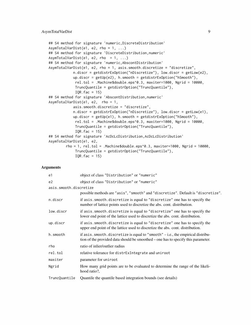
AsymTotalVarDist(e1, e2, ...)## S4 method for signature 'AbscontDistribution,AbscontDistribution'AsymTotalVarDist(e1,e2, rho = 1,
rel.tol = .Machine$double.eps^0.3, maxiter=1000, Ngrid = 10000,TruncQuantile = getdistrOption("TruncQuantile"),IQR.fac = 15)
## S4 method for signature 'AbscontDistribution,DiscreteDistribution'AsymTotalVarDist(e1,e2, rho = 1, ...)## S4 method for signature 'DiscreteDistribution,AbscontDistribution'AsymTotalVarDist(e1,e2, rho = 1, ...)## S4 method for signature 'DiscreteDistribution,DiscreteDistribution'AsymTotalVarDist(e1,e2, rho = 1, ...)
AsymTotalVarDist 9
## S4 method for signature 'numeric,DiscreteDistribution'AsymTotalVarDist(e1, e2, rho = 1, ...)## S4 method for signature 'DiscreteDistribution,numeric'AsymTotalVarDist(e1, e2, rho = 1, ...)## S4 method for signature 'numeric,AbscontDistribution'AsymTotalVarDist(e1, e2, rho = 1, asis.smooth.discretize = "discretize",
n.discr = getdistrExOption("nDiscretize"), low.discr = getLow(e2),up.discr = getUp(e2), h.smooth = getdistrExOption("hSmooth"),rel.tol = .Machine$double.eps^0.3, maxiter=1000, Ngrid = 10000,TruncQuantile = getdistrOption("TruncQuantile"),IQR.fac = 15)
## S4 method for signature 'AbscontDistribution,numeric'AsymTotalVarDist(e1, e2, rho = 1,
asis.smooth.discretize = "discretize",n.discr = getdistrExOption("nDiscretize"), low.discr = getLow(e1),up.discr = getUp(e1), h.smooth = getdistrExOption("hSmooth"),rel.tol = .Machine$double.eps^0.3, maxiter=1000, Ngrid = 10000,TruncQuantile = getdistrOption("TruncQuantile"),IQR.fac = 15)
## S4 method for signature 'AcDcLcDistribution,AcDcLcDistribution'AsymTotalVarDist(e1, e2,
rho = 1, rel.tol = .Machine$double.eps^0.3, maxiter=1000, Ngrid = 10000,TruncQuantile = getdistrOption("TruncQuantile"),IQR.fac = 15)
Arguments
e1 object of class "Distribution" or "numeric"
e2 object of class "Distribution" or "numeric"asis.smooth.discretize
possible methods are "asis", "smooth" and "discretize". Default is "discretize".
n.discr if asis.smooth.discretize is equal to "discretize" one has to specify thenumber of lattice points used to discretize the abs. cont. distribution.
low.discr if asis.smooth.discretize is equal to "discretize" one has to specify thelower end point of the lattice used to discretize the abs. cont. distribution.
up.discr if asis.smooth.discretize is equal to "discretize" one has to specify theupper end point of the lattice used to discretize the abs. cont. distribution.
h.smooth if asis.smooth.discretize is equal to "smooth" – i.e., the empirical distribu-tion of the provided data should be smoothed – one has to specify this parameter.
rho ratio of inlier/outlier radius
rel.tol relative tolerance for distrExIntegrate and uniroot
maxiter parameter for uniroot
Ngrid How many grid points are to be evaluated to determine the range of the likeli-hood ratio?,
TruncQuantile Quantile the quantile based integration bounds (see details)
10 AsymTotalVarDist
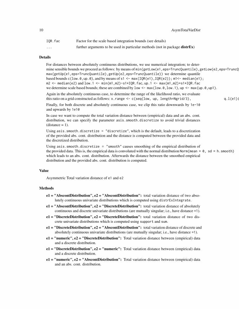
IQR.fac Factor for the scale based integration bounds (see details)
... further arguments to be used in particular methods (not in package distrEx)
Details
For distances between absolutely continuous distributions, we use numerical integration; to deter-mine sensible bounds we proceed as follows: by means of min(getLow(e1,eps=TruncQuantile),getLow(e2,eps=TruncQuantile)),max(getUp(e1,eps=TruncQuantile),getUp(e2,eps=TruncQuantile)) we determine quantilebased bounds c(low.0,up.0), and by means of s1 <- max(IQR(e1),IQR(e2)); m1<- median(e1);m2 <- median(e2) and low.1 <- min(m1,m2)-s1*IQR.fac, up.1 <- max(m1,m2)+s1*IQR.facwe determine scale based bounds; these are combined by low <- max(low.0,low.1), up <- max(up.0,up1).
Again in the absolutely continuous case, to determine the range of the likelihood ratio, we evaluatethis ratio on a grid constructed as follows: x.range <- c(seq(low, up, length=Ngrid/3), q.l(e1)(seq(0,1,length=Ngrid/3)*.999), q.l(e2)(seq(0,1,length=Ngrid/3)*.999))
Finally, for both discrete and absolutely continuous case, we clip this ratio downwards by 1e-10and upwards by 1e10
In case we want to compute the total variation distance between (empirical) data and an abs. cont.distribution, we can specify the parameter asis.smooth.discretize to avoid trivial distances(distance = 1).
Using asis.smooth.discretize = "discretize", which is the default, leads to a discretizationof the provided abs. cont. distribution and the distance is computed between the provided data andthe discretized distribution.
Using asis.smooth.discretize = "smooth" causes smoothing of the empirical distribution ofthe provided data. This is, the empirical data is convoluted with the normal distribution Norm(mean = 0, sd = h.smooth)which leads to an abs. cont. distribution. Afterwards the distance between the smoothed empiricaldistribution and the provided abs. cont. distribution is computed.
Value
Asymmetric Total variation distance of e1 and e2
Methods
e1 = "AbscontDistribution", e2 = "AbscontDistribution": total variation distance of two abso-lutely continuous univariate distributions which is computed using distrExIntegrate.
e1 = "AbscontDistribution", e2 = "DiscreteDistribution": total variation distance of absolutelycontinuous and discrete univariate distributions (are mutually singular; i.e., have distance =1).
e1 = "DiscreteDistribution", e2 = "DiscreteDistribution": total variation distance of two dis-crete univariate distributions which is computed using support and sum.
e1 = "DiscreteDistribution", e2 = "AbscontDistribution": total variation distance of discrete andabsolutely continuous univariate distributions (are mutually singular; i.e., have distance =1).
e1 = "numeric", e2 = "DiscreteDistribution": Total variation distance between (empirical) dataand a discrete distribution.
e1 = "DiscreteDistribution", e2 = "numeric": Total variation distance between (empirical) dataand a discrete distribution.
e1 = "numeric", e2 = "AbscontDistribution": Total variation distance between (empirical) dataand an abs. cont. distribution.
Condition-class 11
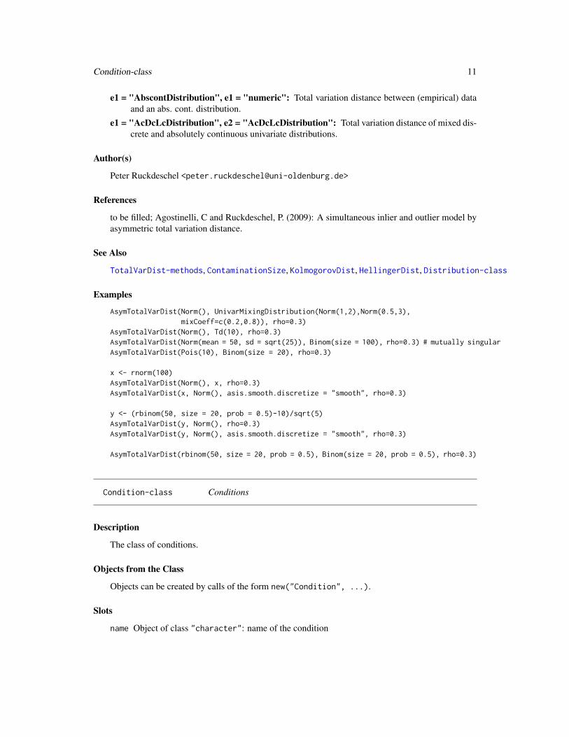
e1 = "AbscontDistribution", e1 = "numeric": Total variation distance between (empirical) dataand an abs. cont. distribution.
e1 = "AcDcLcDistribution", e2 = "AcDcLcDistribution": Total variation distance of mixed dis-crete and absolutely continuous univariate distributions.
Author(s)
Peter Ruckdeschel <[email protected]>
References
to be filled; Agostinelli, C and Ruckdeschel, P. (2009): A simultaneous inlier and outlier model byasymmetric total variation distance.
See Also
TotalVarDist-methods, ContaminationSize, KolmogorovDist, HellingerDist, Distribution-class
Examples
AsymTotalVarDist(Norm(), UnivarMixingDistribution(Norm(1,2),Norm(0.5,3),mixCoeff=c(0.2,0.8)), rho=0.3)
AsymTotalVarDist(Norm(), Td(10), rho=0.3)AsymTotalVarDist(Norm(mean = 50, sd = sqrt(25)), Binom(size = 100), rho=0.3) # mutually singularAsymTotalVarDist(Pois(10), Binom(size = 20), rho=0.3)
x <- rnorm(100)AsymTotalVarDist(Norm(), x, rho=0.3)AsymTotalVarDist(x, Norm(), asis.smooth.discretize = "smooth", rho=0.3)
y <- (rbinom(50, size = 20, prob = 0.5)-10)/sqrt(5)AsymTotalVarDist(y, Norm(), rho=0.3)AsymTotalVarDist(y, Norm(), asis.smooth.discretize = "smooth", rho=0.3)
AsymTotalVarDist(rbinom(50, size = 20, prob = 0.5), Binom(size = 20, prob = 0.5), rho=0.3)
Condition-class Conditions
Description
The class of conditions.
Objects from the Class
Objects can be created by calls of the form new("Condition", ...).
Slots
name Object of class "character": name of the condition
12 ContaminationSize
Methods
name signature(object = "Condition"): accessor function for slot name.
name<- signature(object = "Condition"): replacement function for slot name.
Author(s)
Matthias Kohl <[email protected]>
See Also
UnivariateCondDistribution-class
Examples
new("Condition")
ContaminationSize Generic Function for the Computation of the Convex Contamination(Pseudo-)Distance of Two Distributions
Description
Generic function for the computation of convex contamination (pseudo-)distance of two probabilitydistributions P and Q. That is, the minimal size ε ∈ [0, 1] is computed such that there exists someprobability distribution R with
Q = (1− ε)P + εR
Usage
ContaminationSize(e1, e2, ...)## S4 method for signature 'AbscontDistribution,AbscontDistribution'ContaminationSize(e1,e2)## S4 method for signature 'DiscreteDistribution,DiscreteDistribution'ContaminationSize(e1,e2)## S4 method for signature 'AcDcLcDistribution,AcDcLcDistribution'ContaminationSize(e1,e2)
Arguments
e1 object of class "Distribution"
e2 object of class "Distribution"
... further arguments to be used in particular methods (not in package distrEx)
Details
Computes the distance from e1 to e2 respectively P to Q. This is not really a distance as it is notsymmetric!
ConvexContamination 13
Value
A list containing the following components:
e1 object of class "Distribution"; ideal distribution
e2 object of class "Distribution"; ’contaminated’ distributionsize.of.contamination
size of contamination
Methods
e1 = "AbscontDistribution", e2 = "AbscontDistribution": convex contamination (pseudo-)distanceof two absolutely continuous univariate distributions.
e1 = "DiscreteDistribution", e2 = "DiscreteDistribution": convex contamination (pseudo-)distanceof two discrete univariate distributions.
e1 = "AcDcLcDistribution", e2 = "AcDcLcDistribution": convex contamination (pseudo-)distanceof two discrete univariate distributions.
Author(s)
Matthias Kohl <[email protected]>,Peter Ruckdeschel <[email protected]>
References
Huber, P.J. (1981) Robust Statistics. New York: Wiley.
See Also
KolmogorovDist, TotalVarDist, HellingerDist, Distribution-class
Examples
ContaminationSize(Norm(), Norm(mean=0.1))ContaminationSize(Pois(), Pois(1.5))
ConvexContamination Generic Function for Generating Convex Contaminations
Description
Generic function for generating convex contaminations. This is also known as gross error model.Given two distributions P (ideal distribution), R (contaminating distribution) and the size ε ∈ [0, 1]the convex contaminated distribution
Q = (1− ε)P + εR
is generated.
14 ConvexContamination
Usage
ConvexContamination(e1, e2, size)
Arguments
e1 object of class "Distribution": ideal distribution
e2 object of class "Distribution": contaminating distribution
size size of contamination (amount of gross errors)
Value
Object of class "Distribution".
Methods
e1 = "UnivariateDistribution", e2 = "UnivariateDistribution", size = "numeric": convex com-bination of two univariate distributions
e1 = "AbscontDistribution", e2 = "AbscontDistribution", size = "numeric": convex combina-tion of two absolutely continuous univariate distributions
e1 = "DiscreteDistribution", e2 = "DiscreteDistribution", size = "numeric": convex combina-tion of two discrete univariate distributions
e1 = "AcDcLcDistribution", e2 = "AcDcLcDistribution", size = "numeric": convex combina-tion of two univariate distributions which may be coerced to "UnivarLebDecDistribution".
Author(s)
Matthias Kohl <[email protected]>
References
Huber, P.J. (1981) Robust Statistics. New York: Wiley.
See Also
ContaminationSize, Distribution-class
Examples
# Convex combination of two normal distributionsC1 <- ConvexContamination(e1 = Norm(), e2 = Norm(mean = 5), size = 0.1)plot(C1)
CvMDist 15
CvMDist Generic function for the computation of the Cramer - von Mises dis-tance of two distributions
Description
Generic function for the computation of the Cramer - von Mises distance dµ of two distributions Pand Q where the distributions are defined on a finite-dimensional Euclidean space (Rm,Bm) withBm the Borel-σ-algebra on Rm. The Cramer - von Mises distance is defined as
dµ(P,Q)2 =
∫(P (y ∈ Rm | y ≤ x)−Q(y ∈ Rm | y ≤ x))2 µ(dx)
where ≤ is coordinatewise on Rm.
Usage
CvMDist(e1, e2, ...)## S4 method for signature 'UnivariateDistribution,UnivariateDistribution'CvMDist(e1, e2, mu = e1, useApply = FALSE, ...)## S4 method for signature 'numeric,UnivariateDistribution'CvMDist(e1, e2, mu = e1, ...)
Arguments
e1 object of class "Distribution" or class "numeric"
e2 object of class "Distribution"
... further arguments to be used e.g. by E()
useApply logical; to be passed to E()
mu object of class "Distribution"; integration measure; defaulting to e2
Value
Cramer - von Mises distance of e1 and e2
Methods
e1 = "UnivariateDistribution", e2 = "UnivariateDistribution": Cramer - von Mises distance oftwo univariate distributions.
e1 = "numeric", e2 = "UnivariateDistribution": Cramer - von Mises distance between the em-pirical formed from a data set (e1) and a univariate distribution.
Author(s)
Matthias Kohl <[email protected]>,Peter Ruckdeschel <[email protected]>

16 dim-methods
References
Rieder, H. (1994) Robust Asymptotic Statistics. New York: Springer.
See Also
ContaminationSize, TotalVarDist, HellingerDist, KolmogorovDist, Distribution-class
Examples
CvMDist(Norm(), UnivarMixingDistribution(Norm(1,2),Norm(0.5,3),mixCoeff=c(0.2,0.8)))
CvMDist(Norm(), UnivarMixingDistribution(Norm(1,2),Norm(0.5,3),mixCoeff=c(0.2,0.8)),mu=Norm())
CvMDist(Norm(), Td(10))CvMDist(Norm(mean = 50, sd = sqrt(25)), Binom(size = 100))CvMDist(Pois(10), Binom(size = 20))CvMDist(rnorm(100),Norm())CvMDist((rbinom(50, size = 20, prob = 0.5)-10)/sqrt(5), Norm())CvMDist(rbinom(50, size = 20, prob = 0.5), Binom(size = 20, prob = 0.5))CvMDist(rbinom(50, size = 20, prob = 0.5), Binom(size = 20, prob = 0.5), mu = Pois())
dim-methods Methods for Function dim in Package ‘distrEx’
Description
dim-methods
Methods
dim signature(object = "DiscreteMVDistribution"): returns the dimension of the distribu-tion
See Also
dim-methods,dim
DiscreteCondDistribution-class 17
DiscreteCondDistribution-class
Discrete conditional distribution
Description
The class of discrete conditional univariate distributions.
Objects from the Class
Objects can be created by calls of the form new("DiscreteCondDistribution", ...).
Slots
support Object of class "function": conditional support.
cond Object of class "Condition": condition
img Object of class "rSpace": the image space.
param Object of class "OptionalParameter": an optional parameter.
r Object of class "function": generates random numbers.
d Object of class "OptionalFunction": optional conditional density function.
p Object of class "OptionalFunction": optional conditional cumulative distribution function.
q Object of class "OptionalFunction": optional conditional quantile function.
.withArith logical: used internally to issue warnings as to interpretation of arithmetics
.withSim logical: used internally to issue warnings as to accuracy
.logExact logical: used internally to flag the case where there are explicit formulae for the logversion of density, cdf, and quantile function
.lowerExact logical: used internally to flag the case where there are explicit formulae for thelower tail version of cdf and quantile function
Symmetry object of class "DistributionSymmetry"; used internally to avoid unnecessary calcu-lations.
Extends
Class "UnivariateCondDistribution", directly.Class "Distribution", by class "UnivariateCondDistribution".
Author(s)
Matthias Kohl <[email protected]>
See Also
UnivariateCondDistribution-class
18 DiscreteMVDistribution
Examples
new("DiscreteCondDistribution")
DiscreteMVDistribution
Generating function for multivariate discrete distribution
Description
Generates an object of class "DiscreteMVDistribution".
Usage
DiscreteMVDistribution(supp, prob, Symmetry = NoSymmetry())
Arguments
supp numeric matrix whose rows form the support of the discrete multivariate distri-bution.
prob vector of probability weights for the elements of supp.
Symmetry you may help R in calculations if you tell it whether the distribution is non-symmetric (default) or symmetric with respect to a center.
Details
Typical usages are
DiscreteMVDistribution(supp, prob)DiscreteMVDistribution(supp)
Identical rows are collapsed to unique support values. If prob is missing, all elements in supp areequally weighted.
Value
Object of class "DiscreteMVDistribution"
Author(s)
Matthias Kohl <[email protected]>
See Also
DiscreteMVDistribution-class
DiscreteMVDistribution-class 19
Examples
# Dirac-measure at (0,0,0)D1 <- DiscreteMVDistribution(supp = c(0,0,0))support(D1)
# simple discrete distributionD2 <- DiscreteMVDistribution(supp = matrix(c(0,1,0,2,2,1,1,0), ncol=2),
prob = c(0.3, 0.2, 0.2, 0.3))support(D2)r(D2)(10)
DiscreteMVDistribution-class
Discrete Multivariate Distributions
Description
The class of discrete multivariate distributions.
Objects from the Class
Objects can be created by calls of the form new("DiscreteMVDistribution", ...). More fre-quently they are created via the generating function DiscreteMVDistribution.
Slots
img Object of class "rSpace". Image space of the distribution. Usually an object of class "EuclideanSpace".
param Object of class "OptionalParameter". Optional parameter of the multivariate distribution.
r Object of class "function": generates (pseudo-)random numbers
d Object of class "OptionalFunction": optional density function
p Object of class "OptionalFunction": optional cumulative distribution function
q Object of class "OptionalFunction": optional quantile function
support numeric matrix whose rows form the support of the distribution
.withArith logical: used internally to issue warnings as to interpretation of arithmetics
.withSim logical: used internally to issue warnings as to accuracy
.logExact logical: used internally to flag the case where there are explicit formulae for the logversion of density, cdf, and quantile function
.lowerExact logical: used internally to flag the case where there are explicit formulae for thelower tail version of cdf and quantile function
Extends
Class "MultivariateDistribution", directly.Class "Distribution", by class "MultivariateDistribution".

20 distrExIntegrate
Methods
support signature(object = "DiscreteMVDistribution"): accessor function for slot support.
Author(s)
Matthias Kohl <[email protected]>
See Also
Distribution-class, MultivariateDistribution-class, DiscreteMVDistribution, E-methods
Examples
(D1 <- new("MultivariateDistribution")) # Dirac measure in (0,0)r(D1)(5)
(D2 <- DiscreteMVDistribution(supp = matrix(c(1:5, rep(3, 5)), ncol=2, byrow=TRUE)))support(D2)r(D2)(10)d(D2)(support(D2))p(D2)(lower = c(1,1), upper = c(3,3))q(D2)## in RStudio or Jupyter IRKernel, use q.l(.)(.) instead of q(.)(.)param(D2)img(D2)
e1 <- E(D2) # expectation
distrExIntegrate Integration of One-Dimensional Functions
Description
Numerical integration via integrate. In case integrate fails a Gauss-Legendre quadrature isperformed.
Usage
distrExIntegrate(f, lower, upper, subdivisions = 100,rel.tol = .Machine$double.eps^0.25,abs.tol = rel.tol, stop.on.error = TRUE,distr, order, ...)
distrExIntegrate 21
Arguments
f an R function taking a numeric first argument and returning a numeric vector ofthe same length. Returning a non-finite element will generate an error.
lower lower limit of integration. Can be -Inf.
upper upper limit of integration. Can be Inf.
subdivisions the maximum number of subintervals.
rel.tol relative accuracy requested.
abs.tol absolute accuracy requested.
stop.on.error logical. If TRUE (the default) an error stops the function. If false some errors willgive a result with a warning in the message component.
distr object of class UnivariateDistribution.
order order of Gauss-Legendre quadrature.
... additional arguments to be passed to f. Remember to use argument names notmatching those of integrate and GLIntegrate!
Details
This function calls integrate. In case integrate returns an error a Gauss-Legendre integration isperformed using GLIntegrate. If lower or (and) upper are infinite the GLIntegrateTruncQuantile,respectively the 1-GLIntegrateTruncQuantile quantile of distr is used instead.
Value
Estimate of the integral.
Author(s)
Matthias Kohl <[email protected]>
References
Based on QUADPACK routines dqags and dqagi by R. Piessens and E. deDoncker-Kapenga, avail-able from Netlib.
R. Piessens, E. deDoncker-Kapenga, C. Uberhuber, D. Kahaner (1983) Quadpack: a SubroutinePackage for Automatic Integration. Springer Verlag.
W.H. Press, S.A. Teukolsky, W.T. Vetterling, B.P. Flannery (1992) Numerical Recipies in C. TheArt of Scientific Computing. Second Edition. Cambridge University Press.
See Also
integrate, GLIntegrate, distrExOptions

22 distrExMASK
Examples
fkt <- function(x)x*dchisq(x+1, df = 1)integrate(fkt, lower = -1, upper = 3)GLIntegrate(fkt, lower = -1, upper = 3)try(integrate(fkt, lower = -1, upper = 5))distrExIntegrate(fkt, lower = -1, upper = 5)
distrExMASK Masking of/by other functions in package "distrEx"
Description
Provides information on the (intended) masking of and (non-intended) masking by other other func-tions in package distrEx
Usage
distrExMASK(library = NULL)
Arguments
library a character vector with path names of R libraries, or NULL. The default valueof NULL corresponds to all libraries currently known. If the default is used, theloaded packages are searched before the libraries
Value
no value is returned
Author(s)
Peter Ruckdeschel <[email protected]>
Examples
distrExMASK()
distrExMOVED 23
distrExMOVED Moved functionality from package "distrEx"
Description
Provides information on moved of functionality from package distrEx.
Usage
distrExMOVED(library = NULL)
Arguments
library a character vector with path names of R libraries, or NULL. The default valueof NULL corresponds to all libraries currently known. If the default is used, theloaded packages are searched before the libraries
Value
no value is returned
Author(s)
Peter Ruckdeschel <[email protected]>
Examples
distrExMOVED()
distrExOptions Function to change the global variables of the package ‘distrEx’
Description
With distrExOptions you can inspect and change the global variables of the package distrEx.
Usage
distrExOptions(...)distrExoptions(...)getdistrExOption(x)
Arguments
... any options can be defined, using name = value or by passing a list of suchtagged values.
x a character string holding an option name.
24 distrExOptions
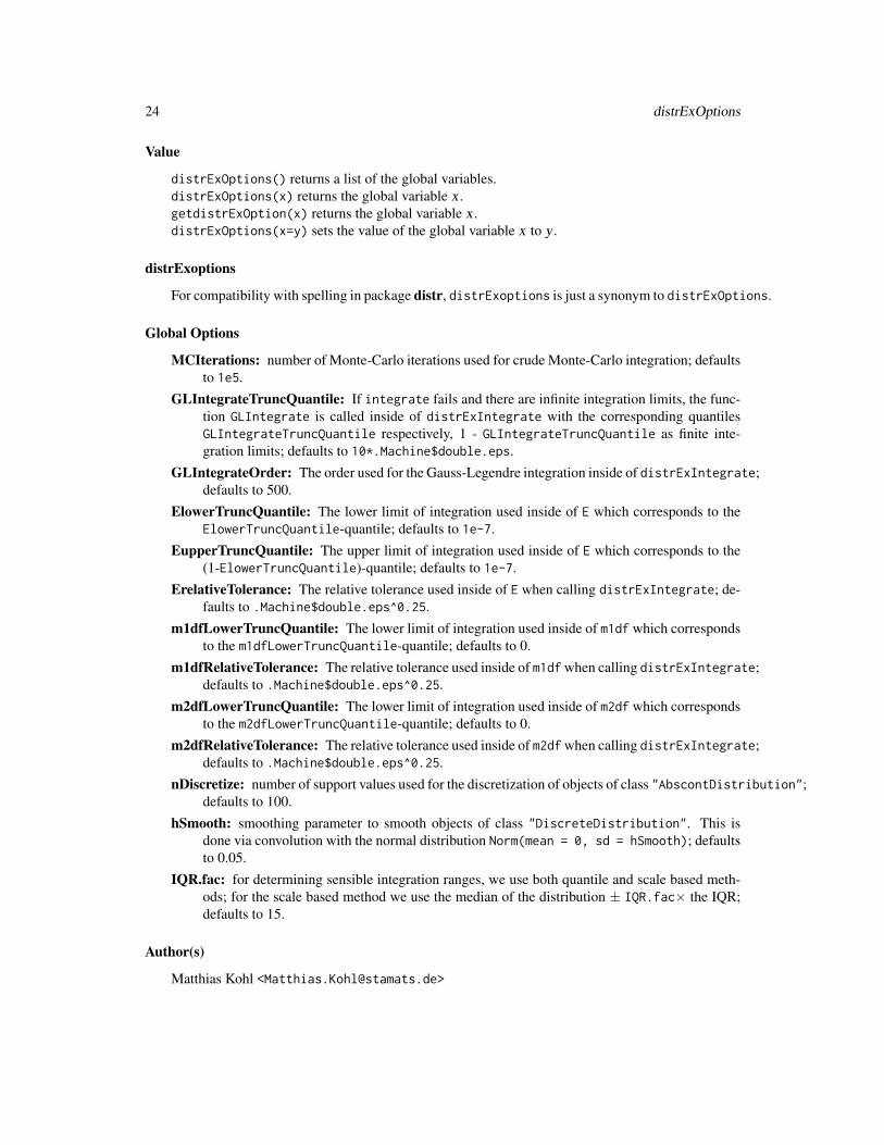
Value
distrExOptions() returns a list of the global variables.distrExOptions(x) returns the global variable x.getdistrExOption(x) returns the global variable x .distrExOptions(x=y) sets the value of the global variable x to y .
distrExoptions
For compatibility with spelling in package distr, distrExoptions is just a synonym to distrExOptions.
Global Options
MCIterations: number of Monte-Carlo iterations used for crude Monte-Carlo integration; defaultsto 1e5.
GLIntegrateTruncQuantile: If integrate fails and there are infinite integration limits, the func-tion GLIntegrate is called inside of distrExIntegrate with the corresponding quantilesGLIntegrateTruncQuantile respectively, 1 - GLIntegrateTruncQuantile as finite inte-gration limits; defaults to 10*.Machine$double.eps.
GLIntegrateOrder: The order used for the Gauss-Legendre integration inside of distrExIntegrate;defaults to 500.
ElowerTruncQuantile: The lower limit of integration used inside of E which corresponds to theElowerTruncQuantile-quantile; defaults to 1e-7.
EupperTruncQuantile: The upper limit of integration used inside of E which corresponds to the(1-ElowerTruncQuantile)-quantile; defaults to 1e-7.
ErelativeTolerance: The relative tolerance used inside of E when calling distrExIntegrate; de-faults to .Machine$double.eps^0.25.
m1dfLowerTruncQuantile: The lower limit of integration used inside of m1df which correspondsto the m1dfLowerTruncQuantile-quantile; defaults to 0.
m1dfRelativeTolerance: The relative tolerance used inside of m1df when calling distrExIntegrate;defaults to .Machine$double.eps^0.25.
m2dfLowerTruncQuantile: The lower limit of integration used inside of m2df which correspondsto the m2dfLowerTruncQuantile-quantile; defaults to 0.
m2dfRelativeTolerance: The relative tolerance used inside of m2df when calling distrExIntegrate;defaults to .Machine$double.eps^0.25.
nDiscretize: number of support values used for the discretization of objects of class "AbscontDistribution";defaults to 100.
hSmooth: smoothing parameter to smooth objects of class "DiscreteDistribution". This isdone via convolution with the normal distribution Norm(mean = 0, sd = hSmooth); defaultsto 0.05.
IQR.fac: for determining sensible integration ranges, we use both quantile and scale based meth-ods; for the scale based method we use the median of the distribution ± IQR.fac× the IQR;defaults to 15.
Author(s)
Matthias Kohl <[email protected]>

E 25
See Also
options, getOption
Examples
distrExOptions()distrExOptions("ElowerTruncQuantile")distrExOptions("ElowerTruncQuantile" = 1e-6)# ordistrExOptions(ElowerTruncQuantile = 1e-6)getdistrExOption("ElowerTruncQuantile")
E Generic Function for the Computation of (Conditional) Expectations
Description
Generic function for the computation of (conditional) expectations.
Usage
E(object, fun, cond, ...)
## S4 method for signature 'UnivariateDistribution,missing,missing'E(object,
low = NULL, upp = NULL, Nsim = getdistrExOption("MCIterations"), ...)
## S4 method for signature 'UnivariateDistribution,function,missing'E(object, fun,
useApply = TRUE, low = NULL, upp = NULL,Nsim = getdistrExOption("MCIterations"), ...)
## S4 method for signature 'AbscontDistribution,function,missing'E(object, fun, useApply = TRUE,
low = NULL, upp = NULL,rel.tol= getdistrExOption("ErelativeTolerance"),lowerTruncQuantile = getdistrExOption("ElowerTruncQuantile"),upperTruncQuantile = getdistrExOption("EupperTruncQuantile"),IQR.fac = getdistrExOption("IQR.fac"), ...)
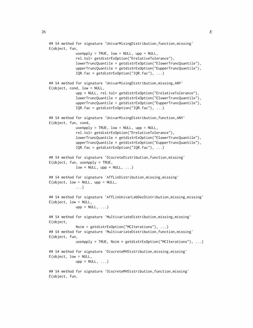
## S4 method for signature 'UnivarMixingDistribution,missing,missing'E(object, low = NULL,
upp = NULL, rel.tol= getdistrExOption("ErelativeTolerance"),lowerTruncQuantile = getdistrExOption("ElowerTruncQuantile"),upperTruncQuantile = getdistrExOption("EupperTruncQuantile"),IQR.fac = getdistrExOption("IQR.fac"), ...)
26 E
## S4 method for signature 'UnivarMixingDistribution,function,missing'E(object, fun,
useApply = TRUE, low = NULL, upp = NULL,rel.tol= getdistrExOption("ErelativeTolerance"),lowerTruncQuantile = getdistrExOption("ElowerTruncQuantile"),upperTruncQuantile = getdistrExOption("EupperTruncQuantile"),IQR.fac = getdistrExOption("IQR.fac"), ...)
## S4 method for signature 'UnivarMixingDistribution,missing,ANY'E(object, cond, low = NULL,
upp = NULL, rel.tol= getdistrExOption("ErelativeTolerance"),lowerTruncQuantile = getdistrExOption("ElowerTruncQuantile"),upperTruncQuantile = getdistrExOption("EupperTruncQuantile"),IQR.fac = getdistrExOption("IQR.fac"), ...)
## S4 method for signature 'UnivarMixingDistribution,function,ANY'E(object, fun, cond,
useApply = TRUE, low = NULL, upp = NULL,rel.tol= getdistrExOption("ErelativeTolerance"),lowerTruncQuantile = getdistrExOption("ElowerTruncQuantile"),upperTruncQuantile = getdistrExOption("EupperTruncQuantile"),IQR.fac = getdistrExOption("IQR.fac"), ...)
## S4 method for signature 'DiscreteDistribution,function,missing'E(object, fun, useApply = TRUE,
low = NULL, upp = NULL, ...)
## S4 method for signature 'AffLinDistribution,missing,missing'E(object, low = NULL, upp = NULL,
...)
## S4 method for signature 'AffLinUnivarLebDecDistribution,missing,missing'E(object, low = NULL,
upp = NULL, ...)
## S4 method for signature 'MultivariateDistribution,missing,missing'E(object,
Nsim = getdistrExOption("MCIterations"), ...)## S4 method for signature 'MultivariateDistribution,function,missing'E(object, fun,
useApply = TRUE, Nsim = getdistrExOption("MCIterations"), ...)
## S4 method for signature 'DiscreteMVDistribution,missing,missing'E(object, low = NULL,
upp = NULL, ...)
## S4 method for signature 'DiscreteMVDistribution,function,missing'E(object, fun,
E 27
useApply = TRUE, ...)
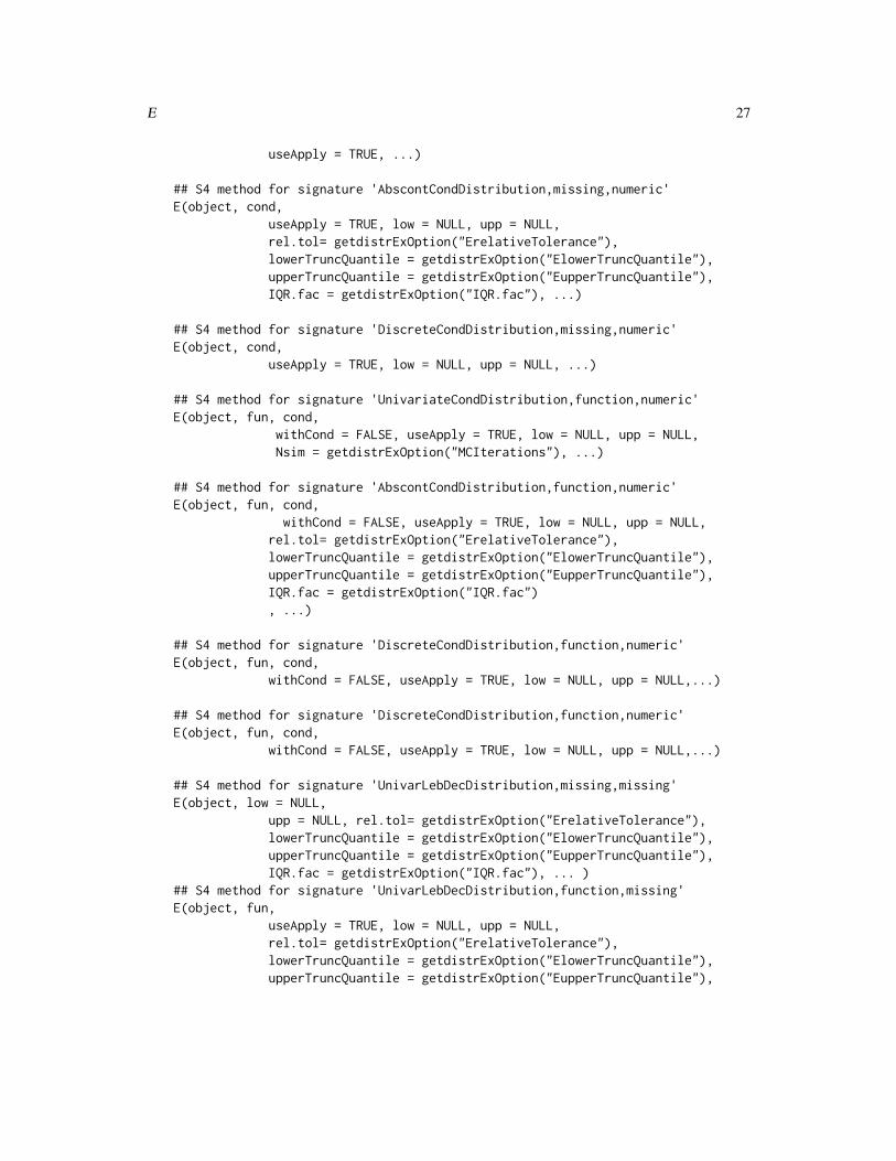
## S4 method for signature 'AbscontCondDistribution,missing,numeric'E(object, cond,
useApply = TRUE, low = NULL, upp = NULL,rel.tol= getdistrExOption("ErelativeTolerance"),lowerTruncQuantile = getdistrExOption("ElowerTruncQuantile"),upperTruncQuantile = getdistrExOption("EupperTruncQuantile"),IQR.fac = getdistrExOption("IQR.fac"), ...)
## S4 method for signature 'DiscreteCondDistribution,missing,numeric'E(object, cond,
useApply = TRUE, low = NULL, upp = NULL, ...)
## S4 method for signature 'UnivariateCondDistribution,function,numeric'E(object, fun, cond,
withCond = FALSE, useApply = TRUE, low = NULL, upp = NULL,Nsim = getdistrExOption("MCIterations"), ...)
## S4 method for signature 'AbscontCondDistribution,function,numeric'E(object, fun, cond,
withCond = FALSE, useApply = TRUE, low = NULL, upp = NULL,rel.tol= getdistrExOption("ErelativeTolerance"),lowerTruncQuantile = getdistrExOption("ElowerTruncQuantile"),upperTruncQuantile = getdistrExOption("EupperTruncQuantile"),IQR.fac = getdistrExOption("IQR.fac"), ...)
## S4 method for signature 'DiscreteCondDistribution,function,numeric'E(object, fun, cond,
withCond = FALSE, useApply = TRUE, low = NULL, upp = NULL,...)
## S4 method for signature 'DiscreteCondDistribution,function,numeric'E(object, fun, cond,
withCond = FALSE, useApply = TRUE, low = NULL, upp = NULL,...)
## S4 method for signature 'UnivarLebDecDistribution,missing,missing'E(object, low = NULL,
upp = NULL, rel.tol= getdistrExOption("ErelativeTolerance"),lowerTruncQuantile = getdistrExOption("ElowerTruncQuantile"),upperTruncQuantile = getdistrExOption("EupperTruncQuantile"),IQR.fac = getdistrExOption("IQR.fac"), ... )
## S4 method for signature 'UnivarLebDecDistribution,function,missing'E(object, fun,
useApply = TRUE, low = NULL, upp = NULL,rel.tol= getdistrExOption("ErelativeTolerance"),lowerTruncQuantile = getdistrExOption("ElowerTruncQuantile"),upperTruncQuantile = getdistrExOption("EupperTruncQuantile"),
28 E
IQR.fac = getdistrExOption("IQR.fac"), ... )## S4 method for signature 'UnivarLebDecDistribution,missing,ANY'E(object, cond, low = NULL,
upp = NULL, rel.tol= getdistrExOption("ErelativeTolerance"),lowerTruncQuantile = getdistrExOption("ElowerTruncQuantile"),upperTruncQuantile = getdistrExOption("EupperTruncQuantile"),IQR.fac = getdistrExOption("IQR.fac"), ... )
## S4 method for signature 'UnivarLebDecDistribution,function,ANY'E(object, fun, cond,
useApply = TRUE, low = NULL, upp = NULL,rel.tol= getdistrExOption("ErelativeTolerance"),lowerTruncQuantile = getdistrExOption("ElowerTruncQuantile"),upperTruncQuantile = getdistrExOption("EupperTruncQuantile"),IQR.fac = getdistrExOption("IQR.fac"), ... )
## S4 method for signature 'AcDcLcDistribution,ANY,ANY'E(object, fun, cond, low = NULL,
upp = NULL, rel.tol= getdistrExOption("ErelativeTolerance"),lowerTruncQuantile = getdistrExOption("ElowerTruncQuantile"),upperTruncQuantile = getdistrExOption("EupperTruncQuantile"),IQR.fac = getdistrExOption("IQR.fac"), ... )
## S4 method for signature 'CompoundDistribution,missing,missing'E(object, low = NULL,
upp = NULL, ...)
## S4 method for signature 'Arcsine,missing,missing'E(object, low = NULL, upp = NULL, ...)## S4 method for signature 'Beta,missing,missing'E(object, low = NULL, upp = NULL, ...)## S4 method for signature 'Binom,missing,missing'E(object, low = NULL, upp = NULL, ...)## S4 method for signature 'Cauchy,missing,missing'E(object, low = NULL, upp = NULL, ...)## S4 method for signature 'Chisq,missing,missing'E(object, low = NULL, upp = NULL, ...)## S4 method for signature 'Dirac,missing,missing'E(object, low = NULL, upp = NULL, ...)## S4 method for signature 'DExp,missing,missing'E(object, low = NULL, upp = NULL, ...)## S4 method for signature 'Exp,missing,missing'E(object, low = NULL, upp = NULL, ...)## S4 method for signature 'Fd,missing,missing'E(object, low = NULL, upp = NULL, ...)## S4 method for signature 'Gammad,missing,missing'E(object, low = NULL, upp = NULL, ...)## S4 method for signature 'Gammad,function,missing'E(object, fun, low = NULL, upp = NULL,
rel.tol = getdistrExOption("ErelativeTolerance"),
E 29
lowerTruncQuantile = getdistrExOption("ElowerTruncQuantile"),upperTruncQuantile = getdistrExOption("EupperTruncQuantile"),IQR.fac = getdistrExOption("IQR.fac"), ...)
## S4 method for signature 'Geom,missing,missing'E(object, low = NULL, upp = NULL, ...)## S4 method for signature 'Gumbel,missing,missing'E(object, low = NULL, upp = NULL, ...)## S4 method for signature 'GPareto,missing,missing'E(object, low = NULL, upp = NULL, ...)## S4 method for signature 'GPareto,function,missing'E(object, fun, low = NULL, upp = NULL,
rel.tol = getdistrExOption("ErelativeTolerance"),lowerTruncQuantile = getdistrExOption("ElowerTruncQuantile"),upperTruncQuantile = getdistrExOption("EupperTruncQuantile"),IQR.fac = max(10000, getdistrExOption("IQR.fac")), ...)
## S4 method for signature 'Hyper,missing,missing'E(object, low = NULL, upp = NULL, ...)## S4 method for signature 'Logis,missing,missing'E(object, low = NULL, upp = NULL, ...)## S4 method for signature 'Lnorm,missing,missing'E(object, low = NULL, upp = NULL, ...)## S4 method for signature 'Nbinom,missing,missing'E(object, low = NULL, upp = NULL, ...)## S4 method for signature 'Norm,missing,missing'E(object, low = NULL, upp = NULL, ...)## S4 method for signature 'Pareto,missing,missing'E(object, low = NULL, upp = NULL, ...)## S4 method for signature 'Pois,missing,missing'E(object, low = NULL, upp = NULL, ...)## S4 method for signature 'Unif,missing,missing'E(object, low = NULL, upp = NULL, ...)## S4 method for signature 'Td,missing,missing'E(object, low = NULL, upp = NULL, ...)## S4 method for signature 'Weibull,missing,missing'E(object, low = NULL, upp = NULL, ...)
Arguments
object object of class "Distribution"
fun if missing the (conditional) expectation is computed else the (conditional) ex-pection of fun is computed.
cond if not missing the conditional expectation given cond is computed.
Nsim number of MC simulations used to determine the expectation.
rel.tol relative tolerance for distrExIntegrate.
low lower bound of integration range.
upp upper bound of integration range.
30 E
lowerTruncQuantile
lower quantile for quantile based integration range.upperTruncQuantile
upper quantile for quantile based integration range.
IQR.fac factor for scale based integration range (i.e.; median of the distribution±IQR.fac×IQR).
... additional arguments to fun
useApply logical: should sapply, respectively apply be used to evaluate fun.
withCond logical: is cond in the argument list of fun.
Details
The precision of the computations can be controlled via certain global options; cf. distrExOptions.Also note that arguments low and upp should be given as named arguments in order to prevent themto be matched by arguments fun or cond. Also the result, when arguments low or upp is given, isthe unconditional value of the expectation; no conditioning with respect to low <= object <= uppis done.
Value
The (conditional) expectation is computed.
Methods
object = "UnivariateDistribution", fun = "missing", cond = "missing": expectation of univari-ate distributions using crude Monte-Carlo integration.
object = "AbscontDistribution", fun = "missing", cond = "missing": expectation of absolutelycontinuous univariate distributions using distrExIntegrate.
object = "DiscreteDistribution", fun = "missing", cond = "missing": expectation of discrete uni-variate distributions using support and sum.
object = "MultivariateDistribution", fun = "missing", cond = "missing": expectation of mul-tivariate distributions using crude Monte-Carlo integration.
object = "DiscreteMVDistribution", fun = "missing", cond = "missing": expectation of discretemultivariate distributions. The computation is based on support and sum.
object = "UnivariateDistribution", fun = "missing", cond = "missing": expectation of univari-ate Lebesgue decomposed distributions by separate calculations for discrete and absolutelycontinuous part.
object = "AffLinDistribution", fun = "missing", cond = "missing": expectation of an affine lin-ear transformation aX+b as aE[X]+b for X either "DiscreteDistribution" or "AbscontDistribution".
object = "AffLinUnivarLebDecDistribution", fun = "missing", cond = "missing": expectationof an affine linear transformation aX+b as aE[X]+b for X either "UnivarLebDecDistribution".
object = "UnivariateDistribution", fun = "function", cond = "missing": expectation of fun un-der univariate distributions using crude Monte-Carlo integration.
object = "UnivariateDistribution", fun = "function", cond = "missing": expectation of fun un-der univariate Lebesgue decomposed distributions by separate calculations for discrete andabsolutely continuous part.
E 31
object = "AbscontDistribution", fun = "function", cond = "missing": expectation of fun un-der absolutely continuous univariate distributions using distrExIntegrate.
object = "DiscreteDistribution", fun = "function", cond = "missing": expectation of fun un-der discrete univariate distributions using support and sum.
object = "MultivariateDistribution", fun = "function", cond = "missing": expectation of mul-tivariate distributions using crude Monte-Carlo integration.
object = "DiscreteMVDistribution", fun = "function", cond = "missing": expectation of fun un-der discrete multivariate distributions. The computation is based on support and sum.
object = "UnivariateCondDistribution", fun = "missing", cond = "numeric": conditional ex-pectation for univariate conditional distributions given cond. The integral is computed usingcrude Monte-Carlo integration.
object = "AbscontCondDistribution", fun = "missing", cond = "numeric": conditional expec-tation for absolutely continuous, univariate conditional distributions given cond. The compu-tation is based on distrExIntegrate.
object = "DiscreteCondDistribution", fun = "missing", cond = "numeric": conditional expec-tation for discrete, univariate conditional distributions given cond. The computation is basedon support and sum.
object = "UnivariateCondDistribution", fun = "function", cond = "numeric": conditional ex-pectation of fun under univariate conditional distributions given cond. The integral is com-puted using crude Monte-Carlo integration.
object = "AbscontCondDistribution", fun = "function", cond = "numeric": conditional expec-tation of fun under absolutely continuous, univariate conditional distributions given cond. Thecomputation is based on distrExIntegrate.
object = "DiscreteCondDistribution", fun = "function", cond = "numeric": conditional expec-tation of fun under discrete, univariate conditional distributions given cond. The computationis based on support and sum.
object = "UnivarLebDecDistribution", fun = "missing", cond = "missing": expectation by sep-arate evaluation of expectation of discrete and abs. continuous part and subsequent weighting.
object = "UnivarLebDecDistribution", fun = "function", cond = "missing": expectation by sep-arate evaluation of expectation of discrete and abs. continuous part and subsequent weighting.
object = "UnivarLebDecDistribution", fun = "missing", cond = "ANY": expectation by sepa-rate evaluation of expectation of discrete and abs. continuous part and subsequent weighting.
object = "UnivarLebDecDistribution", fun = "function", cond = "ANY": expectation by sep-arate evaluation of expectation of discrete and abs. continuous part and subsequent weighting.
object = "UnivarMixingDistribution", fun = "missing", cond = "missing": expectation is com-puted component-wise with subsequent weighting acc. to mixCoeff.
object = "UnivarMixingDistribution", fun = "function", cond = "missing": expectation is com-puted component-wise with subsequent weighting acc. to mixCoeff.
object = "UnivarMixingDistribution", fun = "missing", cond = "ANY": expectation is computedcomponent-wise with subsequent weighting acc. to mixCoeff.
object = "UnivarMixingDistribution", fun = "function", cond = "ANY": expectation is com-puted component-wise with subsequent weighting acc. to mixCoeff.
object = "AcDcLcDistribution", fun = "ANY", cond = "ANY": expectation by first coercing toclass "UnivarLebDecDistribution" and using the corresponding method.
32 E
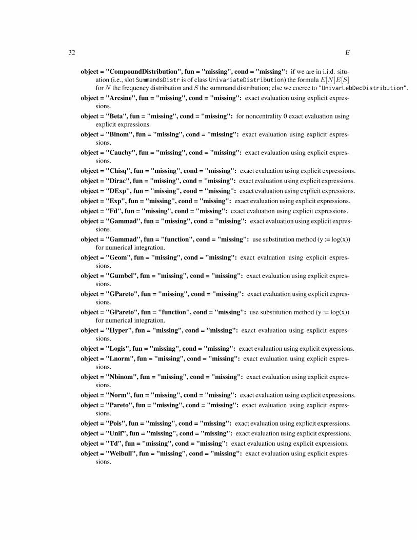
object = "CompoundDistribution", fun = "missing", cond = "missing": if we are in i.i.d. situ-ation (i.e., slot SummandsDistr is of class UnivariateDistribution) the formulaE[N ]E[S]forN the frequency distribution and S the summand distribution; else we coerce to "UnivarLebDecDistribution".
object = "Arcsine", fun = "missing", cond = "missing": exact evaluation using explicit expres-sions.
object = "Beta", fun = "missing", cond = "missing": for noncentrality 0 exact evaluation usingexplicit expressions.
object = "Binom", fun = "missing", cond = "missing": exact evaluation using explicit expres-sions.
object = "Cauchy", fun = "missing", cond = "missing": exact evaluation using explicit expres-sions.
object = "Chisq", fun = "missing", cond = "missing": exact evaluation using explicit expressions.object = "Dirac", fun = "missing", cond = "missing": exact evaluation using explicit expressions.object = "DExp", fun = "missing", cond = "missing": exact evaluation using explicit expressions.object = "Exp", fun = "missing", cond = "missing": exact evaluation using explicit expressions.object = "Fd", fun = "missing", cond = "missing": exact evaluation using explicit expressions.object = "Gammad", fun = "missing", cond = "missing": exact evaluation using explicit expres-
sions.object = "Gammad", fun = "function", cond = "missing": use substitution method (y := log(x))
for numerical integration.object = "Geom", fun = "missing", cond = "missing": exact evaluation using explicit expres-
sions.object = "Gumbel", fun = "missing", cond = "missing": exact evaluation using explicit expres-
sions.object = "GPareto", fun = "missing", cond = "missing": exact evaluation using explicit expres-
sions.object = "GPareto", fun = "function", cond = "missing": use substitution method (y := log(x))
for numerical integration.object = "Hyper", fun = "missing", cond = "missing": exact evaluation using explicit expres-
sions.object = "Logis", fun = "missing", cond = "missing": exact evaluation using explicit expressions.object = "Lnorm", fun = "missing", cond = "missing": exact evaluation using explicit expres-
sions.object = "Nbinom", fun = "missing", cond = "missing": exact evaluation using explicit expres-
sions.object = "Norm", fun = "missing", cond = "missing": exact evaluation using explicit expressions.object = "Pareto", fun = "missing", cond = "missing": exact evaluation using explicit expres-
sions.object = "Pois", fun = "missing", cond = "missing": exact evaluation using explicit expressions.object = "Unif", fun = "missing", cond = "missing": exact evaluation using explicit expressions.object = "Td", fun = "missing", cond = "missing": exact evaluation using explicit expressions.object = "Weibull", fun = "missing", cond = "missing": exact evaluation using explicit expres-
sions.
E 33
Author(s)
Matthias Kohl <[email protected]> and Peter Ruckdeschel <[email protected]>
See Also
distrExIntegrate, m1df, m2df, Distribution-class
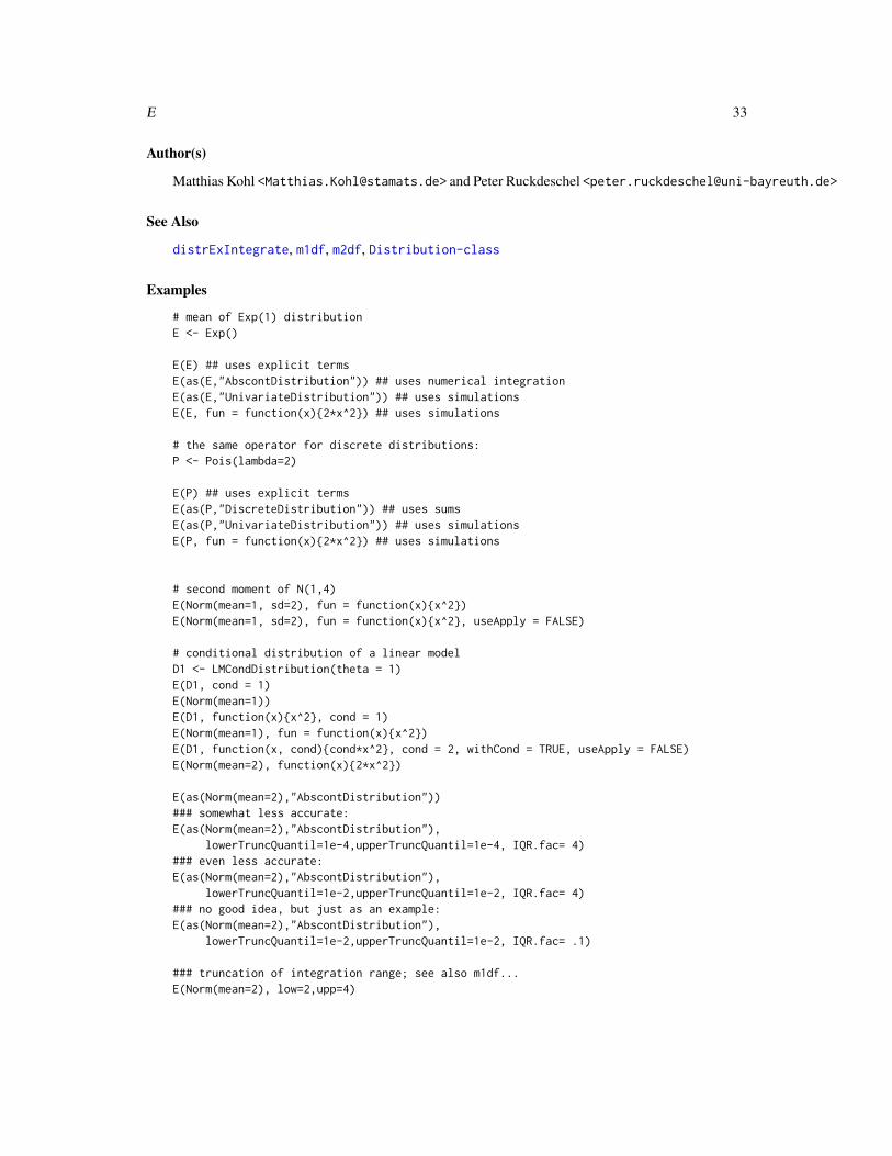
Examples
# mean of Exp(1) distributionE <- Exp()
E(E) ## uses explicit termsE(as(E,"AbscontDistribution")) ## uses numerical integrationE(as(E,"UnivariateDistribution")) ## uses simulationsE(E, fun = function(x)2*x^2) ## uses simulations
# the same operator for discrete distributions:P <- Pois(lambda=2)
E(P) ## uses explicit termsE(as(P,"DiscreteDistribution")) ## uses sumsE(as(P,"UnivariateDistribution")) ## uses simulationsE(P, fun = function(x)2*x^2) ## uses simulations
# second moment of N(1,4)E(Norm(mean=1, sd=2), fun = function(x)x^2)E(Norm(mean=1, sd=2), fun = function(x)x^2, useApply = FALSE)
# conditional distribution of a linear modelD1 <- LMCondDistribution(theta = 1)E(D1, cond = 1)E(Norm(mean=1))E(D1, function(x)x^2, cond = 1)E(Norm(mean=1), fun = function(x)x^2)E(D1, function(x, cond)cond*x^2, cond = 2, withCond = TRUE, useApply = FALSE)E(Norm(mean=2), function(x)2*x^2)
E(as(Norm(mean=2),"AbscontDistribution"))### somewhat less accurate:E(as(Norm(mean=2),"AbscontDistribution"),
lowerTruncQuantil=1e-4,upperTruncQuantil=1e-4, IQR.fac= 4)### even less accurate:E(as(Norm(mean=2),"AbscontDistribution"),
lowerTruncQuantil=1e-2,upperTruncQuantil=1e-2, IQR.fac= 4)### no good idea, but just as an example:E(as(Norm(mean=2),"AbscontDistribution"),
lowerTruncQuantil=1e-2,upperTruncQuantil=1e-2, IQR.fac= .1)
### truncation of integration range; see also m1df...E(Norm(mean=2), low=2,upp=4)
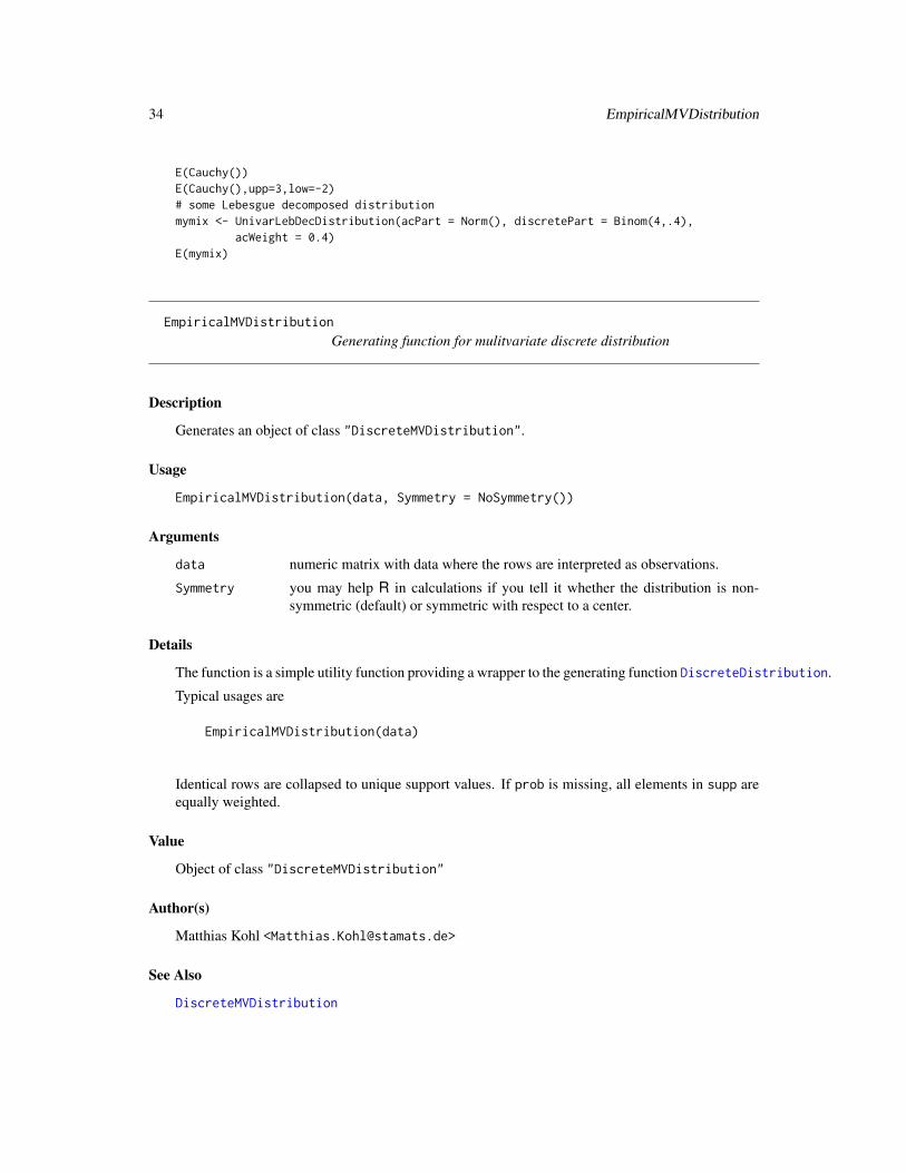
34 EmpiricalMVDistribution
E(Cauchy())E(Cauchy(),upp=3,low=-2)# some Lebesgue decomposed distributionmymix <- UnivarLebDecDistribution(acPart = Norm(), discretePart = Binom(4,.4),
acWeight = 0.4)E(mymix)
EmpiricalMVDistribution
Generating function for mulitvariate discrete distribution
Description
Generates an object of class "DiscreteMVDistribution".
Usage
EmpiricalMVDistribution(data, Symmetry = NoSymmetry())
Arguments
data numeric matrix with data where the rows are interpreted as observations.
Symmetry you may help R in calculations if you tell it whether the distribution is non-symmetric (default) or symmetric with respect to a center.
Details
The function is a simple utility function providing a wrapper to the generating function DiscreteDistribution.
Typical usages are
EmpiricalMVDistribution(data)
Identical rows are collapsed to unique support values. If prob is missing, all elements in supp areequally weighted.
Value
Object of class "DiscreteMVDistribution"
Author(s)
Matthias Kohl <[email protected]>
See Also
DiscreteMVDistribution
EuclCondition 35
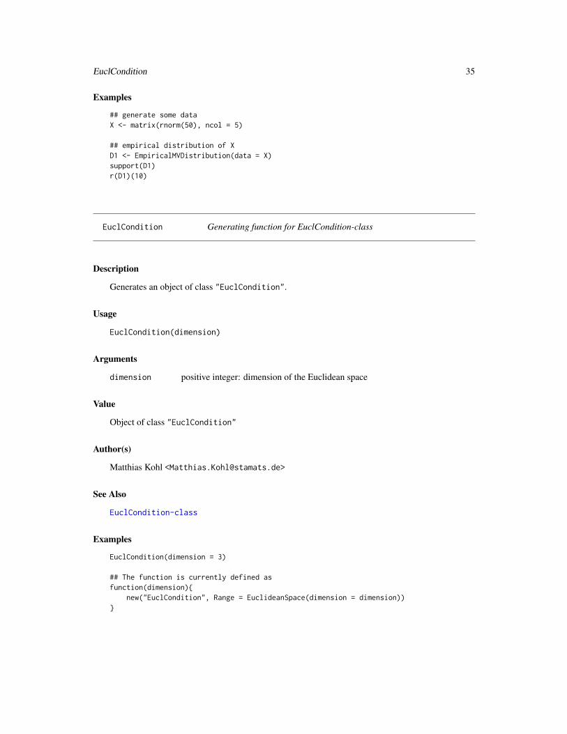
Examples
## generate some dataX <- matrix(rnorm(50), ncol = 5)
## empirical distribution of XD1 <- EmpiricalMVDistribution(data = X)support(D1)r(D1)(10)
EuclCondition Generating function for EuclCondition-class
Description
Generates an object of class "EuclCondition".
Usage
EuclCondition(dimension)
Arguments
dimension positive integer: dimension of the Euclidean space
Value
Object of class "EuclCondition"
Author(s)
Matthias Kohl <[email protected]>
See Also
EuclCondition-class
Examples
EuclCondition(dimension = 3)
## The function is currently defined asfunction(dimension)
new("EuclCondition", Range = EuclideanSpace(dimension = dimension))
36 EuclCondition-class
EuclCondition-class Conditioning by an Euclidean space.
Description
Conditioning by an Euclidean space.
Objects from the Class
Objects can be created by calls of the form new("EuclCondition", ...). More frequently theyare created via the generating function EuclCondition.
Slots
Range Object of class "EuclideanSpace".
name Object of class "character": name of condition.
Extends
Class "Condition", directly.
Methods
Range signature(object = "EuclCondition") accessor function for slot Range.
show signature(object = "EuclCondition")
Author(s)
Matthias Kohl <[email protected]>
See Also
Condition-class, EuclCondition
Examples
new("EuclCondition")
GLIntegrate 37
GLIntegrate Gauss-Legendre Quadrature
Description
Gauss-Legendre quadrature over a finite interval.
Usage
GLIntegrate(f, lower, upper, order = 500, ...)
Arguments
f an R function taking a numeric first argument and returning a numeric vector ofthe same length. Returning a non-finite element will generate an error.
lower finite lower limit of integration.upper finite upper limit of integration.order order of Gauss-Legendre quadrature.... additional arguments to be passed to f. Remember to use argument names not
matching those of GLIntegrate!
Details
In case order = 100, 500, 1000 saved abscissas and weights are used. Otherwise the corre-sponding abscissas and weights are computed using the algorithm given in Section 4.5 of Press etal. (1992).
Value
Estimate of the integral.
Author(s)
Matthias Kohl <[email protected]>
References
W.H. Press, S.A. Teukolsky, W.T. Vetterling, B.P. Flannery (1992) Numerical Recipies in C. TheArt of Scientific Computing. Second Edition. Cambridge University Press.
See Also
integrate, distrExIntegrate
Examples
integrate(dnorm, -1.96, 1.96)GLIntegrate(dnorm, -1.96, 1.96)
38 HellingerDist
HellingerDist Generic function for the computation of the Hellinger distance of twodistributions
Description
Generic function for the computation of the Hellinger distance dh of two distributions P and Qwhich may be defined for an arbitrary sample space (Ω,A). The Hellinger distance is defined as
dh(P,Q) =1
2
∫|√dP −
√dQ |2
where√dP , respectively
√dQ denotes the square root of the densities.
Usage
HellingerDist(e1, e2, ...)## S4 method for signature 'AbscontDistribution,AbscontDistribution'HellingerDist(e1,e2,
rel.tol=.Machine$double.eps^0.3,TruncQuantile = getdistrOption("TruncQuantile"),IQR.fac = 15, ...)
## S4 method for signature 'AbscontDistribution,DiscreteDistribution'HellingerDist(e1,e2, ...)## S4 method for signature 'DiscreteDistribution,AbscontDistribution'HellingerDist(e1,e2, ...)## S4 method for signature 'DiscreteDistribution,DiscreteDistribution'HellingerDist(e1,e2, ...)## S4 method for signature 'numeric,DiscreteDistribution'HellingerDist(e1, e2, ...)## S4 method for signature 'DiscreteDistribution,numeric'HellingerDist(e1, e2, ...)## S4 method for signature 'numeric,AbscontDistribution'HellingerDist(e1, e2, asis.smooth.discretize = "discretize",
n.discr = getdistrExOption("nDiscretize"), low.discr = getLow(e2),up.discr = getUp(e2), h.smooth = getdistrExOption("hSmooth"),
rel.tol=.Machine$double.eps^0.3,TruncQuantile = getdistrOption("TruncQuantile"),IQR.fac = 15, ...)
## S4 method for signature 'AbscontDistribution,numeric'HellingerDist(e1, e2, asis.smooth.discretize = "discretize",
n.discr = getdistrExOption("nDiscretize"), low.discr = getLow(e1),up.discr = getUp(e1), h.smooth = getdistrExOption("hSmooth"),
rel.tol=.Machine$double.eps^0.3,TruncQuantile = getdistrOption("TruncQuantile"),IQR.fac = 15, ...)
## S4 method for signature 'AcDcLcDistribution,AcDcLcDistribution'

HellingerDist 39
HellingerDist(e1,e2,rel.tol=.Machine$double.eps^0.3,TruncQuantile = getdistrOption("TruncQuantile"),IQR.fac = 15, ...)
Arguments
e1 object of class "Distribution" or class "numeric"
e2 object of class "Distribution" or class "numeric"asis.smooth.discretize
possible methods are "asis", "smooth" and "discretize". Default is "discretize".
n.discr if asis.smooth.discretize is equal to "discretize" one has to specify thenumber of lattice points used to discretize the abs. cont. distribution.
low.discr if asis.smooth.discretize is equal to "discretize" one has to specify thelower end point of the lattice used to discretize the abs. cont. distribution.
up.discr if asis.smooth.discretize is equal to "discretize" one has to specify theupper end point of the lattice used to discretize the abs. cont. distribution.
h.smooth if asis.smooth.discretize is equal to "smooth" – i.e., the empirical distribu-tion of the provided data should be smoothed – one has to specify this parameter.
rel.tol relative accuracy requested in integration
TruncQuantile Quantile the quantile based integration bounds (see details)
IQR.fac Factor for the scale based integration bounds (see details)
... further arguments to be used in particular methods (not in package distrEx)
Details
For distances between absolutely continuous distributions, we use numerical integration; to deter-mine sensible bounds we proceed as follows: by means of min(getLow(e1,eps=TruncQuantile),getLow(e2,eps=TruncQuantile)),max(getUp(e1,eps=TruncQuantile),getUp(e2,eps=TruncQuantile)) we determine quantilebased bounds c(low.0,up.0), and by means of s1 <- max(IQR(e1),IQR(e2)); m1<- median(e1);m2 <- median(e2) and low.1 <- min(m1,m2)-s1*IQR.fac, up.1 <- max(m1,m2)+s1*IQR.facwe determine scale based bounds; these are combined by low <- max(low.0,low.1), up <- max(up.0,up1).
In case we want to compute the Hellinger distance between (empirical) data and an abs. cont.distribution, we can specify the parameter asis.smooth.discretize to avoid trivial distances(distance = 1).
Using asis.smooth.discretize = "discretize", which is the default, leads to a discretizationof the provided abs. cont. distribution and the distance is computed between the provided data andthe discretized distribution.
Using asis.smooth.discretize = "smooth" causes smoothing of the empirical distribution ofthe provided data. This is, the empirical data is convoluted with the normal distribution Norm(mean = 0, sd = h.smooth)which leads to an abs. cont. distribution. Afterwards the distance between the smoothed empiricaldistribution and the provided abs. cont. distribution is computed.
Value
Hellinger distance of e1 and e2
40 HellingerDist
Methods
e1 = "AbscontDistribution", e2 = "AbscontDistribution": Hellinger distance of two absolutelycontinuous univariate distributions which is computed using distrExintegrate.
e1 = "AbscontDistribution", e2 = "DiscreteDistribution": Hellinger distance of absolutely con-tinuous and discrete univariate distributions (are mutually singular; i.e., have distance =1).
e1 = "DiscreteDistribution", e2 = "DiscreteDistribution": Hellinger distance of two discrete uni-variate distributions which is computed using support and sum.
e1 = "DiscreteDistribution", e2 = "AbscontDistribution": Hellinger distance of discrete and ab-solutely continuous univariate distributions (are mutually singular; i.e., have distance =1).
e1 = "numeric", e2 = "DiscreteDistribution": Hellinger distance between (empirical) data and adiscrete distribution.
e1 = "DiscreteDistribution", e2 = "numeric": Hellinger distance between (empirical) data and adiscrete distribution.
e1 = "numeric", e2 = "AbscontDistribution": Hellinger distance between (empirical) data andan abs. cont. distribution.
e1 = "AbscontDistribution", e1 = "numeric": Hellinger distance between (empirical) data andan abs. cont. distribution.
e1 = "AcDcLcDistribution", e2 = "AcDcLcDistribution": Hellinger distance of mixed discreteand absolutely continuous univariate distributions.
Author(s)
Matthias Kohl <[email protected]>,Peter Ruckdeschel <[email protected]>
References
Huber, P.J. (1981) Robust Statistics. New York: Wiley.
Rieder, H. (1994) Robust Asymptotic Statistics. New York: Springer.
See Also
distrExIntegrate, ContaminationSize, TotalVarDist, KolmogorovDist, Distribution-class
Examples
HellingerDist(Norm(), UnivarMixingDistribution(Norm(1,2),Norm(0.5,3),mixCoeff=c(0.2,0.8)))
HellingerDist(Norm(), Td(10))HellingerDist(Norm(mean = 50, sd = sqrt(25)), Binom(size = 100)) # mutually singularHellingerDist(Pois(10), Binom(size = 20))
x <- rnorm(100)HellingerDist(Norm(), x)HellingerDist(x, Norm(), asis.smooth.discretize = "smooth")
y <- (rbinom(50, size = 20, prob = 0.5)-10)/sqrt(5)
KolmogorovDist 41
HellingerDist(y, Norm())HellingerDist(y, Norm(), asis.smooth.discretize = "smooth")
HellingerDist(rbinom(50, size = 20, prob = 0.5), Binom(size = 20, prob = 0.5))
KolmogorovDist Generic function for the computation of the Kolmogorov distance oftwo distributions
Description
Generic function for the computation of the Kolmogorov distance dκ of two distributions P and Qwhere the distributions are defined on a finite-dimensional Euclidean space (Rm,Bm) with Bm theBorel-σ-algebra on Rm. The Kolmogorov distance is defined as
dκ(P,Q) = sup|P (y ∈ Rm | y ≤ x)−Q(y ∈ Rm | y ≤ x)||x ∈ Rm
where ≤ is coordinatewise on Rm.
Usage
KolmogorovDist(e1, e2, ...)## S4 method for signature 'AbscontDistribution,AbscontDistribution'KolmogorovDist(e1,e2)## S4 method for signature 'AbscontDistribution,DiscreteDistribution'KolmogorovDist(e1,e2)## S4 method for signature 'DiscreteDistribution,AbscontDistribution'KolmogorovDist(e1,e2)## S4 method for signature 'DiscreteDistribution,DiscreteDistribution'KolmogorovDist(e1,e2)## S4 method for signature 'numeric,UnivariateDistribution'KolmogorovDist(e1, e2)## S4 method for signature 'UnivariateDistribution,numeric'KolmogorovDist(e1, e2)## S4 method for signature 'AcDcLcDistribution,AcDcLcDistribution'KolmogorovDist(e1, e2)
Arguments
e1 object of class "Distribution" or class "numeric"
e2 object of class "Distribution" or class "numeric"
... further arguments to be used in particular methods (not in package distrEx)
Value
Kolmogorov distance of e1 and e2

42 KolmogorovDist
Methods
e1 = "AbscontDistribution", e2 = "AbscontDistribution": Kolmogorov distance of two abso-lutely continuous univariate distributions which is computed using a union of a (pseudo-)random and a deterministic grid.
e1 = "DiscreteDistribution", e2 = "DiscreteDistribution": Kolmogorov distance of two discreteunivariate distributions. The distance is attained at some point of the union of the supports ofe1 and e2.
e1 = "AbscontDistribution", e2 = "DiscreteDistribution": Kolmogorov distance of absolutelycontinuous and discrete univariate distributions. It is computed using a union of a (pseudo-)random and a deterministic grid in combination with the support of e2.
e1 = "DiscreteDistribution", e2 = "AbscontDistribution": Kolmogorov distance of discrete andabsolutely continuous univariate distributions. It is computed using a union of a (pseudo-)random and a deterministic grid in combination with the support of e1.
e1 = "numeric", e2 = "UnivariateDistribution": Kolmogorov distance between (empirical) dataand a univariate distribution. The computation is based on ks.test.
e1 = "UnivariateDistribution", e2 = "numeric": Kolmogorov distance between (empirical) dataand a univariate distribution. The computation is based on ks.test.
e1 = "AcDcLcDistribution", e2 = "AcDcLcDistribution": Kolmogorov distance of mixed dis-crete and absolutely continuous univariate distributions. It is computed using a union of thediscrete part, a (pseudo-)random and a deterministic grid in combination with the support ofe1.
Author(s)
Matthias Kohl <[email protected]>,Peter Ruckdeschel <[email protected]>
References
Huber, P.J. (1981) Robust Statistics. New York: Wiley.
Rieder, H. (1994) Robust Asymptotic Statistics. New York: Springer.
See Also
ContaminationSize, TotalVarDist, HellingerDist, Distribution-class
Examples
KolmogorovDist(Norm(), UnivarMixingDistribution(Norm(1,2),Norm(0.5,3),mixCoeff=c(0.2,0.8)))
KolmogorovDist(Norm(), Td(10))KolmogorovDist(Norm(mean = 50, sd = sqrt(25)), Binom(size = 100))KolmogorovDist(Pois(10), Binom(size = 20))KolmogorovDist(Norm(), rnorm(100))KolmogorovDist((rbinom(50, size = 20, prob = 0.5)-10)/sqrt(5), Norm())KolmogorovDist(rbinom(50, size = 20, prob = 0.5), Binom(size = 20, prob = 0.5))

liesInSupport 43
liesInSupport Generic Function for Testing the Support of a Distribution
Description
The function tests if x lies in the support of the distribution object.
Usage
## S4 method for signature 'DiscreteMVDistribution,numeric'liesInSupport(object, x)## S4 method for signature 'DiscreteMVDistribution,matrix'liesInSupport(object, x)
Arguments
object object of class "Distribution"
x numeric vector or matrix
Value
logical vector
Methods
object = "DiscreteMVDistribution", x = "numeric": does x lie in the support of object.
object = "DiscreteMVDistribution", x = "matrix": does x lie in the support of object.
Author(s)
Matthias Kohl <[email protected]>
See Also
Distribution-class
Examples
M <- matrix(rpois(30, lambda = 10), ncol = 3)D1 <- DiscreteMVDistribution(M)M1 <- rbind(r(D1)(10), matrix(rpois(30, lam = 10), ncol = 3))liesInSupport(D1, M1)
44 LMCondDistribution
LMCondDistribution Generating function for the conditional distribution of a linear regres-sion model.
Description
Generates an object of class "AbscontCondDistribution" which is the conditional distribution ofa linear regression model (given the regressor).
Usage
LMCondDistribution(Error = Norm(), theta = 0, intercept = 0, scale = 1)
Arguments
Error Object of class "AbscontDistribution": error distribution.
theta numeric vector: regression parameter.
intercept real number: intercept parameter.
scale positive real number: scale parameter.
Value
Object of class "AbscontCondDistribution"
Author(s)
Matthias Kohl <[email protected]>
See Also
AbscontCondDistribution-class, E-methods
Examples
# normal error distribution(D1 <- LMCondDistribution(theta = 1)) # corresponds to Norm(cond, 1)plot(D1)r(D1)d(D1)p(D1)q(D1)## in RStudio or Jupyter IRKernel, use q.l(.)(.) instead of q(.)(.)param(D1)cond(D1)
d(D1)(0, cond = 1)d(Norm(mean=1))(0)
LMParameter 45
E(D1, cond = 1)E(D1, function(x)x^2, cond = 2)E(Norm(mean=2), function(x)x^2)
LMParameter Generating function for LMParameter-class
Description
Generates an object of class "LMParameter".
Usage
LMParameter(theta = 0, intercept = 0, scale = 1)
Arguments
theta numeric vector: regression parameter (default =0).
intercept real number: intercept parameter (default =0).
scale positive real number: scale parameter (default =1).
Value
Object of class "LMParameter"
Author(s)
Matthias Kohl <[email protected]>
See Also
LMParameter-class
Examples
LMParameter(theta = c(1,1), intercept = 2, scale = 0.5)
## The function is currently defined asfunction(theta = 0, intercept = 0, scale = 1)
new("LMParameter", theta = theta, intercept = intercept, scale = 1)
46 LMParameter-class
LMParameter-class Parameter of a linear regression model
Description
Parameter of a linear regression model
y = µ+ xτθ + σu
with intercept µ, regression parameter θ and error scale σ.
Objects from the Class
Objects can be created by calls of the form new("LMParameter", ...). More frequently they arecreated via the generating function LMParameter.
Slots
theta numeric vector: regression parameter.
intercept real number: intercept parameter.
scale positive real number: scale paramter.
name character vector: the default name is “parameter of a linear regression model”.
Extends
Class "Parameter", directly.Class "OptionalParameter", by class "Parameter".
Methods
show signature(object = "LMParameter")
Author(s)
Matthias Kohl <[email protected]>
See Also
Parameter-class, LMParameter
Examples
new("LMParameter")
m1df 47
m1df Generic Function for the Computation of Clipped First Moments
Description
Generic function for the computation of clipped first moments. The moments are clipped at upper.
Usage
m1df(object, upper, ...)## S4 method for signature 'AbscontDistribution'm1df(object, upper,
lowerTruncQuantile = getdistrExOption("m1dfLowerTruncQuantile"),rel.tol = getdistrExOption("m1dfRelativeTolerance"), ...)
Arguments
object object of class "Distribution"
upper clipping bound
rel.tol relative tolerance for distrExIntegrate.lowerTruncQuantile
lower quantile for quantile based integration range.
... additional arguments to E
Details
The precision of the computations can be controlled via certain global options; cf. distrExOptions.
Value
The first moment of object clipped at upper is computed.
Methods
object = "UnivariateDistribution": uses call E(object, upp=upper, ...).
object = "AbscontDistribution": clipped first moment for absolutely continuous univariate dis-tributions which is computed using integrate.
object = "LatticeDistribution": clipped first moment for discrete univariate distributions whichis computed using support and sum.
object = "AffLinDistribution": clipped first moment for affine linear distributions which is com-puted on basis of slot X0.
object = "Binom": clipped first moment for Binomial distributions which is computed using pbinom.
object = "Pois": clipped first moment for Poisson distributions which is computed using ppois.
object = "Norm": clipped first moment for normal distributions which is computed using dnormand pnorm.
48 m2df
object = "Exp": clipped first moment for exponential distributions which is computed using pexp.
object = "Chisq": clipped first moment for χ2 distributions which is computed using pchisq.
Author(s)
Matthias Kohl <[email protected]>
See Also
distrExIntegrate, m2df, E
Examples
# standard normal distributionN1 <- Norm()m1df(N1, 0)
# Poisson distributionP1 <- Pois(lambda=2)m1df(P1, 3)m1df(P1, 3, fun = function(x)sin(x))
# absolutely continuous distributionD1 <- Norm() + Exp() # convolutionm1df(D1, 2)m1df(D1, Inf)E(D1)
m2df Generic function for the computation of clipped second moments
Description
Generic function for the computation of clipped second moments. The moments are clipped atupper.
Usage
m2df(object, upper, ...)## S4 method for signature 'AbscontDistribution'm2df(object, upper,
lowerTruncQuantile = getdistrExOption("m2dfLowerTruncQuantile"),rel.tol = getdistrExOption("m2dfRelativeTolerance"), ...)
m2df 49
Arguments
object object of class "Distribution"
upper clipping bound
rel.tol relative tolerance for distrExIntegrate.lowerTruncQuantile
lower quantile for quantile based integration range.
... additional arguments to E
Details
The precision of the computations can be controlled via certain global options; cf. distrExOptions.
Value
The second moment of object clipped at upper is computed.
Methods
object = "UnivariateDistribution": uses call E(object, upp=upper, fun = function, ...).
object = "AbscontDistribution": clipped second moment for absolutely continuous univariatedistributions which is computed using integrate.
object = "LatticeDistribution": clipped second moment for discrete univariate distributions whichis computed using support and sum.
object = "AffLinDistribution": clipped second moment for affine linear distributions which iscomputed on basis of slot X0.
object = "Binom": clipped second moment for Binomial distributions which is computed usingpbinom.
object = "Pois": clipped second moment for Poisson distributions which is computed using ppois.
object = "Norm": clipped second moment for normal distributions which is computed using dnormand pnorm.
object = "Exp": clipped second moment for exponential distributions which is computed usingpexp.
object = "Chisq": clipped second moment for χ2 distributions which is computed using pchisq.
Author(s)
Matthias Kohl <[email protected]>
See Also
m2df-methods, E-methods

50 make01
Examples
# standard normal distributionN1 <- Norm()m2df(N1, 0)
# Poisson distributionP1 <- Pois(lambda=2)m2df(P1, 3)m2df(P1, 3, fun = function(x)sin(x))
# absolutely continuous distributionD1 <- Norm() + Exp() # convolutionm2df(D1, 2)m2df(D1, Inf)E(D1, function(x)x^2)
make01 Centering and Standardization of Univariate Distributions
Description
The function make01 produces a new centered and standardized univariate distribution.
Usage
make01(x)
Arguments
x an object of class "UnivariateDistribution"
Details
Thanks to the functionals provided in this package, the code is a one-liner: (x-E(x))/sd(x).
Value
Object of class "UnivariateDistribution" with expectation 0 and variance 1.
Author(s)
Peter Ruckdeschel <[email protected]>
See Also
E, Var

MultivariateDistribution-class 51
Examples
X <- sin(exp(2*log(abs( Norm())))) ## something weirdX01 <- make01(X)print(X01)plot(X01)sd(X01); E(X01)
MultivariateDistribution-class
Multivariate Distributions
Description
The class of multivariate distributions. One has at least to specify the image space of the distributionand a function generating (pseudo-)random numbers. The slot q is usually filled with NULL fordimensions > 1.
Objects from the Class
Objects can be created by calls of the form new("MultivariateDistribution", ...).
Slots
img Object of class "rSpace". Image space of the distribution. Usually an object of class "EuclideanSpace".
param Object of class "OptionalParameter". Optional parameter of the multivariate distribution.
r Object of class "function": generates (pseudo-)random numbers
d Object of class "OptionalFunction": optional density function
p Object of class "OptionalFunction": optional cumulative distribution function
q Object of class "OptionalFunction": optional quantile function
.withArith logical: used internally to issue warnings as to interpretation of arithmetics
.withSim logical: used internally to issue warnings as to accuracy
.logExact logical: used internally to flag the case where there are explicit formulae for the logversion of density, cdf, and quantile function
.lowerExact logical: used internally to flag the case where there are explicit formulae for thelower tail version of cdf and quantile function
Symmetry object of class "DistributionSymmetry"; used internally to avoid unnecessary calcu-lations.
Extends
Class "Distribution", directly.
52 OAsymTotalVarDist
Methods
show signature(object = "MultivariateDistribution")
plot signature(object = "MultivariateDistribution"): not yet implemented.
Author(s)
Matthias Kohl <[email protected]>
See Also
Distribution-class
Examples
# Dirac-measure in (0,0)new("MultivariateDistribution")
OAsymTotalVarDist Generic function for the computation of (minimal) asymmetric totalvariation distance of two distributions
Description
Generic function for the computation of (minimal) asymmetric total variation distance d∗v of twodistributions P and Q where the distributions may be defined for an arbitrary sample space (Ω,A).This distance is defined as
d∗v(P,Q) = minc
∫|dQ− c dP |
Usage
OAsymTotalVarDist(e1, e2, ...)## S4 method for signature 'AbscontDistribution,AbscontDistribution'OAsymTotalVarDist(e1,e2,
rel.tol = .Machine$double.eps^0.3, Ngrid = 10000,TruncQuantile = getdistrOption("TruncQuantile"),IQR.fac = 15)
## S4 method for signature 'AbscontDistribution,DiscreteDistribution'OAsymTotalVarDist(e1,e2, ...)## S4 method for signature 'DiscreteDistribution,AbscontDistribution'OAsymTotalVarDist(e1,e2, ...)## S4 method for signature 'DiscreteDistribution,DiscreteDistribution'OAsymTotalVarDist(e1,e2, ...)## S4 method for signature 'numeric,DiscreteDistribution'OAsymTotalVarDist(e1, e2, ...)## S4 method for signature 'DiscreteDistribution,numeric'OAsymTotalVarDist(e1, e2, ...)
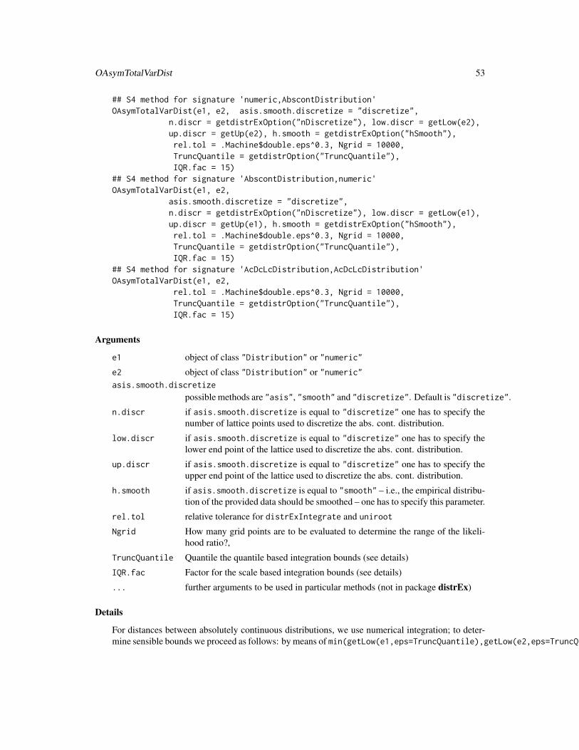
OAsymTotalVarDist 53
## S4 method for signature 'numeric,AbscontDistribution'OAsymTotalVarDist(e1, e2, asis.smooth.discretize = "discretize",
n.discr = getdistrExOption("nDiscretize"), low.discr = getLow(e2),up.discr = getUp(e2), h.smooth = getdistrExOption("hSmooth"),rel.tol = .Machine$double.eps^0.3, Ngrid = 10000,TruncQuantile = getdistrOption("TruncQuantile"),IQR.fac = 15)
## S4 method for signature 'AbscontDistribution,numeric'OAsymTotalVarDist(e1, e2,
asis.smooth.discretize = "discretize",n.discr = getdistrExOption("nDiscretize"), low.discr = getLow(e1),up.discr = getUp(e1), h.smooth = getdistrExOption("hSmooth"),rel.tol = .Machine$double.eps^0.3, Ngrid = 10000,TruncQuantile = getdistrOption("TruncQuantile"),IQR.fac = 15)
## S4 method for signature 'AcDcLcDistribution,AcDcLcDistribution'OAsymTotalVarDist(e1, e2,
rel.tol = .Machine$double.eps^0.3, Ngrid = 10000,TruncQuantile = getdistrOption("TruncQuantile"),IQR.fac = 15)
Arguments
e1 object of class "Distribution" or "numeric"
e2 object of class "Distribution" or "numeric"asis.smooth.discretize
possible methods are "asis", "smooth" and "discretize". Default is "discretize".
n.discr if asis.smooth.discretize is equal to "discretize" one has to specify thenumber of lattice points used to discretize the abs. cont. distribution.
low.discr if asis.smooth.discretize is equal to "discretize" one has to specify thelower end point of the lattice used to discretize the abs. cont. distribution.
up.discr if asis.smooth.discretize is equal to "discretize" one has to specify theupper end point of the lattice used to discretize the abs. cont. distribution.
h.smooth if asis.smooth.discretize is equal to "smooth" – i.e., the empirical distribu-tion of the provided data should be smoothed – one has to specify this parameter.
rel.tol relative tolerance for distrExIntegrate and uniroot
Ngrid How many grid points are to be evaluated to determine the range of the likeli-hood ratio?,
TruncQuantile Quantile the quantile based integration bounds (see details)
IQR.fac Factor for the scale based integration bounds (see details)
... further arguments to be used in particular methods (not in package distrEx)
Details
For distances between absolutely continuous distributions, we use numerical integration; to deter-mine sensible bounds we proceed as follows: by means of min(getLow(e1,eps=TruncQuantile),getLow(e2,eps=TruncQuantile)),
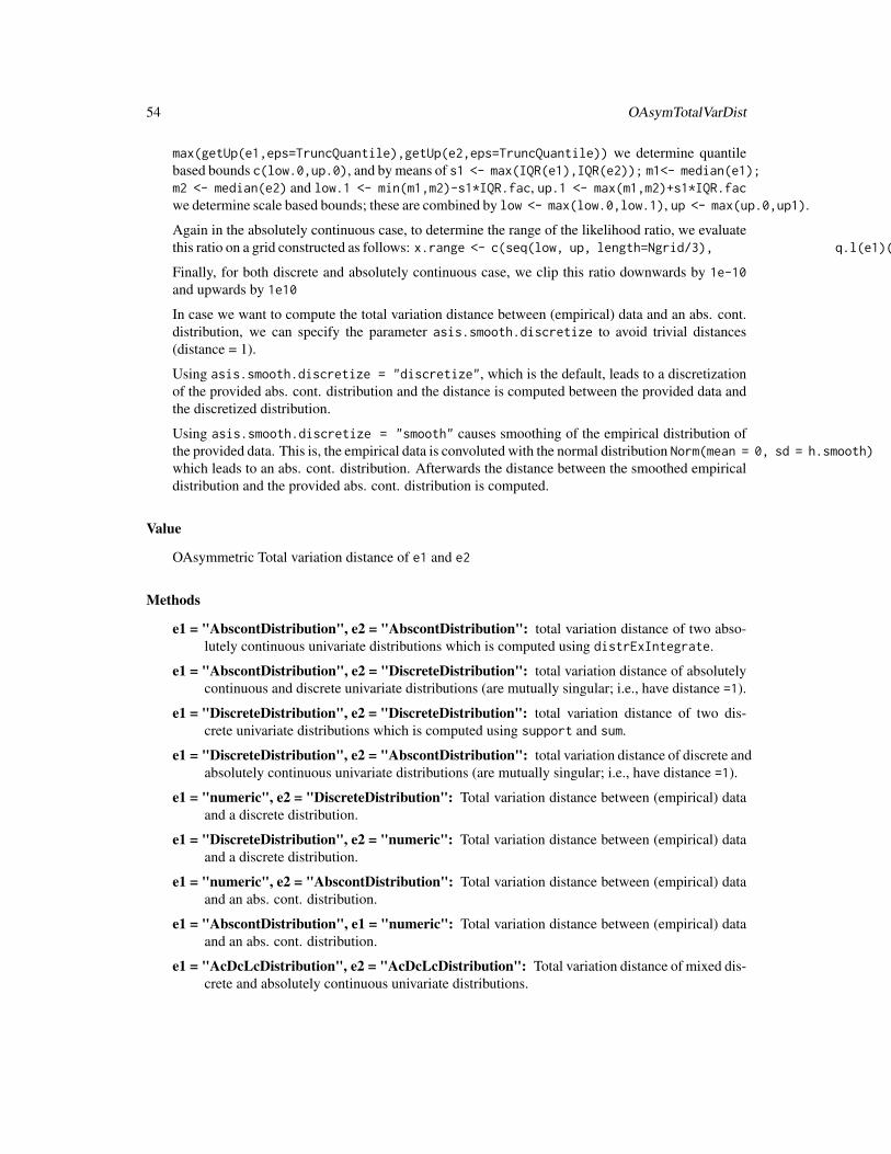
54 OAsymTotalVarDist
max(getUp(e1,eps=TruncQuantile),getUp(e2,eps=TruncQuantile)) we determine quantilebased bounds c(low.0,up.0), and by means of s1 <- max(IQR(e1),IQR(e2)); m1<- median(e1);m2 <- median(e2) and low.1 <- min(m1,m2)-s1*IQR.fac, up.1 <- max(m1,m2)+s1*IQR.facwe determine scale based bounds; these are combined by low <- max(low.0,low.1), up <- max(up.0,up1).
Again in the absolutely continuous case, to determine the range of the likelihood ratio, we evaluatethis ratio on a grid constructed as follows: x.range <- c(seq(low, up, length=Ngrid/3), q.l(e1)(seq(0,1,length=Ngrid/3)*.999), q.l(e2)(seq(0,1,length=Ngrid/3)*.999))
Finally, for both discrete and absolutely continuous case, we clip this ratio downwards by 1e-10and upwards by 1e10
In case we want to compute the total variation distance between (empirical) data and an abs. cont.distribution, we can specify the parameter asis.smooth.discretize to avoid trivial distances(distance = 1).
Using asis.smooth.discretize = "discretize", which is the default, leads to a discretizationof the provided abs. cont. distribution and the distance is computed between the provided data andthe discretized distribution.
Using asis.smooth.discretize = "smooth" causes smoothing of the empirical distribution ofthe provided data. This is, the empirical data is convoluted with the normal distribution Norm(mean = 0, sd = h.smooth)which leads to an abs. cont. distribution. Afterwards the distance between the smoothed empiricaldistribution and the provided abs. cont. distribution is computed.
Value
OAsymmetric Total variation distance of e1 and e2
Methods
e1 = "AbscontDistribution", e2 = "AbscontDistribution": total variation distance of two abso-lutely continuous univariate distributions which is computed using distrExIntegrate.
e1 = "AbscontDistribution", e2 = "DiscreteDistribution": total variation distance of absolutelycontinuous and discrete univariate distributions (are mutually singular; i.e., have distance =1).
e1 = "DiscreteDistribution", e2 = "DiscreteDistribution": total variation distance of two dis-crete univariate distributions which is computed using support and sum.
e1 = "DiscreteDistribution", e2 = "AbscontDistribution": total variation distance of discrete andabsolutely continuous univariate distributions (are mutually singular; i.e., have distance =1).
e1 = "numeric", e2 = "DiscreteDistribution": Total variation distance between (empirical) dataand a discrete distribution.
e1 = "DiscreteDistribution", e2 = "numeric": Total variation distance between (empirical) dataand a discrete distribution.
e1 = "numeric", e2 = "AbscontDistribution": Total variation distance between (empirical) dataand an abs. cont. distribution.
e1 = "AbscontDistribution", e1 = "numeric": Total variation distance between (empirical) dataand an abs. cont. distribution.
e1 = "AcDcLcDistribution", e2 = "AcDcLcDistribution": Total variation distance of mixed dis-crete and absolutely continuous univariate distributions.
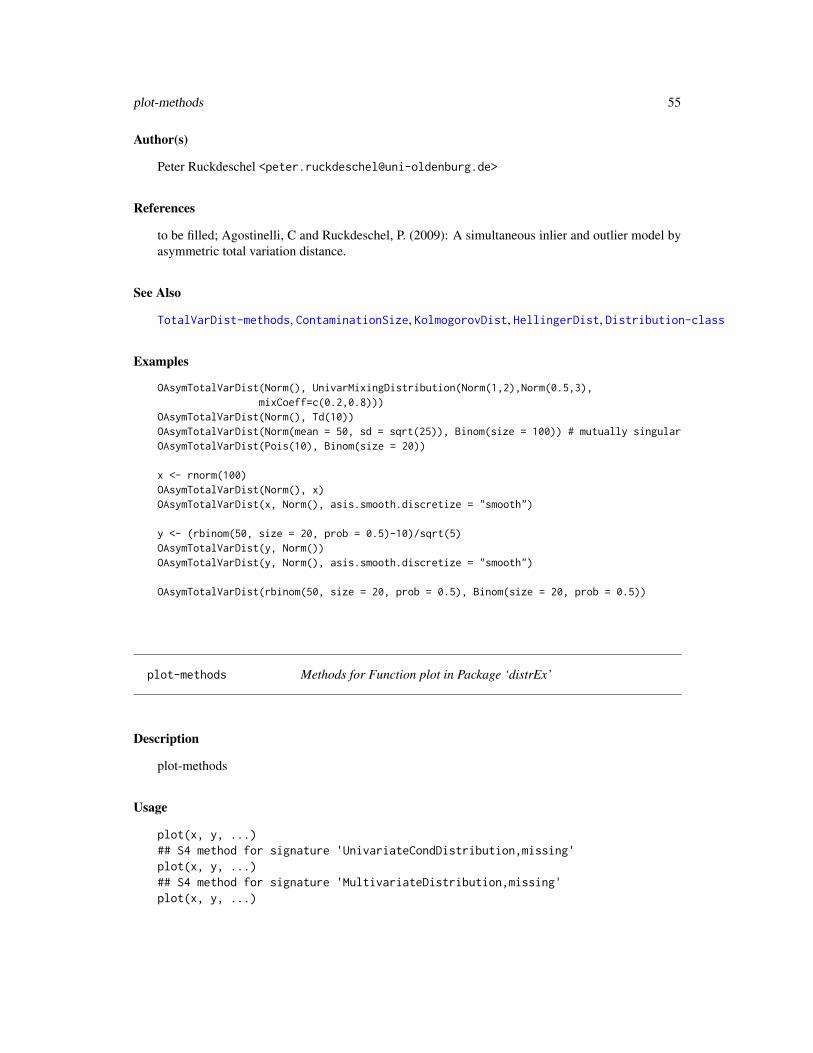
plot-methods 55
Author(s)
Peter Ruckdeschel <[email protected]>
References
to be filled; Agostinelli, C and Ruckdeschel, P. (2009): A simultaneous inlier and outlier model byasymmetric total variation distance.
See Also
TotalVarDist-methods, ContaminationSize, KolmogorovDist, HellingerDist, Distribution-class
Examples
OAsymTotalVarDist(Norm(), UnivarMixingDistribution(Norm(1,2),Norm(0.5,3),mixCoeff=c(0.2,0.8)))
OAsymTotalVarDist(Norm(), Td(10))OAsymTotalVarDist(Norm(mean = 50, sd = sqrt(25)), Binom(size = 100)) # mutually singularOAsymTotalVarDist(Pois(10), Binom(size = 20))
x <- rnorm(100)OAsymTotalVarDist(Norm(), x)OAsymTotalVarDist(x, Norm(), asis.smooth.discretize = "smooth")
y <- (rbinom(50, size = 20, prob = 0.5)-10)/sqrt(5)OAsymTotalVarDist(y, Norm())OAsymTotalVarDist(y, Norm(), asis.smooth.discretize = "smooth")
OAsymTotalVarDist(rbinom(50, size = 20, prob = 0.5), Binom(size = 20, prob = 0.5))
plot-methods Methods for Function plot in Package ‘distrEx’
Description
plot-methods
Usage
plot(x, y, ...)## S4 method for signature 'UnivariateCondDistribution,missing'plot(x, y, ...)## S4 method for signature 'MultivariateDistribution,missing'plot(x, y, ...)
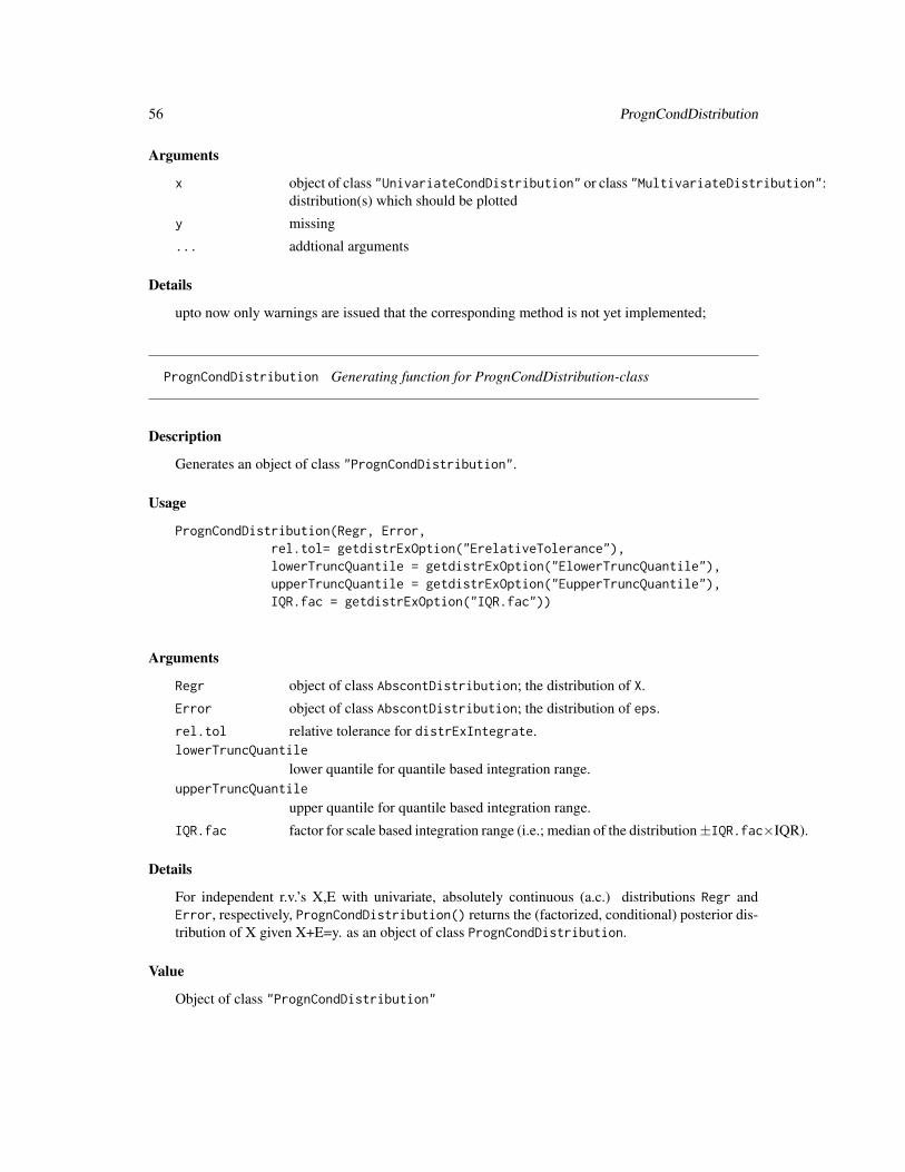
56 PrognCondDistribution
Arguments
x object of class "UnivariateCondDistribution" or class "MultivariateDistribution":distribution(s) which should be plotted
y missing
... addtional arguments
Details
upto now only warnings are issued that the corresponding method is not yet implemented;
PrognCondDistribution Generating function for PrognCondDistribution-class
Description
Generates an object of class "PrognCondDistribution".
Usage
PrognCondDistribution(Regr, Error,rel.tol= getdistrExOption("ErelativeTolerance"),lowerTruncQuantile = getdistrExOption("ElowerTruncQuantile"),upperTruncQuantile = getdistrExOption("EupperTruncQuantile"),IQR.fac = getdistrExOption("IQR.fac"))
Arguments
Regr object of class AbscontDistribution; the distribution of X.
Error object of class AbscontDistribution; the distribution of eps.
rel.tol relative tolerance for distrExIntegrate.lowerTruncQuantile
lower quantile for quantile based integration range.upperTruncQuantile
upper quantile for quantile based integration range.
IQR.fac factor for scale based integration range (i.e.; median of the distribution±IQR.fac×IQR).
Details
For independent r.v.’s X,E with univariate, absolutely continuous (a.c.) distributions Regr andError, respectively, PrognCondDistribution() returns the (factorized, conditional) posterior dis-tribution of X given X+E=y. as an object of class PrognCondDistribution.
Value
Object of class "PrognCondDistribution"

PrognCondDistribution-class 57
Author(s)
Peter Ruckdeschel <[email protected]>,
See Also
PrognCondDistribution-class; demo(‘Prognose.R’).
Examples
PrognCondDistribution(Error = ConvexContamination(Norm(), Norm(4,1), size=0.1))
PrognCondDistribution-class
Posterior distribution in convolution
Description
The posterior distribution of X given (X+E)=y
Objects from the Class
Objects can be created by calls of the form PrognCondDistribution where Regr and error are therespective (a.c.) distributions of X and E and the other arguments control accuracy in integration.
Slots
cond: Object of class "PrognCondition": condition
img: Object of class "rSpace": the image space.
param: Object of class "OptionalParameter": an optional parameter.
r: Object of class "function": generates random numbers.
d: Object of class "OptionalFunction": optional conditional density function.
p: Object of class "OptionalFunction": optional conditional cumulative distribution function.
q: Object of class "OptionalFunction": optional conditional quantile function.
gaps: (numeric) matrix or NULL
.withArith: logical: used internally to issue warnings as to interpretation of arithmetics
.withSim: logical: used internally to issue warnings as to accuracy
.logExact: logical: used internally to flag the case where there are explicit formulae for the logversion of density, cdf, and quantile function
.lowerExact: logical: used internally to flag the case where there are explicit formulae for thelower tail version of cdf and quantile function
Extends
Class "AbscontCondDistribution", directly.Class "Distribution", by classes "UnivariateCondDistribution" and "AbscontCondDistribution".
58 PrognCondition-class
Author(s)
Matthias Kohl <[email protected]>
See Also
PrognCondition-class, UnivariateCondDistribution-class AbscontCondDistribution-class,Distribution-class
Examples
PrognCondDistribution()
PrognCondition-class Conditions of class ’PrognCondition’
Description
The class PrognCondition realizes the condition that X+E=y in a convolution setup
Usage
PrognCondition(range = EuclideanSpace())
Arguments
range an object of class "EuclideanSpace"
Value
Object of class "PrognCondition"
Objects from the Class
Objects can be created by calls of the form PrognCondition(range).
Slots
name Object of class "character": name of the PrognCondition
range Object of class "EuclideanSpace": range of the PrognCondition
Extends
Class "Condition", directly.
Methods
show signature(object = "PrognCondition")
TotalVarDist 59
Author(s)
Matthias Kohl <[email protected]>
See Also
PrognCondDistribution-class,Condition-class
Examples
PrognCondition()
TotalVarDist Generic function for the computation of the total variation distance oftwo distributions
Description
Generic function for the computation of the total variation distance dv of two distributions P andQ where the distributions may be defined for an arbitrary sample space (Ω,A). The total variationdistance is defined as
dv(P,Q) = supB∈A|P (B)−Q(B)|
Usage
TotalVarDist(e1, e2, ...)## S4 method for signature 'AbscontDistribution,AbscontDistribution'TotalVarDist(e1,e2,
rel.tol=.Machine$double.eps^0.3,TruncQuantile = getdistrOption("TruncQuantile"),IQR.fac = 15, ...)
## S4 method for signature 'AbscontDistribution,DiscreteDistribution'TotalVarDist(e1,e2, ...)## S4 method for signature 'DiscreteDistribution,AbscontDistribution'TotalVarDist(e1,e2, ...)## S4 method for signature 'DiscreteDistribution,DiscreteDistribution'TotalVarDist(e1,e2, ...)## S4 method for signature 'numeric,DiscreteDistribution'TotalVarDist(e1, e2, ...)## S4 method for signature 'DiscreteDistribution,numeric'TotalVarDist(e1, e2, ...)## S4 method for signature 'numeric,AbscontDistribution'TotalVarDist(e1, e2, asis.smooth.discretize = "discretize",
n.discr = getdistrExOption("nDiscretize"), low.discr = getLow(e2),up.discr = getUp(e2), h.smooth = getdistrExOption("hSmooth"),rel.tol = .Machine$double.eps^0.3,TruncQuantile = getdistrOption("TruncQuantile"), IQR.fac = 15, ...)
## S4 method for signature 'AbscontDistribution,numeric'

60 TotalVarDist
TotalVarDist(e1, e2, asis.smooth.discretize = "discretize",n.discr = getdistrExOption("nDiscretize"), low.discr = getLow(e1),up.discr = getUp(e1), h.smooth = getdistrExOption("hSmooth"),rel.tol = .Machine$double.eps^0.3,TruncQuantile = getdistrOption("TruncQuantile"), IQR.fac = 15, ...)
## S4 method for signature 'AcDcLcDistribution,AcDcLcDistribution'TotalVarDist(e1, e2,
rel.tol = .Machine$double.eps^0.3,TruncQuantile = getdistrOption("TruncQuantile"),IQR.fac = 15, ...)
Arguments
e1 object of class "Distribution" or "numeric"
e2 object of class "Distribution" or "numeric"asis.smooth.discretize
possible methods are "asis", "smooth" and "discretize". Default is "discretize".
n.discr if asis.smooth.discretize is equal to "discretize" one has to specify thenumber of lattice points used to discretize the abs. cont. distribution.
low.discr if asis.smooth.discretize is equal to "discretize" one has to specify thelower end point of the lattice used to discretize the abs. cont. distribution.
up.discr if asis.smooth.discretize is equal to "discretize" one has to specify theupper end point of the lattice used to discretize the abs. cont. distribution.
h.smooth if asis.smooth.discretize is equal to "smooth" – i.e., the empirical distribu-tion of the provided data should be smoothed – one has to specify this parameter.
rel.tol relative accuracy requested in integration
TruncQuantile Quantile the quantile based integration bounds (see details)
IQR.fac Factor for the scale based integration bounds (see details)
... further arguments to be used in particular methods (not in package distrEx)
Details
For distances between absolutely continuous distributions, we use numerical integration; to deter-mine sensible bounds we proceed as follows: by means of min(getLow(e1,eps=TruncQuantile),getLow(e2,eps=TruncQuantile)),max(getUp(e1,eps=TruncQuantile),getUp(e2,eps=TruncQuantile)) we determine quantilebased bounds c(low.0,up.0), and by means of s1 <- max(IQR(e1),IQR(e2)); m1<- median(e1);m2 <- median(e2) and low.1 <- min(m1,m2)-s1*IQR.fac, up.1 <- max(m1,m2)+s1*IQR.facwe determine scale based bounds; these are combined by low <- max(low.0,low.1), up <- max(up.0,up1).
In case we want to compute the total variation distance between (empirical) data and an abs. cont.distribution, we can specify the parameter asis.smooth.discretize to avoid trivial distances(distance = 1).
Using asis.smooth.discretize = "discretize", which is the default, leads to a discretizationof the provided abs. cont. distribution and the distance is computed between the provided data andthe discretized distribution.
TotalVarDist 61
Using asis.smooth.discretize = "smooth" causes smoothing of the empirical distribution ofthe provided data. This is, the empirical data is convoluted with the normal distribution Norm(mean = 0, sd = h.smooth)which leads to an abs. cont. distribution. Afterwards the distance between the smoothed empiricaldistribution and the provided abs. cont. distribution is computed.
Value
Total variation distance of e1 and e2
Methods
e1 = "AbscontDistribution", e2 = "AbscontDistribution": total variation distance of two abso-lutely continuous univariate distributions which is computed using distrExIntegrate.
e1 = "AbscontDistribution", e2 = "DiscreteDistribution": total variation distance of absolutelycontinuous and discrete univariate distributions (are mutually singular; i.e., have distance =1).
e1 = "DiscreteDistribution", e2 = "DiscreteDistribution": total variation distance of two dis-crete univariate distributions which is computed using support and sum.
e1 = "DiscreteDistribution", e2 = "AbscontDistribution": total variation distance of discrete andabsolutely continuous univariate distributions (are mutually singular; i.e., have distance =1).
e1 = "numeric", e2 = "DiscreteDistribution": Total variation distance between (empirical) dataand a discrete distribution.
e1 = "DiscreteDistribution", e2 = "numeric": Total variation distance between (empirical) dataand a discrete distribution.
e1 = "numeric", e2 = "AbscontDistribution": Total variation distance between (empirical) dataand an abs. cont. distribution.
e1 = "AbscontDistribution", e1 = "numeric": Total variation distance between (empirical) dataand an abs. cont. distribution.
e1 = "AcDcLcDistribution", e2 = "AcDcLcDistribution": Total variation distance of mixed dis-crete and absolutely continuous univariate distributions.
Author(s)
Matthias Kohl <[email protected]>,Peter Ruckdeschel <[email protected]>
References
Huber, P.J. (1981) Robust Statistics. New York: Wiley.
Rieder, H. (1994) Robust Asymptotic Statistics. New York: Springer.
See Also
TotalVarDist-methods, ContaminationSize, KolmogorovDist, HellingerDist, Distribution-class
62 UnivariateCondDistribution-class
Examples
TotalVarDist(Norm(), UnivarMixingDistribution(Norm(1,2),Norm(0.5,3),mixCoeff=c(0.2,0.8)))
TotalVarDist(Norm(), Td(10))TotalVarDist(Norm(mean = 50, sd = sqrt(25)), Binom(size = 100)) # mutually singularTotalVarDist(Pois(10), Binom(size = 20))
x <- rnorm(100)TotalVarDist(Norm(), x)TotalVarDist(x, Norm(), asis.smooth.discretize = "smooth")
y <- (rbinom(50, size = 20, prob = 0.5)-10)/sqrt(5)TotalVarDist(y, Norm())TotalVarDist(y, Norm(), asis.smooth.discretize = "smooth")
TotalVarDist(rbinom(50, size = 20, prob = 0.5), Binom(size = 20, prob = 0.5))
UnivariateCondDistribution-class
Univariate conditional distribution
Description
Class of univariate conditional distributions.
Objects from the Class
Objects can be created by calls of the form new("UnivariateCondDistribution", ...).
Slots
cond Object of class "Condition": condition
img Object of class "rSpace": the image space.
param Object of class "OptionalParameter": an optional parameter.
r Object of class "function": generates random numbers.
d Object of class "OptionalFunction": optional conditional density function.
p Object of class "OptionalFunction": optional conditional cumulative distribution function.
q Object of class "OptionalFunction": optional conditional quantile function.
.withArith logical: used internally to issue warnings as to interpretation of arithmetics
.withSim logical: used internally to issue warnings as to accuracy
.logExact logical: used internally to flag the case where there are explicit formulae for the logversion of density, cdf, and quantile function
.lowerExact logical: used internally to flag the case where there are explicit formulae for thelower tail version of cdf and quantile function
Symmetry object of class "DistributionSymmetry"; used internally to avoid unnecessary calcu-lations.
var 63
Extends
Class "UnivariateDistribution", directly.Class "Distribution", by class "UnivariateDistribution".
Methods
cond signature(object = "UnivariateCondDistribution"): accessor function for slot cond.
show signature(object = "UnivariateCondDistribution")
plot signature(object = "UnivariateCondDistribution"): not yet implemented.
Author(s)
Matthias Kohl <[email protected]>
See Also
Distribution-class
Examples
new("UnivariateCondDistribution")
var Generic Functions for the Computation of Functionals
Description
Generic functions for the computation of functionals on distributions.
Usage
IQR(x, ...)
## S4 method for signature 'UnivariateDistribution'IQR(x)## S4 method for signature 'UnivariateCondDistribution'IQR(x,cond)## S4 method for signature 'AffLinDistribution'IQR(x)## S4 method for signature 'DiscreteDistribution'IQR(x)## S4 method for signature 'Arcsine'IQR(x)## S4 method for signature 'Cauchy'IQR(x)## S4 method for signature 'Dirac'IQR(x)
64 var
## S4 method for signature 'DExp'IQR(x)## S4 method for signature 'Exp'IQR(x)## S4 method for signature 'Geom'IQR(x)## S4 method for signature 'Logis'IQR(x)## S4 method for signature 'Norm'IQR(x)## S4 method for signature 'Unif'IQR(x)
median(x, ...)
## S4 method for signature 'UnivariateDistribution'median(x)## S4 method for signature 'UnivariateCondDistribution'median(x,cond)## S4 method for signature 'AffLinDistribution'median(x)## S4 method for signature 'Arcsine'median(x)## S4 method for signature 'Cauchy'median(x)## S4 method for signature 'Dirac'median(x)## S4 method for signature 'DExp'median(x)## S4 method for signature 'Exp'median(x)## S4 method for signature 'Geom'median(x)## S4 method for signature 'Logis'median(x)## S4 method for signature 'Lnorm'median(x)## S4 method for signature 'Norm'median(x)## S4 method for signature 'Unif'median(x)
mad(x, ...)
## S4 method for signature 'UnivariateDistribution'mad(x)## S4 method for signature 'AffLinDistribution'mad(x)
var 65
## S4 method for signature 'Cauchy'mad(x)## S4 method for signature 'Dirac'mad(x)## S4 method for signature 'DExp'mad(x)## S4 method for signature 'Exp'mad(x)## S4 method for signature 'Geom'mad(x)## S4 method for signature 'Logis'mad(x)## S4 method for signature 'Norm'mad(x)## S4 method for signature 'Unif'mad(x)## S4 method for signature 'Arcsine'mad(x)
sd(x, ...)
## S4 method for signature 'UnivariateDistribution'sd(x, fun, cond, withCond, useApply, ...)## S4 method for signature 'Norm'sd(x, fun, cond, withCond = FALSE, useApply = TRUE, ...)
var(x, ...)
## S4 method for signature 'UnivariateDistribution'var(x, fun, cond, withCond, useApply, ...)## S4 method for signature 'AffLinDistribution'var(x, fun, cond, withCond, useApply, ...)## S4 method for signature 'CompoundDistribution'var(x, ...)## S4 method for signature 'Arcsine'var(x, ...)## S4 method for signature 'Binom'var(x, ...)## S4 method for signature 'Beta'var(x, ...)## S4 method for signature 'Cauchy'var(x, ...)## S4 method for signature 'Chisq'var(x, ...)## S4 method for signature 'Dirac'var(x, ...)## S4 method for signature 'DExp'var(x, ...)
66 var
## S4 method for signature 'Exp'var(x, ...)## S4 method for signature 'Fd'var(x, ...)## S4 method for signature 'Gammad'var(x, ...)## S4 method for signature 'Geom'var(x, ...)## S4 method for signature 'Hyper'var(x, ...)## S4 method for signature 'Logis'var(x, ...)## S4 method for signature 'Lnorm'var(x, ...)## S4 method for signature 'Nbinom'var(x, ...)## S4 method for signature 'Norm'var(x, ...)## S4 method for signature 'Pois'var(x, ...)## S4 method for signature 'Td'var(x, ...)## S4 method for signature 'Unif'var(x, ...)## S4 method for signature 'Weibull'var(x, ...)
skewness(x, ...)## S4 method for signature 'UnivariateDistribution'skewness(x, fun, cond, withCond, useApply, ...)## S4 method for signature 'AffLinDistribution'skewness(x, fun, cond, withCond, useApply, ...)## S4 method for signature 'Arcsine'skewness(x, ...)## S4 method for signature 'Binom'skewness(x, ...)## S4 method for signature 'Beta'skewness(x, ...)## S4 method for signature 'Cauchy'skewness(x, ...)## S4 method for signature 'Chisq'skewness(x, ...)## S4 method for signature 'Dirac'skewness(x, ...)## S4 method for signature 'DExp'skewness(x, ...)## S4 method for signature 'Exp'skewness(x, ...)
var 67
## S4 method for signature 'Fd'skewness(x, ...)## S4 method for signature 'Gammad'skewness(x, ...)## S4 method for signature 'Geom'skewness(x, ...)## S4 method for signature 'Hyper'skewness(x, ...)## S4 method for signature 'Logis'skewness(x, ...)## S4 method for signature 'Lnorm'skewness(x, ...)## S4 method for signature 'Nbinom'skewness(x, ...)## S4 method for signature 'Norm'skewness(x, ...)## S4 method for signature 'Pois'skewness(x, ...)## S4 method for signature 'Td'skewness(x, ...)## S4 method for signature 'Unif'skewness(x, ...)## S4 method for signature 'Weibull'skewness(x, ...)
kurtosis(x, ...)## S4 method for signature 'UnivariateDistribution'kurtosis(x, fun, cond, withCond, useApply, ...)## S4 method for signature 'AffLinDistribution'kurtosis(x, fun, cond, withCond, useApply, ...)## S4 method for signature 'Arcsine'kurtosis(x, ...)## S4 method for signature 'Binom'kurtosis(x, ...)## S4 method for signature 'Beta'kurtosis(x, ...)## S4 method for signature 'Cauchy'kurtosis(x, ...)## S4 method for signature 'Chisq'kurtosis(x, ...)## S4 method for signature 'Dirac'kurtosis(x, ...)## S4 method for signature 'DExp'kurtosis(x, ...)## S4 method for signature 'Exp'kurtosis(x, ...)## S4 method for signature 'Fd'kurtosis(x, ...)
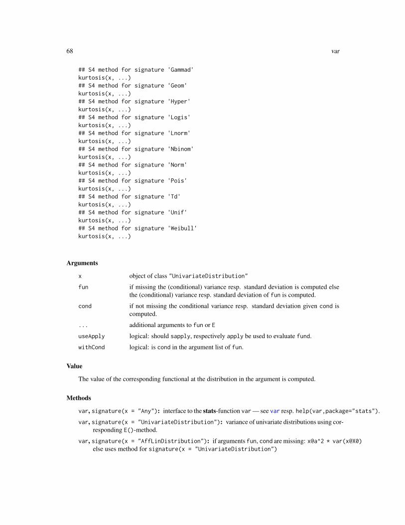
68 var
## S4 method for signature 'Gammad'kurtosis(x, ...)## S4 method for signature 'Geom'kurtosis(x, ...)## S4 method for signature 'Hyper'kurtosis(x, ...)## S4 method for signature 'Logis'kurtosis(x, ...)## S4 method for signature 'Lnorm'kurtosis(x, ...)## S4 method for signature 'Nbinom'kurtosis(x, ...)## S4 method for signature 'Norm'kurtosis(x, ...)## S4 method for signature 'Pois'kurtosis(x, ...)## S4 method for signature 'Td'kurtosis(x, ...)## S4 method for signature 'Unif'kurtosis(x, ...)## S4 method for signature 'Weibull'kurtosis(x, ...)
Arguments
x object of class "UnivariateDistribution"
fun if missing the (conditional) variance resp. standard deviation is computed elsethe (conditional) variance resp. standard deviation of fun is computed.
cond if not missing the conditional variance resp. standard deviation given cond iscomputed.
... additional arguments to fun or E
useApply logical: should sapply, respectively apply be used to evaluate fund.
withCond logical: is cond in the argument list of fun.
Value
The value of the corresponding functional at the distribution in the argument is computed.
Methods
var, signature(x = "Any"): interface to the stats-function var — see var resp. help(var,package="stats").
var, signature(x = "UnivariateDistribution"): variance of univariate distributions using cor-responding E()-method.
var, signature(x = "AffLinDistribution"): if arguments fun, cond are missing: x@a^2 * var(x@X0)else uses method for signature(x = "UnivariateDistribution")

var 69
var, signature(x = "CompoundDistribution"): if we are in i.i.d. situation (i.e., slot SummandsDistris of class UnivariateDistribution) the formula E[N ]var[S]+(E[S]2+var(S))var(N) forN the frequency distribution and S the summand distribution; else we coerce to "UnivarLebDecDistribution".
sd, signature(x = "Any"): interface to the stats-function sd — see sd resp. help(sd,package="stats").
sd, signature(x = "NormParameter"): returns the slot sd of the parameter of a normal distri-bution — see sd resp. help(sd,package="distr").
sd, signature(x = "Norm"): returns the slot sd of the parameter of a normal distribution — seesd resp. help(sd,package="distr").
sd, signature(x = "UnivariateDistribution"): standard deviation of univariate distributionsusing corresponding E()-method.
IQR, signature(x = "Any"): interface to the stats-function IQR — see IQR resp. help(IQR,package="stats").
IQR, signature(x = "UnivariateDistribution"): interquartile range of univariate distributionsusing corresponding q()-method.
IQR, signature(x = "UnivariateCondDistribution"): interquartile range of univariate con-ditional distributions using corresponding q()-method.
IQR, signature(x = "DiscreteDistribution"): interquartile range of discrete distributions us-ing corresponding q()-method but taking care that between upper and lower quartile there is50% probability
IQR, signature(x = "AffLinDistribution"): abs(x@a) * IQR(x@X0)
median, signature(x = "Any"): interface to the stats-function median — see median resp. help(var,package="stats").
median, signature(x = "UnivariateDistribution"): median of univariate distributions usingcorresponding q()-method.
median, signature(x = "UnivariateCondDistribution"): median of univariate conditional dis-tributions using corresponding q()-method.
median, signature(x = "AffLinDistribution"): x@a * median(x@X0) + x@b
mad, signature(x = "Any"): interface to the stats-function mad — see mad.
mad, signature(x = "UnivariateDistribution"): mad of univariate distributions using corre-sponding q()-method applied to abs(x-median(x)).
mad, signature(x = "AffLinDistribution"): abs(x@a) * mad(x@X0)
skewness, signature(x = "Any"): bias free estimation of skewness under normal distribution(default) as well as sample version (by argument sample.version = TRUE).
skewness, signature(x = "UnivariateDistribution"): skewness of univariate distributionsusing corresponding E()-method.
skewness, signature(x = "AffLinDistribution"): if arguments fun, cond are missing: skewness(x@X0)else uses method for signature(x = "UnivariateDistribution")
kurtosis, signature(x = "Any"): bias free estimation of kurtosis under normal distribution (de-fault) as well as sample version (by argument sample.version = TRUE).
kurtosis, signature(x = "UnivariateDistribution"): kurtosis of univariate distributions us-ing corresponding E()-method.
kurtosis, signature(x = "AffLinDistribution"): if arguments fun, cond are missing: kurtosis(x@X0)else uses method for signature(x = "UnivariateDistribution")
70 var
var, signature(x = "Arcsine"): exact evaluation using explicit expressions.
var, signature(x = "Beta"): for noncentrality 0 exact evaluation using explicit expressions.
var, signature(x = "Binom"): exact evaluation using explicit expressions.
var, signature(x = "Cauchy"): exact evaluation using explicit expressions.
var, signature(x = "Chisq"): exact evaluation using explicit expressions.
var, signature(x = "Dirac"): exact evaluation using explicit expressions.
var, signature(x = "DExp"): exact evaluation using explicit expressions.
var, signature(x = "Exp"): exact evaluation using explicit expressions.
var, signature(x = "Fd"): exact evaluation using explicit expressions.
var, signature(x = "Gammad"): exact evaluation using explicit expressions.
var, signature(x = "Geom"): exact evaluation using explicit expressions.
var, signature(x = "Hyper"): exact evaluation using explicit expressions.
var, signature(x = "Logis"): exact evaluation using explicit expressions.
var, signature(x = "Lnorm"): exact evaluation using explicit expressions.
var, signature(x = "Nbinom"): exact evaluation using explicit expressions.
var, signature(x = "Norm"): exact evaluation using explicit expressions.
var, signature(x = "Pois"): exact evaluation using explicit expressions.
var, signature(x = "Td"): exact evaluation using explicit expressions.
var, signature(x = "Unif"): exact evaluation using explicit expressions.
var, signature(x = "Weibull"): exact evaluation using explicit expressions.
IQR, signature(x = "Arcsine"): exact evaluation using explicit expressions.
IQR, signature(x = "Cauchy"): exact evaluation using explicit expressions.
IQR, signature(x = "Dirac"): exact evaluation using explicit expressions.
IQR, signature(x = "DExp"): exact evaluation using explicit expressions.
IQR, signature(x = "Exp"): exact evaluation using explicit expressions.
IQR, signature(x = "Geom"): exact evaluation using explicit expressions.
IQR, signature(x = "Logis"): exact evaluation using explicit expressions.
IQR, signature(x = "Norm"): exact evaluation using explicit expressions.
IQR, signature(x = "Unif"): exact evaluation using explicit expressions.
median, signature(x = "Arcsine"): exact evaluation using explicit expressions.
median, signature(x = "Cauchy"): exact evaluation using explicit expressions.
median, signature(x = "Dirac"): exact evaluation using explicit expressions.
median, signature(x = "DExp"): exact evaluation using explicit expressions.
median, signature(x = "Exp"): exact evaluation using explicit expressions.
median, signature(x = "Geom"): exact evaluation using explicit expressions.
median, signature(x = "Logis"): exact evaluation using explicit expressions.
median, signature(x = "Lnorm"): exact evaluation using explicit expressions.
var 71
median, signature(x = "Norm"): exact evaluation using explicit expressions.
median, signature(x = "Unif"): exact evaluation using explicit expressions.
mad, signature(x = "Arcsine"): exact evaluation using explicit expressions.
mad, signature(x = "Cauchy"): exact evaluation using explicit expressions.
mad, signature(x = "Dirac"): exact evaluation using explicit expressions.
mad, signature(x = "DExp"): exact evaluation using explicit expressions.
mad, signature(x = "Exp"): exact evaluation using explicit expressions.
mad, signature(x = "Geom"): exact evaluation using explicit expressions.
mad, signature(x = "Logis"): exact evaluation using explicit expressions.
mad, signature(x = "Norm"): exact evaluation using explicit expressions.
mad, signature(x = "Unif"): exact evaluation using explicit expressions.
skewness, signature(x = "Arcsine"): exact evaluation using explicit expressions.
skewness, signature(x = "Beta"): for noncentrality 0 exact evaluation using explicit expres-sions.
skewness, signature(x = "Binom"): exact evaluation using explicit expressions.
skewness, signature(x = "Cauchy"): exact evaluation using explicit expressions.
skewness, signature(x = "Chisq"): exact evaluation using explicit expressions.
skewness, signature(x = "Dirac"): exact evaluation using explicit expressions.
skewness, signature(x = "DExp"): exact evaluation using explicit expressions.
skewness, signature(x = "Exp"): exact evaluation using explicit expressions.
skewness, signature(x = "Fd"): exact evaluation using explicit expressions.
skewness, signature(x = "Gammad"): exact evaluation using explicit expressions.
skewness, signature(x = "Geom"): exact evaluation using explicit expressions.
skewness, signature(x = "Hyper"): exact evaluation using explicit expressions.
skewness, signature(x = "Logis"): exact evaluation using explicit expressions.
skewness, signature(x = "Lnorm"): exact evaluation using explicit expressions.
skewness, signature(x = "Nbinom"): exact evaluation using explicit expressions.
skewness, signature(x = "Norm"): exact evaluation using explicit expressions.
skewness, signature(x = "Pois"): exact evaluation using explicit expressions.
skewness, signature(x = "Td"): exact evaluation using explicit expressions.
skewness, signature(x = "Unif"): exact evaluation using explicit expressions.
skewness, signature(x = "Weibull"): exact evaluation using explicit expressions.
kurtosis, signature(x = "Arcsine"): exact evaluation using explicit expressions.
kurtosis, signature(x = "Beta"): for noncentrality 0 exact evaluation using explicit expres-sions.
kurtosis, signature(x = "Binom"): exact evaluation using explicit expressions.
kurtosis, signature(x = "Cauchy"): exact evaluation using explicit expressions.
kurtosis, signature(x = "Chisq"): exact evaluation using explicit expressions.
72 var
kurtosis, signature(x = "Dirac"): exact evaluation using explicit expressions.
kurtosis, signature(x = "DExp"): exact evaluation using explicit expressions.
kurtosis, signature(x = "Exp"): exact evaluation using explicit expressions.
kurtosis, signature(x = "Fd"): exact evaluation using explicit expressions.
kurtosis, signature(x = "Gammad"): exact evaluation using explicit expressions.
kurtosis, signature(x = "Geom"): exact evaluation using explicit expressions.
kurtosis, signature(x = "Hyper"): exact evaluation using explicit expressions.
kurtosis, signature(x = "Logis"): exact evaluation using explicit expressions.
kurtosis, signature(x = "Lnorm"): exact evaluation using explicit expressions.
kurtosis, signature(x = "Nbinom"): exact evaluation using explicit expressions.
kurtosis, signature(x = "Norm"): exact evaluation using explicit expressions.
kurtosis, signature(x = "Pois"): exact evaluation using explicit expressions.
kurtosis, signature(x = "Td"): exact evaluation using explicit expressions.
kurtosis, signature(x = "Unif"): exact evaluation using explicit expressions.
kurtosis, signature(x = "Weibull"): exact evaluation using explicit expressions.
Caveat
If any of the packages e1071, moments, fBasics is to be used together with distrEx the latter mustbe attached after any of the first mentioned. Otherwise kurtosis() and skewness() defined asmethods in distrEx may get masked.To re-mask, you may use kurtosis <- distrEx::kurtosis; skewness <- distrEx::skewness.See also distrExMASK().
Acknowledgement
G. Jay Kerns, <[email protected]>, has provided a major contribution, in particular the functionalsskewness and kurtosis are due to him.
Author(s)
Peter Ruckdeschel <[email protected]>
See Also
distrExIntegrate, m1df, m2df, Distribution-class,sd, var, IQR,median, mad, sd,Sn, Qn
var 73
Examples
# Variance of Exp(1) distributionvar(Exp())
#median(Exp())IQR(Exp())mad(Exp())
# Variance of N(1,4)^2var(Norm(mean=1, sd=2), fun = function(x)x^2)var(Norm(mean=1, sd=2), fun = function(x)x^2, useApply = FALSE)
## sd -- may equivalently be replaced by varsd(Pois()) ## uses explicit termssd(as(Pois(),"DiscreteDistribution")) ## uses sumssd(as(Pois(),"UnivariateDistribution")) ## uses simulationssd(Norm(mean=2), fun = function(x)2*x^2) ## uses simulations#mad(sin(exp(Norm()+2*Pois()))) ## weird
Index
∗Topic distributionAbscontCondDistribution-class, 7AsymTotalVarDist, 8Condition-class, 11ContaminationSize, 12ConvexContamination, 13CvMDist, 15DiscreteCondDistribution-class, 17DiscreteMVDistribution, 18DiscreteMVDistribution-class, 19distrExMASK, 22distrExMOVED, 23distrExOptions, 23E, 25EmpiricalMVDistribution, 34EuclCondition, 35EuclCondition-class, 36HellingerDist, 38KolmogorovDist, 41liesInSupport, 43LMCondDistribution, 44LMParameter-class, 46m1df, 47m2df, 48make01, 50MultivariateDistribution-class, 51OAsymTotalVarDist, 52PrognCondDistribution, 56PrognCondDistribution-class, 57PrognCondition-class, 58TotalVarDist, 59UnivariateCondDistribution-class,
62var, 63
∗Topic documentationdistrExMASK, 22distrExMOVED, 23
∗Topic mathdistrExIntegrate, 20
GLIntegrate, 37∗Topic methods
ConvexContamination, 13dim-methods, 16E, 25liesInSupport, 43m1df, 47m2df, 48var, 63
∗Topic miscdistrExOptions, 23
∗Topic modelsLMCondDistribution, 44LMParameter, 45
∗Topic packagedistrEx-package, 2
∗Topic programmingdistrExMASK, 22distrExMOVED, 23
∗Topic utilitiesdistrExIntegrate, 20GLIntegrate, 37liesInSupport, 43
AbscontCondDistribution-class, 7AsymTotalVarDist, 8AsymTotalVarDist,AbscontDistribution,AbscontDistribution-method
(AsymTotalVarDist), 8AsymTotalVarDist,AbscontDistribution,DiscreteDistribution-method
(AsymTotalVarDist), 8AsymTotalVarDist,AbscontDistribution,numeric-method
(AsymTotalVarDist), 8AsymTotalVarDist,AcDcLcDistribution,AcDcLcDistribution-method
(AsymTotalVarDist), 8AsymTotalVarDist,DiscreteDistribution,AbscontDistribution-method
(AsymTotalVarDist), 8AsymTotalVarDist,DiscreteDistribution,DiscreteDistribution-method
(AsymTotalVarDist), 8AsymTotalVarDist,DiscreteDistribution,LatticeDistribution-method
(AsymTotalVarDist), 8
74
INDEX 75
AsymTotalVarDist,DiscreteDistribution,numeric-method(AsymTotalVarDist), 8
AsymTotalVarDist,LatticeDistribution,DiscreteDistribution-method(AsymTotalVarDist), 8
AsymTotalVarDist,LatticeDistribution,LatticeDistribution-method(AsymTotalVarDist), 8
AsymTotalVarDist,numeric,AbscontDistribution-method(AsymTotalVarDist), 8
AsymTotalVarDist,numeric,DiscreteDistribution-method(AsymTotalVarDist), 8
AsymTotalVarDist-methods(AsymTotalVarDist), 8
cond(UnivariateCondDistribution-class),62
cond,UnivariateCondDistribution-method(UnivariateCondDistribution-class),62
Condition-class, 11ContaminationSize, 11, 12, 14, 16, 40, 42,
55, 61ContaminationSize,AbscontDistribution,AbscontDistribution-method
(ContaminationSize), 12ContaminationSize,AcDcLcDistribution,AcDcLcDistribution-method
(ContaminationSize), 12ContaminationSize,DiscreteDistribution,DiscreteDistribution-method
(ContaminationSize), 12ContaminationSize,DiscreteDistribution,LatticeDistribution-method
(ContaminationSize), 12ContaminationSize,LatticeDistribution,DiscreteDistribution-method
(ContaminationSize), 12ContaminationSize,LatticeDistribution,LatticeDistribution-method
(ContaminationSize), 12ContaminationSize-methods
(ContaminationSize), 12ConvexContamination, 13ConvexContamination,AbscontDistribution,AbscontDistribution,numeric-method
(ConvexContamination), 13ConvexContamination,AbscontDistribution,UnivariateDistribution,numeric-method
(ConvexContamination), 13ConvexContamination,AcDcLcDistribution,AcDcLcDistribution,numeric-method
(ConvexContamination), 13ConvexContamination,DiscreteDistribution,DiscreteDistribution,numeric-method
(ConvexContamination), 13ConvexContamination,DiscreteDistribution,LatticeDistribution,numeric-method
(ConvexContamination), 13ConvexContamination,LatticeDistribution,DiscreteDistribution,numeric-method
(ConvexContamination), 13
ConvexContamination,LatticeDistribution,LatticeDistribution,numeric-method(ConvexContamination), 13
ConvexContamination,UnivariateDistribution,UnivariateDistribution,numeric-method(ConvexContamination), 13
ConvexContamination-methods(ConvexContamination), 13
CvMDist, 15CvMDist,numeric,UnivariateDistribution-method
(CvMDist), 15CvMDist,UnivariateDistribution,UnivariateDistribution-method
(CvMDist), 15CvMDist-methods (CvMDist), 15
dim, 16dim (dim-methods), 16dim,DiscreteMVDistribution-method
(dim-methods), 16dim-methods, 16DiscreteCondDistribution-class, 17DiscreteDistribution, 34DiscreteMVDistribution, 18, 20, 34DiscreteMVDistribution-class, 19distrEx (distrEx-package), 2distrEx-package, 2distrExIntegrate, 20, 33, 37, 40, 48, 72distrExMASK, 22distrExMOVED, 23distrExOptions, 21, 23, 30, 47, 49distrExoptions (distrExOptions), 23
E, 15, 25, 48E,AbscontCondDistribution,function,numeric-method
(E), 25E,AbscontCondDistribution,missing,numeric-method
(E), 25E,AbscontDistribution,function,missing-method
(E), 25E,AbscontDistribution,missing,missing-method
(E), 25E,AcDcLcDistribution,ANY,ANY-method
(E), 25E,AffLinAbscontDistribution,missing,missing-method
(E), 25E,AffLinDiscreteDistribution,missing,missing-method
(E), 25E,AffLinDistribution,missing,missing-method
(E), 25E,AffLinLatticeDistribution,missing,missing-method
(E), 25

76 INDEX
E,AffLinUnivarLebDecDistribution,missing,missing-method(E), 25
E,Arcsine,missing,missing-method (E), 25E,Beta,missing,missing-method (E), 25E,Binom,missing,missing-method (E), 25E,Cauchy,missing,missing-method (E), 25E,Chisq,missing,missing-method (E), 25E,CompoundDistribution,missing,missing-method
(E), 25E,DExp,missing,missing-method (E), 25E,Dirac,missing,missing-method (E), 25E,DiscreteCondDistribution,function,numeric-method
(E), 25E,DiscreteCondDistribution,missing,numeric-method
(E), 25E,DiscreteDistribution,function,missing-method
(E), 25E,DiscreteDistribution,missing,missing-method
(E), 25E,DiscreteMVDistribution,function,missing-method
(E), 25E,DiscreteMVDistribution,missing,missing-method
(E), 25E,Exp,missing,missing-method (E), 25E,Fd,missing,missing-method (E), 25E,Gammad,function,missing-method (E), 25E,Gammad,missing,missing-method (E), 25E,Geom,missing,missing-method (E), 25E,GEV,function,missing-method (E), 25E,GEV,missing,missing-method (E), 25E,GPareto,function,missing-method (E),
25E,GPareto,missing,missing-method (E), 25E,Gumbel,missing,missing-method (E), 25E,Hyper,missing,missing-method (E), 25E,LatticeDistribution,function,missing-method
(E), 25E,LatticeDistribution,missing,missing-method
(E), 25E,Lnorm,missing,missing-method (E), 25E,Logis,missing,missing-method (E), 25E,MultivariateDistribution,function,missing-method
(E), 25E,MultivariateDistribution,missing,missing-method
(E), 25E,Nbinom,missing,missing-method (E), 25E,Norm,missing,missing-method (E), 25E,Pareto,missing,missing-method (E), 25
E,Pois,missing,missing-method (E), 25E,Td,missing,missing-method (E), 25E,Unif,missing,missing-method (E), 25E,UnivariateCondDistribution,function,numeric-method
(E), 25E,UnivariateCondDistribution,missing,numeric-method
(E), 25E,UnivariateDistribution,function,missing-method
(E), 25E,UnivariateDistribution,missing,missing-method
(E), 25E,UnivarLebDecDistribution,function,ANY-method
(E), 25E,UnivarLebDecDistribution,function,missing-method
(E), 25E,UnivarLebDecDistribution,missing,ANY-method
(E), 25E,UnivarLebDecDistribution,missing,missing-method
(E), 25E,UnivarMixingDistribution,function,ANY-method
(E), 25E,UnivarMixingDistribution,function,missing-method
(E), 25E,UnivarMixingDistribution,missing,ANY-method
(E), 25E,UnivarMixingDistribution,missing,missing-method
(E), 25E,Weibull,missing,missing-method (E), 25E-methods (E), 25ElowerTruncQuantile (distrExOptions), 23EmpiricalMVDistribution, 34ErelativeTolerance (distrExOptions), 23EuclCondition, 35, 36EuclCondition-class, 36EupperTruncQuantile (distrExOptions), 23
getdistrExOption (distrExOptions), 23getOption, 25GLIntegrate, 21, 37GLIntegrateOrder (distrExOptions), 23GLIntegrateTruncQuantile
(distrExOptions), 23
HellingerDist, 11, 13, 16, 38, 42, 55, 61HellingerDist,AbscontDistribution,AbscontDistribution-method
(HellingerDist), 38HellingerDist,AbscontDistribution,DiscreteDistribution-method
(HellingerDist), 38
INDEX 77
HellingerDist,AbscontDistribution,numeric-method(HellingerDist), 38
HellingerDist,AcDcLcDistribution,AcDcLcDistribution-method(HellingerDist), 38
HellingerDist,DiscreteDistribution,AbscontDistribution-method(HellingerDist), 38
HellingerDist,DiscreteDistribution,DiscreteDistribution-method(HellingerDist), 38
HellingerDist,DiscreteDistribution,LatticeDistribution-method(HellingerDist), 38
HellingerDist,DiscreteDistribution,numeric-method(HellingerDist), 38
HellingerDist,DiscreteMVDistribution,DiscreteMVDistribution-method(HellingerDist), 38
HellingerDist,LatticeDistribution,DiscreteDistribution-method(HellingerDist), 38
HellingerDist,LatticeDistribution,LatticeDistribution-method(HellingerDist), 38
HellingerDist,numeric,AbscontDistribution-method(HellingerDist), 38
HellingerDist,numeric,DiscreteDistribution-method(HellingerDist), 38
HellingerDist-methods (HellingerDist),38
hSmooth (distrExOptions), 23
integrate, 21, 37IQR, 69, 72IQR (var), 63IQR,AffLinAbscontDistribution-method
(var), 63IQR,AffLinDiscreteDistribution-method
(var), 63IQR,AffLinDistribution-method (var), 63IQR,AffLinLatticeDistribution-method
(var), 63IQR,ANY-method (var), 63IQR,Arcsine-method (var), 63IQR,Cauchy-method (var), 63IQR,DExp-method (var), 63IQR,Dirac-method (var), 63IQR,DiscreteDistribution-method (var),
63IQR,Exp-method (var), 63IQR,Geom-method (var), 63IQR,Logis-method (var), 63IQR,Norm-method (var), 63IQR,Unif-method (var), 63
IQR,UnivariateCondDistribution-method(var), 63
IQR,UnivariateDistribution-method(var), 63
IQR-methods (var), 63IQR.fac (distrExOptions), 23
KolmogorovDist, 11, 13, 16, 40, 41, 55, 61KolmogorovDist,AbscontDistribution,AbscontDistribution-method
(KolmogorovDist), 41KolmogorovDist,AbscontDistribution,DiscreteDistribution-method
(KolmogorovDist), 41KolmogorovDist,AcDcLcDistribution,AcDcLcDistribution-method
(KolmogorovDist), 41KolmogorovDist,DiscreteDistribution,AbscontDistribution-method
(KolmogorovDist), 41KolmogorovDist,DiscreteDistribution,DiscreteDistribution-method
(KolmogorovDist), 41KolmogorovDist,DiscreteDistribution,LatticeDistribution-method
(KolmogorovDist), 41KolmogorovDist,LatticeDistribution,DiscreteDistribution-method
(KolmogorovDist), 41KolmogorovDist,LatticeDistribution,LatticeDistribution-method
(KolmogorovDist), 41KolmogorovDist,numeric,UnivariateDistribution-method
(KolmogorovDist), 41KolmogorovDist,UnivariateDistribution,numeric-method
(KolmogorovDist), 41KolmogorovDist-methods
(KolmogorovDist), 41kurtosis (var), 63kurtosis,AffLinAbscontDistribution-method
(var), 63kurtosis,AffLinDiscreteDistribution-method
(var), 63kurtosis,AffLinDistribution-method
(var), 63kurtosis,AffLinLatticeDistribution-method
(var), 63kurtosis,ANY-method (var), 63kurtosis,Arcsine-method (var), 63kurtosis,Beta-method (var), 63kurtosis,Binom-method (var), 63kurtosis,Cauchy-method (var), 63kurtosis,Chisq-method (var), 63kurtosis,DExp-method (var), 63kurtosis,Dirac-method (var), 63kurtosis,Exp-method (var), 63kurtosis,Fd-method (var), 63

78 INDEX
kurtosis,Gammad-method (var), 63kurtosis,Geom-method (var), 63kurtosis,Hyper-method (var), 63kurtosis,Lnorm-method (var), 63kurtosis,Logis-method (var), 63kurtosis,Nbinom-method (var), 63kurtosis,Norm-method (var), 63kurtosis,Pois-method (var), 63kurtosis,Td-method (var), 63kurtosis,Unif-method (var), 63kurtosis,UnivariateDistribution-method
(var), 63kurtosis,Weibull-method (var), 63kurtosis-methods (var), 63
liesInSupport, 43liesInSupport,DiscreteMVDistribution,matrix-method
(liesInSupport), 43liesInSupport,DiscreteMVDistribution,numeric-method
(liesInSupport), 43LMCondDistribution, 44LMParameter, 45, 46LMParameter-class, 46
m1df, 33, 47, 72m1df,AbscontDistribution-method (m1df),
47m1df,AffLinDistribution-method (m1df),
47m1df,Binom-method (m1df), 47m1df,Chisq-method (m1df), 47m1df,Exp-method (m1df), 47m1df,LatticeDistribution-method (m1df),
47m1df,Norm-method (m1df), 47m1df,Pois-method (m1df), 47m1df,UnivariateDistribution-method
(m1df), 47m1df-methods (m1df), 47m1dfLowerTruncQuantile
(distrExOptions), 23m1dfRelativeTolerance (distrExOptions),
23m2df, 33, 48, 48, 72m2df,AbscontDistribution-method (m2df),
48m2df,AffLinDistribution-method (m2df),
48m2df,Binom-method (m2df), 48
m2df,Chisq-method (m2df), 48m2df,Exp-method (m2df), 48m2df,LatticeDistribution-method (m2df),
48m2df,Norm-method (m2df), 48m2df,Pois-method (m2df), 48m2df,UnivariateDistribution-method
(m2df), 48m2df-methods (m2df), 48m2dfLowerTruncQuantile
(distrExOptions), 23m2dfRelativeTolerance (distrExOptions),
23mad, 69, 72mad (var), 63mad,AffLinAbscontDistribution-method
(var), 63mad,AffLinDiscreteDistribution-method
(var), 63mad,AffLinDistribution-method (var), 63mad,AffLinLatticeDistribution-method
(var), 63mad,ANY-method (var), 63mad,Arcsine-method (var), 63mad,Cauchy-method (var), 63mad,DExp-method (var), 63mad,Dirac-method (var), 63mad,Exp-method (var), 63mad,Geom-method (var), 63mad,Logis-method (var), 63mad,Norm-method (var), 63mad,Unif-method (var), 63mad,UnivariateDistribution-method
(var), 63mad-methods (var), 63make01, 50MASKING (distrExMASK), 22MCIterations (distrExOptions), 23median, 69, 72median (var), 63median,AffLinAbscontDistribution-method
(var), 63median,AffLinDiscreteDistribution-method
(var), 63median,AffLinDistribution-method (var),
63median,AffLinLatticeDistribution-method
(var), 63
INDEX 79
median,ANY-method (var), 63median,Arcsine-method (var), 63median,Cauchy-method (var), 63median,DExp-method (var), 63median,Dirac-method (var), 63median,Exp-method (var), 63median,Geom-method (var), 63median,Lnorm-method (var), 63median,Logis-method (var), 63median,Norm-method (var), 63median,Unif-method (var), 63median,UnivariateCondDistribution-method
(var), 63median,UnivariateDistribution-method
(var), 63median-methods (var), 63MOVEDING (distrExMOVED), 23MultivariateDistribution-class, 51
name,Condition-method(Condition-class), 11
name<-,Condition-method(Condition-class), 11
nDiscretize (distrExOptions), 23
OAsymTotalVarDist, 52OAsymTotalVarDist,AbscontDistribution,AbscontDistribution-method
(OAsymTotalVarDist), 52OAsymTotalVarDist,AbscontDistribution,DiscreteDistribution-method
(OAsymTotalVarDist), 52OAsymTotalVarDist,AbscontDistribution,numeric-method
(OAsymTotalVarDist), 52OAsymTotalVarDist,AcDcLcDistribution,AcDcLcDistribution-method
(OAsymTotalVarDist), 52OAsymTotalVarDist,DiscreteDistribution,AbscontDistribution-method
(OAsymTotalVarDist), 52OAsymTotalVarDist,DiscreteDistribution,DiscreteDistribution-method
(OAsymTotalVarDist), 52OAsymTotalVarDist,DiscreteDistribution,LatticeDistribution-method
(OAsymTotalVarDist), 52OAsymTotalVarDist,DiscreteDistribution,numeric-method
(OAsymTotalVarDist), 52OAsymTotalVarDist,LatticeDistribution,DiscreteDistribution-method
(OAsymTotalVarDist), 52OAsymTotalVarDist,LatticeDistribution,LatticeDistribution-method
(OAsymTotalVarDist), 52OAsymTotalVarDist,numeric,AbscontDistribution-method
(OAsymTotalVarDist), 52
OAsymTotalVarDist,numeric,DiscreteDistribution-method(OAsymTotalVarDist), 52
OAsymTotalVarDist-methods(OAsymTotalVarDist), 52
options, 25
plot (plot-methods), 55plot,MultivariateDistribution,missing-method
(plot-methods), 55plot,MultivariateDistribution-method
(MultivariateDistribution-class),51
plot,UnivariateCondDistribution,missing-method(plot-methods), 55
plot,UnivariateCondDistribution-method(UnivariateCondDistribution-class),62
plot-methods, 55PrognCondDistribution, 56, 57PrognCondDistribution-class, 57PrognCondition (PrognCondition-class),
58PrognCondition-class, 58
Qn, 72
Range (EuclCondition-class), 36Range,EuclCondition-method
(EuclCondition-class), 36
sd, 69, 72sd (var), 63sd,Norm-method (var), 63sd,UnivariateDistribution-method (var),
63sd-methods (var), 63show,EuclCondition-method
(EuclCondition-class), 36show,LMParameter-method
(LMParameter-class), 46show,MultivariateDistribution-method
(MultivariateDistribution-class),51
show,PrognCondition-method(PrognCondition-class), 58
show,UnivariateCondDistribution-method(UnivariateCondDistribution-class),62
skewness (var), 63

80 INDEX
skewness,AffLinAbscontDistribution-method(var), 63
skewness,AffLinDiscreteDistribution-method(var), 63
skewness,AffLinDistribution-method(var), 63
skewness,AffLinLatticeDistribution-method(var), 63
skewness,ANY-method (var), 63skewness,Arcsine-method (var), 63skewness,Beta-method (var), 63skewness,Binom-method (var), 63skewness,Cauchy-method (var), 63skewness,Chisq-method (var), 63skewness,DExp-method (var), 63skewness,Dirac-method (var), 63skewness,Exp-method (var), 63skewness,Fd-method (var), 63skewness,Gammad-method (var), 63skewness,Geom-method (var), 63skewness,Hyper-method (var), 63skewness,Lnorm-method (var), 63skewness,Logis-method (var), 63skewness,Nbinom-method (var), 63skewness,Norm-method (var), 63skewness,Pois-method (var), 63skewness,Td-method (var), 63skewness,Unif-method (var), 63skewness,UnivariateDistribution-method
(var), 63skewness,Weibull-method (var), 63skewness-methods (var), 63Sn, 72support,DiscreteMVDistribution-method
(DiscreteMVDistribution-class),19
TotalVarDist, 13, 16, 40, 42, 59TotalVarDist,AbscontDistribution,AbscontDistribution-method
(TotalVarDist), 59TotalVarDist,AbscontDistribution,DiscreteDistribution-method
(TotalVarDist), 59TotalVarDist,AbscontDistribution,numeric-method
(TotalVarDist), 59TotalVarDist,AcDcLcDistribution,AcDcLcDistribution-method
(TotalVarDist), 59TotalVarDist,DiscreteDistribution,AbscontDistribution-method
(TotalVarDist), 59
TotalVarDist,DiscreteDistribution,DiscreteDistribution-method(TotalVarDist), 59
TotalVarDist,DiscreteDistribution,LatticeDistribution-method(TotalVarDist), 59
TotalVarDist,DiscreteDistribution,numeric-method(TotalVarDist), 59
TotalVarDist,DiscreteMVDistribution,DiscreteMVDistribution-method(TotalVarDist), 59
TotalVarDist,LatticeDistribution,DiscreteDistribution-method(TotalVarDist), 59
TotalVarDist,LatticeDistribution,LatticeDistribution-method(TotalVarDist), 59
TotalVarDist,numeric,AbscontDistribution-method(TotalVarDist), 59
TotalVarDist,numeric,DiscreteDistribution-method(TotalVarDist), 59
TotalVarDist-methods (TotalVarDist), 59
UnivariateCondDistribution-class, 62
var, 63, 68, 72var,AffLinAbscontDistribution-method
(var), 63var,AffLinDiscreteDistribution-method
(var), 63var,AffLinDistribution-method (var), 63var,AffLinLatticeDistribution-method
(var), 63var,ANY-method (var), 63var,Arcsine-method (var), 63var,Beta-method (var), 63var,Binom-method (var), 63var,Cauchy-method (var), 63var,Chisq-method (var), 63var,CompoundDistribution-method (var),
63var,DExp-method (var), 63var,Dirac-method (var), 63var,Exp-method (var), 63var,Fd-method (var), 63var,Gammad-method (var), 63var,Geom-method (var), 63var,Hyper-method (var), 63var,Lnorm-method (var), 63var,Logis-method (var), 63var,Nbinom-method (var), 63var,Norm-method (var), 63var,Pois-method (var), 63var,Td-method (var), 63
INDEX 81
var,Unif-method (var), 63var,UnivariateDistribution-method
(var), 63var,Weibull-method (var), 63var-methods (var), 63
Related Documents