Outline of meteorological satellites*rammb.cira.colostate.edu/wmovl/vrl/texts/satellite_meteorology/... · Chapter 1 Outline of meteorological satellites* 1.1 History of meteorological

Chapter 1 Outline of meteorological satellites*

1.1 History of meteorological satellites

Sputnik was the first satellite in the world. After 3 years flight, the first meteorological satellite TIROS-1 was launched by the United States of America in April 1960. For 6 years after that, 10 satellites of the TIROS series were launched and used for conducting various observations and experiments. The TIROS series were low elevation orbit satellites. In 1966, the first geostationary meteorological satellite ATS-1 was launched by the United States and it was confirmed that the satellite observation was effective for meteorological monitoring.

The success of meteorological satellite observation intensified the trend toward using this new technology to develop meteorology and improve weather forecasting.

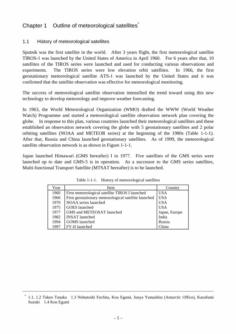
In 1963, the World Meteorological Organization (WMO) drafted the WWW (World Weather Watch) Programme and started a meteorological satellite observation network plan covering the globe. In response to this plan, various countries launched their meteorological satellites and these established an observation network covering the globe with 5 geostationary satellites and 2 polar orbiting satellites (NOAA and METEOR series) at the beginning of the 1980s (Table 1-1-1). After that, Russia and China launched geostationary satellites. As of 1999, the meteorological satellite observation network is as shown in Figure 1-1-1.

Japan launched Himawari (GMS hereafter) I in 1977. Five satellites of the GMS series were launched up to date and GMS-5 is in operation. As a successor to the GMS series satellites, Multi-functional Transport Satellite (MTSAT hereafter) is to be launched.

Table 1-1-1. History of meteorological satellites

Year Item Country 1960 First meteorological satellite TIROS I launched USA 1966 First geostationary meteorological satellite launched USA 1970 NOAA series launched USA 1975 GOES launched USA 1977 GMS and METEOSAT launched Japan, Europe 1982 INSAT launched India 1994 GOMS launched Russia 1997 FY-II launched China

* 1.1, 1.2 Takeo Tanaka 1.3 Nobutoshi Fuchita, Kou Egami, Junya Yamashita (Antarctic Office), Kazufumi

Suzuki 1.4 Kou Egami

- 1 -

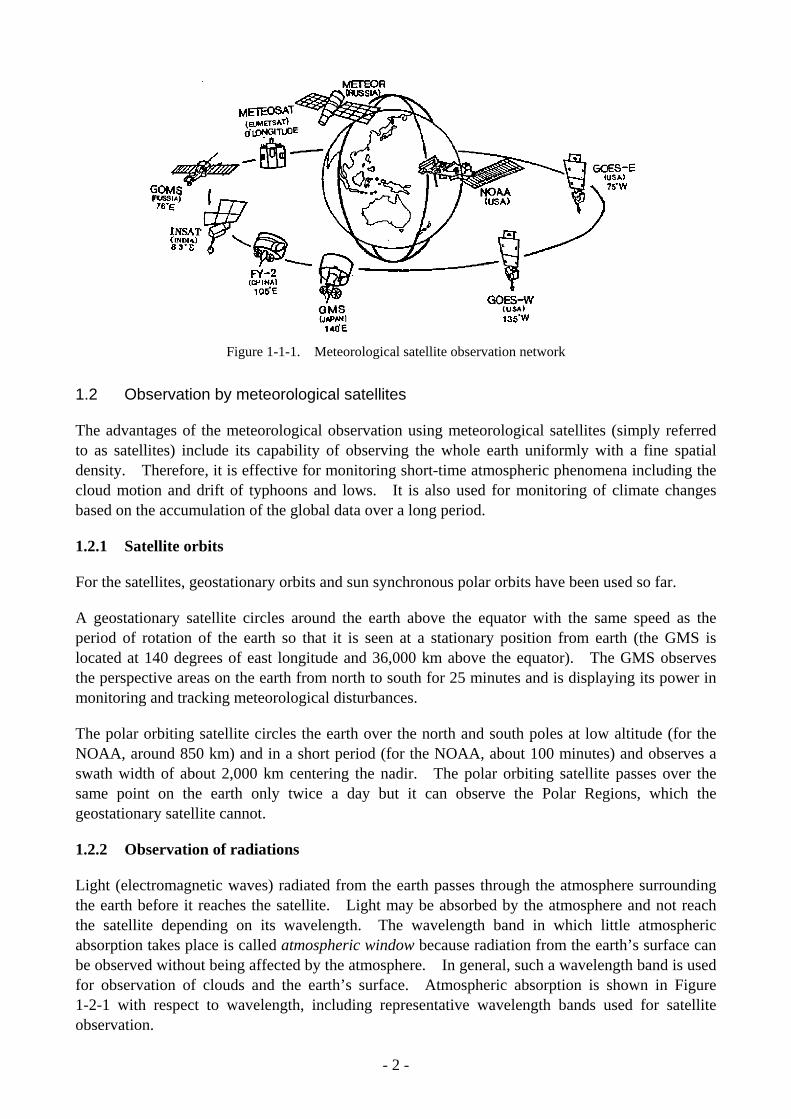
Figure 1-1-1. Meteorological satellite observation network

1.2 Observation by meteorological satellites

The advantages of the meteorological observation using meteorological satellites (simply referred to as satellites) include its capability of observing the whole earth uniformly with a fine spatial density. Therefore, it is effective for monitoring short-time atmospheric phenomena including the cloud motion and drift of typhoons and lows. It is also used for monitoring of climate changes based on the accumulation of the global data over a long period.

1.2.1 Satellite orbits

For the satellites, geostationary orbits and sun synchronous polar orbits have been used so far.

A geostationary satellite circles around the earth above the equator with the same speed as the period of rotation of the earth so that it is seen at a stationary position from earth (the GMS is located at 140 degrees of east longitude and 36,000 km above the equator). The GMS observes the perspective areas on the earth from north to south for 25 minutes and is displaying its power in monitoring and tracking meteorological disturbances.

The polar orbiting satellite circles the earth over the north and south poles at low altitude (for the NOAA, around 850 km) and in a short period (for the NOAA, about 100 minutes) and observes a swath width of about 2,000 km centering the nadir. The polar orbiting satellite passes over the same point on the earth only twice a day but it can observe the Polar Regions, which the geostationary satellite cannot.

1.2.2 Observation of radiations

Light (electromagnetic waves) radiated from the earth passes through the atmosphere surrounding the earth before it reaches the satellite. Light may be absorbed by the atmosphere and not reach the satellite depending on its wavelength. The wavelength band in which little atmospheric absorption takes place is called atmospheric window because radiation from the earth’s surface can be observed without being affected by the atmosphere. In general, such a wavelength band is used for observation of clouds and the earth’s surface. Atmospheric absorption is shown in Figure 1-2-1 with respect to wavelength, including representative wavelength bands used for satellite observation.

- 2 -

AbsorptionVisibleimage 3.7 µm image

Water vaporimage

Infrared 1image

Infrared 2image

Wavelength

Figure 1-2-1. Absorption of electromagnetic waves of various wavelengths by atmosphere and wavelength bands used for satellite observation

The visible band in 0.55-0.90 µm wavelength and infrared bands in 3.5-4.0 µm, 10.5-11.5 µm and 11.5-12.5 µm wavelength are called atmospheric windows.

The image obtained by a sensor that observes the 0.55-0.90 µm wavelength band is called a Visible (VIS) image and it is an observation of sunlight reflected by the earth's surface. The image in the 10.5-11.5 µm and 11.5-12.5 µm wavelength bands is called Infrared 1 (IR1) and Infrared 2 (IR2) image respectively and it is an observation of the amount of thermal radiations emitted from the physical body. The Infrared image is usually referred to as IR1 image. The image in the 3.5-4.0 µm wavelength band is called a 3.7 µm image and it is mainly an observation of reflected sunlight in the daytime and of brightness temperature at night. On the other hand, a lot of absorption takes place from water vapor in the 6.5-7.0 µm band. The image in this band is called a Water Vapor (WV) image and provides information on the amount of water vapor in the upper and middle atmospheric layers. In the IR1, IR2 and WV images and 3.7 µm image taken at night, the amount of infrared radiations is converted into brightness temperature. Brightness temperature means the radiation temperature emitted from a physical body that is assumed to be equivalent to a blackbody.

The radiation IB of blackbody material is represented by the Stephan-Boltzmann's law.

IB = σT4 (σ: Stephan-Boltzmann's constant, T: absolute temperature of blackbody)

The radiation I from a substance that is not a blackbody is represented with the emissivity ε, which is the ratio to the radiation from a blackbody substance.

I = εIB

For the sea surface and thick clouds, ε is close to 1.0 in the infrared region. For thin clouds, however, ε varies a lot and therefore the brightness temperature of the sea surface or cloud cannot be determined exactly unless the value of ε is known.

In this document, brightness temperature is simply called temperature hereafter unless otherwise mentioned.

1.2.3 Resolution

The characteristics of a sensor on board the GMS-5 are shown in Table 1-2-1 accompanied with those of MTSAT for reference. The horizontal spatial resolution of the GMS-5 is 1.25 km in the VIS image and 5 km in the IR images at the sub-satellite point (SSP). The more distant from SSP, the more the earth’s surface is viewed obliquely and the resolution deteriorates. In the vicinity of Japan, the resolution is 1.8 km in the VIS image and 7 km in the IR images.

- 3 -

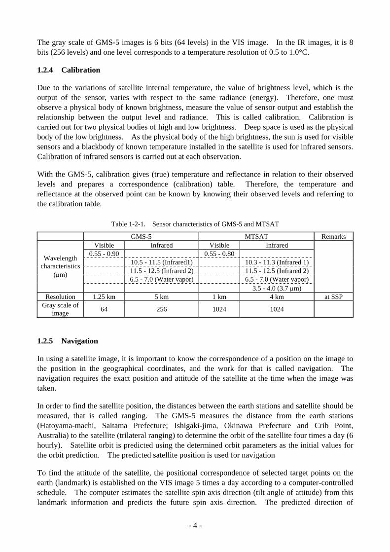
The gray scale of GMS-5 images is 6 bits (64 levels) in the VIS image. In the IR images, it is 8 bits (256 levels) and one level corresponds to a temperature resolution of 0.5 to 1.0°C.

1.2.4 Calibration

Due to the variations of satellite internal temperature, the value of brightness level, which is the output of the sensor, varies with respect to the same radiance (energy). Therefore, one must observe a physical body of known brightness, measure the value of sensor output and establish the relationship between the output level and radiance. This is called calibration. Calibration is carried out for two physical bodies of high and low brightness. Deep space is used as the physical body of the low brightness. As the physical body of the high brightness, the sun is used for visible sensors and a blackbody of known temperature installed in the satellite is used for infrared sensors. Calibration of infrared sensors is carried out at each observation.

With the GMS-5, calibration gives (true) temperature and reflectance in relation to their observed levels and prepares a correspondence (calibration) table. Therefore, the temperature and reflectance at the observed point can be known by knowing their observed levels and referring to the calibration table.

Table 1-2-1. Sensor characteristics of GMS-5 and MTSAT

GMS-5 MTSAT Remarks Visible Infrared Visible Infrared

0.55 - 0.90 0.55 - 0.80 10.5 - 11.5 (Infrared1) 10.3 - 11.3 (Infrared 1) 11.5 - 12.5 (Infrared 2) 11.5 - 12.5 (Infrared 2) 6.5 - 7.0 (Water vapor) 6.5 - 7.0 (Water vapor)

Wavelength characteristics

(µm)

3.5 - 4.0 (3.7 µm)

Resolution 1.25 km 5 km 1 km 4 km at SSP Gray scale of

image 64 256 1024 1024

1.2.5 Navigation

In using a satellite image, it is important to know the correspondence of a position on the image to the position in the geographical coordinates, and the work for that is called navigation. The navigation requires the exact position and attitude of the satellite at the time when the image was taken.

In order to find the satellite position, the distances between the earth stations and satellite should be measured, that is called ranging. The GMS-5 measures the distance from the earth stations (Hatoyama-machi, Saitama Prefecture; Ishigaki-jima, Okinawa Prefecture and Crib Point, Australia) to the satellite (trilateral ranging) to determine the orbit of the satellite four times a day (6 hourly). Satellite orbit is predicted using the determined orbit parameters as the initial values for the orbit prediction. The predicted satellite position is used for navigation

To find the attitude of the satellite, the positional correspondence of selected target points on the earth (landmark) is established on the VIS image 5 times a day according to a computer-controlled schedule. The computer estimates the satellite spin axis direction (tilt angle of attitude) from this landmark information and predicts the future spin axis direction. The predicted direction of

- 4 -

satellite spin axis is used for navigation.

If the orbit or attitude of the satellite deviates from the prescribed position, station-keeping control (east-west maneuver, north-south maneuver or attitude control maneuver) should be performed to keep its position and attitude.

1.3 Properties of image

1.3.1 Visible (VIS) image

(1) Features of VIS image

VIS image represents the intensity of sunlight reflected from clouds and/or the earth’s surface and makes it possible to monitor the conditions of the ocean, land and clouds. Portions of high reflectance are visualized bright and low reflectance dark. In general, the snow surface and clouds look bright because they have high reflectance, the land surface is darker than the clouds, and the sea surface looks the darkest because of its low reflectance. Note, however, that the appearance differs depending on the solar elevation at the observed point. In the morning and evening and in high–latitude districts, the image looks darker because there is little incident light due to the oblique sunlight and the small amount of reflected rays.

(2) Use of VIS image

A. Distinction between thick and thin clouds

The reflectance of a cloud depends on the amount and density of the cloud droplets and raindrops contained in the cloud. In general, low-level clouds contain a larger amount of cloud droplets and raindrops and therefore they appear brighter than high clouds. Cumulonimbus and other thick clouds that have developed vertically contain a lot of cloud droplets and raindrops and they appear bright in a VIS image. Through some thin high-level clouds, the underlying low-level clouds and land or sea surface can be seen.

B. Distinction between convective and stratiform types

Cloud types can be identified from the texture of the cloud top surface. The top surface of a stratiform cloud is smooth and uniform while the top surface of a convective cloud is rugged and uneven. The texture of a cloud top surface is easily observed when sunlight hits the cloud top obliquely.

C. Comparison of cloud top height

If clouds of different heights coexist when sunlight hits them obliquely, it may happen that the cloud of higher top casts a shadow onto the cloud top of lower height. Comparison of cloud height is possible using this property.

1.3.2 Infrared (IR) image

(1) Features of IR image

The IR image represents a temperature distribution and can be observed without any difference between day and night. Therefore, it is useful for watching clouds and/or the earth’s surface

- 5 -

temperature. In the IR image, portions of low temperature are visualized bright and portions of high temperature dark.

(2) Use of IR image

A. Watching over meteorological phenomena

Unlike the VIS image, observation is possible with the IR image under the same conditions against day or night. This is the most advantageous point in watching meteorological disturbances.

B. Observation of cloud top height

It is possible to know the cloud top temperature with the IR image. If the temperature profile of atmosphere is known, the cloud top temperature can be converted into cloud top height. For the estimation of the temperature profile, values by objective analysis or Numerical Weather Prediction (NWP) are often used. In the troposphere, atmospheric temperature is generally lower at the upper layer, and therefore the lower cloud top temperature means a higher cloud top height. It is also possible to monitor the developing level of clouds in the vertical direction by referring to the cloud top temperature.

C. Measurement of earth’s surface temperature

With the IR image, it is possible to measure the earth’s surface temperature in cloud free areas in addition to the cloud top temperature. This gives useful information on sea surface temperature over the ocean that has sparse area of meteorological observations.

1.3.3 Water vapor (WV) image

(1) Features of WV image

The WV image also represents temperature distribution. As with the IR image, portions of low temperature are visualized bright and portions of high temperature dark. For the WV image, absorption by water vapor is dominant and this gives the feature that the brightness of an image corresponds to the amount of water vapor in the upper and middle layer.

The standard atmosphere is simply divided into 3 typical layers of upper, middle and lower atmosphere, and the amount of absorption and re-emission of infrared radiations are schematically shown (Figure 1-3-1). Since temperature is high and a large amount of water vapor is near the earth’s surface and in the lower layer, the amount of infrared emission is large but most of it is absorbed by water vapor and little emission reaches the satellite (a and b in the figure).

With increasing height, temperature falls and the amount of water vapor decreases (c in the figure). In the upper atmosphere, the temperature is still lower and the amount of water vapor is still smaller, and almost all infrared re-emission reach the satellite without absorption but the actual amount of radiation reaching the satellite is small (d in the figure).

In dry portions of little water vapor content in the upper and middle layer, the image is dark because the temperature is high due to the contribution of radiation from the lower layer. In

- 6 -

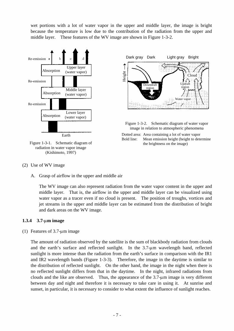
wet portions with a lot of water vapor in the upper and middle layer, the image is bright because the temperature is low due to the contribution of the radiation from the upper and middle layer. These features of the WV image are shown in Figure 1-3-2.

Figure 1-3-1. Schematic diagram of radiation in water vapor image

(Kishimoto, 1997)

Figure 1-3-2. Schematic diagram of water vapor image in relation to atmospheric phenomena

Dotted area: Area containing a lot of water vapor Bold line: Mean emission height (height to determine

the brightness on the image)

Dark gray Dark Light gray Bright

Downdraftregion

Updraftregion

Water vapor

Cloud

Hei

ghtAbsorption

Re-emission

Re-emission

Re-emission

Earth

Upper layer(water vapor)

AbsorptionMiddle layer(water vapor)

AbsorptionLower layer

(water vapor)

(2) Use of WV image

A. Grasp of airflow in the upper and middle air

The WV image can also represent radiation from the water vapor content in the upper and middle layer. That is, the airflow in the upper and middle layer can be visualized using water vapor as a tracer even if no cloud is present. The position of troughs, vortices and jet streams in the upper and middle layer can be estimated from the distribution of bright and dark areas on the WV image.

1.3.4 3.7-µm image

(1) Features of 3.7-µm image

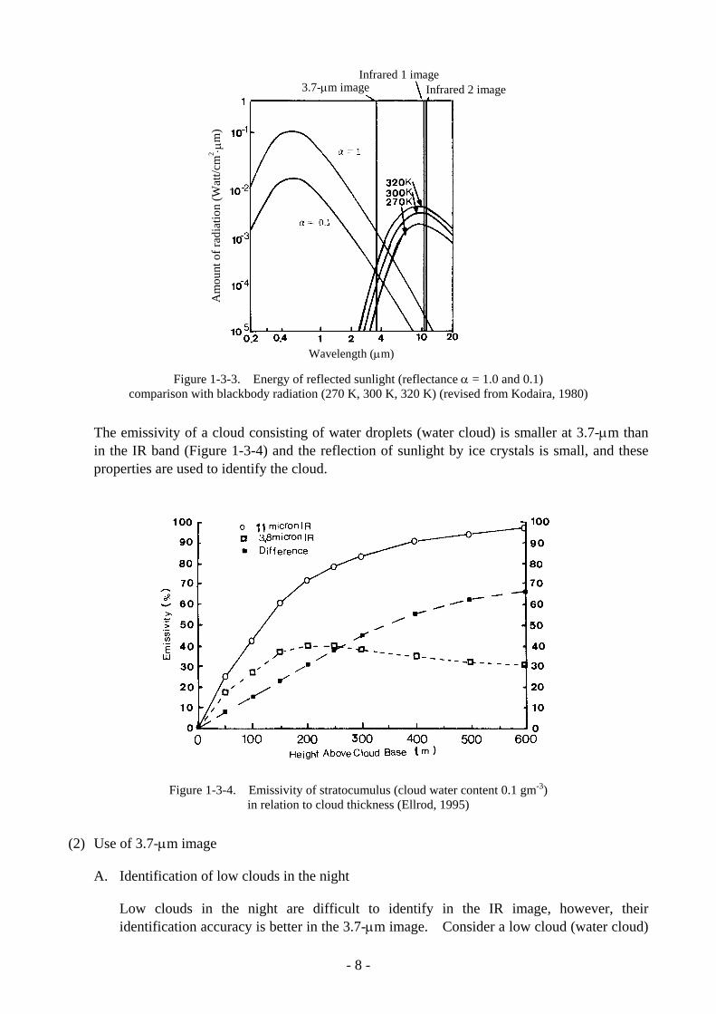
The amount of radiation observed by the satellite is the sum of blackbody radiation from clouds and the earth’s surface and reflected sunlight. In the 3.7-µm wavelength band, reflected sunlight is more intense than the radiation from the earth’s surface in comparison with the IR1 and IR2 wavelength bands (Figure 1-3-3). Therefore, the image in the daytime is similar to the distribution of reflected sunlight. On the other hand, the image in the night when there is no reflected sunlight differs from that in the daytime. In the night, infrared radiations from clouds and the like are observed. Thus, the appearance of the 3.7-µm image is very different between day and night and therefore it is necessary to take care in using it. At sunrise and sunset, in particular, it is necessary to consider to what extent the influence of sunlight reaches.

- 7 -

Wavelength (µm)

3.7-µm imageInfrared 1 image

Infrared 2 image

Am

ount

of r

adia

tion

(Wat

t/cm

2 ⋅µm

)

Figure 1-3-3. Energy of reflected sunlight (reflectance α = 1.0 and 0.1) comparison with blackbody radiation (270 K, 300 K, 320 K) (revised from Kodaira, 1980)

The emissivity of a cloud consisting of water droplets (water cloud) is smaller at 3.7-µm than in the IR band (Figure 1-3-4) and the reflection of sunlight by ice crystals is small, and these properties are used to identify the cloud.

Figure 1-3-4. Emissivity of stratocumulus (cloud water content 0.1 gm-3)

in relation to cloud thickness (Ellrod, 1995)

(2) Use of 3.7-µm image

A. Identification of low clouds in the night

Low clouds in the night are difficult to identify in the IR image, however, their identification accuracy is better in the 3.7-µm image. Consider a low cloud (water cloud)

- 8 -

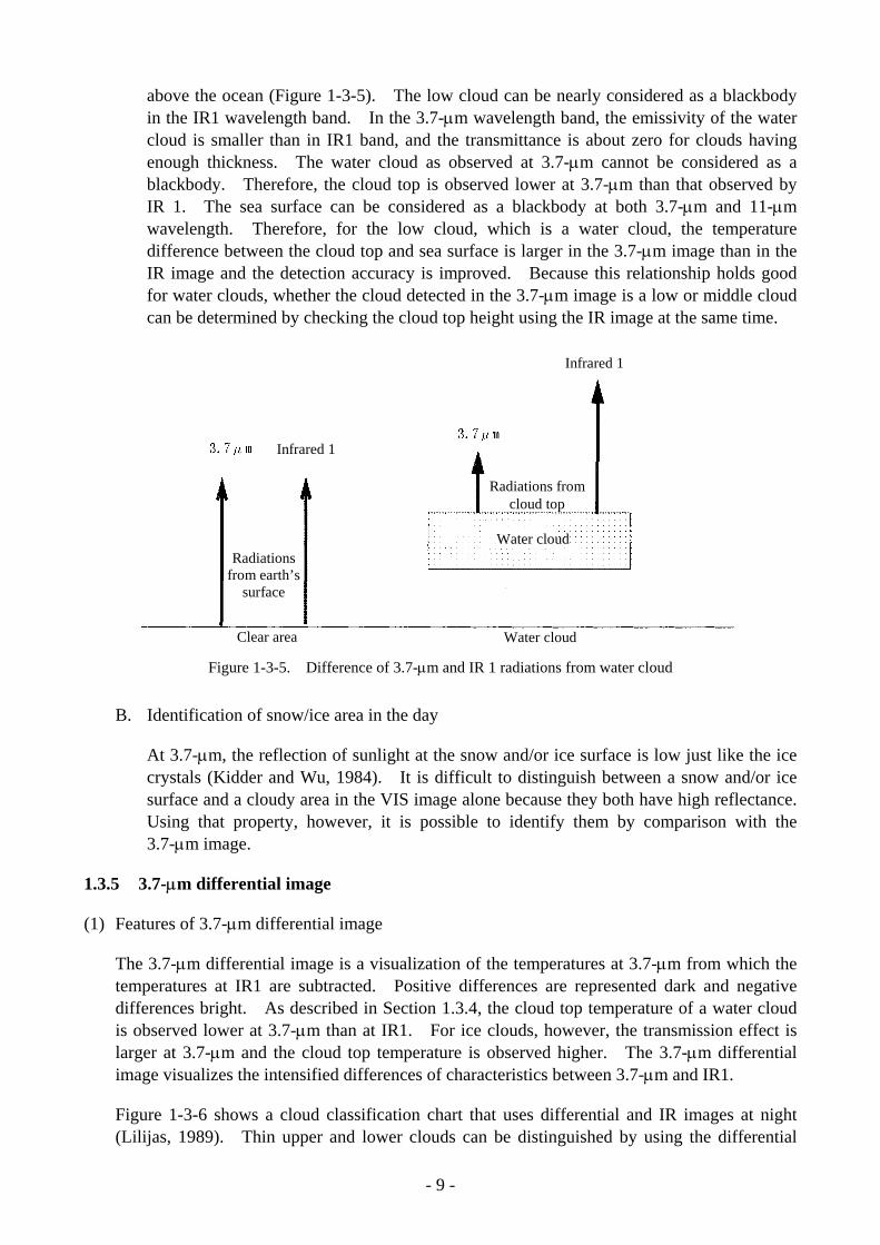
above the ocean (Figure 1-3-5). The low cloud can be nearly considered as a blackbody in the IR1 wavelength band. In the 3.7-µm wavelength band, the emissivity of the water cloud is smaller than in IR1 band, and the transmittance is about zero for clouds having enough thickness. The water cloud as observed at 3.7-µm cannot be considered as a blackbody. Therefore, the cloud top is observed lower at 3.7-µm than that observed by IR 1. The sea surface can be considered as a blackbody at both 3.7-µm and 11-µm wavelength. Therefore, for the low cloud, which is a water cloud, the temperature difference between the cloud top and sea surface is larger in the 3.7-µm image than in the IR image and the detection accuracy is improved. Because this relationship holds good for water clouds, whether the cloud detected in the 3.7-µm image is a low or middle cloud can be determined by checking the cloud top height using the IR image at the same time.

Infrared 1

Radiations fromcloud top

Radiationsfrom earth’s

surface

Water cloud

Clear area Water cloud

Infrared 1

Figure 1-3-5. Difference of 3.7-µm and IR 1 radiations from water cloud

B. Identification of snow/ice area in the day

At 3.7-µm, the reflection of sunlight at the snow and/or ice surface is low just like the ice crystals (Kidder and Wu, 1984). It is difficult to distinguish between a snow and/or ice surface and a cloudy area in the VIS image alone because they both have high reflectance. Using that property, however, it is possible to identify them by comparison with the 3.7-µm image.

1.3.5 3.7-µm differential image

(1) Features of 3.7-µm differential image

The 3.7-µm differential image is a visualization of the temperatures at 3.7-µm from which the temperatures at IR1 are subtracted. Positive differences are represented dark and negative differences bright. As described in Section 1.3.4, the cloud top temperature of a water cloud is observed lower at 3.7-µm than at IR1. For ice clouds, however, the transmission effect is larger at 3.7-µm and the cloud top temperature is observed higher. The 3.7-µm differential image visualizes the intensified differences of characteristics between 3.7-µm and IR1.

Figure 1-3-6 shows a cloud classification chart that uses differential and IR images at night (Lilijas, 1989). Thin upper and lower clouds can be distinguished by using the differential

- 9 -

and IR images together.

Figure 1-3-6. Cloud classification chart by 3.7-µm differential temperature and infrared temperature (Liljas,

1989) Horizontal axis: (3.7-µm – infrared) differential temperature, Vertical axis: Infrared

temperature

(2) Use of 3.7-µm differential image

A. Identification of lower clouds in the night

Lower clouds have a small temperature difference with the surrounding cloud free areas and it is difficult to detect them at night in the IR image alone. The cloud top temperature is calculated lower at 3.7-µm than at IR1 and the difference of calculated temperature is 2 to 10 degrees negative. The 3.7-µm differential image is used for the lower cloud identification in the night because the differences between cloud free area and lower cloud area are more intensified in the 3.7-µm differential image than in the 3.7-µm image.

B. Identification of upper clouds

The 3.7-µm rays have properties that are close to visible light and they easily penetrate the higher cloud with ice crystals. At night, the radiations from the earth’s surface at high temperature penetrate thin higher clouds and are added to the radiations from the cloud top, so the cloud top temperature calculated at 3.7-µm is higher than actual. Because the transmission effect is larger at 3.7-µm than at IR1, the cloud top temperature is higher than the infrared temperature and the temperature difference has a positive value. In this regard, the area of thin higher clouds can be identified with the 3.7-µm differential image. For example, it is possible to distinguish between cumulonimbus, which brings about rainfall, and anvil cirrus, which does not.

- 10 -

1.3.6 Infrared differential image

(1) Features of infrared differential image

The infrared differential image is a visualization of the temperature at IR1 from which the temperature at IR2 is subtracted. These infrared bands are called the atmospheric windows where there is little absorption by water vapor and the atmosphere. However, the absorption by water vapor cannot be always neglected. Absorbency is larger in the IR1 band than in the IR2 band though the difference is slight. The difference in absorbency between IR 1 and IR2 depends on the water vapor content of the atmosphere, and the infrared differential image is visualized darker for larger values of this difference.

(2) Use of infrared differential image

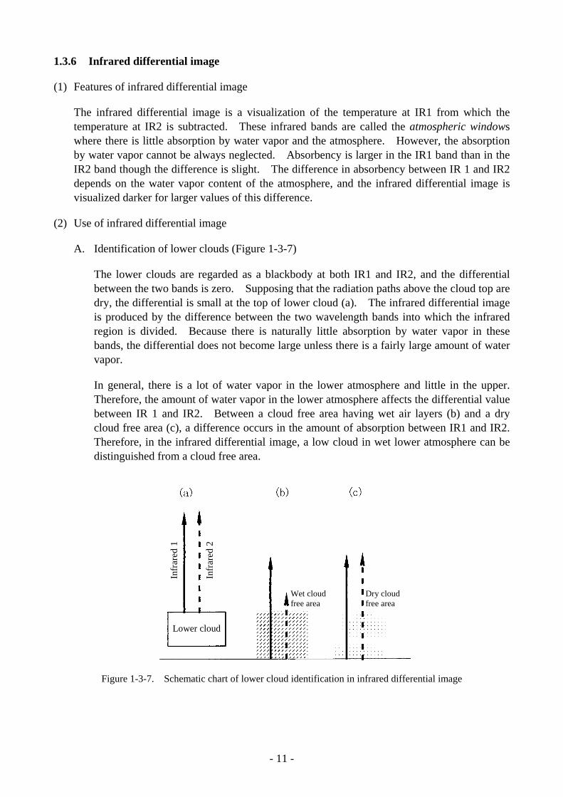
A. Identification of lower clouds (Figure 1-3-7)

The lower clouds are regarded as a blackbody at both IR1 and IR2, and the differential between the two bands is zero. Supposing that the radiation paths above the cloud top are dry, the differential is small at the top of lower cloud (a). The infrared differential image is produced by the difference between the two wavelength bands into which the infrared region is divided. Because there is naturally little absorption by water vapor in these bands, the differential does not become large unless there is a fairly large amount of water vapor.

In general, there is a lot of water vapor in the lower atmosphere and little in the upper. Therefore, the amount of water vapor in the lower atmosphere affects the differential value between IR 1 and IR2. Between a cloud free area having wet air layers (b) and a dry cloud free area (c), a difference occurs in the amount of absorption between IR1 and IR2. Therefore, in the infrared differential image, a low cloud in wet lower atmosphere can be distinguished from a cloud free area.

Infr

ared

1

Infr

ared

2

Lower cloud

Wet cloudfree area

Dry cloudfree area

Figure 1-3-7. Schematic chart of lower cloud identification in infrared differential image

- 11 -

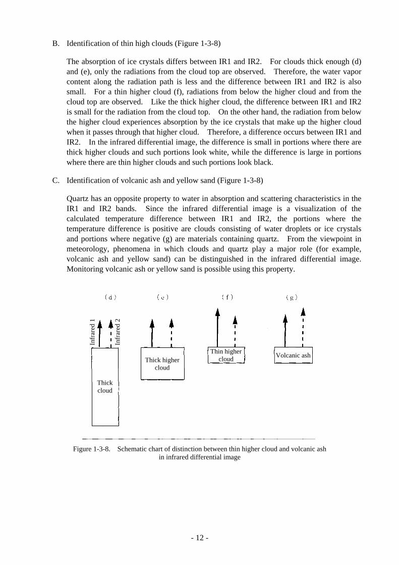
B. Identification of thin high clouds (Figure 1-3-8)

The absorption of ice crystals differs between IR1 and IR2. For clouds thick enough (d) and (e), only the radiations from the cloud top are observed. Therefore, the water vapor content along the radiation path is less and the difference between IR1 and IR2 is also small. For a thin higher cloud (f), radiations from below the higher cloud and from the cloud top are observed. Like the thick higher cloud, the difference between IR1 and IR2 is small for the radiation from the cloud top. On the other hand, the radiation from below the higher cloud experiences absorption by the ice crystals that make up the higher cloud when it passes through that higher cloud. Therefore, a difference occurs between IR1 and IR2. In the infrared differential image, the difference is small in portions where there are thick higher clouds and such portions look white, while the difference is large in portions where there are thin higher clouds and such portions look black.

C. Identification of volcanic ash and yellow sand (Figure 1-3-8)

Quartz has an opposite property to water in absorption and scattering characteristics in the IR1 and IR2 bands. Since the infrared differential image is a visualization of the calculated temperature difference between IR1 and IR2, the portions where the temperature difference is positive are clouds consisting of water droplets or ice crystals and portions where negative (g) are materials containing quartz. From the viewpoint in meteorology, phenomena in which clouds and quartz play a major role (for example, volcanic ash and yellow sand) can be distinguished in the infrared differential image. Monitoring volcanic ash or yellow sand is possible using this property.

Infr

ared

1

Infr

ared

2

ic ash

Thickcloud

Thick highercloud

Thin highercloud Volcan

Figure 1-3-8. Schematic chart of distinction between thin higher cloud and volcanic ash

in infrared differential image

- 12 -

Eclipse operation As seen from a geostationary satellite, the size of the earth is about 20 degrees in angular diameter whereas the sun is only 0.5 degrees. In periods when the sun, Earth and satellite are collinear, the sun is completely hidden behind the Earth as seen from the geostationary satellite. Such an eclipse phenomenon by the Earth occurs around the vernal and autumnal equinox. During these periods, the angle between the direction of the sun and the orbit plane of the satellite are within ± α centering around the vernal or autumnal equinox, as shown in Attached Figure 1. Letting a be the radius of the satellite orbit and Ro be the radius of the Earth, α can be determined from sin α = Ro/a. Supposing that the radius of the orbit is 7 times the radius of the earth, α ≅ 8.5 degrees is derived. Starting at the vernal equinox of March 20, the period when the angle between the sun and the orbit plane is within 8.5 degrees is almost 50 days. The day of the longest eclipse is just the vernal or autumnal equinox, and the eclipse lasts about 70 minutes. That is, the satellite receives no sunlight for more than 1 hour centering on 12 o’clock midnight. If not irradiated with sunlight even for a short time, the solar battery supplies no power at all and the satellite cools rapidly in outer space. During the eclipse, the first requirement is to maintain the satellite function.

Before and after the eclipse, the satellite is operated differently from the usual time as a special operation period including preparations and subsequent treatments. In the eclipse periods from the end of February to the beginning of April and from the end of August to the beginning of October, the GMS observations of 14UTC and 15UTC is suspended and the observation of 16UTC starts 10 minutes delayed to the normal operation schedule. (Kazufumi Suzuki)

Reference: Special issue of Meteorological Satellite Center Technical Note “Outline of meteorological satellite system”, 1986, Meteorological Satellite Center, 57pp.

Attached Figure 1. Position of the Earth and the satellite in the period during which an eclipse

occurs. E: Orbit plane at vernal or autumnal equinox. S: Incident direction of sunlight. Ro: Radius of the Earth.

1.4 Comparison of images

In this section, the features of the above-mentioned various images in daytime or nighttime are separately described using practical instances. The images used are all NOAA images except for the WV image, which was taken by the GMS-5. In the VIS image, the gray scale is represented white for high reflectance and black for low reflectance. In the IR image, it is represented black for high temperature and white for low temperature same as the gray scales in ordinary use. In the infrared differential image, it is represented black for large (positive) differences and white for small (negative) differences. In the 3.7-µm image, the gray scale in the day is represented black for high reflectance and white for low reflectance. Note that this is opposite to the VIS image. At night, the same gray scale as the IR image is used. The 3.7-µm differential image is represented black for positive differences and white for negative differences (Table 1-4-1).

- 13 -

Table 1-4-1. Appearance in images

Appearance in images Image types White Light gray Gray Dark gray Black Visible image ← Reflection large Reflection small → Infrared image ← Temperature low Temperature high →

Water vapor image ← Wet Dry → 3.7-µm image (daytime) ← Reflection small Reflection large →

3.7-µm image (nighttime) ← Temperature low Temperature high → Infrared differential image ← Negative Positive → 3.7-µm differential image ← Negative Positive →

1.4.1 Image in the day

Figures 1-4-1 to 1-4-5 are VIS, IR, WV, infrared differential and 3.7-µm images respectively, taken at the same time in the day. Here, pay attention to cloud area A from Tsugaru Straight to the sea to the south of Hokkaido, cloud area B near Niigata and Toyama Prefectures, cloud area C around the center of the typhoon at the sea to the south of Japan, cloud area D on the northeast side, and cloud area E on the east side of the typhoon.

In the VIS image, cloud area A is observed along with cloud area B as an aggregate of massive clouds, but it is not thick as compared with cloud area B and takes a striped form. Since cloud area A is dark gray in the IR image, this area can be judged an area of convective cloud, i.e. Cumulus (Cu), which has not developed. On the other hand, cloud area B is light gray as compared with cloud area A, and it is judged an area of convective cloud that includes Cumulus congestus (Cg) having a higher cloud top than the Cu area in cloud area A. Both areas cannot be seen at all in the WV image, which is suited for observation of the upper and middle atmosphere. In the infrared differential image, cloud areas A and B are both shown as a spotted pattern from white to light gray. In the 3.7-µm image, they are represented in black or dark gray.

Cloud area C is observed as a generally thick cloud area in the VIS image and it is white in the IR image. Therefore, it can be judged an area of thick convective cloud having a higher cloud top height, that is, it is an area of convective cloud including Cumulonimbus (Cb). In the WV image, it is also represented as a fairly light region (light area). In the infrared differential image, it is represented white or gray, which indicates little temperature difference, and it is found to be an area of thick cloud. On the other hand, it is observed white in the 3.7-µm image.

Cloud area D is thick in the VIS image and white in the IR image. Therefore, it is judged an area of thick cloud including high clouds. On the other hand, cloud area E is white or light gray in the IR image like cloud area D, but it is thinner than cloud area D in the VIS image. Therefore, it is found to be an area of cloud including no-thick higher clouds. In the WV image, it appears in the same way as the IR image. In the infrared differential image, cloud area D is light gray, which means small temperature differences, whereas cloud area E is black, which means large temperature differences. Therefore, cloud area E can be judged an area of thin high clouds. In the 3.7-µm image, cloud area D is observed white, while cloud area E is white or light gray.

- 14 -

Figure 1-4-1. Visible image taken by NOAA at

about 5UTC, November 7, 1997 Figure 1-4-2. Infrared image taken by NOAA at

about 5UTC, November 7, 1997

Figure 1-4-3. Water vapor image taken

by GMS-5 at about 5UTC, November 7, 1997

Figure 1-4-4. Infrared differential image taken by NOAA at about 5UTC,

November 7, 1997

- 15 -

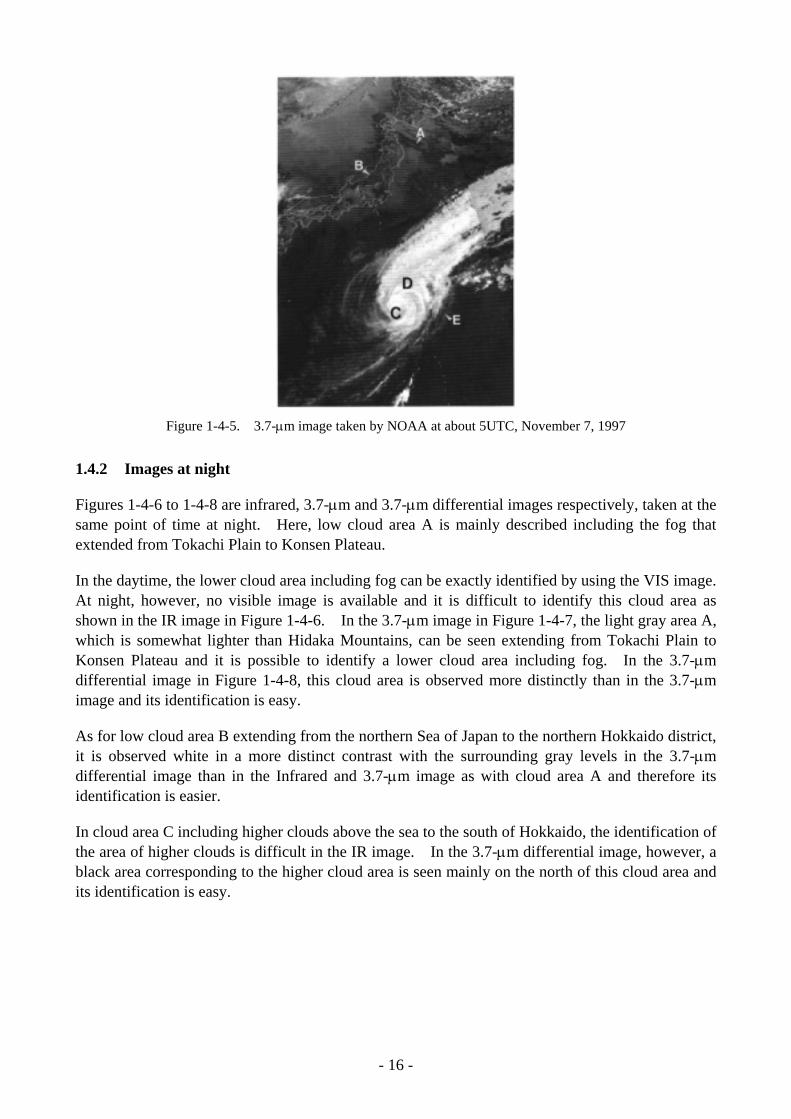
Figure 1-4-5. 3.7-µm image taken by NOAA at about 5UTC, November 7, 1997

1.4.2 Images at night

Figures 1-4-6 to 1-4-8 are infrared, 3.7-µm and 3.7-µm differential images respectively, taken at the same point of time at night. Here, low cloud area A is mainly described including the fog that extended from Tokachi Plain to Konsen Plateau.

In the daytime, the lower cloud area including fog can be exactly identified by using the VIS image. At night, however, no visible image is available and it is difficult to identify this cloud area as shown in the IR image in Figure 1-4-6. In the 3.7-µm image in Figure 1-4-7, the light gray area A, which is somewhat lighter than Hidaka Mountains, can be seen extending from Tokachi Plain to Konsen Plateau and it is possible to identify a lower cloud area including fog. In the 3.7-µm differential image in Figure 1-4-8, this cloud area is observed more distinctly than in the 3.7-µm image and its identification is easy.

As for low cloud area B extending from the northern Sea of Japan to the northern Hokkaido district, it is observed white in a more distinct contrast with the surrounding gray levels in the 3.7-µm differential image than in the Infrared and 3.7-µm image as with cloud area A and therefore its identification is easier.

In cloud area C including higher clouds above the sea to the south of Hokkaido, the identification of the area of higher clouds is difficult in the IR image. In the 3.7-µm differential image, however, a black area corresponding to the higher cloud area is seen mainly on the north of this cloud area and its identification is easy.

- 16 -

Figure 1-4-6. Infrared image taken by NOAA at about 17UTC,

October 13, 1998

Figure 1-4-7. 3.7-µm image taken by NOAA at about 17UTC,

October 13, 1998

Figure 1-4-8. 3.7-µm differential image taken by NOAA at about 17UTC, October 13, 1998

- 17 -

Image of the moon Though rarely, it can happen that a meteorological satellite which observes the earth takes the moon beside the earth in the same picture. Attached Figure 1 is an image taken on such an occasion and the moon appears at the upper right of the picture. In the visible image, the moon looks dim being lit up by the sun. The pattern on the moon’s surface is found indistinctly. In the infrared image, the portion lit up by the sun looks black because it becomes hot. The portion not lit up by the sun looks white like outer space because it is cold. The shape of the moon is distorted, and it is presumably because the relative position of the satellite and moon has shifted during the observation by the satellite. (Kazufumi Suzuki)

Attached Figure 1. Images of the moon (visible image (upper) and infrared image (lower) at 00UTC,

December 19, 1999).

- 18 -