Order conditions for General Linear Nyström methods

Numer Algor (2014) 65:579–595DOI 10.1007/s11075-013-9819-3

ORIGINAL PAPER

Order conditions for General Linear Nystrom methods

Raffaele D’Ambrosio ·Giuseppe De Martino ·Beatrice Paternoster

Received: 27 March 2013 / Accepted: 12 December 2013 / Published online: 10 January 2014© Springer Science+Business Media New York 2014

Abstract The purpose of this paper is to analyze the algebraic theory of order for thefamily of general linear Nystrom (GLN) methods introduced in D’Ambrosio et al.(Numer. Algorithm 61(2), 331–349, 2012) with the aim to provide a general frame-work for the representation and analysis of numerical methods solving initial valueproblems based on second order ordinary differential equations (ODEs). Our inves-tigation is carried out by suitably extending the theory of B-series for second orderODEs to the case of GLN methods, which leads to a general set of order conditions.This allows to recover the order conditions of numerical methods already knownin the literature, but also to assess a general approach to study the order conditionsof new methods, simply regarding them as GLN methods: the obtained results areindeed applied to both known and new methods for second order ODEs.

Keywords Second order ordinary differential equations · General linear methods ·Nystrom methods · Order conditions · B-series

Mathematics Subject Classification (2010) 65L05

Dedicated to John C. Butcher, in occasion of his 80th birthday

R. D’Ambrosio (�) · G. De Martino · B. PaternosterUniversity of Salerno, Fisciano, Italye-mail: [email protected]

G. De Martinoe-mail: [email protected]

B. Paternostere-mail: [email protected]

580 Numer Algor (2014) 65:579–595

1 Introduction

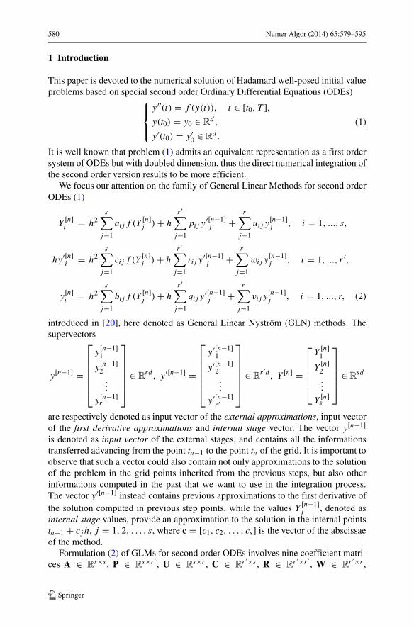
This paper is devoted to the numerical solution of Hadamard well-posed initial valueproblems based on special second order Ordinary Differential Equations (ODEs)

⎧⎪⎨

⎪⎩

y ′′(t) = f (y(t)), t ∈ [t0, T ],y(t0) = y0 ∈ R

d ,

y ′(t0) = y ′0 ∈ Rd .

(1)

It is well known that problem (1) admits an equivalent representation as a first ordersystem of ODEs but with doubled dimension, thus the direct numerical integration ofthe second order version results to be more efficient.

We focus our attention on the family of General Linear Methods for second orderODEs (1)

Y[n]i = h2

s∑

j=1

aijf (Y[n]j )+ h

r ′∑

j=1

pij y′[n−1]j +

r∑

j=1

uij y[n−1]j , i = 1, ..., s,

hy ′[n]i = h2s∑

j=1

cijf (Y[n]j )+ h

r ′∑

j=1

rij y′[n−1]j +

r∑

j=1

wijy[n−1]j , i = 1, ..., r ′,

y[n]i = h2

s∑

j=1

bijf (Y[n]j )+ h

r ′∑

j=1

qij y′[n−1]j +

r∑

j=1

vij y[n−1]j , i = 1, ..., r, (2)

introduced in [20], here denoted as General Linear Nystrom (GLN) methods. Thesupervectors

y[n−1] =

⎡

⎢⎢⎢⎢⎢⎣

y[n−1]1

y[n−1]2...

y[n−1]r

⎤

⎥⎥⎥⎥⎥⎦

∈ Rrd, y ′[n−1] =

⎡

⎢⎢⎢⎢⎢⎣

y ′[n−1]1

y ′[n−1]2...

y ′[n−1]r ′

⎤

⎥⎥⎥⎥⎥⎦

∈ Rr ′d, Y [n] =

⎡

⎢⎢⎢⎢⎣

Y[n]1

Y[n]2...

Y[n]s

⎤

⎥⎥⎥⎥⎦

∈ Rsd

are respectively denoted as input vector of the external approximations, input vectorof the first derivative approximations and internal stage vector. The vector y[n−1]is denoted as input vector of the external stages, and contains all the informationstransferred advancing from the point tn−1 to the point tn of the grid. It is important toobserve that such a vector could also contain not only approximations to the solutionof the problem in the grid points inherited from the previous steps, but also otherinformations computed in the past that we want to use in the integration process.The vector y ′[n−1] instead contains previous approximations to the first derivative ofthe solution computed in previous step points, while the values Y

[n−1]j , denoted as

internal stage values, provide an approximation to the solution in the internal pointstn−1 + cjh, j = 1, 2, . . . , s, where c = [c1, c2, . . . , cs] is the vector of the abscissaeof the method.

Formulation (2) of GLMs for second order ODEs involves nine coefficient matri-ces A ∈ R

s×s , P ∈ Rs×r ′ , U ∈ R

s×r , C ∈ Rr ′×s , R ∈ R

r ′×r ′ , W ∈ Rr ′×r ,

Numer Algor (2014) 65:579–595 581

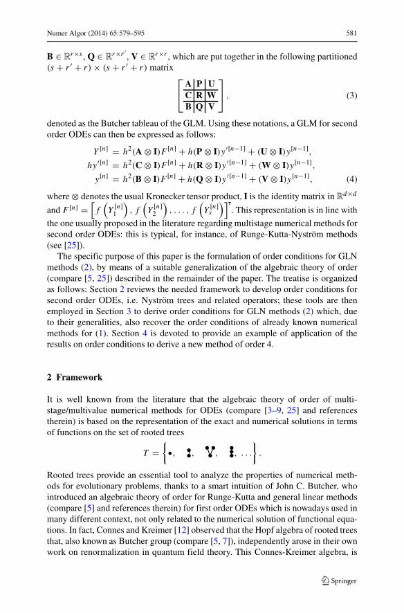
B ∈ Rr×s , Q ∈ R

r×r ′ , V ∈ Rr×r , which are put together in the following partitioned

(s + r ′ + r)× (s + r ′ + r) matrix⎡

⎣A P UC R WB Q V

⎤

⎦ , (3)

denoted as the Butcher tableau of the GLM. Using these notations, a GLM for secondorder ODEs can then be expressed as follows:

Y [n] = h2(A ⊗ I)F [n] + h(P ⊗ I)y ′[n−1] + (U ⊗ I)y[n−1],hy ′[n] = h2(C ⊗ I)F [n] + h(R ⊗ I)y ′[n−1] + (W ⊗ I)y[n−1],y[n] = h2(B ⊗ I)F [n] + h(Q ⊗ I)y ′[n−1] + (V ⊗ I)y[n−1], (4)

where ⊗ denotes the usual Kronecker tensor product, I is the identity matrix in Rd×d

and F [n] =[f(Y[n]1

), f

(Y[n]2

), . . . , f

(Y[n]s

)]T

. This representation is in line with

the one usually proposed in the literature regarding multistage numerical methods forsecond order ODEs: this is typical, for instance, of Runge-Kutta-Nystrom methods(see [25]).

The specific purpose of this paper is the formulation of order conditions for GLNmethods (2), by means of a suitable generalization of the algebraic theory of order(compare [5, 25]) described in the remainder of the paper. The treatise is organizedas follows: Section 2 reviews the needed framework to develop order conditions forsecond order ODEs, i.e. Nystrom trees and related operators; these tools are thenemployed in Section 3 to derive order conditions for GLN methods (2) which, dueto their generalities, also recover the order conditions of already known numericalmethods for (1). Section 4 is devoted to provide an example of application of theresults on order conditions to derive a new method of order 4.

2 Framework

It is well known from the literature that the algebraic theory of order of multi-stage/multivalue numerical methods for ODEs (compare [3–9, 25] and referencestherein) is based on the representation of the exact and numerical solutions in termsof functions on the set of rooted trees

T ={

, , , , . . .

}

.

Rooted trees provide an essential tool to analyze the properties of numerical meth-ods for evolutionary problems, thanks to a smart intuition of John C. Butcher, whointroduced an algebraic theory of order for Runge-Kutta and general linear methods(compare [5] and references therein) for first order ODEs which is nowadays used inmany different context, not only related to the numerical solution of functional equa-tions. In fact, Connes and Kreimer [12] observed that the Hopf algebra of rooted treesthat, also known as Butcher group (compare [5, 7]), independently arose in their ownwork on renormalization in quantum field theory. This Connes-Kreimer algebra, is

582 Numer Algor (2014) 65:579–595

equivalent to the Butcher group, because its dual is the universal enveloping algebraof the Lie algebra of the Butcher group (compare [1]).

For second order equations, due to the presence of the derivative of the exact solu-tion, we need a more general set of rooted trees, namely bi-coloured trees, defined asfollows (compare [25])

NT ={

, , , , , , , , , , . . .

}

.

The vertices τ1 = and τ2 = are combined according to following the rules

1. the root of t ∈ NT is always fat;2. a meagre vertex has at most one son which has to be fat.

Following [10, 25], we adapt the theory of N-trees and of N-series introduced byHairer and Wanner in [23] to the special problem

y ′′(x) = f (y(x)). (5)

By calculating the derivatives of the exact solution of problem (5)

y ′′′ = ∂f

∂yy ′, y(iv) = ∂2f

∂y2 y′2+ ∂f

∂yy ′′, y(v) = ∂3f

∂y3 y′3+3

∂2f

∂y2 y′f+ ∂f

∂yy ′′′, . . .

we observe that the terms including the derivative of f with respect to y ′ disappear,producing a smaller set of trees called Special N-trees (SNT) set [25]

SNT ={

, , , , , . . .

}

.

2.1 Composition and decomposition rules, elementary differentials and functionson SNT

By combining the formalisms introduced in [10, 23], a composition rule of specialNystrom trees is given according to the following scheme. We consider t1, . . . , tk ∈SNT and a new root τ2. Then,

1. if ti �= τ1, then its root is connected to a new meagre node, linked to the new root;2. if ti = τ1, then it is connected to the new root via a new branch.

The resulting SN-tree is denoted as t = [t1, . . . , tk]. Inversely, cutting the branchesleaving from the root of a given t ∈ SNT , let u1, u2, . . ., uk be the resulting subtrees.For any ui �= τ1, we cut off the branch leaving from its root τ1 and denote the remain-ing part as ti . For the remaining ui , we set ti = τ1. Then, the tree is decomposed ast = [t1, . . . , tk].

Given these rules, we can extend the definition of elementary differential given in[5, 25] to the special problem (5). For a given t = [t1, . . . , tk] ∈ SNT , we recursivelydefine the elementary differentials as follows

F( )(y, y ′) = y ′,F ( )(y, y ′) = y ′′ = f,

F (t)(y, y ′) = f (k)(F (t1)(y, y′), . . . , F (tk)(y, y

′)).

Numer Algor (2014) 65:579–595 583

Table 1 Special Nystrom trees up to order 5 and associated elementary differentials

ρ(t) t F (t) α(t)

1 y′ 1

2 f 1

3 f ′y′ 1

4 f ′′(y′, y′) 1

f ′f 1

5 f ′′′(y′, y′, y′) 1

f ′′(y′, f ) 3

f ′f ′y′ 1

Moreover, for a given tree t = [tμ11 , t

μ22 , . . . , t

μk

k

], we recursively define the

following useful functions ρ and α (compare [10, 23])

ρ( ) = 1, ρ( ) = 2, ρ(t) = 2 +k∑

i=1

μiρ(ti),

α( ) = α( ) = 1, α(t) = (ρ(t) − 2)!k∏

i=1

1

μi !(α(ti )

ρ(ti )

)μi

. (6)

The set of Special Nystrom Trees of order up to 5, together with the associatedelementary differentials and functions α(t) are listed in Table 1.

584 Numer Algor (2014) 65:579–595

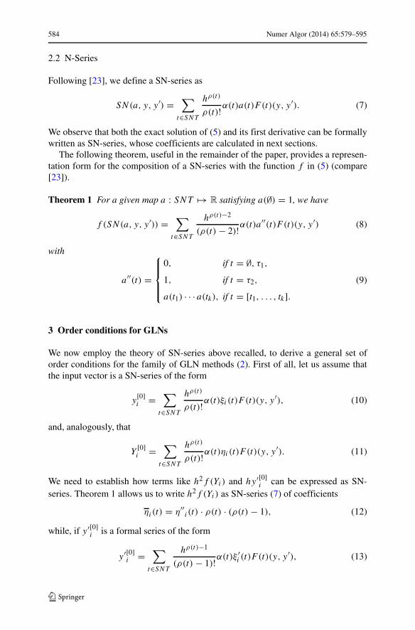
2.2 N-Series

Following [23], we define a SN-series as

SN(a, y, y ′) =∑

t∈SNT

hρ(t)

ρ(t)!α(t)a(t)F (t)(y, y ′). (7)

We observe that both the exact solution of (5) and its first derivative can be formallywritten as SN-series, whose coefficients are calculated in next sections.

The following theorem, useful in the remainder of the paper, provides a represen-tation form for the composition of a SN-series with the function f in (5) (compare[23]).

Theorem 1 For a given map a : SNT �→ R satisfying a(∅) = 1, we have

f (SN(a, y, y ′)) =∑

t∈SNT

hρ(t)−2

(ρ(t) − 2)!α(t)a′′(t)F (t)(y, y ′) (8)

with

a′′(t) =

⎧⎪⎪⎨

⎪⎪⎩

0, if t = ∅, τ1,

1, if t = τ2,

a(t1) · · · a(tk), if t = [t1, . . . , tk].(9)

3 Order conditions for GLNs

We now employ the theory of SN-series above recalled, to derive a general set oforder conditions for the family of GLN methods (2). First of all, let us assume thatthe input vector is a SN-series of the form

y[0]i =

∑

t∈SNT

hρ(t)

ρ(t)!α(t)ξi (t)F (t)(y, y ′), (10)

and, analogously, that

Y[0]i =

∑

t∈SNT

hρ(t)

ρ(t)!α(t)ηi (t)F (t)(y, y ′). (11)

We need to establish how terms like h2f (Yi) and hy ′[0]i can be expressed as SN-series. Theorem 1 allows us to write h2f (Yi) as SN-series (7) of coefficients

ηi(t) = η′′i(t) · ρ(t) · (ρ(t) − 1), (12)

while, if y ′[0]i is a formal series of the form

y ′[0]i =∑

t∈SNT

hρ(t)−1

(ρ(t) − 1)!α(t)ξ′i (t)F (t)(y, y ′), (13)

Numer Algor (2014) 65:579–595 585

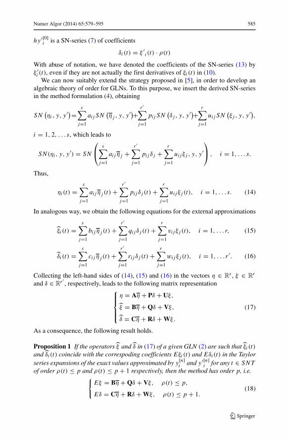
hy ′[0]i is a SN-series (7) of coefficients

δi(t) = ξ ′i(t) · ρ(t)With abuse of notation, we have denoted the coefficients of the SN-series (13) byξ ′i (t), even if they are not actually the first derivatives of ξi(t) in (10).

We can now suitably extend the strategy proposed in [5], in order to develop analgebraic theory of order for GLNs. To this purpose, we insert the derived SN-seriesin the method formulation (4), obtaining

SN(ηi, y, y

′)=s∑

j=1

aijSN(ηj , y, y

′)+r ′∑

j=1

pij SN(δj , y, y

′)+r∑

j=1

uij SN(ξj , y, y

′),

i = 1, 2, . . . s, which leads to

SN(ηi, y, y′) = SN

⎛

⎝s∑

j=1

aijηj +r ′∑

j=1

pij δj +r∑

j=1

uij ξj , y, y′⎞

⎠ , i = 1, . . . s.

Thus,

ηi(t) =s∑

j=1

aijηj (t)+r ′∑

j=1

pij δj (t)+r∑

j=1

uij ξj (t), i = 1, . . . s. (14)

In analogous way, we obtain the following equations for the external approximations

ξi (t) =s∑

j=1

bijηj (t)+r ′∑

j=1

qij δj (t)+r∑

j=1

vij ξj (t), i = 1, . . . r, (15)

δi (t) =s∑

j=1

cij ηj (t)+r ′∑

j=1

rij δj (t)+r∑

j=1

wij ξj (t), i = 1, . . . r ′. (16)

Collecting the left-hand sides of (14), (15) and (16) in the vectors η ∈ Rs , ξ ∈ R

r

and δ ∈ Rr ′ , respectively, leads to the following matrix representation

⎧⎪⎪⎨

⎪⎪⎩

η = Aη + Pδ + Uξ,

ξ = Bη + Qδ + Vξ,

δ = Cη + Rδ + Wξ.

(17)

As a consequence, the following result holds.

Proposition 1 If the operators ξ and δ in (17) of a given GLN (2) are such that ξi (t)and δi (t) coincide with the correspoding coefficients Eξi(t) and Eδi(t) in the Taylorseries expansions of the exact values approximated by y[n]i and y ′[n]i for any t ∈ SNT

of order ρ(t) ≤ p and ρ(t) ≤ p + 1 respectively, then the method has order p, i.e.{Eξ = Bη + Qδ + Vξ, ρ(t) ≤ p,

Eδ = Cη + Rδ + Wξ, ρ(t) ≤ p + 1.(18)

586 Numer Algor (2014) 65:579–595

Moreover, the method has stage order q if the operators ηi(t), i = 1, . . . , s, in (17)coincide with the coefficients Eηi of the Taylor series expansion of y(x0 + cih), forany t ∈ SNT of order ρ(t) ≤ q + 1, i.e.

Eη = Aη + Pδ + Uξ. (19)

By applying the result derived in Proposition 1, we derive the expressions of theoperators (18) and (19) in correspondence of the trees up to order 4 for a GLN method(2). We observe that the algebraic conditions (18) and (19) in Proposition 1 haveto be solved recursively by means of the decomposition rule given in Section 2.1,according to Theorem 1. We first consider (18) and (19) corresponding to the trees∅, τ1 and τ2, which provide the base case of the recursion, obtaining

∅

ηi(∅) =r∑

j=1

uij ξj (∅), i = 1, . . . , s,

Eδi(∅) =r∑

j=1

wij ξj (∅), i = 1, . . . , r ′,

Eξi(∅) =r∑

j=1

vij ξj (∅), i = 1, . . . , r, (20)

ηi( ) =r ′∑

j=1

pij ξ′j ( )+

r∑

j=1

uij ξj ( ), i = 1, . . . , s,

Eδi( ) =r ′∑

j=1

rij ξ′j ( )+

r∑

j=1

wij ξj ( ), i = 1, . . . , r ′,

Eξi( ) =r ′∑

j=1

qij ξ′j ( )+

r∑

j=1

vij ξj ( ), i = 1, . . . , r, (21)

ηi( ) = 2s∑

j=1

aijηj (∅)+ 2r ′∑

j=1

pij ξ′j ( )+

r∑

j=1

uij ξj ( ), i = 1, . . . , s,

Eδi( ) = 2s∑

j=1

cij ηj (∅)+ 2r ′∑

j=1

rij ξ′j ( )+

r∑

j=1

wij ξj ( ), i = 1, . . . , r ′,

Eξi ( ) = 2s∑

j=1

bijηj (∅)+ 2r ′∑

j=1

qij ξ′j ( )+

r∑

j=1

vij ξj ( ), i = 1, . . . , r. (22)

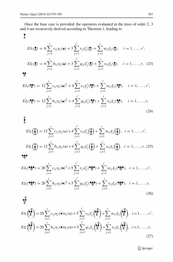
Numer Algor (2014) 65:579–595 587

Once the base case is provided, the operators evaluated in the trees of order 2, 3and 4 are recursively derived according to Theorem 1, leading to

Eδi( ) = 6s∑

j=1

cij ηj ( )+ 3r ′∑

j=1

rij ξ′j ( )+

r∑

j=1

wij ξj ( ), i = 1, . . . , r ′,

Eξi( ) = 6s∑

j=1

bijηj ( )+ 3r ′∑

j=1

qij ξ′j ( )+

r∑

j=1

vij ξj ( ), i = 1, . . . , r, (23)

Eδi( ) = 12s∑

j=1

cij ηj ( )2 + 4r ′∑

j=1

rij ξ′j ( )+

r∑

j=1

wij ξj ( ), i = 1, . . . , r ′,

Eξi( ) = 12s∑

j=1

bijηj ( )2 + 4r ′∑

j=1

qij ξ′j ( )+

r∑

j=1

vij ξj ( ), i = 1, . . . , r,

(24)

Eδi

( )= 12

s∑

j=1

cij ηj ( )+4r ′∑

j=1

rij ξ′j

( )+

r∑

j=1

wij ξj

( ), i = 1, . . . , r ′,

Eξi

( )= 12

s∑

j=1

bijηj ( )+4r ′∑

j=1

qij ξ′j

( )+

r∑

j=1

vij ξj

( ), i = 1, . . . , r, (25)

Eδi( ) = 20s∑

j=1

cij ηj ( )3 +5r ′∑

j=1

rij ξ′j ( )+

r∑

j=1

wij ξj ( ), i = 1, . . . , r ′,

Eξi( ) = 20s∑

j=1

bijηj ( )3+5r ′∑

j=1

qij ξ′j ( )+

r∑

j=1

vij ξj ( ), i = 1, . . . , r,

(26)

Eδi

( )

= 20s∑

j=1

cij ηj ( )ηj ( )+5r ′∑

j=1

rij ξ′j

( )

+r∑

j=1

wij ξj

( )

, i=1, . . . , r ′,

Eξi

( )

= 20s∑

j=1

bijηj ( )ηj ( )+5r ′∑

j=1

qij ξ′j

( )

+r∑

j=1

vij ξj

( )

, i=1, . . . , r,

(27)

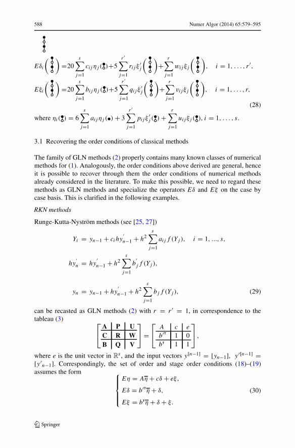
588 Numer Algor (2014) 65:579–595

Eδi

( )

=20s∑

j=1

cij ηj ( )+5r ′∑

j=1

rij ξ′j

( )

+r∑

j=1

wij ξj

( )

, i = 1, . . . , r ′,

Eξi

( )

=20s∑

j=1

bijηj ( )+5r ′∑

j=1

qij ξ′j

( )

+r∑

j=1

vij ξj

( )

, i = 1, . . . , r,

(28)

where ηi( ) = 6s∑

j=1

aijηj ( )+ 3r ′∑

j=1

pij ξ′j ( )+

r∑

j=1

uij ξj ( ), i = 1, . . . , s.

3.1 Recovering the order conditions of classical methods

The family of GLN methods (2) properly contains many known classes of numericalmethods for (1). Analogously, the order conditions above derived are general, henceit is possible to recover through them the order conditions of numerical methodsalready considered in the literature. To make this possible, we need to regard thesemethods as GLN methods and specialize the operators Eδ and Eξ on the case bycase basis. This is clarified in the following examples.

RKN methods

Runge-Kutta-Nystrom methods (see [25, 27])

Yi = yn−1 + cihy′n−1 + h2

s∑

j=1

aijf (Yj ), i = 1, ..., s,

hy′n = hy

′n−1 + h2

s∑

j=1

b′jf (Yj ),

yn = yn−1 + hy′n−1 + h2

s∑

j=1

bjf (Yj ), (29)

can be recasted as GLN methods (2) with r = r ′ = 1, in correspondence to thetableau (3)

⎡

⎣

A P UC R WB Q V

⎤

⎦ =⎡

⎣A c e

b′T 1 0bT 1 1

⎤

⎦ ,

where e is the unit vector in Rs , and the input vectors y[n−1] = [yn−1], y ′[n−1] =

[y ′n−1]. Correspondingly, the set of order and stage order conditions (18)–(19)assumes the form ⎧

⎪⎪⎨

⎪⎪⎩

Eη = Aη + cδ + eξ,

Eδ = b′Tη + δ,

Eξ = bTη + δ + ξ.

(30)

Numer Algor (2014) 65:579–595 589

The values of Eη, Eδ and Eξ are reported in Table 2. We observe that theseconditions match the classical ones (compare [23, 25]).

Coleman hybrid methods

We now consider the following class of methods

Yi = (1 + ci)yn−1 − ciyn−2 + h2s∑

j=1

aijf (Yj ), i = 1, ..., s, (31)

yn = 2yn−1 − yn−2 + h2s∑

j=1

bjf (Yj ),

introduced by Coleman in [10] (also compare [14, 18, 19, 21]), which are denotedas two-step hybrid methods. Such methods (31) can be regarded as GLN methodscorresponding to the reduced tableau

[A UB V

]

=⎡

⎣A e + c −c

bT 2 −10 1 0

⎤

⎦

obtained by assuming the remaining coefficient matrices in (3) equal to thezero matrix. Such methods are characterized by the the input vector y[n−1] =[yn−1 yn−2]T. The corresponding set of order and stage order conditions (18)–(19)takes the form

⎧⎪⎪⎨

⎪⎪⎩

Eη = Aη + e + cξ1 − cξ2,

Eξ1 = bTη + 2ξ1 − ξ2,

Eξ2 = ξ1.

(32)

The coefficients for ξ1, ξ2 can be found in Table 3. We observe that the third equationin (32) is trivial by the definition of ξ1.

Table 2 Values of Eηi , Eδ andEξ for RKN methods regardedas GLN methods

Tree Eξ(t) Eδ(t) Eηi(t)

∅ 1 0 1

1 1 ci

1 2 c2i

1 3 c3i

.

.

....

.

.

....

t 1 ρ(t) cρ(t)i

590 Numer Algor (2014) 65:579–595

Table 3 Values of Eξ1, ξ1 andξ2 for Coleman hybrid methodsregarded as GLNs

Tree Eξ1(t) ξ1(t) ξ2(t)

∅ 1 1 1

1 0 −1

1 0 1

1 0 −1...

.

.

....

.

.

.

t 1 0 (−1)ρ(t)

Two-step Runge-Kutta-Nystrom methods

Two-step Runge-Kutta-Nystrom methods (TSRKN)

Y[n−1]i = yn−2 + hciy

′n−2 + h2

s∑

j=1

aijf (Y[n−1]j ), i = 1, . . . , s,

Y[n]i = yn−1 + hciy

′n−1 + h2

s∑

j=1

aijf (Y[n]j ), i = 1, . . . , s,

hy ′n = (1 − θ)hy ′n−1 + θhy ′n−2 + h2v′jf (Y[n−1]j )+ h2w′

jf (Y[n]j ),

yn = (1 − θ)yn−1 + θyn−2 + h

s∑

j=1

v′j y ′n−2 + h

s∑

j=1

w′j y

′n−1

+h2s∑

j=1

vjf (Y[n−1]j )+ h2

s∑

j=1

wjf (Y[n]j ), (33)

have been introduced and analyzed by Paternoster in [28–31]. Such methods dependon two consecutive approximations to the solution and its first derivative in the gridpoints, but also on two consecutive approximations to the stage values, in line withthe idea employed by Jackiewicz et al. (compare [2, 11, 13, 15–17, 22, 24, 26]) inthe context of two-step Runge–Kutta methods for first order ODEs. TSRKN methodscan be represented as GLNs (2) with r = s + 2 and r ′ = 2 through the tableau (3)

⎡

⎣

A P UC R WB Q V

⎤

⎦ =

⎡

⎢⎢⎢⎢⎢⎢⎣

A c 0 e 0 0

w′T 1 − θ θ 0 0 v′T

0 1 0 0 0 0

wT w′Te v′T

e 1 − θ θ vT

0 0 0 1 0 0I 0 0 0 0 0

⎤

⎥⎥⎥⎥⎥⎥⎦

,

Numer Algor (2014) 65:579–595 591

in correspondence of the input vectors y[n−1] = [yn−1 yn−2 h2f (Y [n−1])]T,y ′[n−1] = [y ′n−1 y ′n−2]T. The set of order conditions for these methods has theform⎧⎪⎪⎪⎪⎪⎪⎪⎪⎪⎪⎪⎪⎪⎪⎪⎪⎪⎪⎨

⎪⎪⎪⎪⎪⎪⎪⎪⎪⎪⎪⎪⎪⎪⎪⎪⎪⎪⎩

Eηi =s∑

j=1

aijηj + ciδ1 + ξ1, i = 1, . . . , s,

Eδ1 =s∑

j=1

w′j ηj + (1 − θ)δ1 + θδ2 +

s∑

j=1

v′j ξ3j ,

Eδ2 = δ1,

Eξ1 =s∑

j=1

wjηj +s∑

j=1

w′j δ1 +

s∑

j=1

v′j δ2 + (1 − θ)ξ1 + θξ2 +s∑

j=1

vj ξ3j ,

Eξ2 = ξ1,

Eξ3i = ηi i = 1, . . . , s,

(34)

whose coefficients Eξ1, Eδ1, ξ1, ξ2, δ1 and δ2 can be found in Table 4. We alsoobserve that in the system (34) there are automatically satisfied conditions, i.e. thethird, the fifth and the sixth.

4 Construction of a family of methods of order 4

We now employ the order results provided in Section 3, to derive a new methodof order 4. We focus our attention on GLN methods (2) whose vectors of externalapproximations satisfy

y[n] ≈

⎡

⎢⎢⎣

y(xn)

h2y ′′(xn)h3y ′′′(xn)h4y(4)(xn)

⎤

⎥⎥⎦ , hy ′[n] ≈ hy ′(xn). (35)

For GLN methods (2) depending on input vectors of the form (35), exact startingvalues can be obtained by differentiation from the initial condition: in fact

ξ ′(t) = δρ(t),1, ξi (t) = ρ(t)δρ(t),i ,

Table 4 Values of Eξ1, Eδ1,ξ1, ξ2, δ1 and δ2 for TSRKNmethods regarded as GLNs

Tree Eξ1(t) Eδ1(t) ξ1(t) ξ2(t) δ1(t) δ2(t)

∅ 1 0 1 1 0 0

1 1 0 −1 1 1

1 2 0 1 0 −1

1 3 0 −1 0 1...

.

.

....

.

.

....

.

.

....

t 1 ρ(t) 0 (−1)ρ(t) 0 (−1)ρ(t)−1

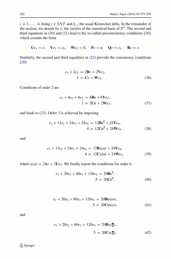
592 Numer Algor (2014) 65:579–595

i = 1, . . . , 4, being t ∈ SNT and δi,j the usual Kronecker delta. In the remainder ofthe section, we denote by ei the vectors of the canonical basis of R4. The second andthird equations in (20) and (21) lead to the so-called preconsistency conditions [20],which assume the form

Ue1 = e, Ve1 = e1, We1 = 0, Pe = c, Qe = e1, Re = e.

Similarly, the second and third equalities in (22) provide the consistency conditions[20]

e1 + 2e2 = 2Be+ 2Ve2,

1 = Ce + We2. (36)

Conditions of order 2 are

e1 + 6e2 + 6e3 = 6Bc + 6Ve3,

1 = 2Cc + 2We3, (37)

and leads to (23). Order 3 is achieved by imposing

e1 + 12e2 + 24e3 + 24e4 = 12Bc2 + 24Ve4,

4 = 12Cc2 + 24We4. (38)

and

e1 + 12e2 + 24e3 + 24e4 = 12Bη( )+ 24Ve4,

4 = 12Cη( )+ 24We4, (39)

where η( ) = 2Ae + 2Ue2. We finally report the conditions for order 4,

e1 + 20e2 + 60e3 + 120e4 = 20Bc3,

5 = 20Cc3, (40)

e1 + 20e2 + 60e3 + 120e4 = 20Bcη( ),

5 = 20Ccη( ), (41)

and

e1 + 20e2 + 60e3 + 120e4 = 20Bη( ),

5 = 20Cη( ), (42)

Numer Algor (2014) 65:579–595 593

where η( ) = 6Ac + 6Ue3. Solving the above order conditions lead to the followingfour-parameter family of one stage order 4 GLN methods (2)

⎡

⎣

A P UC R WB Q V

⎤

⎦ =

⎡

⎢⎢⎢⎢⎢⎢⎢⎢⎢⎢⎢⎢⎢⎣

12 (c

2 − 2u2) c 1 u2 u3 u4

14c3 1 0 4c3−1

4c32c2−1

4c24c−324c

120c3 1 1 10c3−1

20c310c2−3

60c25c−3120c

1c3 0 0 c3−1

c3c2−1c2

c−12c

3c3 0 0 − 3

c3c2−3c2

2c−32c

6c3 0 0 − 6

c3 − 6c2

c−3c

⎤

⎥⎥⎥⎥⎥⎥⎥⎥⎥⎥⎥⎥⎥⎦

,

in correspondence of the input vectors (35). According to [20], we estimate that thesemethods are obviously zero-stable and, therefore, convergent since they are also con-sistent (see [20]) if c > 41/30. An example, for c = 3/2 and u2 = 1/2, u3 = u4 = 1,is given by

⎡

⎣

A P UC R WB Q V

⎤

⎦ =

⎡

⎢⎢⎢⎢⎢⎢⎢⎢⎢⎢⎢⎢⎣

58

32 1 1

2 1 1

227 1 0 25

277

18112

2135 1 1 131

2701390

140

827 0 0 19

2759

16

89 0 0 − 8

9 − 13 0

169 0 0 − 16

9 − 83 −1

⎤

⎥⎥⎥⎥⎥⎥⎥⎥⎥⎥⎥⎥⎦

.

This is GLN method (2) depending one stage and of order 4, which is higher thanthat attainable by one stage RKN methods [23, 25], equal to 2.

5 Conclusions

We have focused our attention on the algebraic theory of order for the family of GLNmethods (2) for second order ODEs (1). By suitably adapting the theory of SN-seriesto the case of GLN methods, we have derived general order conditions, which alsoproperly contain those of other numerical methods already known in the literature, asexplained in Section 3, and constructed a family of one-stage methods of order 4. Thegeneral approach provided here can be used to finally derive new irreducible GLNmethods, which are not Runge-Kutta nor linear multistep methods, more efficientthan existing classical methods.

Acknowledgments The authors are deeply grateful to John C. Butcher for all the profitable discussionshad during last years on several topics concerning numerical methods for ODEs. We also espress ourgratitude to the anonymous referees for their valuable comments.

594 Numer Algor (2014) 65:579–595

References

1. Brouder, C.: Trees, renormalization and differential equations. BIT 44(3), 425–438 (2004)2. Butcher, J.C., Tracogna, S.: Order conditions for two-step Runge-Kutta methods. Appl. Numer.

Math. 24(2–3), 351–364 (1997)3. Butcher, J.C., Chan, T.M.H.: A new approach to the algebraic structures for integration methods.

BIT 42(3), 477–489 (2002)4. Butcher, J.C.: General linear methods. Acta Numer. 15, 157–256 (2006)5. Butcher, J.C.: Numerical Methods for Ordinary Differential Equations, 2nd edn. Wiley, Chichester

(2008)6. Butcher, J.C.: B-series and B-series coefficients. JNAIAM J. Numer. Anal. Ind. Appl. Math. 5(1–2),

39–48 (2010)7. Butcher, J.C., Chan, T.M.H.: The tree and forest spaces with applications to initial-value problem

methods. BIT 50(4), 713–728 (2010)8. Butcher, J.C.: Trees and numerical methods for ordinary differential equations. Numer. Algorithms

53(2–3), 153–170 (2010)9. Chartier, P., Hairer, E., Vilmart, G.: Algebraic structures of B-series. Found. Comput. Math. 10(4),

407–427 (2010)10. Coleman, J.P.: Order conditions for a class of two-step methods for y′′ = f (x, y). IMA J. Numer.

Anal. 23, 197–220 (2003)11. Cong, N.H.: Parallel-iterated pseudo two-step Runge-Kutta-Nystrom methods for nonstiff second-

order IVPs. Comput. Math. Appl. 44(1–2), 143–155 (2002)12. Connes, A., Kreimer, D.: Hopf algebras, renormalization and noncommutative geometry. Commun.

Math. Phys. 199, 203–242 (1998)13. Conte, D., D’Ambrosio, R., Jackiewicz, Z., Paternoster, B.: Numerical search for algebrically stable

two-step continuous Runge-Kutta methods. J. Comput. Appl. Math. 239, 304–321 (2013)14. D’Ambrosio, R., Ferro, M., Paternoster, B.: Two-step hybrid collocation methods for y′′ = f (x, y).

Appl. Math. Lett. 22, 1076–1080 (2009)15. D’Ambrosio, R., Ferro, M., Jackiewicz, Z., Paternoster, B.: Two-step almost collocation methods for

ordinary differential equations. Numer. Algorithms 53(2–3), 195–217 (2010)16. D’Ambrosio, R., Jackiewicz, Z.: Continuous two-step Runge–Kutta methods for ordinary differential

equations. Numer. Algorithms 54(2), 169–193 (2010)17. D’Ambrosio, R., Jackiewicz, Z., Construction and implementation of highly stable two-step contin-

uous methods for stiff differential systems: Math. Comput. Simul. 81(9), 1707–1728 (2011)18. D’Ambrosio, R., Ferro, M., Paternoster, B.: Trigonometrically fitted two-step hybrid methods for

second order ordinary differential equations with one or two frequencies. Math. Comput. Simul. 81,1068–1084 (2011)

19. D’Ambrosio, R., Esposito, E., Paternoster, B.: Exponentially fitted two-step hybrid methods fory′′ = f (x, y). J. Comput. Appl. Math. 235, 4888–4897 (2011)

20. D’Ambrosio, R., Esposito, E., Paternoster, B.: General linear methods for y′′ = f (y(t)). Numer.Algorithm 61(2), 331–349 (2012)

21. D’Ambrosio, R., Esposito, E., Paternoster, B.: Parameter estimation in two-step hybrid methods forsecond order ordinary differential equations. J. Math. Chem. 50(1), 155–168 (2012)

22. D’Ambrosio, R., Paternoster, B.: Two-step modified collocation methods with structured coefficientmatrices for ordinary differential equations. Appl. Numer. Math. 62(10), 1325–1334 (2012)

23. Hairer, E., Wanner, G.: A theory for Nystrom methods. Numer. Math. 25, 383–400 (1976)24. Hairer, E., Wanner, G.: Order conditions for general two-step Runge-Kutta methods. SIAM J. Numer.

Anal. 34(7), 2086–2089 (1997)25. Hairer, E., Nørsett, S.P., Wanner, G.: Solving Ordinary Differential Equations, 2nd edn., Springer

Series in Computational Mathematics, vol. 8. Springer, Berlin (2008)26. Jackiewicz, Z.: General Linear Methods for Ordinary Differential Equations. Wiley, Hoboken (2009)27. Paternoster, B.: Runge-Kutta(-Nystrom) methods for ODEs with periodic solutions based on

trigonometric polynomials. Appl. Numer. Math. 28, 401–412 (1998)28. Paternoster, B.: Two step Runge-Kutta-Nystrom methods for y′′ = f (x, y) and P-stability. In: Sloot,

P.M.A. et al. (eds.) Computational Science - ICCS 2002. Lecture Notes in Computer Science, PartIII, vol. 2331, pp. 459–466. Springer, Amsterdam (2002)

Numer Algor (2014) 65:579–595 595

29. Paternoster, B.: Two step Runge-Kutta-Nystrom methods for oscillatory problems based on mixedpolynomials. In: Sloot, P.M.A., Abramson, D., Bogdanov, A.V., Dongarra, J.J., Zomaya, A.Y.,Gorbachev, Y.E. (eds.) Computational Science - ICCS 2003. Lecture Notes in Computer Science,Part II, vol. 2658, pp. 131–138. Springer, Berlin/Heidelberg (2003)

30. Paternoster, B.: Two step Runge-Kutta-Nystrom methods based on algebraic polynomials. Rend.Mat. Appl. 23, 277–288 (2003)

31. Paternoster, B.: A general family of two step Runge-Kutta-Nystrom methods for y′′ = f (x, y) basedon algebraic polynomials. In: Alexandrov, V.N., et al. (eds.) Computational Science - ICCS 2006.Lecture Notes in Computer Science, Part IV, vol. 3994, pp. 700–707. Springer, Amsterdam (2006)