Sufficient conditions for stability of linear differential equations with distributed delay

DISCRETE AND CONTINUOUS Website: http://math.smsu.edu/journalDYNAMICAL SYSTEMS–SERIES BVolume 1, Number 2, May 2001 pp. 233–256

SUFFICIENT CONDITIONS FOR STABILITY OF LINEARDIFFERENTIAL EQUATIONS WITH DISTRIBUTED DELAY

Samuel Bernard

Departement de Mathematiques et de Statistique andCentre de recherches mathematiques

Universite de MontrealMontreal Quebec H3C 3J7 CANADA

andCentre for Nonlinear Dynamics

McGill University

Jacques Belair

Departement de Mathematiques et de Statistique

Centre de recherches mathematiques andInstitut de Genie Biomedical

Universite de MontrealMontreal Quebec H3C 3J7 CANADA

andCentre for Nonlinear Dynamics

McGill University

Michael C. Mackey

Departments of Physiology, Physics & Mathematics andCentre for Nonlinear Dynamics

McGill University3655 Drummond, Montreal, Quebec H3G 1Y6 CANADA

Abstract. We develop conditions for the stability of the constant (steadystate) solutions of linear delay differential equations with distributed delaywhen only information about the moments of the density of delays is available.We use Laplace transforms to investigate the properties of different distribu-tions of delay. We give a method to parametrically determine the boundaryof the region of stability, and sufficient conditions for stability based on theexpectation of the distribution of the delay. We also obtain a result basedon the skewness of the distribution. These results are illustrated on a recentmodel of peripheral neutrophil regulatory system which include a distributionof delays. The goal of this paper is to give a simple criterion for the stabilitywhen little is known about the distribution of the delay.

1. Introduction. Delay differential equations (DDE) have been studied exten-sively for the past 50 years. They have applications in domains as diverse as en-gineering, biology and medicine where information transmission and/or responsein control systems is not instantaneous. For a good introduction to the subject,

1991 Mathematics Subject Classification. 34K20, 34K06, 92C37.Key words and phrases. Differential Equations, Distributed Delay, Stability, Cyclical

Neutropenia.

233

234 SAMUEL BERNARD, AND JACQUES BELAIR AND MICHAEL C. MACKEY

see [4]. Much of the work that has been done treats DDEs with one or a few discretedelays.A number of realistic physiological models however include distributed delays

and a problem of particular interest is to determine the stability of the steadystate solutions. For applications in physiological systems see [5, 6, 10, 14, 15].Although results concerning DDEs with particular distributed delays (for extensiveresults about the gamma distribution see [3]) have been published, there has beenno systematic study of this problem when little is known about the density of thedelay distribution: most notably, results on sufficient conditions for stability ofsolutions of equations such as those considered in the present paper are given in[7, 16].The problem of stability is very important in physiology and medicine. One class

of diseases is characterized by a dramatic change in the dynamics of a physiologicalvariable or a set of variables and there is sometime good clinical evidence thatthese changes are a consequence of a bifurcation in the underlying dynamics ofthe physiological control system. In [6] it was proposed that these diseases becalled dynamical diseases. In many cases, one variable starts (or stops) to oscillate.In order to treat these diseases, it is useful to know the parameter which causesthe oscillation (or the supression thereoff). An example of a dynamical disease iscyclical neutropenia which is the subject of Section 6.In Section 2 we briefly set the stage for the type of problem that we are consider-

ing. In Section 3, we define our notion of stability and discuss how to parametricallydetermine the region of stability of a simple DDE for three particular distributionsof delay: when the delay is a single discrete delay, a uniformly distributed delayand a distribution with the gamma density. In Section 4 we introduce a sufficientcondition to have stability based on the expected delay and the symmetry of thedistribution of delays. In Section 5 we give some examples again turning to thesingle delay, and the uniformly and gamma distributed cases. In Section 6 we applyour results to a recently published model for the peripheral regulation of neutrophilproduction.

2. Preliminaries. In this paper we study the stability of the linear differentialEquation

x(t) = −αx(t) − β

∫ ∞

0

x(t− τ)f(τ) dτ (1)

where α and β are constants. We show that the symmetry of the distribution fplays an important role in the stability of the trivial solution, and our first resultconsiders the characteristic equation of the DDE (1) if the density f is symmetric.If f is skewed to the left (meaning that there is more weight to the left of theexpectation) then stability is stronger (i.e. holds for a wider range of parametervalues) than for a single delay.We restrict the values of α and β to β ≥ |α| because we are interested in the

influence of the distribution f on the stability properties of (1). It is straightforwardto show that if β ≤ −α then the trivial solution of Equation (1) is not stable.Moreover if α > |β|, Equation (1) is stable for all values of τ . The interestingparameter values are therefore located in the cone β ≥ |α|.

STABILITY AND DISTRIBUTED DELAYS 235

Consider the general differential delay equation

dx(t)dt

= F(x(t), x(t)), (2)

where x(t) is x(t− τ) weighted by a distribution of maturation delays. x(t) is givenexplicitly by

x(t) =∫ ∞

τm

x(t− τ)f(τ)dτ ≡∫ t−τm

−∞x(τ)f(t− τ)dτ. (3)

τm is a minimal delay and f(τ) is the density of the distribution of maturationdelays. Since f(τ) is a density, f ≥ 0 and∫ ∞

0

f(τ)dτ = 1. (4)

To completely specify the semi-dynamical system described by Equations (2) and(3) we must additionally have an initial function

x(t′) ≡ ϕ(t′) for t′ ∈ (−∞, 0). (5)

Steady states x∗ of Equation (2) are defined implicitly by the relation

dx∗dt

≡ 0 ≡ F(x∗, x∗). (6)

Definition 2.0.1. If there is a unique steady state x∗ of Equation (2) it is globallyasymptotically stable if, for all initial functions ϕ,

limt→∞x(t) = x∗. (7)

The primary consideration of this paper is the stability of the steady state(s),defined implicitly by Equation (6), and how that stability may be lost. Though wewould like to be able to examine the global stability of x∗ to perturbations, onemust often be content with an examination of the local stability of x∗.

Definition 2.0.2. A steady state x∗ of Equation (2) is locally asymptotically stableif, for all initial functions ϕ satisfying |ϕ(t′)− x∗| ≤ ε, 0 < ε 1,

limt→∞x(t) = x∗. (8)

3. Local Stability. To examine its local stability, we linearize Equation (2) inthe neighborhood of any one of the steady states defined by (6), and define z(t) =x(t) − x∗ as the deviation of x(t) from that steady state. The resulting linearequation is

dz(t)dt

= −αz(t)− βz(t), (9)

where

z(t) =∫ ∞

τm

z(t− τ)f(τ)dτ ≡∫ t−τm

−∞z(τ)f(t− τ)dτ, (10)

and α and β are defined by

α ≡ −∂F(x, x)∂x

|x=x∗ β ≡ −∂F(x, x)∂x

|x=x∗ . (11)

236 SAMUEL BERNARD, AND JACQUES BELAIR AND MICHAEL C. MACKEY

If we make the ansatz that z(t) est in Equation (9), the resulting eigenvalueequation is

s+ α+ βe−sτm f(s) = 0, (12)

where

f(s) =∫ ∞

0

e−sτf(τ)dτ (13)

is the Laplace transform of f .

3.1. The single delay case. The “usual” situation considered by many authorsis that in which there is a single discrete delay. The density f is then given as aDirac delta function, f(τ) = δ(τ − τ). In this case the eigenvalue Equation (12)takes the form

s+ α+ βe−sτ = 0. (14)

If s = µ + iω, then the boundary between locally stable behaviour (µ < 0) andunstable behaviour (µ > 0) is given by the values of α, β, and τ satisfying

iω + α+ βe−iωτ = 0, (15)

which has been studied by Hayes [12]. Isolating the real

α+ β cos(ωτ) = 0, (16)

and imaginary

ω − β sin(ωτ) = 0 (17)

parts of (15) it is straightforward to show that µ < 0 whenever

1. α > |β|, or if2. β ≥ |α| and

τ < τcrit ≡arccos

(−α

β

)√β2 − α2

. (18)

The stability boundary defined by Equation (18) is shown in Figure 2 in Section 5where we have parametrically plotted

β(ω) =ω

sin(ωτ)(19)

versus

α(ω) = −ω cot(ωτ). (20)

When τ = τcrit there is a Hopf bifurcation [8] to a periodic solution of (9) withHopf period

THopf =2π√

β2 − α2. (21)

STABILITY AND DISTRIBUTED DELAYS 237

3.2. The uniform (rectangular) density. Suppose we have the simple situationwherein there is distribution of delays with a uniform rectangular density given by

f(τ) =

0 0 ≤ τ < τm1δ τm ≤ τ ≤ τm + δ0 τm + δ < τ.

(22)

The expected value E of the delay is

E =∫ ∞

0

τf(τ)dτ =δ

2, (23)

so the average delay is

< τ >= τm + E = τm +δ

2(24)

and the variance (denoted by V ) is

V =δ2

12=E2

3. (25)

The Laplace transform of f as given by (22) is easily computed to be

f(s) =eδs − 1δs

, (26)

so the eigenvalue Equation (12) takes the form

δs(s+ α) + βe−sτm[eδs − 1] = 0. (27)

This may be rewritten in terms of the expectation E as

2Es(s+ α) + βe−sτm[e2Es − 1] = 0. (28)

Taking s = iω and proceeding as before we obtain parametric equations for α(ω)and β(ω) as follows:

α(ω) = −ω sin[(δ − τm)ω] + sin(ωτm)cos[(δ − τm)ω]− cos(ωτm) , (29)

and

β(ω) =δω2

cos[(δ − τm)ω]− cos(ωτm) . (30)

Refer to Figure 3 to see a graphical representation of the region of stability.

3.3. The gamma density. The density of the gamma distribution with parame-ters (a,m)

f(τ) ={

0 0 ≤ τ < τmam

Γ(m) (τ − τm)m−1e−a(τ−τm) τm ≤ τ(31)

with a,m ≥ 0, is often encountered [10] in applications. The parameters m, a,and τm in the density of the gamma distribution can be related to certain easilydetermined statistical quantities. Thus, the average of the unshifted density is givenby

E =∫ ∞

0

τf(τ)dτ =m

a, (32)

so the average delay is

< τ >= τm + E = τm +m

a(33)

238 SAMUEL BERNARD, AND JACQUES BELAIR AND MICHAEL C. MACKEY

and the variance is

V =m

a2. (34)

Using (32) and (34) the parameters m and a can be expressed as

a =E

V(35)

and

m =E2

V. (36)

Using the Laplace transform of (31) the eigenvalue Equation (12) becomes

(s+ α)[1 +

s

a

]m

+ βe−sτm = 0. (37)

Equation (37) can be used to give a pair of parametric equations in α and βdefining the local stability boundary (µ ≡ Re s ≡ 0). We start by setting s = iωand

tan θ =ω

a. (38)

Using de Moivre’s formula in Equation (37) with s = iω gives

(α+ iω)(cos[mθ]) + i sin[mθ]) = −β cosm θ(cosωτm − i sinωτm) (39)

Equating the real and imaginary parts of Equation (39) gives the coupled equations

α+ βr cosωτm = ω tan[mθ], (40)

and

α tan[mθ]− βr sinωτm = −ω, (41)

where

r =cosm θ

cos[mθ]. (42)

Equations (40) and (41) are easily solved for α and β as parametric functions of ωto give

α(ω) = − ω

tan[ωτm +m tan−1(ω/a)](43)

and

β(ω) =ω

cosm[tan−1(ω/a)] sin[ωτm +m tan−1(ω/a)](44)

respectively. Refer to Figure 4 to see the region of stability.

3.4. General density case. The method employed above can be generalized forany density. Consider Equation (12) and let s = iω. Separating the real andimaginary parts leads to

α+ β

∫ ∞

0

cos(ωτ)f(τ)dτ = 0 (45)

ω − β

∫ ∞

0

sin(ωτ)f(τ)dτ = 0. (46)

STABILITY AND DISTRIBUTED DELAYS 239

Define

C(ω) ≡∫ ∞

0

cos(ωτ)f(τ)dτ (47)

and

S(ω) ≡∫ ∞

0

sin(ωτ)f(τ)dτ . (48)

Then we can solve for α and β to obtain them as parametric functions of ω:

α(ω) = −ωC(ω)S(ω)

(49)

and

β(ω) =ω

S(ω). (50)

4. Stability Conditions. One method to study the stability is to find condi-tions for which the eigenvalue equation (or characteristic equation) has no rootswith positive real part. The difficulty with Equation (1) is that the characteris-tic equation often involves a transcendental term. A noticeable exception is theunshifted gamma distribution for which the characteristic equation [Equation (37)with τm = 0] is a polynomial. This term, the Laplace transform of the densityof the distribution of delays, can be expressed as C(ω) + iS(ω) [Equations (47)and (48)] on the imaginary axis. The first Lemma gives a bound on the termC(ω) =

∫ ∞0cos(ωτ)f(τ)dτ when the density f is symmetric.

Lemma 4.0.1. Let f be a probability density such that:

1. f : R −→ R+

2. E =∫ ∞−∞ τ f(τ) dτ ,

3. f(E − τ) = f(E + τ)

(The third property implies that f is symmetric about its expectation). Then

1. for all ω, ∣∣∣∣∫ ∞

−∞cos(ωτ) f(τ) dτ

∣∣∣∣ ≤ |cos(ωE)| ; (51)

2. if ω < π/2E, ∫ ∞

−∞cos(ωτ) f(τ) dτ > 0. (52)

Proof. For the first part of the Lemma, assume that f is piecewise constant andgiven by

f(τ) =N∑

i=1

Ciχ[Ai,Bi](τ)

where χ[Ai,Bi] denotes the indicator function on the interval [Ai, Bi]:

χ[A,B](τ) ={0 τ /∈ [A,B]1 τ ∈ [A,B] . (53)

240 SAMUEL BERNARD, AND JACQUES BELAIR AND MICHAEL C. MACKEY

Then

∣∣∣∣∫ ∞

−∞cos(ωτ)f(τ)dτ

∣∣∣∣ =

∣∣∣∣∣∫ ∞

−∞cos(ωτ)

N∑i=1

Ciχ[Ai,Bi](τ)dτ

∣∣∣∣∣=

∣∣∣∣∣N∑

i=1

Ci

∫ Bi

Ai

cos(ωτ) dτ

∣∣∣∣∣=

∣∣∣∣∣N∑

i=1

Ci

ω(sin(ωBi)− sin(ωAi))

∣∣∣∣∣ ,

which must be less than |cos(ωE)| as we now show.Using the trigonometric identity

sin(x+ y)− sin(x− y) = 2 cos(x) sin(y),

we have

∣∣∣∣∣N∑

i=1

Ci

ω(sin(ωBi)− sin(ωAi))

∣∣∣∣∣ =∣∣∣∣∣

N∑i=1

Ci

ω2 cos(ω

Bi +Ai

2) sin(ω

Bi −Ai

2)

∣∣∣∣∣ .

By the symmetry of f , we know that Ci = CN−i+1, and the distance between theexpectation E and the middle of the ith interval is equal to the one between E andthe middle of the (N − i+ 1)th interval. That is,

∣∣∣∣E − Ai +Bi

2

∣∣∣∣ =∣∣∣∣E − AN−i+1 +BN−i+1

2

∣∣∣∣ .

Set Ei =∣∣E − 1

2 (Ai +Bi)∣∣. For 1 ≤ i ≤ N/2, we have 1

2 (Ai + Bi) = E − Ei,12 (AN−i+1+BN−i+1) = E +EN−i+1 and Ei = EN−i+1. Substitute these values inthe summation:

∣∣∣∣∣N∑

i=1

Ci

ω2 cos(ω

Bi +Ai

2) sin(ω

Bi −Ai

2)

∣∣∣∣∣ =

∣∣∣∣∣∣N/2∑i=1

2Ci

ωsin(ω

Bi −Ai

2)(cos(ω(E − Ei)) + cos(ω(E + Ei))

∣∣∣∣∣∣ =

∣∣∣∣∣∣N/2∑i=1

2Ci

ωsin(ω

Bi −Ai

2)(2 cos(ωE) cos(ωEi)

∣∣∣∣∣∣

The last equality is obtained by the trigonometric identity

cos(x+ y) + cos(x− y) = 2 cos(x) cos(y).

STABILITY AND DISTRIBUTED DELAYS 241

Apply the triangle inequality and bound |cos(ωEi)| by 1 and the sine by its argu-ment to obtain∣∣∣∣∣∣

N/2∑i=1

2Ci

ωsin(ω

Bi −Ai

2)(2 cos(ωE) cos(ωEi)

∣∣∣∣∣∣ ≤

N/2∑i=1

∣∣∣∣4Ci

ωsin(ω

Bi −Ai

2)∣∣∣∣ |cos(ωE)| |cos(ωEi)| ≤

N/2∑i=1

∣∣∣∣4Ci

ωsin(ω

Bi −Ai

2)∣∣∣∣ |cos(ωE)| ≤

N/2∑i=1

∣∣∣∣4CiBi −Ai

2

∣∣∣∣ |cos(ωE)| =N∑

i=1

|Ci(Bi −Ai)| |cos(ωE)|

Since f is a probability density,∫ ∞

−∞f(τ)dτ =

N∑i=1

∫ Bi

Ai

Cidτ =N∑

i=1

Ci(Bi −Ai) = 1.

SoN∑

i=1

|Ci(Bi −Ai)| |cos(ωE)| = |cos(ωE)| .

Then ∣∣∣∣∣N∑

i=1

Ci

ω(sin(ωBi)− sin(ωAi))

∣∣∣∣∣ ≤ |cos(ωE)| .

We thus have (51) when f is piecewise constant. If f is any symmetric probabilitydensity, we can approximate it by a sequence of functions {fn}∞n=1, when fn is apiecewise constant symmetric probability density, with fn → f as n → ∞ and∫ ∞−∞ τfn(τ)dτ =

∫ ∞−∞ τf(τ)dτ = E. Note that∣∣∣∣

∫ ∞

−∞cos(ωτ) fn(τ) dτ

∣∣∣∣ ≤ |cos(ωE)|

for every n, so

limn→∞

∣∣∣∣∫ ∞

−∞cos(ωτ)fn(τ)dτ

∣∣∣∣ =∣∣∣∣∫ ∞

−∞cos(ωτ) lim

n→∞ fn(τ)dτ∣∣∣∣

=∣∣∣∣∫ ∞

−∞cos(ωτ) f(τ) dτ

∣∣∣∣ ≤ |cos(ωE)| .

To prove the second part of the Lemma, observe that

|cos(ω(E − τ))f(E − τ)| ≥ |cos(ω(E + τ))f(E + τ)| ,so the integral over the positive part is greater than the one over the negativepart.

Remark 4.0.2. We can also prove, under the same hypothesis of Lemma 4.0.1,that ∣∣∣∣

∫ ∞

−∞sin(ωτ) f(τ) dτ

∣∣∣∣ ≤ |sin(ωE)| . (54)

242 SAMUEL BERNARD, AND JACQUES BELAIR AND MICHAEL C. MACKEY

The stability of Equation (1) depends on all moments of f about its mean. Theexpectation obviously plays an important role in stability; Anderson [1, 2] alsoshowed the importance of the variance (second moment about the mean) in thesestability considerations.We now study the location of the first root of C(ω). Lemma 4.0.1 states that

the first root of C(ω) is at ω = π/2E whenever the density f is symmetric. Itis of primary interest to see how this root changes when the distribution is notsymmetric. Around ωτ = π/2, the cosine in C(ω) =

∫ ∞0cos(ωτ)f(τ)dτ can be

expanded in Taylor series,

C(ω) =∫ ∞

−∞

∞∑n=0

(−1)n+1 (ωτ − π/2)2n+1

(2n+ 1)!f(τ)dτ , (55)

leading to the integral of a sum of terms with odd power (odd because we expandaround a root). The higher moments about the mean do not necessarily convergeand for this reason we can not usually switch the sum and the integral. The firstterm of this expansion is

− π

2E

∫ ∞

0

(τ − E)f(τ)dτ = 0 (56)

since the mean E is precisely the value for which this relation hold. The secondterm is the third moment about the mean (up to a multiplicative factor).

π3

(2E)33!

∫ ∞

0

(τ − E)3f(τ)dτ . (57)

The third moment is in general the first nonzero term of the Taylor expansion andso the sign of this term has a great importance in determining the position of theroot of C(ω). The skewness of a distribution is usually defined as the third momentabout the mean divided by the third power of the standard deviation. If the densityf is symmetric, all moment about the mean are zero. So a symmetric density hasa skewness equal to zero, which is coherent with intuition. But a third momentequal to zero does not imply that the density is symmetric. We require a definitionin which a skewness equal to zero means that the density is symmetric. For thepurpose of the paper, we will use the following definition of skewness.

Definition 4.0.3. Let f be a probability density with expectation E. The skewnessof f , B(f), is defined as

B(f) = (−1)k+1∫ ∞

0

(τ − E)2k+1f(t+ E)dτ (58)

where

k = min{n

∣∣∣∣∫ ∞

0

(τ −E)2n+1f(t+ E)dτ �= 0}. (59)

The density f is said to be skewed to the left if B(f) > 0 and skewed to the rightif B(f) < 0. In the case where k =∞ we define B(f) = 0.

Remark 4.0.4. It is clear that f is symmetric if and only if all the moments aboutits mean are zero, i.e. f is symmetric if and only if B(f) = 0. In general, for a non-symmetric density, the third moment about the mean is nonzero, so the definitionof B(f) reduces to the standard case (up to a positive multiplicative factor).

We can now look for sufficient conditions for stability of Equation (1).

STABILITY AND DISTRIBUTED DELAYS 243

Theorem 4.0.5 (Sufficient Conditions). Let f be a probability density defined on[0,+∞) with expectation ∫ ∞

0τf(τ)dτ = E. Suppose β > |α|. Then in Equation (1)

1. The solution x∗ = 0 is asymptotically stable (a.s.) if

E <π

(1 + α

β

)c√β2 − α2

(60)

where c = sup {c| cos(x) = 1− cx/π, x > 0} ≈ 2.2764.2. If the skewness B(f) = 0 we have the stronger sufficient condition for asymp-totic stability:

E <arccos

(−αβ

)√β2 − α2

. (61)

3. If the skewness is positive (B(f) > 0), then there is a δ > 0 such that condition(61) holds for |α| < δ.

Proof. The characteristic equation of (1) is

s+ α+ β

∫ ∞

0

e−sτf(τ)dτ = 0. (62)

If E = 0, (62) reduces to s + α + β = 0 which trivially has no root with positivereal part so x∗ = 0 is asymptotically stable. If an increase in E leads to instabilityof x∗ = 0, then a root s of (62) must intersect the imaginary axis, i.e. there existsE such that (62) has pure imaginary roots. We seek roots of the form s = iω, andbecause the roots come in conjugate pairs, we can restrict our search to ω > 0. Inthis case Equation (62) splits into a real part

α+ β

∫ ∞

0

cos(ωτ)f(τ)dτ = 0, (63)

and an imaginary part

ω − β

∫ ∞

0

sin(ωτ)f(τ)dτ = 0. (64)

First note that ω ≤√β2 − α2 since:

[∫ ∞

0

cos(ωτ)f(τ)dτ]2+

[∫ ∞

0

sin(ωτ)f(τ)dτ]2

≤∫ ∞

0

cos2(ωτ)f(τ)dτ +∫ ∞

0

sin2(ωτ)f(τ)dτ =∫ ∞

0

f(τ)dτ = 1.

and thus, by Equations (63) and (64), α2 + ω2 ≤ β2.To show condition (60), notice that∫ ∞

0

cos(ωτ)f(τ)dτ ≥∫ ∞

0

1− cωτ

πf(τ)dτ

=∫ ∞

0

f(τ)dτ − cω

π

∫ ∞

0

τf(τ)dτ = 1− cω

πE.

244 SAMUEL BERNARD, AND JACQUES BELAIR AND MICHAEL C. MACKEY

If 1 − cωE/π > −α/β, Equation (63) thus has no root. However, ω ≤√β2 − α2

so a sufficient condition for (63) to have no root is

E <π

(1 + α

β

)c√β2 − α2

.

For the proof of the second part of Theorem 4.0.5. suppose that f is symmetricabout its mean and α ≥ 0. We want

∫ ∞0cos(ωτ)f(τ)dτ > −α/β for 0 < ω ≤√

β2 − α2. By Lemma 4.0.1, we know that∫ ∞0cos(ωτ)f(τ)dτ > 0 for ω < π/2E.

For ω ≥ π/2E, ∣∣∣∣∫ ∞

0

cos(ωτ) f(τ) dτ∣∣∣∣ ≤ |cos(ωE)| .

This implies that ∫ ∞

0

cos(ωτ)f(τ)dτ ≥ cos(ωE)

whenever∫ ∞0cos(ωτ)f(τ)dτ < 0. If cos(ωE) > −α/β then E < ω−1 arccos(−α/β)

and ∫ ∞

0

cos(ωτ)f(τ)dτ > −α/β.

A sufficient condition for (62) with α ≥ 0 to have no root with positive real part istherefore:

E <arccos

(−αβ

)√β2 − α2

.

If α < 0, compare the boundary of region of stability (α(ω), β(ω)) defined byEquations (49) and (50) and the curve (αE(ω), βE(ω)) defined by the boundary ofregion of stability of the single delay at E. These two curves intersect for ω = 0 atthe point (−1/E, 1/E):

limω→0

α(ω) = limω→0

−ωC(ω)S(ω)

= limω→0

−ωS(ω)

= − limω→0

β(ω)

This limit is 1 over the slope of S(ω) at 0, which is E. This is true for all dis-tributions with expectation E and this is their only intersection point. To haveintersection we must get

−ωC(ω)S(ω)

=−ω cos(ωE)sin(ωE)

andω

S(ω)=

ω

sin(ωE)

which imply, for ω �= 0, that C(ω) = cos(ωE) and S(ω) = sin(ωE). These equalitiescan not occur until ω = π/2E. Moreover, when ω = π/2E, both curves cross theβ-axis and at this point β(ω) > βE(ω) = π/2E. These facts imply that the curve(α(ω), β(ω)) lies always above the “sufficient” curve (αE(ω), βE(ω)) and condition(61) holds for α < 0.

STABILITY AND DISTRIBUTED DELAYS 245

Now we have to show that if B(f) ≥ 0, no root crosses the imaginary axis whenα is sufficiently small. Consider any density f with positive skewness. Let p ∈ [0, 1],and define

fp = pf(τ) + (1− p)f(2E − τ).

The function f1/2 is a symmetric density and we have shown that:∣∣∣∣∫ ∞

−∞cos(ωτ)f1/2(τ)dτ

∣∣∣∣ ≤ |cos(ωE)| .

Moreover we have that∫ ∞

−∞cos(ωτ)fp(τ)dτ =

∫ ∞

−∞

∞∑n=0

(−1)n+1 (ωτ − π/2)2n+1

(2n+ 1)!fp(τ)dτ .

By Definition 4.0.3 the first nonzero term of the series evaluated at ω = π/2E is∫ ∞

−∞

(−1)k+1 (ωτ − π/2)2k+1

(2k + 1)!fp(τ)dτ =

( π

2E

)2k+1 1(2k + 1)!

∫ ∞

−∞(−1)k+1(τ − E)2k+1fp(τ)dτ .

For p > 1/2, it is clear that B(fp) > 0 so( π

2E

)2k+1 1(2k + 1)!

∫ ∞

−∞(τ − E)2k+1fp(τ)dτ =

( π

2E

)2k+1 1(2k + 1)!

B(fp) > 0.

This means that for p = 1/2 + ε, with small ε > 0,∫ ∞

−∞cos(ωτ)fp(τ)dτ > 0

for ω in a neighborhood of π/2E. This implies that∫ ∞

0

cos(ωτ)f(τ)dτ > 0.

Thus, we have shown that

B(f) ≡∫ ∞

0

(τ −E)2k+1f(τ)dτ > 0

implies ∫ ∞

0

cos(ωτ)f(τ)dτ > 0

around ω = π/2E.The first root of C(ω) is thus to the right of ω = π/2E (If this is were not true,

there would be a (continuous) family of densities fµ, µ ∈ [0, 1], with B(f0) = 0,B(fµ) > 0 for µ > 0 and f1 = f . There would then exist µ = µ0 > 0 where aroot of Cfµ0

(ω) appears before π/2E. This would mean that at µ = µ0, a root ofthe characteristic equation could suddenly appear in the right half complex plane,which is impossible (see Lemma 1.1 in [17])).Thus, an increase in p increases∫ ∞

−∞cos(ωτ)fp(τ)dτ ,

246 SAMUEL BERNARD, AND JACQUES BELAIR AND MICHAEL C. MACKEY

and ∫ ∞

0

cos(ωτ)f(τ)dτ >∫ ∞

−∞cos(ωτ)f1/2(τ)dτ .

This means that a positive skewness increases the stability of Equation (1) when|α| is small.

Remark 4.0.6. We can apply condition (61) to any density with a (small) positiveskewness. By the last part of the proof, a small perturbation which increases theskewness of a symmetric density will not cause roots of characteristic equation tocross the imaginary axis.

Conditions (60) and (61) differ only when α is small or negative. If α is of thesame order of magnitude as β, the conditions are equivalent. When α = 0 we getfor conditions (60) and (61) respectively:

E <π

cβ

and

E <π

2β.

The difference is a factor of 2/c ≈ 0.88, and the difference decreases when α in-creases. These two bounds are asymptotic to the line β = α so the differencevanishes asymptotically.

5. Specific Examples. When we know the distribution of the delay in (1), wecan find the region S of stability in the plane of the parameters α and β. Theorem4.0.5 gives sufficient conditions to have stability in a region R, which must thereforebe included in S. A crucial question is: how does R approach S? In case of asymmetric density, the approximation of the real bound is good if α in Equation(1) is small. In any case the stability of (1) tends to increase when the varianceof f increases or the expectation decreases as discussed by Anderson in [1]. If weconsider the relative variance R defined [1, 2] by

R =V

R2,

we can see that (in general) R → S as R → 0. For an example in which this is notthe case see Boese [3]. When R = 0, the distribution is a Dirac delta f = δE(τ),and it is well known [4] that for a discrete delay, Equation (1) is stable if and onlyif

E <arccos

(−αβ

)√β2 − α2

when |α| < β. Moreover, suppose that the distribution has a minimal delay τm(f(τ) = 0 for τ < τm). This distribution has an expectation greater than τm. Thenone could suppose that this distribution is strictly less stable than the single delayat τ = τm because all information comes after this time. Generally, increasing theexpectation of the delay decreases the stability. But other factors also influence thestability. If the variance and skewness are large enough, the stability is improved.

STABILITY AND DISTRIBUTED DELAYS 247

1

2

3

β

±1 1 2 3α

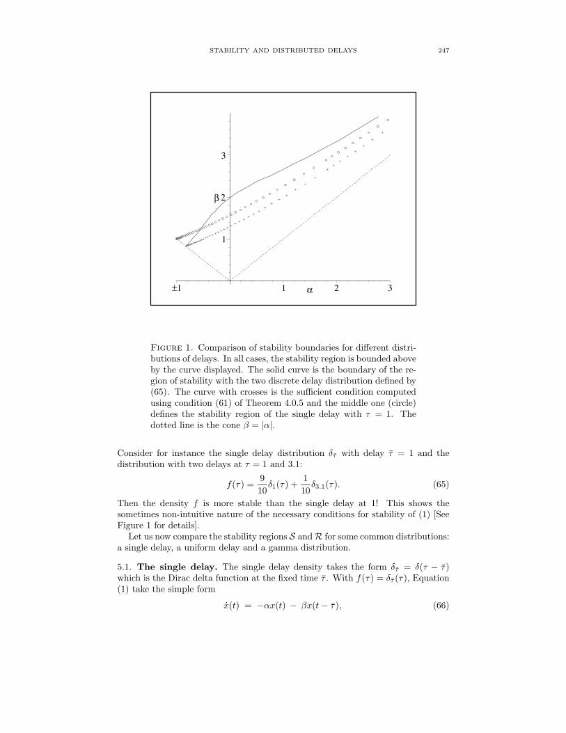
Figure 1. Comparison of stability boundaries for different distri-butions of delays. In all cases, the stability region is bounded aboveby the curve displayed. The solid curve is the boundary of the re-gion of stability with the two discrete delay distribution defined by(65). The curve with crosses is the sufficient condition computedusing condition (61) of Theorem 4.0.5 and the middle one (circle)defines the stability region of the single delay with τ = 1. Thedotted line is the cone β = |α|.

Consider for instance the single delay distribution δτ with delay τ = 1 and thedistribution with two delays at τ = 1 and 3.1:

f(τ) =910δ1(τ) +

110δ3.1(τ). (65)

Then the density f is more stable than the single delay at 1! This shows thesometimes non-intuitive nature of the necessary conditions for stability of (1) [SeeFigure 1 for details].Let us now compare the stability regions S andR for some common distributions:

a single delay, a uniform delay and a gamma distribution.

5.1. The single delay. The single delay density takes the form δτ = δ(τ − τ)which is the Dirac delta function at the fixed time τ . With f(τ) = δτ (τ), Equation(1) take the simple form

x(t) = −αx(t) − βx(t− τ), (66)

248 SAMUEL BERNARD, AND JACQUES BELAIR AND MICHAEL C. MACKEY

1

2

3

4

5

6

β

1 2 3 4 5 6α

Figure 2. Upper bound (solid line) of the region of stability forEquation (66). Here S = R and the delay τ = 2. Note that theboundary is asymptotic to the line β = α (dashed line).

and the characteristic equation is

s+ α+ βe−sτ = 0. (67)

This density is symmetric and by Theorem (4.0.5), we know that Equation (66) isstable if

τ <arccos

(−αβ

)√β2 − α2

.

In this case, this condition is also necessary . Figure 2 shows the region of stability,plotted with the method outlined in Section 3.1.

5.2. Uniform density. When the delay is uniformly distributed, the density canbe written

f(τ) =

0 0 ≤ τ < τm1/δ τm ≤ τ ≤ τm + δ0 τm + δ < τ

(68)

The expectation is E = τm + δ/2. We can apply Theorem 4.0.5, since f issymmetric, to obtain Figure 3 when τm = 2 and δ = 2.

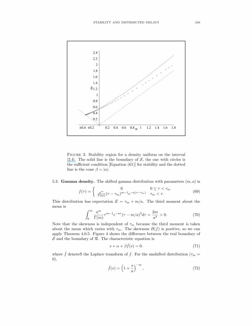
STABILITY AND DISTRIBUTED DELAYS 249

0.2

0.4

0.6

0.8

1

1.2

1.4

1.6

1.8

2

2.2

2.4

β

±0.4 ±0.2 0.2 0.4 0.6 0.8 1 1.2 1.4 1.6 1.8α

Figure 3. Stability region for a density uniform on the interval[2,4]. The solid line is the boundary of S, the one with circles isthe sufficient condition [Equation (61)] for stability and the dottedline is the cone β = |α|.

5.3. Gamma density. The shifted gamma distribution with parameters (m,a) is

f(τ) ={

0 0 ≤ τ < τmam

Γ(m) (τ − τm)m−1e−a(τ−τm) τm < τ.(69)

This distribution has expectation E = τm + m/a. The third moment about themean is ∫ ∞

0

am

Γ(m)τm−1e−aτ (τ −m/a)3dτ =

2ma3

> 0. (70)

Note that the skewness is independent of τm because the third moment is takenabout the mean which varies with τm. The skewness B(f) is positive, so we canapply Theorem 4.0.5. Figure 4 shows the difference between the real boundary ofS and the boundary of R. The characteristic equation is

s+ α+ βf(s) = 0. (71)

where f denoteS the Laplace transform of f . For the unshifted distribution (τm =0),

f(s) =(1 +

s

a

)−m

, (72)

250 SAMUEL BERNARD, AND JACQUES BELAIR AND MICHAEL C. MACKEY

0.20.40.60.8

11.21.41.61.8

22.22.42.62.8

33.23.43.63.8

β

±0.2 0.2 0.4 0.6 0.8 1 1.2 1.4 1.6 1.8 2 2.2 2.4α

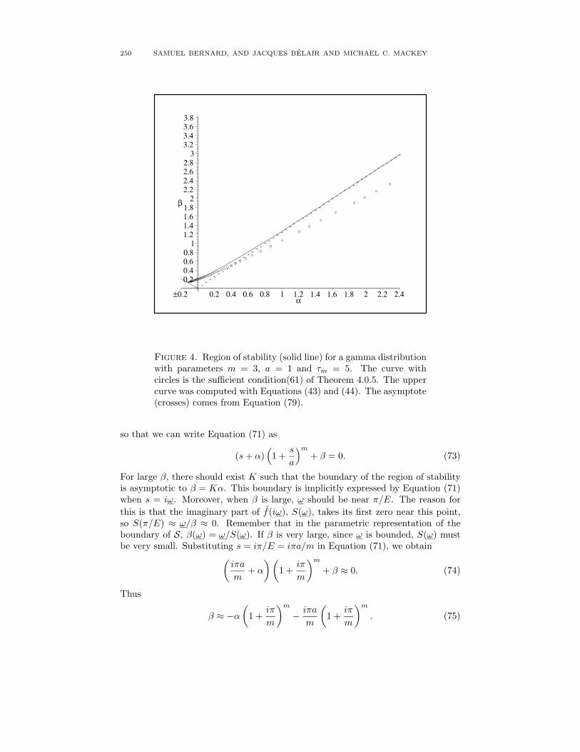
Figure 4. Region of stability (solid line) for a gamma distributionwith parameters m = 3, a = 1 and τm = 5. The curve withcircles is the sufficient condition(61) of Theorem 4.0.5. The uppercurve was computed with Equations (43) and (44). The asymptote(crosses) comes from Equation (79).

so that we can write Equation (71) as

(s+ α)(1 +

s

a

)m

+ β = 0. (73)

For large β, there should exist K such that the boundary of the region of stabilityis asymptotic to β = Kα. This boundary is implicitly expressed by Equation (71)when s = iω. Moreover, when β is large, ω should be near π/E. The reason forthis is that the imaginary part of f(iω), S(ω), takes its first zero near this point,so S(π/E) ≈ ω/β ≈ 0. Remember that in the parametric representation of theboundary of S, β(ω) = ω/S(ω). If β is very large, since ω is bounded, S(ω) mustbe very small. Substituting s = iπ/E = iπa/m in Equation (71), we obtain(

iπa

m+ α

) (1 +

iπ

m

)m

+ β ≈ 0. (74)

Thus

β ≈ −α(1 +

iπ

m

)m

− iπa

m

(1 +

iπ

m

)m

. (75)

STABILITY AND DISTRIBUTED DELAYS 251

When α is large enough, the second term in Equation (75) is negligible and β isasymptotic to

α

∣∣∣∣1 + iπ

m

∣∣∣∣m

. (76)

This term only depends on m. If m increases to infinity, for fixed E, f convergesweakly to a Dirac delta function. In this case the asymptote is β = α and we seethat (

1 +iπ

m

)m

→ eiπ = −1 (77)

as m → ∞, which is consistent with the case of the single delay with density givenby the Dirac delta function. Thus, for large β and large m, we obtain an informalcondition for the stability for the unshifted gamma density:

β ≤ Kα =∣∣∣∣1 + iπ

m

∣∣∣∣m

α. (78)

For the shifted gamma density, we must evaluate S(ω) at π/E = π/(τm +m/a).This leads to the condition

β ≤ Kα =∣∣∣∣1 + iπ

aτm +m

∣∣∣∣m

α. (79)

In our example (Figure 4), m = 3, a = 1 and τm = 5 so K = 1.24.

6. Neutrophil Dynamics. As mentioned in the Introduction, in some diseasesa normally approximately constant physiological variable changes its qualitativedynamics and displays an oscillatory nature. This is the case of cyclical neutropenia(CN) in which there is a periodic fall in the neutrophil count from approximatelynormal to virtually zero and then back up again [9, 10, 11]. Haurie et al. [10]developed a model for the peripheral regulation of neutrophil production. Theirresults and other evidence strongly suggest that the origin of the oscillatory behaviorin CN is not due to an instability in the peripheral neutrophil regulatory system.Rather, the oscillations are probably due to a pathological low level oscillatorystem cell input to the neutrophil regulatory system, caused by a destabilizationof the hematopoietic stem cell compartment [18, 19]. Haurie et al. analyzed thedata from nine grey collies and found different dynamics between dogs. When theamplitude of the oscillation of the neutrophil is low, the oscillation is approximatelysinusoidal. However, when the amplitude increases, a small “bump” appears on thefalling phase of the oscillation which increases the neutrophil count before the countfalls to zero. Many models of neutrophil production incorporate a negative feedbackwith delay. However, in a recent modeling study Hearn et al. [13] have shown thatthis feedback alone cannot lead to the oscillations seen in CN. The principal sourceof oscillation of the neutrophil count comes from the oscillation of the stem cellinput which is exterior to the neutrophil regulatory system.A regulatory model for neutrophil dynamics with delayed negative feedback can

be written as

x(t) = −αx(t) +Mo(x(t)) (80)

where

x(t) =∫ ∞

τm

x(t− τ)f(τ)dτ . (81)

252 SAMUEL BERNARD, AND JACQUES BELAIR AND MICHAEL C. MACKEY

The function Mo(x(t)) is the feedback control and is a decreasing function. Theconstant α is the rate of elimination of neutrophil and f is the distribution ofmaturation delay. This model, proposed by Haurie et al in [10], can be expressedin linearized form as

z(t) = −αz(t) + εI(ω)eiωtMo∗ +M′o∗[1 + εI(ω)eiωt]z(t). (82)

The distribution f is taken to be the shifted gamma defined in Equation (31) sinceit offers an excellent fit to the data [13]. The term εI(ω)eiωt accounts for theoscillation of the stem cell input. The constant Mo∗ is the granulocyte turnoverrate defined by

αx∗ =Mo(x∗) ≡ Mo∗. (83)

where x∗ is the unique stable steady state of Equation (80). The other parametersare the period of oscillation of the stem cell input 2π/ω, ε which is assumed to be1 and M′

o∗, the slope of the feedback function at the steady state x∗. The termI(ω) depends on a and m:

I(ω) =(

a

iω + a

)m+1

e−iωτm . (84)

The value of a is 14.52, m is 8.86 and ω is around 0.45. The maximum value of theoscillation factor ε�I(ω) is nearly one, so

max∣∣M′

o∗[1 + εI(ω)eiωt]∣∣ ≈ 2 |M′

o∗| . (85)

Now if we look at the autonomous part of Equation (82), we get

z(t) = −αz(t) +M′o∗[1 + εI(ω)eiωt]z(t). (86)

When the amplitude of the stem cell input reaches its maximum, we can approxi-mate Equation (86) using Equation (85) by

z(t) = −αz(t) + 2M′o∗z(t). (87)

Since we suppose thatMo(z(t)) is a decreasing function, we know thatM′o∗ is non-

positive. We can therefore apply Theorem 4.0.5 to study the stability of Equation(87). If 2M′

o∗ ≤ α, Equation (87) is always stable. In this case, oscillation in theneutrophil count is due only to the oscillation of the stem cell input in the neutrophilregulatory system and the behavior of the neutrophil count is sinusoidal.However, in some cases, even if M′

o∗ ≤ α, we may have that 2M′o∗ ≥ α. Then

to study the stability, we can use condition (61) which gives

E <arccos(α(2M′

o∗)−1)√

(2M′o∗)2 − α2

. (88)

The decay rate α is between 2.18 and 2.48 (days−1), and the expected delay E isbetween 3.21 and 3.42 days. From data fitting [10], we obtain M′

o∗ ranging from-0.05 to -2.20. Taking α = 2.4, we see that |M′

o∗| ≥ 1.20 can destabilize Equation(87). From Table 4 of Haurie et al. (reproduced in Table 1) the smallest slope|M′

o∗| greater than 1.20 is 1.50. WithM′o∗ = −1.50, a sufficient condition to have

stability is

E <arccos(−0.80)√

3.24= 1.39.

However, since E is far greater than 1.39 (at least 3.21), we expect that Equation(87) will not be stable for values of |M′

o∗| ≥ 1.50. This implies that Equation (82)

STABILITY AND DISTRIBUTED DELAYS 253

Dog M′o∗ M′

o∗ fit ω Tins

127 -0.20 -0.10 0.465 0113 -0.91 -0.05 0.470 0128 -1.09 -2.00 0.464 5.39118 -0.48 -0.50 0.500 0126 -1.00 -1.80 0.463 4.70101 -1.24 -1.50 0.426 3.27125 -1.15 -2.20 0.421 6.55117 -1.05 -1.70 0.438 4.49100 -1.20 -1.80 0.418 5.20

Table 1. Data for nine grey collies. The computations for Tins

were made usingM′o∗ fit. Note that withM′

o∗, only Dog 101 has aslope high enough to destabilize the peripheral regulatory system.This suggests that the fitted values are close to the real ones. Theunits ofM′

o∗,M′o∗ fit and ω are days

−1 and Tins is in days. FromHaurie et al. [10].

will be destabilized when the amplitude of the stem cell input reaches a thresholdwhich depend on M′

o∗. From Table 1, we can estimate the interval of time duringwhich Equation (87) will be destabilized. The expected delay E must satisfy

E�arccos[α{M′o∗(1 + �(εI(ω)))}−1]

[{1 + ε�(I(ω))}2M′o∗2 − α2]

1/2. (89)

At worst this condition becomes

E�π[{1 + ε�(I(ω))}2M′o∗2 − α2]−1/2. (90)

We can approximate �(I(ω)) with Equation (84) by�(I(ω)) 0.96 cos[ω(t− τm)]. (91)

Equation (90) becomes, with α = 2.4,

cos[ω(t− τm)]� 2.71|M′

o∗|− 1.04. (92)

Given that the density of the maturation delays is concentrated around its expec-tation (the variance is 0.042), we can replace in our approximation the symbol �by the usual >. Solving for t gives that t must lie in an interval of length

Tins ≡ 2ωarccos

(2.71|M′

o∗|− 1.04

)(93)

The value of Tins for each dog is given in Table 1. We find that the peripheralneutrophil regulatory system is destabilized during an average of 4.93 days eachperiod of stem cell input which is of length between 12.6 and 15 days. The effectof this is the small bump seen after the spikes of the neutrophil count.

254 SAMUEL BERNARD, AND JACQUES BELAIR AND MICHAEL C. MACKEY

0 0.1 0.20

5

10

15

20

25

30

35

40

freq

pow

er

0 0.1 0.20

5

10

15

20

25

30

freq0 0.1 0.2

0

5

10

15

20

25

30

freq0 0.1 0.2

0

5

10

15

20

25

30

freq

0 500

5

10

15

20

days

126

0 500

5

10

15

20

days

101

0 0.1 0.20

5

10

15

20

25

30

freq0 0.1 0.2

0

5

10

15

20

25

30

freq

0 500

5

10

15

20125

0 0.1 0.20

5

10

15

20

25

30

freq

0 500

5

10

15

20

days

AN

C

127

0 500

5

10

15

20

days

113

0 500

5

10

15

20

days

128

0 500

5

10

15

20

days

118

0 500

5

10

15

20

days

100

0 0.1 0.20

5

10

15

20

25

30

freq

0 500

5

10

15

20117

0 0.1 0.20

5

10

15

20

25

30

freq

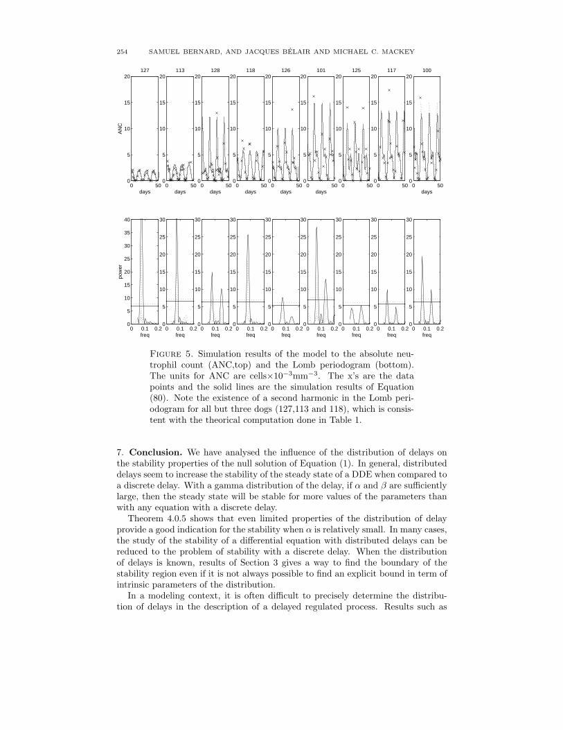
Figure 5. Simulation results of the model to the absolute neu-trophil count (ANC,top) and the Lomb periodogram (bottom).The units for ANC are cells×10−3mm−3. The x’s are the datapoints and the solid lines are the simulation results of Equation(80). Note the existence of a second harmonic in the Lomb peri-odogram for all but three dogs (127,113 and 118), which is consis-tent with the theorical computation done in Table 1.

7. Conclusion. We have analysed the influence of the distribution of delays onthe stability properties of the null solution of Equation (1). In general, distributeddelays seem to increase the stability of the steady state of a DDE when compared toa discrete delay. With a gamma distribution of the delay, if α and β are sufficientlylarge, then the steady state will be stable for more values of the parameters thanwith any equation with a discrete delay.Theorem 4.0.5 shows that even limited properties of the distribution of delay

provide a good indication for the stability when α is relatively small. In many cases,the study of the stability of a differential equation with distributed delays can bereduced to the problem of stability with a discrete delay. When the distributionof delays is known, results of Section 3 gives a way to find the boundary of thestability region even if it is not always possible to find an explicit bound in term ofintrinsic parameters of the distribution.In a modeling context, it is often difficult to precisely determine the distribu-

tion of delays in the description of a delayed regulated process. Results such as

STABILITY AND DISTRIBUTED DELAYS 255

those presented here thus have great interest since they provide general bounds onstability regions, irrespective of the particulars of these distributions.We end this paper with a conjecture which we have found to hold in all cases of

distributions of delays that we have studied. Proving it would be very useful andwould make the results of Section 4 obsolete. In words, it amounts to stating thatthe most destabilizing distribution of delays is a single Dirac δ function. If true,it could provide, by consideration of simplified models containing single discretedelays, uniform upper bounds on regions of stability in parameter space.

Conjecture 7.0.1. In the notation of Section 4, let f be a probability densitydefined on R+ with expectation E. Suppose that ω∗ is the first root of C(ω), then

β(ω∗) ≡ ω∗

S(ω∗)≥ π

2E. (94)

Acknowledgments. Support for this work has been provided by grants from theNatural Sciences and Engineering Research Council (Canada) [OGP-0008806 toJB and OGP-0036920 to MCM], MITACS (Canada) [JB,MCM], the Alexander vonHumboldt Stiftung [MCM] and Le Fonds pour la Formation de Chercheurs et l’Aidea la Recherche (Quebec) [98ER1057 to MCM,JB]. SB is supported by a studentshipfrom MITACS.

REFERENCES .

[1] Anderson R.F.V., Geometric and probabilistic stability criteria for delay systems,Mathematical Biosciences, 105 (1991), 81–96.

[2] , Intrinsic parameters and stability of differential-delay equations, J. ofMathematical analysis and applications, 163 (1992), 184–199.

[3] Boese F. G., The stability chart for the linearized Cushing equation with a dis-crete delay and with a gamma-distributed delay, Journal of Mathematical Analysisand Applications , 140 (1989), 510–536.

[4] El’sgol’ts, “Introduction to the theory of differential equations with deviating argument”,Holden-Day, 1966.

[5] Glass L. Mackey M.C., Pathological conditions resulting from instabilities in phys-iological control systems, Annals of the New York Academy of Sciences 316 (1979),214–235.

[6] , “ From Clocks to Chaos”, Princeton University Press, 1988.[7] Gopalsamy, “Stability and oscillations in delay differential equations of population dynamics”,

MIA, Kluwer Acad. Press, 1992.[8] J.K. Hale and S.M. Verduyn Lunel, “Introduction to functional differential equations”,

Springer-Verlag New York, 1993.[9] C. Haurie, D. C. Dale, and M. C. Mackey, Cyclical neutropenia and other periodic

hematological diseases: A review of mechanisms and mathematical models, Blood 92(1998), 2629–2640.

[10] C. Haurie, D.C. Dale, R. Rudnicki, and M.C. Mackey, Modeling complex neutrophildynamics in the grey collie, J. theor. Biol. (in press) (2000).

[11] C. Haurie, R. Person, D. C. Dale, and M.C. Mackey, Haematopoietic dynamics in greycollies, Exper. Hematol., 27 (1999), 1139–1148.

[12] Hayes N.D., Roots of the transcendental equation associated with a certain

difference-differential equation, J. Lond. Math. Soc., 25 (1950), 226–232.[13] T. Hearn, C. Haurie, and M.C. Mackey, Cyclical neutropenia and the peripheral con-

trol of white blood cell production, J. Theor. Biology, 192 (1998), 167–181.[14] an der Heiden U. Mackey M.C., The dynamics of production and destruction: Analytic

insight into complex behavior, J. Math. Biology, 16 (1982), 75–101.[15] , The dynamics of recurrent inhibition, J. Math. Biology, 19 (1984), 211–225.

256 SAMUEL BERNARD, AND JACQUES BELAIR AND MICHAEL C. MACKEY

[16] Kuang Y., “Delay differential equations with applications in population dynamics”, Math.Science Engineering, vol. 191, Academic Press, 1993.

[17] , Nonoccurence of stability switching in systems of differential equationswith distributed delays, Quaterly of Applied Mathematics, LII (1994), no. 3, 569–578.

[18] M. C. Mackey, A unified hypothesis for the origin of aplastic anemia and periodic

haematopoiesis, Blood , 51 (1978), 941–956.[19] , Mathematical models of hematopoietic cell replication and control, in

“The Art of Mathematical Modeling: Case Studies in Ecology, Physiology and Biofluids”(H.G. Othmer, F.R. Adler, M.A. Lewis, and J.C. Dallon, eds.), Prentice Hall, New York,1996, pp. 149–178.

Received November 2000; in revised January 2001.E-mail address: [email protected]