Optimizing BAO measurements with non-linear transformations of the Lyman-α forest

Prepared for submission to JCAP

Optimizing BAO measurements withnon-linear transformations of theLyman-α forest

Xinkang Wang,1,2 Andreu Font-Ribera2 and Uros Seljak1,2

1Department of Physics, University of California, Berkeley, United States2Lawrence Berkeley National Laboratory, Berkeley, United States

E-mail: [email protected], [email protected], [email protected]

Abstract. We explore the effect of applying a non-linear transformation to the Lyman-αforest transmitted flux F = e−τ and the ability of analytic models to predict the resultingclustering amplitude. Both the large-scale bias of the transformed field (signal) and theamplitude of small scale fluctuations (noise) can be arbitrarily modified, but we were unableto find a transformation that increases significantly the signal-to-noise ratio on large scalesusing Taylor expansion up to the third order. In particular, however, we achieve a 33%improvement in signal to noise for Gaussianized field in transverse direction. On the otherhand, we explore an analytic model for the large-scale biasing of the Lyα forest, and present anextension of this model to describe the biasing of the transformed fields. Using hydrodynamicsimulations we show that the model works best to describe the biasing with respect to velocitygradients, but is less successful in predicting the biasing with respect to large-scale densityfluctuations, especially for very nonlinear transformations.

Keywords: Large scale structure, Lyman-α forest, Baryon acoustic oscillations

arX

iv:1

412.

4727

v2 [

astr

o-ph

.CO

] 8

Apr

201

5

Contents

1 Introduction 1

2 Signal-noise ratio (S/N) in a BAO measurement 2

2.1 Signal: large scale biasing 3

2.2 Noise: 1D power spectrum 3

2.3 Numerical simulations 4

3 S/N of non-linear transformations 6

3.1 Gaussianized field 6

3.2 Generic analytic transformations 7

3.2.1 Results at second order 8

3.2.2 Results at third order 9

4 Analytic model for large-scale bias 10

4.1 Biasing of a generic transformation 11

4.2 Bias computation with Fluctuating Gunn-Peterson Approximation 11

4.3 Testing the model with simulations 12

5 Conclusions 14

A Bias fitting procedures 15

B Large-scale bias for z=2.4 and 2.75 16

1 Introduction

One of the main drivers of current cosmological observations is the study of the acceleratedexpansion of the Universe [1]. One particular probe of the acceleration has recently provenvery successful: the measurement of the Baryon Acoustic Oscillation (BAO) scale in theclustering of galaxies, which can be used as a cosmic ruler to study the geometry of theUniverse at different redshifts [2]. Even though the first measurements of the BAO scale werepresented in the context of galaxy clustering at low redshift [3–6], in theory any tracer of thelarge-scale distribution of matter could be used to measure BAO. At high redshift (z > 2),for instance, the BAO scale was recently measured in the clustering of the absorption featuresin distant quasar spectra [7–10], a technique known as the Lyman-α forest, or Lyα forest.

As light emitted from distant quasars travels through an expanding Universe, it is grad-ually redshifted towards longer wavelengths. Photons that have escaped from the quasarswith energy above the Lyα transition energy might be absorbed by neutral hydrogen atpositions where the redshifted wavelength of the photons equals that of the Lyα transitionenergy. Hence, photons emitted with different energies from a quasar will have to travelthrough different distances to be absorbed (when they reach the Lyα transition wavelength),and as a consequence the fraction of transmitted flux for a given photon wavelength is afunction of the neutral hydrogen density, which in turn is a function of line-of-sight positionfrom the quasar [11, 12]. Although the distribution of neutral hydrogen on very small scales

– 1 –

(e.g., a few kpc) is determined by the thermal properties of intergalactic medium, on cos-mological scales it can be described as a tracer of the underlying density field, which wasconfirmed in the first studies of the clustering of the absorption features in high resolutionspectra from a handful of bright quasars [13–15]. Since then, Lyα forest has become an in-creasingly important tool to study the large-scale structure of the Universe, and up to now itis considered one of the most promising methods to study the clustering on both the smallestscales (via the correlated absorption along a single line of sight) and on the largest scales(via the correlations in neighboring lines of sight).

An interesting question that we will address in this paper is whether the informationextracted from a Lyα forest survey can be increased by a nonlinear transformation of theobserved field. Similar approaches have been suggested in the context of weak lensing andgalaxy clustering [16–19]. In [20], it was suggested that one could increase the signal-to-noiseratio of a measurement by applying proper non-linear transformation to the Lyα transmittedflux fraction (i.e., F → g(F )). In this paper, in particular, we study whether such transfor-mations could improve the BAO measurement from the Lyα forest. We will also comparethe analytic predictions of Lyα forest bias in [20] (for both the flux field and the transformedfields) to simulations.

Specifically, the performance of a Lyα forest BAO survey can be quantified by the errorbars in the measurements of the BAO scale along and across the line of sight, respectively, aswell as their correlation coefficient. In order to optimize this measurement, we would like tohave realistic simulations of a hypothetical survey and directly study the effect of differenttransformations on the error bars of the measured BAO scales. Unfortunately, this is beyondthe reach of current computational facilities. Hydrodynamic simulations are thus required inorder to accurately reproduce the statistics of the Lyα forest. However, these simulations arenot able to simulate boxes large enough to cover a full BAO survey. On the other hand, inorder to test the analysis pipeline and study the effect of potential systematics, current BAOanalyses using the Lyα forest rely on simplified mocks [21, 22]. Despite the fact that thesemocks have the correct 1- and 2-point correlation functions, their higher order statistics aregenerally not correct, and thus would not be useful for our study.

As a forecast, in section 2 we will show that under several assumptions the effect ofa non-linear transformation F → g(F ) boils down to a single quantity: the ratio of large-scale biasing of the transformed field (squared) over the one-dimensional power spectrumof the field in large-scale limit, both of which can be measured with current hydrodynamicsimulations, allowing us to study the effect of non-linear transformations on the Lyα forestin the context BAO measurements. We present the results of this study in section 3. Inaddition, in order to better understand the effect of the transformations, in section 4 weextend the bias model of [20] to describe the bias of non-linear analytic transformations. Weconclude our results in section 5.

2 Signal-noise ratio (S/N) in a BAO measurement

The main goal of a BAO survey is to provide a measurement of the BAO scale at a givenredshfit, as precise as possible. In order to predict the performance of a BAO survey, as aresult, we would like to generate simulations of the survey, measure its power spectrum, fitthe BAO scale on this measurement and look at its precision. We would like the simulationto be as realistic as possible, and we would like the analysis to be similar to that used withthe real data.

– 2 –

In order to simulate accurately the Lyα, however, we need to use expensive hydrody-namic simulations with a really high spatial resolution [23]. This sets the maximum volumethat one can simulate to roughly 1003 h−3Mpc3, clearly insufficient to measure the BAOscale. Fortunately, there are several approximations that we can use to make the problemmore treatable. Specifically, if the detection of the BAO scale is statistically very significant,the variance of the BAO measurement will scale proportionally to the covariance matrix ofour power spectrum measurement, relative to the signal level (the power spectrum itself).Moreover, assuming that linear theory holds on the relevant scales, the different bins in thepower spectrum can be treated as independent, resulting in a diagonal covariance matrix.

We can therefore quantify the precision of a given survey with a signal-to-noise functionS/N(k), defined as the ratio of the power spectrum (signal) and its uncertainty (noise).In this section, we will present further approximations that will allow us to compress theinformation of this function into a single number.

2.1 Signal: large scale biasing

The BAO information in a Lyα forest survey is contained in Fourier modes with rather smallwave numbers k < 0.3 hMpc−1, where we expect the power spectrum PF (k) to follow asimple linear bias model:

PF (k) = b2F (µ) Pm(k) , (2.1)

where Pm(k) is the matter power spectrum, µ = k · z with z being the line-of-sight direc-tion, and bF (µ) describes the large-scale biasing of the Lyα forest including redshift spacedistortions. The angular dependence of the biasing follows the usual Kaiser formula [24]:

bF (µ) = bδF + (fµ2)bηF , (2.2)

where f is the logarithmic growth rate. In particular, this growth rate is close to one in aΛCDM universe at the redshifts of interest (z > 2), where the universe is close to Einstein-deSitter, and will taken as unity from now on except stated otherwise. bδF and bηF are related tothe response of the transmitted flux fraction F to small variations of the density and of theline-of-sight velocity gradient, respectively. In section 4 we will present an analytic model topredict their values, but for now we can think of these as free parameters.

An analytic non-linear transformation of flux F is an analytic function g(F ). Assuminglinear theory holds in the relevant scales, the power spectrum of this transformed field, Pg(k),can be described using the same equations 2.1 and 2.2 with (bδF , b

ηF ) replaced by a different

set of bias parameters: (bδg, bηg). Therefore, the impact of the transformation on the BAO

signal can be described by the ratio of the bias parameters squared: b2g(µ)/b2F (µ).Note that most studies of the large-scale clustering of the Lyα forest focus on the

statistics of the fluctuations around the mean transmitted flux fraction, i.e., δF = F/ 〈F 〉−1.The transformed field, however, might have an arbitrarily small mean, and for simplicity wechoose to focus on the clustering of the F and g(F ) fields themselves.

2.2 Noise: 1D power spectrum

The error bars in the BAO measurements are set by the uncertainty with which we areable to measure the clustering on the Fourier modes relevant for BAO. Following [25], theuncertainty on a given Fourier mode is proportional to

σ2PF

(k) = 2(PF (k) + P effN +A P 1D

F (k‖)/n2Dq

)2. (2.3)

– 3 –

There are three contributions to the noise: i) the first term, PF (k), is set by the signal

and is usually referred as cosmic variance; ii) the second term, P effN , is set by the level ofinstrumental noise in the spectra, and is usually referred as noise power ; iii) the last term,A P 1D

F (k‖)/n2Dq , takes account of the fact that we can only sample the universe in a set of

thin lines of sight, and is thus set both by the level of intrinsic fluctuations (or 1D powerP 1D(k‖)) on a scale ∼ k‖ = kµ and by the 2D density of background sources n2D

q1. This

last term is usually referred as aliasing noise and is equivalent to the shot noise in galaxyclustering studies. Now, as noted in [26], P 1D

F (k‖) is approximately flat on scales relevant forBAO analyses. Since the noise power is also flat (white noise), the last two terms in eq.2.3can thus be described by a single term P 1D

F (k0)/neff , where P 1DF (k0) describes the typical

level of P 1DF (k‖) in the flat regime (i.e., k0 large enough) and neff is an effective density of

lines of sight that takes into account the distribution of noise power in the spectra.

In present and near-future Lyα forest BAO surveys, the contribution from cosmic vari-ance is rather small, and we will ignore it in this study. The other two contributions arecomparable, but for simplicity in this study we will only consider the aliasing term. Andsince the instrumental noise is very close to Gaussian, any non-linear transformation ap-plied to the observed flux field will make the noise properties non-Gaussian. By ignoringthe noise in our analysis, we are simplifying the problem, and our results should be read asthe most optimistic case in the limit of low noise. We will thus characterize the effect of thenon-linear transformation on the BAO uncertainties with the ratio of the amplitudes of theone-dimensional power in small k‖ limit: P 1D

g (k0)/P 1DF (k0).

After all, for any non-linear transformation F → g(F ), we expect the following propor-tionality holds on large scales:

S/N(k) ∝ Rg(µ) = b2g(µ)/P 1Dg (k0). (2.4)

The right-hand side of this equation may serve as a proxy for S/N and is a measurablequantity in simulations. We will focus on the value of Rg in the rest of the paper.

2.3 Numerical simulations

In next section we will study the effect of analytic non-linear transformations g(F ) on thesignal-to-noise ratio (S/N) with which we can measure BAO. To do that we will use hydro-dynamic simulations to measure the large-scale biasing (squared) of the transformed field,b2g(µ) (proxy for signal), and to measure the 1D power spectrum of the transformed in low-k

limit, P 1Dg (k0) (proxy for noise).

The simulation we use is one of the Gadget-3 simulations adopted in the Nyx/Gadget-3comparison project [27], with a box size of 40h−1Mpc and a total of 2× 10243 particles. Thesimulation used a WMAP7 cosmology (Ωb = 0.046, Ωm = 0.0275, ΩΛ = 0.725, h = 0.702,σ8 = 0.816, and ns = 0.96) and the ionizing background prescription of [28]; it also usedthe QUICKLYA option in Gadget to implement a simple star formation recipe. We haverescaled the optical depth in the box in order to have a mean flux of 〈F 〉 = 0.8413 (at z = 2),in agreement with estimates from SDSS [29]. In the main part of this paper we use onlythe simulation output at z = 2, but in appendix B we also present results using outputs atredshift z = 2.4 and z = 2.75.

1The constant A depends on the distribution of weights in the different spectra, but for a given survey thiscan be treated as a constant

– 4 –

0.03

0.3

3

30

0 0.1 0.2 0.3 0.4 0.5 0.6 0.7 0.8 0.9 1 1.1 1.2

Flu

x P

ow

er S

pec

trum

(M

pc/

h)3

k (h Mpc-1)

Measurement Prediction

Figure 1. The plotted scales are k = 0.2, 0.6, 1.0h Mpc−1, each of which has four µ bins. For clarity,at each k the power spectrum with µ = 0.125 is plotted at (k−0.04), µ = 0.375 is plotted at (k−0.02),µ = 0.625 at k, and µ = 0.875 at (k + 0.02).

0

0.02

0.04

0.06

0.08

0.1

0.12

0.14

0.16

0.18

0.2

0 0.2 0.4 0.6 0.8 1 1.2 1.4

P1

D (M

pc/

h)3

k (h Mpc-1)

g1 g2 g3

Figure 2. 1D power spectrum measured in simulations for the original field g1(F ) = F (black line),and the two other fields discussed in the next section. We use the 1D power in the fundamental modeof the simulation (k0 = 0.157 hMpc−1) as a proxy for the noise in a BAO measurement.

We now show that the proxies for signal and noise we chose in previous two subsections(i.e., eq.(2.4)) are valid, respectively. In figure 1, we show (in black) the 3D power spectrumof the transmitted flux fraction F , measured at three different scales k = 0.2, 0.6, 1.0 hMpc−1,and at four different line-of-sight directions (µ = 0.125, 0.375, 0.625, 0.875). The red pointsshow the prediction using eq.2.1 for the values of (bδF = −0.0733, bηF = −0.0995) that bestfit the simulations (see appendix A for a description of how we fit the bias parameters insimulations). The figure clearly shows the validity of squared bias as the proxy for signal.On the other hand, it is important to remind the reader that throughout this paper, we willnot follow the common convention of measuring statistics of fields that have been normalized(i.e., divided by its mean). Therefore, if one wishes to compare the flux biases reported inthis paper, one would have to divide them by the mean flux in the simulation: 〈F 〉 = 0.8413.

– 5 –

In figure 2 we show the measured 1D power spectrum of the transmitted flux fractiong1(F ) = F , and two of the transformed fields discussed in next section: g2(F ) = −0.261F+F 2

and g3(F ) = 1.084F − 3.039F 2 +F 3. In the figure it is clear that P 1Dg (k) is close to constant

at scales relevant in BAO analyses (k < 0.3 hMpc−1). We will use the 1D power at thefundamental mode, k0 = 0.1571 hMpc−1, as a proxy for the noise in a BAO measurement.

3 S/N of non-linear transformations

In the previous section we have shown that under several assumptions, the performance ofa BAO survey can be quantified using the ratio of the large-scale bias (squared) over thelow k limit of the one dimensional power spectrum. We also presented the measurement ofthese quantities in the original Lyα absorption field using hydrodynamic simulations. In thissection, we will use the same simulations to measure the equivalent quantities in differentfields which are obtained by performing non-linear transformations to the original field.

3.1 Gaussianized field

A Gaussian field can be fully described by its 2-point correlation function. The Lyα forestflux field, on the other hand, is highly non-Gaussian, implying that in order to obtain all ofits cosmological information we would need to use higher order statistics. Therefore, it istempting to transform the flux field to make it as Gaussian as possible [13, 30]. For instance,we can assume a monotonic relation between our flux field F and a Gaussianized field g(F ),which is implicitly defined via∫ g(F )

−∞dg′pg(g

′) =

∫ F

0dF ′pF (F ′) , (3.1)

where pg(g) and pF (F ) are the probability distribution function (PDF) of each field. Aftermeasuring the PDF of flux in simulations, pF (F ) (shown in figure 6), we are able to determinethe monotonic function g(F ) and transform the flux into a Gaussianized field, with zero meanand unit variance. In figure 3 we show the transformation measured at different redshifts.We apply such transformation to the flux field in simulation and measure the S/N (i.e., Rg(µ)in eq.(2.4)) of the resulting Gaussianized field.

We measure the one-dimensional power of the Gaussianized field, P 1Dg (k0), to be 19.20±

0.05 times higher than that of the original field F . On the other hand, the bias parameters ofthe Gaussianized field are also larger, by a factor of 5.06±0.32 for bδg and a factor of 2.70±0.41for bηg . Interestingly, this result implies a very anisotropic gain in signal-to-noise ratio: whilethe S/N transverse to the line of sight (µ = 0) is measured a factor of 1.33± 0.17 larger, theS/N along the line of sight (µ = 1) is measured a factor of 0.71± 0.08 smaller. In addition,in large scale structure analyses it is common to define a redshift space distortion parameterβ = fbη/bδ. In our simulations we measure it to be roughly βF = 1.30 for the original fluxfield F . The Gaussianized field g(F ) described above, however, has weaker redshift spacedistortions with only βg = 0.69, where we have used growth rate f = 0.96.

Finally, since standard Lyα forest BAO measurements preferentially measure the line-of-sight scale [7, 9, 10], with very large uncertainties in the transverse direction, the fact thatthe measurement in the transformed Gaussianized field favors the transverse direction mightbe of special interest.

– 6 –

-3

-2

-1

0

1

2

3

4

5

0 0.1 0.2 0.3 0.4 0.5 0.6 0.7 0.8 0.9 1

Gau

ssia

n g

(F)

Flux F

z=2 z=2.4 z=2.75

Figure 3. Monotonical relation g(F ) to convert the simulated flux field into a Gaussianized fieldwith zero mean and unit variance. The different lines correspond to z = 2 (blue), z = 2.4 (red) andz = 2.75 (green). The dashed line (black) is the “zero” reference line.

3.2 Generic analytic transformations

The ultimate goal of this paper is to find an analytic non-linear transformation that max-imally enhances S/N with respect to that of the orignal flux field. To achieve this goal,we need to consider the entire set of generic analytic transformations g(F ) which can beexpressed as an infinite Maclaurin series:

g(F ) =∞∑m=1

am Fm , am =g(m)(0)

m!. (3.2)

In practice, however, we will study only the transformations involving terms up to Fn (an 6=0), and refer to these as transformations of order n. Notice that we have ingored the zerothorder in the series, of which the specific value has no effect on the following study.

We can think of Fm as another tracer of the density field, with bias parameters bFm(µ) =bδFm + (fµ2)bηFm . In linear regime, the large-scale cross-correlation of two tracers is justproportional to the product of their bias parameters, and therefore the cross-power spectrumcan be expressed as the geometric mean of their power spectra. This allows us to define thebiasing of the transformed field g(F ):

bg(µ) =n∑

m=1

am bFm(µ) =n∑

m=1

am(bδFm + (fµ2)bηFm) = bδg + (fµ2)bηg . (3.3)

On the other hand, for the noise, the one-dimensional power spectrum P 1D(k‖) is relatedto the three-dimensional power spectrum P (k‖,k⊥) by an integral over k⊥. Even in the limitof small k‖, the 1D power is affected by high k⊥ modes that are not well described by lineartheory. This implies that the 1D power is not directly proportional to the bias parameters,and that the 1D cross-power of two fields P 1D

(Fm,F i)can not described by the geometric mean

of their 1D powers. Therefore, if we are interested in studying generic transformations upto a certain order n, we have to measure not only all the 1D power spectra P 1D

F j(k0) where

– 7 –

j ≤ n, but also all the 1D cross-power spectra P 1D(F j ,Fk)

(k0):

P 1Dg (k0) =

n∑m=2

m−1∑i=1

ai am−i P1D(F i,Fm−i)(k0), (3.4)

where P 1D(F i,Fm−i) = P 1D

F iif i = m− i. Notice that k0 is the fundamental mode.

To compute S/N for g(F ) of order n, we can compute in simulations the relevant biasesbFm (for m ≤ n) and 1D auto- and cross-power spectra P 1D

(Fm,F i)(k0). Moreover, multiplying

the field by a constant would have no effect on the signal-to-noise ratio, since both quantitieswould be modified by the same multiplicative factor. Therefore, we are only interested ing(F ) of the monic form: g(F ) = q1F + q2F

2 + · · ·+ qn−1Fn−1 + Fn, where qi = ai/an.

Even though the signal is anisotropic, we can compute an angularly average signal (thepower spectrum monopole), and use a single averaged bias parameter to quantify the signal:

b2g =

∫ 1

0dµ b2g(µ) = (bδg)

2 +2

3bδgb

ηg +

1

5(bηg)

2 . (3.5)

Finally, we have an averaged version of S/N for any nth order generic transformation:

Rg =b2g

P 1Dg (k0)

= f(q1, q2, ..., qn−1). (3.6)

The functional form f is to indicate there are only n − 1 variables we need to consider fornth order g(F ). Most importantly, at any given order, by maximizing Rg we can find thetransformation that should result in a larger gain in signal-to-noise ratio. We will comparethe results to the value of Rg for the original flux field: RF = 0.1109.

3.2.1 Results at second order

We consider an arbitrary quadratic field g(F ) = q1F + F 2, which only contains a single pa-rameter q1. Using the measured bias values (bδF , bηF , bδF 2 , bη

F 2), 1D power (P 1DF (k0), P 1D

F 2 (k0))and cross-power (P 1D

(F,F 2)(k0)), we can estimate the angularly averaged signal-to-noise ratio

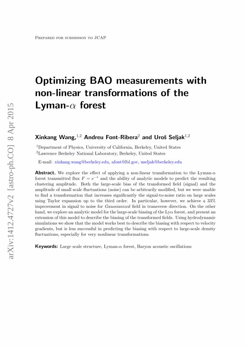
function, f(q1), and numerically/analytically find the global maximum of this function.The signal-to-noise ratio function f(q1) for a generic quadratic transformation is shown

in figure 4 (in black), in which two different angular configurations are also shown for com-parison: Rg(µ = 1) along the line of sight (in red), and Rg(µ = 0) across the transversedirection (in blue). As expected, for large absolute values of q1 we recover the signal-to-noiseratios of the original field F (dashed lines). We find that the angularly averaged function has

a global maximum at q(1)1 = −0.261, where Rg = f(q

(1)1 ) = 0.1147, and the global minimum

is at q(2)1 = −1.22, where the signal drops close to zero. The zero signal is due to the fact

that the signal scales as (q1bδF + bδF 2), and with bδF , b2F 2 fixed there is always a q1 at which

the signal vanishes. Similar argument applies to the higher order case shown in figure 5.In the previous section we saw that when the flux field is Gaussianized, the S/N gain

with respect to that of the original flux field varies anisotropically. Interestingly, this isnot the case for a generic quadratic transformation, since the three gains in figure 4 areremarkably similar. One may wonder why. The angular dependence of the signal is set bythe redshift space distortion parameter of the field, βg = fbηg/bδg. In our simulations we findthat βF 2 ∼ βF , and therefore any linear combination of these fields will have also a similarβg, which explains the weak angular dependence of the S/N gain.

– 8 –

0

0.03

0.06

0.09

0.12

0.15

0.18

0.21

0.24

0.27

0.3

-5 -4 -3 -2 -1 0 1 2 3 4 5

f (q

1)

q1

Quadratic Field (ave)

Quadratic (mu=0)

Quadratic (mu=1)

Linear Field (ave)

Linear Field (mu=0)

Linear Field (mu=1)

Figure 4. Signal-to-noise ratio for generic quadratic transformations g(F ) = q1F +F 2, as a functionof q1. The line-of-sight direction (µ = 1) is shown in red, the transverse direction (µ = 0) is shownin blue and the angular average (equation 3.6) is shown in black. For large absolute values of q1, werecover the signal-to-noise ratios of the original field F (dashed lines).

Finally, we note that even at the global maximum q(1)1 , the predicted signal-to-noise

ratio is only 3.40% larger than that of the original field. To test this prediction, we haveapplied the transformation g2(F ) = −0.261F + F 2 to the flux field in the simulations andhave measured the statistics of the transformed field. The measured signal-to-noise ratio is(3.56±8.74)% larger than the reference value, consistent with our prediction. The uncertaintyin the quoted ratio is set by the uncertainty in our measurement of the bias parameters.

3.2.2 Results at third order

We consider now generic cubic transformations g(F ) = q1F + q2F2 + F 3. After measuring

the bias parameters for F 3, its 1D power spectrum and its cross-power spectra with F andF 2, we can extend the previous study on quadratic fields to include transformations of ordern = 3.

In figure 5 we show the angularly averaged signal-to-noise ratio for generic cubic trans-formations. The global maximum corresponds to the transformation g3(F ) = 1.084F −3.039F 2 + F 3, where Rg is only 3.47% larger than that of the original F field. We havealso tested this in simulations, by applying the transformation g3(F ) to the flux field andmeasuring its statistics. The gain measured in simulations is (4.09± 8.79)%.

We have explored higher order transformations, but the results become numerically veryunstable, and we are not able to reproduce the predicted Rg in simulations. For instance, thenoise term for n = 4 involves a total of ten 1D auto- and cross-power spectra, each of whichhas an associated numerical uncertainty. We have also repeated the analyses at differentredshift outputs (z = 2.4 and z = 2.75), finding results qualitatively similar.

Finally, in table 1 we list several relevant quantities measured in the simulations forsome of the fields mentioned in this section, including the quadratic and the cubic trans-formations with higher angularly averaged signal-to-noise ratio, as well as the Gaussianizedfield. Note that we cannot exclude that there may be other transformations that give a betterimprovement than the ones we explored here: the fact that we do not approach the gains

– 9 –

Figure 5. Angularly averaged signal-to-noise ratio for generic cubic transformations, as a functionof q1 and q2.

g-field 〈g〉 bδg bηg βg P 1Dg (k0) Rg Rg(µ=0) Rg(µ=1)

F 0.8413 -0.0733 -0.0994 1.302 0.1101 0.1109 0.0487 0.2710

F 2 0.7703 -0.0902 -0.1194 1.271 0.1587 0.1145 0.0512 0.2769

F 3 0.7197 -0.0994 -0.1248 1.205 0.1861 0.1143 0.0531 0.2701

g2(F ) 0.5509 -0.0712 -0.0935 1.261 0.0980 0.1148 0.0517 0.2768

g3(F ) -0.7094 0.0957 0.1302 1.306 0.1809 0.1154 0.0507 0.2824

Gaussianized 0.0080 -0.3706 -0.2679 0.694 2.1132 0.1031 0.0650 0.1929

Table 1. Summary of values used in this section (measured directly from simulation). For each fieldg, we present its mean 〈g〉, its density bias bδg, velocity bias bηg , redshift space distortion parameter

βg, 1D power P 1Dg (k0) in low-k limit, angularly averaged signal-to-noise ratio Rg, transverse ratio

Rg(µ=0) and line-of-sight ratio Rg(µ=1). The simulation we use is not able to determine the correctsign of bias by itself, and therefore for consistency we set bias negative for g(F ) with positive mean〈g〉 and vice versa. In particular, to compute β we have used f = 0.96 for precision.

achieved by Gaussianized field for µ = 0 by the third order expansion suggests that it maybe possible to find other transformations that offer large gains, but the Taylor expansionapproach used here does not seem to find them at the order we are working.

4 Analytic model for large-scale bias

Paper [20] presents an analytic model to describe the biasing of the Lyα forest transmittedflux fraction F = e−τ , where the density bias bδF (response to large-scale overdensity) andthe velocity bias bηF (response to line-of-sight velocity gradient) are expressed as

bδF = 〈dFdδ〉+ ν2〈δ

dF

dδ〉 , bηF = 〈τ dF

dτ〉 , (4.1)

– 10 –

with ν2 = 34/21. A third term is present in the biasing model of [20] that is proportional tothe level of non-Gaussianities fNL in the primordial density fluctuations. In this study weassume that fNL = 0, and ignore this extra term.

The derivation in [20] ignores the shift in the overall scale caused by the long wavelengthoverdensity. For second order δ2 bias, this shift term comes as d ln[k3P (k)]/6d ln k [31], whichshould be compared to ν2 = 34/21. At the Lyα forest scale k ∼ 1h/Mpc k3P (k) has a slopeof approximately 0.6, and if we smooth Lyα forest with even smaller R (higher k) then it iseven smaller. The correction is 0.1 relative to 34/21, i.e. it is of order 6δ2 bias term. We willalso continue to ignore this correction here.

4.1 Biasing of a generic transformation

In section 3.2 we have studied the effect of applying a generic analytic transformation to theLyα forest transmitted flux fraction g(F ) =

∑∞m=1 amF

m. Because the derivation of eq.4.1in paper [20] can be applied to an arbitrary analytic function of δ, we can thus compute thebias parameters of the tranformed field by replacing F with g(F ) in eq.4.1:

bδg = 〈dg(F )

dδ〉+ ν2〈δ

dg(F )

dδ〉 , bηg = 〈τ dg(F )

dτ〉 . (4.2)

Furthermore, using the chain rule we can substitute the derivatives of g(F ) by the cor-responding derivatives of F multiplied by the derivative of the transformation itself (i.e.,dg(F )dF =

∑∞m=1mamF

m−1). The biasing of g(F ) can then be expressed as

bg(µ) = bδg+(fµ2)bηg = 〈(∞∑m=1

mamFm−1)(

dF

dδ+ν2δ

dF

dδ)〉+fµ2〈(

∞∑m=1

mamFm−1)τ

dF

dτ〉 . (4.3)

As pointed out in [20], the velocity bias bηF is completely determined by the probabilitydistribution function (PDF) of the field, pF (F ). This is also true for a generic transformation,where the velocity bias can be computed as:

bηg =∞∑m=1

mam〈Fm ln(F )〉 =∞∑m=1

mam

∫ 1

0dF pF (F ) Fm ln(F ) . (4.4)

The PDF can be computed both in the data and in hydrodynamic simulations, allowing fora test of the model presented in [20].

On the other hand, the computation of the density bias bδg requires the derivative of

the transmitted flux fraction with respect to the density field, dFdδ . In order to compute this

value we have to assume an analytic relation F (δ), which will strongly affect the predictedvalue. In the next subsection, we will present the predictions for bηg and bδg using a particularmodel of F (δ).

4.2 Bias computation with Fluctuating Gunn-Peterson Approximation

The Fluctuating Gunn-Peterson Approximation (FGPA) suggests that the optical depth ofLyα has a simple dependence on the local density of the IGM:

τ = A(1 + δ)α . (4.5)

Here, α = 2 − 0.7(γ − 1) = 2 − 0.7 d(lnρ)d(lnT ) , where ρ is the intergalactic gas density and T is

the temperature of the IGM, the amplitude A is proportional to T−0.7Γ−1 where Γ is the

– 11 –

ionization rate by cosmic UV backgroud [32, 33]. In particular, α typically ranges from 1.6to 2 [32]. The FGPA has been shown to be a good approximation at the relevant redshifts ofinterest for BAO measurements 2 . z . 3.5. However, a caveat : eq.4.1 was derived in paper[20] on the basis of Taylor expansion

τ(δ) =∞∑n=0

τ (n)(0)

n!δn, (4.6)

where the convergence radius is 1 in FGPA, which implies the application of FGPA in ourprediction is only valid for at most |δ| ≤ 1. For crude test, we do not restrict ourselvesto this domain of convergence in the following study, but we are aware that this domainrestriction of FGPA might be responsible for any discrepancy between the predictions andthe measurements in section 4.3.

Now, differiating F with respect to δ according to eq.4.5 and defining the auxiliaryfunction r(F ) = α ln(F )(ν2 + (1 − ν2)(− ln(F )

A )−1α ), we can express the density bias of a

generic transformation as

bδg =∞∑m=1

mam〈Fn r(F )〉 =∞∑m=1

mam

∫ 1

0dF pF (F ) Fm r(F ) . (4.7)

Finally, to compute eq.4.4 and eq.4.7, besides the PDF from data or from a simulationwe can also use the theoretically approximated PDF in which the density field δ follows alog-normal distribution:

1 + δ = e(δG−σ2

2) , pG(δG) =

1√2πσ2

e−δ2G2σ2 , (4.8)

where pG(δG) is the PDF of the auxiliary Gaussianized field δG.

4.3 Testing the model with simulations

In order to use the FPGA and the log-normal model for the density field, we need to choosea value for the parameters α,A, and σ. Using the hydrodynamic simulations presented insection 2.3, we fit these parameters by comparing the model predictions and the simulationmeasurements of three different statistics: flux PDF pF (F ), flux moments 〈Fn〉 and 〈FnlnF 〉.

In this section we will focus on the results at z = 2, but we study other redshift outputsin appendix B. The results are qualitatively similar, although in general we find the fits atlower redshift to be slightly better. In figure 6 we compare the flux PDF measured in thesimulation with that predicted by the best fit model: α = 1.22, A = 0.31 and σ = 1.72.Notice that the best fit value of α is smaller than the typical range of 1.6 < α < 2.

Even though the first moments 〈Fn〉 are quite well fitted, as shown in figure 7, it is clearfrom figure 6 that no combination of parameters is able to reproduce the measured PDF,especially at the high flux end. Qualitatively, we find the following trends: (1) increasing αmoves the moments 〈Fn〉 up and vice versa, but higher moments are more sensitive to thechange of α than lower moments with the first moment 〈F 〉 being almost immune to thechange of α; (2) increasing parameter A readily moves all the moments 〈Fn〉 down by similaramount, and vice versa; (3) changing σ has similar effect on the moments as changing α, butthe moments (especially the lower moments) are generally more sensitive to the change of σthan in α case.

– 12 –

0.1

1

10

0 0.1 0.2 0.3 0.4 0.5 0.6 0.7 0.8 0.9 1

dn/d

F

Flux F

Simulation (z=2) Model (z=2)

Figure 6. Comparison of the flux PDF measured in simulations with that predicted by the best fitparameters of the FGPA + log-normal model.

-0.2

-0.1

0

0.1

0.2

0.3

0.4

0.5

0.6

0.7

0.8

0.9

0 1 2 3 4 5 6 7 8 9 10 11

n

Simulation (z=2) Model (z=2)

<Fn>

<FnlnF>

Figure 7. Comparison of the first flux moments in simulations with those predicted by the best fitparameters of the FGPA (upper panel), and of the averages of 〈Fn ln(F )〉 relevant to the computationof velocity biases (lower panel).

As described above, in order to predict the value of the bias parameters we need touse a flux PDF. Since the best fit model does not reproduce very well the PDF measuredin simulations, we will present two predictions for the bias parameter: one using the modelPDF and one using the simulation PDF.

In figure 8 we show the predictions for the bias parameters of F, F 2, . . . , F 6, comparedto the values measured in simulations at z = 2, where the prediction using the model PDFis somewhat closer than the prediction using the measured PDF – however, as shown inappendix B, this is not the case in other redshifts. From the plots it is clear that while weare able to correctly predict the velocity bias for the first orders (bηF , b

ηF 2 , b

ηF 3), the model

fails to reproduce the measured density bias even for the original field bδF . In fact, it isnot surprising that the prediction for the density bias is worse than the prediction for thevelocity bias, since the former not only depends on the PDF but also in the assumed relationτ(δ). And as discussed in section 4.2 that the FGPA application is restricted by |δ| ≤ 1, this

– 13 –

-0.2

-0.1

0

0.1

0.2

0.3

0 1 2 3 4 5 6 7

bD

n

Simulation (z=2)

Model with Mod PDF (z=2)

Model with Sim PDF (z=2)

(a) Density bias bδFn .

-0.18

-0.16

-0.14

-0.12

-0.1

-0.08

-0.06

0 1 2 3 4 5 6 7

bV

n

Simulation (z=2)

Model with Mod PDF (z=2)

Model with Sim PDF (z=2)

(b) Velocity bias bηFn .

Figure 8. Comparison of predicted and measured biases at z = 2. The blue and the red data pointsin both panels correspond to the parameter best-fitting values presented in the main text.

-0.2

0

0.2

0.4

0.6

0.8

1

1.2

1.4

1.6

1.8

2

2.2

0 0.1 0.2 0.3 0.4 0.5 0.6 0.7 0.8 0.9 1

I

F

F F^3 F^5

Figure 9. Plots of integrands I = pF (F )Fnr(F ) in eq.(4.7) for density bias bδF , bδF 3 and bδF 5 , where

pF (F ) is the simulation flux PDF.

domain restriction may be responsible for the poor predictions of density bias.

The prediction of the density bias for the higher order fields Fn is particularly difficult,since it is completely dominated by the high F end of the PDF, where the model performspoorly. This is clearly seen in figure 9, where we show the integrand of equation 4.7 for threefields of interest: F , F 3 and F 5.

5 Conclusions

In the context of optimizing the measurement of the BAO scale in Lyα forest surveys, wehave presented a study of the effect of non-linear transformations of the transmitted fluxfraction F → g(F ) on the expected signal-to-noise ratio of the measurement.

On the large scales relevant in a BAO measurement, the signal is proportional to thesquare of the large-scale biasing of the field. The noise, on the other hand, has severalcontributions. In the limit of being dominated by aliasing noise (equivalent to shot-noise in

– 14 –

a galaxy survey), the noise is proportional to the amplitude of the one-dimensional powerspectrum at low-k limit. Under these assumptions, we study the signal-to-noise ratio fordifferent transformations using hydrodynamic simulations.

The first transformation that we have studied is a monotonic relation g(F ) so that thefinal field has a Gaussian PDF. We have shown that the Gaussianized field obtained withthis transformation would have a ≈ 33% larger signal-to-noise ratio in the transverse BAOmeasurement, but a ≈ 30% smaller ratio along the line of sight. The anisotropy of the gaincan be explained by a significantly lower value of the redshift space distortion parameter βin the Gaussianized field.

We have also studied the case of analytic transformations of the form g(F ) =∑n

m=1 amFm,

and presented results for generic quadratic (n=2) and cubic (n=3) transformations. In bothcases, the angularly averaged maximum gain in signal-to-noise that we measure is rathersmall (< 5%).

Finally, we have extended the biasing model presented in [20] to describe the biasing ofhigher order field Fn. We have shown that while the model is able to describe the velocitybias bη reasonably well for the first orders (n=1, 2, 3), the density bias bδ is difficult to predicteven for the original field F .

Our findings may be of use in attempts to optimize BAO signal to noise in realistic Lyαforest surveys. It is possible that one can use transformations such as Gaussianization tosignificantly improve the measurement of angular diameter distance DA. One could perhapsenvision that the measurement of H along the line of sight is done using flux field itself, whilemeasuring DA in the transverse direction would be done using Gaussianized field. For a morerealistic estimate of the actual gains one should include measurement noise and resolutionin the analysis, which was ignored here. These will depend on individual surveys and arebeyond the scope of this paper, but should be explored further in the future.

Acknowledgments

This work is supported partly by the 2013 Summer Undergraduate Research Fellowship Pro-gram (SURF) at the University of California, Berkeley, and by NASA ATP grant NNX12AG71G.We would like to thank Nishikanta Khandai for providing the hydrodynamic simulation, andAnze Slosar, Patrick McDonald and Martin White for useful discussions.

A Bias fitting procedures

The first step towards measuring the bias parameters of the Lyα transmission flux fractionF is to measure its 3D power spectrum. We measure band powers in a grid of 3 wavenumberbins limited by 0.0, 0.4, 0.8 and 1.2 hMpc−1, and in 4 bins in angular coordinate µ = k‖/k,limited by 0, 0.25, 0.5, 0.75 and 1, for a total of N = 12 bands.

We start by adding the norm of the relevant 3D Fourier modes (obtained with a FFT)within each of the N bands, and treat these values as our data vector (or Po). We then addthe prediction from our fiducial model (described below) for each of the modes in the bands,and treat these as the theoretical prediction (or Pt). We estimate the (diagonal) covarianceC of the data vector by adding 2Pt

2 for each mode within a band. We use these ingredientsto compute a maximum likelihood estimator of the band power, where the likelihood L is

– 15 –

proportional to:

L ∝ det (C)−1/2 exp

[−1

2(Po −Pt)

t C−1 (Po −Pt)

]. (A.1)

We are interested in measuring the scale-independent density bias bδ and the velocitybias bη parameters, which describe the clustering on linear scales. However, it is difficult tofit linear bias parameters in a box that is only 40 h−1Mpc wide, since there are very fewFourier modes that are in the linear regime. Therefore, we need to model the deviationsfrom linear theory in the simulations, and marginalize over the free parameters these. Basedin the description of large scale biasing of [34], we parameterize the deviations from lineartheory with the following analytic model:

PF (k, k‖) =

[bδ(k, k‖) + bη(k, k‖)f

k2‖

k2

]2

P (k) +N(k, k‖), (A.2)

with

bδ(k, k‖) = b0,0δ + b2,0δ (Rk)2 + b0,2δ (Rk‖)2 + b4,0δ (Rk)4 + b0,4δ (Rk‖)

4 + b2,2δ (Rk)2(Rk‖)2, (A.3)

where bm,n are free parameters, and the equivalent for bη(k, k‖) and N(k, k‖). In the expres-sions above, R = 0.2h−1 Mpc is a typical non-linear scale, and P (k) is the linear matter powerspectrum in the simulation. In total, we have 18 free parameters, including 6 parametersdescribing the (shot) noise in the measurement, but we are only interested in the values of bδ

and bη after marginalizing over the other 16 parameters. We have made sure that our resultsdo not vary significantly if we remove all terms with four order in R, or if we increase/reducethe non-linear scale by a factor of 2.

In order to estimate the uncertainties in our measured 3D power, we need to havean initial guess of the clustering. In practice, we iterate between the measurement of the3D power with the fitting of the bias parameters, until it converges (usually within < 5iterations).

B Large-scale bias for z=2.4 and 2.75

In section 4 we presented the predictions for the large scale bias at redshift z = 2. Here wepresent some results at redshifts z = 2.4 and z = 2.75, which are qualitatively similar tothose at z = 2.

The parameters in the FGPA are redshift dependent. At z = 2.4, the best fit values areα = 1.465, A = 0.357 and σ = 1.275, while at z = 2.75 we find α = 1.383, A = 0.511 andσ = 1.175. At different redshifts, simulation PDF (of flux) performs differently with respectto model PDF (of flux) for predicting the biases. As we have seen in figures 6 and figure7, at z = 2 model PDF performs better than simulation PDF for both the density biasesand the velocity biases. However, from figures 10 it is hard to distinguish which version ofPDF works better in general at z = 2.4, and from figures 11 it is obvious that simulationPDF outperforms model PDF at z = 2.75. Overall, observation suggests at high redshiftsimulation PDF performs better than model PDF, and vice versa.

– 16 –

-0.25

-0.2

-0.15

-0.1

-0.05

0

0.05

0.1

0.15

0 1 2 3 4 5 6 7

bD

n

Simulation (z=2.4)

Model with Mod PDF (z=2.4)

Model with Sim PDF (z=2.4)

(a) Basis density biases bδFn .

-0.25

-0.2

-0.15

-0.1

-0.05

0

0 1 2 3 4 5 6 7

bV

n

Simulation (z=2.4)

Model with Mod PDF (z=2.4)

Model with Sim PDF (z=2.4)

(b) Basis velocity biases bηFn .

Figure 10. Comparison of predicted and measured basis biases at z=2.4.

-0.25

-0.2

-0.15

-0.1

-0.05

0

0.05

0.1

0.15

0.2

0 1 2 3 4 5 6 7

bD

n

Simulation (z=2.75)

Model with Mod PDF (z=2.75)

Model with Sim PDF (z-2.75)

(a) Basis density biases bδFn .

-0.25

-0.2

-0.15

-0.1

-0.05

0

0 1 2 3 4 5 6 7

bV

n

Simulation (z=2.75)

Model with Mod PDF (z=2.75)

Model with Sim PDF (z=2.75)

(b) Basis velocity biases bηFn .

Figure 11. Comparison of predicted and measured basis biases at z=2.75.

References

[1] D.H. Weinbeg, et al. Observational probes of cosmic acceleration, Physics Report 530 (2013) 87.

[2] H.J. Seo and D.J. Eisenstein. Probing Dark Energy with Baryonic Acoustic Oscillations fromFuture Large Galaxy Redshift Surveys, The Astrophysical Journal 598 (2003) 720.

[3] L. Anderson, et al. The clustering of galaxies in the SDSS-III Baryon Oscillation SpectroscopicSurvey: baryon acoustic oscillations in the Data Releases 10 and 11 Galaxy samples, MonthlyNotices of the Royal Astronomical Society.441 (2014) 24.

[4] S. Cole, et al. The 2dF Galaxy Redshift Survey: power-spectrum analysis of the final data setand cosmological implications, Monthly Notices of the Rolyal Astronomical Society 362 (2005)505.

[5] C. Blake, et al. The WiggleZ Dark Energy Survey: mapping the distance-redshift relation withbaryon acoustic oscillations, Monthly Notices of the Royal Astronomical Society 418 (2011)1707.

[6] D.J. Eisenstein, et al. Detection of the Baryon Acoustic Peak in the Large-Scale CorrelationFunction of SDSS Luminous Red Galaxies, The Astrophysical Journal 633 (2005) 560.

– 17 –

[7] N.G. Busca, et al. Baryon acoustic oscillations in the Lyα forest of BOSS quasars, Astronomy& Astrophysics 552 (2013) A96.

[8] A. Font-Ribera, et al. Quasar-Lyaman α forest cross-correlation from BOSS DR11: BaryonAcoustic Oscillations, JCAP 05 (2014) 027.

[9] A. Slosar, et al. Measurement of Baryon Acoustic Oscillations in the Lyman-alpha ForestFluctuations in BOSS Data Release 9, JCAP 04 (2013) 026.

[10] T. Delubac, et al. Baryon Acoustic Oscillations in the Lyα forest of BOSS DR11 quasars,Astronomy & Astrophysics . arXiv:1404.1801. 2014.

[11] M. Rauch. The Lyaman Alpha Forest in the Spectra of Quasistellar Objects,Annu.Rev.Astron.Astrophys 35 (1998) 267.

[12] A.A. Meiksin. The physics of the intergalactic medium, Reviews of Modern Physics 81 (2009)1405.

[13] R.A.C. Croft, et al. Recovery of the Power Spectrum of Mass Fluctuations from Observationsof the Lyα Forest, The Astrophysical Journal 495 (1998) 44.

[14] R.A.C Croft, et al. The Power Spectrum of Mass Fluctuations Measured from the Lyα Forest atRedshift z=2.5, The Astrophyiscal Journal 520 (1999) 1.

[15] P. McDonald, et al. The Observed Probability Distribution Function, Power Spectrum, andCorrelation Function of the Transmitted Flux in the Lyα Forest, The Astrophysical Journal543 (2000) 1.

[16] M.C. Neyrinck, et al. Rejuvenating the Matter Power Spectrum: Restoring Information with aLogarithmic Density Mapping, The Astrophysical Journal Letters 698 (2009) L90.

[17] H.J. Seo, et al. Re-capturing Cosmic Information, The Astrophysical Journal Letters 729(2011) L11.

[18] B. Joachimi, et al. Cosmological information in Gaussianized weak lensing signals, MonthlyNotices of the Royal Astronomical Society 418 (2011) 145.

[19] J.Carron and I. Szapudi. Sufficient observables for large-scale structure in galaxy surveys,Monthly Notices of the Royal Astronomical Society 439 (2014) L11.

[20] U. Seljak. Bias, redshift space distortions and primordial nongaussianity of nonlineartransformations: application to Ly-α forest, Journal of Cosmology and Astroparticle Physics03 (2012) 004.

[21] J.E. Bautista, et al. Mock Quasar-Lyman-α Forest Data-sets for the SDSS-III BaryonOscillation Spectroscopic Survey, JCAP (2015). arXiv: 1412.0658.

[22] A. Font-Ribera, et al. Generating mock data sets for large-scale Lyaman-α forest correlationmeasurements, JCAP 01 (2012) 001.

[23] Z. Lukic, et al. The Lyman α forest in optically thin hydrodynamical simulations, MonthlyNotices of the Royal Astronomical Society 446 (2014) 3697.

[24] N. Kaiser. Clustering in real space and in redshift space, Monthly Notices of the RoyalAstronomical Society 227 (1987) 1.

[25] P. McDonald and D.J. Eisenstein. Dark energy and curvature from a future baryonic acousticoscillation survey using the Lyman-α forest, Physics Review D 76 (2007) 063009.

[26] M. McQuinn and M. White. On Estimating Lyα Forest Correlations between MultipleSightlines, Mon.Not.Roy.Astron.Soc. 415(2011) 2257.

[27] C. Stark, et al. The Lyman-α Forest in SPH and Eulerian Hydrodynamic Simulations. Inpreparation.

– 18 –

[28] C.A Faucher-Giguere, et al. A New Calculation of the Ionizing Background Spectrum and theEffects of He II Reionization, the Astrophysical Journal 703 (2009) 1416.

[29] P. McDonald, et al. The Lyman-α Forest Power Spectrum from the Sloan Digital Sky Survey,The Astrophysical Journal 163 (2006) 80.

[30] D.H. Weinberg. Reconstructing primordial density fluctuations. I - Method, Monthly Notices ofthe Royal Astronomical Society 254 (1992) 315.

[31] B.D. Sherwin and M.Zaldarriaga. Shift of the baryon acoustic oscillation scale: A simplephysical picture, Physical Review D 85 (2012) 103523.

[32] D.H. Weinberg, et al. The Lyman-α Forest as a Cosmological Tool, AIP Conf. Proc. 666(2013) 157.

[33] R. Dave. Simulations of the Intergalactic Medium. arXiv: astro-ph/0311518v2. 2003.

[34] P. McDonald and A. Roy. Clustering of dark matter tracers: generalizing bias for the comingera of precision LSS, JCAP 08 (2009) 020.

– 19 –