Optimized design of collector topology for offshore wind farm ...

Optimized design of collector topology for offshore wind farmbased on ant colony optimization with multiple travellingsalesman problem

Ramu SRIKAKULAPU1 , Vinatha U1

Abstract A layout of the offshore wind farm (OSWF)

plays a vital role in its capital cost of installation. One of

the major contributions in the installation cost is electrical

collector system (ECS). ECS includes: submarine cables,

number of wind turbines (WTs), offshore platforms etc. By

considering the above mentioned problem having an opti-

mized design of OSWF provides the better feasibility in

terms of economic considerations. This paper explains the

methodology for optimized designing of ECS. The pro-

posed methodology is based on combined elitist ant colony

optimization and multiple travelling salesman problem.

The objective is to minimize the length of submarine cable

connected between WTs and to minimize the wake loss in

the wind farm in order to reduce the cost of cable and cable

power loss. The methodology is applied on North Hoyle

and Horns Rev OSWFs connected with 30 and 80 WTs

respectively and the results are presented.

Keywords Ant colony optimization, Offshore wind farm,

Multiple travelling salesman problem, Wake effect, Wake

loss

1 Introduction

In last two decades, the utilization of wind energy was

elevated to an appreciable level. Wind energy is a solution

for drawbacks of traditional energy sources. Based on the

placement of wind turbine (WT) the wind farms are clas-

sified into two types. They are offshore and onshore. The

offshore wind farms (OSWFs) are gaining importance over

onshore wind farms because of: � no land requirement and

space restrictions [1]; ` higher installation capacity; ´

availability of strong wind flow; ˆ no limitation for higher

rated wind turbine installations. The OSWFs are designed

in clusters and each consisting of tens to hundreds of WTs.

The OSWF contains WTs, transformers, offshore plat-

forms, and submarine cables etc. Collector topology plays

an important role in connecting these turbines to the hub. In

order to increase the rating of OSWFs either of the fol-

lowing is to be carried out.

1) Increase in number of WTs, consequently increases

the length of submarine cable connected between the

WTs and collector hub.

2) It requires larger size collector system and higher

rating transformers.

Due to the above reasons, the capital cost of OSWF will

be higher. In addition, OSWF has higher maintenance and

outage cost due to a critical operational environment and

low accessibility [2]. Reduction in cost can be achieved by

the optimized design of wind farm in terms of collector

system and cable layout. In [3, 4], authors have used

geometric programming and genetic algorithm (GA)

respectively for optimization of the layout. In [5, 6],

combination of improved GA and multiple travelling

salesmen problem (MTSP) is proposed for the same con-

text. GA approach discussed in [7] addresses the problem

CrossCheck date: 7 December 2017

Received: 10 October 2016 /Accepted: 7 December 2017

� The Author(s) 2018. This article is an open access publication

& Ramu SRIKAKULAPU

[email protected]

Vinatha U

[email protected]

1 Department of Electrical and Electronics Engineering,

National Institute of Technology Karnataka,

Surathkal, Mangalore 575025, India

123

J. Mod. Power Syst. Clean Energy

https://doi.org/10.1007/s40565-018-0386-4

of the optimal micro siting of WTs. In [8], Bender’s

decomposition strategy, scenario aggregation technique

and progressive contingency incorporation techniques are

applied to improve the computation time of optimal design.

The fuzzy C-mean (FCM) with binary integer program-

ming method is applied to automatically allocate the WTs

to nearest substations [9]. Minimum spanning tree (MST)

method was used for the design of an optimal electrical

layout in [9, 10]. Finally, a hybrid AC-DC OSWF topology

with mixed integer nonlinear programming method is used

to obtain the optimal performances like cost minimization

and reduction in a number of AC-DC power converters

[1].

The particle swarm optimization (PSO) [11, 12] and

mixed integer PSO [13] techniques are adopted to optimize

the wind farm layout in terms of optimal placement allo-

cation of WTs. Clarke and Wright savings heuristic method

with vehicle routing [14], ant colony optimization (ACO)

with GA [15] and capacitated MST [16] were implemented

for the optimization of inter-array cable routing between

WTs in OSWFs. A self-adaptive allocation (SAA) method

was proposed to place the substations and WTs in OSWF

[17]. The SAA method is based on a combination of PSO

and FCM clustering algorithm. In [18], the combination of

adaptive PSO and MST methods were applied to optimize

the OSWF and compared the optimized layout by MST,

Dynamic MST, and APSO-MST. Optimized power dis-

patch method and PSO are employed to minimize the

levelized production cost value and design optimally the

regular shaped offshore wind farm respectively [19].

A DMST method on the irregular shaped wind farm is

applied in [20].

The wake effect is an important factor in wind farm

design. A higher rating of WTs gets more affected by the

wake. In case of larger OSWFs, wake effect decreases the

total power generation of the wind farm. Wake is the

variation of wind speed from weaker to strengthen point

behind the WT. The downstream WTs experience the wake

effect. The wake effect depends on the allocation of WT in

the wind farm. If the distance between the consequent WTs

is less, the effect of wake on downstream side WT will be

more. In [21], authors have calculated the power loss in

OSWF considering turbulence intensity and atmospheric

stability. These two parameters strongly affect the wake

formation. Wake models are proposed to analyze the wake

effects in [22]. Those are Jensen model by N.O.Jensen,

Larsen model by G.C. Larsen, Storpark analytical model by

Frandsen and Ainslie Model by J.F.Ainslie. Larsen wake

model is chosen in this paper to optimize the OSWF.

In Section 2, ACO and elitist ACO with MTSP

approach are explained. Section 3 explains the model of

OSWF. It gives a detailed explanation of wake model.

Section 4 elucidates the problem formulation. Section 5

presents the case study and results. Finally, Section 6 gives

the conclusion.

2 Ant colony optimization

ACO is a biological motivation of ants to locate the

shortest path between the nest and food. It is a population

based search technique. In the process of searching food,

ants release a chemical (pheromone) on the ground in the

path. Ants are choosing the random path from a nest and

decide the shortest path based on strength of pheromone.

The strength of pheromone decays fast with time; hence the

length of the path is less if the strength of pheromone in a

particular path is more. Remaining ants follow the path

almost blindly and hardly use vision. They decide the path

by the probability to follow the optimal strength of pher-

omone and the remaining ants will follow it. The mathe-

matical explanation of ACO is described as follows

[23]:

At the starting of the food search process, the strength of

pheromone sij is constant.

sij ¼ 1 8 i; jð Þ 2 A ð1Þ

where A is the set of travel points of ant.

The probability rule to choose the next point j of ant k is

given in (2).

pkij ¼saijPl2Nk

isaij

ð2Þ

where Nki is the region of ant k when it in ith point.

Update the pheromone value as follows:

sij ¼ ð1� qÞsij þ Dsk ð3Þ

where Dsk is specified in (4).

Dsk ¼ 1=Lk ð4Þ

where Lk is the length of ant k path.

2.1 Multiple travelling salesmen problem

In MTSP, n numbers of cities are allotted to m number

of salesmen. The main aim of the method is that multiple

salesmen have to travel the specified cities. First, the

salesmen start the tour from any city and travel to set of

cities without arriving the starting point in between. The

conditions are: � each salesman has to take different route;

` they have to touch every specified city without fail; ´ if

a salesman has covered a particular city then other sales-

men should not travel to that city; ˆ in each route, sales-

men has to travel city only once in their tour [23].

Ramu SRIKAKULAPU, Vinatha U

123

2.2 Elitist ACO with MTSP

In combined elitist ACO and MTSP, the number of ants

is chosen by a number of cities. Every ant randomly

chooses the city and makes individual tour from an initial

city. Depending on the probability rule, ants will select

next city to go. Probability rule is a function of the distance

between the cities and strength of pheromone on the con-

necting cities.

The elitist strategy for ACO with MTSP is explained as

follows:

An initial value of pheromone is constant and it is

sij(0) = 1.

Visibility gij is routing the desirable nearest city.

gij ¼ 1�dij ð5Þ

where dij is the distance between the city i to j.

Probability rule [24] is given in below.

pij ¼sij� �a

gij� �b

P

x2allowedsij� �a

gij� �b ð6Þ

where pij is the probability value to select the next city; a is

the pheromone trail constant; b is the guide investigation

constant; sij is the pheromone strength of path between city

i to j.

In (6),P

x2allowedadds the untouched cities in a tour.

Update the pheromone trails using (7).

sij ¼ 1� qð Þsij þXm

k¼1

Dskij þ eDsbsij ð7Þ

where q is evaporation rate of pheromone (0 to 1); Dsijk is

the updated pheromone value of kth ant; Dsijbs is the

pheromone value of the best-so-far; e is the weight

parameter of the best-so-for tour; m is the numbers of

ants.

In (7), Dskij ¼ Q=Lk if kth ant tour in (i, j), otherwise 0.

Dsbsij ¼ Q=Lbs if kth ant tour best-so-far in (i, j), otherwise

0. Lbs is the length of tour best-so-far, L0 is the initial tour

length, Q is the amount of raise pheromone coefficient.

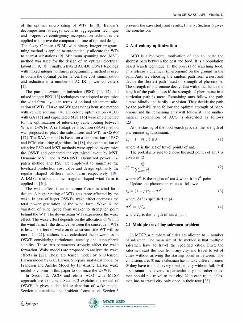
2.3 Elitist ACO with MTSP realization

The elitist ACO with MTSP algorithm is explained by

flow chart as shown in Fig. 1.

The process of elitist ACO with MTSP is enlightened as

following steps:

1) Initialize the basic parameters. The number of ants

and cities are equal to Nwt?1. The number of

salesmen depends on the current carrying capacity of

the cable.

2) Select the random WTs for ants or salesmen to start

the tour.

3) Calculate the distance matrix dij between the WTs

and visibility matrix gij of WTs by (5).

4) Create a random tour matrix T of WTs. The salesmen

will select their random tours for travel.

5) The probability rule (6) decides the salesman to

travel ith WT to next WT in a random tour.

6) Update the tour of salesmen by the strength of

pheromone value.

7) After the completion of the tour by salesmen,

calculate the length of the each tour.

8) Check whether the number of the specified tours is

completed or not. If not select the next random tour

in T and repeat the steps 5 to 8.

9) Update the pheromone trails by (7). Find the

minimum length of the tour from the length matrix.

10) Calculate the error value err = L0-Lk. If err[ 0.001

then go to step 4.

11) Check the condition err\ 0.001, then finalize the

optimum tour and length of the tour.

Fig. 1 Flow chart of elitist ACO-MTSP algorithm

Optimized design of collector topology for offshore wind farm based on ant colony…

123

3 Model of OSWF

The modeling of OSWF mainly depends on wake

model. The effective performance and power extraction of

a wind farm are strongly linked with wake effect. The wake

model gives a clear idea of wake effect in wind farm and

effective spacing between the WTs.

3.1 Wake model

Wakes in wind farms are of two types which are clas-

sified based on their distance from the WT. They are near

wake and far wake. The distance varies from one to several

times of the WT rotor diameter. The far wake models can

either be kinematic wake models or field models. In this

paper, a kinematic far wake model is taken into consider-

ation. The methodical equations of wake model are

explained below.

3.1.1 Larsen wake model

The Larsen model was proposed by G.C. Larsen. It is a

kinematic model and is formulated using the Prandtl tur-

bulent boundary layer equations. This wake model can give

solutions for the mean velocity profile in the wake and the

width of the wake. The assumptions are stationary and

strong air flow by neglecting wind share [22]. The Larsen

model first order equations and solutions are given

below.

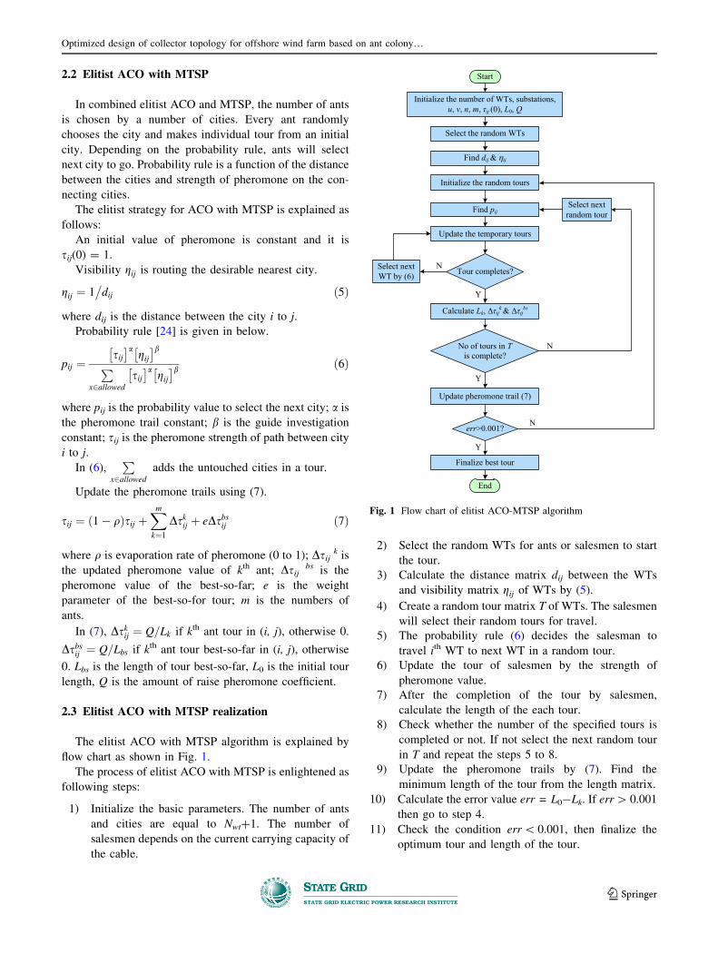
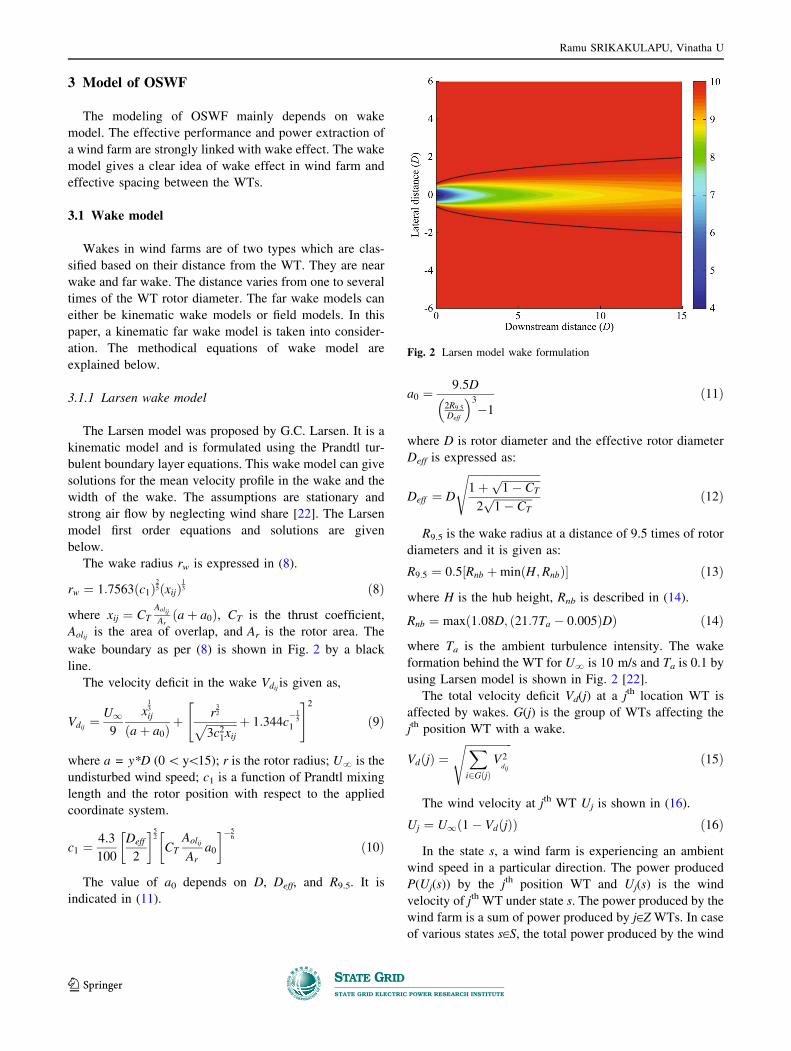
The wake radius rw is expressed in (8).

rw ¼ 1:7563ðc1Þ25ðxijÞ

13 ð8Þ

where xij ¼ CTAolij

Arðaþ a0Þ, CT is the thrust coefficient,

Aolij is the area of overlap, and Ar is the rotor area. The

wake boundary as per (8) is shown in Fig. 2 by a black

line.

The velocity deficit in the wake Vdij is given as,

Vdij ¼U19

x13

ij

ðaþ a0Þþ r

32

ffiffiffiffiffiffiffiffiffiffiffi3c21xij

p þ 1:344c�1

5

1

" #2

ð9Þ

where a = y*D (0\ y\15); r is the rotor radius; U? is the

undisturbed wind speed; c1 is a function of Prandtl mixing

length and the rotor position with respect to the applied

coordinate system.

c1 ¼4:3

100

Deff

2

� �52

CT

Aolij

Ar

a0

� ��56

ð10Þ

The value of a0 depends on D, Deff, and R9.5. It is

indicated in (11).

a0 ¼9:5D

2R9:5

Deff

� 3�1

ð11Þ

where D is rotor diameter and the effective rotor diameter

Deff is expressed as:

Deff ¼ D

ffiffiffiffiffiffiffiffiffiffiffiffiffiffiffiffiffiffiffiffiffiffiffiffiffiffi1þ

ffiffiffiffiffiffiffiffiffiffiffiffiffiffi1� CT

p

2ffiffiffiffiffiffiffiffiffiffiffiffiffiffi1� CT

p

s

ð12Þ

R9.5 is the wake radius at a distance of 9.5 times of rotor

diameters and it is given as:

R9:5 ¼ 0:5 Rnb þminðH;RnbÞ½ � ð13Þ

where H is the hub height, Rnb is described in (14).

Rnb ¼ maxð1:08D; ð21:7Ta � 0:005ÞDÞ ð14Þ

where Ta is the ambient turbulence intensity. The wake

formation behind the WT for U? is 10 m/s and Ta is 0.1 by

using Larsen model is shown in Fig. 2 [22].

The total velocity deficit Vd(j) at a jth location WT is

affected by wakes. G(j) is the group of WTs affecting the

jth position WT with a wake.

VdðjÞ ¼ffiffiffiffiffiffiffiffiffiffiffiffiffiffiffiffiffiX

i2GðjÞV2

dij

s

ð15Þ

The wind velocity at jth WT Uj is shown in (16).

Uj ¼ U1ð1� VdðjÞÞ ð16Þ

In the state s, a wind farm is experiencing an ambient

wind speed in a particular direction. The power produced

P(Uj(s)) by the jth position WT and Uj(s) is the wind

velocity of jth WT under state s. The power produced by the

wind farm is a sum of power produced by j[Z WTs. In case

of various states s[S, the total power produced by the wind

Fig. 2 Larsen model wake formulation

Ramu SRIKAKULAPU, Vinatha U

123

farm PT is obtained in each state s weighted by the

probability of its realization ps [25].

PT ¼X

s2SpsX

j2ZPðUjðsÞÞ

¼X

s2SpsX

j2ZPðUsð1� VdðjÞÞÞ ð17Þ

The power produced by WT is proportional to U3. The

assumptions for assessment of the wind farm power

production are: ps is constant for every WT in OSWF;

WTs rated are same and experience constant wind velocity.

PT /X

j2ZPj �

X

j2ZðUjÞ3 ð18Þ

4 Problem formulation

The formulation is based on the optimization of an

offshore wind farm. It mainly deals with the allocation of

WTs and substation in the wind farm to reduce the length

of interconnection cable between the WTs. The elitist ACO

with MTSP approach was used to get the optimal design of

offshore wind farm. In (19), n is equal to the sum of a total

number of WTs Nwt and substations in wind farm Nss. Each

substation has a set of transformers and it depends on the

rating of a wind farm.

n ¼ Nwt þ Nss ð19Þ

The number of inter-array cables is equal to a number of

salesmen. Each inter-array cable can connect to a

substation and set of WTs. The number of WTs

interconnects through the cable N depends on the cable

cross-sectional area and current carrying capacity.

The current flow through the inter-array MV submarine

cable I from WT is described as below.

I ¼ Pffiffiffi3

p ð20Þ

where P is the power rating of WT.

N ¼ Ic

Ið21Þ

where Ic is the current carrying capacity of the inter-array

submarine cable.

The cost of total inter-array cable CCT is the sum of the

interconnecting cable cost given in (22).

CCT ¼Xm

z¼1

CðLkðzÞÞ ¼Xm

z¼1

LkðzÞ

!

CC ð22Þ

where Lk(z) = (Lk(1),Lk(2),…,Lk(m)) is the length of m inter-

array cables; CC is the cost of MV submarine cable.

5 Case study and results

In this section, small OSWF and large OSWF are taken

as reference for the case study. OSWF specifications are as

per North Hoyle OSWF and Horns Rev OSWF. The opti-

mization of small and large OSWFs are done by using

elitist ACO with MTSP and the analysis is carried out for

both with and without wake effect. The wake effect cal-

culations are discussed in subsections. The North Hoyle

OSWF is located at Prestatyn in the Irish Sea, United

Kingdom. It is consisting of 30 WTs in 6 rows and each

row has 5 WTs and its area is 10 km2. The distance

between the WTs in a row is 800 m whereas in a column is

350 m. The rated power of WT is 2 MW and rotor diam-

eter D is 80 m. The transmission type is MVAC/HVAC

with operating voltage level of 33 /132 kV. The inter-array

cables interconnect the WTs by 2 radial cables with 15

WTs. The inter-array cable is 33 kV XLPE type AC sub-

marine cable with a cross-sectional area of 185 mm2 and

the total length of cable is 18 km. Two export cables are

used to interconnect the collector hub and substation. It has

a length of 10.781/13.176 km and each cable has 33 kV

XLPE type with cross-sectional area of 630 mm2. The

Horns Rev OSWF is located at Blavandshuk in the North

Sea, Denmark. The specifications of OSWFs are given in

Table 1 [26, 27]. The parameters of AC inter-array sub-

marine cable are provided in Table 2 [17]. The power

curve specifications of OSWFs are shown in Table 3.

5.1 Computation of wake effect

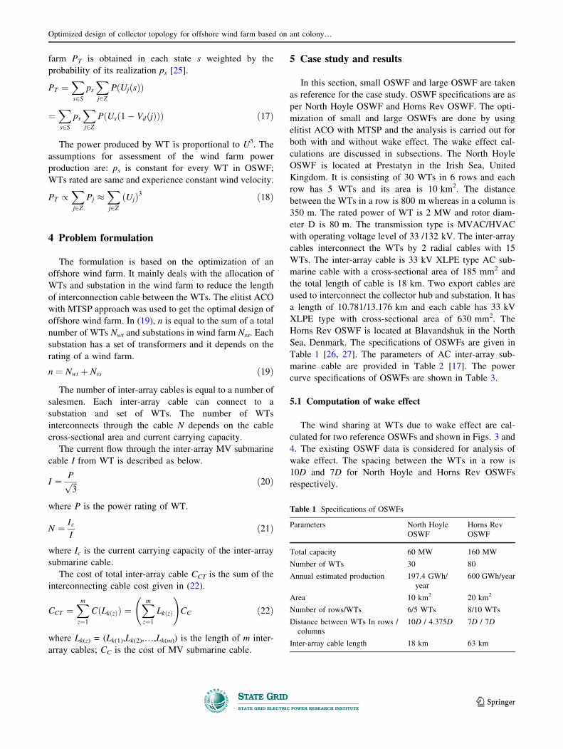
The wind sharing at WTs due to wake effect are cal-

culated for two reference OSWFs and shown in Figs. 3 and

4. The existing OSWF data is considered for analysis of

wake effect. The spacing between the WTs in a row is

10D and 7D for North Hoyle and Horns Rev OSWFs

respectively.

Table 1 Specifications of OSWFs

Parameters North Hoyle

OSWF

Horns Rev

OSWF

Total capacity 60 MW 160 MW

Number of WTs 30 80

Annual estimated production 197.4 GWh/

year

600 GWh/year

Area 10 km2 20 km2

Number of rows/WTs 6/5 WTs 8/10 WTs

Distance between WTs In rows /

columns

10D / 4.375D 7D / 7D

Inter-array cable length 18 km 63 km

Optimized design of collector topology for offshore wind farm based on ant colony…

123

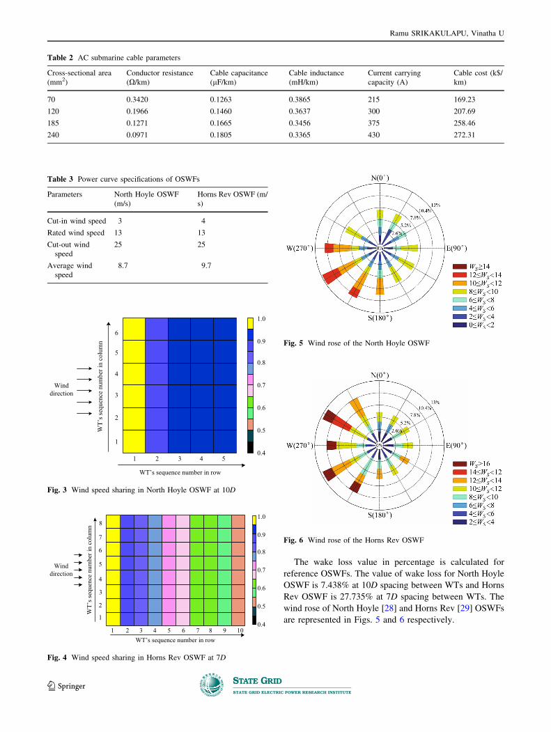
The wake loss value in percentage is calculated for

reference OSWFs. The value of wake loss for North Hoyle

OSWF is 7.438% at 10D spacing between WTs and Horns

Rev OSWF is 27.735% at 7D spacing between WTs. The

wind rose of North Hoyle [28] and Horns Rev [29] OSWFs

are represented in Figs. 5 and 6 respectively.

Table 2 AC submarine cable parameters

Cross-sectional area

(mm2)

Conductor resistance

(X/km)

Cable capacitance

(lF/km)

Cable inductance

(mH/km)

Current carrying

capacity (A)

Cable cost (k$/

km)

70 0.3420 0.1263 0.3865 215 169.23

120 0.1966 0.1460 0.3637 300 207.69

185 0.1271 0.1665 0.3456 375 258.46

240 0.0971 0.1805 0.3365 430 272.31

Table 3 Power curve specifications of OSWFs

Parameters North Hoyle OSWF

(m/s)

Horns Rev OSWF (m/

s)

Cut-in wind speed 3 4

Rated wind speed 13 13

Cut-out wind

speed

25 25

Average wind

speed

8.7 9.7

Fig. 3 Wind speed sharing in North Hoyle OSWF at 10D

Fig. 4 Wind speed sharing in Horns Rev OSWF at 7D

Fig. 5 Wind rose of the North Hoyle OSWF

Fig. 6 Wind rose of the Horns Rev OSWF

Ramu SRIKAKULAPU, Vinatha U

123

5.2 Optimized design of OSWF

In this paper, optimized design of OSWF is made

with the help of elitist ACO and MTSP technique. The

spacing between the WTs in a row is taken as

7D (560 m) and that of in a column is taken as

4D (320 m). To achieve an optimized design of OSWF,

wake effect and minimum length of inter-array cable are

taken into consideration.

5.2.1 Case 1: without wake effect

In this case, the wake effect is not taken into consider-

ation and minimum length of inter-array cable is accounted

while designing optimal model of OSWF. Figures 7 and 8

show the optimized design of OSWF without wake for

North Hoyle (NHWOW) and Horns Rev (HRWOW)

OSWFs respectively based on the minimum length of the

inter-array cable. The value of wake loss for North Hoyle

OSWF is 16.90% and Horns Rev OSWF is 27.735% at

7D spacing between WTs.

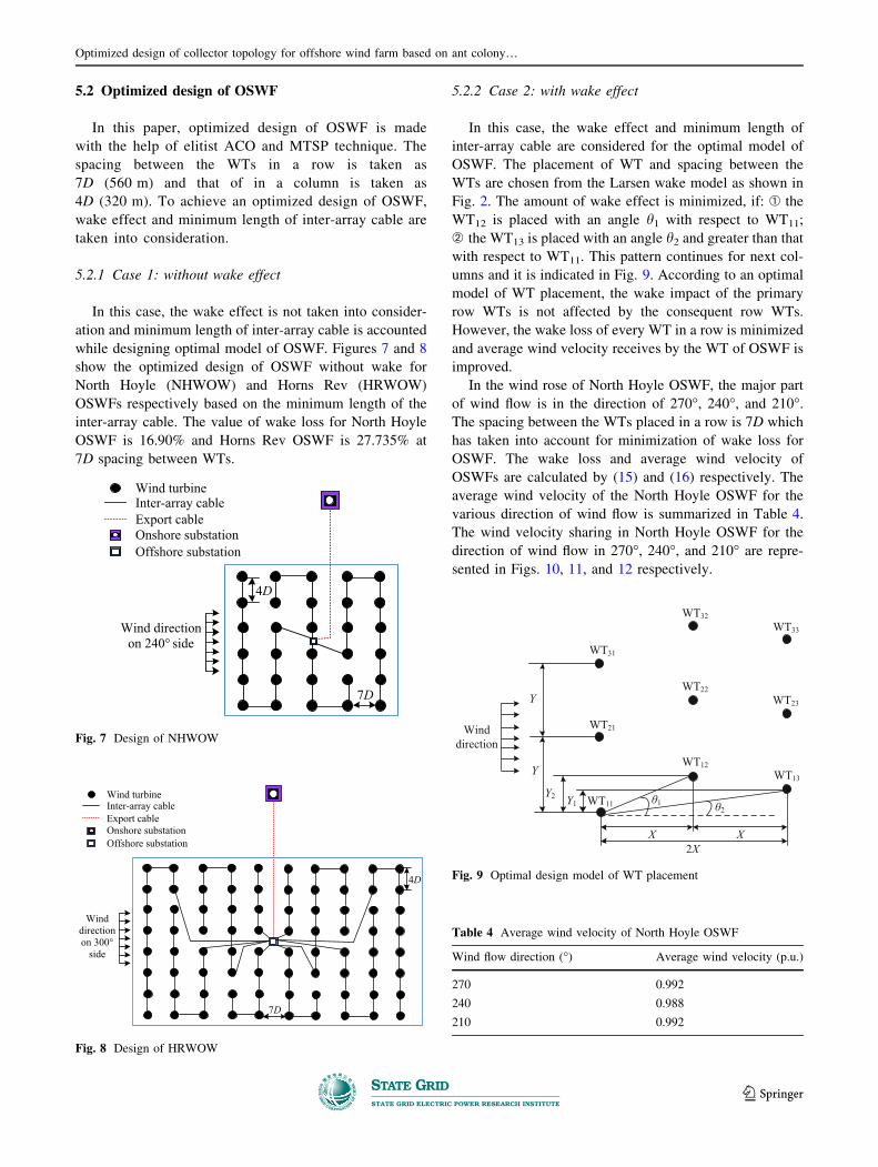
5.2.2 Case 2: with wake effect

In this case, the wake effect and minimum length of

inter-array cable are considered for the optimal model of

OSWF. The placement of WT and spacing between the

WTs are chosen from the Larsen wake model as shown in

Fig. 2. The amount of wake effect is minimized, if: � the

WT12 is placed with an angle h1 with respect to WT11;

` the WT13 is placed with an angle h2 and greater than thatwith respect to WT11. This pattern continues for next col-

umns and it is indicated in Fig. 9. According to an optimal

model of WT placement, the wake impact of the primary

row WTs is not affected by the consequent row WTs.

However, the wake loss of every WT in a row is minimized

and average wind velocity receives by the WT of OSWF is

improved.

In the wind rose of North Hoyle OSWF, the major part

of wind flow is in the direction of 270�, 240�, and 210�.The spacing between the WTs placed in a row is 7D which

has taken into account for minimization of wake loss for

OSWF. The wake loss and average wind velocity of

OSWFs are calculated by (15) and (16) respectively. The

average wind velocity of the North Hoyle OSWF for the

various direction of wind flow is summarized in Table 4.

The wind velocity sharing in North Hoyle OSWF for the

direction of wind flow in 270�, 240�, and 210� are repre-

sented in Figs. 10, 11, and 12 respectively.

Fig. 7 Design of NHWOW

Fig. 8 Design of HRWOW

Fig. 9 Optimal design model of WT placement

Table 4 Average wind velocity of North Hoyle OSWF

Wind flow direction (�) Average wind velocity (p.u.)

270 0.992

240 0.988

210 0.992

Optimized design of collector topology for offshore wind farm based on ant colony…

123

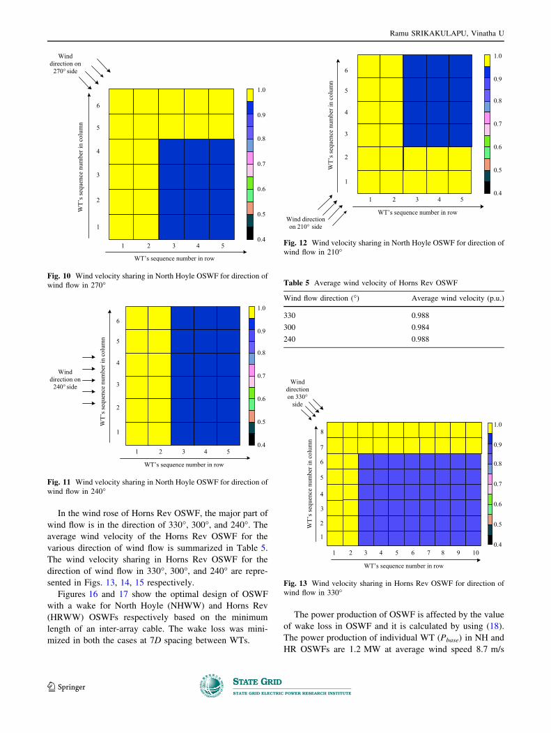
In the wind rose of Horns Rev OSWF, the major part of

wind flow is in the direction of 330�, 300�, and 240�. Theaverage wind velocity of the Horns Rev OSWF for the

various direction of wind flow is summarized in Table 5.

The wind velocity sharing in Horns Rev OSWF for the

direction of wind flow in 330�, 300�, and 240� are repre-

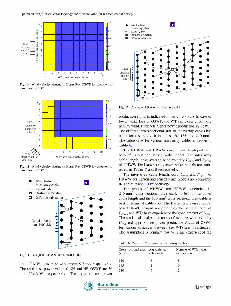
sented in Figs. 13, 14, 15 respectively.

Figures 16 and 17 show the optimal design of OSWF

with a wake for North Hoyle (NHWW) and Horns Rev

(HRWW) OSWFs respectively based on the minimum

length of an inter-array cable. The wake loss was mini-

mized in both the cases at 7D spacing between WTs.

The power production of OSWF is affected by the value

of wake loss in OSWF and it is calculated by using (18).

The power production of individual WT (Pbase) in NH and

HR OSWFs are 1.2 MW at average wind speed 8.7 m/s

Fig. 10 Wind velocity sharing in North Hoyle OSWF for direction of

wind flow in 270�

Fig. 11 Wind velocity sharing in North Hoyle OSWF for direction of

wind flow in 240�

Fig. 12 Wind velocity sharing in North Hoyle OSWF for direction of

wind flow in 210�

Table 5 Average wind velocity of Horns Rev OSWF

Wind flow direction (�) Average wind velocity (p.u.)

330 0.988

300 0.984

240 0.988

Fig. 13 Wind velocity sharing in Horns Rev OSWF for direction of

wind flow in 330�

Ramu SRIKAKULAPU, Vinatha U

123

and 1.7 MW at average wind speed 9.7 m/s respectively.

The total base power value of NH and HR OSWF are 36

and 136 MW respectively. The approximate power

production Paprox is indicated in per units (p.u.). In case of

lower wake loss of OSWF, the WT can experience more

healthy wind. It reflects higher power production in OSWF.

The different cross-sectional area of inter-array cables has

taken for case study. It includes 120, 185, and 240 mm2.

The value of N for various inter-array cables is shown in

Table 6.

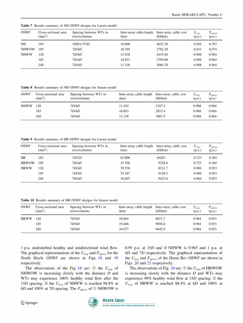
The NHWW and HRWW designs are developed with

help of Larsen and Jensen wake model. The inter-array

cable length, cost, average wind velocity Uavg, and Paprox

of NHWW for Larsen and Jensen wake models are com-

pared in Tables 7 and 8 respectively.

The inter-array cable length, cost, Uavg, and Paprox of

HRWW for Larsen and Jensen wake models are compared

in Tables 9 and 10 respectively.

The results of NHWW and HRWW concludes the

240 mm2 cross-sectional area cable is best in terms of

cable length and the 120 mm2 cross-sectional area cable is

best in terms of cable cost. The Larsen and Jensen model

based OSWF designs are producing the same amount of

Paprox and WTs have experienced the good amount of Uavg.

The statistical analysis in terms of average wind velocity

Uavg and approximate power production Paprox of OSWF

for various distances between the WTs are investigated.

The assumption is primary row WTs are experienced the

Fig. 14 Wind velocity sharing in Horns Rev OSWF for direction of

wind flow in 300�

Fig. 15 Wind velocity sharing in Horns Rev OSWF for direction of

wind flow in 240�

Fig. 16 Design of NHWW for Larsen model

Fig. 17 Design of HRWW for Larsen model

Table 6 Value of N for various inter-array cables

Cross-sectional area

(mm2)

Approximate

value of N

Number of WTs taken

into account

120 8 8

185 11 10

240 13 12

Optimized design of collector topology for offshore wind farm based on ant colony…

123

1 p.u. undisturbed healthy and unidirectional wind flow.

The graphical representations of the Uavg and Paprox for the

North Hoyle OSWF are shown in Figs. 18 and 19

respectively.

The observations of the Fig. 18 are: � the Uavg of

NHWOW is increasing slowly with the distance D and

WTs may experience 100% healthy wind flow after the

15D spacing; ` the Uavg of NHWW is reached 98.8% at

6D and 100% at 7D spacing. The Paprox of � NHWOW is

0.95 p.u. at 15D and ` NHWW is 0.965 and 1 p.u. at

6D and 7D respectively. The graphical representation of

the Uavg and Paprox of the Horns Rev OSWF are shown in

Figs. 20 and 21 respectively.

The observations of Fig. 20 are: � the Uavg of HRWOW

is increasing slowly with the distance D and WTs may

experience 99% healthy wind flow at 15D spacing; ` the

Uavg of HRWW is reached 98.4% at 6D and 100% at

Table 7 Results summary of NH OSWF designs for Larsen model

OSWF Cross-sectional area

(mm2)

Spacing between WTs in

rows/columns

Inter-array cable length

(km)

Inter-array cable cost

(k$/km)

Uavg

(p.u.)

Paprox

(p.u.)

NH 185 10D/4.375D 18.000 4652.30 0.926 0.793

NHWOW 185 7D/4D 10.765 2782.30 0.831 0.574

NHWW 120 7D/4D 11.630 2415.44 0.988 0.964

185 7D/4D 10.832 2799.60 0.988 0.964

240 7D/4D 11.328 3084.70 0.988 0.964

Table 8 Results summary of NH OSWF designs for Jensen model

OSWF Cross-sectional area

(mm2)

Spacing between WTs in

rows/columns

Inter-array cable length

(km)

Inter-array cable cost

(k$/km)

Uavg

(p.u.)

Paprox

(p.u.)

NHWW 120 7D/4D 11.542 2397.2 0.988 0.964

185 7D/4D 10.893 2815.4 0.988 0.964

240 7D/4D 11.338 3087.5 0.988 0.964

Table 9 Results summary of HR OSWF designs for Larsen model

OSWF Cross-sectional area

(mm2)

Spacing between WTs in

rows/columns

Inter-array cable length

(km)

Inter-array cable cost

(k$/km)

Uavg

(p.u.)

Paprox

(p.u.)

HR 185 7D/7D 63.000 16283 0.723 0.384

HRWOW 185 7D/4D 35.706 9228.6 0.723 0.384

HRWW 120 7D/4D 39.538 8211.7 0.984 0.953

185 7D/4D 35.287 9120.3 0.984 0.953

240 7D/4D 34.607 9423.8 0.984 0.953

Table 10 Results summary of HR OSWF designs for Jensen model

OSWF Cross-sectional area

(mm2)

Spacing between WTs in

rows/columns

Inter-array cable length

(km)

Inter-array cable cost

(k$/km)

Uavg

(p.u.)

Paprox

(p.u.)

HRWW 120 7D/4D 38.864 8071.7 0.984 0.953

185 7D/4D 35.046 9058.0 0.984 0.953

240 7D/4D 34.677 9442.9 0.984 0.953

Ramu SRIKAKULAPU, Vinatha U

123

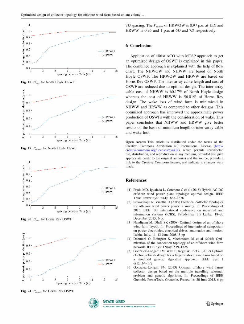
7D spacing. The Paprox of HRWOW is 0.97 p.u. at 15D and

HRWW is 0.95 and 1 p.u. at 6D and 7D respectively.

6 Conclusion

Application of elitist ACO with MTSP approach to get

an optimized design of OSWF is explained in this paper.

The combined approach is explained with the help of flow

chart. The NHWOW and NHWW are based on North

Hoyle OSWF. The HRWOW and HRWW are based on

Horns Rev OSWF. The inter-array cable length and cost of

OSWF are reduced due to optimal design. The inter-array

cable cost of NHWW is 60.17% of North Hoyle design

whereas the cost of HRWW is 56.01% of Horns Rev

design. The wake loss of wind farm is minimized in

NHWW and HRWW as compared to other designs. This

optimized approach has improved the approximate power

production of OSWFs with the consideration of wake. This

paper concludes that NHWW and HRWW give better

results on the basis of minimum length of inter-array cable

and wake loss.

Open Access This article is distributed under the terms of the

Creative Commons Attribution 4.0 International License (http://

creativecommons.org/licenses/by/4.0/), which permits unrestricted

use, distribution, and reproduction in any medium, provided you give

appropriate credit to the original author(s) and the source, provide a

link to the Creative Commons license, and indicate if changes were

made.

References

[1] Prada MD, Igualada L, Corchero C et al (2015) Hybrid AC-DC

offshore wind power plant topology: optimal design. IEEE

Trans Power Syst 30(4):1868–1876

[2] Srikakulapu R, Vinatha U (2015) Electrical collector topologies

for offshore wind power plants: a survey. In: Proceedings of

2015 IEEE 10th international conference on industrial and

information systems (ICIIS), Peradeniya, Sri Lanka, 18–20

December 2015, 6 pp

[3] Nandigam M, Dhali SK (2008) Optimal design of an offshore

wind farm layout. In: Proceedings of international symposium

on power electronics, electrical drives, automation and motion,

Ischia, Italy, 11–13 June 2008, 5 pp

[4] Dahmani O, Bourguet S, Machmoum M et al (2015) Opti-

mization of the connection topology of an offshore wind farm

network. IEEE Syst J 9(4):1519–1528

[5] Gonzalez-Longatt FM, Wall P, Regulski P et al (2012) Optimal

electric network design for a large offshore wind farm based on

a modified genetic algorithm approach. IEEE Syst J

6(1):164–172

[6] Gonzalez-Longatt FM (2013) Optimal offshore wind farms

collector design based on the multiple travelling salesman

problem and genetic algorithm. In: Proceedings of IEEE

Grenoble PowerTech, Grenoble, France, 16–20 June 2013, 6 pp

Fig. 18 Uavg for North Hoyle OSWF

Fig. 19 Paprox for North Hoyle OSWF

Fig. 20 Uavg for Horns Rev OSWF

Fig. 21 Paprox for Horns Rev OSWF

Optimized design of collector topology for offshore wind farm based on ant colony…

123

[7] Gonz JS, Pay MB, Santos JR et al (2013) A new and efficient

method for optimal design of large offshore wind power plants.

IEEE Trans Power Syst 28(3):3075–3084

[8] Lumbreras S, Ramos A (2013) Optimal design of the electrical

layout of an offshore wind farm applying decomposition

strategies. IEEE Trans Power Syst 28(2):1434–1441

[9] Chen Y, Dong Z, Meng K et al (2013) A novel technique for the

optimal design of offshore wind farm electrical layout.

J Modern Power Syst Clean Energy 1(3):258–263

[10] Dutta S, Overbye TJ (2012) Optimal wind farm collector system

topology design considering total trenching length. IEEE Trans

Sustain Energy 3(3):339–348

[11] Hou P, Hu W, Soltani M et al (2015) Optimized placement of

wind turbines in large-scale offshore wind farm using particle

swarm optimization algorithm. IEEE Trans Sustain Energy

6(4):1272–1282

[12] Hou P, Hu W, Chen C et al (2017) Overall optimization for

offshore wind farm electrical system. Wind Energy

20(6):1017–1032

[13] Hou P, Hu W, Soltani M et al (2017) Combined optimization for

offshore wind turbine micro siting. Appl Energy 189:271–282

[14] Joanna B, Lysgaard J (2015) The offshore wind farm array cable

layout problem: a planar open vehicle routing problem. J Oper

Res Soc 66(3):360–368

[15] Wu YK, Lee CY, Chen CR et al (2014) Optimization of the

wind turbine layout and transmission system planning for a

large-scale offshore windfarm by AI technolgy. IEEE Trans Ind

Appl 50(3):2071–2080

[16] Pillai AC, Chick J, Johanning L et al (2015) Offshore wind farm

electrical cable layout optimization. Eng Optim

47(12):1689–1708

[17] Chen Y, Dong ZY, Meng K et al (2016) Collector system layout

optimization framework for large-scale offshore wind farms.

IEEE Trans Sustain Energy 7(4):1398–1407

[18] Hou P, Hu W, Chen Z et al (2016) Optimisation for offshore

wind farm cable connection layout using adaptive particle

swarm optimisation minimum spanning tree method. IET

Renew Power Gener 10(5):694–702

[19] Hou P, Hu W, Zhang B et al (2016) Optimised power dispatch

strategy for offshore wind farms. IET Renew Power Gener

10(3):399–409

[20] Hou P, Hu W, Chen C et al (2016) Optimisation of offshore

wind farm cable connection layout considering levelised pro-

duction cost using dynamic minimum spanning tree algorithm.

IET Renew Power Gener 10(2):175–183

[21] Barthelmie RJ, Hansen KS, Pryor SC et al (2013) Meteoro-

logical controls on wind turbine wakes. Proc IEEE

101(4):1010–1019

[22] Renkema DJ (2007) Validation of wind turbine wake models.

Delft University of Technology, Delft

[23] Dorigo M, Birattari M, Stutzle T (2006) Ant colony optimiza-

tion. The MIT press, Cambridge

[24] Colorni A, Dorigo M, Maniezzo V (1992) Distributed opti-

mization by ant colonies. In: Proceedings of European confer-

ence on artificial life, Vienna, Austria, 3–7 August 1992, 9 pp

[25] Samorani M (2013) The wind farm layout optimization prob-

lem. Springer, Germany, pp 21–38

[26] North hoyle offshore wind farm. http://www.4coffshore.com/

windfarms/north-hoyle-united-kingdom-uk16.html

[27] Horns rev offshore wind farm, http://www.4coffshore.com/

windfarms/horns-rev-1-denmark-dk3.html

[28] BERR (2007) Capital grant scheme for the North Hoyle off-

shore wind farm annual report: July 2006–June 2007. Power

Renewables Limited

[29] Hansen KS, Barthelmie RJ, Jensen LE et al (2012) The impact

of turbulence intensity and atmospheric stability on power

deficits due to wind turbine wakes at Horns Rev wind farm.

Wind Energy 15(1):183–196

Ramu SRIKAKULAPU received his B.Tech degree from VIIT

Visakhapatnam, JNTU Hyderabad, India in 2008, M.Tech degree

from NIT Kurukshetra, India in 2012, all in Electrical Engineering.

He is now a research scholar at Department of Electrical and

Electronics Engineering, NITK Surathkal, India. His research interest

includes grid integration of renewable energy sources, optimal

controllers for HVDC transmission, and optimization algorithms

and its application to renewable energy sources.

Vinatha U received her B.Tech and M.Tech degrees from KREC

Surathkal, Mangalore University, India respectively in 1986 and 1992

and Ph.D degree from NITK Surathkal, India in 2013, all in Electrical

Engineering. She is now an associate professor at Department of

Electrical and Electronics Engineering, NITK Surathkal. Her

research interest includes power electronics and drives, power

electronic converters in renewable systems, multilevel inverters and

wave energy conversion system.

Ramu SRIKAKULAPU, Vinatha U

123