Optimization techniques for Available Transfer Capability (ATC) and market calculations

IMA Journal of Management Mathematics (2004)15, 321–337

Optimization techniques for Available Transfer Capability(ATC) and market calculations

SUNG-KWAN JOO AND CHEN-CHING LIU

Department of Electrical Engineering, University of Washington, Seattle WA98195, USA

YANGFANG SHEN AND ZELDA B. ZABINSKY

Department of Industrial Engineering, University of Washington, Seattle WA98195, USA

AND

JACQUESLAWA RREE

Department of Economics, University of Washington, Seattle WA 98195, USA

The recent movement towards an open, competitive market environment introduced newoptimization problems such as market clearing mechanism, bidding decision and AvailableTransfer Capability (ATC) calculation. These optimization problems are characterized bythe complexity of power systems and the uncertainties in the electricity market. Accurateevaluation of the transfer capability of a transmission system is required to maximizethe utilization of the existing transmission systems in a competitive market environment.The transfer capability of the transmission networks can be limited by various systemconstraints such as thermal, voltage and stability limits. The ability to incorporate suchlimits into the optimization problem is a challenge in the ATC calculation from anengineering point of view. In the competitive market environment, a power supplier needsto find an optimal strategy that maximizes its own profits under various uncertaintiessuch as electricity prices and load. On the other hand, an efficient market clearingmechanism is needed to increase the social welfare, i.e. the sum of the consumers’ andproducers’ surplus. The need to maximize the social welfare subject to system operationalconstraints is also a major challenge from a societal point of view. This paper presentsnew optimization techniques motivated by the competitive electricity market environment.Numerical simulation results are presented to demonstrate the performance of the proposedoptimization techniques.

Keywords: Markov decision process; market optimization; improving hit-and-run; powersystem economics; available transfer capability.

1. Introduction

Optimization techniques have been applied to various traditional power system problemsincluding minimization of generation costs and system losses. Various optimization toolshave been developed to solve optimal power flow, economic dispatch and unit commitment(Wood & Wollenberg, 1996). These problems are complex due to both the nonlinearnature of power flows and a large number of continuous or discrete decision variablesand constraints. The recent movement towards an open, competitive market environment

IMA Journal of Management Mathematics Vol. 15 No. 4c© Institute of Mathematics and its Applications 2004; all rights reserved.

322 S.-K. JOOET AL.

introduced new optimization problems such as market clearing mechanism, biddingdecision and available transfer capability (ATC) calculation. These new optimizationproblems become more complicated due to the complexity of power systems and theuncertainties in the electricity market.

In a competitive market environment, the system operator needs to know how muchadditional power can be transferred from one area to another area without violating systemconstraints. Accurate evaluation of the transfer capability of a transmission system isrequired to maximize the utilization of the existing transmission systems. In practice,the transfer capability of the transmission networks can be limited by various systemconstraints such as thermal, voltage and stability limits (Graveneret al., 1999). Theability to incorporate such limits into the optimization problem is a challenge in the ATCcalculation from an engineering perspective.

In a deregulated power market where electric power is traded through spot andbilateral markets, a power supplier chooses an optimal strategy to maximize its own profitsunder various uncertainties such as electricity prices and load. Rotting & Gjelsvik (1993)and Kayeet al. (1990) proposed optimization-based methods for scheduling of bilateralcontracts. Songet al. (2000) used a Markov decision process (MDP) model to find anoptimal bidding strategy in the spot market environment. In trading, a power supplier needsto find optimal coordination of the bilateral contracts and spot market bidding decisionwhile taking into account the supplier’s production limit. Therefore, maximization of thecombined profits in both markets requires optimization of the combined problem ratherthan optimization of each individual problem. On the other hand, from a societal pointof view, an efficient market clearing mechanism is needed to increase the social welfarethat is the sum of the consumers’ and producers’ surplus. The need to maximize the socialwelfare subject to system operational constraints is also a major challenge from a societalpoint of view.

This paper presents state-of-the-art optimization techniques: (i) to maximize the powertransfer between areas, (ii) to maximize the expected profit for a power supplier, and(iii) to maximize social welfare in a competitive market environment. The sensitivity ofthe energy margin can provide information on how changes in generations can influencethe degree of stability of a system (Fouad & Vittal, 1992). The proposed ATC methoddetermines ATC between areas by running a series of numerical simulations directed byenergy margin sensitivity as well as energy margin. The decision-making process of thebilateral contract affects the bidding strategy to the spot market since bidding decision-making in electricity markets is coupled with the bilateral contract position. An MDP-based optimization technique is intended to assist a market participant to make decisions onbilateral contracts and bidding to the spot market. Given the nonlinearity of power systems,the market optimization problem (MOP) requires the use of the global optimizationtechnique to maximize the social welfare of a market. A global optimization algorithmin combination with sequential quadratic programming (SQP) is applied to solve the MOPincorporating the complex characteristics of large-scale nonlinear power systems.

The remainder of this paper is organized as follows. In Section 2, the ATC calculationproblem, suppliers’ optimization problem (SOP) and MOP are formulated with the powersystem model incorporating the nonlinear nature of power systems. Section 3 presentsoptimization techniques to solve the problems described in Section 2.

OPTIMIZATION TECHNIQUES FOR ATC 323

2. Problem description

2.1 Available Transfer Capability

According to the report of NERC (1995), transfer capability refers to the ability oftransmission systems to reliably transfer power from one area to another over alltransmission paths between those areas under given system conditions. The mathematicaldefinition of ATC given in the report of NERC (1996) is ‘. . . the Total TransferCapability (TTC) less the Transmission Reliability Margin (TRM), less the sum of existingtransmission commitments and the Capacity Benefit Margin (CBM)’:

ATC = TTC − TRM − existing transmission commitments (including CBM). (2.1)

TTC refers to the maximum amount of electric power that can be transferred overtransmission systems without violating system security constraints. The accuracy of theATC calculation is highly dependent on the accuracy of available network data, loadforecast, and the estimation of future energy transactions. Therefore, there is uncertaintyin ATC calculation associated with errors in load forecast and estimation of future energytransactions. TRM is a safety margin to protect against the overload of the transmissionsystem considering those uncertain factors in ATC calculation. ‘Existing transmissioncommitments’ means ‘existing transfers between areas’. The ATC between two areasprovides an indication of the maximum amount of additional MW transfer possiblebetween two parts of a power system.

ATC between areas can be calculated by increasing generation in the sending area andat the same time increasing the same amount of load in the receiving area until the powersystem reaches system limits. The evaluation of ATC can be formulated as an optimizationproblem. The objective function to be maximized is expressed as

max∑

i∈area A

∆Pi (2.2)

subject to

x = f (x, y) (2.3)

0 = g(x, y) (2.4)

0 � Pi + ∆Pi � Pmaxi (2.5)

−Fmax � F(x, y) � Fmax (2.6)

V min � V � V max (2.7)

E M(x, y) > 0, (2.8)

where Pi is power injection at the bus of generator ‘i ’ and∑

i∈area A∆Pi is the sum ofthe increased generation in the sending area A,x is a vector of state variables andy isa vector of algebraic variables. Equation (2.3) represents differential equations describingthe dynamic behaviours of the power system while (2.4) represents algebraic equationsincluding power flow equations. Equations (2.5)–(2.8) are inequality constraints.Pmax

iis the upper limit of active power output of generator ‘i ’. Fmax is the vector of thermallimits of transmission lines.V min and V max are the vectors of lower and upper limits

324 S.-K. JOOET AL.

of bus voltage magnitudes, respectively.E M(x, y) is energy margin which provides aquantitative measure of the degree of stability of power systems (Fouad & Vittal, 1992).The energy margin of a power system indicates how far the power system is from thestability boundary. The technical details for computing the second-kick-based energymargin of the system can be found in the work of Hashimotoet al. (2002).

The limiting conditions of transmission systems can shift among thermal, voltage, andstability limits as the operating condition of the power system change over time. Stabilitylimits of systems may become more restrictive than static limits depending on systemoperating conditions. The ATC calculation must be evaluated based on the most restrictiveone of those limiting factors. Therefore, the accuracy of ATC calculation is not reliableif the stability limits of the system are not taken into account. It is desirable to considerstability limits in addition to static limits in the ATC calculation.

2.2 Suppliers’ optimization problem

In a competitive market environment, power suppliers choose their optimal strategiesto maximize their own profits. A power supplier may participate in a bilateral marketin addition to a spot market. A supplier’s existing bilateral contracts would influenceits bidding decision to the spot market since the total amount of electricity that canbe simultaneously traded in both markets is restricted by its capacity limit. Therefore,a supplier’s scheduling of bilateral contract needs to be coordinated with its biddingdecisions to spot market in order to maximize the combined profits (Joo & Liu, 2000).

This study assumes that a power supplier has an obligation to provide a certain contractvolume over a time horizon. The power supplier with bilateral obligations decides thescheduling of the bilateral contracts and simultaneously chooses a bidding strategy tothe spot market to maximize the total profit over the planning horizon. In this section,an MDP-based optimization technique is used to find a supplier’s optimal decisions overthe planning horizon. A MDP consists of four elements such as states, decision options,transition probabilities, and rewards (Howard, 1960). The MDP provides a multi-stagedecision model where the status of a system is represented by a stochastic process withdecision options that induce stochastic transitions from one state to another state.

Power suppliers submit bids to the spot market to sell electricity. The spot prices aredetermined by the bids from power suppliers and the load demand. Hence, the biddingbehaviours of market players will be affected by the spot price, the load demand andtomorrow’s load forecast. Scheduling of the flexible bilateral contract is considered as thedecision-making process that affects bidding strategy to the spot market. With this in mind,the state of electricity markets is defined by all possible combinations of RCV (remainingcontract volume) of a given bilateral contract, spot price, cleared-demand and tomorrow’sload forecast in the spot market. Then, the number of possible states is (the number ofpossible RCV)× (the number of possible spot price)× (the number of possible demand)× (the number of possible forecastload). The number of states does not increase as thenumber of players or the duration of the planning horizon increases. The decision optionsof the power supplier consist of all possible combinations of the usage of a given flexiblebilateral contract and the bidding decision to the spot market.

Transition probabilities can be modelled by statistical analysis based on competitors’bidding data, historical prices and load information. In this paper, Pr(t, i, k, j) represents


the transition probability from statei to state j if the decision maker makes decisionoption ‘k’ f or each time periodt . The calculation of transition probability requires theidentification of market scenarios, which include the other player’s probabilistic biddinginformation as well as the decision option of the power producer. If all possible aggregatebidding data with forecasted demand in statei are put into the market clearing system,a transition can be found according to the market clearing price and RCV. Then, onemust find all scenarios which contribute to statej , and add up all the probabilities of thevarious scenarios. The overall probability represents the transition probability from stateito statej . The availability of the competitors’ bidding data is critical for the accuracy ofthe transition probabilities.

The power supplier earnsri j dollars when the electric market system moves from statei to statej . Theri j associated with the transition from statei to j is called the ‘reward’.Reward is the difference between the revenue and the cost of the power supplier. For eachtime periodt , the immediate reward of a power supplier from statei to statej with decisionoption ‘k’ i s calculated as follows:

r(t, i, k, j) = S P(t, j) × Q(t, j) + BC P × x(t, k) − Cost[Q(t, j) + x(t, k)] (2.9)

whereS P(t, j) = spot market price in statej at time periodt , Q(t, j) = power producer’squantity that is accepted into spot market in statej at time periodt , x(t, k) = schedulingdecision of bilateral contract with decision optionk at time periodt , andBC P = bilateralcontract price per MW. After the transition probabilities and rewards are calculated, thenext step is to find the optimal decision option in thei th state that maximizes the expectedvalue of accumulated rewards over the planning horizon. A value iteration algorithm isused to find an optimal decision option to maximize the following value iteration equation:

V (i, τ + 1) = Kmaxk=1

N∑j=1

{Pr(i, k, j) ∗ [r(i, k, j) + V ( j, τ )]} (2.10)

whereV (i, τ + 1) is the total expected reward inτ + 1 remaining stages starting fromstatei if an optimal policy is followed. OnceV is computed over the decision options,the optimal policy is immediately obtained by choosing any decision which satisfies themaximum function of the value iteration equation.

2.3 Market Optimization Problem

From a market point of view, it is desirable to maximize the social welfare, which isdefined by the sum of the consumers’ and producers’ surplus. There are transmissionsystem constraints based on the nonlinear power flow model. Generators also have theircapacity availability constraints and ramping constraints that limit the rate of power thatcan be increased. In the work of Shenet al. (2003), the market mechanism problem wasfirst formulated based on a 30-bus power flow system. The mathematical optimizationmodel based on a general power flow system to find the optimal combination of the powergenerated,P1, . . . , Pm , and the load delivered,L1, . . . , Ln , to maximize the social welfareis stated below.

maxn∑

i=1

ULi −m∑

j=1

CPj (2.11)

326 S.-K. JOOET AL.

where producers’ cost function

CPj = α j P2j + β j Pj + γ j for j = 1, . . . , m (2.12)

and consumers’ gross surplus function

ULi = −vi L2i + νi Li for i = 1, . . . , n (2.13)

subject to

Lmini � Li � Lmax

i for i = 1, . . . , m (2.14)

Pminj � Pj � Pmax

j for j = 1, . . . , n (2.15)

−Fmaxbk � sin(θb − θk)

xb k� Fmax

bk for all connected busesb, k, (b < k) (2.16)

∑k:busk isconnectedto busb

sin(θb − θk)

xb k= 0 + Pg(b) − Ll(b) for b = 1, . . . , B (2.17)

whereα j , β j andγ j are the parameters of the generatorj ’s cost function,νi , vi are theparameters of the loadi ’s gross consumer surplus function,Pmax

j , Pminj and Lmax

i , Lmini

represent the upper and lower bounds of thej th generator and thei th load respectively,Fmax

bk is the capacity of the transmission line that connects busb and busk, and xb k isthe reactance of the line. In the balance equation constraints,g(b) is the generator numberconnected to busb andl(b) is the load number connected to the bus. Note that if there is nogenerator or load connected to the bus, the right-hand side of the balance equation equalszero.

Unlike the traditional optimal power flow model used by Sunet al. (1984) and Alsacet al. (2003), the power flow equations considered here in the MOP model are nonlinearfunctions, involving sinusoidal functions. This is more difficult for existing optimizationtechniques. If the objective function and intersection of nonlinear constraints are convex,then local optimization techniques may be applied, such as SQP (Boggs & Tolle, 1995).However, a complex power system may have a non-convex feasible region. Shenet al.(2003) showed that by using SQP with the starting point being chosen by trial and error, twodifferent local optima were found for the MOP based on a 30-bus power flow system. Thenonlinear and global nature of the problem would imply that other optimization techniquesare necessary. Currently, simulated annealing and genetic algorithms are employed forcomplex global optimization problems in other arenas with little underlying structure (seePham & Karaboga, 2000). In Section 3.3, Improving Hit-and-Run (Zabinskyet al., 1993)will be combined with SQP to solve an example of MOP with a two-area, four-machinetest system.


120 110 11

12

13

101 1

3

2

10 20

G11

G12G2

G1

Area A Area B

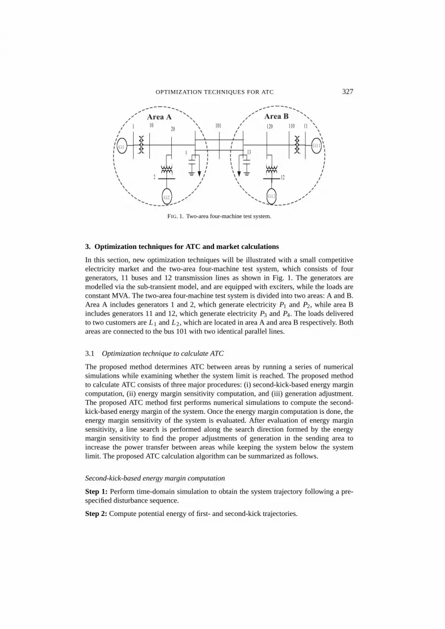
FIG. 1. Two-area four-machine test system.

3. Optimization techniques for ATC and market calculations

In this section, new optimization techniques will be illustrated with a small competitiveelectricity market and the two-area four-machine test system, which consists of fourgenerators, 11 buses and 12 transmission lines as shown in Fig. 1. The generators aremodelled via the sub-transient model, and are equipped with exciters, while the loads areconstant MVA. The two-area four-machine test system is divided into two areas: A and B.Area A includes generators 1 and 2, which generate electricityP1 and P2, while area Bincludes generators 11 and 12, which generate electricityP3 and P4. The loads deliveredto two customers areL1 andL2, which are located in area A and area B respectively. Bothareas are connected to the bus 101 with two identical parallel lines.

3.1 Optimization technique to calculate ATC

The proposed method determines ATC between areas by running a series of numericalsimulations while examining whether the system limit is reached. The proposed methodto calculate ATC consists of three major procedures: (i) second-kick-based energy margincomputation, (ii) energy margin sensitivity computation, and (iii) generation adjustment.The proposed ATC method first performs numerical simulations to compute the second-kick-based energy margin of the system. Once the energy margin computation is done, theenergy margin sensitivity of the system is evaluated. After evaluation of energy marginsensitivity, a line search is performed along the search direction formed by the energymargin sensitivity to find the proper adjustments of generation in the sending area toincrease the power transfer between areas while keeping the system below the systemlimit. The proposed ATC calculation algorithm can be summarized as follows.

Second-kick-based energy margin computation

Step 1: Perform time-domain simulation to obtain the system trajectory following a pre-specified disturbance sequence.

Step 2: Compute potential energy of first- and second-kick trajectories.

328 S.-K. JOOET AL.

Step 3: Calculate the potential energy difference at the respective peaks of the first-kickand second-kick disturbances for the energy margin.

Step 4: Stop if 0 < E M < ε. (ε represents a pre-specified tolerance value). Else go toEnergy Margin Sensitivities computation procedure.

Energy margin sensitivities computation

Step 5: Perform the trajectory sensitivity analysis to obtain the trajectory sensitivity tochanges in generations of generators in sending area.

Step 6: Calculate∂ E M∂ Pm,i

, the energy margin sensitivity with respect to change in generationsof generator ‘i ’.

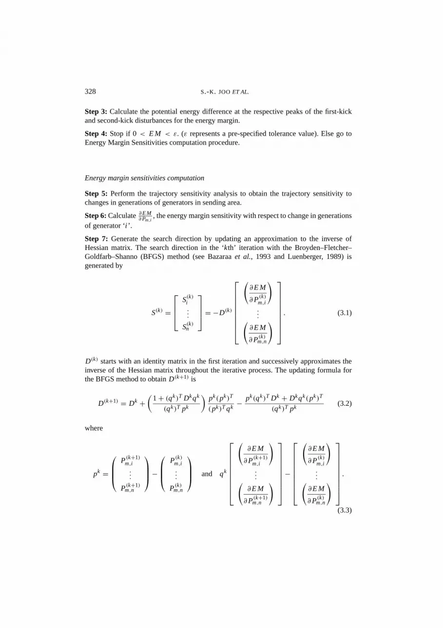
Step 7: Generate the search direction by updating an approximation to the inverse ofHessian matrix. The search direction in the ‘kth’ iteration with the Broyden–Fletcher–Goldfarb–Shanno (BFGS) method (see Bazaraaet al., 1993 and Luenberger, 1989) isgenerated by

S(k) =

S(k)i

···S(k)

n

= −D(k)

(∂ E M

∂ P(k)m,i

)

···(∂ E M

∂ P(k)m,n

)

. (3.1)

D(k) starts with an identity matrix in the first iteration and successively approximates theinverse of the Hessian matrix throughout the iterative process. The updating formula forthe BFGS method to obtainD(k+1) is

D(k+1) = Dk +(

1 + (qk)T Dkqk

(qk)T pk

)pk(pk)T

(pk)T qk− pk(qk)T Dk + Dkqk(pk)T

(qk)T pk(3.2)

where

pk =

P(k+1)m,i

···P(k+1)

m,n

−

P(k)m,i

···P(k)

m,n

and qk

(∂ E M

∂ P(k+1)m,i

)

···(∂ E M

∂ P(k+1)m,n

)

−

(∂ E M

∂ P(k)m,i

)

···(∂ E M

∂ P(k)m,n

)

.

(3.3)


Generation adjustment

Step 8: Determine the adjustments of generations of the sending area using the followingequation:

∆Pm,i

···∆Pm,n

=

α(k)i ×

(S(k)

i

)−1

···α

(k)n ×

(S(k)

n

)−1

× E M = kp

Pm,i

···Pm,n

(3.4)

where∑

i∈area Aα(k)i = 1. α

(k)i andkp are introduced to distribute the energy margin to

each generator such that generators in the sending area are adjusted in proportion to theirgenerations in the basecase. If the sending area includes only one generator, the generationof the generator in the sending area is adjusted using the following equation:

∆Pm,i =(

S(k)i

)−1 × E M . (3.5)

Step 9: Update generations of the sending area using the following equation:

Pnewm,1

···Pnew

m,k

=

Poldm,1

···Pold

m,k

+

∆Pm,1

···∆Pm,k

. (3.6)

Step 10: Go to second-kick-based Energy Margin Computation procedure and repeatalgorithms with rescheduled generations.

The proposed ATC calculation method will be illustrated with the two-area four-machine test system. First, it is necessary to establish a basecase, in which the systemload is supplied without violating any system limits such as thermal, voltage and stabilitylimits. The power transferred from area A to area B in the established basecase isequal to 453 MW. In the following example, the proposed ATC calculation methodattempts to determine ATC from area A to area B by increasing generation in area A andsimultaneously increasing the same amount of load at bus 13 in area B while examiningwhether stability limits are reached.

EXAMPLE 1 It is assumed in this example that the generation of generator 2 in area A isadjusted to increase power transfer from area A to area B while holding the generation ofgenerator 1 in area A. This assumption is made to calculate a point-to-point ATC from bus2 in area A to bus 13 in area B. Energy margin computation and energy margin sensitivityanalysis were performed with the established basecase. The second-kick scenario consistsof a temporary three-phase fault at bus 3, followed by another temporary three-phase faultat bus 20. The duration of the second-kick, which is a three-phase fault at bus 20, is selectedsuch as to yield a marginally stable trajectory. Results of the proposed ATC calculationmethod for Example 1 are summarized in Table 1.

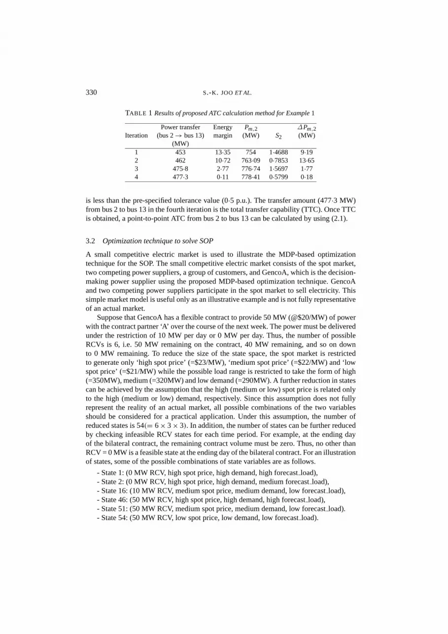
As can be seen in Table 1, the energy margin is reduced from iteration to iteration. Inthe fourth iteration, the proposed ATC calculation algorithm stops since the energy margin

330 S.-K. JOOET AL.

TABLE 1 Results of proposed ATC calculation method for Example 1

Power transfer Energy Pm,2 ∆Pm,2Iteration (bus 2→ bus 13) margin (MW) S2 (MW)

(MW)1 453 13·35 754 1·4688 9·192 462 10·72 763·09 0·7853 13·653 475·8 2·77 776·74 1·5697 1·774 477·3 0·11 778·41 0·5799 0·18

is less than the pre-specified tolerance value (0·5 p.u.). The transfer amount (477·3 MW)from bus 2 to bus 13 in the fourth iteration is the total transfer capability (TTC). Once TTCis obtained, a point-to-point ATC from bus 2 to bus 13 can be calculated by using (2.1).

3.2 Optimization technique to solve SOP

A small competitive electric market is used to illustrate the MDP-based optimizationtechnique for the SOP. The small competitive electric market consists of the spot market,two competing power suppliers, a group of customers, and GencoA, which is the decision-making power supplier using the proposed MDP-based optimization technique. GencoAand two competing power suppliers participate in the spot market to sell electricity. Thissimple market model is useful only as an illustrative example and is not fully representativeof an actual market.

Suppose that GencoA has a flexible contract to provide 50 MW (@$20/MW) of powerwith the contract partner ‘A’ over the course of the next week. The power must be deliveredunder the restriction of 10 MW per day or 0 MW per day. Thus, the number of possibleRCVs is 6, i.e. 50 MW remaining on the contract, 40 MW remaining, and so on downto 0 MW remaining. To reduce the size of the state space, the spot market is restrictedto generate only ‘high spot price’ (=$23/MW), ‘medium spot price’ (=$22/MW) and ‘lowspot price’ (=$21/MW) while the possible load range is restricted to take the form of high(=350MW), medium (=320MW) and low demand (=290MW). A further reduction in statescan be achieved by the assumption that the high (medium or low) spot price is related onlyto the high (medium or low) demand, respectively. Since this assumption does not fullyrepresent the reality of an actual market, all possible combinations of the two variablesshould be considered for a practical application. Under this assumption, the number ofreduced states is 54(= 6× 3× 3). In addition, the number of states can be further reducedby checking infeasible RCV states for each time period. For example, at the ending dayof the bilateral contract, the remaining contract volume must be zero. Thus, no other thanRCV = 0 MW is a feasible state at the ending day of the bilateral contract. For an illustrationof states, some of the possible combinations of state variables are as follows.

- State 1: (0 MW RCV, high spot price, high demand, high forecastload),- State 2: (0 MW RCV, high spot price, high demand, medium forecastload),- State 16: (10 MW RCV, medium spot price, medium demand, low forecastload),- State 46: (50 MW RCV, high spot price, high demand, high forecastload),- State 51: (50 MW RCV, medium spot price, medium demand, low forecastload).- State 54: (50 MW RCV, low spot price, low demand, low forecastload).


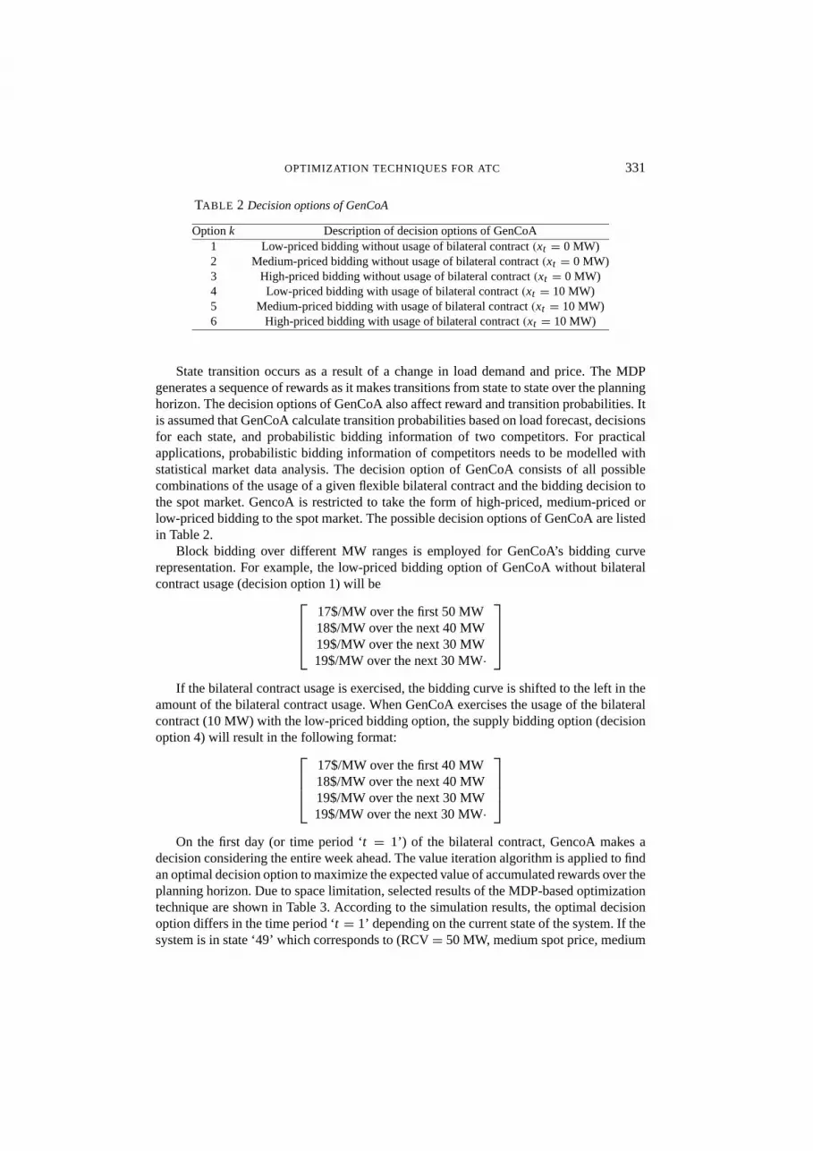
TABLE 2 Decision options of GenCoA

Optionk Description of decision options of GenCoA1 Low-priced bidding without usage of bilateral contract(xt = 0 MW)2 Medium-priced bidding without usage of bilateral contract(xt = 0 MW)3 High-priced bidding without usage of bilateral contract(xt = 0 MW)4 Low-priced bidding with usage of bilateral contract(xt = 10 MW)5 Medium-priced bidding with usage of bilateral contract(xt = 10 MW)6 High-priced bidding with usage of bilateral contract(xt = 10 MW)

State transition occurs as a result of a change in load demand and price. The MDPgenerates a sequence of rewards as it makes transitions from state to state over the planninghorizon. The decision options of GenCoA also affect reward and transition probabilities. Itis assumed that GenCoA calculate transition probabilities based on load forecast, decisionsfor each state, and probabilistic bidding information of two competitors. For practicalapplications, probabilistic bidding information of competitors needs to be modelled withstatistical market data analysis. The decision option of GenCoA consists of all possiblecombinations of the usage of a given flexible bilateral contract and the bidding decision tothe spot market. GencoA is restricted to take the form of high-priced, medium-priced orlow-priced bidding to the spot market. The possible decision options of GenCoA are listedin Table 2.

Block bidding over different MW ranges is employed for GenCoA’s bidding curverepresentation. For example, the low-priced bidding option of GenCoA without bilateralcontract usage (decision option 1) will be

17$/MW over the first 50 MW18$/MW over the next 40 MW19$/MW over the next 30 MW19$/MW over the next 30 MW·

If the bilateral contract usage is exercised, the bidding curve is shifted to the left in theamount of the bilateral contract usage. When GenCoA exercises the usage of the bilateralcontract (10 MW) with the low-priced bidding option, the supply bidding option (decisionoption 4) will result in the following format:

17$/MW over the first 40 MW18$/MW over the next 40 MW19$/MW over the next 30 MW19$/MW over the next 30 MW·

On the first day (or time period ‘t = 1’) of the bilateral contract, GencoA makes adecision considering the entire week ahead. The value iteration algorithm is applied to findan optimal decision option to maximize the expected value of accumulated rewards over theplanning horizon. Due to space limitation, selected results of the MDP-based optimizationtechnique are shown in Table 3. According to the simulation results, the optimal decisionoption differs in the time period ‘t = 1’ depending on the current state of the system. If thesystem is in state ‘49’ which corresponds to (RCV= 50 MW, medium spot price, medium

332 S.-K. JOOET AL.

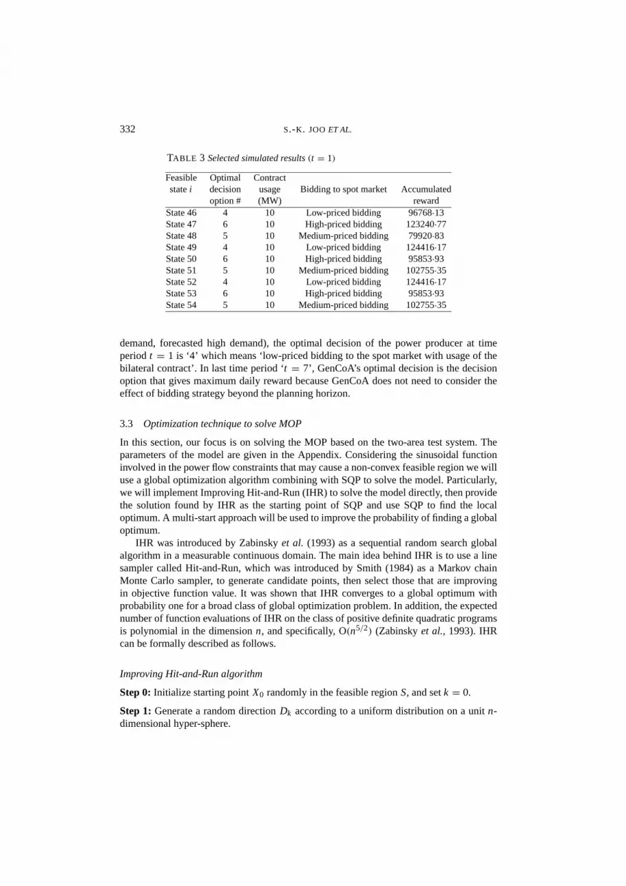
TABLE 3 Selected simulated results (t = 1)

Feasible Optimal Contractstatei decision usage Bidding to spot market Accumulated

option # (MW) rewardState 46 4 10 Low-priced bidding 96768·13State 47 6 10 High-priced bidding 123240·77State 48 5 10 Medium-priced bidding 79920·83State 49 4 10 Low-priced bidding 124416·17State 50 6 10 High-priced bidding 95853·93State 51 5 10 Medium-priced bidding 102755·35State 52 4 10 Low-priced bidding 124416·17State 53 6 10 High-priced bidding 95853·93State 54 5 10 Medium-priced bidding 102755·35

demand, forecasted high demand), the optimal decision of the power producer at timeperiodt = 1 is ‘4’ which means ‘low-priced bidding to the spot market with usage of thebilateral contract’. In last time period ‘t = 7’, GenCoA’s optimal decision is the decisionoption that gives maximum daily reward because GenCoA does not need to consider theeffect of bidding strategy beyond the planning horizon.

3.3 Optimization technique to solve MOP

In this section, our focus is on solving the MOP based on the two-area test system. Theparameters of the model are given in the Appendix. Considering the sinusoidal functioninvolved in the power flow constraints that may cause a non-convex feasible region we willuse a global optimization algorithm combining with SQP to solve the model. Particularly,we will implement Improving Hit-and-Run (IHR) to solve the model directly, then providethe solution found by IHR as the starting point of SQP and use SQP to find the localoptimum. A multi-start approach will be used to improve the probability of finding a globaloptimum.

IHR was introduced by Zabinskyet al. (1993) as a sequential random search globalalgorithm in a measurable continuous domain. The main idea behind IHR is to use a linesampler called Hit-and-Run, which was introduced by Smith (1984) as a Markov chainMonte Carlo sampler, to generate candidate points, then select those that are improvingin objective function value. It was shown that IHR converges to a global optimum withprobability one for a broad class of global optimization problem. In addition, the expectednumber of function evaluations of IHR on the class of positive definite quadratic programsis polynomial in the dimensionn, and specifically, O(n5/2) (Zabinskyet al., 1993). IHRcan be formally described as follows.

Improving Hit-and-Run algorithm

Step 0: Initialize starting pointX0 randomly in the feasible regionS, and setk = 0.

Step 1: Generate a random directionDk according to a uniform distribution on a unitn-dimensional hyper-sphere.


Step 2: Generate a pointYk+1 uniformly distributed on the line set

L = S ∩ {x |x = Xk + λDk, λ a real scalar}. (3.7)

Step 3: If the objective function value at the pointYk+1 is better than that at the pointXk ,setXk+1 = Yk+1. Otherwise, setXk+1 = Xk .

Step 4: If a stopping criterion is satisfied, then stop. Otherwise incrementk and return tostep 1.

In contrast to IHR, the SQP method is a deterministic algorithm that searches for alocal optimum nearest to a given starting point. At each iteration of SQP, an approximationis made of the Hessian of the Lagrangian function. This is then used to generate a quadraticprogramming sub-problem involving the minimization of a quadratic approximation of theobjective function, subject to a linear approximation of the constraints. The solution ofthe sub-problem is then used to form a search direction for a line search procedure. Anoverview of SQP is found in Boggs & Tolle (1995).

As a deterministic algorithm, SQP is not a suitable algorithm for a global optimizationproblem. The performance of SQP is very sensitive to the initial starting point, whichinfluences which local optimum is detected. Therefore, instead of using SQP to solve theMOP directly, it is proposed to first use IHR, the global optimization algorithm, to finda good starting point, and then use SQP to search for the local optimum nearest to thestarting point. In order to improve the probability of finding the global optimum, a multi-start approach with our mixed algorithm will be used to solve the model. Particularly, inour code, the mixed algorithm will be run 50 times, and for each run, the maximum numberof iterations of IHR is 100 and the maximum number of iterations of SQP is 500.

A difficult step in the two-area MOP is to solve for bus angles embedded within theoptimization algorithm. Instead of choosingP1, . . . , P4 andL1, L2 as decision variables,our approach is to choose angle differences as decision variables. Particularly, five angledifferences,(θ1 − θ10), (θ2 − θ20), (θ3 − θ101), (θ13 − θ120) and(θ12 − θ120), are chosen asdecision variables, and the values of other angle differences andP1, . . . , P4, L1, L2 are thefunctions of the five decision variables. Considering the nature of the sinusoidal function,it is reasonable to set the upper and lower bounds of each decision variable to be−90◦ and90◦.

In our mixed algorithm, IHR is used to obtain a good starting point for SQP.Considering the difficulties for IHR to handle inequality and equality constraints, thoseconstraints are put into the objective function by adding a penalty on violated constraints.Therefore the feasible region S for IHR becomes a five-dimensional box with−90◦ and90◦ as the upper and lower bounds of angle difference, i.e.

S = {(∆θ1, . . . ,∆θ5) : ∆θi ∈ �−90◦, 90◦�, for i = 1, . . . , 5

}. (3.8)

It may cause the problem that, under some combination of decision variables inS, theremay exist complex numbers for other angle differences in the model. This drawback isalso considered in the objection function by adding another penalty. The penalty objectivefunction used for IHR is therefore as follows:

max f (∆θ) =4∑

i=1

ULi −2∑

j=1

CPj − µ (3.9)

334 S.-K. JOOET AL.

120 110 11

12

13

101 1

3

2

10 20

G11

G12G2

G1

1.451.60P1

P2P3

P4

L1 L2

1.60

1.40

3.00 0.18 0.18

0.180.18

3.36

1.453.00

1.55

2.64

FIG. 2. Optimal solution of two-area MOP.

where

CPj = α j P2j + β j Pj + γ j for j = 1, . . . , 4 (3.10)

ULi = −vi L2i + νi Li for i = 1, 2 (3.11)

µ ={

108 if complex number exists in the modelκ · 106 otherwise

(3.12)

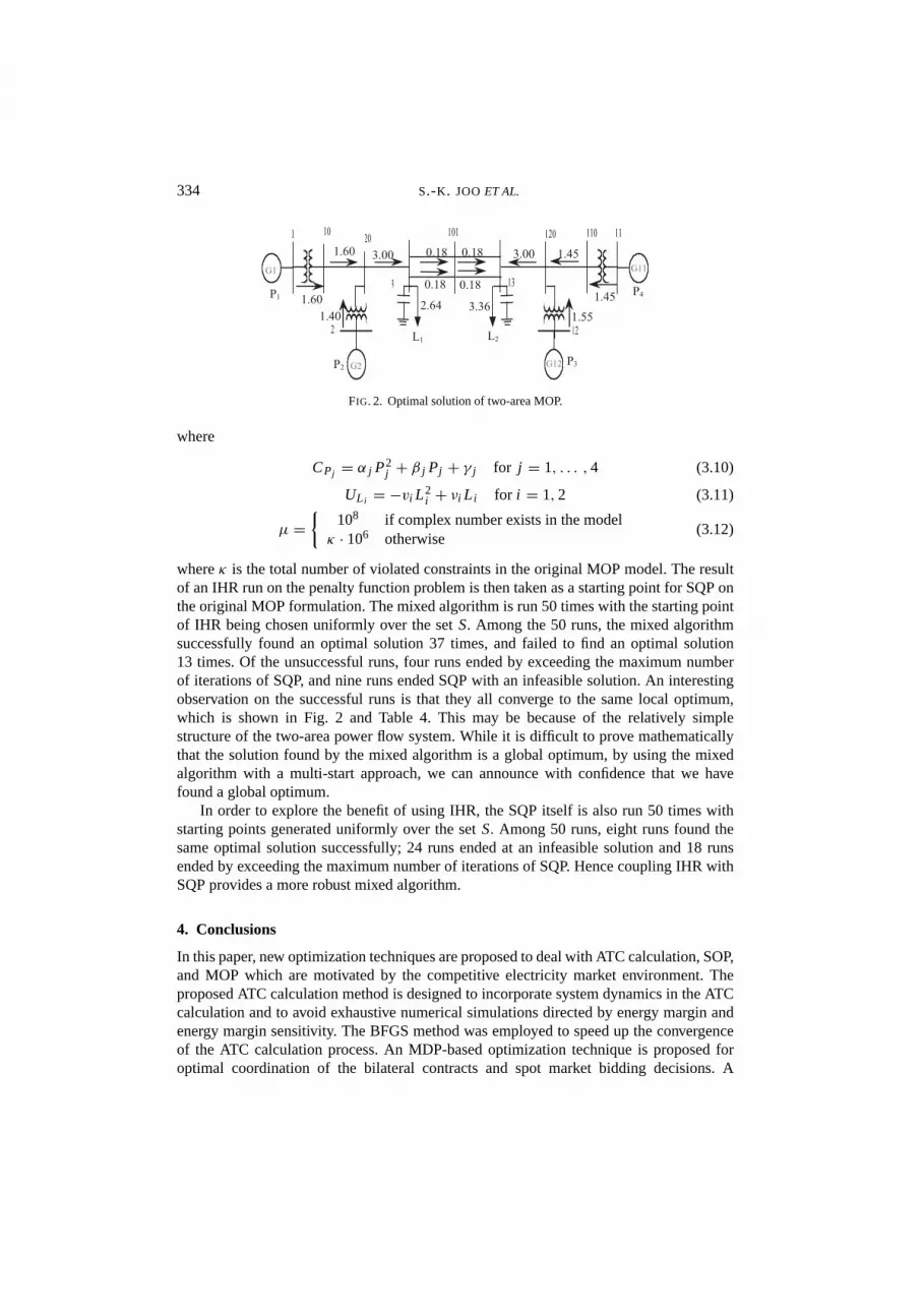
whereκ is the total number of violated constraints in the original MOP model. The resultof an IHR run on the penalty function problem is then taken as a starting point for SQP onthe original MOP formulation. The mixed algorithm is run 50 times with the starting pointof IHR being chosen uniformly over the setS. Among the 50 runs, the mixed algorithmsuccessfully found an optimal solution 37 times, and failed to find an optimal solution13 times. Of the unsuccessful runs, four runs ended by exceeding the maximum numberof iterations of SQP, and nine runs ended SQP with an infeasible solution. An interestingobservation on the successful runs is that they all converge to the same local optimum,which is shown in Fig. 2 and Table 4. This may be because of the relatively simplestructure of the two-area power flow system. While it is difficult to prove mathematicallythat the solution found by the mixed algorithm is a global optimum, by using the mixedalgorithm with a multi-start approach, we can announce with confidence that we havefound a global optimum.

In order to explore the benefit of using IHR, the SQP itself is also run 50 times withstarting points generated uniformly over the setS. Among 50 runs, eight runs found thesame optimal solution successfully; 24 runs ended at an infeasible solution and 18 runsended by exceeding the maximum number of iterations of SQP. Hence coupling IHR withSQP provides a more robust mixed algorithm.

4. Conclusions

In this paper, new optimization techniques are proposed to deal with ATC calculation, SOP,and MOP which are motivated by the competitive electricity market environment. Theproposed ATC calculation method is designed to incorporate system dynamics in the ATCcalculation and to avoid exhaustive numerical simulations directed by energy margin andenergy margin sensitivity. The BFGS method was employed to speed up the convergenceof the ATC calculation process. An MDP-based optimization technique is proposed foroptimal coordination of the bilateral contracts and spot market bidding decisions. A


TABLE 4 Optimal solution of two-area MOP

Decision variables:θ1 − θ10 = 1·5311◦, θ2 − θ20 = 1·3397◦,θ3 − θ101 = 1·1380◦, θ13 − θ120 = −1·7191◦, θ12 − θ120 = 1·4858◦

Bus angle Bus angle(setθ1 = 0◦) (setθ1 = 0◦)

Bus 1 0◦ Bus 11 −2·6409◦Bus 10 −1·5311◦ Bus 110 −4·0260◦Bus 20 −3·8236◦ Bus 120 −6·0996◦Bus 2 −2·4839◦ Bus 12 −4·6138◦Bus 3 −5·5427◦ Bus 13 −7·8188◦Bus 101 −6·6807◦

Maximum social welfare= 13893

global optimization algorithm, IHR, combined with the traditional SQP is introducedto solve marketing optimization problems. The proposed optimization techniques wereimplemented and tested on the two-area four-machine test system. The test results haveshown the effectiveness of the proposed optimization techniques.

Many other opportunities exist for the application of optimization techniques toelectricity market problems. Uncertainties in the market price require statistical forecastingtechniques. Prediction of the market behaviour is a natural problem for heuristiccomputational methods. The concept of efficient frontier in finance for risk managementrequires multi-objective optimization and the concept of Pareto optimality. Market clearingmechanisms may involve combinatorial optimization to select generating units to meet theload demand. The determination of a market equilibrium given a number of supply anddemand bids is an optimization problem.

Acknowledgements

This research is partially supported by the Advanced Power Technologies (APT) Centreat the University of Washington and the U.S. National Science Foundation Under Grant‘Transmission Expansion in an Open Access Environment: Reliability and Economics(ECS 0217701)’. The APT Centre is funded by AREVA T&D, BPA, CESI, LGIS,Mitsubishi Electric, PJM and RTE.

REFERENCES

ALSAC, O., BRIGHT, J., PRAIS, M. & STOTT, B. (1990) Further developments in lp-based optimalpower flow.IEEE Trans. Power Syst., 5, 697–711.

BAZARAA , M. S., SHERALI, H. D. & SHETTY, C. M. (1993)Nonlinear Programming. NewYork:Wiley, pp. 325–327.

BOGGS, P. T. & TOLLE, J. W. (1995) Sequential quadratic programming.Acta Numer., 4, 1–51.FOUAD, A. A. & V ITTAL , V. (1992)Power System Transient Stability Analysis Using the Transient

Energy Function Method. Englewood Cliffs, NJ: Prentice-Hall.GRAVENER, M. H., NWANKPA, C. & YEOH, T. (1999) ATC computational issues.Proc. 32nd

Hawaii Int. Conf. on System Sciences. pp. 1–6.

336 S.-K. JOOET AL.

HOWARD, R. A. (1960)Dynamic Programming and Markov Process. NewYork: MIT Press.JOO, S. K. & LIU, C. C. (2000) Electricity market simulation based on a markov decision model.

Proc. 4th Int. Conf. on Power Systems Operation and Planning. pp. 102–103.KAYE, R.J., OUTHRED, H. R. & BANNISTER, C. H. (1990) Forward contracts for the operation of

an electricity industry under spot pricing.IEEE Trans. Power Syst., 5, 46–52.LUENBERGER, D. G. & , (1989) Linear and Nonlinear Programming. Reading, MA: Addison-

Wesley, pp. 268–271.NORTH AMERICAN ELECTRIC RELIABILITY COUNCIL (1995)Transmission Transfer Capability.

Princeton, NJ: NERC.NORTH AMERICAN ELECTRIC RELIABILITY COUNCIL (1996) Available Transfer Capability

Definitions and Determination. Princeton, NJ: NERC.PHAM , D. T. & K ARABOGA, D. (2000)Intelligent Optimisation Techniques: Genetic Algorithms,

Tabu Search, Simulated Annealing and Neural Networks. London: Springer.ROTTING, T. A. & GJELSVIK, A. (1993) Stochastic dual dynamic programming for seasonal

scheduling in the Norwegian power system.IEEE Trans. Power Syst., 7, 273–279.SHEN, Y., LAWARREE, J., LIU, C. C. & ZABINSKY, Z. B. (2003) Global optimization in an

electricity market environment.Proc. IEEE Bologna Power Tech.SMITH , R. L. (1984) Efficient Monte Carlo procedures for generating points uniformly distributed

over bounded region.Oper. Res., 32, 1296–1308.SONG, H., LIU, C. C., LAWARREE, J. & DAHLGREN, R. (2000) Optimal electricity supply bidding

by Markov decision process.IEEE Trans. Power Syst., 15, 618–624.SUN, D., ASHLEY, B., BREWER, B., HUGHES, A. & T INNEY, W. F. (1984) Optimal power flow

by Newton approach.IEEE Trans. Power Apparatus Syst., 103, 2864–2880.WOOD, A. & W OLLENBERG, B. (1996) Power Generation Operation and Control. New York:

Wiley.ZABINSKY , Z. B., SMITH , R. L., MCDONALD, J. F., ROMEIJN, H. E. & KAUFMAN , D. E. (1993)

Improving hit-and-run for global optimization.J. Global Optim., 3, 171–192.

Appendix

TABLE A1 Parameters of cost functions of generators andthe upper and lower bounds of generators

Generator (P) Lower Upper Cost function parametersbounds bounds α β γ

1 0 5 100 700 3002 0 4 150 600 1003 0 3 200 400 1504 0 3·5 180 500 150


TABLE A2 Parameters of utilityfunctions of loads

Loads Utility function parameters(L) ν v

1 160 35002 200 4000

TABLE A3 Capacities and reactance of transmission lines

Connected buses Capacity(C APbk) Reactance(xb k)

Busb Busk1 10 3·0 0·016710 20 3·0 0·02502 20 3·0 0·016720 3 3·0 0·01003 101 (1) 3·0 0·11003 101 (2) 3·0 0·110013 101 (1) 3·0 0·110013 101 (2) 3·0 0·1100120 13 3·0 0·010012 120 3·0 0·0167110 120 3·0 0·025011 110 3·0 0·0167

Note:xb k = xk b

Optimization techniques for Available Transfer Capability (ATC) and market calculations

Documents