Optimization of a District Heating Network - TU Delft Repositories

Optimization of a Dis-trict Heating Networkwith the Focus on Heat Loss

T.J. de Boer

TechnischeUniversiteitDelft

Optimization of a District HeatingNetwork

with the Focus on Heat Loss

by

T.J. de Boer

in partial fulfillment of the requirements for the degree of

Master of Sciencein Mechanical Engineering

at the Delft University of Technology,to be defended publicly on Monday August 27, 2018 at 2:00 PM.

Supervisor: Prof. dr. ir. B. J. BoersmaThesis committee: Dr. ir. J. W. Haverkort, TU Delft

Dr. R. Delfos, TU DelftIng. S. M. F. Bunnik, Nuon Energy N.V.

An electronic version of this thesis is available at http://repository.tudelft.nl/.

Abstract

In the Netherlands most houses and buildings are connected to a gas network since the nineteenseventies to heat our houses and cook. In march of this year the new Dutch government announcedthat to meet the climate accord of Paris all dutch household should be of the gas net in 2030. To do thismultiple alternatives to heat homes are available and one of those which has proven to be feasible overthe last years is district heat. In a district heating network hot water is pumped round a city through anetwork of pipe lines to houses and other buildings. The network is split into a primary and a secondarynetwork. In the primary network the heat is transported from the source, and in the secondary networkthe heat is pumped from a substation to the customers. The heat usually is rest heat of a STEG- orwaste incineration power plant. With the increasing demand for heat due to the disconnection of thegas network, and at the same time the search for a more sustainable heat source for the district heatingnetwork like geothermal heat the prices and costs rise rapidly. This makes the heat loss in the systema more important issue also from a financial perspective. The current installed networks are all series1 single pipe lines of ST/PUR/PE, this means the inner pipe through which the water flows is steal,followed by an insulating PUR layer which is covered by a protective PE layer. To decrease the heat lossfrom the pipe lines Nuon is looking at two possible options. Series 2 single piping which has a thickerinsulating PUR layer and second the twin pipeline where both the steal supply and return lines areembedded into one insulating PUR layer and a protective PE shell. The heat loss calculations for theburied pipelines in the ground are done using empirical formulas found in literature. These are checkednumerical using a pde-solver. Comparing both results it was the concluded the empirical formulas givea good approximation of the heat loss. It also showed the heat loss is for a great deal depended on thetemperature in the pipe and the ground temperature. In current heat loss calculations done by Nuonthe temperature gradient of the water entering the network and leaving the network in not taken intoconsideration. By using the ambient temperature and a formula formulated in literature an estimationof the ground temperature at the buried depth of the pipelines can be made. By dividing the networkinto a number of pieces with length 𝑑𝑥 and an individual temperature 𝑇 the temperature gradient overthe entire network is taken into account. Collected data by Nuon concerning the user demand andthe ambient temperature makes it possible to simulate what is the mass flow through the system atany given time and to analyze how the system responds to a demand fluctuation. By analyzing whathappens in the networks in term of heat loss during a diurnal heat curve the results show that the heatloss stays nearly constant during a day. There are however big differences between different days indifferent times of the year. Analyzing what happens over the course of a year especially in the summerduring times of very low demand the system under performs. A main reason for this is caused by theminimum required temperature of 70 degrees Celsius at the customers due to salmonella regulations.This causes a lot of extra mass flow of hot water pumped around the system which heats up the returnflow. This is also clearly notable from the efficiency of the network which drops tremendously in thesummer. Comparing the difference in heat loss for the series 1, series 2 and twin system the resultswhere as expected an decrease in the amount of heat lost, by 14.6% for series 2 and 39.70% for twincompared to series 1. The overall image of what happens actually stays the same with high returntemperature and relative high heat loss and low efficiency in summer. There are a few options tofurther improve the performance of the system with a few percent by changing the inlet temperatureor the location of the bypass valve. Financially speaking the twin system is also the better choice ofthe three. Compared to series 1 for series 2 the investment costs will increase because the materialsand instalment costs will increase. For the twin system the prices of the materials will increase and theplacements of the welds will become more expansive however only half the number of pipe lines andjoints is needed, so in total the prices will stay nearly the same compared to series 1. There is a lot ofdiscussion on whether or not the maintenance costs will increase for the twin system, arguments forboth cases are given. However the maintenance costs are so small compared to the costs of the heatloss that in every case the twin system is clearly the better choice.

iii

Preface

The presented report is written to fulfill the final master thesis assignment that is part of the processand energy track of the master mechanical Engineering at the TU Delft. In this report you will find myfindings on the research I did on Optimization of a District heating Network with the Focus on HeatLoss.

Over the last few months I was able to work on my master thesis project at Nuon Energy N.V.they assigned me with the question of what the advantages and disadvantages for using the series2 and twin pipeline system would be as compared to the current used series 1. It was for me todetermine from what perspective I would approach this problem, where I would lay the focus on andwhat methods I would use to answer the questions. I’m really thank full for Nuon they gave me theopportunity and that they gave me this freedom for me to do useful research for them and also ensureI could do work on my master thesis. I would like to say special thanks to Stephan Bunnik from Nuonfor being my daily supervisor during the time I was working at Nuon.

I would like to thank Prof. dr. ir. Bendiks Jan Boersma for being my supervisor at the TU delft, andthe rest of the committee for being part of this.

T.J. de BoerDelft, August 2018

v

Contents

Abstract iii

List of Figures ix

List of Tables xi

1 Introduction 11.1 Design of a secondary district heating network . . . . . . . . . . . . . . . . . . . . . 2

1.1.1 piping. . . . . . . . . . . . . . . . . . . . . . . . . . . . . . . . . . . . . . . . . . 21.1.2 Heat transfer station. . . . . . . . . . . . . . . . . . . . . . . . . . . . . . . . . 21.1.3 Heat delivery set . . . . . . . . . . . . . . . . . . . . . . . . . . . . . . . . . . . 3

1.2 Scope of the thesis . . . . . . . . . . . . . . . . . . . . . . . . . . . . . . . . . . . . . . 3

2 Steady state heat loss calculations 52.1 Empirical heat loss calculations . . . . . . . . . . . . . . . . . . . . . . . . . . . . . . 5

2.1.1 Steady state heat flux . . . . . . . . . . . . . . . . . . . . . . . . . . . . . . . . 52.1.2 Heat Capacity of Water and conduction factors of materials . . . . . . . . . 5

2.2 Heat loss from a single insulated pipe . . . . . . . . . . . . . . . . . . . . . . . . . . 62.2.1 Single pipe in the ground . . . . . . . . . . . . . . . . . . . . . . . . . . . . . . 62.2.2 Two pipes in the ground. . . . . . . . . . . . . . . . . . . . . . . . . . . . . . . 62.2.3 Twin pipe in the ground . . . . . . . . . . . . . . . . . . . . . . . . . . . . . . . 7

2.3 Numerical solution . . . . . . . . . . . . . . . . . . . . . . . . . . . . . . . . . . . . . . 92.3.1 Model and boundary conditions.. . . . . . . . . . . . . . . . . . . . . . . . . . 92.3.2 Heat transmission form the ground to the air . . . . . . . . . . . . . . . . . . 102.3.3 Calculations . . . . . . . . . . . . . . . . . . . . . . . . . . . . . . . . . . . . . . 10

2.4 Results . . . . . . . . . . . . . . . . . . . . . . . . . . . . . . . . . . . . . . . . . . . . . 112.5 Conclusion . . . . . . . . . . . . . . . . . . . . . . . . . . . . . . . . . . . . . . . . . . 11

3 Model 133.1 Heat loss of hot water flowing through a pipe . . . . . . . . . . . . . . . . . . . . . . 133.2 state-space calculations. . . . . . . . . . . . . . . . . . . . . . . . . . . . . . . . . . . 14

3.2.1 Size of 𝑑𝑥 and time step 𝑑𝑡 . . . . . . . . . . . . . . . . . . . . . . . . . . . . . 143.2.2 Model . . . . . . . . . . . . . . . . . . . . . . . . . . . . . . . . . . . . . . . . . . 15

4 District Heating Network 174.1 Installed capacity of the HTS . . . . . . . . . . . . . . . . . . . . . . . . . . . . . . . . 18

4.1.1 Piping network . . . . . . . . . . . . . . . . . . . . . . . . . . . . . . . . . . . . 184.2 Operating the system . . . . . . . . . . . . . . . . . . . . . . . . . . . . . . . . . . . . 18

4.2.1 Bypass flow . . . . . . . . . . . . . . . . . . . . . . . . . . . . . . . . . . . . . . 194.2.2 Pump . . . . . . . . . . . . . . . . . . . . . . . . . . . . . . . . . . . . . . . . . . 19

5 Analysis of a system in operating conditions 215.1 Design condition . . . . . . . . . . . . . . . . . . . . . . . . . . . . . . . . . . . . . . . 215.2 Load condition . . . . . . . . . . . . . . . . . . . . . . . . . . . . . . . . . . . . . . . . 21

5.2.1 Diurnal Load curve. . . . . . . . . . . . . . . . . . . . . . . . . . . . . . . . . . 215.2.2 Annual Load Curve. . . . . . . . . . . . . . . . . . . . . . . . . . . . . . . . . . 22

5.3 Ground Temperature . . . . . . . . . . . . . . . . . . . . . . . . . . . . . . . . . . . . 225.3.1 Measured Temperature . . . . . . . . . . . . . . . . . . . . . . . . . . . . . . . 24

5.4 Ground conductivity . . . . . . . . . . . . . . . . . . . . . . . . . . . . . . . . . . . . . 24

vii

viii Contents

6 Heat loss 276.1 Logstor calculation tool . . . . . . . . . . . . . . . . . . . . . . . . . . . . . . . . . . . 276.2 Full load condition . . . . . . . . . . . . . . . . . . . . . . . . . . . . . . . . . . . . . . 27

6.2.1 Heat loss calculation using Matlab model . . . . . . . . . . . . . . . . . . . . 276.3 Operating condition . . . . . . . . . . . . . . . . . . . . . . . . . . . . . . . . . . . . . 286.4 Diurnal load curve . . . . . . . . . . . . . . . . . . . . . . . . . . . . . . . . . . . . . . 28

6.4.1 Mass flow . . . . . . . . . . . . . . . . . . . . . . . . . . . . . . . . . . . . . . . 286.4.2 Heat flux . . . . . . . . . . . . . . . . . . . . . . . . . . . . . . . . . . . . . . . . 29

6.5 Annual load curve results. . . . . . . . . . . . . . . . . . . . . . . . . . . . . . . . . . 306.5.1 Heat loss . . . . . . . . . . . . . . . . . . . . . . . . . . . . . . . . . . . . . . . . 306.5.2 mass flow . . . . . . . . . . . . . . . . . . . . . . . . . . . . . . . . . . . . . . . 306.5.3 Efficiency . . . . . . . . . . . . . . . . . . . . . . . . . . . . . . . . . . . . . . . 30

7 Results 337.1 Series 2 and Twin . . . . . . . . . . . . . . . . . . . . . . . . . . . . . . . . . . . . . . 33

7.1.1 Effect on heat loss . . . . . . . . . . . . . . . . . . . . . . . . . . . . . . . . . . 33

8 Changing the operating settings 358.1 By pass flow . . . . . . . . . . . . . . . . . . . . . . . . . . . . . . . . . . . . . . . . . . 358.2 Temperature. . . . . . . . . . . . . . . . . . . . . . . . . . . . . . . . . . . . . . . . . . 36

8.2.1 Temp decrease (Tin 72.5) . . . . . . . . . . . . . . . . . . . . . . . . . . . . . . 368.2.2 Temp increase (Tin 77.5 - 85) . . . . . . . . . . . . . . . . . . . . . . . . . . . 368.2.3 Changing the location of the bypass flow. . . . . . . . . . . . . . . . . . . . . 38

9 Total Cost of Ownership Analysis 399.1 Capex. . . . . . . . . . . . . . . . . . . . . . . . . . . . . . . . . . . . . . . . . . . . . . 39

9.1.1 Material Costs. . . . . . . . . . . . . . . . . . . . . . . . . . . . . . . . . . . . . 399.1.2 Contractor Costs . . . . . . . . . . . . . . . . . . . . . . . . . . . . . . . . . . . 39

9.2 Opex . . . . . . . . . . . . . . . . . . . . . . . . . . . . . . . . . . . . . . . . . . . . . . 399.2.1 Maintenance Costs . . . . . . . . . . . . . . . . . . . . . . . . . . . . . . . . . . 409.2.2 Heat loss Costs . . . . . . . . . . . . . . . . . . . . . . . . . . . . . . . . . . . . 40

9.3 Results . . . . . . . . . . . . . . . . . . . . . . . . . . . . . . . . . . . . . . . . . . . . . 40

10Conclusion and Recommendation 4310.1Conclusion . . . . . . . . . . . . . . . . . . . . . . . . . . . . . . . . . . . . . . . . . . 4310.2Recommendation . . . . . . . . . . . . . . . . . . . . . . . . . . . . . . . . . . . . . . . 43

Bibliography 45

A Size Table Logstor Piping 47

B Heat Transfer Station(HTS) 53

C Side view of the pipes in the ground. 55

D Numerical results 57D.1 Series 2 . . . . . . . . . . . . . . . . . . . . . . . . . . . . . . . . . . . . . . . . . . . . 57D.2 Twin . . . . . . . . . . . . . . . . . . . . . . . . . . . . . . . . . . . . . . . . . . . . . . 58

E Pressure triangle 59

F Pump Curve 61

G Ground 63

H Kasuda 65

I TCO 67

List of Figures

1.1 Main components in a district heating network . . . . . . . . . . . . . . . . . . . . . . 11.2 Single pipe . . . . . . . . . . . . . . . . . . . . . . . . . . . . . . . . . . . . . . . . . . 21.3 Twin pipe . . . . . . . . . . . . . . . . . . . . . . . . . . . . . . . . . . . . . . . . . . . 2

2.1 Two pipes in the ground. . . . . . . . . . . . . . . . . . . . . . . . . . . . . . . . . . . 72.2 Two pipes embedded in one circular insulation. . . . . . . . . . . . . . . . . . . . . . . 82.3 Heat loss in 𝑊/𝑚 for each DN-size. . . . . . . . . . . . . . . . . . . . . . . . . . . . . 82.4 Rectangular model of the ground mesh (top) with the single piping (middle left) and the

twin piping (middle right). Mesh of the single piping in the ground (left) and twin (right). 102.5 Temperature field in a single pipe (left), and twin (right). Temperature supply-return-

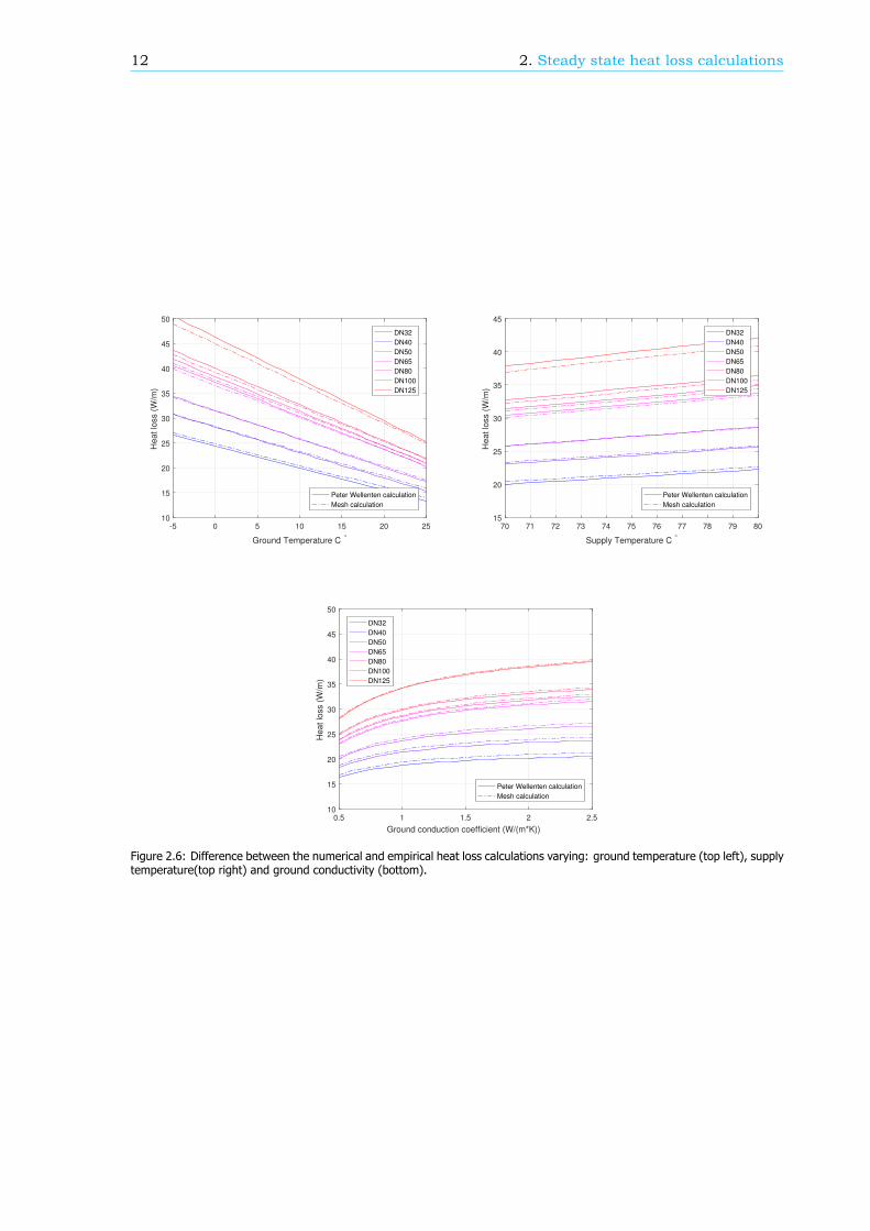
ground: 70-40-10 C. . . . . . . . . . . . . . . . . . . . . . . . . . . . . . . . . . . . . 112.6 Difference between the numerical and empirical heat loss calculations varying: ground

temperature (top left), supply temperature(top right) and ground conductivity (bottom). 12

3.1 Heat loss in a pipe section with length 𝑑𝑥. . . . . . . . . . . . . . . . . . . . . . . . . . 133.2 Flow chart of the Matlab model. . . . . . . . . . . . . . . . . . . . . . . . . . . . . . . 15

4.1 Aerial view of the district Schuytgraaf in Arnhem the Netherlands and a layout of thedistrict heating piping network. . . . . . . . . . . . . . . . . . . . . . . . . . . . . . . . 17

4.2 Schematic of the heat transfer station . . . . . . . . . . . . . . . . . . . . . . . . . . . 19

5.1 Percentage of the installed capacity demanded. . . . . . . . . . . . . . . . . . . . . . . 225.2 Daily demand curves, averaged for each month. . . . . . . . . . . . . . . . . . . . . . 225.3 Demand curves for January(Left) and August (right) . . . . . . . . . . . . . . . . . . . 235.4 Measured hourly demand data of an entire year with polynomial fit. . . . . . . . . . . . 235.5 Measured ambient temperature and plot for the ground temperature at a depth of 0.6m

as given by Kasuda. . . . . . . . . . . . . . . . . . . . . . . . . . . . . . . . . . . . . . 24

6.1 Mass flows in the system for an average day in winter(Left) and summer(right). . . . . 286.2 Return temperature curve for and average day in winter(Left) and summer(right). . . . 296.3 Heat flow in the system on a average day in winter(Left) and summer(right). . . . . . . 296.4 Heat loss supply pipe lines (Left) and return pipe lines (right) . . . . . . . . . . . . . . 306.5 Mass flows through the system. . . . . . . . . . . . . . . . . . . . . . . . . . . . . . . 316.6 Efficiency of the system. . . . . . . . . . . . . . . . . . . . . . . . . . . . . . . . . . . 31

7.1 Heat loss supply (Left) and return (right) for series 1, series 2 and twin. . . . . . . . . 337.2 Mass flows through the system for series 1, series 2 and twin. . . . . . . . . . . . . . 347.3 Efficiency (left) and return temperature(right) for series 1, series 2 and twin. . . . . . . 34

8.1 Increased mass flow. . . . . . . . . . . . . . . . . . . . . . . . . . . . . . . . . . . . . 358.2 Return Temperature for increased mass flow. . . . . . . . . . . . . . . . . . . . . . . . 368.3 Mass flows in the system for a range of inlet temperatures. . . . . . . . . . . . . . . . 368.4 Return temperatures for different inlet temperatures. . . . . . . . . . . . . . . . . . . . 378.5 Heat loss of the supply pipelines(right) and return pipelines(left). . . . . . . . . . . . . 378.6 Total heat loss of the piping network . . . . . . . . . . . . . . . . . . . . . . . . . . . . 388.7 Total heat loss of the piping network . . . . . . . . . . . . . . . . . . . . . . . . . . . . 38

9.1 Bar graph of the total cost of ownership over 30 years for series 1, series 2 and twin. . 41

B.1 Heat transfer station. . . . . . . . . . . . . . . . . . . . . . . . . . . . . . . . . . . . . 53

ix

x List of Figures

D.1 Difference between the numerical and empirical heat loss calculations varying: groundtemperature (top left), supply temperature(top right) and ground conductivity (bottom). 57

D.2 Difference between the numerical and empirical heat loss calculations varying: groundtemperature (top left), supply temperature(top right) and ground conductivity (bottom). 58

E.1 Pressure triangle. . . . . . . . . . . . . . . . . . . . . . . . . . . . . . . . . . . . . . . 59

F.1 Pump curve of the Wilo Stratos GIGA 65/1-21/2,3. . . . . . . . . . . . . . . . . . . . . 61

G.1 Daily ambient temperature plot with both Kasuda and Baggs prediction fot the temperature. 63

H.1 Temperature predictions done different depths with the formula of Kasuda at. . . . . . 65

I.1 Normalized prize development of the cost of heat for a gigajoule of heat. . . . . . . . . 67I.2 Bar graph of the TCO, difference between 30 and 40 year lifetime(top) and 200% in-

crease in maintenance costs(bottom). . . . . . . . . . . . . . . . . . . . . . . . . . . . 68

List of Tables

2.1 Heat conductivity of different Materials . . . . . . . . . . . . . . . . . . . . . . . . . . . 6

4.1 Piping in the AGH12 net. . . . . . . . . . . . . . . . . . . . . . . . . . . . . . . . . . . 18

6.1 Heat loss calculated by the Logstos calculation tool . . . . . . . . . . . . . . . . . . . . 276.2 Heat loss in GJ/year in the ideal situation . . . . . . . . . . . . . . . . . . . . . . . . . 28

7.1 Heat loss in GJ/year. . . . . . . . . . . . . . . . . . . . . . . . . . . . . . . . . . . . . . 34

8.1 Heat loss in GJ/year. . . . . . . . . . . . . . . . . . . . . . . . . . . . . . . . . . . . . . 38

xi

Nomenclature

𝛿𝑇 Temperature change

Mass flow

𝜈 Viscosity

𝑐 Distance between return and supply flow pipes

𝐶𝑝 Heat capacity

𝑑 Diameter of steel pipe

𝑑 Diameter of PUR layer

𝑑 Diameter of PE layer

𝑑𝑡 Time step

𝑑𝑥 Length delta x of a section of the pipe

𝐻 Depth at which the pipe is buried

ℎ Heat transmission

𝑘 Conductivity of steal pipe

𝑘 Conductivity of PUR layer

𝑘 Conductivity of PE layer

𝑘 Conductivity of steal pipe

𝑄 Heat in the system

𝑄 Heat flow in section

𝑞 Heat loss

𝑄 Heat flow out section

𝑅 Heat resistance

𝑅𝑒 Reynolds number

𝑇 Temperature

𝑇 Temperature

𝑇 Temperature

𝑇 Temperature

𝑇 Ambient temperature

𝑇 Ground temperature

𝑇 Return temperature

𝑇 Supply temperature

𝑇 Inlet temperature

𝑇 Outlet temperature

𝑣 Flow speed

xiii

1Introduction

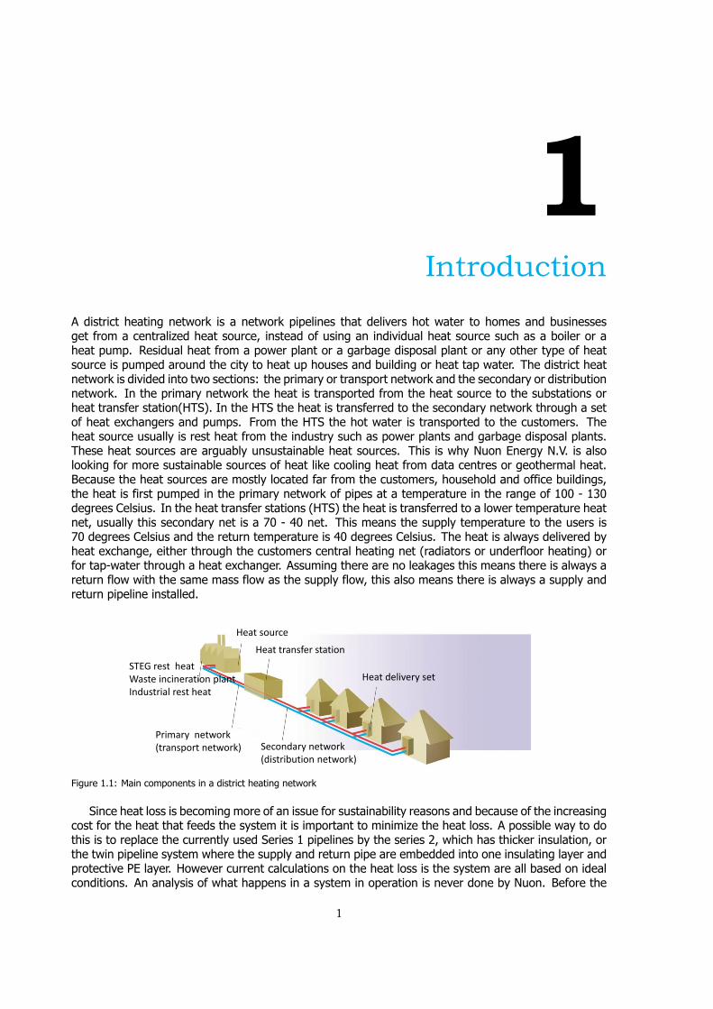
A district heating network is a network pipelines that delivers hot water to homes and businessesget from a centralized heat source, instead of using an individual heat source such as a boiler or aheat pump. Residual heat from a power plant or a garbage disposal plant or any other type of heatsource is pumped around the city to heat up houses and building or heat tap water. The district heatnetwork is divided into two sections: the primary or transport network and the secondary or distributionnetwork. In the primary network the heat is transported from the heat source to the substations orheat transfer station(HTS). In the HTS the heat is transferred to the secondary network through a setof heat exchangers and pumps. From the HTS the hot water is transported to the customers. Theheat source usually is rest heat from the industry such as power plants and garbage disposal plants.These heat sources are arguably unsustainable heat sources. This is why Nuon Energy N.V. is alsolooking for more sustainable sources of heat like cooling heat from data centres or geothermal heat.Because the heat sources are mostly located far from the customers, household and office buildings,the heat is first pumped in the primary network of pipes at a temperature in the range of 100 - 130degrees Celsius. In the heat transfer stations (HTS) the heat is transferred to a lower temperature heatnet, usually this secondary net is a 70 - 40 net. This means the supply temperature to the users is70 degrees Celsius and the return temperature is 40 degrees Celsius. The heat is always delivered byheat exchange, either through the customers central heating net (radiators or underfloor heating) orfor tap-water through a heat exchanger. Assuming there are no leakages this means there is always areturn flow with the same mass flow as the supply flow, this also means there is always a supply andreturn pipeline installed.

Heat source

Heat transfer station

Heat delivery set

Secondary network (distribution network)

Primary network (transport network)

STEG rest heat Waste incineration plant Industrial rest heat

Figure 1.1: Main components in a district heating network

Since heat loss is becoming more of an issue for sustainability reasons and because of the increasingcost for the heat that feeds the system it is important to minimize the heat loss. A possible way to dothis is to replace the currently used Series 1 pipelines by the series 2, which has thicker insulation, orthe twin pipeline system where the supply and return pipe are embedded into one insulating layer andprotective PE layer. However current calculations on the heat loss is the system are all based on idealconditions. An analysis of what happens in a system in operation is never done by Nuon. Before the

1

2 1. Introduction

question of how much heat loss can be saved by using the series 2 or twin system can be answered adetailed analysis of the performance of a district heating system in operation mode is done.

1.1. Design of a secondary district heating networkThe secondary district heating network can be split into three parts. First the HTS where the heatis transferred from the primary net to the distribution network. Second the distribution net whichconsists of a pipeline network through which the hot water is pumped towards the customers. Andlastly a supply set at the customers where the heat is delivered to either the central heating or thetap-water system.

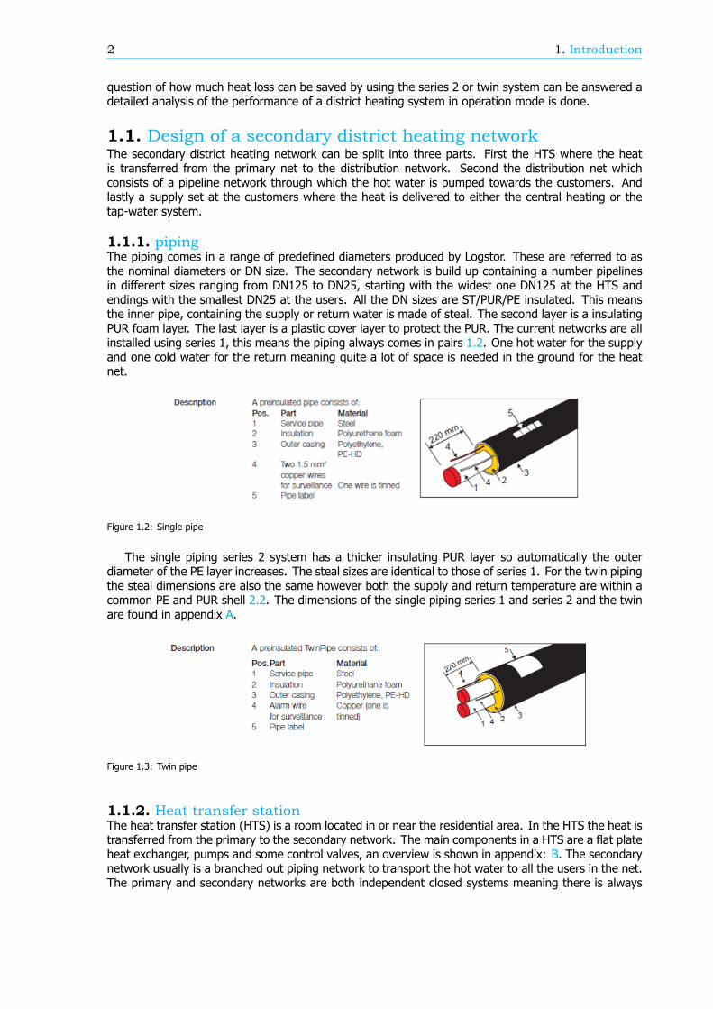
1.1.1. pipingThe piping comes in a range of predefined diameters produced by Logstor. These are referred to asthe nominal diameters or DN size. The secondary network is build up containing a number pipelinesin different sizes ranging from DN125 to DN25, starting with the widest one DN125 at the HTS andendings with the smallest DN25 at the users. All the DN sizes are ST/PUR/PE insulated. This meansthe inner pipe, containing the supply or return water is made of steal. The second layer is a insulatingPUR foam layer. The last layer is a plastic cover layer to protect the PUR. The current networks are allinstalled using series 1, this means the piping always comes in pairs 1.2. One hot water for the supplyand one cold water for the return meaning quite a lot of space is needed in the ground for the heatnet.

Figure 1.2: Single pipe

The single piping series 2 system has a thicker insulating PUR layer so automatically the outerdiameter of the PE layer increases. The steal sizes are identical to those of series 1. For the twin pipingthe steal dimensions are also the same however both the supply and return temperature are within acommon PE and PUR shell 2.2. The dimensions of the single piping series 1 and series 2 and the twinare found in appendix A.

Figure 1.3: Twin pipe

1.1.2. Heat transfer stationThe heat transfer station (HTS) is a room located in or near the residential area. In the HTS the heat istransferred from the primary to the secondary network. The main components in a HTS are a flat plateheat exchanger, pumps and some control valves, an overview is shown in appendix: B. The secondarynetwork usually is a branched out piping network to transport the hot water to all the users in the net.The primary and secondary networks are both independent closed systems meaning there is always

1.2. Scope of the thesis 3

a return flow of water. In the HTS the heat is transferred from the primary to the secondary networkthrough a flat plate heat exchanger. The water is pumped round in the secondary network by the twopumps in the HTS. The sizes of the heat exchanger and pumps are dependent on the amount andcapacity of the users in the secondary net. Usually this is somewhere between the 200 and 600 userswith an installed capacity of 8 to 22 kW depending on the size and demand of the user.

1.1.3. Heat delivery setThe users all have a supply set in their homes. The water is delivered to the users with a minimumtemperature of 70 degrees Celsius from here the hot water goes either directly into the central heatingsystem of the user or through a heat exchanger to heat the tap-water. Depending on the capacitythere is an maximum mass flow of water that can flow through the set. To heat the tap water thehot water always goes through a heat exchanger this is also the reason the temperature delivered toconsumers should always be 70 degrees Celsius, this is because of salmonella regulations. In times ofno, or very low, heat demand the temperature of the water will cool below that 70 degrees. In orderto keep the system at temperature a bypass is installed in the form of a temperature regulated valve,this is to ensure the water keeps flowing and stays at temperature.

1.2. Scope of the thesisThe scope of this project will be the heat losses in the secondary pipeline network under differentconditions and settings. The heat loss in the HTS, the supply set, and the performance of the heatexchangers and pumps are not taken into consideration. Also during operation other types of heatlosses can accrue such as heat losses caused by leakages or illegal tapping, these will all not be takeninto consideration.

2Steady state heat loss calculations

At first a solution to find the heat loss in the form of a steady state calculation is presented. This is donewith solutions based on explicit formulas found in literature which give an approximation for the heatloss of a buried district heating pipe in 𝑊/𝑚. Secondly the explicit formulae are checked for accuracyby a numerical evaluation. These calculation are done with a numerical partial differential equation(pde) solution using the pde-solver in MATLAB.

2.1. Empirical heat loss calculationsThe steady state heat loss of a district heating pipe system in the ground is analyzed. The empiricalformulas for heat loss calculation in the pipes are based on the literature by Petter Wallentén [1] andBenny Böhm [2].

2.1.1. Steady state heat fluxThe system is assumed to run continuous over time. So all the heat will settle in the ground over time,assuming the only heat loss is caused by the convection and radiation from the ground to the air. This iswhy the heat loss can be assumed to be steady state. The temperature fluctuation is not high enoughto take the transient heat loss in consideration. Also the temperature in the pipe is assumed uniformin a cross section: no laminar heat flux profile will form in the water. This can also be concluded fromthe fact that turbulent flow is assumed which follows from the calculations on the Reynolds numberfrom pipe flow.

𝑅𝑒 = 𝑣 ∗ 𝐷𝜈 (2.1)

The Reynold number is dependent on the flow velocity of the water(𝑣), the diameter of the pipe(𝐷)and the viscosity of the water(𝜈), equation: 2.1. The diameter is depending on the DN-size of the pipe.The viscosity is depended on the temperature and pressure of the water, which varies throughout theentire network. The flow speed is depending on the demand of the individual users. This means manyunique Reynolds numbers are found in the system. The flow is assumed laminar when the Reynoldsnumber is below 2100 [3]. When the total demand is assumed at max capacity of the system and isdistributed equally over all the users and the temperature in the entire system is set at 70 degreesthe Reynolds number is above 2100 everywhere. At 40% of maximum mass flow the first pipe sectiondrops below 2100, a DN32 section. At 10% all of the DN25 and still only the one DN32 section have aReynolds number below 2100. However in reality the demand won’t be distributed equally over all theusers. This will mean that in some sections the flow will be zero while in others the flow will be higherat any given time, this is especially true for the DN25 pipes which are at the end of a string connectingthe user. This means it is save to assume the flow is always turbulent.

2.1.2. Heat Capacity of Water and conduction factors of materialsAlthough the heat capacity of water is temperature dependent in this thesis and in the model, becauseof calculation time the 𝐶𝑝 of water is assumed constant and set at a value of 4180 𝐽/𝑘𝑔𝐾. The

5

6 2. Steady state heat loss calculations

conduction factors used are in table 2.1.

Material Conductivity [W/m*K] VariableSteel (ST) 43 𝑘PUR 0.03 𝑘PE 0.33 𝑘Ground 1.6 𝑘

Table 2.1: Heat conductivity of different Materials

All these values for conductivity are assumed constant so independent of the temperature. Alsothe conductivity for PUR increases over time [4], this is not taken in account but the live-time averageis taken. The conductivity for the ground or soil is influenced a lot by all different factors dependingon the type of soil and for example moist level, this will be discussed in chapter 5. The most commonvalue in the Netherlands is 1.6𝑊/(𝑚 ∗ 𝐾).

2.2. Heat loss from a single insulated pipeThe formula for the heat loss of a single pipe in any medium is given by equation 2.2 [5].

𝑞 = 2 ∗ 𝜋 ∗ 𝐿 ∗ 𝑘 ∗ (𝑇 − 𝑇 )/𝑙𝑛(𝑟 /𝑟 ). (2.2)

2.2.1. Single pipe in the groundThe empirical formulae of Petter Wellenten also take in account the effect of the ground and the effectof the interaction between the supply and return heat.

The heat loss is a function of the temperature difference and the thermal conductivity of the ground.The heat loss is given by 2.3 in [W/m]. The variables are defined showed in figure ??. The dimensionsare depending on the DN-size given in appendix ??.

𝑞 = 2 ∗ 𝜋 ∗ 𝑘 ∗ (𝑇 − 𝑇 ) ∗ ℎ (𝐻/𝑟 , Β). (2.3)

For the dimensionless heat loss factor h1 we get:

ℎ 1 = 𝑙𝑛(2𝐻𝑟 ) + Β. (2.4)

The dimensionless parameter Β is given as:

Β = 𝑘 ∗ ( 1𝑘 𝑙𝑛(𝑟𝑟 ) +1𝑘 𝑙𝑛(𝑟𝑟 ) +

1𝑘 𝑙𝑛(𝑟𝑟 )). (2.5)

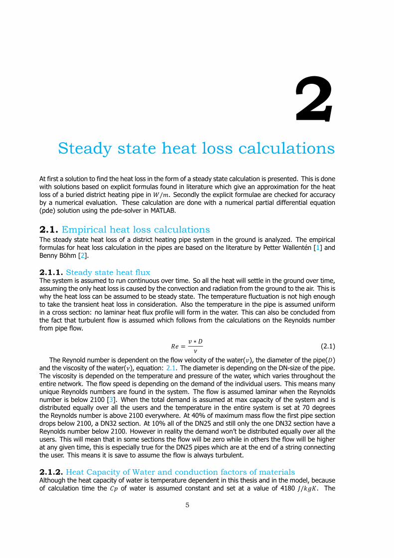
2.2.2. Two pipes in the groundFor two pipes in the ground an extra term is added for the influence the two pipes have on each-other.Two formulas for the heat loss of buried district heating pipes are mentioned in literature [1] and [2].The formula given by Wellenten:

𝑞 = 4 ∗ 𝜋 ∗ 𝑘 ∗ ((𝑇 + 𝑇2 − 𝑇 ) ∗ ℎ (𝐻/𝑟 , 𝐷/𝑟 , Β). (2.6)

𝑇 and 𝑇 are defined as:

𝑇 = 𝑇 + 𝑇2 . (2.7)

𝑇 = 𝑇 − 𝑇2 . (2.8)

and

ℎ 1 = 𝑙𝑛(2𝐻𝑟 ) + Β + 𝑙𝑛(√1 + (𝐻𝐷 ) ). (2.9)

2.2. Heat loss from a single insulated pipe 7

Figure 2.1: Two pipes in the ground.

Or the formula as given by Böhm:

𝑞 = Δ𝑇/𝑅. (2.10)

𝑞 =(𝑇 − 𝑇 ) ∗ (𝑅 + 𝑅 ) − (𝑇 − 𝑇 ) ∗ 𝑅

(𝑅 + 𝑅 ) ∗ (𝑅 + 𝑅 ) − 𝑅 . (2.11)

1/𝑅 =∑(1/𝑅 + 1/𝑅 + 1/𝑅 + ... + 1/𝑅 ). (2.12)

1/𝑅 = 2𝜋𝑙𝑛 + 𝑙𝑛

. (2.13)

1/𝑅 = 2𝜋𝑘𝑙𝑛

. (2.14)

1/𝑅4𝜋𝑘𝑙𝑛(1 + ( ) )

. (2.15)

2.2.3. Twin pipe in the groundThe empirical formula for the heat loss of the twin-pipe system in the ground is also given by PetterWallentén.

𝑞 = 𝑞 + 𝑞 (2.16)

𝑞 = 𝑞 − 𝑞 (2.17)

𝑞 = (𝑇 − 𝑇 ) ∗ 2𝜋𝜆 ∗ ℎ (𝑟 /𝑟 , 𝐷/𝑟 ) (2.18)

𝑞 = 𝑇 ∗ 2𝜋𝜆 ∗ ℎ (𝑟 /𝑟 , 𝐷/𝑟 ) (2.19)

ℎ 1 = 𝑙𝑛( 𝑟2𝐷𝑟 ) − 𝑙𝑛(𝑟

𝑟 − 𝐷 ) (2.20)

8 2. Steady state heat loss calculations

Figure 2.2: Two pipes embedded in one circular insulation.

ℎ 1 = 𝑙𝑛(2𝐷𝑟 ) − 𝑙𝑛(𝑟 + 𝐷𝑟 − 𝐷 ) (2.21)

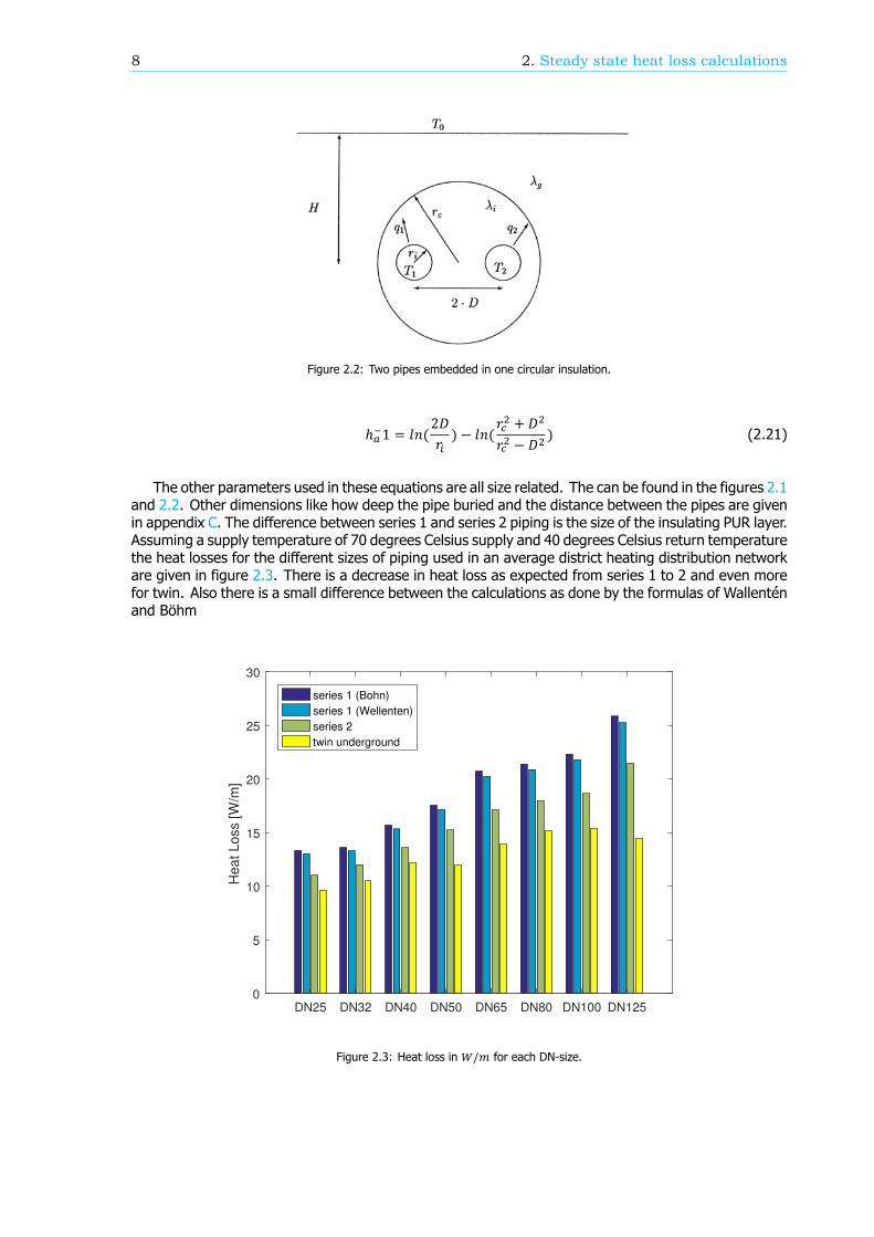
The other parameters used in these equations are all size related. The can be found in the figures 2.1and 2.2. Other dimensions like how deep the pipe buried and the distance between the pipes are givenin appendix C. The difference between series 1 and series 2 piping is the size of the insulating PUR layer.Assuming a supply temperature of 70 degrees Celsius supply and 40 degrees Celsius return temperaturethe heat losses for the different sizes of piping used in an average district heating distribution networkare given in figure 2.3. There is a decrease in heat loss as expected from series 1 to 2 and even morefor twin. Also there is a small difference between the calculations as done by the formulas of Wallenténand Böhm

DN25 DN32 DN40 DN50 DN65 DN80 DN100 DN1250

5

10

15

20

25

30

He

at

Lo

ss [

W/m

]

series 1 (Bohn)

series 1 (Wellenten)

series 2

twin underground

Figure 2.3: Heat loss in / for each DN-size.

2.3. Numerical solution 9

2.3. Numerical solutionBesides an empirical solution the heat loss of the pipeline will be analyzed using a numerical model tovalidate the empirical solution. The results will be compared in this next section. To find a numericalsolution for this problem the side view is divided in a grid, each section of the mesh is then given atemperature so a partial differential equation (pde) can be used to determine the heat flux betweenneighboring grid sections. There are different software packages that are used to solve problems likethis. In this case the pde-solver toolbox of Matlab is used. The same assumptions can be done asin the previous part so a steady state is assumed. This means the net heat flux in the ground willapproach zero and the only heat loss is from convection and radiation form the ground to the air. Alsothe flow in the pipe is assumed fully developed and the temperature of the temperature of the wateris uniform distributed over a cross section.

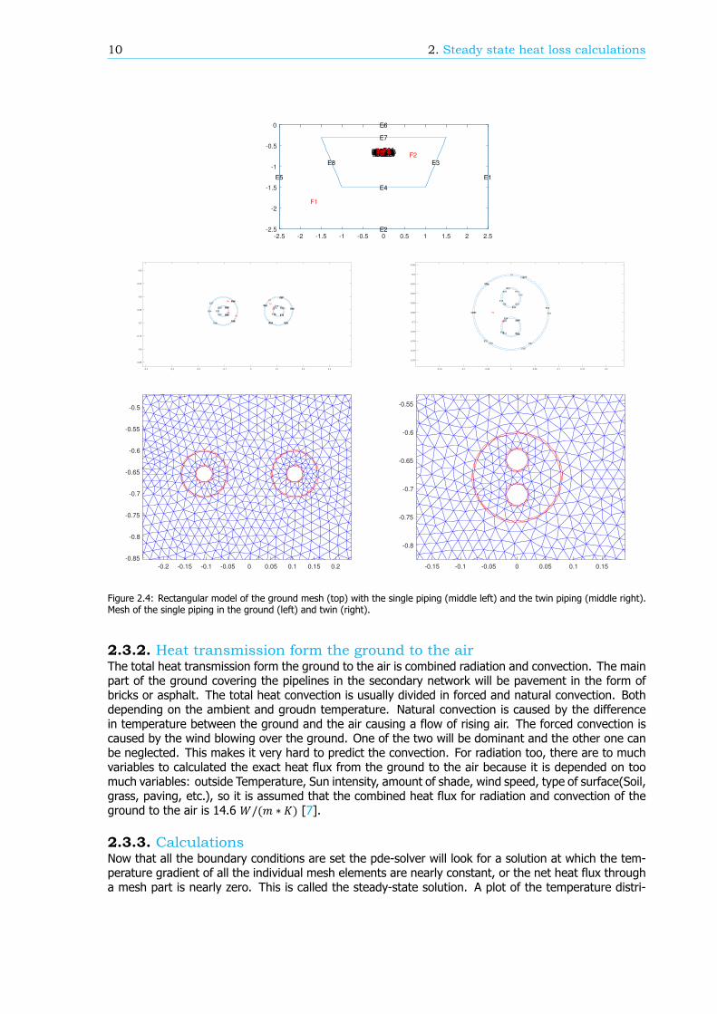
2.3.1. Model and boundary conditions.The model is a grid of 5000 mm by 2500 mm 2.4. This is to be the limit at which the ground temperatureis influenced by the heat from the pipes [6]. A too large model will cost to much computing powerespecially since the sizes of the mesh need to be small enough so the different layers of the insulatedpipes can be defined. At these boundaries the temperature of the ground is assumed to be no longerinfluenced by the heat from the pipe meaning that the heat flux at these boundaries is set to zero.This also means the only heat flux in the system is at the boundary between the ground and the air.This heat flux is combined heat radiation and convection. The last boundary conditions are set at theinside of the pipelines. These are set at a constant temperature.

10 2. Steady state heat loss calculations

-2.5 -2 -1.5 -1 -0.5 0 0.5 1 1.5 2 2.5

-2.5

-2

-1.5

-1

-0.5

0

E1

E2

E3

E4

E5

E6

E7

E8

E9E10E11E12E13E14E15E16E17E18E19E20E21E22E23E24E25E26

E27E28E29E30E31E32E33E34E35E36E37

E38E39E40

F1

F2F3F4F5F6F7F8

-0.4 -0.3 -0.2 -0.1 0 0.1 0.2 0.3

-0.85

-0.8

-0.75

-0.7

-0.65

-0.6

-0.55

-0.5

E9 E10

E11E12

E13E14

E15

E16E17

E18 E19

E20

E21

E22

E23 E24

E25

E26

E27 E28

E29E30

E31

E32

E33

E34

E35

E36E37

E38E39

E40

F3

F4F5

F6

F7

F8

-0.2 -0.15 -0.1 -0.05 0 0.05 0.1 0.15 0.2

-0.85

-0.8

-0.75

-0.7

-0.65

-0.6

-0.55

-0.5

Block with Finite Element Mesh Displayed

-0.15 -0.1 -0.05 0 0.05 0.1 0.15 0.2

-0.78

-0.76

-0.74

-0.72

-0.7

-0.68

-0.66

-0.64

-0.62

-0.6

-0.58

E9 E10

E11E12

E13

E14

E15

E16

E17 E18

E19E20

E21E22

E23E24

E25

E26 E27

E28

E29

E30

E31

E32

E33

E34

E35

E36

F3

F4

F5

F6

-0.15 -0.1 -0.05 0 0.05 0.1 0.15

-0.8

-0.75

-0.7

-0.65

-0.6

-0.55

Block with Finite Element Mesh Displayed

Figure 2.4: Rectangular model of the ground mesh (top) with the single piping (middle left) and the twin piping (middle right).Mesh of the single piping in the ground (left) and twin (right).

2.3.2. Heat transmission form the ground to the airThe total heat transmission form the ground to the air is combined radiation and convection. The mainpart of the ground covering the pipelines in the secondary network will be pavement in the form ofbricks or asphalt. The total heat convection is usually divided in forced and natural convection. Bothdepending on the ambient and groudn temperature. Natural convection is caused by the differencein temperature between the ground and the air causing a flow of rising air. The forced convection iscaused by the wind blowing over the ground. One of the two will be dominant and the other one canbe neglected. This makes it very hard to predict the convection. For radiation too, there are to muchvariables to calculated the exact heat flux from the ground to the air because it is depended on toomuch variables: outside Temperature, Sun intensity, amount of shade, wind speed, type of surface(Soil,grass, paving, etc.), so it is assumed that the combined heat flux for radiation and convection of theground to the air is 14.6 𝑊/(𝑚 ∗ 𝐾) [7].

2.3.3. CalculationsNow that all the boundary conditions are set the pde-solver will look for a solution at which the tem-perature gradient of all the individual mesh elements are nearly constant, or the net heat flux througha mesh part is nearly zero. This is called the steady-state solution. A plot of the temperature distri-

2.4. Results 11

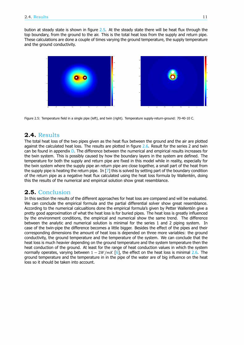
bution at steady state is shown in figure 2.5. At the steady state there will be heat flux through thetop boundary, from the ground to the air. This is the total heat loss from the supply and return pipe.These calculations are done a couple of times varying the ground temperature, the supply temperatureand the ground conductivity.

Figure 2.5: Temperature field in a single pipe (left), and twin (right). Temperature supply-return-ground: 70-40-10 C.

2.4. ResultsThe total heat loss of the two pipes given as the heat flux between the ground and the air are plottedagainst the calculated heat loss. The results are plotted in figure 2.6. Result for the series 2 and twincan be found in appendix D. The difference between the numerical and empirical results increases forthe twin system. This is possibly caused by how the boundary layers in the system are defined. Thetemperature for both the supply and return pipe are fixed in this model while in reality, especially forthe twin system where the supply pipe an return pipe are close together, a small part of the heat fromthe supply pipe is heating the return pipe. In [7] this is solved by setting part of the boundary conditionof the return pipe as a negative heat flux calculated using the heat loss formula by Wallentén, doingthis the results of the numerical and empirical solution show great resemblance.

2.5. ConclusionIn this section the results of the different approaches for heat loss are compared and will be evaluated.We can conclude the empirical formula and the partial differential solver show great resemblance.According to the numerical calcualtions done the empirical formula’s given by Petter Wallentén give apretty good approximation of what the heat loss is for buried pipes. The heat loss is greatly influencedby the environment conditions, the empirical and numerical show the same trend. The differencebetween the analytic and numerical solution is minimal for the series 1 and 2 piping system. Incase of the twin-pipe the difference becomes a little bigger. Besides the effect of the pipes and theircorresponding dimensions the amount of heat loss is depended on three more variables: the groundconductivity, the ground temperature and the temperature of the system. We can conclude that theheat loss is much heavier depending on the ground temperature and the system temperature then theheat conduction of the ground. At least for the range of heat conduction values in which the systemnormally operates, varying between 1 − 2𝑊/𝑚𝐾 [6], the effect on the heat loss is minimal 2.6. Theground temperature and the temperature in in the pipe of the water are of big influence on the heatloss so it should be taken into account.

12 2. Steady state heat loss calculations

-5 0 5 10 15 20 25

Ground Temperature C °

10

15

20

25

30

35

40

45

50

He

at

loss (

W/m

)

DN32

DN40

DN50

DN65

DN80

DN100

DN125

Peter Wellenten calculation

Mesh calculation

70 71 72 73 74 75 76 77 78 79 80

Supply Temperature C °

15

20

25

30

35

40

45

He

at

loss (

W/m

)

DN32

DN40

DN50

DN65

DN80

DN100

DN125

Peter Wellenten calculation

Mesh calculation

0.5 1 1.5 2 2.5

Ground conduction coefficient (W/(m*K))

10

15

20

25

30

35

40

45

50

He

at

loss (

W/m

)

DN32

DN40

DN50

DN65

DN80

DN100

DN125

Peter Wellenten calculation

Mesh calculation

Figure 2.6: Difference between the numerical and empirical heat loss calculations varying: ground temperature (top left), supplytemperature(top right) and ground conductivity (bottom).

3Model

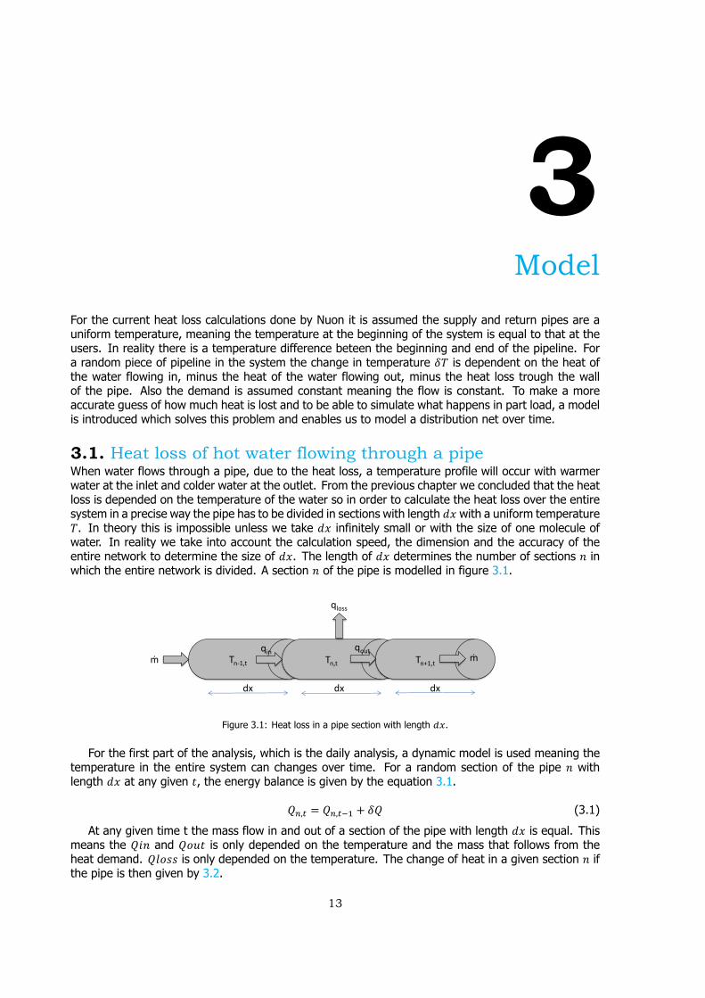
For the current heat loss calculations done by Nuon it is assumed the supply and return pipes are auniform temperature, meaning the temperature at the beginning of the system is equal to that at theusers. In reality there is a temperature difference beteen the beginning and end of the pipeline. Fora random piece of pipeline in the system the change in temperature 𝛿𝑇 is dependent on the heat ofthe water flowing in, minus the heat of the water flowing out, minus the heat loss trough the wallof the pipe. Also the demand is assumed constant meaning the flow is constant. To make a moreaccurate guess of how much heat is lost and to be able to simulate what happens in part load, a modelis introduced which solves this problem and enables us to model a distribution net over time.

3.1. Heat loss of hot water flowing through a pipeWhen water flows through a pipe, due to the heat loss, a temperature profile will occur with warmerwater at the inlet and colder water at the outlet. From the previous chapter we concluded that the heatloss is depended on the temperature of the water so in order to calculate the heat loss over the entiresystem in a precise way the pipe has to be divided in sections with length 𝑑𝑥 with a uniform temperature𝑇. In theory this is impossible unless we take 𝑑𝑥 infinitely small or with the size of one molecule ofwater. In reality we take into account the calculation speed, the dimension and the accuracy of theentire network to determine the size of 𝑑𝑥. The length of 𝑑𝑥 determines the number of sections 𝑛 inwhich the entire network is divided. A section 𝑛 of the pipe is modelled in figure 3.1.

Tn-1,t Tn,t Tn+1,t

dx dx dx

ṁ ṁ

qloss

qin qout

Figure 3.1: Heat loss in a pipe section with length .

For the first part of the analysis, which is the daily analysis, a dynamic model is used meaning thetemperature in the entire system can changes over time. For a random section of the pipe 𝑛 withlength 𝑑𝑥 at any given 𝑡, the energy balance is given by the equation 3.1.

𝑄 , = 𝑄 , + 𝛿𝑄 (3.1)

At any given time t the mass flow in and out of a section of the pipe with length 𝑑𝑥 is equal. Thismeans the 𝑄𝑖𝑛 and 𝑄𝑜𝑢𝑡 is only depended on the temperature and the mass that follows from theheat demand. 𝑄𝑙𝑜𝑠𝑠 is only depended on the temperature. The change of heat in a given section 𝑛 ifthe pipe is then given by 3.2.

13

14 3. Model

𝛿𝑄 = 𝑄𝑖𝑛 − 𝑄𝑜𝑢𝑡 − 𝑄𝐿𝑜𝑠𝑠 (3.2)

𝑄 , = 𝑄 , + 𝑄𝑖𝑛 , − 𝑄𝑜𝑢𝑡 , − 𝑄𝑙𝑜𝑠𝑠 , (3.3)

𝑄 , = (𝑇 , − 𝑇 𝑒𝑓) ∗ 𝑚 , ∗ 𝑐 (3.4)

The heat flow from the section 𝑛 − 1 to 𝑛 and from 𝑛 to 𝑛 + 1 are defined as:

��𝑖𝑛 , = (𝑇 , − 𝑇 ) ∗ �� , ∗ 𝑐 (3.5)

��𝑜𝑢𝑡 , = (𝑇 , − 𝑇 ) ∗ �� , ∗ 𝑐 (3.6)

The equations for the heat loss 𝑞 function given in the previous chapter has units (𝑊/𝑚) so itneeds to be multiplied by 𝑑𝑥. Everything added together we get:

𝑄 , (𝑚, 𝑇 , ) = 𝑄 , (𝑚, 𝑇 , ) + 𝑄𝑖𝑛 , (��, 𝑇 , ) − 𝑄𝑜𝑢𝑡 , (��, 𝑇 , ) − 𝑞 (𝑚, 𝑇 , ) ∗ 𝑑𝑥 (3.7)

When this is done for all pieces 𝑑𝑥 in which the entire net is divided the temperature and heat lossof each specific peace of pipe at a specific time can be calculated in a much more accurate way whichwill give a more accurate value for the heat loss of the entire system. However to do this for everypiece with length 𝑑𝑥 for an entire net will take a long time even with a computer. For this reason thestate-space calculation method is introduced.

3.2. state-space calculationsThe equation 3.7 can be written in the state-space form. This means the heat loss calculations for allthe pieces 𝑑𝑥 of the entire system can be done at once by multiplying an array with all the temperatures𝑇n,t with a state-space matrix A. The state space form is given in equation 3.9. In which 𝑇𝑠 is the supplytemperature, the heat loss (2.11) is also depended on the return temperature 𝑇𝑟. This is why there isalso a state-space matrix B.

𝛿𝑇 = 𝑄 /(𝑚 ∗ 𝑐 ) (3.8)

𝑄 , = 𝐴 ∗ 𝑇𝑠 − 𝐵(𝑛) ∗ 𝑇𝑟 (3.9)

in which Ts is an array of all the temperatures in the system and A is the state space matrix.

𝐴 =⎡⎢⎢⎣

𝑎 , 𝑎 , ⋯ 𝑎 ,𝑎 , 𝑎 , ⋯ 𝑎 ,⋮ ⋮ ⋱ ⋮

𝑎 , 𝑎 , ⋯ 𝑎 ,

⎤⎥⎥⎦

Now the calculations for the entire system can be done at ones for a time step 𝑑𝑡.

[𝑇 ,𝑇 ,𝑇 ,

] = ( [𝑚 − −

�� ∗ 𝑑𝑡 𝑚 − �� ∗ 𝑑𝑡 −− �� ∗ 𝑑𝑡 𝑚 − �� ∗ 𝑑𝑡

] × [𝑇 ,𝑇 ,𝑇 ,] ∗ 𝑐 − [

𝑞𝑙𝑜𝑠𝑠 ,𝑞𝑙𝑜𝑠𝑠 ,𝑞𝑙𝑜𝑠𝑠 ,

] )/( [𝑚𝑚𝑚] ∗ 𝑐 ) (3.10)

3.2.1. Size of 𝑑𝑥 and time step 𝑑𝑡The length of a pipe sections 𝑑𝑥 is chosen as 0.1 meter, the smaller the chose 𝑑𝑥 the better the accuracybecause each part is simulated at constant temperature, while in reality there is a temperature slopein the length. A too small 𝑑𝑥 will decrease the speed of the calculations. With 0.1m the total systemin the chosen case network contains 30277 units. The 𝑑𝑡 is depended on the mass flow through asection 𝑑𝑥 in the time 𝑑𝑡. A too big 𝑑𝑡 will make the system numerical in stable. This instability occurswhen the mass flowing through a piece of pipe with length 𝑑𝑥 in the time 𝑑𝑡 is bigger than the massof the water in that section.

3.2. state-space calculations 15

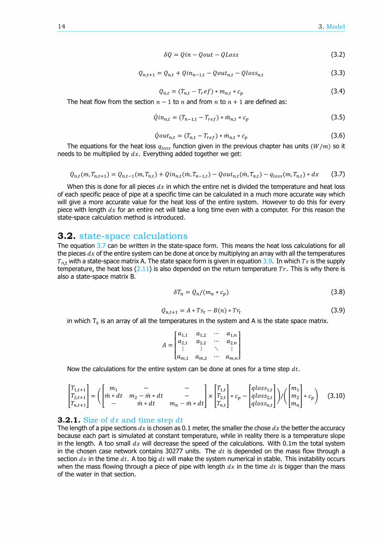
3.2.2. ModelThe input of the model is the temperature array for which the first value is the inlet temperature inthe HTS. Depending on the demand, the mass flow in the system and the time step is determined andthe A-matrix is made. The heat loss is calculated as a function of the temperature. Then the statespace calculation is done to determine the temperature array for the next time step. This is continuedover time until either one of two things happen. The demand changes so the mass flow changes anda new A-matrix needs to be formed or the temperature at one of the users drops below the minimumrequired temperature which means the mass flow also needs to increase and a new A-matrix needsto be formed ??. This way either a simulations of a time dependent demand curve can be done or asteady-state solution with the required total mass flow to get the minimum required temperature of 70degrees C can be calculated. For a daily curve the first will be done while to simulate what happensover a year the second will be done because it would take to long to do a real time simulation for anentire year.

Calculatemass flow Demand

Definedt andA-Matrix

Updateby-passmass flow

CalculateT(t+dt)

T < TminT(t) =T(t+dt)

t < tmax

Stop

yes

no

yes

no

Figure 3.2: Flow chart of the Matlab model.

4District Heating Network

The network that will be analyzed for heat loss in the heat distribution system is the AGH12 network.This is a averaged sized and designed network of Nuon Energy N.V. located in the neighborhoodof Schuytgraaf in Arnhem. It covers 247 connection in the form of single family homes and someapartments. The average capacity is 12.2 kW. Near the centre of the piping network the HTS fromwhere the hot water is pumped through the pipeline network to all the users. The layout of the networkof pipes is shown in figure 4.1.

Figure 4.1: Aerial view of the district Schuytgraaf in Arnhem the Netherlands and a layout of the district heating piping network.

17

18 4. District Heating Network

4.1. Installed capacity of the HTSThe installed capacity of the entire Schuytgraaf net is determined using the total installed capacity ofthe users in the net and the simultaneity factor. A simultaneity of max 65% is assumed in the systembased on experience. This means it is assumed at any given time the maximum load is 65% of thepotential heat demand in the system. Every user in the system has a heat connection that is capableof 8 - 22 kW of heat delivery. The Schuytgraaf net has 247 users connected to it with on average 12.2kW so this would mean 12.2 ∗ 247 = 3013.4𝑘𝑊. However it is assumed that in reality this will neverbe the demand but that the maximum is 65% of this demand. 3013.4 ∗ 0.65 = 1960𝑘𝑊.

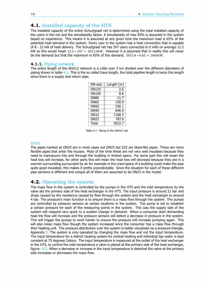
4.1.1. Piping networkThe entire length of the AGH12 network is a Little over 3 km divided over the different diameters ofpiping shown in table 4.1. This is the so called trace length, the total pipeline length is twice this lengthsince there is a supply and return pipe.

DN-size Length [m]DN125 2.6DN100 8.6DN80 21.7DN65 150.9DN50 236.1DN40 646.9DN32 1168.3DN25 787.6Total 3022.7

Table 4.1: Piping in the AGH12 net.

DN25The pipes marked as DN25 are in most cases not DN25 but S25 are Steel-flex pipes. These are moreflexible pipes that enter the houses. Most of the time these are not very well insulated because theyneed to manoeuvre into and through the building in limited space. For some part this will mean theheat loss will increase, for other parts this will mean the heat loss will decrease because they are in awarmer surrounding surrounded by air for example in the crawl space of a building could make the pipequite good insulated, this makes it pretty unpredictable. Since the situation for each of these differentpipe sections is different and unique all of them are assumed to be DN25 in the model.

4.2. Operating the systemThe mass flow in the system is controlled by the pumps in the HTS and the inlet temperature by thevalve ate the primary side of the heat exchanger in the HTS. The input pressure is around 22 bar anddrops caused by the resistance caused by flow through the system and the heat exchanger to around4 bar. The pressure’s main function is to ensure there is a mass flow through the system. The pumpsare controlled by pressure sensors at certain locations in the system. The pump is set to establisha certain pressure for each of the measuring points in the system. This way the supply side of thesystem will respond very quick to a sudden change in demand. When a consumer start demandingheat the flow will increase and the pressure sensors will detect a decrease in pressure in the system.This will trigger the pumps to work harder to ensure the pressure will increase pumping again. Thiswill also mean mass flow though the system increased since the consumer has a mass flow throughtheir heating unit. The pressure distribution over the system is better visualized via a pressure triangle,Appendix E. The system is only operated by changing the mass flow and not the input temperature.The input temperature for a district heating system for central heating and individual tap water is keptconstant at 75 degrees Celsius. The input temperature is measured at the outlet of the heat exchangerin the HTS, to control the inlet temperature a valve is placed at the primary side of the heat exchanger,figure: 4.2. When a decrease or increase in the input temperature is detected the valve at the primaryside increases or decreases the mass flow.

4.2. Operating the system 19

Figure 4.2: Schematic of the heat transfer station

4.2.1. Bypass flowIn the ideal scenario, there is a temperature input of Tin and the temperature at all the customerswould be 70 degrees. Some customers are further away from the heat source then others meaningthe ones furthest away will normally get a lower temperature. Especially with alternating environmentconditions and individual heat demand it is very difficult to regulate the system. In the current situationthe supply sets at the users ensure they get the minimum temperature by letting water flow througha valve even when there is no heat demanded by that user, this is the bypass flow.

4.2.2. PumpThe flow in the system is regulated with two pumps in the HTS. The pumps are parallel connected. Thismeans they can easily be operated independent of each other. One pump should be able to produce50 - 70 % of the design flow when the other is switched off. This will mean the rest of the time whenthe system is not operating in design condition the amount of pumping power is overdimensioned.This could have a big effect on the pump efficiency when a pump is not operating within it’s pumpingrange. Every pump has an optimum operating range in the efficiency curve. When a pump is operatingfar form the operating curve the efficiency will drop significantly. This means it is important to matchthe operation conditions with the pump. The absolute minimum mass flow in the system is duringsummer time at 1.162𝑘𝑔/𝑠 corresponding with 3.816𝑚 /ℎ. This is on the very low side but still withinthe range, pump curves are in the appendix F.

5Analysis of a system in operating

conditions

5.1. Design conditionThe design condition of the system is in ideal conditions, which means a few assumptions are made.The supply temperature is set at 70 degrees Celsius for the entire supply pipeline. The temperatureof the ground is always at 10 degrees Celsius and the load or demand is constant, which means themass flow is constant. The total load in this case is the design load or the maximum load condition. Inthis case the minimum input temperature for the system,to make sure all consumers get the requiredminimum temperature of 70 degrees is higher then the 70 degrees. That is why Nuon sets the inputtemperature for the system at 75 degrees. This will mean the users closer to the HTS will receive awater temperature of somewhere between the input temperature and the required 70 degrees whilethe users at the end of a string will get the minimum temperature of 70 degrees.

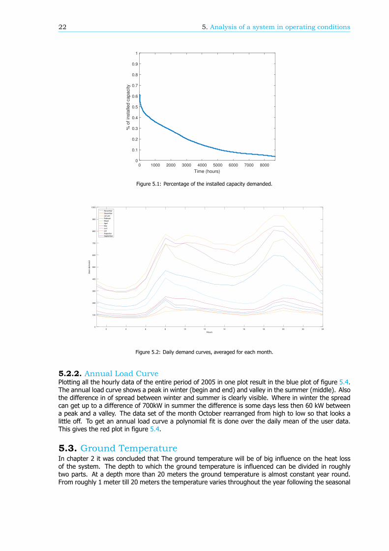
5.2. Load conditionIn reality the system almost never operates in the design condition. The maximum heat demand isalmost never met. Not even in very cold winters. The data of the AGH12 network from 2005 wasmonitored and is analyzed. The percentage of heat demanded per hour vs the total installed power isplotted in figure 5.1. Over an period of one hour the total demand is never higher then 60 %. Themaximum heat demand over a period of 5 seconds in this system for this year was 78 %. Although thewinter of that year hasn’t been a very mild one this winter was also not as cold as others have been[8]. Other district heating nets which had their data logged show roughly the same numbers.

5.2.1. Diurnal Load curveThe daily load curve shows a small peak in the morning when people get up to start their day andtake a shower. And a big peak in the afternoon when people get home and start heat their homes.In summer the two peaks are almost similar in size while in winter the second peak is much higherbecause people heat their homes. In winter months the base load is quite high because people wantto keep their houses at a minimal temperature and in the summer people turn of their central heatingsystems and the only demand is used for tap-water. This is also the reason the daily spread is muchbigger in winter. The curves in figure 5.2 clearly show not besides that the demand is much higher inwinter also the daily peaks of the demand are much higher during winter, or the spread between theminimal and maximal demand.

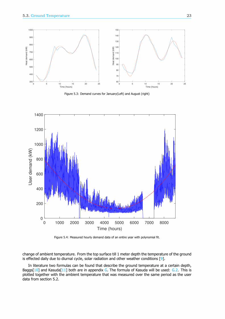
As the data is collected with an interval of one hour the averaged load curves still show an angularpattern. To solve this and to get a smoother, more realistic load curve a polynomial fit is done over themonthly average data, figure:5.3.

21

22 5. Analysis of a system in operating conditions

0 1000 2000 3000 4000 5000 6000 7000 8000

Time (hours)

0

0.1

0.2

0.3

0.4

0.5

0.6

0.7

0.8

0.9

1

% o

f in

sta

lled c

apacity

Figure 5.1: Percentage of the installed capacity demanded.

2 4 6 8 10 12 14 16 18 20 22 24

Hours

0

100

200

300

400

500

600

700

800

900

1000

User

dem

and

November

December

Januari

Februari

Maart

April

Mai

Juni

Juli

Augustus

September

Figure 5.2: Daily demand curves, averaged for each month.

5.2.2. Annual Load CurvePlotting all the hourly data of the entire period of 2005 in one plot result in the blue plot of figure 5.4.The annual load curve shows a peak in winter (begin and end) and valley in the summer (middle). Alsothe difference in of spread between winter and summer is clearly visible. Where in winter the spreadcan get up to a difference of 700kW in summer the difference is some days less then 60 kW betweena peak and a valley. The data set of the month October rearranged from high to low so that looks alittle off. To get an annual load curve a polynomial fit is done over the daily mean of the user data.This gives the red plot in figure 5.4.

5.3. Ground TemperatureIn chapter 2 it was concluded that The ground temperature will be of big influence on the heat lossof the system. The depth to which the ground temperature is influenced can be divided in roughlytwo parts. At a depth more than 20 meters the ground temperature is almost constant year round.From roughly 1 meter till 20 meters the temperature varies throughout the year following the seasonal

5.3. Ground Temperature 23

0 5 10 15 20 25

Time (hours)

300

400

500

600

700

800

900

1000

He

at

de

ma

nd

(kW

)

0 5 10 15 20 25

Time (hours)

60

70

80

90

100

110

120

130

140

150

He

at

de

ma

nd

(kW

)

Figure 5.3: Demand curves for January(Left) and August (right)

0 1000 2000 3000 4000 5000 6000 7000 8000

Time (hours)

0

200

400

600

800

1000

1200

1400

User

dem

and (

kW

)

Figure 5.4: Measured hourly demand data of an entire year with polynomial fit.

change of ambient temperature. From the top surface till 1 meter depth the temperature of the groundis effected daily due to diurnal cycle, solar radiation and other weather conditions [9].

In literature two formulas can be found that describe the ground temperature at a certain depth,Baggs[10] and Kasuda[11] both are in appendix G. The formula of Kasuda will be used: G.2. This isplotted together with the ambient temperature that was measured over the same period as the userdata from section 5.2.

24 5. Analysis of a system in operating conditions

𝑇 ( , ) = 𝑇 − 𝑇 ∗ 𝑒𝑥𝑝(−𝐷√ 𝜋365𝛼 ∗ 𝑐𝑜𝑠

2𝜋365(𝑡 − 𝑡 − 𝐷/2√ 365

𝜋 ∗ 𝛼 )) (5.1)

1000 2000 3000 4000 5000 6000 7000 8000-10

-5

0

5

10

15

20

25

30

35

hourly ambient

0 50 100 150 200 250 300 350

-10

-5

0

5

10

15

20

25

30

35

Kasuda 0.6m

Figure 5.5: Measured ambient temperature and plot for the ground temperature at a depth of 0.6m as given by Kasuda.

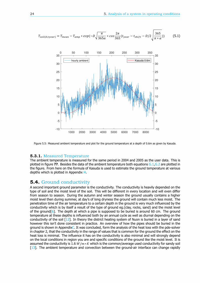
5.3.1. Measured TemperatureThe ambient temperature is measured for the same period in 2004 and 2005 as the user data. This isplotted in figure ??. Besides the data of the ambient temperature both equations G.1,G.2 are plotted inthe figure. From here on the formula of Kasuda is used to estimate the ground temperature at variousdepths which is plotted in Appendix H.

5.4. Ground conductivityA second important ground parameter is the conductivity. The conductivity is heavily depended on thetype of soil and the moist level of the soil. This will be different in every location and will even differfrom season to season. During the autumn and winter season the ground usually contains a highermoist level then during summer, at day’s of long dryness the ground will contain much less moist. Thepenetration time of the air temperature to a certain depth in the ground is very much influenced by theconductivity which is by itself a result of the type of ground eg.(clay, rocks, sand) and the moist levelof the ground[6]. The depth at which a pipe is supposed to be buried is around 60 cm. The groundtemperature at these depths is influenced both by an annual cycle as well as diurnal depending on theconductivity of the soil [12]. In theory the district heating system of Nuon is buried in a layer of sandhowever this isn’t done consistent in practice. An overview of how the pipes should be buried in theground is shown in AppendixC. It was concluded, form the analysis of the heat loss with the pde-solverin chapter 2, that the conductivity in the range of values that is common for the ground the effect on theheat loss is minimal. The influence it has on the conductivity is also minimal and will strongly dependon the local conditions in region you are and specific conditions of the ground like the moist level. It isassumed the conductivity is 1.6𝑊/𝑚∗𝐾 which is the common/average used conductivity for sandy soil[13]. The ambient temperature and convection between the ground-air interface can change rapidly

5.4. Ground conductivity 25

during a period of 24 hours (day and night) or even shorter due to the change in weather conditionsor the difference between shadow or direct sun. As discussed in the section for ground temperaturethis effect will be neglected. The daily temperature fluctuation at a depth of 60 cm is very small andwill not be taken into account [14],[15].

6Heat loss

An analysis is done determine what happens in the system during operating conditions. First the heatloss is calculated for full load or ideal conditions. Then the system is evaluated for some diurnal andannual load curves as determined in the chapter 5.

6.1. Logstor calculation toolLogstor is the supplier of the pipe sections. They provide an online calculating tool which can be used toestimate the heat losses in a system. For the Logstor heat loss calculations the conditions are assumedideal meaning 70 degrees Celsius supply, 40 degrees Celsius return and 10 degrees Celsius ambient.The results for series 1, series 2 and twin are displayed in table 6.1.

piping system Heat loss ideal [MWh/year] Heat loss [GJ/year]Series 1 484.84 1745.42Series 2 357.38 1340.92Twin 270.04 1017.75

Table 6.1: Heat loss calculated by the Logstos calculation tool

It is still assumed the temperature is constant over the entire system while in reality there is a heatgradient from the input of the net to the users. To get an more accurate calculation of the heat lossin the system and an better understanding of what happens in the system the heat gradient shouldbe taken into account the Logstor calculation tool is no longer workable, so the state-space calculationmethod is introduced.

6.2. Full load conditionIn the design condition the load is as explained at 65% simultaneity. For the considered network thismeans a total customer demand of 1995 kW. The input temperature is 75 degrees and the referencetemperature is the ground temperature at 10 degrees Celsius. In this case the heat pumped into thesystem is at 75 degrees Celsius. For the calculation model we assume the total demand is equallydivided over all the users independent on the size of their supply set.

6.2.1. Heat loss calculation using Matlab modelThe results from the heat losses calculated using the Matlab model for a system in operation will bediscussed and evaluated here and compared to the Logstor calculations. The results for the full loadconditions are displayed in table 6.2. The results from Logstor were given in 𝑀𝑊ℎ but converted to𝐺𝐽 because the commodity trading for heat is done in gigajoules. Comparing the Logstor and Matlabcalculations for the ideal situation already a difference is noted.

27

28 6. Heat loss

piping system Ideal Logstor [GJ/year] Ideal Matlab [GJ/year]Series 1 1745.42 1939.5Series 2 1340.92 1671.8Twin 1017.75 1165.3

Table 6.2: Heat loss in GJ/year in the ideal situation

6.3. Operating conditionIn reality the system is almost always in part load condition. There will be extra heat loss due to massflow being pump round the system to keep the system at a minimum temperature of 70 degrees Celsiusfor the customers. In practice this means the heat loss in the return flow increases a lot because thereturn flow heats up rapidly. This is not seen in the full load conditions because the mass flow is highenough to keep the system at temperature. The daily and the annual load conditions are discussed.The ground temperature is kept constant during the course of a day because the diurnal effect oftemperature change at a depth of 0.6 meter is set to be zero. However the ground temperature isassumed to be the monthly average for that month. These calculations are done real time to simulatewhat happens in the system.

6.4. Diurnal load curveThe analyzes have been done for a case with high demand during winter and low demand duringsummer. During winter time there is a wide spread between peaks and valleys in terms of demand,the month with on average the highest demand is January. During summer time the average demandis much lower and also the peaks in the demand are relatively much lower then during winter time,the demand is more constant during the course of a day. The month with the lowest average demandand peaks is August. A polynomial fit is applied as discussed in the previous chapter to smooth out theangular profile caused by the data being measured with an interval of one hour 5.3.

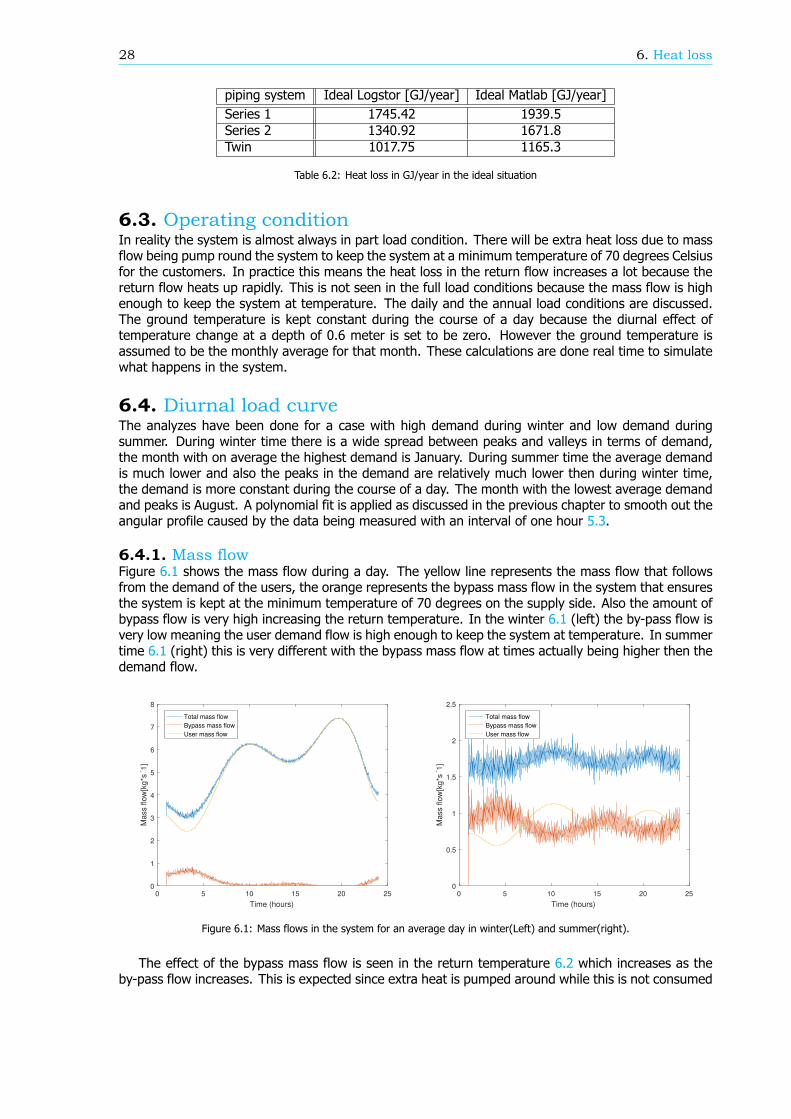
6.4.1. Mass flowFigure 6.1 shows the mass flow during a day. The yellow line represents the mass flow that followsfrom the demand of the users, the orange represents the bypass mass flow in the system that ensuresthe system is kept at the minimum temperature of 70 degrees on the supply side. Also the amount ofbypass flow is very high increasing the return temperature. In the winter 6.1 (left) the by-pass flow isvery low meaning the user demand flow is high enough to keep the system at temperature. In summertime 6.1 (right) this is very different with the bypass mass flow at times actually being higher then thedemand flow.

0 5 10 15 20 25

Time (hours)

0

1

2

3

4

5

6

7

8

Ma

ss f

low

[kg

*s- 1

]

Total mass flow

Bypass mass flow

User mass flow

0 5 10 15 20 25

Time (hours)

0

0.5

1

1.5

2

2.5

Ma

ss f

low

[kg

*s- 1

]

Total mass flow

Bypass mass flow

User mass flow

Figure 6.1: Mass flows in the system for an average day in winter(Left) and summer(right).

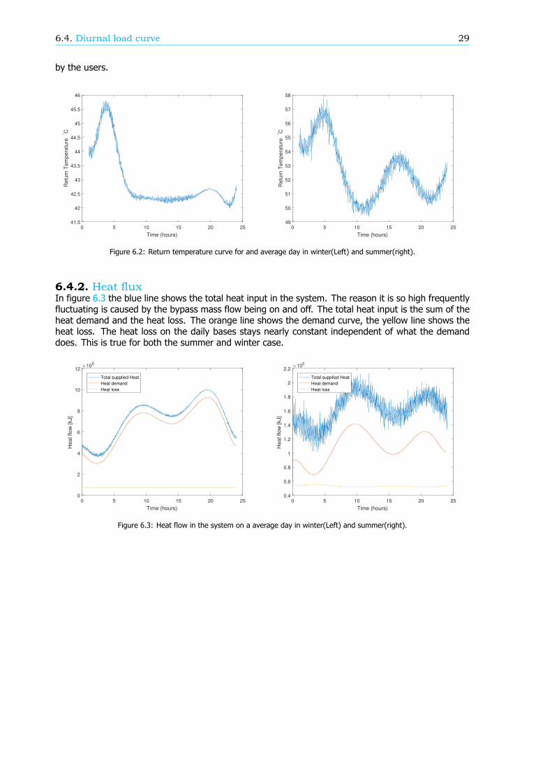
The effect of the bypass mass flow is seen in the return temperature 6.2 which increases as theby-pass flow increases. This is expected since extra heat is pumped around while this is not consumed

6.4. Diurnal load curve 29

by the users.

0 5 10 15 20 25

Time (hours)

41.5

42

42.5

43

43.5

44

44.5

45

45.5

46

Re

turn

Te

mp

era

ture

°C

0 5 10 15 20 25

Time (hours)

49

50

51

52

53

54

55

56

57

58

Re

turn

Te

mp

era

ture

°C

Figure 6.2: Return temperature curve for and average day in winter(Left) and summer(right).

6.4.2. Heat fluxIn figure 6.3 the blue line shows the total heat input in the system. The reason it is so high frequentlyfluctuating is caused by the bypass mass flow being on and off. The total heat input is the sum of theheat demand and the heat loss. The orange line shows the demand curve, the yellow line shows theheat loss. The heat loss on the daily bases stays nearly constant independent of what the demanddoes. This is true for both the summer and winter case.

0 5 10 15 20 25

Time (hours)

0

2

4

6

8

10

12

He

at

flo

w [

kJ]

105

Total supplied Heat

Heat demand

Heat loss

0 5 10 15 20 25

Time (hours)

0.4

0.6

0.8

1

1.2

1.4

1.6

1.8

2

2.2

He

at

flo

w [

kJ]

105

Total supplied Heat

Heat demand

Heat loss

Figure 6.3: Heat flow in the system on a average day in winter(Left) and summer(right).

30 6. Heat loss

From here on it is assumed that for the analysis of the annual heat loss, the daily demand andthe heat loss can be averaged, because the results will stay the same. Although the demand curve isfluctuating a lot the heat loss stays nearly constant. This means averaging both over the course of aday will give the same results for the total. The averaged annual heat curve is given by the polynomialfit over the demand data in figure 5.4.

6.5. Annual load curve resultsWhen the annual situation is analyzed the daily demand is averaged as explained in chapter 5. Theannual change in ground temperature at a depth of 0.6m is taken in account using the formula ofKasuda 5.5. The bypass flow should be taken into account. For a daily average demand and groundtemperature the heat loss is calculated by iterating the heat loss calculation and increasing the bypassmass flow until the minimum required temperature of 70 C is met and the temperature gradient isstable. This will also reduce the calculation time because a year round real time calculation would taketoo much time. Besides from the data set some measurements are missing or disturbed, by using a fitover to determine demand curve all of this is immediately solved.

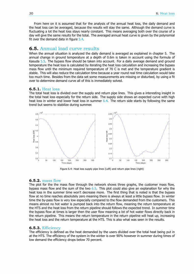
6.5.1. Heat lossThe total heat loss is divided over the supply and return pipe lines. This gives a interesting insight inthe total heat loss especially for the return side. The supply side shows an expected curve with highheat loss in winter and lower heat loss in summer 6.4. The return side starts by following the sametrend but seems to stabilize during summer.

0 50 100 150 200 250 300 350

Time (days)

3.2

3.4

3.6

3.8

4

4.2

4.4

4.6

4.8

He

at

loss (

kW

)

105

0 50 100 150 200 250 300 350

Time (days)

2.1

2.15

2.2

2.25

2.3

2.35

2.4

2.45

2.5

2.55

He

at

loss k

W

105

Figure 6.4: Heat loss supply pipe lines (Left) and return pipe lines (right)

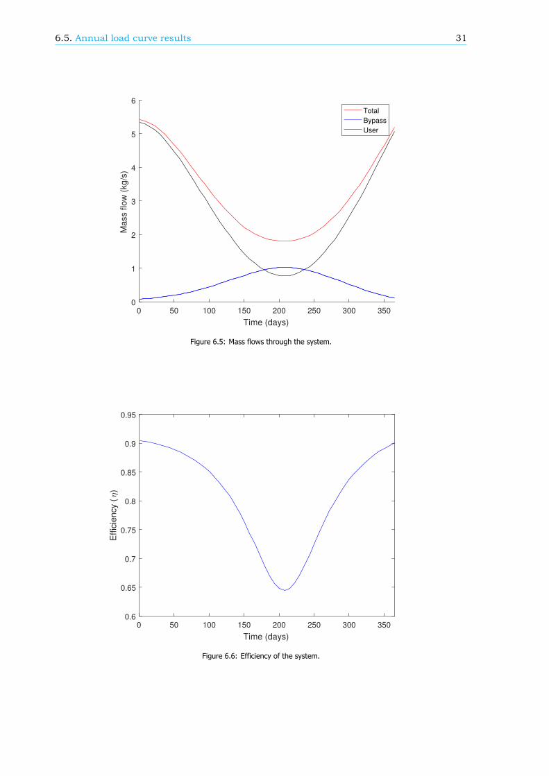
6.5.2. mass flowThe plot for the the mass flow through the network shows three graphs, the customer mass flow,bypass mass flow and the sum of the two 6.5. This plot could also give an explanation for why theheat loss in the summer time won’t decrease more. The first thing that is noted is that the bypassflow at no time reaches absolutely zero meaning there is always at least a little bypass flow. In wintertime the by-pass flow is very low especially compared to the flow demanded from the customers. Thismeans almost no hot water is pumped back into the return flow, meaning the return temperature atthe HTS and the heat loss from the return pipeline should follows the expected trend. In summer timethe bypass flow at times is larger then the user flow meaning a lot of hot water flows directly back inthe return pipeline. This means the return temperature in the return pipeline will heat up, increasingthe heat loss and the return temperature at the HTS. This is also what was seen in the results.

6.5.3. EfficiencyThe efficiency is defined as the heat demanded by the users divided over the total heat being put inat the HTS. The efficiency of the system in the winter is over 90% however in summer during times oflow demand the efficiency drops below 70 percent.

6.5. Annual load curve results 31

0 50 100 150 200 250 300 350

Time (days)

0

1

2

3

4

5

6

Ma

ss f

low

(kg

/s)

Total

Bypass

User

Figure 6.5: Mass flows through the system.

0 50 100 150 200 250 300 350

Time (days)

0.6

0.65

0.7

0.75

0.8

0.85

0.9

0.95

Eff

icie

ncy (

)

Figure 6.6: Efficiency of the system.

7Results

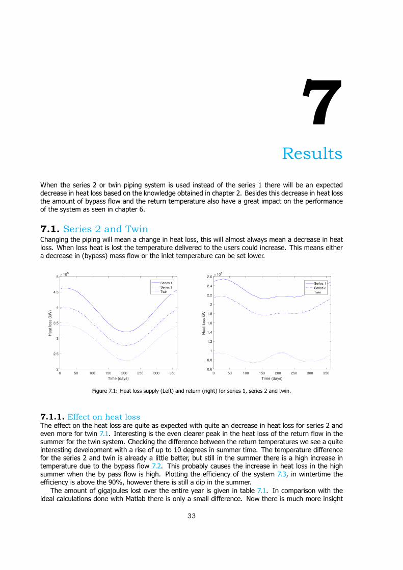
When the series 2 or twin piping system is used instead of the series 1 there will be an expecteddecrease in heat loss based on the knowledge obtained in chapter 2. Besides this decrease in heat lossthe amount of bypass flow and the return temperature also have a great impact on the performanceof the system as seen in chapter 6.

7.1. Series 2 and TwinChanging the piping will mean a change in heat loss, this will almost always mean a decrease in heatloss. When loss heat is lost the temperature delivered to the users could increase. This means eithera decrease in (bypass) mass flow or the inlet temperature can be set lower.

0 50 100 150 200 250 300 350

Time (days)

2

2.5

3

3.5

4

4.5

5

He

at

loss (

kW

)

105

Series 1

Series 2

Twin

0 50 100 150 200 250 300 350

Time (days)

0.6

0.8

1

1.2

1.4

1.6

1.8

2

2.2

2.4

2.6

He

at

loss k

W

105

Series 1

Series 2

Twin

Figure 7.1: Heat loss supply (Left) and return (right) for series 1, series 2 and twin.

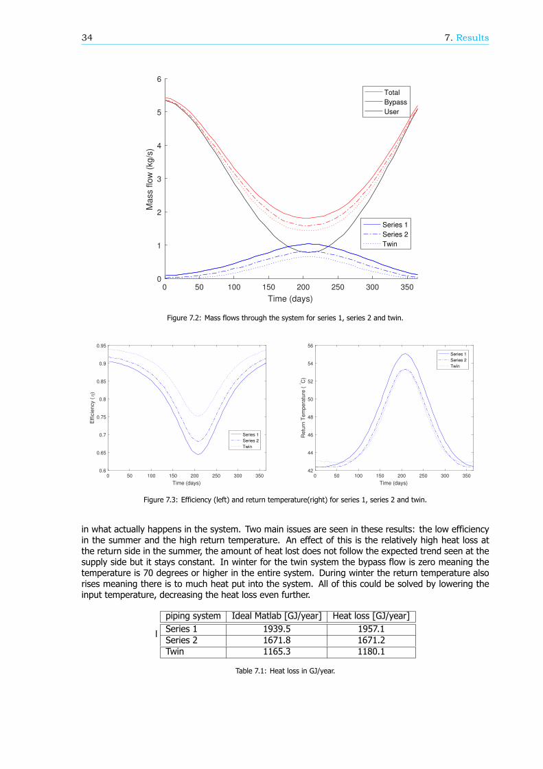
7.1.1. Effect on heat lossThe effect on the heat loss are quite as expected with quite an decrease in heat loss for series 2 andeven more for twin 7.1. Interesting is the even clearer peak in the heat loss of the return flow in thesummer for the twin system. Checking the difference between the return temperatures we see a quiteinteresting development with a rise of up to 10 degrees in summer time. The temperature differencefor the series 2 and twin is already a little better, but still in the summer there is a high increase intemperature due to the bypass flow 7.2. This probably causes the increase in heat loss in the highsummer when the by pass flow is high. Plotting the efficiency of the system 7.3, in wintertime theefficiency is above the 90%, however there is still a dip in the summer.

The amount of gigajoules lost over the entire year is given in table 7.1. In comparison with theideal calculations done with Matlab there is only a small difference. Now there is much more insight

33

34 7. Results

0 50 100 150 200 250 300 350

Time (days)

0

1

2

3

4

5

6

Ma

ss f

low

(kg

/s)

Total

Bypass

User

Series 1

Series 2

Twin

Figure 7.2: Mass flows through the system for series 1, series 2 and twin.

0 50 100 150 200 250 300 350

Time (days)

0.6

0.65

0.7

0.75

0.8

0.85

0.9

0.95

Eff

icie

ncy (

)

Series 1

Series 2

Twin

0 50 100 150 200 250 300 350

Time (days)

42

44

46

48

50

52

54

56

Re

turn

Te

mp

era

ture

(°C

)

Series 1

Series 2

Twin

Figure 7.3: Efficiency (left) and return temperature(right) for series 1, series 2 and twin.

in what actually happens in the system. Two main issues are seen in these results: the low efficiencyin the summer and the high return temperature. An effect of this is the relatively high heat loss atthe return side in the summer, the amount of heat lost does not follow the expected trend seen at thesupply side but it stays constant. In winter for the twin system the bypass flow is zero meaning thetemperature is 70 degrees or higher in the entire system. During winter the return temperature alsorises meaning there is to much heat put into the system. All of this could be solved by lowering theinput temperature, decreasing the heat loss even further.

l

piping system Ideal Matlab [GJ/year] Heat loss [GJ/year]Series 1 1939.5 1957.1Series 2 1671.8 1671.2Twin 1165.3 1180.1

Table 7.1: Heat loss in GJ/year.

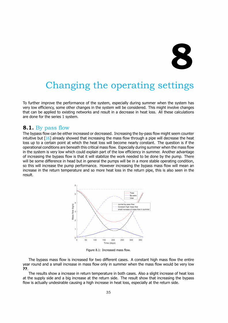
8Changing the operating settings

To further improve the performance of the system, especially during summer when the system hasvery low efficiency, some other changes in the system will be considered. This might involve changesthat can be applied to existing networks and result in a decrease in heat loss. All these calculationsare done for the series 1 system.

8.1. By pass flowThe bypass flow can be either increased or decreased. Increasing the by-pass flow might seem counterintuitive but [16] already showed that increasing the mass flow through a pipe will decrease the heatloss up to a certain point at which the heat loss will become nearly constant. The question is if theoperational conditions are beneath this critical mass flow. Especially during summer when the mass flowin the system is very low which could explain part of the low efficiency in summer. Another advantageof increasing the bypass flow is that it will stabilize the work needed to be done by the pump. Therewill be some difference in head but in general the pumps will be in a more stable operating condition,so this will increase the pump performance. However increasing the bypass mass flow will mean anincrease in the return temperature and so more heat loss in the return pipe, this is also seen in theresult.

0 50 100 150 200 250 300 350

Time (days)

0

1

2

3

4

5

6

Ma

ss f

low

(kg

/s)

Total

By-pass

User

normal by-pass flow

Constant high mass flow

small increase of mass flow in summer

Figure 8.1: Increased mass flow.

The bypass mass flow is increased for two different cases. A constant high mass flow the entireyear round and a small increase in mass flow only in summer when the mass flow would be very low??.

The results show a increase in return temperature in both cases. Also a slight increase of heat lossat the supply side and a big increase at the return side. The result show that increasing the bypassflow is actually undesirable causing a high increase in heat loss, especially at the return side.

35

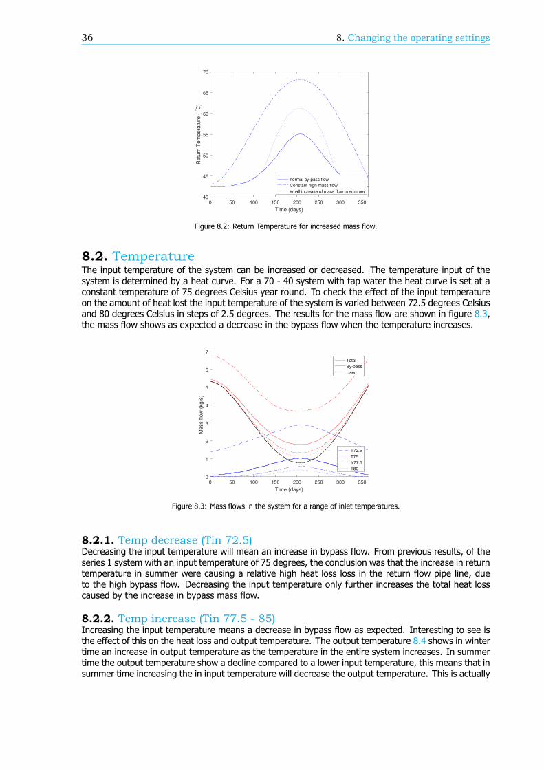
36 8. Changing the operating settings

0 50 100 150 200 250 300 350

Time (days)

2.1

2.2

2.3

2.4

2.5

2.6

2.7

2.8

2.9

3

He

at

loss k

W

104

normal by-pass flow

Constant high mass flow

small increase of mass flow in summer

0 50 100 150 200 250 300 350

Time (days)

40

45

50

55

60

65

70

Re

turn

Te

mp

era

ture

(°C

)

normal by-pass flow

Constant high mass flow

small increase of mass flow in summer

Figure 8.2: Return Temperature for increased mass flow.

8.2. TemperatureThe input temperature of the system can be increased or decreased. The temperature input of thesystem is determined by a heat curve. For a 70 - 40 system with tap water the heat curve is set at aconstant temperature of 75 degrees Celsius year round. To check the effect of the input temperatureon the amount of heat lost the input temperature of the system is varied between 72.5 degrees Celsiusand 80 degrees Celsius in steps of 2.5 degrees. The results for the mass flow are shown in figure 8.3,the mass flow shows as expected a decrease in the bypass flow when the temperature increases.

0 50 100 150 200 250 300 350

Time (days)

0

1

2

3

4

5

6

7

Ma

ss f

low

(kg

/s)

Total

By-pass

User

T72.5

T75

Y77.5

T80

Figure 8.3: Mass flows in the system for a range of inlet temperatures.

8.2.1. Temp decrease (Tin 72.5)Decreasing the input temperature will mean an increase in bypass flow. From previous results, of theseries 1 system with an input temperature of 75 degrees, the conclusion was that the increase in returntemperature in summer were causing a relative high heat loss loss in the return flow pipe line, dueto the high bypass flow. Decreasing the input temperature only further increases the total heat losscaused by the increase in bypass mass flow.

8.2.2. Temp increase (Tin 77.5 - 85)Increasing the input temperature means a decrease in bypass flow as expected. Interesting to see isthe effect of this on the heat loss and output temperature. The output temperature 8.4 shows in wintertime an increase in output temperature as the temperature in the entire system increases. In summertime the output temperature show a decline compared to a lower input temperature, this means that insummer time increasing the in input temperature will decrease the output temperature. This is actually

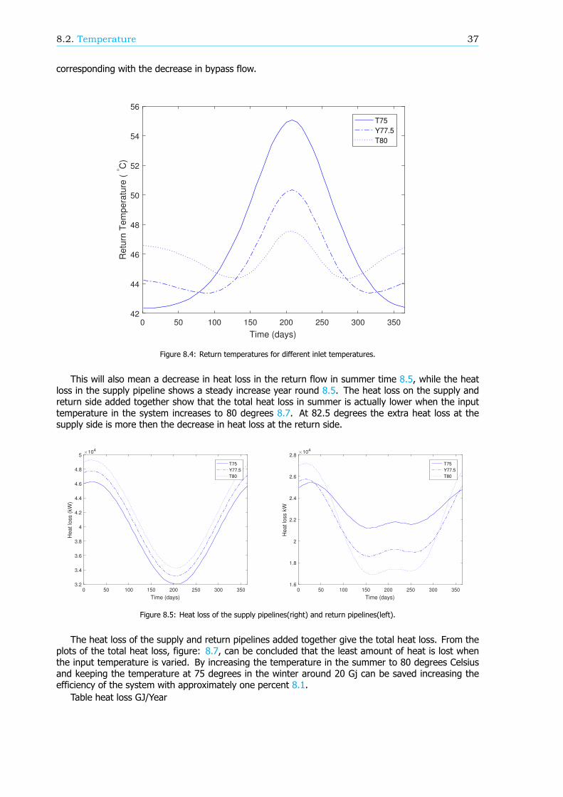
8.2. Temperature 37

corresponding with the decrease in bypass flow.

0 50 100 150 200 250 300 350

Time (days)

42

44

46

48

50

52

54

56

Re

turn

Te

mp

era

ture

(°C

)T75

Y77.5

T80

Figure 8.4: Return temperatures for different inlet temperatures.

This will also mean a decrease in heat loss in the return flow in summer time 8.5, while the heatloss in the supply pipeline shows a steady increase year round 8.5. The heat loss on the supply andreturn side added together show that the total heat loss in summer is actually lower when the inputtemperature in the system increases to 80 degrees 8.7. At 82.5 degrees the extra heat loss at thesupply side is more then the decrease in heat loss at the return side.

0 50 100 150 200 250 300 350

Time (days)

3.2

3.4

3.6

3.8

4

4.2

4.4

4.6

4.8

5

He

at

loss (

kW

)

104

T75

Y77.5

T80

0 50 100 150 200 250 300 350

Time (days)

1.6

1.8

2

2.2

2.4

2.6

2.8

He

at

loss k

W

104

T75

Y77.5

T80

Figure 8.5: Heat loss of the supply pipelines(right) and return pipelines(left).

The heat loss of the supply and return pipelines added together give the total heat loss. From theplots of the total heat loss, figure: 8.7, can be concluded that the least amount of heat is lost whenthe input temperature is varied. By increasing the temperature in the summer to 80 degrees Celsiusand keeping the temperature at 75 degrees in the winter around 20 Gj can be saved increasing theefficiency of the system with approximately one percent 8.1.

Table heat loss GJ/Year

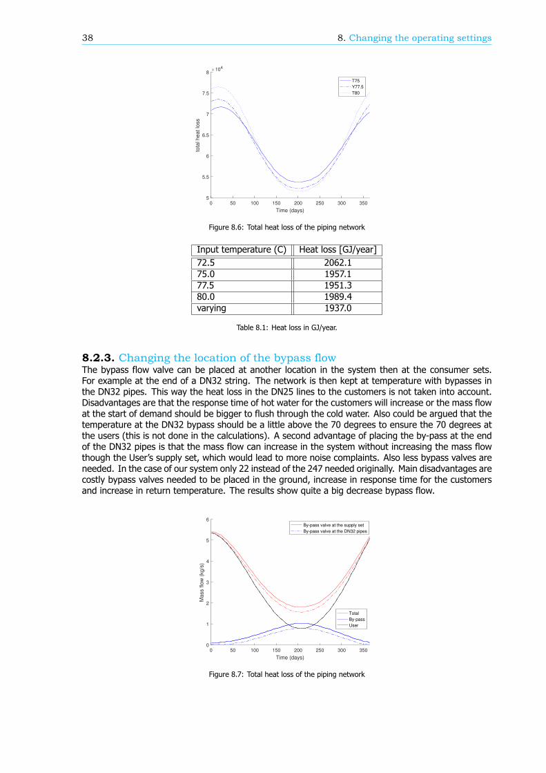
38 8. Changing the operating settings

0 50 100 150 200 250 300 350

Time (days)

5

5.5

6

6.5

7

7.5

8

tota

l h

ea

t lo

ss

104

T75

Y77.5

T80

Figure 8.6: Total heat loss of the piping network

Input temperature (C) Heat loss [GJ/year]72.5 2062.175.0 1957.177.5 1951.380.0 1989.4varying 1937.0

Table 8.1: Heat loss in GJ/year.

8.2.3. Changing the location of the bypass flowThe bypass flow valve can be placed at another location in the system then at the consumer sets.For example at the end of a DN32 string. The network is then kept at temperature with bypasses inthe DN32 pipes. This way the heat loss in the DN25 lines to the customers is not taken into account.Disadvantages are that the response time of hot water for the customers will increase or the mass flowat the start of demand should be bigger to flush through the cold water. Also could be argued that thetemperature at the DN32 bypass should be a little above the 70 degrees to ensure the 70 degrees atthe users (this is not done in the calculations). A second advantage of placing the by-pass at the endof the DN32 pipes is that the mass flow can increase in the system without increasing the mass flowthough the User’s supply set, which would lead to more noise complaints. Also less bypass valves areneeded. In the case of our system only 22 instead of the 247 needed originally. Main disadvantages arecostly bypass valves needed to be placed in the ground, increase in response time for the customersand increase in return temperature. The results show quite a big decrease bypass flow.

0 50 100 150 200 250 300 350

Time (days)

0

1

2

3

4

5

6

Ma

ss f

low

(kg

/s)

Total

By-pass

User

By-pass valve at the supply set

By-pass valve at the DN32 pipes

Figure 8.7: Total heat loss of the piping network

9Total Cost of Ownership Analysis

The total cost of ownership (TCO) is divided in the capital expense (capex) and operating expense(opex). Both will be evaluated in this chapter for series 1, series 2 and twin. The costs for the series 1system can be calculated pretty accurate, nearly all costs are known at Nuon from the current installednetworks. For series 2 and twin a lot of assumptions need to be made. Several sensitivity studies willbe done to find out what would happen in different case studies and to cover all the uncertainties.

9.1. CapexThe capex include all the initially investment costs, this divided into two subcategories: the materialsand the contractor activities. Using series 2 instead of series 1 will increase the costs because materialsget larger and heavier. Also the space needed underground increases meaning the digging of the gutterwill cost more. Using twin piping could decrease the costs because there needs to be dug only onegutter and only half of the joints need to be made. However the pipes need to be welded together andthis will be a lot harder, also bends and splits will be more complex to make which could increase thecosts.

9.1.1. Material CostsMaterials are mostly pipeline sections and joints. Pipelines come in all different sizes and forms, besidesthe straight lines there is normal 90 degree bends and specials like Z-bends and T-splits. The materialcosts for the series 1 and series 2 are known at Nuon, all materials are bought from the supplier andmanufacturer Logstor. They currently have a contract in which all the prices are negotiated. The pricesfor the twin system are assumed equal to the deal made in Sweden. The main materials are pipes indifferent sizes and shapes and joints.

9.1.2. Contractor CostsInstallation of the piping network is done by contractors hired by Nuon. For series 1 the costs are knownfrom current deals with contractors. The prices are given in installation costs per meter depending onthe DN-size. For the Series 2 the sizes are the same as series 1, the only difference is the outerdimensions of the insulation layer are one size bigger. That is why it is assumed the costs for series 2piping are the same as those for the series 1 but DN-size plus one, so the price for intalling a series2 DN25 pipe will cost the same as a series 1 DN32 pipe and so on. The prizes for the twin systemare harder to predict. On the positive side the number of pipes installed is halved and less digging isneeded. Also only half the amount of joints need to be placed, however these are bigger in size andso the cost per joint will increase. Other cost increasing factors are the welds that are much harder tomake because the two steal pipes are close together.

9.2. OpexThe operating expense of the system and the costs for maintenance on the network. As shown the heatloss compared to series 1 will decrease using series 2 and even more so using the twin pipe system.

39

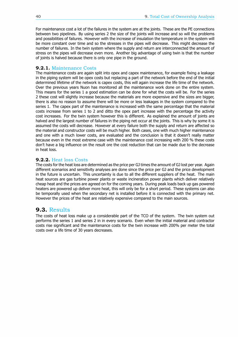
40 9. Total Cost of Ownership Analysis

For maintenance cost a lot of the failures in the system are at the joints. These are the PE connectionsbetween two pipelines. By using series 2 the size of the joints will increase and so will the problemsand possibilities of failures. However with the increase of insulation the temperature in the system willbe more constant over time and so the stresses in the pipes will decrease. This might decrease thenumber of failures. In the twin system where the supply and return are interconnected the amount ofstress on the pipes will decrease even more. Another big advantage of using twin is that the numberof joints is halved because there is only one pipe in the ground.

9.2.1. Maintenance CostsThe maintenance costs are again split into opex and capex maintenance, for example fixing a leakagein the piping system will be opex costs but replacing a part of the network before the end of the initialdetermined lifetime of the network is capex costs, this will again increase the life time of the network.Over the previous years Nuon has monitored all the maintenance work done on the entire system.This means for the series 1 a good estimation can be done for what the costs will be. For the series2 these cost will slightly increase because the materials are more expensive and the sizes are bigger,there is also no reason to assume there will be more or less leakages in the system compared to theseries 1. The capex part of the maintenance is increased with the same percentage that the materialcosts increase from series 1 to 2 and ditto the opex part increase with the percentage the activitycost increases. For the twin system however this is different. As explained the amount of joints arehalved and the largest number of failures in the piping net occur at the joints. This is why by some it isassumed the costs will decrease. However at every failure both the supply and return are affected sothe material and constructor costs will be much higher. Both cases, one with much higher maintenanceand one with a much lower costs, are evaluated and the conclusion is that it doesn’t really matterbecause even in the most extreme case with the maintenance cost increasing with 200 % these costsdon’t have a big influence on the result ore the cost reduction that can be made due to the decreasein heat loss.

9.2.2. Heat loss CostsThe costs for the heat loss are determined as the price per GJ times the amount of GJ lost per year. Againdifferent scenarios and sensitivity analyses are done since the price per GJ and the price developmentin the future is uncertain. This uncertainty is due to all the different suppliers of the heat. The mainheat sources are gas turbine power plants or waste incineration power plants which deliver relativelycheap heat and the prices are agreed on for the coming years. During peak loads back up gas poweredheaters are powered up deliver more heat, this will only be for a short period. These systems can alsobe temporally used when the secondary net is installed before it is connected with the primary net.However the prices of the heat are relatively expensive compared to the main sources.

9.3. ResultsThe costs of heat loss make up a considerable part of the TCO of the system. The twin system outperforms the series 1 and series 2 in in every scenario. Even when the initial material and contractorcosts rise significant and the maintenance costs for the twin increase with 200% per meter the totalcosts over a life time of 30 years decreases.

9.3. Results 41

Figure 9.1: Bar graph of the total cost of ownership over 30 years for series 1, series 2 and twin.

10Conclusion and Recommendation

10.1. ConclusionThe main purpose of this research project was to determine if Nuon should use a different type ofpipe in the form of a series 2 or twin pipe instead of the series 1 that is currently being used. Fromboth a heat loss and financial considerations the twin pipe line is the best choice. Using the series 2or twin instead of the series 1 piping will result in a heat loss reduction of 14.6% respectively 39.70%.By controlling the temperature in a smart way and by placing the by-pass valves in a more strategicplace some more savings can be done. Changing the location of the by-pass will be a costly operationin existing systems. In new systems this will mean vulnerable pieces are placed underground wherethey are harder to reach for maintenance. Besides the response time for customers to receive warmwater will increase meaning the overall quality of the product will decrease. These facts combined withthe low increase in efficiency and decrease in heat loss result in a negative advise on relocating thelocation of the bypass flow valve to the end of the DN32 pipes.Increasing the inlet temperature in summer to reduce the amount bypass flow in the system will alsoresult in a slight decrease in heat loss. This can be achieved by changing the inlet temperature in theHTS. Because of the extra reduction of heat loss that can be accomplished this way it is recommendedto experiment with this. Especially when the twin system is used because in that case it is best tochange the inlet temperature also during peak-load in winter.Financially the series 2 is not that more attractive then the series 1. Twin is the best choice with thebiggest costs reduction being caused by the save on heat loss. Even taken in account the uncertaintyof the price for the installation and maintenance, in the absolute worst case scenario with maintenancecosts rising by 200% it is still the better choice.

10.2. RecommendationFurther research is recommended in addition to this report to get even better understanding on howthe network is functioning and to further decrease the amount of heat lost during transport and in otherparts of the system. In addition on the research done in this report and the conclusion that controllingthe inlet conditions in a more passive way can have a positive influence on the reduction of heat lossit is recommended to further investigate and explore this. For example taking in account the daily orhourly fluctuation of heat demand which can fluctuate a lot especially during winter time.To get an even better understanding on how the system works and how much heat is actually lost fieldresearch is needed. The research done during this project is still only theoretical, and so still a lot ofassumptions are made. To know what is happening in reality field research can be done. This could bemeasurements in the ground to measure the actual ground temperature and to measure the increasein ground temperature caused by the heat loss.Secondly a study can be done on the local conditions of the ground and the affect it has on the heatloss. As explained an average value is taken for the heat conductivity of the ground. These values willactually differ locally, and this will have an effect on the amount of heat lost in the system. Local andregional differences could also effect the choices that are made in the design of the system to get theoptimal system for the local conditions.

43

44 10. Conclusion and Recommendation

At last research could be done to further improve the very low efficiency of the system in summer.For example in systems that only deliver heat and no tap-water the temperature of a 70-40 net islowered in summer to a 50-30 net. In the systems with tap-water where the salmonella regulationsneed to be met this would mean the tap-water needs to be further heated by for example electricityor a heat pump. A hybrid solution like this could be an interesting solution for the problem of the verylow efficiency in summer.

Bibliography

[1] P. Wallentén, Steady-state heat loss from insulated pipes, Ph.D. thesis, Lund University (1991).

[2] B. Bohm, On transient heat losses from buried district heating pipes, International Journal ofEnergy Research 24, 1311 (2000).

[3] T. K. T., On the critical reynolds number for transition from laminar to turbulent flow, (2017).

[4] C. Persson, Predicting the Long-Ter Insulation Performance of District Heating Pipes, Ph.D. thesis,Chalmers University of Technology (2015).

[5] M. A.F., Basic Heat and Mass Transfer: Pearson International Edition (Pearson Education Limited,2013).

[6] S. B. Matjaz Perpar, Zlatko Rek and I. Zun, Soil thermal condutivity prediction for district heatingpre-insulated pipeline in operation, elsevier Energy(2012), 197 (2012).

[7] S. S. Della Rosa A., Li H., Method for optimal design of pipes for low-energy heating, with focuson heat loss, Elsevier January 2011, 2407 (2011).

[8] M. of Infrastructure and the Environment, Climatology daily weather data for the netherlands,(2018).

[9] G. A. Florides and S. A. Kalgirou, Annual ground temperature measurements at various depths,OAI -, (2014).

[10] W. J. Popiel CO and B. B, Measurements of temperature distribution in ground, Elsevier Experi-mental thermal and fluid science 25, 301 (2001).

[11] K. T. and A. P.R., Eart temperature and thermal diffusivity at selected stations in the united states,ASHRAE Transactions 71, (1965).

[12] G. A. Florides and S. A. Kalgirou, Measurements of ground temperature at various depths, OAI -,(2014).

[13] R. M. Alrtimi A. and H. S., Thermal conductivity of sandy soil, Applied Thermal Engineering 106,551 (2016).

[14] R. Sandor and N. Fodor, Simulation of soil temperature dynamics with models using differentconcepts, The Scientific World Journal 2012, 8 (2012).

[15] W. J. Popiel CO, Temperature distributions of ground in the urban region of poznan city, Elsevier51, 135 (2013).

[16] A. A. Heijde van der B. and H. L., Modeling steady-state thermal behaviour of double thermalnetwork pipes, International Journal of Thermal Sciences 117, 316 (2017).

45

ASize Table Logstor Piping

47

Product Catalogue · 2017.03 LOGSTOR A/S · Tel. +45 99 66 10 00

2.0.2.1

Application

Description

The bonded pipe systemDistrict heating pipes - Insulation series 1

Preinsulated pipes of insulation series 1 are used for all common construction works where it is not necessary to make allowance for e.g. extreme outside temperature influences, especially high energy prices etc.

:::LOGSTOR:::160:::03,0:::PEHD:::MRF:::0,2-0,7:::1:::2 15 06:::

A preinsulated pipe of insulation series 1 can be immediately identified by its pipe label, from which other data also appear, see page 1.3.0.2.

All preinsulated pipes are delivered with embedded copper wires for surveillance.

The dimensions ø 26.9/90 - ø 219.1/315 mm are available with diffusion barrier in 12 and 16 m lengths. See page 2.0.1.1.

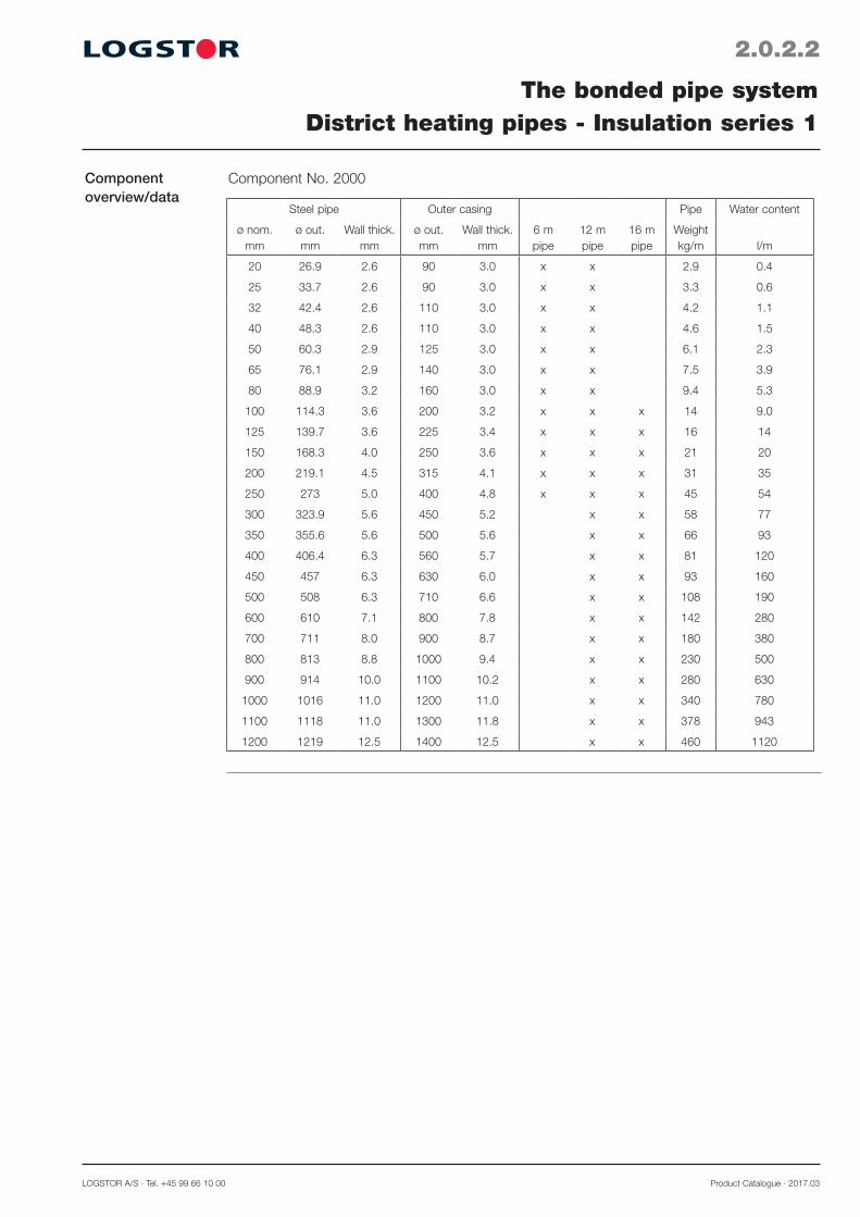
LOGSTOR A/S · Tel. +45 99 66 10 00 Product Catalogue · 2017.03

2.0.2.2

The bonded pipe systemDistrict heating pipes - Insulation series 1

Componentoverview/data

Component No. 2000

Steel pipe Outer casing Pipe Water content

ø nom. mm

ø out. mm

Wall thick. mm

ø out. mm

Wall thick. mm

6 m pipe

12 m pipe

16 m pipe

Weight kg/m l/m

20 26.9 2.6 90 3.0 x x 2.9 0.4

25 33.7 2.6 90 3.0 x x 3.3 0.6

32 42.4 2.6 110 3.0 x x 4.2 1.1

40 48.3 2.6 110 3.0 x x 4.6 1.5

50 60.3 2.9 125 3.0 x x 6.1 2.3

65 76.1 2.9 140 3.0 x x 7.5 3.9

80 88.9 3.2 160 3.0 x x 9.4 5.3

100 114.3 3.6 200 3.2 x x x 14 9.0

125 139.7 3.6 225 3.4 x x x 16 14

150 168.3 4.0 250 3.6 x x x 21 20

200 219.1 4.5 315 4.1 x x x 31 35

250 273 5.0 400 4.8 x x x 45 54

300 323.9 5.6 450 5.2 x x 58 77

350 355.6 5.6 500 5.6 x x 66 93

400 406.4 6.3 560 5.7 x x 81 120

450 457 6.3 630 6.0 x x 93 160

500 508 6.3 710 6.6 x x 108 190

600 610 7.1 800 7.8 x x 142 280

700 711 8.0 900 8.7 x x 180 380

800 813 8.8 1000 9.4 x x 230 500

900 914 10.0 1100 10.2 x x 280 630

1000 1016 11.0 1200 11.0 x x 340 780

1100 1118 11.0 1300 11.8 x x 378 943

1200 1219 12.5 1400 12.5 x x 460 1120

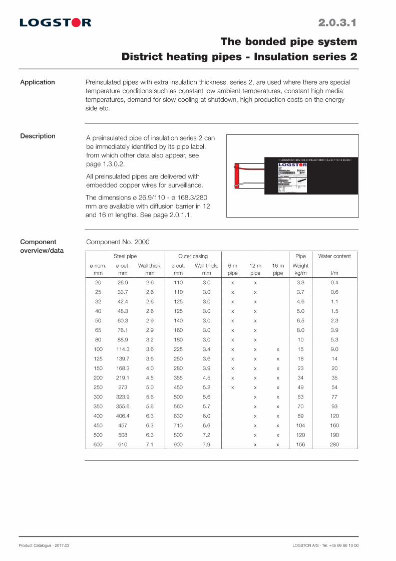
Product Catalogue · 2017.03 LOGSTOR A/S · Tel. +45 99 66 10 00

2.0.3.1

The bonded pipe systemDistrict heating pipes - Insulation series 2

Application

Description

Preinsulated pipes with extra insulation thickness, series 2, are used where there are special temperature conditions such as constant low ambient temperatures, constant high media temperatures, demand for slow cooling at shutdown, high production costs on the energy side etc.

A preinsulated pipe of insulation series 2 can be immediately identified by its pipe label, from which other data also appear, see page 1.3.0.2.

All preinsulated pipes are delivered with embedded copper wires for surveillance.

The dimensions ø 26.9/110 - ø 168.3/280 mm are available with diffusion barrier in 12 and 16 m lengths. See page 2.0.1.1.

:::LOGSTOR:::315:::03,0:::PEHD:::MRF:::0,2-0,7:::1:::2 15 06:::

Componentoverview/data

Component No. 2000

Steel pipe Outer casing Pipe Water content

ø nom. mm

ø out. mm

Wall thick. mm

ø out. mm

Wall thick. mm

6 m pipe

12 m pipe

16 m pipe

Weight kg/m l/m

20 26.9 2.6 110 3.0 x x 3.3 0.4

25 33.7 2.6 110 3.0 x x 3.7 0.6

32 42.4 2.6 125 3.0 x x 4.6 1.1

40 48.3 2.6 125 3.0 x x 5.0 1.5

50 60.3 2.9 140 3.0 x x 6.5 2.3

65 76.1 2.9 160 3.0 x x 8.0 3.9

80 88.9 3.2 180 3.0 x x 10 5.3

100 114.3 3.6 225 3.4 x x x 15 9.0

125 139.7 3.6 250 3.6 x x x 18 14

150 168.3 4.0 280 3.9 x x x 23 20

200 219.1 4.5 355 4.5 x x x 34 35

250 273 5.0 450 5.2 x x x 49 54

300 323.9 5.6 500 5.6 x x 63 77

350 355.6 5.6 560 5.7 x x 70 93

400 406.4 6.3 630 6.0 x x 89 120

450 457 6.3 710 6.6 x x 104 160

500 508 6.3 800 7.2 x x 120 190

600 610 7.1 900 7.9 x x 156 280

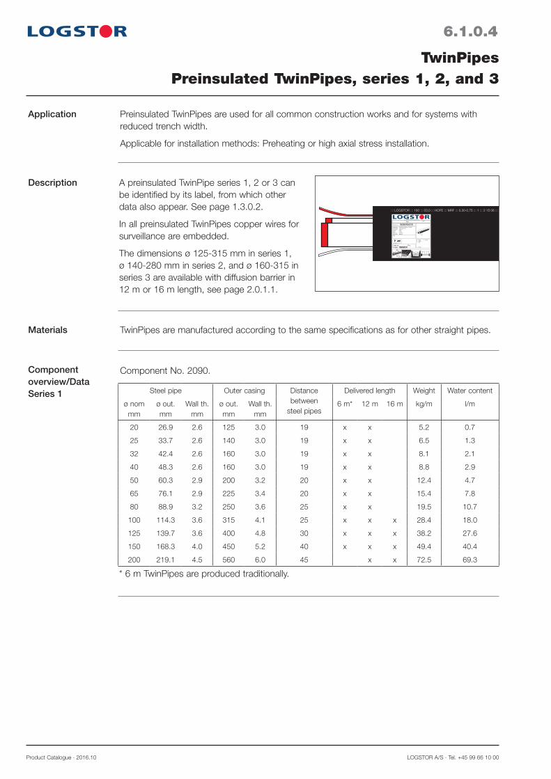
Product Catalogue · 2016.10 LOGSTOR A/S · Tel. +45 99 66 10 00

6.1.0.4

TwinPipesPreinsulated TwinPipes, series 1, 2, and 3

Application Preinsulated TwinPipes are used for all common construction works and for systems with reduced trench width.

Applicable for installation methods: Preheating or high axial stress installation.

Component overview/DataSeries 1

Description A preinsulated TwinPipe series 1, 2 or 3 can be identified by its label, from which other data also appear. See page 1.3.0.2.

In all preinsulated TwinPipes copper wires for surveillance are embedded.

The dimensions ø 125-315 mm in series 1, ø 140-280 mm in series 2, and ø 160-315 in series 3 are available with diffusion barrier in 12 m or 16 m length, see page 2.0.1.1.

::: LOGSTOR ::: 160 ::: 03,0 ::: HDPE ::: MRF ::: 0,30-0,75 ::: 1 ::: 2 15 06 :::

Pipe Date

Material no. : 20000076012726Media pipe : P235TR1/P235GH, EN 10217Jacket pipe : Konti standardInsulation : Series 1Foam : PURWires : NordicPipe end : 220 mmReference : EN 253Note :

SPCR 127 FVF 2000:14 NR: 33 40 02

P-order : 100528131Sales no.: Pos.:

d : 76 mmD : 140 mmL : 12 M

x : 150 mm

S : 2,9 mm

Tel. + 45 99 66 10 00 - www.logstor.com

min100 mm

min400 mm

min min400 mm

min100 mm

min 100 mm

X90° 90°

Materials TwinPipes are manufactured according to the same specifications as for other straight pipes.

Component No. 2090.

Steel pipe Outer casing Distance between

steel pipes

Delivered length Weight Water content

ø nom mm

ø out. mm

Wall th. mm

ø out. mm

Wall th. mm

6 m* 12 m 16 m kg/m l/m

20 26.9 2.6 125 3.0 19 x x 5.2 0.7

25 33.7 2.6 140 3.0 19 x x 6.5 1.3

32 42.4 2.6 160 3.0 19 x x 8.1 2.1

40 48.3 2.6 160 3.0 19 x x 8.8 2.9

50 60.3 2.9 200 3.2 20 x x 12.4 4.7

65 76.1 2.9 225 3.4 20 x x 15.4 7.8

80 88.9 3.2 250 3.6 25 x x 19.5 10.7

100 114.3 3.6 315 4.1 25 x x x 28.4 18.0

125 139.7 3.6 400 4.8 30 x x x 38.2 27.6

150 168.3 4.0 450 5.2 40 x x x 49.4 40.4

200 219.1 4.5 560 6.0 45 x x 72.5 69.3

* 6 m TwinPipes are produced traditionally.

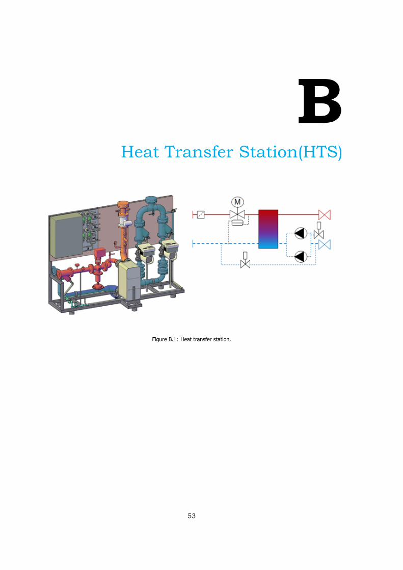
BHeat Transfer Station(HTS)

Figure B.1: Heat transfer station.

53

CSide view of the pipes in the ground.

55

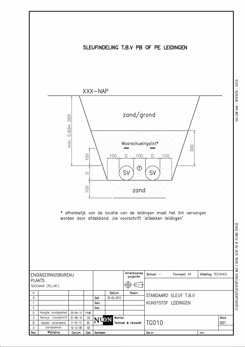
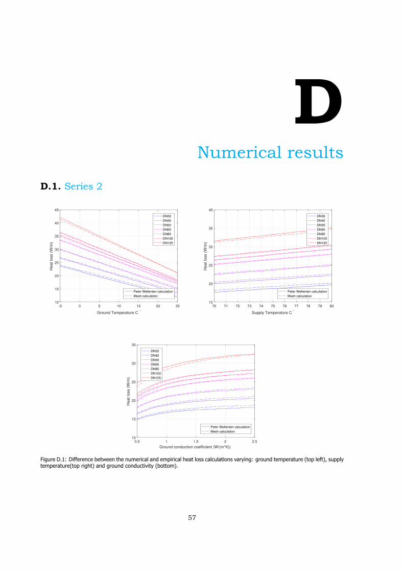
DNumerical results

D.1. Series 2

-5 0 5 10 15 20 25

Ground Temperature C °

10

15

20

25

30

35

40

45

He

at

loss (

W/m

)

DN32

DN40

DN50

DN65

DN80

DN100

DN125

Peter Wellenten calculation

Mesh calculation

70 71 72 73 74 75 76 77 78 79 80

Supply Temperature C °

15

20

25

30

35

40

He

at

loss (

W/m

)

DN32

DN40

DN50

DN65

DN80

DN100

DN125

Peter Wellenten calculation

Mesh calculation

0.5 1 1.5 2 2.5

Ground conduction coefficient (W/(m*K))

10

15

20

25

30

35

He

at

loss (

W/m

)

DN32

DN40

DN50

DN65

DN80

DN100

DN125

Peter Wellenten calculation

Mesh calculation

Figure D.1: Difference between the numerical and empirical heat loss calculations varying: ground temperature (top left), supplytemperature(top right) and ground conductivity (bottom).

57

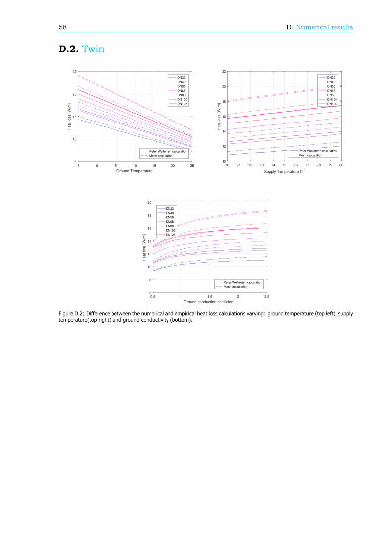
58 D. Numerical results

D.2. Twin

-5 0 5 10 15 20 25

Ground Temperature

5

10

15

20

25H

ea

t lo

ss [

W/m

]

DN32

DN40

DN50

DN65

DN80

DN100

DN125

Peter Wellenten calculation

Mesh calculation

70 71 72 73 74 75 76 77 78 79 80

Supply Temperature C °

10

12

14

16

18

20

22

He

at

loss (

W/m

)

DN32

DN40

DN50

DN65

DN80

DN100

DN125

Peter Wellenten calculation

Mesh calculation

0.5 1 1.5 2 2.5

Ground conduction coefficient

6

8

10

12

14

16

18

20

He

at

loss [

W/m

]

DN32

DN40

DN50

DN65

DN80

DN100

DN125

Peter Wellenten calculation

Mesh calculation

Figure D.2: Difference between the numerical and empirical heat loss calculations varying: ground temperature (top left), supplytemperature(top right) and ground conductivity (bottom).

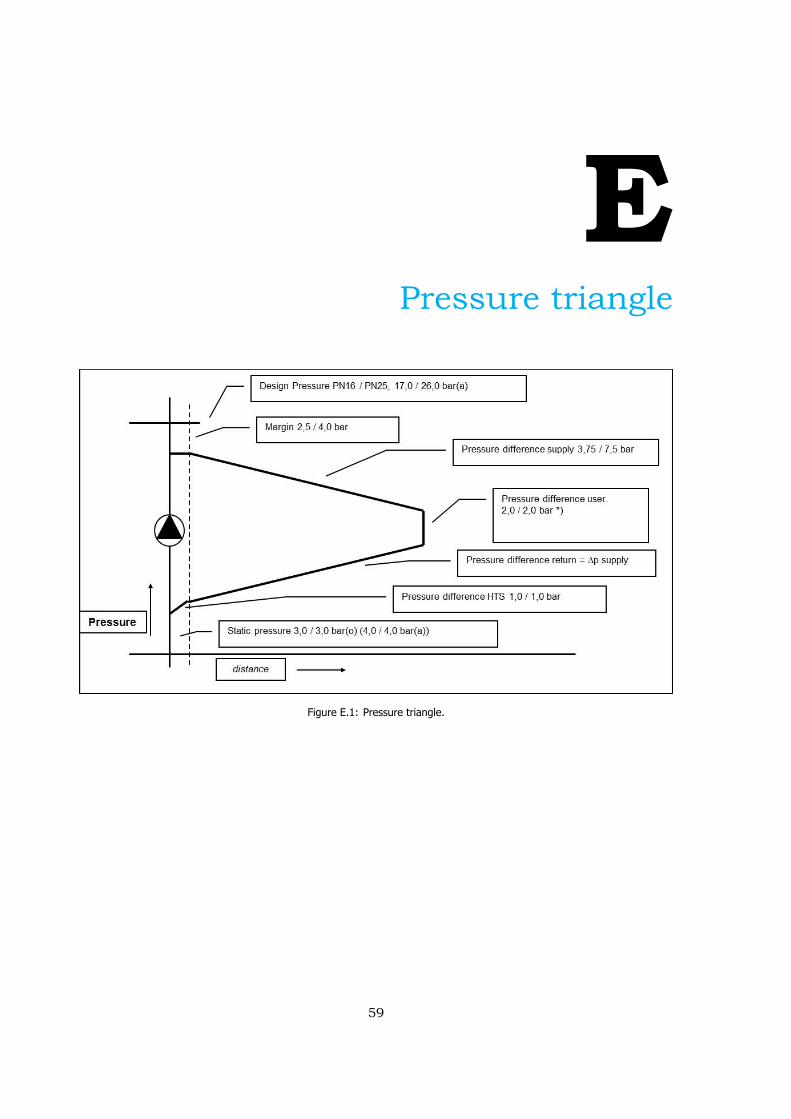
EPressure triangle

Figure E.1: Pressure triangle.

59

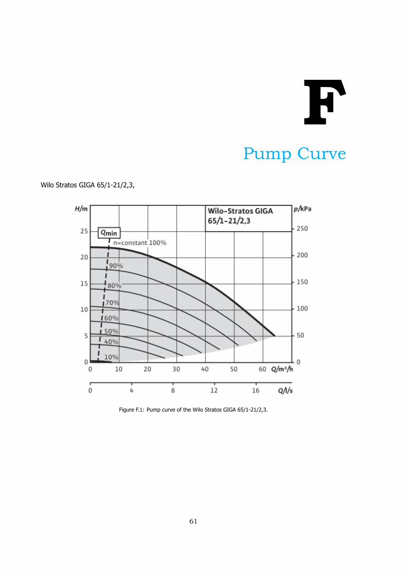
FPump Curve

Wilo Stratos GIGA 65/1-21/2,3,

Figure F.1: Pump curve of the Wilo Stratos GIGA 65/1-21/2,3.

61

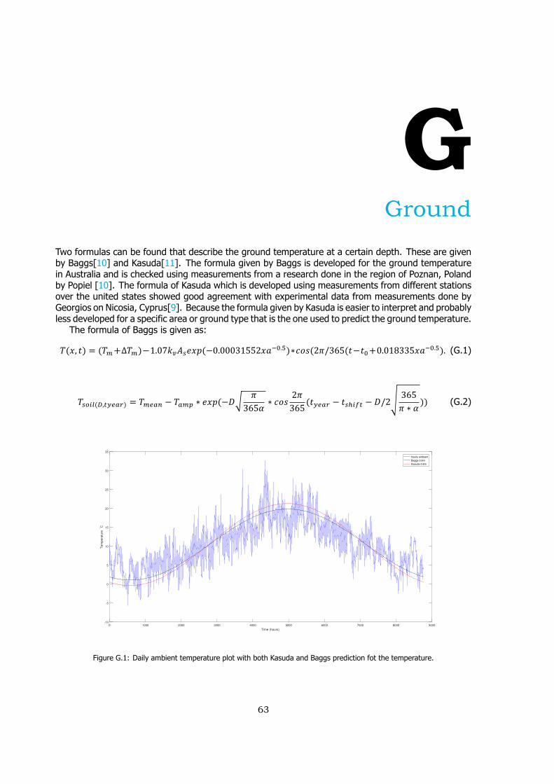
GGround

Two formulas can be found that describe the ground temperature at a certain depth. These are givenby Baggs[10] and Kasuda[11]. The formula given by Baggs is developed for the ground temperaturein Australia and is checked using measurements from a research done in the region of Poznan, Polandby Popiel [10]. The formula of Kasuda which is developed using measurements from different stationsover the united states showed good agreement with experimental data from measurements done byGeorgios on Nicosia, Cyprus[9]. Because the formula given by Kasuda is easier to interpret and probablyless developed for a specific area or ground type that is the one used to predict the ground temperature.

The formula of Baggs is given as:

𝑇(𝑥, 𝑡) = (𝑇 +Δ𝑇 )−1.07𝑘 𝐴 𝑒𝑥𝑝(−0.00031552𝑥𝑎 . )∗𝑐𝑜𝑠(2𝜋/365(𝑡−𝑡 +0.018335𝑥𝑎 . ). (G.1)

𝑇 ( , ) = 𝑇 − 𝑇 ∗ 𝑒𝑥𝑝(−𝐷√ 𝜋365𝛼 ∗ 𝑐𝑜𝑠

2𝜋365(𝑡 − 𝑡 − 𝐷/2√ 365

𝜋 ∗ 𝛼 )) (G.2)

0 1000 2000 3000 4000 5000 6000 7000 8000 9000

Time (hours)

-10

-5

0

5

10

15

20

25

30

35

Te

mpera

ture

°C

hourly ambient

Baggs 0.6m

Kasuda 0.6m

Figure G.1: Daily ambient temperature plot with both Kasuda and Baggs prediction fot the temperature.

63

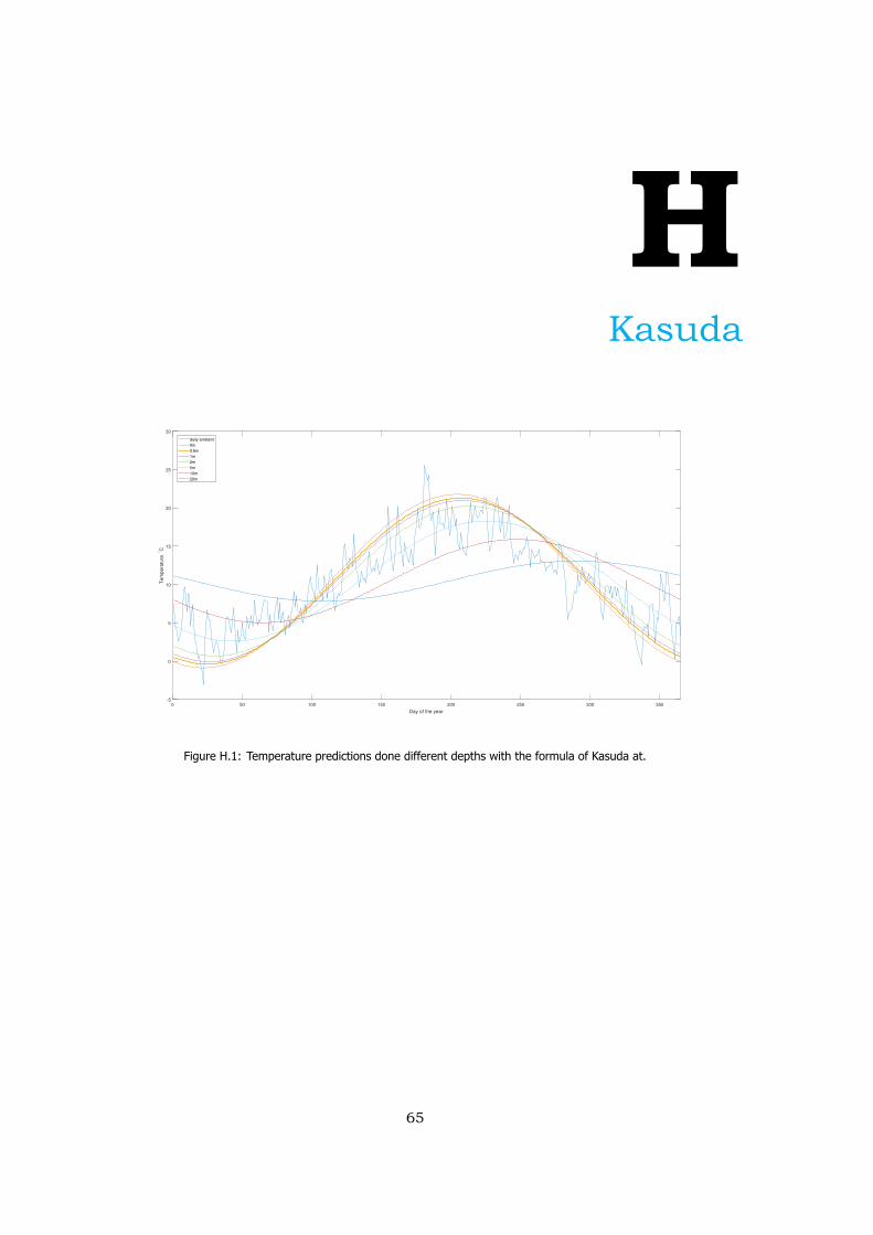
HKasuda

0 50 100 150 200 250 300 350

Day of the year

-5

0

5

10

15

20

25

30

Te

mpera

ture

°C

daily ambient

0m

0.6m

1m

2m

5m

10m

20m

Figure H.1: Temperature predictions done different depths with the formula of Kasuda at.

65

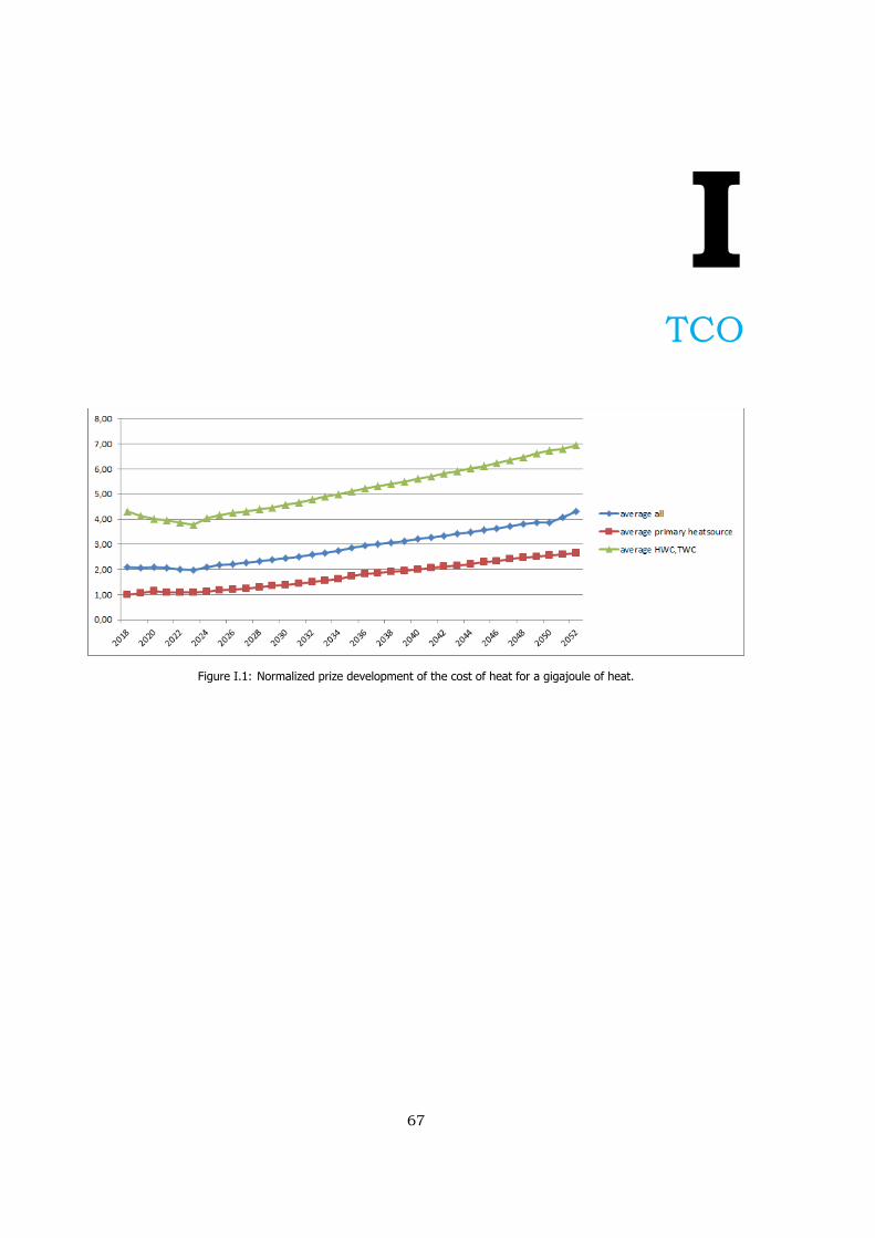
ITCO

Figure I.1: Normalized prize development of the cost of heat for a gigajoule of heat.

67

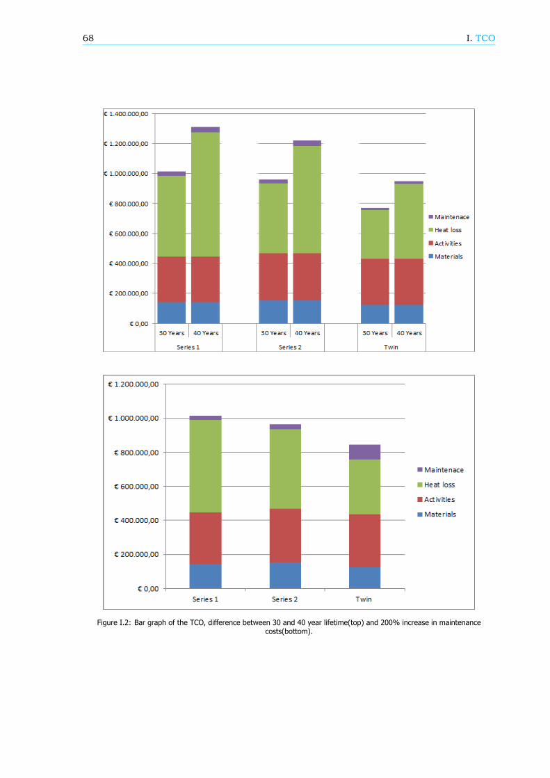
68 I. TCO

Figure I.2: Bar graph of the TCO, difference between 30 and 40 year lifetime(top) and 200% increase in maintenancecosts(bottom).