Latent Dirichlet Allocation, explained and improved upon for applications in marketing intelligence Iris Koks Technische Universiteit Delft

Welcome message from author
This document is posted to help you gain knowledge. Please leave a comment to let me know what you think about it! Share it to your friends and learn new things together.
Transcript

Latent Dirichlet Allocation, explainedand improved upon for applications inmarketing intelligence
Iris Koks
Tech
nisc
heUn
iversite
itDe
lft


Latent Dirichlet Allocation, explained andimproved upon for applications in
marketing intelligenceby
Iris Koksto obtain the degree of Master of Science
at the Delft University of Technology,
to be defended publicly on Friday March 22, 2019 at 2:00 PM.
Student number: 4299981Project duration: August, 2018 – March, 2019Thesis committee: Prof. dr. ir. Geurt Jongbloed, TU Delft, supervisor
Dr. Dorota Kurowicka, TU DelftDrs. Jan Willem Bikker PDEng, CQM
An electronic version of this thesis is available at http://repository.tudelft.nl/.


"La science, mon garçon, est faite d’erreurs, mais ce sont des erreurs qu’il est utile de faire, parcequ’elles conduisent peu à peu à la vérité."
- Jules Verne, in "Voyage au centre de la Terre"

Abstract
In today’s digital world, customers give their opinions on a product that they have purchased online in theform of reviews. The industry is interested in these reviews, and wants to know about which topics their clientswrite, such that the producers can improve products on specific aspects. Topic models can extract the maintopics from large data sets such as the review data. One of these is Latent Dirichlet Allocation (LDA). LDA is ahierarchical Bayesian topic model that retrieves topics from text data sets in an unsupervised manner. Themethod assumes that a topic is assigned to each word in a document (review), and aims to retrieve the topicdistribution for each document, and a word distribution for each topic. Using the highest probability wordsfrom each topic-word distribution, the content of each topic can be determined, such that the main subjectscan be derived. Three methods of inference to obtain the topic and word distributions are considered in thisresearch: Gibbs sampling, Variational methods, and Adam optimization to find the posterior mode. Gibbssampling and Adam optimization have the best theoretical foundations for their application to LDA. Fromresults on artificial and real data sets, it is concluded that Gibbs sampling has the best performance in terms ofrobustness and perplexity.In case the data set consists of reviews, it is desired to extract the sentiment (positive, neutral, negative) fromthe documents, in addition to the topics. Therefore, an extension to LDA that uses sentiment words andsentence structure as additional input is proposed: LDA with syntax and sentiment. In this model, a topicdistribution and a sentiment distribution for each review are retrieved. Furthermore, a word distribution pertopic-sentiment combination can be estimated. With these distributions, the main topics and sentiments ina data set can be determined. Adam optimization is used as inference method. The algorithm is tested onsimulated data and found to work well. However, the optimization method is very sensitive to hyperparametersettings, so it is expected that Gibbs sampling as inference method for LDA with syntax and sentiment performsbetter. Its implementation is left for further research.
Keywords: Latent Dirichlet Allocation, topic modeling, sentiment analysis, opinion mining, review analysis,Hierarchical Bayesian inference
v

Preface
With this thesis, my student life comes to an end. Although I started with studying French after high school,after 4 years, I finally came to my senses, such that now, I have become a mathematician. Fortunately, mypassion for languages has never completely disappeared, and it could even be incorporated in this finalresearch project.
During the last 8 months, I have been doing research and writing my master thesis at CQM in Eindhoven. Ihave had a wonderful time with my colleagues there, and I would like to thank all of them for making it theinteresting, nice time it was. I learned a lot about industrial statistics, machine learning, consultancy and theCQM-way of working. Special thanks go to my supervisors Jan Willem Bikker, Peter Stehouwer and MatthijsTijink, for their sincere interest and helpfulness during every meeting. Next to the interesting conversationsabout mathematics, we also had nice talks about careers, life and personal development, which I will alwaysremember.Although he was not my direct supervisor, Johan van Rooij helped me a lot with programming and implemen-tation questions, and by thinking along patiently when I got stuck in some mathematical derivation, for whichI am very grateful.
Furthermore, I would like to thank my other supervisor, professor Geurt Jongbloed, for his guidance throughthis project and for bringing out the best of me on a mathematical level. Naturally, I also enjoyed our talksabout all aspects of life and the laughs we had. Also, I would like to thank Dorota Kurowicka for being on mygraduation committee, and for her interesting lectures about copulas. Unfortunately, I could not incorporatethem in this project, but maybe in my career as (financial) risk analyst?
Then, of course, I would like to express my gratitude to Jan Frouws, for his unconditional care and supportduring these last 8 months. He was always there to listen to me, mumbling on and on about reviews, topics,strollers and optimization methods. Without you, throughout this project, the ups would not have been thathigh and the downs would have been way deeper. I am really proud of how we manage and enjoy life together.
In addition, I would like to thank my parents for always supporting me during my entire educational journey.Because of them, I always liked going to school and learning, hence my broad interests in languages, economics,physics and mathematics. Also, thanks to my brother Corné, with whom I made my homework together foryears and I had the most interesting (political) discussions.
Lastly, I would like to thank my friends that I met in all different places. With you, I have had a wonderfulstudent life in which I started (and immediately quit) rowing, bouldering, learned to cook properly and forlarge groups (making sushi, pasta, ravioli, mexican wraps, massive Heel Holland Bakt cakes...), learned aboutChristianity, air planes and bit coins, lost my ‘Brabants’ accent such that I became a little more like a ‘Randstad’person, and gained interest in the financial world, in which I hope to get a nice career.
Iris KoksEindhoven, March 2019
vii


Nomenclature
Tn n-dimensional closed simplex
D Corpus, set of all documents
L Log likelihood
Σ Number of different sentiments
σ Sentiment index
α Hyperparameter vector of size K with belief on document-topic distribution
β Hyperparameter vector of size V with belief on topic-word distribution
γ Hyperparameter vector of size Σwith belief on document-sentiment distribution
φk Word probability vector of size V for topic k
πd Sentiment probability vector of size Σ for document d
θd Topic probability vector of size K for document d
C Number of different parts-of-speech considered
c Part-of-speech
d Document index
H Entropy
h Shannon information
K Number of topics
M Number of documents in a data set
Nd Number of words in document d
Ns Number of words in phrase s
s Phrase or sentence index
Sd Number of phrases in document d
V Vocabulary size, i.e. number of unique words in data set
w Word index
z Topic index
Adam Adaptive moment estimation (optimization method)
JS Jensen-Shannon
KL Kullback-Leibler
LDA Latent Dirichlet Allocation
MAP Maximum a posteriori or posterior mode
NLP Natural Language Processing
VBEM Variational Bayesian Expectation Maximization
ix

Contents
List of Figures xiii
List of Tables xv
1 Introduction 11.1 Costumer insights using Latent Dirichlet Allocation . . . . . . . . . . . . . . . . . . . . . . . 11.2 Research questions . . . . . . . . . . . . . . . . . . . . . . . . . . . . . . . . . . . . . . . . 21.3 Thesis outline . . . . . . . . . . . . . . . . . . . . . . . . . . . . . . . . . . . . . . . . . . . 21.4 Note on notation . . . . . . . . . . . . . . . . . . . . . . . . . . . . . . . . . . . . . . . . . 4
2 Theoretical background 52.1 Bayesian statistics. . . . . . . . . . . . . . . . . . . . . . . . . . . . . . . . . . . . . . . . . 52.2 Dirichlet process and distribution . . . . . . . . . . . . . . . . . . . . . . . . . . . . . . . . 7
2.2.1 Stick-breaking construction of Dirichlet process . . . . . . . . . . . . . . . . . . . . . . 82.2.2 Dirichlet distribution . . . . . . . . . . . . . . . . . . . . . . . . . . . . . . . . . . . 8
2.3 Natural language processing . . . . . . . . . . . . . . . . . . . . . . . . . . . . . . . . . . . 132.4 Model selection criteria . . . . . . . . . . . . . . . . . . . . . . . . . . . . . . . . . . . . . . 14
3 Latent Dirichlet Allocation 173.1 Into the mind of the writer: generative process . . . . . . . . . . . . . . . . . . . . . . . . . . 183.2 Important distributions in LDA . . . . . . . . . . . . . . . . . . . . . . . . . . . . . . . . . . 213.3 Probability distribution of the words . . . . . . . . . . . . . . . . . . . . . . . . . . . . . . . 213.4 Improvements and adaptations to basic LDA model . . . . . . . . . . . . . . . . . . . . . . . 24
4 Inference methods for LDA 274.1 Posterior mean . . . . . . . . . . . . . . . . . . . . . . . . . . . . . . . . . . . . . . . . . . 29
4.1.1 Analytical determination. . . . . . . . . . . . . . . . . . . . . . . . . . . . . . . . . . 294.1.2 Markov chain Monte Carlo methods . . . . . . . . . . . . . . . . . . . . . . . . . . . . 30
4.2 Posterior mode . . . . . . . . . . . . . . . . . . . . . . . . . . . . . . . . . . . . . . . . . . 384.2.1 General variational methods . . . . . . . . . . . . . . . . . . . . . . . . . . . . . . . . 384.2.2 Variational Bayesian EM for LDA. . . . . . . . . . . . . . . . . . . . . . . . . . . . . . 43
5 Determination posterior mode estimates for LDA using optimization 475.1 LDA’s posterior density . . . . . . . . . . . . . . . . . . . . . . . . . . . . . . . . . . . . . . 475.2 Gradient descent . . . . . . . . . . . . . . . . . . . . . . . . . . . . . . . . . . . . . . . . . 495.3 Stochastic gradient descent . . . . . . . . . . . . . . . . . . . . . . . . . . . . . . . . . . . . 505.4 Adam optimization . . . . . . . . . . . . . . . . . . . . . . . . . . . . . . . . . . . . . . . . 51
5.4.1 Softmax transformation . . . . . . . . . . . . . . . . . . . . . . . . . . . . . . . . . . 545.4.2 Regularization . . . . . . . . . . . . . . . . . . . . . . . . . . . . . . . . . . . . . . . 55
6 LDA with syntax and sentiment 576.1 Into the more complicated mind of the writer: generative process . . . . . . . . . . . . . . . . 576.2 Practical choices in phrase detection . . . . . . . . . . . . . . . . . . . . . . . . . . . . . . . 606.3 Estimating the variables of interest . . . . . . . . . . . . . . . . . . . . . . . . . . . . . . . . 61
6.3.1 Posterior mode: optimization . . . . . . . . . . . . . . . . . . . . . . . . . . . . . . . 636.3.2 Posterior mean: Gibbs sampling . . . . . . . . . . . . . . . . . . . . . . . . . . . . . . 64
7 Validity of topic-word distribution estimates 697.1 Normalized symmetric KL-divergence . . . . . . . . . . . . . . . . . . . . . . . . . . . . . . 697.2 Symmetrized Jensen-Shannon divergence . . . . . . . . . . . . . . . . . . . . . . . . . . . . 70
xi

xii Contents
8 Results 718.1 Posterior density visualization of LDA. . . . . . . . . . . . . . . . . . . . . . . . . . . . . . . 71
8.1.1 Influence of the hyperparameters in LDA . . . . . . . . . . . . . . . . . . . . . . . . . 718.1.2 VBEM’s posterior density approximation . . . . . . . . . . . . . . . . . . . . . . . . . 73
8.2 LDA: different methods of inference . . . . . . . . . . . . . . . . . . . . . . . . . . . . . . . 748.2.1 Small data set: Cats and Dogs . . . . . . . . . . . . . . . . . . . . . . . . . . . . . . . 758.2.2 Towards more realistic analyses: stroller data . . . . . . . . . . . . . . . . . . . . . . . 79
8.3 LDA with syntax and sentiment: is this the future? . . . . . . . . . . . . . . . . . . . . . . . . 868.3.1 Model testing on gibberish. . . . . . . . . . . . . . . . . . . . . . . . . . . . . . . . . 868.3.2 Stroller data set: deep dive on a single topic . . . . . . . . . . . . . . . . . . . . . . . . 91
9 Discussion 939.1 Latent Dirichlet Allocation . . . . . . . . . . . . . . . . . . . . . . . . . . . . . . . . . . . . 93
9.1.1 Assumptions . . . . . . . . . . . . . . . . . . . . . . . . . . . . . . . . . . . . . . . . 939.1.2 Linguistics . . . . . . . . . . . . . . . . . . . . . . . . . . . . . . . . . . . . . . . . . 949.1.3 Influence of the prior . . . . . . . . . . . . . . . . . . . . . . . . . . . . . . . . . . . 949.1.4 Model selection measures . . . . . . . . . . . . . . . . . . . . . . . . . . . . . . . . . 95
9.2 LDA with syntax and sentiment . . . . . . . . . . . . . . . . . . . . . . . . . . . . . . . . . . 96
10 Conclusion and recommendations 9710.1 Main findings . . . . . . . . . . . . . . . . . . . . . . . . . . . . . . . . . . . . . . . . . . . 9710.2 Further research . . . . . . . . . . . . . . . . . . . . . . . . . . . . . . . . . . . . . . . . . 97
A Mathematical background and derivations 99A.1 Functional derivative and Euler-Lagrange equation. . . . . . . . . . . . . . . . . . . . . . . . 99A.2 Expectation of logarithm of Beta distributed random variable . . . . . . . . . . . . . . . . . . 102A.3 LDA posterior mean determination . . . . . . . . . . . . . . . . . . . . . . . . . . . . . . . . 103
B Results and data sets 107B.1 Stroller topic-word distributions . . . . . . . . . . . . . . . . . . . . . . . . . . . . . . . . . 107B.2 Top stroller reviews topic 5 . . . . . . . . . . . . . . . . . . . . . . . . . . . . . . . . . . . . 112B.3 Data sets . . . . . . . . . . . . . . . . . . . . . . . . . . . . . . . . . . . . . . . . . . . . . 114B.4 Conjunction word list . . . . . . . . . . . . . . . . . . . . . . . . . . . . . . . . . . . . . . . 117B.5 Stop word list . . . . . . . . . . . . . . . . . . . . . . . . . . . . . . . . . . . . . . . . . . . 118B.6 Sentiment word lists . . . . . . . . . . . . . . . . . . . . . . . . . . . . . . . . . . . . . . . 120
Bibliography 139
List of Figures
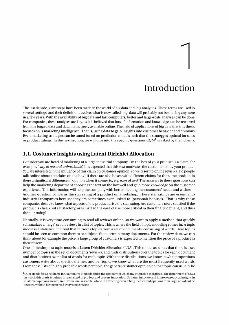
1.1 Overview of methods of inference to estimate model parameters of Latent Dirichlet Allocation.The posterior distribution can either be calculated analytically, after which the posterior modelcan be found through optimization, or it can be approximated using Gibbs sampling or Varia-tional Bayes methods. The latter methods are discussed in chapter 4 of this thesis, while the firstinference method is described in chapter 5, as it is one of the main contributions of this research. 3
2.1 Bayesian statistics: A prior density is imposed on the random parameter Θ and results in aposterior density ofΘ given the observed data. The three possible estimators forΘ are given infigure 2.1b. . . . . . . . . . . . . . . . . . . . . . . . . . . . . . . . . . . . . . . . . . . . . . . . . . . . 7
2.2 Three-dimensional simplex T3(1). On the gray plane lie the values of X1, X2 and X3 for X ∈T3(1),such that the sum of X1, X2 and X3 equal to 1. . . . . . . . . . . . . . . . . . . . . . . . . . . . . . . 11
2.3 100 samples from Dir(α) distribution with the same (α)i for i ∈ 1,2,3. . . . . . . . . . . . . . . . 122.4 100 samples from asymmetric Dirichlet distributions. The axis of X1 is on the left, the one of X3
on the right and of X2 on below the triangle. . . . . . . . . . . . . . . . . . . . . . . . . . . . . . . . 132.5 Data preprocessing workflow in KNIME. . . . . . . . . . . . . . . . . . . . . . . . . . . . . . . . . . 13
3.1 Plate notation of Latent Dirichlet Allocation as visualized in [25]. The hyperparameters α andβ are denoted with a dotted circle. Θ represents the document-topic distribution, andΦ is thetopic-word distribution. Random variable Z is the topic that has one-to-one correspondencewith word W . . . . . . . . . . . . . . . . . . . . . . . . . . . . . . . . . . . . . . . . . . . . . . . . . . 20
4.1 Posterior densities of Θd and 1−Θd , i.e. the probabilities of respectively topic 1 and 2 fordocument d . . . . . . . . . . . . . . . . . . . . . . . . . . . . . . . . . . . . . . . . . . . . . . . . . . . 28
4.2 Visualization of the posterior densities p(θ1,θ2,φ1,φ2|w1,w2,α,β) with θ1 and θ2 fixed on thevalue of a mode. The maximum of the 4-dimensional posterior density is found using grid search.The two documents consists only of two possible words, for ease of notation denoted by 1 and 2.Document 1 is then ‘2 2 1 1 1’ and document 2 consists of ‘1 1 1 1 1 1 2’. Hyperparameters α andβ are set to respectively 0.9 and 1.1 and are symmetric i.e. the same for all dimensions. . . . . . 29
4.3 Schematic overview of an example of variational methods. There are n instances of X and Y ,where X depends on the parameter θ. X is a latent random variable, θ is a fixed parameter and yis an observed random variable. . . . . . . . . . . . . . . . . . . . . . . . . . . . . . . . . . . . . . . 38
4.4 Schematic overview of an example of variational methods in a Bayesian setting. There are ninstances of X and Y , where X depends on the parameterΘ. X is a latent random variable,Θ is arandom variable depending on fixed hyperparameter α, and y is an observed random variable. 40
5.1 Posterior density p(θ1,φ1,φ2|w1, w2, w3,α,β) for two fixed values of θ1 and hyperparametersα= (0.9,0.9) and β= (1,1). . . . . . . . . . . . . . . . . . . . . . . . . . . . . . . . . . . . . . . . . . . 48
5.2 Basic gradient descent algorithm visualized. Every step is made in the direction of the steepestdescent. In this one-dimensional case, one can only move upwards or downwards. Therefore,this is an easy minimization problem. The (local) minimum is reached, and no more steps canbe made downwards. . . . . . . . . . . . . . . . . . . . . . . . . . . . . . . . . . . . . . . . . . . . . . 49
5.3 Example of finding the minimum of an ellipse-like hill. From the red dot, the gradient in the x-direction is smaller than in the y-direction, so the algorithm makes a larger step in the x-directionthan in the y-direction. . . . . . . . . . . . . . . . . . . . . . . . . . . . . . . . . . . . . . . . . . . . 53
5.4 Contour plot of f (x, y) = (x −1)4 +0.5y4. The minimum of f is located at (x, y) = (1,0). . . . . . . 535.5 Parameters used in Adam optimization to find the location of the minimum of f (x, y) = (x −
1)4 +0.5y4. With step size is meant the size of the change in each iteration, that is: xn+1 −xn =−[stepsize] for each iteration n. If the step size is negative, the algorithm walks forwards. . . . . 54
xiii
xiv List of Figures
6.1 Plate notation of the extension of LDA specifically designed for review studies, also called ‘LDAwith syntax and sentiment’. Each rectangle represents a repetitive action with in the right bottomcorner the number of times the action (e.g. a draw from a distribution) is executed. . . . . . . . . 60
8.1 Posterior densities for different settings for symmetric hyperparametersα and β. There are threedocuments: w1 = [1111], w2 = [121122] and w3 = [12222222]. The vocabulary size is V = 2 andthe number of topics is K = 2. Because the posterior density for this case has 5 parameters andis therefore six-dimensional, the surface plots actually show the joint posterior density of Φ1
andΦ2 conditional on the words, hyperparameters and the values ofΘ1,Θ2 andΘ3. For the θd
(with d = 1,2,3), the optimal values are taken, that is the values for each θ for which the posteriordensity is maximal. Note that due to the coarse grid, each value has a rounding error. . . . . . . 72
8.2 Surface plot of join posterior density of Φ1,Φ2 conditional on Θ1 = 0.5, Θ2 = 0.8, Θ3 = 0.25.Hyperparameters are set to α= 1.1 and β= 1. The number of topics is K = 2, the vocabulary sizeis V = 2 and there are 3 documents: M = 3. The data consists of three documents: w1 = [1,2],w2 = [1,1,1,1,2] and w3 = [1,2,2,2,1,2,2,2]. Also the approximation of the conditional posteriordensity, q , is shown and it can be seen that their maxima lie on different locations, resulting indifferent posterior modes. Note that for the sake of comparison, all values are normalized suchthat the maximal value equal 1 for both surfaces. . . . . . . . . . . . . . . . . . . . . . . . . . . . . 74
8.3 Word probabilities of the top 20 words of topic 5. This φ5 topic-word distribution is estimatedusing Adam optimization with (α)i = 1.1 and (β)i = 1.1, and with random initialization. . . . . . 83
List of Tables
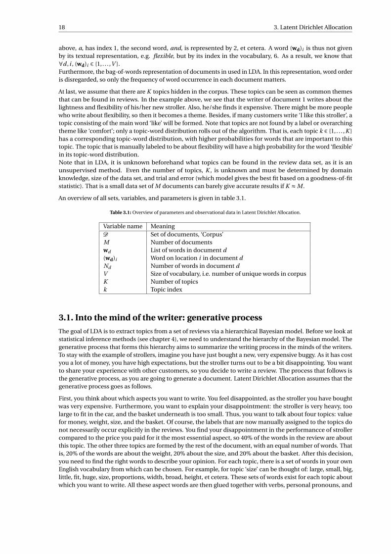
3.1 Overview of parameters and observational data in Latent Dirichlet Allocation. . . . . . . . . . . . 183.2 Random variables and constants used in Latent Dirichlet Allocation. . . . . . . . . . . . . . . . . 20
6.1 (Random) variables used in Latent Dirichlet Allocation with syntax and sentiment. . . . . . . . . 59
8.1 ‘Cats and dogs’ data set. Simple, small data set with distinctive topic clusters by construction.Documents in gray belong to the ‘cat’ topic, while those in white are part of the ‘dog’ topic. . . . 75
8.2 Estimates of the topic-word distributions Φ1 and Φ2, based on the intuitive construction oftopics by reading the documents. The probabilities are calculated using relative frequencies. . . 76
8.3 Optimization results for φ1 and φ2 with symmetric (α)i = 0.99 and symmetric (β)i = 1. TheAdam gradient descent algorithm is used with a learning rate of 0.001, a stopping criterion of10−4 for the relative change and a maximum of 20,000 iterations. Regularization as described in5.4.2 is applied. . . . . . . . . . . . . . . . . . . . . . . . . . . . . . . . . . . . . . . . . . . . . . . . . 76
8.4 Variational Bayesian EM results forΦ1 andΦ2 with symmetric (α)i = 0.99 and symmetric (β)i = 1. 778.5 Gibbs sampling results from KNIME forΦ1 andΦ2 with symmetric (α)i = 0.99 and symmetric
(β)i = 1. 1000 iterations are executed on 8 different threads. . . . . . . . . . . . . . . . . . . . . . . 778.6 Combinations of hyperparameters α and β, both taken as symmetric vectors, for which the
optimization results are satisfactory concerning estimations of θ and φ. . . . . . . . . . . . . . . 788.7 Overview of results for LDA on stroller data using different inference methods. Adam optimiza-
tion and Variational Bayesian Expectation Maximization are used to determine the posteriormode, while the KNIME implementation estimates the model parameters via Gibbs sampling.Two different initialization methods are used for the optimization algorithm: random initializa-tion and taking the estimates of VBEM as the initial value. Besides the model validation scores, itis an indication whether, for either optimization method, the maximum number of iterations isreached. The optimization method is truncated after 100
learningrate iterations. . . . . . . . . . . . . . 80
8.8 Perplexity and log posterior scores for LDA applied to 2000 reviews about strollers. The hyperpa-rameters are set to (α)i = 0.999 and (β)i = 0.999. There are ten topics to be found, thus K = 10.The Adam optimization algorithm is used with a stopping criterion threshold of 10−3 and randominitialization. The same split in training and test set is used to avoid measuring multiple effectsat the same time. The only variance comes from the initialization and the steps taken in thealgorithm. . . . . . . . . . . . . . . . . . . . . . . . . . . . . . . . . . . . . . . . . . . . . . . . . . . . 82
8.9 Perplexity and log posterior scores for LDA applied to 2000 reviews about strollers. The hyperpa-rameters are set to (α)i = 0.999 and (β)i = 0.999. There are ten topics to be found, thus K = 10.The KNIME Topic Extractor is used with different seeds. The training and test set are kept thesame throughout the analysis. . . . . . . . . . . . . . . . . . . . . . . . . . . . . . . . . . . . . . . . 82
8.10 Perplexity and log posterior scores for LDA applied to 2000 reviews about strollers. The hyperpa-rameters are set to (α)i = 0.99 and (β)i = 0.99. There are 10 topics to be found, thus K = 10. TheAdam optimization algorithm is used with a threshold of 10−3 and random initialization. To avoidmeasuring multiple effects at the same time, the random initialization of Adam optimizationis fixed using a seed. The training and test set division is now to only random effect, and it ischecked that, for each run, the training and test sets are different. . . . . . . . . . . . . . . . . . . 83
8.11 Normalized KL-divergence scores between all estimated topic-word distributions φ1, . . . ,φK,which are determined for the stroller data using Adam optimization with symmetric (α)i = 1.1and (β)i = 1.1, and setting the number of topics K = 10. . . . . . . . . . . . . . . . . . . . . . . . . 84
8.12 Normalized symmetric JS-divergence similarity scores between all estimated topic-word dis-tributions φ1, . . . ,φK, which are determined for the stroller data using Adam optimization withsymmetric (α)i = 1.1 and (β)i = 1.1, and setting the number of topics K = 10. . . . . . . . . . . . 85
8.13 Simulated document-topic distributions that are independently drawn from a Dirichlet(0.5,0.5)distribution. . . . . . . . . . . . . . . . . . . . . . . . . . . . . . . . . . . . . . . . . . . . . . . . . . . 87
xv
xvi List of Tables
8.14 Posterior mode estimates of the document-topic distributions of the simulated data, determinedwith Adam optimization in which the hyperparameter settings are (α)i = 1.8, (γ)i = 1.1, and βo
for o = 1,2,3 constructed as described above. A learning rate of 0.0001 and random initializationhave been used. . . . . . . . . . . . . . . . . . . . . . . . . . . . . . . . . . . . . . . . . . . . . . . . . 87
8.15 Simulated document-sentiment distributions that are independently drawn from a Dirichlet(0.5,0.5, 0.5) distribution. . . . . . . . . . . . . . . . . . . . . . . . . . . . . . . . . . . . . . . . . . . . . . 88
8.16 Posterior mode estimates of the document-sentiment distributions of the simulated data, deter-mined with Adam optimization in which the hyperparameter settings are (α)i = 1.8, (γ)i = 1.1,and βo for o = 1,2,3 constructed as described above. A learning rate of 0.0001 and randominitialization have been used. . . . . . . . . . . . . . . . . . . . . . . . . . . . . . . . . . . . . . . . . 88
8.17 Simulated topic-sentiment-word distributions that are independently drawn from Dirichlet(βo)distributions corresponding to their sentiment. Hyperparameters βo are constructed by dividingthe probability mass over the corresponding sentiment words and the rest of the vocabulary. . 89
8.18 Posterior mode estimates of the topic-sentiment-word distributions of the simulated data, deter-mined with Adam optimization in which the hyperparameter settings are (α)i = 1.8, (γ)i = 1.1,and βo for o = 1,2,3 constructed as described above. A learning rate of 0.0001 and randominitialization have been used. . . . . . . . . . . . . . . . . . . . . . . . . . . . . . . . . . . . . . . . . 90
8.19 NJSS for columns in estimated and row simulated . . . . . . . . . . . . . . . . . . . . . . . . . . . . 908.20 Estimated topic-sentiment-word distributions for subtopic 1 for stroller reviews that belong
to topic 5 of an analysis with plain LDA (with hyperparameters (α)i = 1.1, (β)i = 1.1). In thisanalysis for LDA with syntax and sentiment, (α)i = 2, (γ)i = 2, and β is constructed as explainedin section 8.3.2. . . . . . . . . . . . . . . . . . . . . . . . . . . . . . . . . . . . . . . . . . . . . . . . . 91
8.21 Topic-sentiment-word distributions for subtopic 2 for stroller reviews that belong to topic 5 ofan analysis with plain LDA (with hyperparameters (α)i = 1.1, (β)i = 1.1). In the analysis for LDAwith syntax and sentiment, (α)i = 2, γ= 2, and β is constructed as explained in section 8.3.2. . . 92
B.1 ‘Cats and dogs’ data set. Simple, small data set with distinctive topic clusters by construction. . 114B.2 Simulated data for test of Adam optimization applied to determining the posterior mode esti-
mates in the LDA with syntax and sentiment model. The data is simulated with hyperparametersα = (0.5,0.5), γ = (0.5,0.5,0.5), and βo for o = 1,2,3 as explained in chapter 6. There are 20documents in total, of which 11 are shown here. A period is used to indicate the end of a phrase. 115
B.3 Simulated data for test of Adam optimization applied to determining the posterior mode esti-mates in the LDA with syntax and sentiment model. The data is simulated with hyperparametersα = (0.5,0.5), γ = (0.5,0.5,0.5), and βo for o = 1,2,3 as explained in chapter 6. There are 20documents in total, of which 9 are shown here. A period is used to indicate the end of a phrase. 116
1Introduction
The last decade, giant steps have been made in the world of big data and ‘big analytics’. These terms are used inseveral settings, and their definitions evolve; what is now called ‘big’ data will probably not be that big anymorein a few years. With the availability of big data and fast computers, better and large-scale analyses can be done.For companies, these analyses are key, as it is believed that lots of information and knowledge can be retrievedfrom the logged data and data that is freely available online. The field of applications of big data that this thesisfocuses on is marketing intelligence. That is, using data to gain insights into customer behavior and opinions.Even marketing strategies can be tuned based on prediction models such that the strategy is optimal for salesor product ratings. In the next section, we will dive into the specific questions CQM1 is asked by their clients.
1.1. Costumer insights using Latent Dirichlet Allocation
Consider you are head of marketing of a large industrial company. On the box of your product is a claim, forexample, ‘easy to use and unbreakable’. It is expected that this text motivates the customer to buy your product.You are interested in the influence of this claim on customer opinion, so we resort to online reviews. Do peopletalk online about the claim on the box? If there are also boxes with different claims for the same product, isthere a significant difference in opinion when it comes to, e.g. ease of use? The answers to these questions canhelp the marketing department choosing the text on the box well and gain more knowledge on the customerexperience. This information will help the company with better meeting the customers’ needs and wishes.Another question concerns the star rating of a product on a webshop. These star ratings are essential toindustrial companies because they are sometimes even linked to (personal) bonuses. That is why thesecompanies desire to know what aspects of the product drive the star rating. Are customers more satisfied if theproduct is cheap but satisfactory, or is instead the ease of use more critical in their final judgment, and thusthe star rating?
Naturally, it is very time-consuming to read all reviews online, so we want to apply a method that quicklysummarizes a (large) set of reviews in a list of topics. This is where the field of topic modeling comes in. A topicmodel is a statistical method that retrieves topics from a set of documents, consisting of words. Here topicsshould be seen as common themes or subjects that occur in many documents. For the review data, we canthink about for example the price; a large group of customers is expected to mention the price of a product intheir review.One of the simplest topic models is Latent Dirichlet Allocation (LDA). This model assumes that there is a setnumber of topics in the set of documents/reviews, and finds distributions over the topics for each documentand distributions over a list of words for each topic. With these distributions, we know in what proportionscustomers write about specific themes, and per topic, we know what are the most frequently used words.From these lists of highly probable words per topic, the general customer opinion on that topic can usually be
1CQM stands for Consultants in Quantitative Methods and is the company in which my internship took place. The department of CQMin which this thesis is written is specialized in product and process innovation. To better innovate and improve products, insights incustomer opinions are required. Therefore, research is done in extracting overarching themes and opinions from large sets of onlinereviews, without having to read every single review.
1

2 1. Introduction
concluded. Latent Dirichlet Allocation is therefore well applicable for review analyses and forms the maintheme of this thesis.
1.2. Research questionsThis research is conducted in collaboration with CQM. Therefore, the research questions that are studied inthis thesis, follow from issues encountered in the day-to-day work at CQM.First of all, the Bayesian model called Latent Dirichlet Allocation needs a more thorough explanation. Thereare many different applications of LDA in software, but a mathematical explanation of the method of inferenceused in that software often lacks. Also in literature, articles might offer too little information on what isreally behind the model of Latent Dirichlet Allocation, and different methods of inference are proposed.An overview of these methods including extensive derivations is thus given in this thesis. Secondly, LatentDirichlet Allocation is a model that can be applied to all kinds of documents. However, in the field of marketingintelligence, LDA might not give the desired results, and more information is expected to be ‘hidden’ in theanalyzed reviews. An improvement upon the basic LDA model to make it more suitable for review analyses isresearched.
As a conclusion, two research questions that are to be answered in this thesis.
• What is Latent Dirichlet Allocation and which methods of inference are possible for thisBayesian hierarchical model?
• How can Latent Dirichlet Allocation be improved upon to make it more suitable for reviewanalyses using linguistics?
1.3. Thesis outlineAt the moment, you, the reader, have already been given the motivation to use Latent Dirichlet Allocation.Before being able to elaborate on the precise working principle of LDA model in chapter 3, in chapter 2 sometheoretical background information essential to understanding chapter 3 is given. Apart from fundamentallyunderstanding what LDA does and what assumptions are made, different methods of inference are possibleand are explained in chapter 4. To make a clear distinction between which methods are already frequentlyused in the literature, and which method is a new contribution of this thesis, in chapter 4 only the inferencemethods that are present in literature and widely used are explained. In chapter 5, a new, different inferencemethod is explained, which is, to the best of author’s knowledge, not yet applied to LDA.Because CQM gets specific questions from clients about customer opinions on products, an extension of LDAthat is, in particular, suitable to extract this kind of information from large data sets is described in chapter6. This extension has been given the name ‘LDA with syntax and sentiment’, as it extends plain LDA with acombination of the sentiment of words (i.e., positive and negative opinion words) with the their part-of-speech.Then, in chapter 7, a small note is made on how to interpret the results of LDA and which conclusions shouldand should not be drawn. In chapter 8, the actual results of the application of LDA to different data sets aredisplayed. Firstly, the different inference methods are compared, and secondly, results for LDA with syntaxand sentiment are given. Naturally, a discussion on the results is present in chapter 9, and lastly, in chapter 10,conclusions on the different inference methods for LDA, and the extended version of LDA specifically designedfor CQM are drawn. Also, recommendations on further research can be read about in chapter 10.
1.3. Thesis outline 3
LDA
mo
del
Infe
ren
ce
Po
ster
ior
An
alyt
ical
Ap
pro
xim
atio
n
Po
ster
ior
mo
de
Gib
bs
Var
iati
on
alB
ayes
Op
tim
izat
ion
colla
pse
dn
on
-co
llap
sed
mea
n-fi
eld
VB
Sto
chas
tic
VB
sam
ple
mea
nm
argi
nal
dis
trib
uti
on
s
sam
ple
mea
nm
argi
nal
dis
trib
uti
on
s
’po
ster
ior’
mo
de
’po
ster
ior’
mo
de
Ch
apte
r5
Ch
apte
r4
Figu
re1.
1:O
verv
iew
ofm
eth
od
so
fin
fere
nce
toes
tim
ate
mo
del
par
amet
ers
ofL
aten
tDir
ich
letA
lloca
tio
n.T
he
po
ster
ior
dis
trib
uti
on
can
eith
erb
eca
lcu
late
dan
alyt
ical
ly,a
fter
wh
ich
the
po
ster
ior
mo
del
can
be
fou
nd
thro
ugh
op
tim
izat
ion
,or
itca
nb
eap
pro
xim
ated
usi
ng
Gib
bs
sam
plin
go
rV
aria
tio
nal
Bay
esm
eth
od
s.T
he
latt
erm
eth
od
sar
ed
iscu
ssed
inch
apte
r4
oft
his
thes
is,w
hile
the
firs
tin
fere
nce
met
ho
dis
des
crib
edin
chap
ter
5,as
itis
on
eo
fth
em
ain
con
trib
uti
on
so
fth
isre
sear
ch.
4 1. Introduction
1.4. Note on notationIn the field of mathematics, there are many different ways of saying the same. Therefore, in this section, someclarity is given about the notations used in this thesis.
First, all constants or one-dimensional parameters are simply given by its letter in italic, albeit from the Greekor Roman alphabet, or upper or lower case. Then, when the parameter is a vector, the corresponding letteris given in boldface. Sometimes, for ease of notation, also sets of vectors are given in boldface, such thatφ= φ1, . . . ,φK, while, strictly speaking, φ is a set of vectors. In case this simplified notation is used, it willhave been mentioned.Very often in this thesis, only one element of a vector is used in an equation or a density. This element is thendenoted with a subscript, while the vector remains in boldface and is surrounded with round brackets. Forexample, the i th element of vector φj is denoted with (φj)i (where j is used to indicate which vector φ is used,as there are many vectors φ).
Secondly, random variables are, conventionally, denoted with capital letters. Once they take a value, the nota-tion changes to lower case to show that we are dealing with data. There are some constants also denoted witha capital letter, such as the data set size. When in doubt, the nomenclature can be consulted for clarification.As conventional, the expectation of a random variable is given by E. If a probability of a random variable Xtaking value x, is denoted with P(X = x), we use P to indicate the probability measure that belongs to theprobability space in which X lives.
Lastly, for densities, we use the Bayesian notation, as will be explained in chapter 2 more extensively. Withthe Bayesian notation, we mean that the density of random variable X , fX (x), is denoted with p(x). Theconditional density of random variable X given Y , fX |Y (x|y), becomes p(x|y).
2Theoretical background
"Inside every non-Bayesian, there is a Bayesian struggling to get out"
Dennis Lindley (1923-2013)
This chapter contains the theoretical background needed to understand the rest of this thesis. Firstly, theprinciples of Bayesian statistics are explained, since LDA is a hierarchical Bayesian model. Secondly, a sectionis dedicated to the Dirichlet process and Dirichlet distribution, because the latter is used multiple times in themodel.Next, natural language processing (NLP), an overlapping field in computer science, artificial intelligence andlinguistics, is introduced. Some principles of NLP are used in the preprocessing steps of review analyses withLDA. Lastly, model selection criteria that are frequently used in topic modeling are explained.
2.1. Bayesian statistics
In the field of statistics, there are two types of statisticians (generally speaking): frequentists and Bayesianbelievers. The latter group considers all unknowns to be random variables, including the parameters [46]. Wewill explain this way of thinking and doing statistics using a simple example.
Consider flipping a coin of which we do not know whether it is fair or not. Suppose we do this n times, andXi |Θ∼ Bernoulli(Θ) for i = 1, . . . ,n. The probability of throwing heads is represented by random variable Θ,while the probability of getting tails is 1−Θ. The random variables X1, . . . , Xn are the flips and can either beheads or tails, i.e. Xi ∈ H ,T , for i = 1, . . . ,n. Note that each flip is executed separately and with the samecoin (and other circumstances), therefore X1, . . . Xn are conditionally independent and identically distributed.Note that conditional independence is specific for Bayesian statistics, as parameter Θ is a random variable.Therefore, conditional onΘ, the flips are independent. BecauseΘ is a random variable, it has a distributionreflecting our belief.
Beforehand, we believe that the probability of heads is in the neighborhood of 12 , as would be the case for a
fair coin. This belief is inserted into the model via a prior distribution. This is the distribution ofΘwe believeto be true before generating the data. After having observed X1 = x1, . . . , Xn = xn , the posterior distribution isconstructed, as the name suggests. The posterior density is determined via Bayes’ rule:
fΘ|X(θ|x) = fX|Θ(x|θ) · fΘ(θ)
fX(x)(2.1)
Here fΘ|X(θ|x) is the conditional density of parameter Θ given the observations X = x, and is referred to asthe posterior. fX|Θ(x|θ) is the conditional multivariate density function of random variables X1, . . . Xn givenparameterΘ= θ, fΘ(θ) is the density of the initial distribution ofΘ, that is the prior density, and the term in thedenominator, fX(x), is called the evidence. This is the marginal distribution of the data and can be determinedby integrating the numerator in equation 2.1 over θ.
5

6 2. Theoretical background
An appropriate prior that represents our strong belief that the coin will have approximately equal probabilitiesfor heads and tails, is given by the Beta distribution with equal parameters and thus mean 1
2 . Because we arerelatively certain that the coin is fair, we choose both a and b to be 4. Therefore, we take as prior Θ∼ Beta(4,4):
fΘ(θ) = 1
B(4,4)θ3 · (1−θ)3 (2.2)
With B(a,b) the beta function, defined as:
B(a,b) =∫ 1
0t a−1(1− t )b−1 dt (2.3)
Which can be rewritten in terms of the gamma function Γ(a) = ∫ ∞0 t a−1e−t dt , as shown in e.g. [37]:
B(a,b) = Γ(a)Γ(b)
Γ(a +b)(2.4)
Instead of determining fX|Θ(x|θ) directly, it is wise to define Y as the total number of heads first, such thatY ∼ Binomial(n,Θ). The probability density function of Y is then:
fY |Θ(y |θ) = n!
y !(n − y)!θy · (1−θ)n−y (2.5)
Using Bayes’ rule from equation 2.1, the posterior distribution becomes:
fΘ|X(θ|x1, . . . , xn) = fΘ|Y
(θ|Y =
n∑i=1
1xi=H
)(∗)
∝ fY |Θ(y |θ) · fΘ(θ) (∗∗)
= n!
y !(n − y)!θy · (1−θ)n−y · 1
B(4,4)θ3 · (1−θ)3
∝ θy+3 · (1−θ)n−y+3
(2.6)
(*): Because the data x1, . . . , xn is categorical data, namely heads (H) or tails (T), it is better to work with randomvariable Y , as introduced above.(**): We only take the part of equation 2.1 that depends on θ because we are merely interested in the distributionof this random variable. The denominator of 2.1 does not depend on θ, therefore this term is left out.Note that both n and y are known; n is fixed, and y is given by the data. In equation 2.6, θ is the only unknown.We recognize in the posterior density in equation 2.6 a Beta density with parameters y +4 and n − y +4 , i.e.,Θ|X ∼ Beta(y +4,n − y +4).
The posterior distribution does not give us directly the value of Θ, it is only a density over all values that Θcan attain. A natural way to get an estimator from the posterior is to compute the mean or the mode of thedistribution. These can be straightforwardly determined using:
posterior mean = Θmean =∫ 1
0θ · fΘ|X(θ|x)dθ (2.7)
posterior mode = Θmode = argmaxθ′
fΘ|X(θ′|x)
(2.8)
For the beta distribution, these two estimators can easily be computed, as their expressions are known (andeasily derived) in terms of the parameters. The two estimators for our example with flipping a coin n timesbecome:
Θmean = y +4
n +8(2.9)
Θmode =y +3
n +6(2.10)
2.2. Dirichlet process and distribution 7
When considering the coin flipping experiment as a frequentist statistician, a possible estimator for theprobability of heads, θ would be the maximum likelihood estimator. It is easy to verify that:
θMLE = y
n(2.11)
Comparing this estimator with the posterior mean and mode above, we can observe the influence of the priordistribution. Also note that for increasing sample size n, the influence of the prior diminishes. This principle isgeneralized in the Bernstein-Von Mises theorem in e.g. [46].
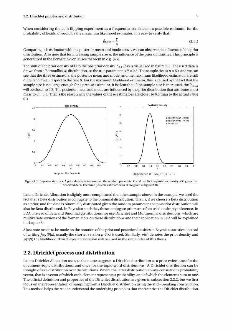
The shift of the prior density ofΘ to the posterior density fΘ|X(θ|x) is visualized in figure 2.1. The used data isdrawn from a Bernoulli(0.3) distribution, so the true parameter is θ = 0.3. The sample size is n = 50, and we cansee that the three estimators, the posterior mean and mode, and the maximum likelihood estimator, are stillquite far off with respect to the true θ. For the maximum likelihood estimator, this is caused by the fact that thesample size is not large enough for a precise estimator. It is clear that if the sample size is increased, the θMLE
will be closer to 0.3. The posterior mean and mode are influenced by the prior distribution that attributes mostmass to θ = 0.5. That is the reason why the values of these estimators are closer to 0.5 than to the actual value0.3.
0 0.1 0.2 0.3 0.4 0.5 0.6 0.7 0.8 0.9 10
0.5
1
1.5
2
2.5
f(
)
Prior density
(a) prior: Θ∼ Beta(4,4)
0 0.1 0.2 0.3 0.4 0.5 0.6 0.7 0.8 0.9 10
1
2
3
4
5
6
7
f | Y
( | y
)
Posterior density
posterior mean = 0.397
posterior mode = 0.393
mle = 0.380
(b) posterior: Θ∼ Beta(y +4,n − y +4)
Figure 2.1: Bayesian statistics: A prior density is imposed on the random parameterΘ and results in a posterior density ofΘ given theobserved data. The three possible estimators forΘ are given in figure 2.1b.
Latent Dirichlet Allocation is slightly more complicated than the example above. In the example, we used thefact that a Beta distribution is conjugate to the binomial distribution. That is, if we choose a Beta distributionas a prior, and the data is binomially distributed given the random parameter, the posterior distribution willalso be Beta distributed. In Bayesian statistics, these conjugate priors are often used to simply inference. InLDA, instead of Beta and Binomial distributions, we use Dirichlet and Multinomial distributions, which aremultivariate versions of the former. More on these distributions and their application in LDA will be explainedin chapter 3.
A last note needs to be made on the notation of the prior and posterior densities in Bayesian statistics. Insteadof writing fΘ|X(θ|x), usually the shorter version p(θ|x) is used. Similarly, p(θ) denotes the prior density andp(x|θ) the likelihood. This ‘Bayesian’ notation will be used in the remainder of this thesis.
2.2. Dirichlet process and distributionLatent Dirichlet Allocation uses, as the name suggests, a Dirichlet distribution as a prior twice; once for thedocument-topic distributions, and once for the topic-word distributions. A Dirichlet distribution can bethought of as a distribution over distributions. Where the latter distribution always consists of a probabilityvector, that is a vector of which each element represents a probability, and of which the elements sum to one.The official definition and properties of the Dirichlet distribution are given in subsection 2.2.2, but we firstfocus on the representation of sampling from a Dirichlet distribution using the stick-breaking construction.This method helps the reader understand the underlying principles that characterize the Dirichlet distribution.
8 2. Theoretical background
2.2.1. Stick-breaking construction of Dirichlet process
A common representation of sampling from a Dirichlet distribution is given by the stick-breaking construction,introduced by Sethuraman in [40]. We will first state the constructive definition of a Dirichlet distribution,after which the intuition behind it will be explained.If a vector θ of length K is constructed according to:
θ =∞∑
i=1Vi
i−1∏j=1
(1−V j )eYi
Vi ∼ Beta(1,α) i .i .d .
Yi ∼ Multinomial(1,g0) i .i .d . (∗),
(2.12)
then θ ∼ Dirichlet(α·g0). At (∗), a draw from a Multinomial(1,g0) results in a unit vector, with in one dimensioni ∈ 1, . . . ,K all probability mass, and zero probability mass in all other dimensions. Yi is then the index ofthe dimension in which all mass is concentrated. The vector eYi is the unit vector in the dimension Yi , asYi ∈ 1, . . . ,K . As conventionally, i.i.d. means independent and identically distributed.For the proof of θ from equation 2.12 having the same distribution as θ ∼ Dirichlet(α ·g0), we refer to [34].
Let us go step by step through the process. For i = 1, we draw a V1 from the Beta distribution and a Y1 from theMultinomial distribution. Y1 denotes a dimension, and V1 denotes the mass assigned to that dimension inthe vector θ. Then, for the second iteration, again a dimension Y2 and a length V2 are drawn. The mass V2
is assigned to dimension Y2 in θ, while mass V2 · (1−V1) is assigned to the initially drawn dimension Y1 of θ.Note that Y1 might be the same as Y2, as they are drawn from the same distribution and they are independentrandom variables.It is easy to see that the probability mass for each i , Vi
∏i−1j=1(1−V j ), lies between 0 and 1. This means that we
can look at the assignment of the mass in each iteration as consequently breaking a stick, hence the name. Westart with a stick of unit length and break V1 from it. Then, from the remainder of the stick, V2 is broken. Thiscontinues for i →∞, such that in total, the mass is distributed over the K dimensions as θ.Parameters α and g0 influence this distribution. The smaller α, the larger the probability of drawing a largeVi , such that only in the first few iterations, almost all mass is already distributed. On the other hand, if α islarge, the density of the Beta(1,α) will be skewed to the left, and the Vi will be small, resulting in the end in amore uniformly distributed probability vector θ, given a symmetric g0. This second parameter, g0, handlesthe preference to certain dimensions. If (g0)1 is much larger than all other elements of g0, most mass will beassigned to the first dimension in the iterative process of equations 2.12, such that (θ)1 will be much largerthan all other elements of θ.It can be concluded that α is a scaling parameter, which with can be steered towards a more uniform distri-bution, or, on the other hand, a distribution that assigns most probability mass to one or a few dimensions.With g0, we can incorporate preference to certain dimensions in the distribution. It can be seen as a locationparameter. If g0 is symmetric and consists of, for example, only ones, Yi can take on each dimension withequal probability in every step i in the constructive process.
In general, the parameter vector of a Dirichlet distribution is given by α, in which both the scaling as thelocation parameter are collected. In the next section, the general definition of a Dirichlet distributed randomvariable will be given, and its properties are derived and visualized.
2.2.2. Dirichlet distribution
Now that the process of sampling from a Dirichlet distribution is explained, we have gained understanding ofthe parameters of this distribution and their functions. For the official definition, we first need to understandthe simplex. In this thesis, it is chosen to define the Dirichlet distribution using the closed simplex, as in [33].
2.2. Dirichlet process and distribution 9
Definition 2.1 (Closed simplex)Let c be a positive number. The n-dimensional closed simplex Tn(c) in Rn is defined by1:
Tn(c) =
(x1, . . . , xn)T : xi > 0, 1 ≤ i ≤ n,n∑
i=1xi = c
An alternative is the open simplex, in which we define the sum of∑n−1
i=1 xi to be smaller than constant c. It is amatter of choice to use either the open or closed simplex, as long as we ensure that the elements of a Dirichletdistributed random vector sum to 1 and live in (0,1)n for an n-dimensional vector:
Definition 2.2 (Dirichlet density [33])A random vector X = (X1, . . . , Xn)T ∈ Tn(1) is said to have a Dirichlet distribution if the density of X−n =(X1, . . . , Xn−1)T is:
Dirichletn(X−n |α) = Γ(∑n
i=1αi)∏n
i=1Γ(αi )
n∏i=1
xαi−1i (2.13)
where α= (α1, . . . ,αn)T is a strictly positive parameter vector. We will write X ∼ Dirichletn(α) on Tn(1). That is∑ni=1 Xi = 1.
The Dirichlet distribution thanks its name to the integral in 2.14, studied by Peter Gustav Lejeune Dirichlet in1839, to which the integral of the Dirichlet density from equation 2.13 is proportional.
∫ (n−1∏i=1
xαi−1i
)(1−
n−1∑i=1
xi
)an−1
dx1 · · ·dxn−1 =∏n
i=1Γ(αi )
Γ(∑n
i=1αi) (2.14)
Furthermore, note that for n = 2, we obtain a Beta distribution.
Beta(α1,α2) = Γ(α1 +α2)
Γ(α1)Γ(α2)xα1−1(1−x)α2−1
= 1
B(α1,α2)xα1−1(1−x)α2−1
(2.15)
Consequently, the Dirichlet distribution can be thought of as a higher dimensional version of the Beta distribu-tion.
Properties
The Dirichlet distribution has nice closed-form properties when it comes to marginal distributions, conditionaldistributions and product moment generating functions. Most of them are used in this thesis.
First, we take a look at the theorem containing the marginal and conditional distributions from [33]. The proofof this theorem can be found in [33].
Theorem 2.1 (Marginals and conditionals [33])Let X ∼ Dirichletn(α) on Tn , then we have the following results.
1. For any s < n, the subvector (X1, . . . , Xs )T has a Dirichlet distribution with parameters (α1, . . . ,αs ;∑n
j=s+1α j ).
In particular, Xi ∼ Beta(αi ,α+−αi ) with α+ =∑ni=1αi .
2. The conditional distribution of X ′i = Xi
1−∑sj=1 x∗
jfor i ∈ s +1, . . . ,n −1 given X1 = x∗
1 , . . . , Xs = x∗s , follows a
Dirichlet distribution with parameters (αs+1, . . . ,αn−1,αn).
To give an idea of the proof of the marginal distributions, we show the derivation for a one-dimensionalmarginal distribution of a three-dimensional Dirichlet distribution. The method used in this derivation, canbe informative for other derivations in this thesis.We want to show that the marginal distribution of a 3-dimensional Dirichlet distribution on Tn(1) is a Betadistribution with parameters αi and
∑3j=1,i 6= j α j , following theorem 2.1. This result can later be generalized
1Note that this is not a closed space in the topological sense.
10 2. Theoretical background
for a n-dimensional Dirichlet distribution. For ease of notation, let us derive the margin of X1. BecauseX3 = 1−X1 −X2, we only need to integrate out X2.
fX1 (x1) = Γ(∑3
i=1αi )∏3i=1Γ(αi )
∫ 1
0xα1−1
1 xα2−12 (1−x1 −x2)α3−1 dx2
= Γ(∑3
i=1αi )∏3i=1Γ(αi )
xα1−11
∫ 1−x1
0xα2−1
2 (1−x1 −x2)α3−1 dx2 ∗
= Γ(∑3
i=1αi )∏3i=1Γ(αi )
xα1−11
∫ 1
0(1−x1)α2−1uα2−1(1−x1)α3−1(1−u)α3−1(1−x1) du ∗∗
= Γ(∑3
i=1αi )∏3i=1Γ(αi )
xα1−11 (1−x1)α2+α3−1
∫ 1
0uα2−1(1−u)α3−1 du
= Γ(∑3
i=1αi )∏3i=1Γ(αi )
xα1−11 (1−x1)α2+α3−1 Γ(α2)Γ(α3)
Γ(α2 +α3)
= Γ(α1 +α2 +α3)
Γ(α1)Γ(α2 +α3)xα1−1
1 (1−x1)α2+α3−1
(2.16)
∗ Combining 0 ≤ x2 ≤ 1 with 0 ≤ 1−x1 −x2 ≤ 1 results in 0 ≤ x2 ≤ 1−x1.∗∗ Substitution of x2 = (1−x1)u.
The last expression in 2.16 is exactly the density function of a Beta(α1,α2 +α3) distributed random variable.
This result can be generalized for an n-dimensional Dirichlet distribution by integrating out all variables x j
for j 6= i , j ∈ 1, . . . ,n −1. Note that the Dirichlet distribution of an n-dimensional vector has support on the(n −1)-simplex by definition. For xn we therefore use 1−x1 −·· ·−xn−1. The same result follows:
Xi ∼ Beta
(αi ,
n∑j=1, j 6=i
α j
)
and we can easily see that:
E[Xi ] = αi∑nj=1α j
(2.17)
As for any Beta(a,b) distribution, the mean is given by aa+b .
Another property of the Dirichlet distribution that is used in derivations in this thesis, is the product momentgenerating function. It is expressed as follows.
Proposition 2.1 (Product moment generating function)Let X ∼ Dirichletn(α) onTn(1). Let m be a n-dimensional vector with non-negative values. The product momentof X is given by:
E
[n∏
i=1(X)mi
i
]= Γ
(∑ni=1αi
)Γ
(∑ni=1(mi +αi )
) n∏i=1
Γ(mi +αi )
Γ(αi )(2.18)
To show that equation 2.18 is true, only a smart substitution is needed. Let us start with the definition of theexpectation.
E
[n∏
i=1(X)mi
i
]=
∫ (n∏
i=1xmi
i
)· Γ(
∑ni=1αi )∏n
i=1Γ(αi )
n−1∏i=1
xαi−1i · (1−x1 −·· ·−xn−1)αn−1 dx1 · · ·dxn−1
= Γ(∑n
i=1αi )∏ni=1Γ(αi )
∫ n−1∏l=1
xmi+αi−1i (1−x1 −·· ·−xn−1)mn+αn−1 dx1 · · ·dxn−1
(2.19)
To compute this integral, we need to do the same trick as in 2.16, but now iteratively. Substitute:xn−1 = (1−x1 −·· ·−xn−2)un−1, xn−2 = (1−x1 −·· ·−xn−3)un−2, and so on till x2 = (1−x1)u2.
2.2. Dirichlet process and distribution 11
E
[n∏
i=1(X)mi
i
]= Γ(
∑ni=1αi )∏n
i=1Γ(αi )
∫ n−1∏l=1
xmi+αi−1i (1−x1 −·· ·−xn−1)mn+αn−1 dx1 · · ·dxn−1
= Γ(∑n
i=1αi )∏ni=1Γ(αi )
∫ 1
0xm1+α1−1
1 (1−x1)∑n
i=2(mi+αi )−1 dx1
·∫ 1
0um2+α2−1
2 (1−u2)∑n
i=3(mi+αi )−1 du2 · . . . ·∫ 1
0umn−1+αn−1−1
n−1 (1−un−1)mn+αn−1 dun−1
= Γ(∑n
i=1αi )∏ni=1Γ(αi )
·B
(m1 +α1,
n∑i=2
(mi +αi )
)·B
(m2 +α2,
n∑i=3
(mi +αi )
)· . . . ·B(mn−1 +αn−1,mn +αn)
= Γ(∑n
i=1αi)
Γ(∑n
i=1(mi +αi )) n∏
i=1
Γ(mi +αi )
Γ(αi )(2.20)
Where B(·, ·) is the beta function, and in the last step, its gamma function representation from equation 2.4 isused.
Visualization
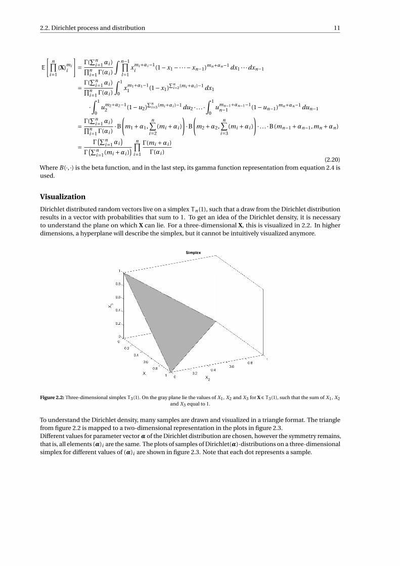
Dirichlet distributed random vectors live on a simplex Tn(1), such that a draw from the Dirichlet distributionresults in a vector with probabilities that sum to 1. To get an idea of the Dirichlet density, it is necessaryto understand the plane on which X can lie. For a three-dimensional X, this is visualized in 2.2. In higherdimensions, a hyperplane will describe the simplex, but it cannot be intuitively visualized anymore.
Figure 2.2: Three-dimensional simplex T3(1). On the gray plane lie the values of X1, X2 and X3 for X ∈T3(1), such that the sum of X1, X2and X3 equal to 1.
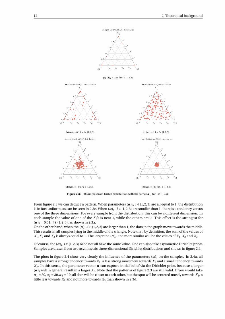
To understand the Dirichlet density, many samples are drawn and visualized in a triangle format. The trianglefrom figure 2.2 is mapped to a two-dimensional representation in the plots in figure 2.3.Different values for parameter vectorα of the Dirichlet distribution are chosen, however the symmetry remains,that is, all elements (α)i are the same. The plots of samples of Dirichlet(α)-distributions on a three-dimensionalsimplex for different values of (α)i are shown in figure 2.3. Note that each dot represents a sample.
12 2. Theoretical background
(a) (α)i = 0.01 for i ∈ 1,2,3.
(b) (α)i = 0.1 for i ∈ 1,2,3. (c) (α)i = 1 for i ∈ 1,2,3.
(d) (α)i = 10 for i ∈ 1,2,3. (e) (α)i = 100 for i ∈ 1,2,3.
Figure 2.3: 100 samples from Dir(α) distribution with the same (α)i for i ∈ 1,2,3.
From figure 2.3 we can deduce a pattern. When parameters (α)i , i ∈ 1,2,3 are all equal to 1, the distributionis in fact uniform, as can be seen in 2.3c. When (α)i , i ∈ 1,2,3 are smaller than 1, there is a tendency versusone of the three dimensions. For every sample from the distribution, this can be a different dimension. Ineach sample the value of one of the Xi ’s is near 1, while the others are 0. This effect is the strongest for(α)i = 0.01, i ∈ 1,2,3, as shown in 2.3a.On the other hand, when the (α)i , i ∈ 1,2,3 are larger than 1, the dots in the graph move towards the middle.This results in all samples lying in the middle of the triangle. Note that, by definition, the sum of the values ofX1, X2 and X3 is always equal to 1. The larger the (α)i , the more similar will be the values of X1, X2 and X3.
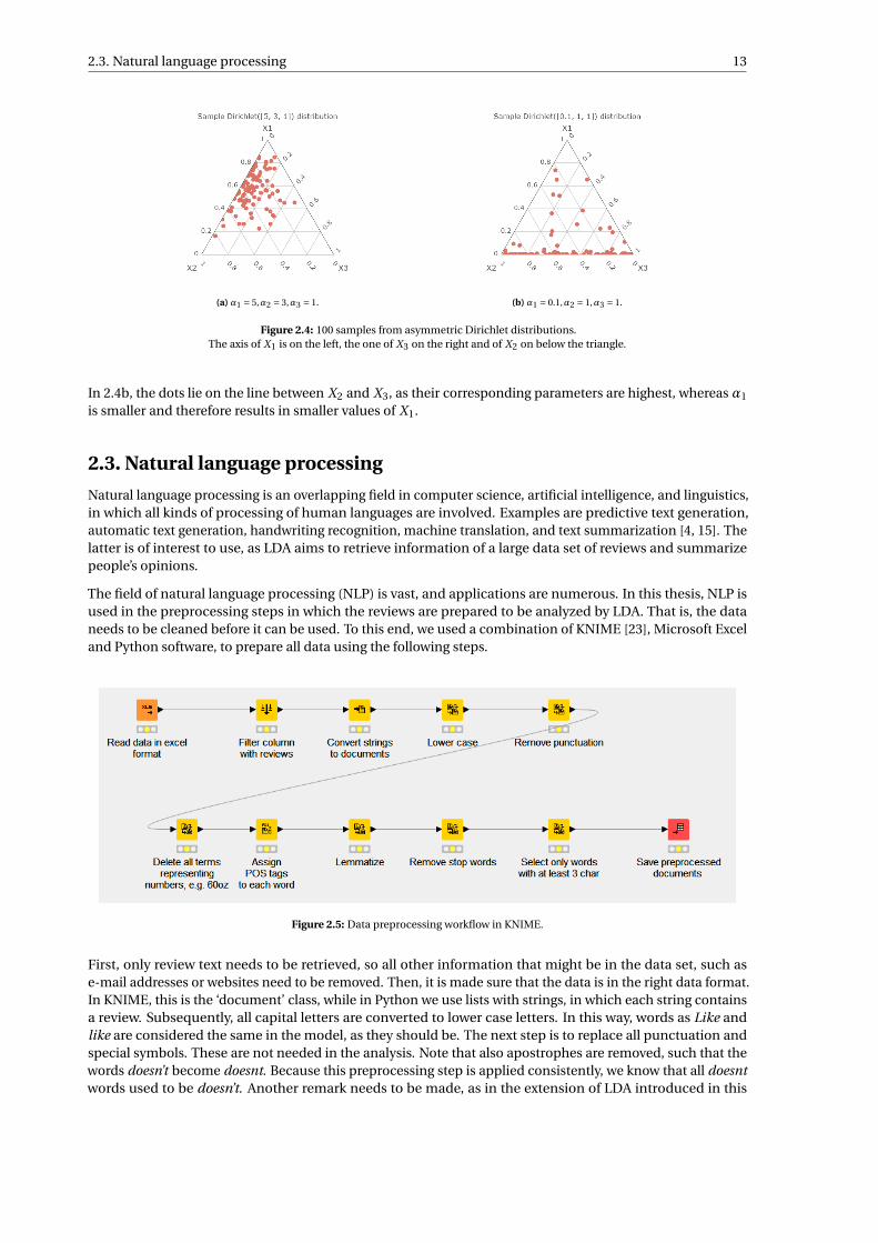
Of course, the (α)i , i ∈ 1,2,3 need not all have the same value. One can also take asymmetric Dirichlet priors.Samples are drawn from two asymmetric three-dimensional Dirichlet distributions and shown in figure 2.4.
The plots in figure 2.4 show very clearly the influence of the parameters (α)i on the samples. In 2.4a, allsamples have a strong tendency towards X1, a less strong movement towards X2 and a small tendency towardsX3. In this sense, the parameter vector α can capture initial belief via the Dirichlet prior, because a larger(α)i will in general result in a larger Xi . Note that the patterns of figure 2.3 are still valid. If you would takeα1 = 50,α2 = 30,α3 = 10, all dots will be closer to each other, but the spot will be centered mostly towards X1, alittle less towards X2 and not more towards X3 than shown in 2.3d.
2.3. Natural language processing 13
(a) α1 = 5,α2 = 3,α3 = 1. (b) α1 = 0.1,α2 = 1,α3 = 1.
Figure 2.4: 100 samples from asymmetric Dirichlet distributions.The axis of X1 is on the left, the one of X3 on the right and of X2 on below the triangle.
In 2.4b, the dots lie on the line between X2 and X3, as their corresponding parameters are highest, whereas α1
is smaller and therefore results in smaller values of X1.
2.3. Natural language processing
Natural language processing is an overlapping field in computer science, artificial intelligence, and linguistics,in which all kinds of processing of human languages are involved. Examples are predictive text generation,automatic text generation, handwriting recognition, machine translation, and text summarization [4, 15]. Thelatter is of interest to use, as LDA aims to retrieve information of a large data set of reviews and summarizepeople’s opinions.
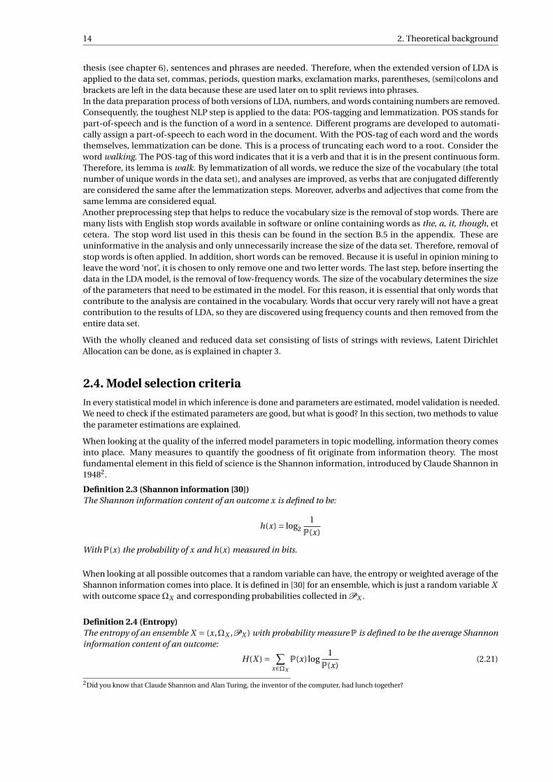
The field of natural language processing (NLP) is vast, and applications are numerous. In this thesis, NLP isused in the preprocessing steps in which the reviews are prepared to be analyzed by LDA. That is, the dataneeds to be cleaned before it can be used. To this end, we used a combination of KNIME [23], Microsoft Exceland Python software, to prepare all data using the following steps.
Figure 2.5: Data preprocessing workflow in KNIME.
First, only review text needs to be retrieved, so all other information that might be in the data set, such ase-mail addresses or websites need to be removed. Then, it is made sure that the data is in the right data format.In KNIME, this is the ‘document’ class, while in Python we use lists with strings, in which each string containsa review. Subsequently, all capital letters are converted to lower case letters. In this way, words as Like andlike are considered the same in the model, as they should be. The next step is to replace all punctuation andspecial symbols. These are not needed in the analysis. Note that also apostrophes are removed, such that thewords doesn’t become doesnt. Because this preprocessing step is applied consistently, we know that all doesntwords used to be doesn’t. Another remark needs to be made, as in the extension of LDA introduced in this
14 2. Theoretical background
thesis (see chapter 6), sentences and phrases are needed. Therefore, when the extended version of LDA isapplied to the data set, commas, periods, question marks, exclamation marks, parentheses, (semi)colons andbrackets are left in the data because these are used later on to split reviews into phrases.In the data preparation process of both versions of LDA, numbers, and words containing numbers are removed.Consequently, the toughest NLP step is applied to the data: POS-tagging and lemmatization. POS stands forpart-of-speech and is the function of a word in a sentence. Different programs are developed to automati-cally assign a part-of-speech to each word in the document. With the POS-tag of each word and the wordsthemselves, lemmatization can be done. This is a process of truncating each word to a root. Consider theword walking. The POS-tag of this word indicates that it is a verb and that it is in the present continuous form.Therefore, its lemma is walk. By lemmatization of all words, we reduce the size of the vocabulary (the totalnumber of unique words in the data set), and analyses are improved, as verbs that are conjugated differentlyare considered the same after the lemmatization steps. Moreover, adverbs and adjectives that come from thesame lemma are considered equal.Another preprocessing step that helps to reduce the vocabulary size is the removal of stop words. There aremany lists with English stop words available in software or online containing words as the, a, it, though, etcetera. The stop word list used in this thesis can be found in the section B.5 in the appendix. These areuninformative in the analysis and only unnecessarily increase the size of the data set. Therefore, removal ofstop words is often applied. In addition, short words can be removed. Because it is useful in opinion mining toleave the word ‘not’, it is chosen to only remove one and two letter words. The last step, before inserting thedata in the LDA model, is the removal of low-frequency words. The size of the vocabulary determines the sizeof the parameters that need to be estimated in the model. For this reason, it is essential that only words thatcontribute to the analysis are contained in the vocabulary. Words that occur very rarely will not have a greatcontribution to the results of LDA, so they are discovered using frequency counts and then removed from theentire data set.
With the wholly cleaned and reduced data set consisting of lists of strings with reviews, Latent DirichletAllocation can be done, as is explained in chapter 3.
2.4. Model selection criteriaIn every statistical model in which inference is done and parameters are estimated, model validation is needed.We need to check if the estimated parameters are good, but what is good? In this section, two methods to valuethe parameter estimations are explained.
When looking at the quality of the inferred model parameters in topic modelling, information theory comesinto place. Many measures to quantify the goodness of fit originate from information theory. The mostfundamental element in this field of science is the Shannon information, introduced by Claude Shannon in19482.
Definition 2.3 (Shannon information [30])The Shannon information content of an outcome x is defined to be:
h(x) = log21
P(x)
With P(x) the probability of x and h(x) measured in bits.
When looking at all possible outcomes that a random variable can have, the entropy or weighted average of theShannon information comes into place. It is defined in [30] for an ensemble, which is just a random variable Xwith outcome spaceΩX and corresponding probabilities collected in PX .
Definition 2.4 (Entropy)The entropy of an ensemble X = (x,ΩX ,PX ) with probability measure P is defined to be the average Shannoninformation content of an outcome:
H(X ) = ∑x∈ΩX
P(x) log1
P(x)(2.21)
2Did you know that Claude Shannon and Alan Turing, the inventor of the computer, had lunch together?
2.4. Model selection criteria 15
Here, capital X is used to denote the fact that entropy is computed of a discrete random variable X , with samplespaceΩX and probability measure P. If P(x) = 0 for some x ∈ΩX , then P(x) log 1
P(x) is defined to be equal to 0.Furthermore H(X ) is measured in bits, and is also referred to as the uncertainty of X .
The idea of entropy can best be understood when considering the example of flipping a coin again. First, as-sume that we have a fair coin, such that the probability of heads and tails is equal: P(H ) = (T ) = 1
2 . Substitutingthis in equation 2.21 with X being the random variable with sample space H ,T and the aforementionedprobabilities, we get H(X ) = log2(2) = 1. This means that we need only 1 bit to communicate the outcomeof the coin flip, namely 1 for heads and 0 for tails (or vice versa). In the same way for a 4-sided dice with 4different outcomes, we need 2 bits, as H(X ) = 1
4 log2(4)+ 14 log(4)+ 1
4 log(4)+ 14 log(4) = 2. However, if we have
a strange dice, with 1 unique side (e.g. 1) and 3 sides that show the same number (e.g. 2), the probabilitiesand the entropy will change: H (X ) = 1
4 log2(4)+ 34 log2( 4
3 ) ≈ 0.81. Note that the entropy is lower than for the fairdice, where we needed 2 bits to communicate the result. One can think of this result as if more informationis already hidden in the outcome and does not have to be communicated, so only ‘0.81’ bit is needed to tellthe result of the throw to your opponent. This result is in general true, as is stated in the second item of thehighlighted properties of the entropy from [30].
Theorem 2.2 (Properties entropy)• H(X ) ≥ 0, with equality if and only if ∃i such that pi =P(X = ai ) = 1
• H(X ) is maximized if p = (p1, . . . p I ) is uniform. That is if pi = 1|ΩX | ,∀i ∈ 1, . . . I . Then H(X ) = log(|ΩX |).
In general, we have H(X ) ≤ log(|ΩX |).
• The joint entropy of random variables X and Y with sample spaces ΩX and ΩY and joint probabilitymeasure P, is defined as:
H(X ,Y ) = ∑x∈ΩX ,y∈ΩY
P(x, y) log1
P(x, y)
and if X and Y independent random variables, then H(X ,Y ) = H(X )+H(Y ).
A metric that is often used for the comparison of two probability distributions is the Kullback-Leibler divergence.In the field of information theory, it is called the relative entropy. Note that it is not an actual distance in themathematical sense.
Definition 2.5 (Relative entropy, KL-divergence)The relative entropy, also called the Kullback-Leibler divergence, between two discrete probability distributionsp and q that are defined over the same sample spaceΩX is given by:
DK L(p‖q) = ∑x∈ΩX
p(x) logp(x)
q(x)(2.22)
To give an idea of the working principle of this relative entropy, we consider a small example. Let p =(0.6,0.2,0.1,0.05,0.05) and q = (0.6,0.2,0.05,0.05,0.1). The relative entropy is then DK L(p‖q) = 0.05 · log(2) ≈0.03. The only differences between p and q are the swapped probabilities of the third and fifth element, whichhave both already small probability mass. If we would halve the first element and triple the third element of pto get q, i.e. q = (0.3,0.2,0.3,0.05,0.05), the relative entropy will be DK L(p‖q) = 0.6 · log(2)−0.1 · log(3) ≈ 0.31,which is a lot higher than the previous score. As expected, large changes in probability mass (in the absolutesense) result in larger KL-divergence scores than small changes (in the absolute sense).
The relative entropy is also defined for the comparison of densities of two continuous random variablessharing the same domain. Then, the sum in the definition above becomes an integral over the domain, and theprobability densities replace the probability mass functions. For the qualification of our model parameters, wecannot compare the estimated distributions q with the true distribution p, as the true distribution is unknown.Nevertheless, the Kullback-Leibler divergence is used for other purposes in chapter 7 and section 4.2.1.
In topic modelling, another statistic is used for model comparison: the perplexity. In the field of NLP, andlanguage and topic models (such as LDA), this measure is most frequently used to observe the difference inthe quality of the model when parameters like the number of topics, the vocabulary size or the number ofiterations are changed. The model with the lowest perplexity is then assumed to be the best fit on the data.

16 2. Theoretical background
The definition of the perplexity is taken from the original LDA paper [7] by Blei et al..
Definition 2.6 (Perplexity)Consider a model that is trained on training data wtrain to obtain estimates for the model parameters. Then, theperplexity of the left-out test data set wtest is defined as:
Perplexity(wtest) = 2−log2(P(wtest))
|wtest |
= e−log(P(wtest))
|wtest |(2.23)
Where |wtest| is the size of the test set.
One can think of the perplexity as a comparison of the inferred model with the case of a uniform distribution.Remember that in the latter case, the entropy was highest, so in the perplexity, we observe to what extent themodel has improved on the uninformative prior. Because the perplexity is only used for comparison amongmodels or parameter settings, the ‘best’ model is the one that has the lowest entropy and thus retrieved themost information from the data.
3Latent Dirichlet Allocation
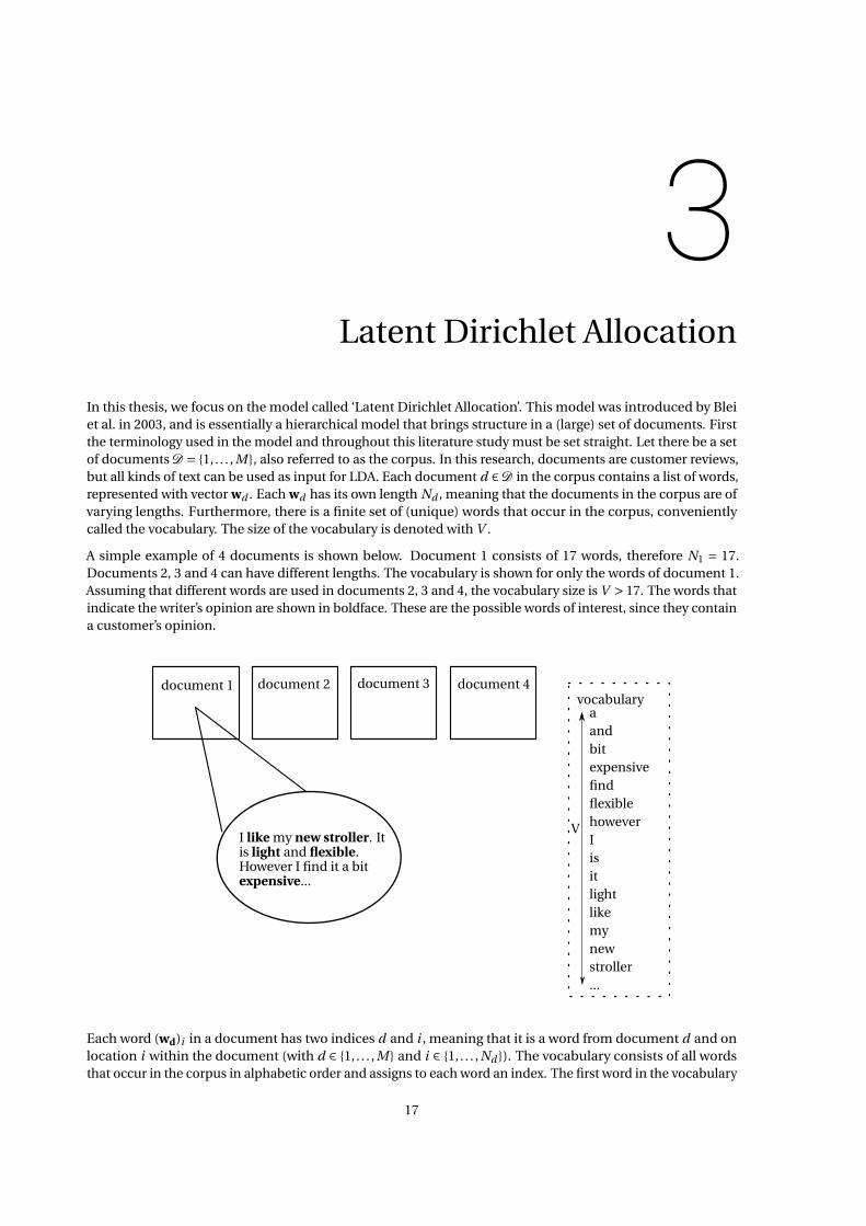
In this thesis, we focus on the model called ‘Latent Dirichlet Allocation’. This model was introduced by Bleiet al. in 2003, and is essentially a hierarchical model that brings structure in a (large) set of documents. Firstthe terminology used in the model and throughout this literature study must be set straight. Let there be a setof documents D = 1, . . . , M , also referred to as the corpus. In this research, documents are customer reviews,but all kinds of text can be used as input for LDA. Each document d ∈D in the corpus contains a list of words,represented with vector wd . Each wd has its own length Nd , meaning that the documents in the corpus are ofvarying lengths. Furthermore, there is a finite set of (unique) words that occur in the corpus, convenientlycalled the vocabulary. The size of the vocabulary is denoted with V .
A simple example of 4 documents is shown below. Document 1 consists of 17 words, therefore N1 = 17.Documents 2, 3 and 4 can have different lengths. The vocabulary is shown for only the words of document 1.Assuming that different words are used in documents 2, 3 and 4, the vocabulary size is V > 17. The words thatindicate the writer’s opinion are shown in boldface. These are the possible words of interest, since they containa customer’s opinion.
document 1 document 2 document 3 document 4
I like my new stroller. Itis light and flexible.However I find it a bitexpensive...
aandbitexpensivefindflexiblehoweverIisitlightlikemynewstroller...
vocabulary
V
Each word (wd)i in a document has two indices d and i , meaning that it is a word from document d and onlocation i within the document (with d ∈ 1, . . . , M and i ∈ 1, . . . , Nd ). The vocabulary consists of all wordsthat occur in the corpus in alphabetic order and assigns to each word an index. The first word in the vocabulary
17
18 3. Latent Dirichlet Allocation
above, a, has index 1, the second word, and, is represented by 2, et cetera. A word (wd)i is thus not givenby its textual representation, e.g. flexible, but by its index in the vocabulary, 6. As a result, we know that∀d , i , (wd)i ∈ 1, . . . ,V .Furthermore, the bag-of-words representation of documents in used in LDA. In this representation, word orderis disregarded, so only the frequency of word occurrence in each document matters.
At last, we assume that there are K topics hidden in the corpus. These topics can be seen as common themesthat can be found in reviews. In the example above, we see that the writer of document 1 writes about thelightness and flexibility of his/her new stroller. Also, he/she finds it expensive. There might be more peoplewho write about flexibility, so then it becomes a theme. Besides, if many customers write ‘I like this stroller’, atopic consisting of the main word ‘like’ will be formed. Note that topics are not found by a label or overarchingtheme like ‘comfort’; only a topic-word distribution rolls out of the algorithm. That is, each topic k ∈ 1, . . . ,K has a corresponding topic-word distribution, with higher probabilities for words that are important to thistopic. The topic that is manually labeled to be about flexibility will have a high probability for the word ‘flexible’in its topic-word distribution.Note that in LDA, it is unknown beforehand what topics can be found in the review data set, as it is anunsupervised method. Even the number of topics, K , is unknown and must be determined by domainknowledge, size of the data set, and trial and error (which model gives the best fit based on a goodness-of-fitstatistic). That is a small data set of M documents can barely give accurate results if K ≈ M .
An overview of all sets, variables, and parameters is given in table 3.1.
Table 3.1: Overview of parameters and observational data in Latent Dirichlet Allocation.
Variable name MeaningD Set of documents, ‘Corpus’M Number of documentswd List of words in document d(wd)i Word on location i in document dNd Number of words in document dV Size of vocabulary, i.e. number of unique words in corpusK Number of topicsk Topic index
3.1. Into the mind of the writer: generative process
The goal of LDA is to extract topics from a set of reviews via a hierarchical Bayesian model. Before we look atstatistical inference methods (see chapter 4), we need to understand the hierarchy of the Bayesian model. Thegenerative process that forms this hierarchy aims to summarize the writing process in the minds of the writers.To stay with the example of strollers, imagine you have just bought a new, very expensive buggy. As it has costyou a lot of money, you have high expectations, but the stroller turns out to be a bit disappointing. You wantto share your experience with other customers, so you decide to write a review. The process that follows isthe generative process, as you are going to generate a document. Latent Dirichlet Allocation assumes that thegenerative process goes as follows.
First, you think about which aspects you want to write. You feel disappointed, as the stroller you have boughtwas very expensive. Furthermore, you want to explain your disappointment: the stroller is very heavy, toolarge to fit in the car, and the basket underneath is too small. Thus, you want to talk about four topics: valuefor money, weight, size, and the basket. Of course, the labels that are now manually assigned to the topics donot necessarily occur explicitly in the reviews. You find your disappointment in the performancce of strollercompared to the price you paid for it the most essential aspect, so 40% of the words in the review are aboutthis topic. The other three topics are formed by the rest of the document, with an equal number of words. Thatis, 20% of the words are about the weight, 20% about the size, and 20% about the basket. After this decision,you need to find the right words to describe your opinion. For each topic, there is a set of words in your ownEnglish vocabulary from which can be chosen. For example, for topic ‘size’ can be thought of: large, small, big,little, fit, huge, size, proportions, width, broad, height, et cetera. These sets of words exist for each topic aboutwhich you want to write. All these aspect words are then glued together with verbs, personal pronouns, and
3.1. Into the mind of the writer: generative process 19
determinants to form a review of clear and correct English.
Mathematically speaking, this generative process of writing a review can be summarized in a hierarchicalBayesian model, with a prior belief on how the writer chooses its topics and a prior belief on which wordsoccur in the set of words to choose from for each possible topic. The following scheme from [7] summarizes it.
1. For each document d ∈ 1, . . . , M ,draw a topic distribution parameter vectorΘd from a Dirichlet(α) distribution, i.e. Θd ∼ Dirichlet(α)
2. For each topic k ∈ 1, . . . ,K ,draw a topic-word distribution parameter vectorΦk from a Dirichlet(β) distribution, i.e. Φk ∼ Dirichlet(β)
3. For each word i in document d ,
(a) Draw a topic (Zd)i from a Multinomial(1,Θd)
(b) Draw a word (Wd)i from a Multinomial(1,Φ(zd)i )
Attention must be paid to steps 3a and 3b, because drawing from a Multinomial(1,Θd) results in drawing avector instead of an integer. Therefore we define Zd,i ∼ Multinomial(1,Θd), such that (zd)i = k ⇐⇒ zd,i =(0,0, . . . ,1,0, . . . ,0) with only one 1 on the k-th dimension of zd,i. That is zd,i is the unit vector in dimensionk. So when it is written in this thesis that (Zd)i is drawn from Multinomial(1,Θd), actually Zd,i is drawn fromMultinomial(1,Θd) and the mapping (zd,i)k = 1 ⇒ (zd)i = k for some k ∈ 1, . . . ,K is applied.A similar definition can be made for the words: (wd)i = k ⇐⇒ (wd,i)k = 1 for Wd,i ∼ Multinomial(1,Φ(zd)i ).Consequently, the same steps are applied when we ‘draw’ (Wd)i from Multinomial(1,Φ(zd)i ).
In the generative process, some critical assumptions on independence are made. Each document-topicdistributionΘd is drawn independently from all otherΘi for i 6= d . This is reasonable, as it is probable that thewriters of the reviews decide about which topics they want to write independently. It is thus assumed thatthere has been no communication between them beforehand. However, all customers write about the sameproduct, so independence is a strong assumption that is expected not to be satisfied in each data set.The same is valid for the topic-word distributions: each Φk is drawn independently from all other Φj forj 6= k. That is, the word probabilities that belong to a particular topic are independent of the word probabilitydistributions of other topics.Furthermore, allΘ andΦ are independent by construction, which makes sense, as the topic distribution of acertain review and the sets of words to choose from per topic have nothing to do with each other.Lastly, each topic (Zd)i is drawn independently from the corresponding Multinomial(1,Θd) and therefore eachpair ((Zd)i , (Wd)i ) is independent from every other pair
((Zi) j , (Wi) j
). These assumptions will be used later on
in statistical inference on the hierarchical model.
The generative process can be visualized in a plate notation, shown in figure 3.1. One should read figure 3.1 asfollows. The three rectangles can be read as three ‘for loops’ and they represent three levels in the hierarchicalmodel. First consider the two on the right of figure 3.1. The outer rectangle represents the corpus or the loopover documents. The hyperparameter vector α is outside the rectangle and is therefore independent of thedocuments. Random vectorΘ is within the loop, so this vector is drawn for each document. One level deeper,we look at the word in the document. For each word instance in the document, we first draw a topic and then aword. These draws are done as often as there are words in the document, therefore Nd times for document d .The rectangle on the left is separate and does not depend directly on the documents. The hyperparametervector β is outside the rectangle, meaning that this prior belief on the topic-word distributionsΦ is the samefor each topic. Then, a random vectorΦ is drawn K times, as is denoted in the corner. For clarity, the indicesare left out in figure 3.1.Furthermore, the gray variable in the plate notation represents the word random variable W , which is actuallyobserved. The circles with α and β are dotted because they are pre-set values and thus constant. These arelocated in the top of our hierarchical scheme. No further distribution is imposed on either α or β in the basicLDA model.
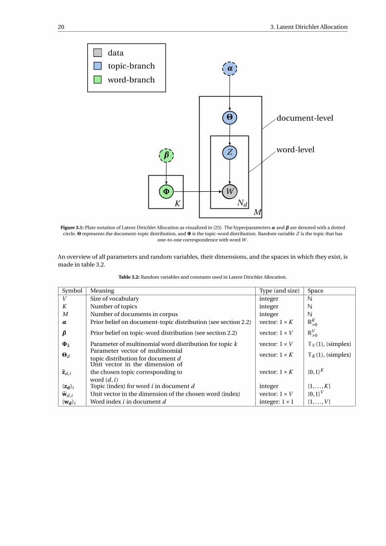
20 3. Latent Dirichlet Allocation
Φ
β
Θ
Z
W
data
topic-branch
word-branch
K NdM
α
document-level
word-level
Figure 3.1: Plate notation of Latent Dirichlet Allocation as visualized in [25]. The hyperparameters α and β are denoted with a dottedcircle. Θ represents the document-topic distribution, andΦ is the topic-word distribution. Random variable Z is the topic that has
one-to-one correspondence with word W .
An overview of all parameters and random variables, their dimensions, and the spaces in which they exist, ismade in table 3.2.
Table 3.2: Random variables and constants used in Latent Dirichlet Allocation.
Symbol Meaning Type (and size) SpaceV Size of vocabulary integer N
K Number of topics integer N
M Number of documents in corpus integer N
α Prior belief on document-topic distribution (see section 2.2) vector: 1×K RK>0
β Prior belief on topic-word distribution (see section 2.2) vector: 1×V RV>0
Φk Parameter of multinomial word distribution for topic k vector: 1×V TV (1), (simplex)
ΘdParameter vector of multinomialtopic distribution for document d
vector: 1×K TK (1), (simplex)
zd ,i
Unit vector in the dimension ofthe chosen topic corresponding toword (d , i )
vector: 1×K 0,1K
(zd)i Topic (index) for word i in document d integer 1, . . . ,K wd ,i Unit vector in the dimension of the chosen word (index) vector: 1×V 0,1V
(wd)i Word index i in document d integer: 1×1 1, . . . ,V
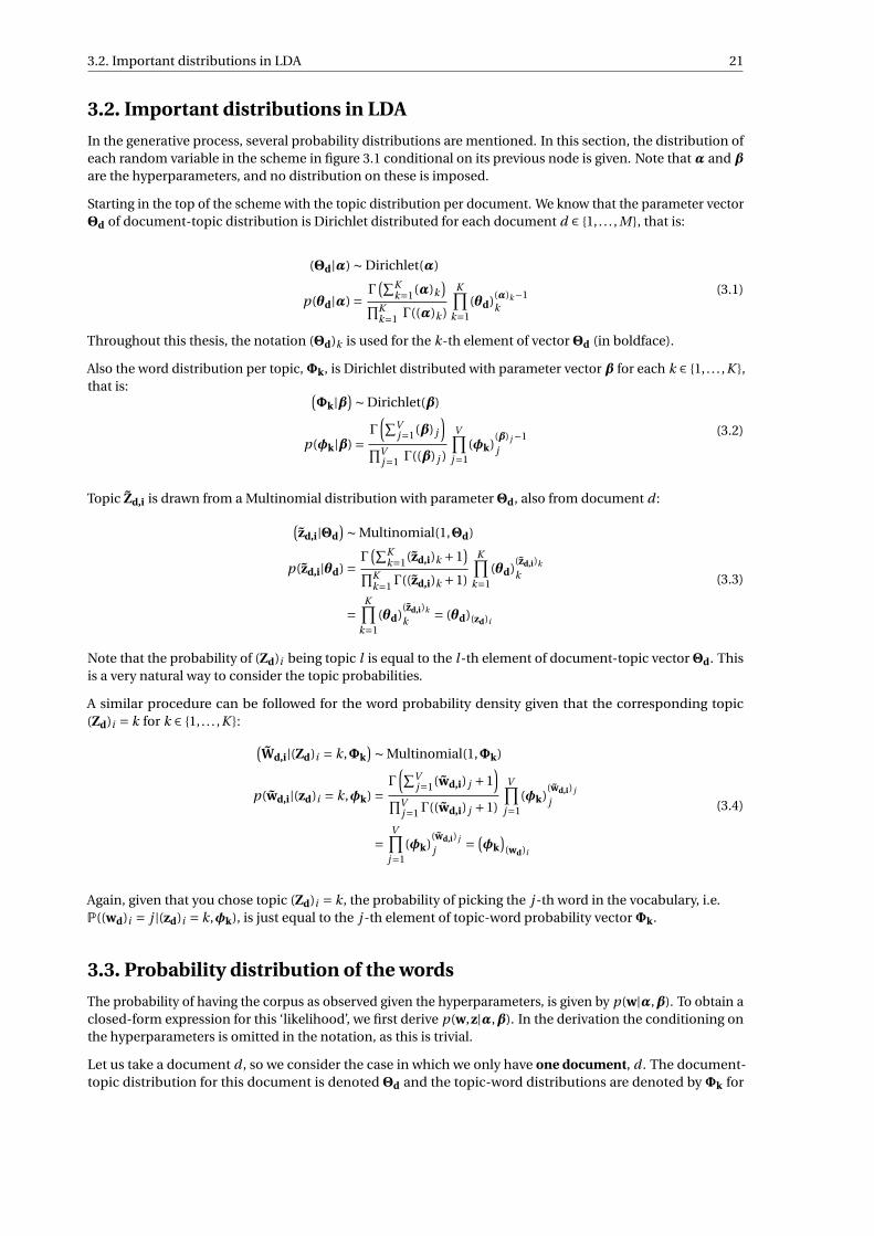
3.2. Important distributions in LDA 21
3.2. Important distributions in LDA
In the generative process, several probability distributions are mentioned. In this section, the distribution ofeach random variable in the scheme in figure 3.1 conditional on its previous node is given. Note that α and βare the hyperparameters, and no distribution on these is imposed.
Starting in the top of the scheme with the topic distribution per document. We know that the parameter vectorΘd of document-topic distribution is Dirichlet distributed for each document d ∈ 1, . . . , M , that is:
(Θd|α) ∼ Dirichlet(α)
p(θd|α) = Γ(∑K
k=1(α)k)∏K
k=1 Γ((α)k )
K∏k=1
(θd)(α)k−1k
(3.1)
Throughout this thesis, the notation (Θd)k is used for the k-th element of vectorΘd (in boldface).
Also the word distribution per topic,Φk, is Dirichlet distributed with parameter vector β for each k ∈ 1, . . . ,K ,that is: (
Φk|β)∼ Dirichlet(β)
p(φk|β) =Γ
(∑Vj=1(β) j
)∏V
j=1 Γ((β) j )
V∏j=1
(φk)(β) j −1j
(3.2)
Topic Zd,i is drawn from a Multinomial distribution with parameterΘd, also from document d :(zd,i|Θd
)∼ Multinomial(1,Θd)
p(zd,i|θd) = Γ(∑K
k=1(zd,i)k +1)∏K
k=1Γ((zd,i)k +1)
K∏k=1
(θd)(zd,i)k
k
=K∏
k=1(θd)
(zd,i)k
k = (θd)(zd)i
(3.3)
Note that the probability of (Zd)i being topic l is equal to the l -th element of document-topic vectorΘd. Thisis a very natural way to consider the topic probabilities.
A similar procedure can be followed for the word probability density given that the corresponding topic(Zd)i = k for k ∈ 1, . . . ,K : (
Wd,i|(Zd)i = k,Φk)∼ Multinomial(1,Φk)
p(wd,i|(zd)i = k,φk) =Γ
(∑Vj=1(wd,i) j +1
)∏V
j=1Γ((wd,i) j +1)
V∏j=1
(φk)(wd,i) j
j
=V∏
j=1(φk)
(wd,i) j
j = (φk
)(wd)i
(3.4)
Again, given that you chose topic (Zd)i = k, the probability of picking the j -th word in the vocabulary, i.e.P((wd)i = j |(zd)i = k,φk), is just equal to the j -th element of topic-word probability vectorΦk.
3.3. Probability distribution of the words
The probability of having the corpus as observed given the hyperparameters, is given by p(w|α,β). To obtain aclosed-form expression for this ‘likelihood’, we first derive p(w,z|α,β). In the derivation the conditioning onthe hyperparameters is omitted in the notation, as this is trivial.
Let us take a document d , so we consider the case in which we only have one document, d . The document-topic distribution for this document is denoted Θd and the topic-word distributions are denoted byΦk for
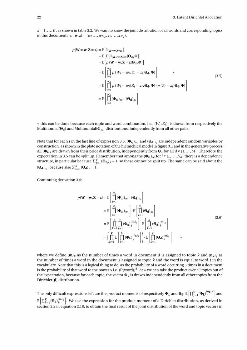
22 3. Latent Dirichlet Allocation
k = 1, . . . ,K , as shown in table 3.2. We want to know the joint distribution of all words and corresponding topicsin this document i.e. (w,z) = (w1, . . . wNd , z1, . . . , zNd ).
p(W = w,Z = z) = E[1W=w,Z=z
]= E[
E[1W=w,Z=z|Θd,Φ
]]= E[
p (W = w,Z = z|Θd,Φ)]
= E[
Nd∏i=1
p (Wi = wi , Zi = zi |Θd,Φ)
]∗
= E[
Nd∏i=1
p (Wi = wi |Zi = zi ,Θd,Φ) ·p (Zi = zi |Θd,Φ)
]
= E[
Nd∏i=1
(Φzi )wi · (Θd)zi
](3.5)
∗ this can be done because each topic and word combination, i.e., (Wi , Zi ), is drawn from respectively theMultinomial(Θd) and Multinomial(Φzi ) distributions, independently from all other pairs.
Note that for each i in the last line of expression 3.5, (Φzi )wi and (Θd)zi are independent random variables byconstruction, as shown in the plate notation of the hierarchical model in figure 3.1 and in the generative process.All (Φi) j are drawn from their prior distribution, independently fromΘd for all d ∈ 1, . . . , M . Therefore theexpectation in 3.5 can be split up. Remember that among the (Φzi )wi for j ∈ 1, . . . , Nd there is a dependencestructure, in particular because
∑Vj=1(Φzi ) j = 1, so these cannot be split up. The same can be said about the
(Θd)zi , because also∑K
k=1(Θd)k = 1.
Continuing derivation 3.5:
p(W = w,Z = z) = E[
Nd∏i=1
(Φzi )wi · (Θd)zi
]
= E[
Nd∏i=1
(Φzi )wi
]·E
[Nd∏i=1
(Θd)zi
]
= E[
K∏k=1
V∏j=1
(Φk)(nk) j
j
]·E
[K∏
k=1(Θd)(m)k
k
]
=(
K∏k=1
E
[V∏
j=1(Φk)
(nk) j
j
])·E
[K∏
k=1(Θd)(m)k
k
]∗
(3.6)
where we define (m)k as the number of times a word in document d is assigned to topic k and (nk) j asthe number of times a word in the document is assigned to topic k and the word is equal to word j in thevocabulary. Note that this is a logical thing to do, as the probability of a word occurring 5 times in a documentis the probability of that word to the power 5 i.e. (P(word))5. At ∗ we can take the product over all topics out ofthe expectation, because for each topic, the vectorΦk is drawn independently from all other topics from theDirichlet(β) distribution.
The only difficult expressions left are the product moments of respectivelyΦk andΘd: E[∏V
j=1(Φk)(nk) j
j
]and
E[∏K
k=1(Θd)(m)kk
]. We use the expression for the product moment of a Dirichlet distribution, as derived in
section 2.2 in equation 2.18, to obtain the final result of the joint distribution of the word and topic vectors in
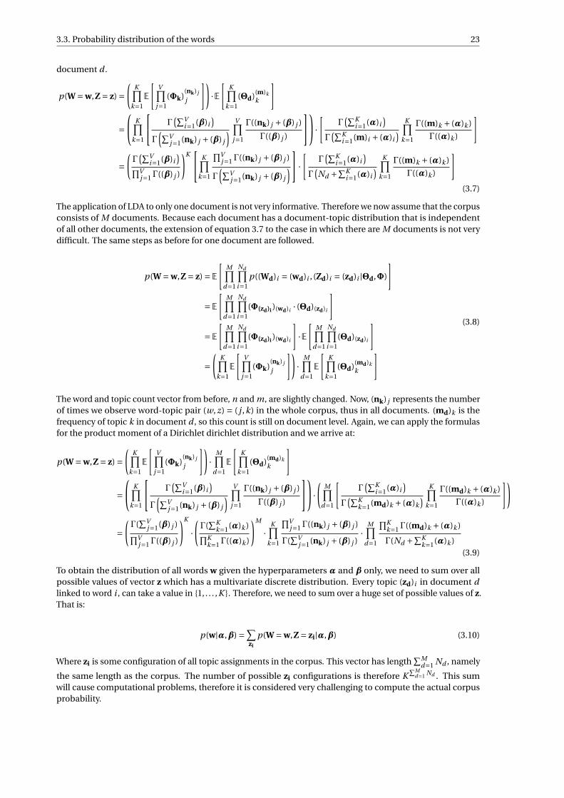
3.3. Probability distribution of the words 23
document d .
p(W = w,Z = z) =(
K∏k=1
E
[V∏
j=1(Φk)
(nk) j
j
])·E
[K∏
k=1(Θd)(m)k
k
]
= K∏
k=1
Γ(∑V
i=1(β)i)
Γ(∑V
j=1(nk) j + (β) j
) V∏j=1
Γ((nk) j + (β) j )
Γ((β) j )
·[
Γ(∑K
i=1(α)i)
Γ(∑K
i=1(m)i + (α)i) K∏
k=1
Γ((m)k + (α)k )
Γ((α)k )
]
=(Γ
(∑Vi=1(β)i
)∏Vj=1Γ((β) j )
)K K∏
k=1
∏Vj=1Γ((nk) j + (β) j )
Γ(∑V
j=1(nk) j + (β) j
) ·
[Γ
(∑Ki=1(α)i
)Γ
(Nd +∑K
i=1(α)i) K∏
k=1
Γ((m)k + (α)k )
Γ((α)k )
](3.7)
The application of LDA to only one document is not very informative. Therefore we now assume that the corpusconsists of M documents. Because each document has a document-topic distribution that is independentof all other documents, the extension of equation 3.7 to the case in which there are M documents is not verydifficult. The same steps as before for one document are followed.
p(W = w,Z = z) = E[
M∏d=1
Nd∏i=1
p((Wd)i = (wd)i , (Zd)i = (zd)i |Θd,Φ)
]
= E[
M∏d=1
Nd∏i=1
(Φ(zd)i )(wd)i · (Θd)(zd)i
]
= E[
M∏d=1
Nd∏i=1
(Φ(zd)i )(wd)i
]·E
[M∏
d=1
Nd∏i=1
(Θd)(zd)i
]
=(
K∏k=1
E
[V∏
j=1(Φk)
(nk) j
j
])·
M∏d=1
E
[K∏
k=1(Θd)(md)k
k
](3.8)
The word and topic count vector from before, n and m, are slightly changed. Now, (nk) j represents the numberof times we observe word-topic pair (w, z) = ( j ,k) in the whole corpus, thus in all documents. (md)k is thefrequency of topic k in document d , so this count is still on document level. Again, we can apply the formulasfor the product moment of a Dirichlet dirichlet distribution and we arrive at:
p(W = w,Z = z) =(
K∏k=1
E
[V∏
j=1(Φk)
(nk) j
j
])·
M∏d=1
E
[K∏
k=1(Θd)(md)k
k
]
= K∏
k=1
Γ(∑V
i=1(β)i)
Γ(∑V
j=1(nk) j + (β) j
) V∏j=1
Γ((nk) j + (β) j )
Γ((β) j )
·(
M∏d=1
[Γ
(∑Ki=1(α)i
)Γ
(∑Kk=1(md)k + (α)k
) K∏k=1
Γ((md)k + (α)k )
Γ((α)k )
])
=(Γ(
∑Vj=1(β) j )∏V
j=1Γ((β) j )
)K
·(Γ(
∑Kk=1(α)k )∏K
k=1Γ((α)k )
)M
·K∏
k=1
∏Vj=1Γ((nk) j + (β) j )
Γ(∑V
j=1(nk) j + (β) j )·
M∏d=1
∏Kk=1Γ((md)k + (α)k )
Γ(Nd +∑Kk=1(α)k )
(3.9)
To obtain the distribution of all words w given the hyperparameters α and β only, we need to sum over allpossible values of vector z which has a multivariate discrete distribution. Every topic (zd)i in document dlinked to word i , can take a value in 1, . . . ,K . Therefore, we need to sum over a huge set of possible values of z.That is:
p(w|α,β) =∑zi
p(W = w,Z = zi|α,β) (3.10)
Where zi is some configuration of all topic assignments in the corpus. This vector has length∑M
d=1 Nd , namely
the same length as the corpus. The number of possible zi configurations is therefore K∑M
d=1 Nd . This sumwill cause computational problems, therefore it is considered very challenging to compute the actual corpusprobability.
24 3. Latent Dirichlet Allocation
3.4. Improvements and adaptations to basic LDA model
Latent Dirichlet Allocation is the simplest unsupervised topic model. Because it is applied in different scientificfields [19], there are many extensions and applications of LDA, of which the most important ones (inventedbetween 2003 and 2017) are summarized in [19]. To give an idea of the vast area of modeling possibilities, wemention the extensions that are the most interesting for applications in opinion mining below.
LDA is a hierarchical Bayesian model, and hierarchical models can easily be extended by just adding a nodeto the graphical structure, which is done in the dynamic topic model [6]. This model gives information onhow the average topic distribution and the word distributions per topic evolve. The model is developed forpolitical sciences, but can also be applied to opinion mining, as the development of the customer opinion cansay something about, e.g. the durability of the product or effect of a campaign might be reflected in people’sviews. Another model that looks at the evolution of topics over time is presented in [51].
LDA can also be adapted by changing the model parameters that reflect our prior belief about the topics. Withthe adaptation in [49], we can influence the topic distribution beforehand by steering documents towards onebroad topic. If there is a reasonable prior belief that this will occur in the review data set, this can improve theresults of the topic model.
Multi-grain LDA makes a distinction between local and global topics [44]. This distinction can be incorporatedinto the model by adding a layer to the hierarchical structure of LDA. In the setting of review analyses, localtopics can be thought of as ratable aspects like price or ease of use. Global topics are then the types of productsor brands. In this way, you can retrieve information about competitive products and improve decision-makingon product development to outperform your competitors.
To quickly summarize a large set of research papers, one can use the labels or tags that are usually mentionedin an article to improve the topic model. In this LDA extension, the labels form an extra layer in the hierarchicalscheme of LDA, and the highest probable words are now given per label instead of per topic. Topics and labelsare considered the same. This model can, therefore, be seen as a semi-supervised topic model, as we know thetopics beforehand. Although it is more useful in the scientific world, it can also be applied to review analysis,as sometimes customers give their opinion on each aspect specifically.
As previously mentioned, topics in opinion mining or review analysis are often aspects of the product aboutwhich customers give their opinion. Therefore, it is useful to make a distinction between aspect words andbackground words. In the topic-aspect model described in [36] this distinction is made, and the most probablewords per aspect and topic (e.g., product type) are given.
In basic LDA, a bag-of-words representation is used. This means that each document consists of a set of words,whose order is ignored. Every word is an individual entity and its relation with the surrounding words is lost.Finding topics is therefore done on document level, making it difficult to link the corresponding opinion words(e.g. ‘nice’) with the right aspect of the product. In sentence LDA [21] this bag-of-words assumption is slightlyrelaxed because it is assumed that a sentence consists of only one topic.In the same paper, the aspect and sentiment unification model (ASUM) is described. In this model, it isassumed that every document has one sentiment and tells about different topics. As a result, highly probablewords per sentiment-aspect combination are given. Therefore, one can draw more detailed conclusions on thesentiment about specific topics.
The topic sentiment mixture model (TSMM) belongs to the same type of models. In this model, a distinctionbetween background, positive and negative words is made [31]. Again, the results consist of lists with themost probable words per topic and per type of words (background, positive or negative). Note that thesemodels, sentence LDA, ASUM and TSMM, are comparable concerning functionality. Differences can mostlybe found in the order of picking sentiments or aspects. Compare the case in which customers first decide ifthey are positive, neutral or negative about a product and then decide on their opinion of the aspect, with thecase in which the customers first decide which topics they want to mention in their review and subsequentlywhat their sentiment is on these topics. Other similar models are the joint sentiment topic (JST) model [26],sentiment LDA [25], dependency-sentiment LDA [25], reverse joint sentiment topic model [27] and the latentaspect rating analysis (LARA) model [50].
One of the newest extensions is called part-of-speech LDA [10]. This method introduces syntactic information,that is, the function of words in a sentence, into LDA. The bag-of-words representation is let go off, and word

3.4. Improvements and adaptations to basic LDA model 25
order is incorporated. The results consist again of lists of highly probable words, but now per combination oftopic and syntax class. Syntax categories are for example nouns, adjectives, adverbs or determinants, but thereare many more [15].This last model is used as inspiration for the development of a new extension of LDA that fills the needs ofCQM in their ratings and review studies.

4Inference methods for LDA
“We may at once admit that any inference from the particular to the general must be attended with some degreeof uncertainty, but this is not the same as to admit that such inference cannot be absolutely rigorous, for the
nature and degree of the uncertainty may itself be capable of rigorous expression.”
Sir Ronald Fisher (1890-1962)
While Latent Dirichlet Allocation is usually described as a generative process, the actual use of it is reverse.The corpus is formed by a set of reviews, whose words are observed, while the topics they belong to areunknown. The goal of LDA is to determine about which topics customers write and which topics occur moreoften than others. In other words, the aim is to estimate the topic-word distributions Φk for k ∈ 1, . . . ,K and the document-topic distributions Θd for d ∈ 1, . . . , M . The topic assignments (Zd)i for d ∈ 1, . . . , M and i ∈ 1, . . . , Nd are merely auxiliary variables to link the document-topic distributions with the topic-worddistributions.
As described before, LDA is a hierarchical Bayesian model. On the two ends of the hierarchical structure infigure 3.1, that is onΘ andΦ, priors are imposed, representing the degree of belief in values of the document-topic distributions and the topic-word distributions respectively. The priors are probability densities withfixed parameters, respectively α and β. After having observed the data, i.e., the words, posterior probabilitiescan be constructed. The mechanics of Bayesian statistics were explained in section 2.1.
One of the advantages of this Bayesian way of estimating a variable is that we can give extra information tothe model. Expert opinions can be taken into account by choosing a prior that reflects their belief. Thus,we can select the values of α and β such that they correspond with our expectation on a typical document-topic distribution and topic-word distribution. If we do not have any prior knowledge, we can choose thehyperparameters to be equal to vectors with only 1’s, which is the multivariate uniform distribution andtherefore is an uninformative prior.
The posterior distribution of all hidden variables Θ, Φ and Z can be expressed using Bayes’ rule, where weabuse the notation ofΦ andΘ, which actually represent sets of vectors: Φ=
φ1, . . . ,φK
andΘ= θ1, . . . ,θM.In w, all words from all documents are collected, and in z all topics.
p(θ,φ,z|w,α,β) = p(θ,φ,z,w|α,β)
p(w|α,β)(4.1)
However, we are only interested inΘd for d = 1, . . . , M , andΦk for k = 1, . . . ,K , so we can marginalize out thetopic assignments z.
27
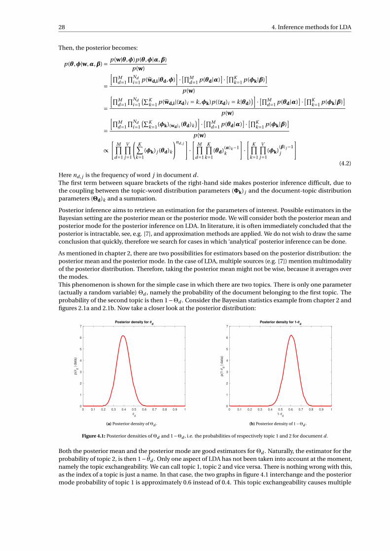
28 4. Inference methods for LDA
Then, the posterior becomes:
p(θ,φ|w,α,β) = p(w|θ,φ)p(θ,φ|α,β)
p(w)
=[∏M
d=1
∏Ndi=1 p(wd,i|θd,φ)
]· [∏M
d=1 p(θd|α)] · [∏K
k=1 p(φk|β)]
p(w)
=[∏M
d=1
∏Ndi=1
(∑Kk=1 p(wd,i|(zd)i = k,φk)p((zd)i = k|θd)
)] · [∏Md=1 p(θd|α)
] · [∏Kk=1 p(φk|β)
]p(w)
=[∏M
d=1
∏Ndi=1
(∑Kk=1(φk)(wd)i (θd)k
)] · [∏Md=1 p(θd|α)
] · [∏Kk=1 p(φk|β)
]p(w)
∝[
M∏d=1
V∏j=1
(K∑
k=1(φk) j (θd)k
)nd , j]·[
M∏d=1
K∏k=1
(θd)(α)k−1k
]·[
K∏k=1
V∏j=1
(φk)(β) j −1j
](4.2)
Here nd , j is the frequency of word j in document d .The first term between square brackets of the right-hand side makes posterior inference difficult, due tothe coupling between the topic-word distribution parameters (Φk) j and the document-topic distributionparameters (Θd)k and a summation.
Posterior inference aims to retrieve an estimation for the parameters of interest. Possible estimators in theBayesian setting are the posterior mean or the posterior mode. We will consider both the posterior mean andposterior mode for the posterior inference on LDA. In literature, it is often immediately concluded that theposterior is intractable, see, e.g. [7], and approximation methods are applied. We do not wish to draw the sameconclusion that quickly, therefore we search for cases in which ‘analytical’ posterior inference can be done.
As mentioned in chapter 2, there are two possibilities for estimators based on the posterior distribution: theposterior mean and the posterior mode. In the case of LDA, multiple sources (e.g. [7]) mention multimodalityof the posterior distribution. Therefore, taking the posterior mean might not be wise, because it averages overthe modes.This phenomenon is shown for the simple case in which there are two topics. There is only one parameter(actually a random variable) Θd , namely the probability of the document belonging to the first topic. Theprobability of the second topic is then 1−Θd . Consider the Bayesian statistics example from chapter 2 andfigures 2.1a and 2.1b. Now take a closer look at the posterior distribution:
0 0.1 0.2 0.3 0.4 0.5 0.6 0.7 0.8 0.9 1
d
0
1
2
3
4
5
6
7
p(
d | d
ata
)
Posterior density for d
(a) Posterior density of Θd .
0 0.1 0.2 0.3 0.4 0.5 0.6 0.7 0.8 0.9 1
1-d
0
1
2
3
4
5
6
7
p(1
-d | d
ata
)
Posterior density for 1-d
(b) Posterior density of 1−Θd .
Figure 4.1: Posterior densities ofΘd and 1−Θd , i.e. the probabilities of respectively topic 1 and 2 for document d .
Both the posterior mean and the posterior mode are good estimators for Θd . Naturally, the estimator for theprobability of topic 2, is then 1− θd . Only one aspect of LDA has not been taken into account at the moment,namely the topic exchangeability. We can call topic 1, topic 2 and vice versa. There is nothing wrong with this,as the index of a topic is just a name. In that case, the two graphs in figure 4.1 interchange and the posteriormode probability of topic 1 is approximately 0.6 instead of 0.4. This topic exchangeability causes multiple
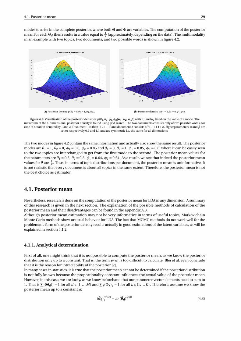
4.1. Posterior mean 29
modes to arise in the complete posterior, where bothΘ andΦ are variables. The computation of the posteriormean for eachΘd then results in a value equal to 1
K (approximately, depending on the data). The multimodalityin an example with two topics, two documents, and two possible words is shown in figure 4.2.
(a) Posterior density p(θ1 = 0,θ2 = 1,φ1 ,φ2). (b) Posterior density p(θ1 = 1,θ2 = 0,φ1 ,φ2).
Figure 4.2: Visualization of the posterior densities p(θ1,θ2,φ1,φ2|w1,w2,α,β) with θ1 and θ2 fixed on the value of a mode. Themaximum of the 4-dimensional posterior density is found using grid search. The two documents consists only of two possible words, forease of notation denoted by 1 and 2. Document 1 is then ‘2 2 1 1 1’ and document 2 consists of ‘1 1 1 1 1 1 2’. Hyperparameters α and β are
set to respectively 0.9 and 1.1 and are symmetric i.e. the same for all dimensions.
The two modes in figure 4.2 contain the same information and actually also show the same result. The posteriormodes are θ1 = 1, θ2 = 0, φ1 = 0.6, φ2 = 0.85 and θ1 = 0, θ2 = 1, φ1 = 0.85, φ2 = 0.6, where it can be easily seento the two topics are interchanged to get from the first mode to the second. The posterior mean values forthe parameters are θ1 = 0.5, θ2 = 0.5, φ1 = 0.64, φ2 = 0.64. As a result, we see that indeed the posterior meanvalues for θ are 1
K . Thus, in terms of topic distributions per document, the posterior mean is uninformative. Itis not realistic that every document is about all topics in the same extent. Therefore, the posterior mean is notthe best choice as estimator.
4.1. Posterior mean
Nevertheless, research is done on the computation of the posterior mean for LDA in any dimension. A summaryof this research is given in the next section. The explanation of the possible methods of calculation of theposterior mean and their disadvantages can be found in the appendix A.3.Although posterior mean estimation may not be very informative in terms of useful topics, Markov chainMonte Carlo methods show unusual behavior for LDA. The fact that MCMC methods do not work well for theproblematic form of the posterior density results actually in good estimations of the latent variables, as will beexplained in section 4.1.2.
4.1.1. Analytical determination
First of all, one might think that it is not possible to compute the posterior mean, as we know the posteriordistribution only up to a constant. That is, the term p(w) is too difficult to calculate. Blei et al. even concludethat it is the reason for intractability of the posterior [7].In many cases in statistics, it is true that the posterior mean cannot be determined if the posterior distributionis not fully known because the proportionality constant influences the actual value of the posterior mean.However, in this case, we are lucky, as we know beforehand that our parameter vector elements need to sum to1. That is
∑i (Θd)i = 1 for all d ∈ 1, . . . M and
∑j (Φk) j = 1 for all k ∈ 1, . . .K . Therefore, assume we know the
posterior mean up to a constant a:
(θd)(true)i = a · (θd)(est)
i (4.3)
30 4. Inference methods for LDA
with true denoting the true posterior mean and est the posterior mean estimated using the posterior inequation 4.2. Then the actual posterior mean values can be determined with:
(θd)(true)i = a · (θd)(est)
i∑Ki=1 a · (θd)(est)
i
= (θd)(est)i∑K
i=1(θd)(est)i
(4.4)
The same procedure can be followed for posterior mean estimators for all vectorsΦk, k = 1, . . .K . Hence, theactual value of p(w) is not needed for the computation of the posterior means and we can continue with theposterior in equation 4.2.
In appendix A.3 is explained how this posterior mean can be computed analytically, and if not possible, howit can be approximated. Unfortunately, the circumstances and model choices in Latent Dirichlet Allocationare such that neither analytical computation nor feasible approximation methods of the posterior mean arepossible.Therefore, it is better to focus on either the posterior mode or the posterior mean of a subspace of the domainaround the posterior mode. The latter can be approximated using Markov chain Monte Carlo methods and iselaborated on in the section.
4.1.2. Markov chain Monte Carlo methods
Markov chain Monte Carlo (MCMC) methods form a collection of techniques with which samples of the poste-rior distribution can be obtained. If there are enough samples, the techniques result in a good approximationof the posterior distribution. With this posterior density approximation, the posterior mean can be computed.The official definition of an MCMC method is given in [46].
Definition 4.1 (MCMC method)A Markov chain Monte Carlo method for the simulation of a distribution π is any method producing an ergodicMarkov chain whose stationary distribution is π.
Remember that one can think of an ergodic Markov chain as a chain in which each state can be reached fromevery other state. The stationary distribution of the Markov chain is its distribution in the limit of infinitelymany samples.
There are various simulation methods proposed in the literature: the Metropolis-Hastings algorithm, Gibbssampling and collapsed Gibbs sampling, where the latter is an extension of Gibbs sampling.
Metropolis-Hastings
The Metropolis-Hastings algorithm has been invented in 1953 by among others Nicholas Metropolis. W.K.Hastings generalized his idea in 1970 to the now commonly known ‘Metropolis-Hastings’ algorithm. Tosummarize the idea of this algorithm, the notation of Smith and Roberts in [41] is followed.
Let π(x) =π(x1, . . . , xk ) for x j ∈Rn , j = 1, . . . ,k, denote a joint density and let π(xi |x−i ) denote the conditionaldensities of xi for i ∈ 1, . . . ,k given all other x j ’s, i.e. x−i = (x j , j 6= i ). The goal of the algorithm is to constructa Markov chain X 1, . . . , X t , . . . with state space Ω and equilibrium distribution π(x). The state space Ω is thespace of all values that x can take.The Metropolis-Hastings algorithm works with transition probabilities from one state to the next, e.g. X t = xto X t+1 = y, for some state y ∈Ω. These transition probabilities are denoted with the transition probabilityfunction q , such that q(x,y) =P(X t = x, X t+1 = y).
However, further randomization is applied: with some probability the new state in X t+1 is accepted, whilewith complementary probability the new state is rejected and X t+1 remains in the same state as X t . Intuitivelyspeaking, we do not jump to the next state, but remain in the state in which we already were. Formally defined,
4.1. Posterior mean 31
the transition probability of the Markov chain is given by function p. For ease of notation, we have left out thevector notation.
p(x, y) =
q(x, y)α(x, y) if y 6= x
1−∑y ′∈Ω q(x, y ′)α(x, y ′) if y = x
(4.5)
With:
α(x, y) =
minπ(y)q(y,x)π(x)q(x,y) ,1
if π(x)q(x, y) > 0
1 if π(x)q(x, y) = 0(4.6)
Note that the so-called detailed balance is complied to: π(x)p(x, y) =π(y)p(y, x), which is necessary for theMarkov chain to be irreducible and aperiodic, ergo ergodic. With this condition, π(x) will be the equilibriumdistribution of the Markov chain, as desired [41]. Furthermore, because in the computation of α(x, y) the jointdensity π arises both in the numerator and the denominator, it is only needed to know π up to a proportionalityconstant.For the transition probability function q there are several possibilities to choose from [46]. If π is a continuousdensity, one can take for example a random walk distribution for q . Another possibility is taking q(x, ·) = f (·),such that the transition probability from state x is independent of x. It is useful to take for f a probabilitydensity that resembles the target function π, but is tractable, in contrast to π. More possibilities for q can befound in [46].
Because in the case of LDA, there are many parameters, resulting in a high dimensionality, it is difficult to findgood proposal densities q [46]. Therefore, we will not dive more deeply into the Metropolis-Hastings algorithmand its properties, but rather resort to Gibbs sampling.
Gibbs sampling
Often applied to (variants of) LDA is Gibbs sampling, which is actually a special case of the one-at-a-timeversion of the Metropolis-Hastings algorithm.In one-at-a-time Metropolis-Hastings, only one component of the vector x is sampled at a time, as the namesuggests. For each xi , i ∈ 1, . . . ,k, there is a specific transition probability function qi . First, consider atwo-dimensional example of sampling π(x1, x2), where x = (x1, x2) denotes the current state, and y = (y1, y2)the next state. Thus, suppose we have (x1, x2), the Markov chain evolves using the following steps [46]:
1. Draw y1 ∼ q1(x1, y1|x2) where conditioning on x2 means that you keep the value of x2 fixed in this step.
2. Accept the transition with probability α1:
α1 = min
π(y1, x2)q1(y1, x1|x2)
π(x1, x2)q1(x1, y1|x2),1
(4.7)
else y1 = x1 (no jump).
3. Draw y2 ∼ q2(x2, y2|y1) where conditioning on y1 means that you keep the obtained value of the firstcomponent (y1) from the current/next index in the Markov chain fixed.
4. Accept the transition with probability α2:
α2 = min
π(y1, y2)q2(y2, x2|y1)
π(y1, x2)q2(x2, y2|y1),1
(4.8)
else y2 = x2 (no jump).
The Gibbs sampler algorithm then arises when you use the following transition probability functions qi , againfor the 2-dimensional example:
q1(x1, y1|x2) =π(y1|x2)
q2(x2, y2|y1) =π(y2|x1)(4.9)
That is, when the transition probability functions qi are defined as the conditional distributions derived fromthe target distribution π and only one component of the random vector is sampled at a time, the Metropolis-Hastings method becomes Gibbs sampling. Note that with these functions qi , the acceptance probabilities αi
will always be 1, therefore, you always draw the next state in the Markov chain from the conditional distribution.
32 4. Inference methods for LDA
Gibbs sampling is only applicable when the conditional distributions are of a known form. Therefore, Bayesianstatisticians usually use conjugate priors, such that the posterior distribution is from the same family ofdistributions as the prior. Then, one can easily sample from conditional distributions. If the posteriordistribution is not a known density, it is very challenging to obtain samples, which is why in those casesMetropolis-Hastings is used.
One of the main advantages of Gibbs sampling or Markov chain Monte Carlo methods in general is that theyconverge under relatively weak assumptions. In [42], these assumptions are explained. Define K (x,y) to be thetransition kernel of the Markov chain, that is, for the two-dimensional example above [42]:
K (x,y) =π(y1|x2) ·π(y2|y1) (4.10)
provided that∫π(y1, x2)dy1 > 0 and
∫π(y1, y2)dy2 > 0, otherwise in determining the conditional densities, we
would divide by 0. If one of these conditions in not satisfied, K (x,y) = 0 by definition. The kernel K (x,y) mapsfrom D ×D to R2, where D = x ∈Ω,π(x) > 0 withΩ the state space of x, in this section chosen to be R2.Smith and Roberts state convergence of the Gibbs sampler in the following theorem:
Theorem 4.1 (Convergence Gibbs sampler)If K is π-irreducible and aperiodic, then for all x ∈ D:
1.∫Ω |K (t )(x,y)−π(y)|dy → 0 for t →∞.
2. for real-valued, π-integrable function f ,
t−1 (f (X 1)+ . . . f (X t )
)→ ∫Ω
f (x)π(x)dx
almost surely for t →∞.
Here t is the number of samples in the Markov chain. K (t ) is the kernel describing t iterations, more thoroughlyexplained in [42]. From the theorem, we can conclude that the kernel K converges to π in L1. Furthermore,the sample mean of all samples in the Markov chain (corrected for the initial, transient phase, also called theburn-in period) converges to the actual mean of π almost surely. Hence, in Gibbs sampling, the sample meanis used as an approximation for the posterior mean.To use theorem 4.1, we need to show that the kernel is π-irreducible and aperiodic. Smith and Roberts givesimple conditions for the standard Gibbs sampling formulas to satisfy these two assumptions in [42]. Theyexplain that it is hard to find settings for Gibbs sampling in which these two assumptions are not satisfied.Therefore, we expect Gibbs sampling to be a reliable method to obtain posterior mean estimate for the latentrandom variables of interest in LDA.
Example Gibbs sampling To illustrate the algorithm of Gibbs sampling, a 2-dimensional example is workedout, which is, in fact, the 2-dimensional basis of LDA. Therefore, the link to higher dimensional is easy to make,as the hierarchical scheme of LDA has already been explained.Consider a group of students that makes a test. The test consists of N questions, and each student is assumedto have a probability ofΘi to give the right answer to a question. There are n students, and the only observedvariables are X1, . . . Xn , the number of questions that each student has answered correctly. Furthermore, weassume that each student works independently and all questions are equally difficult, so Xi ∼ Binomial(Θi , N )with no correlation between the Xi . The probability of giving the right answer is a priori Beta distributed i.e.Θi ∼ Beta(a,b) i .i .d . Then the posterior distribution ofΘ|X can be derived.
p(θ|x, a,b) = p(θ,x|a,b)
p(x|a,b)
∝ p(x|θ, a,b)p(θ|a,b)
=n∏
i=1
(n
xi
)θ
xii (1−θi )N−xi · Γ(a +b)
Γ(a)Γ(b)θa−1
i (1−θi )b−1
∝n∏
i=1θ
xi+a−1i (1−θi )N−xi+b−1
(4.11)
4.1. Posterior mean 33
BecauseΘi is independent of all otherΘ j for j 6= i , we can easily see that:
p(θi |θ1,θi−1,θi+1,θn ,x, a,b) ∝ θx1+a−1i (1−θi )N−xi+b−1
⇒Θi |xi , a,b ∼ Beta(xi +a, N −xi +b)(4.12)
Note that the Beta distribution is a conjugate prior to the Binomial distribution. The Gibbs sampling procedurebecomes:
• Draw θ1 from Beta(x1 +a, N −x1 +b)
• . . .
• Draw θn from Beta(xn +a, N −xn +b)
When this procedure is executed sufficiently often, the samples for each Θi will approximate the posteriordistribution p(θi |xi , a,b) with which then the value of Θi can be estimated via the posterior mode or posteriormean.
Gibbs sampling for LDA In Latent Dirichlet Allocation, many latent variables need to be retrieved usingGibbs sampling. The observed data are the words w, where w has a length of
∑Md=1 Nd . The fixed parameters,
also called hyperparameters areα andβ. The unknown parameters areΘd for d ∈ 1, . . . , M ,Φk for k ∈ 1, . . . ,K and Z, which has the same length as w. This means that there are M +K +1 vectors to be estimated that haveM ·K +K ·V + (∑M
d=1 Nd)
components together. To give an idea; assume we have 10,000 reviews with each 100words. We assume that 20 topics are written about. In total, there are 1000 words in the vocabulary. This meansthat we have to estimate 10,000 ·20+20 ·1000+10,000 ·100 = 320,000 components. Luckily, it is possible tosample the vectorsΘd andΦk at once, and no component-wise inference needs to be done. The conditionaldistributions are derived as follows.
A single document d from the set 1, . . . , M can be considered, because in LDA, it is assumed that eachdocument is generated independently. The full conditional distribution ofΘd is derived.
p(θd|θ1, . . . ,θd−1,θd+1, . . . ,θM,φ1, . . . ,φK,z,w,α,β) = p(θ1, . . . ,θM,φ1, . . . ,φK,z,w|α,β)
p(θ1, . . . ,θd−1,θd+1, . . . ,θM,φ1, . . . ,φK,z,w|α,β)
∝ p(θ1, . . . ,θM,φ1, . . . ,φK,z,w|α,β)
∝ p(θd,φ1, . . . ,φK,zd,wd|α,β)
=(
Nd∏i=1
p(wi |zi ,θd,φ1, . . . ,φK,α,β)p(zi |θd,φ1, . . . ,φK,α,β)
)·(
K∏k=1
p(φk|β)
)·p(θd|α)
=(
Nd∏i=1
p(wi |zi ,φ1, . . . ,φK)p(zi |θd)
)·(
K∏k=1
p(φk|β)
)·p(θd|α)
∝(
Nd∏i=1
p(zi |θd)
)·p(θd|α)
∝(
Nd∏i=1
K∏k=1
(θd)(zi)kk
)·
K∏k=1
(θd)(α)k−1k
=K∏
k=1(θd)(md)k+(α)k−1
k
(4.13)
Here we define md ,k as the number of times a word in document d is assigned to topic k. The expression in4.13 can be recognized as a Dirichlet distribution:
(Θd|θ1, . . . ,θd−1,θd+1, . . . ,θM,φ1, . . . ,φK,z,w,α,β
)∼ Dirichlet(md +α) (4.14)
With md the vector of topic frequencies (md)k for k = 1, . . . ,K .
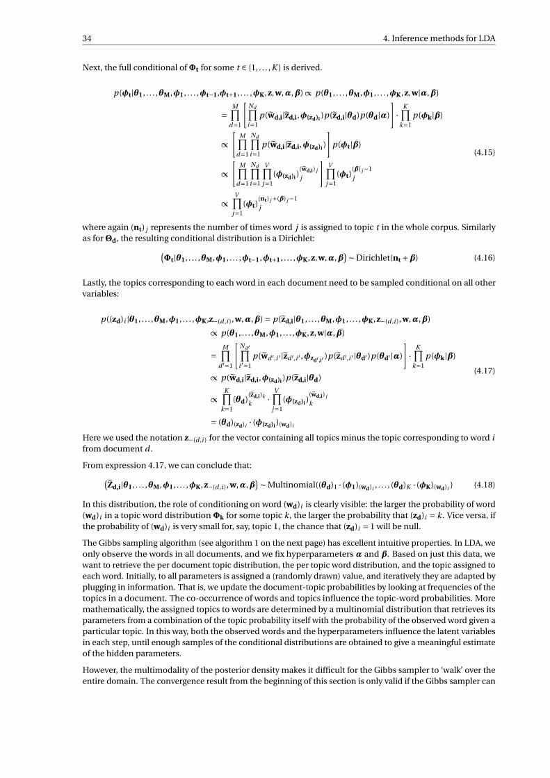
34 4. Inference methods for LDA
Next, the full conditional ofΦt for some t ∈ 1, . . . ,K is derived.
p(φt|θ1, . . . ,θM,φ1, . . . ,φt−1,φt+1, . . . ,φK,z,w,α,β) ∝ p(θ1, . . . ,θM,φ1, . . . ,φK,z,w|α,β)
=M∏
d=1
[Nd∏i=1
p(wd,i|zd,i,φ(zd)i )p(zd,i|θd)p(θd|α)
]·
K∏k=1
p(φk|β)
∝[
M∏d=1
Nd∏i=1
p(wd,i|zd,i,φ(zd)i )
]p(φt|β)
∝[
M∏d=1
Nd∏i=1
V∏j=1
(φ(zd)i )(wd,i) j
j
]V∏
j=1(φt)
(β) j −1j
∝V∏
j=1(φt)
(nt) j +(β) j −1j
(4.15)
where again (nt) j represents the number of times word j is assigned to topic t in the whole corpus. Similarlyas forΘd, the resulting conditional distribution is a Dirichlet:(
Φt|θ1, . . . ,θM,φ1, . . . ,φt−1,φt+1, . . . ,φK,z,w,α,β)∼ Dirichlet(nt +β) (4.16)
Lastly, the topics corresponding to each word in each document need to be sampled conditional on all othervariables:
p((zd)i |θ1, . . . ,θM,φ1, . . . ,φK,z−(d ,i ),w,α,β) = p(zd,i|θ1, . . . ,θM,φ1, . . . ,φK,z−(d ,i ),w,α,β)
∝ p(θ1, . . . ,θM,φ1, . . . ,φK,z,w|α,β)
=M∏
d ′=1
[Nd ′∏i ′=1
p(wd ′,i ′ |zd ′,i ′ ,φzd′ ,i′ )p(zd ′,i ′ |θd′ )p(θd′ |α)
]·
K∏k=1
p(φk|β)
∝ p(wd,i|zd,i,φ(zd)i )p(zd,i|θd)
∝K∏
k=1(θd)
(zd,i)k
k ·V∏
j=1(φ(zd)i )
(wd,i) j
k
= (θd)(zd)i · (φ(zd)i )(wd)i
(4.17)
Here we used the notation z−(d ,i ) for the vector containing all topics minus the topic corresponding to word ifrom document d .
From expression 4.17, we can conclude that:(Zd,i|θ1, . . . ,θM,φ1, . . . ,φK,z−(d ,i ),w,α,β
)∼ Multinomial((θd)1 · (φ1)(wd)i , . . . , (θd)K · (φK)(wd)i ) (4.18)
In this distribution, the role of conditioning on word (wd)i is clearly visible: the larger the probability of word(wd)i in a topic word distributionΦk for some topic k, the larger the probability that (zd)i = k. Vice versa, ifthe probability of (wd)i is very small for, say, topic 1, the chance that (zd)i = 1 will be null.
The Gibbs sampling algorithm (see algorithm 1 on the next page) has excellent intuitive properties. In LDA, weonly observe the words in all documents, and we fix hyperparameters α and β. Based on just this data, wewant to retrieve the per document topic distribution, the per topic word distribution, and the topic assigned toeach word. Initially, to all parameters is assigned a (randomly drawn) value, and iteratively they are adapted byplugging in information. That is, we update the document-topic probabilities by looking at frequencies of thetopics in a document. The co-occurrence of words and topics influence the topic-word probabilities. Moremathematically, the assigned topics to words are determined by a multinomial distribution that retrieves itsparameters from a combination of the topic probability itself with the probability of the observed word given aparticular topic. In this way, both the observed words and the hyperparameters influence the latent variablesin each step, until enough samples of the conditional distributions are obtained to give a meaningful estimateof the hidden parameters.
However, the multimodality of the posterior density makes it difficult for the Gibbs sampler to ‘walk’ over theentire domain. The convergence result from the beginning of this section is only valid if the Gibbs sampler can
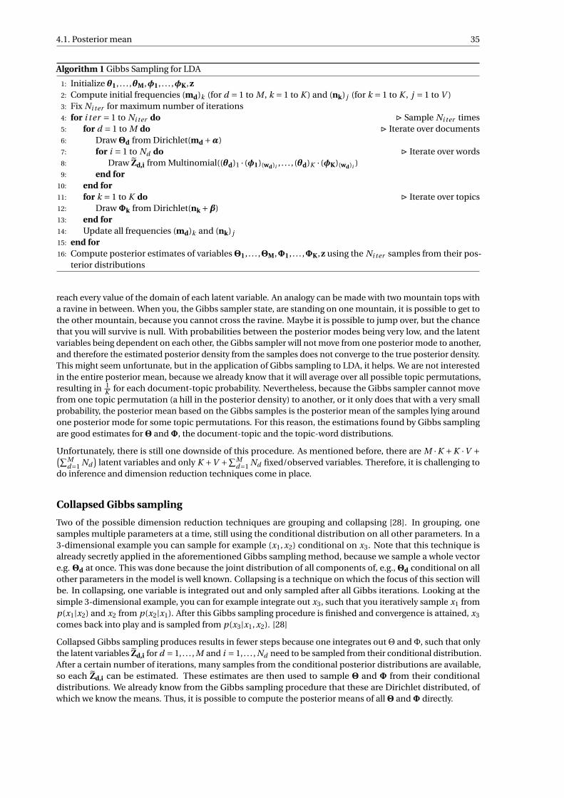
4.1. Posterior mean 35
Algorithm 1 Gibbs Sampling for LDA
1: Initialize θ1, . . . ,θM,φ1, . . . ,φK,z2: Compute initial frequencies (md)k (for d = 1 to M , k = 1 to K ) and (nk) j (for k = 1 to K , j = 1 to V )3: Fix Ni ter for maximum number of iterations4: for i ter = 1 to Ni ter do . Sample Ni ter times5: for d = 1 to M do . Iterate over documents6: DrawΘd from Dirichlet(md +α)7: for i = 1 to Nd do . Iterate over words8: Draw Zd,i from Multinomial((θd)1 · (φ1)(wd)i , . . . , (θd)K · (φK)(wd)i )9: end for
10: end for11: for k = 1 to K do . Iterate over topics12: DrawΦk from Dirichlet(nk +β)13: end for14: Update all frequencies (md)k and (nk) j
15: end for16: Compute posterior estimates of variablesΘ1, . . . ,ΘM,Φ1, . . . ,ΦK,z using the Ni ter samples from their pos-
terior distributions
reach every value of the domain of each latent variable. An analogy can be made with two mountain tops witha ravine in between. When you, the Gibbs sampler state, are standing on one mountain, it is possible to get tothe other mountain, because you cannot cross the ravine. Maybe it is possible to jump over, but the chancethat you will survive is null. With probabilities between the posterior modes being very low, and the latentvariables being dependent on each other, the Gibbs sampler will not move from one posterior mode to another,and therefore the estimated posterior density from the samples does not converge to the true posterior density.This might seem unfortunate, but in the application of Gibbs sampling to LDA, it helps. We are not interestedin the entire posterior mean, because we already know that it will average over all possible topic permutations,resulting in 1
K for each document-topic probability. Nevertheless, because the Gibbs sampler cannot movefrom one topic permutation (a hill in the posterior density) to another, or it only does that with a very smallprobability, the posterior mean based on the Gibbs samples is the posterior mean of the samples lying aroundone posterior mode for some topic permutations. For this reason, the estimations found by Gibbs samplingare good estimates forΘ andΦ, the document-topic and the topic-word distributions.
Unfortunately, there is still one downside of this procedure. As mentioned before, there are M ·K +K ·V +(∑Md=1 Nd
)latent variables and only K +V +∑M
d=1 Nd fixed/observed variables. Therefore, it is challenging todo inference and dimension reduction techniques come in place.
Collapsed Gibbs sampling
Two of the possible dimension reduction techniques are grouping and collapsing [28]. In grouping, onesamples multiple parameters at a time, still using the conditional distribution on all other parameters. In a3-dimensional example you can sample for example (x1, x2) conditional on x3. Note that this technique isalready secretly applied in the aforementioned Gibbs sampling method, because we sample a whole vectore.g. Θd at once. This was done because the joint distribution of all components of, e.g.,Θd conditional on allother parameters in the model is well known. Collapsing is a technique on which the focus of this section willbe. In collapsing, one variable is integrated out and only sampled after all Gibbs iterations. Looking at thesimple 3-dimensional example, you can for example integrate out x3, such that you iteratively sample x1 fromp(x1|x2) and x2 from p(x2|x1). After this Gibbs sampling procedure is finished and convergence is attained, x3
comes back into play and is sampled from p(x3|x1, x2). [28]
Collapsed Gibbs sampling produces results in fewer steps because one integrates out Θ and Φ, such that onlythe latent variables Zd,i for d = 1, . . . , M and i = 1, . . . , Nd need to be sampled from their conditional distribution.After a certain number of iterations, many samples from the conditional posterior distributions are available,so each Zd,i can be estimated. These estimates are then used to sample Θ and Φ from their conditionaldistributions. We already know from the Gibbs sampling procedure that these are Dirichlet distributed, ofwhich we know the means. Thus, it is possible to compute the posterior means of allΘ andΦ directly.
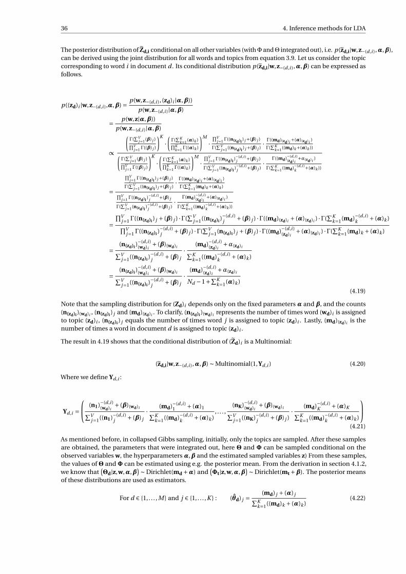
36 4. Inference methods for LDA
The posterior distribution of Zd,i conditional on all other variables (withΦ andΘ integrated out), i.e. p(zd,i|w,z−(d ,i ),α,β),can be derived using the joint distribution for all words and topics from equation 3.9. Let us consider the topiccorresponding to word i in document d . Its conditional distribution p(zd,i|w,z−(d ,i ),α,β) can be expressed asfollows.
p((zd)i |w,z−(d ,i ),α,β) = p(w,z−(d ,i ), (zd)i |α,β))
p(w,z−(d ,i )|α,β)
= p(w,z|α,β))
p(w,z−(d ,i )|α,β)
∝
(Γ(
∑Vj=1(β) j )∏V
j=1Γ((β) j )
)K
·(Γ(
∑Kk=1(α)k )∏K
k=1Γ((α)k )
)M
·∏V
j=1Γ((n(zd)i ) j +(β) j )
Γ(∑V
j=1((n(zd)i ) j +(β) j )· Γ((md)(zd)i +(α)(zd)i )
Γ(∑K
k=1((md)k+(α)k ))(Γ(
∑Vj=1(β) j )∏V
j=1Γ((β) j )
)K
·(Γ(
∑Kk=1(α)k )∏K
k=1Γ((α)k )
)M
·∏V
j=1Γ((n(zd)i )−(d ,i )j +(β) j )
Γ(∑V
j=1((n(zd)i )−(d ,i )j +(β) j )
· Γ((md)−(d ,i )(zd)i
+α(zd)i )
Γ(∑K
k=1((md)−(d ,i )k +(α)k ))
=
∏Vj=1Γ((n(zd)i ) j +(β) j )
Γ(∑V
j=1((n(zd)i ) j +(β) j )· Γ((md)(zd)i +(α)(zd)i )
Γ(∑K
k=1(md)k+(α)k )∏Vj=1Γ((n(zd)i )−(d ,i )
j +(β) j
Γ(∑V
j=1(n(zd)i )−(d ,i )j +(β) j )
· Γ(md)−(d ,i )(zd)i
+(α)(zd)i )
Γ(∑K
k=1((md)−(d ,i )k +(α)k ))
=∏V
j=1Γ((n(zd)i ) j + (β) j ) ·Γ(∑V
j=1((n(zd)i )−(d ,i )j + (β) j ) ·Γ((md)(zd)i + (α)(zd)i ) ·Γ(
∑Kk=1(md)−(d ,i )
k + (α)k )∏Vj=1Γ((n(zd)i )
−(d ,i )j + (β) j ) ·Γ(
∑Vj=1(n(zd)i ) j + (β) j ) ·Γ((md)−(d ,i )
(zd)i+ (α)(zd)i ) ·Γ(
∑Kk=1(md)k + (α)k )
=(n(zd)i )
−(d ,i )(wd)i
+ (β)(wd)i∑Vj=1((n(zd)i )
−(d ,i )j + (β) j
·(md)−(d ,i )
(zd)i+α(zd)i∑K
k=1((md)−(d ,i )k + (α)k )
=(n(zd)i )
−(d ,i )(wd)i
+ (β)(wd)i∑Vj=1((n(zd)i )
−(d ,i )j + (β) j
·(md)−(d ,i )
(zd)i+α(zd)i
Nd −1+∑Kk=1(α)k )
(4.19)
Note that the sampling distribution for (Zd)i depends only on the fixed parameters α and β, and the counts(n(zd)i )(wd)i , (n(zd)i ) j and (md)(zd)i . To clarify, (n(zd)i )(wd)i represents the number of times word (wd)i is assignedto topic (zd)i , (n(zd)i ) j equals the number of times word j is assigned to topic (zd)i . Lastly, (md)(zd)i is thenumber of times a word in document d is assigned to topic (zd)i .
The result in 4.19 shows that the conditional distribution of (Zd)i is a Multinomial:
(zd,i|w,z−(d ,i ),α,β) ∼ Multinomial(1,Yd ,i ) (4.20)
Where we define Yd ,i :
Yd ,i = (n1)−(d ,i )
(wd)i+ (β)(wd)i∑V
j=1((n1)−(d ,i )j + (β) j
· (md)−(d ,i )1 + (α)1∑K
k=1((md)−(d ,i )k + (α)k )
, . . . ,(nK)−(d ,i )
(wd)i+ (β)(wd)i∑V
j=1((nK)−(d ,i )j + (β) j )
· (md)−(d ,i )K + (α)K∑K
k=1((md)−(d ,i )k + (α)k )
(4.21)
As mentioned before, in collapsed Gibbs sampling, initially, only the topics are sampled. After these samplesare obtained, the parameters that were integrated out, here Θ and Φ can be sampled conditional on theobserved variables w, the hyperparameters α,β and the estimated sampled variables z) From these samples,the values ofΘ andΦ can be estimated using e.g. the posterior mean. From the derivation in section 4.1.2,we know that
(Θd|z,w,α,β
)∼ Dirichlet(md +α) and(Φt|z,w,α,β
)∼ Dirichlet(mt +β). The posterior meansof these distributions are used as estimators.
For d ∈ 1, . . . , M and j ∈ 1, . . . ,K : (θd) j =(md) j + (α) j∑K
k=1((md)k + (α)k )(4.22)
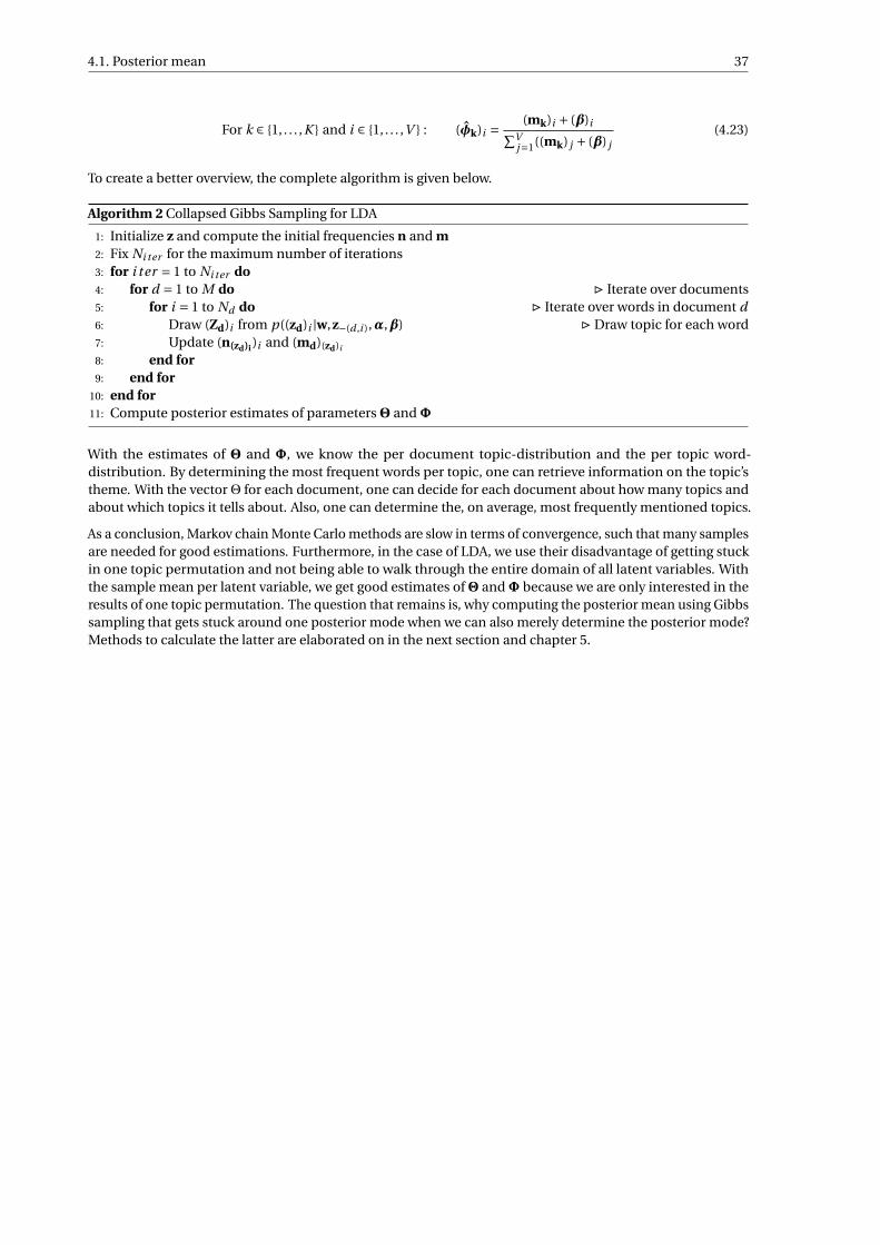
4.1. Posterior mean 37
For k ∈ 1, . . . ,K and i ∈ 1, . . . ,V : (φk)i = (mk)i + (β)i∑Vj=1((mk) j + (β) j
(4.23)
To create a better overview, the complete algorithm is given below.
Algorithm 2 Collapsed Gibbs Sampling for LDA
1: Initialize z and compute the initial frequencies n and m2: Fix Ni ter for the maximum number of iterations3: for i ter = 1 to Ni ter do4: for d = 1 to M do . Iterate over documents5: for i = 1 to Nd do . Iterate over words in document d6: Draw (Zd)i from p((zd)i |w,z−(d ,i ),α,β) .Draw topic for each word7: Update (n(zd)i )i and (md)(zd)i
8: end for9: end for
10: end for11: Compute posterior estimates of parametersΘ andΦ
With the estimates of Θ and Φ, we know the per document topic-distribution and the per topic word-distribution. By determining the most frequent words per topic, one can retrieve information on the topic’stheme. With the vectorΘ for each document, one can decide for each document about how many topics andabout which topics it tells about. Also, one can determine the, on average, most frequently mentioned topics.
As a conclusion, Markov chain Monte Carlo methods are slow in terms of convergence, such that many samplesare needed for good estimations. Furthermore, in the case of LDA, we use their disadvantage of getting stuckin one topic permutation and not being able to walk through the entire domain of all latent variables. Withthe sample mean per latent variable, we get good estimates ofΘ andΦ because we are only interested in theresults of one topic permutation. The question that remains is, why computing the posterior mean using Gibbssampling that gets stuck around one posterior mode when we can also merely determine the posterior mode?Methods to calculate the latter are elaborated on in the next section and chapter 5.
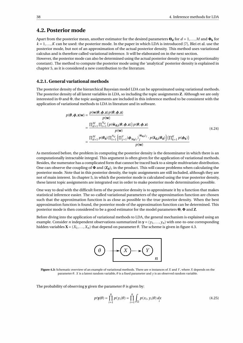
38 4. Inference methods for LDA
4.2. Posterior mode
Apart from the posterior mean, another estimator for the desired parametersΘd for d = 1, . . . , M andΦk fork = 1, . . . ,K can be used: the posterior mode. In the paper in which LDA is introduced [7], Blei et al. use theposterior mode, but not of an approximation of the actual posterior density. This method uses variationalcalculus and is therefore called variational inference. It will be elaborated on in the next section.However, the posterior mode can also be determined using the actual posterior density (up to a proportionalityconstant). The method to compute the posterior mode using the ‘analytical’ posterior density is explained inchapter 5, as it is considered a new contribution to the literature.
4.2.1. General variational methods
The posterior density of the hierarchical Bayesian model LDA can be approximated using variational methods.The posterior density of all latent variables in LDA, so including the topic assignments Z. Although we are onlyinterested inΘ andΦ, the topic assignments are included in this inference method to be consistent with theapplication of variational methods to LDA in literature and in software.
p(θ,φ,z|w) = p(w|θ,φ,z)p(θ,φ,z)
p(w)
=∏M
d=1
∏Ndi=1
(p(wd,i|θ,φ,z)
)p(θ,φ,z)
p(w)
=∏M
d=1 p(θd)∏Nd
i=1
(∏Vj=1(φ(zd)i
)(wd,i) j
j ·p(zd,i|θd))(∏K
k=1 p(φk))
p(w)
(4.24)
As mentioned before, the problem in computing the posterior density is the denominator in which there is ancomputationally intractable integral. This argument is often given for the application of variational methods.Besides, the numerator has a complicated form that cannot be traced back to a simple multivariate distribution.One can observe the coupling ofΦ and (Zd)i in the product. This will cause problems when calculating theposterior mode. Note that in this posterior density, the topic assignments are still included, although they arenot of main interest. In chapter 5, in which the posterior mode is calculated using the true posterior density,these latent topic assignments are integrated out in order to make posterior mode determination possible.
One way to deal with the difficult form of the posterior density is to approximate it by a function that makesstatistical inference easier. The so-called variational parameters of the approximation function are chosensuch that the approximation function is as close as possible to the true posterior density. When the bestapproximation function is found, the posterior mode of the approximation function can be determined. Thisposterior mode is then considered to be a good estimator for the model parametersΘ,Φ and Z.
Before diving into the application of variational methods to LDA, the general mechanism is explained using anexample. Consider n independent observations summarized in y = (y1, . . . , yn) with one-to-one correspondinghidden variables X = (X1, . . . , Xn) that depend on parameter θ. The scheme is given in figure 4.3.
θ X Y
n
Figure 4.3: Schematic overview of an example of variational methods. There are n instances of X and Y , where X depends on theparameter θ. X is a latent random variable, θ is a fixed parameter and y is an observed random variable.
The probability of observing y given the parameter θ is given by:
p(y|θ) =n∏
i=1p(yi |θ) =
n∏i=1
∫Ω
p(xi , yi |θ)dxi
(4.25)
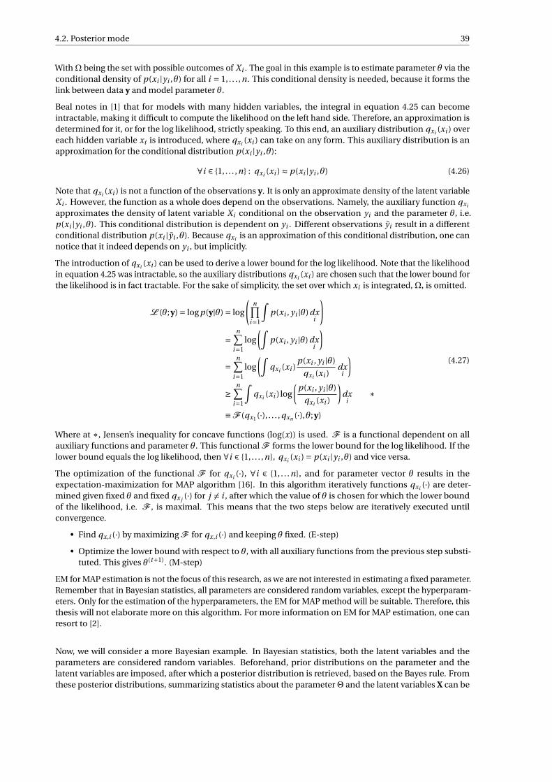
4.2. Posterior mode 39
WithΩ being the set with possible outcomes of Xi . The goal in this example is to estimate parameter θ via theconditional density of p(xi |yi ,θ) for all i = 1, . . . ,n. This conditional density is needed, because it forms thelink between data y and model parameter θ.
Beal notes in [1] that for models with many hidden variables, the integral in equation 4.25 can becomeintractable, making it difficult to compute the likelihood on the left hand side. Therefore, an approximation isdetermined for it, or for the log likelihood, strictly speaking. To this end, an auxiliary distribution qxi (xi ) overeach hidden variable xi is introduced, where qxi (xi ) can take on any form. This auxiliary distribution is anapproximation for the conditional distribution p(xi |yi ,θ):
∀i ∈ 1, . . . ,n : qxi (xi ) ≈ p(xi |yi ,θ) (4.26)
Note that qxi (xi ) is not a function of the observations y. It is only an approximate density of the latent variableXi . However, the function as a whole does depend on the observations. Namely, the auxiliary function qxi
approximates the density of latent variable Xi conditional on the observation yi and the parameter θ, i.e.p(xi |yi ,θ). This conditional distribution is dependent on yi . Different observations yi result in a differentconditional distribution p(xi |yi ,θ). Because qxi is an approximation of this conditional distribution, one cannotice that it indeed depends on yi , but implicitly.
The introduction of qxi (xi ) can be used to derive a lower bound for the log likelihood. Note that the likelihoodin equation 4.25 was intractable, so the auxiliary distributions qxi (xi ) are chosen such that the lower bound forthe likelihood is in fact tractable. For the sake of simplicity, the set over which xi is integrated,Ω, is omitted.
L (θ;y) = log p(y|θ) = log
(n∏
i=1
∫p(xi , yi |θ)dx
i
)
=n∑
i=1log
(∫p(xi , yi |θ)dx
i
)=
n∑i=1
log
(∫qxi (xi )
p(xi , yi |θ)
qxi (xi )dx
i
)≥
n∑i=1
∫qxi (xi ) log
(p(xi , yi |θ)
qxi (xi )
)dx
i∗
≡F (qx1 (·), . . . , qxn (·),θ;y)
(4.27)
Where at ∗, Jensen’s inequality for concave functions (log(x)) is used. F is a functional dependent on allauxiliary functions and parameter θ. This functional F forms the lower bound for the log likelihood. If thelower bound equals the log likelihood, then ∀i ∈ 1, . . . ,n, qxi (xi ) = p(xi |yi ,θ) and vice versa.
The optimization of the functional F for qxi (·), ∀i ∈ 1, . . .n, and for parameter vector θ results in theexpectation-maximization for MAP algorithm [16]. In this algorithm iteratively functions qxi (·) are deter-mined given fixed θ and fixed qx j (·) for j 6= i , after which the value of θ is chosen for which the lower boundof the likelihood, i.e. F , is maximal. This means that the two steps below are iteratively executed untilconvergence.
• Find qx,i (·) by maximizing F for qx,i (·) and keeping θ fixed. (E-step)
• Optimize the lower bound with respect to θ, with all auxiliary functions from the previous step substi-tuted. This gives θ(t+1). (M-step)
EM for MAP estimation is not the focus of this research, as we are not interested in estimating a fixed parameter.Remember that in Bayesian statistics, all parameters are considered random variables, except the hyperparam-eters. Only for the estimation of the hyperparameters, the EM for MAP method will be suitable. Therefore, thisthesis will not elaborate more on this algorithm. For more information on EM for MAP estimation, one canresort to [2].
Now, we will consider a more Bayesian example. In Bayesian statistics, both the latent variables and theparameters are considered random variables. Beforehand, prior distributions on the parameter and thelatent variables are imposed, after which a posterior distribution is retrieved, based on the Bayes rule. Fromthese posterior distributions, summarizing statistics about the parameterΘ and the latent variables X can be

40 4. Inference methods for LDA
retrieved (e.g. the mean or the mode). Besides, estimators for Θ and X can be determined. This is a slightlydifferent setting. Therefore, we extend the EM for MAP algorithm to the so-called Variational Bayesian EM(VBEM).Consider the same situation as in figure 4.3. In VBEM, also for Θ an auxiliary distribution is needed, asit is a random variable. Therefore, a general auxiliary distribution over all latent variables is introduced:q(x1, . . . , xn ,θ). The prior distribution of Θ depends on some fixed hyperparameter α, i.e. the prior has theform p(θ|α).
Θ X Y
nα
Figure 4.4: Schematic overview of an example of variational methods in a Bayesian setting. There are n instances of X and Y , where Xdepends on the parameterΘ. X is a latent random variable,Θ is a random variable depending on fixed hyperparameter α, and y is an
observed random variable.
For ease of notation, we summarize the latent variables in vector X = (X1, . . . , Xn) and the observed data iny = (y1, . . . , yn). The log likelihood of the model becomes:
L (α;y) = log p(y|α) = log
(∫ ∫p(x,y,θ|α)dxdθ
)= log
(∫ ∫qx,θ(x,θ)
p(x,y,θ|α)
qx,θ(x,θ)dxdθ
)≥
∫ ∫qx,θ(x,θ) log
(p(x,y,θ|α)
qx,θ(x,θ)
)dxdθ ∗
(4.28)
At ∗ again Jensen’s inequality is used. With the two integral signs, it is denoted that we integrate over θ once,and over xi for all i = 1, . . . ,n. Note that the difference between the likelihood L (α;y) and the lower bound inequation 4.28 is exactly the Kullback-Leibler divergence of qx,θ(·, ·) with respect to p(·, ·|y,α) [8].
KL(qx,θ(·, ·)‖p(·, ·|y,α)
)= ∫ ∫q(x,θ) log
(q(x,θ)
p(x,θ|y,α)
)dxdθ
= Eqx,θ
[log qx,θ(X,Θ)
]−Eqx,θ
[log p(X,Θ|y,α)
]= Eqx,θ
[log qx,θ(X,Θ)
]−Eqx,θ
[log
p(X,Θ,y|α)
p(y|α)
]= Eqx,θ
[log qx,θ(X,Θ)
]−Eqx,θ
[log p(X,Θ,y|α)
]+ log p(y|α)
= Eqx,θ
[log qx,θ(X,Θ)
]−Eqx,θ
[log p(X,Θ,y|α)
]+L (α;y)
=−∫ ∫
qx,θ(x,θ) log
(p(x,y,θ|α)
qx,θ(x,θ)
)dxdθ+L (α;y)
(4.29)
⇒L (α;y) =∫ ∫
qx,θ(x,θ) log
(p(x,y,θ|α)
qx,θ(x,θ)
)dxdθ+KL
(qx,θ(·, ·)‖p(·, ·|y,α)
)(4.30)
Note that in the derivation above, the notation Eqx,θ is used. The subscript qx,θ is used to indicate that theexpectation of a function of random variables X andΘ is computed with the joint density of X andΘ being qx,θ .From equation 4.30, it can be concluded that minimizing the KL-divergence of qx,θ(·, ·) with respect to p(·, ·|y,α)is equivalent to maximizing the lower bound given in equation 4.28. Minimization of the KL-divergence mightbe more intuitive when approximating one function to another. However, in the derivation of the VBEMalgorithm, we will stick to maximizing the log likelihood.
There are many possible functional forms for qx,θ(·, ·), but the most frequently used choice is the mean fieldapproximation [47]. This approximation originates in the field of statistical physics [35] and assumes that allvariables X1, . . . , Xn ,Θ are independent. This is also the method used by Blei et al. in their original paper of LDA.For the example in figure 4.4, the mean field method restricts the choice in auxiliary functions to those that
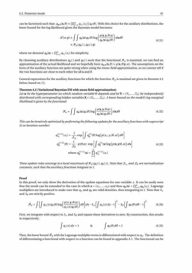
4.2. Posterior mode 41
can be factorized such that: qx,θ(x,θ) ≈ (∏ni=1 qxi (xi )
)qθ(θ). With this choice for the auxiliary distributions, the
lower bound for the log likelihood given the Bayesian model becomes:
L (α;y) ≥∫ ∫
qx(x)qθ(θ) log
(p(x,y,θ|α)
qx(x)qθ(θ)
)dxdθ
≡Fα(qx(·), qθ(·);y)
(4.31)
where we denoted qx(x) =∏ni=1 qxi (xi ) for simplicity.
By choosing auxiliary distributions qx(·) and qθ(·) such that the functional Fα is maximal, we can find anapproximation of the actual likelihood and we hopefully have qx,θ(x,θ) ≈ p(x,θ|y,α). The assumptions on theform of the auxiliary function are quite strong when using the mean-field approximation, so we cannot tell ifthe two functions are close to each other for all x and θ.
General expressions for the auxiliary functions for which the function Fα is maximal are given in theorem 4.2below, based on [1].
Theorem 4.2 (Variational Bayesian EM with mean field approximation)Let α be the hyperparameter on which random variable Θ depends and let Y = (Y1, . . . ,Yn) be independentlydistributed with corresponding hidden variables X = (X1, . . . , Xn). A lower bound on the model’s log marginallikelihood is given by the functional:
Fα =∫ ∫
qx(x)qθ(θ) log
(p(x,y,θ|α)
qx(x)qθ(θ)
)dxdθ (4.32)
This can be iteratively optimized by performing the following updates for the auxiliary functions with superscript(t) as iteration number:
q (t+1)xi
(xi ) = 1
Zxi
exp
[∫q (t )θ
(θ) log(p(xi , yi |θ,α)
)dθ
]q (t+1)θ
(θ) = 1
Zθ·p(θ|α) ·exp
[∫q (t )
x (x) log(p(x,y|θ,α)
)dx
]where q (t+1)
x (x) =n∏
i=1q (t+1)
xi(xi )
(4.33)
These update rules converge to a local maximum of Fα(qx(·), qθ(·)). Note that Zxi and Zθ are normalizationconstants, such that the auxiliary functions integrate to 1.
ProofIn this proof, we only show the derivation of the update equations for one variable x. It can be easily seenthat the result can be extended to the case in which x = (x1, . . . , xn) and thus qx(x) = ∏n
i=1 qxi (xi ). Lagrangemultipliers are introduced to make sure that qx and qθ are valid densities, thus integrating to 1. Note that λx
and λθ are strictly positive.
Fα =∫ (∫
qx (x)qθ(θ) log
(p(x,y,θ|α)
qx (x)qθ(θ)
)dθ
)dx−λx
(∫qx (x)dx−1
)2
−λθ(∫
qθ(θ)dθ−1
)2
(4.34)
First, we integrate with respect to λx and λθ and equate these derivatives to zero. By construction, this resultsin respectively: ∫
qx (x)dx = 1 &∫
qθ(θ)dθ = 1 (4.35)
Then, the lower bound Fα with the Lagrange multiplier terms is differentiated with respect to qx . The definitionof differentiating a functional with respect to a function can be found in appendix A.1. The functional can be
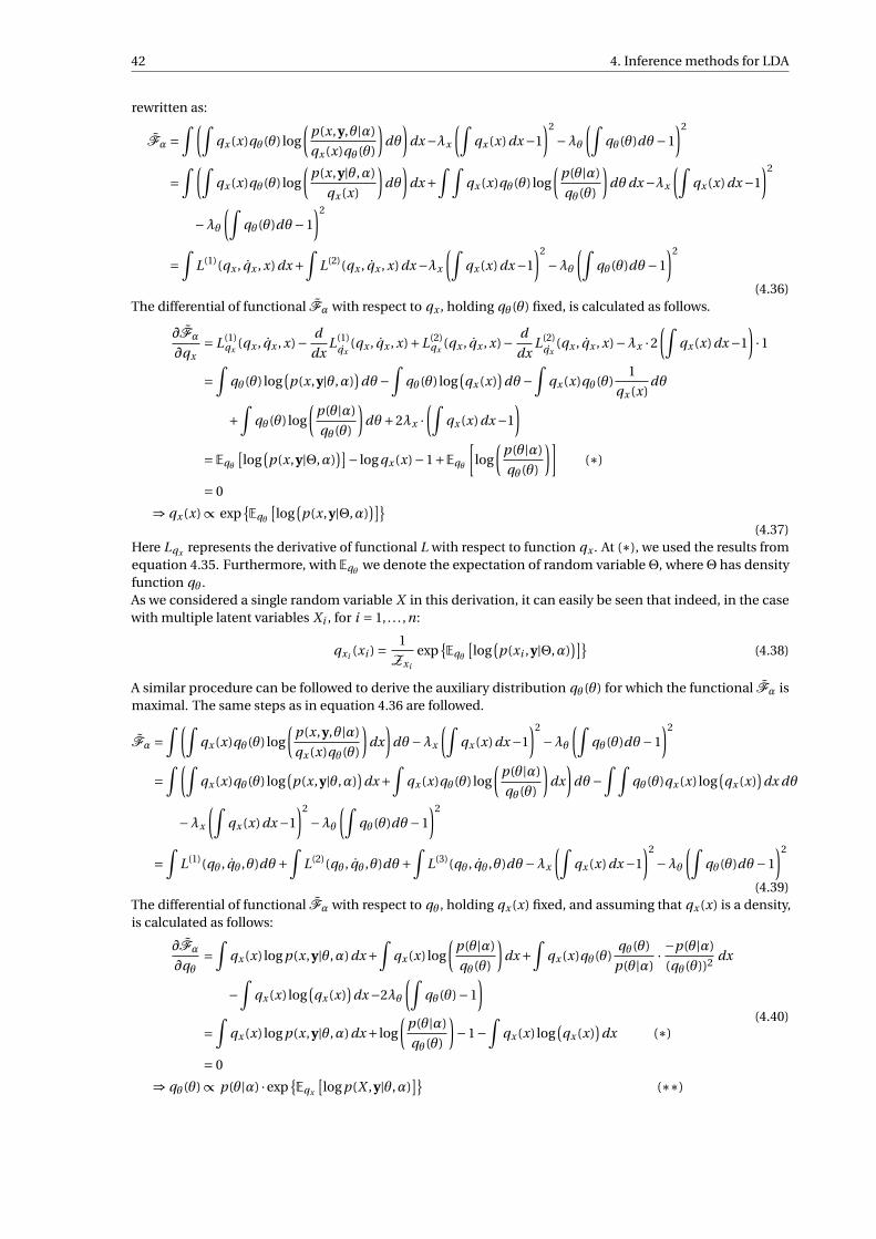
42 4. Inference methods for LDA
rewritten as:
Fα =∫ (∫
qx (x)qθ(θ) log
(p(x,y,θ|α)
qx (x)qθ(θ)
)dθ
)dx−λx
(∫qx (x)dx−1
)2
−λθ(∫
qθ(θ)dθ−1
)2
=∫ (∫
qx (x)qθ(θ) log
(p(x,y|θ,α)
qx (x)
)dθ
)dx+
∫ ∫qx (x)qθ(θ) log
(p(θ|α)
qθ(θ)
)dθdx−λx
(∫qx (x)dx−1
)2
−λθ(∫
qθ(θ)dθ−1
)2
=∫
L(1)(qx , qx , x)dx+∫
L(2)(qx , qx , x)dx−λx
(∫qx (x)dx−1
)2
−λθ(∫
qθ(θ)dθ−1
)2
(4.36)The differential of functional Fα with respect to qx , holding qθ(θ) fixed, is calculated as follows.
∂Fα
∂qx= L(1)
qx(qx , qx , x)− d
dxL(1)
qx(qx , qx , x)+L(2)
qx(qx , qx , x)− d
dxL(2)
qx(qx , qx , x)−λx ·2
(∫qx (x)dx−1
)·1
=∫
qθ(θ) log(p(x,y|θ,α)
)dθ−
∫qθ(θ) log
(qx (x)
)dθ−
∫qx (x)qθ(θ)
1
qx (x)dθ
+∫
qθ(θ) log
(p(θ|α)
qθ(θ)
)dθ+2λx ·
(∫qx (x)dx−1
)= Eqθ
[log
(p(x,y|Θ,α)
)]− log qx (x)−1+Eqθ
[log
(p(θ|α)
qθ(θ)
)](∗)
= 0
⇒ qx (x) ∝ expEqθ
[log
(p(x,y|Θ,α)
)](4.37)
Here Lqx represents the derivative of functional L with respect to function qx . At (∗), we used the results fromequation 4.35. Furthermore, with Eqθ we denote the expectation of random variableΘ, whereΘ has densityfunction qθ .As we considered a single random variable X in this derivation, it can easily be seen that indeed, in the casewith multiple latent variables Xi , for i = 1, . . . ,n:
qxi (xi ) = 1
Zxi
expEqθ
[log
(p(xi ,y|Θ,α)
)](4.38)
A similar procedure can be followed to derive the auxiliary distribution qθ(θ) for which the functional Fα ismaximal. The same steps as in equation 4.36 are followed.
Fα =∫ (∫
qx (x)qθ(θ) log
(p(x,y,θ|α)
qx (x)qθ(θ)
)dx
)dθ−λx
(∫qx (x)dx−1
)2
−λθ(∫
qθ(θ)dθ−1
)2
=∫ (∫
qx (x)qθ(θ) log(p(x,y|θ,α)
)dx+
∫qx (x)qθ(θ) log
(p(θ|α)
qθ(θ)
)dx
)dθ−
∫ ∫qθ(θ)qx (x) log
(qx (x)
)dx dθ
−λx
(∫qx (x)dx−1
)2
−λθ(∫
qθ(θ)dθ−1
)2
=∫
L(1)(qθ, qθ ,θ)dθ+∫
L(2)(qθ, qθ ,θ)dθ+∫
L(3)(qθ, qθ,θ)dθ−λx
(∫qx (x)dx−1
)2
−λθ(∫
qθ(θ)dθ−1
)2
(4.39)The differential of functional Fα with respect to qθ, holding qx (x) fixed, and assuming that qx (x) is a density,is calculated as follows:
∂Fα
∂qθ=
∫qx (x) log p(x,y|θ,α)dx+
∫qx (x) log
(p(θ|α)
qθ(θ)
)dx+
∫qx (x)qθ(θ)
qθ(θ)
p(θ|α)· −p(θ|α)
(qθ(θ))2 dx
−∫
qx (x) log(qx (x)
)dx−2λθ
(∫qθ(θ)−1
)=
∫qx (x) log p(x,y|θ,α)dx+ log
(p(θ|α)
qθ(θ)
)−1−
∫qx (x) log
(qx (x)
)dx (∗)
= 0
⇒ qθ(θ) ∝ p(θ|α) ·expEqx
[log p(X ,y|θ,α)
](∗∗)
(4.40)
4.2. Posterior mode 43
At (∗), we used the results from 4.35, and at (∗∗) the proportionality sign arises from the fact that we are onlyinterested in the terms that contain θ. The update equation for qθ becomes:
qθ(θ) = 1
Zθp(θ|α) ·exp
Eqx
[log p(X,y|θ,α)
](4.41)
The functional derivatives are computed under the assumption that Fα is smooth and differentiable. Alsowe assume that there is a local maximum. At least, it is known that a maximum of Fα exists, as it is boundedfrom above by the log likelihood. The precise proof of this convergence needs more work and is left for futureresearch.
In a less formally described way, variational Bayesian EM can be explained as follows. Suppose the posteriordensity is intractable. We introduce auxiliary distributions over the latent variables. The auxiliary distributionsare chosen in such a way that the lower bound for the likelihood of the observed data is as tight as possible tothe actual likelihood. This means that the product of all auxiliary densities is an approximation of the actualposterior density of all latent variables and random parameters given the data. That is, the posterior densityof all variables of interest. Lastly, with these approximate distributions, the values of the latent variables andparameters easily can be estimated using, e.g. the posterior mean or the posterior mode of each auxiliarydistribution.
4.2.2. Variational Bayesian EM for LDA
The variational Bayesian EM algorithm is used for inference in the paper by Blei et al. [7]. However, we willfollow the derivation in [8], because in this paper variational Bayes is applied to the so-called smoothed LDAfrom [7], which corresponds to how LDA is defined in this thesis, that is with a prior distribution on topic-worddistributionsΦ. In theorem 4.2, variational Bayesian EM is defined using the terminology of latent variablesand parameters. In LDA these can be considered the same, as the hyperparameters α and β are fixed and donot need statistical inference. AllΦ,Θ and Z are latent variables.The log likelihood of the latent variables in LDA and the lower bound are given by 4.42. For ease of notationand because they are fixed, the conditioning on the hyperparameters α and β is omitted.
L (α,β;w) = log p(w) = log
(∫ ∫ ∑z
p(φ,θ,z,w)dθdφ
)≥
∫ ∫ ∑z
q(φ,θ,z) logp(φ,θ,z,w)
q(φ,θ,z)dθdφ
(4.42)
In [8], it is assumed that p(φ,θ,z|w) can be approximated by a mean field variational family consisting ofauxiliary distributions. Note that in the expressions for latent variables Z, the topics, a simple Z is used,representing the topic index. Actually, the topic is distributed as Z ∼ Multinomial(1,Θ), such that the onlynon-zero component of vector Z gives the value of topic Z (e.g. Z = e6 ⇒ Z = 6). For simplicity, we called thevector with all topics z, but when looking at its distribution, Z can better be used. The mean field approximationfor the latent variables becomes:
q(φ,θ,z) =K∏
k=1qφk (φk;λk)
D∏d=1
qθd (θd;γd)Nd∏i=1
qzd,i (zd,i;νd,i) (4.43)
Each auxiliary distribution is chosen to come from the same family of distributions as the one to which theconditional distribution of each latent variable conditioned on all other variables in the model belongs. Notethat these conditional distributions have already been derived in section 4.1.2. This means that:
qφk (φk;λk) ← Dirichlet(λk)
qθd (θd;γd) ← Dirichlet(γd)
qzd,i (zd,i;νd,i) ← Multinomial(1,νd,i)
(4.44)
44 4. Inference methods for LDA
In order to be consistent with theorem 4.2, the lower bound of L (α,β;w) is denoted with F .
F(qφ(·), qθ(·), qz(·))= ∫ ∫ ∑
zq(φ,θ,z) log
(p(φ,θ,z,w|α,β)
q(φ,θ,z)
)dθdφ
= Eqφ,θ,z
[log p(Φ,Θ,Z,w|α,β)
]−Eqφ,θ,z
[log q(Φ,Θ,Z)
]= Eqθ
[M∑
d=1log p(Θd|α)
]+Eqφ
[K∑
k=1log p(Φk|β)
]+Eqθ,z
[M∑
d=1
Nd∑i=1
log p(Zd,i|Θd)
]
+Eqφ,z
[M∑
d=1
Nd∑i=1
log p(wd,i|Zd,i,Φk)
]−Eqφ
[K∑
k=1log q(Φk|λk)
]
−Eqθ
[M∑
d=1log q(Θd|γd)
]−Eqz
[M∑
d=1
Nd∑i=1
log q(Zd,i|νd,i)
](4.45)
Substituting the known conditionals and the auxiliary distributions as proposed in 4.44:
F(qφ(·), qθ(·), qz(·))= M∑
d=1
(log
(Γ(
K∑k=1
(α)k )
)−
K∑k=1
log(Γ((α)k ))+K∑
k=1((α)k −1) ·Eqθ
[log(Θd)k
])
+K∑
k=1
(log
(Γ(
V∑j=1
(β) j
)−
V∑j=1
log(Γ((β) j
)+ V∑j=1
((β) j −1) ·Eqφ
[log(Φk) j
])
+M∑
d=1
Nd∑i=1
Eqθ
[Eqz
[log
(p(Zd,i|Θd)
)∣∣∣Θ]]+
M∑d=1
Nd∑i=1
Eqφ
[Eqz
[log
(p(wd,i|Φ, Zd,i)
)∣∣∣Φ]]−
M∑d=1
(log
(Γ(
K∑k=1
(γd)k )
)−
K∑k=1
log(Γ((γd)k )
)+ K∑k=1
((γd)k −1) ·Eqθ
[log(Θd)k
])
−K∑
k=1
(log
(Γ(
V∑j=1
(λk) j )
)−
V∑j=1
log(Γ((λk) j )
)+ V∑j=1
((λk) j −1) ·Eqφ
[log(Φk) j
])
−M∑
d=1
Nd∑i=1
K∑k=1
log((νd,i)k
)Eqz
[(Zd,i)k
]=C +
M∑d=1
K∑k=1
((α)k − (γd)k +
Nd∑i=1
(νd,i)k
)·Eqθ
[log(Θd)k
]+
K∑k=1
V∑j=1
((β) j − (λk) j +
M∑d=1
Nd∑i=1
(wd,i) j · (νd,i)k
)·Eqφ
[log(Φk) j
]−
M∑d=1
(log
(Γ(
K∑k=1
(γd)k )
)−
K∑k=1
log(Γ((γd)k )
))
−K∑
k=1
(log
(Γ(
V∑j=1
(λk) j )
)−
V∑j=1
log(Γ((λk) j )
))
−M∑
d=1
Nd∑i=1
K∑k=1
(νd,i)k log((νd,i)k
)
(4.46)
Differentiating F with respect to each variational parameter separately leads to the following update equations.Through the choice of the auxiliary distributions, we already know that they integrate to 1. Therefore, Lagrangemultipliers are not needed in this case.For the variational parameter vector belonging to Zd,i, we get a proportionality:
(νd,i)k ∝ exp
Eqθ [log(Θd)k ]+
V∑j=1
(wd,i) jEqφ [log(Φk) j ]
= exp
Ψ
((γd)k
)−Ψ(K∑
k=1(γd)k
)+Ψ(
(λk)wd ,i
)−Ψ(V∑
j=1(λk) j
) (4.47)

4.2. Posterior mode 45
Where Ψ(·) is the digamma function. The derivation of Eqθ [log(Θd)k ] is elaborated on in the appendix. Theexact value of (νd,i)k is retrieved via normalization i.e.
∑Kk=1(νd,i)k must equal 1, so one needs to divide every
(νd,i)k by∑K
k=1(νd,i)k .The variational parameter vector belonging toΘd can be determined directly:
γd =α+Nd∑i=1
νd,i (4.48)
We obtain the variational parameter vector belonging toΦk via:
λk =β+M∑
d=1
Nd∑i=1
(νd,i)k wd,i (4.49)
The method of variational Bayesian EM is summarized in algorithm 3 [8]. The E-step consists of computingthe variational parameters γ, ν and λ, after which the lower bound F is determined. These steps are executedalternately until a local maximum of F is attained (M-step). Only a local optimum can be found because theobjective function is non-convex due to the mean-field approximation [47].
Algorithm 3 Variational Bayesian EM for LDA
1: Initialize γ, λ and ν2: Compute the lower bound F
3: Set ε4: Start with i = 15: while |F [i +1]−F [i ]| > ε do6: for d = 1 to M do . Iterate over documents7: for i = 1 to Nd do . Iterate over words in document d8: Compute γd
9: Compute νd,i
10: end for11: end for12: for k = 1 to K do13: Compute λk
14: end for15: Compute F [i +1]16: i = i +117: end while18: Compute posterior means forΘ,Φ and Z using the variational parameters γ,λ and ν.
When the algorithm has converged, values for the variational parameters are retrieved. With these parameters,we know the complete auxiliary distributions, whose product approximates the posterior density of all latentvariables. The values of the latent variables can then be estimated using the posterior mode. The posteriormode is not determined using the true posterior density, but using the approximation by the auxiliary dis-tributions. Because each latent variable has its own auxiliary density function, the posterior modes can bedetermined independently. For example, if we want to get the estimator ofΘd:
θd = maxθd
p(θ,φ,z|w,α,β)
≈ max
θd
K∏
k=1qφk (φk;λk)
D∏d ′=1
qθd′ (θd′ ;γd′ )Nd ′∏i=1
qzd′ ,i (zd′,i;νd′,i)
= max
θd
qθd (θd;γd)
=
((γd)1 −1∑K
k=1(γd)k −K, . . . ,
(γd)K −1∑Kk=1(γd)k −K
)(∗)
(4.50)
46 4. Inference methods for LDA
At (∗), we used the expression for the mode of a Dirichlet distributed random vector. Note that this expressionis only valid if all (γd)i with i = 1, . . . ,K are larger than 1. Because the mean-field assumption is quite strong, itis not guaranteed that the posterior mode of the approximation function is close to the posterior mode of theposterior density. In chapter 8, we will visualize the variational approximation function and the true posteriordensity for a small example, such that more insight in gained in the functioning of the VBEM algorithm.
Zhang et al. made a complete overview of variational inference methods in [53], and concluded that researchis needed on the theoretical aspects of variational inference such as the approximation errors that are involvedwhen an approximation function replaces the posterior density. Presently, the writer of this thesis has notfound quantitative methods to determine the accuracy of the variational approximation, and therefore onlyempirical results are shown in chapter 8.Because one of the arguments against the application of variational inference to LDA is the fact that themean-field approximation is too strong, improvements on this assumption are made and given in [53].Furthermore, instead of using the update equations of 4.2, the lower bound of the likelihood, Fα can beoptimized using stochastic optimization. Still, the mean-field approximation is used on the auxiliary functions,but the optimization method is different. The version of variational inference is called Stochastic Variationalinference (SVI). Further improvements on this method are made in Structured Stochastic Variational Inference,by [5]. In this method, also the mean-field approximation is let go off, and dependencies between the latentvariables are allowed. These dependencies can be modeled in a hierarchical structure, thus called HierarchicalVariational Inference [38]. Another option to model dependencies is using copulas. The auxiliary functionthen takes the form:
q(θ) =(
M∏d=1
q(θd ;λd )
)· c(Q(θ1), . . . ,Q(θM )) (4.51)
With c(. . . ) a copula and each Q the cumulative distribution function corresponding to the auxiliary densitiesq . For more information on this extension of variational inference, we refer to [45].
Although promising improvements on variational inference and in particular variational methods appliedto LDA are present in literature, the method still lacks theoretical evidence of accuracy. Furthermore, otherinference methods for LDA, such as Markov chain Monte Carlo methods exist, and have better convergenceresults. Also, even though the posterior mode cannot easily be calculated analytically, optimization methodsexist that are already proven to be useful in deep learning and neural networks. One of these optimizationmethods is elaborated on in the next chapter, ‘Posterior mode estimation for LDA’, in which we propose anoptimization method that aims to find the posterior mode of the high-dimensional posterior density functionof LDA.
5Determination posterior mode estimates
for LDA using optimization
In the previous chapter, different inference methods to obtain estimates of the parameters Θ and Φ (re-spectively the document-topic distributions and the topic-word distributions) for LDA are mentioned. Theposterior mode can be determined in another way than proposed in the literature, namely via optimizationmethods. These techniques are often used in neural network and deep learning algorithms, and can be easilyapplied to hierarchical Bayesian models like LDA.Posterior mode estimation is often referred to as MAP estimation, where MAP stands for Maximum A Posteriori(posterior mode). In figure 1.1 in the introduction, the method in this chapter is described as ‘analytical’, whilewe still estimate the values ofΘ andΦ. The reason to still call this optimization method ‘analytical’, is the factthat the posterior density is not approximated via some method. We use the actual posterior density (up to aproportionality constant) and search for its maximum.
5.1. LDA’s posterior density
The posterior mode is given by the values of all parametersΘd andΦk (with d = 1, . . . , M and k = 1, . . . ,K ) forwhich the posterior density in equation 5.1 is maximal. Note that the proportionality constant is not neededfor this estimator. Because the posterior density is not convex in most cases, smart optimization techniquesare needed.
p(θ,φ|w,α,β) ∝[
M∏d=1
V∏j=1
(K∑
k=1(φk) j (θd)k
)nd , j]·[
M∏d=1
K∏k=1
(θd)(α)k−1k
]·[
K∏k=1
V∏j=1
(φk)(β) j −1j
](5.1)
To demonstrate the form of the posterior density and its non-convexity, we will first consider a simple case inwhich dimensionality is small enough for visualization.
Consider the example in which we have only one document (think of the silly document ‘nice stupid nice’)consisting of three words: w1 = 1, w2 = 2, w3 = 1. There are only two possible words as the word index is either1 or 2. This means that the vocabulary size V is 2. Furthermore, it is assumed that there are 2 possible topics,that is K = 2. At last, the hyperparameters are symmetric and are set to α = 0.1 and β = 1. The parametersof the model that we want to estimate are: Θ1, Φ1, Φ2, as Θ1 +Θ2 = 1 and (Φ1)1 + (Φ1)2 = 1. Thus, with Φ1 isdenoted the probability of word 1 for topic 1. Φ2 is then the probability of word 1 for topic 2.
The posterior density (up to a proportionality constant) is given by:
p(θ1,φ1,φ2|w) ∝[
V∏j=1
(φ1, j ·θ1 +φ2, j · (1−θ1)
)n1, j
]· [θα−1
1 · (1−θ1)α−1][K∏
k=1φβ−1k · (1−φk )β−1
]
=[(φ1 ·θ1 +φ2 · (1−θ1)
)2 · ((1−φ1) ·θ1 + (1−φ2) · (1−θ1))] · [θ−0.9
1 · (1−θ1)−0.9] ·1
(5.2)
47
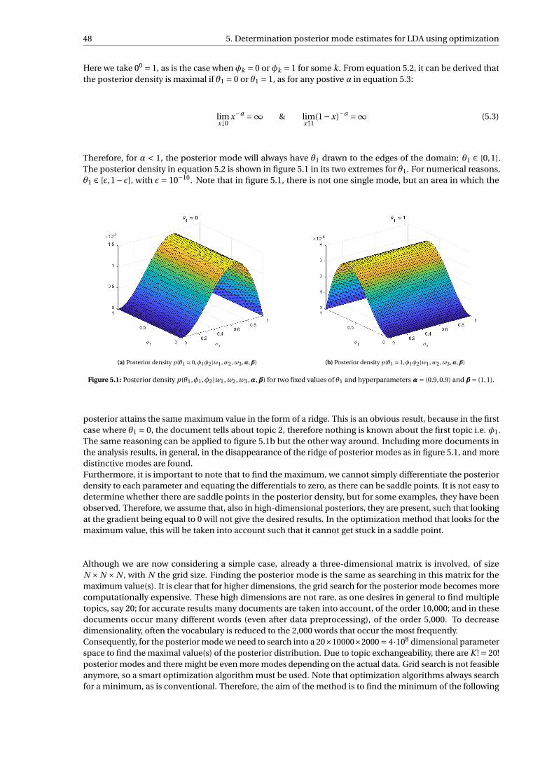
48 5. Determination posterior mode estimates for LDA using optimization
Here we take 00 = 1, as is the case when φk = 0 or φk = 1 for some k. From equation 5.2, it can be derived thatthe posterior density is maximal if θ1 = 0 or θ1 = 1, as for any postive a in equation 5.3:
limx↓0
x−a =∞ & limx↑1
(1−x)−a =∞ (5.3)
Therefore, for α < 1, the posterior mode will always have θ1 drawn to the edges of the domain: θ1 ∈ 0,1.The posterior density in equation 5.2 is shown in figure 5.1 in its two extremes for θ1. For numerical reasons,θ1 ∈ [ε,1− ε], with ε = 10−10. Note that in figure 5.1, there is not one single mode, but an area in which the
(a) Posterior density p(θ1 ≈ 0,φ1φ2|w1 , w2 , w3 ,α,β) (b) Posterior density p(θ1 ≈ 1,φ1φ2|w1 , w2 , w3 ,α,β)
Figure 5.1: Posterior density p(θ1,φ1,φ2|w1, w2, w3,α,β) for two fixed values of θ1 and hyperparameters α= (0.9,0.9) and β= (1,1).
posterior attains the same maximum value in the form of a ridge. This is an obvious result, because in the firstcase where θ1 ≈ 0, the document tells about topic 2, therefore nothing is known about the first topic i.e. φ1.The same reasoning can be applied to figure 5.1b but the other way around. Including more documents inthe analysis results, in general, in the disappearance of the ridge of posterior modes as in figure 5.1, and moredistinctive modes are found.Furthermore, it is important to note that to find the maximum, we cannot simply differentiate the posteriordensity to each parameter and equating the differentials to zero, as there can be saddle points. It is not easy todetermine whether there are saddle points in the posterior density, but for some examples, they have beenobserved. Therefore, we assume that, also in high-dimensional posteriors, they are present, such that lookingat the gradient being equal to 0 will not give the desired results. In the optimization method that looks for themaximum value, this will be taken into account such that it cannot get stuck in a saddle point.
Although we are now considering a simple case, already a three-dimensional matrix is involved, of sizeN ×N ×N , with N the grid size. Finding the posterior mode is the same as searching in this matrix for themaximum value(s). It is clear that for higher dimensions, the grid search for the posterior mode becomes morecomputationally expensive. These high dimensions are not rare, as one desires in general to find multipletopics, say 20; for accurate results many documents are taken into account, of the order 10,000; and in thesedocuments occur many different words (even after data preprocessing), of the order 5,000. To decreasedimensionality, often the vocabulary is reduced to the 2,000 words that occur the most frequently.Consequently, for the posterior mode we need to search into a 20×10000×2000 = 4·108 dimensional parameterspace to find the maximal value(s) of the posterior distribution. Due to topic exchangeability, there are K ! = 20!posterior modes and there might be even more modes depending on the actual data. Grid search is not feasibleanymore, so a smart optimization algorithm must be used. Note that optimization algorithms always searchfor a minimum, as is conventional. Therefore, the aim of the method is to find the minimum of the following
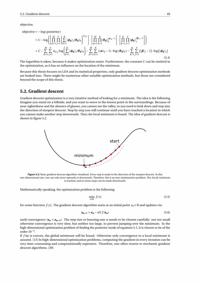
5.2. Gradient descent 49
objective.
objective =− log(posterior)
=C − log
([M∏
d=1
V∏j=1
(K∑
k=1(φk) j (θd)k
)nd , j]·[
M∏d=1
K∏k=1
(θd)(α)k−1k
]·[
K∏k=1
V∏j=1
(φk)(β) j −1j
])
=C −M∑
d=1
V∑j=1
nd , j log
(K∑
k=1(φk) j (θd)k
)−
M∑d=1
K∑k=1
((α)k −1) · log((θd)k )−K∑
k=1
V∑j=1
((β) j −1
) · log((φk) j
)(5.4)
The logarithm is taken, because it makes optimization easier. Furthermore, the constant C can be omitted inthe optimization, as it has no influence on the location of the minimum.
Because this thesis focuses on LDA and its statistical properties, only gradient descent optimization methodsare looked into. There might be numerous other suitable optimization methods, but those are consideredbeyond the scope of this thesis.
5.2. Gradient descentGradient descent optimization is a very intuitive method of looking for a minimum. The idea is the following.Imagine you stand on a hillside, and you want to move to the lowest point in the surroundings. Because ofnear-sightedness and the absence of glasses, you cannot see the valley, so you need to look down and step intothe direction of steepest descent. Step by step you will continue until you have reached a location in whichyou cannot make another step downwards. Then the local minimum is found. The idea of gradient descent isshown in figure 5.2.
Figure 5.2: Basic gradient descent algorithm visualized. Every step is made in the direction of the steepest descent. In thisone-dimensional case, one can only move upwards or downwards. Therefore, this is an easy minimization problem. The (local) minimum
is reached, and no more steps can be made downwards.
Mathematically speaking, the optimization problem is the following:
minx∈R
f (x) (5.5)
for some function f (x). The gradient descent algorithm starts at an initial point x0 ∈R and updates via:
xn+1 = xn −a∇ f (xn) (5.6)
until convergence (xn ≈ xn+1). The step size or learning rate a needs to be chosen carefully: not too smallotherwise convergence is very slow, but neither too large, to prevent jumping over the minimum. In thehigh-dimensional optimization problem of finding the posterior mode of equation 5.1, it is chosen to be of theorder 10−3.If f (x) is convex, the global minimum will be found. Otherwise only convergence to a local minimum isassured. [13] In high-dimensional optimization problems, computing the gradient in every iteration can bevery time-consuming and computationally expensive. Therefore, one often resorts to stochastic gradientdescent algorithms. [39]
50 5. Determination posterior mode estimates for LDA using optimization
5.3. Stochastic gradient descentStochastic gradient descent uses an update formula akin to the one used in the basic gradient descent algorithm,only a noise term is added:
xn+1 = xn −a(∇ f (xn)+wn
)(5.7)
The following proposition gives assumptions that are necessary for the algorithm to converge.
Proposition 5.1 (Stochastic gradient descent convergence, from [3])Let xn be a sequence generated by the method:
xn+1 = xn +γn (sn +wn) (5.8)
where γn is a deterministic positive step size, sn a descent direction and wn random noise. Let Fn be an increasingsequence of σ-fields. One can consider Fn to be the history of the algorithm, so it contains information aboutx0,s0,γ0,w0, . . . ,xn−1,sn−1,γn−1,wn−1.The function f : Rd → R (for some positive integer d) needs to be optimized. Furthermore, function ∇ f isLipschitz continuous with some constant L.We assume the following:
1. xn and sn are Fn-measurable.
2. ∃ positive scalars c1 and c2 such that ∀n:
c1 · ‖∇ f (xn)‖2 ≤−(∇ f (xn))T sn & ‖sn‖ ≤ c2
(1+‖∇ f (xn)‖) (5.9)
3. For all n and with probability 1:E[wn|Fn] = 0 (5.10)
andE[‖wn‖2|Fn] ≤ A
(1+‖∇ f (xn)‖2) (5.11)
where A is a positive deterministic constant.
4. We have: ∞∑t=0
γn =∞ &∞∑
t=0γ2
n <∞ (5.12)
Then, either f (xn) →−∞ or else f (xn) converges to a finite value and limn→∞∇ f (xn) = 0 almost surely. Further-more, every limit point of xn is a stationary point of f 1.
The proof of this proposition can be found in [3] and is quite extensive. Note that the fourth assumptionensures the algorithm to have steps γn large enough to find the stationary point of f , but at the same time nottoo large, such that continuing jumping over the minimum is prevented.In the proposition, we see that for a Lipschitz continuous first derivative of function f , and noise with zeromean and bounded variance, we have almost sure convergence (or the minimum is −∞). Note that thedomain of function f is Rd in this proposition. One might get confused here, because for the posteriormode optimization problem for LDA, we want to find probability vectors that live in (0,1). However, a smarttransformation trick is used, such that the optimization domain is again Rd . This trick is called the softmaxtransformation and is elaborated on in section 5.4.1.The stochasticity in stochastic gradient descent is not further specified other than adding random noise to thegradient. However, other choices than random noise can be made to turn the gradient descent algorithm intostochastic gradient descent.In the domain of deep learning, the objective function often exists of a sum of functions, i.e. f (x) =∑m
i=1 fi (x).Stochastic gradient descent is then defined as [3]:
xn+1 = xn −a ·∇ f j (x) (5.13)
1A stationary point of function f :Rd →R is a coordinate in Rd in which the derivative ∇ f is zero.
5.4. Adam optimization 51
for some j ∈ 1, . . . ,m. This update formula can be rewritten in the form of equation 5.8 [3]:
xn+1 = xn −a ·(
1
m
m∑i=1
∇ fi (xn)+[∇ f j (xn)− 1
m
m∑i=1
∇ fi (xn)
])(5.14)
Note that 1m
∑mi=1∇ fi (xn) = 1
m · ∇ f (xn), so it indeed is a direction of descent. Furthermore, we can checkassumption 3 from proposition 5.1 [3]:
E[wn|Fn] = E[∇ f j (xn)− 1
m
m∑i=1
∇ fi (xn)|Fn
]
= 1
m
m∑i=1
∇ fi (xn)− 1
m
m∑i=1
∇ fi (xn)
= 0
(5.15)
where we used the fact that j is chosen randomly and uniformly from the set 1, . . .m. The second item inassumption 3 is the bound of the squared L2-norm of wn [3]:
E[‖wn‖2|Fn] = E[‖∇ f j (xn)‖2|Fn]−E [‖wn‖|Fn]2
≤ E[‖∇ f j (xn)‖2|Fn] (5.16)
Now assume that there exist positive constants C and D such that:
‖∇ fi (x)‖ ≤C +D · ‖∇ f (x)‖ ∀i ,x. (5.17)
Then, it follows that:E[‖wn‖2|Fn] ≤ 2C +2D · ‖∇ f (xn)‖2 (5.18)
which clearly satisfies equation 5.11 for adapted constant A. The other assumptions from proposition 5.1are also satisfied as shown in [3]. As mentioned in [22], the stochasticity in this type of stochastic gradientdescent does not come from random noise, but from the random selection of j for f j (x). Note that this form ofstochastic gradient descent is called incremental gradient descent in [3]. Sometimes multiple ‘sub-functions’are used instead of only f j , to improve accuracy. Especially in high-dimensional problems with an objectivethat consists of a great summation, this is more accurate than taking only one sub-function. This type ofgradient descent can also be referred to as mini-batch gradient descent.The python package that is used for the implementation of posterior mode determination using optimizationis called Tensorflow2 and uses this mini-batch gradient descent method. Apart from computing the gradient ofonly a smaller sum of subfunctions of which the objective consists, also other adaptations to the basic gradientdescent method are applied to increase performance. These adaptations together form the used method inthis thesis: Adam optimization.
5.4. Adam optimization
Over the years and with the development of deep learning and neural networks, more high-end algorithmshave been invented that speed up convergence and can better deal with non-convex objective functions andhigh-dimensional parameter spaces. Among them are Adadelta, RMSprop, Adagrad and Adam [39]. Adamoptimization is used in this thesis to compute the posterior mode and is the most versatile for large-scalehigh-dimensional machine learning problems [22].
Adam is a type of stochastic gradient descent algorithm with adaptive learning rates. Its name stands for‘adaptive moment estimation’ which already reveals that it uses the first and second moments of the gradientfor this adaptation. We will state the algorithm for a one-dimensional problem, for ease of notation, and thenexplain what each step’s necessity is.
2One of the main advantages of Tensorflow’s optimization methods is that it computes gradients using automatic differentiation insteadof numerical differentiation.
52 5. Determination posterior mode estimates for LDA using optimization
Algorithm 4 Adam optimization in one dimension
1: Set α,β1,β2,ε2: Initialize x = x0, m0 = 0, v0 = 0, n = 0.
3: whilef (xn )− f (xn− j )
f (xn ) > threshold do4: gn+1 =∇ f (xn)5: mn+1 =β1 ·mn + (1−β1) · gn
6: vn+1 =β2 · vn + (1−β2) · g 2n
7: mn+1 = mn+11−(β1)n+1
8: vn+1 = vn+11−(β2)n+1
9: xn+1 = xn −a · mn+1pvn+1+ε
10: n = n +111: end while12: Return posterior mode approximation: xn
First, the hyperparameters are set. Recommended values are a = 0.001, β1 = 0.9, β2 = 0.999 and ε = 10−10
[22]. Depending on the dimensionality of the objective, learning rate a can be adapted, because in a highdimensional problem, we want to take smaller steps than in a lower dimensional problem. The initial locationin the parameter space from which the algorithm starts searching for a minimum is denoted with x0. Then,the Adam algorithm starts ‘walking’ through the parameter space until convergence. Convergence is attainedwhen the relative difference of the objective with the j -th previous value of the objective is smaller than acertain threshold. In the experiments in this thesis, for small dimensional problems, j = 100, and for largedimensional problems, j = 1000. The threshold is set to 10−4, since this results in the best trade-off of accurateresults within a reasonable amount of time.In higher dimensional problems, the steps in algorithm 4 are applied to each dimension separately, that is,the gradient is determined for each dimension, there are m-terms and v-terms for each dimension, and withthese dimension-specific algorithm steps, the coordinate of each dimension is updated according to step 9 in
algorithm 4. For the two-dimensional case, we get xn+1 = xn −a · mx,n+1pvx,n+1+ε
and yn+1 = yn −a · my,n+1pvy,n+1+ε
.
The update step in Adam is formed by combining ideas from momentum gradient descent and the RMSpropalgorithm. Let us look at the update formulas in algorithm 4 step by step.In step 4 from algorithm 4, the gradient is computed. If x has a dimension larger than 1, the result gn is a vectorwith the gradient computed with respect to each parameter dimension. Then, in step 5, a momentum term forthe gradient is calculated. The formula in step 5 is a recurrence relation for the exponential moving average.Using the setting that m0 = 0, we can rewrite it as:
mn+1 = (1−β1) ·n+1∑i=1
(β1)n+1−i · gi (5.19)
A ‘basic’ moving average takes into account gradients from a number of previous steps, all with equal weight.The exponential moving average is slightly different because the weights are decreasing for gradients furtherback in time. That is, the previous gradient has a larger influence on mn+1 than the gradient e.g. ten iterationsback. Parameter β1 is chosen in the interval [0,1]. The larger β1, the larger the influence of previous steps. Ifβ1 is for example 0.5, the weight for the 10th previous iteration is only 0.001, while if β1 = 0.9, that same weightis 0.35. This momentum term is used in optimization algorithms to damp out oscillations in the gradient. It iscalled a momentum term after the analogy of momentum used in physics, p = m ·v, with m the mass and vthe velocity. One can think of a ball rolling down the slope of a bowl with initial speed not in the direction ofthe minimum. It will roll down towards the minimum, but its initial momentum results in a path that circles alittle around the minimum.The same momentum mechanism is applied to the gradient squared: g 2
n . Note that the square is element-wise,resulting in a vector of the same size as gn . So, also for the gradient squared, we look at the previous iterations.Because β2 is even larger than β1 in the recommended settings, namely 0.999, iterations further in the past aretaken into account. The reason for the computation of g 2
n will be elaborated on in the explanation of step 9.Then step 7 and 8 are bias correction terms. Both mn and vn are biased towards 0 in the first iterations of thealgorithm because both have initial value 0. Therefore, if divided by respectively 1−βn
1 and 1−βn2 , they will
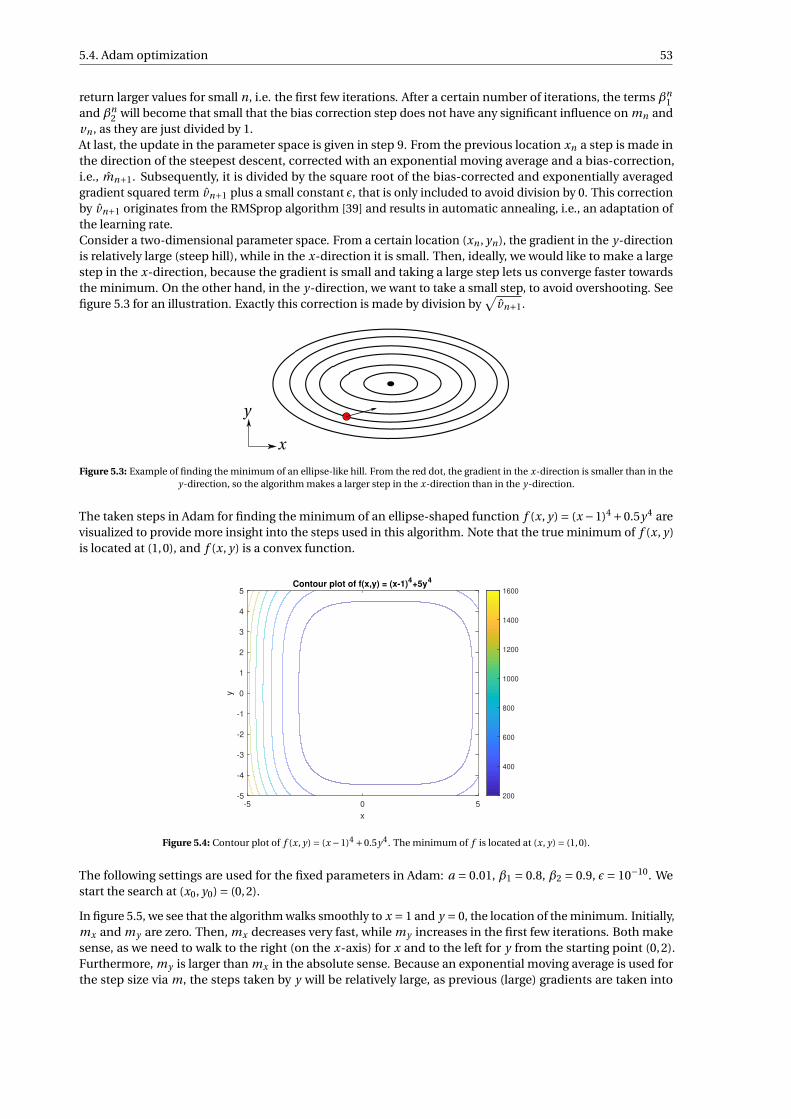
5.4. Adam optimization 53
return larger values for small n, i.e. the first few iterations. After a certain number of iterations, the terms βn1
and βn2 will become that small that the bias correction step does not have any significant influence on mn and
vn , as they are just divided by 1.At last, the update in the parameter space is given in step 9. From the previous location xn a step is made inthe direction of the steepest descent, corrected with an exponential moving average and a bias-correction,i.e., mn+1. Subsequently, it is divided by the square root of the bias-corrected and exponentially averagedgradient squared term vn+1 plus a small constant ε, that is only included to avoid division by 0. This correctionby vn+1 originates from the RMSprop algorithm [39] and results in automatic annealing, i.e., an adaptation ofthe learning rate.Consider a two-dimensional parameter space. From a certain location (xn , yn), the gradient in the y-directionis relatively large (steep hill), while in the x-direction it is small. Then, ideally, we would like to make a largestep in the x-direction, because the gradient is small and taking a large step lets us converge faster towardsthe minimum. On the other hand, in the y-direction, we want to take a small step, to avoid overshooting. Seefigure 5.3 for an illustration. Exactly this correction is made by division by
√vn+1.
y
x
Figure 5.3: Example of finding the minimum of an ellipse-like hill. From the red dot, the gradient in the x-direction is smaller than in they-direction, so the algorithm makes a larger step in the x-direction than in the y-direction.
The taken steps in Adam for finding the minimum of an ellipse-shaped function f (x, y) = (x −1)4 +0.5y4 arevisualized to provide more insight into the steps used in this algorithm. Note that the true minimum of f (x, y)is located at (1,0), and f (x, y) is a convex function.
Contour plot of f(x,y) = (x-1)4+5y
4
-5 0 5
x
-5
-4
-3
-2
-1
0
1
2
3
4
5
y
200
400
600
800
1000
1200
1400
1600
Figure 5.4: Contour plot of f (x, y) = (x −1)4 +0.5y4. The minimum of f is located at (x, y) = (1,0).
The following settings are used for the fixed parameters in Adam: a = 0.01, β1 = 0.8, β2 = 0.9, ε= 10−10. Westart the search at (x0, y0) = (0,2).
In figure 5.5, we see that the algorithm walks smoothly to x = 1 and y = 0, the location of the minimum. Initially,mx and my are zero. Then, mx decreases very fast, while my increases in the first few iterations. Both makesense, as we need to walk to the right (on the x-axis) for x and to the left for y from the starting point (0,2).Furthermore, my is larger than mx in the absolute sense. Because an exponential moving average is used forthe step size via m, the steps taken by y will be relatively large, as previous (large) gradients are taken into
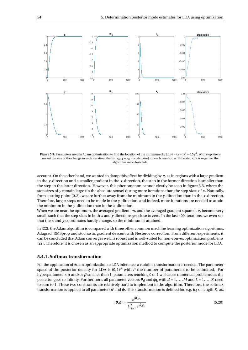
54 5. Determination posterior mode estimates for LDA using optimization
0 500 1000
0
0.2
0.4
0.6
0.8
1x
0 500 1000
-3.5
-3
-2.5
-2
-1.5
-1
-0.5
0
mx
0 500 1000
0
2
4
6
8
10
vx
0 500 1000
-0.01
-0.008
-0.006
-0.004
-0.002
0step size x
0 500 1000
0
0.5
1
1.5
2y
0 500 1000
0
2
4
6
8
10
12
14
my
0 500 1000
0
50
100
150
200
vy
0 500 1000
0
0.002
0.004
0.006
0.008
0.01step size y
Figure 5.5: Parameters used in Adam optimization to find the location of the minimum of f (x, y) = (x −1)4 +0.5y4. With step size ismeant the size of the change in each iteration, that is: xn+1 −xn =−[stepsize] for each iteration n. If the step size is negative, the
algorithm walks forwards.
account. On the other hand, we wanted to damp this effect by dividing by v , as in regions with a large gradientin the y-direction and a smaller gradient in the x-direction, the step in the former direction is smaller thanthe step in the latter direction. However, this phenomenon cannot clearly be seen in figure 5.5, where thestep sizes of y remain large (in the absolute sense) during more iterations than the step sizes of x. Naturally,from starting point (0,2), we are further away from the minimum in the y-direction than in the x-direction.Therefore, larger steps need to be made in the y-direction, and indeed, more iterations are needed to attainthe minimum in the y-direction than in the x-direction.When we are near the optimum, the averaged gradient, m, and the averaged gradient squared, v , become verysmall, such that the step sizes in both x and y directions get close to zero. In the last 400 iterations, we even seethat the x and y coordinates hardly change, so the minimum is attained.
In [22], the Adam algorithm is compared with three other common machine learning optimization algorithms:Adagrad, RMSprop and stochastic gradient descent with Nesterov correction. From different experiments, itcan be concluded that Adam converges well, is robust and is well-suited for non-convex optimization problems[22]. Therefore, it is chosen as an appropriate optimization method to compute the posterior mode for LDA.
5.4.1. Softmax transformation
For the application of Adam optimization to LDA inference, a variable transformation is needed. The parameterspace of the posterior density for LDA is (0,1)P with P the number of parameters to be estimated. Forhyperparameters α and/or β smaller than 1, parameters reaching 0 or 1 will cause numerical problems, as theposterior goes to infinity. Furthermore, all parameter vectors θd and φk with d = 1, . . . , M and k = 1, . . . ,K needto sum to 1. These two constraints are relatively hard to implement in the algorithm. Therefore, the softmaxtransformation is applied to all parameters θ and φ. This transformation is defined for, e.g. θd of length K , as:
(θd)i = e(θd )i∑Kj=1 e(θd ) j
(5.20)
5.4. Adam optimization 55
where (θd)i is between 0 and 1, as desired, and∑K
i=1(θd)i = 1. Now, the optimization takes place in the
parameter space of (θd )i , which is actually R. With this transformation, both constraints are automaticallyimplemented, and there are no numerical problems around 0 or 1.However we need to be careful. If the posterior mode is attained for θi = 0, as can be the case for α or βsmaller than 1, (θd )i must go to −∞. Therefore, the optimization will keep running, pushing θi towards −∞. Aregularization term creates a bound on the size of (θd )i , such that the optimization algorithm will be punishedif it keeps pushing a transformation parameter, e.g. (θd )i towards −∞. For LDA inference, we do not needparameters that are very accurate. That is, if θi = 0 in the true posterior mode, then θi = 10−4 is more thanaccurate enough, especially because the number of topics K (and thus the size of θ) is rarely larger than 50.
With the softmax transformation, the solution found by Adam is not unique anymore in terms of transformedvariables θd for d = 1, . . . , M and φk for k = 1, . . . ,K , that each live in Rd with d = K for the document-topicdistributions, and d =V for the topic-word distributions. To each (θd )i a constant can be added and solution(θd )i will be the same. Exactly because the parameters we are interested in, (θd )i , are invariant under thesenon-uniqueness of (θd )i , we do not mind the multiple solutions. Furthermore, with regularization can besteered towards small values of (θd )i , as will be explained in the next section.
5.4.2. Regularization
Adam optimization with the softmax transformation works well without regularization if both hyperparametersare larger than 1, as will be seen in chapter 8. However, if one of them is smaller than 1, the algorithm will keepwalking towards the edges of the domain, which is R for each parameter if we use the softmax transformation.Regularization is applied to prevent this undesired behavior of the algorithm.Different choices can be made for regularization. The two most common ones, especially in machine learning,are lasso and ridge regularization. The lasso ensures that the L1-norm of each parameter vector is not too large,while in ridge regularization, the L2-norm is used. Note that sometimes ridge regularization is referred to asTikhonov regularization [14]. In terms of the objective, we get:
objective =− log(posterior)+λx · ‖x‖p (5.21)
Where for the lasso, p = 1, and for ridge regularization, p = 2. An appropriate value forλneeds to be determinediteratively. For high-dimensional problems with both α and β (much) smaller than 1, λ is chosen to be a bitlarger than for lower-dimensional problems or if only one hyperparameter is smaller than 1. One can thinkof λ= 10 for the first case, and λ= 1 for the latter. Each parameter can have its own corresponding λ, but inpractice, they are chosen to be all equal.
Both lasso and ridge regularization are implemented with Adam optimization and seem to do their jobs.However, in the extreme cases in which dimensionality is high or α or β are (much) smaller than 1, theregularization is not strong enough to prevent the algorithm from going to −∞. Therefore, another strongertype of regularization is used, based on the maximum value of each random vector that is estimated. Followingthe example in equation 5.20 with vector θd for some d ∈ 1, . . . , M :
objective =− log(posterior)+λθd·(max
iθi
)4
(5.22)
In practice, each λ is set to 1, as the regularization term itself is already strong enough to compete with the− log(posterior) term in the optimization algorithm. The maximal value of each random vector is drawn to 0,as we are minimizing the objective and the maximum to the fourth power cannot be negative. Note that for αand β smaller than 1, all other elements will be negative. With the maximum of each vector constrained, theother elements of that same vector will also automatically be constrained, since they are highly dependenton each other. Remember that after the softmax transformation, each random vector that is estimated sumsto 1. With one element being close to 0 in the transformed space (R), the others have to follow to preventgetting only unit vectors as estimations forΘ andΦ, which is probably not the location of the minimum of− log(posterior).


6LDA with syntax and sentiment
"The integers of language are sentences, and their organs are the parts-of-speech. Linguistic organization, then,consists in the differentiation of the parts-of-speech and the integration of the sentence."
John Wesley Powell (1834-1902)
The aim of the application of LDA to a large set of reviews is to extract about which topics people write. To thisend, a topic distribution per document and a word distribution per topic are determined. The first shows inwhich proportions topics are written about, and therefore, which are the most important to each customerand on average. The second distribution tells what story or theme is linked to each topic. Based on the worddistribution, we hope to draw a founded conclusion on the overarching issue of that topic.
Although the basic version of LDA can already be very informative, it would be better to know a sentimentper topic from the reviews. Think about knowing which words are used to describe a favorable opinion on,e.g., the price of a product. Secondly, the topic-word distributions consist of all types of words in terms ofparts-of-speech: nouns, adjectives, verbs, pronouns et cetera. It would be ideal if each topic tells about oneaspect of a product, linked with opinion words such that a story is told in that topic. An aspect is typicallydescribed using nouns or verbs, while opinion words are from the lexical categories adjectives or adverbs.Combining the wishes above results in the extension defined in this chapter. The results from ‘LDA with syntaxand sentiment’ consist of topic-distributions per document, sentiment-distributions per document and, mostimportantly, a word-distribution per topic, sentiment, and part-of-speech combined. This means that thereare K ·Σ ·C word-distributions, where K is the number of topics, Σ is the number of possible sentiments, andC the number of different parts-of-speech used.
An extra feature of the extension from this chapter is the integration of sentence LDA. Instead of only lookingat documents as with a bag of words, we focus the attention to sentences or even clauses, hereafter referred toas phrase, although, strictly speaking, this is not the best terminology. The critical and strong assumption ismade that each phrase is about one topic and has one sentiment. It is expected that with this assumption, andwith the construction of bags of words within each phrase instead of on document-level, the results of LDAwill become more accurate.
In this chapter, first the generative model will be explained, and the plate notation of LDA with syntaxand sentiment will be elaborated on. Then some small notes on practicalities are made, e.g., how to splitdocuments into phrases? Lastly, the posterior distribution of the desired random variables is derived, andinference methods are explained.
6.1. Into the more complicated mind of the writer: generative process
In this section, we will dive again into the mind of the writer of a review, but now we assume that there aremore steps involved than those described in section 3.1. We will take the example of a stroller review again.
As a writer, you first think about which aspects you want to write. Suppose you feel disappointed, as the stroller
57
58 6. LDA with syntax and sentiment
you have bought was very expensive, and you are not satisfied with the product. Then, you want to explainyour disappointment: the stroller is cumbersome, too large to fit in the car, and the basket underneath is toosmall. As a consequence, you want to talk about four topics: value for money, weight, size, and the basket. Inaddition to these topics, a sentiment is added. The value for money aspect gives you a negative sentiment. Thesame is valid for weight, size, and basket. When you start writing the review, in each sentence or clause, oneaspect is described with negative sentiment. This supports the assumption that every phrase has only onetopic and one sentiment.Secondly, once you have chosen the topic and your opinion, words need to be selected. In general, you will usenouns or verbs to describe aspects. Think of the example above in which ‘fit’ and ‘basket’ are nouns. Then, thesentiment is often described by an adjective or adverb; ‘too large’ or ‘too small’. Note that we need the word‘too’ here to describe a negative sentiment. If the words ‘too’ and ‘small’ occur together in many phrases, theywill both have a high probability in the word distributions for that topic, and therefore the negative sentimentcan be extracted.
The process of writing a review can be summarized in the following steps.
1. For each topic k ∈ 1, . . . ,K :
(a) For each sentiment o ∈ 1, . . . ,Σ:
i. Draw a topic-sentiment-word distributionΦk,o from Dirichlet(βo)
2. For each document d ∈ 1, . . . , M :
(a) Draw a topic distributionΘd from Dirichlet(α)
(b) Draw a sentiment distributionΠd from Dirichlet(γ)
(c) For each phrase s ∈ 1, . . . ,Sd :
i. Draw a topic Zd ,s from Multinomial(1,Θd)
ii. Draw a sentiment Σd ,s from Multinomial(1,Πd)
iii. For each word i in sentence s:
A. Pick a part-of-speech cd ,s,i
B. Draw a word (Wd,s)i from Multinomial(1,Φ(zd)s′ ,(σd)s′ ,cd,s,i )
Again, attention must be paid to all steps in which is drawn from a Multinomial distribution. Drawing from aMultinomial(1,Θd) results in drawing a vector instead of an integer. Therefore, remember we defined in section3.1, Zd,s ∼ Multinomial(1,Θd), such that (Zd)s′ = k ⇐⇒ Zd ,s = (0,0, . . . ,1,0, . . . ,0) with only one 1 on the k-thdimension of Zd,s. That is Zd,s is the unit vector in dimension k. When Zd ,s is drawn from Multinomial(1,Θd),actually Zd,s is drawn from Multinomial(1,Θd) and the mapping (Zd,s)k = 1 ⇒ (Zd)s′ = k for some k ∈ 1, . . . ,K is applied.
Although in the process above, a part-of-speech cd ,s,i is drawn, we do not include it in the final model. Thereason for this choice is the fact that the part-of-speech of a word cannot be learned from data, such that thetopic-sentiment-word distributions per part-of-speech would be very inaccurate. One improvement couldbe to set the prior distribution βo,c for sentiment o and part-of-speech c such that words in the vocabularycorresponding to part-of-speech c have a higher probability. However, to this end, we would still needto determine the part-of-speech of each word in the vocabulary, which is similar to first finding the topic-sentiment-word distributions with all parts-of-speech included, and then, afterwards, do the split. We concludethat the latter method is a better way to determine the word distributions per topic, per sentiment and perpart-of-speech, albeit for a lower dimensionality of the parameter set that needs to be inferred.
The sentiment of the reviews can be found by taking smart prior vectors βo. There exist lists with positiveand negative words in the English language (see appendix B.6). With these lists, it can be determined whichwords in the vocabulary of the concerned corpus are positive, and which are negative. The remaining wordsare considered neutral. Then, the hyperparameter vector βpos, imposed on the positive sentiment topic-word

6.1. Into the more complicated mind of the writer: generative process 59
vectorsΦk,pos, are chosen such that the positive words get a higher weight than the neutral and negative words.Note that the latter are not given probability zero, following Cromwell’s rule1.
An overview of all sets, random variables and random vectors is given in table 6.1.
Table 6.1: (Random) variables used in Latent Dirichlet Allocation with syntax and sentiment.
Symbol Meaning Type (and size) SpaceV Size of vocabulary integer N
K Number of topics integer N
M Number of documents in corpus integer N
Σ Number of sentiments integer N
C Number of parts-of-speech integer N
Sd Number of phrases in document d integer N
NSd Number of words in phrase Sd integer: 1×1 N
α Prior belief on document-topic distribution vector: 1×K RK>0
βo Prior belief on word distribution for a sentiment vector: 1×V RV>0
γ Prior belief on document-sentiment distribution vector: 1×Σ RΣ>0
φk,o Parameter vector of multinomial word distribution for topic k, sentiment o vector: 1×V TV (1), (simplex)Θd Parameter vector of multinomial topic distribution for document d vector: 1×K TK (1), (simplex)Πd Parameter vector of multinomial sentiment distribution for document d vector: 1×Σ TΣ(1), (simplex)Zds Unit vector in the dimension of the chosen topic for phrase s vector: 1×K 0,1K
(Zd)s′ Topic (index) for phrase s in document d integer 1, . . . ,K Σds Unit vector in the dimension of the chosen sentiment for phrase s vector: 1×Σ 0,1Σ
(Σd)s′ Sentiment (index) for phrase s in document d integer 1, . . . ,Σ(wd,s)i Word index i corresponding to location i in phrase s from document d integer 1, . . . ,V
For simplicity, several assumptions on independence are made. We assume that each sentiment distributionΠd and each topic distributionΘd is drawn from its prior independently of the sentiment and topic distribu-tions of other documents, andΠd andΘd are independent random vectors. The latter is a strict assumptionwhich might be violated in some reviews because topics and sentiment can be correlated. However, theseassumptions are needed for tractable inference.Furthermore, the topic for each phrase is drawn independently of the previous topics of phrases in the samedocument. This assumption will probably not be true in most cases, as the probability of writing about thesame topic in the current phrase as in the previous phrase is different from the probability of writing aboutthat topic in the first case. Also, the sentiment of each sentence is drawn independently from the precedingsentiments in the same document.At the deepest level, the word level, also independence assumptions are made. Each word (Wd,s)i is drawn inde-pendently of the other words in that phrase. Also, all word distributions per topic and sentiment combination,Φk,o from some topic k and sentiment o, are assumed to be independent.
The resulting plate notation (c.f. figure 3.1) of LDA with syntax and sentiment is given in figure 6.1.
1Oliver Cromwell (1599-1658) was an English political leader, who wrote in one of his letters to the General Assembly of Scotland: "Ibeseech you, in the bowels of Christ, think it possible that you may be mistaken." [9]. Later, this quote was used by statisticians to say thatyou should always leave some positive probability for unexpected things to happen, and assign a probability smaller than 1 for eventsthat are (almost) definitely occur.
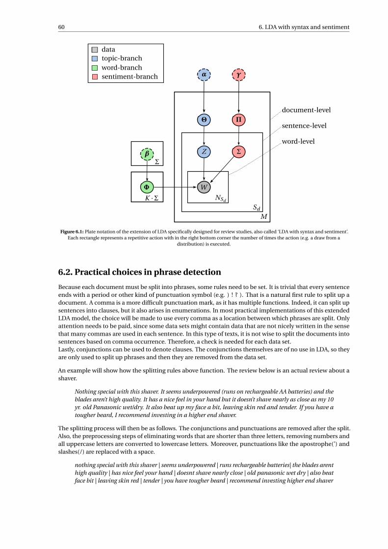
60 6. LDA with syntax and sentiment
Φ
β
Θ Π
Z
α γ
W
Σ
NSd
Sd
M
K ·Σ
Σ
document-level
sentence-level
word-level
datatopic-branchword-branchsentiment-branch
Figure 6.1: Plate notation of the extension of LDA specifically designed for review studies, also called ‘LDA with syntax and sentiment’.Each rectangle represents a repetitive action with in the right bottom corner the number of times the action (e.g. a draw from a
distribution) is executed.
6.2. Practical choices in phrase detection
Because each document must be split into phrases, some rules need to be set. It is trivial that every sentenceends with a period or other kind of punctuation symbol (e.g. ) ! ? ). That is a natural first rule to split up adocument. A comma is a more difficult punctuation mark, as it has multiple functions. Indeed, it can split upsentences into clauses, but it also arises in enumerations. In most practical implementations of this extendedLDA model, the choice will be made to use every comma as a location between which phrases are split. Onlyattention needs to be paid, since some data sets might contain data that are not nicely written in the sensethat many commas are used in each sentence. In this type of texts, it is not wise to split the documents intosentences based on comma occurrence. Therefore, a check is needed for each data set.Lastly, conjunctions can be used to denote clauses. The conjunctions themselves are of no use in LDA, so theyare only used to split up phrases and then they are removed from the data set.
An example will show how the splitting rules above function. The review below is an actual review about ashaver.
Nothing special with this shaver. It seems underpowered (runs on rechargeable AA batteries) and theblades aren’t high quality. It has a nice feel in your hand but it doesn’t shave nearly as close as my 10yr. old Panasonic wet/dry. It also beat up my face a bit, leaving skin red and tender. If you have atougher beard, I recommend investing in a higher end shaver.
The splitting process will then be as follows. The conjunctions and punctuations are removed after the split.Also, the preprocessing steps of eliminating words that are shorter than three letters, removing numbers andall uppercase letters are converted to lowercase letters. Moreover, punctuations like the apostrophe(’) andslashes(/) are replaced with a space.
nothing special with this shaver | seems underpowered | runs rechargeable batteries| the blades arenthigh quality | has nice feel your hand | doesnt shave nearly close | old panasonic wet dry | also beatface bit | leaving skin red | tender | you have tougher beard | recommend investing higher end shaver
6.3. Estimating the variables of interest 61
The parts-of-speech that are of interest in this model are chosen to be: nouns, verbs, adverbs, and adjectives.Also, interjections are kept, although they do not occur very often. When we highlight these parts-of-speech inboldface, the aspects and corresponding sentiments in the review become clear.
nothing special with this shaverseems underpoweredruns rechargeable batteriesthe blades arent high qualityhas nice feel your handdoesnt shave nearly closeold panasonic wet dryalso beat face bitleaving skin redtenderyou have tougher beardrecommend investing higher end shaver
From the review example above, we conclude that, theoretically, LDA with syntax and sentiment is promisingand suitable for review analyses.
A remark needs to be made for this example. The review considered is written very nicely with commaswhere they need to be and proper English. In most review data sets, however, reviews are not written thiswell, and either no commas or a lot of commas are used, such that the phrases based on comma splits arenot informative anymore. Therefore, one needs to decide per data set which splitting rules are the mostappropriate and give the best results.
6.3. Estimating the variables of interest
LDA with syntax and sentiment aims to retrieve the topics customers write about, in combination withtheir sentiment about them. Also, after having retrieved the word distributions per topic and sentimentcombination, a further split per part-of-speech is made, such that the final result consists of topic-sentiment-word distributions per part-of-speech, in which the following parts-of-speech are taken into account: nouns,verbs, adjectives, and adverbs.In formulas: the goal is to retrieve estimates for Θd andΠd with d = 1, . . . , M , andΦk,o with k = 1, . . . ,K ando = 1, . . .Σ. The word distributionsΦk,o can then be split into word distributions per part-of-speech, i.e. φk,o,c
with c being a noun, verb, adjective or adverb.
Again, different methods can be chosen to estimate the desired parameters. Because we use a Bayesianhierarchical model, it is natural to determine the posterior mean or mode. Given the topic and sentimentexchangeability, the posterior mean of the whole posterior distribution is not wise to use as an estimator forthe parameters mentioned earlier. A more thorough explanation can be read in chapter 4.Two good possibilities remain, the posterior mean via Gibbs sampling, and the posterior mode. The posteriormode estimate can be determined via Adam optimization, as described in chapter 5.
The posterior density can be expressed as follows. Note that we slightly abuse the notationΘ, with which weactually meanΘ1, . . . ,ΘM. The shorter notation helps to keep the posterior distribution readable.
p(θ,π,φ|w) = p(w|θ,π,φ) ·p(θ,π,φ)
p(w)
∝ p(w|θ,π,φ) ·p(θ,π,φ)
(6.1)
First, we will look at the left factor on the right-hand side, i.e. the likelihood.
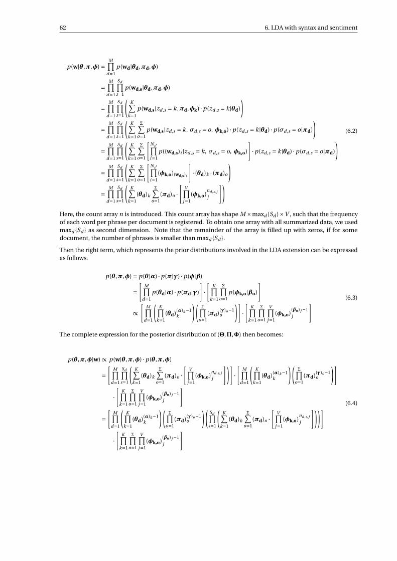
62 6. LDA with syntax and sentiment
p(w|θ,π,φ) =M∏
d=1p(wd|θd,πd,φ)
=M∏
d=1
Sd∏s=1
p(wd,s|θd,πd,φ)
=M∏
d=1
Sd∏s=1
(K∑
k=1p(wd,s|zd ,s = k,πd,φk) ·p(zd ,s = k|θd)
)
=M∏
d=1
Sd∏s=1
(K∑
k=1
Σ∑o=1
p(wd,s|zd ,s = k, σd ,s = o, φk,o) ·p(zd ,s = k|θd) ·p(σd ,s = o|πd)
)
=M∏
d=1
Sd∏s=1
(K∑
k=1
Σ∑o=1
[Ns′∏i=1
p((wd,s)i |zd ,s = k, σd ,s = o, φk,o)
]·p(zd ,s = k|θd) ·p(σd ,s = o|πd)
)
=M∏
d=1
Sd∏s=1
(K∑
k=1
Σ∑o=1
[Ns′∏i=1
(φk,o)(wd,s)i
]· (θd)k · (πd)o
)
=M∏
d=1
Sd∏s=1
(K∑
k=1(θd)k
Σ∑o=1
(πd)o ·[
V∏j=1
(φk,o)nd ,s, j
j
])
(6.2)
Here, the count array n is introduced. This count array has shape M ×maxd Sd ×V , such that the frequencyof each word per phrase per document is registered. To obtain one array with all summarized data, we usedmaxd Sd as second dimension. Note that the remainder of the array is filled up with zeros, if for somedocument, the number of phrases is smaller than maxd Sd .
Then the right term, which represents the prior distributions involved in the LDA extension can be expressedas follows.
p(θ,π,φ) = p(θ|α) ·p(π|γ) ·p(φ|β)
=[
M∏d=1
p(θd|α) ·p(πd|γ)
]·[
K∏k=1
Σ∏o=1
p(φk,o|βo)
]
∝[
M∏d=1
(K∏
k=1(θd)(α)k−1
k
)(Σ∏
o=1(πd)(γ)o−1
o
)]·[
K∏k=1
Σ∏o=1
V∏j=1
(φk,o)(βo) j −1j
] (6.3)
The complete expression for the posterior distribution of (Θ,Π,Φ) then becomes:
p(θ,π,φ|w) ∝ p(w|θ,π,φ) ·p(θ,π,φ)
=[
M∏d=1
Sd∏s=1
(K∑
k=1(θd)k
Σ∑o=1
(πd)o ·[
V∏j=1
(φk,o)nd ,s, j
j
])]·[
M∏d=1
(K∏
k=1(θd)(α)k−1
k
)(Σ∏
o=1(πd)(γ)o−1
o
)]
·[
K∏k=1
Σ∏o=1
V∏j=1
(φk,o)(βo) j −1j
]
=[
M∏d=1
(K∏
k=1(θd)(α)k−1
k
)(Σ∏
o=1(πd)(γ)o−1
o
)(Sd∏
s=1
(K∑
k=1(θd)k
Σ∑o=1
(πd)o ·[
V∏j=1
(φk,o)nd ,s, j
j
]))]
·[
K∏k=1
Σ∏o=1
V∏j=1
(φk,o)(βo) j −1j
](6.4)

6.3. Estimating the variables of interest 63
6.3.1. Posterior mode: optimization
With the expression of the posterior density, we can determine the posterior mode. This statistic is expected tobe a good estimator for all latent random variables of interest in the model, that isΘ1, . . . ,ΘM,Π1, . . . ,ΠM andΦ1,1, . . . ,Φ1,Σ, . . . ,ΦK,1, . . . ,ΦK,Σ.
For the application of Adam optimization to find the posterior mode, the log(posterior) can better be used:
log(p(θ,π,φ|w)
)=C +M∑
d=1
[K∑
k=1((α)k −1)log((θd)k )+
Σ∑o=1
((γ)o −1)log((πd)o)+Sd∑
s=1log
(K∑
k=1(θd)k
Σ∑o=1
(πd)o ·[
V∏j=1
(φk,o)nd ,s, j
j
])]
+K∑
k=1
Σ∑o=1
V∑j=1
((βo) j −1)log((φk,o) j
)=C +
M∑d=1
[K∑
k=1((α)k −1)log((θd)k )+
Σ∑o=1
((γ)o −1)log((πd)o)
]
+M∑
d=1
Sd∑s=1
log
(K∑
k=1(θd)k
Σ∑o=1
(πd)o ·exp
[V∑
j=1nd ,s, j log
(φk,o) j
])
+K∑
k=1
Σ∑o=1
V∑j=1
((βo) j −1)log((φk,o) j
)(6.5)
Here, the constant C originates from the fact that the posterior density in equation 6.4 is only expressed up toa proportionality constant.In equation 6.5 we can see that again the posterior density has a satisfactory form, for which optimization iswell possible. The sum of subfunctions allows us to do stochastic gradient descent which is used in Adamoptimization, and the python package Tensorflow can run the algorithm parallel, keeping computation timewith reasonable bounds. Furthermore, the sum in the third term of the log(posterior) are actually three tensorproducts. The tensor product can be seen as a product of two high-dimensional arrays in which the dimensionover which is summed is specified, and it can easily be implemented in Tensorflow.The same softmax transformation and regularization methods are used as explained in chapter 5. Only anextra trick needs to be applied, as this extended version of LDA has more problems when the hyperparametersare smaller than 1.
Numerical stability via the log-sum-exp trick
The posterior density or the log posterior of LDA with syntax and sentiment is even more complicated than theposterior density in plain LDA. Therefore, other numerical problems arise. If some parameter (Θd)k , (Πd)o or(Φk,o) j gets too close to zero during the optimization process, the algorithm will reach the bounds of numericalprecision when computing the exponent in the softmax transformation. The calculated objective will returna ‘NaN’, resulting in an immediate exit from the optimization. This problem, caused by a lack of numericalprecision, can be solved by using a smart way of rewriting the log posterior.
Consider an example in which the xi , i = 1, . . . ,n are such that log(∑
i exi ) is hard to compute numerically, forexample due to the xi being too negative. If exi is smaller than the machine precision, log(exi ) will return either−∞ or NaN, both resulting in an objective that cannot be computed. Therefore, the optimization algorithm isstopped, and no results are given. To avoid this type of problems with machine precision, the ‘log-sum-exp’transformation, often used in machine learning, is used:
log
(n∑
i=1exi
)= x∗+ log
(n∑
i=1exi−x∗
)(6.6)
Here, x∗ is the maximum of all parameters, i.e. x∗ = maxi xi . Naturally, x∗ can always be calculated, as it willbe of the order -50 for ex∗
close to 0. This is often the case when the optimization drives the optimal values ofthe parameters to the left bound of the domain [0,1]. Additionally, exi−x∗
can now be computed. Where e−100
could not be computed, e−100−(−50) can, considering the example in which x∗ =−50. Note that in the left hand
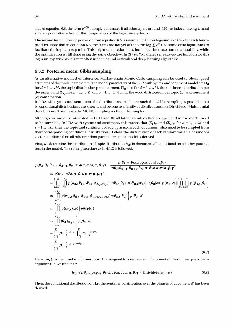
64 6. LDA with syntax and sentiment
side of equation 6.6, the term e−50 strongly dominates if all other x j are around -100, so indeed, the right handside is a good alternative for the computation of the log-sum-exp term.
The second term in the log posterior from equation 6.5 is rewritten with this log-sum-exp trick for each tensorproduct. Note that in equation 6.5, the terms are not yet of the form log(
∑exi ), so some extra logarithms to
facilitate the log-sum-exp trick. This might seem redundant, but it does increase numerical stability, whilethe optimization is still done using the same objective. In Tensorflow there is a ready-to-use function for thislog-sum-exp trick, as it is very often used in neural network and deep learning algorithms.
6.3.2. Posterior mean: Gibbs sampling
As an alternative method of inference, Markov chain Monte Carlo sampling can be used to obtain goodestimates of the model parameters. The model parameters of the LDA with syntax and sentiment model areΘd
for d = 1, . . . , M , the topic distribution per document,Πd also for d = 1, . . . , M , the sentiment distribution perdocument andΦk,o for k = 1, . . . ,K and o = 1, . . . ,Σ, that is, the word distribution per topic (k) and sentiment(o) combination.In LDA with syntax and sentiment, the distributions are chosen such that Gibbs sampling is possible, thatis, conditional distributions are known, and belong to a family of distributions like Dirichlet or Multinomialdistributions. This makes the MCMC sampling method a lot simpler.
Although we are only interested in Θ, Π and Φ, all latent variables that are specified in the model needto be sampled. In LDA with syntax and sentiment, this means that (Zd)s′ and (Σd)s′ for d = 1, . . . , M ands = 1, . . . ,Sd , thus the topic and sentiment of each phrase in each document, also need to be sampled fromtheir corresponding conditional distributions. Below, the distribution of each random variable or randomvector conditional on all other random parameters in the model is derived.
First, we determine the distribution of topic distributionΘd′ in document d ′ conditional on all other parame-ters in the model. The same procedure as in 4.1.2 is followed.
p(θd′ |θ1,θd′−1,θd′+1,θM,π,φ,z,σ,w,α,β,γ) = p(θ1, · · ·θM,π,φ,z,σ,w|α,β,γ)
p(θ1,θd′−1,θd′+1,θM,π,φ,z,σ,w|α,β,γ)
∝ p(θ1, · · ·θM,π,φ,z,σ,w|α,β,γ)
=(
M∏d=1
[Sd∏
s=1p(wd,s|zd,s,σd,s,φzd,s,σd,s ) ·p(zd,s|θd) ·p(σd,s|πd)
]p(θd|α) ·p(πd|γ)
)(K∏
k=1
Σ∏o=1
p(φk,o|βo)
)
∝(
Sd ′∏s=1
p(wd′,s|zd′,s,σd′,s,φ(zd′ )s′ ,(σd′ )s′ )p(zd′,s|θd′ )
)p(θd′ |α)
∝(
Sd ′∏s=1
p(zd′,s|θd′ )
)p(θd′ |α)
∝(
Sd ′∏s=1
(θd′ )(zd′ )s′
)p(θd′ |α)
=K∏
k=1(θd′ )
(md′ )k
k ·K∏
k=1(θd′ )(α)k−1
k
=K∏
k=1(θd′ )
(md′ )k+(α)k−1k
(6.7)
Here, (md)k is the number of times topic k is assigned to a sentence in document d . From the expression inequation 6.7, we find that:
Θd′ |θ1,θd′−1,θd′+1,θM,π,φ,z,σ,w,α,β,γ∼ Dirichlet(md′ +α) (6.8)
Then, the conditional distribution ofΠd′ , the sentiment distribution over the phrases of document d ′ has beenderived.
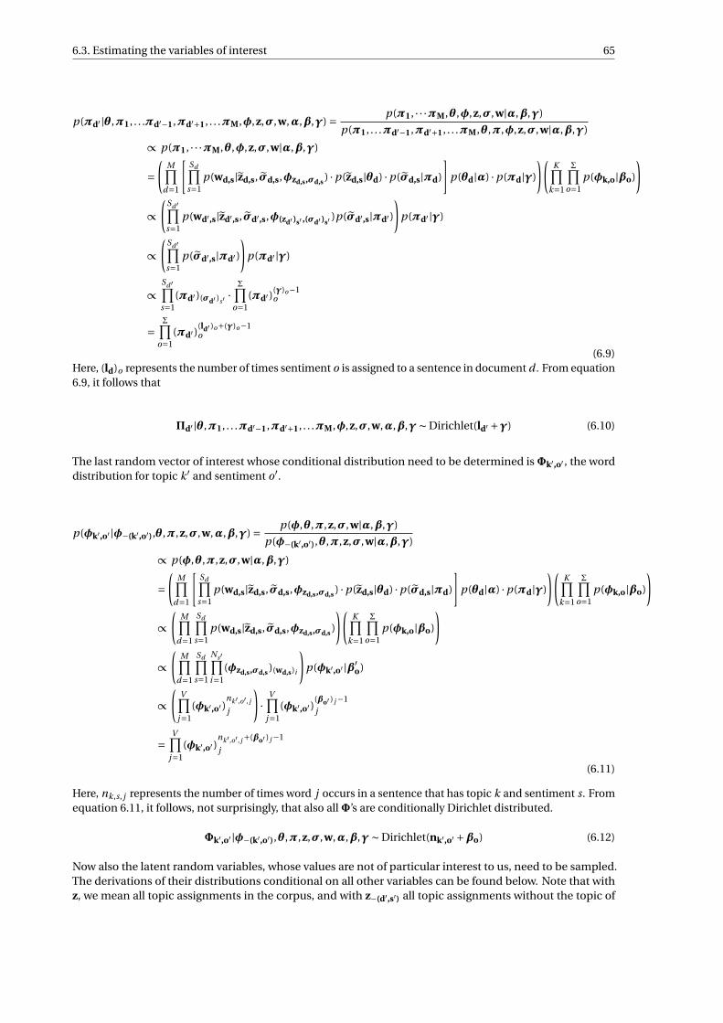
6.3. Estimating the variables of interest 65
p(πd′ |θ,π1, . . .πd′−1,πd′+1, . . .πM,φ,z,σ,w,α,β,γ) = p(π1, · · ·πM,θ,φ,z,σ,w|α,β,γ)
p(π1, . . .πd′−1,πd′+1, . . .πM,θ,π,φ,z,σ,w|α,β,γ)
∝ p(π1, · · ·πM,θ,φ,z,σ,w|α,β,γ)
=(
M∏d=1
[Sd∏
s=1p(wd,s|zd,s,σd,s,φzd,s,σd,s ) ·p(zd,s|θd) ·p(σd,s|πd)
]p(θd|α) ·p(πd|γ)
)(K∏
k=1
Σ∏o=1
p(φk,o|βo)
)
∝(
Sd ′∏s=1
p(wd′,s|zd′,s,σd′,s,φ(zd′ )s′ ,(σd′ )s′ )p(σd′,s|πd′ )
)p(πd′ |γ)
∝(
Sd ′∏s=1
p(σd′,s|πd′ )
)p(πd′ |γ)
∝Sd ′∏s=1
(πd′ )(σd′ )s′ ·Σ∏
o=1(πd′ )(γ)o−1
o
=Σ∏
o=1(πd′ )
(ld′ )o+(γ)o−1o
(6.9)Here, (ld)o represents the number of times sentiment o is assigned to a sentence in document d . From equation6.9, it follows that
Πd′ |θ,π1, . . .πd′−1,πd′+1, . . .πM,φ,z,σ,w,α,β,γ∼ Dirichlet(ld′ +γ) (6.10)
The last random vector of interest whose conditional distribution need to be determined isΦk′,o′ , the worddistribution for topic k ′ and sentiment o′.
p(φk′,o′ |φ−(k′,o′),θ,π,z,σ,w,α,β,γ) = p(φ,θ,π,z,σ,w|α,β,γ)
p(φ−(k′,o′),θ,π,z,σ,w|α,β,γ)
∝ p(φ,θ,π,z,σ,w|α,β,γ)
=(
M∏d=1
[Sd∏
s=1p(wd,s|zd,s,σd,s,φzd,s,σd,s ) ·p(zd,s|θd) ·p(σd,s|πd)
]p(θd|α) ·p(πd|γ)
)(K∏
k=1
Σ∏o=1
p(φk,o|βo)
)
∝(
M∏d=1
Sd∏s=1
p(wd,s|zd,s,σd,s,φzd,s,σd,s )
)(K∏
k=1
Σ∏o=1
p(φk,o|βo)
)
∝(
M∏d=1
Sd∏s=1
Ns′∏i=1
(φzd,s,σd,s )(wd,s)i
)p(φk′,o′ |β′
o)
∝(
V∏j=1
(φk′,o′ )nk′ ,o′ , j
j
)·
V∏j=1
(φk′,o′ )(βo′ ) j −1j
=V∏
j=1(φk′,o′ )
nk′ ,o′ , j +(βo′ ) j −1
j
(6.11)
Here, nk,s, j represents the number of times word j occurs in a sentence that has topic k and sentiment s. Fromequation 6.11, it follows, not surprisingly, that also allΦ’s are conditionally Dirichlet distributed.
Φk′,o′ |φ−(k′,o′),θ,π,z,σ,w,α,β,γ∼ Dirichlet(nk′,o′ +βo) (6.12)
Now also the latent random variables, whose values are not of particular interest to us, need to be sampled.The derivations of their distributions conditional on all other variables can be found below. Note that withz, we mean all topic assignments in the corpus, and with z−(d′,s′) all topic assignments without the topic of

66 6. LDA with syntax and sentiment
sentence s′ in document d ′.
p((zd′ )s′ |z−(d ′,s′),θ,π,φ,σ,w,α,β,γ) = p(z,θ,π,φ,σ,w|α,β,γ)
p(z−(d ′,s′),θ,π,φ,σ,w|α,β,γ)
∝ p(z,θ,π,φ,σ,w|α,β,γ)
=(
M∏d=1
[Sd∏
s=1p(wd,s|zd,s,σd,s,φzd,s,σd,s ) ·p(zd,s|θd) ·p(σd,s|πd)
]p(θd|α) ·p(πd|γ)
)(K∏
k=1
Σ∏o=1
p(φk,o|βo)
)
∝M∏
d=1
Sd∏s=1
p(wd,s|zd,s,σd,s,φzd,s,σd,s ) ·p(zd,s|θd)
∝ p(wd′,s′ |zd′,s′ ,σd′,s′ ,φ(zd′ )s′ ,(σd′ )s′ ) ·p(zd′,s′ |θd′ )
=(
Ns′∏i=1
(φ(zd′ )s′ ,(σd′ )s′ )(wd′ ,s′ )i
)(θd′ )(zd′ )s′
=(
V∏j=1
(φ(zd′ )s′ ,(σd′ )s′ )n(zd′ )s′ ,(σd′ )s′ , j
j
)(θd′ )(zd′ )s′
(6.13)
Therefore, (Zd′ )s′ |z−(d ′,s′),θ,π,φ,σ,w,α,β,γ has a Multinomial distribution with parameters:
(Zd′,s′ )|all other parameters ∼ Multinomial
(1,
[V∏
j=1(φ1,(σd′ )s′ )
n1,(σd′ )s′ , j
j
]· (θd′ )1 , . . . ,
[V∏
j=1(φK,(σd′ )s′ )
nK ,(σd′ )s′ , j
j
]· (θd′ )K
)(6.14)
Lastly, the conditional distribution of the sentiment assignment to each phrase in each document is derived.
p((σd′ )s′ |σ−(d ′,s′),θ,π,φ,w,z,α,β,γ) = p(σ,θ,π,φ,w,z|α,β,γ)
p(σ−(d ′,s′),θ,π,φ,w,z|α,β,γ)
∝ p(σ,θ,π,φ,w,z|α,β,γ)
=(
M∏d=1
[Sd∏
s=1p(wd,s|zd,s,σd,s,φzd,s,σd,s ) ·p(zd,s|θd) ·p(σd,s|πd)
]p(θd|α) ·p(πd|γ)
)(K∏
k=1
Σ∏o=1
p(φk,o|βo)
)
∝M∏
d=1
Sd∏s=1
p(wd,s|zd,s,σd,s,φzd,s,σd,s ) ·p(σd,s|πd)
∝ p(wd′,s′ |zd′,s′ ,σd′,s′ ,φ(zd′ )s′ ,(σd′ )s′ ) ·p(σd′,s′ |πd′ )
=(
Ns′∏i=1
(φ(zd′ )s′ ,(σd′ )s′ )(wd′ ,s′ )i
)(πd′ )(σd′ )s′
=(
V∏j=1
(φ(zd′ )s′ ,(σd′ )s′ )n(zd′ )s′ ,(σd′ )s′ , j
j
)(πd′ )(σd′ )s′
(6.15)
Therefore, (Σd′ )s′ |σ−(d ′,s′),θ,π,φ,z,w,α,β,γ has a Multinomial distribution with parameters:
(Σd′ )s′ |all other parameters ∼ Multinomial
(1,
[V∏
j=1(φ(zd′ )s′ ,1)
n(zd′ )s′ ,1, j
j
]· (πd′ )1 , . . . ,
[V∏
j=1(φ(zd′ )s′ ,Σ)
n(zd′ )s′ ,Σ, j
j
]· (πd′ )Σ
)(6.16)
The Gibbs sampling algorithm for the extended version of LDA described in this chapter is given in algorithm5. Although Gibbs sampling has good convergence properties, it is not implemented in this research, becauseconvergence can take a long time, especially with the many parameter samples that are needed. Programmingthe algorithm in such a way that its implementation is fast and convergence is reached within a reasonableamount of time, is considered beyond the scope of this thesis.

6.3. Estimating the variables of interest 67
Algorithm 5 Gibbs Sampling for LDA with syntax and sentiment
1: Initialize θ1, . . . ,θM,π1, . . . ,πM,φ1,1, . . . ,φK,Σ,z,σ2: Compute initial frequencies (md)k (for d = 1, . . . , M , k = 1, . . . ,K ), (ld)o (for o = 1, . . . ,Σ)3: and (nk,o) j (for k = 1 to K ,o = 1, . . . ,Σ and j = 1 to V )4: Fix Ni ter for the maximum number of iterations5: for i ter = 1 to Ni ter do . Sample Ni ter times6: for d = 1 to M do . Iterate over documents7: DrawΘd from Dirichlet(md +α)8: DrawΠd from Dirichlet(ld +γ)9: for s = 1 to Sd do . Iterate over phrases
10: Draw Zds from the Multinomial distribution in equation 6.1411: Draw Σds from the Multinomial distribution in equation 6.1612: end for13: end for14: Update frequencies (nk,o) j
15: for k = 1 to K do . Iterate over topics16: for o = 1 to Σ do . Iterate over sentiments17: DrawΦk,o from Dirichlet(nk,o +βo)18: end for19: end for20: Update frequencies (md)k and (ld)o
21: end for22: Compute posterior estimates of Θ1, . . . ,ΘM,Π1, . . . ,ΠM,Φ1,1, . . . ,ΦK,Σ,Z,Σ using the Ni ter samples from
their posterior distributions

7Validity of topic-word distribution
estimates
In the previous chapters, we have discussed different inference methods for both the plain LDA model andLDA with syntax and sentiment. All methods of inference result in estimates for the latent random variables ofinterest. That is for each document d ∈ 1, . . . , M , we want to know the document-topic distributionΘd, andfor each topic k ∈ 1, . . . ,K , the topic-word distributionΦk is estimated.After having obtained these estimates, we need to take a look at their validity before drawing conclusions. Theresults are considered not valid, if each topic-word distribution is similar, as will be explained in this chapter.Therefore, the difference in probability vectors is ‘measured’.
The most insightful of the latent variables are the topic-word distributionsΦ, from which we can qualitativelysee what the topics are about, and therefore what customers find essential to write about in their reviews.Because words form the topics, the human brain can creatively interpret what general theme is behind eachtopic when looking at, for example, the top 10 words. However, one needs to be careful here, because to beallowed to draw conclusions from the topic-word distribution, also mathematically the topic must be distinctfrom the others, otherwise it might fit noise or it consists of multiple topics. It can be the case that multipletopics have similar top 10 words, such that these topics are difficult to distinguish. To be able to determinequantitatively which topics are too similar to be interpreted independently, and which are distinctive andunique, different similarity measures are proposed in the literature.
7.1. Normalized symmetric KL-divergenceKoltcov et al. derived a similarity measure based on the Kullback-Leibler divergence. They have found thatlarge proportions of the topics fit noise if the chosen number of topics K is too large. This results in differentresults for runs with different initializations [24].
Their similarity measure can be thought of as a rescaled symmetric KL-divergence. Symmetric KL-divergenceis defined for discrete probability distributions as follows [43].
Definition 7.1 (Symmetric KL-divergence)The symmetric Kullback-Leibler divergence of a discrete probability distribution q with respect to another discreteprobability distribution p, where q and p have the same supportΩ, is given by:
K Ls ym(q‖p) = 1
2
(K L(p‖q)+K L(q‖p)
)(7.1)
With:
K L(q‖p) = ∑x∈Ω
q(x) log
(q(x)
p(x)
)(7.2)
Note that the general Kullback-Leibler divergence was already introduced in chapter 2, as the relative entropy.In [24] it is mentioned that the symmetric KL-divergence for the topic distributions of LDA is sensitive
69
70 7. Validity of topic-word distribution estimates
to vocabulary sizes because it is dominated by the long tail of rare words in estimate φ. Therefore, oneimprovement can be to look at, e.g., the top x% words, where the percentage x can be varied and optimizedper data set. Another option is to normalize the symmetric KL-divergence to obtain a better interpretablesimilarity measure. Koltcov et al. introduce the Normalized Kullback-Leibler Similarity (NKLS) measure:
N K LS(q‖p) = 1− K Ls ym(q‖p)
maxq′,p′K Ls ym(q′‖p′)
(7.3)
The NKLS takes values in the interval [0,1], where 1 is reached if the two probability distributions are exactlyequal, and 0 if the two distributions are the most distinctive among all possible combinations of q′ and p′.In NKLS for LDA, this means that we compare the similarity of each combination of estimated vectors φk andφl (for some k, l ∈ 1, . . . ,K ) with the two most distinctive vectors among all possible combinations of k andl . The latter gives the maximal KL-divergence of two distributions φ with respect to each other. A similaritymatrix can thus be constructed from which we can conclude which topics are very similar concerning theword probabilities and which topics are more distinctive.A topic is considered valid if its similarity scores with all other estimated topic-word distributions is largerthan a threshold. Koltcov et al. found that a threshold of 0.9 is reasonable, as with this value of NKLS, the top30-50 words (depending on the size of the vocabulary and the data set) are the same, only the probabilities aredifferent [24]. For values below 0.9, the top 30-50 words can be completely different, while for values above 0.9,the order of the top 30-50 words is almost the same. Therefore, in the results of this thesis, it is also decided toclassify topics with a similarity score higher than 0.9 to belong to the same topic or subject, while topics withsimilarity scores with all other topics below 0.9 are distinctive and can safely be interpreted as results.
Not only for the quality of the topics, the NKLS score can be used, but also to check the stability of the inferenceprocedure for LDA. That is, two runs can be performed with different initializations, and the similarity ofthe result can be measured. One expects a stable algorithm to give the same topic-word distributions twice.Remember that there is topic exchangeability in LDA, so with the score, we can automatically match the righttopic index k ∈ 1, . . . ,K from the first run with index k ′ ∈ 1, . . . ,K from the second run. In practice, this istoo much work in comparison with just sorting the topics based on the average θM over all documents forevery method. Therefore, the last method is used to ensure that we are comparing results of the same topicpermutation.
7.2. Symmetrized Jensen-Shannon divergenceIn [43], the symmetrized Jensen-Shannon (JS) divergence is used to determine the similarity between docu-ments, but naturally it can also be applied to find similar topic-word distributions. The JS-divergence is basedon the Kullback-Leibler divergence, only it compares a probability distribution with the pointwise arithmeticmean of the same distribution with a second one. In formulas:
JSs ym(p,q) = 1
2
[K L
(p‖1
2(p+q)
)+K L
(q‖1
2(p+q)
)](7.4)
If p and q represent the same probability density function, the symmetrized JS-divergence is 0, as the arithmeticmean of the two is equal to both p and q. According to [43], both the symmetrized JS-divergence as thesymmetric KL-divergence work well in practice. Because also for the Jensen-Shannon divergence, it is expectedthat the long tail of low probabilities will dominate the score, the same type of normalization can be applied,such that we get the normalized Jensen-Shannon similarity measure.
N JSS(q‖p) = 1− JSs ym(q‖p)
maxq′,p′
JSs ym(q′‖p′) (7.5)
One can compute a similarity matrix using either divergence method and compare. A decision on which topicsto take into account in the review analysis will be better founded based on both the NKLS and the NJSS.
8Results
The main research in this thesis can be split up into two different parts, as is represented in the researchquestions. The first subject concerns the ‘basic’ model of Latent Dirichlet Allocation and the different inferencemethods that can be used to estimate the model parameters. The results of this research are given in section 2of this chapter. However, we need to know more about the properties and shape of the posterior density first,to fully understand the LDA results in section 2. To this end, the first section of this chapter elaborates on thevisualization of the posterior density. Secondly, an extension to LDA called ‘LDA with syntax and sentiment’has been constructed, whose results on various data sets will be shown in section 3 of this chapter.
8.1. Posterior density visualization of LDA
Before we apply Latent Dirichlet Allocation to actual data sets, it is interesting to learn more about the form ofthe posterior density. Especially when using the optimization method to find the posterior mode, it is essentialto understand its shape.
8.1.1. Influence of the hyperparameters in LDA
Firstly, we will look at one of the smallest possible data sets to which LDA can be applied. With this example,we want to understand more about the influence of the hyperparameters α and β in LDA.Consider a toy example with one two topics (K = 2), two possible words (V = 2), and the three documents(M = 3):
1. document: [1 1 1 1]
2. document: [1 2 1 1 2 2]
3. document: [1 2 2 2 2 2 2 2]
Remember that the numbers in the document lists stand for either word 1 or word 2. It is not necessary toknow what the exact words are to understand this example. The order of the words does not influence theform of the posterior density, since only the frequencies per document are taken into account. Naturally, thisis an unrealistic example to apply LDA on, but nevertheless we already have 5 parameters to estimate: θ1, θ2,θ3, φ1 and φ2, making visualization a challenge.
Using a grid on [ε,1−ε]5 with 21 nodes in each dimension, the posterior density can be computed over thegrid. We use ε instead of 0 to avoid numerical problems, where ε is set to 10−8. Connecting the nodes, we get a5-dimensional hyperplane that forms the posterior density.
In figure 8.1, the posterior densities are visualized using 8 different settings for hyperparameters α andβ. Because we can only easily understand a three-dimensional surface plot, the conditional densitiesp(φ1,φ2|θ1 = θ1,opt,θ2 = θ2,opt,θ3 = θ3,opt) are shown instead of the full posterior densities. With ‘opt’ isdenoted the value of each θd (with d = 1,2,3) for which the maximum is attained.
71
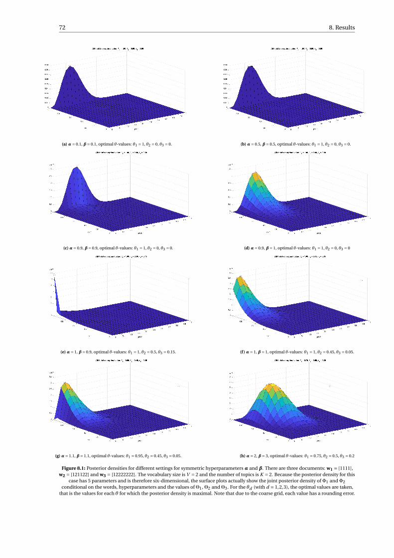
72 8. Results
(a)α= 0.1, β= 0.1, optimal θ-values: θ1 = 1, θ2 = 0, θ3 = 0. (b)α= 0.5, β= 0.5, optimal θ-values: θ1 = 1, θ2 = 0, θ3 = 0.
(c)α= 0.9, β= 0.9, optimal θ-values: θ1 = 1, θ2 = 0, θ3 = 0. (d)α= 0.9, β= 1, optimal θ-values: θ1 = 1, θ2 = 0, θ3 = 0
(e)α= 1, β= 0.9, optimal θ-values: θ1 = 1, θ2 = 0.5, θ3 = 0.15. (f )α= 1, β= 1, optimal θ-values: θ1 = 1, θ2 = 0.45, θ3 = 0.05.
(g)α= 1.1, β= 1.1, optimal θ-values: θ1 = 0.95, θ2 = 0.45, θ3 = 0.05. (h)α= 2, β= 3, optimal θ-values: θ1 = 0.75, θ2 = 0.5, θ3 = 0.2
Figure 8.1: Posterior densities for different settings for symmetric hyperparameters α and β. There are three documents: w1 = [1111],w2 = [121122] and w3 = [12222222]. The vocabulary size is V = 2 and the number of topics is K = 2. Because the posterior density for this
case has 5 parameters and is therefore six-dimensional, the surface plots actually show the joint posterior density ofΦ1 andΦ2conditional on the words, hyperparameters and the values ofΘ1,Θ2 andΘ3. For the θd (with d = 1,2,3), the optimal values are taken,
that is the values for each θ for which the posterior density is maximal. Note that due to the coarse grid, each value has a rounding error.
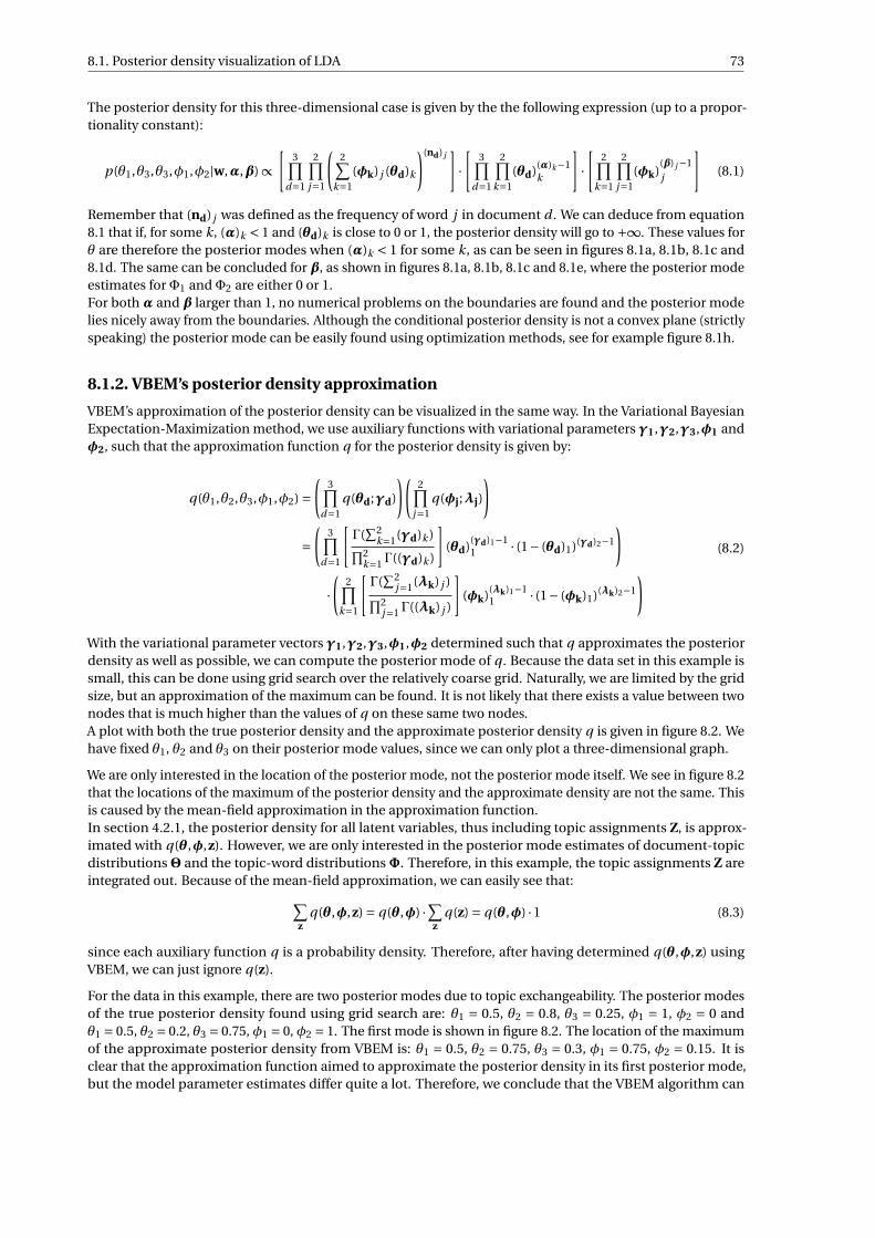
8.1. Posterior density visualization of LDA 73
The posterior density for this three-dimensional case is given by the the following expression (up to a propor-tionality constant):
p(θ1,θ3,θ3,φ1,φ2|w,α,β) ∝[
3∏d=1
2∏j=1
(2∑
k=1(φk) j (θd)k
)(nd) j]·[
3∏d=1
2∏k=1
(θd)(α)k−1k
]·[
2∏k=1
2∏j=1
(φk)(β) j −1j
](8.1)
Remember that (nd) j was defined as the frequency of word j in document d . We can deduce from equation8.1 that if, for some k, (α)k < 1 and (θd)k is close to 0 or 1, the posterior density will go to +∞. These values forθ are therefore the posterior modes when (α)k < 1 for some k, as can be seen in figures 8.1a, 8.1b, 8.1c and8.1d. The same can be concluded for β, as shown in figures 8.1a, 8.1b, 8.1c and 8.1e, where the posterior modeestimates forΦ1 andΦ2 are either 0 or 1.For both α and β larger than 1, no numerical problems on the boundaries are found and the posterior modelies nicely away from the boundaries. Although the conditional posterior density is not a convex plane (strictlyspeaking) the posterior mode can be easily found using optimization methods, see for example figure 8.1h.
8.1.2. VBEM’s posterior density approximation
VBEM’s approximation of the posterior density can be visualized in the same way. In the Variational BayesianExpectation-Maximization method, we use auxiliary functions with variational parameters γ1,γ2,γ3,φ1 andφ2, such that the approximation function q for the posterior density is given by:
q(θ1,θ2,θ3,φ1,φ2) =(
3∏d=1
q(θd;γd)
)(2∏
j=1q(φj;λj)
)
=(
3∏d=1
[Γ(
∑2k=1(γd)k )∏2
k=1Γ((γd)k )
](θd)(γd)1−1
1 · (1− (θd)1)(γd)2−1
)
·(
2∏k=1
[Γ(
∑2j=1(λk) j )∏2
j=1Γ((λk) j )
](φk)(λk)1−1
1 · (1− (φk)1)(λk)2−1
) (8.2)
With the variational parameter vectors γ1,γ2,γ3,φ1,φ2 determined such that q approximates the posteriordensity as well as possible, we can compute the posterior mode of q . Because the data set in this example issmall, this can be done using grid search over the relatively coarse grid. Naturally, we are limited by the gridsize, but an approximation of the maximum can be found. It is not likely that there exists a value between twonodes that is much higher than the values of q on these same two nodes.A plot with both the true posterior density and the approximate posterior density q is given in figure 8.2. Wehave fixed θ1, θ2 and θ3 on their posterior mode values, since we can only plot a three-dimensional graph.
We are only interested in the location of the posterior mode, not the posterior mode itself. We see in figure 8.2that the locations of the maximum of the posterior density and the approximate density are not the same. Thisis caused by the mean-field approximation in the approximation function.In section 4.2.1, the posterior density for all latent variables, thus including topic assignments Z, is approx-imated with q(θ,φ,z). However, we are only interested in the posterior mode estimates of document-topicdistributionsΘ and the topic-word distributionsΦ. Therefore, in this example, the topic assignments Z areintegrated out. Because of the mean-field approximation, we can easily see that:∑
zq(θ,φ,z) = q(θ,φ) ·∑
zq(z) = q(θ,φ) ·1 (8.3)
since each auxiliary function q is a probability density. Therefore, after having determined q(θ,φ,z) usingVBEM, we can just ignore q(z).
For the data in this example, there are two posterior modes due to topic exchangeability. The posterior modesof the true posterior density found using grid search are: θ1 = 0.5, θ2 = 0.8, θ3 = 0.25, φ1 = 1, φ2 = 0 andθ1 = 0.5, θ2 = 0.2, θ3 = 0.75, φ1 = 0, φ2 = 1. The first mode is shown in figure 8.2. The location of the maximumof the approximate posterior density from VBEM is: θ1 = 0.5, θ2 = 0.75, θ3 = 0.3, φ1 = 0.75, φ2 = 0.15. It isclear that the approximation function aimed to approximate the posterior density in its first posterior mode,but the model parameter estimates differ quite a lot. Therefore, we conclude that the VBEM algorithm can

74 8. Results
approximate the posterior density in a general good direction, but the approximation is still too far off to drawconclusions for the model parameters. This conclusion will be supported with the application of LDA to twodata sets.
Figure 8.2: Surface plot of join posterior density ofΦ1,Φ2 conditional onΘ1 = 0.5, Θ2 = 0.8, Θ3 = 0.25. Hyperparameters are set to α= 1.1and β= 1. The number of topics is K = 2, the vocabulary size is V = 2 and there are 3 documents: M = 3. The data consists of three
documents: w1 = [1,2], w2 = [1,1,1,1,2] and w3 = [1,2,2,2,1,2,2,2]. Also the approximation of the conditional posterior density, q , isshown and it can be seen that their maxima lie on different locations, resulting in different posterior modes. Note that for the sake of
comparison, all values are normalized such that the maximal value equal 1 for both surfaces.
8.2. LDA: different methods of inference
There are different methods to estimate the model parameters1 Θd with d = 1, . . . , M , andΦk with k = 1, . . . ,K ,respectively the document-topic distributions and the topic-word distributions. The estimators are based onthe posterior mean or the posterior mode.
Although the posterior mean estimator calculated from the complete posterior distribution does not result ingood explanatory results for the topic and word distribution due to topic exchangeability, it is used in Gibbssampling. This is possible because the Gibbs sampling algorithm is expected to ‘circle’ around one topicpermutation, as the probability to go from one hill in the posterior density to another is very small. Therefore,we use the fact that Gibbs sampling does not work properly (in terms of convergence), to get informativeestimators for our latent random variables of interest. There is a good implementation of Gibbs sampling forLDA in the open source program KNIME [23]. The results from this implementation are considered to be goodGibbs sampling results, even though it is not entirely clear what steps are taken in this software exactly. In thedocumentation, methods described in [32, 52] are referred to.Another possibility, apart from programming the Gibbs algorithm with the update formulas from algorithm 1yourself, is using the JAGS package in either R or Python, whichever is preferred. JAGS stands for ‘just anotherGibbs sampler’ and allows for Markov chain Monte Carlo sampling for almost every hierarchical Bayesianmodel. Only the conditional distributions need to be specified, then JAGS determines whether Gibbs samplingcan be done or Metropolis-Hastings sampling is needed. Remember that Gibbs sampling is only possible if the
1Strictly speaking, these are latent random variables in a Bayesian setting.

8.2. LDA: different methods of inference 75
distributions and dependencies in the hierarchical model are chosen such that the conditional distribution ofeach parameter given all other parameters and data is of a known, closed form. Unfortunately, JAGS is not avery fast implementation of Gibbs. Therefore, results are not generated by this implementation.
The posterior mode is very challenging to compute analytically. However, we can use the posterior distributionin its exact form and look for an optimum. This optimization method is described in chapter 5. Unfortunately,it cannot be guaranteed that a global optimum is found, only local optima can be reached by the algorithm.Besides, there are many local optima due to topic exchangeability. We conclude that all posterior modes thatare symmetric due to topic exchangeability are equally good and give the same result concerning how thetopics are distributed and what words are most frequently used per topic (i.e., estimations for respectivelyΘ andΦ), based on observations from low-dimensional versions of LDA. The optimization algorithm is notstable in finding the same posterior mode every time, as different initializations are used. However, when thetopics are sorted in the same way after every optimization, we can conclude that indeed, every posterior modeis equally good and give the same results when looking at the estimations ofΘ andΦ.Another method to estimate model parameters via the posterior model that is often used by topic modelersis Variational Bayesian Expectation Maximization (VBEM). In particular, VBEM with the mean-field approx-imation is very common. In this method, the posterior distribution is approximated by a simpler functionof which the mode can be computed analytically. The approximation function is based on the mean-fieldapproximation, which means that each latent variable is assumed to be independent, such that the product oftheir marginal density functions gives an approximation of the posterior distribution. Naturally, this is a verystrong assumption, but we will see in the results that the method can perform relatively well in terms of theestimations for the document-topic and topic-word distributions.
8.2.1. Small data set: Cats and Dogs
First, a simple data set with distinctive documents is considered. This data set is created by the author of thisthesis, based on the principle that if two documents tell about a different subject and use different words todo that, these documents belong to two distinct topics. The data set and the preprocessed version of it canbe found in appendix B.3. There are documents about dogs, and documents about cats. Also, some textswrite about animals in general, but the words used in these documents are also used in the cat documents,meaning that they are expected to be assigned to the ‘cat’-topic. If a person who understands English dividedthe documents into two clusters or topics, this person would get the following classification.
Table 8.1: ‘Cats and dogs’ data set. Simple, small data set with distinctive topic clusters by construction. Documents in gray belong to the‘cat’ topic, while those in white are part of the ‘dog’ topic.
Documentscats are animalsdogs are canids
cats are fluffydogs barkcats meow
fluffy are catsanimals are large
dogs bitecats scratch
dogs bitecats scratch
dogs barkcats are fluffy
animals are coolnot all animals are fluffy
dogs are toughcanids are special
bark dogscool cats
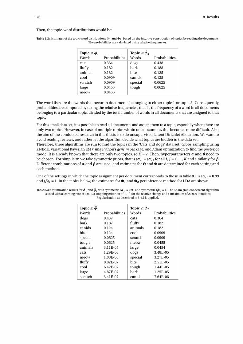
76 8. Results
Then, the topic-word distributions would be:
Table 8.2: Estimates of the topic-word distributionsΦ1 andΦ2, based on the intuitive construction of topics by reading the documents.The probabilities are calculated using relative frequencies.
Topic 1: φ1 Topic 2: φ2
Words Probabilities Words Probabilitiescats 0.364 dogs 0.438fluffy 0.182 bark 0.188animals 0.182 bite 0.125cool 0.0909 canids 0.125scratch 0.0909 special 0.0625large 0.0455 tough 0.0625meow 0.0455
The word lists are the words that occur in documents belonging to either topic 1 or topic 2. Consequently,probabilities are computed by taking the relative frequencies, that is, the frequency of a word in all documentsbelonging to a particular topic, divided by the total number of words in all documents that are assigned to thattopic.
For this small data set, it is possible to read all documents and assign them to a topic, especially when there areonly two topics. However, in case of multiple topics within one document, this becomes more difficult. Also,the aim of the conducted research in this thesis is to do unsupervised Latent Dirichlet Allocation. We want toavoid reading reviews, and rather let the algorithm decide what topics are hidden in the data set.Therefore, three algorithms are run to find the topics in the ‘Cats and dogs’ data set: Gibbs sampling usingKNIME, Variational Bayesian EM using Python’s gensim package, and Adam optimization to find the posteriormode. It is already known that there are only two topics, so K = 2. Then, hyperparameters α and β need tobe chosen. For simplicity, we take symmetric priors, that is (α)i = (α) j for all i , j = 1, . . . ,K and similarly for β.Different combinations of α and β are used, and estimates forΘ andΦ are determined for each setting andeach method.
One of the settings in which the topic assignment per document corresponds to those in table 8.1 is (α)i = 0.99and (β)i = 1. In the tables below, the estimates forΦ1 andΦ2 per inference method for LDA are shown.
Table 8.3: Optimization results for φ1 and φ2 with symmetric (α)i = 0.99 and symmetric (β)i = 1. The Adam gradient descent algorithmis used with a learning rate of 0.001, a stopping criterion of 10−4 for the relative change and a maximum of 20,000 iterations.
Regularization as described in 5.4.2 is applied.
Topic 1: φ1 Topic 2: φ2
Words Probabilities Words Probabilitiesdogs 0.437 cats 0.364bark 0.187 fluffy 0.182canids 0.124 animals 0.182bite 0.124 cool 0.0909special 0.0625 scratch 0.0909tough 0.0625 meow 0.0455animals 3.11E-05 large 0.0454cats 1.29E-06 dogs 3.48E-05meow 1.08E-06 special 3.27E-05fluffy 8.82E-07 bite 2.51E-05cool 6.42E-07 tough 1.44E-05large 4.87E-07 bark 1.25E-05scratch 3.41E-07 canids 7.64E-06
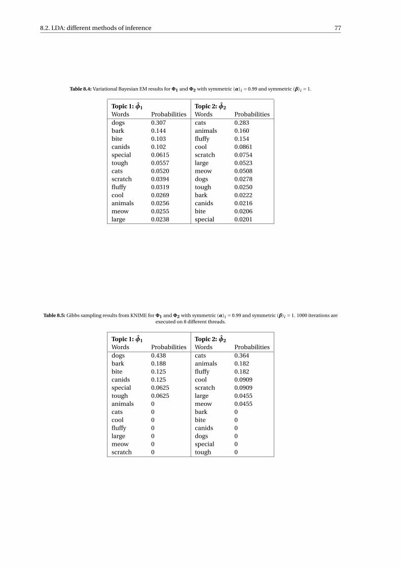
8.2. LDA: different methods of inference 77
Table 8.4: Variational Bayesian EM results forΦ1 andΦ2 with symmetric (α)i = 0.99 and symmetric (β)i = 1.
Topic 1: φ1 Topic 2: φ2
Words Probabilities Words Probabilitiesdogs 0.307 cats 0.283bark 0.144 animals 0.160bite 0.103 fluffy 0.154canids 0.102 cool 0.0861special 0.0615 scratch 0.0754tough 0.0557 large 0.0523cats 0.0520 meow 0.0508scratch 0.0394 dogs 0.0278fluffy 0.0319 tough 0.0250cool 0.0269 bark 0.0222animals 0.0256 canids 0.0216meow 0.0255 bite 0.0206large 0.0238 special 0.0201
Table 8.5: Gibbs sampling results from KNIME forΦ1 andΦ2 with symmetric (α)i = 0.99 and symmetric (β)i = 1. 1000 iterations areexecuted on 8 different threads.
Topic 1: φ1 Topic 2: φ2
Words Probabilities Words Probabilitiesdogs 0.438 cats 0.364bark 0.188 animals 0.182bite 0.125 fluffy 0.182canids 0.125 cool 0.0909special 0.0625 scratch 0.0909tough 0.0625 large 0.0455animals 0 meow 0.0455cats 0 bark 0cool 0 bite 0fluffy 0 canids 0large 0 dogs 0meow 0 special 0scratch 0 tough 0
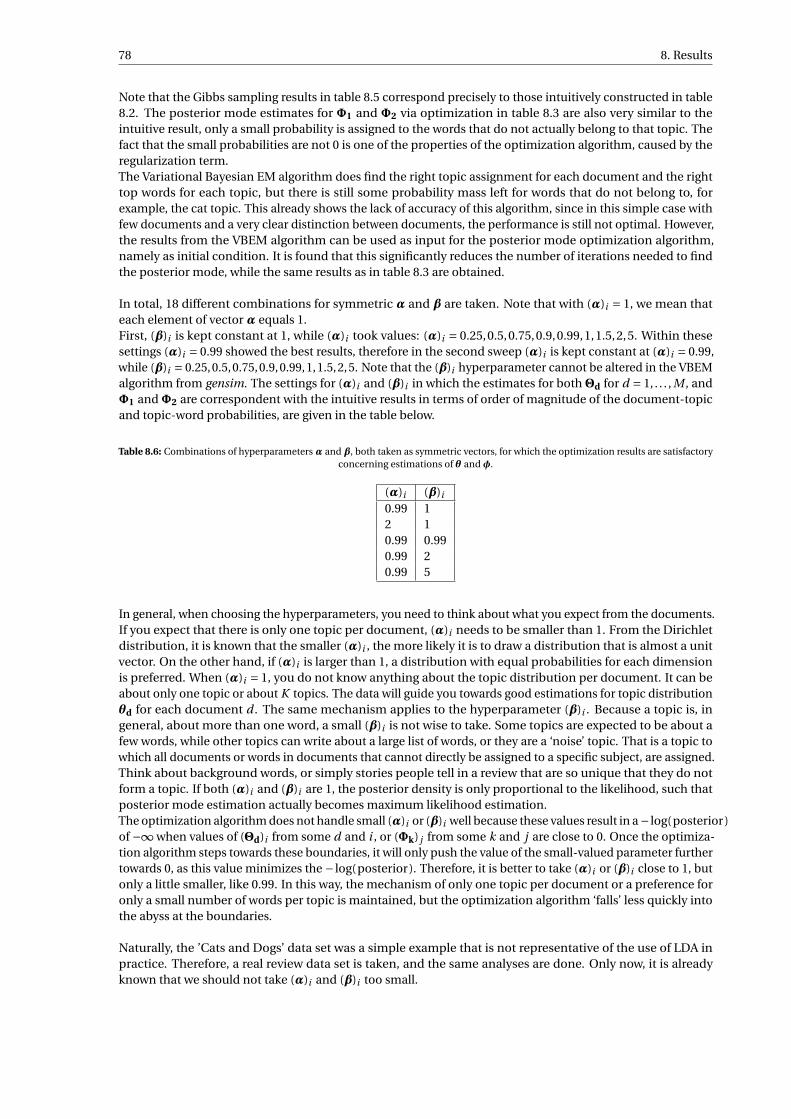
78 8. Results
Note that the Gibbs sampling results in table 8.5 correspond precisely to those intuitively constructed in table8.2. The posterior mode estimates for Φ1 and Φ2 via optimization in table 8.3 are also very similar to theintuitive result, only a small probability is assigned to the words that do not actually belong to that topic. Thefact that the small probabilities are not 0 is one of the properties of the optimization algorithm, caused by theregularization term.The Variational Bayesian EM algorithm does find the right topic assignment for each document and the righttop words for each topic, but there is still some probability mass left for words that do not belong to, forexample, the cat topic. This already shows the lack of accuracy of this algorithm, since in this simple case withfew documents and a very clear distinction between documents, the performance is still not optimal. However,the results from the VBEM algorithm can be used as input for the posterior mode optimization algorithm,namely as initial condition. It is found that this significantly reduces the number of iterations needed to findthe posterior mode, while the same results as in table 8.3 are obtained.
In total, 18 different combinations for symmetric α and β are taken. Note that with (α)i = 1, we mean thateach element of vector α equals 1.First, (β)i is kept constant at 1, while (α)i took values: (α)i = 0.25,0.5,0.75,0.9,0.99,1,1.5,2,5. Within thesesettings (α)i = 0.99 showed the best results, therefore in the second sweep (α)i is kept constant at (α)i = 0.99,while (β)i = 0.25,0.5,0.75,0.9,0.99,1,1.5,2,5. Note that the (β)i hyperparameter cannot be altered in the VBEMalgorithm from gensim. The settings for (α)i and (β)i in which the estimates for bothΘd for d = 1, . . . , M , andΦ1 andΦ2 are correspondent with the intuitive results in terms of order of magnitude of the document-topicand topic-word probabilities, are given in the table below.
Table 8.6: Combinations of hyperparameters α and β, both taken as symmetric vectors, for which the optimization results are satisfactoryconcerning estimations of θ and φ.
(α)i (β)i
0.99 12 10.99 0.990.99 20.99 5
In general, when choosing the hyperparameters, you need to think about what you expect from the documents.If you expect that there is only one topic per document, (α)i needs to be smaller than 1. From the Dirichletdistribution, it is known that the smaller (α)i , the more likely it is to draw a distribution that is almost a unitvector. On the other hand, if (α)i is larger than 1, a distribution with equal probabilities for each dimensionis preferred. When (α)i = 1, you do not know anything about the topic distribution per document. It can beabout only one topic or about K topics. The data will guide you towards good estimations for topic distributionθd for each document d . The same mechanism applies to the hyperparameter (β)i . Because a topic is, ingeneral, about more than one word, a small (β)i is not wise to take. Some topics are expected to be about afew words, while other topics can write about a large list of words, or they are a ‘noise’ topic. That is a topic towhich all documents or words in documents that cannot directly be assigned to a specific subject, are assigned.Think about background words, or simply stories people tell in a review that are so unique that they do notform a topic. If both (α)i and (β)i are 1, the posterior density is only proportional to the likelihood, such thatposterior mode estimation actually becomes maximum likelihood estimation.The optimization algorithm does not handle small (α)i or (β)i well because these values result in a− log(posterior)of −∞ when values of (Θd)i from some d and i , or (Φk) j from some k and j are close to 0. Once the optimiza-tion algorithm steps towards these boundaries, it will only push the value of the small-valued parameter furthertowards 0, as this value minimizes the − log(posterior). Therefore, it is better to take (α)i or (β)i close to 1, butonly a little smaller, like 0.99. In this way, the mechanism of only one topic per document or a preference foronly a small number of words per topic is maintained, but the optimization algorithm ‘falls’ less quickly intothe abyss at the boundaries.
Naturally, the ’Cats and Dogs’ data set was a simple example that is not representative of the use of LDA inpractice. Therefore, a real review data set is taken, and the same analyses are done. Only now, it is alreadyknown that we should not take (α)i and (β)i too small.
8.2. LDA: different methods of inference 79
8.2.2. Towards more realistic analyses: stroller data
The stroller data set consists of 2000 reviews from Amazon concerning different brands and types of strollers.The goal is to retrieve about which aspects, issues or stories people write in reviews. We expect some elementsof a stroller to each form a topic, but also a topic with only positive or negative opinion words, without manyexplanatory words, think of for example ‘Great!’ or ‘I love it’. Furthermore, there can be some reviews withspam or advertisements included in the data set. These documents are also expected to form a topic. With thisreasoning, we set the number of topics to 10: K = 10. The reviews are relatively large (sizes vary between 1 and500 words), so we want (α)i to be close to 1. In this setting, a document/review can write about only one topic,but also about five topics for example. Variation among document-topic distribution is still possible, as (α)i isclose to 1. Beforehand, we believe that there will be a slight preference for a few topics in a document. It is notlikely that a review writes about all ten topics. Therefore (α)i slightly smaller than 1 is expected to give the bestresults.
Three different methods of inference are used: Gibbs sampling using KNIME, Variational Bayesian EM usingthe gensim package in Python and Adam optimization for finding the posterior mode. The maximal vocabularysize V is set to 2000, meaning that if there are more than 2000 different words in all 2000 reviews together,those that occur the least frequently are removed.Note that, in total, K ·M (document-topic probabilities) plus K ·V (topic-word probabilities) parameters needto be estimated, resulting in at most 40000 (taking V = 2000) estimations. This parameter space is enormous,resulting in slow convergence in both the Gibbs and VBEM algorithms. Also, the optimization method hasmore problems with finding the optimum, especially when either (α)i or (β)i is smaller than 1. Therefore, theregularization term is given more weight to keep the parameter estimations away from the boundaries of thedomain [0,1].
Because it is not easily feasible to read all reviews and manually assign topics to them, we cannot comparethe inference results with natural results, as had been done for the ‘Cats and Dogs’ data set. Therefore, modelvalidation measures come into place. In section 2.4, perplexity was introduced for a general training and testset. To compute the perplexity for the LDA model, we need to define it further. For a test set consisting of Mdocuments, each having Nd words, document-topic distribution θd and given the topic-word distributions φk
for k = 1, . . . ,K , the perplexity is computed using:
Perplexity(wtest) = exp
− log(P(wtest|θ,φ))
|wtest|
∝ exp
−
∑Md=1
∑Vj=1(nd) j log
(∑Kk=1(φk) j · (θd)k
)∑M
d=1 Nd
(8.4)
The perplexity compares the inferred model with the case in which each word is equally likely, which is theleast informative model and has the highest entropy. The lower the perplexity, the better the model, that is, themore informative the model has retrieved from the data set.The computation of the perplexity for our text data is not straightforward. Every document d has its ownestimated parameter vector θd. The exact meaning and independence assumptions of all parameters in LatentDirichlet Allocation will be elaborated on in the next chapter. For now, it is important to understand that wecannot split the review data set into a set of reviews belonging to the training data set, and a set of reviewsbelonging to the test set. Namely, the parameter vectors θd for all documents d in the test set cannot beestimated. Therefore, the data set is split into a train and test set differently. Every document consists of a setof words, which can easily be split into two. The largest part, in this thesis 80% of the words (up to a roundingerror), is assigned to the training set. The remaining part of the document is then the test set. With this setting,all model parameters are estimated using the training set, and perplexity is calculated with the test set. Thismethod to compute the perplexity is proposed in [48].Another way of comparing inferred parameters can be done by looking at the logarithm of the posterior,which resembles maximum likelihood estimation, only now, instead of looking at the likelihood, we use theposterior distribution. That is the likelihood times the prior distributions. Earlier in this thesis, Bayesianstatistics was introduced. Here we made a distinction between posterior mean and posterior mode estimator.If different methods are used to estimate the posterior mode, it is straightforward to substitute these parameterestimations into the posterior distribution as a check which results in the highest posterior, or highest logposterior. Therefore, the value of the log posterior is also used for model comparison. The model with thehighest log posterior value is considered the best.
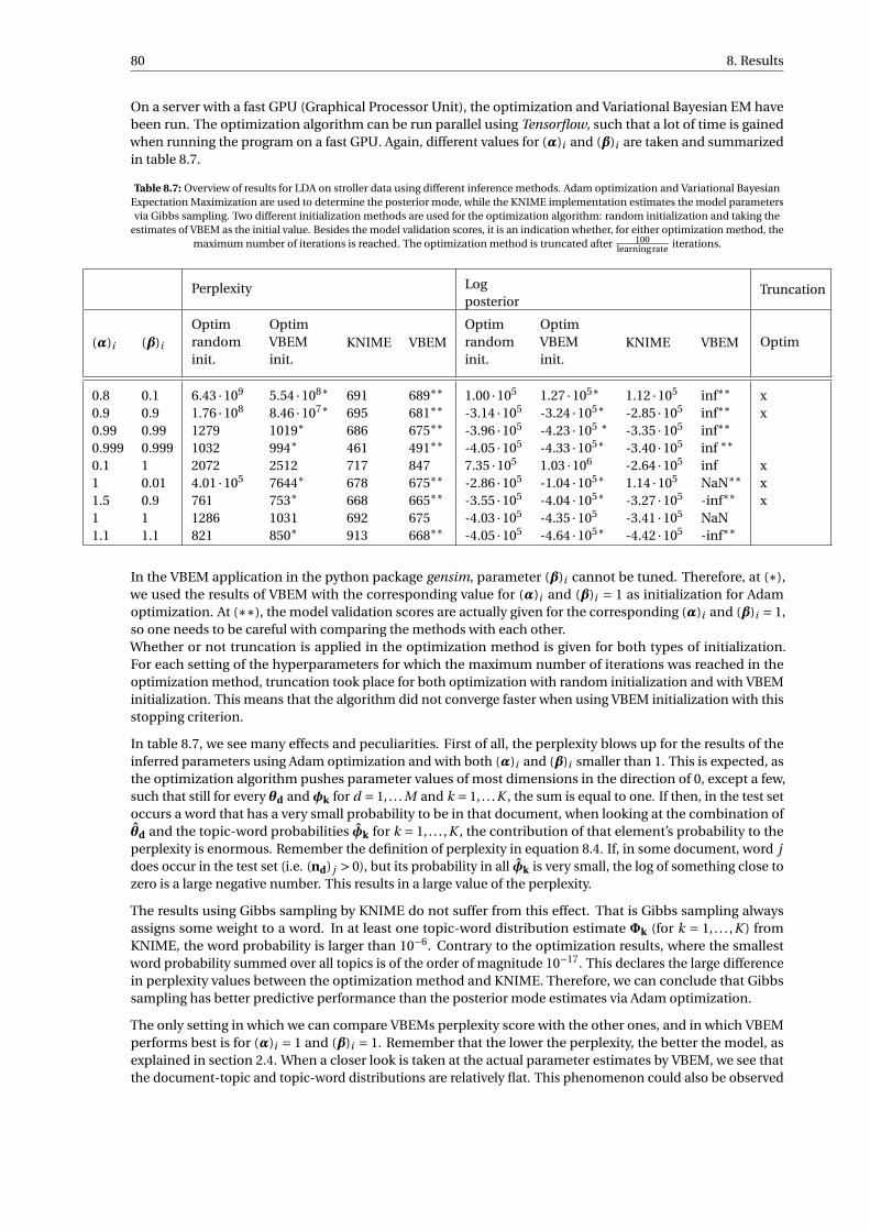
80 8. Results
On a server with a fast GPU (Graphical Processor Unit), the optimization and Variational Bayesian EM havebeen run. The optimization algorithm can be run parallel using Tensorflow, such that a lot of time is gainedwhen running the program on a fast GPU. Again, different values for (α)i and (β)i are taken and summarizedin table 8.7.
Table 8.7: Overview of results for LDA on stroller data using different inference methods. Adam optimization and Variational BayesianExpectation Maximization are used to determine the posterior mode, while the KNIME implementation estimates the model parametersvia Gibbs sampling. Two different initialization methods are used for the optimization algorithm: random initialization and taking the
estimates of VBEM as the initial value. Besides the model validation scores, it is an indication whether, for either optimization method, themaximum number of iterations is reached. The optimization method is truncated after 100
learningrate iterations.
Perplexity Logposterior
Truncation
(α)i (β)i
Optimrandominit.
OptimVBEMinit.
KNIME VBEMOptimrandominit.
OptimVBEMinit.
KNIME VBEM Optim
0.8 0.1 6.43 ·109 5.54 ·108∗ 691 689∗∗ 1.00 ·105 1.27 ·105∗ 1.12 ·105 inf∗∗ x0.9 0.9 1.76 ·108 8.46 ·107∗ 695 681∗∗ -3.14 ·105 -3.24 ·105∗ -2.85 ·105 inf∗∗ x0.99 0.99 1279 1019∗ 686 675∗∗ -3.96 ·105 -4.23 ·105 ∗ -3.35 ·105 inf∗∗0.999 0.999 1032 994∗ 461 491∗∗ -4.05 ·105 -4.33 ·105∗ -3.40 ·105 inf ∗∗0.1 1 2072 2512 717 847 7.35 ·105 1.03 ·106 -2.64 ·105 inf x1 0.01 4.01 ·105 7644∗ 678 675∗∗ -2.86 ·105 -1.04 ·105∗ 1.14 ·105 NaN∗∗ x1.5 0.9 761 753∗ 668 665∗∗ -3.55 ·105 -4.04 ·105∗ -3.27 ·105 -inf∗∗ x1 1 1286 1031 692 675 -4.03 ·105 -4.35 ·105 -3.41 ·105 NaN1.1 1.1 821 850∗ 913 668∗∗ -4.05 ·105 -4.64 ·105∗ -4.42 ·105 -inf∗∗
In the VBEM application in the python package gensim, parameter (β)i cannot be tuned. Therefore, at (∗),we used the results of VBEM with the corresponding value for (α)i and (β)i = 1 as initialization for Adamoptimization. At (∗∗), the model validation scores are actually given for the corresponding (α)i and (β)i = 1,so one needs to be careful with comparing the methods with each other.Whether or not truncation is applied in the optimization method is given for both types of initialization.For each setting of the hyperparameters for which the maximum number of iterations was reached in theoptimization method, truncation took place for both optimization with random initialization and with VBEMinitialization. This means that the algorithm did not converge faster when using VBEM initialization with thisstopping criterion.
In table 8.7, we see many effects and peculiarities. First of all, the perplexity blows up for the results of theinferred parameters using Adam optimization and with both (α)i and (β)i smaller than 1. This is expected, asthe optimization algorithm pushes parameter values of most dimensions in the direction of 0, except a few,such that still for every θd and φk for d = 1, . . . M and k = 1, . . .K , the sum is equal to one. If then, in the test setoccurs a word that has a very small probability to be in that document, when looking at the combination ofθd and the topic-word probabilities φk for k = 1, . . . ,K , the contribution of that element’s probability to theperplexity is enormous. Remember the definition of perplexity in equation 8.4. If, in some document, word jdoes occur in the test set (i.e. (nd) j > 0), but its probability in all φk is very small, the log of something close tozero is a large negative number. This results in a large value of the perplexity.
The results using Gibbs sampling by KNIME do not suffer from this effect. That is Gibbs sampling alwaysassigns some weight to a word. In at least one topic-word distribution estimate Φk (for k = 1, . . . ,K ) fromKNIME, the word probability is larger than 10−6. Contrary to the optimization results, where the smallestword probability summed over all topics is of the order of magnitude 10−17. This declares the large differencein perplexity values between the optimization method and KNIME. Therefore, we can conclude that Gibbssampling has better predictive performance than the posterior mode estimates via Adam optimization.
The only setting in which we can compare VBEMs perplexity score with the other ones, and in which VBEMperforms best is for (α)i = 1 and (β)i = 1. Remember that the lower the perplexity, the better the model, asexplained in section 2.4. When a closer look is taken at the actual parameter estimates by VBEM, we see thatthe document-topic and topic-word distributions are relatively flat. This phenomenon could also be observed
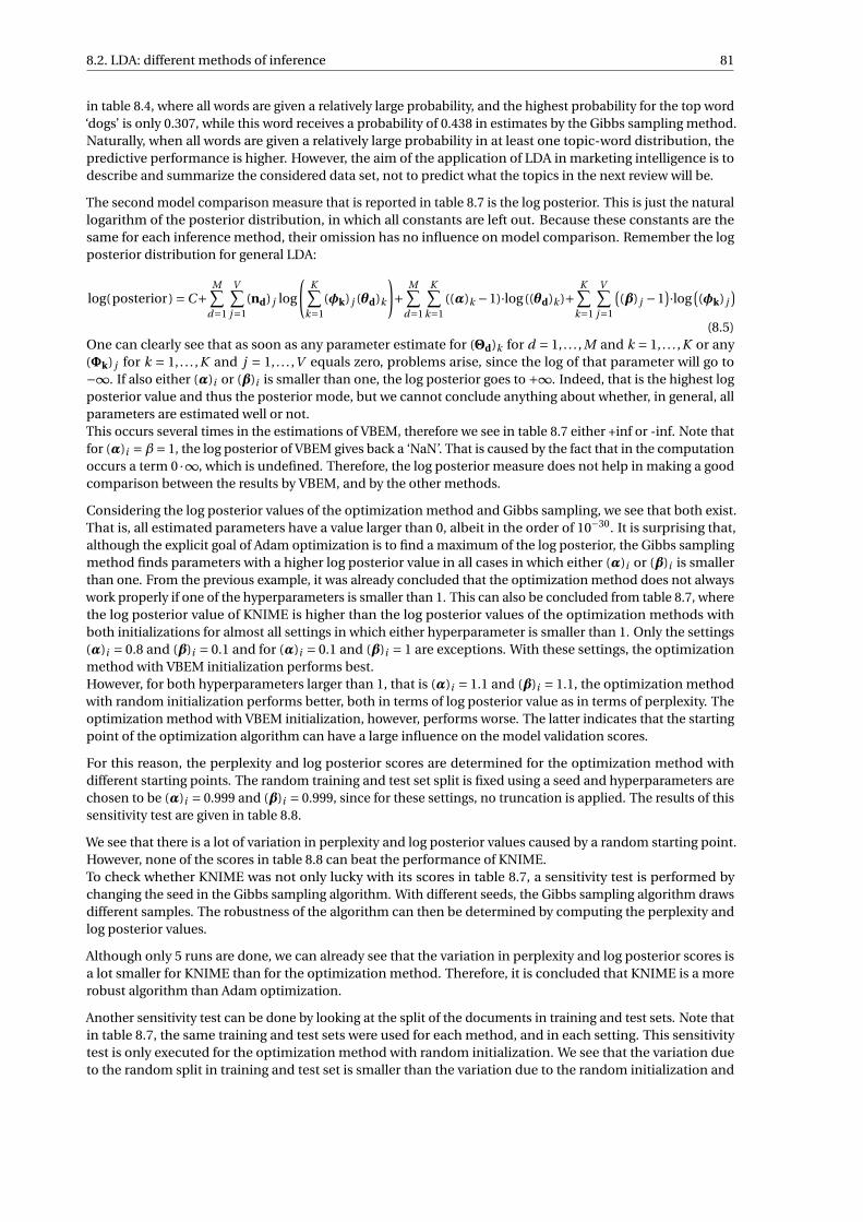
8.2. LDA: different methods of inference 81
in table 8.4, where all words are given a relatively large probability, and the highest probability for the top word‘dogs’ is only 0.307, while this word receives a probability of 0.438 in estimates by the Gibbs sampling method.Naturally, when all words are given a relatively large probability in at least one topic-word distribution, thepredictive performance is higher. However, the aim of the application of LDA in marketing intelligence is todescribe and summarize the considered data set, not to predict what the topics in the next review will be.
The second model comparison measure that is reported in table 8.7 is the log posterior. This is just the naturallogarithm of the posterior distribution, in which all constants are left out. Because these constants are thesame for each inference method, their omission has no influence on model comparison. Remember the logposterior distribution for general LDA:
log(posterior) =C+M∑
d=1
V∑j=1
(nd) j log
(K∑
k=1(φk) j (θd)k
)+
M∑d=1
K∑k=1
((α)k −1)·log((θd)k )+K∑
k=1
V∑j=1
((β) j −1
)·log((φk) j
)(8.5)
One can clearly see that as soon as any parameter estimate for (Θd)k for d = 1, . . . , M and k = 1, . . . ,K or any(Φk) j for k = 1, . . . ,K and j = 1, . . . ,V equals zero, problems arise, since the log of that parameter will go to−∞. If also either (α)i or (β)i is smaller than one, the log posterior goes to +∞. Indeed, that is the highest logposterior value and thus the posterior mode, but we cannot conclude anything about whether, in general, allparameters are estimated well or not.This occurs several times in the estimations of VBEM, therefore we see in table 8.7 either +inf or -inf. Note thatfor (α)i =β= 1, the log posterior of VBEM gives back a ‘NaN’. That is caused by the fact that in the computationoccurs a term 0 ·∞, which is undefined. Therefore, the log posterior measure does not help in making a goodcomparison between the results by VBEM, and by the other methods.
Considering the log posterior values of the optimization method and Gibbs sampling, we see that both exist.That is, all estimated parameters have a value larger than 0, albeit in the order of 10−30. It is surprising that,although the explicit goal of Adam optimization is to find a maximum of the log posterior, the Gibbs samplingmethod finds parameters with a higher log posterior value in all cases in which either (α)i or (β)i is smallerthan one. From the previous example, it was already concluded that the optimization method does not alwayswork properly if one of the hyperparameters is smaller than 1. This can also be concluded from table 8.7, wherethe log posterior value of KNIME is higher than the log posterior values of the optimization methods withboth initializations for almost all settings in which either hyperparameter is smaller than 1. Only the settings(α)i = 0.8 and (β)i = 0.1 and for (α)i = 0.1 and (β)i = 1 are exceptions. With these settings, the optimizationmethod with VBEM initialization performs best.However, for both hyperparameters larger than 1, that is (α)i = 1.1 and (β)i = 1.1, the optimization methodwith random initialization performs better, both in terms of log posterior value as in terms of perplexity. Theoptimization method with VBEM initialization, however, performs worse. The latter indicates that the startingpoint of the optimization algorithm can have a large influence on the model validation scores.
For this reason, the perplexity and log posterior scores are determined for the optimization method withdifferent starting points. The random training and test set split is fixed using a seed and hyperparameters arechosen to be (α)i = 0.999 and (β)i = 0.999, since for these settings, no truncation is applied. The results of thissensitivity test are given in table 8.8.
We see that there is a lot of variation in perplexity and log posterior values caused by a random starting point.However, none of the scores in table 8.8 can beat the performance of KNIME.To check whether KNIME was not only lucky with its scores in table 8.7, a sensitivity test is performed bychanging the seed in the Gibbs sampling algorithm. With different seeds, the Gibbs sampling algorithm drawsdifferent samples. The robustness of the algorithm can then be determined by computing the perplexity andlog posterior values.
Although only 5 runs are done, we can already see that the variation in perplexity and log posterior scores isa lot smaller for KNIME than for the optimization method. Therefore, it is concluded that KNIME is a morerobust algorithm than Adam optimization.
Another sensitivity test can be done by looking at the split of the documents in training and test sets. Note thatin table 8.7, the same training and test sets were used for each method, and in each setting. This sensitivitytest is only executed for the optimization method with random initialization. We see that the variation dueto the random split in training and test set is smaller than the variation due to the random initialization and
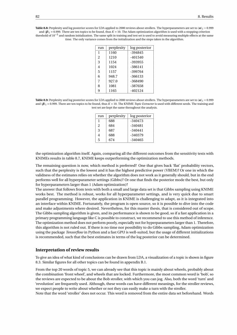
82 8. Results
Table 8.8: Perplexity and log posterior scores for LDA applied to 2000 reviews about strollers. The hyperparameters are set to (α)i = 0.999and (β)i = 0.999. There are ten topics to be found, thus K = 10. The Adam optimization algorithm is used with a stopping criterion
threshold of 10−3 and random initialization. The same split in training and test set is used to avoid measuring multiple effects at the sametime. The only variance comes from the initialization and the steps taken in the algorithm.
run perplexity log posterior1 1160 -3948452 1210 -4015403 1154 -3939554 1024 -3861415 1157 -3997646 948.7 -3661337 927.0 -3684908 1081 -3876589 1165 -402124
Table 8.9: Perplexity and log posterior scores for LDA applied to 2000 reviews about strollers. The hyperparameters are set to (α)i = 0.999and (β)i = 0.999. There are ten topics to be found, thus K = 10. The KNIME Topic Extractor is used with different seeds. The training and
test set are kept the same throughout the analysis.
run perplexity log posterior1 688 -3404732 684 -3404813 687 -3404414 688 -3403795 674 -340465
the optimization algorithm itself. Again, comparing all the different outcomes from the sensitivity tests withKNIMEs results in table 8.7, KNIME keeps outperforming the optimization methods.
The remaining question is now, which method is preferred? One that gives back ‘flat’ probability vectors,such that the perplexity is the lowest and it has the highest predictive power (VBEM)? Or one in which thevalidness of the estimates relies on whether the algorithm does not work as it generally should, but in the endperforms well for all hyperparameter settings (Gibbs)? Or one that finds the posterior mode the best, but onlyfor hyperparameters larger than 1 (Adam optimization)?The answer that follows from tests with both a small and large data set is that Gibbs sampling using KNIMEworks best. The method is robust, works for all hyperparameter settings, and is very quick due to smartparallel programming. However, the application in KNIME is challenging to adapt, as it is integrated intoan interface within KNIME. Fortunately, the program is open source, so it is possible to dive into the codeand make adjustments where desired. Nevertheless, for this master thesis, that is considered out of scope.The Gibbs sampling algorithm is given, and its performance is shown to be good, so if a fast application in aprimary programming language like C is possible to construct, we recommend to use this method of inference.The optimization method does not perform poorly, especially not for hyperparameters larger than 1. Therefore,this algorithm is not ruled out. If there is no time nor possibility to do Gibbs sampling, Adam optimizationusing the package Tensorflow in Python and a fast GPU is well-suited, but the usage of different initializationsis recommended, such that the best estimates in terms of the log posterior can be determined.
Interpretation of review results
To give an idea of what kind of conclusions can be drawn from LDA, a visualization of a topic is shown in figure8.3. Similar figures for all other topics can be found in appendix B.1.
From the top 20 words of topic 5, we can already see that this topic is mainly about wheels, probably aboutthe combination ‘front wheel’, and wheels that are locked. Furthermore, the most common word is ‘bob’, sothe reviews are expected to be about the Bob stroller, with which you can jog. Also, both the word ‘turn’ and‘revolution’ are frequently used. Although, these words can have different meanings, for the stroller reviews,we expect people to write about whether or not they can easily make a turn with the stroller.Note that the word ‘stroller’ does not occur. This word is removed from the entire data set beforehand. Words
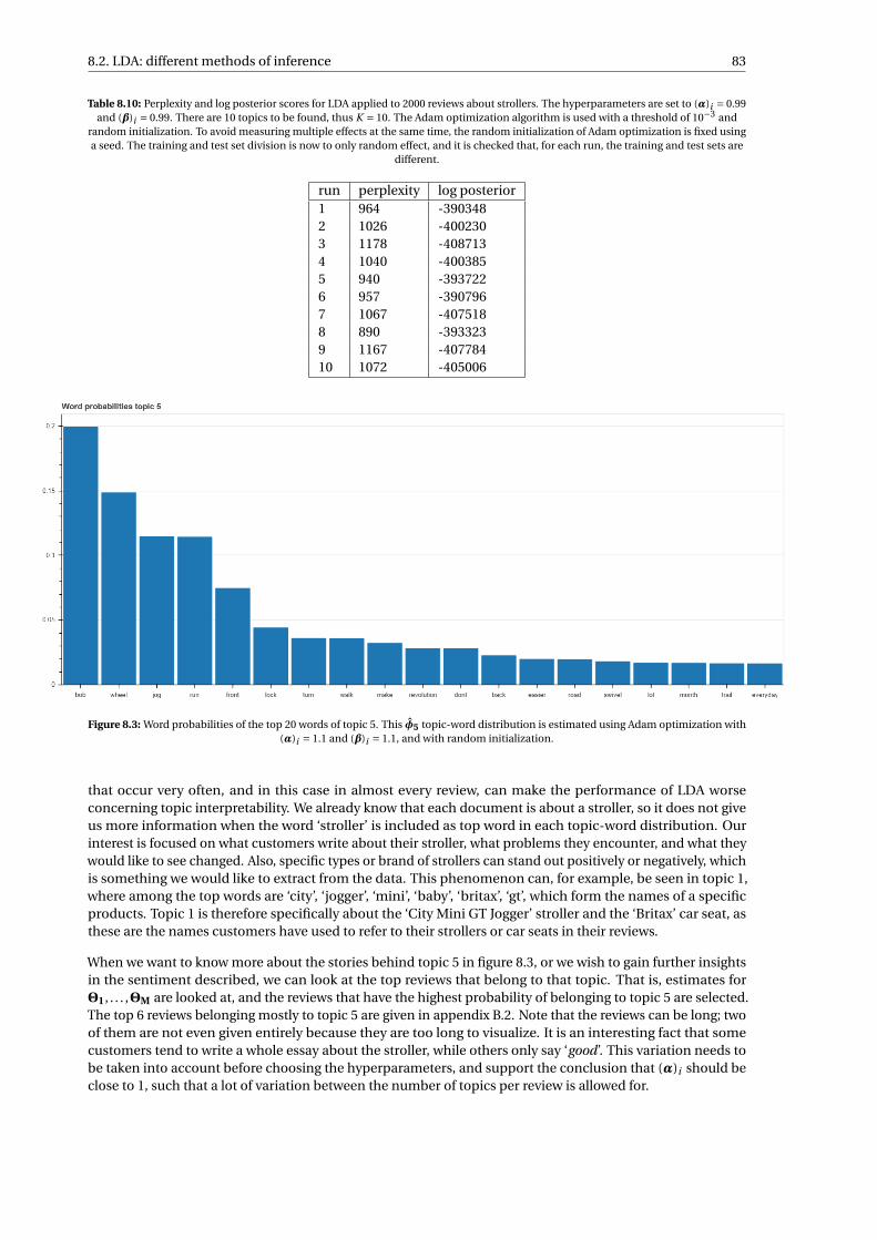
8.2. LDA: different methods of inference 83
Table 8.10: Perplexity and log posterior scores for LDA applied to 2000 reviews about strollers. The hyperparameters are set to (α)i = 0.99and (β)i = 0.99. There are 10 topics to be found, thus K = 10. The Adam optimization algorithm is used with a threshold of 10−3 and
random initialization. To avoid measuring multiple effects at the same time, the random initialization of Adam optimization is fixed usinga seed. The training and test set division is now to only random effect, and it is checked that, for each run, the training and test sets are
different.
run perplexity log posterior1 964 -3903482 1026 -4002303 1178 -4087134 1040 -4003855 940 -3937226 957 -3907967 1067 -4075188 890 -3933239 1167 -40778410 1072 -405006
Figure 8.3: Word probabilities of the top 20 words of topic 5. This φ5 topic-word distribution is estimated using Adam optimization with(α)i = 1.1 and (β)i = 1.1, and with random initialization.
that occur very often, and in this case in almost every review, can make the performance of LDA worseconcerning topic interpretability. We already know that each document is about a stroller, so it does not giveus more information when the word ‘stroller’ is included as top word in each topic-word distribution. Ourinterest is focused on what customers write about their stroller, what problems they encounter, and what theywould like to see changed. Also, specific types or brand of strollers can stand out positively or negatively, whichis something we would like to extract from the data. This phenomenon can, for example, be seen in topic 1,where among the top words are ‘city’, ‘jogger’, ‘mini’, ‘baby’, ‘britax’, ‘gt’, which form the names of a specificproducts. Topic 1 is therefore specifically about the ‘City Mini GT Jogger’ stroller and the ‘Britax’ car seat, asthese are the names customers have used to refer to their strollers or car seats in their reviews.
When we want to know more about the stories behind topic 5 in figure 8.3, or we wish to gain further insightsin the sentiment described, we can look at the top reviews that belong to that topic. That is, estimates forΘ1, . . . ,ΘM are looked at, and the reviews that have the highest probability of belonging to topic 5 are selected.The top 6 reviews belonging mostly to topic 5 are given in appendix B.2. Note that the reviews can be long; twoof them are not even given entirely because they are too long to visualize. It is an interesting fact that somecustomers tend to write a whole essay about the stroller, while others only say ‘good’. This variation needs tobe taken into account before choosing the hyperparameters, and support the conclusion that (α)i should beclose to 1, such that a lot of variation between the number of topics per review is allowed for.

84 8. Results
From the reviews, we can deduce that topic 5 is indeed about the Bob jogger stroller, with which you can easilyjog. There are two modes of this stroller: walk and jog mode. In the jog mode, the front wheel is locked, suchthat the jogger keeps going straight. The customers think you can easily switch the front wheel from beinglocked to unlocked and are satisfied which this option. Also, they are happy with the front wheel being lockedwhile jogging, as this makes jogging with it easier. Two customers write about the wrist strap that keeps thestroller attached to you when you are jogging. Both are not using it because they think it is dangerous to use.Only one customer is not satisfied, as his/her stroller’s front wheel locks on its own every time, while this is notdesired.
Instead of having to read 1000 reviews and manually summarize the major themes in the whole data set,LDA gives us the main topics. From the highest probability words (via estimates φk), the story of the topiccan already be speculated about, but when reading the top reviews (determined from θd estimates) for thatspecific topic, a more detailed story is retrieved. With this information, a next-generation type of strollers canbe improved, or marketing strategies can be adjusted.
In chapter 7 about validity of the topic-word distribution estimates, it is said that even after having estimatedmodel parameters Θ and Φ and getting interpretable results, attention needs to be paid to their validness.The number of topics K is chosen based on intuition and expectation. However, it is not certain that K fitsthe data. It might be the case that there are more topics hidden in the data than we have set in K , whichresults in two subjects being joined in one topic in the current model. On the other hand, when K is too largecompared to the actual number of topics in the data set, some topics will fit noise. To this end, in chapter 7, theNKLS (normalized Kullback-Leibler divergence similarity) and NJSS (normalized symmetric Jensen-Shannondivergence similarity) measures are defined. These measures2 indicate the extent of similarity between twotopics. That is, if two topics both fit noise, they will be more similar than two topics that have their own stories.The NKLS scores are computed and summarized in table 8.11 for the estimates of allΦk for k = 1, . . . ,K of thestroller data set determined with Adam optimization. The NJSS scores of the same estimates are shown intable 8.12.
Table 8.11: Normalized KL-divergence scores between all estimated topic-word distributions φ1, . . . ,φK, which are determined for thestroller data using Adam optimization with symmetric (α)i = 1.1 and (β)i = 1.1, and setting the number of topics K = 10.
φ0 φ1 φ2 φ3 φ4 φ5 φ6 φ7 φ8 φ9
φ0 1 0.262 0.105 0.114 0.584 0.334 0.378 0.483 0.327 0.465φ1 0.262 1 0.049 0.106 0.354 0.324 0.322 0.395 0.193 0.421φ2 0.105 0.049 1 0 0.359 0.069 0.281 0.132 0.104 0.146φ3 0.113 0.106 0 1 0.185 0.073 0.211 0.190 0.010 0.197φ4 0.584 0.354 0.359 0.185 1 0.446 0.550 0.580 0.456 0.565φ5 0.334 0.324 0.069 0.073 0.446 1 0.424 0.452 0.241 0.327φ6 0.377 0.322 0.281 0.211 0.550 0.424 1 0.463 0.392 0.349φ7 0.483 0.395 0.132 0.190 0.580 0.452 0.463 1 0.459 0.639φ8 0.327 0.193 0.104 0.010 0.456 0.241 0.391 0.459 1 0.454φ9 0.465 0.421 0.146 0.197 0.565 0.327 0.349 0.639 0.455 1
There are no remarkable differences between the NKLS and NJSS scores in tables 8.11 and 8.12. All non-zeroand non-one NJSS scores are smaller than the corresponding NKLS scores, but, in general, the same conclu-sions can be drawn from both tables. Therefore, we will only focus on the NKLS scores from table 8.11.Naturally, there are diagonals with NKLS = 1, as each topic-word distribution is exactly the same as itself.Furthermore, there are two zeros for the combination φ2 and φ3, meaning that these two topic-word distribu-tions are the most different among all combinations. All other NKLS values are in between, meaning that thecloser to zero, the more similar two topic-word probability vectors are. In chapter 7, we have said that when aNKLS score is higher than 0.9, two φs are considered to be about the same topic. Fortunately, in table 8.11 allsimilarity scores (except the diagonal of course) are below 0.9, meaning that each topic can be interpretedseparately. This might even be an indicator that K can be increased, as we are not fitting noise yet.
It is wise to always perform this check after having estimated all topic-word distributions. In this way, one candraw better conclusions, and noise is observed beforehand, instead of after having read the top reviews for
2They are not measures in the mathematical sense.

8.2. LDA: different methods of inference 85
Table 8.12: Normalized symmetric JS-divergence similarity scores between all estimated topic-word distributions φ1, . . . ,φK, which aredetermined for the stroller data using Adam optimization with symmetric (α)i = 1.1 and (β)i = 1.1, and setting the number of topics
K = 10.
φ0 φ1 φ2 φ3 φ4 φ5 φ6 φ7 φ8 φ9
φ0 1 0.253 0.087 0.106 0.494 0.320 0.323 0.451 0.332 0.458φ1 0.252 1 0.034 0.130 0.336 0.347 0.267 0.407 0.237 0.415φ2 0.087 0.034 1 0 0.283 0.043 0.211 0.148 0.073 0.128φ3 0.106 0.130 0 1 0.176 0.103 0.211 0.195 0.015 0.238φ4 0.493 0.336 0.283 0.176 1 0.453 0.498 0.577 0.449 0.532φ5 0.320 0.347 0.043 0.103 0.453 1 0.414 0.457 0.299 0.365φ6 0.323 0.267 0.211 0.211 0.498 0.414 1 0.456 0.361 0.338φ7 0.451 0.407 0.148 0.195 0.577 0.457 0.456 1 0.460 0.619φ8 0.332 0.237 0.073 0.015 0.449 0.299 0.361 0.460 1 0.441φ9 0.457 0.415 0.128 0.238 0.532 0.365 0.338 0.619 0.441 1
each topic, and not being able to retrieve a coherent story behind the topic. As the difference between theNKLS and NJSS scores are so small, the similarity score based on the symmetrized Kullback-Leibler divergenceis preferred, as a more thorough study is performed in [24].
86 8. Results
8.3. LDA with syntax and sentiment: is this the future?The model of LDA with syntax and sentiment is an extension of basic LDA; thus, the parameter space in whichwe search for the posterior mode location is larger. In this extension, we look for a topic distribution perdocument, a sentiment distribution per document, and word distributions per topic-sentiment combination.In LDA with syntax and sentiment, a topic is drawn per phrase instead of per word as in plain LDA. Also,a sentiment is assigned to each phrase, and all words in a phrase or sentence are drawn from the worddistribution for the corresponding topic-sentiment combination belonging to that phrase. Although differentmethods of inference were researched for basic LDA, in this extension, only Adam optimization is used to findthe posterior mode estimates for respectivelyΘd for d = 1, . . . , M ,Πd for d = 1, . . . , M , andΦk,o for k = 1, . . . ,Kand o = 1, . . . ,Σ.
The increased number of parameters to be estimated and the addition of sentiments make the form of theposterior density for this LDA extension more complicated compared to the one for basic LDA. This results ina slower convergence in the optimization. Furthermore, a count array with the frequencies of each word perphrase and per document needs to be computed. The latter is the most significant bottleneck encountered inthe inference of LDA with syntax and sentiment. This count matrix3 has proportions that large, that the usedcomputer server cannot handle it in terms of memory. The count matrix consists of floating points with 32 bits,which is required for steps in the optimization algorithm to prevent accuracy loss. For the application of LDAwith syntax and sentiment to 200 reviews with at most 100 phrases (otherwise they are removed from the dataset), and a vocabulary size of 1000, the count matrix has 200 ·100 ·1000 = 2 ·107 elements, and each elementis a floating point of 32 bits. This results in a count matrix that is too large to keep in memory. Although thearray consists of many zeros, it is not possible to convert it to a sparse array because the Adam optimizationimplementation in Tensorflow cannot handle sparse arrays. For this reason, LDA with syntax and sentiment inthe current implementation can only be used for small data sets.
In this section, first, the algorithm and model are tested for a simulated data set of which the model parametersare known. Then, we gain more intuition of the model by its application to a toy data set. Consequently, withmore knowledge about which settings to use in Adam optimization to obtain good estimates, the algorithm istested on the stroller data set. Unfortunately, only a minimal number of reviews can be used due to memoryproblems.
8.3.1. Model testing on gibberish
First, we generate a small data set following the generative process of LDA with syntax and sentiment fromchapter 6. A data set has been created consisting of 20 documents with 2 hidden topics. As usual, there arethree sentiments: positive, neutral and negative. There are 26 words in the vocabulary, from which 5 arepositive, 9 are negative, and the rest is neutral. Because we want distinct topics that can relatively easily befound by the inference method, hyperparameters α and γ are symmetric and set to respectively (0.5,0.5) and(0.5,0.5,0.5). These form the parameters of a Dirichlet prior. With all parameters being smaller than 1, weexpect the documents to be mostly about a single topic and to have one sentiment. The last hyperparameter isβo for o = 1,2,3. In β1, the hyperparameter vector for the positive sentiment topic-word distribution, 50% ofthe probability mass is given to the positive words, and the other half is given to the neutral and negative wordstogether. Then, in β2, 70% of the probability mass is given to the neutral words, and 30% to the positive andnegative words. A higher percentage is chosen here because there are more neutral words in the vocabularythan positive words, and we want the values of each βo to be of the same order of magnitude. Lastly, in β3,60% of the probability mass is given to the negative words, and the rest to the positive and neutral words.With these hyperparameters, we can drawΘd from Dirichlet(α) andΠd from Dirichlet(γ) for each documentd ∈ 1, . . . , M . Subsequently, for each o ∈ 1,2,3 and k = 1,2, we drawΦk,o from Dirichlet(βo). To constructdocuments, we first need to draw a number of phrases Sd for each document. This is done using a Poisson(2)distribution. Each document consists of at least 10 sentences plus S, where S ∼ Poisson(2). Also the number ofwords per phrase is random, and is drawn from a Poisson(1) distribution. The minimal number of words is 5,to which the Poisson draw is added.Consequently, with all θd, πd and Sd being generated, we can draw a topic and a sentiment for each phrase ineach document. Then, given the topic-sentiment combination and the number of words in each sentence,words can be drawn. This results in a gibberish data set as can be seen in tables B.2 and B.3 in appendix B.3.
3Strictly speaking, this is an array with size N ×maxd Sd ×V . In Tensorflow, the variable type is a tensor with the aforementioned shape.

8.3. LDA with syntax and sentiment: is this the future? 87
However, the values of the latent random variables in the model,Θd for d = 1, . . . , M ,Πd for d = 1, . . . , M , andΦk,o for k = 1, . . . ,K and o = 1, . . . ,Σ, are known, and we can check if the posterior mode estimates determinedby Adam optimization correspond to the true values.
Adam optimization for LDA with syntax and sentiment has to deal with a large parameter space in which itsearches for find the maximum (i.e. the posterior mode). If we set the values of one hyperparameter vector αor γ smaller than 1, it quickly falls into the abyss at the boundaries, as explained in the previous section forAdam optimization applied to basic LDA. Therefore, we choose the values of (α)i and (γ)i to be larger than 1.The best posterior mode estimates forΘ andΠ are obtained for α= (1.8,1.8) and γ= (1.1,1.1). From runs withdifferent hyperparameter choices, we conclude that the algorithm quickly ‘decides’ that a document belongs toonly one topic, even if we set (α)i larger than 1. Therefore, this hyperparameter vector has larger values than γ.It is more challenging to find the settings of hyperparameter vectors βo with o = 1,2,3 for which the posteriormode estimates correspond with the true parameters. Empirically, we found that the best settings for βo witho = 1,2,3 are obtained if they are constructed by applying 90% of the probability mass to respectively thepositive, neutral, or negative words. Consequently, the obtained vectors are multiplied by 50 for the positivehyperparameter vector β1, and 40 for both the neutral and negative hyperparameter vectors β2 and β3.
But how can we determine which estimates are the best? For the computation of the perplexity, we need tosplit up the data set into a training and test set. Because LDA with syntax and sentiment focuses on topicsand sentiments on a sentence-level, and, in practice, many reviews consists only of a few sentences, it is notwise to split. Therefore, we have reported the estimates ofΘd for d = 1, . . . , M ,Πd for d = 1, . . . , M , andΦk,o fork = 1, . . . ,K and o = 1, . . . ,Σ, and compared them manually with the corresponding true parameters.
Firstly, we take a look at the posterior mode estimates of all document-topic distributions. In table 8.13, thetrue values of θd for d = 1, . . . , M are shown, and in table 8.14, the corresponding estimates are given.
Table 8.13: Simulated document-topic distributions that areindependently drawn from a Dirichlet(0.5,0.5) distribution.
d (θd)1 (θd)2
1 0.176 0.8242 0.878 0.1223 0.999 0.0014 0.971 0.0295 0.332 0.6686 0.821 0.1797 0.839 0.1618 0.989 0.0119 0.973 0.02710 0.973 0.02711 0.017 0.98312 0.244 0.75613 0.599 0.40114 0.979 0.02115 0.013 0.98716 0.931 0.06917 0.781 0.21918 1.000 0.00019 0.426 0.57420 0.932 0.068
Table 8.14: Posterior mode estimates of the document-topicdistributions of the simulated data, determined with Adam
optimization in which the hyperparameter settings are(α)i = 1.8, (γ)i = 1.1, and βo for o = 1,2,3 constructed asdescribed above. A learning rate of 0.0001 and random
initialization have been used.
d (θd)1 (θd)2
1 0.059 0.9412 0.931 0.0693 0.941 0.0594 0.945 0.0555 0.245 0.7556 0.818 0.1827 0.845 0.1558 0.931 0.0699 0.945 0.05510 0.778 0.22211 0.059 0.94112 0.534 0.46613 0.651 0.34914 0.941 0.05915 0.055 0.94516 0.868 0.13217 0.759 0.24118 0.931 0.06919 0.222 0.77820 0.857 0.143
The estimates are considered good if the following principles are satisfied. The allocation of the main topiccorresponds to the true allocation, that is, if a document is mainly about one topic (for example document 3),this is also the case in the estimation results. Secondly, if a document is about both topics (for example topic
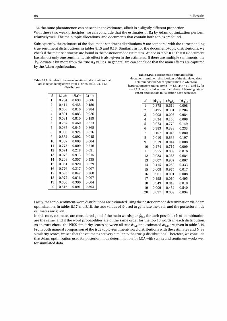
88 8. Results
13), the same phenomenon can be seen in the estimates, albeit in a slightly different proportion.With these two weak principles, we can conclude that the estimates of Θd by Adam optimization performrelatively well. The main topic allocations, and documents that contain both topics are found.
Subsequently, the estimates of the document-sentiment distributions π are compared with the correspondingtrue sentiment distributions in tables 8.15 and 8.16. Similarly as for the document-topic distributions, wecheck if the main sentiments are found in the posterior mode estimates. We see in table 8.16 that if a documenthas almost only one sentiment, this effect is also given in the estimates. If there are multiple sentiments, theπd, deviate a bit more from the true πd values. In general, we can conclude that the main effects are capturedby the Adam optimization.
Table 8.15: Simulated document-sentiment distributions thatare independently drawn from a Dirichlet(0.5, 0.5, 0.5)
distribution.
d (πd)1 (πd)2 (πd)3
1 0.294 0.699 0.0062 0.414 0.435 0.1503 0.006 0.010 0.9844 0.891 0.083 0.0265 0.031 0.810 0.1596 0.267 0.460 0.2737 0.087 0.045 0.8688 0.000 0.924 0.0769 0.862 0.092 0.04510 0.387 0.609 0.00411 0.775 0.009 0.21612 0.091 0.218 0.69113 0.072 0.913 0.01514 0.208 0.357 0.43515 0.051 0.920 0.02916 0.776 0.217 0.00717 0.693 0.047 0.26018 0.977 0.016 0.00719 0.000 0.396 0.60420 0.516 0.091 0.393
Table 8.16: Posterior mode estimates of thedocument-sentiment distributions of the simulated data,
determined with Adam optimization in which thehyperparameter settings are (α)i = 1.8, (γ)i = 1.1, and βo foro = 1,2,3 constructed as described above. A learning rate of
0.0001 and random initialization have been used.
d (πd)1 (πd)2 (πd)3
1 0.378 0.614 0.0082 0.495 0.301 0.2043 0.008 0.008 0.9844 0.834 0.158 0.0085 0.073 0.778 0.1496 0.383 0.383 0.2337 0.107 0.013 0.8808 0.010 0.883 0.1079 0.979 0.014 0.00810 0.274 0.717 0.00911 0.975 0.009 0.01612 0.083 0.233 0.68413 0.007 0.987 0.00714 0.415 0.252 0.33315 0.008 0.975 0.01716 0.901 0.091 0.00817 0.495 0.010 0.49518 0.949 0.042 0.01019 0.009 0.452 0.54020 0.097 0.009 0.894
Lastly, the topic-sentiment-word distributions are estimated using the posterior mode determination via Adamoptimization. In tables 8.17 and 8.18, the true values ofΦ used to generate the data, and the posterior modeestimates are given.In this case, estimates are considered good if the main words per φk,o for each possible (k,o)-combinationare the same, and if the word probabilities are of the same order for the top 10 words in each distribution.As an extra check, the NJSS similarity scores between all true φk,o and estimated φk,o are given in table 8.19.From both manual comparison of the true topic-sentiment-word distributions with the estimates and NJSSsimilarity scores, we see that the estimates are very similar to the true φ distributions. Therefore, we concludethat Adam optimization used for posterior mode determination for LDA with syntax and sentiment works wellfor simulated data.
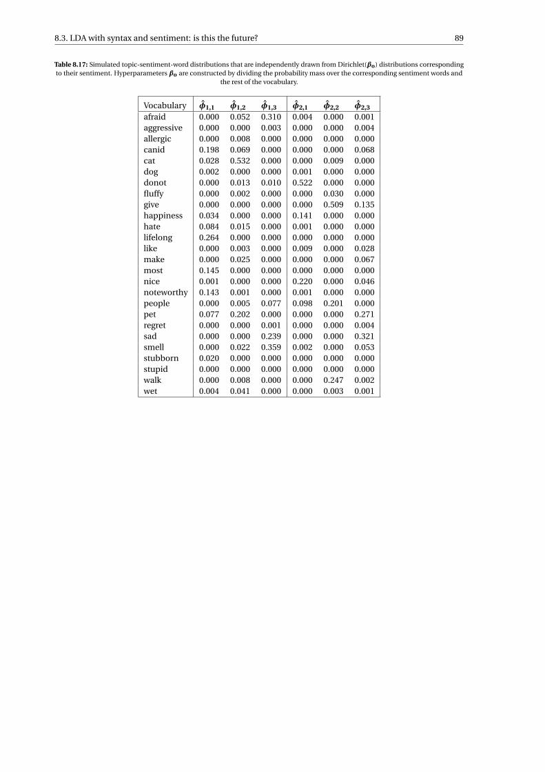
8.3. LDA with syntax and sentiment: is this the future? 89
Table 8.17: Simulated topic-sentiment-word distributions that are independently drawn from Dirichlet(βo) distributions correspondingto their sentiment. Hyperparameters βo are constructed by dividing the probability mass over the corresponding sentiment words and
the rest of the vocabulary.
Vocabulary φ1,1 φ1,2 φ1,3 φ2,1 φ2,2 φ2,3
afraid 0.000 0.052 0.310 0.004 0.000 0.001aggressive 0.000 0.000 0.003 0.000 0.000 0.004allergic 0.000 0.008 0.000 0.000 0.000 0.000canid 0.198 0.069 0.000 0.000 0.000 0.068cat 0.028 0.532 0.000 0.000 0.009 0.000dog 0.002 0.000 0.000 0.001 0.000 0.000donot 0.000 0.013 0.010 0.522 0.000 0.000fluffy 0.000 0.002 0.000 0.000 0.030 0.000give 0.000 0.000 0.000 0.000 0.509 0.135happiness 0.034 0.000 0.000 0.141 0.000 0.000hate 0.084 0.015 0.000 0.001 0.000 0.000lifelong 0.264 0.000 0.000 0.000 0.000 0.000like 0.000 0.003 0.000 0.009 0.000 0.028make 0.000 0.025 0.000 0.000 0.000 0.067most 0.145 0.000 0.000 0.000 0.000 0.000nice 0.001 0.000 0.000 0.220 0.000 0.046noteworthy 0.143 0.001 0.000 0.001 0.000 0.000people 0.000 0.005 0.077 0.098 0.201 0.000pet 0.077 0.202 0.000 0.000 0.000 0.271regret 0.000 0.000 0.001 0.000 0.000 0.004sad 0.000 0.000 0.239 0.000 0.000 0.321smell 0.000 0.022 0.359 0.002 0.000 0.053stubborn 0.020 0.000 0.000 0.000 0.000 0.000stupid 0.000 0.000 0.000 0.000 0.000 0.000walk 0.000 0.008 0.000 0.000 0.247 0.002wet 0.004 0.041 0.000 0.000 0.003 0.001
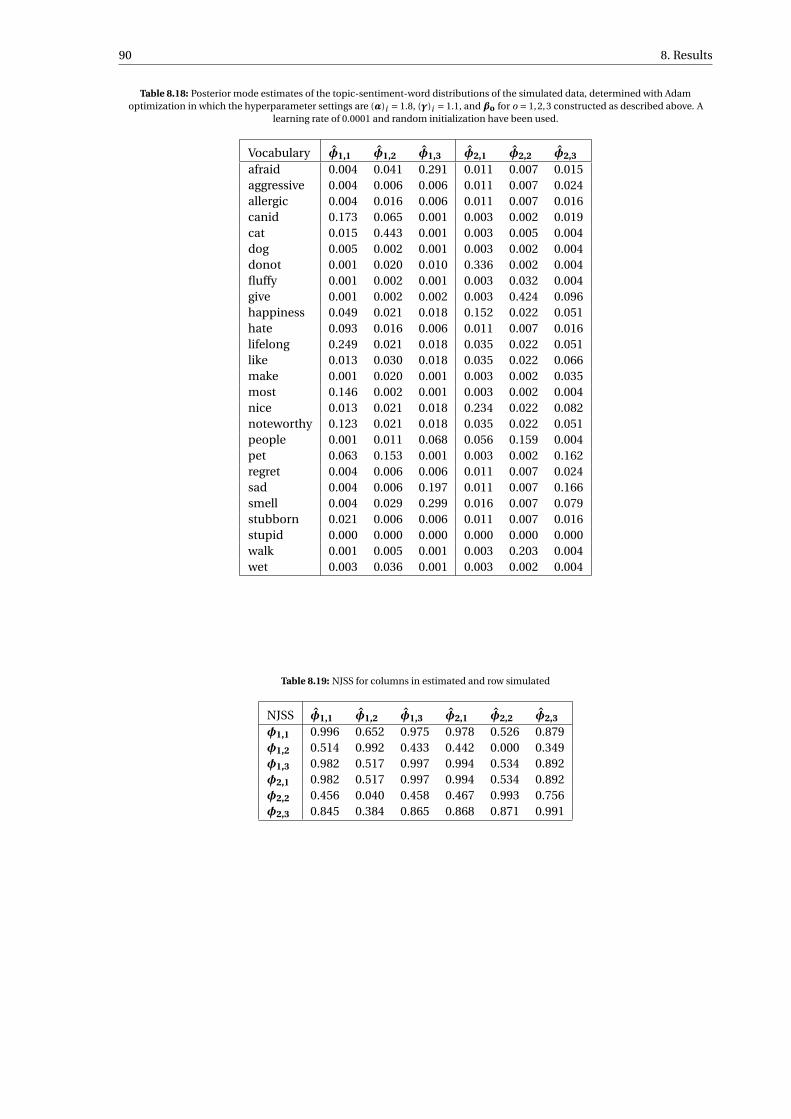
90 8. Results
Table 8.18: Posterior mode estimates of the topic-sentiment-word distributions of the simulated data, determined with Adamoptimization in which the hyperparameter settings are (α)i = 1.8, (γ)i = 1.1, and βo for o = 1,2,3 constructed as described above. A
learning rate of 0.0001 and random initialization have been used.
Vocabulary φ1,1 φ1,2 φ1,3 φ2,1 φ2,2 φ2,3
afraid 0.004 0.041 0.291 0.011 0.007 0.015aggressive 0.004 0.006 0.006 0.011 0.007 0.024allergic 0.004 0.016 0.006 0.011 0.007 0.016canid 0.173 0.065 0.001 0.003 0.002 0.019cat 0.015 0.443 0.001 0.003 0.005 0.004dog 0.005 0.002 0.001 0.003 0.002 0.004donot 0.001 0.020 0.010 0.336 0.002 0.004fluffy 0.001 0.002 0.001 0.003 0.032 0.004give 0.001 0.002 0.002 0.003 0.424 0.096happiness 0.049 0.021 0.018 0.152 0.022 0.051hate 0.093 0.016 0.006 0.011 0.007 0.016lifelong 0.249 0.021 0.018 0.035 0.022 0.051like 0.013 0.030 0.018 0.035 0.022 0.066make 0.001 0.020 0.001 0.003 0.002 0.035most 0.146 0.002 0.001 0.003 0.002 0.004nice 0.013 0.021 0.018 0.234 0.022 0.082noteworthy 0.123 0.021 0.018 0.035 0.022 0.051people 0.001 0.011 0.068 0.056 0.159 0.004pet 0.063 0.153 0.001 0.003 0.002 0.162regret 0.004 0.006 0.006 0.011 0.007 0.024sad 0.004 0.006 0.197 0.011 0.007 0.166smell 0.004 0.029 0.299 0.016 0.007 0.079stubborn 0.021 0.006 0.006 0.011 0.007 0.016stupid 0.000 0.000 0.000 0.000 0.000 0.000walk 0.001 0.005 0.001 0.003 0.203 0.004wet 0.003 0.036 0.001 0.003 0.002 0.004
Table 8.19: NJSS for columns in estimated and row simulated
NJSS φ1,1 φ1,2 φ1,3 φ2,1 φ2,2 φ2,3
φ1,1 0.996 0.652 0.975 0.978 0.526 0.879φ1,2 0.514 0.992 0.433 0.442 0.000 0.349φ1,3 0.982 0.517 0.997 0.994 0.534 0.892φ2,1 0.982 0.517 0.997 0.994 0.534 0.892φ2,2 0.456 0.040 0.458 0.467 0.993 0.756φ2,3 0.845 0.384 0.865 0.868 0.871 0.991
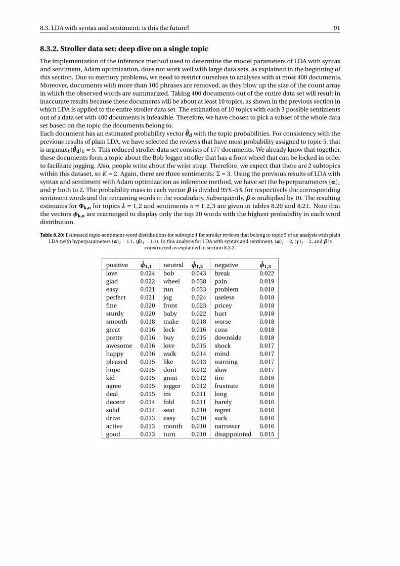
8.3. LDA with syntax and sentiment: is this the future? 91
8.3.2. Stroller data set: deep dive on a single topic
The implementation of the inference method used to determine the model parameters of LDA with syntaxand sentiment, Adam optimization, does not work well with large data sets, as explained in the beginning ofthis section. Due to memory problems, we need to restrict ourselves to analyses with at most 400 documents.Moreover, documents with more than 100 phrases are removed, as they blow up the size of the count arrayin which the observed words are summarized. Taking 400 documents out of the entire data set will result ininaccurate results because these documents will be about at least 10 topics, as shown in the previous section inwhich LDA is applied to the entire stroller data set. The estimation of 10 topics with each 3 possible sentimentsout of a data set with 400 documents is infeasible. Therefore, we have chosen to pick a subset of the whole dataset based on the topic the documents belong to.Each document has an estimated probability vector θd with the topic probabilities. For consistency with theprevious results of plain LDA, we have selected the reviews that have most probability assigned to topic 5, thatis argmaxk (θd)k = 5. This reduced stroller data set consists of 177 documents. We already know that together,these documents form a topic about the Bob Jogger stroller that has a front wheel that can be locked in orderto facilitate jogging. Also, people write about the wrist strap. Therefore, we expect that there are 2 subtopicswithin this dataset, so K = 2. Again, there are three sentiments: Σ= 3. Using the previous results of LDA withsyntax and sentiment with Adam optimization as inference method, we have set the hyperparameters (α)i
and γ both to 2. The probability mass in each vector β is divided 95%-5% for respectively the correspondingsentiment words and the remaining words in the vocabulary. Subsequently, β is multiplied by 10. The resultingestimates for Φk,o for topics k = 1,2 and sentiments o = 1,2,3 are given in tables 8.20 and 8.21. Note thatthe vectors φk,o are rearranged to display only the top 20 words with the highest probability in each worddistribution.
Table 8.20: Estimated topic-sentiment-word distributions for subtopic 1 for stroller reviews that belong to topic 5 of an analysis with plainLDA (with hyperparameters (α)i = 1.1, (β)i = 1.1). In this analysis for LDA with syntax and sentiment, (α)i = 2, (γ)i = 2, and β is
constructed as explained in section 8.3.2.
positive φ1,1 neutral φ1,2 negative φ1,3
love 0.024 bob 0.043 break 0.022glad 0.022 wheel 0.038 pain 0.019easy 0.021 run 0.033 problem 0.018perfect 0.021 jog 0.024 useless 0.018fine 0.020 front 0.023 pricey 0.018sturdy 0.020 baby 0.022 hurt 0.018smooth 0.018 make 0.018 worse 0.018great 0.016 lock 0.016 cons 0.018pretty 0.016 buy 0.015 downside 0.018awesome 0.016 love 0.015 shock 0.017happy 0.016 walk 0.014 mind 0.017pleased 0.015 like 0.013 warning 0.017hope 0.015 dont 0.012 slow 0.017kid 0.015 great 0.012 tire 0.016agree 0.015 jogger 0.012 frustrate 0.016deal 0.015 im 0.011 long 0.016decent 0.014 fold 0.011 barely 0.016solid 0.014 seat 0.010 regret 0.016drive 0.013 easy 0.010 suck 0.016active 0.013 month 0.010 narrower 0.016good 0.013 turn 0.010 disappointed 0.015
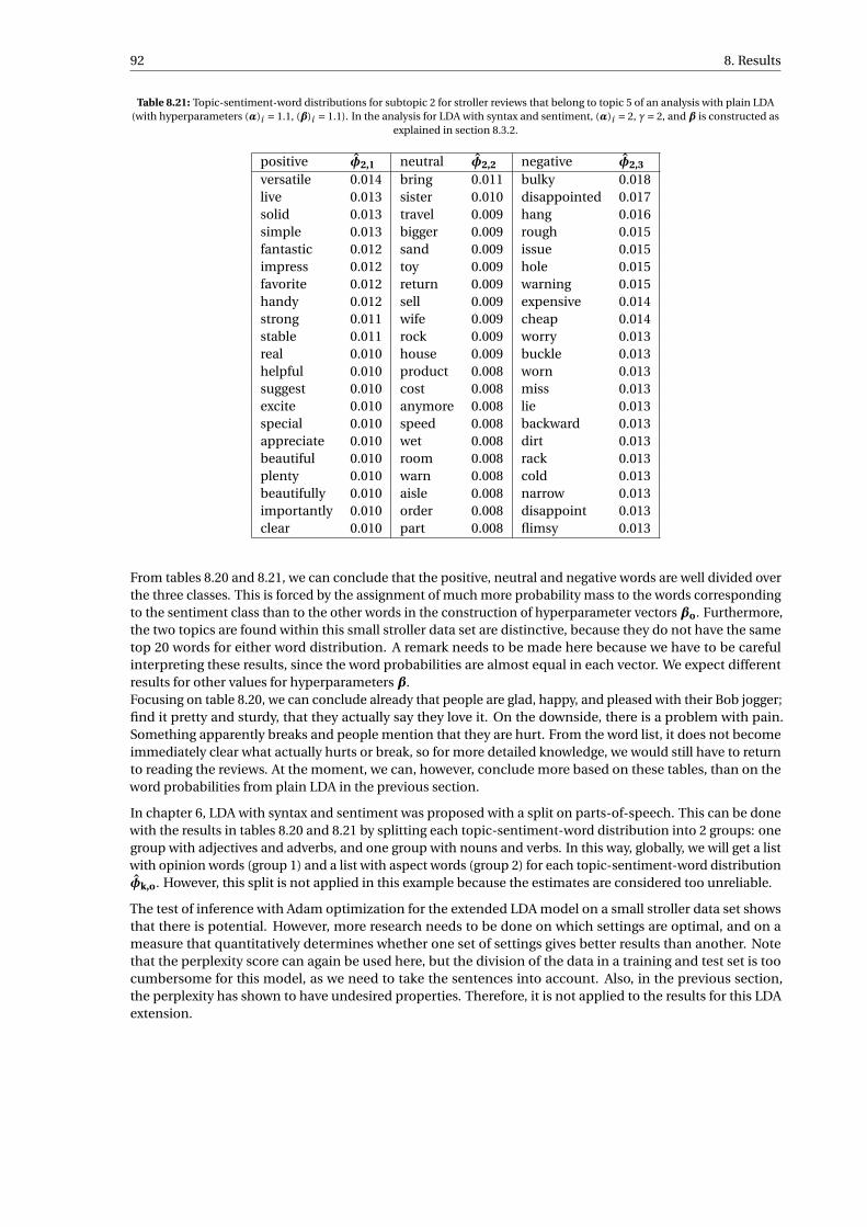
92 8. Results
Table 8.21: Topic-sentiment-word distributions for subtopic 2 for stroller reviews that belong to topic 5 of an analysis with plain LDA(with hyperparameters (α)i = 1.1, (β)i = 1.1). In the analysis for LDA with syntax and sentiment, (α)i = 2, γ= 2, and β is constructed as
explained in section 8.3.2.
positive φ2,1 neutral φ2,2 negative φ2,3
versatile 0.014 bring 0.011 bulky 0.018live 0.013 sister 0.010 disappointed 0.017solid 0.013 travel 0.009 hang 0.016simple 0.013 bigger 0.009 rough 0.015fantastic 0.012 sand 0.009 issue 0.015impress 0.012 toy 0.009 hole 0.015favorite 0.012 return 0.009 warning 0.015handy 0.012 sell 0.009 expensive 0.014strong 0.011 wife 0.009 cheap 0.014stable 0.011 rock 0.009 worry 0.013real 0.010 house 0.009 buckle 0.013helpful 0.010 product 0.008 worn 0.013suggest 0.010 cost 0.008 miss 0.013excite 0.010 anymore 0.008 lie 0.013special 0.010 speed 0.008 backward 0.013appreciate 0.010 wet 0.008 dirt 0.013beautiful 0.010 room 0.008 rack 0.013plenty 0.010 warn 0.008 cold 0.013beautifully 0.010 aisle 0.008 narrow 0.013importantly 0.010 order 0.008 disappoint 0.013clear 0.010 part 0.008 flimsy 0.013
From tables 8.20 and 8.21, we can conclude that the positive, neutral and negative words are well divided overthe three classes. This is forced by the assignment of much more probability mass to the words correspondingto the sentiment class than to the other words in the construction of hyperparameter vectors βo. Furthermore,the two topics are found within this small stroller data set are distinctive, because they do not have the sametop 20 words for either word distribution. A remark needs to be made here because we have to be carefulinterpreting these results, since the word probabilities are almost equal in each vector. We expect differentresults for other values for hyperparameters β.Focusing on table 8.20, we can conclude already that people are glad, happy, and pleased with their Bob jogger;find it pretty and sturdy, that they actually say they love it. On the downside, there is a problem with pain.Something apparently breaks and people mention that they are hurt. From the word list, it does not becomeimmediately clear what actually hurts or break, so for more detailed knowledge, we would still have to returnto reading the reviews. At the moment, we can, however, conclude more based on these tables, than on theword probabilities from plain LDA in the previous section.
In chapter 6, LDA with syntax and sentiment was proposed with a split on parts-of-speech. This can be donewith the results in tables 8.20 and 8.21 by splitting each topic-sentiment-word distribution into 2 groups: onegroup with adjectives and adverbs, and one group with nouns and verbs. In this way, globally, we will get a listwith opinion words (group 1) and a list with aspect words (group 2) for each topic-sentiment-word distributionφk,o. However, this split is not applied in this example because the estimates are considered too unreliable.
The test of inference with Adam optimization for the extended LDA model on a small stroller data set showsthat there is potential. However, more research needs to be done on which settings are optimal, and on ameasure that quantitatively determines whether one set of settings gives better results than another. Notethat the perplexity score can again be used here, but the division of the data in a training and test set is toocumbersome for this model, as we need to take the sentences into account. Also, in the previous section,the perplexity has shown to have undesired properties. Therefore, it is not applied to the results for this LDAextension.
9Discussion
"I have not failed. I’ve just found 10,000 ways that won’t work."Thomas Edison (1847-1931)
In this master thesis, topic model Latent Dirichlet Allocation is thoroughly researched, and different methodsof inference are applied to estimate the desired model parameters. Throughout the process, several questionshave arisen, and the LDA results for two data sets using different methods of inference have shown that someof them performs not satisfactorily, caused by several phenomena on which will be elaborated in the firstsection of this chapter. Shortcomings and arisen questions of the extension of LDA, LDA with syntax andsentiment, are explained and described in section 9.2.
9.1. Latent Dirichlet Allocation
9.1.1. Assumptions
First of all, the assumptions made in LDA are quite strong. Each review is considered to consist of a list ofwords that have no syntactic relation with each other, which means that all words can be permuted, while it isassumed that no information is lost. This bag-of-words assumption is the weakest part of LDA because thesepermutations result in weak topics. Naturally, some words are strictly linked to one topic, but many of themonly have a clear meaning in relation to the words surrounding them in a sentence. Words like ‘the’ and ‘for’are removed beforehand because they are considered to be ‘stop words’, but other frequently occurring wordsthat are, for example, adjectives are still included in the data set. These words can have different meaningsdepending on the context, which is entirely lost in the bag-of-words representation.To improve upon this aspect of LDA, the extension with syntax and sentiment is invented. The bag-of-wordsrepresentation is still used, but now only on sentence level. However, the exchangeability of words in onlyapplicable to the sentence or phrase level. With this splitting of documents into phrases, less information islost, and the meaning of adjectives is linked to words in that same phrase, resulting, in theory, in more accuratetopics .
Besides, on a more mathematical level, the assumptions made in the hierarchical structure of LDA are ques-tionable. All topic-word distributions are assumed to be independent. It is really dependent on the data setwhether this assumption is valid or not. If you look at the ‘newsgroups’ data set consisting of news articles,which is often used in the literature, it is natural to assume that topic-word distributions are independent,as they are very distinctive. However, for review data, this is less likely. There can be two topics that de-scribe overlapping aspects or opinions, such that their topic-word distributions are not wholly distinctive norindependent making it harder to do inference.
93
94 9. Discussion
9.1.2. Linguistics
Some aspects of language can not be taken into account in either basic LDA or the invented extension. Aproblematic word that quickly comes to mind is ‘not’. This word says a lot about someone’s opinion orsentiment on the product, while it is only considered a word, nothing more, nothing less. That is only if theword ‘not’ and a certain adjective or verb often occur together in a review, both words will be linked to a topic,and the sentiment of ‘not + other word’ can be retrieved from the estimated topic-word distributions φ. If thisco-occurrence is not present, unfortunately, the sentiment or opinion linked to a topic will be inaccurate.At the moment, in review analyses done by CQM, the phenomenon is counteracted by reading the topreviews belonging to each topic. Reading only a limited number of reviews saves time, while still, opinionscorresponding to topics can be extracted. However, it would be better to improve LDA and its way to cope withwords as ‘not’, such that the topic-word distributions themselves show the correct reviewers’ opinions, andreading becomes superfluous.Possibilities to incorporate the function of ‘not’ in an opinion in the data analysis are, for example, attachingthe word ‘not’ to the previous or next word. This method is not very accurate, but easy to implement. Anotheroption is to parse each sentence automatically (this can easily be done in Python using the package nltk),and retrieve the link of ‘not’ with the corresponding verb, adjective, adverb, or another part-of-speech in thesentence using the part-of-speech tagging. This is an implementable option, but it will take a lot of time toparse each sentence in each review. Besides, some reviews are not written in proper English, making accuratelyparsing more challenging. The last option is the incorporation of word order in the Latent Dirichlet Allocationmodel. This has already been done by some topic modellers (see for example [18], [17],[10]), and has beenproved to work well. However, these models have increased complexity, and require thus, in general, morecomputation time and better programming skills.
9.1.3. Influence of the prior
In Bayesian statistics, we have seen that if the data set is large enough, the influence of the prior distributionwill be negligible. Firstly, it is difficult to know when the data set is large enough to accurately estimate alllatent random variables of interest. In general, whether the data set is large enough can be determined bychanging the hyperparameters and checking the influence on the results. If this influence is null, the data setis large enough. If it is small and the main conclusions remain the same, the data set can be worked with, but ifthe results significantly change for different parameters, the data set is not large enough. Unfortunately, datasets cannot easily be increased, so the number of parameters should be decreased, leaving more relativelymore data to estimate fewer parameters. Unfortunately, if the number of topics is decreased, it might be thecase that two actual themes in the data set are assigned to the same topic. Therefore, the results must beinterpreted more carefully in this case.Furthermore, we have seen that the Adam optimization method is very sensitive to the values of the hyper-parameters. This is an undesirable property, as the influence of the hyperparameters should vanish for largedata sets. Therefore, Adam optimization as inference method is not preferred. Gibbs sampling shows a lot lesssensitivity, so for the application of LDA to data, this method is recommended. Variational Bayesian EM isoften used in LDA applications, but this inference method is above all advised against due to its independenceassumptions that are considered too strong.
Given the fact that, in general, the data set is too small to make the influence of the prior disappear, we needto be considerate with choosing the prior distributions and the corresponding hyperparameters. Dirichletdistributions are good priors for Multinomial distributions, and Multinomials are appropriate for drawingcategorical random variables such as topics or sentiments. Therefore, these prior distributions are a good fitfor the topic modeling aim of Latent Dirichlet Allocation.However, as mentioned before, the values of hyperparametersα andβ can have a large influence on the results.Instead of choosing a symmetric α of β hyperparameter vector, also an asymmetric prior can be chosen. Inthis way, one topic (in case of α) or a few words (in case of β) are given preference in each document or eachtopic. Especially for the document-topic distributions, this can be wise, since it is not rare that every documentis expected to go about one topic. This topic is then given preference beforehand in the chosen α by assigningmore mass to one dimension in the parameter vector of the Dirichlet distribution.Because the asymmetric hyperparameter vector is still a powerful prior, an extra prior on α can be imposed. Acombination of extra priors on α has been researched. One prior is imposed for the (a)symmetry, and anotherfor the order of magnitude of α. The product then forms α, the hyperparameter for the document-topic
9.1. Latent Dirichlet Allocation 95
distributions. As we have seen before, the order of magnitude of α has a large influence on the way topics aredistributed. A value larger than one for symmetric α gives preference to a uniform distribution over the topics,whileα smaller than 1 gives preference to a distribution that assigns most mass to only one or a few dimensions.We want to learn this scaling aspect of α from the data, and thus impose a prior on it. The supplementary(a)symmetry prior has been chosen to be a Dirichlet distribution with a parameter vector consisting of onlyones, such that any possible document-topic distribution is equally probable. The distribution of the scalingprior is more difficult to choose, and several options have been thought of. Because we care about the order ofmagnitude, one might think of drawing n ∼ Uniform([−2,2]), and then take 10n for the order of magnitude.There are other possibilities for the distribution of n, as long as the resulting orders of magnitude are between10−2 and 102. These are considered reasonable orders of magnitude for α. Because a double prior on α causesthe hierarchical model to become more complex concerning the form of the posterior density, this idea isnot worked out more elaborately. It is however determined that with such a double prior, conjugacy in theBayesian model is lost, and both Gibbs sampling and posterior mode determination via Adam optimizationbecome computationally more challenging.
9.1.4. Model selection measures
We have seen in the results in chapter 8 that it is not easy to find a suitable measure to compare different models,whether the difference comes from different estimation methods, or different hyperparameters. Perplexity is awidely used measure based on information theory and is appropriate for topic models. However, it can onlywork with training and test sets, making it a lot more difficult to apply to LDA because the data set needs to besplit. In this thesis, the split is performed within each document, such that approximately 80% of the words ina document is taken to train the model and estimate the required parameters, while 20 % is left for the testset. We have seen that the perplexity measure gives preference to models with flat distributions, that is eachtopic and each word have a relatively large probability on the document-topic and topic-word distributionsrespectively. However, if a topic does not occur in a document, it is preferred that the probability of that topicin the document-topic distribution is 0. Therefore, flat distributions are usually not good representations ofthe data. Numerically, document-topic probabilities being zero cause problems. As a consequence, 10−20 or aneven smaller number is used instead. These numbers occur in the estimates ofΘ andΦ by Adam optimization,but they react very poorly to the perplexity, resulting in a bad perplexity score.One method to improve the perplexity score that can easily be implemented is the following. When computingthe perplexity over a test set, words with low estimated probabilities in all topics can be ignored, such thattheir contribution to the perplexity is removed, whereas otherwise their small probabilities would have causedthe perplexity to increase. Although this does not solve the entire problem, it is expected that the perplexityscore will become more stable and less sensitive to low values in the topic-word distributions. Note that we donot wish to throw out topics with low probabilities in the same manner. If a topic has an overall low probabilityin all documents, we could better reduce the number of topics K . Other methods to improve the perplexitybased on a different splitting the data sets into a training and test set are proposed in [48].
Besides the disappointing property of perplexity of dealing poorly with probabilities close to 0, it also does notcorrect for the number of parameters considered. This means that a lower and thus better perplexity score isreached for increasing K , the number of topics. However, for higher K , you might be overfitting, and accuracyof the topics decreases for an increasing number of parameters.As an alternative, the value of the log posterior for the estimated random variablesΘ andΦ is proposed. Thismeasure does not suffer from the effects of training and test sets. The larger the log posterior value, the betterthe parameter estimations. This measure is based on the posterior mode being the best representation ofthe model. The aim of each inference method is then to get as close as possible to the posterior mode. Thisprinciple is comparable to maximum likelihood estimation in classical statistics. However, this measure canonly be used to compare different methods of inference or different hyperparameters, since the number ofparameters in total needs to be the same in each model. Whether the posterior mode indeed gives the bestmodel parameters for LDA is not researched in this thesis. For annotated data sets, this phenomenon canbe looked into by comparing the log posterior value for the actual, true model parameters with the posteriormode.
Apart from the perplexity and the log posterior value, measures for better model comparison need to be found.Fortunately, the data in LDA consists of words, such that through reading, when can get qualitatively validatethe correctness of the model parameters. This becomes however more difficult for large data sets with many
96 9. Discussion
parameters. It is better to find a quantitative measure with a valid mathematical argumentation to concludeon which inference method is the best for LDA, and to find the best settings for K and hyperparameters αand β. More research can thus be done on good model comparison and model validation measures for topicmodeling.
9.2. LDA with syntax and sentimentThe extension to LDA using sentences and sentiments has a good theoretical foundation. The assumption thatin each phrase, only one topic is described with one sentiment is reasonable, although not always true. Also,the manner of splitting a review into sentences can be discussed, as rules do not apply to each review. Think ofsplitting on the word ‘and’ for example. This word can either be part of a summation, in which it is not alwaysinformative to split on ‘and’, or can be a conjunction between two main phrases. In the latter case, it is wise tosplit on ‘and’ because a complete phrase exists on both sides of the word. The same can be said about splittingon commas. Therefore, it is recommended to read a small subset of the (review) data set to get a grasp of thewriting style that is used, such that, with this knowledge, you can decide which splitting rules are the mostappropriate.
Furthermore, for the assignment of positive and negative sentiment to a review, word lists with the mostcommon positive and negative words in the English language are used. These word lists are not perfect, and itwill be the case that some words are classified to a sentiment incorrectly. In further applications, these wordlists need to be perfected and adapted according to the used data set. Words that are positive in one context,might be negative in another, think of, e.g., ‘close’.
Lastly, Adam optimization is not robust to hyperparameter settings and initialization. It can find the parametersof a simulated data set, but a remark needs to be made there. The simulated data set consisted of very distincttopic-sentiment-word distributions, making it easier to find the correct parameters. We have seen for thestroller data, that is a lot more difficult to find the right settings and interpretable estimates.Furthermore, the algorithm only works on small data sets in the current implementation. More research canbe done on the both the robustness and the upscaling of Adam optimization for determining the posteriormode estimates of interest in LDA with syntax and sentiment.Besides, in the comparison of inference methods for plain LDA, we have seen that Gibbs sampling performsbetter than Adam optimization in terms of parameter estimation. Therefore, it is expected that Gibbs samplingfor LDA with syntax and sentiment will give us better results, with which hopefully manually reading becomessuperfluous.

10Conclusion and recommendations
The main goal of this work is to find good methods to summarize customers’ opinions in review data, withouthaving to read all reviews. To this end, Latent Dirichlet Allocation has been described, and various inferencemethods to estimate its model parameters have been researched. Moreover, a new method of inference, Adamoptimization, has been applied to LDA for two different data sets.Because this thesis is written in collaboration with CQM, an extension to LDA that is more suitable for reviewanalyses and opinion mining is invented, called LDA with syntax and sentiment. For this new topic model,only one inference method is tested on a simulated data set, and a real data set. The main conclusions will begiven in the first section of this chapter. Subsequently, recommendations are proposed for further research.
10.1. Main findings
Latent Dirichlet Allocation is a hierarchical Bayesian topic model that allocates topics to words, and findsin this way topic distributions per document and word distributions per topic. From the document-topicdistributions, we can conclude which topics occur most frequently in the reviews. The topic-word distributionsgive insights in what the topics are about, such that we know more about the customers’ opinions on thespecific product they describe in the set of reviews. Marketing strategies and product innovations can then besteered into a specific direction using the conclusions from the topics in the review data set.
Three different inference methods are used to estimate the document-topic and topic-word distributions inLDA: Gibbs sampling, Variational Bayesian Expectation-Maximization, and Adam optimization. From thesemethods, Gibbs sampling using the application in the program KNIME gives the most robust and best results.The inference method which is new concerning its application for LDA, Adam optimization, disappoints, sinceit is sensitive to hyperparameter settings and initialization. Only for hyperparameters larger than 1, a settingthat is only preferred in a limited number of cases, the algorithm performs well.
After having estimated the parameters in the topic-word distributions, a check is needed to determine whetherthe chosen number of topics was correct. That is if the number of topics is too large, the model overfits,which results in some topics consisting of noise. This noise is not informative and should not be interpreted.Therefore, two similarity measures are computed for all topic-word distribution combinations, the normalizedsymmetric Kullback-Leibler divergence and the normalized symmetric Jensen-Shannon divergence. Bothperform well and can thus be used to check for overfitting in terms of the number of topics.
10.2. Further research
Although in this thesis different methods of inference are looked into, a new one is proposed, and even an newtopic model is introduced, research is never finished. Therefore, we will shortly discuss recommendations forfurther research in this section.
Firstly, better model validation and model comparison measures need to be defined. Currently, in the field of
97

98 10. Conclusion and recommendations
topic modeling, the perplexity is used. For this measure, a division of the data set in a training and test set isrequired. However, model parameters are estimated on document-level, with as result that this split is notstraightforward. More research can be done on methods to form a training and test set for the computation ofthe perplexity. Moreover, the perplexity has two disadvantages that are both inherent to its definition: it has apreference for flat distributions and for overfitted models. Lastly, it says something about the predictive powerof LDA, while the aim of LDA in this research is to summarize data sets.Another possible method to compare model outcomes is the log posterior value. This is the value of theposterior density (up to a proportionality constant) for the estimated model parameter. It is essential thatthe parameters of the models that are compared have the same dimensions. This is a downfall, as it wouldbe ideal if the model comparison score could give insights in the best number of topics to use. Furthermore,it is not certain that the highest log posterior value, that is, the posterior mode, also gives the best estimatesof the model parameters for LDA. More research can be done whether or not this is true for Latent DirichletAllocation.Because both model validation scores do not perform satisfactorily, a better score needs to be thought of. Theoutcomes of topic models are often interpreted qualitatively, thus, a score in which human interpretation oftext can be combined with automatic reading is preferred.
Secondly, Adam optimization has been applied to the posterior density of the Latent Dirichlet Allocation modelto find the posterior mode. This method can only find the posterior mode and estimate model parametercorrectly for specific hyperparameter settings. That is for hyperparameters smaller than 1, the algorithm walkstowards the boundaries of the domain, with as result that optimization is only performed in a limited numberof dimensions. A method to prevent the algorithm from showing this behavior can be researched. Either thealgorithm can be improved, or another way of making the model prefer documents having only a few topics byusing, for example, an extra prior can be thought of.
Lastly, the extended version of LDA, specifically designed for review analyses, can be perfected. The theoreticframework underlying LDA with syntax and sentiment is realistic, but Adam optimization as inference methodleaves much to be desired. Adam optimization is used to search for the posterior mode estimates for thedocument-topic, document-sentiment, and topic-sentiment-word distributions, but it is challenging to findthe good settings in the algorithm, and the method is very sensitive to initialization. Only for a simulated dataset with distinct topic-sentiment-word distributions, good estimates have been found.Already for basic LDA, it had been shown that Adam optimization does not work as desired. Therefore, it isrecommended to apply Gibbs sampling to LDA with syntax and sentiment to find estimates for the modelparameter. Still, much is expected from the new extension to LDA, only the best method of inference needs tobe discovered.
After all, research is nothing more than searching for answers to your problems, and consequently adaptingthe questions themselves. Following the wise words of Sherlock Holmes in the works of Sir Arthur Conan Doyle(1859-1930):
"Once you eliminate the impossible, whatever remains, no matter how improbable, must be thetruth."
AMathematical background and derivations
A.1. Functional derivative and Euler-Lagrange equation
In the derivation of the variational Bayesian EM algorithm with the mean field approximation, a functionalderivative is used to determine the form of the auxiliary distribution for which the functional, in this case alower bound for the log likelihood, is maximal. In this section, the functional derivative will be derived and thedefinition of the differential (derivative of functional) is given. But first some general definitions and resultfrom functional analysis are stated.
Let X be a vector space, Y a normed space and T a transformation defined on a domain D ⊂ X and havingrange R ⊂ Y . [29]
Definition A.1 (Gateaux differential)Let x ∈ D ⊂ X and let h be arbitrary in X . If the limit
δT (x;h) = limα→0
1
α[T (x +αh)−T (x)] (A.1)
exists, it is called the Gateaux differential of T at x with increment h. If the limit in A.1 exists for each h ∈ X , thetransformation T is said to be Gateaux differentiable at x.
A more frequently used definition of the Gateaux differential is the following [29]: if f is a functional on X , theGateaux differential of f , if it exists, is
δ f (x;h) = d
dαf (x +αh)
∣∣∣α=0
(A.2)
and for each fixed x ∈ X , δ f (x;h) is a functional with respect to the variable h ∈ X .
A stronger differential is the Fréchet differential, which is defined on a normed space X . This differentialenhances continuity. [29]
Definition A.2 (Fréchet differential)Let T be a transformation defined on an open domain D in a normed space X and having range in a normedspace Y . If for fixed x ∈ D and each h ∈ X , there exists δT (x;h) ∈ Y which is linear and continuous with respectto h such that
lim‖h‖→0
‖T (x +h)−T (x)−δT (x;h)‖‖h‖ = 0 (A.3)
then T is said to be Fréchet differentiable at x and δT (x;h) is said to be the Fréchet differential of T at x withincrement h.
Three general propositions from [29] are summarized in proposition A.1. For the proofs, we refer to [29].
99

100 A. Mathematical background and derivations
Proposition A.1 (Properties Fréchet differential)The following are true for a transformation T defined on an open domain D in a normed space X and havingrange in a normed space Y :
• If the transformation T has a Fréchet differential, it is unique.
• If the Fréchet differential of T exists at x, then the Gateaux differential exists at x and they are equal.
• If the transformation T defined on an open set D in X has a Fréchet differential at x, then T is continuousat x.
Now consider a functional F of the form:
F =∫ x2
x1
L(q(x), q(x), x)dx (A.4)
Where q(x) = d qdx .
A classical problem in the field of variational calculus is finding a function q on [x1, x2] that minimizes thefunctional F [29]. The admissible set of functions for this problem consists of all functions that are continuousand whose derivatives are continuous in the range [x1, x2]. Besides let q be an admissible function and supposethere exists h such q +h is also admissible. All such possible functions h are collected in the class of so-calledadmissible variations. Also restrict the set of admissible functions to those whose end points i.e. q(x1) andq(x2) are fixed.
The Gateaux differential of functional F , assume that it exists, is given by:
δF (q ;h) = d
dα
∫ x2
x1
L(q +αh, q +αh, x)dx∣∣∣α=0
=∫ x2
x1
Lq (q, q , x)h(x)dx+∫ x2
x1
L q (q, q , x)h(x)dx(A.5)
It can be verified that this differential is also Fréchet [29]. Now, theorem A.1 gives a necessary condition for theextrema of functional F , as desired.[29]
Theorem A.1 (Extrema of a functional)Let the real-valued function f have a Gateaux differential on a vector space X . A necessary condition for f tohave an extremum at x0 ∈ X is that δ f (x0;h) = 0 for all h ∈ X .
As proposition A.1 indicates that every Fréchet differential is also a Gateaux differential, we can apply theoremA.1 to equation A.5 to find the extremum.
δF (q ;h) =∫ x2
x1
Lq (q, q , x)h(x)dx+∫ x2
x1
L q (q, q , x)h(x)dx = 0
=∫ x2
x1
[Lq (q, q , x)h(x)+L q (q, q , x)h(x)
]dx = 0
(A.6)
To arrive from the equation above to the Euler-Lagrange equation, we use one of the fundamental lemmasfrom variational calculus [29]:
Lemma A.1If α(t ) and β(t ) are continuous in [t1, t2] and∫ t2
t1
[α(t )h(t )+β(t )h(t )
]dt = 0 (A.7)
for every h ∈ D[t1, t2] with h(t1) = h(t2) = 0, then β is differentiable and β(t ) ≡α(t ) in [t1, t2].
Note that in equation A.6, we have the same form as in lemma A.1. Therefore:

A.1. Functional derivative and Euler-Lagrange equation 101
Lq (q, q , x) = d
d tL q (q, q , x)
⇒ Lq (q, q , x)− d
d tL q (q, q , x) = 0
(A.8)
This last result in known as the Euler-Lagrange equation, which is used in this thesis for the derivation of thevariational Bayesian EM update equations.
102 A. Mathematical background and derivations
A.2. Expectation of logarithm of Beta distributed random variableIn the derivation of the update equations in variational Bayesian EM for general LDA, the expectation of thelogarithm of a Beta distributed random variable occurs several times. In this section its computation willbe elaborated on. Consider the latent random vectorΘwhich is Dirichlet distributed with parameter vectorα. From previous results, we know that (Θ)i is Beta distributed with parameters (α)i and
∑j 6=i (α) j . The
probability density function of (Θ)i is therefore:
p((θ)i |(α)i ,∑j 6=i
(α) j ) = Γ(∑K
k=1(α)k)
Γ((α)i ) ·Γ(∑j 6=i (α) j
) · (θ)(α)i−1i · (1− (θ)i )
∑j 6=i (α) j −1
= exp
((α)i −1)log((θ)i )+ (
∑j 6=i
(α) j −1)log(1− (θ)i )+ log
(Γ
(K∑
k=1(α)k
))− log
(Γ
(∑j 6=i
(α) j
))− log(Γ((α)i ))
= h((θ)i ) ·exp
η1t1((θ)i )+η2t2((θ)i )− A(η)
(A.9)
From equation A.9 we can conclude that the distribution of (Θ)i belongs to an exponential family with naturalstatistics log((θ)i ) and log(1− (θ)i ) and natural parameters (α)i −1 and
∑j 6=i (α) j . The normalization constant
is given by A(η). Now we can use some useful results from exponential family distribution, namely its momentgenerating function, which we will derive for the first moment as follows.First note that:
e A(η1,η2) =∫
h((θ)i ) ·expηTt((θ)i )
d(θ)i (A.10)
Differentiating both sides with respect to η gives:
∇ηe A(η1,η2) =∇η(∫
h((θ)i ) ·expηTt((θ)i )
d(θ)i
)e A(η1,η2)∇ηA(η1,η2) =
(∫h((θ)i )t1((θ)i )exp
ηTt((θ)i )
d(θ)i ,
∫h((θ)i )t2((θ)i )exp
ηTt((θ)i )
d(θ)i
)⇒∇ηA(η1,η2) = (E [t1((θ)i )] ,E [t2((θ)i )])
(A.11)
Where integration and differentiation can be interchanged via dominated convergence. The result is that wehave obtained expressions for the expectations of each natural statistic. For the derivation of the variationalBayesian EM algorithm for LDA, the expectation of log(Θ) was needed, which is also one of the two naturalstatistics. Therefore:
E[log((θ)i )
]= ∂A(η1,η2)
∂η1= ∂
∂((α)i −1)
(− log
(Γ
(K∑
k=1(α)k
))+ log
(Γ
(∑j 6=i
(α) j
))+ log(Γ((α)i ))
)
=−Ψ(Γ(
K∑k=1
(α)k )
)+Ψ ((α)i )
(A.12)
WithΨ(·) being the digamma function.
A.3. LDA posterior mean determination 103
A.3. LDA posterior mean determinationOne of the possibilities to estimate parameters using Bayesian statistics is to compute the posterior mean. Inthis section, the determination of the posterior mean for the high-dimensional hierarchical Bayesian modelthat LDA is, is derived.
Suppose we start with the computation of the posterior mean for eachΘd. To retrieve an expression for thisestimator from the joint posterior distribution p(θ,φ|w), we can first condition on φ and then compute themean overΦ. In formulas:
E[Θ|w] = EΦ[EΘ|Φ [Θ|Φ,w]
](A.13)
The subscript in EΦ denotes the fact that the expectation is taken with respect to random variableΦ. Becauseeach Θd is independent of the topic distributions of other documents, Θj for j 6= d , the posterior mean forΘd can be computed separately for each document. Note that we still need to condition on all topic-worddistributionsΦk for k = 1, . . . ,K .
E [Θd|w] = EΦ[EΘd|Φ [Θd|Φ,w]
](A.14)
To this end, we need an expression for the conditional posterior ofΘd givenΦ and w. Using equation 4.2, wearrive at:
p(θ|φ,w) ∝[
M∏d=1
V∏j=1
(K∑
k=1(φk) j (θd)k
)nd , j]·[
M∏d=1
K∏k=1
(θd)(α)k−1k
]
=M∏
d=1
[V∏
j=1
(K∑
k=1(φk) j (θd)k
)nd , j]·[
K∏k=1
(θd)(α)k−1k
]
p(θd|φ,w) ∝[
V∏j=1
(K∑
k=1(φk) j (θd)k
)nd , j]·[
K∏k=1
(θd)(α)k−1k
] (A.15)
The distribution of (Θd|Φ,w) in equation A.15 is called the generalized Dirichlet distribution and is defined in[11] as follows.
Definition A.3 (Generalized Dirichlet distribution)Let u and b be K -dimensional vectors, let Z be a [K ×κ] matrix and let β be a κ-dimensional vector. If u isdistributed as Dirκ(b,Z,β), then its probability density function defined on the (K −1)-simplex is given by:
f (u;b,Z,β) =B(b)−1
(∏Ki=1 ubi−1
i
)[∏κj=1
(∑Ki=1 ui zi , j
)−β j]
R−β(b,Z,β)(A.16)
Where R is a double Dirichlet average [11], which is explained in definition A.4 below.
Therefore we know that(Θd|φ,w
)∼ DirV (α,Φ,−nd), where matrix Φ consists of all vectors φ concatenatedrow-wise. That is, matrix elementΦi , j is the j -th element of topic-word distribution vector φi.
Definition A.4 (Double Dirichlet average)The double Dirichlet average is the generalization of the function R, Carlson’s multiple hypergeometric function.Consider a matrix Z (K ×κ), vectors u and b of size K ×1 and vectors v and β of size κ×1. The double Dirichletaverage for some a is then defined as follows:
Ra(b, Z ,β) = Eu|b[Ev|β
[(uT Z v)a]]
= Eu|b[Ra(β; Z T u)
] (A.17)
For a =−β·, where β· =∑i βi , the double average becomes [11]:
R−β(b, Z ,β) = Eu|b
[K∏
j=1
(K∑
i=1ui · zi , j
)−β j]
(A.18)
104 A. Mathematical background and derivations
In [20], Jiang et al. present several methods to approximate Carlson’s R and they derive its exact computationfor certain special cases.
In order to obtain the posterior mean of Θ, we need to know the mean of the distribution of(Θ|φ,w
)first.
Therefore an expression for the product moment function of a generalized Dirichlet distribution could beused.
Proposition A.2 (Product moment generalized Dirichlet distributed random variable)Consider the case in definition A.3, that is u ∼ Dirκ(b, Z ,β). Then its product moment for vectors m and µ is:
Eu|b,Z ,β
[(K∏
i=1umi
i
)κ∏
j=1
(K∑
k=1ui · zi , j
)−µ j]= B(b+m)
B(b)
R−(β+µ)(b+m, Z ,β+µ)
R−β(b, Z ,β)(A.19)
In the case of the document-topic distribution in LDA, we know that(Θd|φ,w
)∼ DirV (α,Φ,nd), with θd thetopic distribution of document d , α the prior parameter vector, Φ the matrix with topic-word probabilitieshaving size (K ×V ) and nd the vector with all word occurrences (in counts) in document d . With this analyticalexpression for the conditional distribution, we can compute the conditional posterior mean in closed form,using equation A.19. Taking m = i (with i the unit vector i.e. (0,0, . . . ,1,0, . . . ,0) with 1 in the i -th place) andµ= 0 in equation A.19:
E [(Θd)i |Φ,w] = B(α+ i)
B(α)
R−Nd (α+ i,Φ,nd)
R−Nd (α,Φ,nd)(A.20)
As a result, there is an analytical expression for the conditional posterior mean of (Θd)i for each documentd and each dimension i = 1, . . . ,K . However, in order to obtain a general, unconditional posterior mean for(Θd)i , the expected value of expression A.20 with respect to Φ needs to be determined. Therefore, we need tointegrate over the ratio of double Dirichlet averages R. To this end, it is better to have a simplified expressionfor R(α+ i,Φ,nd), such that we might recognize a probability distribution of which an exact form of the meanis known or equation A.20 can be written such that we can compute the integral.
Jiang et al. propose in [20] two methods to compute the double Dirichlet average analytically and two methodsthat approximate its value. For the first two methods, matrixΦ needs to satisfy several assumptions, which aretrue for LDA only in rare cases. The first method, in which R can be calculated relatively easily, requires thatmatrix Φ must be a n-level nested partition indicator matrix. A n-level nested partition indicator matrix isa matrix whose columns are indicator vectors of the n-level nested partition subsets. The indicator vectorsare vectors that take on value 1 for index i if category i is in the subset and value 0 otherwise. The n-levelnested partition subsets are explained more thoroughly in [20], but one can think of these sets as forming apartition of the set 1, . . . ,V while either being subsets of each other or being disjoint. That is, the subsets inthe n-level nested partition cannot partially overlap. Note that in the case of LDA, matrixΦ is the consideredmatrix in R, which is a probability matrix with values in the interval [0,1] summing row-wise to 1. Therefore itcan only satisfy the requirement for exact computation if each topic-word distribution gives all probability toone word and 0 probability to all other words in the vocabulary. Only then the matrix will consist of 0’s and 1’s,as required in this method. Because this is not a realistic case for the considered model in this thesis, the firstmethod of exact computation of the double Dirichlet average is discarded.
Secondly, the so-called ‘expansion method’ is proposed in [20]. This method is valid for any matrixΦ and usesthe fact that vector nd consists of non-negative integers. This results in a simplification of R(α+ i,Φ,nd) viathe introduction of matrix W . For the exact procedure, we will refer to the explanation in [20]. This methoddoes result in an analytical expression for R, however, we need to sum over all possible matrices W , whichresults in a sum over
∏Uu=1 ((nd)u +1) terms, where U is the number of unique words in document d and (nd)u
the frequency of word u in document d . Furthermore, note that the entries of matrixΦ are unknown, as theyare still random variables of which the expectation needs to be computed. Although analytically it is possibleto write out all possibilities for W and get an expression of the double Dirichlet average R for each possible Win terms of beta functions andΦ, the method is considered computationally intractable. This conclusion isalso drawn in [20] for high dimensional data sets, which is the case in this project.
The first approximation method of Jiang et al. is the application of Laplace’s approximation. In order to beallowed to apply this formula, we need the function:
A.3. LDA posterior mean determination 105
g (θd) =J∏
j=1
(K∑
k=1(Φk) j · (Θd)K
)m j
(A.21)
to have one single mode. Requirements for this condition to be true are that all terms m j are strictly positiveand the columns ofΦmust span the K -dimensional vector space. The first requirement is not always true, as invector m the word counts for document d , nd, are included and it is not seldom that a word in the vocabularydoes not occur in the specific document d such that nd , j = 0 for word j . The second requirement that thecolumns of Φ span the K -dimensional vector space is not verifiable beforehand, as Φ is a random matrixwhose values are unknown. Therefore it cannot be guaranteed that function g (θd) has a single mode, whichwe already expected due to the possibility of topic permutations. With this being a strict requirement for theLaplace approximation, this method can unfortunately not be applied to the double Dirichlet averages inequation A.20.
At last, a Monte Carlo method is proposed to determine R. Here the fact that R is actually the mean of afunction of the form in equation A.21, as stated in equation A.18 in the definition of the double Dirichletaverage, is used. Therefore, given matrix Φ, we could simulate the Dirichlet process by drawing xi from agamma((α)i ,1) distribution for i = 1, . . . ,K (see section 2.2.1), then computing ui = xi∑
j x jand substituting this
in equation A.18. Note that vector β in equation A.18 is known and we have assumed that matrix Φ is alsoknown. However, as aforementioned,Φ is a random matrix whose values are unknown, so the Monte Carloprocedure to determine R cannot be executed. Naturally, we could take different numerical examples forΦand use these in the approximation. Only there are infinitely many options for matrixΦ, as each element cantake on any value in [0,1] as long as they sum row-wise to 1. It is therefore considered unfeasible to use thismethod for the approximation of R.
Research on approximations of Carlson’s multiple hypergeometric function R is mostly focused on problemsin a Bayesian setting, categorical data and missing values, see for example [12]. In those cases, the matrix in R
is a n-level nested partition indicator matrix or can be transformed to one. Consequently, the posterior meancan be determined analytically. The writer of this thesis has not found other methods than those proposed in[20] to determine R and therefore the posterior mean of θd is considered both computationally and in mostcases also analytically intractable. That is, computations are too exhaustive and in most cases no analyticalexpression for the posterior mean is known.
Besides, when we look at the posterior mean forΦ, which naturally also needs to be determined, we see that theconditional posterior distribution of (Φ|θ,w) is not even a generalized Dirichlet distribution. Computationsare expected to be even more difficult in this case, so the same conclusion can be drawn.
In conclusion, the posterior mean of the desired parameters cannot be determined analytically, therefore wewill need to resort to approximation methods for the posterior distribution in order to compute the posteriormean.

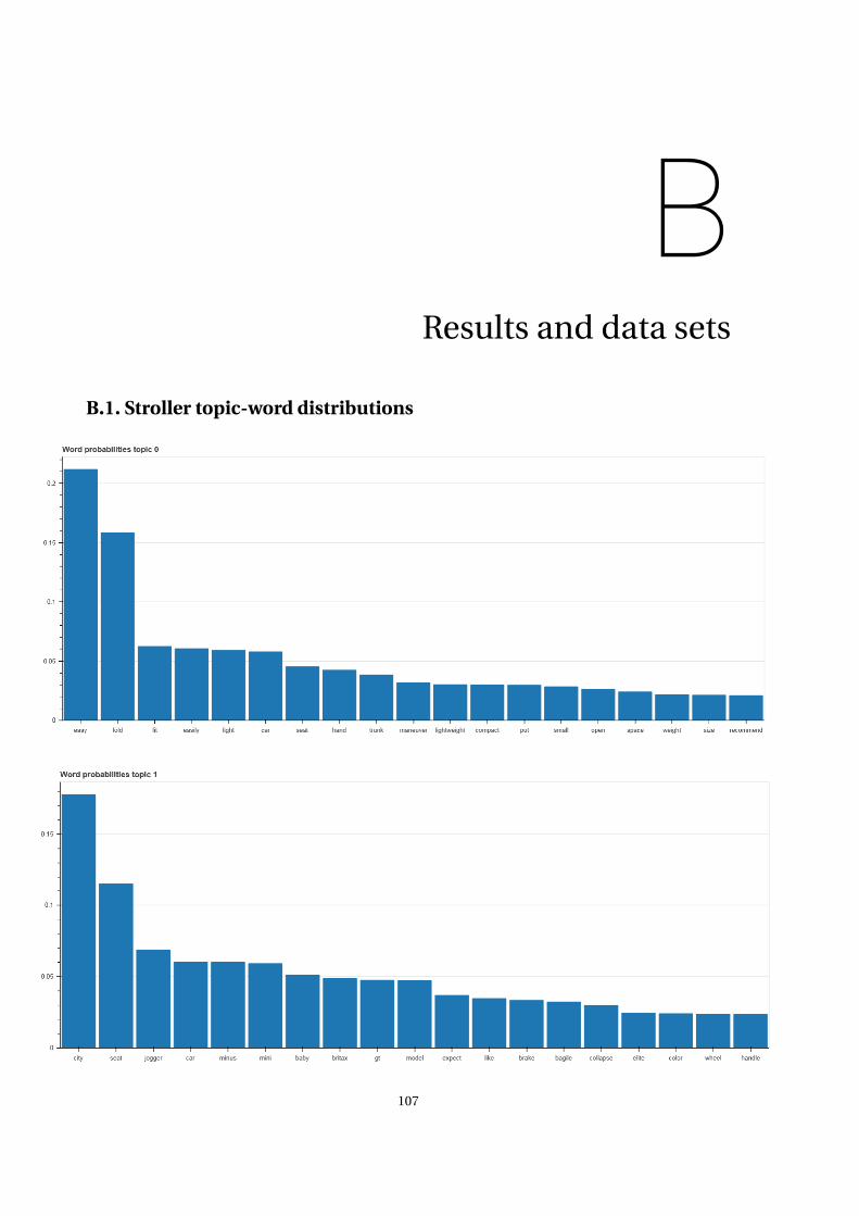
BResults and data sets
B.1. Stroller topic-word distributions
107
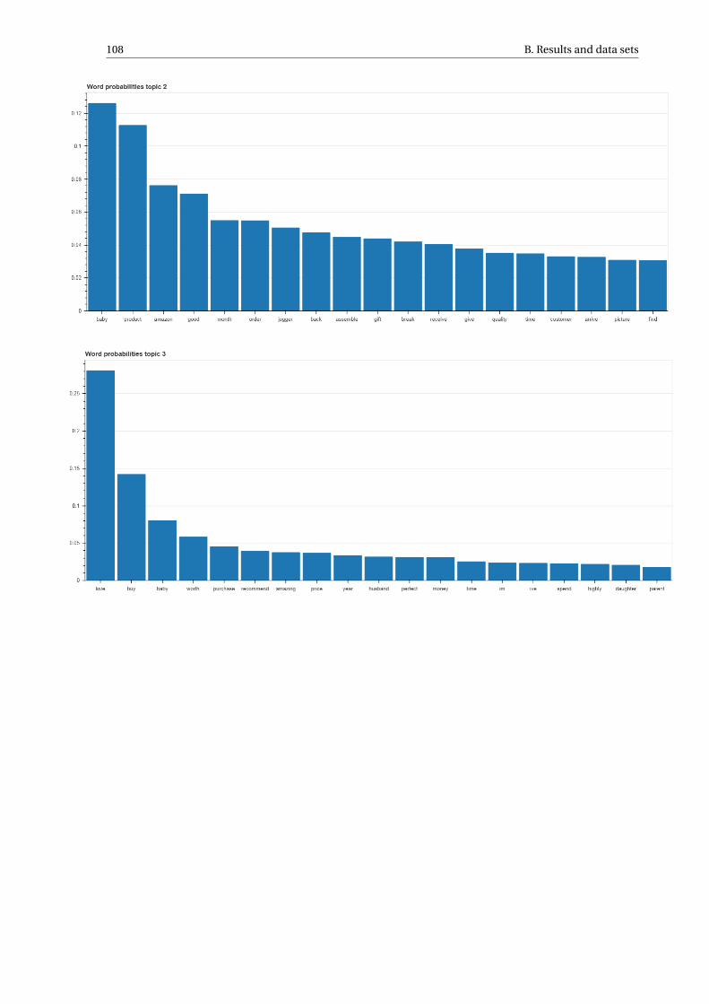
108 B. Results and data sets
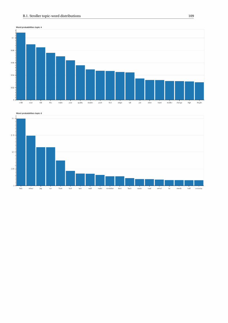
B.1. Stroller topic-word distributions 109
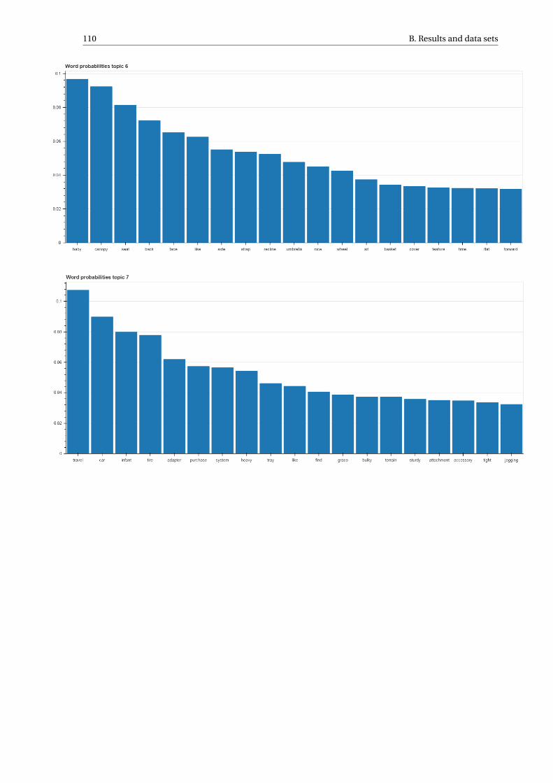
110 B. Results and data sets
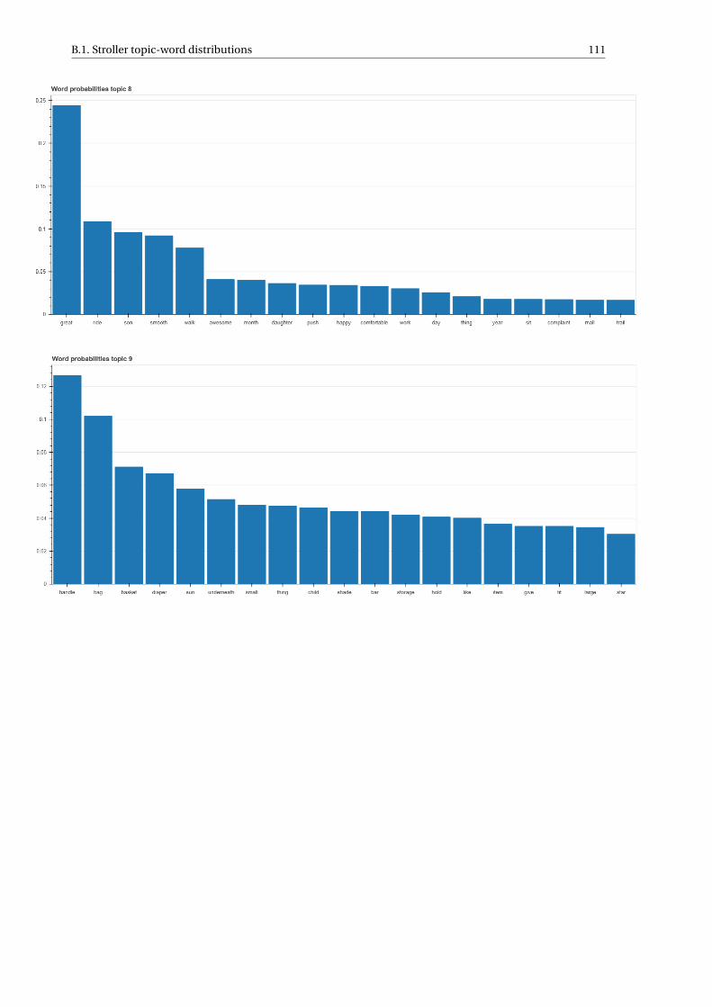
B.1. Stroller topic-word distributions 111
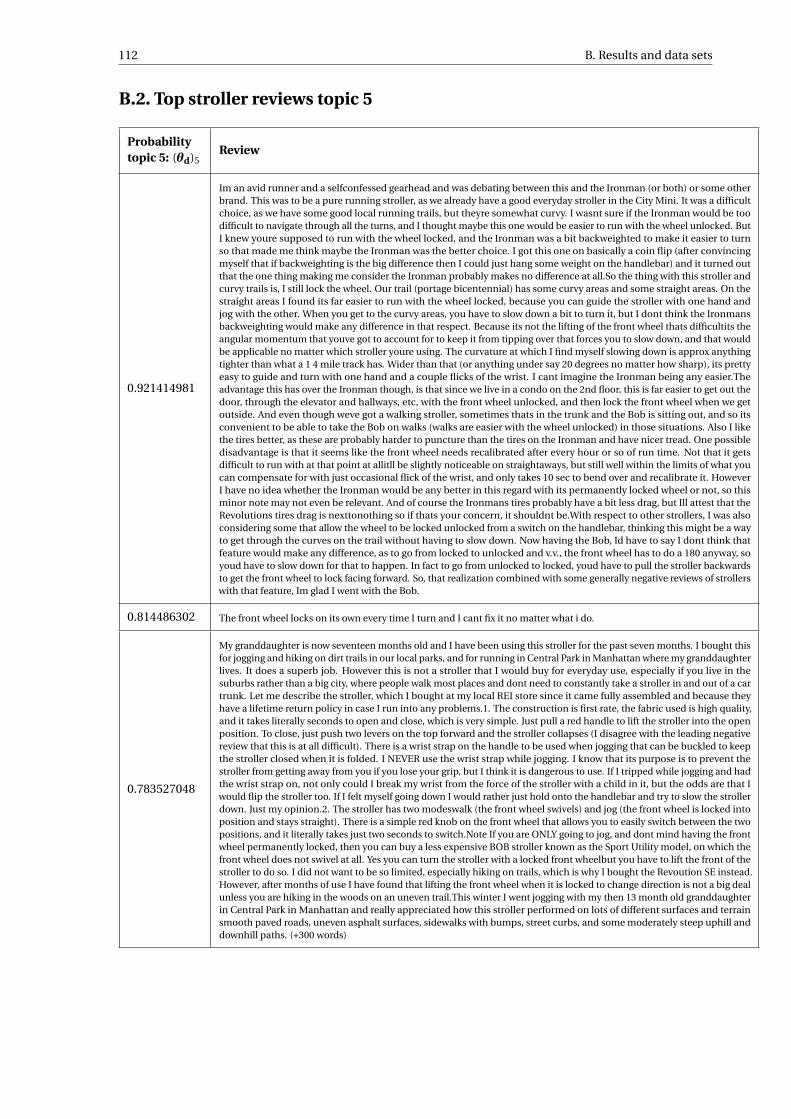
112 B. Results and data sets
B.2. Top stroller reviews topic 5
Probabilitytopic 5: (θd)5
Review
0.921414981
Im an avid runner and a selfconfessed gearhead and was debating between this and the Ironman (or both) or some otherbrand. This was to be a pure running stroller, as we already have a good everyday stroller in the City Mini. It was a difficultchoice, as we have some good local running trails, but theyre somewhat curvy. I wasnt sure if the Ironman would be toodifficult to navigate through all the turns, and I thought maybe this one would be easier to run with the wheel unlocked. ButI knew youre supposed to run with the wheel locked, and the Ironman was a bit backweighted to make it easier to turnso that made me think maybe the Ironman was the better choice. I got this one on basically a coin flip (after convincingmyself that if backweighting is the big difference then I could just hang some weight on the handlebar) and it turned outthat the one thing making me consider the Ironman probably makes no difference at all.So the thing with this stroller andcurvy trails is, I still lock the wheel. Our trail (portage bicentennial) has some curvy areas and some straight areas. On thestraight areas I found its far easier to run with the wheel locked, because you can guide the stroller with one hand andjog with the other. When you get to the curvy areas, you have to slow down a bit to turn it, but I dont think the Ironmansbackweighting would make any difference in that respect. Because its not the lifting of the front wheel thats difficultits theangular momentum that youve got to account for to keep it from tipping over that forces you to slow down, and that wouldbe applicable no matter which stroller youre using. The curvature at which I find myself slowing down is approx anythingtighter than what a 1 4 mile track has. Wider than that (or anything under say 20 degrees no matter how sharp), its prettyeasy to guide and turn with one hand and a couple flicks of the wrist. I cant imagine the Ironman being any easier.Theadvantage this has over the Ironman though, is that since we live in a condo on the 2nd floor, this is far easier to get out thedoor, through the elevator and hallways, etc, with the front wheel unlocked, and then lock the front wheel when we getoutside. And even though weve got a walking stroller, sometimes thats in the trunk and the Bob is sitting out, and so itsconvenient to be able to take the Bob on walks (walks are easier with the wheel unlocked) in those situations. Also I likethe tires better, as these are probably harder to puncture than the tires on the Ironman and have nicer tread. One possibledisadvantage is that it seems like the front wheel needs recalibrated after every hour or so of run time. Not that it getsdifficult to run with at that point at allitll be slightly noticeable on straightaways, but still well within the limits of what youcan compensate for with just occasional flick of the wrist, and only takes 10 sec to bend over and recalibrate it. HoweverI have no idea whether the Ironman would be any better in this regard with its permanently locked wheel or not, so thisminor note may not even be relevant. And of course the Ironmans tires probably have a bit less drag, but Ill attest that theRevolutions tires drag is nexttonothing so if thats your concern, it shouldnt be.With respect to other strollers, I was alsoconsidering some that allow the wheel to be locked unlocked from a switch on the handlebar, thinking this might be a wayto get through the curves on the trail without having to slow down. Now having the Bob, Id have to say I dont think thatfeature would make any difference, as to go from locked to unlocked and v.v., the front wheel has to do a 180 anyway, soyoud have to slow down for that to happen. In fact to go from unlocked to locked, youd have to pull the stroller backwardsto get the front wheel to lock facing forward. So, that realization combined with some generally negative reviews of strollerswith that feature, Im glad I went with the Bob.
0.814486302 The front wheel locks on its own every time I turn and I cant fix it no matter what i do.
0.783527048
My granddaughter is now seventeen months old and I have been using this stroller for the past seven months. I bought thisfor jogging and hiking on dirt trails in our local parks, and for running in Central Park in Manhattan where my granddaughterlives. It does a superb job. However this is not a stroller that I would buy for everyday use, especially if you live in thesuburbs rather than a big city, where people walk most places and dont need to constantly take a stroller in and out of a cartrunk. Let me describe the stroller, which I bought at my local REI store since it came fully assembled and because theyhave a lifetime return policy in case I run into any problems.1. The construction is first rate, the fabric used is high quality,and it takes literally seconds to open and close, which is very simple. Just pull a red handle to lift the stroller into the openposition. To close, just push two levers on the top forward and the stroller collapses (I disagree with the leading negativereview that this is at all difficult). There is a wrist strap on the handle to be used when jogging that can be buckled to keepthe stroller closed when it is folded. I NEVER use the wrist strap while jogging. I know that its purpose is to prevent thestroller from getting away from you if you lose your grip, but I think it is dangerous to use. If I tripped while jogging and hadthe wrist strap on, not only could I break my wrist from the force of the stroller with a child in it, but the odds are that Iwould flip the stroller too. If I felt myself going down I would rather just hold onto the handlebar and try to slow the strollerdown. Just my opinion.2. The stroller has two modeswalk (the front wheel swivels) and jog (the front wheel is locked intoposition and stays straight). There is a simple red knob on the front wheel that allows you to easily switch between the twopositions, and it literally takes just two seconds to switch.Note If you are ONLY going to jog, and dont mind having the frontwheel permanently locked, then you can buy a less expensive BOB stroller known as the Sport Utility model, on which thefront wheel does not swivel at all. Yes you can turn the stroller with a locked front wheelbut you have to lift the front of thestroller to do so. I did not want to be so limited, especially hiking on trails, which is why I bought the Revoution SE instead.However, after months of use I have found that lifting the front wheel when it is locked to change direction is not a big dealunless you are hiking in the woods on an uneven trail.This winter I went jogging with my then 13 month old granddaughterin Central Park in Manhattan and really appreciated how this stroller performed on lots of different surfaces and terrainsmooth paved roads, uneven asphalt surfaces, sidewalks with bumps, street curbs, and some moderately steep uphill anddownhill paths. (+300 words)
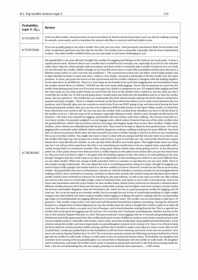
B.2. Top stroller reviews topic 5 113
Probabilitytopic 5: (θd)5
Review
0.757429179 LOVE our Bob stroller. Dont know how we survived without it! Rarely lock the front wheel, and I use this for walking running.Its smooth, turns easily, and is a musthave for anyone who likes to exercise with their kiddo in tow.
0.751979336If you are actually going to run with a stroller, this is the one you want. I had previously purchased a Baby Trend stroller andwish I would have paid more the first time for the Bob. The stroller runs so smoothly, especially with the front wheel lockedin place. The other stroller wobbled when you ran and made it a lot more challenging to run.
0.736783563
My grandchild is one year old and I bought this stroller for jogging and hiking on dirt trails in our local parks. It does asuperb job for each. However this is not a stroller that I would buy for everyday use, especially if you live in the suburbsrather than a big city, where people walk most places and dont need to constantly take a stroller in and out of a car trunk.Let me describe the stroller, which I bought at my local REI store since it came fully assembled and because they have alifetime return policy in case I run into any problems.1. The construction is first rate, the fabric used is high quality, andit takes literally seconds to open and close, which is very simple. Just pull a red handle to lift the stroller into the openposition. To close, just push two levers on the top forward and the stroller collapses (I disagree with the leading negativereview that this is at all difficult). There is a wrist strap on the handle to be used when jogging that can be buckled to keepthe stroller closed when it is folded. I NEVER use the wrist strap while jogging. I know that its purpose is to prevent thestroller from getting away from you if you lose your grip, but I think it is dangerous to use. If I tripped while jogging and hadthe wrist strap on, not only could I break my wrist from the force of the stroller with a child in it, but the odds are that Iwould flip the stroller too. If I felt myself going down I would rather just hold onto the handlebar and try to slow the strollerdown. Just my opinion.2. The stroller has two modeswalk (the front wheel swivels) and jog (the front wheel is locked intoposition and stays straight). There is a simple red knob on the front wheel that allows you to easily switch between the twopositions, and it literally takes just two seconds to switch.Note If you are ONLY going to jog, and dont mind having the frontwheel permanently locked, then you can buy a less expensive BOB stroller known as the Sport Utility model, on which thefront wheel does not swivel at all. Yes you can turn the stroller with a locked front wheelbut you have to lift the front ofthe stroller to do so. I did not want to be so limited, especially hiking on trails, which is why I bought the Revoution SEinstead.3. This rides very smooth for jogging, and handles off road surface well when walking. The reason is that this is avery heavy stroller (24 poundsI weighed it on my luggage scale, which makes it heavier than any of the other strollers thatmy grandchild has, which I discuss below) and has very large wheelsagain larger than on her other strollers. Unlike otherstrollers, these wheels are inflatable just like bicycle tires. They need to be kept at 30psi for best performance. Of coursejogging with a seriously under inflated wheel could be dangerous ordinary walking would just be more difficult. You donthave to check tire pressure all the time, but ask yourself if you want to bother having to check it at all if you are consideringthis as an everyday stroller. You might not want to have to deal with an unexpected flat tire just when you need to usethe stroller.This takes up a lot of space in a trunk, and is heavy to put in and take out. Yes, each of the wheels has a quickrelease lever (just like bicycle wheels), so you can take them all off to save trunk space. This might make sense on a longtrip, but I can tell you from experience that this is not something you would want to do on a regular basis, especially with acranky young child or in inclement weather. Plus, using quick release wheels takes some getting used to. As the directionspoint out, if the quick release lever does not leave a visible imprint in the palm of your hand after you put the wheel backon, then you have not done it right.4. I do agree with the leading negative review that there is no soft padding on the seat,though I disagree that the crotch strap is too short (it is adjustable) or that buckling your child in is any more difficult thanon any other stroller. When the canopy is fully extended, there is a window on top that lets you see your child. There isalso ample storage underneath. You can adjust the seat to a reclining position using two straps, though for jogging youneed to keep it fully upright (the further back it is, the less stability you have).However I would not use this as an everydaystroller. My grandchild (who lives in Manhattan) started out with the Bubaboo Cameleon stroller for local neighborhoodwalking (which I have reviewed on Amazon), and then at about nine months also started using the Maclaren Quest Sportstroller (which I have reviewed on Amazon) for traveling in cabs and subways, as well as day trips out of the city (like visitingme and my wife) since it is more light weight, easier to fold and close, and easier to carry with a carrying strap. And at myhouse she sometimes used the Graco Infant Car Seat stroller frame (which I have reviewed on Amazon).I mention thesedifferent strollers because all of these provide more comfortable seating, and are lighter and more compact (except maybethe heavier and bulkier Bugaboo) than the Revolution SE, which for me is a special purpose stroller for jogging and offroad use. Yes, it can be used as an everyday stroller, but its strength lies not in lots of comfortable padding or a light weightcompact size when folded, but rather in great stability while jogging or walking off road.For walking only the recommendedage range is 8 weeks8months for jogging offroad use it is 8 months5 years. The stroller can accommodate a child up to 70pounds.5. This stroller comes with a very clear and well illustrated manual that explains everything. Among the advancedfeatures is a simple form of wheel alignment in case the stroller does not roll in a straight line (which could occur after offroad use, the same as when a car goes over lots of bumps), and a shock absorber setting.Bottom line This is a special usestroller that works great for jogging and off road use. For everyday use I would get something else whether you live in thecity or the suburbs.Update February 23, 2012 This past weekend I went jogging with my 13 month old granddaughter inManhattan and really appreciated how this stroller performed on lots of different surfaces and terrain smooth paved roads,uneven asphalt surfaces, sidewalks with bumps, street curbs, and some moderately steep uphill and downhill paths. It wasa breeze using this stroller and more importantly my granddaughter enjoyed every minute of it. Since it is critical to keepthe front wheel in a locked position while running, anytime that I needed to make a turn (like at a street corner after we leftCentral Park), I easily just pulled back on the handlebars to lift the front wheel up and move it into the new position. Veryeasy to do and no big deal.Update June 10, 2012 The instruction manual contains the following warning in bold letters Neverjog with the stroller in walk mode. Doing so could result in loss of control and serious injury. Nevertheless my daughter andsoninlaw went running with my granddaughter in Central Park in Manhattan with the stroller in walk mode. My daughtersaid it worked fine, and made the stroller much easier to maneuver going back and forth to the Park and running inside thePark. I am not recommending this, but am simply pointing out someone elses experience... (+300 words)
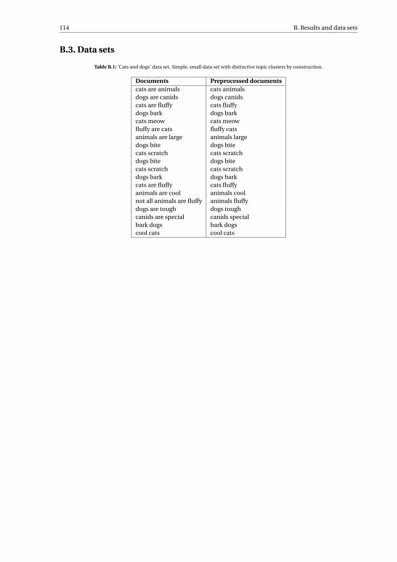
114 B. Results and data sets
B.3. Data sets
Table B.1: ‘Cats and dogs’ data set. Simple, small data set with distinctive topic clusters by construction.
Documents Preprocessed documentscats are animals cats animalsdogs are canids dogs canidscats are fluffy cats fluffydogs bark dogs barkcats meow cats meowfluffy are cats fluffy catsanimals are large animals largedogs bite dogs bitecats scratch cats scratchdogs bite dogs bitecats scratch cats scratchdogs bark dogs barkcats are fluffy cats fluffyanimals are cool animals coolnot all animals are fluffy animals fluffydogs are tough dogs toughcanids are special canids specialbark dogs bark dogscool cats cool cats
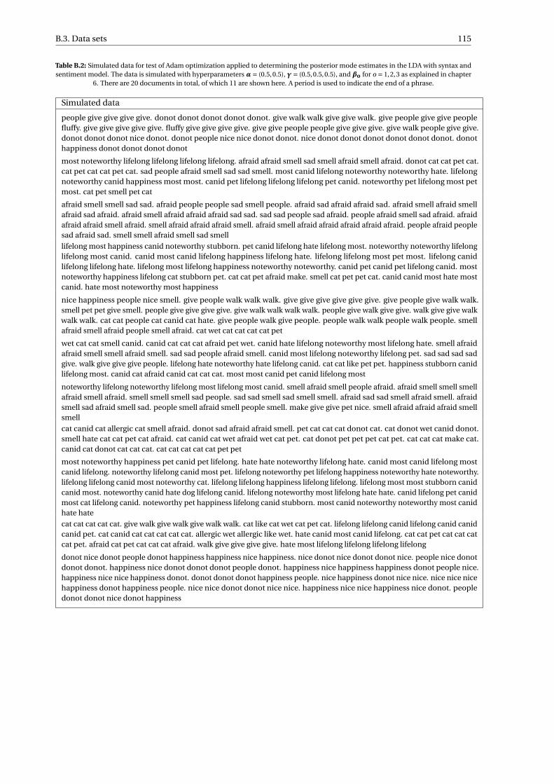
B.3. Data sets 115
Table B.2: Simulated data for test of Adam optimization applied to determining the posterior mode estimates in the LDA with syntax andsentiment model. The data is simulated with hyperparameters α= (0.5,0.5), γ= (0.5,0.5,0.5), and βo for o = 1,2,3 as explained in chapter
6. There are 20 documents in total, of which 11 are shown here. A period is used to indicate the end of a phrase.
Simulated data
people give give give give. donot donot donot donot donot. give walk walk give give walk. give people give give peoplefluffy. give give give give give. fluffy give give give give. give give people people give give give. give walk people give give.donot donot donot nice donot. donot people nice nice donot donot. nice donot donot donot donot donot donot. donothappiness donot donot donot donot
most noteworthy lifelong lifelong lifelong lifelong. afraid afraid smell sad smell afraid smell afraid. donot cat cat pet cat.cat pet cat cat pet cat. sad people afraid smell sad sad smell. most canid lifelong noteworthy noteworthy hate. lifelongnoteworthy canid happiness most most. canid pet lifelong lifelong lifelong pet canid. noteworthy pet lifelong most petmost. cat pet smell pet cat
afraid smell smell sad sad. afraid people people sad smell people. afraid sad afraid afraid sad. afraid smell afraid smellafraid sad afraid. afraid smell afraid afraid afraid sad sad. sad sad people sad afraid. people afraid smell sad afraid. afraidafraid afraid smell afraid. smell afraid afraid afraid smell. afraid smell afraid afraid afraid afraid afraid. people afraid peoplesad afraid sad. smell smell afraid smell sad smell
lifelong most happiness canid noteworthy stubborn. pet canid lifelong hate lifelong most. noteworthy noteworthy lifelonglifelong most canid. canid most canid lifelong happiness lifelong hate. lifelong lifelong most pet most. lifelong canidlifelong lifelong hate. lifelong most lifelong happiness noteworthy noteworthy. canid pet canid pet lifelong canid. mostnoteworthy happiness lifelong cat stubborn pet. cat cat pet afraid make. smell cat pet pet cat. canid canid most hate mostcanid. hate most noteworthy most happiness
nice happiness people nice smell. give people walk walk walk. give give give give give give. give people give walk walk.smell pet pet give smell. people give give give give. give walk walk walk walk. people give walk give give. walk give give walkwalk walk. cat cat people cat canid cat hate. give people walk give people. people walk walk people walk people. smellafraid smell afraid people smell afraid. cat wet cat cat cat cat pet
wet cat cat smell canid. canid cat cat cat afraid pet wet. canid hate lifelong noteworthy most lifelong hate. smell afraidafraid smell smell afraid smell. sad sad people afraid smell. canid most lifelong noteworthy lifelong pet. sad sad sad sadgive. walk give give give people. lifelong hate noteworthy hate lifelong canid. cat cat like pet pet. happiness stubborn canidlifelong most. canid cat afraid canid cat cat cat. most most canid pet canid lifelong most
noteworthy lifelong noteworthy lifelong most lifelong most canid. smell afraid smell people afraid. afraid smell smell smellafraid smell afraid. smell smell smell sad people. sad sad smell sad smell smell. afraid sad sad smell afraid smell. afraidsmell sad afraid smell sad. people smell afraid smell people smell. make give give pet nice. smell afraid afraid afraid smellsmell
cat canid cat allergic cat smell afraid. donot sad afraid afraid smell. pet cat cat cat donot cat. cat donot wet canid donot.smell hate cat cat pet cat afraid. cat canid cat wet afraid wet cat pet. cat donot pet pet pet cat pet. cat cat cat make cat.canid cat donot cat cat cat. cat cat cat cat cat pet pet
most noteworthy happiness pet canid pet lifelong. hate hate noteworthy lifelong hate. canid most canid lifelong mostcanid lifelong. noteworthy lifelong canid most pet. lifelong noteworthy pet lifelong happiness noteworthy hate noteworthy.lifelong lifelong canid most noteworthy cat. lifelong lifelong happiness lifelong lifelong. lifelong most most stubborn canidcanid most. noteworthy canid hate dog lifelong canid. lifelong noteworthy most lifelong hate hate. canid lifelong pet canidmost cat lifelong canid. noteworthy pet happiness lifelong canid stubborn. most canid noteworthy noteworthy most canidhate hate
cat cat cat cat cat. give walk give walk give walk walk. cat like cat wet cat pet cat. lifelong lifelong canid lifelong canid canidcanid pet. cat canid cat cat cat cat cat. allergic wet allergic like wet. hate canid most canid lifelong. cat cat pet cat cat catcat pet. afraid cat pet cat cat cat afraid. walk give give give give. hate most lifelong lifelong lifelong lifelong
donot nice donot people donot happiness happiness nice happiness. nice donot nice donot donot nice. people nice donotdonot donot. happiness nice donot donot donot people donot. happiness nice happiness happiness donot people nice.happiness nice nice happiness donot. donot donot donot happiness people. nice happiness donot nice nice. nice nice nicehappiness donot happiness people. nice nice donot donot nice nice. happiness nice nice happiness nice donot. peopledonot donot nice donot happiness

116 B. Results and data sets
Table B.3: Simulated data for test of Adam optimization applied to determining the posterior mode estimates in the LDA with syntax andsentiment model. The data is simulated with hyperparameters α= (0.5,0.5), γ= (0.5,0.5,0.5), and βo for o = 1,2,3 as explained in chapter
6. There are 20 documents in total, of which 9 are shown here. A period is used to indicate the end of a phrase.
Simulated data
pet canid sad canid sad give smell. pet wet cat cat people pet. aggressive regret pet sad give pet. sad sad sad smell smellafraid. smell smell smell sad sad afraid people. smell smell smell smell sad sad. pet pet pet give pet nice. afraid sad afraidsmell afraid. sad sad afraid afraid smell sad sad. walk people walk give give give give. give walk give walk give. afraid sadsad people smell afraid. donot donot nice people donot happiness donot
give give give give give walk. people canid make cat canid cat. people give give people give give. cat cat cat cat pet cat cat.pet afraid canid cat pet cat cat canid. give give give walk people people walk. make pet cat pet pet cat. pet cat cat cat catcanid. walk people people give walk give give. make pet canid pet cat. pet cat cat cat pet cat cat make. cat cat pet cat catcat. cat hate canid cat pet cat pet cat. afraid cat cat smell pet pet pet. people give give give walk give
most pet hate noteworthy hate pet most. afraid smell afraid smell afraid smell. lifelong hate lifelong hate hate most. smellsad smell afraid afraid. lifelong stubborn noteworthy lifelong canid. smell smell smell sad sad sad donot. sad sad sad sadsmell afraid. cat walk cat pet cat cat. cat afraid cat cat wet. most hate cat lifelong canid. canid hate noteworthy lifelonglifelong. canid cat canid cat cat
give give give give walk people people. walk cat people give give. give give give give give. give walk people people givepeople. people walk people give walk. fluffy give give give people. give people people walk people. walk give walk walkwalk walk. people people people give give give. give fluffy people people give. people people give give walk. fluffy give walkgive fluffy fluffy. give give walk give walk give
donot donot happiness donot happiness happiness nice nice donot. canid hate hate pet lifelong. lifelong most lifelonglifelong stubborn. lifelong canid lifelong lifelong dog pet pet. canid pet cat pet smell cat cat. cat noteworthy lifelong lifelonglifelong lifelong noteworthy stubborn. pet cat canid noteworthy lifelong noteworthy. lifelong most pet canid lifelong most.noteworthy hate cat pet canid wet most. noteworthy most canid most noteworthy most. lifelong lifelong canid lifelongcanid noteworthy pet canid. noteworthy most canid canid lifelong hate happiness
pet sad nice pet like. noteworthy lifelong lifelong lifelong most canid most happiness. noteworthy hate lifelong hate canidmost canid most. canid hate most canid noteworthy. donot afraid people afraid smell. pet sad pet smell give. most canidcanid most most pet. smell afraid people smell sad sad sad afraid. sad smell smell afraid smell sad. hate canid most mosthate most
hate lifelong canid canid lifelong hate. canid canid lifelong lifelong lifelong lifelong. lifelong most hate noteworthynoteworthy lifelong. noteworthy canid hate canid hate noteworthy. hate most pet noteworthy canid noteworthy. canidhappiness happiness lifelong most lifelong canid. canid canid most noteworthy lifelong canid noteworthy most lifelongmost happiness. lifelong noteworthy most canid canid. canid pet lifelong happiness lifelong. lifelong lifelong lifelongcanid canid lifelong
smell smell smell afraid smell. sad smell pet make pet. give sad sad smell smell pet. make sad sad give pet sad pet. pet catcat cat cat. give people give give give walk walk. give walk walk walk people. people give people give give. fluffy fluffy givewalk give walk. sad make pet sad smell sad. give pet give nice sad like
sad sad smell smell people. sad afraid sad afraid afraid smell afraid. afraid afraid afraid afraid afraid smell. smell sad afraidpeople smell smell. smell smell smell people sad. afraid smell sad smell afraid afraid. afraid sad sad people smell smell.smell smell afraid smell afraid people people. donot donot nice nice donot donot nice donot nice. sad smell afraid sadsmell smell afraid. afraid afraid afraid smell smell smell afraid

B.4. Conjunction word list 117
B.4. Conjunction word list
butsoorandafterbeforealthougheven thoughbecauseasifas long asprovided thattilluntilunlesswhenonceas soon aswhilewhereasin spite ofdespitein additionfurthermorehoweveron the other handthereforeconsequentlyfirstlysecondly
thirdlyfinallyaccordinglyalsoanywaybesidesfor examplefor instancefurtherhenceincidentallyindeedin factinsteadlikewisemeanwhilemoreovernamelyof courseon the contraryotherwiseneverthelessnonethelesssimilarlyso faruntil nowthenthereforethus
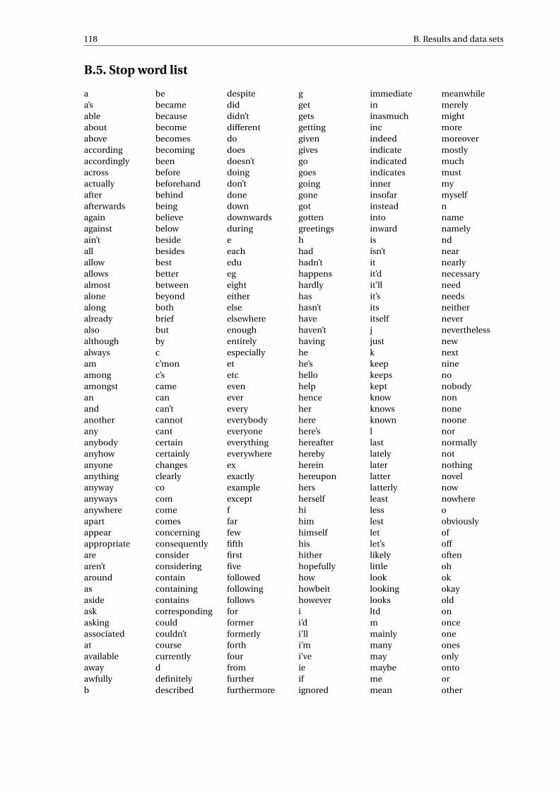
118 B. Results and data sets
B.5. Stop word list
aa’sableaboutaboveaccordingaccordinglyacrossactuallyafterafterwardsagainagainstain’tallallowallowsalmostalonealongalreadyalsoalthoughalwaysamamongamongstanandanotheranyanybodyanyhowanyoneanythinganywayanywaysanywhereapartappearappropriatearearen’taroundasasideaskaskingassociatedatavailableawayawfullyb
bebecamebecausebecomebecomesbecomingbeenbeforebeforehandbehindbeingbelievebelowbesidebesidesbestbetterbetweenbeyondbothbriefbutbycc’monc’scamecancan’tcannotcantcertaincertainlychangesclearlycocomcomecomesconcerningconsequentlyconsiderconsideringcontaincontainingcontainscorrespondingcouldcouldn’tcoursecurrentlyddefinitelydescribed
despitediddidn’tdifferentdodoesdoesn’tdoingdon’tdonedowndownwardsduringeeacheduegeighteitherelseelsewhereenoughentirelyespeciallyetetcevenevereveryeverybodyeveryoneeverythingeverywhereexexactlyexampleexceptffarfewfifthfirstfivefollowedfollowingfollowsforformerformerlyforthfourfromfurtherfurthermore
ggetgetsgettinggivengivesgogoesgoinggonegotgottengreetingshhadhadn’thappenshardlyhashasn’thavehaven’thavinghehe’shellohelphenceherherehere’shereafterherebyhereinhereuponhersherselfhihimhimselfhishitherhopefullyhowhowbeithoweverii’di’lli’mi’veieifignored
immediateininasmuchincindeedindicateindicatedindicatesinnerinsofarinsteadintoinwardisisn’titit’dit’llit’sitsitselfjjustkkeepkeepskeptknowknowsknownllastlatelylaterlatterlatterlyleastlesslestletlet’slikelylittlelooklookinglooksltdmmainlymanymaymaybememean
meanwhilemerelymightmoremoreovermostlymuchmustmymyselfnnamenamelyndnearnearlynecessaryneedneedsneitherneverneverthelessnewnextninenonobodynonnonenoonenornormallynotnothingnovelnownowhereoobviouslyofoffoftenohokokayoldononceoneonesonlyontoorother

B.5. Stop word list 119
othersotherwiseoughtouroursourselvesoutoutsideoveroverallownpparticularparticularlyperperhapsplacedpleasepluspossiblepresumablyprobablyprovidesqquequiteqvrratherrdrereallyreasonablyregardingregardlessregardsrelativelyrespectivelyrightssaidsame
sawsaysayingsayssecondsecondlyseeseeingseemseemedseemingseemsseenselfselvessensiblesentseriousseriouslysevenseveralshallsheshouldshouldn’tsincesixsosomesomebodysomehowsomeonesomethingsometimesometimessomewhatsomewheresoonspecifiedspecifyspecifyingstill
subsuchsupsurett’staketakentelltendsththanthankthanksthanxthatthat’sthatsthetheirtheirsthemthemselvesthenthencetherethere’sthereaftertherebythereforethereintheresthereuponthesetheythey’dthey’llthey’rethey’vethinkthirdthis
thoroughthoroughlythosethoughthreethroughthroughoutthruthustotogethertootooktowardtowardstriedtriestrulytrytryingtwicetwouununderunfortunatelyunlessunlikelyuntiluntoupuponususeusedusesusingusuallyuucpvvaluevarious
veryviavizvswwantwantswaswasn’twaywewe’dwe’llwe’rewe’vewelcomewellwentwereweren’twhatwhat’swhateverwhenwhencewheneverwherewhere’swhereafterwhereaswherebywhereinwhereuponwhereverwhetherwhichwhilewhitherwhowho’swhoeverwhole
whomwhosewhywillwillingwishwithwithinwithoutwon’twonderwouldwouldwouldn’txyyesyetyouyou’dyou’llyou’reyou’veyouryoursyourselfyourselveszzeroyou’reyou’veyouryoursyourselfyourselveszzero

120 B. Results and data sets
B.6. Sentiment word lists
Positive words:
abidanceabideabilitiesabilityableaboundaboveabove-averageabsolveabundanceabundantaccedeacceptacceptableacceptanceaccessibleacclaimacclaimedacclamationaccoladeaccoladesaccommodativeaccomplishaccomplishmentaccomplishmentsaccordaccordanceaccordantlyaccurateaccuratelyachievableachieveachievementachievementsacknowledgeacknowledgementacquitactiveacumenadaptabilityadaptableadaptiveadeptadeptlyadequateadherenceadherentadhesionadmirableadmirablyadmirationadmireadmireradmiringadmiringlyadmission
admitadmittedlyadorableadoreadoredadoreradoringadoringlyadroitadroitlyadulateadulationadulatoryadvancedadvantageadvantageousadvantagesadventureadventuresomeadventurismadventurousadviceadvisableadvocacyadvocateaffabilityaffableaffablyaffectionaffectionateaffinityaffirmaffirmationaffirmativeaffluenceaffluentaffordaffordableafloatagileagilelyagilityagreeagreeabilityagreeableagreeablenessagreeablyagreementallayalleviateallowallowableallurealluringalluringlyally
almightyaltruistaltruisticaltruisticallyamazeamazedamazementamazingamazinglyambitiousambitiouslyameliorateamenableamenityamiabilityamiabilyamiableamicabilityamicableamicablyamityamnestyamourampleamplyamuseamusementamusingamusinglyangelangelicanimatedapostleapotheosisappealappealingappeaseapplaudappreciableappreciateappreciationappreciativeappreciativelyappreciativenessappropriateapprovalapproveaptaptitudeaptlyardentardentlyardoraristocraticarousalarouse
arousingarrestingarticulateascendantascertainableaspirationaspirationsaspireassentassertionsassertiveassetassiduousassiduouslyassuageassuranceassurancesassureassuredlyastonishastonishedastonishingastonishinglyastonishmentastoundastoundedastoundingastoundinglyastuteastutelyasylumattainattainableattentiveattestattractionattractiveattractivelyattuneauspiciousauthenticauthoritativeautonomousaveravidavidlyawardaweawedawesomeawesomelyawesomenessawestruckbackbackbonebalanced
bargainbasicbaskbeaconbeatifybeauteousbeautifulbeautifullybeautifybeautybefitbefittingbefriendbelievablebelovedbenefactorbeneficentbeneficialbeneficiallybeneficiarybenefitbenefitsbenevolencebenevolentbenignbestbest-knownbest-performingbest-sellingbetterbetter-knownbetter-than-expectedblamelessblessblessingblissblissfulblissfullyblithebloomblossomboastboldboldlyboldnessbolsterbonnybonusboomboomingboostboundlessbountifulbrainsbrainy
bravebraverybreakthroughbreakthroughsbreathlessnessbreathtakingbreathtakinglybrightbrightenbrightnessbrilliancebrilliantbrilliantlybriskbroadbrookbrotherlybullbullishbuoyantcalmcalmingcalmnesscandidcandorcapabilitycapablecapablycapitalizecaptivatecaptivatingcaptivationcarecarefreecarefulcatalystcatchycelebratecelebratedcelebrationcelebratorycelebritychampchampioncharismaticcharitablecharitycharmcharmingcharminglychastecheercheerfulcheerycherishcherished

B.6. Sentiment word lists 121
cherubchicchivalrouschivalrychumcivilcivilitycivilizationcivilizeclarityclassiccleancleanlinesscleanseclearclear-cutclearerclearlycleverclosenesscloutco-operationcoaxcoddlecogentcoherecoherencecoherentcohesioncohesivecolorfulcolossalcomebackcomelycomfortcomfortablecomfortablycomfortingcommendcommendablecommendablycommensuratecommitmentcommodiouscommonsensecommonsensiblecommonsensiblycommonsensicalcompactcompassioncompassionatecompatiblecompellingcompensatecompetencecompetencycompetentcompetitivecompetitivenesscomplementcompliant
complimentcomplimentarycomprehensivecompromisecompromisescomradesconceivableconciliateconciliatoryconclusiveconcreteconcurcondoneconduciveconferconfidenceconfidentconfutecongenialcongratulatecongratulationscongratulatoryconquerconscienceconscientiousconsensusconsentconsiderateconsistentconsoleconstancyconstructiveconsummatecontentcontentmentcontinuitycontributionconvenientconvenientlyconvictionconvinceconvincingconvincinglycooperatecooperationcooperativecooperativelycordialcornerstonecorrectcorrectlycost-effectivecost-savingcouragecourageouscourageouslycourageousnesscourtcourteouscourtesycourtly
covenantcozycravecravingcreativecredencecrediblecrispcrusadecrusadercure-allcuriouscuriouslycutedancedaredaringdaringlydarlingdashingdauntlessdawndaydreamdaydreamerdazzledazzleddazzlingdealdeardecencydecentdecisivedecisivenessdedicateddefenddefenderdefensedeferencedefinitedefinitelydefinitivedefinitivelydeflationarydeftdelectabledelicacydelicatedeliciousdelightdelighteddelightfuldelightfullydelightfulnessdemocraticdemystifydependabledeservedeserveddeservedlydeservingdesirable
desiredesirousdestinedestineddestiniesdestinydeterminationdevotedevoteddevoteedevotiondevoutdexteritydexterousdexterouslydextrousdigdignifieddignifydignitydiligencediligentdiligentlydiplomaticdiscerningdiscreetdiscretiondiscriminatingdiscriminatinglydistinctdistinctiondistinctivedistinguishdistinguisheddiversifieddivinedivinelydodgedotedotinglydoubtlessdreamdreamlanddreamsdreamydrivedrivendurabilitydurabledynamiceagereagerlyeagernessearnestearnestlyearnestnesseaseeasiereasiesteasilyeasiness
easyeasygoingebullienceebullientebullientlyeclecticeconomicalecstasiesecstasyecstaticecstaticallyedifyeducableeducatededucationaleffectiveeffectivenesseffectualefficaciousefficiencyefficienteffortlesseffortlesslyeffusioneffusiveeffusivelyeffusivenessegalitarianelanelateelatedelatedlyelationelectrificationelectrifyeleganceelegantelegantlyelevateelevatedeligibleeliteeloquenceeloquenteloquentlyemancipateembellishemboldenembraceeminenceeminentempowerempowermentenableenchantenchantedenchantingenchantinglyencourageencouragementencouraging
encouraginglyendearendearingendorseendorsementendorserendurableendureenduringenergeticenergizeengagingengrossingenhanceenhancedenhancementenjoyenjoyableenjoyablyenjoymentenlightenenlightenmentenlivenennobleenraptenraptureenrapturedenrichenrichmentensureenterprisingentertainentertainingenthralenthrallenthralledenthuseenthusiasmenthusiastenthusiasticenthusiasticallyenticeenticingenticinglyentranceentrancedentrancingentreatentreatinglyentrustenviableenviablyenvisionenvisionsepicepitomeequalityequitableeruditeespeciallyessential
122 B. Results and data sets
establishedesteemeternityethicaleulogizeeuphoriaeuphoriceuphoricallyevenevenlyeventfuleverlastingevidentevidentlyevocativeexaltexaltationexaltedexaltedlyexaltingexaltinglyexceedexceedingexceedinglyexcelexcellenceexcellencyexcellentexcellentlyexceptionalexceptionallyexciteexcitedexcitedlyexcitednessexcitementexcitingexcitinglyexclusiveexcusableexcuseexemplarexemplaryexhaustiveexhaustivelyexhilarateexhilaratingexhilaratinglyexhilarationexonerateexpansiveexperiencedexpertexpertlyexplicitexplicitlyexpressiveexquisiteexquisitelyextolextoll
extraordinarilyextraordinaryexuberanceexuberantexuberantlyexultexultationexultinglyfabulousfabulouslyfacilitatefairfairlyfairnessfaithfaithfulfaithfullyfaithfulnessfamefamedfamousfamouslyfancyfanfarefantasticfantasticallyfantasyfarsightedfascinatefascinatingfascinatinglyfascinationfashionablefashionablyfast-growingfast-pacedfastest-growingfathomfavorfavorablefavoredfavoritefavourfearlessfearlesslyfeasiblefeasiblyfeatfeatlyfeistyfelicitatefelicitousfelicityfertileferventferventlyfervidfervidlyfervorfestivefidelity
fieryfinefinelyfirst-classfirst-ratefitfittingflairflameflatterflatteringflatteringlyflawlessflawlesslyflexibleflourishflourishingfluentfondfondlyfondnessfoolproofforemostforesightforgaveforgiveforgivenforgivenessforgivingforgivinglyfortitudefortuitousfortuitouslyfortunatefortunatelyfortunefragrantfrankfreefreedomfreedomsfreshfriendfriendlinessfriendlyfriendsfriendshipfrolicfruitfulfulfillmentfull-fledgedfunfunctionalfunnygaietygailygaingainfulgainfullygallantgallantly
galoregemgemsgenerositygenerousgenerouslygenialgeniusgentlegenuinegermanegiddygiftedgladgladdengladlygladnessglamorousgleegleefulgleefullyglimmerglimmeringglistenglisteningglitterglorifygloriousgloriouslygloryglossyglowglowingglowinglygo-aheadgod-givengodlikegoldgoldengoodgoodlygoodnessgoodwillgorgeousgorgeouslygracegracefulgracefullygraciousgraciouslygraciousnessgrailgrandgrandeurgratefulgratefullygratificationgratifygratifyinggratifyinglygratitude
greatgreatestgreatnessgreetgringritgroovegroundbreakingguaranteeguardianguidanceguiltlessgumptiongushgustogutsyhailhalcyonhalehallowedhandilyhandsomehandyhankerhappilyhappinesshappyhard-workinghardierhardyharmlessharmoniousharmoniouslyharmonizeharmonyhavenheadwayheadyhealhealthfulhealthyheartheartenhearteningheartfeltheartilyheartwarmingheavenheavenlyhelphelpfulheraldheroheroicheroicallyheroineheroizeheroshigh-qualityhighlighthilarious
hilariouslyhilariousnesshilarityhistoricholyhomagehonesthonestlyhonestyhoneymoonhonorhonorablehopehopefulhopefullyhopefulnesshopeshospitablehothughumanehumanistshumanityhumankindhumblehumilityhumorhumoroushumorouslyhumourhumourousidealidealismidealistidealizeideallyidolidolizeidolizedidyllicilluminateilluminatiilluminatingillumineillustriousimaginativeimmaculateimmaculatelyimpartialimpartialityimpartiallyimpassionedimpeccableimpeccablyimpelimperialimperturbableimperviousimpetusimportanceimportant
B.6. Sentiment word lists 123
importantlyimpregnableimpressimpressionimpressionsimpressiveimpressivelyimpressivenessimproveimprovedimprovementimprovingimproviseinalienableincisiveincisivelyincisivenessinclinationinclinationsinclinedinclusiveincontestableincontrovertibleincorruptibleincredibleincrediblyindebtedindefatigableindelibleindeliblyindependenceindependentindescribableindescribablyindestructibleindispensabilityindispensableindisputableindividualityindomitableindomitablyindubitableindubitablyindulgenceindulgentindustriousinestimableinestimablyinexpensiveinfallibilityinfallibleinfalliblyinfluentialinformativeingeniousingeniouslyingenuityingenuousingenuouslyingratiateingratiating
ingratiatinglyinnocenceinnocentinnocentlyinnocuousinnovationinnovativeinoffensiveinquisitiveinsightinsightfulinsightfullyinsistinsistenceinsistentinsistentlyinspirationinspirationalinspireinspiringinstructiveinstrumentalintactintegralintegrityintelligenceintelligentintelligibleintercedeinterestinterestedinterestinginterestsintimacyintimateintricateintrigueintriguingintriguinglyintuitiveinvaluableinvaluablelyinventiveinvigorateinvigoratinginvincibilityinvincibleinviolableinviolateinvulnerableirrefutableirrefutablyirreproachableirresistibleirresistiblyjauntilyjauntyjestjokejollifyjolly
jovialjoyjoyfuljoyfullyjoylessjoyousjoyouslyjubilantjubilantlyjubilatejubilationjudiciousjustjusticejustifiablejustifiablyjustificationjustifyjustlykeenkeenlykeennesskempkidkindkindlinesskindlykindnesskingmakerkissknowledgeablelargelarklaudlaudablelaudablylavishlavishlylaw-abidinglawfullawfullyleadingleanlearnedlearninglegendarylegitimacylegitimatelegitimatelylenientlenientlyless-expensiveleveragelevityliberalliberalismliberallyliberateliberationlibertylifeblood
lifelonglightlight-heartedlightenlikablelikelikinglionheartedliteratelivelivelyloftylogicallovablelovablylovelovelinesslovelyloverlow-costlow-risklower-pricedloyalloyaltylucidlucidlyluckluckierluckiestluckilyluckinessluckylucrativeluminouslushlusterlustrousluxuriantluxuriateluxuriousluxuriouslyluxurylyricalmagicmagicalmagnanimousmagnanimouslymagneticmagnificencemagnificentmagnificentlymagnifymajesticmajestymanageablemanifestmanlymannerlymarvelmarvellousmarvelous
marvelouslymarvelousnessmarvelsmastermasterfulmasterfullymasterpiecemasterpiecesmastersmasterymatchlessmaturematurelymaturitymaximizemeaningfulmeekmellowmemorablememorializemendmentormercifulmercifullymercymeritmeritoriousmerrilymerrimentmerrinessmerrymesmerizemesmerizingmesmerizinglymeticulousmeticulouslymightmightilymightymildmindfulministermiraclemiraclesmiraculousmiraculouslymiraculousnessmirthmoderatemoderationmodernmodestmodestymollifymomentousmonumentalmonumentallymoralmoralitymoralizemotivate
motivatedmotivationmovingmyriadnaturalnaturallynavigableneatneatlynecessarilynecessaryneutralizenicenicelyniftynimblenoblenoblynon-violencenon-violentnormalnotablenotablynoteworthynoticeablenourishnourishingnourishmentnovelnurturenurturingoasisobedienceobedientobedientlyobeyobjectiveobjectivelyobligedobviateoffbeatoffsetokayonwardopenopenlyopennessopportuneopportunityoptimaloptimismoptimisticopulentorderlyoriginaloriginalityoutdooutgoingoutshineoutsmartoutstanding
124 B. Results and data sets
outstandinglyoutstripoutwitovationoverachieveroverjoyedoverturepacifistpacifistspainlesspainlesslypainstakingpainstakinglypalatablepalatialpalliatepamperparadiseparamountpardonpassionpassionatepassionatelypatiencepatientpatientlypatriotpatrioticpeacepeaceablepeacefulpeacefullypeacekeeperspeerlesspenetratingpenitentperceptiveperfectperfectionperfectlypermissibleperseveranceperseverepersistentpersonagespersonalityperspicuousperspicuouslypersuadepersuasivepersuasivelypertinentphenomenalphenomenallypicturesquepietypillarpinnaclepiouspithyplacate
placidplainplainlyplausibilityplausibleplayfulplayfullypleasantpleasantlypleasepleasedpleasingpleasinglypleasurablepleasurablypleasurepledgepledgesplentifulplentyplushpoeticpoeticizepoignantpoisepoisedpolishedpolitepolitenesspopularpopularityportableposhpositivepositivelypositivenessposteritypotentpotentialpowerfulpowerfullypracticablepracticalpragmaticpraisepraiseworthypraisingpre-eminentpreachpreachingprecautionprecautionsprecedentpreciousprecisepreciselyprecisionpreeminentpreemptivepreferpreferable
preferablypreferencepreferencespremierpremiumpreparedpreponderancepressprestigeprestigiousprettilyprettypricelessprideprincipleprincipledprivilegeprivilegedprizepropro-Americanpro-Beijingpro-Cubapro-peaceproactiveprodigiousprodigiouslyprodigyproductiveprofessproficientproficientlyprofitprofitableprofoundprofoundlyprofuseprofuselyprofusionprogressprogressiveprolificprominenceprominentpromisepromisingpromoterpromptpromptlyproperproperlypropitiouspropitiouslyprospectprospectsprosperprosperityprosperousprotectprotectionprotective
protectorproudprovidenceprowessprudenceprudentprudentlypunctualpunditspurepurificationpurifypuritypurposefulquaintqualifiedqualifyquasi-allyquenchquickenradianceradiantrallyrapportrapprochementraptraptureraptureousraptureouslyrapturousrapturouslyrationalrationalityravere-conquestreadilyreadyreaffirmreaffirmationrealrealistrealisticrealisticallyreasonreasonablereasonablyreasonedreassurancereassurereceptivereclaimrecognitionrecommendrecommendationrecommendationsrecommendedrecompensereconcilereconciliationrecord-settingrecover
rectificationrectifyrectifyingredeemredeemingredemptionreestablishrefinerefinedrefinementreformrefreshrefreshingrefugeregalregallyregardrehabilitaterehabilitationreinforcereinforcementrejoicerejoicingrejoicinglyrelaxrelaxedrelentrelevancerelevantreliabilityreliablereliablyreliefrelieverelishremarkableremarkablyremedyreminiscentremuneraterenaissancerenewalrenovaterenovationrenownrenownedrepairreparationrepayrepentrepentancereputablerescueresilientresoluteresolveresolvedresoundresoundingresourcefulresourcefulness
respectrespectablerespectfulrespectfullyrespiteresplendentresponsibilityresponsibleresponsiblyresponsiverestfulrestorationrestorerestraintresurgentreuniterevelrevelationreverereverencereverentreverentlyrevitalizerevivalreviverevolutionrewardrewardingrewardinglyrichrichesrichlyrichnessrightrightenrighteousrighteouslyrighteousnessrightfulrightfullyrightlyrightnessrightsriperisk-freerobustromanticromanticallyromanticizerosyrousingsacredsafesafeguardsagacitysagesagelysaintsaintlinesssaintlysalable
B.6. Sentiment word lists 125
salivatesalutarysalutesalvationsanctifysanctionsanctitysanctuarysanesanguinesanitysatisfactionsatisfactorilysatisfactorysatisfysatisfyingsavorsavvyscenicscruplesscrupulousscrupulouslyseamlessseasonedsecuresecurelysecurityseductiveselectiveself-determinationself-respectself-satisfactionself-sufficiencyself-sufficientsemblancesensationsensationalsensationallysensationssensesensiblesensiblysensitivesensitivelysensitivitysentimentsentimentalitysentimentallysentimentssereneserenitysettlesexysheltershieldshimmershimmeringshimmeringlyshineshiny
shrewdshrewdlyshrewdnesssignificancesignificantsignifysimplesimplicitysimplifiedsimplifysinceresincerelysincerityskillskilledskillfulskillfullysleekslenderslimsmartsmartersmartestsmartlysmilesmilingsmilinglysmittensmoothsociablesoft-spokensoftensolacesolicitoussolicitouslysolicitudesolidsolidaritysoothesoothinglysophisticatedsoundsoundnessspacioussparesparingsparinglysparklesparklingspecialspectacularspectacularlyspeedyspellbindspellbindingspellbindinglyspellboundspiritspiritedspiritualsplendid
splendidlysplendorspotlesssprightlyspursquarelystabilitystabilizestablestainlessstandstarstarsstatelystatuesquestaunchstaunchlystaunchnesssteadfaststeadfastlysteadfastnesssteadinesssteadystellarstellarlystimulatestimulatingstimulativestirringstirringlystoodstraightstraightforwardstreamlinedstridestridesstrikingstrikinglystrivingstrongstudiousstudiouslystunnedstunningstunninglystupendousstupendouslysturdystylishstylishlysuavesublimesubscribesubstantialsubstantiallysubstantivesubtlesucceedsuccesssuccessfulsuccessfully
sufficesufficientsufficientlysuggestsuggestionssuitsuitablesumptuoussumptuouslysumptuousnesssunnysupersuperbsuperblysuperiorsuperlativesupportsupportersupportivesupremesupremelysupurbsupurblysuresurelysurgesurgingsurmisesurmountsurpasssurvivalsurvivesurvivorsustainabilitysustainablesustainedsweepingsweetsweetensweetheartsweetlysweetnessswiftswiftnesssworntacttalenttalentedtantalizetantalizingtantalizinglytastetemperancetemperatetempttemptingtemptinglytenacioustenaciouslytenacitytender
tenderlytendernessterrificterrificallyterrifiedterrifyterrifyingterrifyinglythankthankfulthankfullythinkablethoroughthoughtfulthoughtfullythoughtfulnessthriftthriftythrillthrillingthrillinglythrillsthrivethrivingtickletidytime-honoredtimelytingletitillatetitillatingtitillatinglytoasttogethernesstolerabletolerablytolerancetoleranttolerantlytoleratetolerationtoptorridtorridlytraditiontraditionaltranquiltranquilitytreasuretreattremendoustremendouslytrendytrepidationtributetrimtriumphtriumphaltriumphanttriumphantlytruculent
truculentlytruetrulytrumptrumpettrusttrustingtrustinglytrustworthinesstrustworthytruthtruthfultruthfullytruthfulnesstwinklyultimateultimatelyultraunabashedunabashedlyunanimousunassailableunbiasedunbosomunboundunbrokenuncommonuncommonlyunconcernedunconditionalunconventionalundauntedunderstandunderstandableunderstandingunderstateunderstatedunderstatedlyunderstoodundisputableundisputablyundisputedundoubtedundoubtedlyunencumberedunequivocalunequivocallyunfazedunfetteredunforgettableuniformuniformlyuniqueunityuniversalunlimitedunparalleledunpretentiousunquestionableunquestionablyunrestricted

126 B. Results and data sets
unscathedunselfishuntoucheduntrainedupbeatupfrontupgradeupheldupholdupliftupliftingupliftinglyupliftmentuprightupscaleupsideupwardurgeusableusefulusefulnessutilitarianutmostuttermost
valiantvaliantlyvalidvalidityvalorvaluablevaluevaluesvanquishvastvastlyvastnessvenerablevenerablyvenerateverifiableveritableversatileversatilityviabilityviablevibrantvibrantlyvictorious
victoryvigilancevigilantvigorousvigorouslyvindicatevintagevirtuevirtuousvirtuouslyvisionaryvitalvitalityvivaciousvividvoluntarilyvoluntaryvouchvouchsafevowvulnerablewantwarmwarmhearted
warmlywarmthwealthywelcomewelfarewellwell-beingwell-connectedwell-educatedwell-establishedwell-informedwell-intentionedwell-managedwell-positionedwell-publicizedwell-receivedwell-regardedwell-runwell-wisherswellbeingwhimsicalwhitewholeheartedlywholesome
widewide-openwide-rangingwillwillfulwillfullywillingwillingnesswinkwinnablewinnerswisdomwisewiselywishwisheswishingwittywonderwonderfulwonderfullywonderouswonderouslywondrous
wooworkableworld-famousworshipworthworth-whileworthinessworthwhileworthywowwryyearnyearningyearninglyyepyesyouthfulzealzenithzest

B.6. Sentiment word lists 127
Negative words:
abandonabandonedabandonmentabaseabasementabashabateabdicateaberrationabhorabhorredabhorrenceabhorrentabhorrentlyabhorsabjectabjectlyabjureabnormalabolishabominableabominablyabominateabominationabradeabrasiveabruptabscondabsenceabsent-mindedabsenteeabsurdabsurdityabsurdlyabsurdnessabuseabusesabusiveabysmalabysmallyabyssaccidentalaccostaccountableaccursedaccusationaccusationsaccuseaccusesaccusingaccusinglyacerbateacerbicacerbicallyacheacridacridlyacridness
acrimoniousacrimoniouslyacrimonyadamantadamantlyaddictaddictionadmonishadmonisheradmonishinglyadmonishmentadmonitionadriftadulterateadulteratedadulterationadversarialadversaryadverseadversityaffectationafflictafflictionafflictiveaffrontafraidagainstaggravateaggravatingaggravationaggressionaggressiveaggressivenessaggressoraggrieveaggrievedaghastagitateagitatedagitationagitatoragoniesagonizeagonizingagonizinglyagonyailailmentaimlessairsalarmalarmedalarmingalarminglyalasalienatealienatedalienation
allegationallegationsallegeallergicaloofaltercationalthoughambiguityambiguousambivalenceambivalentambushamissamputateanarchismanarchistanarchisticanarchyanemicangerangrilyangrinessangryanguishanimosityannihilateannihilationannoyannoyanceannoyedannoyingannoyinglyanomalousanomalyantagonismantagonistantagonisticantagonizeanti-anti-Americananti-Israelianti-Semitesanti-USanti-occupationanti-proliferationanti-socialanti-whiteantipathyantiquatedantitheticalanxietiesanxietyanxiousanxiouslyanxiousnessapatheticapatheticallyapathy
apeapocalypseapocalypticapologistapologistsappalappallappalledappallingappallinglyapprehensionapprehensionsapprehensiveapprehensivelyarbitraryarcanearchaicarduousarduouslyargueargumentargumentativeargumentsarrogancearrogantarrogantlyartificialashamedasinineasininelyasinininityaskanceasperseaspersionaspersionsassailassassinassassinateassaultastrayasunderatrociousatrocitiesatrocityatrophyattackaudaciousaudaciouslyaudaciousnessaudacityaustereauthoritarianautocratautocraticavalancheavariceavariciousavariciously
avengeaverseaversionavoidavoidanceawfulawfullyawfulnessawkwardawkwardnessaxbabblebackbitebackbitingbackwardbackwardnessbadbadlybafflebaffledbafflementbafflingbaitbalkbanalbanalizebanebanishbanishmentbankruptbarbarbarianbarbaricbarbaricallybarbaritybarbarousbarbarouslybarelybarrenbaselessbashfulbastardbatteredbatteringbattlebattle-linesbattlefieldbattlegroundbattybearishbeastbeastlybedlambedlamitebefoulbegbeggarbeggarly
beggingbeguilebelaborbelatedbeleaguerbeliebelittlebelittledbelittlingbellicosebelligerencebelligerentbelligerentlybemoanbemoaningbemusedbentberatebereavebereavementbereftberserkbeseechbesetbesiegebesmirchbestialbetraybetrayalbetrayalsbetrayerbewailbewarebewilderbewilderedbewilderingbewilderinglybewildermentbewitchbiasbiasedbiasesbickerbickeringbid-riggingbitchbitchybitingbitinglybitterbitterlybitternessbizarreblabblabberblackblackmailblah
128 B. Results and data sets
blameblameworthyblandblandishblasphemeblasphemousblasphemyblastblastedblatantblatantlyblatherbleakbleaklybleaknessbleedblemishblindblindingblindinglyblindnessblindsideblisterblisteringbloatedblockblockheadbloodbloodshedbloodthirstybloodyblowblunderblunderingblundersbluntblurblurtboastboastfulbogglebogusboilboilingboisterousbombbombardbombardmentbombasticbondagebonkersboreboredomboringbotchbotherbothersomebowdlerizeboycottbraggartbragger
brainwashbrashbrashlybrashnessbratbravadobrazenbrazenlybrazennessbreachbreakbreak-pointbreakdownbrimstonebristlebrittlebrokebroken-heartedbroodbrowbeatbruisebrusquebrutalbrutalisingbrutalitiesbrutalitybrutalizebrutalizingbrutallybrutebrutishbucklebugbulkybulliesbullybullyinglybumbumpybunglebunglerbunkburdenburdensomeburdensomelyburnbusybusybodybutcherbutcherybyzantinecacklecajolecalamitiescalamitouscalamitouslycalamitycallouscalumniatecalumniationcalumnies
calumniouscalumniouslycalumnycancercancerouscannibalcannibalizecapitulatecapriciouscapriciouslycapriciousnesscapsizecaptivecarelesscarelessnesscaricaturecarnagecarpcartooncartoonishcash-strappedcastigatecasualtycataclysmcataclysmalcataclysmiccataclysmicallycatastrophecatastrophescatastrophiccatastrophicallycausticcausticallycautionarycautiouscavecensurechafechaffchagrinchallengechallengingchaoschaoticcharismachastenchastisechastisementchatterchatterboxcheapcheapencheatcheatercheerlesschidechildishchillchillychitchoke
choppychorechronicclamorclamorousclashclicheclichedcliqueclogclosecloudclumsycoarsecockycoercecoercioncoercivecoldcoldlycollapsecollidecolludecollusioncombativecomedycomicalcommiseratecommonplacecommotioncompelcomplacentcomplaincomplainingcomplaintcomplaintscomplexcomplicatecomplicatedcomplicationcomplicitcompulsioncompulsivecompulsoryconcedeconceitconceitedconcernconcernedconcernsconcessionconcessionscondemncondemnablecondemnationcondescendcondescendingcondescendinglycondescensioncondolencecondolences
confessconfessionconfessionsconflictconfoundconfoundedconfoundingconfrontconfrontationconfrontationalconfuseconfusedconfusingconfusioncongestedcongestionconspicuousconspicuouslyconspiraciesconspiracyconspiratorconspiratorialconspireconsternationconstrainconstraintconsumecontagiouscontaminatecontaminationcontemptcontemptiblecontemptuouscontemptuouslycontendcontentioncontentiouscontortcontortionscontradictcontradictioncontradictorycontrarinesscontrarycontravenecontrivecontrivedcontroversialcontroversyconvolutedcopingcorrodecorrosioncorrosivecorruptcorruptioncostlycounterproductivecoupistscovetouscow
cowardcowardlycrackdowncraftycrampedcrankycrasscravencravenlycrazecrazilycrazinesscrazycredulouscrimecriminalcringecripplecripplingcrisiscriticcriticalcriticismcriticismscriticizecriticscrookcrookedcrosscrowdedcrudecruelcrueltiescrueltycrumblecrumplecrushcrushingcryculpablecumbersomecuplritcursecursedcursescursorycurtcusscutcutthroatcynicalcynicismdamagedamagingdamndamnabledamnablydamnationdamneddamningdanger

B.6. Sentiment word lists 129
dangerousdangerousnessdangledarkdarkendarknessdarndashdastarddastardlydauntdauntingdauntinglydawdledazedazeddeaddeadbeatdeadlockdeadlydeadweightdeafdearthdeathdebacledebasedebasementdebaserdebatabledebatedebauchdebaucherdebaucherydebilitatedebilitatingdebilitydecadencedecadentdecaydecayeddeceitdeceitfuldeceitfullydeceitfulnessdeceivedeceiverdeceiversdeceivingdeceptiondeceptivedeceptivelydeclaimdeclinedecliningdecreasedecreasingdecrementdecrepitdecrepitudedecrydeep
deepeningdefamationdefamationsdefamatorydefamedefeatdefectdefectivedefensivedefiancedefiantdefiantlydeficiencydeficientdefiledefilerdeformdeformeddefraudingdefunctdefydegeneratedegeneratelydegenerationdegradationdegradedegradingdegradinglydehumanizationdehumanizedeigndejectdejecteddejectedlydejectiondelinquencydelinquentdeliriousdeliriumdeludedeludeddelugedelusiondelusionaldelusionsdemeandemeaningdemisedemolishdemolisherdemondemonicdemonizedemoralizedemoralizingdemoralizinglydenialdenigratedenouncedenunciatedenunciation
denunciationsdenydepletedeplorabledeplorablydeploredeploringdeploringlydepravedepraveddepravedlydeprecatedepressdepresseddepressingdepressinglydepressiondeprivedeprivedderidederisionderisivederisivelyderisivenessderogatorydesecratedesertdesertiondesiccatedesiccateddesolatedesolatelydesolationdespairdespairingdespairinglydesperatedesperatelydesperationdespicabledespicablydespisedespiseddespitedespoildespoilerdespondencedespondencydespondentdespondentlydespotdespoticdespotismdestabilisationdestitutedestitutiondestroydestroyerdestructiondestructivedesultory
deterdeterioratedeterioratingdeteriorationdeterrentdetestdetestabledetestablydetractdetractiondetrimentdetrimentaldevastatedevastateddevastatingdevastatinglydevastationdeviatedeviationdevildevilishdevilishlydevilmentdevilrydeviousdeviouslydeviousnessdevoiddiabolicdiabolicaldiabolicallydiametricallydiatribediatribesdictatordictatorialdifferdifficultdifficultiesdifficultydiffidencedigdigressdilapidateddilemmadilly-dallydimdiminishdiminishingdindinkydiredirelydirenessdirtdirtydisabledisableddisaccorddisadvantagedisadvantaged
disadvantageousdisaffectdisaffecteddisaffirmdisagreedisagreeabledisagreeablydisagreementdisallowdisappointdisappointeddisappointingdisappointinglydisappointmentdisapprobationdisapprovaldisapprovedisapprovingdisarmdisarraydisasterdisastrousdisastrouslydisavowdisavowaldisbeliefdisbelievedisbelieverdisclaimdiscombobulatediscomfitdiscomfititurediscomfortdiscomposedisconcertdisconcerteddisconcertingdisconcertinglydisconsolatedisconsolatelydisconsolationdiscontentdiscontenteddiscontentedlydiscontinuitydiscorddiscordancediscordantdiscountenancediscouragediscouragementdiscouragingdiscouraginglydiscourteousdiscourteouslydiscreditdiscrepantdiscriminatediscriminationdiscriminatorydisdain
disdainfuldisdainfullydiseasediseaseddisfavordisgracedisgraceddisgracefuldisgracefullydisgruntledisgruntleddisgustdisgusteddisgustedlydisgustfuldisgustfullydisgustingdisgustinglydisheartendishearteningdishearteninglydishonestdishonestlydishonestydishonordishonorabledishonorablelydisillusiondisillusioneddisinclinationdisinclineddisingenuousdisingenuouslydisintegratedisintegrationdisinterestdisinteresteddislikedislocateddisloyaldisloyaltydismaldismallydismalnessdismaydismayeddismayingdismayinglydismissivedismissivelydisobediencedisobedientdisobeydisorderdisordereddisorderlydisorganizeddisorientdisorienteddisowndisparage
130 B. Results and data sets
disparagingdisparaginglydispensabledispiritdispiriteddispiritedlydispiritingdisplacedisplaceddispleasedispleasingdispleasuredisproportionatedisprovedisputabledisputedisputeddisquietdisquietingdisquietinglydisquietudedisregarddisregardfuldisreputabledisreputedisrespectdisrespectabledisrespectablitydisrespectfuldisrespectfullydisrespectfulnessdisrespectingdisruptdisruptiondisruptivedissatisfactiondissatisfactorydissatisfieddissatisfydissatisfyingdissembledissemblerdissensiondissentdissenterdissentiondisservicedissidencedissidentdissidentsdissocialdissolutedissolutiondissonancedissonantdissonantlydissuadedissuasivedistastedistastefuldistastefully
distortdistortiondistractdistractingdistractiondistraughtdistraughtlydistraughtnessdistressdistresseddistressingdistressinglydistrustdistrustfuldistrustingdisturbdisturbeddisturbed-letdisturbingdisturbinglydisunitydisvaluedivergentdividedivideddivisiondivisivedivisivelydivisivenessdivorcedivorceddizzingdizzinglydizzydodderingdodgeydoggeddoggedlydogmaticdoldrumsdominancedominatedominationdomineerdomineeringdoomdoomsdaydopedoubtdoubtfuldoubtfullydoubtsdowndownbeatdowncastdownerdownfalldownfallendowngradedownhearteddownheartedly
downsidedrabdraconiandraconicdragondragonsdragoondraindramadrasticdrasticallydreaddreadfuldreadfullydreadfulnessdrearydronesdroopdroughtdrowningdrunkdrunkarddrunkendubiousdubiouslydubitableduddulldullarddumbdumbfounddumbfoundeddummydumpduncedungeondungeonsdupedustydwindledwindlingdyingearsplittingeccentriceccentricityedgyeffigyeffronteryegoegocentricegomaniaegotismegotisticalegotisticallyegregiousegregiouslyejaculateelection-riggereliminateeliminationemaciated
emasculateembarrassembarrassingembarrassinglyembarrassmentembattledembroilembroiledembroilmentemotionalempathizeempathyemphaticemphaticallyemptinessemptyencroachencroachmentendangerendlessenemiesenemyenervateenfeebleenflameengulfenjoinenmityenormitiesenormityenormousenormouslyenrageenragedenslaveentangleentanglemententrapentrapmentenviousenviouslyenviousnessenvyepidemicequivocaleradicateeraseerodeerosionerrerranterraticerraticallyerroneouserroneouslyerrorescapadeeschewesotericestrangedeternal
evadeevasionevasiveevilevildoerevilseviscerateexacerbateexactingexaggerateexaggerationexasperateexasperatingexasperatinglyexasperationexcessiveexcessivelyexclaimexcludeexclusionexcoriateexcruciatingexcruciatinglyexcuseexcusesexecrateexhaustexhaustionexhortexileexorbitantexorbitantanceexorbitantlyexpedienciesexpedientexpelexpensiveexpireexplodeexploitexploitationexplosiveexposeexposedexpropriateexpropriationexpulseexpungeexterminateexterminationextinguishextortextortionextraneousextravaganceextravagantextravagantlyextremeextremelyextremismextremist
extremistsfabricatefabricationfacetiousfacetiouslyfadingfailfailingfailurefailuresfaintfaintheartedfaithlessfakefallfallaciesfallaciousfallaciouslyfallaciousnessfallacyfalloutfalsefalsehoodfalselyfalsifyfaminefamishedfanaticfanaticalfanaticallyfanaticismfanaticsfancifulfar-fetchedfarcefarcicalfarcical-yet-provocatve farcicallyfarfetchedfascismfascistfastidiousfastidiouslyfastuousfatfatalfatalisticfatalisticallyfatallyfatefulfatefullyfathomlessfatiguefattyfatuityfatuousfatuouslyfaultfaultyfawningly
B.6. Sentiment word lists 131
fazefearfearfulfearfullyfearsfearsomefecklessfeeblefeeblelyfeeblemindedfeignfeintfellfelonfeloniousferociousferociouslyferocityfetidfeverfeverishfiascofiatfibfibberficklefictionfictionalfictitiousfidgetfidgetyfiendfiendishfiercefightfigureheadfilthfilthyfinaglefinefissuresfistflabbergastflabbergastedflaggingflagrantflagrantlyflakflakeflakeyflakyflashflashyflat-outflauntflawflawedflawsfleerfleetingflighty
flimflamflimsyflirtflirtyflooredflounderflounderingfloutflusterfoefoolfoolhardyfoolishfoolishlyfoolishnessforbidforbiddenforbiddingforceforcefulforebodingforebodinglyforfeitforgedforgetforgetfulforgetfullyforgetfulnessforlornforlornlyformidableforsakeforsakenforswearfoulfoullyfoulnessfractiousfractiouslyfracturefragilefragmentedfrailfranticfranticallyfranticlyfraternizefraudfraudulentfraughtfrazzlefrazzledfreakfreakishfreakishlyfreneticfreneticallyfrenziedfrenzyfretfretful
frictionfrictionsfrigginfrightfrightenfrighteningfrighteninglyfrightfulfrightfullyfrigidfrivolousfrownfrozenfruitlessfruitlesslyfrustratefrustratedfrustratingfrustratinglyfrustrationfudgefugitivefull-blownfulminatefumblefumefunfundamentalismfuriousfuriouslyfurorfuryfussfussyfustigatefustyfutilefutilelyfutilityfuzzygabblegaffgaffegagagagglegainsaygainsayergallgallinggallinglygamblegamegapegarbagegarishgaspgauchegaudygawkgawkygeezer
genocideget-richghastlyghettogibbergibberishgibeglareglaringglaringlyglibgliblyglitchgloatinglygloomgloomyglossglowerglumglutgnawinggoadgoadinggod-awfulgoddamgoddamngoofgossipgracelessgracelesslygraftgrandiosegrapplegrategratinggratuitousgratuitouslygravegravelygreedgreedygriefgrievancegrievancesgrievegrievinggrievousgrievouslygrillgrimgrimacegrindgripegrislygrittygrossgrosslygrotesquegrouchgrouchygroundless
grousegrowlgrudgegrudgesgrudginggrudginglygruesomegruesomelygruffgrumbleguileguiltguiltilyguiltygulliblehaggardhagglehalfheartedhalfheartedlyhallucinatehallucinationhamperhamstringhamstrunghandicappedhaphazardhaplessharangueharassharassmentharboringharborshardhard-hithard-linehard-linerhardballhardenhardenedhardheadedhardheartedhardlinerhardlinershardlyhardshiphardshipsharmharmfulharmsharpyharridanharriedharrowharshharshlyhasslehastehastyhatehatefulhatefully
hatefulnesshaterhatredhaughtilyhaughtyhaunthauntinghavochawkishhazardhazardoushazyheadacheheadachesheartbreakheartbreakerheartbreakingheartbreakinglyheartlessheartrendingheathenheavilyheavy-handedheavyheartedheckhecklehectichedgehedonisticheedlesshegemonismhegemonistichegemonyheinoushellhell-benthellionhelplesshelplesslyhelplessnessheresyheretichereticalhesitanthideoushideouslyhideousnesshinderhindrancehoardhoaxhobbleholehollowhoodwinkhopelesshopelesslyhopelessnesshordehorrendoushorrendously
132 B. Results and data sets
horriblehorriblyhorridhorrifichorrificallyhorrifyhorrifyinghorrifyinglyhorrorhorrorshostagehostilehostilitieshostilityhotbedshotheadhotheadedhothousehubrishucksterhumblinghumiliatehumiliatinghumiliationhungerhungryhurthurtfulhustlerhypocrisyhypocritehypocriteshypocriticalhypocriticallyhysteriahysterichystericalhystericallyhystericsicyidiociesidiocyidiotidioticidioticallyidiotsidleignobleignominiousignominiouslyignominyignoranceignorantignoreillill-advisedill-conceivedill-fatedill-favoredill-manneredill-natured
ill-sortedill-temperedill-treatedill-treatmentill-usageill-usedillegalillegallyillegitimateillicitilliquidilliterateillnessillogicillogicalillogicallyillusionillusionsillusoryimaginaryimbalanceimbecileimbroglioimmaterialimmatureimminenceimminentimminentlyimmobilizedimmoderateimmoderatelyimmodestimmoralimmoralityimmorallyimmovableimpairimpairedimpasseimpatienceimpatientimpatientlyimpeachimpedanceimpedeimpedimentimpendingimpenitentimperfectimperfectlyimperialistimperilimperiousimperiouslyimpermissibleimpersonalimpertinentimpetuousimpetuouslyimpietyimpinge
impiousimplacableimplausibleimplausiblyimplicateimplicationimplodeimpoliteimpolitelyimpoliticimportunateimportuneimposeimposersimposingimpositionimpossibleimpossiblityimpossiblyimpotentimpoverishimpoverishedimpracticalimprecateimpreciseimpreciselyimprecisionimprobabilityimprobableimprobablyimproperimproperlyimproprietyimprudenceimprudentimpudenceimpudentimpudentlyimpugnimpulsiveimpulsivelyimpunityimpureimpurityinabilityinaccessibleinaccuraciesinaccuracyinaccurateinaccuratelyinactioninactiveinadequacyinadequateinadequatelyinadverentinadverentlyinadvisableinadvisablyinaneinanely
inappropriateinappropriatelyinaptinaptitudeinarticulateinattentiveincapableincapablyincautiousincendiaryincenseincessantincessantlyinciteincitementincivilityinclementincognizantincoherenceincoherentincoherentlyincommensurateincomparableincomparablyincompatibilityincompatibleincompetenceincompetentincompetentlyincompleteincompliantincomprehensibleincomprehensioninconceivableinconceivablyinconclusiveincongruousincongruouslyinconsequentinconsequentialinconsequentiallyinconsequentlyinconsiderateinconsideratelyinconsistenceinconsistenciesinconsistencyinconsistentinconsolableinconsolablyinconstantinconvenienceinconvenientinconvenientlyincorrectincorrectlyincorrigibleincorrigiblyincredulousincredulouslyinculcate
indecencyindecentindecentlyindecisionindecisiveindecisivelyindecorumindefensibleindefiniteindefinitelyindelicateindeterminableindeterminablyindeterminateindifferenceindifferentindigentindignantindignantlyindignationindignityindiscernibleindiscreetindiscreetlyindiscretionindiscriminateindiscriminatelyindiscriminatingindisposedindistinctindistinctiveindoctrinateindoctrinationindolentindulgeineffectiveineffectivelyineffectivenessineffectualineffectuallyineffectualnessinefficaciousinefficacyinefficiencyinefficientinefficientlyineleganceinelegantineligibleineloquentineloquentlyineptineptitudeineptlyinequalitiesinequalityinequitableinequitablyinequitiesinertiainescapable
inescapablyinessentialinevitableinevitablyinexactinexcusableinexcusablyinexorableinexorablyinexperienceinexperiencedinexpertinexpertlyinexpiableinexplainableinexplicableinextricableinextricablyinfamousinfamouslyinfamyinfectedinferiorinferiorityinfernalinfestinfestedinfidelinfidelsinfiltratorinfiltratorsinfirminflameinflammatoryinflatedinflationaryinflexibleinflictinfractioninfringeinfringementinfringementsinfuriateinfuriatedinfuriatinginfuriatinglyingloriousingrateingratitudeinhibitinhibitioninhospitableinhospitalityinhumaninhumaneinhumanityinimicalinimicallyiniquitousiniquityinjudicious
B.6. Sentiment word lists 133
injureinjuriousinjuryinjusticeinjusticesinnuendoinopportuneinordinateinordinatelyinsaneinsanelyinsanityinsatiableinsecureinsecurityinsensibleinsensitiveinsensitivelyinsensitivityinsidiousinsidiouslyinsignificanceinsignificantinsignificantlyinsincereinsincerelyinsincerityinsinuateinsinuatinginsinuationinsociableinsolenceinsolentinsolentlyinsolventinsoucianceinstabilityinstableinstigateinstigatorinstigatorsinsubordinateinsubstantialinsubstantiallyinsufferableinsufferablyinsufficiencyinsufficientinsufficientlyinsularinsultinsultedinsultinginsultinglyinsupportableinsupportablyinsurmountableinsurmountablyinsurrectioninterfereinterference
intermittentinterruptinterruptionintimidateintimidatingintimidatinglyintimidationintolerableintolerablelyintoleranceintolerantintoxicateintractableintransigenceintransigentintrudeintrusionintrusiveinundateinundatedinvaderinvalidinvalidateinvalidityinvasiveinvectiveinveigleinvidiousinvidiouslyinvidiousnessinvoluntarilyinvoluntaryirateiratelyireirkirksomeironicironiesironyirrationalirrationalityirrationallyirreconcilableirredeemableirredeemablyirreformableirregularirregularityirrelevanceirrelevantirreparableirreplacibleirrepressibleirresoluteirresolvableirresponsibleirresponsiblyirretrievableirreverenceirreverent
irreverentlyirreversibleirritableirritablyirritantirritateirritatedirritatingirritationisolateisolatedisolationitchjabberjadedjamjarjaundicedjealousjealouslyjealousnessjealousyjeerjeeringjeeringlyjeersjeopardizejeopardyjerkjitteryjoblessjokerjoltjumpyjunkjunkyjuvenilekaputkeenkickkillkillerkilljoyknaveknifeknockkookkookylacklackadaisicallackeylackeyslackinglacklusterlaconiclaglambastlambastelamelame-ducklament
lamentablelamentablylanguidlanguishlanguorlanguorouslanguorouslylankylapselasciviouslast-ditchlaughlaughablelaughablylaughingstocklaughterlawbreakerlawbreakinglawlesslawlessnesslaxlazyleakleakageleakyleastlechlecherlecherouslecherylectureleechleerleeryleft-leaninglessless-developedlessenlesserlesser-knownletchlethallethargiclethargylewdlewdlylewdnessliabilityliableliarliarslicentiouslicentiouslylicentiousnesslielierlieslife-threateninglifelesslimitlimitation
limitedlimplistlesslitigiouslittlelittle-knownlividlividlyloathloatheloathingloathlyloathsomeloathsomelylonelonelinesslonelylonesomelonglonginglonginglyloopholeloopholeslootlornloseloserlosinglosslostlousylovelesslovelornlowlow-ratedlowlyludicrousludicrouslylugubriouslukewarmlulllunaticlunaticismlurchlureluridlurklurkinglyingmacabremadmaddenmaddeningmaddeninglymaddermadlymadmanmadnessmaladjustedmaladjustmentmalady
malaisemalcontentmalcontentedmaledictmalevolencemalevolentmalevolentlymalicemaliciousmaliciouslymaliciousnessmalignmalignantmalodorousmaltreatmentmaneuvermanglemaniamaniacmaniacalmanicmanipulatemanipulationmanipulativemanipulatorsmarmarginalmarginallymartyrdommartyrdom-seekingmassacremassacresmaverickmawkishmawkishlymawkishnessmaxi-devaluationmeagermeanmeaninglessmeannessmeddlemeddlesomemediocremediocritymelancholymelodramaticmelodramaticallymenacemenacingmenacinglymendaciousmendacitymenialmercilessmercilesslymeremerelymessmessy
134 B. Results and data sets
midgetmiffmilitancymindmindlessmindlesslymiragemiremisapprehendmisbecomemisbecomingmisbegottenmisbehavemisbehaviormiscalculatemiscalculationmischiefmischievousmischievouslymisconceptionmisconceptionsmiscreantmiscreantsmisdirectionmisermiserablemiserablenessmiserablymiseriesmiserlymiserymisfitmisfortunemisgivingmisgivingsmisguidancemisguidemisguidedmishandlemishapmisinformmisinformedmisinterpretmisjudgemisjudgmentmisleadmisleadingmisleadinglymislikemismanagemisreadmisreadingmisrepresentmisrepresentationmissmisstatementmistakemistakesmistifiedmistrustmistrustful
mistrustfullymisunderstandmisunderstandingmisunderstandingsmisunderstoodmisusemoanmockmockeriesmockerymockingmockinglymolestmolestationmonotonousmonotonymonstermonstrositiesmonstrositymonstrousmonstrouslymoodymoonmootmopemorbidmorbidlymordantmordantlymoribundmortificationmortifiedmortifymortifyingmotionlessmotleymournmournermournfulmournfullymuddlemuddymudslingermudslingingmulishmulti-polarizationmundanemurdermurderousmurderouslymurkymuscle-flexingmysteriousmysteriouslymysterymystifymythnagnaggingnaive
naivelynarrownarrowernastilynastinessnastynationalismnaughtynauseatenauseatingnauseatinglynebulousnebulouslyneedneedlessneedlesslyneedynefariousnefariouslynegatenegationnegativeneglectneglectednegligencenegligentnegligiblenemesisnervousnervouslynervousnessnettlenettlesomeneuroticneuroticallynigglenightmarenightmarishnightmarishlynixnoisynon-confidencenonexistentnonsensenoseynotoriousnotoriouslynuisancenumbobeseobjectobjectionobjectionableobjectionsobliqueobliterateobliteratedobliviousobnoxiousobnoxiouslyobscene
obscenelyobscenityobscureobscurityobsessobsessionobsessionsobsessiveobsessivelyobsessivenessobsoleteobstacleobstinateobstinatelyobstructobstructionobtrusiveobtuseobviouslyoddodderoddestodditiesoddityoddlyoffenceoffendoffendingoffensesoffensiveoffensivelyoffensivenessofficiousominousominouslyomissionomitone-sideone-sidedonerousonerouslyonslaughtopinionatedopponentopportunisticopposeoppositionoppositionsoppressoppressionoppressiveoppressivelyoppressivenessoppressorsorphanostracizeoutbreakoutburstoutburstsoutcastoutcry
outdatedoutlawoutmodedoutrageoutragedoutrageousoutrageouslyoutrageousnessoutragesoutsiderover-actedover-valuationoveractoveractedoveraweoverbalanceoverbalancedoverbearingoverbearinglyoverblownovercomeoverdooverdoneoverdueoveremphasizeoverkilloverlookoverplayoverpoweroverreachoverrunovershadowoversightoversimplificationoversimplifiedoversimplifyoversizedoverstateoverstatementoverstatementsovertaxedoverthrowoverturnoverwhelmoverwhelmingoverwhelminglyoverworkedoverzealousoverzealouslypainpainfulpainfullypainspalepaltrypanpandemoniumpanicpanickyparadoxicalparadoxically
paralizeparalyzedparanoiaparanoidparasitepariahparodypartialitypartisanpartisanspassepassivepassivenesspatheticpatheticallypatronizepaucitypauperpauperspaybackpeculiarpeculiarlypedanticpedestrianpeevepeevedpeevishpeevishlypenalizepenaltyperfidiousperfidityperfunctoryperilperilousperilouslyperipheralperishperniciousperplexperplexedperplexingperplexitypersecutepersecutionpertinaciouspertinaciouslypertinacityperturbperturbedperverseperverselyperversionperversitypervertpervertedpessimismpessimisticpessimisticallypestpestilent

B.6. Sentiment word lists 135
petrifiedpetrifypettifogpettyphobiaphobicphonypickypillagepillorypinchpinepiquepitiablepitifulpitifullypitilesspitilesslypittancepityplagiarizeplagueplaythingpleapleasplebeianplightplotplottersployplunderplundererpointlesspointlesslypoisonpoisonouspoisonouslypolarisationpolemizepollutepolluterpolluterspolutionpompouspoorpoorlyposturingpoutpovertypowerlesspratepratfallprattleprecariousprecariouslyprecipitateprecipitouspredatorypredicamentprejudgeprejudice
prejudicialpremeditatedpreoccupypreposterouspreposterouslypressingpresumepresumptuouspresumptuouslypretencepretendpretensepretentiouspretentiouslyprevaricatepriceypricklepricklespridefulprimitiveprisonprisonerproblemproblematicproblemsprocrastinateprocrastinationprofaneprofanityprohibitprohibitiveprohibitivelypropagandapropagandizeproscriptionproscriptionsprosecuteprotestprotestsprotractedprovocationprovocativeprovokeprypugnaciouspugnaciouslypugnacitypunchpunishpunishablepunitivepunypuppetpuppetspuzzlepuzzledpuzzlementpuzzlingquackqualmsquandary
quarrelquarrellousquarrellouslyquarrelsquarrelsomequashqueerquestionablequibblequitquitterracismracistracistsrackradicalradicalizationradicallyradicalsrageraggedragingrailrampagerampantramshacklerancorrankranklerantrantingrantinglyrascalrashratrationalizerattleravageravingreactionaryrebelliousrebuffrebukerecalcitrantrecantrecessionrecessionaryrecklessrecklesslyrecklessnessrecoilrecoursesredundancyredundantrefusalrefuserefutationrefuteregressregressionregressive
regretregretfulregretfullyregrettableregrettablyrejectrejectionrelapserelentlessrelentlesslyrelentlessnessreluctancereluctantreluctantlyremorseremorsefulremorsefullyremorselessremorselesslyremorselessnessrenouncerenunciationrepelrepetitivereprehensiblereprehensiblyreprehensionreprehensiverepressrepressionrepressivereprimandreproachreproachfulreprovereprovinglyrepudiaterepudiationrepugnrepugnancerepugnantrepugnantlyrepulserepulsedrepulsingrepulsiverepulsivelyrepulsivenessresentresentfulresentmentreservationsresignedresistanceresistantrestlessrestlessnessrestrictrestrictedrestrictionrestrictive
retaliateretaliatoryretardreticentretireretractretreatrevengerevengefulrevengefullyrevertrevilereviledrevokerevoltrevoltingrevoltinglyrevulsionrevulsiverhapsodizerhetoricrhetoricalridridiculeridiculousridiculouslyriferiftriftsrigidrigorrigorousrileriledriskriskyrivalrivalryroadblocksrockyroguerollercoasterrotrottenroughrubbishruderueruffianruffleruinruinousrumblingrumorrumorsrumoursrumplerun-downrunawayrupturerusty
ruthlessruthlesslyruthlessnesssabotagesacrificesadsaddensadlysadnesssagsalacioussanctimonioussapsarcasmsarcasticsarcasticallysardonicsardonicallysasssatiricalsatirizesavagesavagedsavagelysavagerysavagesscandalscandalizescandalizedscandalousscandalouslyscandalsscantscapegoatscarscarcescarcelyscarcityscarescaredscarierscariestscarilyscarredscarsscaryscathingscathinglyschemeschemingscoffscoffinglyscoldscoldingscoldinglyscorchingscorchinglyscornscornfulscornfullyscoundrel
136 B. Results and data sets
scourgescowlscreamscreechscrewscumscummysecond-classsecond-tiersecretivesedentaryseedyseetheseethingself-coupself-criticismself-defeatingself-destructiveself-humiliationself-interestself-interestedself-servingselfinterestedselfishselfishlyselfishnesssenilesensationalizesenselesssenselesslyseriousseriouslyseriousnesssermonizeservitudeset-upseversevereseverelyseverityshabbyshadowshadowyshadyshakeshakyshallowshamshamblesshameshamefulshamefullyshamefulnessshamelessshamelesslyshamelessnesssharksharpsharplyshattersheer
shipwreckshirkshirkershivershockshockingshockinglyshoddyshort-livedshortageshortchangeshortcomingshortcomingsshortsightedshortsightednessshowdownshredshrewshriekshrillshrillyshrivelshroudshroudedshrugshunshunnedshyshylyshynesssicksickensickeningsickeninglysicklysicknesssidetracksidetrackedsiegesillilysillysimmersimplisticsimplisticallysinsinfulsinfullysinistersinisterlysinkingskeletonsskepticalskepticallyskepticismsketchyskimpyskittishskittishlyskulkslackslander
slandererslanderousslanderouslyslandersslapslashingslaughterslaughteredslavessleazyslightslightlyslimesloppilysloppyslothslothfulslowslow-movingslowlyslugsluggishslumpslurslysmacksmashsmearsmellingsmokescreensmoldersmolderingsmothersmouldersmoulderingsmugsmuglysmutsmuttiersmuttiestsmuttysnaresnarlsnatchsneaksneakilysneakysneersneeringsneeringlysnubso-calso-calledsobsobersoberingsolemnsombersoresorelysoreness
sorrowsorrowfulsorrowfullysorrysoundingsoursourlyspadespankspillingspinsterspiritlessspitespitefulspitefullyspitefulnesssplitsplittingspoilspookspookierspookiestspookilyspookyspoon-fedspoon-feedspoonfedsporadicspotspottyspuriousspurnsputtersquabblesquabblingsquandersquashsquirmstabstaggerstaggeringstaggeringlystagnantstagnatestagnationstaidstainstakestalestalematestammerstampedestandstillstarkstarklystartlestartlingstartlinglystarvationstarvestatic
stealstealingsteepsteeplystenchstereotypestereotypicalstereotypicallysternstewstickystiffstiflestiflingstiflinglystigmastigmatizestingstingingstinginglystinkstinkingstodgystolestolenstoogestoogesstormstormystragglestragglerstrainstrainedstrangestrangelystrangerstrangeststranglestrenuousstressstressfulstressfullystrickenstrictstrictlystridentstridentlystrifestrikestringentstringentlystruckstrugglestrutstubbornstubbornlystubbornnessstuffystumblestumpstun
stuntstuntedstupidstupiditystupidlystupifiedstupifystuporstysubduedsubjectedsubjectionsubjugatesubjugationsubmissivesubordinatesubserviencesubservientsubsidesubstandardsubtractsubversionsubversivesubversivelysubvertsuccumbsuckersuffersufferersuffererssufferingsuffocatesugar-coatsugar-coatedsugarcoatedsuicidalsuicidesulksullensullysundersuperficialsuperficialitysuperficiallysuperfluoussuperioritysuperstitionsuperstitioussupposedsuppresssuppressionsupremacysurrendersusceptiblesuspectsuspicionsuspicionssuspicioussuspiciouslyswaggerswamped

B.6. Sentiment word lists 137
swearswindleswipeswoonsworesympatheticsympatheticallysympathiessympathizesympathysymptomsyndrometabootainttaintedtampertangledtantrumtardytarnishtaunttauntingtauntinglytauntstawdrytaxingteaseteasinglytedioustediouslytemeritytempertempesttemptationtensetensiontentativetentativelytenuoustenuouslytepidterribleterriblenessterriblyterrorterror-genicterrorismterrorizethanklessthirstthornythoughtlessthoughtlesslythoughtlessnessthrashthreatthreatenthreateningthreatsthrottlethrow
thumbthumbsthwarttimidtimiditytimidlytimidnesstinytiretiredtiresometiringtiringlytoiltolltootoppletormenttormentedtorrenttortuoustorturetorturedtorturoustorturouslytotalitariantouchytoughnesstoxictraducetragedytragictragicallytraitortraitoroustraitorouslytramptrampletransgresstransgressiontraumatraumatictraumaticallytraumatizetraumatizedtravestiestravestytreacheroustreacherouslytreacherytreasontreasonoustrialtricktrickerytrickytrivialtrivializetriviallytroubletroublemaker
troublesometroublesomelytroublingtroublinglytruanttrytryingtumultuousturbulentturmoiltwisttwistedtwiststyrannicaltyrannicallytyrannytyrantughuglinessuglyulteriorultimatumultimatumsultra-hardlineunableunacceptableunacceptablelyunaccustomedunattractiveunauthenticunavailableunavoidableunavoidablyunbearableunbearablelyunbelievableunbelievablyuncertainunciviluncivilizeduncleanunclearuncollectibleuncomfortableuncompetitiveuncompromisinguncompromisinglyunconfirmedunconstitutionaluncontrolledunconvincingunconvincinglyuncouthundecidedundefinedundependabilityundependableunderdogunderestimateunderlingsundermine
underpaidundesirableundeterminedundidundignifiedundoundocumentedundoneundueuneaseuneasilyuneasinessuneasyuneconomicalunequalunethicalunevenuneventfulunexpectedunexpectedlyunexplainedunfairunfairlyunfaithfulunfaithfullyunfamiliarunfavorableunfeelingunfinishedunfitunforeseenunfortunateunfortunatelyunfoundedunfriendlyunfulfilledunfundedungovernableungratefulunhappilyunhappinessunhappyunhealthyunilateralismunimaginableunimaginablyunimportantuninformeduninsuredunipolarunjustunjustifiableunjustifiablyunjustifiedunjustlyunkindunkindlyunlamentableunlamentablyunlawfulunlawfully
unlawfulnessunleashunlicensedunlikelyunluckyunmovedunnaturalunnaturallyunnecessaryunneededunnerveunnervedunnervingunnervinglyunnoticedunobservedunorthodoxunorthodoxyunpleasantunpleasantriesunpopularunprecedentunprecedentedunpredictableunpreparedunproductiveunprofitableunqualifiedunravelunraveledunrealisticunreasonableunreasonablyunrelentingunrelentinglyunreliabilityunreliableunresolvedunrestunrulyunsafeunsatisfactoryunsavoryunscrupulousunscrupulouslyunseemlyunsettleunsettledunsettlingunsettlinglyunskilledunsophisticatedunsoundunspeakableunspeakablelyunspecifiedunstableunsteadilyunsteadinessunsteadyunsuccessful
unsuccessfullyunsupportedunsureunsuspectingunsustainableuntenableuntestedunthinkableunthinkablyuntimelyuntrueuntrustworthyuntruthfulunusualunusuallyunwantedunwarrantedunwelcomeunwieldyunwillingunwillinglyunwillingnessunwiseunwiselyunworkableunworthyunyieldingupbraidupheavaluprisinguproaruproariousuproariouslyuproarousuproarouslyuprootupsetupsettingupsettinglyurgencyurgenturgentlyuselessusurpusurperutterutterlyvagrantvaguevaguenessvainvainlyvanishvanityvehementvehementlyvengeancevengefulvengefullyvengefulnessvenom
138 B. Results and data sets
venomousvenomouslyventvestigesvetovexvexationvexingvexinglyviceviciousviciouslyviciousnessvictimizevievilevilenessvilifyvillainousvillainouslyvillainsvillianvillianousvillianously
villifyvindictivevindictivelyvindictivenessviolateviolationviolatorviolentviolentlyvipervirulencevirulentvirulentlyvirusvocallyvociferousvociferouslyvoidvolatilevolatilityvomitvulgarwailwallow
wanewaningwantonwarwar-likewarfarewarilywarinesswarlikewarningwarpwarpedwarywastewastefulwastefulnesswatchdogwaywardweakweakenweakeningweaknessweaknessesweariness
wearisomewearywedgeweeweedweepweirdweirdlywhateverwheedlewhimperwhinewhipswickedwickedlywickednesswidespreadwildwildlywileswiltwilywincewithheld
withholdwoewoebegonewoefulwoefullywornworriedworriedlyworrierworriesworrisomeworryworryingworryinglyworseworsenworseningworstworthlessworthlesslyworthlessnesswoundwoundswrangle
wrathwreckwrestwrestlewretchwretchedwretchedlywretchednesswrithewrongwrongfulwronglywroughtyawnyelpzealotzealouszealously
Bibliography
[1] Matthew J Beal. Variational algorithms for approximate Bayesian inference. PhD thesis, University ofLondon, 2003.
[2] JM Bernardo, MJ Bayarri, JO Berger, AP Dawid, D Heckerman, AFM Smith, M West, et al. The variationalbayesian em algorithm for incomplete data: with application to scoring graphical model structures.Bayesian statistics, 7:453–464, 2003.
[3] Dimitri P Bertsekas and John N Tsitsiklis. Gradient Convergence In Gradient Methods With Errors. SIAMJournal on Optimization, 10(3):627–642, 2000.
[4] Bird, Steven and Klein, Ewan and Loper, Edward. Natural Language Processing with Python. O’ReillyMedia, 2009.
[5] David M. Blei and Matthew D. Hoffman. Structured Stochastic Variational Inference. Journal of MachineLearning Research, 38:361–369, 2015. ISSN 00369543. doi: 10.1093/screen/38.3.282.
[6] David M Blei and John D Lafferty. Dynamic topic models. In Proceedings of the 23rd internationalconference on Machine learning, pages 113–120. ACM, 2006.
[7] David M Blei, Andrew Y Ng, and Michael I Jordan. Latent Dirichlet Allocation. Journal of MachineLearning Research, 3:993–1022, 2003.
[8] David M. Blei, Alp Kucukelbir, and Jon D. McAuliffe. Variational Inference: A Review for Statisticians.Journal of the American Statistical Association, 112(518):859–877, 2017.
[9] Thomas Carlyle. Oliver Cromwell’s Letter and Speeches. Harper, 1855.
[10] William Darling and Fei Song. Probabilistic Topic and Syntax Modeling with Part-of-Speech LDA. Arxiv,pages 1–24, 2013.
[11] James M Dickey. Multiple Hypergeometric Functions: Probabilistic Interpretations and Statistical Uses.Journal of the American Statistical Association, 78(383):628–637, 2016.
[12] James M. Dickey, Jhy Ming Jiang, and Joseph B. Kadane. Bayesian methods for censored categorical data.Journal of the American Statistical Association, 82(399):773–781, 1987.
[13] John C Duchi. Introductory Lectures on Stochastic Optimization. Graduate Summer School Lectures,2016.
[14] Bradley Efron and Trevor Hastie. Computer age statistical inference: Algorithms, evidence, and data science.Cambridge University Press, 2016. ISBN 9781316576533. doi: 10.1017/CBO9781316576533.
[15] Victoria Fromkin, Robert Rodman, and Nina Hyams. An Introduction to Language. Cengage Learning,2011.
[16] Zoubin Ghahramani. Variational methods, part of course ‘statistical approaches to learning and discovery’,April 2003.
[17] Mohammad Shoaib Jameel. Latent Probabilistic Topic Discovery for Text Documents Incorporating SegmentStructure andWord Order. PhD thesis, The Chinese University of Hong Kong (Hong Kong), 2014.
[18] Shoaib Jameel and Wai Lam. An unsupervised topic segmentation model incorporating word order.Proceedings of the 36th international ACM SIGIR conference on Research and development in informationretrieval - SIGIR ’13, page 203, 2013.
139
140 Bibliography
[19] Hamed Jelodar, Yongli Wang, Chi Yuan, Xia Feng, Xiahui Jiang, Yanchao Li, and Liang Zhao. Latentdirichlet allocation (lda) and topic modeling: models, applications, a survey. Multimedia Tools andApplications, pages 1–43, 2017.
[20] Thomas J. Jiang, Joseph B. Kadane, and James M. Dickey. Computation of Carlson’s Multiple Hyperge-ometric Function R for Bayesian Applications. Journal of Computational and Graphical Statistics, 1(3):231–251, 1992.
[21] Yohan Jo and Alice H Oh. Aspect and sentiment unification model for online review analysis. In Proceed-ings of the fourth ACM international conference on Web search and data mining, pages 815–824. ACM,2011.
[22] Diederik P. Kingma and Jimmy Lei Ba. ADAM: A method for stochastic optimization. In ICLR conferenceproceedings, 2015. ISBN 9780735412705. doi: 10.1063/1.4902458.
[23] KNIME AG. Knime. URL https://www.knime.com.
[24] Sergei Koltcov, Olessia Koltsova, and Sergey I. Nikolenko. Latent Dirichlet Allocation: Stability andApplications to Studies of User-generated Content. Proceedings of the 2014 ACM Conference on WebScience, pages 161–165, 2014.
[25] Fangtao Li, Minlie Huang, and Xiaoyan Zhu. Sentiment analysis with global topics and local dependency.In AAAI, volume 10, pages 1371–1376, 2010.
[26] Chenghua Lin and Yulan He. Joint sentiment/topic model for sentiment analysis. In Proceedings of the18th ACM conference on Information and knowledge management, pages 375–384. ACM, 2009.
[27] Chenghua Lin, Yulan He, and Richard Everson. A comparative study of bayesian models for unsupervisedsentiment detection. In Proceedings of the fourteenth conference on computational natural languagelearning, pages 144–152. Association for Computational Linguistics, 2010.
[28] Jun S. Liu. The collapsed Gibbs sampler in Bayesian computations with applications to a gene regulationproblem. Journal of the American Statistical Association, 89(427):958–966, 1994.
[29] David G. Luenberger. Optimization by vector space methods. John Wiley & Sons, 1969.
[30] David J.C. MacKay. Information theory, inference and learning algorithms. Cambridge University Press,2003.
[31] Qiaozhu Mei, Xu Ling, Matthew Wondra, Hang Su, and ChengXiang Zhai. Topic sentiment mixture:modeling facets and opinions in weblogs. In Proceedings of the 16th international conference on WorldWide Web, pages 171–180. ACM, 2007.
[32] David Newman, Arthur Asuncion, Padhraic Smyth, and Max Welling. Distributed algorithms for topicmodels. Journal of Machine Learning Research, 10(Aug):1801–1828, 2009.
[33] Kai Wang Ng, Guo-Liang Tian, and Man-Lai Tang. Dirichlet and related distributions: Theory, methodsand applications, volume 888. John Wiley & Sons, 2011.
[34] John Paisley. A simple proof of the stick-breaking construction of the dirichlet process. Technical report,Princeton University, 2010.
[35] G. Parisi. Statistical Field Theory. Addison-Wesley, 1988.
[36] Michael Paul and Roxana Girju. A two-dimensional topic-aspect model for discovering multi-facetedtopics. Urbana, 51(61801):36, 2010.
[37] Wiebe R. Pestman. Mathematical Statistics. Walter de Gruyter GmbH & Co, 1998.
[38] Rajesh Ranganath, Dustin Tran, and David Blei. Hierarchical variational models. In InternationalConference on Machine Learning, pages 324–333, 2016.
[39] Sebastian Ruder. An overview of gradient descent optimization algorithms. CoRR, abs/1609.04747, 2016.
Bibliography 141
[40] J. Sethuraman. A constructive definition of dirichlet priors. Statistics Sinica, 4:639–650, 1994.
[41] A.F.M Smith and G.O. Roberts. Bayesian Computation Via the Gibbs sampler and Related Markov ChainMonte Carlo Methods. Journal of the Royal Statistical Society, 55(1):1–24, 1993.
[42] A.F.M Smith and G.O. Roberts. Simple conditions for the convergence of the Gibbs sampler and Metropolis-Hastings algorithms. Stochastic Processes and Their Applications, 49:207–216, 1994.
[43] Mark Steyvers and Tom Griffiths. Probabilistic Topic Models, volume 3. 2007.
[44] Ivan Titov and Ryan McDonald. A joint model of text and aspect ratings for sentiment summarization.proceedings of ACL-08: HLT, pages 308–316, 2008.
[45] Viet Hung Tran. Copula Variational Bayes inference via information geometry. IEEE Transactions onInformation Theory, pages 1–23, 2018.
[46] Frank van der Meulen. Lecture notes statistical inference (wi4455), December 2017.
[47] Martin J. Wainwright and Michael I. Jordan. Graphical Models, Exponential Families, and VariationalInference. Foundations and Trends® in Machine Learning, 1(1–2):1–305, 2007.
[48] Hanna M Wallach and David Mimno. Evaluation Methods for Topic Models. In Proceedings of the 26thInternational Conference on Machine Learning, pages 1105–1112, 2009.
[49] Hanna M. Wallach, David M. Mimno, and Andrew McCallum. Rethinking LDA: Why Priors Matter. CurranAssociates, Inc., 2009.
[50] Hongning Wang, Yue Lu, and Chengxiang Zhai. Latent aspect rating analysis on review text data: a ratingregression approach. In Proceedings of the 16th ACM SIGKDD international conference on Knowledgediscovery and data mining, pages 783–792. ACM, 2010.
[51] Xuerui Wang and Andrew McCallum. Topics over time: a non-markov continuous-time model of topicaltrends. In Proceedings of the 12th ACM SIGKDD international conference on Knowledge discovery and datamining, pages 424–433. ACM, 2006.
[52] Limin Yao, David Mimno, and Andrew McCallum. Efficient methods for topic model inference onstreaming document collections. In Proceedings of the 15th ACM SIGKDD international conference onKnowledge discovery and data mining, pages 937–946. ACM, 2009.
[53] Cheng Zhang, Judith Butepage, Hedvig Kjellstrom, and Stephan Mandt. Advances in Variational Inference.arXiv preprint arXiv:1711.05597, 2017.
Related Documents