OPTIMAL HARVESTING OF THE NORWEGIAN SPRING SPAWNING HERRING STOCK AND A SPATIAL MODEL

Helsinki University of Technology

Systems Analysis Laboratory Research Reports E2, October 1999

OPTIMAL HARVESTING OF THE NORWEGIAN SPRING-

SPAWNING HERRING STOCK AND A SPATIAL MODEL

Mitri Kitti Marko Lindroos Veijo Kaitala

1

Publisher:

Systems Analysis Laboratory

Helsinki University of Technology

P.O. Box 1100

FIN-02015 HUT, FINLAND

Tel. +358-9-451 3056

Fax. +358-9-451 3096

E-mail: [email protected]

ISBN 951-22-4740-2

ISSN 1456-5218

2

Mitri KittiHelsinki University of TechnologySystems Analysis LaboratoryP.O. Box 1100, FIN-02015 HUTe-mail: [email protected]

Marko LindroosHelsinki University of TechnologySystems Analysis LaboratoryP.O. Box 1100, FIN-02015 HUTe-mail: [email protected]: http://kyyppari.hkkk.fi/~k21658/

Veijo KaitalaDepartment of Biological and Environmental ScienceUniversity of JyväskyläP.O. Box 35, FIN-40351 Jyväskyläe-mail: [email protected]: http://www.jyu.fi/~vkaitala/

Abstract

In this report we study optimal harvesting of the Norwegian spring-spawning herring stock and present simulations using a spatial model forthe population. Moreover, a game-theoretic approach for the harvesting ofthe stock is discussed briefly. The emphasis is on the optimisations. Thebiological model is described by a discrete time age structured model andthe spatial model is based on the zonal distributions of the population. Theoptimal harvesting patterns are studied numerically and the results showthat when using a linear cost function and constant price in theoptimisation model, the optimal harvesting pattern is pulse fishing. Thespatial model is studied briefly with an open access simulation and asimulation with constant fishing efforts.

This paper is a part of the FAIR Project PL 96.1778 "The Management of High SeasFisheries", funded by the European Commission. This document does not necessarilyreflect the views of the Commission of the European Communities and in no caseanticipates the Commission's position in this domain.

Acknowledgements: We are grateful for the comments of Suzanne Touzeau and theProject partners. M. Lindroos acknowledges financial support from the FinnishCultural Foundation.

Correspondence to [email protected]

3

1 INTRODUCTION............................................................................................................................... 4

2 MODEL................................................................................................................................................ 5

2.1 NOTATIONS......................................................................................................................................... 52.2 POPULATION DYNAMICS...................................................................................................................... 52.3 ECONOMIC MODEL.............................................................................................................................. 8

3 SPATIAL MODEL ............................................................................................................................. 9

3.1 OPEN ACCESS.................................................................................................................................... 113.2 EFFECTS OF MIGRATION.................................................................................................................... 14

4 OPTIMAL HARVESTING STRATEGIES.................................................................................... 15

4.1 OPTIMISATION MODEL....................................................................................................................... 154.1.1 Optimal fishing patterns ........................................................................................................... 174.1.2 Sensitivity to planning horizon and discount rate .................................................................... 204.1.3 Sensitivity to initial population ................................................................................................. 214.1.4 Sensitivity to first fishing age.................................................................................................... 224.1.5 Sensitivity to price and costs .................................................................................................... 234.1.6 Sensitivity to constraints ........................................................................................................... 25

4.2 SEVERAL COUNTRIES HARVESTING THE STOCK................................................................................. 264.2.1 Co-operation ............................................................................................................................ 264.2.2 Competition .............................................................................................................................. 27

5 DISCUSSION AND CONCLUSIONS............................................................................................. 28

REFERENCES..................................................................................................................................... 30

APPENDIX A: PARAMETERS ......................................................................................................... 32

APPENDIX B: OPEN ACCESS SIMULATIONS WITH NON-LINEAR COST FUNCTION .... 34

APPENDIX C: SIMULATIONS WITH SEASONAL SPATIAL MODEL .................................... 36

APPENDIX D: SIMULATIONS WITH RICKER’S STOCK-RECRUITMENT FUNCTION .... 39

4

1 Introduction

The Norwegian spring-spawning herring is the largest fish stock in the North Atlanticand it is an important source of food and revenue. The development of fishingequipment in 1960’s caused tremendous increase in the efficiency of purse seine fleetsand the formerly healthy stock was harvested almost to extinction. It took about 20years for the stock to recover. During the recovery period, the stock remained in theExclusive Economic Zone (EEZ) of Norway but in the 1990’s the stock has shownhealthy growth and it has resumed its traditional migratory pattern [1].

The migrations of Norwegian spring-spawning herring have been the subject ofconsiderable interest and debate since the beginning of the century. Nowadays theannual migration pattern of herring is well known. Adult herring spawn in Februaryand March along the western coast of Norway after which they spread out in a feedingmigration into the Norwegian Sea. The extent of this feeding migration has beenvariable between years depending on the stock size and oceanic factors such as thetemperature during the year. After the summer feeding period, from the end of Apriluntil late September, the fish usually gather to overwintering area whose location alsohas been variable [14]. The young herring which hatch out from the eggs driftnorthwards with the currents and spend the first three years of their lives on nurserygrounds along the Norwegian coast and in the Barents Sea. Most of them begin tofollow the adult migration pattern from about four years old and they mature atbetween four and seven.

Optimal harvesting of the herring stock has become more important since the stockhas become scarcer due to the overfishing of recent decades. As the herring stock is astraddling stock, several countries are each trying to maximise the utility obtained forharvesting the stock. Therefore, it is necessary to include the migration pattern to thebioeconomic model.

The aim of this work is to investigate optimal fishing strategies and to study theproperties of the spatial model. The spatial model and the optimal fishing strategiesare presented separately. The results give some insight into the properties of the modelfor further development but not any realistic suggestions for harvesting the stock.Game-theoretic approach for analysing the harvesting of the stock will be presentedonly briefly in this work.

In this report, second section introduces the population dynamics model and economicmodels used in this work. Third section concentrates on the spatial model with anopen access situation. In fourth section we construct an optimisation model andanalyse the optimal fishing patterns numerically.

5

2 Model

This section introduces the biological and economic models used in the current work.Depending on the section, we have different modifications to these models; in section3 we add a spatial dimension to the biological model and in section 4 we modify themodel for the purposes of optimisation. In this section we present all the models in themost general form.

To ease the reading of this report we introduce most of the notations first in subsection2.1 and the values and units are shown in following subsections. Subsection 2.2introduces the population dynamics model and section 2.3 the economic model.

2.1 Notations

We summarise the notations in table 1 but here are some general remarks of themodel:

• The population is distributed in 17 age classes, beginning from recruitment ageclass 0.

• To calculate the flow into the first age class, a classical stock-recruitmentrelationship is used linking the number of recruits R to the spawning stockbiomass SSB. In this work, we use Beverton-Holt function.

• In the simulations of the section 3, five zones (countries) are included to thespatial model: Faroe Islands, Iceland, Norway, high seas and other zones (OC).Moreover, all the fleets are identical.

2.2 Population dynamics Population dynamics of a fish stock can be described by the following (continuostime) differential equation known in fisheries literature as Ricker’s model:

( )dN

df m Na

a a a

( )( ) ( ) ( )

ττ

τ τ τ= − + (1)

In equation (1) m is the natural mortality of the stock and f is mortality caused byharvesting the stock. Natural mortality is mostly due to predation, senescent andspawning stress.

6

Subscripts definition rangea age 0,1,2,...,16q year quarter 1,2,3,4i country/zone number 1,2,...,number of zones=5k reaction strategy 1,2,...,4yc year class 1950, 1959, 1972, 1983

Variables definition unit subscriptst time years noneN abundance numbers a, iN abundancies vector numbers i

SSB spawning stock biomass kg noneR recruitment numbers noneC catch numbers a,i,TY total yield kg iQ cost (nonlinear cost function) NOK iP profit NOK if fishing mortality 1/year a, i

Nv number of vessels numbers ip spatial distribution rates percentage a,i

Parameters definition unit subscriptst0 initial time years noneδ timestep years none

CW catch weight kg/numbers aSW stock weight kg/numbers aMO maturity ogive percentage am natural mortality 1/years a

TH time horizon years noner discount rate percentage ia1 first fishing age years ih price NOK/kg ic variable cost NOK/kg i

Co fixed cost NOK iθ individual fishing mortality 1/(numbers years) iq1 nonlinear cost function parameter NOK/numbers iq2 nonlinear cost function parameter none iQ4 nonlinear cost function parameter kg/numbers i

µ, β, γ, η reactivity parameters none idt reaction lag parameter years ia yield proportion parameter percentage iπ spatial distribution reference rates percentage a,i,q,yc

Table 1: Notations

7

Assuming the total instantaneous mortality of the age class a constant and integratingequation (1) over the period [t, t+δ] (now 0 < 1δ ≤ ) we obtain the followingexpression for the number of fish:

( )N t N t e t t t t TH t Ta t a tm t f ta a

( ) ( )( ) ( )( ) ( ) , , ,...,+

− −+ = = + + = +δδδ δ δ 0 0 0 0 (2)

Where T is the number of time steps needed to reach the time horizon TH. In thiswork time step δ is one year or one quarter of a year (Appendix C). Age class a is afunction of time because we consider that the whole population is represented throughage classes 0,1,2,...,16 and there are no such age class as for example 4.25 years oldfish; the age of a cohort stays constant over one year period*. To ease the notation, weignore the argument t and use a instead of a(t) in the rest of this report. Moreover, weconsider that the unit of mortalities m and f is always 1/ δ so that in the previousequation (2) δ in the exponent can be ignored. Considering the age of recruitment is zero and the recruitment takes place in thebeginning of each year, the population dynamics of the fish stock can be described by:

( )N t R t t t

N t N t e

a

a am t f ta a

( ) ( ), mod( )

( ) ( ) ( ) ( )

+ = + + − =

+ = − +

δ δ δ

δ δ

if 0 0 (3)

Note that in this work the biological model is density independent, which means thatsome biomass dependent variables are replaced by fixed values estimated fromhistorical data (Appendix A). We describe the population growth using annualindividual weights at age SWa. Thus, for the total population biomass holds:

B t SW N ta aa

( ) ( )==

∑0

16

(4)

Stock recruitment function used in this report is Beverton-Holt (5) but some analysiswas also done using Ricker’s stock recruitment functionR t aSSB t e ebSSB t t g t( ) ( ) ( ) ( ) ( )= + −ε ε 1 and those results are presented in Appendix D.

R taSSB t

SSB t be( )

( )

( ) //=

+12σ (5)

Spawning stock biomass that determines the recruitment is the SSB before therecruitment:

* For function a(t) holds: a t a t na t t n

a( ) ( )

, mod( ) mod( )

,= + =

+ − = =

0

1 0 0δ

δ if

otherwise, where n =1,2,...,T,

a =0,1,2,...,16 and mod(x) is the modulus of x with respect to one.

8

( )SSB t MO SW N t MO SW N t ea a aa

a a am t f t

a

a a( ) ( ) ( ) ( ) ( )= = −+ + +=

+ +− − + −

=∑ ∑1 1 1

0

15

1 10

15

δ δ δ δ (6)

We assume that only the older part of the population is fully mature, whereas theyounger does not spawn and intermediate age classes are only partially mature. Inequation 6, maturity ogives MOa define the proportions of mature individuals in ageclasses (Appendix A). Equations (5) and (6) imply:

( )

R tae

MO SW N t ea a aa

m t f ta a

( )( )

/

( ) ( )

=−+ +

=

− − + −∑

σ

δ δ δδ

2

1 10

16 (7)

In this work we consider deterministic recruitment. For stochastic simulations see[10], where also the model calibration is studied briefly. The values of the stock-recruitment parameters a, b, σ and g are presented in table 2*.

Parameters value unit

a 32.459 kg-1

b 3044.867 106kg σ 1.763 none

Table 2: Stock-recruitment parameters

2.3 Economic model The total yield for a fleet depends on the zone where the fleet operates and on theproportion of fish died of harvesting of the fleet during the time period on the zone.The following catch in numbers for fleet j of country i is obtained:

( )( )C tf t

m t f tN t N t ea i

a i

a a ia i a i

m t f ta a

,,

,, ,

( ) ( )( )( )

( ) ( )( ) ( )=

+− − + δ (8)

Where Na,i is the number of fish in zone i. To get the yield in kilos catch weights atage (CWa), which are estimated from historical data, are needed. Total yield for thefleet j of country i in kilos is:

( )( )TY t CW N tf t

m t f tei a a i

a i

a a i

m t f t

a

a a( ) ( )( )

( ) ( ),,

,

( ) ( )=+

− − +

=∑ 1

0

16δ (9)

* Because our simulations reflect the average values of the biomass we have deterministic recruitment

and the stochastic term in equations (5) and (7) is replaced with its expectation value eσ /2 .

9

Profit each fleet makes depends on the price per kilo, total yield and costs:

P t h t TY t Q ti i i i( ) ( ) ( ) ( )= − (10)

The harvesting costs are composed of fixed costs and variable costs that areproportional to the total yield. Simple linear cost function for harvesting costs wouldbe:

Q t c t TY t Coi i i i( ) ( ) ( )= + (11) Costs could also be defined by using the number of vessels because number of vesselsin a fleet must increase proportionally to the increase of the fishing mortality

(f t

Nv tt

i j

i ji j

,

,,

( )

( )= ∀θ ). Costs as a function of total yield and the number of vessels

would be [2]:

Q t q Nv tTY t Q

Nv ti i i

i i

i

q i

( ) ( )( ) /

( ),,

,

=

1

42

(12)

This cost function was not used in this work because of difficulties in choosing theparameters q1, q2 and Q4. However, we present some simulation results using theprevious non-linear (log-linear) cost function in Appendix B. The fishing mortality fa,i,j is related to the fishing effort of the fleet j of the country i onthe age class a and it is the result of the effort on the whole stock and the selectivitySa,i,j of the gear:

f t S t f ta i a i i, ,( ) ( ) ( )= (13)

We apply a knife-edge selectivity for which holds:

• age classes that are not harvested: Sa,i = 0 for a < a1,i

• age classes that are harvested: Sa,i = 1 for a ≥ a1,i

Realistic range for the fishing mortality would be [ ] [ ]f t fi ( ) , ,max∈ =0 0 2 .

3 Spatial model

We add a spatial dimension to the model by using stock distribution parameters thatdefine the proportion of population in each EEZ. This approach is based on Hamre’smodel [7]. Exclusive Economic Zones were established in 1982 when the Law of theSea Convention [19] was ratified in the United Nations. The agreement providescoastal states with sovereign rights over the marine resources within 200 nauticalmiles from their coastlines (this zone is EEZ). The high seas, where no nation hasjurisdiction of its own, constitute a smaller part of the world’s oceans.

10

The fish are not supposed to migrate between the zones during each fishing period; themigration across boundaries is limited. After each fishing period the stock recruits andredistributes itself over the zones. Parameter pa,i(t) is the proportion of an age class ain zone i at time t. Thus, the repartition of the fish in different zones is introduced inthe following way [18]:

( )N t p t N t p t N t ea i a i a a i a im t f ta a

, , , ,( ) ( )( ) ( ) ( ) ( ) ( )+ = + + = + − +δ δ δ δ δ (14)

Spatial parameters pa,i(t) are defined using reference distribution rates π fromhistorical seasonal year class data [14]. If the stock is below some critical level Blow, aswas the situation in early 70’s, then the year class 1972 data are used in determiningspatial parameters. If SSB is larger than Bhigh, parameters are estimated using yearclasses 1950, 1959 and 1983 data. If SSB is between Blow and Bhigh spatial parametersare estimated using all previously mentioned year classes data. The model stems fromPatterson’s report [14]:

( )

( )p t

q t B

B q t B

a i

a i q t a i q t a i q t

high

a i q t a i q t a i q t

a i q t

low high

a i q t

,

, , ( ), , , ( ), , , ( ),

, , ( ), , , ( ), , , ( ),

, , ( ),

, , (

( )

, ( )

( ) ,

( )

( )

=

+ +−

+ ++ −

≤ − ≤

−

π π πδ

φπ π π

φ π

δ

φ π

1950 1959 1983

1950 1959 1983

1972

31

31

1

1

SSB t - ( ) >

SSB t - ( )

( )), , ( )1972 1 SSB t - ( )q t Blow− <

δ

(15)

where ( )

φδ

=−

−SSB - ( ) -t q t B

B Blow

high low

( ) 1 and function q(t) picks the number of the part

(season) of the year. In the simulations where δ =1, p ta i, ( ) is defined in a similar way

with seasonal proportions π a i q yc, , , in equation (15) replaced by average annual

proportions ππ

a i yc

a i q yc

q, ,

, , ,==

∑ 41

4

. Values of spatial parameters when the spawning

stock biomass is larger than Bhigh are presented in Appendix A. Year class 1972 data isnot presented because in this year class all the fish were in the Norwegian coast.

Parameter Value UnitBlow 360 106 kgBhigh 500 106 kg

Table 3: Critical levels of biomass

In this model following zones are included: Faroe Islands, Iceland, Norway, JanMayen, Russia, Int.Bar. Int.Nor., Spitsbergen and EU. In the simulations of thissection we consider Int.Bar and Int.Nor belonging to high seas and Russia, Jan Mayen,Spitsbergen and EU belong to other zones (OC in figures).

11

The spatial model was designed to the purposes of estimating the historicalattachments of fish to national EEZs, and as such is not necessarily appropriate forforecasting or modelling purposes. In literature there has been also other ways tomodel the spatial dynamics of a population. For example, an analytical spatialpopulation model would be [16]:

& ( )x f x x d x d x ni i i i ii i ij jjj i

n

= + +=≠

∑ i = 1,...,1

(16)

Where xi is the biomass in patch i, dii is the rate of emigration from patch i (dii<0) anddij is the dispersal rate between patches i and j. In some studies the migration of thepopulation is modelled by supposing that all the population is in one point at a timeand the distance of the fleet from the population affects the costs (see for example[12]). Hannesson has studied a game-theoretic setting where the migration is includedby supposing that the population migrates sequentially between two areas [8].However, the spatial model used in the current work is appropriate for numericalsimulations because there exists data for estimating the spatial parameters and anydispersal rates would be very difficult to determine. The model was implemented as aMatlab routine and the implementation is discussed more thoroughly in [18].

3.1 Open access

In the following open access simulation, when δ =1, the fleets react to the sign of theprofits (equation (17a)). Other open access strategies have been studied (17b-c) in[10], where fleets may also react to the sign of the change of the profits and to the signof the change of the total catch. Some simulations have shown that sustainablestrategies that are based on the change of the spawning stock biomass areeconomically more profitable than profit related open access strategies [10]. Thereaction to the change is not instant and has a lag (dt). Thus, for the annual fishingmortality parameter holds the first of the following equations:

( )f t sign P t dt f t dt f t dti i i i i i i( ) ( ) ( ) ( )= − − + −µ (17a)

( )f t sign P t dt P t dt f t dt f t dti i i i i i i i( ) ( ) ( ) ( ) ( )= − − − − − + −µ 1 (17b)

( )f t sign TY t dt TY t dt f t dt f t dti i i i i i i i( ) ( ) ( ) ( ) ( )= − − − − − + −µ 1 (17c)

We suppose that in each zone included there is only one fleet, all the fleets are similar,i.e., they have the same parameters (table 4). Other zones (OC) are considered as onezone.

12

Parameter Value Unitma 0.9, a=0,..,3 1/years

0.15, a=4,...,16TH 60 yearsr 0* percentagea1 3 yearsh 1.4 NOK/kgc 0.5 NOK/kg

Co 107 NOKµ 0.02 nonedt 2 years

fi(0)** 0.2 1/years

Table 4: Simulation parameters

When reacting to the sign of the profits the fleets raise their fishing efforts until theprofits are zero or negative (figure 1). This happens when the spawning stock biomasshas collapsed close to Blow and the stock is already fished very close to extinction(figure 2). At this point the population stays in the Norwegian zone and theNorwegian fleet still raises the harvesting effort until fishing is not profitableanymore. Note that, raising the first fishing age can change the situation because as thefirst fishing age gets large enough the population can not be harvested to extinction.

The sensitivity of the SSB to the selectivity is studied in more detail in [10]. When theopen access dynamics is based on the sign of the profits (equation (17b)) the stockwill be harvested to extinction even in a situation where harvesting is restricted to onezone, at least when the proportion of the population in the zone is large enough. Forexample if all the other zones except for Norwegian EEZ are conserved (fi(t)=0, for alli iNorway≠ ), the open access still leads to extinction.

* We suppose in the simulations that the discount rate is zero though it is commonly asserted that anopen access fishery is characterised by an infinite discount rate [4].** Initial value of fishing mortality, same in every zone.

13

2000 2010 2020 2030 2040 2050 2060 2070 2080 2090 21000

0.2

0.4

0.6

0.8

1

1.2

Time (year)

Fis

hing

mor

talit

y

Faroes

High seas Iceland

OC

Norway

Figure 1: Fishing mortalities in the open access simulation

2000 2010 2020 2030 2040 2050 2060 2070 2080 20900

1

2

3

4

5

x 109

Time (year)

SS

B (

kg)

B

B

high

low

Figure 2: SSB in the open access simulation

Harvesting patterns based on the change of profit or yield tend to spin: decreasing thefishing mortality leads to decrease in profits (or yield) which leads to further decreaseof the fishing mortality. The fishing effort is raised until the change of profit or yieldis negative. After this point the harvesting decreases towards zero level. As therecruitment is growing function of SSB the harvesting patterns based on the change ofprofit or yield behave always this way. When the strategies of several fleets are basedon the change of the profits or yield the harvesting patterns are very sensitive to thechoice of reactivity parameter µ and lag parameter dt. Even the beginning transient ofthe simulation can lead to the spin. Therefore, using open access dynamics describedby equations (17b) and (17c) is not of more interest.

14

3.2 Effects of migration

To investigate the effects of migration more carefully we simulate the model withconstant fishing mortalities, 0.2 in each zone. We do not change the basic scenario,i.e., same zones are included as before. Obviously, the number of fish in a zone affectsthe yield harvested from the zone. The Norwegian fleets harvest about half of the totalyield harvested in a year as the proportion of the population that is in the Norwegianwaters is almost the half of the total biomass.

2000 2010 2020 2030 2040 2050 2060 2070 2080 2090 21000

1

2

3

4

5

6

7

x 108

Time (year)

Yie

ld (

kg)

Norway

OC

Iceland

Faroes

High seas

Figure 3: Distribution of yield

The percentages of the yield and biomass in the zones after the stock has stabilized tothe equilibrium are presented in table 5. Due to the non-homogenous age-structures ofthe zones the distribution in the equilibrium changes if the fishing effort is changed. Inzones (Norway, Russia and Int.Bar) where the proportions of ageclasses that are notharvested is significant, the proportions of the biomass increase as the fishing effortincreases – supposing it is same in all the zones – in any other zone the proportiondecreases.

Faroes Iceland Norway Jan M. Russia Int.Bar Int.Nor Spitsb EUBiomass 5.7% 16.1% 45.1% 4.3% 19.2% 0.5% 5.3% 3.5% 0.49%Yield 6.0% 17.9% 47.8% 4.7% 14.5% 0.28% 5.6% 2.8% 0.51%

Table 5: Distributions of biomass and yield

The differences in the distributions of biomass and yield are due to different agestructures of the population in different zones (Appendix A).

15

2000 2010 2020 2030 2040 2050 2060 2070 2080 2090 21000

0.5

1

1.5

2

2.5

3

3.5

4x 10

9

Time (year)

Bio

mas

s (k

g)Norway

OC

Iceland

High seas Faroes

Figure 4: Distribution of biomass

In the open access simulations migration affects so that when SSB is below Blow thestock stays in the Norwegian EEZ and other countries gain no profits. In real life whenthere is no more fish in a zone the fleets would probably fish other species or exit thefishery but in this model we do not have any exit conditions.

4 Optimal harvesting strategies

In this section we study optimal harvesting strategies using population dynamics andeconomic models presented in section 2. First we construct a simple dynamicoptimisation model in case of one country harvesting the stock and investigate theproperties of the model. In subsection, 4.2 we expand that model into situation ofseveral players harvesting the stock.

4.1 Optimisation model

In this section the time step δ is one year. The optimisation criterion used is the netpresent value of all profits of the planning period and the objective function is similarto that used in [3]. In real life countries may have some other, such as for exampleemployment, or even several criteria that are important.

Supposing that only one country is harvesting the stock and all the fleets of thecountry are similar we have only one control variable in the problem (f(t)). However,the model could be modified to the situation where the country has several types offleets with different properties and the country is optimising the effort combination ofthe gear [15].

16

Most notations used in this section are same as those used before but now the totalyield and profits are functions of control variable f, state variable N and time t and thefleet index j is ignored in this section. Additionally, we denote the vector-valued state

variable

{ }N( ): ( )t N ta a=

=0

16and for the discount factor ρ in the following equations

holds ρ( ) ( )t r t t= + −1 0 .

Requiring that the spawning stock biomass should not go below the level of SSBcrit =2.5.109 kg, which is recommended in [1], and taking into account the restriction of therange of the fishing mortality, the following optimal control problem is obtained:

0 0

0

≤ ≤ =

+

∑f t f t t

TH t

P f t t t t( ) max

max ( ( ), ( ), ) / ( )N ρ (18a)

N G N N( ) ( ( ), ( )), ( )t t f t t+ =1 0 known (18b)

SSB t SSBcrit( ) ≥ ∀ t = t ,...,TH + t0 0 (18c)

Where the vector valued function { }G N N( ( ), ( )): ( ( ), ( ))t f t G t f ta a=

=0

16 describes the

population dynamics:

( )G t f tR t a

N t e aa

am t f ta a

( ( ), ( ))( ),

( ) , , ...,( ) ( )N =

+ =

=

−− +− −

1 0

1 2, 1611 1

δ (19)

Now we suppose that the constraint of SSB, equation (18c), in the optimal controlproblem holds also for the initial population that is known.

For the abundance holds:

( )

( )N t

N t e t a t

R t a e t a t

a

a t t

m t k f t k

m t k f t k

a k a kk

t t

a k a kk

a( )

( ) ,

( ) ,

( ) ( )

( ) ( )

=

∑≤ +

−∑

> +

+ −

− − + −

− − + −

− −=

−

− −=

0

1

0

1

0

0

(20)

This equation tells that the abundance of a year class at time t depends on therecruitment when the year class was born (or the initial abundance) and the totalmortality from its birth (or from the initial time) until time t. Equation (20) impliesthat for the spawning stock biomass holds:

17

( )

( )

SSB t MO SW R t a e

MO SW N t e

t=t t TH

a a

m t k f t k

a

t t

a t t a t t a

m t k f t k

a

t t

a k a kk

a

a k a kk

t t

( ) ( )

( )

,...,

( ) ( )min( , )

( ) ( )

= − −∑

+∑

+ +

+ +

− − − + − −

=

− −

+ − + −

− + + +

=

− +

− −=

+ +=

− −

∑

∑

1 1

1 1

0

2 15

00

16

0 0

1

1

0

0

0 0

0 00

0 1

0

where

(21)

Plugging equation (21) in equation (7) yields a recursion formula for R and becauseSSB(t0+1) depends only on the initial population, the stock recruitment depends onlyon the initial population and fishing mortalities. Hence, the initial conditions and thecontrols define the abundance of the population. The total yield and the profits havethe same property because they are functions of the controls and the abundances.Thus, the value of the objective function in the problem (18a) depends only on theinitial population and the controls.

4.1.1 Optimal fishing patterns

In the optimisations of this subsection the price and the cost parameters are constant,values are presented in table 4 but the discount rate is 3%. For other parameters valuesare presented in Appendix A and in table 2. When the price and cost parameters areconstant and h>c, the same optimal control for the problem (18a) can be found bymaximising the sum of the discounted total yield over the planning period*.Discounting of the yield has the effect of reducing the future value of fish in relationto the current value. If h c≤ fishing is not profitable.

We compare two optimal strategies: the situation where the control is fixed (i.e., f(t)=ffor all t) and the situation where it may fluctuate. Optimisations were done applyingMatlab routines (sequential quadratic programming, SQP) to the static optimisationproblem obtained when (18b) is plugged in the objective function. The optimalsolutions found for the problem are presented in figure 5.

*

−−=

−−=

− ∑∑∑∑tttt

t

Co

t

tTYch

t

CotcTYthTY

t

tQthTY

)()(

)()(max

)(

)()(max

)(

)()(max

ρρρρ

∑∑ −

−=

ttt

Co

t

tTYch

)()(

)(max)(

ρρ Hence, the criterion max(ΣP(t)/ρ(t)) gives the same optimal

control as max(ΣTY(t)/ ρ(t)) o

18

2000 2010 2020 2030 2040 20500

0.5

1

1.5

Time (year)

Fis

hing

mor

talit

y

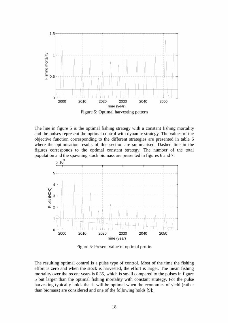
Figure 5: Optimal harvesting pattern

The line in figure 5 is the optimal fishing strategy with a constant fishing mortalityand the pulses represent the optimal control with dynamic strategy. The values of theobjective function corresponding to the different strategies are presented in table 6where the optimisation results of this section are summarised. Dashed line in thefigures corresponds to the optimal constant strategy. The number of the totalpopulation and the spawning stock biomass are presented in figures 6 and 7.

2000 2010 2020 2030 2040 20500

1

2

3

4

5

x 109

Time (year)

Pro

fit (

NO

K)

Figure 6: Present value of optimal profits

The resulting optimal control is a pulse type of control. Most of the time the fishingeffort is zero and when the stock is harvested, the effort is larger. The mean fishingmortality over the recent years is 0.35, which is small compared to the pulses in figure5 but larger than the optimal fishing mortality with constant strategy. For the pulseharvesting typically holds that it will be optimal when the economics of yield (ratherthan biomass) are considered and one of the following holds [9]:

19

1. There are large economies of scale, in the sense that it is economically moreefficient to take a large catch every few years than a smaller catch each year.

2. The economic value of old individuals is much higher than the economic value of

young individuals. This is true for our model since old herring individuals weighmore and the price per kilogram is the same for all age classes.

Although the optimality of the pulse control seems unrealistic it is reasonable forexample in a multispecies fishery. Furthermore, adding a simple market mechanism tothe optimisation model changes the situation (subsection 4.1.5).

2000 2010 2020 2030 2040 20500

2

4

6

8

x 109

Time (year)

SS

B (

kg)

SSB crit

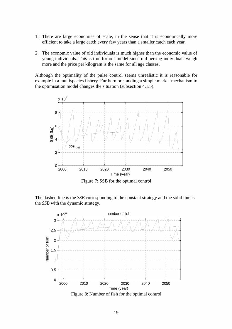
Figure 7: SSB for the optimal control

The dashed line is the SSB corresponding to the constant strategy and the solid line isthe SSB with the dynamic strategy.

2000 2010 2020 2030 2040 20500

0.5

1

1.5

2

2.5

3

x 1011 number of fish

Time (year)

Num

ber

of f

ish

Figure 8: Number of fish for the optimal control

20

The number of fish during the planning period is similar to SSB. For the constantstrategy the number of fish is stable after a short transient. For the dynamic strategythe number of fish behaves like SSB with a short lag.

Objective functionCase: Constant DynamicOriginal problem* 31.1785 32.2343Market mechanismincluded (4.1.5)

29.8632 30.3421

(19c) ignored (4.1.6) 31.1785 32.7398a1=8 37.3914 37.3914

.Table 6: Summary of the optimisation results in billions

Note that the constant and dynamic optimal strategies coincide when harvesting isbegun from age 8. Furthermore, this is the optimal strategy compared to any otherconstant or dynamic strategy.

4.1.2 Sensitivity to planning horizon and discount rate

In the sensitivity analysis of this subsection, we fix the fishing mortality and ignorethe constraint (18c). First the planning horizon TH varies and the discount rate isconstant: r=3%.

0 0.2 0.4 0.6 0.8 1 1.2 1.4 1.6 1.8 20

1

2

3

4x 10

10

Fishing mortality

NP

V (

NO

K)

TH=500

TH=100

TH=60

TH=20

Figure 9: Objective function with different planning periods

* The value of the objective function corresponding to the open access control of section 3 is 30.056109 NOK with the discount rate 3% and all the profits of the fleets summed together.

21

One can notice that as TH gets larger the changes in optimum become smaller (figure9). Between values TH=200 and TH=500 there is no visible change in the objectivefunction. As the planning horizon decreases the optimal constant fishing mortalityincreases slowly.

0 0.2 0.4 0.6 0.8 1 1.2 1.4 1.6 1.8 20

2

4

6

8x 10

10

Fishing mortality

NP

V (

NO

K)

r=0%

r=2%

r=6%

r=3%

r=18%

Figure 10: Objective function with different discount rates

The value of the objective function is quite sensitive for the changes of r but the valueof f in the optimum does not change very rapidly (figure 10). When the discount rate islarger than 18% the maximal fishing effort would be optimal.

4.1.3 Sensitivity to initial population

As noted in the subsection 4.1.1, the value of the objective function depends on theinitial abundance and the controls when parameters in the model are fixed. In thissubsection we study the changes of objective function when the initial populationchanges. In figure 11 objective function is presented with four different initialpopulations: the initial population has its original value (Appendix A), the initialpopulation is ten, five and half times the original.

22

0 0.2 0.4 0.6 0.8 1 1.2 1.4 1.6 1.8 20

2

4

6

8

10

12x 10

10

Fishing mortality

NP

V (

NO

K)

N =0.5 N 0 orig

N =N

N =5 N

N =10 N

0 orig

0 orig

0 orig

Figure 11: Objective function with different initial populations

The value of the objective function grows as the initial population grows but again theoptimal f changes slowly.

4.1.4 Sensitivity to first fishing age

Raising the first fishing age changes the optimal control and the larger the first fishingage gets the larger the optimal fishing mortality grows (figure 12). If the first fishingage is larger or equal than seven years the optimum is found when f is in its maximumlevel during the whole planning period. However the constraint for SSB is limiting thefishing effort, and if the equation (18c) is included to the optimisation the maximumlevel of f would be optimal when the first fishing age is eight years.

0 0.2 0.4 0.6 0.8 1 1.2 1.4 1.6 1.8 20

1

2

3

4x 10

10

Fishing mortality

NP

V (

NO

K)

a =0

a =4

a =6

a =2

a =5

a =9 a =8

a =7

1

1

1 1

1 1

1 1

Figure 12: Objective function with different selectivities

23

When the first fishing age is seven years, though the level of fishing mortality reachesits maximum level, the size of the population grows very high because of the highlevel of abundance of the younger age classes that are not harvested.

4.1.5 Sensitivity to price and costs

When the price and cost parameters are constant and the price is larger than variablecosts, the optimum does not change because the optimum can be found by maximisingthe discounted total yield. When the price is smaller than the variable cost, theoptimum changes to zero effort because fishing is not economical. Changing the fixedcosts affects only the value of the objective function but not the optimal control.

In the previous model price was a constant parameter and the rate of harvesting didnot affect the price received for the fish. In other words, the fishery faced an infinitelyelastic demand [5]. In this subsection, we add a simple supply-demand relationship tothe model and study optimal harvesting patterns for the problem (18). An isoelasticdemand curve (figure 13) for the price depending on the total yield would be:

h TY xTY y( ) = − (22)

With arbitrary parameters x=5.57 103, y=0.4 while all the other parameters are sameas before. As the supply (total yield) grows the price decreases, which affects theoptimal control so that it is not pulse fishing anymore.

0 0.5 1 1.5 2 2.5 30

0.5

1

1.5

2

Total yield (billion kg)

Pric

e (N

ok/k

g)

Figure 13: Demand curve

The optimal fishing strategy with constant fishing mortality and the dynamic solutiondo not differ very much (figure 14) and except for short transients, they are almostsame. The transient in the end of the planning period is caused by the fact that underfour years old fish are not mature. Therefore, harvesting the population to the

24

minimum level is optimal in four last periods. The optimal profits with the twostrategies are close to each other (figure 15) and the value of the objective function isclose to 30 billion (109) NOK with both strategies (table 6).

2000 2010 2020 2030 2040 20500

0.1

0.2

0.3

0.4

0.5

0.6

Time (year)

Fis

hing

mor

talit

y

Figure 14: Optimal harvesting pattern with the market mechanism

2000 2010 2020 2030 2040 20500

5

10

15x 10

8

Time (year)

Pro

fit (

NO

K)

Figure 15: Present value of optimal profits with the market mechanism

As the price tends to infinity when the yield goes to zero, the pulse fishing can not beoptimal because fishing even little is more profitable than to fish nothing. In thiswork, we do not analyse the sensitivity to the elasticity of the demand in more detail.

25

4.1.6 Sensitivity to constraints

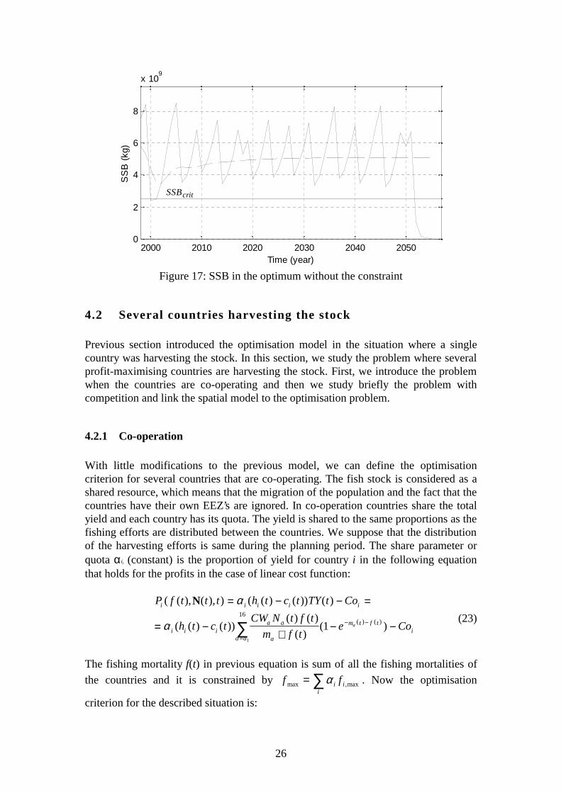
In the optimisation results of subsection 4.1.1 the spawning stock biomass was notallowed to go below the critical level and obviously this constraint is limiting theoptimum. Thus, it would be interesting to study the change of the optimal controlwhen the constraint (18c) is removed. In this case, it is possible that maximal fishingeffort is optimal, i.e., it is optimal to harvest the population to extinction.Nevertheless, this does not happen and removing the constraint changes the optimalcontrol only a little. Optimal fishing pattern (figure 16) is similar to the previousoptimal pattern (figure 5) with the difference that in the end of the period thepopulation is harvested to extinction. The spawning stock biomass is presented infigure 17.

Removing the constraint of the fishing mortality would change the optimal controlonly by allowing to harvest the population to extinction during one period. However,previous results show that harvesting the population to extinction as soon as possibleis not optimal and SSB stays at a healthy level during the planning period except forthe last few periods.

2000 2010 2020 2030 2040 20500

0.5

1

1.5

2

Time (year)

Fis

hing

mor

talit

y

Figure 16: Optimal fishing mortality without the constraint for SSB

26

2000 2010 2020 2030 2040 20500

2

4

6

8

x 109

Time (year)

SS

B (

kg)

SSB crit

Figure 17: SSB in the optimum without the constraint

4.2 Several countries harvesting the stock

Previous section introduced the optimisation model in the situation where a singlecountry was harvesting the stock. In this section, we study the problem where severalprofit-maximising countries are harvesting the stock. First, we introduce the problemwhen the countries are co-operating and then we study briefly the problem withcompetition and link the spatial model to the optimisation problem.

4.2.1 Co-operation

With little modifications to the previous model, we can define the optimisationcriterion for several countries that are co-operating. The fish stock is considered as ashared resource, which means that the migration of the population and the fact that thecountries have their own EEZ’s are ignored. In co-operation countries share the totalyield and each country has its quota. The yield is shared to the same proportions as thefishing efforts are distributed between the countries. We suppose that the distributionof the harvesting efforts is same during the planning period. The share parameter orquota αii (constant) is the proportion of yield for country i in the following equationthat holds for the profits in the case of linear cost function:

P f t t t h t c t TY t Co

h t c tCW N t f t

m f te Co

i i i i i

i i ia a

aa a

m t f ti

a

( ( ), ( ), ) ( ( ) ( )) ( )

( ( ) ( ))( ) ( )

( )( )( ) ( )

N = − − =

= −+

− −=

− −∑

α

α1

16

1(23)

The fishing mortality f(t) in previous equation is sum of all the fishing mortalities of

the countries and it is constrained by f fi ii

max ,max= ∑α . Now the optimisation

criterion for the described situation is:

27

0 1 0

0

≤ ≤ =

+

=∑∑

f t fi i i

t t

TH t

i

n

P f t t t t( ) max

max ( ( ), ( ), ) / ( )β ρN (24)

Parameters βi, for which it holds that β1+...+ βn =1, are used in the objective functionto determine a Pareto optimal solution. Together with the constraints (18b) and (18c)we have an optimal control problem, which has similar properties with the previousproblem of a single country. In equation (23) countries may have different cost andprice parameters. If they are constant and the discount rates are equal then changingthe value of the parameter beta does not change the optimal control and the Paretosurface reduces to one point. The optimal control would be same for any number ofplayers because the optimal control can be found by maximising the discounted totalyield (when h>c)*. In this situation the corresponding Pareto control equals the Nashbargaining solution, which could be found by using the following optimisationcriterion with threat points equal to zero:

0 1 0

0

≤ ≤ =

+

=∑∏

f t fi i

t t

TH t

i

n

P f t t t t( ) max

max ( ( ), ( ), ) / ( )N ρ (25)

The numerical results of co-operation are not presented in this work because theresults would be very similar to those presented in previous subsections for the onecountry case.

In the co-operative situation, the best Pareto optimal solution may be obtained whenonly the country that gains the largest profits is harvesting the stock. This can be madepossible when the most efficient country is paying for other countries for notharvesting the stock.

4.2.2 Competition

As the Norwegian spring-spawning herring is a straddling stock (for definitions see[8]), the migration of the population should be taken into account when the countriesare not co-operating with each other. Countries are maximising the net present valueof profits but now the yield comes from two sources: from their own EEZ (TYi,1) andfrom the high seas (TYi,2). Thus, each country i has two control variables: fishingmortality in their own EEZ (fi,1) and in the high seas (fi,2). Note that zones andfisheries are not assimilated. The optimisation problem for a single country i wouldbe:

( )f t ff t f

i i i it t

TH t

i i

i i

P f t f t N t t t, , ,max

, , ,max

( )( )

, ,max ( ), ( ), ( ), / ( )1 1

2 20

0

1 2≤≤

=

+

∑ ρ (26)

*

∑ ∑∑∑∑ ∑∑ +

−=

−−

i t

ii

tiiiii

i t

ii

tiiii t

Co

t

tTYch

t

Co

t

tTYch

)()(

)(max)(

)()(

)()(max

ρβ

ραβ

ρβ

ραβ

o

28

With the profit function (27) and the yield functions (28):

( ) ( )P f t f t t t h t TY t TY t Q ti i i i i i i, , , ,( ), ( ), ( ), ( ) ( ) ( ) ( )1 2 1 2N = + − (27)

TY f t t t CW N tf t

m t f tei i a a i

i

a ia a

m t f t

i

a i

, , ,,

,

( ) ( )( ( ), ( ), ) ( )( )

( ) ( )( )

,

,

1 11

1

16

1

11N =+

−=

− −∑ (28a)

TY f t t t CW N tf t

m t f tei i a a H

i

aa a

m t f t

i

a, , ,

, ( ) ( )( ( ), ( ), ) ( )( )

( ) ( )( )

,

2 22

2

16

1

21N =+

−=

− −∑ (28b)

Where f t f tii

2 2( ) ( ),= ∑ and H denotes the high seas. Different costs for fleets

operating in high seas and in national zones can be taken into account in the costfunction. The migration pattern could be included to the model by supposing thatequation (15) holds for the population. This allows a game theoretic approach to theproblem of exploitation of the herring stock. Unfortunately, game theoretic solutionsare beyond the scope of this work.

The recursive dynamic game presented above could be solved as a dynamic or a quasi-static game according to the degree of commitment [13]. Solving iteratively an openloop Nash-equilibrium strategy for the above game would be a straightforward butdepending on the planning horizon very time requiring task. Yet there are somedifficulties when solving the problem. The objective function is not unimodal and theNash-equilibrium may not be unique. The non-unimodality is not proved in this workbut it is due to non-unimodal yield function. The conclusion is that the age-structuredbiological model might be too complicated for game theoretic analysis and using asimpler biological model might give qualitatively similar results. However, the multi-cohort model is useful for analysing how the selectivity affects the stock. Especially ina competitive spatial model countries could have different distributions of age-classesin their zone.

In many papers where the game-theoretic settings are studied, no matter of the detailsof the models, the negative bioeconomic effects of dynamic externality – thebioeconomic loss which arises when there are several players harvesting the stock –have been quite significant [17]. In the context of the current model it would beinteresting to study the conditions for which it would be optimal for Norway todeplete the stock to the level where it stays within the Norwegian EEZ.

5 Discussion and conclusions

We presented simulations using the spatial model and studied optimal harvestingpatterns and finally discussed a game theoretic setting for several countries harvestingthe stock. Open access simulations with the spatial model showed that open accessleads to the extinction of the population. Moreover we studied the effects of migrationon the distributions of the biomass and yield over the EEZ's.

29

The optimal harvesting patterns were studied numerically and the most importantqualitative result is that when using a linear cost function and constant price (isoelasticdemand) in the optimisation model, the optimal harvesting pattern is pulse fishing.When a simple isoelastic market mechanism is included to the model the pulsatoryproperties of the optimal control disappear. These results show the importance of theeconomic model.

When several countries are harvesting the stock and they are all co-operating, theoptimal harvesting pattern is similar to the optimal control obtained for a singleplayer. The model can be modified to the case where the countries are competing andthe migration of the population can be included to the game theoretic setting.However, results of the competition were not studied in this work.

Estimating a supply-demand relationship is one step for the further development of theeconomic model. Another is to study some empirical data to define a realistic cost-function for the fishery. The linear cost function where the variable costs areproportional to the yield is non-realistic because it is possible that the yield is smallthough the fishing effort is large. Using the non-linear cost function (12) would be abetter choice because it takes into account the connection between number of vesselsand the effort on the stock. However, the parameters of the log-linear cost-functionshould be studied more closely if it would be used.

In this work the bioeconomic model was deterministic, though uncertainty is presentat all levels in fishery: fish stocks fluctuate, economic conditions change and decisionsare based on uncertain information. Therefore, risk analysis view point to the fisheryshould be considered before any serious conclusions from the results presented in thiswork are drawn.

30

References

[1] Bjørndal, T., Hole, A. D., Slinde, W.M. and F. Asche. Norwegian SpringSpawning Herring -- Some Biological and Economic Issues. SNF - Workingpaper No. 46/1998.

[2] Bjørndal, T. and D.V. Gordon. Cost Functions for the Norwegian Spring

Spawning Fishery. SNF-Working paper No. 41/1998. 1998 [3] Bjørndal, T. and A. Ussif. A Bioeconomic Analysis of the Norwegian Spring

Spawning Herring (NSSH) Stock. Manuscript.1999. [4] Bjørndal, T. The Optimal Management of North Sea Herring. Journal of

Environmental Economics and Management vol. 15. 1988. [5] Clark C.W. Mathematical Bioeconomics: the Optimal Management of

Renewable Resources. John Wiley & Sons. 1976 [6] Flaaten, O. The optimal harvesting of a natural resource with seasonal growth.

Canadian Journal of Economics vol. 3. 1983. [7] Hamre, J., A Model of Estimating Biological Attachment of Fish Stocks to

Exclusive Economic Zones. ICES CM 1993/D:43. [8] Hannesson, R. Sequential Fishing: Cooperative and Non-cooperative Equilibria.

Norwegian School of Economics and Business Administration. Centre forFisheries Economics. Reprint series no. 43. 1996.

[9] Hilborn, R., C.J. Walters. Quantitative Fisheries Stock Assessment: Choice,

Dynamics & Uncertainty. Chapman & Hall. 1992. [10] Junttila, V., M. Lindroos and V.Kaitala. Exploitation and Conservation of

Norwegian Spring-spawning Herring: Open Access versus Optimal HarvestingStrategies. Helsinki University of Technology, Systems Analysis LaboratoryResearch Report E1. October 1999.

[11] Kaitala, V. and M. Lindroos. Sharing the Benefits of Co-operation in High Seas

Fisheries: a Characteristic Function Game Approach. Natural ResourceModeling vol. 11, no. 4.1998.

[12] Magnússon, G. and R. Arnason. The Atlanto-Scandian Herring Fishery: A

Stylized Game Model. Paper presented for the Conference on the Managementof straddling Fish Stocks and Highly Migratory Fish Stocks. 1999.

[13] Mesterton-Gibbons, M., Game-theoretic Resource Modeling. Natural Resource

Modeling vol. 7, no. 2. 1993.

31

[14] Patterson, K.R. 1998. Biological Modelling of the Norwegian Spring-spawningHerring Stock. Fisheries Research Services Report No 1/98.

[15] Pintassilgo, P. Optimal Management of Northern Atlantic Bluefin Tuna.

Working Paper n. 355. Universidade Nova de Lisboa, Faculdade de Economia.1999.

[16] Sanchirico, J.N. and J.E. Wilen. Bioeconomics of Spatial Exploitation in a

Patchy Environment. Journal of Environmental Economics and Management,vol. 37, no. 2. 1999.

[17] Sumaila, U.R. A review of game-theoretic models of fishing. Marine policy, vol.

23, no 1. 1999. [18] Touzeau, S., Kaitala, V. and M. Lindroos. Implementation of the Norwegian

Spring-spawning Herring Stock Dynamics and Risk Analysis. HelsinkiUniversity of Technology, Systems Analysis Laboratory Research Report A75,September 1998.

[19] United Nations. Convention on the Law of the Sea, Montego Bay, <URL:

gopher://gopher.un.org/11/LOS/UNCLOS82>

32

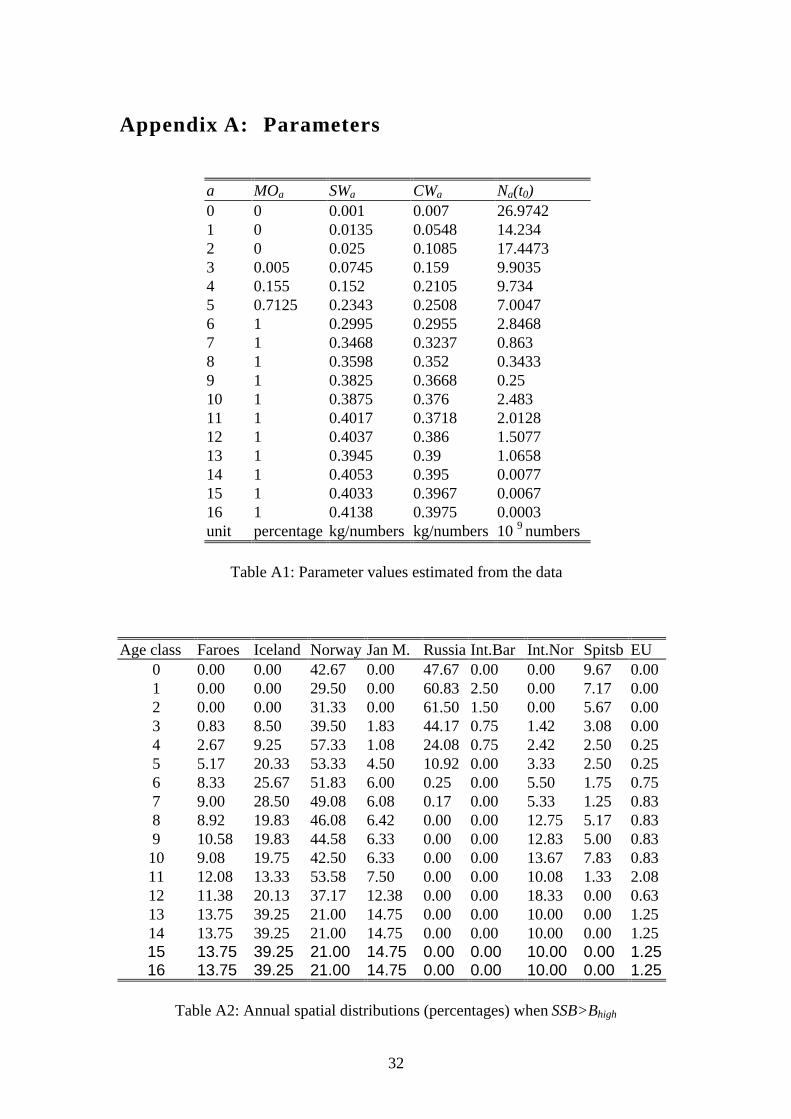
Appendix A: Parameters

a MOa SWa CWa Na(t0)0 0 0.001 0.007 26.97421 0 0.0135 0.0548 14.2342 0 0.025 0.1085 17.44733 0.005 0.0745 0.159 9.90354 0.155 0.152 0.2105 9.7345 0.7125 0.2343 0.2508 7.00476 1 0.2995 0.2955 2.84687 1 0.3468 0.3237 0.8638 1 0.3598 0.352 0.34339 1 0.3825 0.3668 0.2510 1 0.3875 0.376 2.48311 1 0.4017 0.3718 2.012812 1 0.4037 0.386 1.507713 1 0.3945 0.39 1.065814 1 0.4053 0.395 0.007715 1 0.4033 0.3967 0.006716 1 0.4138 0.3975 0.0003unit percentage kg/numbers kg/numbers 10 9 numbers

Table A1: Parameter values estimated from the data

Age class Faroes Iceland Norway Jan M. Russia Int.Bar Int.Nor Spitsb EU0 0.00 0.00 42.67 0.00 47.67 0.00 0.00 9.67 0.001 0.00 0.00 29.50 0.00 60.83 2.50 0.00 7.17 0.002 0.00 0.00 31.33 0.00 61.50 1.50 0.00 5.67 0.003 0.83 8.50 39.50 1.83 44.17 0.75 1.42 3.08 0.004 2.67 9.25 57.33 1.08 24.08 0.75 2.42 2.50 0.255 5.17 20.33 53.33 4.50 10.92 0.00 3.33 2.50 0.256 8.33 25.67 51.83 6.00 0.25 0.00 5.50 1.75 0.757 9.00 28.50 49.08 6.08 0.17 0.00 5.33 1.25 0.838 8.92 19.83 46.08 6.42 0.00 0.00 12.75 5.17 0.839 10.58 19.83 44.58 6.33 0.00 0.00 12.83 5.00 0.8310 9.08 19.75 42.50 6.33 0.00 0.00 13.67 7.83 0.8311 12.08 13.33 53.58 7.50 0.00 0.00 10.08 1.33 2.0812 11.38 20.13 37.17 12.38 0.00 0.00 18.33 0.00 0.6313 13.75 39.25 21.00 14.75 0.00 0.00 10.00 0.00 1.2514 13.75 39.25 21.00 14.75 0.00 0.00 10.00 0.00 1.2515 13.75 39.25 21.00 14.75 0.00 0.00 10.00 0.00 1.2516 13.75 39.25 21.00 14.75 0.00 0.00 10.00 0.00 1.25

Table A2: Annual spatial distributions (percentages) when SSB>Bhigh

33

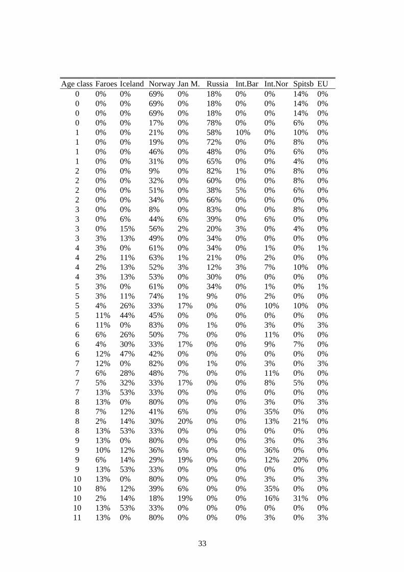
Age class Faroes Iceland Norway Jan M. Russia Int.Bar Int.Nor Spitsb EU0 0% 0% 69% 0% 18% 0% 0% 14% 0%0 0% 0% 69% 0% 18% 0% 0% 14% 0%0 0% 0% 69% 0% 18% 0% 0% 14% 0%0 0% 0% 17% 0% 78% 0% 0% 6% 0%1 0% 0% 21% 0% 58% 10% 0% 10% 0%1 0% 0% 19% 0% 72% 0% 0% 8% 0%1 0% 0% 46% 0% 48% 0% 0% 6% 0%1 0% 0% 31% 0% 65% 0% 0% 4% 0%2 0% 0% 9% 0% 82% 1% 0% 8% 0%2 0% 0% 32% 0% 60% 0% 0% 8% 0%2 0% 0% 51% 0% 38% 5% 0% 6% 0%2 0% 0% 34% 0% 66% 0% 0% 0% 0%3 0% 0% 8% 0% 83% 0% 0% 8% 0%3 0% 6% 44% 6% 39% 0% 6% 0% 0%3 0% 15% 56% 2% 20% 3% 0% 4% 0%3 3% 13% 49% 0% 34% 0% 0% 0% 0%4 3% 0% 61% 0% 34% 0% 1% 0% 1%4 2% 11% 63% 1% 21% 0% 2% 0% 0%4 2% 13% 52% 3% 12% 3% 7% 10% 0%4 3% 13% 53% 0% 30% 0% 0% 0% 0%5 3% 0% 61% 0% 34% 0% 1% 0% 1%5 3% 11% 74% 1% 9% 0% 2% 0% 0%5 4% 26% 33% 17% 0% 0% 10% 10% 0%5 11% 44% 45% 0% 0% 0% 0% 0% 0%6 11% 0% 83% 0% 1% 0% 3% 0% 3%6 6% 26% 50% 7% 0% 0% 11% 0% 0%6 4% 30% 33% 17% 0% 0% 9% 7% 0%6 12% 47% 42% 0% 0% 0% 0% 0% 0%7 12% 0% 82% 0% 1% 0% 3% 0% 3%7 6% 28% 48% 7% 0% 0% 11% 0% 0%7 5% 32% 33% 17% 0% 0% 8% 5% 0%7 13% 53% 33% 0% 0% 0% 0% 0% 0%8 13% 0% 80% 0% 0% 0% 3% 0% 3%8 7% 12% 41% 6% 0% 0% 35% 0% 0%8 2% 14% 30% 20% 0% 0% 13% 21% 0%8 13% 53% 33% 0% 0% 0% 0% 0% 0%9 13% 0% 80% 0% 0% 0% 3% 0% 3%9 10% 12% 36% 6% 0% 0% 36% 0% 0%9 6% 14% 29% 19% 0% 0% 12% 20% 0%9 13% 53% 33% 0% 0% 0% 0% 0% 0%10 13% 0% 80% 0% 0% 0% 3% 0% 3%10 8% 12% 39% 6% 0% 0% 35% 0% 0%10 2% 14% 18% 19% 0% 0% 16% 31% 0%10 13% 53% 33% 0% 0% 0% 0% 0% 0%11 13% 0% 80% 0% 0% 0% 3% 0% 3%

34

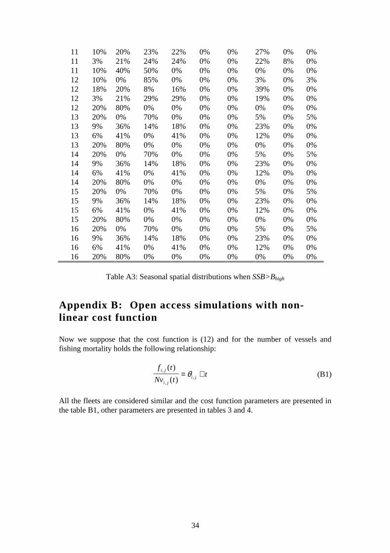
11 10% 20% 23% 22% 0% 0% 27% 0% 0%11 3% 21% 24% 24% 0% 0% 22% 8% 0%11 10% 40% 50% 0% 0% 0% 0% 0% 0%12 10% 0% 85% 0% 0% 0% 3% 0% 3%12 18% 20% 8% 16% 0% 0% 39% 0% 0%12 3% 21% 29% 29% 0% 0% 19% 0% 0%12 20% 80% 0% 0% 0% 0% 0% 0% 0%13 20% 0% 70% 0% 0% 0% 5% 0% 5%13 9% 36% 14% 18% 0% 0% 23% 0% 0%13 6% 41% 0% 41% 0% 0% 12% 0% 0%13 20% 80% 0% 0% 0% 0% 0% 0% 0%14 20% 0% 70% 0% 0% 0% 5% 0% 5%14 9% 36% 14% 18% 0% 0% 23% 0% 0%14 6% 41% 0% 41% 0% 0% 12% 0% 0%14 20% 80% 0% 0% 0% 0% 0% 0% 0%15 20% 0% 70% 0% 0% 0% 5% 0% 5%15 9% 36% 14% 18% 0% 0% 23% 0% 0%15 6% 41% 0% 41% 0% 0% 12% 0% 0%15 20% 80% 0% 0% 0% 0% 0% 0% 0%16 20% 0% 70% 0% 0% 0% 5% 0% 5%16 9% 36% 14% 18% 0% 0% 23% 0% 0%16 6% 41% 0% 41% 0% 0% 12% 0% 0%16 20% 80% 0% 0% 0% 0% 0% 0% 0%

Table A3: Seasonal spatial distributions when SSB>Bhigh

Appendix B: Open access simulations with non-linear cost function

Now we suppose that the cost function is (12) and for the number of vessels andfishing mortality holds the following relationship:

f t

Nv tt

i j

i ji j

,

,,

( )

( )= ∀θ (B1)

All the fleets are considered similar and the cost function parameters are presented inthe table B1, other parameters are presented in tables 3 and 4.

35

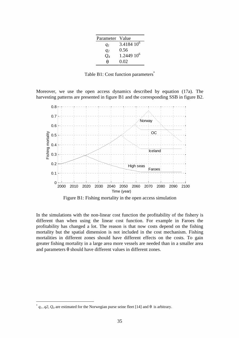
Parameter Valueq1 3.4184 106

q2 0.56Q4 1.2449 106

θ 0.02

Table B1: Cost function parameters*

Moreover, we use the open access dynamics described by equation (17a). Theharvesting patterns are presented in figure B1 and the corresponding SSB in figure B2.

2000 2010 2020 2030 2040 2050 2060 2070 2080 2090 21000

0.1

0.2

0.3

0.4

0.5

0.6

0.7

0.8

Time (year)

Fis

hing

mor

talit

y

Faroes High seas

Iceland

OC

Norway

Figure B1: Fishing mortality in the open access simulation

In the simulations with the non-linear cost function the profitability of the fishery isdifferent than when using the linear cost function. For example in Faroes theprofitability has changed a lot. The reason is that now costs depend on the fishingmortality but the spatial dimension is not included in the cost mechanism. Fishingmortalities in different zones should have different effects on the costs. To gaingreater fishing mortality in a large area more vessels are needed than in a smaller areaand parameters θ should have different values in different zones.

* q1 , q2, Q4 are estimated for the Norwegian purse seine fleet [14] and θ is arbitrary.

36

2000 2010 2020 2030 2040 2050 2060 2070 2080 20900

1

2

3

4

5

x 109

Time (year)

SS

B (

kg)

B

B

high

low

Figure B2: SSB in the open access simulation

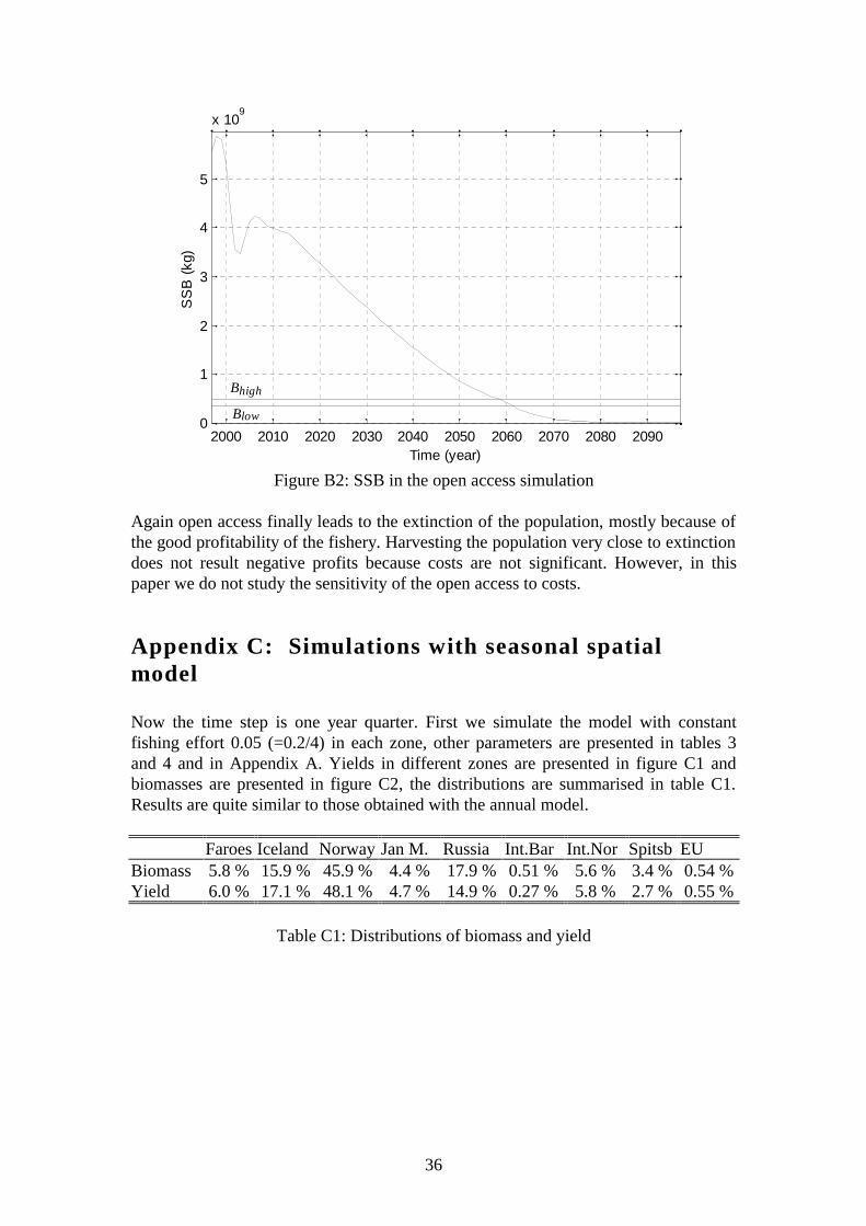
Again open access finally leads to the extinction of the population, mostly because ofthe good profitability of the fishery. Harvesting the population very close to extinctiondoes not result negative profits because costs are not significant. However, in thispaper we do not study the sensitivity of the open access to costs.

Appendix C: Simulations with seasonal spatialmodel

Now the time step is one year quarter. First we simulate the model with constantfishing effort 0.05 (=0.2/4) in each zone, other parameters are presented in tables 3and 4 and in Appendix A. Yields in different zones are presented in figure C1 andbiomasses are presented in figure C2, the distributions are summarised in table C1.Results are quite similar to those obtained with the annual model.

Faroes Iceland Norway Jan M. Russia Int.Bar Int.Nor Spitsb EUBiomass 5.8 % 15.9 % 45.9 % 4.4 % 17.9 % 0.51 % 5.6 % 3.4 % 0.54 %Yield 6.0 % 17.1 % 48.1 % 4.7 % 14.9 % 0.27 % 5.8 % 2.7 % 0.55 %

Table C1: Distributions of biomass and yield

37

2000 2010 2020 2030 2040 2050 2060 2070 2080 2090 21000

1

2

3

4

5

6

7

x 108

Time (year)

Ann

ual y

ield

(kg

)

Norway

OC

Iceland

Faroes

High seas

Figure C1: Distribution of the annual yield

2000 2010 2020 2030 2040 2050 2060 2070 2080 2090 21000

0.5

1

1.5

2

2.5

3

3.5

4x 10

9

Time (year)

Ave

rage

bio

mas

s (k

g)

Norway

OC

Iceland

High seas Faroes

Figure C2: Distribution of the annual average biomass*

Next we suppose that the fleets react after the following open access dynamics:

[ ]f t f t k t t k t k k= ,...,Ti i( ) ( ), ,= + ∈ + + + −0 0 0 1 0 1 when where (C1)

( ) ( )f t k sign P j f t k dt f t k dti ij t k dt

t k dt

i i i i

ii

i

( ) ( )02

0 0

0

0

+ =

+ − + + −

= + −

+ −

∑µ

(C2)

According to this open access dynamics the harvesting effort is constant one year after

* The reason to use averages of one year instead of original seasonal values is that because of seasonalfluctuations – biomass and yield decrease during the year – the figures would be very unclear.

38

which it is fixed according to the sign of cumulative profits from the period [t0+k-2dti, t0+k-dti].

The reactivity parameters are:

Parameter Valuedt 2µ 0.02

fi(0) 0.2

Table C2: Reactivity parameters

Resulting fishing mortality and stock biomass are presented in following figures. Thedifferences between zones are now larger. In the high seas and Faroes the fishing isnot as profitable as it was in the simulations with annual model and the harvesting inthese zones turn to decrease earlier.

2000 2010 2020 2030 2040 2050 2060 2070 2080 2090 21000

0.05

0.1

0.15

0.2

Time (year)

Fis

hing

mor

talit

y

Norway

Iceland

High seas

OC

Faroes

Figure C3: Fishing mortality in the open access simulation

39

2000 2010 2020 2030 2040 2050 2060 2070 2080 2090 21000

1

2

3

4

5

x 109

Time (year)

SS

B (

kg)

B

B

high

low

Figure C4: SSB in the open access simulation

When using the seasonal spatial model also the changes in the weight of fish shouldbe taken into account [1]. Thus, catch weight and stock weight parameters shouldchange seasonally. The optimisation model could be modified to the seasonal case butif the seasonal growth of the population is ignored the results are similar to the resultsobtained for the annual model. Some studies show that with the seasonal growth theoptimally managed fishery should have a shorter fishing season than would occurunder an open-access fishery [6].

Appendix D: Simulations with Ricker’s stock-recruitment function

In these simulations the models are same as in sections 2 and 3 with the exception thatnow we are using Ricker’s stock-recruitment function:

R t aSSB t ebSSB t( ) ( ) ( ) /= +σ 2 (D1)

Parameter Value unita 26.753 kg-1

b 1.2105 10-10kg-1

σ 1.802 noneg 0 none

Table D1: Stock-recruitment parameters

40

The stochastic term in the recruitment function is ignored. We simulate the modelwith constant fishing mortalities together 0.2 in each zone. We do not change thebasic scenario, i.e., same zones and fleets are included as before. The biomass of thepopulation is plotted in figure D1.

2000 2010 2020 2030 2040 2050 2060 2070 2080 2090 21000

2

4

6

8

10

12x 10

9

Time (year)

Bio

mas

s (k

g)

Ricker

Beverton-Holt

Figure D1: Biomass with different recruitment functions

Compared to the results obtained using Beverton-Holt stock-recruitment function(figure D1) the level of stock biomass stabilises to higher level after a short transient.

2000 2010 2020 2030 2040 2050 2060 2070 2080 2090 21000

1

2

3

4

5

6

7

8x 10

11

Num

ber

of F

ish

Time (year)Figure D2: Number of fish with the decreased mortality

When the mortality is small enough (for example ma/5, with ma as in table 5) theabundance of the population fluctuates with long frequency (figure D2), which doesnot happen with Beverton-Holt stock-recruitment function. The fluctuation is a result

41

of cannibalism; as the stock gets large enough the recruitment starts to decrease,which leads to the decrease of the abundance. The opposite happens when the stockreaches low enough level. In figures D2 and D3 the natural mortality is fifth part ofthe original (Appendix A) and fishing mortality is zero. Stock biomass fluctuates afterthe abundance with a short lag resulting from the age-structure of the population.

2000 2010 2020 2030 2040 2050 2060 2070 2080 2090 21000

1

2

3

4

5

6

7

8

9x 10

10

Time (year)

Bio

mas

s (k

g)

Figure D3: Biomass with the decreased mortality

42

Systems Analysis LaboratoryResearch Reports, Series A

*) Downloadable in pdf-format at: http://www.sal.hut.fi/Publications/

A68* Planning and Control Models for Elevators in High-RiseOctober 1997 Buildings

Marja-Liisa Siikonen

A69* Behavioral and Procedural Consequences of StructuralNovember 1997 Variation in Value Trees

Mari Pöyhönen, Hans C.J. Vrolijk and Raimo P. Hämäläinen

A70* On Arbitrage, Optimal Portfolio and Equilibrium underFebruary 1998 Frictions and Incomplete Markets

Jussi Keppo

A71* Optimal Home Currency and the Curved International February 1998 Equilibrium

Jussi Keppo

A72* Market Conditions under Frictions and without DynamicFebruary 1998 Spanning

Jussi Keppo

A73* On Attribute Weighting in Value TreesMarch 1998 Mari Pöyhönen

A74* There is Hope in Attribute WeightingMarch 1998 Mari Pöyhönen and Raimo P. Hämäläinen

A75* Implementation of the Norwegian Spring-Spawning HerringSeptember 1998 Stock Dynamics and Risk Analysis

Suzanne Touzeau, Veijo Kaitala and Marko Lindroos

A76* Management of Regional Fisheries Organisations: AnNovember 1998 Application of the Shapley Value

Marko Lindroos

A77 Bayesian Ageing Models and Indicators for RepairableJanuary 1999 Components

Urho Pulkkinen and Kaisa Simola

A78* Determinants of Cost Efficiency of Finnish Hospitals: AMay 1999 Comparison of DEA and SFA

Miika Linna and Unto Häkkinen

A79* The Impact of Health Care Financing Reform on the May 1999 Productivity Change in Finnish Hospitals

Miika Linna

43

Systems Analysis LaboratoryResearch Reports, Series B

B14 RiskianalyysiOctober 1989 Toim. Raimo P. Hämäläinen, Urho Pulkkinen ja

Risto Karjalainen

B15 Riskianalyysi energiapoliittisessa päätöksenteossaNovember 1989 Risto Karjalainen ja Raimo P. Hämäläinen

B16 Sähkön dynaaminen hinnoittelu kysynnän ohjaamisessaFebruary 1990 Jukka Ruusunen, Mika Räsänen ja Raimo P. Hämäläinen

B17 Verkoston tilan seuranta mittauksilla ja kuormitusmalleillaMay 1992 Mika Räsänen ja Jukka Ruusunen

B18 TEHO Terästehtaan energianhallinnan optimointiNovember 1993 Risto Lahdelma

B19 Ympäristön arvottaminen - Taloustieteelliset jaJune 1996 monitavoitteiset menetelmät

Toim. Pauli Miettinen ja Raimo P. Hämäläinen

B20 Sovellettu todennäköisyyslaskuSeptember 1996 Pertti Laininen (uudistettu painos 1997)

B21 Monitavoitteisen päätöksenteon mallit vesistön June 1997 säännöstelyssä

Toim. Raimo P. Hämäläinen

Systems Analysis LaboratoryResearch Reports, Series EElectronic Reports: http://e-reports.sal.hut.fi

E1 Exploitation and Conservation of Norwegian Herring:October 1999 Spring-Spawning Open Access Versus Optimal Harvesting

StrategiesVirpi Junttila, Marko Lindroos and Veijo Kaitala

Orders: Helsinki University of TechnologySystems Analysis LaboratoryP.O. Box 1100, FIN-02015 HUT, FinlandE-mail: [email protected]