Unit 1 Introduction to Operational Research Lesson 1: Introduction to Operational Research Introduction to Operational Research This teaching module is designed to be an entertaining and representative introduction to the subject of Operational Research. It is divided into a number of sections each covering different aspects of OR. What is Operational Research? This looks at the characteristics of Operational Research, how you define what OR is and why organisations might use it. It considers the scientific nature of OR and how it helps in dealing with problems involving uncertainty, complexity and conflict. OR is the representation of real-world systems by mathematical models together with the use of quantitative methods (algorithms) for solving such models, with a view to optimising. Battle of the Atlantic Considers the origins of OR in the British military and looks at how OR helped to ensure the safety of merchant ships during the "Battle of the Atlantic" in World War II. Introduction to OR Terminology The British/Europeans refer to "operational research", the Americans to "operations research" - but both are often shortened to just "OR" (which is the term we will use). Another term which is used for this field is "management science" ("MS"). The Americans sometimes combine the terms OR and MS together and say "OR/MS" or "ORMS". Yet other terms sometimes used are "industrial engineering" ("IE") and "decision science" ("DS"). In recent years there has been a move towards a standardisation upon a single term for the field, namely the term "OR".

Operations research Lecture Series
Nov 22, 2014
Welcome message from author
This document is posted to help you gain knowledge. Please leave a comment to let me know what you think about it! Share it to your friends and learn new things together.
Transcript

Unit 1
Introduction to Operational Research
Lesson 1: Introduction to Operational Research
Introduction to Operational Research This teaching module is designed to be an entertaining and representative introduction to the subject of Operational Research. It is divided into a number of sections each covering different aspects of OR.
What is Operational Research?
This looks at the characteristics of Operational Research, how you define what OR is and why organisations might use it. It considers the scientific nature of OR and how it helps in dealing with problems involving uncertainty, complexity and conflict.
OR is the representation of real-world systems by mathematical models together with the use of quantitative methods (algorithms) for solving such models, with a view to optimising.
Battle of the Atlantic
Considers the origins of OR in the British military and looks at how OR helped to ensure the safety of merchant ships during the "Battle of the Atlantic" in World War II.
Introduction to OR
Terminology
The British/Europeans refer to "operational research", the Americans to "operations research" - but both are often shortened to just "OR" (which is the term we will use).
Another term which is used for this field is "management science" ("MS"). The Americans sometimes combine the terms OR and MS together and say "OR/MS" or "ORMS". Yet other terms sometimes used are "industrial engineering" ("IE") and "decision science" ("DS"). In recent years there has been a move towards a standardisation upon a single term for the field, namely the term "OR".
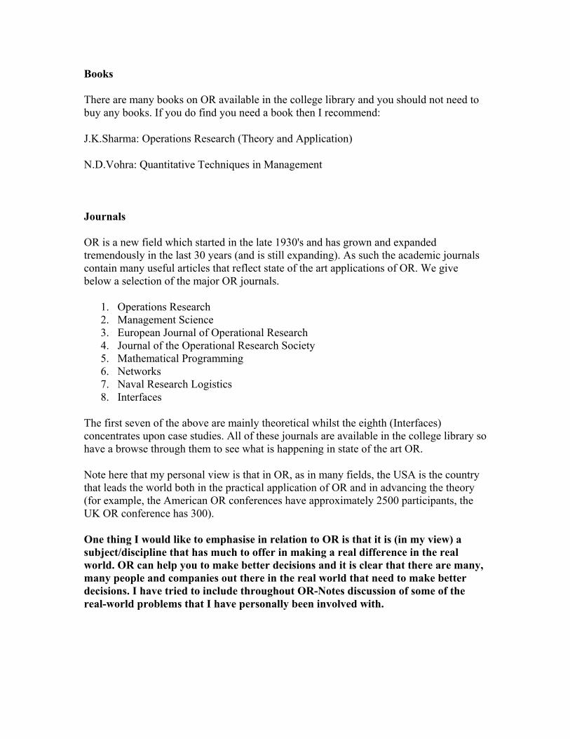
Books
There are many books on OR available in the college library and you should not need to buy any books. If you do find you need a book then I recommend:
J.K.Sharma: Operations Research (Theory and Application)
N.D.Vohra: Quantitative Techniques in Management
Journals
OR is a new field which started in the late 1930's and has grown and expanded tremendously in the last 30 years (and is still expanding). As such the academic journals contain many useful articles that reflect state of the art applications of OR. We give below a selection of the major OR journals.
1. Operations Research 2. Management Science 3. European Journal of Operational Research 4. Journal of the Operational Research Society 5. Mathematical Programming 6. Networks 7. Naval Research Logistics 8. Interfaces
The first seven of the above are mainly theoretical whilst the eighth (Interfaces) concentrates upon case studies. All of these journals are available in the college library so have a browse through them to see what is happening in state of the art OR.
Note here that my personal view is that in OR, as in many fields, the USA is the country that leads the world both in the practical application of OR and in advancing the theory (for example, the American OR conferences have approximately 2500 participants, the UK OR conference has 300).
One thing I would like to emphasise in relation to OR is that it is (in my view) a subject/discipline that has much to offer in making a real difference in the real world. OR can help you to make better decisions and it is clear that there are many, many people and companies out there in the real world that need to make better decisions. I have tried to include throughout OR-Notes discussion of some of the real-world problems that I have personally been involved with.

History of OR
OR is a relatively new discipline. Whereas 70 years ago it would have been possible to study mathematics, physics or engineering (for example) at university it would not have been possible to study OR, indeed the term OR did not exist then. It was really only in the late 1930's that operational research began in a systematic fashion, and it started in the UK. As such I thought it would be interesting to give a short history of OR and to consider some of the problems faced (and overcome) by early OR workers.
Whilst researching for this short history I discovered that history is not clear cut, different people have different views of the same event. In addition many of the participants in the events described below are now elderly/dead. As such what is given below is only my understanding of what actually happened.
Note: some of you may have moral qualms about discussing what are, at root, more effective ways to kill people. However I cannot change history and what is presented
below is essentially what happened, whether one likes it or not.
1936
Early in 1936 the British Air Ministry established Bawdsey Research Station, on the east coast, near Felixstowe, Suffolk, as the centre where all pre-war radar experiments for both the Air Force and the Army would be carried out. Experimental radar equipment was brought up to a high state of reliability and ranges of over 100 miles on aircraft were obtained.
It was also in 1936 that Royal Air Force (RAF) Fighter Command, charged specifically with the air defense of Britain, was first created. It lacked however any effective fighter aircraft - no Hurricanes or Spitfires had come into service - and no radar data was yet fed into its very elementary warning and control system.
It had become clear that radar would create a whole new series of problems in fighter direction and control so in late 1936 some experiments started at Biggin Hill in Kent into the effective use of such data. This early work, attempting to integrate radar data with ground based observer data for fighter interception, was the start of OR.
1937
The first of three major pre-war air-defence exercises was carried out in the summer of 1937. The experimental radar station at Bawdsey Research Station was brought into operation and the information derived from it was fed into the general air-defense warning and control system. From the early warning point of view this exercise was encouraging, but the tracking information obtained from radar, after filtering and transmission through the control and display network, was not very satisfactory.
1938

In July 1938 a second major air-defense exercise was carried out. Four additional radar stations had been installed along the coast and it was hoped that Britain now had an aircraft location and control system greatly improved both in coverage and effectiveness. Not so! The exercise revealed, rather, that a new and serious problem had arisen. This was the need to coordinate and correlate the additional, and often conflicting, information received from the additional radar stations. With the out-break of war apparently imminent, it was obvious that something new - drastic if necessary - had to be attempted. Some new approach was needed.
Accordingly, on the termination of the exercise, the Superintendent of Bawdsey Research Station, A.P. Rowe, announced that although the exercise had again demonstrated the technical feasibility of the radar system for detecting aircraft, its operational achievements still fell far short of requirements. He therefore proposed that a crash program of research into the operational - as opposed to the technical - aspects of the system should begin immediately. The term "operational research" [RESEARCH into (military) OPERATIONS] was coined as a suitable description of this new branch of applied science. The first team was selected from amongst the scientists of the radar research group the same day.
1939
In the summer of 1939 Britain held what was to be its last pre-war air defence exercise. It involved some 33,000 men, 1,300 aircraft, 110 antiaircraft guns, 700 searchlights, and 100 barrage balloons. This exercise showed a great improvement in the operation of the air defence warning and control system. The contribution made by the OR teams was so apparent that the Air Officer Commander-in-Chief RAF Fighter Command (Air Chief Marshal Sir Hugh Dowding) requested that, on the outbreak of war, they should be attached to his headquarters at Stanmore in north London.
Initially, they were designated the "Stanmore Research Section". In 1941 they were redesignated the "Operational Research Section" when the term was formalised and officially accepted, and similar sections set up at other RAF commands.
1940
On May 15th 1940, with German forces advancing rapidly in France, Stanmore Research Section was asked to analyse a French request for ten additional fighter squadrons (12 aircraft a squadron - so 120 aircraft in all) when losses were running at some three squadrons every two days (i.e. 36 aircraft every 2 days). They prepared graphs for Winston Churchill (the British Prime Minister of the time), based upon a study of current daily losses and replacement rates, indicating how rapidly such a move would deplete fighter strength. No aircraft were sent and most of those currently in France were recalled.

1941 onward
In 1941 an Operational Research Section (ORS) was established in Coastal Command which was to carry out some of the most well-known OR work in World War II.
The responsibility of Coastal Command was, to a large extent, the flying of long-range sorties by single aircraft with the object of sighting and attacking surfaced U-boats (German submarines). Amongst the problems that ORS considered were:
• organisation of flying maintenance and inspection
Here the problem was that in a squadron each aircraft, in a cycle of approximately 350 flying hours, required in terms of routine maintenance 7 minor inspections (lasting 2 to 5 days each) and a major inspection (lasting 14 days). How then was flying and maintenance to be organised to make best use of squadron resources?
ORS decided that the current procedure, whereby an aircrew had their own aircraft, and that aircraft was serviced by a devoted ground crew, was inefficient (as it meant that when the aircraft was out of action the aircrew were also inactive). They proposed a central garage system whereby aircraft were sent for maintenance when required and each aircrew drew a (different) aircraft when required.
The advantage of this system is plainly that flying hours should be increased. The disadvantage of this system is that there is a loss in morale as the ties between the aircrew and "their" plane/ground crew and the ground crew and "their" aircrew/plane are broken.
This is held by some to be the most strategic contribution to the course of the war made by OR (as the aircraft and pilots saved were consequently available for the successful air defense of Britain, the Battle of Britain).
The first use of OR techniques in India, was in the year] 1949 at Hyderabad,
where at the Regional Research Institute, an independent operations research unit was
set-up. To identify evaluate and solve the problems related to planning, purchases and
proper maintenance of stores, an operations research unit was also setup at the Defence
Science Laboratory use of OR tools and techniques was done during India's second five
year Plan in demand forecasting and suggesting the most suitable scheme which would
lead to the overall growth and the development of the economy. Even today, Planning
Commission utilises some. of these techniques in framing policies and sector-wise
performance evaluation.

In 1953, at the Indian Statistical Institute (Calcutta). A self-sufficient operations
research unit was established for the purpose of national planning & survey. OR Society
of India was folined in 1957 which publishes journal titled "Of search". Many big and
prominent business & industrial houses are using extensively the tools of OR for the
optimum utilisation of precious and scarce resources available to them. This phenomenon
is not limited to the private sector only. Even good companies in the public sector ("Nav
Ratnas") are reaping the benefits of fully functional sound OR units. Example of such
corporate, both private & public are: SAIL, BHEL, NTPC, Indian Railways, Indian
Airlines, Air-India, Hindustan Lever, TELCO & TISCO etc. Textile companies engaged
in the process of manufacture of various types of fabrics use some of the tools of OR like
lenear programming & PERT in their blending, dyeing and other manufacturing
operations.
Various other Indian companies are .employing OR techniques for solving problems
pertaining to various spheres of activities, as diverse as advertising, sales promotion,
inspection, quality control, staffing, personnel, investment & production planning, etc.
These organisations are not only employing the operations research techniques
and analysis on a short-term trouble-shooting basis but also for ong-range strategic
planning.
Basic OR concepts
Definition
So far we have avoided the problem of defining exactly what OR is. In order to get a clearer idea of what OR is we shall actually do some by considering the specific problem below and then highlight some general lessons and concepts from this specific example.
Two Mines Company
The Two Mines Company own two different mines that produce an ore which, after being crushed, is graded into three classes: high, medium and low-grade. The company has contracted to provide a smelting plant with 12 tons of high-grade, 8 tons of medium-grade and 24 tons of low-grade ore per week. The two mines have different operating characteristics as detailed below.
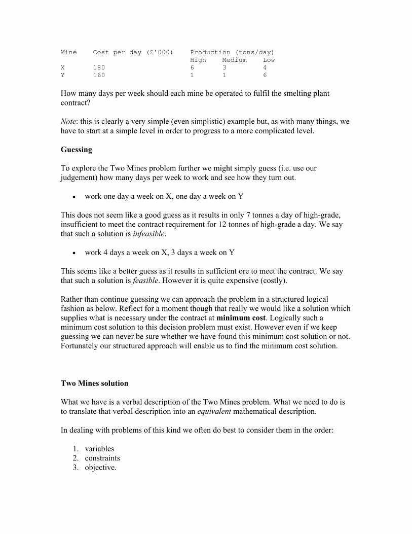
Mine Cost per day (£'000) Production (tons/day) High Medium Low X 180 6 3 4 Y 160 1 1 6
How many days per week should each mine be operated to fulfil the smelting plant contract?
Note: this is clearly a very simple (even simplistic) example but, as with many things, we have to start at a simple level in order to progress to a more complicated level.
Guessing
To explore the Two Mines problem further we might simply guess (i.e. use our judgement) how many days per week to work and see how they turn out.
• work one day a week on X, one day a week on Y
This does not seem like a good guess as it results in only 7 tonnes a day of high-grade, insufficient to meet the contract requirement for 12 tonnes of high-grade a day. We say that such a solution is infeasible.
• work 4 days a week on X, 3 days a week on Y
This seems like a better guess as it results in sufficient ore to meet the contract. We say that such a solution is feasible. However it is quite expensive (costly).
Rather than continue guessing we can approach the problem in a structured logical fashion as below. Reflect for a moment though that really we would like a solution which supplies what is necessary under the contract at minimum cost. Logically such a minimum cost solution to this decision problem must exist. However even if we keep guessing we can never be sure whether we have found this minimum cost solution or not. Fortunately our structured approach will enable us to find the minimum cost solution.
Two Mines solution
What we have is a verbal description of the Two Mines problem. What we need to do is to translate that verbal description into an equivalent mathematical description.
In dealing with problems of this kind we often do best to consider them in the order:
1. variables 2. constraints 3. objective.

We do this below and note here that this process is often called formulating the problem (or more strictly formulating a mathematical representation of the problem).
(1) Variables
These represent the "decisions that have to be made" or the "unknowns".
Let
x = number of days per week mine X is operated y = number of days per week mine Y is operated
Note here that x >= 0 and y >= 0.
(2) Constraints
It is best to first put each constraint into words and then express it in a mathematical form.
• ore production constraints - balance the amount produced with the quantity required under the smelting plant contract
Ore High 6x + 1y >= 12 Medium 3x + 1y >= 8 Low 4x + 6y >= 24
Note we have an inequality here rather than an equality. This implies that we may produce more of some grade of ore than we need. In fact we have the general rule: given a choice between an equality and an inequality choose the inequality.
For example - if we choose an equality for the ore production constraints we have the three equations 6x+y=12, 3x+y=8 and 4x+6y=24 and there are no values of x and y which satisfy all three equations (the problem is therefore said to be "over-constrained"). For example the values of x and y which satisfy 6x+y=12 and 3x+y=8 are x=4/3 and y=4, but these values do not satisfy 4x+6y=24.
The reason for this general rule is that choosing an inequality rather than an equality gives us more flexibility in optimising (maximising or minimising) the objective (deciding values for the decision variables that optimise the objective).
• days per week constraint - we cannot work more than a certain maximum number of days a week e.g. for a 5 day week we have
x <= 5 y <= 5

Constraints of this type are often called implicit constraints because they are implicit in the definition of the variables.
(3) Objective
Again in words our objective is (presumably) to minimise cost which is given by 180x + 160y
Hence we have the complete mathematical representation of the problem as:
minimise 180x + 160y subject to 6x + y >= 12 3x + y >= 8 4x + 6y >= 24 x <= 5 y <= 5 x,y >= 0
There are a number of points to note here:
• a key issue behind formulation is that IT MAKES YOU THINK. Even if you never do anything with the mathematics this process of trying to think clearly and logically about a problem can be very valuable.
• a common problem with formulation is to overlook some constraints or variables and the entire formulation process should be regarded as an iterative one (iterating back and forth between variables/constraints/objective until we are satisfied).
• the mathematical problem given above has the form o all variables continuous (i.e. can take fractional values) o a single objective (maximise or minimise) o the objective and constraints are linear i.e. any term is either a constant or
a constant multiplied by an unknown (e.g. 24, 4x, 6y are linear terms but xy is a non-linear term).
o any formulation which satisfies these three conditions is called a linear program (LP). As we shall see later LP's are important..
• we have (implicitly) assumed that it is permissible to work in fractions of days - problems where this is not permissible and variables must take integer values will be dealt with under integer programming.
• often (strictly) the decision variables should be integer but for reasons of simplicity we let them be fractional. This is especially relevant in problems where the values of the decision variables are large because any fractional part can then

usually be ignored (note that often the data (numbers) that we use in formulating the LP will be inaccurate anyway).
• the way the complete mathematical representation of the problem is set out above is the standard way (with the objective first, then the constraints and finally the reminder that all variables are >=0).
Discussion
Considering the Two Mines example given above:
• this problem was a decision problem
• we have taken a real-world situation and constructed an equivalent mathematical representation - such a representation is often called a mathematical model of the real-world situation (and the process by which the model is obtained is called formulating the model). Just to confuse things the mathematical model of the problem is sometimes called the formulation of the problem.
• having obtained our mathematical model we (hopefully) have some quantitative method which will enable us to numerically solve the model (i.e. obtain a numerical solution) - such a quantitative method is often called an algorithm for solving the model.
Essentially an algorithm (for a particular model) is a set of instructions which, when followed in a step-by-step fashion, will produce a numerical solution to that model. You will see some examples of algorithms later in this course..
• our model has an objective, that is something which we are trying to optimise.
• having obtained the numerical solution of our model we have to translate that solution back into the real-world situation.
Hence we have a definition of OR as:
OR is the representation of real-world systems by mathematical models together with the use of quantitative methods (algorithms) for solving such models, with a view to optimising.
One thing I wish to emphasise about OR is that it typically deals with decision problems. You will see examples of the many different types of decision problem that can be tackled using OR.
We can also define a mathematical model as consisting of:

• Decision variables, which are the unknowns to be determined by the solution to the model.
• Constraints to represent the physical limitations of the system. • An objective function. • A solution (or optimal solution) to the model is the identification of a set of
variable values which are feasible (i.e. satisfy all the constraints) and which lead to the optimal value of the objective function.
Philosophy
In general terms we can regard OR as being the application of scientific methods/thinking to decision making. Underlying OR is the philosophy that:
• decisions have to be made; and • using a quantitative (explicit, articulated) approach will lead (on average) to better
decisions than using non-quantitative (implicit, unarticulated) approaches (such as those used (?) by human decision makers).
Indeed it can be argued that although OR is imperfect it offers the best available approach to making a particular decision in many instances (which is not to say that using OR will produce the right decision).
Often the human approach to decision making can be characterised (conceptually) as the "ask Fred" approach, simply give Fred ('the expert') the problem and relevant data, shut him in a room for a while and wait for an answer to appear.
The difficulties with this approach are:
• speed (cost) involved in arriving at a solution • quality of solution - does Fred produce a good quality solution in any particular
case • consistency of solution - does Fred always produce solutions of the same quality
(this is especially important when comparing different options).
You can form your own judgement as to whether OR is better than this approach or not.
Phases of an OR project
Drawing on our experience with the Two Mines problem we can identify the phases that a (real-world) OR project might go through.
1. Problem identification
• Diagnosis of the problem from its symptoms if not obvious (i.e. what is the problem?)
• Delineation of the subproblem to be studied. Often we have to ignore parts of the entire problem.
• Establishment of objectives, limitations and requirements.
2. Formulation as a mathematical model
It may be that a problem can be modelled in differing ways, and the choice of the appropriate model may be crucial to the success of the OR project. In addition to algorithmic considerations for solving the model (i.e. can we solve our model numerically?) we must also consider the availability and accuracy of the real-world data that is required as input to the model.
Note that the "data barrier" ("we don't have the data!!!") can appear here, particularly if people are trying to block the project. Often data can be collected/estimated, particularly if the potential benefits from the project are large enough.
You will also find, if you do much OR in the real-world, that some environments are naturally data-poor, that is the data is of poor quality or nonexistent and some environments are naturally data-rich. As examples of this church location study (a data-poor environment) and an airport terminal check- in desk allocation study (a data-rich environment).
This issue of the data environment can affect the model that you build. If you believe that certain data can never (realistically) be obtained there is perhaps little point in building a model that uses such data.
3. Model validation (or algorithm validation)
Model validation involves running the algorithm for the model on the computer in order to ensure:
• the input data is free from errors • the computer program is bug-free (or at least there are no outstanding bugs) • the computer program correctly represents the model we are attempting to
validate • the results from the algorithm seem reasonable (or if they are surprising we can at
least understand why they are surprising). Sometimes we feed the algorithm historical input data (if it is available and is relevant) and compare the output with the historical result.
4. Solution of the model
Standard computer packages, or specially developed algorithms, can be used to solve the model (as mentioned above). In practice, a "solution" often involves very many solutions

under varying assumptions to establish sensitivity. For example, what if we vary the input data (which will be inaccurate anyway), then how will this effect the values of the decision variables? Questions of this type are commonly known as "what if" questions nowadays.
Note here that the factors which allow such questions to be asked and answered are:
• the speed of processing (turn-around time) available by using pc's; and • the interactive/user-friendly nature of many pc software packages.
5. Implementation
This phase may involve the implementation of the results of the study or the implementation of the algorithm for solving the model as an operational tool (usually in a computer package).
In the first instance detailed instructions on what has to be done (including time schedules) to implement the results must be issued. In the second instance operating manuals and training schemes will have to be produced for the effective use of the algorithm as an operational tool.
It is believed that many of the OR projects which successfully pass through the first four phases given above fail at the implementation stage (i.e. the work that has been done does not have a lasting effect). As a result one topic that has received attention in terms of bringing an OR project to a successful conclusion (in terms of implementation) is the issue of client involvement. By this is meant keeping the client (the sponsor/originator of the project) informed and consulted during the course of the project so that they come to identify with the project and want it to succeed. Achieving this is really a matter of experience.
A graphical description of this process is given below.
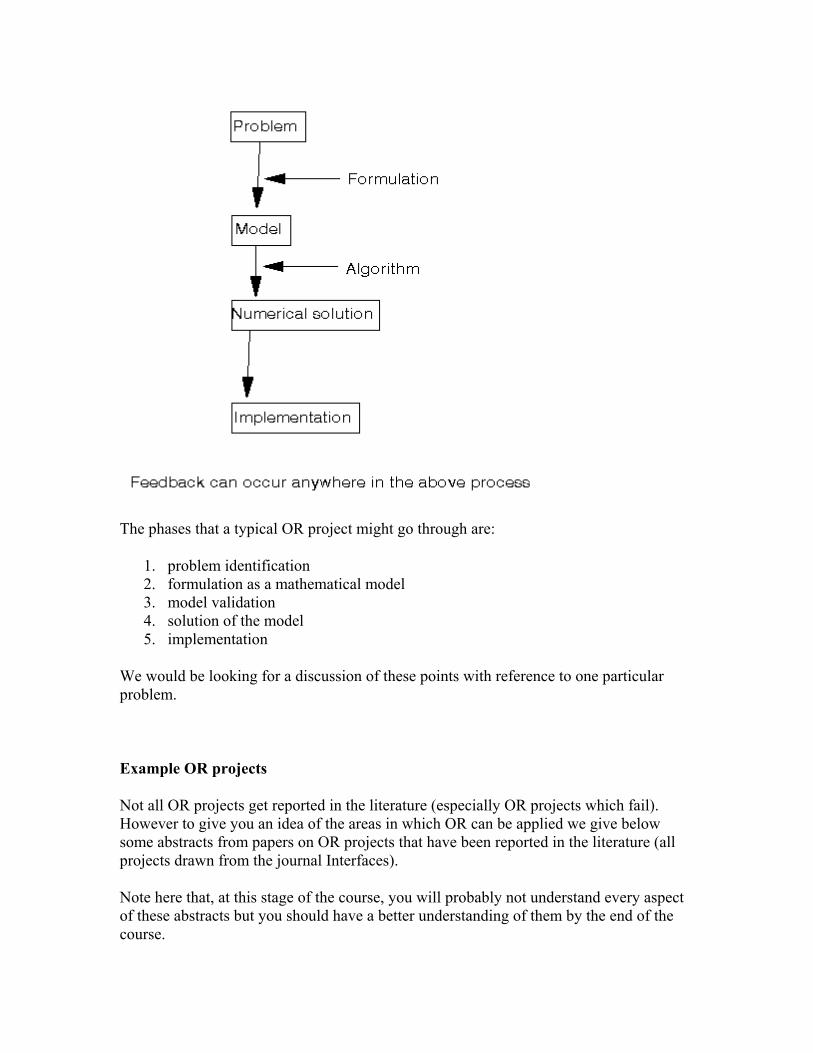
The phases that a typical OR project might go through are:
1. problem identification 2. formulation as a mathematical model 3. model validation 4. solution of the model 5. implementation
We would be looking for a discussion of these points with reference to one particular problem.
Example OR projects
Not all OR projects get reported in the literature (especially OR projects which fail). However to give you an idea of the areas in which OR can be applied we give below some abstracts from papers on OR projects that have been reported in the literature (all projects drawn from the journal Interfaces).
Note here that, at this stage of the course, you will probably not understand every aspect of these abstracts but you should have a better understanding of them by the end of the course.
• Yield management at American Airlines
Critical to an airline's operation is the effective use of its reservations inventory. American Airlines began research in the early 1960's in managing revenue from this inventory. Because of the problem's size and difficulty, American Airlines Decision Technologies has developed a series of OR models that effectively reduce the large problem to three much smaller and far more manageable subproblems: overbooking, discount allocation and traffic management. The results of the subproblem solutions are combined to determine the final inventory levels. American Airlines estimates the quantifiable benefit at $1.4 billion over the last three years and expects an annual revenue contribution of over $500 million to continue into the future. Yield management is also sometimes referred to as capacity management. It applies in systems where the cost of operating is essentially fixed and the focus is primarily, though not exclusively, on revenue maximisation. For example all transport systems (air, land, sea) operating to a fixed timetable (schedule) could potentially benefit from yield management. Hotels would be another example of a system where the focus should primarily be on revenue maximisation.
To give you an illustration of the kind of problems involved in yield management suppose that we consider a specific flight, say the 4pm on a Thursday from Chicago O'Hare to New York JFK. Further suppose that there are exactly 100 passenger seats on the plane subdivided into 70 economy seats and 30 business class seats (and that this subdivision cannot be changed). An economy fare is $200 and a business class fare is $1000. Then a fundamental question (a decision problem) is :
How many tickets can we sell ?
One key point to note about this decision problem is that it is a routine one, airlines need to make similar decisions day after day about many flights.
Suppose now that at 7am on the day of the flight the situation is that we have sold 10 business class tickets and 69 economy tickets. A potential passenger phones up requesting an economy ticket. Then a fundamental question (a decision problem) is : Would you sell it to them ? Reflect - do the figures given for fares $200 economy, $1000 business affect the answer to this question or not ?
Again this decision problem is a routine one, airlines need to make similar decisions day after day, minute after minute, about many flights. Also note that in this decision problem an answer must be reached quickly. The potential passenger on the phone expects an immediate answer. One factor that may influence your thinking here is consider certain money (money we are sure to get) and uncertain money (money we may, or may not, get).
Suppose now that at 1pm on the day of the flight the situation is that we have sold 30 business class tickets and 69 economy tickets. A potential passenger phones up

requesting an economy ticket. Then a fundamental question (a decision problem) is : Would you sell it to them ?
• NETCAP - an interactive optimisation system for GTE telephone network planning
With operations extending from the east coast to Hawaii, GTE is the largest local telephone company in the United States. Even before its 1991 merger with Contel, GTE maintained more than 2,600 central offices serving over 15.7 million customer lines. It does extensive planning to ensure that its $300 million annual investment in customer access facilities is well spent. To help GTE Corporation in a very complex task of planning the customer access network, GTE Laboratories developed a decision support tool called NETCAP that is used by nearly 200 GTE network planners, improving productivity by more than 500% and saving an estimated $30 million per year in network construction costs.
• Managing consumer credit delinquency in the US economy: a multi-billion dollar management science application
GE Capital provides credit card services for a consumer credit business exceeding $12 billion in total outstanding dollars. Its objective is to optimally manage delinquency by improving the allocation of limited collection resources to maximise net collections over multiple billing periods. We developed a probabilistic account flow model and statistically designed programs to provide accurate data on collection resource performance. A linear programming formulation produces optimal resource allocations that have been implemented across the business. The PAYMENT system has permanently changed the way GE Capital manages delinquent consumer credit, reduced annual losses by approximately $37 million, and improved customer goodwill.
Note here that GE Capital also operates in the UK.
Operational research example 1987 UG exam
Managing director of the company started as a tea-boy 40 years ago and rose through the ranks of the company (without any formal education) to his present position. He believes that all a person needs to succeed in business are (innate) ability and experience. What arguments would you use to convince him that the decision-making techniques dealt with in this course are of value?
Solution
The points that we would expect to see in an answer include:
• OR obviously of value in tactical situations where data well defined • an advantage of explicit decision making is that it is possible to examine
assumptions explicitly

• might expect an "analytical" approach to be better (on average) than a person • OR techniques combine the ability and experience of many people • sensitivity analysis can be performed in a systematic fashion • OR enables problems too large for a person to tackle effectively to be dealt with • constructing an OR model structures thought about what is/is not important in a
problem • a training in OR teaches a person to think about problems in a logical fashion • using standard OR techniques prevents a person having to "reinvent the wheel"
each time they meet a suitable problem • OR techniques enable computers to be used with (usually) standard packages and
consequently all the benefits of computerised analysis (speed, rapid (elapsed) solution time, graphical output, etc)
• OR techniques an aid (complement) to ability and experience not a substitute for them
• many OR techniques simple to understand and apply • there have been many successful OR projects (e.g. ...) • other companies use OR techniques - do we want to be left behind? • ability and experience are vital but need OR to use these effectively in tackling
large problems • OR techniques free executive time for more creative tasks

Unit 1
Linear Programming
Lesson 2: Introduction to linear programming And
Problem formulation
Definition And Characteristics Of Linear Programming
Linear Programming is that branch of mathematical programming which is
designed to solve optimization problems where all the constraints as will as the objectives
are expressed as Linear function .It was developed by George B. Denting in 1947. Its
earlier application was solely related to the activities of the second’ World War. However
soon its importance was recognized and it came to occupy a prominent place in the
industry and trade.
Linear Programming is a technique for making decisions under certainty i.e.;
when all the courses of options available to an organisation are known & the objective of
the firm along with its constraints are quantified. That course of action is chosen out of
all possible alternatives which yields the optimal results. Linear Programming can also be
used as a verification and checking mechanism to ascertain the accuracy and the
reliability of the decisions which are taken solely on the basis of manager's experience-
without the aid of a mathematical model.
Some of the definitions of Linear Programming are as follows:

"Linear Programming is a method of planning and operation involved in
the construction of a model of a real-life situation having the following elements:
(a) Variables which denote the available choices and
(b) the related mathematical expressions which relate the variables to the
controlling conditions, reflect clearly the criteria to be employed for measuring the
benefits flowing out of each course of action and providing an accurate measurement of
the organization’s objective. The method maybe so devised' as to ensure the selection of
the best alternative out of a large number of alternative available to the organization
Linear Programming is the analysis of problems in which a Linear function of a
number of variables is to be optimized (maximized or minimized) when whose variables
are subject to a number of constraints in the mathematical near inequalities.
From the above definitions, it is clear that:
(i) Linear Programming is an optimization technique, where the underlying
objective is either to maximize the profits or to minim is the Cosp.
(ii) It deals with the problem of allocation of finite limited resources amongst
different competiting activities in the most optimal manner.
(iil) It generates solutions based on the feature and characteristics of the actual
problem or situation. Hence the scope of linear programming is very wide as it
finds application in such diverse fields as marketing, production, finance &
personnel etc.
(iv) Linear Programming has be-en highly successful in solving the following types
of problems :
(a) Product-mix problems
(b) Investment planning problems
(c) Blending strategy formulations and
(d) Marketing & Distribution management.
(v) Even though Linear Programming has wide & diverse’ applications, yet all LP
problems have the following properties in common:

(a)The objective is always the same (i.e.; profit maximization or cost
minimization).
(b) Presence of constraints which limit the extent to which the objective can be
pursued/achieved.
(c) Availability of alternatives i.e.; different courses of action to choose from, and
(d) The objectives and constraints can be expressed in the form of linear relation.
(VI) Regardless of the size or complexity, all LP problems take the same form i.e.
allocating scarce resources among various compete ting alternatives. Irrespective
of the manner in which one defines Linear Programming, a problem must have
certain basic characteristics before this technique can be utilized to find the
optimal values.
The characteristics or the basic assumptions of linear programming are as follows:
1. Decision or Activity Variables & Their Inter-Relationship. The decision or
activity variables refer to any activity which are in competition with other variables for
limited resources. Examples of such activity variables are: services, projects, products
etc. These variables are most often inter-related in terms of utilization of the scarce
resources and need simultaneous solutions. It is important to ensure that the relationship
between these variables be linear.
2. Finite Objective Functions. A Linear Programming problem requires a clearly
defined, unambiguous objective function which is to be optimized. It should be capable
of being expressed as a liner function of the decision variables. The single-objective
optimization is one of the most important prerequisites of linear programming. Examples
of such objectives can be: cost-minimization, sales, profits or revenue maximization &
the idle-time minimization etc
3. Limited Factors/Constraints. These are the different kinds of limitations on the
available resources e.g. important resources like availability of machines, number of man
hours available, production capacity and number of available markets or consumers for
finished goods are often limited even for a big organisation. Hence, it is rightly said that
each and every organisation function within overall constraints 0 11 both internal and
external.

These limiting factors must be capable of being expressed as linear equations or in equations in terms of decision variables 4. Presence of Different Alternatives. Different courses of action or alternatives should be available to a decision maker, who is required to make the decision which is the most effective or the optimal.
For example, many grades of raw material may be available, the’ same raw material can be purchased from different supplier, the finished goods can be sold to various markets, production can be done with the help of different machines. 5. Non-Negative Restrictions. Since the negative values of (any) physical quantity has no meaning, therefore all the variables must assume non-negative values. If some of the variables is unrestricted in sign, the non-negativity restriction can be enforced by the help of certain mathematical tools – without altering the original informati9n contained in the problem. 6. Linearity Criterion. The relationship among the various decision variables must be directly proportional Le.; Both the objective and the constraint,$ must be expressed in terms of linear equations or inequalities. For example. if--6ne of the factor inputs (resources like material, labour, plant capacity etc.) Creases, then it should result in a proportionate manner in the final output. These linear equations and in equations can graphically be presented as a straight line. 7. Additively. It is assumed that the total profitability and the total amount of each resource utilized would be exactly equal to the sum of the respective individual amounts. Thus the function or the activities must be additive - and the interaction among the activities of the resources does not exist. 8. Mutually Exclusive Criterion. All decision parameters and the variables are assumed to be mutually exclusive In other words, the occurrence of anyone variable rules out the simultaneous occurrence of other such variables. 9. Divisibility. Variables may be assigned fractional values. i.e.; they need not necessarily always be in whole numbers. If a fraction of a product can not be produced, an integer programming problem exists.
Thus, the continuous values of the decision variables and resources must be permissible in obtaining an optimal solution. 10. Certainty. It' is assumed that conditions of certainty exist i.e.; all the relevant parameters or coefficients in the Linear Programming model are ful1y and completely known and that they don't change during the period. However, such an assumption may not hold good at all times. 11. Finiteness. 'Linear Programming assumes the presence of a finite number of activities and constraints without which it is not possible to obtain the best or the optimal solution. Advantages & Limitations Of Linear Programming
Advantages of Linear Programming .Following are some of the advantages of Linear Programming approach:

1. Scientific Approach to Problem Solving. Linear Programming is the application of scientific approach to problem solving. Hence it results in a better and true picture of the problems-which can then be minutely analysed and solutions ascertained.
2. Evaluation of All Possible Alternatives. Most of the problems faced by the present organisations are highly complicated - which can not be solved by the traditional approach to decision making. The technique of Linear Programming ensures that’ll possible solutions are generated - out of which the optimal solution can be selected.
3. Helps in Re-Evaluation. Linear Programming can also be used in .re-evaluation of a basic plan for changing conditions. Should the conditions change while the plan is carried out only partially, these conditions can be accurately determined with the help of Linear Programming so as to adjust the remainder of the plan for best results.
4. Quality of Decision. Linear Programming provides practical and better quality of decisions’ that reflect very precisely the limitations of the system i.e.; the various restrictions under which the system must operate for the solution to be optimal. If it becomes necessary to deviate from the optimal path, Linear Programming can quite easily evaluate the associated costs or penalty.
5. Focus on Grey-Areas. Highlighting of grey areas or bottlenecks in the production process is the most significant merit of Linear Programming. During the periods of bottlenecks, imbalances occur in the production department. Some of the machines remain idle for long periods of time, while the other machines are unable toffee the demand even at the peak performance level.
6. Flexibility. Linear Programming is an adaptive & flexible mathematical technique and hence can be utilized in analyzing a variety of multi-dimensional problems quite successfully.
7. Creation of Information Base. By evaluating the various possible alternatives in the light of the prevailing constraints, Linear Programming models provide an important database from which the allocation of precious resources can be don rationally and judiciously.
8. Maximum optimal Utilization of Factors of Production. Linear Programming helps in optimal utilization of various existing factors of production such as installed capacity,. labour and raw materials etc.
Limitations of Linear Programming. Although Linear Programming is a highly successful having wide applications in business and trade for solving optimization' problems, yet it has certain demerits or defects.
Some of the important-limitations in the application of Linear Programming are as follows: 1. Linear Relationship. Linear Programming models can be successfully applied only in those situations where a given problem can clearly be represented in the form of linear relationship between different decision variables. Hence it is based on the implicit assumption that the objective as well as all the constraints or the limiting factors can be stated in term of linear expressions - which may not always hold good in real life situations. In practical business problems, many objective function & constraints can not
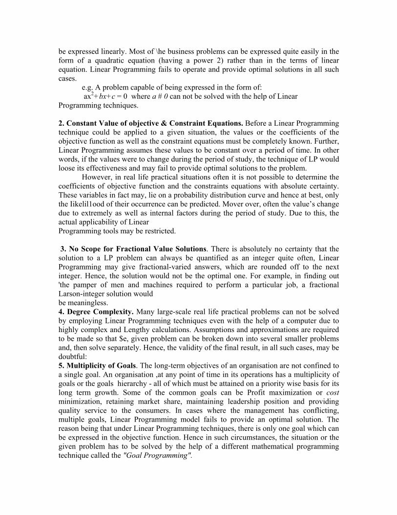
be expressed linearly. Most of \he business problems can be expressed quite easily in the form of a quadratic equation (having a power 2) rather than in the terms of linear equation. Linear Programming fails to operate and provide optimal solutions in all such cases.
e.g. A problem capable of being expressed in the form of: ax2+bx+c = 0 where a # 0 can not be solved with the help of Linear
Programming techniques.
2. Constant Value of objective & Constraint Equations. Before a Linear Programming technique could be applied to a given situation, the values or the coefficients of the objective function as well as the constraint equations must be completely known. Further, Linear Programming assumes these values to be constant over a period of time. In other words, if the values were to change during the period of study, the technique of LP would loose its effectiveness and may fail to provide optimal solutions to the problem.
However, in real life practical situations often it is not possible to determine the coefficients of objective function and the constraints equations with absolute certainty. These variables in fact may, lie on a probability distribution curve and hence at best, only the Iikelil1ood of their occurrence can be predicted. Mover over, often the value’s change due to extremely as well as internal factors during the period of study. Due to this, the actual applicability of Linear Programming tools may be restricted. 3. No Scope for Fractional Value Solutions. There is absolutely no certainty that the solution to a LP problem can always be quantified as an integer quite often, Linear Programming may give fractional-varied answers, which are rounded off to the next integer. Hence, the solution would not be the optimal one. For example, in finding out 'the pamper of men and machines required to perform a particular job, a fractional Larson-integer solution would be meaningless. 4. Degree Complexity. Many large-scale real life practical problems can not be solved by employing Linear Programming techniques even with the help of a computer due to highly complex and Lengthy calculations. Assumptions and approximations are required to be made so that $e, given problem can be broken down into several smaller problems and, then solve separately. Hence, the validity of the final result, in all such cases, may be doubtful: 5. Multiplicity of Goals. The long-term objectives of an organisation are not confined to a single goal. An organisation ,at any point of time in its operations has a multiplicity of goals or the goals hierarchy - all of which must be attained on a priority wise basis for its long term growth. Some of the common goals can be Profit maximization or cost minimization, retaining market share, maintaining leadership position and providing quality service to the consumers. In cases where the management has conflicting, multiple goals, Linear Programming model fails to provide an optimal solution. The reason being that under Linear Programming techniques, there is only one goal which can be expressed in the objective function. Hence in such circumstances, the situation or the given problem has to be solved by the help of a different mathematical programming technique called the "Goal Programming".

6. Flexibility. Once a problem has been properly quantified in terms of objective function and the constraint equations and the tools of Linear Programming are applied to it, it becomes very difficult to incorporate any changes in the system arising on account of any change in the decision parameter. Hence, it lacks the desired operational flexibility. Mathematical model of LPP. Linear Programming is a mathematical technique for generating & selecting the optimal or the best solution for a given objective function. Technically, Linear Programming may be formally defined as a method of optimizing (i.e.; maximizing or minimizing) a linear function for a number of constraints stated in the form of linear in equations. Mathematically the problem of Linear Programming may be stated as that of the optimization of linear objective function of the following form : nnii XCxCxcxCZ ++++= .....................2211 Subject to the Linear constrains of the form: 1ln1.313212111 ...................... bxaxaxaxaxa nii
≤≥+++++
222.32322211 ...................... bxaxaxaxaxa nniij≤≥+++++
1.33322211 ...................... bmxaxamxaxaxa njniij≤≥+++++
≤
mnmnii bXaxamxamnamnam ≤+++ ...................332211 These are called the non-negative constraints. From the above, it is linear that a LP problem has: (I) linear objective function which is to be maximized or minimized. (ii) various linear constraints which are simply the algebraic statement of the
limits of the resources or inputs at the disposal. (iii) Non-negatively constraints.
Linear Programming is one of the few mathematical tools that can be used to provide solution to a wide variety of large, complex managerial problems.
For example, an oil refinery can vary its product-mix by its choice among the different grades of crude oil available from various parts of the world. Also important is the process selected since parameters such as temperature would also affect the yield. As prices and demands vary, a Linear Programming model recommends which inputs and processes to use in order to maximize the profits.
Livestock gain in value as they grow, but the rate of gain depends partially on the feed choice of the proper combination of ingredients to maximize the net gain. This value can be expressed in terms of Linear Programming. A firm which distributes products over a large territory faces an unimaginable number of different choices in deciding how best to meet demand from its network of godown and warehouses. Each warehouse has a very limited number of items and demands often can not be met from the nearest warehouse. If their are 25 warehouses and 1,000 customers, there are 25,000 possible match ups
between customer and warehouse. LP can quickly recommend the shipping quantities and destinations so as to minimize the cost of total distribution.
These are just a few of the managerial problems that have been addressed successfully by LP. A few others are described throughout this text. Project scheduling can be improved by allocating funds appropriately among the most critical task so as to most effectively reduce the overall project duration. Production planning over a year or more can reduce costs by careful timing of the use of over time and inventory to control changes in the size of the workforce. In the short run, personnel work schedules must take into consideration not only the production, work preferences for day offs and absenteeism etc.
Besides recommending solutions to problems like these, LP can provide useful information for managerial decisions, that can be solved by Linear Programming. The application, however, rests on certain postulates and assumptions which have to hold good for the optimality of the solution to be effective during the planning period.
Applications Of Linear Programming Techniques In Indian Economy
In a third world developing country like India, the various factors of productions such as skilled labour, capital and raw material etc. are very precious and scarce. The policy planner is, therefore faced with the problem of scarce resource allocation to meet the various competing demands and numerous conflicting objectives. The traditional and conventional methods can no longer be applied in the changed circumstances for solving this problem and are hence fast losing their importance in the current economy. Hence, the planners in our country are continuously and constantly in search of highly objective and result oriented techniques for sound and proper decision making which can be effective at all levels of economic planning. Nonprogrammed decisions consist of capacity expansion, plant location, product line diversification, expansion, renovation and modernization etc. On the other hand, the programmed decisions consist of budgeting, replacement, procurement, transportation and maintenance etc.
In These modern times, a number of new and better methods ,techniques and tools have been developed by the economists all over the globe. All these findings form the basis of operations research. Some of these well-known operations research techniques have been successfully applied in Indian situations, such as: business forecasting, inventory models - deterministic and probabilistic, Linear Programming.Goal programming, integer programming and dynamic programming etc.
The main applications of the Linear Programming techniques, in Indian context are as follows:
1. Plan Formulation. In the formulation of the country's five year plans, the Linear Programming approach and econometric models are being used in various diverse areas such as : food grain storage planning, transportation, multi-level planning at the national, state and district levels and urban systems.
2. Railways. Indian Railways, the largest employer in public sector undertakings, has successfully applied the methodology of Linear Programming in various key areas.

For example, the location of Rajendra Bridge over the Ganges linking South Bihar and North Bihar in Mokama in preference to other sites has been achieved only by the help of Linear Programming.
3. Agriculture Sector. Linear Programming approach is being extensively used in agriculture also. It has been tried on a limited scale for the crop rotation mix of cash crops, food crops and to/ascertain the optimal fertilizer mix.
4. Aviation Industry. Our national airlines are also using Linear Programming in the selection of routes and allocation of air-crafts to various chosen routes. This has been made possible by the application of computer system located at the headquarters. Linear Programming has proved to be a very useful tool in solving such problems. '
5. Commercial Institutions. The commercial institutions as well as the individual traders are also using Linear Programming techniques for cost reduction and profit maximization. The oil refineries are using this technique for making effective and optimal blending or mixing decisions and for the improvement of finished products.
6. Process Industries. Various process industries such as paint industry makes decisions pertaining to the selection of the product mix and locations of warehouse for distribution etc. with the help of Linear Programming techniques. This mathematical technique is being extensively used by highly reputed corporations such as TELCO for deciding what castings and forging to be manufactured in own plants and what should be purchased from outside suppliers. '
7. Steel Industry. The major steel plants are using Linear Programming techniques for determining the optimal combination of the final products such as : billets, rounds, bars, plates and sheets.
8. Corporate Houses. Big corporate houses such as Hindustan Lever employ these techniques for the distribution of consumer goods throughout the country. Linear Programming approach is also used for capital budgeting decisions such as the selection of one project from a number of different projects. Main Application Areas Of Linear Programming In the last few decades since 1960s, no other mathematical tool or technique has had such a profound impact on the management's decision making criterion as Linear Programming well and truly it is one of the most important decision making tools of the last century which has transformed the way in which decisions are made and businesses are conducted. Starting with the Second World War till the Y -2K problem in computer applications, it has covered a great distance.
We discuss below some of the important application areas of Linear Programming:
I. Military Applications. Paradoxically the most appropriate example of an organization is the military and worldwide, Second World War is considered to be one of the best managed or organized events in the history of the mankind. Linear Programming is extensively used in military operations. Such applications include the problem of selecting an air weapon system against the enemy so as to keep them pinned down and at the same time minimizes the amount of fuel used. Other examples are dropping of bombs

on pre-identified targets from aircraft and military assaults against localized terrorist outfits.
2. Agriculture. Agriculture applications fall into two broad categories, farm economics and farm management. The former deals with the agricultural economy of a nation or a region, while the latter is concerned with the problems of the individual form. Linear Programming can be gainfully utilized for agricultural planning e:g. allocating scarce limited resources such as capital, factors of production like labour, raw material etc. in such a way 'so as to maximize the net revenue.
3. Environmental Protection. Linear programming is used to evaluate the various possible a1temative for handling wastes and hazardous materials so as to satisfy the stringent provisions laid down by the countries for environmental protection. This technique also finds applications in the analysis of alternative sources of energy, paper recycling and air cleaner designs.
4. Facilities Location. Facilities location refers to the location nonpublic health care facilities (hospitals, primary health centers) and’ public recreational facilities (parks, community hal1s) and other important facilities pertaining to infrastructure such as telecommunication booths etc. The analysis of facilities location can easily be done with the help of Linear Programming. Apart from these applications, LP can also be used to plan for public expenditure and drug control. '
5. Product-Mix. The product-mix of a company is the existence of various products that the company can produce and sell. However, each product in the mix requires finite amount of limited resources. Hence it is vital to determine accurately the quantity of each product to be produced knowing their profit margins and the inputs required for producing them. The primary objective is to maximize the profits of the firm subject to the limiting factors within which it has to operate.
6. Production. A manufacturing company is quite often faced with the situation where it can manufacture several products (in different quantities) with the use of several different machines. The problem in such a situation is to decide which course of action will maximize output and minimize the costs. Another application area of Linear Programming in production is the assembly by-line balancing - where a component or an item can be manufactured by assembling different parts. In such situations, the objective of a Linear Programming model is to set the assembly process in the optimal (best possible) sequence so that the total elapsed time could be minimized.
7. Mixing or Blending. Such problems arise when the same product can be produced with the help of a different variety of available raw-materials each having a fixed composition and cost. Here the objective is to determine the minimum cost blend or mix (Le.; the cost minimizations) and the various constraints that operate are the availability of raw materials and restrictions on some of the product constituents.
8. Transportation & Trans-Shipment. Linear Programming models are employed to determine the optimal distribution system i.e.; the best possible channels of distribution available to an organisation for its finished product sat minimum total cost of transportation or shipping from company's godown to the respective markets. Sometimes the products are not transported as finished products but are required to be manufactured at various. sources. In such a

situation, Linear Programming helps in ascertaining the minimum cost of producing or manufacturing at the source and shipping it from there.
9. Portfolio Selection. Selection of desired and specific investments out of a large number of investment' options available10 the managers (in the form of financial institutions such as banks, non-financial institutions such as mutual funds, insurance companies and investment services etc.) is a very difficult task, since it requires careful evaluation of all the existing options before arriving at C\ decision. The objective of Linear Programming, in such cases, is to find out the allocation/which maximizes the total expected return or minimizes the total risk under different situations.
10. Profit Planning & Contract. Linear Programming is also quite useful in profit planning and control. The objective is to maximize the profit margin from investment in the plant facilities and machinery, cash on hand and stocking-hand.
11. Traveling Salesmen Problem. Traveling salesmen problem refers to the problem of a salesman to find the shortest route originating from a particular city, visiting each of the specified cities and then returning back to the originating point of departure. The restriction being that no city must be visited more than once during a particular tour. Such types of problems can quite easily be solved with the help of Linear Programming.
12. Media Selection/Evaluation. Media selection means the selection of the optimal media-mix so as to maximise the effective exposure. The various constraints in this case are: Budget limitation, different rates for different media (i.e.; print media, electronic media like radio and T.V. etc.) and the minimum number of repeated advertisements (runs) in the various media. The use of Linear Programming facilities like the decision making process.
13. Staffing. Staffing or the man-power costs are substantial for a typical organisation which make its products or services very costly. Linear Programming techniques help in allocating the optimum employees (man-power or man-hours) to the job at hand. The overall objective is to minimize the total man-power or overtime costs.
14. Job Analysis. Linear Programming is frequently used for evaluation of jobs in an organisation and also for matching the right job with the right worker.
15. Wages and Salary Administration. Determination of equitable salaries and various incentives and perks becomes easier with the application of Linear Programming. LP tools” can also be utilized to provide optimal solutions in other areas of personnel management such as training and development and recruitment etc.
Linear Programming problem Formation Steps In Formulating A Linear Programming Model Linear programming is one of the most useful techniques for effective decision making. It is an optimization approach with an emphasis on providing the optimal solution for resource allocation. How best to allocate the scarce organisational or national resources among different competing and conflicting needs (or uses) forms the core of its working. The scope for application of linear programming is very wide and it occupies a central place in many diversified decisional problems. The effective use and application of linear programming requires the formulation of a realistic model which represents accurately

the objectives of the decision making subject to the constraints in which it is required to be made.
The basic steps in formulating a linear programming model are as follows: Step I. Identification of the decision variables. The decision variables (parameters) having a bearing on the decision at hand shall first be identified, and then expressed or determined in the form of linear algebraic functions or in equations.
Step II. Identification of the constraints. All the constraints in the given problem which restrict the operation of a firm at a given point of time must be identified in this stage. Further these constraints should be broken down as linear functions in terms of the pre-defined decision variables.
Step III. Identification of the objective. In the last stage, the objective which is required to be optimized (i.e., maximized or memorized) must be dearly identified and expressed in terms of the pre-defined decision variables.
Example 1
High Quality furniture Ltd. Manufactures two products, tables & chairs. Both the products have to be processed through two machines Ml & M2 the total machine-hours available are: 200 hours ofM1 and 400 hours of M2 respectively. Time in hours required for producing a chair and a table on both the machines is as follows:
Time in Hours
Machine Table Chair
MJ 7 4 M2 5 , 5
Profit from the Sale of table is Rs. 40 and that from a chair is Rs. 30 determine optimal mix of tables & chairs so as to maximized the total profit Contribution. Let x1 = no. of tables produced and X2 = no. of Chairs produced
Step I. The objective function for maximizing the profit is given by maximize Z=50x1 +30x2 ( objective function )
( Since profit per unit from a table and a chair is Rs. 50 & Rs. 30 respectively). Step II. List down all the constraints. (i) Total time on machine M1 can not exceed 200 hours. 200 4x2 7x1 ≤+∴
( Since it takes 7 hours to produce a table & 4 hours to produce a chair on machine M1) (ii) Total time on machine M2 cannot exceed 400 hours.

200 4x2 7x1 ≤+∴ ( Since it takes 5 hours to produce both a table & a chair on machine M2) Step III Presenting the problem. The given problem can now be formulated as a linear programming model as follows: Maximise Z = 50x1 + 30x2 Subject: : 200 4x 7x 21 ≤+ 400 5x x5 21 ≤+ Further; 0 x x1 2 ≥+ (Since if x1 & x2 < 0 it means that negative quantities of products are being manufactured – which has no meaning).
Example 2.
Alpha Limited produces & sells 2 different products under the brand name black & white. The profit per unit on these products in Rs. 50 & Rs. 40 respectively. Both black & white employ the same manufacturing process which has a fixed total capacity of 50,000 man-hours. As per the estimates of the marketing research department of Alpha Limited, there is a market demand for maximum 8,000 units of Black & 10,000 units of white. Subject to the overall demand, the products can be sold in any possible combination. If it takes 3 hours to produce one unit of black & 2 hours to produce one unit of white, formulate the about as a linear programming model.
Let x1, x2 denote the number of units produced of products black & white respectively.
Step 1: The objective function for maximizing the profit is given by : maximize
Z= 50x1 + 40x2 ( objective function )
Step II: List down all the constraints.
(i) Capacity or man-hours constraint:
( Since it takes 3 hours to produce one unit of x1 & hours to produce 1 unit of x2 & the total available man – hours are 50,000)

(ii) Marketing constraints:
000,81 ≤x
(Since maximum 8,000 units of x1 can be sold )
000,102 ≤x
(Since maximum 10,000 units of x2 can be sold).
Step III: Presenting the problem. Now, the given problem can be written as a linear programming model in the follows:
Maximize Z = 50x1 + 50x2 Subject: : 000,50 2x x3 21 ≤+ 8000 x1 ≤ 000,102 ≤x Further; 0 x x1 2 ≥+( Since if x1,x2< 0, it means that negative Quantities of products are being manufactured – which has no meaning )
Example 3. Good results company manufactures & sells in the export market three different kinds of products P1 , P2 & P3. The anticipated sales for the three products are 100 units of P1, 200 units of P2 & 300 units of P3. As per the terms of the contract Good results must produce at least 50 units of P1 & 70 units of P3. Following is the break – up of the various production times:
Production Hours per Unit Product
Department (A)
Department (B)
Department(C)
Department (D)
(Rs.) Unit
Profit P1 P2 P3
0.05 0.10 0.20
0.06 0.12 0.09
0.07 -- 0.07
0.08 0.30 0.08
15 20 25
Available hours
40.00 45.00 50.00 55.00
Management is free to establish the production schedule subject to the above constraints.
Formulate as a linear programming model assuming profit maximization criterion for Good results company.

Ans. Let X1 , X2 , X3 denote the desired quantities of products P1 , P2 & P3 respectively. Step I. The objective function for maximizing total profits is given by: Maximize Z 15x1 + 20x2 + 25x3 ( objective function ) Step II. List down all the constraints. The available production hours for each of the products must satisfy the following criterion for each department:
(i) 0.05x1+0.10x2+0.20x3 ≤ 40.00 Total hours available on product – wise basis in Department A
(ii) 0.06x1+0.12x2+00.09x3 ≤ 45.00 Total hours available on product – wise basis in Department B
(iii) 0.07x1+0x2+0.07x3 50.00 ≤Total hours available on product – wise basis in Department C
(iv) 0.08x1+0.30x2+0.08x3 ≤ 55.00 Total hours available on product – wise basis in Department D
(v) 10050 1 ≤≤ x Minimum 50 units of P1 must be produced subject of maximum of 100 units.
(vi) 2000 2 ≤≤ xMaximum units of P2 that can be sold is 200 units.
(vii) 30070 3 ≤≤ xMinimum 70 units of P3 must be produced subject to a maximum of 300 units
(viii) Further , x1,x2,x3 0 ≥Since negative values of P1 , P2 & P3 has no meaning Step III: Presenting the Problem The given problem ca be reduced as a LP model as under: Maximise Z=15x1 + 20x2 + 25x3 Subject to: 0.05x1+0.10x2+0.20x3 ≤ 40.00
0.06x1+0.12x2+00.09x3 ≤ 45.00 0.07x1+0x2+0.07x3 ≤ 50.00 0.08x1+0.30x2+0.08x3 ≤ 55.00 10050 1 ≤≤ x 2000 2 ≤≤ x 30070 3 ≤≤ x x1, x2, x3 ≥ 0
Example 4. The management of Surya Chemicals is considering the optimal mix of two possible processes. The values of input & output for both these process are given as follows:
Process Units – inputs Units – Outputs I1 I2 O1 O2
X Y
2 4
6 8
3 5
7 9
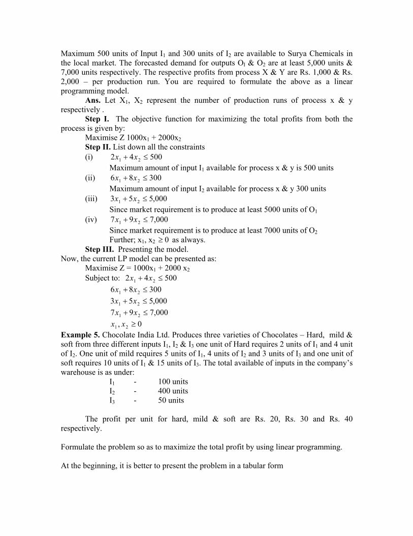
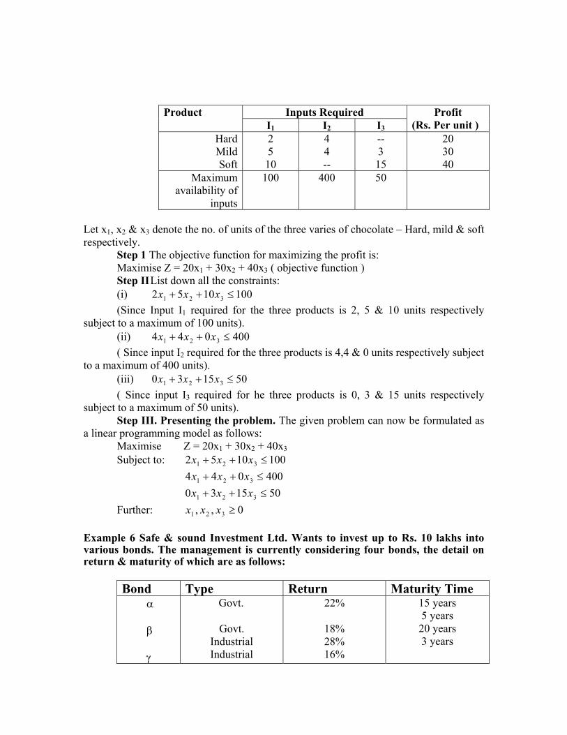
Maximum 500 units of Input I1 and 300 units of I2 are available to Surya Chemicals in the local market. The forecasted demand for outputs OI & O2 are at least 5,000 units & 7,000 units respectively. The respective profits from process X & Y are Rs. 1,000 & Rs. 2,000 – per production run. You are required to formulate the above as a linear programming model. Ans. Let X1, X2 represent the number of production runs of process x & y respectively . Step I. The objective function for maximizing the total profits from both the process is given by: Maximise Z 1000x1 + 2000x2 Step II. List down all the constraints (i) 2 5004 21 ≤+ xx Maximum amount of input I1 available for process x & y is 500 units (ii) 6 3008 21 ≤+ xx Maximum amount of input I2 available for process x & y 300 units (iii) 3 000,55 21 ≤+ xx Since market requirement is to produce at least 5000 units of O1 (iv) 7 000,79 21 ≤+ xx Since market requirement is to produce at least 7000 units of O2 Further; x1, x2 ≥ as always. 0 Step III. Presenting the model. Now, the current LP model can be presented as: Maximise Z = 1000x1 + 2000 x2 Subject to: 50042 21 ≤+ xx 6 3008 21 ≤+ xx 3 000,55 21 ≤+ xx 7 000,79 21 ≤+ xx 0, 21 ≥xxExample 5. Chocolate India Ltd. Produces three varieties of Chocolates – Hard, mild & soft from three different inputs I1, I2 & I3 one unit of Hard requires 2 units of I1 and 4 unit of I2. One unit of mild requires 5 units of I1, 4 units of I2 and 3 units of I3 and one unit of soft requires 10 units of I1 & 15 units of I3. The total available of inputs in the company’s warehouse is as under: I1 - 100 units I2 - 400 units I3 - 50 units The profit per unit for hard, mild & soft are Rs. 20, Rs. 30 and Rs. 40 respectively. Formulate the problem so as to maximize the total profit by using linear programming. At the beginning, it is better to present the problem in a tabular form
Inputs Required Product I1 I2 I3
Profit (Rs. Per unit )
HardMildSoft
2 5 10
4 4 --
-- 3 15
20 30 40
Maximum availability of
inputs
100 400 50
Let x1, x2 & x3 denote the no. of units of the three varies of chocolate – Hard, mild & soft respectively. Step 1 The objective function for maximizing the profit is: Maximise Z = 20x1 + 30x2 + 40x3 ( objective function ) Step II List down all the constraints: (i) 2 100105 321 ≤++ xxx (Since Input I1 required for the three products is 2, 5 & 10 units respectively subject to a maximum of 100 units). (ii) 4 40004 321 ≤++ xxx ( Since input I2 required for the three products is 4,4 & 0 units respectively subject to a maximum of 400 units). (iii) 0 50153 321 ≤++ xxx ( Since input I3 required for he three products is 0, 3 & 15 units respectively subject to a maximum of 50 units). Step III. Presenting the problem. The given problem can now be formulated as a linear programming model as follows: Maximise Z = 20x1 + 30x2 + 40x3 Subject to: 2 100105 321 ≤++ xxx 4 40004 321 ≤++ xxx 0 50153 321 ≤++ xxx Further: x 0,, 321 ≥xx
Example 6 Safe & sound Investment Ltd. Wants to invest up to Rs. 10 lakhs into various bonds. The management is currently considering four bonds, the detail on return & maturity of which are as follows:
Bond Type Return Maturity Time α
β
γ
Govt.
Govt. Industrial Industrial
22%
18% 28% 16%
15 years 5 years 20 years 3 years

θ
The company has decided not to put less than half of its investment in the government bonds and that the average age of the portfolio should not be more than 6 years. The investment should be such which maximizes the return on investment, subject to the above restriction.
Formulate the above as a LP problem.
Ans. Let X1 = amount to be invested in bond α Govt. X2 = amount to be invested in bond β Govt. X3 = amount to be invested in bond γ Industrial X4 = amount to be invested in bond θ Industrial Step I. The objective function which maximizes the return on investment Is: Maximise Z = 0.22x1 + 0.18x2 + 0.28x3 + 0.16x4 ( Based on the respective rate of respective rate of return for each bond. Step II. List down all the constraints: (i) Sum of all the investments can not exceed the total fund available. 000,00,104321 ≤+++∴ xxxx
(ii) Sum of investments in government bonds should not be less than 50%. 000,00,521 ≤+∴ xx
(iii) Average :
≤
++++++
riodmaturilypeenotesNumeratord
xxxxxxxx
63205
4321
432115
Or 15 43214321 66663205 xxxxxxxx +++≤+++ Or 6( 0)63()620()65()15 4321 ≤−+−−+ xxxx−
03149 4321 ≤−+−∴ xxxx Step III. Presenting the problem The given problem can now be formulated as a LP model: Maximise Z = 0.22x1 + 0.18x2 + 0.28x3 + 0.16x4
Subject to: 000,00,104321 ≤+++ xxxx 000,00,521 ≤+ xx
9 0314 4321 ≤−+− xxxx Further ; 04321 ≤+++ xxxx
Example7 Good products Ltd. Produces its product in two plants P1 & P2 and distributes this product from two warehouses W1 & W2. Each plant can produce a maximum of 80 units. Warehouse W1 can sell 100 units while W2 can sell only 60 units. Following table shows the cost of shipping one unit from plants to the warehouses:

(cost in Rs) To
from
Warehouse (W1) Warehouse (W2)
Plant (P1) Plant (P1)
40 70
60 75
Determine the total no. of units to be shipped for each plant to each warehouse, such that the capacity of plants is not exceeded, demand at each warehouse is fully satisfied & the total cost of transportation is minimized. Ans. Let Sij = No. of units shipped form plant i to warehouse j. Where i = p1, p2 and j = w1, w2
Further assume C to be the transportation cost of shipping a unit form plant to the warehouse then, we have: Cp1w1 = cost of shipping a unit form plant p1 to warehouse w1, Cp1w2 = cost of shipping a unit form plant p1 to warehouse w2, Cp2w1 = cost of shipping a unit form plant p2 to warehouse w1 & Cp2w2 = cost of shipping a unit form plant p12to warehouse w2, Formulate the problem in a tabular from as under.
P1 to w1 P1 to w2 P2 to w1 P2 to w2 Resources Warehouse W1 demand Warehouse w2 demand
Plant P2 supply Plant p2 supply
shipping costs (Rs.)
1 0 1 0
40
0 1 1 0
60
1 0 0 1
70
0 1 0 1
75
100 units 60 units 80 units 80 units
Formulating as a LP Noble in the usual manner:
Objective – function
Minimize Z = 40 CP1W1 + 60 C P1W2 + 70C P2W1 + 75 Cp2w2 Ware hose constraints. Cp1w1 + Cp1w2 = 100

Cp1w2 + Cp2w2 = 60
Plant constraints
Cp1w1 + Cp1w2 = 80 Cp1w2 + Cp2w2 = 80 Where Cp1w1 , Cp1w2, Cp2w1 , Cp2w2 ≤ 0 (since these denote costs in a minimization problem) Example 8. To maintain good health, a person must fulfil certain minimum daily requirements of several kinds of nutrients. For the sake of simplicity let us assume that only three kinds of these needs to be considered calcium, protein vitamin A. also assume that the person’s diet is to consist of only 2 food items, I & II; whose prices & nutrient content’s are given in the following table. Find out the optimal combination of the two food items that will satisfy the daily requirements & entail the least cost.
Food Calcium Protein Vitamin A Cost of unit FI F2
10 4
5 5
2 6
6 1
Daily minimum Requirement
20
20
12
Ans. Let x1 = Quantity of F1 to be purchased X2 = Quantity of F2 to be purchased Step 1. the objective function for minimizing the total cost is given by: Minimize Z = 6x1 + x2 (objective – function) Step II. List down all the constraints: (i) calcium constraint: 10x1 + 4x2 ≥ 20
(ii) protein constraint: 5x1 + 5x2 ≥ 20 (iii) vitamin constraint: 2x1 + 6x2 ≥ 12 step III. Presenting as a Lp model: minimize Z = 6x2 + X2 10x1 + 4x2 ≥ 20 5x1 + 5x2 ≥ 20 2x1 + 6x2 ≥12 further x1, x2 ≥ 0 Example9. A steel plant manufactures two grades of steel S1 & S2 . Data given below shows the total resources consumed & profit per unit associated with S1 & S2 .iron and labour are the only resources which are consumed in the manufacturing process. The

manager of the firm wishes to determine the different units of S1 & S2 . which should be manufactured to maximize the total profit. Resource utilized Unit-requirement
S1 S2
Amount
Available Lron (kg) labour
(Hours) 30 5
20 10
300 110
Profit (Rs.) 6 8
Ans. Let x1 = no. of units of S1 to be manufactured. x2 = no. of units of S2 to be manufactured. Step I The objective function for maximizing to be manufactured. Z = 6x1 + 8x2 ( objective – function ) ( Since profit per unit of S1 & S2 are Rs. 6 and Rs. 8 respectively ) Step II. List down all the constraints: (i) Iron – constraint: 30x1 +20x2 300 ≤(ii) Labour – constraint:
5x1 +10x2 110 ≤Step III. Presenting as a LP Model Maximize Z = 6x1 + 8x2 Subject to: 30x1 +20x2 300 ≤ 5x1 +10x2 ≤ 110 Further : x1,x2≥ 0 Example 10. Mr. Khanna is exploring the various investment options for maximizing his return on investment. The investments that can be made by him pertain to the following areas: Govt. bonds, fixed deposits of companies equity shares time deposits in banks, Indira Vikas Patra & real estate. The data pertaining to the return on investment, the number of years for which the funds will be blocked to earn this return on investment and the related risks are as follows: Option Return No. of years Risk factor
Govt. bonds Company deposits
Equity shares
6% 15% 20%
15 3 6
1 3 7
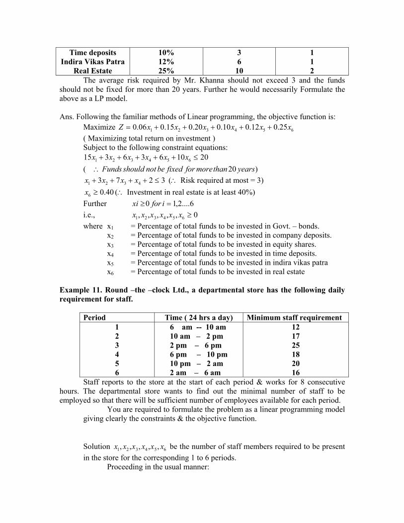
Time deposits Indira Vikas Patra
Real Estate
10% 12% 25%
3 6 10
1 1 2
The average risk required by Mr. Khanna should not exceed 3 and the funds should not be fixed for more than 20 years. Further he would necessarily Formulate the above as a LP model. Ans. Following the familiar methods of Linear programming, the objective function is: Maximize 0Z = 654321 25.012.010.020.015.006. xxxxxx +++++ ( Maximizing total return on investment ) Subject to the following constraint equations: 2010636315 654321 ≤+++++ xxxxxx ( Funds )20 yearsthanmoreforfixedbenotshould∴ 3 (273 4321 ≤++++ xxxx ∴ Risk required at most = 3)
40.06 ≥x (∴ Investment in real estate is at least 40%) Further 6....2,10 =≥ iforxi i.e., 0,,,,, 654321 ≥xxxxxxwhere x1 = Percentage of total funds to be invested in Govt. – bonds. x2 = Percentage of total funds to be invested in company deposits. x3 = Percentage of total funds to be invested in equity shares. x4 = Percentage of total funds to be invested in time deposits. x5 = Percentage of total funds to be invested in indira vikas patra x6 = Percentage of total funds to be invested in real estate
Example 11. Round –the –clock Ltd., a departmental store has the following daily requirement for staff.
Period Time ( 24 hrs a day) Minimum staff requirement
1 2 3 4 5 6
6 am -- 10 am 10 am – 2 pm 2 pm – 6 pm 6 pm – 10 pm 10 pm – 2 am 2 am – 6 am
12 17 25 18 20 16
Staff reports to the store at the start of each period & works for 8 consecutive hours. The departmental store wants to find out the minimal number of staff to be employed so that there will be sufficient number of employees available for each period.
You are required to formulate the problem as a linear programming model giving clearly the constraints & the objective function. Solution be the number of staff members required to be present in the store for the corresponding 1 to 6 periods.
654321 ,,,,, xxxxxx
Proceeding in the usual manner:

The objective function can be expressed as under: Minimize xZ = 654321 ,,,,, xxxxx ( Since objective is to minimize the no. of staff) Constraint equation: Since each person has to work for 8 consecutive hours, the X1 employee who are employed during the Ist period shall still be on duty when the IInd period starts. Thus, during the II period there will be x1 + x2 employees.
Since the minimal number of staff required during the 2nd period is given to be 17, therefore we must have the first constraint equation as: x1 +x2 ≥ 17 like wise the remaining constraint equations can be written as :
x2 +x3 ≥ 25 x3 +x4 ≥ 18 x4 +x5 ≥ 20 x5 +x6 ≥ 16 and x16+x1 ≥ 2 where X1, X2 ……….. ≥ 0 Example12.The management of Quality Toys wants to determine the number of advertisement to be placed in three monthly magazines M1 , M2 & M3 the primary objective for advertising is to maximize the total exposure to the customers & the potential buyers of its high quality & safe toys. Percentages of readers for each of the 3 magazines M1 , M2 & M3 are know with the help of a readership survey. The following information is provided. Magazines Readers (in lakh) 2 1.60 1.40 Principal buyer 10% 10% 5% Cost / advertisement(Rs.)
5000 4000 3000
The maximum advertisement budget is Rs. 10 lakhs. The management has already decided that magazine M1 should not have more than 12 advertisements & that M2 & M3 can each have at least 2 advertisements. Formulate the above as a LP model. (exposure in a magazine = No. of advertisement placed X no. of principal buyers) Ans. Let X1 , X2 , X3 denoted the required no. of advertisements in magazines M1 , M2 & M3 respectively. Step 1. the total exposure of principal buyers of the magazine is: Z = (10% of 200000) X1 +(10% of 160000) X2 + (5% of 140000) X3 = 20000 X1 + 16000 X2 + 7000 X3 Step 2. list down the constrain equations: X1 ≤ 12 9since M1 can not have more than 12 advertisements) X2 ≥ 2 since M1 M2 can have at least 2 advertisements X3 ≥ 2

Step 3. present as LP model i.e., Z = 20000 X1 + 16000 X2 +7000 X3 Maximize (Exposures are ot be maximized) Subject to : X1≤ 12 X2≤ 2 X3≤ 2 Further X1 , X2 , X3 ≥ 0 Example 13.Precise manufacturing works produces a product each unit of which consists of 10 units of component A & 8 unit of component. B Both these components are manufactured form two different raw materials of which 100 units & 80 unit are available respectively. The manufacture of both these components A & B is done in three distinct departments. The following results pertaining to both the components are given: Department Input per cycle Output per cycle Raw material Raw material Component Component X Y A B P 18 16 17 15 Q 15 19 16 19 R 13 18 18 14 Formulate the given problem as a linear programming model so as to find out the optimal m=number of production runs for each of the three departments that will maximize the total number of complete units of the final product. Let X1 , X2 , X3 respect the no. of production runs for the three departments P,Q,& R respectively Step 1. Write the objective function
The objective is to maximize the total no. of units of final product. Since each unit of product requires 10 units of component A& 8 units of component B, there fore the maximum number of units of the final products can not exceed the smaller value of : (17 X1 + 16X2 + 18 X3 ) /10 (i.e. the np. Of units of component A produced by different departments divided by the no. units of A required for the final product ) also 15X1 + 19 X2 + 14X3 / 8 (i.e. the no of units of component B manufactured by various departments divided by the no. of units of B required for the final product) the objective function hence becomes: Maximize
Z = Minimum of
++++
8 X 14 19X X 15,
10 X 18 16X X 17 32 132 1
Step II. Give the constraint equations: Raw material constraints:
100131518 321 ≤++ xxx ( Raw material : X)

80181916 321 ≤++ xxx ( Raw material : Y ) Subject to x1, x2, x3 0 ≥Hence, the model can be formulated.
Example 14.Unique Ltd. Is contemplating investment expenditure for its plant evaluation & modernization ( R& X). Various proposals are lying with the unique Ltd. Has generated the following data which would be utilized in evaluating & selecting the best set of proposals.
Option
Definition Expenditure
(Rs. .000) Engineering
required Ist
year II
nd Year Valu
e (Rs.
‘000 )
Hours (’00)
1. Renovate Assembly 2. New assembly 3. New machinery 4. Renovate shops 5. Process materials 6. New process 7. New storage facility
22 9.2
2 -- 6 6 19.
50 8
-- 2
7 1
7 1
0 2
2 -- 3.
20
7 9.20 6 8 14.50 7 4.50
5 8 4
.30 9 4
.50 3 --
Following are the budgetary constraints: Expenditure for Ist year : 4.00 lacs Expenditure for IInd year : 14.40 lacs Total engineering hours : 25,000 hours The prevailing situation necessitates that a new or modernized shop floor be provided. The machinery for production line is applicable only to the new shop floor. The management does not desire to opt for building or buying of raw material processing facilities. Formulate the problem so as to for maximize the total gains to the company i.e. the engineering value. Assign the following relation to parameter x1 1, if project I is to be under taken i.e., Let xi = 0, otherwise
Objective function Maximize

7654321 50.4750148650.97 xxxxxxxZ ++−++++= (Since value of engineering i. e money is to be maximized Constraints: (i) The total expenditure in the first year should not exceed Rs 4 lacs i.e.; 400850.1966050.922 7654321 ≤++++++ xxxxxxx (ii) The total expenditure in the second year should not exceed 14.40 lacs i.e.; 14402.30221017270 7654321 ≤++++++ xxxxxxx (iii) The total number of hours required for engineering cannot exceed the maximum
of 25,000 hrs. i.e.; 25030350.4930.485 7654321 ≤++++++ xxxxxxx (iv) Both the options or new and modernized shop floor can not be taken together.
However, at least one option has to be exercised i.e; 121 =+ xx(v) Option 3 may be exercised only if option 2 is exercised i.e.;
25 xx ≥ (vii) or for all i. 0≥xi Based on the above constraints & the objective function, a linear programming model may be constructed.

Unit 1
Lesson 3: Graphical method for solving LPP.
Learning outcome
1.Finding the graphical solution to the linear programming model
Graphical Method of solving Linear Programming Problems
Introduction
Dear students, during the preceding lectures, we have learnt how to formulate a given problem as a Linear Programming model. The next step, after the formulation, is to devise effective methods to solve the model and ascertain the optimal solution. Dear friends, we start with the graphical method and once having mastered the same, would subsequently move on to simplex algorithm for solving the Linear Programming model. But let’s not get carried away. First thing first. Here we go.
We seek to understand the IMPORTANCE OF GRAPHICAL METHOD OF SOLUTION IN LINEAR PROGRAMMING and seek to find out as to how the graphical method of solution be used to generate optimal solution to a Linear Programming problem.
Once the Linear programming model has been formulated on the basis of the given objective & the associated constraint functions, the next step is to solve the problem & obtain the best possible or the optimal solution various mathematical & analytical techniques can be employed for solving the Linear-programming model.
The graphic solution procedure is one of the method of solving two
variable Linear programming problems. It consists of the following steps:-
Step I Defining the problem. Formulate the problem mathematically. Express it in
terms of several mathematical constraints & an objective function. The objective function relates to the optimization aspect is, maximisation or minimisation Criterion.
Step II
Plot the constraints Graphically. Each inequality in the constraint equation has to be treated as an equation. An arbitrary value is assigned to one variable & the value of the other variable is obtained by solving the equation. In the similar manner, a different arbitrary value is again assigned to the variable & the corresponding value of other variable is easily obtained.
These 2 sets of values are now plotted on a graph and connected by a straight line. The same procedure has to be repeated for all the constraints. Hence, the total straight lines would be equal to the total no of equations, each straight line representing one constraint equation.
Step III
Locate the solution space. Solution space or the feasible region is the graphical area which satisfies all the constraints at the same time. Such a solution point (x, y) always occurs at the comer. points of the feasible Region the feasible region is determined as follows:
(a) For" greater than" & " greater than or equal to" constraints (i.e.;), the feasible region or the solution space is the area that lies above the constraint lines.
(b) For" Less Then" &" Less than or equal to" constraint (ie; ). The feasible region or the solution space is the area that lies below the constraint lines.
Step IV
Selecting the graphic technique. Select the appropriate graphic technique to be used for generating the solution. Two techniques viz; Corner Point Method and Iso-profit (or Iso-cost) method may be used, however, it is easier to generate solution by using the corner point method.

(a) Corner Point Method. (i) Since the solution point (x. y) always occurs at the corner point of the feasible or solution space, identify each of the extreme points or corner points of the feasible region by the method of simultaneous equations.
(ii) By putting the value of the corner point's co-ordinates [e.g. (2,3)] into the objective function, calculate the profit (or the cost) at each of the corner points.
(iii) In a maximisation problem, the optimal solution occurs at that
corner point which gives the highest profit.
In a minimisation problem, the optimal solution occurs at that corner point which gives the lowest profit.
Dear students, let us now turn our attention to the important theorems which are used in solving a linear programming problem. Also allow me to explain the important terms used in Linear programming. Here we go.
IMPORTANT THEOREMS
While obtaining the optimum feasible solution to the linear programming problem, the statement of the following four important theorems is used:- Theorems I. The feasible solution space constitutes a convex set. Theorems II. within the feasible solution space, feasible solution correspond to the extreme ( or Corner) points of the feasible solution space. Theorem III. There are a finite number of basic feasible solution with the feasible solution space. Theorem IV The optimum feasible solution, if it exists. will occur at one, or more, of the extreme points that are basic feasible solutions.

Note. Convex set is a polygon "Convex" implies that if any two points of the polygon are selected arbitrarily then straight line segment Joining these two points lies completely within the polygon. The extreme points of the convex set are the basic solution to the linear programming problem.
IMPORTANT TERMS
Some of the important terms commonly used is linear programming are disclosed as follows:
(i) Solution Values of the decision variable x;(i = 1,2,3, in) satisfying the constraints of a general linear programming model is known as the solution to that linear programming model. (ii) Feasible solution Out of the total available solution a solution that also satisfies the non-negativity restrictions of the linear programming problem is called a feasible solution. (iii) Basic solution For a set of simultaneous equations in Q unknowns (p Q) a solution obtained by setting (P - Q) of the variables equal to zero & solving the remaining P equation in P unknowns is known as a basic solution. .
The variables which take zero values at any solution are detained as non-basic variables & remaining are known as-basic variables, often called basic.
(iv) Basic feasible solution A feasible solution to a general linear programming problem which is also basic solution is called a basic feasible solution. (v) Optimal feasible solution Any basic feasible solution which optimizes (ie; maximise or minimises) the objective function of a linear programming modes known as the optimal feasible solution to that linear programming model. (vi) Degenerate Solution A basic solution to the system of equations is termed as degenerate if one or more of the basic variables become equal to zero.
I hope the concepts that we have so far discussed have been fully understood by
all of you.
Friends, it is now the time to supplement our understanding with the help of
examples.
Example 1.
X Ltd wishes to purchase a maximum of3600 units of a product two types
of product a. & are available in the market Product a occupies a space of 3 cubic Jeet & cost Rs. 9 whereas occupies a space of 1 cubic feet & cost Rs. 13 per unit. The budgetary constraints of the company do not allow to spend more than Rs. 39,000. The total availability of space in the company's godown is 6000 cubic feet. Profit margin of both the product a & is Rs. 3 & Rs. 4 respectively. Formulate as a linear programming model and solve using graphical method. You are required to ascertain the best possible combination of purchase of a & so that the total profits are maximized.
Solution
Let x1 = no of units of product α & x2 = no of units of product β Then the problem can be formulated as a P model as follows:- Objective function, Maximise 21 43 xxZ += Constraint equations: - int)(360021 ConstraUnitsMaximumxx ≤+ 3 600021 ≤+ xx ( Storage area constraint ) 9 3900013 21 ≤+ xx ( Budgetary constraint ) 021 ≤+ xx Step I Treating all the constraints as equality, the first constraint is 360021 =+ xx Put ⇒= ox The point is (0, 3600) ∴=360021 x Put = ox The point is (3600, 0) ∴=⇒ 360012 xDraw is graph with x1 on x-axis & x2 on y-axis as shown in the figure.
Step II Determine the set of the points which satisfy the constraint: 360021 =+ xxThis can easily be done by verifying whether the origin(0,0) satisfies the constraint. Here,
360000 =+ . Hence all the points below the line will satisfy the constraint. Step III The 2nd constraint is: 60003 21 ≤+ xx Put ⇒= ox and the point is ( 0, 6000) 600021 =x Put ⇒= ox and the point is ( 200, 0) 20012 =x
Now draw its graph.
Step IV
Like it’s in the above step II, determine the set of points which satisfy the constraint 60003 21 ≤+ xx . At origin;
. Hence, all the points below the line will satisfy the constraint.
600000 <+
Step V
The 3rd constraint is: 39000129 21 ≤+ xx Put =⇒= xox & the point is (0, 3000) 300021
Put
0,
313000int&
313000
12 ispothe=⇒= xox
Now draw its graph.
Step VI
Again the point (0,0) ie; the origin satisfies the constraint 9 3900012 21 ≤+ xx . Hence, all the points below the line will satisfy the constraint.
Step VII
The intersection of the above graphic denotes the feasible region for the given problem.
Step VIII
Finding Optimal Solution
Always keep in mind two things: -
(i) For ≥ constraint the feasible region will be the area, which lies above the constraint lines, and for ≤ constraints, it will lie below the constraint lines.
This would be useful in identifying the feasible region.
(ii) According to a theorem on linear programming, an optimal solution to a problem ( if it exists ) is found at a corner point of the solution space.
Step IX At corner points ( O, A, B, C), find the profit value from the objective function. That point which maximize the profit is the optimal point. Corner Point W-Ordinates Objective Func
21 43 xxZ += Value
O A C
(0,0) (0,3000) (2000,0)
Z=0+0 Z=0+4x3000
Z=0+3x2000+0
0 12,000 6,000
For point B, solve the equation 9 3900012 21 ≤+ xx And to find point B 600063 21 ≤+ xx( ,BA +∴ these two lines are intersecting ) ie, 60003 =21 + x …(1) x …(2) 390009 21 =+ xxMultiply equ (i) by 3 on both sides:
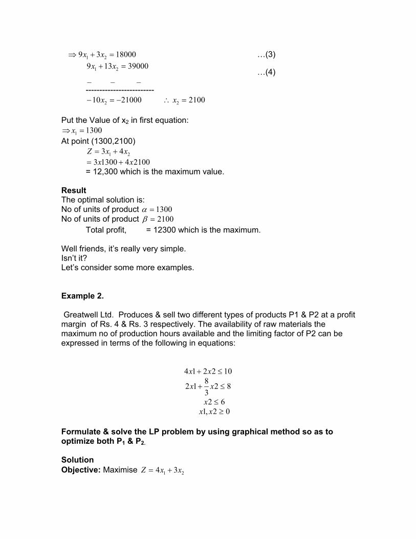
1800039 21 =+⇒ xx …(3)
___39000139 21 =+ xx
…(4)
------------------------- 2100010 2 −=− x 21002 =∴ x
Put the Value of x2 in first equation:
13001 =⇒ x
At point (1300,2100) 21 43 xxZ += 2100413003 xx += = 12,300 which is the maximum value. Result The optimal solution is: No of units of product 1300=α No of units of product 2100=β Total profit, = 12300 which is the maximum. Well friends, it’s really very simple. Isn’t it? Let’s consider some more examples.
Example 2.
Greatwell Ltd. Produces & sell two different types of products P1 & P2 at a profit margin of Rs. 4 & Rs. 3 respectively. The availability of raw materials the maximum no of production hours available and the limiting factor of P2 can be expressed in terms of the following in equations:
102214 ≤+ xx
823812 ≤+ xx
62 ≤x 02,1 ≥xx
Formulate & solve the LP problem by using graphical method so as to optimize both P1 & P2. Solution Objective: Maximise 21 34 xxZ +=

Since the origin (0,0) satisfies each and every constraint, all points below the line will satisfy the corresponding constraints.
Consider constraints as equations & plot then as under:
102214 ≤+ xx put and the point is (0,5) …(1) 501 =⇒= xx
Put 2502 =⇒= xx and the point is ( 5/2, 0)
823812 ≤+ xx …(2)
put and the point is (, 3) 3201 =⇒= xxput and the point is ( 4, 0) 4102 =⇒= xxx1 = 6 …(3) The area under the curve OABC is the solution space. The constraint x1=6 is not considered since it does not contain the variable x2. Getting optimal solution.
Corner Point Co-ordinates Obj.-Func. 21 34 xxZ +=
Value
0 A B C
(0,0) (0,3) * (5/2,0)
Z=0+0 Z=0+3x3 *
8254 2 == xxZ
0 9 * 10
Point B is the intersection of the curves &1024 21 =+ xx
838
21 =xx2
Solving as system of simultaneous equation: Point B is ( 8/5, 9/5
21 34 xxZ +=∴ 5/59)5/9(3)5/8(4 =+=

Result The optimal solution is: Not of units of P2 = 9/5 Total profit = 59/5 Remarks. Since 8/5 & 9/5 units of a product can not be produced , hence these values must be rounded off. This is the limitation of the linear programming technique.
Dear students, we have now reached the end of our discussion scheduled for today. See you all in the next lecture. Bye.
Dear students, I hope all of us have by now properly grasped the intricacies involved in the graphical method.
It’s now time to supplement our understanding of the concept by taking various examples.
Here we go.
Example 3.
Due to the unavailability of desired quality of raw materials, ABC Ltd. Can manufacture maximum 80 units of product A & 60 units of product B. A consumes 5 units and B consumes 6 units of raw materials in the manufacture respectively and their respective profit margins one Rs. 50 & Rs. 80. Further, A requires 1 man-day of labour per unit & B requires 2 man-day of labour per unit. The constraints operating are: Supply of raw material - maximum 600 units Supply of labour - maximum 160 man-days. Formulate as a LP model & solve graphically.

Solution
The question can be presenter in a tabular form as under: Product Raw Material
Required Labour Required
Maximum Units Produced
Profit Per Unit
A B
5 6
1 2
80 60
50 80
Let x1 = number of units of Product A x2 = number of units of Product B Since the objective of the company is to maximize its profit. Then the model can be stated as follows: Maximize Z = 50x1 + 80x2 Subject to the linear constraints x1 ≤ 80 Functional restrictions x2 ≤ 60 5x1 + 6x2 ≤ 600 (Electronic restrictions) x1 , 2x2 ≤ 160 (Labour supply) and x1, x2 ≥ 0 Step 2 Graph the constraint inequalities For the problem, x1 axis will represent product. A and B respectively. Each inequality will be treated as an equality and then their respective intercepts on both the axis can be determined. For the first two constraints, we have x1= 80 and x2 = 60, i.e., draw a graph with production of product A and product B, as shown below in Fig. 2-1 and Fig 2-2. Since no more than 80 units of x1 and 60 units of x2 can be produced per day i.e., x1≤ 80 and x2≤60, it
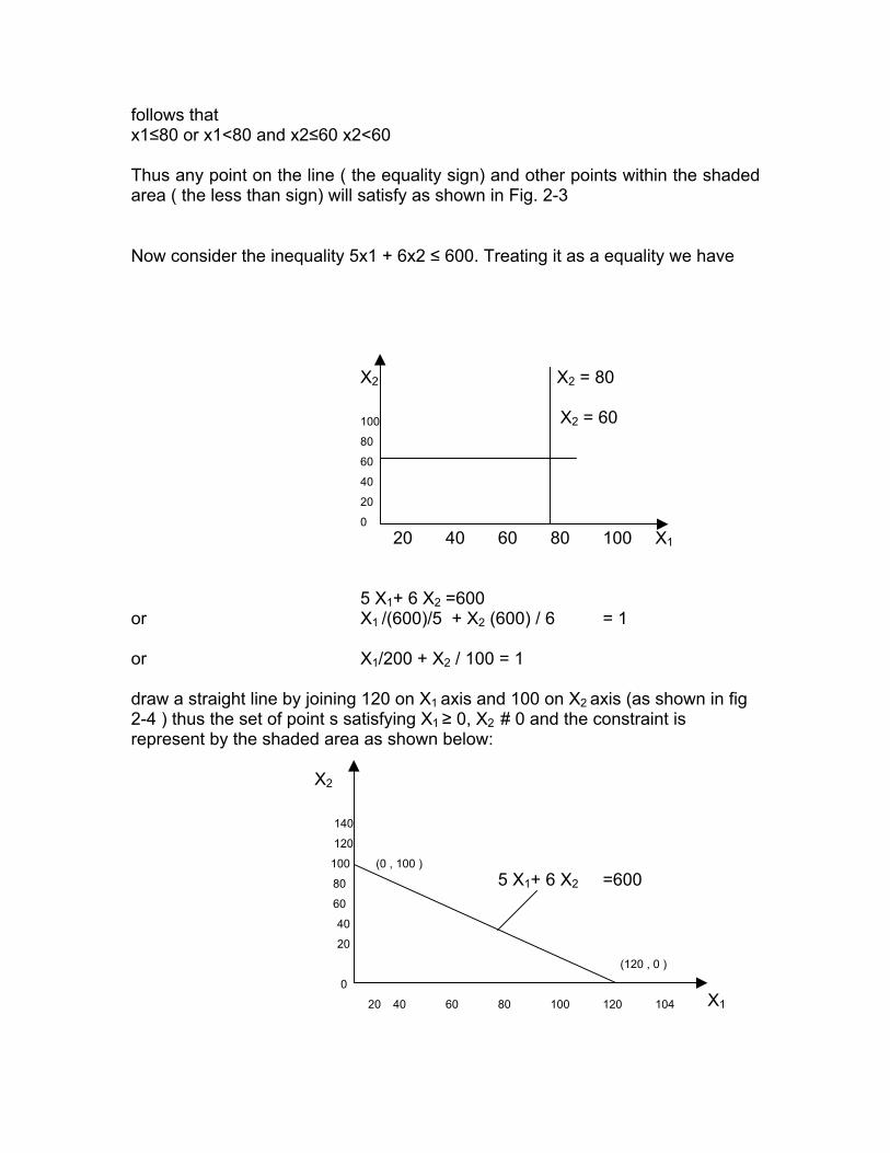
follows that x1≤80 or x1<80 and x2≤60 x2<60 Thus any point on the line ( the equality sign) and other points within the shaded area ( the less than sign) will satisfy as shown in Fig. 2-3
Now consider the inequality 5x1 + 6x2 ≤ 600. Treating it as a equality we have
X2 X2 = 80
100 X2 = 60 80
60
40
20
0 20 40 60 80 100 X1 5 X1+ 6 X2 =600 or X1 /(600)/5 + X2 (600) / 6 = 1 or X1/200 + X2 / 100 = 1 draw a straight line by joining 120 on X1 axis and 100 on X2 axis (as shown in fig 2-4 ) thus the set of point s satisfying X1 ≥ 0, X2 # 0 and the constraint is represent by the shaded area as shown below: X2 140
120
100 (0 , 100 )
80 5 X1+ 6 X2 =600 60
40
20
(120 , 0 )
0 20 40 60 80 100 120 104 X1
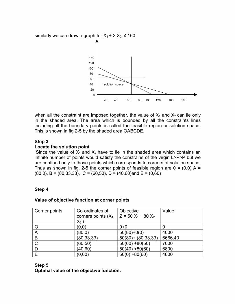
similarly we can draw a graph for X1 + 2 X2 ≤ 160
140
120
100
80
60
40 solution space
20
0
20 40 60 80 100 120 160 180 when all the constraint are imposed together, the value of X1 and X2 can lie only in the shaded area. The area which is bounded by all the constraints lines including all the boundary points is called the feasible region or solution space. This is shown in fig 2-5 by the shaded area OABCDE. Step 3 Locate the solution point Since the value of X1 and X2 have to lie in the shaded area which contains an infinite number of points would satisfy the constrains of the virgin L>P>P but we are confined only to those points which corresponds to corners of solution space. Thus as shown in fig. 2-5 the corner points of feasible region are 0 = (0,0) A = (80,0), B = (80,33,33), C = (60,50), D = (40,60)and E = (0,60)
Step 4
Value of objective function at corner points
Corner points Co-ordinates of corners points (X1, X2 )
Objective Z = 50 X1 + 80 X2
Value
O (0,0) 0+0 0 A (80,0) 50(80)+0(0) 4000 B (80,33.33) 50(80)+ (80,33.33) 6666.40 C (60,50) 50(60) +80(50) 7000 D (40,60) 50(40) +80(60) 6800 E (0,60) 50(0) +80(60) 4800 Step 5 Optimal value of the objective function.

Here we see that the maximum profit of Rs. 7000 is obtained at the point C = (60,50) I,e, X1 = 60 and X2 =50 which together satisfy all the constraints. Hence to maximize profit, the company must produce 60 units of product A and 50 units of product B.
Example4.
Alpha ltd. produces two products X and Y each requiring same production capacity. The total installed production capacity is 9 tones per days. Alpha Ltd. Is a supplier of Beta Ltd. Which must supply at least 2 tons of X & 3 tons of Y to Beta Ltd. Every day. The production time for X and Y is 20 machine hour pr units & 50 machine hour per unit respectively the daily maximum possible machine hours is 360 profit margin for X & Y is Rs. 80 per ton and Rs. 120 per ton respectively. Formulate as a LP model and use the graphical method of generating the optimal solution for determining the maximum number of units of X & Y, which can be produced by Alpha Limited.
Solution Objective function Maximize (total profit) Z = 80 X1 + 120 X2 Subject to the constraints: X1 + X2 ≤ 9, X1 ≥ 2, X2 ≥ 3 (Supply constraint) 20 X1 + 50 X2 ≤ 360 (Machine hours constraint) and X1 ≥ , X2 ≥ 0
Where;
x1 = Number of units ( in tones ) of Product X.
x2 = Number of units ( in tones ) of Product Y.
Now the region of feasible solution shown in the following figure is bounded by the graphs of the Linear equalities:
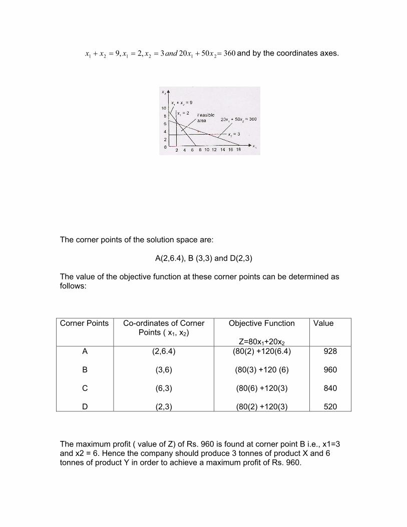
36050203,2,9 212121 =+===+ xxandxxxx and by the coordinates axes.
The corner points of the solution space are:
A(2,6.4), B (3,3) and D(2,3)
The value of the objective function at these corner points can be determined as follows:
Corner Points Co-ordinates of Corner Points ( x1, x2)
Objective Function
Z=80x1+20x2
Value
A
B
C
D
(2,6.4)
(3,6)
(6,3)
(2,3)
(80(2) +120(6.4)
(80(3) +120 (6)
(80(6) +120(3)
(80(2) +120(3)
928
960
840
520
The maximum profit ( value of Z) of Rs. 960 is found at corner point B i.e., x1=3 and x2 = 6. Hence the company should produce 3 tonnes of product X and 6 tonnes of product Y in order to achieve a maximum profit of Rs. 960.

Example 5.
Unique Car Ltd. Manufacturers & sells three different types of Cars A, B, & C. These Cars are manufactured at two different plants of the company having different manufacturing capacities. The following details pertaining to the manufacturing process are provided:
Manufacturing Plants
Maximum Production (of Cars) Operating cost of Plants
A B C
1
2
Demand
( Cards)
50
60
2500
100
60
3000
100
200
7000
2500
3500
Using the graphical method technique of linear programming , find the least number of days of operations per month so as to minimize the total cost of operations at the two plants.
Solution
Let x1 = no-of days plant 1 operates; and
X2 = no-of days plant 2 operates.
The objective of uniques Car Ltd. Is to minimize the operating costs of both its plants.
The above problem can be formulated as follows:
Ie; Minimize Z = 2,500x1+3,500x2 ) Objective )

Subject to:
50 500,260 21 ≥+ xx
000,360100 21 ≥+ xx
100 000,7200 21 ≥+ xx
and 0, 21 ≥xx
Making the graphs of the above constraints:
The solution space lines at the points A,B,C & D Calculating the Optimal solution:
Points Co-ordinates Objective – func Value 0
A
B
C
D
(0,0)
(70,0)
(20,25)
(10,33.33)
(0,50)
Z=0+0
Z=2500x70+0
Z=2500x20+3500x25
Z=2500x10+3500x33.33
Z=0+3500x50
0
1,75,000
1,37,500
1,41,655
1,75,000

Thus, the least monthly operately cost is at the point B. Where x1=20 days, x2=25 days & operating cost = Rs. 1,37,500.
Example 6.
The chemical composition of common ( table ) salt is sodium chloride ( NACL). Free Flow Salts Pvt. Ltd. Must produce 200 kg of salt per day. The two ingredients have the following cost – profile:
Sodium (Na) - Rs. 3 per kg
Chloride (CL) - Rs. 5 per kg
Using Linear programming find the minimum cost of salt assuming that not more than 80 kg of sodium and at lest 60 kg of chloride must be used in the production process.
Solution Formulating as a LP model: Minimise Z=3x+5y ( objective ) Subject to: x+y = 200 ( Total 200 kg to be produced per day ) x≤80 ( Sodium not to exceed 80 kg) y ≥ 60 ( Chloride to be used at least 60 kg ) x,y≥ 0 Where x = Qty of sodium required in the production & y = Qty of chloride required in the production. It is clear from the graph that there is no feasible solution area. It has only one feasible point having the co-ordinates ( 80,120)
Optimal solution:- x = 80, y = 120, and z=3x80+5x120=840 Thus, 80 kg of sodium & 120 kg of chloride shall be mixed in the production of salt at a minimum cost of Rs. 840. Dear students, we have now reached the end of our discussion scheduled for today. See you all in the next lecture. Bye.

Unit 1
Lesson 4: Graphical solution to a LPP
Learning Outcomes
• How to get an optimal solution to a linear programming model using Iso profit (or Iso cost method)
Iso profit or Iso cost method for solving LPP graphically
The term Iso-profit sign if is that any combination of points produces the same profit as any other combination on the same line. The various steps involved in this method are given below.
1. Identify the problem- the decision variables, the objective and the restrictions.
2. Set up the mathematical formulation of the problem.
3. Plot a graph representing all the constraints of the problem and identify the feasible region. The feasible region is the intersection of all the regions represented by the constraint of the problem and is restricted to the first quadrant only.
4. The feasible region obtained in step 3 may be bounded or unbounded. Compute the coordinates of all the corner points of the feasible region.
5. Choose a convenient profit (or cost) and draw iso profit (iso cost)line so that it falls within the feasible region.
6. Move the iso profit (iso cost line to itself farther (closer) from (to) the origin.
7. Identify the optimum solution as the coordinates of that point on the feasible region touched by the highest possible iso profit line( or lower possible cost line).
8. Compute the optimum feasible solution.

Let us do some examples to understand this method more clearly.
Example 1
A company makes two products (X and Y) using two machines (A and B). Each unit of X that is produced requires 50 minutes processing time on machine A and 30 minutes processing time on machine B. Each unit of Y that is produced requires 24 minutes processing time on machine A and 33 minutes processing time on machine B.
At the start of the current week there are 30 units of X and 90 units of Y in stock. Available processing time on machine A is forecast to be 40 hours and on machine B is forecast to be 35 hours.
The demand for X in the current week is forecast to be 75 units and for Y is forecast to be 95 units. Company policy is to maximize the combined sum of the units of X and the units of Y in stock at the end of the week.
Formulate the problem of deciding how much of each product to make in the current week as a linear program.
Solve this linear program graphically.
Solution
Let
• x be the number of units of X produced in the current week • y be the number of units of Y produced in the current week
then the constraints are:
• 50x + 24y <= 40(60) machine A time • 30x + 33y <= 35(60) machine B time • x >= 75 - 30 • i.e. x >= 45 so production of X >= demand (75) - initial stock (30), which
ensures we meet demand • y >= 95 - 90 • i.e. y >= 5 so production of Y >= demand (95) - initial stock (90), which
ensures we meet demand
The objective is: maximize (x+30-75) + (y+90-95) = (x+y-50) i.e. to maximize the number of units left in stock at the end of the week

It is plain from the diagram below that the maximum occurs at the intersection of x=45 and 50x + 24y = 2400
Solving simultaneously, rather than by reading values off the graph, we have that x=45 and y=6.25 with the value of the objective function being 1.25
Example 2.
A firm manufactures & sells two product p1 & p2 at a profit of Rs. 45 per unit & Rs. 80 per unit respectively. The quantities of raw materials required for both p1 & p2 are given below:
Product Raw Materials
P1 P2 R1 R2
5 10
20 15
The maximum availability of both R1 & R2 is 400 & 450 units respectively. You are required to formulate as a LP model & solve using the
graphical method. Solution To find the second point let us assume that the entire amount of input A is used to
produce the produce I and no unit of product II is produced, i.e., X2 = 0. Therefore x1 ≤ i.e., the firm can produce either 80 or less then 80 units of product I. If we take the

maximum production x1 = 80. So the second point is (80,0) and this point Q in graph denotes product of 80 units of product I and zero unit of product II .
By joining the two points P (0,20) and Q (80,0) we get a straight line shows the
maximum quantities of product I and product II that can be produced with the help of input A. The area POQ is the graphic representation of constraint It may
be emphasized here that the constraint is represented by the area POQ and not be the line PQ. As far as the constraint of input A is concerned, production is possible at any point on the line PQ or left to it [ dotted area in the graph.]
.4002052
1 ≤xx
In a similar way the second constraint 10 .45015 21 ≤xx 45, 0 be drawn graphically. For this purpose we obtain two points as
follows: (a) If production of product I is zero, the maximum production of
product II is units. Point R ( 0,30) represents this combination in graph.
(b) If production of product II is zero, the maximum production of product I is 45 units. Point S ( 45, 0) in the graph represents this combination.
By joining points R and S we get a straight line RS. This line again represents the maximum quantities of product I and II that can be produced with the help of input B. ROS represents the feasibility region as far as the input B is concerned.
After plotting the two constraints next step is to find out the feasibility region. Feasibility region is that region in the graph which satisfies all the constraints simultaneously. Region POST in third graph represents feasible region. This region POST satisfies first constraint as well as second constraint. ROS is the feasible region

under first constant. But out of this RPT region does not fulfill second constraint. In a same way region POQ is the feasibility under constraint second but out of this, region TSQ does not satisfy constraint first.
Region POST thus satisfies first constraint as well as second constraint and is thus feasible region. Each point in the feasible region POST satisfies both the linear constraints and is therefore a feasible solution. Non-negative constraints are also being satisfied in this region because we are taking first quadrant of the graph in which both the axes are positive. The feasible region is covered by the linked boundary PTS.
The corner points on the kinked boundary P, T and S are called as extreme points.
Extreme points occur either at the inter-section of the two constraints (T in this example’ or at the intersection of one constraint and one axis ( P and S in our example ).
These extreme points are of great significance in optimal solution. Optimal solution will always be one of the these extreme points.
Final step in solving linear programming problem with the help of graph is to find out the optimal solution out of many feasible solution in the region POST. For this purpose we will have to introduce objective function into our graph. Our objective function is :-
21 8045 xxZ += OR 80 12 45xZx −=
13 8045
80xZx −= OR 12 16
980
xZ−=x
Our objective function which is linear has negative slope.
It is plotted as dotted line z1z1 in the following z1z1 is in-fact Iso-profit line. The different combinations of I and product II of this line yield same profits ( say 20

units ) firm. Any line ( parallel to this line ) which is higher ( right to this z1z1 line signifies higher profit level ( say 25 units ) a line which is lower to the line z1z1 implies lower profit above graph; z1z1 line representing a specified level of profit be moved rightward still remaining in the feasible region. In words profits can be increase still remaining in the feasible.
However, this is possible only up to znzn. Different combination on znzn give the first a same level of profits. Point T (24,14) is in the feasible region POST and also on line znzn. In other words this point ‘T’ represents a combination of the two products which can be produced under the combination of inputs and profits are maximum possible. Point T represents optimum combination. znzn iso-profit line, though signify higher profit is not in the feasible region. The firm, therefore, should produce 24 units of product I and 14 units of product II. Its profits will be maximum possible, equal to :-
Z=45x1+80x2 = (45)(24) +(80)(14)
= 1080 +1120 =Rs. 2200.
Optimum combination can be found also, without the introduction of profits function in our graph. As written above the corner points. P, T and S of the kinked cover of feasible region POST are called as extreme point and optimum T and S yields Maximum profit to the firm.
Point P, x1 = 0 x2 = 20

Z=45x1+80x2 = 45(0) +80(20) = Rs. 1600
Point T, x1 = 24, x2 = 0
Z=45x1+80x2 = (45)(24) +(80)(14) = Rs. 2200
Point S, x1=45, x2 = 0
Z=45x1+80x2 = (45)(245 +(80)(0) = Rs. 2025
So combination T (24,14) is the intimation and Rs. 2200 is the maximum possible level of profits.
Example 3.
A firm produces two components which are then assembled into a final product. The cost per unit of these components is 0.60 and 1.00 respectively. The minimum amount of the various grades of raw material require3d for the manufacturing process are as follows:
Components Raw material required R1 R2 R3
C1
C2
10
4
5
5
2
6
Due to the requirement for a better quality product, the minimum usage value of the raw materials should be 20 units, 20 units & 12 units respectively.
Formulate as a LP problem & solve graphically.
Solution
The objective function is to minimize the total cost of production of both the components C1 & C2
Minimize Z=0. 60x1+1.00x2

Subject to:
20410 21 ≥+ xx
2055 21 ≥+ xx
1262 21 ≥+ xx
20, 21 ≥xx
First constraint, i.e., constraint of nutrient A
20410 21 ≥+ xx
If we consume no unit of food , I i.e., xi=0 then for satisfying the first constraint we will have to take either, 5 units or more than 5 units of good II. If
We consume minimum units of good II for minimizing cost ) then x2 = 5, In this way we get the first point x1(0,5) in first graph. Similarly if we do not take

Food II, i.e., x2=0, the minimum requirement of food 1 is 2 for satisfying the
First constraint. In this way we get the second point Q (2,0) in the first graph. The line PQ represents the minimum quantities of food I and II that must be taken to satisfy the first constraint. Thus dotted area in the first graph represents feasibility region as far as the first constraint is concerned.
In the same way second and third constraints of nutrient B and C respectively are plotted in the second graph and the third graph. In a fourth graph the three constraints are plotted collectively. Shaded area in this graph represents that area where all the constraints are satisfied simultaneously.
In other words, shaded area in the fourth graph is our feasible region. Feasible region is covered by kinked curve with P (0,5), W (0.66, .33) , T (3,1) and V (16, 0) as the extreme

points. Optimum combination is one of these extreme points. To find the optimum combination, i.e., a combination of good I and II which minimize cost as well as satisfy the three constraints, let us introduce the objective function into our graph. Our objective function is
T.C = 0.6x1+1x2
X2 = T.C. – 0.6x1 or x2 = T.C. 121 x−
In our objectives function is a linear function with negatives slope equal to 1/2TC. TC in above graph represents the objective function. In fact Tc1 Tc2 is an iso-cost line a line representing the different combinations of food I and II having the same cost any of Rs. 20.
Any time which is higher to line Tci Tci implies higher cost and any line lower to the line Tci Tci means lower cost. The iso-cost line Tci Tci can be moved leftward still remaining in the feasible region. This means that cost can be reduced still remaining the feasible region. However, this is possible up to Tcn Tcn. If iso-cost line is still moved leftward, it will go out of feasible region. All the combinations on line Tcn Tcn result same cost (which is minimum) but out of these combinations any combination T is in the feasible region. S.T (3.1) is the optimum combination. When three units of

food 1 and one unit of food II are taken all the constraints are satisfied and the cost is minimum possible. Minimum cost is. T.C = 0.6xi + 1xi = (0.6) (3) + (1) (1) = Rs. 2.8 As in the case of maximisation in minimisation, we also can find optimum combination without introducing objective function in to our graph. As optimum point is one of the extreme points, use can use simple arithmetic to find which of these extreme points will result in minimum cost. Point P xi = O, x2 = 5 T.C = 0.6x1 + 1x2 (0.6) (0) + (1)5 = Rs. 5 Point W x1 = 0.66, x2 = 3.3 T.C = 0.6x1 + 1x2 = (0.6) (0.66) + (3.3) = Rs. 3.696 Point T x1 = 3, x2 = 1 T.C. = 0.6x1 + 1x2 = (0.6) (3) + (1) (1) = Rs. 2.8 Point V x1 = 6, x2 = 0 T.C. = 0.6x1 + 1x2 = (0.6) (6) + (1) (0) = Rs. 3.6 Cost is minimum when x1 = 3 and x2 = 1. Minimum cost is Rs. 2.8 (Students should note that answer is same)
Case study
Example 4
A company is involved in the production of two items (X and Y). The resources need to produce X and Y are two fold, namely machine time for automatic processing and craftsman time for hand finishing. The table below gives the number of minutes required for each item:
Machine time Craftsman time Item X 13 20 Y 19 29
The company has 40 hours of machine time available in the next working week but only 35 hours of craftsman time. Machine time is costed at £10 per hour worked and craftsman time is costed at £2 per hour worked. Both machine and craftsman idle times incur no costs. The revenue received for each item produced (all production is sold) is £20 for X and £30 for Y. The company has a specific contract to produce 10 items of X per week for a particular customer.

Formulate the problem of deciding how much to produce per week as a linear program. Solve this linear program graphically.
Example 4
A company manufactures two products (A and B) and the profit per unit sold is £3 and £5 respectively. Each product has to be assembled on a particular machine, each unit of product A taking 12 minutes of assembly time and each unit of product B 25 minutes of assembly time. The company estimates that the machine used for assembly has an effective working week of only 30 hours (due to maintenance/breakdown).
Technological constraints mean that for every five units of product A produced at least two units of product B must be produced.
Formulate the problem of how much of each product to produce as a linear program. Solve this linear program graphically.
The company has been offered the chance to hire an extra machine, thereby doubling the effective assembly time available. What is the maximum amount you would be prepared to pay (per week) for the hire of this machine and why?
Example 5.
Solve the following linear program graphically:
Maximize 5x1 + 6x2
subject to
x1 + x2 <= 10
x1 - x2 >= 3
5x1 + 4x2 <= 35
x1,x2 >= 0
Example 6.
A carpenter makes tables and chairs. Each table can be sold for a profit of £30 and each chair for a profit of £10. The carpenter can afford to spend up to 40 hours per week working and takes six hours to make a table and three hours to make a chair. Customer demand requires that he makes at least three times as

many chairs as tables. Tables take up four times as much storage space as chairs and there is room for at most four tables each week.
Formulate this problem as a linear programming problem and solve it graphically.
Example 7.
A cement manufacturer produces two types of cement, namely granules and powder. He cannot make more than 1600 bags a day due to a shortage of vehicles to transport the cement out of the plant. A sales contract means that he must produce at least 500 bags of powdered cement per day. He is further restricted by a shortage of time - the granulated cement requires twice as much time to make as the powdered cement. A bag of powdered cement requires 0.24 minutes to make and the plant operates an 8 hour day. His profit is £4 per bag for granulated cement and £3 per bag for the powdered cement.
Formulate the problem of deciding how much he should produce as a linear program.
Solve this linear program graphically.
Today you have learnt about arriving at an optimal solution from a basic feasible solution. There may be an L.P.P. for which no solution exist or for which the only solution obtained is an unbounded one they are the special cases . In the next lecture I will discuss about these special cases.

Unit 1
Lesson 5. : Special cases of LPP
Learning Outcomes
Special cases of linear programming problems
• Alternative Optima • Infeasible Solution • Unboundedness
In the previous lecture we have discussed some linear programming problems which may be called ‘ well behaved’ problems. In such cases, a solution was obtained, in some cases it took less effort while in some others it took a little more. But a solution was finally obtained.
a) Alternative Optima, b) Infeasible(or non existing) solution, c) unbounded solution.
First Special Cases
a)Alternative Optima
When the objective function is parallel to a binding constraint (a constraint that is satisfied in the equality sense by the optimal solution), the objective function will assume the same optimal value at more than one solution point. For this reason they are called alternative optima. The example 1 shows that normally there is infinity of such solutions. The example also demonstrates the practical significance of encountering alternative optima.

Example1
Maximize z= 2 x1+ 4 x2
Subject to
x1+ 2x2≤5
x1+ x2≤4
x1, x2 ≥0
Figure demonstrates how alternative optima can arise in LP model when the objective function is parallel to a binding constraint. Any point on the line segment BC represents an alternative optimum with the same objective value z = 10. Mathematically, we can determine all the points ( x1, x2) on the line segment BC as a
nonnegative weighted average of the points B and C. That is, given 0 α 1 and
B: x1= 0,x2=5/2
C: x1= 3, x2= 1
Then all points on the line segment BC are given by
x1=α(0) + 3 (1-α) =3 - 3α
x2=α(5/2) + 1 (1-α) =1 + 3α/2
Observe that whenα=0, ( x1, x2) = ( 3, 1 ), which is point C. Whenα=1,( x1, x2) = ( 0, 5/2), which is point B. For values ofαbetween 0 and 1, ( x1, x2) lies between B and C.
In practice, knowledge of alternative optima is useful because it gives management the opportunity to choose the solution that best suits their situation without experiencing any deterioration in the objective value. In the example, for instance, the solution at B shows that only activity 2 is at a positive level, whereas at C both activities are positive. If the example represents a product-mix situation, it may be advantageous from the standpoint of sales competition to produce two products rather than one. In this case the solution at C would be recommended.
b) Infeasible 2-var LP's
Consider again the original prototype example, modified by the additional requirements (imposed by the company's marketing department) that the daily production of product must be at least 30 units, and that of product should exceed 20 units. These requirements introduce two new constraints into the problem formulation, i.e.,

Attempting to plot the feasible region for this new problem, we get Figure 2,
which indicates that there are no points on the -plane that satisfy all constraints, and therefore our problem is infeasible (over-constrained).
Figure 2: An infeasible LP
c) Unbounded 2-var LP's
Example 3.
Fresh Products Ltd. Is engaged in the business of breading cows quits farm. Since it is necessary to ensure a particular level of nutrients in their diet, Fresh Product Ltd. Buys two products P1 & P2 the details of nutrient constituents in each of which are as follows:
Nutrient Type Nutrient Constituents in the product Minimum nutrient
requirements P1 P2
A B C
36 3 20
6 12 10
108 36 100
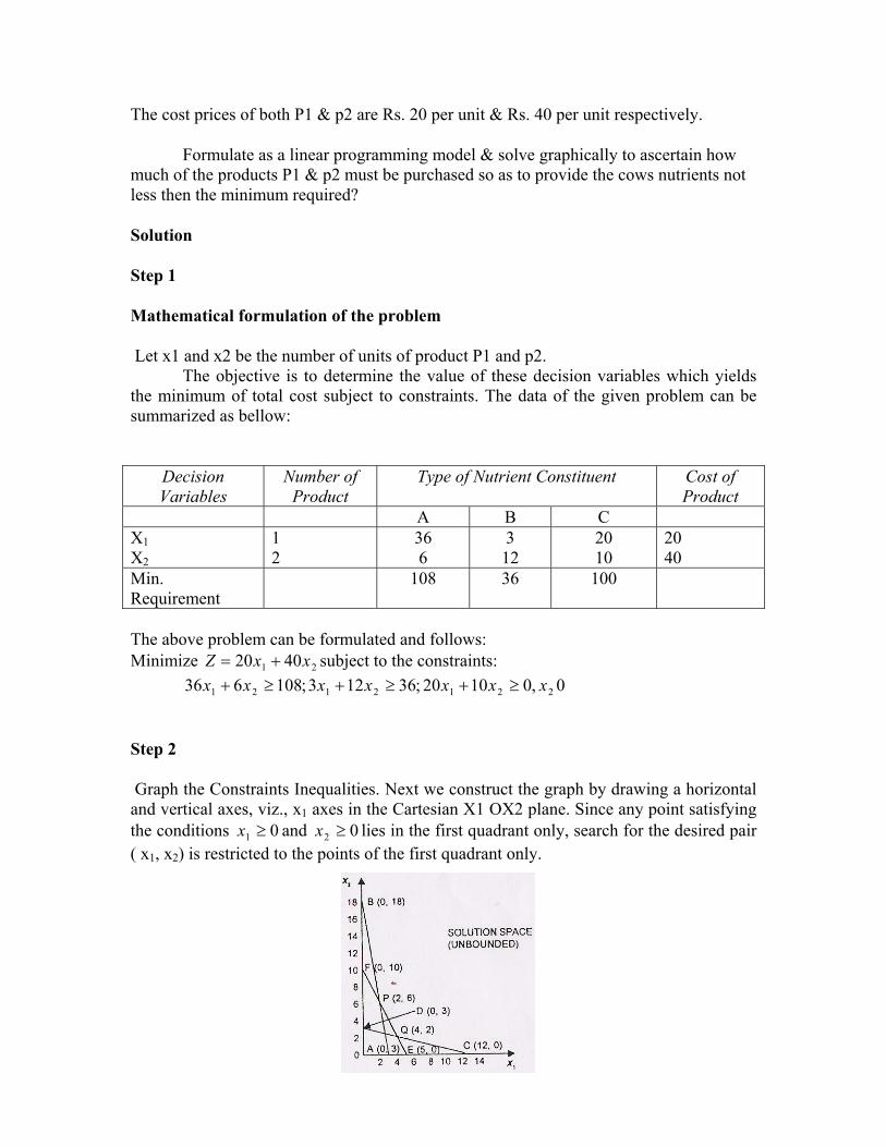
The cost prices of both P1 & p2 are Rs. 20 per unit & Rs. 40 per unit respectively.
Formulate as a linear programming model & solve graphically to ascertain how much of the products P1 & p2 must be purchased so as to provide the cows nutrients not less then the minimum required?
Solution
Step 1
Mathematical formulation of the problem
Let x1 and x2 be the number of units of product P1 and p2. The objective is to determine the value of these decision variables which yields the minimum of total cost subject to constraints. The data of the given problem can be summarized as bellow:
Decision Variables
Number of Product
Type of Nutrient Constituent Cost of Product
A B C X1 X2
1 2
36 6
3 12
20 10
20 40
Min. Requirement
108 36 100
The above problem can be formulated and follows: Minimize subject to the constraints: 21 4020 xxZ += 0,01020;36123;108636 2212121 xxxxxxx ≥+≥+≥+
Step 2
Graph the Constraints Inequalities. Next we construct the graph by drawing a horizontal and vertical axes, viz., x1 axes in the Cartesian X1 OX2 plane. Since any point satisfying the conditions and lies in the first quadrant only, search for the desired pair ( x
01 ≥x 02 ≥x1, x2) is restricted to the points of the first quadrant only.

The constraints of the given problem are plotted as described earlier by treating them as equations: 1001020;36123;108636 212121 =+=+=+ xxandxxxx Since each of them happened to be ‘greater than or equal to type’, the points ( x1,x2) satisfying them all will lie in the region that falls towards the right of each of these straight lines.
The solution space is the intersection of all these regions in the first quadrant. This is shown shaded in the adjoining figure.
Step 3
Locate the solution point. The solution space is open with B,P,Q and C as lower points. Note 1. For ≥ constraints soln. Space is above the constraint line, as space 2. Now, consider only corner Pb of the sdn. Space according to LP therein.
Step 4
Value of objective function at corner points. Corner points Co-ordinates of
Corner Points ( x1,x2)
ZObjective function
21 4020 xx += Value
B P Q C
(0,18) (2,6) (4,2) (12,0)
20(0) + 40(18) 20(2) + 40(6) 20(4) + 40(2) 20(12) + 40(0)
720 280 160 240
Step 5
Optimum value of the objective function . Here, we find that minimum cost of Rs. 160 is found at point Q(4,2), i.e., x1 = 4 and x2 = 2 Hence the first should purchase 4 units of product P1 and 2 units of product P2 in order to maintain a minimum cost of Rs. 160.

In the LP's considered above, the feasible region (if not empty) was a bounded
area of the -plane. For this kind of problems it is obvious that all values of the LP objective function (and therefore the optimal) are bounded. Consider however the following LP:
Example 4.
s.t.
The feasible region and the direction of improvement for the isoprofit lines for this problem are given in Figure
An unbounded LP
It is easy to see that the feasible region of this problem is unbounded, and furthermore, the orientation of the isoprofit lines is such that no matter how far we ``slide'' these lines in the direction of increasing the objective function, they will always share some points with the feasible region. Therefore, this is an example of a (2-var) LP whose objective function can take arbitrarily large values. Such an LP is characterized as unbounded. Notice, however, that even though an
unbounded feasible region is a necessary condition for an LP to be unbounded, it is not sufficient; to convince yourself, try to graphically identify the optimal solution for the above LP in the case that the objective function is changed to:
.
Summarizing the above discussion, I have shown that a 2-var LP can either
• have a unique optimal solution which corresponds to a ``corner'' point of the feasible region, or
• have many optimal solutions that correspond to an entire ``edge'' of the feasible region, or
• be unbounded, or be infeasible.

Unit 1
Lesson 6: Simplex Method
• Set up and solve LP problems with simplex tableau. • Interpret the meaning of every number in a simplex tableau.
Dear Students, all of us have by now mastered the graphical method of SOLVING A LINEAR PROGRAMMING MODEL Well friends, let us now focus on the LIMITATIONS OF THE GRAPHICAL METHOD OF SOLVING A LINEAR PROGRAMMING MODEL. Let us see what the limitations are, and how can these be tackled? Here we go.
LIMITATIONS OF THE GRAPHICAL METHOD
Well friends, once a Linear programming model has been constructed on the basis of the given constraints & the objective function, it can easily be solved by using the graphical method (as discussed in earlier lectures)) & the optimal solution can be generated.
However, the applicability of the graphical method is very limited in scope. This is due to the fact that it is quite simple to identity all the corner points & then test them for optimality-in the case of a two-variable problem. As a result, the graphical method can not be always employed to solve the real-life practical Linear programming models which involve more than two decision-variables.
The above limitation of the graphical method is tackled by what is known as the simplex method. Developed in 1947 by George B-Dantizg, it remains a widely applicable method for solving complex LP problems. It can be applied to any LP problem which can be expressed in terms of a Linear Objective function subject to a set of Linear Constraints. As such, no theoretical restrictions are placed on the number of decisi9n variables or constraints contained in a linear programming problem.
The simplex method employed in solving LP problem is discussed as under:
The simplex method The graphical method, as discussed in the previous lectures, is capable of solving
problems having a maximum of two variables. Hence, this method is used which can solve LP problems with any no. of variable or constraints it is geared towards

solving optimization problems which have constraints of less than or equal to type.
(i) This method utilizes the property of a LP problem of having optimal solution
only’ at the corner point of the feasible solution space. It systematically generates corner point solutions & evaluates them for optimality. The method stops when an optimal solution is found. Hence, it is an iterative (repetitive) technique.
If we get more variables & less equations, we can set extra variables equal to
zero, to obtain a system of equal variables & equal equations. Such solution is called basic solution.
(ii) The variables having positive values in a basic feasible solution are called
basic variable while the variables which are set equal to zero, so as to define a corner point are called non-basic variables.
(iii) Slack variables are the fictitious variables which indicate how much of a
particular resource remains unused in any solution. These variables can not be assigned negative values. A zero value indicates that all the resources are fully used up in the production process.
(iv) Cj column denotes the unit contribution margin. (v) Cj row is simply a statement of the projective function.
(vi) Zj row denotes the contribution margin lost if one unit is brought into the
solution. Hence, it represents the opportunity cost. (Opportunity cost is the cost of sacrifice i.e., the opportunity foregone by selecting a particular course of action out of a number of different available alternatives).
(ix) Cj - Zj row denotes the Net Potential contribution or the Net unit
Margin potential, per unit.
(vii) The rules used under simplex method, for solving a linear programming problem are as follows:-
1. Convert the LP to the following form:
Convert the given problem into Standard maximization Problem i.e. minimization problem into a maximization one (by multiplying the objective function by -1). All variables must be non-negative.
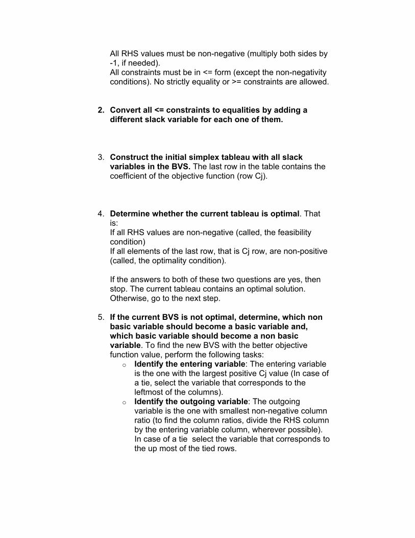
All RHS values must be non-negative (multiply both sides by -1, if needed). All constraints must be in <= form (except the non-negativity conditions). No strictly equality or >= constraints are allowed.
2. Convert all <= constraints to equalities by adding a different slack variable for each one of them.
3. Construct the initial simplex tableau with all slack variables in the BVS. The last row in the table contains the coefficient of the objective function (row Cj).
4. Determine whether the current tableau is optimal. That is: If all RHS values are non-negative (called, the feasibility condition) If all elements of the last row, that is Cj row, are non-positive (called, the optimality condition).
If the answers to both of these two questions are yes, then stop. The current tableau contains an optimal solution. Otherwise, go to the next step.
5. If the current BVS is not optimal, determine, which non basic variable should become a basic variable and, which basic variable should become a non basic variable. To find the new BVS with the better objective function value, perform the following tasks:
o Identify the entering variable: The entering variable is the one with the largest positive Cj value (In case of a tie, select the variable that corresponds to the leftmost of the columns).
o Identify the outgoing variable: The outgoing variable is the one with smallest non-negative column ratio (to find the column ratios, divide the RHS column by the entering variable column, wherever possible). In case of a tie select the variable that corresponds to the up most of the tied rows.
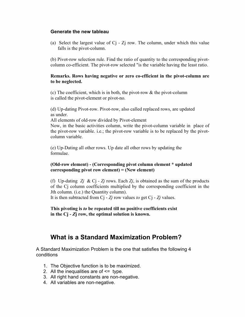
Generate the new tableau
(a) Select the largest value of Cj - Zj row. The column, under which this value falls is the pivot-column.
(b) Pivot-row selection rule. Find the ratio of quantity to the corresponding pivot-column co-efficient. The pivot-row selected "is the variable having the least ratio. Remarks. Rows having negative or zero co-efficient in the pivot-column are to be neglected.
(c) The coefficient, which is in both, the pivot-row & the pivot-column is called the pivot-element or pivot-no. (d) Up-dating Pivot-row. Pivot-row, also called replaced rows, are updated as under.
All elements of old-row divided by Pivot-element Now, in the basic activities column, write the pivot-column variable in place of the pivot-row variable. i.e.; the pivot-row variable is to be replaced by the pivot-column variable.
(e) Up-Dating all other rows. Up date all other rows by updating the formulae. (Old-row element) - (Corresponding pivot column element * updated corresponding pivot row element) = (New element)
(f) Up-dating Zj & Cj - Zj rows. Each Zj, is obtained as the sum of the products of the Cj column coefficients multiplied by the corresponding coefficient in the Jth column. (i.e.) the Quantity column).
It is then subtracted from Cj - Zj row values to get Cj - Zj values. This pivoting is to be repeated till no positive coefficients exist
in the Cj - Zj row, the optimal solution is known.
What is a Standard Maximization Problem?
A Standard Maximization Problem is the one that satisfies the following 4 conditions
1. The Objective function is to be maximized. 2. All the inequalities are of <= type. 3. All right hand constants are non-negative. 4. All variables are non-negative.

Friends, let us consider some examples to test our understanding of the solution algorithm that has been discussed so far. Example 1. Smart Limited manufactures two types of adhesives which are sold under the brand name quick and Tuff. Each product consumes the same raw materials but in varying proportions. The following table depicts the amount of raw materials along with their respective cost. Raw material type Price Quick Tuff
(Rs/lton) N 600 350 200 A 400 50 100 P 400 50 100 I 200 550 600
1000 kg 1000 kg
Quick can be blended @ 1000 kg /hour whereas the blending rate for Tuff is 1250 kg /hour. Their respective selling prices are Rs. 1010 & Rs. 845. You may assume the variable costs to be Rs. 500 per hour of plant production time. The maximum availability of raw materials is:
Raw Material Types Max available (kg) N 1000 A 300 P 250 I 1800
Formulate as a linear programming model and find out the optimal units of quick & tuff to be produced so as to maximise the profits. Solution Step I List the objective & constraint equations. Step II Introduce the slack variables Step III Arrange in the form of 1st tableau (table)

Step IV Find out the profit-margins from given sales price. Step V Generate solutions. The detailed solutions are as under:
Simplex Method (I) Converting in equations into equations by using slack-variable Maximise Cont-margin = 150x 1 + 125x2 Subject to 350xI + 200x2 + Sl = 1000
25010050 221 =++ Sxx 1800600550 321 =++ Sxx
Si, xj ≥ 0 for all i & j. Note. We have dropped : 50 300100 21 =+ πxx as it is already contained in
25010050 21 ≤=+ xx Also, slack can’t be larger than the const. On RHS ( Sl = 1000, S2 = 250 etc) It is were to be so, then some other variable must be negative for equality to exist, which is not possible. (2) Rewriting as: Maximising cost. Margin - 150 32121 125 OSOSOSxx ++++ Subject to 1000200350 32121 =++++ OSOSSxx 50 250100 32121 =++++ OSOSOSxx 1800600550 32121 =++++ OSOSOSxx Si, xj ≥ 0 & ( i, j)
(3) Arranging in tableau-form: Cj
(Rs.) Basic
Activities (Rs.) Qty.
150 x1
125 x2
0 S1
0 S2
0 S3
0 0 0
S1 S2 S3
ZJ(Rs.) Cj-Zj (Rs.)
1000 250 1800
0
350 50 50 0
150
200 100 600 0
125
1 0 0 0 0
0 1 0 0 0
0 0 1 0 0
(4) Pivot Column = x1 ( Largest value of Cj – Zj) (5) Pivot row
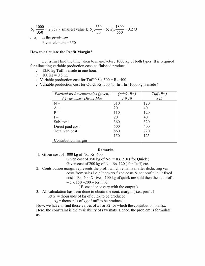
857.2350
1000,1 =S ( smallest value ); 273.3550
1800,;550350, 32 == SS
1S∴ is the pivot- row Pivot element = 350
How to calculate the Profit Margin? Let is first find the time taken to manufacture 1000 kg of both types. It is required for allocating variable production costs to finished product.
∴ 1250 kg Tuff is made in one hour. ∴ 100 kg = 0.8 hr. ∴Variable production cost for Tuff 0.8 x 500 = Rs. 400 ∴Variable production cost for Quick Rs. 500 (∴ In 1 hr. 1000 kg is made )
Particulars Revenue/sales (given) (-) var costs: Direct Mat
Quick (Rs.) 1,0,10
Tuff (Rs.) 845
N – A – P – I – Sub-total Direct paid cost Total var. cost Contribution margin
310 20 110 20 360 500 860 150
120 40 120 40 320 400 720 125
Remarks
1. Given cost of 1000 kg of No. Rs. 600 Given cost of 350 kg of No. = Rs. 210 ( for Quick ) Given cost of 200 kg of No. Rs. 120 ( for Tuff) etc. 2. Contribution margin represents the profit which remains if after deducting var
costs from sales i.e.,; It covers fixed costs & net profit i.e. it fixed cost = Rs. 200 X five – 100 kg of quick are sold then the net profit = 5 x 150 –200 = Rs. 550
( F. cost donot vary with the output ) 3. All calculation has been done to obtain the cont. margin ( i.e., profit ) let x1 = thousands of kg of quick to be produced. x2 = thousands of kg of tuff to be produced. Now, we have to find those values of x1 & x2 for which the contribution is max. Here, the constraint is the availability of raw mats. Hence, the problem is formulate as;

Maxmise 150x1+ 125x2 Subject to:
1000200350 21 ≤+ xx 30010050 21 ≤+ xx
x1, x2 ≥ 0 Hence, the problem has been formulated
1800600550 21 ≤+ xx (6) up-dating Pivot-row
0,0,0029.03501,5714.0
350200,1
350350,8571.2
3501000
====
Make the pivot-row of 2nd tableau: Cj 150 125 0 0 0 Basic Act. Qty. x1 x2 S1 S2 S3 150 x1 2.8571 1 0.5714 .0029 0 0 0 S2 0 S3 ( Pivot column variable in place of Pivot row variable ) (7) S2 row is up-dated as follows:
Old Row Element -
(Corresp. Pivot column element x
Updated corresp. Pivot row element
= New S2 raw element
250 – 50 – 100 – 0 – 1 – 0 -
( 50 x (50 x (50 x (50 x (50 x (50 x (50 x
2.8571) 1) 0.5714 0.0029) 0) 0)
= 107.145 = 0 = 71.43 = -0.145 = 1 = 0
(8) S3 row is similarly updated:
Old Row Element -
(Corresp. Pivot column element x
Updated corresp. Pivot row element
= New S2 raw element
1800 – 550 – 600 – 0 – 0 – 1 -
( 50 x ( 550 x (550 x (550 x (550 x (550 x (550 x
2.8571) 1) 0.5714) 0.0029) 0) 0)
= 228.595 = 0 = 285.73 = -1.595 = 0 = 1

(9) Complete IInd tableau is:
Cj (Rs)
Basic Activity
(Rs.) Qty.
1.50 x1
125 x2
0 S1
0 S2
0 S3
150 0 0 - -
X1 S2 S3 Zj (Rs.) Cj-Zj (Rs.)
2.857 107.145 228.595 428.55 --
1 0 0 150 0
0.5714 71.43 285.73 85.71 39.29
0.0029 -0.145 1.595 0.435 -0.435
0 1 0 0 0
0 0 1 0 0
Zj is calculated as under: Zj value for QTY Column = 150x2.857+0x107.145+0x228.595=428.55 For x1=15x 1+ 0 x 0 + 0 x 0 =150 x2= 150 x 0.5714 + 0+0 = 85.71 S1 = 150x 0.0029 + 0+0=0.435 S2 = 0 S3 = 0 Now perform Cj – Zj to get Cj – Zj row values. (10) The + ve value of 39.29 in Cj – Zj -> It is not the optimal soln Hence, once again pivoting is required. Developing IIIrd tableau. Now, pivot column – x2 ( Largest value of Cj – Zj ), Pivot row = S3 Pivot element = 285.73 Updating Pivot row ( S3; Old row element ÷ Pivot no.
,0,0056.073.285
595.1,173.28373.285,0,8.0
73.285595.228
−=−
==
0035.073.285
1=
Completed IIIrd Tableau is.
Cj (Rs)
Basic Activity
(Rs.) Qty.
150 x1
125 x2
0 S1
0 S2
0 S3
150 0 125
x1 S2 x2 Zj (Rs.) Cj-Zj (Rs.)
2.4 50 0.8 460
1 0 0 150 0
0 0 1 125 0
0.006 0.225 -0.0056 0.02 -0.02
0 1 0 0 0
-0.002 -0.25 0.0035 0.1375 -0.1375
Note (1) x1 row is up-dated as: 2.857-(0.5714x0.8+ =2.4 1-(0.5714x0) = 1

0.5714 – (0.5714 x 1 ) = 0 0.0029 – ( 0.5714 x –0.0056) = 0.006 0-(0.5714x0 ) = 0 0-(0.5714 x 0.0035) = - 0.002 (2) S2 row is up dated as: 107.145 – (71.43 x 0.8 ) = 50 0-(71.43x0) = 0 71.43 – (71.43x1) = 0 -0.145 – (71.43 x-0.0056 )=0.255 1-(71.43 x 0 ) = 1 0-(71.43 x0.0035) = -0.25 4 X2
Zj (Rs.) Cj- Zj (Rs.)
2100 3/10 12300 +1/10 - 1/10
1 4 0
0 0 0
0 0 0
1/10 3/10 -3/10
Up-dating S1 row
600 - 2001300134
=
x
01134
134
=
−− x
1340
1340 −
=
− x
152
3013
1340 =
−
− x
-1 - 10134
−=
X
- 15
130
1134
131 −
=
−
− X
Updating x2 row
3000 - 21001300139
=
x
01139
139
=
− x
1 - 10139
=
X
0 - 103
3013
139
=
−X
0- 00139
=
X
=−
−101
13113
9131
X
Up dating zj row: zj values for: Qty = 3 x 1300 + 4 x 2100 = 12300 X1 = 3 X2 = 4
S2 = 10
11012
3039 −
=+−

S2 = 0
S1 = 103
104
=+
Since no positive co-efficient exists in the C1 – z1 row, this is the optimal solution. X1 = 1300 = maximum pens to be manufactured X2 = 2100 = maximum pencils to be manuf. Z1= 1300 = maximum profit possible . Example 2. X Ltd. Produces two products p1, p2 having profit of Rs. 4 $ Rs. 3 each p1, p2 require 4 hrs. & 2 hrs. of machining respectively, the total available machining time is 10 hours. P1 , p2 consume 2 units & 8/3 units of raw material respectively subject to a total of maximum 8 units. Any no. of p2 j can be produced & sold but the no. of p1 must not be more than 6. Formulate as a (P model & solve by the simplex method.) Solution Maximise = 4x1 + 3x2+ os2+ os3 Subject to : 4x1 + 2x2+ s1+ os2+ os3 = 10
2x1 + 123os+
8 x + os2+ os3 = 8 x1 ; x2 ≥ 0
x1 + ox2+ os1 + os2 + os3 = 6
Ist Tableau
Cj (Rs.) (Rs.)
Basic Act. Qty. 4 x1
3 x2
0 S1
0 S2
0 S3
0 0 0
S1 S2 S3 Zj (Rs.) Cj-Zj (Rs.)
10 8 6 0
4 2 1 0 4
2 8/3 0 0 3
1 0 0 0 0
0 1 0 0 0
0 0 1 0 0
Pivot Column = x1
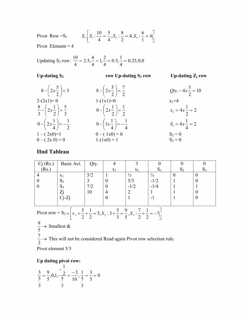
Pivot Row =S1
=== 6
16:,4
28:,
45
410: 3211 SSSS
Pivot Element = 4
Updating S2 row: 0,0,25.041,5.0
42,1
44,5.2
4====
10
Up-dating S2 row Up-dating S3 row Up-dating Zj row
32528 =
− x
27
2528 =
− x 10
254. =− xQty
2-(2x1)= 0 1-(1x1)=0 x1=4
35
212
38
=
− x
21
2120 =
− x 2
2142 == xx
21
4120 −=
− x
41
4110 −=
− x 2
4141 == xS
1 – ( 2x0)=1 0 – ( 1x0) = 0 S2 = 0 0 – ( 2x 0) = 0 1-(1x0) = 1 S3 = 0
IInd Tableau
Cj (Rs.) (Rs.)
Basic Act. Qty. 4 x1
3 x2
0 S1
0 S2
0 S3
4 0 0
x1 S2 S3 Zj Cj-Zj
5/2 3 7/2 10
1 0 0 4 0
½ 5/3 -1/2 2 1
¼ -1/2 -1/4 1 -1
0 1 1 1 1
0 0 1 0 0
Pivot row = S2
−=÷=÷=÷+× 7
21
27:,
59
353:,5
21
25
321 SS×
→59 Smallest &
→27 This will not be considered Read again Pivot row selection rule.
Pivot element 5/3 Up dating pivot row:
053
351,
103
3521
,1,0,59
353
==−
=−
=

Up –dating x1 row: Updating S3: Up-dating Zj row:
×−
59
21
25
= 58
−27
522
59
21
=
×− Q + y = 4
593
58 ×
+×
0021
=
×−−0
0121
21
=
×− 01
21
21
=
×−−−
10211 =
×−
52
21
41
=
×−
52
43
21
41 −
=
−
×−−−
103
53
210 −
=
×−
103
53
210 =
×−−
00210 =
×− 10
211 =
×−−
IIIrd Tableau
CJ(Rs.) 3 4 0 0 0 (Rs.) Basic
Act. Qty. X1 X2 S1 S2 S3
0 X1 8/5 1 0 2/5 -3/10 0 3 X2 9/5 0 1 -3/10 3/5 0 4 S3 22/5 0 0 -2/5 3/10 1 ZJ 59/5 4 3 7/10 3/5 0 CJ - ZJ 0 0 -7/10 -3/5 0 There are no +ve values in CJ - ZJ row, optional soln. Is reached. Hence X1 = 8/5, X2 =9/5 & max. = 59/5 Ans. Dear students, we have now reached the end of our discussion scheduled for today. See you all in the next lecture. Bye.


Unit 1
Lesson 7: Simplex Method Ctnd.
Learning outcomes:
• Set up and solve LP problems with simplex tableau. • Interpret the meaning of every number in a simplex tableau.
Dear students, today we discuss small cases or case-lets on the above topic. The situations presented below are real business problems, modified slightly to suit our purpose.
We start now.
Case-let-1
A firm makes air coolers of three types and markets these under the brand name “Symphony”. The relevant details are as follows:- Profit / unit (Rs.)
300 Product A (hrs. / unit)
700 Product B (hrs. / unit)
900 Product C (hrs,/ unit)
Totoal hrs. available
Designing 0 10 20 320 Manufacturing 60 90 120 1600 Painting 30 40 60 1120 What Qty. of each product must be made to maximize the total profit of the firm? Solution Let X1, X2, X3 denote the Qty. of each product made Then: Maximize: 300 X1+ 700 X2 +900 X3
Subject to: 0 X1 +10 X2 + 20 X3 320≤ 60 X1 +90 X2 + 120 X3 1600≤

30 X1 +40 X2 + 60 X3 1120≤
Introducing slacks: Maximize: 300 X1 +700 X2 + 900 X3 +0S1+ 0S2+ 0S3
Subject to: 0 X1 +10 X2 + 20 X3 +S1+ 0S2+ 0S3 =320 60 X1 +90 X2 + 120 X3 +0S1+ S2+ 0S3 =1600 30 X1 +40 X2 + 60 X3 +0S1+ 0S2+ S3 =1120 1st Tableau CJ(Rs.) 300 700 900 0 0 0 (Rs.) Basic
Act. Qty. X1 X2 X3 S1 S2 S3
0 S1 320 0 10 20 1 0 0 0 S2 1600 60 90 120 0 1 0 0 S3 1120 30 40 60 0 0 1 ZJ 0 0 0 0 0 0 0 CJ - ZJ 300 700 900 0 0 0 Pivot column = X3
Pivot –row = S2
===
356
601120:,
340
1201600:,16
20320:S 32 1 SS
Pivot element = 120
Pivot row updating : 0,120
1,0,1,43
12090,
21
12060,
340
1201600
===
Up-dating S1 row: Updating S3 row:
3160
34020320 =
− x 320
34060
201
=
− x
10211200 −=
− X 0
216030 −=
− X
5432020 −=
− x 5
436040 −=
− X
( ) 50201 =− x ( ) 00600 =− x
61
1201200 −
=
− x
21
1201600 −
=
− x
( ) 00201 =− x ( ) 10601 =− x

IInd Tableau Cj (Rs.)
(Rs.) Basic Act. Qty. 300
x1 700 x2
900 X3
0 S1
0 S2
0 S3
0 900 0
S1 X3 S3 Zj (Rs.) Cj-Zj (Rs.)
160/3 40/3 320 2000
-10 ½ 0 450 -150
-5 ¾ -5 675 25
0 1 0 900 0
1 0 0 0 0
-1/6 1/120 -1/2 15/2 -15/2
0 0 1 0 0
Since, There is still one + ve term in row, pivoting is requd. Pivot – Column = x2 Pivot – row =
=÷−= .)(
5320:,
9160
43
340:),3(5
3160: 3313 NotconsiSxdconsidereNotSx
Pivot – element =3/4 Pivot-row updating:
0,901
43
1201,0,
34
431,1,
32
43
21,
9160
43
340
=÷=÷=÷=÷
Updating S1 row: Updating S3 row:
91280
91605
3160
=
−− x
93680
91605320 =
−− x
320
32510 =
−−− x
310
325 =
−− x0
( ) 0155 =−− x ( ) 0155 =−−− x
320
3450 =
−− x
320
345 =
−− x0
( ) 1051 =−− x ( ) 0050 =−− x
91
9015
61 −
=
−−− x
94
9015
61 −
=
−− x−
( ) 0050 =−− x ( ) 1051 =−− x

IIIrd Tableau Cj (Rs.)
(Rs.) Basic Act. Qty. 300
x1 700 x2
900 x3
0 S1
0 S2
0 S3
0 700 0
x1 S2 S3 Zj (Rs.) Cj-Zj (Rs.)
1280/9 160/9 3680/9 112000
-20/30 2/3 10/3 1400/3 -500/3
0 1 0 700 0
20/3 4/3 20/3 2800/3 -100/3
1- 0 0 0 0
1/9 1-90 -4/9 70/9 -70/9
0 0 1 0 0
Since Cj – Zj row has no. + ve value left. ∴It is the optional soln.
Case-let-II
Two materials A & B are required to construct table & book cases. For one table, 12 units of A & 16 units of B are required while for a book case 16 units of A and 8 units of B are required. The profit on book case is Rs 25 and Rs 20 on a table. 100 units of A & 80 units of B are available. Formulate as a Linear programming problem & determine the optimal number of book cases & tables to be produced so as to maximise the profits. Solution
Let x1 = no. of unit of tables to be produced, and X2 = no. of unit of book cases to be produced. Formulating as a LP problem, we have:- Maximise Z ( objective function ) 21 2520 xx +=Subject to the constraints: 1001612 21 ≤+ xx 16 80
0
0080
8 21 ≤+ xx , 21 ≥xxIntroducing the slack variable, we have: 12 116 121 ≤++ Sxx 16 8 221 ≤++ Sxx

Re-writing as:
=
+
+
+
80100
1001
01
816
1612
2121 SSxx
or PoSPSPxPxP =+++ 24132211
∴ our problem becomes Maximise Subject to 20F 2121 0025 SSxx ×+×++= …(1) Where P PoSPSPxPx =+++ …(ii) 24132211
=
=
+
+
816
1613
01
01
80100
22420 PPPPP
element of Cj row are values of Po, P2,P4,P1, in (i) by comparing with (2) i.e. elements of Cj are 0, 0, 20, 25. Simplex Method Cj 0 0 0 20 25 Ratio Vectors Po P2 P4 P1 P3
0 P3 100 1 0 12 16 100/16=6.25 0 P4 80 0 1 16 0 80/8=10 Zj 0 0 0 0 0 6.25 is least ratio Zj – Cj
0 0 0 20 25 ∴ replaced vector is P2
R1 is 16
1R
R2 = R2 – R1 x 8/16
Since 25 is the most postive No. in row C4 - Z4 ∴ Replacing vector is P2
25 P2 425 1/16 0
43 1
425 /
45 =
325 =8.33
0 P4 30 31
− 1 10 0 30/10=3
Zj 4
625
1625 0
475 25
R1 R2 Stage I R1
R2 Stage I
Zj – Cj
4
625
1625 0
45
− 0
Θ 3 is least ratio ∴ replaced vector is P4
Θ 45
− is least – ve no.
∴ replaced vector is P1
10
12
RisR
R1 = R – R2 403
104/3
21 RR −=
The elements of column Cj are values of P3 and P4 is (I) as compared with (2). The column P0,P2,P4,P1,P3 are values of P0,P2,P1 etc. in (3)

R1 25 P2 4 1/10 /3/40 0 1 R2 20 P4 3 -1/20 1 1 0 Stage I Zj 160 1.5 1/8 20 25 Zj – Cj 160 1.5 1/8 0 0 Since in stage III all elements of row Zj – Cj are +ve or zero, hence an optimal solution has been achieved. The solution is given by column is Stage III. 210 43 PPP +=∴ compare it with 024132211 PSPSPxPxP =+++
0,0,4,3 2121 ==== SSxx Note I. the elements of row Zj is the sum of product of corresponding elements of column Cj with Po,P3,P4,P1,P2 respectively. For example in stage II, the elements of row Zj are
4
625300425
=+ xx25
1625
210
161
−
=+ xx25
25x 0+0 x 1=0
4
7510043
=+ xx25
25 x 1 + 0x 0 =25. Note 2. When we replace vector P2 in place of P3 in stage II, the elements to left of P3 under column Cj is also changed. Note. To check the results. At x=3, x2 = 4 Constraints are 10010064361612 21 ≤=+=+ xx 16 808032488 21 ≤=+=+ xx
Case-let-III
A manufacturer produces children’s bicycles & scooters both of which one processed through two machines. Machine 1 has a maximum of 120 hours available & machine 2 has a maximum of 180 hours. Manufacturing a bicycle requires 6 hours on machine 1 x 4 hours on machine 2. A scooter requires 3 hours on machine 1 & ten hours on machine 2. If the profit is Rs 45 on a bicycle & Rs. 55 on a scooter determine the number of bicycles & scooters that should be produced in order to maximise profit.
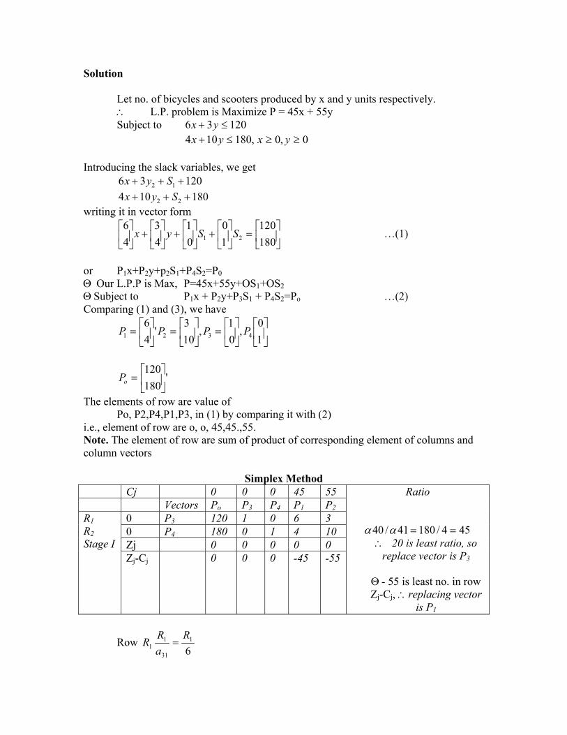
Solution Let no. of bicycles and scooters produced by x and y units respectively.
∴ L.P. problem is Maximize P = 45x + 55y Subject to 12036 ≤+ yx 4 0,0,18010 ≥≥≤+ yxyx Introducing the slack variables, we get 12036 12 +++ Syx 180104 22 +++ Syxwriting it in vector form
…(1)
=
+
+
+
180120
10
01
43
46
21 SSyx
or P1x+P2y+p2S1+P4S2=P0 Θ Our L.P.P is Max, P=45x+55y+OS1+OS2 Θ Subject to P1x + P2y+P3S1 + P4S2=Po …(2) Comparing (1) and (3), we have
=
=
=
10
,01
,103
'46
4321 PPPP
' 180120
=oP
The elements of row are value of Po, P2,P4,P1,P3, in (1) by comparing it with (2) i.e., element of row are o, o, 45,45.,55. Note. The element of row are sum of product of corresponding element of columns and column vectors
Simplex Method Cj 0 0 0 45 55 Vectors Po P3 P4 P1 P2
0 P3 120 1 0 6 3 0 P4 180 0 1 4 10 Zj 0 0 0 0 0
R1 R2 Stage I
Zj-Cj 0 0 0 -45 -55
Ratio
454/18041/40 ==αα ∴ 20 is least ratio, so
replace vector is P3
Θ - 55 is least no. in row Zj-Cj, ∴replacing vector
is P1
Row 6
1
31
11
RaRR =

Row 64
1231
41122 ×−×− RR
aaR= RR .
Further calculations are left to the students as an exercise.
Case-let-IV
.A firm has the following availabilities :
Type-available Amount-available (kg) Wood Plastic Steel
240 370 180
The firm produces two products A & B having a selling price of Rs. 4 per unit & Rs. 6 per unit respectively. The requirements for the manufacture of A & B are as follows:
Requirements of (kg) Product Wood Plastic Steel
A B
1 3
3 4
2 1
Formulate as a LP problem & solve by using the simplex method to maximise the gross income of the firm.
Case-let-V
Ace- advantage Ltd. faces the following situation: Media available - electronic (A) & print (B) Cost of available in - media A: Rs.1000 Media B: Rs.1500 Annual advertising budget - Rs. 20000 The following constraints are applicable: Electronic Media (A) can not have more than 12 advertisements in a year and not less than 5 advertisement must be placed in the print media (B). The estimated audience are as follows: Electronic media (A) - 40000 Print media (B) - 55000 You are required to develop a mathematical model & solve it for maximizing the total effective audience.
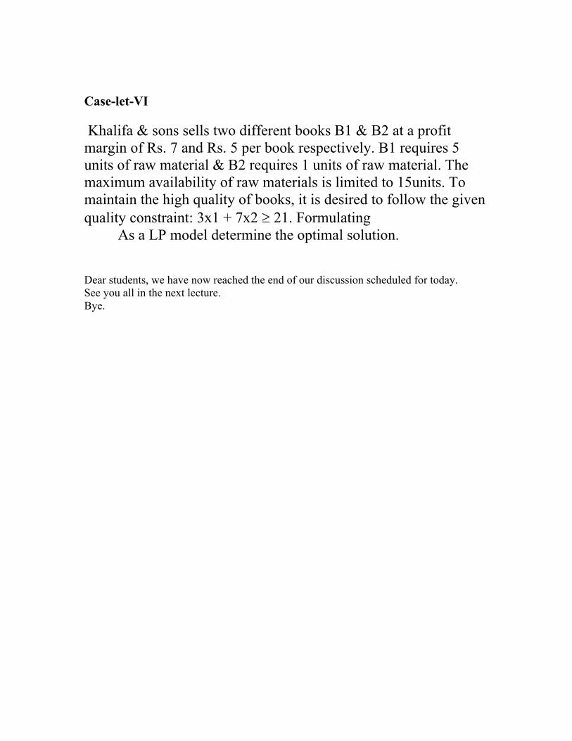
Case-let-VI
Khalifa & sons sells two different books B1 & B2 at a profit margin of Rs. 7 and Rs. 5 per book respectively. B1 requires 5 units of raw material & B2 requires 1 units of raw material. The maximum availability of raw materials is limited to 15units. To maintain the high quality of books, it is desired to follow the given quality constraint: 3x1 + 7x2 ≥ 21. Formulating
As a LP model determine the optimal solution.
Dear students, we have now reached the end of our discussion scheduled for today. See you all in the next lecture. Bye.


Unit 1
Lesson 8: Special cases of LPP
Learning outcomes
SolvingSpecial cases of Linear Programming Problem using Simplex Method :
• Alternate Optimal Solutions. • Degeneracy. • Unboudedness. • Infeasibility.
In the previous lecture we have learnt how to solve a linear program using simplex method. Properties of Linear Programs
There are three possible outcomes for a linear program: it is infeasible, it has an unbounded optimum or it has an optimal solution.
If there is an optimal solution, there is a basic optimal solution. Remember that the number of basic variables in a basic solution is equal to the number of constraints of the problem, say m. So, even if the total number of variables, say n, is greater than m, at most m of these variables can have a positive value in an optimal basic solution.
Today in this lecture we will study about Alternate Optimal Solutions, Degeneracy, Unboudedness, Infeasibility
Alternate Optimal Solutions
Let us solve a small example:
Example1
As before, we add slacks and , and we solve by the simplex method, using tableau representation.
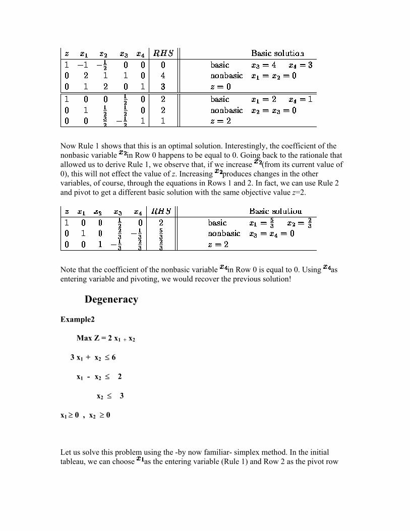
Now Rule 1 shows that this is an optimal solution. Interestingly, the coefficient of the nonbasic variable in Row 0 happens to be equal to 0. Going back to the rationale that allowed us to derive Rule 1, we observe that, if we increase (from its current value of 0), this will not effect the value of z. Increasing produces changes in the other variables, of course, through the equations in Rows 1 and 2. In fact, we can use Rule 2 and pivot to get a different basic solution with the same objective value z=2.
Note that the coefficient of the nonbasic variable in Row 0 is equal to 0. Using as entering variable and pivoting, we would recover the previous solution!
Degeneracy
Example2
Max Z = 2 x1 + x2
3 x1 + x2 ≤ 6
x1 - x2 ≤ 2
x2 ≤ 3
x1 ≥ 0 , x2 ≥ 0
Let us solve this problem using the -by now familiar- simplex method. In the initial tableau, we can choose as the entering variable (Rule 1) and Row 2 as the pivot row

(the minimum ratio in Rule 2 is a tie, and ties are broken arbitrarily). We pivot and this yields the second tableau below.
Note that this basic solution has a basic variable (namely ) which is equal to zero. When this occurs, we say that the basic solution is degenerate. Should this be of concern? Let us continue the steps of the simplex method. Rule 1 indicates that is the entering
variable. Now let us apply Rule 2. The ratios to consider are in Row 1 and in Row 3. The minimum ratio occurs in Row 1, so let us perform the corresponding pivot.
We get exactly the same solution! The only difference is that we have interchanged the names of a nonbasic variable with that of a degenerate basic variable ( and ). Rule 1 tells us the solution is not optimal, so let us continue the steps of the simplex method. Variable is the entering variable and the last row wins the minimum ratio test. After pivoting, we get the tableau:
By Rule 1, this is the optimal solution. So, after all, degeneracy did not prevent the simplex method to find the optimal solution in this example. It just slowed things down a little. Unfortunately, on other examples, degeneracy may lead to cycling, i.e. a sequence

of pivots that goes through the same tableaus and repeats itself indefinitely. In theory, cycling can be avoided by choosing the entering variable with smallest index in Rule 1, among all those with a negative coefficient in Row 0, and by breaking ties in the minimum ratio test by choosing the leaving variable with smallest index (this is known as Bland's rule). This rule, although it guaranties that cycling will never occur, turns out to be somewhat inefficient. Actually, in commercial codes, no effort is made to avoid cycling. This may come as a surprise, since degeneracy is a frequent occurence. But there are two reasons for this:
• Although degeneracy is frequent, cycling is extremely rare. • The precision of computer arithmetic takes care of cycling by itself: round off
errors accumulate and eventually gets the method out of cycling.
Our example of degeneracy is a 2-variable problem, so you might want to draw the constraint set in the plane and interpret degeneracy graphically.
Unbounded Optimum
Example 3 Max Z = 2 x1 + x2
s.t -x1 + x2 ≤ 1
x1 - 2 x2 ≤ 2
x1 ≥ 0 , x2 ≥ 0
Solving by the simplex method, we get:
At this stage, Rule 1 chooses as the entering variable, but there is no ratio to compute, since there is no positive entry in the column of . As we start increasing , the value of z increases (from Row 0) and the values of the basic variables increase as well (from Rows 1 and 2). There is nothing to stop them going off to infinity. So the problem is unbounded.

So you have seen how the special cases are solved.
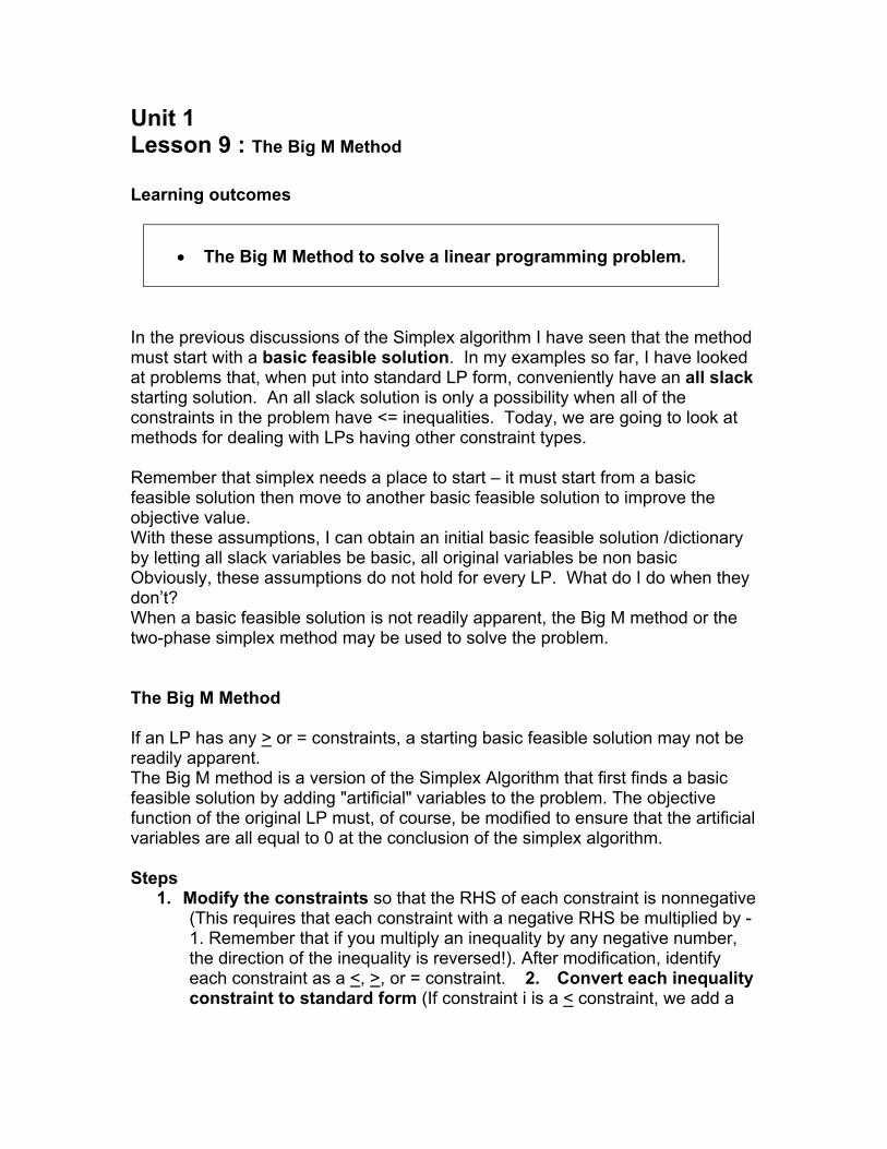
Unit 1 Lesson 9 : The Big M Method Learning outcomes
• The Big M Method to solve a linear programming problem.
In the previous discussions of the Simplex algorithm I have seen that the method must start with a basic feasible solution. In my examples so far, I have looked at problems that, when put into standard LP form, conveniently have an all slack starting solution. An all slack solution is only a possibility when all of the constraints in the problem have <= inequalities. Today, we are going to look at methods for dealing with LPs having other constraint types. Remember that simplex needs a place to start – it must start from a basic feasible solution then move to another basic feasible solution to improve the objective value. With these assumptions, I can obtain an initial basic feasible solution /dictionary by letting all slack variables be basic, all original variables be non basic Obviously, these assumptions do not hold for every LP. What do I do when they don’t? When a basic feasible solution is not readily apparent, the Big M method or the two-phase simplex method may be used to solve the problem. The Big M Method If an LP has any > or = constraints, a starting basic feasible solution may not be readily apparent. The Big M method is a version of the Simplex Algorithm that first finds a basic feasible solution by adding "artificial" variables to the problem. The objective function of the original LP must, of course, be modified to ensure that the artificial variables are all equal to 0 at the conclusion of the simplex algorithm. Steps
1. Modify the constraints so that the RHS of each constraint is nonnegative (This requires that each constraint with a negative RHS be multiplied by -1. Remember that if you multiply an inequality by any negative number, the direction of the inequality is reversed!). After modification, identify each constraint as a <, >, or = constraint. 2. Convert each inequality constraint to standard form (If constraint i is a < constraint, we add a

slack variable si; and if constraint i is a > constraint, we subtract an excess variable ei).
3. Add an artificial variable ai to the constraints identified as > or = constraints at the end of Step 1. Also add the sign restriction ai > 0.
4. If the LP is a max problem, add (for each artificial variable) -Mai to the objective function where M denote a very large positive number.
5. If the LP is a min problem, add (for each artificial variable) Mai to the objective function.
6. Solve the transformed problem by the simplex . Since each artificial variable will be in the starting basis, all artificial variables must be eliminated from row 0 before beginning the simplex. Now (In choosing the entering variable, remember that M is a very large positive number!).
If all artificial variables are equal to zero in the optimal solution, we have found the optimal solution to the original problem. If any artificial variables are positive in the optimal solution, the original problem is infeasible!!! Let’s look at an example. Example 1 Minimize z = 4x1 + x2 Subject to: 3x1 + x2 = 3 4x1 + 3x2 >= 6 x1 + 2x2 <= 4 x1, x2 >= 0 By introducing a surplus in the second constraint and a slack in the third we get the following LP in standard form: Minimize z = 4x1 + x2 Subject to: 3x1 + x2 = 3 4x1 + 3x2 – S2 = 6 x1 + 2x2 + s3 = 4 x1, x2, S2, s3 >= 0 Neither of the first two constraint equations has a slack variable or other variable that we can use to be basic in a feasible starting solution so we

must use artificial variables. If we introduce the artificial variables R1 and R2 into the first two constraints, respectively, and MR1 + MR2 into the objective function, we obtain: Minimize z = 4x1 + x2 + MR1 + MR2 Subject to: 3x1 + x2 + R1 = 3 4x1 + 3x2 – S2 + R2 = 6 x1 + 2x2 + s3 = 4 x1, x2, S2, s3, R1, R2 >= 0 We can now set x1, x2 and S2 to zero and use R1, R2 and s3 as the starting basic feasible solution. In tableau form we have: Basic z x1 x2 S2 R1 R2 s3 Solutionz 1 -4 -1 0 -M -M 0 0 R1 0 3 1 0 1 0 0 3 R2 0 4 3 -1 0 1 0 6 s3 0 1 2 0 0 0 1 4 At this point, we have our starting solution in place but we must adjust our z-row to reflect the fact that we have introduced the variables R1 and R2 with non-zero coefficients (M). We can see that if we substitute 3 and 6 into the objective function for R1 and R2, respectively, that z = 3M + 6M = 9M. In our tableau, however, z is shown to be equal to 0. We can eliminate this inconsistency by substituting out R1 and R2 in the z-row. Because each artificial variable’s column contains exactly one 1, we can accomplish this by multiplying each of the first two constraint rows by M and adding them both to the current z-row. New z-row = Old z-row + M*R1-row + M*R2-row Old z-row: (1 -4 -1 0 -M -M 0 0 ) + M*R1-row: (0 3M M 0 M 0 0 3M ) + M*R2-row: (0 4M 3M –M 0 M 0 6M ) New z-row: ( 1 -4+7M –1+4M –M 0 0 0 9M)

Our tableau now becomes Basic z x1 x2 S2 R1 R2 s3 Solutionz 1 -4+7M -1+4M -M 0 0 0 9M R1 0 3 1 0 1 0 0 3 R2 0 4 3 -1 0 1 0 6 s3 0 1 2 0 0 0 1 4 Now we have the expected form for our starting solution. We now apply the simplex method as before. Since this is a minimization problem we select the entering variable with the most positive objective row coefficient. In this case, that is x1. Calculating the intercept ratios we get: R1 – 3/3 = 1 R2 – 6/4 = 1.5 s3 -- 4/1 = So we select R1 as our leaving variable. Performing the Gauss-Jordan row operations, we obtain the new tableau: Basic z x1 x2 S2 R1 R2 s3 Solutionz 1 0 (1+5M)/3 -M (4-7M)/3 0 0 4+2M x1 0 1 1/3 0 1/3 0 0 1 R2 0 0 5/3 -1 -4/3 1 0 2 s3 0 0 5/3 0 -1/3 0 1 3 In this tableau, we can see that x2 will be our next entering variable and R2 will leave. We can thus see that the simplex algorithm will quickly remove both R1 and R2 from the solution just as we intended when we assigned them the coefficient of M in the objective function. If we continue to apply the simplex algorithm, we will find that the optimal solution is: x1 = 2/5 x2 = 9/5 S2 = 1 with z = 17/5 Two important considerations accompany use of the M method.

The use of the penalty M may not always force the artificial variable to zero level by the final iteration. This can occur in the case where the given LP has no feasible solution. If any artificial variable is positive in the final iteration than the LP has no feasible solution space. Theoretically, the application of the M technique requires that M approaches infinity but to computerize the solution algorithm, M must be finite while being “sufficiently large.” The pitfall in this case is, however, if M is too large it can lead to substantial round-off error yielding an incorrect optimal solution. For this reason, most commercial LP solvers do not apply the M-method but use, rather, an artificial variable method called the two-phase method. For educational purposes, TORA, allows the implementation of the M-method with a user selected value for M where M is sufficiently large to allow solution of the problem. The definition of the term “sufficiently large” is dependent upon the problem in question and requires some judgment for implementation. Example 2 Minimise z = 2x1 -3x2 + x3 subject to
3x1 -2x2 + x3 ≤ 5, x1 +3x2 -4x3 ≤ 9,
x2 +5x3 ≥ 1, x1 + x2 + x3 = 6, x1, x2, x3 ≥ 0.
Solution We obtain the linear programming problem: minimise x8 subject to
3x1 -2x2 + x3 + x4=5, x1 +3x2 -4x3 + x5=9, x1 + x2 + x3 + x6=6, - x2 -5x3 + x7=-1, -2x1 +3x2 - x3 + x8=0, x1,..., x7 ≥ 0,
• where x6 is an artificial variable. In tableau T1 of Table 1, pivoting about y33 (= 1) removes a6 from the basis. The rows of tableau T2 are then rearranged to give tableau T3 so that the bad row is below the others, and column a6 is ignored from here on. Pivoting in T3 about y12 (= 7) gives tableau T4 which has the basic feasible solution (0, 33/7, 9/7, 92/7, 0, 0, 71/7, - 90/7). This has x6 = 0 and is an optimal solution, so x1 = 0, x2 = 33/7, x3 = 9/7 is an optimal solution of the original problem with optimal value -90/7.

Min z = 2x1+3x2
s.t.
1/2x1+1/4x2 ≤ 4…………………1
x1+3x2 ≥ 20………………………2
x1+x2=10…………………………3
x1,x2 ≥ 0
Step1: Make the right hand side of all constraints positive.
We don’t have any negative right hand side.
Step2:Identify each constraint which is ≥ or=.
Constraints 2 and 3 apply the above conditions.
Step3: For each<= constraint add a slack variable and for each�constraint subtract an excess variable to make them equalities.
1……………………….1/2x1+1/4x2+s1 =4
2…………………………..x1+ 3x2 -e1=20
Step4:For each>=or = constraint add an artificial variable ai(ai’s>0),which is to be chosen in the starting bfs.
2……………………….x1+3x2-e1+a2=20
3……………………….x1+x2+ +a3=10
Step5: If the LP is a min add +Mai to the objective function. If it is a max add –Mai to the objective function. Here M represents a very big number such that in the min problem +Mai is arbitrarily large so that ai the artificial variable is best to be chosen as zero, which we require . Similar reasoning applies in the max problem.
Min z =2x1+3x2+Ma2+Ma3
Step6: Choose those artificial variables in the starting bfs and proceed to find the Optimal Tableau. If in the end, artificial variables
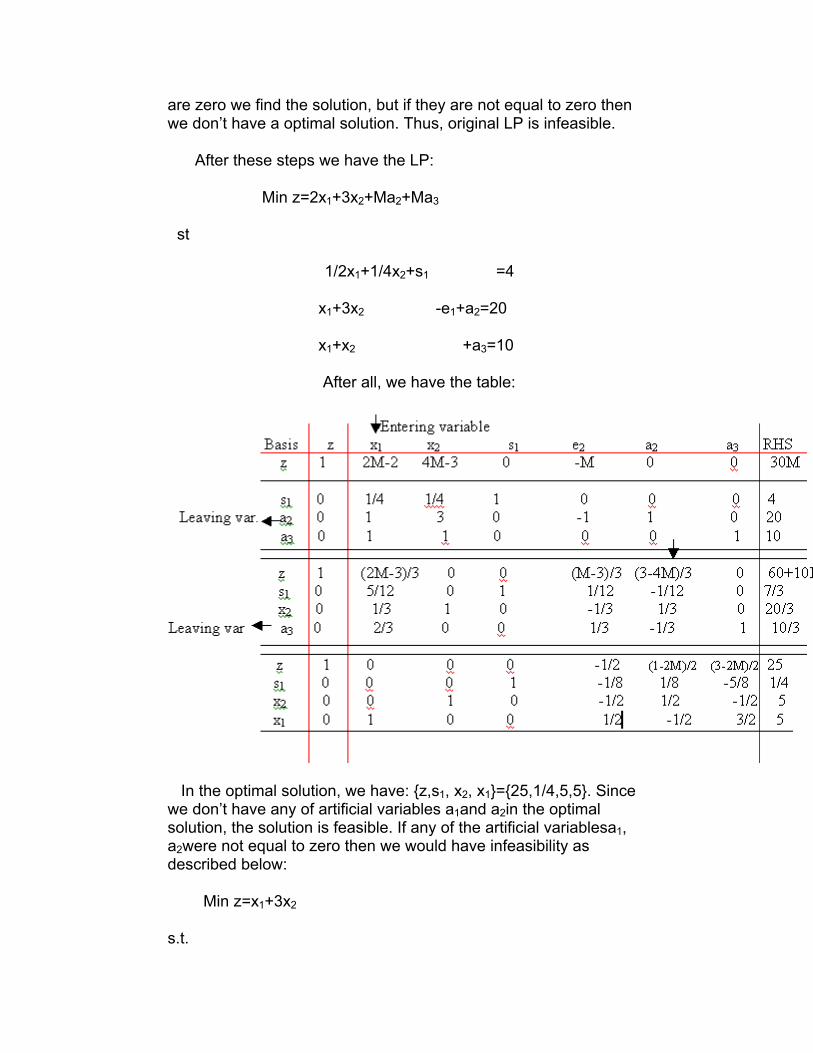
are zero we find the solution, but if they are not equal to zero then we don’t have a optimal solution. Thus, original LP is infeasible.
After these steps we have the LP:
Min z=2x1+3x2+Ma2+Ma3
st
1/2x1+1/4x2+s1 =4
x1+3x2 -e1+a2=20
x1+x2 +a3=10
After all, we have the table:
In the optimal solution, we have: {z,s1, x2, x1}={25,1/4,5,5}. Since we don’t have any of artificial variables a1and a2in the optimal solution, the solution is feasible. If any of the artificial variablesa1, a2were not equal to zero then we would have infeasibility as described below:
Min z=x1+3x2
s.t.

1/2x1+1/4x2 ≤ 4
x1+3x2 ≥ 10
x1+x2 =10
After going through all the steps described above we end with the optimal tableau:
In the above example, we have the optimal tableau since reduced costs of all non basic variables are non positive. However note that the optimal solution contains the very big number M, which should not have been the case for a min problem, thus we say that our original LP was infeasible. We also say that from the fact that we have the artificial variablea2 in the basic variables, which shouldn’t have been the case for a feasible LP.
Example 3 Maximize Z = x1 + 5x2 Subject to: 3x1 + 4x2 £ 6 x1 + 3x2 ³ 2 Where x1, x2 ³ 0
Solution
Introducing slack and surplus variables
3x1 + 4x2 + x3 = 6 x1 + 3x2 – x4 = 2
Where: x3 is a slack variable x4 is a surplus variable.
The surplus variable x4 represents the extra units.

Now if we let x1 and x2 equal to zero in the initial solution, we will have x3 = 6 and x4 = –2, which is not possible because a surplus variable cannot be negative. Therefore, we need artificial variables.
Maximize x1 + 5x2 – MA1
Subject to:
3x1 + 4x2 + x3 = 6 x1 + 3x2 – x4 + A1 = 2
Where: x1 ³ 0, x2 ³ 0, x3 ³ 0, x4 ³ 0, A1 ³ 0
Cj 1 5 0 0 –M
CB Basic variables
B
x1 x2 x3 x4 A1 Solution values b (= XB)
0 x3 3 4 1 0 0 6
–M A1 1 3 0 –1 1 2
Zj – Cj –M – 1
–3M – 5
0 M 0
Here, a11 = 3, a12 = 4, a13 = 1, a14 = 0, a15 = 0, b1 = 6 a21 = 1, a22 = –3, a23 = 0, a24 = –1, a25 = 1, b2 = 2
Calculating Zj – Cj
First column = 0 * 3 + (–M) * 1 – 1 = –M – 1 Second column = 0 * 4 + (–M) * 3 – 5 = –3M–5 Third column = 0 * 1 + (–M) * 0 – 0 = 0 Fourth column = 0 * 0 + (–M) * (–1) – 0 = M Fifth column = 0 * 0 + (–M) * 1 – (–M) = 0 Choose the smallest negative value from Zj – Cj. Substitute M = 0 Smallest negative value is –5. So second column is the element column. Now find out the minimum positive value.
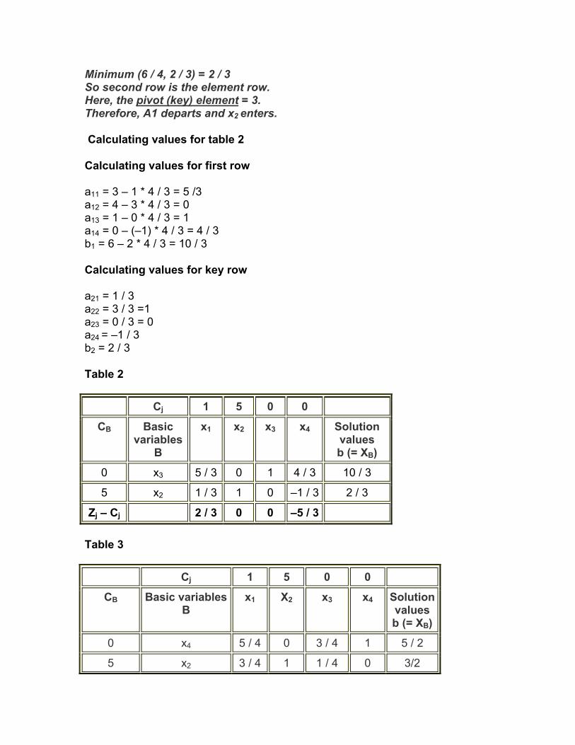
Minimum (6 / 4, 2 / 3) = 2 / 3 So second row is the element row. Here, the pivot (key) element = 3. Therefore, A1 departs and x2 enters.
Calculating values for table 2
Calculating values for first row
a11 = 3 – 1 * 4 / 3 = 5 /3 a12 = 4 – 3 * 4 / 3 = 0 a13 = 1 – 0 * 4 / 3 = 1 a14 = 0 – (–1) * 4 / 3 = 4 / 3 b1 = 6 – 2 * 4 / 3 = 10 / 3
Calculating values for key row
a21 = 1 / 3 a22 = 3 / 3 =1 a23 = 0 / 3 = 0 a24 = –1 / 3 b2 = 2 / 3
Table 2
Cj 1 5 0 0
CB Basic variables
B
x1 x2 x3 x4 Solution values b (= XB)
0 x3 5 / 3 0 1 4 / 3 10 / 3
5 x2 1 / 3 1 0 –1 / 3 2 / 3
Zj – Cj 2 / 3 0 0 –5 / 3
Table 3
Cj 1 5 0 0
CB Basic variables B
x1 X2 x3 x4 Solution values b (= XB)
0 x4 5 / 4 0 3 / 4 1 5 / 2
5 x2 3 / 4 1 1 / 4 0 3/2
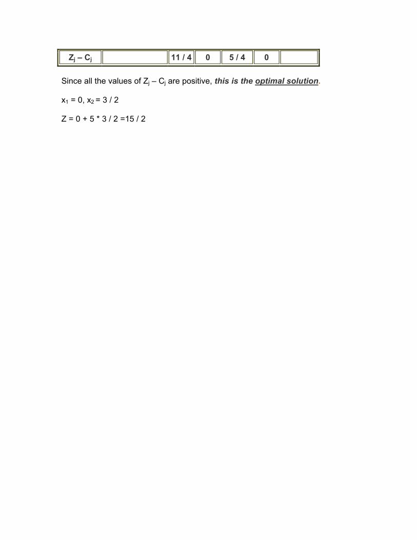
Zj – Cj 11 / 4 0 5 / 4 0
Since all the values of Zj – Cj are positive, this is the optimal solution.
x1 = 0, x2 = 3 / 2
Z = 0 + 5 * 3 / 2 =15 / 2


Unit 1 Lesson 10: Two-Phase Simplex Learning Objective:
• Two-Phase Method to solve LPP
So far, you have developed an algorithm to solve formulated linear programs (The Simplex Method). Notice that, your algorithm starts with an initial basic feasible solution and if all the inequalities of the constraints are of “less than or equal to” type, the origin is always our starting point.
For a “greater than or equal to” constraint, the slack variable in the equality form has a negative coefficient for the origin. Again, “equality” constraints have no slack variables. If either type of constraint is part of the model, there is no convenient initial basic feasible solution.
This is where Two-Phase Simplex comes in. It involves two phases (thus the name!):
Phase 1: Has the goal of finding a basic feasible solution,
Phase 2: Has the goal of finding the optimum solution.
The procedure of this technique is as follows:
Phase 1:
1.First, add nonnegative variables to the left hand side of the types “≥” and “=”.
These variables are called “artificial variables“.
2.Formulate a new problem by replacing the original objective function by the
sum of the artificial variables and minimize it to ensure that the artificial variables
will be zero in the final solution which gives you a basic feasible solution that you
searched.
Phase 2:

1.If at the end of Phase 1, all artificial variables can be set to zero value, then a
basic feasible solution is found and we can pass to the second phase.
In order to start the second phase, the objective function must be expressed in
terms of the non basic variables only. After applying the proper transformations,
proceed with the regular steps of the simplex method.
To show how a two phase method is applied, see an example.
Example 1
1 2
1 2
1 2
1
1 2
1 2
Z=2X +3X s.t. -X + X 5 X +3X 35 X 20
3 X + X 102
and, X ,X 0.
Max
≤≤≤
≥
≥
First, the standard form of the problem can be converted from the canonical form
as follows:
1 2
1 2 1
1 2 2
1 3
1 2
Z=2X +3X s.t. -X + X +S 5 X +3X +S 35 X +S 20
3 X + X 2
Max
===
4
1 2
-S +a 10
and, X ,X 0.
=
≥

where “a” is the artificial variable added as it is explained above. Now, it is time to
go through Phase 1.
Phase 1: Implement the new problem of minimizing the sum of the artificial
variables.
W=aMin
since there is on one artificial variable.
Because the artificial variable is the basic variable of the fourth equation, we
should write W function in terms of non basic variables. That is,
1 23 W=10- X X S2
Min + −
4.
Now, solve this by the simplex method.
Iteration 1.1
Basic X1 X2 S1 S2 S3 S4 a RHS
W 1 3/2 0 0 0 -1 0 10
S1 -1 1 1 0 0 0 0 5S2 1 3 0 1 0 0 0 35S3 1 0 0 0 1 0 0 20a 1 3/2 0 0 0 -1 1 10
In the table above, entering and leaving variables are selected as follows:
Iteration 1. 2
Basic X1 X2 S1 S2 S3 S4 a RHS
W 1 3/2 0 0 0 -1 0 10 S1 -1 1 1 0 0 0 0 5 5 S2 1 3 0 1 0 0 0 35 35/3 S3 1 0 0 0 1 0 0 20 a 1 3/2 0 0 0 -1 1 10 20/3

After applying the calculations, you will get
Iteration 1. 3
Basic X1 X2 S1 S2 S3 S4 a RHS
W 5/2 0 -3/2 0 0 -1 0 5/2
X2 -1 1 1 0 0 0 0 5S2 4 0 -3 1 0 0 0 20S3 1 0 0 0 1 0 0 20A 5/2 0 -3/2 0 0 -1 1 5/2
This table above is not optimum so you go on iterating.
Iteration 2.1
Basic X1 X2 S1 S2 S3 S4 a RHS
W 5/2 0 -3/2 0 0 -1 0 5/2
X2 -1 1 1 0 0 0 0 5 S2 4 0 -3 1 0 0 0 20 5 S3 1 0 0 0 1 0 0 20 20 A 5/2 0 -3/2 0 0 -1 1 5/2 1
Apply the calculations again and reach to the optimum W=0:
Iteration 2.2
Basic X1 X2 S1 S2 S3 S4 a RHS
W 0 0 0 0 0 0 -1 0

X2 0 1 2/5 0 0 -2/5 0 6S2 0 0 -3/5 1 0 8/5 0 16S3 0 0 3/5 0 1 2/5 0 19X1 1 0 -3/5 0 0 -2/5 1 1
Now, you have an initial basic feasible solution, which is ( X1 , X2 ) = (1,6). So,
the phase 1 is completed and you can pass through phase 2.
Phase 2: The objective function Z must be expressed in terms of non basic
variables. Our non basic variables are S1 and S4 and we will write the basic
variables in the original equation in terms of them.
1 2 1 4 1 4
4
3 2 2 2 Z=2X +3X =2 1+ S + S +3 6 S + S5 5 5 5
Z=20+2S
Max −
⇒
You can write the first table of phase 2 now. The last table in phase 1 is just
copied with two exceptions. You delete the column of the artificial variable and
change the W equation to Z equation.
Iteration 3.1
Basic X1 X2 S1 S2 S3 S4 RHS
Z 0 0 0 0 0 -2 20
X2 0 1 2/5 0 0 -2/5 6S2 0 0 -3/5 1 0 8/5 16S3 0 0 3/5 0 1 2/5 19X1 1 0 -3/5 0 0 -2/5 1
Since this is a maximization problem, this table is not optimum and you have to
apply simplex method to find the optimum.
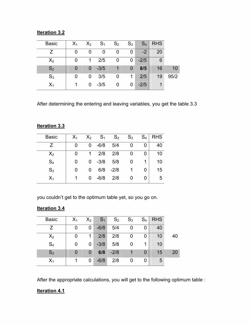
Iteration 3.2
Basic X1 X2 S1 S2 S3 S4 RHS
Z 0 0 0 0 0 -2 20
X2 0 1 2/5 0 0 -2/5 6 S2 0 0 -3/5 1 0 8/5 16 10 S3 0 0 3/5 0 1 2/5 19 95/2 X1 1 0 -3/5 0 0 -2/5 1
After determining the entering and leaving variables, you get the table 3.3
Iteration 3.3
Basic X1 X2 S1 S2 S3 S4 RHS
Z 0 0 -6/8 5/4 0 0 40
X2 0 1 2/8 2/8 0 0 10S4 0 0 -3/8 5/8 0 1 10S3 0 0 6/8 -2/8 1 0 15X1 1 0 -6/8 2/8 0 0 5
you couldn’t get to the optimum table yet, so you go on.
Iteration 3.4
Basic X1 X2 S1 S2 S3 S4 RHS
Z 0 0 -6/8 5/4 0 0 40
X2 0 1 2/8 2/8 0 0 10 40 S4 0 0 -3/8 5/8 0 1 10 S3 0 0 6/8 -2/8 1 0 15 20 X1 1 0 -6/8 2/8 0 0 5
After the appropriate calculations, you will get to the following optimum table :
Iteration 4.1

Basic X1 X2 S1 S2 S3 S4 RHS
Z 0 0 0 1 1 0 55
X2 0 1 0 1/3 -1/3 0 5S4 0 0 0 1/2 ½ 1 35/2S1 0 0 1 -1/3 4/3 0 20X1 1 0 0 2/8 1 0 20
That is, ( X1 , X2 ) = (20,5) is the optimum point with optimum Z = 55.
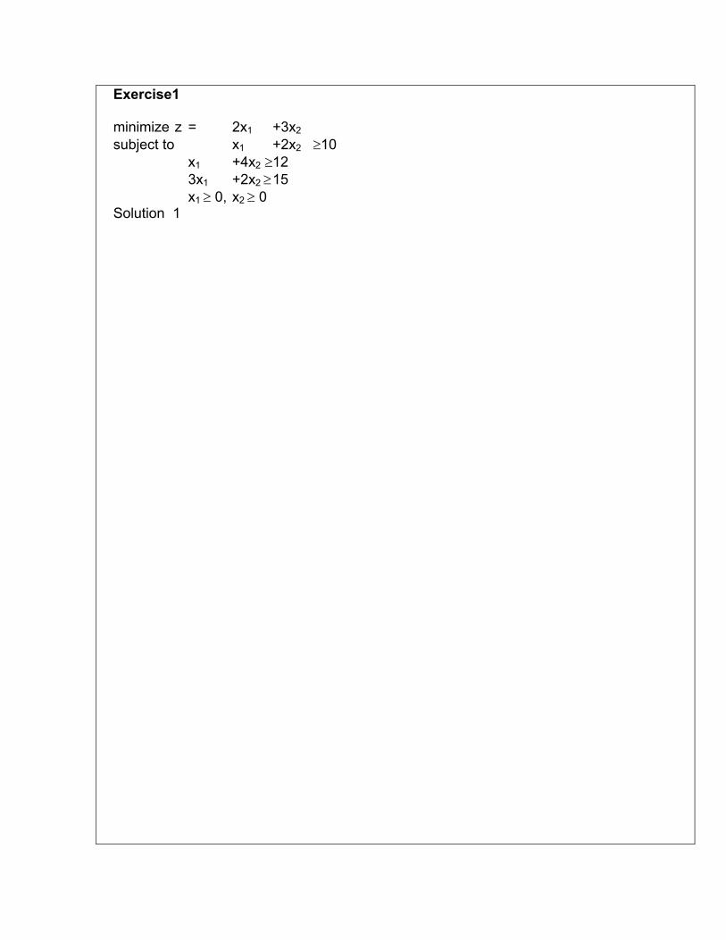
Exercise1 minimize z = 2x1 +3x2 subject to x1 +2x2 ≥10 x1 +4x2 ≥12 3x1 +2x2 ≥ 15 x1 ≥ 0, x2 ≥ 0 Solution 1

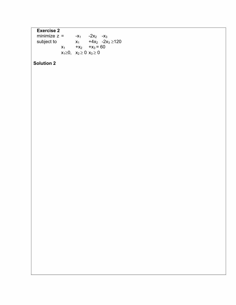
Exercise 2 minimize z = -x1 -2x2 -x3 subject to x1 +4x2 -2x3 ≥120 x1 +x2 +x3 = 60 x1≥0, x2 ≥ 0 x3 ≥ 0
Solution 2


Exercise 3
Solution 3 0, 3 42
1 s.t. 3max
21
21
21
21
21
≥=+≤+≥+−
+=
xxxxxxxxxxz

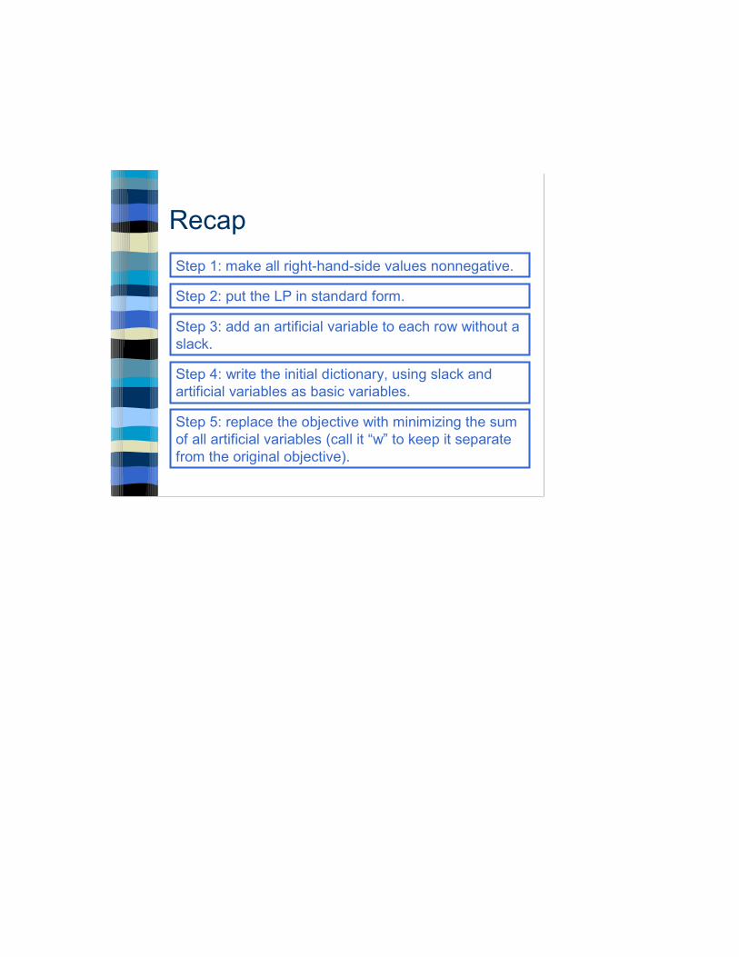
RecapStep 1: make all right-hand-side values nonnegative.
Step 2: put the LP in standard form.
Step 3: add an artificial variable to each row without a slack.
Step 4: write the initial dictionary, using slack and artificial variables as basic variables.
Step 5: replace the objective with minimizing the sum of all artificial variables (call it “w” to keep it separate from the original objective).

Recap
Step 9: Optimize the Phase II LP. As artificial variables become nonbasic, delete them.
Step 6: write the new objective in terms of nonbasic variables.
Step 7: solve the Phase I LP. If w > 0, the original LP is infeasible.
Step 8: replace the original objective, in terms of nonbasic variables. Delete all nonbasic artificial variables. This creates the Phase II LP.

RecapThree outcomes when solving Phase I LP:
– Minimum w > 0: LP infeasible– Mimimum w = 0, all artificial variables nonbasic:
• replace objective• delete artificial variables• continue with Phase II
– Minimum w = 0, some artificial variable basic (and equal to zero):
• replace objective• delete nonbasic artificial variables• continue with Phase II• delete each artificial variable as it becomes nonbasic.

Unit 1
Lesson 11: Duality in linear programming Learning objectives:
• Introduction to dual programming. • Formulation of Dual Problem.
Introduction For every LP formulation there exists another unique linear programming formulation called the 'Dual' (the original formulation is called the 'Primal'). The - Dual formulation can be derived from the same data from which the primal was formulated. The Dual formulated can be solved in the same manner in which the Primal is solved since the Dual is also a LP formulation. The Dual can be considered as the 'inverse' of the Primal in every respect. The column coefficients in the Primal constrains become the row co-efficients in the Dual constraints. The coefficients in the Primal objective function become the right hand side constraints in the Dual constraints. The column of constants on the right hand side of the Primal constraints becomes the row of coefficients of the dual objective function. The 'direction of the inequalities are reversed. If the primal objective function is a 'Maximization' function then the dual objective function is a 'Minimization' function and vice-versa. The concept of duality is very much in useful to obtain additional information about the variation in the optimal solution when certain changes are effected in the constraint co-efficient, resourse availabilities and objective function co-efficients. This is termed as post optimality or sensitivity analysis.
Dual Problem Construction:
- If the primal is a maximization problem, then its dual is a minimization problem (and vise versa).
- Use the variable type of one problem to find the constraint type of the other problem.
- Use the constraint type of one problem to find the variable type of the other problem.
- The RHS elements of one problem become the objective function coefficients of the other problem (and vice versa).
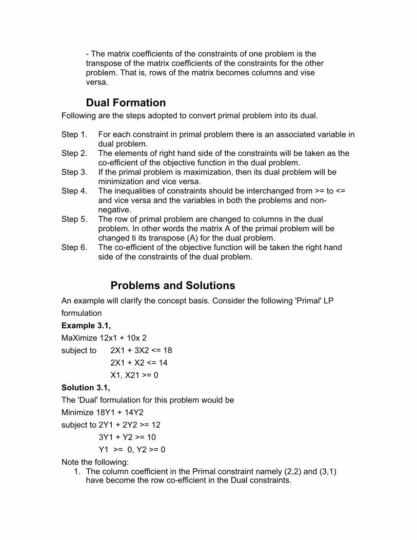
- The matrix coefficients of the constraints of one problem is the transpose of the matrix coefficients of the constraints for the other problem. That is, rows of the matrix becomes columns and vise versa.
Dual Formation Following are the steps adopted to convert primal problem into its dual. Step 1. For each constraint in primal problem there is an associated variable in
dual problem. Step 2. The elements of right hand side of the constraints will be taken as the
co-efficient of the objective function in the dual problem. Step 3. If the primal problem is maximization, then its dual problem will be
minimization and vice versa. Step 4. The inequalities of constraints should be interchanged from >= to <=
and vice versa and the variables in both the problems and non-negative.
Step 5. The row of primal problem are changed to columns in the dual problem. In other words the matrix A of the primal problem will be changed ti its transpose (A) for the dual problem.
Step 6. The co-efficient of the objective function will be taken the right hand side of the constraints of the dual problem.
Problems and Solutions
An example will clarify the concept basis. Consider the following 'Primal' LP formulation Example 3.1, MaXimize 12x1 + 10x 2 subject to 2X1 + 3X2 <= 18
2X1 + X2 <= 14 X1, X21 >= 0
Solution 3.1, The 'Dual' formulation for this problem would be Minimize 18Y1 + 14Y2 subject to 2Y1 + 2Y2 >= 12
3Y1 + Y2 >= 10 Y1 >= 0, Y2 >= 0
Note the following: 1. The column coefficient in the Primal constraint namely (2,2) and (3,1)
have become the row co-efficient in the Dual constraints.

2. The co-efficient of the Primal objective function namely, 12 and 10 have become the constants in the right hand side of the Dual constraints.
3. The constants of the Primal constraints, namely 18 and 14, have become the co-efficeint in the Dual obejctive function.
4. The direction of the inequalities have been reserved. The Primal constraints have the in equalities of::; while the Dual constraints have the inequalities of ~ .
5. While the Primal is a 'Maximization' problem the Dual is a 'Minimization' problem Why construct the Dual formulation? This is for a number of reasons. The solution to the dual problem provides all essential information about the solution to the Primal problem. For an LP problem, the solution can be determined either by solving the original problem or the dual problem. Sometimes it may be easier to solve the Dual problem rather than the Primal problem. (For instance, when the primal involves few variables but many constraints.)
Example 3.2, Obtain the dual problem of the following primal formulation.
Maximize Z = 2X1 + 5X2 + 6X3 Subject to 5X1 + 6X2 -X3 <= 3 -2x1 + X2 + 4X3 <= 4 X1 - 5X2 + 3X3 <= 1 -3X1 - 3X2 + 7X3 <= 6 X1, X2, X3 >= 0 Solution 3.2, Step 1 : Write the objective function of the Dual. As there are four constraints in the primal, the objective function of the dual will have 4 variables. Minimize r* = 3W1 + 4W2 + W3 + 6W4 Step 2 : Write the constraints of the dual. As all the constraints in the primal are '<', the constraints in the dual will be '>'. The column COM+ efficients of the primal become the row co-efficients of the dual. Constriants. 5W1 - 2W2 + W3 - 3W4 >= 2
6W1 + W2 - 5W3 -W4 >= 5 -W1 + 4W2 + 3W3 + 7W4 >= 6
Step 3 : Therefore the dual of the Primal is : Minimize Z = 3W1 + 4W2 + W3 + 6W4

Subject to : 5W1 - 2W2 + W3 - 3W4 >= 2 6W1+ W2 - 5W3 - 3W4 >= 5
- W1 + 4W2 + 3W3 + 7W4 >= 6 W1, W2, W3, W4 >= 0 Example 3.3,
Obtain the dual of the- following linear programming problem.
Minimize Z = 5X1 -6X2 + 4X3
Subject to the constriants :
3X1 + 4X2 + 6X3 >= 9 X1 + 3X2 + 2X3 >= 5 7X1 - 2X2 - X3 >= 10 X1 - 2X2 + 4X3 >= 4 2X1 + 5X2 - 3X3 >= 3 X1, X2, X3 >= 0 Solution 3.3, In this problem one of the primal constraints (namely 7X1 - 2X2 - X3 <=10) is a "<= ", constraints while all the other are ">=”I constraints. The dual cannot be worked out unless all the constraints are in the same direction. To convert this into ">=” constraint, multiply both the sides of the equation by "-" sign. After multiplying the constraint by "-". sign, it will become 7x1 + 2x2 + x3 >= -10. Now all the constraints are in the same direction and the dual can be worked out. The dual formulation is :
Maximize Z = 9W1 + 5W2 - 10W3 + 4W4 + 3W5 Subject to :
3W1 + W2 - 7W3 + W4 + 2W5 <= 5 4W1 + 3W2 + 2W3 - 2W4 + 5W5 <= -6 6W1 + 2W2 + W3 + 4W4 + -3W5 <= 4 W1, W2, W3, W4, W5 >= 0


Unit 1 Lesson 12: A Presentation on Duality Theorem
1
Duality Theory
The duality theory deals with the relationship between original and dual LP problems.
It is very important in optimization and other areas of applied mathematics.

2
For the Simplex Method so far, we have only considered maximisation problems, with ≤functional constraints. We will now consider minimisation problems with ≥ functional constraints.We still require all variables to be non-negative.We shall use Duality Theory for this purpose.
Duality Theory
3
Consider the following LP problem. Observethat here we use minrather than max, and ≥rather than ≤ for the functional constraints.
Since these “violate” the format we used so far, we cannot use our Simplex Method to solve this problem directly. We shall solve it indirectly via Duality Theory.
min C = 5x1 + 3x2
s.t. x1 + 3x 2 ≥ 82x1 − 4x2 ≥ 7
x1,x2 ≥ 0
Duality Theory

4
Dual Problem: Given a (min, ≥) problem, we create a (max, ≤) problem by the following transformations:
min max≥ ≤ in the functional constraintsRHS Objective function coefficientsObjective function coefficients RHSConstraint coefficients are transposed
Transpose:Interchange rows and columns of a matrix, table, etc.
a b cd e f
⇒
a db ec f
Duality Theory
5
?
Constructing the dualproblem of the primalproblem. min C = 5x1 + 3x2
s.t. x1 + 3x2 ≥ 82x1 − 4x2 ≥ 7
x1,x2 ≥ 0
Problem P (Primal)
max P = 8y1 + 7y2
s.t. y1 + 2y2 ≤ 53y1 − 4y2 ≤ 3
y1, y2 ≥ 0
Problem D (Dual)
Duality Theory

6 Duality TheoryMinimisation Problem in canonical form:
min C = b1x1 + b2 x2 +Λ + bmxm
s.t.s.t.
m variablesn functional constraints
x1, x2,Λ ,xm≥ 0
a11x1 + a12x2 + Λ +a1mxm≥ c1
......an1 x1+ an2 x2+Λ + anmxm≥ cn
a21 x1+ a22 x2+Λ + a2mxm≥ c2
7 Duality Theory
Dual Problem:
max P = c1y1 + c2 y2 +Λ + cnyn
s.t.s.t.
n variablesm functional constraints
y1, y2,Λ ,yn ≥ 0
a11y1 + a21y2 + Λ +an1 yn ≤ b1
......a1my1+ a2my2+Λ + anmyn ≤ bm
a12 y1+ a22 y2+Λ + an2 yn ≤ b2

8
Example 3.2 (see also Ex.1, Section 5-5, B & Z) Construct the dual of the following problem: Minimise: C = 2x1 + 8x2+ 3x3
s.t. x1 + 2x2 + 4x3 ≥ 6x1 + 3x2 − 5x3 ≥ 8x1, x2, x3 ≥ 0
Dual Problem: Maximize P = 6y1 + 8y2s.t. y1 + y2 ≤ 2
2y1 + 3y2 ≤ 84y1 − 5y2 ≤ 3y1 , y2 ≥ 0
Duality Theory
9 Duality TheoremA LP problem has an optimal solution if and only
if its dual has an optimal solution.If an optimal solution exists, then the optimal
values of the objective functions of the two problems are the same. That is,
Max P = Min C
Good News: This theorem is constructive in that it gives a simple recipe for obtaining an optimal solution for the dual problem from the final simplex tableau of the original problem and vice versa.

10 Duality Theory
RecipeHow can we obtain an optimal solution to a (min, ≥)problem from the final simplex tableau of its dual (max, ≤) problem ?
Solve the dual (max, ≤) problem using theSimplex Method.
Record the entries of the slack variables in the last row of the final simplex tableau.
These coefficients are equal to the optimal values of the respective dual variables.
11 Duality Theory
Example 3.3 (see also Ex.2, Section 5-5, B & Z)Solve the following problem by first constructing its dual, and then using the simplex method on the dual.
Minimise: C = x1 + 2 x2
subject to: x1 + 0.5x2 ≥ 2x1 − x2 ≥ 2x1 + x2 ≥ 3x1, x2 ≥ 0
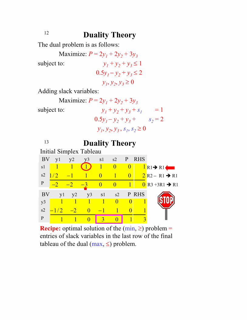
12 Duality TheoryThe dual problem is as follows:
Maximize: P = 2y1 + 2y2 + 3y3
subject to: y1 + y2 + y3 ≤ 10.5y1 − y2 + y3 ≤ 2
y1, y2, y3 ≥ 0Adding slack variables:
Maximize: P = 2y1 + 2y2 + 3y3
subject to: y1 + y2 + y3 + s1 = 10.5y1 − y2 + y3 + s2 = 2y1, y2, y3 , s1, s2 ≥ 0
13 Duality Theory
Initial Simplex Tableau
1 1 1 1 0 0 11/ 2 −1 1 0 1 0 2
−2 −2 −3 0 0 1 0
BV y1 y2 y3 s1 s2 P RHSs1
s2
P
R1 R1
R2 − R1 R1
R3 +3R1 R1
1 1 1 1 0 0 1−1/ 2 −2 0 −1 1 0 1
1 1 0 3 0 1 3
BV y1 y2 y3 s1 s2 P RHSy3
s2
P
Recipe: optimal solution of the (min, ≥) problem =entries of slack variables in the last row of the final tableau of the dual (max, ≤) problem.

14
Do Questions 1-4, Example Sheet 4.Look at (no need to do unless you want to) the
application problems at the end of Sections 5-5, 5-6 and Review, to get an idea of some applications of LP.
Do Example 3.5 graphically to check the answer.
Duality TheoryReport:
The optimal solution to the dual (max, ≤) problem is (y1 , y2 , y3) = (0, 0, 1).
The optimal solution to the original (min, ≥) problem is (x1, x2) = (3, 0).
The optimal values of the objective functions are: Max P = Min C = 3
Unit 1 Lesson 13: Sensitivity Analysis
Learning Objectives
• What is Sensitivity Analysis ? • Role of sensitivity analysis in Linear programming.
Finding the optimal solution to a linear programming model is important, but it is not the only information available. There is a tremendous amount of sensitivity information, or information about what happens when data values are changed.
Recall that in order to formulate a problem as a linear program, you had to invoke a certainty assumption: you had to know what value the data took on, and you have made decisions based on that data. Often this assumption is somewhat dubious: the data might be unknown, or guessed at, or otherwise inaccurate. How can you determine the effect on the optimal decisions if the values change? Clearly some numbers in the data are more important than others. Can you find the ``important'' numbers?
Can you determine the effect of misestimation?
Linear programming offers extensive capability for addressing these questions. In this lecture I will show you how data changes show up in the optimal table. I am giving you two examples of how to interpret Solver's extensive output.
Sensitivity Analysis
Suppose you solve a linear program ``by hand'' ending up with an optimal table (or tableau to use the technical term). You know what an optimal tableau looks like: it has all non-negative values in Row 0 (which we will often refer to as the cost row), all non-negative right-hand-side values, and a basis (identity matrix) embedded. To determine the effect of a change in the data, I will try to determine how that change effected the final tableau, and try to reform the final tableau accordingly.
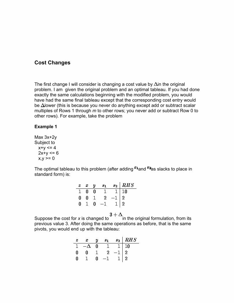
Cost Changes
The first change I will consider is changing a cost value by in the original problem. I am given the original problem and an optimal tableau. If you had done exactly the same calculations beginning with the modified problem, you would have had the same final tableau except that the corresponding cost entry would be lower (this is because you never do anything except add or subtract scalar multiples of Rows 1 through m to other rows; you never add or subtract Row 0 to other rows). For example, take the problem
Example 1
Max 3x+2y Subject to x+y <= 4 2x+y <= 6 x,y >= 0
The optimal tableau to this problem (after adding and as slacks to place in standard form) is:
Suppose the cost for x is changed to in the original formulation, from its previous value 3. After doing the same operations as before, that is the same pivots, you would end up with the tableau:

Now this is not the optimal tableau: it does not have a correct basis (look at the column of x). But you can make it correct in form while keeping the same basic variables by adding times the last row to the cost row. This gives the tableau:
Note that this tableau has the same basic variables and the same variable values (except for z) that your previous solution had.
Does this represent an optimal solution? It does only if the cost row is all non-negative. This is true only if
which holds for . For any in that range, our previous basis (and
variable values) is optimal. The objective changes to .
In the previous example, we changed the cost of a basic variable. Let's go through another example. This example will show what happens when the cost of a nonbasic variable changes.
Example2
Max 3x+2y + 2.5w Subject to x+y +2w <= 4 2x+y +2w <= 6 x,y,w >= 0
Here, the optimal tableau is :
Now suppose I change the cost on w from 2.5 to in the formulation. Doing the same calculations as before will result in the tableau:

In this case,I already have a valid tableau. This will represent an optimal solution
if , so . As long as the objective coefficient of w is no more than 2.5+1.5=4 in the original formulation, my solution of x=2,y=2 will remain optimal.
The value in the cost row in the simplex tableau is called the reduced cost. It is zero for a basic variable and, in an optimal tableau, it is non-negative for all other variables (for a maximization problem).
Summary: Changing objective function values in the original formulation will result in a changed cost row in the final tableau. It might be necessary to add a multiple of a row to the cost row to keep the form of the basis. The resulting analysis depends only on keeping the cost row non-negative.
Right Hand Side Changes
For these types of changes, concentrate on maximization problems with all constraints. Other cases are handled similarly.
Take the following problem:
Example 3
The optimal tableau, after adding slacks and is
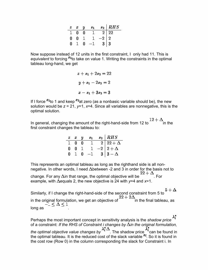
Now suppose instead of 12 units in the first constraint, I only had 11. This is equivalent to forcing to take on value 1. Writing the constraints in the optimal tableau long-hand, we get
If I force to 1 and keep at zero (as a nonbasic variable should be), the new solution would be z = 21, y=1, x=4. Since all variables are nonnegative, this is the optimal solution.
In general, changing the amount of the right-hand-side from 12 to in the first constraint changes the tableau to:
This represents an optimal tableau as long as the righthand side is all non-negative. In other words, I need between -2 and 3 in order for the basis not to
change. For any in that range, the optimal objective will be . For example, with equals 2, the new objective is 24 with y=4 and x=1.
Similarly, if I change the right-hand-side of the second constraint from 5 to
in the original formulation, we get an objective of in the final tableau, as
long as .
Perhaps the most important concept in sensitivity analysis is the shadow price of a constraint: If the RHS of Constraint i changes by in the original formulation,
the optimal objective value changes by . The shadow price can be found in the optimal tableau. It is the reduced cost of the slack variable . So it is found in the cost row (Row 0) in the column corresponding the slack for Constraint i. In
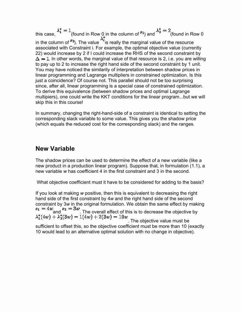
this case, (found in Row 0 in the column of ) and (found in Row 0
in the column of ). The value is really the marginal value of the resource associated with Constraint i. For example, the optimal objective value (currently 22) would increase by 2 if I could increase the RHS of the second constraint by
. In other words, the marginal value of that resource is 2, i.e. you are willing to pay up to 2 to increase the right hand side of the second constraint by 1 unit. You may have noticed the similarity of interpretation between shadow prices in linear programming and Lagrange multipliers in constrained optimization. Is this just a coincidence? Of course not. This parallel should not be too surprising since, after all, linear programming is a special case of constrained optimization. To derive this equivalence (between shadow prices and optimal Lagrange multipiers), one could write the KKT conditions for the linear program...but we will skip this in this course!
In summary, changing the right-hand-side of a constraint is identical to setting the corresponding slack variable to some value. This gives you the shadow price (which equals the reduced cost for the corresponding slack) and the ranges.
New Variable
The shadow prices can be used to determine the effect of a new variable (like a new product in a production linear program). Suppose that, in formulation (1.1), a new variable w has coefficient 4 in the first constraint and 3 in the second.
What objective coefficient must it have to be considered for adding to the basis?
If you look at making w positive, then this is equivalent to decreasing the right hand side of the first constraint by 4w and the right hand side of the second constraint by 3w in the original formulation. We obtain the same effect by making
and . The overall effect of this is to decrease the objective by
. The objective value must be sufficient to offset this, so the objective coefficient must be more than 10 (exactly 10 would lead to an alternative optimal solution with no change in objective).
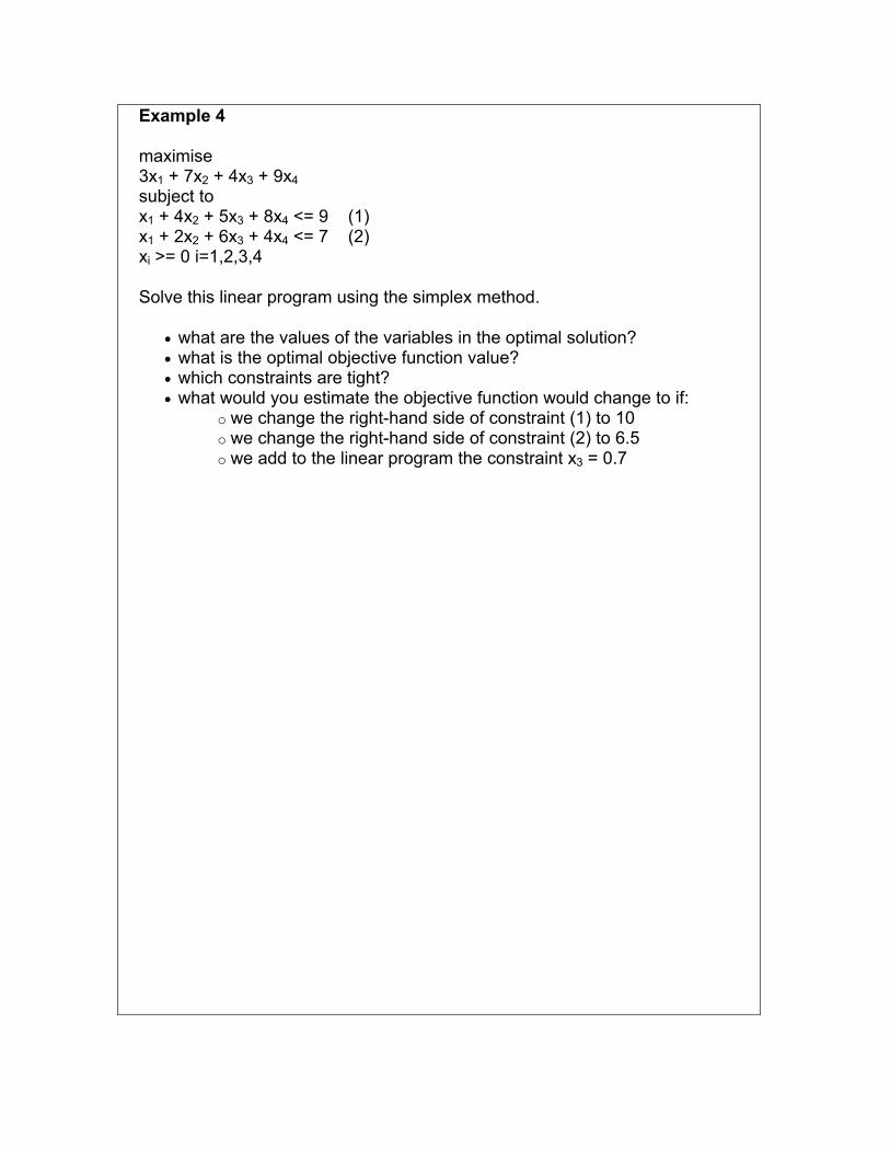
Example 4
maximise 3x1 + 7x2 + 4x3 + 9x4 subject to x1 + 4x2 + 5x3 + 8x4 <= 9 (1) x1 + 2x2 + 6x3 + 4x4 <= 7 (2) xi >= 0 i=1,2,3,4
Solve this linear program using the simplex method.
• what are the values of the variables in the optimal solution? • what is the optimal objective function value? • which constraints are tight? • what would you estimate the objective function would change to if:
o we change the right-hand side of constraint (1) to 10 o we change the right-hand side of constraint (2) to 6.5 o we add to the linear program the constraint x3 = 0.7


Unit 1
Lesson 14: Transportation Models
Learning Objective : • What is a Transportation Problem? • How can we convert a transportation problem into a linear
programming problem? • How to form a Transportation table?
and the basic terminology
Introduction
Today I am going to discuss about Transportation problem.
First question that comes in our mind is what is a transportation problem?
The transportation problem is one of the subclasses of linear programming problem where the objective is to transport various quantities of a single homogeneous product that are initially stored at various origins, to different destinations in such a way that the total transportation is minimum. F.I. Hitchaxic developed the basic transportation problem in 1941. However it could be solved for optimally as an answer to complex business problem only in 1951, when George B. Dantzig applied the concept of Linear Programming in solving the Transportation models. Transportation models or problems are primarily concerned with the optimal (best possible) way in which a product produced at different factories or plants (called supply origins) can be transported to a number of warehouses (called demand destinations). The objective in a transportation problem is to fully satisfy the destination requirements within the operating production capacity constraints at the minimum possible cost. Whenever there is a physical movement of goods from the point of manufacture to the final consumers through a variety of channels of distribution (wholesalers, retailers, distributors etc.), there is a need to minimize the cost of transportation so as to increase the profit on sales. Transportation problems arise in all such cases. It aims at providing assistance to the top management in ascertaining how many units
1

of a particular product should be transported from each supply origin to each demand destinations to that the total prevailing demand for the company’s product is satisfied, while at the same time the total transportation costs are minimized.
Mathematical Model of Transportation Problem Mathematically a transportation problem is nothing but a special linear programming problem in which the objective function is to minimize the cost of transportation subjected to the demand and supply constraints. Let ai = quantity of the commodity available at the origin i, bj = quantity of the commodity needed at destination j, cij = transportation cost of one unit of a commodity from origin I to destination j, and xij = quantity transported from origin I to the destination j. Mathematically, the problem is Minimize z = ∑∑ xij cij S.t. ∑xij = ai, i= 1,2,…..m ∑xij = bj, j= 1,2,…..,n
and xij ≥ 0 for all i and j .
Let us consider an example to understand the formulation of mathematical model of transportation problem of transporting single commodity from three sources of supply to four demand destinations. The sources of supply can be production facilities, warehouse or supply point, characterized by available capacity. The destination are consumption facilities, warehouse or demand point, characterized by required level of demand. FORMULATION OF TRANSPORATATION PROBLEM AS A
LINEAR PROGRAMMING MODEL
Let P denote the plant (factory) where the goods are being manufactured & W denote the warehouse (godown) where the
2

finished products are stored by the company before shipping to various destinations.
Further let, xij = quantity (amount of goods) shipped from plant
Pi to the warehouse Wj, and Cij = transportation cost per unit of shipping from
plant Pi to the Warehouse Wj.
Objective-function. The objection function can be represented as: Minimize Z = c11x11 + C12x12 + C13x13 (i.e. cost of shipping + c21x21 + c22x22 + c23x23 from a plant + c31x31 + c32x32 + c33x33 to the ware house)
Supply constraints.
x11 + x12 + x13 = S1 x21 + x22 + x23 = S2 x31 + x32 + x33 = S3
Demand constraints. x11 + x21 + x31 = D1 x21 + x22 + x23 = D2 x31 + x32 + x33 = D3
Either, xij ≥ for all values of I and j (ie; x11, x12, … all such values are ≥ 0) It is further assumed that: S1 + S2 + S3 = D1 + D2 + D3
i.e.; The total supply available at the plants exactly matches the total demand at the destinations. Hence, there is neither excess supply nor excess demand.
Such type of problems where supply and demand are exactly equal
are known as Balanced Transportation Problem. Supply (from various sources) are written in the rows, while a column is an expression for the demand of different warehouses. In general, if a transportation problem has m rows an n column, then the problem is solvable if there are exactly (m + n –1) basic variables.
A transportation problem is said to be unbalanced if the supply and demand are not equal.
3

(i) If Supply < demand, a dummy supply variable is introduced in the equation to make it equal to demand.
Likewise, if demand < supply, a dummy demand variable is introduced in the equation to make it equal to supply.
Example 1 : A firm has 3 factories located at A, E, and K which produce the same product. There are four major product district centers situated at B, C, D, and M. Average daily product at A, E, K is 30, 40, and 50 units respectively. The average daily requirement of this product at B, C, D, and M is 35, 28, 32, 25 units respectively. The cost in Rs. of transportation per unit of product from each factory to each district centre is given in table 1
Factories B C D M Supply
A 6 8 8 5 30
E 5 11 9 7 40
K 8 9 7 13 50
Demand 35 28 32 25
Table 1 The problem is to determine the name of product, no. of units of product to be transported from each factory to various district centers at minimum cost .
Factories B C D M Supply
A x11 x12 x13 x14 30
E x21 x22 x23 x24 40
K x31 x 32 x 33 x 34 50
Demand 35 28 32 25
Table 2
Xij = No. of unit of product transported from ith factory to jth district centre.
Total transportation cost: Minimize = 6x11 + 8x12 + 8x13 + 5x14 +…
4

+ 5x21 + 11x22 + 9x23 + 7x24 + 8x31 + 9x32 + 7x33 + 13x34
subject to : x11 + x12 + x13 + x14 = 30 x21 + x22 + x23 + x24 = 40 x31 + x32 + x33 + x34 = 50 x11 + x21 + x31 = 35 x12 + x22 + x32 = 28 x13 + x23 + x33 = 32 x14 + x24 + x34 = 25
xij ≥ 0
Since number of variables is very high, simplex method is not applicable.
Feasible condition: Total supply = total demand. Or ∑ ai = ∑ bj = K(say) i= 1,2,…..,n and j = 1,2,….,n
Things to know:
1) Total supply = total demand then it is a balanced transportation problem, otherwise it is a unbalanced problem.
2) The unbalanced problem can be balanced by adding a dummy supply center (row) or a dummy demand center (column) as the need arises.
3) When the number of positive allocation at any stage of feasible solution is less than the required number (row + Column – 1) the solution is said to be degenerate otherwise non-degenarete.
4) Cell in the transportation table having positive allocation will be called occupied cells, otherwise empty or non
5

occupiedcell.
Solution for a transportation problem The solution algorithm to a transpiration problem can be summarized into following steps:
Step 1. Formulate the problem and set up in the matrix form. The formulation of transportation problem is similar to LP problem formulation. Here the objective function is the total transportation cost and the constraints are the supply and demand available at each source and destination, respectively.
Step 2. Obtain an initial basic feasible solution. This initial basic solution can be obtained by using any of the following methods:
i. North West Corner Rule ii. Matrix Minimum Method iii. Vogel Approximation Method
The solution obtained by any of the above methods must fulfill following conditions:
i. The solution must be feasible, i.e., it must satisfy all the supply and demand constraints. This is called RIM CONDITION.
ii. The number of positive allocations must be equal to m + n – 1, where, m is number of rows and n is number of columns
The solution that satisfies both the above mentioned conditions are called a non-degenerate basic feasible solution.
Step 3. Test the initial solution for optimality. Using any of the following methods can test the optimality of obtained initial basic solution:
i. Stepping Stone Method ii. Modified Distribution Method (MODI)
If the solution is optimal then stop, otherwise, determine a new improved solution.
6

Step 4. Updating the solution Repeat Step 3 until the optimal solution is arrived at.
7
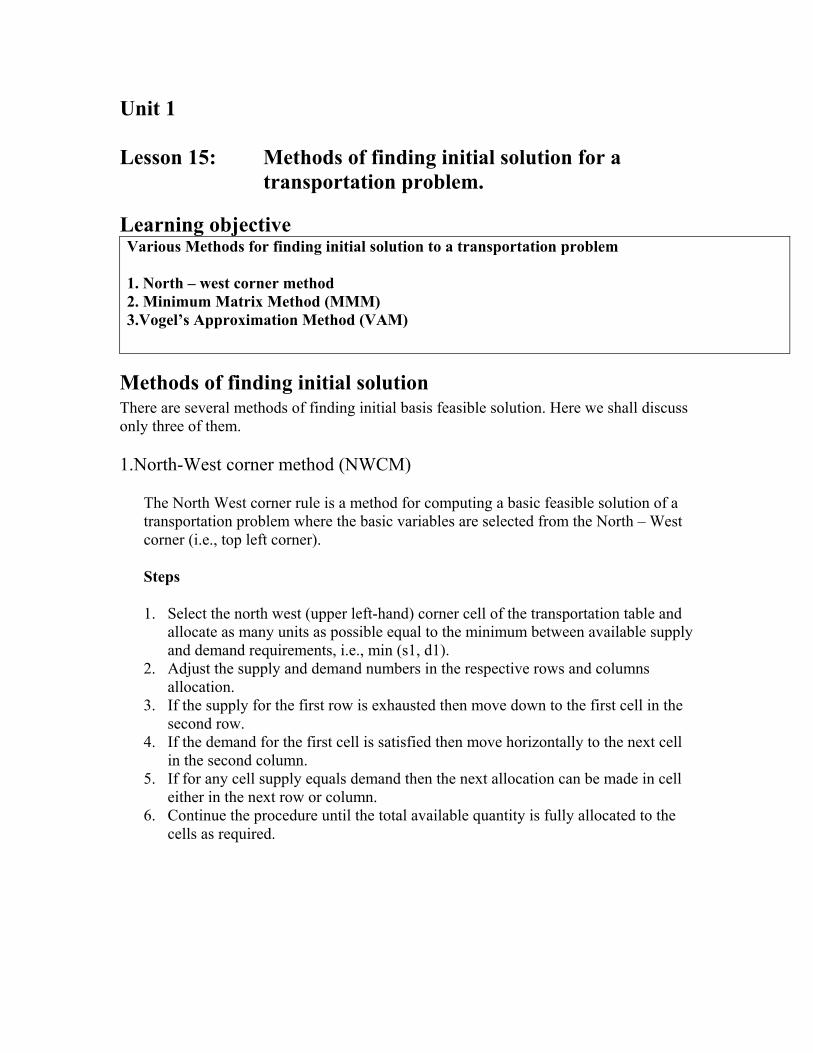
Unit 1 Lesson 15: Methods of finding initial solution for a transportation problem. Learning objective Various Methods for finding initial solution to a transportation problem 1. North – west corner method 2. Minimum Matrix Method (MMM) 3.Vogel’s Approximation Method (VAM)
Methods of finding initial solution There are several methods of finding initial basis feasible solution. Here we shall discuss only three of them. 1.North-West corner method (NWCM)
The North West corner rule is a method for computing a basic feasible solution of a transportation problem where the basic variables are selected from the North – West corner (i.e., top left corner).
Steps
1. Select the north west (upper left-hand) corner cell of the transportation table and allocate as many units as possible equal to the minimum between available supply and demand requirements, i.e., min (s1, d1).
2. Adjust the supply and demand numbers in the respective rows and columns allocation.
3. If the supply for the first row is exhausted then move down to the first cell in the second row.
4. If the demand for the first cell is satisfied then move horizontally to the next cell in the second column.
5. If for any cell supply equals demand then the next allocation can be made in cell either in the next row or column.
6. Continue the procedure until the total available quantity is fully allocated to the cells as required.
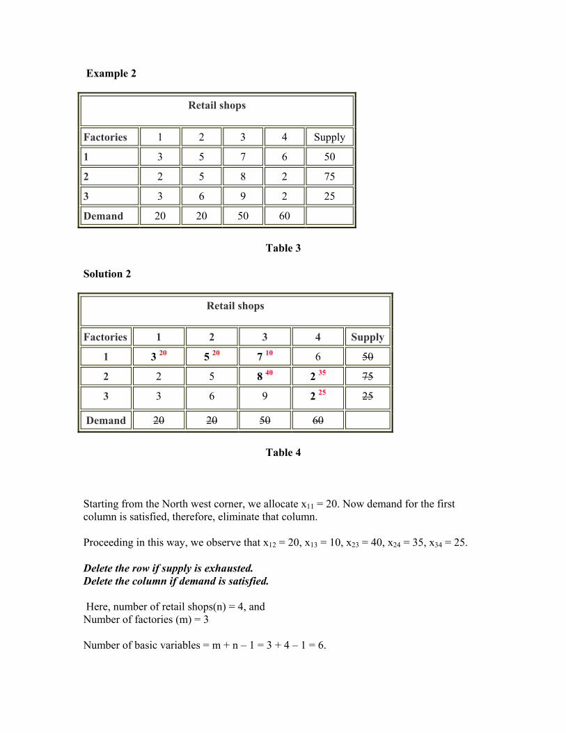
Example 2
Retail shops
Factories 1 2 3 4 Supply
1 3 5 7 6 50
2 2 5 8 2 75
3 3 6 9 2 25
Demand 20 20 50 60
Table 3
Solution 2
Retail shops
Factories 1 2 3 4 Supply
1 3 20 5 20 7 10 6 50
2 2 5 8 40 2 35 75
3 3 6 9 2 25 25
Demand 20 20 50 60
Table 4
Starting from the North west corner, we allocate x11 = 20. Now demand for the first column is satisfied, therefore, eliminate that column.
Proceeding in this way, we observe that x12 = 20, x13 = 10, x23 = 40, x24 = 35, x34 = 25.
Delete the row if supply is exhausted. Delete the column if demand is satisfied.
Here, number of retail shops(n) = 4, and Number of factories (m) = 3
Number of basic variables = m + n – 1 = 3 + 4 – 1 = 6.

Initial basic feasible solution:
20 * 3 + 20 * 5 + 10 * 7 + 40 * 8 + 35 * 2 + 25 * 2 = 670
2. Minimum Matrix Method (MMM)
Matrix minimum method is a method for computing a basic feasible solution of a transportation problem where the basic variables are chosen according to the unit cost of transportation.
Steps
1. Identify the box having minimum unit transportation cost (cij). 2. If there are two or more minimum costs, select the row and the column
corresponding to the lower numbered row. 3. If they appear in the same row, select the lower numbered column. 4. Choose the value of the corresponding xij as much as possible subject to the
capacity and requirement constraints. 5. If demand is satisfied, delete the column . 6. If supply is exhausted, delete the row. 7. Repeat steps 1-6 until all restrictions are satisfied.
Example 3
Retail shops
Factories 1 2 3 4 Supply
1 3 5 7 6 50
2 2 5 8 2 75
3 3 6 9 2 25
Demand 20 20 50 60

Table 5
Solution 3
Retail shops
Factories 1 2 3 4 Supply
1 3 5 20 7 30 6 50
2 2 20 5 8 2 55 75
3 3 6 9 20 2 5 25
Demand 20 20 50 60
Table 6
We observe that c21 =2, which is the minimum transportation cost. So, x21 = 20.
Proceeding in this way, we observe that x24 = 55, x34 = 5, x12 = 20, x13 = 30, x33 = 20.
Number of basic variables = m + n –1 = 3 + 4 – 1 = 6.
The initial basic feasible solution:
20 * 2 + 55 * 2 + 5 * 2 + 20 * 5 + 30 * 7 + 20 * 9 = 650.
3.Vogel’s Approximation Method (VAM)
The Vogel approximation method is an iterative procedure for computing a basic feasible solution of the transportation problem.
Steps
1. Identify the boxes having minimum and next to minimum transportation cost in each row and write the difference (penalty) along the side of the table against the corresponding row.

2. Identify the boxes having minimum and next to minimum transportation cost in each column and write the difference (penalty) against the corresponding column
3. Identify the maximum penalty. If it is along the side of the table, make maximum allotment to the box having minimum cost of transportation in that row. If it is below the table, make maximum allotment to the box having minimum cost of transportation in that column.
4. If the penalties corresponding to two or more rows or columns are equal, select the top most row and the extreme left column.
Example 4
Consider the transportation problem presented in table7 :
Destination
Origin 1 2 3 4 Supply
1 20 22 17 4 120
2 24 37 9 7 70
3 32 37 20 15 50
Demand 60 40 30 110 240
Table 7

Solution 4
Destination
Origin 1 2 3 4 Supply Penalty
1 20 22 40 17 4 120 80 13
2 24 37 9 7 70 2
3 32 37 20 15 50 5
Demand 60 40 30 110 240
Penalty 4 15 8 3
Table 8
The highest penalty occurs in the second column. The minimum cij in this column is c12 (i.e., 22). Hence, x12 = 40 and the second column is eliminated.
Now again calculate the penalty
Destination
Origin 1 2 3 4 Supply Penalty
1 20 22 40 17 4 80 120 13
2 24 37 9 7 70 2
3 32 37 20 15 50 5
Demand 60 40 30 110 240
Penalty 4 - 8 3
Table 9
The highest penalty occurs in the first row. The minimum cij in this row is c14 (i.e., 4). So x14 = 80 and the first row is eliminated.

Final table
Now we are assuming that you can calculate the values yourself.
Destination
Origin 1 2 3 4 Supply Penalty
1 20 22 40 17 4 80 120 3 13 - - - -
2 24 10
37 9 30 7 30 70 2 2 2 17 24 24
3 32 50
37 20 15 50 5 5 5 17 32 -
Demand 60 40 30 110 240
4 15 8 3
4 - 8 3
8 - 11 8
8 - - 8
8 - - -
Penalty
24 - - -
Table 10
The initial basic feasible solution:
22 * 40 + 4 * 80 + 24 * 10 + 9 * 30 + 7 * 30 + 32 * 50 = 3520

Unit 1 Lesson 16: Test for Optimal solution to a
Transportation Problem Learning Objective:
Test for Optimality
• Stepping Stone Method
Before learning the methods to find the optimal solution try and practice few more questions to find the initial solution of the transportation problem.
Question1
Find the initial basic feasible solution to the following transportation problem using 1)North west corner rule (NWCR) 2)Matrix Minima Method (MMM) 3)Vogel’s Approximation Method (VAM)
Retail shops
Factories 1 2 3 4 Supply
1 11 13 17 14 250
2 16 18 14 10 300
3 21 24 13 10 400
Demand 200 275 275 250

Example 2
Find the initial basic feasible solution to the following transportation problem using 1)North west corner rule (NWCR) 2)Matrix Minima Method (MMM) 3)Vogel’s Approximation Method (VAM)
Destination
Origin 1 2 3 4 Supply
1 1 2 3 4 6
2 4 3 2 0 8
3 0 2 2 1 10
Demand 4 6 8 6 24
Test for Optimality Once the initial feasible solution is reached, the next step is to check the optimality. An optimal solution is one where there is no other set of transportation routes (allocations) that will further reduce the total transportation cost. Thus, we’ll have to evaluate each unoccupied cell (represents unused routes) in the transportation table in terms of an opportunity of reducing total transportation cost. 1.Stepping Stone Method It is a method for computing optimum solution of a transportation problem.
Steps
Step 1
Determine an initial basic feasible solution using any one of the following:

• North West Corner Rule • Matrix Minimum Method • Vogel Approximation Method
Step 2
Make sure that the number of occupied cells is exactly equal to m+n-1, where m is the number of rows and n is the number of columns.
Step 3
Select an unoccupied cell.
Step 4
Beginning at this cell, trace a closed path using the most direct route through at least three occupied cells used in a solution and then back to the original occupied cell and moving with only horizontal and vertical moves. The cells at the turning points are called "Stepping Stones" on the path.
Step 5
Assign plus (+) and minus (-) signs alternatively on each corner cell of the closed path just traced, starting with the plus sign at unoccupied cell to be evaluated.
Step 6
Compute the net change in the cost along the closed path by adding together the unit cost figures found in each cell containing a plus sign and then subtracting the unit costs in each square containing the minus sign.
Step 7
Check the sign of each of the net changes. If all the net changes computed are greater than or equal to zero, an optimum solution has been reached. If not, it is possible to improve the current solution and decrease the total transportation cost.
Step 8
Select the unoccupied cell having the most negative net cost change and determine the maximum number of units that can be assigned to a cell marked with a minus sign on the closed path corresponding to this cell. Add this number to the unoccupied cell and to all other cells on the path marked with a plus sign. Subtract this number from cells on the closed path marked with a minus sign.

Step 9
Repeat the procedure until you get an optimum solution.
Example 3
Consider the following transportation problem (cost in rupees). Find the optimum solution
Depot
Factory D E F G Capacity
A 4 6 8 6 700
B 3 5 2 5 400
C 3 9 6 5 600
Requirement 400 450 350 500 1700
Solution:
First, find out an initial basic feasible solution by Matrix Minimum Method
Depot
Factory D E F G Capacity
A 4 6 450 8 6 250 700
B 3 50 5 2 350 5 400
C 3 350 9 6 5 250 600
Requirement 400 450 350 500 1700

Here, m + n - 1 = 6. So the solution is not degenerate.
The cell AD (4) is empty so allocate one unit to it. Now draw a closed path from AD.
Depot
Factory D E F G Capacity
A 4 +1 6 450 8 6 249 700
B 3 50 5 2 350 5 400
C 3 349 9 6 5 251 600
Requirement 400 450 350 500 1700
Please note that the right angle turn in this path is permitted only at occupied cells and at the original unoccupied cell.
The increase in the transportation cost per unit quantity of reallocation is +4 – 6 + 5 – 3 = 0.
This indicates that every unit allocated to route AD will neither increase nor decrease the transportation cost. Thus, such a reallocation is unnecessary.
Choose another unoccupied cell. The cell BE is empty so allocate one unit to it. Now draw a closed path from BE
Depot
Factory D E F G Capacity
A 4 6 449 8 6 251 700
B 3 49 5+1 2 350 5 400
C 3 351 9 6 5 249 600
Requirement 400 450 350 500 1700

The increase in the transportation cost per unit quantity of reallocation is +5 – 6 + 6 – 5 + 3 – 3 = 0
This indicates that every unit allocated to route BE will neither increase nor decrease the transportation cost. Thus, such a reallocation is unnecessary.
The allocations for other unoccupied cells are:
Unoccupied cells
Increase in cost per unit of reallocation
Remarks
CE +9 – 6 + 6 – 5 = 4 Cost Increases
CF +6 – 3 + 3 – 2 = 4 Cost Increases
AF +8 – 6 +5 – 3 + 3 – 2 = 5 Cost Increases
BG +5 – 5 + 3 – 3 = 0 Neither increase nor decrease
Since all the values of unoccupied cells are greater than or equal to zero, the solution obtained is optimum.
Minimum transportation cost is: 6 * 450 + 6 * 250 + 3 * 250 + 2 * 250 +3 *350 +5 * 250 = Rs. 7350
Example 4
A company has factories at A,B and C which supply warehouse at D,E and F. Weekly factory capacities are 200, 160 and 90 units respectively. Weekly Warehouse requirement are 180, 120 and 150 units respt.. Unit shipping costs (in rupees)are as follows.
Factory D E F Capacity
A 16 20 12 200
B 14 8 18 160
C 26 24 16 90
Requirement 180 120 150 450

Determine the optimum distribution for this company to minimize shipping cost.
Solution:
First, find out an initial basic feasible solution by Vogel’s approximation Method
Factory D E F Capacity
A 16 140 20 12 60 200
B 14 40 8 120 18 160
C 26 24 16 90 90
Requirement 180 120 150 450
Here, m + n - 1 = 5 So the solution is not degenerate.
The cell AE (20) is empty so allocate one unit to it. Now draw a closed path from AD.
Factory D E F Capacity
A 16 139 20 +1 12 60 200
B 14 41 8 119 18 160
C 26 24 16 90 90
Requirement 180 120 150 450
The increase in the transportation cost per unit quantity of reallocation is +20 – 8 + 14 – 16 = 10.
This indicates that every unit allocated to route AD will increase the transportation cost by Rs.10. Thus, such a reallocation is not included.
Choose another unoccupied cell. The cell BF is empty so allocate one unit to it. Now draw a closed path from BE

Factory D E F Capacity
A 16 141 20 12 59 200
B 14 39 8 120 18 +1 160
C 26 24 16 90 90
Requirement 180 120 150 450
The opportunity cost in the transportation cost per unit quantity of
reallocation is +18 – 12 + 16 – 14 = 8
This indicates that every unit allocated to route BE will increase the transportation cost by Rs. 8. Thus, such a reallocation is not included.
The allocations for other unoccupied cells are:
Unoccupied cells
Increase in cost per unit of reallocation
Remarks
CD +26 – 16 + 12 – 16 = 6 Cost Increases
CE +24 – 16 + 12 – 16 +14 – 8= 10 Cost Increases
Since all the values of unoccupied cells are greater than zero, the solution obtained is optimum.
Minimum transportation cost is: 16 * 140 + 12 * 60 + 14 * 40 + 8 * 120 +16 *90 = Rs. 5,920
Example 5 Maruti Udyog Limited (MUL) produces & sells cars. It has two warehouses (A, B) and three whole sellers (1,2,3). The status at present in the warehouses is as follows:
Warehouse Cars
40 60
A B
Total 100

The wholesalers have placed the following order from the month: Whole seller Demand (Cars) 1 2 3
20 30 40
The transportation charges (in shipping from warehouse to the whole seller) are given below: Warehouse
Whole sellers (Costs in Rs. ‘000)
A B
2 4 3 5 2 4
Your are required to determine the optimal number of cars to be shipped for each warehouse to each whole seller so as to minimize the total transportation costs. Example 6. Good Manufactures Limited has 3 warehouses (A, B, C) AND FOUR STORES (W, X, Y, Z). For a particular product, there is a surplus of 150 units at all the warehouse taken together, as given below:
Warehouse Units of product A B C
50 60 40
Total 150 The transportation costs of shipping one unit of the product from warehouses to stories is given below:
Stores Warehouse
Costs (in Rs)
A B C
W 50 80 15
X 150 70 87
Y 70 90 79
Z 60 10 81
The monthly requirement of the stores is as follows:
Store Requirement (of product)
W X Y
20 70 50
Z 10 You are required to obtain the optimal solution to the given transportation problem.

Unit 1 Lesson 17: Test for optimal solution to a transportation Problem Learning Objective:
Test for Optimality
• Modified Distribution Method (MODI)
Modified Distribution Method (MODI)
It is a method for computing optimum solution of a transportation problem.
STEPS
Step 1
Determine an initial basic feasible solution using any one of the three methods given below:
• North West Corner Rule • Matrix Minimum Method • Vogel Approximation Method
Step 2
Determine the values of dual variables, ui and vj, using ui + vj = cij
Step 3
Compute the opportunity cost using cij – ( ui + vj ).
Step 4

Check the sign of each opportunity cost. If the opportunity costs of all the unoccupied cells are either positive or zero, the given solution is the optimum solution. On the other hand, if one or more unoccupied cell has negative opportunity cost, the given solution is not an optimum solution and further savings in transportation cost are possible.
Step 5
Select the unoccupied cell with the smallest negative opportunity cost as the cell to be included in the next solution.
Step 6
Draw a closed path or loop for the unoccupied cell selected in the previous step. Please note that the right angle turn in this path is permitted only at occupied cells and at the original unoccupied cell.
Step 7
Assign alternate plus and minus signs at the unoccupied cells on the corner points of the closed path with a plus sign at the cell being evaluated.
Step 8
Determine the maximum number of units that should be shipped to this unoccupied cell. The smallest value with a negative position on the closed path indicates the number of units that can be shipped to the entering cell. Now, add this quantity to all the cells on the corner points of the closed path marked with plus signs and subtract it from those cells marked with minus signs. In this way an unoccupied cell becomes an occupied cell.
Step 9 Repeat the whole procedure until an optimum solution is obtained.
Example 1 A company is spending Rs. 1000 on transportation of its units from these plants to four distribution centers. The supply and requirement of units, with unity cost of transportation are given as:
Distribution centres
D1 D2 D3 D4 Supply
P1 19 30 50 12 7 Plants
P2 70 30 40 60 10

P3 40 10 60 20 18
Requirement 5 8 7 15
Determine the optimum solution of the above problem.
Solution:
Now, solve the above problem by Matrix Minimum Method.
Distribution centres
D1 D2 D3 D4 Supply
P1 19 30 50 12 7 7
P2 70 3 30 40 7 60 10 Plants
P3 40 2 10 8 60 20 8 18
Requirement 5 8 7 15
The solution is basic feasible as there are m + n – 1, i.e., 4 + 3 – 1 = 6 allocations in independent solutions.
Initial basic feasible solution: 12 * 7 + 70 * 3 + 40 * 7 + 40 * 2 + 10 * 8 + 20 * 8 = Rs. 894. Calculating ui and vj using ui + vj = cij
Substituting u1 = 0, we get
u1 + v4 = c14 ⇒ 0 + v4 = 12 or v4 = 12 u2 + v4 = c24⇒u2 + 12 = 60 or u2 = 38 u2 + v3 = c23 ⇒ 38 + v3 = 40 or v3 = 2 u3 + v4 = c34 ⇒ u3 + 12 = 20 or u3 = 8 u3 + v2 = c32 ⇒8 + v2 = 10 or v2 = 2 u3 + v1 = c31 ⇒ 8 + v1 = 40 or v1 = 32

Distribution centres
D1 D2 D3 D4 Supply ui
P1 19 30 50 12 7 7 0
P2 70 3 30 40 7 60 10 38 Plants
P3 40 2 10 8 60 20 8 18 8
Requirement 5 8 7 15
vj 32 2 2 12
Calculating opportunity cost using cij – ( ui + vj )
Unoccupied cells Opportunity cost
(P1, D1) C11 – ( u1 + v1 ) = 19 – (0 + 32) = –13
(P1, D2) C12 – ( u1 + v2 ) = 30 – (0 + 2) = 28
(P1, D3) C13 – ( u1 + v3 ) = 50 – (0 + 2) = 48
(P2, D2) C22 – ( u2 + v2 ) = 30 – (38 + 2) = –10
(P2, D4) C14 – ( u2 + v4 ) = 60 – (38 + 12) = 10
(P3, D3) C33 – ( u3 + v3 ) = 60 – (8 + 2) = 50
Distribution centres
D1 D2 D3 D4 Supply ui
P1 –13 19 28 30 48 50 12 7 7 0
P2 70 3 –10 30 40 7 10 60 10 38 Plants
P3 40 2 10 8 50 60 20 8 18 8

Requirement 5 8 7 15
vj 32 2 2 12
Distribution centres
D1 D2 D3 D4 Supply ui
P1 –13 19+ 28 30 48 50 12 7_ 7 0
P2 70 3 –10 30 40 7 10 60 10 38 Plants
P3 40 2 _ 10 8 50 60 20 8+ 18 8
Requirement 5 8 7 15
vj 32 2 2 12
Choose the smallest negative value from opportunity cost (i.e., –13). Now draw a closed path from P1D1 .
Choose the smallest value with a negative position on the closed path(i.e., 2), it indicates the number of units that can be shipped to the entering cell. Now, add this quantity to all the cells on the corner points of the closed path marked with plus signs and subtract it from those cells marked with minus signs. In this way an unoccupied cell becomes an occupied cell.
Now again calculate the values for ui and vj.
Distribution centres
D1 D2 D3 D4 Supply ui
P1 19 2 28 30 61 50 12 5 7 0
P2 70 3 –23 30 40 7 –3 60 10 51 Plants
P3 13 40 10 8 63 60 20 10 18 8
Requirement 5 8 7 15
vj 19 2 –11 12
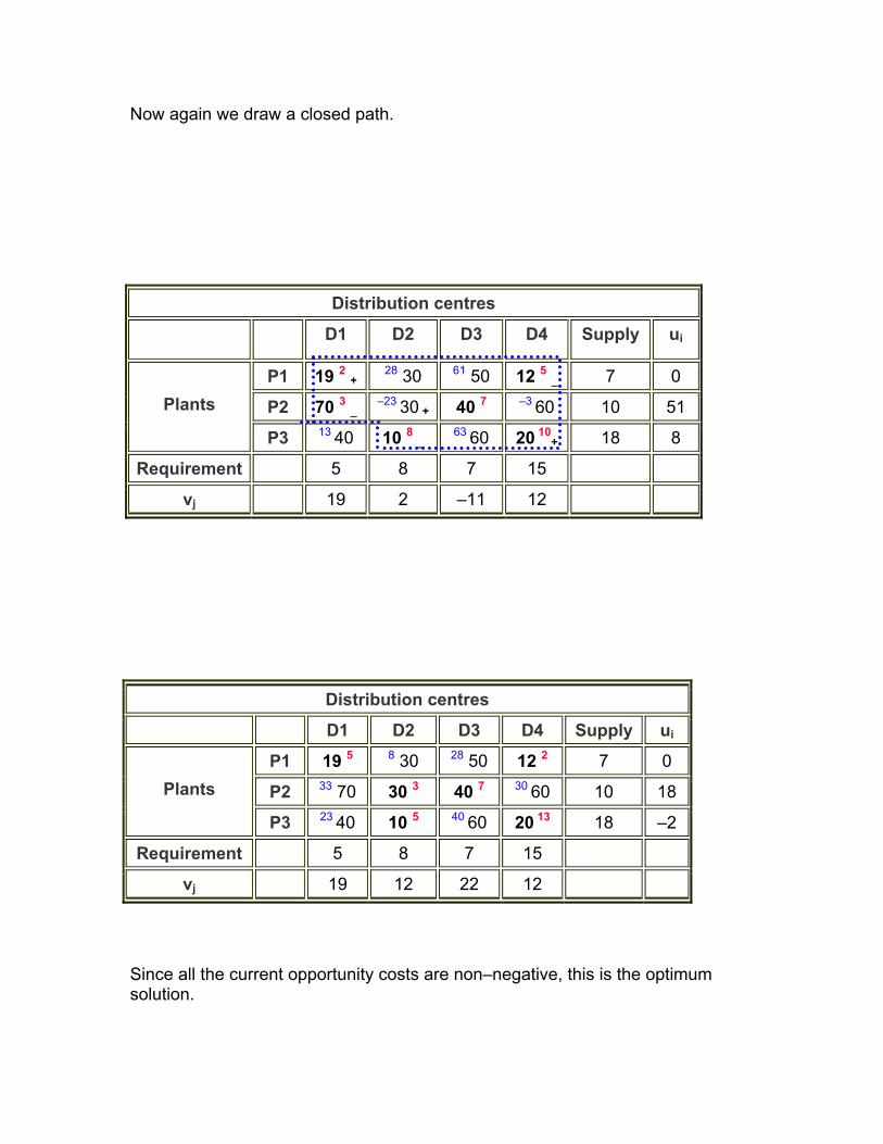
Now again we draw a closed path.
Distribution centres
D1 D2 D3 D4 Supply ui
P1 19 2 + 28 30 61 50 12 5 _ 7 0
P2 70 3 _ –23 30 + 40 7 –3 60 10 51 Plants
P3 13 40 10 8 _ 63 60 20 10
+ 18 8
Requirement 5 8 7 15
vj 19 2 –11 12
Distribution centres
D1 D2 D3 D4 Supply ui
P1 19 5 8 30 28 50 12 2 7 0
P2 33 70 30 3 40 7 30 60 10 18 Plants
P3 23 40 10 5 40 60 20 13 18 –2
Requirement 5 8 7 15
vj 19 12 22 12
Since all the current opportunity costs are non–negative, this is the optimum solution.

So the minimum transportation cost is: 19 * 5 + 12 * 2 + 30 * 3 + 40 * 7 + 10 * 5 + 20 * 13 = Rs. 799
Example 2 Given below are the costs of shipping a product from various
warehouses to different stores: Warehouses Stores (costs in rupees) Supply
A B C D
1 7 5 8 6
2 3 5 6 1
3 5 7 6 6
4 5 6 5 4
34 15 12 19
Demand 21 25 17 17 80 Generate an initial feasible solution & check it for optimality. Try yourself Example 3 Alpha Ltd. has 3 factories (A, B, C) & warehouses (P, Q, R, S). It supplies the finished goods from each of its three factories to the four warehouses, the relevant shipping cost of which are as follows:
↓
Warehouse
Factory→ A B C
P Q R S
4 5 2 5
3 8 4 8
7 4 7 4
Assuming the monthly production capacity of A, B & C to be 120, 80 & 200 tons respectively, determine the optimum transportation schedule so as to minimize the total transportation costs by using Vogel’s method. (The monthly requirements for the warehouses are as follows:
Warehouse Monthly requirement (tons)
60 50
140 50
P Q R S
Total 300 (tons) Try yourself

Example 4. A company has three factories and five warehouses, where the finished goods are shipped from the factories. The following relevant details are provided to you: - Warehouses→
Factory ↓
(Costs in Rs.)
1 2 3
Requirement
1 3 5 2 10
2 5 4 5 15
3 8 10 8 25
4 9 7 7 30
5 11 10 5 40
Availability 20 40 30 120/90
Solve the above transportation problem.
Try yourself Example 5. Consider the following network representation of a transportation problem. 14 25 30 9 7 15 8 10 20 5 10
Jefferson city
St. Louis
Des Moines
Kansas city
Omaha
Supplies Demands The supply, demand and transportation costs per units are shown on the network.
a. Develop a Transportation model for this problem.

b. Solve the Transportation model to determine the optimal solution. Try yourself


Unit 1
Lecture 18 Special cases in Transportation Problems
Learning Objectives:
Special cases in Transportation Problems
Multiple Optimum Solution Unbalanced Transportation Problem Degeneracy in the Transportation Problem Miximisation in a Transportation Problem
Special cases Some variations that often arise while solving the transportation problem could be as follows :
1.Multiple Optimum Solution 2.Unbalanced Transportation Problem
3.Degeneracy in the Transportation Problem 1.Multiple Optimum Solution This problem occurs when there are more than one optimal solutions. This would be indicated when more than one unoccupied cell have zero value for the net cost change in the optimal solution. Thus a reallocation to cell having a net cost change equal to zero will have no effect on transportation cost. This reallocation will provide another solution with same transportation cost, but the route employed will be different from those for the original optimal solution. This is important because they provide management with added flexibility in decision making.
1

2.Unbalanced Transportation Problem If the total supply is not equal to the total demand then the problem is known as unbalanced transportation problem. If the total supply is more than the total demand, we introduce an additional column, which will indicate the surplus supply with transportation cost zero. Similarly, if the total demand is more than the total supply, an additional row is introduced in the table, which represents unsatisfied demand with transportation cost zero.
Example1
Warehouses
Plant W1 W2 W3 Supply
A 28 17 26 500
B 19 12 16 300
Demand 250 250 500
Solution:
The total demand is 1000, whereas the total supply is 800. Total demand > total supply. So, introduce an additional row with transportation cost zero indicating the unsatisfied demand.
Warehouses
Plant W1 W2 W3 Supply
A 28 17 26 500
B 19 12 16 300
Unsatisfied demand 0 0 0 200
Demand 250 250 500 1000
2
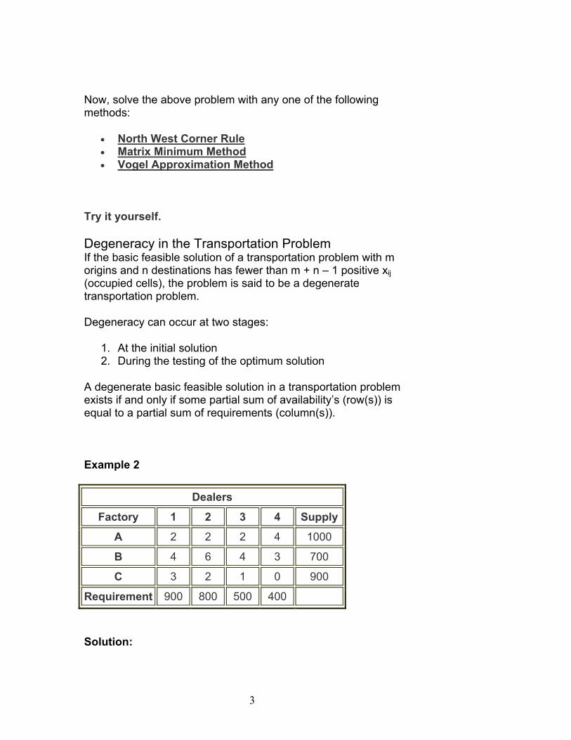
Now, solve the above problem with any one of the following methods:
• North West Corner Rule • Matrix Minimum Method • Vogel Approximation Method
Try it yourself.
Degeneracy in the Transportation Problem If the basic feasible solution of a transportation problem with m origins and n destinations has fewer than m + n – 1 positive xij (occupied cells), the problem is said to be a degenerate transportation problem.
Degeneracy can occur at two stages:
1. At the initial solution 2. During the testing of the optimum solution
A degenerate basic feasible solution in a transportation problem exists if and only if some partial sum of availability’s (row(s)) is equal to a partial sum of requirements (column(s)).
Example 2
Dealers
Factory 1 2 3 4 Supply
A 2 2 2 4 1000
B 4 6 4 3 700
C 3 2 1 0 900
Requirement 900 800 500 400
Solution:
3

Here, S1 = 1000, S2 = 700, S3 = 900 R1 = 900, R2 = 800, R3 = 500, R4 = 400
Since R3 + R4 = S3 so the given problem is a degeneracy problem.
Now we will solve the transportation problem by Matrix Minimum Method.
To resolve degeneracy, we make use of an artificial quantity(d). The quantity d is so small that it does not affect the supply and demand constraints.
Degeneracy can be avoided if we ensure that no partial sum of si (supply) and rj (requirement) are the same. We set up a new problem where:
si = si + d i = 1, 2, ....., m rj = rj rn = rn + md
Dealers
Factory 1 2 3 4 Supply
A 2 900 2 100+d 2 4 1000 +d
B 4 6 700–d 4 2d 3 700 + d
C 3 2 1 500 –2d 0 400+3d 900 +d
Requirement 900 800 500 400 + 3d
Substituting d = 0.
Dealers
Factory 1 2 3 4 Supply
A 2 900 2 100 2 4 1000
B 4 6 700 4 0 3 700
C 3 2 1 500 0 400 900
Requirement 900 800 500 400 + 3d
4

Initial basic feasible solution:
2 * 900 + 2 * 100 + 6 * 700 + 4 * 0 + 1 * 500 + 0 * 400 = 6700.
Now degeneracy has been removed.
To find the optimum solution, you can use any one of the following:
• Stepping Stone Method. • MODI Method.
Miximisation in a Transportation Problem Although transportation model is used to minimize transportation cost. However it can also be used to get a solution with an objective of maximizing the total value or returns. Since the criterion of optimality is maximization, the converse of the rule for minimization will be used. The rule is : A solution is optimal if all – opportunity costs dij for the unoccupied cell are zero or negative. Let us take an example for this:
Example 3
A firm has three factories X, Y and Z. It supplies goods to four dealers spread all over the country. The production capacities of these factories are 200, 500 and 300 per month respectively.
Factory A B C D Capacity
X 12 18 6 25 200
Y 8 7 10 18 500
Z 14 3 11 20 300
Demand 180 320 100 400
5

Determine suitable allocation to maximize the total net return.
Solution:
Maximization transportation problem can be converted into minimization transportation problem by subtracting each transportation cost from maximum transportation cost.
Here, the maximum transportation cost is 25. So subtract each value from 25.
Factory A B C D Capacity
X 13 7 19 0 200
Y 17 18 15 7 500
Z 11 22 14 5 300
Demand 180 320 100 400
Now, solve the above problem by first finding initial solution any one of the following methods:
• North West Corner Rule • Matrix Minimum Method • Vogel Approximation Method
Then , testing the initial solution for optimality using either
• Stepping stone method or • MODI method
6

Example 4. A product is produced at three plants and shipped to three warehouses (the transportation costs per unit are shown in the following table.)
Warehouse Plant W1 W2 W3 Plant capacity P1 P2 P3 Warehouse demand
20 10 12 200
16 10 18 400
24 8 10 300
300 500 100
a) Show a network representation of the problem. b) Solve this model to determine the minimum cost solution.
c) c. Suppose that the entries in the table represent profit per
unit produced at plant I and sold to warehouse j. How does the solution change from that in part (b) ?
Try it yourself.
Example 5. Tri-county utilities, Inc.., supplies natural gas to customers in a three country area. The company purchases natural gas form two companies. Southern gas and Northwest Gas. Demand forecasts for the coming winter season are Hamilton county, 400 units; Butler county, 200 units: and Clermont county. 300 units. Contracts to provide the following quantities have been written. South Gas, 500 units; and Northwest Gas, 400 units, Distribution costs for the counties vary, depending upon the location of the suppliers. The distribution costs per unit (in thousands of dollars) are as follows:
7

To From Hamilton Butler Clermont Southern Gas Northwest Gas
10 12
20 15
15 18
a. Develop a network representation of this problem. b. Describe the distribution plan and show the total distribution
cost.
c. Recent residential and industrial growth in Butter county has
the potential for increasing demand by as much as 100 units. Which supplier should Tri- county contract with to supply the additional capacity?
Try it yourself.
8

Unit 1
Lesson 19: Assignment problem
Learning Objective :
• Recognize an Assignment problem. • Convert an assignment problem into a transportation problem. • State assignment problem in LP form.
Introduction
In the world of trade Business Organisations are confronting the conflicting need for optimal utilization of their limited resources among competing activities. When the information available on resources and relationship between variables is known we can use LP very reliably. The course of action chosen will invariably lead to optimal or nearly optimal results. The problems which gained much importance under LP are :
Transportation problems (discussed in the previous chapter)
Assignment problems (covered under this chapter)
The assignment problem is a special case of transportation problem in which the objective is to assign a number of origins to the equal number of destinations at the minimum cost(or maximum profit). Assignment problem is one of the special cases of the transportation problem. It involves assignment of people to projects, jobs to machines, workers to jobs and teachers to classes etc., while minimizing the total assignment costs. One of the important characteristics of assignment problem is that only one job (or worker) is assigned to one machine (or project). Hence the number of sources are equal the number of destinations and each requirement and capacity value is exactly one unit.
1
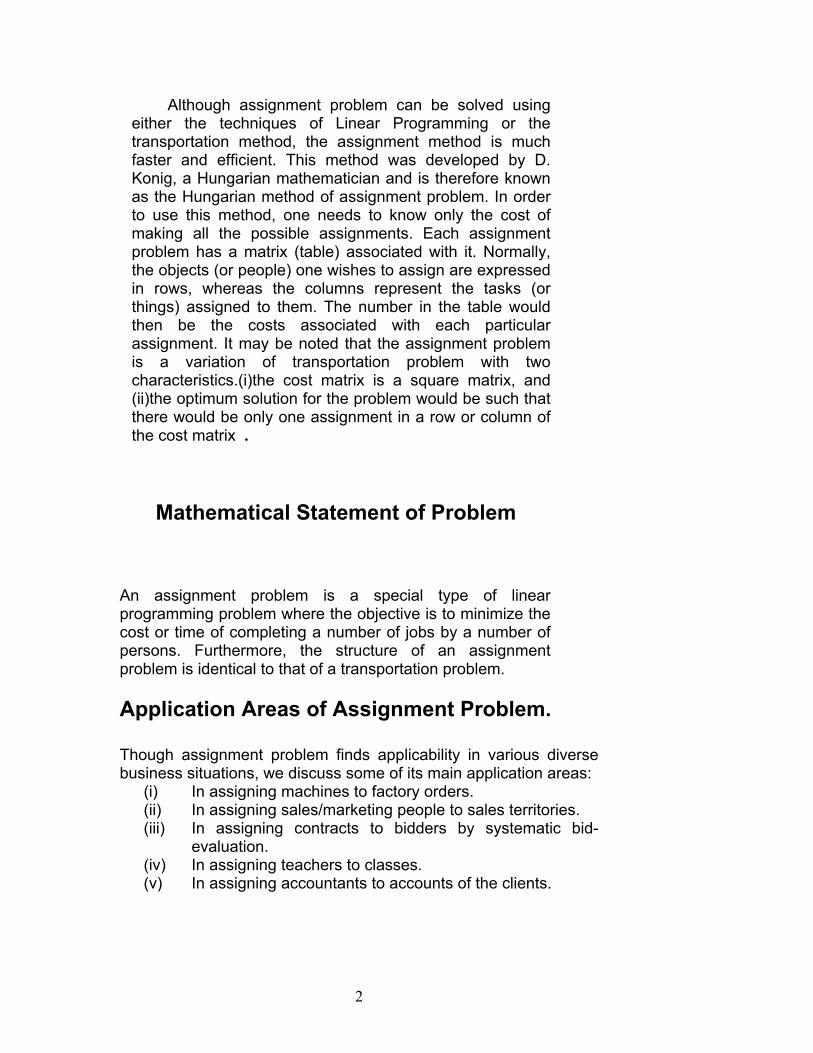
Although assignment problem can be solved using either the techniques of Linear Programming or the transportation method, the assignment method is much faster and efficient. This method was developed by D. Konig, a Hungarian mathematician and is therefore known as the Hungarian method of assignment problem. In order to use this method, one needs to know only the cost of making all the possible assignments. Each assignment problem has a matrix (table) associated with it. Normally, the objects (or people) one wishes to assign are expressed in rows, whereas the columns represent the tasks (or things) assigned to them. The number in the table would then be the costs associated with each particular assignment. It may be noted that the assignment problem is a variation of transportation problem with two characteristics.(i)the cost matrix is a square matrix, and (ii)the optimum solution for the problem would be such that there would be only one assignment in a row or column of the cost matrix .
Mathematical Statement of Problem
An assignment problem is a special type of linear programming problem where the objective is to minimize the cost or time of completing a number of jobs by a number of persons. Furthermore, the structure of an assignment problem is identical to that of a transportation problem.
Application Areas of Assignment Problem. Though assignment problem finds applicability in various diverse business situations, we discuss some of its main application areas:
(i) In assigning machines to factory orders. (ii) In assigning sales/marketing people to sales territories. (iii) In assigning contracts to bidders by systematic bid-
evaluation. (iv) In assigning teachers to classes. (v) In assigning accountants to accounts of the clients.
2

In assigning police vehicles to patrolling areas.
Jobs Persons j1 j2 ------ jn
I1 X11 X12 ----- X1n I2 X21 X22 ----- X2n --- ----- ---- ----- ----- In ----- ---- ----- Xnn
Cij is the cost of performing jth job by ith worker. Xij is the number ith individual assigned to jth job.
Total cost = X11 * C11 + X12 * C12 + ----- + Xnn * Cnn.
Mathematically the assignment problem can be expressed as
The objective function is Minimize C11X11 + C12X12 + ------- + CnnXnn.
This can also be written as:
n n Z = ∑ ∑ Cij
Xij i=1 j=1
Subject to the constraints n ∑ Xij = 1 for all i (resourse availability) j=1
n ∑ Xij = 1 for all i (activity requirement) i=1
and Xij = 0 or 1, for all i to activity j.
Solution Methods
The assignment problem can be solved by the following four methods :
3

Enumeration method Simplex method Transportation method Hungarian method
1. Enumeration method
In this method, a list of all possible assignments among the given resources and activities is prepared. Then an assignment involving the minimum cost, time or distance or maximum profits is selected. If two or more assignments have the same minimum cost, time or distance, the problem has multiple optimal solutions. This method can be used only if the number of assignments is less. It becomes unsuitable for manual calculations if number of assignments is large
2. Simplex method
As discussed in chapter no. 2
3. Transportation method
As assignment is a special case of transportation problem it can also be solved using transportation model discussed in previous chapter. But the degeneracy problem of solution makes the transportation method computationally inefficient for solving the assignment problem.
4.Hungarian method
Algorithms for Solving
4

There are various ways to solve assignment problems. Certainly it can be formulated as a linear program (as we saw above), and the simplex method can be used to solve it. In addition, since it can be formulated as a network problem, the network simplex method may solve it quickly.
However, sometimes the simplex method is inefficient for assignment problems (particularly problems with a high degree of degeneracy). The Hungarian Algorithm developed by Kuhn has been used with a good deal of success on these problems and is summarized as follows.
Step 1. Determine the cost table from the given problem.
(i) If the no. of sources is equal to no. of destinations, go to step 3.
(ii) If the no. of sources is not equal to the no. of destination, go to step2.
Step 2. Add a dummy source or dummy destination, so that the cost table becomes a square matrix. The cost entries of the dummy source/destinations are always zero.
Step 3. Locate the smallest element in each row of the given cost matrix and then subtract the same from each element of the row.
Step 4. In the reduced matrix obtained in the step 3, locate the smallest element of each column and then subtract the same from each element of that column. Each column and row now have at least one zero.
Step 5. In the modified matrix obtained in the step 4, search for the optimal assignment as follows:
(a) Examine the rows successively until a row with a single zero is found. Enrectangle this row ( )and cross off (X) all other zeros in its column. Continue in this manner until all the rows have been taken care of.
(b) Repeat the procedure for each column of the reduced matrix. (c) If a row and/or column has two or more zeros and one cannot
be chosen by inspection then assign arbitrary any one of these zeros and cross off all other zeros of that row / column.
(d) Repeat (a) through (c) above successively until the chain of assigning ( ) or cross (X) ends.
5

Step 6. If the number of assignment ( ) is equal to n (the order of the cost matrix), an optimum solution is reached.
If the number of assignment is less than n(the order of the matrix), go to the next step.
Step7. Draw the minimum number of horizontal and/or vertical lines to cover all the zeros of the reduced matrix.
Step 8. Develop the new revised cost matrix as follows:
(a)Find the smallest element of the reduced matrix not covered by any of the lines.
(b)Subtract this element from all uncovered elements and add the same to all the elements laying at the intersection of any two lines.
Step 9. Go to step 6 and repeat the procedure until an optimum solution is attained.
See diagrammatic Representation of Hungarian Approach
6

YES
CONVERT THE MATRIX INTO MINIMIZATION MATRIX BY SUBTRACTING ALL ELEMENTS OUT OF THE HIGHEST ELEMENT OF THE MATRIX
IS IT A BALNCED CASE ? ADD DUMMY COLUMNS OR
ROWS TO BALANCE IT.
YES
DRAW A COST MATRIX FOR THE PROBLEM
START
FIND THE OPPORTUNITY COST A. SUBSTRACT THE SMALLEST ELEMENT IN EACH
ROW FROM EVERY ELEMENT IN THAT ROW B. IN THE REDUCED MATRIX REPEAT THIS PROCESS
COLUMNWISE.
IS IT A CASE OF MAXIMISATION ?
MAKE ASSIGNMENTZERO & ELIMINATEASSIGNMENT IS MA REPEAT SAME PROC
IS THE NUMBER OF
ASSIGNMENTS EQUAL THE NUMBER OF
ROWS OR COLUMNS ?
7
NO
NO
ROWWISE HAVING ONLY ONE ROW AND COLUMN ONCE THE DE. ESS COLUMNWISE.
REVISE OPPORTUNITY COST TABLE a. DRAW MINIMUM POSSIBLE LINES
ON COLUMNS AND/OR ROWS SO AS TO COVER ALL ZEROS.
b. CHOOSE THE SMALLEST NUMBER
NO NOT COVERED BY THE LINES. SUBTRACT IT FROM ITSELF AND EVERY OTHER UNCOVERED NUMBER.c. ADD THIS NUMBER AT THE INTERSECTION OF ANY TWO LINES.
**THIS IS THE OPTIMUM SOLUTION **
YES

8

Unit 1
Lesson 20 :Solving Assignment problem
Learning objectives:
• Solve the assignment problem using Hungarian method. • Analyze special cases in assignment problems. Writing of an assignment problem as a Linear programming problem
Example 1. Three men are to to be given 3 jobs and it is assumed that a person is fully capable of doing a job independently. The following table gives an idea of that cost incurred to complete each job by each person: Jobs → Men ↓
J1 J2 J3 Supply
M1 M2 M3 Demand
20 15 8 1
28 35 32 1
21 17 20 1
1 1 1
Formulate as a Linear programming problem. Ans. The given problem can easily be formulated as a Linear Programming (transportation) model as under: Minimize Z = (20x11 + 28x12 + 21x13) + (15x21 + 35x22 + 17x23) (objective-function) + (18x31 + 32x32 + 20x33) 3 3
(it can also be written as: Minimise Z = Σ Σ CiJ x iJ
i = l J = 1 Subject to the following constraints:
1

x11 + x12 + x13 = 1
(i) x21 + x22 + x23 = 1 or xij = 1 where i = 1, 2,3 3
Σi = l
x31 + x32 + x33 = 1
(Since every person can be assigned only one job, therefore three constraint equation for three persons.) x11 + x21 + x31 = 1 (ii) x12 + x22 + x32 = 1 or xij = 1 where J = 1, 2, 3
3
Σj = l
x13 + x23 + x33 = 1 (Since each job can be assigned to only one person, therefore three equations for three different jobs)
1, if person I is assigned to job J (iii) xij = { 0, if person I is not assigned to job J ∵ ai = bJ = 1 ⇒ the given problem is just a special case of the transportation problem.
Problems based on Hungarian Method
Example 2 :
A job has four men available for work on four separate jobs. Only one man can work on any one job. The cost of assigning each man to each job is given in the following table. The objective is to assign men to jobs such that the total cost of assignment is minimum.
Jobs
Persons 1 2 3 4
A 20 25 22 28
B 15 18 23 17
C 19 17 21 24
D 25 23 24 24
2

Solution:
Step 1
Identify the minimum element in each row and subtract it from every element of that row.
Table
Jobs
Persons 1 2 3 4
A 0 5 2 8
B 0 3 8 2
C 2 0 4 7
D 2 0 1 1
Step 2
Identify the minimum element in each column and subtract it from every element of that column.
Table
Jobs
Persons 1 2 3 4
A 0 5 1 7
B 0 3 7 1
C 2 0 3 6
D 2 0 0 0
Step 3
Make the assignment for the reduced matrix obtain from steps 1 and 2 in the following way:
a. Examine the rows successively until a row with exactly one unmarked zero is found. Enclose this zero
3

in a box as an assignment will be made there and cross (X) all other zeros appearing in the corresponding column as they will not be considered for future assignment. Proceed in this way until all the rows have been examined.
b. After examining all the rows completely, examine the columns successively until a column with exactly one unmarked zero is found. Make an assignment to this single zero by putting square around it and cross out (X) all other assignments in that row, proceed in this manner until all columns have been examined.
c. Repeat the operations (a) and (b) successively until one of the following situations arises:
• All the zeros in rows/columns are either marked or crossed (X) and there is exactly one assignment in each row and in each column. In such a case optimum assignment policy for the given problem is obtained.
• There may be some row (or column) without assignment, i.e., the total number of marked zeros is less than the order of the matrix. In such a case proceed to next step 4.
Table
4

Step 4
Draw the minimum number of vertical and horizontal lines necessary to cover all the zeros in the reduced matrix obtained from step 3 by adopting the following procedure:
i. Mark all the rows that do not have assignments. ii. Mark all the columns (not already marked) which have
zeros in the marked rows. iii. Mark all the rows (not alreay marked) that have
assignmets in marked columns. iv. Repeat steps 4 (ii) and (iii) until no more rows or
columns can be marked. v. Draw straight lines through all unmarked rows and
columns.
You can also draw the minimum number of lines by inspection
Table
Step 5
Select the smallest element from all the uncovered elements. Subtract this smallest element from all the uncovered elements and add it to the elements, which lie at the intersection of two lines. Thus, we obtain another reduced matrix for fresh assignment.
5

Table
Jobs
Persons 1 2 3 4
A 0 4 0 6
B 0 2 6 0
C 3 0 3 6
D 3 0 0 0
Go to step 3 and repeat the procedure until you arrive at an optimum assignment.
Final Table
Since the number of assignments is equal to the number of rows (& columns), this is the optimal solution.
The total cost of assignment = A1 + B4 + C2 + D3
Substitute the values from original table: 20 + 17 + 24 + 17 = 78.
Example 3.
A departmental head has four subordinates, and four tasks to be performed. The subordinates differ in efficiency, and
6

the tasks differ in there intrinsic difficulty. His estimate, of the time each man would take to perform each task, is given the matrix below
Men
Persons 1 2 3 4
A 18 26 17 11
B 13 28 14 26
C 38 19 18 15
D 19 26 24 10
Solution:
Step 1
Identify the minimum element in each row and subtract it from every element of that row, we get the reduced matrix
Table
Men
Persons 1 2 3 4
A 7 15 6 0
B 0 15 1 13
C 23 4 3 0
D 9 16 14 0
Step 2
7
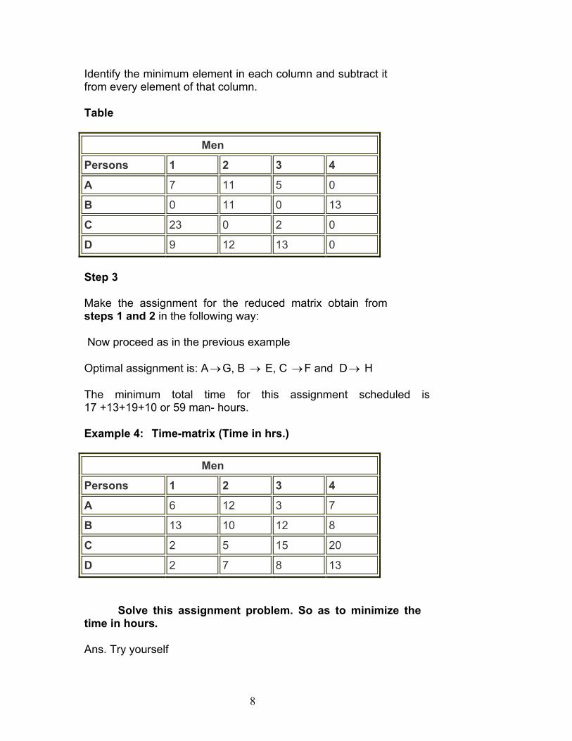
Identify the minimum element in each column and subtract it from every element of that column.
Table
Men
Persons 1 2 3 4
A 7 11 5 0
B 0 11 0 13
C 23 0 2 0
D 9 12 13 0
Step 3
Make the assignment for the reduced matrix obtain from steps 1 and 2 in the following way:
Now proceed as in the previous example
Optimal assignment is: A G, B → E, C →F and D→ H →
The minimum total time for this assignment scheduled is 17 +13+19+10 or 59 man- hours.
Example 4: Time-matrix (Time in hrs.)
Men
Persons 1 2 3 4
A 6 12 3 7
B 13 10 12 8
C 2 5 15 20
D 2 7 8 13
Solve this assignment problem. So as to minimize the time in hours.
Ans. Try yourself
8

Variation of Assignment Problem
Multiple Optimum Solutions
This situation of more than one optimal solutions the manager has a elasticity in decision making. Here the manager can choose any of the solutions by his will and experience.
Maximisation case in Assignment Problem
Some assignment problems entail maximizing the profit, effectiveness, or layoff of an assignment of persons to tasks or of jobs to machines. The Hungarian Method can also solve such problems, as it is easy to obtain an equivalent minimization problem by converting every number in the matrix to an opportunity loss. The conversion is accomplished by subtracting all the elements of the given effectiveness matrix from the highest element. It turns out that minimizing opportunity loss produces the same assignment solution as the original maximization problem.
Example 5:
Five different machines can do any of the five required jobs, with different profits resulting from each assignment as given below:
Machines
Jobs A B C D E
1 30 37 40 28 40
2 40 24 27 21 36
3 40 32 33 30 35
4 25 38 40 36 36
5 29 62 41 34 39
Find out the maximum profit possible through optimum assignment.
9

Solution:
Here, the highest element is 62. So we subtract each value from 62.
Machines
Jobs A B C D E
1 32 25 22 34 22
2 22 38 35 41 26
3 22 30 29 32 27
4 37 24 22 26 26
5 33 0 21 28 23
Now use the Hungarian Method to solve the above problem.
The maximum profit through this assignment is 214.
Example 6. XYZ Ltd. employs 100 workers of which 5 are highly skilled workers that can be assigned to 5 technologically advanced machines. The profit generated by these highly skilled workers while working on different machines are as follows: Machines
→ (Profit-matrix)
workers ↓
III IV V VI VII
A B C D E
40 42 50 20 58
40 30 48 19 60
35 16 40 20 59
25 25 60 18 55
50 27 50 25 53
Solve the above assignment problem so as to maximize the
profits of the company.
10

Unbalanced Assignment Problem
It is an assignment problem where the number of persons is not equal to the number of jobs.
If the number of persons is less than the number of jobs then we introduce one or more dummy persons (rows) with zero values to make the assignment problem balanced. Likewise, if the number of jobs is less than the number of persons then we introduce one or more dummy jobs (columns) with zero values to make the assignment problem balanced
Example 7 :
Jobs
Persons 1 2 3 4
A 20 25 22 28
B 15 18 23 17
C 19 17 21 24
Solution:
Since the number of persons is less than the number of jobs, we introduce a dummy person (D) with zero values. The revised assignment problem is given below:
Jobs
Persons 1 2 3 4
A 20 25 22 28
B 15 18 23 17
C 19 17 21 24
D (dummy)
0 0 0 0
11

Now use the Hungarian Method to solve the above problem.
Example8. In a typical assignment problem, four different machines are to be assigned to three different jobs with the restriction that exactly one machine is allowed for each job. The associated costs (in rupees ‘’000) are as follows:
Jobs
Persons 1 2 3
A 60 80 50
B 50 30 60
C 70 90 40
D 80 50 70
Prohibited Assignment Sometimes it may happen that a particular resource (say a man or machine) cannot be assigned to perform a particular activity. In such cases, the cost of performing that particular activity by a particular resource is considered to be very high (written as M or ∞) so as to prohibit the entry of this pair of resource-activity into the final solution.
12
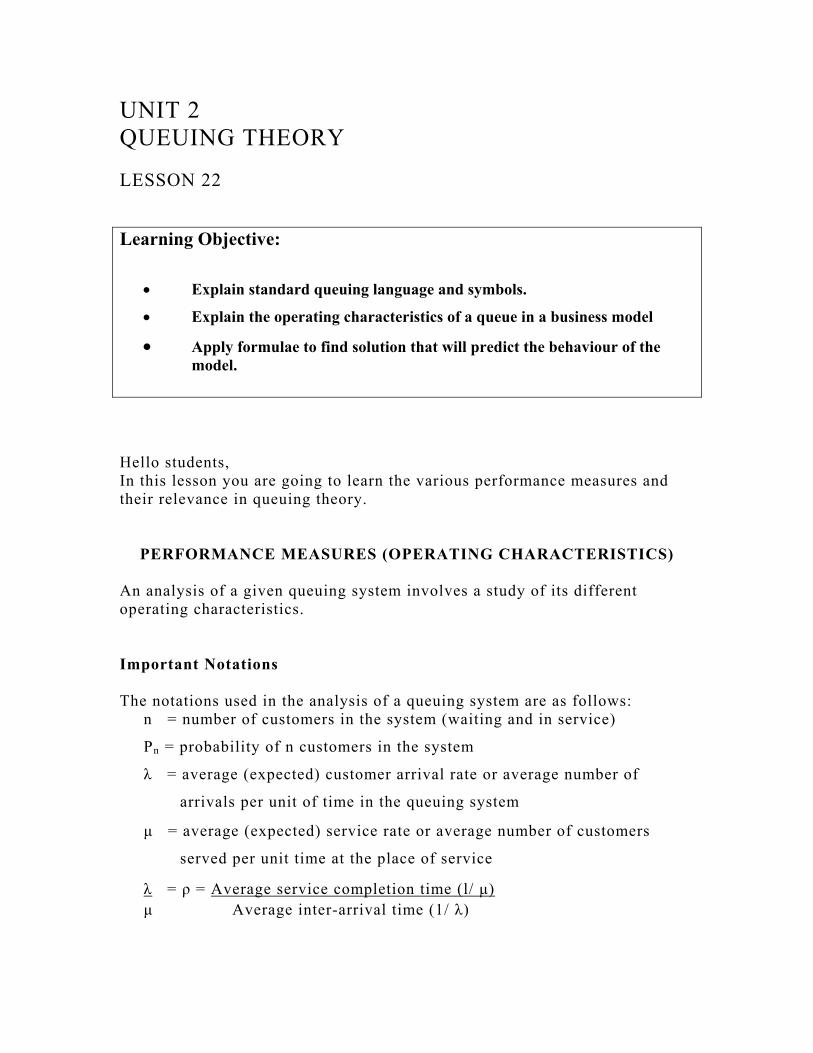
UNIT 2 QUEUING THEORY LESSON 22 Learning Objective:
• Explain standard queuing language and symbols.
• Explain the operating characteristics of a queue in a business model
• Apply formulae to find solution that will predict the behaviour of the model.
Hello students, In this lesson you are going to learn the various performance measures and their relevance in queuing theory.
PERFORMANCE MEASURES (OPERATING CHARACTERISTICS) An analysis of a given queuing system involves a study of its different operating characteristics. Important Notations The notations used in the analysis of a queuing system are as follows:
n = number of customers in the system (waiting and in service)
Pn = probability of n customers in the system
λ = average (expected) customer arrival rate or average number of
arrivals per unit of time in the queuing system
µ = average (expected) service rate or average number of customers
served per unit time at the place of service
λ = ρ = Average service completion time (l/ µ) µ Average inter-arrival time (1/ λ)

= traffic intensity or server utilization factor (the expected fraction of
time for which server is busy)
s = number of service channels (service facilities or servers)
N = maximum number of customers allowed in the system.
Ls = average (expected) number of customers in the system (waiting and
in service)
Lq = average (expected) number of customers in the queue (queue length)
Lb = average (expected) length of non-empty queue
Ws = average (expected) waiting time in the system (waiting and in
service)
Wq = average (expected) waiting time in the queue
Pw = probability that an arriving customer has to wait
Some of the performance measures (operating characteristics of any queuing system that are of general interest for the evaluation of the performance of an existing queuing system, and to design a new system in terms of the level of service a customer receives as well as the proper utilization of the service facilities are listed:- 1. Time-related questions for the customers
a) What is the average (or expected) time an arriving customer has to wait
in the queue (denoted by Wq) before being served.
b) What is the average (or expected) time an arriving customer spends in
the system (denoted by Ws) including waiting and service. This data
can be used to make economic comparison of alternative queuing
systems.
2. Quantitative questions related to the number of customers
a) Expected number of customers who are in the queue (queue length) for
service, and is denoted by Lq

b) Expected number of customers who are in the system either waiting in
the queue or being serviced (denoted by Ls). The data can be used for
finding the mean customer time spent in the system.
3. Questions involving value of time both for customers and servers
a) What is the probability that an arriving customer has to wait before
being served (denoted by Pw)? It is also called blocking probability.
b) What is the probability that a server is busy at any particular point in
time (denoted by ρ )? It is the proportion of the time that a server
actually spends with the customer, i.e. the fraction of the time a server
is busy.
c) What is the probability of n customers being in the queuing system
when it is in steady state condition? It is denoted by Pn, n = 0, 1……
d) What is the probability of service denial when an arriving customer
cannot enter the system because the queue is full? It is denoted by Pd .
4. Cost-related questions
a) What is the average cost needed to operate the system per unit of time?
b) How many servers (service centres) are needed to achieve cost
effectiveness?
To describe the distribution of these variables, we should specify its
average value, standard deviation and the probability that the variable exceeds
a certain value.
Transient-State and Steady-State When a service system is started it progresses through a number of changes. However, it attains stability after some time. Before the start of the service operations it is very much influenced by the initial conditions (number of customers in the system) and the elapsed time. This period of transition is termed as transient-state. However, after sufficient time has passed, the system becomes independent of the initial conditions and of the elapsed time (except under very special conditions) and enters a steady- state condition.

In this chapter an analysis of the queuing system will be discussed under steady-state conditions. Let Pn(t) denote the probability that there are n customers in the system at time t. The rate of change in the value Pn(t) with respect to time t is denoted by the derivative of Pn(t) with respect to t, i.e. Pn(t). In the case of steady - state, we have
lim Pn(t) = Pn (independent of t) t→∞
or lim d { Pn(t)} = d (Pn) t→∞ dt dt or lim P′n(t) = 0 t→∞ In some cases when arrival rate of customers in the system is more than the service rate, then a steady - state cannot be reached regardless of the length of the elapsed time. Relationships Among Performance Measures By definition of various measures of performance (operating characteristic), we have
∞ ∞ Ls = ∑ n Pn and Lq = ∑ (n-s) Pn
n=0 n=s Some general relationships between the average system characteristics
true for all queuing models are as follows: (i) Expected number of customers in the system is equal to the expected
number of customers in queue plus in service.
Ls = Lq + Expected number of customers in service
= Lq + λ/µ
The value of expected number of customers in service, should not be confused with the number of service facilities but it is equal to ρ for all queuing models except finite queue case.
(ii) Expected waiting time of the customer in the system is equal to the
average waiting time in queue plus the expected service time.

1 Ws = Wq + ---
µ (iii) Expected number of customers served per busy period is given by
Ls µ Lb = ----------- = ------------
P(n ≥ s) µ - λ Where P(n ≥ s) = probability that the system being busy (iv) Expected length of queue during busy period is given by
Wq 1
Wb = ----------------- = ----------- P(n ≥ s) µ - λ (v) Expected number of customers in the system is equal to the average
number of arrivals per unit of time multiplied by the average time spent by the customer in the system.
Ls = λWs
1 or Ws = ---- Ls
λ (vi) Lq = λWq
1 or Wq = ---- Lq
λ
= Ls --- µ For applying formula (v) and (vi) for system with finite queue, instead of using λ, its effective value λ ( 1-PN) must be used.

(vii) The probability, Pn of n customers in the queuing system at any time can be used to determine all the basic measures of performance in the following order. ∞
Ls = ∑ nPn n=0
Ls => Ws = ----- λ 1 => Wq = Ws ― ----- µ => Lq = λWq
PROBABILITY DISTRIBUTIONS IN QUEUING SYSTEMS It is assumed that customers joining a queuing system arrive in random manner and follow a Poisson distribution or equivalently the inter-arrival times follow exponential distribution. In most of the cases, service times are also assumed to be exponentially distributed. It implies that the probability of service completion in any short-time period is constant and independent of the length of time that the service has been in progress. The basic reason for assuming exponential service is that it helps in formulating simple mathematical models which ultimately help in analyzing a number of aspects of queuing problems. The number of arrivals and departures (those served) during an interval of time in a queuing system is controlled by the following assumptions (also called axioms).
(i) The probability of an event ( arrival or departure ) occurring during the time interval ( t, t+∆t ) depends on the length of time interval ∆t. That is, probability of the event does not depend either on number of events that occur unto time t or the specific value of t, meaning that the events that occur in non- overlapping time are statistically independent.
(ii) The probability of more than one event occurring during the time
interval ( t, t+ ∆t ) is negligible. It is denoted by 0(∆t).

(iii) Atmost one event (arrival or departure) can occur during a small
time interval ∆t. the probability of an arrival during the time interval ( t, t + ∆t) is given by
P1 (∆t ) = λ∆t +0(∆t)
where λ is a constant and independent of the total number of arrivals up to time t; ∆t is a small time interval and 0(∆t) represents the quantity that becomes negligible when compared to ∆t as ∆t→0, i.e.
Lim { 0 (∆t) / ∆t } =0
∆t→0 DISTRIBUTION OF ARRIVALS ( pure birth process) The arrival process assumes that the customers arrive at the queuing at the queuing system and never leave it. Such a process is called pure birth process. The aim is to derive an expression for the probability Pn (t) if n arrivals during time interval ( t, t+ ∆t). the terms commonly used in the development of various queuing models are the following: ∆t = a time interval so small that the probability of more than one customer’s arrival is negligible, i.e. during any given small interval of time ∆t only one customer can arrive.
λ∆t = probability that a customer will arrive in the system during time ∆t.
1- λ∆t = probability that no customer will arrive in the system during
time ∆t. If the arrivals are completely random, then the probability distribution of a number of arrivals in a fixed time interval follows Poisson distribution.
DISTRIBUTION OF INTER- ARRIVAL TIMES ( exponential process) If the number of arrivals, n, in time t follows the Poisson distribution, then

Pn (t) = (λt)n e -λ t , n = 0,1,2,… n ! is an associated random variable defined as the inter – arrival time T follows the exponential distribution f(t) =λ e –λ t and vice – versa. Markovian property of inter- arrival times The markovian property of inter arrival times states that the probability that a customer currently in service is completed at some time t is independent of how long he has already been in service. That is
Prob. ={T ≥ t1 T ≥ to} = prob. { 0 ≤ T ≤ t1 -to} where T is the time between successive arrivals. DISTRIBUTION OF DEPARTURES ( pure death process) The departure process assumes that no customer joins the system while service is continued for those who are already in the system. Let, at time t =0 (starting time) there be N ≥ 1 customers in the system. Since service is being provided at the rate of µ. Therefore, customers leave the system at the rate µ after being serviced. Such a process is called pure death process
Basic axioms (i) probability of the departure during time ∆ t is µ ∆ t. (ii) probability of more than one departure between time t and
t + ∆ t is negligible. (iii) The number o f departures in non- overlapping intervals are
statistically independent. The following terms are used in the development of various queuing models. µ ∆ t = probability that a customer in-services at time t will complete service during time ∆ t. 1 - µ ∆ t = probability that the customer in-service at time t will not complete service during time ∆ t.
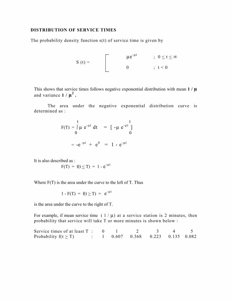
DISTRIBUTION OF SERVICE TIMES The probability density function s(t) of service time is given by µe-µt ; 0 < t < ∞ S (t) = 0 ; t < 0
This shows that service times follows negative exponential distribution with mean 1 / µ and variance 1 / µ2 . The area under the negative exponential distribution curve is determined as : t t F(T) = ∫ µ e-µt dt = [ -µ e-µt ] 0 0
= -e -µt + e0 = 1 - e-µt It is also described as : F(T) = f(t < T) = 1 - e-µt Where F(T) is the area under the curve to the left of T. Thus 1 - F(T) = f(t > T) = e-µt is the area under the curve to the right of T. For example, if mean service time ( 1 / µ) at a service station is 2 minutes, then probability that service will take T or more minutes is shown below : Service times of at least T : 0 1 2 3 4 5 Probability f(t > T) : 1 0.607 0.368 0.223 0.135 0.082

So, now let us summarize today’s discussion: Summary We have discussed in details about
• Symbols used in queuing theory • Operating characteristics of queuing. • Relationships Among Performance Measures • Probability distributions in queuing systems

Slide 1
M e a s u r in g S y s t e m P e r fo r m a n c e
T h e to ta l t im e a n “ e n t ity ” s p e n d s in th e s y s te m .
D e n o te d b y W .
T h e t im e a n “ e n t ity s p e n d s in th e q u e u e .D e n o te d b y W q .
T h e n u m b e r o f “ e n t it ie s ” in th e s y s te m .D e n o te d b y L .
T h e n u m b e r o f “ e n t it ie s ” in th e q u e u e .D e n o te d b y L q .
T h e p e r c e n ta g e o f t im e th e s e r v e r s a r e b u s y .T h e s e q u a n t it ie s a re v a r ia b le o v e r t im e .W h a t m ig h t w e b e in te re s te d in k n o w in g a b o u t th e s e q u a n t it ie s ?
________________________________________________________________________
________________________________________________________________________
________________________________________________________________________
________________________________________________________________________
________________________________________________________________________
________________________________________________________________________
________________________________________________________________________
________________________________________________________________________
________________________________________________________________________
________________________________________________________________________
________________________________________________________________________
____________________________________________________________________

Slide 2
A n E x a m p le o f L a c k o f M e m o r y
S u p p o s e t h a t t h e a m o u n t o f t im e o n e s p e n d s in a b a n k is e x p o n e n t ia l ly d is t r ib u te d w it h m e a n te n m in u te s .
W h a t is λ ?
W h a t is t h e p r o b a b il i t y t h a t a c u s t o m e r w il l s p e n d m o r e a q u a r t e r o f a n h o u r in t h e b a n k ?
Y o u h a v e b e e n w a it in g fo r t e n m in u te s a lr e a d y . N o w w h a t is p r o b a b il i t y t h a t y o u w i l l s p e n d m o r e t h a n a q u a r t e r o f a n h o u r in t h e b a n k ?
W h a t h a s a la c k o f m e m o r y , y o u o r t h e d is t r ib u t io n ?
________________________________________________________________________
________________________________________________________________________
________________________________________________________________________
________________________________________________________________________
________________________________________________________________________
________________________________________________________________________
________________________________________________________________________
________________________________________________________________________
________________________________________________________________________
________________________________________________________________________
________________________________________________________________________
____________________________________________________________________

Slide 3
P o in t P ro c e sse s
A Po in t P ro ce ss is a s to ch as tic p ro ce ss th a t on ly ch an ge s a t d isc re te po in ts in t im e .Fo r in s tan ce , th e nu m be r o f peop le in a fa s t food re s tau ran t is a po in t p ro ce ss .
It is 9 am an d th e doo rs to M acR on a ld ’s h ave ju s t open ed .T h e firs t cu s tom e r a rr ive s a fte r 3 m in u te s an d is se rved im m ed ia te ly , ta k in g a to ta l o f 4 m in u te s to fil l th e o rd e r.T h e n ex t cu s tom e r a rr iv e s a fte r 2 m in u te s an d is se rved , ta k in g 3 m inu te s .T h e n ex t cu s tom e r a rr iv e s a fte r an o th e r 1 m in u te an d h as to w a it a s o n ly 2 se rve rs a re w o rk in g .T h e 3 rd cu s tom e rs se rv ice ta ke s 5 m in u tes .
________________________________________________________________________
________________________________________________________________________
________________________________________________________________________
________________________________________________________________________
________________________________________________________________________
________________________________________________________________________
________________________________________________________________________
________________________________________________________________________
________________________________________________________________________
________________________________________________________________________
________________________________________________________________________
____________________________________________________________________
UNIT 2 QUEUING THEORY LESSON 23 Learning Objective:
• Identify the classification of queuing models.
• Apply formulae to find solution that will predict the behaviour of the single server model I.
Hello students, In this lesson you are going to learn the models of queuing theory.
CLASSIFICATION OF QUEUING MODELS
There is a standard notation system to classify queuing systems as A/B/C/D/E, where:
• A represents the probability distribution for the arrival process • B represents the probability distribution for the service process • C represents the number of channels (servers) • D represents the maximum number of customers allowed in the
queueing system (either being served or waiting for service) • E represents the queue discipline or service mechanism
Common options for A and B are:
• M for a Poisson arrival distribution (exponential interarrival distribution) or a exponential service time distribution
• D for a deterministic or constant value • G for a general distribution (but with a known mean and variance)

If D is not specified then it is assumed that it is infinite.
For example the M/M/1 queueing system, the simplest queueing system, has a Poisson arrival distribution, an exponential service time distribution and a single channel (one server).
Single server model
(M/ M/1) QUEUING MODEL The M/M/1 queuing model is a queuing model where the arrivals follow a Poisson process, service times are exponentially distributed and there is one server. The assumption of M/M/1 queuing model are as follows :
1. The number of customer arriving in a time interval t follows a poison process with parameter λ.
2. The interval between any two successive arrival is exponentially distributed with parameters λ.
3. The time taken to complete a single service is exponentially distributed with parameter µ.
4. The number of server is one. 5. Although not explicitly stated both the population and the queue size
can be infinity. 6. The order of service is assumed to be FCFS.
If λ < 1 the steady state probabilities exist and Pn the number of customers in µ the system follows a geometric distribution with parameter λ (also known as traffic intensity). µ The probabilities are : Pn = P(No. of customers in the system =n) = ( λ/µ )n ( 1 – λ/µ ) ; n = 1, 2, …….. Po = 1 – λ/µ
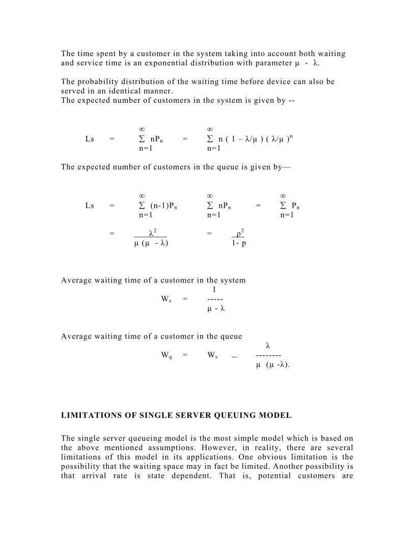
The time spent by a customer in the system taking into account both waiting and service time is an exponential distribution with parameter µ - λ. The probability distribution of the waiting time before device can also be served in an identical manner. The expected number of customers in the system is given by -- ∞ ∞
Ls = ∑ nPn = ∑ n ( 1 – λ/µ ) ( λ/µ )n n=1 n=1 The expected number of customers in the queue is given by— ∞ ∞ ∞
Ls = ∑ (n-1)Pn ∑ nPn = ∑ Pn n=1 n=1 n=1 = λ2 = ρ2
µ (µ - λ) 1- p
Average waiting time of a customer in the system 1
Ws = ----- µ - λ
Average waiting time of a customer in the queue λ
Wq = Ws ― -------- µ (µ -λ).
LIMITATIONS OF SINGLE SERVER QUEUING MODEL
The single server queueing model is the most simple model which is based on the above mentioned assumptions. However, in reality, there are several limitations of this model in its applications. One obvious limitation is the possibility that the waiting space may in fact be limited. Another possibility is that arrival rate is state dependent. That is, potential customers are

discouraged from entering the queue if they observe a long line at the time they arrive. Another practical limitation of the model is that the arrival process is not stationary. It is quite possible that the service station would experience peak periods and slack periods during which the arrival rate is higher and lower respectively than the overall average. These could occur at particular times during a day or a week or particular weeks during a year. There is not a great deal one can do to account for stationary without complicating the mathematics enormously. The population of customers served may be finite, the queue discipline may not be first come first serve. In general, the validity of these models depends on stringent assumptions that are often unrealistic in practice. Even when the model assumptions are realistic, there is another limitation of queuing theory that is often overlooked. Queuing models give steady state saluting, that is, the models tell us what will happen after queuing system has been in operation long enough to eliminate the effects of starting with an empty queue at the beginning of each business day. In some applications, the queuing system never reaches a steady state, so the model solution is of little value. APPLICABILITY OF QUEUING MODEL TO INVENTORY PROBLEMS
Queues are common feature in inventory problems. We are confronted with queue-like situations in stores for spare parts in which machines wait for components and spare parts in service station. We can also look at the flow of materials as inventory queues in which demands wait in lines, conversely materials also wait in queues for demands to be served. If there is a waiting line of demands, inventory state tends to be higher than necessary. Also, if there is a negative state of inventories, then demands form a queue and remain unfulfilled. Thus, the management is faced with the problem of choosing a combination of controllable quantities that minimize losses resulting from the delay of some units in the queue and the occasional waste of service capacity in idleness. An increase in the potential service capacity will reduce the intensity of congestion. But at the same time, it will also increase the expense due to idle facilities in periods of “No demand’. Therefore, the ultimate goal is to achieve an economic balance between the cost of service and the cost associated with the waiting of that service. Queuing theory contributes vital information required for such a decision by predicting various characteristics of the waiting line, such as average queue length. Based on probability theory, it attempts to minimize the extent and duration of queue with minimum of investment in inventory and service facilities. Further, it gives the estimated average time and intervals under sampling methods, and helps in decision of optimum capacity so that the cost of investment is minimum keeping the amount of queue tolerance limits.

Single server model I
{(M/ M/1) : (∞ / FCFS)}-- Exponential service; Unlimited queue Practical formulae involved in single server model I
• Arrival rate per hour • Service rate per hour • Average utilization rate ( or utilization
factor), ρ • Average waiting time in the system, (waiting and servicing time) Ws
• Average waiting time in the queue, Wq
• Average number of customers (including the one who is being served ) in the system, Ls
• Average number of customers( excluding
the one who is being served ) in the queue Lq
• Average number of customers in non-
empty queue that forms time to time
• Probability of no customer in the system, or, system is idle or idle men in the factor Po
• Probability of no customer in queue and
a customer is being served P1
• Probability of having ‘n’ customers in the system
• Probability of having ‘n’ customers in
the queue
= λ = µ = λ / µ = 1 / (µ-λ) = λ µ (µ -λ)
= λ (µ - λ) = λ2 µ( µ-λ) = µ / (µ-λ) = 1 –(λ / µ) or1 – ρ = 1- utilization factor = (1 – λ / µ) (λ / µ )
=(1 – λ / µ) (λ / µ )n
= (1 – λ / µ) (λ / µ )n+1

• Probability of having more than ‘n’
customers in the system
• Probability of having less than n customers in the system or probability that an arrival will not have to wait outside the indicated space
• Probability of having n or more
customers in the system or , probability that an arrival will have to wait outside the indicated space
• Probability that a customer will wait for
more than ‘t’ hours in the queue
• Total costs associated with system
• Total costs associated with queue
= (λ / µ)n+1
= 1― (λ / µ)n
=(λ / µ)n
=ρ x e-t/ws
= λ x e-t(µ -λ) µ = Average no. of customers in system x opportunity cost of customer + cost of serving department. =Average no. of customers in queue x opportunity cost of customer + cost of serving department.
Example The Toolroom problem
The J.C. Nickel Company toolroom is staffed by one clerk who can serve 12 production employees, on the average, each hour. The production employees arrive at the toolroom every six minutes, on the average. Find the measures of performance.
Toolroom Problem Solution

• Assume this is an M/M/1 queue • Arrival rate is one employee (emp) every six minutes
– Arrival times between employees follow a negative
exponential distribution with mean 1/ λ = 6 (minutes/emp) –Thus, λ = 1/6 (emp/minute) = 10 (emp/hour)
• Mean service rate is 12 employees per hour
–Thus µ = 12 (emp/hour)
It is necessary first to change the time dimensions of λ and µ to a common denominator. λ is given in minutes, µ in hours. We will use hours as the common denominator. 1. Average waiting time in the system (toolroom)
5.01012
11=
−=
−=
λµW
hours, per employee 2. The average waiting time in the line
( ) ( ) 417.0101212
10=
−=
−=
λµµλ
qW hours, per employee
3. The average number of employees in the system (toolroom area)
51012
10=
−=
−=
λµλL
employees 4. The average number of employees in the line.

( ) ( ) 17.4101212
1002
=−
=−
=λµµ
λqL
employees 5. The probability that the toolroom clerk will be idle
167.01210110 =−=−=
µλ
P
6. The probability of finding the system busy
833.01210
==
=
µλρ
7. The chance of waiting longer than 1/2 hour in the system. That is T = 1/2
( ) ( )( ) 368.012/11210 ===> −
eeTtP
8. The probability of finding four employees in the system, n = 4
0.0804122
1210
µλ1
µλ
P4n
4n =
=
−
==
9. The probability of finding more than three employees in the system.
488.01210 41
3 =
=
=
+
>
N
nP µλ

Case of sales counter
Customers arrive at a sales counter manned by a single person according to a poisson process with a mean rate of 20 per hour. The time required to serve a customer has an exponential distribution with a mean of 100 seconds. Find the average waiting time of a customer. Solution Arrival rate = λ =20 customers per hour Service rate = µ = 3600 =36 customers per hour 100
The average waiting time of a customer in the queue
= λ = 20 µ (µ - λ) 36(36-20)
= 5 hours = 5 x 60 x 60 = 125 seconds
36 x 4 36 x 4
The average waiting time of a customer in the system
= 1 = 1 (µ-λ) 36-20)
= 1 hours = 1 x 60 x60 x 60 = 225seconds 16 16
Case of cafetaria Self service at a university cafeteria, at an average rate of 7 minutes per customer, is slower than attendant service, which has a rate of 6 minutes per student. The manager of the cafeteria wishes to calculate the average time each student spends waiting for service. Assume that customers arrive randomly at each time, at the rate of 5 per hour. Calculate the appropriating statistics for this cafeteria.

Solution Self service line Attended line A B C D E F
Arrival rate (λ) Service rate (µ) Expected number of Students in cafeteria λ --- µ-λ Expected number of students waiting for service = λ2 µ( µ-λ) Average time in system 1 --- µ-λ Average time in queue 1 λ ------ x -- µ-λ µ
5
8.571
5 ------------
8.571-5
=1.40
25 ----------------------
8.57 (8.571-5)
=0.82
1 -------------------
(8.571 - 5)
= .28 hour or 16.8 min.
1 5 ------- x ----- 8.571-5 8.571
= 0.1633 hour or 9.8 min
5
10
5 --------
10-5
=1
25 ----------- 10(10-5)
=0.5
1 --------------
10 - 5
= .20 hour or 12 min.
1 5 -------- x --------
10-5 10
= .10 hour or 6 min.

Case of airport The mean rate of arrival of planes at an airport during the peak period is 20 per hour. And the actual number of arrivals in any hour follows a poisson distribution. The airport can land 60 planes per hour on an average in good weather and 30 planes per hour in bad weather, but the actual number landed in any hour follows a poisson distribution with these respective averages. When there is congestion, the planes that arrived earlier,
(i) How many planes would be flying over the field in the stack on an average in good weather and in bad weather ?
(ii) How long a plane would be in the stack and in the process of landing in good and in bad weather ?
(iii) How long a plane would be in the process of landing in good and bad weather after stack awaiting ?
Solution Good weather Bad weather A B C D
Arrival rate (λ) Service rate (µ) Average number of the planes in queue
λ2 1 ------------ X ------- µ µ -λ
Average waiting time in the system
1 ----- µ -λ
20 60 400 1 ------ x ------- 60 40 1 = ----- 6 1 1 --- = -----hour60–20 40 = 1.5 min
20 30 400 1 ------ x ----- 30 10 4 = ----- 3 1 1 ----------- = ----- (30 –20) 10 hour or 6 min
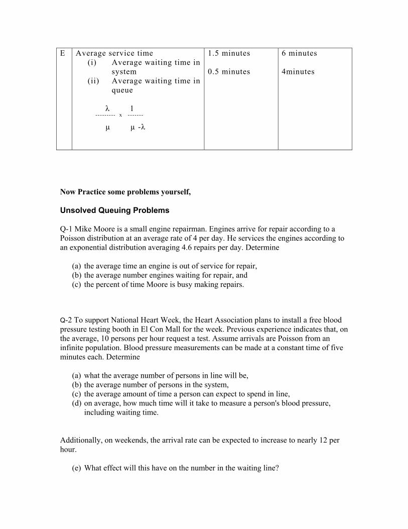
E
Average service time (i) Average waiting time in
system (ii) Average waiting time in
queue
λ 1 --------- x ------- µ µ -λ
1.5 minutes 0.5 minutes
6 minutes 4minutes
Now Practice some problems yourself,
Unsolved Queuing Problems
Q-1 Mike Moore is a small engine repairman. Engines arrive for repair according to a Poisson distribution at an average rate of 4 per day. He services the engines according to an exponential distribution averaging 4.6 repairs per day. Determine
(a) the average time an engine is out of service for repair, (b) the average number engines waiting for repair, and (c) the percent of time Moore is busy making repairs.
Q-2 To support National Heart Week, the Heart Association plans to install a free blood pressure testing booth in El Con Mall for the week. Previous experience indicates that, on the average, 10 persons per hour request a test. Assume arrivals are Poisson from an infinite population. Blood pressure measurements can be made at a constant time of five minutes each. Determine
(a) what the average number of persons in line will be, (b) the average number of persons in the system, (c) the average amount of time a person can expect to spend in line, (d) on average, how much time will it take to measure a person's blood pressure,
including waiting time.
Additionally, on weekends, the arrival rate can be expected to increase to nearly 12 per hour.
(e) What effect will this have on the number in the waiting line?
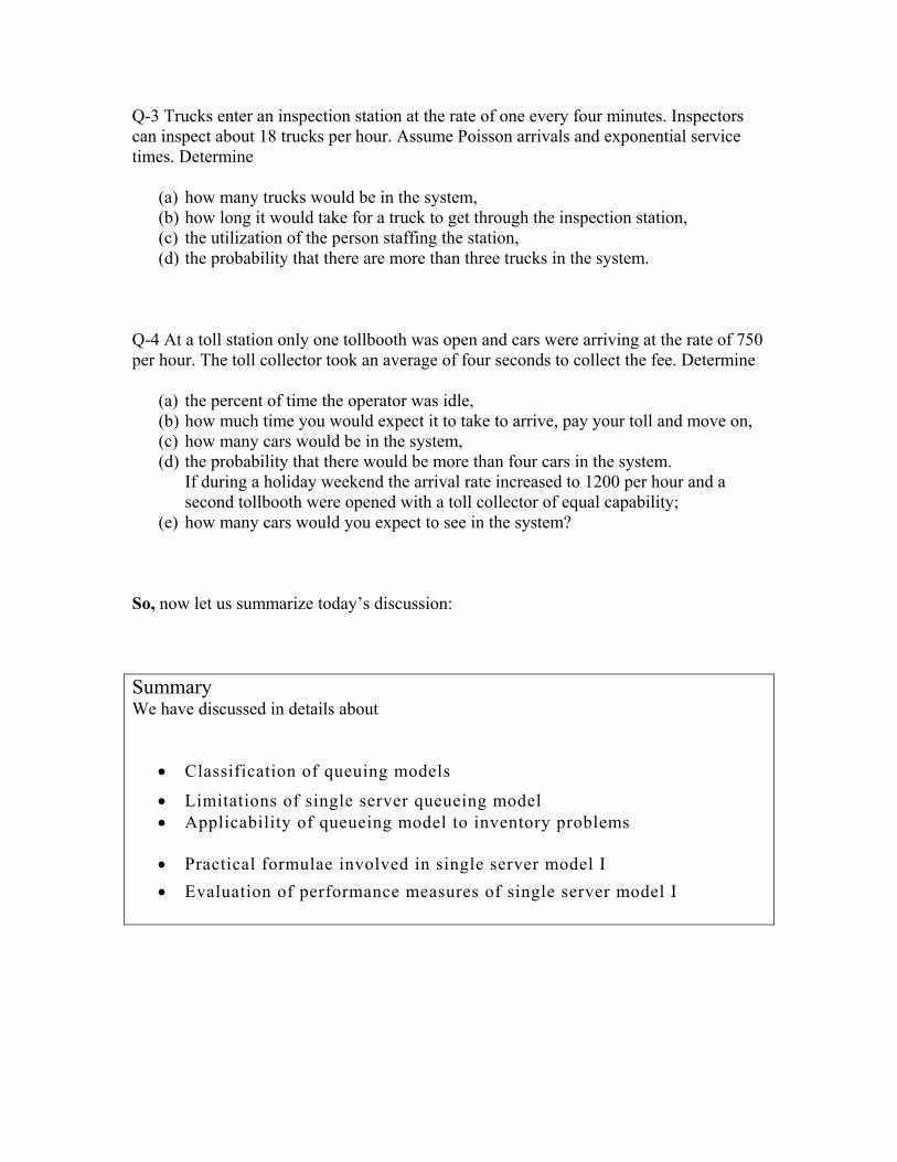
Q-3 Trucks enter an inspection station at the rate of one every four minutes. Inspectors can inspect about 18 trucks per hour. Assume Poisson arrivals and exponential service times. Determine
(a) how many trucks would be in the system, (b) how long it would take for a truck to get through the inspection station, (c) the utilization of the person staffing the station, (d) the probability that there are more than three trucks in the system.
Q-4 At a toll station only one tollbooth was open and cars were arriving at the rate of 750 per hour. The toll collector took an average of four seconds to collect the fee. Determine
(a) the percent of time the operator was idle, (b) how much time you would expect it to take to arrive, pay your toll and move on, (c) how many cars would be in the system, (d) the probability that there would be more than four cars in the system.
If during a holiday weekend the arrival rate increased to 1200 per hour and a second tollbooth were opened with a toll collector of equal capability;
(e) how many cars would you expect to see in the system?
So, now let us summarize today’s discussion: Summary We have discussed in details about
• Classification of queuing models
• Limitations of single server queueing model • Applicability of queueing model to inventory problems
• Practical formulae involved in single server model I • Evaluation of performance measures of single server model I

Slide 1
Kendall-Lee Notation
Kendall (1951) defined the following notation to describe a queuing system.There are 6 characteristics
1/2/3/4/5/6
The first specifies the arrivals processM = inter-arrivals are i.i.d exponential.D = inter-arrivals are i.i.d and deterministic.Ek = inter-arrivals are i.i.d Erlang(k).GI = inter-arrivals are i.i.d and have some general distribution.
The second specifies the service processThe notation is the same as for arrivals.
The third specifies the number of servers.
________________________________________________________________________
________________________________________________________________________
________________________________________________________________________
________________________________________________________________________
________________________________________________________________________
________________________________________________________________________
________________________________________________________________________
________________________________________________________________________
________________________________________________________________________
________________________________________________________________________
________________________________________________________________________
____________________________________________________________________

Slide 2
K e n d a ll-L e e N o ta tio n
T h e fou rth sp e c if ie s th e se rv ice o rde rFC FS = F irs t C om e F irs t S e rvedLC FS = Las t C om e F irs t S e rvedS IR O = S e rv ice in R an dom O rde rG D = G ene ra l Q ueu in g D isc ip lin e
T h e fifth spe c if ie s th e m ax im um a llow ab le n u m be r o f cu stom e rs in th e sy s tem .T h e s ix th sp e c if ie s th e s ize o f th e popu la tio n from w h ich a rr iva ls a re d raw n .T h e firs t queue w e w ill e xam ine is the M /M /1 /FC FS /∞ /∞ .W h a t d oe s th is m ean?T h is n o ta tio n is o ften sho rtened to M /M /1 .
________________________________________________________________________
________________________________________________________________________
________________________________________________________________________
________________________________________________________________________
________________________________________________________________________
________________________________________________________________________
________________________________________________________________________
________________________________________________________________________
________________________________________________________________________
________________________________________________________________________
________________________________________________________________________
________________________________________________________________________

Slide 3
M /M /1 q u e u in g m o d e lS u m m a ry
D is tr ib u t io n o f n u m b e r in s y s te mE x p e c te d n u m b e r in s y s te m E x p e c te d n u m b e r in q u e u eE x p e c te d t im e in s y s tem E x p e c te d t im e in q u eu eP ro b a b ilit ie s co n ce rn in g t im e in q u eu e
( )
( )λµµλλ
λµµλ
µ
λµλλ
λµ
−==
−=−=
−==
−=
2
1
1
q
WL
WW
WL
W
( )ρρπ
µλρ
−===
=
1)( nNPn
________________________________________________________________________
________________________________________________________________________
________________________________________________________________________
________________________________________________________________________
________________________________________________________________________
________________________________________________________________________
________________________________________________________________________
________________________________________________________________________
________________________________________________________________________
________________________________________________________________________
________________________________________________________________________
____________________________________________________________________
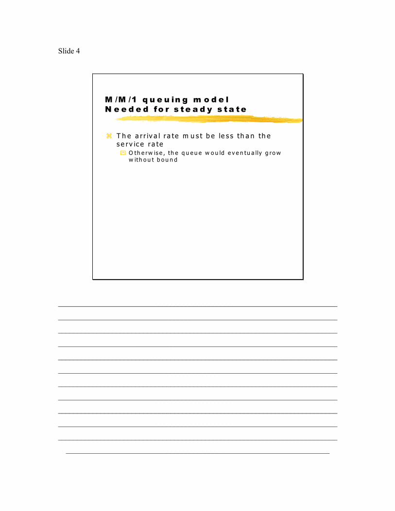
Slide 4
M /M /1 q u e u in g m o d e lN e e d e d fo r s te a d y s t a te
T h e a r r iv a l r a te m u s t b e le s s th a n th e s e rv ic e r a te
O th e rw is e , th e q u e u e w o u ld e v e n tu a lly g ro w w ith o u t b o u n d
________________________________________________________________________
________________________________________________________________________
________________________________________________________________________
________________________________________________________________________
________________________________________________________________________
________________________________________________________________________
________________________________________________________________________
________________________________________________________________________
________________________________________________________________________
________________________________________________________________________
________________________________________________________________________
____________________________________________________________________
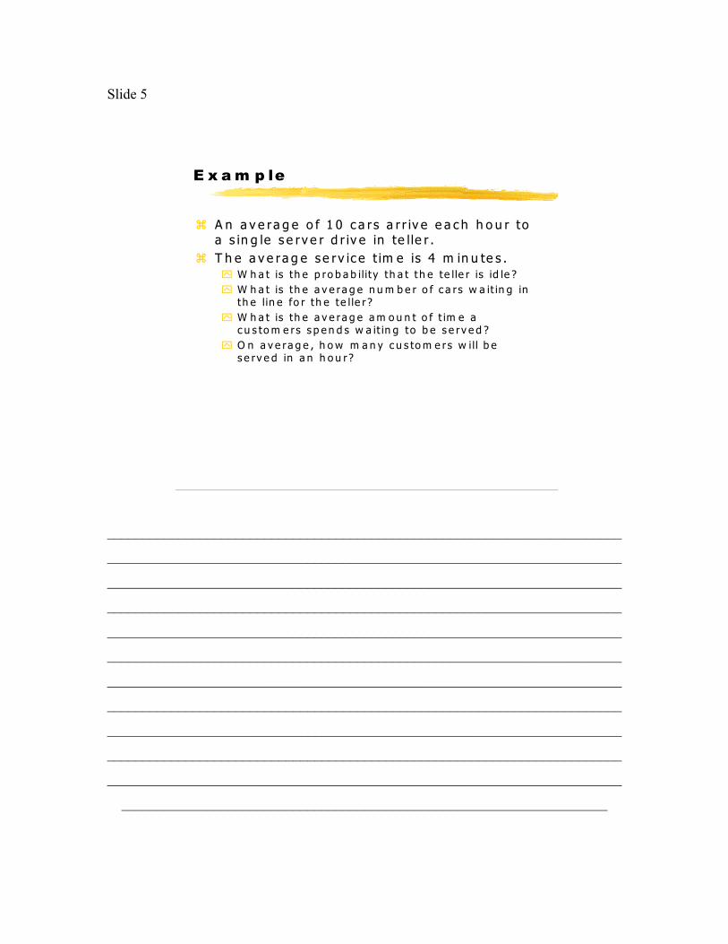
Slide 5
E x a m p le
A n a v e ra g e o f 1 0 c a r s a r r iv e e a c h h o u r to a s in g le s e rv e r d r iv e in te lle r .T h e a v e ra g e s e rv ic e t im e is 4 m in u te s .
W h a t is th e p ro b a b ilit y th a t t h e te lle r is id le ?W h a t is th e a v e ra g e n u m b e r o f c a rs w a it in g in th e lin e fo r th e te l le r ?W h a t is th e a v e ra g e a m o u n t o f t im e a c u s to m e rs s p e n d s w a it in g to b e s e rv e d ?O n a v e ra g e , h o w m a n y c u s to m e rs w i ll b e s e rv e d in a n h o u r?
________________________________________________________________________
________________________________________________________________________
________________________________________________________________________
________________________________________________________________________
________________________________________________________________________
________________________________________________________________________
________________________________________________________________________
________________________________________________________________________
________________________________________________________________________
________________________________________________________________________
________________________________________________________________________
____________________________________________________________________
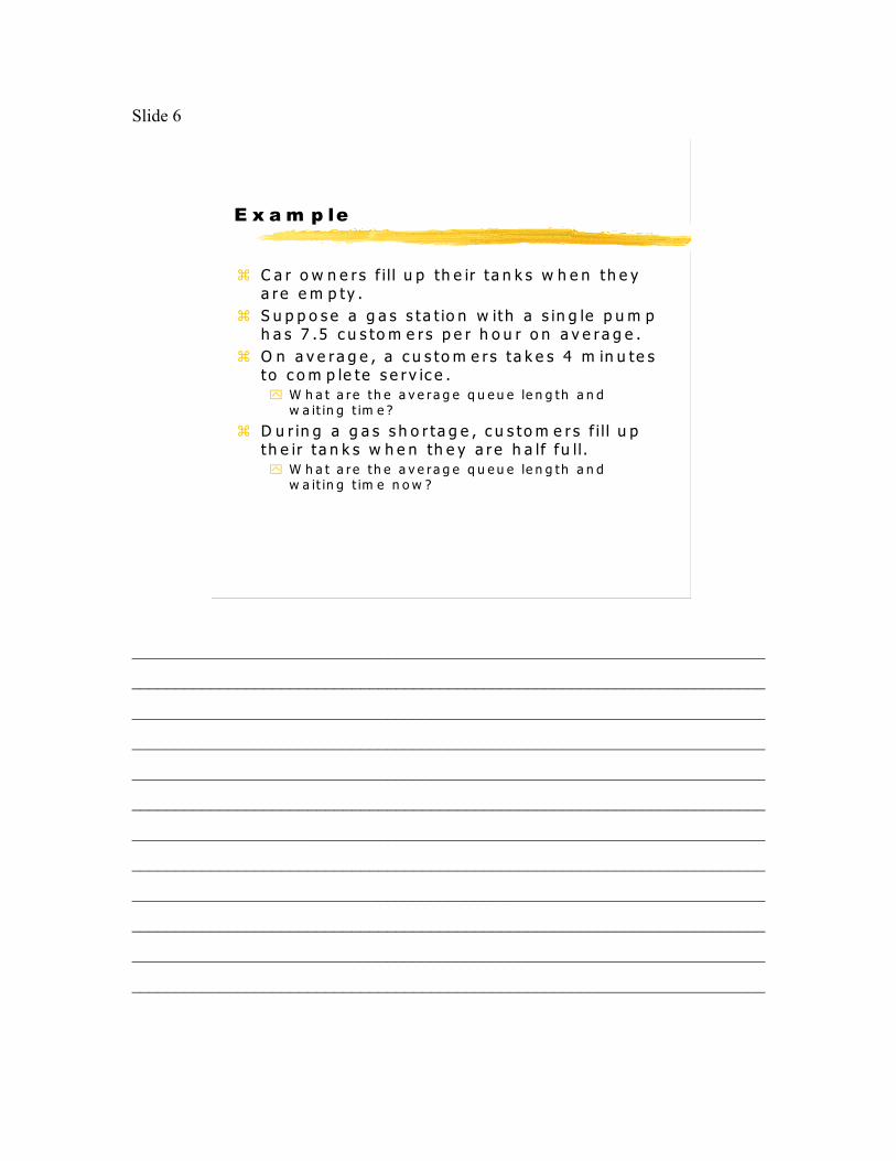
Slide 6
E x a m p le
C a r o w n e r s f i l l u p th e ir ta n k s w h e n th e y a r e e m p ty .S u p p o s e a g a s s ta t io n w ith a s in g le p u m p h a s 7 .5 c u s to m e r s p e r h o u r o n a v e r a g e .O n a v e r a g e , a c u s to m e rs t a k e s 4 m in u te s to c o m p le te s e r v ic e .
W h a t a r e th e a v e r a g e q u e u e le n g th a n d w a it in g t im e ?
D u r in g a g a s s h o r ta g e , c u s to m e r s f i l l u p th e ir t a n k s w h e n th e y a r e h a lf fu l l .
W h a t a r e th e a v e r a g e q u e u e le n g th a n d w a it in g t im e n o w ?
________________________________________________________________________
________________________________________________________________________
________________________________________________________________________
________________________________________________________________________
________________________________________________________________________
________________________________________________________________________
________________________________________________________________________
________________________________________________________________________
________________________________________________________________________
________________________________________________________________________
________________________________________________________________________
________________________________________________________________________

UNIT 2 QUEUING THEORY LESSON 24 Learning Objective:
• Apply formulae to find solution that will predict the behaviour of the single server model II.
• Apply formulae to find solution that will predict the behaviour of the single server model III.
• Apply formulae to find solution that will predict the behaviour of the single server model IV
Hello students, In this lesson you are going to study about three more types of single server models that differ from single server model I in terms of their queue discipline.
Single server model II
{(M/M/1) : (∞ / SIRO)} model This model is identical to the Model I with a difference only in queue discipline. In this model the selection of the customers is made in random order. Since the derivation of Pn is independent of any specific queue discipline, therefore in this model also we have Pn = (1- ρ) ρn N = 1, 2, 3, …… Consequently, other performance measures will also remain unchanged in any queuing system as long as Pn remains unchanged.

Single server model III
{(M/ M/1) : (N / FCFS)}-- Exponential service; Limited queue Suppose that no more than N customers can be accommodated at any time in the system due to certain reasons. For example, a finite queue may arise due to physical constraint such as emergency room in a hospital; a clinic with certain number of chairs for waiting patients, etc. Assumptions of this model are same as that of Model I except that the length of the queue be limited. In this case the service rate does not have to exceed arrival rate in order to obtain steady state equations. Therefore, The probability of a customer in the system for n = 0, 1, 2, …., N are obtained as follows:
Pn = ( λ / µ)n Po ; n < N The steady_state solution in this case exists even for ρ > 1. This is due to the limited capacity of the system which controls the arrivals by the queue length ( = N - 1) not by the relative rates of arrival, departure, λ and µ. If λ < µ and N -->∞, then Pn = ( 1 - λ / µ) ( λ / µ)n, which is same as in Model I.
Performance Measures for Model III
• Expected number of customers in the system
N N
Ls = ∑ nPn = ∑ n ( 1 – λ/µ ) ( λ/µ )n n=1 n=1 1 – (λ/µ) N+1 N = ∑ n ( 1 – ρ ) ρn n=1 (1- ρN+1)

N = ( 1 – ρ ) ∑ nρn (1- ρN+1) n=0
= ( 1 – ρ ) (ρ + 2 ρ2 +3 ρ3 + …. + N ρ n)
(1- ρN+1)
• Expected queue length or expected number of customers waiting in the system
Lq = Ls - λ/µ = Ls – λ(1 – Pn) / µ
• Expected waiting time of a customer in the system (waiting + service)
Ws = Ls λ (1-Pn)
• Expected waiting time of a customer in the queue
Wq = Ws – 1/µ or Lq
λ (1-PN)
• Fraction of potential customers lost ( = fraction of time system is full)
PN = Po ρN

Example Consider a single server queuing system with Poisson input, exponential service times. Suppose the mean arrival rate is 3 calling units per hour, the expected service time is 0.25 hour and the maximum permissible calling units in the system is two. Derive the steady-state probability distribution of the number of calling units in the system, and then calculate the expected number in the system.
Solution
From the data of the problem, we have λ = 3 units per hour; µ = 4 units per hour, and N = 2 Then traffic intensity, p = λ / µ = 3/4 = 0.75 The steady-state probability distribution of the number of n customers (calling units) in the system is Pn = ( 1 – ρ ) ρn ; ρ ≠ 1
1 - ρN+1
= ( 1-0.75) (0.75) n = (0.43) (0.75)n
1 – (0.75) 2+1
and the expected number of calling units in the system is given by N 2
Ls = ∑ nPn = ∑ n ( 0.43 ) ( 0.75 )n n=1 n=1
2 = 0.43 ∑ n (0.75)n n=1
= 0.43 {(0.75) + 2 (0.75)2 3 (0.75)3 + …. + N (0.75)n)} = 0.81
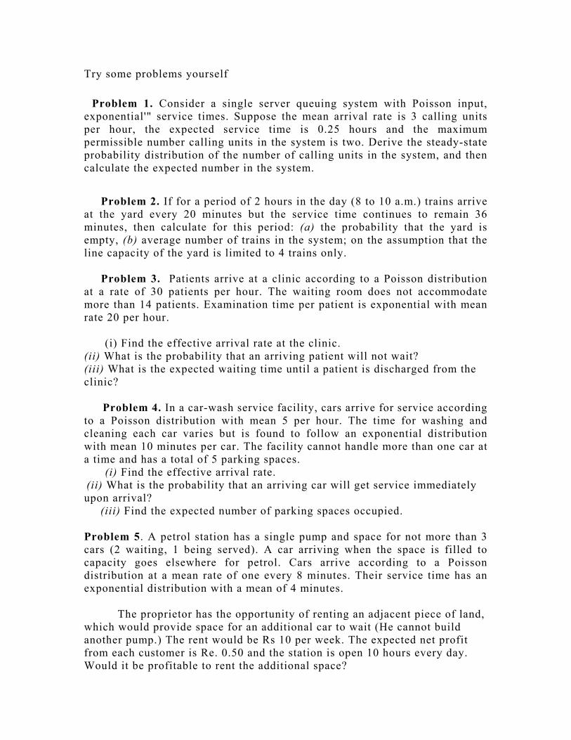
Try some problems yourself
Problem 1. Consider a single server queuing system with Poisson input, exponential'" service times. Suppose the mean arrival rate is 3 calling units per hour, the expected service time is 0.25 hours and the maximum permissible number calling units in the system is two. Derive the steady-state probability distribution of the number of calling units in the system, and then calculate the expected number in the system.
Problem 2. If for a period of 2 hours in the day (8 to 10 a.m.) trains arrive
at the yard every 20 minutes but the service time continues to remain 36 minutes, then calculate for this period: (a) the probability that the yard is empty, (b) average number of trains in the system; on the assumption that the line capacity of the yard is limited to 4 trains only.
Problem 3. Patients arrive at a clinic according to a Poisson distribution
at a rate of 30 patients per hour. The waiting room does not accommodate more than 14 patients. Examination time per patient is exponential with mean rate 20 per hour. (i) Find the effective arrival rate at the clinic. (ii) What is the probability that an arriving patient will not wait? (iii) What is the expected waiting time until a patient is discharged from the clinic?
Problem 4. In a car-wash service facility, cars arrive for service according
to a Poisson distribution with mean 5 per hour. The time for washing and cleaning each car varies but is found to follow an exponential distribution with mean 10 minutes per car. The facility cannot handle more than one car at a time and has a total of 5 parking spaces. (i) Find the effective arrival rate. (ii) What is the probability that an arriving car will get service immediately upon arrival? (iii) Find the expected number of parking spaces occupied. Problem 5. A petrol station has a single pump and space for not more than 3 cars (2 waiting, 1 being served). A car arriving when the space is filled to capacity goes elsewhere for petrol. Cars arrive according to a Poisson distribution at a mean rate of one every 8 minutes. Their service time has an exponential distribution with a mean of 4 minutes.
The proprietor has the opportunity of renting an adjacent piece of land, which would provide space for an additional car to wait (He cannot build another pump.) The rent would be Rs 10 per week. The expected net profit from each customer is Re. 0.50 and the station is open 10 hours every day. Would it be profitable to rent the additional space?

Problem 6. If for a period of 2 hours in the day (8 to 10 a.m.) trains arrive at the yard every 20 minutes but the service time continues to remain 36 minutes, then calculate for this period
(a) the probability that the yard is empty, and (b) the average number of trains in the system, on the assumption that the line
capacity of the yard is limited to 4 trains only. Problem 7. At a railway station, only one train is handled at a time. The railway yard is sufficient only for two trains to wait while the other is given signal to leave the station. Trains arrive at the station at an average rate of 6 per hour and the railway station can handle them on an average of 12 per hour. Assuming Poisson arrivals and exponential service distribution, find the steady-state probabilities for the various number of trains in the system. Also find the average waiting time of a new train coming into the yard.
Problem 8. Patients arrive at a clinic according to a Poisson distribution at the rate of 30 patients per hour. The waiting room does not accommodate more than 14 patients. Examination time per patient is exponential with mean rate per hour.
i Find the effective arrival rate at the clinic. ii What is the probability that an arriving patient will not wait? Will he
find a vacant seat in the room? iii What is the expected waiting time until a patient is discharged from the clinic?
Problem 9. Assume that goods trains are coming in a yard at the rate of 30 trains per day and suppose that the inter-arrival times follow an exponential distribution. The service time for each train is assumed to be exponential with an average of 36 minutes. If the yard can admit 9 trains at a time (there being 10 lines one of which is reserved for shunting purpose). Calculate the probability that the yard is empty and find the average queue length.
Problem 10. A petrol station has a single pump and space for not more than 3 cars (2 waiting, 1 being served). A car arriving when the space is filled to capacity goes elsewhere for petrol. Cars arrive according to a Poisson distribution at a mean rate of one every 8 minutes. Their service time has an exponential distribution with a mean of 4 minutes.
The owner has the opportunity of renting an adjacent piece of land, which
would provide space for an additional car to wait. (He cannot build another pump.) The rent would be Rs 2000 per month. The expected net profit from each customer is Rs 2 and the station is open 10 hours everyday. Would it be profitable to rent the additional space?
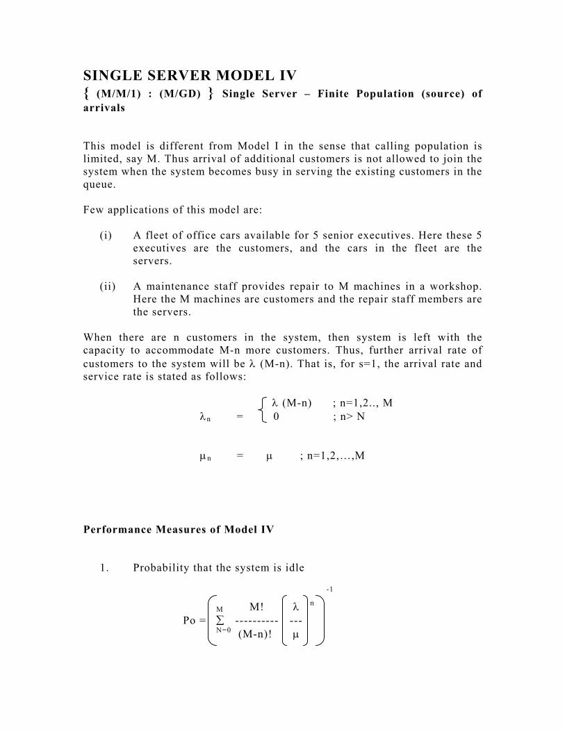
SINGLE SERVER MODEL IV { (M/M/1) : (M/GD) } Single Server – Finite Population (source) of arrivals This model is different from Model I in the sense that calling population is limited, say M. Thus arrival of additional customers is not allowed to join the system when the system becomes busy in serving the existing customers in the queue. Few applications of this model are:
(i) A fleet of office cars available for 5 senior executives. Here these 5 executives are the customers, and the cars in the fleet are the servers.
(ii) A maintenance staff provides repair to M machines in a workshop.
Here the M machines are customers and the repair staff members are the servers.
When there are n customers in the system, then system is left with the capacity to accommodate M-n more customers. Thus, further arrival rate of customers to the system will be λ (M-n). That is, for s=1, the arrival rate and service rate is stated as follows:
λ (M-n) ; n=1,2.., M λn = 0 ; n> N
µn = µ ; n=1,2,…,M
Performance Measures of Model IV
1. Probability that the system is idle
-1 M M! λ n Po = ∑ ---------- --- N=0 (M-n)! µ

2. Probability that there are n customers in the system M! λ n Pn = ----------- --- Po ; n=1,2,…, M (M-n)! µ
3 Expected number of customers in the queue (or queue length )
M λ +µ Lq = ∑ (n-1) Pn = M - --------- (1-Po) n=1 λ
4 Expected number of customers in the system M Ls = ∑ nPn = Lq + ( 1-Po) n=0 µ = M – --- ( 1-Po) λ
5 Expected waiting time of a customer in the system Lq
Wq = ------------------ λ (M-Ls)

6. Expected waiting time of a customer in the system
1 Ls Ws = Wq + ----- or ---------------------
µ λ (M-Ls)
Example
A mechanic repairs four machines. The mean time between service requirements is 5 hours for each machine and forms an exponential distribution. The mean repair time is one hour and also follows the same distribution pattern. Determine the following:
(a) Probability that the service facility will be idle, (b) Probability of various number of machines ( 0 through 4 ) to be out
of order and being repaired, (c) Expected number of machines waiting to be repaired, and being
repaired,
Would it be economical to engage two mechanics, each repairing only two machines? Solution: λ = 1/5 =0.2 machine/hour µ = 1 machine /hour M = 4 machines ρ =λ/µ 0.2 (a) probability that the system shall be idle is -1 M M! λ n Po = ∑ ----------- --- n=0 (M-n)! µ

- 1 M 4! n
= ∑ ---------- (0.2) n=0 (4-n)! -1 4! 4! 4! 4! = 1+ -------- ( 0.2) + -------(0.2)2 + -------- (0.2)3 + ------ (0.2)4 3! 2! 1! 0! = [ 1+4(0.2) + 4 x3 (0.04) + (4x3x2 ) (0.008) + (4x3x2x1) (0.00016 ]-1
= [ 1+0.8 + 0.48 + 0.192 + 0.000384] –1 = ( 2.481)-1 = 0.4030. (b) Probability that there shall be various number of machines ( 0 through
4) in the system
M! λ Pn = ---------- ---- Po ; n ≤ M ( M-n)! µ (c) The expected number of machines to be out of order and being repaired
µ 1 Ls = M – ---- ( 1 – Po ) = 4 - --- ( 1-0.403 ) λ 0.2 = 4 – 2.985 = 1.015 machines

Calculation of Pn
N M! λ n ---------- -- (M-n)! µ
Probability
(1) (2) (3) = (2) x Po 0 1 2 3 4
1.00 0.80 0.48 0.19 0.00
0.4030 0.3224 0.1934 0.0765 0.0000
( The sum total of these probabilities is 0.9953 instead of 1. It is because of the approximation error. ) (d) Expected time a machine will wait in queue to be repaired 1 M λ+µ 4 0.2 + 1 Wq = ---- ------ – ---------- = ----------------- – -------------- µ 1-Po λ 1-0.403 0.2
4 = ---------- – 6 = 0.70 hours or 42 minutes 0.597
(e) If there are two mechanics each serving two machines, then M = 2, and therefore, n -1
2 M! λ Po = ∑ ----------- ---
n=0 ( M-n )! µ
= [1+2(0.2) + 2 x 1(0.2)2 ] = 0.68

So, now let us summarise today’s discussion: Summary We have discussed in details about
• Single server model II. • Single server model III. • Single server model IV • Performance Measures of Single server model III, IV

Unit 3 GAME THEORY Lesson 25 Learning Objective: This chapter aims at showing you
• How games can be analyzed; • How games can be related to numbers • To demonstrate the theory of a representative collection of [mathematical]
games
• To show how new games can be investigated and related to other games.
Hello students,
In this course I will give an overview into methods for `solving games' as well as give examples for how games are used to model various scenarios.
Let us begin with the introduction of game theory What is game theory? Game theory is the study of how optimal strategies are formulated in conflict. It is concerned with the requirement of decision making in situations where two or more rational opponents are involved under conditions of competition and conflicting interests in anticipation of certain outcomes over a period of time. You are surely aware of the fact that
In a competitive environment the strategies taken by the opponent organizations or individuals can dramatically affect the outcome of a particular decision by an organization.

In the automobile industry, for example, the strategies of competitors to introduce certain models with certain features can dramatically affect the profitability of other carmakers.
So in order to make important decisions in business, it is necessary to consider what other organizations or individuals are doing or might do. Game theory is a way to consider the impact of the strategies of one, on the strategies and outcomes of the other. In this you will determine the rules of rational behavior in the game situations, in which the outcomes are dependent on the actions of the interdependent players. A GAME refers to a situation in which two or more players are competing. It involves the players (decision makers) who have different goals or objectives. They are in a situation in which there may be a number of possible outcomes with different values to them. Although they might have some control that would influence the outcome, they do not have complete control over others. Unions striking against the company management, players in a chess game, firm striving for larger share of market are a few illustrations that can be viewed as games. Now I throw some light on the evolution of game theory AN OUTLINE OF THE HISTORY OF GAME THEORY
Some game-theoretic ideas can be traced to the 18th century, but the major
development of the theory began in the 1920s with the work of the mathematician Emile Borel (1871Œ1956) and the polymath John von Neumann (1903Œ57). A decisive event in the development of the theory was the publication in 1944 of the book Theory of games and economic behavior by von Neumann and Oskar Morgenstern, which established the foundations of the field. In the early 1950s, John F. Nash developed a key concept (Nash equilibrium) and initiated the game-theoretic study of bargaining.
Soon after Nash's work, game-theoretic models began to be used in economic theory and political science, and psychologists began studying how human subjects behave in experimental games. In the 1970s game theory was first used as a tool in evolutionary biology. Subsequently, game-theoretic methods have come to dominate microeconomic theory and are used also in many other fields of economics and a

wide range of other social and behavioral sciences. The 1994 Nobel Prize in economics was awarded to the game theorists John C. Harsanyi (1920Œ2000), John F. Nash (1928Œ), and Reinhard Selten (1930Œ).
GAME THEORY MODELS You will gradually learn that the models in the theory of games can be classified depending upon the following factors: Number of players
It is the number of competitive decision makers, involved in the game. A game involving two players is referred to as a “Two-person game”. However if the number of players is more ( say n>2 ) then the game is called an n-person game.
Total Payoff
It is the sum of gains and losses from the game that are available to the players. If in a game sum of the gains to one player is exactly equal to the sum of losses to another player, so that the sum of the gains and losses equals zero then the game is said to be a zero-sum game. There are also games in which the sum of the players’ gains and losses does not equal zero, and these games are denoted as non-zero-sum games.
Strategy
In a game situation, each of the players has a set of strategies available. The strategy for a player is the set of alternative courses of action that he will take for every payoff (outcome) that might arise. It is assumed that the players know the rules governing the choices in advance. The different outcomes resulting from the choices are also known to the players in advance and are expressed in terms of the numerical values ( e.g. money, market share percentage etc. )
Strategy may be of two types: (a) Pure strategy
If the players select the same strategy each time, then it is referred as pure – strategy. In this case each player knows exactly what the opponent is

going to do and the objective of the players is to maximize gains or to minimize losses.
(b) Mixed Strategy
When the players use a combination of strategies with some fixed probabilities and each player kept guessing as to which course of action is to be selected by the other player at a particular occasion then this is known as mixed strategy. Thus, there is probabilistic situation and objective of the player is to maximize expected gains or to minimize losses strategies. Mixed strategy is a selection among pure strategies with fixed probabilities.
Optimal Strategy
A strategy which when adopted puts the player in the most preferred position, irrespective of the strategy of his competitors is called an optimal strategy. The optimal strategy involves maximal pay-off to the player. The games can also be classified on the basis of the number of strategies. A game is said to be finite if each player has the option of choosing from only a finite number of strategies otherwise it is called infinite.
Now we move on to the most important part of this chapter
TWO PERSON ZERO SUM GAME A game which involves only two players, say player A and player B, and where the gains made by one equals the loss incurred by the other is called a two person zero sum game. For example,
If two chess players agree that at the end of the game the loser would pay Rs 50 to the winner then it would mean that the sum of the gains and losses equals zero. So it is a two person – zero sum game. All this will require you to know about Payoff matrix of the game: The payoffs (a quantitative measure of satisfaction which a player gets at the end of the play) in terms of gains or losses, when players select their particular strategies, can be represented in the form of a matrix, called the payoff matrix.

Since the game is zero sum, the gain of one player is equal to the loss of the other and vice-versa.
This means, one players’ payoff table would contain same amounts in payoff table of the other player with the opposite sign. So it is sufficient to construct payoff table for any one of the players.
If Player A has m strategies represented as A1, A2, -------- , Am and player B has n strategies represented by B1, B2, ------- ,Bn. Then the total number of possible outcomes is m x n. Here it is assumed that each player knows not only his own list of possible courses of action but also those of his opponent. It is assumed that player A is always a gainer whereas player B a loser. Let aij be the payoff which player A gains from player B if player A chooses strategy i and player B chooses strategy j. Then the payoff matrix is :
Player Player B’s Strategies A’s Strategies
B1 B2 Bn
A1 a11 a12 ……..a1n A2 a21 a22 …….. a2n
. . . . . . . . .
Am am1 am2 …….. amn By convention, the rows of the payoff Matrix denote player A’s strategies and the columns denote player B’s strategies. Since player A is assumed to be the gainer always so he wishes to gain a payoff a ij as large as possible and B tries to minimize the same. Now consider a simple game Suppose that there are two lighting fixture stores, X and Y. The respective market shares have been stable until now, but the situation then changes. The owner of store X has developed two distinct advertising strategies, one using radio spots and the other newspaper advertisements. Upon hearing this, the owner of store Y also proceeds to prepare radio and newspaper advertisements.

Payoff matrix
Player Player Y’s Strategies X’s Strategies
Y1(Use radio) Y2(Use newspaper )
X1 2 7 (Use radio)
X2 6 −4
(Use newspaper) The 2 x 2 payoff matrix shows what will happen to current market shares if both stores begin advertising. The payoffs are shown only for the first game player X as Y’s payoffs will just be the negative of each number. For this game, there are only two strategies being used by each player X and Y. Here a positive number in the payoff matrix means that X wins and Y loses. A negative number means that Y wins and X loses. This game favors competitor X, since all values are positive except one. If the game had favored player Y, the values in the table would have been negative. So the game is biased against Y. However since Y must play the game, he or she will play to minimize total losses. From this game can you state the outcomes of each player?
GAME OUTCOMES
X’s Strategy Y’s Strategy Outcome ( % Change in market share)
X1 (use radio) Y1 (use radio) X wins 2 and Y loses 2
X1 (use radio) Y2 (use newspaper) X wins 7 and Y loses 7
X2 (use newspaper) Y1 (use radio) X wins 6 and Y loses 6
X2 (use newspaper) Y2 (use newspaper) X loses 4 and Y wins 4
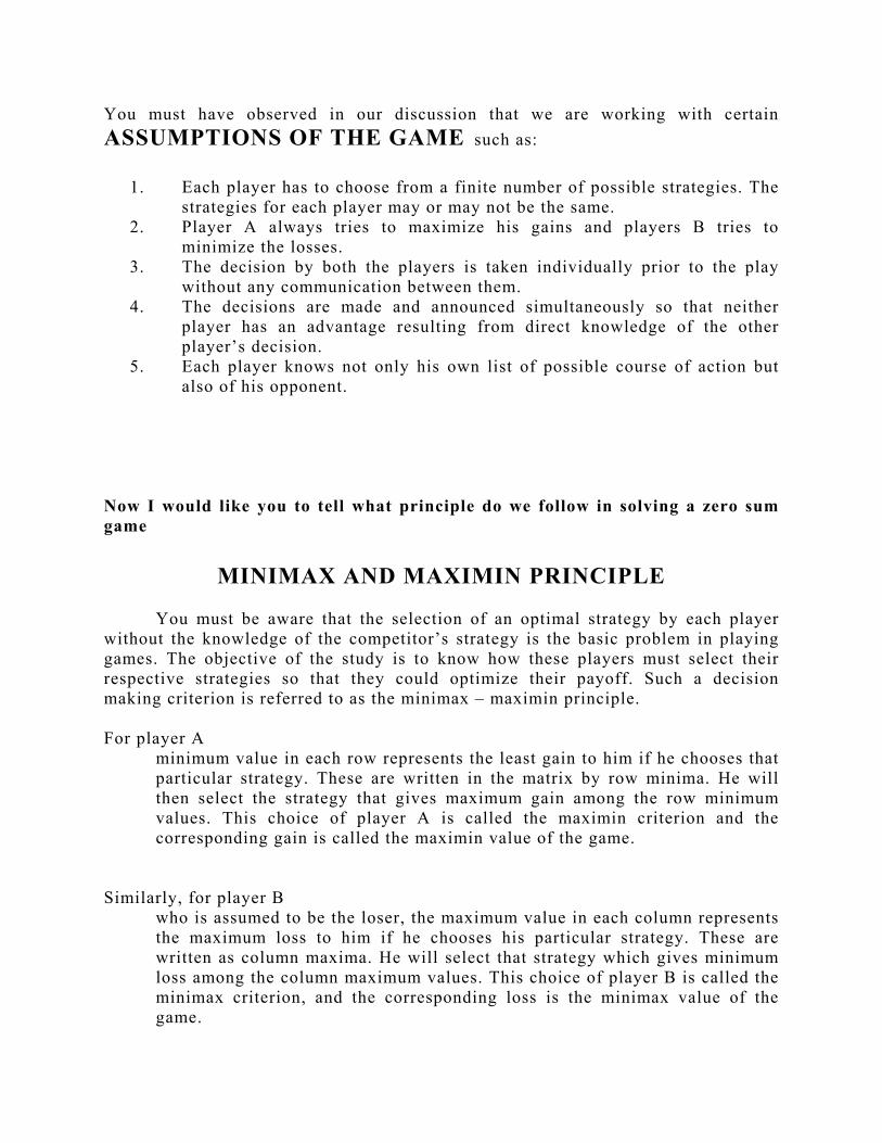
You must have observed in our discussion that we are working with certain ASSUMPTIONS OF THE GAME such as:
1. Each player has to choose from a finite number of possible strategies. The strategies for each player may or may not be the same.
2. Player A always tries to maximize his gains and players B tries to minimize the losses.
3. The decision by both the players is taken individually prior to the play without any communication between them.
4. The decisions are made and announced simultaneously so that neither player has an advantage resulting from direct knowledge of the other player’s decision.
5. Each player knows not only his own list of possible course of action but also of his opponent.
Now I would like you to tell what principle do we follow in solving a zero sum game
MINIMAX AND MAXIMIN PRINCIPLE
You must be aware that the selection of an optimal strategy by each player without the knowledge of the competitor’s strategy is the basic problem in playing games. The objective of the study is to know how these players must select their respective strategies so that they could optimize their payoff. Such a decision making criterion is referred to as the minimax – maximin principle. For player A
minimum value in each row represents the least gain to him if he chooses that particular strategy. These are written in the matrix by row minima. He will then select the strategy that gives maximum gain among the row minimum values. This choice of player A is called the maximin criterion and the corresponding gain is called the maximin value of the game.
Similarly, for player B
who is assumed to be the loser, the maximum value in each column represents the maximum loss to him if he chooses his particular strategy. These are written as column maxima. He will select that strategy which gives minimum loss among the column maximum values. This choice of player B is called the minimax criterion, and the corresponding loss is the minimax value of the game.

If the maximin value equals the minimax value, then the game is said to have a saddle point and the corresponding strategies are called optimal strategies. The amount of payoff at an equilibrium point is known as the VALUE of the game. A game may have more than one saddle point or no saddle point. To illustrate the minimax – maximin principle,
consider a two person zero – sum game with the given payoff matrix for player A.
Payoff matrix
Player Player B’s Strategies A’s Strategies
B1 B2
A1 4 3 A2 8 6 A3 5 4
Let the pure strategies of the two players be denoted by
SA = {A1, A2, A3} and
SB = {B1, B2}
Suppose that player A starts the game knowing that whatever strategy he adopts, B will select that particular counter strategy which will minimize the payoff to A. Thus if A selects the strategy A1 then B will select B2 as his corresponds to the minimum payoff to A corresponding to A1. Similarly, if A chooses the strategy A2, he may gain 8 or 6 depending upon the choice of B. If A chooses A2 then A can guarantee a gain of at least min {8,6} = 6 irrespective of the choice of B. Obviously A would prefer to maximize his minimum assured gains. In this example the selection of strategy A2 gives the maximum of the minimum gains to A.
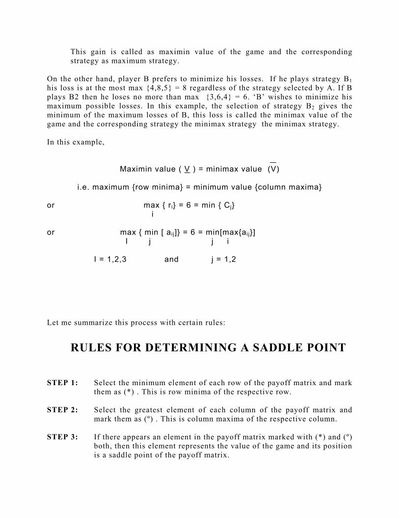
This gain is called as maximin value of the game and the corresponding strategy as maximum strategy.
On the other hand, player B prefers to minimize his losses. If he plays strategy B1 his loss is at the most max {4,8,5} = 8 regardless of the strategy selected by A. If B plays B2 then he loses no more than max {3,6,4} = 6. ‘B’ wishes to minimize his maximum possible losses. In this example, the selection of strategy B2 gives the minimum of the maximum losses of B, this loss is called the minimax value of the game and the corresponding strategy the minimax strategy the minimax strategy. In this example,
Maximin value ( V ) = minimax value (V)
i.e. maximum {row minima} = minimum value {column maxima} or max { ri} = 6 = min { Cj} i
or max { min [ aij]} = 6 = min[max{aij}]
I j j i
I = 1,2,3 and j = 1,2
Let me summarize this process with certain rules:
RULES FOR DETERMINING A SADDLE POINT STEP 1: Select the minimum element of each row of the payoff matrix and mark
them as (*) . This is row minima of the respective row. STEP 2: Select the greatest element of each column of the payoff matrix and
mark them as (º) . This is column maxima of the respective column. STEP 3: If there appears an element in the payoff matrix marked with (*) and (º)
both, then this element represents the value of the game and its position is a saddle point of the payoff matrix.
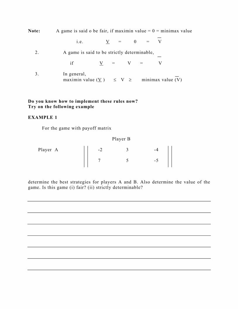
Note: A game is said o be fair, if maximin value = 0 = minimax value
i.e. V = 0 = V
2. A game is said to be strictly determinable, if V = V = V
3. In general, maximin value (V ) ≤ V ≥ minimax value (V)
Do you know how to implement these rules now? Try on the following example EXAMPLE 1 For the game with payoff matrix
Player B
Player A -2 3 -4
7 5 -5
determine the best strategies for players A and B. Also determine the value of the game. Is this game (i) fair? (ii) strictly determinable?
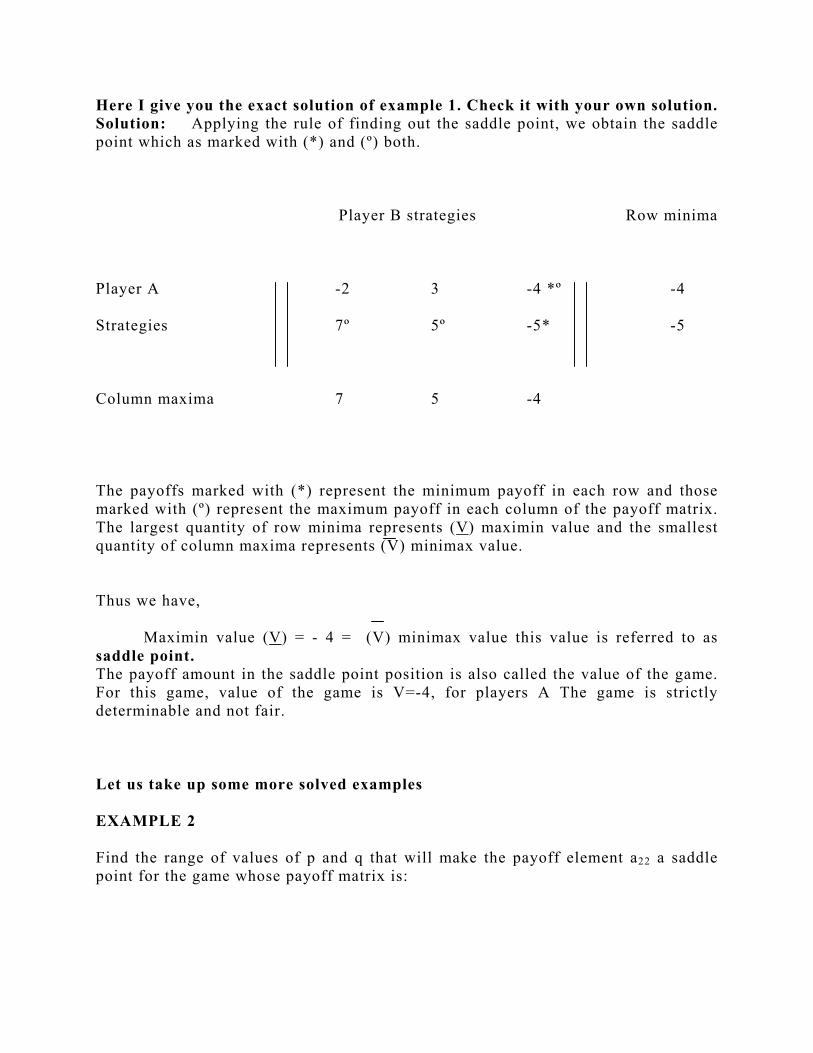
Here I give you the exact solution of example 1. Check it with your own solution. Solution: Applying the rule of finding out the saddle point, we obtain the saddle point which as marked with (*) and (º) both.
Player B strategies Row minima
Player A -2 3 -4 *º -4
Strategies 7º 5º -5* -5
Column maxima 7 5 -4
The payoffs marked with (*) represent the minimum payoff in each row and those marked with (º) represent the maximum payoff in each column of the payoff matrix. The largest quantity of row minima represents (V) maximin value and the smallest quantity of column maxima represents (V) minimax value. Thus we have, Maximin value (V) = - 4 = (V) minimax value this value is referred to as saddle point. The payoff amount in the saddle point position is also called the value of the game. For this game, value of the game is V=-4, for players A The game is strictly determinable and not fair. Let us take up some more solved examples EXAMPLE 2 Find the range of values of p and q that will make the payoff element a22 a saddle point for the game whose payoff matrix is:

Player B
Player A 2 4 5
10 7 q
4 p 6 Solution: First ignoring the values of p and q in the payoff matrix, determine the maximin and minimax values of the payoff matrix. Player B Row minima
Player A 2* 4 5 2
10º 7*º q 7
4* p 6 4
Column maxima 10 7 6 Since there does not exist a unique saddle point, the element a22 will be a saddle point only when p ≤ 7 and q ≥7 EXAMPLE 3 A company management and the labour union are negotiating a new 3 year settlement . Each of these has 4 strategies. I: Hard and aggressive bargaining II: Reasoning and logical approach III: Legalistic strategy IV: Conciliatory approach.
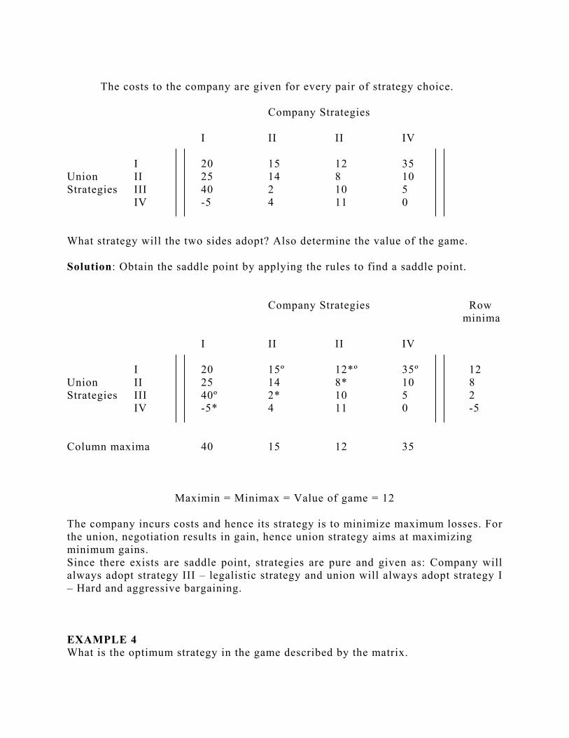
The costs to the company are given for every pair of strategy choice. Company Strategies I II II IV I 20 15 12 35 Union II 25 14 8 10 Strategies III 40 2 10 5 IV -5 4 11 0 What strategy will the two sides adopt? Also determine the value of the game. Solution: Obtain the saddle point by applying the rules to find a saddle point.
Company Strategies Row minima
I II II IV I 20 15º 12*º 35º 12 Union II 25 14 8* 10 8 Strategies III 40º 2* 10 5 2 IV -5* 4 11 0 -5 Column maxima 40 15 12 35
Maximin = Minimax = Value of game = 12 The company incurs costs and hence its strategy is to minimize maximum losses. For the union, negotiation results in gain, hence union strategy aims at maximizing minimum gains. Since there exists are saddle point, strategies are pure and given as: Company will always adopt strategy III – legalistic strategy and union will always adopt strategy I – Hard and aggressive bargaining. EXAMPLE 4 What is the optimum strategy in the game described by the matrix.

-5 3 2 10 5 5 4 6
-4 -2 0 -5 Solution: We determine the saddle point
PLAYER B PLAYER A
I II III IV I -5 3 2* 10º II 5º 5º 4*º 6
III -4 -2 0 -5*
Maximin = Minimax = Value of the game = 4 Hence the solution to the game is
1. The optimal strategy for player A is II 2. The optimal strategy for player B is III 3. The value of the game is 5.
EXAMPLE 5 Shruti Ltd has developed a sales forecasting function for its products and the products of its competitor, Purnima Ltd. There are four strategies S1, S2, S3 and S4 available to Shruti Ltd. and three strategies P1, P2 and P3 to Purnima Ltd. The pay-offs corresponding to all the twelve combinations of the strategies are given below. From the table we can see that, for example, if strategy S1 is employed by Shruti Ltd. and strategies P1 by Purnima Ltd., then there shall be a gain of Rs. 30,000 in quarterly sales to the former. Other entries can be similarly interpreted. Considering this information, state what would be the optimal strategy for Shruti Ltd.? Purnima Ltd.? What is the value of the game? Is the game fair?

Purnima Ltd.’s Strategy P1 P2 P3 S1 30,000 -21,000 1,000 Shruti’s Strategy S2 18,000 14,000 12,000 S3 -6,000 28,000 4,000 S4 18,000 6,000 2,000 Solution: For determining the optimal strategies for the players’ we shall determine if saddle point exists for this Purnima’s Strategy P1 P2 P3 Row Minima S1 30,000º -21,000* 1,000 -21,000 Shruti’s Strategy S2 18,000 14,000 12,000*º 12,000 S3 - 6,000* 28,000º 4,000 -6,000 S4 18,000 6,000 2,000* 2,000 Column maxima 30,000 28,000 12,000 Here saddle point exists at the intersection of S2 and P3. These represent optimal policies, respectively, of Shruti Ltd. and Purnima Ltd. Correspondingly, the value of game, V=12,000. Since V ≠ 0, the game is not a fair one. EXAMPLE 6 Solve the game whose pay off matrix is given by Player B
B1 B2 B3
A1 1 3 1
Player A A2 0 -4 -3
A3 1 5 -1

Solution : Player B
B1 B2 B3 Row minima
A1 1*º 3 1*º 1
Player A A2 0 -4* -3 -4
A3 1º 5º -1* -1
Column maxima 1 5 1
Maxi (minimum) = Max (1, -4, -1) = 1 Mini (maximum) = Min (1,5,1) = 1
ie., Maximin value v= 1 = Minimax value v Therefore, Saddle point exists. The value of the game is the saddle point which is 1. The optimal strategy is the position of the saddle point and is given by (A1,B1). EXAMPLE 7 For what value of λ, the game with the following matrix is strictly determinable?
Player B B1 B2 B3 A1 λ 6 2 Player A A2 -1 λ -7 A3 -2 4 λ Solution Ignoring the value of λ, the payoff matrix is given by
Player B B1 B2 B3 Row minima A1 λ 6 2 2 Player A A2 -1 λ -7 -7 A3 -2 4 λ -2
Column maxima -1 6 2

The game is strictly determinable, if
v = v = v Hence v = 2
v = -1
-1 ≤ λ ≤ 2 Now, I will give you some unsolved problems Problem 1: Burger Giant and Pizza mania are competing for a larger share of the
fast-food market. Both are contemplating the use of promotional coupons. If Burger Giant does not spend any money of promotional coupons, it will not lose any share of the market if Pizza mania also does not spend any money on promotional coupons. Burger Giant will lose 4 percent of the market if Pizza mania spends Rs. 2500 on coupons, and it will lose 6 percent of the market if Pizza mania spends Rs. 3000 on coupons. If Burger Giant spends Rs. 2500 on coupons, it will gain 3 percent of the market if pizza mania spends Rs. 0, and it will gain 2 percent if Pizza mania Spends Rs. 2500, and it will lose 1 percent of the market if Pizza mania spends Rs. 3000. If Burger Giant Spends Rs. 3000, it will gain 5% of the market if Pizza mania spends Rs 0, it will gain 3% of the market if Pizza mania spends Rs. 2500, and gains 2% of the market if Pizza mania spends Rs. 3000.
(a) Develop a payoff table for this game. (b) Determine the strategies that Burger Giant and Pizza mania should adopt. (c) What is the value of this game?
Problem 2: The two major scooter companies of India, ABC and XYZ, are
competing for a fixed market. If both the manufacturers make major model changes in a year, then their shares of the market do not change. Also, if they both do not make major model changes, their shares of the market remain constant. If ABC makes a major model change and XYZ does not, then ABC is able to take away a% of the market away from XYZ, and if XYZ makes a major model change ABC does not, XYZ is able to take away b% of the market away from ABC. Express it as a two-by-two game and solve for the optimal strategy for each of the producers.
So, now let us summarize today’s discussion: Summary We have discussed about:
• Factors influencing game theory models. • Identification of two person zero sum games. • Minimax and Maximin Principle • Importance and application of saddle point.
Slide 1
GAME THEORY
LECTURE 1
______________________________________________________________________________
______________________________________________________________________________
______________________________________________________________________________
______________________________________________________________________________
______________________________________________________________________________
______________________________________________________________________________
______________________________________________________________________________
______________________________________________________________________________
______________________________________________________________________________
______________________________________________________________________________
__________________________________________________________________________

Slide 2
INTRODUCTION
Game theory is the study of how optimal strategies are formulated in conflict.
______________________________________________________________________________
______________________________________________________________________________
______________________________________________________________________________
______________________________________________________________________________
______________________________________________________________________________
______________________________________________________________________________
______________________________________________________________________________
______________________________________________________________________________
______________________________________________________________________________
______________________________________________________________________________
_____________________________________________________________________

Slide 3
WHAT IS A GAME?
A game refers to a situation in which two or more players are competing having different goals or objectives.
______________________________________________________________________________
______________________________________________________________________________
______________________________________________________________________________
______________________________________________________________________________
______________________________________________________________________________
______________________________________________________________________________
______________________________________________________________________________
______________________________________________________________________________
______________________________________________________________________________
______________________________________________________________________________
______________________________________________________________________________
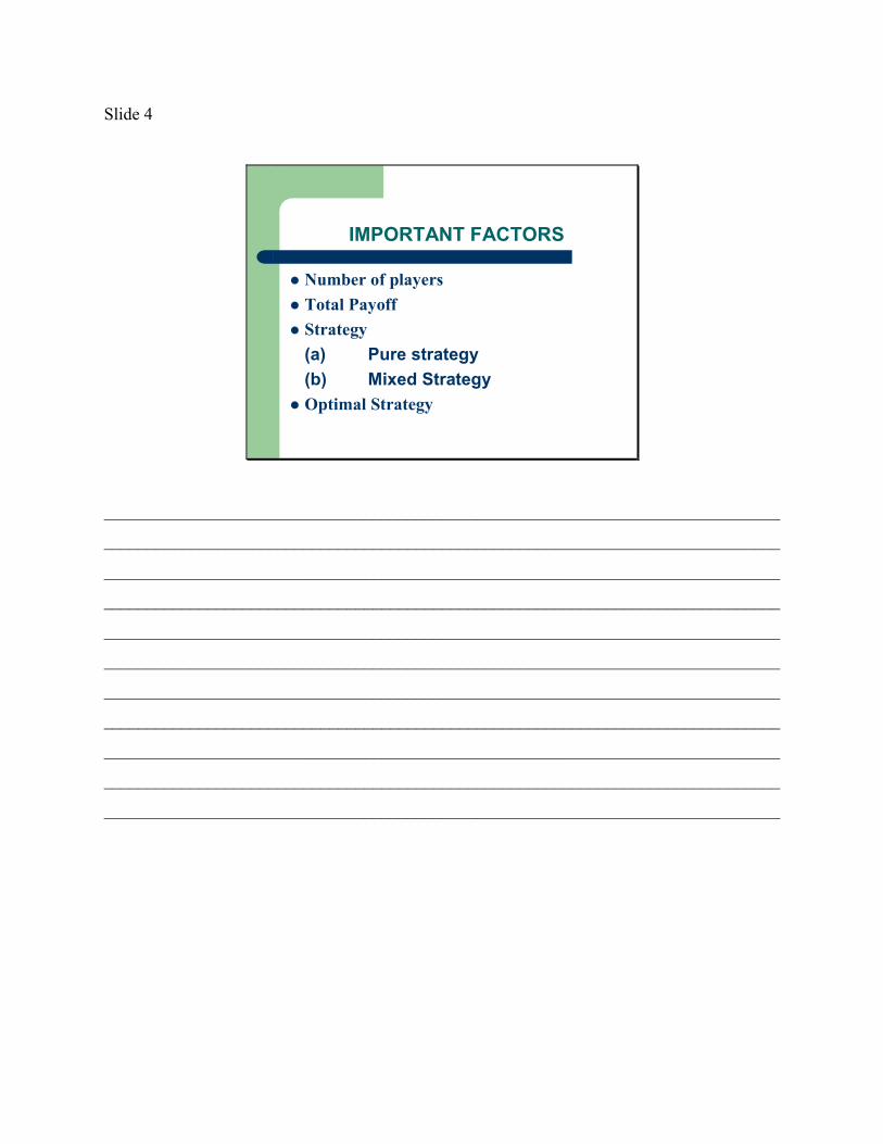
Slide 4
IMPORTANT FACTORS
Number of playersTotal PayoffStrategy(a) Pure strategy(b) Mixed Strategy Optimal Strategy
______________________________________________________________________________
______________________________________________________________________________
______________________________________________________________________________
______________________________________________________________________________
______________________________________________________________________________
______________________________________________________________________________
______________________________________________________________________________
______________________________________________________________________________
______________________________________________________________________________
______________________________________________________________________________
______________________________________________________________________________

Slide 5
TWO PERSON ZERO SUM GAME
Involving only two players.
The gains made by one equals the loss incurred by the other.
______________________________________________________________________________
______________________________________________________________________________
______________________________________________________________________________
______________________________________________________________________________
______________________________________________________________________________
______________________________________________________________________________
______________________________________________________________________________
______________________________________________________________________________
______________________________________________________________________________
______________________________________________________________________________
______________________________________________________________________________
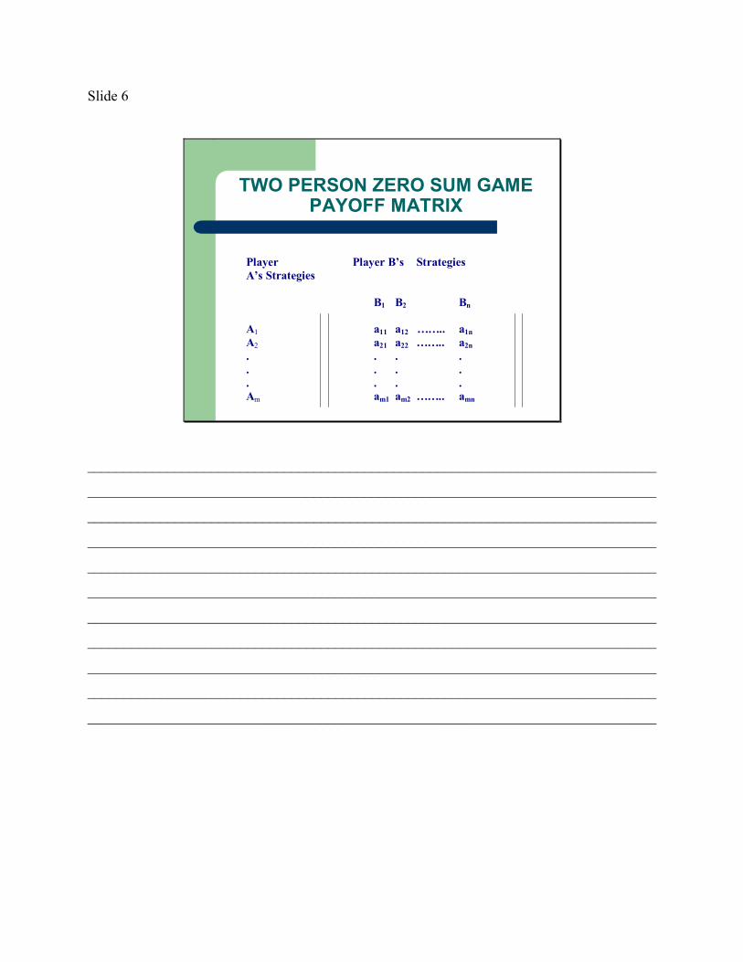
Slide 6
TWO PERSON ZERO SUM GAMEPAYOFF MATRIX
Player Player B’s Strategies A’s Strategies
B1 B2 Bn
A1 a11 a12 …….. a1n A2 a21 a22 …….. a2n
. . . . . . . . . . . .
Am am1 am2 …….. amn
______________________________________________________________________________
______________________________________________________________________________
______________________________________________________________________________
______________________________________________________________________________
______________________________________________________________________________
______________________________________________________________________________
______________________________________________________________________________
______________________________________________________________________________
______________________________________________________________________________
______________________________________________________________________________
______________________________________________________________________________

Slide 7
WHAT IS MINIMAX AND MAXIMIN PRINCIPLE ?
Minimax – Maximin principle is a decision making criterion that specifies how the players must select their respective strategies .
______________________________________________________________________________
______________________________________________________________________________
______________________________________________________________________________
______________________________________________________________________________
______________________________________________________________________________
______________________________________________________________________________
______________________________________________________________________________
______________________________________________________________________________
______________________________________________________________________________
______________________________________________________________________________
______________________________________________________________________________

Slide 8
RULES FOR DETERMINING A SADDLE POINT
• Select the lowest element of each row of the payoff matrix and mark it as (*) .
• Select the greatest element of each column of the payoff matrix and mark it as (º) .
• The element in the payoff matrix marked with (*) and (º) both is a saddle point of the payoff matrix.
______________________________________________________________________________
______________________________________________________________________________
______________________________________________________________________________
______________________________________________________________________________
______________________________________________________________________________
______________________________________________________________________________
______________________________________________________________________________
______________________________________________________________________________
______________________________________________________________________________
______________________________________________________________________________
______________________________________________________________________________

Unit 3 GAME THEORY Lesson 26 Hello students, In previous lecture you learned to solve the zero-sum games having saddle point. Learning Objective: • In this lecture you are going to study How to solve the zero sum games
which do not possess a saddle point?
TWO PERSON ZERO SUM GAME ( WITHOUT A SADDLE POINT)
You have observed that in game situations which have a saddle point(s) are provided
with an adequate theory of how best to play the game. It is possible that there is no
saddle point of a game and then it is not possible to find its solution in terms of the
pure strategies – the maximin and the minimax.
Games without saddle point are not strictly determined. The solution to such
problems calls for employing mixed strategies i.e. to solve such games both the
players must determine an optimal mixture of strategies to find a saddle point. A
mixed strategy therefore represents a combination of two or more strategies that are
selected one at a time, according to pre-determined probabilities. Thus in employing
a mixed strategy, a player decides to mix his choices among several alternatives in a
certain ratio.
Consider this with the help of an example EXAMPLE 1

Determine the optimal strategies for the players and value of the game from the following payoff matrix.
Player B Player A
B1 B2 A1 8 -7
A2 -6 4 Solution: The given problem does not have a saddle point. Therefore, the method of saddle point is not sufficient to determine optimal strategies. If A plays A1 then B would play B2 while if A plays A2 then B would choose B1 to play. So if B knows what choice A will make then B can ensure that he gains by choosing a strategy, opposite to the one desired by A. Thus it is important for A to make it difficult for B to guess as to what choice he is going to make. Similarly, B would like to make it very difficult for A to assess the strategy he is likely to adopt.
Now suppose that A plays strategy A1, with probability p1 and plays strategy A2 with probability p2 = 1 – p1 . If B plays strategy B1, then A’s expected payoff can be determines by the figures in the first column of the payoff matrix as: Expected payoff (if B plays B1) = 8p1 - 6p2 = 8p1 – 6 ( 1-p1) Similarly, If B plays B2, the expected payoff to A can be determined as: Expected pay off (if B plays B2) = -7p1 + 4p2 = -7p1 + 4(1-p1) Now, we determine a value of p1 so that the expected pay – off for A is the same irrespective of the strategy adopted by B Thus, 8p1 – 6(1-p1) = - 7p1 + (1-p1)
8p1 – 6 + 6p1 = - 7p1+4-4p1

=> p1 = 10 = 2 --- --
25 5 p2 = 1-p1 = 3
-- 5
A would do best to adopt the strategies A1 and A2, choosing in random manner, in the ratio 2:3 ( 2/5 and 3/5) . The expected pay off for A using this mixed strategy is given by.
8 x 2 - 6 x 3 = -2 5 5 5
or -7 x 2 - 4x 3 = 2
5 5 5 Thus he will have a loss of 2/5 per play. Now, we determine the mixed strategy for B in a similar manner. Let us suppose B plays strategy B1, with probability q1 and strategy B2 with probability q2 = 1-q1 Then, Expected payoff (given that A plays A1) = 8q1 – 7q2 = 8q1 – 7 ( 1-q1)
Expected payoff ( given that A plays A2) = -6q1 + 4q2 = - 6q1 + 4 (1-q1) The value of q1 so that the expected payoff for B is same irrespective of the strategy of A is obtained as.
8q1 – 7(1-q1) = -6q1 + 4 ( 1-q1)
8q1 – 7 + 7q1 = - 6q1 + 4 – 4q1
q1 = 11 , q2 = 14
--- --- 25 25
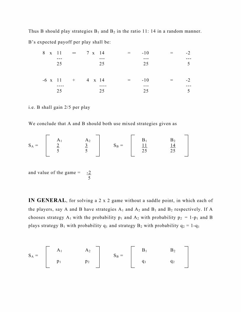
Thus B should play strategies B1 and B2 in the ratio 11: 14 in a random manner. B’s expected payoff per play shall be: 8 x 11 ─ 7 x 14 = -10 = -2 --- --- --- ---
25 25 25 5
-6 x 11 + 4 x 14 = -10 = -2 ---- ---- --- ---
25 25 25 5 i.e. B shall gain 2/5 per play We conclude that A and B should both use mixed strategies given as A1 A2 B1 B2 SA = 2 3 SB = 11 14 5 5 25 25 and value of the game = -2 5 IN GENERAL, for solving a 2 x 2 game without a saddle point, in which each of
the players, say A and B have strategies A1 and A2 and B1 and B2 respectively. If A
chooses strategy A1 with the probability p1 and A2 with probability p2 = 1-p1 and B
plays strategy B1 with probability q1 and strategy B2 with probability q2 = 1-q1
A1 A2 B1 B2 SA = SB = p1 p2 q1 q2
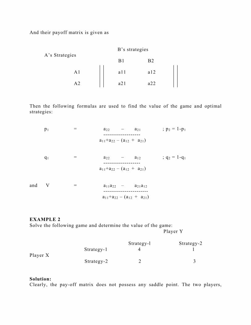
And their payoff matrix is given as
B’s strategies A’s Strategies
B1 B2 A1 a11 a12
A2 a21 a22
Then the following formulas are used to find the value of the game and optimal strategies: p1 = a22 – a21 ; p2 = 1-p1 -------------------
a11+a22 – (a12 + a21)
q1 = a22 – a12 ; q2 = 1-q1 -------------------
a11+a22 – (a12 + a21) and V = a11a22 – a21a12 -----------------------
a11+a22 – (a12 + a21) EXAMPLE 2 Solve the following game and determine the value of the game: Player Y Strategy-l Strategy-2 Strategy-1 4 1 Player X Strategy-2 2 3
Solution: Clearly, the pay-off matrix does not possess any saddle point. The two players,
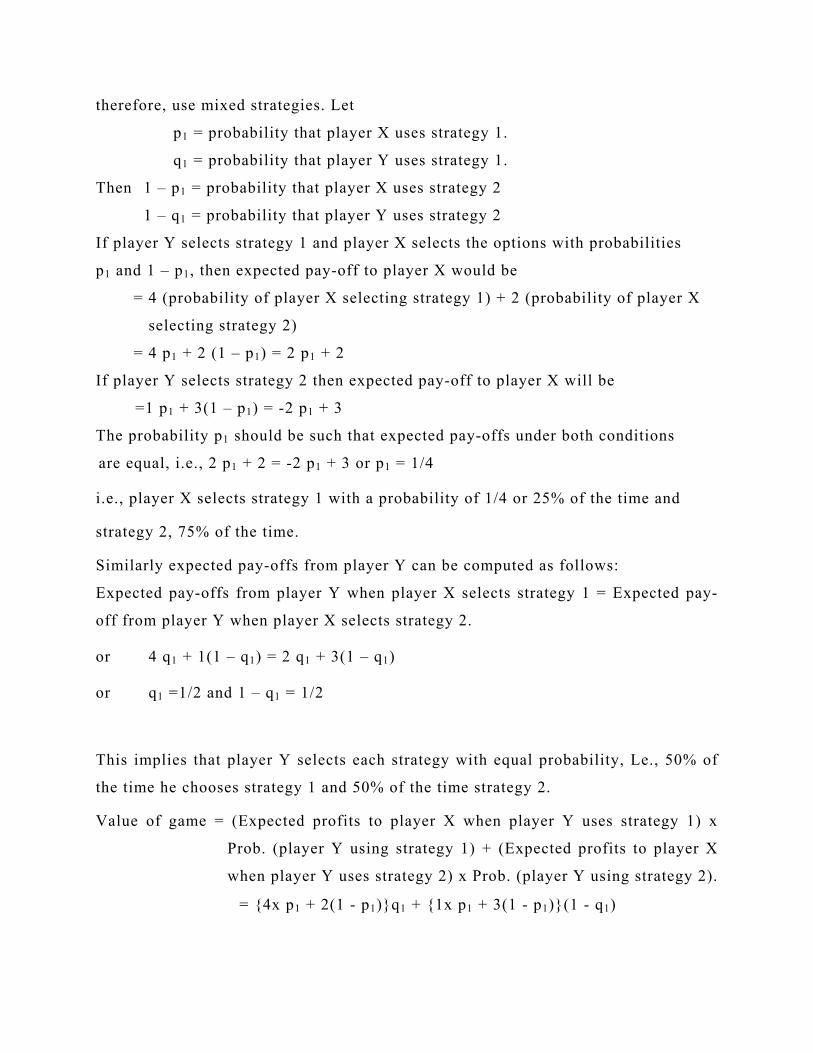
therefore, use mixed strategies. Let
p1 = probability that player X uses strategy 1.
q1 = probability that player Y uses strategy 1.
Then 1 – p1 = probability that player X uses strategy 2
1 – q1 = probability that player Y uses strategy 2
If player Y selects strategy 1 and player X selects the options with probabilities
p1 and 1 – p1, then expected pay-off to player X would be
= 4 (probability of player X selecting strategy 1) + 2 (probability of player X
selecting strategy 2)
= 4 p1 + 2 (1 – p1) = 2 p1 + 2
If player Y selects strategy 2 then expected pay-off to player X will be
=1 p1 + 3(1 – p1) = -2 p1 + 3
The probability p1 should be such that expected pay-offs under both conditions
are equal, i.e., 2 p1 + 2 = -2 p1 + 3 or p1 = 1/4
i.e., player X selects strategy 1 with a probability of 1/4 or 25% of the time and
strategy 2, 75% of the time.
Similarly expected pay-offs from player Y can be computed as follows:
Expected pay-offs from player Y when player X selects strategy 1 = Expected pay-
off from player Y when player X selects strategy 2.
or 4 q1 + 1(1 – q1) = 2 q1 + 3(1 – q1)
or q1 =1/2 and 1 – q1 = 1/2
This implies that player Y selects each strategy with equal probability, Le., 50% of
the time he chooses strategy 1 and 50% of the time strategy 2.
Value of game = (Expected profits to player X when player Y uses strategy 1) x
Prob. (player Y using strategy 1) + (Expected profits to player X
when player Y uses strategy 2) x Prob. (player Y using strategy 2).
= {4x p1 + 2(1 - p1)}q1 + {1x p1 + 3(1 - p1)}(1 - q1)

={4x1/4 + 2(1-1/4)}1/2 +{lx1/4 +3 (1-1/4)} (1-1/2)
= 10/4 Alternatively: The optimum mixed strategies for player X and Y are determined by :
p1 = a22 – a21 = 3-2 = 1
------------------- ---------- -- a11+a22 – (a12 + a21) 4+3-(2+1) 4
q1 = a22 – a12 = 4-2 = 1 ------------------- ---------- --
a11+a22 – (a12 + a21) 4+3-(2+1) 2
The expected value of the game is given by V = a11a22 – a21a12 = 4x3-2x1 = 10 ----------------------- ------------ ---
a11+a22 – (a12 + a21) 4+3-(2+1) 4 Hence the optimum strategies for the two players are: X1 X2 Y1 Y2 SX = SY = 1/4 3/4 1/2 1/2
EXAMPLE 3 Determine the optimal strategies for the players and value of the game from the following payoff matrix.
Player B Player A
B1 B2 A1 5 1
A2 3 4

Solution:
The given problem does not have a saddle point. Therefore, the method of saddle point is not sufficient to determine optimal strategies. Let the payoff matrix is given by
B’s strategies A’s Strategies
B1 B2 A1 a11 a12
A2 a21 a22
Then the optimal mixed strategies are
A1 A2 B1 B2 SA = SB = p1 p2 q1 q2
where
p1 = a22 – a21 = 4-3 = 1
------------------- ---------- -- a11+a22 – (a12 + a21) 5+4-(1+3) 5
p2 = 1-p1 = 4/5
q1 = a22 – a12 = 4-1 = 3 ------------------- ---------- --
a11+a22 – (a12 + a21) 5+4-(1+3) 5
q2 = 1-q1 = 2/5

The expected value of the game is given by V = a11a22 – a21a12 = (5x4)-(1x3) = 17 ----------------------- -------------- ---
a11+a22 – (a12 + a21) 5+4-(1+3) 5
Hence the optimal mixed strategies are
A1 A2 B1 B2 SA = SB = 1/5 4/5 3/5 2/5
EXAMPLE 4 Determine the optimal strategies for the players and value of the game from the following payoff matrix.
Player B Player A
B1 B2 A1 4 -4
A2 -4 4 Solution:
The given problem does not have a saddle point. Therefore, the method of saddle point is not sufficient to determine optimal strategies. Let the payoff matrix is given by
B’s strategies A’s Strategies
B1 B2 A1 a11 a12
A2 a21 a22

Then the optimal mixed strategies are
A1 A2 B1 B2 SA = SB = p1 p2 q1 q2
where p1 = a22 – a21 = 4-(-4) = 1
------------------- ---------- -- a11+a22 – (a12 + a21) 4+4-(-4-4) 2
p2 = 1-p1 = 1/2
q1 = a22 – a12 = 4-(-4) = 1 ------------------- ---------- --
a11+a22 – (a12 + a21) 4+4-(-4-4) 2
q2 = 1-q1 = 1/2 The expected value of the game is given by V = a11a22 – a21a12 = (4x4)-(-4x(-4)) = 0 ----------------------- ------------------
a11+a22 – (a12 + a21) 4+4-(-4+(-4))
Hence the optimal mixed strategies are
A1 A2 B1 B2 SA = SB = 1/2 1/2 1/2 1/2
Now, Apply this method on an Unsolved Problem yourself Q.1. Determine the strategies for player. A and B in the following game. Also
indicate the value of the game. B1 B2 A1 20 25
A2 30 -15 So, now let us summarize today’s discussion: Summary We have discussed about:
• Factors influencing game theory models. • Identification of two person zero sum games. • Minimax and Maximin Principle • Importance and application of saddle point.
Slide 1
GAME THEORY
LESSON 2

Slide 2
TWO PERSON ZERO SUM GAME (WITHOUT A SADDLE POINT)
Player A has strategy A1 and A2
Player B has strategy B1 and B2
A chooses strategy A1 with the probability p1and A2 with probability p2 = 1-p1
B plays strategy B1 with probability q1 and strategy B2 with probability q2 = 1-q1
______________________________________________________________________________
______________________________________________________________________________
______________________________________________________________________________
______________________________________________________________________________
______________________________________________________________________________
______________________________________________________________________________
______________________________________________________________________________
______________________________________________________________________________
______________________________________________________________________________
______________________________________________________________________________
______________________________________________________________________________

Slide 3
PAYOFF MATRIX OF A AND B
B’S STRATEGIES A’S STRATEGIES
B1 B2 A1 a11 a12
A2 a21 a22
______________________________________________________________________________
______________________________________________________________________________
______________________________________________________________________________
______________________________________________________________________________
______________________________________________________________________________
______________________________________________________________________________
______________________________________________________________________________
______________________________________________________________________________
______________________________________________________________________________
______________________________________________________________________________
______________________________________________________________________________

Slide 4
Evaluation of Probabilities p1 = a22 – a21 ; p2 = 1-p1 -------------------
a11+a22 – (a12 + a21)
q1 = a22 – a12 ; q2 = 1-q1 ---------------------
a11+a22 – (a12 + a21)
and V = a11a22 – a21a12 -----------------------
a11+a22 – (a12 + a21)
______________________________________________________________________________
______________________________________________________________________________
______________________________________________________________________________
______________________________________________________________________________
______________________________________________________________________________
______________________________________________________________________________
______________________________________________________________________________
______________________________________________________________________________
______________________________________________________________________________
______________________________________________________________________________
______________________________________________________________________________
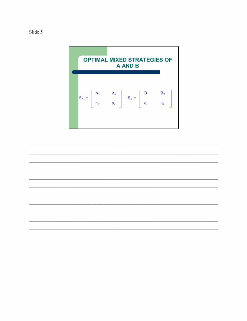
Slide 5
OPTIMAL MIXED STRATEGIES OF A AND B
A1 A2 B1 B2 SA = SB = p1 p2 q1 q2
______________________________________________________________________________
______________________________________________________________________________
______________________________________________________________________________
______________________________________________________________________________
______________________________________________________________________________
______________________________________________________________________________
______________________________________________________________________________
______________________________________________________________________________
______________________________________________________________________________
______________________________________________________________________________
______________________________________________________________________________

Unit 3 GAME THEORY Lesson 27 Learning Objective: • To learn to apply dominance in game theory. • Generate solutions in functional areas of business and management. Hello students, In our last lecture you learned to solve zero sum games having mixed strategies. But... Did you observe one thing that it was applicable to only 2 x 2 payoff matrices? So let us implement it to other matrices using dominance and study the importance of DOMINANCE
In a game, sometimes a strategy available to a player might be found to be
preferable to some other strategy / strategies. Such a strategy is said to dominate the other one(s). The rules of dominance are used to reduce the size of the payoff matrix. These rules help in deleting certain rows and/or columns of the payoff matrix, which are of lower priority to at least one of the remaining rows, and/or columns in terms of payoffs to both the players. Rows / columns once deleted will never be used for determining the optimal strategy for both the players. This concept of domination is very usefully employed in simplifying the two – person zero sum games without saddle point. In general the following rules are used to reduce the size of payoff matrix. The RULES ( PRINCIPLES OF DOMINANCE ) you will have to follow are: Rule 1: If all the elements in a row ( say ith row ) of a pay off matrix are less than or equal to the corresponding elements of the other row ( say jth row ) then the player A

will never choose the ith strategy then we say ith strategy is dominated by jth strategy and will delete the ith row. Rule 2: If all the elements in a column ( say rth column ) of a payoff matrix are greater than or equal to the corresponding elements of the other column ( say sth column ) then the player B will never choose the rth strategy or in the other words the rth strategy is dominated by the sth strategy and we delete rth column . Rule 3: A pure strategy may be dominated if it is inferior to average of two or more other pure strategies. Now, consider some simple examples
Example 1
Given the payoff matrix for player A, obtain the optimum strategies for both the players and determine the value of the game. Player B
Player A 6 -3 7
-3 0 4
Solution Player B
B1 B2 B3
Player A A1 6 -3 7
A2 -3 0 4
When A chooses strategy A1 or A2, B will never go to strategy B3. Hence strategy
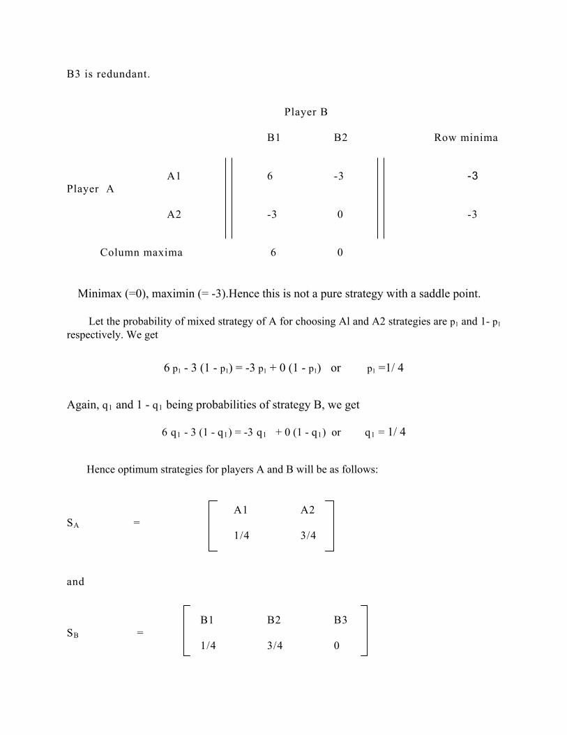
B3 is redundant.
Player B
B1 B2 Row minima
A1 6 -3 -3 Player A
A2 -3 0 -3
Column maxima 6 0 Minimax (=0), maximin (= -3).Hence this is not a pure strategy with a saddle point.
Let the probability of mixed strategy of A for choosing Al and A2 strategies are p1 and 1- p1 respectively. We get
6 p1 - 3 (1 - p1) = -3 p1 + 0 (1 - p1) or p1 =1/ 4
Again, q1 and 1 - q1 being probabilities of strategy B, we get
6 q1 - 3 (1 - q1) = -3 q1 + 0 (1 - q1) or q1 = 1/ 4
Hence optimum strategies for players A and B will be as follows:
A1 A2 SA =
1/4 3/4
and
B1 B2 B3 SB =
1/4 3/4 0
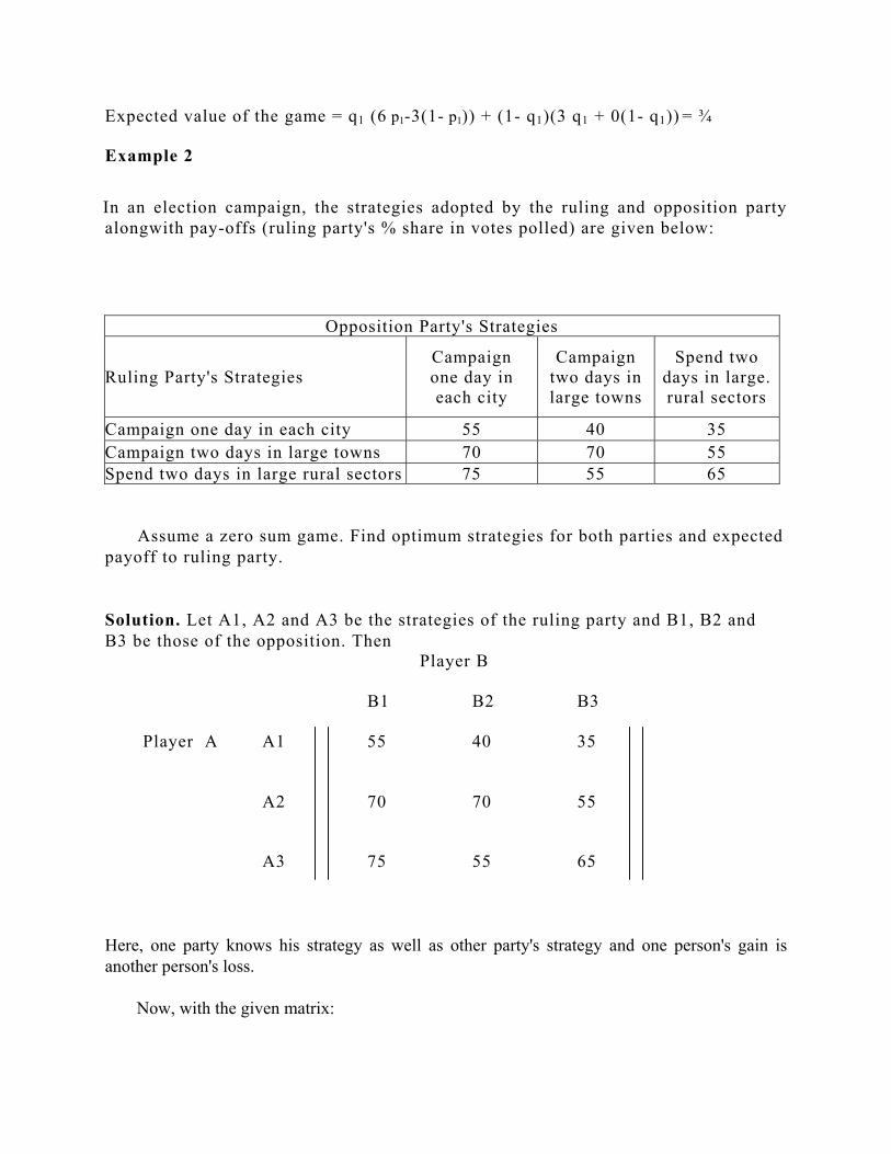
Expected value of the game = q1 (6 p1-3(1- p1)) + (1- q1)(3 q1 + 0(1- q1)) = ¾
Example 2 In an election campaign, the strategies adopted by the ruling and opposition party alongwith pay-offs (ruling party's % share in votes polled) are given below:
Opposition Party's Strategies
Ruling Party's Strategies Campaign one day in each city
Campaign two days in large towns
Spend two days in large.rural sectors
Campaign one day in each city 55 40 35 Campaign two days in large towns 70 70 55 Spend two days in large rural sectors 75 55 65 Assume a zero sum game. Find optimum strategies for both parties and expected payoff to ruling party. Solution. Let A1, A2 and A3 be the strategies of the ruling party and B1, B2 and B3 be those of the opposition. Then Player B
B1 B2 B3
Player A A1 55 40 35
A2 70 70 55
A3 75 55 65 Here, one party knows his strategy as well as other party's strategy and one person's gain is another person's loss. Now, with the given matrix:

Player B
B1 B2 B3 Row minima
Player A A1 55 40 35 35
A2 70 70 55 55
A3 75 55 65 65
Column maxima 75 70 65
As maximin = 55 and minimax = 65 , there is no saddle point. Row 1 is dominated by row 2 and column 1 is dominated by column 2 giving the reduced 2 x 2 matrix as :
B2 B3
A2 70 55
A3 55 65
For ruling party: Let the ruling party select strategy A2 with a probability of p1 and therefore opposition party selects strategy A3 with a probability of (1 – p1) Suppose the opposition selects strategy B2. Then the expected gain to ruling party for this game is given by :
70 p1 + 55 (1 - p1) = 15 p1 + 55 On the other hand, if opposition party selects strategy B3, then ruling party's expected gain is :
55 p1 + 65 (1- p1) = -10 p1 + 65 Now, in order for ruling party to be indifferent to which strategy, opposition
party selects, the optimum plan for ruling party requires that its expected gain should be equal for each of opposition party's possible strategies. Thus equating two equations of expected gain, we get
15 p1 + 55 = -10Pl + 65 or p1 = 2/5 and 1 - p1 = 3/5
Hence ruling party would select strategy A2 with probability of 0.4 and

strategy A3 with probability of 0.6. For opposition party. Let opposition party select strategy B2 and B3 with a
probability of ql and (1 – q1) respectively. The expected loss to opposition party when ruling party adopts strategy A2 and A3 respectively is : 70 q1 + 55(1 – q1) = 15ql + 55 and 55 q1 + 65 (1 - ql) = -10ql + 65 By equating expected losses of opposition party, regardless of what ruling party would choose, we get
15 q1 + 55 = -l0ql + 65 so that q1 = 2/5 and (1 – q1) = 3/5
Hence opposition party would choose strategy B2 and B3 with a probability of 0.4 and 0.6 respectively. The value of the game is determined by substituting the value of p1 and q1 in any of the expected values and is determined as 61, i. e., Expected gain to ruling party: (i) 15 x 0.4 + 55 = 61 (ii)-10 x 0.4 + 65 = 61 Expected loss to opposition party: (i) 15 x 0.4 + 55 = 61 (ii) -10 x 0.4 + 65 = 61
Example 3
Even though there are several manufacturers of scooters, two firms with branch names Janta and Praja, control their market in Western India. If both manufacturers make model changes of the same type for this market segment in the same year, their respective market shares remain constant. Likewise, if neither makes model changes, then also their market shares remain constant. The pay-off matrix in terms of increased/decreased percentage market share under different possible conditions is given below: Praja Janta No change Minor change Major change No change 0 -4 -10 Minor change 3 0 5 Major change 8 1 0

(i) Find the value of the game. (ii) What change should Janta consider if this information is available only to itself? .
Solution. (i) Clearly, the game has no saddle point. Making use of dominance principle,
since the first row is dominated by the third row, we delete the first row. Similarly, first column is dominated by the second column and hence we delete the first column. The reduced pay-off matrix will be as follows: Praja Minor change Major change Janta Minor change 0 5 Major change 1 0 As the reduced pay-off matrix does not possess any saddle point, the players will use mixed strategies. The optimum mixed strategy for player A is determined by :
p1 = a22 – a21 = 0-1 = 1
------------------- ---------- -- a11+a22 – (a12 + a21) 0+0-(5+1) 6
p2 = 1-p1 = 5/6
q1 = a22 – a12 = 0-5 = 5 ------------------- ---------- --
a11+a22 – (a12 + a21) 0+0-(5+1) 6
q2 = 1-q1 = 1/6 The expected value of the game is given by

V = a11a22 – a21a12 = (0x0)-(1x5) = 5/6 ----------------------- ------------------
a11+a22 – (a12 + a21) 0+0-(5+1)
Hence the optimal mixed strategies are
A1 A2 A3 SA = 0 1/6 5/6 B1 B2 B3 SB = 0 5/6 1/6
(ii) Janta may consider to have minor change with probability 5/6 and of major
change with probability 1/6 . Now,
Apply this method on some Unsolved Problems yourself Q.1. Indicate the value of the game. 10 8 4 10
10 11 3 7 9 7 5 4

Q.2. For the following ‘two-person, zero-sum’ game, find the optimal strategies for the two players and value of the game:
Player B B1 B2 B3 A1 9 9 3 Player A A2 6 -12 -11 A3 8 16 10
Determine it using the principle of dominance.
Q.3. Assume that two firms are competing for market share for a particular product.
Each firm is considering what promotional strategy to employ for the coming period. Assume that the following payoff matrix describes the increase in market share of Firm A and the decrease in market share for Firm B. Determine the optimal strategies for each firm.
Firm B Firm A Non Promotion Moderate Promotion Much Promotion Non Promotion 5 0 -10
Moderate Promotion 10 6 12
Much Promotion 20 15 10
(i) Which firm would be the winner, in terms of market share? (ii) Would the solution strategies necessarily maximize profits for either of the
firms? (iii) What might the two firms do to maximize their profits?

So, now let us summarize today’s discussion: Summary We have discussed about:
• Importance of Dominance. • Rules for Dominance. • Applications of Dominance.
Slide 1
GAME THEORY
LESSON 3
______________________________________________________________________________
______________________________________________________________________________
______________________________________________________________________________
______________________________________________________________________________
______________________________________________________________________________
______________________________________________________________________________
______________________________________________________________________________
______________________________________________________________________________
______________________________________________________________________________
______________________________________________________________________________
______________________________________________________________________________

Slide 2
DOMINANCE
What is a Dominant Strategy?
A particular strategy that is found to be preferable over other strategies available to a player is called the “dominant strategy” for that player.
______________________________________________________________________________
______________________________________________________________________________
______________________________________________________________________________
______________________________________________________________________________
______________________________________________________________________________
______________________________________________________________________________
______________________________________________________________________________
______________________________________________________________________________
______________________________________________________________________________
______________________________________________________________________________
______________________________________________________________________________

Slide 3
PRINCIPLES OF DOMINANCE
RULE 1If all the elements in a row ( say ith row ) of a pay off matrix are less than or equal to the corresponding elements of the other row ( say jth
row ) then the player A will never choose the ithstrategy then we say ith strategy is dominated by jth
strategy and will delete the ith row.
______________________________________________________________________________
______________________________________________________________________________
______________________________________________________________________________
______________________________________________________________________________
______________________________________________________________________________
______________________________________________________________________________
______________________________________________________________________________
______________________________________________________________________________
______________________________________________________________________________
______________________________________________________________________________
______________________________________________________________________________

Slide 4
PRINCIPLES OF DOMINANCE
RULE 2If all the elements in a column ( say rth column ) of a payoff matrix are greater than or equal to the corresponding elements of the other column ( say sth column ) then the player B will never choose the rth strategy or in the other words the rth strategy is dominated by the sth
strategy and we delete rth column .
______________________________________________________________________________
______________________________________________________________________________
______________________________________________________________________________
______________________________________________________________________________
______________________________________________________________________________
______________________________________________________________________________
______________________________________________________________________________
______________________________________________________________________________
______________________________________________________________________________
______________________________________________________________________________
______________________________________________________________________________

Slide 5
PRINCIPLES OF DOMINANCE
RULE 3
A pure strategy may be dominated if it is inferior to average of two or more other pure strategies.
______________________________________________________________________________
______________________________________________________________________________
______________________________________________________________________________
______________________________________________________________________________
______________________________________________________________________________
______________________________________________________________________________
______________________________________________________________________________
______________________________________________________________________________
______________________________________________________________________________
______________________________________________________________________________
______________________________________________________________________________

Unit 3 GAME THEORY Lesson 28 Learning Objective: • To learn to apply graphical method in game theory. • Generate solutions in functional areas of business and management
using graphs.
Hello students, Objective: In this lecture you are going to study How to solve the zero sum games which do not possess a saddle point using GRAPHICAL SOLUTION ? Solution of 2 x n and m x 2 Games Now, consider the solution of games where either of the players has only two strategies available:
When the player A, for example, has only 2 strategies to choose from and the player B has n, the game shall be of the order 2 x n, whereas in case B has only two strategies available to him and A has m strategies, the game shall be a m x 2 game.
The problem may originally be a 2 x n or a m x 2 game or a problem might have been reduced to such size after applying the dominance rule. In either case, we can use graphical method to solve the problem. By using the graphical approach, it is aimed to reduce a game to the order of 2 x 2 by identifying and eliminating the dominated strategies, and then solve it by the analytical method used for solving such games. The resultant solution is also the solution to the original problem. Although the game value and the optimal strategy can be read off from the graph, we generally adopt the analytical method (for 2 x 2 games) to get the answer.

We shall illustrate the solution of the 2 x n and m x 2 games in turn with the help of the following examples. Example 1 Solution of a game using graphical approach:
Payoff matrix
Player Player B’s Strategies A’s Strategies
B1 B2 B3 B4
A1 8 5 -7 9 A2 -6 6 4 -2
Here A has two strategies A1 and A2, which suppose, he plays with probabilities p1
and 1 – p1 respectively. When B chooses to play B1, the expected payoff for A shall be
8 p1 + (-6) (1 – p1) or 14 p1 - 6. Similarly, the expected pay-off functions in respect of B2, B3 and B4 can be derived
as being 6 - p1; 4 - 11 p1; and 11 p1 - 2, "respectively. We can represent these by graphically plotting each pay-off as a function of p1.

The lines are marked B1, B2, B3 and B4 and they represent the respective strategies.
For each value of p1, the height of the lines at that point denotes the pay-offs of each of B's strategies against (p1, 1 - p1) for A. A is concerned with his least pay-off when he plays a particular strategy, which is represented by the lowest of the four lines at that point, and wishes to choose p1 so as to maximize this minimum pay-off. This is at K in the figure where the lower envelope (represented by the shaded region), the lowest of the lines at point, is the highest. This point lies at the intersection of the lines representing strategies B1 and B3. The distance KL = -0.4 (or –2/5) in the figure represents the game value, V and p1 = OL (= 0.4 or 2/5) is the optimal strategy for A.
Alternatively, the game can be written as a 2 x 2 game as follows, with strategies A1
and A2 for A, and B1 and B3 for B.
B1 B2
A1 8 -7 A2 -6 4
Here,
p1 = a22 – a21 = 4-(-6) = 2 ------------------- ---------- --
a11+a22 – (a12 + a21) 8+4-(-7-6) 5
q1 = a22 – a12 = 4-(-7) = 11 ------------------- ---------- -- a11+a22 – (a12 + a21) 8+4-(-7-6) 25
The expected value of the game is given by V = a11a22 – a21a12 = 8x4-(-7)(-6) = -2 ----------------------- ------------ ---
a11+a22 – (a12 + a21) 8+4-(-7-6) 5

Hence the optimum strategies for the two players are: A1 A2 SA =
2/5 3/5
B1 B2 B3 B4 SB =
11/25 0 14/25 0 Example 2 Solve the following game using the graphical method:
Payoff matrix
Player Player B’s Strategies A’s Strategies
B1 B2
A1 -7 6 A2 7 -4 A3 -4 -2 A4 8 -6
Let B play the strategies B1 and B2 with respective probabilities q1 and 1- q1, the expected pay-off for which, when A chooses to play A1, shall be –7 q1 + 6(1- q1) or –13 q1 + 6. Similarly, pay-offs in respect of other strategy plays can be determined. These are presented graphically as:
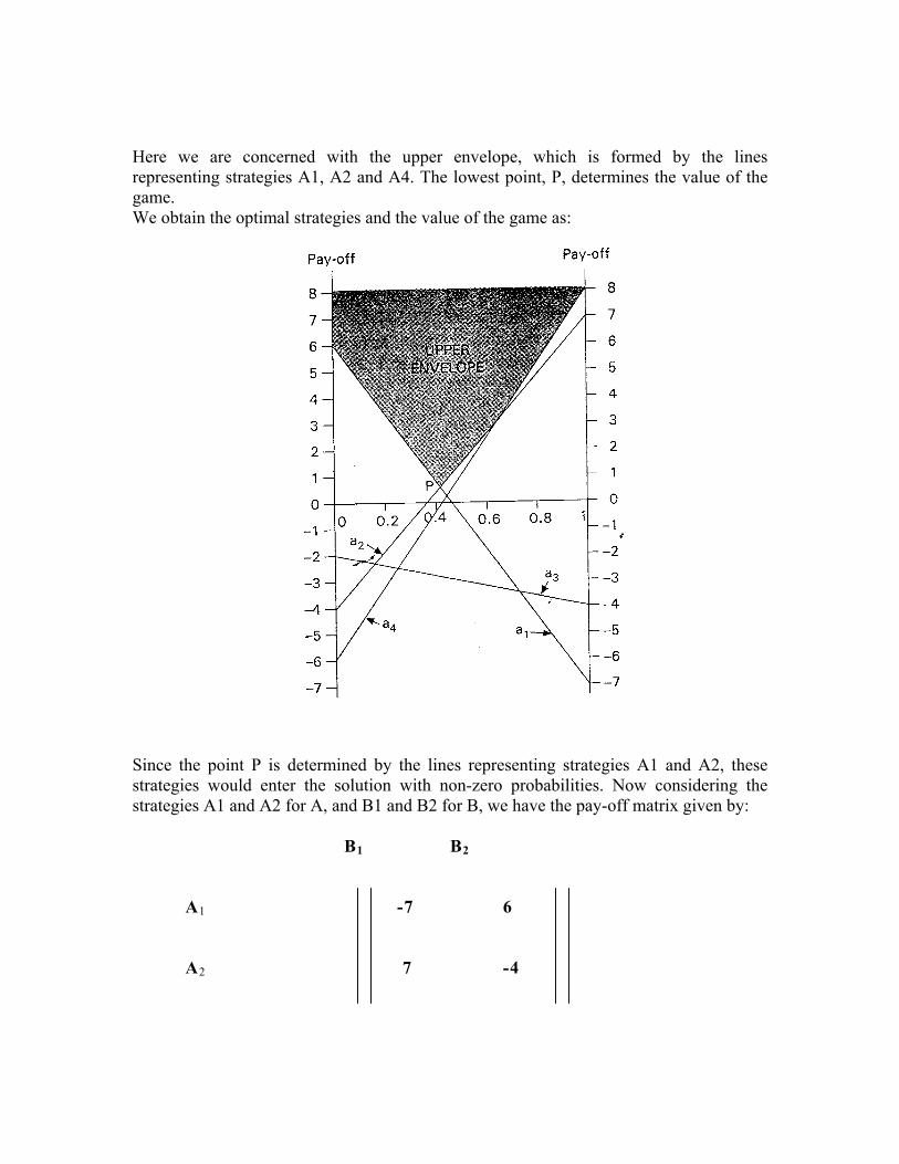
Here we are concerned with the upper envelope, which is formed by the lines representing strategies A1, A2 and A4. The lowest point, P, determines the value of the game. We obtain the optimal strategies and the value of the game as:
Since the point P is determined by the lines representing strategies A1 and A2, these strategies would enter the solution with non-zero probabilities. Now considering the strategies A1 and A2 for A, and B1 and B2 for B, we have the pay-off matrix given by: B1 B2
A1 -7 6 A2 7 -4
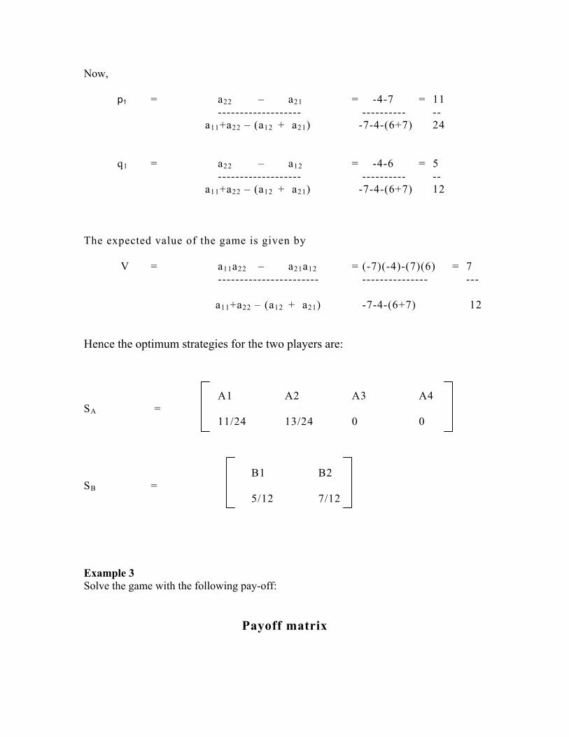
Now, p1 = a22 – a21 = -4-7 = 11
------------------- ---------- -- a11+a22 – (a12 + a21) -7-4-(6+7) 24
q1 = a22 – a12 = -4-6 = 5 ------------------- ---------- -- a11+a22 – (a12 + a21) -7-4-(6+7) 12
The expected value of the game is given by V = a11a22 – a21a12 = (-7)(-4)-(7)(6) = 7 ----------------------- --------------- ---
a11+a22 – (a12 + a21) -7-4-(6+7) 12 Hence the optimum strategies for the two players are:
A1 A2 A3 A4 SA =
11/24 13/24 0 0 B1 B2 SB =
5/12 7/12
Example 3 Solve the game with the following pay-off:
Payoff matrix

Player Player B’s Strategies A’s Strategies
B1 B2 B3
A1 6 4 3 A2 2 4 8
Solution: The lower envelope representing the feasible region is shaded. There is no single point representing the highest point. The value of the game is clearly 4 and any value of p1, between the points represented by K and L shall be optimal for A.
To obtain K, p1 = a22 – a21 = 4-2 = 2 =0.5
------------------- ---------- -- a11+a22 – (a12 + a21) 6+4-(2+4) 4
To obtain L,
p1 = 8-4 = 4 = 0.8 ------------------- -----
4+8 – (3 + 4) 5

Thus an optimal strategy for A is any pair of (p1, 1- p1) where 0.5≤ p1≤0.8
Now, Apply this graphical method on some Unsolved Problems yourself Problem 1. Determine the optimal minimax strategies for each player in the
following game. B1 B2 B3 B4 A1 -5 2 0 7 A2 5 1 4 8 A3 4 0 2 -3
Problem 2. Solve the following games by using maximin - minimax principle whose payoff matrix are given below: Include in your answer:
(i) Strategy selection for each player.
(ii) The value of the game to each player.
(iii) Does the game have a saddle point?
Player B
(a) Player A B1 B2 B3 B4
A1 1 7 3 4 A2 5 6 2 5 A3 7 4 0 3
Player B
(b) Player A B1 B2 B3 B4 A1 3 -5 0 6 A2 -4 -2 1 2 A3 5 -4 2 3
So, now let us summarize today’s discussion: Summary We have discussed about:
• Graphical solutions • Solution of 2 x n and m x 2 Games using graphs
Slide 1
GAME THEORY
LESSON 4

Slide 2
GRAPHICAL SOLUTION OF 2 X n AND m X 2 GAMES
Graphical approach is aimed to reduce a game payoff matrix to the order of 2 x 2
by identifying and eliminating the dominated strategies.
________________________________________________________________________
________________________________________________________________________
________________________________________________________________________
________________________________________________________________________
________________________________________________________________________
________________________________________________________________________
________________________________________________________________________
________________________________________________________________________
________________________________________________________________________
________________________________________________________________________
________________________________________________________________________
____________________________________________________________________

Unit 3 GAME THEORY Lesson 29
Learning Objective:
• On completion of this lesson you will be familiar with the key economic models dealing with interactive competition amongst firms when the behavior of rivals must be accommodated.
• You will learn to apply creative approaches to game theory. • This course concentrates on the thinking process itself and the
application of this process to decisions under conflict. You will apply new theories and creative approaches on a challenge from your work.
Hello students,
Let us begin with a very important practical game of the concept under our study.
The Prisoners' Dilemma Tucker's invention of the Prisoners' Dilemma example was very important. This example, which can be set out in one page, could be the most influential one page in the social sciences.
This remarkable innovation did not come out in a research paper, but in a classroom.
While addressing an audience of psychologists at Stanford University, where he was a visiting professor, Mr. Tucker created the Prisoners' Dilemma to illustrate the difficulty of analyzing" certain kinds of games. "Mr. Tucker's simple explanation has since given rise to a vast body of literature in subjects as diverse as philosophy, ethics, biology, sociology, political science, economics, and, of course, game theory."

The Game
Tucker began with a little story, like this:
• Two burglars, Bob and Al, are captured near the scene of a burglary and are given the "third degree" separately by the police.
• Each has to choose whether or not to confess and implicate the other. • If neither man confesses, then both will serve one year on a charge of carrying a
concealed weapon. • If each confesses and implicates the other, both will go to prison for 10 years. • However, if one burglar confesses and implicates the other, and the other burglar
does not confess, the one who has collaborated with the police will go free, while the other burglar will go to prison for 20 years on the maximum charge.
The strategies in this case are: confess or don't confess. The payoffs (penalties, actually) are the sentences served.
We can express all this compactly in a "payoff table" of a kind that has become pretty standard in game theory.
Just look at the payoff table for the Prisoners' Dilemma game:
Table 1
Al
Confess Don’t
Confess 10,10 0,20 Bob
Don’t 20,0 1,1
The table is read like this:
• Each prisoner chooses one of the two strategies. In effect, Al chooses a column and Bob chooses a row.
• The two numbers in each cell tell the outcomes for the two prisoners when the corresponding pair of strategies is chosen.
• The number to the left of the comma tells the payoff to the person who chooses the rows (Bob) while the number to the right of the column tells the payoff to the

person who chooses the columns (Al). Thus (reading down the first column) if they both confess, each gets 10 years, but if Al confesses and Bob does not, Bob gets 20 and Al goes free.
So:
How to solve this game?
What strategies are "rational" if both men want to minimize the time they spend in jail?
Al might reason as:
"Two things can happen: Bob can confess or Bob can keep quiet. Suppose Bob confesses. Then I get 20 years if I don't confess, 10 years if I do, so in that case it's best to confess. On the other hand, if Bob doesn't confess, and I don't either, I get a year; but in that case, if I confess I can go free. Either way, it's best if I confess. Therefore, I'll confess."
But Bob can and presumably will reason in the same way -- so that they both confess and go to prison for 10 years each. Yet, if they had acted "irrationally," and kept quiet, they each could have gotten off with one year each.
Dominant Strategies
What has happened here is that the two prisoners have fallen into something called a "dominant strategy equilibrium."
DEFINITIONS
What is Dominant Strategy?
Let an individual player in a game evaluate separately each of the strategy combinations he may face, and, for each combination, choose from his own strategies the one that gives the best payoff. If the same strategy is chosen for each of the different combinations of strategies the player might face, that strategy is called a "dominant strategy" for that player in that game.
Now,
What is Dominant Strategy Equilibrium?
If, in a game, each player has a dominant strategy, and each player plays the dominant strategy, then that combination of (dominant) strategies and the corresponding payoffs are said to constitute the dominant strategy equilibrium for that game.

In the Prisoners' Dilemma game, to confess is a dominant strategy, and when both prisoners confess, that is a dominant strategy equilibrium.
Now, let us see some issues regarding Prisoners’ Dilemma
Issues With Respect to the Prisoners' Dilemma
This remarkable result -- that individually rational action results in both persons being made worse off in terms of their own self-interested purposes -- is what has made the wide impact in modern social science. For there are many interactions in the modern world that seem very much like that, from arms races through road congestion and pollution to the depletion of fisheries and the overexploitation of some subsurface water resources. These are all quite different interactions in detail, but are interactions in which (we suppose) individually rational action leads to inferior results for each person, and the Prisoners' Dilemma suggests something of what is going on in each of them. That is the source of its power.
Having said that, we must also admit candidly that the Prisoners' Dilemma is a very simplified and abstract -- if you will, "unrealistic" -- conception of many of these interactions. A number of critical issues can be raised with the Prisoners' Dilemma, and each of these issues has been the basis of a large scholarly literature:
• The Prisoners' Dilemma is a two-person game, but many of the applications of the idea are really many-person interactions.
• We have assumed that there is no communication between the two prisoners. If they could communicate and commit themselves to coordinated strategies, we would expect a quite different outcome.
• In the Prisoners' Dilemma, the two prisoners interact only once. Repetition of the interactions might lead to quite different results.
• Compelling as the reasoning that leads to the dominant strategy equilibrium may be, it is not the only way this problem might be reasoned out. Perhaps it is not really the most rational answer after all.
We will consider some of these points in what follows.
An Information Technology Example Game theory provides a promising approach to understanding strategic problems of all sorts, and the simplicity and power of the Prisoners' Dilemma and similar examples make

them a natural starting point. But there will often be complications we must consider in a more complex and realistic application.
Let's see how we might move from a simpler to a more realistic game model in a real-world example of strategic thinking: choosing an information system.
For this example,
The players will be a company considering the choice of a new internal e-mail or intranet system, and a supplier who is considering producing it.
The two choices are to install a technically advanced or a more proven system with less functionality.
Assume that the more advanced system really does supply a lot more functionality, so that the payoffs to the two players, net of the user's payment to the supplier, are as shown in Table 2.
Table 2
User
Advanced Proven
Advanced 20,20 0,0 Supplier
Proven 0,0 5,5
We see that both players can be better off, on net, if an advanced system is installed. (We are not claiming that that's always the case! We're just assuming it is in this particular decision). But the worst that can happen is for one player to commit to an advance system while the other player stays with the proven one. In that case there is no deal, and no payoffs for anyone. The problem is that the supplier and the user must have a compatible standard, in order to work together, and since the choice of a standard is a strategic choice, their strategies have to mesh.
Although it looks a lot like the Prisoners' Dilemma at first glance, this is a more complicated game. We'll take several complications in turn:
Looking at it carefully, we see that there this game has no dominated strategies. The best strategy for each participant depends on the strategy chosen by the other participant. Thus, we need a new concept of game-equilibrium, that will allow for that complication.

When there are no dominant strategies, we often use an equilibrium conception called the Nash Equilibrium, named after Nobel Memorial Laureate John Nash. The Nash Equilibrium is a pretty simple idea: we have a Nash Equilibrium if each participant chooses the best strategy, given the strategy chosen by the other participant.
In the example,
If the user opts for the advanced system, then it is best for the supplier to do that too. So (Advanced, Advanced) is a Nash-equilibrium.
But, hold on here!
If the user chooses the proven system, it's best for the supplier to do that too.
There are two Nash Equilibria! Which one will be chosen?
It may seem easy enough to opt for the advanced system which is better all around, but if each participant believes that the other will stick with the proven system -- being a bit of a stick in the mud, perhaps -- then it will be best for each player to choose the proven system -- and each will be right in assuming that the other one is a stick in the mud! This is a danger typical of a class of games called coordination games -- and what we have learned is that the choice of compatible standards is a coordination game.
• We have assumed that the payoffs are known and certain. In the real world, every strategic decision is risky -- and a decision for the advanced system is likely to be riskier than a decision for the proven system. Thus, we would have to take into account the players' subjective attitudes toward risk, their risk aversion, to make the example fully realistic. We won't attempt to do that in this example, but we must keep it in mind.
• The example assumes that payoffs are measured in money. Thus, we are not only leaving risk aversion out of the picture, but also any other subjective rewards and penalties that cannot be measured in money. Economists have ways of measuring subjective rewards in money terms -- and sometimes they work -- but, again, we are going to skip over that problem and assume that all rewards and penalties are measured in money and are transferable from the user to the supplier and vice versa.

• Real choices of information systems are likely to involve more than two players, at least in the long run -- the user may choose among several suppliers, and suppliers may have many customers. That makes the coordination problem harder to solve. Suppose, for example, that "beta" is the advanced system and "VHS" is the proven system, and suppose that about 90% of the market uses "VHS." Then "VHS" may take over the market from "beta" even though "beta" is the better system. Many economists, game theorists and others believe this is a main reason why certain technical standards gain dominance. (This is being written on a Macintosh computer. Can you think of any other possible examples like the beta vs. VHS example?)
• On the other hand, the user and the supplier don't have to just sit back and wait to see what the other person does -- they can sit down and talk it out, and commit themselves to a contract. In fact, they have to do so, because the amount of payment from the user to the supplier -- a strategic decision we have ignored until now -- also has to be agreed upon. In other words, unlike the Prisoners' Dilemma, this is a cooperative game, not a non-cooperative game. On the one hand, that will make the problem of coordinating standards easier, at least in the short run. On the other hand, Cooperative games call for a different approach to solution.
So let us recapitulate Zero-Sum Games
By the time Tucker invented the Prisoners' Dilemma, Game Theory was already a going concern. But most of the earlier work had focused on a special class of games: zero-sum games.
In his earliest work, von Neumann made a striking discovery. He found that if poker players maximize their rewards, they do so by bluffing; and, more generally, that in many games it pays to be unpredictable. This was not qualitatively new, of course -- baseball pitchers were throwing change-up pitches before von Neumann wrote about mixed strategies. But von Neumann's discovery was a bit more than just that. He discovered a unique and unequivocal answer to the question:
"How can I maximize my rewards in this sort of game?" without any markets, prices, property rights, or other institutions in the picture.
It was a very major extension of the concept of absolute rationality in neoclassical economics. But von Neumann had bought his discovery at a price. The price was a strong simplifying assumption: von Neumann's discovery applied only to zero-sum games.

For example,
Consider the children's game of "Matching Pennies."
In this game, the two players agree that one will be "even" and the other will be "odd." Each one then shows a penny. The pennies are shown simultaneously, and each player may show either a head or a tail. If both show the same side, then "even" wins the penny from "odd;" or if they show different sides, "odd" wins the penny from "even". Here is the payoff table for the game.
Table 3
Odd
Head Tail
Head 1, -1 -1,1 Even
Tail -1,1 1, -1
If we add up the payoffs in each cell, we find 1-1=0. This is a "zero-sum game."
Zero-Sum game: If we add up the wins and losses in a game, treating losses as negatives, and we find that the sum is zero for each set of strategies chosen, then the game is a "zero-sum game."
In less formal terms, a zero-sum game is a game in which one player's winnings equal the other player's losses. Do notice that the definition requires a zero sum for every set of strategies. If there is even one strategy set for which the sum differs from zero, then the game is not zero sum.
Another Example
Here is another example of a zero-sum game. It is a very simplified model of price competition. Like Augustin Cournot (writing in the 1840's) we will think of two companies that sell mineral water. Each company has a fixed cost of $5000 per period, regardless whether they sell anything or not. We will call the companies Perrier and Apollinaris, just to take two names at random.
The two companies are competing for the same market and each firm must choose a high price ($2 per bottle) or a low price ($1 per bottle). Here are the rules of the game:

1) At a price of $2, 5000 bottles can be sold for a total revenue of $10000.
2) At a price of $1, 10000 bottles can be sold for a total revenue of $10000.
3) If both companies charge the same price, they split the sales evenly between them.
4) If one company charges a higher price, the company with the lower price sells the whole amount and the company with the higher price sells nothing.
5) Payoffs are profits -- revenue minus the $5000 fixed cost.
Here is the payoff table for these two companies
Table 4
Perrier
Price=$1 Price=$2
Price=$1 0,0 5000, -5000 Apollinaris
Price=$2 -5000, 5000 0,0 (Verify for yourself that this is a zero-sum game.) For two-person zero-sum games, there is a clear concept of a solution. The solution to the game is the maximin criterion -- that is, each player chooses the strategy that maximizes her minimum payoff. In this game, Appolinaris' minimum payoff at a price of $1 is zero, and at a price of $2 it is -5000, so the $1 price maximizes the minimum payoff. The same reasoning applies to Perrier, so both will choose the $1 price. Here is the reasoning behind the maximin solution: Apollinaris knows that whatever she loses, Perrier gains; so whatever strategy she chooses, Perrier will choose the strategy that gives the minimum payoff for that row. Again, Perrier reasons conversely.
SOLUTION: Maximin criterion For a two-person, zero sum game it is rational for each player to choose the strategy that maximizes the minimum payoff, and the pair of strategies and payoffs such that each player maximizes her minimum payoff is the "solution to the game."
Mixed Strategies
Now let's look back at the game of matching pennies.
It appears that this game does not have a unique solution. The minimum payoff for each of the two strategies is the same: -1. But this is not the whole story. This game can have more than two strategies. In addition to the two obvious strategies, head and tail, a player can "randomize" her strategy by offering either a head or a tail, at random, with specific probabilities. Such a randomized strategy is called a "mixed strategy." The obvious two strategies, heads and tails, are called "pure strategies." There are infinitely many mixed strategies corresponding to the infinitely many ways probabilities can be assigned to the two pure strategies.
DEFINITION
Mixed strategy If a player in a game chooses among two or more strategies at random according to specific probabilities, this choice is called a "mixed strategy."
The game of matching pennies has a solution in mixed strategies, and it is to offer heads or tails at random with probabilities 0.5 each way.
Here is the reasoning:
If odd offers heads with any probability greater than 0.5, then even can have better than even odds of winning by offering heads with probability 1.
On the other hand, if odd offers heads with any probability less than 0.5, then even can have better than even odds of winning by offering tails with probability 1.
The only way odd can get even odds of winning is to choose a randomized strategy with probability 0.5, and there is no way odd can get better than even odds.
The 0.5 probability maximizes the minimum payoff over all pure or mixed strategies.
And even can reason the same way (reversing heads and tails) and come to the same conclusion, so both players choose 0.5.
Von Neumann's Discovery
We can now say more exactly what von Neumann's discovery was.

Von Neumann showed that every two-person zero sum game had a maximin solution, in mixed if not in pure strategies. This was an important insight, but it probably seemed more important at the time than it does now. In limiting his analysis to two-person zero sum games, von Neumann had made a strong simplifying assumption. Von Neumann was a mathematician, and he had used the mathematician's approach: take a simple example, solve it, and then try to extend the solution to the more complex cases. But the mathematician's approach did not work as well in game theory as it does in some other cases. Von Neumann's solution applies unequivocally only to "games" that share this zero-sum property. Because of this assumption, von Neumann's brilliant solution was and is only applicable to a small proportion of all "games," serious and non-serious. Arms races, for example, are not zero-sum games. Both participants can and often do lose. The Prisoners' Dilemma is not a zero-sum game, and that is the source of a major part of its interest. Economic competition is not a zero-sum game. It is often possible for most players to win, and in principle, economics is a win-win game. Environmental pollution and the overexploitation of resources, again, tend to be lose-lose games: it is hard to find a winner in the destruction of most of the world's ocean fisheries in the past generation. Thus, von Neumann's solution does not -- without further work -- apply to these serious interactions.
The serious interactions are instances of "non-constant sum games," since the winnings and losses may add up differently depending on the strategies the participants choose. It is possible, for example, for rival nations to choose mutual disarmament, save the cost of weapons, and both be better off as a result -- so the sum of the winnings is greater in that case. In economic competition, increasing division of labor, specialization, investment, and improved coordination can increase "the size of the pie," leading to "that universal opulence which extends itself to the lowest ranks of the people," in the words of Adam Smith. In cases of environmental pollution, the benefits to each individual from the polluting activity is so swamped by others' losses from polluting activity that all can lose -- as we have often observed.
Poker and baseball are zero-sum games. It begins to seem that the only zero-sum games are literal games that human beings have invented -- and made them zero-sum -- for our own amusement. "Games" that are in some sense natural are non-constant sum games. And even poker and baseball are somewhat unclear cases.
A "friendly" poker game is zero-sum, but in a casino game, the house takes a proportion of the pot, so the sum of the winnings is less the more the players bet. And even in the friendly game, we are considering only the money payoffs -- not the thrill of gambling and the pleasure of the social event, without which presumably the players would not play. When we take those rewards into account, even gambling games are not really zero-sum.
Von Neumann and Morgenstern hoped to extend their analysis to non-constant sum games with many participants, and they proposed an analysis of these games. However, the problem was much more difficult, and while a number of solutions have been

proposed, there is no one generally accepted mathematical solution of non-constant sum games.
To put it a little differently, there seems to be no clear answer to the question, "Just what is rational in a non-constant sum game?"
So, now let us summarize today’s discussion: Summary We have discussed about:
Several Examples The Prisoner’s Dilemma Information Technology example The game of matching pennies

Unit 3 GAME THEORY Lesson 30 Learning Objective:
• Analyze two person non-zero sum games.
• Analyze games involving cooperation.
Hello students,
The well-defined rational policy in neoclassical economics -- maximization of reward -- is extended to zero-sum games but not to the more realistic category of non-constant sum games.
"Solutions" to Non-constant Sum Games The maximin strategy is a "rational" solution to all two-person zero sum games. However, it is not a solution for non-constant sum games. The difficulty is that there are a number of different solution concepts for non-constant sum games, and no one is clearly the "right" answer in every case. The different solution concepts may overlap, though.
We have already seen one possible solution concept for non-constant sum games: the dominant strategy equilibrium.
Let's take another look at the example of the two mineral water companies.
Two companies sell mineral water. Each company has a fixed cost of $5000 per period, regardless whether they sell anything or not. We will call the companies Perrier and Apollinaris, just to take two names at random.

The two companies are competing for the same market and each firm must choose a high price ($2 per bottle) or a low price ($1 per bottle). Here are the rules of the game:
1) At a price of $2, 5000 bottles can be sold for a total revenue of $10000.
2) At a price of $1, 10000 bottles can be sold for a total revenue of $10000.
3) If both companies charge the same price, they split the sales evenly between them.
4) If one company charges a higher price, the company with the lower price sells the whole amount and the company with the higher price sells nothing.
5) Payoffs are profits -- revenue minus the $5000 fixed cost.
Here is the payoff table for these two companies
Table 1
Perrier
Price=$1 Price=$2
Price=$1 0,0 5000, -5000 Apollinaris
Price=$2 -5000, 5000 0,0
We saw that the maximin solution was for each company to cut price to $1. That is also a dominant strategy equilibrium.
It's easy to check that: Apollinaris can reason that either Perrier cuts to $1 or not. If they do, Apollinaris is better off cutting to 1 to avoid a loss of $5000. But if Perrier doesn't cut, Apollinaris can earn a profit of 5000 by cutting. And Perrier can reason in the same way, so cutting is a dominant strategy for each competitor.
But this is, of course, a very simplified -- even unrealistic -- conception of price competition.
Let's look at a more complicated, perhaps more realistic pricing example:
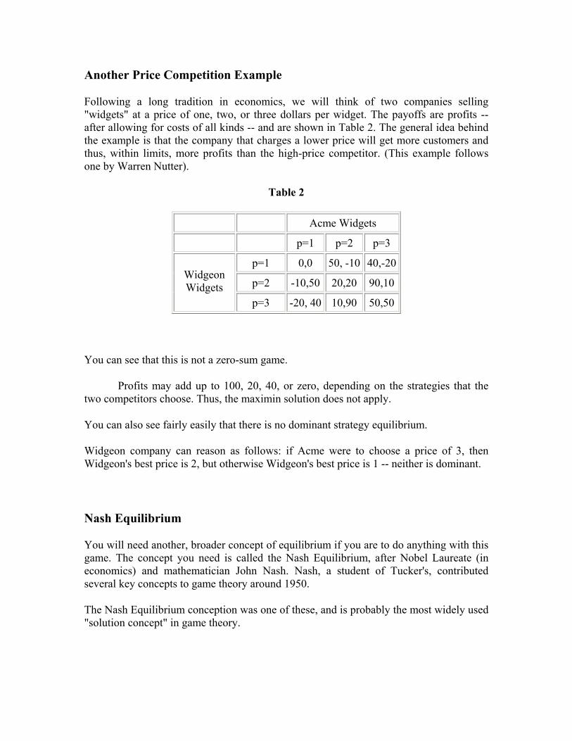
Another Price Competition Example
Following a long tradition in economics, we will think of two companies selling "widgets" at a price of one, two, or three dollars per widget. The payoffs are profits -- after allowing for costs of all kinds -- and are shown in Table 2. The general idea behind the example is that the company that charges a lower price will get more customers and thus, within limits, more profits than the high-price competitor. (This example follows one by Warren Nutter).
Table 2
Acme Widgets
p=1 p=2 p=3
p=1 0,0 50, -10 40,-20
p=2 -10,50 20,20 90,10 Widgeon Widgets
p=3 -20, 40 10,90 50,50
You can see that this is not a zero-sum game.
Profits may add up to 100, 20, 40, or zero, depending on the strategies that the two competitors choose. Thus, the maximin solution does not apply.
You can also see fairly easily that there is no dominant strategy equilibrium.
Widgeon company can reason as follows: if Acme were to choose a price of 3, then Widgeon's best price is 2, but otherwise Widgeon's best price is 1 -- neither is dominant.
Nash Equilibrium
You will need another, broader concept of equilibrium if you are to do anything with this game. The concept you need is called the Nash Equilibrium, after Nobel Laureate (in economics) and mathematician John Nash. Nash, a student of Tucker's, contributed several key concepts to game theory around 1950.
The Nash Equilibrium conception was one of these, and is probably the most widely used "solution concept" in game theory.

If there is a set of strategies with the property that no player can benefit by changing her strategy while the other players keep their strategies unchanged, then that set of strategies and the corresponding payoffs constitute the Nash Equilibrium.
Let's apply that definition to the widget-selling game.
First, for example, you can see that the strategy pair p=3 for each player (bottom right) is not a Nash-equilibrium. From that pair, each competitor can benefit by cutting price, if the other player keeps her strategy unchanged. Or consider the bottom middle -- Widgeon charges $3 but Acme charges $2. From that pair, Widgeon benefits by cutting to $1. In this way, you can eliminate any strategy pair except the upper left, at which both competitors charge $1.
You will see that the Nash equilibrium in the widget-selling game is a low-price, zero-profit equilibrium. Many economists believe that result is descriptive of real, highly competitive markets -- although there is, of course, a great deal about this example that is still "unrealistic."
Let's go back and take a look at that dominant-strategy equilibrium in Table 1 of this lecture. You will see that it, too, is a Nash-Equilibrium. Check it out!
Also, look again at the dominant-strategy equilibrium in the Prisoners' Dilemma. It, too, is a Nash-Equilibrium. In fact, any dominant strategy equilibrium is also a Nash Equilibrium. The Nash equilibrium is an extension of the concepts of dominant strategy equilibrium and of the maximin solution for zero-sum games.
It would be nice to say that that answers all our questions.
But, of course, it does not…….
Here is just the first of the questions it does not answer:
Could there be more than one Nash-Equilibrium in the same game?
And what if there were more than one?

This leads us to a new concept
Games with Multiple Nash Equilibria Here is another example to try the Nash Equilibrium approach on…..
Two radio stations (WIRD and KOOL) have to choose formats for their broadcasts. There are three possible formats: Country-Western (CW), Industrial Music (IM) or all-news (AN). The audiences for the three formats are 50%, 30%, and 20%, respectively. If they choose the same formats they will split the audience for that format equally, while if they choose different formats, each will get the total audience for that format. Audience shares are proportionate to payoffs. The payoffs (audience shares) are in Table 3.
Table 3 KOOL
CW IM AN
CW 25,25 50,30 50,20
IM 30,50 15,15 30,20 WIRD
AN 20,50 20,30 10,10
You should be able to verify that this is a non-constant sum game, and that there are no dominant strategy equilibria.
If you find the Nash Equilibria by elimination, you will find that there are two of them -- the upper middle cell and the middle-left one, in both of which one station chooses CW and gets a 50 market share and the other chooses IM and gets 30. But it doesn't matter which station chooses which format.
It may seem that this makes little difference, since
• the total payoff is the same in both cases, namely 80 • both are efficient, in that there is no larger total payoff than 80
There are multiple Nash Equilibria in which neither of these things is so, as you will see in some later examples. But even when they are both true, the multiplication of equilibria creates a danger. The danger is that both stations will choose the more profitable CW format -- and split the market, getting only 25 each! Actually, there is an even worse

danger that each station might assume that the other station will choose CW, and each choose IM, splitting that market and leaving each with a market share of just 15.
More generally, the problem for the players is to figure out which equilibrium will in fact occur. In other words, a game of this kind raises a "coordination problem:"
How can the two stations coordinate their choices of strategies and avoid the danger of a mutually inferior outcome such as splitting the market?
Games that present coordination problems are sometimes called coordination games.
From a mathematical point of view, this multiplicity of equilibria is a problem. For a "solution" to a "problem," we want one answer, not a family of answers. And many economists would also regard it as a problem that has to be solved by some restriction of the assumptions that would rule out the multiple equilibria.
But, from a social scientific point of view, there is another interpretation. Many social scientists (myself included) believe that coordination problems are quite real and important aspects of human social life.
From this point of view, we might say that multiple Nash equilibria provide us with a possible "explanation" of coordination problems. That would be an important positive finding, not a problem!
Any bit of information that all participants in a coordination game would have, that could enable them all to focus on the same equilibrium.
In determining a national boundary, for example, the highest mountain between the two countries would be an obvious enough landmark that both might focus on setting the boundary there -- even if the mountain were not very high at all.
Another source of a hint that could solve a coordination game is social convention.
Here is a game in which social convention could be quite important. That game has a long name: "Which Side of the Road to Drive On?"
In Britain, you know, people drive on the left side of the road; in the US they drive on the right.

In abstract, how do we choose which side to drive on?
• There are two strategies: drive on the left side and drive on the right side.
• There are two possible outcomes: the two cars pass one another without incident or they crash.
• Arbitrarily assign a value of one each to passing without problems and of -10 each to a crash.
Here is the payoff table:
Table 4 Mercedes
L R
L 1,1 -10,-10 Buick
R -10,-10 1,1
Verify that LL and RR are both Nash equilibria. But, if we do not know which side to choose, there is some danger that we will choose LR or RL at random and crash.
How can we know which side to choose?
The answer is, of course, that for this coordination game we rely on social convention. Conversely, we know that in this game, social convention is very powerful and persistent, and no less so in the country where the solution is LL than in the country where it is RR.
Next, we move on to what is called as cooperative games.
Cooperative Games Games in which the participants cannot make commitments to coordinate their strategies are "non-cooperative games." The solution to a "non-cooperative game" is a "non-cooperative solution."

In a non-cooperative game, the rational person's problem is to answer the question "What is the rational choice of a strategy when other players will try to choose their best responses to my strategy?"
Conversely, games in which the participants can make commitments to coordinate their strategies are "cooperative games," and the solution to a "cooperative game" is a "cooperative solution." In a cooperative game, the rational person's problem is to answer the question, "What strategy choice will lead to the best outcome for all of us in this game?"
If that seems excessively idealistic, you should keep in mind that cooperative games typically allow for "side payments," that is, bribes and quid pro quo arrangements so that every one is (might be?) better off.
Thus the rational person's problem in the cooperative game is actually a little more complicated than that. The rational person must ask not only "What strategy choice will lead to the best outcome for all of us in this game?" but also "How large a bribe may I reasonably expect for choosing it?"
A Basic Cooperative Game
Cooperative games are particularly important in economics. Here is an example that may illustrate the reason why.
• Suppose that Joey has a bicycle.
• Joey would rather have a game machine than a bicycle, and he could buy a game machine for $80, but Joey doesn't have any money. We express this by saying that Joey values his bicycle at $80.
• Mikey has $100 and no bicycle, and would rather have a bicycle than anything else he can buy for $100. We express this by saying that Mikey values a bicycle at $100.
• The strategies available to Joey and Mikey are to give or to keep. That is, Joey can give his bicycle to Mikey or keep it, and Mikey can give some of this money to Joey or keep it all.

• It is suggested that Mikey give Joey $90 and that Joey give Mikey the bicycle. This is what we call "exchange."
Here are the payoffs:
Table 5
Joey
give keep
give 110, 90 10, 170 Mikey
keep 200, 0 100, 80
EXPLANATION:
• At the upper left, Mikey has a bicycle he values at $100, plus $10 extra, while Joey has a game machine he values at $80, plus an extra $10.
• At the lower left, Mikey has the bicycle he values at $100, plus $100 extra. At the upper left, Joey has a game machine and a bike, each of which he values at $80, plus $10 extra, and Mikey is left with only $10.
• At the lower right, they simply have what they begin with -- Mikey $100 and Joey a bike.
If we think of this as a non-cooperative game, it is much like a Prisoners' Dilemma. To keep is a dominant strategy and keep, keep is a dominant strategy equilibrium. However, give, give makes both better off. Being children, they may distrust one another and fail to make the exchange that will make them better off. But market societies have a range of institutions that allow adults to commit themselves to mutually beneficial transactions.
Thus, we would expect a cooperative solution, and we suspect that it would be the one in the upper left. But what cooperative "solution concept" may we use?

Pareto Optimum
We have observed that both participants in the bike-selling game are better off if they make the transaction. This is the basis for one solution concept in cooperative games.
First, we define a criterion to rank outcomes from the point of view of the group of players as a whole. We can say that one outcome is better than another (upper left better than lower right, e.g.) if at least one person is better off and no one is worse off. This is called the Pareto criterion, after the Italian economist and mechanical engineer, Vilfredo Pareto.
If an outcome (such as the upper left) cannot be improved upon, in that sense -- in other words, if no-one can be made better off without making somebody else worse off -- then we say that the outcome is Pareto Optimal, that is, Optimal (cannot be improved upon) in terms of the Pareto Criterion.
If there were a unique Pareto optimal outcome for a cooperative game, that would seem to be a good solution concept. The problem is that there isn't -- in general, there are infinitely many Pareto Optima for any fairly complicated economic "game."
In the bike-selling example, every cell in the table except the lower right is Pareto-optimal, and in fact any price between $80 and $100 would give yet another of the (infinitely many) Pareto-Optimal outcomes to this game. All the same, this was the solution criterion that von Neumann and Morgenstern used, and the set of all Pareto-Optimal outcomes is called the "solution set."
Alternative Solution Concepts
If we are to improve on this concept, we need to solve two problems.
• One is to narrow down the range of possible solutions to a particular price or, more generally, distribution of the benefits. This is called "the bargaining problem."
• Second, we still need to generalize cooperative games to more than two participants.
There are a number of concepts, including several with interesting results; but here attention will be limited to one. It is the Core, and it builds on the Pareto Optimal solution set, allowing these two problems to solve one another via "competition."

An Information Technology Example Revisited
When we looked at "Choosing an Information Technology," one of the two introductory examples, we came to the conclusion that it is more complex than the Prisoners' Dilemma in several ways. Unlike the Prisoners' Dilemma, it is a cooperative game, not a non-cooperative game. Now let's look at it from that point of view.
When the information system user and supplier get together and work out a deal for an information system, they are forming a coalition in game theory terms. (Here we have been influenced more by political science than economics, it seems!)
• The first decision will be whether to join the coalition or not. In this example, that's a pretty easy decision. Going it alone, neither the user nor the supplier can be sure of a payoff more than 0. By forming a coalition, both choosing the advanced system, they can get a total payoff of 40 between them.
• The next question is: how will they divide that 40 between them? How much will the user pay for the system?
We need a little more detail about this game before we can go on. The payoff table above was net of the payment. It was derived from the following gross payoffs:
Table 6
User
Advanced Proven
Advanced -50,90 0,0 Supplier
Proven 0,0 -30,40
The gross payoffs to the supplier are negative, because the production of the information system is a cost item to the supplier, and the benefits to the supplier are the payment they get from the user, minus that cost.
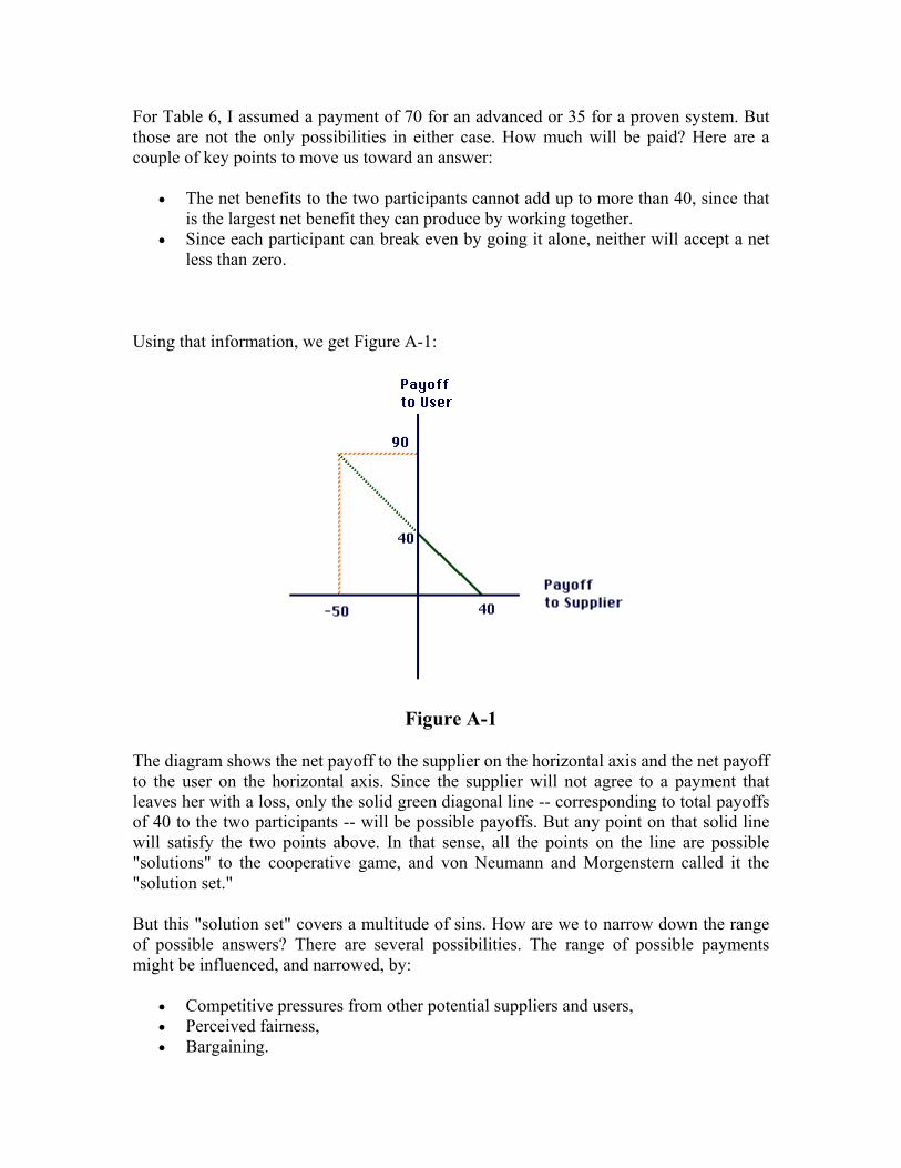
For Table 6, I assumed a payment of 70 for an advanced or 35 for a proven system. But those are not the only possibilities in either case. How much will be paid? Here are a couple of key points to move us toward an answer:
• The net benefits to the two participants cannot add up to more than 40, since that is the largest net benefit they can produce by working together.
• Since each participant can break even by going it alone, neither will accept a net less than zero.
Using that information, we get Figure A-1:
Figure A-1
The diagram shows the net payoff to the supplier on the horizontal axis and the net payoff to the user on the horizontal axis. Since the supplier will not agree to a payment that leaves her with a loss, only the solid green diagonal line -- corresponding to total payoffs of 40 to the two participants -- will be possible payoffs. But any point on that solid line will satisfy the two points above. In that sense, all the points on the line are possible "solutions" to the cooperative game, and von Neumann and Morgenstern called it the "solution set."
But this "solution set" covers a multitude of sins. How are we to narrow down the range of possible answers? There are several possibilities. The range of possible payments might be influenced, and narrowed, by:
• Competitive pressures from other potential suppliers and users, • Perceived fairness, • Bargaining.

There are game-theoretic approaches based on all these approaches, and on combinations of them. Unfortunately, this leads to several different concepts of "solutions" of cooperative games, and they may conflict. One of them -- the core, based on competitive pressures -- will be explored in these pages. We will have to leave the others for another time.
There is one more complication to consider, when we look at the longer run. What if the supplier does not continue to support the information system chosen? What if the supplier invests to support the system in the long run, and the user doesn't continue to use it? In other words, what if the commitments the participants make are limited by opportunism?
So, now let us summarize today’s discussion: Summary We have discussed about:
Several Examples Solution to Non-constant sum games Nash equilibrium Multiple Nash equilibrium Cooperative game Pareto Optimum.
Unit 3 GAME THEORY Lesson 31 Learning Objective:
• Analyze different types of non zero sum games Hawk vs. Dove game. Advertising problem. Problem of companies polluting the environment.
• Rationalizability or Iterative Elimination of Dominated Strategies.
Hello students, In the previous lectures you have learned the concept of solution for non-zero sum games. So let us today apply it on a very important illustration……..
Non-zero sum games: example – Hawk vs. Dove
• Suppose you have two countries, A and B, which share a border. There is an offshore oilfield which both of the countries claim belongs to them.
• Suppose that the oil field has value = V .
• We can simplify the possible outcomes facing the countries into: (1)
they decide to share the oil field 50-50 without fighting a war, (2) country A threatens war and country B surrenders, (3) country B threatens war and country A surrenders, or (4) they both fight a war.

• We can simplify the strategy choice for each country as (1) fight a war
or be willing to fight a war (Hawk), or (2) not be willing to fight a war (Dove).
• If we make the additional assumption that the countries are evenly matched militarily, and that the total cost of fighting a war is = C we can model this situation as a non-zero sum game with the following payoff table:
B
Hawk Dove
Hawk (V – C) , (V – C) 2 2 V , 0
A Dove
0 , V V , V 2 2
• The entry corresponding to the Hawk-Hawk combination is (V – C) / 2 for both countries.
• This assumes that if both countries play the Hawk strategy then they will fight a war with cost C and then they still end up splitting the resources after the war.
• This could be interpreted as a deterministic quantity if we were certain that the outcome of the war were a draw.
• However we can also consider the outcome of the war as a stochastic quantity and use the expected value of the outcome for the Hawk-Hawk strategy, this is more realistic since the outcome of the war would not be known with certainty.

B
Hawk Dove
Hawk (V – C) , (V – C) 2 2 V , 0
A Dove
0 , V V , V 2 2
• If we still assume that the countries are evenly matched then we can consider the case in which before the war is fought Pr(A wins) = Pr(B wins) = 0:50 or Pr(A wins) = Pr(B wins) = Pr(draw) = 1 What is the expected value for the Hawk-Hawk combination in this case?
------------------------------------------------------------------------------------ ------------------------------------------------------------------------------------ ------------------------------------------------------------------------------------
• How to solve this game?
• Non-zero sum games often involve a combination of cooperation and competition built into the outcomes.
• If we think in terms of the overall good for both countries what seems
to be the best possible outcome? What is the worst possible outcome?
Can you identify? ------------------------------------------------------------------------------------ ------------------------------------------------------------------------------------ ------------------------------------------------------------------------------------

B
Hawk Dove
Hawk (V – C) , (V – C) 2 2 V , 0
A Dove
0 , V V , V 2 2
• If we want to find a dominant strategy equilibrium we suppose that
player A reasons as follows: if player B plays Dove, what is my best strategy in terms of the best possible outcome? if player B plays hawk, what is my best strategy ? We also assume player B thinks similarly
• This outcome is a dominant strategy equilibrium, if either player
unilaterally changes strategy then they will end up with a worse result.
• From the table, under what conditions, on V and C will there be a dominant strategy equilibrium, and what will be the outcome that corresponds to this equilibrium ?
• In the Hawk-Dove game, if V > C we have a result similar to the
Prisoner's Dilemma game in which the sub optimal strategy, in this case Hawk-Hawk, in Prisoner's Dilemma.
Confess-Confess is a dominant strategy equilibrium solution.
Non zero sum game Another illustration:
Now, can you answer a simple question?
Why do firms spend so much money on advertising ?
------------------------------------------------------------------------------------
------------------------------------------------------------------------------------
So let us implement this on an example:

• Consider two large competing companies each with a 0.5 market share and thus a 50% share of the total available profits P.
• The firms need to choose whether or not to spend money on advertising
their products.
• Suppose that if neither of the firms advertises then they will maintain the current market share i.e. 50 - 50.
• However suppose that if one of the firms advertises and the other does
not, the firm that advertises will get an increase in their proportion by I, thus the other firm will lose I.
• Suppose that the cost of launching an advertising campaign is equal to
C. What will the payoff table look like for the two companies:
B
Advertise Don't
Advertise A
Don't
• Under what conditions will there be a dominant strategy equilibrium(ia), and what will it(they) be ? Does this seem optimal ?

Illustration 3 Why do companies (or individuals) pollute the environment ?
• Suppose you have N companies who need to choose between using methods that are cheaper and cause considerable pollution, or methods that don't pollute but are more expensive, and thus lead to smaller profits.
• Suppose that the cost to each company that results if all companies
choose to pollute is D, this is not a financial cost but the cost of having to breathe bad air, drink bad water etc.
• We can also assume that each individual company contributes D / N to
the pollution.
• Suppose that the profit to each company that adopts the cheaper but polluting methods is P whereas the profit to companies that choose the more expensive non-polluting methods is P – C, thus C > 0 represents the additional cost of not polluting.
• To be realistic we would need to consider this as an N unit (company)
game, but for simplicity we can consider one company, Company A, as the row player, making their decision, considering the possible moves of the other N –1 companies, who then constitute the column player.
• If we assume that all of the other companies make the same decision,
what does the payoff matrix look like:
Other companies
Pollute Don't
Pollute A
Don't
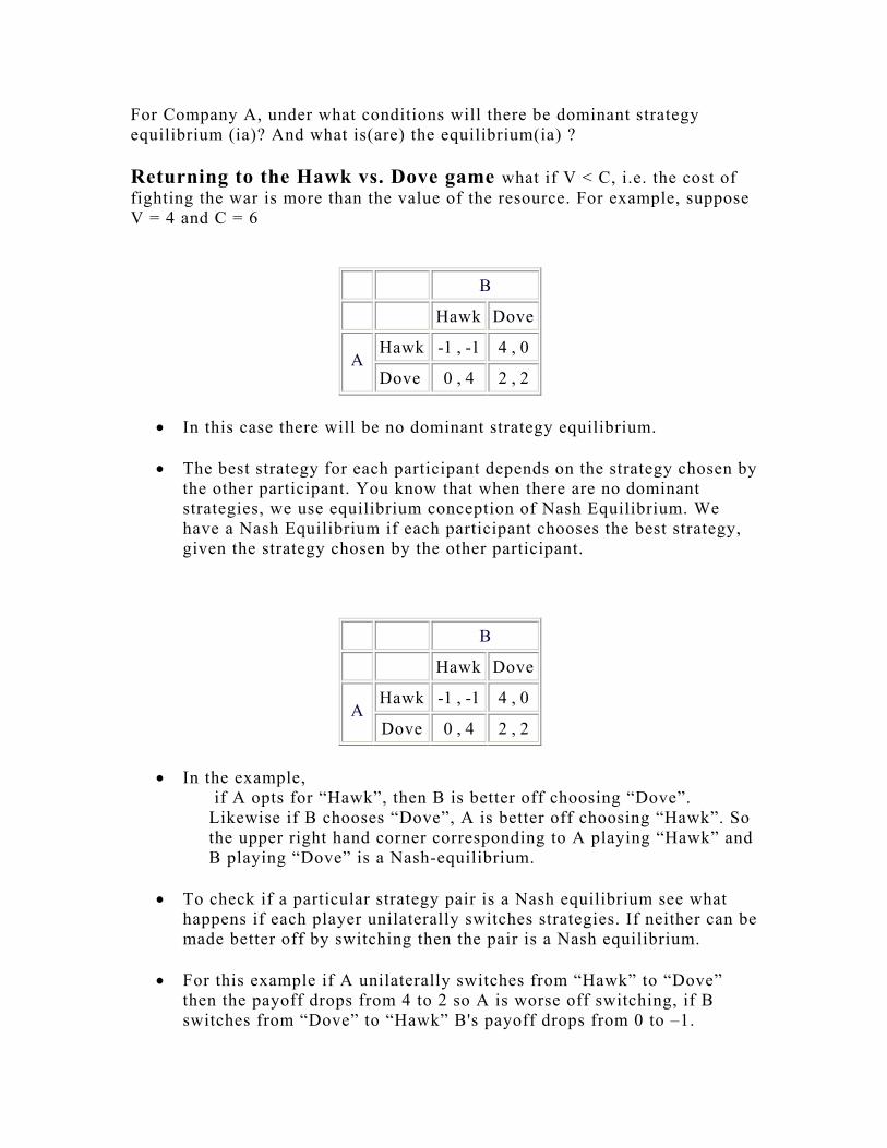
For Company A, under what conditions will there be dominant strategy equilibrium (ia)? And what is(are) the equilibrium(ia) ? Returning to the Hawk vs. Dove game what if V < C, i.e. the cost of fighting the war is more than the value of the resource. For example, suppose V = 4 and C = 6
B
Hawk Dove
Hawk -1 , -1 4 , 0 A
Dove 0 , 4 2 , 2
• In this case there will be no dominant strategy equilibrium.
• The best strategy for each participant depends on the strategy chosen by the other participant. You know that when there are no dominant strategies, we use equilibrium conception of Nash Equilibrium. We have a Nash Equilibrium if each participant chooses the best strategy, given the strategy chosen by the other participant.
B
Hawk Dove
Hawk -1 , -1 4 , 0 A
Dove 0 , 4 2 , 2
• In the example, if A opts for “Hawk”, then B is better off choosing “Dove”. Likewise if B chooses “Dove”, A is better off choosing “Hawk”. So the upper right hand corner corresponding to A playing “Hawk” and B playing “Dove” is a Nash-equilibrium.
• To check if a particular strategy pair is a Nash equilibrium see what
happens if each player unilaterally switches strategies. If neither can be made better off by switching then the pair is a Nash equilibrium.
• For this example if A unilaterally switches from “Hawk” to “Dove”
then the payoff drops from 4 to 2 so A is worse off switching, if B switches from “Dove” to “Hawk” B's payoff drops from 0 to –1.

• Every dominant strategy equilibrium is also a Nash equilibrium,
however not every Nash equilibrium is a dominant strategy equilibrium and, in fact, a game can have more than one Nash equilibria.
• If we return to the previous example, in addition to the upper right hand
corner, is there another Nash equilibrium ?
B
Hawk Dove
Hawk -1 , -1 4 , 0 A
Dove 0 , 4 2 , 2
• Note in this case the actual outcome of the game is uncertain.
Other methods for “solving” games: Rationalizability or
Iterative Elimination of Dominated Strategies
• Consider the following non-zero sum game matrix:
B
1 2 3
1 (10; 10) (12; 8) (10; 5)
2 (6; 11) (7; 12) (15; 5) A
3 (5; 5) (5; 15) (5; 20)
• To solve this game we first assume perfect information, i.e. each player knows their own payoffs and the other player’s payoffs for each set of
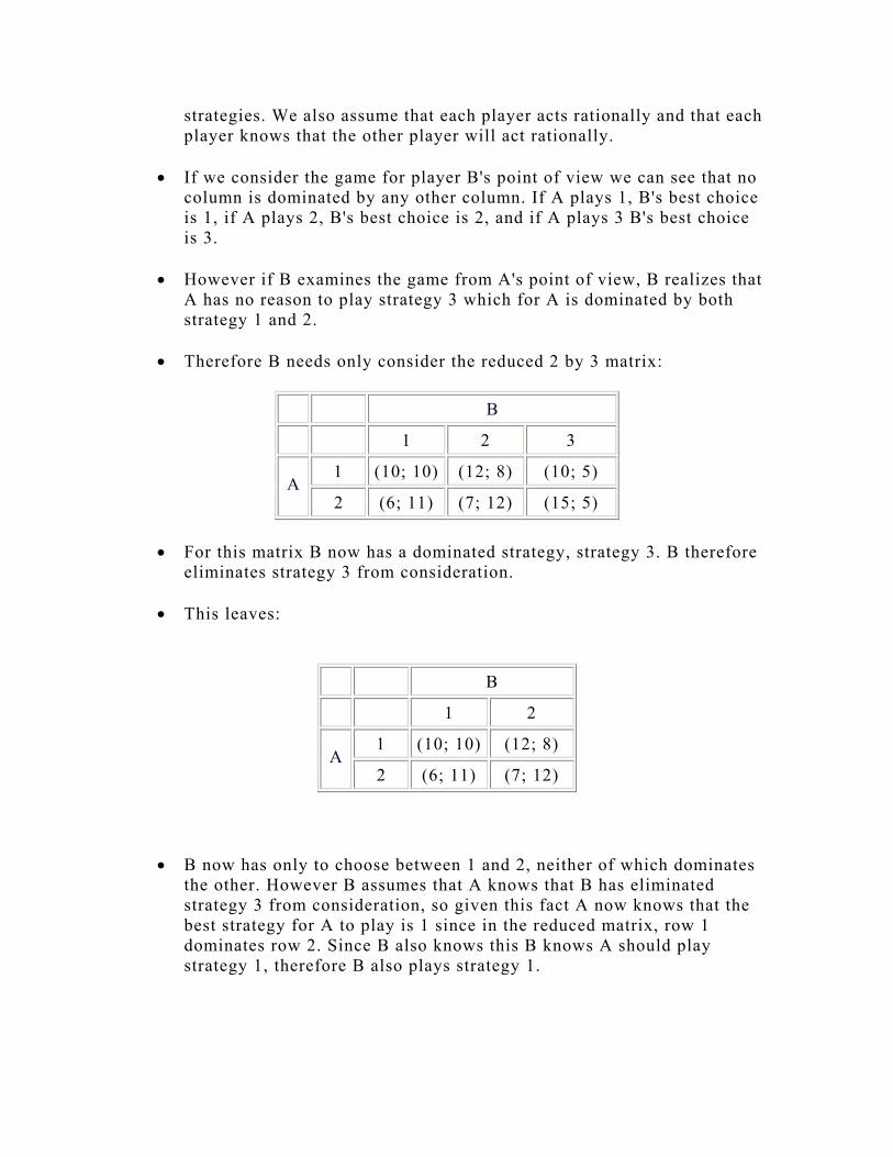
strategies. We also assume that each player acts rationally and that each player knows that the other player will act rationally.
• If we consider the game for player B's point of view we can see that no
column is dominated by any other column. If A plays 1, B's best choice is 1, if A plays 2, B's best choice is 2, and if A plays 3 B's best choice is 3.
• However if B examines the game from A's point of view, B realizes that
A has no reason to play strategy 3 which for A is dominated by both strategy 1 and 2.
• Therefore B needs only consider the reduced 2 by 3 matrix:
B
1 2 3
1 (10; 10) (12; 8) (10; 5) A
2 (6; 11) (7; 12) (15; 5)
• For this matrix B now has a dominated strategy, strategy 3. B therefore eliminates strategy 3 from consideration.
• This leaves:
B
1 2
1 (10; 10) (12; 8) A
2 (6; 11) (7; 12)
• B now has only to choose between 1 and 2, neither of which dominates the other. However B assumes that A knows that B has eliminated strategy 3 from consideration, so given this fact A now knows that the best strategy for A to play is 1 since in the reduced matrix, row 1 dominates row 2. Since B also knows this B knows A should play strategy 1, therefore B also plays strategy 1.
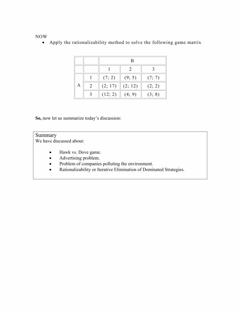
NOW
• Apply the rationalizability method to solve the following game matrix
B
1 2 3
1 (7; 2) (9; 5) (7; 7)
2 (2; 17) (2; 12) (2; 2) A
3 (12; 2) (4; 9) (3; 8) So, now let us summarize today’s discussion: Summary We have discussed about:
• Hawk vs. Dove game. • Advertising problem. • Problem of companies polluting the environment. • Rationalizability or Iterative Elimination of Dominated Strategies.
Unit 4 DECISION ANALYSIS Lesson 32

Learning Objective :
In this unit, you will gain insights on making better decisions within group or department settings in the more network-oriented organizational structures typical of the New Economy.
Acquire a variety of strategies for framing problems, and learn when to apply them.
Learn to accurately assess the degree of uncertainty in individual problems.
Recognize when you have enough information, the right information, or when you need to do more research.
Structure more complex challenges to ensure you are addressing the right issues.
Involve the proper people at the right time in the right way. Create environments that foster feedback and learning.
Introduction
So Let us first describe what is called as Decision Analysis:
Making decisions in an atmosphere of increasing time pressure, uncertainty, and conflicting expert opinions creates challenges for any manager. Making such leadership decisions in crisis situations is even more demanding.
I think that you all agree with me on this statement.
To a great extent, the success or failure that you (or any individual) experience even in day-to-day life depends on the decisions made by you. Decision making in today’s environment and especially in business is far more complex than earlier and the cost of making errors is too high. Thus to make a right decision a systematic approach is necessary.

Decision analysis provides an analytic and systematic approach to decision making. Now you must be thinking how to implement this analysis? This require a study of decision models. Before embarking on our study of decision modeling (or system-analytic approaches to decision making), it would be good to catch a glimpse of the basic approach used by managers to make important (non routine) decisions. Let's begin with a widely accepted definition for the term decision: Decision - the act or process of choosing one course of action from among several alternatives This is literally a descriptive definition of the process of making a choice. In order to conduct the process rationally (i.e., coherently), professional managers tend to follow these steps: 1. Define the problem
This refers to the process of correctly identifying and making explicit the fundamental problem or opportunity (as opposed to apparent symptoms) faced by the decision maker. Defining the problem allows the decision maker to pose the all-important question: What must be done to solve this particular problem? Thus, problem definition focuses attention on possible action alternatives that in principle should lead to the attainment of concrete objectives.
2. Gather information
Information gathering aims to ascertain relevant facts related to the decision problem. This usually reduces to a search problem. Typical sources of information are published articles and reports, internal company records, market surveys and intelligence, personal views and opinions of various stakeholders culled by interviews and questionnaires or even informal conversations, professional consultations, and direct observation by the decision maker of actual problem-related processes within or outside the organization.

3. Identify action alternatives Creativity is called upon in this phase of the overall decision process. As the decision maker gathers information, s/he begins crystallizing possible solution alternatives. Classical decision making draws heavily on subjective aspects such as intuition, experience and judgment in order to produce sound action alternatives. More formal methods may also be invoked, such as brainstorming, focus groups and quality circles. The emphasis at this point should be on generating alternatives, not criticizing them.
4. Evaluate the alternatives
The decision maker compares the pros and cons inherent to each action alternative. Costs and benefits are estimated and their impact on organizational objectives is assessed. Weak alternatives are winnowed out and a minimal set of preferred choices is determined, often consisting of two final contenders.
5. Select the best alternative
This is the classic decision-making point. The decision maker ought to be clear on which alternative offers the best course of action. Consequently, making use of the best personal judgement, the decision is made.
6. Implement the chosen alternative
The decision maker sets in motion a course of action that involves the customary managerial tasks: planning, organizing, leading and controlling. It is at this point that the functional business specialties come into play: production/operations, marketing, finance, accounting and, to the required extent, human resource management.
Now I would like you to see the distinction between different types of decisions made in an organization. Basically there are two types of decisions
• Programmed or Structured decisions. • Non-Programmed or Unstructured decisions.

Now, Let us see what is a programmed or structured decision. Programmed decision is the one which is well defined. In this you as the decision maker, are aware of the extent of the decision and has a clear set of options to make your choice. All this require a decision rule with which you can choose the ideal alternative at your disposal. Let me state this with an example…
A manager has to choose a new packaging machine from a choice of two models. Suppose the two models are similar to a certain existing machine and are known to be reliable. The manager here want to choose the machine that offers the most attractive post-tax discounted return for a period of five year.
Now, what do you think that the manager need to do first?
At first he should collect the details of each machine such as price and
operating costs. He may collect these details using certain formula approved by the
organization for capital expenditure proposals. Using these details in a systematic manner he will come to a decision
for the model of machine he should order. Now coming to the second type of decision.

Non-Programmed or unstructured When decisions are unique and not routined, they can be classified as non-programmed or unstructured. The example of this type of model, I want to take up later in the section “Decision making under uncertainity”. Let us discuss now,
Some of the rationale behind how people seek and interpret information, and actually make decisions.
Image Theory - This theory has three parts (images). The value image consists of the decision maker's principles; what's right or wrong, any organizational rules or principles that must be followed, etc. The second image is the trajectory image, the goals that the decision maker wants to achieve. The third image is the strategic image, which are the plans adopted to achieve the goals, including making decisions, evaluating, and modifying approaches based on results. Decisions can be made by screening out candidates because they don't pass a minimum level, or by doing some sort of combined comparison to rank the candidates in preference order.
Recognition Primed Decision Making (RPD) - This model describes how experts make decisions under stressful situations, perhaps due to time pressure or rapidly changing environments. The decision maker uses their expertise and experience to quickly assess the situation and to come up with an acceptable course of action. They then "play out" the course of action to see whether it is feasible or requires modification. If the first choice doesn't work, they will go back, select another option, and do the evaluation again. A good example is a firefighting captain who arrives on the scene of a burning building. He will quickly recognize what to do and act accordingly, but the situation may change rapidly and he will have to stay on top of the situation, perhaps changing priorities on the fly. One aspect of RPD is that the expert can quickly rule out unimportant information or unusable solutions, almost on a subconscious level, whereas a novice would need much more time to explicitly think through all possibilities.
Explanation Based Model - There are two parts to this model: The coherent story and the choices. The theory says that the decision maker will attempt to create a full story from some incomplete raw facts and then match this story against possible choice options to come up with a solution. For example, a jury will try to formulate a full explanation of a defendant's behavior from the evidence, general knowledge about similar events, and knowledge about story structures in general. With their completed story, they will then try to match

that with the choices (verdict categories). If a match is found, they can make a decision, otherwise the process would have to be repeated with additional inputs.
Lens Model - The lens model is a part of Social Judgment Theory. It tries to analytically build a model of how well a person's judgments match up with the environment they are trying to predict. The interface between the two are the cues that represent the environment. An example is a trader trying to predict what the market will do so that they can pick good stocks. Some of the cues might be unemployment rate, price/earnings ratio of the stock, inflation rate, etc. The trader observes the cues and makes a judgment on how to interpret them, then selects stocks. The lens model takes a large number of these trial cases and comes up with equations for how well the trader does, plus other models for how well the cues are judged or how well they represent the environment. Even with perfect information, most task success rates are nowhere near 100%. This is due to many factors, including errors in judgment, insufficient or unrecognized cues, or important cue patterns that are hard to determine.
Dominance Testing - There are four major steps to making a decision. First, the decision maker simply screens out alternatives that do not meet minimum standards. After that, if there is more than one choice left, the second step is to select a promising alternative. This can be a fairly subjective choice based on preferences or initial reaction. The third step is to test for dominance. An alternative is dominant if, for all the selection criteria, the alternative has no disadvantages and at least one advantage, it is selected. Often, this is not the case, and the fourth step is entered. This is where the decision maker tries to restructure or reinterpret the information in order to make the promising alternative dominant so it can be selected. This can be good or bad, since if overdone it can mean talking yourself into making a bad decision.
Let us move on to a very important aspect of decision making.
ESSENTIAL CHARACTERISTICS OF DECISION MAKING

Irrespective of the type of decision model, there are certain essential characteristics which are common to all: DECISION ALTERNATIVES
A finite number of decision alternatives are available to you (the decision maker) at the time of making a decision. The number and type of such alternatives may depend on the previous decisions made and the consequences of those decisions. These alternatives are also called courses of actions, acts or strategies and are under control and known to you that is you will determine what courses of action are possible.
Decision alternatives must be mutually exclusive (clearly distinct among themselves) and, ideally, collectively exhaustive (cover all reasonable options open to management). Determining a realistic set of action alternatives demands creativity and experience on the nature of the problem under consideration. Managerial intuition is extremely valuable at this stage of the analysis.
STATES OF NATURE
Decision theory will require you (the decision maker) to develop a mutually exclusive and collectively exhaustive list of possible future events. These future events are referred to as states of nature and they depend upon certain factors which are beyond the control. There may be a great deal of uncertainity with respect to the occurrence of the states of nature.
PAYOFF
A payoff is a quantitative measure of the result of taking a particular course of action combined with the occurrence of a particular state of nature. It is the net gain or loss obtained as the outcome of the decision that accrues from a given combination of decision alternatives and events. They are also known as conditional profit values. In business, payoffs are usually expressed using monetary values. In decision analysis, however, one can make use of either monetary values or abstract utilities

PAYOFF TABLE The payoff estimates are presented in terms of the interaction of the decision alternatives and the states of nature in the form of a payoff table.
GENERAL STRUCTURE OF PAYOFF TABLE Suppose the problem under consideration has n possible states of nature denoted by E1, E2, ………………… , En and m alternative actions denoted by A1, A2, …………., Am. Then the payoff corresponding to your(the decision maker) selected action Aj under the state of nature Ei will be denoted by aij
where i = 1, 2, ………., n ; j = 1, 2, …………., m
DECISION ALTERNATIVES
STATES OF NATURE A1 A2 ……………………… Am
E1 a11 a12 ……………………… a1m
E2 a21 a22 ……………………… a2m . . . . . . . . . . . . . . . . . . . . . . . .
En an1 an2 ……………………… anm
So, now let us summarize today’s discussion:

Summary We have discussed about
• Steps followed by professional managers for taking decisions. • Types of decisions. • Characteristics of decision-making.
Slide 1
DECISION THEORY
LECTURE 1
________________________________________________________________________
________________________________________________________________________
________________________________________________________________________
________________________________________________________________________
________________________________________________________________________
________________________________________________________________________
___________________________________________________________________
Slide 2
INTRODUCTION
Decision analysis provides an analytic and systematic approach to decision
making.
________________________________________________________________________
________________________________________________________________________
________________________________________________________________________
________________________________________________________________________
________________________________________________________________________
________________________________________________________________________
________________________________________________________________________
________________________________________________________________________
________________________________________________________________________
________________________________________________________________________
________________________________________________________________________
____________________________________________________________________

Slide 3
WHAT IS A DECISION?
Decision is the act or process of choosing one course of action amongst several alternatives.
________________________________________________________________________
________________________________________________________________________
________________________________________________________________________
________________________________________________________________________
________________________________________________________________________
________________________________________________________________________
________________________________________________________________________
________________________________________________________________________
________________________________________________________________________
________________________________________________________________________
________________________________________________________________________
____________________________________________________________________

Slide 4
TYPES OF DECISIONS
Programmed or Structured decisions.
Non-Programmed or Unstructured decisions.
________________________________________________________________________
________________________________________________________________________
________________________________________________________________________
________________________________________________________________________
________________________________________________________________________
________________________________________________________________________
________________________________________________________________________
________________________________________________________________________
________________________________________________________________________
________________________________________________________________________
________________________________________________________________________
____________________________________________________________________

Slide 5
DECISION MODELS
Image TheoryRecognition Primed Decision Making Explanation Based Model Lens Model Dominance Testing
________________________________________________________________________
________________________________________________________________________
________________________________________________________________________
________________________________________________________________________
________________________________________________________________________
________________________________________________________________________
________________________________________________________________________
________________________________________________________________________
________________________________________________________________________
________________________________________________________________________
________________________________________________________________________
____________________________________________________________________

Slide 6
ESSENTIAL CHARACTERISTICS OF DECISION MAKING
DECISION ALTERNATIVES
STATES OF NATURE
PAYOFF
________________________________________________________________________
________________________________________________________________________
________________________________________________________________________
________________________________________________________________________
________________________________________________________________________
________________________________________________________________________
________________________________________________________________________
________________________________________________________________________
________________________________________________________________________
________________________________________________________________________
________________________________________________________________________
____________________________________________________________________

Slide 7
GENERAL STRUCTURE OF PAYOFF TABLE
DECISION ALTERNATIVES
STATES OF NATURE A1 A2 ……………………… Am
E1 a11 a12 ……………………… a1m
E2 a21 a22 ……………………… a2m . . . . . . . . . . . . . . . . . . . . En an1 an2 ……………………… anm
________________________________________________________________________
________________________________________________________________________
________________________________________________________________________
________________________________________________________________________
________________________________________________________________________
________________________________________________________________________
________________________________________________________________________
________________________________________________________________________
________________________________________________________________________
________________________________________________________________________
________________________________________________________________________
____________________________________________________________________

Unit 4 DECISION ANALYSIS Lesson 33 Learning Objective:
• In this lesson you will study about the steps of Decision Process and about Decision Environment.
Hello students, Firstly we have; The steps that you should follow to make a good decision are:- DECISION PROCESS Step 1:
You, the decision maker, clearly define the problem at hand. Step 2:
List the possible alternatives (courses of action), which are available to you for making the decision. The number of possible alternatives may be large in some case, but in most of the situations only a reasonable number of alternatives will be required. Step 3:
After you choose an alternative, a state of nature occurs that is beyond your control. You should take care to include all possible future events that might occur. Here, at this point of time you are likely to be unsure as of which specific event will occur. Step 4:

Determine and list the payoff for each combination of alternatives and outcomes. Present these payoffs in a payoff table. You can express these payoffs in terms of profits, losses, revenues, costs, utilities, or nay other appropriate parameter of measurement. Step 5:
Select one of the mathematical decision theory models to choose the best alternative from the given list on the basis of some criterion that results in the desired payoff. Now in general what do you think about general what do you after determining the payoff table for making the best decision.
• You, select one of the alternative (course of action). Suppose you have selected A1
• A state of nature occurs that is beyond your control. Suppose that state E2 occurs.
• You receive a certain return that can be determined from payoff table. Since you choose A1 and state of nature E2 occurred, the return is a21.
• Again you choose an alternative and then are of the states of nature occurs.
Examine that once the alternative is selected, it can’t be changed after the state of nature occurs. So, in general terms the question is, which of the alternatives should you select? What are you views on this? ……….
Let me share my personal feelings with you as regards this. You would like to have as large a return as possible, that is, the largest possible value of aij where i represent the state of nature that occurs and j represents the alternative selected. It is obvious that the action you may select will depend on your belief concerning what nature will do, i.e., which state of nature will occur. If you believe state 1 will occur, you select the alternative associated with the largest number corresponding to state 1. If you believe state 2 is more likely to occur, choose the decision corresponding to the largest payoff with it and so on. Let us view all this with the help of an interesting example:

You are the founder and president of Ken Manufacturing, Inc., a reputed firm located in Mumbai.
• The problem that you identify is whether or not to build more manufacturing plants for expansion.
• You decide that your alternatives are to construct
(1) A large new plant manufacturing the product (2) A small plant, or (3) No plant at all
• You determine that there are only two possible out comes of the various
alternatives.
The market for your product could be favorable, meaning that there is a high demand for the product, or
The market could be unfavorable, meaning that there is a low demand for your product.
• Nextly, you express the payoff resulting from each possible combination of alternatives and out comes. As you are interested in maximizing your profits, you can use ‘profit’ to evaluate each consequence. Of course, not every alternative can be based on money alone so any appropriate means of measuring benefit is acceptable.
• You have already evaluated the potential profits associated with the various
outcomes.
With a favorable market, you think a large plant would result in a net profit of Rs. 2,00,000 to your firm. This return is conditional upon both building a large plant and having a good market, so it is a conditional value.
The conditional value if the market is unfavorable would be a Rs, 1,80,000 net loss. Similarly, a small plant would result in a net profit of Rs, 1,00,000 in a favorable market, but a net loss of Rs. 20,000 would occur if the market is unfavorable. Finally, doing nothing would result in Rs. 0 profit in either market. The easiest way to present these value in by constructing a payoff table.
• You apply decision theory to take the appropriate decision.
This involves selecting a decision model depending on the environment in which you are operating and the amount of risk and uncertainty involved So this requires to know about DECISION MAKING ENVIRONMENTS Decisions are made based upon he date available about eh occurrence of events as well as the decision situation or environment. Basically, there are four different state of decision environment: certainty, risk, uncertainty and conflict. We shall discuss each decision environment in greater detail. Type 1: Decision making under certainty In this case, you (the decision maker) have all the information of the consequence of every alternative or decision choice with certainty. In other words, under certainty we can predict the outcome of each alternative course of action exactly. Here you recall the linear programming problems. In linear programming problems you know exactly how much of each of the different resources are required to produce a particular product, thus you can accurately predict that product’s unit profit. Many of the decision problems you face daily are under certainity. Where to have lunch – McDonald’s, Pizza hut or one of the many fine food outlets in nearby area?
You know exactly how much a meal costs at each of the locations, and you know the quality you will receive for your money. Consider another sort of example, let’s say You have Rs 10,000 to invest for a year you have two alternatives to select from:- either you open saving A/c Paying a 4% Interest or invest in fixed deposits paying 6% interest. As both investments are secure and guaranteed. Obviously , Fixed deposits will pay a higher return. ( i.e. Rs. 600 of interest ) In this decision model, only one possible state of nature exits. Type 2: Decision making under Risk. In this case, you (decision maker) knows the probability of occurrence of each outcome. For example,

Suppose that you are manager of a computer store and considering stocking a new personal computer (PC) just introduced into the market. Your immediate concern is to decide how many units of the PC to stock. The PC costs Rs 2,5,000 and the suggested retail price is Rs. 32,000. Any unsold PC can be sold to the local high school for Rs 20,000. After a discussion with the manufacturers representative and analysis of past sales records of new PCs, you arrive at the following estimate of sales for the next month:
PCs Probability 2 0.10 3 0.25 4 0.30 5 0.25 6 0.10
1.00 With this data, you will be able to determine the number of PCs to purchase for the next month. The solution is not guaranteed to be the best possible under all conditions that could occur, but it will be the best solution on average. Clearly, you have examined that in decision making under risk, you attempt to maximize your expected gains. Decision theory models for business problems in this environment typically employ two equivalent criteria.
• Maximization of expected monetary value • Minimization of expected loss.
Type 3: Decision making under uncertainity Uncertainity refers to the situation in which you do not have any knowledge about the probability of occurrence of any of occurrence any state of nature. Under uncertainity, it is impossible to estimate the probabilities of the various possible outcomes. In the microcomputer case, for example, sales may be totally unpredictable because too many factors affect sales – reputation of the manufacturer, software availability, price, warranty, service and other similar factors. Here, you may think of it as a hopeless case. Isn’t it? Although this sounds like a hopeless case, in reality, decision making under uncertainity is perhaps the most common situation humans have to deal with.

Obviously, we cannot just give up making decisions because uncertainity exists. You must find ways to reduce uncertainity and there are several approaches suggested by different personalities for decision-making under uncertainity. The first approach is to obtain additional information about the problem. This process may yield at least partial probabilities of consequences. Then the problem is no longer a “shot in the dark” but rather a “Shot in the fog”. Although additional information can make the problem more clearly understood, the question of the cost of obtaining the additional information is important. So, what do you say for the relation between the benefit with the additional information and the cost of additional information??? In my view, The benefit derived from additional information should exceed the cost of obtaining this information. Now Let’s take up another approach for handling decision – making under uncertainity. Can you reduce it to a problem under risk? ………………..….. of course, yes. You can do this by incorporating your own subjective feelings or estimates as probabilities. There are several strategies that can be employed for this purpose. Type 4: Decision Making under conflict. A condition of conflict exists when the interest of two or more decision makers compete. For example, If decision maker A benefits from a course of action, it is possible only because decision maker B has also taken a certain course of action. Hence in decision analysis, the decision makers are interested not only in what they do individually but also in what other do.
Such situations are common, when firms are involved in competitive market strategies, new product development, recruitment of experienced executives, or advertising campaigns. Although, decision making under conflict may sound simple; In reality it is extremely complex. We may have a decision – making problem under uncertainty that is further compounded by fierce opponents or competitors. Game theory has been suggested as a theoretical approach to decision making under conflict. So, now let us summarize today’s discussion: Summary We have discussed brief concepts of
• Steps followed in a decisions process. • Decision making under certainity. • Decision making under uncertainity. • Decision making under risk. • Decision making under conflict.

Slide 1
DECISION THEORY
LECTURE 2
______________________________________________________________________________
______________________________________________________________________________
______________________________________________________________________________
______________________________________________________________________________
______________________________________________________________________________
______________________________________________________________________________
______________________________________________________________________________
______________________________________________________________________________
______________________________________________________________________________
______________________________________________________________________________
______________________________________________________________________________
______________________________________________________________________________
______________________________________________________________________________
______________________________________________________________________________
______________________________________________________________________________
______________________________________________________________________________
______________________________________________________________________________
______________________________________________________________________________
______________________________________________________________________________

Slide 2
STEPS OF DECISION MAKING
Clearly define the problem.List the possible alternatives.Include all states of nature.List the payoff for each combination of alternatives and state of nature.Apply a decision theory model and make your decision.
______________________________________________________________________________
______________________________________________________________________________
______________________________________________________________________________
______________________________________________________________________________
______________________________________________________________________________
______________________________________________________________________________
______________________________________________________________________________
______________________________________________________________________________
______________________________________________________________________________
______________________________________________________________________________
______________________________________________________________________________
______________________________________________________________________________
______________________________________________________________________________
______________________________________________________________________________
______________________________________________________________________________
______________________________________________________________________________
______________________________________________________________________________
______________________________________________________________________________
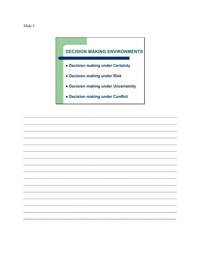
Slide 3
DECISION MAKING ENVIRONMENTS
Decision making under Certainty
Decision making under Risk
Decision making under Uncertainity
Decision making under Conflict
______________________________________________________________________________
______________________________________________________________________________
______________________________________________________________________________
______________________________________________________________________________
______________________________________________________________________________
______________________________________________________________________________
______________________________________________________________________________
______________________________________________________________________________
______________________________________________________________________________
______________________________________________________________________________
______________________________________________________________________________
______________________________________________________________________________
______________________________________________________________________________
______________________________________________________________________________
______________________________________________________________________________
______________________________________________________________________
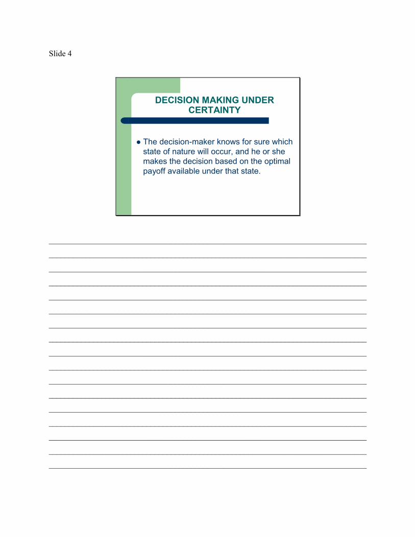
Slide 4
DECISION MAKING UNDER CERTAINTY
The decision-maker knows for sure which state of nature will occur, and he or she makes the decision based on the optimal payoff available under that state.
______________________________________________________________________________
______________________________________________________________________________
______________________________________________________________________________
______________________________________________________________________________
______________________________________________________________________________
______________________________________________________________________________
______________________________________________________________________________
______________________________________________________________________________
______________________________________________________________________________
______________________________________________________________________________
______________________________________________________________________________
______________________________________________________________________________
______________________________________________________________________________
______________________________________________________________________________
______________________________________________________________________________
______________________________________________________________________________
______________________________________________________________________________

Slide 5
DECISION MAKING UNDER UNCERTAINITY
It is unknown which state of nature will occur and the probability or relative likelihood of any particular state occurring is also unknown.
______________________________________________________________________________
______________________________________________________________________________
______________________________________________________________________________
______________________________________________________________________________
______________________________________________________________________________
______________________________________________________________________________
______________________________________________________________________________
______________________________________________________________________________
______________________________________________________________________________
______________________________________________________________________________
______________________________________________________________________________
______________________________________________________________________________
______________________________________________________________________________
______________________________________________________________________________
______________________________________________________________________________

Slide 6
DECISION MAKING UNDER RISK
It is unknown which state of nature will occur, but the decision maker knows, or has estimates of, the probabilities that various states of nature will occur.
______________________________________________________________________________
______________________________________________________________________________
______________________________________________________________________________
______________________________________________________________________________
______________________________________________________________________________
______________________________________________________________________________
______________________________________________________________________________
______________________________________________________________________________
______________________________________________________________________________
______________________________________________________________________________
______________________________________________________________________________
______________________________________________________________________________
______________________________________________________________________________
______________________________________________________________________________
______________________________________________________________________________
______________________________________________________________________________
______________________________________________________________________________
Slide 7
DECISION MAKING UNDER CONFLICT
A condition of conflict exists when the interest of two or more decision makers compete.
______________________________________________________________________________
______________________________________________________________________________
______________________________________________________________________________
______________________________________________________________________________
______________________________________________________________________________
______________________________________________________________________________
______________________________________________________________________________
______________________________________________________________________________
______________________________________________________________________________
______________________________________________________________________________
______________________________________________________________________________
______________________________________________________________________________
______________________________________________________________________________
______________________________________________________________________________
______________________________________________________________________________
______________________________________________________________________________

Unit 4 DECISION ANALYSIS Lesson 34 Learning Objective:
• To enable students to make business and management decisions when there is uncertainty.
Hello class. Lets discuss through this lesson about the construction of a decision matrix and apply a number of decision criteria and calculate the best decision.
In this lecture you will study about the different criterion used for taking DECISION UNDER UNCERTAINITY.
INTRODUCTION
In decision under uncertainity you (the decision maker) are unwilling or unable to specify the probabilities with which the various states of nature will occur.
There is a long standing debate as to whether such a situation should exist; i.e., should you always be willing to specify the probabilities even when you do not know anything or much about what state of nature is apt to occur?
Although, this is hard to imagine on actual business decision being made under such a cloud, we’ll leave this debate to the philosophers and let us turn to the various approaches suggested for this class of models.
So,
Let us follow the different criterion on the following example:

ACME Road Runner Traps
• ACME International is considering building an overseas manufacturing facility to produce a new, high-tech version of their famous Road Runner Trap.
• Forecasted demand for road runner traps is highly uncertain, depending on two interrelated parameters that are difficult to assess: road runner population and coyote population.
• ACME's CEO, Wolfgang E. Cactus, believes demand in the next five years could be high, medium or low.
• If demand was to be high and ACME builds a large plant, they expect
to make $15 million in (net present value) profits. If demand were
medium, ACME would clear only $3 million with a large plant. But if
demand were low, ACME would incur a $6 million loss.
• Were ACME to build a small plant, Cactus is confident they would
avoid losses altogether but stand to make much less profit: $3 million,
$2 million and $1 million for high, medium and low demands,
respectively.
• ACME's VP for strategic analysis, Goldie Lockes, has proposed
building a mid-size plant she calls "just right." With this plant, she
estimates profits would be $9 million on a high-demand scenario and
$4 million under medium demand. Low demand would produce an
estimated loss of $2 million.
• Cactus and Lockes are in agreement about these estimates as well as a
planning horizon of five years.
In this example, we have no knowledge about the probabilities of occurrence of different states of nature i.e. demand (high, medium, low).
Let's follow the approach I recommended you previously to formulate the model with a payoff table for this decision problem.

• Given that Cactus and Lockes are in agreement in order to maximize
net present value profits for the five year period.
• They identify the alternatives (courses of action) as to build either a
large plant, small plant, or "just right" plant, or build no plant at all!
• Demand for road runner traps turns out to be high, medium or low.
• The profit figures will serve as the corresponding payoffs.
• It is assumed in this example that no probability information about the
states of nature is available to ACME’s managers.
ALTERNATIVES STATES OF
NATURE Large plant
Just Right plant
Small plant
No plant
High demand
15 9 3 0
Medium demand
3 4 2 0
Low demand
-6 -2 1 0
Now, I describe about the different criterion for Decision under uncertainity…… THE OPTIMIST CRITERION (MAXIMAX CRITERION) The optimist criterion attempts to describe the decision-making behavior of people who are overly optimistic in their expectations. If you are optimistic decision maker then you are likely to be attracted by large rewards and you are willing to risk high losses in order to obtain them. You’ll evaluate each decision by the “best thing that can happen” if you make that decision.

It is possible to model the optimist profile with the MAXIMAX decision rule when the payoffs are positive-flow rewards, such as profits or income. When payoffs are given as negative-flow rewards, such as costs or losses, the optimist decision rule is MINIMIN. Note that negative-flow rewards are expressed with positive numbers. Let's assume that ACME's managers are thoroughly optimistic. We would suppose they would therefore go for a large manufacturing facility in hopes of attaining the maximum profit. Thus the psychological processes leading to such behavior can be captured by the two-step logic of the Maximax rule. Maximax decision rule
1. Determine the maximum possible payoff for each alternative (course of action).
2. From these maxima, select the maximum payoff. The alternative that corresponds to this maximum payoff is the chosen decision.
Use ACME's payoff table defined previously:
ALTERNATIVES STATES
OF NATURE
Large plant
Just Right plant
Small plant
No plant
High demand
15 9 3 0
Medium demand
3 4 2 0
Low demand
-6 -2 1 0
Maximum payoff
15 Maximax
9 3 0
Decision : To build a large plant
The Minimin decision rule is applicable when the payoff matrix consists of negative-flow rewards, such as costs or losses. An optimistic decision maker amongst you would be attracted by lower costs.
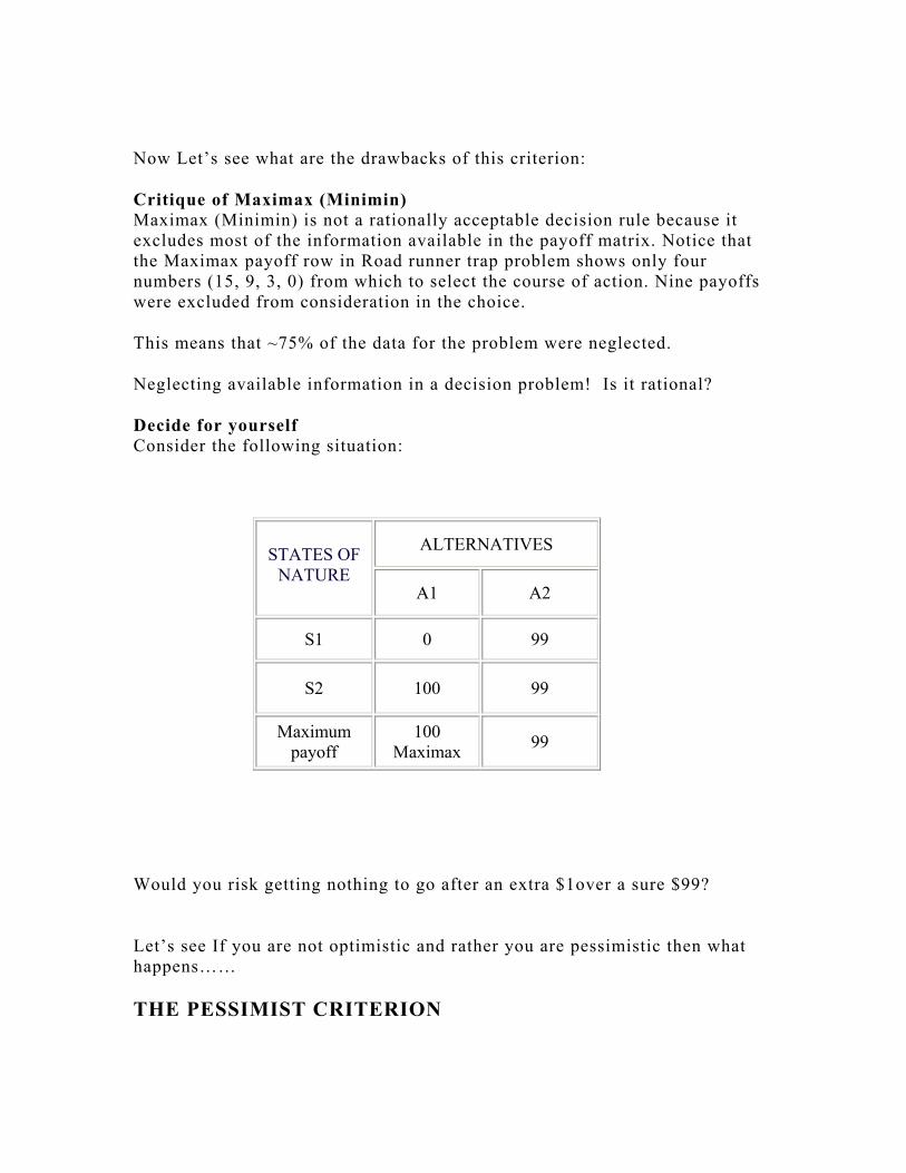
Now Let’s see what are the drawbacks of this criterion:
Critique of Maximax (Minimin) Maximax (Minimin) is not a rationally acceptable decision rule because it excludes most of the information available in the payoff matrix. Notice that the Maximax payoff row in Road runner trap problem shows only four numbers (15, 9, 3, 0) from which to select the course of action. Nine payoffs were excluded from consideration in the choice.
This means that ~75% of the data for the problem were neglected.
Neglecting available information in a decision problem! Is it rational?
Decide for yourself Consider the following situation:
ALTERNATIVES STATES OF NATURE
A1 A2
S1 0 99
S2 100 99
Maximum payoff
100 Maximax 99
Would you risk getting nothing to go after an extra $1over a sure $99?
Let’s see If you are not optimistic and rather you are pessimistic then what happens…… THE PESSIMIST CRITERION
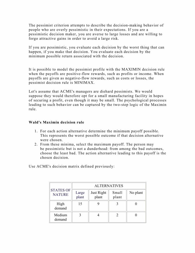
The pessimist criterion attempts to describe the decision-making behavior of people who are overly pessimistic in their expectations. If you are a pessimistic decision maker, you are averse to large losses and are willing to forgo attractive gains in order to avoid a large risk. If you are pessimistic, you evaluate each decision by the worst thing that can happen, if you make that decision. You evaluate each decision by the minimum possible return associated with the decision. It is possible to model the pessimist profile with the MAXIMIN decision rule when the payoffs are positive-flow rewards, such as profits or income. When payoffs are given as negative-flow rewards, such as costs or losses, the pessimist decision rule is MINIMAX. Let's assume that ACME's managers are diehard pessimists. We would suppose they would therefore opt for a small manufacturing facility in hopes of securing a profit, even though it may be small. The psychological processes leading to such behavior can be captured by the two-step logic of the Maximin rule. Wald's Maximin decision rule
1. For each action alternative determine the minimum payoff possible. This represents the worst possible outcome if that decision alternative were chosen.
2. From these minima, select the maximum payoff. The person may be pessimistic but is not a dunderhead: from among the bad outcomes, choose the least bad. The action alternative leading to this payoff is the chosen decision.
Use ACME's decision matrix defined previously:
ALTERNATIVES STATES OF
NATURE Large plant
Just Right plant
Small plant
No plant
High demand
15 9 3 0
Medium demand
3 4 2 0

Low demand
-6 -2 1 0
Minimum payoff
-6
-2 1 Maximin
0
Decision : To build a small plant
The Minimax decision rule applies when the payoff matrix measures negative-flow rewards, such as costs. A pessimistic decision maker would tend to avoid higher costs. The minimax rule guarantees the lesser of possible worst evils. It portrays a very conservative approach to risk.
Now Let’s see what are the drawbacks of this criterion:
Critique of Maximin (Minimax) Maximin (Minimax) is not a rationally acceptable decision rule because it excludes most of the information available in the payoff matrix. In this example, nine payoffs were excluded from consideration in making the choice. Since ~75% of the data for the problem were neglected, the decision process was not rational.
Decide for yourself Consider the following situation:
ALTERNATIVES STATES OF NATURE
A1 A2
S1 100 1
S2 0 1
Minimum payoff 0 1
Maximin
Would you pass up the chance of getting $100 to avoid losing $1?

……………………Surely, No?
Let us move on to the next criterion.
THE HURWICZ CRITERION The Hurwicz criterion attempts to find a middle ground between the extremes posed by the optimist and pessimist criteria. Instead of assuming total optimism or pessimism, Hurwicz incorporates a measure of both by assigning a certain percentage weight to optimism and the balance to pessimism.
A weighted average can be computed for every action alternative with an alpha-weight α , called the coefficient of realism. "Realism" here means that the unbridled optimism of maximax is replaced by an attenuated optimism as denoted by the α . Note that 0 ≤ α ≤ 1. Thus, a better name for the coefficient of realism is coefficient of optimism. An α = 1 implies absolute optimism (maximax) while an α = 0 implies absolute pessimism (maximin).
Selecting a value for α simultaneously produces a coefficient of pessimism 1 - α , which reflects the decision maker's aversion to risk. A Hurwicz weighted average H can now be computed for every action alternative Ai in A as follows:
H (Ai) = α (column maximum) + ( 1 - α ) (column minimum) for positive-flow payoffs (profits, income)
H (Ai) = α (column minimum) + ( 1 - α ) (column maximum) for negative-flow payoffs (costs, losses)
Hurwicz decision rule
1. Select a coefficient of optimism value α. 2. For every action alternative compute its Hurwicz weighted average.

3. Choose the action alternative with the best Hurwicz weighted average as the chosen decision. ("Best" means the maximum H for positive-flow payoffs, and the minimum H for negative-flow payoffs.)
Let's assume that ACME's managers have agreed to assess their level of optimism at 60%. Thus α = 0.6. Using the decision matrix defined previously:
ALTERNATIVES STATES OF
NATURE Large plant
Just Right plant
Small plant
No plant
High demand
15 9 3 0
Medium demand
3 4 2 0
Low demand
-6 -2 1 0
H (L) = 0.6 (15) + 0.4 (-6) = 6.6
H (JR) = 0.6 (9) + 0.4 (-2) = 4.6
H (S) = 0.6 (3) + 0.4 (1) = 2.2
H (N) = 0.6 (0) + 0.4 (0) = 0
Here, consider that Hurwicz weighted average is maximum for alternative ‘to build a large plant’.
So, you decide to build a large plant.
You might wish to redo the computations for α = 0.3 to see the effect a greater degree of pessimism on the decision.
Now Let’s see what are the drawbacks of this criterion:
Critique of Hurwicz Criterion
Although Hurwicz is an improvement of sorts over Maximax and Maximin (more of the available data are taken into consideration), it still falls short of being a rationally sound approach because part of the information is neglected. In this particular case ~33% of the data was excluded. But if there had been, say, ten states of nature, then 80% of the data would have been ignored. Ignoring intermediate payoffs can lead to questionable decisions.
Now, Try some problems yourself:
1. A food product company is contemplating the introduction of a revolutionary new product with new packing to replace the existing product at much higher price (S1) or a moderate change in the composition of the existing product with a new packaging at a small increase in price (S2) or a small change in the composition of the existing expect the word ‘New’ with a negligible increase in price (S3). The three possible states of nature of events are
(i) High increase in sales (N1) (ii) No change in sales (N2) and (iii) Decrease in sales (N3). The marketing department of the company worked out the payoffs in term of
yearly net profits for each of the strategies for these events (expected sales). This is represented in following table:

State of nature Payoffs (in Rs.) Strategies S1 S2 S3
A1 A2 A3
7,00,000 5,00,000 3,00,000
3,00,000 4,50,000 3,00,000
1,50,000 0
3,00,000 Which strategy should the executive concerned choose on the basis of : (i) Maximin criterion, (ii) Maximax criterion, (iii) Hurwicz criterion (with α = 0.7)
2. Dr. Mohan Lal has been thinking about starting his own independent nursing
home. The problem is to decide how large nursing home should be? The annual returns will depend on both the size of nursing home and a number of marketing factors. After a careful analysis, Dr. Mohan Lal developed the following table:
Size of Nursing home
Good market (Rs.)
Fair market (Rs.)
Poor market (Rs.)
Small Medium
Large Very large
50,000 80,000 1,00,000 3,00,000
20,000 30,000 30,000 25,000
─ 10,000 ─ 20,000 ─ 40,000 ─ 1,60,000
(i) Develop a decision table for this decision. (ii) What is the maximax decision?
(iii) What is the maximin decision?
(iv) What is the criterion of realism decision? Use α value of 0.8.
3. The proprietor of a food stall has invented a new food-delicacy, which he calls Whim. He has calculated that the cost of manufacture is Re. 1 per piece and because of its novelty it can be sold for Rs. 3 per piece. It is, however, perishable, and good unsold at the end of the day are a dead loss. He expected the demand to very between 10 and 15. How many pieces should be manufactured so that his net profit is maximum? Use Maximin and Minimax criteria.

So, now let us summarize today’s discussion: Summary We have discussed in details about Decision making under uncertainity.
• The Optimist Criterion. • The Pessimist Criterion • The Hurwicz Criterion.
Slide 1
DECISION THEORY
LECTURE 3
________________________________________________________________________
________________________________________________________________________
________________________________________________________________________
________________________________________________________________________
________________________________________________________________________
________________________________________________________________________
________________________________________________________________________
________________________________________________________________________

________________________________________________________________________
________________________________________________________________________
Slide 2
THE OPTIMIST CRITERION (MAXIMAX CRITERION)
THE PESSIMIST CRITERION (MAXIMIN CRITERION)
THE HURWICZ CRITERION
DECISION MAKING UNDER UNCERTAINITY
________________________________________________________________________
________________________________________________________________________
________________________________________________________________________
________________________________________________________________________
________________________________________________________________________
________________________________________________________________________
________________________________________________________________________
________________________________________________________________________
________________________________________________________________________
________________________________________________________________________
________________________________________________________________________
____________________________________________________________________
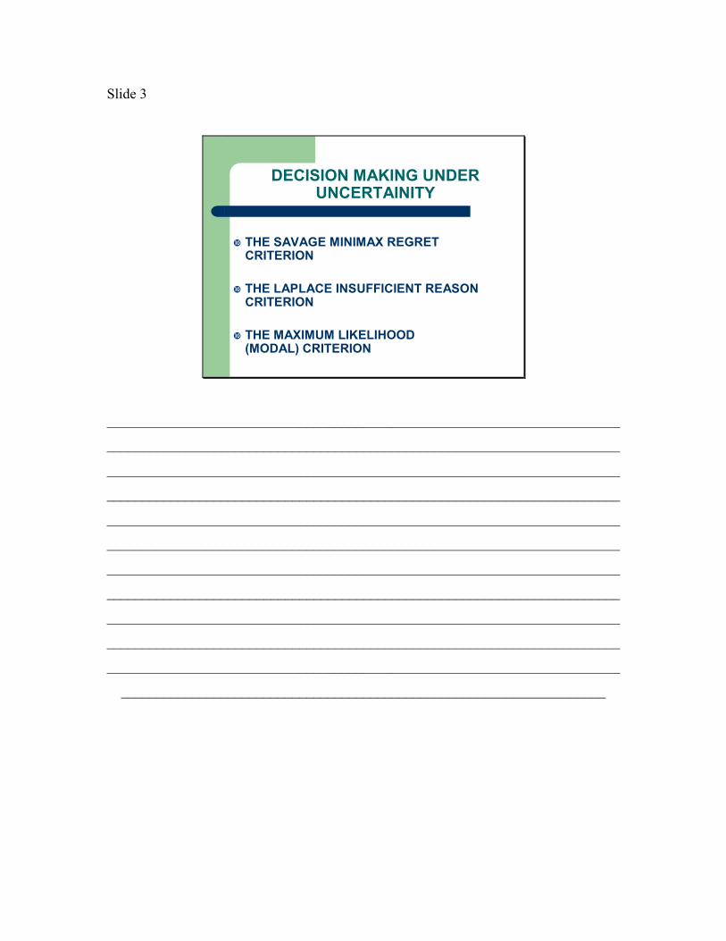
Slide 3
THE SAVAGE MINIMAX REGRET CRITERION
THE LAPLACE INSUFFICIENT REASON CRITERION
THE MAXIMUM LIKELIHOOD (MODAL) CRITERION
DECISION MAKING UNDER UNCERTAINITY
________________________________________________________________________
________________________________________________________________________
________________________________________________________________________
________________________________________________________________________
________________________________________________________________________
________________________________________________________________________
________________________________________________________________________
________________________________________________________________________
________________________________________________________________________
________________________________________________________________________
________________________________________________________________________
____________________________________________________________________
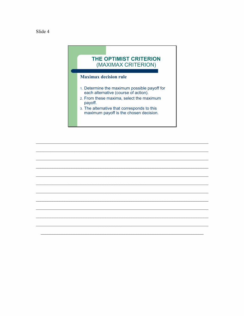
Slide 4
THE OPTIMIST CRITERION(MAXIMAX CRITERION)
Maximax decision rule
1. Determine the maximum possible payoff for each alternative (course of action).
2. From these maxima, select the maximum payoff.
3. The alternative that corresponds to this maximum payoff is the chosen decision.
________________________________________________________________________
________________________________________________________________________
________________________________________________________________________
________________________________________________________________________
________________________________________________________________________
________________________________________________________________________
________________________________________________________________________
________________________________________________________________________
________________________________________________________________________
________________________________________________________________________
________________________________________________________________________
____________________________________________________________________

Slide 5
THE PESSIMIST CRITERION(MAXIMIN CRITERION)
Maximin decision rule
1. For each action alternative determine the minimum payoff possible.
2. From these minima, select the maximum payoff.
3. The action alternative leading to this payoff is the chosen decision.
________________________________________________________________________
________________________________________________________________________
________________________________________________________________________
________________________________________________________________________
________________________________________________________________________
________________________________________________________________________
________________________________________________________________________
________________________________________________________________________
________________________________________________________________________
________________________________________________________________________
________________________________________________________________________
____________________________________________________________________

Slide 6
THE HURWICZ CRITERION
Hurwicz decision rule
1. Select a coefficient of optimism value α .2. For every action alternative compute its
Hurwicz weighted average.3. Choose the action alternative with the best
Hurwicz weighted average as the chosen decision
________________________________________________________________________
________________________________________________________________________
________________________________________________________________________
________________________________________________________________________
________________________________________________________________________
________________________________________________________________________
________________________________________________________________________
________________________________________________________________________
________________________________________________________________________
________________________________________________________________________
________________________________________________________________________
____________________________________________________________________

Unit 4 DECISION ANALYSIS Lesson 35 Learning Objective:
• Illustrate the models of decision making under conditions of uncertainity.
Hello students, In previous lesson you learned three criterions for decision under uncertainity. Now, In this lesson you will study about the other three criterion used for taking decision under uncertainity. The fourth criterion is: SAVAGE MINIMAX REGRET CRITERION The Minimax Regret criterion focuses on avoiding regrets that may result from making a non-optimal decision. Although regret is a subjective emotional state, the assumption is made that it is quantifiable in direct (linear) relation to the rewards of the payoff matrix. Regret is defined as the opportunity loss to the decision maker if action alternative Ai is chosen and state of nature Sj happens to occur. Opportunity loss is the payoff difference between the best possible outcome under Sj and the actual outcome resulting from choosing Ai. Formally: OLij = (row j maximum payoff) - Rij for positive-flow payoffs (profits, income) OLij = Rij - (row j minimum payoff) for negative-flow payoffs (costs, losses) where Rij is the reward value (payoff) for column i and row j of the payoff matrix R.

Note that opportunity losses are defined as nonnegative numbers. The best possible OL is zero (no regret) and the higher the OL value, the greater the regret. Savage's Minimax Regret decision rule
1. Convert the payoff matrix R = {Rij } into an opportunity loss matrix OL = {OLij }.
2. Apply the minimax rule to the OL matrix. Let's assume that ACME's managers have decided to analyze the problem using opportunity losses instead of the monetary payoffs. First they must derive the OL table from the payoff matrix R.
ALTERNATIVES STATES OF
NATURE Large plant
Just Right plant
Small plant
No plant Best
High demand
15 9 3 0 15
Medium demand
3 4 2 0 4
Low demand
-6 -2 1 0 1
Note, Row max = best possible outcome for that particular Sj The OL table can now be obtained by subtracting each entry Rij from its column's best payoff. The minimax rule is then applied to the OL (regret) table:

ALTERNATIVES STATES OF
NATURE Large plant
Just Right plant
Small plant
No plant
High demand
0 6 12 15
Medium demand
1 0 2 4
Low demand
7 3 0 1
Minimax Regret
7 6 Minimax
12 15
Decision is “Just Right” Let us find out what is the Economic Interpretation of Opportunity Losses OL values consist of two components: actual monetary losses (if any) and unrealized potential profits. Consider the OL for JR x H, which is 6. ACME would stand to make $9 million (R matrix) if they choose plant JR and market state H occurs. So there would be no monetary loss. Still, by choosing JR ACME's managers would forgo the opportunity to gain an additional $6 million — assuming state H actually occurs. If state H does indeed happen, ACME's managers would not feel entirely satisfied: there would be an element of regret present for not having made the "correct" decision, which was plant L. This regret is assumed to be equal to the lost opportunity: $6 million. Consider now the OL value for JR x W, which is 3. The actual payoff would be a $2 million loss. But in addition there would be a regret factor for not capitalizing on the $1 million profit ACME could have had IF they had chosen plant S. Finally, notice that the OL for S x W is zero because that was the right decision for that particular state of nature: there is no actual monetary loss and no potential profits were forgone. Thus, no regrets. Note that for every column in OL there must be at least one entry OLij = 0 (that is, at least one "best" outcome for each state of nature). This is not necessarily true for every row. It should be clear that standard accounting information is incomplete in the sense that OL values are neither recorded nor obtainable ex post facto. Accounting rules state that a journal entry is performed only if a transaction

actually occurs. Consequently, the potential benefits of alternate decision strategies cannot be determined from financial accounting statements. Now Let’s see what are the drawbacks of this criterion: Critique of Minimax Regret Criterion Minimax Regret is a better decision criterion than Maximax or Maximin and, arguably, Hurwicz as well. Although it employs the far-from-robust minimax logic, the values over which it operates (opportunity losses) contain more problem information (actual monetary losses plus unrealized potential profits), leading to a more informed decision than was possible with any of the three previous models. Nevertheless, it still fails to employ all of the available problem information and is therefore not a rationally acceptable criterion. Minimax Regret is a conservative criterion, as is Maximin/Minimax. However, it is not as extreme in its pessimism as the latter. Note that in ACME's decision problem, Minimax Regret recommended a different (middle-of-the-road) decision alternative than Maximin. There is no guarantee this will always be so, but it does show that minimaxing regrets is not as conservative an approach as maximining positive-flow payoffs. Another important criterion is: LAPLACE INSUFFICIENT REASON CRITERION The Laplace criterion is the first to make use of explicit probability assessments regarding the likelihood of occurrence of the states of nature. As a result, it is the first elementary model to use all of the available information in the payoff matrix. The Laplace argument makes use of Johann Bernoulli's Principle of Insufficient Reason. To begin with, Laplace posits that to deal with uncertainty rationally, probability theory must be invoked.
This means that for each state of nature Sj in S, you (the decision maker) should assess the probability pj that Sj will occur.

Now the Principle of Insufficient Reason states that if no probabilities have been assigned by you (assumed to be rational and capable of handling basic probability theory), then it follows there was insufficient reason for you to indicate that any one state Sj was more or less likely to occur than any other state. (I feel a rational decision maker, would assign a probability distribution to S as a matter of course.) Consequently, all the states Sj must be equally likely. Therefore, the probability pj for every Sj must be 1/n, where n is the number of states of nature in S. Pretty neat logic! We'll check it out in the critique. Laplace decision rule 1. Assign pj = p(Sj) = 1/n to each Sj in S, for j = 1, 2, ..., n. 2. For each Ai (payoff matrix row), compute its expected value:
E (Ai) = Σ j pj (Rij). 3. Select the action alternative with the best E (Ai) as the chosen decision. "Best" means max for positive-flow payoffs (profits, revenues) and min for negative-flow payoffs (costs, losses). Let's assume that ACME's managers believe all three market states (H, M, W) to be equally probable. Then and only then is the use of the Laplace criterion warranted. Here according to Laplace decision each state of nature occurs with a probability 1/3.
ALTERNATIVES STATES
OF NATURE
Large plant Just Right
plant Small plant
No plant
High demand
15 9 3 0
Medium demand
3 4 2 0
Low demand
-6 -2 1 0
E (Ai)
(15+3-6)/3 = 4
(9+4-2)/3 = 3.67
(3+2+1)/3 = 2
(0+0+0)/3 = 0

The decision comes out to choose “to build a large plant”. Now Let’s see what are the drawbacks of this criterion: Critique of Laplace Insufficient Reason Criterion By assigning a (uniform) probability distribution to S, Laplace is able to take into account all of the available information in R and is therefore a rationally acceptable decision criterion assuming the states of nature Sj are indeed uniformly distributed (that is to say, are equally probable). There is nothing intrinsically wrong with the Laplace criterion but there is a danger of improperly using it when the states of nature are not in fact equally probable. We shall see this again in our discussion of assessing probabilities subjectively. The weakness in the argument posed by the Principle of Insufficient Reason is the implicit assumption that all decision makers who have not assigned a probability distribution to S have not done so because there is no reason to believe the states are not equally probable. Real people can and commonly do depart from the idealized paradigm of the rational decision maker, and may well not assess probabilities quantitatively because they are not accustomed to do so. Now we move on to last but not the least criterion of decision making under uncertainity. MAXIMUM LIKELIHOOD (MODAL) CRITERION This criterion considers only the event (state of nature) most likely to occur as the basis for the decision, excluding all other events from consideration. Maximum likelihood is a widely used statistical decision rule employed in many scientific and technical applications, usually in conjunction with other quantitative methods. It is also often used informally in personal decision making by non-specialists, usually by itself. This latter usage, commonly called the modal criterion, can lead to improper reasoning, flawed problem analysis and poor decisions. The term "modal" refers to the mode of a statistical distribution. Let's assume that ACME's managers, perhaps because of habit, were inclined to use the modal decision criterion. They would then act in the following manner:

Maximum likelihood (modal) decision rule 1. Select the state Sj most likely to occur. This can be done qualitatively by judgment or intuition. 2. Exclude from further consideration the remaining states of nature in S. 3. Determine the best payoff (max for positive flows, min for negative flows) in the chosen column (Sj). The action alternative Ai corresponding to this payoff is the chosen decision. Use ACME's decision matrix defined previously and assume state Medium demand as the most likely:
ALTERNATIVES STATES OF
NATURE Large plant
Just Right plant
Small plant
No plant
High demand
15 9 3 0
Medium demand
3 4 2 0
Low demand
-6 -2 1 0
This would yield
ALTERNATIVES STATES OF
NATURE Large plant
Just Right plant
Small plant
No plant
Medium demand
3 4 2 0
Decision is : Just Right plant Now Let’s see what are the drawbacks of this criterion:

Critique of Maximum Likelihood (Modal) Criterion We have been criticizing all decision rules that leave out available problem information as irrational, and here comes the modal criterion that does precisely that. In real life, however, things are usually a bit more complicated and irrationality may not be as obvious. The payoffs in the decision matrix are not, for the most part, given a priori: they represent data that must be collected. This means time and effort (and hence, a cost) must be expended in collecting the data. Some decision makers may see no point in collecting payoff data for states of nature deemed unlikely to occur from the modal perspective. So the decision matrix they develop may actually be just the column vector for the modal state. The danger of this approach should be clear: decisions are being made from a position of ignorance. Decide for yourself Consider the following table:
ALTERNATIVES Probability pj
STATES OF NATURE A1 A2
0.4 S1 1 0
0.2 S2 0 100
0.2 S3 0 100
0.2 S4 0 100 The modal decision for the matrix below is A1. Would you forgo a 60% chance of getting $100 just because the mode points to a $1 gain? So, now let us summarize today’s discussion: Summary We have discussed in details about Decision making under uncertainity.
• The Savage Minimax Regret Criterion. • The Laplace Insufficient Reason Criterion • The Maximum Likelihood (Modal) Criterion.

Slide 1
DECISION THEORY
LECTURE 4
________________________________________________________________________
________________________________________________________________________
________________________________________________________________________
________________________________________________________________________
________________________________________________________________________
________________________________________________________________________
________________________________________________________________________
________________________________________________________________________
________________________________________________________________________
________________________________________________________________________
________________________________________________________________________
____________________________________________________________________

Slide 2
THE SAVAGE MINIMAX REGRET CRITERION
Savage's Minimax Regret decision rule
1. Convert the payoff matrix R = {Rij } into an opportunity loss matrix OL = {OLij }.
2. Apply the minimax rule to the OL matrix.
________________________________________________________________________
________________________________________________________________________
________________________________________________________________________
________________________________________________________________________
________________________________________________________________________
________________________________________________________________________
________________________________________________________________________
________________________________________________________________________
________________________________________________________________________
________________________________________________________________________
________________________________________________________________________
____________________________________________________________________

Slide 3
THE LAPLACE INSUFFICIENT REASON CRITERION
Laplace decision rule
1. Assign pj = p(Sj) = 1/n to each Sj in S, for j= 1, 2, ..., n.
2. For each Ai (payoff matrix row), compute its expected value: E (Ai) = Σj pj (Rij).
3. Select the action alternative with the best E (Ai) as the chosen decision.
________________________________________________________________________
________________________________________________________________________
________________________________________________________________________
________________________________________________________________________
________________________________________________________________________
________________________________________________________________________
________________________________________________________________________
________________________________________________________________________
________________________________________________________________________
________________________________________________________________________
________________________________________________________________________
____________________________________________________________________

Slide 4
THE MAXIMUM LIKELIHOOD (MODAL) CRITERION
Maximum likelihood (modal) decision rule
1. Select the stateSj most likely to occur. This can be done qualitatively by judgment or intuition.
2. Exclude from further consideration the remaining states of nature in S.
3. Determine the best payoff (max for positive flows, min for negative flows) in the chosen column (Sj).
4. The action alternative Ai corresponding to this payoff is the chosen decision.
________________________________________________________________________
________________________________________________________________________
________________________________________________________________________
________________________________________________________________________
________________________________________________________________________
________________________________________________________________________
________________________________________________________________________
________________________________________________________________________
________________________________________________________________________
________________________________________________________________________
________________________________________________________________________
____________________________________________________________________
Unit 4 DECISION ANALYSIS Lesson 36 Learning Objective:
• Review risk as a decision environment, and review methods useful for making decisions in this environment.
• Demonstrate how monetary value and probability information can be
combined for more effective decision making.
• Illustrate expected value as a decision criterion under conditions of
risk.
Decision Making Under Risk In this situation, the decision maker faces several states of nature. But he is supposed to have believable evidential information, knowledge, experience or judgment to enable him to assign probability values to the likelihood of occurrence of each state of nature. Probabilities could be assigned to future events by reference to similar previous experience and information. Sometimes past experience, or past records often enable the decision-maker to assign probability values to the likely possible occurrence of each state of nature. Knowing the probability distribution of the states of nature, the best decision is to select that course of action that has the largest expected payoff value. For decision problems involving risk situations one most popular method of decision criterion for evaluating the alternative strategies is the Expected Monetary Value (EMV) or expected pay-off. The objective should be to optimize the expected pay-off, which may mean either maximization of expected profit or minimization of expected regret. Before this, let us have a look at certain conceptual approaches to Probability:

The Concept of Probability Probability theory is the rational way to think about uncertainty. It is the branch of mathematics devoted to measuring quantitatively the likelihood that a given event will occur. These two definitions derive from two different approaches to the concept of probability: subjective versus objective.
The objective probability viewpoint posits that the likelihood that a particular event will occur is a property of the system under study, which is ultimately grounded on the physical laws bearing on the given system. The subjective impressions that an observer may have about the likelihood of occurrence of that event in no way affect the actual probability of occurrence. Put succinctly, probability resides in the object, not the subject. It is wholly independent of the observer's state of mind. The subjective probability viewpoint argues that the likelihood that a particular event will occur is a measure of the belief of the observer of the system given his/her state of information at the time. It is meaningless to talk about "the actual probability of occurrence" of an event because such a conception is unknowable and impossible to define outside the observer's mental space. Put succinctly, probability resides in the subject, not the object. It is intrinsically bound to the observer's state of mind. All this may sound a tad philosophical —which it is— yet is relevant for the development and understanding of expected value decision models. To see why, let's examine in more detail what "objectivity" entails. Objective probability can be approached axiomatically or statistically. Axiomatic probability refers to the use of the mathematical theory of probability (axioms and theorems) along with the logical framework of the system being studied to derive quantitative measures of the likelihood of occurrence of particular events solely on the basis of theoretical and logical considerations. In all such cases, clearly defining the sample space of interest

is essential. An example of an axiomatic probability assessment is the statement «the probability of heads on a coin toss is 1/2» when based on the assumptions that the coin is fair, the toss is unbiased, and the sample space consists of two symmetrical event subspaces (either heads or tails must come up; coins stuck upright in a groove, for instance, are disqualified). No actual toss of the coin is required. Axiomatic probability relies instead on gedanken (thought) experiments. Statistical probability, on the other hand, makes use of physical experiments (in addition to both the mathematical theory of probability and the experiment's logical framework) to assess the likelihood of occurrence of events by means of relative frequency of event outcomes. Thus, statistical probability is empirical in nature. An example of a statistical probability assessment is the statement «the probability of heads on a coin toss is 1/2» when based on the results of numerous trials of actual coin tosses conducted under identical conditions. Actual trials, however, need not and often do not square up to an even 50-50. Recourse to probability theory is required to reconcile experimental discrepancies with axiomatic inferences. It should be noted that the two objective approaches to probability follow to the letter two of the three epistemologically valid approaches to ascertaining knowledge: rigorous mathematical/logical reasoning and controlled empirical procedures. (We will explore the third epistemologically valid approach later on.) So why should one bother with subjective probability? Because, unfortunately, real-world problems are not always amenable to the demanding conditions imposed by objective probability. Consider Wolfgang Cactus and Goldie Lockes, ACME's executive managers. In order to determine objectively the probability distribution for the states of nature in their decision problem, they would need to either know everything affecting the market for road runner traps (including such things as the state of the world economy at every point in time throughout the five-year period covered by the decision!) in order to properly define the sample space for the gedanken experiment, or conduct numerous trials with the new, improved road runner traps under all possible market conditions to assess the probabilities statistically. The former approach is impossible because the required information is simply not obtainable (nor digestible), while the latter is impossible because once the first trial is conducted with the new traps, the market reacts (competitors may enter the market, for instance) and conditions will forever be different. Yes, market trials may not be perfect but can be of value. We'll look into this shortly. The point is that subsequent experimental conditions are no longer identical to the initial trial, violating the tenets of statistical probability.

In the absence of reliable objective probabilities, subjective estimates are the best game in town, say some folks. Even when they are available, retort others. Prof. Ronald Howard of Stanford likes to elucidate this with a fine little story. This astronaut was being strapped to his seat in the cockpit when he asks the crew chief if the rocket is safe. "It's 99.9% safe," replies the chief. "Determined axiomatically by NASA's engineers." The astronaut glances outside, sees an identical rocket on the neighboring launch pad, and requests that it be launched as a test. After much arguing from Mission Control (rockets don't come cheap), they acquiesce and launch the other rocket. Suddenly, moments into the liftoff, the thing explodes in a fireball. Strictly speaking, since the probability of a safe launch was determined axiomatically, the two rocket launches are independent events and the astronaut's rocket is still 99.9% safe. "Yeah, right," said the astronaut as he walked away from his rocket. When you're in the cockpit, the only probability that matters is your own. Assessing Probabilities Subjectively We recall that the Laplace decision criterion began with the premise that to deal with uncertainty rationally, probability theory must be employed. This means that a probability distribution must be assigned to every set of uncertain states of nature in the decision problem. As we saw on the previous page, probabilities can be determined either objectively or subjectively. If reliable objective probabilities are available, they should ordinarily be used. If, on the contrary, no reliable objective probabilities are available, Laplace prescribes that subjective probabilities are assessed. (It is only because no probabilities had been posted on the decision matrix that Laplace concluded, by the Principle of Insufficient Reason, that the states of nature had to be equally probable.) One way of putting it: it is better to have subjective probabilities, even if somewhat inaccurate, than to have no probabilities at all. For without probabilities, all decision criteria are less than satisfactory, as we have seen. Moreover, it is possible to revise subjective probabilities with access to additional information, thus improving the accuracy of the subjective estimates. That precisely is why market studies are performed. Decision makers do not work in a vacuum. They usually know something, oftentimes quite a lot, about the decision problem they are dealing with — including its environment and, hence, the states of nature affecting the decision. They routinely make use of this knowledge when managing their affairs. Consequently, quantifying their knowledge (and intuition) about the likelihood of occurrence of uncertain events is not at all unreasonable. In fact, it is the logical thing to do.

A Method for Eliciting Subjective Probabilities: 1. Rank orders the states of nature Sj in terms of their likelihood of occurrence. (Ties are allowed and should be denoted by placing tied states [Sk, Sl, etc.] at the same level in the list.) 2. Assign an arbitrary weight of 1 (actually, any number will do) to the most likely event Sj. 3. Assess the degree of relative likelihood of the next state Sk by assigning a fractional weight in proportion to the most likely state Sj. (Ties require a duplicate weight.) 4. Assess the degree of relative likelihood of the remaining states Sl by assigning fractional weights in proportion to any other previously weighted state Sx. 5. Sum the weights. 6. Normalize the weights (divide each weight by the sum of the weights). 7. The resulting numbers are the probabilities of occurrence for each of the states. (They must add up to 1.) Rationality is bounded, and people rarely possess the ability to recite a nontrivial probability distribution off the cuff. But it has been shown that pair wise comparisons between uncertain events lead to reasonably accurate probability estimates when the assessor is more or less informed about the problem at hand. Let's assume that ACME's managers believe that the most likely market demand for newfangled road runner traps is M (medium demand), followed by W (low) and lastly, H (high). The event list would be ordered accordingly. Assign a weight of 1 to event M. Event Weight M 1 W H Now suppose Cactus and Lockes believe W to be half as likely as M, and H to be one-third as likely as W. Event Weight M 1 = 6/6 W 1/2 (1) = 3/6 H 1/3 (1/2) = 1/6 10/6
Normalizing the weights: Event Normalization Probability M 6/6 (6/10) = 0.6 W 3/6 (6/10) = 0.3 H 1/6 (6/10) = 0.1 1.0 Expected Value Models EMV & EOL Once a probability distribution has been assessed for each set of uncertain states of nature—and this can always be done, subjectively— it is straightforward to apply the next step called for by Laplace, namely, compute the expected value for each action alternative. Since there are two ways to look at the same problem (actual monetary values and opportunity losses), we can compute the expected values on either one of the payoff tables. Expected Monetary Value
It is possible to obtain probability estimates for each state of nature in decision-making situations. We use the expected monetary value criterion (used in Statistics) to identify the best decision alternative. The expected monetary value EMV is calculated by multiplying each decision outcome (payoff value) for each state of nature by the probability of its occurrence. Then the best decision is the one with the largest expected monetary value.
Using the original payoff matrix, the formula for expected monetary value (EMV) is:
E (Ai) = Σ j pj (Rij)
Thus, using the probability distribution derived previously: Best decision is : Just Right plant
ALTERNATIVES PROBABILITIES
STATES OF NATURE
Large plant
Just Right plant
Small plant
No plant
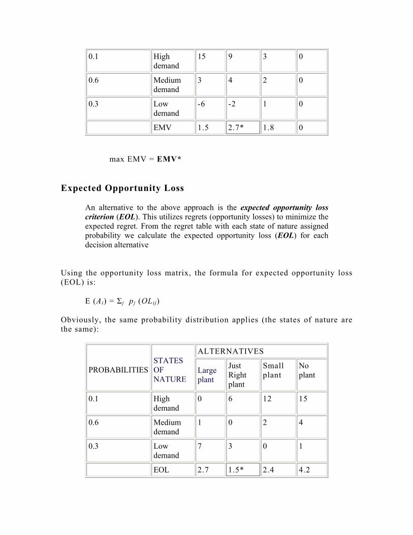
0.1 High demand
15 9 3 0
0.6 Medium demand
3 4 2 0
0.3 Low demand
-6 -2 1 0
EMV 1.5 2.7* 1.8 0
max EMV = EMV* Expected Opportunity Loss
An alternative to the above approach is the expected opportunity loss criterion (EOL). This utilizes regrets (opportunity losses) to minimize the expected regret. From the regret table with each state of nature assigned probability we calculate the expected opportunity loss (EOL) for each decision alternative
Using the opportunity loss matrix, the formula for expected opportunity loss (EOL) is:
E (Ai) = Σ j pj (OLij)
Obviously, the same probability distribution applies (the states of nature are the same):
ALTERNATIVES PROBABILITIES
STATES OF NATURE
Large plant
Just Right plant
Small plant
No plant
0.1 High demand
0 6 12 15
0.6 Medium demand
1 0 2 4
0.3 Low demand
7 3 0 1
EOL 2.7 1.5* 2.4 4.2

min EOL = EOL*
The best decision results from minimizing the regret. In this case, the decision is a "Just Right Plant." The expected value and expected opportunity loss criteria result in the same decision. You may wonder why you need two separate approaches to reach the same conclusion. This will be discussed in the next section.
The Relationship Between EMV and EOL Note that both decision criteria (EMV and EOL) pointed to the same action alternative JR. Will this always be the case? Yes it will. To see why consider an uncannily accurate forecaster making this same exact decision a large number of times. This is hypothetical, of course. In reality, the decision situation is unique and will never be the same once the first decision is made, so repeatability is out of the question. But let's assume repeatability for the sake of discussion. Since the event market demand S is a random variable but our master forecaster never fails, she will predict H 10% of the time, M 60% of the time, and W 30% of the time she makes the forecast. (Remember, the forecaster can predict but cannot control the outcome event. Consequently, her forecast record will mirror the probability distribution.) Now, with perfect forecasting she will never experience opportunity losses. The OL matrix shows this when an OLij value is equal to zero. The corresponding Rij payoffs for those matrix cells are 15, 4, and 1, respectively: the highest possible payoffs under the different market-demand conditions. Taking the expected value of these best-possible payoffs:
E (A* ) = 0.1 (15) + 0.6 (4) + 0.3 (1) = 4.2
where A* is the optimal action alternative for each state of nature. This means that the highest expected value possible for this problem (under conditions of infallible forecasts) is 4.2. Note that this idealized expected payoff (or expected payoff given perfect forecasts) arises if and only if the expected opportunity loss is zero. Now, any expected opportunity loss that is incurred must come out of forgone expected payoffs, by definition. Since the maximum (idealized) expected payoff is fixed at 4.2 for this problem, and since the expected monetary value is what remains after an expected opportunity loss is deducted from the maximum expected payoff, the following equation holds:
EMV + EOL = 4.2 for this particular problem.
This is true for every action alternative. In general,
EMV + EOL = Expected Payoff given Perfect Forecasts for all Ai in A.
Clearly, Max EMV can only be obtained with Min EOL. Thus, both criteria must point to the same Ai. Critique of Expected Value Models The fact that both EMV and EOL select the same action alternative Ai is a welcome departure from our experience with the elementary models that did not use probability. The lack of consistency in recommending an action alternative exhibited by those models greatly reduces our confidence in them as reliable decision tools. EMV and EOL are certainly more robust in this sense. They also employ all of the available information about the problem, complying with a basic requirement of rationality. Another attractive aspect is that by making use of subjective probability, these models are able to incorporate the decision maker's personal impressions about future events. In other words, the models do not impose a "rigid theoretical solution" on the decision maker. Rather, the decision maker can adapt the model to conform to his/her judgment, intuition, experience and expectations. In principle, expected value models work just fine. In practice, there is still one more point to examine: the subjectivity of utility. This will be done shortly. EVPI Expected Value of Perfect Information In our last episode we left our intrepid and ever fearless managers in possession of a probability distribution they had derived subjectively. Now, even as Wolfgang Cactus expressed satisfaction with said distribution and accepted the results of the expected value models (EMV and EOL) as valid, Goldie Lockes had lingering doubts. "What if," she rhetorically asked, "the so-called said distribution, based on our limited knowledge about the problem situation (as must be the case because of bounded rationality), fails to reflect accurately the perilous nuances of risk that could be abridged with recourse to additional market information?" To which Cactus just stared dumbfounded. Subjectively derived probability distributions are useful, yes, but there is no guarantee they are the best possible distributions if the subject (person) is not 100% informed about the problem situation. Most people on this planet are not 100% informed about anything. Consequently, it is generally possible to

obtain additional information about the problem that could be used to improve the accuracy of the subjective estimates. Obtaining additional problem information does not mean one should relinquish one's original assessment of the situation. After all, any other source of information is also subject to bounded rationality. Additional information should rationally be used to revise our prior estimates, not to supplant them (assuming, of course, the original estimates were not a haphazard guess). Acquiring additional information involves work. Work implies expenses. When we buy something, are we willing to pay any price whatsoever for the purchase? If one is not a teenager buying recorded music, no. Everything has a price. The price reflects what the buyer is willing to pay in order to increase her/his satisfaction or well-being above and beyond the cost (setback) of obtaining the purchase. That is to say, one would be willing to acquire additional information if, and only if, the additional information translates into higher expected earnings. Otherwise, no dice. Price is a function of quality. The higher the quality of a good, the more we'd be willing to pay for it. As regards information, higher quality means better accuracy. If the information is totally worthless, the price we'd be willing to pay is zero (no added benefit would accrue). If it's somewhat reliable, we'd be willing to pay something, though not much. If it's really good, we'd be willing to pay more. If it is perfect (infallible) information, how much would we be willing to pay? To be sure, there is a limit to the amount we'd be willing to pay: we would pay to the extent that the perfect information improves our expected earnings (assuming a rational decision maker). If obtaining the additional information reduces our net expected earnings, we'd rather do without the information. So there is a maximum price we'd be willing to pay for perfect—absolutely infallible—information. Time to bring back our good friend, the uncannily accurate forecaster. She is so good she is actually referred to as a prophet, although an economic one at that. If we had access to such a prophetess, we would ask her what state of nature (market demand) was "destined" to occur and she would tell us. (Prophets are always nice guys and have to tell. Otherwise they wouldn't be called prophets.) The prophetess, keep in mind, only tells what is bound to occur; she does not alter "destiny." If the prophet augurs that market demand for newfangled road runner traps is going to be high (H), ACME's managers, conscious of her unerring predictions, would choose to build a large (L) manufacturing plant (see payoff table):

ALTERNATIVES PROBABILITIES
STATES OF NATURE
Large plant
Just Right plant
Small plant
No plant
0.1 High demand
15 9 3 0
0.6 Medium demand
3 4 2 0
0.3 Low demand
-6 -2 1 0
This can be done for every possible prophecy: H, M, W. Consequently, ACME's managers would know which decision is optimal given perfect information. This is shown in the decision tree below:
But ACME's managers do not know what the prophetess is going to foretell. (If they knew, they would not need to ask her.) So the prophecy itself is an uncertain state of affairs, as represented by the circle node in the decision tree above. However, by applying the probability distribution they already have (which represents the best information currently at their disposal), ACME's managers can compute the expected value of that decision tree, that is, the Expected Value given Perfect Information (EV|PI):
EV|PI = Σ j pj (Rij*)
where Rij* is the best payoff under state Sj. Thus EV|PI = 4.2. Which we already knew (perfect information is the same as perfect forecasts, but the former term is the standard nomenclature; thus, EP|PF = EV|PI). Does this mean that the prophetess's information is worth $4.2 million to ACME's managers? No way! Cactus and Locke were able to "secure" an expected
monetary payoff of $2.7 million on their own without the assistance of the prophetess (see EMV* on previous page). Hence, the prophetess should not be credited with the first $2.7 million of expected payoffs. Only the expected amount above and beyond the initial (or a priori) expected payoff of $2.7 million is due to her information. Therefore, the Expected Value of Perfect Information (EVPI) is:
EVPI = EV|PI - EMV*
which in ACME's case works out to $1.5 million. Perfect information would increase ACME's expected payoff by $1.5 million, so that is what the perfect information is worth (to ACME's managers). Note that 1.5 is the minimum expected opportunity loss (EOL*). Consequently, since EMV + EOL = EV|PI and EMV* → EOL*:
EVPI = EOL*
Or look at it this way: The EOL|PI is zero. EOL* is the minimum EOL without additional information. Thus, it is the additional perfect information that makes it possible to reduce the prior EOL* to zero. Hence, the value of this information is equal to its economic contribution: EOL* - EOL|PI = EVPI. Of course, prophets don't exist in economics, as we all know rather well, economics being the dismal science. But EVPI provides a criterion by which to judge ordinary mortal forecasters. If the cost of acquiring additional real-world information about ACME's market demand is greater than $1.5 million, ACME should decline. It's not worth that much to ACME, irrespective of its degree of perfection. If real-world information were to cost less than $1.5 million, should ACME's managers buy it? That depends on the quality of the information, remember. EVPI can be used to reject costly proposals but not to accept any forecasting offers because one needs to know the quality of the information one is acquiring. It may well be cheap, but it could be worthless. It is necessary to evaluate the quality of real-world (or imperfect) information. Terms EVPI (Expected Value of Perfect Information) – the theoretical maximum worth to the decision maker of additional information about uncertain states of nature that is absolutely unerring. EV|PI (Expected Value given Perfect Information) – the expected monetary value that would result if the decision maker had access to perfect information.
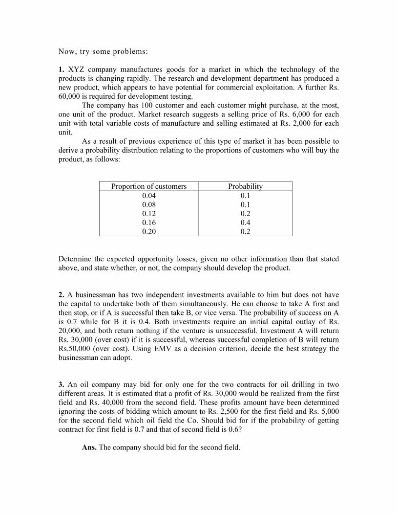
Now, try some problems: 1. XYZ company manufactures goods for a market in which the technology of the products is changing rapidly. The research and development department has produced a new product, which appears to have potential for commercial exploitation. A further Rs. 60,000 is required for development testing. The company has 100 customer and each customer might purchase, at the most, one unit of the product. Market research suggests a selling price of Rs. 6,000 for each unit with total variable costs of manufacture and selling estimated at Rs. 2,000 for each unit. As a result of previous experience of this type of market it has been possible to derive a probability distribution relating to the proportions of customers who will buy the product, as follows:
Proportion of customers Probability 0.04 0.08 0.12 0.16 0.20
0.1 0.1 0.2 0.4 0.2
Determine the expected opportunity losses, given no other information than that stated above, and state whether, or not, the company should develop the product. 2. A businessman has two independent investments available to him but does not have the capital to undertake both of them simultaneously. He can choose to take A first and then stop, or if A is successful then take B, or vice versa. The probability of success on A is 0.7 while for B it is 0.4. Both investments require an initial capital outlay of Rs. 20,000, and both return nothing if the venture is unsuccessful. Investment A will return Rs. 30,000 (over cost) if it is successful, whereas successful completion of B will return Rs.50,000 (over cost). Using EMV as a decision criterion, decide the best strategy the businessman can adopt. 3. An oil company may bid for only one for the two contracts for oil drilling in two different areas. It is estimated that a profit of Rs. 30,000 would be realized from the first field and Rs. 40,000 from the second field. These profits amount have been determined ignoring the costs of bidding which amount to Rs. 2,500 for the first field and Rs. 5,000 for the second field which oil field the Co. Should bid for if the probability of getting contract for first field is 0.7 and that of second field is 0.6? Ans. The company should bid for the second field.

4. Calculate the loss table from the following payoff table: Event
Action E1 E2 E3 E4 A1 A2 A3 A4
50 400 -50 0
300 0 200 300
-150 100 0 300
50 0 100 0
Suppose that the probabilities of the events in this table are: P (E1) = 0.15; P (E2) = 0.45; P (E3) = 0.25; P(E4) = 0.15 Calculate the expected payoff and the expected loss of each action. 5. A company is trying to decide what size plant to build in a certain area. Three alternatives are being considered; plants with capacity of 20,000; 30,000 and 40,000 units respectively. Demand for the product is uncertain, but management has assigned the probabilities listed below to five levels of demand. The table below also shows the profit for each alternative and each possible level of demand (output may exceed rated capacity).
Payoff table showing profits (Cores of Rupees for various sizes of plants and levels of demand):
Profit (Rs. Crores) for different Courses of Action-Build plant with capacity Demand
Units Probability 20,000 units 30,000 units 40,000 units
10,000 20,000 30,000 40,000 50,000
0.2 0.3 0.2 0.2 0.1
-4.0 1.0 1.5 2.0 2.0
-6.0 0.0 6.0 7.5 8.0
-8.0 -2.0 5.0 11.0 12.0
What size plant should be built?
6. A toy company is bringing out a new type of toy. The company is attempting to decide whether to bring out a full, partial, or minimal product line. The company has three level of product acceptance and has estimated their probability of occurrence. Management will make its decision on the basis of maximizing the expected profit from the year of production. The relevant data are show in the following table:

First-year Profit (Rs. ‘000) Product Line
Product Acceptance
Probability Full Partial Minimum
Good Fair Poor
0.2 0.4 0.4
80 50 -25
70 45 -10
50 40 0
(a) What is the optimum product line and its expected profit?
(b) Develop an opportunity loss table and calculate the EOL values. What is optimum value of EOL and the optimum course of action? [Ans. (a) Partial; Rs. 28,000 (b) Rs. 8,000] 7. The Zeta Manufacturing Company Ltd. is proposing to introduce to the market a radio controlled toy car. It has three different possible models X, Y and Z that vary in complexity but it has sufficient capacity to manufacture only one model. An analysis of the probable acceptance of the three models has been carried out and the resulting profit estimated: Model Acceptance Probability Annual Profits
X (Rs. ‘000’s)
Y Model Type
Z Excellent Moderate
Poor
0.3 0.5 0.2
120 80 -30
100 60 -20
60 50 0
(i) Determine the model type that maximizes the expected profit. What is the
expected profit? (ii) Obtain an opportunity loss table and show that the difference between
expected opportunity losses is the same as the difference between expected profits.
(iii) How much would it be worth to know the model acceptance level before
making the decision on which model type to produce?

CASE STUDY Ski Right After retiring as a physician, Bob Guthrie became an avid downhill skier on the steep slopes of the Utah Rocky Mountains. As an amateur inventor, Bob was always looking for something new. With the recent deaths of several celebrity skiers, Bob knew he could use his creative mind to make skiing safer and his bank account larger. He knew that many deaths on the slopes were caused by head injuries. Although ski helmets have been on the market for some time, most skiers considered them boring and basically ugly. As a physician, Bob knew that some type of new ski helmet was the answer.
Bob’s biggest challenge was to invent a helmet that was attractive, safe, and fun to wear. Multiple colors, using the latest fashion designs would be a must. After years of skiing, Bob knew that many skiers believed that how you looked on the slopes was more important than how you skied. His helmets would have to look good and fit in with current fashion trends. But attractive helmets were not enough. Bob had to make the helmets fun and useful. The name of the new ski helmet, Ski Right, was sure to be a winner. If Bob could come up with a good idea, he believed that there was a 20% chance that the market for the Ski Right Helmet would be excellent. The chance of a good market should be 40%. Bob also knew that the market for his helmet could be only average (30% chance) or even poor (10% chance).
The idea of how to make ski helmets fun and useful came to Bob on a gondola ride to the top of a mountain. A busy executive on the gondola ride was on his cell phone trying to complete a complicated merger. When the executive got off of the gondola, he dropped the phone and it was crushed by the gondola mechanism. Bob decided that his new ski helmet would have a built-in cell phone and an AM/FM Stereo radio. All of the electronics could be operated by a control pad worn on a skier’s arm or leg.
Bob decided to try a small pilot project for Ski Right. He enjoyed being retired
and didn’t want a failure to cause him to go back to work. After some research, Bob found Progressive Products (PP). The company was willing to be a partner in developing the Ski Right and sharing any profits. If the market were excellent, Bob would net $5,000. With a good market, Bob would net $2,000. An average market would result in a loss of $2,000, and a poor market would mean Bob would be out $5,000.
Another option for Bob was to have Leadville Barts (LB) make the helmet. The
company had extensive experience in making bicycle helmets. Progressive would then take the helmets made by Leadville Barts and do the rest. Bob had a greater risk. He estimated that he could lose $10,000 in a poor market or $4,000 in an average market. A good market for Ski Right would result in a $6,000 profit for Bob, while an excellent market would mean a $12,000 profit.
A third option for Bob was to use TalRad TR, a radio company in Tallahassee,
Florida. TalRad had extensive experience in making military radios. Leadville Barts

could make the helmets, and Progressive Products could do the rest. Again, Bob would be taking on greater risk. A poor market would mean a $15,000 loss, while an average market would mean a $10,000 loss. A good market would result in a net profit of $7,000 for Bob. An excellent market would return $13,000.
Bob could also have Celestial Cellular (CC) develop the cell phones. Thus,
another option was to have Celestial make the phones and have Progressive do the rest of the production and distribution. Because the cell phone was the most expensive component of the helmet, Bob could lose $30,000 in a poor market. He could lose $20,000 in an average market. If the market were good or excellent, Bob would see a net profit of $10,000 or $30,000, respectively.
Bob’s final option was to forget about Progressive Products entirely. He could use
Leadville Barts to make the helmets, Celestial Cellular to make the phones, and TalRad to make the AM/FM stereo radios. Bob could then hire some friends to assemble everything and market the finished Ski Right helmets. With this final alternative, Bob could realize a net profit of $55,000 in an excellent market. Even if the market were just good, Bob would net $20,000. An average market, however, would mean a loss of $35,000. If the market were poor, Bob would lose $60,000. Discussion Questions
1. What do you recommend? 2. What is the opportunity loss for this problem? 3. Compute the expected value of perfect information. 4. Was Bob completely logical in how he approached this decision problem?
So, now let us summarize today’s discussion: Summary We have discussed in details about Decision making under risk.
• Conceptual Approaches to Probability • Expected Monetary Value • Expected Opportunity Loss • The Relationship Between EMV and EOL • Expected Value of Perfect Information
Unit 4 DECISION ANALYSIS
Lesson 37
D
H
Dwa
Learning objectives:
• To learn how to use decision trees. • To structure complex decision making problems. • To analyze the above problems. • To find out limitations & advantages of decision tree analysis.
Helping you to think your way to an excellent life!
ecision Theory and Decision Trees
ello Students,
ecision trees are excellent tools for making financial or number based decisions here a lot of complex information needs to be taken into account. They provide n effective structure in which alternative decisions and the implications of taking

those decisions can be laid down and evaluated. They also help you to form an accurate, balanced picture of the risks and rewards that can result from a particular choice.
What is a decision tree ?
Decision tree is a classifier in the form of a tree structure.
So far, the decision criteria are applicable to situations where we have to make a single decision. There is another technique for analyzing a decision situation. A decision tree is a schematic diagram consisting of nodes and branches. There are some advantages of using this technique:
1. It provides a pictorial representation of the sequential decision process. Each process requires one payoff table.
2. It is easier to compute the expected value (opportunity loss). We can do them directly on the tree diagram.
3. More than one decision maker can be easily involved with the decision processes.
There are only three rules governing the construction of a decision tree:
branches emanating from a decision node reflect the alternative decisions possible at that point.
If a decision situation requires a series of decisions, then a payoff table approach cannot accommodate the multiple layers of decision - making. A decision tree approach becomes the best method. However, a tree diagram will contain nothing but more squares (decision nodes). We can still apply the expected value criterion at each decision node from the right to the left of a tree diagram (backward process).

A decision tree can be used to classify an example by starting at the root of the tree and moving through it until an event node occurs, which provides the classification of the instance.
Decision tree induction is a typical inductive approach to learn knowledge on classification. The key requirements to do mining with decision trees are:
o Attribute-value description: object or case must be expressible in terms of
a fixed collection of properties or attributes. This means that we need to
discretize continuous attributes, or this must have been provided in the
algorithm.
o Predefined classes (target attribute values): The categories to which
examples are to be assigned must have been established beforehand
(supervised data).
o Discrete classes: A case does or does not belong to a particular class, and
there must be more cases than classes.
o Sufficient data: Usually hundreds or even thousands of training cases.
How to Draw a Decision Tree?
You start a decision tree with a decision that needs to be made. This decision is represented by a small square towards the left of a large piece of paper. From this box draw out lines towards the right for each possible solution, and write that solution along the line. Keep the lines apart as far as possible so that you can expand your thoughts. At the end of each solution line, consider the results. If the result of taking that decision is uncertain, draw a small circle. If the result is another decision that needs to be made, draw another square. Squares represent decisions, circles represent uncertainty or random factors. Write the decision or factor to be considered above the square or circle. If you have completed the solution at the end of the line, just leave it blank. Starting from the new decision squares on your diagram, draw out lines representing the options that could be taken. From the circles draw out lines representing possible outcomes. Again mark a brief note on the line saying what it means. Keep on doing this until you have drawn down as many of the possible outcomes and decisions as you can see leading on from your original decision.

An example of the sort of thing you will end up with is shown below:
PORTRAY OF A DECISION TREE
Once you have done this, review your tree diagram. Challenge each square and circle to see if there are any solutions or outcomes you have not considered. If there are, draw them in. If necessary, redraft your tree if parts of it are too congested or untidy. You should now have a good understanding of the range of possible outcomes.
Starting to Evaluate Your Decision Tree
Now you are ready to evaluate the decision tree. This is where you can calculate the decision that has the greatest worth to you. Start by assigning a cash or numeric value to each possible outcome - how much you think it would be worth to you. Next look at each circle (representing an uncertainty point) and estimate the probability of each outcome. If you use percentages, the total must come to 100% at each circle. If you use fractions, these must add up to 1. If you have data on past events you may be able to make rigorous estimates of the probabilities. Otherwise write down your best guess.

Calculating Tree Values
Once you have worked out the value of the outcomes, and have assessed the probability of the outcomes of uncertainty, it is time to start calculating the values that will help you make your decision. We start on the right hand side of the decision tree, and work back towards the left. As we complete a set of calculations on a node (decision square or uncertainty circle), all we need to do is to record the result. All the calculations that lead to that result can be ignored from now on - effectively that branch of the tree can be discarded. This is called 'pruning the tree'.
Calculating The Value of Decision Nodes
When you are evaluating a decision node, write down the cost of each option along each decision line. Then subtract the cost from the value of that outcome that you have already calculated. This will give you a value that represents the benefit of that decision. Sunk costs, amounts already spent, do not count for this analysis. When you have calculated the benefit of each decision, select the decision that has the largest benefit, and take that as the decision made and the value of that node.
Now, consider this with a simple example…..
Example 1. An executive has to make a decision. He has four alternatives D1, D2, D3 and D4. When the decision has been made events may lead such that any of the four results may occur. The results are R1, R2, R3 and R4. Probabilities of occurrence of these results are as follows:
R1 = 0.5, R2 = 0.2, R3 = 0.2, R4 = 0.1
The matrix of pay-off between the decision and the results is indicated below:
R1 R2 R3 R4 D1 D2 D3 D4
14 11 9 8
9 10 10 10
10 8 10 11
5 7 11 13
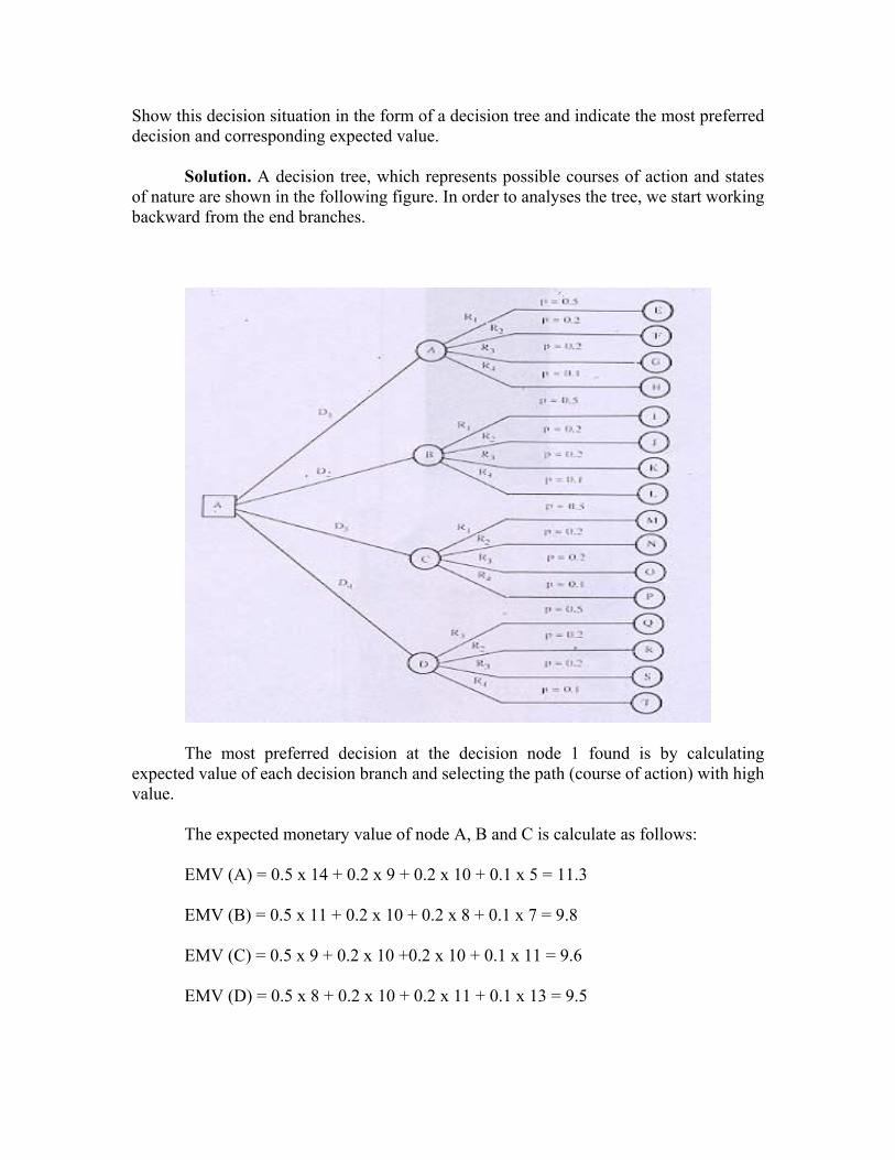
Show this decision situation in the form of a decision tree and indicate the most preferred decision and corresponding expected value. Solution. A decision tree, which represents possible courses of action and states of nature are shown in the following figure. In order to analyses the tree, we start working backward from the end branches.
The most preferred decision at the decision node 1 found is by calculating expected value of each decision branch and selecting the path (course of action) with high value. The expected monetary value of node A, B and C is calculate as follows: EMV (A) = 0.5 x 14 + 0.2 x 9 + 0.2 x 10 + 0.1 x 5 = 11.3
EMV (B) = 0.5 x 11 + 0.2 x 10 + 0.2 x 8 + 0.1 x 7 = 9.8
EMV (C) = 0.5 x 9 + 0.2 x 10 +0.2 x 10 + 0.1 x 11 = 9.6
EMV (D) = 0.5 x 8 + 0.2 x 10 + 0.2 x 11 + 0.1 x 13 = 9.5

Since node A has the highest EMV, the decision at node 1 will be to choose the course of action D4. Example 2. A farm owner is seriously considering of drilling farm well. In the past, only 70% of wells drilled were successful at 200 feet of depth in the area. Moreover, on finding no water at 200 ft., some persons drilled it further up to 250 feet but only 20% struck water at 250 ft. The prevailing cost of drilling is Rs. 50 per feet. The farm owner has estimated that in case he loss not get his own well, he will have to pay Rs. 15,000 over the next 10 years (in PV terms) to buy water from the neighbor. The following decisions can be optimal:
(i) do not drill any well, (ii) drill up to 200 ft. (iii) if no water is found at 200 ft., drill further up to 250 ft.
Draw an appropriate decision tree and determine the farm owner’s strategy under EMV approach.
Solution. The given data can easily be represented by the following decision tree diagram.
Consequence of outflow (Rs.)

There are two decision points in the tree indicated by 1 and 2. In order to decide between the two basis alternatives, we have to fold back (backward induction) the tree from the decision point 2, using EMV as criterion:
EVALUATION OF DECISION POINTS
Decision point
State of
Nature
Probability
Cash outflows
Expected cash
Outflow
Decision at point D2
1. Drill up to
250 fit.
Water struck 0.2 Rs. 12,5000 Rs. 2,500
No water struck 0.8 27,500 22,000
EMV (outflows) = 24,500
2. Do not drill
up to 250 ft.
EMV (outflow) = Rs. 25,000
The decision at D2 is : Drill up to 250 feet.
Decision at point D2
1. Drill up to
200 ft.
Water struck 0.7 Rs. 10,000 Rs. 7,000
Not water struck
0.3 24,500 7,350
EMV (outflow) = Rs. 14,350
2. Do not drill
up to 200 ft.
EMV (outflow) = Rs. 15,000
The decision at D1 is : Drill up to 200 ft.
Thus the optimal strategy for the farm-owner is to drill the well up to 200 ft. and if no water is struck, then further drill it up to 250 ft.
Example 3. A businessman has two independent investments A and B available to him; but he lacks the capital to undertake both of them simultaneously. He can choose to

take A first and then stop, or if A is successful then take B, or vice versa. The probability of success of A is 0.7, while for B it is 0’4. Both investments require an initial capital outlay of Rs. 2,000, and both return nothing if the venture is unsuccessful. Successful competitions of A will return Rs. 3,000 (over cost), and successful completion of B will return Rs. 5,000 (over cost). Draw the decision tree and determine the best strategy.
Solution. The appropriate decision tree is shown below:
There are three decision points in the above decision tree indicated by D1, D2 and D3.
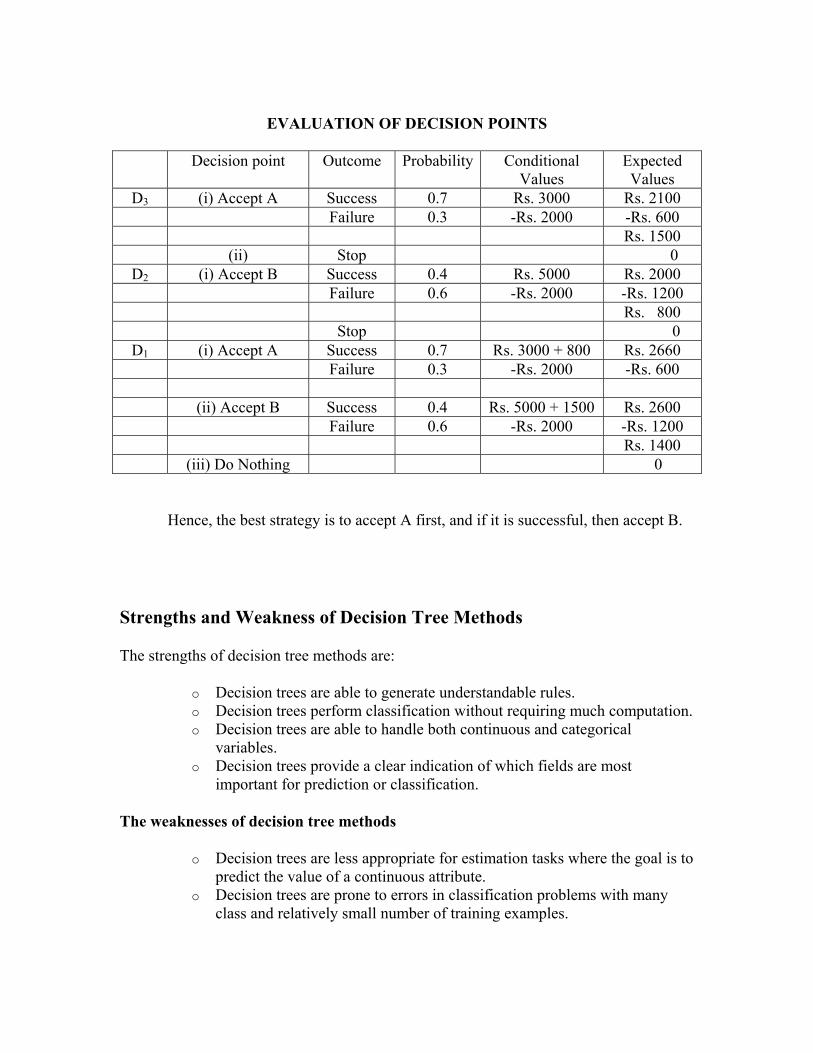
EVALUATION OF DECISION POINTS
Decision point Outcome Probability Conditional
Values Expected Values
D3 (i) Accept A Success 0.7 Rs. 3000 Rs. 2100 Failure 0.3 -Rs. 2000 -Rs. 600 Rs. 1500 (ii) Stop 0
D2 (i) Accept B Success 0.4 Rs. 5000 Rs. 2000 Failure 0.6 -Rs. 2000 -Rs. 1200 Rs. 800 Stop 0
D1 (i) Accept A Success 0.7 Rs. 3000 + 800 Rs. 2660 Failure 0.3 -Rs. 2000 -Rs. 600 (ii) Accept B Success 0.4 Rs. 5000 + 1500 Rs. 2600 Failure 0.6 -Rs. 2000 -Rs. 1200 Rs. 1400 (iii) Do Nothing 0
Hence, the best strategy is to accept A first, and if it is successful, then accept B.
Strengths and Weakness of Decision Tree Methods
The strengths of decision tree methods are:
o Decision trees are able to generate understandable rules. o Decision trees perform classification without requiring much computation. o Decision trees are able to handle both continuous and categorical
variables. o Decision trees provide a clear indication of which fields are most
important for prediction or classification.
The weaknesses of decision tree methods
o Decision trees are less appropriate for estimation tasks where the goal is to predict the value of a continuous attribute.
o Decision trees are prone to errors in classification problems with many class and relatively small number of training examples.
o Decision tree can be computationally expensive to train. The process of growing a decision tree is computationally expensive. At each node, each candidate splitting field must be sorted before its best split can be found. In some algorithms, combinations of fields are used and a search must be made for optimal combining weights. Pruning algorithms can also be expensive since many candidate sub-trees must be formed and compared.
o Decision trees do not treat well non-rectangular regions. Most decision-tree algorithms only examine a single field at a time. This leads to rectangular classification boxes that may not correspond well with the actual distribution of records in the decision space.
In this lecture you must have got a hang as to how decision tree analysis is used to arrive at business decisions.
Summary
Decision trees provide an effective method of decision making because they:
• clearly lay out the problem so that all choices can be viewed, discussed and challenged
• provide a framework to quantify of the values of outcomes and the probabilities of achieving them
• help us to make the best decisions on the basis of our existing information and best guesses.
As with all decision-making methods, though, decision tree analysis should be used in conjunction with common sense. They are just one important part of your decision-making tool kit.

Unit 5 SIMULATION THEORY Lesson 38 W TwShbp W
Sts S
Learning objectives:
• To learn to tackle a wide variety of problems by simulation. • To understand the seven steps of conducting a simulation. • Explain the advantages and disadvantages of simulation.
hy Simulation?
his is a fundamental and quantitative way to understand complex systems/phenomena hich is complementary to the traditional approaches of theory and experiment. imulation (Sim.) is concerned with powerful methods of analysis designed to exploit igh performance computing. This approach is becoming increasingly widespread in asic research and advanced technological applications, cross cutting the fields of hysics, chemistry, mechanics, engineering, and biology.
hat is Simulation?
imulation means imitation of reality. The purpose of simulation in the business world is o understand the behavior of a system. Before making many important decisions, we imulate the result to insure that we are doing the right thing. imulation is used under two conditions.
• First, when experimentation is not possible. Note that if we can do a real experiment, the results would obviously be better than simulation.
• Second condition for using simulation is when the analytical solution procedure
is not known. If analytical formulas are known then we can find the actual expected value of the results quickly by using the formulas. In simulation we can hope to get the same results after simulating thousands of times.

Simulation is basically a data generation technique. Sometimes it is time consuming to conduct real study to know about a situation or problem. One useful application for computers is the simulation of real life events that we consider to be partially or totally random. An example is the simulation of the flow of customers into and out of a bank, to help determine service requirements. The use of simulation frees the programmer and user from having to observe a bank and keep track of exactly when each customer arrives and leaves. A more familiar computer application of randomness is in computer games. If the sequence of events in such a game were predetermined, the player would quickly learn the sequence and become bored. One solution would be to have a large number of games stored in the program, but this could take up an inordinate amount of memory space. The usual solution is for the game program to choose its own moves at random. Thus, simulation is used when actual experimentation is not feasible.
The meaning of the term Simulation can be best explained with a few illustrations. We read and hear about Air force pilots being trained under simulated conditions. Since it would be impossible to train a person when an actual war is going on, all the conditions that would prevail during a war are reconstructed and enacted so that the trainee could develop the skills and instincts that would be required of him during combat conditions. Thus, war conditions are simulated to impart training.
Let us take another example of simulation. All automobile manufacturing companies have a test-track on which the vehicles would be initially driven. The test-track would ideally have all the bends, slopes, potholes etc., that can be found on the roadways on which the vehicles would be subsequently driven. The test-track is therefore, a simulated version of the actual conditions of the various roadways. Simulation, in general, means the creation of conditions that prevail in reality, in order to draw certain conclusions from the trials that are conducted in the artificial conditions. A vehicle manufacturer, by driving the vehicle on the test-track, is conducting a trial in artificial conditions in order to draw conclusions regarding the road-worthiness of the vehicle.
Simulation as an Approach to Decision Making
Decision-making involves choosing an action from several available alternatives. In a business the idea is to choose the course of action which would in some sense optimize the results obtained. While on one hand we may apply intuitive methods or subjective methods based on 'hunches' or previous experiences and knowledge of the person taking the decision on the other, we may apply quantitative or mathematical methods also to the process of decision making in a business environment.
When quantitative or mathematical methods are applied, we may adopt two approaches. They are,
(1) Analytical approach (covered under previous chapter of ‘Queuing) and
(2) Simulation

We will only use the word simulation, when a system has one or more random variables. Changing parameters and analyzing a deterministic system is generally referred to as sensitivity analysis. The general procedure for simulation can be described as follows.
1. Make sure you understand all the variables involved in the system, how they interact with one another, the input parameters of the system, and the performance measures you are interested in calculating.
2. Prepare a cumulative probability distribution for each random variable. For well-
known distributions like Normal, it is enough to identify the parameters.
3. Generate simulated sample of required size, by repeating the following steps as
many times as necessary.
• Pick a random number between 0 and 1. • For discrete distributions find the smallest X where the cumulative probability
> the random number. For continuous distributions, find X where area to the left equals the random number.
4. Track, accumulate and report performance measures.
There Are Many Kinds of Simulations.
• This unit teaches the concepts of Monte Carlo simulation, but it also notes that there are many physical kinds of simulation models as well.
• The idea of simulation is analogous whether we are conducting a wind tunnel
simulation or a math simulation.

Simulation
What it is & What it is not?
Simulation is Simulation is not
A technique which uses computers. An analytical technique
which provide exact solution
An approach for reproducing the processes by which events of chance and change are created in a computer
A programming language but it could be programmed into a set of commands that can form a language to facilitate the programming of simulation.
Simulation Development
A procedure for testing and experimenting on models to answer
what if………. then so……… and ………
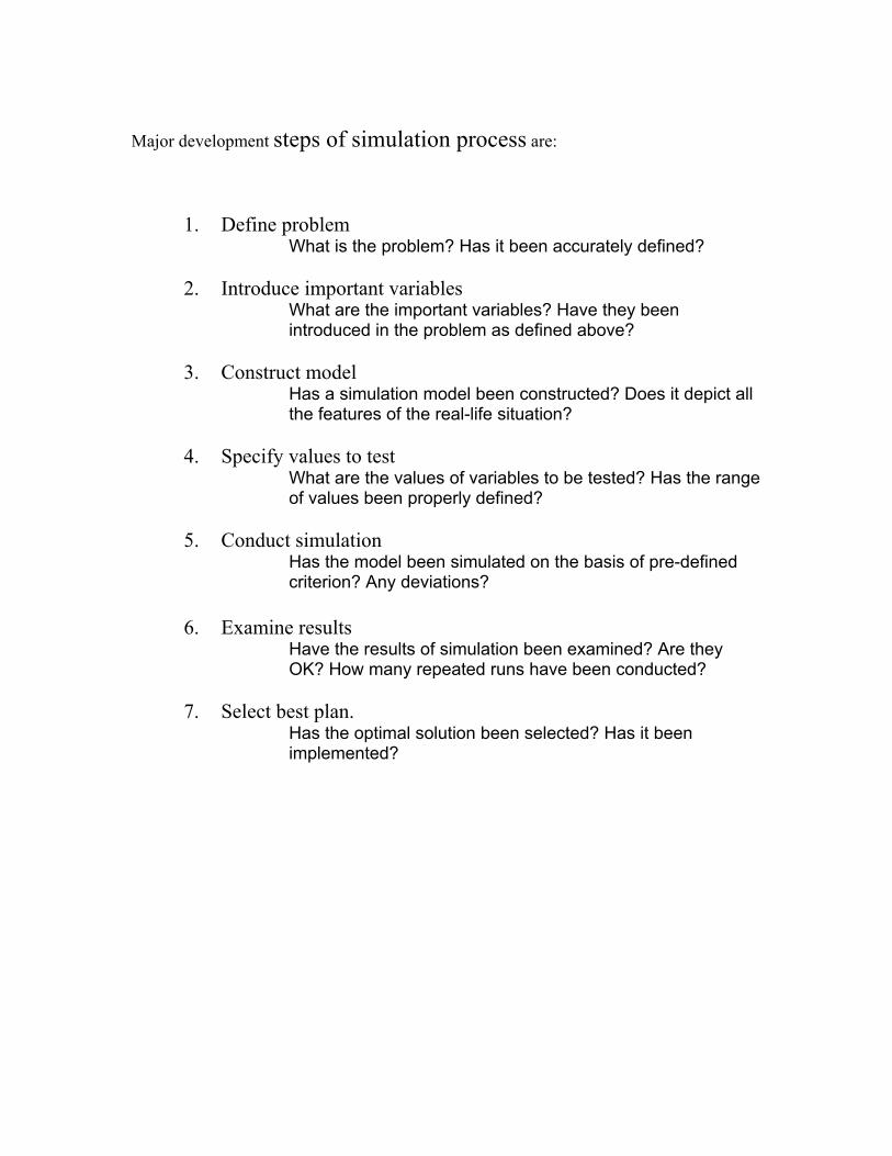
Major development steps of simulation process are:
1. Define problem What is the problem? Has it been accurately defined? 2. Introduce important variables
What are the important variables? Have they been introduced in the problem as defined above?
3. Construct model Has a simulation model been constructed? Does it depict all the features of the real-life situation?
4. Specify values to test What are the values of variables to be tested? Has the range of values been properly defined?
5. Conduct simulation Has the model been simulated on the basis of pre-defined criterion? Any deviations?
6. Examine results Have the results of simulation been examined? Are they OK? How many repeated runs have been conducted?
7. Select best plan. Has the optimal solution been selected? Has it been implemented?

NO
YES
Identify decision variables, performance
criterion and decision rules
Construct a simulation model
Validate the Model
Design experiments (specify values of decision variables to be tested)
Run or Conduct the Simulation
Examine the results and select the best
course of action.
Is simulation process complete?
Modify the model by changing
the input data, i.e. values or decision variables
Identify the Problem
Steps in Simulation Process

Advantages of simulation Disadvantages of simulation
Relatively straightforward Requires generation of all conditions and constraints of real-world problem
Can solve large, complex problems Each model is unique
Allows “what if” questions Often requires long, expensive process
Does not interfere with real-world systems Does not generate optimal solutions
Allows study of interactive variables
Allows time compression
Allows inclusion of real-world complications
CONSTRUCTION OF A MATHEMATICAL MODEL
The construction of a mathematical model for simulation can easily be understood with the help of an example - discussed below: The Bread-Seller Problem.
We try to discuss the formulation of a mathematical simulation model with the help of the bread-seller problem. Consider a bread seller who has to decide on the number of loaves of bread he must buy everyday so as to maximize his daily total profits. The demand in this case is of a variable nature.
If the seller buys more units than he can sell, then the unsold bread is a waste,
reflecting loss to him. On the other hand, if he buys less units than the demand, then there is an opportunity cost involved. i.e.; he losses the opportunity to sell additional units of bread and hence his profit is not maximized.
Step I. Suppose, the cost price per unit is Rs. 5 and the sales price per unit is Rs. 8.
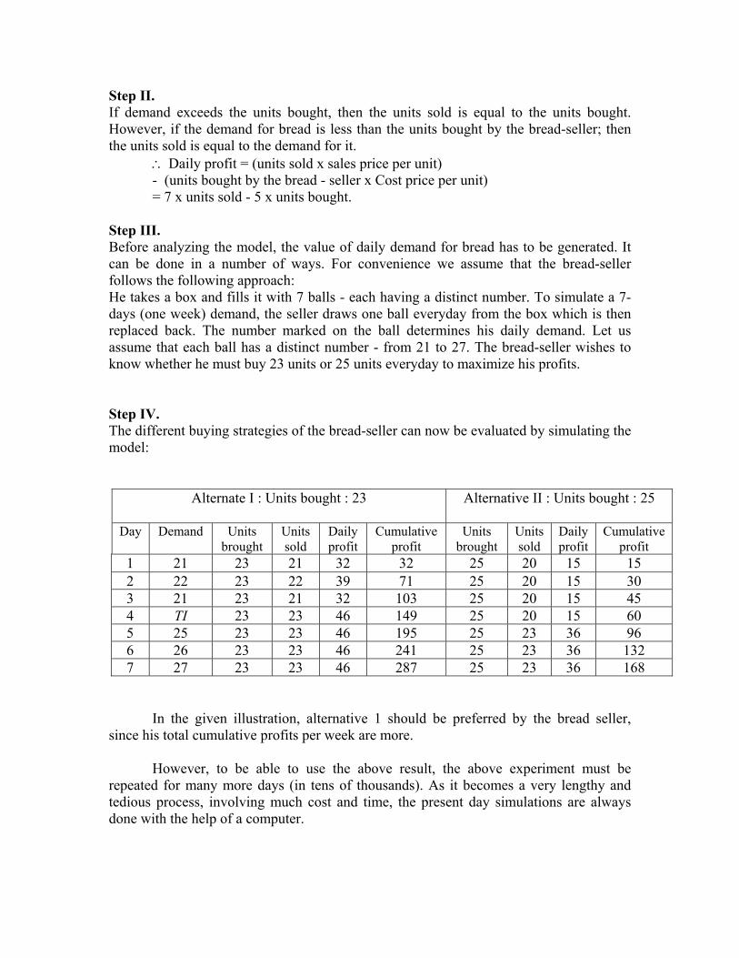
Step II. If demand exceeds the units bought, then the units sold is equal to the units bought. However, if the demand for bread is less than the units bought by the bread-seller; then the units sold is equal to the demand for it. ∴ Daily profit = (units sold x sales price per unit)
- (units bought by the bread - seller x Cost price per unit) = 7 x units sold - 5 x units bought.
Step III. Before analyzing the model, the value of daily demand for bread has to be generated. It can be done in a number of ways. For convenience we assume that the bread-seller follows the following approach: He takes a box and fills it with 7 balls - each having a distinct number. To simulate a 7-days (one week) demand, the seller draws one ball everyday from the box which is then replaced back. The number marked on the ball determines his daily demand. Let us assume that each ball has a distinct number - from 21 to 27. The bread-seller wishes to know whether he must buy 23 units or 25 units everyday to maximize his profits. Step IV. The different buying strategies of the bread-seller can now be evaluated by simulating the model:
Alternate I : Units bought : 23
Alternative II : Units bought : 25
Day Demand Units brought
Units sold
Daily profit
Cumulative profit
Units brought
Units sold
Daily profit
Cumulative profit
1 21 23 21 32 32 25 20 15 15 2 22 23 22 39 71 25 20 15 30 3 21 23 21 32 103 25 20 15 45 4 TI 23 23 46 149 25 20 15 60 5 25 23 23 46 195 25 23 36 96 6 26 23 23 46 241 25 23 36 132 7 27 23 23 46 287 25 23 36 168
In the given illustration, alternative 1 should be preferred by the bread seller,
since his total cumulative profits per week are more. However, to be able to use the above result, the above experiment must be
repeated for many more days (in tens of thousands). As it becomes a very lengthy and tedious process, involving much cost and time, the present day simulations are always done with the help of a computer.

Step V. Simulation Using Computers. The above experiment requires a large number of repetitions to be of any use to the bread-seller decision-making. The bread-seller generated his daily demand by using marked balls kept in a box. In simulations using computers; the demand is generated with the help of random numbers.
A random number means a number which is equally likely to be drawn at random
from all the available choices. For example, all ten single digit numbers from 0 to 9 are equally likely to be drawn from a box containing them. Hence, the probability of drawing anyone of them is 1/10 or 0.10. Such random numbers can also be picked up from a random number table, alternatively, these can be generated by using a completely deterministic mathematical process such as the mid-square or the congruential method - both of which are beyond the scope of our current discussion.
Use of Computers for Speedy Simulations
Computers are critical and have given life to the simulation process. Instead of conducting simulation twenty or thirty times by hand, with computers we can run it hundreds or thousands of times. This also ties in with the issue of time compression mentioned earlier in the chapter.
Summary
To conclude I can say that simulation is needed in a situation where characteristics such as uncertainty, complexity, dynamic interaction between the decision and subsequent event, and need to develop detailed procedures & finely divided time intervals, combined in one situation, it becomes too complex to be solved by any of the techniques of mathematical programming and probabilistic models. It can be added that the simulations technique is a dependable tool in situations where mathematical analysis is either too costly or too complex.

____________________________________________________________________________________________________________________________________________________________________________________________________________________________________________________________________________________________________________________________________________________________________________________________________________________________________________________________________________________________________________________________________________________________________________________________________________________________________________________________________________________________________________________________________________________________________________________________________________________________________________________________________________________________
2Simulation
SimulationWhat Is Simulation?• A model/process used to duplicate or mimic the real
system
Types of Simulation Models• Physical simulation• Computer simulation
When to Use (Computer) Simulation Models?• Problems/systems are too complex • There are random components in the system
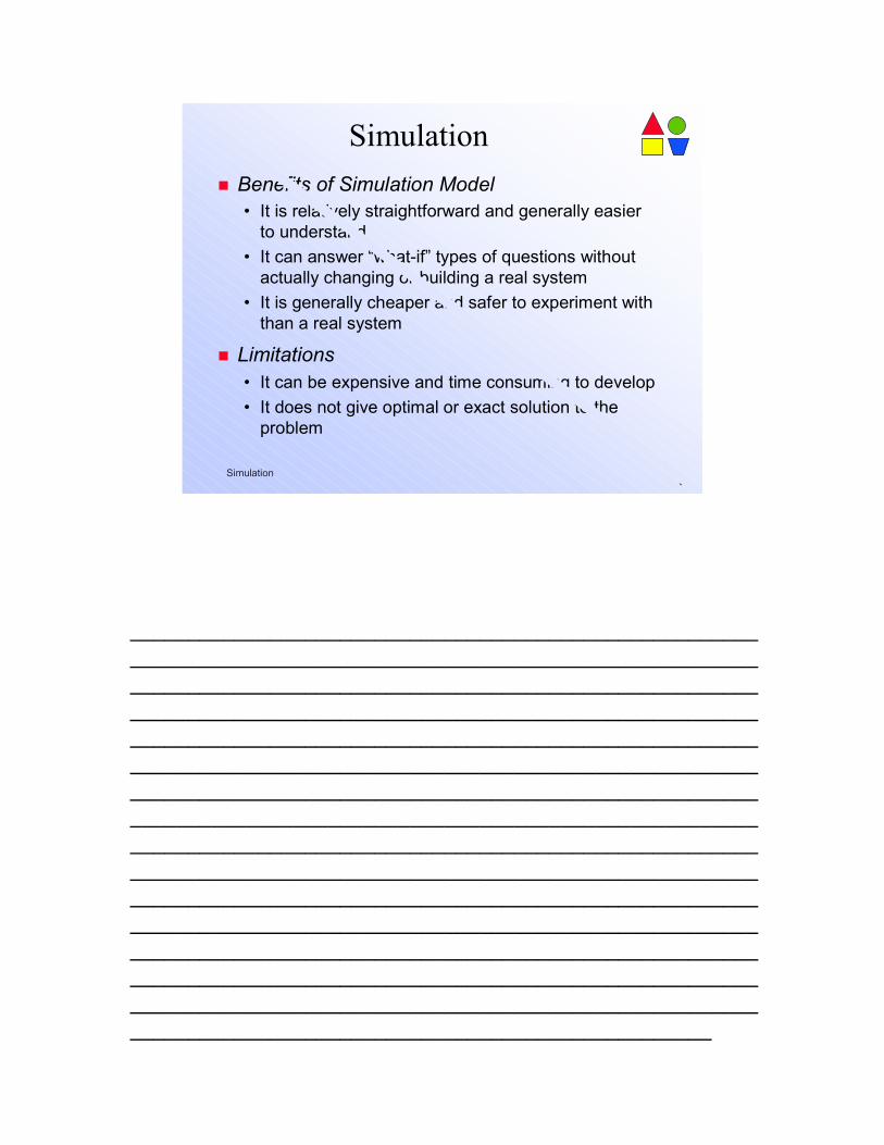
____________________________________________________________________________________________________________________________________________________________________________________________________________________________________________________________________________________________________________________________________________________________________________________________________________________________________________________________________________________________________________________________________________________________________________________________________________________________________________________________________________________________________________________________________________________________________________________
3Simulation
SimulationBenefits of Simulation Model• It is relatively straightforward and generally easier
to understand• It can answer “what-if” types of questions without
actually changing or building a real system• It is generally cheaper and safer to experiment with
than a real system
Limitations• It can be expensive and time consuming to develop• It does not give optimal or exact solution to the
problem
________________________________________________________________________________________________________
Unit 5 SIMULATION THEORY
Lesson 39
Yo
R
Rpgwgtfo
R
IpesAapt
Learning objective:
• To learn random number generation. • Methods of simulation. • Monte Carlo method of simulation
ou’ve already read basics of simulation now I will be taking up method f simulation, that is Random Number Generation
andom Number Generation
andom numbers or Pseudo-random numbers are often required for simulations erformed on parallel computers. The requirements for parallel random number enerators are more stringent than those for sequential random number generators. As ell as passing the usual sequential tests on each processor, a parallel random number enerator must give different, independent sequences on each processor. We consider he requirements for a good parallel random number generator, and discuss generators or the uniform and normal distributions. These generators can give very fast vector r parallel implementations.
andom Numbers and Simulation
n many fields of engineering and science, we use a computer to simulate natural henomena rather than experiment with the real system. Examples of such computer xperiments are simulation studies of physical processes like atomic collisions, imulation of queuing models in system engineering, sampling in applied statistics. lternatively, we simulate a mathematical model, which cannot be treated by
nalytical methods. In all cases a simulation is a computer experiment to determine robabilities empirically. In these applications, random numbers are required to make hings realistic.

Random number generation has also applications in cryptography, where the requirements on randomness may be even more stringent.
Hence, we need a good source of random numbers. Since the validity of a simulation will heavily depend on the quality of such a source, its choice or construction will be fundamental importance. Tests have shown that many so-called random functions supplied with programs and computers are far away from being random.
By generating random numbers, we understand producing a sequence of independent random numbers with a specified distribution. The fundamental problem is to generate random numbers with a uniform discrete distribution on {0,1,2,…,N} or more suitable on {0,1/N,2/N,…,1}, say. This is the distribution where each possible number is equally likely. For N large this distribution approximates the continuous uniform distribution U(0,1) on the unit interval. Other discrete and continuous distributions will be generated from transformations of the U(0,1) distribution.
At first, scientists who needed random numbers would generate them by performing random experiments like rolling dice or dealing out cards. Later tables of thousands of random digits created with special machines for mechanically generating random numbers or taken from large data sets as census reports were published.
With the introduction of computers, people began to search for efficient ways to obtain random numbers using arithmetic operations of a computer - an approach suggested by John von Neumann in the 1940's. Since the digital computer cannot generate random numbers, the idea is, for a given probability distribution, to develop an algorithm such that the numbers generated by this algorithm appear to be random with the specified distribution. Sequences generated in a deterministic way we call pseudo-random numbers. To simulate a discrete uniform distribution John von Neumann used the so-called middle square method, which is to take the square of the previous random number and to extract the middle digits.
Example: If we generate 4-digit numbers starting from 3567 we obtain 7234 as the next number since the square of 3567 equals 12723489. Continuing in the same way the next number will be 3307.
Of course, the sequence of numbers generated by this algorithm is not random but it appears to be. However, as computations show the middle square method is a poor source of random numbers.
To summarize our discussion we need
• Precise mathematical formulations of the concept of randomness • Detailed analysis of algorithms for generating pseudo-random numbers • Empirical tests of random number generators

What is a random sequence?
A sequence of real numbers between zero and one generated by a computer is called "pseudo-random" sequence if it behaves like a sequence of random numbers. So far this statement is satisfactory for practical purposes but what one needs is a quantitative definition of random behaviour.
In practice we need a list of mathematical properties characterizing random sequences and tests to see whether a sequence of pseudo-random numbers yields satisfactory results or not. Loosely speaking, basic requirements on random sequences are that their elements are uniformly distributed and uncorrelated. The tests we can perform will be of theoretical and/or empirical nature.
Some definitions
D.H. Lehmer(1951) : "A random sequence is a vague notion embodying the idea of a sequence in which each term is unpredictable to the uninitiated and whose digits pass a certain number of tests, traditional with statisticians and depending somewhat on the uses to which the sequence is to be put."
J.N. Franklin (1962): " A sequence (U0, U1,…) (note: with Ui taking values in the unit interval [0,1]) is random if it has every property that is shared by all infinite sequences of independent samples of random variables from the uniform distribution."
Generating uniform random numbers
Deterministic generators yield numbers in a fixed sequence such that the forgoing k numbers determine the next number. Since the set of numbers used by a computer is finite, the sequence will become periodic after a certain number of iterations.
The general form of algorithms generating random numbers may be described by the following recursive procedure.
Xn= f(Xn-1,Xn-2,..., Xn-k)
with initial conditions X0, X1,...,Xk-1. Here f is supposed to be a mapping from {0,1,...,m-1}k into {0,1,...,m-1}.
For most generators k=1 in which case the recursive relation simplifies to
Xn= f(Xn-1)
with a single initial value X0, the seed of the generator. Now f is a mapping from {0,1,...,m-1} into itself.

In most cases the goal is to simulate the continuous uniform distribution U(0,1). Therefore the integers Xn are rescaled to
Un= Xn/m.
If m is large, the resulting granularity is negligible when simulating a continuous distribution.
A good generator should be of a long period and resulting subsequences of pseudo-random numbers should be uniform and uncorrelated. Finally, the algorithm should be efficient.
Remark: You should note that initializing the generator with the same seed X0 would give the same sequence of random numbers. Usually one uses the clock time to initialize the generator.
Mathematicians have devised a variety of procedures to generate random numbers. With these procedures, random number generation can be done either manually or with the help of a computer. Also, several collections of random number tables are available. The most commonly used table contains uniformly distributed (or normally distributed) random numbers over the interval 0 to 1. To generate other types of random numbers which obey other distribution laws, we would require access to a computer.
The simplest method for obtaining random events is coin tossing. This method can be used to obtain an ideal random number generator. Here, we show that logistic map is able to simulate the coin tossing method. Also, we describe a numerical implementation of the ideal uniform random number generator. Comparing to usual congruential random number generators, which are periodic, the logistic generator is infinite, aperiodic and not correlated.
In modern science, random number generators have proven invaluable in simulating natural phenomena and in sampling data [1-2]. There are only a few methods for obtaining random numbers. For example, the simplest method is coin tossing, where the occurrence of heads or tails are random events. By virtue of the symmetry of the coin the events are equally probable. Hence they are called equally probable events. It is therefore considered that the probability of heads (tails) is equal to 1/2.
Coin tossing : The coin tossing belongs to the category of mechanical methods which includes also: dices, cards, roulettes, urns with balls and other gambling equipments. The mechanical methods are not frequently used in science because of the low generation speed. The methods characterized by high generation speed are those, which are based on intrinsic random physical processes such as the electronic and radioactive noise. Because the sequence of numbers generated with mechanical and physical methods are not reproducible, these methods have a great disadvantage in numerical simulations.
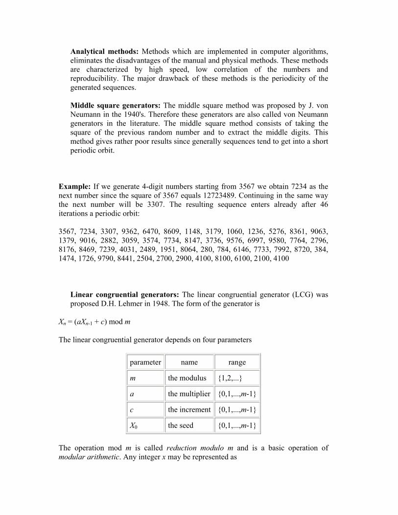
Analytical methods: Methods which are implemented in computer algorithms, eliminates the disadvantages of the manual and physical methods. These methods are characterized by high speed, low correlation of the numbers and reproducibility. The major drawback of these methods is the periodicity of the generated sequences.
Middle square generators: The middle square method was proposed by J. von Neumann in the 1940's. Therefore these generators are also called von Neumann generators in the literature. The middle square method consists of taking the square of the previous random number and to extract the middle digits. This method gives rather poor results since generally sequences tend to get into a short periodic orbit.
Example: If we generate 4-digit numbers starting from 3567 we obtain 7234 as the next number since the square of 3567 equals 12723489. Continuing in the same way the next number will be 3307. The resulting sequence enters already after 46 iterations a periodic orbit:
3567, 7234, 3307, 9362, 6470, 8609, 1148, 3179, 1060, 1236, 5276, 8361, 9063, 1379, 9016, 2882, 3059, 3574, 7734, 8147, 3736, 9576, 6997, 9580, 7764, 2796, 8176, 8469, 7239, 4031, 2489, 1951, 8064, 280, 784, 6146, 7733, 7992, 8720, 384, 1474, 1726, 9790, 8441, 2504, 2700, 2900, 4100, 8100, 6100, 2100, 4100
Linear congruential generators: The linear congruential generator (LCG) was proposed D.H. Lehmer in 1948. The form of the generator is
Xn = (aXn-1 + c) mod m
The linear congruential generator depends on four parameters
parameter name range
m the modulus {1,2,...}
a the multiplier {0,1,...,m-1}
c the increment {0,1,...,m-1}
X0 the seed {0,1,...,m-1}
The operation mod m is called reduction modulo m and is a basic operation of modular arithmetic. Any integer x may be represented as

x = floor(x/m)·m + x mod m
where the floor function floor(t) is the greatest integer less than or equal to t. This equation may be taken as definition of the reduction modulo m.
If c = 0 the generator is called multiplicative. For nonzero c the generator is called mixed.
Monte Carlo Method of Simulation
The Monte Carlo method owes its development to the two mathematicians, John Von Neumann and Stanislaw Ulam, during World War II. The principle behind this method of simulation is representative of the given system under analysis by a system described by some known probability distribution and then drawing random samples for probability distribution by means of random number. In case it is not possible to describe a system in terms of standard probability distribution such as normal, Poisson, exponential, gamma, etc., an empirical probability distribution can be constructed.
The deterministic method of simulation cannot always be applied to complex real life situations due to inherently high cost and time values required so as to obtain any meaningful results from the simulated model. Since there are a large number of interactions between numerous variables, the system becomes too complicated to offer an effective simulation approach. In such cases where it is not feasible to use an expectation approach for simulating systems, Monte Carlo method of simulation is used.
It can be usefully applied in cases where the system to be simulated has a large number of elements that exhibit chance (probability) in their behaviour. As already mentioned, the various types of probability distributions are used to represent the uncertainty of real-life situations in the model. Simulation is normally undertaken only with the help of a very high-speed data processing machine such as computer. The user of simulation technique must always bear in mind that the actual frequency or probability would approximate the theoretical value of probability only when the number of trials are very large i.e. when the simulation is repeated a large no. of times. This can easily be achieved with the help of a computer by generating random numbers.
A random number table is presented here for the quick reference of the students.
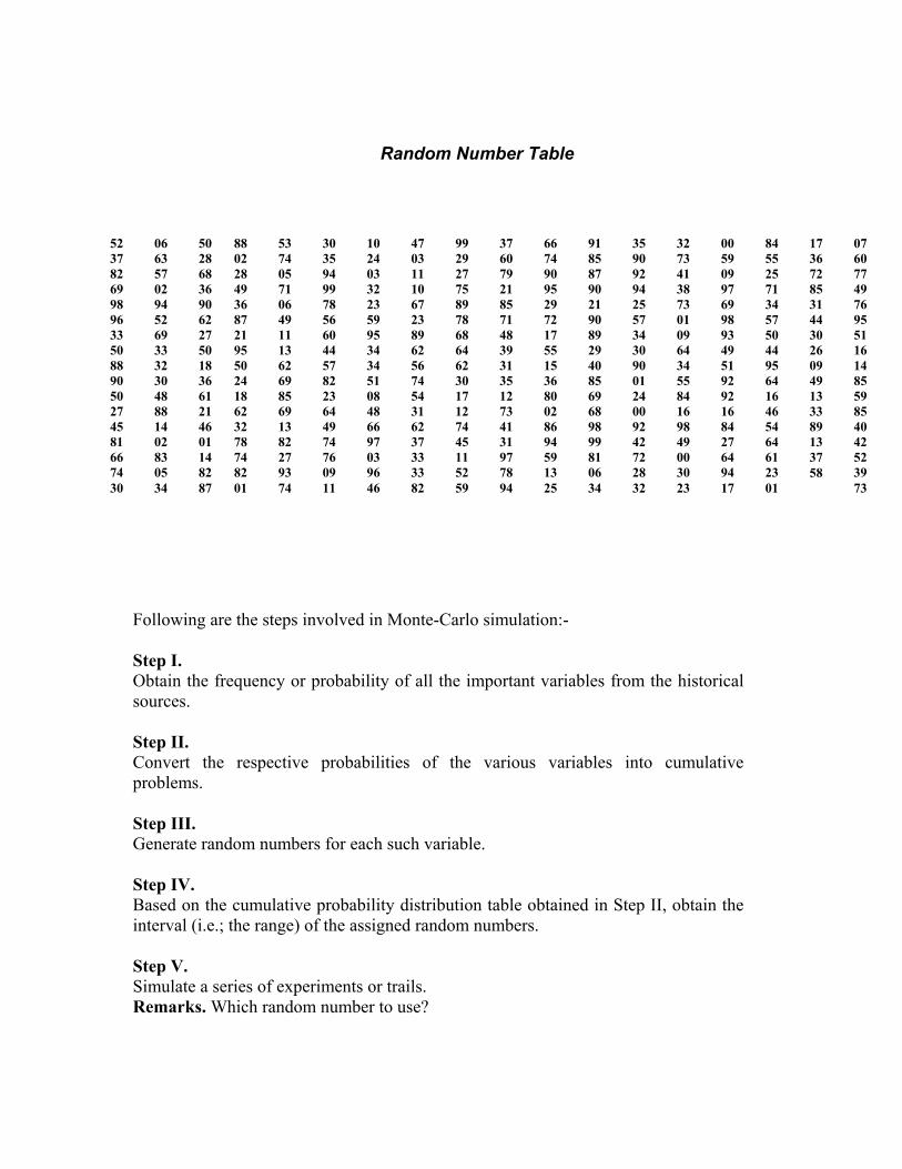
Random Number Table
52 37 82 69 98 96 33 50 88 90 50 27 45 81 66 74 30
06 63 57 02 94 52 69 33 32 30 48 88 14 02 83 05 34
50 28 68 36 90 62 27 50 18 36 61 21 46 01 14 82 87
88 02 28 49 36 87 21 95 50 24 18 62 32 78 74 82 01
53 74 05 71 06 49 11 13 62 69 85 69 13 82 27 93 74
30 35 94 99 78 56 60 44 57 82 23 64 49 74 76 09 11
35 90 92 94 25 57 34 30 90 01 24 00 92 42 72 28 32
32 73 41 38 73 01 09 64 34 55 84 16 98 49 00 30 23
10 24 03 32 23 59 95 34 34 51 08 48 66 97 03 96 46
00 59 09 97 69 98 93 49 51 92 92 16 84 27 64 94 17
47 03 11 10 67 23 89 62 56 74 54 31 62 37 33 33 82
84 55 25 71 34 57 50 44 95 64 16 46 54 64 61 23 01
99 29 27 75 89 78 68 64 62 30 17 12 74 45 11 52 59
17 36 72 85 31 44 30 26 09 49 13 33 89 13 37 58
37 60 79 21 85 71 48 39 31 35 12 73 41 31 97 78 94
66 74 90 95 29 72 17 55 15 36 80 02 86 94 59 13 25
07 60 77 49 76 95 51 16 14 85 59 85 40 42 52 39 73
91 85 87 90 21 90 89 29 40 85 69 68 98 99 81 06 34
Following are the steps involved in Monte-Carlo simulation:- Step I. Obtain the frequency or probability of all the important variables from the historical sources. Step II. Convert the respective probabilities of the various variables into cumulative problems. Step III. Generate random numbers for each such variable. Step IV. Based on the cumulative probability distribution table obtained in Step II, obtain the interval (i.e.; the range) of the assigned random numbers. Step V. Simulate a series of experiments or trails. Remarks. Which random number to use?

The selection of specific random number is determined by establishing a systematic and thorough selection strategy before examining the list of digits given in the random number table. In general, the practical life situations or systems are simulated by building, first a basic inherent model & subsequently relaxing some or all of the assumptions so as to obtain a more precise model representation. Thus model building for simulations is a stepwise process and the final model emerges only after a large number of successive refinements. Application of Monte-Carlo Simulation: Monte-Carlo simulation can now easily be applied to an example of the bread-seller. Let us suppose that the demands per unit of the bread along with their respective probabilities are as follows:
Days No. Demand (per unit) Probability
1 2 3 4 5 6 7
20 21 22 23 24 25 26
0.10 0.15 0.25 0.20 0.10 0.05 0.15
We can easily use a sequence of 2-digit random numbers of generating the demand based on the above information. By assigning two digit random numbers to each of the possible outcomes or daily demand, we have:
(Per unit) Days No. Demand Probability
Cumulative Probability Random Nos.
1 2 3 4 5 6 7
20 21 22 23 24 25 26
0.10 0.15 0.25 0.20 0.10 0.05 0.15
0.10 0.25 0.50 0.70 0.80 0.85 1.00
00 to 09 10 to 24 25 to 49 50 to 69 70 to 79 80 to 84 85 to 99
The first entry in the random number table is 00 to 09. It means that there are 10 random numbers (00 to 09). Since each of the ten numbers has an even chance of appearing. The probability of each

number = 1/10 or 0.10; a fact that is fully supported by the cumulative probability table. Using the above procedure, by Monte Carlo method of simulation, demand for the required number of days can easily be determined using the random number table.
Now I’ll take up few examples of random number to explain this & make its practical application clear.
Example 1
New Delhi Bakery House keeps stock of a popular brand of cake. Previous experience indicates the daily demand as given below:
Table 1
Daily demand Probability
0 0.01
15 0.15
25 0.20
35 0.50
45 0.12
50 0.02
Consider the following sequence of random numbers: R. No. : 21, 27, 47, 54, 60, 39, 43, 91, 25, 20.
Using this sequence, simulate the demand for the next 10 days. Find out the stock situation if the owner of the bakery house decides to make 30 cakes every day. Also estimate the daily average demand for the cakes on the basis of simulated data.
Solution :
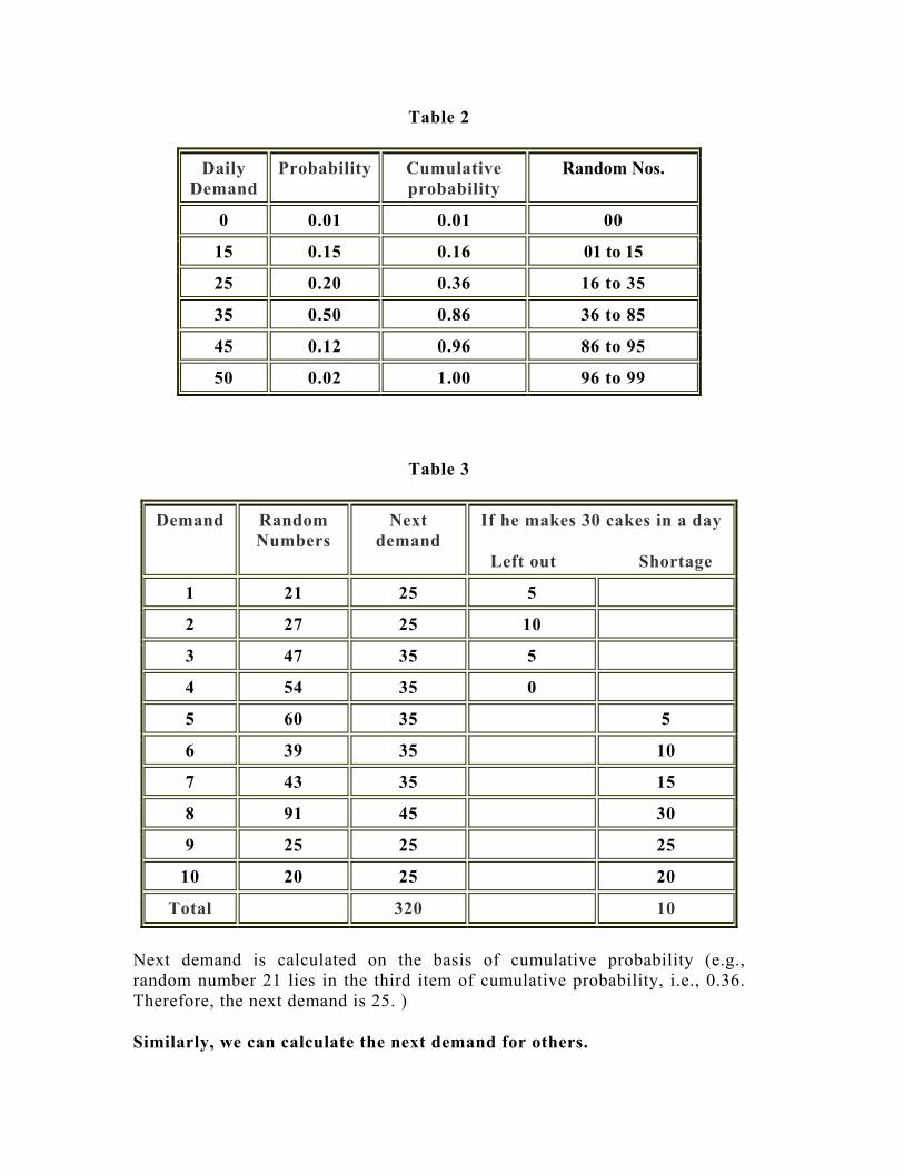
Table 2
Daily Demand
Probability Cumulative probability
Random Nos.
0 0.01 0.01 00
15 0.15 0.16 01 to 15
25 0.20 0.36 16 to 35
35 0.50 0.86 36 to 85
45 0.12 0.96 86 to 95
50 0.02 1.00 96 to 99
Table 3
Demand Random Numbers
Next demand
If he makes 30 cakes in a day
Left out Shortage
1 21 25 5
2 27 25 10
3 47 35 5
4 54 35 0
5 60 35 5
6 39 35 10
7 43 35 15
8 91 45 30
9 25 25 25
10 20 25 20
Total 320 10
Next demand is calculated on the basis of cumulative probability (e.g., random number 21 lies in the third item of cumulative probability, i.e., 0.36. Therefore, the next demand is 25. )
Similarly, we can calculate the next demand for others.

Total demand = 320
Average demand = Total demand / no. of days
The daily average demand for the cakes = 320 / 10 = 32 cakes.
Summary
Hope you have understood the random number method of simulation. In next lesson we will study about the practical application of simulation.
4Simulation
Monte Carlo SimulationKey element is randomness• Assume that some inputs are random variables• Modeling randomness by generating random
variables from their probability distributions
Simulation Modeling Process• Develop the basic model that “behaves like” the
real problem, with a special consideration of the random or probabilistic input variables
• Conduct a series of computer runs (called trials) to learn the behavior of the simulation model
• Compute the summary (output) statistics and make inferences about the real problem
Slide 1

Slide 2
____________________________________________________________________
________________________________
_
_____________________________________________________________________
_____________________________________________________________________
_____________________________________________________________________
_____________________________________________________________________
_____________________________________________________________________
_____________________________________________________________________
_____________________________________________________________________
_____________________________________________________________________
_____________________________________________________________________
_____________________________________________________________________
_____________________________________________________________________
5Simulation
Monte Carlo SimulationSince some inputs to the model are random, outputs from the model are random too.Simulation process is similar to statistical inference process• Statistics: start with a population, sampling from the
population, and then based on sample information to infer population
• Simulation: start with a basic model to represent real problem, replicating the basic model, and then based on the replication results to help solve real problem
• The larger the number of trials (sample size), the more reliable will be the simulation result

Slide 3
____________________________________________________________________
____________________________________________________________________
_____________________________________________________________________
_
_
_____________________________________________________________________
_____________________________________________________________________
_____________________________________________________________________
_____________________________________________________________________
_____________________________________________________________________
_____________________________________________________________________
_____________________________________________________________________
6Simulation
Basic Model: Profit = f(demand)
Input:Demand
Relationship:function f
Output:Profit
How simulation works:Step 1: basic model development: generate one possible
random Demand and find the corresponding ProfitStep 2: basic model replication: generate many possible
values of Demand and find corresponding ProfitsStep 3: result summarization: calculate summarized
statistics on the Profit such as average, min, max etc.
Example
Unit 5 SIMULATION THEORY
Lesson 40
Learning objectives:
• To acquaint yourself with the practical applications of simulation methods.
Hello students,
Now when you are aware of the methods of simulation and techniques of random number generation I’ll take few examples of business / practical application of simulation. Simulation is widely used for the following
• Simulation of Inventory Problem
• Simulation of Queuing Problem
• Simulation of investment problem
• Simulation of Maintenance Problem
• Simulation of PERT Problem
Firstly, let us find out how simulation can be utilized for an inventory problem.
Simulation of Inventory Problem
Many of the inventory problems, especially storage problem, cannot be solved analytically because of the complex nature of the distribution

followed by demand or supply. It is however possible to get the solution by using simulation techniques. The basic approach would be to determine the probability distribution of the input and output functions from the past data, and run the inventory system artificially by generating the future observations on the assumptions of the same distribution. Subsequently, the decision-making regarding the optimization problems would be made by the trial-and-error method.
Many companies are looking to reduce their inventory costs, however before risking adverse customer service they want to determine the consequences and test different alternatives. By building a model of the inventory system, we can test variations of the existing setup.
Example 1
Using the random number to simulate a sample, find the probability that a packet does not contain any defective product, when the production line produces 10% defective products. Compare your answer with the expected probability.
Solution
Given that 10 per cent of the total production is defective and 90 per cent is non-defective. If we have 100 random numbers (0 to 99), then 90 or 90 per cent of them represent non-defective products and remaining 10 (or 10 per cent) of them represent defective products. Thus, the random numbers 00 to 89 are assigned to variables representing non-defective products and 90 to 100 are assigned to variables representing defective products.
If we choose a set of 2-digit random numbers in the range 00 to 99 to represent a packet of 6 products as shown below, then we would expect that 90 per cent of the time they would fall in the range 00 to 89.
Table 1
Sample Number Random Number
A 86 02 22 57 51 68
B 39 77 32 77 09 79
C 28 06 24 25 93 22

D 97 66 63 99 61 80
E 69 30 16 09 05 53
F 33 63 99 19 87 26
G 87 14 77 43 96 43
H 99 53 93 61 28 52
I 93 86 52 77 65 15 J 18 46 23 34 25 85
Here it may be noted that out of ten simulated samples 6 contain one or more defectives and 4 contain no defectives. Thus, the expected percentage of non-defective products is 40 per cent. However theoretically the probability that a packet of 6 products containing no defective products is (0.9)6 = 0.53144 = 53.14%
Example 2
A bakery keeps stock of a popular brand of cake. Previous experience shows the demand pattern for the item with associated probabilities, as given below:
Daily demand (number): 0 10 20 30 40 50
Probability : 0.01 020 0.15 0.50 0.12 0.02
Use the following sequence of random numbers to simulate the demand for next 10 days.
Random numbers: 25, 39, 65, 76, 12, 05, 73, 89, 19, 49.
Also estimate the daily average demand for the cakes on the basis of simulated data.

Solution
Using the daily demand distribution, we obtain a probability distribution as shown in the following table:
Table 2 Daily Demand Distribution
Daily Demand Probability Cumulative Random Number
Probability Interval
0 0.01 0.01 00
10 0.20 0.21 01-20 20 0.15 0.36 21-35 30 0.50 0.86 36-85 40 0.12 0.98 86-97 50 0.02 1.00 98-99
Conduct the simulation experiment for demand by taking a sample of 10 random numbers from a table of random numbers, which represent the sequence of 10 samples. Each random sample number here is a sample of demand
The simulation calculations for a period of 10 days are given in table below:
Table 3 : Simulation Experiment
Days Random Number Demand 1 40 30 because 0.36 < 0.40 < 0.85 2 19 10 because 0.01 < 0.19 < 0.20, 3 87 40 and so on 4 83 30 5 73 30 6 84 30 7 29 20 8 09 10 9 02 10 10 20 10
Total = 220

Expected demand = 220/1 0 = 22 units per day
Example 3
A bookstore wishes to carry a particular book in stock. Demand is probabilistic and replenishment of stock takes 2 days (i.e. if an order is placed on March 1, it will be delivered at the end of the day on March 3). The probabilities of demand are given below:
Demand (daily) : 0 1 2 3 4
Probability : 0.05 0.10 0.30 0.45 0.10
Each time an order is placed, the store incurs an ordering cost of Rs. 10 per order. The store also incurs a carrying cost of Re 0.05 per book per day. The inventory carrying cost is calculated on the basis of stock at: the end of each day. The manager of the bookstore wishes to compare two options for his inventory decision
A : Order 5 books when the inventory at the beginning of the day plus orders outstanding is less than 8 books.
B: Order 8 books when the inventory at the beginning of the day plus orders outstanding is less than 8.
Currently (beginning of 1st day) the store has a stock of 8 books plus 6 books ordered two days ago and expected to arrive next day. Using Monte Carlo simulation for 10 cycles, recommend which option the manager should choose.
The two digit random numbers are: 89, 34, 78, 63, 61, 81, 39, 16, 13, 73
Solution
Using the daily demand distribution, we obtain a probability distribution as shown in Table 4 below
Table 4 Daily Demand Distribution
Daily Demand Probability Cumulative Probability
Random Number Interval

0 0.05 0.05 00-04
1 0.10 0.15 05-14
2 0.30 0.45 15-44
3 0.45 0.90 45-89
4 0.10 1.00 90-99
Given that stock in hand is of 8 books and stock on order is 5 books (expected next day)
Table 5 Option A
Random Number
Daily Demand
Closing Stock in
Hand
Receipt Opening Stock in
Hand
Stock on
Order
Order Quantity Closing Stock
(1) (2) (3) (4) (4)+(3)-(2)=(5) (6) (7) (8)
89 3 8 - 8-3=5 6 - 6 34 2 5 6 6+5-2=9 - - - 78 3 9 - 9-3=6 - 5 5 63 3 6 - 6-3=3 5 - 5 61 3 3 - 3-3=0 5 5 10 81 3 0 5 5-3=2 5 5 10 39 2 2 - 2-2=0 10 - 10 16 2 0 5 5-2=3 5 - 5 13 1 3 5 5 + 3 - 1= 7 0 5 5 73 3 7 - 7-3=4 5 - 5
Since 5 books have been ordered four times as shown in Table 5, therefore, total ordering cost Rs. (4 x 10)=Rs. 40.

Closing stock of 10 days is of 39 (= 5 + 9 + 6 + 3 + 2 + 3 + 7 + 4) books. Therefore, the holding cost at the rate of Re 0.5 per book per day is Rs. (39 x 0.5) = Rs. 19.5.
Total cost for 10 days = Ordering cost + Holding cost = Rs. (40 + 19.5) = Rs. 59.5.
Table 6 Option B
Random Number
Demand Daily
Closing Stock in
Hand
Receipt Opening Stock in Hand
Stock on
Order
Order Quantity
Closing Stock
(1) (2) (3) (4) (5) (6) (7) (8) 89 3 8 - 8-3=5 6 - 6 34 2 5 6 6+5-2=9 - - - 78 3 9 - 9-3=6 - 8 8 63 3 6 - 6-3=3 8 - 8 61 3 3 - 3-3=0 8 - 8 81 3 0 8 8+0-3=5 - 8 8 39 2 5 - 5-2=3 8 - 8 16 2 3 - 3-2=1 8 - 8 13 1 1 8 8 + 1 - 1 = 8 - - - 73 3 8 - 8-3=5 - 8 8
Since 8 books have been ordered three times as shown in Table 6, when the inventory of books at the beginning of the day plus orders outstanding is less than 8. Therefore, total ordering cost is : Rs. 30 (3 X 10)
Closing stock of 10 days is of 45 (=5+9+6+3+5+3+1+8+5) books. Therefore, holding cost, re. 0.5 per book is Rs. 22.50 (45 X 0.5)
Total cost for 10 days = Ordering Cost + Holding Cost + Rs. 52.20. Since option B has lower total cost than option A, therefore, manager should choose option B
Simulation of Queuing Problem
Example :
A visitor's bureau in Orlando is open 5 days a week. The information desk is staffed with part time help. The staff is paid $6/hr (after all, it is Orlando we're talking about). The manager has decided that if visitors arrive at a rate of more than
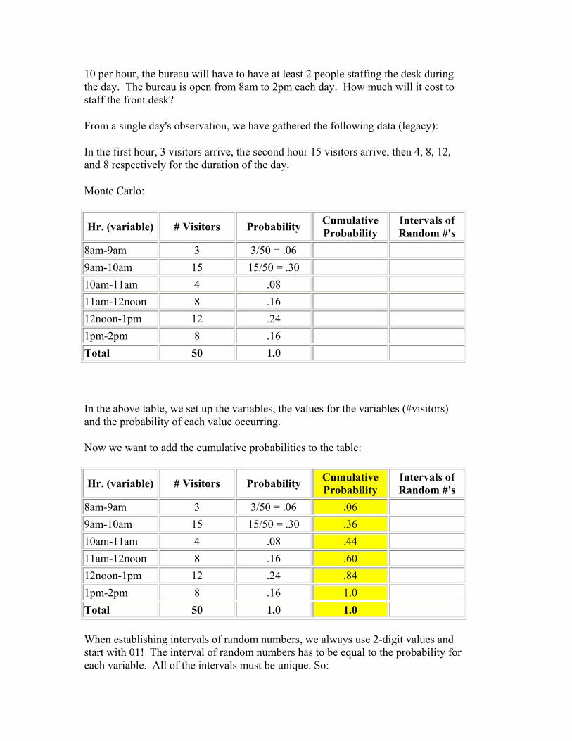
10 per hour, the bureau will have to have at least 2 people staffing the desk during the day. The bureau is open from 8am to 2pm each day. How much will it cost to staff the front desk?
From a single day's observation, we have gathered the following data (legacy):
In the first hour, 3 visitors arrive, the second hour 15 visitors arrive, then 4, 8, 12, and 8 respectively for the duration of the day.
Monte Carlo:
Hr. (variable) # Visitors Probability Cumulative Probability
Intervals of Random #'s
8am-9am 3 3/50 = .06 9am-10am 15 15/50 = .30 10am-11am 4 .08 11am-12noon 8 .16 12noon-1pm 12 .24 1pm-2pm 8 .16 Total 50 1.0
In the above table, we set up the variables, the values for the variables (#visitors) and the probability of each value occurring.
Now we want to add the cumulative probabilities to the table:
Hr. (variable) # Visitors Probability Cumulative Probability
Intervals of Random #'s
8am-9am 3 3/50 = .06 .06 9am-10am 15 15/50 = .30 .36 10am-11am 4 .08 .44 11am-12noon 8 .16 .60 12noon-1pm 12 .24 .84 1pm-2pm 8 .16 1.0 Total 50 1.0 1.0
When establishing intervals of random numbers, we always use 2-digit values and start with 01! The interval of random numbers has to be equal to the probability for each variable. All of the intervals must be unique. So:

Hr. (variable) # Visitors Probability Cumulative Probability
Intervals of Random #'s
8am-9am 3 3/50 = .06 .06 00-05
9am-10am 15 15/50 = .30 .36 06-35
10am-11am 4 .08 .44 36-43
11am-12noon 8 .16 .60 44-59
12noon-1pm 12 .24 .84 60-83
1pm-2pm 8 .16 1.0 84-99
Total 50 1.0 1.0
We then determine how many trials we are going to run. Let's say we want to run 10 trials. We generate random numbers from our Random Number Table (given in last lesson) to run these trials.
Let's use Row 1 from the table to get our random numbers. When a random number is generated, we look to see where it falls relative to the random intervals established above. We then assign the value (# visitors) to :
Trial Random Generated Number
# of Visitors from Random Intervals
1 52 8 2 06 15 3 50 8 4 88 8 5 53 8 6 30 15 7 10 15 8 47 8 9 99 8 10 37 4 Total = 97
From the above table, we see for ten trials, the total number of visitors equals 85. We take the average to determine the how many visitors will arrive per hour.

97/10 = 9.7
Based on this information, we do not need to staff another person at the front desk. Our total daily costs are:
(6hrs/day)*($6/hr) = $36/day
Similarly Monte Carlo Simulation is useful and can be applied for Investment Analysis, Maintenance Policies, Operational Gaming, and Systems Simulation.
I hope that the concept of simulation is now clear to you. It is suggested to you to practice few problems to make the point clear. So let us stop here for now.
Related Documents