Operations Research Lecture 2

Operations Research

Lecture 2:

Linear Programming:

Mathematical Models

Instructors:

Dr. Safaa Amin

Dr. Doaa Ezzat2020/2021

formulating linear programm

The steps for formulating the linear programming are:

1. Identify the unknown decision variables to be determined

and assign symbols to them.

2. Identify the objective or aim and represent it also as a

linear function of decision variables.

3. Identify all the restrictions or constraints in the problem

and express them as linear equations or inequalities of

decision variables.

Construct linear programming model for the following

problems:

2

Example 1

A retail store stocks two types of shirts A and B. These are

packed in attractive cardboard boxes. During a week the store

can sell a maximum of 400 shirts of type A and a maximum

of 300 shirts of type B. The storage capacity, however, is

limited to a maximum of 600 of both types combined. Type A

shirt fetches a profit of Rs. 2 per unit and type B a profit of

Rs. 5 per unit. How many of each type the store should stock

per week to maximize the total profit? Formulate a

mathematical model of the problem.

3

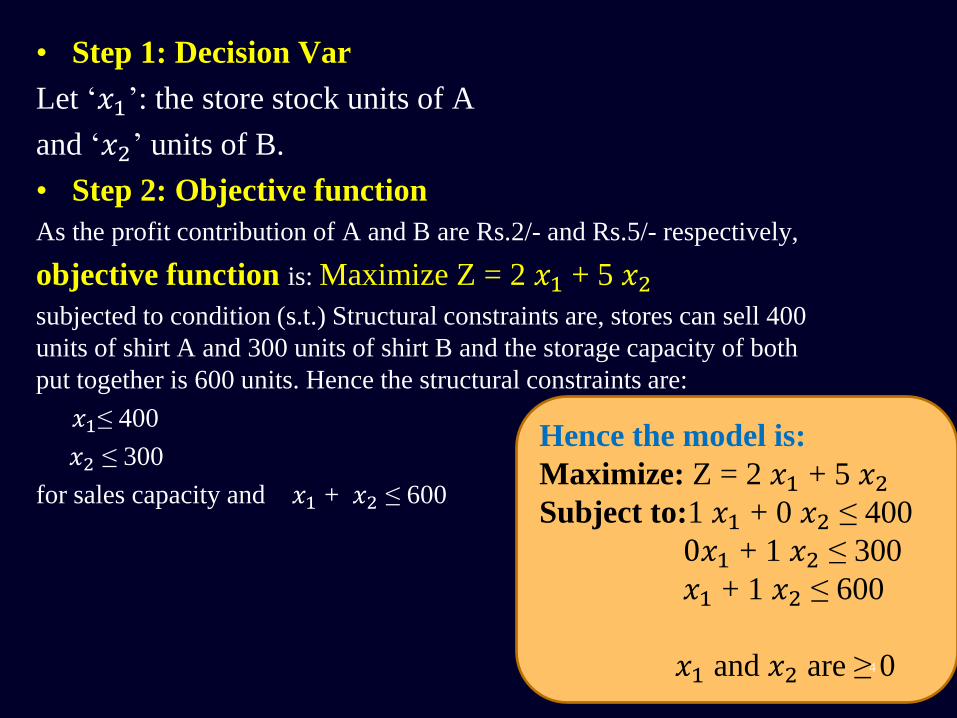
• Step 1: Decision Var

Let ‘𝑥1’: the store stock units of A

and ‘𝑥2’ units of B.

• Step 2: Objective function

As the profit contribution of A and B are Rs.2/- and Rs.5/- respectively,

objective function is: Maximize Z = 2 𝑥1 + 5 𝑥2subjected to condition (s.t.) Structural constraints are, stores can sell 400

units of shirt A and 300 units of shirt B and the storage capacity of both

put together is 600 units. Hence the structural constraints are:

𝑥1≤ 400

𝑥2 ≤ 300

for sales capacity and 𝑥1 + 𝑥2 ≤ 600

4

Hence the model is:

Maximize: Z = 2 𝑥1 + 5 𝑥2Subject to:1 𝑥1 + 0 𝑥2 ≤ 400

0𝑥1 + 1 𝑥2 ≤ 300

𝑥1 + 1 𝑥2 ≤ 600

𝑥1 and 𝑥2 are ≥ 0

Example 2• patient consult a doctor to check up his ill health. Doctor examines

him and advises him that he is having deficiency of two

vitamins, vitamin A and vitamin D. Doctor advises him to

consume vitamin A and D regularly for a period of time so that

he can regain his health. Doctor prescribes tonic X and tonic Y,

which are having vitamin A, and D in certain proportion. Also

advises the patient to consume at least 40 units of vitamin A and

50 units of vitamin D Daily. The cost of tonics X and Y and the

proportion of vitamin A and D that present in X and Y are given

in the table below. Formulate l.p. to minimize the cost of tonics.

5

Example 2 cont.

• Solution: Let x be the units of X that the patient buy

and y units of Y that that the patient buy .

• Objective function:

Minimize Z = 5x + 3y

s.t. 2x + 4y ≥ 40

3x + 2y ≥ 50 and

Both x and y are ≥ 0.

6

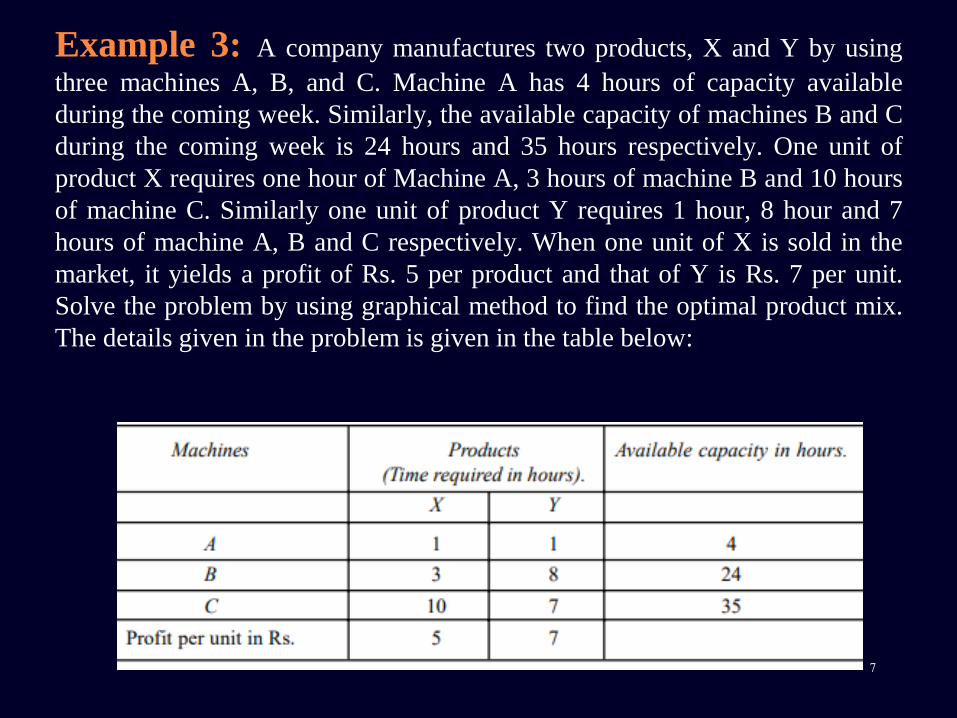
Example 3: A company manufactures two products, X and Y by using

three machines A, B, and C. Machine A has 4 hours of capacity available

during the coming week. Similarly, the available capacity of machines B and C

during the coming week is 24 hours and 35 hours respectively. One unit of

product X requires one hour of Machine A, 3 hours of machine B and 10 hours

of machine C. Similarly one unit of product Y requires 1 hour, 8 hour and 7

hours of machine A, B and C respectively. When one unit of X is sold in the

market, it yields a profit of Rs. 5 per product and that of Y is Rs. 7 per unit.

Solve the problem by using graphical method to find the optimal product mix.

The details given in the problem is given in the table below:

7

Example 3 cont.

• Let the company manufactures x units of X and y

units of Y, and then the L.P. model is:

Maximize Z = 5x + 7y

• Subject to:

1x + 1y ≤ 4

3x + 8y ≤ 24

10x + 7y ≤ 35

Both x and y are ≥ 0.

8

Example 3 cont.

• As we cannot draw graph for inequalities, let us

consider them as equations.

• Maximise Z = 5x + 7y

• s.t. 1x + 1y = 4

• 3x + 8y = 24

• 10x + 7y = 35

• and both x and y are ≥ 0

9

x + y = 4Let us take machine A. and

find the boundary

conditions. If x = 0,

machine A can manufacture

4 units of y

Similarly, if y = 0, machine

A can manufacture 4 units

of x.

10

3x + 8y = 24

Machine B

When x = 0 , y = 3

and when y = 0 x = 8

10x + 7y = 35

Machine C When

x = 0, y = 3.5 and

when y = 0, x = 5.

Graphical Solution to Example 3

11

• Method 1. Here we find the co-ordinates of corners of the closed

polygon ROUVW and substitute the values in the objective function.

• In maximization problem, we select the co-ordinates giving

maximum value.

• And in minimisaton problem, we select the co-ordinates, which gives

minimum value.

• In the problem the co-ordinates of the corners are: R = (0, 3.5), O = (0,0), U =

(3.5,0), V = (2.5, 1.5) and W = (1.6,2.4).

• Substituting these values in objective function:

• Z( 0,3.5) = 5 × 0 + 7 × 3.5 = Rs. 24.50, at point R

• Z (0,0) = 5 × 0 + 7 × 0 = Rs. 00.00, at point O

• Z(3.5,0) = 5 × 3.5 + 7 × 0 = Rs. 17.5 at point U

• Z (2.5, 1.5) = 5 × 2.5 + 7 × 1.5 = Rs. 23.00 at point V

• Z (1.6, 2.4) = 5 × 1.6 + 7 × 2.4 = Rs. 24.80 at point W

• Hence the optimal solution for the problem is company has to manufacture 1.6

units of product X and 2.4 units of product Y, so that it can earn a maximum profit of

Rs. 24.80 in the planning period.12

13

Method 2. profit Line Method: profit line, a line on the graph

drawn as per the objective function, assuming certain profit.

On this line any point showing the values of x and y will yield

same profit. For example in the given problem, the objective

function is Maximize Z = 5x + 7y. If we assume a profit of Rs.

35, to get Rs. 35, the company has to manufacture either 7

units of X or 5 units of Y.

Hence, we draw line Z (preferably dotted line) for 5x + 7y =

35. Then draw parallel line to this line Z at origin. The line at

origin indicates zero rupees profit. No company will be willing

to earn zero rupees profit. Hence slowly move this line away

from origin. Each movement shows a certain profit, which is

greater than Rs.0.00. While moving it touches corners of the

polygon showing certain higher profit. Finally, it touches the

farthermost corner covering all the area of the closed polygon.

This point where the line passes (farthermost point) is the

OPTIMAL SOLUTION of the problem. In the figure 2.6. the

line ZZ passing through point W covers the entire area of the

polygon, hence it is the point that yields highest profit. Now

point W has co-ordinates (1.6, 2.4). Now Optimal profit Z = 5

× 1.6 + 7 × 2.4 = Rs. 24.80.

Points to be Noted:

14

If the profit line passes through single point, it means to say that

the problem has unique solution.

(i) If the profit line coincides any one line of the polygon, then

all the points on the line are solutions, yielding the same

profit. Hence the problem has infinite solutions.

(ii) If the line do not pass through any point (in case of open

polygons), then the problem does not have solution, and we

say that the problem is UNBOUND.

Example 4: Product Mix Problem• A company manufactures three products namely X, Y and Z. Each of

the product require processing on three machines, Turning, Milling and

Grinding. Product X requires 10 hours of turning, 5 hours of milling

and 1 hour of grinding. Product Y requires 5 hours of turning, 10 hours

of milling and 1 hour of grinding, and Product Z requires 2 hours of

turning, 4 hours of milling and 2 hours of grinding. In the coming

planning period, 2700 hours of turning, 2200 hours of milling and 500

hours of grinding are available. The profit contribution of X, Y and Z

are Rs. 10, Rs.15 and Rs. 20 per unit respectively. Find the optimal

product mix to maximize the profit.

15

Z

Example 4 cont.

• Let the company manufacture x units of X, y units

of Y and z units of Z Inequalities: Equations:

• Maximize: Z = 10x + 15 y + 20 z

Subject to: 10 x+ 5y + 2z ≤ 2700

5x + 10y + 4z ≤ 2,200

1x + 1y + 2z ≤ 500

All x, y and z are ≥ 0

16

Period 1 2 3 4 5 6

time 00-04 04-08 08-12 12-16 16-20 20-24

Min required

number

5 10 20 12 22 8

•A truck company requires the following number of drivers for its

trucks during 24 hours: According to the shift schedule, a driver

works eight consecutive hours, starting at the beginning of one of

the six periods. Determine a daily driver worksheet which satisfies

the requirements with the least number of drivers. (Formulate the

mathematical program only)

Example 5 : Manpower Problem

Example 5 : Manpower Problem cont.

Let 𝑥𝑖 𝑖𝑠 𝑡ℎ𝑒 𝑛𝑢𝑚𝑏𝑒𝑟 𝑜𝑓 𝑑𝑟𝑖𝑣𝑒𝑟𝑠 𝑏𝑒𝑔𝑖𝑛𝑖𝑛𝑔 𝑡ℎ𝑒𝑖𝑟 𝑠ℎ𝑖𝑓𝑡 𝑎𝑡 𝑝𝑒𝑟𝑖𝑜𝑑 𝑖𝑥1 + 𝑥6 ≥ 5

𝑥1 + 𝑥2 ≥ 10

𝑥2+𝑥3 ≥ 20

𝑥3 + 𝑥4 ≥ 12𝑥4+𝑥5 ≥ 22

𝑥5+ 𝑥6 ≥ 8

With all variables ≥ 0 and integer

Period 1 2 3 4 5 6

time 00-04 04-08 08-12 12-16 16-20 20-24

Min required

number

5 10 20 12 22 8

Example 6: Transportation Problem

• Four factories, A, B, C and D produce sugar and the

capacity of each factory is given below: Factory A

produces 10 tons of sugar and B produces 8 tons of sugar,

C produces 5 tons of sugar and that of D is 6 tons of sugar.

The sugar has demand in three markets X, Y and Z. The

demand of market X is 7 tons, that of market Y is 12 tons

and the demand of market Z is 4 tons. The following

matrix gives the transportation cost of 1 ton of sugar from

each factory to the destinations.

• Find the optimal solution for least

transportation cost.19

20

𝑥𝑖𝑗: 𝑡ℎ𝑒 𝑛𝑢𝑚𝑏𝑒𝑟 𝑜𝑓 𝑢𝑛𝑖𝑡𝑠 𝑡𝑜 𝑏𝑒 𝑡𝑟𝑎𝑛𝑠𝑝𝑜𝑟𝑡𝑒𝑑 𝑓𝑟𝑜𝑚 𝑓𝑖 𝑡𝑜 𝑀𝑎𝑟𝑘𝑒𝑡 𝑗

Minimize: Z= 4𝑥11 + 3𝑥12 + 2𝑥13…+ 6𝑥31 + 4𝑥32 + 3𝑥33 + 3𝑥41+ 5𝑥42 + 4𝑥43Subject to:

ൢ

𝑥11 + 𝑥12 + 𝑥13 ≤ 10𝑥21 + 𝑥22 + 𝑥23 ≤ 8𝑥31 + 𝑥32 + 𝑥33 ≤ 5𝑥41 + 𝑥42 + 𝑥43 ≤ 6

Supply

constraints

(because the sum must be less

than or equal to the available

capacity)

Transportation Problem cont.

If the total Supply = the Total Demand then

we can rewrite all the constraints as equal

constraints

21

ቑ

𝑥11 + 𝑥21 + 𝑥31 + 𝑥41 ≥ 7𝑥12 + 𝑥22 + 𝑥32 + 𝑥42 ≥ 12𝑥13 + 𝑥23 + 𝑥33 + 𝑥43 ≥ 4

𝑥𝑖𝑗 ≥ 0 where i=1,2,3,4 and j=1,2,3

Demand

constraints

(This is because we cannot

supply negative elements)

Example 7: Assignment Model

• There are 3 jobs A, B, and C

and three machines X, Y, and

Z. All the jobs can be processed on

all machines. The time required for

processing job on a machine is

given below in the form of matrix.

Make allocation to minimize the

total processing time.22

Case1 Case2 Case3 Case4 Case5

Lawyer1 145 122 130 95 115

Lawyer2 80 63 85 48 78

Lawyer3 121 107 93 69 95

Lawyer4 118 83 116 80 105

Lawyer5 97 75 120 80 111 23

•A legal firm has accepted five new cases, each of which can be

handled by any one of its five junior partners. Due to difference in

experience and expertise, however, the junior partners would spend

varying amounts of time on the cases. A senior partner has

estimated the time required in hours as shown below

Determine the optimal assignment of cases to lawyers such that

each junior partner receives a different case. And the total hours

expected by the firm is minimized. Formulate the corresponding

mathematical program.

Example 7: Assignment Model

24

𝑥𝑖𝑗: 𝑡ℎ𝑒 𝑛𝑢𝑚𝑏𝑒𝑟 𝑜𝑓 𝑡𝑖𝑚𝑒𝑠 𝑡ℎ𝑎𝑡 𝐿𝑎𝑤𝑦𝑒𝑟𝑖 𝑎𝑠𝑠𝑖𝑔𝑛𝑒𝑑 𝑡𝑜 𝑐𝑎𝑠𝑒 𝑗

Minimize: Z=145𝑥11 + 122𝑥12 + 130𝑥13…+ 121𝑥31 + 107𝑥32 + 93𝑥33 + 118𝑥41+ 83𝑥42 + 116𝑥43 + 80𝑥44 + 105𝑥45…+ 111𝑥55Subject to:

Case1 Case2 Case3 Case4 Case5

Lawyer1 145 122 130 95 115

Lawyer2 80 63 85 48 78

Lawyer3 121 107 93 69 95

Lawyer4 118 83 116 80 105

Lawyer5 97 75 120 80 111

𝒙𝟏𝟏 + 𝒙𝟏𝟐 + 𝒙𝟏𝟑 + 𝒙𝟏𝟒 + 𝒙𝟏𝟓 = 𝟏𝒙𝟐𝟏 + 𝒙𝟐𝟐 + 𝒙𝟐𝟑 +𝒙𝟐𝟒 +𝒙𝟐𝟓 = 𝟏𝒙𝟑𝟏 + 𝒙𝟑𝟐 + 𝒙𝟑𝟑 + 𝒙𝟑𝟒 + 𝒙𝟑𝟓 = 𝟏𝒙𝟒𝟏 + 𝒙𝟒𝟐 + 𝒙𝟒𝟑 + 𝒙𝟒𝟒 + 𝒙𝟒𝟓 = 𝟏𝒙𝟓𝟏 + 𝒙𝟓𝟐 + 𝒙𝟓𝟑 + 𝒙𝟓𝟒 + 𝒙𝟓𝟓 = 𝟏

𝑥11 + 𝑥21 + 𝑥31 + 𝑥41 + 𝑥51 = 1𝑥12 + 𝑥22 + 𝑥32 +𝑥42 +𝑥52 = 1𝑥13 + 𝑥23 + 𝑥33 + 𝑥43 + 𝑥53 = 1𝑥14 + 𝑥24 + 𝑥34 + 𝑥44 + 𝑥54 = 1𝑥15 + 𝑥25 + 𝑥35 + 𝑥45 + 𝑥55 = 1

Each lawyer is

assigned to one

case

Each case is

assigned to one

lawyer

with all variables non-negative and integer

What if???

Number of Cases is Less than the number of

Lawyers (3 cases and 5 lawyers)

25

3 cases and 5 Lawyers

26

𝒙𝟏𝟏 + 𝒙𝟏𝟐 + 𝒙𝟏𝟑 ≤ 𝟏𝒙𝟐𝟏 + 𝒙𝟐𝟐 + 𝒙𝟐𝟑 ≤ 𝟏𝒙𝟑𝟏 + 𝒙𝟑𝟐 + 𝒙𝟑𝟑 ≤ 𝟏𝒙𝟒𝟏 + 𝒙𝟒𝟐 + 𝒙𝟒𝟑 ≤ 𝟏𝒙𝟓𝟏 + 𝒙𝟓𝟐 + 𝒙𝟓𝟑 ≤ 𝟏

𝑥11 + 𝑥21 + 𝑥31 + 𝑥41 + 𝑥51 = 1𝑥12 + 𝑥22 + 𝑥32 +𝑥42 +𝑥52 = 1𝑥13 + 𝑥23 + 𝑥33 + 𝑥43 + 𝑥53 = 1

Example 8: Inspection Model

• A company has two grades of inspectors, I and II to undertake

quality control inspection. At least 1,500 pieces must be

inspected in an 8-hours day. Grade I inspector can check 20

pieces in an hour with an accuracy of 96%. Grade II inspector

checks 14 pieces an hour with an accuracy of 92%. Wages of

grade I inspector are $5 per hour while those of grade II

inspector are $4 per hour. Any error made by an inspector

costs $3 to the company. If there are, in all, 10 grade I

inspectors and 15 grade II inspectors in the company, find the

optimal assignment of inspectors that minimize the daily

inspection cost (Formulate only the mathematical problem).

27

Example 8: Inspection Model

• Let x the number of grade I that may be

assigned the job of quality control

inspection

• Let y the number of grade II that may be

assigned the job of quality control

inspection

28

• The objective is to

minimize the daily cost of

inspection

• Two cost: wages paid by

inspectors and the cost of

inspector error

29

Grade IIGrade I

Check 14

pieces /h

Check 20

pieces /h

92%96%Accuracy

0.080.04Error 3costs

45Wages

1510 inspectorsavailable

• The cost of grade I inspector per hour

• (5+3x0.04x20)=7.4

• The cost of grade II inspector per hour

(4+3x0.08x14)=7.36

The objective function

Z=8 (7.4x+7.36y)

Example 8: Inspection Model

30

• x≤ 10

• 𝑦 ≤ 15

• 20*8x+14*8y≥ 1500

• With all variable non-negative and integer

31