Operating capability of long AC EHV transmission cables

Electric Power Systems Research 75 (2005) 17–27

Operating capability of long AC EHV transmission cables

Roberto Benato∗, Antonio Paolucci1

University of Padova, Department of Electrical Engineering, Via Gradenigo 6/A, 35131 Padova, Italy

Received 29 April 2004; accepted 23 November 2004Available online 18 April 2005

Abstract

The operating constraints involved in power transmission of long AC cable links are presented and here throughout developed. The possibilityof transmitting high power rating is examined and the transmission length limits are evaluated. The procedure, which uses the great computationand graphical facilities of modern computers, is essentially based on the classical transmission equations and their pertaining diagrams. Ithas been particularly applied to XLPE cables and gas-insulated lines but it is worth applying to any distributed-parameter transmission line(including overhead lines). The capability chart proposed in the paper is a useful tool to highlight the operating characteristics of a cable linkand a guide to evaluate the results of different degrees of reactive compensation. The authors hope that the results can offer the transmissions©

K

1

itlto[iefiqatd

wl

n if

giesbe-

hus,op-

luateable

aser

bethe

yupon

0d

ystem operators very effective means in order to evaluate the existing and future underground cable links.2005 Elsevier B.V. All rights reserved.

eywords:XLPE cable; EHV transmission lines; Underground technology; Gas insulated lines

. Introduction

Deregulation of the electricity supply markets and grow-ng environmental awareness stress the necessity of newransmission line solutions alternative to traditional overheadines. So the transmission scenario is paying a great atten-ion to the underground technologies. In particular, the usef XLPE AC cable lines seems very promising for new links

1–3]. EHV cables can be used mainly for power transmissionn large urban heavily populated agglomerations, as feed-rs in outdoor substations, and as generator bus-ducts. Therst major (i.e. where a significant number of joints is re-uired) XLPE cable systems have been in service since 1997t 400 kV and 2000 at 500 kV. Since those dates, the impor-

ance and the interest on these applications are increased andeserve a very careful consideration.

Another promising technology is represented by cablesith gas mixture insulation (the so called gas insulated

ines (GIL)): the world installations amount today roughly

∗ Corresponding author. Tel.: +39 049 8277532; fax: +39 049 8277599.

to 100 km and the maximum line length is 3.3 km evemuch longer runs are under study[4].

Hence, in the future the variety of employed technoloin the EHV transmission could be much more than nowing the network chiefly constituted by overhead lines. Tit results fundamental to give the transmission systemerators simple but precise engineering means to evathe transmission operating characteristics of long AC clinks.

2. Settlement of the question

The main function of a cable in a EHV/HV network (well as any transmission line) is to transmit active powPwith a small amount of inductive powerQ.

Moreover, it is well known that a long service life canreached only with these constraints in any point alongcable:

- Avoiding that the currents exceed the cable ampacitIc,meant as the current carrying capacity (depending

E-mail address:[email protected] (R. Benato).1 Tel.: +39 049 8277516; fax: +39 049 8277599.

the installation conditions) under stated thermal conditionswithout degradation.

378-7796/$ – see front matter © 2005 Elsevier B.V. All rights reserved.oi:10.1016/j.epsr.2004.11.011

18 R. Benato, A. Paolucci / Electric Power Systems Research 75 (2005) 17–27

Table 1Data of 400 kV XLPE cables under study

Cable #a Cable #b

Cross sectional area (mm2) 2500 Cu 630 CuConductor diameter (mm) 65.0 30.8Conductor screen diameter (mm) 71.6 32.8Insulation diameter (mm) 122.0 92.8Insulation screen diameter (mm) 128.3 94.8Metallic shield diameter (mm) 130.9 Al 101.8 PbJacket of PE diameter (mm) 142.5 117Overall diameter (mm) 142.5 117Total mass (kg/m) 37 28

- Avoiding that the phase-to-earth voltages|U- o| exceed thehighest rms. VoltageUm/

√3 (Insulation Co-ordination In-

ternational Standard) for cable both on-load and no-loadconditions.

It is evident that foreseeing any operating conditions israther impossible; notwithstanding, reasonable essential cri-teria are generally considered not to exceed, during operation,the ampacity limits at both ends (S forSending-endand R forReceiving-end) and to assure a phase-to-earth voltage levelin one of the two ends (in this paper S will be always chosen):

|I-R| ≤ Ic (1)

|I-S| ≤ Ic (2)

|U- oS| = Uoc. (3)

In the following investigations, whereUm = 420 kV, it hasretained the levelUoc = 230 kV = 95%Um/

√3.

A throughout analysis of the cable operating characteris-tics with the aforementioned constraints has been presentedin [5], which constitutes (chiefly by means of a general aba-cus) one of the first elegant (dated 1986) approaches. It hasbeen a strong suggestion for the authors.

By a purely theoretical point of view, any cable line isan asymmetrical multiconductor system because of both thec nge-m

t ofp in this

formulation a single-phase positive sequence two-port net-work will be simply considered.

Let’s consider a uniform transmission line with distributedparameters: the starting point is a rigorous application of thefamous transmission formulae (solution of the telegraphist’sequations) first written in 1876 by Oliver Heaviside[6] andthen used, rearranged and divulged by Steinmetz[7], Rossler[8], La Cour[9]:

U- oS = A- · U- oR + B- · I-R (4)

I-S = C- · U- oR + A- · I-R; (5)

(the per unit method will not be used in this paper to achievehigher engineering concreteness in terms of line operation).

Tables 1 and 2report the main data for two different EHV#a and #b cables.

Firstly, cable #a will be considered.

3. First analysis:U- oS and |I-R| constrained

A first analysis on the possible operating conditions can beperformed if both the current magnitude at R and the voltagephasorU- oS at S are constrained as follows:

IR = (Ic∠0) = (1.6 kA∠0) on the real axis

U

s d( ns:

U

I

TP

C (I

P r (mP (mP g (nP c (C Z- 0

P k- (kSC Ica

A Ic (

onsideration of the shields and asymmetrical laying arraents.Nevertheless, since in the EHV cable line laying a lo

hase transpositions and cross-bondings are adopted,

able 2arameters of 400 kV XLPE cables under study

ross sectional areanstallation

er unit length resistance of phase conductor at 90Cer unit length series inductanceer unit length shunt leakance (50 Hz) with loss factor tanδ= 0.0007er unit length shunt capacitance withεr = 2.3haracteristic impedanceropagation factorurge impedance loading at 400 kVapacitive current related toUo = 400 kV/

√3

mpacity

-

- oS = (Uo∠δ) = (230 kV∠δ) δ = 0–2π

o that the remaining quantitiesU- oRandI-Scan be determinesee(A3) in Appendix A) by means of subsequent equatio

- oR = 1

A-· U- oS − B-

A-· I-R → U- oR

= 1

A-· (230 kV∠δ) − B-

A-· (1.6 kA∠0) (6)

-S = C-A-

· U- oS + 1

A-· I-R → I-S

= C-A-

· (230 kV∠δ) + 1

A-· (1.6 kA∠0) (7)

Cable #a Cable #b

mm2) 2500 Cu 630 CuDirectly buried withspacing 0.35 m

Directly buried trefoilspacing 0.12 m

/km) 10.8 36H/km) 0.571 0.460S/km) 53 27F/km) 0.240 0.123

() 48.84∠−.03 rad 62.01∠−.12 radm−1) (0.1 + j3.7)× 10−3 (0.3 + j2.4)× 10−3

SIL (MVA) 3276 2577

p (A/km) 17.40 8.92A) 1600 650

R. Benato, A. Paolucci / Electric Power Systems Research 75 (2005) 17–27 19

Fig. 1. Phasorial diagram of the Eq.(7) with 1.6 kA ampacity at R.

In particular, Eq.(7) gives the phasorial diagram ofFig. 1(where only for graphical purpose, pointN has been placedsensibly far from pointM). The foregoing diagram shows,once fixedI-R = 1.6 kA on the real axis, how the angleδ ofU- oS = (230 kV∠δ) can value the whole interval 0–2π givingrise to two different groups:

(i) any regimes with|I-S| < 1.6 kA = |I-R| compatible withthe cable ampacity (e.g. see the phasors OL1, OL2 andOL3);

(ii) any regimes with|I-S| > 1.6 kA not allowable (e.g. seethe phasors OH1, OH2 and OH3).

In particular, the phasors OK1 and OK2 which yield atδ1 = 21.08 andδ2 = 158.9, respectively (when consideringcable #a withd= 60 km) correspond to|I-S| = 1.6 kA = |I-R|,and concern two very meaningful regimes for power flowsbetween S and R (see Section6).

It is trivial that the calculation ofU- oR by means of(6)allows individuating and consequently warning of possibleoperations with too high voltages (dangerous for the insula-tion) or too low voltages (unsuitable for operation). At the endof this first analysis, an allowable group of complex power atS and at R becomes known.

4

tingc (be-ytA

U

Fig. 2. Phasorial diagram of Eq.(9) with 1.6 kA ampacity at S.

I-R = −C- · U- oS + A- · I-S → I-R

= −C- · (230 kV∠ϑ) + A- · (1.6 kA∠0) (9)

it is possible to analyze the effects of|I-S| = 1.6 kA (on thereal axis) and ofU- oS = (230 kV∠ϑ), whereϑ (angle ofU- oSwith respect toI-S) ranging between 0 and 2π. Eq.(9) can bevisualized by means of the phasor diagram ofFig. 2. This dia-gram shows, once fixedI-S = 1.6 kA on the real axis, how theangleϑ of U- oS = (230 kV∠ϑ) can value the whole interval0–2π giving rise to two different groups:

(iii) any regimes with|I-R| < 1.6 kA compatible with the ca-ble ampacity (e.g. OL′, OL′′ and OL′′′);

(iv) any regimes with|I-R| > 1.6 kA not allowable (e.g. OH′,OH′′ and OH′′′).

In particular, the phasors OK′ and OK′′ which yield atϑ′ = 197.1 andϑ′′ = 343.1, respectively (when consideringcable #a withd= 60 km) individuate again two regimes (asOK2 and OK1 in the first analysis) with|I-R| = 1.6 kA = |I-S|.In addition, the use of(8) allows warning of unsatisfactoryvoltage levels (too high or too low) at R. At the end of thissecond analysis, another allowable group of complex powerat S and at R becomes known.

5

ing-e e oft antt ordert t and

. Second analysis:U- oS and |I-S| constrained

In order to complete the analysis of the possible operaonditions, let us consider the allowable regimes whenond the phasorU- oS) the sending-end current|I-S| is fixed athe cable ampacityIc. By means of(8) and(9) (see(A4) inppendix A)

- oR = A- · U- oS − B- · I-S → U- oR

= A- · (230 kV∠ϑ) − B- · (1.6 kA∠0) (8)

. Voltages and currents along the cable

The knowledge of the currents and voltages at sendnd S and receiving-end R is not completely exhaustiv

he whole electric behaviour of cable: in fact it is importo examine the currents and voltages along the cable ino investigate possible points exceeding the fixed curren


Fig. 3. Current magnitudes along the cable #a with ampacity at R (I analysis).

Fig. 4. Voltage magnitudes along the cable #a with ampacity at R (I analysis).

voltage limits; to this aim, the use of(A5) could be suitable.Fig. 3 shows for cable #a withd= 60 km the behaviour ofthe current along the cable in some allowable cases by the“first analysis”: it is of note the curve 1′ (see point K1 inFig. 1) where both the end currents have same magnitudesequal to the ampacity. The other curves 2′–6′ regard otherregimes (e.g. current phasors as OL ofFig. 1) not exceedingthe ampacity along the cable.Fig. 4shows the voltages alongthe cable in the same regimes; analogously,Figs. 5 and 6show the results along the cable for some allowable regimesby the “second analysis”.

These kinds of analysis along the line performed for othercables have shown analogous behaviours since the ampacityis much lower than the “natural current”In = Uoc/|Z- 0|. Itseems that this fact has passed unobserved.

In any case, the mid-line valuesU- oT andI-T included intothe matrix analysis(A8) and(A9) can give a suggestion forinvestigations in further points.

In order to complete the operating analyses, the current andvoltage in no-load condition must be evaluated. By settingI-R = 0 into (6) and(7), the no-load voltage and current can

Fig. 5. Current magnitudes along the cable #a with ampacity at S (II analy-sis).

Fig. 6. Voltage magnitudes along the cable #a with ampacity at S (II analysis)

be computed as follows:

(U- oR)I-R=0 = 1

A-· U- oS; (I-S)I-R=0 = C-

A-· U- oSU- oS. (10)

In particular, (see,Table 3) for cable #a, the limit length forno-load voltage isdU = 87.75 km and that for no-load currentis dI = 88.95 km.

6. Power capability chart

The performing of the numerical analysis in Sections3–5does not present any problem; particular attention must bedevoted to the classification of numerous computed regimesin order to single out those technically allowable and to per-form curves which are helpful for evaluating and eventuallyincreasing the transmission power capability. In this regard,the curves inFig. 7can give (not withstanding their graphicalsimplicity) very meaningful information on cable #a powercapability features varying its length (30, 60 and 90 km).

Table 3Current and voltage magnitudes in no-load condition

Cable #a Cable lengthd (km)

Nt R (kV

o-load at R;|U- oS| = 230 kV Current magnitude at S (kA)Phase-to-earth voltage magnitude a

30 60 87.75 88.95 90 120

0.52 1.06 1.58 1.60 1.62 2.23) 231.4 235.7 242.5 243.8 243.2 254.3


Fig. 7. Power capability charts for cable #a.

- By using the criteria of Section3, the regimes compatiblewith the constraints|I-R| = 1.6 kA and|I-S| = 1.6 kA havebeen evaluated and their receiving-end complex power (e.g.points• 1–4) has been reported forming the solid lines a(seeFig. 7), whilst the corresponding sending-end complexpower (e.g. pointso 1–4) forming the solid line b.

- Analogously, by analysing the regimes|I-S| = 1.6 kA and|I-R| ≤ 1.6 kA, according to Section4, the dashed curves cand d have been drawn; the curve c represents the receiving-end complex power (e.g. points• 4–7, 1) and d the sending-end complex power (e.g. pointso 4–7, 1).

Therefore, once fixed the cable ampacity at 1.6 kA, thecontours a–c set the boundaries of allowable receiving-endpower area whereas the contours b–d that of allowablesending-end power. As it can be gathered by power balanceof Fig. 7, each sending-end power givesPS just higher thanPR (since the active power lossesp are low) butQS muchinferior toQR (since the cable itself generates high inductivepowerq).

In particular, points 1 and 4 (maximum active power flowbetween S and R) correspond to the K regimes ofFigs. 1 and 2.The shadowed areas in the diagrams ofFig. 7highlight howthe power flows with high cosϕ are more and more limitedwhile increasing the cable length (up to almost zeroed asin Fig. 7III). This seriously jeopardizes the chief aim of thetransmission link most of all in the proximity of ampacitylimit. By this important point of view, the length of 25–30 km(seeFig. 7I) can be already considered as a length limit[5].

Fig. 8shows the dramatic worsening of permissible powerfactor withd= 120 km.

However, this length would result not allowed because ofnvfi ase-t

a omicp orko ofF olt-a

ita ther

o-load condition: the point O (namelyPR + jQR = 0) laysery far from theReceiving-end Power Area, asTable 3con-rms showing a no-load current of 2.23 kA at S and a pho-ground voltage of 254.3 kV at R.

On the contrary, strong reactive power flows (seeFig. 7)re possible, but they are often not convenient by an econoint of view and hence less important in the normal netwperation. Exclusively in the neighbourhoods of point 6ig. 7III (grey-solid lines) the regimes request too high vges at R (UoR >Um/

√3 = 242.5 kV).

Fig. 7III also highlights very well the no-load current limt S when R is not loaded: it is sufficient to note thateceiving-end powerPR + jQR = 0 lays (point• 6) almost on

Fig. 8. Power capability chart for cable #a;d= 120 km.


Fig. 9. Power capability chart comparison between cable #b and cable #a;d= 60 km.

dashed line c with parameter|I-S| = 1.6 kA (exactly it wouldbe 1.62 kA as inTable 3).

Even the only analysis of these few cases (d= 30, 60, 90and 120 km) seems to highlight very well how, in the useof EHV cable, the first important problems, (which increasewith the lengthd) are the difficulties to have consistent activepower flows with high cosϕ (shadowed areas inFig. 7); onlysuccessively (seeTable 3), the Ferranti effect and the no-loadcurrent take a predominant and decisive role. This could bedrastically inverted if “weak networks” are considered (as itcould be shown in further researches). The main responsibleof these problems is the well-known high capacitive suscep-tance, which has to be sensibly compensated by means ofshunt reactors.

The analyses up to here have been performed for cable #aover different lengths: if cable #b is considered, the featuresbecome slightly worse. For instance, the comparison inFig. 9,performed ford= 60 km, shows that cable #b suffers in themaximum transmissible active power a stronger reductionthan in the ampacity and a worsening in the correspondingpower factor.Table 4reports the no-load conditions of cable#b and is worth comparing withTable 3of cable #a.

Furthermore, it could be useful for transmission systemoperators to enhance the capability chart (seeFig. 10) addingalso the curves referring to current values less than cable am-pacity so that for each transmissible complex power the mar-g rvesi ect)

Fig. 10. Enhanced capability chart at receiving-end for cable #a;d= 60 km.

Fig. 10.bis. Triangles for Briggs formula application.

can be adopted alternatively to analysis in Sections3 and 4:it is based upon Eq.(A10) andFig. 10.bis. It is sufficient tonote that the value ofβ can be derived by means of well-known Briggs formula applied on the two triangles OL′Nand OL′′N (once set the magnitudes of their sides|A- ||I-S|,|I-R| and| − C-U- oS|, which have to be geometrically compat-ible). Eq.(A10) must be obviously computed twice for bothI′R = IR ej(α−β) andI-R

′′= IR ej(α+β).

The calculations ofU- oS andU- oR and the complex powerare rather immediate.

TC

C Cable lengthd (km)

30 60 72.5 90 120

N 0.27 0.54 0.65 0.81 1.11at R (kV) 230.6 232.3 233.4 235.3 239.6

ins are immediately evident. For computation of the cun Fig. 10a single procedure (less heuristic but more dir

able 4urrent and voltage magnitudes in no-load condition

able #b

o-load at R;|U- oS| = 230 kV Current magnitude at S (kA)Phase-to-earth voltage magnitude


7. Effects of shunt compensation

If the hypothesis of uniformly distributed compensationis retained, the abovementioned procedures are still valid: infact, once the new admittancey

-(function of the compensa-

tion degreeξsh) has been computed by means of(A12) andonce all the other parameters (k-, Z- 0, and so on) have beenupdated, all the aforementioned procedures (Sections3–6)can be suitably used in order to evaluate the compensationeffects. This hypothesis, notwithstanding being merely theo-retical, presents small differences from real installation tech-niques[10]. The capability charts ofFig. 11evidence (with animmediate comparative view) the more or less advantageous

effects depending uponξsh for cable #a. The comparison be-tweenTable 3andTable 5shows how smallξsh can renderpermissible the no-load regimes up to great lengths. Further-more, it should be noted that also the lengthd= 120 km canbe fully re-qualified ifξsh= 0.85.

As a result of application of an increasingly highercompensation degreeξsh (from 0.5 to 0.85), the cableline increasingly approaches to a mere series impedance(ohmic–inductive one).

This effect yields higher voltage drop for reactive powerflows: in the capability charts, the “upper” grey-solidcurves represent regimes with too low voltage profiles (i.e.|U- oR| < 215 kV) whilst the “lower” ones regimes with too

Fig. 11. Power capability charts for cable #a w
ithd= 60, 90 and 120 km andξsh= 0.85; 0.5.


Table 5Current and voltage magnitudes in no-load condition with two differentξsh

Cable #a Cable lengthd (km)

60 90 120

ξsh= 0.50 Current magnitude at S (kA) 0.525 0.795 1.076Phase-to-earth voltage magnitude at R (kV) 232.8 236.4 241.6

ξsh= 0.85 Current magnitude at S (kA) 0.16 0.235 0.315Phase–to–earth voltage magnitude at R (kV) 230.8 231.9 233.4

Table 6Typical data of 400 kV GIL under study

Gas insulated line

Cross sectional area of phase (Al IACS = 61%) (mm2) 5341Cross sectional area of enclosure (Al alloy

IACS = 52.57%) (mm2)16022

Phase outer diameter (mm) 180Phase thickness (mm) 10Enclosure inner diameter (mm) 500Enclosure thickness (mm) 10

high voltage profiles (i.e|U- oR| > 420/√

3); the grey-printedvalues indicate the minimum and maximum voltages at R,respectively.

8. Cables with gas insulation: GILs

The proposed procedure has been suitably applied to an-other kind of cable with gas mixture insulation namely gasinsulated transmission line[11]: Tables 6 and 7report thetypical data and the parameters used in the following analy-sis.

FromTable 7it is of note the low per unit length capaci-tancec (54.5 nF/km) and the high ampacity (2400 A).

By using Eq.(A11) the following no-load voltage andcurrent limit lengths arise, respectively:

dU = 308 km; dI = 542 km

Table 7Parameters of 400 kV GIL under study

Gas insulated line

Installation Directly buried flatwith axial spacing1.3 m

Per unit length resistance of phase at60C, r (m/km)

6.286

P

PPPCPSC

A

Fig. 12. Power capability chart for GIL;d= 120 km.

It is worth noting that the limitdU is much more restric-tive thandI . Also the other criterion, which deals with thepower capability, is few limiting: bothFig. 12(d= 120 km)andFig. 13(d= 240 km) highlight that GILs are suitable forbulk power transmission even if without compensation. Thisgood behaviour fades slightly up to 300 km. The ultimate re-tained criteria are the voltages and currents along the GIL:the current magnitudes never exceed the ampacity whereas

ph

er unit length resistance of enclosure at50C, ren (m/km)

2.330

er unit length series inductance, (mH/km) 0.204er unit length shunt leakage,g (nS/km) Negligibleer unit length shunt capacitance,c (F/km) 0.0545haracteristic impedance,Z- 0 () 61.46∠−0.07 radropagation factor,k- (km−1) 0.0001 + j0.001urge impedance loading at 400 kV, SIL (MVA) 2604apacitive current related toUo = 400 kV/

√3, Icap (A/km)

3.95

mpacity,Ic (A) 2400
Fig. 13. Power capability chart for GIL;d= 240 km.


the regimes exceeding the voltage limit are highlighted inFigs. 12 and 13by means of grey lines; this confirms thewell-known difficulties to transmit high reactive power flowsover long distances. The capability chart (along with “greywarnings”) computed for higher ampacity (e.g.Ic = 3000 A)would show shorter length limits (100–150 km).

9. Regimes withUoc =230 kV

In the foregoing cases it has been always set|UoS| =Uc = 230 kV according to(3). Other capability chartswith Uoc< or >230 kV could be helpful to transmission sys-tem operators in order to optimise the network regimes indaily load variations.

10. Conclusion

The paper gives efficient means in order to evaluate thepower capability of EHV ac cables. The power capabilitychart represents an immediate and precise outlook on the pos-sibilities of active and reactive power flows along the link. Ineach capability chart, the regimes that give rise to receiving-end voltages too high or too low are highlighted. The voltageand current magnitudes in any point along the cable havebeen also considered. The cable limit lengths can be over-c hartss ationd lied tog rfor-m n thec opedi

A

DiM edt ighV ens

A

[

w

A

C

d (km) cable length;

k- = √z- · y

-(km−1) propagation factor;

Z- 0 =√z-y-

(Ω) characteristic impedance;

z- = r + jω (/km); y-

= g + jωc (S/km); (A2)

r (/km); (H/km); c (F/km);g=ωctanδ (S/km).These values can be easily computed or obtained by means

of cable manufacturers.The Eqs.(6) and (7)used in the first analysis can be syn-

thesized by[U- oR

I-S

]=[

1/A- −B- /A-C- /A- 1/A-

]︸︷︷︸

M1-

·[U- oS

I-R

], (A3)

whilst Eqs.(8) and (9)of the second analysis by means of[U- oR

I-R

]=[

A- −B-−C- A-

]︸︷︷︸

M2-

·[U- oS

I-S

]. (A4)

From(A4) it is rather immediate to achieve[

w thecm

ca[

w

[

t

ome by means of shunt compensation: the capability chow the different benefits depending upon the compensegree. The procedure has been also successfully appas insulated transmission lines showing promising peance in power transmission. The method is based o

lassic transmission formulae and has been fully develn matrix form.

cknowledgements

The authors gratefully acknowledge both Ing. Claudioario (Italian GRTN–Grid Division) for having appreciat

he paper aims and Prof. Rudolf Woschizt (Institute of Holtage Engineering, University of Graz) for having givome technological data on shunt reactors.

ppendix A

The Eqs.(4) and (5)can be rearranged in matrix form:

U- oS

I-S

]=[A- B-C- A-

]︸︷︷︸

M-

·[U- oR

I-R

](A1)

here

- = cosh(k-d); B- = Z- 0 · sinh(k-d);

- = [sinh(k-d)]/Z- 0;

U- ox

I-x

]=[

A- x −B- x−C- x A- x

]︸︷︷︸

Mx-

·[U- oS

I-S

], (A5)

hich allows calculating the voltages and currents alongable (at a distancex from S) havingA- x, B- x andC- x obviouseaning.By observing the diagrams ofFigs. 3–6it is sufficient to

alculate (similarly to(A5)) simply the mid-line valuesUoTndIT by means of

U- oT

I-T

]=[

A- T −B- T

−C- T A- T

]·

︸︷︷︸MT-

[U- oS

I-S

](A6)

here the subscript T refers to line mid point.In conclusion, since(A7) can be obtained by(A3)

U- oS

I-S

]=[

1 0

C- /A- 1/A-

]︸︷︷︸

M ′-

·[U- oS

I-R

], (A7)

he first analysis can be wholly computed with

U- oR

I-S

U- oT

I-T

=

M- 1

M- TM-′

·

[U- oS

I-R

]. (A8)


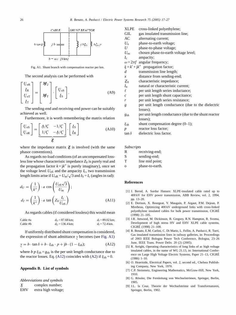
Fig. A1. Shunt branch with compensation reactor per km.

The second analysis can be performed withU- oR

I-R

U- oT

I-T

=

M- 2

M- T

·

[U- oS

I-S

]. (A9)

The sending-end and receiving-end power can be suitablyachieved as well.

Furthermore, it is worth remembering the matrix relation[U- oS

U- oR

]=[A- /C- −1/C-1/C- −A- /C-

]︸︷︷︸

Z-

·[I-S

I-R

](A10)

where the impedance matrixZ- is involved (with the samephasor conventions).

As regards no-load conditions (of an uncompensated loss-less line whose characteristic impedanceZ0 is purely real andthe propagation factork= jk′′ is purely imaginary), once setthe voltage levelUoS and the ampacityIc, two transmissionlength limits arise ifUoR =Um/

√3 andIS = Ic (angles in rad):

dU =(

1

k′′

)· a cos

(UoS

√3

Um

);

( ) ( )

ean

C ;C

red,t

y

w tot

A

AX

E

XLPE cross-linked polyethylene;GIL gas insulated transmission line;AC alternating current;Uo phase-to-earth voltage;U phase-to-phase voltage;Uoc chosen phase-to-earth voltage level;Ic ampacity;ω = 2πf angular frequency;k- =k′ + jk′′ propagation factor;d transmission line length;x distance from sending-end;Z- 0 characteristic impedance;In natural or characteristic current; per unit length series inductance;c per unit length shunt capacitance;r per unit length series resistance;g per unit length conductance (due to the dielectric

losses);gsh per unit length conductance (due to the shunt reactor

losses);ξsh shunt compensation degree (0–1);p reactor loss factor;tanδ dielectric loss factor.

SubscriptsRSTo

R

p to94,

, P.kedGR

ma,ms,

ri,dings3–26

agenfer-IGR

blish-

ork,

,

n,

dI = 1

k′′ · a tan Z0Ic

UoS(A11)

As regards cables (if considered lossless) this would m

able #a dU = 87.68 km; dI = 89.02 kmable #b dU = 136.4 km; dI = 72.4 km.

If uniformly distributed shunt compensation is considehe expression of shunt admittancey

-becomes (seeFig. A1)

-= b · tanδ + b · ξsh · p + jb · (1 − ξsh); (A12)

hereb p ξsh=gsh is the per unit length conductance duehe reactor losses. Eq.(A12) coincides with(A2) if ξsh= 0.

ppendix B. List of symbols

bbreviations and symbols

- complex number;HV extra high voltage;

receiving-end;sending-end;line mid point;phase-to-earth.

eferences

[1] J. Bernd, A. Surdur Hansen: XLPE-insulated cable rated u400 kV for EHV power transmission, ABB Review, vol. 2, 19pp. 13–20.

[2] E. Dorison, X. Bourgeat, Y. Maugain, P. Argaut, P.M. DejeanMirebeau, Optimizing 400 kV underground links with cross-linpolyethylene insulated cables for bulk power transmission, CIE(1998) 21–105.

[3] J.R. Attwood, M. Dickinson, B. Gregory, R.N. Hampton, R. SvoDevelopment of high stress HV and EHV XLPE cable systeCIGRE (1998) 21–108.

[4] R. Benato, E.M. Carlini, C. Di Mario, L. Fellin, A. Paolucci, R. TurGas insulated transmission lines in railway galleries, in: Proceeof 2003 IEEE Bologna Power Tech Conference, Bologna, 2June, IEEE Trans. Power Deliv. 20 (2) (2005).

[5] R. Arrighi, Operating characteristics of long links of ac high voltinsulated cables, in the name of WG 21.13, in: International Coence on Large High Voltage Electric Systems, Paper 21–13, CE(1986) 1–10.

[6] O. Heaviside, Electrical Papers, vol. 2, second ed., Chelsea Puing Company, New York, 1970.

[7] C.P. Steinmetz, Engineering Mathematics, McGraw-Hill, New Y1910.

[8] G. Rossler, Die Fernleitung von Wechselstromen, Springer, Berlin1905.

[9] J.L. la Cour, Theorie der Wechselstrome und TransformatoreSpringer, Berlin, 1902.


[10] P. Halvarsson, et al., A novel approach to long buried ac transmissionsystem, CIGRE 21 (2002) 201.

[11] C.G. Henningsen, G. Kaul, H. Koch, A. Schuette, R. Plath, Electricaland mechanical long-time behaviour of gas-insulated transmissionlines, CIGRE 21–23 (2000), 33-03.

Roberto Benatowas born in Venezia, Italy, in 1970. He received the Dr.Ing. degree in electrical engineering from the University of Padova in1995 and Ph.D. in Power Systems Analysis in 1999. In 2002, he wasappointed as Assistant Professor in the Power System Group at the De-partment of Electrical Engineering at Padova University. His main fieldsof research are multiconductor analysis, EHV-HV transmission lines andadvanced matricial techniques for the static and dynamic power system

analysis. He is member of CIGRE WG B1.08 “Cable systems in multipur-pose or shared structures” and secretary of CIGRE JWG B3-B1.09 “HighCapability Applications of Long Gas-Insulated Lines in Structures”. Heis a member of AEIT.

Antonio Paolucciwas born in Padova, Italy, in 1924. He received the Dr.Ing. degree in electrical engineering from the University of Padova in1950. He joined the Department of Electrical Engineering of the Univer-sity of Padova in 1952 where he was Assistant and later Associate Pro-fessor. From 1973 to 2000 he has been Full Professor of Power SystemsAnalysis. His fields of interest also include design of industry electricpower plants and large laboratory research power plants. He is a memberof AEIT.

Operating capability of long AC EHV transmission cables

Documents