Operating and Financial Leverage 5 Chapter Copyright © 2011 by The McGraw-Hill Companies, Inc. All rights reserved. McGraw-Hill/Irwin.

Operating and Financial Leverage5

Chapter

Copyright © 2011 by The McGraw-Hill Companies, Inc. All rights reserved.McGraw-Hill/Irwin

5-2

Chapter Outline

• What is leverage?

• Break-even analysis

• Operating leverage

• Financial leverage

• Combined leverage

• Potential profits or increased risk?

5-3

What is Leverage?

• Use of special forces and effects to magnify or produce more than normal results from a given course of action– Can produce beneficial results in favorable

conditions– Can produce highly negative results in

unfavorable conditions

5-4

Leverage in a Business

• Determining type of fixed operational costs– Plant and equipment

• Eliminates labor in production of inventory– Expensive labor

• Lessens opportunity for profit but reduces risk exposure

• Determining type of fixed financial costs– Debt financing

• Substantial profits but failure to meet contractual obligations can result in bankruptcy

– Selling equity• Reduces potential profits but minimizes risk exposure

5-5

Operating Leverage

• Extent to which fixed assets and associated fixed costs are utilized in a business

• Operational costs include:– Fixed– Variable– Semivariable

5-6

Break-Even Chart: Leveraged Firm

5-7

Break-Even Analysis

• The break-even point is at 50,000 units, where the total costs and total revenue lines intersect

Units = 50,000 .

Total Variable Fixed Costs Total Costs Total Revenue Operating Income

Costs (TVC) (FC) (TC) (TR) (loss)

(50,000 X $0.80) (50,000 X $2)

$40,000 $60,000 $100,000 $100,000 0

5-8

Break-Even Analysis (cont’d)

• The break-even point can also be calculated by:

Fixed costs = Fixed costs = FC

Contribution margin Price – Variable cost per unit P – VC

i.e. $60,000 = $60,000 = 50,000 units

$2.00 - $0.80 $1.20

5-9

Volume-Cost-Profit Analysis: Leveraged Firm

Table 5-2

5-10

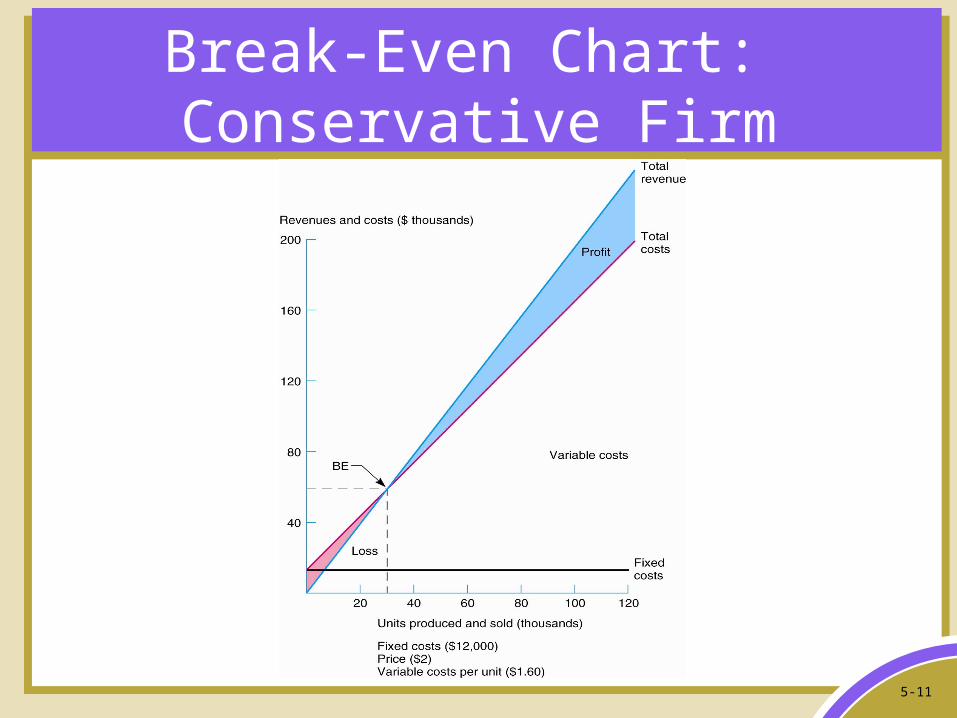
A Conservative Approach

• Some firms choose not to operate at high degrees of operating leverage– More expensive variable costs may be

substituted for automated plant and equipment– This approach may cut into potential profitability

of the firm

5-11

Break-Even Chart: Conservative Firm

5-12

Volume-Cost-Profit Analysis: Conservative Firm

Table 5-3

5-13

The Risk Factor

• Factors influencing decision on maintaining a conservative or leveraged position include:– Economic condition– Competitive position within industry– Future position – stability versus market

leadership– Matching an acceptable return with a desired

level of risk

5-14

Cash Break-Even Analysis

• Deals with cash flows rather than accounting flows

• Helps in analyzing the short-term outlook of a firm

• Examples of noncash items that are excluded:– Depreciation– Credit sales – Credit purchase of materials

5-15

Degree of Operating Leverage (DOL)

• Percentage change in operating income as a result of a percentage change in units sold

• Computed only over a profitable range of operations

• More when it is computed closer to BEP

DOL = Percent change in operating income

Percent change in unit volume

5-16

Operating Income or Loss

5-17

Computation of DOL

• Leveraged firm:

DOL = Percent change in operating income = $24,000 X 100 Percent change in unit volume $36,000

20,000 X 100 80,000 = 67% = 2.7 25%• Conservative firm:

DOL = Percent change in operating income = $8,000 X 100 Percent change in unit volume $20,000

20,000 X 100

80,000 = 40% = 1.6 25%

5-18

Algebraic Formula for DOL

DOL = Q (P – VC) , Q (P – VC) – FC

Where,• Q = Quantity at which DOL is computed• P = Price per unit• VC = Variable costs per unit• FC = Fixed costs• For the leveraged firm, assume Q = 80,000, with P = $2, VC = $0.80,

and FC = $60,000:

DOL = 80,000 ($2.00 - $0.80) ; 80,000 ($2.00 - $0.80) - $60,000 = 80,000 ($1.20) = $96,000 ; 80,000 ($1.20) - $60,000 $96,000 - $60,000DOL = 2.7

5-19

Limitations of Analysis

• Assumption of existence of constant or linear function for revenues and costs as volume changes– May not hold good in real world

• Price weakening to capture increasing market• Cost overruns when moved beyond optimum-size

operation

– Relationships are not so fixed as assumed

5-20

Nonlinear Break-Even Analysis

• Assumption of exact linear relation does not hold good in reality

5-21

Financial Leverage

• Reflects the amount of debt used in the capital structure of the firm

• Determines how the operation is to be financed

• Determines the performance between two firms having equal operating capabilities

BALANCE SHEET

Assets Liabilities and Net Worth

Operating leverage Financial leverage

5-22

Impact on Earnings

• Examine two financial plans for a firm, where $200,000 is required to carry the assets

Total Assets = $200,000

Plan A (leveraged) Plan B (conservative)Debt (8% interest) $150,000 ($12,000 interest) $ 50,000 ($4,000 interest) Common stock 50,000 (8000 shares at $6.25) 150,000 (24,000 shares at

$6.25)

Total financing $200,000 $200,000

5-23

Impact of Financing Plan on Earnings per Share

Table 5-5

5-24

Financing Plans and Earnings per Share

5-25

Degree of Financial Leverage

DFL = Percent change in EPS Percent change in EBIT

• For the purpose of computation, it can be restated as: DFL = EBIT .

EBIT – I• DFL for two plans can be calculated using values from Table 5-5

– Plan A (Leveraged):DFL = EBIT = $36,000 = $36,000 = 1.5

EBIT – I $36,000 - $12,000 $24,000

– Plan B (Conservative):DFL = EBIT = $36,000 = $36,000 = 1.1

EBIT – I $36,000 - $4,000 $32,000

5-26

Limitations to Use of Financial Leverage

• Beyond a point, debt financing is detrimental to the firm– Lenders will perceive a greater financial risk– Common stockholders may drive down the

price

• Recommended for firms that are:– In an industry that is generally stable– In a positive stage of growth– Operating in favorable economic conditions

5-27

Combining Operating and Financial Leverage

• Combined leverage: when both leverages allow a firm to maximize returns– Operating leverage:

• Affects the asset structure of the firm• Determines the return from operations

– Financial leverage:• Affects the debt-equity mix• Determines how the benefits received will be

allocated

5-28

Combined Leverage Influence on the Income Statement

• Last item under operating leverage, operating income, becomes the initial item for determining financial leverage

• “Operating income” and “Earnings before interest and taxes” are one and the same, representing the return to the owners before interest and taxes are paid

5-29

Combining Operating and Financial Leverage

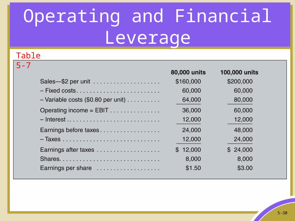
5-30

Operating and FinancialLeverage

Table 5-7

5-31

Degree of Combined Leverage

• Uses the entire income statement• Shows the impact of a change in sales or

volume on bottom-line earnings per share

DCL = Percentage change in EPS ; Percentage change in sales (or volume)

• Using data from Table 5-7:

Percent change in EPS $1.50 X 100 $1.50 = 100% = 4Percent change in sales $40,000 X 100 25% $160,000

=

5-32

Degree of Combined Leverage (cont’d)

DCL = Q (P – VC) ,

Q (P – VC) – FC – I

From Table 5-7,• Q (Quantity) = 80,000; P (Price per unit) = $2.00; VC (Variable

costs per unit) = $0.80; FC (Fixed costs) = $60,000; and I (Interest) = $12,000.

DCL = 80,000 ($2.00 – $0.80) =

80,000 ($2.00 - $0.80) – $60,000 – $12,000

= 80,000 ($1.20) =

80,000 ($1.20) – $72,000

DCL = $96,000 = $96,000 = 4

$96,000 – $72,000 $24,000