Open Queueing Networks: Optimization and Performance - CiteSeer

Open Queueing Networks: Optimization andPerformance Evaluation Models for Discrete

Manufacturing Systems

byGabriel R. Bitran

Reinaldo Morabito

WP #3743-94 November 1994

Open Queueing Networks: Optimization and PerformanceEvaluation Models for Discrete Manufacturing Systems

Gabriel R. Bitran Reinaldo MorabitoMassachusetts Institute of Technology Universidade Federal de Sdo Carlos, Brazil

Sloan School of Management Dept. Engenharia de ProduCgo

November 23, 1994

Abstract

In this survey we review methods to analyze open queueing network models for discretemanufacturing systems. We focus on design and planning models for job-shops. The surveyis divided in two parts: in the first we review exact and approximate decomposition methodsfor performance evaluation models for single and multiple product class networks. The secondpart reviews optimization models of three categories of problems: the first minimizes capitalinvestment subject to attaining a performance measure (WIP or leadtime), the second seeks tooptimize the performance measure subject to resource constraints, and the third explores recentresearch developments in complexity reduction through shop redesign and products partitioning.

Keywords: open queueing networks, optimization and performance evaluation, decompositionmethods, discrete manufacturing systems, job-shop design -

0

1 Introduction

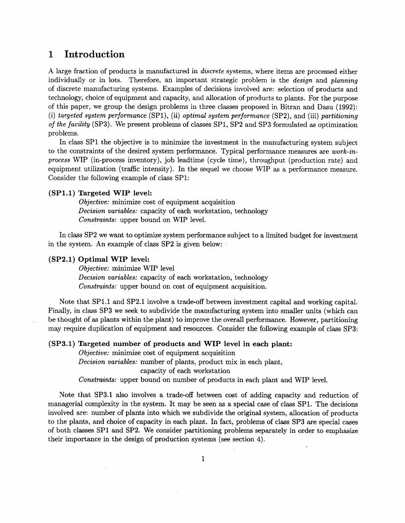
A large fraction of products is manufactured in discrete systems, where items are processed eitherindividually or in lots. Therefore, an important strategic problem is the design and planningof discrete manufacturing systems. Examples of decisions involved are: selection of products andtechnology, choice of equipment and capacity, and allocation of products to plants. For the purposeof this paper, we group the design problems in three classes proposed in Bitran and Dasu (1992):(i) targeted system performance (SP1), (ii) optimal system performance (SP2), and (iii) partitioningof the facility (SP3). We present problems of classes SP1, SP2 and SP3 formulated as optimizationproblems.

In class SP1 the objective is to minimize the investment in the manufacturing system subjectto the constraints of the desired system performance. Typical performance measures are work-in-process WIP (in-process inventory), job leadtime (cycle time), throughput (production rate) andequipment utilization (traffic intensity). In the sequel we choose WIP as a performance measure.Consider the following example of class SP1:

(SP1.1) Targeted WIP level:Objective: minimize cost of equipment acquisitionDecision variables: capacity of each workstation, technologyConstraints: upper bound on WIP level.

In class SP2 we want to optimize system performance subject to a limited budget for investmentin the system. An example of class SP2 is given below:

(SP2.1) Optimal WIP level:Objective: minimize WIP levelDecision variables: capacity of each workstation, technologyConstraints: upper bound on cost of equipment acquisition.

Note that SP1.1 and SP2.1 involve a trade-off between investment capital and working capital.Finally, in class SP3 we seek to subdivide the manufacturing system into smaller units (which canbe thought of as plants within the plant) to improve the overall performance. However, partitioningmay require duplication of equipment and resources. Consider the following example of class SP3:

(SP3.1) Targeted number of products and WIP level in each plant:Objective: minimize cost of equipment acquisitionDecision variables: number of plants, product mix in each plant,

capacity of each workstationConstraints: upper bound on number of products in each plant and WIP level.

Note that SP3.1 also involves a trade-off between cost of adding capacity and reduction ofmanagerial complexity in the system. It may be seen as a special case of class SP1. The decisionsinvolved are: number of plants into which we subdivide the original system, allocation of productsto the plants, and choice of capacity in each plant. In fact, problems of class SP3 are special casesof both classes SP1 and SP2. We consider partitioning problems separately in order to emphasizetheir importance in the design of production systems (see section 4).

1

This paper reviews the developments of optimization models for classes SP1, SP2 and SP3,combining techniques of mathematical programming and the theory of open queueing networks(OQNs). We focus on design and planning models for job-shops. For completeness, the paper isdivided in two parts. In the first part we review the so called performance evaluation models tocompute performance measures for OQNs, such as WIP and leadtimes, and in the second part wereview the optimization models. Roughly speaking, the difference between a performance evaluationand an optimization model for OQNs is that the first one describes performance measures undercertain condition while the second prescribes decisions.

In a previous survey, Bitran and Dasu (1992) analyzed several optimization and performanceevaluation models for job shops. In this present review that survey is updated and extendedwith a more quantitative flavor. We present multiple product class OQN models in more detail,emphasizing the importance of interference among classes and light-traffic approximations. Solutionalgorithms are presented based on marginal analysis and greedy heuristics. We include also recentdevelopments such as products partitioning, and suggest perspectives for future research.

1.1 Network of Queues Representation of Discrete Manufacturing Systems

Job-shops are complex discrete manufacturing systems that process a wide variety of products orjobs in low volumes (Chase and Aquilano, 1992). In general, job-shops involve complex job flowsthrough the workstations (or simply stations) and waiting queues in front of the machines. Wecan represent a job-shop as a network of queues, where nodes correspond to the stations and arcscorrespond to job flows between the stations.

The study of queueing networks began basically with the work of Erlang (1917) in telephony.Since then, various examples appeared in different areas; for example, communication, computation,transportation, production, maintenance, biology (neural networks), health (behavior models),chemistry and materials (polymerization), among others; see Disney and Konig (1985). Hsu etal (1993) and Suri et al (1993) provided a broad description of the use of queueing networks torepresent manufacturing systems. Each node contains the following elements: (i) arrival process,(ii) service process, and (iii) waiting queue. Figure 1 illustrates this representation.

The arrival process at a station is described by job interarrival times, which can be deterministic(D) or probabilistic. If the arrival process is probabilistic, it may either depend on other interarrivaltimes and the service process, or consist of independent and identically distributed (iid) interarrivaltimes. The former case is called a G-arrival process and the latter case, a GI-arrival process orrenewal process. An example of a G-arrival process dependent on the service process occurs if anarriving job balks when the waiting queue is too long, or if the job is removed from the queue afterwaiting for a long time. An instance of a particular GI-arrival process is when the interarrivaltimes are exponential (memoryless or Markovian process M). We can have all jobs belonging toa single class or product family, or different jobs belonging to multiple classes (sometimes one jobclass may be artificially used to model interruptions such as machine breakdowns). All jobs of thesame class are assumed statistically identical. We may also have either individual job arrivals orbulk-arrivals at the station.

The service process at a station is described by job service times, classified as deterministic(D) or probabilistic. If the service process is probabilistic, it may either depend on other servicetimes and the arrival process, or consist of iid service times. Some authors have called the former

2

arrfival service process

process waitingqueue

jobs jobsarriving jobs waiting departing

for service

jobs beingserviced

Figure 1: A station with identical machines and a single queue

case as a G-service process and the latter case as a GI-service process (Disney and Konig, 1985).Here we will refer to both as a G-service process since it is more usual in the literature. Anexample of the G-service process dependent on the arrival process occurs when the service timevaries according to the number of jobs in the queue. Similarly to interarrival times, service timesmay be independent and identically exponential random variables (M-service process). Stationsmay have only one machine (single server), or many machines (multiple servers). The machine mayexecute an operation for each job individually or in batch (bulk-service), and eventually breaksdown. Each machine may represent a set of resources like different machines, operators, tools, etc.We use, for example, the notation GI/G/m to denote a single queueing system where the arrivalprocess is a renewal process (the first GI), the service times are iid random variables (the secondG), and the number of servers in the system is m.

Finally, the waiting queue (or buffer queue) of a station may have either limited or unlimitedcapacity for the number of jobs in the queue, which is generally determined by the available physicalspace. If it is full, new job arrivals at the queue are blocked. The queue has a discipline or ruleto sequence jobs waiting for service. Examples of queueing disciplines are: first-come first-served(FCFS), job priority, shortest-processing-time-first, and largest-processing-time-first. When therule is based on job priority, preemption may or may not be allowed. In the preemptive case, thehighest priority job in the queue starts service as soon as it arrives, even if a job with lower priorityis already in service. In the non-preemptive case, a job already in service can not be interrupteduntil it is completed.

A set of nodes, arcs and jobs constitute a network of queues with the following characteristics:(i) number of stations (nodes), (ii) sequence of operations (routing), and (iii) type of queueingnetwork: open, closed and mixed. The number of nodes in the network (greater or equal to 1)corresponds to the number of stations offering different operations. The sequence of operations orrouting through the stations may be sequential, sequential with feedback, assembly, arborescent,acyclic, and cyclic. Feedback arcs can be used to represent, for example, rework in manufacturing,

3

and probabilistic routings can model, for example, machine failures',A queueing network can be classified as either open, closed, or mixed. In an open queueing

network (OQN), jobs enter the network, receive service at one or more nodes, and eventually leavethe network. The number of jobs flowing among the nodes is a random variable. In a closedqueueing network (CQN), there are no external job arrivals or departures. The departure ratefrom any designated node is a random variable but the number of jobs flowing among the nodesis fixed. However, we can artificially represent external job arrivals and departures in a station ofa CQN by defining this station as an instantaneous load-unload station. The load-unload stationswitches at the same moment an internal job arrival with an external job arrival without varying thetotal number of jobs in the CQN. Note that, in this way, we can represent a flexible manufacturingsystem (FMS) as a CQN. If the network has multiple classes, we can redefine open sub-networksfor some classes and closed sub-networks for other classes. In this case, the resulting network ofqueues is called mixed.

The queueing network models analyzed in this paper assume that the system attains equilibriumor steady-state. The arrival processes are probabilistic with iid interarrival times at stations. Jobsmay belong to a single class or to multiple classes, and arrive individually. There is no limit onthe number of jobs in each class, but jobs can not change from one class to another. The serviceprocesses are also probabilistic with iid service times at stations. Each station may have one ormore identical machines and each machine serves only one job at a time. Jobs can not be combinedor created in the network, and the waiting queues have unlimited capacity with discipline FCFS.All models discussed in this paper correspond to OQNs with acyclical or cyclical structures anddeterministic or probabilistic routings (note that OQN models are analytically more tractable thanCQN models, and may approximate CQN models; see e.g. Whitt (1984) and Calabrese (1992)).Other models for the various cases not considered in this review can be found in the literaturediscussed below and in the references cited there.

1.2 Related Literature Reviews

Disney and Konig (1985) presented an extensive survey of queueing network theory, covering theseminal works of Jackson and the extensions of Kelly, including a bibliography of more than 300references. Other surveys are Lemoine (1977) and Koenigsberg (1982). Buzacott and Yao (1986)discussed the developments of CQN models before 1986 (oriented to FMS applications) and classi-fied the approaches based on the different research groups. Suri et al (1993) examined performanceevaluation models for different manufacturing systems such as single stage systems (single queues),production lines (tandem queues), assembly lines (arborescent queues), job-shops (OQN), and FMS(CQN). Suri et al commented on the use of queueing theory in topics like MRP II, JIT, Kanban,and suggested alternative approaches such as sensitivity analysis in simulation, models based onPetri net, and hierarchical queueing networks.

Buzacott and Shanthikumar (1992, 1993), Hsu et al (1993) and Bitran and Dasu (1992) analyzedboth performance evaluation models and optimization models for queueing networks. Buzacott andShanthikumar presented an extensive analysis oriented to the design of different manufacturingsystems such as flow lines, automated transfer lines, job shops, FMS and multicellular systems.They analyzed optimal design problems and, in particular, considered some optimization models injob shops that will not be covered here, such as optimal allocation of workers to stations, optimal

4

number of operators in the system, optimal allocation of jobs to stations, and analysis of routingand time diversity effects in job processing. Hsu et al examined optimization models for FMSbased in CQNs; they also suggested the use of alternative techniques like algebra max-plus, fuzzysets and expert systems. Bitran and Dasu discussed strategic, tactical and operational problemsof manufacturing systems based on the OQN methodology, with a special attention to design andplanning models for job-shops. As we mentioned earlier, this focus is extended in this paper.

Most approaches to optimization models are based on decomposition methods (see below) toevaluate performance measures for an OQN. More recently, alternative approaches have been ex-plored (Brownian models) based on heavy-traffic limit theorems to evaluate performance measures.In section 3.2.1 we describe an example of this approach (Wein, 1990) without exploring furtherdevelopments on this topic since Harrison and Nguyen (1993) recently reviewed the state of the artof Brownian models for multiple-class OQNs.

1.3 Structure and Notation

In section 2 we examine decompositon methods for performance evaluation models for OQNs. Insection 2.1 we briefly review exact decomposition methods for Jackson networks (M/M/m queue-ing networks), and in section 2.2 we review approximate decomposition methods for generalizedJackson networks (GI/G/m queueing networks). In section 3 we deal with problems SP1.1 andSP2.1, and review solution methods based on some convexity results and performance evaluationmodels of section 2. In section 3.1 we present algorithms to solve SP1.1 and SP2.1 for Jacksonnetworks, and in section 3.2 we present algorithms to solve SP1.1 and SP2.1 for generalized Jacksonnetworks. Finally, in section 4 we emphasize the importance of problem SP3.1 in the manufacturingenvironment and suggest some perspectives for future research.

In the following sections, we generally use the indices i and j to indicate station, the index kto indicate product class, and the index 1 to indicate class operation at stations. The notationsE(x), V(x) and cx denote respectively the expected value, the variance and the square coefficientof variation (scv) of a random variable x. The scv is defined as cx = I.

2 Performance Evaluation Models for OQNs

Performance evaluation models have been addressed using: (i) exact methods, (ii) approximatemethods, and (iii) simulation and related techniques. Exact methods exist for Jackson networks(section 2.1). The main result is that if the external interarrival and service times are exponentiallydistributed, we can define the equilibrium distribution (if it exists) of the number of jobs in thenetwork as a product form, and decompose the network in a set of stocastically independent stations.Thus each station is individually analyzed as an independent M/M/m system.

In most manufacturing systems the arrival and service processes are generally less variablethan the Poisson process, and the assumption above does not apply. In the absence of exactmethods for general OQNs, we can use simulation and related techniques (Law and Haider, 1989,Law and McComas, 1989). These approaches allow the use of more elaborate assumptions that areclose to reality. The main drawback is the computational requirements that limit the number ofalternatives to be considered. Techniques like perturbation analysis suggest possible ways to reduce

5

the computational cost. These techniques are beyond the scope of this work and are described inHo and Cao (1983), Ho (1987) and Suri (1989).

The limitations imposed by exact methods and simulation led authors to develop approxi-mate methods. These are classified in five categories: (i) diffusion approximations, (ii) mean valueanalysis, ((iii) operational analysis, (iv) exponentialization approximations, and (v) decompositionmethods.

Diffusion approximations are motivated by heavy-traffic limit theorems and have generatednew solution methods for OQNs (e.g., Reiman, 1990, Harrison and Nguyen, 1990). They have beenapplied to scheduling and operational control problems. Mean value analysis (Seidmann et al, 1987,Suri et al, 1993), operational analysis (Denning and Buzen, 1978, Dallery and David, 1986) andexponentialization approximations (Yao and Buzacott, 1986, Hsu et al, 1993) have been basicallyused to analyze CQNs. The most frequently used approximate methods to analyze OQN models forjob-shops have been decomposition methods. In this paper we only review decomposition methods(section 2.2).

2.1 Jackson Networks (Exact Decomposition Methods)

Consider a network of queues composed of n stations, each one with one or more identical machinesand infinite waiting capacity. Stations 1, 2,..., n are internal stations and station 0 is the externalstation of the system. For each internal station j, jobs arrive from station 0 with iid interarrivaltimes a0oj, wait in queue for an available machine, and are processed with iid service times sj. Afterbeing processed, jobs leave station j with interdeparture times dj and go to station i, i = 0,..., n,with transition probability defined by a Markov chain. We assume that any sequence of externalinterarrival times, service times and routing decisions are mutually independent, and that jobs areserviced at each station according to a FCFS discipline.

We refer to the network above as a Jackson open queueing network when we have exponentialdistributed external interarrival and service times (Poisson processes). Otherwise we have a gener-alized Jackson open queueing network (or simply, a general OQN). Jackson networks have elegantexact solutions in a product form which were shown by Jackson (1957, 1963), as we will see below.

2.1.1 Single Class M/MI/m OQNs

Assume that all jobs belong to the same class. Consider the following notation for the input data:n number of internal stations in the network.

For each station j, j = 1,... , n:m j number of identical machines at station j, mj > 1Aoj expected external arrival rate at station j (A0 j ao )

psj expected service rate of each machine at station j (j =For each pair (i, j), i = O,..., n,j = O,.. .,n:rij probability of a job going to station j after completing service at station i.

Thus our input data has (n + 1)2 + 3n numbers and each station j is described by 3 parameters:{mj, A0oj, j }. Successive stations are visited according to an absorbing Markov chain with transitionmatrix R = {rij ,O < rij < 1,i = 0,...,n,j = 0,...,n}, where En=ori = 1,i = 0,...,n, and= - ',= ', Yj=0rij= 1, i= O,..,n, an

6

roo = 1 by definition. Note that roo = 1 eliminates any chance of a job returning to the systemand so, it reduces the input data to n2 + 3n numbers.

Let Q = {qij E R, i = 1 , j = 1,..., n} and qi = 1- Z iqij. Q is the matrix R withoutline 0 (probability of a job entering the system at station j) and without column 0 (probability of ajob leaving the system by station i). Similarly, qio, i = 1,..., n, is the column 0 of matrix R withoutthe element of line 0. A deterministic job routing may be also described by Q and qio for all i, sinceit is a particular case of a probabilistic routing. If qjj > 0, we say that station j has an immediatefeedback arc. To illustrate the transition matrix, consider a symmetric job shop (Shanthikumarand Buzacott, 1981) for which Q = (qij = I;qii = i ~ j,i = i,...,n,j = 1,...,n) and qio =ni = 1,..., n. Now consider a deterministic flow-shop with all stations in series in the sequence1, 2,..., n, for which Q = {qi,i+l = 1, i = 1,..., n - 1; qij = 0 otherwise}, qio = , i = 1,..., n -1and qno = 1. Note that these two examples do not contain immediate feedback arcs.

Traffic Rate Equations

The traffic rate equations provide the expected arrival rate at each station. Let Aj be the expectedarrival rate at station j, defined as Aj = E(la), where aj is the interarrival time at station j. Underthe assumption of steady-state, Aj is obtained from the following system of linear equations:

n

A = Aoj + ± qijAi for j = 1,..., n (1)i=l

Given that qio > 0 for i = 1,..., n, it can be shown that (1) has a unique solution satisfyingAj > 0 for all j. Using this solution we can calculate the expected utilization pj (or traffic intensity)of station j, defined as:

Pi = A (2)

where 0 < pj < 1. The ratio A in (2) is called offered loaa (or workload), and corresponds to theexpected number of busy machines at station j, also denoted by aj = pjmj. The expected arrivalrate at station j from station i is given by:

Aij = Aiqij (3)

and the expected (external) departure rate to station 0 from station j is given by:

n

Ajo = Aj(1 - Z qji) (4)i=l

Adding Ajo (or Aoj) for all j, we obtain the throughput Ao (or production rate) of the network.The expected number of visits E(Vj) of an arbitrary job to station j is then evaluated by:

E(Vj)= i (5)

Let L be a state of the system defined as a vector L = (L 1, L 2,..., Ln), where Lj correspondsto the number of jobs in queue and in service at station j. Assuming that the system reaches

7

steady-state, let 7r(L) be the probability of the system being in equilibrium at state L. Jacksonshowed that 7r(L) is given by the following product form:

n

7r(L) = rj(Lj) (6)j=1

with

-F--'-- = if L < m3

7rj(Lj) = tj Lj3-!irr(O)Ai pi

mj m! if Lj > mj

where rj(Lj) is the probability of station j having Lj jobs (Lj = 0, 1,...) and rj(O) is a normalizingconstant. These results imply that in order to compute the equilibrium probability for a given stateL, we may consider each station independently (note that (6) is the product of the probabilitiesof each M/M/mj queue in the network). Thus, after applying the linear system (1) to determineeach Aj we may decompose the network into n individual M/M/mj stations, each one describedby {mj, Aj, j . To evaluate performance measures we just consider each station individually andindependently of the others. For example, the expected waiting time E(Wqj) (or mean delay) of ajob in the M/M/mj queue of station j can be derived from (6), given by (Tijms, 1986, p.333):

E(Wqj) = (mjPj)m ir (0) (7)!,jmj(1 - pj)2mj!

where

r(O) 1 (mjpjt + (mjpj)mr() = { (1 - pj)mj! }-t= 0

Note in (7) that if mj = 1, then E(Wqj) = - - The expected number of jobs E(Lqj) inqueue of station j can be easily obtained applying Little's law: E(Lqj) = AjE(Wqj).

The expected leadtime E(T) (or cycle time) for an arbitrary job, including waiting times andservice times spent in the network from the first arrival until the final departure, is given by:

n

E(T) = r E(Vj)(E(Wqj) + E(sj)) (8)j=1

where E(Vj) is the expected number of visits at station j defined by (5), E(Wqj) is defined by(7), and E(sj) is the expected service time of a job at station j. The expected number of jobs inthe network can be defined in a similar way. An interesting observation is that, even though thenumber of jobs at the stations are statistically independent at a given instant of time, the waitingtimes at different stations are in general not independent random variables. The variance of theleadtime in the network is usually approximated by ignoring the correlation in the waiting times(Shanthikumar and Buzacott, 1984). Buzacott and Shantikhumar (1993) provided an analysis ofJackson networks considering the correlation above.

8

2.1.2 Multiple Class M/M/m OQNs

Kelly (1975, 1979) extended Jackson's product form solutions to multiple class queueing networksfor the case in which service times are independent of job class (see also Baskett et al, 1975).The model allows the definition of a deterministic routing for each class. Even if we impose otherservice disciplines (e.g., priority queues), we obtain a solution in product form. Consider the stateS = (S1, S 2,..., Sn), where Sj denotes the state of station j. Each Sj corresponds to a row vector(sjl, sj2,..., sj,Lq), where Lqj is the queue length of station j and sjl, I = 1,..., Lqj, specifies theclass of the job at the l-th position in the queue. The equilibrium probability 7r(S) has the followingproduct form:

7r(S) = K f(S) gl(S1) g2(S2)... gn(Sn) (9)

where K is a normalizing constant, f(.) is a function of state S, and gj(.) is a function of station j.Although these results are interesting, practical implementations are difficult due to the size of thestate space in (9). Furthermore, the assumptions underlying Jackson networks are very restrictivefor general job shops and other manufacturing systems. For instance, Bitran and Tirupati (1988)suggested that exponential distributions overstate the variability in the service times found in manymanufacturing operations. For further details regarding Jackson networks the readers are referredto the surveys of Disney and Konig (1985), Walrand (1990), Suri et al (1993) and Buzacott andShanthikumar (1993), and the references cited there.

2.2 Generalized Jackson Networks (Approximate Decomposition Methods)

Decomposition methods may be seen as efforts to extend Jackson's product form solution and the"independence" between stations to general OQNs (generalized Jackson networks). The arrivaland departure processes are approximated by renewal processes, and each station is analyzed asa stocastically independent GI/GIm queue. The complete decomposition procedure is essentiallydescribed in three steps:

Step 1: Analysis of interaction between stations of the OQN,Step 2: Decomposition of the OQN into systems of individual and independent stations,Step 3: Recomposition of the decomposition results to analyze the general performance of the

OQN.

In step 1 we determine the internal arrival flows for each station. In step 2 we compute theperformance measures for each station separately. In step 3 we compute the performance measuresfor the whole network. Step 1 is fundamental in this procedure and involves three basic processes,namely: (i) merging or superposition of arrivals, (ii) departures, and (iii) decomposition or splittingof departures.

Figure 2 illustrates each one of these processes. The superposition process merges the individualarrival flows from other stations (including the external station), producing a merged arrival flowto the station. The departure process analyzes the effects of the merged arrival flow in the queueof a station, producing a merged departure flow from this station. Finally, the splitting processdecomposes the merged departure flow from a station into individual departure flows to otherstations (including the external station).

9

superposition splitting ofh of arivals departures

departures

Figure 2: Superposition of arrivals, departures, and splitting of departures

In general, just the first two moments of the distributions (typically the mean and the scv) aresufficient to provide a good approximation, and they have been often utilized to describe the flowsabove. This approach was initially proposed by Reiser and Kobayashi (1974) and was improvedby Sevcik et al. (1977), Kuehn (1979), Shanthikumar and Buzacott (1981), Albin (1982), Whitt(1983a), Bitran and Tirupati (1988), Segal and Whitt (1989), Whitt (1994), among others. Shan-thikumar and Buzacott were the first to apply this method to manufacturing systems. In section2.2.1 we present steps 1, 2 and 3 for a single class GI/G/1 queueing networks with probabilisticrouting. In section 2.2.2 we extend these steps to GI/G/m queueing networks, and in section 2.2.3we deal with multiple class GI/GIm queueing networks with deterministic routing for each class.This last case is widely considered in practice to model job-shop systems.

2.2.1 Single Class GI/G/1 OQNs with Probabilistic Routing

In this section we assume that all jobs belong to the same class and move through stations accordingto a probabilistic routing. Both external interarrival times and service times are lid but now weconsider general distributions. Initially we assume single server stations. Consider the followingnotation for the input data:

n number of internal stations in the network.For each station j, j = 1, . . ., n:

Aoj expected external arrival rate to station j (Aoj = E(I)

caoj scv or variability of external interarrival time at station j (caoj = E(ao)2

/ij expected service rate at station j (j = -) .

csj scv or variability of service time at station j (csj = v ).For each pair (i,j),i = 1,..., n,j = 1,..., n:

qij probability of a job going to station j after completing service at station i.

10

Thus our input data has n2 + 4n numbers and each station j is described by 4 parameters:{Aoj,caoj, Ij,csj}. Similarly to section 2.1, let the transition matrix Q = {qij,i = 1,..., n,j =1,..., n} and qio = 1-j= qij. In what follows we consider only OQNs with no immediate feedbackarcs (i.e., qii = 0, i = 1,..., n). If an OQN originally contains immediate feedback arcs, then wecan easily remove them from the OQN adjusting the initial parameters (see Whitt, 1983a). Thisprocedure improves the quality of the approximations. All assumptions for the Jackson networksare also assumed here except, of course, exponential distributions for external arrival and serviceprocesses (which result in caoj = 1 and csj = 1 for each station j).

Step 1

In step 1 we want to determine two parameters for each station j: (i) the expected arrival rateXj and (ii) the scv or variability of interarrival time caj (note that for Jackson networks we ob-tain V(aj) = E(aj)2 and, therefore, caj = 1). In other words, starting with the initial parame-ters {Aoj,caoj,j, csj} and the matrix Q, we want to describe each station j by the parameters{Aj, caj, I-L, csj}. The two parameters Aj and caj are determined solving two linear systems. Firstly,we obtain exact expected arrival rates from the traffic rate equations (1), similarly to the Jacksonnetworks. These are used to obtain approximate variability parameters from the traffic variabilityequations defined below. These systems can be shown to have a unique non-negative solution.

Traffic Variability Equations

The traffic variability equations involve the three processes discussed earlier: superposition ofarrivals, departures, and splitting of departures. They provide approximations for the interarrivaltime variability caj at each station j. These approximations combine two basic methods: theasymptotic method (Sevcik et al, 1977) and the stationary-interval method (Kuehn, -1979).

Superposition of Arrivals

In the superposition process (figure 2), the expected arrival rates and interarrival time variabilityparameters at station j are combined, producing the merged expected arrival rate Aj (from (1))

and the merged interarrival time variability caj (remember that Aj -E and caj = (a) Theasymptotic method and the stationary-interval method may be used to determine caj (or V(aj)).These methods are also called macro and micro, respectively, because of the macroscopic and themicroscopic view of the arrival process (Whitt, 1982).

Assume that the arrivals are occurring at station j since t = -oo, and a new arrival occursat t = 0. Let Sp be the elapsed time until the p-th arrival after t = 0. Both methods yield thesame expected time interval E(aj), but may yield very different variances V(aj). The asymptoticmethod takes a macroscopic view and try to match process behavior over a relatively long timeinterval, yielding V(aj) = limp,, v(sP). The stationary-interval method takes a microscopic viewPand try to match process behavior during a relatively short time interval. It yields V(aj) = V(S1),where S1 is referred as the stationary interval. Moreover, the asymptotic method is asymptoticallycorrect as pj - 1 (heavy-traffic intensity), and the interval-stationary method is asymptoticallycorrect as p -+ oo, when the arrival process tends to a Poisson process.

Let caij be the interarrival time variability at station j from station i. Based on the asymptotic

11

method, the superposition caj is a convex combination of caij given by (Sevcik et al, 1977):

ca 3 = AOJ Ac ~aij (10)caj = _j caoj+Zn i.aij._ = i caij (10)Aj i=1 aj i=0 a

where ij and j are obtained from (3) and (1), respectively. Based on the interval-stationarymethod, the superposition caj results in a non-linear function (Kuehn, 1979). Note that if thearrival process is Poisson (i.e., caij = 1, i = O,..., n), then (10) is exact and returns caj = 1.

The asymptotic approximation (10) does not reflect the convergence to the Poisson processas p - oo; on the other hand, the stationary-interval approximation deteriorates as pj - 1.Albin (1982, 1984) suggested a more refined approximation to caj with a relative error around3% in comparison to simulation. This approximation is based on the convex combination betweenthe value obtained by (10) and the value obtained by the stationary-interval method. Whitt(1983b) simplified Albin's refinement substituting the stationary-interval method by a Poissonprocess obtaining:

n Aijcaj = wj E-caij + 1 - Wj (11)

i=O j

where1

w = 1 + 4(1 - pj)2 (vj - 1)

1

vi =O ij )2

The approximation (11) yields results very close to Albin's hybrid approximation.

Departures

In the departure process (figure 2), the merged expected arrival rate and the merged interarrivaltime variability at station j, together with the service time variability csj, are used to determinethe merged expected departure rate and the merged interdeparture time variability from stationj. If station j is not saturated (i.e., pj < 1) and is in steady-state, then we have the expecteddeparture rate equal to the expected arrival rate. However, the evaluation of the interdeparturetime variability is not so easy.

Let cj be the scv or variability of interdeparture time at station j. Based on the stationary-interval method and using Marshall's formulae for a GI/G/1 system we obtain (Kuehn, 1979):

cdj = ca3 + 2p2cs 2pj(1 - pj)E(Wqj) (12)

where E(Wqj) is the expected waiting time in queue at station j. Substituting in (12) theKraemer&Lagenback-Belz approximation for E(Wqj) (see equation (16) below), we obtain theinterdeparture time variability as a convex combination of caj and csj given by:

cdj = pcsj + (1 - pj2)caj (13)

12

where pj is known from (2). Note that if the arrival process and the service process are Poisson (i.e.,caj = csj = 1), then (13) is exact and produces cdj = 1. Note also that if pj -+ 1, then we obtaincdj -+ csj, suggesting that the interdeparture time variability tends to the service time variabilityas the expected utilization of station j becomes very high (i.e., long queues at station j tend todiminish the effect of the interarrival time variability). On the other hand, if pj -+ 0, then weobtain cdj -+ caj, suggesting that the interdeparture time variability tends to the interarrival timevariability as the expected utilization of station j is very low and no waiting queues are expected.

Based on the asymptotic method we obtain an elementary approximation to cdj, given by(Whitt, 1983a):

cdj = caj (14)

The approximation (14) is also exact if the arrival and service processes are Poisson. Further-more, it becomes more accurate at station j as the expected utilization increases in the subsequentstations to station j. For example, consider an OQN composed of two stations in series, say sta-tion 1 and 2 with parameters {A0o, cao, pi, cs1} and 0,0, 2, cs2}, respectively, and q2 = 1 and

lli = q22 = q2i = 0. Using (1) we obtain Al = A2 = A0 1 - In addition, if we have 2 - A2 and Aiconstant, we obtain P2 - 1. Based on heavy-traffic limit theorems, Whitt (1983a) observed thatthe performance measures of station 2 are asymptotically the same as if station 1 is removed (i.e.,1 _ 0). In other words, the arrival process at station 2 is the same arrival process at station 1.

Under these conditions, (14) is asymptotically correct for station 1 resulting cal = cd1 = ca2 , whilea heavy-traffic bottleneck phenomenon occurs at station 2.

A possible refinement is to combine the approximations from the two methods above, similarlyto the superposition process. However, Whitt observed that this refinement is not as critical asfor the superposition case, and suggested the use of (13). More recently, Suresh and Whitt (1990)observed that the heavy-traffic bottleneck can occur in practice at reasonable expected utilizationlevels. Experiments with various stations in series and different parameters revealed limitationsin the use of the approximations (13) and (14) separately. Suresh and Whitt suggested that itshould be appropriate to consider hybrid approximations to the departure process, combining thestationary-interval method and the asymptotic method. They observed that the expected waitingtime E(Wqj) at station j does not reflect the heavy-traffic phenomenon because caj is assumedtotally independent of pj (see (16) below). Then, they suggested that caj should be a functionof cal,csl,cs2,... , csj_l and Pl,P2,.. ,pj. For instance, caj could be a convex combination ofcal, csi, cs2, ... , csj-i with weights that are continuous functions of P1, P2,. . , Pj.

Splitting of Departures

In the splitting process (figure 2), the merged expected departure rate and merged interdeparturetime variability from station j are decomposed, producing the expected rates Aji according to (3).The interdeparture time variability cdji between stations j and i is defined below as a function ofcdj (Sevcik et al, 1977, or Kuehn, 1979):

cdji = qjicdj + 1 - qji (15)

If the departure process is Poisson (i.e., cdj = 1), then (15) is exact and gives cdji = 1. Notethat if qji -+ 1, then (15) results in cdji -+ cdj. That is, as the expected departure rate from stationj to station i tends to the merged expected departure rate from station j, the interdeparture time

13

variability from station j to station i also tends to the merged interdeparture time variability fromstation j. Furthermore, if qji -+ 0, then (15) results in cdji - 1, indicating that as the proportion offlow between stations j and i tends to zero, the departure process between these two stations tendsto a Poisson process. Note also that cdji in (15) is equal to caji in (11), that is, the interdeparturetime variability from station j to station i is exactly the same as the interarrival time variabilityat station i from station j. Assuming that the departure process is renewal and qji, i = 1, ... , n,represents independent events (Markovian routing), then (15) is exact and the stationary-intervalapproximation and the asymptotic approximation coincide.

Combining equations (11), (13) and (15), we obtain the second linear system as a function ofcaj, cdj, and caij (or cdij) to approximate the scv caj for each station j, j = 1,..., n. The solutionof the two linear systems discussed so far (traffic rate and traffic variability equations) allows thedescription of each station j by the desired parameters (Aj, caj, Uj, csj). We can then proceed tosteps 2 and 3. Note that if the network is acyclic (i.e., the job routing do not form cycles), thenthe stations 1, 2,..., n can be relabeled as jl, j2,... ,jin, such that jobs visit station ji after stationjk for ji > jk. Since there are no cycles, the parameters Aj and caj can be easily computed foreach station j following the increasing order of the station labels.

Steps 2 and 3

In step 1 we decomposed the OQN into a collection of independent stations, each one describedby {Aj, caj , pj, csj}. In step 2 we want to evaluate performance measures for each station, suchas expected waiting time in queue, expected length of queue, and so on. These measures maybe approximated by formulas from queueing theory (e.g., Kleinrock, 1975, Tijms, 1986). Whitt(1983a) observed that since the arrival process is usually not a renewal process and only twoparameters (mean and scv) are known for each distribution, then there is little to be gained frommore elaborate procedures.

For illustration, the expected waiting time E(Wqj) in the GI/G/1 queue of station j may beestimated by the Kraemer&Lagenbach-Belz formulae (modified by Whitt), defined as:

E(Wqj) = pj(caj + csj)g(pj, caj, csj) (16)21pj(1- pj)

where

3pj (caj +csj)g(pj,caj,csj) = { ex p(1ca)(csj): } if caj < 1i if caj Ž1

Note that for a M/M/1 queue, (16) and (7) produce the same result. For a study and comparisonof other approximations for E(Wqj), see for example Shanthikumar and Buzacott (1981) andBuzacott and Shanthikumar (1993).

Finally, in step 3 we want to evaluate performance measures for the whole network, for example,the expected job leadtime, expected number of jobs, and production rate. For instance, let'sconsider the expected leadtime for an arbitrary job, including waiting times and service timesspent in the network. Similarly to (8), we obtain:

n

E(T) = E(Vj)(E(Wqj) + E(sj)) (17)j=l

14

where E(Vj) is the expected number of visits at station j defined by (5), E(Wqj) is defined by (16),and E(sj) is the expected service time at station j. As in the Jackson networks, the variance ofthe leadtime is usually approximated by ignoring the correlation in the waiting times at differentstations. Further details of steps 2 and 3 may be found in Whitt (1983a, 1983b) and Suri et al(1993).

2.2.2 Single Class GI/G/m OQNs with Probabilistic Routing

The model above considers single machine stations. The more general case with one or moreidentical machines in each station can be derived from the previous one. Let mj,m j > 1, be thenumber of machines in station j, now defined by 5 parameters: mj, A0O, caoj, , csj}. In step 1equation (13) is replaced by:

cd = 1 + (1- pj)(caj - 1) + p( - ) (18)

Note that if mj = 1, then (18) reduces to (13), and that for M/M/mj (caj = 1, csj =1) and M/G/oo (caj = 1, mj -+ oo) systems, (18) correctly results in a Poisson process (i.e.,cdj = 1). However for a M/D/1 (caj = 1, csj = 0) system, (18) or (13) incorrectly produce aninterdeparture time variability less than the interarrival time variability (i.e., cdj = 1 - pj < 1).In fact, Shanthikumar and Buzacott (1981) did not find good results (relative to simulation) uponapplying (13) to M/D/1 and GI/D/1 queueing networks. In order to reduce this distortion, Whitt(1983a) suggested to modify (18) to:

?p(maxfcs 0.2} - 1)cdj = 1 + (1 - pj)(caj - 1) + pi(max{csj.2}1) (19)

where pj is known from (2). Finally, combining equations (11), (19) and (15) we obtain the followinglinear system as a function of caj, cdj and cdji (or caji) to determine the scv caj for each station j:

n

caj = j + E cai3ij for j 1,...,n (20)i=l

wheren

j = 1 + wj{(pojcaoj - 1) + Epij[(l - qij) + qijPiXi]}i=l

ij = wjpijqij(1 - pi2)

with wj defined according to (11) and

Pij A (where Pij = and qij = Pij i 0

(max{csi, 0.2} - 1)

15

Steps 2 and 3 are similar to the previous section, using performance measure formulas derivedfrom GI/GIm queueing theory. For example, the expected waiting time E(Wqj) at station j canbe approximated by:

E(Wqj) = (caj + csj) E(Wqj(M/Mmj)) (21)2 1 )

where E(Wqj(M/M/mj)) is the expected waiting time for a M/M/mj queue defined in (7). Notethat if the arrival and service processes are Poisson, then (21) reduces to (7). Moreover, if mj = 1and ca > 1, then (21) reduces to (16) (for improved approximations of E(Wqj), see e.g. Whitt(1993) and Buzacott and Shanthikumar (1993)). The expected job leadtime E(T) in the networkcan be defined similarly to (17).

2.2.3 Multiple Class GI/GIm OQNs with Deterministic Routings

In this section we modify the prior model (sections 2.2.1 and 2.2.2) to deal with multiple job classOQNs. Each job class has its own routing which defines the sequence of stations to be visited.For a class routing, each visit to a station corresponds to a different operation, and we may havevarious visits to the same station. For example, the sequence (2, 3, 1, 3, 4) defines a class routingwhose jobs visit four different stations for five operations (the two operations produced at station3 may be different). Contrary to the previous sections, now routing is deterministic. Consider thefollowing notation for the input data:

n number of internal stations in the networkr number of classes in the network.

For each station j,j = 1,..., n:m j number of machines at station j.

For each class k, k = 1,..., r:nk number of operations in the routing of class k)A expected external arrival rate of class kcak scv or variability of external interarrival time of class k.

For each class k, k = 1,..., r, and for each operation 1, 1 = 1,..., nk in the routing of class k:nkt station visited for operation I in the routing of class kE(skl) expected service time for operation in the routing of class kor ktl expected service rate for operation in the routing of class k (i.e., ,k = E(Sk)

cskl scv or variability of service time for operation I in the routing of class k.

The routing of class k is now described by nk and nkl (instead of matrix Q), and may havea different service time distribution for each operation. Whitt (1983a) presented a procedure toaggregate all classes in a single one and utilize the single class model discussed before (sections 2.2.1and 2.2.2). Note that in this way the original multiple class OQN is reduced to a single aggregateclass OQN. After this aggregate class OQN has been analyzed, we return to the original networkand estimate the performance measures for each class individually. This procedure is describedbelow.

Firstly we obtain the initial parameters {mj, 0oj, caoj, p j, csj} of the aggregate class for eachstation j, j = 1,..., n and then, we utilize step 1 from previous sections to obtain the final parame-ters {mj, Aj, caj , 1lj, csj} of the aggregate class. Let 1H(x) = 1 if x E H and 1H(x) = 0 otherwise.

16

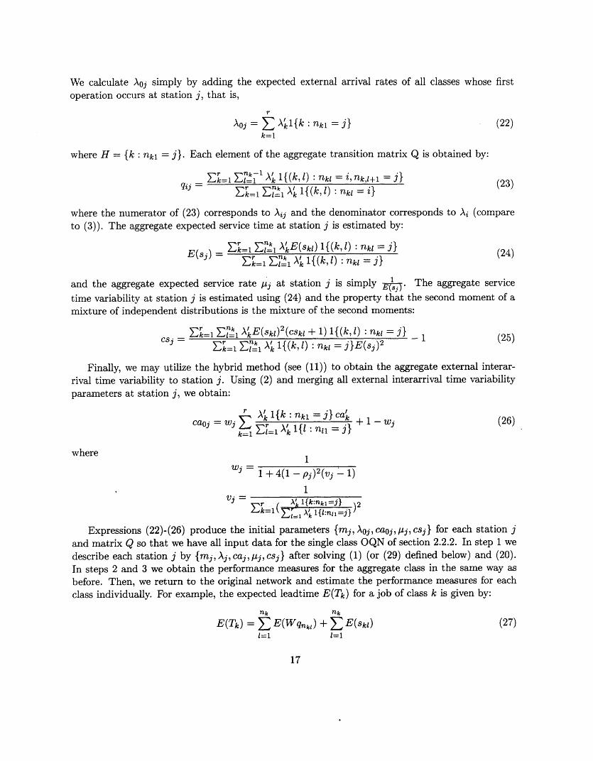
We calculate Aoj simply by adding the expected external arrival rates of all classes whose firstoperation occurs at station j, that is,

r

A0o = Al{k nkl = j} (22)k=l

where H = {k: nkl = j}. Each element of the aggregate transition matrix Q is obtained by:

E= l nk =1 A' 1{(k, 1): nkl = i, nk,1+l = j}Lkqij I~l k (23)

ilj = = 1 Zk A 1{(k,1) : nkl =i}

where the numerator of (23) corresponds to Aij and the denominator corresponds to Ai (compareto (3)). The aggregate expected service time at station j is estimated by:

E(sj) = l 1 Ak {(k 1) (24)z= l l A% l{(k,l) nk1 = j}

and the aggregate expected service rate pj at station j is simply 1 The aggregate service

time variability at station j is estimated using (24) and the property that the second moment of amixture of independent distributions is the mixture of the second moments:

-=l =1 AkE(skl) 2 (cSk l + 1) 1(k, ) n: j} _ (25)CS A'k=l 1{(k, 1) 1)nk: = j}E(sj)2

Finally, we may utilize the hybrid method (see (11)) to obtain the aggregate external interar-rival time variability to station j. Using (2) and merging all external interarrival time variabilityparameters at station j, we obtain:

A' 1{k : nkl jJ}ca'caoj = wj' l + 1-Wj (26)

where1

wj= 1+4(1-pj) 2 (vj -1)

1=- ] 1 A' l{k:nkl j}

Expressions (22)-(26) produce the initial parameters {mj, A0j, caoj, Lj, csj} for each station jand matrix Q so that we have all input data for the single class OQN of section 2.2.2. In step 1 wedescribe each station j by {mj,Aj, caj, lj, csj} after solving (1) (or (29) defined below) and (20).In steps 2 and 3 we obtain the performance measures for the aggregate class in the same way asbefore. Then, we return to the original network and estimate the performance measures for eachclass individually. For example, the expected leadtime E(Tk) for a job of class k is given by:

nk nk

E(Tk) = E(Wqn,,) + E(skl) (27)1=1 1=1

17

where E(Wqnkl) is the expected waiting time at station nki (i.e., the station relative to the -thoperation in the routing of class k), and can be evaluated by (21). Note that the first term in (27)corresponds to the total expected waiting time for a job of class k, and the second term correspondsto the total expected service time for a job of class k. Similarly, the variance of leadtime V(Tk) fora job of class k is given by:

nk nk

V(Tk) = Z V(Wqnkl) + E E(skl) 2cskl (28)1=1 1=1

where the first and second terms correspond to the variances of waiting times and service times,respectively.

Interference Among Classes

Bitran and Tirupati (1988) showed that expression (15) may be less effective for the splitting processwhen we have multiple class OQNs with deterministic routings. Note in (15) that if qji - 0, thencdji -+ 1. Bitran and Tirupati extended (15) to represent the interference among classes. For each

class at a station, the analysis is reduced to two classes: (i) the class of interest itself and (ii) theaggregation of all other classes arriving between two successive arrivals of the class of interest. Wecall this second class the aggregate class (do not confuse with the aggregate class of the previoussection).

Let class k be the class of interest at a certain station j in a multiple class OQN with deter-ministic routings. For convenience, assume that class k has one and only one operation at stationj, say operation I (the approximations below are also valid for the case when class k has more thanone operation at station j). Hence, nkl = j. Assume also that the interarrival and interdeparturetimes of all classes at station j are id. Since we have only deterministic routings in the network,we can easily obtain Aj by adding the expected arrival rates from all classes (including class k)which operations occur at station j, that is,

r nk

Aj = ) A'1 l(k, 1): nkl = j} (29)k=1 1=1

It is also easy to obtain the proportion of the class of interest k at station j, qkl = j (recall

that j = nkl). Let dkl be the interdeparture time of class k from station j, dj be the interdeparturetime of all classes from station j, and Zk be the number of jobs of the aggregate class that arriveat station j during one interarrival time of class k. Note that dki is the sum of zkl + 1 id randomvariables. Define zl = Zkl + 1. Since the expectation and variance of the sum of Zkl id randomvariables are E(dki) = E(zl)E(dj) and V(dkl) = E(zl)V(dj ) + V(zl)E(dj)2 , where E(dkl) -

and E(dj) = 1 it follows that E(zkl) = = i and cdki is given by:

cdkl = qklcdj + czkl' (30)

Bitran and Tirupati observed that the first term on the right hand side of (30) reflects the effectof the queue process at station j, while the second term does not depend on the service process. Itcaptures the effect of the aggregate class arrival process between two successive arrivals of class k.

18

Bitran and Tirupati proposed two approximations to czl based on the assumption that zkl has aPoisson and Erlang distributions, respectively. Assuming that Zkl has a Poisson distribution withrate Aj(l - qkl), it follows that czl = (1 - qkl)[qkl + (1 - qkl)cakl], and expression (30) (splittingprocess) can be written as:

cdkl = qklcdj + (1 - qkl)qkl + (1 - qkl)2Cakl (31)

where j = nkl, qkl = , and cakl is the interarrival time variability of the class of interest k at

station j. Note that cakl = cdk,1l1. We may also rewrite expression (11) (superposition process)as a function of cakl:

caj = wj E "'- vk cakl l{(k,l), nk = j} + - wj (32)k=1 1=1 Xj

where1

j = 1 + 4(1 - pj)2 (vj - 1)

1

=l =1 nk 1 )2 l{(k, 1), j}

and Aj is obtained from (29). Combining (32), (19) and (31), we obtain an alternative linear systemas a function of caj, cdj, and cdkl (or cak,l+l) to determine caj. After obtaining the parameters{mj, Aj, caj, /j, csj} from step 1, we proceed to steps 2 and 3 as before. This approach based on (31)produces much better estimates for caj than (20), which is based on (15) (see the computationalresults in Bitran and Tirupati, 1988, 1989b).

In fact, expression (31) can be seen as a generalization of (15). To see that, consider a particularsituation where jobs of the class of interest k enter the network at station j, wait in line togetherwith jobs of other classes and, after finishing service, only the jobs of class k proceed to a certainstation i. Thus, the expected departure rate of arc (j, i) is \ji = Ak, and the rate proportion (or

probability) of jobs going from station j to station i is qji Following the same steps as above,

we can define dji, zji, zi and so on, and rewrite (30) as: cdji = qjicdj + czi. Assuming that Zjihas a Poisson distribution with rate Aj(l - qji), it follows that czi = (1 - qji)[qji + (1 - qji)ca],and (31) can be written as:

cdji = qjicdj + (1 - qji)qji + (1 - qji)2ca' (33)

Note that if the arrival process of class k is Poisson (i.e., ca = 1), then (33) reduces to (15).In fact, it can be shown that (15) is the special case of (33) when zi is geometrically distributedwith parameter qji, yielding czgi = 1 - qji. Note also that if qji - 1, then (15) and (33) lead tocdji -+ cdj but, if qji -+ 0, then only (33) leads to cdji -+ ca'. This last result is asymptoticallyexact (Bitran and Tirupati, 1988, remark 1), and permitted two important approximations tomultiple class OQNs with deterministic routings, presented by Whitt (1988). Initially, consider acertain station in the network (Whitt, 1988, p.1335):

19

"If the arrival rate of one class upon one visit to some queue is a small proportion ofthe total arrival rate there, then the departure process for that class from that visit tothat queue tends to be nearly the same as the arrival process for that class for that visitto that queue."

Whitt observed that this principle may be seen as a light-traffic approximation, where only theclass of interest must have low utilization (i.e., the overall utilization of the station need not below). Consider now a certain class with deterministic routing in the network (Whitt, 1988, p.1335):

"If the contribution to the arrival rate by this class at each visit to each queue is a smallproportion of the total arrival rate at that queue, then the departure process of that classfrom each visit to each queue, and thus from the entire network, is nearly the same asthe external arrival process of this class to the network. "

Based on (33) and the approximations above, Segal and Whitt (1989) proposed an alternativeexpression for the splitting process of multiple class OQNs with deterministic routings. Let cejbe the average of the external interarrival time variability parameters of the classes at station j,weighted by the expected number of visits of each class at station j (see expression (5)). We define:

;-=1 nk ' 1(k, 1) nkl 3ce = 1j}ca (34)Using (34), the variability parameter cd be(k,tween) stations j and i is redefined by (compare to

Using (34), the variability parameter cdji between stations j and i is redefined by (compare to(15)):

cdji = qjiccj + (1 - qji)qjicaj + (1 - qji) 2cej (35)

Segal and Whitt suggested to replace (15) by (35) if the classes follow purely deterministicroutings (they also suggested the use of a convex combination of (15) and (35) to capture the effectof probabilistic routings). Note that as we substitute (15) by (35), we must modify the linearsystem (20) with (11), (19) and (35). Steps 2 and 3 are as before. However, we are not aware ofany computational experience comparing the performance of this approximation based on (35) andthe previous one based on (31).

Recently, Whitt (1994) proposed an extension of (31) defined as:

cdkl = qklcdj + (1 - qkl)qklCakl + (1 - qk)2cakl (36)

where akl is the interarrival time variability of the aggregation of all classes arriving between twosuccessive arrivals of class k for operation I at station j, j = nkl. Whitt presented computationalresults suggesting that (36) is more effective for the splitting process than (31). Note that (31) canbe seen as a special case of (36) when we assume that the arrival process of the aggregate class isPoisson (i.e., cakl = 1). Whitt proposed also other approximations for the splitting process underthe assumption that the server is continuously busy, which will not be discussed here.

The approximate decomposition methods can be used to evaluate the performance measuresof OQNs modeling real manufacturing networks. In addition to the instances discussed in thissection, more complex situations including batch service and overtime (Bitran and Tirupati, 1989c,1991), and machine breakdowns, changes in lot sizes, product testing and repairing (Segal and

20

Whitt, 1989), may be also incorporated to these methods with little modification. The effect ofmaterial handling in manufacturing networks is discussed in Buzacott and Shanthikumar (1993).The potential of practical applications motivated the development of various software packagesbased on these methods, such as the QNA - Queueing Network Analyzer (Whitt, 1983a, 1983b;Segal and Whitt, 1989), ManuPlan (Suri et al., 1986, Brown, 1988), MPX (Suri and De Treville,1991), QNAP - Queueing Network Analysis Package (Pujolle and Ai, 1986), Operations Planner(Jackman and Johnson, 1993) and X-FLO (Karmarkar, 1993). For references of major corporationapplications and case studies, see for example Suri et al (1993).

3 Optimization Models for OQNs

In section 2 we reviewed models to evaluate the performance of a given OQN representing a job-shop system. In this section we analyze models to either design an OQN or redesign an existingOQN representing a job-shop. Clearly, if the design is one of selecting from a small number ofalternatives, then we may utilize the models from section 2 to choose the alternative with the bestperformance, otherwise we need models based on optimization techniques. Bitran and Dasu (1992)classified optimization models for OQNs in: (i) optimal design and (ii) optimal control.

Optimal design models assume a simple operational rule to optimize the system design, forexample, the FCFS discipline. Optimal control models determine the optimal operational rule forthe system. This paper reviews only optimal design models. For a recent discussion of optimalcontrol models based on Brownian motion, see Harrison and Nguyen (1993).

Problems SP1.1, SP2.1 and SP3.1 presented in section 1 are examples of optimal design prob-lems. As discussed in section 1, various performance measures may be utilized such as WIP,leadtime or throughput. In what follows we formulate problems SP1.1 and SP2.1 choosing WIPas a performance measure. Since WIP and leadtime are linearly related through Little's law, thealgorithms presented below also apply to leadtime. The readers are referred to Bitran and Sarkar(1994a) for a similar study utilizing the throughput as a performance measure. For simplicity,we adopt the notation Lj(.) and Wj(.), instead of E(Lj(.)) and E(Wj(.)), to denote the expectednumber of jobs and waiting time in queue and service at station j. Let:

Aj expected service rate of each machine at station jmj number of identical machines at station jFj (,j, mj) cost of allocating capacity (j, mj) at station jFT available budget for the network capacityLj(ll, ml; . . .

. .. mn) expected number of jobs at station j as a function of the network capacityvj mean monetary value of a job at station j (independent of the job class)LT upper bound on the network WIP.

Recall that the WIP is a mean monetary value of the expected number of jobs in the networkdefined as 'jv=l vjLj(pl, ml; 2, m2; ... ; An, mn). Each monetary value vj associated to a job atstation j can be estimated using practical experience, or as a weighted average proportional to theexpected arrival rate and expected waiting time of each class (the expected waiting time may becomputed approximately by a procedure given in Albin, 1986). Obviously, if vj = 1 for all j, thenthe WIP corresponds to the expected number of jobs in the network.

21

The targeted WIP performance problem SP1.1 is the problem of determining capacity (j, mj)for each station j in such a way to minimize total cost and satisfy a WIP target constraint for thenetwork. SP1.1 is formulated as:

n

(SP1.1) min EFj(,j,mj)j=1

n

subject to: E vjLj(l1l, ml; Pl2, m2; ... ; ln, mn) < LTj=l

with: (j,mj) E Pj ,j = 1,...,n

where Pj is a given domain of the variables. Similarly, the optimal WIP performance problemSP2.1 is the problem of determining capacity (j, mj) for each station j in such a way to minimizetotal WIP and satisfy a budget constraint for the network. SP2.1 is formulated as:

n

(SP2.1) min vjLj(1l,M l;L2,m2; ... ; n, mn)j=1

n

subject to: Fj (j, mj) = FTj=1

with: (tj,mj)E Pj,j = 1,...,n

Different authors have presented solution methods for te two problems above. In the followingsections, we review some of these approaches. In order to present them in a more structured way,we adopt the notation suggested by Bitran and Dasu (1992) denoting each instance by a/,3/X/6,where a E{SP1.1, SP2.1, SP3.1 }, E{ J, G }, X E{ S, M } and E{ R, N }. The symbol aindicates problem type, / indicates if the problem is applied to a Jackson OQN (J) or to a generalOQN (G), X indicates if the stations have a simple machine (S) or multiple machines (M), and6 indicates the decision variable: expected service rate (R) or number of machines (N) in eachstation.

Problems SP1.1 and SP2.1 are considered in both sections 3.1 and 3.2. In section 3.1 we reviewmodels and solution methods to Jackson OQNs and in section 3.2, to general OQNs. For relatedapproaclhes to CQNs, the readers are referred to Shanthikumar and Yao (1987, 1988), Dallery andStecke (1990), and Calabrese (1992).

3.1 Models ./J/./. (Jackson Networks)

As we saw in section 2.1, we can analyze exactly each station j of a Jackson network as a stocasticallyindependent system. Thus, Lj in SP1.1 and SP2.1 becomes a function of /lj and mj only, insteadof a function of /lu, ml; /12, m2; · · ; In, n-.

22

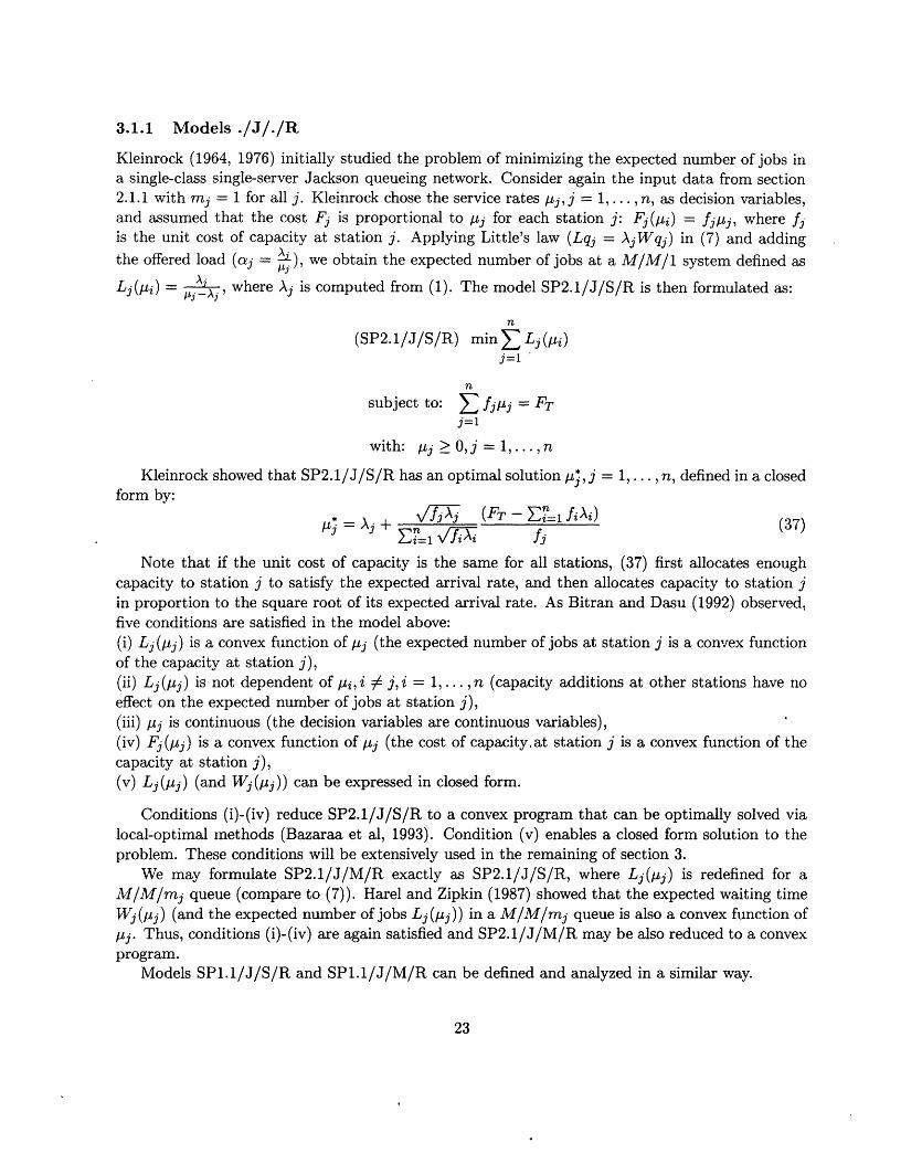
3.1.1 Models ./J/./R

Kleinrock (1964, 1976) initially studied the problem of minimizing the expected number of jobs ina single-class single-server Jackson queueing network. Consider again the input data from section2.1.1 with mj = 1 for all j. Kleinrock chose the service rates j,j = 1,..., n, as decision variables,and assumed that the cost Fj is proportional to j for each station j: Fj(lpi) = fjpj, where fjis the unit cost of capacity at station j. Applying Little's law (Lqj = AjWqj) in (7) and addingthe offered load (j = ), we obtain the expected number of jobs at a M/M/1 system defined as

Lj(pi) = A'X where Aj is computed from (1). The model SP2.1/J/S/R is then formulated as:

n

(SP2.1/J/S/R) minELj(pi)j=1

n

subject to: E fjpj = FTj=l

with: j > O, j = 1,...,n

Kleinrock showed that SP2.1/J/S/R has an optimal solution j, j = 1,., n, defined in a closedform by:

f/-jA (FT - E= 1 fiAi) (37)A"3 j + ~n (37)

Note that if the unit cost of capacity is the same for all stations, (37) first allocates enoughcapacity to station j to satisfy the expected arrival rate, and then allocates capacity to station jin proportion to the square root of its expected arrival rate. As Bitran and Dasu (1992) observed,five conditions are satisfied in the model above:(i) Lj (lj) is a convex function of /j (the expected number of jobs at station j is a convex functionof the capacity at station j),(ii) Lj(pj) is not dependent of pi, i # j, i = 1, .. , n (capacity additions at other stations have noeffect on the expected number of jobs at station j),(iii) j is continuous (the decision variables are continuous variables),(iv) Fj(,j) is a convex function of j (the cost of capacity.at station j is a convex function of thecapacity at station j),(v) Lj(pj) (and Wj(pj)) can be expressed in closed form.

Conditions (i)-(iv) reduce SP2.1/J/S/R to a convex program that can be optimally solved vialocal-optimal methods (Bazaraa et al, 1993). Condition (v) enables a closed form solution to theproblem. These conditions will be extensively used in the remaining of section 3.

We may formulate SP2.1/J/M/R exactly as SP2.1/J/S/R, where Lj(pj) is redefined for aM/M/mj queue (compare to (7)). Harel and Zipkin (1987) showed that the expected waiting timeWj (j) (and the expected number of jobs Lj(pj)) in a M/M/mj queue is also a convex function ofpj. Thus, conditions (i)-(iv) are again satisfied and SP2.1/J/M/R may be also reduced to a convexprogram.

Models SP1.1/J/S/R and SP1.1/J/M/R can be defined and analyzed in a similar way.

23

3.1.2 Models ./J/M/N

In sequel, we discuss models SP1.1/J/M/N and SP2.1/J/M/N. Now we have integer decision vari-ables corresponding to the number of machines in each station. Boxma et al (1990) presented aheuristic and an exact algorithm to solve both problems. The manufacturing network is repre-sented by a multiple-class multiple-server Jackson OQN with a different deterministic routing foreach class (see sections 2.1.2 and 2.2.3). Consider again the input data described in section 2.2.3with cak = 1 and CSk = 1 for each class k, and mj > 1 for each station j.

Aggregating all classes into a unique class, we obtain each station j described by 3 parameters(mj, Aj, Aj } (see section 2.1.2). Kelly (1979) showed that the equilibrium distribution of the numberof jobs in the network can be expressed as a product form, and that each station j in steady-statebehaves as a M/M/mj system. Applying Little's law in (7) and adding the offered load, we obtainthe expected number of jobs Lj as a function of mj, Aj and j, given by:

2L)'(oxjLj(mj, ij, j) = ljm + A (38)

whereMj-1 C( t ( )mj

7(0) = A E t! + j(1 ) 1t=0 t!( 1 )mj!

Boxma et al considered mj,j = 1,...,n, as decision variables in models SP1.1/J/M/N andSP2.1/J/M/N, and observed that Lj(mj,Aj,pj) in (38), namely Lj(mj), is a convex decreasingfunction of mj (conditions (i) and (ii) are satisfied). They chose WIP as a performance measurefor the network. Note that this analysis is easily extended to leadtime since WIP and leadtime arelinearly related through Little's law. Let m be the vector of decision variables (ml, m2,... ,mn).The network WIP, L(m), is given by:

n

L(m) = ZvjLj(mj) (39)j=1

The choice of mj in each station must satisfy the condition pj < 1, in order to prevent systeminstability. Let Izl denote the largest integer number less than z. Using this condition and (2), itfollows that mj must be an integer number greater than or equal to the lower bound m °, definedas:

mj = jj + 1 (40)

Model SP1.1/J/M/N

In model SP1.1/J/M/N we want to find a minimal cost solution satisfying a WIP level less thanor equal to the specified limit LT, where LT < L(m°). Let Fj(mj) be the cost of allocatingmj machines at station j, defined as a convex non-decreasing function of mj (condition (iv) issatisfied). Using (39) and (40) we obtain the targeted WIP level problem (also called server

24

allocation problem):n

(SP1.1/J/M/N) min F(m) = Fj(mj)j=1

subject to: L(m) < LT

with: mj > m ° , mjinteger,j = 1, . . ., n

Note that since SP1.1/J/M/N is a convex program with integer variables, the use of marginalanalysis schemes do not lead necessarily to optimality (condition (iii) is not satisfied). Let PIj (mj)be a priority index defined as the quotient of the increase of cost and the decrease of WIP at stationj, given by:

PIj(mj) AFj(m ) (41)-vjALj(mj + 1)

whereAFj(mj + 1) = Fj(mj + 1) - Fj(mj) >

ALj(mj + 1) = Lj(mj + 1) - Lj(mj) < 0

PIj is a result from the marginal analysis of Fj and Lj. Boxma et al (1990) presented a simpleheuristic algorithm (algorithm 1) based on the greedy method to solve problem SP1.1/J/M/N (seealso Sundarraj et al (1994). for a related approach to a similar problem). The algorithm starts withthe smallest possible machine allocation (40) for each station. At every iteration it then adds onemachine at the station where the priority index. (41) is the smallest. The algorithm terminates assoon as adding a machine makes the allocation feasible.

Algorithm 1

1. Start with the allocation m = j = m,j = 1,..., n. This solution is infeasible (L(m °) > LT) andits cost F(m ° ) is less than the minimum cost of SP1.1/J/M/N.

2. At each iteration, update the cost F(m), WIP L(m) (using (38) and (39)), and PIj(mj) (using(41)). Add one machine at the station j* which results in the smallest quotient PIj* (greedystrategy), given by:

PIj* = min{PIj(mj),j = 1,...,n} (42)

3. Stop as soon as L(m) reaches the target LT (feasible solution).

Note that station j* chosen in (42) produces the smallest increase of F(m) per unit of decreaseof L(m), indicated by PIj.. From the convexity of Fj and Lj, we obtain:

AFj(mj + 1) AFj(mj) (43)(43)

-vjALj(mj + 1) - -vjLj(mj)

An interesting result from (43) is that we can verify the quality of the heuristic solution gen-erated by algorithm 1, just comparing the solutions generated in the last two iterations. Let p bethe last iteration, and m l, m 2 ,..., m - l , m be the solution generated in each iteration. Obviously,

25

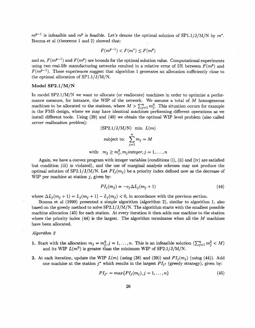
mp-1 is infeasible and m p is feasible. Let's denote the optimal solution of SP1.1/J/M/N by m*Boxma et al (theorems 1 and 2) showed that:

F(mP - ) < F(m*) < F(mP )

and so, F(mP- 1) and F(mP) are bounds for the optimal solution value. Computational experimentsusing two real-life manufacturing networks resulted in a relative error of 5% between F(mP) andF(mP-1). These experiences suggest that algorithm 1 generates an allocation sufficiently close tothe optimal allocation of SP1.1/J/M/N.

Model SP2.1/M/N

In model SP2.1/M/N we want to allocate (or reallocate) machines in order to optimize a perfor-mance measure, for instance, the WIP of the network. We assume a total of M homogeneousmachines to be allocated to the stations, where M > jn=l m0 . This situation occurs for examplein the FMS design, where we may have identical machines performing different operations as weinstall different tools. Using (39) and (40) we obtain the optimal WIP level problem (also calledserver reallocation problem):

(SP2.1/J/M/N) min L(m)n

subject to: E mj= Mj=1

with: mj >m,0 mjinteger,j .= 1,..., n

Again, we have a convex program with integer variables (conditions (i), (ii) and (iv) are satisfiedbut condition (iii) is violated), and the use of marginal analysis schemes may not produce theoptimal solution of SP2.1/J/M/N. Let PIj(mj) be a priority index defined now as the decrease ofWIP per machine at station j, given by:

PIj(mj) = -vjALj(mj + 1) (44)

where ALj(mj + 1) = Lj(mj + 1) - Lj(mj) < 0, in accordance with the previous section.Boxma et al (1990) presented a simple algorithm (algorithm 2), similar to algorithm 1, also

based on the greedy method to solve SP2.1/J/M/N. The algorithm starts with the smallest possiblemachine allocation (40) for each station. At every iteration it then adds one machine to the stationwhere the priority index (44) is the largest. The algorithm terminates when all the M machineshave been allocated.

Algorithm 2

1. Start with the allocation mj = m,j = 1,... , n. This is an infeasible solution (jn=l m < M)and its WIP L(m °) is greater than the minimum WIP of SP2.1/J/M/N.

2. At each iteration, update the WIP L(m) (using (38) and (39)) and PIj(mj) (using (44)). Addone machine at the station j* which results in the largest PIj* (greedy strategy), given by:

PIj. = max{PIj(mj), j = 1,..., n} (45)

26

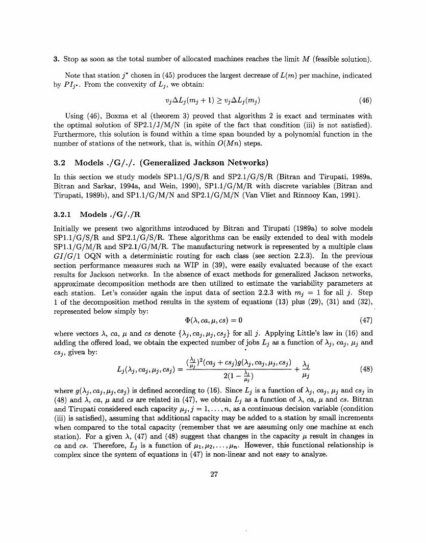
3. Stop as soon as the total number of allocated machines reaches the limit M (feasible solution).

Note that station j* chosen in (45) produces the largest decrease of L(m) per machine, indicatedby PIj.. From the convexity of Lj, we obtain:

vjALj(mj + 1) > vjALj(mj) (46)

Using (46), Boxma et al (theorem 3) proved that algorithm 2 is exact and terminates withthe optimal solution of SP2.1/J/M/N (in spite of the fact that condition (iii) is not satisfied).Furthermore, this solution is found within a time span bounded by a polynomial function in thenumber of stations of the network, that is, within O(Mn) steps.

3.2 Models ./G/./. (Generalized Jackson Networks)

In this section we study models SP1.1/G/S/R and SP2.1/G/S/R (Bitran and Tirupati, 1989a,Bitran and Sarkar, 1994a, and Wein, 1990), SP1.1/G/M/R with discrete variables (Bitran andTirupati, 1989b), and SP1.1/G/M/N and SP2.1/G/M/N (Van Vliet and Rinnooy Kan, 1991).

3.2.1 Models ./G/./R

Initially we present two algorithms introduced by Bitran and Tirupati (1989a) to solve modelsSP1.1/G/S/R and SP2.1/G/S/R. These algorithms can be easily extended to deal with modelsSP1.1/G/M/R and SP2.1/G/M/R. The manufacturing network is represented by a multiple classGI/G/1 OQN with a deterministic routing for each class (see section 2.2.3). In the previoussection performance measures such as WIP in (39), were easily evaluated because of the exactresults for Jackson networks. In the absence of exact methods for generalized Jackson networks,approximate decomposition methods are then utilized to estimate the variability parameters ateach station. Let's consider again the input data of section 2.2.3 with mj = 1 for all j. Step1 of the decomposition method results in the system of equations (13) plus (29), (31) and (32),represented below simply by:

(A, ca, i, cs) = 0 (47)

where vectors A, ca, p and cs denote {Aj, caj, j, csj} for all j. Applying Little's law in (16) andadding the offered load, we obtain the expected number of jobs Lj as a function of Aj, caj, pj andcsj, given by:

= ()2(caj + csj)g(Aj, caj, Aj, csj) AjLj(Aj, caj, ,jj, csj) = (1-j )+ - (48)~2 (1 -~I-'tj

where g(Aj, caj, tj, csj) is defined according to (16). Since Lj is a function of Aj, caj, j and csj in(48) and A, ca, IL and cs are related in (47), we obtain Lj as a function of A, ca, and cs. Bitranand Tirupati considered each capacity pj,j = 1, . . ., n, as a continuous decision variable (condition(iii) is satisfied), assuming that additional capacity may be added to a station by small incrementswhen compared to the total capacity (remember that we are assuming only one machine at eachstation). For a given A, (47) and (48) suggest that changes in the capacity p result in changes inca and cs. Therefore, L is a function of 1l, 2,... ,n. However, this functional relationship iscomplex since the system of equations in (47) is non-linear and not easy to analyze.

27

Bitran and Tirupati assumed that ca and cs are independent of changes in capacity Pu. In thisway, Lj is not dependent on i, i j (condition (ii) is satisfied). They assumed that as we modifyp, the mean and variance of the service time vary in the same proportion and hence, cs remainsnearly constant. Furthermore, the sensitivity of ca to changes in , seems to be small, as we increasethe number of classes, and the proportion of load due to each class decreases (see the numericalresults in Bitran and Tirupati (1988) and the discussion in Whitt (1988)). The consequence ofthese assumptions is that we can first solve system (47) for a given initial capacity, and then treatthe resulting ca as known parameters in (48). Under these assumptions, Bitran and Tirupati alsoshowed that Lj(Aj, caj, Lj, csj) in (48) is a convex function of Pj, now denoted simply by Lj(Plj)(condition (i) is satisfied). The WIP of the network may be expressed as (compare to (39)):

n

L(u) = vjLj(ftj) (49)j=1

Finally, we denote by Aj a lower bound on the capacity at station j. Note that this bound mustsatisfy the condition pj < 1 to avoid system instability:

> A (50)

Model SP1.1/G/S/R

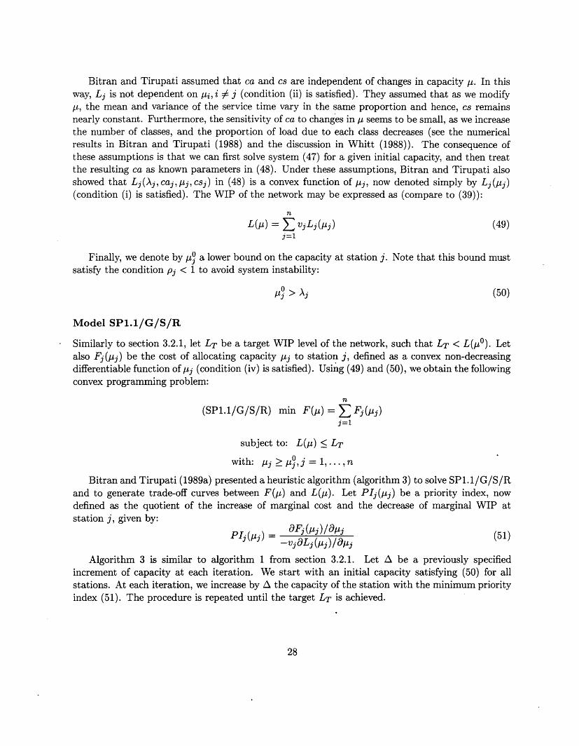
Similarly to section 3.2.1, let LT be a target WIP level of the network, such that LT < L(P°). Letalso Fj(pj) be the cost of allocating capacity j to station j, defined as a convex non-decreasingdifferentiable function of /j (condition (iv) is satisfied). Using (49) and (50), we obtain the followingconvex programming problem:

n

(SP1.1/G/S/R) min F(p) = Fj(pj)j=1

subject to: L(p) < LT

with: j > j °,j = ,...,n

Bitran and Tirupati (1989a) presented a heuristic algorithm (algorithm 3) to solve SP1.1/G/S/Rand to generate trade-off curves between F(p) and L(p). Let PIj(pj) be a priority index, nowdefined as the quotient of the increase of marginal cost and the decrease of marginal WIP atstation j, given by:

PIj(uj)= - 9Fj (/)/p (51)

Algorithm 3 is similar to algorithm 1 from section 3.2.1. Let A be a previously specifiedincrement of capacity at each iteration. We start with an initial capacity satisfying (50) for allstations. At each iteration, we increase by A the capacity of the station with the minimum priorityindex (51). The procedure is repeated until the target LT is achieved.

28

Algorithm 3

1. Start with the allocation pj = pu° (sufficiently small), and compute caj and CSj (using (47)) foreach station j, j=1,...,n. This solution is infeasible (L(/y°) > LT) and its cost F(/, °) is lessthan the minimum cost of SP1.1/G/S/R.

2. At each iteration, update the cost F(t,), WIP L(t,) (using (48) and (49)) and PIj(p/j) (using(51)). Add capacity A to the station j* which results in the smallest PIj. (greedy strategy),given by:

PIj = min{PIj(plj),j = 1,..., n} (52)

3. Stop as soon as L(p) reaches the target LT (feasible solution).

As we choose smaller values for A, algorithm 3 generates more precise trade-off curves. Bi-tran and Tirupati (proposition 2) showed that in the limit A - 0, algorithm 3 optimally solvesSP1.1/G/S/R (remember that we have assumed that all conditions (i)-(iv) are satisfied), andPIj(lj) obtained in the last iteration corresponds to the dual multiplier associated with the WIPconstraint of station j.

Bitran and Tirupati (proposition 3) also presented an error bound for the approximate solutionvalue produced by algorithm 3. Let's suppose that algorithm 3 finds a feasible solution after piterations, and let's denote this solution by up and the optimal solution of SP1.1/G/S/R by *.Then:

0 < F(j) - F < (LT -L(P)) + 6 (53)

Phiwhere = A EP=1(1 - ) and PI.* is the quotient obtained by (52) at iteration i,i = 1,... ,p.

Computational experiences with A = 0.1 applied to a real-life example with 13 stations and 10product classes resulted in a relative error of 0.6% between F(AP) and F(p*). This is acceptablein many practical situations. These experiences also indicated that the previous assumption ofconsidering ca and cs independent of changes in is reasonable (observe in algorithm 3 that caand cs are maintained constant). As an illustration, as the WIP was reduced from an initial valueof 70000 to a final value of 30000 in the example above, the maximum change found in ca was 3%.This change was obtained by updating ca according to (47) at the final network configuration.

A refinement of algorithm 3 is to update ca in (47). In fact, Bitran and Sarkar (1994b) haveexplored this alternative. When the ca are not considered independent of capacity, there is noguarantee that SP1.1/G/S/R is a convex program. We do not know if L in (49) stays convex inp because ca now changes as changes, according to (47). Thus, this alternative procedure maynot converge to an optimal solution or even to a feasible solution. Nevertheless, Bitran and Sarkar(op.cit.) showed that the procedure converges under certain conditions for the initial data.

Model SP2.1/G/S/R

In this section, we analyze the problem of redistributing the existing capacity in the stations tominimize WIP. This redistribution is meaningful in networks with homogeneous capacity, that is,

29

resources that can be shared by different stations (e.g., labor). Let 4 be the initial existing capacityat station j, such that 1A > p1 . Using (49) and (50), we obtain:

(SP2.1/G/S/R) min L(j)

n n

subject to: E Ail = E/pj=1 j=1

with: j >/°,j 1,...,n

Bitran and Tirupati (1989a) presented a heuristic algorithm (algorithm 4) also based on thegreedy method to solve SP2.1/G/S/R (again, conditions (i)-(iv) are satisfied). Let A be definedas before (see algorithm 3), and let PIj(pj) be defined now as the decrease of marginal WIP atstation j, given by:

9Lj (Mj)PIj(/lj) = -vj 9(j) (54)

Algorithm 4

1. Start with the feasible allocation j = jl, and compute caj and csj (using (47)) for each stationj, j=l,... ,n. Define Jo as the set of available stations, J1 as the set of stations to whichcapacity is increased, and J2 as the set of stations to which capacity is reduced. Initially,Jo = {1, 2, ... , n}, and J1 and J2 are empty. Compute ej such that:

Plj(lpj)(Aj + j) = max{PIj(lj),j E Jo} (55)

2. At each iteration, update the WIP L() (using (48) and (49)), and PIj(lj) (using (54)). Findthe station jl which results in the smallest PIjl given by:

PIj1 = min{PIj(/lj),j E Jo} (56)

and the station j2 which results in the largest PIj2 given by:

PIj2 = max{PIj(tj),j E Jo} (57)

2a. If jl E J1, then make Jo +- Jo - {j }.

2b. If j 2 E J2, then make Jo +- Jo - {j2}.

2c. If jl ¢ J1 and j2 0 J2, then define Al = min{A, ljl -Aj -Ej 1} and make Ij, + /j -A 1,ij2 - Pj2 + A 1, J1 +- J1 U {j2} and J 2 +- J2 U {jl}.

3. Stop if Jo is empty or unitary, or PIj = PIj2.

Note that, at each iteration, (56) and (57) correspond to the stations that produce the largestand smallest marginal reduction in L(/l), respectively. Expression (55) together with A1l guaranteesthat the solution generated by algorithm 4 satisfies !Uj > Aj +ej, j = 1,..., n. Hence, it satisfies (50)and is feasible. Bitran and Tirupati (1989a, remark) showed that in the limit A -+ 0, this solution

30

is optimal to SP2.1/G/S/R (remember that we have assumed all conditions (i)-(iv) satisfied), andall PIj(Itj) in the last iteration have the same value. As before, each PIj(ipj) can be interpretedas the dual multiplier associated to the capacity constraint at station j. It represents the rate ofdecrease in WIP due to marginal additions in the capacity of this station.

Bitran and Tirupati (proposition 4) also presented an error bound for the approximate solutionvalue produced by algorithm 4. Let P denote the heuristic solution found at the last iteration p,and * denote the optimal solution of SP2.1/G/S/R. Then:

o < F(I1P) - F(y*) < n PI2 (58)

where PIP is the priority index obtained from (57) at the last iteration p. Note in (58) that thesolution tpP is optimal in the limit - 0. Computational experience with A = 0.02 applied tothe same practical example of the previous section resulted in a relative error smaller than 2%between F(tuP) and F(/i*), indicating that algorithm 4 is a good approximation to SP2.1/G/S/R.Bitran and Tirupati reported an interesting result from this example: the WIP is reduced froma initial value of 70000 to a final value around 40000 just by redistributing the initial capacity ofthe network (note however that they have assumed that the capacity of one station is completelytransferable to other station). In order to test the hypothesis of independence of ca to capacitychanges, they recomputed ca according to (47) at the final network configuration (remember thatalgorithm 4 maintains ca and cs fixed during the iterations). The largest variation found in ca wasaround 3%.

Note that algorithms 2 and 4 help balancing a manufacturing system, whereas algorithms 1 and 3efficiently add resources to that system. One may generate trade-off curves between working capital(WIP) and investment capital by, firstly, applying algorithm 4 to the original system configurationand then, utilizing the solution obtained, pP, as a starting capacity for algorithm 3 (i.e., M0 +_ P,where p0 is the initial capacity at step 1 of algorithm 3). For a computational experience andanalysis of trade-off curves, see e.g. Bitran and Tirupati (1989a) and Bitran and Morabito (1994).

Wein (1990) analyzed the model SP2.1/G/S/R for a single-class GI/G/1 OQN with all jobsfollowing a probabilistic routing. Starting from the Brownian model proposed by Harrison andWilliams (1987), which is based on heavy-traffic approximations (Reiman, 1984), Wein obtainedthe expected number of jobs at station j (in equilibrium) given by:

Ljj)= 13 A (59)

wheren

aj = Aojcaj + Ajcsj + 3 Aiqi(csiqij + 1 - qij)i=l

Note that expression (59) is not derived from the approximate decomposition methods discussedin section 2.2, such as expression (48). Furthermore, (59) is valid only if a certain condition, calledskew-symmetry, is satisfied (see expression (4) in Wein, 1990). Let's consider again the budgetconstraint used by Kleinrock (1964) and discussed in the section 3.1.1. Assuming that the skew-symmetry condition is satisfied and using (59), the model SP2.1/G/S/R may be formulated asbelow: n

(SP2.1/G/S/R') min ELj(i)j=1

31

n

subject to: E fjj - FTj=1

with: j O,j = , . . .,n

After deriving the Lagrangean function of this problem, Wein obtained a closed form solutionLj,j = 1,..., n, given by:

fa 3 (FT - E1 fi(6i)J -- ' + _ Z- (60)

fj

Wein observed that the skew-symmetry condition is satisfied for Jackson networks (i.e., M/M/1systems with caj = 1 and csj = 1,j = 1,... , n), and (60) reduces to (37) which is the optimalsolution to SP2.1/J/S/R'. Note that if fj is equal for all stations, then (60) first allocates enoughcapacity to station j just to compensate Aj, and then allocates capacity to station j in proportionto the square root of the parameter aj.

Wein presented computational experiences from a simple network example satisfying the skew-symmetry condition. These results showed that (60) produces a solution very close to the optimalsolution found by simulation. Although (60) is derived under heavy-traffic conditions (pj > 0.9),it may also produce good approximations for low traffic intensities. An important question is toinvestigate the quality of the solution generated by (60) in situations where the skew-symmetrycondition is not satisfied.

3.2.2 Model SP1.1/G/M/R with Discrete Variables

Bitran and Tirupati (1989b) presented a heuristic algorithm to solve the model SP1.1/G/M/R withdiscrete alternatives for capacity changes at each station. Jobs belong to multiple classes and eachclass follows a different deterministic route, according to section 2.2.3. Similarly as we have done insection 3.2.1, the system of equations (19) plus (29), (31) and (32) from step 1 of the decompositionmethod is described below simply as:

((m, A, ca, ,p, cs) = 0 (61)

where vectors m, A, ca, and cs denote respectively the parameters m j , Aj, caj,pj, csj} for allstations j,j = 1,..., n. Applying Little's law in (21) and adding the offered load, we obtain theexpected number of jobs at station j, given by:

Lj (mj, Aj, caj, +j, csj) = ) Lqj(M/M/mj) + A (62)2 Ai(

where Lqj(M/M/mj) denotes the expected number of jobs in queue at a M/M/mj system. Notethat Lqj(M/M/m j ) corresponds to the first term on the right hand side of (38). Similarly to (48),Lj(mj, Aj,caj ,lpj, csj) in (62) is a function of mj, Aj, caj, ,j and csj satisfying (61) (for otherapproximations of Lj, see e.g. Whitt (1993)). Instead of choosing m or p as the decision variablesof the model, Bitran and Tirupati considered a finite number of alternatives for capacity change ateach station. Let's define nj as the total number of alternatives at station j. For each alternativek, k = 1,..., nj, the following input data is given:

32

mjk number of identical machines at station j in alternative k1j3k expected service rate of each machine at station j in alternative kfjk cost of station j in alternative k.

Define Ujk as a 0-1 decision variable (condition (iii) is not satisfied), such that:

U i if alternative k is chosen for station jUjk = 0 otherwise

where -k=- 1 Ujk = 1. For each station j, the capacity choice is represented by the vector (ujl, uj2,u .. , j,nk) where all elements are null except one. In this way, we have mj = k=L1 mjkujk and Lj =

Ek-=,l jkUjk and hence, (61) and (62) depend on Ujk. Let u = {ujk,j = 1, ... ,n; k = 1,...,nj).Similarly to section 3.2.1, Bitran and Tirupati assumed that ca and cs are independent of capacitychanges in the network (see the discussion in the section 3.2.1). As a consequence, we may firstsolve system (61) for a given u (i.e., a given capacity m and p ), and then treat the resulted values ofca and cs as fixed parameters in (62). Furthermore, as we choose an alternative k at station j (i.e.,Ujk = 1 and ujl = 0,l $ k), we may refer to Lj(mj, Xj, caj,pj, csj) in (62) simply as Ljk, where

Ljk = Lj(mjk, Aj, caj, jk, csj). Note that, in this way, we can compute Ljk for every alternativek and every station j using (62). Without loss of generality, we assume that if Ljk > Ljl, thenfjk < fjl, k l , k, = 1,..., nj. Similarly to (49), the network WIP can be written as:

n ni

L(u) = I] jjuk (63)j=l k=1

where, as before, vj is the mean value of a job at station j. Using (63), we obtain the followingproblem:

n nj

(SP1.1/G/M/R) min F(u) = Z Z fkujkj=1 k=1

subject to: L(u) < LT

nj

Ujk = , for j = 1, ...,nk=1

with: ujk E {O, 1},j = 1,...,n,k= 1,...,nj

where LT is a given target for the network WIP. Note that L(u) and F(u) are assumed to belinear functions of u. SP1.1/G/M/R models situations in which the target LT is achieved byincreasing capacity either by means of additional machines, workers, or by increasing the availabilitywith overtime, or additional shift operations. Bitran and Tirupati proposed a heuristic algorithm(algorithm 5) to solve the integer linear program SP1.1/G/M/R above. They showed that: (i) theoptimal solution of the linear program relaxation of SP1.1/G/M/R has either zero or two differentvariables ujk with fractional values (proposition 3.1), and (ii) if this optimal solution has twovariables with fractional values, then they correspond to the same station (corollary)-. The nextalgorithm described below produces the approximate solution ul:

33

Algorithm 5

1. Let u ° be the optimal solution to the LP relaxation of SP1.1/G/M/R. If u° is a feasible solutionto SP1.1/G/M/R, then u1 = u is an optimal solution to SP1.1/G/M/R, otherwise go tostep 2.

2. Let i be the station which variables are fractional values for some k and k 2 ( < ukl < 1,

0 < u°k2 < 1). A feasible solution to SP 1.1/G/M/R is given by:

=ik = ujkj ij = ,...,n,k = 1,... ,nj

1 /1 ifk = Ii otherwise

where 1 is such that:

Lil = max{LikLik < LiklUkl LLik 2Uik2, k = 1,..., ni}

The authors also presented an error bound on the value of approximate solution ul generatedby algorithm 5. Without loss of generality assume that Lik > Lik2, and denote by u* the optimalsolution of SP1.1/G/M/R. Then:

0 < F(u l ) - F(u*) < fik2 -fik < max{fjk,j = 1,... ,n,k = 1,..., nj}

Computational experiences from a real-life network example of 13 stations and 10 productclasses indicate that algorithm 5 is a good approximation to SP1.1/G/M/R when the number ofclasses is relatively large. In this example, as the network WIP was reduced from an initial valueof 80000 to a final value below 30000, the relative error between F(ul) and F(u*) was less than0.08%. The largest change in ca was equal to 4.6%, corresponding to a change of 0.5% in the WIP(remember that the values of ca and cs are also kept constant in algorithm 5). Bitran and Tirupatileft the development of approaches to situations involving a small number of classes and mixturesof deterministic and probabilistic routings for future investigation..

3.2.3 Models ./G/M/N

Van Vliet and Rinnooy Kan (1991) presented two algorithms to solve models SP1.1/G/M/N andSP2.1/G/M/N, based on marginal analysis and greedy methods. These algorithms are closelyrelated to the two algorithms presented by Boxma et al (1990) to solve models SP1.1/J/M/N andSP2.1/J/M/N (described in the section 3.1.2). Again, jobs belong to multiple classes and eachclass follows a different deterministic route. In contrast with section 3.2.2, the decision variablesare the number of machines at the stations.

Let's consider again the system of equations (61), and expression (62) for the expected numberof jobs in a GI/G/mj queue at station j. Van Vliet and Rinnooy Kan considered each capacitymj, j = 1,..., n, as an integer decision variable. Given A and , (61) and (62) suggest that changesin capacity m result in changes in ca and cs (Lj is a function of ml, m 2,..., mn). Note, however,that this functional relationship is not easy to analyze.

34

Based on the results from Bitran and Tirupati (1989a) (see section 3.2.1), Van Vliet and Rin-nooy Kan assumed that ca and cs are independent of changes in capacity m. Therefore, Lj isnot dependent on mi,i $ j (condition (ii) is satisfied). They argued that as we modify m, themean and variance of the service time vary in the same proportion and hence, cs remains nearlyconstant. Furthermore, the sensitivity of ca to changes in m seems to be small as the number ofclasses increases and the proportion of load due to each class decreases. Hence, once the set ofequations (61) is calculated, we can regard ca and cs as parameters for (62). This means thatLj(mj, Ajj, caj,uj, csj) in (62) can be seen as a function of mj only, now denoted by Lj(mj). SinceLqj(M/M/mj) is a convex function of mj, and we are assuming ca and cs as parameters, thenLj(mj) becomes a convex function of mj (condition (i) is satisfied). Following the same steps ofsection 3.1.2, the network WIP L(m) is defined according to (39) (where Lj(mj) is given by (62),instead of (38)), and the initial number of machines m ° must satisfy (40).

Model SP1.1/G/M/N

The model SP1.1/G/M/N is formulated exactly as SP1.1/J/M/N described in section 3.1.2, whereF(m) is a convex non-decreasing function of m (condition (iv) is satisfied), and L(m) is assumedto be convex in m, in accordance with the discussion above. SP1.1/G/M/N, also called the serverallocation problem, is a convex program with integer variables and the use of marginal analysis donot lead necessarily to optimality (condition (iii) is not satisfied). The problem can be regarded asthe minimum-cost allocation of machines so that the WIP is less than a given target WIP.

Van Vliet and Rinnooy Kan utilized algorithm 1 (section 3.1.2) to solve SP1.1/G/M/N. Thealgorithm starts with the smallest possible allocation of machines m ° for all stations (infeasibleallocation). At every iteration, it adds one machine at the station with the smallest priority index(i.e., the quotient of the increase of the objective function and the decrease of the network WIP).Note that this priority index is a result of marginal analysis. It is obtained by substituting (62) in(41). The algorithm terminates as soon as adding a machine makes the allocation feasible.

The error bound provided by Boxma et al (1990) (discussed in section 3.1.2) can also be appliedhere. For instance, if p is the last iteration of algorithm 1 and m* is the optimal solution ofSP1.1/G/M/N, we have: F(m P-1 ) < F(m*) < F(mP). Van Vliet and Rinnooy Kan generatedtrade-off curves between cost and WIP similar to those discussed by Bitran and Tirupati (1989a).Using different computational results from two network examples, they found a relative error of 7%in the solution of the first example and 5% in the solution of the second example. This relative errordecreases as the target WIP imposed to the problem decreases. Van Vliet and Rinnooy Kan alsorecalculated ca for the final configuration of the network to verify the sensitivity of ca to changes ofm. They obtained an error in ca below 6%, suggesting that this approach is a good approximationto problem SP1.1/G/M/N.

Model SP2.1/G/M/N

Similarly, the model SP2.1/G/M/N is formulated exactly as the model SP2.1/J/M/N described insection 3.1.2, where M is the number of available machines such that M > j=l m. Again, we havethe objective function and the constraint of the problem as convex functions of m. SP2.1/G/M/N,also called the server reallocation problem, is a convex program with integer variables and it canbe regarded as the minimum-WIP redistribution of the M machines over the network.

35

Van Vliet and Rinnooy Kan utilized algorithm 2 (section 3.1.2) to solve SP2.1/G/M/N. Thealgorithm starts with the smallest possible allocation of machines m °. At every iteration, it addsone machine to the station with the largest priority index (i.e., the greatest decrease in the networkWIP per machine). Note that this priority index is obtained from marginal analysis by substituting(62) in (44). The algorithm terminates when all the M machines have been allocated.

Since we are assuming L(m) as a convex function of m, algorithm 2 terminates after O(Mn)steps with an optimal reallocation of machines (see section 3.1.2 for details). Computational exper-iments with the two examples above indicated that the sensitivity of ca to changes in m is small.Therefore, the optimal solution produced by algorithm 2 to the assumed convex problem may beutilized as a good approximation to the original problem.

4 Perspectives for Further Research

In this section, we suggest topics for future research. The first one is concerned with the relevanceof class SP3 (see section 1) to the focused factory design. Then, we discuss the importance of light-traffic approximations to manufacturing networks with multiple classes and deterministic routings(according to section 2.2.3). Finally, we return to the critical question of the existence of steady-state for an OQN representing a discrete manufacturing system.

4.1 Relevance of Class SP3

Different authors have pointed out that modern manufacturing systems are becoming more com-plex due to: (i) the large number of product classes competing for common resources, (ii) theuncertainty of product demands, and (iii) the reduction of life cycles. In addition to developingefficient methods to analyze more complex systems, we may also try to reduce the complexity ofthe manufacturing environment. Much of the success of JIT and other related methods comesfrom simplification. Examples of alternatives to reduce complexity include partitioning existingproduction lines, duplication of resources, and redesigning products and manufacturing processes.Note that problems of class SP3 (e.g., problem SP3.1 in section 1) can be regarded in this context.

Recent attempts based on OQN models have been made to analyze the trade-off between thepartitioning of product lines and duplication of machines (Bitran and Sarkar, 1994c; see also Tangand Yoo (1991) for a related study of customer partition and server allocation applied to a singlenode service system). The idea is to relate complexity and predictability of a system, suggestingthat more complex systems tend to have poorer predictability. Therefore, we can use systempredictability of job completion as a measure of complexity. For instance, as we increase thenumber of product classes manufactured in a system, complexity tends to increase and predictabilitytends to decrease due to product interference at stations. Of course we may reduce complexity byadding capacity to stations. We may also reduce complexity by simply partitioning the shop. Inwhat follows, we suggest possible measures of complexity to capture this notion. We consider: (i)measures of complexity from a product management point of view, (ii) measures of complexityfrom a station management point of view.

36

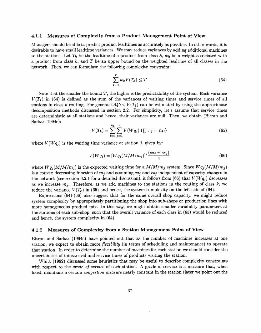
4.1.1 Measures of Complexity from a Product Management Point of View

Managers should be able tc predict product leadtimes as accurately as possible. In other words, it isdesirable to have small leadtime variances. We may reduce variances by adding additional machinesto the stations. Let Tk be the leadtime of a product from class k, wk be a weight associated witha product from class k, and T be an upper bound on the weighted leadtime of all classes in thenetwork. Then, we can formulate the following complexity constraint:

E wkV(Tk) < T (64)k=l

Note that the smaller the bound T, the higher is the predictability of the system. Each varianceV(Tk) in (64) is defined as the sum of the variances of waiting times and service times of allstations in class k routing. For general OQNs, V(Tk) can be estimated by using the approximatedecomposition methods discussed in section 2.2. For simplicity, let's assume that service timesare deterministic at all stations and hence, their variances are null. Then, we obtain (Bitran andSarkar, 1994c):

nk n

V(Tk) = E V(Wqj) l{j : j = nkl} (65)1=1 j=l

where V(Wqj) is the waiting time variance at station j, given by:

V(Wqj) = [Wqj(M/M/mj)]2 (caj + csj) (66)4

where Wqj(M/M/mj) is the expected waiting time for a M/M/mj system. Since Wqj(M/M/m j )is a convex decreasing function of mj and assuming caj and csj independent of capacity changes inthe network (see section 3.2.1 for a detailed discussion), it follows from (66) that V(Wqj) decreasesas we increase mj. Therefore, as we add machines to the stations in the routing of class k, wereduce the variance V(Tk) in (65) and hence, the system complexity on the left side of (64).

Expressions (64)-(66) also suggest that for the same overall shop capacity, we might reducesystem complexity by appropriately partitioning the shop into sub-shops or production lines withmore homogeneous product mix. In this way, we might obtain smaller variability parameters atthe stations of each sub-shop, such that the overall variance of each class in (65) would be reducedand hence, the system complexity in (64).

4.1.2 Measures of Complexity from a Station Management Point of View

Bitran and Sarkar (1994c) have pointed out that as the number of machines increases at onestation, we expect to obtain more flexibility (in terms of scheduling and maintenance) to operatethat station. In order to determine the number of machines for each station we should consider theuncertainties of interarrival and service times of products visiting the station.

Whitt (1992) discussed some heuristics that may be useful to describe complexity constraintswith respect to the grade of service of each station. A grade of service is a measure-that, whenfixed, maintains a certain congestion measure nearly constant in the station (later we point out the

37

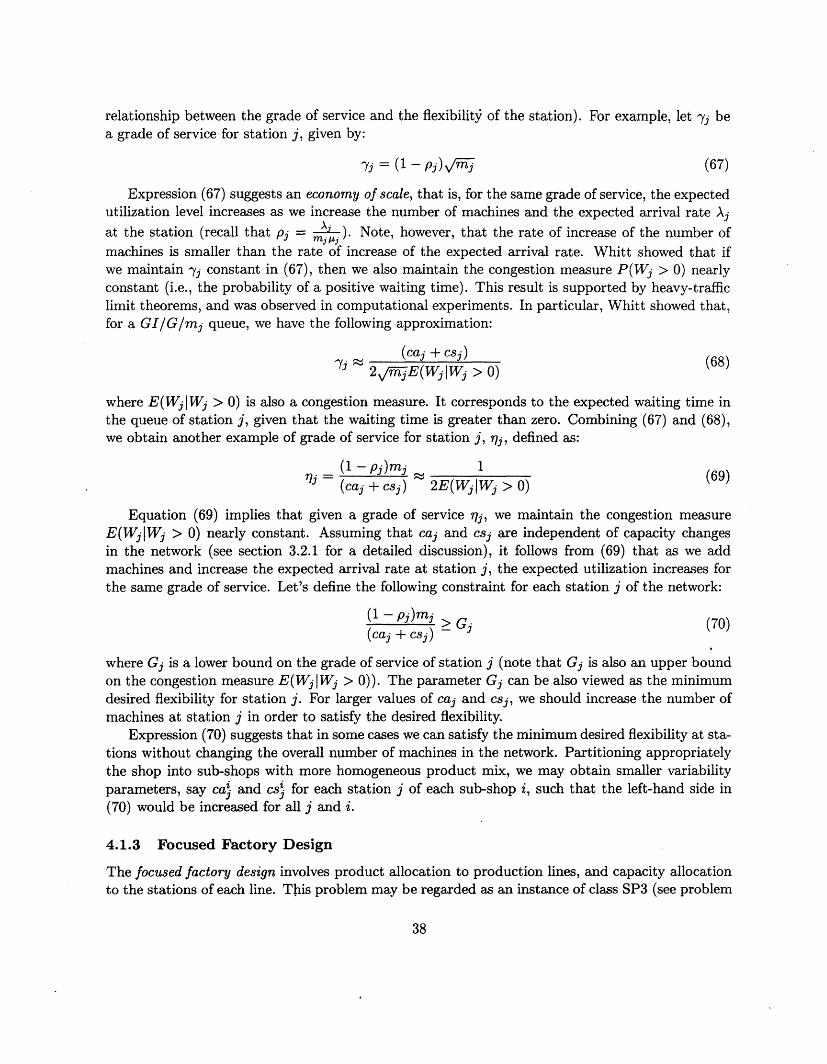
relationship between the grade of service and the flexibility of the station). For example, let yj bea grade of service for station j, given by:

Vj = (1-p/j)2; (67)

Expression (67) suggests an economy of scale, that is, for the same grade of service, the expectedutilization level increases as we increase the number of machines and the expected arrival rate Aj

at the station (recall that pj = j ). Note, however, that the rate of increase of the number ofmachines is smaller than the rate of increase of the expected arrival rate. Whitt showed that ifwe maintain yj constant in (67), then we also maintain the congestion measure P(Wj > 0) nearlyconstant (i.e., the probability of a positive waiting time). This result is supported by heavy-trafficlimit theorems, and was observed in computational experiments. In particular, Whitt showed that,for a GI/G/mj queue, we have the following approximation:

(caj + csj)2x/- E(WjlW > O) (68)

where E(WjlWj > 0) is also a congestion measure. It corresponds to the expected waiting time inthe queue of station j, given that the waiting time is greater than zero. Combining (67) and (68),we obtain another example of grade of service for station j, r7j, defined as:

(1 - pj )m s 1(caj +csj) 2E(WjlWj > 0)

Equation (69) implies that given a grade of service rj, we maintain the congestion measureE(WjlWj > 0) nearly constant. Assuming that caj and csj are independent of capacity changesin the network (see section 3.2.1 for a detailed discussion), it follows from (69) that as we addmachines and increase the expected arrival rate at station j, the expected utilization increases forthe same grade of service. Let's define the following constraint for each station j of the network:

(1 - j) > Gj (70)(cas + csj)

where Gj is a lower bound on the grade of service of station j (note that Gj is also an upper boundon the congestion measure E(WjlWj > 0)). The parameter Gj can be also viewed as the minimumdesired flexibility for station j. For larger values of caj and csj, we should increase the number ofmachines at station j in order to satisfy the desired flexibility.

Expression (70) suggests that in some cases we can satisfy the minimum desired flexibility at sta-tions without changing the overall number of machines in the network. Partitioning appropriatelythe shop into sub-shops with more homogeneous product mix, we may obtain smaller variabilityparameters, say caj and cs, for each station j of each sub-shop i, such that the left-hand side in(70) would be increased for all j and i.

4.1.3 Focused Factory Design

The focused factory design involves product allocation to production lines, and capacity allocationto the stations of each line. This problem may be regarded as an instance of class SP3 (see problem

38

SP3.1 in section 1), and it is different from problems discussed in section 3, where only capacityallocation was involved.

An interesting research issue is developing optimization models to analyze the trade-off betweenthe partitioning of product lines and the duplication of machines in the focused factory design.We might incorporate to these models the complexity constraints from the product and stationmanagement points of views, such as (64) and (70) discussed above. These constraints can help usrepresent desired product leadtimes and desired station flexibility in the system.

A recent research based on these ideas (Bitran and Sarkar, 1994c) reveals an unexpected result:

Contrary to the commonly view, the number of machines required can be less whenproduction lines are partitioned (compared to when they are put in one shop only).

This result suggests that we may reduce the complexity of the network (left side of (64)),or increase the flexibility of the stations (left side of (70)), by only partitioning the facility intoproduct lines. Further research might investigate the stability of optimal partitions. For instance,the solution sensitivity to changes on the expected arrival rate of products, or to changes on thedesired grade of service of stations. We might also consider particular situations where privilegedproduct classes must have lower leadtimes, or follow routings through high service grade stations.

4.2 Light-Traffic Approximations

In this section, we emphasize the importance of light-traffic approximations to analyze OQNs withmultiple classes and deterministic routings. Upon certain conditions, these approximations mayeffectively simplify performance evaluation of large and complex manufacturing networks such asjob-shops.

As discussed in section 2.2.3, Bitran and Tirupati (1988, remark 2) suggested that if the numberof product classes processed at each station is large enough, we may ignore the interaction betweenstations and analyze each station individually. The mean and variance of each product class arepreserved throughout the network, and we may assume that at every station, the mean and varianceare the same as those of the external arrival process of this class. In other words, as the numberof classes increases, we expect that qkl -+ 0 and cdkl -+ cakl in (31) for all k and 1, and hence,cdkl -+ ca'. The network may be decomposed in a set of independent stations, each one analyzedas a single queue system (similarly to the Jackson networks discussed in section 2.1). Note that,in this way, we have virtually no limits on the size of the OQN that could be analyzed. However,practical manufacturing networks usually have one or more stations working under heavy-trafficintensity condition.

Based on the argument above, Whitt (1988) observed that if the arrival rate of one class uponone visit at a station is a small proportion of the total arrival rate there (i.e., qkl is small for classk during visit I to a certain station), then the departure process for that class from that stationshould be nearly the same as the arrival process for that class for that visit (i.e., Cdk - caki). Notethat this can be regarded as a light-traffic approximation, where the class of interest has light-trafficat the station; however, the overall traffic intensity of the station does not need to be low. Thisobservation can be extended to the network. If the light-traffic condition occurs at every stationin the routing of the class, then the arrival and departure processes for this class at the stationsin its routing should be nearly the same as its external arrival process (i.e., caki -+ ca' and so,

39

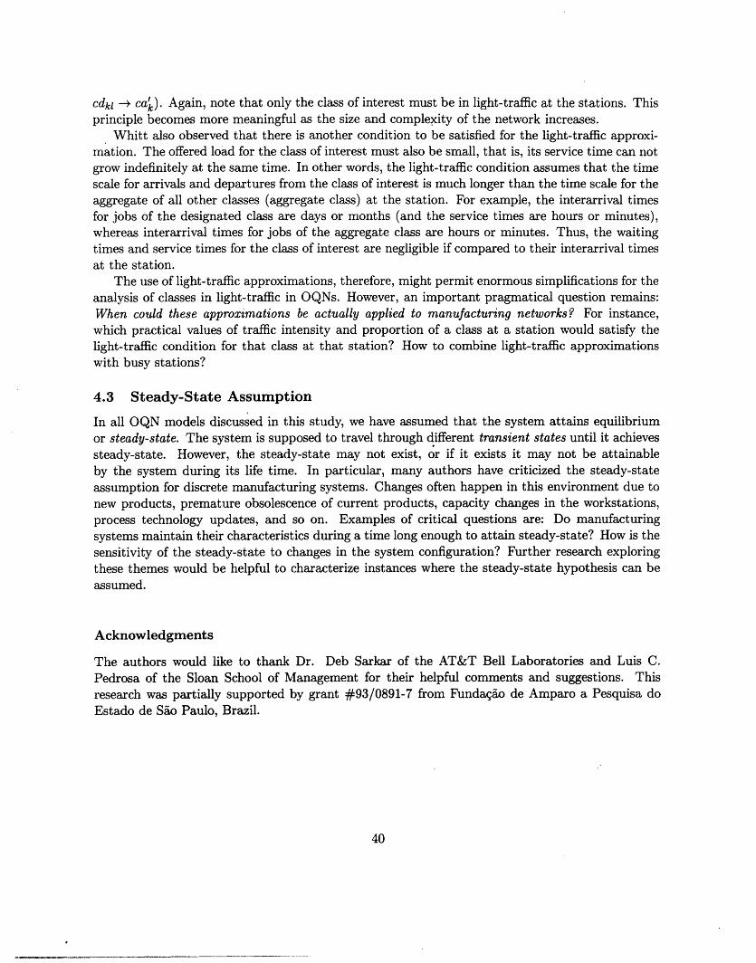
Cdkl -+ ca). Again, note that only the class of interest must be in light-traffic at the stations. Thisprinciple becomes more meaningful as the size and complexity of the network increases.

Whitt also observed that there is another condition to be satisfied for the light-traffic approxi-mation. The offered load for the class of interest must also be small, that is, its service time can notgrow indefinitely at the same time. In other words, the light-traffic condition assumes that the timescale for arrivals and departures from the class of interest is much longer than the time scale for theaggregate of all other classes (aggregate class) at the station. For example, the interarrival timesfor jobs of the designated class are days or months (and the service times are hours or minutes),whereas interarrival times for jobs of the aggregate class are hours or minutes. Thus, the waitingtimes and service times for the class of interest are negligible if compared to their interarrival timesat the station.

The use of light-traffic approximations, therefore, might permit enormous simplifications for theanalysis of classes in light-traffic in OQNs. However, an important pragmatical question remains:When could these approximations be actually applied to manufacturing networks? For instance,which practical values of traffic intensity and proportion of a class at a station would satisfy thelight-traffic condition for that class at that station? How to combine light-traffic approximationswith busy stations?

4.3 Steady-State Assumption

In all OQN models discussed in this study, we have assumed that the system attains equilibriumor steady-state. The system is supposed to travel through different transient states until it achievessteady-state. However, the steady-state may not exist, or if it exists it may not be attainableby the system during its life time. In particular, many authors have criticized the steady-stateassumption for discrete manufacturing systems. Changes often happen in this environment due tonew products, premature obsolescence of current products, capacity changes in the workstations,process technology updates, and so on. Examples of critical questions are: Do manufacturingsystems maintain their characteristics during a time long enough to attain steady-state? How is thesensitivity of the steady-state to changes in the system configuration? Further research exploringthese themes would be helpful to characterize instances where the steady-state hypothesis can beassumed.

Acknowledgments

The authors would like to thank Dr. Deb Sarkar of the AT&T Bell Laboratories and Luis C.Pedrosa of the Sloan School of Management for their helpful comments and suggestions. Thisresearch was partially supported by grant #93/0891-7 from Fundaso de Amparo a Pesquisa doEstado de So Paulo, Brazil.

40

_Y�_II_ _______ _I__�____·�_______�__ �

References

Albin, S. L. (1982). Poisson approximations for superposition arrival processes inqueues. Mgmt. Sci. 28(2), 126-137.

Albin, S. L. (1984). Approximating a point process by a renewal process, II: Superpo-sition arrival processes of queues. Oper. Res. 32, 1133-1162.

Albin, S. L. (1986). Delays for customers from different arrival streams to a queue.Mgmt. Sci. 32, 329-340.

Baskett, F., K. M. Chandy, R. R. Muntz and F. G. Palacios (1975). Open, closed,and mixed networks of queues with different classes of customers. J. ACM 22(2),248-260.

Bazaraa, M. S., H. D. Sherali and C. M. Shetty (1993). Nonlinear programming: Theoryand algorithms, 2nd.ed., Wiley, NY.

Bitran, G. R. and S. Dasu (1992). A review of open queueing network models ofmanufacturing systems. Queueing Syst. 12, 95-134.

Bitran, G. R. and R. Morabito (1994). Manufacturing systems design: Trade-off curveanalysis. Working Paper, Sloan School of Management, MIT.

Bitran, G. R. and D. Sarkar (1994a). Throughput analysis in manufacturing networks.EJOR 74, 448-465.

Bitran, G. R. and D. Sarkar (1994b). Targeting problems in manufacturing queueingnetworks - An iterative scheme and convergence. EJOR 76, 501-510.

Bitran, G. R. and D. Sarkar (1994c). Focused factory design: Complexity, capacity andinventory tradeoffs. Technical Memorandum, AT&T Bell Lab., 36p.

Bitran, G. R. and D. Tirupati (1988). Multiproduct queueing networks with determin-istic routing: Decomposition approach and the notion of interference. Mgmt. Sci.34(1), 75-100.

Bitran, G. R. and D. Tirupati (1989a). Tradeoff curves, targeting and balancing inmanufacturing queueing networks. Oper. Res. 37, 547-564.

Bitran, G. R. and D. Tirupati (1989b). Capacity planning in manufacturing networkswith discrete options. Annals of Oper. Res. 17, 119-136.

Bitran, G. R. and D. Tirupati (1989c). Approximations for product departures from asingle server station with batch processing in multi-product queues. Mgmt. Sci. 35,851-878.

Bitran, G. R. and D. Tirupati (1991). Approximations for network of queues withovertime. Mgmt. Sci. 37(3), 282-300.

Boxma, O. J., A. Rinnooy Kan and M. Van Vliet (1990). Machine allocation problemsin manufacturing networks. EJOR 45, 47-54.

Brown, E. (1988). IBM combines rapid modeling technique and simulation to designPCB factory-of-the-future. Ind. Eng., June 88, 23-90.

41

Buzacott, J. A. and J. G. Shanthikumar (1992). Design of manufacturing systems usingqueueing models. Queueing Syst. 12, 135-214.

Buzacott, J. A. and J. G. Shanthikumar (1993). Stochastic models of manufacturingsystems, Prentice-Hall, Englewood Cliffs, NJ.

Buzacott, J. A. and D. D. Yao (1986). Flexible manufacturing systems: A review ofanalytical models. Mgmt. Sci. 32(7), 890-905.

Calabrese, J. M. (1992). Optimal Workload Allocation in Open Networks of MultiserverQueues. Mgmt. Sci. 38(12), 1792-1802.

Chase, R. B. and N. J. Aquilano (1992). Production and operations management - Alife cycle approach, Irwin, Homewood, MA.

Dallery, Y. and R. David (1986). Operational analysis of multiclass queueing networks.Proc. 25th IEEE Conf. Decision and Control, 1728-1732.

Dallery, Y. and K. E. Stecke (1990). On the optimal allocation of servers and workloadsin closed queueing networks. Oper. Res. 38(4), 694-703.

Denning, P. J. and J. P. Buzen (1978). The operational analysis of queueing networks.ACM Computing Surveys 10(3), 225-261.

Disney, R. L. and D. Konig (1985). Queueing networks: A survey of their randomprocesses. SIAM Rev. 27(3), 335-403.

Erlang, A. K. (1917). Solution of some problems in the theory of probabilities of somesignificance in automatic telephone exchanges. Post Office Electrical Engineer'sJournal 10, 189-197.

Gershwin, S. B. (1994). Manufacturing systems engineering, PrenticeHall, Englewood-Cliffs, NJ.

Harel, A. and P. Zipkin (1987). Strong convexity results for queueing systems. Oper.Res. 35, 405-418.

Harrison, J. and V. Nguyen (1990). The QNET method for two-moment analysis ofopen queueing networks. Queueing Syst. 6, 1-32.

Harrison, J. and V. Nguyen (1993). Brownian models of multiclass queueing networks:Current status and open problems. Queueing Syst. 13, 5-40.

Harrison, J. and R. Williams (1987). Brownian models of open queueing networks withhomogeneous customer populations. Stochastic 22, 77-115.

Ho, Y. C. (1987). Performance evaluation and perturbation analysis of discrete eventdynamic systems. IEEE Trans. Automat. Control 32, 563-572.

Ho, Y. C. and X. Cao (1983). Perturbation analysis and optimization of queueingnetworks. J. Optimization Theory and Applications 40(4), 559-582.

Hsu, L. F., C. S. Tapiero and C. Lin (1993). Network of queues modeling in flexiblemanufacturing systems: A survey. RAIRO 27(2), 201-248.

42

Jackman, J. and E. Johnson (1993). The role of queueing network models in perfor-mance evaluation of manufacturing systems. J. Opl. Res. Soc. 44(8), 797-807.

Jackson, J. R. (1957). Networks of waiting lines. Oper. Res. 5, 518-521.

Jackson, J. R. (1963). Job shop-like queueing systems. Mgmt. Sci. 10, 131-142.

Karmarkar, U. S. (1993). Manufacturing lead times, order release and capacity loading.Handbooks in OR/MS, S. C. Graves (ed.), vol 4, Elsevier, North-Holland, Amster-dam.

Kelly, F. P. (1975). Networks of queues with customers of different types. J. Appl.Prob. 12, 542-554.

Kelly, F. P. (1979). Reversibility and Stochastic Processes, Wiley, NY.

Kleinrock, L. (1964). Communication nets: stochastic message flow and delay, DoverPubl., NY.

Kleinrock, L. (1975). Queueing systems, vol 1: Computer applications, Wiley, NY.

Kleinrock, L. (1976). Queueing systems, vol 2: Computer applications, Wiley, NY.

Kobayashi, H. (1974). Application of the diffusion approximation to queueing networksI: Equilibrium queue distributions. J. ACM 21(2), 316-328.

Koenigsberg, E. (1982). Twenty five years of cyclic queues and closed queue networks:A review. J. Opl. Res. Soc. 33, 605-619.

Kuehn, P. J. (1979). Approximate analysis of general networks by decomposition. IEEETrans. Commun. 27(1), 113-126.

Law, A. M. and S. W. Haider (1989). Selecting simulation software for manufacturingapplications: practical guidelines & software survey. Ind. Eng., May 89, 33-46.

Law, A. M. and M. G. McComas (1989). Pitfalls to avoid in the simulation of manu-facturing systems. Ind. Eng., May 89, 28-69.

Lemoine, A. J. (1977). Networks of queues - a survey of equilibrium analysis. Mgmt.Sci. 24, 464-481.

Pujolle, G. and W. Ai (1986). A solution for multiserver and multiclass open queueingnetworks. INFOR 24(3), 221-230.

Reiman, M. I. (1984). Open queueing networks in heavy-traffic. Math. of Oper. Res.9, 441-458.

Reiman, M. I. (1990). Asymptotically exact decomposition approximations for openqueueing networks. Oper. Res. Lett. 9, 363-370.

Reiser, M. and H. Kobayashi (1974). Accuracy of diffusion approximations for' somequeueing systems. IBM J. Res. Dev. 18, 110-124.

Ross, S. M. (1985). Introduction to Probability Models, Academic Press, Inc., Orlando,FL.

43

Sevcik, K. C., A. I. Levy, S. K. Tripathi and J. L. Zahorjan (1977). Improving approx-imations of aggregated queueing network systems. Computer Performance (eds. K.Chandy and M. Reiser), North-Holland, 1-22.

Segal, M. and W. Whitt (1989). A queueing network analyzer for manufacturing.Teletraffic Science for New Cost-Effective Systems, Networks and Services, ITC-12,M. Bonatti (ed.), Elsevier, North-Holland, Amsterdam, 1146-1152.

Seidmann, A., P. J. Schweitzer and S. Shalev-Oren (1987). Computerized closed queue-ing network models of flexible manufacturing systems: A comparative evaluation.Large Scale Systems 12, 91-107.

Shanthikumar, J. G. and J. A. Buzacott (1981). Open queueing network models ofdynamic job shops. Int. J. Prod. Res. 19, 255-266.

Shanthikumar, J. G. and J. A. Buzacott (1984). The time spent in a dynamic job shop.EJOR 17, 215-226.

Shanthikumar, J. G. and D. D. Yao (1987). Optimal server allocation in a system ofmulti-server stations. Mgmt. Sci. 33(9), 1173-1180.

Shanthikumar, J. G. and D. D. Yao (1988). On server allocation in multiple centermanufacturing systems. Oper. Res. 36(2), 333-342.

Sundarraj, R. P., P. S. Sundararaghavan, D. R. Fox (1994). Optimal server acquisitionin open queueing networks. J. Oper. Res. Soc. 45(5), 549-558.

Suresh, S. and W. Whitt (1990). The heavy-traffic bottleneck phenomenon in openqueueing networks. Oper. Res. Lett. 9, 355-362.

Suri, R. (1989). Perturbation analysis: The state of the art and research issues explainedvia the G/G/1 queue. Proc. IEEE 77, 114-137.

Suri, R. and S. De Treville (1991). Full speed ahead: A look at rapid modeling tech-nology in operations management. OR/MS Today 18, 34-42.

Suri, R., G. W. Diehl and R. Dean (1986). Quick and easy manufacturing systemsanalysis using ManuPlan. Proc. Spring IIE Conf., Dallas, TX, 195-205.

Suri, R., J. L. Sanders, M. Kamath (1993). Performance evaluation of productionnetworks. Handbooks in OR/MS, S. C. Graves (ed.), vol 4, Elsevier, North-Holland,Amsterdam.

Tang, C. S. and S. Yoo (1991). System planning and configuration problems for optimalsystem design. EJOR 54, 163-175.

Tijms, H. C. (1986). Stochastic modeling and analysis: A computational approach,Wiley, NY.

Van Vliet, M. and A. Rinnooy Kan (1991). Machine allocation algorithms for job shopmanufacturing. Journal of Intelligent Manufacturing 2, 83-94.

Walrand, J. (1990). Queueing networks. Handbooks in OR/MS, D. P. Heyman and M.J. Sobel (ed.), vol 2, Elsevier, North-Holland, Amsterdam.

44

Wein, L. M. (1990). Capacity allocation in generalized Jackson networks. Oper. Res.Lett. 15, 215-242.

Wein, L. M. (1990). Scheduling networks of queues: Heavy traffic analysis of a two-station network with controllable inputs. Oper. Res. 38(6), 1065-1078.

Whitt, W. (1982). Approximating a point process by a renewal process, I: Two basicmethods. Oper. Res. 30, 125-147.

Whitt, W. (1983a). The queueing network analyzer. Bell Syst. Tech. J. 62, 2779-2815.

Whitt, W. (1983b). Performance of the queueing network analyzer. Bell Syst. Tech. J.62, 2817-2843.

Whitt, W. (1984). Open and closed models for networks of queues. ATfT Bell Lab.Tech. J. 63(9), 1911-1979.

Whitt, W. (1988). A light-traffic approximation for single-class departures from multi-class queues. Mgmt. Sci. 34(11), 1333-1346.

Whitt, W. (1992). Understating the efficiency of multi-server service systems. Mgmt.Sci. 38(5), 708-723.

Whitt, W. (1993). Approximations for the GI/G/m queue. Production and Oper.Mgmt.2(2), 114-161.

Whitt, W. (1994). Towards better multi-class parametric-decomposition approxima-tions for open queueing networks. Annals of Oper.Res. 48, 221-248.

Yao, D. D. and J. A. Buzacott (1986). The exponentialization approach to flexiblemanufacturing system models with general processing times. EJOR 24, 410-416.

45