Online Stereo Calibration using FPGAs - nipe.senipe.se/publications/pettersson_thesis_2005.pdf · Online Stereo Calibration using FPGAs ... 2.2.1 Edge detection, using the Sobel operator

Thesis for the degree of Master of Science

Online Stereo Calibration usingFPGAs

Niklas Pettersson

Division of Physical Resource Theory - Complex Systems

Chalmers University of Technology

Goteborg, Sweden, 2005

Online Stereo Calibration using FPGAsniklas pettersson© niklas pettersson 2005

Division of Physical Resource Theory - Complex SystemsChalmers University of TechnologySE-412 96 GoteborgSwedenTelephone +46(0)31-772 1000

Chalmers ReproserviceGoteborg, Sweden, 2005

Online Stereo Calibration using FPGAsniklas pettersson

Division of Physical Resource Theory - Complex SystemsChalmers University of Technology

Abstract

Stereo vision is something that most people do everyday without even re-alizing it. More specifically, as we walk around our environment, our twoeyes are constantly taking in a pair of images of the world. Our brain thenfuses these two images and unconsciously computes the approximate depthof the objects you see around you. In the field of computer vision, our twoeyes are replaced by two cameras and our brain is replaced by a computer.However, the aim of stereopsis remains the same. That is, given a pair ofstereo images, we want to compute the scene depth.

Now, with human vision, in order to calculate scene depth, your brain prob-ably needs to know how far apart your eyes are and what orientations youreyes are in. Similarly, with computer vision, you need to know the transla-tion and rotation between the cameras before you can calculate scene depth.Determining the translation and rotation is known as stereo calibration.

This thesis deals with the problem of stereo calibration. More specifically,given a continuous stream of image pairs, we want to perform stereo cali-bration in real time. However, due to the computational intensity of thesecalibration calculations, today’s computers are not yet fast enough to dothis in real time. In order to solve this problem, we suggest using pro-grammable logic, i.e. Field Programmable Gate Arrays (FPGAs), for partsof the calibration process.

The reason for using programmable logic is that many of the steps neededin the stereo calibration algorithm can be done independently of each other.This means that a parallel approach, such as using FPGAs, will have a clearadvantage. By implementing steps in the algorithm in parallel on FPGAs,we can reduce the computational time needed per frame and achieve realtime performance.

The resulting stereo calibration that was achieved in this thesis is very ac-curate. For example, we can determine the verge angle between the twocameras with an accuracy of less than one degree with the system runningat speeds exceeding the frame rate needed for real time performance. Hence,this thesis clearly shows the advantage of using FPGAs to solve computa-tionally intensive computer vision tasks.

Keywords: FPGA, Computer Vision, Multiple View Geometry, Stereo Vision, Essential Matrix

Acknowledgements

I would like to thank my supervisor in Australia, Lars Petersson, for all hissupport throughout this work. Without his help and continuous support,this would never have been possible. Thanks also to Kristian Lindgren, mysupervisor in Sweden, for his advice and guidance. Kristy, thanks for all thesupport. Without your superior knowledge in the English language, I wouldbe lost. I would also like to thank Andrew Dankers for help with the dataacquisition.

Niklas PetterssonSomewhere over the Pacific Ocean, 2005

5

Contents

1 Introduction 1

1.1 Motivation . . . . . . . . . . . . . . . . . . . . . . . . . . . . 1

1.2 What is Computer Vision . . . . . . . . . . . . . . . . . . . . 2

1.3 Problem specification . . . . . . . . . . . . . . . . . . . . . . . 3

1.4 Contributions . . . . . . . . . . . . . . . . . . . . . . . . . . . 4

1.5 Roadmap . . . . . . . . . . . . . . . . . . . . . . . . . . . . . 5

2 Previous work 6

2.1 Automated Stereo Calibration . . . . . . . . . . . . . . . . . . 6

2.1.1 Real Time Motion and Stereo Cues for Active VisualObservers . . . . . . . . . . . . . . . . . . . . . . . . . 6

2.2 Related work on FPGAs . . . . . . . . . . . . . . . . . . . . . 7

2.2.1 Edge detection, using the Sobel operator . . . . . . . . 7

2.2.2 Convolution . . . . . . . . . . . . . . . . . . . . . . . . 7

2.2.3 General Image processing . . . . . . . . . . . . . . . . 7

2.2.4 Calculation of Arctan in hardware . . . . . . . . . . . 7

3 Theory 8

3.1 Stereo Vision . . . . . . . . . . . . . . . . . . . . . . . . . . . 8

3.1.1 Notation . . . . . . . . . . . . . . . . . . . . . . . . . . 8

3.1.2 2D Projective Transformations . . . . . . . . . . . . . 9

3.1.3 Stereo and Epipolar Geometry . . . . . . . . . . . . . 10

3.1.4 The Essential Matrix . . . . . . . . . . . . . . . . . . . 11

3.1.5 The Sobel edge detector . . . . . . . . . . . . . . . . . 12

3.1.6 RANSAC . . . . . . . . . . . . . . . . . . . . . . . . . 13

6

3.2 Convolutions . . . . . . . . . . . . . . . . . . . . . . . . . . . 14

3.3 Kalman filtering . . . . . . . . . . . . . . . . . . . . . . . . . 14

3.4 Field Programmable Gate Arrays (FPGAs) . . . . . . . . . . 15

3.4.1 Programming language, VHDL . . . . . . . . . . . . . 15

4 Implementation 16

4.1 System Overview . . . . . . . . . . . . . . . . . . . . . . . . . 16

4.1.1 Experimental setup . . . . . . . . . . . . . . . . . . . . 17

4.1.2 CEDAR head . . . . . . . . . . . . . . . . . . . . . . . 18

4.1.3 Frame grabber . . . . . . . . . . . . . . . . . . . . . . 18

4.1.4 Videoserver . . . . . . . . . . . . . . . . . . . . . . . . 19

4.2 Gaussian Pyramid and Local min/max detection . . . . . . . 20

4.2.1 Gaussian stage . . . . . . . . . . . . . . . . . . . . . . 20

4.2.2 Linebuffers . . . . . . . . . . . . . . . . . . . . . . . . 21

4.2.3 Convolutions . . . . . . . . . . . . . . . . . . . . . . . 22

4.2.4 Choosing the size of the kernel . . . . . . . . . . . . . 24

4.2.5 Thoughts on discretisation of Gaussian filter . . . . . 25

4.3 Sobel Operator . . . . . . . . . . . . . . . . . . . . . . . . . . 27

4.3.1 First step of implementation . . . . . . . . . . . . . . 27

4.3.2 Second step of implementation . . . . . . . . . . . . . 27

4.4 Finding and matching points in images . . . . . . . . . . . . . 31

4.4.1 Feature detection . . . . . . . . . . . . . . . . . . . . . 31

4.4.2 Keypoint descriptor extraction . . . . . . . . . . . . . 32

4.4.3 Keypoint matching . . . . . . . . . . . . . . . . . . . . 32

4.4.4 Profiling of SIFT in C-implementation . . . . . . . . . 33

4.5 Stereo calibration . . . . . . . . . . . . . . . . . . . . . . . . . 35

4.5.1 Calculating the Essential Matrix . . . . . . . . . . . . 35

4.5.2 Dealing with ambiguity . . . . . . . . . . . . . . . . . 37

4.5.3 Calculating the vergence angle . . . . . . . . . . . . . 37

5 Results 38

5.1 Experimental setup . . . . . . . . . . . . . . . . . . . . . . . . 38

5.1.1 Indoor, lab . . . . . . . . . . . . . . . . . . . . . . . . 38

5.1.2 Outdoor, car . . . . . . . . . . . . . . . . . . . . . . . 38

5.2 Stereo calibration . . . . . . . . . . . . . . . . . . . . . . . . . 39

5.2.1 Moving Cameras . . . . . . . . . . . . . . . . . . . . . 39

5.2.2 Fixed Cameras . . . . . . . . . . . . . . . . . . . . . . 40

5.2.3 Using RANSAC . . . . . . . . . . . . . . . . . . . . . 40

5.3 Distribution of matched keypoints . . . . . . . . . . . . . . . 41

6 Conclusions 43

6.1 Feature detector . . . . . . . . . . . . . . . . . . . . . . . . . 43

6.2 Computer Vision in FPGAs . . . . . . . . . . . . . . . . . . . 43

6.3 Future work . . . . . . . . . . . . . . . . . . . . . . . . . . . . 44

A Paper presented at the IEEE Intelligent Vehicles Sympo-sium, Las Vegas, 2005 47

Chapter 1

Introduction

The aim of this chapter is to introduce the reader to the vast area that isknown as Computer Vision. We also give an outline of the thesis so thatthe reader will get a feeling for what is to come. The thesis is written insuch a way that it can be read on various levels, the top one being quitebroad, whilst the bottom level gives a detailed view of how things have beenimplemented.

1.1 Motivation

The work conducted in computer vision research has many applications. Forexample:� Robotics and autonomous agents. In robotics, the aim of the

vision system is to gather as much information as possible using theleast number of sensors and lowest computing power. Examples ofautonomous agents include the Mars rover(NASA), vehicles in theDARPA Grand Challenge and various humanoid robots.� Driver assistance. As of yet, we cannot create an autonomous driverthat gets even close to a human in performance. Still, we know thata human driver is far from perfect. In the area of Driver Assistance,we aim to improve the driver using advanced driver assistance systems(ADAS). These systems include pedestrian detection using cameras,sign detection, sign recognition and lane departure warning.� Entertainment. Computer vision techniques can also be used tocreate 3D maps of interesting places such as historic buildings andtourist attractions. This lets you virtually visit places you never wouldhave visited otherwise.

The work in this thesis has applications in the area of Driver Assistance.

1

CHAPTER 1. INTRODUCTION

1.2 What is Computer Vision

As humans we are equipped with five senses - sight, sound, taste, touch andsmell. Out of these five senses, most of us rely most heavily on our sight. Weuse our eyes to recognise objects and friends, read text, and to see where weput our feet in order not to fall over. The simple task of dressing becomesso much more difficult if you try it without using your eyes.

The area of computer vision aims to give computers the ability to “see”. Inthe foreword of [10], Oliver Faugeras says this about computer vision:

Making a computer see was something that leading experts inthe field of Artificial Intelligence thought to be at the level of dif-ficulty of a summer student’s project back in the sixties. Fortyyears later the task is still unsolved and seems formidable. Awhole field, called Computer Vision, has emerged as a disciplinein itself with string connections to mathematics and computerscience and looser connections to physics, the psychology of per-ception and the neurosciences.

In computer vision, a camera is analogous to the human eye whilst thecomputer itself is analogous to the brain. The camera takes pictures of theworld which is then fed into the computer for processing and interpretation.

There are many ways in which these images may be processed and inter-preted. These include:� Segmentation. From a single image, it is easy for a human to see

where one object ends and another begins. In computers, this problemis often solved using edges and differences in colours and textures.� Tracking. Given an image sequence, computer vision techniques mayalso be used to track a particular object over several frames. It isalso possible to calculate the object’s velocity and distance from thecamera as well as predict the future path of the tracked object.� Detection/Classification/Recognition. Humans can easily spotthe presence of, detect, certain objects. Further, humans can classifythese objects as beeing tables, chairs, humans etc. Also, a particularobject can be recognised as your favorite chair or perhaps a friend.� Stereo Vision. By using several images of a stationary scene, we canfind matching points between the images, determine the camera po-sitions and orientations and reconstruct the three dimensional shapesin the scene.

This is only a subset of the vast area of computer vision. Henceforth, weconcentrate on the area of stereo vision.

2


1.3 Problem specification

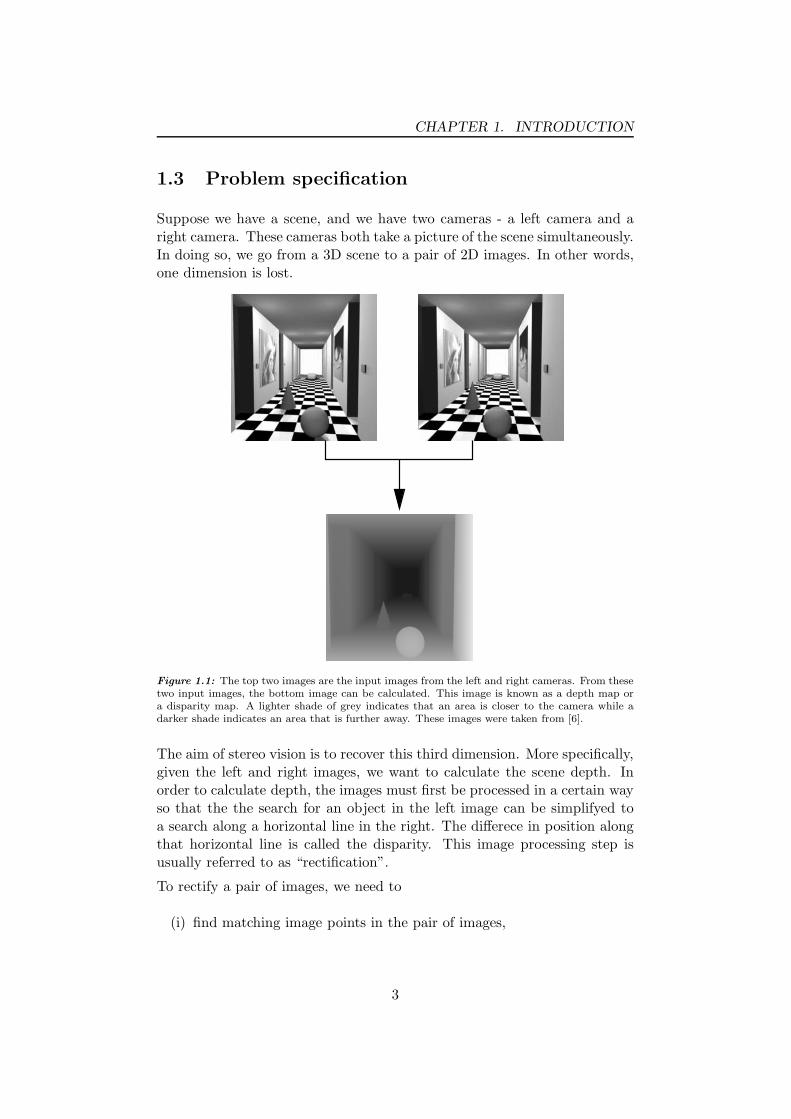
Suppose we have a scene, and we have two cameras - a left camera and aright camera. These cameras both take a picture of the scene simultaneously.In doing so, we go from a 3D scene to a pair of 2D images. In other words,one dimension is lost.

Figure 1.1: The top two images are the input images from the left and right cameras. From thesetwo input images, the bottom image can be calculated. This image is known as a depth map ora disparity map. A lighter shade of grey indicates that an area is closer to the camera while adarker shade indicates an area that is further away. These images were taken from [6].

The aim of stereo vision is to recover this third dimension. More specifically,given the left and right images, we want to calculate the scene depth. Inorder to calculate depth, the images must first be processed in a certain wayso that the the search for an object in the left image can be simplifyed toa search along a horizontal line in the right. The differece in position alongthat horizontal line is called the disparity. This image processing step isusually referred to as “rectification”.

To rectify a pair of images, we need to

(i) find matching image points in the pair of images,

3


(ii) calculate something called the essential matrix 1.

(iii) use the essential matrix to “warp” or rectify the images into the desiredform.

Much research has been done on step (iii). In this thesis, we concentrate onthe first two steps.

Now, in the application we are interested in (i.e. driver assistance), we arecontinuously capturing a new pair of stereo images. This means that weneed to calculate our depth maps from these stereo images in real time. Inthis application, the cameras can move actively, due to vibrations or otherexternal factors. Hence, we also have to find the matching image points,calculate the essential matrix and rectify the images in real time.

To achieve this real time performance, we observed that a lot of the compu-tations could be reformulated and implemented directly in hardware. Nor-mally, these computations are done in a serial fashion in a standard com-puter. However, these computations can actually be done in parallel sincethey are independent. By implementing these computations in dedicatedhardware, it is possible to perform many operations simultaneously.

Thus, the problem may be stated as follows:

Given a pair of images of a scene, we want to find matching imagepoints and calculate the essential matrix in real time by imple-menting many of these computations in dedicated hardware.

1.4 Contributions

The task of finding matching image points and calculating the essentialmatrix is also called stereo calibration. Our contribution is to formulate thisproblem in such a way that it is possible to perform these calculations in realtime. These calculations are naturally quite complex and computationallyintensive.

Our suggestion is to use computer vision algorithms implemented in ded-icated hardware to accelerate this process. The implementation has beendone using VHDL, a commonly used hardware description programminglanguage, to program an FPGA. An FPGA is an integrated circuit in whichyou can combine the gates and logic to perform specific tasks. This is alsoreferred to as programmable logic. An FPGA is more versatile than a mi-crocontroller or a digital signal processor(DSP), but also more difficult toprogram.

1More details on the essential matrix are given in Chapter 3 of this thesis

4


The approach of using dedicated hardware to perform automated stereocalibration has to our knowledge not been done before.

1.5 Roadmap

Chapter 2 gives a brief survey of related work. Chapter 3 introduces thereader to the notation used as well as the theory necessary for understand-ing the later parts of the thesis. This chapter also presents a model forcalculating the essential matrix in the case of a stereo head with three de-grees of freedom. We provide details of our implementation in Chapter 4.Section 4.1.1 gives an overview of the hardware and software used in the ex-perimental setup. Sections 4.2 and 4.3 discuss issues related to the hardwareimplementation of the Gaussian pyramid and the Sobel filter respectively.The Gaussian pyramid and Sobel filter are used as parts of an algorithm fordetecting points in the left and right stereo images.

In Section 4.4.4, we provide a complexity analysis of the algorithm used todetect these feature points. We also describe how matches between thesefeature points are found. In Section 4.5, we show how the point correspon-dences are used to calculate the essential matrix. Lastly, Chapter 5 presentsour experimental results. Further, this chapter also discusses future workand improvements.

5

Chapter 2

Previous work

This chapter gives some background on the work related to this thesis. Sec-tion 2.1 discusses previous work on automated stereo calibration. In Sec-tion 2.2, we give references to some previous work on the implementation ofcomputer vision algorithms in hardware such as Field Programmable GateArrays(FPGAs). As of yet, no work combining the two fields has been found.

2.1 Automated Stereo Calibration

This section aims to give a brief understanding of what has been done inthe area of automated stereo calibration. A number of methods of howto perform the actual calibration is presented by Hartley and Zisserman in[10]. Indeed, in theory, the problem is considered to be “solved”. However,in practice, it is not yet possible to do the calibration in real time especially ifyou include the problem of finding and matching points between the images.

2.1.1 Real Time Motion and Stereo Cues for Active VisualObservers

In his PhD thesis[4], Marten Bjorkman describes the theory involved inautomatically calibrating a stereo head with three degrees of freedom. Thesetup he used is similar to the one described in section 4.1.2 of this thesis.He also describes a system capable of stereo calibration in real time. AHarris corner detector [8] was used to detect feature points while intensitycorrelation between image patches was used for matching. This resulted ina relatively large number of false matches. Bjorkman dealt with this byemploying a robust iterative algorithm for estimating the Essential matrix.We believe that this method is well worth using in a future version of oursystem. This particular part of his thesis is also published as a paper [5].

6

CHAPTER 2. PREVIOUS WORK

2.2 Related work on FPGAs

Here, we sample related work in the image processing and signal processingdomain, using dedicated hardware (i.e. FPGAs).

2.2.1 Edge detection, using the Sobel operator

In a note [2], Atmel describes the implementation of a Sobel edge detectorin a small FPGA. Atmel also gives a brief introduction to the Sobel operatorand an explanation on how to pipeline the implementation. The basic ideais to perform as many computations as possible in parallel. This reducesthe time needed to perform each convolution.

The article [16], gives another implementation of the Sobel operator. Herethe Sobel operator is used as a step towards performing template matching.

2.2.2 Convolution

Atmel has another interesting application note on how to efficiently performconvolutions in FPGAs entitled “3x3 Convolver with Run-time Reconfig-urable Vector Multiplier in Atmel AT6000 FPGAs” [3]. The basic idea hereis to avoid multiplications by using a pre-calculated look-up tables. By per-forming convolutions in this way we can reduce the area used in the FPGA.

2.2.3 General Image processing

A system for FPGA-based image processing is described in [17]. The au-thors show ways of implementing image weight calculations and a Houghline transform, although not in any detail.

2.2.4 Calculation of Arctan in hardware

“Optimisation and implementation of the arctan function for the power do-main” [1] describes how to implement the arctan function in hardware usingvarious methods. The various methods were also compared with respectto power consumed by the FPGA. However, these comparisons were madebased on the assumption that only the angle between the two vectors wasimportant. In this thesis, we are also interested in the magnitude of thesum of the vectors. Thus, the worst performing implementation with re-gards to power was used, the CORDIC [20], since it calculates the angle andmagnitude simultaneously.

7

Chapter 3

Theory

The purpose of this chapter is to provide the reader with the background andtheory necessary for understanding the later parts of this thesis. Sections3.1 introduces the mathematical notation used as well as the basic conceptsof stereo vision. Sections 3.2 and 3.3 describe convolutions and the Kalmanfilter respectively. Finally, specific information regarding FPGAs and howto program these using VHDL is presented in Section 3.4.

3.1 Stereo Vision

As explained in Chapter 1, the aim of stereo vision is to calculate scenedepth given a pair of stereo images.

3.1.1 Notation

We will use bold-face symbols, such as x, to denote a column vector. Thesedefinitions and notations are from [18] and [10].

Homogeneous coordinates

The world we live in obeys Euclidean geometry. Only Euclidean transfor-mations such as translations and rotations are allowed. However, when wetake an image of the world with a camera, the transformation mapping the3D scene to a 2D image is not an Euclidean transformation but a projectivetransformation. Consequently, we need to introduce some concepts fromprojective geometry.

One concept from projective geometry is homogeneous coordinates. In Eu-clidean geometry, a 2D point is usually represented by a 2-vector x = (x, y)T .This is known as an inhomogeneous vector. In projective geometry, a 2D

8

CHAPTER 3. THEORY

point is represented by a 3-vector x = (x1, x2, x3)T . This is known as a

homogeneous vector. (Throughout this report, homogeneous vector quanti-ties are denoted as x, while the corresponding non-homogeneous quantitiesare denoted with a tilde as in x.) Homogeneous vectors are only definedup to a scale factor. Therefore, the homogeneous vectors (x1, x2, x3)

T andk(x1, x2, x3)

T represent the same point for any non-zero k.

If a 2D point has inhomogeneous coordinates x = (x, y)T and homogeneouscoordinates x = (x1, x2, x3)

T , then the relationship between the inhomoge-neous and homogeneous coordinates is given by

x =x1

x3, y =

x2

x3

Note that if x3 → 0, then x → ∞ and y → ∞. Therefore, any point withhomogeneous coordinates x = (x1, x2, 0)

T is a point at infinity.

Skew symmetric matrix

A matrix is skew symmetric if A = −AT . From here on we use the followingnotation to describe a skew symmetric matrix:

[t]× =

0 −t3 t2t3 0 −t1−t2 t1 0

(3.1)

This can also be thought of as a cross product between two 3-vectors a×b:

a × b = [a]×b =(

aT [b]×)T

(3.2)

Inliers and Outliers

When referring to data, we need to know when a measured data point com-plies with the model and when it does not. The standard terminology forthis is inliers and outliers respectively. Inliers is data that is consistent withthe model we are using plus some kind of Gaussian noise. Outliers on theother hand, is data that is inconsistent with the chosen model. For example,when you want to estimate the geometry of a camera setup, you have to beable to minimize the effect of outliers in order to get a stable result.

3.1.2 2D Projective Transformations

A 2D projective transformation is an invertible transformation that mapspoints in 2D projective space P

2 to points in P2 in such a way that straight

lines remain straight lines. More precisely,

9

CHAPTER 3. THEORY

(a)

P

P’

X

x x’

image 1 image 2

planar surface

(b)

Figure 3.1: Examples of 2D projective transformations. (a) The projective transformation be-tween the image of a plane (the end of the building) and the image of its shadow onto anotherplane (the ground plane). (b) The projective transformation between two images induced by aworld plane. These images were taken from [10].

a 2D projective transformation is an invertible mapping H fromP

2 to P2 such that three points x1, x2 and x3 lie on the same

line if and only if H(x1), H(x2) and H(x3) do.

A projective transformation is also called a projectivity, a collineation or ahomography. Examples of such mappings can be seen in Figure 3.1.

3.1.3 Stereo and Epipolar Geometry

Epipolar geometry is the geometry relating two views of the same scene.Consider two cameras with camera centres cl and cr (Figure 3.2). Thecamera at cl captures an image of the world, resulting in image Il. Similarly,the camera at cr captures an image of the world, resulting in image Ir.

Consider an arbitrary point X in the scene. This scene point X will projectto image point xl in Il. The point X will also project to image point xr inIr. Thus, xl and xr are matching, or corresponding, image points.

To further explain Figure 3.2, it is necessary to first introduce some termi-nology:� The baseline is the line joining the two camera centres.� The epipolar plane Π is the plane containing the scene point X and

the camera centres cl and cr.� The epipole el is the point where the baseline intersects image Il.From Figure 3.2, we can see that el is simply the image of the second

10

CHAPTER 3. THEORY

Π

cl cr

IlIr

xl xr

ll lr

el er

epipolar plane

X

Figure 3.2: Epipolar geometry is the geometry between two views. This image was taken from[18].

camera centre cr in the first image Il. Similarly, epipole er is thepoint where the baseline intersects image Ir while epipole er is theimage of the first camera centre cl in the second image Ir.� The epipolar line ll is the line where the epipolar plane Π intersectsimage Il. The epipolar line lr is the line where the epipolar plane Πintersects image Ir.

3.1.4 The Essential Matrix

For a stereo camera setup to be calibrated, we need to know the relationbetween image points in the two images. This relation is a correlation trans-ferring a point in one image to a line in the other. The correlation is knownas the Essential matrix.

Using this relation, and searching for an object from the first image alongthe epipolar line in the other, one can calculate the offset (or disparity).From this disparity, calculating the distance to the object in question isa straightforward task. Objects with a large positive disparity are close,objects with zero disparity are on what is known as the fovia and objectswith negative disparity are further away. Performing this calculation overa number of surfaces gives an estimation of the distance to various parts ofan image. An example of this was shown earlier in Figure 1.1.

Derivation

Consider the stereo camera setup described earlier with camera centres po-sitioned at cl and cr with the baseline t = cr − cl. Also, consider a scene

11

CHAPTER 3. THEORY

point X. This point X together with the two camera centers forms a plane,as shown in Figure 3.2.

The vectors xl = X − cl and xr = X − cr represent the projection of thepoint X onto the cameras. Since the three vectors xl, xr and t all lie inthe same plane they must be linearly dependent. Thus, the determinantdet(xl, t, xr) = 0. This property is know as the epipolar constraint and wasintroduced independently by [13] and [19] in 1981. This implies that thetransformation relating an image point in one image to another image, mustbe of rank 2. Thus, the transformation transfers a point onto a line, theepipolar line. A transformation with these properties is also known as acorrelation.

Now, using the rotational matrices Rl and Rr to represent the rotation ofeach camera from a setup with the camera pointing perpendicular to thebaseline, the two projections xl and xr can be given in the local referenceframe of each camera. Thus, we form:

xl = Rlxl and xr = Rrxr (3.3)

Using these relations we can write the epipolar constraint as:

det(xl, t, xr) = |xl · (t × xr)| == |xl · ([t]xxr)| == |xl · (Txr)| == xT

l Txr =

= xTRlTRrTxl =

= xTr Exr

(3.4)

where E = RlTRrT . E is also known as the Essential matrix. This deriva-

tion has been taken from [5].

3.1.5 The Sobel edge detector

The Sobel operator is a way of finding edges in images. This is done byapplying two separate filters. That is, convolving the image with two kernels:

Sx = 18

−1 0 1−2 0 2−1 0 1

Sy = 18

−1 −2 −10 0 01 2 1

(3.5)

Sx gives a large respons on vertical edges while Sy detects horizontal edges.Now, let Sx and Sy be two vectors, each representing the derivative in therespective direction. By combining these vectors one can calculate the gra-dient field in an image, with magnitude and orientation of the gradients.

12

CHAPTER 3. THEORY

(a)

a

b

c

d

(b)

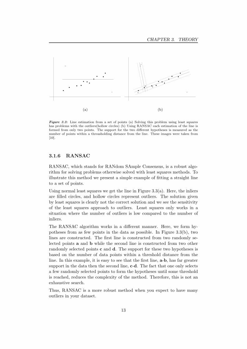
Figure 3.3: Line estimation from a set of points (a) Solving this problem using least squareshas problems with the outliers(hollow circles) (b) Using RANSAC each estimation of the line isformed from only two points. The support for the two different hypotheses is measured as thenumber of points within a threasholding distance from the line. These images were taken from[10].

3.1.6 RANSAC

RANSAC, which stands for RANdom SAmple Consensus, is a robust algo-rithm for solving problems otherwise solved with least squares methods. Toillustrate this method we present a simple example of fitting a straight lineto a set of points.

Using normal least squares we get the line in Figure 3.3(a). Here, the inliersare filled circles, and hollow circles represent outliers. The solution givenby least squares is clearly not the correct solution and we see the sensitivityof the least squares approach to outliers. Least squares only works in asituation where the number of outliers is low compared to the number ofinliers.

The RANSAC algorithm works in a different manner. Here, we form hy-potheses from as few points in the data as possible. In Figure 3.3(b), twolines are constructed. The first line is constructed from two randomly se-lected points a and b while the second line is constructed from two otherrandomly selected points c and d. The support for these two hypotheses isbased on the number of data points within a threshold distance from theline. In this example, it is easy to see that the first line, a-b, has far greatersupport in the data then the second line, c-d. The fact that one only selectsa few randomly selected points to form the hypotheses until some thresholdis reached, reduces the complexity of the method. Therefore, this is not anexhaustive search.

Thus, RANSAC is a more robust method when you expect to have manyoutliers in your dataset.

13

CHAPTER 3. THEORY

3.2 Convolutions

The general definition of a convolution is

sc =

∫

Sf(x)g(x)dx (3.6)

In computer vision, this is interpreted as applying the kernel g(x) to theimage data f(x). Performing this two dimensional convolution can be in-terpreted as moving a small window representing the kernel over the imageand taking the dot product of the kernel and the image patch to form a newimage. Computationally, this is a very expensive operation. For each pixelin the image data, you have to perform as many multiplications as sites inthe kernel. For a square image of size NxN and a kernel of size nxn, thisresults in O((Nn)2) operations per image. However, a kernel is separable ifit can be written as:

K = k1 · kT2 (3.7)

where K is the 2D kernel and k1 and k2 are 1D kernels.

A convolution in one dimension is defined as

sc =

∫

∞

−∞

f(x)g(x)dx (3.8)

sd =

n∑

i=0

f(i)g(i) (3.9)

Performing these two separate one dimensional convolutions gives the com-plexity O(N2n), which is a significant improvement for a large kernel.

3.3 Kalman filtering

In 1960, R.E. Kalman published his famous paper[11] describing a recursivesolution to the discrete-data linear filtering problem. Since that time, theKalman filter has been the subject of extensive research and application,particularly in the area of target tracking.

The online encyclopedia, Wikipedia [21], has this to say about the Kalmanfilter:

The Kalman filter is an efficient recursive filter which estimatesthe state of a dynamic system from a series of incomplete andnoisy measurements. An example of an application would beto provide accurate continuously-updated information about theposition and velocity of an object given only a sequence of ob-servations about its position, each of which includes some error.

14

CHAPTER 3. THEORY

It is used in a wide range of engineering applications from radarto computer vision. Kalman filtering is an important topic incontrol theory and control systems engineering.

Basically, Kalman filtering is a recursive process for filtering a signal. It usestwo steps, measurement update and time propagation. The time propaga-tion builds on a model of how the signal can change. Estimating the nextvalue from this model and previous data we get a likely measurement. Whenthe value is to be updated, the measurement and estimation is weighed inproportion to how much one “trusts” the measurement and the model re-spectively.

3.4 Field Programmable Gate Arrays (FPGAs)

An FPGA is an Integrated Circuit (IC) with a large number of logical gatesinside. These gates can be AND, OR, XOR and small lookup tables. Theadvantage of an FPGA is that these gates can be connected in differentpatterns to perform all sorts of operations. The behaviour of the FPGA cantherefore be changed quickly to suit a new application. This is almost like asmall processor, only that all gates can operate independently of each otherand in parallel, whereas a processor performs operations in a sequentialmanner. The number of gates, the area, in the FPGA is limited so there isa trade-off between speed and area. Another issue is to set up the gates insuch a way that the delay from input to output from a module is less thana given clock frequency so that we can perform the calculations fast enoughto keep up with the input data stream.

3.4.1 Programming language, VHDL

The way of instructing the FPGA to do what we want, is to program it.This can be done in a number of ways from manipulating single gates toprogramming using one of the higher level programming languages. Thetwo most used languages for programming FPGAs are VHSIC HardwareDescription Language (VHDL) and Verilog. VHDL is an Ada like languagewith very strict type checking. Verilog is more like C. In the work relatedto this thesis, VHDL was used. The first thing one has to learn when pro-gramming in these kinds of languages is that things happen all at once, andnot like in a normal computer program where things have a more sequentialnature.

15

Chapter 4

Implementation

This chapter works its way from our experimental setup and how to performa number of computer vision processes in hardware, to the actual calculationof the stereo calibration parameters. Details are given on how to implementthis in a FPGA by using VHDL with various techniques. Firstly, we presentour experimental setup and where this work was conducted.

In Sections 4.2 and 4.3, we describe how feature points are extracted fromthe input stereo images. We also describe how this is achieved in real timeby moving a number of steps in the point extraction process from softwareimplementation to hardware implementation in a FPGA. Section 4.4 showshow we obtain point correspondences between the images and Section 4.5describes how we calculate the essential matrix from these point correspon-dences.

4.1 System Overview

The information path is shown in figure 4.1. We obtain two images from thetwo cameras on the stereo head. These are the input to the framegrabber

Frame Grabber

FPGA

images

Host Computer

filtered images

candidate points

and matching

Feature extraction

correpondances

Point

Stereo Calibrationcalculation

Image

filtering

Candidatedetection

Figure 4.1: Information path and overview of the system used.

16

CHAPTER 4. IMPLEMENTATION

Figure 4.2: Toyota Landcruiser, the research platform used

board. On this board resides an FPGA which takes the camera imagesas input, creates a Gaussian pyramid, performs local max/min calculationsand computes the edge image using the Sobel operator. It then outputs thisinformation together with the unprocessed raw images to the host computer.Using this information, the software in the host computer computes thepoint correspondences. Finally, the essential matrix is calculated using thesecorrespondences.

The stereo calibration calculations are extremely sensitive to outliers in thedata. This leads to the selection of the Scale Invarant Feature Transform(SIFT), presented by David Lowe in 1999[14], for feature extraction anddetection of the point correspondences. The SIFT algorithm is able to ro-bustly find corresponding points in the two images, thereby minimising thenumber of outliers.

4.1.1 Experimental setup

This work was conducted at the Computer Vision and Robotics lab atANU/NICTA in Canberra, Australia. For practical tests and evaluation,this lab possesses a 4wd Toyota Landcruiser equipped with a wide range ofsensors and actuators. The aim of the research performed is to create driverassistance systems to aid the driver, giving him a safer and more relaxeddriving experience. To achieve this, a number of algorithms are being de-veloped including Pedestrian Detection, Sign Detection, Lane Tracking andObstacle Detection to mention a few.

The sensors used for this work are a pair of cameras mounted in a stereosystem named CeDAR[7]. The cameras output analog NTSC signals whichare digitized by a frame grabber equipped with an FPGA. The raw andfiltered images are then transferred via the PCI bus to the Videoserver inthe host computer.

17


d = 0.3 m

αl −αr

Figure 4.3: LEFT: CeDAR head, RIGHT: CeDAR head from above showing the cameras’degrees of freedom.

4.1.2 CEDAR head

CeDAR[7] is a high-speed, high-precision stereo active vision system. Themechanism is lightweight, yet capable of motions that exceed human per-formance. Figure 4.3 shows the standard CeDAR unit. In our system, thesystem is inverted(upside down) and mounted for use with driver assistancein the vehicle shown in figure 4.2. The head has three degrees of freedomwith encoders on each axis. The cameras are mounted 0.3 m apart and canrotate around an axis through their optical center independently of eachother. The third degree of freedom is the tilt axis.

The cameras used for this work were normal NTSC cameras. These deliveran analog signal consisting of Red, Green and Blue (RGB) information aboutthe scene in front of the cameras. This scene is divided into 640 by 480 pixels.Every second line is delivered in a batch known as a field at a rate of 60fields per second. Therefore, we get an image of size 640 by 240 pixels 60times per second delivered through the analog signal. This signal is thensampled by the frame grabber.

4.1.3 Frame grabber

The frame grabber is a PicProdigy development board from Atlantek Mi-crosystems equipped with a Xilinx Virtex II FPGA with 2M gates. Atlantekuses this FPGA for buffering and to interface with the host computer via thePCI bus. Currently they do not use the entire FPGA. Our image processingis being inserted in between the buffering and the PCI interface, divertingthe pipeline in the FPGA. Once the image input and processing is done, theimages are transferred to the host computer and its videoserver.

18


4.1.4 Videoserver

In the host computer, the videoserver includes the software used to capturethe images from the board and deliver them to the different client programsused in the vehicle. With this work it is possible not only to provide rawimage data, but also filtered images as well as stereo calibration information.This can then be used by the clients in the system.

19


...Inputimage

Octave Octave

Inte

rest

Inte

rest

poin

ts

poin

ts

sobel

sobel

images

images

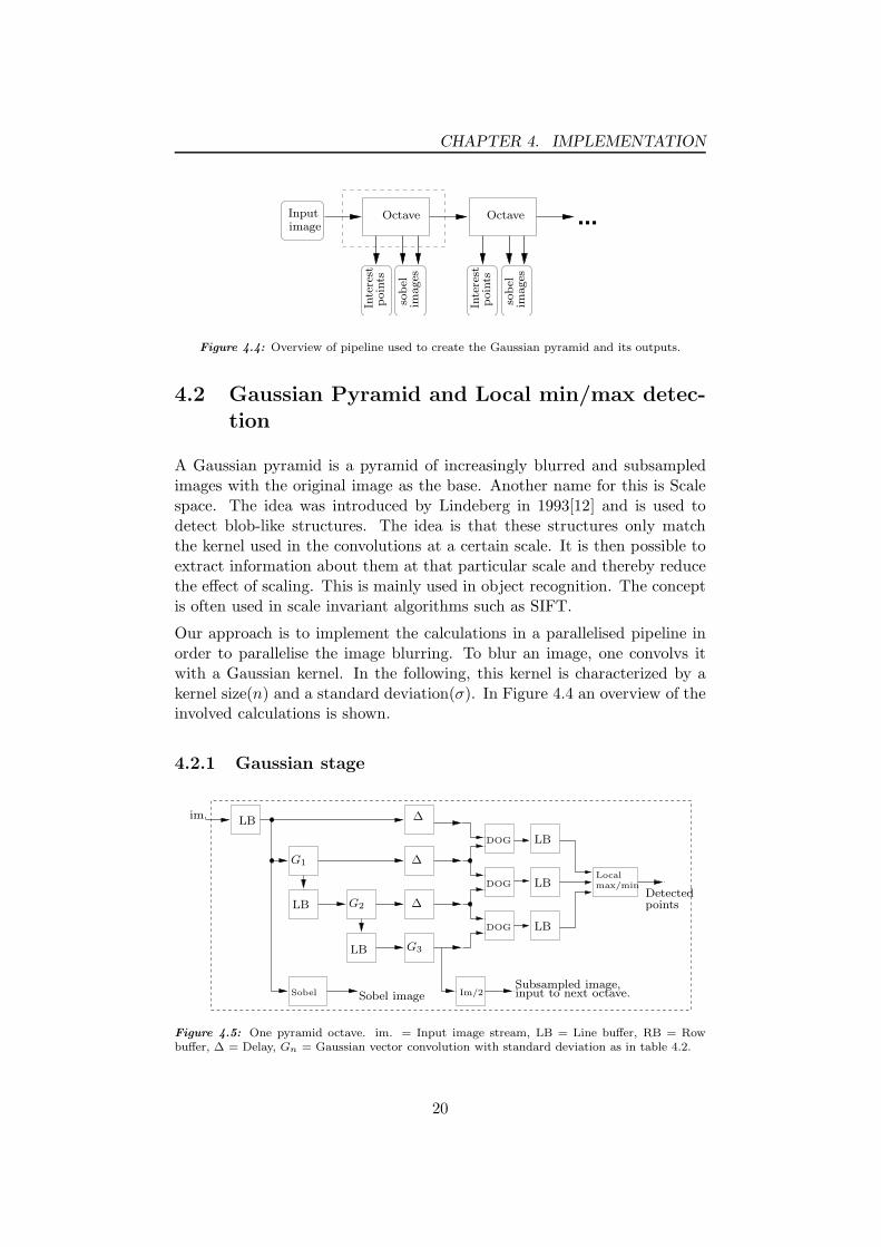
Figure 4.4: Overview of pipeline used to create the Gaussian pyramid and its outputs.

4.2 Gaussian Pyramid and Local min/max detec-tion

A Gaussian pyramid is a pyramid of increasingly blurred and subsampledimages with the original image as the base. Another name for this is Scalespace. The idea was introduced by Lindeberg in 1993[12] and is used todetect blob-like structures. The idea is that these structures only matchthe kernel used in the convolutions at a certain scale. It is then possible toextract information about them at that particular scale and thereby reducethe effect of scaling. This is mainly used in object recognition. The conceptis often used in scale invariant algorithms such as SIFT.

Our approach is to implement the calculations in a parallelised pipeline inorder to parallelise the image blurring. To blur an image, one convolvs itwith a Gaussian kernel. In the following, this kernel is characterized by akernel size(n) and a standard deviation(σ). In Figure 4.4 an overview of theinvolved calculations is shown.

4.2.1 Gaussian stage

LB

LB

LB

LB

LB

LB

G1

G2

G3

∆

∆

∆

DOG

DOG

DOG

Localmax/min

im.

Sobel Sobel imageSubsampled image,input to next octave.Im/2

Detectedpoints

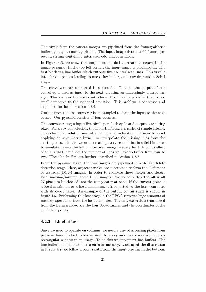
Figure 4.5: One pyramid octave. im. = Input image stream, LB = Line buffer, RB = Rowbuffer, ∆ = Delay, Gn = Gaussian vector convolution with standard deviation as in table 4.2.

20


The pixels from the camera images are pipelined from the framegrabber’sbuffering stage to our algorithms. The input image data is a 60 frames persecond stream containing interlaced odd and even fields.

In Figure 4.5, we show the components needed to create an octave in theimage pyramid. In the top left corner, the input image is pipelined in. Thefirst block is a line buffer which outputs five de-interlaced lines. This is splitinto three pipelines leading to one delay buffer, one convolver and a Sobelstage.

The convolvers are connected in a cascade. That is, the output of oneconvolver is used as input to the next, creating an increasingly blurred im-age. This reduces the errors introduced from having a kernel that is toosmall compared to the standard deviation. This problem is addressed andexplained further in section 4.2.4.

Output from the last convolver is subsampled to form the input to the nextoctave. Our pyramid consists of four octaves.

The convolver stages input five pixels per clock cycle and output a resultingpixel. For a row convolution, the input buffering is a series of simple latches.The column convolution needed a bit more consideration. In order to avoidapplying an asymmetric kernel, we interpolate the missing lines from theexisting ones. That is, we are recreating every second line in a field in orderto simulate having the full uninterlaced image in every field. A bonus effectof this is that it reduces the number of lines we have to buffer from four totwo. These linebuffers are further described in section 4.2.2

From the pyramid stage, the four images are pipelined into the candidatedetection stage. Here, adjacent scales are subtracted to form the Differenceof Gaussian(DOG) images. In order to compare these images and detectlocal maxima/minima, these DOG images have to be buffered to allow all27 pixels to be clocked into the comparator at once. If the current point isa local maximum or a local minimum, it is reported to the host computerwith its coordinates. An example of the output of this stage is shown infigure 4.6. Performing this last stage in the FPGA removes huge amounts ofmemory operations from the host computer. The only extra data transferredfrom the framegrabber are the four Sobel images and the coordinates of thecandidate points.

4.2.2 Linebuffers

Since we need to operate on columns, we need a way of accessing pixels fromprevious lines. In fact, often we need to apply an operation or a filter to arectangular window in an image. To do this we implement line buffers. Theline buffer is implemented as a circular memory. Looking at the illustrationin Figure 4.7, we follow a pixel’s path from the input pipeline in the bottom.

21


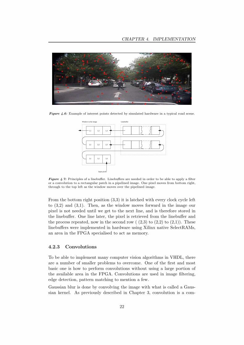
Figure 4.6: Example of interest points detected by simulated hardware in a typical road scene.

Linebuffer

1,1 1,3

2,1 2,2

3,1 3,2 3,3

1,2

2,3

Input pixels

Window in the image

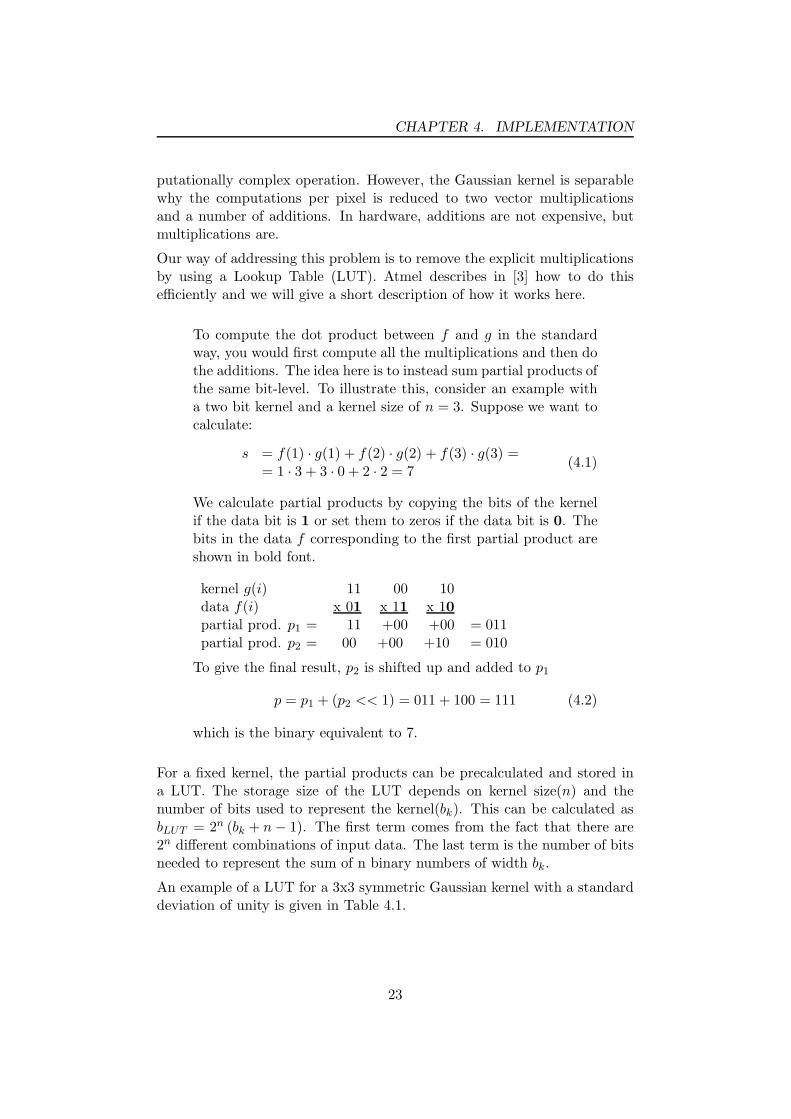
Figure 4.7: Principles of a linebuffer. Linebuffers are needed in order to be able to apply a filteror a convolution to a rectangular patch in a pipelined image. One pixel moves from bottom right,through to the top left as the window moves over the pipelined image.

From the bottom right position (3,3) it is latched with every clock cycle leftto (3,2) and (3,1). Then, as the window moves forward in the image ourpixel is not needed until we get to the next line, and is therefore stored inthe linebuffer. One line later, the pixel is retrieved from the linebuffer andthe process repeated, now in the second row ( (2,3) to (2,2) to (2,1)). Theselinebuffers were implemented in hardware using Xilinx native SelectRAMs,an area in the FPGA specialised to act as memory.

4.2.3 Convolutions

To be able to implement many computer vision algorithms in VHDL, thereare a number of smaller problems to overcome. One of the first and mostbasic one is how to perform convolutions without using a large portion ofthe available area in the FPGA. Convolutions are used in image filtering,edge detection, pattern matching to mention a few.

Gaussian blur is done by convolving the image with what is called a Gaus-sian kernel. As previously described in Chapter 3, convolution is a com-

22


putationally complex operation. However, the Gaussian kernel is separablewhy the computations per pixel is reduced to two vector multiplicationsand a number of additions. In hardware, additions are not expensive, butmultiplications are.

Our way of addressing this problem is to remove the explicit multiplicationsby using a Lookup Table (LUT). Atmel describes in [3] how to do thisefficiently and we will give a short description of how it works here.

To compute the dot product between f and g in the standardway, you would first compute all the multiplications and then dothe additions. The idea here is to instead sum partial products ofthe same bit-level. To illustrate this, consider an example witha two bit kernel and a kernel size of n = 3. Suppose we want tocalculate:

s = f(1) · g(1) + f(2) · g(2) + f(3) · g(3) == 1 · 3 + 3 · 0 + 2 · 2 = 7

(4.1)

We calculate partial products by copying the bits of the kernelif the data bit is 1 or set them to zeros if the data bit is 0. Thebits in the data f corresponding to the first partial product areshown in bold font.

kernel g(i) 11 00 10data f(i) x 01 x 11 x 10partial prod. p1 = 11 +00 +00 = 011partial prod. p2 = 00 +00 +10 = 010

To give the final result, p2 is shifted up and added to p1

p = p1 + (p2 << 1) = 011 + 100 = 111 (4.2)

which is the binary equivalent to 7.

For a fixed kernel, the partial products can be precalculated and stored ina LUT. The storage size of the LUT depends on kernel size(n) and thenumber of bits used to represent the kernel(bk). This can be calculated asbLUT = 2n (bk + n − 1). The first term comes from the fact that there are2n different combinations of input data. The last term is the number of bitsneeded to represent the sum of n binary numbers of width bk.

An example of a LUT for a 3x3 symmetric Gaussian kernel with a standarddeviation of unity is given in Table 4.1.

23


f(1)if(2)if(3)i pi

000 → 0000001 → 0010010 → 0100011 → 0110100 → 0010101 → 0100110 → 0110111 → 1000

Table 4.1: Example of Lookup Table (LUT) for a Gaussian kernel of size n = 3, standarddeviation σ = 1 and a kernel bitsize of bk = 2. f(j)i means the i’th bit of f(j).

Gn standard deviation, σ discrete σ

(0 1.4142 1.1592)1 0.7664 0.82922 0.9656 0.93543 1.2166 1.1040

Tot. (eq.4.3) 1.988 2.040

Table 4.2: The standard deviations(σ) used between scales.

4.2.4 Choosing the size of the kernel

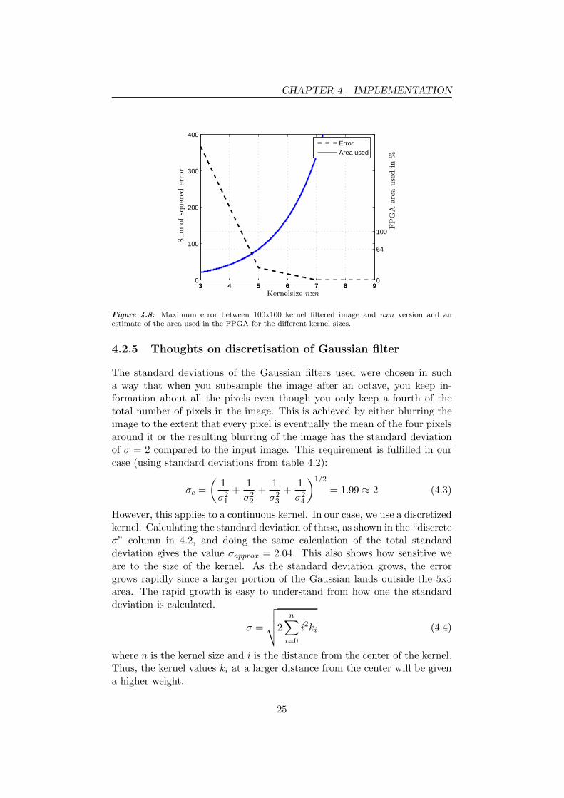
In order to know how big a kernel needs to be to avoid problems nearthe kernel edges, we conducted an experiment comparing a relatively smallkernel to an extremely large one. The experiment was done using five scalesof gaussians, computed in a cascade. That is, one image is fed into thenext scale as input. This reduces the standard deviation needed in a singleconvolution, thereby reducing the error introduced by the edges of the kernel.To have ground truth data to compare against, we did the convolutions usinga 100x100 kernel and compared that to the image we got for a nxn kernel.The standard deviations used are shown in Table 4.2. In Table 4.2, thefirst standard deviation (σ for G0) is used in the input filtering, in the samemanner as in [15]. The following values were used to create the three extrafiltered images needed to create an octave.

Based on the results shown in Figure 4.8, we decided to use a kernel size offive pixels, as a trade-off between area usage on the FPGA and accuracy inthe calculations.

24


3 4 5 6 7 8 90

100

200

300

400

3 4 5 6 7 8 90

64

100

ErrorArea used

Kernelsize nxn

Sum

ofsq

uare

der

ror

FP

GA

are

ause

din

%

Figure 4.8: Maximum error between 100x100 kernel filtered image and nxn version and anestimate of the area used in the FPGA for the different kernel sizes.

4.2.5 Thoughts on discretisation of Gaussian filter

The standard deviations of the Gaussian filters used were chosen in sucha way that when you subsample the image after an octave, you keep in-formation about all the pixels even though you only keep a fourth of thetotal number of pixels in the image. This is achieved by either blurring theimage to the extent that every pixel is eventually the mean of the four pixelsaround it or the resulting blurring of the image has the standard deviationof σ = 2 compared to the input image. This requirement is fulfilled in ourcase (using standard deviations from table 4.2):

σc =

(

1

σ21

+1

σ22

+1

σ23

+1

σ24

)1/2

= 1.99 ≈ 2 (4.3)

However, this applies to a continuous kernel. In our case, we use a discretizedkernel. Calculating the standard deviation of these, as shown in the “discreteσ” column in 4.2, and doing the same calculation of the total standarddeviation gives the value σapprox = 2.04. This also shows how sensitive weare to the size of the kernel. As the standard deviation grows, the errorgrows rapidly since a larger portion of the Gaussian lands outside the 5x5area. The rapid growth is easy to understand from how one the standarddeviation is calculated.

σ =

√

√

√

√2

n∑

i=0

i2ki (4.4)

where n is the kernel size and i is the distance from the center of the kernel.Thus, the kernel values ki at a larger distance from the center will be givena higher weight.

25


Figure 4.9: Gaussian pyramid example, created with simulated hardware. This figure containsfour octaves.

26


4.3 Sobel Operator

Many computer vision algorithms rely on gradient and orientation informa-tion from images. This is the case with SIFT as well. Instead of calculatingthe gradient and its orientation using finite differences, we decided to im-plement a Sobel operator, since this has a wider range of applications andgives a good approximation of the gradient’s magnitude and orientation. Inthe implementation of SIFT given by Lowe in [15], 36 histogram bins areused for the orientation. This roughly indicates the needed accuracy.

4.3.1 First step of implementation

The Sobel operator can be divided into two major steps. The first stepcalculates the gradient in two directions using convolution with the twostandard Sobel kernels shown in (3.5).

This convolution is especially suited for hardware since it only containsshifts and additions. This is due to the fact that multiplication by a factorof the type 2n can be done by shifting the binary representation of thenumber n bits to the left. Calculating the two gradient vectors Sx and Sy

is straightforward and uses the same line buffer as the Gaussian Pyramid tosave logic. The second step estimates the orientation and magnitude of thegradient vector from the two vectors.

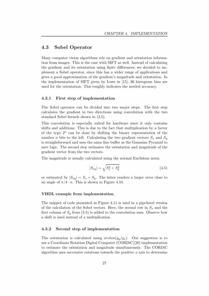
The magnitude is usually calculated using the normal Euclidean norm

|Sxy| =√

S2x + S2

y (4.5)

or estimated by |Sxy| = Sx + Sy. The latter renders a larger error close toan angle of π/4 · n. This is shown in Figure 4.10.

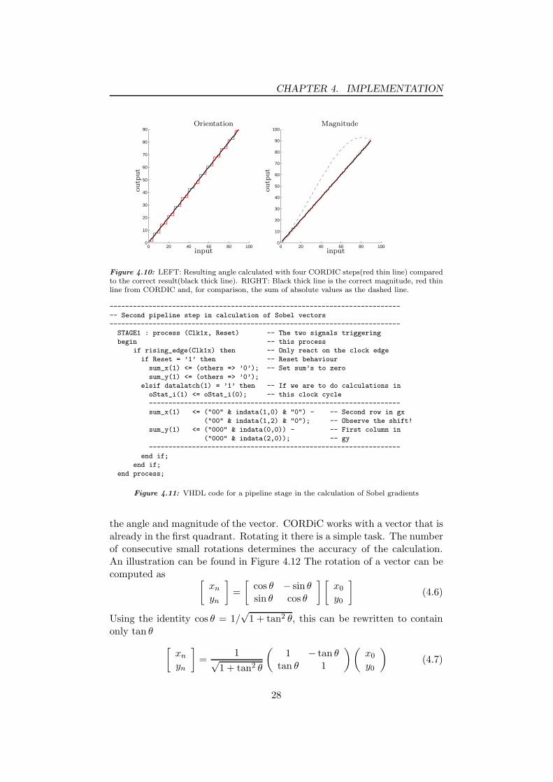
VHDL example from implementation

The snippet of code presented in Figure 4.11 is used in a pipelined versionof the calculation of the Sobel vectors. Here, the second row in Sx and thefirst column of Sy from (3.5) is added to the convolution sum. Observe howa shift is used instead of a multiplication.

4.3.2 Second step of implementation

The orientation is calculated using arctan(gy/gx). Our suggestion is touse a Coordinate Rotation Digital Computer (CORDiC)[20] implementationto estimate the orientation and magnitude simultaneously. The CORDiCalgorithm uses successive rotations towards the positive x axis to determine

27


0 20 40 60 80 1000

10

20

30

40

50

60

70

80

90

0 20 40 60 80 1000

10

20

30

40

50

60

70

80

90

100Orientation Magnitude

inputinput

outp

ut

outp

ut

Figure 4.10: LEFT: Resulting angle calculated with four CORDIC steps(red thin line) comparedto the correct result(black thick line). RIGHT: Black thick line is the correct magnitude, red thinline from CORDIC and, for comparison, the sum of absolute values as the dashed line.

--------------------------------------------------------------------------

-- Second pipeline step in calculation of Sobel vectors

--------------------------------------------------------------------------

STAGE1 : process (Clk1x, Reset) -- The two signals triggering

begin -- this process

if rising_edge(Clk1x) then -- Only react on the clock edge

if Reset = ’1’ then -- Reset behaviour

sum_x(1) <= (others => ’0’); -- Set sum’s to zero

sum_y(1) <= (others => ’0’);

elsif datalatch(1) = ’1’ then -- If we are to do calculations in

oStat_i(1) <= oStat_i(0); -- this clock cycle

----------------------------------------------------------------

sum_x(1) <= ("00" & indata(1,0) & "0") - -- Second row in gx

("00" & indata(1,2) & "0"); -- Observe the shift!

sum_y(1) <= ("000" & indata(0,0)) - -- First column in

("000" & indata(2,0)); -- gy

----------------------------------------------------------------

end if;

end if;

end process;

Figure 4.11: VHDL code for a pipeline stage in the calculation of Sobel gradients

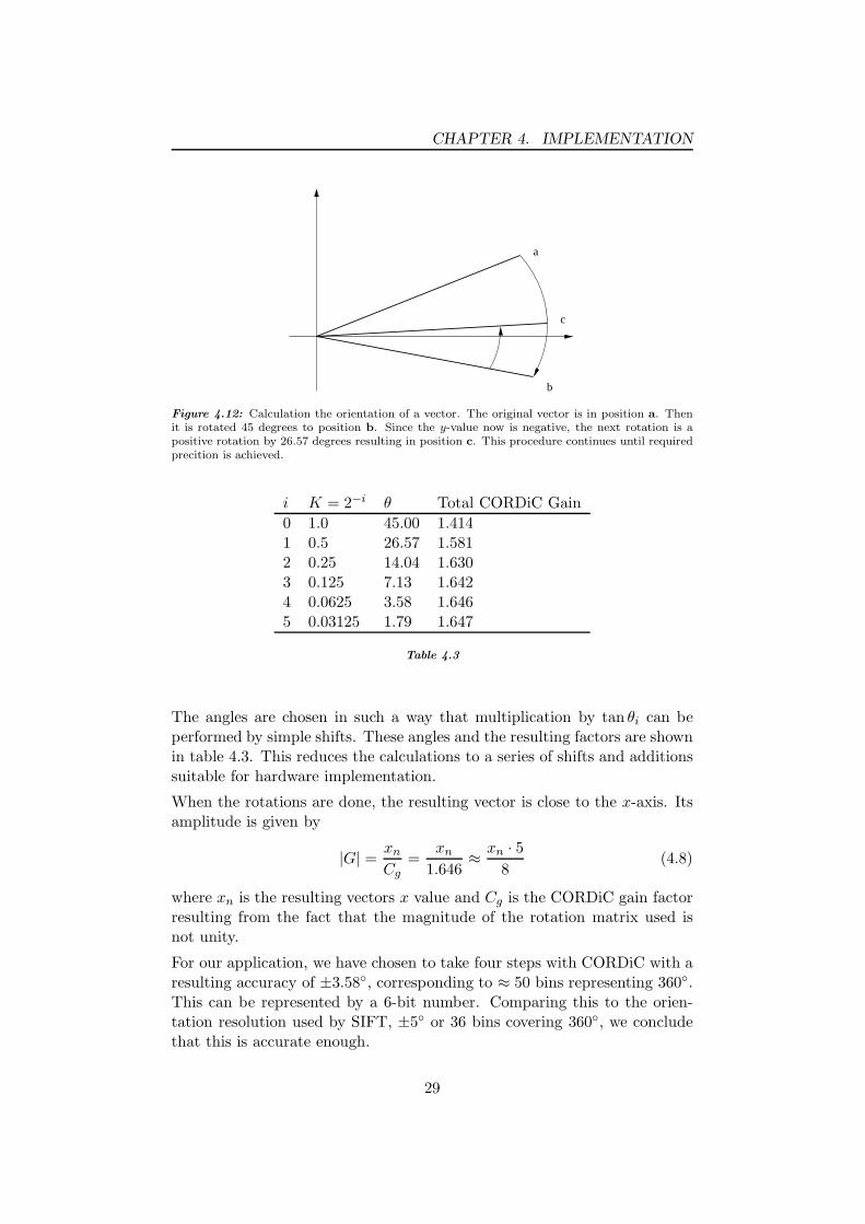
the angle and magnitude of the vector. CORDiC works with a vector that isalready in the first quadrant. Rotating it there is a simple task. The numberof consecutive small rotations determines the accuracy of the calculation.An illustration can be found in Figure 4.12 The rotation of a vector can becomputed as

[

xn

yn

]

=

[

cos θ − sin θsin θ cos θ

] [

x0

y0

]

(4.6)

Using the identity cos θ = 1/√

1 + tan2 θ, this can be rewritten to containonly tan θ

[

xn

yn

]

=1√

1 + tan2 θ

(

1 − tan θtan θ 1

)(

x0

y0

)

(4.7)

28


a

b

c

Figure 4.12: Calculation the orientation of a vector. The original vector is in position a. Thenit is rotated 45 degrees to position b. Since the y-value now is negative, the next rotation is apositive rotation by 26.57 degrees resulting in position c. This procedure continues until requiredprecition is achieved.

i K = 2−i θ Total CORDiC Gain

0 1.0 45.00 1.4141 0.5 26.57 1.5812 0.25 14.04 1.6303 0.125 7.13 1.6424 0.0625 3.58 1.6465 0.03125 1.79 1.647

Table 4.3

The angles are chosen in such a way that multiplication by tan θi can beperformed by simple shifts. These angles and the resulting factors are shownin table 4.3. This reduces the calculations to a series of shifts and additionssuitable for hardware implementation.

When the rotations are done, the resulting vector is close to the x-axis. Itsamplitude is given by

|G| =xn

Cg=

xn

1.646≈ xn · 5

8(4.8)

where xn is the resulting vectors x value and Cg is the CORDiC gain factorresulting from the fact that the magnitude of the rotation matrix used isnot unity.

For our application, we have chosen to take four steps with CORDiC with aresulting accuracy of ±3.58◦, corresponding to ≈ 50 bins representing 360◦.This can be represented by a 6-bit number. Comparing this to the orien-tation resolution used by SIFT, ±5◦ or 36 bins covering 360◦, we concludethat this is accurate enough.

29


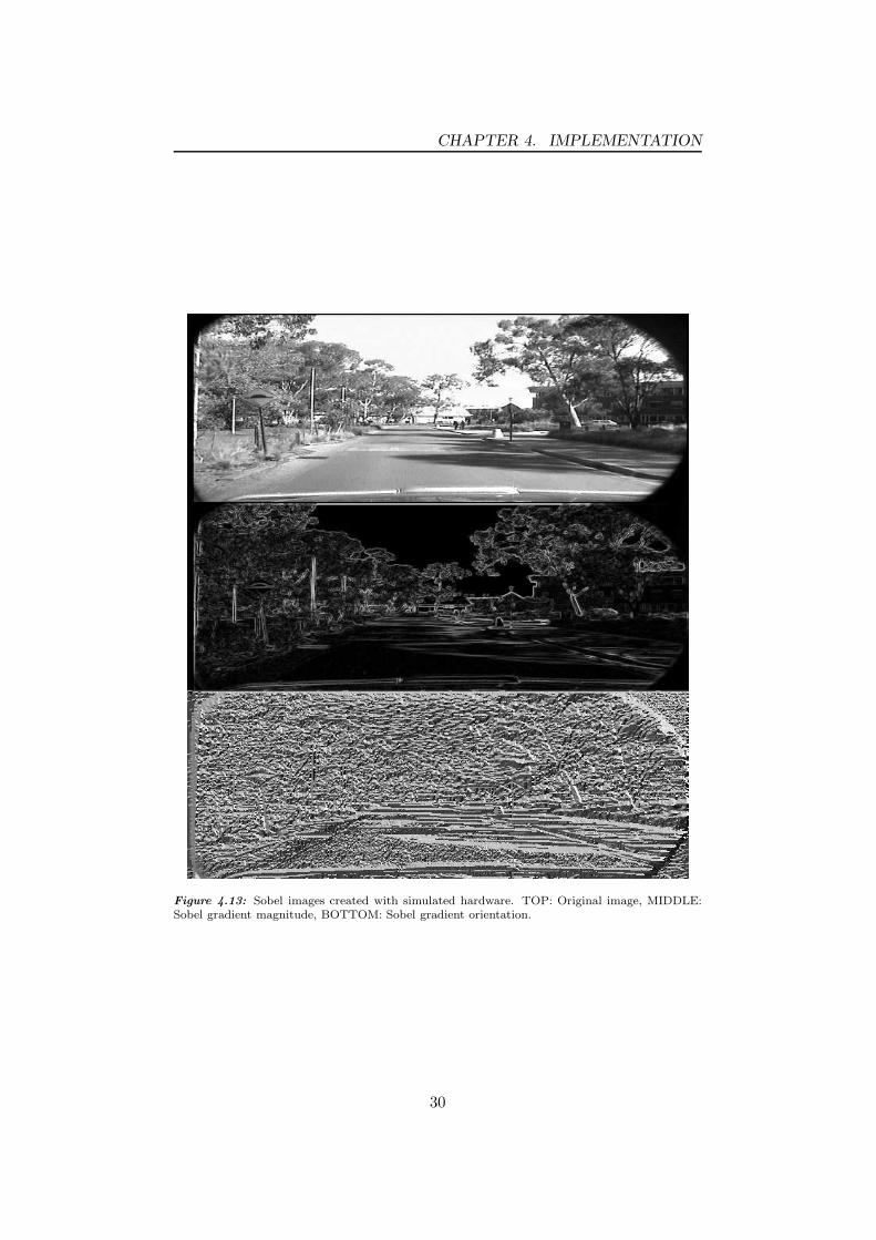
Figure 4.13: Sobel images created with simulated hardware. TOP: Original image, MIDDLE:Sobel gradient magnitude, BOTTOM: Sobel gradient orientation.

30


4.4 Finding and matching points in images

Taking images of an object from several different views, we want an al-gorithm that selects the same features in all these different images. Forexample, corners of a cube photographed from different directions. Thesefeatures are henceforth called keypoints. An example of an algorithm thatdoes this, and also extracs a feature-descriptor/vector that can be used tomatch two keypoints from two different images, is SIFT.

The SIFT algorithm extracts scale and rotationally invariant keypoints andtheir descriptors making it possible to find known objects in complex scenes.SIFT is a scale invariant feature detector which can cope with small affinetransformations between the images that are to be matched. Since ourcamera setup has a relatively short baseline (0.3 m), small transformationsmay be assumed in our system.

σoct

ave

Gaussianblurred images

...

DOG images Local Max/Mininput image

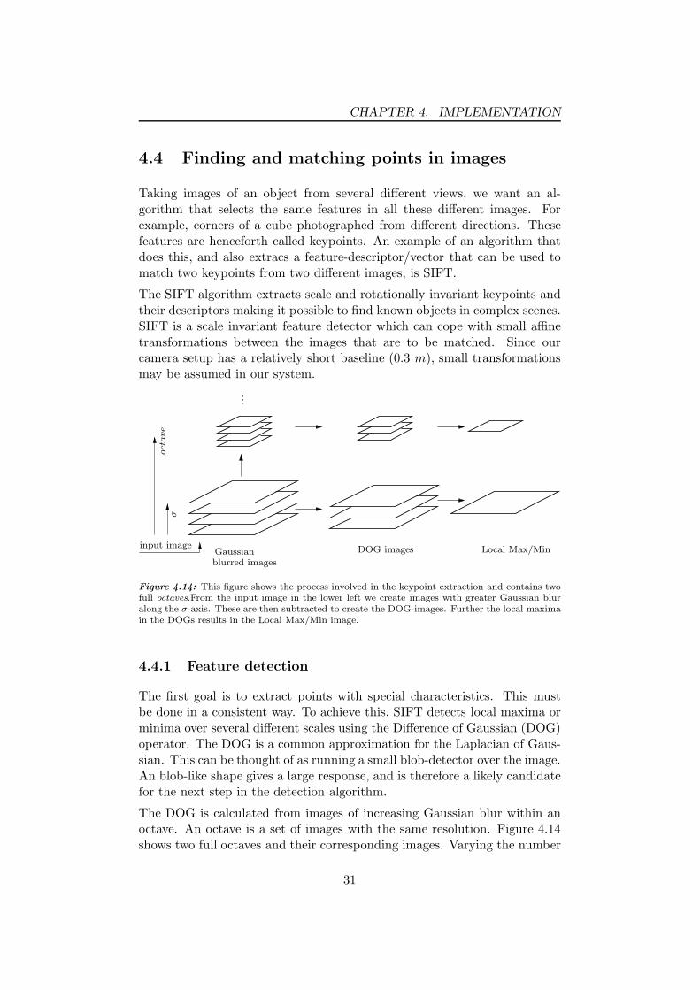
Figure 4.14: This figure shows the process involved in the keypoint extraction and contains twofull octaves.From the input image in the lower left we create images with greater Gaussian bluralong the σ-axis. These are then subtracted to create the DOG-images. Further the local maximain the DOGs results in the Local Max/Min image.

4.4.1 Feature detection

The first goal is to extract points with special characteristics. This mustbe done in a consistent way. To achieve this, SIFT detects local maxima orminima over several different scales using the Difference of Gaussian (DOG)operator. The DOG is a common approximation for the Laplacian of Gaus-sian. This can be thought of as running a small blob-detector over the image.An blob-like shape gives a large response, and is therefore a likely candidatefor the next step in the detection algorithm.

The DOG is calculated from images of increasing Gaussian blur within anoctave. An octave is a set of images with the same resolution. Figure 4.14shows two full octaves and their corresponding images. Varying the number

31


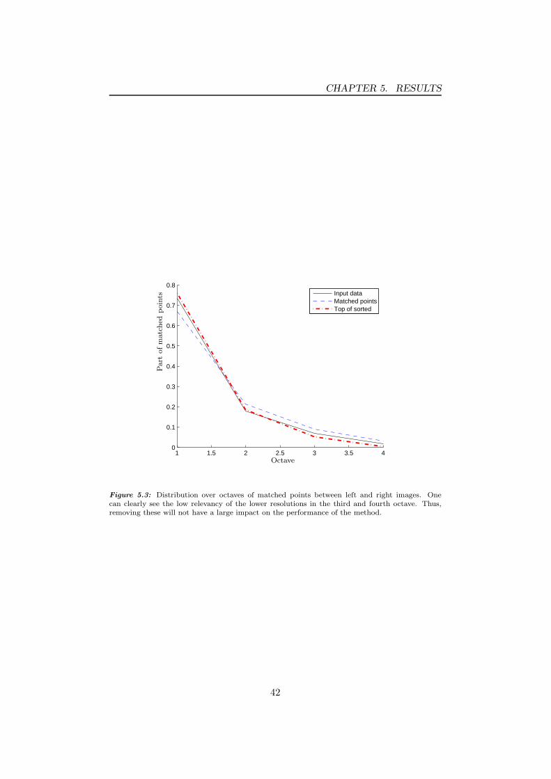
of scales within an octave affects the number of detected points. For thisapplication, we chose to have four scales in each octave and four octaves intotal. This gives three DOG images. To qualify as being a local minimumor maximum, each potential keypoint must have a DOG value higher orlower than all of its 26 neighbors in a 3x3x3 surrounding cube. Again,for this particular application, the need for the three subsampled octaves isquestionable. The distribution over acquired keypoints from the four octavesis shown in figure 5.3. This clearly shows the dominance of the first octavein the number of points actually used in the matching. More details of theseprocedures can be found in [15].

In order to achieve rotational invariance, an orientation is assigned to eachkeypoint using the orientation of the gradient in the vicinity of the keypoint.This leads to a need to calculate the gradient’s magnitude and orientation.

4.4.2 Keypoint descriptor extraction

The points detected in the previous steps are referred to as keypoints. Forthe descriptor to be rotationally invariant, an area of 16x16 pixels aroundthe keypoint is rotated according to the orientation calculated previously.Instead of using the intensity values of the small patch we use the orienta-tions of each pixel. Basically, the orientation is the direction in a 2D space ofthe local image gradient. In our case, this is calculated from the Sobel imageand the details are given in 4.3. The distribution of directions is estimatedusing histograms. This gives robustness against small affine transforma-tions. From these histograms, from the 16x16 patch a 128-element featurevector is formed. This is what we call the keypoint descriptor. More detailsof how the descriptor is constructed are provided in [15].

4.4.3 Keypoint matching

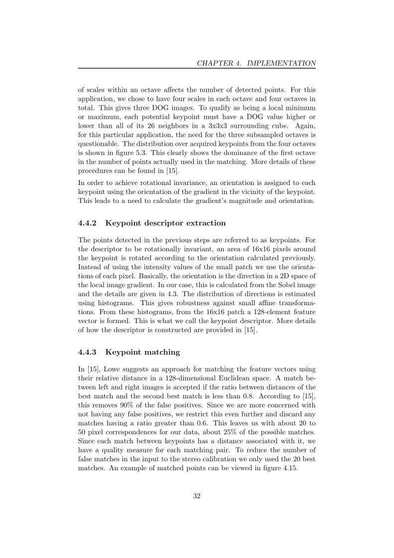
In [15], Lowe suggests an approach for matching the feature vectors usingtheir relative distance in a 128-dimensional Euclidean space. A match be-tween left and right images is accepted if the ratio between distances of thebest match and the second best match is less than 0.8. According to [15],this removes 90% of the false positives. Since we are more concerned withnot having any false positives, we restrict this even further and discard anymatches having a ratio greater than 0.6. This leaves us with about 20 to50 pixel correspondences for our data, about 25% of the possible matches.Since each match between keypoints has a distance associated with it, wehave a quality measure for each matching pair. To reduce the number offalse matches in the input to the stereo calibration we only used the 20 bestmatches. An example of matched points can be viewed in figure 4.15.

32


Figure 4.15: This figure shows matched points between two camera images. A point in the leftimage is connected to it’s corresponding point in the right image. Don’t fear, our car was notmoving when we took these example images.

4.4.4 Profiling of SIFT in C-implementation

The SIFT-algorithm in a pure software implementation is to cpu-intensive tohave running along with other software in our servers. Therefore we decidedto perform what is known as a profiling of the software. Profiling is donein order to find out which steps in the program that takes up most of thecpu time. Knowing this, one knows which functions to move from softwareto hardware.

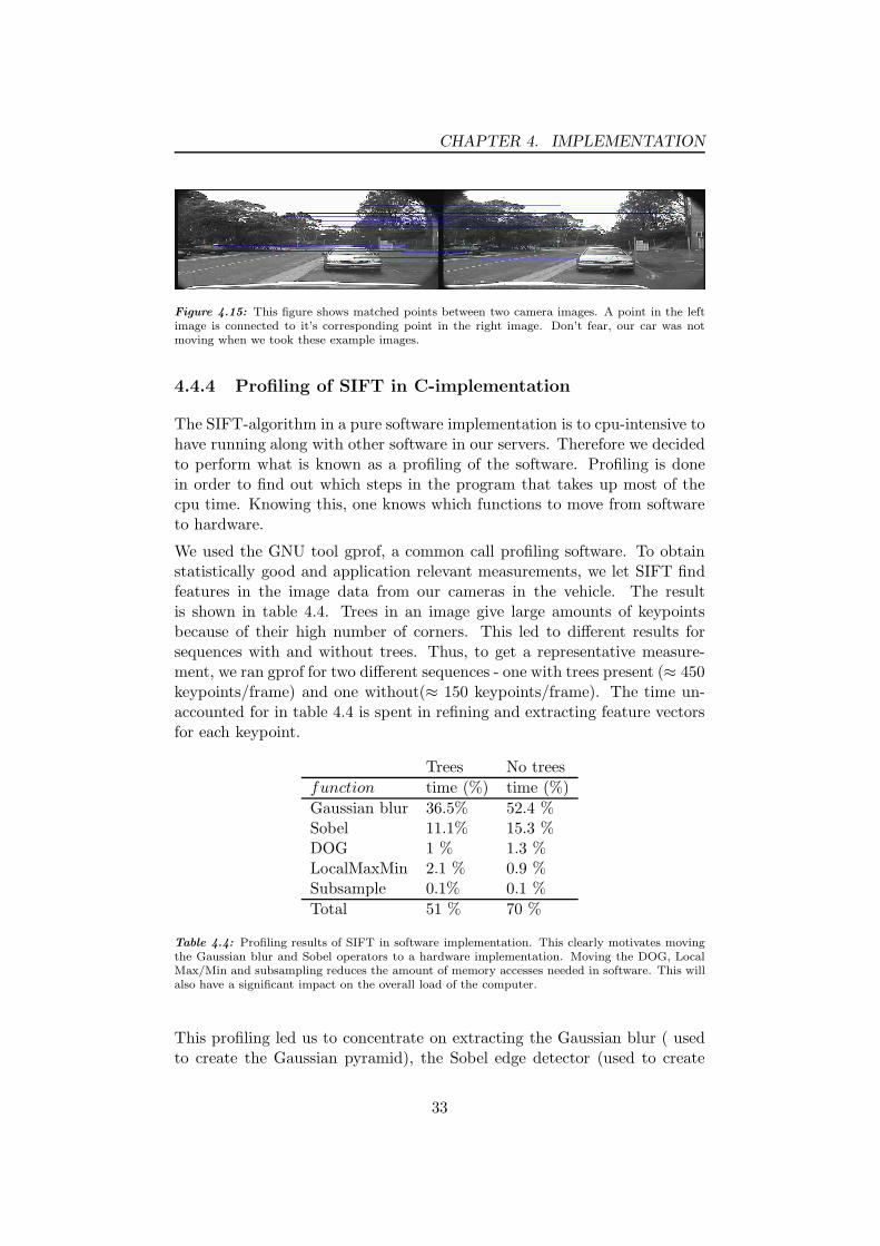
We used the GNU tool gprof, a common call profiling software. To obtainstatistically good and application relevant measurements, we let SIFT findfeatures in the image data from our cameras in the vehicle. The resultis shown in table 4.4. Trees in an image give large amounts of keypointsbecause of their high number of corners. This led to different results forsequences with and without trees. Thus, to get a representative measure-ment, we ran gprof for two different sequences - one with trees present (≈ 450keypoints/frame) and one without(≈ 150 keypoints/frame). The time un-accounted for in table 4.4 is spent in refining and extracting feature vectorsfor each keypoint.

Trees No trees

function time (%) time (%)

Gaussian blur 36.5% 52.4 %Sobel 11.1% 15.3 %DOG 1 % 1.3 %LocalMaxMin 2.1 % 0.9 %Subsample 0.1% 0.1 %

Total 51 % 70 %

Table 4.4: Profiling results of SIFT in software implementation. This clearly motivates movingthe Gaussian blur and Sobel operators to a hardware implementation. Moving the DOG, LocalMax/Min and subsampling reduces the amount of memory accesses needed in software. This willalso have a significant impact on the overall load of the computer.

This profiling led us to concentrate on extracting the Gaussian blur ( usedto create the Gaussian pyramid), the Sobel edge detector (used to create

33


orientations), the DOG and the Local Max/Min detection. This, in total,gives a speedup of at least 50%-70%. Another factor that has to be takeninto account is the speedup due to the smaller amount of data that has tobe processed by the cpu. If we can keep this to a minimum, the cpu canwork more efficiently since it can keep all the data it needs in the fast cachememory, reducing the need to access the relatively slow external memory.

34


4.5 Stereo calibration

From the point correspondences calculated in the previous section, we cannow calculate the stereo calibration as described in Chapter 3. Thus, thissection describes our approach to this problem. As input to the stereocalibration calculation, we have the point correspondences between the leftand right camera images.

4.5.1 Calculating the Essential Matrix

There are many methods for performing stereo calibration. The most com-mon way is to estimate either the the Essential matrix. Several approachesare reviewed in [10]. What they have in common is that they are all basedon point correspondences between the left and right camera images. How-ever, these methods apply to a general unconstrained camera configuration.Estimating the geometry of a completely unconstrained configuration is notrobust due to the many unknown parameters and requires a large number ofpoint correspondences. Instead, by exploiting the fact that the cameras aremounted on a 3 DOF stereo head, a reduced model with fewer parameterscan be used. In doing so, the estimation problem becomes more tractable.

Our case, constrained

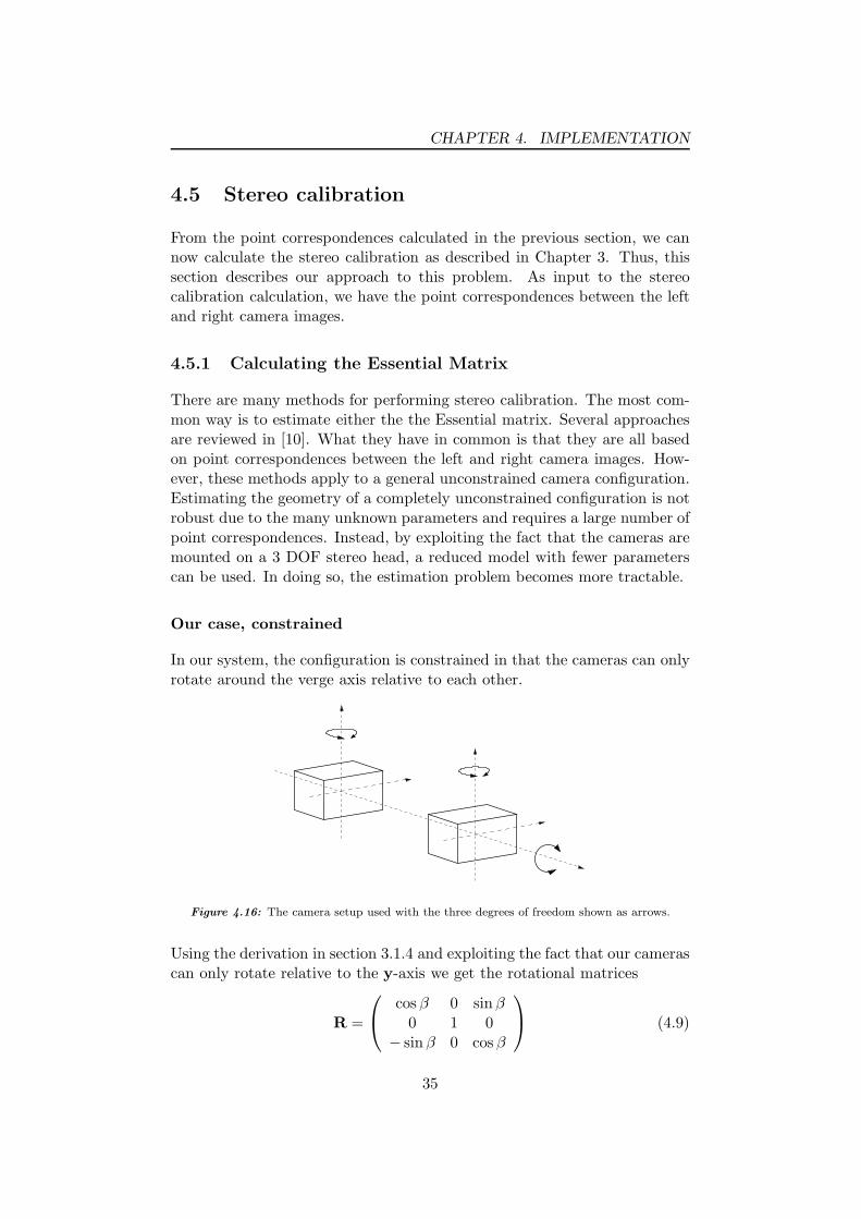
In our system, the configuration is constrained in that the cameras can onlyrotate around the verge axis relative to each other.

Figure 4.16: The camera setup used with the three degrees of freedom shown as arrows.

Using the derivation in section 3.1.4 and exploiting the fact that our camerascan only rotate relative to the y-axis we get the rotational matrices

R =

cos β 0 sin β0 1 0

− sin β 0 cos β

(4.9)

35


where β is the angle of the individual camera, αl and αr. A zero angle meansthat the camera is oriented along the z-axis.

The baseline for this system is simply a displacement of the right cameraa distance d along the z-axis. Thus, t is given by t = (d, 0, 0)T and theskew-symmetric matrix

T = [t]x =

0 0 00 0 −d0 d 0

(4.10)

Now, we can calculate the form of the Essential matrix for our constrainedcamera setup:

E = RTR′T =

=

cos αl 0 sin αl

0 1 0− sinαl 0 cos αl

0 0 00 0 −d0 d 0

cos αr 0 sin αr

0 1 0− sin αr 0 cos αr

T

=

= d

0 − sin αl 0− sin αr 0 cos αr

0 − cos αl 0

(4.11)

This is the same setup used and exploited in [5] rendering an Essentialmatrix of the form:

E =

0 −sin(αl) 0−sin(αr) 0 cos(αr)0 −cos(αl) 0

(4.12)

where αl, αr are the angles of the left and right cameras relative to thebaseline as shown in figure 4.3. The axis of rotation is defined as the y-axisand the translation of the right camera relative to the left is 0.3 m along thex-axis.

To calculate the Essential matrix one seeks to minimize

err = |xTr Exl| (4.13)

This problem is easy to formulate as a Least Squares problem. Unfortu-nately, this approach is very sensitive to outliers. Robust methods such asRANSAC can be used to reduce the number of outliers. However, thesemethods become computationally expensive if the number of points is large.This is one of the reasons why we chose to use SIFT-features since thenumber of false matches between these features is very small.

36


Now, (4.13) may be expanded as:

xTr Exl =

(

ur vr 1...

......

)

0 e1 0e2 0 e4

0 e3 0

ul . . .vl . . .1 . . .

=

=

(

urvl ulvr vl vr...

......

...

)

(

e1 e2 e3 e4

)T

(4.14)

Using the method suggested by Hartley in [9], (4.14) can be solved usingthe Singular Value Decomposition (SVD). As shown in Section 3.1.4, theEssential matrix must have rank 2. Writing E in the form E = UDVT, wecan ensure that this holds by setting the smallest singular value in D tozero and setting the remaining two to the mean of the two largest singularvalues. This results in a new matrix D′ and E′ = UD′VT will then havethe correct properties.

4.5.2 Dealing with ambiguity

Unfortunately, the method above gives an ambiguous solution. That is, E isnot unique. The resulting E might equally well represent a system rotated180 degrees around the x-axis due to ambiguity in the essential matrix[10].This is dealt with by studying U in the SVD decomposition of E above.The columns of U are the eigenvectors of EET. Since we constrained theEssential matrix to only contain a translation along the x-axis and a rotationaround the y axis, one of the eigenvectors of U is the y-axis. However, it isambiguous whether it is the positive or negative axis. If the eigenvector isnegative, we rotate E by 180 degrees around the x-axis.

R =

1 0 00 cos β sin β0 − sin β cos β

=

1 0 00 −1 00 0 −1

(4.15)

This enables us to get a consistent estimate of E over time.

4.5.3 Calculating the vergence angle

Theoretically, it is easy to calculate the two separate angles αl and αr from(4.12). However, due to the short baseline it is only the relative angle thatis of any numerical stability. Thus, instead of calculating αl and αr, wecalculate the verge angle

θ = αl − αr (4.16)

This angle is of interest since we can get encoder data from the CeDAR headto verify our estimate. Experimental results are presented in Chapter 5.

37

Chapter 5

Results

5.1 Experimental setup

In addition to the results from simulations done of the separate parts shownin the previous chapter, we decided to do some real world experiments. Thefirst experiment, indoor in the lab, were done to verify the calculation stereocalibration. This experiments verifyes that the movements of the cameras asindicated by the encoders on the different axes are correctly calculated fromthe image information only. Further, the second experiment using a movingvehicle shows the stability of the system during a period of no intendedcamera motion.

5.1.1 Indoor, lab

To be able to make a precise comparison to other methods, we collectedimages and encoder data in a laboratory environment at the lab in Canberra.The setup is a replica of the car setup using the same type of camera setup.However, since the computers used in these laboratory experiments wereolder than the ones used in the car, we had to deal with lower and less reliableframerate. The framerate for the indoor, moving cameras, experiment wasonly about 15 frames per second. While collecting data from the cameras,angles from the encoders on the axis of the cameras were recorded in asynchronized fashion. The motion of the cameras is created by manuallymoving each camera independently.

5.1.2 Outdoor, car

For the experiment with “fixed cameras”, we used the setup in the intelli-gent vehicle. In this sequence, we fixated the cameras using the actuators

38

CHAPTER 5. RESULTS

and drove the car in a city environment. This sequence was recorded atapproximately 30 frames per second.

5.2 Stereo calibration

We have shown a way of improving the speed of creating feature points andultimately calculating the stereo calibration (the Essential matrix). Thisis done by using dedicated hardware instead of software in vital steps inthe algorithm. In doing so, the computation time is reduced by 50%-70%for the feature extraction, not taking into account the effect of reducingthe number of memory accesses. Further, the feature extraction now startsbefore the image is fully digitized and transferred to the computer. Thisreduces the lag from image capture to image understanding since softwarenormally have to wait for the frame grabber to capture and transfer anentire image to memory before it can start to process it. Using a pipelineclock of 54 MHz, the delay from retrieving the first pixel in the raw image toretrieving the first pixel in the last pyramid octave is estimated to be about40µs. This should be compared to the time it takes for a camera to outputa full frame, 16.7ms.

Partial results from the different SIFT stages moved into hardware can beseen in Figures 4.9, 4.13, 4.6 and 4.15. These images show the filteredimages, extracted candidate points and matched points respectively.

5.2.1 Moving Cameras

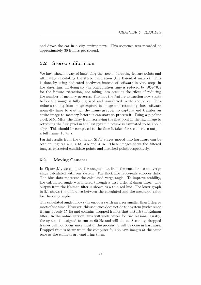
In Figure 5.1, we compare the output data from the encoders to the vergeangle calculated with our system. The thick line represents encoder data.The blue dots represent the calculated verge angle. To improve stability,the calculated angle was filtered through a first order Kalman filter. Theoutput from the Kalman filter is shown as a thin red line. The lower graphin 5.1 shows the difference between the calculated and the measured valuefor the verge angle.

The calculated angle follows the encoders with an error smaller than 1 degreemost of the time. However, this sequence does not do the system justice sinceit runs at only 15 Hz and contains dropped frames that disturb the Kalmanfilter. In the online version, this will work better for two reasons. Firstly,the system is designed to run at 60 Hz and will do so. Secondly, droppedframes will not occur since most of the processing will be done in hardware.Dropped frames occur when the computer fails to save images at the samepace as the cameras are capturing them.

39

CHAPTER 5. RESULTS

0 50 100 150 200 250 300 350 400 450 500−20

−10

0

10

20

0 50 100 150 200 250 300 350 400 450 500

0

−2

2

−4

1

−1

4

motion blur

dropped frames

verg

eangle

indegre

es

frame

frame

diff

ere

nce

indegre

es

Figure 5.1: TOP: Comparison between encoder data (thick black line) and verge angle calculatedby our methods. Blue dots represent measurements and the thin red line is the Kalman filteredmeasurements. BOTTOM: (Encoder angle) − calculated angle.

5.2.2 Fixed Cameras

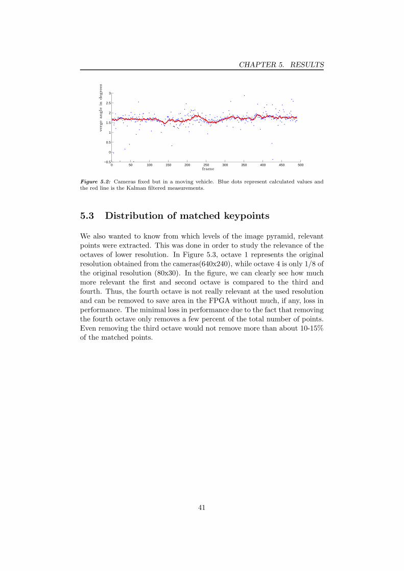
Since our stereo head mounted in the vehicle cannot yet report encoderangles, we did a simple experiment where the cameras were fixed. Thegraph in Figure (5.2) shows the results from this setup with the car drivingin a city environment. The verge angle varies from 1.43◦ to 1.86◦, a span ofonly 0.4◦. The variation is most probably a superposition of movement inthe stereo head and noise from the matching and calculations.

5.2.3 Using RANSAC

We implemented a RANSAC algorithm in order to see if that would improvestability. The results are almost impossible to distinguish from Figure 5.2.We interpreted this to be due to the low number of outliers in the data,which gives further support for our choice of SIFT as the feature detector.

40

CHAPTER 5. RESULTS

0 50 100 150 200 250 300 350 400 450 500−0.5

0

0.5

1

1.5

2

2.5

3

verg

eangle

indegre

es

frame

Figure 5.2: Cameras fixed but in a moving vehicle. Blue dots represent calculated values andthe red line is the Kalman filtered measurements.

5.3 Distribution of matched keypoints

We also wanted to know from which levels of the image pyramid, relevantpoints were extracted. This was done in order to study the relevance of theoctaves of lower resolution. In Figure 5.3, octave 1 represents the originalresolution obtained from the cameras(640x240), while octave 4 is only 1/8 ofthe original resolution (80x30). In the figure, we can clearly see how muchmore relevant the first and second octave is compared to the third andfourth. Thus, the fourth octave is not really relevant at the used resolutionand can be removed to save area in the FPGA without much, if any, loss inperformance. The minimal loss in performance due to the fact that removingthe fourth octave only removes a few percent of the total number of points.Even removing the third octave would not remove more than about 10-15%of the matched points.

41

CHAPTER 5. RESULTS

1 1.5 2 2.5 3 3.5 40

0.1

0.2

0.3

0.4

0.5

0.6

0.7

0.8Input dataMatched pointsTop of sorted

Octave

Part

ofm

atc

hed

poin

ts

Figure 5.3: Distribution over octaves of matched points between left and right images. Onecan clearly see the low relevancy of the lower resolutions in the third and fourth octave. Thus,removing these will not have a large impact on the performance of the method.

42

Chapter 6

Conclusions

We have described a method of calculating the stereo calibration of an activestereo head using FPGAs, SIFT features and a robust estimation of theEssential matrix. Several stages of the SIFT algorithm were moved fromsoftware to hardware taking a significant load off the host computer. Byparallelizing these stages we also removed time-delay between images andfeatures, thereby enabling a faster interpretation of the images and enablingthe system to respond quicker to any danger in front of the vehicle.

6.1 Feature detector

There are many other feature detectors suitable for the specific task of per-forming automated stereo calibration. SIFT is normally not considered forthis task since its great advantage is that it is scale invariant. For thisapplication, that is not really needed and a simple corner detector wouldprobably suffice. Also, the SIFT descriptor is possibly “overkill” in this ap-plication, and a reduced version should suffice. However, this also reducesthe quality in the matching of the keypoints and thus creates a need for amore robust estimation of the Essential matrix. Therefore, since the aimfrom the Smart Cars project was not only to calibrate the cameras online,but also to extract more information from the images, SIFT was chosen asfeature extractor and descriptor.

6.2 Computer Vision in FPGAs

The concept of implementing Computer Vision in FPGAs is in our opinionunderestimated. The gain from parallelising algorithms in dedicated hard-ware shows that FPGAs is a clear challenger to the otherwise so commonlyused Digital Signal Processors (DSPs). We feel that this is something we

43

CHAPTER 6. CONCLUSIONS

have shown quite clearly with the work related to this thesis. However, sinceimplementing algorithms in VHDL on FPGAs is a time consuming task, oneshould chose which algorithms to convert very carefully.

6.3 Future work

Firstly, adding an iterative refinement step in the stereo calibration calcu-lations would improve on accuracy at the price of complexity. However, byusing a reduced version of the SIFT-features with 16 instead of 128 terms,the matching of points would be far less complex, thus allowing for refine-ments in other steps.

Moving the calculation of the feature vectors to hardware will be possibleif we omit to rotate the patch before extraction. As our main concern is tomatch points between cameras on a fixed baseline, this rotation should nothave a significant impact on matching performance.

From this base of filters now implemented in VHDL, there are quite a fewother computer vision algorithms we can make run in real time.

44

Bibliography

[1] T. W. A.Th. Schwarzbacher, A. Brasching and J. Foley. Optimisa-tion and implementation of the arctan function for the power domain.Electronic Circuits and Systems Conference, Bratislava, Slovakia, pages33–36, 1999.

[2] Atmel. Edge detection in at6000 fpgas. Application notes., 1997.

[3] Atmel. 3x3 convolver with run-time reconfigurable vector multiplier inatmel at6000 fpgas. Application notes., 1999.

[4] M. Bjorkman. Real Time Motion and Stereo Cues for Active Visual Ob-servers. PhD thesis, Royal Institute of Technology, Stockholm, Sweden,2002.

[5] M. Bjorkman and J.-O. Eklundh. Real-time epipolar geometry estima-tion of binocular stereo heads. IEEE Transactions on pattern analysisand machine intelligence, 24(3), 2002.

[6] V. Gerdes. Stereo images with ground truth disparity and occlusion,2001. http://www-dbv.cs.uni-bonn.de/stereo data/.

[7] S. R. Harley Truong, Samer Abdallah and A. Zelinsky. A novel mecha-nism for stereo active vision. In Proc. Australian Conference on Roboticsand Automation, Melbourne Australia, 2000.

[8] C. Harris and M. Stephens. A combined corner and edge detector. InAlvey Vis Conference, 1999.

[9] R. Hartley. Estimation of relative camera positions for uncalibratedcameras. In Proc. Second European Conf. Computer Vision, pages 579–587, 1992.

[10] R. Hartley and A. Zisserman. Multiple View Geometry in computervision, 2nd edition. Cambridge University Press, 2003.

[11] E. Kalman. A new approach to linear filtering and prediction prob-lems. Transactions of the ASME–Journal of Basic Engineering, 82(Se-ries D):35–45, 1960.

45

BIBLIOGRAPHY

[12] T. Lindeberg. Detecting salient blob-like image structures and theirscales with a scale-space primal sketch: A method for focus-of-attention.International Journal of Computer Vision, 11(3):283–318, 1993.

[13] H. Longuet-Higgins. A computer algoritm for reconstructing a scenefrom two projections. Nature, 293:133–135, 1981.

[14] D. G. Lowe. Object recognition from local scale-invariant features.In Proc. of the International Conference on Computer Vision ICCV,Corfu, pages 1150–1157, 1999.

[15] D. G. Lowe. Distinctive image features from scale-invariant keypoints.International Journal of Computer Vision, 60(2), 2004.

[16] A. K. S. Hezel, D.M. Gavrila and R. Manner. Fpga-based tem-plate matching using distance transforms. IEEE Symposium on Field-Programmable Custom Computing Machines, 2002.

[17] Shinichi, Masakazu, and Tatsuhiko. Implementing image processingalgoritms in fpga-based realtime vision system. In 11th Synthesis andSystem Integration of Mixed Information Technologies (SASIMI 2003),2003.

[18] K. Sim. Constrained optimization and multiple view geometry. Tech-nical report, Research Scool of Information Sciences and Engineering,Australian National University, Canberra, Australia, 2004.

[19] R. Tsai and T. Huang. Estimating 3-d motion parameters of a rigidplanar patch. IEEE Trans. on Acoustic, Speech and Signal Processing,29:1147–1152, 1981.

[20] J. Volder. The cordic trigonometric computing technique. IRE Trans.Electron. Comput., 1959.

[21] Wikipedia. the free encyclopedia. http://www.wikipedia.org.

46

Appendix A

Paper presented at the IEEEIntelligent VehiclesSymposium, Las Vegas, 2005

47

Online Stereo Calibration using FPGAs - nipe.senipe.se/publications/pettersson_thesis_2005.pdf · Online Stereo Calibration using FPGAs ... 2.2.1 Edge detection, using the Sobel operator

Documents