ON USING AMOS, EQS, LISREL, Mx, RAMONA & SEPATH · 4.4.3 creating lisrel/simplis syntax using path diagram 139 4.4.4 drawing a path diagram interactively in lisrel 8.30 for windows

ON USING AMOS, EQS, LISREL, Mx, RAMONA & SEPATH

FOR

STRUCTURAL EQUATION MODELING

by

Sylvester Peprah

ON USING AMOS, EQS, LISREL, Mx, RAMONA AND SEPATH

FOR

STRUCTURAL EQUATION MODELING

by

SYLVESTER PEPRAH

Submitted in partial fulfillment of the requirements for the degree of

Magister Scientiae in the Faculty of Science

at the University of Port Elizabeth.

March 2000

Supervisor: Gerhard Mels University of Port Elizabeth

ii

ACKNOWLEDGEMENTS My sincere thanks goes to my supervisor Gerhard Mels of the University of Port Elizabeth1 for his

ideas for this treatise, his constructive criticisms and guidance throughout this project. His advice

and guidance throughout my studies here at University of Port Elizabeth are very much appreciated.

I sincerely thank Prof. I.N. Litvine, the head of department of the Department of Mathematical

Statistic of the University of Port Elizabeth, for allowing me to use the departmental facilities. The

encouragement and guidance he gave to me throughout my studies are very much appreciated. I

would also like to thank the rest of the staff of the department for their support.

I thank the following people for their help in one way or the other towards this project: Kwaku

Mensah, Hon. Kwadwo Boateng, Kofi Siaw, Thomas Allotey Bray, Elder Alfred “Bob” Blain, Clare

Blain, Elder Rueben Maggerman, N.D. Naidoo, Dr. R. Banful, Kwame Andoh, Thokozani Simelani,

C.N. Namponya and Zola Bob.

I would like to thank the following friends whose contributions to my studies can not be measured

by mere words: Akonta Samuel Oduro, Akonta Thomas Gyedu-Ababio, Akonta Addo-Bediako and

Dr. Ubomba-Jaswa. May the Lord Almighty richly bless you all. I would like to give special thanks

to my mother, Abena Manu Febiri, brothers, Gilbert Yaw Agyenim-Boateng, Michael Baah,

Kwabena Kyeremeh and Kwadwo Asamoah and our sister, Agather, for their moral support,

understanding and prayers.

I would like to thank my wife, Florence Adwoa Boateng, my sons: Oscar, Kofi Kusi and Kofi

Asante for sacrificing a family fortune to enable me undertake my postgraduate studies. My absence

from home most of the time was very painful but you endured it. Words cannot express how grateful

I am. Finally, I would like to thank my Creator who made all things possible through His Son Jesus

Christ. Thank you Father for the good health I have enjoyed throughout my studies and all that you

have done and continue doing in my life.

1 Gerhard is currently a senior programmer at Scientific Software International.

iii

DEDICATION

I dedicate this work to the memories of:

My late father, Mark Kofi Asante

My late brother and friend, Kwabena Amponsah Moses

and My late friend, Edmund Ofori Ayeh.

iv

CONTENTS Page

CHAPTER 1 INTRODUCTION 1

1.1 INTRODUCTORY BACKGROUND 1

1.2 A MODEL FOR PEER INFLUENCES ON AMBITION 5

1.3 MOTIVATION 9

1.4 SUMMARY OF CONTENTS 11

CHAPTER 2 AMOS 13

2.1 HISTORICAL BACKGROUND 13

2.2 THE AMOS INPUT SYSTEM 14

2.2.1 MODEL INFORMATION 15

2.2.2 MODEL SPECIFICATION 16

2.2.3 ESTIMATION METHOD(S) 18

2.2.4 DATA 19

2.2.5 GROUP NAME 19

2.2.6 OUTPUT 19

2.2.7 INPUT FILE: EXAMPLE 2 19

2.3 ILLUSTRATIVE EXAMPLE

THE DUNCAN, HALLER AND PORTES’ APPLICATION 22

2.3.1 CREATING THE AMOS DATA FILE FOR THE DUNCAN, HALLER

AND PORTES’ APPLICATION 22

2.3.2 CREATING AMOS GRAPHIC FILE FOR THE MODEL OF THE

DUNCAN, HALLER AND PORTES’ APPLICATION 24

2.3.3 RUNNING AMOS 34

2.3.4 THE AMOS OUTPUT FILE 35

v

CHAPTER 3 EQS 52


3.2 THE EQS INPUT FILE 52

3.2.1 MODEL AND DATA INFORMATION 53

3.2.2 MODEL SPECIFICATION WITH EQS 55

3.2.3 DATA 57


THE DUNCAN, HALLER, AND PORTES’ APPLICATION 59

3.3.1 CREATING THE EQS INPUT FILE 59

3.3.2 INPUT FILE: EXAMPLE 3 67

3.3.3 RUNNING EQS 69

3.3.4 THE EQS OUTPUT FILE 70

CHAPTER 4 LISREL 87


4.2 THE LISREL INPUT SYSTEM 89

4.2.1 THE LISREL INPUT FILE SYNTAX 91

4.3 TYPING A SIMPLIS FILE USING SIMPLIS COMMAND LANGUAGE 108

4.3.1 THE SYNTAX OF THE SIMPLIS FILE 110

4.3.2 SIMPLIS FILE FOR THE MODEL DEPICTED IN FIGURE 1.2 118

4.4 ILLUSTRATIVE EXAMPLE 120

4.4.1 CREATING LISREL SYNTAX INTERACTIVELY FOR THE DUNCAN,

HALLER AND PORTES’ MODEL DEPICTED IN FIGURE 1.2 120

4.4.2 CREATING SIMPLIS SYNTAX FILES INTERACTIVELY 137

4.4.3 CREATING LISREL/SIMPLIS SYNTAX USING PATH DIAGRAM 139

4.4.4 DRAWING A PATH DIAGRAM INTERACTIVELY IN LISREL 8.30 FOR

WINDOWS FOR THE DUNCAN, HALLER AND PORTES’ APPLICATION 140

4.4.5 RUNNING LISREL 8.30 153

4.4.6 THE LISREL OUTPUT FILE 154

vi

CHAPTER 5 Mx 172


5.2 THE Mx INPUT SCRIPT FILE 173

5.2.1 PREPARING AN Mx INPUT SCRIPT FILE 174

5.2.2 AN Mx INPUT SCRIPT FOR THE MODEL DEPICTED IN FIGURE 1.2 187

5.3 ILLUSTRATIVE EXAMPLE: THE DUNCAN, HALLER AND PORTES’

APPLICATION 189

5.3.1 CREATING Mx INPUT SCRIPT FROM PATH DIAGRAM 189

5.3.2 RUNNING Mx 201

5.3.3 THE Mx OUTPUT FILE 202

CHAPTER 6 RAMONA 216


6.2 THE RAMONA INPUT FILE 216

6.2.1 MODEL INFORMATION 217

6.2.2 MODEL SPECIFICATION 219

6.2.3 DATA 221


6.3.1 VARIABLE NAMES 222

6.3.2 INPUT FILE 223

6.3.3 RUNNING RAMONA 224

6.3.4 THE RAMONA OUTPUT FILE 229

CHAPTER 7 SEPATH 243


7.2 THE SEPATH INPUT SYSTEM 243

7.2.1 THE SEPATH DATA FILE 243

vii

7.2.2 THE SEPATH MODEL FILE 244


7.3.1 CREATING THE SEPATH DATA FILE FOR THE DUNCAN, HALLER

AND PORTES’ APPLICATION 246

7.3.2 THE SEPATH MODEL FILE FOR THE DUNCAN, HALLER AND

PORTES’ APPLICATION 251

7.3.3 MODEL FILE 257

7.3.4 RUNNING SEPATH 258

7.3.5 THE SEPATH OUTPUT FILE 264

CHAPTER 8 CONCLUSIONS AND RECOMMENDATIONS 274

8.1 INTRODUCTION 274

8.2 AMOS 274

8.3 EQS 276

8.4 LISREL 278

8.5 Mx 279

8.6 RAMONA 281

8.7 SEPATH 282

8.8 COMPARING PARAMETER ESTIMATES OBTAINED FROM AMOS, EQS,

LISREL, Mx, RAMONA AND SEPATH 283

8.9 RECOMMENDATIONS FOR FUTURE RESEARCH 287

REFERENCES 288

viii

SUMMARY Structural Equation Modeling is a common name for the statistical analysis of Structural Equation

Models. Structural Equation Models are models that specify relationships between a set of variables

and can be specified by means of path diagrams. A number of Structural Equation Modeling

programs have been developed. These include, amongst others, AMOS, EQS, LISREL, Mx,

RAMONA and SEPATH. A number of studies have been published on the use of some of the

applications mentioned above. They include, amongst others, Brown (1986), Waller (1993) and

Kano (1997). Structural Equation Models are increasingly being used in the social, economic and

behavioral sciences. More and more people are therefore making use of one or more of the Structural

Equation Modeling applications on the market. This study is performed with the aim of using each

of the Structural Equation Modeling applications AMOS, EQS, LISREL, Mx, RAMONA and

SEPATH for the first time and document the experience, joy and the difficulties encountered while

using them. This treatise is different from the comparisons already published in that it is based on the

use of AMOS, EQS, LISREL, Mx, RAMONA and SEPATH to fit a Structural Equation Model for

peer influences on ambition, which is specified for data obtained by Duncan, Haller and Portes

(1971), by myself as a first time user of each of the programs mentioned. The impressive features as

well as the difficulties encountered are listed for each application. Recommendations for possible

improvements to the various applications are also proposed. Finally, recommendations for future

studies on the use of Structural Equation Modeling programs are made.

ix

OPSOMMING

Strukturele Vergelykingsmodellering is 'n algemene term vir die statistiese ontleding van

Strukturele Vergelykingsmodelle. Hierdie modelle spesifiseer verwantskappe tussen 'n stel

veranderlikes en kan deur middel van pyldiagramme voorgestel word. Verskeie programme

vir Strukturele Vergelykingsmodellering is ontwikkel. Hierdie programme sluit, onder andere,

AMOS, EQS, LISREL, Mx, RAMONA en SEPATH in. Verskeie artikels oor die gebruik van

hierdie programme is reeds gepubliseer (Brown 1986, Waller l993, Kano 1997). Strukturele

Vergelykingsmodelle word toenemend in die sosiale, ekonomiese en gedragswetenskappe

gebruik. Gevolglik word ‘n positiewe toename in die gebruik van een of meer programme vir

Strukturele Vergelykingsmodellering in die praktyk ondervind. Hierdie studie is gemik op die

aanvanklike gebruik van sekere programme vir Strukturele Vergelykingsmodellering, naamlik

AMOS, EQS, LISREL, Mx, RAMONA en SEPATH. Dit dokumenteer die suksesse en

probleme wat ondervind word met die gebruik daarvan deur ‘n nuwe gebruiker. Hierdie

verhandeling verskil ten opsigte van die vergelykings, wat alreeds gepubliseer is,

aangesien dit gebaseer is op die gebruik van AMOS, EQS, LISREL, Mx, RAMONA en

SEPATH deur ‘n nuwe gebruiker. Ek, as ‘n nuwe gebruiker, pas ‘n Strukturele

Vergelykingsmodel vir portuur-invloede op ambisie op data, wat deur van Duncan, Haller en

Portes (1971) versamel is, met behulp van elk van die ses programme. My persoonlike

indrukwekkende eienskappe, sowel as die probleme wat ek ondervind het, word vir elke

program verskaf. Voorstelle vir moontlike verbeterings vir die verskillende programme word

gemaak. Ten slotte, word aanbevelings vir toekomstige studies oor die gebruik van die

programme vir Strukturele Vergelykingsmodellering ook voorgestel.

1

CHAPTER 1

INTRODUCTION

1.1 INTRODUCTORY BACKGROUND Structural Equation Modeling is a common name for the statistical analysis of Structural Equation

Models. Structural Equation Models are models that specify relationships between a set of variables.

A nice aspect of structural equation models is that they can be represented as a path diagram. A path

diagram is a fairly simple graphical display of a structural equation model on which the relationships

between all the structural equation model variables are indicated by means of uni-directional (for

dependence relationships) and bi-directional (for covariances, variances and correlations) arrows. In

a path diagram rectangles or squares are used to represent the observed or manifest variables and

circles or ellipses are used to represent unobserved or latent variables.

Every Structural Equation Model can be specified by means of a mathematical model(s) which

specifies the statistical relationships between the variables of the model. For example, the manifest

variable X may be modeled as a measurement of the latent variable Y, with an error term E1. This

relationship is shown in Figure 1.1 below. Figure 1.1: The measurement path between X and Y The measurement equation for the model depicted in Figure 1.1 is: X = λ Y + E1

where λ is the measurement strength of X as a measurement of Y.

Several general mathematical models have been proposed for the specification of Structural

Equation Models. The mathematical models differ from each other merely in the way the variables

in the general Structural Equation Modeling framework (system) are partitioned. The first general

mathematical model for the specification of Structural Equation Models is known as the LISREL

Y X E1

2

model (Jöreskog 1973, 1977; Jöreskog & Sörbom 1979, 1981; Wiley 1973). This model consists of a

measurement model for the endogenous (receiving at least one uni-directional arrow) latent

variables, a measurement model for the exogenous (emitting at least one uni-directional arrow) latent

variables and a latent variable model. Adapting the measurement model incorporates endogenous

manifest variables (excluding measurements of latent variables) for the endogenous latent variables

using duplicated endogenous latent variables. A similar adaptation of the measurement model for the

exogenous latent variables is used to incorporate exogenous manifest variables.

The mathematical models for Structural Equation Modeling with Latent Variables can not be

analyzed directly since no observations on the latent variables are available. However, the

mathematical models which describe the relationships between the variables (manifest and latent) in

the Structural Equation Modeling system lead to a structural model for the population covariance or

correlation matrix of the manifest variables, i.e., to a covariance or correlation structure for the

manifest variables, respectively. Consequently, statistical methods (estimation and measures of

goodness-of-fit) for the analysis of Covariance and Correlation Structures (cf. Jöreskog, 1970, 1978;

Browne, 1974, 1982, 1984; Bentler, 1983; Shapiro, 1983, 1985, 1986, 1987; Mels, 1988, 2000) can

be used to fit Structural Equation Models to observed data. Several statistical software packages have been developed for the analysis of Structural Equation

Models. The first commercial version of such an application, LISREL (Linear Structural

RELations), was developed by Jöreskog and Sörbom (1981). The general LISREL model leads to a

Covariance Structure, which contains eight parameter matrices. Initially, a user had to specify his/her

model in terms of these eight parameter matrices.

The next Structural Equation Modeling application after LISREL was BENWEE developed by

Browne and Cudeck (1983). BENWEE was based on a general model specification for Structural

Equation Models known as the Bentler and Weeks’ model proposed by Bentler and Weeks (1980).

The user of BENWEE had to specify his/her model in terms of the three large sparse parameter

matrices of the Bentler and Weeks model.

An alternative method to represent Structural Equation Models is by using structural equations such

as measurement and regression equations. The Structural Equation Modeling application EQS

3

(Bentler, 1985) utilizes this representation in the sense that the model is specified as a set of

structural equations. EQS implements the Bentler and Weeks model (Bentler & Weeks, 1980).

Mels (1988) introduced the Structural Equation Modeling application RAMONA as part of his

Masters dissertation in Statistics at the University of South Africa. The program RAMONA

implements the RAMONA model (Mels, 1988) which is a minor adaptation of the Recticular Action

Model proposed by McArdle and McDonald (1984). RAMONA was developed using Steiger’s

suggestion of the use of the ASCII symbols <--: for dependence paths and <--> for

covariance/variance paths to create ASCII representations of path diagrams of Structural Equation

Models. The use of the ASCII symbols allows users to specify their models in terms of text path

diagrams instead of matrices. RAMONA was the first program of its kind to yield correct results

whenever the sample correlation matrix instead of the sample covariance matrix is analyzed. The

program also addressed the problems with negative variance and out of bound estimates.

Steiger (1989) developed the Structural Equation Modeling program EzPATH as a module of a

statistical software package SYSTAT. This program was strongly influenced by Steiger’s ideas for

user-machine communication. Steiger left SYSTAT and joined forces with the statistical software

package STATISTICA to develop the SEM program known as SEPATH (Steiger, 1995) for

Windows. This program is strongly influenced by the conventions used in RAMONA and the ideas

contained in Mels (1988).

An alternative method for specifying a structural equation model, different from the ones mentioned

above, is by means of a graphics file of the path diagram of the model. The structural equation model

application AMOS (Arbuckle, 1994), was the first program of its kind to use a graphics file of a path

diagram to specify the model and to display the parameter estimates on the path diagram. It is

equipped with powerful path diagram drawing tools that allow a user to specify his/her model by

creating a graphics file for the path diagram graphically. The AMOS graphics input file makes no

references to matrices or any ASCII symbols.

Mx (Neale, 1994) is a combination of a matrix algebra interpreter and a numerical optimizer. It

enables exploration of matrix algebra through a variety of operations and functions. There are many

built-in functions, which enables Mx to handle Structural Equation Modeling and other statistical

modeling of data. The input script file in Mx is created by entering the required entries of the three

4

parameter matrices of the RAM model. Complex nonstandard models are easy to specify. For further

general applicability, it allows users to specify their own fit functions, and optimization may be

performed subject to linear and non-linear equality or boundary constraints.

The first version of each of the applications mentioned above has been updated more than once. The

table below gives the name of the applications, the date of the latest version and the author(s) of the

latest version.

Table 1.1: Name, date of latest release and authors of the six programs to be reviewed.

Name of program

Date of release

of latest version

Author(s)

1

AMOS

1996

Jim Arbuckle

2

EQS

1995

Peter M. Bentler

3

LISREL

1999

Karl Jöreskog & Dag Sörbom

4

Mx

1999

Michael C. Neale, Steven M. Boker

Gary Xie & Hermine H. Maes

5

RAMONA

1998

Gerhard Mels & Michael W. Browne

6

SEPATH

1995

James H. Steiger

There are other Structural Equations Modeling applications which are not considered in this study.

These include, amongst others, COSAN (Fraser & McDonald, 1988), LINCS (Schoenberg and

Arminger, 1988), LISCOMP (Muthen, 1987), MECOSA 3 (Arminger, 1997), SAS PROC CALIS

(SAS Institute, 1990), and a program using SAS Interactive Matrix Language (IML) by Cudeck,

Klebe and Henly (1993).

In the next section, a brief account of the Duncan, Haller and Portes (1971) Structural Equations

Modeling application is given. The path diagram of the application, Figure 1.2 below, is also used to

introduce the basic concepts involved in Structural Equation Modeling.

5

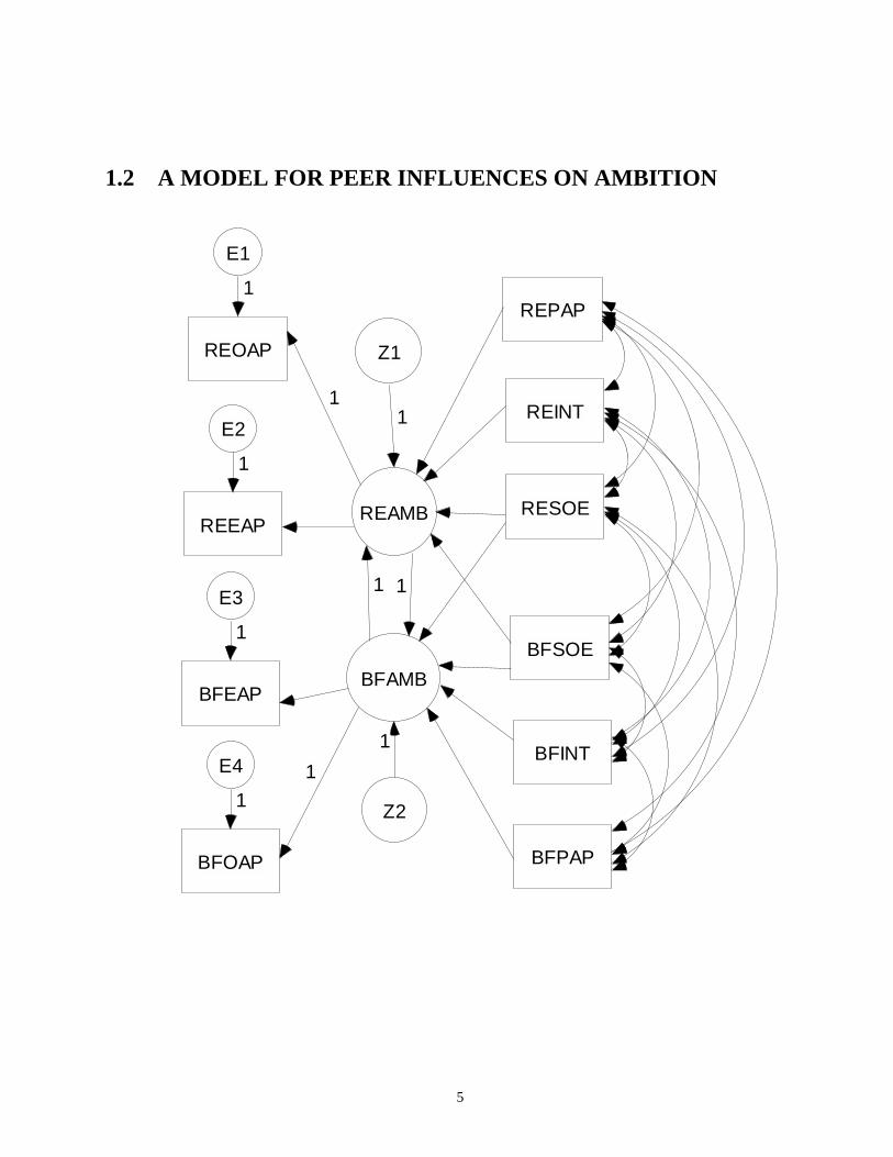
1.2 A MODEL FOR PEER INFLUENCES ON AMBITION

REAMB

BFAMB

Z1

1

Z2

1

REOAP

REEAP

BFEAP

BFOAP

REPAP

REINT

RESOE

BFSOE

BFINT

BFPAP

1

1

1 1

E2

1

E3

1

E4

1

E1

1

6

Sociologists have often called attention to the way in which one’s peers- e.g., best friends- influence

one’s decisions- e.g., choice of occupation. They have recognized that the relation must be

reciprocal- if my best friend influences my choice, I must influence his. The model depicted in figure

1.2, is based on data by Duncan, Haller, & Portes (1971). The data was collected from a study

conducted using a sample of 329 Michigan high-school students paired with their best friends. The

model was analyzed by Jöreskog (1977) by using fixed path coefficients rather than constrained

variances. In Figure 1.2, the descriptive names for the variables and their full names are:

REPAP Respondent’s parental aspiration.

REINT Respondent’s intelligence.

RESOE Respondent’s socioeconomic status.

REOAP Respondent’s occupational aspiration.

REEAP Respondent’s educational aspiration.

BFINT Best friend’s intelligence.

BFPAP Best friend’s parental aspiration.

BFSOE Best friend’s socioeconomic status.

BFOAP Best friend’s occupational aspiration.

BFEAP Best friend’s educational aspiration.

The path diagram in Figure 1.2 will now be used to introduce the basic concepts involved in

Structural Equation Modeling.

Latent variables:

A latent variable is an unobservable variable that is indicated by circle (ellipse) on a path diagram.

The latent variables of the model depicted in Figure 1.2 are REAMB and BFAMB.

Latent variables can, however, be measured by using measuring instruments. A measuring

instrument consists of common measurements (items, tests, questions, etc) of the latent variable of

interest. A summary of the measuring instruments for the latent variables of the model depicted in

Figure 1.2 is found in Table 1.2.

7

Table 1.2: Measuring Instruments of the Latent Variables in Figure 1.2

Latent Variable Measuring Instrument

REAMB REOAP, REEAP

BFAMB BFEAP, BFOAP

Measuring Instruments

A measuring instrument (scale) for a latent variable consists of a set of measurements. Each

measurement is a manifest (observable) variable and is usually psychometric test, a questionnaire

item or physical measurement. A measurement error is associated with each individual

measurement. These measurement errors are latent variables, which emits only one uni-directional

arrow. In Figure 1.2, E1, E2, E3 and E4 denote measurement errors.

Manifest Variables

Manifest variables are observable variables. On a path diagram a square or rectangle box indicates

manifest variable. In the model depicted in Figure 1.2, REOAP, REEAP, REPAP, REINT, RESOE,

BFEAP, BFOAP, BFSOE, BFINT and BFPAP are manifest variables.

Dependence Paths

The variables of Structural Equation Models are classified as being endogenous or exogenous. An

endogenous variable receives at least one uni-directional arrow while an exogenous variable only

emits unidirectional arrows. From Figure 1.2, REOAP, REEAP, REAMB, BFAMB, BFEAP and

BFOAP are all endogenous variables while REPAP, REINT, RESOE, BFSOE, BFINT, BFPAP, E1,

E2, E3, E4, Z1 and Z2 are exogenous variables.

Dependence paths are used for defining the relationships between endogenous and exogenous

variables and are indicated on a path diagram by means of a uni-directional arrow. For example, the

dependence path between RESOE, REAMB and the error term Z1 taken from Figure 1.2 is as shown

in Figure 1.3 below.

1

Figure 1.3: The dependence path between REAMB, RESOE and Z1

RESOE REAMB

Z1

8

Variance and Covariance Paths

A variance or covariance path is used to indicate the variance of a variable as well as the covariance

or correlation between two variables and is represented on a path diagram by means of a bi-

directional arrow. In Figure 1.2, the variance of the error terms, the measurement errors, the latent

variables and the six manifest variables: REPAP, REINT, RESOE, BFSOE, BFINT and BFPAP are

covariance paths. The correlations between the six manifest variables: REPAP, REINT, RESOE,

BFSOE, BFINT and BFPAP are shown on clearly in Figure 1.2. The variances of the error terms and

the measurement errors are usually unknown parameters while the variances of the latent variables

are frequently fixed or constrained at unity.

The Parameters

Structural Equation Models contain known (fixed) and unknown (free) parameters. Fixed

parameters are usually shown on a path diagram by displaying their values along the corresponding

paths while no values are usually indicated on paths associated with free parameters. In Figure 1.2,

the coefficients of the measurement errors and the error terms as well as all the variances are fixed at

unity. The measurement strengths of the measurements REOAP, REEAP, BFEAP, BFOAP, the

strength of the linear influences of REPAP, REINT, RESOE, BFSOE, BFINT and BFPAP and the

correlations between REPAP, REINT, RESOE, BFSOE, BFINT and BFPAP represent the unknown

parameters of the Structural Equation Model shown in Figure 1.2.

The Statistical Methods

The Statistical Methods for the analysis of Structural Equation Models consist of methods to

estimate the unknown (free) parameters of the model and methods to assess the goodness-of-fit of

the model to the data.

The table below was the sample correlation matrix obtained by Duncan, Haller and Portes (1971) for

the sample of 329 students. The descriptive names of the variables are given full meaning in Section

1.2 above.

9

Table 1.3: The correlation matrix for the Duncan, Haller and Portes’ Application given in lower

triangular format.

REINT 1.0000 REPAP .1839 1.0000 RESOE .2220 .0489 1.0000 REOAP .4105 .2137 .3240 1.0000 REEAP .4043 .2742 .4047 .6247 1.0000 BFINT .3355 .0782 .2302 .2995 .2863 1.0000 BFPAP .1021 .1147 .0931 .0760 .0702 .2087 1.0000 BFSOE .1861 .0186 .2707 .2930 .2407 .2950 -.0438 1.0000 BFOAP .2598 .0839 .2786 .4216 .3275 .5007 .1988 .3607 1.0000 BFEAP .2903 .1124 .3054 .3269 .3669 .5191 .2784 .4105 .6404 1.0000 Standard deviations are not given in Duncan, Haller, & Portes (1971).

1.3 MOTIVATION

A number of studies have been published on the use of some of the applications mentioned above.

These include, amongst others, Brown (1986), Waller (1993) and Kano (1997). Each of these

authors used a different approach to investigate the use of the Structural Equation Modeling

applications. Brown (1986) published a paper on the comparison of LISREL and EQS for obtaining

parameter estimates in confirmatory factor analysis. He focused on the computational accuracy of

the parameter estimates of the two programs. Waller (1993), reviews seven confirmatory factor

analysis programs that run on a personal computer: EQS, EzPATH, LINCS, LISCOMP, LISREL,

SIMPLIS, and CALIS along five dimensions: (1) clarity of documentation, (2) ease of use, (3)

computational accuracy and estimator options, (4) error diagnostics and assessment of model fit, and

(5) model flexibility. Kano (1997) is the latest publication of the review of Structural Equation

Modeling applications. He invited eleven authors of Structural Equation Modeling applications to

write a description of their own program and to answer the questionnaire enclosed. Seven responses

were received from the authors of the following programs: AMOS, COSAN, EQS, LISREL,

MECOSA 3, RAMONA and SEPATH. The answers to the questionnaire were summarized in tables

under the following headings: (1) author affiliation, (2) version (date of release), (3) working

circumstance, (4) name, the full meaning of the software name, (5) manual, (6) data import, (7) basic

statistics and plots, (8) data manipulation, (9) path diagram and matrix algebra, (10) estimation

method, (11) variable type, (12) starting value, (13) constraint, (14) goodness-of-fit index, (15) LM

10

(Lagrange multiplier test) and Wald statistics, (16) improper solution, (17) multiple populations and

mean structure, (18) simulation, (19) user support and (20) address.

Structural Equation Models are increasingly being used in the social, economic and behavioral

sciences. More and more people are therefore making use of one or more of the Structural Equation

Modeling applications. As is the case of everything in this world, there is always a first time at which

one comes to use one of the Structural Equation Modeling applications. The study is done with the

aim of using each of the Structural Equation Modeling applications AMOS, EQS, LISREL, Mx,

RAMONA and SEPATH for the first time and document the experiences, joys and the difficulties

encountered while using them.

This treatise is different from the comparisons already published in that it is based on the use of

AMOS, EQS, LISREL, Mx, RAMONA and SEPATH to fit the Structural Equation Model depicted

in Figure 1.2 to the data in Table 1.3 by myself as a first time user of each of the programs

mentioned, working by trial and error to fit the model to the data. Notes were made on the

experiences, joys and difficulties encountered and the ways in which they were solved so that each

of the programs would run finally. I also noted the complexities in the model specifications in each

of the programs. The time it took for the start of each program to the time an output file was

produced was also noted. This was done to have an idea of how long it will take a first time user to

use each of the programs.

Based on the brief discussions above, the following objectives for the study on using AMOS, EQS,

LISREL, Mx, RAMONA and SEPATH for Structural Equation Modeling as a first time user were

formulated.

1. To review the use of AMOS, EQS, LISREL, Mx, RAMONA and SEPATH for Structural

Equation Modeling.

2. To illustrate the use of AMOS, EQS, LISREL, Mx, RAMONA and SEPATH to fit the

structural equation model in Figure 1.2 to the sample correlation matrix in Table 1.3.

3. To formulate positive impressions and difficulties encountered in fitting the model in Figure

1.2 to the sample correlation matrix in Table 1.3 (for each application).

4. To formulate recommendations for the program author(s) to improve the applications to suite

first users.

11

The model depicted in Figure 1.2 represents a special case of Jöreskog’s (1977, Figure 2) very well

known path analysis model for data of Duncan, Haller and Portes (1971) on peer influence on

ambition. It has the same structure as the model employed in Table IV of Jöreskog (1977). The only

difference is the manner in which the scales of the latent variables REAMB and BFAMB are set.

The model, depicted in Figure 1.2, was chosen for this study for the following reasons: 1) It consists

of most of the different types of variables one encounters in Structural Equation Models. The only

exception is exogenous latent variables (excluding error variables). 2) The data to be analyzed is a

correlation matrix. In Kano (1997), it is claimed that RAMONA is one of the few Structural

Equation Modeling programs that can fit the model in Figure 1.2 correctly to the sample correlation

matrix provided in Table 1.3. Consequently, this example may be used to compare the results

produced by the SEM programs with the ability to analyze the sample correlation matrix correctly

with those produced by the programs that treat correlation structures as if they were covariance

structures.

1.4 SUMMARY OF CONTENTS

In Chapter Two, the use of AMOS is illustrated by describing the creation of a path diagram for the

Duncan, Haller and Portes’ application. The use of the path diagram to fit the model in Figure 1.2 to

the Sample Correlation Matrix in Table 1.3 with AMOS is then outlined. A description of the entries

of the AMOS output file for the Duncan, Haller and Portes’ application concludes the contents of the

chapter.

In Chapter Three, the use of EQS is illustrated by describing how to specify the Duncan, Haller and

Portes’ application in terms of structural equations. The use of the input file created to fit the model

in Figure 1.2. to the Sample Correlation Matrix in Table 1.3 with EQS is then outlined. A description

of the entries of the EQS output file for the Duncan, Haller and Portes’ application concludes the

contents of the chapter.

In Chapter Four, the use of LISREL is illustrated by describing the specification of the Duncan,

Haller and Portes’ application in terms of the LISREL eight parameter matrices of the LISREL

model, the use of the SIMPLIS command language to specify the same model and the creation of a

12

path diagram for the Duncan, Haller and Portes’ application. The use of the path diagram to fit the

model in Figure 1.2 to the Sample Correlation Matrix in Table 1.3 with LISREL is then outlined. A

description of the entries of the LISREL output file for the Duncan, Haller and Portes’ application

concludes the contents of the chapter.

In Chapter Five, the use of Mx is illustrated by describing how to specify the Duncan, Haller and

Portes’ application in terms of the RAM model. The creation of a Mx input script file for the model

depicted in Figure 1.2 by using the path diagram is also illustrated. The use of the input file created

to fit the model in Figure 1.2. to the Sample Correlation Matrix in Table 1.3 with Mx is then

outlined. A description of the entries of the Mx output file for the Duncan, Haller and Portes’

application concludes the contents of the chapter.

In Chapter Six, the use of RAMONA is illustrated by describing how to specify the Duncan, Haller

and Portes’ application by using the ASCII symbols of <--: for dependence paths and <--> for

variance/covariance paths. The use of the input file created to fit the model in Figure 1.2. to the

Sample Correlation Matrix in Table 1.3 with RAMONA is then outlined. A description of the entries

of the RAMONA output file for the Duncan, Haller and Portes’ application concludes the contents of

the chapter.

In Chapter Seven, the use of SEPATH is illustrated by describing how to specify the Duncan, Haller

and Portes’ application by using the ASCII symbols of <-- for dependence paths and -- for

variance/covariance paths. The use of the input file created to fit the model in Figure 1.2. to the

Sample Correlation Matrix in Table 1.3 with SEPATH is then outlined. A description of the entries

of the SEPATH output file for the Duncan, Haller and Portes’ application concludes the contents of

the chapter.

Chapter Eight deals with my personal positive impressions about each of the applications used to fit

the model depicted in Figure 1.2 to the Sample Correlation Matrix in Table 1.3 and the difficulties I

encountered as a first time user of each application. In addition, a comparison of the parameter

estimates produced by the SEM programs with the ability to analyze the sample correlation matrix

correctly is made with those produced by the programs that treat correlation structures as if they

were covariance structures. The chapter is concluded with some proposed recommendations for each

application based on my experience of using each of them.

13

CHAPTER 2

AMOS

2.1 HISTORICAL BACKGROUND

The acronym AMOS stands for Analysis of MOment Structures. The first version of AMOS was

developed by Jim Arbuckle in 1994. AMOS is a graphically based program for covariance structure

analysis that has the ability to calculate maximum likelihood estimates in the presence of missing

data, to compare multiple models, and to perform extensive bootstrap and Monte-Carlo analyses.

The graphical interface allows a structural equation model to be specified by drawing its path

diagram. The program then displays parameter estimates, including means and intercepts in

regression equations, directly on the path diagram. The path diagrams are of presentation quality.

They can be printed directly, and can be imported into other applications such as word processors or

desktop publishing programs, and general purpose graphics programs.

AMOS can fit multiple models in a single analysis. The program examines every pair of models for

which one model can be obtained by replacing restrictions on the parameters of the other. AMOS

reports several statistics appropriate for comparing such nested models. In common with other

programs for covariance structure analysis, AMOS allows multiple-group analyses.

AMOS was originally intended as a tool for teaching. For this reason, ease of use was a primary

design goal. Two features are specifically provided for pedagogical purposes.

(1) It is possible to display the degrees of freedom for a model at any time during the course of

drawing its path diagram. Students can use this feature to observe the change in degrees of

freedom as new elements are added to a path diagram or as parameter constraints are modified.

(2) The modeling laboratory allows the student to enter an arbitrary choice of parameter values, and

then observe the resulting implied moments and the resulting value of the discrepancy function.

This capability allows the student to try out one set of parameter values after another in an

attempt to make the implied moments resemble the sample moments.

The 1994 version of AMOS was updated in 1996. The new version accommodates the use of kanji

characters in path diagrams. Even complex structural equation models are specified and evaluated

14

graphically, as path diagrams. Several intelligent drawing aids are built into the program to make

graphical modeling easy. The program also has an online manual which can be accessed any time. A

demonstration version of AMOS is available from the worldwide web site

http://www.smallwaters.com.

2.2 THE AMOS INPUT SYSTEM

There are two ways of fitting a structural equation model to data with AMOS. These are:

1) To specify the structural equation model in an AMOS input file by using the appropriate AMOS

commands. This input file is a text file with extension “.ami” and can be prepared manually by

using text editor such as Notepad or Wordpad. Once the input file is prepared, the model is fitted

to the data by running AMOSWIND.EXE.

2) To use AMOSGRAF to draw the path diagram of the structural equation model to create an

AMOS graphics file. This graphics file is saved with file extension “.amw”. The model is then

fitted to the data by using the “Model-Fit” menu of AMOSGRAF.EXE

The data to be analyzed is provided in an AMOS data file. An AMOS data file is a text file that

contains the raw data matrix, the sample covariance matrix or sample correlation matrix with

standard deviations in free format.

GENERAL RULES FOR TYPING AMOS INPUT FILES

• Each section of the Input file is preceded by a dollar sign ($).

• The exclamation (!) sign precedes comments added to the Input file.

• Each parameter name can be alphanumeric and as long as one desires.

An AMOS Input File may be divided into six sections. These are:

1. Model information

2. Model Specification

3. Estimation Methods

4. Data

5. Group name (optional) and

6. Output

15

2.2.1 MODEL INFORMATION

Model Information is specified in three paragraphs namely: Title paragraph, Observed variable

paragraph and Unobserved variable paragraph.

(a) TITLE PARAGRAPH

This paragraph provides a description for the analysis to be performed. It is provided as a

comment and may be left out without affecting the job to be run. The title paragraph ends in

a full stop. For the model depicted in Figure 1.2, we may have the following title paragraph:

Duncan, Haller and Portes’ Application

(b) OBSERVED (MANIFEST) PARAGRAPH

• An observed variable is represented by means of a rectangle or square on a path

diagram.

• The observed variable paragraph allows the user to give descriptive names to the

observed variables of a model.

• The observed variable paragraph starts with the word “Observed” preceeded by the

dollar sign ($).

• Each descriptive name of an observed variable may not exceed eight (8) characters.

• Descriptive names must be on separate lines.

For the model depicted in Figure 1.2, we may have an observed paragraph as shown below:

$Observed

REINT

REPAP

RESOE

REOAP

REEAP

BFINT

BFPAP

BFSOE

BFOAP

BFEAP

16

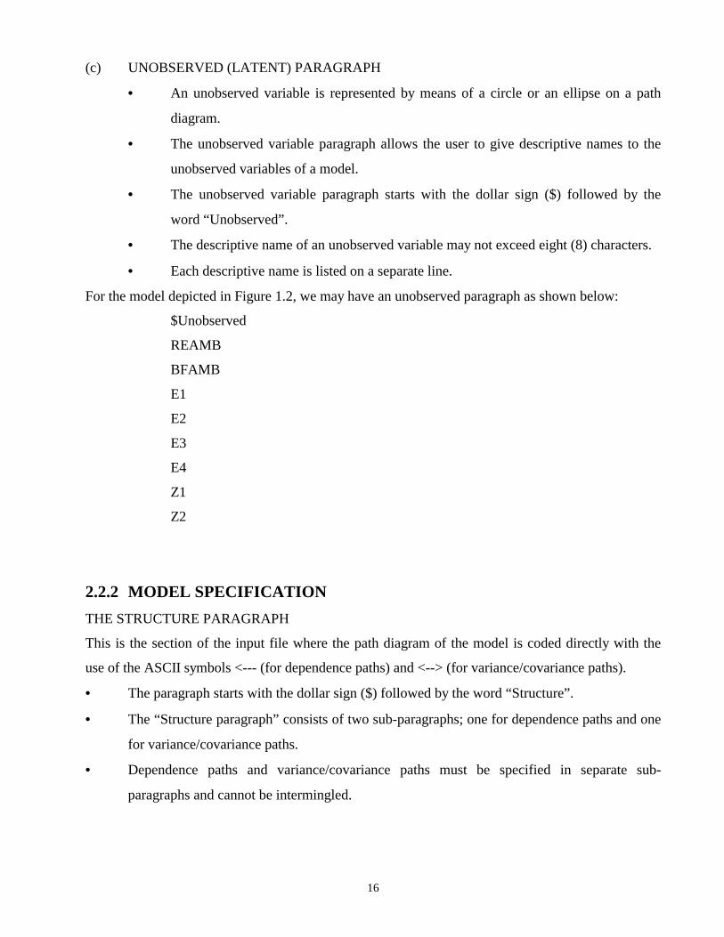
(c) UNOBSERVED (LATENT) PARAGRAPH

• An unobserved variable is represented by means of a circle or an ellipse on a path

diagram.

• The unobserved variable paragraph allows the user to give descriptive names to the

unobserved variables of a model.

• The unobserved variable paragraph starts with the dollar sign ($) followed by the

word “Unobserved”.

• The descriptive name of an unobserved variable may not exceed eight (8) characters.

• Each descriptive name is listed on a separate line.

For the model depicted in Figure 1.2, we may have an unobserved paragraph as shown below:

$Unobserved

REAMB

BFAMB

E1

E2

E3

E4

Z1

Z2

2.2.2 MODEL SPECIFICATION THE STRUCTURE PARAGRAPH

This is the section of the input file where the path diagram of the model is coded directly with the

use of the ASCII symbols <--- (for dependence paths) and <--> (for variance/covariance paths).

• The paragraph starts with the dollar sign ($) followed by the word “Structure”.

• The “Structure paragraph” consists of two sub-paragraphs; one for dependence paths and one

for variance/covariance paths.

• Dependence paths and variance/covariance paths must be specified in separate sub-

paragraphs and cannot be intermingled.

17

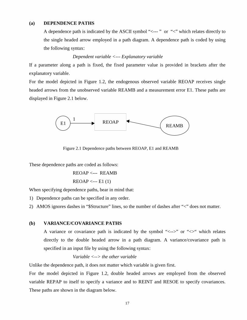
(a) DEPENDENCE PATHS

A dependence path is indicated by the ASCII symbol “<--- ” or “<” which relates directly to

the single headed arrow employed in a path diagram. A dependence path is coded by using

the following syntax:

Dependent variable <--- Explanatory variable

If a parameter along a path is fixed, the fixed parameter value is provided in brackets after the

explanatory variable.

For the model depicted in Figure 1.2, the endogenous observed variable REOAP receives single

headed arrows from the unobserved variable REAMB and a measurement error E1. These paths are

displayed in Figure 2.1 below.

Figure 2.1 Dependence paths between REOAP, E1 and REAMB

These dependence paths are coded as follows:

REOAP <--- REAMB

REOAP <--- E1 (1)

When specifying dependence paths, bear in mind that:

1) Dependence paths can be specified in any order.

2) AMOS ignores dashes in “$Structure” lines, so the number of dashes after “<” does not matter.

(b) VARIANCE/COVARIANCE PATHS

A variance or covariance path is indicated by the symbol “<-->” or “<>“ which relates

directly to the double headed arrow in a path diagram. A variance/covariance path is

specified in an input file by using the following syntax:

Variable <--> the other variable

Unlike the dependence path, it does not matter which variable is given first.

For the model depicted in Figure 1.2, double headed arrows are employed from the observed

variable REPAP to itself to specify a variance and to REINT and RESOE to specify covariances.

These paths are shown in the diagram below.

REOAPREAMBE1

1

18

Figure 2.2 Variance/covariance paths between REPAP, RESOE, and REINT

These paths are specified in the sentences below.

REPAP <--> REPAP

REPAP <--> REINT

REPAP <--> RESOE

REINT <--> REINT

REINT <--> RESOE

RESOE <--> RESOE

or REPAP <>REINT

REPAP <>RESOE

REINT <>REINT

REINT <>RESOE

RESOE <>RESOE

2.2.3 ESTIMATION METHOD(S) This is the section of the input file where the method or methods of estimation are specified. Each

method is specified on a separate line and must be preceded by the dollar sign “$”.

The estimation methods available in AMOS are:

$ml maximum likelihood estimation

$gls generalized least squares estimates

$adf asymptotic distribution-free estimation

$sls scale free least squares estimation

$uls unweighted least squares estimation

REPAP REINT RESOE

19

2.2.4 DATA The name of the AMOS data file is specified in this section. The data file is a text file with the

extension “.amd”. The file name is specified after the key word “Include=” preceded by the dollar

sign “$”. For the model depicted in Figure 1.2, the correlation matrix with standard deviations to be

analyzed resides in a file “pep-dhp.amd”. This is specified as:

$Include = pep-dhp.amd

2.2.5 GROUP NAME (Optional) When analyzing data by using more than one model, each model is treated as a group and then given

a group name. The command, “$groupname” is used to assign a name to a group as shown below.

$groupname= “name”

where “name” is the name given to a group.

By default, AMOS assigns the names ‘group number 1’, ‘group number 2’, and so on.

If this option is not included in the input file, AMOS assumes that there is only one model in the

analysis and will therefore assign the group name ‘group_number_1’. In the example depicted in

Figure 1.2, the group is not specified since only one model is being used in the analysis. AMOS

therefore gives the group name as “$groupname= Group_number_1”.

2.2.6 OUTPUT The input file ends with the keyword “Output” preceded by a dollar sign ($). The “$output”

command instructs AMOS to write selected output to an output file in a text format, that is suitable

for reading by other programs. The new output file is given the same name as the input file, but with

the extension “.amo” instead of “.ami”.

2.2.7 INPUT FILE: EXAMPLE 2 The complete AMOS input file for the model depicted in Figure 1.2 is shown below.

$Observed

REOAP

REEAP

BFEAP

BFOAP

REPAP

REINT

20

RESOE

BFSOE

BFINT

BFPAP

$Unobserved

REAMB

BFAMB

Z1

Z2

E2

E3

E4

E1

$Structure

REAMB <--- Z1 (1)

BFAMB <--- Z2 (1)

REOAP <--- REAMB (1)

BFEAP <--- BFAMB

BFOAP <--- BFAMB (1)

REEAP <--- REAMB

REAMB <--- REPAP

REAMB <--- REINT

REAMB <--- RESOE

BFAMB <--- BFSOE

BFAMB <--- RESOE

REAMB <--- BFSOE

BFAMB <--- BFINT

BFAMB <--- BFPAP

REAMB <--- BFAMB

BFAMB <--- REAMB

REEAP <--- E2 (1)

BFEAP <--- E3 (1)

BFOAP <--- E4 (1)

21

REOAP <--- E1 (1)

REINT <--> REPAP

RESOE <--> REPAP

BFSOE <--> REPAP

BFINT <--> REPAP

BFPAP <--> REPAP

RESOE <--> REINT

BFSOE <--> REINT

BFINT <--> REINT

BFPAP <--> REINT

BFSOE <--> RESOE

BFINT <--> RESOE

BFPAP <--> RESOE

BFINT <--> BFSOE

BFPAP <--> BFSOE

BFPAP <--> BFINT

REPAP<--> REPAP

REINT <--> REINT

RESOE <--> RESOE

BFSOE <--> BFSOE

BFINT <--> BFINT

BFPAP <--> BFPAP

$Include = C:\AMOS\PEPRAH\PEPDHP.amd

$Group name = Group_number_1

$Output

22

2.3 ILLUSTRATIVE EXAMPLE.

THE DUNCAN, HALLER AND PORTES’ APPLICATION.

2.3.1 CREATING THE AMOS DATA FILE FOR THE DUNCAN, HALLER

AND PORTES’ APPLICATION. The step by step methods of creating an AMOS data file for the Duncan, Haller and Portes’

application are outlined below.

• Double click on the “Notepad” icon shown below.

• This action will open the window below.

• Type in the Input data to produce the window below.

• Click on the “Save As” option from the Notepad “File” menu to load the dialog box shown

below.

23

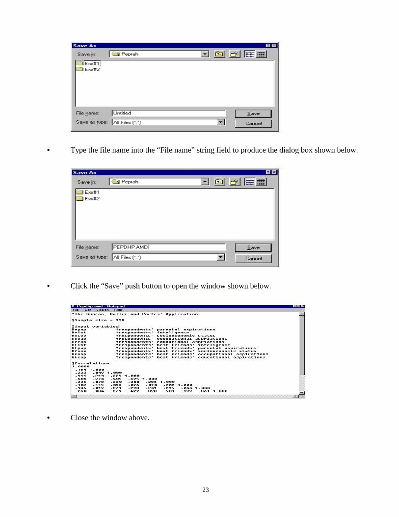
• Type the file name into the “File name” string field to produce the dialog box shown below.

• Click the “Save” push button to open the window shown below.

• Close the window above.

24

2.3.2 CREATING AN AMOS GRAPHIC FILE FOR THE MODEL OF THE

DUNCAN, HALLER AND PORTES’ APPLICATION. The model information may also be specified in the form of a path diagram. The path diagram is

drawn using the several intelligent drawing aids built into the program. In the model, depicted in

Figure 1.2, the Latent variables REAMB (Respondents Ambition) and BFAMB (Best Friends

Ambition) are modeled to influence one another. These paths are drawn as follows:

• Double click on the AMOS icon shown below.

The above action will open the “Unnamed project” window of AMOSGRAF, part of which is shown

below.

• Click on the push button

• Click inside the graphic field on the right hand side of the set of push buttons to draw an

ellipse (or circle) for a latent variable as shown below.

25

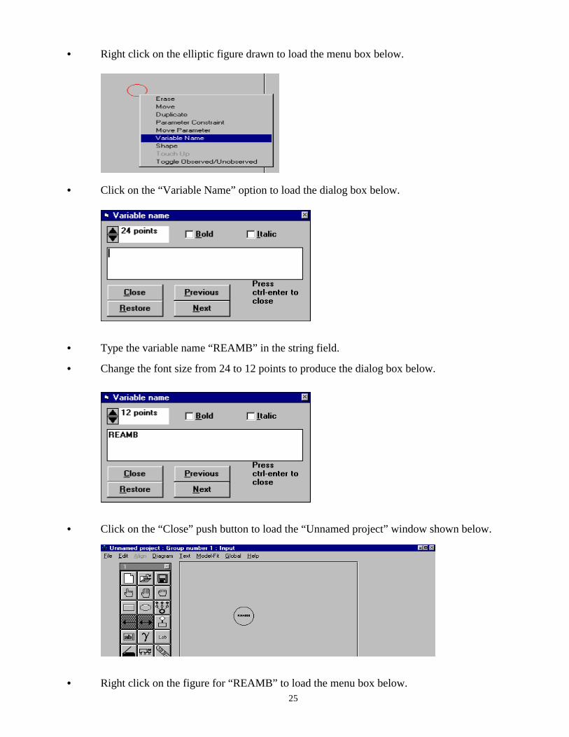
• Right click on the elliptic figure drawn to load the menu box below.

• Click on the “Variable Name” option to load the dialog box below.

• Type the variable name “REAMB” in the string field.

• Change the font size from 24 to 12 points to produce the dialog box below.

• Click on the “Close” push button to load the “Unnamed project” window shown below.

• Right click on the figure for “REAMB” to load the menu box below.

26

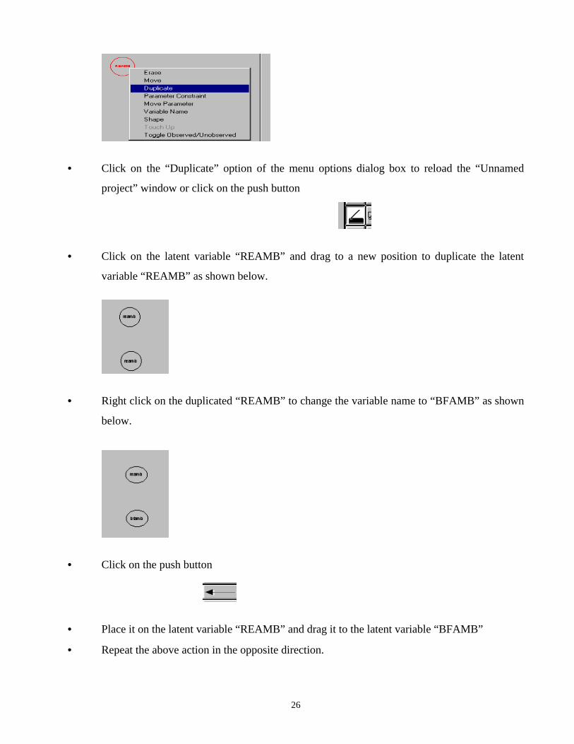
• Click on the “Duplicate” option of the menu options dialog box to reload the “Unnamed

project” window or click on the push button

• Click on the latent variable “REAMB” and drag to a new position to duplicate the latent

variable “REAMB” as shown below.

• Right click on the duplicated “REAMB” to change the variable name to “BFAMB” as shown

below.


• Place it on the latent variable “REAMB” and drag it to the latent variable “BFAMB”

• Repeat the above action in the opposite direction.

27

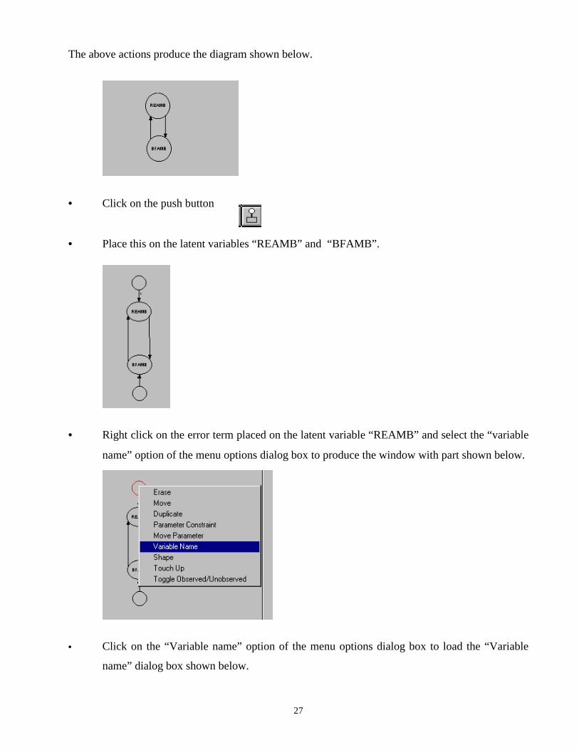
The above actions produce the diagram shown below.


• Place this on the latent variables “REAMB” and “BFAMB”.

• Right click on the error term placed on the latent variable “REAMB” and select the “variable

name” option of the menu options dialog box to produce the window with part shown below.

• Click on the “Variable name” option of the menu options dialog box to load the “Variable

name” dialog box shown below.

28

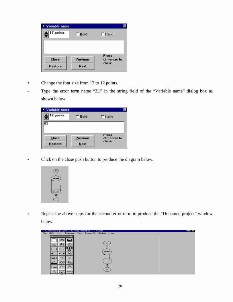
• Change the font size from 17 to 12 points.

• Type the error term name “Z1” in the string field of the “Variable name” dialog box as

shown below.

• Click on the close push button to produce the diagram below.

• Repeat the above steps for the second error term to produce the “Unnamed project” window

below.

29

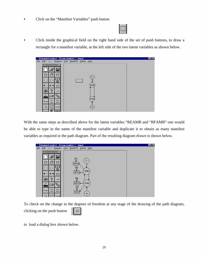
• Click on the “Manifest Variables” push button

• Click inside the graphical field on the right hand side of the set of push buttons, to draw a

rectangle for a manifest variable, at the left side of the two latent variables as shown below.

With the same steps as described above for the latent variables “REAMB and “BFAMB” one would

be able to type in the name of the manifest variable and duplicate it to obtain as many manifest

variables as required in the path diagram. Part of the resulting diagram drawn is shown below.

To check on the change in the degrees of freedom at any stage of the drawing of the path diagram,

clicking on the push button

to load a dialog box shown below.

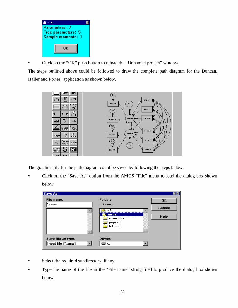
30

• Click on the “OK” push button to reload the “Unnamed project” window.

The steps outlined above could be followed to draw the complete path diagram for the Duncan,

Haller and Portes’ application as shown below.

The graphics file for the path diagram could be saved by following the steps below.

• Click on the “Save As” option from the AMOS “File” menu to load the dialog box shown

below.

• Select the required subdirectory, if any.

• Type the name of the file in the “File name” string filed to produce the dialog box shown

below.

31

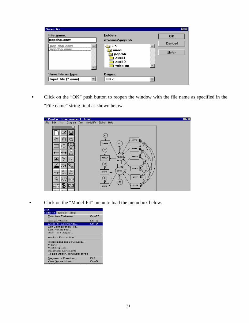
• Click on the “OK” push button to reopen the window with the file name as specified in the

“File name” string field as shown below.

• Click on the “Model-Fit” menu to load the menu box below.

32

• Click on the “Enter “$” Commands…” option of the “Model-Fit” menu to open the window

shown below.

• Double click on the “Include” option in the “Commands” list box to load the dialog box

below.

• Type the “Data” file’s name in the string filed of the dialog box to produce the dialog box

below.

• Click on the “OK” push button to produce the window shown below.

33

• Click on the close button to close the window above.


• Click on the “View Spreadsheet…” option of the “Model-Fit” menu to open the “View

Spreadsheet” dialog box shown below.

• Check the entries in the spreadsheet to see if all the paths in the path diagram have been

correctly specified.

• Click on the close button to close the “View Spreadsheet” dialog box above.

34

2.3.3 RUNNING AMOS To run AMOS:


• Click on the “Calculate Estimates” option of the “Model-Fit” menu to run the program.

• If there are no syntax errors, the program will run and the appearance of the window below

indicates the end of the iterations.

35

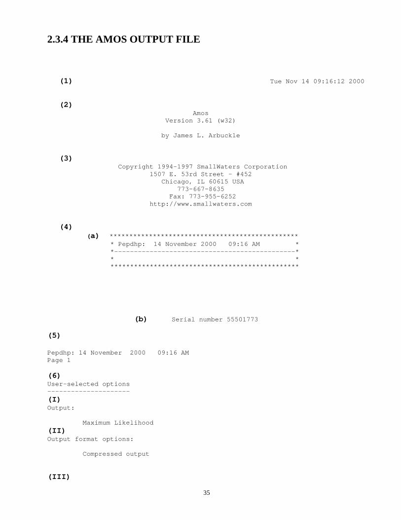
2.3.4 THE AMOS OUTPUT FILE

(1) Tue Nov 14 09:16:12 2000 (2) Amos Version 3.61 (w32) by James L. Arbuckle (3) Copyright 1994-1997 SmallWaters Corporation 1507 E. 53rd Street - #452 Chicago, IL 60615 USA 773-667-8635 Fax: 773-955-6252 http://www.smallwaters.com (4) (a) ************************************************ * Pepdhp: 14 November 2000 09:16 AM * *----------------------------------------------* * * ************************************************ (b) Serial number 55501773 (5) Pepdhp: 14 November 2000 09:16 AM Page 1 (6) User-selected options --------------------- (I) Output: Maximum Likelihood (II) Output format options: Compressed output (III)

36

Minimization options: Technical output Standardized estimates Squared multiple correlations Machine-readable output file (IV) Sample size: 329 (7) Your model contains the following variables REOAP observed endogenous BFEAP observed endogenous BFOAP observed endogenous REEAP observed endogenous REPAP observed exogenous REINT observed exogenous RESOE observed exogenous BFSOE observed exogenous BFINT observed exogenous BFPAP observed exogenous REAMB unobserved endogenous BFAMB unobserved endogenous Z1 unobserved exogenous Z2 unobserved exogenous E2 unobserved exogenous E3 unobserved exogenous E4 unobserved exogenous E1 unobserved exogenous (8) (I) Number of variables in your model: 18 (II) Number of observed variables: 10 (III) Number of unobserved variables: 8 (IV) Number of exogenous variables: 12 (V) Number of endogenous variables: 6 (9) (I) (II) (III) (IV) (V) (VI) Weights Covariances Variances Means Intercepts Total ------- ----------- --------- ----- ---------- ----- (I) Fixed: 8 0 0 0 0 8 (II) Labeled: 0 0 0 0 0 0 (III)Unlabeled: 12 15 12 0 0 39 ------- ----------- --------- ----- ---------- ----- (IV) Total: 20 15 12 0 0 47 The model is nonrecursive. Model: Your_model

37

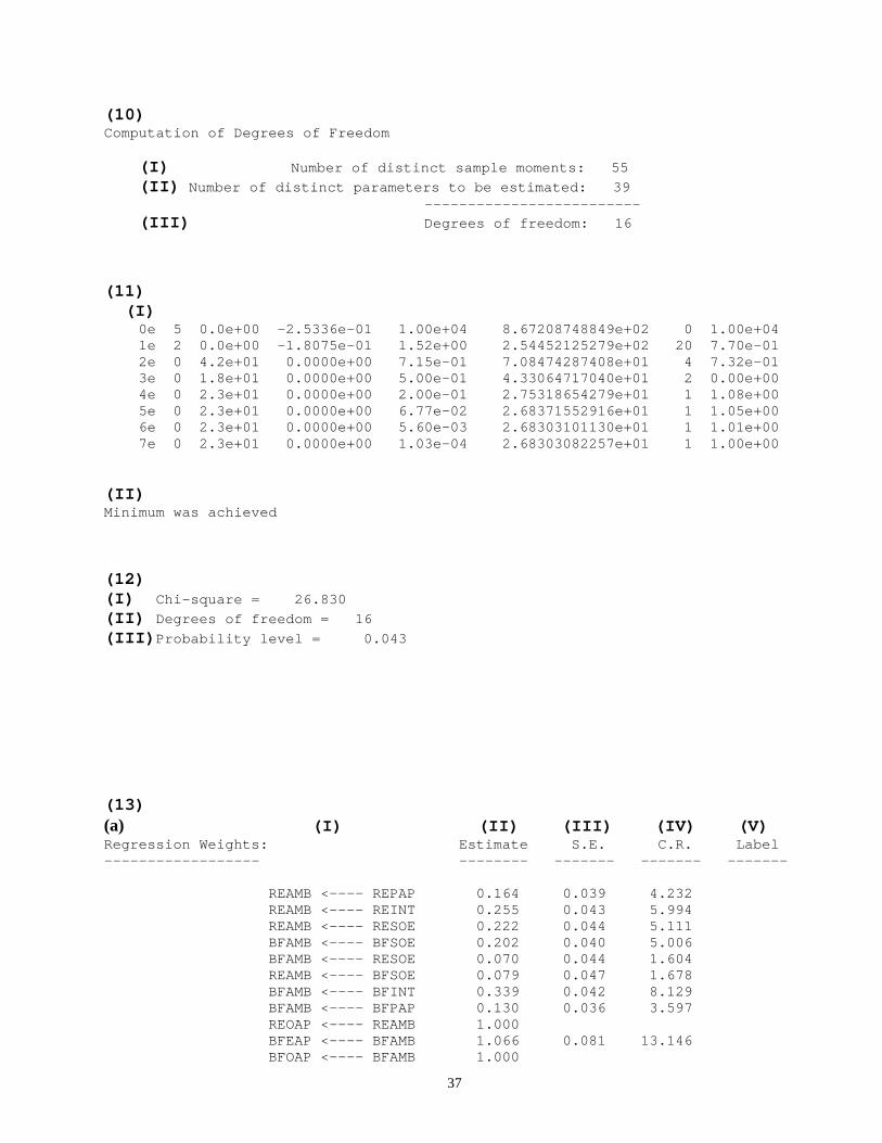
(10) Computation of Degrees of Freedom (I) Number of distinct sample moments: 55 (II) Number of distinct parameters to be estimated: 39 ------------------------- (III) Degrees of freedom: 16 (11) (I) 0e 5 0.0e+00 -2.5336e-01 1.00e+04 8.67208748849e+02 0 1.00e+04 1e 2 0.0e+00 -1.8075e-01 1.52e+00 2.54452125279e+02 20 7.70e-01 2e 0 4.2e+01 0.0000e+00 7.15e-01 7.08474287408e+01 4 7.32e-01 3e 0 1.8e+01 0.0000e+00 5.00e-01 4.33064717040e+01 2 0.00e+00 4e 0 2.3e+01 0.0000e+00 2.00e-01 2.75318654279e+01 1 1.08e+00 5e 0 2.3e+01 0.0000e+00 6.77e-02 2.68371552916e+01 1 1.05e+00 6e 0 2.3e+01 0.0000e+00 5.60e-03 2.68303101130e+01 1 1.01e+00 7e 0 2.3e+01 0.0000e+00 1.03e-04 2.68303082257e+01 1 1.00e+00 (II) Minimum was achieved (12) (I) Chi-square = 26.830

(II) Degrees of freedom = 16 (III)Probability level = 0.043 (13) (a) (I) (II) (III) (IV) (V) Regression Weights: Estimate S.E. C.R. Label ------------------ -------- ------- ------- ------- REAMB <---- REPAP 0.164 0.039 4.232 REAMB <---- REINT 0.255 0.043 5.994 REAMB <---- RESOE 0.222 0.044 5.111 BFAMB <---- BFSOE 0.202 0.040 5.006 BFAMB <---- RESOE 0.070 0.044 1.604 REAMB <---- BFSOE 0.079 0.047 1.678 BFAMB <---- BFINT 0.339 0.042 8.129 BFAMB <---- BFPAP 0.130 0.036 3.597 REOAP <---- REAMB 1.000 BFEAP <---- BFAMB 1.066 0.081 13.146 BFOAP <---- BFAMB 1.000

38

REEAP <---- REAMB 1.060 0.090 11.819 REAMB <---- BFAMB 0.173 0.087 1.987 BFAMB <---- REAMB 0.190 0.081 2.352 (b) Standardized Regression Weights: Estimate -------------------------------- -------- (I) (II) REAMB <---- REPAP 0.214 REAMB <---- REINT 0.333 REAMB <---- RESOE 0.290 BFAMB <---- BFSOE 0.282 BFAMB <---- RESOE 0.088 REAMB <---- BFSOE 0.104 BFAMB <---- BFINT 0.438 BFAMB <---- BFPAP 0.196 REOAP <---- REAMB 0.767 BFEAP <---- BFAMB 0.825 BFOAP <---- BFAMB 0.774 REEAP <---- REAMB 0.813 REAMB <---- BFAMB 0.174 BFAMB <---- REAMB 0.184

(c) (I) (II) (III) (IV) (V) Covariances: Estimate S.E. C.R. Label ------------ -------- ------- ------- ------- REPAP <---> REINT 0.184 0.056 3.277 REPAP <---> RESOE 0.049 0.055 0.886 REPAP <---> BFSOE 0.019 0.055 0.344 REPAP <---> BFINT 0.336 0.058 5.768 REPAP <---> BFPAP 0.102 0.056 1.838 REINT <---> RESOE 0.049 0.055 0.886 REINT <---> BFSOE 0.019 0.055 0.344 REINT <---> BFINT 0.078 0.055 1.408 REINT <---> BFPAP 0.115 0.056 2.069 RESOE <---> BFSOE 0.271 0.057 4.737 RESOE <---> BFINT 0.230 0.057 4.059 RESOE <---> BFPAP 0.093 0.055 1.677 BFSOE <---> BFINT 0.295 0.058 5.124 BFSOE <---> BFPAP 0.044 0.055 0.796 BFINT <---> BFPAP 0.209 0.056 3.705 (d) Correlations: Estimate ------------- -------- (I) (II) REPAP <---> REINT 0.184 REPAP <---> RESOE 0.049 REPAP <---> BFSOE 0.019 REPAP <---> BFINT 0.078 REPAP <---> BFPAP 0.115 REINT <---> RESOE 0.222 REINT <---> BFSOE 0.186 REINT <---> BFINT 0.336 REINT <---> BFPAP 0.102 RESOE <---> BFSOE 0.271 RESOE <---> BFINT 0.230 RESOE <---> BFPAP 0.093

39

BFSOE <---> BFINT 0.295 BFSOE <---> BFPAP 0.044 BFINT <---> BFPAP 0.209

(e) (I) (II) (III) (IV) (V) Variances: Estimate S.E. C.R. Label ---------- -------- ------- ------- ------- REPAP 1.000 0.078 12.806 REINT 1.000 0.078 12.806 RESOE 1.000 0.078 12.806 BFSOE 1.000 0.078 12.806 BFINT 1.000 0.078 12.806 BFPAP 1.000 0.078 12.806 Z1 0.282 0.047 6.018 Z2 0.234 0.040 5.883 E2 0.338 0.052 6.528 E3 0.318 0.046 6.892 E4 0.400 0.046 8.628 E1 0.411 0.051 8.052 (f) Squared Multiple Correlations: Estimate ------------------------------ -------- (I) (II) BFAMB 0.609 REAMB 0.521 REEAP 0.662 BFOAP 0.599 BFEAP 0.681 REOAP 0.589 (g) Stability index for the following variables is 0.033 BFAMB REAMB

(14) (a) (I) (II) (III) (IV) (V) (VI) Model NPAR CMIN DF P CMIN/DF ---------------- ---- --------- -- --------- --------- Your_model 39 26.830 16 0.043 1.677 Saturated model 55 0.000 0 Independence model 10 862.753 45 0.000 19.172

40

(b) (I) (II) (III) (IV) (V) Model RMR GFI AGFI PGFI ---------------- ---------- ---------- ---------- ---------- Your_model 0.021 0.984 0.946 0.350 Saturated model 0.000 1.000 Independence model 0.276 0.544 0.443 0.445

(c) (I) (II) (III) (IV) (V) (VI) DELTA1 RHO1 DELTA2 RHO2 Model NFI RFI IFI TLI CFI ---------------- ---------- ---------- ---------- ---------- ---------- Your_model 0.969 0.913 0.987 0.963 0.987 Saturated model 1.000 1.000 1.000 Independence model 0.000 0.000 0.000 0.000 0.000

(d) (I) (II) (III) (IV) Model PRATIO PNFI PCFI ---------------- ---------- ---------- ---------- Your_model 0.356 0.344 0.351 Saturated model 0.000 0.000 0.000 Independence model 1.000 0.000 0.000 (e) (I) (II) (III) (IV) Model NCP LO 90 HI 90 ---------------- ---------- ---------- ---------- Your_model 10.830 0.326 29.183 Saturated model 0.000 0.000 0.000 Independence model 817.753 726.062 916.858 (f) (I) (II) (III) (IV) (V) Model FMIN F0 LO 90 HI 90 ---------------- ---------- ---------- ---------- ---------- Your_model 0.082 0.033 0.001 0.089 Saturated model 0.000 0.000 0.000 0.000 Independence model 2.630 2.493 2.214 2.795 (g) (I) (II) (III) (IV) (V)

41

Model RMSEA LO 90 HI 90 PCLOSE ---------------- ---------- ---------- ---------- ---------- Your_model 0.045 0.008 0.075 0.563 Independence model 0.235 0.222 0.249 0.000 (h) (I) (II) (III) (IV) (V) Model AIC BCC BIC CAIC ---------------- ---------- ---------- ---------- ---------- Your_model 104.830 107.537 342.677 291.877 Saturated model 110.000 113.817 445.425 373.783 Independence model 882.753 883.447 943.739 930.713 (i) (I) (II) (III) (IV) (V) Model ECVI LO 90 HI 90 MECVI ---------------- ---------- ---------- ---------- ---------- Your_model 0.320 0.288 0.376 0.328 Saturated model 0.335 0.335 0.335 0.347 Independence model 2.691 2.412 2.993 2.693 (j)

(I) (II) (III) HOELTER HOELTER Model .05 .01 ---------------- ---------- ---------- Your_model 322 392 Independence model 24 27 (15) Execution time summary: (I) Minimization: 0.520 (II) Miscellaneous: 0.752 (III) Bootstrap: 0.000 (IV) Total: 1.272

ENTRIES OF THE AMOS OUTPUT FILE

1. Date and time of the analysis.

2. The name, the version and the author of AMOS.

3. Information about the company with the right to distribute AMOS.

4. (a) Name of the input file used in the analysis and the date, day and time of the analysis.

(b) Serial number of the particular installation of AMOS.

5. Same as 4(a).

42

6. User-selected options

(I) The method of estimation used.

(II) The format in which the output file is to be provided.

(III) Minimization options

(IV) Size of the sample used in the analysis.

7. The list of descriptive names of all the variables of the model fitted to the data.

8. (I) The total number of variables of the model.

(II) The number of observed variables of the model.

(III) The number of unobserved variables of the model.

(IV) The number of exogenous variables of the model.

(V) The number of endogenous variables of the model.

9. Column (I): number of weights or parameters.

Column (II): number of covariances in the model.

Column (III): number of variances in the model

Column (IV): number of means provided in the data for the analysis.

Column (V): number of intercepts specified in the data for the analysis.

Column (VI): the total for each row.

Row(I): the number of the fixed parameters in the model.

Row(II): the number of parameters of the model that are labeled.

Row(III): the number of parameters of the model are neither fixed nor labeled. These

parameters are free to take on any value.

Row(IV): the total of each column.

10. Computation of Degrees of Freedom

Row(I): the number of distinct sample moments ( sample variances and nonduplicated

covariances), usually denoted by p.

Row(II): the number of distinct parameters to be estimated in the model, usually

denoted by q.

Row(III): degrees of freedom is given by d = p – q

43

11. (I) Minimization history.

The details of the progress of the minimization of the discrepancy function.

(II) Minimum was achieved. This sentence indicates that the minimization process was

without any disruptions.

12. (I) The value of the Chi-square test Statistic.

This is given by (Steiger, Shapiro and Browne, 1985)

∃ ∃C nF=

where ∃ ( , )C aα−

is the minimum value of the discrepancy functions (Browne, 1982,

1984) of the form:

( ) [ ] ( )C a N r F aα α, ,− −= − ,

where ( )F aN f x S

N

g

g

Gg g g

αµ

,, ; ,( ) ( ) ( ) ( )

−

= −

∧

=

∑ ∑1 , and

r is a nonnegative integer specified by the “$chicorrect” command.

f(.) denotes the discrepancy function which measures the discrepancy between the

model and the sample moments,

n= N-r,

N N g

g

G

==∑ ( )

1

, the total number of observations in all groups combined,

α γ( ) is the vector of order p containing the population moments for all groups

according to the model,

−a is the vector of order p containing the sample moments for all groups,

∃γ is the value of γ that minimizes ( )F aα γ( );−

,

N g( ) is the number of observations in group g,

G is the number of groups,

µ γ( ) ( )g is the mean vector for group g, according to the model,

44

( ) ( )g γ∑ is the covariance matrix for group g, according to the model,

( )gS is the sample covariance matrix for group g,

xN

xg

gir

g

r

Ng( ) ( ) ,=

=∑1

1

xirg( ) is the r-th observation on the i-th variable in group g.

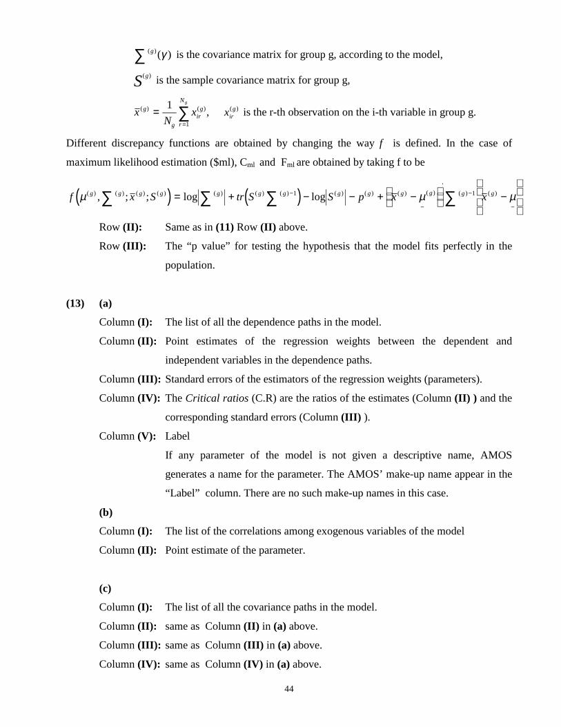
Different discrepancy functions are obtained by changing the way f is defined. In the case of

maximum likelihood estimation ($ml), Cml and Fml are obtained by taking f to be

( ) ( )f x S tr S S p x xg g g g g g g g g g g g gµ µ µ( ) ( ) ( ) ( ) ( ) ( ) ( ) ( ) ( ) ( ) ( )'

( ) ( ), ; ; log log∑ ∑ ∑ ∑= + − − + −

−

−

−

−

−

1 1

Row (II): Same as in (11) Row (II) above.

Row (III): The “p value” for testing the hypothesis that the model fits perfectly in the

population.

(13) (a)

Column (I): The list of all the dependence paths in the model.

Column (II): Point estimates of the regression weights between the dependent and

independent variables in the dependence paths.

Column (III): Standard errors of the estimators of the regression weights (parameters).

Column (IV): The Critical ratios (C.R) are the ratios of the estimates (Column (II) ) and the

corresponding standard errors (Column (III) ).

Column (V): Label

If any parameter of the model is not given a descriptive name, AMOS

generates a name for the parameter. The AMOS’ make-up name appear in the

“Label” column. There are no such make-up names in this case.

(b)

Column (I): The list of the correlations among exogenous variables of the model

Column (II): Point estimate of the parameter.

(c)

Column (I): The list of all the covariance paths in the model.

Column (II): same as Column (II) in (a) above.

Column (III): same as Column (III) in (a) above.

Column (IV): same as Column (IV) in (a) above.

45

Column (V): same as Column (V) in (a) above.

(d)

Column (I): same as Column (I) in (c) above.

Column (II): same as Column (II) in (c) above.

(e)

Column (I): The list of all variance paths in the model

Column (II): same as Column (II) in (a) above.

Column (III): same as Column (III) in (a) above.

Column (IV): same as Column (IV) in (a) above.

Column (V): same as Column (V) in (a) above.

(f)

Column (I): The list of the endogenous variables of the model

Column (II): Point estimate of the squared multiple correlation between each endogenous

variable and the variables (other than residual variables) that directly affect it.

(g)

The stability index for the unobserved variables BFAMB and REAMB. This is computed from:

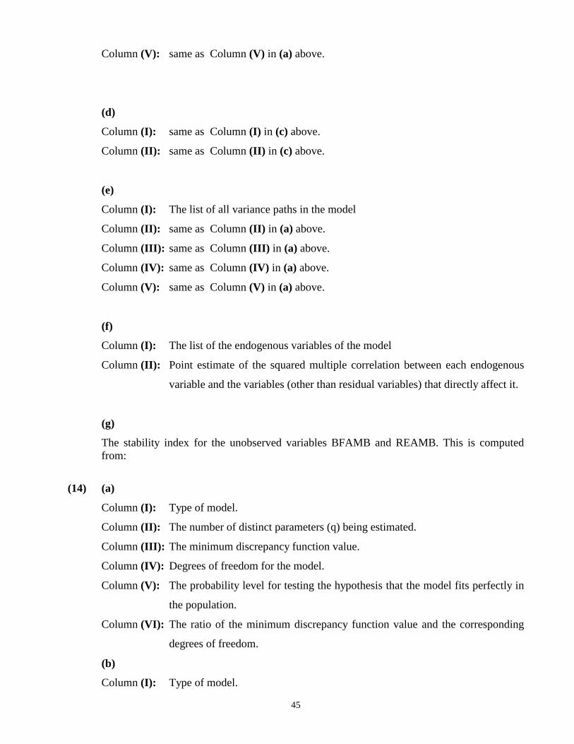
(14) (a)

Column (I): Type of model.

Column (II): The number of distinct parameters (q) being estimated.

Column (III): The minimum discrepancy function value.

Column (IV): Degrees of freedom for the model.

Column (V): The probability level for testing the hypothesis that the model fits perfectly in

the population.

Column (VI): The ratio of the minimum discrepancy function value and the corresponding

degrees of freedom.

(b)


46

Column (I): The square root of the average squared amount by which sample variances

and covariances differ from their estimates obtained under the assumption that

the model used in the analysis is correct. It is computed from:

( )RMR S pijg g

j

jsi

i

Pg

g

G

g

G g

= −

== ==

∑∑ ∑∑ ∃ ./( ) ( ) *( )σ11 11

where ( )σ γ γ( ) ( )( ) ( )g gvec= ∑

p g*( ) is the number of sample moments in group g.

Column (III): The goodness of fit index (GFI) is given by ( Jöreskog and Sörbom, 1984;

Tanaka and Huba, 1985)

GFI FFb

= −1∃∃

where ∃Fb is obtained by evaluating F with ( )g∑ = 0 , g=1, 2, …, G.

An exception has to be made for maximum likelihood estimation, since f(.) is

not defined for ( )g∑ = 0 . For the purpose of computing GFI in the case of

maximum likelihood estimation, f g gS( ) ( );∑

is computed as

f g gS( ) ( );∑

= ( )[ ]12

1 2tr g g gK S( ) ( ) ( )− −∑

with ( )( ) ( ) ∃g gMLK = ∑ γ ,

where ∃γ is the maximum likelihood estimate of γ .

Column (IV): The adjusted goodness of fit index (AGFI) is given by:

AGFI GFI dd

b= − −1 1( )

where d pbg

g

G

==∑ *( )

1

Column (V): The PGFI, parsimony of fit index; is given by (Mulaik, et. al, 1989):

PGFI = GFI ddb

.

(c)

47

Column (I): Type of model

Column (II): The normed fit index (NFI) or delta1,∆1 , is obtained from (Bentler and

Bonett, 1980):

NFI = ∆1 = 1− =∃∃

∃∃

CC

FFb b

where ∃ ∃C nFb b= is the minimum discrepancy function value for the baseline

model.

Column (III): The relative fit index (RFI) or rho1, ρ1 , is obtained from (Bollen, 1989):

RFI = ρ1 = 1 1− = −∃ /∃ /

∃ /∃ /

C dC d

F dF db b b b

.

Column (IV): The incremental fit index (IFI) or delta2, ∆2 , is obtained from (Bollen, 1989):

IFI = ∆2 = ∃ ∃∃

C CC d

b

b

−−

.

Column (V): The Tucker-Lewis coefficient of rho2, ρ2 , also known as Bentler and Bonett

non-normed fit index (NNFI) is given by (Bentler and Bonett, 1980):

TLI = ρ2 = 1 00

− −−

=max( ∃ , )

max( ∃ , )C d

C dNCPNCPd b d

.

where NCP is the noncentrality parameter estimate for the model being

evaluated and NCPd is the noncentrality parameter estimate for the baseline

model.

(d)


Column (II): The parsimony ratio (PRATIO) is given by (James, Mulaik and Brett, 1982,

Mulaik, et. al, 1989):

PRATIO = ddi

.

where di is the degrees of freedom of the independence model.

Column (III): The PNIF is the result of applying James, et. al.’s 1982, parsimony to the NFI.

It is obtained from:

PNFI = (NFI)(PRATIO) = NFI ddb

.

48

Column (IV): The PCFI is the result of applying James, et al.’s (1982) parsimony adjustment

to the CFI. It is obtained from:

PCFI = (CFI)(PRATIO) = CFI ddb

.

(e)


Column (II): NCP = max( ∃ , )C d− 0 is an estimate of the noncentrality parameter,

δ = =C nFo o .

where Fo is the value of the discrepancy function obtained by fitting a model

to the population moments rather than to sample moments. Fo is given by:

Fo = min[ ( ( ), )γ

α γ αF o .

Column (III): LO90 is the lower limit δ L of a 90% confidence interval, on δ and is

obtained by solving the equation:

( )Φ ∃ / ,C dδ = 0.95

for δ where ( )Φ x d/ ,δ is the distribution function of the noncentral chi-

squared distribution with noncentrality parameter δ and d degrees of

freedom.

Column (IV): HI90 is the upper limit δU of a 90% confidence interval, on δ and is obtained

by solving the equation:

( )Φ ∃ / ,C dδ = 0.05 for δ .

(f)


Column (II): this is the minimum value, ∃F , of the discrepancy function F.

Column (III): LO90 is the lower limit,δ L , of a 90% confidence interval on Fo. It is given by:

LO90 = δ L

n.

Column (IV): HI90 is the upper limit value,δU , of a 90% confidence interval on Fo. It is

given by:

HI90 = δU

n.

49

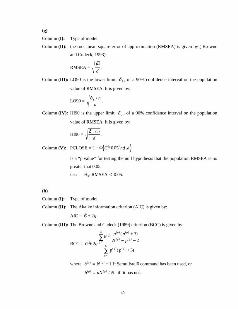
(g)


Column (II): the root mean square error of approximation (RMSEA) is given by ( Browne

and Cudeck, 1993):

RMSEA = ∃Fd

o .

Column (III): LO90 is the lower limit, δ L , of a 90% confidence interval on the population

value of RMSEA. It is given by:

LO90 = δ L nd/ .

Column (IV): HI90 is the upper limit, δU , of a 90% confidence interval on the population

value of RMSEA. It is given by:

HI90 = δU nd/ .

Column (V): PCLOSE = ( )1 0 052− Φ ∃ / . ,C nd d

Is a “p value” for testing the null hypothesis that the population RMSEA is no

greater that 0.05.

i.e.: Ho: RMSEA ≤ 0.05.

(h)


Column (II): The Akaike information criterion (AIC) is given by:

AIC = ∃C q+ 2 .

Column (III): The Browne and Cudeck (1989) criterion (BCC) is given by:

BCC = ∃

( )

( )

( )( ) ( )

( ) ( )

( ) ( )C q

b p pN p

p p

gg g

g gg

G

g g

g

G+

+− −

+

=

=

∑

∑2

32

3

1

1

where b Ng g( ) ( )= −1 if $emulisrel6 command has been used, or

b nN Ng g( ) ( ) /= if it has not.

50

Column (IV): The Bayes information criterion (Schwarz 1978; Raftery, 1993) is given by

the formula:

BIC = ∃ ( )( ) ( )C qLn N p+ 1 1 . Note that g=1 in this case.

Column (IV): Bozdogan’s (1987) CAIC (consistent AIC) is given by the formula

CAIC = ∃ ( )( )C q LnN+ +1 1 .

(i)


Column (II): The expected cross-validation index (ECVI) is given by the formula:

ECVI = 1 2n

AIC F qn

( ) ∃= + .

Column (III): LO90 is the lower limit, δ L , of 90% confidence interval on the population

ECVI. It is computed from:

LO90 = δ L d qn

+ + 2 .

Column (IV): HI90 is the upper limit, δU , of 90% confidence interval on the population

ECVI. It is computed from:

HI90 = δU d qn+ +2 .

Column (V): The modified expected cross-validation index (MECVI) is given by the

formula:

MECVI = 1n

BCC( ) = ∃

( )

( )

( )( ) ( )

( ) ( )

( ) ( )C q

a p pN p

p p

gg g

g gg

G

g g

g

G+

+− −

+

=

=

∑

∑2

32

3

1

1

.

where a N N Gg g( ) ( )( ) / (= − −1 if the $emulisrel6 command has been used,

or a N Ng g( ) ( ) /= if it has not.

(j)

51


Column (II): Hoelter’s (1983) “critical N” is the largest sample size for which one would

accept the hypothesis that a model is correct at 0.05 level of significance.

Column (III): Hoelter’s (1983) “critical N” is the largest sample size for which one would

accept the hypothesis that a model is correct at 0.01 level of significance.

(15) Row (I): The time for AMOS’s minimization algorithm.

Row (II): The time used for anything not falling into another category, but consisting

mostly of input parsing and output formatting.

Row (III): The time used to for bootstrap algorithm.

Row (IV): The sum of the times in Row (I) to Row (III).

52

CHAPTER 3

EQS 3.1 HISTORICAL BACKGROUND Peter Bentler developed the first commercial version of the Structural Equation Modeling program

EQS (which can be pronounced like the letter “X”) in 1985. The acronym EQS stands for

EQuationS. EQS implements the Bentler and Weeks model (Bentler & Weeks, 1979, 1980, 1982,

1985; Bentler, 1983a,b). The first commercial release of EQS was through BMDP. Bentler

developed an updated version in 1989. The latest version of EQS (Bentler, 1995) is available for

Windows. An Apple Macintosh version of EQS is also available.

The computer program EQS was developed to meet two major needs in statistical software. At the

theoretical level, applied multivariate analysis based on methods that are more general than those

stemming from multinormal theory have not been available to statisticians and researchers for

routine use. At the applied level, powerful and general methods have also required extensive

knowledge of matrix algebra and related topics that are often not routinely available among

researchers. EQS is meant to make advanced multivariable analysis methods accessible to the

applied statistician and practicing data analyst. EQS is intended for users who are familiar with the

basic concepts of structural equation modeling.

3.2 THE EQS INPUT FILE

To run EQS, the user must prepare an EQS Input File. An EQS Input File is a text file that consists

of several paragraphs. This file may be created by typing it manually in a text editor such as

Notepad, Wordpad or by using the “Model Specifications” dialog box of EQS.

GENERAL RULES FOR TYPING EQS INPUT FILES

• A slash, followed by a capitalized keyword, begin each section.

• V1, V2, etc are used for manifest variables whereas F1, F2, etc are used for latent variables.

• /END appears at the end of each input file.

53

• In the /EQUATIONS paragraph of the input file, there is one equation for each dependent

variable in the model. A dependent variable is one that is a structured regression function of

other variables and it is recognised in the path diagram by having one or more arrows aiming

at it.

• For each parameter within an equation, an asterisk or star “*” after a numerical value

specifies that the parameter is to be estimated, with the number to the left of the asterisks as a

starting value. If no number is given next to the “*”, the program will insert the starting

value. Numerical values not followed by asterisks specify that the parameter is to be fixed to

the numerical value.

• Every independent variable in the model must have a variance.

• The fixed constant V999, which is used in the structured means models, does not have a

variance.

• When the raw data matrix is used as the input data matrix, it could be provided in another

file.

• When a covariance or correlation matrix is used as the input data matrix, it should be part of

the input file or it could be provided in another file.

An EQS Input File may be divided into three sections. These are:

1. Model and Data Information,

2. Model Specification and

3. Data

3.2.1 MODEL AND DATA INFORMATION

Model information is specified in three paragraphs, namely the TITLE, SPECIFICATIONS and

LABELS paragraphs.

Details of each paragraph are discussed below.

(a) TITLE Paragraph

This paragraph provides a description for the analysis to be performed. It starts with /TITLE. For the

model, depicted in Figure 1.2, we may have a title paragraph as follows:

54

/TITLE

Duncan, Haller and Portes (1971) Path Analysis Model for Data on Peer Influence on

Ambition;

(b) SPECIFICATIONS Paragraph

This paragraph starts with the keyword “/SPECIFICATIONS”. It describes the problem to be

analyzed, including the number of cases (observations), the number of variables and the type of

input data matrix, the method(s) of estimation desired, input datafile’s name, cases to be deleted, etc

as explained below.

The syntax for the SPECIFICATIONS paragraph is given by:

VARIABLES = p;

where p denotes the number of manifest variables in the model.

CASES = n;

where n denotes the number of observations, cases or objects under study.

MATRIX= Any of the following options:

COV (Covariance matrix input)

COR (Correlation matrix input)

RAW (Raw data input)

If the sample covariance or correlation matrix is to be analyzed, it may be included in the input file

after the Model information and the Model specification, or created separately as an EQS system file

and then saved with extension “.ess”. If the input covariance or correlation matrix is provided in a

separate file, the name of the file must be specified as part of the “Specifications” paragraph. As a

default, EQS uses a “free-field” input format, which requires that elements of the matrix be

separated by at least one blank space. It is assumed that no extraneous information, such labels,

missing data codes etc. exists. Typically, when a correlation matrix is input, standard deviations

must also be provided. When a raw data matrix is to be analyzed, a separate text file, that contains

the data matrix, should be prepared. The rows and columns refer to the cases and variables,

respectively of the data. The raw data matrix can be created in EQS or imported from other files

such as MICROSOFT EXCEL files and then saved as EQS system file with the extension “.ess”. For

an external data file, the file name may be specified as follows:

DA= filename

where “filename” is the name of the file containing the raw data matrix, covariance or correlation

55

matrix. MATRIX = COV is the default in this paragraph. This means that if the input data matrix is

not a covariance matrix, it must be specified else the program will take it to be a covariance matrix

in the analysis.

METHOD = method;

where method is one of:

Least squares, abbreviated LS,

Generalized least squares, abbreviated GLS,

Maximum likelihood, abbreviated ML,

Elliptical least squares, abbreviated ELS,

Elliptical generalized least squares, abbreviated EGLS,

Elliptical reweighted least squares, abbreviated ERLS,

Arbitrary distribution generalized least squares, abbreviated AGLS, (requires MATRIX = RAW),

and

Robust statistics, xx (any method except AGLS), abbreviated xx, ROBUST.

ML is the default method.

For the model, depicted in Figure 1.2, we may have a /SPECIFICATIONS paragraph as follows:

/SPECIFICATIONS

METHOD = ML; CASES=329; VARIABLES=10; MATRIX= COR;

(c) LABELS paragraph

This paragraph allows the user to provide descriptive names for the variables in the model. Each

variable is given a descriptive name of at most eight characters. For the model, depicted in Figure

1.2, we may have a /LABELS paragraph as follows:

/LABELS

V1= REINT; V2= REPAP; V3=RESOE; V4=REOAP; V5=REEAP; V6=BFINT; V7=BFPAP;

V8= BFSOE; V9= BFOAP; V10 = BFEAP; FI= REAMB; F2=BFAMB;

56

3.2.2 MODEL SPECIFICATION WITH EQS.

Using several EQS paragraphs, many of which are not required for simple models, specifies the

model. Brief descriptions of some of the sections are given below. Those sections, that are not

always needed, are indicated as optional.

/EQUATIONS

This section contains the structural equations involved in the model under consideration. The

/EQUATIONS section also provides information for the automatic selection of variables from the

input matrix. For the model, depicted in Figure 1.2, the endogenous manifest variable V4 (REOAP)

receives single headed arrows from the latent variable F1 (REAMB) and a measuring error E4

respectively. These paths are displayed in Figure 3.1 below.

1.0

Figure 3.1 Regression path between V4 and F1.

These regression path above is written in an equation form as

V4 = +*F1 + E4;

where "+*" indicates that the coefficient of F1 is to be estimated with a starting value to be provided

by EQS. The “+” in front of E4, without “*” indicates that the coefficient of E4 is fixed, in this case,

to “1”.

/VARIANCES

The variances of the independent variables are specified in this section.

For the model depicted in Figure 1.2, double headed arrows are employed from the manifest variable

V2 (REPAP) to itself to specify a variance and to V3 (RESOE), and V1 (REINT), to specify

covariances. These paths are shown in the diagram below.

Figure 3.2 Variance/Covariance Paths between V2, V3 and V1.

E4V4

F1

REPAP REINT RESOE

57

These variances are specified as the following structural equations:

/VARIANCES

V1 = 1;

V2 = 1;

V3 = 1;

where "=1" indicates that the variance is fixed at 1.

/COVARIANCES (Optional)

If independent variables are correlated, the covariances between them are specified in this section. In

addition to the usual covariances, such as those between the residuals of observed variables or

between independent latent variables, the covariances between any pairs of independent variables

may be estimated, subjected only to the requirement that the model be identified. The covariances,

which exist between V1 and V2, V2 and V3 and between V1 and V3, may be specified as the

following structural equations.

V2 , V1= *;

V2 , V3= *;

V1 , V3=*;

/CONSTRAINTS (Optional)

Parameters, that are constrained to be equal, are indicated in this section.

/INEQUALITIES (Optional)

An upper and/or lower bound for any free parameter to be estimated can be specified in this section.

The basic convention uses capitalized FORTRAN –like greater than (GT), greater than or equal to

(GE), less than (LT), and less than or equal to (LE) symbols. For example, the inequality (V1,V2)

GT 0.1, LE1; specifies that the covariance between V1 and V2 is to be greater than 0.1 and less than

or equal to one.

3.2.3 DATA

This keyword should be used if: 1) the data to be analyzed is in an external file, i.e., it is not the

covariance/correlation matrix given in the /MATRIX section of the SPECIFICATIONS paragraph;

58

and 2) the user’s computer system is interactive, for example, an IBM/PC, VAX, or equivalent

system. The external data file is specified under the SPECIFICATION paragraph with the keyword

“DA=” or “DATA=” followed by the filename, in single quotes, with the extension “DAT” for raw

data and “ESS” for correlation or covariance matrix. The content of the file can be a raw data matrix,

a covariance matrix or a correlation matrix. Neither missing data nor missing data codes are

permitted.

For the analysis of the model depicted in Figure 1.2, the sample correlation matrix used is provided

in lower triangle form in free format as shown below.

/MATRIX

1.0000 .184 1.000 .222 .049 1.000 .411 .214 .324 1.000 .404 .274 .405 .625 1.000 .336 .078 .230 .300 .286 1.000 .102 .115 .093 .076 .070 .209 1.000 .186 .019 .271 .293 .241 .295 .044 1.000 .260 .084 .279 .422 .328 .501 .199 .361 1.000 .290 .112 .305 .327 .367 .519 .278 .411 .640 1.000

/STANDARD DEVIATIONS (Optional)

If the input matrix to be analyzed is a correlation matrix, the standard deviations should be provided.

Providing the standard deviations cues the program to transform the correlation matrix into a

covariance matrix prior to estimation and fit. An example is given below.

/STANDARD DEVIATIONS

1.043 2.440 1.138 3.476 6.206 0.953 2.441 1.593 0.741 4.337

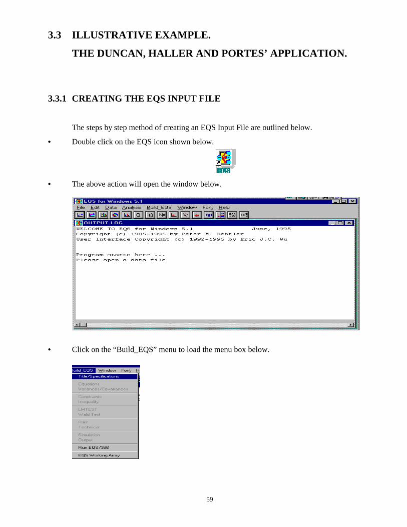
59

3.3 ILLUSTRATIVE EXAMPLE.

THE DUNCAN, HALLER AND PORTES’ APPLICATION.

3.3.1 CREATING THE EQS INPUT FILE

The steps by step method of creating an EQS Input File are outlined below.

• Double click on the EQS icon shown below.

• The above action will open the window below.

• Click on the “Build_EQS” menu to load the menu box below.

60

• Click on the “Title/Specifications” option of the “Build_EQS” menu to load the "Title for

EQS Model’s” dialog box shown below.

• Type the title "DUNCAN, HALLER AND PORTES' APPLICATION" into the "EQS models

title is" string field to produce the dialog box shown below.

• Click on the "OK" push button to load the "EQS Model Specification" dialog box shown

below.

61

• Type the number of manifest variables into the "Variables" string field.

• Type the number of cases into the "Cases" string field.

• Activate the "Correlation Matrix" radio button of the "Input Data Type is" radio buttons to

produce the dialog box shown below.

• Click on the "OK" push button to load the "EQS for Windows" dialog box below.

• Click on the “OK” push button in the "EQS For Windows" dialog box above to load the

"Build Equations" dialog box shown below.

62

• Type the number of latent variables into the "Number of Factors" string field to produce the

dialog box shown below.

• Click on the "OK" push button to load the “Create New Equations” dialog box shown below.

In the model, depicted in Figure 1.2, a single headed arrow is drawn from F1 (REAMB) to V4

(REOAP) and also from F1 to V5 (REEAP) as shown below.

Figure 3.3: The dependence paths between F1, V4 and V5.

REOAP

REEAP

REAMB

63

• The dependence path F1 to V4 is indicated in the windows above by clicking on the space

corresponding to Column "F1" and Row "V4”. An asterisk “*” appears in the space clicked.

The dependence path “F1 to V5 “ is also indicated in windows above by clicking on the

space corresponding to Column "F1" and Row "V5”.

• Continue with the steps above for all the other dependence paths in the model depicted in

Figure 1.2 to produce the “ Create New Equations” dialog box shown below.

• Click on the “DONE” push button to load the “Create Variances/Covariances” dialog box

shown below.

All the variances in the model would be automatically indicated at this stage.

For the model, depicted in Figure 1.2, double headed arrows are employed from the manifest

variable V2 (REPAP) to itself to specify a variance and to V3 (RESOE), and V1 (REINT), to specify

covariances. These paths are shown in the diagram below.

64

Figure 3.4 Variance/Covariance Paths between V2, V3 and V1.

The covariances above are added to the equations by the following actions.

• Click on the cell in Row "V2" and Column "V1” of the “Create Variances/Covariances”

window above until an asterisk “*” appears.

• Click on the cell Row "V3" and Colunm "V1”.

• Repeat the above step for all the other covariance paths in the model to produce the “ Create

Variances/Covariances” dialog box shown below.

• Click on the “Done” push button to open the window below.

REPAP REINT RESOE

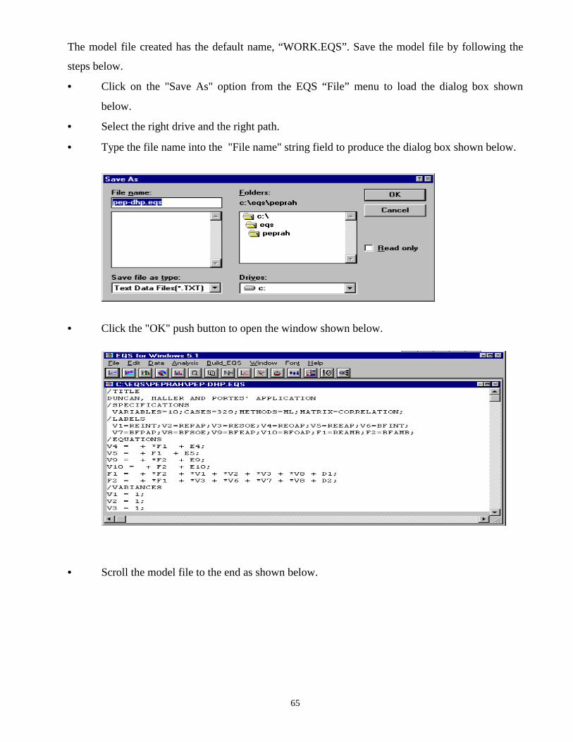
65

The model file created has the default name, “WORK.EQS”. Save the model file by following the

steps below.

• Click on the "Save As" option from the EQS “File” menu to load the dialog box shown

below.

• Select the right drive and the right path.

• Type the file name into the "File name" string field to produce the dialog box shown below.

• Click the "OK" push button to open the window shown below.

• Scroll the model file to the end as shown below.

66

• Type the keyword “/MATRIX” after the last row in the model file.

• Type in the entries of the correlation matrix.

• In the next row after the matrix, type in the keyword “/STANDARD DEVIATIONS” and

enter the standard deviations of each of the manifest variables.

• Type in the keyword “/END” at the end of the model file to produce the window shown

below.

67

3.3.2 INPUT FILE: EXAMPLE 3

The complete EQS input file for the Duncan, Haller and Portes' Application is provided below.

/TITLE

DUNCAN, HALLER AND PORTES' APPLICATION

/SPECIFICATIONS

VARIABLES=10;CASES=329;METHODS=ML;MATRIX=COR;

/LABELS

V1=REINT; V2=REPAP; V3=RESOE; V4=REOAP; V5=REEAP; V6=BFINT;

V7=BFPAP; V8=BFSOE; V9=BFEAP; V10=BFOAP; F1=REAMB; F2=BFAMB;

/EQUATIONS

V4 = + *F1 + E4;

V5 = + F1 + E5;

V9 = + *F2 + E9;

V10 = + F2 + E10;

F1 = + *F2 + *V1 + *V2 + *V3 + *V8 + D1;

F2 = + *F1 + *V3 + *V6 + *V7 + *V8 + D2;

/VARIANCES

V1 = 1;

V2 = 1;

V3 = 1;

V6 = 1;

V7 = 1;

V8 = 1;

E4 = *;

E5 = *;

E9 = *;

E10 = *;

D1 = *;

D2 = *;

/COVARIANCES

V2, V1 = *;

V2, V3 = *;

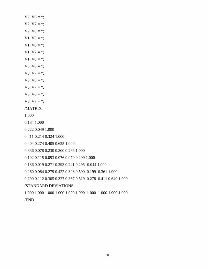
68

V2, V6 = *;

V2, V7 = *;

V2, V8 = *;

V1, V3 = *;

V1, V6 = *;

V1, V7 = *;

V1, V8 = *;

V3, V6 = *;

V3, V7 = *;

V3, V8 = *;

V6, V7 = *;

V8, V6 = *;

V8, V7 = *;

/MATRIX

1.000

0.184 1.000

0.222 0.049 1.000

0.411 0.214 0.324 1.000

0.404 0.274 0.405 0.625 1.000

0.336 0.078 0.230 0.300 0.286 1.000

0.102 0.115 0.093 0.076 0.070 0.209 1.000

0.186 0.019 0.271 0.293 0.241 0.295 -0.044 1.000

0.260 0.084 0.279 0.422 0.328 0.500 0.199 0.361 1.000

0.290 0.112 0.305 0.327 0.367 0.519 0.278 0.411 0.640 1.000

/STANDARD DEVIATIONS

1.000 1.000 1.000 1.000 1.000 1.000 1.000 1.000 1.000 1.000

/END

69

3.3.3 RUNNING EQS To run EQS:

• Click on the “Build EQS” menu to load the following menu box.

• Click on the “Run EQS/386” option to load the “ EQS for Windows” dialog box below.

• Click on the “OK” push button to start the iteration process.

When the iteration is completed, the following DOS window appears.

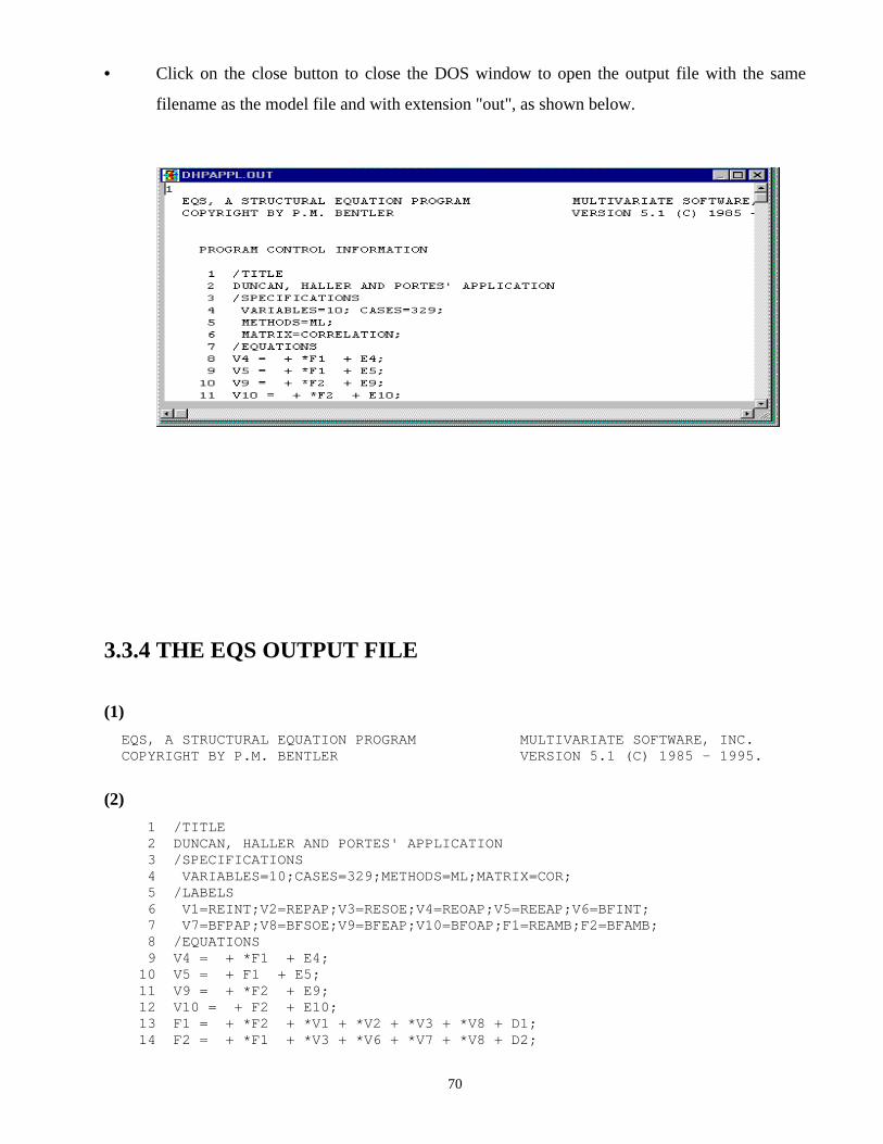
70

• Click on the close button to close the DOS window to open the output file with the same

filename as the model file and with extension "out", as shown below.

3.3.4 THE EQS OUTPUT FILE

(1) EQS, A STRUCTURAL EQUATION PROGRAM MULTIVARIATE SOFTWARE, INC. COPYRIGHT BY P.M. BENTLER VERSION 5.1 (C) 1985 - 1995.

(2) 1 /TITLE 2 DUNCAN, HALLER AND PORTES' APPLICATION 3 /SPECIFICATIONS 4 VARIABLES=10;CASES=329;METHODS=ML;MATRIX=COR; 5 /LABELS 6 V1=REINT;V2=REPAP;V3=RESOE;V4=REOAP;V5=REEAP;V6=BFINT; 7 V7=BFPAP;V8=BFSOE;V9=BFEAP;V10=BFOAP;F1=REAMB;F2=BFAMB; 8 /EQUATIONS 9 V4 = + *F1 + E4; 10 V5 = + F1 + E5; 11 V9 = + *F2 + E9; 12 V10 = + F2 + E10; 13 F1 = + *F2 + *V1 + *V2 + *V3 + *V8 + D1; 14 F2 = + *F1 + *V3 + *V6 + *V7 + *V8 + D2;

71

15 /VARIANCES 16 V1 = 1; 17 V2 = 1; 18 V3 = 1; 19 V6 = 1; 20 V7 = 1; 21 V8 = 1; 22 E4 = *; 23 E5 = *; 24 E9 = *; 25 E10 = *; 26 D1 = *; 27 D2 = *; 28 /COVARIANCES 29 V2 , V1 = *; 30 V2 , V3 = *; 31 V2 , V6 = *; 32 V2 , V7 = *; 33 V2 , V8 = *; 34 V1 , V3 = *; 35 V1 , V6 = *; 36 V1 , V7 = *; 37 V1 , V8 = *; 38 V3 , V6 = *; 39 V3 , V7 = *; 40 V3 , V8 = *; 41 V6 , V7 = *; 42 V8 , V6 = *; 43 V8 , V7 = *; 44 /MATRIX 45 1.000 46 0.184 1.000 47 0.222 0.049 1.000 48 0.411 0.214 0.324 1.000 49 0.404 0.274 0.405 0.625 1.000 50 0.336 0.078 0.230 0.300 0.286 1.000 51 0.102 0.115 0.093 0.076 0.070 0.209 1.000 52 0.186 0.019 0.271 0.293 0.241 0.295 -0.044 1.000

(3) TITLE: DUNCAN, HALLER AND PORTES' APPLICATION 17/11/00 PAGE : 2 53 0.260 0.084 0.279 0.422 0.328 0.500 0.199 0.361 1.000 54 0.290 0.112 0.305 0.327 0.367 0.519 0.278 0.411 0.640 1.000 55 /STANDARD DEVIATIONS 56 1.000 1.000 1.000 1.000 1.000 1.000 1.000 1.000 1.000 1.000 57 /END

(4) 57 RECORDS OF INPUT MODEL FILE WERE READ TITLE: DUNCAN, HALLER AND PORTES' APPLICATION 17/11/00 PAGE : 3

72

(5) REINT REPAP RESOE REOAP REEAP

V 1 V 2 V 3 V 4 V 5 REINT V 1 1.000 REPAP V 2 0.184 1.000 RESOE V 3 0.222 0.049 1.000 REOAP V 4 0.411 0.214 0.324 1.000 REEAP V 5 0.404 0.274 0.405 0.625 1.000 BFINT V 6 0.336 0.078 0.230 0.300 0.286 BFPAP V 7 0.102 0.115 0.093 0.076 0.070 BFSOE V 8 0.186 0.019 0.271 0.293 0.241 BFEAP V 9 0.260 0.084 0.279 0.422 0.328 BFOAP V 10 0.290 0.112 0.305 0.327 0.367 BFINT BFPAP BFSOE BFEAP BFOAP V 6 V 7 V 8 V 9 V 10 BFINT V 6 1.000 BFPAP V 7 0.209 1.000 BFSOE V 8 0.295 -0.044 1.000 BFEAP V 9 0.500 0.199 0.361 1.000 BFOAP V 10 0.519 0.278 0.411 0.640 1.000

(6) NUMBER OF DEPENDENT VARIABLES = 6 DEPENDENT V'S : 4 5 9 10 DEPENDENT F'S : 1 2 NUMBER OF INDEPENDENT VARIABLES = 12 INDEPENDENT V'S : 1 2 3 6 7 8 INDEPENDENT E'S : 4 5 9 10 INDEPENDENT D'S : 1 2 3RD STAGE OF COMPUTATION REQUIRED 5297 WORDS OF MEMORY. PROGRAM ALLOCATE 100000 WORDS

(7) DETERMINANT OF INPUT MATRIX IS 0.70018E-01 TITLE: DUNCAN, HALLER AND PORTES' APPLICATION 17/11/00 PAGE : 4

(8) MAXIMUM LIKELIHOOD SOLUTION (NORMAL DISTRIBUTION THEORY)

(9) PARAMETER ESTIMATES APPEAR IN ORDER, NO SPECIAL PROBLEMS WERE ENCOUNTERED DURING OPTIMIZATION.

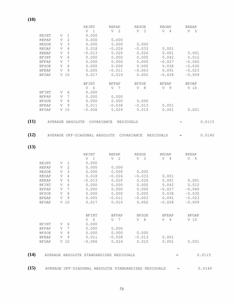
73

(10) REINT REPAP RESOE REOAP REEAP V 1 V 2 V 3 V 4 V 5 REINT V 1 0.000 REPAP V 2 0.000 0.000 RESOE V 3 0.000 0.000 0.000 REOAP V 4 0.018 -0.026 -0.033 0.001 REEAP V 5 -0.013 0.020 0.026 0.001 0.001 BFINT V 6 0.000 0.000 0.000 0.042 0.012 BFPAP V 7 0.000 0.000 0.000 -0.027 -0.040 BFSOE V 8 0.000 0.000 0.000 0.038 -0.030 BFEAP V 9 0.005 -0.011 -0.003 0.091 -0.023 BFOAP V 10 0.017 0.010 0.002 -0.028 -0.009 BFINT BFPAP BFSOE BFEAP BFOAP V 6 V 7 V 8 V 9 V 10 BFINT V 6 0.000 BFPAP V 7 0.000 0.000 BFSOE V 8 0.000 0.000 0.000 BFEAP V 9 0.011 -0.038 -0.013 0.001 BFOAP V 10 -0.006 0.024 0.010 0.001 0.001

(11) AVERAGE ABSOLUTE COVARIANCE RESIDUALS = 0.0115

(12) AVERAGE OFF-DIAGONAL ABSOLUTE COVARIANCE RESIDUALS = 0.0140

(13) REINT REPAP RESOE REOAP REEAP V 1 V 2 V 3 V 4 V 5 REINT V 1 0.000 REPAP V 2 0.000 0.000 RESOE V 3 0.000 0.000 0.000 REOAP V 4 0.018 -0.026 -0.033 0.001 REEAP V 5 -0.013 0.020 0.026 0.001 0.001 BFINT V 6 0.000 0.000 0.000 0.042 0.012 BFPAP V 7 0.000 0.000 0.000 -0.027 -0.040 BFSOE V 8 0.000 0.000 0.000 0.038 -0.030 BFEAP V 9 0.005 -0.011 -0.003 0.091 -0.023 BFOAP V 10 0.017 0.010 0.002 -0.028 -0.009 BFINT BFPAP BFSOE BFEAP BFOAP V 6 V 7 V 8 V 9 V 10 BFINT V 6 0.000 BFPAP V 7 0.000 0.000 BFSOE V 8 0.000 0.000 0.000 BFEAP V 9 0.011 -0.038 -0.013 0.001 BFOAP V 10 -0.006 0.024 0.010 0.001 0.001

(14) AVERAGE ABSOLUTE STANDARDIZED RESIDUALS = 0.0115

(15) AVERAGE OFF-DIAGONAL ABSOLUTE STANDARDIZED RESIDUALS = 0.0140

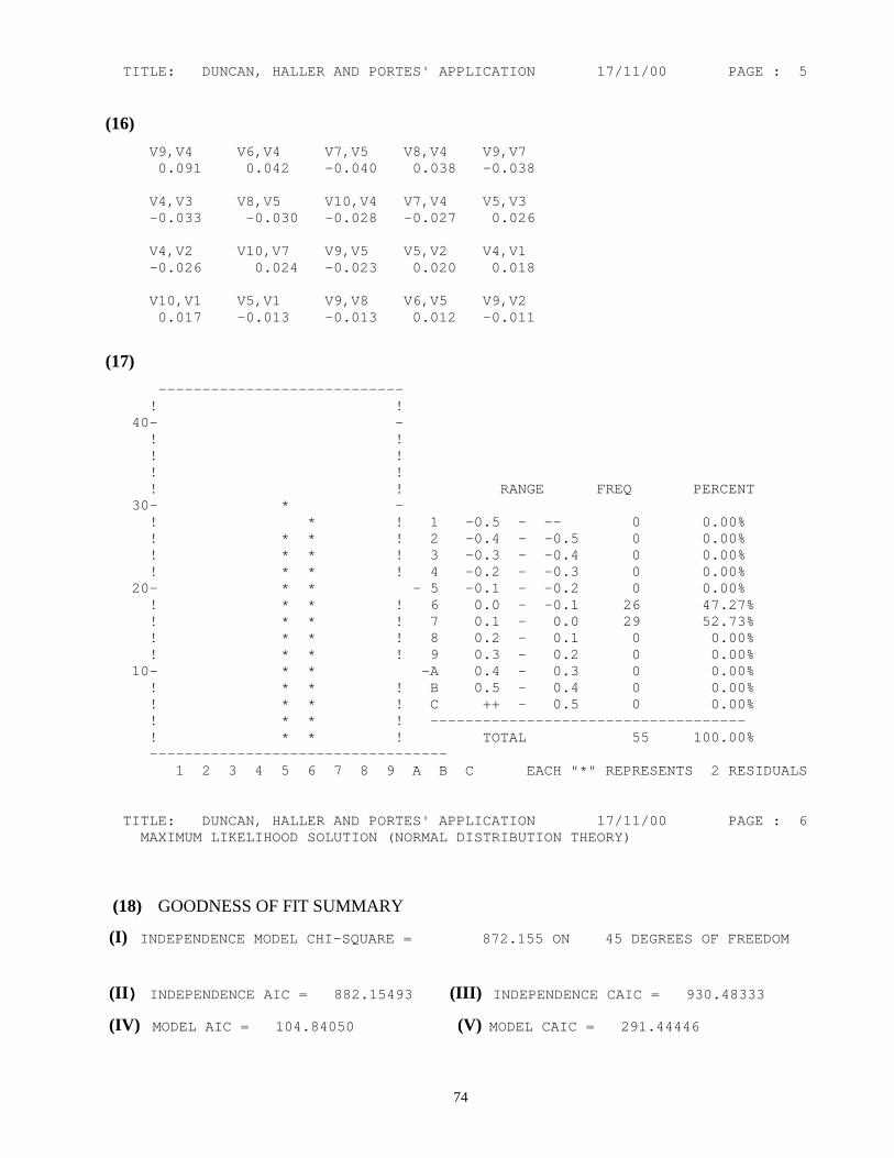
74

TITLE: DUNCAN, HALLER AND PORTES' APPLICATION 17/11/00 PAGE : 5

(16) V9,V4 V6,V4 V7,V5 V8,V4 V9,V7 0.091 0.042 -0.040 0.038 -0.038 V4,V3 V8,V5 V10,V4 V7,V4 V5,V3 -0.033 -0.030 -0.028 -0.027 0.026 V4,V2 V10,V7 V9,V5 V5,V2 V4,V1 -0.026 0.024 -0.023 0.020 0.018 V10,V1 V5,V1 V9,V8 V6,V5 V9,V2 0.017 -0.013 -0.013 0.012 -0.011

(17) ---------------------------- ! ! 40- - ! ! ! ! ! ! ! ! RANGE FREQ PERCENT 30- * - ! * ! 1 -0.5 - -- 0 0.00% ! * * ! 2 -0.4 - -0.5 0 0.00% ! * * ! 3 -0.3 - -0.4 0 0.00% ! * * ! 4 -0.2 - -0.3 0 0.00% 20- * * - 5 -0.1 - -0.2 0 0.00% ! * * ! 6 0.0 - -0.1 26 47.27% ! * * ! 7 0.1 - 0.0 29 52.73% ! * * ! 8 0.2 - 0.1 0 0.00% ! * * ! 9 0.3 - 0.2 0 0.00% 10- * * -A 0.4 - 0.3 0 0.00% ! * * ! B 0.5 - 0.4 0 0.00% ! * * ! C ++ - 0.5 0 0.00% ! * * ! ------------------------------------ ! * * ! TOTAL 55 100.00% ---------------------------------- 1 2 3 4 5 6 7 8 9 A B C EACH "*" REPRESENTS 2 RESIDUALS TITLE: DUNCAN, HALLER AND PORTES' APPLICATION 17/11/00 PAGE : 6 MAXIMUM LIKELIHOOD SOLUTION (NORMAL DISTRIBUTION THEORY) (18) GOODNESS OF FIT SUMMARY

(I) INDEPENDENCE MODEL CHI-SQUARE = 872.155 ON 45 DEGREES OF FREEDOM

(II) INDEPENDENCE AIC = 882.15493 (III) INDEPENDENCE CAIC = 930.48333

(IV) MODEL AIC = 104.84050 (V) MODEL CAIC = 291.44446

75

(VI) CHI-SQUARE = 26.840 BASED ON 16 DEGREES OF FREEDOM

(VII) PROBABILITY VALUE FOR THE CHI-SQUARE STATISTIC IS LESS THAN 0.002

(VIII) THE NORMAL THEORY RLS CHI-SQUARE FOR THIS ML SOLUTION IS 26.084.

(IX) BENTLER-BONETT NORMED FIT INDEX = 0.969

(X) BENTLER-BONETT NONNORMED FIT INDEX = -0.406

(XI) COMPARATIVE FIT INDEX (CFI) = 0.969

(19)

PARAMETER ITERATION ABS CHANGE ALPHA FUNCTION 1 0.595770 1.00000 10.54929 2 0.437456 1.00000 8.01110 3 0.200444 1.00000 7.85747 4 0.182135 1.00000 5.98122 5 0.158818 1.00000 4.52051 6 0.190420 1.00000 3.01704 7 0.104382 1.00000 2.04361 8 0.083959 1.00000 1.05939 9 0.055219 1.00000 0.21761 10 0.020089 1.00000 0.08861 11 0.005698 1.00000 0.08194 12 0.001084 1.00000 0.08184 13 0.000273 1.00000 0.08183 TITLE: DUNCAN, HALLER AND PORTES' APPLICATION 17/11/00 PAGE : 7 MAXIMUM LIKELIHOOD SOLUTION (NORMAL DISTRIBUTION THEORY)

(20) REOAP =V4 = .943*F1 + 1.000 E4 .080 11.815 REEAP =V5 = 1.000 F1 + 1.000 E5 BFEAP =V9 = .932*F2 + 1.000 E9 .070 13.226 BFOAP =V10 = 1.000 F2 + 1.000 E10

76

TITLE: DUNCAN, HALLER AND PORTES' APPLICATION 17/11/00 PAGE : 8 MAXIMUM LIKELIHOOD SOLUTION (NORMAL DISTRIBUTION THEORY)

(21) REAMB =F1 = .173*F2 + .270*V1 + .174*V2 + .236*V3 .085 .044 .041 .045 2.040 6.101 4.264 5.178 .084*V8 + 1.000 D1 .050 1.673 BFAMB =F2 = .188*F1 + .072*V3 + .354*V6 + .163*V7 .080 .046 .043 .039 2.341 1.545 8.238 4.215 .234*V8 + 1.000 D2 .043 5.471 TITLE: DUNCAN, HALLER AND PORTES' APPLICATION 17/11/00 PAGE : 9 MAXIMUM LIKELIHOOD SOLUTION (NORMAL DISTRIBUTION THEORY) (22) ---------------------------------- V F --- --- V1 -REINT 1.000 I I I I I I I I V2 -REPAP 1.000 I I I I I I I I V3 -RESOE 1.000 I I I I I I I I V6 -BFINT 1.000 I I I I I I I I V7 -BFPAP 1.000 I I I I I I I I V8 -BFSOE 1.000 I I I I

77


(23)

-----------------------------------------

E D

--- ---

E4 -REOAP .412*I D1 -REAMB .317*I

.051 I .053 I

8.056 I 6.022 I

I I

E5 -REEAP .338*I D2 -BFAMB .263*I

.052 I .045 I

6.514 I 5.836 I

I I

E9 -BFEAP .404*I I

.046 I I

8.755 I I

I I

E10 -BFOAP .314*I I

.046 I I

6.855 I I

I I


(24) --------------------------------------- V F --- --- V2 -REPAP .184*I I V1 -REINT .052 I I 3.507 I I I I V3 -RESOE .222*I I V1 -REINT .051 I I 4.344 I I I I V6 -BFINT .336*I I V1 -REINT .046 I I 7.244 I I I I V7 -BFPAP .102*I I V1 -REINT .054 I I 1.884 I I

78

I I V8 -BFSOE .186*I I V1 -REINT .052 I I 3.571 I I I I V3 -RESOE .049*I I V2 -REPAP .055 I I .892 I I I I V6 -BFINT .078*I I V2 -REPAP .055 I I 1.430 I I I I V7 -BFPAP .115*I I V2 -REPAP .054 I I 2.125 I I I I V8 -BFSOE .019*I I V2 -REPAP .055 I I .345 I I I I V6 -BFINT .230*I I V3 -RESOE .051 I I 4.532 I I I I V7 -BFPAP .093*I I V3 -RESOE .054 I I 1.710 I I I I V8 -BFSOE .271*I I V3 -RESOE .049 I I 5.498 I I I I


(25) --------------------------------------------------- V7 -BFPAP .209*I I V6 -BFINT .052 I I 4.049 I I I I V8 -BFSOE .295*I I V6 -BFINT .048 I I 6.115 I I I I V8 -BFSOE -.044*I I V7 -BFPAP .055 I I -.804 I I I I

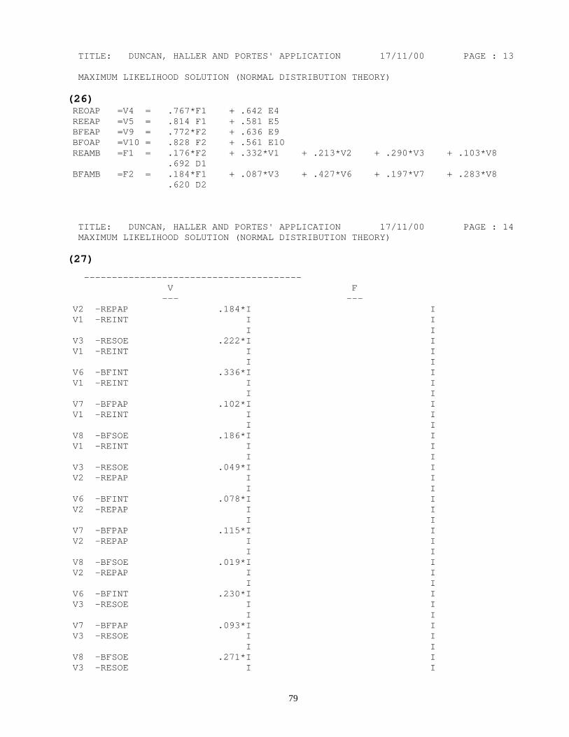
79

TITLE: DUNCAN, HALLER AND PORTES' APPLICATION 17/11/00 PAGE : 13 MAXIMUM LIKELIHOOD SOLUTION (NORMAL DISTRIBUTION THEORY) (26) REOAP =V4 = .767*F1 + .642 E4 REEAP =V5 = .814 F1 + .581 E5 BFEAP =V9 = .772*F2 + .636 E9 BFOAP =V10 = .828 F2 + .561 E10 REAMB =F1 = .176*F2 + .332*V1 + .213*V2 + .290*V3 + .103*V8 .692 D1 BFAMB =F2 = .184*F1 + .087*V3 + .427*V6 + .197*V7 + .283*V8 .620 D2 TITLE: DUNCAN, HALLER AND PORTES' APPLICATION 17/11/00 PAGE : 14 MAXIMUM LIKELIHOOD SOLUTION (NORMAL DISTRIBUTION THEORY) (27)

--------------------------------------- V F --- --- V2 -REPAP .184*I I V1 -REINT I I I I V3 -RESOE .222*I I V1 -REINT I I I I V6 -BFINT .336*I I V1 -REINT I I I I V7 -BFPAP .102*I I V1 -REINT I I I I V8 -BFSOE .186*I I V1 -REINT I I I I V3 -RESOE .049*I I V2 -REPAP I I I I V6 -BFINT .078*I I V2 -REPAP I I I I V7 -BFPAP .115*I I V2 -REPAP I I I I V8 -BFSOE .019*I I V2 -REPAP I I I I V6 -BFINT .230*I I V3 -RESOE I I I I V7 -BFPAP .093*I I V3 -RESOE I I I I V8 -BFSOE .271*I I V3 -RESOE I I

80

I I V7 -BFPAP .209*I I V6 -BFINT I I I I V8 -BFSOE .295*I I V6 -BFINT I I I I V8 -BFSOE -.044*I I V7 -BFPAP I I

(28)

------------------------------------------------------------------------------- E N D O F M E T H O D ------------------------------------------------------------------------------- (I) Execution begins at 01:56:12.57 (II) Execution ends at 01:56:13.61 (III) Elapsed time = 1.04 seconds

ENTRIES IN THE EQS OUTPUT FILE

(1) This paragraph gives the name of the Program, the author's name and the publishers of EQS.

(2) Program control information.

This paragraph gives the number of records or lines of the actual input file. This input

feedback helps locate any problems in the input, and also provide a summary of the proposed

analysis. The title of the input file will be part of this paragraph and it is repeated as the first

line of every page.

(3) Continuation of the Program control information.

(4) This paragraph gives the details of the number of rows in the complete model file used in the

analysis.

81

(5) The input correlation matrix to be analyzed, the number of variables and the number of cases

appear in this paragraph. The matrix reproduced here enables the user to check that the

arrangement of the variables and the variable codes were correctly entered in the input file.

(6) Bentler-Weeks Structural Representation.

The program input is decoded to generate a matrix specification consistent with the Bentler-

Weeks designation of dependent and independent variables. The number of dependent

variables is printed, and index numbers are given for all measured and latent variables in the

sequence V, F, E, D with all V variables listed first, F variables listed next, and so on. Then

the number of independent variables is printed along with the index numbers for the

variables, again in the sequence V, F, E, D. This information enables the user, if necessary, to

determine whether the model was specified as intended.

(7) This paragraph gives the determinant of the input correlation matrix.

(8) This is the line of information on the estimation method and the distributional theory used in

the analysis. This printed information will head each page of output associated with the given

method. When this information changes, a new solution method is being reported.

(9) This message appears if the estimates for all parameters seem to be technically acceptable.

This message should always be located prior to evaluating the meaning of any results.

(10) Residual covariance matrix (S - ∑∧

).

This is the difference between the sample covariance matrix S (or the covariance matrix

calculated from the input correlation matrix) and the reproduced covariance matrix ∑∧

. The

closer the entries are to zero, the better the model fits the data.

(11) The average absolute covariance residuals.

This value is the average of the absolute standardized residuals including the diagonal

elements.

(12) The average off-diagonal absolute covariance residuals.

This value is the average of the absolute standardized residuals excluding the diagonal

elements.

82

(13) Standardized residual matrix.

This the matrix produced by a standardization on the Residual Covariance Matrix so that the

elements are in a more similar range. The residual matrix (S - ∑∧

) is pre- and post-

multiplied by the diagonal matrix of inverse elements of standard deviations of the manifest

variables, so that the resulting residual matrix can be interpreted in the metric of correlations

among the input variables. The standardized residual matrix contains elements given by

r s sij ij i j− ∃ /θ

where rij is the observed correlation between the two manifest variables Vi and Vj, ∃θ ij is the

corresponding reproduced model covariance, and si and sj are standard deviations of the

manifest variables Vi and Vj respectively.

(14) The average absolute standardized residuals.

Same as in (9) above.

(15) The average off-diagonal absolute standardized residuals.

Same as in (10) above.

(16) Largest standardized residual.

In this paragraph, the elements from the Standardized Residual Matrix are ordered from large

to small in absolute value, and the largest twenty of these are printed out along with a

designation of which pairs of variables are involved.

(17) Distribution of standardized residuals.

A frequency distribution of the standardized residuals is given in this paragraph. The legend

for the figure describes how many residual elements are described by a single asterisk in the

figure, and information on the specific frequencies and percentages that fall within a given

range used in the figure. Note that the diagram is labeled 1, 2, …, 9. A, B, C. Each of these

numbers or letters refers to a given range of numbers that describes the size of the residuals.

(18) Goodness of Fit Indices.

(I) The Independence model chi-square is given by

Independence model χ 2 = N ∃Fo .

83

where ∃Fo denotes the minimal discrepancy function value for the independence

model and N denotes the number of cases. (II) The Independent Akaike’s Information Criterion (AIC) is given by

Independence AIC = Independence model χ 2 - 2di

where di denotes the degrees of freedom of the independence model.

(III) The Independence Cross-validated Akaike’s Information Criterion (CAIC) is given

by (Bozdogan, 1987)

Independence CAIC = Independence model χ 2 - (In N + 1)di

(IV) The model Akaike’s Information Criterion (AIC) is given by

Model AIC = Model χ 2 - 2dk

where dk denotes the degrees of freedom of the model of interest.

(V) The model Cross-validated Akaike Information Criterion (CAIC) is given by

Model CAIC = model χ 2 - (In N + 1)dk.

(VI) The chi-square (model χ 2 test statistic) is calculated as n x F∧

.

where F∧

is the minimal sample discrepancy function value.

(VII) This is the probability of obtaining a χ 2 value as greater or equal to the value

actually obtained, given that the model is correct.

(VIII) This is the value obtained from the normal theory rewieghted least squares chi-square

for maximum likelihood solution.

(IX) The Bentler-Bonett normed fit index (NFI) value is computed from

NFI = 1−∃∃

QQ

k

i

,

where ∃Qk and ∃Qi are the minimal values of the fitting functions obtained for the

model of interest and the corresponding independence model, respectively. The

general fitting function Q is given by:

Q = ( ) ( )s W s− ′ −σ θ σ θ( ) ( ) ,

where s is the vector of 12

p(p+1) elements obtained by stringing out the lower

triangular elements of the unbiased sample covariance matrix S, σ is the

corresponding vector obtained from ,∑ and θ is the vector of free parameters of the

structural equation model.

84

(X) The Bentler-Bonett non-normed fit index (NNFI) value is computed from

NNFI = ( )( )f f

fi k

i

−

−

∃

∃ 1

where ∃ ∃ /f NQ di i i= and ∃ ∃ /f NQ dk k k= are χ 2 variates divided by the associated

degrees of freedom for the null (di) and substantive models (dk), respectively.

(XI) The Comparative Fit Index (CFI) is computed from

CFI = 1 - ∃∃ττ

k

i

,

where ( )∃ max[ ∃ , ]τ k k kNQ d= − 0 based on the model of interest and

( ) ( )∃ max[ ∃ , ∃ , ]τ i i i k kNQ d NQ d= − − 0

(19) Iterative summary.

This paragraph contains information obtained from each iteration.

Column 1: Iteration number

Column 2: Change in parameter estimate.

Column 3: Alpha.

Alpha is the value of the stepsize parameter used in the iteration.

Column 4: Function.

The value of the sample discrepancy function.

(20) Measurement equations with standard errors and test statistics.

In this paragraph, the measurement equations that relate manifest dependent variables (Vs) to

other variables are printed. The equations are printed with the updated parameter estimates

rather than the starting values using a three-line format as follows:

Line 1: the equation with estimated parameter values.

Line 2: the standard error of the estimator(s).

Line 3: the test statistic(s) for the significance of the parameter(s).

(21) Construct equations with standard errors and test statistics.

The construct equations that have dependent latent variables (Fs) are printed in this

paragraph. Each measurement equation with optimal estimates for free parameters is printed

in the same format as outlined in (20) above.

(22) Variances of independent variables.

85

There are four columns in this paragraph.

Column 1:

Manifest variables (Vs).

Column 2:

Latent variables (Fs).

Column 3:

Error terms (Es).

Column 4:

Disturbances (Ds).

Column 3 and Column 4 are printed separately in paragraph (23) below.

(23) Variances of independent variables continued.

This paragraph is the E and D part of paragraph (22) above.

(24) Covariances among independent variables.

The same format and column headings are used in this paragraph as in paragraphs (22) and

(23) above. The labels for the pair of variables involved in a covariance are printed below

each other.

(25) Covariances among independent variables.

This paragraph is the continuation of paragraph (24) above.

(26) The maximum likelihood solution (normal distribution theory). Standardized solution.

In this paragraph, each measurement and construct equation is printed out giving the

standardized solution. This is a complete standardized path analysis type of solution, except

that manifest variables are not standardized: all V, F, E, and D model variables are rescaled

to have unit variances. Standardization is done for all variables in the linear structural

equation system, including errors and disturbances. Consequently, all coefficients in the

equations have similar interpretation, and the magnitude of these standardized coefficients

may be easier to interpret than the magnitudes of the coefficients obtained from the

covariance or raw data matrix.

(27) Correlations among independent variables.

These correlations accompany the standardized solution when it is computed. These must be

scanned to see whether they are in the necessary ± 1 range. If not, the solution has a problem

that may imply theoretical or empirical under identification.

(28) End of Method.

The phrase “End of Method” delineates the end of output from a given estimation problem

with a given method. It has three rows described below:

86

(I) The time the execution (iteration) started.

(II) The time the execution (iteration) ended.

(III) The elapsed time. This is the difference between (ii) and (i).

87

CHAPTER 4

LISREL


The acronym LISREL stands for Linear Structural RELationships. Karl Jöreskog and Dag Sörbom

developed a DOS application that implements the LISREL methodology in 1974. The 1974 version

was improved upon in 1978 and again in 1986. LISREL 5 and LISREL 6 were released in 1981 and

1984 respectively. LISREL 7 was released in 1989 and LISREL 8 in 1996. The latest version is

LISREL 8.30, which was released in 1999. The Scientific Software International Inc (SSI) publishes

LISREL. One may obtain more information about LISREL from the SSI website

www.ssicentral.com.

The LISREL model specifies linear relationships between observed and/or unobserved variables. In

its general form the LISREL model is defined by the following system of linear structural relations:

X−

= Λ x ξ δ− −+

Y−

= Λ y η ε− −+

η η ξ ζ− − − −

= + +B Γ

where X−

represents the vector of all exogenous manifest variables and the measurements of

exogenous latent variable of the model,

Y−

represents the vector of all measurements of endogenous latent variables and the endogenous

manifest variables of the model,

η−

represents the vector of all the dependent latent variables of the model,

ξ−

represents the vector of all the independent latent variables of the model,

ζ−

represents the random vector of residuals (errors in equations, random disturbance terms),

B x, , ,Γ Λ and Λ y are parameter matrices.

88

The covariance structure of the observed variables which is also known as the Covariance

Structure of the LISREL model is given by

( ) ( )( ) ( )

( ) ( )=

− + − + −

− − +

− − −

− −∑ Cov

I B I B I B

I B I B

y y y x

x y x y

Λ ΓΦΓ Ψ Λ Θ Λ ΓΦΛ

Λ ΦΓ Λ Λ ΦΓ Λ Θ

1 1 1

1 1

' ' ' '

' ' ' ' '

ε

δ

where

Φ denotes the covariance matrix of ξ−

,

Ψ denotes the covariance matrix of ζ−

,

Θε denotes the covariance matrix of ε−

and

Θδ denotes the covariance matrix of δ−

.

The LISREL model is, as seen above, a formal mathematical model, which has to be, given

substantive content in each application. The meaning of the terms involved in the model varies from

one application to another. The formal LISREL model defines a large class of models within which

one can work and this class contains several useful subclasses as special cases.

The program LISREL 8.30 implements the LISREL model. LISREL8.30 consists of two programs:

PRELIS and LISREL. One can run PRELIS or LISREL separately or PRELIS and LISREL in

sequence. PRELIS handles everything that has to do with raw data; LISREL handles the fitting and

testing of models to summary statistics produced by PRELIS, i.e. PRELIS is a preprocessor for

LISREL. But it can also be conveniently used to provide a first descriptive look at raw data even

when LISREL analysis is intended or when other programs will do further analysis.

The LISREL8.30 command language requires a user to be familiar with matrices so as to be able to

formulate a model in matrix form using Greek matrix notations. Beginning users of LISREL8.30 and

users who often make mistakes when they specify the LISREL model can use the SIMPLIS

command language as this is much easier to learn and reduces the possibilities for mistakes to a

minimum. The SIMPLIS command language is in plain English. The user is only required to name

the variables of the model and then formulate the model to be estimated.

89

The LISREL 8.30 for windows program allows the user to create and run the LISREL syntax

interactively. One way to do this is to draw the appropriate path diagram on the screen and then to

build the corresponding SIMPLIS or LISREL code directly from the path diagram. The model can

be modified interactively at run time by adding or deleting paths in the diagram.

4.2 THE LISREL INPUT SYSTEM

There are three ways of fitting a structural equation model to data with LISREL8.30. These are:

1) To specify the structural equation model in a LISREL input file by using the LISREL command

language to create LS8 or LPJ files. These input files are text files that specify the structural

equation model in terms of the eight parameter matrices of the LISREL model.

2) To specify the structural equation model by using the SIMPLIS command language to create

SPL or SPJ files. These files are text files that can be created using any text editor such as

notepad.

3) To specify the structural equation model by creating a graphics file which contains the path

diagram for the model and then build the corresponding LISREL syntax file directly from the

path diagram. The graphics file created is saved with the extension “*.PTH”.

The data to be analyzed, is provided in a LISREL data file with the extension “*.DAT” or a data

system file with the extension “*.DSF”. A LISREL data file is a text file that contains the raw data

matrix, the sample covariance matrix or sample correlation matrix. Data can also be imported from

other applications, such as SPSS, SYSTAT, BMDP, EXCEL, etc.

GENERAL RULES FOR TYPING LISREL INPUT FILES

• Uppercase elements are commands, keywords or options. They must be entered as they

appear, or they may be lengthened (LABELS instead of LA, for example). Thus, except for

the ALL option on the VA and ST commands and the PATH DIAGRAM command,

everything has two significant characters.

• Only the first two characters are significant in command names, options, keywords and

character keyword values. Any additional character up to the first blank, comma, semicolon,

or equals sign will be ignored. Thus DA, DATA, DAta, and data are all equivalent.

90

• An exclamation mark (!) or the slash-asterisk combination (/*) may be used to indicate that

everything that follows on the line is to be regarded as comments. Blank (empty) lines are

accepted without the ! or /*.

• The order of the options and keywords is immaterial.

• Equal signs are required after option names and keywords.

• Commas or blanks are used to separate subcommand names, keywords, and options.

• Blanks on either side of equal sign are allowed.

• A command ends with a return character.

• More than one command may appear on a physical line as long as semicolons separate them.

• A line may not exceed 127 columns except under some operating systems that restricts input

lines to 80 columns.

• A command line which exceeds 127 characters may be continued on the next physical line by

replacing the original option or keyword with C (for continue).

• Detail lines giving additional information may follow a command.

• It is recommended to place the data to be analyzed in an external file.

• Any number of problems may be stacked together and analyzed in one run.

• A parameter matrix element should be written as a parameter matrix name (LY, LX, BE, GA,

PH, PS, TE, TD, or TH), followed by row and column positions (or linear indexes) of the

specific element. Row and column positions may be separated by a comma and enclosed in

parentheses, for example LY(3,2), LX(4,1), or separated from the matrix name and each

other by spaces, for example LY 3 2 LX 4 l.

• The order of the form and mode values for the parameter matrices on the MO subcommand is

optional, but if both are given, a comma in between is required.

• Order of commands. The order of the LISREL commands is arbitrary except for the

following conditions:

♣ After optional title lines, a DA (data) command must always come first.

♣ The OU (output) command must always be last.

♣ The LK, LE, FR, FI, EQ, CO, IR, PA, VA, ST, MA, PL, and NF commands must

always come after the MO (model) command.

♣ The MO command is optional only if no LISREL model is analyzed. If the MO

command is missing, only the matrix to be analyzed will be printed out. Otherwise,

the MO command must appear in the command file.

91

♣ Although the order of other commands is relatively free, a later command will

overrule earlier command, in so far as the same elements are referenced.

4.2.1 THE LISREL INPUT FILE SYNTAX

The basic structure of the LISREL 8.30 input file is outlined below. The commands, options and

keywords that are not always required are indicated as “optional”. The three phases, data

specification, model specification and the output results are outlined separately.

Data Specification

TITLE STATEMENT (Optional)

Purpose

To provide a description of the analysis to be performed.

Syntax

TITLE = title

where “title” denotes a character string of at most 137 characters.

Example

For the model depicted in Figure 1.2 the “TITLE STATEMENT” may be given as follows:

TITLE = The Duncan, Haller and Portes’ Application

DA command

Purpose

To specify the data to be analyzed. This should be the first command after the optional title

statement. The available options and keywords under DA are given below.

NI keyword

Purpose

To specify the Number of Input variables in the data file.

Syntax

NI = p

where p denotes the number of input variables in the data file to be analyzed.

92

Example

For the model depicted in Figure 1.2, there are 10 observed variables. This is specified as:

NI=10

NO keyword

Purpose

To specify the Number of cases or Observations in the data file. This is optional if raw data

are read in from an external file. Otherwise, it is required.

Syntax

NO=n

where n is number of cases in the data file.

Example

For the model depicted in Figure 1.2, there were 329 cases. This is therefore specified as:

NO=329

NG keyword (Optional)

Purpose

To specify the Number of Groups in multi-group or multi-sample analysis.

Syntax

NG=k

where k is the number of groups in the data to be analyzed.

Default

NG=1

Example

For the model depicted in Figure 1.2, there is only one group. This is therefore specified as:

NG=1

MA keyword

Purpose

To specify the Matrix to be Analyzed, not the matrix to be input.

Syntax

MA= matrix

where “matrix” denote any of the following possible specifications:

MA=CM (covariance matrix)

93

MA=MM (moment matrix)

MA=AM (augmented moment matrix)

MA=KM (correlation matrix of Pearson correlations)

MA=PM (polychoric correlation matrix)

MA=OM (canonical correlation matrix of Optimal scores)

MA=TM (Kendall's Tau-c correlation matrix)

MA=RM (Spearman rank correlation matrix)

Default

MA= CM

Example

For the model depicted in Figure 1.2, the matrix to be analyzed is correlation matrix of

Pearson correlations. This is specified as

MA=KM

LA command (Optional).

Purpose

The descriptive name of each observed variable for the model is listed after the LA (or

LABEL) command. If no LA command appears, default labels (VAR 1, VAR 2, etc.) are

used. The order of the labels follows the order of the input variables. When both x- and y-

variables are present, y-variables should come first. The maximum length for each label is

eight characters.

Syntax

LA

VAR 1 VAR 2…. VAR p

where “VAR 1 VAR 2 …VAR p” denotes the descriptive names of the input variables.

Example

For the model depicted in Figure 1.2, the 10 observed variables listed after the LA command

may be as shown below:

LA

REINT REPAP RESOE REOAP REEAP BFINT BFPAP BFSOE BFOAP BFEAP

94

KM command

Purpose

To read summary statistics for the LISREL analysis: covariances, correlations, or moments

about zero. Using KM means that a Pearson correlation matrix will be read.

Other possibilities:

CM (covariance matrix)

MM (matrix of moments)

OM (matrix of optimal scores)

PM (polychoric correlation matrix)

RM (Spearman rank correlation matrix)

TM (Kendall's Tau-c correlation matrix)

SE command

Purpose

To SElect in any order any number of variables from the NI input variables. The selected

variables should be listed either by number or by label in the order that they are wanted in the

model and the y-variables should be listed first. The list ends with a forward slash (/).

Syntax

SE

List of numbers or variable names

Example

For the model depicted in Figure 1.2, the y-variables are in the 4th, 5th, 9th and the 10th

positions in the correlation matrix to be analyzed. The x-variables are in the 1st, 2nd, 3rd, 6th,

7th, and 8th positions.

This order is specified as:

SE

4 5 9 10 1 2 3 6 7 8 /

Default

The list of names follows the SE command.

95

Model Specification

MO command

Purpose

To specify the LISREL variables and the LISREL model to be fitted to the data.

The various options and keywords under the MO command are given below.

NY keyword (Optional)

Purpose

To specify the Number of Y-variables (indicators of endogenous latent (eta) variables and/or

other endogenous manifest variables) of the model.

Syntax

NY=ny

where ny denotes the number of indicators of endogenous latent variables and other

endogenous manifest variables.

Example

For the model depicted in Figure1, there are four y-variables. This is specified as follows:

NY=4

Default

NY= 0

NX keyword (Optional)

Purpose

To specify the Number of X-variables (indicators of exogenous latent (ksi) variables and/or

other exogenous manifest variables) of the model.

Syntax

NX=nx

where nx denotes the number of indicators of exogenous latent variables and exogenous

manifest variables.

Example

For the model depicted in Figure1, there are six x-variables. This is specified as follows:

NX=6

Default

NX= 0

96

NE keyword (Optional)

Purpose

To specify the Number of Eta-variables (endogenous latent variables) of the model.

Syntax

NE=ne

where ne denotes the number of endogenous latent variables of the model.

Example

For the model depicted in Figure1, there are two eta-variables. This is specified as follows:

NE=2

Default

NE= 0

NK keyword (Optional)

Purpose

To specify the Number of Ksi-variables (exogenous latent variables) of the model.

Syntax

NK=nk

where nk denotes the number of exogenous latent variables of the model.

Example

For the model depicted in Figure1, there are no ksi-variables. This is specified as follows:

NK=0

Default

NK=0

FI command (Optional)

Purpose

To FIx the parameter matrix elements in the list.

LY keyword (optional)

Purpose

To specify the format of the Lambda-Y matrix of the LISREL model. The elements of this

matrix consist of the regression weights of the regression relationships between the Y and the

Eta variables.

97

Syntax

LY= form, mode

where “form” is one of:

♠ DI (diagonal)

♠ FU (full)

♠ ID (identity)

♠ IZ (identity, zero)

♠ ZI (zero, identity)

and “modes” is one of:

♠ FI (fixed)

♠ FR (free)

♠ PS (same pattern and starting values)

♠ SP (same pattern)

♠ SS (same starting values)

♠ IN (invariant)

The last four modes are only used in multi-group analysis.

Example

For the model depicted in Figure 1.2, the Lambda-Y matrix has the form FU and mode FI.

These are specified as:

LY=FU, FI

Default

LY=FU, FI

LX keyword (optional)

Purpose

To specify the format of the Lambda-X matrix of the LISREL model. The elements of this

matrix consist of the regression weights of the regression relationships between the X and the

Ksi-variables.

Syntax

LX= form, mode


♠ DI (diagonal)

♠ FU (full)

98

♠ ID (identity)


♠ ZI (zero, identity)

and “modes” is one of:

♠ FI (fixed)

♠ FR (free)




♠ IN (invariant)


Example

For the model depicted in Figure 1.2, there are no Ksi-variables therefore the LX does not

appear at all.

Default

LX=FU,FI

BE keyword (Optional)

Purpose

To specify the format of the BEta matrix of the LISREL model. The elements of this matrix

consist of the regression weights of the regression relationships between the Eta variables.

Syntax

BE= form, mode


♠ FU (full)

♠ SD (subdiagonal)

♠ ZE (zero)

and “mode” is one of:

♠ FI (fixed)

♠ FR (free)


99



♠ IN (invariant)


Example

For the model depicted in Figure 1.2, the form of the BE is FU and the mode FI. These are

specified as:

BE=FU, FI

Default

BE=ZE, FI

GA keyword (Optional)

Purpose

To specify the format of the GAmma matrix of the LISREL model. The elements of this

matrix consist of the regression weights of the regression relationships between the Ksi

variables and the Eta variables.

Syntax

BE= form, mode


♠ DI (diagonal)

♠ ID (identity)

♠ FU (full)



♠ FI (fixed)

♠ FR (free)




♠ IN (invariant)


100

Example

For the model depicted in Figure 1.2, the form of the GA is FU and the mode FI. These are

specified as:

GA=FU, FI

Default

GA=FU, FR

PH keyword (Optional)

Purpose

To specify the format of the PHi matrix of the LISREL model. The elements of this matrix

consist of the covariances and the variances of the KSI-variables.

Syntax

PH= form, mode


♠ DI (diagonal)

♠ ID (identity)

♠ SY (symmetric)

♠ ST (standardized symmetric)

The specification PH=ST means that the diagonal elements are fixed at one and the off-

diagonal elements are free. This specification cannot be overridden by fixing and/or freeing

elements of PH on FI, FR, or PA commands. The specification PH=ST, FI or PH=ST,FR is

not permitted and “mode” is one of:

♠ FI (fixed)

♠ FR (free)




♠ IN (invariant)


Example

For the model depicted in Figure 1.2, the form of the PH is SY and the mode FR. These are

specified as:

PH=SY, FR

101

Default

PH=SY, FR

PS keyword (Optional)

Purpose

To specify the format of the PSi matrix of the LISREL model. The elements of this matrix

consist of the covariances and the variances of the residuals ( )ζ

Syntax

PS= form, mode


♠ DI (diagonal)

♠ SY (symmetric)

♠ ZE (zero matrix)


♠ FI (fixed)

♠ FR (free)




♠ IN (invariant)


Example

For the model depicted in Figure 1.2, the form of the PS is DI and the mode FR. These are

specified as:

PS=DI, FR

Default

PS=DI, FR

102

TE keyword (Optional)

Purpose

To specify the format of the Theta-Epsilon matrix of the LISREL model. The elements of

this matrix consist of the covariances and the variances of the error terms ( )ε associated with

endogenous manifest variables.

Syntax

TE= form, mode


♠ DI (diagonal)

♠ SY (symmetric)



♠ FI (fixed)

♠ FR (free)




♠ IN (invariant)


Example

For the model depicted in Figure 1.2, the form of the TE is DI and the mode FR. These are

specified as:

TE=DI, FR

Default

TE=DI, FR

TD keyword (Optional)

Purpose

To specify the format of the Theta-Delta matrix of the LISREL model. The elements of this

matrix consist of the covariances and the variances of the error terms ( )δ−

associated with the

indicators of the exogenous latent variables.

103

Syntax

TD= form, mode


♠ DI (diagonal)

♠ SY (symmetric)



♠ FI (fixed)

♠ FR (free)




♠ IN (invariant)


LK command (Optional).

Purpose

To provide descriptive names for the Ksi variables. If no LK command appears, the default labels for

the latent KSI variables (KSI 1, KSI 2, etc.) are used. The maximum length for each label is eight

characters.

Syntax

LK

KSI 1 KSI 2 … KSI k

where “KSI 1 KSI 2 …KSI k” denotes the descriptive names for the Ksi variables.

Example

For the model depicted in Figure 1.2, there are no KSI variables and so the LK command does not

appear.

104

LE command (Optional).

Purpose

To provide descriptive names for the Eta variables. If no LE command appears, the default labels for

the latent ETA variables (ETA 1, ETA 2, etc.) are used. The maximum length for each label is eight

characters.

Syntax

LE

ETA 1 ETA 2 … ETA q

where “ETA 1 ETA 2 … Eta q” denotes the descriptive names for the ETA variables.

Example

For the model depicted in Figure 1.2, the names of the ETA-variables in the model are REAMB and

BFAMB. These are specified as:

LE

REAMB BFAMB

FR command (Optional).

Purpose

To free certain parameter matrix elements which are specified in the form: LY(i,j) BE(i,j) or LY i j

, BE i j , where i and j are used to indicate the ith row and the jth column of the matrix respectively.

Syntax

FR LY(i,j) BE(r,a)

where (i,j) and (r,a) indicate the positions of the elements in the LY and BE matrices, respectively, to

be freed.

Example

For the model depicted in Figure1, the element in the 3rd row and 1st column of the LY matrix was

freed, the element in the 2nd row and 1st column of the BE matrix was freed and the element in the 1st

row and 3rd column of the GA matrix was freed. These free parameters are specified as follows:

FR LY(3,1) BE(2,1) GA(1,3)

PD command (Optional).

Purpose

To generate a Path Diagram of the specified model.

The PD command should be given after the DA command and before the OU command.

105

Path Diagram may be used instead of PD.

Syntax

PD

Output Results

OU command (Required Command).

Purpose

To specify the results to be printed by LISREL 8.30.

The options and keywords under this command are discussed below.

IT keyword (Optional).

Purpose

To specify the maximum number of ITerations allowed for the current problem.

Syntax

IT=nt

where nt denotes the maximum number of iterations allowed for the current problem.

Example

For the model depicted in Figure1, the user may allow the maximum number of iterations of

250. This may be specified as:

IT=250

Default

IT=five times the number of free parameters.

ND keyword

Purpose

To specify the number of decimal places allowed for the current problem.

Syntax

ND=k

where k is an integer.

Example

For the model depicted in Figure 1.2, the number of places allowed is 3. This is specified as:

106

ND=3

Default

ND=2

ME keyword

Purpose

To specify the Method of Estimation.

Syntax

ME= method

where “method” may be one of the following methods:

IV (Instrumental variables)

TS (Two-stage least squares)

UL (Unweighted least squares)

GL (Generalized least squares)

ML (Maximum likelihood)

WL (Generally weighted least squares)

DW (Diagonally weighted least squares)

Default

ME=ML

Options of printed Output (1)

Purpose

To select the printed output of LISREL.

Syntax

OU option 1 option 2 … option k

where “option 1 to k ” denotes some or all of the following options.

SS (print Standardized Solution)

SC (print Complete Standardized solution)

VA (print VAriances and covariances)

PC (Print Correlations of parameter estimates)

PT (Print Technical information)

FS (print Factor Scores regression)

107

EF (print total and indirect EFfects, their standard errors, and t-values)

RS (print Residuals, Standardized residuals, Q-plot, and fitted covariance

(or correlation, or moment) matrix sigma)

ALL (Print everything)

For the model depicted in Figure1, the OU command may be specified as shown below.

OU ME=ML PC RS FS SS SC EF IT=250 ND=3

Options of printed Output (2)

Purpose

To save various matrices in specified files at termination.

Syntax

OU matrix1=filename1 matrix2=filename2 …

where “matrixi" may be any of the following matrices:

LY, LX, BE, GA, PH, PS, TE, TD, TH, AL, KA, TX, TY, or

MA (The Matrix Analyzed after selection and/or reordering of variables).

SI (The fitted (moment, covariance, or correlation) matrix, ∧

∑ (SI for Sigma).

RM (The Regression Matrix of latent variables on observed variables).

EC (The Estimated asymptotic Covariance matrix of the LISREL parameter

estimates).

GF (All the Goodness-of-Fit measures).

PV (Free Parameters Vector)

SV (Standard errors Vector).

TV (T-values Vector)

and “filename” are the names of the files containing the matrices and vectors specified above which

will be the same as the input file name but with different extensions.

Using the above definitions and description, a LISREL Input File for the model depicted in Figure

1.2, may be obtained as shown below.

108

TI !DUNCAN, HALLER AND PORTES' APPLICATION DA NI=10 NO=329 NG=1 MA=KM LA REINT REPAP RESOE REOAP REEAP BFINT BFPAP BFSOE BFOAP BFEAP KM FI=C:\LISREL83\PEPRAH\PEPDHP.COR SE 4 5 10 9 1 2 3 6 7 8 / MO NX=6 NY=4 NE=2 LY=FU,FI BE=FU,FI GA=FU,FI PH=SY,FR PS=DI,FR TE=DI,FR TD=DI,FR LE REAMB BFAMB FR LY(3,2) LY(2,1) BE(1,2) BE(2,1) GA(1,1) GA(1,2) GA(1,3) GA(1,4) GA(2,3) FR GA(2,4) GA(2,5) GA(2,6) VA 1.00 LY(1,1) LY(4,2) EQ BE(1,2) BE(2,1) PD OU ME=ML PC RS FS SS SC IT=250 ND=3 LY=PEPDHP.lys BE=PEPDHP.bes GA=PEPDHP.gas

4.3 TYPING A SIMPLIS FILE USING SIMPLIS COMMAND

LANGUAGE The LISREL input file, given in Section 4.2.3 can also be specified by using the SIMPLIS

command language. The SIMPLIS command language uses plain English input commands,

so that no matrix notations have to be used. It requires the names of the observed and latent

(if any) variables and a specification of the model to be estimated. GENERAL RULES FOR TYPING INPUT FILE USING SIMPLIS COMMAND

LANGUAGE.

• A SIMPLIS file must contain ASCII characters only.

• The exclamation mark (!) or the slash-asterisks combination (/*) may be used to

indicate that everything that follows on this line is to be regarded as comments.

• A SIMPLIS command line ends either with a RETURN and/or LINE FEED character

or a semicolon (;). By using a semicolon to end a command line, several of these can

109

be put on the same physical line. Thus, for example, the physical line

Correlation Matrix from File PEPDHP.COR; Sample Size = 329

consists of the two SIMPLIS command lines:

Correlation Matrix from File PEPDHP.COR

Sample Size = 329

• A SIMPLIS file consists of a number of header lines, each followed by the type of

information that the header indicates.

• Any number of problems may be stacked together and analyzed in one run.

• The first line for each problem may be a title line containing any information used as

a heading for the problem. Title lines are optional but strongly recommended.

Important note: Although title lines are optional in single-sample problems, at least

one title line is necessary for each group except the first in multi-sample problems,

and the first title line for each group must begin with the word

Group.

• After the title line, if any, a header line must follow with the either the words

Observed Variables or the word Labels.

• The labels determine both the number of variables and the order of the variables.

Each label may consist of any number of characters, but only the first eight characters

will be retained and printed by the program.

• After the line with either the words Observed Variables or the word Labels, a space

(space character) or a colon and a space and then a list of names (labels) of the

observed variables in the data. The names can begin on the header line itself or on the

next line or they can be read from a file. The same rule holds when listing the latent

variables.

• The labels should be entered in free format. Spaces, commas, and return characters

(carriage returns or line feeds) should be used as delimiters. Therefore, spaces and

commas should not be used within a label unless the label is enclosed in single

quotes. The same holds for - (dash or minus sign), which has a special meaning.

• Labels are case sensitive; upper case or lower case can be used without restriction but

one must use the same name to refer to the same variable each time.

• It is recommended that each variable be given a unique name. However, if you do not

want to name all the variables, the following options are available.

110

If there are 10 variables, say, the line

VAR1 - VAR10

will automatically name the variables VAR1, VAR2,. . ., VAR10. Even more simply,

one can use the line

1 - 10

to label the variables 1, 2, . . ., 10.

The general rule is that if two labels end with integers m and n, with m less than n,

one can use a - (dash or minus sign) to name all variables that end with consecutive

integers from m through n. Whatever appears before the integer m will also appear

before all the other integers.

4.3.1 THE SYNTAX OF THE SIMPLIS FILE

A SIMPLIS file consists of a number of header lines, each followed by the type of information that

the header indicates. All header lines and all information on them are presented in the following

sections. This material is presented in the order it normally arises in the preparation of the SIMPLIS

file.

Title (Optional)

Purpose

To specify the title line containing any information used as a heading for the problem. The title line

may be the first line for each problem.

Syntax

TITLE= "Title"

where “Title” denotes the title as specified by the user.

Example

For the model depicted in Figure 1.2, the title may be given as:

The Duncan Haller and Portes’ Application

Observed Variables or Labels keyword:

Purpose

To specify the Observed Variables or Labels of the model. In the SIMPLIS command language, the

words Labels and Observed Variables are synonymous.

111

Syntax

Observed Variables

VAR 1 VAR 2 …

where “VAR 1 VAR 2…” denote the descriptive name of the observed variables of the model.

or Observed Variables from File = filename

or Labels from File = filename

where “filename” denotes the name of the external file containing “VAR 1 VAR 2 …”

Example

For the model depicted in Figure 1.2, this section of the input file may be specified as:

Observed Variables

REINT REPAP RESOE REOAP REEAP BFINT BFPAP BFSOE BFOAP BFEAP

Data

Purpose

To specify the data be fitted to the model.

Syntax

Data

where "data" is given in the SIMPLIS file as " Matrix From File Filename", "Matrix" denotes any of

the following matrices:

Raw data matrix

Covariance matrix

Covariance matrix and means

Correlation matrix

Correlation matrix and standard deviations

Correlation matrix, standard deviations, and means

Asymptotic Covariance Matrix, and

“Filename” denotes the name of the external file in which the data to be to be fitted to the model is

found.

Example

For the model depicted in Figure 1.2, the data to be analyzed is a correlation matrix and it is found in

the file “PEPDHP.COR”. This is specified as:

Correlation Matrix from File PEPDHP.COR

112

Sample Size command

Purpose

To specify the sample size (the number of cases) on which the covariance or correlation matrix is

based.

Syntax

Sample Size=n

or Sample Size n

or Sample Size: n

where “n” is an integer value for the number of cases.

Example

For the model depicted in Figure 1.2, the sample size was 329. This may be specified as:

Sample Size 329

The sample size is needed to compute standard errors, t-values of parameter estimates, goodness-of-

fit measures, and modification indices. If the sample size is not specified in the input file, the

program will stop.

Latent Variables or Unobserved Variables command

Purpose

To specify the descriptive names of the Latent Variables or Unobserved Variables of the model.

Syntax

Latent Variables

VAR 1 VAR 2 …

where “VAR 1 VAR 2 …” here, denotes the descriptive names of the latent variables of the model.

Example

For the model depicted in Figure 1.2, the latent variables section may be specified as:

Latent Variables

Reamb Bfamb

Relationships command (Optional)

Purpose

To specify the relationships found in the model. This keyword is optional, i.e., relationships can be

entered without this keyword.

113

Syntax

For each relationship, enter a list of variables of the form:

left-hand variable = right-hand variables

where left-hand variable is a name of a dependent variable and right-hand variables is a list of all

variables on which the left-hand variable depends. The variable names are separated by spaces or +

signs. In a path diagram, a left-hand variable is a variable (observed or latent) such that one or more

one-way (unidirected) arrows are pointing to it, and the right-hand variables are the variables where

these arrows are coming from. As a mnemonic, we may also consider the relationship as

TO variable = FROM variables

Example

The figure below is part of the model depicted in Figure1.2.

Figure 4.1: Dependence paths between REAMB and REOAP and REEAP

These relationships are specified as follows:

REOAP REEAP = REAMB

Paths

Purpose

To specify relationships in a model in terms of paths instead of relationships.

Syntax

FROM variables - > TO variables

where in the model there is a path from each variable in the “FROM variables” to all variables in the

“TO variables”.

Example

The paths depicted in Figure 4.1 above may be specified in the path form as:

REAMB -> REOAP REEAP

REOAP

REAMB

REEAP

114

Equal Paths

Purpose

To specify equal path coefficients. This means that the two coefficients will be treated as a single

free parameter rather than as two independent parameters.

Syntax

Set the Path from VAR A to VAR B Equal to the Path from VAR C to VAR D

or

The following shorter versions of this can also be used.

Set Path from VAR A to VAR B = Path from VAR C to VAR D

Set Path VAR A -> VAR B = Path VAR C -> VAR D

Set VAR A -> VAR B = VAR C -> VAR D

or

using “Let” lines instead of “Set” lines, this can also be expressed as:

Let the Path from VAR A to VAR B be Equal to the Path from VAR C to VAR D

Let Path from VAR A to VAR B = Path from VAR C to VAR D

Let Path VAR A -> VAR B = Path VAR C -> VAR D

Let VAR A -> VAR B = VAR C -> VAR D

Example

For the model depicted in Figure 1.2, the coefficients of the path from Reamb to REOAP and from

Bfamb to BFOAP are fixed to 1. These are specified in SIMPLIS command language as:

Reamb->REOAP = Bfamb->BFOAP

OUTPUT FILE

One can choose to obtain the estimated LISREL solution either in SIMPLIS output or in LISREL

output. In SIMPLIS output, the estimated model is presented in equation form, while in LISREL

output the model is presented in matrix form. Otherwise, the two output formats contain the same

information. SIMPLIS output will be obtained by default if SIMPIS syntax file is used.

The keywords and options described below are used to request for the information required in the

output file.

ME keyword (Optional)

Purpose

To specify the Method of Estimation to be used in the analysis.

115

Syntax

ME= method

where “method” denotes one of the following seven options:

IV (Instrumental Variables)

TSLS (Two-Stage Least Squares)

ULS (Unweighted Least Squares)

GLS (Generalized Least Squares)

ML (Maximum Likelihood)

WLS (Generally Weighted Least Squares)

DWLS (Diagonally Weighted Least Squares)

or put the corresponding option on the Options line as:

Options: ... UL ...

The dots (...) indicate that there may be other options or keywords on the Options line.

Example

For the model depicted in Figure 1.2, the method of estimation is ML. This is specified as:

ME = ML

Default

ME = ML

ND keyword (Optional)

Purpose

To specify the Number of Decimal places required in the output file.

Syntax

ND = n

where n is a positive integer.

Example

For the model depicted in Figure 1.2, the number of decimal places was 3. This is specified as:

ND = 3

Default

ND= 2

116

IT keyword (Optional)

Purpose

To specify the maximum Number of Iterations allowed by the user. For models that are reasonable

for the data to be analyzed, the iterations will converge before this maximum is reached.

Syntax

IT = k

where “k” denotes the maximum number of iterations allowed.

or

Options: ... IT=100 ...

where the dots (...) indicate that there may be other options or keywords on the Options line.

Example

For the model depicted in Figure 1.2, the maximum number of iterations allowed is 250. This is

specified as:

IT = 250

Default

IT = 20

Options keyword

Purpose

To specify the various options available to be printed in the output file. Each option can either be

spelled out directly on a separate line or be put as a two-character keyword on an “Options line”.

Syntax

Options: options

where “options” denotes the keywords and options that are requested for to be printed in the output

file.

Example

For the model depicted in Figure 1.2, the “Options line” may be specified as:

Options: ME=ML ND=3 IT=250 …

where the dots (...) indicate that there may be other options or keywords on the Options line.

The other options available under the “Options command or line" are:

SS (Print Standardized Solution) Optional.

117

This option requests a standardized solution, i.e., a solution in which the latent variables are

standardized but not the observed. If the EF option is given also, the standardized effects for

the SS solution will be given as well.

SC (Print Completely Standardized Solution) (Optional)

This option requests a completely standardized solution, i.e., the solution in which both latent

and observed variables are standardized. If the EF option is also specified, the standardized

effects for the SC solution will be given as well.

EF (Print Total and indirect EFfects, their standard errors, and t-values). (Optional.

Include the total and indirect effects in the output.

VA (Print VAriances and covariances) (Optional)

To print variances and covariances of the model.

MR (Equivalent to RS and VA)

FS (Print Factor Scores regression) (Optional)

Include the factor-scores regression in the output.

PC (Print Correlations of Parameter estimates) (Optional).

Both the covariance matrix and the correlation matrix of the parameter estimates are printed

in the output file.

PT (Print Technical information)

The above options and keywords could be put together to form the “Options line" below.

Output: SS SC EF SE VA MR FS PC PT ND=3 IT=250 ME=ML

118

PD (Optional)

Purpose

To produce the Path Diagram, corresponding to the model that was fitted to the data, from the

SIMPLIS syntax created.

Syntax

PD

End of Problem (Optional)

Purpose

To indicate the end of the problem. This is optional but recommended, especially when several

problems are stacked together in the same input file. In multi-sample problems one puts End of

Problem after the last group, not after each group.

Syntax

End of Problem

4.3.1 SIMPLIS FILE FOR THE MODEL DEPICTED IN FIGURE 1.2

A complete SIMPLIS FILE FOR THE MODEL DEPICTED IN Figure 1.2 may be as shown below.

The Duncan Haller and Portes’ Application Observed Variables REINT REPAP RESOE REOAP REEAP BFINT BFPAP BFSOE BFOAP BFEAP Correlation Matrix From File PEPDHP.COR Standard Deviations From File PEPDHP.STD Sample Size = 329 Latent Variables REAMB BFAMB Relationships REOAP =1*REAMB REEAP = REAMB

119

BFEAP = BFAMB BFOAP =1*BFAMB REAMB = BFAMB REPAP REINT RESOE BFSOE BFAMB = REAMB RESOE BFSOE BFINT BFPAP Options: SS SC SE VA MR FS PC EF PT RS WP ME=ML ND=3 IT=250 Path Diagram End of Problem


The model depicted in Figure 1.2 will now be used to illustrate the interactive use of LISREL8.30 to

create the LISREL input file and the path diagram of the model.

4.4.1 CREATING LISREL SYNTAX INTERACTIVELY FOR THE DUNCAN,

HALLER AND PORTES’ MODEL DEPICTED IN FIGURE 1.2

LISREL8.30 for Windows allows the user to create LISREL syntax interactively by making use of a

set of menus and dialogs. The steps to be followed to create the input file listed in section 4.3.2

follow.

• Create an external data file in any text editor, such as Notepad, to obtain the data file

“pepdhp.cor" shown below.

120

• Double click the LISREL8.30 icon

to open the window shown below.

• Click on the “File” menu to load the menu box below.

• Click on the “New” option of the “File” menu to load the “New” dialog box shown below.

121

• Select the “LISREL Project” option to produce the dialog box shown below.

• Click on the “OK” push button to load the “File Save As” dialog box shown below.

• Type the file name “pepdhp.lpj” in the “File name” string field of the “File Save As” dialog

box to produce the dialog box shown below.

• Click on the “OK” push button to open the window shown below.

122

• Click on the “Setup” menu to load the menu box below.

• Click on the “Title and Comments” option of the “Setup” menu to load the “Title and

Comments” dialog box below.

• Type the title in the “Title” string field and comments, if any, in the “Comments” string field

to produce the dialog box below.

• Click on the “Next” push button to load the “Group Names” dialog box below.

123

• Click on the “Next” push button to load the “Labels” dialog box below.

• Click on the “VAR1” in the “Observed Variables” string field.

• Press the “Insert” key on the keyboard to insert empty rows or the “Delete” key to delete

selected rows.

The above actions produce the “Labels" dialog box shown below.

• Click on the “VAR1” in the “Observed Variables” string field and type “REINT”, the

descriptive name of the first manifest variable in the data matrix.

• Press the “Down” arrow on the keyboard to insert one row at a time once a label has been

typed in the previous row.


124

• Click on the “Name” push button under the “Latent Variables” in the “Labels” dialog box.


selected rows.

• Type the descriptive latent variable names in the same way as was done for the manifest

variables.


• Click on the “Next” push button to load the “Data” dialog box below.

• From the “Statistics from” menu field options, select “Correlations”.

• From the “Matrix to be analyzed menu field options, select “Correlations”

• From the “File type” menu field options, select “LISREL System Data”

• In the “File name” string field, type in the path to the external file containing the data to be

analyzed or click on the “Browse” push button to select the file from the correct directory.

• Type the number of observations in the “Number of observations” string field.

125

The above actions produce the dialog box below.

• Click on the “Next” push button to load the dialog box below.

• Click on the number next to REOAP (a Y- variable).

This action will cause row 4 to be highlighted in blue colour as shown in the “Define Observed

Variables” dialog shown below.

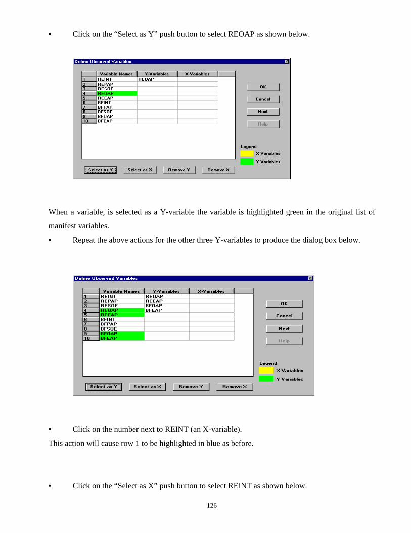
126

• Click on the “Select as Y” push button to select REOAP as shown below.

When a variable, is selected as a Y-variable the variable is highlighted green in the original list of

manifest variables.

• Repeat the above actions for the other three Y-variables to produce the dialog box below.

• Click on the number next to REINT (an X-variable).

This action will cause row 1 to be highlighted in blue as before.

• Click on the “Select as X” push button to select REINT as shown below.

127

• Repeat the above actions for the other five X-variables.

The above actions will produce the “Define Observed Variables” dialog box below.

• Click on the “Next” push button to load the “Define Latent Variables” dialog box below.

• Click on the number next to the latent variable “REAMB”.

• Click on the “Select Eta” push button to select REAMB as an Eta-variable.

128

The above actions produce the “Define Latent Variables” dialog box below.

• Repeat the above steps for the latent variable BFAMB.

The above actions produce the “Define Latent Variables” dialog box below.

• Click on the “Next” push button to load the “Model Parameters” dialog box below.

• Select the “Lambda-Y Full Matrix Fixed” option in the "Model Summary" menu field of the

“Model Parameters" dialog box.

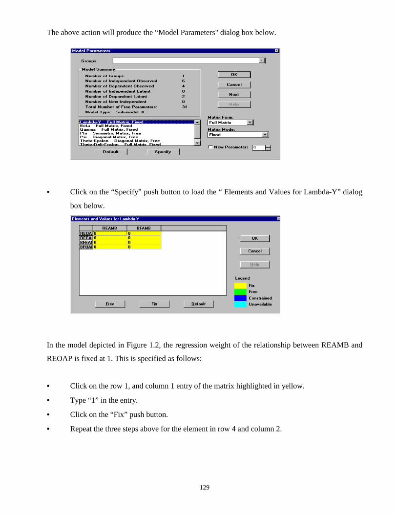
129

The above action will produce the “Model Parameters" dialog box below.

• Click on the “Specify” push button to load the “ Elements and Values for Lambda-Y” dialog

box below.

In the model depicted in Figure 1.2, the regression weight of the relationship between REAMB and

REOAP is fixed at 1. This is specified as follows:

• Click on the row 1, and column 1 entry of the matrix highlighted in yellow.

• Type “1” in the entry.

• Click on the “Fix” push button.

• Repeat the three steps above for the element in row 4 and column 2.

130

• Click on the “OK” push button to load the “ Elements and Values for Lambda-Y” dialog box

below.

In the model depicted in Figure 1.2, the regression weight of the relationship between REAMB and

REEAP is a free parameter to be estimated. This is specified as follows:

• Click on the row 2 and column 1 entry.

• Click on the “Free” push button.

These actions highlights the row 2 and column 1 entry in green colour, indicating that it is now a free

parameter to be estimated in the analysis.

• Repeat the above steps for the row 3 and column 2 entry.

• Click on the “OK” push button to load the “ Elements and Values for Lambda-Y” dialog box

below.

• Click on the “OK” push button to reload the “Model Parameters" dialog box.

131

• Select the “Beta Full Matrix, Fixed” option from the "Model Type" menu field of the “Model

Parameters" dialog box as shown below.

• Click on the “Specify” push button to load the “Elements and Values for Beta” dialog box

below.

For the model depicted in Figure1.2, the regression weight for the relationship between BFAMB and

REAMB is to be estimated. This free parameter is specified as follows:

• Click on the row 2 and column 1 entry.

• Click on the “Free” push button.

132

The above actions produce the “Elements and Values for Beta” dialog box below.

• Repeat the two steps above for the entry in row 1 and column 2.

• Click on the “OK” push button to load the “Elements and Values for Beta” dialog box below.

• Click on the “OK” push button to reload the “Model Parameters” dialog box.

The other parameter matrices can be specified in the a similar way as described for the Lambda-Y

and the Beta matrices.

133

• Click on the “Next” push button after the last parameter matrix for the model has been

specified to load the “Constraints” dialog box below.

In the Beta matrix, the elements BE(1,2) and BE(2,1) are constrained to be equal. This is specified as

follows:

• Click on the “EQ” push button of the “Constraints” dialog box to produce the “Constraints”

dialog box below.

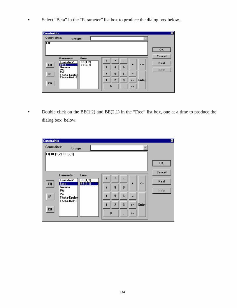
134

• Select “Beta” in the “Parameter” list box to produce the dialog box below.

• Double click on the BE(1,2) and BE(2,1) in the “Free” list box, one at a time to produce the

dialog box below.

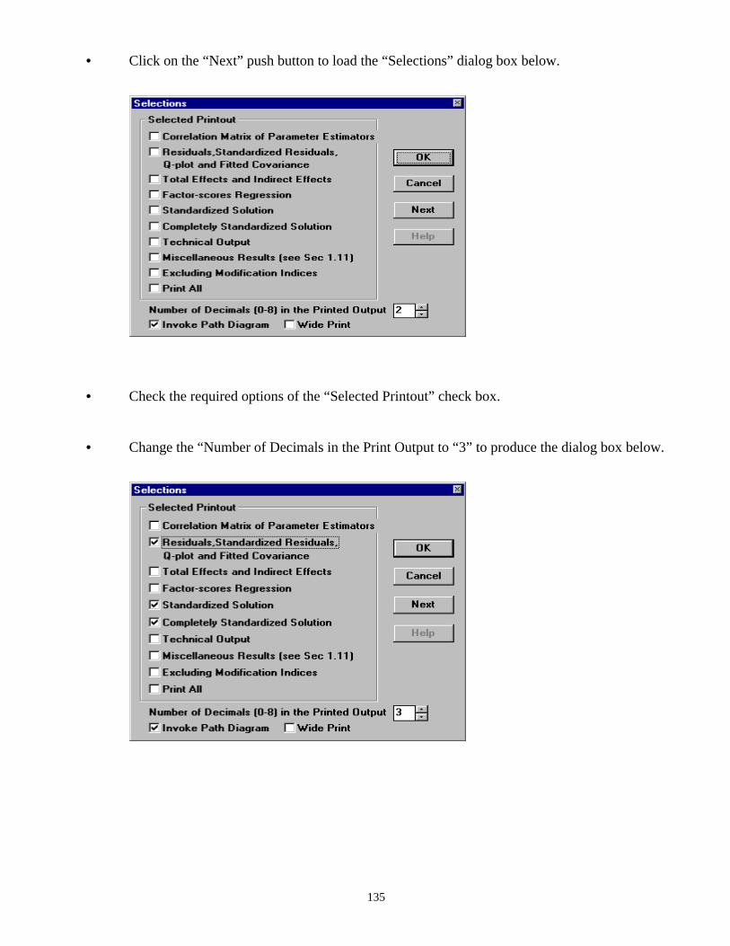
135

• Click on the “Next” push button to load the “Selections” dialog box below.

• Check the required options of the “Selected Printout” check box.

• Change the “Number of Decimals in the Print Output to “3” to produce the dialog box below.

136

• Click on the “Next” push button to load “Save matrices” dialog box below.

• Check the desired check boxes to produce the dialog box below.

• Click on the “OK” push button to open the “LISREL Windows Application” window below.

137

4.4.2 CREATING SIMPLIS SYNTAX FILES INTERACTIVELY

LISREL 8.30 for Windows allows the user to create SIMPLIS syntax interactively by making use of

a text window and keypad dialog box.

The following steps should be followed to open this window and keypad dialog box.

• Double click on the LISREL 8.30 icon

• Click on the “File” menu to load the file menu box.

• Click on the “New” option from the menu box to open a “New” dialog box.

• Select the “SIMPLIS Project” option from the “New” dialog box.

• Click on the “OK” push button to load the “File Save As” dialog box.

• Give the “SIMPLIS Project” a filename and save the file.

• Click on the “OK” push button to open the text window and dialog box shown below.

Clicking (left mouse button) on the appropriate symbol operates the keypad. Note that the <==

symbol represents the backspace key while the symbol <--| denotes the enter key.

To enter the descriptive names of the variables of the model you have to do the following (See

Section 4.4.1).

• Click on the “Setup” menu to load a “Setup” menu box.

• Click on the “Title and Comments” option of the “Setup” menu to load a “Title and

Comments” dialog box.

138

• Type the title and comments in the “Title” string and “Comments” string fields respectively.

• Continue with similar steps as described in Section 4.4.1 to enter the descriptive names of the

variables of the model to produce the window shown below.

• Click on the “Setup” menu again to reload the “Setup” menu box below.

• Click on the “Build SIMPLIS Syntax” option of the “Setup” menu to open the text window

below.

The skeleton model in the text window would enable you to put the paths, covariances and variances

at the correct section of the input file.

139

To specify a relationship, for example, between two variables “REAMB” and “REOAP”, you may

do the following:

• Click on “REOAP”.

• Hold and drag it to the section of the input file in the text window headed “Relationships”

and drop it.

• Put the cursor after the variable.

• Click on the “=” push button.

• Click on “REAMB”.

• Hold and drag it to the right hand side of the “=” sign and drop it.

• Follow similar steps to those described above to specify the other relationships and the

covariances or variances of the model.

4.4.3 CREATING LISREL/SIMPLIS SYNTAX USING PATH

DIAGRAMS A path diagram is a graphical representation of the relationships among variables in the LISREL

model. If drawn and labeled correctly and in sufficient details, the diagram can specify exactly the

fixed, constrained or free status of all parameters in the model.

GENERAL RULES FOR DRAWING PATH DIAGRAMS

• The observed x- and y- variables are enclosed in boxes.

• The latent variables ξ and η are enclosed in circles or ellipses.

• The error variables ε , δ , and ζ appear in the diagram but are not enclosed.

• A one-way arrow between two variables indicates a postulated direct influence of one

variable on another. A two-way arrow between two variables indicates that these variables

are correlated without any assumed direct relationship. One-way arrows are drawn straight,

while two-way arrows are generally curved.

• There are a fundamental distinction between independent variables (ξ -variables) and

dependent variables ( η -variables). Variation and covariation in the dependent variables is

140

to be accounted for or explained by the independent variables. In a path diagram this

corresponds to the statements,

1 no one-way arrow can point to a ξ -variable;

2 all one-way arrows pointing to an η -variable come from ξ - and η -variables.

• All direct influences of one variable on another must be included in the path diagram. The

non-existence of an arrow between two variables means that the two variables are assumed

not to be directly related.

4.4.4 DRAWING A PATH DIAGRAM INTERACTIVELY IN LISREL 8.30

FOR WINDOWS FOR THE DUNCAN, HALLER AND PORTES’

APPLICATION

LISREL 8.30 includes features, which allows a user to interactively draw a path diagram for a model

to be analyzed. The step by step ways of doing this for the Duncan, Haller and Portes’ example is

described in details below.

• Double click on the LISREL8.30 icon

to open the window with part shown below.

• Click on the "File" menu to load the menu box below.

141

• Click on the "New" option of the "File" menu to load the “New” dialog box shown below.

• Select the "Path Diagram" option to produce the dialog box shown below.

• Click on the "OK" push button to load the "File Save AS" dialog box shown below.

142

• Type the file name "pepdhp.pth" in the "File name" string field of the "File Save As" dialog

box to produce the dialog box shown below.

• Click on the "OK" push button to open the windows shown below.

• Click on the "Setup" menu to load the menu box below.

• Click on the "Title and Comments" option of the "Setup" menu to load the “Title and

Comments” dialog box below.

143

• Type the title, "DUNCAN HALLER AND PORTES' APPLICATION", in the "Title" string

field.

• Type comments, if any, in the "Comments" string filed to produce the "Title and Comments"

dialog box below.

• Click on the "Next" push button to load the "Group Names" dialog box below.

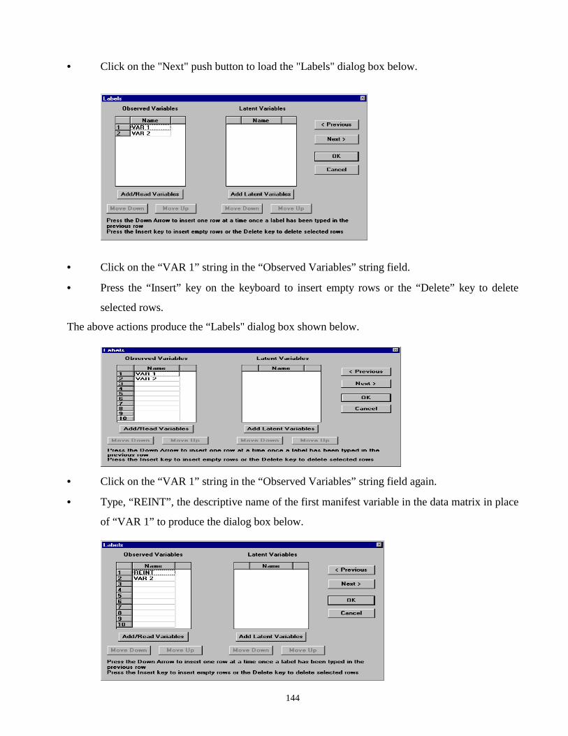
144

• Click on the "Next" push button to load the "Labels" dialog box below.

• Click on the “VAR 1” string in the “Observed Variables” string field.


selected rows.


• Click on the “VAR 1” string in the “Observed Variables” string field again.

• Type, “REINT”, the descriptive name of the first manifest variable in the data matrix in place

of “VAR 1” to produce the dialog box below.

145

• Press the “Down” arrow on the keyboard to insert one row at a time once a label has been

typed in the previous row.


• Click on the “Name” push button under the “Latent Variables” string field in the “Labels”

dialog box.


selected rows.

• Type the descriptive latent variable names in the same way as for the manifest variables.


• Click on the “Next” push button to load the “Data” dialog box below.

146

• In the “Statistics form” menu filed select “Correlations”.

• In the “File Type” menu field select “LISREL System Data”.

• In the “Filename” string field, type the filename or click on the Browse button to locate the

required data file.

• Type the number of observations, “329” , in the “Number of observations” string field.

• In the “Matrix to be analysed ” menu field select “Correlations”.

The above actions produce the “Data” dialog box below.

• Click on the “OK” push button to open the “LISREL Windows Application” window.

• Click on the radio buttons next to the indicators of endogenous latent variables and other

endogenous manifest variables (y-variables) and also the radio buttons next to the eta-

variables.

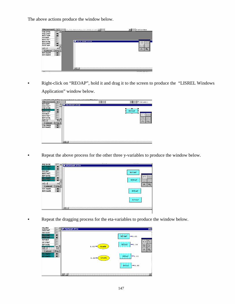
147

The above actions produce the window below.

• Right-click on “REOAP”, hold it and drag it to the screen to produce the “LISREL Windows

Application” window below.

• Repeat the above process for the other three y-variables to produce the window below.

• Repeat the dragging process for the eta-variables to produce the window below.

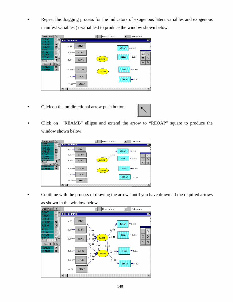
148

• Repeat the dragging process for the indicators of exogenous latent variables and exogenous

manifest variables (x-variables) to produce the window shown below.

• Click on the unidirectional arrow push button

• Click on “REAMB” ellipse and extend the arrow to “REOAP” square to produce the

window shown below.

• Continue with the process of drawing the arrows until you have drawn all the required arrows

as shown in the window below.

149

To run the project, you have to follow the same steps as described under Section 4.4.2.

If you did not specify the options and keywords under the OU (Output) command, they can be

specified after the drawing of the path diagram. The way to do these are described below.

• Click on the “Output” menu to load the menu box below.

• Click on the “LISREL Output” option of the “Output” menu to load the dialog box below.

• Click on the “Estimations” option to load the “Estimations” dialog box shown below.

• Select the method of estimation by checking the radio button for the appropriate method.

150

• Click on the “OK” push button to reopen the graphics window below.


• Click on the “LISREL Output” option of the “Output” menu to load the dialog box below.

• Click on the “Selections” option to load the “Selections” dialog box shown below.

151

• Select the required options of the “Selected Printout" by checking the check box for the

appropriate option.

• Click on the “OK” push button to reopen the graphics window below.

If the SIMPLIS output is required follow the following steps.


• Click on the “SIMPLIS Output” option of the “Output” menu to load the dialog box below.

152

• Select the required options and keywords and fill in the appropriate numbers in the string

field.

• Click on the “OK” push button to accept the changes and to reopen the window with the path

diagram as described above.

The steps below would enable you to build either the LISREL syntax or the SIMPLIS syntax from

the path diagram drawn prior to running of the analysis.

To obtain the LISREL syntax do the following:

• Click on the “Setup” option to load the menu box below.

• Select the “Build LISREL Syntax” option of the “Setup” menu to open the window below.

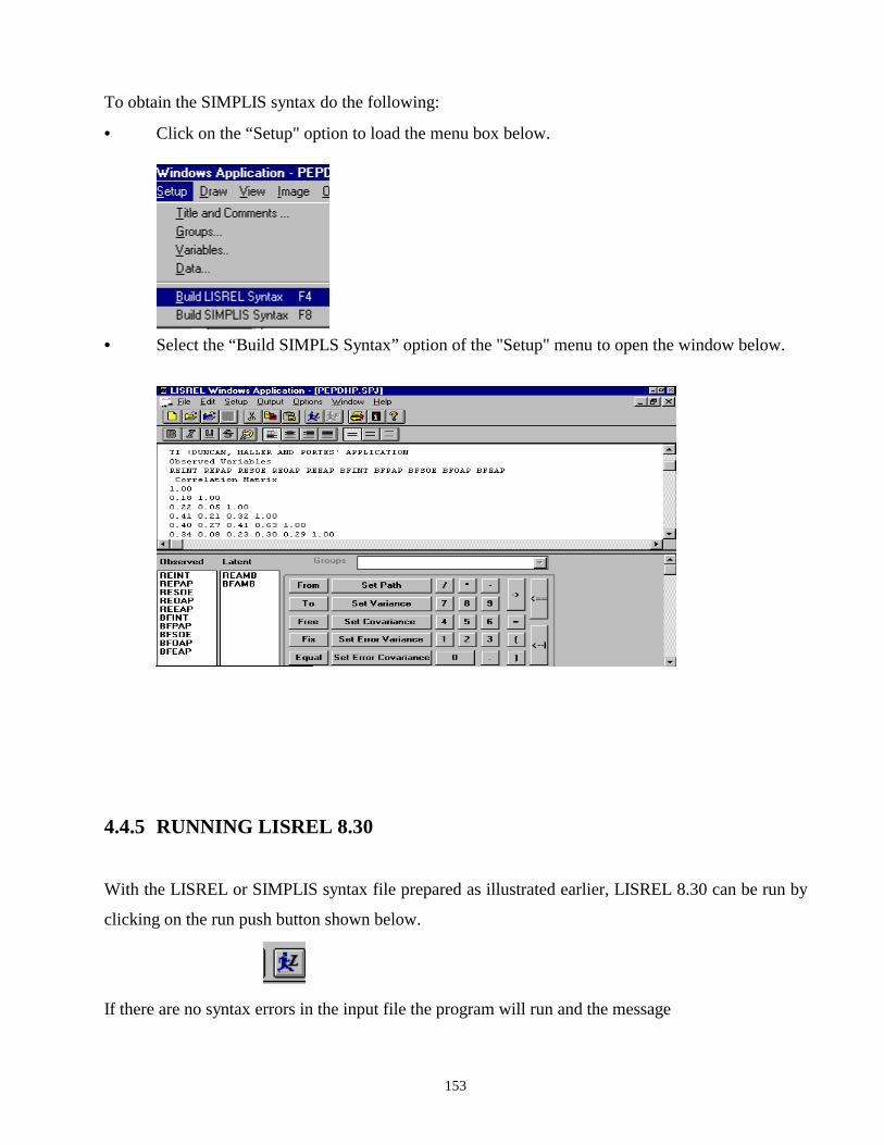
153

To obtain the SIMPLIS syntax do the following:

• Click on the “Setup" option to load the menu box below.

• Select the “Build SIMPLS Syntax” option of the "Setup" menu to open the window below.

4.4.5 RUNNING LISREL 8.30

With the LISREL or SIMPLIS syntax file prepared as illustrated earlier, LISREL 8.30 can be run by

clicking on the run push button shown below.

If there are no syntax errors in the input file the program will run and the message

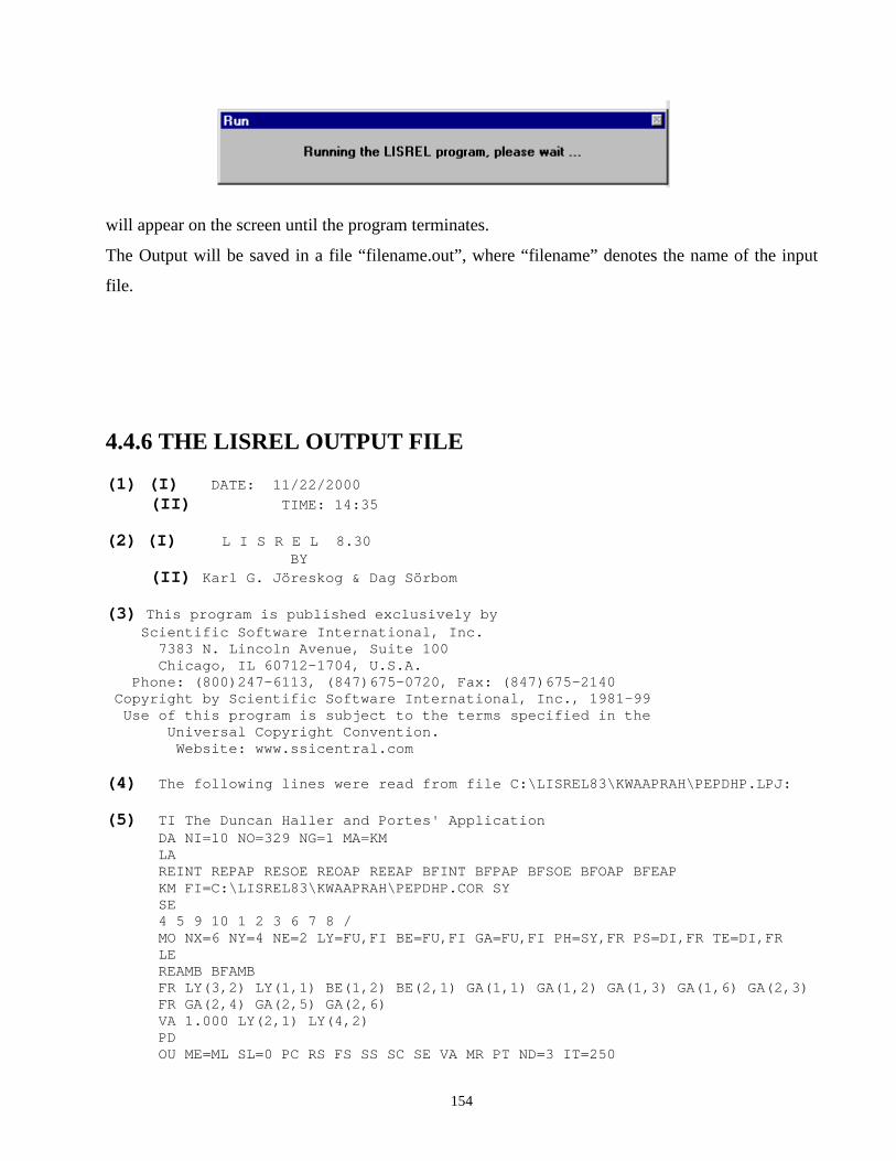
154

will appear on the screen until the program terminates.

The Output will be saved in a file “filename.out”, where “filename” denotes the name of the input

file.

4.4.6 THE LISREL OUTPUT FILE (1) (I) DATE: 11/22/2000

(II) TIME: 14:35 (2) (I) L I S R E L 8.30 BY (II) Karl G. Jöreskog & Dag Sörbom (3) This program is published exclusively by Scientific Software International, Inc. 7383 N. Lincoln Avenue, Suite 100 Chicago, IL 60712-1704, U.S.A. Phone: (800)247-6113, (847)675-0720, Fax: (847)675-2140 Copyright by Scientific Software International, Inc., 1981-99 Use of this program is subject to the terms specified in the Universal Copyright Convention. Website: www.ssicentral.com (4) The following lines were read from file C:\LISREL83\KWAAPRAH\PEPDHP.LPJ: (5) TI The Duncan Haller and Portes' Application DA NI=10 NO=329 NG=1 MA=KM LA REINT REPAP RESOE REOAP REEAP BFINT BFPAP BFSOE BFOAP BFEAP KM FI=C:\LISREL83\KWAAPRAH\PEPDHP.COR SY SE 4 5 9 10 1 2 3 6 7 8 /

MO NX=6 NY=4 NE=2 LY=FU,FI BE=FU,FI GA=FU,FI PH=SY,FR PS=DI,FR TE=DI,FR LE REAMB BFAMB

FR LY(3,2) LY(1,1) BE(1,2) BE(2,1) GA(1,1) GA(1,2) GA(1,3) GA(1,6) GA(2,3) FR GA(2,4) GA(2,5) GA(2,6) VA 1.000 LY(2,1) LY(4,2) PD OU ME=ML SL=0 PC RS FS SS SC SE VA MR PT ND=3 IT=250

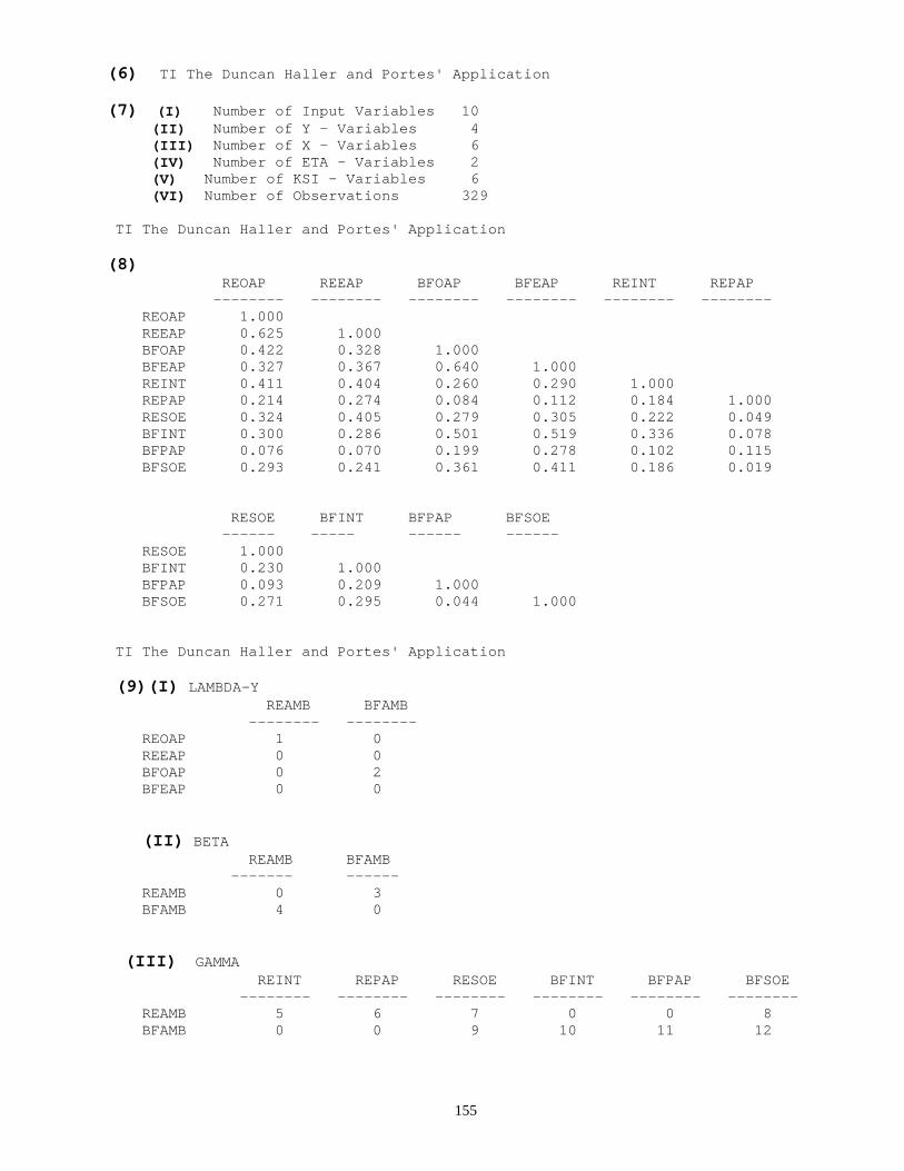
155

(6) TI The Duncan Haller and Portes' Application (7) (I) Number of Input Variables 10 (II) Number of Y - Variables 4 (III) Number of X - Variables 6 (IV) Number of ETA - Variables 2 (V) Number of KSI - Variables 6 (VI) Number of Observations 329 TI The Duncan Haller and Portes' Application (8) REOAP REEAP BFOAP BFEAP REINT REPAP -------- -------- -------- -------- -------- -------- REOAP 1.000 REEAP 0.625 1.000 BFOAP 0.422 0.328 1.000 BFEAP 0.327 0.367 0.640 1.000 REINT 0.411 0.404 0.260 0.290 1.000 REPAP 0.214 0.274 0.084 0.112 0.184 1.000 RESOE 0.324 0.405 0.279 0.305 0.222 0.049 BFINT 0.300 0.286 0.501 0.519 0.336 0.078 BFPAP 0.076 0.070 0.199 0.278 0.102 0.115 BFSOE 0.293 0.241 0.361 0.411 0.186 0.019 RESOE BFINT BFPAP BFSOE ------ ----- ------ ------ RESOE 1.000 BFINT 0.230 1.000 BFPAP 0.093 0.209 1.000 BFSOE 0.271 0.295 0.044 1.000 TI The Duncan Haller and Portes' Application (9)(I) LAMBDA-Y REAMB BFAMB -------- -------- REOAP 1 0 REEAP 0 0 BFOAP 0 2 BFEAP 0 0 (II) BETA REAMB BFAMB ------- ------ REAMB 0 3 BFAMB 4 0 (III) GAMMA REINT REPAP RESOE BFINT BFPAP BFSOE -------- -------- -------- -------- -------- -------- REAMB 5 6 7 0 0 8 BFAMB 0 0 9 10 11 12

156

(IV) PHI REINT REPAP RESOE BFINT BFPAP BFSOE -------- -------- -------- -------- -------- -------- REINT 13 REPAP 14 15 RESOE 16 17 18 BFINT 19 20 21 22 BFPAP 23 24 25 26 27 BFSOE 28 29 30 31 32 33 (V) PSI Note: This matrix is diagonal. REAMB BFAMB -------- -------- 34 35 (VI) THETA-EPS REOAP REEAP BFOAP BFEAP -------- -------- -------- -------- 36 37 38 39 TI The Duncan Haller and Portes' Application (10) Number of Iterations = 6 (11)(I) LAMBDA-Y REAMB BFAMB -------- -------- REOAP 0.943 - - (0.080) 11.817 REEAP 1.000 - - BFOAP - - 0.938 (0.071) 13.146 BFEAP - - 1.000 (II) BETA REAMB BFAMB -------- -------- REAMB - - 0.172 (0.086) 1.995 BFAMB 0.191 - - (0.081) 2.365

157

(III) GAMMA REINT REPAP RESOE BFINT BFPAP BFSOE ------ ------ ------ ------ ------ ------ REAMB 0.270 0.174 0.236 - - - - 0.084 (0.044) (0.041) (0.046) (0.050) 6.104 4.274 5.182 1.678 BFAMB - - - - 0.075 0.362 0.139 0.215 (0.047) (0.043) (0.038) (0.043) 1.604 8.400 3.619 5.067 (12) REAMB BFAMB REINT REPAP RESOE BFINT BFPAP BFSOE ------ ------ ----- ------ ------ ----- ------ ------- REAMB 0.661 BFAMB 0.376 0.681 REINT 0.417 0.272 1.000 REPAP 0.254 0.101 0.184 1.000 RESOE 0.379 0.302 0.222 0.049 1.000 BFINT 0.273 0.524 0.336 0.078 0.230 1.000 BFPAP 0.117 0.253 0.102 0.115 0.093 0.209 1.000 BFSOE 0.270 0.400 0.186 0.019 0.271 0.295 0.044 1.000 (13) PHI REINT REPAP RESOE BFINT BFPAP BFSOE ------ ------ ------- ------ ------ ------ REINT 1.000 (0.078) 12.806 REPAP 0.184 1.000 (0.056) (0.078) 3.276 12.806 RESOE 0.222 0.049 1.000 (0.057) (0.055) (0.078) 3.925 0.886 12.806 BFINT 0.336 0.078 0.230 1.000 (0.058) (0.055) (0.057) (0.078) 5.761 1.408 4.059 12.806 BFPAP 0.102 0.115 0.093 0.209 1.000 (0.056) (0.056) (0.055) (0.056) (0.078) 1.840 2.069 1.677 3.705 12.806 BFSOE 0.186 0.019 0.271 0.295 0.044 1.000 (0.056) (0.055) (0.057) (0.058) (0.055) (0.078) 3.314 0.344 4.737 5.124 0.796 12.806

158

(14) PSI Note: This matrix is diagonal. REAMB BFAMB ------ ------- 0.317 0.266 (0.053) (0.045) 6.009 5.868 (15) REAMB BFAMB ------ ------ 0.475 0.563 (16) THETA-EPS REOAP REEAP BFOAP BFEAP ------- ------ ------ ------ 0.412 0.338 0.400 0.318 (0.051) (0.052) (0.046) (0.046) 8.059 6.518 8.629 6.892 (17) REOAP REEAP BFOAP BFEAP ------ ------ ------ ------ 0.588 0.662 0.599 0.681

(18) Goodness of Fit Statistics.

(I) (a) Degrees of Freedom = 16

(b) Minimum Fit Function Chi-Square = 26.833 (P = 0.0434) (c) Normal Theory Weighted Least Squares Chi-Square = 26.197 (P = 0.0513) (d) Estimated Non-centrality Parameter (NCP) = 10.197 (e)90 Percent Confidence Interval for NCP = (0.0 ; 28.315) (II) (a) Minimum Fit Function Value = 0.0818 (b) Population Discrepancy Function Value (F0) = 0.0311 (c) 90 Percent Confidence Interval for F0 = (0.0 ; 0.0863) (d) Root Mean Square Error of Approximation (RMSEA) = 0.0441 (e) 90 Percent Confidence Interval for RMSEA = (0.0 ; 0.0735) (f) P-Value for Test of Close Fit (RMSEA < 0.05) = 0.591 (III) (a) Expected Cross-Validation Index (ECVI) = 0.318 (b) 90 Percent Confidence Interval for ECVI = (0.287 ; 0.373) (c) ECVI for Saturated Model = 0.335 (d) ECVI for Independence Model = 2.691 (IV) (a) Chi-Square for Independence Model with 45 Degrees of Freedom = 862.637 (b) Independence AIC = 882.637 (c) Model AIC = 104.197 (d) Saturated AIC = 110.000

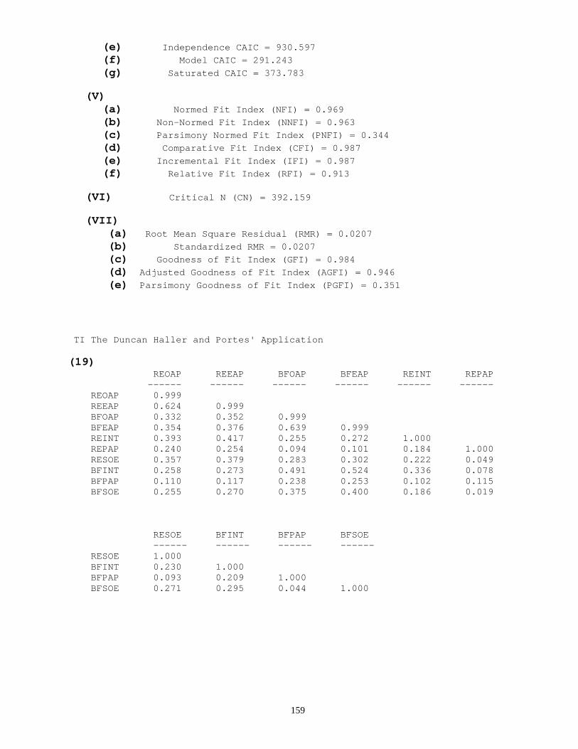
159

(e) Independence CAIC = 930.597 (f) Model CAIC = 291.243 (g) Saturated CAIC = 373.783 (V) (a) Normed Fit Index (NFI) = 0.969 (b) Non-Normed Fit Index (NNFI) = 0.963 (c) Parsimony Normed Fit Index (PNFI) = 0.344 (d) Comparative Fit Index (CFI) = 0.987 (e) Incremental Fit Index (IFI) = 0.987 (f) Relative Fit Index (RFI) = 0.913 (VI) Critical N (CN) = 392.159 (VII) (a) Root Mean Square Residual (RMR) = 0.0207 (b) Standardized RMR = 0.0207 (c) Goodness of Fit Index (GFI) = 0.984 (d) Adjusted Goodness of Fit Index (AGFI) = 0.946 (e) Parsimony Goodness of Fit Index (PGFI) = 0.351 TI The Duncan Haller and Portes' Application (19) REOAP REEAP BFOAP BFEAP REINT REPAP ------ ------ ------ ------ ------ ------ REOAP 0.999 REEAP 0.624 0.999 BFOAP 0.332 0.352 0.999 BFEAP 0.354 0.376 0.639 0.999 REINT 0.393 0.417 0.255 0.272 1.000 REPAP 0.240 0.254 0.094 0.101 0.184 1.000 RESOE 0.357 0.379 0.283 0.302 0.222 0.049 BFINT 0.258 0.273 0.491 0.524 0.336 0.078 BFPAP 0.110 0.117 0.238 0.253 0.102 0.115 BFSOE 0.255 0.270 0.375 0.400 0.186 0.019 RESOE BFINT BFPAP BFSOE ------ ------ ------ ------ RESOE 1.000 BFINT 0.230 1.000 BFPAP 0.093 0.209 1.000 BFSOE 0.271 0.295 0.044 1.000

160

(20)(I) REOAP REEAP BFOAP BFEAP REINT REPAP ------ ------ ------ ------ ------ ------ REOAP 0.001 REEAP 0.001 0.001 BFOAP 0.090 -0.024 0.001 BFEAP -0.027 -0.009 0.001 0.001 REINT 0.017 -0.013 0.005 0.018 - - REPAP -0.026 0.020 -0.010 0.011 - - - - RESOE -0.033 0.026 -0.004 0.003 - - 0.000 BFINT 0.042 0.013 0.010 -0.005 - - - - BFPAP -0.034 -0.047 -0.039 0.025 0.000 0.000 BFSOE 0.038 -0.029 -0.014 0.011 - - 0.000 RESOE BFINT BFPAP BFSOE ------ ------ ------ ------ RESOE - - BFINT - - - - BFPAP 0.000 - - - - BFSOE - - - - 0.000 - - (II) (a) Smallest Fitted Residual = -0.047 (b) Median Fitted Residual = 0.000 (c) Largest Fitted Residual = 0.090 (d) - 4|7

- 2|9439764 - 0|430954000000000000000000000 0|11111135011378 2|0568 4|2 6| 8|0 (21)(I) REOAP REEAP BFOAP BFEAP REINT REPAP ------ ------ ------ ------ ------ ------ REOAP 0.464 REEAP 0.464 0.464 BFOAP 3.196 -0.951 0.464 BFEAP -1.092 -0.397 0.464 0.464 REINT 0.916 -0.882 0.132 0.561 - - REPAP -1.054 1.057 -0.256 0.298 - - - - RESOE -1.630 1.630 -0.176 0.176 - - - - BFINT 1.351 0.443 0.639 -0.409 - - - - BFPAP -0.799 -1.141 -1.567 1.333 - - - - BFSOE 1.595 -1.595 -0.690 0.690 - - - - RESOE BFINT BFPAP BFSOE ------ ------ ------ ------ RESOE - - BFINT - - - - BFPAP - - - - - - BFSOE - - - - - - - - (II)(a) Smallest Standardized Residual = -1.630 (b) Median Standardized Residual = 0.000

(c) Largest Standardized Residual = 3.196

161

(d) - 1|666 - 1|1110 - 0|987 - 0|4432000000000000000000000 0|1234 0|5555556679 1|134 1|66 2| 2| 3|2

(e) Residual for BFOAP and REOAP 3.196 (22) 3.5.......................................................................... . .. . . . . . . . . . . . . . . . . . . . . . . . . . . . . . x . . . . . .x . . . x . N . . x . o . .x x . r . x . m . xx . a . xx . l . * . . . * . Q . . * . u . . x x . a . .x x . n . x x . t . x .x . i . xx. . l . x . e . xx . s . .x . . x . . . x. . . . . . . x . . . . . . . . . . . . . . . . . . . . . . . . . -3.5.......................................................................... -3.5 3.5 Standardized Residuals

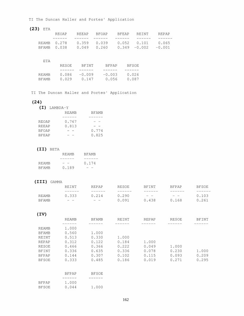
162

TI The Duncan Haller and Portes' Application (23) ETA REOAP REEAP BFOAP BFEAP REINT REPAP ------ ------ ------ ------ ------ ------ REAMB 0.278 0.359 0.039 0.052 0.101 0.065 BFAMB 0.038 0.049 0.260 0.349 -0.002 -0.001 ETA RESOE BFINT BFPAP BFSOE ------ ------ ------ ------ REAMB 0.086 -0.009 -0.003 0.026 BFAMB 0.029 0.147 0.056 0.087 TI The Duncan Haller and Portes' Application (24) (I) LAMBDA-Y REAMB BFAMB ------ ------ REOAP 0.767 - - REEAP 0.813 - - BFOAP - - 0.774 BFEAP - - 0.825 (II) BETA REAMB BFAMB ------ ------ REAMB - - 0.174 BFAMB 0.189 - -

(III) GAMMA REINT REPAP RESOE BFINT BFPAP BFSOE ------ ------ ------ ------ ------ ------ REAMB 0.333 0.214 0.290 - - - - 0.103 BFAMB - - - - 0.091 0.438 0.168 0.261 (IV) REAMB BFAMB REINT REPAP RESOE BFINT ------ ------ ------ ------ ------ ------ REAMB 1.000 BFAMB 0.560 1.000 REINT 0.513 0.330 1.000 REPAP 0.312 0.122 0.184 1.000 RESOE 0.466 0.366 0.222 0.049 1.000 BFINT 0.336 0.635 0.336 0.078 0.230 1.000 BFPAP 0.144 0.307 0.102 0.115 0.093 0.209 BFSOE 0.333 0.485 0.186 0.019 0.271 0.295 BFPAP BFSOE ------ ------ BFPAP 1.000 BFSOE 0.044 1.000

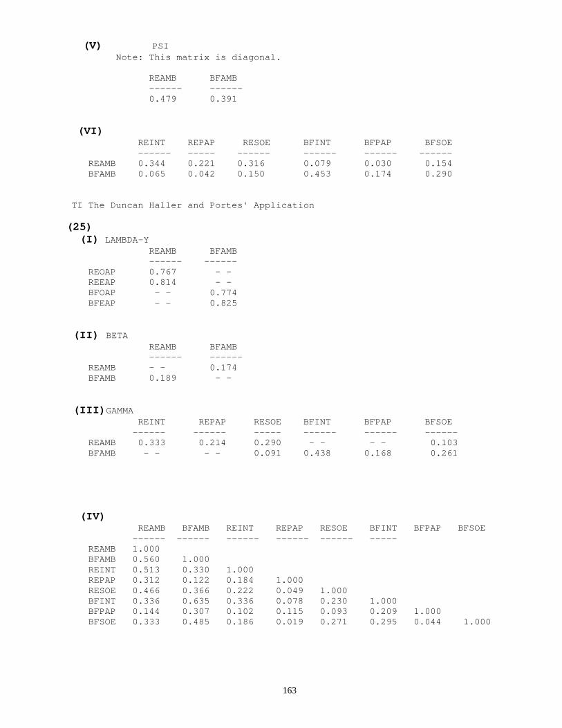
163

(V) PSI Note: This matrix is diagonal. REAMB BFAMB ------ ------ 0.479 0.391 (VI) REINT REPAP RESOE BFINT BFPAP BFSOE ------ ----- ------ ------ ------ ------ REAMB 0.344 0.221 0.316 0.079 0.030 0.154 BFAMB 0.065 0.042 0.150 0.453 0.174 0.290 TI The Duncan Haller and Portes' Application (25) (I) LAMBDA-Y REAMB BFAMB ------ ------ REOAP 0.767 - - REEAP 0.814 - - BFOAP - - 0.774 BFEAP - - 0.825 (II) BETA REAMB BFAMB ------ ------ REAMB - - 0.174 BFAMB 0.189 - - (III)GAMMA REINT REPAP RESOE BFINT BFPAP BFSOE ------ ------ ----- ------ ------ ------ REAMB 0.333 0.214 0.290 - - - - 0.103 BFAMB - - - - 0.091 0.438 0.168 0.261 (IV) REAMB BFAMB REINT REPAP RESOE BFINT BFPAP BFSOE ------ ------ ------ ------ ------ ----- REAMB 1.000 BFAMB 0.560 1.000 REINT 0.513 0.330 1.000 REPAP 0.312 0.122 0.184 1.000 RESOE 0.466 0.366 0.222 0.049 1.000 BFINT 0.336 0.635 0.336 0.078 0.230 1.000 BFPAP 0.144 0.307 0.102 0.115 0.093 0.209 1.000 BFSOE 0.333 0.485 0.186 0.019 0.271 0.295 0.044 1.000

164

(V) PSI Note: This matrix is diagonal. REAMB BFAMB ------ ------ 0.479 0.391 (VI) THETA-EPS REOAP REEAP BFOAP BFEAP ------ ------ ------ ------ 0.412 0.338 0.401 0.319 (VII) REINT REPAP RESOE BFINT BFPAP BFSOE ------ ------ ------ ------ ------ ------ REAMB 0.344 0.221 0.316 0.079 0.030 0.154 BFAMB 0.065 0.042 0.150 0.453 0.174 0.290 (26) The Problem used 27712 Bytes (= 0.0% of Available Workspace) (27) Time used: 0.879 Seconds

ENTRIES OF THE LISREL OUTPUT FILE

(1) (I) Date on which the analysis was performed.

(II) Time at which the analysis was performed.

(2) (I) Name and the version of the program.

(II) The authors of the program.

(3) The details of the company which handles the sales and distribution of LISREL 8.30.

(4) The complete path and filename of the file containing the data to be analyzed.

(5) Reproduction of the LISREL input file used for the analysis.

(6) Repeat of the Title Statement (This appears first on each new page).

(7) Row (I) The number of input variables.

Row (II) The number of endogenous manifest variables.

Row (III) The number of exogenous manifest variables.

Row (IV) The number of endogenous latent variables.

165

Row (V) The number of exogenous latent variables.

Row (VI) The number of observations or cases.

(8) (I) Correlation matrix to be analyzed.

(9) Parameter Specifications.

(I) Specifications of the order in which the elements of the Lambda-Y matrix are

specified.

(II) Specifications of the order in which the elements of the Beta matrix are specified.

(III) Specifications of the order in which the elements of the Gamma matrix are specified.

(IV) Specifications of the order in which the elements of the Phi matrix are specified.

(V) Specifications of the order in which the elements of the Psi matrix are specified.

(VI) Specifications of the order in which the elements of the Theta-Eps matrix are

specified.

(10) Number of iterations the program went through before reaching a local minimum.

(11) LISREL Estimates (Maximum Likelihood).

(I) The estimated values, standard error estimates and t-test statistic values for the

unknown elements of the Lambda-Y matrix.

(II) The estimated values, standard error estimates and t-test statistic values for the

unknown elements of the Beta matrix.

(III) The estimated values, standard error estimates and t-test statistic values for the

unknown elements of the Gamma matrix.

(12) The estimated values of the Covariance Matrix between the ETA and KSI-variables.

(13) The estimated values, standard error estimates and t-test statistic values for the unknown

elements of the PHI matrix.


elements of the PSI matrix.

(15) The Squared Multiple Correlations for the Structural Equations.


elements of the THETA-EPS matrix.

(17) The Squared Multiple Correlations for the Y-Variables.

The squared multiple correlation for the i-th Y-variable is given by:

1−∃∃θσ

ii

ii

166

where ∃θ ii is the estimated error variance and ∃σ ii is the estimated total variance of the i-th

Y-variable.

(18) Goodness of Fit Statistics.

(I) (a) Degrees of Freedom, d, is given by:

d k k t= + −12

1( )

where k being the number of observed variables analyzed and t the number of free

parameters.

(b) Minimum Fit Function Chi-square value, is obtained from

c nF=

−

∑S,^θ

which is approximately distributed as χ 2 with d degrees of freedom, where n=N-1, F

is the fit function, S is the sample covariance matrix , ( )θ−

∑ the population covariance

matrix and θ−

is the vector of the t parameters in the statistical model.

(c) Normal Theory Weighted Least Squares Chi-Square test statistic value, given by

( )χWLS WLSN F2 1= − ∃

where ∃FWLS is the minimum value for FWLS with

( ) ( )

( )( )F S W S

W S S

WLS

g

k

h

g

i

kgh ij

gh gh ij ijj

i

= − −

= − −

−

= = = =∑ ∑ ∑ ∑

σ σ

σ σ

'

'

1

1 1 1 1

where ( )S s s s s skk−=' , , , ,...,11 21 22 31 is a vector of the elements in the lower half including

the diagonal, of the covariance matrix S,

( )σ σ σ σ σ σ' , , , ,...,−

= 11 21 22 31 kk

is the vector of corresponding elements of ( )θ−

∑ reproduced from the model

parameter vector θ−

and

W gh ij, is a typical element of the positive definite matrix W −1 . W is a consistent

estimate of the asymptotic covariance matrix of the sample variances and covariances.

167

(d) Estimated Non-centrality Parameter (NCP), is given by (Browne and Cudeck, 1993):

NCP= ∃λ = max( , )c d− 0

(e) 90% confidence interval for the NCP is obtained by solving for ∃λ L and ∃λ U from the

equations below:

( )G c dL\ , .λ = 0 95 and ( )G c dU\ , .λ = 0 05

where ( )G x d\ ,λ is the distribution function of the non-central chi-square distribution

with non-centrality parameter λ and d degrees of freedom.

(II)

(a) The Minimal Discrepancy Function Value

This is the minimal value of the discrepancy function F(S, ( )θ−

∑ ),

where S is the sample covariance matrix, θ−

contains the unknown parameters of the

Structural Equation Model and ( )θ−

∑ is the structural model for the population

covariance matrix ∑ .

(b) The Estimated Population Discrepancy Function Value, ∃FO , is given by (McDonald,

1989; Browne and Cudeck, 1993):

( ){ }∃ ∃ / ,F Max F d nO = − 0

where ∃F is the minimum value of the fit function.

(c) The 90% confidence interval for ∃FO is calculated as:

∃

;∃λ λL U

n n

.

(d) The Root Mean Square Error of Approximation (RMSEA) value. It is obtained by

(Browne & Cudeck, 1993):

ε =∃FdO

(e) The 90% confidence interval for the RMSEA value is calculated as:

∃

;∃λ λKL U

nd nd

168

(f) The p-value for a lower tail test for close fit is calculated as (Browne & Cudeck,

1993):

( )p G c nd d= −1 0 0025\ . ,

(III)

(a) The Expected Cross Validation Index (ECVI) is given as (Browne & Cudeck, 1989):

ECVI= cn

tn

+

2 .

(b) The 90% confidence interval for the ECVI is computed a:

∃;

∃λ λL Us tn

s tn

+ + + +

(c) The ECVI value for Saturated Model. This is when the ECVI value is calculated with

no structure imposed on ∑ .

(d) The ECVI value for the Independence Model.

(IV)

(a) The Independence model chi-square is given by

Independence model χ 2 = N ∃FI .

where ∃FI denotes the minimal discrepancy function value for the independence

model and N denotes the number of cases. (b) The Independent Akaike’s Information Criterion (AIC) is given by

Independence AIC = Independence model χ 2 - 2dI

where dI denotes the degrees of freedom of the independence model.

(c) The model Akaike’s Information Criterion (AIC) is given by (Akaike, 1974, 1987):

Model AIC = c-2t

(d) The Saturated AIC is given by

Saturated AIC = k(k+1)

(e) The Independence Cross-validated Akaike’s Information Criterion (CAIC) is given

by (Bozdogan,1987):

Independence CAIC = Independence model χ 2 - (In N + 1)di

(f) The model Cross-validated Akaike Information Criterion (CAIC) is given by

(Bozdogan,1987):

169

Model CAIC = c + (1+InN)t.

(g) The Saturated CAIC is given by

Saturated CAIC = (lnN +1)[ k(k+1)]

(V)

(a) The Bentler-Bonett Normed Fit Index is computed from (Bentler and Bonett, 1980):

NFI =1−∃∃FFI

(b) The Non-Normed Fit Index (NNFI) is computed as (Bentler & Bonett, 1980):

NNFI = ∃ ∃∃

f ffI

I

−−1

where ∃f = nFd

∃, and ∃f I = nF

dI

∃

(c) The Parsimony Fit Index (PNFI) is computed as (James, Mulaik, and Brett, 1982):

PNFI = dd

FFi i

−

1

∃∃

where d the degrees of freedom for the estimated model.

(d) The Comparative Fit Index (CFI) is computed as (Bentler, 1990):

CFI =1- ∃∃ττ I

where ∃τ =max( nF∃ – d, 0) and ∃τ I = max ( )nF d nF dI I∃ , ∃ ,− − 0

(e) The Incremental Fit Index (IFI) is computed as (Bollen, 1986, 1989a,b):

IFI = nF nFnF d

I

I

∃ ∃∃

−−

(f) The Relative Fit Index (RFI) is computed as (Bollen, 1986, 1989a,b):

RFI = ∃ ∃

∃f f

fI

I

−

(VI) The Critical N (CN) value is computed as (Hoelter, 1983):

CN = χ α12

1− +∃F

where χ α12− is the 100(1-α )th percentile of the chi-square distribution with d

degrees of freedom.

170

(VII)

(a) The Root Mean Square Residual(RMR) is computed from (Bentler, 1995)

RMR = ( ) ( )21

2

11k k ij ijj

i

i

p

+−

−==

∑∑ S g ∃θ

(b) The Standardized Root Mean Squared Residual(SRMR) is computed as

(Bentler, 1995)

SRMR = 21

2

11k ks g s sij ij ii jj

j

i

i

p

( )/

+−

−

∧

==∑∑ θ

(c) The Goodness of Fit Index (GFI) is computed as (Jöreskog and Sörbom, 1989):

GFI = 1 - ( )[ ]( )[ ]

F

F

S

S 0

, ∃

,

θ∑∑

(d) The Adjusted Goodness of Fit Index (AGFI) is given by (Jöreskog and Sörbom,

1989): AGFI = 1 - ( )k kd+1

2(1 – GFI)

(e) The Parsimony Normed Fit Index (PGFI) is computed as (Mulaik, et al; 1989):

PGFI = ( )2 1dk

k + GFI

(19) The fitted Covariance Matrix. This is the covariance matrix calculated from the

model by using the final parameters estimated as the parameter values of the model.

(20)

(I) The fitted residuals. This is the matrix of the difference between the sample

covariance matrix (the sample moment matrix) and the fitted covariance matrix.

(II) The summary statistics for the fitted residuals.

(a) Smallest Fitted Residual.

(b) Median Fitted Residual.

(c) Largest Fitted Residual.

(d) The steam-and-leaf plot of the fitted residuals.

(21)

(I) Standardized Residuals. These are fitted residuals divided by the largest sample

standard error of the residuals.

(II) Summary statistics for standardized residuals.

171

(a) Smallest standardized residual.

(b) Medium standardized residual.

(c) Largest standardized residual.

(d) The stem-and-leaf plot of the standardized residuals.

(e) The largest positive standardized residuals.

(22) Q-plot of standardized residuals.

(23) Factor Scores Regressions.

These are estimates of the measurement strengths of the manifest variables as

measurements of the two latent variables.

(24) Standardized solution. The parameters are estimated with the condition that the latent

variables are scaled to have standard deviations equal to unity.

(I) The standardized estimates of the elements of the Lambda-Y matrix.

(II) The standardized estimates of the elements of the Beta matrix.

(III) The standardized estimates of the elements of the Gamma matrix.

(IV) Correlation matrix of exogenous manifest variables.

(V) The estimates of the elements of the Psi.

(VI) Regression matrix Eta on X (standardized).

(25) Complete standardized solutions. The parameters are estimated with the condition

that the observed as well as the latent variables are standardized.

(I) The completely standardized estimates of the elements of the Lambda-Y matrix.

(II) The completely standardized estimates of the elements of the Beta matrix.

(III) The completely standardized estimates of the elements of the Gamma matrix.

(IV) Correlation matrix of Eta and Ksi variables.

(V) The completely standardized estimates of the elements of the Psi matrix.

(VI) The completely standardized estimates of the elements of the theta Eps matrix.

(VII) Regression matrix of eta on X (standardized)

(26) The disk space taken by the entire problem.

(27) Time, in seconds, used by the program to perform the analysis.

172

CHAPTER 5

Mx


The acronym Mx stands for MatriX algebra interpreter. Michael C. Neal developed the first version

of Mx in 1991. The development of Mx was greatly influenced by LISREL (Jöreskog & Sörbom

1981-1999). The first version was improved upon in 1994. Mx is a combination of a matrix algebra

interpreter and a numerical optimizer. It enables exploration of matrix algebra through a variety of

operations and functions. There are many built-in functions to enable Structural Equation Modeling

and other types of statistical modeling of data. It offers the fitting functions found in commercial

software such as LISREL, LISCOMP, EQS, SEPATH, AMOS and CALIS, including facilities for

maximum likelihood estimation of parameters from missing data structure, under normal theory.

Complex ‘nonstandard’ models are easy to specify. For further general applicability, it allows the

users to define their own fit functions, and optimization may be performed subject to linear and

nonlinear equality or boundary constraints.

There have been other improvements upon the 1994 version. The latest version was released in

1999. The 1999 version has many additional new features. One of the new features is the path

diagram drawing software, RAMPATH. This new feature allows the user to generate the Mx script

by simply drawing the path diagram of the model to be fitted to the data. This has made Mx user-

friendlier, especially, to those who find it difficult to write the Mx script in the matrix language.

Mx is available free of charge from the internet at http://griffin.vcu.edu/mx/. With a suitable browser,

you can obtain the program, documentation and examples, send comments, see the latest version

available for your platform, and so on.

173

5.2 THE Mx INPUT SCRIPT FILE

There are two ways of fitting a structural model to data with Mx. These are:

1) To prepare an Mx Input Script File by using the appropriate Mx commands. The Mx Input

Script File is a text file and can be prepared with any text editor of one’s choice and should

have the extension “.mx”.

2) To use the path diagram drawing software, RAMPATH to draw the path diagram of the

model to be fitted to the data. The path diagram can be saved as a graphics file with

extension “.mxd”. An Mx Input Script file may then be generated from the graphics file.

GENERAL RULES FOR PREPARING Mx INPUT SCRIPT FILES.

• At the beginning of an Mx script, you have to specify how many groups there are with a

#Ngroup statement.

• Input files should be prepared with the text editor of your choice. If you use a word processor

(such as Word Perfect or MS Word) the input file should be saved in DOS text (ASCII)

format.

• The Title line is required.

• The Matrices line is required and starts the declaration of matrices that will be used in the

covariance statement.

• The keyword Specify is used to put free parameters into matrices. All the usable elements of

the matrix are listed (i.e. only the lower triangle for symmetric matrices, or only the diagonal

elements for diagonal matrices)

• A zero indicates that the element of the matrix is fixed, and a positive integer indicates that it

is free. Different positive integers represent different free parameters, i.e. if we wish to have

parameter 1 and 2 set equal, we would replace the 2 with a 1.

• The fixed values of 1 for the variances of the latent variables are given with a Value

statement.

• Start 0.5 all sets all the free parameters to 0.5 as an initial guess of the parameter estimates.

• You may put comments anywhere in your input file by using the character “!” to preceed the

comment.

• Lines in Mx script may be up to 1200 characters long on most systems. The Mx command

processor ignores anything after column 1200.

174

• Mx ignores blank lines.

• The processor is also entirely insensitive to case, except for filenames under UNIX.

• Unless explicitly stated otherwise, the first two letters of a keyword used in Mx script are

sufficient to identify it. Keywords are separated by one or more blank spaces. Once the

program has identify a keyword you can extend it to anything you like as long as it does not

have a blank character in it, so Data and Data_for_all have the same effect.

• Quite often, a keyword has the format KEY= n where n is a numeric value to be input. This is

called a parameter. Mx ignores all (including blanks) non-numeric characters found between

recognition of a parameter and reading a number, so that “NI =100” and “Ninput_vars are

equal to 100” have the same effect.

The exception to this rule is when it encounters a #define’d variable, which it will accept

instead of a number.

• The syntax described for commands follows these conventions:

♣ alternatives are represented by /

♣ optional parameters or keywords are enclosed by {and}

♣ items to be substituted according to the specific application are enclosed by <and>

5.2.1 PREPARING AN Mx INPUT SCRIPT FILE

An Mx input script file consists of three sections, namely: Specify the Data, Specify the Model and

Specify Options.

Details of each part are discussed below. The paragraphs, which may be omitted without causing any

problems, are indicated as (Optional).

(a) SPECIFY THE DATA

The following information are provided under this section.

(i) #NGroup Sentence

Purpose

To specify the Number of Group(s) there are in the Mx input script file. In a multi-

group job, the number for that group must be indicated first before any information is

provided for the group.

175

Syntax

#Ngroup k

where k is an integer.

Example

For the model depicted in Figure 1.2, there is only one group in the script file. This is

specified as follows:

#Ngroup 1

(ii) Title Sentence (Optional)

Purpose

To provide a description for the analysis to be performed.

Syntax

TITLE: “Title”

where “Title” denotes the title as specified by the user.

Example

For the model depicted in Figure 1.2, we may have a title paragraph as follows:

Title The Duncan Haller and Portes’ Application

(iii) Data Sentence

Purpose

To provide the following information: Number of observations, Number of input

variables and the number of group(s) (if the number of groups is not specified

already).

Syntax

Data NObservations=n NInput_variables=p Ngroup=k

where n, p and k are integers indicating the number of observations, observed

variables and groups respectively.

Example

For the model depicted in Figure 1.2, we may have a data paragraph as follows:

Data NObservation =329 NInput_variables=10 Ngroup=1

(iv) Matrix Sentence

Purpose

To provide the data matrix to be analyzed.

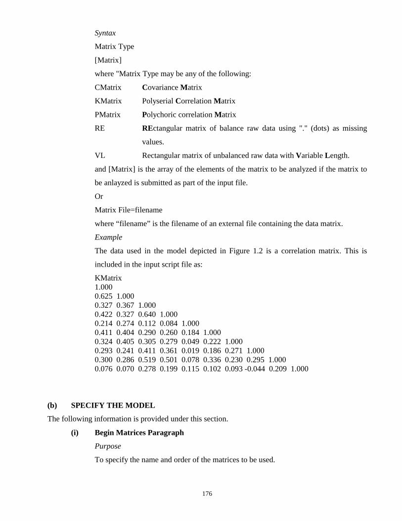
176

Syntax

Matrix Type

[Matrix]

where "Matrix Type may be any of the following:

CMatrix Covariance Matrix

KMatrix Polyserial Correlation Matrix

PMatrix Polychoric correlation Matrix

RE REctangular matrix of balance raw data using "." (dots) as missing

values.

VL Rectangular matrix of unbalanced raw data with Variable Length.

and [Matrix] is the array of the elements of the matrix to be analyzed if the matrix to

be anlayzed is submitted as part of the input file.

Or

Matrix File=filename

where “filename” is the filename of an external file containing the data matrix.

Example

The data used in the model depicted in Figure 1.2 is a correlation matrix. This is

included in the input script file as:

KMatrix 1.000 0.625 1.000 0.327 0.367 1.000 0.422 0.327 0.640 1.000 0.214 0.274 0.112 0.084 1.000 0.411 0.404 0.290 0.260 0.184 1.000 0.324 0.405 0.305 0.279 0.049 0.222 1.000 0.293 0.241 0.411 0.361 0.019 0.186 0.271 1.000 0.300 0.286 0.519 0.501 0.078 0.336 0.230 0.295 1.000 0.076 0.070 0.278 0.199 0.115 0.102 0.093 -0.044 0.209 1.000

(b) SPECIFY THE MODEL

The following information is provided under this section.

(i) Begin Matrices Paragraph

Purpose

To specify the name and order of the matrices to be used.

177

Syntax

Begin Matrices;

<Matrix name 1> <Type 1> <r 1> <c 1>




End Matrices;

where “<Matrix name i>” is any of the following:

S matrix for the Symmetric paths, or double-headed arrows.

A matrix for Asymmetric paths, or single-headed arrows.

F matrix for Filtering the observed variables out of the whole set.

I Identity matrix.

“<Type i>” is either Symmetric (Symm) or Full. If the matrix type is “Symmetric”

only the lower triangle entries are provided. If the matrix type is “Full” all the entries

are to provided.

“<r i>” denotes the number of rows in the matrix and

“<c i>” denotes the number of columns in the matrix.

Example

For the model depicted in Figure 1.2, the RAM model specification requires four

matrices which are specified as follows:

Begin Matrices;

S Symm 18 18

A Full 18 18

F Full 10 18

I Iden 18 18

End Matrices;

(ii) Matrix S Paragraph

Purpose

To provide the entries of the Symmetric paths of the model.

178

Syntax

Matrix S

<c,r>

where c indicates the position of the observed variable in the column from which the arrow

starts and r indicates the position of the observed variable in the row at which the arrow ends.

Example

For the model depicted in Figure 1.2, the two manifest variables “REINT” and “RESOE” are

connected by a double-headed arrow as shown Figure 5.1 below.

Figure 5.1 Covariance path between REINT and RESOE.

In the list of variables “REINT” and “RESOE” are in the 6th and 7th positions respectively.

The entry in Figure 5.1 above is specified by entering a starting value, 0.75, say in the cell at

row 7, column 6. The same approach is used for the other double-headed arrows of the

model.

The complete matrix S may be as shown below.

Matrix S

0 0 0 0 0 0 0 0 0 0 0 0 0 0 1 0 0 0 0 0.75 1 0 0 0 0 0.75 0.75 1 0 0 0 0 0.75 0.75 0.75 1 0 0 0 0 0.75 0.75 0.75 0.75 1 0 0 0 0 0.75 0.75 0.75 0.75 0.75 1 0 0 0 0 0 0 0 0 0 0 0 0 0 0 0 0 0 0 0 0 0 0 0 0 0 0 0 0 0 0 0 0 0 0 0 0.75 0 0 0 0 0 0 0 0 0 0 0 0 0 0.75 0 0 0 0 0 0 0 0 0 0 0 0 0 0 0.75 0 0 0 0 0 0 0 0 0 0 0 0 0 0 0 0.75 0 0 0 0 0 0 0 0 0 0 0 0 0 0 0 0 0.75 0 0 0 0 0 0 0 0 0 0 0 0 0 0 0 0 0 0.75

REINT RESOE

179

(iii) Specify S Paragraph

Purpose

To Specify the parameter numbers of matrix S, i.e. the order in which the starting values and

the fixed parameters were entered in the matrix S.

Syntax

Matrix S <numlist>

where <numlist> is a free format list of numbers.

Example

If the entry for Figure 5.1 was the 14th value to be entered, the number 14 is entered as the

parameter number in row 7, column 6. The same approach is used for the other double-

headed arrows of the model.

The complete “Specify S” matrix may be as shown below.

Specify S

0 0 0 0 0 0 0 0 0 0 0 0 0 0 7 0 0 0 0 8 13 0 0 0 0 9 14 18 0 0 0 0 10 15 19 22 0 0 0 0 11 16 20 23 25 0 0 0 0 12 17 21 24 26 27 0 0 0 0 0 0 0 0 0 0 0 0 0 0 0 0 0 0 0 0 0 0 0 0 0 0 0 0 0 0 0 0 0 0 0 1 0 0 0 0 0 0 0 0 0 0 0 0 0 2 0 0 0 0 0 0 0 0 0 0 0 0 0 0 3 0 0 0 0 0 0 0 0 0 0 0 0 0 0 0 4 0 0 0 0 0 0 0 0 0 0 0 0 0 0 0 0 5 0 0 0 0 0 0 0 0 0 0 0 0 0 0 0 0 0 6 Label Row S Paragraph

Purpose

To provide a list of the descriptive names for all the variables of the model, in the order in

which they appear in the Rows of matrix S.

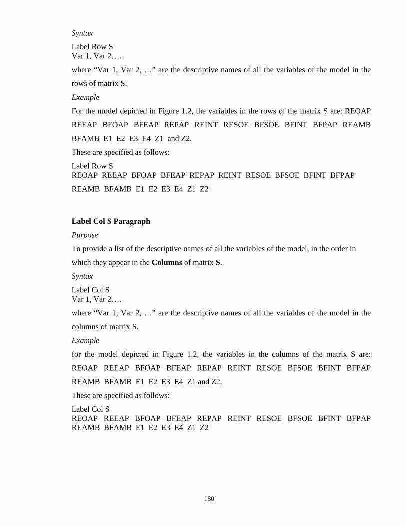
180

Syntax

Label Row S Var 1, Var 2….

where “Var 1, Var 2, …” are the descriptive names of all the variables of the model in the

rows of matrix S.

Example

For the model depicted in Figure 1.2, the variables in the rows of the matrix S are: REOAP

REEAP BFOAP BFEAP REPAP REINT RESOE BFSOE BFINT BFPAP REAMB

BFAMB E1 E2 E3 E4 Z1 and Z2.

These are specified as follows:

Label Row S REOAP REEAP BFOAP BFEAP REPAP REINT RESOE BFSOE BFINT BFPAP

REAMB BFAMB E1 E2 E3 E4 Z1 Z2

Label Col S Paragraph

Purpose

To provide a list of the descriptive names of all the variables of the model, in the order in

which they appear in the Columns of matrix S.

Syntax

Label Col S Var 1, Var 2….


columns of matrix S.

Example

for the model depicted in Figure 1.2, the variables in the columns of the matrix S are:

REOAP REEAP BFOAP BFEAP REPAP REINT RESOE BFSOE BFINT BFPAP

REAMB BFAMB E1 E2 E3 E4 Z1 and Z2.


Label Col S REOAP REEAP BFOAP BFEAP REPAP REINT RESOE BFSOE BFINT BFPAP REAMB BFAMB E1 E2 E3 E4 Z1 Z2

181

(iv) Matrix A Paragraph

Purpose

To Specify the entries of the Asymmetric paths or single-headed arrows of the model.

Syntax

Matrix A

<c,r>

where c indicates the position of the observed variable in the column from which the arrow

starts and r indicates the position of the observed variable in the row at which the arrow ends.

Example

For the model depicted in Figure 1.2, a single-headed arrow starts from the latent variable

REAMB and ends on the manifest variable REOAP as shown in Figure 5.2 below.

Figure 5.2 Dependence path between REAMB and REOAP.

In the list of all the labels of the observed variables, REAMB and REOAP are in the 1st and

11th positions respectively. The entry in Figure 5.2 above is specified by entering a starting

value, 0.75, say in the cell at row 1, column 11. The same approach is used for the other

single-headed arrows of the model.

The complete matrix A may be as shown below.

Matrix A

0 0 0 0 0 0 0 0 0 0 0.75 0 1 0 0 0 0 0 0 0 0 0 0 0 0 0 0 0 1 0 0 1 0 0 0 0 0 0 0 0 0 0 0 0 0 0 0 1 0 0 1 0 0 0 0 0 0 0 0 0 0 0 0 0 0 0.75 0 0 0 1 0 0 0 0 0 0 0 0 0 0 0 0 0 0 0 0 0 0 0 0 0 0 0 0 0 0 0 0 0 0 0 0 0 0 0 0 0 0 0 0 0 0 0 0 0 0 0 0 0 0 0 0 0 0 0 0 0 0 0 0 0 0 0 0 0 0 0 0 0 0 0 0 0 0 0 0 0 0 0 0 0 0 0 0 0 0 0 0 0 0 0 0 0 0 0 0 0 0 0 0 0 0 0 0 0 0 0 0 0 0 0 0 0 0 0.75 0.75 0.75 0.75 0 0 0 0.75 0 0 0 0 1 0 0 0 0 0 0 0 0.75 0.75 0.75 0.75 0.75 0 0 0 0 0 0 1 0 0 0 0 0 0 0 0 0 0 0 0 0 0 0 0 0 0 0 0 0 0 0 0 0 0 0 0 0 0 0 0 0 0 0 0 0 0 0 0 0 0 0 0 0 0 0 0 0 0 0 0 0 0

REOAP REAMB

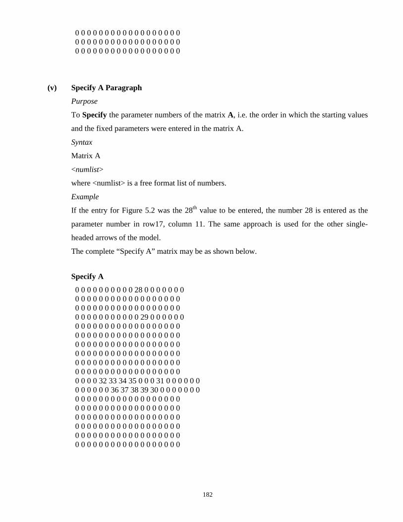
182

0 0 0 0 0 0 0 0 0 0 0 0 0 0 0 0 0 0 0 0 0 0 0 0 0 0 0 0 0 0 0 0 0 0 0 0 0 0 0 0 0 0 0 0 0 0 0 0 0 0 0 0 0 0

(v) Specify A Paragraph

Purpose

To Specify the parameter numbers of the matrix A, i.e. the order in which the starting values

and the fixed parameters were entered in the matrix A.

Syntax

Matrix A

<numlist>

where <numlist> is a free format list of numbers.

Example

If the entry for Figure 5.2 was the 28th value to be entered, the number 28 is entered as the

parameter number in row17, column 11. The same approach is used for the other single-

headed arrows of the model.

The complete “Specify A” matrix may be as shown below.

Specify A

0 0 0 0 0 0 0 0 0 0 28 0 0 0 0 0 0 0 0 0 0 0 0 0 0 0 0 0 0 0 0 0 0 0 0 0 0 0 0 0 0 0 0 0 0 0 0 0 0 0 0 0 0 0 0 0 0 0 0 0 0 0 0 0 0 29 0 0 0 0 0 0 0 0 0 0 0 0 0 0 0 0 0 0 0 0 0 0 0 0 0 0 0 0 0 0 0 0 0 0 0 0 0 0 0 0 0 0 0 0 0 0 0 0 0 0 0 0 0 0 0 0 0 0 0 0 0 0 0 0 0 0 0 0 0 0 0 0 0 0 0 0 0 0 0 0 0 0 0 0 0 0 0 0 0 0 0 0 0 0 0 0 0 0 0 0 0 0 0 0 0 0 0 0 0 0 0 0 0 0 0 0 0 0 32 33 34 35 0 0 0 31 0 0 0 0 0 0 0 0 0 0 0 0 36 37 38 39 30 0 0 0 0 0 0 0 0 0 0 0 0 0 0 0 0 0 0 0 0 0 0 0 0 0 0 0 0 0 0 0 0 0 0 0 0 0 0 0 0 0 0 0 0 0 0 0 0 0 0 0 0 0 0 0 0 0 0 0 0 0 0 0 0 0 0 0 0 0 0 0 0 0 0 0 0 0 0 0 0 0 0 0 0 0 0 0 0 0 0 0 0 0 0 0 0 0 0 0 0 0 0 0 0 0 0 0 0 0 0 0 0 0 0 0

183

Label Row A Paragraph

Purpose


which they appear in the Rows of matrix A.

Syntax

Label Row A Var 1, Var 2….


rows of matrix A.

Example

For the model depicted in Figure 1.2, the variables in the rows of the matrix A are: REOAP

REEAP BFOAP BFEAP REPAP REINT RESOE BFSOE BFINT BFPAP REAMB

BFAMB E1 E2 E3 E4 Z1 and Z2.


Label Row A REOAP REEAP BFOAP BFEAP REPAP REINT RESOE BFSOE BFINT BFPAP REAMB BFAMB E1 E2 E3 E4 Z1 Z2 Label Col A Paragraph

Purpose

To provide a list of the descriptive names of all the variables of the model, in in the order in

which they appear the Columns of matrix A.

Syntax

Label Col A Var 1, Var 2….


columns of matrix A.

Example

For the model depicted in Figure 1.2, the variables in the columns of the matrix S are:


REAMB BFAMB E1 E2 E3 E4 Z1 and Z2.


Label Col S REOAP REEAP BFOAP BFEAP REPAP REINT RESOE BFSOE BFINT BFPAP REAMB BFAMB E1 E2 E3 E4 Z1 Z2

184

(vi) Matrix F Paragraph

Purpose

To provide a matrix which Filters the observed variables out of the whole set of variables of

the model.

Syntax

Matrix F

<numlist>

where “<numlist>” is a free format list of the numbers “1” and “0”.

Example

For the list of the variables in the model depicted in Figure 1.2, REOAP is the first manifest

variable. The number “1” is entered in the cell with position row 1 and column 1. The

number “1” is also entered in the cell with position row 2 and column 2 to indicate the

second manifest variable REEAP. A similar procedure is carried out for the eight other

manifest variables of the model.

The complete matrix F may be as shown below.

Matrix F

1 0 0 0 0 0 0 0 0 0 0 0 0 0 0 0 0 0 0 1 0 0 0 0 0 0 0 0 0 0 0 0 0 0 0 0 0 0 1 0 0 0 0 0 0 0 0 0 0 0 0 0 0 0 0 0 0 1 0 0 0 0 0 0 0 0 0 0 0 0 0 0 0 0 0 0 1 0 0 0 0 0 0 0 0 0 0 0 0 0 0 0 0 0 0 1 0 0 0 0 0 0 0 0 0 0 0 0 0 0 0 0 0 0 1 0 0 0 0 0 0 0 0 0 0 0 0 0 0 0 0 0 0 1 0 0 0 0 0 0 0 0 0 0 0 0 0 0 0 0 0 0 1 0 0 0 0 0 0 0 0 0 0 0 0 0 0 0 0 0 0 1 0 0 0 0 0 0 0 0

Label Row F Paragraph

Purpose

To provide a list of the descriptive names of all the observed variables of the model, in the

order in which they appear in the Rows of matrix F.

Syntax

Label Row F Var 1, Var 2….

185

where “Var 1, Var 2, …” are the descriptive names of all the observed variables of the model

in the rows of matrix F.

Example

For the model depicted in Figure 1.2, the observed variables are: REOAP REEAP BFOAP

BFEAP REPAP REINT RESOE BFSOE BFINT and BFPAP.


Label Row F REOAP REEAP BFOAP BFEAP REPAP REINT RESOE BFSOE BFINT BFPAP.

Label Col F Paragraph

Purpose


which they appear in the Columns of matrix F.

Syntax

Label Col F Var 1, Var 2….


columns of matrix F.

Example

For the model depicted in Figure 1.2, the variables in the columns of the matrix F are:


REAMB BFAMB E1 E2 E3 E4 Z1 and Z2


Label Col F REOAP REEAP BFOAP BFEAP REPAP REINT RESOE BFSOE BFINT BFPAP REAMB BFAMB E1 E2 E3 E4 Z1 Z2

(c) SPECIFY OPTIONS

(i) Covariance Keyword

Purpose

To specify the formula for the covariance structure.

186

Syntax

Begin Algebra:

Algebra

where "Algebra" denotes the covariance structure to be used in the analysis.

Example

For the model depicted in Figure 1.2, the covariance structure used is specified in the

input script file as:

Begin Algebra:

Covariance F&((I-A)≅ & S);

(ii) Options Sentence

Purpose

To specify options required in the output file.

Syntax

Options <options>

where “<options>” denotes any of the following:

RSidual ReSidual

nDecimal=k number of Decimals (k is an iteger-the required number of decimals)

CI=p Confidence Intervals (equals p, i.e. p% confidence interval).

Example

For the model depicted in Figure 1.2, the options are specified as follows:

Options RSidual

Options nDecimal =3

Options CI= 90

(d) END OF GROUP Sentence

Purpose

To signify the end of the current project.

Syntax

End;

Example

For the model depicted in Figure 1.2, the end of the input script file is specified as:

End;

187

5.2.2 AN Mx INPUT SCRIPT FOR THE MODEL DEPICTED IN FIGURE 1.2 A complete Mx Input Script would appear as shown below. !Mx Frontend Auto-generated Script. ver 1.0 !Created at 15:56:11 on 29 Dec 2000 by !SmartUser ! -------------- Group ID 1---------------- #NGroups 1 Title The Duncan Haller and Portes Application Data NInput=10 NObservation=329 KMatrix 1.000 0.625 1.000 0.327 0.367 1.000 0.422 0.327 0.640 1.000 0.214 0.274 0.112 0.084 1.000 0.411 0.404 0.290 0.260 0.184 1.000 0.324 0.405 0.305 0.279 0.049 0.222 1.000 0.293 0.241 0.411 0.361 0.019 0.186 0.271 1.000 0.300 0.286 0.519 0.501 0.078 0.336 0.230 0.295 1.000 0.076 0.070 0.278 0.199 0.115 0.102 0.093 -0.044 0.209 1.000 #define NumManifest 10 Begin Matrices; S Symm 18 18 A Full 18 18 F Full 10 18 I Iden 18 18 End Matrices; Matrix S 0 0 0 0 0 0 0 0 0 0 0 0 0 0 1 0 0 0 0 0.75 1 0 0 0 0 0.75 0.75 1 0 0 0 0 0.75 0.75 0.75 1 0 0 0 0 0.75 0.75 0.75 0.75 1 0 0 0 0 0.75 0.75 0.75 0.75 0.75 1 0 0 0 0 0 0 0 0 0 0 0 0 0 0 0 0 0 0 0 0 0 0 0 0 0 0 0 0 0 0 0 0 0 0 0 0.75 0 0 0 0 0 0 0 0 0 0 0 0 0 0.75 0 0 0 0 0 0 0 0 0 0 0 0 0 0 0.75 0 0 0 0 0 0 0 0 0 0 0 0 0 0 0 0.75 0 0 0 0 0 0 0 0 0 0 0 0 0 0 0 0 0.75 0 0 0 0 0 0 0 0 0 0 0 0 0 0 0 0 0 0.75 Specify S 0 0 0 0 0 0 0 0 0 0 0 0 0 0 7

188

0 0 0 0 8 13 0 0 0 0 9 14 18 0 0 0 0 10 15 19 22 0 0 0 0 11 16 20 23 25 0 0 0 0 12 17 21 24 26 27 0 0 0 0 0 0 0 0 0 0 0 0 0 0 0 0 0 0 0 0 0 0 0 0 0 0 0 0 0 0 0 0 0 0 0 1 0 0 0 0 0 0 0 0 0 0 0 0 0 2 0 0 0 0 0 0 0 0 0 0 0 0 0 0 3 0 0 0 0 0 0 0 0 0 0 0 0 0 0 0 4 0 0 0 0 0 0 0 0 0 0 0 0 0 0 0 0 5 0 0 0 0 0 0 0 0 0 0 0 0 0 0 0 0 0 6 Label Row S REOAP REEAP BFOAP BFEAP REPAP REINT RESOE BFSOE BFINT BFPAP REAMB BFAMB E1 E2 E3 E4 Z1 Z2 Label Col S REOAP REEAP BFOAP BFEAP REPAP REINT RESOE BFSOE BFINT BFPAP REAMB BFAMB E1 E2 E3 E4 Z1 Z2 Matrix A 0 0 0 0 0 0 0 0 0 0 0.75 0 1 0 0 0 0 0 0 0 0 0 0 0 0 0 0 0 1 0 0 1 0 0 0 0 0 0 0 0 0 0 0 0 0 0 0 1 0 0 1 0 0 0 0 0 0 0 0 0 0 0 0 0 0 0.75 0 0 0 1 0 0 0 0 0 0 0 0 0 0 0 0 0 0 0 0 0 0 0 0 0 0 0 0 0 0 0 0 0 0 0 0 0 0 0 0 0 0 0 0 0 0 0 0 0 0 0 0 0 0 0 0 0 0 0 0 0 0 0 0 0 0 0 0 0 0 0 0 0 0 0 0 0 0 0 0 0 0 0 0 0 0 0 0 0 0 0 0 0 0 0 0 0 0 0 0 0 0 0 0 0 0 0 0 0 0 0 0 0 0 0 0 0 0 0.75 0.75 0.75 0.75 0 0 0 0.75 0 0 0 0 1 0 0 0 0 0 0 0 0.75 0.75 0.75 0.75 0.75 0 0 0 0 0 0 1 0 0 0 0 0 0 0 0 0 0 0 0 0 0 0 0 0 0 0 0 0 0 0 0 0 0 0 0 0 0 0 0 0 0 0 0 0 0 0 0 0 0 0 0 0 0 0 0 0 0 0 0 0 0 0 0 0 0 0 0 0 0 0 0 0 0 0 0 0 0 0 0 0 0 0 0 0 0 0 0 0 0 0 0 0 0 0 0 0 0 0 0 0 0 0 0 0 0 0 0 0 0 0 0 0 0 0 0 Specify A 0 0 0 0 0 0 0 0 0 0 28 0 0 0 0 0 0 0 0 0 0 0 0 0 0 0 0 0 0 0 0 0 0 0 0 0 0 0 0 0 0 0 0 0 0 0 0 0 0 0 0 0 0 0 0 0 0 0 0 0 0 0 0 0 0 29 0 0 0 0 0 0 0 0 0 0 0 0 0 0 0 0 0 0 0 0 0 0 0 0 0 0 0 0 0 0 0 0 0 0 0 0 0 0 0 0 0 0 0 0 0 0 0 0 0 0 0 0 0 0 0 0 0 0 0 0 0 0 0 0 0 0 0 0 0 0 0 0 0 0 0 0 0 0 0 0 0 0 0 0 0 0 0 0 0 0 0 0 0 0 0 0 0 0 0 0 0 0 0 0 0 0 0 0 0 0 0 0 0 0 0 0 0 0 32 33 34 35 0 0 0 31 0 0 0 0 0 0 0 0 0 0 0 0 36 37 38 39 30 0 0 0 0 0 0 0 0 0 0 0 0 0 0 0 0 0 0 0 0 0 0 0 0 0 0 0 0 0 0 0 0 0 0 0 0 0 0 0 0 0 0 0 0 0 0 0 0 0 0 0 0 0 0 0 0 0 0 0 0 0 0 0 0 0 0 0 0 0 0 0 0 0 0 0 0 0 0 0 0 0 0 0 0 0 0 0 0 0 0 0 0 0 0 0 0 0 0 0 0 0 0 0 0 0 0 0 0 0 0 0 0 0 0 0

189

Label Row A REOAP REEAP BFOAP BFEAP REPAP REINT RESOE BFSOE BFINT BFPAP REAMB BFAMB E1 E2 E3 E4 Z1 Z2 Label Col A REOAP REEAP BFOAP BFEAP REPAP REINT RESOE BFSOE BFINT BFPAP REAMB BFAMB E1 E2 E3 E4 Z1 Z2 Matrix F 1 0 0 0 0 0 0 0 0 0 0 0 0 0 0 0 0 0 0 1 0 0 0 0 0 0 0 0 0 0 0 0 0 0 0 0 0 0 1 0 0 0 0 0 0 0 0 0 0 0 0 0 0 0 0 0 0 1 0 0 0 0 0 0 0 0 0 0 0 0 0 0 0 0 0 0 1 0 0 0 0 0 0 0 0 0 0 0 0 0 0 0 0 0 0 1 0 0 0 0 0 0 0 0 0 0 0 0 0 0 0 0 0 0 1 0 0 0 0 0 0 0 0 0 0 0 0 0 0 0 0 0 0 1 0 0 0 0 0 0 0 0 0 0 0 0 0 0 0 0 0 0 1 0 0 0 0 0 0 0 0 0 0 0 0 0 0 0 0 0 0 1 0 0 0 0 0 0 0 0 Label Row F REOAP REEAP BFOAP BFEAP REPAP REINT RESOE BFSOE BFINT BFPAP Label Col F REOAP REEAP BFOAP BFEAP REPAP REINT RESOE BFSOE BFINT BFPAP REAMB BFAMB E1 E2 E3 E4 Z1 Z2 Covariance F & ((I - A)~ & S); Options RSidual Options nDecimals=3 Options CI=90 End Group;

5.3 ILLUSTRATIVE EXAMPLE: THE DUNCAN, HALLER AND

PORTES’ APPLICATION

5.3.1 CREATING Mx INPUT SCRIPT FROM PATH DIAGRAM FOR THE

DUNCAN, HALLER AND PORTES' APPLICATION The path diagram drawing software, RAMPATH may be used to generate an Mx script file

by simply drawing the path diagram of the model to be fitted to the data. The step by step

method for doing this for the Duncan, Haller and Portes’ application is outlined below.

• Double-click on the Mx icon to open the window below:

190

• Click on the “New Drawing” push button to open the window below.

• Click on the “Rectangle” push button to change the cursor into a rectangle.

• Click at the appropriate portion of the window to drop the rectangle to produce the window

below.

191

• Click on the “Default cursor” push button to stop the duplication of the rectangles.

• Double-click on the default label of the manifest variable to produce a window with part

shown below.

• Type in the required variable name to replace the default name as shown below.

• Click outside the rectangle to produce the window shown below.

192

• Repeat the steps used above to draw the other nine manifest variables of the model to

produce the window shown below.

• Click on the “Circle” push button to change the cursor into a circle.

• Click on the appropriate part of the window to drop the circle to produce the window below.

193

• Go through the same steps as above to insert the descriptive name of the latent variable.

• Follow the same steps to draw and label the other latent variable to produce the window

below:

• Click on the “Single Arrow” push button, to change the cursor to a single-headed

arrow.

• Click on the latent variable, “REAMB”.

• Hold the click and drag it to “REOAP” to produce a window such as the one shown below:

194

• By following the same steps as those used to draw the unidirectional arrow from “REAMB”

to “REOAP”, you would be able to draw all the required unidirectional arrows needed in the

diagram to produce the window below:

• Click on the “Double Arrow” push button .

• Click on the manifest variable “REPAP”.

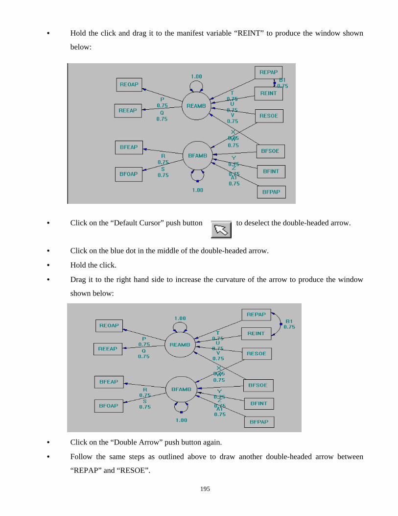
195

• Hold the click and drag it to the manifest variable “REINT” to produce the window shown

below:

• Click on the “Default Cursor” push button to deselect the double-headed arrow.

• Click on the blue dot in the middle of the double-headed arrow.

• Hold the click.

• Drag it to the right hand side to increase the curvature of the arrow to produce the window

shown below:

• Click on the “Double Arrow” push button again.

• Follow the same steps as outlined above to draw another double-headed arrow between

“REPAP” and “RESOE”.

196

• Continue with the same steps to draw all the double-headed arrow of the model to produce

the window shown below:

• Draw the error terms in the same way as you did for the latent variables to produce the

window below:

• Click on the path from “E1” to “REOAP” to select it.

• Double-click on the highlighted path to load the dialog box below:

197

• Click in the “Start Value” string field.

• Type the number “1.00” in the string field.

• Check the “Fix This Parameter” check box.

• Click on the “OK” push button to fix the parameter H2, between “E1” and “REOAP” to 1.

• Follow the same steps to fix the parameters P and S between REAMB and REOAP, and

BFAMB and BFOAP respectively, to 1.

The same steps could be used to fix or set free any of the default parameters values shown on the

path diagram.

• Click on the menu to load the file menu box shown below:

• Click on the “Save As” option to load the dialog box shown below:

• Type the appropriate file name, for example, “pepdhp”, say, in the “File name” string field

to produce the dialog box shown below:

198

• Click on the “Save” push button to save the path diagram.

• Click on the “To Script” push button to load the dialog box shown

below:

• Type the appropriate name for the script file in the “Job Name" string field to produce the

dialog box shown below:

• Click on the “OK” push button to open the dialog box shown below:

199

• Click on the “Save” push button to open the saved input script file shown in the window

below.

• Type in the matrix to be analyzed or copy and paste from an external source to replace the

default identity matrix in the input script.

• Type the correct number of observations to replace the default number 100 to produce the

window shown below:

• Click on the “Preference” menu to load the preference menu box shown below:

200

• Click on the “Job Options” option to load the dialog box shown below:

• Change any of the options to the desired option.

• Check the “Standardized” check box to produce the dialog box shown below:

• Click on the “OK” push button.

• Click on the “Preference” menu again to load the preference menu box.

• Click on the “Matrix Options” option to load the dialog box shown below:

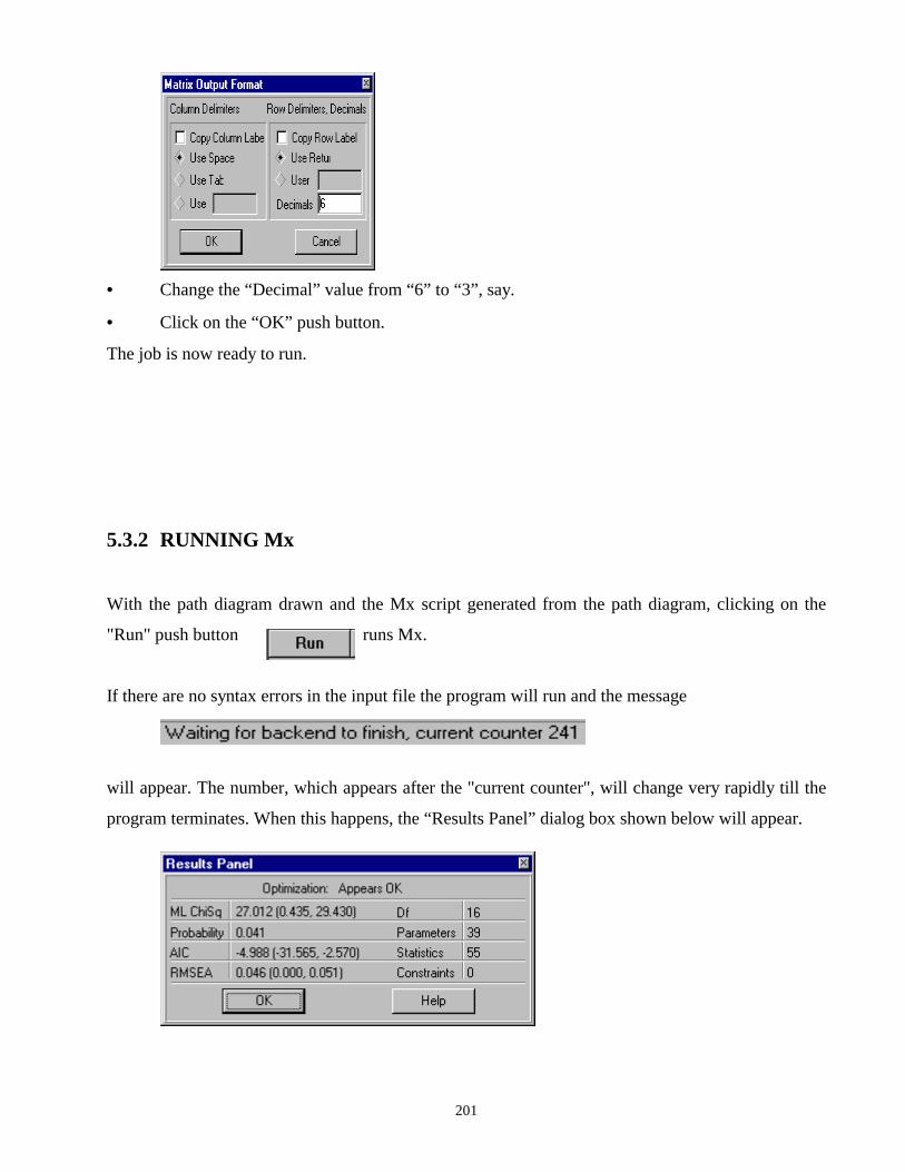
201

• Change the “Decimal” value from “6” to “3”, say.

• Click on the “OK” push button.

The job is now ready to run.

5.3.2 RUNNING Mx

With the path diagram drawn and the Mx script generated from the path diagram, clicking on the

"Run" push button runs Mx.

If there are no syntax errors in the input file the program will run and the message

will appear. The number, which appears after the "current counter", will change very rapidly till the

program terminates. When this happens, the “Results Panel” dialog box shown below will appear.

202

• Click on the “OK” push button to open the window shown below:

In this window you will find the matrices specified in the Input Script file, the order and the type of

each matrix. The test statistic values and the parameter estimates can be viewed from the window

above by clicking on the “Statistics” or the “Value” push buttons.

5.3.3 THE Mx OUTPUT FILE (1)** Mx startup successful ** (2) (I) **MX-PC 1.50** Job started on 12/29/00 at 16:07:53

(II) !Mx Frontend Auto-generated Script. ver 1.0 !Created at 15:56:11 on 29 Dec 2000 by !SmartUser ! -------------- Group ID 1---------------- (3) The following MX script lines were read for group 1 (4) (I) #NGROUPS 1 (II) Note: #NGroup set number of groups to 1

203

(III) TITLE THE DUNCAN HALLER AND PORTES APPLICATION (IV) DATA NINPUT=10 NOBSERVATION=329 (V) KMATRIX 1.000 0.625 1.000 0.327 0.367 1.000 0.422 0.327 0.640 1.000 0.214 0.274 0.112 0.084 1.000 0.411 0.404 0.290 0.260 0.184 1.000 0.324 0.405 0.305 0.279 0.049 0.222 1.000 0.293 0.241 0.411 0.361 0.019 0.186 0.271 1.000 0.300 0.286 0.519 0.501 0.078 0.336 0.230 0.295 1.000 0.076 0.070 0.278 0.199 0.115 0.102 0.093 -0.044 0.209 1.000 (VI) #DEFINE NUMMANIFEST 10 (5) (I) BEGIN MATRICES; (II) S SYMM 18 18 (III) A FULL 18 18 (IV) F FULL 10 18 (V) I IDEN 18 18 (VI) END MATRICES; (6) (I) MATRIX S 0 0 0 0 0 0 0 0 0 0 0 0 0 0 1 0 0 0 0 0.75 1 0 0 0 0 0.75 0.75 1 0 0 0 0 0.75 0.75 0.75 1 0 0 0 0 0.75 0.75 0.75 0.75 1 0 0 0 0 0.75 0.75 0.75 0.75 0.75 1 0 0 0 0 0 0 0 0 0 0 0 0 0 0 0 0 0 0 0 0 0 0 0 0 0 0 0 0 0 0 0 0 0 0 0 0.75 0 0 0 0 0 0 0 0 0 0 0 0 0 0.75 0 0 0 0 0 0 0 0 0 0 0 0 0 0 0.75 0 0 0 0 0 0 0 0 0 0 0 0 0 0 0 0.75 0 0 0 0 0 0 0 0 0 0 0 0 0 0 0 0 0.75 0 0 0 0 0 0 0 0 0 0 0 0 0 0 0 0 0 0.75

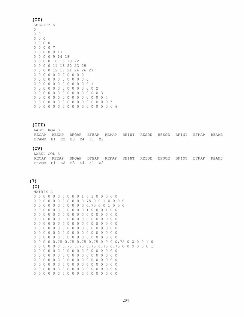
204

(II) SPECIFY S 0 0 0 0 0 0 0 0 0 0 0 0 0 0 7 0 0 0 0 8 13 0 0 0 0 9 14 18 0 0 0 0 10 15 19 22 0 0 0 0 11 16 20 23 25 0 0 0 0 12 17 21 24 26 27 0 0 0 0 0 0 0 0 0 0 0 0 0 0 0 0 0 0 0 0 0 0 0 0 0 0 0 0 0 0 0 0 0 0 0 1 0 0 0 0 0 0 0 0 0 0 0 0 0 2 0 0 0 0 0 0 0 0 0 0 0 0 0 0 3 0 0 0 0 0 0 0 0 0 0 0 0 0 0 0 4 0 0 0 0 0 0 0 0 0 0 0 0 0 0 0 0 5 0 0 0 0 0 0 0 0 0 0 0 0 0 0 0 0 0 6 (III) LABEL ROW S

REOAP REEAP BFOAP BFEAP REPAP REINT RESOE BFSOE BFINT BFPAP REAMB BFAMB E1 E2 E3 E4 Z1 Z2

(IV) LABEL COL S


(7) (I) MATRIX A 0 0 0 0 0 0 0 0 0 0 1 0 1 0 0 0 0 0 0 0 0 0 0 0 0 0 0 0 0.75 0 0 1 0 0 0 0 0 0 0 0 0 0 0 0 0 0 0 0.75 0 0 1 0 0 0 0 0 0 0 0 0 0 0 0 0 0 1 0 0 0 1 0 0 0 0 0 0 0 0 0 0 0 0 0 0 0 0 0 0 0 0 0 0 0 0 0 0 0 0 0 0 0 0 0 0 0 0 0 0 0 0 0 0 0 0 0 0 0 0 0 0 0 0 0 0 0 0 0 0 0 0 0 0 0 0 0 0 0 0 0 0 0 0 0 0 0 0 0 0 0 0 0 0 0 0 0 0 0 0 0 0 0 0 0 0 0 0 0 0 0 0 0 0 0 0 0 0 0 0 0 0 0 0 0 0 0.75 0.75 0.75 0.75 0 0 0 0.75 0 0 0 0 1 0 0 0 0 0 0 0 0.75 0.75 0.75 0.75 0.75 0 0 0 0 0 0 1 0 0 0 0 0 0 0 0 0 0 0 0 0 0 0 0 0 0 0 0 0 0 0 0 0 0 0 0 0 0 0 0 0 0 0 0 0 0 0 0 0 0 0 0 0 0 0 0 0 0 0 0 0 0 0 0 0 0 0 0 0 0 0 0 0 0 0 0 0 0 0 0 0 0 0 0 0 0 0 0 0 0 0 0 0 0 0 0 0 0 0 0 0 0 0 0 0 0 0 0 0 0 0 0 0 0 0 0

205

(II) SPECIFY A 0 0 0 0 0 0 0 0 0 0 0 0 0 0 0 0 0 0 0 0 0 0 0 0 0 0 0 0 28 0 0 0 0 0 0 0 0 0 0 0 0 0 0 0 0 0 0 29 0 0 0 0 0 0 0 0 0 0 0 0 0 0 0 0 0 0 0 0 0 0 0 0 0 0 0 0 0 0 0 0 0 0 0 0 0 0 0 0 0 0 0 0 0 0 0 0 0 0 0 0 0 0 0 0 0 0 0 0 0 0 0 0 0 0 0 0 0 0 0 0 0 0 0 0 0 0 0 0 0 0 0 0 0 0 0 0 0 0 0 0 0 0 0 0 0 0 0 0 0 0 0 0 0 0 0 0 0 0 0 0 0 0 0 0 0 0 0 0 0 0 0 0 0 0 0 0 0 0 0 0 0 0 0 0 32 33 34 35 0 0 0 31 0 0 0 0 0 0 0 0 0 0 0 0 36 37 38 39 30 0 0 0 0 0 0 0 0 0 0 0 0 0 0 0 0 0 0 0 0 0 0 0 0 0 0 0 0 0 0 0 0 0 0 0 0 0 0 0 0 0 0 0 0 0 0 0 0 0 0 0 0 0 0 0 0 0 0 0 0 0 0 0 0 0 0 0 0 0 0 0 0 0 0 0 0 0 0 0 0 0 0 0 0 0 0 0 0 0 0 0 0 0 0 0 0 0 0 0 0 0 0 0 0 0 0 0 0 0 0 0 0 0 0 0 (III) LABEL ROW A


(IV) LABEL COL A REOAP REEAP BFOAP BFEAP REPAP REINT RESOE BFSOE BFINT BFPAP

REAMB BFAMB E1 E2 E3 E4 Z1 Z2 (8) (I) MATRIX F 1 0 0 0 0 0 0 0 0 0 0 0 0 0 0 0 0 0 0 1 0 0 0 0 0 0 0 0 0 0 0 0 0 0 0 0 0 0 1 0 0 0 0 0 0 0 0 0 0 0 0 0 0 0 0 0 0 1 0 0 0 0 0 0 0 0 0 0 0 0 0 0 0 0 0 0 1 0 0 0 0 0 0 0 0 0 0 0 0 0 0 0 0 0 0 1 0 0 0 0 0 0 0 0 0 0 0 0 0 0 0 0 0 0 1 0 0 0 0 0 0 0 0 0 0 0 0 0 0 0 0 0 0 1 0 0 0 0 0 0 0 0 0 0 0 0 0 0 0 0 0 0 1 0 0 0 0 0 0 0 0 0 0 0 0 0 0 0 0 0 0 1 0 0 0 0 0 0 0 0 (II) LABEL ROW F REOAP REEAP BFOAP BFEAP REPAP REINT RESOE BFSOE BFINT BFPAP (III) LABEL COL F REOAP REEAP BFOAP BFEAP REPAP REINT RESOE BFSOE BFINT BFPAP

REAMB BFAMB E1 E2 E3 E4 Z1 Z2

206

(9) (I) COVARIANCE F & ((I - A)~ & S); (II) OPTIONS RSIDUAL (III) OPTIONS NDECIMALS=3 (IV) OPTIONS CI=90 (V) OPTION NULL=472.155, 45 (VI) END GROUP; (10) PARAMETER SPECIFICATIONS (I) GROUP NUMBER: 1 (II) Title The Duncan Haller and Portes Application (11) MATRIX A This is a FULL matrix of order 18 by 18 REOAP REEAP BFOAP BFEAP REPAP REINT RESOE BFSOE BFINT REOAP 0 0 0 0 0 0 0 0 0 REEAP 0 0 0 0 0 0 0 0 0 BFOAP 0 0 0 0 0 0 0 0 0 BFEAP 0 0 0 0 0 0 0 0 0 REPAP 0 0 0 0 0 0 0 0 0 REINT 0 0 0 0 0 0 0 0 0 RESOE 0 0 0 0 0 0 0 0 0 BFSOE 0 0 0 0 0 0 0 0 0 BFINT 0 0 0 0 0 0 0 0 0 BFPAP 0 0 0 0 0 0 0 0 0 REAMB 0 0 0 0 32 33 34 35 0 BFAMB 0 0 0 0 0 0 36 37 38 E1 0 0 0 0 0 0 0 0 0 E2 0 0 0 0 0 0 0 0 0 E3 0 0 0 0 0 0 0 0 0 E4 0 0 0 0 0 0 0 0 0 Z1 0 0 0 0 0 0 0 0 0 Z2 0 0 0 0 0 0 0 0 0 BFPAP REAMB BFAMB E1 E2 E3 E4 Z1 Z2 REOAP 0 28 0 0 0 0 0 0 0 REEAP 0 0 0 0 0 0 0 0 0 BFOAP 0 0 0 0 0 0 0 0 0 BFEAP 0 0 29 0 0 0 0 0 0 REPAP 0 0 0 0 0 0 0 0 0 REINT 0 0 0 0 0 0 0 0 0 RESOE 0 0 0 0 0 0 0 0 0 BFSOE 0 0 0 0 0 0 0 0 0 BFINT 0 0 0 0 0 0 0 0 0 BFPAP 0 0 0 0 0 0 0 0 0 REAMB 0 0 31 0 0 0 0 0 0 BFAMB 39 30 0 0 0 0 0 0 0 E1 0 0 0 0 0 0 0 0 0 E2 0 0 0 0 0 0 0 0 0 E3 0 0 0 0 0 0 0 0 0 E4 0 0 0 0 0 0 0 0 0 Z1 0 0 0 0 0 0 0 0 0 Z2 0 0 0 0 0 0 0 0 0

207

(12) MATRIX F This is a FULL matrix of order 10 by 18 It has no free parameters specified (13) MATRIX I This is an IDENTITY matrix of order 18 by 18 (14) MATRIX S This is a SYMMETRIC matrix of order 18 by 18 REOAP REEAP BFOAP BFEAP REPAP REINT RESOE BFSOE BFINT REOAP 0 REEAP 0 0 BFOAP 0 0 0 BFEAP 0 0 0 0 REPAP 0 0 0 0 7 REINT 0 0 0 0 8 13 RESOE 0 0 0 0 9 14 18 BFSOE 0 0 0 0 10 15 19 22 BFINT 0 0 0 0 11 16 20 23 25 BFPAP 0 0 0 0 12 17 21 24 26 REAMB 0 0 0 0 0 0 0 0 0 BFAMB 0 0 0 0 0 0 0 0 0 E1 0 0 0 0 0 0 0 0 0 E2 0 0 0 0 0 0 0 0 0 E3 0 0 0 0 0 0 0 0 0 E4 0 0 0 0 0 0 0 0 0 Z1 0 0 0 0 0 0 0 0 0 Z2 0 0 0 0 0 0 0 0 0 BFPAP REAMB BFAMB E1 E2 E3 E4 Z1 Z2 REOAP REEAP BFOAP BFEAP REPAP REINT RESOE BFSOE BFINT BFPAP 27 REAMB 0 0 BFAMB 0 0 0 E1 0 0 0 1 E2 0 0 0 0 2 E3 0 0 0 0 0 3 E4 0 0 0 0 0 0 4 Z1 0 0 0 0 0 0 0 5 Z2 0 0 0 0 0 0 0 0 6

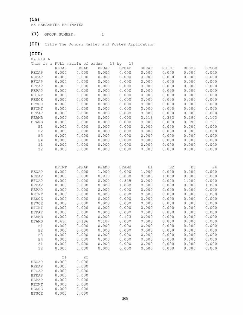
208

(15) MX PARAMETER ESTIMATES (I) GROUP NUMBER: 1 (II) Title The Duncan Haller and Portes Application (III) MATRIX A This is a FULL matrix of order 18 by 18 REOAP REEAP BFOAP BFEAP REPAP REINT RESOE BFSOE REOAP 0.000 0.000 0.000 0.000 0.000 0.000 0.000 0.000 REEAP 0.000 0.000 0.000 0.000 0.000 0.000 0.000 0.000 BFOAP 0.000 0.000 0.000 0.000 0.000 0.000 0.000 0.000 BFEAP 0.000 0.000 0.000 0.000 0.000 0.000 0.000 0.000 REPAP 0.000 0.000 0.000 0.000 0.000 0.000 0.000 0.000 REINT 0.000 0.000 0.000 0.000 0.000 0.000 0.000 0.000 RESOE 0.000 0.000 0.000 0.000 0.000 0.000 0.000 0.000 BFSOE 0.000 0.000 0.000 0.000 0.000 0.000 0.000 0.000 BFINT 0.000 0.000 0.000 0.000 0.000 0.000 0.000 0.000 BFPAP 0.000 0.000 0.000 0.000 0.000 0.000 0.000 0.000 REAMB 0.000 0.000 0.000 0.000 0.213 0.333 0.290 0.103 BFAMB 0.000 0.000 0.000 0.000 0.000 0.000 0.090 0.281 E1 0.000 0.000 0.000 0.000 0.000 0.000 0.000 0.000 E2 0.000 0.000 0.000 0.000 0.000 0.000 0.000 0.000 E3 0.000 0.000 0.000 0.000 0.000 0.000 0.000 0.000 E4 0.000 0.000 0.000 0.000 0.000 0.000 0.000 0.000 Z1 0.000 0.000 0.000 0.000 0.000 0.000 0.000 0.000 Z2 0.000 0.000 0.000 0.000 0.000 0.000 0.000 0.000 BFINT BFPAP REAMB BFAMB E1 E2 E3 E4 REOAP 0.000 0.000 1.000 0.000 1.000 0.000 0.000 0.000 REEAP 0.000 0.000 0.813 0.000 0.000 1.000 0.000 0.000 BFOAP 0.000 0.000 0.000 0.825 0.000 0.000 1.000 0.000 BFEAP 0.000 0.000 0.000 1.000 0.000 0.000 0.000 1.000 REPAP 0.000 0.000 0.000 0.000 0.000 0.000 0.000 0.000 REINT 0.000 0.000 0.000 0.000 0.000 0.000 0.000 0.000 RESOE 0.000 0.000 0.000 0.000 0.000 0.000 0.000 0.000 BFSOE 0.000 0.000 0.000 0.000 0.000 0.000 0.000 0.000 BFINT 0.000 0.000 0.000 0.000 0.000 0.000 0.000 0.000 BFPAP 0.000 0.000 0.000 0.000 0.000 0.000 0.000 0.000 REAMB 0.000 0.000 0.000 0.173 0.000 0.000 0.000 0.000 BFAMB 0.437 0.196 0.187 0.000 0.000 0.000 0.000 0.000 E1 0.000 0.000 0.000 0.000 0.000 0.000 0.000 0.000 E2 0.000 0.000 0.000 0.000 0.000 0.000 0.000 0.000 E3 0.000 0.000 0.000 0.000 0.000 0.000 0.000 0.000 E4 0.000 0.000 0.000 0.000 0.000 0.000 0.000 0.000 Z1 0.000 0.000 0.000 0.000 0.000 0.000 0.000 0.000 Z2 0.000 0.000 0.000 0.000 0.000 0.000 0.000 0.000 Z1 Z2 REOAP 0.000 0.000 REEAP 0.000 0.000 BFOAP 0.000 0.000 BFEAP 0.000 0.000 REPAP 0.000 0.000 REINT 0.000 0.000 RESOE 0.000 0.000 BFSOE 0.000 0.000

209

BFINT 0.000 0.000 BFPAP 0.000 0.000 REAMB 1.000 0.000 BFAMB 0.000 1.000 E1 0.000 0.000 E2 0.000 0.000 E3 0.000 0.000 E4 0.000 0.000 Z1 0.000 0.000 Z2 0.000 0.000 (IV) MATRIX F This is a FULL matrix of order 10 by 18 REOAP REEAP BFOAP BFEAP REPAP REINT RESOE BFSOE REOAP 1.000 0.000 0.000 0.000 0.000 0.000 0.000 0.000 REEAP 0.000 1.000 0.000 0.000 0.000 0.000 0.000 0.000 BFOAP 0.000 0.000 1.000 0.000 0.000 0.000 0.000 0.000 BFEAP 0.000 0.000 0.000 1.000 0.000 0.000 0.000 0.000 REPAP 0.000 0.000 0.000 0.000 1.000 0.000 0.000 0.000 REINT 0.000 0.000 0.000 0.000 0.000 1.000 0.000 0.000 RESOE 0.000 0.000 0.000 0.000 0.000 0.000 1.000 0.000 BFSOE 0.000 0.000 0.000 0.000 0.000 0.000 0.000 1.000 BFINT 0.000 0.000 0.000 0.000 0.000 0.000 0.000 0.000 BFPAP 0.000 0.000 0.000 0.000 0.000 0.000 0.000 0.000 BFINT BFPAP REAMB BFAMB E1 E2 E3 E4 REOAP 0.000 0.000 0.000 0.000 0.000 0.000 0.000 0.000 REEAP 0.000 0.000 0.000 0.000 0.000 0.000 0.000 0.000 BFOAP 0.000 0.000 0.000 0.000 0.000 0.000 0.000 0.000 BFEAP 0.000 0.000 0.000 0.000 0.000 0.000 0.000 0.000 REPAP 0.000 0.000 0.000 0.000 0.000 0.000 0.000 0.000 REINT 0.000 0.000 0.000 0.000 0.000 0.000 0.000 0.000 RESOE 0.000 0.000 0.000 0.000 0.000 0.000 0.000 0.000 BFSOE 0.000 0.000 0.000 0.000 0.000 0.000 0.000 0.000 BFINT 1.000 0.000 0.000 0.000 0.000 0.000 0.000 0.000 BFPAP 0.000 1.000 0.000 0.000 0.000 0.000 0.000 0.000 Z1 Z2 REOAP 0.000 0.000 REEAP 0.000 0.000 BFOAP 0.000 0.000 BFEAP 0.000 0.000 REPAP 0.000 0.000 REINT 0.000 0.000 RESOE 0.000 0.000 BFSOE 0.000 0.000 BFINT 0.000 0.000 BFPAP 0.000 0.000 (V) MATRIX I This is an IDENTITY matrix of order 18 by 18

210

(VI) MATRIX S This is a SYMMETRIC matrix of order 18 by 18 REOAP REEAP BFOAP BFEAP REPAP REINT RESOE BFSOE REOAP 0.000 REEAP 0.000 0.000 BFOAP 0.000 0.000 0.000 BFEAP 0.000 0.000 0.000 0.000 REPAP 0.000 0.000 0.000 0.000 1.000 REINT 0.000 0.000 0.000 0.000 0.184 1.000 RESOE 0.000 0.000 0.000 0.000 0.049 0.222 1.000 BFSOE 0.000 0.000 0.000 0.000 0.019 0.186 0.271 1.000 BFINT 0.000 0.000 0.000 0.000 0.078 0.336 0.230 0.295 BFPAP 0.000 0.000 0.000 0.000 0.115 0.102 0.093 -0.044 REAMB 0.000 0.000 0.000 0.000 0.000 0.000 0.000 0.000 BFAMB 0.000 0.000 0.000 0.000 0.000 0.000 0.000 0.000 E1 0.000 0.000 0.000 0.000 0.000 0.000 0.000 0.000 E2 0.000 0.000 0.000 0.000 0.000 0.000 0.000 0.000 E3 0.000 0.000 0.000 0.000 0.000 0.000 0.000 0.000 E4 0.000 0.000 0.000 0.000 0.000 0.000 0.000 0.000 Z1 0.000 0.000 0.000 0.000 0.000 0.000 0.000 0.000 Z2 0.000 0.000 0.000 0.000 0.000 0.000 0.000 0.000 BFINT BFPAP REAMB BFAMB E1 E2 E3 E4 REOAP REEAP BFOAP BFEAP REPAP REINT RESOE BFSOE BFINT 1.000 BFPAP 0.209 1.000 REAMB 0.000 0.000 0.000 BFAMB 0.000 0.000 0.000 0.000 E1 0.000 0.000 0.000 0.000 0.412 E2 0.000 0.000 0.000 0.000 0.000 0.338 E3 0.000 0.000 0.000 0.000 0.000 0.000 0.314 E4 0.000 0.000 0.000 0.000 0.000 0.000 0.000 0.404 Z1 0.000 0.000 0.000 0.000 0.000 0.000 0.000 0.000 Z2 0.000 0.000 0.000 0.000 0.000 0.000 0.000 0.000 Z1 Z2 REOAP REEAP BFOAP BFEAP REPAP REINT RESOE BFSOE BFINT BFPAP REAMB BFAMB E1

211

E2 E3 E4 Z1 0.317 Z2 0.000 0.263 (16) OBSERVED COVARIANCE MATRIX 1 2 3 4 5 6 7 8 1 1.000 2 0.625 1.000 3 0.327 0.367 1.000 4 0.422 0.327 0.640 1.000 5 0.214 0.274 0.112 0.084 1.000 6 0.411 0.404 0.290 0.260 0.184 1.000 7 0.324 0.405 0.305 0.279 0.049 0.222 1.000 8 0.293 0.241 0.411 0.361 0.019 0.186 0.271 1.000 9 0.300 0.286 0.519 0.501 0.078 0.336 0.230 0.295 10 0.076 0.070 0.278 0.199 0.115 0.102 0.093 -0.044

9 10 1 2 3 4 5 6 7 8 9 1.000 10 0.209 1.000 (17) EXPECTED COVARIANCE MATRIX 1 2 3 4 5 6 7 8 1 0.999 2 0.624 0.999 3 0.354 0.376 0.999 4 0.331 0.351 0.639 0.999 5 0.240 0.254 0.102 0.095 1.000 6 0.393 0.417 0.273 0.255 0.184 1.000 7 0.357 0.379 0.303 0.282 0.049 0.222 1.000 8 0.255 0.270 0.401 0.374 0.019 0.186 0.271 1.000 9 0.258 0.274 0.525 0.490 0.078 0.336 0.230 0.295 10 0.103 0.110 0.254 0.237 0.115 0.102 0.093 -0.044 9 10 1 2 3 4 5 6 7 8 9 1.000 10 0.209 1.000

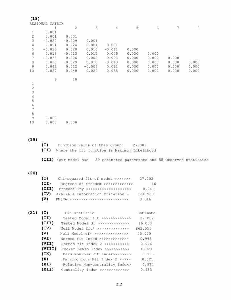
212

(18) RESIDUAL MATRIX 1 2 3 4 5 6 7 8 1 0.001 2 0.001 0.001 3 -0.027 -0.009 0.001 4 0.091 -0.024 0.001 0.001 5 -0.026 0.020 0.010 -0.011 0.000 6 0.018 -0.013 0.017 0.005 0.000 0.000 7 -0.033 0.026 0.002 -0.003 0.000 0.000 0.000 8 0.038 -0.029 0.010 -0.013 0.000 0.000 0.000 0.000 9 0.042 0.012 -0.006 0.011 0.000 0.000 0.000 0.000 10 -0.027 -0.040 0.024 -0.038 0.000 0.000 0.000 0.000 9 10 1 2 3 4 5 6 7 8 9 0.000 10 0.000 0.000 (19) (I) Function value of this group: 27.002 (II) Where the fit function is Maximum Likelihood (III) Your model has 39 estimated parameters and 55 Observed statistics (20) (I) Chi-squared fit of model >>>>>>> 27.002 (II) Degrees of freedom >>>>>>>>>>>>> 16 (III) Probability >>>>>>>>>>>>>>>>>>>> 0.041 (IV) Akaike's Information Criterion > 104.988 (V) RMSEA >>>>>>>>>>>>>>>>>>>>>>>>>> 0.046 (21) (I) Fit statistic Estimate (II) Tested Model fit >>>>>>>>>>>>> 27.002 (III) Tested Model df >>>>>>>>>>>>>> 16.000 (IV) Null Model fit* >>>>>>>>>>>>>> 862.555 (V) Null Model df* >>>>>>>>>>>>>>> 45.000 (VI) Normed fit Index >>>>>>>>>>>>> 0.943 (VII) Normed fit Index 2 >>>>>>>>>>> 0.976 (VIII) Tucker Lewis Index >>>>>>>>>>> 0.927 (IX) Parsimonious Fit Index>>>>>>>> 0.335 (X) Parsimonious Fit Index 2 >>>>> 0.021 (XI) Relative Non-centrality Index> 0.974 (XII) Centrality Index >>>>>>>>>>>>> 0.983

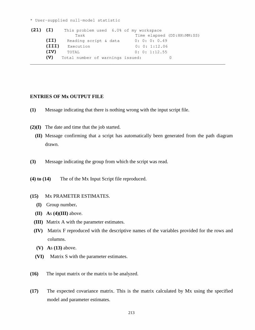
213

* User-supplied null-model statistic (21) (I) This problem used 6.0% of my workspace

Task Time elapsed (DD:HH:MM:SS) (II) Reading script & data 0: 0: 0: 0.49 (III) Execution 0: 0: 1:12.06 (IV) TOTAL 0: 0: 1:12.55 (V) Total number of warnings issued: 0 ______________________________________________________________________________

ENTRIES OF Mx OUTPUT FILE (1) Message indicating that there is nothing wrong with the input script file.

(2)(I) The date and time that the job started.

(II) Message confirming that a script has automatically been generated from the path diagram

drawn.

(3) Message indicating the group from which the script was read.

(4) to (14) The of the Mx Input Script file reproduced.

(15) Mx PRAMETER ESTIMATES.

(I) Group number.

(II) As (4)(III) above.

(III) Matrix A with the parameter estimates.

(IV) Matrix F reproduced with the descriptive names of the variables provided for the rows and

columns.

(V) As (13) above.

(VI) Matrix S with the parameter estimates.

(16) The input matrix or the matrix to be analyzed.

(17) The expected covariance matrix. This is the matrix calculated by Mx using the specified

model and parameter estimates.

214

(18) Residual matrix. This is the difference between the matrices in (16) and (17).

(19)(I) The minimum value of the discrepancy function according to the model specified.

(II) The method of estimation used.

(III) Information about the number of estimated parameters and observed parameters in the

model.

(20)(I) The chi-square value.

(II) Degrees of freedom, df. It is computed as total number of parameter minus the number of

free parameters.

(III) This is the probability of obtaining a X2 value as greater or equal to the value actually

obtained, given that the model is correct.

(IV) The Akaike’s Information Criterion is computed as:

AIC = X2 – 2df

(V) The Root Mean Squared Error of Approximation, RMSEA, (Steiger & Lind, 1980;

McDonald, 1989) is computed for single group case by:

RMSEA df n df= −( ) / /χ 2

(VI) Information regarding what happened before the calculation of the confidence intervals.

(21) Column (I): Name of Fit Statistic.

Column (II): Estimate of the statistic.

(I) As (20) (I).

(II) As (20) (II).

(III) A Null Model chi-squared value supplied by the user.

(IV) A Null Model degrees of freedom supplied by the uesr.

(V) The Normed Fit Index, NFI, which is calculated as (Bentler and Bonett, 1980)

NFI F FF

N

N

= − τ

where FN and Fτ are goodness-of-fit (chi-squared) statistic respectively obtained under the

Null and Tested models.

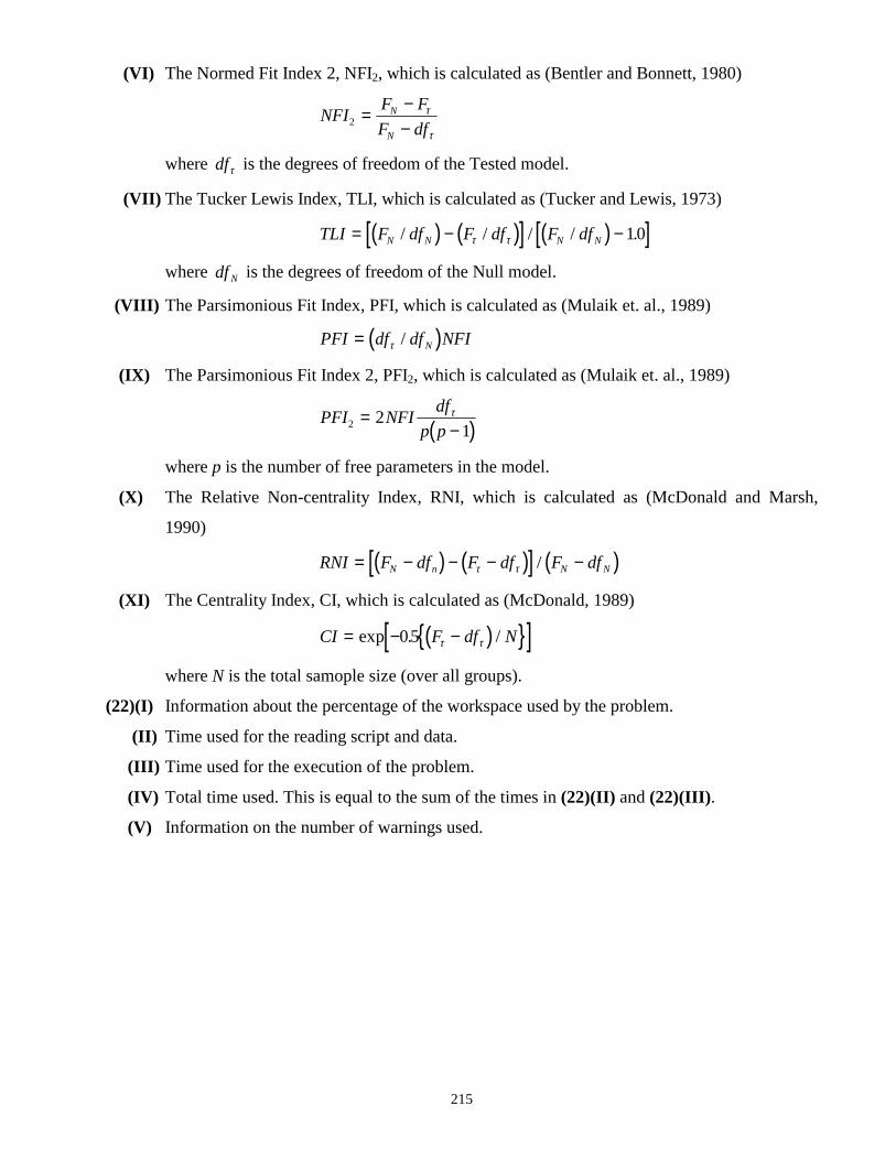
215

(VI) The Normed Fit Index 2, NFI2, which is calculated as (Bentler and Bonnett, 1980)

NFI F FF df

N

N2 = −

−τ

τ

where dfτ is the degrees of freedom of the Tested model.

(VII) The Tucker Lewis Index, TLI, which is calculated as (Tucker and Lewis, 1973)

( ) ( )[ ] ( )[ ]TLI F df F df F dfN N N N= − −/ / / / .τ τ 10

where df N is the degrees of freedom of the Null model.

(VIII) The Parsimonious Fit Index, PFI, which is calculated as (Mulaik et. al., 1989)

( )PFI df df NFIN= τ /

(IX) The Parsimonious Fit Index 2, PFI2, which is calculated as (Mulaik et. al., 1989)

( )PFI NFI dfp p2 2

1=

−τ

where p is the number of free parameters in the model.

(X) The Relative Non-centrality Index, RNI, which is calculated as (McDonald and Marsh,

1990)

( ) ( )[ ] ( )RNI F df F df F dfN n N N= − − − −τ τ /

(XI) The Centrality Index, CI, which is calculated as (McDonald, 1989)

( ){ }[ ]CI F df N= − −exp . /05 τ τ

where N is the total samople size (over all groups).

(22)(I) Information about the percentage of the workspace used by the problem.

(II) Time used for the reading script and data.

(III) Time used for the execution of the problem.

(IV) Total time used. This is equal to the sum of the times in (22)(II) and (22)(III).

(V) Information on the number of warnings used.

216

CHAPTER 6

RAMONA 6.1 HISTORICAL BACKGROUND The acronym RAMONA stands for Reticular Action MOdel or Near Approximation. RAMONA is

influenced greatly by Steiger’s suggestion of the use of the ASCII symbols <--: for dependence paths

and <--> for variance/covariance paths to create ASCII representations of the path diagrams of

Structural Equation Models. This suggestion allows users to specify their models in terms of a path

diagram instead of parameter matrices. The program RAMONA implements the RAMONA model

(Mels, 1988). Mels (1988) developed the initial version of RAMONA. Browne and Mels

(1990,1992) have updated this initial version of RAMONA. A DOS version of RAMONA (Mels,

Browne and Coward, 1994) forms part of the statistical software package SYSTAT version 6 for

DOS. RAMONA is also available in SYSTAT version 6 for Windows. Browne and Mels (1998)

developed the latest stand-alone version for Windows. The SYSTAT versions differ from the other

versions in the fact that it uses <- and <-> for dependence and covariance paths, instead of <--: and

<-->, respectively.

RAMONA is a program for path analysis with manifest and latent variables and it implements the

McArdle and McDonald (1984) Reticular Action Model (RAM). The deviation from RAM is minor

in that no distinction is made between residual variables and other exogenous latent variables. The

program brought to rest the problem with negative variance and out of bound estimates and was the

computer program of its kind to yield correct results whenever the sample correlation matrix instead

of sample covariance matrix is analyzed.

RAMONA is intended for users with knowledge of latent variable modeling but can be employed by

researchers with no mathematical background. The user only needs to know how to formulate a

model in the form of a path diagram. Knowledge of matrix algebra is not essential.

6.2 THE RAMONA INPUT FILE To run RAMONA, the user must prepare an Input File. A RAMONA Input File is a text file that

consists of five paragraphs and the data to be analyzed. Each paragraph consists of a sentence(s).

217

The following general rules apply to the paragraphs and sentences of a RAMONA Input File.

GENERAL RULES FOR RAMONA INPUT FILES

• Each sentence consists of a maximum of 80 characters.

• Each sentence ends with a slash.

• Each paragraph start with a unique keyword followed by = (equal sign) and ends with a

semicolon.

• The five paragraphs may appear in any order.

• The matrix or raw data to be analyzed is the final section of the input file and is

preceded with the word DATA, the type of data (“RAW DATA”, “COVARIANCE

MATRIX” or “CORRELATION MATRIX”) and an integer value for the number of cases

on three different lines.

A RAMONA Input File may be divided into three sections. These are:

1. Model Information

2. Model Specification

3. Data

6.2.1 MODEL INFORMATION

Model information is specified in three paragraphs, namely: TITLE paragraph, MANIFEST variable

paragraph and LATENT variable paragraph.

Details of each paragraph are discussed below.

(a) TITLE Paragraph

This paragraph provides a description for the analysis to be performed. It starts with TITLE =. For

the model depicted in Figure 1.2 we may have a TITLE paragraph as follows:

TITLE = Duncan, Haller and Portes’ (1971) Application;

218

(b) MANIFEST Variable Paragraph

• A manifest variable is represented by means of a rectangle or square on a path

diagram.

• The manifest variable paragraph allows the user to give descriptive names to the

manifest variables.

Rules for the MANIFEST Variable paragraph

• The manifest variable paragraph starts with MANIFEST=.

• Each descriptive name of a manifest variable may not exceed eight (8) characters.

• The order of the manifest variables corresponds to the order of the columns of

the covariance, correlation or raw data matrix provided in the final section of the

input file.

• The descriptive names of the manifest variables are separated by at least one blank space.

For the model depicted in Figure 1.2, we may have a manifest variable paragraph as shown below.

MANIFEST=REINT REPAP RSOEC REOAP REEAP /

BFINT BFPAP BFSOE BFOAP BFEAP;

(c) LATENT Variable paragraph

• Latent variables are indicated on a path diagram by means of circles or ellipses.

• The latent variable paragraph is used to give descriptive names to the latent

variables in the model.

Rules for the LATENT Variable paragraph.

• The LATENT variable paragraph starts with LATENT=.

• Each descriptive name of a latent variable may not exceed eight (8) characters.

• The latent variables may be provided in any order.

• The descriptive names of the latent variables are separated by at least one blank space.

For the model depicted in Figure 1.2, the following latent variable paragraph may be used:

LATENT= REAMB BFAMB E1 E2 E3 E4 Z1 Z2;

219

6.2.2 MODEL SPECIFICATION This is the section of the input file where the path diagram of the model is coded directly with the

use of the ASCII symbols <--: (for dependence paths) and <--> ( for covariance paths) and it is

specified in the MODEL paragraph of the RAMONA Input file.

Rules for the MODEL Paragraph.

• This paragraph starts with the keyword MODEL=.

• The MODEL paragraph consists of two sub-paragraphs, one for dependence

paths and one for variance/covariance paths.

• Dependence paths and covariance paths must be specified in separate

subparagraphs and cannot be intermingled.

(i) DEPENDENCE PATHS

A dependence path is indicated by the symbol <--: which relates directly to the single headed

arrow employed in a path diagram. A dependence path is coded as follows:

Dependent Variable <--: (Explanatory Variable, Parameter Number, Starting Value)/

For the model depicted in Figure 1.2 the endogenous manifest variable REOAP receives single

headed arrow from the latent variable REAMB and a measurement error E1. These paths are


1 1

Figure 6.1 Dependence paths between REOAP, E1 and REAMB.

These dependence paths are coded as

REOAP <--: (REAMB, 0, 1.0)/

REOAP <--: (E1, 0, 1.0)/

REOAP REAMB E1

220

It is not necessary to have a different sentence for each path. Several paths with the same dependent

(receiving) variable may be combined into one sentence. The sentence must fit on one line of not

more than 80 characters. Otherwise, more than one sentence is necessary.

Since the same endogenous variable, REOAP, is involved in the two dependence paths, the two

paths may be coded in a single sentence as:

REOAP <--: (REAMB, 0, 1.0) (E1, 0, 1.0)/

When specifying dependence paths, bear in mind that:

• Dependence paths can be specified in any order.

• A sentence can specify several dependence paths involving the same endogenous variable.

• In some cases, a dependent variable may be involved in too many dependence paths for a

single sentence. In this situation, make use of several sentences with the same dependent

variable.

• Parameter numbers need not be sequential. If they are not, RAMONA will reassign path

numbers.

(ii) VARIANCE/COVARIANCE PATHS

A variance or covariance path is indicated by the symbol <--> which relates directly to the

double headed arrow used in a path diagram. A covariance paths is specified in an input file as

follows:

Variable <--> (Name of the other Variable, Parameter number, Starting value)/

Unlike in the case of the dependence paths, it does not matter which variable is given first.

For the model depicted in Figure 1.2, double headed arrows are employed from the manifest variable

REPAP to itself to specify a variance and to RESOE, REINT, and BFINT to specify covariances.


Figure 6.2 Covariance Paths between REPAP, RESOE and REINT.

REPAP REINT RESOE

221


REPAP <--> (REPAP, *, *)/

REPAP <-->(RESOE, *, *)/

REPAP <--> (REINT, *, *)/

Since the same variable, REPAP, is involved in all the three sentences, they can be combined into

one sentence as shown below.

REPAP <--> (REPAP, *, *) (RESOE, *, *) (REINT, *, *)/

When specifying covariance paths bear in mind that:

• Covariance paths can be specified in any order.

• Several covariance paths per sentence can be specified. For example, the variance of an

exogenous variable as well as its covariance with other variables can be specified in the same

sentence.

• If every endogenous manifest variable has a corresponding measurement error with an

unconstrained variance, the coding of these variances can be omitted. When all error path

coefficients are fixed, and no error variance paths are specified for the measurement errors,

RAMONA will automatically provide the error variance paths.

• If there are exogenous manifest variables and if all their variances and covariances are

present in the model and are unrestricted, the coding of these variance and covariance paths

may be omitted. When no variance and covariance paths for exogenous manifest variables

are specified, the RAMONA will automatically provide them.

6.2.3 DATA

The data must be provided last and are preceded by the key word DATA followed by the type of

data (“RAW DATA”, “COVARIANCE MATRIX” or “CORRELATION MATRIX”) and an

integer value of the number of cases on separate lines. If a distribution free analysis is required, the

raw data must be provided. Otherwise the correlation or covariance matrix may be input. The

correlation (covariance) matrix is provided in free format, one row at a time.

For the model depicted in Figure 1.2, the correlation matrix in Table 1.3, may be specified in the

RAMONA input file as shown below.

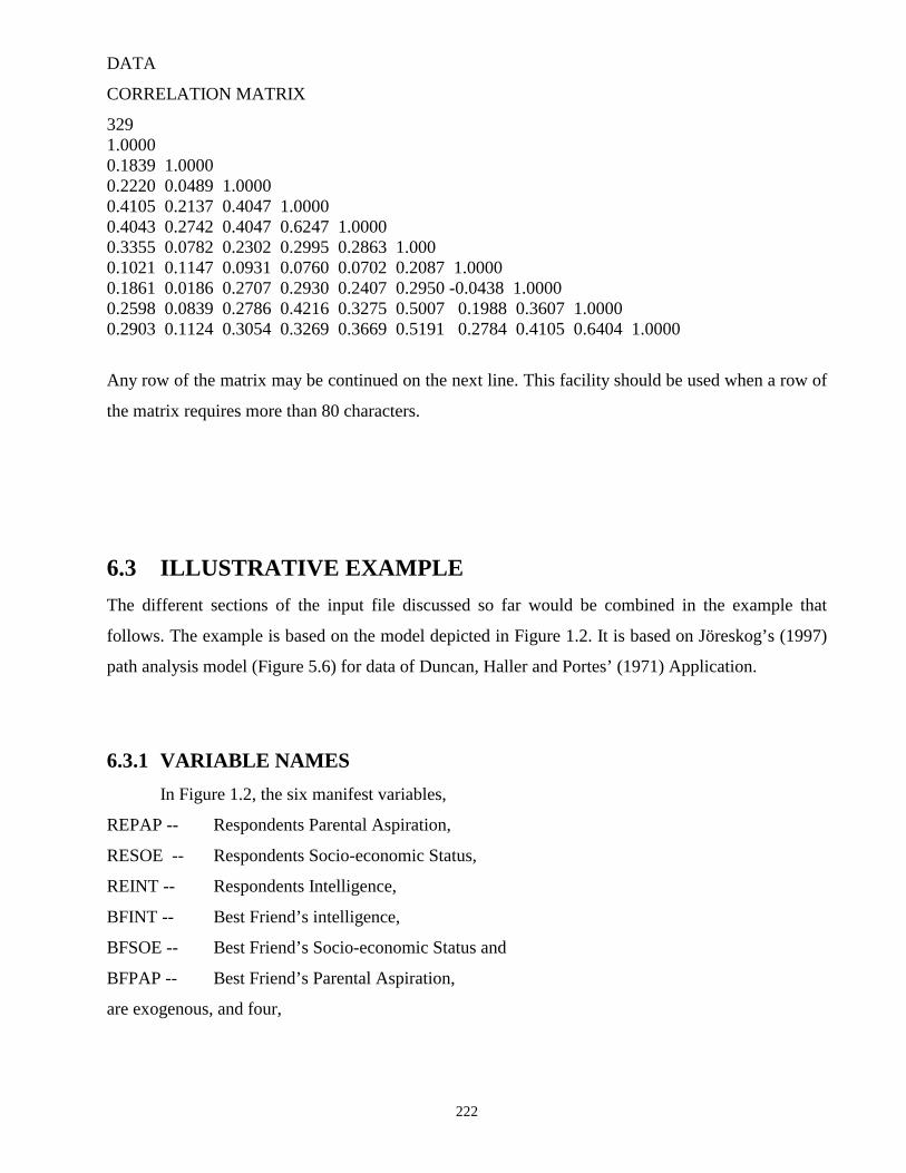
222

DATA

CORRELATION MATRIX

329 1.0000 0.1839 1.0000 0.2220 0.0489 1.0000 0.4105 0.2137 0.4047 1.0000 0.4043 0.2742 0.4047 0.6247 1.0000 0.3355 0.0782 0.2302 0.2995 0.2863 1.000 0.1021 0.1147 0.0931 0.0760 0.0702 0.2087 1.0000 0.1861 0.0186 0.2707 0.2930 0.2407 0.2950 -0.0438 1.0000 0.2598 0.0839 0.2786 0.4216 0.3275 0.5007 0.1988 0.3607 1.0000 0.2903 0.1124 0.3054 0.3269 0.3669 0.5191 0.2784 0.4105 0.6404 1.0000

Any row of the matrix may be continued on the next line. This facility should be used when a row of

the matrix requires more than 80 characters.

6.3 ILLUSTRATIVE EXAMPLE The different sections of the input file discussed so far would be combined in the example that

follows. The example is based on the model depicted in Figure 1.2. It is based on Jöreskog’s (1997)

path analysis model (Figure 5.6) for data of Duncan, Haller and Portes’ (1971) Application.

6.3.1 VARIABLE NAMES In Figure 1.2, the six manifest variables,

REPAP -- Respondents Parental Aspiration,

RESOE -- Respondents Socio-economic Status,

REINT -- Respondents Intelligence,

BFINT -- Best Friend’s intelligence,

BFSOE -- Best Friend’s Socio-economic Status and

BFPAP -- Best Friend’s Parental Aspiration,

are exogenous, and four,

223

REOAP -- Respondents Occupational Aspiration,

REEAP -- Respondents Educational Aspiration,

BFEAP -- Best Friend’s Educational Aspiration and

BFOAP -- Best Friend’s Occupational Aspiration,

are endogenous.

The Latent Variables

REAMB -- Respondent’s Ambition and

BFAMB -- Best Friend’s Ambition,

are endogenous, and the rest, E1, E2, E3, E4, Z1 and Z2 are (exogenous) error variables.

6.3.2 INPUT FILE A complete RAMONA input file therefore may be as shown below.

TITLE= Duncan, Haller and Portes Model; MANIFEST=REINT REPAP RESOE REOAP REEAP/ BFINT BFPAP BFSOE BFOAP BFEAP; LATENT = REAMB BFAMB E1 E2 E3 E4 Z1 Z2; MODEL= REOAP <--: (REAMB,*,*) (E1,0,1.0)/ REEAP <--: (REAMB,*,*) (E2,0,1.0)/ BFEAP <--: (BFAMB,*,*) (E3,0,1.0)/ BFOAP <--: (BFAMB,*,*) (E4,0,1.0)/ REAMB <--: (BFAMB,*,*) (REPAP,*,*) (REINT,*,*) / REAMB <--: (RESOE,*,*) (BFSOE,*,*) (Z1,0,1.0) / BFAMB <--: (BFSOE,*,*) (BFINT,*,*) (BFPAP,*,*) / BFAMB <--: (REAMB,*,*) (RESOE,*,*) (Z2,0,1.0); REINT <--> (REINT,0,1.0) (RESOE,*,*) (REPAP,*,*)/ REINT <--> (BFINT,*,*) (BFSOE,*,*) (BFPAP,*,*) / REPAP <--> (REPAP,0,1.0) (RESOE,*,*)/ REPAP <--> (BFSOE,*,*) (BFINT,*,*) (BFPAP,*,*) / RESOE <--> (RESOE,0,1.0) / RESOE <--> (BFSOE,*,*) (BFINT,*,*) (BFPAP,*,*) / BFSOE <--> (BFSOE,0,1.0) (BFINT,*,*) (BFPAP,*,*)/ BFINT <--> (BFINT,0,1.0) (BFPAP,*,*)/ BFPAP <--> (BFPAP,0,1.0)/ REAMB <--> (REAMB,0,1.0)/ BFAMB <--> (BFAMB,0,1.0)/ E1 <--> (E1,*,*)/ E2 <--> (E2,*,*)/ E3 <--> (E3,*,*)/ E4 <--> (E4,*,*)/ Z1 <--> (Z1,*,*)/ Z2 <--> (Z2,*,*);

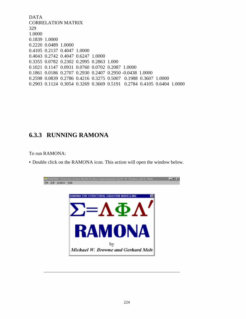
224

DATA CORRELATION MATRIX 329 1.0000 0.1839 1.0000 0.2220 0.0489 1.0000 0.4105 0.2137 0.4047 1.0000 0.4043 0.2742 0.4047 0.6247 1.0000 0.3355 0.0782 0.2302 0.2995 0.2863 1.000 0.1021 0.1147 0.0931 0.0760 0.0702 0.2087 1.0000 0.1861 0.0186 0.2707 0.2930 0.2407 0.2950 -0.0438 1.0000 0.2598 0.0839 0.2786 0.4216 0.3275 0.5007 0.1988 0.3607 1.0000 0.2903 0.1124 0.3054 0.3269 0.3669 0.5191 0.2784 0.4105 0.6404 1.0000

6.3.3 RUNNING RAMONA

To run RAMONA:

• Double click on the RAMONA icon. This action will open the window below.

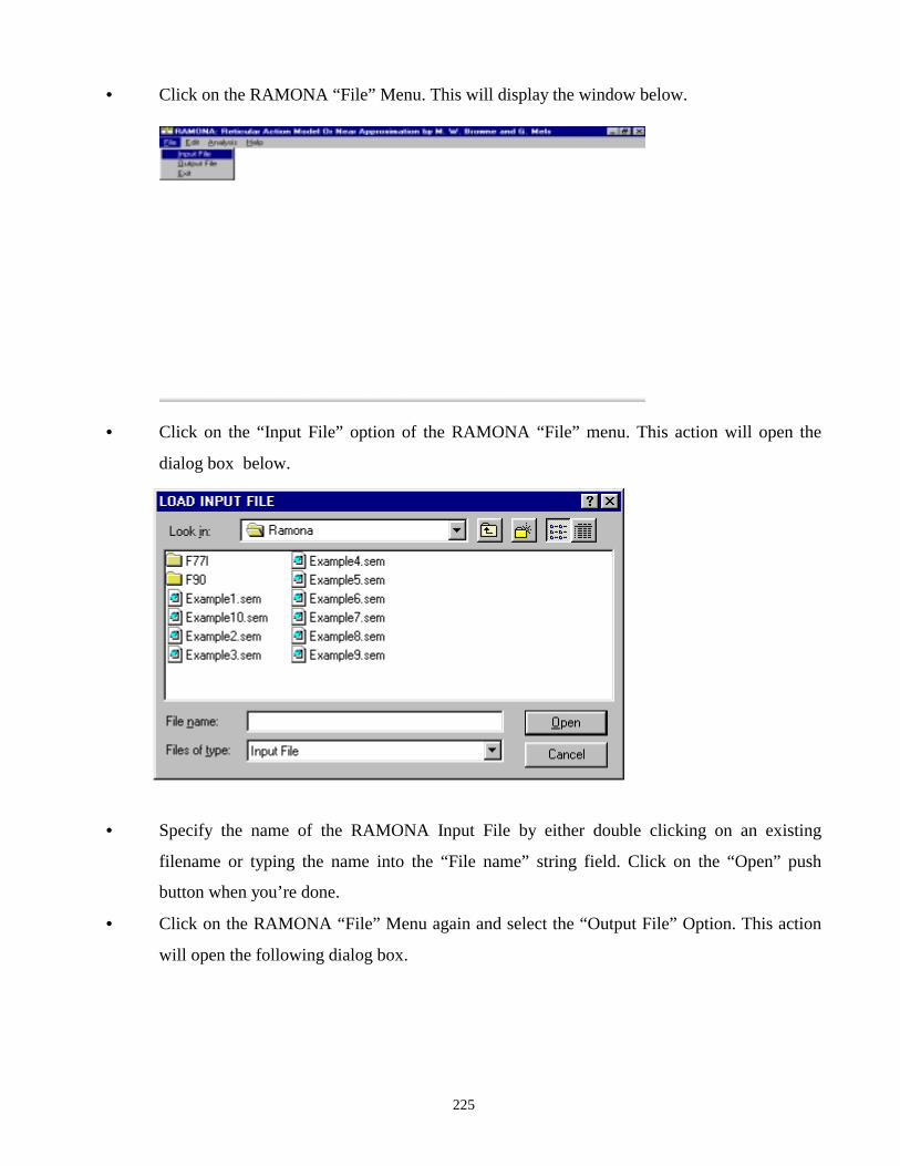
225

• Click on the RAMONA “File” Menu. This will display the window below.

• Click on the “Input File” option of the RAMONA “File” menu. This action will open the

dialog box below.

• Specify the name of the RAMONA Input File by either double clicking on an existing

filename or typing the name into the “File name” string field. Click on the “Open” push

button when you’re done.

• Click on the RAMONA “File” Menu again and select the “Output File” Option. This action

will open the following dialog box.

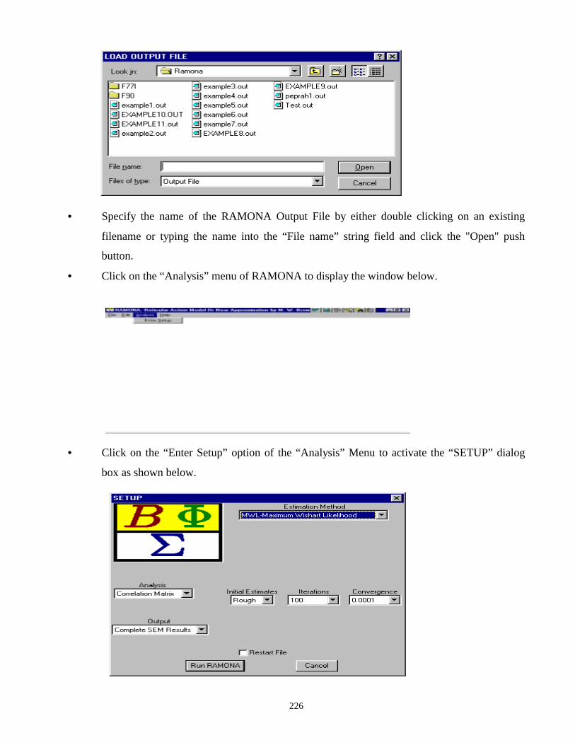
226

• Specify the name of the RAMONA Output File by either double clicking on an existing

filename or typing the name into the “File name” string field and click the "Open" push

button.

• Click on the “Analysis” menu of RAMONA to display the window below.

• Click on the “Enter Setup” option of the “Analysis” Menu to activate the “SETUP” dialog

box as shown below.

227

• The dialog box requests the user to specify the various options for the analysis.

• The options are specified by clicking on the various menu fields in the dialog box and then

selecting the appropriate option.

Detail descriptions of each of the options follow:

ANALYSIS

•••• This option is used to specify the matrix to which the model must be fitted.

• The alternatives available are Covariance Matrix and Correlation Matrix.

ESTIMATION METHOD

• This option specifies the method of estimation to be used by RAMONA.

• The alternatives available are MWL, GLS, OLS, TGLS, TSLS, ADFG, and ADFU. Each of

these is an abbreviation and their full meanings are provided below.

• MWL - Maximum Wishart Likelihood.

• GLS - Generalized Least Squares assuming Wishart distribution for the sample

covariance matrix S.

• OLS - Ordinary Least Squares.

• TGLS – True Generalized Least Squares.

• TSLS – Two Stage Least Squares.

• ADFG - an Asymptotically Distribution Free procedure which uses a biased but Gramian

(non-negative definite) estimate of the asymptotic covariance matrix, Γ, of the elements of

the sample covariance matrix.

• ADFU - an Asymptotically Distribution Free procedure which uses an Unbiased estimate of

the asymptotic covariance matrix, Γ.

• Default is MWL.

INITIAL ESTIMATES

• The alternatives for this option are ROUGH and CLOSE.

• If ROUGH is chosen the initial iterations are OLS. After partial convergence, the

program switches to the procedure specified by the METHOD option.

• If CLOSE is used the estimation procedure specified by the METHOD option is

employed from the start of the iterative procedure.

228

• The default is ROUGH. This means that if neither ROUGH nor CLOSE

is specified the program takes the ROUGH alternative.

OUTPUT

• This option is used to restrict the amount of output of RAMONA.

• The alternatives available are COMPLETE RAMONA RESULTS, COMPLETE SEM

RESULTS or BASIC SEM RESULTS.

If the option “COMPLETE RAMONA RESULTS” is chosen the following information are provided

as output.

(a) The job specification system.

(b) Details of the iterative procedure.

(c) The sample covariance or correlation matrix.

(d) The reproduced covariance or correlation matrix.

(e) The matrix of residuals.

(f) A table consisting of path coefficient estimates, 90% confidence intervals,

standard errors and t-statistics (estimate divided by standard error).

(g) A table consisting of variance and covariance or correlation estimates, 90%

confidence intervals, standard errors and t statistics.

(h) Information about equality constraints on variances (if applicable).

(i) Measures of fit of the model.

(j) The asymptotic correlation matrix of the estimators.

If “COMPLETE SEM RESULTS” is chosen, (j) is omitted from the list above.

If “BASIC SEM RESULTS” is chosen, (b), (d), (e), (h) and (j) are omitted.

The default is COMPLETE SEM RESULTS.

CONVERGENCE

• This option specifies the tolerance limit for the residual cosine employed by the

program as a convergence criterion.

• It also controls the number of decimal places provided during output of estimates.

If CONVERGENCE =0.1 x 10k then k decimal places are provided.

• The default is 0.0001.

229

ITERATIONS

• This option allows the user to specify the maximum number of iterations allowed for the

iterative procedure.

• The default value is 100.

RESTART FILE

A text file with the same filename as the RAMONA Input File and with extension .RST, that is a

duplicate of the RAMONA Input file in which the original parameter estimates are replaced by the

final parameter estimates, is created if the “Restart File” check box is activated. Otherwise, this file

is not created.

After selecting the required option(s) click on the “Run RAMONA” push button. If there are no

syntax errors in the input file, then iteration will proceed. When the iterations are completed, the

message box

appears.

6.5 THE RAMONA OUTPUT FILE (1) o-----------------------------------------------o | | | RAMONA for Windows Version 1.0: November 1998 | | | | Reticular Action Model Or Near Approximation | | | | | | Program authors: | | Michael W. Browne and Gerhard Mels | | | o-----------------------------------------------o

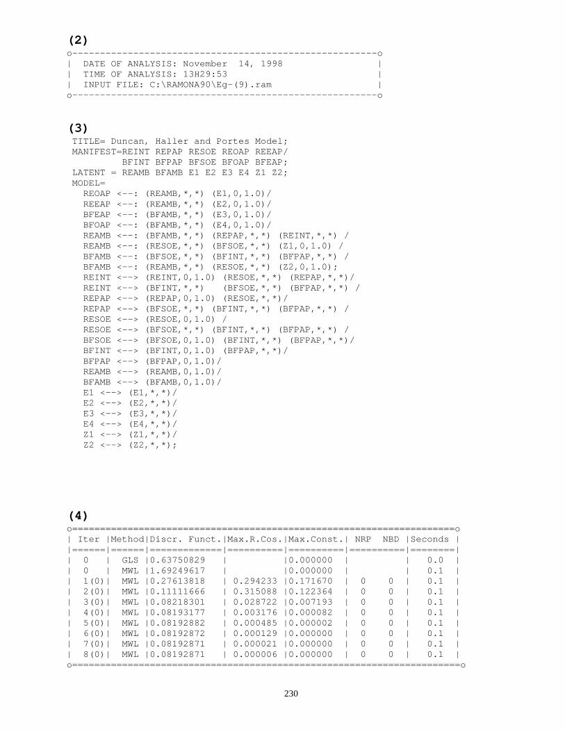
230

(2) o-------------------------------------------------------o | DATE OF ANALYSIS: November 14, 1998 | | TIME OF ANALYSIS: 13H29:53 | | INPUT FILE: C:\RAMONA90\Eg-(9).ram | o-------------------------------------------------------o

(3) TITLE= Duncan, Haller and Portes Model; MANIFEST=REINT REPAP RESOE REOAP REEAP/ BFINT BFPAP BFSOE BFOAP BFEAP; LATENT = REAMB BFAMB E1 E2 E3 E4 Z1 Z2; MODEL= REOAP <--: (REAMB,*,*) (E1,0,1.0)/ REEAP <--: (REAMB,*,*) (E2,0,1.0)/ BFEAP <--: (BFAMB,*,*) (E3,0,1.0)/ BFOAP <--: (BFAMB,*,*) (E4,0,1.0)/ REAMB <--: (BFAMB,*,*) (REPAP,*,*) (REINT,*,*) / REAMB <--: (RESOE,*,*) (BFSOE,*,*) (Z1,0,1.0) / BFAMB <--: (BFSOE,*,*) (BFINT,*,*) (BFPAP,*,*) / BFAMB <--: (REAMB,*,*) (RESOE,*,*) (Z2,0,1.0); REINT <--> (REINT,0,1.0) (RESOE,*,*) (REPAP,*,*)/ REINT <--> (BFINT,*,*) (BFSOE,*,*) (BFPAP,*,*) / REPAP <--> (REPAP,0,1.0) (RESOE,*,*)/ REPAP <--> (BFSOE,*,*) (BFINT,*,*) (BFPAP,*,*) / RESOE <--> (RESOE,0,1.0) / RESOE <--> (BFSOE,*,*) (BFINT,*,*) (BFPAP,*,*) / BFSOE <--> (BFSOE,0,1.0) (BFINT,*,*) (BFPAP,*,*)/ BFINT <--> (BFINT,0,1.0) (BFPAP,*,*)/ BFPAP <--> (BFPAP,0,1.0)/ REAMB <--> (REAMB,0,1.0)/ BFAMB <--> (BFAMB,0,1.0)/ E1 <--> (E1,*,*)/ E2 <--> (E2,*,*)/ E3 <--> (E3,*,*)/ E4 <--> (E4,*,*)/ Z1 <--> (Z1,*,*)/ Z2 <--> (Z2,*,*);

(4) o=====================================================================o | Iter |Method|Discr. Funct.|Max.R.Cos.|Max.Const.| NRP NBD |Seconds | |======|======|=============|==========|==========|==========|========| | 0 | GLS |0.63750829 | |0.000000 | | 0.0 | | 0 | MWL |1.69249617 | |0.000000 | | 0.1 | | 1(0)| MWL |0.27613818 | 0.294233 |0.171670 | 0 0 | 0.1 | | 2(0)| MWL |0.11111666 | 0.315088 |0.122364 | 0 0 | 0.1 | | 3(0)| MWL |0.08218301 | 0.028722 |0.007193 | 0 0 | 0.1 | | 4(0)| MWL |0.08193177 | 0.003176 |0.000082 | 0 0 | 0.1 | | 5(0)| MWL |0.08192882 | 0.000485 |0.000002 | 0 0 | 0.1 | | 6(0)| MWL |0.08192872 | 0.000129 |0.000000 | 0 0 | 0.1 | | 7(0)| MWL |0.08192871 | 0.000021 |0.000000 | 0 0 | 0.1 | | 8(0)| MWL |0.08192871 | 0.000006 |0.000000 | 0 0 | 0.1 | o======================================================================o

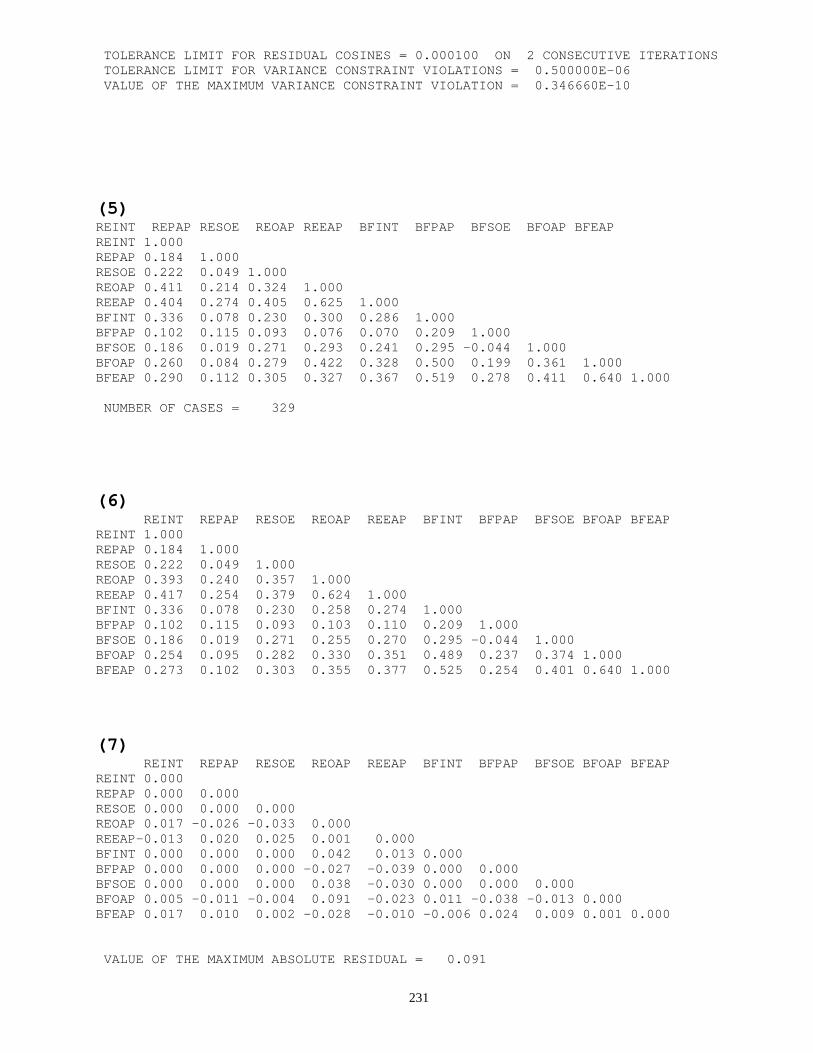
231

TOLERANCE LIMIT FOR RESIDUAL COSINES = 0.000100 ON 2 CONSECUTIVE ITERATIONS TOLERANCE LIMIT FOR VARIANCE CONSTRAINT VIOLATIONS = 0.500000E-06 VALUE OF THE MAXIMUM VARIANCE CONSTRAINT VIOLATION = 0.346660E-10

(5) REINT REPAP RESOE REOAP REEAP BFINT BFPAP BFSOE BFOAP BFEAP REINT 1.000 REPAP 0.184 1.000 RESOE 0.222 0.049 1.000 REOAP 0.411 0.214 0.324 1.000 REEAP 0.404 0.274 0.405 0.625 1.000 BFINT 0.336 0.078 0.230 0.300 0.286 1.000 BFPAP 0.102 0.115 0.093 0.076 0.070 0.209 1.000 BFSOE 0.186 0.019 0.271 0.293 0.241 0.295 -0.044 1.000 BFOAP 0.260 0.084 0.279 0.422 0.328 0.500 0.199 0.361 1.000 BFEAP 0.290 0.112 0.305 0.327 0.367 0.519 0.278 0.411 0.640 1.000 NUMBER OF CASES = 329

(6) REINT REPAP RESOE REOAP REEAP BFINT BFPAP BFSOE BFOAP BFEAP REINT 1.000 REPAP 0.184 1.000 RESOE 0.222 0.049 1.000 REOAP 0.393 0.240 0.357 1.000 REEAP 0.417 0.254 0.379 0.624 1.000 BFINT 0.336 0.078 0.230 0.258 0.274 1.000 BFPAP 0.102 0.115 0.093 0.103 0.110 0.209 1.000 BFSOE 0.186 0.019 0.271 0.255 0.270 0.295 -0.044 1.000 BFOAP 0.254 0.095 0.282 0.330 0.351 0.489 0.237 0.374 1.000 BFEAP 0.273 0.102 0.303 0.355 0.377 0.525 0.254 0.401 0.640 1.000

(7) REINT REPAP RESOE REOAP REEAP BFINT BFPAP BFSOE BFOAP BFEAP REINT 0.000 REPAP 0.000 0.000 RESOE 0.000 0.000 0.000 REOAP 0.017 -0.026 -0.033 0.000 REEAP-0.013 0.020 0.025 0.001 0.000 BFINT 0.000 0.000 0.000 0.042 0.013 0.000 BFPAP 0.000 0.000 0.000 -0.027 -0.039 0.000 0.000 BFSOE 0.000 0.000 0.000 0.038 -0.030 0.000 0.000 0.000 BFOAP 0.005 -0.011 -0.004 0.091 -0.023 0.011 -0.038 -0.013 0.000 BFEAP 0.017 0.010 0.002 -0.028 -0.010 -0.006 0.024 0.009 0.001 0.000 VALUE OF THE MAXIMUM ABSOLUTE RESIDUAL = 0.091

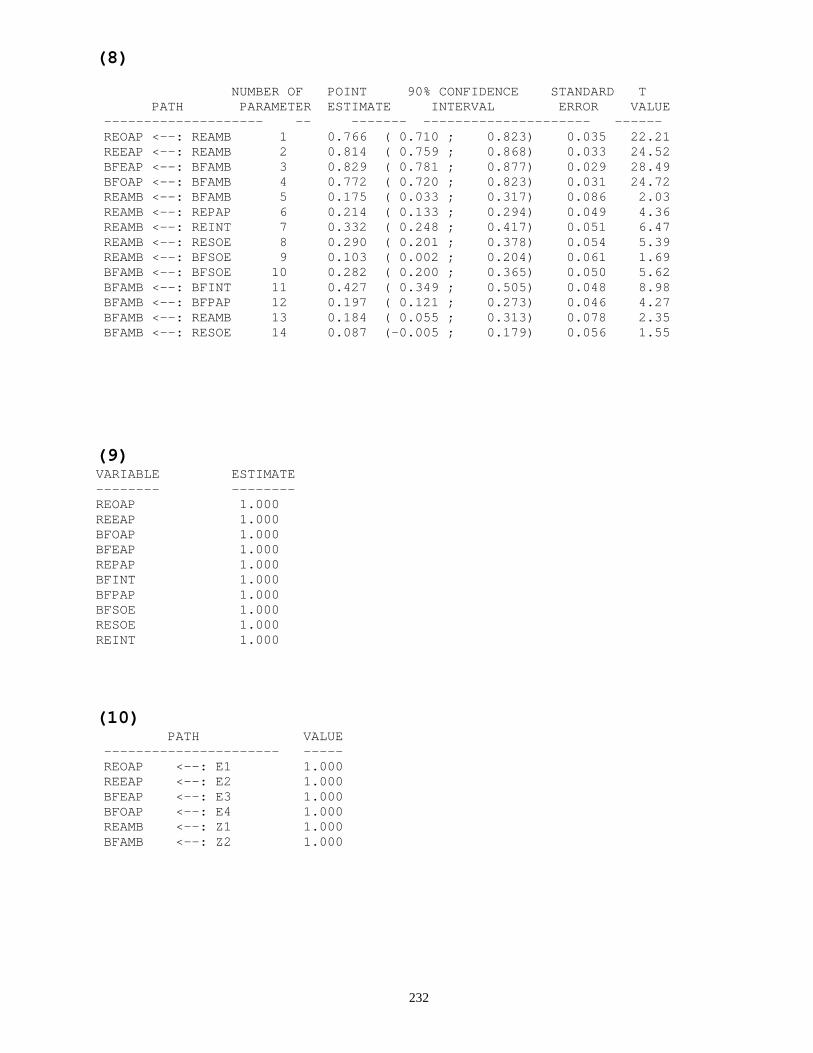
232

(8) NUMBER OF POINT 90% CONFIDENCE STANDARD T PATH PARAMETER ESTIMATE INTERVAL ERROR VALUE -------------------- -- ------- --------------------- ------ REOAP <--: REAMB 1 0.766 ( 0.710 ; 0.823) 0.035 22.21 REEAP <--: REAMB 2 0.814 ( 0.759 ; 0.868) 0.033 24.52 BFEAP <--: BFAMB 3 0.829 ( 0.781 ; 0.877) 0.029 28.49 BFOAP <--: BFAMB 4 0.772 ( 0.720 ; 0.823) 0.031 24.72 REAMB <--: BFAMB 5 0.175 ( 0.033 ; 0.317) 0.086 2.03 REAMB <--: REPAP 6 0.214 ( 0.133 ; 0.294) 0.049 4.36 REAMB <--: REINT 7 0.332 ( 0.248 ; 0.417) 0.051 6.47 REAMB <--: RESOE 8 0.290 ( 0.201 ; 0.378) 0.054 5.39 REAMB <--: BFSOE 9 0.103 ( 0.002 ; 0.204) 0.061 1.69 BFAMB <--: BFSOE 10 0.282 ( 0.200 ; 0.365) 0.050 5.62 BFAMB <--: BFINT 11 0.427 ( 0.349 ; 0.505) 0.048 8.98 BFAMB <--: BFPAP 12 0.197 ( 0.121 ; 0.273) 0.046 4.27 BFAMB <--: REAMB 13 0.184 ( 0.055 ; 0.313) 0.078 2.35 BFAMB <--: RESOE 14 0.087 (-0.005 ; 0.179) 0.056 1.55

(9) VARIABLE ESTIMATE -------- -------- REOAP 1.000 REEAP 1.000 BFOAP 1.000 BFEAP 1.000 REPAP 1.000 BFINT 1.000 BFPAP 1.000 BFSOE 1.000 RESOE 1.000 REINT 1.000

(10) PATH VALUE ---------------------- ----- REOAP <--: E1 1.000 REEAP <--: E2 1.000 BFEAP <--: E3 1.000 BFOAP <--: E4 1.000 REAMB <--: Z1 1.000 BFAMB <--: Z2 1.000

233

(11) NUMBER OF POINT 90% CONFIDENCE STANDARD T PATH PARAMETER ESTIMATE INTERVAL ERROR VALUE -------------------- -- ------- --------------------- ------- REINT <--> RESOE 15 0.222 ( 0.136 ; 0.308) 0.052 4.23 REINT <--> REPAP 16 0.184 ( 0.096 ; 0.272) 0.053 3.45 REINT <--> BFINT 17 0.336 ( 0.255 ; 0.416) 0.049 6.85 REINT <--> BFSOE 18 0.186 ( 0.098 ; 0.274) 0.053 3.49 REINT <--> BFPAP 19 0.102 ( 0.012 ; 0.192) 0.055 1.87 REPAP <--> RESOE 20 0.049 ( -0.042 ; 0.140) 0.055 0.89 REPAP <--> BFSOE 21 0.019 ( -0.072 ; 0.109) 0.055 0.34 REPAP <--> BFINT 22 0.078 ( -0.012 ; 0.168) 0.055 1.42 REPAP <--> BFPAP 23 0.115 ( 0.025 ; 0.204) 0.054 2.10 RESOE <--> BFSOE 24 0.271 ( 0.187 ; 0.355) 0.051 5.29 RESOE <--> BFINT 25 0.230 ( 0.144 ; 0.316) 0.052 4.40 RESOE <--> BFPAP 26 0.093 ( 0.003 ; 0.183) 0.055 1.70 BFSOE <--> BFINT 27 0.295 ( 0.212 ; 0.378) 0.050 5.85 BFSOE <--> BFPAP 28 -0.044 ( -0.134 ; 0.047) 0.055 -0.79 BFINT <--> BFPAP 29 0.209 ( 0.122 ; 0.296) 0.053 3.95 E1 <--> E1 30 0.413 ( 0.334 ; 0.510) 0.053 7.80 E2 <--> E2 31 0.338 ( 0.259 ; 0.439) 0.054 6.25 E3 <--> E3 32 0.313 ( 0.243 ; 0.403) 0.048 6.50 E4 <--> E4 33 0.404 ( 0.332 ; 0.492) 0.048 8.40 Z1 <--> Z1 34 0.480 ( 0.390 ; 0.570) 0.055 8.64 Z2 <--> Z2 35 0.385 ( 0.305 ; 0.471) 0.051 7.60

(12) PATH VALUE ---------------------- ----- REINT <--> REINT 1.000 REPAP <--> REPAP 1.000 RESOE <--> RESOE 1.000 BFSOE <--> BFSOE 1.000 BFINT <--> BFINT 1.000 BFPAP <--> BFPAP 1.000

(13) CONSTRAINT VALUE LAGRANGE MULTIPLIER STANDARD ERROR ---------------------- ------ ------------------- -------------- REAMB <--> REAMB 1.0000 0.0000 0.0000 BFAMB <--> BFAMB 1.0000 0.0000 0.0000 REOAP <--> REOAP 1.0000 0.0000 0.0000 REEAP <--> REEAP 1.0000 0.0000 0.0000 BFOAP <--> BFOAP 1.0000 0.0000 0.0000 BFEAP <--> BFEAP 1.0000 0.0000 0.0000

234

(14) o-----------------------------------------------------------------------o | Sample Discrepancy Function Value (I) :0.082 ( 0.819287E-01)| | Population Discrepancy Function Value, Fo | | Bias Adjusted Point Estimate (II) : 0.033 | | 90 Percent Confidence Interval (III):( 0.001 ; 0.089) | | | | Root Mean Square Error of Approximation | | Steiger-Lind : RMSEA = SQRT(Fo/DF) | | Point Estimate (IV) : 0.046 | | 90 Percent Confidence Interval (V) :( 0.008 ; 0.075) | | | | Expected Cross-Validation Index | | Point Estimate (Modified AIC) (VI) : 0.320 | | 90 Percent Confidence Interval (VII):( 0.288 ; 0.376) | | ECVI (MODIFIED AIC)for the Saturated Model(VIII): 0.335 | | | | Test Statistic (IX) : 26.87 | | Exceedance Probabilities:- | | Ho: Perfect Fit (RMSEA = 0.0) (X) : 0.043 | | Ho: Close Fit (RMSEA <= 0.050) (XI) : 0.561 | | Multiplier for obtaining Test Statistic = 328.0 | | Degrees of Freedom = 16 | | Effective Number of Parameters = 39 | o-----------------------------------------------------------------------o

(15) o----------------------------------------------------------------o | LISREL GFI (I) : 0.984 | | LISREL Adjusted GFI (II) : 0.946 | | Mulaik Parsimonious GFI (III) : 0.350 | | | | Schwarz Bayesian Criterion (IV) : 0.771 | | Browne-Cudeck Single Sample CVI (V) : 0.328 | | | | Bentler-Bonett Normed Fit Index (VI) : 0.969 | | Bentler-Bonett Non-Normed Fit Index (VII) : 0.963 | | Bentler Comparative Fit Index (CFI) (VIII): 0.987 | | McDonald-Marsh Relative Noncentrality Index (RNI)(IX): 0.987 | | James-Mulaik-Brett Parsimonious Normed Fit Index (X) : 0.345 | | James-Mulaik-Brett Parsimonious CFI (XI): 0.351 | | Bollen Rho (RFI) (XII): 0.913 | | Bollen Delta (IFI) (XIII) : 0.987 | | Tucker-Lewis Index (TLI) (XIV) : 0.963 | | | | McDonald Index for Noncentrality (XV) : 0.984 | | | | Root Mean Squared Residual (RMR) (XVI) : 0.020 | | Standardised Root Mean Squared Residual (SRMR)(XVII) : 0.020 | o----------------------------------------------------------------o

235

(16) o---------------------------------------------------------------------o | Sample Discrepancy Function Value : 0.080 ( 0.796592E-01) | | Population Discrepancy Function Value, Fo | | Bias Adjusted Point Estimate : 0.031 | | 90 Percent Confidence Interval :( 0.000 ; 0.086) | | | | Root Mean Square Error of Approximation | | Steiger-Lind : RMSEA = SQRT(Fo/DF) | | Point Estimate : 0.044 | | 90 Percent Confidence Interval :( 0.000 ; 0.073) | | | | Expected Cross-Validation Index | | Point Estimate (Modified AIC) : 0.317 | | 90 Percent Confidence Interval :( 0.287 ; 0.373) | | ECVI (MODIFIED AIC) for the Saturated Model: 0.335 | | | | Test Statistic : 26.13 | | Exceedance Probabilities:- | | Ho: Perfect Fit (RMSEA = 0.0) : 0.052 | | Ho: Close Fit (RMSEA <= 0.050) : 0.594 | | Multiplier for obtaining Test Statistic = 328.0 | | Degrees of Freedom = 16 | | Effective Number of Parameters = 39 | o---------------------------------------------------------------------o

(17) o-------------------------------------------------------------o | LISREL GFI : 0.984 | | LISREL Adjusted GFI : 0.946 | | Mulaik Parsimonious GFI : 0.350 | | | | Schwarz Bayesian Criterion : 0.769 | | Browne-Cudeck Single Sample CVI : 0.326 | | | | Bentler-Bonett Normed Fit Index : 0.970 | | Bentler-Bonett Non-Normed Fit Index : 0.966 | | Bentler Comparative Fit Index (CFI) : 0.988 | | McDonald-Marsh Relative Noncentrality Index (RNI): 0.988 | | James-Mulaik-Brett Parsimonious Normed Fit Index : 0.345 | | James-Mulaik-Brett Parsimonious CFI : 0.351 | | Bollen Rho (RFI) : 0.916 | | Bollen Delta (IFI) : 0.988 | | Tucker-Lewis Index (TLI) : 0.966 | | | | McDonald Index for Noncentrality : 0.985 | | | | Root Mean Squared Residual (RMR) : 0.020 | | Standardised Root Mean Squared Residual (SRMR) : 0.020 | o ------------------------------------------------------------o

236

ENTRIES IN THE RAMONA OUTPUT FILE.

(1) RAMONA For Windows. This gives the full name of the Program and the authors

of the Program.

(2) Date and time of Analysis and the Input File name.

(3) Model information

(4) Details of Iterations.

Column 1: The iteration number.

Column 2: The method used for the estimation of the parameters.

Column 3: The discrepancy function value F(θ∧

), where θ∧

is the estimate of the parameter

vector θ .

Column 4: The maximum residual cosine.

Column 5: The maximum absolute constraint value.

Column 6: Number of redundant parameters.

Column 7: The number of parameters on the bound. For example, for a correlation the

upper and lower bounds are –1 and +1 respectively.

(5) Sample Correlation Matrix.

The Sample correlation matrix, R(kxk), of the manifest variables X1, X2 ,…,X k is

computed from a raw data matrix X(nxk) as

R = 11n −

z zi ii

n'

=∑

1

where zi−

denotes the ith standardized observation, i.e.

zi−

= Ds-1 ( x x

i− −

−− )

where Ds denotes a diagonal matrix with the sample standard deviations of X1,X 2,…,X k

on the diagonal.

(6) Reproduced Correlation Matrix.

This is the estimated correlation structure (model) P(θ∧

).

(7) Residual Matrix (Correlation).

This is the difference between the sample correlation matrix and the reproduced correlation

matrix.

237

(8) Maximum Wishart Likelihood Estimates of Free Parameters in Dependence Paths.

Column 1: The dependence path.

Column 2: Parameters number.

Column 3: Point estimate of the parameter.

Column 4: The 90% confidence interval estimate of the parameter.

Column 5: The standard error of the estimator of the parameter.

Column 6: The t test statistic, which is the ratio of the estimate and the standard error.

(9) Scaled Standard Deviations (Nuisance Parameters).

Column1: The manifest variable.

Column2: Estimate of the scaled standard deviation.

(10) Values of Fixed Parameters in dependence paths.

A list of the dependence paths with parameter number zero and their values.

(11) Maximum Wishart Likelihood Estimates of Free Parameters in Variance/Covariance Paths.

Column1: Variance/Covariance path.

Column 2: Parameters number.

Column 3: Point estimate of the parameters.

Column 4: The 90% confidence interval estimate of the parameter.

Column 5: The standard error of the estimator of the parameter.

Column 6: The t test statistic, which is the ratio of the estimate and the standard error.

(12) Values of Fixed Parameters in Variance/Covariance Paths.

A list of the variance/covariance paths with parameter number zero and their values.

(13) Equality Constraints On Variances.

Column1: The variance path of the constraint.

Column2: Value of the constraint.

Column3: Lagrange multiplier.

Column4: Standard error of Lagrange multiplier.

238

(14) Measures of Fit of the model.

(I) The minimal sample discrepancy function value is given by

F∧

= minγ

F(S,ΣΣΣΣ( )γ )

(II) The unbiased point estimator of the population discrepancy function value Fo is given

by (Browne & Mels, 1996)

F Max F d no

∧ ∧= −

/ ,0

where the discrepancy function F is given by

F(S,∑) = In|∑| - In|S| + tr[S∑-1 ] – p

where S is the sample covariance matrix,

∑ is the covariance structure and

p is the number of variables.

(III) A 90% confidence interval on Fo is given by (Browne & Mels, 1996)

(n-1δ L ; n-1δU )

where δ L , the lower limit, is the solution of δ of the equation

( )Φ x dδ, = 0.95

and δU , the upper limit, is the solution for δ of

( )Φ x dδ, = 0.05

where ( )Φ x dδ, is the cumulative distribution function of a noncentral Chi-squared

distribution with noncentrality parameter δ and d degrees of freedom.

(IV) An estimate of the Steiger-Lind Root Mean Square Error of Approximation RMSEA

is given by (Steiger & Lind, 1980)

RMSEA = dF∧

(V) A 90% confidence interval of the RMSEA is given by (Browne & Mels, 1996)

Interval Estimate (RMSEA) = δ δL U

nd nd;

where n is the sample size.

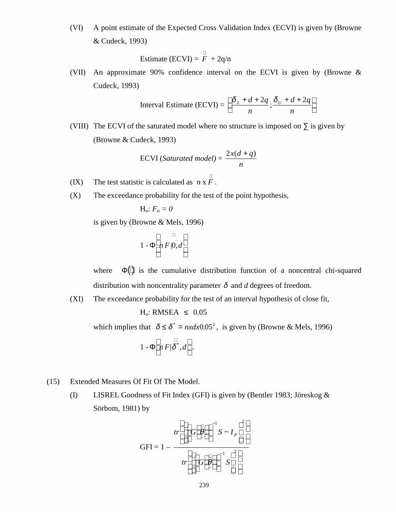
239

(VI) A point estimate of the Expected Cross Validation Index (ECVI) is given by (Browne

& Cudeck, 1993)

Estimate (ECVI) = F∧

+ 2q/n

(VII) An approximate 90% confidence interval on the ECVI is given by (Browne &

Cudeck, 1993)

Interval Estimate (ECVI) = δ δL Ud q

nd qn

+ + + +

2 2;

(VIII) The ECVI of the saturated model where no structure is imposed on ∑ is given by

(Browne & Cudeck, 1993)

ECVI (Saturated model) = 2x d qn

( )+

(IX) The test statistic is calculated as n x F∧

.

(X) The exceedance probability for the test of the point hypothesis,

Ho: Fo = 0

is given by (Browne & Mels, 1996)

1 - Φ n F d| ,.

0∧

where ( )⋅Φ is the cumulative distribution function of a noncentral chi-squared

distribution with noncentrality parameter δ and d degrees of freedom.

(XI) The exceedance probability for the test of an interval hypothesis of close fit,

Ho: RMSEA ≤ 0.05

which implies that δ δ≤ =* .nxdx0 052 , is given by (Browne & Mels, 1996)

1 - Φ n F d| ,*δ∧

.

(15) Extended Measures Of Fit Of The Model.

(I) LISREL Goodness of Fit Index (GFI) is given by (Bentler 1983; Jöreskog &

Sörbom, 1981) by

GFI = 1 –

tr G S I

tr G S

Pθ

θ

−

∧ −

−

∧ −

−

1 2

1 2

240

where Ip is a pxp identity matrix.

(II) Lisrel Adjusted GFI:

The Adjusted Goodness of fit Index is computed from Jöreskog & Sörbom 1981:

AGFI = 1 - (1- GFI).

(III) Mulaik Parsimonious (GFI) is computed from (James-Mulaik-Brett)

π υυk

k

o

NFI=

where υ k =degrees of freedom for the k’th model,

υ o =degrees of freedom for the “Null Model and NFI is the Bentler-Bonett Normed

Fit Index given in (VI) below.

(IV) Schwarz Bayesian Criterion is given by (Schwarz, 1978)

S F f In NNk ML kk= +

−,( )

1

where FML,k is the maximum likelihood discrepancy function, fk is the number of free

parameters for the model and N is the sample size.

(V) Browne-Cudeck Single sample CVI is computed from (Browne & Cudeck, 1989)

Ck = FML(Sv , ( ))θ υ+

− −∑ 22

kk N p

where υ k is the number of free parameters in model k, p is the number of manifest

variables, and N is the sample size.

(VI) Bentler-Bonett Normed Fit Index(NFI) is given by (Bentler, 1995)

NFI = 1 -

∧

−

∧

−

IF

F

θ

θ

where θ−

∧

I denotes the estimate of the unknown parameter of the independence

model.

241

(VII) The nonnormed Bentler-Bonnett Fit Index is given by (Bentler, 1995)

NNFI = ( ) / ( ) /

( ) /

n F d n F d

n F d

I

I

−

− −

−

−

−

∧

−

∧

−

∧

1 1

1 1

θ θ

θ

where dI = p(p-1)/2 denotes the degrees of freedom of the independence model.

(VIII) The Bentler Comparative Fit Index CFI is given by (Bentler, 1995)

CFI = 1 - max ( ) ,

max ( ) ,

n F d

n F dI I

−

−

−

−

−

∧

−

∧

1 0

1 0

θ

θ

(IX) McDonald’s Index for Noncentrality is given by (Bentler, 1995)

MFI = exp − −

−

−

∧n n F d2

1( ) θ

(X) The Root Mean Square Residual(RMR) is computed from (Bentler 1995)

RMR = ( )2

1

2

11p p ij ijj

i

i

p

s g+−

−

∧

=−∑∑ θ

while the Standardized Root Mean Squared Residual(SRMR) is computed as

(Bentler 1995)

SRMR = 21 11

2

p p ij ij ii jjj

i

i

p

s g s s( )/

+−

−

∧

==∑∑ θ

(16) Generalized Least Squares Discrepancy Function – Measures Of Fit Of The Model.

These are the measures of fit of the model for Generalized Least Squares Methods. The

entries are similar to those described under the Maximum Wishart Likelihood method above,

i.e. (14) above.

242

(17) Extended Measures Of Fit Of The Model.

These are the extended measures of fit values obtained by using the Generalized Least

Squared methods. The entries are similar to those described under (15) above.

243

CHAPTER 7

SEPATH


Steiger (1989) developed the structural equation modeling program EzPATH as a module of the

statistical software package SYSTAT. This program was strongly influenced by Steiger’s ideas for

user-machine communication. Steiger left SYSTAT and joined forces with the statistical software

package STATISTICA to develop the structural equation modeling program known as SEPATH

(Steiger, 1995) for Windows. The acronym SEPATH stands for Structural Equations and PATH

analysis. This program is strongly influenced by the conventions used in RAMONA and by the ideas

contained in Mels (1988).

Steiger used the ASCII symbols -> for dependence paths and -- for variance/covariance paths to

create ASCII representations for the path diagrams of Structural Equation Models. These symbols,

-> and -- are called arrow and wire respectively.

SEPATH is intended for users with knowledge of latent variable modeling but can be employed by

researchers with no mathematical background. The user only needs to know how to formulate a

model in the form of a path diagram. Knowledge of matrix algebra is not essential.

7.2 THE SEPATH INPUT SYSTEM

The SEPATH input system consists of a data file and a model file.

7.2.1 SEPATH DATA FILE

The SEPATH data file is a STATISTICA data file. The STATISTICA data file is a STATISTICA

workbook in which the rows and columns refer to the cases and the variables, respectively, of the

244

data. The data may be raw data, a covariance matrix or a correlation matrix. It can be created in

STATISTICA or imported from other files such as MICROSOFT EXCEL files and then saved as

STATISTICA data file with extension “STA”.

If the data is a covariance or correlation matrix, only the entries in the lower triangle of the matrix are

entered. Entering a number at the case name "MATRIX" specifies the type of matrix. The number

1.0000 specifies a covariance matrix whereas the number 4.0000 specify a correlation matrix. The

number of cases is also specified as part of the data. The number is typed in the first cell next to case

name “No. of Cases” in the data matrix.

7.2.2 SEPATH MODEL FILE

The model file is a text file with the extension “.CMD” and is used to specify the structural equation

model by means of a text path diagram by using the PATH1 language. The path diagram of the model

is coded directly with the use of the ASCII symbols --> (for dependence paths) and -- (for

variance/covariance paths). The Model File can be typed manually in any text editor and then

imported into STATISTICA. The Model File may also be created in STATISTICA by using the

“Path Construction Tool”. For specific models such as Confirmatory Factor Analysis (CFA) the

model file may be created using the “Path Wizards”.

GENERAL RULES FOR SEPATH MODEL FILES

• Each arrow and wire is represented on a separate line.

• Blanks never count. They are stripped from the line before parsing.

•••• Blank lines, and any lines beginning with an * (asterisk), are treated as comment lines, and

are not analyzed as PATH1 statements.

• Manifest variable names are represented as the FULL variable name enclosed within

brackets. The name enclosed in the brackets must not be more than 8 alphanumeric

characters in length. Characters must be upper case. The underscore character “_” is also

allowed.

Examples. [REOAP]

or [RE_OAP]

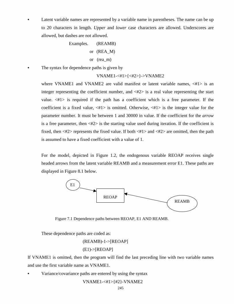
245

• Latent variable names are represented by a variable name in parentheses. The name can be up

to 20 characters in length. Upper and lower case characters are allowed. Underscores are

allowed, but dashes are not allowed.

Examples. (REAMB)

or (REA_M)

or (rea_m)

• The syntax for dependence paths is given by

VNAME1-<#1>{<#2>}->VNAME2

where VNAME1 and VNAME2 are valid manifest or latent variable names, <#1> is an

integer representing the coefficient number, and <#2> is a real value representing the start

value. <#1> is required if the path has a coefficient which is a free parameter. If the

coefficient is a fixed value, <#1> is omitted. Otherwise, <#1> is the integer value for the

parameter number. It must be between 1 and 30000 in value. If the coefficient for the arrow

is a free parameter, then <#2> is the starting value used during iteration. If the coefficient is

fixed, then <#2> represents the fixed value. If both <#1> and <#2> are omitted, then the path

is assumed to have a fixed coefficient with a value of 1.

For the model, depicted in Figure 1.2, the endogenous variable REOAP receives single

headed arrows from the latent variable REAMB and a measurement error E1. These paths are


Figure 7.1 Dependence paths between REOAP, E1 AND REAMB.

These dependence paths are coded as:

(REAMB)-1->[REOAP]

(E1)->[REOAP]

If VNAME1 is omitted, then the program will find the last preceding line with two variable names

and use the first variable name as VNAME1.

• Variance/covariance paths are entered by using the syntax

VNAME1-<#1>{#2}-VNAME2

E1

REOAP

REAMB

246

where VNAME1, VNAME2, <#1> and <#2> are the same as in the preceding section.

For the model, depicted in Figure 1.2, double headed arrows are employed from the manifest

variable REPAP to itself to specify a variance and to REINT and RESOE to specify covariances.


Figure 7.2 Variance/covariance paths between REPAP, REINT and RESOE.


[RESOE]--[RESOE]

[REINT]-- [REINT]

[REPAP]--[REPAP]

[REPAP]-22-[REINT]

[REPAP]-23-[RESOE]

[RESOE]-24-[REINT]

7.3 ILLUSTRATIVE EXAMPLE The model depicted in Figure 1.2 will now be used to illustrate the use of SEPATH.

7.3.1 CREATING THE SEPATH DATA FILE FOR THE DUNCAN, HALLER

AND PORTES MODEL DEPICTED IN FIGURE 1.2 The following steps may be followed to enter the sample correlation matrix for the Duncan, Haller

and Portes application.

• Double click on the STATISTICA icon on the Desktop.

• In the "STATISTICA Module Switcher" menu select the SEPATH option to produce the

menu below.

REPAP REINT RESOE

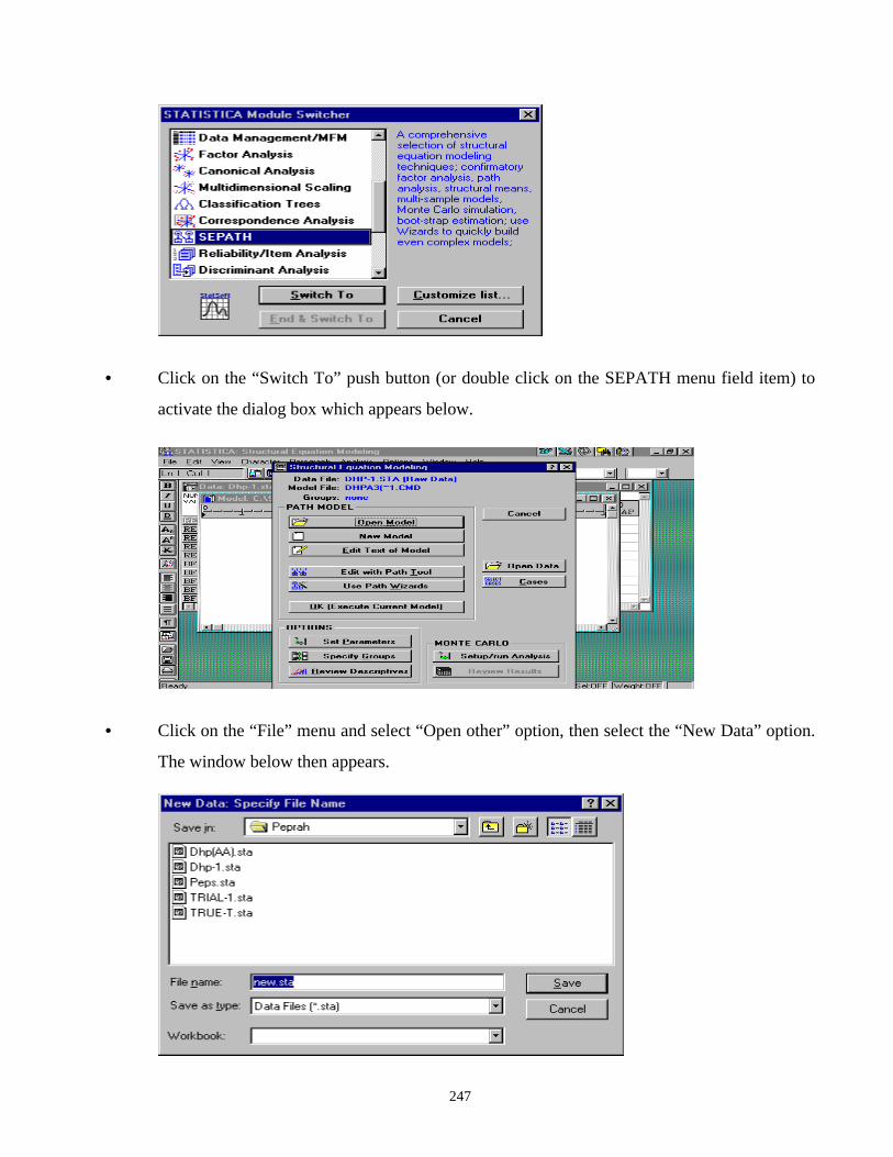
247

• Click on the “Switch To” push button (or double click on the SEPATH menu field item) to

activate the dialog box which appears below.

• Click on the “File” menu and select “Open other” option, then select the “New Data” option.

The window below then appears.

248

• Type the data file name in the string field “File name” and click on the “Save” push

button. After these actions the blank data file shown below appears.

• Click on the “Vars” (Manifest Variables) push button. Then select the “All Specs” option.

This action opens the window shown below.

• Type in the manifest variables’ names in the “Name” column as shown below.

• Type in the manifest variable names.

249

• Click on the “Close" push button to produce the window shown below.

• Click on the “Cases” push button to load the dialog box below.

• Click on the “Yes” push button if the number which appears in the dialog box is equal to the

number of manifest variables specified above. The window below would then appear.

• Type in the manifest variable names in the same order as above.

• Click on the “OK” push button when all 10 manifest variables are typed in to fill the rows

of the matrix with the manifest variable names as shown below.

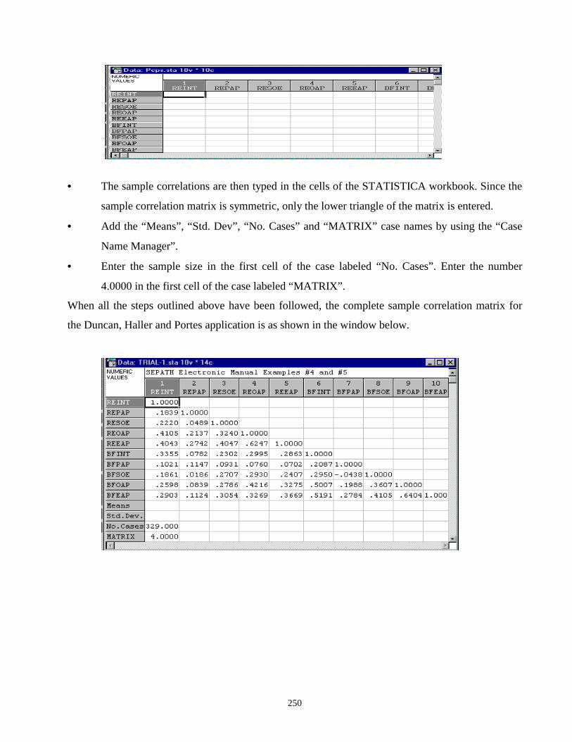
250

• The sample correlations are then typed in the cells of the STATISTICA workbook. Since the

sample correlation matrix is symmetric, only the lower triangle of the matrix is entered.

• Add the “Means”, “Std. Dev”, “No. Cases” and “MATRIX” case names by using the “Case

Name Manager”.

• Enter the sample size in the first cell of the case labeled “No. Cases”. Enter the number

4.0000 in the first cell of the case labeled “MATRIX”.

When all the steps outlined above have been followed, the complete sample correlation matrix for

the Duncan, Haller and Portes application is as shown in the window below.

251

7.3.2 SEPATH MODEL FILE FOR THE DUNCAN, HALLER AND PORTES'

APPLICATION After the Data File has been completed, the following steps may be used to specify the model.

• Click on the “Startup” push button (or click on the “Analysis Menu” and then select the

“Startup Panel” option). This action will open the dialog box shown below.

• Click on the “Edit with Path Tool” push button. This action will activate the “Path

Construction Tool" dialog box shown below.

• Click on the “Edit Latent” push button to activate the “Edit Latent Variable Names” dialog

box shown below.

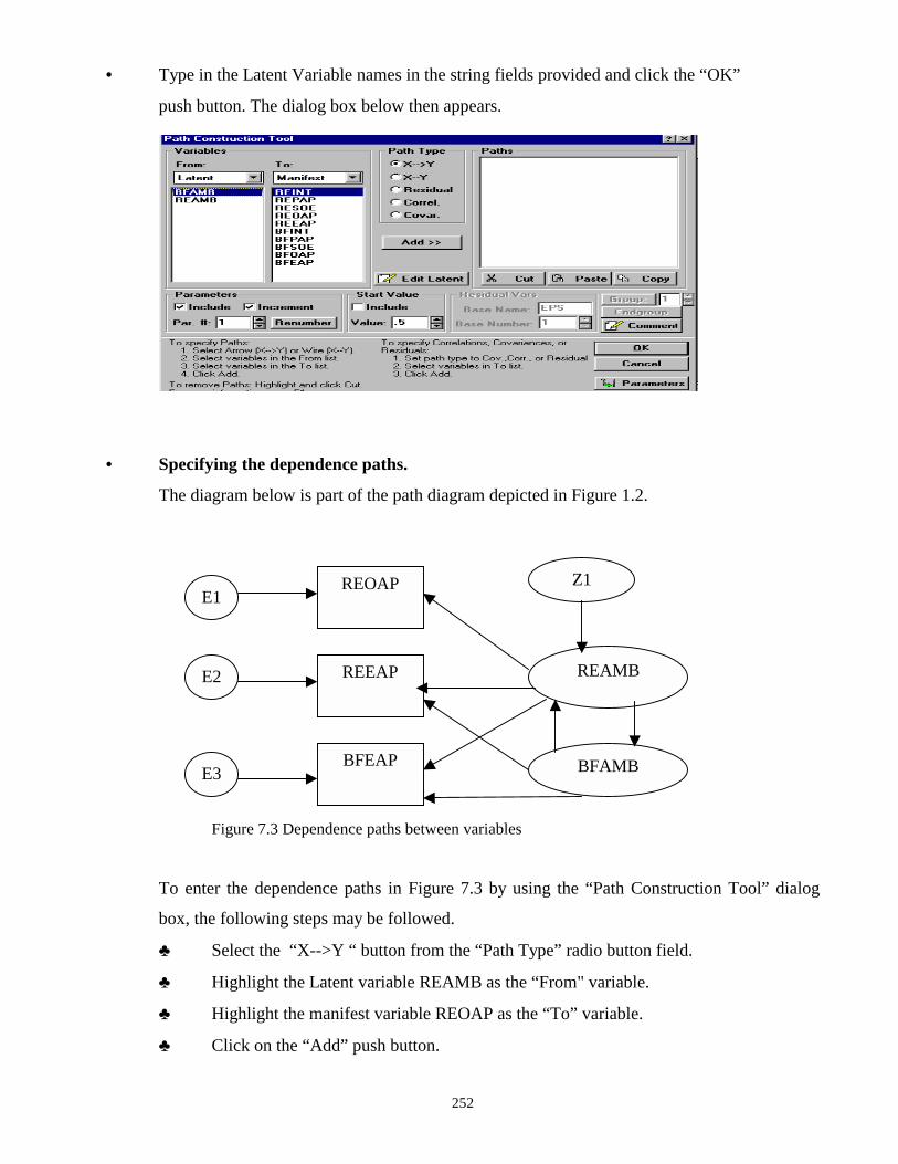
252

• Type in the Latent Variable names in the string fields provided and click the “OK”

push button. The dialog box below then appears.

• Specifying the dependence paths.

The diagram below is part of the path diagram depicted in Figure 1.2.

Figure 7.3 Dependence paths between variables

To enter the dependence paths in Figure 7.3 by using the “Path Construction Tool” dialog

box, the following steps may be followed.

♣ Select the “X-->Y “ button from the “Path Type” radio button field.

♣ Highlight the Latent variable REAMB as the “From" variable.

♣ Highlight the manifest variable REOAP as the “To” variable.

♣ Click on the “Add” push button.

REOAP

REEAP

BFEAP

E1 Z1

E2

E3

REAMB

BFAMB

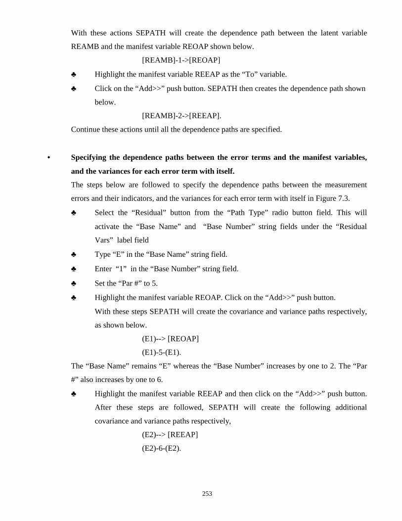
253

With these actions SEPATH will create the dependence path between the latent variable

REAMB and the manifest variable REOAP shown below.

[REAMB]-1->[REOAP]

♣ Highlight the manifest variable REEAP as the “To” variable.

♣ Click on the “Add>>” push button. SEPATH then creates the dependence path shown

below.

[REAMB]-2->[REEAP].

Continue these actions until all the dependence paths are specified.

• Specifying the dependence paths between the error terms and the manifest variables,

and the variances for each error term with itself.

The steps below are followed to specify the dependence paths between the measurement

errors and their indicators, and the variances for each error term with itself in Figure 7.3.

♣ Select the “Residual” button from the “Path Type” radio button field. This will

activate the “Base Name” and “Base Number” string fields under the “Residual

Vars” label field

♣ Type “E” in the “Base Name” string field.

♣ Enter “1” in the “Base Number” string field.

♣ Set the “Par #” to 5.

♣ Highlight the manifest variable REOAP. Click on the “Add>>” push button.

With these steps SEPATH will create the covariance and variance paths respectively,

as shown below.

(E1)--> [REOAP]

(E1)-5-(E1).

The “Base Name” remains “E” whereas the “Base Number” increases by one to 2. The “Par

#” also increases by one to 6.

♣ Highlight the manifest variable REEAP and then click on the “Add>>” push button.

After these steps are followed, SEPATH will create the following additional

covariance and variance paths respectively,

(E2)--> [REEAP]

(E2)-6-(E2).

254

The “Base Name” remains “E” whereas the “Base Number” increases by one to 3. The “Par

#” also increases by one to 7. The paths created by following the actions above actions are

shown in the string field “Paths” in the dialog box shown below.

Continue with this process until similar paths have been formed with E3 (and then E4 found

in Figure 1.2).

♣ Select the “Latent” field from the “To” menu field.

♣ Highlight the latent variable REAMB.

♣ Change the “Base Name” from “E” to “Z” and the “Base Number” from whatever

value to “1”.

♣ Click on the “Add>>” push button.

SEPATH then creates the paths shown below.

(Z1)--> (REAMB)

(Z1)-17-(Z1).

The “Base Name” remains “Z” whereas the “Base Number” increases by 1 to 2. The “Par #”

also increases by 1 to 18.

♣ Highlight the latent variable BFAMB and then click on the “Add” push button.

With this action, SEPATH will create the paths shown below.

(Z2)--> (BFAMB)

(Z2)-18-(Z2).

The paths created by following the actions above are shown on lines 7 and 8, and the last

two lines in the “Paths” string field in the dialog box shown below.

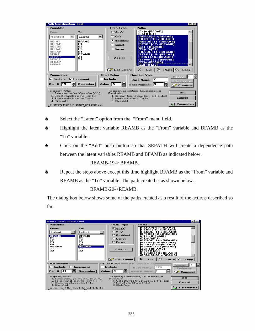
255

♣ Select the “Latent” option from the “From” menu field.

♣ Highlight the latent variable REAMB as the “From” variable and BFAMB as the

“To" variable.

♣ Click on the “Add” push button so that SEPATH will create a dependence path

between the latent variables REAMB and BFAMB as indicated below.

REAMB-19-> BFAMB.

♣ Repeat the steps above except this time highlight BFAMB as the “From” variable and

REAMB as the “To” variable. The path created is as shown below.

BFAMB-20->REAMB.

The dialog box below shows some of the paths created as a result of the actions described so

far.

256

• Specifying the Variance/Covariance paths

The diagram in Figure 7.4 shows some of the variance/covariance paths depicted in Figure

1.2.

Figure 7.4 Variance/Covariance paths between REPAP, REINT and RESOE.

The “Path Construction Tool” dialog box may be used as follows to enter the paths in Figure

7.4.

♣ Select the button “X--Y" from the “Path Type” radio button field.

♣ Select the “Manifest” fields from the “From:” and “To:” menu fields. The resulting

dialog box is as shown below.

♣ Highlight REPAP, REINT and RESOE as the “From” and “To" variables.

Click on the “Add” push button. SEPATH will then create variance paths on lines 21

to 29 in the “Paths” string field of the “Path Construction Tool” dialog box shown

below.

REPAP REINT RESOE

257

♣ The above steps are repeated until all the covariance and variance paths between the

manifest variables in Figure 1.2 are specified.

♣ The path number for variances must be removed since they are fixed as per the path

diagram in Figure 1.2. For example in the path [REPAP]-21-[REPAP], the path

number 21 must be removed to give

[REPAP]--[REPAP].

When the above steps have been followed for all the dependence, variance and covariance paths in

the path diagram depicted in Figure 1.2, the complete model file for the Duncan, Hallers and Portes

application would appear as shown in next section.

7.3.3 MODEL FILE The complete SEPATH model file for the model depicted in Figure 1.2 follows:

(REAMB)-1->[REOAP] (REAMB)-2->[REEAP] (BFAMB)-3->[BFOAP] (BFAMB)-4->[BFEAP] (E1)-->[REOAP] (E1)-5-(E1) (E2)-->[REEAP] (E2)-6-(E2) (E3)-->[BFEAP] (E3)-7-(E3)

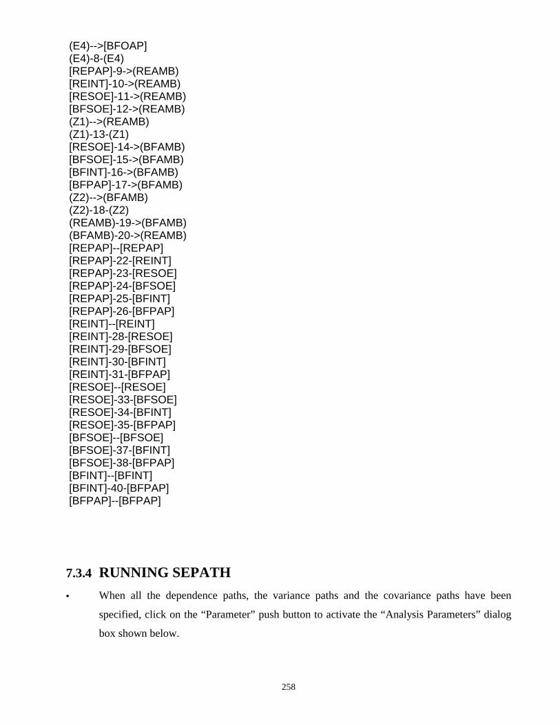
258

(E4)-->[BFOAP] (E4)-8-(E4) [REPAP]-9->(REAMB) [REINT]-10->(REAMB) [RESOE]-11->(REAMB) [BFSOE]-12->(REAMB) (Z1)-->(REAMB) (Z1)-13-(Z1) [RESOE]-14->(BFAMB) [BFSOE]-15->(BFAMB) [BFINT]-16->(BFAMB) [BFPAP]-17->(BFAMB) (Z2)-->(BFAMB) (Z2)-18-(Z2) (REAMB)-19->(BFAMB) (BFAMB)-20->(REAMB) [REPAP]--[REPAP] [REPAP]-22-[REINT] [REPAP]-23-[RESOE] [REPAP]-24-[BFSOE] [REPAP]-25-[BFINT] [REPAP]-26-[BFPAP] [REINT]--[REINT] [REINT]-28-[RESOE] [REINT]-29-[BFSOE] [REINT]-30-[BFINT] [REINT]-31-[BFPAP] [RESOE]--[RESOE] [RESOE]-33-[BFSOE] [RESOE]-34-[BFINT] [RESOE]-35-[BFPAP] [BFSOE]--[BFSOE] [BFSOE]-37-[BFINT] [BFSOE]-38-[BFPAP] [BFINT]--[BFINT] [BFINT]-40-[BFPAP] [BFPAP]--[BFPAP]

7.3.4 RUNNING SEPATH • When all the dependence paths, the variance paths and the covariance paths have been

specified, click on the “Parameter” push button to activate the “Analysis Parameters” dialog

box shown below.

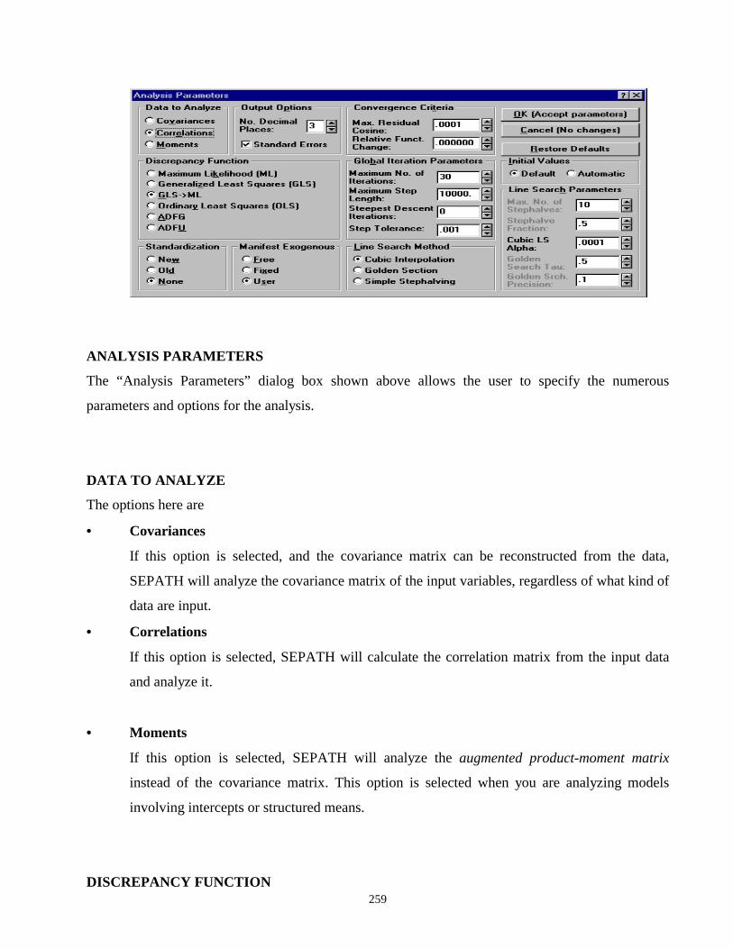
259

ANALYSIS PARAMETERS

The “Analysis Parameters” dialog box shown above allows the user to specify the numerous

parameters and options for the analysis.

DATA TO ANALYZE

The options here are

• Covariances

If this option is selected, and the covariance matrix can be reconstructed from the data,

SEPATH will analyze the covariance matrix of the input variables, regardless of what kind of

data are input.

• Correlations

If this option is selected, SEPATH will calculate the correlation matrix from the input data

and analyze it.

• Moments

If this option is selected, SEPATH will analyze the augmented product-moment matrix

instead of the covariance matrix. This option is selected when you are analyzing models

involving intercepts or structured means.

DISCREPANCY FUNCTION

260

In this section of the “Analysis parameters" dialog box, the user specifies the estimation method to

yield parameter estimates. The options available are

• Maximum Likelihood (ML)

• Generalized Least Squares (GLS)

• GLS --> ML (GLS followed by ML). This is the default option.

• Ordinary Least Squares (OLS)

• Asymptotically Distribution Free Gramian (ADFG)

• Asymptotically Distribution Free Unbiased (ADFU)

STANDARDIZATION

In this section of the “Analysis Parameters” dialog box, the user chooses to generate either a

standardized solution (where latent variables all have unit variances) by one of two methods, or an

unstandadized solution. The three options are

• New.

If this option is selected, SEPATH estimates a standardized solution via constrained

estimation.

• Old.

If this option is selected, SEPATH estimates a standardized solution without using

constrained estimation.

• None.

If this option is selected, an unstandardized solution is calculated.

MANIFEST EXOGENOUS

The options available are

• Fixed

If this option is selected, the variances and covariances for manifest exogenous variables are

fixed (at the value of the observed variances and covariances) during iteration, then treated as

if they were free parameters at the end of the iteration.

• Free

If this option is selected, the variances and covariances among the manifest exogenous

variables are treated as free parameters and added to the model, although their values are not

shown.

• User

261

If this option is selected, the user must account for the variances and covariances of all

manifest exogenous variables, using standard PATH1 syntax.

INITIAL VALUES

In this section of the “Analysis Parameters” dialog box, the user selects the method employed to find

initial values for free parameters. The options available are:

• Default.

The default method uses 0.5 for all free parameters, except variances and covariances (or

correlations) of manifest exogenous variables.

• Automatic

If this option is selected, the initial values are obtained by using a minor adaptation of the

technique described by McDonald and Hartmann (1992).

CONVERGENCE CRITERIA

In this box of the “Analysis Parameters" dialog box, you can adjust constants that can directly affect

the point during iteration at which the program decides convergence has occurred. The default

values produce desirable results for a wide variety of problems, and you will seldom need to adjust

these criteria. The options available are:

• Maximum residual cosine criterion.

The default value for this option is 0.0001.

• Relative function change criterion.

In general, the value here must be kept very low, or it may cause iteration to terminate

prematurely.

GLOBAL ITERATION PARAMETERS.

In this section of the “Analysis Parameters” dialog box, you enter parameters that control the basic

iterative process. The options available are:

• Maximum number of iterations.

In this field, you enter the maximum number of iterations allowed. The default number is 30.

• Maximum step length.

262

In this field, you enter the maximum length of the step vector that will be allowed. The

default number is 10000.

• Number of steepest descent iterations.

In this field, you enter a number of Steepest Descent Iterations to proceed the standard

iterations. The default value is 0.

• Step tolerance.

In this field, you enter a tolerance value at which a parameter is temporarily eliminated from

the iterative process. The tolerance value is basically one minus the squared multiple

correlation of a parameter with the other parameters. The default value is 0.0001.

LINE SEARCH METHOD

In this section of the “Analysis Parameters” dialog box, you choose a basic line search method.

There are three methods for choosing the length of the steps. These are:

• Cubic interpolation.

This method is reasonably fast and rather robust. It works well in a vast majority of

circumstances.

• Golden section.

This method tries to solve the one dimensional minimization problem exactly on each

iteration. It often converges in slightly less iteration than cubic interpolation, but takes

longer, because it requires more function evaluations on each iteration.

• Simple stephalving.

This method is the fastest, but will fail to converge for a fair number of problems on which

the other two, more sophisticated methods succeed.

LINE SEARCH PARAMETERS.

In this section of the “Analysis Parameter" dialog box, you choose numerical parameters that control

the performance of the line search method you have chosen. The options available are:

• Max. no. of stephalves.

This parameter sets the maximum number of stephalves allowed on a single iteration if the

Simple stephalving line search method is used.

• Stephalve fraction

This parameter sets the fraction by which the current step is multiplied when Simple

Stephalving is used as the line search method.

263

• Cubic LS alpha.

This parameter controls how large a reduction in the discrepancy function has to be made

before a step is considered acceptable when the Cubic Interpolation line search is used. The

default value is 0,0001.

• Golden section tau.

This parameter controls the width of the range to which the Golden Section line search is

limited.

• Golden search precision.

This parameter controls the precision of estimation in a Golden Section line search.

OUTPUT OPTIONS

The options in this section of the “Analysis Parameters" dialog box allow you some preliminary

control over the appearance of your output. The options available are:

• No. of decimal places.

Here you can set the number of decimal places displayed by default in the text output. The

number can be any integer from 1 to 6.

• Standard error

If this box is checked, the program will display estimated standard errors for all parameters in

the PATH1 text output, and Model Summary Scrollsheet. However, if OLS estimation is

performed, or the “old” standardization method is employed, standard errors will not be

available.

• Select the required parameters by clicking on the right Check Boxes and then click on the

“OK (accept parameters)” push button.

• The above action will again activate the “Startup” dialog box shown below again.

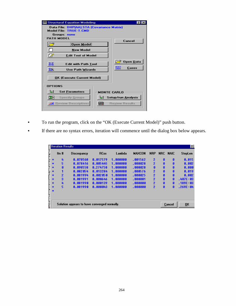
264

• To run the program, click on the “OK (Execute Current Model)” push button.

• If there are no syntax errors, iteration will commence until the dialog box below appears.

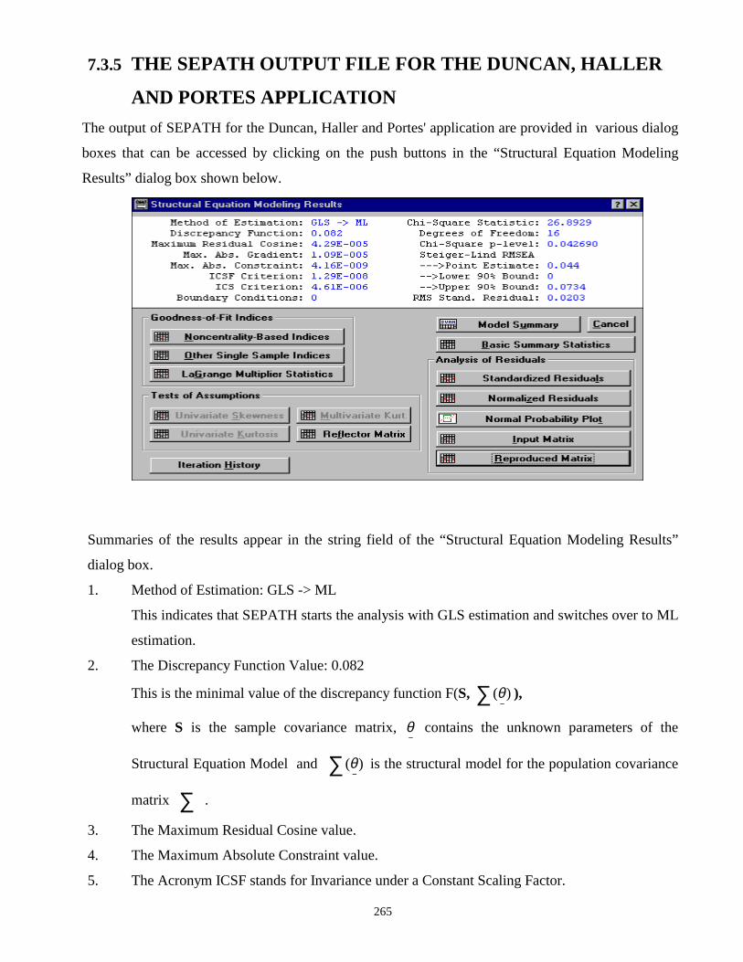
265

7.3.5 THE SEPATH OUTPUT FILE FOR THE DUNCAN, HALLER

AND PORTES APPLICATION The output of SEPATH for the Duncan, Haller and Portes' application are provided in various dialog

boxes that can be accessed by clicking on the push buttons in the “Structural Equation Modeling

Results” dialog box shown below.

Summaries of the results appear in the string field of the “Structural Equation Modeling Results”

dialog box.

1. Method of Estimation: GLS -> ML

This indicates that SEPATH starts the analysis with GLS estimation and switches over to ML

estimation.

2. The Discrepancy Function Value: 0.082

This is the minimal value of the discrepancy function F(S, ( )θ−

∑ ),

where S is the sample covariance matrix, θ−

contains the unknown parameters of the

Structural Equation Model and ( )θ−

∑ is the structural model for the population covariance

matrix ∑ .

3. The Maximum Residual Cosine value.

4. The Maximum Absolute Constraint value.

5. The Acronym ICSF stands for Invariance under a Constant Scaling Factor.

266

6. The Acronym ICS stands for Invariance under Change of Scale.

7. Value of the Chi-square Statistic. This value is obtained as (N-1)FML(S, ( ∃ ))θ−

∑ , where N

denotes the sample size and ∃θ−

is the estimate of θ−

.

8. The Degrees of Freedom of the Chi-square distribution of (N-1)F(S, ( )∑ θ̂ ) is given by

[p(p+1)/2]-q, where p is the number of manifest variables and q denotes the number of free

parameters.

9. Chi-square significance level. This is the area under the chi-square distribution curve to the

right hand side of the chi-square statistic.

10. Steiger-Lind RMSEA (Root Mean Square Error of Approximation) point estimate. This

value is obtained by using the formula R*= F*

υ , where υ is the degrees of freedom and F*

is given by F* = ( )( ){ } 21)ˆ(ˆ

21

−

−∑∑ θθSTr .

where Tr[A] is the trace of the square matrix A.

11. The lower and upper limits of the 90% confidence interval for the RMSEA.

12. RMS (Root Mean Square) Standardized Residual.

GOODNESS OF FIT INDICES

Under this heading we have the "Noncentrality-Based Indices", "Other Single Sample Indices" and

the "LaGrange Multiplier Statistics as" shown in the dialog box above.

• Click on the "Noncentrality-Based Indices" push button to load the dialog box shown below.

♣ The Point estimate of the Population Noncentrality Parameter is given by NF*

The 90% confidence interval for the Population Noncentrality Parameter is also given

in the string field the of "Structural Equation Modeling Results" dialog box.

♣ The Steiger-Lind RMSEA Index point estimate and confidence interval are as

267

described in 10 above.

♣ The McDonald Noncentrality Index is given by

Exp( 2

*F ).

♣ The estimated Population Gamma Index is given by

211

)(

=Γ

∑ ∑−∧

∧

θTr

p

♣ The estimated Adjusted Population Gamma Index is given by

∃ ∃ ∃ /∃ ∃ / *Γ2 1= − ′′

ε εσ σ

W VW p

where ( )S&−= σε ˆˆ , ( )( )∑= θσ ˆˆ vecs , & ( )S vec S= , and Vecs(S) denotes the 12

p(p+1) x 1

vector formed by stacking the non-duplicated elements of the p x p symmetric matrix S.

• To view the other Goodness of fit Indices, click on the “Continue” push button. This action

will load the “Structural Equation Modeling Results” dialog box.

• Click on the “Other Single Sample Indices” push button to load the dialog box shown below.

♣ The rbomoSreskogoJ &&&& − GFI is computed as

268

∧Γ2 21

Σ

=−∧

MLTr

p

θS

♣ The rbomoSreskogoJ &&&& − AGFI is given by

1 – (p*/υ )(1- ML

∧γ )

where ML

∧γ is the GFI index ML

∧γ 21

Σ

=−∧

MLTr

p

θS

.

♣ The rescaled Akaike Information Criterion is computed from

Ak= ∧F ML,k +

12

−Nfk

where ∧F ML,k is the minimal value of the maximum likelihood discrepancy function,

fk is the number of free parameters for the model and N is the sample size.

♣ Schwarz’s Bayesian Creterion is computed from

Sk=∧F ML,k +

1)(

−NNInfk

♣ The Browne-Cudeck Cross Validation Index is computed from

Ck = FML( ∑

∧

kS θυ, ) +

22

−− pNkυ

where kυ is the degrees of freedom for the k’th model.

♣ The Independence Model Chi-square and df are the Chi-square goodness-of–fit

statistic, and associated degrees of freedom, for the hypothesis that the population

covariances are all zero. Under the assumption of multivariate normality, this

hypothesis can only be true if the variables are all independent. The “Independence

Model” is used as the “Null Model” in several comparative fit indices.

♣ The Bentler-Bonett Normed Fit Index is computed from

Bk = o

ko

F

FF∧

∧∧−

where oF∧

is the minimal discrepancy function value for the “Null Model”

269

kF∧

is the minimal discrepancy function value for the k’th model.

♣ The Bentler-Bonett Non-Normed Fit Index is computed from

BNNK =

11ˆ

ˆˆ

−−

−

NF

FF

o

o

k

k

o

o

υ

υυ

where oυ is the degrees of freedom for the “Null Model”

♣ The Bentler Comparative Fit Index (CFIk) is computed as

CFIk =1- ∧

∧

o

k

τ

τ

where ∧

kτ is the estimated non-centrality parameter for the k’th model

∧

oτ is the estimated non-centrality parameter for the “Null Model”.

♣ The James-Mulaik-Brett Parsimonious Fix Index is computed from the formula

ko

kk B

υυπ =ˆ

♣ Bollen’s Rho is computed as:

o

o

k

k

o

o

k

F

FF

υ

υυρˆ

ˆˆ

ˆ−

=

♣ Bollen’s Delta is computed from:

NF

FFk

o

kok υ−

−=∆ˆ

ˆˆˆ

• To view the remaining Goodness of fit Indices, click on the “Continue" push button to reload

“Structural Equation Modeling Results” dialog box.

• Click on the “LaGrange Multiplier Statistics" push button to load the dialog box shown

below.

270

♣ The values of the Lagrange multipliers that were used to constrain the variances of

the endogenous manifest variables to unity and the corresponding standard errors are

shown in the dialog box above.

• To view the “Model Summary”, click on the “Continue” push button to reload the


• Click on the “Model Summary" push button to load the dialog box shown below.

The "Model Summary" dialog box presents model output in a Scrollsheet form that is

convenient for further analyses. For each path of the model, the following information is

given:

♣ Path representation

♣ Parameter estimate

♣ Standard error

♣ T-statistic

♣ Probability level.

• To view the “Basic Summary Statistics”, click on the “Continue" push button to reload the

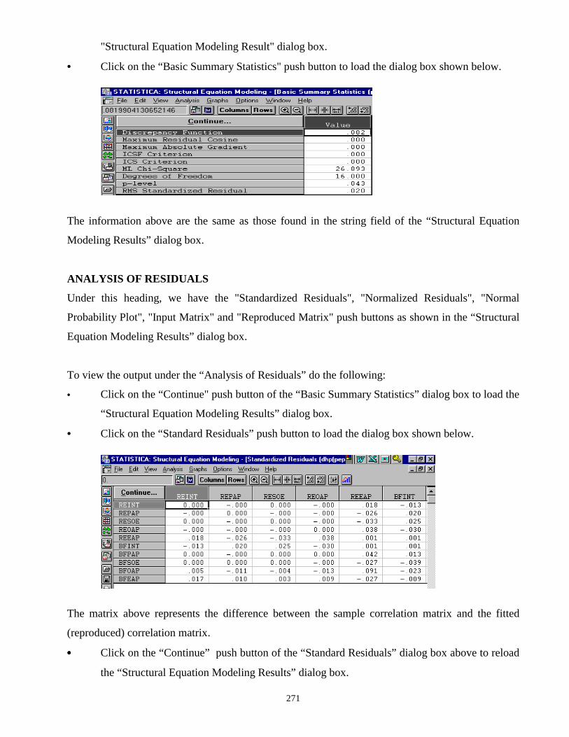
271

"Structural Equation Modeling Result" dialog box.

• Click on the “Basic Summary Statistics" push button to load the dialog box shown below.

The information above are the same as those found in the string field of the “Structural Equation

Modeling Results” dialog box.

ANALYSIS OF RESIDUALS

Under this heading, we have the "Standardized Residuals", "Normalized Residuals", "Normal

Probability Plot", "Input Matrix" and "Reproduced Matrix" push buttons as shown in the “Structural

Equation Modeling Results” dialog box.

To view the output under the “Analysis of Residuals” do the following:

• Click on the “Continue" push button of the “Basic Summary Statistics” dialog box to load the


• Click on the “Standard Residuals” push button to load the dialog box shown below.

The matrix above represents the difference between the sample correlation matrix and the fitted

(reproduced) correlation matrix.

•••• Click on the “Continue” push button of the “Standard Residuals” dialog box above to reload

the “Structural Equation Modeling Results” dialog box.

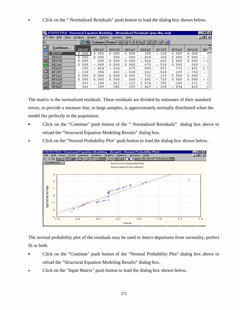
272

• Click on the “ Normalized Residuals” push button to load the dialog box shown below.

The matrix is the normalized residuals. These residuals are divided by estimates of their standard

errors, to provide a measure that, in large samples, is approximately normally distributed when the

model fits perfectly in the population.

•••• Click on the “Continue" push button of the “ Normalized Residuals” dialog box above to

reload the “Structural Equation Modeling Results” dialog box.

•••• Click on the "Normal Probability Plot" push button to load the dialog box shown below.

The normal probability plot of the residuals may be used to detect departures from normality, perfect

fit or both.

•••• Click on the “Continue" push button of the “Normal Probability Plot" dialog box above to

reload the “Structural Equation Modeling Results” dialog box.

•••• Click on the "Input Matrix" push button to load the dialog box shown below.

273

This is the sample correlation matrix used in the analysis.

•••• Click on the “Continue" push button of the “Input Matrix” dialog box above to reload the

“Structural Equation Modeling Results” dialog box shown below.

• Click on the "Reproduced Matrix" push button to load the dialog box shown below.

This is the correlation matrix calculated from the model by using the final parameter estimates as the

parameter values of the model.

274

CHAPTER 8

CONCLUSIONS AND RECOMMENDATIONS

8.1 INTRODUCTION

In this treatise the use of six Structural Equation Modeling programs, namely: AMOS, EQS,

LISREL, Mx, RAMONA and SEPATH have been reviewed. The six programs were reviewed in

terms of general application. In addition, the use of the software for fitting the Duncan, Haller and

Portes’ model Figure 1.2 to the Sample Correlation matrix in Table 1.3 are illustrated.

When using each of the programs to fit the model depicted in Figure 1.2 to the correlation matrix in

Table 1.3, the positive impressions and the difficulties encountered with each program were noted.

In the next six sections of this chapter, the positive impressions and the difficulties encountered with

each program are provided. In addition, some recommendations are made based on the difficulties

encountered as a first time user of these programs.

8.2 AMOS

The following impressive observations were made on using AMOS to fit the model depicted in

Figure 1.2 to the correlation matrix provided in Table 1.3.

1. I found the drawing of the path diagram in Figure 1.2 in AMOS very easy.

2. The resulting path diagram is of excellent quality.

3 I admired the display of the degrees of freedom at any stage in the drawing of a path

diagram. It helped me to see whether I was doing the right thing or not at each stage of

drawing the path diagram in Figure 1.2 in AMOS.

4. The modeling laboratory was very useful to me as a first time user. It allowed me to enter an

arbitrary choice of parameter values, and then observe the resulting implied moments and the

275

resulting value of the discrepancy function. This unique feature could only be found in

AMOS.

Certain difficulties were encountered on using AMOS to fit the model depicted in Figure 1.2 to the

correlation matrix provided in Table 1.3. The difficulties are given below.

1. I was unable to draw the variances of the variables on the path diagram.

2. Although it was very easy to add error terms to variables in a path diagram, it took quite an

effort and time to get the error terms into positions to improve the appearance of the path

diagram. Moving an error term around in the diagram was not a straightforward matter for

me.

3. I had to fix the regression coefficients for the paths between “REAMB” and “REOAP”, and

“BFAMB” and “BFOAP” to one (1) before I could successfully run the job.

4. I was unable to open the input file with the extension “.amj” generated from the path diagram

in AMOS. I had to use Microsoft Word and Windows explorer to open this file.

5. I had to type the variances of the variables manually in the “.amj” file to complete the model

specification prior to running the job.

6. I found the User’s Guide too comprehensive. It took me a very long time to read through all

the relevant portions.

Based on my experience of using AMOS for the first time, I would like to propose the following

recommendations:

1. The inclusion of features, which would enable users to draw the variances of variables,

would allow the user to draw more comprehensive path diagrams.

2. The feature, which enables the error terms to be moved around in a path diagram, should, if

possible, be improved to make it easier and faster to use.

3. The AMOS input file created from the path diagram is saved with an automatic extension

“.amj”. It would be a nice idea if this could be replaced by “.ami” to reflect the fact that it is

an “AMOS Input” file.

4. It would be a good idea if the AMOS input file is reproduced in the AMOS output file. This

would assist users in finding the parameter estimates in the output file because the input file

indicates which parameters are to be estimated as well as their paths.

5. I would like to suggest that a summarized version of the User’s Guide be made for first time

users so that they may not have to read big volumes to know how to use the program.

6. A feature, which allows users to open their input files within AMOS, will improve the user-

friendliness of AMOS.

276

8.3 EQS The following impressive observations were made on using EQS to fit the model depicted in Figure

1.2 to the correlation matrix provided in Table 1.3.

1. I found the use of equations to specify the model very easy.

2. I found the structural equations very clear and unambiguous.

3. I found the specification of the model not complex at all. The structural equations were as

such that they were written for the paths as they appear in the path diagram of the model.

4. With the use of the “Create New Equations” window, I did not have to type the lines of the

structural equations for the model. This I found very useful in that it reduced the chance of

making a typing mistake to zero.

5. When I specified the model by typing in all the structural equations, it did not take long at all

since variables used in the structural equations are coded into V’s for manifest variables and

F’s for latent variables.

6. The input file is reproduced as part of the output file and numbered sequentially. This, I

found very helpful when reading the parameter estimates in the output file because the input

file indicated which parameters were to be estimated and on which path that was.

There were certain difficulties I encountered on using EQS to fit the model depicted in Figure 1.2 to

the correlation matrix provided in Table 1.3. These were:

1. I had to manually enter the fixed parameters in the model, because the fixing of the

parameters could not be done when specifying the structural equations in the input file. This

took a bit of time to do.

2. I had to manually enter the labels in the input file after the input file had been created.

3. I had to enter all the specifications of the correlations between the independent variables in

the path diagram in the input file since those were not automatically generated as part of the

input file.

4. I had to fix the regression coefficients for the paths between “REAMB” (F1) and “REOAP”

(V4), and “BFAMB” (F2) and “BFOAP” (V10) to one (1) before I could successfully run

the job.

5. I found that it was not possible to get back to the “Create New Equations” window after it

has been used once to create the structural equations for the model. This meant that I had to

277

restart the specification of the structural equations whenever I found that a mistake had been

made.



Based on my experience on using EQS for the first time, I would like to propose the following

recommendations:

1. It would be a nice idea if the file name for files created in EQS could have more than eight

characters. There are times when one has to provide a file name, which has more than eight

characters, for identification purposes. This is not possible in EQS at the moment.

2. The inclusion of a feature, which would enable users to specify fixed parameters as the

structural equations are being constructed, would improve the user-friendliness of EQS.

3. The keyword “/DATA=” is included automatically in the input file even when it has been

indicated that a separate data file has not been provided. A way should be found to stop this

“redundant” keyword from appearing.

4. The inclusion of a feature, which would enable users to provide labels for the input variables

at the start of the model specification, would improve the user-friendliness of EQS.

5. The user-friendliness of EQS would be further enhanced if users are allowed to get back to

the “Create New Equations” window which is used to create the structural equations of the

model.



8.4 LISREL

The following impressive observations were made on using LISREL to fit the model depicted in


1. I was immensely impressed by the fact that there are three different ways of fitting Structural

Equation Models to data with LISREL 8.30.

278

2. I could generate the path diagram in Figure 1.2 from the SIMPLIS input file and also from

the LISREL input file. I could also do the reverses of these, that is, generate the SIMPLIS or

the LISREL input file from the drawing of the path diagram in Figure 1.2 in LISREL.

3. It was very easy to type the input file for the model depicted in Figure 1.2 in the SIMPLIS

command language. The SIMPLIS command language is very easy to understand and use.

This quality allowed me to specify the model in the input file by directly translating the path

diagram into the input commands.

4. It was easier for me to create the SIMPLIS input file interactively.

5. I found it very easy to draw the path diagram in Figure 1.2 in LISREL. The path diagram I

drew was of excellent quality.

6. I could easily display the initial values and fixed values on the path diagram.

7. I found the dialog boxes, which I used to specify the model in terms of the eight parameter

matrices of the LISREL model, very user-friendly.

8. I found that the LISREL 8.30 output file contained several goodness-of–fit statistics that are

well arranged.

9. The arrangement of the parameter estimates and the goodness-of-fit statistics in the output

file is very impressive.

10. The LISREL syntax or the SIMPLIS syntax in the input file was reproduced in the output

file. The presence of the reproduced input file helped me a lot to locate the parameter

estimates easily.

I encountered certain difficulties on using LISREL 8.30 to fit the model depicted in Figure 1.2 to the

correlation matrix in Table 1.3. The difficulties included:

1. It was extremely difficult for me to know how to partition the parameters to be able to

specify the model in terms of the eight parameter matrices of the LISREL model.

2. I also found the specification of the model depicted in Figure 1.2 in the LISREL syntax too

theoretical. I only managed to get the model right after several trials.



4. I had to fix the factor loading for the paths between REAMB and REOAP, and BFAMB and

BFOAP to 1 before the program ran.

Based on my experience of using LISREL for the first time, I would like to propose the following recommendations:

279

1. I would like to strongly recommend that a way be found to make it easier for a user to

specify the eight parameter matrices of the LISREL model differently from what it is

currently. Getting to know which of the variables goes into which of the matrices: Eta, Beta,

Gamma, and so on is too mathematical.



8.5 Mx

The following impressive observations were made on using Mx to fit the model depicted in Figure

1.2 to the correlation matrix provided in Table 1.3.

1. It was very easy to type the input script file of the model depicted in Figure 1.2.

2. I found the final input script file created for the model depicted in Figure 1.2, very easy to

read.

3. I found the use of the path diagram to generate the input script file of the model depicted in

Figure 1.2 easy.

4. The quality of the path diagram I drew was excellent.

5. I found the feature in Mx, which automatically assigns a starting value to a free parameter,

very helpful.

6. I found the feature, which enabled me to change the default starting values to the required

value, very helpful.

7. I was impressed with the fact that Mx provided an identity matrix as the matrix to be

analyzed in the graphics file created from the drawing of the path diagram for the model

depicted in Figure 1.2.

8. I like the fact that the Mx input script file was reproduced as part of the output file.

Certain difficulties were encountered on using Mx to fit the model depicted in Figure 1.2 to the

correlation matrix provided in Table 1.3. The difficulties are given below.

280

1. Since Mx uses the RAM model specification, I had to reorganize the order of the manifest

variables in the correlation matrix provided in Table 1.3 to reflect the variable order of the

RAM model before the job ran successfully.

2. Getting to know how to enter the values and numbers which were used to specify the model

in the matrices proved very difficult for me at the beginning. It took several trials before I got

things right.

3. Typing the Mx commands and keywords to form the input script was very time consuming.

All the required entries and the numerous zeros for all the four matrices of the RAM model

had to be entered.

4. The input script which was generated from the path diagram I drew for the model depicted in

Figure 1.2, had the number of manifest variable correctly as 10 but the number of

observations was automatically assigned to 100. I had to change it to the correct number 329.



6. Mx ran for a long time before it terminated.

7. I had to fix the factor loading for the paths between REAMB and REOAP, and BFAMB and

BFEAP to 1 before the program ran.

Based on my experience of using Mx for the first time, I would like to propose the following recommendations:

1. The Mx input script file for the model depicted in Figure 1.2 was saved with an automatic

extension of “.mx”. All the other file extensions have three letters. I would like to suggest

that the extension “.mx” be made “.mxi” to reflect that the file is an Mx input file.

2. The Mx script file is generated automatically from the drawing of a path diagram. If the

reverse of this can be done, i.e. generating the path diagram form a script file, it would be

very helpful. It would help to easily identify errors if they occur, especially, in the script file.

3. If possible, changes should be made to the program so that user would not have to deal

directly with matrices as it is now. Figuring out which matrices to use and how to specify the

few required entries was very difficult for me.

4. It may be a good idea to have a blank, instead of the automatic “100” for the number of

observations in the input script generated from the path diagram. This may help to avoid the

possibility of a user making a mistake of using the number of observations of 100 instead of

another number.

281


users so that they may not have to read to volumes of material before they can use the

program.

6. The time it took before Mx terminated was very long. If this could be reduced, it would

improve the efficiency of the program.

8.6 RAMONA

The following impressive observations were made on using RAMONA to fit the model depicted in


1. I like the explanations and examples given in the RAMONA User’s Guide. The explanations

in the guide are precise. I did not have to read volumes of material before I figured out the

various paragraphs in the RAMONA Input System.

2. Typing the various commands, keywords and options in the input system for the model

depicted in Figure 1.2 was not difficult at all.

3. I did not have to make reference to any matrix in the typing of the various commands and

options.

4. I like the fact that the RAMONA input file was reproduced as part of the output file.

5. I found that the RAMONA output file contained a lot of goodness-of–fit statistics and that it

was very nicely arranged.

I encountered some difficulties on using RAMONA to fit the model depicted in Figure 1.2 to

the correlation matrix provided in Table 1.3. These included:

1. Every path in the path diagram had to be typed manually in the input file. I found this very

time consuming.

2. The fact that I had to type the variable name as many times as they occur in the path diagram

of the depicted in Figure 1.2 meant that I had to be very careful not to make typing errors.

That made me go very slow in the typing.

3. I found the typing very time consuming since every path in the path diagram had to be

specified in the input file.

Based on my experience of using RAMONA for the first time, I would like to propose the following

recommendations:

282

1. Improvements should be made to the program, if possible, to enable users to specify paths

between variables by simple clicks of push buttons.

2. The inclusion of a feature, which would enable users to enter the variable names only once

and be able to use them by simply selecting the variable needed, would help reduce the time

spent to type the input file.

8.7 SEPATH

The following impressive observations were made on using SEPATH to fit the model depicted in


1. I had the option of either typing the necessary commands to specify the model in the input

file or use the path tools available to generate the input file.

2. I found the use of the path tools to generate the input files to be very easy.

3. I typed the variable names once and used those I needed by simply selecting them.

4. I could specify several paths in the input file within a very short time.

5. I found the set up of the path tools very simple and it did not take long before I could use it

successfully.

6. I did not have to make reference to any matrix during the specification of the model in the

input file.

7. The single-headed and double-headed arrows are presented as check boxes. I only had to

check the required one to get it into the input file.

8. With just little care, I completed the specification of the model without errors.

I encountered some difficulties on using SEPATH to fit the model depicted in Figure 1.2 to the

correlation matrix provided in Table 1.3. These included:

1. The output files produced in dialog boxes look excellent. What I did not like about them, is

that one has to scroll up and down and/or left and right to be able to read a complete file.

2. I had to manually delete the parameter numbers of all the double-headed arrows before the

program ran successfully.

3. I found the Text output file difficult to read. It is too compact.



283

Based on my experience of using SEPATH for the first time, I would like to propose the following

recommendations:

1. The presentation of the output files in the dialog boxes should be improved to provide users

with access to view all parts of each dialog box at a time.

2. The layout of the text output file should be improved to make it clearer than at present.

3. Only a few goodness-of-fit statistics appear in the Text output file, as compared with the

output files in the dialog boxes. This should be checked so that the same information is found

in both types of output.


users so that they may not have to read volumes of material before they can use the program.

8.8 COMPARING PARAMETER ESTIMATES OBTAINED FROM

AMOS, EQS, LISREL, Mx, RAMONA AND SEPATH

The parameter and standard error estimates, produced by AMOS, EQS, LISREL, Mx, RAMONA

and SEPATH for the Duncan, Haller and Portes SEM Application, are listed in Table 8.1

Table 8.1: Parameter Estimates produced by AMOS, EQS, LISREL, Mx, RAMONA and SEPATH.

PROGRAM

PATH AMOS EQS LISREL Mx RAMONA SEPATH

1 REAMB REOAP 0.767 0.767 0.767 1.000 0.766 0.766

2 REAMB REEAP 0.813 0.814 0.813 0.813 0.814 0.814

3 BFAMB BFEAP 0.825 0.828 0.825 0.825 0.829 0.828

4 BFAMB BFOAP 0.774 0.772 0.774 1.000 0.772 0.772

5 BFAMB REAMB 0.174 0.176 0.174 0.176 0.175 0.175

6 REAMB BFAMB 0.184 0.184 0.184 0.187 0.184 0.184

7 REPAP REAMB 0.214 0.213 0.214 0.213 0.214 0.214

8 REINT REAMB 0.333 0.332 0.333 0.333 0.332 0.332

9 RESOE REAMB 0.290 0.290 0.290 0.290 0.290 0.290

10 RESOE BFAMB 0.088 0.087 0.088 0.090 0.087 0.087

284

11 BFSOE REAMB 0.104 0.103 0.103 0.103 0.103 0.103

12 BFSOE BFAMB 0.282 0.283 0.282 0.281 0.282 0.282

13 BFINT BFAMB 0.428 0.427 0.438 0.437 0.427 0.427

14 BFPAP BFAMB 0.196 0.197 0.197 0.196 0.197 0.197

15 REPAP REINT 0.184 0.184 0.184 0.184 0.184 0.184

16 REPAP RESOE 0.049 0.049 0.049 0.049 0.049 0.049

17 REPAP BFSOE 0.019 0.019 0.019 0.019 0.019 0.019

18 REPAP BFINT 0.078 0.078 0.078 0.078 0.078 0.078

19 REPAP BFPAP 0.115 0.115 0.115 0.115 0.115 0.115

20 REINT RESOE 0.222 0.222 0.222 0.222 0.222 0.222

21 REINT BFSOE 0.186 0.186 0.186 0.186 0.186 0.186

22 REINT BFINT 0.336 0.336 0.336 0.336 0.336 0.336

23 REINT BFPAP 0.102 0.102 0.102 0.102 0.102 0.102

24 RESOE BFSOE 0.271 0.271 0.271 0.271 0.271 0.271

25 RESOE BFINT 0.230 0.230 0.230 0.230 0.230 0.230

26 BFSOE BFPAP 0.093 0.093 0.093 0.093 0.093 0.093

27 BFSOE BFINT 0.295 0.295 0.295 0.295 0.295 0.295

28 BFSOE BFPAP 0.044 -0.044 0.044 -0.044 -0.044 -0.044

29 BFINT BFPAP 0.209 0.209 0.209 0.209 0.209 0.209

Table 8.2: Standard Error Estimates produced by AMOS, EQS, LISREL, Mx, RAMONA and SEPATH.

PROGRAM

PATH AMOS EQS LISREL Mx RAMONA SEPATH

1 REAMB REOAP 0.035 0.034

2 REAMB REEAP 0.033 0.033

3 BFAMB BFEAP 0.029 0.029

4 BFAMB BFOAP 0.031 0.031

5 BFAMB REAMB 0.086 0.086

6 REAMB BFAMB 0.078 0.078

7 REPAP REAMB 0.049 0.049

8 REINT REAMB 0.051 0.051

9 RESOE REAMB 0.054 0.054

10 RESOE BFAMB 0.056 0.056

11 BFSOE REAMB 0.061 0.061

12 BFSOE BFAMB 0.050 0.050

13 BFINT BFAMB 0.048 0.048

14 BFPAP BFAMB 0.046 0.046

15 REPAP REINT 0.053 0.053

16 REPAP RESOE 0.049 0.049

17 REPAP BFSOE

0.055 0.055

285

18 REPAP BFINT 0.055 0.055

19 REPAP BFPAP 0.054 0.054

20 REINT RESOE 0.052 0.052

21 REINT BFSOE 0.053 0.053

22 REINT BFINT 0.049 0.049

23 REINT BFPAP 0.055 0.055

24 RESOE BFSOE 0.051 0.051

25 RESOE BFINT 0.052 0.052

26 BFSOE BFPAP 0.055 0.055

27 BFSOE BFINT 0.050 0.050

28 BFSOE BFPAP 0.055 0.055

29 BFINT BFPAP 0.053 0.053

Table 8.3: Measures of Fit produced by AMOS, EQS, LISREL, Mx, RAMONA and SEPATH.

PROGRAM

MEASURES OF FIT AMOS EQS LISREL Mx RAMONA SEPATH

1 Minimum Fit Function Chi-Square 26.803 26.840 26.833 27.002 26.870 26.893

2 Degrees of Freedom 16 16 16 16 16 16

3 p value 0.043 0.044 0.051 0.041 0.043 0.043

4 Normal Theory weighted least square chi-

square

26.084 26.197

5 Minimum Fit Function Value 0.083 0.082 0.082 0.082

6 Population Discrepancy Function Value (Fo) 0.033 0.031 0.033

7 Root Mean Square Error of Approximation

(RMSEA)

0.045

0.044

0.046

0.046

0.044

8 p-value for Test of Close Fit (RMSEA <0.05) 0.591 0.561

9 Chi-square for Independence 862.753 872.155 862.637 862.155 872.001

10 Degrees of Freedom 45 45 45 45 45

11 Expected Cross-validation Index (ECVI) 0.320 0.318 0.320

12 ECVI for Saturated Model 0.335 0.335 0.335

13 ECVI for Independence Model 2.691 2.691

14 Independence AIC 882.753 782.155 882.637

15 Model AIC 104.830 104..801 104.197 104.988

16 Saturated AIC 110.000 110.000

17 Independence CAIC 930..484 930.597

18 Model CAIC 291.877 291.444 291.243

19 Saturated CAIC 373.783 373.783

20 Normed Fit Index (NFI) 0.969 0.969 0.969 0.943 0.969 0.969

21 Non-Normed Fit Index (NNFI) -0.406 0.963 0.976 0.963 0.963

22 Parsimony Normed Fit Index (PNFI) 0.344 0.335 0.345 0.345

286

23 Comparative Fit Index (CFI) 0.987 0.969 0.987 0.987 0.987

24 Incremental Fit Index (IFI) 0.987 0.987 0.987 0.987

25 Relative Fit Index (RFI) 0.913 0.913 0.913 0.913

26 Critical N (CN) 392.159

27 Estimated Non-centrality Parameter (NCP) 10.197

28 Root Mean Square Residual (RMR) 0.021 0.021 0.020 0.020

29 Standardized RMR 0.021 0.020 0.020

30 Goodness of Fit Index (GFI) 0.984 0.984 0.984 0.984

31 Adjusted Goodness of Fit Index (AGFI) 0.946 0.946 0.946 0.946

32 Parsimony Goodness of Fit Index (PGFI) 0.350 0.351 0.350

33 Tucker-Lewis Index (TLI) 0.963 0.963

34 BCC 107.537

35

BIC 342.677

36 Relative Non-centrality Index 0.974 0.987

37 Centrality Index 0.983

38 Schwarz Bayesian Criterion 0.771 0.771

39 Browne-Cudeck Single Sample Index (CVI) 0.328 0.328

40 James-Mulaik-Brett Parsimonious CFI 0.345

41 McDonald Index for Noncentrality 0.984 0.985

42 Population Noncentrality Parameter 0.031

43 Population Gamma Index 0.994

44 Adjusted Population Gamma Index 0.979

45 Akaike Information Criterion 0.320 0.320

The following observations were made from the parameter estimates produced by the six SEM

programs, parts of which are shown in Table 8.1, Table 8.2 and Table 8.3 above.

1. RAMONA and SEPATH, which have the ability to analyze sample correlation matrix

correctly, produce estimated standard errors for the standardized parameter estimators while

AMOS, EQS, LISREL and Mx, which treat correlation structures as if they were covariance

structures, only produce the standardized parameter estimates.

2. The parameter estimates produced by AMOS, EQS, LISREL, Mx, RAMONA and SEPATH

are very close to each other.

3. All the six programs produced the same standardized solutions for the correlations between

the variables.

4. For all the measures of fit indices produced by more than one of the programs, the values

obtained are almost the same.

287

8.9 RECOMMENDATIONS FOR FUTURE RESEARCH

There are many other Structural Equation Modeling programs that were not used in this study. These

include, amongst others, COSAN, LINCS, LISCOMP, MECOSA, SAS PROC CALIS. A study on

the use of these programs by a first time user to fit the model depicted in Figure 1.2 to the data in

provided in Table 1.3 would be interesting. The comments and recommendations would complement

those made in this study to give a comprehensive overview of the problems that first time users

encounter when using Structural Equation Modeling programs. The resulting recommendations

could be used to improve the user-friendliness of these SEM software packages.

All the six programs used in this study, except for RAMONA, can perform multi-group analyses. A

study in which the SEM programs with a multi-group analysis facility are compared in terms of the

experiences of a first time user in performing a multi-group analysis would be of interest.

A study in which a survey is conducted amongst users of Structural Equation Modeling programs

with the objective of assessing the user-friendliness and the difficulties encountered by them would

be interesting. Users could be asked to give their personal comments and recommendations on the

programs. Such a study could assist the authors of Structural Equation Modeling programs to

determine possible areas for improvements.

288

REFERENCES Akaike H. (1974).

A new look at Statistical Model Identification. IEEE Transactions on Automatic Control, 19, 716-

723.

Akaike, H. (1987). Factor analysis and AIC. Psychometrika. 52, 42-44. Arbuckle, J.L. (1994). AMOS - Analysis of Moment Structures. Psychometrika, 59, 135-137. Arminger, G. (1997). MECOSA 3. Behaviormetrika, 24(1), 102-104. Bentler, P.M. (1983). Some contributions to efficient statistics for structural model: Specification and estimation of moment structures. Psychometrika, 48, 493-517. Bentler, P.M. (1985). Theory and Implementation of EQS, A Structural Equations Program. Los Angeles: BMDP Statistical Software. Bentler, P.M. (1990). Comparative Fit Indices in Structural Models. Psychological Bulletin, 107, 238-246. Bentler, P.M. (1995). EQS Structural Equations Program Manual. Encino, CA: Multivariate Software, Inc. Bentler, P.M. & Bonett, D.G. (1980). Significance teats and goodness of fit in the analysis of covariance structures. Psychological Bulletin, 88, 588-606. Bentler, P.M. & Weeks, D.G. (1980). Linear structural equations with latent variables. Psychometrika, 45, 289-308. Bollen, K.A. (1986). Sample Size and Bentler & Bonett’s Nonnormed Fit Index. Psychometrika, 51, 375-377. Bollen, K.A. (1989a). Structural Equations with Latent Variables: Wiley. Bollen, K.A. (1989b). A new incremental fix indiex for general structural equation models. Sociological Methods and Research, 17, 303-316. Bozdogan, H. (1987). Model Selection and Akaike’s Information Criteria. Psychometrika, 52, 345-370.

289

Brown, R.L. (1986). A Comparison of LISREL and EQS programs for obtaining parameter estimates in confirmatory factor analysis studies. Behavior Research Methods, Instruments, and Computers, 18, 382-388. Browne, M.W. (1974). Generalized least squares estimators in the analysis of covariance structures. South African Statistical Journal, 8, 1-24. Browne, M.W. (1982). Covariance Structures. In D.M. Hawkins(Ed): Topics in Applied Multivariate Analysis. Cambridge: Cambridge University Press, 72-141. Browne, M.W. (1984). Asymptotically distribution-free methods in the analysis of covariance structures. British Journal of Mathematical and Statistical Psychology, 37, 62-83. Browne, M.W. & Cudeck, R. (1983). BENWEE (Version II): A Computer Program for Path Analysis with Latent Variables. Report P-46. Pretoria: Human Science Research Council. Browne, M.W., & Cudeck, R. (1989). Single sample cross-validation indices for Covariance Structures. British Journal of Mathematical and Statistical Psychology, 42, 445-455. Browne, M.W. & Cudeck, R. (1990). Single Sample Cross-validation indices for Covariance Structures. Multivariate Behavioral Research, 24, 445-455. Browne, M.W. & Cudeck, R. (1993). Alternative Ways of Assessing Model Fit. In K.A. Bollen & J.S. Long (Eds.), Testing Structural Equation Models, 136-162 Beverley Hills, CA: Sage. Browne, M.W. & Mels, G. (1990). RAMONA PC User’s Guide. Unpublished Manual. Pretoria: Human Science Research Council. Browne, M.W. & Mels, G. (1992). RAMONA PC User’s Guide. Unpublished Manual. Columbus: Department of Psychology. Ohio State University. Browne, M.W., Mels, G. & Coward, M. (1994). Path Analysis: RAMONA, SYSTAT FOR DOS; Advanced Applications, Version 6. Evanston, IL; Systat. 163-224. Browne, M.W. & Mels, G. (1996). Path Analysis: RAMONA, SYSTAT 6.0 for Windows; Statistics, chapter 18, 607-665. Chicago, IL; SPSS Inc. Cudeck, R., Klebe, K.J. & Henly, S.J. (1993). A simple Gauss-Newton procedure for covariance structure analysis with high-level computer language. Psychometrika, 58, 211-232.

290

Duncan, O.D., Haller, A.O. & Portes, A. (1971). Peer Influence on Aspirations, a Reinterpretation. In H.M. Blalock (Ed.), Causal Models in the Social Sciences, 219-244. Aldine-Atherstone, Inc. Fraser, C. & McDonald, R.P. (1988). COSAN: Covariance Structure Analysis. Multivariate Behavioral Research, 23, 258-348. Hartman, W. M., (1990). SAS PROC CALIS. Cary, NC: SAS Institute Inc. Hartmann, W.M., (1995). The CALIS Procedure Release 6.11, Extended User’s Guide. Cary, NC: SAS Institute Inc. Hoelter, J.W. (1983). The analysis of Covariance Structures. Goodness-of-fit indices. Sociological Methods and Research, 2, 235-344. James, L.R., Mulaik, S.A. & Brett, J.M. (1982). Causal analysis: Assumptions, models and data. Bevery Hills C.A.: Sage. Jöreskog, K. G. (1970). A general method for analysis of covariance structures. Biometrika, 57, 239-251. Jöreskog, K. G. (1973). A general method for estimating a linear structural equation system. In A.S. Goldberger & O.D. Duncan (eds). Structural Equation Models in the Social Sciences, 85-107. New York: Seminar Press. Jöreskog, K. G. (1977). Structural equation models in the social sciences: Specification estimation and testing. In P.R. Krishnaiah (ed). Applications of Statistics, 265-287. Amsterdam: North Holland. Jöreskog, K. G. (1978). Structural Analysis of Covariance and Correlation Matrices. Psychometrika, 43, 443-473 Jöreskog, K. G. & Sörbom, D. (1981). LISREL V User’s Guide (3rd ed.). Mooresville, IN: Scientific Software. Jöreskog, K. G. & Sörbom, D. (1984). LISREL VI: Analysis of Linear Structural Relationships by the Method of Maximum Likelihood. Chicago: National Education Resources. Jöreskog, K. G. & Sörbom, D. (1987). New developments in LISREL. Paper presented at the National Symposium on Methodological Issues in Causal Modeling, University of Alabama, Tuscaloosa.

291

Jöreskog, K. G. & Sörbom, D. (1989). LISREL 7: User’s Reference Guide. Mooresville, IN: Scientific Software. Jöreskog, K. G. & Sörbom, D. (1993). LISREL 8: User’s Reference Guide. Chicago, Illinois: Scientific Software International. Jöreskog, K. G. & Sörbom, D. (1999). LISREL 8.30: User’s Reference Guide. Chicago, Illinois: Scientific Software International. Kano, Yutaka (1997). Software. Behaviormetrika, 24, 85-125. Institute of Mathematics, University of Tsukuba. McArdle, J.J. & McDonald, R.P. (1984). Some algebraic properties of the Recticular Action Model for moment structures. British Journal of Mathematical and Statistical Psychology, 37, 234-251. McDonald, R.P. (1989). An index of goodness-of-fit based on noncentrality. Journal of Classification, 6, 97-103. McDonald, R.P. & Marsh, H.W. (1990). Choosing a multivariate model: Noncentrality and goodness of fit. Psychological Bulletin, 107, 247-255. Mels, G. (1988). A General System for Path Analysis with Latent Variables. Unpublished M.Sc. dissertation. Pretoria: University of South Africa. Mels, G. (2000) Statistical Methods for Correlation Matrices. Unpublished Ph.D. Thesis. Port Elizabeth: University of Port Elizabeth. Mels, G & Browne, M.W. (1998). RAMONA for Structural Equation Modeling. Unpublished Windows 95 Application. Port Elizabeth: Department of Mathematical Statistics, University of Port Elizabeth. Mulaik, S., James, L.R., Van Alstine, J., Bennett, N., Lind, S. & Stillwell, C.D. (1989). An evaluation of goodness of fit indicies for structural equation models. Psychological Bulletin, 105, 430-445. Muthen, B.O. (1987). LISCOMP. Analysis of Linear Structural Equations with a Comprehensive Measurement Model. Theoretical Integration and User’s Guide. Mooresville, IN: Scientific Software. Neale, M.C. (1994). Mx: Statistical Modelling. Unpublished Manual. Richmond, VA: Virginia Institute for Psychiatric and Behavioral Genetics, Virginia Commonwealth University. Neale, M.C., Boker, S.M., Xie, G. Maes, H.H. (1999). Mx: Statistical Modeling. Box 126 MCV, Richmond, VA 23298: Department of Psychiatry. 5th Edition.

292

Rafferty, A.E. (1993). Bayesian Model Selection in Structural Equation Models. In K.A. Bollen & J.S. Long (Eds.): Testing Structural Equation Models, 163-180. Beverley Hills, CA: Sage. SAS Institute Inc. (1990). SAS/STATTM User’s Guide, Release 6.04 Edition. Cary, NC: SAS Institute Inc. Schoenberg, R., & Arminger, G. (1988). LINCS 2: A program for Linear Covariance Structure Analysis. Kensington MD: RJS Software. Schwarz, G. (1978). Estimating the Dimension of a Model. Annals of Statistics, 6, 461-464. Shapiro, A. (1983). Asymptotic Distribution Theory in the Analysis of Covariance Structures. South African Statistical Journal, 17, 33-81. Shapiro, A. (1985). Asymptotic equivalence of minimum discrepancy function estimators to GLS estimators. South African Statistical Journal, 19, 73-81. Shapiro, A. (1986). Asymptotic Theory of overparameterized structural models. Journal of the American Statistical Association, 81, 142-149. Shapiro, A. (1987). Robustness properties of the MDF analysis of moment structures. South African Statistical Journal, 21, 39-62. Steiger, J.H. (1989). EzPATH: A supplementary module for SYSTAT and SYSGRAPH. Evanston, IL: SYSTAT Inc. Steiger, J.H. (1995). Structural Equation Modeling. In Statistica for Windows (Volume III): STATISTICA II, 2nd Edition, 3539-3684. Tulsa: StatSoft, Inc. Steiger, J.H. & Lind J.C. (1980). Statistically based tests for the number of common factors. Paper presented at the annual Spring meeting of the Psychometric Society in Iowa City. Steiger, J.H., Shapiro, A. & Browne, M.W. (1985). On the asymptotic distribution of sequential chi-square statistics. Psychometrika, 50, 253-264. Tucker, L.R. & Lewis, C. (1973). A Reliability Coefficient for Maximum Likelihood Factor Analysis. Psychometrika, 38, 1-10.

293

Waller. N.G. (1993). Software Review. Seven Confirmatory Factor Analysis Programs: EQS, EzPATH, LINCS, LISCOMP, LISREL 7, SIMPLIS, and CALIS. Applied Psychological Measurement, 17, 73-100. Wiley, D.E. (1973). The Identification Problem for Structural Equation Models with Unmeasured Variables. In A.S. Goldberger & O.D. Duncan (Eds.): Structural Equation Models in the Social Sciences. New York: Seminar Press, 69-83.

ON USING AMOS, EQS, LISREL, Mx, RAMONA & SEPATH · 4.4.3 creating lisrel/simplis syntax using path diagram 139 4.4.4 drawing a path diagram interactively in lisrel 8.30 for windows

Documents