ON THE ORIGIN AND PROPERTIES OF TWO-POPULATION NEURAL FIELD MODELS - A TUTORIAL INTRODUCTION

January 6, 2007 17:9 WSPC/INSTRUCTION FILE Neuralfield˙060107

Biophysical Reviews and Lettersc© World Scientific Publishing Company

ON THE ORIGIN AND PROPERTIES OF TWO-POPULATIONNEURAL FIELD MODELS - A TUTORIAL INTRODUCTION

JOHN WYLLER

Department of Mathematical Sciences and Technology & CIGENENorwegian University of Life Sciences, As, N-1432 Norway

[email protected]

PATRICK BLOMQUIST


[email protected]

GAUTE T. EINEVOLL


[email protected]

Received Day Month YearRevised Day Month Year

Neural field models have a long tradition in mathematical neuroscience, and in thepresent tutorial paper we outline the neurobiological and biophysical origin of suchmodels, in particular two-population field models describing excitatory and inhibitoryneurons interacting via nonlocal spatial connections. Results from investigations of suchmodels on the existence and stability of stationary localized activity pulses (’bumps’)and generation of stationary spatial and spatiotemporal oscillations through Turing-typeinstabilities are described.

Keywords: Neural field model; stationary localized activity levels; Turing instability.

1. Introduction

The increasing use of methods from mathematics, theoretical physics and computerscience in the exploration of biological systems is one of the hallmarks of today’sscience. A main reason for this is the great strides made over the last decades inmapping out the inner workings of biological systems that have allowed for theformulation of more meaningful and better constrained mathematical models. Asecond important reason is the continuing growth in computing power availablefor numerical calculations and simulations, opening up for extensive mathematicalstudies of the complex interconnected processes characteristic for living systems.Biology has been predicted to dominate science in the 21st century, and present andexpected funding opportunities thus offer a third, and more mundane, reason for

1


2 J. Wyller, P. Blomquist & G.T. Einevoll

the increased attention the field now receives from mathematicians and theoreticalphysicists.

The human brain is commonly characterized as the most complex known organin the universe. It is the home of our ability to think, as well as maybe the mostintriguing question in natural science: How can a network of about hundred billionneurons (nerve cells) in the human brain be aware of itself? One might a prioriexpect that this most complex organ would be among the last biological struc-tures amenable to mathematical modeling, but on the contrary, neuroscience is nowamong the biological sub-disciplines where the use of mathematical techniques ismost established and recognized. An important reason for this is the success ofHodgkin and Huxley1 fifty years ago of describing signal transport neurons as amodified electrical circuit governing the flow of Na+, K+, Cl− and other ions insideand through the cell membranes of neurons. This mathematical formulation, knownas Hodgkin-Huxley theory, could not only account for the results from experimentsused to construct the model and fit the model parameters. From their model theycould also predict the shape and velocity of the so called action potential, a pulse-likeelectrical disturbance propagating down thin outgrowths, called axons, of neurons.From their model they calculated the propagation velocity of the action potentialin their experimental system, the squid giant axon, to be 18.8 m/s, only about10% off the experimental value of 21.2 m/s. Such quantitatively accurate modelpredictions are quite rare in theoretical biology. (For comprehensive introductionsto Hodgkin-Huxley theory, see Refs. 2, 3, 4, 5).

The Hodgkin-Huxley approach was soon adapted to account for membrane phe-nomena in electrically excitable cells outside the nervous system, e.g., in the heart6.It was also generalized to include modeling of the signal processing properties ofentire neurons7,8, and modelers now have a relatively firm starting point for mathe-matical explorations of neural activity. The signal processing properties of neurons,i.e., the generation of output (action potentials) from a set of inputs from other neu-rons, can in principle be well modeled using so called compartmental modeling8,9,10.In this scheme the neuron is sectioned into small interconnected compartments, andthe dynamics of the crucial variable, the local electrical-potential difference acrossthe cell membrane, is governed by a large set of up to several thousand coupled ordi-nary differential equations. So if the shape of the neuron and its spatial distributionof electrical conductances inside the cell and across the membrane are known, thenumerical mathematical solution is straightforward. But this is a big if. Unlike in, forexample, electronic structure calculations in solid-state physics where the handfulof necessary model parameters are well known, the numerous parameters neededin compartmental modeling are typically poorly known. Simpler neuron models,such as the renowned integrate-and-fire neuron11, capturing salient features of theinput-output relationship of neurons are therefore often used instead. These simplermodels often include only a few dynamical variables, allowing for detailed scrutinyof their properties using well-established nonlinear dynamical systems theory5.

A single neuron is not particularly smart, however. Our amazing mental abil-


Two-Population Neural Field Models 3

ities stem from intricate interactions between thousands, millions, and ultimatelybillions, of neurons connected in complex networks. The understanding of the prop-erties of such biological neural networks is still quite limited. Following the earlywork of Hartline and Ratliff12,13 on the retina of the horse shoe crab, some success-ful network models connecting directly to experimental data have been developedfor stimulus-driven responses for the early visual system of mammals, i.e., account-ing for responses to visual stimuli for neurons in retina, thalamus, and primaryvisual cortex (see, e.g., Ch. 2 in Ref. 4). Cortical networks are more strongly inter-connected and less well mapped out, and hardly any biologically realistic modelsclearly identifying the origin of experimentally observed network phenomena, havebeen reported.

Starting with the pioneering work of, e.g., Wilson and Cowan14 and Amari15

in the 1970’s, a tradition for studying simplified cortical-network models based onneural fields has developed. Here the individual times for firing of action potentialsare not modeled, only the firing rate, that is, the probability densities for firing.Likewise, a continuum description of the set of neurons constituting the neuralnetwork is typically used, so that the neural firing activities can be described byscalar fields in terms of a time and one or two space coordinates. Neural fieldmodels have been widely used to investigate generic features such as the generationand/or stability of coherent structures such as spatially localized bumps, spatiallyor spatiotemporally oscillating patterns, and traveling waves, pulses and fronts. Forreviews of the comprehensive literature, see Refs. 16, 17, 18.

Neurons in cortex group into two main categories: excitatory and inhibitory.While inputs from excitatory neurons increase the probability for the receivingneurons to fire action potentials, inputs from inhibitory neurons have the oppo-site effect. The dynamics of cortical networks seems to be governed by a delicatecompetition between the overall levels of excitation and inhibition. Consequently,two-population neural field models, incorporating a single excitatory population in-teracting with a single inhibitory population, have thus become a common modelchoice when studying generic features of cortical networks.14,19,20,21,22,23,24,25,26,27,28

The goal of the present tutorial paper is to (i) give an introduction to theneurobiological and biophysical origins of neural field models describing activityin cortical networks and (ii) to present and discuss our own recent work from in-vestigations of two-population neural field models. In Sec. 2 we first outline theneurobiological background and then discuss how the simplified firing-rate pictureemerges from more comprehensive compartmental neural models. In Sec. 3 we de-scribe the particular two-population model investigated in the later sections. InSec. 4 we study the existence and stability of stationary localized activity patterns(’bumps’), and in Sec. 5 we study the generation of stationary spatial patterns andspatiotemporal oscillations through Turing-type instabilities. In the final Sec. 6 wegive some concluding remarks and briefly discuss the prospects for relating resultsfrom neural-field modeling to experimental data.



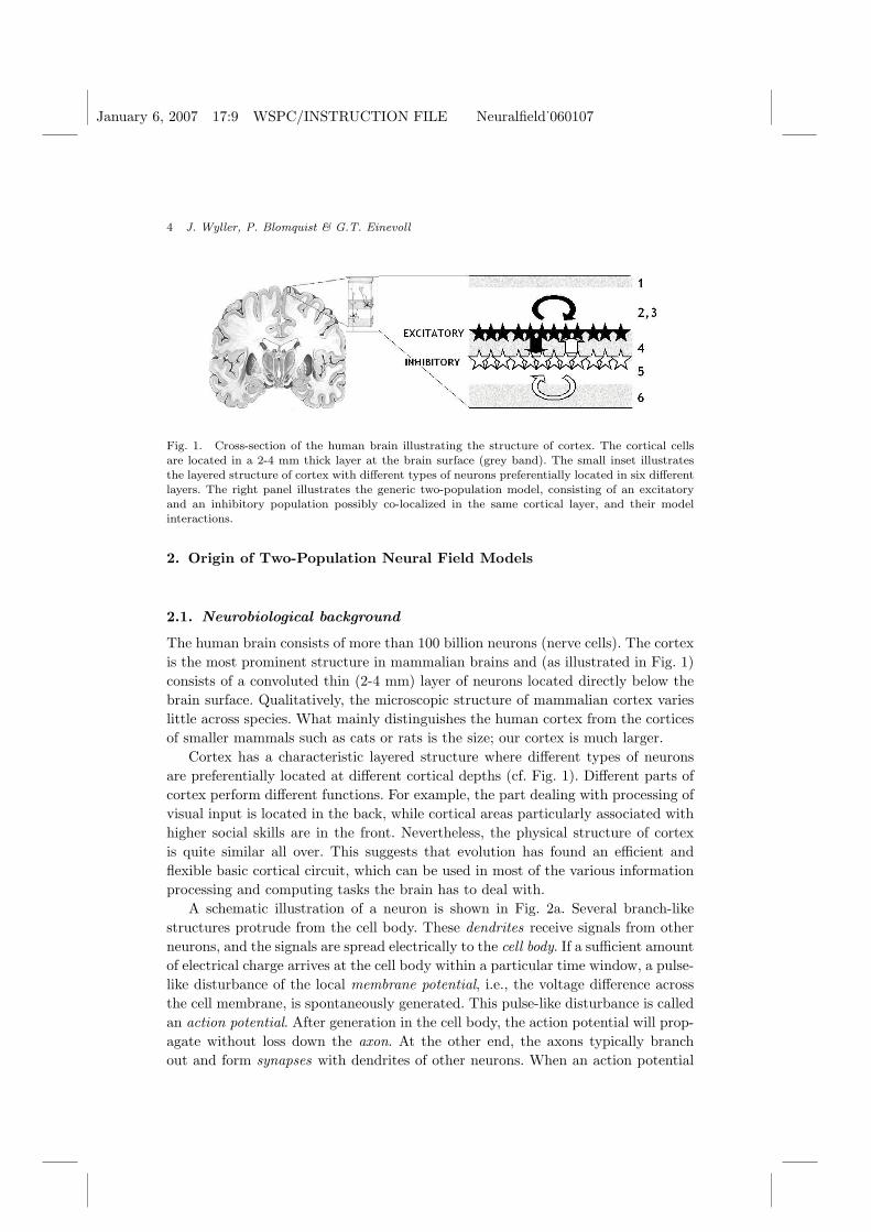
Fig. 1. Cross-section of the human brain illustrating the structure of cortex. The cortical cellsare located in a 2-4 mm thick layer at the brain surface (grey band). The small inset illustratesthe layered structure of cortex with different types of neurons preferentially located in six differentlayers. The right panel illustrates the generic two-population model, consisting of an excitatoryand an inhibitory population possibly co-localized in the same cortical layer, and their modelinteractions.

2. Origin of Two-Population Neural Field Models

2.1. Neurobiological background

The human brain consists of more than 100 billion neurons (nerve cells). The cortexis the most prominent structure in mammalian brains and (as illustrated in Fig. 1)consists of a convoluted thin (2-4 mm) layer of neurons located directly below thebrain surface. Qualitatively, the microscopic structure of mammalian cortex varieslittle across species. What mainly distinguishes the human cortex from the corticesof smaller mammals such as cats or rats is the size; our cortex is much larger.

Cortex has a characteristic layered structure where different types of neuronsare preferentially located at different cortical depths (cf. Fig. 1). Different parts ofcortex perform different functions. For example, the part dealing with processing ofvisual input is located in the back, while cortical areas particularly associated withhigher social skills are in the front. Nevertheless, the physical structure of cortexis quite similar all over. This suggests that evolution has found an efficient andflexible basic cortical circuit, which can be used in most of the various informationprocessing and computing tasks the brain has to deal with.

A schematic illustration of a neuron is shown in Fig. 2a. Several branch-likestructures protrude from the cell body. These dendrites receive signals from otherneurons, and the signals are spread electrically to the cell body. If a sufficient amountof electrical charge arrives at the cell body within a particular time window, a pulse-like disturbance of the local membrane potential, i.e., the voltage difference acrossthe cell membrane, is spontaneously generated. This pulse-like disturbance is calledan action potential. After generation in the cell body, the action potential will prop-agate without loss down the axon. At the other end, the axons typically branchout and form synapses with dendrites of other neurons. When an action potential



Fig. 2. (a) Schematic illustration of neuron (nerve cell). (b) Schematic illustration of synapsesfunctionally connecting two neurons. (c) Illustration of principle for construction of a compart-mental neuron model from an anatomically reconstructed neuron. The example neuron has beentaken from Ref. 29.

reaches a synapse, designated molecules called neurotransmitters are released intothe narrow cleft between two neurons, see Fig. 2b. These neurotransmitters rapidlydiffuse across the cleft, and the arrival of these at designated receptors at the re-ceiving neuron results in the generation of an electrical ion current. This electricalsignal will then be spread down to the cell body of the receiving neuron, and thewhole cycle can start again.

Action potentials appear to be the most important carrier of information be-tween neurons. The shape and duration of these action potentials generated in aparticular neuron vary little, and the information must thus be encoded in the se-quence of time points when they are generated. The firing times of action potentialsare thus deemed as the most salient output from neurons, and most mathematicalexplorations of neural-network activity have thus focused on the modeling of these.

Cortical networks are strongly connected; cortical neurons typically projectsynapses onto ∼10000 other neurons. These neurons can be grouped into two maincategories, excitatory and inhibitory, depending on whether they tend to bring theirpostsynaptic partners closer to, or further away from, firing action potentials. Thesetwo categories of neurons are intermingled in all cortical layers, and their close in-teraction is a key element determining the dynamical properties of cortical tissue.

2.2. Neuron models

Various types of mathematical models are used to describe the signal processingproperties of neurons. These model types are distinguished by their scope and theamount of biophysical details incorporated in the description.



2.2.1. Compartmental modeling

Compartmental modeling represents the highest level of detail. Here the neuron isdivided into compartments, so small that the electrical potential can be assumedto be the same throughout the compartment. Every compartment is described asa small electrical circuit where the current is carried by ions (not electrons as incomputers). The most important dynamical variable is the membrane potential,and the equation describing the dynamics of this variable follows from Kirchhoff’scurrent law stating that current cannot vanish.

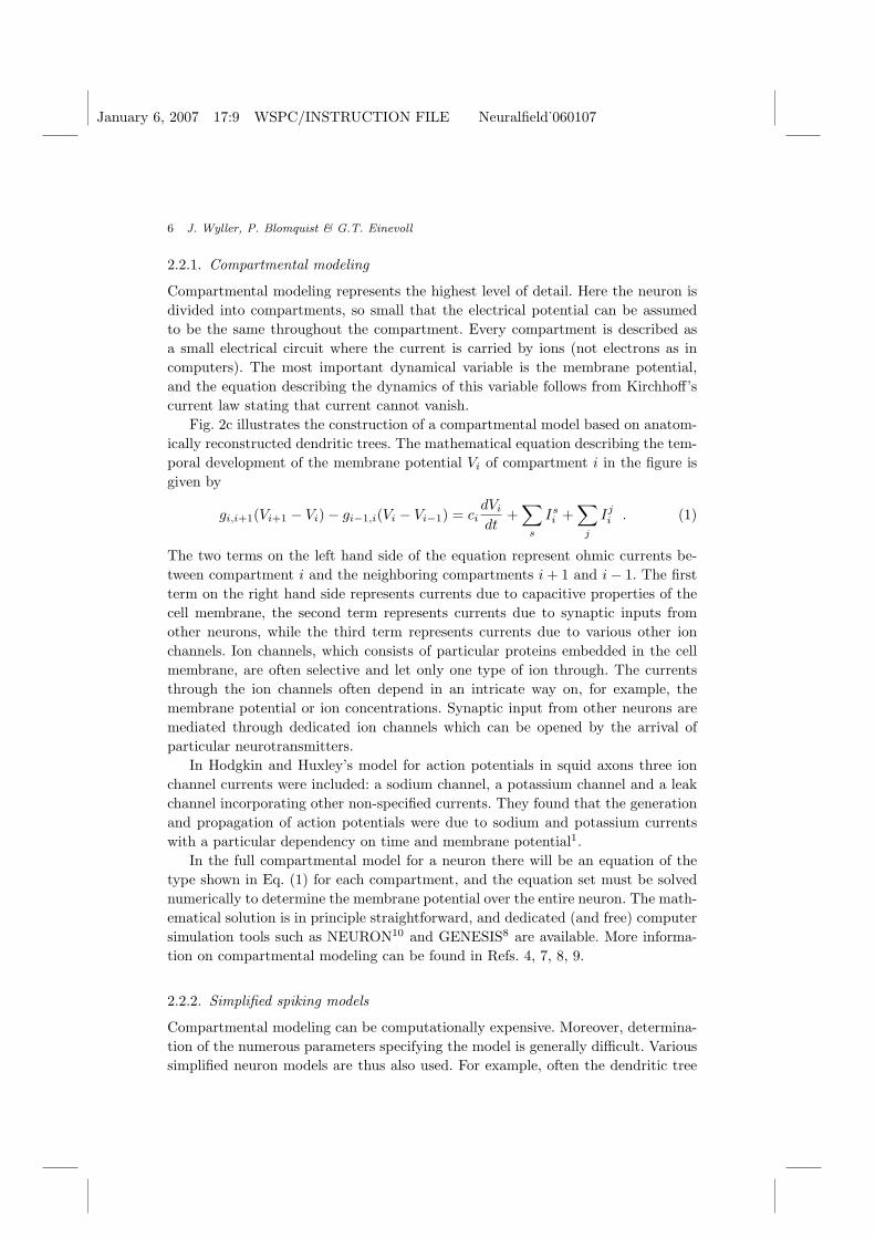
Fig. 2c illustrates the construction of a compartmental model based on anatom-ically reconstructed dendritic trees. The mathematical equation describing the tem-poral development of the membrane potential Vi of compartment i in the figure isgiven by

gi,i+1(Vi+1 − Vi)− gi−1,i(Vi − Vi−1) = cidVi

dt+

∑s

Isi +

∑

j

Iji . (1)

The two terms on the left hand side of the equation represent ohmic currents be-tween compartment i and the neighboring compartments i + 1 and i− 1. The firstterm on the right hand side represents currents due to capacitive properties of thecell membrane, the second term represents currents due to synaptic inputs fromother neurons, while the third term represents currents due to various other ionchannels. Ion channels, which consists of particular proteins embedded in the cellmembrane, are often selective and let only one type of ion through. The currentsthrough the ion channels often depend in an intricate way on, for example, themembrane potential or ion concentrations. Synaptic input from other neurons aremediated through dedicated ion channels which can be opened by the arrival ofparticular neurotransmitters.

In Hodgkin and Huxley’s model for action potentials in squid axons three ionchannel currents were included: a sodium channel, a potassium channel and a leakchannel incorporating other non-specified currents. They found that the generationand propagation of action potentials were due to sodium and potassium currentswith a particular dependency on time and membrane potential1.

In the full compartmental model for a neuron there will be an equation of thetype shown in Eq. (1) for each compartment, and the equation set must be solvednumerically to determine the membrane potential over the entire neuron. The math-ematical solution is in principle straightforward, and dedicated (and free) computersimulation tools such as NEURON10 and GENESIS8 are available. More informa-tion on compartmental modeling can be found in Refs. 4, 7, 8, 9.

2.2.2. Simplified spiking models

Compartmental modeling can be computationally expensive. Moreover, determina-tion of the numerous parameters specifying the model is generally difficult. Varioussimplified neuron models are thus also used. For example, often the dendritic tree



and cell body are collapsed into a single point, essentially saying that the membranepotential is the same throughout the neuron.

Further, the modeling of the dynamics of the membrane potential does often notinclude the generation of the action potential (spike) itself. Action potentials havea standardized all-or-none behavior, and it is not necessary to calculate the detailedtime course every time. Instead the action potentials are generated by a separaterule: when the membrane potential reaches a preset threshold for action-potentialfiring, an action potential is simply recorded, and the membrane voltage is resetto another predefined value. The integrate-and-fire model11 has been the commonchoice, but other models of the same type have also been studied5. In this modelthe subthreshold dynamics of the membrane potential (in the single compartment)is given by

cdV

dt= −gL(V − EL)−

∑s

Is . (2)

This equation follows directly from Eq. (1) by (i) omitting the terms due to cur-rents between compartments and (ii) including only an ohmic leak current withconductance gL (in addition to the synaptic currents). EL corresponds to the rest-ing potential, i.e., the membrane potential of the point neuron in the absence ofsynaptic inputs.

Even with this drastic simplification, it is still difficult to find analytical solutionsfor most situations of interest. One generally has to resort to numerical solution,but they require less computer resources than full compartmental simulations.

2.2.3. Firing-rate models

At the coarsest level of detail, we have firing-rate models where only the probabil-ity for action-potential firing is modeled. Then the “activity level” (for example,membrane potential in the cell body) is typically converted to a firing rate r via anon-linear sigmoidal function, i.e., r = F (V ). This mimics the observed conversionof membrane potential in the cell body to firing of action potentials; the mem-brane potential has to be above a particular threshold before action potentials aregenerated.

Firing-rate models have commonly been utilized in the investigation of networkproperties of the strongly interconnected cortical networks. In neural field modelsthe cortical tissue has in addition been modeled as continuous lines or sheets ofneurons14,15. In such models the spatiotemporally varying neural activity are de-scribed by a single or several scalar fields, one for each neuron type incorporated inthe model. Mathematically these models are formulated in terms of differential orintegro-differential equations, and the absence of the δ-function like action-potentialspikes in this coarse-grained formulation makes the mathematical analysis of net-work behavior significantly easier and more transparent. While neural field modelshave many virtues, it should therefore be kept in mind that they only apply as long



as the spatial and temporal scales are larger than the single-neuron scales.

3. Two-Population Model

We now consider a two-population model assuming co-localized excitatory and in-hibitory neurons in a one-dimensional strip of cortical tissue. We further assumethat (i) all neurons receive synaptic inputs from, in principle, all neurons in thenetwork (cf. right panel in Fig. 1), (ii) the synaptic weights depend only on thetype of pre- and postsynaptic neurons and their absolute spatial distance, (iii) thenet activity level in each neuron depends on a weighted sum over the past firingactivity in the presynaptic neurons, and (iv) the neuronal firing rates at a certaintime are given by applying particular non-linear functions to the neuronal activitylevels at the same time. The nonlocal model for the excitatory activity level ue andthe inhibitory activity level ui in one spatial dimension then reads27

ue = αee ∗ ωee ⊗ Pe(ue − θe)− αie ∗ ωie ⊗ Pi(ui − θi) (3a)

ui = αei ∗ ωei ⊗ Pe(ue − θe)− αii ∗ ωii ⊗ Pi(ui − θi) (3b)

with ωmn ⊗ Pm(um − θm) defined as the spatial convolution integral(ωmn ⊗ Pm(um − θm)

)(x, t)

=∫ ∞

−∞ωmn(y − x)Pm(um(y, t)− θm))dy, m, n = e, i (4)

and αmn ∗ f as the temporal convolution integral

(αmn ∗ f)(x, t)

=∫ t

−∞αmn(t− s)f(x, s)ds, m, n = e, i . (5)

Here x, y ∈ R denote the spatial coordinates and t, s ∈ R the temporal coordinates.The spatial distribution of synaptic connection strength in the network is de-

scribed by the connectivity functions ωmn (m,n = e, i), which are assumed to bereal-valued, positive, bounded, symmetric, normalized and parameterized by meansof synaptic footprints σmn,m, n = e, i, i.e.,

ωmn(x) = σ−1mnΦmn(ξmn), ξmn = x/σmn (6)

where Φmn are scaling functions. Note that in the present paper the synaptic weightsare assumed to be ’balanced’ (and normalized) in the sense that

∫∞−∞ ωmn(x)dx = 1

for all connections.The impact of past neural firing on the present activity levels in the network is

described by the temporal kernels αmn(t) (m,n = e, i) typically parameterized bya single time constant. The conversion of activity levels to action-potential firingactivities of the neurons is modeled by means of the firing-rate functions denotedPe and Pi, respectively, for the excitatory and the inhibitory neural elements. These



functions are smooth, increasing functions parameterized by an inclination param-eter βm > 0. Here, they are chosen to map the set of real numbers onto the unitinterval (so that the true firing rates are obtained by multiplying the output ofthese functions with appropriate constants). The firing-rate functions approach theHeaviside function H as βm →∞. In what follows we will assume that

Pm(u) =12(1 + tanh(βmu)

). (7)

Finally, the parameters θm represent threshold values for firing, which by assumptionsatisfy the requirement 0 < θm ≤ 1 (m = e, i).

In the sequel we will consider the special case where the temporal kernels areassumed to be modeled by means of exponentially decaying functions:

αee(t) = αie(t) = e−t, αei(t) = αii(t) =1τ

e−t/τ (8)

Within the framework of the model (3) this assumption signifies that the action-potential firing at the present time carries most weight in determining the currentactivity levels, and that the impact from earlier times are exponentially decaying.In this case it directly follows from use of the linear chain trick30 that any smoothsolution to the model (3) satisfies the following rate equation model25:

∂tue = −ue + ωee ⊗ Pe(ue − θe)− ωie ⊗ Pi(ui − θi) (9a)

τ∂tui = −ui + ωei ⊗ Pe(ue − θe)− ωii ⊗ Pi(ui − θi) . (9b)

Here we have tacitly assumed that we measure the time evolution in units of theexcitatory time constant. The parameter τ thus represents the ratio between theinhibitory and the excitatory time constant, we will hereafter refer to τ as therelative inhibition time. The firing-rate model (9) will be the starting point for ourfurther explorations in Secs. 4 and 5.

It should be noted that the model (9) is similar, but not identical, to the Wilson-Cowan model14. In the Wilson-Cowan model the source terms on the right handsides of (9a) and (9b) are different; instead of a linear sum of sigmoidal-functioninputs, the sigmoidal functions apply to the net sum of inputs. The neurobiologicalinterpretation of the model is also different, see Ref. 16.

4. Localized Activity Patterns (’Bumps’)

4.1. Existence and uniqueness

When approximating the firing-rate functions Pm with Heaviside functions H,one obtains closed form expressions for stationary, localized solutions Ue and Ui

(’bumps’) of (9) on the form25

Ue(x) =∫ a

−a

ωee(x− x′)dx′ −∫ b

−b

ωie(x− x′)dx′ (10a)

Ui(x) =∫ a

−a

ωei(x− x′)dx′ −∫ b

−b

ωii(x− x′)dx′ (10b)



(a)

−1 0 1−0.1

0

0.1

0.2Excitatory pulse

x

Ue(x)

−1 0 1

−0.05

0

0.05

0.1

Inhibitory pulse

x

Ui(x)

θe

θi

(b)

−1 0 1

0

0.04

0.08

0.12

Excitatory pulse

x

Ue(x)

−1 0 1

0

0.02

0.04

0.06

0.08

Inhibitory pulse

x

Ui(x)

θe θ

i

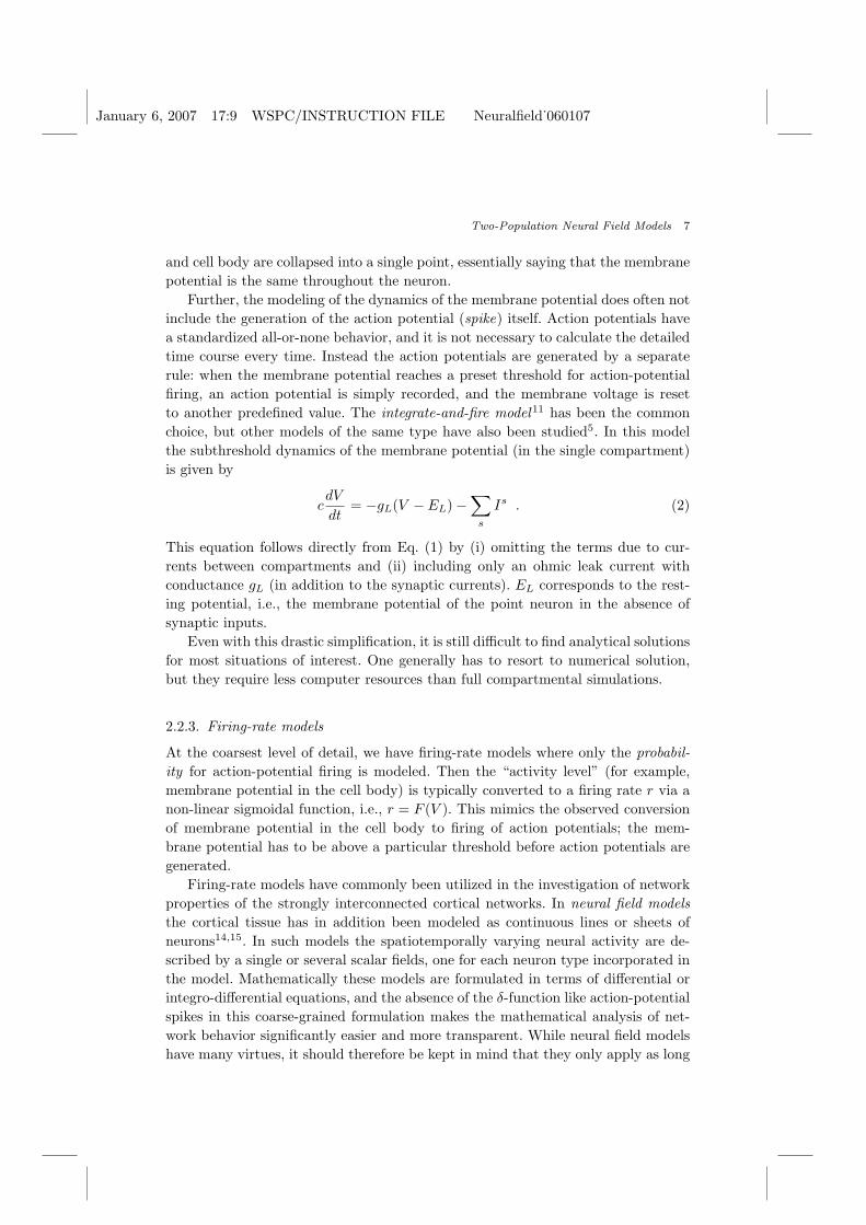
Fig. 3. Numerical example of (a) a broad pulse pair and (b) a narrow pulse pair. The connectivityfunctions are Gaussians with synaptic footprints σee = 0.35, σei = 0.48, σie = 0.60, and σii = 0.69.The threshold values are θe = 0.12 and θi = 0.08. The firing-rate pulses correspond to the regionswhere Um(x) is above the corresponding threshold value, θm, m = e, i. Adapted from Ref. 25.

where a, b satisfy the equations

fe(a, b) = θe (11a)

fi(a, b) = θi (11b)

with fe and fi given as

fe(a, b) = Wee(2a)−Wie(a + b) + Wie(a− b) (12a)

fi(a, b) = Wei(a + b)−Wei(b− a)−Wii(2b) . (12b)

Here Wmn(ξ) is defined as the integral

Wmn(ξ) =∫ ξ

0

ωmn(y)dy . (13)

The parameters a, b which are unique solutions of Ue(±a) = θe and Ui(±b) = θi,measure the pulse widths of Ue(x) and Ui(x). It turns out that a typical situationconsists of two pairs of pulses (’bumps’) (Ue(x), Ui(x)) for each set of thresholdvalues (θe, θi), one broad and one narrow pulse pair. This result has also been foundfor one-population models15 and simpler two-population models24. In addition, onefinds that an excitatory pulse may exist without an accompanying inhibitory pulseand that the inhibitory cannot exist alone25. In Fig. 3 broad and narrow pulse pairsfor Gaussian connectivity functions are displayed.

4.2. Stability

One approach for investigation of the stability of the bumps is based on perturbingthe bumps Ue and Ui, i.e., ue(x, t) = Ue(x) + χ(x, t), ui(x, t) = Ui(x) + ψ(x, t).The resulting linearized non-local evolution equations for the disturbances (χ, ψ)



are then found to be25

χt = −χ + ωee ∗ (δ(Ue − θe)χ)− ωie ∗ (δ(Ui − θi)ψ) (14a)

τψt = −ψ + ωei ∗ (δ(Ue − θe)χ)− ωii ∗ (δ(Ui − θi)ψ) (14b)

and the assumption of spatiotemporal separability, i.e., χ(x, t) = eλtχ1(x), ψ(x, t) =eλtψ1(x), yields the equations

τλ2 + (α− βτ)λ + γ = 0 (15a)

τλ2 + (α′ − β′τ)λ = 0 (15b)

for the growth rate λ of the disturbances χ(x, t) and ψ(x, t)). The coefficients(α,α′,β,β′,γ) are found to be complicated functions of the connectivity functionsevaluated at certain values given by the bump-width coordinates (aeq, beq) and theslopes of the activity levels at the pulse edges25. Two general relationships, β ≥ β′

and α ≥ α′ > 0, can immediately be established, however25.An alternative approach to the stability analysis is the method originally sug-

gested by Amari15: One represents each stationary pulse with its width, and a2D autonomous dynamical system, consistent with the model equations, for thetemporal evolution of the width parameters a and b (defined by the constraintsue(a(t), t) = θe and ui(b(t), t) = θi) is derived25. The equilibrium point of thissystem corresponds to the widths of the stationary bumps. It turns out25 that theeigenvalues of the Jacobian of the resulting 2D system evaluated at the equilibriumsatisfy the quadratic equation (15a). The equation (15b), however, is interestinglyfound to be absent in the results from using this Amari approach.

It is therefore important to determine when the stability issue can solely bebased on (15a), and when one has to take (15b) into account. From the eigenvalueequations (15a) - (15b) we arrive at the following conclusions:

1. When γ is negative we have a saddle point instability, irrespective of the propertiesof the roots of (15b). Both the pulse widths and the synaptic footprints regulatethe magnitude of γ.

2. In the complementary regime, i.e., when γ is positive, one has to separate thediscussion into the following subcases:

(a) β > 0 ≥ β′.Even though β according to the Amari analysis is found to always be positive,β′ may be non-positive. In this case (15b) gives a negative value for the non-zero eigenvalue. But, since β > 0, there is a Hopf bifurcation point at a criticalτ -value for (15a), given by τ = τH ≡ α/β. In this case the stability situationis governed by the latter equation.

(b) β ≥ β′ > 0.For β′ > 0 there are two different critical τ -values, τH and τ ′H , given as

τH =α

βand τ ′H =

α′

β′. (16)



For β′, γ′ > 0 it is shown in Ref. 25 that for the present system the Amari approachis applicable if

τH ≤ τ ′H (17)

while in the complementary regime

τH > τ ′H , (18)

the Amari approach predicts stability for the range τ ′H < τ < τH , whereas the fulllinear stability analysis yields instability. Thus for certain values of the inhibitorytime constant the Amari approach is found to give incorrect stability results. Nu-merical examples demonstrating this result can be found in Fig. 4 of Ref. 25.

Another important result relates to the existence of two pulse pairs for each setof threshold values25: One can show that narrow pulse pairs always are unstable,corresponding to a saddle point of the Amari system, while the broader pulse pairsare converted to breathers as τ passes the critical value τH , similar to what wasseen by Pinto and Ermentrout for a simpler two-population model24. The analysisdetailed in Ref. 25 also indicates that there are possibilities of having stable andunstable breathers excited at the Hopf bifurcation point τ = τH .

5. Generation of Activity Patterns

A separate question is how regular activity patterns such as ’bumps’, or spatial andspatiotemporal oscillations can be generated, and here we will demonstrate how thiscan occur through Turing-type instabilities due to the nonlocal spatial interactionspresent in the model. Note that the sigmoidal firing-rate function in (7) (with finiteinclinations) is used throughout.

In the local limit, i.e., σmn → 0 (m,n = e, i), so that ωmn(x) → δ(x), thesystem (9) always possesses at least one equilibrium point28. We first rig our model,by adjusting the firing-rate parameters βm, θm,m = e, i, so that a single equilibriumpoint exists. Further, the relative inhibition time τ is chosen to assure stability ofthis equilibrium point in the limit with local spatial interactions. Next, by switchingon nonlocal effects, i.e., σmn 6= 0 (m, n = e, i), the same equilibrium is found tobecome unstable for a quite large class of connectivity functions. In fact, one canprove that the instability structure in the generic case consists of a finite number ofwell-separated unstable wave number bands28. Finally, by following these bands intothe nonlinear regime, one gets energy leakage into the linearly most unstable modeafter the initial linear phase. The final result after saturation is typically regularspatial and spatiotemporal patterns.

5.1. Existence and uniqueness of homogeneous equilibrium states

The spatial homogeneous equilibrium of (3) satisfies the coupled set of equations28

ue = ui (19a)

F (ue) ≡ ue + Pi(ue − θi)− Pe(ue − θe) = 0 . (19b)



The conditions imposed on the firing-rate functions Pm, i.e., that 0 < Pm(u) < 1for |u| < ∞, imply that possible equilibrium points must lie on the straight lineue = ui subject to the constraint −1 < um < 1 (m = e, i) for all choices of firing-rate function parameters βm and θm.

5.2. Linear stability theory in local limit

Now we assume that the synaptic connections are strictly local, i.e., σmn (m, n =e, i) approach zero. Then (3) is reduced to a 2D autonomous dynamical system

∂tue = −ue + Pe(ue − θe)− Pi(ui − θi) (20a)

τ∂tui = −ui + Pe(ue − θe)− Pi(ui − θi) . (20b)

The results of the linear stability analysis of (20) is conveniently expressed in termsof the parameters

P ′m ≡ dPm(v)dv

∣∣∣v=um,eq−θm

= βm sech2(βm(um,eq − θm)

)/2, m = e, i, (21)

τ∗ ≡ (P ′i + 1)/(P ′e − 1) (22)

F ′(ueq) = 1 + P ′i − P ′e . (23)

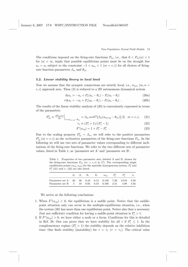
Due to the scaling property P ′m ∼ βm, we will refer to the positive parametersP ′m (m = e, i) as the inclination parameters of the firing-rate functions Pm. In thefollowing we will use two sets of parameter values corresponding to different incli-nations of the firing-rate functions. We refer to the two different sets of parametervalues, listed in Table 1, as ’parameter set A’ and ’parameter set B’.

Table 1. Properties of two parameter sets, labeled A and B, chosen forthe firing-rate functions Pm (m = e, i) in (7). The corresponding singleequilibrium points (ueq, ueq) for the spatially homogeneous system, P ′e andP ′i (21) and τ∗ (22) are also listed.

βe βi θe θi ueq P ′e P ′i τ∗

Parameter set A 20 30 0.10 0.12 0.129 7.26 13.94 2.39Parameter set B 5 10 0.05 0.10 0.106 2.31 4.98 4.56

We arrive at the following conclusions:

1. When F ′(ueq) < 0, the equilibrium is a saddle point. Notice that the saddle-point situation only can occur in the multiple-equilibrium situation, i.e., whenthe system (20) has more than one equilibrium point. Notice also that a necessary(but not sufficient) condition for having a saddle-point situation is P ′e > 1.

2. If F ′(ueq) > 0, we have either a node or a focus. Conditions for this is detailedin Ref. 28. One can prove that we have stability for all τ if P ′e ≤ 1. In thecomplementary regime (P ′e > 1) the stability depends on the relative inhibitiontime: One finds stability (instability) for τ < τ∗ (τ > τ∗). The critical value



τ∗ corresponds to a Hopf bifurcation point. The outcome of this bifurcation isaccording to standard theory the excitation of a limit cycle (temporal oscillations).

5.3. Linear stability analysis in the nonlocal regime

We insert the ansatz ue(x, t) = ueq +φ(x, t), ui(x, t) = ueq +ψ(x, t) into the system(9). Here φ and ψ are small perturbations imposed on the constant backgrounddescribed by (ueq, ueq) (|φ|, |ψ| ¿ |ueq|). The resulting equations are linearized andthereafter Fourier transformed, giving28

∂tX = A ·X . (24)

Here A and X are defined as

A =[

P ′eωee − 1 −P ′i ωie

τ−1P ′eωei −τ−1(P ′i ωii + 1)

], (25)

X = [φ, ψ]T (26)

where ωmn(k), φ(k, t) and ψ(k, t) are Fourier transforms of the connectivity func-tions ωmn(x), φ(x, t) and ψ(x, t), respectively, and k corresponds to the (spatial)wave number of the modulations imposed on the homogeneous background.

We always have two modes in the problem corresponding to the two eigenvaluesλ+ and λ−, given in terms of the invariants of the coefficient matrix A:

λ± =12(tr(A)±

√(tr(A)2 − 4det(A))) (27a)

det(A) = τ−1((1 + P ′i ωii)(1− P ′eωee) + P ′eP′i ωieωei) (27b)

tr(A) = P ′eωee − 1− τ−1(P ′i ωii + 1) . (27c)

The mode corresponding to λ+ (λ−) is referred to as the λ+(λ−)-mode. Notice alsothat since ωmn(k) = ωmn(−k), we have λ±(k) = λ±(−k). Hence the variation of theeigenvalues with the wave number k can be expressed in terms of the squared wavenumber η = k2. Now, since the differential equations (24)-(26) constitute a 2D linearautonomous system with constant coefficients, we can exploit the invariants of thecoefficient matrix A to determine the stability properties: Each η = k2 correspondsto a point in the (tr(A), det(A))-plane (which we refer to as the invariant plane).Thus, when letting η vary continuously from 0 to +∞, a parameterized curve γ

defined as

γ(η) = (tr(A)(η), det(A)(η)), η ≥ 0 (28)

is traced out in the invariant plane. This means that we can study the stabilityproblem in a simple geometrical way: We have stability if the curve γ remainsin the second quadrant for all η ≥ 0, while an instability occurs if there is anη-interval for which the curve is outside this quadrant. Moreover, the number oftransversal crossings of the tr(A)-axis and the positive det(A)-axis in the invariantplane determines the number of unstable bands. Finally, formation and coalescence



of unstable bands are connected to nontransversal crossings of the tr(A)-axis andthe positive det(A)-axis in the invariant plane of the trajectory γ defined by (27)and (28). These types of crossings indicate that bifurcation phenomena take place.The special case characterized by a wave number k∗ for which we locally have (i)det(A)(ηh = k2

h) > 0 and tr(A)(η∗ = k2∗) = 0, and (ii) tr(A) < 0 for η 6= ηh (i.e.,

a non-transversal crossing at η = ηh), is referred to as a Turing-Hopf bifurcation31.The corresponding relative inhibition time τ is denoted by τh. In analogy with theprocedure detailed in Ref. 31, a Hopf normal form of the system (3) can be derivedfor the approximate behavior of the dynamics in the vicinity of the Hopf point.Based on this normal form one can show that a breather or a traveling wave isexcited. Moreover, conditions for having stable breathers and traveling waves canbe expressed in terms of the coefficients of the normal form.

5.4. Pattern generation for exponentially decaying connectivities

We now assume the connectivity functions (6) to be exponentially decaying,i.e., Φmn(ξmn) = 1

2 exp(−|ξmn|) for which the Fourier transform is given as theLorentzian

ωmn(η) =1

1 + σ2mnη

, η = k2, m, n = e, i , (29)

and particulary focus on situations where the firing-rate functions are given by oneof the two parameter sets A and B in Table 1.

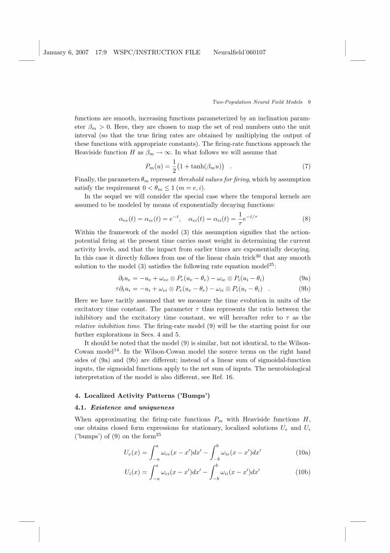
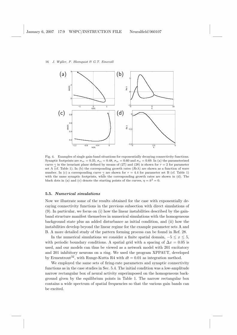
First we consider parameter set A: These parameters as well as τ are chosento comply with the condition P ′e > 1 and τ < τ∗ to assure stability in the long-wavelength limit. As seen in Fig. 4a, the trajectory γ starts and ends in the secondquadrant but passes through the other three quadrants. The corresponding growthrate curve is shown in Fig. 4b, illustrating that the real part of one or both eigen-values is positive unless the trajectory γ is in the second quadrant.

For the situation seen in Fig. 4c for parameter set B the situation is qualita-tively different: Here det(A) > 0 for the entire trajectory, and an unstable band isexcited when the trajectory passes into the first quadrant (tr(A) > 0). The corre-sponding growth-rate curve is displayed in Fig. 4d. Notice that the eigenvalues ofthe coefficient matrix A in this case are complex conjugate for all wave numbersin the unstable band, and hence each unstable mode in the band exhibits temporaloscillations. The frequency of the oscillations is given by the imaginary part of theeigenvalues. A detailed analysis28 now reveals that we get a unique Turing-Hopfbifurcation if

σ2ii

σ2ee

> τ∗P ′eP ′i

, P ′e > 1 (30)

and τ fulfills the condition τc < τ < τ∗, where

τc ≡(P ′i + 1 +

σ2ii

σ2ee

)/((P ′e − 1)

σ2ii

σ2ee

− 1)

(31)

and τ∗ is the local Hopf time given by (22).



(a)

−1 0 1

0

2

4

tr(A)

det(

A)

(b)

0 5 10−1

0

1

k

Re

λ

(c)

−1.2 −0.8 −0.4 0

0.2

0.4

0.6

0.8

tr(A)

det(

A)

(d)

0 2.5 5−0.4

−0.2

0

k

Re

λ

Fig. 4. Examples of single gain-band situations for exponentially decaying connectivity functions.Synaptic footprints are σee = 0.35, σei = 0.48, σie = 0.60 and σii = 0.69. In (a) the parameterizedcurve γ in the invariant plane defined by means of (27) and (28) is shown for τ = 2 for parameterset A (cf. Table 1). In (b) the corresponding growth rates (Reλ) are shown as a function of wavenumber. In (c) a corresponding curve γ are shown for τ = 4.4 for parameter set B (cf. Table 1)with the same synaptic footprints, while the corresponding growth rates are shown in (d). Theblack dots in (a) and (c) denote the starting points of the curves, η = k2 = 0.

5.5. Numerical simulations

Now we illustrate some of the results obtained for the case with exponentially de-caying connectivity functions in the previous subsection with direct simulations of(9). In particular, we focus on (i) how the linear instabilities described by the gain-band structure manifest themselves in numerical simulations with the homogeneousbackground state plus an added disturbance as initial condition, and (ii) how theinstabilities develop beyond the linear regime for the example parameter sets A andB. A more detailed study of the pattern forming process can be found in Ref. 28.

In the numerical simulations we consider a finite spatial domain, −5 ≤ x ≤ 5,with periodic boundary conditions. A spatial grid with a spacing of ∆x = 0.05 isused, and our models can thus be viewed as a network model with 201 excitatoryand 201 inhibitory neurons on a ring. We used the program XPPAUT, developedby Ermentrout32, with Runge-Kutta R4 with dt = 0.01 as integration method.

We employed the same sets of firing-rate parameters and synaptic connectivityfunctions as in the case studies in Sec. 5.4. The initial condition was a low-amplitudenarrow rectangular box of neural activity superimposed on the homogeneous back-ground given by the equilibrium points in Table 1. The narrow rectangular boxcontains a wide spectrum of spatial frequencies so that the various gain bands canbe excited.



(a)

x

t

−4 −2 0 2 4

0

75

150 −0.1

0

0.1

0.2

(b)

x

t

−4 −2 0 2 4

0

75

150 −0.1

0

0.1

0.2

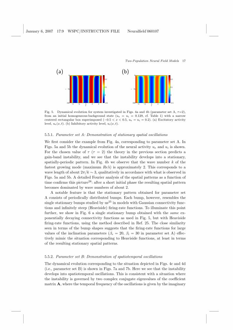
Fig. 5. Dynamical evolution for system investigated in Figs. 4a and 4b (parameter set A, τ=2),from an initial homogeneous-background state (ue = ui = 0.129, cf. Table 1) with a narrowcentered rectangular box superimposed (−0.5 < x < 0.5, ue = ui = 0.2). (a) Excitatory activitylevel, ue(x, t). (b) Inhibitory activity level, ui(x, t).

5.5.1. Parameter set A: Demonstration of stationary spatial oscillations

We first consider the example from Fig. 4a, corresponding to parameter set A. InFigs. 5a and 5b the dynamical evolution of the neural activity ue and ui is shown.For the chosen value of τ (τ = 2) the theory in the previous section predicts again-band instability, and we see that the instability develops into a stationary,spatially-periodic pattern. In Fig. 4b we observe that the wave number k of thefastest growing mode (maximum Reλ) is approximately 2. This corresponds to awave length of about 2π/k ∼ 3, qualitatively in accordance with what is observed inFigs. 5a and 5b. A detailed Fourier analysis of the spatial patterns as a function oftime confirms this picture28: after a short initial phase the resulting spatial patternbecomes dominated by wave numbers of about 2.

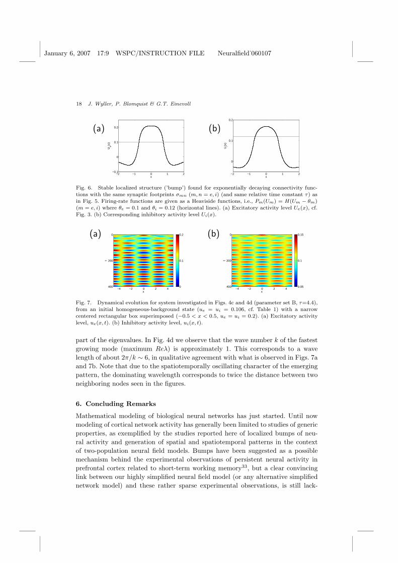
A notable feature is that the stationary pattern obtained for parameter setA consists of periodically distributed bumps. Each bump, however, resembles thesingle stationary bumps studied by us25 in models with Gaussian connectivity func-tions and infinitely steep (Heaviside) firing-rate functions. To illuminate this pointfurther, we show in Fig. 6 a single stationary bump obtained with the same ex-ponentially decaying connectivity functions as used in Fig. 5, but with Heavisidefiring-rate functions, using the method described in Ref. 25. The close similarityseen in terms of the bump shapes suggests that the firing-rate functions for largevalues of the inclination parameters (βe = 20, βi = 30 in parameter set A) effec-tively mimic the situation corresponding to Heaviside functions, at least in termsof the resulting stationary spatial patterns.

5.5.2. Parameter set B: Demonstration of spatiotemporal oscillations

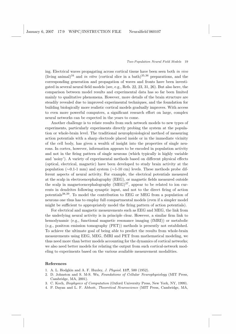
The dynamical evolution corresponding to the situation depicted in Figs. 4c and 4d(i.e., parameter set B) is shown in Figs. 7a and 7b. Here we see that the instabilitydevelops into spatiotemporal oscillations. This is consistent with a situation wherethe instability is governed by two complex conjugate eigenvalues of the coefficientmatrix A, where the temporal frequency of the oscillations is given by the imaginary



(a)

−2 −1 0 1 2−0.1

0

0.1

0.2

x

Ue(x

)

(b)

−2 −1 0 1 2

0

0.1

0.2

x

Ui(x

)

Fig. 6. Stable localized structure (’bump’) found for exponentially decaying connectivity func-tions with the same synaptic footprints σmn (m, n = e, i) (and same relative time constant τ) asin Fig. 5. Firing-rate functions are given as a Heaviside functions, i.e., Pm(Um) = H(Um − θm)(m = e, i) where θe = 0.1 and θi = 0.12 (horizontal lines). (a) Excitatory activity level Ue(x), cf.Fig. 3. (b) Corresponding inhibitory activity level Ui(x).

(a)

x

t

−4 −2 0 2 4

0

200

400 0

0.1

0.2 (b)

x

t

−4 −2 0 2 4

0

200

400 0.05

0.1

0.15

Fig. 7. Dynamical evolution for system investigated in Figs. 4c and 4d (parameter set B, τ=4.4),from an initial homogeneous-background state (ue = ui = 0.106, cf. Table 1) with a narrowcentered rectangular box superimposed (−0.5 < x < 0.5, ue = ui = 0.2). (a) Excitatory activitylevel, ue(x, t). (b) Inhibitory activity level, ui(x, t).

part of the eigenvalues. In Fig. 4d we observe that the wave number k of the fastestgrowing mode (maximum Reλ) is approximately 1. This corresponds to a wavelength of about 2π/k ∼ 6, in qualitative agreement with what is observed in Figs. 7aand 7b. Note that due to the spatiotemporally oscillating character of the emergingpattern, the dominating wavelength corresponds to twice the distance between twoneighboring nodes seen in the figures.

6. Concluding Remarks

Mathematical modeling of biological neural networks has just started. Until nowmodeling of cortical network activity has generally been limited to studies of genericproperties, as exemplified by the studies reported here of localized bumps of neu-ral activity and generation of spatial and spatiotemporal patterns in the contextof two-population neural field models. Bumps have been suggested as a possiblemechanism behind the experimental observations of persistent neural activity inprefrontal cortex related to short-term working memory33, but a clear convincinglink between our highly simplified neural field model (or any alternative simplifiednetwork model) and these rather sparse experimental observations, is still lack-



ing. Electrical waves propagating across cortical tissue have been seen both in vivo(living animal)34 and in vitro (cortical slice in a bath)35,36 preparations, and thecorresponding generation and propagation of waves and fronts have been investi-gated in several neural field models (see, e.g., Refs. 22, 23, 31, 26). But also here, thecomparison between model results and experimental data has so far been limitedmainly to qualitative phenomena. However, more details of the brain structure aresteadily revealed due to improved experimental techniques, and the foundation forbuilding biologically more realistic cortical models gradually improves. With accessto even more powerful computers, a significant research effort on large, complexneural networks can be expected in the years to come.

Another challenge is to relate results from such network models to new types ofexperiments, particularly experiments directly probing the system at the popula-tion or whole-brain level. The traditional neurophysiological method of measuringaction potentials with a sharp electrode placed inside or in the immediate vicinityof the cell body, has given a wealth of insight into the properties of single neu-rons. In cortex, however, information appears to be encoded in population activityand not in the firing pattern of single neurons (which typically is highly variableand ’noisy’). A variety of experimental methods based on different physical effects(optical, electrical, magnetic) have been developed to study brain activity at thepopulation (∼0.1-1 mm) and system (∼1-10 cm) levels. These methods probe dif-ferent aspects of neural activity. For example, the electrical potentials measuredat the scalp in electroencephalography (EEG), or magnetic fields measured outsidethe scalp in magnetoencephalography (MEG)37, appear to be related to ion cur-rents in dendrites following synaptic input, and not to the direct firing of actionpotentials38,39. To model the contribution to EEG or MEG from a population ofneurons one thus has to employ full compartmental models (even if a simpler modelmight be sufficient to appropriately model the firing pattern of action potentials).

For electrical and magnetic measurements such as EEG and MEG, the link fromthe underlying neural activity is in principle clear. However, a similar firm link tohemodynamic (e.g., functional magnetic resonance imaging (fMRI)) or metabolic(e.g., positron emission tomography (PET)) methods is presently not established.To achieve the ultimate goal of being able to predict the results from whole-brainmeasurements using EEG, MEG, fMRI and PET from mathematical modeling, wethus need more than better models accounting for the dynamics of cortical networks;we also need better models for relating the output from such cortical-network mod-eling to experiments based on the various available measurement modalities.

References

1. A. L. Hodgkin and A. F. Huxley, J. Physiol. 117, 500 (1952).2. D. Johnston and S. M-S. Wu, Foundations of Cellular Neurophysiology (MIT Press,

Cambridge, MA, 2001).3. C. Koch, Biophysics of Computation (Oxford University Press, New York, NY, 1999).4. P. Dayan and L. F. Abbott, Theoretical Neuroscience (MIT Press, Cambridge, MA,



2001).5. E. M. Izhikevitch, Dynamical Systems in Neuroscience (MIT Press, Cambridge, MA,

2007).6. D. Noble, The Initiation of the Heartbeat (Clarendon Press, Oxford, 1979).7. C. Koch and I. Segev (eds.), Methods in Neuronal Modeling, 2nd edn. (MIT Press,

Cambridge, MA, 1998).8. J. M. Bower and D. Beeman (eds.), The Book of Genesis: Exploring Realistic Neural

Models with the General Neural Simulation System, 2nd edn. (Springer, New York, NY,1998).

9. E. de Schutter, Computational Neuroscience - Realistic Modeling for Experimentalists(CRC Press, New York, NY, 2000).

10. N. T. Carnevale and M. L. Carnevale, The NEURON Book (Cambridge UniversityPress, Cambridge, UK, 2006).

11. L. Lapique, J. Physiol. Pathol. Gen. 9, 620 (1907).12. H. K. Hartline and F. Ratliff, J. Gen. Physiol. 40, 357 (1957).13. H. K. Hartline and F. Ratliff. J. Gen. Physiol. 41, 1049 (1958).14. H. R. Wilson and J. D. Cowan, Kybernetik 13, 55 (1973).15. S. Amari, Biol. Cybern. 27, 77 (1977).16. B. Ermentrout, Rep. Prog. Phys. 61, 353 (1998).17. S. Coombes, Biol. Cybern. 93, 91 (2005).18. T. P. Vogels, K. Rajan and L. F. Abbott, Ann. Rev. Neurosci. 28, 357 (2005).19. G. B. Ermentrout and J. D. Cowan, J. Math. Biol. 7, 265 (1979).20. G. B. Ermentrout, Biol. Cybern. 34 137 (1979).21. G. B. Ermentrout and J. D. Cowan, SIAM J. Appl. Math. 38, 1 (1980).22. G. B. Ermentrout and J. D. Cowan, SIAM J. Appl. Math. 39, 323 (1980).23. D. J. Pinto and G. B. Ermentrout, SIAM J. Appl. Math. 62, 206 (2001).24. D. J. Pinto and G. B. Ermentrout, SIAM J. Appl. Math. 62, 226 (2001).25. P. Blomquist, J. Wyller and G. T. Einevoll, Physica D 206, 180 (2005).26. A. Hutt and F. M. Atay, Physica D 203, 30 (2005).27. C. Laing and S. Coombes, Network: Comp. Neur. Syst. 17, 151 (2006).28. J. Wyller, P. Blomquist and G. T. Einevoll, Physica D 225, 75 (2007).29. Z. F. Mainen and T. J. Sejnowski, Nature 382, 363-366, (1996). The example neuron

has been downloaded from http://www.cnl.salk.edu/∼zach/methods.html .30. J. M. Cushing. Integrodifferential Equations and Delay Models in Population Dynam-

ics, Lecture Notes in Biomathematics (Springer, New York, NY, 1977).31. R. Curtu and B. Ermentrout, SIAM J. Appl. Dyn. Syst. 3, 131 (2004).32. B. Ermentrout, Simulating, Analyzing, and Animating Dynamical Systems: A Guide

to XPPAUT to Researchers and Students (SIAM, Philadelphia, PA, 2002).33. X.-J. Wang, Trends in Neurosci. 24, 455 (2001).34. J. C. Prechtl, L. B. Cohen, B. Pesaran, P. P. Mitra and D. Kleinfeld, Proc. Natl. Acad.

Sci. (USA) 94, 7621 (1997).35. R. D. Chervin, P. A. Pierce and B. W. Connors, J. Neurophysiol. 60 1695 (1988).36. J. Y. Wu, L. Guan and Y. Tsau, J. Neurosci. 19, 5005 (1999).37. M. Hamalainen, R. Hari, R. Ilmoniemi, J. Knuutila, J. and O. V. Lounasmaa, Rev.

Mod. Phys. 65, 413 (1993).38. P. Nunez and R. Srinvasan, Electrical Fields of the Brain: The Neurophysics of EEG

(Oxford University Press, New York, NY, 2006).39. G. T. Einevoll, K. H. Pettersen, A. Devor, I. Ulbert, E. Halgren, and A. M. Dale,

Laminar Population Analysis: Estimating firing rates and evoked synaptic activity frommultielectrode recordings in rat barrel cortex, to appear in J. Neurophysiol.

ON THE ORIGIN AND PROPERTIES OF TWO-POPULATION NEURAL FIELD MODELS - A TUTORIAL INTRODUCTION

Documents