Identifying signal and noise structure in neural population ...

Identifying signal and noise structure in neuralpopulation activity with Gaussian process factor

models

Stephen L. KeeleyPrinceton Neuroscience Institute

Princeton University,Princeton, NJ 08544

[email protected]

Mikio C. AoiPrinceton Neuroscience Institute

Princeton University,Princeton, NJ 08544

Yiyi YuDept. of Electrical

Computer EngineeringUniversity of California Santa Barbara

Santa Barbara, CA

Spencer L. SmithDept. of Electrical

Computer EngineeringUniversity of California Santa Barbara

Santa Barbara, CA

Jonathan W. PillowPrinceton Neuroscience Institute

Princeton University,Princeton, NJ 08544

Abstract

Neural datasets often contain measurements of neural activity across multipletrials of a repeated stimulus or behavior. An important problem in the analysisof such datasets is to characterize systematic aspects of neural activity that carryinformation about the repeated stimulus or behavior of interest, which can beconsidered “signal”, and to separate them from the trial-to-trial fluctuations inactivity that are not time-locked to the stimulus, which for purposes of suchanalyses can be considered “noise”. Gaussian Process factor models provide apowerful tool for identifying shared structure in high-dimensional neural data.However, they have not yet been adapted to the problem of characterizing signaland noise in multi-trial datasets. Here we address this shortcoming by proposing“signal-noise” Poisson-spiking Gaussian Process Factor Analysis (SNP-GPFA), aflexible latent variable model that resolves signal and noise latent structure in neuralpopulation spiking activity. To learn the parameters of our model, we introducea Fourier-domain black box variational inference method that quickly identifiessmooth latent structure. The resulting model reliably uncovers latent signal andtrial-to-trial noise-related fluctuations in large-scale recordings. We use this modelto show that in monkey V1, noise fluctuations perturb neural activity within asubspace orthogonal to signal activity, suggesting that trial-by-trial noise doesnot interfere with signal representations. Finally, we extend the model to capturestatistical dependencies across brain regions in multi-region data. We show that inmouse visual cortex, models with shared noise across brain regions out-performmodels with independent per-region noise.

34th Conference on Neural Information Processing Systems (NeurIPS 2020), Vancouver, Canada.

1 Introduction

Recent advances in electrophysiological and calcium fluorescence imaging technologies have enabledthe collection of increasingly high-dimensional neural datasets. Making sense of such datasets willrely on the development of flexible statistical methods for extracting relevant structure. Gaussianprocess factor models provide one powerful tool for identifying low-dimensional latent structurefrom high-dimensional neural response data. These models seek to characterize neural time-seriesdata in terms of a small number of smoothly evolving latent variables, and have been successfullyused to characterize neural representations in a variety of contexts [1, 2, 3, 4, 5, 6].

Standard Gaussian Process factor analysis (GPFA) uses a Gaussian process prior to impose smooth-ness on inferred latent variables, but do not explicitly consider stimulus or task conditions. However,neural data often exist in the form of repeated trials, whereby the same condition is presented to ananimal multiple times. These repeated presentations give rise to neural activity that varies across trialsaround some time-varying “signal” component that is typically estimated using the peri-stimulustime histogram (PSTH). Understanding this signal, and its relationship to trial-to-trial variability, isof central importance to the models of coding in the nervous system [7, 8], yet latent factor modelshave not been developed to explicitly study this question. Here we address this shortcoming bydeveloping an extension to Gaussian process factor analysis with Poisson spiking (P-GPFA) whichwe call signal and noise P-GPFA (SNP-GPFA). This model incorporates both signal and independentper-trial components that vary across trials. We refer to these latter components as “noise”, in thesense that they are not time-locked to the repeated stimulus, though they may well reflect other signalsunrelated to the experimental stimulus of interest.

In both P-GPFA and SNP-GPFA models, because the Gaussian process is not a conjugate prior for aPoisson observation model, posterior inference is intractable in closed form. Variational inferencemethods have become increasingly common for applications of Gaussian processes [9, 10, 5].They achieve tractability by approximating the posterior distribution pθ(x|y)with a well-behavedvariational distribution qφ(x|y) [11]. For P-GPFA and SNP-GPFA, because the calculation of theexpectation under qφ(x|y) of the joint distribution pθ(x,y) is also intractable, we use a ‘black-box’approach, which works via sampling of the joint distribution [12].

However, black-box variational inference approaches for Gaussian Process Factor models with longtime-series can be computationally cumbersome. Therefore, we introduce a variant of black-boxvariational inference which uses a Fourier-transformed latent representation that factorizes acrossFourier modes. This procedure diagonalizes the Gaussian Process (GP) covariance, avoiding a largematrix inversion during inference, thereby providing speed and computational improvements. Wedemonstrate the inference technique is fast and flexible in a simpler P-GPFA framework, and thenuse it to learn the SNP-GPFA model quickly and efficiently.

The SNP-GPFA model recovers separate signal and noise subspaces, which allows us to answer anumber of scientific questions regarding these facets of neural activity. Here, we address two scientificquestions with SNP-GPFA. 1) We characterize the overlap between signal and noise subspaces inmonkey V1 data, and 2) We characterize the extent to which noise is shared across cortical regionusing multi-region neural recordings from rodent V1 and a higher cortical visual region.

For the first, the alignment of subspaces that reflect different aspects of neural activity has beenexplored in other contexts [6, 13], as well as the characterization of the subspace of neural noise [14].Previous work suggests that signal and noise subspaces may be orthogonal [14], and such orthogonalrepresentations may preserve neural information [15]. Our model directly addresses this question.Using SNP-GPFA on primate data we find that there is indeed more noise activity orthogonal tothe signal subspace than in the signal subspace, particularly when a visual stimulus is present. Thissuggests that in monkey V1 trial-by-trial variability does not interfere with stimulus encoding.

To address the second scientific question, we include SNP-GPFA analyses on simultaneously recordedvisual regions in rodent cortex to ask if trial-varying activity is shared or independent across corticalregions. We compare performance of SNP-GPFA models that varying in their number of shared andindependent noise latents across cortical regions. We find that the model that has shared noise latentsperforms best on cross-validation measures, suggesting trial-by-trial variability has shared structureacross cortical regions in the rodent visual system.

2

RBF covariance Fourier domain cov

Fourier coeff20 40

Four

ier c

oeff

20

401

1

filter coeff100 200

filte

r coe

ff100

2001

1

A

Time Elapsed (sec)

ELBO

Val

ue

FourierFourier w/ pruning

Standard

B

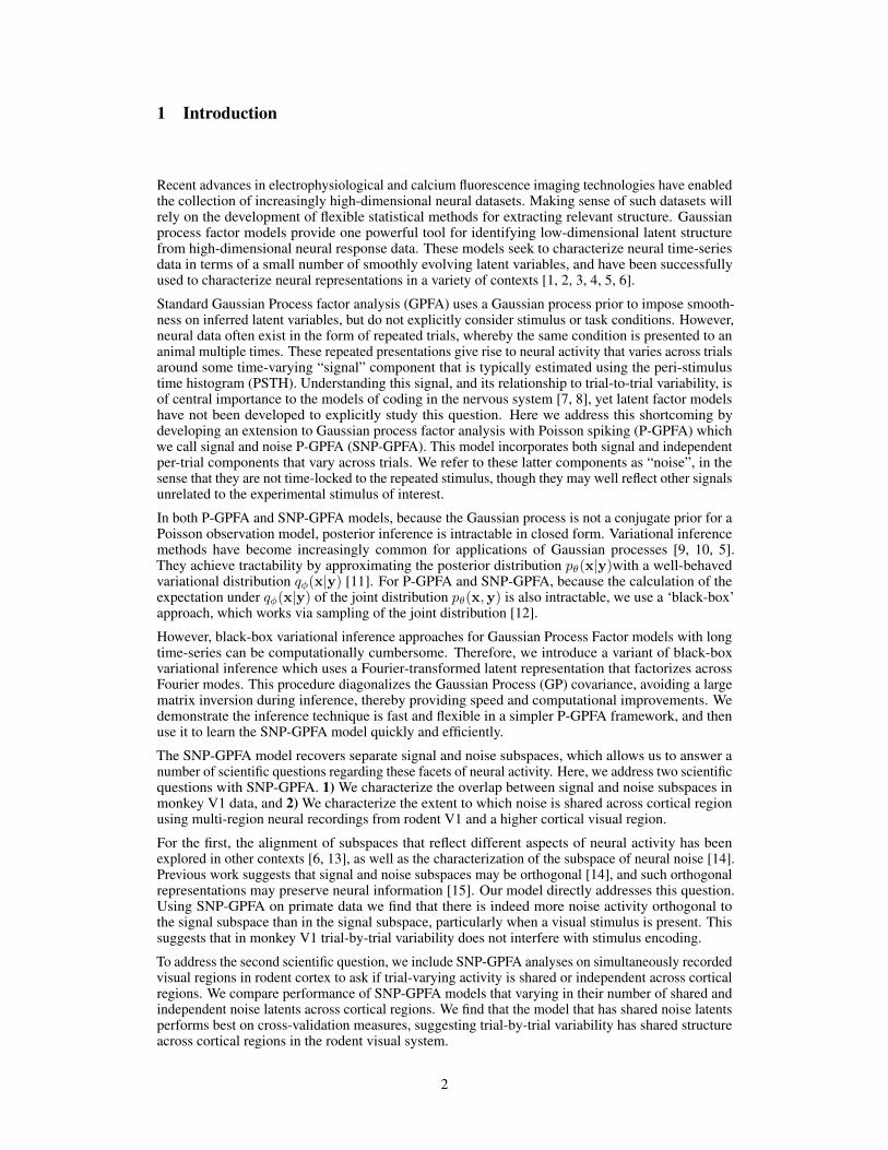
Figure 1: Efficient representation of GP covariance. (A) Standard GP covariance matrix for 1Dvectorization of 200 timepoints, with length scale ` = 15, and its Fourier representation, pruned. (B)Time to maximization of the ELBO in the time-domain inference and in the Fourier domain with andwithout a minimum frequency.

2 Poisson Gaussian Process Factor Analysis (P-GPFA)

We begin by introducing the Poisson-GPFA model, which has been used previously to identifycontinuous latent states from population spike train recordings [10, 16, 6]. The observations of ourmodel are spike-train data, represented by the neurons-by-time matrix Y ∈ NN×T .

We seek to learn a P-dimensional latent variable x(t) ∈ IRP that linearly maps to the data via aloadings matrix W ∈ IRN×P , followed by some nonlinear function f and Poisson observations.

Y = Poiss(f(W>X)) (1)

Our choice of non-linear function f is the softplus f(x) = log(1 + exp(x)).

Each latent xj(t) (j ∈ {1 . . . P}, t ∈ {1, 2 . . . T}) evolves according to a Gaussian process, xj(t) ∼GP(0,K(θj)), with covariance matrix K(θ) defined by a squared exponential kernel [K(θ)]tt′ =ρ exp(−|z(t)− z(t′)|2/2`2), where hyperparameters θ = {`, ρ} include a length scale ` controllingsmoothness and a marginal variance ρ controlling magnitude.

Given that the marginal likelihood of this model, p(Y|W) =∫p(Y|W,X)p(X|θ)dX is not

available in closed-form, it is common to use a variational inference approach to learn the parametersof such models [16, 10]. Recall that variational inference seeks to maximize an evidence lowerbound (ELBO) using a variational distribution [11]. Here, because the expectation term in the ELBO,Eqφ [log(p(y|x,w))], cannot be calculated analytically, we employ a ’black box approach’ whichuses Monte-Carlo samples to estimate the expectation term [17]. This inference method is calledblack-box variational inference (BBVI).

2.1 Fourier-domain black-box variational inference

BBVI can be computationally cumbersome. Therefore, to learn the P-GPFA and SNP-GPFA models,we introduce a novel inference method which performs BBVI over a Fourier-represented latent space,which increases both inference tractability and speed. Factorizing and learning the time series in theFourier domain, rather than the time domain, allows us to take advantage of computational savingsconferred by a diagonal covariance matrix while overcoming problems of uncorrelated timepointswhich is typical when the variational distribution is factorized over time [18].

Our motivation for this approach is that the GP prior over x(t) describes a stationary process, as itscovariance only depends on pairwise distances. This allows us to diagonalize the covariance K by theFourier transform (Figure 1A). Here, the covariance matrix K is diagonalized by K̃ = BKB> whereB is the orthonormal discrete Fourier transform matrix with [B]ω,t =

1√Pe−i2πωt/m, i ≡

√−1. The

diagonalized kernel is represented as c̃(ω̃) = ρ̃e−12 ω̃

2`2 where ρ̃ =√2πρ` is the frequency-domain

variance and ω̃ = 2πm ω represents an adjusted frequency of the GP kernel.

3

Inference can be conducted completely in the Fourier domain, precluding the need to invert the priorcovariance K. The joint likelihood is expressed as

`(Y,X|W, θ) = `(Y, X̃|W, θ) (2)

≈∑i

log(f(wi>X̃B))i +

(f(wi

>X̃B)− log(i!))1T

− 12

(Pd log 2π + P

∑ω̃

log c̃θ(ω̃) +∑p

x̃p>diag(W̃nθ)

−1x̃p

),

(3)

where X̃ represents the Fourier-transformed latents and 1T is a length-T vector of ones, andi ∈ {1, 2 . . . N} denotes neuron index. The diagonalized representation demonstrably speedsup computational time (Figure 1B). Moreover, the inversion of the time-domain K can presenttractability challenges due to computer precision [19], however, the inversion of K̃ is trivial so longas the vector along the diagonal, W̃θ, does not contain values that are too small. When small valuesare present, we regularize W̃θ by adding a small constant value (10−7).

This Fourier-represented GP has additional computational advantages, including methods to pruneunnecessary Fourier coefficients that do not substantially contribute to explaining variability in Y.Pruning frequencies constrains the number of coefficients in the Fourier representation to a muchsmaller number than would be necessary in the time-domain. Pruning of the Fourier representationhas the additional consequence of pruning the variational distribution, which shrinks the number ofvariational parameters. Finally, because Fourier BBVI uses a diagonal Fourier-domain variationaldistribution, time-correlations are preserved (despite BBVI sampling) due to off-diagonal elements inthe time-domain variational distribution.

Fourier methods have been used previously to improve inference for GP models [20, 21, 22], this is toour knowledge the first time this approach has been used with BBVI. Ultimately, this Fourier-domainBBVI method can be viewed as an alternative to many other methods that work to make Gaussianprocesses computationally efficient, including inducing points and sparse GP approximations [21, 22,23, 22, 24].

We use our Fourier-domain BBVI to learn the Fourier latents X̃ via direct optimization of thevariational distribution qφ(X̃), factor loading parameters W, and hyperparameters `. (Note thereis an invariance between hyperparameter ρ, and the loadings matrix W, so we need not directlylearn ρ in this model.) The speed up from optimization with Fourier domain BBVI can be realizedmost starkly in the domain where the time-series is very long. Figure 1B compares Fourier-domaininference to time-domain inference for a Poisson observation GPFA model with a single latent (i.e.P = 1, T = 1500) and N = 10 neurons. Inference is sped up by conversion to the Fourier domainas the bottleneck in time-domain inference is the inversion of a 1500× 1500 covariance matrix K.By additionally specifying a minimum frequency, sufficiently small frequencies are pruned and thevariational distribution and prior covariance can be cut from 1500 values to 62. This provides anadditional substantial speed advantage of approximately an order of magnitude. It is important tonote that the speed-up of our method depends on the specifics of the number of neurons, latents,latent length, and pruning. For subsequent analyses in this paper, the speed-up of BBVI due to theFourier-domain implementation is anywhere from 20-70%.

GPFA P-GPFA0.00

0.04

0.08

0.12

Rat

e (H

z)

True LatentInferred Latent

Time (sec)

Inferred Rate True Rate

Time (sec)

A B C

Number of Latents

ELBO

Cro

ss-V

alid

ated

MSE

1 2 3 4 5 65 1005 1005 1005 100

0

-2

2

0

-2

2

0

2

40

2

10

2

1

0

2

D

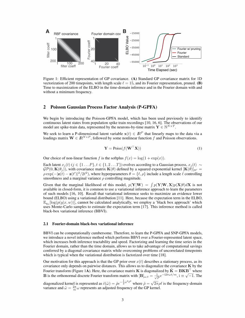
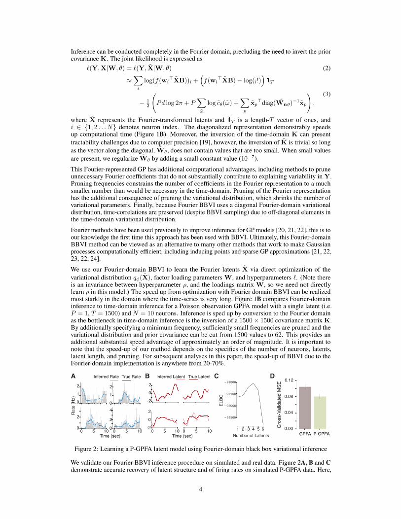
Figure 2: Learning a P-GPFA latent model using Fourier-domain black box variational inference

We validate our Fourier BBVI inference procedure on simulated and real data. Figure 2A, B and Cdemonstrate accurate recovery of latent structure and of firing rates on simulated P-GPFA data. Here,

4

30 neuronal firing rates are generated from a four-dimensional GP-latent space. Figure 2A shows thelearned and true rates of four simulated neurons. Grey bars indicate spike PSTHs. Figure 2B showsthe four generative latents and learned latents from Fourier BBVI rotated to their optimal mappingvia regression. Figure 2C demonstrates that the ELBO value after inference is maximal when usingthe true number of latents.

The non-conjugacy of P-GPFA (and SNP-GPFA), and thus the reason we need to use the sophisticatedinference of Fourier-BBVI, is due to the fact that the observations are Poisson, as opposed to Gaussian.This is an important choice as Poisson observations better describe neural data. We show, usingdata from rodent visual cortex, the cross-validated mean squared error of the inferred spike rate tosmoothed spike rate from held-out trials (Figure 2D). The model with Poisson observations performssignificantly better that the GPFA model with Gaussian observations. Others have noted similaradvantages to Poisson observation factor models for neural data in other settings [10]. For this reasonwe wish to use a Poisson observation characterization for our SNP-GPFA model.

3 SNP-GPFA

To isolate noise and signal subspaces in the P-GPFA framework, we introduce a model that includesseparate noise and signal latent structure (SNP-GPFA). We assess the model first on simulated data,and then on two neural data sets. The first of the datasets contains multi-neuron spiking activity from65 neurons recorded in primate V1 during passive viewing of a drifting sinusoidal grating stimulus,with 72 different orientations for D = 35 repeated trials. The second consists of spiking activity from67 neurons from two regions of rodent visual cortex, recorded during passive viewing of D = 20repeats of a 32-second sinusoidal grating stimulus. Gratings had 8 different orientations whichpersisted for 4 seconds each. For more information on the data, see [25, 26] and the supplementalmaterials.

The SNP-GPFA model describes neural activity on trial j as

yj = Poiss(f(Ws>Xs +Wn

>Xnj )) (4)

where P signal latents are drawn from a “signal” Gaussian process, xsp ∼ GP(0,Ks) withcovariance Ks and concatenated to form Xs> = (xs1,x

s2, . . . ,x

sP ), which are shared across trials.

On each trial, Q independent noise latents are drawn from a “noise” Gaussian process, xnq ∼GP(0,Kn) with covariance Kn, forming Xn> =

(xn1 ,x

n2 , . . . ,x

nQ

). Loading weights Ws

> andWn

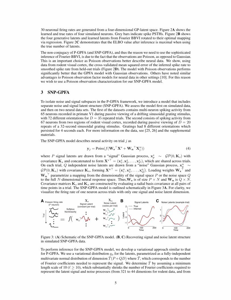
> parametrize a mapping from the dimensionality of the signal space P or the noise space Qto the full N -dimensional neural response space. Thus,Ws is of size P × N and Wn is Q × N .Covariance matrices Ks and Kn are constructed by evaluating a radial basis covariance at all pairs oftime points in a trial. The SNP-GPFA model is outlined schematically in Figure 3A. For clarity, wevisualize the firing rate of one neuron across trials with only one signal and noise latent dimension.

A

••

•

•

•

Noise Latent(varies per trial)

Signal Latent(constant per trial)

+••

••

SoftplusNonlinearity

Tria

l

Poisson firing rate(ith neuron)

Late

nt

Time Time

TrueInferred

Signal Latents Noise Latents (example trial)CB

0 100 200 0 100 200

0

1

2

-1

0

1

-1

Figure 3: (A) Schematic of the SNP-GPFA model. (B, C) Recovering signal and noise latent structurein simulated SNP-GPFA data.

To perform inference for the SNP-GPFA model, we develop a variational approach similar to thatfor P-GPFA. We use a variational distribution qφ for the latents, parametrized as a fully-independentmultivariate normal distribution of dimension T̃ (P+QD) where T̃ , which corresponds to the numberof Fourier coefficients needed to represent the signal. We determine T̃ by assuming a minimumlength scale of 10 (` ≥ 10), which substantially shrinks the number of Fourier coefficients required torepresent the latent signal and noise processes (from 321 to 44 dimenions for rodent data, and from

5

511 to 108 dimensions for primate data). This choice is appropriate, as we typically we do not learnlength scales smaller than this value.

To validate the model fit, we show that the Fourier BBVI procedure on the SNP-GPFA model byshowing accurate recovery of signal and noise latent structure from simulated SNP-GPFA data. Here,these simulated data consisted of 20 trials of 30 simulated Poisson neurons and were generated froma two dimensional signal and two dimensional noise subspace. Figure 3 shows that our inferenceprocedure accurately recovers the signal (B) and noise (C) subspace from these simulated data. Onlya single trial of the noise subspace is shown for clarity.

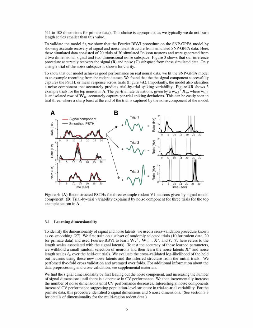
To show that our model achieves good performance on real neural data, we fit the SNP-GPFA modelto an example recording from the rodent dataset. We found that the the signal component successfullycaptures the PSTH, or mean response across trials (Figure 4A). Importantly, the model also identifiesa noise component that accurately predicts trial-by-trial spiking variability. Figure 4B shows 3example trials for the top neuron in A. The per-trial rate deviations, given by a wn,i

>Xn, where wn,i

is an isolated row of Wn, accurately capture per-trial spiking deviations. This can be easily seen intrial three, where a sharp burst at the end of the trial is captured by the noise component of the model.

ASignal componentSmoothed PSTH

B

Rat

e (H

z)R

ate

(Hz)

Rat

e (H

z)

Time (sec) Time (sec)

Rat

e (H

z)R

ate

(Hz)

Rat

e (H

z)

0

2

4

+

+

+

=

=

=

Trial 1

Trial 2

Trial 3

Figure 4: (A) Reconstructed PSTHs for three example rodent V1 neurons given by signal modelcomponent. (B) Trial-by-trial variability explained by noise component for three trials for the topexample neuron in A.

3.1 Learning dimensionality

To identify the dimensionality of signal and noise latents, we used a cross-validation procedure knownas co-smoothing [27]. We first train on a subset of randomly selected trials (10 for rodent data, 20for primate data) and used Fourier-BBVI to learn Ws

>, Wn>, Xs, and `s (`s here refers to the

length scales associated with the signal latents). To test the accuracy of these learned parameters,we withhold a small random selection of neurons and then learn the noise latents Xn and noiselength scales `n over the held-out trials. We evaluate the cross-validated log-likelihood of the heldout neurons using these new noise latents and the inferred structure from the initial trials. Weperfomed five-fold cross validation and averaged over folds. For additional information about thedata preprocessing and cross-validation, see supplemental materials.

We find the signal dimensionality by first leaving out the noise component, and increasing the numberof signal dimensions until there is a decrease in CV performance. We then incrementally increasethe number of noise dimensions until CV performance decreases. Interestingly, noise componentsincreased CV performance suggesting population-level structure in trial-to-trial variability. For theprimate data, this procedure identified 5 signal dimensions and 6 noise dimensions. (See section 3.3for details of dimensionality for the multi-region rodent data.)

6

0.0 0.5 1.0 1.5 2.0 2.5 0.0 0.5 1.0 1.5 2.0 2.5 0.0 0.5 1.0 1.5 2.0 2.5

Time (sec)0.0 0.5 1.0 1.5 2.0 2.5

Time (sec)0.0 0.5 1.0 1.5 2.0 2.5

Time (sec)0.0 0.5 1.0 1.5 2.0 2.5

Signal Noise Noise Latent Per Trial

Noise Projections Noise Projections (Normalized) Noise Projections (average)

In Sig SpaceOrth Sig Space

0

2

4

6

8

10

L2 N

orm

0.0

0.2

0.4

0.6

0.8

1.0

L2 N

orm

(fra

c)

0.45

0.50

0.55

0.65

0.70

0.60

Late

nt

L2 N

orm

(fra

c)

-1.0

-0.5

0.0

0.5

-1

0

1

-1

0

1

Late

nt

Late

nt

A B C

D E F

PC1PC2PC3

PC1PC2PC3

All TrialsAll Trials+ Oriens

Trial 1Trial 2Trail 3

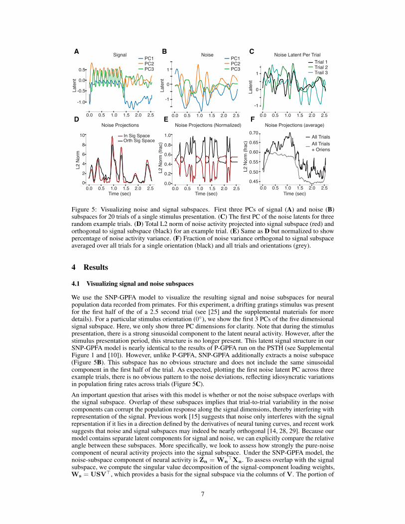
Figure 5: Visualizing noise and signal subspaces. First three PCs of signal (A) and noise (B)subspaces for 20 trials of a single stimulus presentation. (C) The first PC of the noise latents for threerandom example trials. (D) Total L2 norm of noise activity projected into signal subspace (red) andorthogonal to signal subspace (black) for an example trial. (E) Same as D but normalized to showpercentage of noise activity variance. (F) Fraction of noise variance orthogonal to signal subspaceaveraged over all trials for a single orientation (black) and all trials and orientations (grey).

4 Results

4.1 Visualizing signal and noise subspaces

We use the SNP-GPFA model to visualize the resulting signal and noise subspaces for neuralpopulation data recorded from primates. For this experiment, a drifting gratings stimulus was presentfor the first half of the of a 2.5 second trial (see [25] and the supplemental materials for moredetails). For a particular stimulus orientation (0◦), we show the first 3 PCs of the five dimensionalsignal subspace. Here, we only show three PC dimensions for clarity. Note that during the stimuluspresentation, there is a strong sinusoidal component to the latent neural activity. However, after thestimulus presentation period, this structure is no longer present. This latent signal structure in ourSNP-GPFA model is nearly identical to the results of P-GPFA run on the PSTH (see SupplementalFigure 1 and [10]). However, unlike P-GPFA, SNP-GPFA additionally extracts a noise subspace(Figure 5B). This subspace has no obvious structure and does not include the same sinusoidalcomponent in the first half of the trial. As expected, plotting the first noise latent PC across threeexample trials, there is no obvious pattern to the noise deviations, reflecting idiosyncratic variationsin population firing rates across trials (Figure 5C).

An important question that arises with this model is whether or not the noise subspace overlaps withthe signal subspace. Overlap of these subspaces implies that trial-to-trial variability in the noisecomponents can corrupt the population response along the signal dimensions, thereby interfering withrepresentation of the signal. Previous work [15] suggests that noise only interferes with the signalreprsentation if it lies in a direction defined by the derivatives of neural tuning curves, and recent worksuggests that noise and signal subspaces may indeed be nearly orthogonal [14, 28, 29]. Because ourmodel contains separate latent components for signal and noise, we can explicitly compare the relativeangle between these subspaces. More specifically, we look to assess how strongly the pure-noisecomponent of neural activity projects into the signal subspace. Under the SNP-GPFA model, thenoise-subspace component of neural activity is Zn = Wn

>Xn. To assess overlap with the signalsubspace, we compute the singular value decomposition of the signal-component loading weights,Ws = USV>, which provides a basis for the signal subspace via the columns of V. The portion of

7

variance of the noise within the signal subspace for each time point is then given by ||VV>Zn,t||22,where Zn,t is the tth column of Zn, or the L2 norm along the six noise dimensions. The portion ofvariance orthogonal to the signal subspace is thus simply ||Zn,t −VV>Zn,t||22.

Figure 5D shows the resulting L2-norm time-series both within and orthogonal to the signal subspace.This is for a single example trial for the same single stimulus as in A-C (orientation of 0◦). Tovisualize the fractional variance into and out of the signal subspace, we normalize each trace by thetotal variance at each time point, ||Zn,t||22 (Figure 5E). For this trial, the noise activity tends to mostlylie in the subspace orthogonal to the stimulus activity. However, this is not true when the overallnoise variance is high. At these moments, the noise exists mostly in the signal subspace. Figure5F shows the fractional noise variance orthogonal to the signal subspace averaged over all trials forthe orientation of 0◦ (black line) and all trials and orientations (grey line). It is primarily during thestimulus presentation time that the noise activity is preferentially orthogonal to the stimulus subspace.When there is no stimulus, after the halfway point of the trial, there is a slight preference for the noiseactivity to lie in the signal subspace.

4.2 Shared and independent noise in multi-region data

The rodent dataset we examined contained data from two simultaneously-recorded visual corticalregions, an upstream area “V1” and a downstream area “AL”. The SNP-GFPA model can thereforebe extended to allow for a characterization of shared variability across these regions. For simplicity,let’s consider two versions of the model: (1) a “shared-noise” model, which is the SNP-GPFAmodel applied to both regions simultaneously (see eq 4); or (2) an independent noise model, whichincludes a block-diagonalization of Wn into a V1 component Wn

V 1 and AL component WnAL.

The independent noise model describing neural activity for trial j is thus:[yV 1j

yALj

]= Poiss

(f(Ws

>Xs +

[Wn

V 1 00 Wn

AL

][Xn,V 1j

Xn,ALj

])

)(5)

where Xn,V 1j are noise latents that map exclusively to V1 activity, and Xn,AL

j are noise latentsthat map exclusively to AL activity. By contrast, departures from a block-diagonal structure in theloadings matrix reflects the degree to which latent variability is shared across brain regions.

A Multi-region rodentdata

Cro

ss V

alid

ated

LL

CSimulated datafull

B Simulated datablock

Full inference

Block inference

Full inference

Block inference Number of shared latents

0 1 2 3 4-6200

-6150

-6100

-6050

-5180

-5170

-5160

-5150

-5140

-4544

-4542

-4540

-4538

-4536

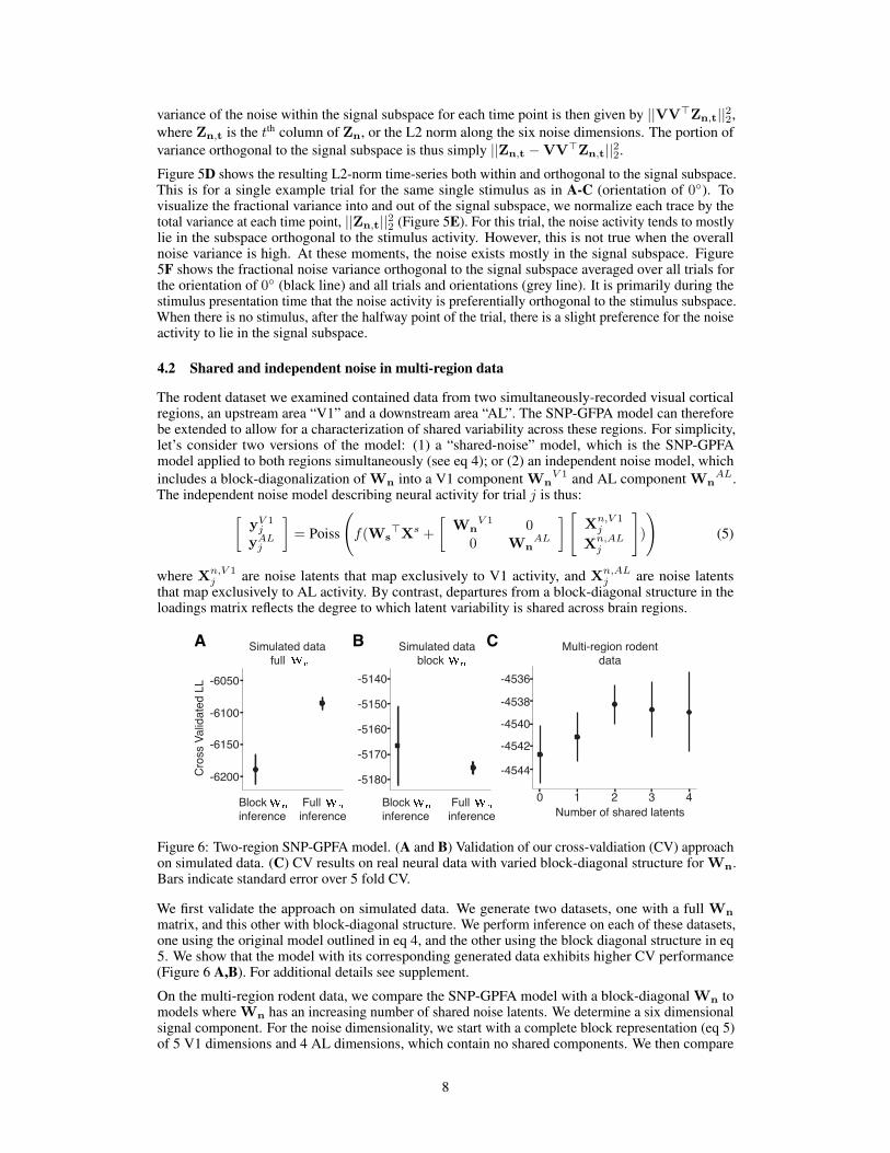
Figure 6: Two-region SNP-GPFA model. (A and B) Validation of our cross-valdiation (CV) approachon simulated data. (C) CV results on real neural data with varied block-diagonal structure for Wn.Bars indicate standard error over 5 fold CV.

We first validate the approach on simulated data. We generate two datasets, one with a full Wn

matrix, and this other with block-diagonal structure. We perform inference on each of these datasets,one using the original model outlined in eq 4, and the other using the block diagonal structure in eq5. We show that the model with its corresponding generated data exhibits higher CV performance(Figure 6 A,B). For additional details see supplement.

On the multi-region rodent data, we compare the SNP-GPFA model with a block-diagonal Wn tomodels where Wn has an increasing number of shared noise latents. We determine a six dimensionalsignal component. For the noise dimensionality, we start with a complete block representation (eq 5)of 5 V1 dimensions and 4 AL dimensions, which contain no shared components. We then compare

8

CV performance of this model to ones where increasing numbers of noise latents are shared betweenthe regions (Figure 6C). For information regarding how we select the proper number of noise andsignal dimensions in this framework, see supplemental materials. We find that models with at leasttwo shared noise dimensions perform better than models with one or fewer shared noise dimensions.Means and standard error shown over five-fold CV (Figure 6). This suggests that there is trial-varyingstructure in neural population activity that is shared across cortical regions.

5 Conclusion

We have introduced a Gaussian process factor analytic model for spike train data that extracts separatesignal and noise latent structure from trial-structured data. To learn this model we employ a novelinference method based on black-box variational inference in the Fourier domain, which allows forfaster and more stable inference by diagonalizing the posterior covariance and pruning unnecessaryfrequencies. The resulting SNP-GPFA model is able to extract signal latents that characterizepopulation PSTHs in real neural data, and noise latents that capture trial-to-trial variability that isshared across neurons. We would like to mention that this is not the first model to include a trialvarying GP latent with a stimulus fixed component [30, 16]. However, this is the first model weare aware of explicitly designed to uncover separate signal and noise latent subspaces with varyingdimensionality. We go on to use the results of the model fit to suggest answers to scientific questionsabout trial-based neural data. We find that in monkey V1, noise activity tends to project primarily ina subspace orthogonal to signal activity, especially when a gratings stimulus is present, suggestingan optimal type of neural encoding [15]. We additionally use our model on multi-region rodentdata and compare performance where noise is shared between cortical regions as opposed to beingindependent to each region. We find that, for these rodent data, noise models with shared structurebetter predict held-out spike trains, suggesting variability in the spiking activity is shared acrosscortical regions. Overall, the model is a promising method for understanding the relationship betweenstimulus-locked and trial-varying neural activity at the population level. We believe there is a greatnumber of additional scientific questions that the SNP-GPFA model can help answer, includingdetermining how signal and noise representations relate to behavior, and further exploring howblock-diagonal loadings matrices may partition signal and noise latent representations in multi-regiondata. We provide downloadable code for the community to use the SNP-GPFA model on their owntrial-based neural data.

Broader Impact

Here, we propose a new model for neuroscientists to uncover latent structure in trial-based neuralpopulation data. Trial-based neural recordings with identical stimuli are ubiquitous in neuroscienceresearch. However, trial-by-trial variability in neural activity is not well understood. More broadly,it is unclear in general what the function of neural noise is in the brain. Our model works onneural population data to separate out neural noise latent representations from stimulus-lockedrepresentations. It additionally uses a novel inference technique that is rapid and stable. Here, weprovide a general, easy-to-use tool for neuroscientists, and we hope others are encouraged to employit to understand trial-based neural information in their own experimental set-up. We provide codefor download here: https://github.com/skeeley/SNP_GPFA. We do not foresee any negativeconsequences to society resulting from this work.

Acknowledgements

SLK was supported by NIH grant F32MH115445-03 , MCA and JWP were supported by grantsfrom the Simons Collaboration on the Global Brain (SCGB AWD543027), and a U19 NIH-NINDSBRAIN Initiative Award (5U19NS104648). JWP was also supported by the NIH BRAIN initiative(NS104899 and R01EB026946). YY and SLS were supported by the NIH (R01EY024294 andR01NS091335), the NSF (1450824 and 1707287) the Simons Foundation (SCGB 325407) and theMcKnight Foundation.

9

References[1] BM Yu, JP Cunningham, G Santhanam, SI Ryu, KV Shenoy, and M Sahani. Gaussian-process factor

analysis for low-dimensional single-trial analysis of neural population activity. In Adv neur inf proc sys,pages 1881–1888, 2009.

[2] John P Cunningham and B M Yu. Dimensionality reduction for large-scale neural recordings. Natureneuroscience, 17(11):1500–1509, 2014.

[3] Anqi Wu, Nicholas G Roy, Stephen Keeley, and Jonathan W Pillow. Gaussian process based nonlinearlatent structure discovery in multivariate spike train data. In I. Guyon, U. V. Luxburg, S. Bengio, H. Wallach,R. Fergus, S. Vishwanathan, and R. Garnett, editors, Advances in Neural Information Processing Systems30, pages 3499–3508. Curran Associates, Inc., 2017.

[4] KC Lakshmanan, PT Sadtler, EC Tyler-Kabara, AP Batista, and BM Yu. Extracting low-dimensional latentstructure from time series in the presence of delays. Neural computation, 2015.

[5] Evan Archer, Il Memming Park, Lars Buesing, John Cunningham, and Liam Paninski. Black box variationalinference for state space models. arXiv preprint arXiv:1511.07367, 2015.

[6] Yuan Zhao, Jacob L Yates, Aaron J Levi, Alexander C Huk, and Il Memming Park. Stimulus-choice (mis)alignment in primate area mt. PLOS Computational Biology, 16(5):e1007614, 2020.

[7] Mark M Churchland, M Yu Byron, Maneesh Sahani, and Krishna V Shenoy. Techniques for extractingsingle-trial activity patterns from large-scale neural recordings. Current opinion in neurobiology, 17(5):609–618, 2007.

[8] Jacob L Yates, Il Memming Park, Leor N Katz, Jonathan W Pillow, and Alexander C Huk. Functionaldissection of signal and noise in mt and lip during decision-making. Nature neuroscience, 20(9):1285,2017.

[9] AC Damianou, MK Titsias, and ND Lawrence. Variational inference for uncertainty on the inputs ofgaussian process models. arXiv preprint arXiv:1409.2287, 2014.

[10] Yuan Zhao and Il Memming Park. Variational latent gaussian process for recovering single-trial dynamicsfrom population spike trains. Neural computation, 29(5):1293–1316, 2017.

[11] David M Blei, Andrew Y Ng, and Michael I Jordan. Latent dirichlet allocation. Journal of machineLearning research, 3(Jan):993–1022, 2003.

[12] Rajesh Ranganath, Sean Gerrish, and David Blei. Black box variational inference. In Artificial Intelligenceand Statistics, pages 814–822, 2014.

[13] João D Semedo, Amin Zandvakili, Christian K Machens, M Yu Byron, and Adam Kohn. Cortical areasinteract through a communication subspace. Neuron, 2019.

[14] Carsen Stringer, Marius Pachitariu, Nicholas Steinmetz, Charu Bai Reddy, Matteo Carandini, andKenneth D Harris. Spontaneous behaviors drive multidimensional, brainwide activity. Science,364(6437):eaav7893, 2019.

[15] Rubén Moreno-Bote, Jeffrey Beck, Ingmar Kanitscheider, Xaq Pitkow, Peter Latham, and AlexandrePouget. Information-limiting correlations. Nature neuroscience, 17(10):1410, 2014.

[16] Lea Duncker and Maneesh Sahani. Temporal alignment and latent gaussian process factor inference inpopulation spike trains. In Advances in Neural Information Processing Systems, pages 10445–10455, 2018.

[17] Diederik P Kingma, Tim Salimans, and Max Welling. Variational dropout and the local reparameterizationtrick. In Advances in Neural Information Processing Systems, pages 2575–2583, 2015.

[18] Richard E Turner and Maneesh Sahani. Two problems with variational expectation maximisation fortime-series models. Bayesian Time series models, 1(3.1):3–1, 2011.

[19] Magda Peligrad and Wei Biao Wu. Central limit theorem for fourier transforms of stationary processes.The Annals of Probability, pages 2009–2022, 2010.

[20] Mikio Aoi and Jonathan W Pillow. Scalable bayesian inference for high-dimensional neural receptivefields. bioRxiv, page 212217, 2017.

[21] Christopher J Paciorek. Bayesian smoothing with gaussian processes using fourier basis functions in thespectralgp package. Journal of statistical software, 19(2):nihpa22751, 2007.

10

[22] James Hensman, Nicolo Fusi, and Neil D Lawrence. Gaussian processes for big data. In Uncertainty inArtificial Intelligence, page 282, 2013.

[23] MK Titsias and ND Lawrence. Bayesian gaussian process latent variable model. In AISTATS, volume 9,pages 844–851, 2010.

[24] Edward Snelson and Zoubin Ghahramani. Local and global sparse gaussian process approximations. InArtificial Intelligence and Statistics, pages 524–531, 2007.

[25] Arnulf BA Graf, Adam Kohn, Mehrdad Jazayeri, and J Anthony Movshon. Decoding the activity ofneuronal populations in macaque primary visual cortex. Nature neuroscience, 14(2):239, 2011.

[26] Yiyi Yu, Jeffery N Stirman, Christopher R Dorsett, and Spencer LaVere Smith. Mesoscale correlationstructure with single cell resolution during visual coding. bioRxiv, page 469114, 2018.

[27] Jakob H Macke, Lars Buesing, John P Cunningham, M Yu Byron, Krishna V Shenoy, and Maneesh Sahani.Empirical models of spiking in neural populations. In Advances in neural information processing systems,pages 1350–1358, 2011.

[28] Oleg I Rumyantsev, Jérôme A Lecoq, Oscar Hernandez, Yanping Zhang, Joan Savall, Radosław Chrap-kiewicz, Jane Li, Hongkui Zeng, Surya Ganguli, and Mark J Schnitzer. Fundamental bounds on the fidelityof sensory cortical coding. Nature, 580(7801):100–105, 2020.

[29] Ramon Bartolo, Richard C Saunders, Andrew R Mitz, and Bruno B Averbeck. Information-limitingcorrelations in large neural populations. Journal of Neuroscience, 40(8):1668–1678, 2020.

[30] Alexander S Ecker, Philipp Berens, R James Cotton, Manivannan Subramaniyan, George H Denfield,Cathryn R Cadwell, Stelios M Smirnakis, Matthias Bethge, and Andreas S Tolias. State dependence ofnoise correlations in macaque primary visual cortex. Neuron, 82(1):235–248, 2014.

11