On the ICP Algorithm Esther Ezra, Micha Sharir Alon Efrat.

On the ICP AlgorithmOn the ICP Algorithm

Esther Ezra, Micha SharirEsther Ezra, Micha Sharir

Alon EfratAlon Efrat

The problem: Pattern MatchingThe problem: Pattern Matching

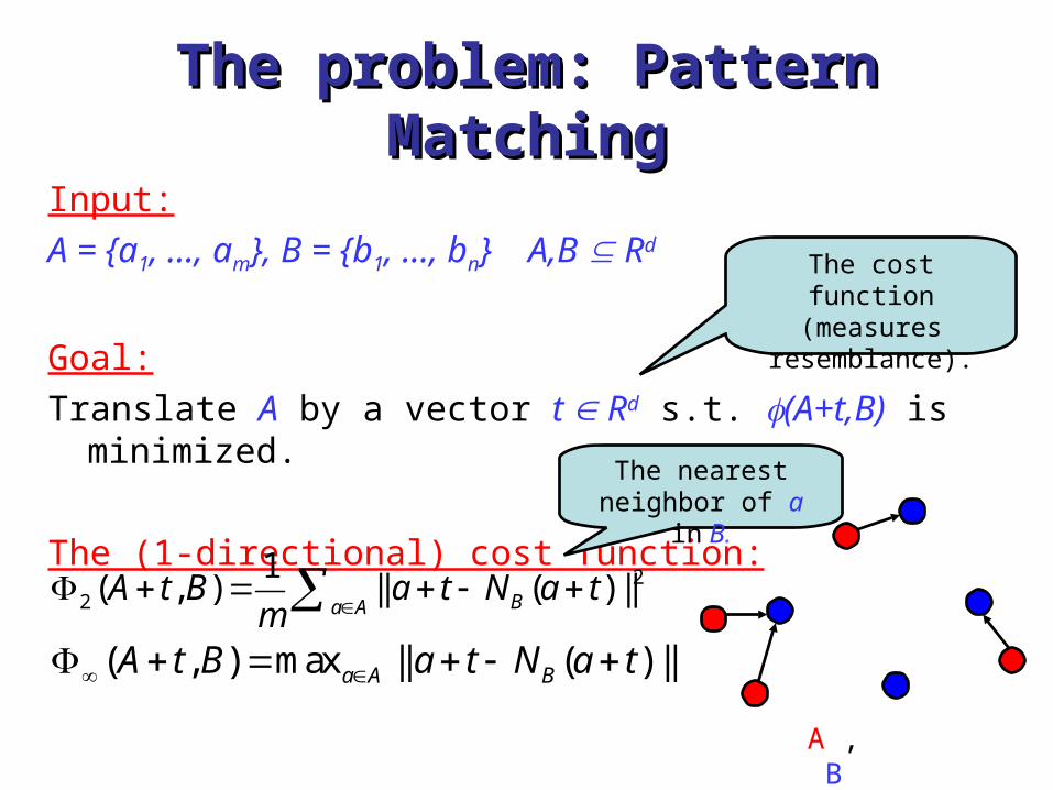
Input:

A = {a1, …, am}, B = {b1, …, bn} A,B Rd

Goal:

Translate A by a vector t Rd s.t. (A+t,B) is minimized.

The (1-directional) cost function:

22

1( , ) || ( ) ||Ba AA t B a t N a t

m

The cost function (measures

resemblance).

The nearest neighbor of a in B.

A , B

( , ) max || ( ) ||a A BA t B a t N a t

The algorithm [Besl & Mckay 92]The algorithm [Besl & Mckay 92]

Use local improvements:

Repeat: At each iteration i, with cumulative translation ti-1

• Assign each point a+ti-1 A+ti-1 to its NN b = NB(a+ti-1)

• Compute the relative translation ti that minimizes with respect to this fixed (frozen) NN-assignment.

Translate the points of A by ti (to be aligned to B). ti ti-1 + ti .

• Stop when the value of does not decrease.

The overall translation vector previously computed. t0 = 0 .

Some of the points of A may acquire

new NN in B.

The algorithm: Convergence

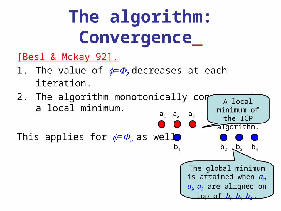
[Besl & Mckay 92].

1. The value of =2 decreases at each iteration.

2. The algorithm monotonically converges to a local minimum.

This applies for = as well.a1 a2 a3

b1 b2 b3 b4

A local minimum of the ICP algorithm.

The global minimum is attained when a1, a2, a3 are aligned on top of b2,

b3, b4 .

NN and Voronoi diagramsNN and Voronoi diagrams

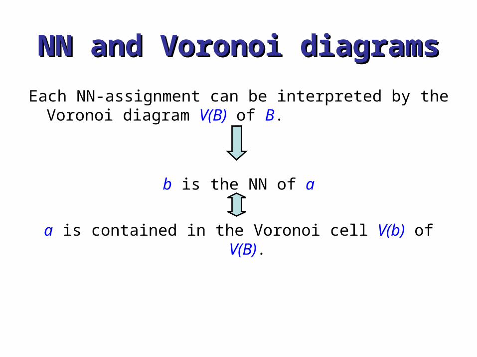
Each NN-assignment can be interpreted by the Voronoi diagram V(B) of B.

b is the NN of a

a is contained in the Voronoi cell V(b) of V(B).

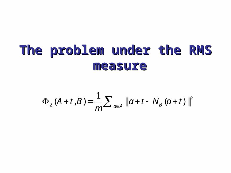
The problem under the RMS The problem under the RMS measuremeasure

22

1( , ) || ( ) ||Ba AA t B a t N a t

m

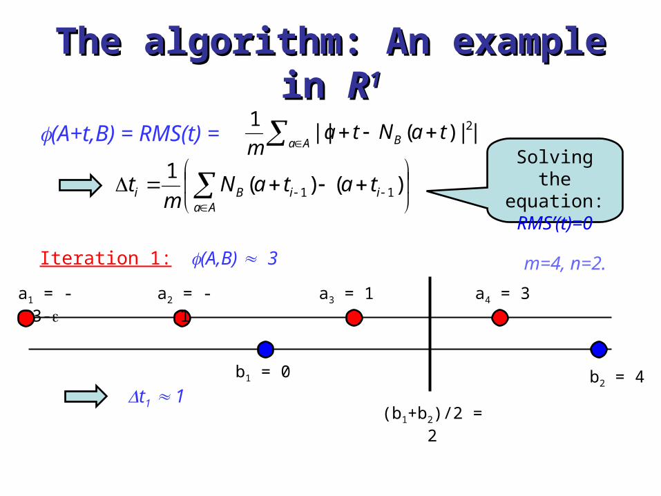
The algorithm: An example in The algorithm: An example in RR11

(A+t,B) = RMS(t) =

Iteration 1:

Aa B taNtam

2||)(||1

b1 = 0 b2 = 4

a3 = 1 a4 = 3a1 = -3-

)()(

111 i

AaiBi tataN

mt

t1 1

m=4, n=2.

(b1+b2)/2 = 2

a2 = -1

(A,B) 3

Solving the equation: RMS’(t)=0

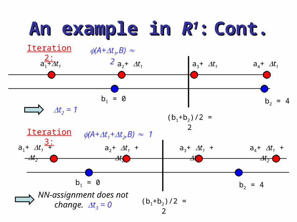
An example in An example in RR11:: Cont.Cont.Iteration 2:

b1 = 0 b2 = 4

a4+ t1

t2 = 1(b1+b2)/2 = 2

a3+ t1 a2+ t1 a1+t1

Iteration 3:

b1 = 0 b2 = 4

NN-assignment does not change. t3 = 0 (b1+b2)/2 = 2

a1+ t1 + t2 a2+ t1 + t2 a3+ t1 + t2 a4+ t1 + t2

(A+t1,B) 2

(A+t1+t2,B) 1

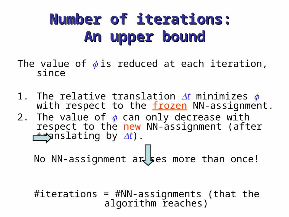
Number of iterations: Number of iterations: An upper boundAn upper bound

The value of is reduced at each iteration, since

1. The relative translation t minimizes with respect to the frozen NN-assignment.

2. The value of can only decrease with respect to the new NN-assignment (after translating by t).

No NN-assignment arises more than once!

#iterations = #NN-assignments (that the algorithm reaches)

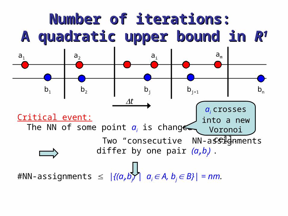
Number of iterations: Number of iterations: A quadratic upper bound in A quadratic upper bound in RR11

Critical event: The NN of some point ai is changed.

Two “consecutive” NN-assignments differ by one pair (ai,bj) .

#NN-assignments |{(ai,bj) | ai A, bj B}| = nm.

b1

a2ama1

b2 bn

ai

bj bj+1

tai crosses into a new

Voronoi cell.

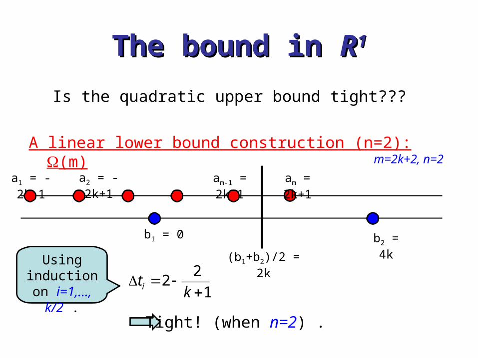
The bound in The bound in RR11

Is the quadratic upper bound tight???

A linear lower bound construction (n=2): (m)

b1 = 0

am-1 = 2k-1 am = 2k+1a1 = -2k-1

(b1+b2)/2 = 2k

Tight! (when n=2) .

b2 = 4k

a2 = -2k+1

Using induction on i=1,…, k/2 . 1

22

k

ti

m=2k+2, n=2

Structural properties in Structural properties in RR11

Lemma:At each iteration i2 of the algorithm

Corollary (Monotonicity):The ICP algorithm always moves A in the same (left or

right) direction.

Either ti 0 for each i0, or ti 0 for each i0.

)()(1

21

iBAa

iBi taNtaNm

t

j

k kj tt1

Use induction on i.

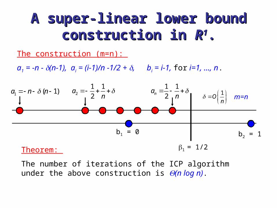
A super-linear lower bound A super-linear lower bound construction in construction in RR11..

2

1 1

2a

n 1 ( 1)a n n

b1 = 0 b2 = 1

1 1

2na n

m=n1

On

The construction (m=n):

a1 = -n - (n-1), ai = (i-1)/n -1/2 + , bi = i-1, for i=1, …, n.

Theorem:

The number of iterations of the ICP algorithm under the above construction is (n log n).

1 = 1/2

2

1 1

2a

n

3 1

2na n

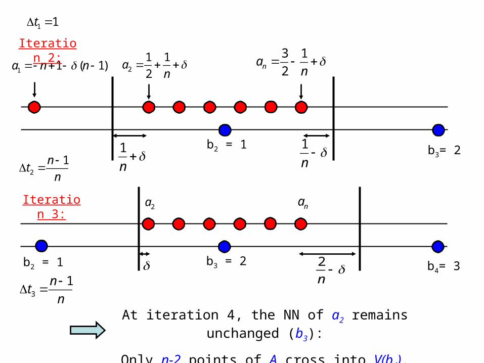
1 1t

1 1 ( 1)a n n

b2 = 1 b3= 2

2

1nt

n

b3 = 2 b4= 3b2 = 1 2

n

1

n

3

1nt

n

1

n

Iteration 2:

Iteration 3:2a na

At iteration 4, the NN of a2 remains unchanged (b3):

Only n-2 points of A cross into V(b4).

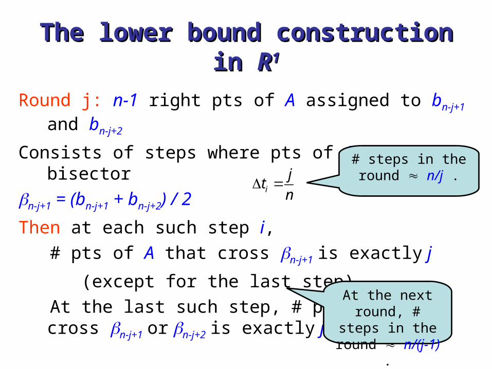
The lower bound construction in The lower bound construction in RR11

Round j: n-1 right pts of A assigned to bn-j+1 and bn-j+2

Consists of steps where pts of A cross the bisector

n-j+1 = (bn-j+1 + bn-j+2) / 2

Then at each such step i,

# pts of A that cross n-j+1 is exactly j

(except for the last step).

At the last such step, # pts of A that cross n-j+1 or n-j+2 is exactly j-1.

i

jt

n

# steps in the round n/j .

At the next round, # steps in the

round n/(j-1) .

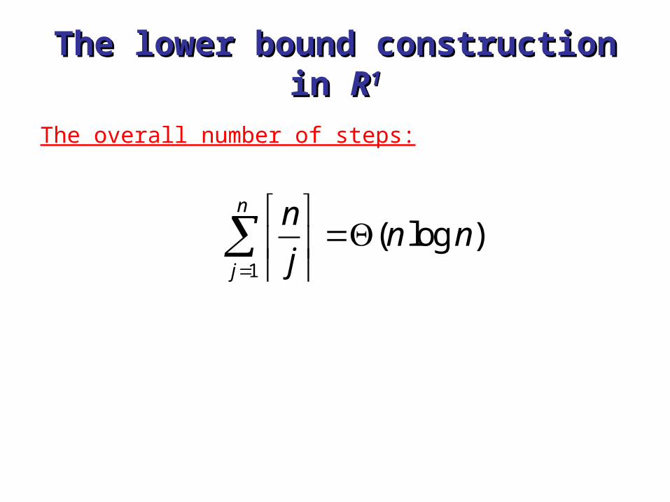
The lower bound construction in The lower bound construction in RR11

The overall number of steps:

1

( log )n

j

nn n

j

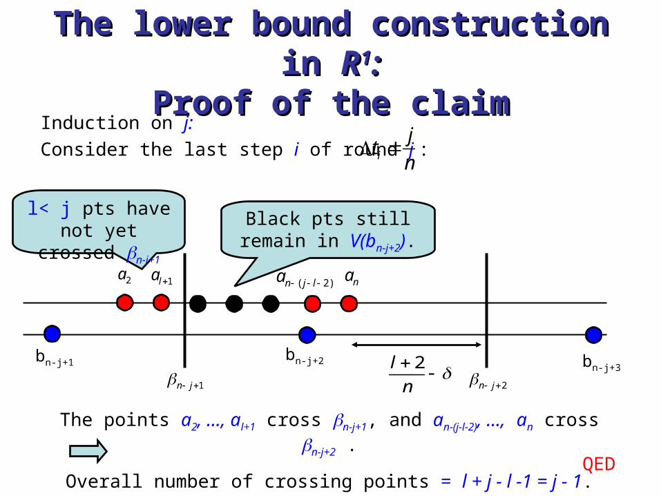
The lower bound construction in The lower bound construction in RR11::Proof of the claimProof of the claim

Induction on j:

Consider the last step i of round j :

( 2)n j la

bn-j+2 bn-j+3bn-j+1 2l

n

2a na1la

i

jt

n

The points a2, …, al+1 cross n-j+1, and an-(j-l-2), …, an cross n-j+2 .

Overall number of crossing points = l + j - l -1 = j - 1.

Black pts still remain in V(bn-j+2).

1n j 2n j

l< j pts have not yet crossed n-j+1

QED

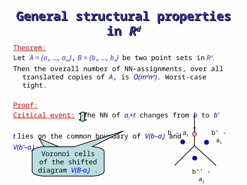
General structural properties in General structural properties in RRdd

Theorem:

Let A = {a1, …, am}, B = {b1, …, bn} be two point sets in Rd.

Then the overall number of NN-assignments, over all translated copies of A, is O(mdnd). Worst-case tight.

Proof:

Critical event: The NN of ai+t changes from b to b’

t lies on the common boundary of V(b–ai) and

V(b’–ai)

Voronoi cells of the shifted diagram

V(B-ai) .

tb - ai b’ - ai

b’’ - ai

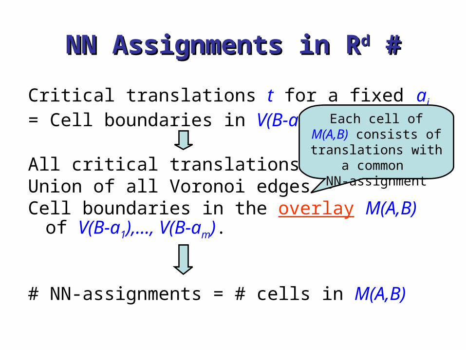
# #NN Assignments in RNN Assignments in Rdd

Critical translations t for a fixed ai

= Cell boundaries in V(B-ai) .

All critical translations = Union of all Voronoi edges = Cell boundaries in the overlay M(A,B)

of V(B-a1),…, V(B-am).

# NN-assignments = # cells in M(A,B)

Each cell of M(A,B) consists of translations

with a common NN-assignment

# NN Assignments in R# NN Assignments in Rdd

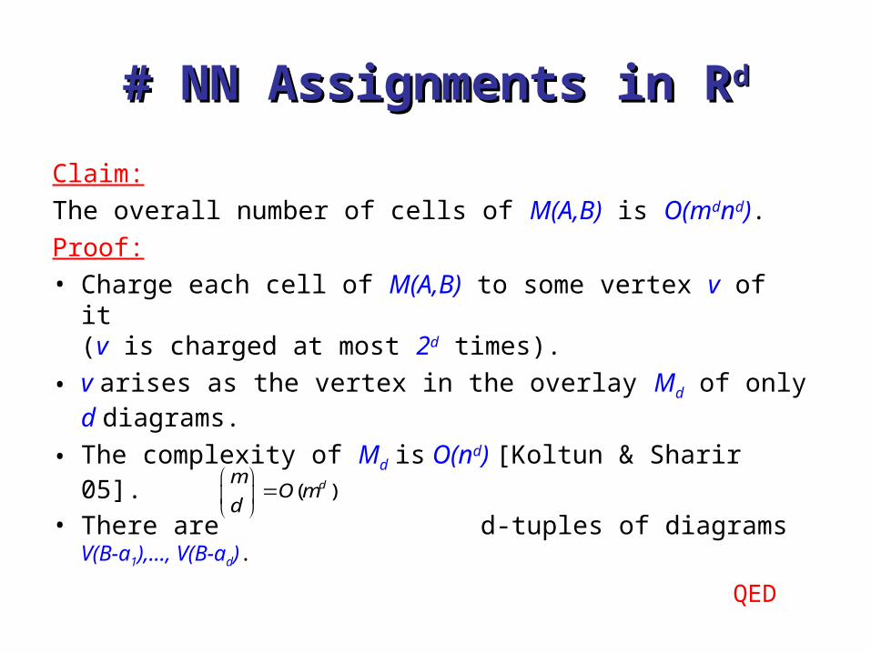
Claim:

The overall number of cells of M(A,B) is O(mdnd).

Proof:• Charge each cell of M(A,B) to some vertex v of it

(v is charged at most 2d times).

• v arises as the vertex in the overlay Md of only d diagrams.

• The complexity of Md is O(nd) [Koltun & Sharir 05].

• There are d-tuples of diagrams V(B-a1),…, V(B-ad).

( )dm

O md

QED

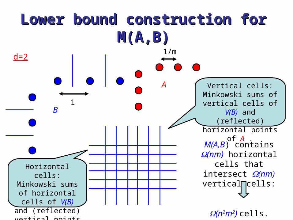
Lower bound construction for M(A,B)Lower bound construction for M(A,B)

B

d=2

A

1/m

1

Horizontal cells: Minkowski sums of horizontal cells of

V(B) and (reflected) vertical points of A .

Vertical cells: Minkowski sums of vertical cells of V(B)

and (reflected) horizontal points of A .

M(A,B) contains (nm) horizontal cells that intersect (nm)

vertical cells:

(n2m2) cells.

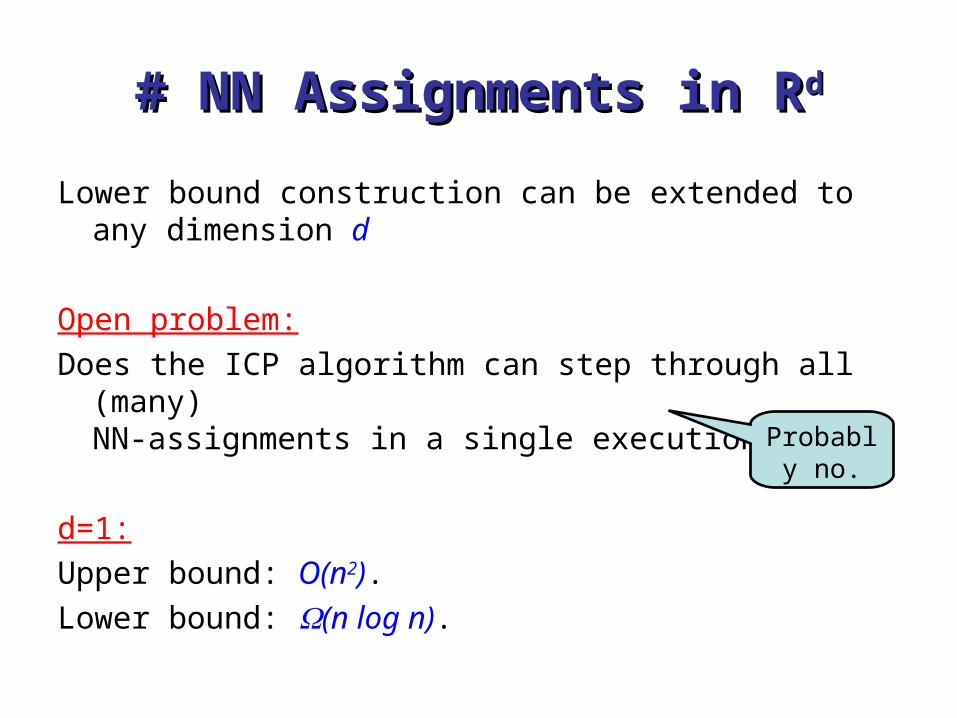
# NN Assignments in R# NN Assignments in Rdd

Lower bound construction can be extended to any dimension d

Open problem:

Does the ICP algorithm can step through all (many) NN-assignments in a single execution?

d=1:

Upper bound: O(n2).

Lower bound: (n log n).

Probably no.

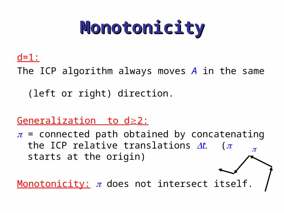
MonotonicityMonotonicity

d=1:

The ICP algorithm always moves A in the same (left or right) direction.

Generalization to d2:

= connected path obtained by concatenating the ICP relative translations t. ( starts at the origin)

Monotonicity: does not intersect itself.

MonotonicityMonotonicity

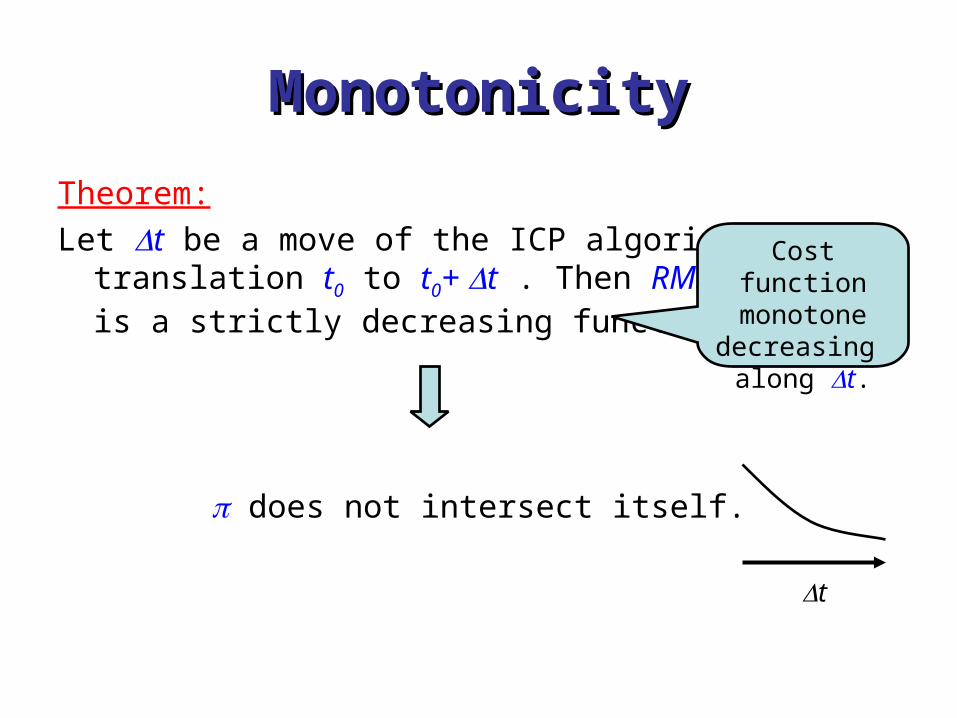
Theorem:

Let t be a move of the ICP algorithm from translation t0 to t0+ t . Then RMS(t0+ t) is a strictly decreasing function of .

does not intersect itself.

Cost function monotone

decreasing along t.

t

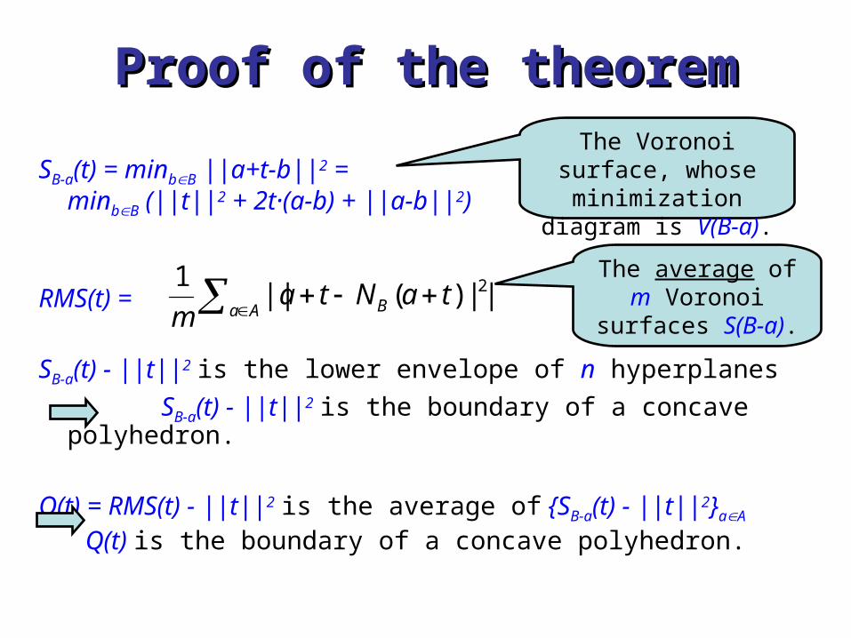
Proof of the theoremProof of the theorem

SB-a(t) = minbB ||a+t-b||2 = minbB (||t||2 + 2t·(a-b) + ||a-b||2)

RMS(t) =

SB-a(t) - ||t||2 is the lower envelope of n hyperplanes

SB-a(t) - ||t||2 is the boundary of a concave polyhedron.

Q(t) = RMS(t) - ||t||2 is the average of {SB-a(t) - ||t||2}aA

Q(t) is the boundary of a concave polyhedron.

Aa B taNtam

2||)(||1

The Voronoi surface, whose minimization diagram is V(B-a).

The average of m Voronoi surfaces

S(B-a).

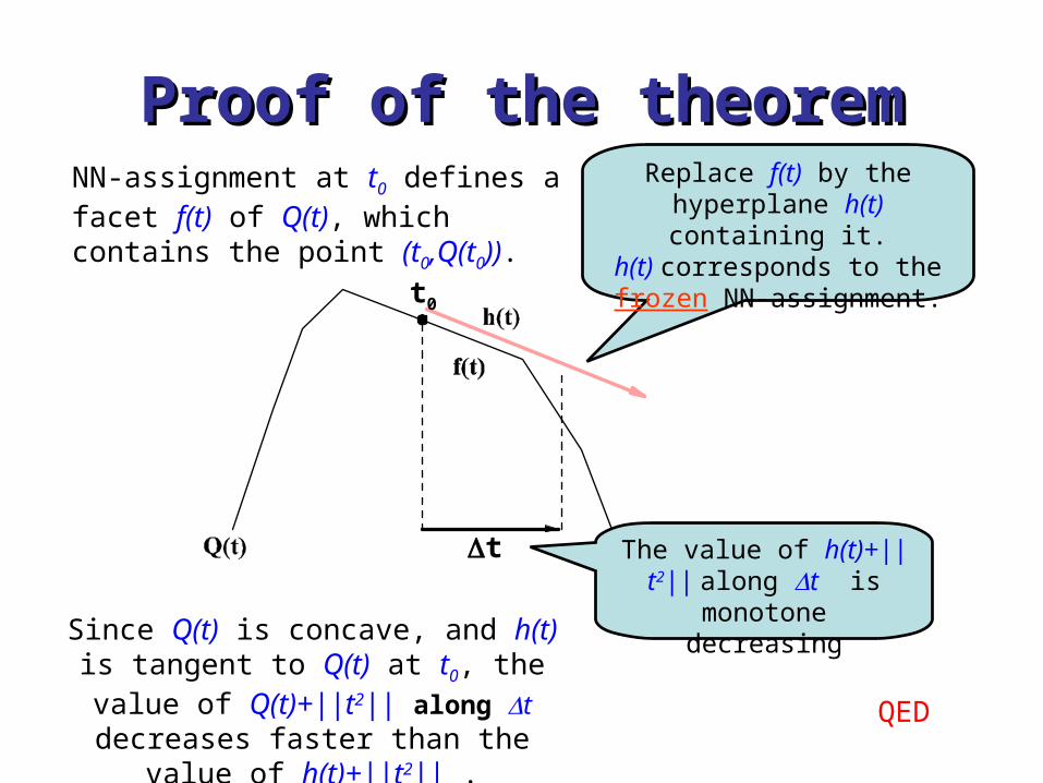
Proof of the theoremProof of the theoremNN-assignment at t0 defines a facet f(t) of Q(t), which contains the point (t0,Q(t0)).

Replace f(t) by the hyperplane h(t) containing it.h(t) corresponds to the frozen

NN-assignment.

The value of h(t)+||t2|| along t is monotone

decreasingSince Q(t) is concave, and h(t) is tangent to Q(t) at t0, the value of Q(t)+||t2|| along

t decreases faster than the value of h(t)+||t2|| .

QED

t0

t

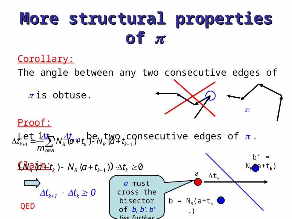
More structural properties of More structural properties of

Corollary:

The angle between any two consecutive edges of is obtuse.

Proof:

Let tk, tk+1 be two consecutive edges of .

Claim:

tk+1 tk 0

1 1

1( ) ( )k B k B k

a A

t N a t N a tm

1( ) ( ) 0B k B k kN a t N a t t b’ = NB(a+tk)

a

b = NB(a+tk-1)

tka must cross the bisector

of b, b’. b’ lies further aheadQED

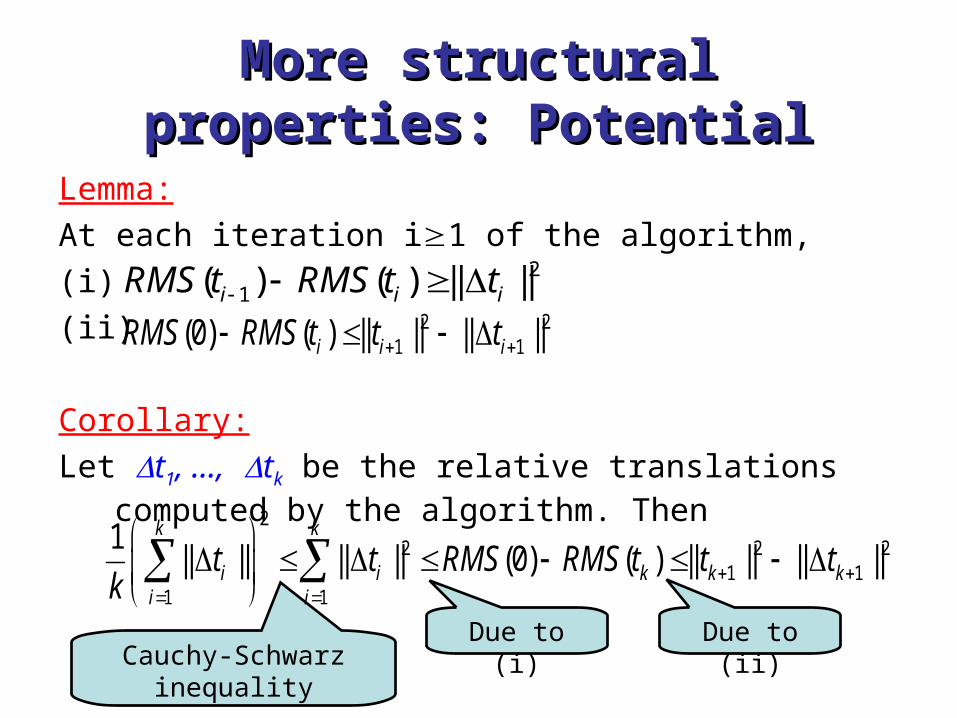
Cauchy-Schwarz

inequality

More structural properties: More structural properties: PotentialPotential

Lemma:

At each iteration i1 of the algorithm,

(i)

(ii)

Corollary:

Let t1, …, tk be the relative translations computed by the algorithm. Then

21( ) ( ) || ||i i iRMS t RMS t t

2 21 1(0) ( ) || || || ||i i iRMS RMS t t t

2

2 2 21 1

1 1

1|| || || || (0) ( ) || || || ||

k k

i i k k ki i

t t RMS RMS t t tk

Due to (i) Due to (ii)

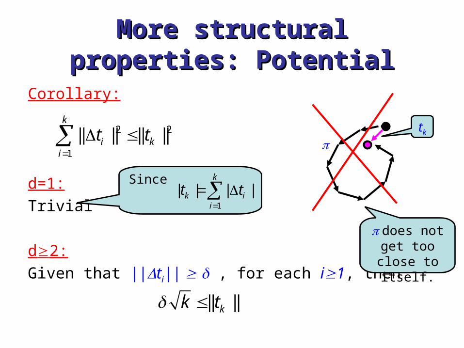
More structural properties: More structural properties: PotentialPotential

Corollary:

d=1:

Trivial

d2:

Given that ||ti|| , for each i1, then

2 2

1

|| || || ||k

i ki

t t

|| ||kk t

Since

1

| | | |k

k ii

t t

tk

does not get too close

to itself.

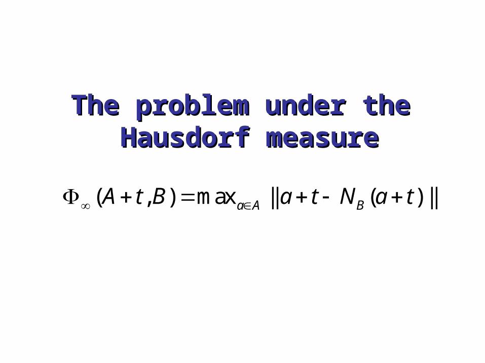
The problem under the Hausdorf The problem under the Hausdorf measuremeasure

( , ) max || ( ) ||a A BA t B a t N a t

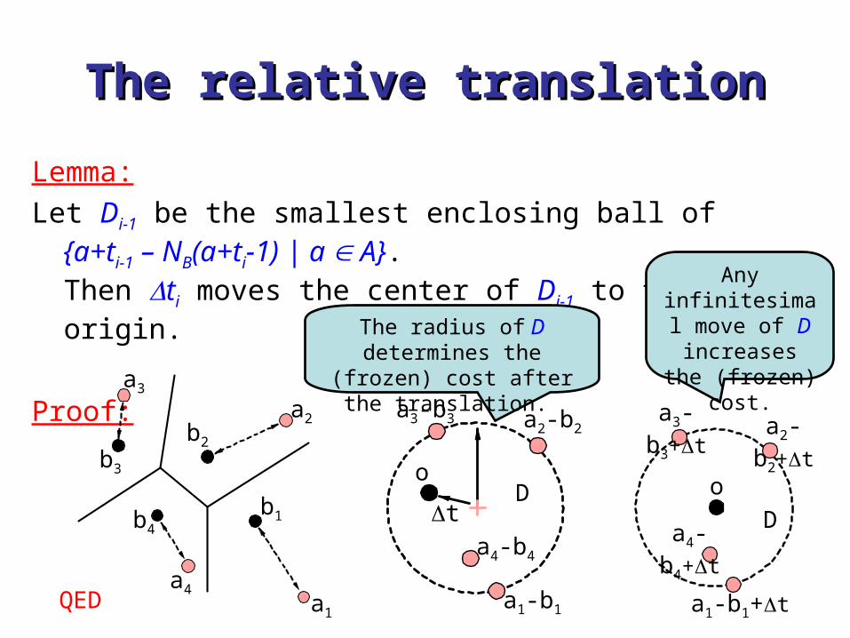
The relative translationThe relative translation

Lemma:

Let Di-1 be the smallest enclosing ball of {a+ti-1 – NB(a+ti-1) | a A}. Then ti moves the center of Di-1 to the origin.

Proof:

t

o

a1

b1

a2b2

a3

b3

a4

b4

a1-b1

a2-b2

a4-b4

a3-b3

a1-b1+t

a2-b2+t

a4-b4+t

a3-b3+t

o

The radius of D determines the (frozen) cost after the

translation.

Any infinitesimal move of D

increases the (frozen) cost.

DD

QED

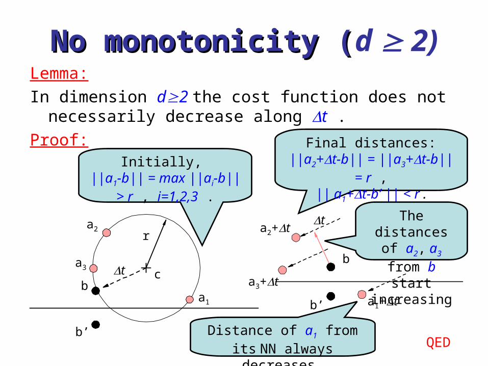
No monotonicity (No monotonicity (d 2)Lemma:

In dimension d2 the cost function does not necessarily decrease along t .

Proof:

a1

a2

a3

b

b’

t

r

c

ta2+t

a3+t

a1+t

b

b’

Initially, ||a1-b|| = max ||ai-b|| > r ,

i=1,2,3 .

Final distances:||a2+t-b|| = ||a3+t-b|| = r ,

|| a1+t-b’ || < r .

The distances of a2, a3 from b start increasing

Distance of a1 from its NN always decreases. QED

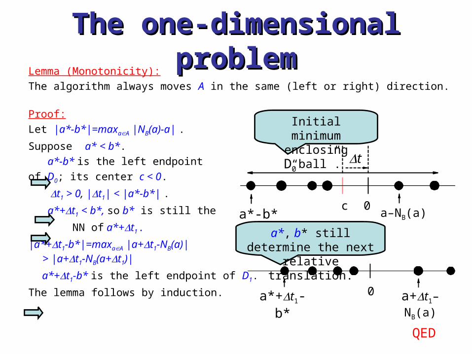
The one-dimensional problemThe one-dimensional problemLemma (Monotonicity):

The algorithm always moves A in the same (left or right) direction.

Proof:

Let |a*-b*|=maxaA |NB(a)-a| .

Suppose a* < b*.

a*-b* is the left endpoint

of D0; its center c < 0.

t1 > 0, |t1| < |a*-b*| .

a*+t1 < b*, so b* is still the

NN of a*+t1 .

|a*+t1-b*|=maxaA |a+t1-NB(a)|> |a+t1-NB(a+t1)|

a*+t1-b* is the left endpoint of D1.

The lemma follows by induction.

a*-b*

tD0

0ca–NB(a)

Initial minimum enclosing “ball”.

0a*+t1-b* a+t1–NB(a)

a*, b* still determine the next relative translation.

QED

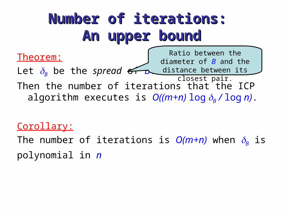
Number of iterations: Number of iterations: An upper boundAn upper bound

Theorem:

Let B be the spread of B.

Then the number of iterations that the ICP algorithm executes is O((m+n) log B / log n).

Corollary:

The number of iterations is O(m+n) when B is

polynomial in n

Ratio between the diameter of B and the distance between its

closest pair.

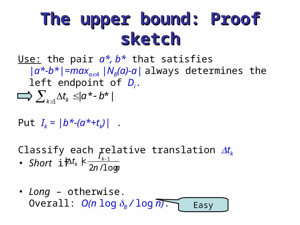
The upper bound: Proof sketchThe upper bound: Proof sketch

Use: the pair a*, b* that satisfies |a*-b*|=maxaA |NB(a)-a| always determines the left endpoint of Di.

Put Ik = |b*-(a*+tk)| .

Classify each relative translation tk

• Short if

• Long – otherwise.Overall: O(n log B / log n).

nn

It kk log/2|| 1

Easy

1|**|

k k bat

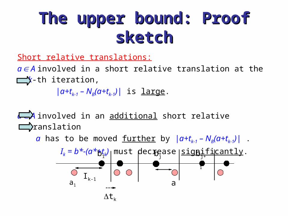
The upper bound: Proof sketchThe upper bound: Proof sketch

Short relative translations:

a A involved in a short relative translation at the k-th iteration,

|a+tk-1 – NB(a+tk-1)| is large.

a A involved in an additional short relative translation

a has to be moved further by |a+tk-1 – NB(a+tk-1)| .

Ik = b*-(a*+tk) must decrease significantly.

b1 bj bj+1

a

tk

Ik-1a1

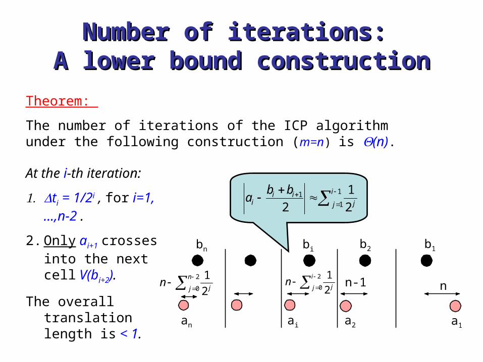
Number of iterations: Number of iterations: A lower bound constructionA lower bound construction

2

0 2

1n

j jn

At the i-th iteration:

1. ti = 1/2i , for i=1,…,n-2 .

2. Only ai+1 crosses into the next cell V(bi+2).

The overall translation length is < 1.

Theorem:

The number of iterations of the ICP algorithm under the following construction (m=n) is (n).

a1a2an

b1b2bn

nn-1

2

0 2

1i

j jn

ai

1

11

2

1

2

i

j jii

i

bba

bi

Many open problems:

• Bounds on # iterations• How many local minima?• Other cost functions• More structural properties• Analyze / improve running time, vs. running time of directly computing minimizing translation And so on…