Near-Linear Approximation Algorithms for Geometric Hitting Sets Pankaj Agarwal Esther Ezra Micha Sharir Duke Duke Tel-Aviv University University University.

Near-Linear Approximation Near-Linear Approximation Algorithms for Geometric Algorithms for Geometric

Hitting SetsHitting Sets

Pankaj Agarwal Esther Ezra Micha SharirPankaj Agarwal Esther Ezra Micha Sharir Duke Duke Tel-Aviv Duke Duke Tel-Aviv

University University University University University University

Range SpacesRange Spaces

Range space (X, R) :

X – Ground set.

R – Ranges: Subsets of X .

|R| 2|X|

Abstract form: Hypergraphs.

X – vertices.

R – hyperedges.

specification: X d, R = set of simply-shaped regions in d

X – Points on the real line.R – Intervals.

X – Points on the plane.R – halfplanes.

X – Points on the plane.R – Disks.

Geometric Range SpacesGeometric Range Spaces

X finite: Discrete model ,

X infinite: Continuous model

The hitting-set problemThe hitting-set problem

A hitting set for (X, R) is a subset H X, s.t., for any Q R , Q H .

Goal: find smallest hitting set.

Useful applications: art-gallery,sensor networking, and more.

Hardness of hitting setsHardness of hitting sets

Finding a hitting set of smallest size is NP-hard,

even for geometric range spaces!

Use an approximation algorithm instead.

Abstract range spaces:

Greedy algorithm [Chvatal 79].

Geometric range spaces:

Iterative reweighed scheme [Bronimann-Goodrich95], [Clarkson 93].

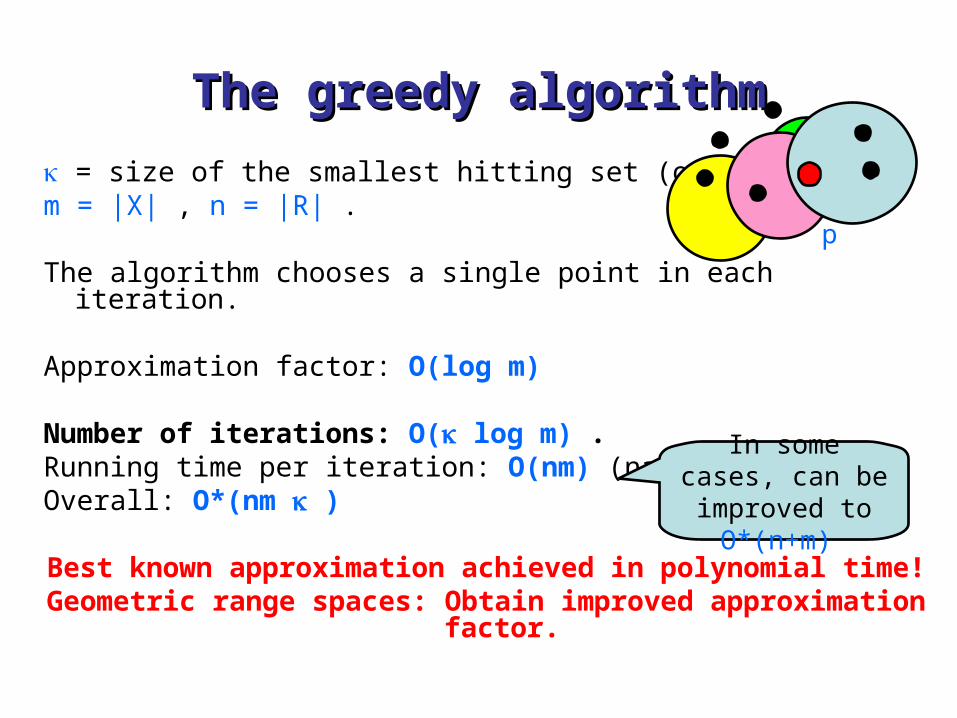
The greedy algorithmThe greedy algorithm

= size of the smallest hitting set (optimum).m = |X| , n = |R| .

The algorithm chooses a single point in each iteration.

Approximation factor: O(log m)

Number of iterations: O( log m) .Running time per iteration: O(nm) (naïve).Overall: O*(nm )

Best known approximation achieved in polynomial time!Geometric range spaces: Obtain improved approximation factor.

p

In some cases, can be improved to

O*(n+m)

Iterative reweighted scheme Iterative reweighted scheme [Bronimann-Goodrich-95], [Clarkson-93][Bronimann-Goodrich-95], [Clarkson-93]

= size of the smallest hitting set.m = |X| , n = |R| .

Approximation factor: O(log ) .Sometimes, the approximation factor is even smaller!

Number of iterations: O( log (m/)) .

Running time per iteration: O*(n + m) (naïve).Overall: O*(m + n2 )

Goal: Improve the running time.A (near) linear-time algorithm?

In some cases, can be improved to

O*(n+m)

Improved!

Our resultOur resultPlanar regions:Obtain a O*(log n) approximation in near-linear time , when the union complexity of R is near-linear.

Applied in both discrete and continuous models.

Specifically:Union complexity of any subset R’ R, |R’| = r is O(r (r)) . Obtain a hitting set for (X, R) of size O( () log n)in (randomized expected) time O*(m + n) .

() is a slowly growing function.

The running time is O*(n) for the

continuous model.

The union boundary

Our result: Axis-parallel boxes in Our result: Axis-parallel boxes in dd

Discrete model: Approximation factor O(log n)Running time: O*(m + n)

Continuous model:Approximation factor O(logd-1)Running time: O(n log n)

Fast implementation for the iterative reweighting scheme:Approximation factor O(log ) in any dimension d.Running time: O*(m + n + d+1)

Union complexity: quadratic

O(loglog ), for d=2,3.[Aronov etal. 2009]

Discrete model

Improved approximation factorsImproved approximation factors(achieved in near-linear time)(achieved in near-linear time)

Ranges bound d=2Disks (pseudo-disks) O(log n) -fat wedges O(log n) -fat triangles O(log n loglog n) Locally -fat objects O(polylog n) d 1Axis-parallel boxes (discrete) O(log n)Axis-parallel boxes (continuous) O(logd-1)

Planar regions with near-linear union Planar regions with near-linear union complexitycomplexity

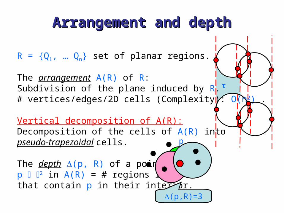
Arrangement and depthArrangement and depth

R = {Q1, … Qn} set of planar regions.

The arrangement A(R) of R:Subdivision of the plane induced by R.# vertices/edges/2D cells (Complexity): O(n2) .

Vertical decomposition of A(R):Decomposition of the cells of A(R) intopseudo-trapezoidal cells.

The depth (p, R) of a point p 2 in A(R) = # regions in R that contain p in their interior.

p

(p,R)=3

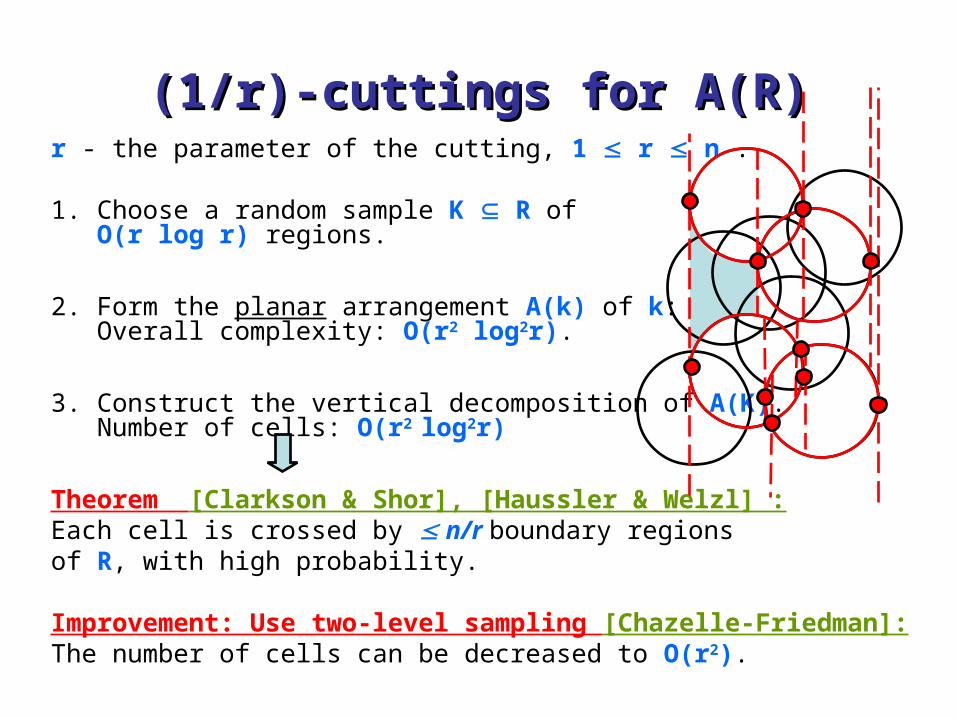
(1/r)-cuttings for A(R)(1/r)-cuttings for A(R)r - the parameter of the cutting, 1 r n .

(1/r)-cuttings for A(R):Set of pairwise disjoint pseudo-trapezoidal cells, s.t.

1. They cover A(R).2. Each cell is crossed by n/r

boundary regions of R.

Simple Construction [Clarkson Shor 89]:• Choose a random sample K R of

O(r log r) regions.• Form the planar arrangement A(K) of K.• Construct the vertical decomposition of A(K).• # cells: O(r2 log2 r)

#cells = f(r)

Properties of (1/r)-cuttingsProperties of (1/r)-cuttings

Theorem [Matousek 92], [Agarwal etal. 2000]:

Put = max p 2 {(p, R)} .

There exists (1/r)-cutting, s.t.,# cells : O(q r (r/q)) , where q = (r/n) + 1 .

In particular:For r = min {cn / , n} .# cells of the cutting: O(r (r)) = O(n/ (n/)) .

When c, we have r = n, and then # cells: O(n (n)) .

union complexity

c > 0 sufficiently large constant.

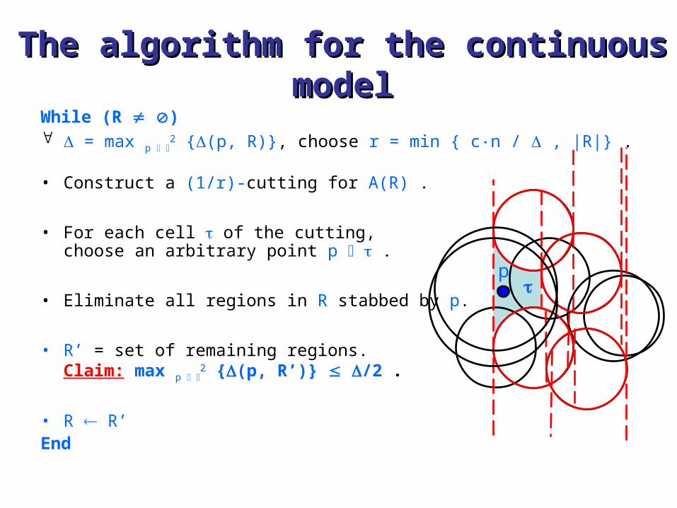
While (R ) = max p

2 {(p, R)}, choose r = min { cn / , |R|} .

• Construct a (1/r)-cutting for A(R) .

• For each cell of the cutting, choose an arbitrary point p .

• Eliminate all regions in R stabbed by p.

• R’ = set of remaining regions.Claim: max p

2 {(p, R’)} /2 .

• R R’End

The algorithm for the continuous modelThe algorithm for the continuous model

p

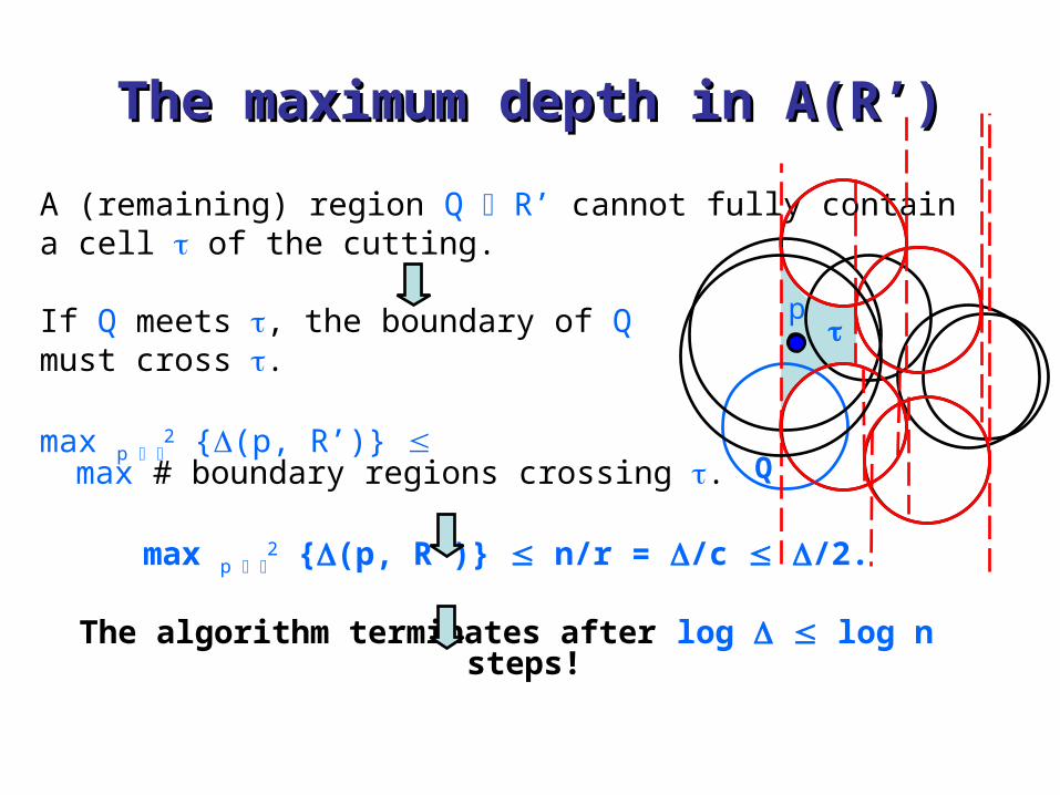
A (remaining) region Q R’ cannot fully contain a cell of the cutting.

If Q meets , the boundary of Q must cross .

max p 2 {(p, R’)}

max # boundary regions crossing .

max p 2 {(p, R’)} n/r = /c /2.

The algorithm terminates after log log n steps!

The maximum depth in A(R’)The maximum depth in A(R’)

Q

p

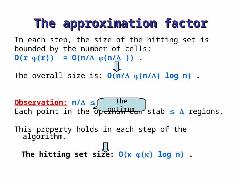
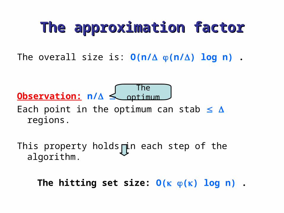
The approximation factorThe approximation factorIn each step, the size of the hitting set is bounded by the number of cells: O(r (r)) = O(n/ (n/ )) .

The overall size is: O(n/ (n/) log n) .

Observation: n/ .Each point in the optimum can stab regions.

This property holds in each step of the algorithm.

The hitting set size: O( () log n) .

The optimum

The discrete modelThe discrete model

The points of the hitting set are chosen from a given set X.

Apply a more intricate variant of the algorithm: = max p X {(p, R)}, choose r = min {cn/ , n}.

Use (1/r)-cutting to cover only the portions of A(R) at depth .

Choose a point in each non-empty cell of the cutting.

In each step, the cutting size is O(n/ (n/)) = O( ()) .Overall size: O( () log n) .

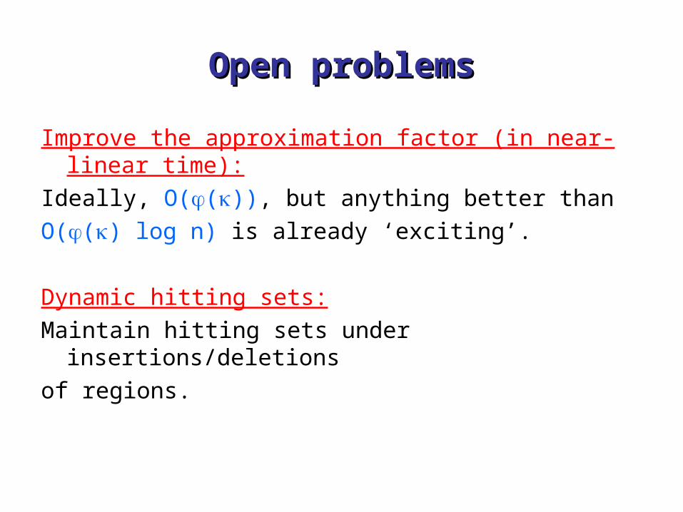
Open problemsOpen problems

Improve the approximation factor (in near-linear time):

Ideally, O(()), but anything better than

O(() log n) is already ‘exciting’.

Dynamic hitting sets:

Maintain hitting sets under insertions/deletions

of regions.

merci beaucoup!merci beaucoup!

ImplementationImplementation

Two major tasks:

• Construct the shallow cutting.

• Efficiently report all regions stabs by the points p X for each non-empty cell of the cutting.

Use a variant of the randomized incremental construction

of [Agarwal etal.] to construct Al(R) .

Randomly permute the regions in R,

and apply the algorithm for the first r steps.

randomized incremental constructionrandomized incremental construction

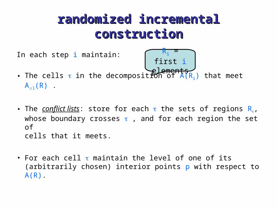
In each step i maintain:

• The cells in the decomposition of A(Ri) that meet Al(R) .

• The conflict lists: store for each the sets of regions R,whose boundary crosses , and for each region the set of cells that it meets.

• For each cell maintain the level of one of its (arbitrarily chosen) interior points p with respect to A(R).

Ri = first i elements

Inserting a new regionInserting a new region

i = region inserted at the i-th step.

• Use the conflict lists to:

– Find all cells in the decomposition of A(Ri) that i meets.

– Split these cells, re-decompose them, update the conflict lists,and update the level information of the new cells ’.

• Then test if each of the new cells ’ meets Al(R) .

Theorem:

Running time: O(n log2 r + r) (n/)) .

For our choice of , r, the running time is: O(n log2 () log2 )

A single step of the algorithm

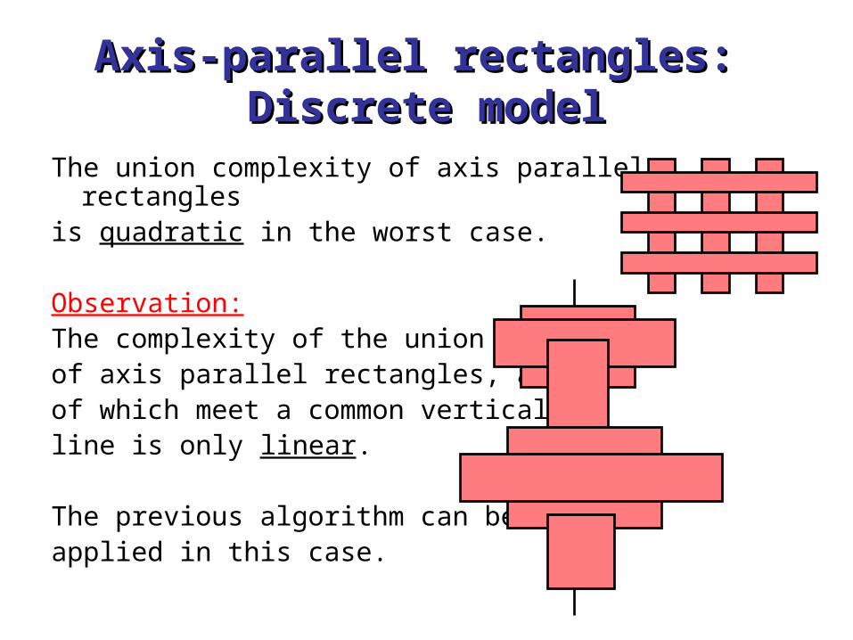
Axis-parallel rectangles: Axis-parallel rectangles: Discrete modelDiscrete model

The union complexity of axis parallel rectanglesis quadratic in the worst case.

Observation:The complexity of the unionof axis parallel rectangles, allof which meet a common verticalline is only linear.

The previous algorithm can be applied in this case.

Project all rectangles and points onto the x-axis:

Obtain a set I of n intervals.

Compute in O(n log n) time an optimal hitting Q set for I.

The set L of the vertical lines x = q, q Q

intersect all rectangles in R. |L| = |Q| .

The plane decompositionThe plane decomposition

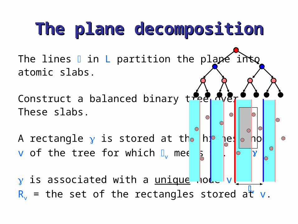
The plane decompositionThe plane decomposition

The lines in L partition the plane into atomic slabs.

Construct a balanced binary tree over These slabs.

A rectangle is stored at the highest node

v of the tree for which v meets .

is associated with a unique node v.

Rv = the set of the rectangles stored at v.

v

v

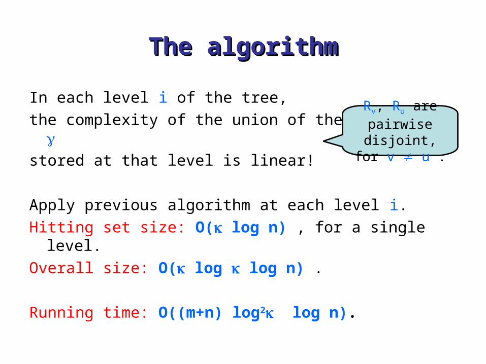
The algorithmThe algorithm

In each level i of the tree,

the complexity of the union of the rectangles

stored at that level is linear!

Apply previous algorithm at each level i.

Hitting set size: O( log n) , for a single level.

Overall size: O( log log n) .

Running time: O((m+n) log2 log n).

Rv, Ru are pairwise disjoint,

for v u .

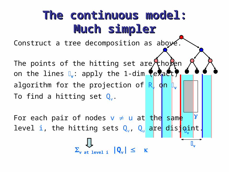
The continuous model:The continuous model:Much simplerMuch simpler

Construct a tree decomposition as above.

The points of the hitting set are chosen

on the lines v: apply the 1-dim (exact)

algorithm for the projection of Rv on v

To find a hitting set Qv.

For each pair of nodes v u at the same

level i, the hitting sets Qv, Qu are disjoint.

v at level i |Qv|

v

v

The continuous modelThe continuous modelOverall size: O( log ) .

Running time: O(n log n) .

The algorithm can be extended to any dimension d, using induction on d:

• Project all boxes onto the xd-axis.

• Apply the 1-dim (exact) algorithm on the xd-axis.

• Obtains a tree decomposition with the (d-1)-hyperplanesorthogonal to the xd-axis.

• Solve the problem recursively on each hyperplane.

• At the i-th level obtain a hitting set of size O( logd-2 ) .

Overall size: O( logd-1 ) .

Thank youThank you

Input:C – set of clients .A - locations of antennas , each

of which with a unit sensing radius.

Goal: Find minimum-size set of antennas that serve all clients.

Hitting-set instance:X – antennas locations

R – (,1): unit disks with client-centers.

Sensor networking applicationSensor networking application

covers iff is inside (,1)

Approximation for geometric Approximation for geometric hitting setshitting sets

Geometric range spaces:

Achieve improved approximation factor!

Approximation factor: O(1 + log ) ,

Sometimes, the approximation factor is even smaller!

Points and disks or pseudo-disks in 2D: O(1) .

Points and halfspaces in 2D and 3D: O(1) .

Points and axis-parallel boxes in 2D and 3D: O(log log ) .

This is achieved via -nets

-nets for range spaces-nets for range spacesGiven:

• A range space (X, R) , assume X is finite, |X| = n .

• A parameter 0 < < 1 ,

An -net for (X, R) is a subset N X that hits every

range Q R, with |Q X| n .

N is a hitting set for all the ``heavy'' ranges.

Example:

Points and intervals on the real line: |N| = 1/ .

n

Bound does not depend on n.

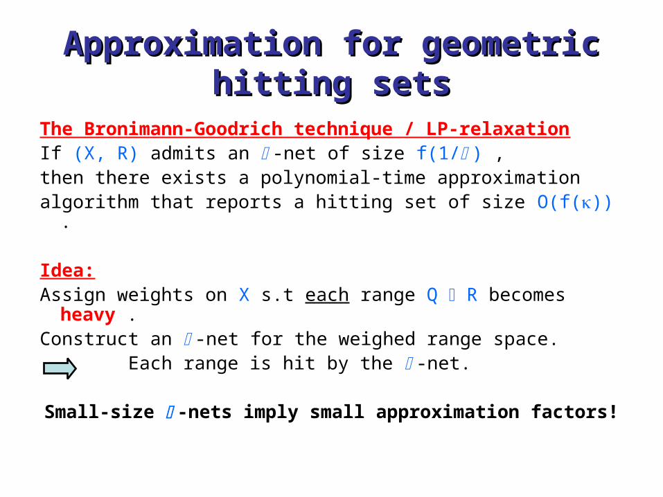
Approximation for geometric hitting Approximation for geometric hitting setssets

The Bronimann-Goodrich technique / LP-relaxationIf (X, R) admits an -net of size f(1/ ) ,then there exists a polynomial-time approximation algorithm that reports a hitting set of size O(f()) .

Idea: Assign weights on X s.t each range Q R becomes heavy .Construct an -net for the weighed range space. Each range is hit by the -net.

Small-size -nets imply small approximation factors!

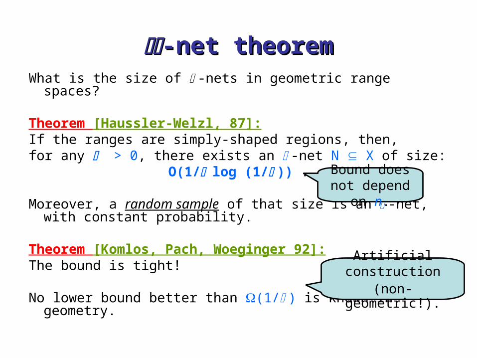
-net theorem-net theoremWhat is the size of -nets in geometric range spaces?

Theorem [Haussler-Welzl, 87]:If the ranges are simply-shaped regions, then, for any > 0, there exists an -net N X of size:

O(1/ log (1/ )) .

Moreover, a random sample of that size is an -net, with constant probability.

Theorem [Komlos, Pach, Woeginger 92]:The bound is tight!

No lower bound better than (1/ ) is known in geometry.

Bound does not depend on n.

Artificial construction(non-geometric!).

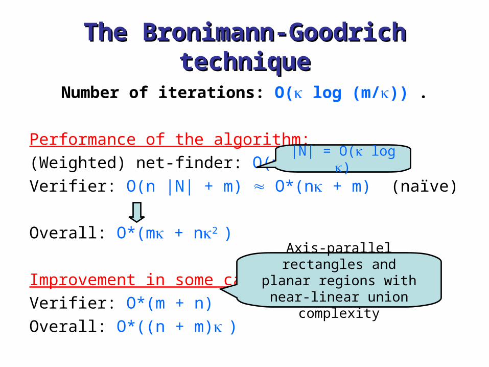
The Bronimann-Goodrich techniqueThe Bronimann-Goodrich technique

Number of iterations: O( log (m/)) .

Performance of the algorithm:

(Weighted) net-finder: O(m)

Verifier: O(n |N| + m) O*(n + m) (naïve)

Overall: O*(m + n2 )

Improvement in some cases:

Verifier: O*(m + n)

Overall: O*((n + m) )

|N| = O( log )

Axis-parallel rectangles andplanar regions with near-linear

union complexity

Arrangement and levelsArrangement and levels

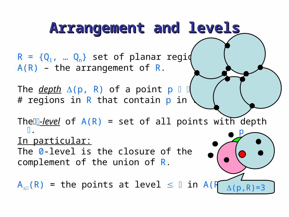
R = {Q1, … Qn} set of planar regions.A(R) – the arrangement of R.

The depth (p, R) of a point p 2 in A(R) =# regions in R that contain p in their interior.

The-level of A(R) = set of all points with depth .In particular:The 0-level is the closure of the complement of the union of R.

A(R) = the points at level in A(R) .

p

(p,R)=3

Complexity of AComplexity of A(R)(R)

Using Clarkson & Shor:

The complexity of A() is:O(2 f(n/)) = O(n (n/) )

Vertical decomposition of A() (or A() ) :Partition each cell of A() (or A() ) intopseudo-trapezoidal cells.The decomposition has the same complexity as

A() (or A() ) .

Vertical decomposition

of level 1

Union complexity

= n/ (n/) .

Need to assume constant description

complexity

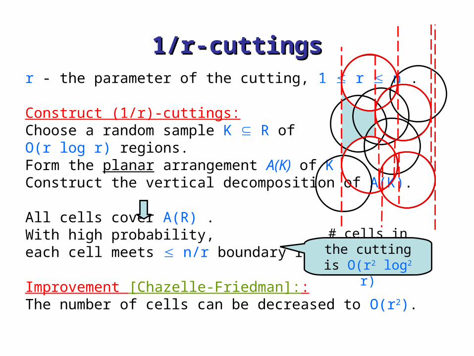
1/r-cuttings1/r-cuttingsr - the parameter of the cutting, 1 r n .

Construct (1/r)-cuttings:Choose a random sample K R of O(r log r) regions.Form the planar arrangement A(K) of KConstruct the vertical decomposition of A(K).

All cells cover A(R) .With high probability, each cell meets n/r boundary regions.

Improvement [Chazelle-Friedman]:: The number of cells can be decreased to O(r2).

# cells in the cutting is O(r2 log2 r)

(1/r)-cuttings for A(R)(1/r)-cuttings for A(R)r - the parameter of the cutting, 1 r n .

1. Choose a random sample K R of O(r log r) regions.

2. Form the planar arrangement A(k) of k: Overall complexity: O(r2 log2r).

3. Construct the vertical decomposition of A(K).Number of cells: O(r2 log2r)

Theorem [Clarkson & Shor], [Haussler & Welzl] :Each cell is crossed by n/r boundary regions of R, with high probability.

Improvement: Use two-level sampling [Chazelle-Friedman]: The number of cells can be decreased to O(r2).

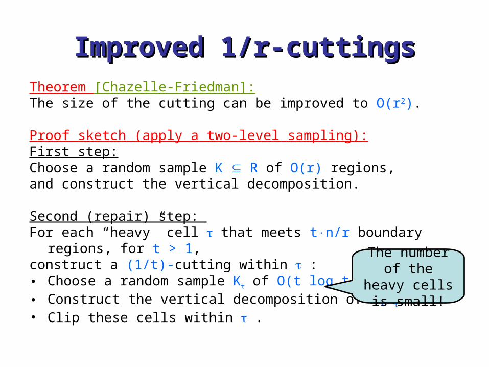
Improved 1/r-cuttingsImproved 1/r-cuttingsTheorem [Chazelle-Friedman]:The size of the cutting can be improved to O(r2).

Proof sketch (apply a two-level sampling):First step: Choose a random sample K R of O(r) regions, and construct the vertical decomposition.

Second (repair) step: For each “heavy” cell that meets tn/r boundary regions, for t > 1, construct a (1/t)-cutting within :• Choose a random sample K of O(t log t) regions.

• Construct the vertical decomposition of A(K) .• Clip these cells within .

The number of the heavy cells is

small!

Shallow cuttingsShallow cuttings

A shallow cutting is a (1/r)-cutting that covers Al(R) .

Construct shallow cuttings:Discard all cells of the full (1/r)- cutting that do not meet Al(R) .

Theorem [Matousek, Agarwal etal.]The size of the shallow cutting is

O(q r (r/q)) ,where q = (r/n) + 1 .

When = n, # cells is O(r2) .

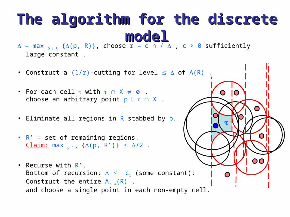
= max p X {(p, R)}, choose r = c n / , c > 0 sufficiently large constant .

• Construct a (1/r)-cutting for level of A(R) .

• For each cell with X , choose an arbitrary point p X .

• Eliminate all regions in R stabbed by p.

• R’ = set of remaining regions.Claim: max p X {(p, R’)} /2 .

• Recurse with R’.Bottom of recursion: c1 (some constant):Construct the entire A (R) , and choose a single point in each non-empty cell.

The algorithm for the discrete modelThe algorithm for the discrete model

The maximum depth in A(R’)The maximum depth in A(R’)

A (remaining) region in R’ cannot fully contain a non-empty cell of the cutting.

The boundary of these regions cross cells .

max p X {(p, R’)} = max # crossing boundary regions in a cell

max p X {(p, R’)} n/r = /c /2.

The algorithm terminates after log log n steps!

R’

The size of the hitting set in each The size of the hitting set in each stepstep

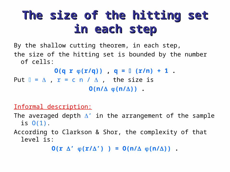
By the shallow cutting theorem, in each step,

the size of the hitting set is bounded by the number of cells:

O(q r (r/q)) , q = (r/n) + 1 .

Put = , r = c n / , the size is

O(n/ (n/)) .

Informal description:

The averaged depth ’ in the arrangement of the sample is O(1).

According to Clarkson & Shor, the complexity of that level is:

O(r ’ (r/’) ) = O(n/ (n/)) .

The approximation factorThe approximation factor

The overall size is: O(n/ (n/) log n) .

Observation: n/ .

Each point in the optimum can stab regions.

This property holds in each step of the algorithm.

The hitting set size: O( () log n) .

The optimum