On the annual cycle of the sea surface temperature and the mixed layer depth in the Gulf of México

Atmósfera (2005) 127-148

On the annual cycle of the sea surface temperature and the mixedlayer depth in the Gulf of México.

V. M. MENDOZA, E. E. VILLANUEVA and J. ADEM

Centro de Ciencias de la Atmósfera, UNAM, Circuito Exterior, C. U., 04510, México, D. F., México

Corresponding author: V. M. Mendoza; e-mail: [email protected]

Received March 1, 2004; accepted February 22, 2005

RESUMEN

Usando un modelo integrado en la capa de mezcla hemos obtenido una simulación del ciclo anual de latemperatura de la superficie del mar (SST), de la profundidad de la capa de mezcla (MLD) en el Golfo deMéxico, así como del ciclo anual de la velocidad de penetración vertical turbulenta a través de la termoclina enla región más profunda del Golfo de México. El modelo se basa en las ecuaciones de conservación de energíatérmica y mecánica, ésta última derivada de la teoría de Kraus-Turner, ambas ecuaciones están acopladas eintegradas verticalmente en la capa de mezcla. Las ecuaciones del modelo se resuelven en una malla regularde 25 km en el Golfo de México, la región noroeste del Mar Caribe y la costa este de Florida. La velocidad dela corriente oceánica superficial y las variables atmosféricas son prescritas en el modelo usando valoresobservados. Mostramos la importancia que tiene el bombeo de Ekman en la velocidad de penetración turbu-lenta. Encontramos que la surgencia tiene un papel importante en incrementar la penetración turbulentaproduciendo un enfriamiento del agua superficial y una disminución en la profundidad de la capa de mezclaen la Bahía de Campeche. En el resto del Golfo el hundimiento tiende a reducir la penetración turbulenta y aincrementar la temperatura de la superficie y la profundidad de la capa de mezcla. Una comparación del cicloanual de la SST y de la MLD calculados con el modelo muestran concordancia con las correspondientesobservaciones reportadas por Robinson (1973). En la región profunda del Golfo de México, los datos deconcentración de pigmentos fotosintéticos, obtenidos de análisis ambientales, muestran en enero, abril,mayo junio y septiembre correlación significativa con el ciclo anual de la velocidad de penetración verticalturbulenta calculada.

ABSTRACT

Using an integrated mixed layer model we carry out a simulation of the annual cycle of the sea surfacetemperature (SST) and of the mixed layer depth (MLD) in the Gulf of México. We also compute the annual

128 V. M. Mendoza et al.

cycle of the entrainment velocity in the deepest region of the Gulf of México. The model is based on thethermal energy equation and on an equation of mechanical and thermal energy balance based on the Kraus-Turner theory; both equations are coupled and are vertically integrated in the mixed layer. The model equationsare solved in a uniform grid of 25 km in the Gulf of México, the northwestern region of the Caribbean Sea andthe eastern coast of Florida. The surface ocean current velocity and the atmospheric variables are prescribedin the model using observed values. We show the importance of the Ekman pumping in the entrainmentvelocity. We found that the upwelling plays an important role in increasing the entrainment velocity, producingan important reduction in the SST and diminishing the depth of the mixed layer in the Campeche Bay. In therest of the Gulf of México the downwelling tends to reduce the entrainment velocity, increasing the SST andthe MLD. Comparison of the computed annual cycle of the SST and the MLD with the correspondingobservations reported by Robinson (1973), shows a good agreement. In the deepest region of the Gulf ofMéxico, the photosynthetic pigment concentration data obtained from the Mexican Pacific CD-ROM ofenvironmental analysis shows significative correlation with the computed annual cycle of the computedentrainment velocity only in January, April, May, June and September.

Keywords: Sea surface temperature; mixed layer depth; Gulf of México.

1. IntroductionWe have used a model that is based in the thermal energy equation applied to the surface layer ofthe Gulf of México to simulate the annual cycle of sea surface temperature (SST) (Adem et al.,1991), the ocean-atmosphere heat fluxes (Adem et al., 1993), as well as to predict the SST anomaliesand their month-to-month changes in the Gulf of México (Adem et al., 1994), obtaining somedegree of skill in the simulations and predictions.

The incorporation in the model of the Kraus and Turner (1967) theory and of the AlexanderWoo-Kim hypothesis (Niiler and Kraus, 1977; Kim, 1976) to compute the cooling in the mixed layerby entrainment through the thermocline improves the skill of the simulations of the SST anomalies,mainly for the summer and the fall seasons (Mendoza et al., 1997). Other authors as Zavala et al.(2002) have studied the average and seasonal variation of the heat fluxes and the SST in the Gulfof México, considering the relative importance of the heat advection and the entrainment.

This work is a contribution to modeling of the ocean upper layer using an integrated mixed layermodel based in the thermal energy equation instead of one based in the hydrodynamic equations,such as was proposed by Blumberg and Mellor (1983), Price et al. (1978), Price (1983), Price andWeller (1986), and Bender and Ginis (2000). The advantage of this model is that has a lesscomputational cost and provides a method to show the importance of the entrainment mechanismand the Ekman pumping on the annual cycle of the SST and the mixed layer depth (MLD).

2. Mixed-layer modelThe ocean mixed layer is the top layer which is well mixed by wind, so that we can assume that ithas a vertically uniform temperature. The mixed layer thickness (h) is defining the depth at whicha sharp gradient of temperature indicates the start of the thermocline. The bottom of the mixedlayer allows a mass vertical flux across it, defined as entrainment (if upwards).

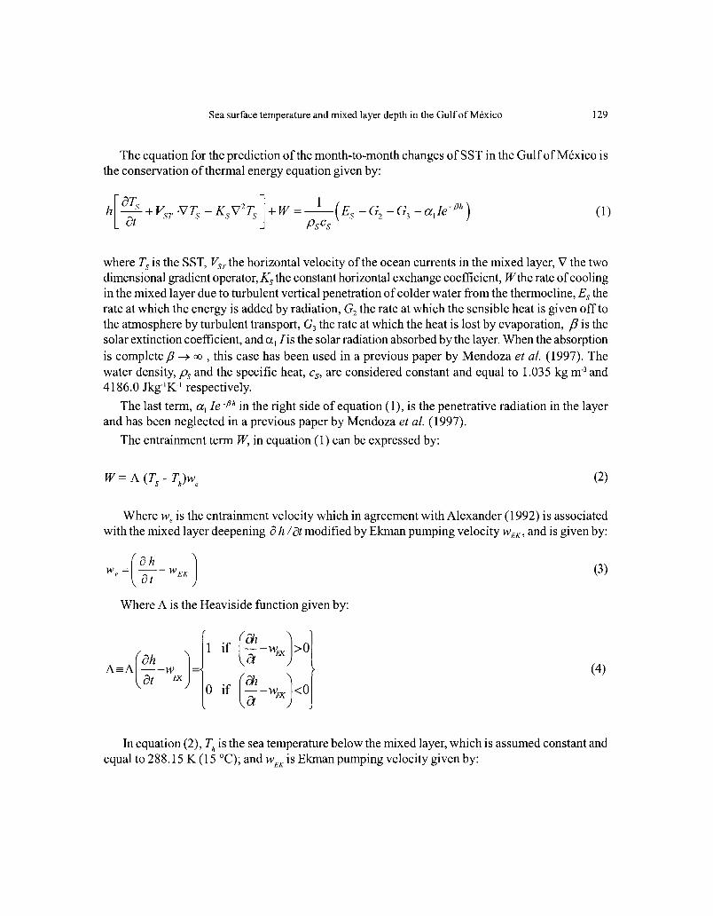
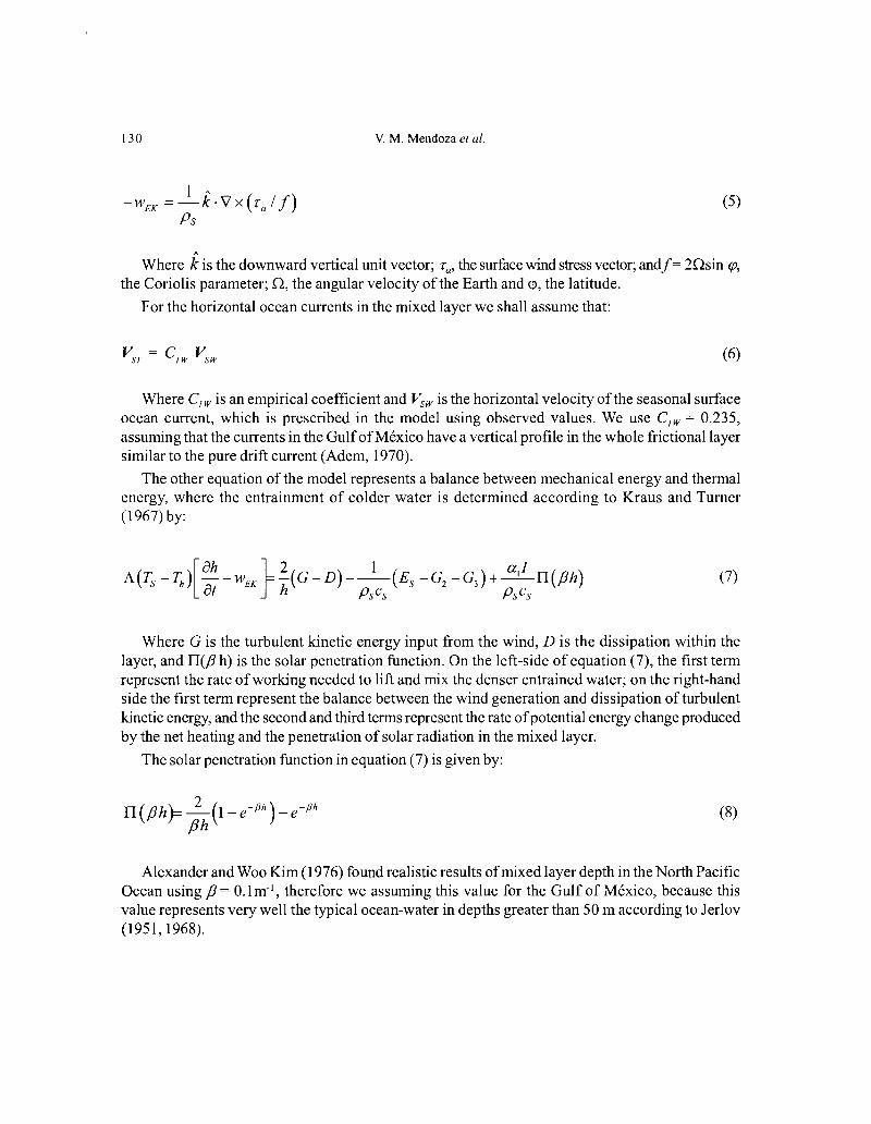
131Sea surface temperature and mixed layer depth in the Gulf of México

Where α = 2.1 × 10-4 K-1 is the thermal expansion coefficient of sea water; g = 9.8 ms-2, theacceleration of gravity; m0 = 1.25, an empirical parameter; nD = 1.25 and γ = 0.05 m-1, parametersof dissipation; ν* the frictional velocity related to the surface wind stress by τa = ρsv*

2 Alexanderand Woo Kim obtained optimal results of the mixed layer depth in the summer season, using aparameter of background dissipation εM = 2.0 × 10-8 m2 s-3, which exists even in the absence ofwind stress; we found the best results with εM = 2.0 × 10-8 m2 s-3 for spring, εM = 3.2 × 10-8 m2 s-3

for summer and εM = 0 for fall and winter.For the surface wind stress, we use the bulk formula (Isemer and Hasse, 1987):

τa = ρa CD|Va|2

Where ρa and |Va| are the surface air density and the surface wind speed, respectively; and CD,the atmospheric drag coefficient.

The components west-east and south-north of the wind stress vector are, respectively, given by:

τax= ρa CD|Va|ua

τay= ρa CD|Va|va

Where ua and νa are the components west-east and south-north of the surface wind vector,respectively.

2.1 The heating functionThe rate at which the energy is added by radiation at the sea surfac (ES) is computed as Budyko(1974):

ES = − δ σ Ta4 [0.254 − 0.00495 Ues (Ta)] (1 − cε) − 4δ σ Ta

3 (TS − Ta) + α1 I

Where δ = 0.96 is the emissivity of the sea surface: σ, the Stefan-Boltzmann constant; Ta , the

The difference between the rate of generation and dissipation of turbulent kinetic energy isgiven in accordance with Alexander and Woo Kim by:

( ) 30 *

1 h MD

hG D m n e vg g

γ εα α

−− = + − (9)

(10)

(11)

(12)


surface air temperature; U, the surface air relative humidity; eS(Tα), the saturation vapor pressureat the surface air temperature in hPa; ε, the fractional amount of cloudiness; and c = 0.65, a cloudcover coefficient.

For the solar radiation absorbed by the ocean layer (α1 I), we use the Barliand-Budyko equation:

α1I = (Q + q)0 [1 − (a + εb) ε](1 − αS)

Where (Q + q)0 is the total solar radiation received by the surface with clear sky; αS, thealbedo of the sea surface; and a and b are the coefficients taken from Budyko (1974). The coefficienta is a function of the latitude and the coefficient b is a constant equal to 0.38. For the Gulf ofMéxico we use a = 0.35, which corresponds to 25 °N of latitude.

The heating functions G2 and G3 are given by the following equations (Mendoza et al, 1997):

G2 = ρa cp CH |Va|(TS - Ta)

30.622 | |[0.981 ( ) ( )]a E a S S a S a

a

G L C V e T U e TP

ρ= −

(14)

(13)

(15)

Where cp= 1.004 Jkg-1K-1 is the specific heat of air at constant pressure; L= 2.44 × 106Jkg-1, thelatent heat of vaporization which is considered constant; Pa, the sea level pressure; CH and CE, thevertical turbulent transport coefficients of the sensible and latent heat, respectively. The coefficientsCD, CH and CE are determined according with Huang (1978) by:

Where CDN = 2.5 × 10-3 and CHN = 1.2 × 10-3 are the drag coefficient for momentum and sensibleheat for the neutral case, respectively, and R1 is the bulk Richardson number given by:

( )10

0

( ) 0.981 ( )0.38 a S a S Si a S a

aV a

gZ U e T e TR T T TPT

⎡ ⎤−= − +⎢ ⎥

⎣ ⎦V

exp ( 9.4 )For stable cases ( 0)

exp ( 9.4 )D DN i

iH E HN i

C C RR

C C C R= − ⎫

>⎬= = − ⎭(16a)

71 ln (1 52.9 )52.9

For unstable cases ( 0)111 ln (1 53.2 )

53.2

D DN i

i

H E HN i

C C RR

C C C R

⎫⎡ ⎤= + − ⎪⎢ ⎥⎣ ⎦ ⎪ <⎬⎡ ⎤⎪= = + −⎢ ⎥⎪⎣ ⎦⎭

(16b)

(17)


The temperature Ts and the depth h computed in the last time-step is now used as initial conditionto compute the temperature and the depth for February, and so on.

This iteration process is continued for several annual cycles until the temperature and the depthcomputed for each month between two consecutive years have a difference smaller than 0.01 °Cand 0.01 m, respectively. These conditions are achieved after a run of 5 years.

For the spatial derivatives in equation (19), we use centered differences with a regular grid of 25Km where the horizontal transport of heat by ocean currents and by turbulent eddies are taken aszero at the points in the closed boundaries (coasts). At the points in the open boundaries (in theCaribbean Sea and Atlantic ocean regions contiguous to Florida), we assume that the horizontaltransport of heat by turbulent eddies is zero. For the horizontal transport of heat by ocean currentsin the open boundaries, we compute the term −Vst • ∇Ts using climatic observed values of thesurface ocean currents and the sea surface temperatures.

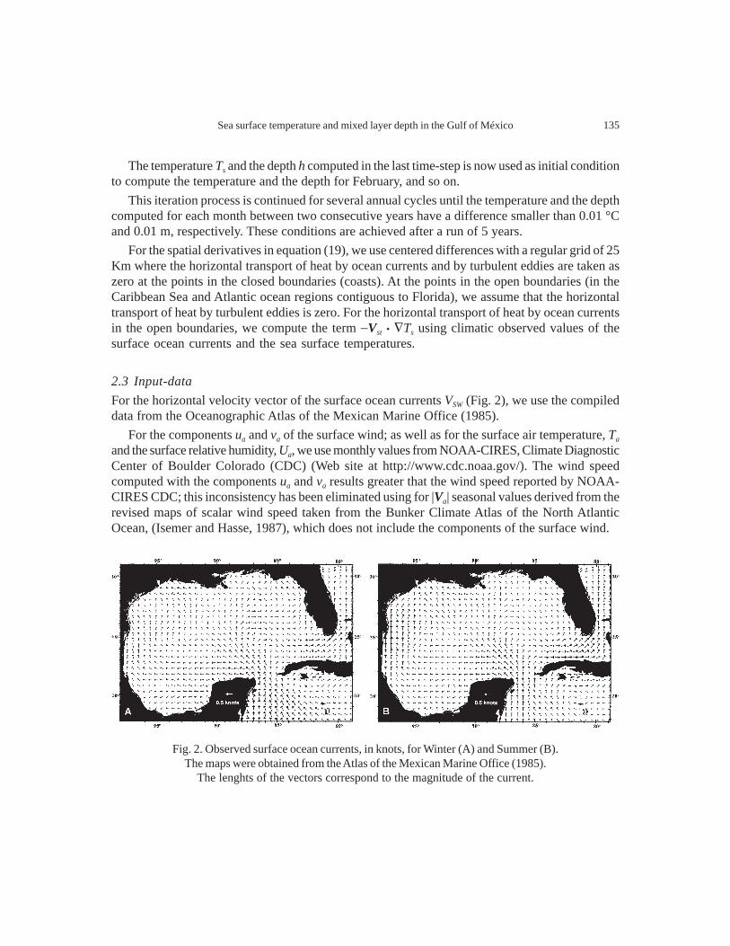
2.3 Input-dataFor the horizontal velocity vector of the surface ocean currents VSW (Fig. 2), we use the compileddata from the Oceanographic Atlas of the Mexican Marine Office (1985).

For the components ua and va of the surface wind; as well as for the surface air temperature, Ta

and the surface relative humidity, Ua, we use monthly values from NOAA-CIRES, Climate DiagnosticCenter of Boulder Colorado (CDC) (Web site at http://www.cdc.noaa.gov/). The wind speedcomputed with the components ua and va results greater that the wind speed reported by NOAA-CIRES CDC; this inconsistency has been eliminated using for |Va| seasonal values derived from therevised maps of scalar wind speed taken from the Bunker Climate Atlas of the North AtlanticOcean, (Isemer and Hasse, 1987), which does not include the components of the surface wind.

Fig. 2. Observed surface ocean currents, in knots, for Winter (A) and Summer (B).The maps were obtained from the Atlas of the Mexican Marine Office (1985).

The lenghts of the vectors correspond to the magnitude of the current.


Seasonal values of the fractional amount of cloudiness, ε, and the albedo of the sea surface, αs,were obtained from data files of the Adem’s thermodynamic climate model (Adem, 1965).

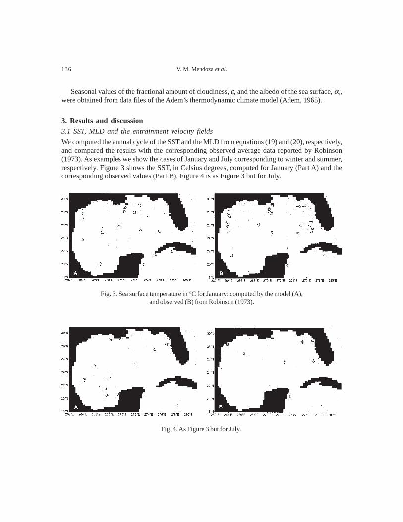
3. Results and discussion3.1 SST, MLD and the entrainment velocity fieldsWe computed the annual cycle of the SST and the MLD from equations (19) and (20), respectively,and compared the results with the corresponding observed average data reported by Robinson(1973). As examples we show the cases of January and July corresponding to winter and summer,respectively. Figure 3 shows the SST, in Celsius degrees, computed for January (Part A) and thecorresponding observed values (Part B). Figure 4 is as Figure 3 but for July.

Fig. 4. As Figure 3 but for July.

Fig. 3. Sea surface temperature in °C for January: computed by the model (A),and observed (B) from Robinson (1973).


The comparison of part A with part B, for the case of January and July, shows that the modelhas some skill to simulate the SST.

In January, it is clearly shown the effect that on the SST has the water flow through the YucatánChannel, associated with the Loop Current (Fig. 3, Part B). This effect on the SST has been, inpart, simulated by the model due to the prescribed observed currents. In the central part of the Gulfof México the model simulates temperatures very close to the observations. However in the Texas-Louisiana shelf it is observed a more pronounced northward cooling than the one computed by themodel. Temperatures approximately uniform of 29°C are observed in July (Fig. 4, Part B), decreasingone degree toward the west coast of the Gulf, and toward the Yucatán and Florida shelves. Themodel also simulates approximately uniform temperatures of 29ºC in the center of the Gulf, with adecrease towards the northeast, however the temperatures simulated by the model over the CampecheBay of up to 27 ºC (Fig. 4, Part A) are not observed in the Part B of Figure 4. These low temperatures,over the Campeche Bay, simulated by the model are produced by a relatively strong upwelling (Fig.8, Part B), that produces an important entrainment of cold water from the thermocline (Fig. 9, Part B).

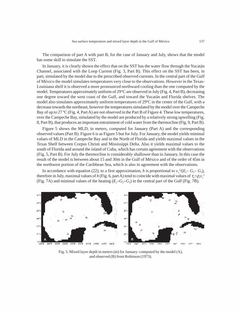
Figure 5 shows the MLD, in meters, computed for January (Part A) and the correspondingobserved values (Part B). Figure 6 is as Figure 5 but for July. For January, the model yields minimalvalues of MLD in the Campeche Bay and in the North of Florida and yields maximal values in theTexas Shelf between Corpus Christi and Mississippi Delta. Also it yields maximal values to thesouth of Florida and around the island of Cuba, which has certain agreement with the observations(Fig. 5, Part B). For July the thermocline is considerably shallower than in January. In this case theresult of the model is between about 15 and 30m in the Gulf of México and of the order of 45m inthe northwest portion of the Caribbean Sea, which is also in agreement with the observations.

In accordance with equation (22), to a first approximation, h is proportional to v*3/(Es− G2− G3),

therefore in July, maximal values of h (Fig. 6, part A) tend to coincide with maximal values of τa=ρsv*3

(Fig. 7A) and minimal values of the heating (Es−G2−G3) in the central part of the Gulf (Fig. 7B).

Fig. 5. Mixed layer depth in meters (m) for January: computed by the model (A),and observed (B) from Robinson (1973).


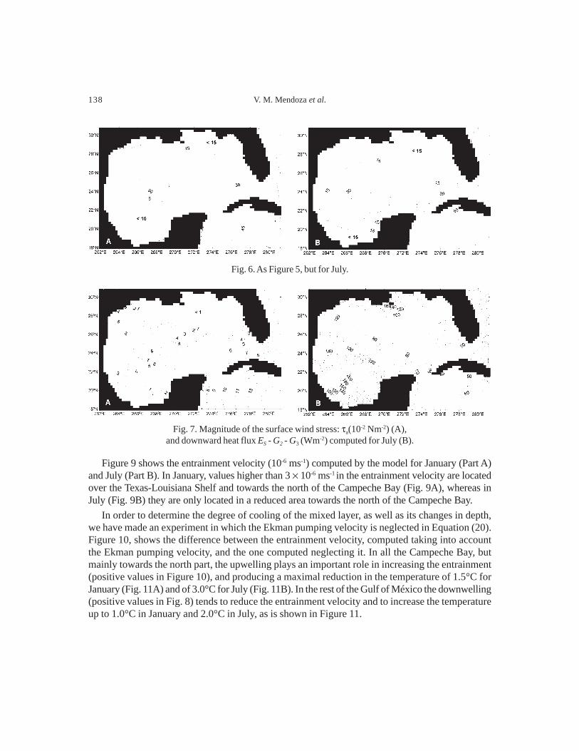
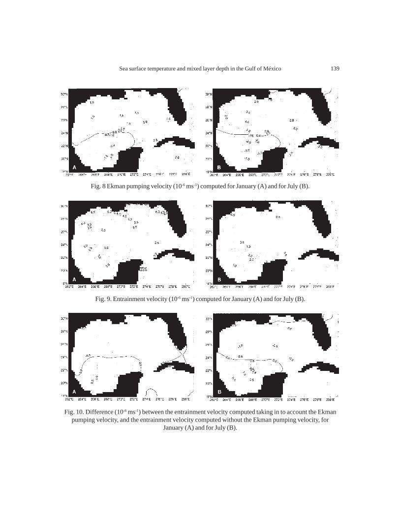
Figure 9 shows the entrainment velocity (10-6 ms-1) computed by the model for January (Part A)and July (Part B). In January, values higher than 3 × 10-6 ms-1 in the entrainment velocity are locatedover the Texas-Louisiana Shelf and towards the north of the Campeche Bay (Fig. 9A), whereas inJuly (Fig. 9B) they are only located in a reduced area towards the north of the Campeche Bay.

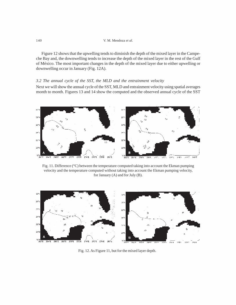
In order to determine the degree of cooling of the mixed layer, as well as its changes in depth,we have made an experiment in which the Ekman pumping velocity is neglected in Equation (20).Figure 10, shows the difference between the entrainment velocity, computed taking into accountthe Ekman pumping velocity, and the one computed neglecting it. In all the Campeche Bay, butmainly towards the north part, the upwelling plays an important role in increasing the entrainment(positive values in Figure 10), and producing a maximal reduction in the temperature of 1.5°C forJanuary (Fig. 11A) and of 3.0°C for July (Fig. 11B). In the rest of the Gulf of México the downwelling(positive values in Fig. 8) tends to reduce the entrainment velocity and to increase the temperatureup to 1.0°C in January and 2.0°C in July, as is shown in Figure 11.

Fig. 6. As Figure 5, but for July.

Fig. 7. Magnitude of the surface wind stress: τa(10-2 Nm-2) (A),and downward heat flux ES - G2 - G3 (Wm-2) computed for July (B).


Fig. 10. Difference (10-6 ms-1) between the entrainment velocity computed taking in to account the Ekmanpumping velocity, and the entrainment velocity computed without the Ekman pumping velocity, for

January (A) and for July (B).

Fig. 8 Ekman pumping velocity (10-6 ms-1) computed for January (A) and for July (B).

Fig. 9. Entrainment velocity (10-6 ms-1) computed for January (A) and for July (B).


Figure 12 shows that the upwelling tends to diminish the depth of the mixed layer in the Campe-che Bay and, the downwelling tends to increase the depth of the mixed layer in the rest of the Gulfof México. The most important changes in the depth of the mixed layer due to either upwelling ordownwelling occur in January (Fig. 12A).

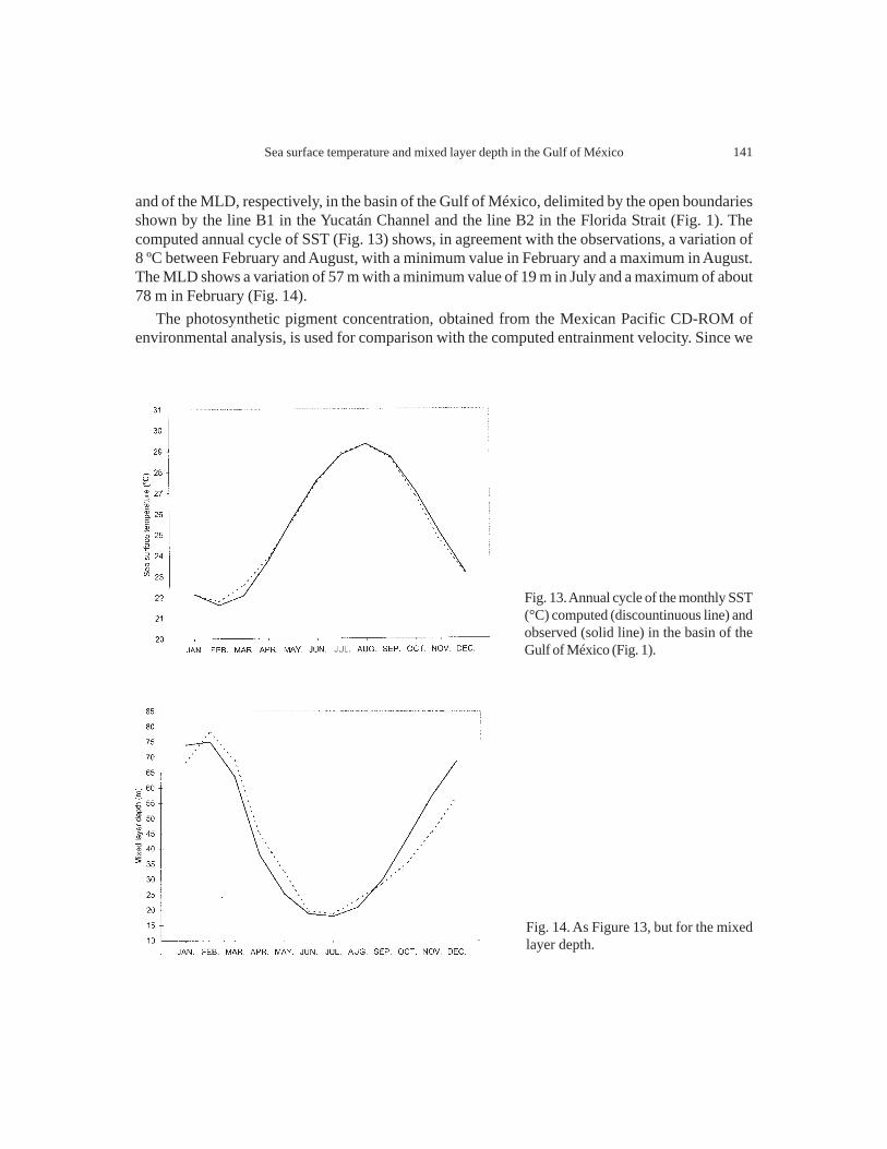
3.2 The annual cycle of the SST, the MLD and the entrainment velocityNext we will show the annual cycle of the SST, MLD and entrainment velocity using spatial averagesmonth to month. Figures 13 and 14 show the computed and the observed annual cycle of the SST

Fig. 12. As Figure 11, but for the mixed layer depth.

Fig. 11. Difference (°C) between the temperature computed taking into account the Ekman pumpingvelocity and the temperature computed without taking into account the Ekman pumping velocity,

for January (A) and for July (B).


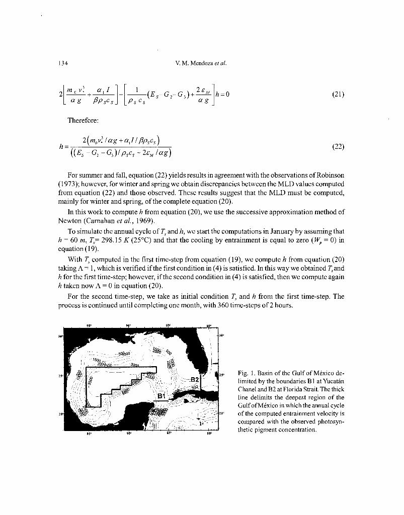
and of the MLD, respectively, in the basin of the Gulf of México, delimited by the open boundariesshown by the line B1 in the Yucatán Channel and the line B2 in the Florida Strait (Fig. 1). Thecomputed annual cycle of SST (Fig. 13) shows, in agreement with the observations, a variation of8 ºC between February and August, with a minimum value in February and a maximum in August.The MLD shows a variation of 57 m with a minimum value of 19 m in July and a maximum of about78 m in February (Fig. 14).

The photosynthetic pigment concentration, obtained from the Mexican Pacific CD-ROM ofenvironmental analysis, is used for comparison with the computed entrainment velocity. Since we

Fig. 13. Annual cycle of the monthly SST(°C) computed (discountinuous line) andobserved (solid line) in the basin of theGulf of México (Fig. 1).

Fig. 14. As Figure 13, but for the mixedlayer depth.


did not take into account the photosynthetic pigment concentration due to the rivers and lagoons,this comparison is carried out in the deepest closed region of the Gulf of México delimited by thepolygon shown in Figure 1.

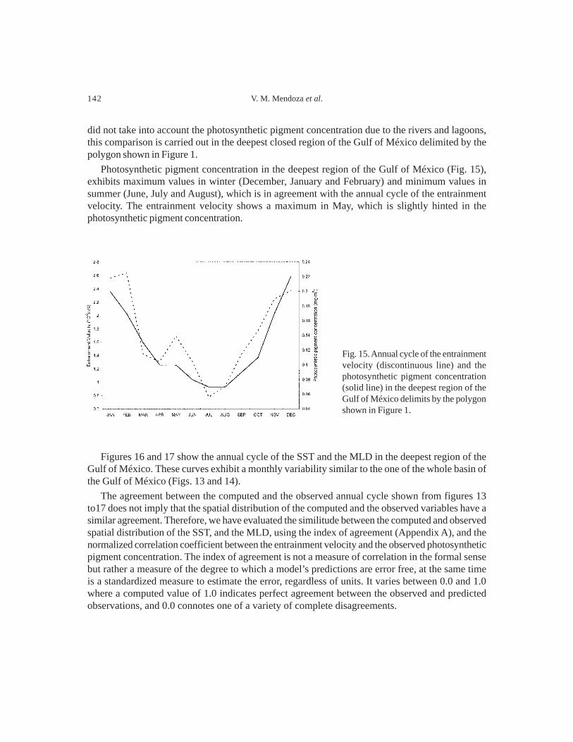
Photosynthetic pigment concentration in the deepest region of the Gulf of México (Fig. 15),exhibits maximum values in winter (December, January and February) and minimum values insummer (June, July and August), which is in agreement with the annual cycle of the entrainmentvelocity. The entrainment velocity shows a maximum in May, which is slightly hinted in thephotosynthetic pigment concentration.

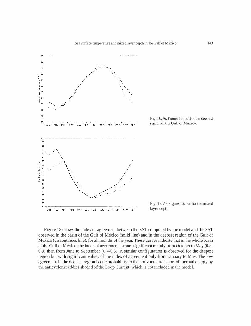
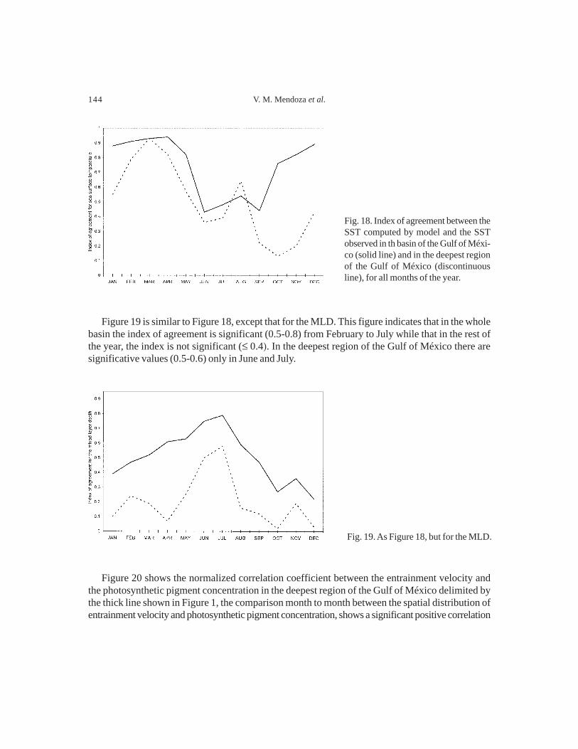
Figures 16 and 17 show the annual cycle of the SST and the MLD in the deepest region of theGulf of México. These curves exhibit a monthly variability similar to the one of the whole basin ofthe Gulf of México (Figs. 13 and 14).

The agreement between the computed and the observed annual cycle shown from figures 13to17 does not imply that the spatial distribution of the computed and the observed variables have asimilar agreement. Therefore, we have evaluated the similitude between the computed and observedspatial distribution of the SST, and the MLD, using the index of agreement (Appendix A), and thenormalized correlation coefficient between the entrainment velocity and the observed photosyntheticpigment concentration. The index of agreement is not a measure of correlation in the formal sensebut rather a measure of the degree to which a model’s predictions are error free, at the same timeis a standardized measure to estimate the error, regardless of units. It varies between 0.0 and 1.0where a computed value of 1.0 indicates perfect agreement between the observed and predictedobservations, and 0.0 connotes one of a variety of complete disagreements.

Fig. 15. Annual cycle of the entrainmentvelocity (discontinuous line) and thephotosynthetic pigment concentration(solid line) in the deepest region of theGulf of México delimits by the polygonshown in Figure 1.


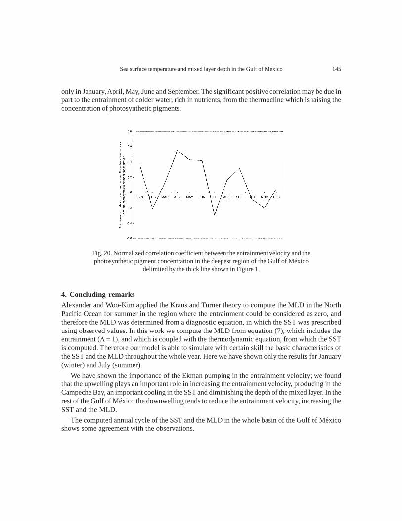
Figure 18 shows the index of agreement between the SST computed by the model and the SSTobserved in the basin of the Gulf of México (solid line) and in the deepest region of the Gulf ofMéxico (discontinues line), for all months of the year. These curves indicate that in the whole basinof the Gulf of México, the index of agreement is more significant mainly from October to May (0.8-0.9) than from June to September (0.4-0.5). A similar configuration is observed for the deepestregion but with significant values of the index of agreement only from January to May. The lowagreement in the deepest region is due probability to the horizontal transport of thermal energy bythe anticyclonic eddies shaded of the Loop Current, which is not included in the model.

Fig. 16. As Figure 13, but for the deepestregion of the Gulf of México.

Fig. 17. As Figure 16, but for the mixedlayer depth.


Figure 19 is similar to Figure 18, except that for the MLD. This figure indicates that in the wholebasin the index of agreement is significant (0.5-0.8) from February to July while that in the rest ofthe year, the index is not significant (≤ 0.4). In the deepest region of the Gulf of México there aresignificative values (0.5-0.6) only in June and July.

Fig. 18. Index of agreement between theSST computed by model and the SSTobserved in th basin of the Gulf of Méxi-co (solid line) and in the deepest regionof the Gulf of México (discontinuousline), for all months of the year.

Fig. 19. As Figure 18, but for the MLD.

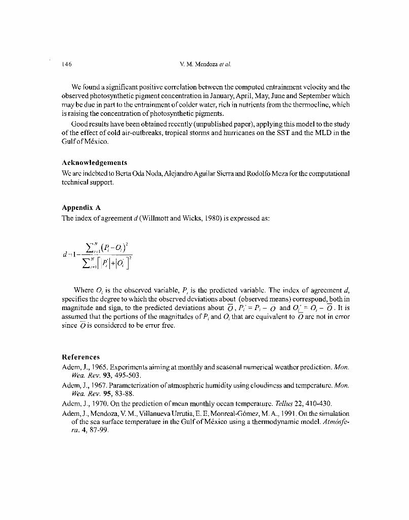
Figure 20 shows the normalized correlation coefficient between the entrainment velocity andthe photosynthetic pigment concentration in the deepest region of the Gulf of México delimited bythe thick line shown in Figure 1, the comparison month to month between the spatial distribution ofentrainment velocity and photosynthetic pigment concentration, shows a significant positive correlation


only in January, April, May, June and September. The significant positive correlation may be due inpart to the entrainment of colder water, rich in nutrients, from the thermocline which is raising theconcentration of photosynthetic pigments.

Fig. 20. Normalized correlation coefficient between the entrainment velocity and thephotosynthetic pigment concentration in the deepest region of the Gulf of México

delimited by the thick line shown in Figure 1.

4. Concluding remarksAlexander and Woo-Kim applied the Kraus and Turner theory to compute the MLD in the NorthPacific Ocean for summer in the region where the entrainment could be considered as zero, andtherefore the MLD was determined from a diagnostic equation, in which the SST was prescribedusing observed values. In this work we compute the MLD from equation (7), which includes theentrainment (Λ = 1), and which is coupled with the thermodynamic equation, from which the SSTis computed. Therefore our model is able to simulate with certain skill the basic characteristics ofthe SST and the MLD throughout the whole year. Here we have shown only the results for January(winter) and July (summer).

We have shown the importance of the Ekman pumping in the entrainment velocity; we foundthat the upwelling plays an important role in increasing the entrainment velocity, producing in theCampeche Bay, an important cooling in the SST and diminishing the depth of the mixed layer. In therest of the Gulf of México the downwelling tends to reduce the entrainment velocity, increasing theSST and the MLD.

The computed annual cycle of the SST and the MLD in the whole basin of the Gulf of Méxicoshows some agreement with the observations.


Adem, J., Villanueva, E. E., Mendoza, V. M., 1993. A new method for estimating the seasonal cycleof the heat balance at the ocean surface, with application to the Gulf of México. Geofís. Int. 32,21-34.

Adem, J., Villanueva, E. E., Mendoza, V. M., 1994. Preliminary experiments in the prediction of seasurface temperature anomalies in the Gulf of México. Geofís. Int. 33, 511-521.

Alexander, M. A., 1992. Midlatitude atmosphere-ocean interaction during El Niño. Part I: TheNorth Pacific Ocean. J. Climate, 944-958.

Alexander, R. C., Jeong-Woo Kim, 1976. Diagnostic model study of mixed-layer depths in thesummer North Pacific. J. Phys. Ocean. 6, 293-298.

Bender, M.A. and Ginis, I., 2000. Real-case simulation of hurricane-ocean interaction using a high-resolution coupled model: effects on hurricane intensity. Mon. Wea. Rev. 128, 917-946.

Blumberg, A. F. and Mellor G. L., 1983. Diagnostic and prognostic numerical circulation studies ofthe South Atlantic Bight. J. Phys. Res. 88, C8, 4579-4592.

Budyko, M. I., 1974. Climate and Life. International Geophysics Series, 18, Academic Press,New York. 508 pp.

Carnahan, B., Luther, H. A., Wilkes, J. O., 1969. Applied Numerical Methods. John Wiley &Sons, INC. 604 pp.

Huang, J. C. K., 1978 Numerical simulation studies of oceanic anomalies in the North PacificBasin, I. The ocean model and the long-term mean state. J. Phys. Oceanogr. 8, 755-778.

Isemer, H. J., Hasse, L., 1987. The Bunker Climatic Atlas of the North Atlantic Ocean, Vol. 2.Air-Sea Interactions. Springer-Verlag, Berlin, 252 pp.

Jerlov, N. G., 1951. Optical studies of ocean water. Rept. Swed. Deep-Sea Exped., 3, 1-59.Jerlov, N. G., 1968. Optical Oceanography. Elsevier, 199 pp.Kim, J. W., 1976. A generalized bulk model of the oceanic mixed layer. J. Phys. Ocean. 686-695.Kraus, E. B., Turner, J. S., 1967. A one-dimensional model of the seasonal thermocline, II. The

general theory and its consequences. Tellus 19, 98-106.Mendoza, V. M., Villanueva, E. E., Adem, J., 1997. Numerical experiments on the prediction of the

sea surface temperature anomalies in the Gulf of México. J. Mar. Sys. 13, 83-99.Niiler, P.P., Kraus, E. B., 1977. One-dimensional models of the upper ocean. Modelling and

Prediction of the Upper Layers of the ocean. E. B. Kraus, Ed., Pergamon Press, 143-172.Price, J. F., Mooers, C. N. K., Van Leer, J. C., 1978. Observation and simulation of storm-induced

mixed layer deepening. J. Phys. Ocean.8, 582-599.Price, J. F., 1983. Internal wave wake of a moving storm. Part I: scales, energy budget and

observations. J. Phys. Ocean. 13, 949-965.Price, J. F., Weller, R. A., 1986. Diurnal cycling: observations and models of the upper ocean

response to diurnal heating, cooling and wind mixing. J. Geophys. Res. 91, C7, 8411-8427.Robinson, M. K., 1973. Atlas of monthly mean sea surface and subsurface temperature and depth

of the top of the thermocline Gulf of México and Caribbean Sea. Scripps Inst. Ocean., Univ.California, San Diego, SIO Ref. 73-8.


Willmott, C., Wicks, D. E., 1980. An empirical method for the spatial interpolation of monthlyprecipitation within California. Phys. Geogr. 1, 59-73.

Zavala-Hidalgo J., Parés-Sierra, J., Ochoa, J., 2002. Seasonal variability of the temperature andheat fluxes in the Gulf of México. Atmósfera 15, 81-104.

On the annual cycle of the sea surface temperature and the mixed layer depth in the Gulf of México

Documents