arXiv:1004.3348v1 [quant-ph] 20 Apr 2010 ON MUTUALLY UNBIASED BASES THOMAS DURT TONA Free University of Brussels, Pleinlaan 2, B-1050 Brussels, Belgium [email protected] BERTHOLD-GEORG ENGLERT Centre for Quantum Technologies, National University of Singapore 3 Science Drive 2, Singapore 117543, Singapore and Department of Physics, National University of Singapore 2 Science Drive 3, Singapore 117542, Singapore [email protected] INGEMAR BENGTSSON Stockholms Universitet, Fysikum, Alba Nova, 106 91 Stockholm, Sweden [email protected] KAROL ˙ ZYCZKOWSKI Instytut Fizyki Uniwersytetu Jagiello´ nskiego, ul. Reymonta 4, 30-059 Krak´ow, Poland and Centrum Fizyki Teoretycznej PAN, Al. Lotnik´ ow 32/44, 02-668 Warszawa, Poland [email protected] (Posted on the arXiv on 20 April 2010) Mutually unbiased bases for quantum degrees of freedom are central to all theoretical investigations and practical exploitations of complementary properties. Much is known about mutually unbiased bases, but there are also a fair number of important questions that have not been answered in full as yet. In particular, one can find maximal sets of N + 1 mutually unbiased bases in Hilbert spaces of prime-power dimension N = p m , with p prime and m a positive integer, and there is a continuum of mutually unbiased bases for a continuous degree of freedom, such as motion along a line. But not a single example of a maximal set is known if the dimension is another composite number (N =6, 10, 12,... ). In this review, we present a unified approach in which the basis states are labeled by numbers 0, 1, 2,...,N − 1 that are both elements of a Galois field and ordinary in- tegers. This dual nature permits a compact systematic construction of maximal sets of mutually unbiased bases when they are known to exist but throws no light on the open existence problem in other cases. We show how to use the thus constructed mutually un- biased bases in quantum-informatics applications, including dense coding, teleportation, entanglement swapping, covariant cloning, and state tomography, all of which rely on an explicit set of maximally entangled states (generalizations of the familiar two–q-bit Bell states) that are related to the mutually unbiased bases. There is a link to the mathematics of finite affine planes. We also exploit the one-to- one correspondence between unbiased bases and the complex Hadamard matrices that turn the bases into each other. The ultimate hope, not yet fulfilled, is that open ques- tions about mutually unbiased bases can be related to open questions about Hadamard 1

Welcome message from author
This document is posted to help you gain knowledge. Please leave a comment to let me know what you think about it! Share it to your friends and learn new things together.
Transcript
arX
iv:1
004.
3348
v1 [
quan
t-ph
] 2
0 A
pr 2
010 ON MUTUALLY UNBIASED BASES
THOMAS DURT
TONA Free University of Brussels, Pleinlaan 2, B-1050 Brussels, Belgium
BERTHOLD-GEORG ENGLERT
Centre for Quantum Technologies, National University of Singapore3 Science Drive 2, Singapore 117543, Singapore
and Department of Physics, National University of Singapore2 Science Drive 3, Singapore 117542, Singapore
INGEMAR BENGTSSON
Stockholms Universitet, Fysikum, Alba Nova, 106 91 Stockholm, Sweden
KAROL ZYCZKOWSKI
Instytut Fizyki Uniwersytetu Jagiellonskiego, ul. Reymonta 4, 30-059 Krakow, Polandand Centrum Fizyki Teoretycznej PAN, Al. Lotnikow 32/44, 02-668 Warszawa, Poland
(Posted on the arXiv on 20 April 2010)
Mutually unbiased bases for quantum degrees of freedom are central to all theoreticalinvestigations and practical exploitations of complementary properties. Much is knownabout mutually unbiased bases, but there are also a fair number of important questionsthat have not been answered in full as yet. In particular, one can find maximal sets ofN + 1 mutually unbiased bases in Hilbert spaces of prime-power dimension N = pm, withp prime and m a positive integer, and there is a continuum of mutually unbiased bases fora continuous degree of freedom, such as motion along a line. But not a single example of amaximal set is known if the dimension is another composite number (N = 6, 10, 12, . . . ).
In this review, we present a unified approach in which the basis states are labeledby numbers 0, 1, 2, . . . , N − 1 that are both elements of a Galois field and ordinary in-tegers. This dual nature permits a compact systematic construction of maximal sets ofmutually unbiased bases when they are known to exist but throws no light on the openexistence problem in other cases. We show how to use the thus constructed mutually un-biased bases in quantum-informatics applications, including dense coding, teleportation,entanglement swapping, covariant cloning, and state tomography, all of which rely onan explicit set of maximally entangled states (generalizations of the familiar two–q-bitBell states) that are related to the mutually unbiased bases.
There is a link to the mathematics of finite affine planes. We also exploit the one-to-one correspondence between unbiased bases and the complex Hadamard matrices thatturn the bases into each other. The ultimate hope, not yet fulfilled, is that open ques-tions about mutually unbiased bases can be related to open questions about Hadamard
1
2 T. Durt, B.-G. Englert, I. Bengtsson, and K. Zyczkowski
matrices or affine planes, in particular the notorious existence problem for dimensionsthat are not a power of a prime.
The Hadamard-matrix approach is instrumental in the very recent advance, surveyedhere, of our understanding of the N = 6 situation. All evidence indicates that a maximalset of seven mutually unbiased bases does not exist — one can find no more than threepairwise unbiased bases — although there is currently no clear-cut demonstration of thecase.
Keywords: Mutually unbiased bases, complex Hadamard matrices, generalized Bell
states
Contents
Acronyms . . . . . . . . . . . . . . . . . . . . . . . . . . . . . . . . . . . . . . 3
Introduction . . . . . . . . . . . . . . . . . . . . . . . . . . . . . . . . . . . . 3
1 Elements of quantum kinematics . . . . . . . . . . . . . . . . . . . . . . . . 6
1.1 The Weyl–Schwinger legacy . . . . . . . . . . . . . . . . . . . . . . . . 6
1.1.1 Complementary observables and mutually unbiased bases . . . . 6
1.1.2 Existence of a basic pair of complementary observables . . . . . 8
1.1.3 Algebraic completeness of the basic pair of operators . . . . . . 9
1.1.4 The Heisenberg–Weyl group; the Clifford group . . . . . . . . . 10
1.1.5 Composite degrees of freedom . . . . . . . . . . . . . . . . . . . 11
1.1.6 Prime degrees of freedom . . . . . . . . . . . . . . . . . . . . . . 12
1.1.7 The continuous limit of N →∞ . . . . . . . . . . . . . . . . . . 14
1.1.8 Continuous degree of freedom 1: Motion along a line . . . . . . 16
1.1.9 Continuous degree of freedom 2: Motion along a circle . . . . . 19
1.1.10 Continuous degree of freedom 3: Radial motion . . . . . . . . . 20
1.1.11 Continuous degree of freedom 4: Motion within a segment . . . 22
1.2 A geometrically motivated measure of mutual unbiasedness . . . . . . 23
2 Construction of mutually unbiased bases in prime power dimensions . . . . 26
2.1 Galois fields . . . . . . . . . . . . . . . . . . . . . . . . . . . . . . . . . 26
2.2 The computational basis . . . . . . . . . . . . . . . . . . . . . . . . . . 31
2.3 The dual basis . . . . . . . . . . . . . . . . . . . . . . . . . . . . . . . 32
2.4 Construction of the remaining N -1 mutually unbiased bases . . . . . . 35
2.4.1 Heisenberg–Weyl group . . . . . . . . . . . . . . . . . . . . . . . 35
2.4.2 Abelian subgroups . . . . . . . . . . . . . . . . . . . . . . . . . 37
2.4.3 The remaining N − 1 bases . . . . . . . . . . . . . . . . . . . . . 41
2.5 Complementary period-N observables . . . . . . . . . . . . . . . . . . 42
3 Generalized Bell states and their applications . . . . . . . . . . . . . . . . . 43
3.1 Generalized Bell states . . . . . . . . . . . . . . . . . . . . . . . . . . . 43
3.2 Quantum dense coding . . . . . . . . . . . . . . . . . . . . . . . . . . . 47
3.3 Quantum teleportation . . . . . . . . . . . . . . . . . . . . . . . . . . . 47
3.4 Quantum cryptography, covariant cloning machines, and error operators 48
3.5 Entanglement swapping . . . . . . . . . . . . . . . . . . . . . . . . . . 52
4 The Mean King’s problem and quantum state tomography . . . . . . . . . 52

On mutually unbiased bases 3
4.1 The Mean King’s problem in prime power dimensions . . . . . . . . . 52
4.2 State tomography with discrete Weyl and Wigner phase-space functions 55
4.2.1 Discrete Weyl-type unitary operator basis and phase-space func-
tion . . . . . . . . . . . . . . . . . . . . . . . . . . . . . . . . . . 56
4.2.2 The limit N →∞ of continuous degrees of freedom . . . . . . . 58
4.2.3 Discrete Wigner-type hermitian operator basis and phase-space
function . . . . . . . . . . . . . . . . . . . . . . . . . . . . . . . 58
4.2.4 Covariance of the Wigner-type basis . . . . . . . . . . . . . . . 66
4.3 Mutually unbiased bases and finite affine planes . . . . . . . . . . . . . 67
5 Mutually unbiased Hadamard matrices . . . . . . . . . . . . . . . . . . . . 72
5.1 Pairs of mutually unbiased bases and Hadamard matrices . . . . . . . 72
5.2 Triplets of mutually unbiased bases and circulant matrices . . . . . . . 74
5.3 Classification of Hadamard matrices of size N ≤ 5 . . . . . . . . . . . 76
5.4 Affine families and tensor products . . . . . . . . . . . . . . . . . . . . 77
5.5 Hadamard matrices of size N = 6 . . . . . . . . . . . . . . . . . . . . . 78
5.6 Hadamard matrices for N ≥ 7 . . . . . . . . . . . . . . . . . . . . . . . 83
5.7 All mutually unbiased bases for N ≤ 5 . . . . . . . . . . . . . . . . . . 83
5.8 Triplets of mutually unbiased bases in dimension 6 . . . . . . . . . . . 86
5.9 A maximal set of mutually unbiased bases when N = 6? . . . . . . . . 87
5.10 Heisenberg–Weyl group approach for N = 6 . . . . . . . . . . . . . . . 88
6 Brief summary and concluding remarks . . . . . . . . . . . . . . . . . . . . 89
Acknowledgments . . . . . . . . . . . . . . . . . . . . . . . . . . . . . . . . . 92
Appendix A Generalized position and momentum operators for spherical co-
ordinates . . . . . . . . . . . . . . . . . . . . . . . . . . . . . . . 92
Appendix B Standard sets of mutually unbiased Hadamard matrices for
prime dimension . . . . . . . . . . . . . . . . . . . . . . . . . . 93
Appendix C A prime-distinguishing function . . . . . . . . . . . . . . . . . . 94
Appendix D Mutually unbiased bases for N = 4 . . . . . . . . . . . . . . . . 100
References . . . . . . . . . . . . . . . . . . . . . . . . . . . . . . . . . . . . . . 101
Acronyms
MU mutually unbiased
MUB mutually unbiased bases
MUHM mutually unbiased Hadamard matrices
POVM positive operator valued measure
SIC symmetric informationally complete
Introduction
Two orthonormal bases of a Hilbert space are said to be mutually unbiased (MU)
if the transition probabilities from each state in one basis to all states of the other
basis are the same irrespective of which pair of states is chosen. Put differently,
if the physical system is prepared in a state of the first basis, then all outcomes
4 T. Durt, B.-G. Englert, I. Bengtsson, and K. Zyczkowski
are equally probable when we conduct a measurement that probes for the states
of the second basis. This situation is symmetrical, it does not matter from which
of the two bases we choose the prepared state and which is the other basis that is
measured: Unbiasedness of bases is a mutual property, possessed jointly by both
bases. Familiar examples are the bases of position and momentum eigenstates for
a particle moving along a line, and the spin states of a spin- 12 particle for two
perpendicular directions.
When the Hilbert space dimension N is a prime power, N = pm, there exist
sets of N + 1 mutually unbiased bases (MUB). These sets are maximal in the sense
that it is not possible to find more than N + 1 MUB in any N -dimensional Hilbert
space, there is simply no room for the (N + 2)th basis. Such a maximal set of MUB
is also complete because when we know all the probabilities of transition of a given
quantum state towards the states of the bases of this set — exceptional situations
aside, there are (N + 1)(N − 1) = N2 − 1 independent probabilities — we can
reconstruct the statistical operator that characterizes this quantum state; in other
words we can perform full tomography or complete quantum state determination.
The existence of a maximal set of MUB for N = pm is demonstrated by an
explicit construction, not by an abstract existence proof. Various methods have
been used for the construction of maximal sets of MUB, including the Galois–
Fourier approach of this review. Other constructions are based on generalized Pauli
matrices, discrete Wigner functions, abelian subgroups, mutually orthogonal Latin
squares, and finite-geometry methods.
All known constructions rely on the fact that N is the power of a prime and,
therefore, they say nothing about other dimensions, of which N = 6 is the smallest
one and also the one that has been studied most intensely. At present, there is
a widely shared conviction that one cannot have a maximal set of seven MUB
for N = 6 and that the largest sets of MUB have no more than three bases. This
conviction is strongly founded in a solid body of evidence but, strictly speaking, it
is an unproven conjecture.
This situation is reminiscent of seemingly similar existence questions about finite
affine planes, Graeco-Latin squares, and related geometrical structures where prime-
power dimensions also play a privileged role. As suggestive as these similarities may
be, there is, however, no known connection as yet between the two kinds of existence
problems.
There is a plethora of applications whenever maximal sets of MUB are available,
in particular when the physical system is composed of many q-bits (N = 2m), the
building blocks of devices for quantum information processing. Not surprisingly,
then, the rise of quantum information science has triggered fresh interest in MUB
and, as a consequence, our knowledge about MUB and their applications is much
richer now. But the various facts are scattered over a large number of publications,
and the many pieces of the puzzle do not readily fit together and do not compose
a uniform picture.
We are here reviewing the state of affairs in an attempt to offer a unified view,
On mutually unbiased bases 5
with emphasis on both the structural properties of MUB and their use in quantum-
information applications. As in all constructions of MUB in prime power dimension,
a crucial element is a finite commutative division ring — a Galois field of N ele-
ments.a Finite fields with N elements exist if and only if N is a power of a prime,
and the mathematical properties of Galois fields are exploited in all constructions
of maximal sets of MUB. Modifications of these constructions in the absence of a
finite field do not yield maximal sets of MUB for other dimensions.
The paper is structured as follows. We begin with a brief survey of elements
of quantum kinematics in Sec. 1. The legacy of Weyl and Schwinger: the notion of
complementary observables and their algebraic completeness, the MUB associated
with them, and the N →∞ limit of continuous degrees of freedom — all these
are central to the story told in Sec. 1.1. It is supplemented by remarks on the
Heisenberg–Weyl group of unitary operators and the related Clifford group as well
as, in Sec. 1.2, a geometrically motivated “measure of unbiasedness” of two bases,
a distance in a real euclidean vector space.
Section 2 deals with the construction of a maximal set of MUB in prime power di-
mension, N = pm, systematically treated as a composite system of m p-dimensional
subsystems. For the purpose of introducing some notational conventions, but also
for the benefit of the typical working physicist for whom Galois fields are hardly the
daily bread, we recall the most important and most relevant properties of Galois
fields in Sec. 2.1. We are making extensive use of a formalism in which the num-
bers 0, 1, 2, . . . , N − 1 play a dual role — they are elements of a Galois field, but
also ordinary integers. This somewhat unconventional approach enables us to give
a compact, transparent construction of a maximal set of MUB in Sec. 2.2–2.4. A
fitting version of the discrete Heisenberg–Weyl group, also known as the general-
ized Pauli group, is an important tool for the construction; its abelian subgroups
define the MUB. In passing, we establish the contact between these MUB and the
complementary observables of the Weyl–Schwinger methodology (Sec. 2.5).
The survey of applications of the maximal set of MUB in Sec. 3 begins with the
construction of a complete set of maximally entangled states, the analogs of the
familiar Bell states of two–q-bit systems, in Sec. 3.1. After brief accounts of their
use for quantum dense coding (Sec. 3.2) and teleportation (Sec. 3.3), we discuss
in Sec. 3.4 how the generalized Bell states facilitate quantum cryptography and
eavesdropping with the aid of covariant cloning machines and comment on the role
of the Heisenberg–Weyl operators in error correction. Section 3 closes with a brief
discussion of entanglement swapping (Sec. 3.5).
The prime-power version of the so-called Mean King’s problem (Sec. 4.1) opens
the section on quantum state tomography. The Mean King’s problem is, in fact, very
aA ring is a set that is closed under two operations: addition and multiplication. They obey theusual rules, associativity and commutativity of both operations, the distributive law, existence ofa unique neutral element 0 for the addition and a neutral element 1 for the multiplication. A field,or division ring, is a ring with multiplicative inverses for every nonzero element.
6 T. Durt, B.-G. Englert, I. Bengtsson, and K. Zyczkowski
closely related to the discrete analog of Wigner’s continuous phase space function
which — jointly with its Fourier partner, the analog of Weyl’s characteristic function
— is the subject matter of Sec. 4.2. We comment on the covariance of the Wigner-
type operator basis and discuss the N →∞ limit of continuous degrees of freedom.
The relation to finite affine planes in Sec. 4.3 provides further insights into the
underlying geometry.
Section 5 is devoted to the matrices that transform pairs of MUB into each
other: the complex Hadamard matrices. Pairs of bases may be equivalent or not, in
the sense that one can map the basis states of one pair on those of the other pair
by a unitary transformation in conjunction with permutations of the basis states
(Sec. 5.1). The equivalence of triplets of MUB is more difficult to check (Sec. 5.2).
Mutually unbiased Hadamard matrices (MUHM) are encountered when there are
more than two MUB. Accordingly, one can investigate sets of MUB by studying
the corresponding sets of MUHM, and vice versa. All Hadamard matrices of size
N ≤ 5 have been classified (Sec. 5.3), and all sets of MUB are known for N < 6
(Sec. 5.7). The situation is not so clear, and thus more interesting, for N = 6; we
report what is known about the families of 6× 6 Hadamard matrices in Sec. 5.5,
after a general discussion of affine families and tensor products in Sec. 5.4, and we
deal with MUB for N = 6 in Secs. 5.8–5.10. Hadamard matrices for N > 6 get their
share of attention in Sec. 5.6.
We close with a brief summary and concluding remarks (Sec. 6) and provide
some additional technical details in three appendixes. The standard set of MUHM
for prime dimension is given in Appendix B, and a prime-distinguishing function
related to this standard set is introduced in Appendix C. Finally, Appendix D deals
with MUB for the two–q-bit case of N = 4.
1. Elements of quantum kinematics
1.1. The Weyl–Schwinger legacy
1.1.1. Complementary observables and mutually unbiased bases
As emphasized by Bohr in his 1927 Como lecture,1 quantum systems have properties
that are complementary: equally real but mutually exclusive. If one such property is
known accurately, then the complementary property is completely unknown. Here,
“known accurately” means that the outcome of a measurement can be predicted
with certainty, whereas “completely unknown” means that all outcomes are equally
likely — the two properties are maximally incompatible. Familiar examples are the
position and momentum of a particle moving along a line, and the x and z spin
components of a spin- 12 object. These are, in fact, the extreme cases of a continuous
degree of freedom and a binary degree of freedom — the latter being the “q-bit” of
recent quantum information terminology.
Intermediate are “q-nits,” N -dimensional quantum degrees of freedom (N > 1),
for which the measurement of a physical property can have at most N exclusive
On mutually unbiased bases 7
outcomes. Following Weyl2, 3 and Schwinger,4–6 we call a pair of observables, A and
B, complementary if their eigenvalues are not degenerate (there is the full count
of N different possible measurement results) and the sets of normalized kets |aj〉and |bk〉 that describe states with predictable measurement outcomes for A and B,
respectively, are MU,
∣∣〈aj |bk〉∣∣2 =
1
Nfor all j, k = 0, 1, . . . , N − 1 . (1.1)
The important detail is not the value on the right, which is implied by the normal-
ization to unit total probability, but that the transition probabilities on the left do
not depend on the quantum numbers aj and bk.b
Technically speaking, A and B are normal operatorsc and |aj〉, |bk〉 are their
eigenkets, which make up two bases that are orthonormal and complete,
〈aj |ak〉 = δj,k = 〈bj |bk〉 ,N−1∑
j=0
|aj〉〈aj | = 1 =N−1∑
k=0
|bk〉〈bk| , (1.2)
where 1 is the identity operator. We recognize that the complementarity of A and
B is in fact a property of their respective eigenket bases. The particular eigenvalues
are irrelevant, we just need to know that they are not degenerate. It follows in
particular that, if A and B are complementary, then αA and βB with αβ 6= 0 are
complementary as well. And if a unitary transformation turns A into A′ and B
into B′, then the pair A′, B′ is complementary if the pair A,B is. Therefore, we
can shift the focus from the pair A,B of complementary observables to the pair
|aj〉, |bk〉 of MUB.
Whenever is it expedient to be specific about the observables associated with
a basis, we will follow the guidance of Weyl and Schwingerd and choose unitary
operators to represent physical quantities. In the present context, these will be
nondegenerate cyclic operators with period N ,
AN = 1 , BN = 1 , (1.3)
with products of fewer than N factors not equaling the identity. The eigenvalues of
A and B are then the N different Nth roots of unity,
A|aj〉 = |aj〉γjN , B|bk〉 = |bk〉γkN with γN = ei2π/N . (1.4)
That these cyclic operators are a pair of complementary operators can be stated as
1
NtrAmBn
= δm,0δn,0 for m,n = 0, 1, . . . , N − 1 , (1.5)
which is the operator version of (1.1). Indeed, (1.1) and (1.5) imply each other.8
bIn fact, there can be different right-hand sides for infinite degrees of freedom, when normalizationis more subtle; see Secs. 1.1.8–1.1.11. We will mostly deal with finite degrees of freedom.cA normal operator A commutes with its adjoint A†: AA† = A†A, and can be regarded either asa function of a more fundamental hermitian operator or as a function of a unitary operator.dA brief account of the history of the subject can be found in Ref. 7.
8 T. Durt, B.-G. Englert, I. Bengtsson, and K. Zyczkowski
1.1.2. Existence of a basic pair of complementary observables
The first question we address is whether there always is a pair of complementary
observables for each quantum degree of freedom. The affirmative answer begins
with selecting an orthonormal reference basis |0〉, |1〉, . . . , |N − 1〉 — we will refer
to it as the computational basis from Sec. 2.2 onwards. Then we define a second
orthonormal basis |0〉, |1〉, . . . , |N − 1〉 by means of the discrete quantum Fourier
transformation,
|j〉 = 1√N
N−1∑
k=0
|k〉γ−jkN , (1.6)
so that
〈j|k〉 = 1√NγjkN for j, k = 0, 1, . . . , N − 1 (1.7)
by construction — the two bases are MU, indeed.
In analogy with the Pauli operators σx and σz , we introduce the cyclic operators
X and Z in accordance with
X |j〉 = |j〉γjN , XN = 1 and Z|k〉 = |k〉γkN , ZN = 1 . (1.8)
As an immediate consequence of (1.7), we note that X and Z are unitary shift
operators that permute the kets or bras of the respective other basis cyclically,
X |k〉 = |k + 1〉 for k = 0, 1, . . . , N − 2 , X |N − 1〉 = |0〉 (1.9)
as well as
〈j|Z = 〈j + 1| for j = 0, 1, . . . , N − 2 , 〈N − 1|Z = 〈0| , (1.10)
and (1.5) holds for (A,B) = (X,Z), as it must. The fundamental Weyl commu-
tation rule ZX = γNXZ follows. It is the analog of the familiar N = 2 identity
σzσx = −σxσz and is more generally, and more usefully, stated as
XmZn = γ−mnN ZnXm , (1.11)
valid for all integer values of m and n, both positive and negative.
When we change the kets of the reference basis by phase factors, |k〉 → |k〉eiφk ,
the resulting second basis will change accordingly and we get another complemen-
tary partnerX to the same observable Z. This freedom to adjust phases that do not
affect the projectors |k〉〈k| of the reference basis but modify the projectors |j〉〈j|of the Fourier transformed basis is crucial for quantifying Einstein’s9, 10 and de
Broglie’s11 wave-particle duality in the context of two-path12, 13 and multi-path14
interferometers.
On mutually unbiased bases 9
1.1.3. Algebraic completeness of the basic pair of operators
The second question, which also has an affirmative answer, is whether the pair X,Z
of complementary observables parameterizes the degree of freedom completely. Put
differently: Are all other operators functions of X and Z?
As a first step, we observe that the projectors onto the respective eigenstates
are polynomials of X or Z,
δX,γj
N= |j〉〈j| = 1
N
N−1∑
n=0
(γ−jN X
)n,
δZ,γkN= |k〉〈k| = 1
N
N−1∑
m=0
(γ−kN Z
)m, (1.12)
where the Kronecker delta symbols are to be understood in the usual sense of an
operator function, as exemplified by
f(Z) =
N−1∑
k=0
|k〉f(γkN)〈k| . (1.13)
The second step in writing an arbitrary operator F as a function of X and Z is to
exploit the completeness of the two bases,
F =∑
j,k
|j〉〈j|F |k〉〈k| =∑
j,k
δX,γj
Nfj,kδZ,γk
Nwith fj,k =
〈j|F |k〉〈j|k〉
, (1.14)
where the denominator is assuredly nonvanishing.e This answers the second question
by giving an explicit expression for F as a polynomial of X and Z, here written
in a unique way as an XZ-ordered function: In products, all X operators stand
to the left of all Z operators. Of course, quite analogously, we can also write F
in a unique ZX-ordered form — as an example recall the equivalence of the XZ-
ordered operator on the left of (1.11) with the ZX-ordered product on the right. In
summary, there is not just one function of X and Z that equals the given operator
F , there are many such functions.
The lesson of these considerations is that the pairX,Z is algebraically complete,
there are no operators that are not linear combinations of products of powers of
X and Z. Accordingly, we can phrase Bohr’s Principle of Complementarity, the
fundamental principle of quantum kinematics, in the following technical terms:
For each degree of freedom the dynamical variables are a pair of complementary
observables.16 For a textbook discussion, see Ref. 17.
eNumbers of the form of fj,k are known as “weak values” of F in the context of “weak measure-ments.”15
10 T. Durt, B.-G. Englert, I. Bengtsson, and K. Zyczkowski
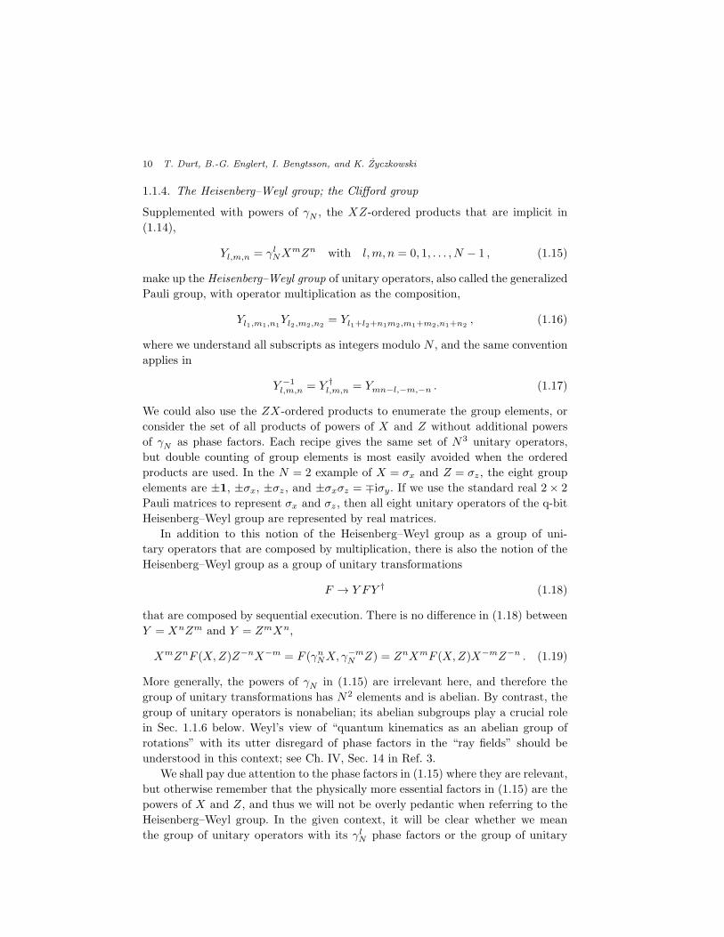
1.1.4. The Heisenberg–Weyl group; the Clifford group
Supplemented with powers of γN , the XZ-ordered products that are implicit in
(1.14),
Yl,m,n = γlNXmZn with l,m, n = 0, 1, . . . , N − 1 , (1.15)
make up the Heisenberg–Weyl group of unitary operators, also called the generalized
Pauli group, with operator multiplication as the composition,
Yl1,m1,n1Yl2,m2,n2
= Yl1+l2+n1m2,m1+m2,n1+n2, (1.16)
where we understand all subscripts as integers modulo N , and the same convention
applies in
Y −1l,m,n = Y †
l,m,n = Ymn−l,−m,−n . (1.17)
We could also use the ZX-ordered products to enumerate the group elements, or
consider the set of all products of powers of X and Z without additional powers
of γN as phase factors. Each recipe gives the same set of N3 unitary operators,
but double counting of group elements is most easily avoided when the ordered
products are used. In the N = 2 example of X = σx and Z = σz , the eight group
elements are ±1, ±σx, ±σz , and ±σxσz = ∓iσy. If we use the standard real 2× 2
Pauli matrices to represent σx and σz , then all eight unitary operators of the q-bit
Heisenberg–Weyl group are represented by real matrices.
In addition to this notion of the Heisenberg–Weyl group as a group of uni-
tary operators that are composed by multiplication, there is also the notion of the
Heisenberg–Weyl group as a group of unitary transformations
F → Y FY † (1.18)
that are composed by sequential execution. There is no difference in (1.18) between
Y = XnZm and Y = ZmXn,
XmZnF (X,Z)Z−nX−m = F (γnNX, γ−mN Z) = ZnXmF (X,Z)X−mZ−n . (1.19)
More generally, the powers of γN in (1.15) are irrelevant here, and therefore the
group of unitary transformations has N2 elements and is abelian. By contrast, the
group of unitary operators is nonabelian; its abelian subgroups play a crucial role
in Sec. 1.1.6 below. Weyl’s view of “quantum kinematics as an abelian group of
rotations” with its utter disregard of phase factors in the “ray fields” should be
understood in this context; see Ch. IV, Sec. 14 in Ref. 3.
We shall pay due attention to the phase factors in (1.15) where they are relevant,
but otherwise remember that the physically more essential factors in (1.15) are the
powers of X and Z, and thus we will not be overly pedantic when referring to the
Heisenberg–Weyl group. In the given context, it will be clear whether we mean
the group of unitary operators with its γlN phase factors or the group of unitary

On mutually unbiased bases 11
transformations. An example is the observation that the Nth power of Yl,m,n can
differ from the identity operator,
(Yl,m,n
)N=
1 if N is odd,
(−1)mn1 if N is even.(1.20)
For the group of unitary operators, the appearance of (−1)mn is crucial, telling us
that one quarter of the Yl,m,n have period 2N for even N , whereas this is of no
concern for the group of unitary transformations. As an example, consider once
more the N = 2 situation with X = σx and Z = σz, for which
(σxσz)2 = −1 , (σxσz)
2F (σx, σz)(σxσz)2 = F (σx, σz) . (1.21)
The unitary operators C that map the Heisenberg–Weyl group onto itself un-
der conjugation,f that is: Yl,m,n → CYl,m,nC† equals one of the Yl,m,ns, constitute
the so-called Clifford group.18–21 It contains the Heisenberg–Weyl group as a sub-
group, but is truly larger. For N = 2, the Clifford group contains 24 unitary trans-
formations (and is isomorphic to the symmetry group of the cube) whereas the
Heisenberg–Weyl group contains only four unitary transformations. An example of
a transformation belonging to the former but not the latter is the “q-bit Hadamard
gate” (σx + σz)/√2 that is represented by the familiar Hadamard matrix
H =1√2
(1 1
1 −1
), (1.22)
if we use the standard 2× 2 matrices for σx and σz.
1.1.5. Composite degrees of freedom
If N is a composite number, N = N1N2 with N1 > 1 and N2 > 1, then some of the
Heisenberg–Weyl operators have a shorter period, as exemplified by (Y0,N1,0)N2 =
(XN1)N2 = XN = 1. As a consequence, there are Heisenberg–Weyl operators that
have different spectral properties and are not related to each other by a unitary
transformation.
It is then methodical to regard the N -dimensional degree of freedom as com-
posed of a N1-dimensional and a N2-dimensional degree of freedom. Accordingly,
the labels k of the kets |k〉 of the reference basis are understood as pairs k1, k2 with
k = k1 + k2N1 whereby k1 = 0, 1, . . . , N1 − 1 and k2 = 0, 1, . . . , N2 − 1. The action
of the corresponding cyclic operators X1 and X2 is given by
X1|k〉 = X1|k1, k2〉 = |k1 + 1, k2〉 = |k + 1〉 for k1 = 0, 1, . . . , N1 − 2 ,
X2|k〉 = X2|k1, k2〉 = |k1, k2 + 1〉 = |k +N1〉 for k2 = 0, 1, . . . , N2 − 2 ,
(1.23)
fAnti-unitary operators could be, and often are, included — see Ref. 18, for example — but wehave no use for them here.
12 T. Durt, B.-G. Englert, I. Bengtsson, and K. Zyczkowski
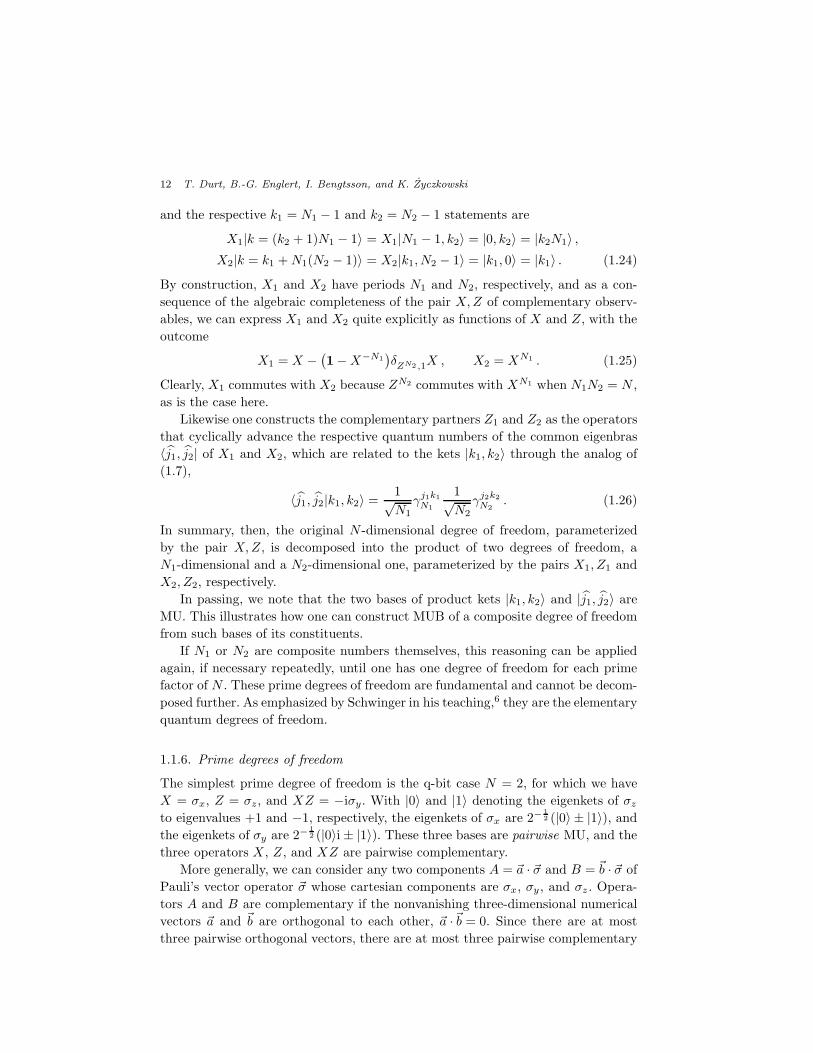
and the respective k1 = N1 − 1 and k2 = N2 − 1 statements are
X1|k = (k2 + 1)N1 − 1〉 = X1|N1 − 1, k2〉 = |0, k2〉 = |k2N1〉 ,X2|k = k1 +N1(N2 − 1)〉 = X2|k1, N2 − 1〉 = |k1, 0〉 = |k1〉 . (1.24)
By construction, X1 and X2 have periods N1 and N2, respectively, and as a con-
sequence of the algebraic completeness of the pair X,Z of complementary observ-
ables, we can express X1 and X2 quite explicitly as functions of X and Z, with the
outcome
X1 = X −(1−X−N1
)δZN2 ,1X , X2 = XN1 . (1.25)
Clearly, X1 commutes with X2 because ZN2 commutes with XN1 when N1N2 = N ,
as is the case here.
Likewise one constructs the complementary partners Z1 and Z2 as the operators
that cyclically advance the respective quantum numbers of the common eigenbras
〈j1, j2| of X1 and X2, which are related to the kets |k1, k2〉 through the analog of
(1.7),
〈j1, j2|k1, k2〉 =1√N1
γj1k1
N1
1√N2
γj2k2
N2. (1.26)
In summary, then, the original N -dimensional degree of freedom, parameterized
by the pair X,Z, is decomposed into the product of two degrees of freedom, a
N1-dimensional and a N2-dimensional one, parameterized by the pairs X1, Z1 and
X2, Z2, respectively.
In passing, we note that the two bases of product kets |k1, k2〉 and |j1, j2〉 areMU. This illustrates how one can construct MUB of a composite degree of freedom
from such bases of its constituents.
If N1 or N2 are composite numbers themselves, this reasoning can be applied
again, if necessary repeatedly, until one has one degree of freedom for each prime
factor of N . These prime degrees of freedom are fundamental and cannot be decom-
posed further. As emphasized by Schwinger in his teaching,6 they are the elementary
quantum degrees of freedom.
1.1.6. Prime degrees of freedom
The simplest prime degree of freedom is the q-bit case N = 2, for which we have
X = σx, Z = σz, and XZ = −iσy. With |0〉 and |1〉 denoting the eigenkets of σzto eigenvalues +1 and −1, respectively, the eigenkets of σx are 2−
1
2 (|0〉 ± |1〉), andthe eigenkets of σy are 2−
1
2 (|0〉i± |1〉). These three bases are pairwise MU, and the
three operators X , Z, and XZ are pairwise complementary.
More generally, we can consider any two components A = ~a · ~σ and B = ~b · ~σ of
Pauli’s vector operator ~σ whose cartesian components are σx, σy , and σz . Opera-
tors A and B are complementary if the nonvanishing three-dimensional numerical
vectors ~a and ~b are orthogonal to each other, ~a ·~b = 0. Since there are at most
three pairwise orthogonal vectors, there are at most three pairwise complementary

On mutually unbiased bases 13
operators and at most three MUB. The choice σx, σy, σz for the three operators is,
therefore, not particular, but typical.
If N is an odd prime, N = 3, 5, 7, 11, 13, . . . , then all unitary Heisenberg–Weyl
operators Yl,m,n of (1.15) are cyclic with periodN , except for the identity 1 = Y0,0,0.
Further, we observe that the N + 1 operators
X , XZ , XZ2 , . . . , XZN−1 , Z (1.27)
are pairwise complementary,8 as one verifies most directly with the aid of (1.5) and
(1.16) in conjunction with
trYl,m,n
= NγlNδm,0δn,0 . (1.28)
It follows that the N + 1 bases of eigenkets, one for each of the operators in (1.27),
are MU. In addition to the eigenbases of X and Z that we met in Sec. 1.1.2, there
are thus N − 1 more such bases.
And there cannot be a (N + 2)th basis because a counting argument shows
that one can at most have N + 1 bases that are MU.22 One way of seeing this is
presented in Sec. 1.2 below.
In this context, we note here that the powers of the operators in (1.27) make
up N + 1 abelian cyclic subgroups of the Heisenberg–Weyl group with N unitary
operators in each subgroup. Remembering that the identity is contained in each
subgroup, this gives a total count of (N + 1)(N − 1) + 1 = N2 operators, one rep-
resentative for each set of Yl,m,ns with common m,n values, that is: one count for
each XmZn product.
Explicitly, ket |i, k〉, the kth eigenket of the ith basis, XZi|i, k〉 = |i, k〉γkN , is
given by
N odd: |i, k〉 = 1√N
N−1∑
l=0
|l〉γ−klN γ
il(l−1)/2N for i = 0, 1, 2, . . . , N − 1 (1.29)
in terms of the reference basis of eigenkets of Z. For i = 0 we have the eigenstates
of X , |k〉 = |0, k〉. While (1.29) correctly states the eigenkets of XZi for all odd N ,
these bases are pairwise MU only if N is prime. With due attention to the extra
phase factors required by (1.20) one can give a similar expression for |i, k〉 when Nis even.
In summary, we can systematically construct N + 1 bases that are MU if N is
prime. As noted, the construction based on the cyclic operators in (1.27) does not
work if N is composite; try N = 4 to see what goes wrong. We return to the case
of N = 6 in Sec. 5.10, and a general discussion for arbitrary N ≥ 2 is given in
Appendix C.
Yet, this is not the end of the story. If N = pm is the power of a prime, for which
N = 8 = 23 and N = 9 = 32 are examples, it is possible to modify the construction
such that it does work in a closely analogous way. The clue is to replace the modulo-
N shifts of (1.9) and (1.10) by shifts of a Galois field arithmetic that treats the

14 T. Durt, B.-G. Englert, I. Bengtsson, and K. Zyczkowski
N -dimensional degree of freedom systematically as composed of m p-dimensional
constituents. This is the theme of Sec. 2, followed by applications in Secs. 3 and 4.
This Galois cure is, however, not available for N = 6 and N = 10 or other com-
posite N values that are not powers of a prime, simply because the number of
elements in a finite field is always a prime power. Section 5 contains a report on
what is known about these cases, in particular about N = 6. The question whether
there are seven MUB for N = 6 is currently unanswered, but there is a lot of ev-
idence, and a growing conviction in the community, that there are no more than
three such bases. And three such bases are immediately available by pairing each of
the three q-bit bases (N1 = 2) with one of the four q-trit bases (N2 = 3) to product
bases as in (1.26).
1.1.7. The continuous limit of N →∞Since composite values of N refer to composite quantum degrees of freedom, we
take the limit N → ∞ through prime values of N , thereby dealing with a single
degree of freedom of increasing complexity. The prime nature of N will not be so
crucial, however, but we make use of the fact that large primes are odd numbers and
relabel the kets of the reference basis |k〉 and the bras 〈j| of the Fourier-transformed
basis such that now j, k = 0,±1,±2, . . . ,± 12 (N − 1).
Next, we introduce a small, eventually infinitesimal, parameter ǫ by
N =2π
ǫ2(1.30)
to account for the fact that the basic unit of complex phase 2π/N gets arbitrarily
small when N → ∞. Aiming at a continuous degree of freedom in this limit, we
also relabel the states in accordance with
j −→ jǫ = a = 0,±ǫ,±2ǫ, . . . ,±(πǫ− ǫ
2
),
k −→ kǫ = b = 0,±ǫ,±2ǫ, . . . ,±(πǫ− ǫ
2
). (1.31)
The numbers a and b will cover the real axis, −∞ < a, b <∞, when N →∞, ǫ→ 0.
The unitary operatorX acting on |k〉 increases k by 1, so that it effects b→ b+ ǫ.
Likewise Z applied to 〈j| results in a→ a+ ǫ. This suggests the identification of
hermitian operators A and B such that
X = eiǫA with A = A† ,
Z = eiǫB with B = B† . (1.32)
The Weyl commutation relation (1.11) then appears as
XkZj = e−i 2πN
jkZjXk −→ eikǫAeijǫB = e−ijǫkǫeijǫBeikǫA (1.33)
or
eibAeiaB = e−iabeiaBeibA . (1.34)

On mutually unbiased bases 15
The two equivalent versions
eib(A− a1) = e−iaBeibAeiaB = eib e−iaBA eiaB ,
eia(B − b1) = eibAeiaBe−ibA = eia eibAB e−ibA
(1.35)
seem to imply that
e−iaBA eiaB = A− a1 ,eibAB e−ibA = B − b1 , (1.36)
but this does not follow without imposing a restricting condition, just as eiα = eiβ
does not imply α = β, but only that α− β is an integer multiple of 2π.
The said restriction is that, for large N , only a, b values from a finite vicinity
of 0 matter, which is to say that we break the cyclic nature of the labels a, b,
〈a|eia′B = 〈a+ a′ (mod 2π/ǫ)| , eib′A|b〉 = |b+ b′ (mod 2π/ǫ)〉 , (1.37)
and take for granted that all relevant values of a, a′ and b, b′ are such that we
stay inside the range −(π/ǫ − ǫ/2) · · · (π/ǫ − ǫ/2). Put differently, we give up the
periodicity that would force us to identify a = +∞ with a = −∞ in the ǫ→ 0 limit.
After performing the N →∞, ǫ→ 0 limit with this restriction, the statements
of (1.36) hold with continuous values for a and b. We can, therefore, exhibit the
terms that are linear in a or b and arrive at
AB −BA = [A,B] = i1 . (1.38)
We recognize, of course, Heisenberg’s commutation relation for a pair of comple-
mentary hermitian observables of a continuous degree of freedom, such as position
A and momentum B (in natural units) for the motion along a line.
These N → ∞ considerations for X and Z have to be supplemented by coun-
terparts for their respective kets and bras. We need to identify
〈a| = 1√ǫ〈j|∣∣∣∣∣ǫ→0
with jǫ = a, and |b〉 = |k〉 1√ǫ
∣∣∣∣∣ǫ→0
with kǫ = b, (1.39)
and then get
〈a|b〉 = 1√2π
eiab (1.40)
as the analog of (1.7) as well as
〈a|a′〉 = δ(a− a′) , 〈b|b′〉 = δ(b− b′) (1.41)
and∞∫
−∞
da |a〉〈a| = 1 =
∞∫
−∞
db |b〉〈b| (1.42)
as the continuum versions of the orthogonality and completeness relations in (1.2).
16 T. Durt, B.-G. Englert, I. Bengtsson, and K. Zyczkowski
This discussion of the N → ∞ limit is a variant of Schwinger’s treatment in
Sec. 1.16 of Ref. 6; see also Sec. 1.2.5 in Ref. 17. It should be appreciated that
N →∞ is not a limit in the precise sense that one has in calculus. Rather, it is a
systematic method for inferring the properties of the basic operators for continuous
degrees of freedom, but these operators then stand on their own and the consistency
of the inferred algebraic properties must be verified.
We note that, in addition to the standard symmetric limit that treats X and
Z on equal footing and results in the Heisenberg pair of A and B (position and
momentum for motion along a line), there are also asymmetric limits. For instance,
if the position variable — the analog of the hermitian A of (1.32) — is kept periodic
over a finite range in the limit, one obtains the pair of azimuth-angle operator
and angular-momentum operator for motion on a circle,23 with which we deal in
Sec. 1.1.9. In a third way of taking the N →∞ limit, the hermitian position variable
is kept positive throughout and one arrives at a continuous quantum degree of
freedom of the kind that parameterizes radial motion; see Sec. 1.1.10. Finally, there
is a fourth procedure, in which the position values cover a finite range without,
however, retaining the cyclic nature by identifying the boundaries with each other;
this results in a degree of freedom of the kind associated with the polar angle in
spherical coordinates (Sec. 1.1.11).
1.1.8. Continuous degree of freedom 1: Motion along a line
Knowing that there are N + 1 pairwise complementary observables for prime de-
grees of freedom, we expect to find an infinite number of them for a continuous
degree of freedom. Indeed, there is a continuum of pairwise complementary observ-
ables and, therefore, a continuum of MUB, although an interesting complication
can be observed too.24
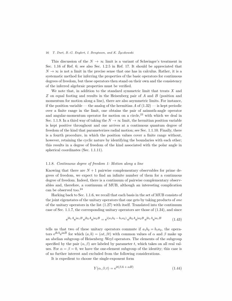
Harking back to Sec. 1.1.6, we recall that each basis in the set of MUB consists of
the joint eigenstates of the unitary operators that one gets by taking products of one
of the unitary operators in the list (1.27) with itself. Translated into the continuum
case of Sec. 1.1.7, the corresponding unitary operators are those of (1.34), and since
eib1Aeia1B eib2Aeia2B = ei(a1b2 − b1a2) eib2Aeia2B eib1Aeia1B (1.43)
tells us that two of these unitary operators commute if a1b2 = b1a2, the opera-
tors eibAeiaB for which (a, b) = (αt, βt) with common values of α and β make up
an abelian subgroup of Heisenberg–Weyl operators. The elements of the subgroup
specified by the pair (α, β) are labeled by parameter t, which takes on all real val-
ues. For α = β = 0, we have the one-element subgroup of the identity; this case is
of no further interest and excluded from the following considerations.
It is expedient to choose the single-exponent form
Y (α, β; t) = eit(βA+ αB) (1.44)
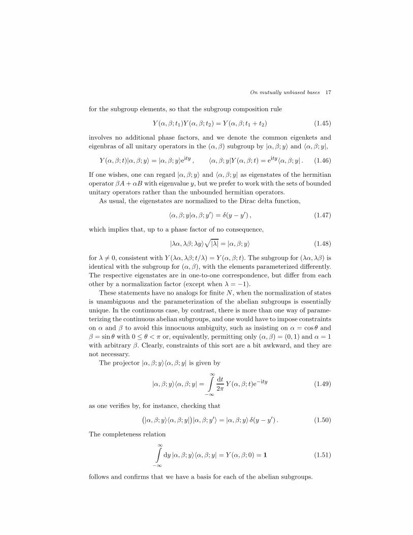
On mutually unbiased bases 17
for the subgroup elements, so that the subgroup composition rule
Y (α, β; t1)Y (α, β; t2) = Y (α, β; t1 + t2) (1.45)
involves no additional phase factors, and we denote the common eigenkets and
eigenbras of all unitary operators in the (α, β) subgroup by |α, β; y〉 and 〈α, β; y|,
Y (α, β; t)|α, β; y〉 = |α, β; y〉eity , 〈α, β; y|Y (α, β; t) = eity〈α, β; y| . (1.46)
If one wishes, one can regard |α, β; y〉 and 〈α, β; y| as eigenstates of the hermitian
operator βA+ αB with eigenvalue y, but we prefer to work with the sets of bounded
unitary operators rather than the unbounded hermitian operators.
As usual, the eigenstates are normalized to the Dirac delta function,
〈α, β; y|α, β; y′〉 = δ(y − y′) , (1.47)
which implies that, up to a phase factor of no consequence,
|λα, λβ;λy〉√|λ| = |α, β; y〉 (1.48)
for λ 6= 0, consistent with Y (λα, λβ; t/λ) = Y (α, β; t). The subgroup for (λα, λβ) is
identical with the subgroup for (α, β), with the elements parameterized differently.
The respective eigenstates are in one-to-one correspondence, but differ from each
other by a normalization factor (except when λ = −1).These statements have no analogs for finite N , when the normalization of states
is unambiguous and the parameterization of the abelian subgroups is essentially
unique. In the continuous case, by contrast, there is more than one way of parame-
terizing the continuous abelian subgroups, and one would have to impose constraints
on α and β to avoid this innocuous ambiguity, such as insisting on α = cos θ and
β = sin θ with 0 ≤ θ < π or, equivalently, permitting only (α, β) = (0, 1) and α = 1
with arbitrary β. Clearly, constraints of this sort are a bit awkward, and they are
not necessary.
The projector |α, β; y〉〈α, β; y| is given by
|α, β; y〉〈α, β; y| =∞∫
−∞
dt
2πY (α, β; t)e−ity (1.49)
as one verifies by, for instance, checking that
(|α, β; y〉〈α, β; y|
)|α, β; y′〉 = |α, β; y〉 δ(y − y′) . (1.50)
The completeness relation
∞∫
−∞
dy |α, β; y〉〈α, β; y| = Y (α, β; 0) = 1 (1.51)
follows and confirms that we have a basis for each of the abelian subgroups.

18 T. Durt, B.-G. Englert, I. Bengtsson, and K. Zyczkowski
Next, we consider two different abelian subgroups, specified by (α, β) and
(α′, β′), respectively, with αβ′ 6= βα′, and evaluate the transition probability den-
sityg between their respective eigenstates by means of
∣∣〈α, β; y|α′, β′; y′〉∣∣2 = tr
(|α, β; y〉〈α, β; y|
)(|α′, β′; y′〉〈α′, β′; y′|
)
=
∫dt dt′
(2π)2trY (α, β; t)Y (α′, β′; t′)
e−i(ty + t′y′)
=
∫dt dt′
(2π)22πδ(t)δ(t′)∣∣αβ′ − βα′
∣∣ e−i(ty + t′y′)
=1
2π∣∣αβ′ − βα′
∣∣ , (1.52)
which is Eq. (11) in Ref. 24. Since the value of∣∣〈α, β; y|α′, β′; y′〉
∣∣2 does not depend
on the quantum numbers y and y′ that label the states of the two bases, the two
bases are MU. This is true for the bases to any two different abelian subgroups.
Indeed, we have a continuum of MUB for a continuous degree of freedom.
As a consequence, the hermitian operators βA+ αB and β′A+ α′B are com-
plementary observables if their commutator i[βA + αB, β′A+ α′B] = (αβ′ − βα′)1
does not vanish. The absolute value of this commutator appears in the denominator
of (1.52). Not unexpectedly, for a continuous degree of freedom, there is a continuum
of pairwise complementary observables.
We could have arrived at the same conclusion by the following more di-
rect argument that exploits the observations made after (1.2). There are uni-
tary transformations that turn βA+ αB into κA and β′A+ α′B into κ′B with
κκ′ = αβ′ − βα′ 6= 0. Now, since the pair A,B is complementary, so is the pair
κA, κ′B, which implies that the pair βA+ αB, β′A+ α′B is complementary as
well, and their bases of eigenstates are MU.
Whereas the right-hand side of (1.1) has the same value of N−1 for any pair
of MUB for a N -dimensional degree of freedom, this is not the case for the right-
hand side of (1.52); recall footnote ‘b’. For a given pair of bases specified by the
coefficients (α, β) and (α′, β′), we can either choose (α′′, β′′) = (α + α′, β + β′) or
(α′′, β′′) = (α − α′, β − β′) to supplement them with a third basis such that these
three MUB have the same numerical value for the constant transition probability
densities between each pair of bases. The basis for any fourth choice (α′′′, β′′′) will
have a different value for one or more of its transition probability densities with
the earlier three bases. This observation by Weigert and Wilkinson24 means that
the continuous set of MUB, composed of the bases of (1.46), contains three-element
subsets that are polytopes of MUB in the sense of Sec. 1.2.
gIt is a density because we need to multiply with dy dy′ to get the probabilities referring toinfinitesimal intervals of y and y′.
On mutually unbiased bases 19
1.1.9. Continuous degree of freedom 2: Motion along a circle
We parameterize the position around the circle by the 2π-periodic azimuth ϕ —
with |ϕ〉 = |ϕ+2π〉, for instance — and normalize the corresponding bras and kets
in accordance with the orthogonality and completeness relations
〈ϕ|ϕ′〉 = 2πδ(2π)(ϕ− ϕ′) ,
∫
(2π)
dϕ
2π|ϕ〉〈ϕ| = 1 , (1.53)
where the integration range is any 2π interval and δ(2π)( ) denotes the 2π-periodic
version of Dirac’s delta function,
δ(2π)(ϕ− ϕ′) =1
2π
∞∑
l=−∞eil(ϕ− ϕ′) . (1.54)
We regard the azimuthal states |ϕ〉 as eigenstates of a unitary operator E,
E|ϕ〉 = |ϕ〉eiϕ , E =
∫
(2π)
dϕ
2π|ϕ〉eiϕ〈ϕ| . (1.55)
This E is the proper N →∞ limit of X in the present context.
All azimuthal wave functions ψ(ϕ) = 〈ϕ| 〉 = ψ(ϕ + 2π) are periodic, and the
Fourier series of 〈ϕ| identifies the eigenstates of the associated angular momentum
operator L,
〈ϕ| =∞∑
l=−∞eilϕ〈l| , L|l〉 = |l〉l . (1.56)
Their orthonormality and completeness relations are
〈l|l′〉 = δl,l′ ,
∞∑
l=−∞|l〉〈l| = 1 , (1.57)
consistent with (1.53).
In view of
〈ϕ|l〉 = eilϕ ,∣∣〈ϕ|l〉
∣∣2 = 1 , (1.58)
the ϕ-basis and the l-basis are MU. The respective unitary shift operators are
powers of E and exponential functions of L,
Em|l〉 = |l+m〉 , 〈ϕ|eiφL = 〈ϕ+ φ| . (1.59)
Their products EmeiαL make up the Heisenberg–Weyl group with the basic Weyl
commutation relation given by
EmeiφL = e−imφeiφLEm , (1.60)
which is the analog of (1.34). For each modulo-2π value of φ, there is an abelian
subgroup composed of the unitary operators (EeiφL)m with m = 0,±1,±2, . . . .
20 T. Durt, B.-G. Englert, I. Bengtsson, and K. Zyczkowski
Despite these analogies and the great structural similarities with the situation
of Sec. 1.1.8, there is a striking difference: There is no third basis that is MU with
respect to both the ϕ-basis and the l-basis.
To make this point, let us assume that ket | 〉 belongs to such a third basis.
Then it must be true that∣∣〈ϕ| 〉
∣∣2 = λ > 0 for all ϕ and∣∣〈l| 〉
∣∣2 = µ > 0 for all l. (1.61)
The completeness relations in (1.53) and (1.57) then imply
〈 | 〉 =∫
(2π)
dϕ
2π
∣∣〈ϕ| 〉∣∣2 =
∫
(2π)
dϕ
2πλ = λ
and 〈 | 〉 =∞∑
l=−∞
∣∣〈l| 〉∣∣2 =
∞∑
l=−∞µ =∞ , (1.62)
which contradict each other. It follows that there is not even a single ket with the
properties (1.61); indeed, there is no third basis.
This situation of a missing third basis is a unique feature of the E,L-type
continuous degree of freedom. There always is a third basis for finite N — the
three eigenbases to X , Z, and XZ of (1.27) are pairwise MU for all N > 1 — and
there is a continuum of MUB for the continuous degrees of freedom of the three
other types. It appears that the combination of the continuous position variable E
with the discrete momentum variable L is at the heart of the matter. For the other
continuous degrees of freedom, the respective position and momentum variables are
both continuous, as will be discussed below.
The nonexistence of a third basis that supplements the ϕ-basis and the l-basis
does not exclude the possibility that there are other bases that are MU, perhaps
with sets of MUB that have more than two elements. Currently, we are not aware
of any such set, however, but its bases would have to be rather unusual. For, two
different discrete bases (such as the l-basis) cannot be MU, nor can two different
continuous bases (such as the ϕ-basis) be MU. And if one basis is discrete and the
other continuous, the dilemma of (1.62) cannot be avoided.
1.1.10. Continuous degree of freedom 3: Radial motion
Radial motion is characterized by a positive position operator R > 0,
R|r〉 = |r〉r with r > 0 , 〈r|r′〉 = rδ(r − r′) ,∞∫
0
dr
r|r〉〈r| = 1 , (1.63)
whereas the eigenvalues of its complementary partner S are all real numbers,
S|s〉 = |s〉s with −∞ < s <∞ , 〈s|s′〉 = δ(s−s′) ,∞∫
−∞
ds |s〉〈s| = 1 . (1.64)

On mutually unbiased bases 21
The transition amplitudes
〈r|s〉 = ris√2π
(1.65)
confirm that the r-basis and the s-basis are MU and that R and S are a pair of
complementary observables.
The unitary shift operators Rit and eiλS have the expected effect when applied
to the states of the other basis,
〈r|eiλS = 〈eλr| , Rit|s〉 = |s+ t〉 , (1.66)
as follows from (1.65). The resulting Weyl commutation relation
RiteiλS = e−iλteiλSRit (1.67)
and the Heisenberg commutator
[R,S
]= iR (1.68)
tell us that S is the hermitian generator of scaling transformations,
e−iλSR eiλS = e−λR , (1.69)
fitting to the positive nature of R.
The unitary operator products in (1.67) make up the Heisenberg–Weyl group
here, and the abelian subgroups can be characterized by common values of τ and
µ in (t, λ) = κ(τ, µ). In full analogy with (1.46)–(1.52), then, the bases defined by
eiκ2τµ/2RiκτeiκµS |τ, µ;α〉 = |τ, µ;α〉eiκα (1.70)
for (τ, µ) 6= (0, 0) are pairwise MU,
∣∣〈τ, µ;α|τ ′, µ′;α′〉∣∣2 =
1
2π∣∣τµ′ − µτ ′
∣∣ . (1.71)
Just as in Sec. 1.1.8, here too we have a continuum of pairwise complementary
observables and a continuum of MUB, and the set of MUB has three-element poly-
topes in the sense of Ref. 24. The R,S-type degree of freedom is really quite similar
to the A,B-type degree of freedom of the Heisenberg kind, because logR and S
are a Heisenberg pair of operators: [logR,S] = i1. This commutator is a particular
case of
[f(R), S
]= iR
∂f(R)
∂R, (1.72)
which follows from (1.68) or from (1.69).
22 T. Durt, B.-G. Englert, I. Bengtsson, and K. Zyczkowski
1.1.11. Continuous degree of freedom 4: Motion within a segment
After dealing with the azimuthal and radial degrees of freedom in Secs. 1.1.9 and
1.1.10, we now turn to the degree of freedom associated with the polar angle ϑ
of spherical coordinates, (x, y, z) = (r sinϑ cosϕ, r sinϑ sinϕ, r cosϑ). Since the
values of ϑ are restricted to a finite interval 0 ≤ ϑ ≤ π, where the endpoints are
not identified with each other as is the case for the periodic azimuth ϕ, we speak
of “motion within a segment,” very much like the popular textbook example of
the “particle in a box,” about which some non-textbook material is reported in
Ref. 25. The relations between the position and momentum operators for cartesian
and spherical coordinates are discussed in Appendix A.
The eigenstates of the position variable Θ and its complementary partner Ω are
related to each other by
〈ϑ|ω〉 = 1√2π
(tan
ϑ
2
)iωwith 0 < ϑ < π and −∞ < ω <∞ , (1.73)
and the respective orthonormality and completeness relations are
〈ϑ|ϑ′〉 = sinϑ δ(ϑ− ϑ′) ,π∫
0
dϑ
sinϑ|ϑ〉〈ϑ| = 1 (1.74)
for the ϑ-basis as well as
〈ω|ω′〉 = δ(ω − ω′) ,
∞∫
−∞
dω |ω〉〈ω| = 1 (1.75)
for the ω-basis. Accordingly, the unitary shift operators are specified by
〈ϑ|eiλΩ = 〈ϑ′|∣∣∣ϑ′ = 2arctan(eλ tan ϑ
2),
(tan
Θ
2
)iω′
|ω〉 = |ω + ω′〉 , (1.76)
telling us that the unitary transformation effected by eiλΩ has no simple geometrical
meaning.
The Weyl commutation relation reads
(tan
Θ
2
)iωeiλΩ = e−iωλeiλΩ
(tan
Θ
2
)iω, (1.77)
from which we get the Heisenberg commutator[Θ,Ω
]= i sinΘ . (1.78)
More generally, we have the analog of (1.72),
[f(Θ),Ω
]= i sinΘ
∂f(Θ)
∂Θ, (1.79)
and the particular case[log tan
Θ
2,Ω]= i1 (1.80)

On mutually unbiased bases 23
identifies log tan Θ2 and Ω as a Heisenberg pair of complementary observables. Re-
membering the lessons of Secs. 1.1.8 and 1.1.10, we conclude that the abelian sub-
groups of the Heisenberg–Weyl group composed of the unitary operators of (1.77)
define a continuum of MUB, with the set of MUB having three-element subsets
that are MUB polytopes in the sense of Ref. 24.
We close this excursion into the realm of continuous degrees of freedom with a
comment on the completeness and orthonormality relations (1.63) and (1.74). Why
did we not absorb the factors r and sinϑ into the normalization of the respective
bras and kets? There are two good reasons: (i) Such a change of normalization
would spoil the relations (1.65) and (1.73); (ii) these factors would re-appear in a
disturbing way when the orthonormality and completeness relations are rewritten
in terms of the eigenstates for the Heisenberg partners logR and log tan Θ2 of S and
Ω, respectively. In other words, it is very natural to have the factors r and sinϑ in
(1.63) and (1.74).
In view of the various subtle issues regarding the normalization of eigenkets and
eigenbras for continuous degrees of freedom, the definition of what constitutes a
pair of complementary observables — given above in the context of (1.1) — should
perhaps be modified to state more carefully that two nondegenerate observables
A and B are complementary if one can normalize their respective eigenstates con-
sistently such that∣∣〈a|b〉
∣∣2 has the same value for all eigenbras 〈a| of A and all
eigenkets |b〉 of B.
1.2. A geometrically motivated measure of mutual unbiasedness
The kets | 〉 in N -dimensional Hilbert space, and their adjoint bras 〈 | = | 〉†, arerather abstract geometrical objects, and so are the linear operators that map kets
on kets and bras on bras, among them the statistical operator ρ that summarizes
our knowledge about the state of the physical N -dimensional degree of freedom
under consideration. With reference to a specified basis, the kets are represented
by numerical column vectors ψ (N ×1 matrices), the bras by row vectors ψ† (1×Nmatrices), and the linear operators by N × N matrices, among them the density
matrix for the statistical operator ρ. We denote these relationships by ψ = | 〉,ψ† = 〈 |, and = ρ, respectively.
There are many density matrices, one for each reference basis, to one and the
same statistical operator, much like there are many trios of components for the
velocity vector of the moon, one trio for each coordinate system. One should not
confuse the velocity vector with its components, or the statistical operator with the
density matrix used to represent it numerically.
When they exist, maximal sets of MUB form a very distinct geometrical pattern
in the set of hermitian matrices of unit trace — the real euclidean space that
contains the set of density matrices. This is where we begin our story about maximal
sets of MUB, although in most of what follows we will prefer to work directly in
Hilbert space. The two pictures ought to be considered as complementary, each of

24 T. Durt, B.-G. Englert, I. Bengtsson, and K. Zyczkowski
them possessing advantages and drawbacks.
The set of density matrices is a convex body in the set of hermitian matrices
of unit trace. Its pure states are the one-dimensional projectors. The set of its pure
states has real dimension 2(N−1), and can be identified with the complex projective
Hilbert space. The dimension of is N2 − 1, and the space in which it sits can
be regarded as a vector space, with its origin at the maximally mixed state
⋆ =1
N1 =
1
N1 = ρ⋆ , (1.81)
where 1 is the identity operator of (1.2) and 1 is the unit matrix that represents it.
With any hermitian matrix M of unit trace we associate a traceless matrix
m =M − ⋆ . (1.82)
The set of these traceless matrices forms a vector space, and we will think of them
as vectors. The matrix representation is used to define the inner product
m1 ·m2 =1
2tr(M1 − ⋆)(M2 − ⋆)
. (1.83)
Thus the squared distance between the tips of the two vectors m1 and m2 is
D(m1,m2)2 =
1
2tr(M1 −M2)
2. (1.84)
With any unit ket |e〉 in Hilbert space we associate a vector e in RN2−1, the space
of (N2 − 1)-component real vectors, through
e = ψeψ†e − ⋆ = |e〉〈e| − ρ⋆ (1.85)
so that the squared length of e is
|e|2 =N − 1
2N. (1.86)
All vectors in RN2−1 with this specific length sit on the surface of the outsphere
of the body , the smallest sphere containing the body. But it is important to
realize that it is only a small 2(N − 1)-dimensional subset of this outsphere that
corresponds to vectors in Hilbert space — most of the outsphere lies outside the
body. The case N = 2 is an exception: In this case the outsphere is the familiar
Bloch sphere, which is identical to the boundary of the body of density matrices.
Note furthermore that the relations
〈ei|ej〉 = δi,j , ei · ej =1
2δi,j −
1
2N(1.87)
imply each other. If |ei〉 is an orthonormal basis of kets, the corresponding vectors
ei form a regular simplex that spans an (N − 1)-plane, and clearly
N−1∑
i=0
ei = 0 . (1.88)

On mutually unbiased bases 25
Hence the simplex is centered at the origin. We have normalized its edge lengths
to unity.
Next consider two MUB with kets |ei〉 and |fj〉, respectively, represented by the
vectors ei and fj . The two equations
∣∣〈ei|fj〉∣∣2 =
1
N, ei · fj = 0 (1.89)
are equivalent ways of stating that the bases are MU and, therefore, the two planes
spanned by a pair of MUB are totally orthogonal: Each vector in one plane is
orthogonal to all vectors in the other plane. Since the dimension of our space is
N2 − 1 = (N + 1)(N − 1), we can fit at most N + 1 totally orthogonal (N − 1)-
planes into it. This is one way of seeing that the maximal number of MUB is N+1.
Let us now momentarily forget that our vectors ei, fi, and so on, are supposed
to come from unit vectors in Hilbert space. Whatever the value of N , we can always
find N + 1 totally orthogonal (N − 1)-planes in RN2−1, and if we place a regular
simplex in each we will obtain a quite interesting convex polytope with N(N + 1)
vertices.26 When N = 2, it is in fact a regular octahedron, but for other values of
N it needs a name of its own. We will call it the MUB polytope, without implying
that there exists a maximal set of MUB in the N -dimensional Hilbert space. The
MUB polytope and the body of density matrices share the same outsphere and,
in this manner, the existence problem for MUB can be turned into the problem
of rotating the MUB polytope in such a way that all its vertices fit into the small
subset of pure quantum states that are present in that outsphere. This is a hard
problem (unless N = 2). Indeed, from this perspective it is not obvious that we
can find even one pair of MUB but, as we have seen in Sec. 1.1.2, we can always do
this. It is the existence of a maximal set, with N + 1 bases that are pairwise MU,
which is in doubt for general N .
Viewing bases as (N − 1)-planes in RN2−1 gives us the means to quantify how
close a given pair of bases is to being MU. The trick is to regard n-planes in Rm
as rank-n projectors in a vector space of real m ×m matrices, in analogy to the
way we go from vectors in Hilbert space to density matrices. This gives us an
embedding of the Grassmannian of n-planes into a flat vector space equipped with
a natural euclidean distance, and hence a natural notion of distance between vectors
in Hilbert space. To derive it, consider the N vectors ei. Then form the (N2−1)×Nmatrix
B =[e1 e2 . . . eN
]. (1.90)
It has rank N−1 because of (1.88). Next form the projector onto the (N−1)-plane
spanned by the linearly dependent vectors ei. It is
Π = 2BBT . (1.91)
Finally, the square of the chordal Grassmannian distance between a pair of planes
26 T. Durt, B.-G. Englert, I. Bengtsson, and K. Zyczkowski
is27
Dc(Πe,Πf )2 ≡ 1
2tr(Πe −Πf )
2= N − 1−
∑
a,b
(∣∣〈ea|fb〉∣∣2 − 1
N
)2
=∑
a,b
∣∣〈ea|fb〉∣∣2(1−
∣∣〈ea|fb〉∣∣2), (1.92)
where the kets |ea〉 are related to Πe through (1.85), (1.90), and (1.91), and the kets
|fb〉 are analogously related to Πf . The last expression of (1.92) shows that Dc = 0
if the projectors |fb〉〈fb| are a permutation of the projectors |ea〉〈ea|, in which case
we have the same basis twice, possibly with different labeling.
One can check that
0 ≤ D2c ≤ N − 1 , (1.93)
and that the distance is maximal if and only if the two bases are MU. This notion of
distance has been used to study packing problems for n-planes,28 and as a measure
of “MUness”.27 If we pick our bases at random, using the unitarily invariant Fubini–
Study measure to define “random,” we find that the average squared distance is
given by
〈D2c 〉FS =
N
N + 1(N − 1) . (1.94)
If the dimension is large, N ≫ 1, two bases picked at random are likely to be almost
MU. Let us finally mention that entropic uncertainty relations in effect provide an
interesting alternative measure of “MUness”.29–31
2. Construction of mutually unbiased bases in prime power
dimensions
2.1. Galois fields
In what follows, we work in a Hilbert space of prime power dimension N = pm with
p a prime number and m a positive integer. These are the dimensions for which
maximal sets of MUB are known to exist. Moreover, and not coincidentally, there
is a finite Galois field with N = pm elements. We shall label these elements by
integer numbers i, 0 ≤ i ≤ N − 1, or, equivalently, by m-tuples (i0, i1, . . . , im−1) of
integers, each integer running from 0 to p−1, that we get from the p-ary expansion
of i:
i = (i0, i1, . . . , im−1) if i =
m−1∑
n=0
inpn . (2.1)
Each field is characterized by two operations, a multiplication and an addition,
that we shall denote by ⊙ and ⊕ respectively. As in footnote ‘a’, we shall use the
symbols 0 and 1 for the neutral elements of addition and multiplication, respectively,
throughout the paper, consistent with their meaning as integers.

On mutually unbiased bases 27
Further, we adopt the particular convention that the elements of the field are
labeled in such a way that the addition is equivalent to the component-wise addition
modulo p, that is
i = j ⊕ k is tantamount to in = jn + kn (mod p) (2.2)
for n = 0, 1, . . . ,m− 1, where in, jn, kn are the respective coefficients of (2.1). As a
consequence, the summation in (2.1) is also a field summation,
i = (i0p0)⊕ (i1p
1)⊕ · · · ⊕ (im−1pm−1) =
m−1⊕
n=0
inpn . (2.3)
All fields with the same number of elements are equivalent up to a relabeling,
and there is no strict obligation for the convention (2.2), but it is natural and
convenient in the present context, because it allows us to regard the elements of
the field both as labels of basis states and as integer numbers that we can use for
getting powers of complex numbers in accordance with the usual computation rules.
Actually, that there exists a relabeling such that the addition is equivalent to
the addition modulo p component-wise is a direct consequence of the fact that for
all finite fields the characteristics of the field — the smallest number of times that
we must add the element 1 (neutral for the multiplication) to itself before we obtain
the element 0 (neutral for the addition) — is always equal to a prime number (p
when N = pm).
Unfortunately, there is no similarly simple convention for the field multiplica-
tion ⊙, and — the exceptions N = p and N = 4 aside — one has a choice between
several equally good ways of defining the field multiplication ⊙ such that it is con-
sistent with the component-wise definition of the field addition ⊕. In view of the
associative and distributive nature of ⊙, that is: (a ⊙ b) ⊙ c = a ⊙ (b ⊙ c) and
(a ⊕ b) ⊙ c = (a ⊙ c) ⊕ (b ⊙ c), respectively, we only need to state the values of
pj ⊙ pk, the products of powers of p, with j, k = 0, 1, . . . ,m− 1.
For m = 1, N = p, the field multiplication is just multiplication modulo p. For
m > 1, we have the Galois construction
pj ⊙ pk =
pj+k if j + k < m ,
m−1∑
l=0
µlpl = (µ0, µ1, . . . , µm−1) if j + k = m ,
p⊙ (pj−1 ⊙ pk) recursively, if j + k > m .
(2.4)
Hereby, the coefficients that define the j + k = m products are restricted by the
requirement that
x 7→ xm −m−1∑
l=0
µlxl (2.5)
is an irreducible polynomial over the Galois field with p elements, which is to say
that it cannot be factored into two nonconstant polynomials whose coefficients are
modulo-p integers.

28 T. Durt, B.-G. Englert, I. Bengtsson, and K. Zyczkowski
In a standard textbook parameterization of the Galois field with N = pm ele-
ments,32 one identifies the field elements with polynomials that are defined by the
coefficients of the p-ary expansion of (2.1),
i = (i0, i1, . . . , im−1)←→m−1∑
m=0
imxm . (2.6)
Addition and multiplication of the field elements are then carried out as addi-
tion and multiplication of the corresponding polynomials modulo the polynomial of
(2.5), with the resulting sums and products stated as polynomials of degree m− 1
with modulo-p integer coefficients. Clearly, this gives the component-wise addition
of (2.2) and multiplication in accordance with (2.4). Since the field multiplication
is not familiar to readers with a typical theoretical-physics background, we now
discuss it in some detail.
For instance, the choice 2 ⊙ 2 = 3 is unique for N = 4, and for p odd and
N = p2, one can always choose p⊙ p = µ0 with µ0 not a square, such as 3⊙ 3 = 2,
5⊙ 5 = 2 or 5⊙ 5 = 3, 7⊙ 7 = 3 or 7⊙ 7 = 5 or 7⊙ 7 = 6, and so forth. For higher
powers of p = 2, there are several choices too; they include 2 ⊙ 4 = 5 for N = 8,
2⊙ 8 = 3 for N = 16, and 2⊙ 16 = 5 for N = 32.
As a final example, we mention 3⊙ 9 = (1, 2, 2) = 25 for N = 33.h This implies
first 9⊙ 9 = (2, 2, 0) = 8 and then
N = 27 : (a0, a1, a2)⊙ (b0, b1, b2) = a⊙ b = c = (c0, c1, c2)
with c0 = a0b0 + a1b2 + a2b1 − a2b2 (mod 3) ,
c1 = a0b1 + a1b0 − a1b2 − a2b1 − a2b2 (mod 3) ,
c2 = a0b2 + a1b1 + a2b0 − a1b2 − a2b1 (mod 3) ,
(2.7)
for the multiplication of two arbitrary field elements. The special cases 3⊙ 13 = 1
and 9⊙ 17 = 1 may serve as illustrations.
More generally, when writing
pj ⊙ pk =(M
(j+k)0 ,M
(j+k)1 , . . . ,M
(j+k)m−1
), (2.8)
we have
M (j+k)m = δj+k,m for j + k = 0, 1, . . . ,m− 1 , and M (m)
m = µm , (2.9)
and the coefficients for j + k = m+ 1,m+ 2, . . . , 2m− 2 are successively calculated
with the aid of the recurrence relation
M (j+k)m = (1− δm,0)M
(j+k−1)m−1 + µmM
(j+k−1)m−1 (mod p) , (2.10)
which is valid for j+k = 1, 2, . . . , 2m−2. The field product of two arbitrary elements
is then given by
a⊙ b =(aM0b
T , aM1bT , . . . , aM
m−1bT), (2.11)
hThe choice 3⊙9 = 25 is the largest one of the eight permissible values. The other seven values for(µ0, µ1, µ2) are (1, 1, 0) = 4, (2, 1, 0) = 5, (2, 0, 1) = 11, (1, 1, 1) = 13, (2, 2, 1) = 17, (1, 0, 2) = 19,and (2, 1, 2) = 23. Each of them yields a consistent implementation of the field multiplication.
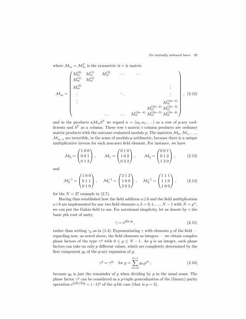
On mutually unbiased bases 29
whereMm =MTm is the symmetric m×m matrix
Mm =
M(0)m M
(1)m M
(2)m · · · · · ·
M(1)m M
(2)m
M(2)m
......
. . ....
... M(2m−4)m
M(2m−4)m M
(2m−3)m
. . . . . . M(2m−4)m M
(2m−3)m M
(2m−2)m
, (2.12)
and in the products aMmbT we regard a = (a0, a1, . . . ) as a row of p-ary coef-
ficients and bT as a column. These row×matrix× column products are ordinary
matrix products with the outcome evaluated modulo p. The matricesM0,M1, . . . ,
Mm−1 are invertible, in the sense of modulo-p arithmetic, because there is a unique
multiplicative inverse for each non-zero field element. For instance, we have
M0 =
1 0 0
0 0 1
0 1 2
, M1 =
0 1 0
1 0 2
0 2 2
, M2 =
0 0 1
0 1 2
1 2 0
, (2.13)
and
M−10 =
1 0 0
0 1 1
0 1 0
, M−1
1 =
2 1 2
1 0 0
2 0 2
, M−1
2 =
1 1 1
1 1 0
1 0 0
, (2.14)
for the N = 27 example in (2.7).
Having thus established how the field addition a⊕ b and the field multiplication
a⊙b are implemented for any two field elements a, b = 0, 1, . . . , N − 1 with N = pm,
we can put the Galois field to use. For notational simplicity, let us denote by γ the
basic pth root of unity,
γ = ei2π/p , (2.15)
rather than writing γp as in (1.4). Exponentiating γ with elements g of the field —
regarding now, as noted above, the field elements as integers — we obtain complex
phase factors of the type γg with 0 ≤ g ≤ N − 1 . As g is an integer, such phase
factors can take on only p different values, which are completely determined by the
first component g0 of the p-ary expansion of g,
γg = γg0 for g =
m−1∑
m=0
gmpm , (2.16)
because g0 is just the remainder of g when dividing by p in the usual sense. The
phase factor γg can be considered as a p-tuple generalization of the (binary) parity
operation ei(2π/2)g = (−1)g of the q-bit case (that is p = 2).
30 T. Durt, B.-G. Englert, I. Bengtsson, and K. Zyczkowski
The following identity plays a fundamental role:
N−1∑
j=0
γj⊙i = Nδi,0 . (2.17)
Indeed, if i = 0, then
N−1∑
j=0
γj⊙i =
N−1∑
j=0
1 = N . Otherwise,
i 6= 0 :
N−1∑
j=0
γj⊙i =
N−1∑
j′=0
γj′
(2.18)
because the field multiplication is invertible, and then
N−1∑
j′=0
γj′
= pm−1
p−1∑
j′0=0
γj′
0 = pm−1 (1− γp)(1 − γ) = 0 , (2.19)
where the first step exploits (2.16) and recognizes that there are pm−1 field elements
j′ with the same value of j′0.
The fact that the field addition is the component-wise addition modulo p, com-
bined with the rule (2.16), implies the following useful identity:
γiγj = γi+j = γi0+j0 = γ(i⊕j)0 = γi⊕j . (2.20)
In the final expression on the right, the sum i ⊕ j is the Galois sum of i and j,
which is then regarded as an integer, just as we regard the result of the Galois
multiplication j ⊙ i in (2.17) and (2.18) as an integer, and so get integer powers of
γ. Relation (2.20) expresses, in the language of mathematicians, that the pth roots
of unity are additive characters of the Galois field.32
It is important to note, in order to avoid confusions, that different types of
operations are present at this level: The internal field operations (⊕ and ⊙) must
not be confused with the modulo-N operations. As an illustration of the differences
between these operations, we consider the case p = 2, m = 2, N = pm = 4 and give
the tables for field addition (⊕) and field multiplication (⊙) in Table 1(a) as well
as the tables for modulo-N addition and multiplication (⊕4 and ⊙4, respectively)
in Table 1(b).
One can check that the field and modulo-4 multiplications are distributive with
respect to the associated addition, but that there are no non-zero dividers of 0
only in the case of the field multiplication, whereas we have 0 = 2 ⊙4 2 for the
modulo-4 multiplication. As a consequence, the field multiplication table exhibits
an invertible group structure when the first line and first column are removed. All
operations are commutative as can be seen from the invariance of all four tables
under transposition.
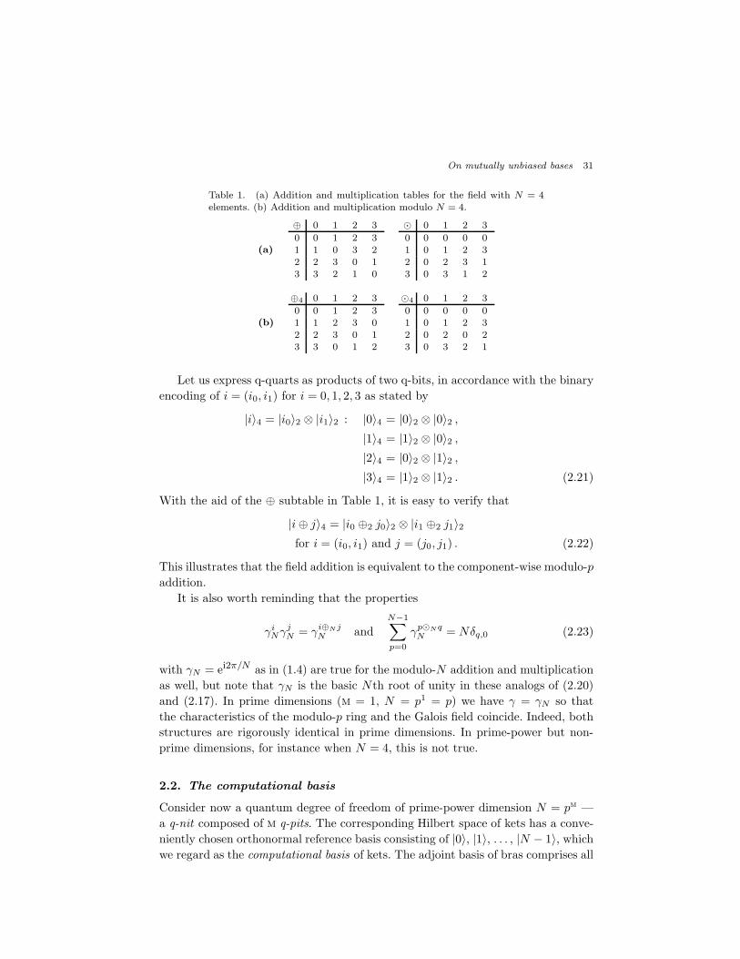
On mutually unbiased bases 31
Table 1. (a) Addition and multiplication tables for the field with N = 4elements. (b) Addition and multiplication modulo N = 4.
(a)
⊕ 0 1 2 3
0 0 1 2 31 1 0 3 22 2 3 0 13 3 2 1 0
⊙ 0 1 2 3
0 0 0 0 01 0 1 2 32 0 2 3 13 0 3 1 2
(b)
⊕4 0 1 2 3
0 0 1 2 31 1 2 3 02 2 3 0 13 3 0 1 2
⊙4 0 1 2 3
0 0 0 0 01 0 1 2 32 0 2 0 23 0 3 2 1
Let us express q-quarts as products of two q-bits, in accordance with the binary
encoding of i = (i0, i1) for i = 0, 1, 2, 3 as stated by
|i〉4 = |i0〉2 ⊗ |i1〉2 : |0〉4 = |0〉2 ⊗ |0〉2 ,|1〉4 = |1〉2 ⊗ |0〉2 ,|2〉4 = |0〉2 ⊗ |1〉2 ,|3〉4 = |1〉2 ⊗ |1〉2 . (2.21)
With the aid of the ⊕ subtable in Table 1, it is easy to verify that
|i⊕ j〉4 = |i0 ⊕2 j0〉2 ⊗ |i1 ⊕2 j1〉2for i = (i0, i1) and j = (j0, j1) . (2.22)
This illustrates that the field addition is equivalent to the component-wise modulo-p
addition.
It is also worth reminding that the properties
γiNγjN = γi⊕N j
N and
N−1∑
p=0
γp⊙NqN = Nδq,0 (2.23)
with γN = ei2π/N as in (1.4) are true for the modulo-N addition and multiplication
as well, but note that γN is the basic Nth root of unity in these analogs of (2.20)
and (2.17). In prime dimensions (m = 1, N = p1 = p) we have γ = γN so that
the characteristics of the modulo-p ring and the Galois field coincide. Indeed, both
structures are rigorously identical in prime dimensions. In prime-power but non-
prime dimensions, for instance when N = 4, this is not true.
2.2. The computational basis
Consider now a quantum degree of freedom of prime-power dimension N = pm —
a q-nit composed of m q-pits. The corresponding Hilbert space of kets has a conve-
niently chosen orthonormal reference basis consisting of |0〉, |1〉, . . . , |N − 1〉, whichwe regard as the computational basis of kets. The adjoint basis of bras comprises all

32 T. Durt, B.-G. Englert, I. Bengtsson, and K. Zyczkowski
〈n| = |n〉† with n = 0, 1, . . . , N − 1. As usual, the inner products ( · , · ) of two kets
or two bras are given by Dirac brackets (≡ bra-kets), for which the orthonormality
relations(|i〉, |j〉
)=(〈i|, 〈j|
)= 〈i|j〉 = δi,j (2.24)
are an elementary illustration.
2.3. The dual basis
Let us now consider the unitary transformations V 0l that shift each label of the
states of the computational basis |0〉, |1〉, . . . , |i〉, . . . , |N − 1〉 by l,|i〉 → V 0
l |i〉 = |i⊕ l〉 , (2.25)
so that each V 0l implements a permutation among the kets of the computational
basis, but does not change the basis as a whole. The shift in (2.25) is a shift modulo
N in prime dimensions only (N=p) and then V 0l is identical with X l of Sec. 1.1.2;
in prime power dimensions (N = pm, m > 1) the shift consists of m shifts modulo p,
component-wise. The transformations effected by V 0l with l = 0, 1, . . . , N − 1 make
up a commutative group of permutations with N elements that is isomorphic to
the Galois addition.
Generalizing the procedure outlined in Ref. 33, we employ a suitable discrete
Fourier-type transformation — the inverse Galois–Fourier transformation — to
define the dual basis as follows:
|j〉 = 1√N
N−1∑
k=0
|k〉γ⊖k⊙j (2.26)
where the symbol ⊖ represents the inverse of the Galois addition ⊕, that is: x = ⊖yif x⊕y = 0. It is easy to check that these dual kets are joint eigenkets of the unitary
permutation operators V 0l . Indeed, we have
V 0l |j〉 =
1√N
N−1∑
k=0
|k ⊕ l〉γ⊖k⊙j
=1√N
N−1∑
k′=0
|k′〉γ⊖(k′⊖l)⊙j = |j〉γl⊙j , (2.27)
which identifies the eigenvalues γl⊙j . These are p different eigenvalues, each occur-
ring pm−1 times.
Obviously, the dual basis and the computational basis are MU by construction,
∣∣〈j|k〉∣∣2 =
∣∣∣∣1√Nγj⊙k
∣∣∣∣2
=1
Nfor all j, k = 0, 1, . . . , N − 1 . (2.28)
When the dimension is prime (N = p), the dual basis is the standard discrete
Fourier transform of the computational basis, as in (1.6); when N is a power of 2,
the Galois–Fourier transform is a real Hadamard transform.33

On mutually unbiased bases 33
Let us denote by V l0 the unitary transformations that shift each label of the
states of the dual basis |0〉, |1〉, . . . , |i〉, . . . , |N − 1〉 by ⊖l,
|i〉 → V l0 |i〉 = |i⊖ l〉 , 〈i| → 〈i|V l
0 = 〈i⊕ l| , (2.29)
so that each V l0 implements a permutation among the kets of the dual basis, but does
not change the basis as a whole. In perfect analogy with the permutation operators
V 0l of (2.25), the transformations effected by V l
0 with l = 0, 1, . . . , N − 1 upon the
bras 〈i| also compose a commutative group of permutations with N elements that
is isomorphic to the Galois addition.
These permutation operators are diagonal in the computational basis,
V l0 =
N−1∑
k=0
|k〉〈k ⊕ l| =N−1∑
k=0
|k〉γk⊙l〈k| . (2.30)
This is the dual counterpart of the analogous expression for the shifts in the com-
putational basis,
V 0l =
N−1∑
k=0
|k ⊕ l〉〈k| =N−1∑
k=0
|k〉γk⊙l〈k| , (2.31)
which is equivalent to (2.27) and follows from that eigenket statement.
The unitary operators V 0l and V l
0 are obviously analogs of the operators X l and
Z l of Sec. 1.1.2, but for m > 1 these operators are markedly different. In particular,
the period of V 01 and V 1
0 is p, not N = pm. We indicate the difference by writing 〈i|for the dual basis here, whereas the notation 〈 i | is employed in Sec. 1.1.2.
As mentioned above, it is immediately clear that |k〉 → V 0l |k〉 = |k ⊕ l〉 is
a component-wise addition, where the components of the q-nit ket |k〉 are the m
q-pits that compose it, as is illustrated by (2.21) and (2.22) for p = 2 and m = 2.
More generally,
V 0l |k〉 = V 0
l
(|k0〉 ⊗ |k1〉 ⊗ · · · ⊗ |km−1〉
)
= |k0 + l0〉 ⊗ |k1 + l1〉 ⊗ · · · ⊗ |km−1 + lm−1〉 , (2.32)
where each factor |km〉 in the tensor product is a q-pit ket, and the sums km+lm are
modulo-p sums. It follows that V 0l is a product of factors, each of which referring
to one of the q-pits,
V 0l =
(V 01
)l0 (V 0p
)l1 (V 0p2
)l2 · · · =m−1∏
m=0
(V 0pm
)lm, (2.33)
where the mth factor affects the mth q-pit only, with V 0pm giving a unit shift of the
mth modulo-p label.
34 T. Durt, B.-G. Englert, I. Bengtsson, and K. Zyczkowski
In order to see that 〈k| → 〈k|V l0 = 〈k ⊕ l| is a q-pit–wise shift as well, we first
observe that the Galois–Fourier transformation (2.26) factorizes,
〈k| = 1√N
N−1∑
j=0
γk⊙j〈j| = 1√N
N−1∑
j=0
γkM0jT 〈j0| ⊗ 〈j1| ⊗ 〈j2| ⊗ · · · ⊗ 〈jm−1|
=1√p
p−1∑
j0=0
γ(kM0)0j0〈j0| ⊗1√p
p−1∑
j1=0
γ(kM0)1j1〈j1| ⊗ · · ·
= 〈k0| ⊗ 〈k1| ⊗ · · · ⊗ 〈km−1| , (2.34)
whereM0 is the 0th multiplication matrix in (2.11) and km is the mth component
of kM0 = (k0, k1, . . .). SinceM0 is invertible, we can parameterize the field element
k in terms of the coefficients km,
k = (k0, k1, . . .)M−10 = (k0, k1, . . .)
g0g1...
gm−1
=
m−1∑
m=0
kmgm , (2.35)
with the field elements gm defined such that their p-ary coefficients make up the
rows of the m × m matrix M−10 . Alternatively, we could define the gms by their
basic property
γpm⊙gn = γδm,n =
γ if m = n ,
1 if m 6= n .(2.36)
Therefore, a unit increase of km means the addition of gm to k, and the shift
operator V l0 factorizes accordingly into a product of powers of single–q-pit Fourier
operators, each of which (the mth, say) acting on the single–q-pit bras 〈jm| onlyand leaving the other m− 1 q-pit bras in the products of (2.34) unaffected,
V l0 = (V g0
0 )l0 (V g1
0 )l1 (V g2
0 )l2 · · · =
m−1∏
m=0
(V gm0 )
lm , (2.37)
with the mth factor affecting the mth q-pit only,
(V gm0 )
lm |km〉 = |km〉γkmlm . (2.38)
For instance, we have g0 = 1, g1 = 12, g2 = 3, and k0 = k0, k1 = k2, k2 = k1 − k2for the N = 27 example of (2.7), (2.13), and (2.14).
The respective unitary operator factors for unit shifts in (2.33) and (2.37) com-
mute if they refer to different q-pits,
V 0pmV
gn0 = V gn
0 V 0pm if m 6= n , (2.39)
which essentially states that the Galois shifts with their component-wise addition
are consistent with the factorization of the N = pm-dimensional degree of freedom
On mutually unbiased bases 35
into m p-dimensional degrees of freedom, as discussed in Sec. 1.1.5. And for the pair
of operators to the same q-pit, one easily verifies the Weyl commutation rule
V 0pmV
gm0 = γ−1V gm
0 V 0pm . (2.40)
Equations (2.39) and (2.40) are particular cases of (2.42) below.
2.4. Construction of the remaining N-1 mutually unbiased bases
In the previous section we established a pair of MUB, the computational basis,
which can be chosen arbitrarily, and its dual basis, defined by (2.26). In this section,
we shall generalize this construction in order to obtain the other N − 1 bases that
complement the computational basis and its dual basis such that the bases of each
of the N(N + 1)/2 pairs are MU.
2.4.1. Heisenberg–Weyl group
Let us denote by V ji the compositions of the shifts in the computational and the
dual bases, obtained by ordinary operator multiplication of V j0 and V 0
i ,
V ji = V j
0 V0i =
N−1∑
k=0
|k ⊕ i〉γ(k⊕i)⊙j〈k| for i, j = 0, 1, . . . , N − 1 , (2.41)
the building blocks of the Heisenberg–Weyl group. This is consistent with the pre-
vious expressions for i = 0 or j = 0 because V 00 is the identity. In particular, for
i = 0 and j = l we get the second sum of (2.30), and for i = l and j = 0 we have
the first sum of (2.31).
We note that the order of multiplication of V j0 and V 0
j matters in the definition
(2.41) because these unitary shift operators do not commute,
V 0i V
j0 = γ⊖i⊙jV j
0 V0i . (2.42)
We recognize here the Weyl commutation rule for the two unitary operators V j0
and V 0i , which is their basic algebraic relation.2, 3
In dimension N = p = 2, the commutation relation (2.42) is that of the Pauli
group (identify V 10 with σx and V 0
1 with σz once more). When the dimension is
a prime number, the field operations are the addition and multiplication modulo
p, and the properties of MUB are well-known;22 recall the discussion in Sec. 1.1.6
with its emphasis on the Heisenberg–Weyl group.
Currently, we consider the Heisenberg–Weyl group associated with the Galois
addition and multiplication rather than the Heisenberg–Weyl group associated with
the usual modulo-N operations. These groups coincide in prime dimensions but
differ for non-prime but prime-power dimensions. Notably, the Galois field is iso-
morphic to the modulo-N ring in prime dimensions only (N = p). Nevertheless,
the Heisenberg–Weyl group factorizes in dimension pm into products of operators
that belong to the local q-pit Heisenberg–Weyl group. In the case of translations

36 T. Durt, B.-G. Englert, I. Bengtsson, and K. Zyczkowski
of the computational basis, the factorization is straightforward and given above in
(2.33). And in the case of translations of the dual basis, where the mapping from
global operator labels to local operator labels is more intricate, see (2.34)–(2.36),
the factorization is stated in (2.37).
The composition law of the N2 unitary operators introduced in (2.41) is
V ji V
lk = V j
0 V0i V
l0V
0k
= γ⊖i⊙lV j0 V
l0V
0i V
0k = γ⊖i⊙lV j⊕l
i⊕k , (2.43)
which implies
V lk
−1= V l
k
†= γ⊖k⊙lV ⊖l
⊖k (2.44)
and
V lkV
ji V
lk
†= γl⊙i⊖j⊙kV j
i (2.45)
for example. Another implication is
(V ji
)p=(γ⊖i⊙j
)1+2+···+(p−1)
V 00 =
(γ⊖i⊙j
) 1
2p(p−1)
1
=
(−1)i⊙j1 for p = 2 ,
1 for p = 3, 5, 7, 11, . . . ,(2.46)
which is reminiscent of (1.20) and once again shows a difference between the single
even prime p = 2 and the odd primes p > 2.
Yet another implication is the orthonormality relation for the V ji s, with respect
to the Hilbert–Schmidt inner product,
(V ji , V
lk
)= tr
V ji
†V lk
= Nδi,kδj,l , (2.47)
because all V ji s are traceless, except V 0
0 = 1. The other side of this coin is the
relation,
1
N2
N−1∑
m,n=0
V nm AV n
m† =
1
NtrA1 , (2.48)
which one may regard as a manifestation of Schur’s lemma, inasmuch as the right-
hand side follows after observing that the sum on the left commutes with all V ij
and must therefore be a multiple of the identity. Schwinger4 calls such statements
about equal-weight averages over the whole phase space ergodic relations.
Equation (2.43) is the discrete analog of the familiar Baker–Campbell–Hausdorff
relation for exponentiated position and momentum operators that we encountered
in (1.34). An immediate consequence of (2.43) is
V ji V
kl = V k
l Vji if (i⊙ k)0 = (j ⊙ l)0 and only then, (2.49)
where ( )0 has the same meaning as in (2.20). In particular, (2.49) is fulfilled if
i⊙ k = j ⊙ l, which we note for later reference.
On mutually unbiased bases 37
2.4.2. Abelian subgroups
Up to a global phase, (2.43) looks like a group composition law. Indeed, one can
show34 that there is a true analog of what we observed in Sec. 1.1.6 for prime N :
The N2 unitary operators V ji with i, j = 0, 1, . . . , N − 1 make up N +1 commuting
sets (abelian subgroups of the Heisenberg–Weyl group) of N elements each that
have only the identity V 00 in common. For each of these commuting sets, there is
a basis of joint eigenkets of all V ji s in the set. The N + 1 bases thus identified
are pairwise MU. In passing, we note that this property can be shown, following
an alternative approach developed in Ref. 35, to be a consequence of the fact that
the V ji operators form what is called “a maximally commuting basis of orthogonal
unitary matrices.”
It is expedient to introduce a fitting notation and terminology before we proceed.
We shall denote by U il the elements of these abelian subgroups, where i labels the
subgroup and runs from 0 to N to account for N + 1 subgroups, while l labels the
N elements in the subgroup and runs from 0 to N −1. For the basis kets associated
with the subgroups we use the convention that the kth basis ket for the ith subgroup
is denoted by |eik〉.The abelian subgroups for i = N and i = 0 are composed of the two sets of
commuting operators of Sec. 2.3, respectively,
UNl = V l
0 =
N−1∑
k=0
|k〉γk⊙l〈k| =N−1∑
k=0
|eNk 〉γk⊙l〈eNk | ,
U0l = V 0
l =
N−1∑
k=0
|k〉γk⊙l〈k| =N−1∑
k=0
|e0k〉γk⊙l〈e0k| , (2.50)
with l = 0, 1, . . . , N − 1. As indicated, we identify |k〉 with |eNk 〉, and |k〉 with |e0k〉.In other words, we choose the convention that the computational basis is the Nth
basis, and the dual basis is the 0th basis.
This suggests strongly that the other N − 1 sets can be chosen such that
U il =
N−1∑
k=0
|eik〉γk⊙l〈eik| (2.51)
with i = 1, 2, . . . , N − 1 and l = 0, 1, . . . , N − 1. To complete the picture, we need
to find the kets |eil〉, such that those with common label i make up orthonormal
sets, and the sets with different i labels are MU. These requirements are compactly
summarized by
∣∣〈eik|ejl 〉∣∣2 = δi,jδk,l +
1− δi,jN
=
δk,l for i = j (orthonormal),
1/N for i 6= j (mutually unbiased),(2.52)
which have to hold for i, j = 0, 1, . . . , N and k, l = 0, 1, . . . , N − 1.
38 T. Durt, B.-G. Englert, I. Bengtsson, and K. Zyczkowski
Irrespective of the choice for the ith orthonormal set of kets and bras in (2.51),
the U il are unitary and commute with each other for fixed i,
U ilU
il′ = U i
l′Uil = U i
l⊕l′ , (2.53)
which is an immediate consequence of distributivity and the identity (2.20). In view
of (2.49), we can guess that the U il of the ith set are operators V k
l such that the
Galois ratio k⊘l has the same i-dependent value for all of them.i For, if k⊘l = k′⊘l′,then k′ ⊙ l = k ⊙ l′, and (2.49) implies that V k
l and V k′
l′ commute.
We are thus invited to try the ansatzj
U il = αi
lVi⊙ll for i = 0, 1, . . . , N − 1 , (2.54)
where the phase factors αil have to be chosen consistently. In particular we have
α0l = 1 : U0
l = V 0l for l = 0, 1, . . . , N − 1
and αi0 = 1 : U i
0 = V 00 for i = 0, 1, . . . , N − 1 , (2.55)
and the said consistency with (2.53) requires
αikα
il = αi
k⊕lγi⊙k⊙l , (2.56)
where (2.20) and (2.43) have been used repeatedly. We note that all U il s of (2.50)
and (2.51) have period p, which tells us that the inclusion of αil in (2.54) removes
the even-odd distinction of (2.46).
The orthonormality relation (2.47) carries over to the U il s in the form
trU ik
†U jl
= Nδk,lδi⊙k,j⊙l =
N for k = l = 0 ,
Nδi,j for k = l 6= 0 ,
0 for k 6= l .
(2.57)
This is, of course, (1.5) in the present context.
Any choice for the phase factors αil that obeys (2.55) and (2.56) is permissible
in (2.54), but these conditions do not determine the phase factors uniquely (except
for i = 0). Just as (2.53) remains valid when we replace U il by γbi⊙lU i
l with an
arbitrary field element bi,k the replacement αi
l → αilγ
bi⊙l has no effect in (2.55)
and (2.56), and in (2.54) it amounts to a permutation of the states in the ith basis:
|eik〉 → |eik⊖bi〉, but leaves the basis as a whole unchanged.34 Indeed, irrespective
of the particular choice made for the phase factors in (2.54), the set of common
eigenkets |eik〉 of the N unitary operators in the ith abelian subgroup must always
be the same — a different phase convention can only result in a different labeling
of the eigenkets.
It remains to be shown, though, that there are consistent choices for all phase
factors. This task has been completed in Ref. 34, from where we take the following
explicit solutions.
iFor l 6= 0, one naturally defines k ⊘ l by (k ⊘ l)⊙ l = k.jFor N = p odd, we make contact with Sec. 1.1.6 for U i
l = (XZi)l, that is αil = γ−il(l+1)/2.
kAnalogously, we could introduce a phase factor eib(α, β)t in (1.44) without affecting (1.45).

On mutually unbiased bases 39
In odd prime-power dimensions (p = 3, 5, 7, . . . ), where 1 ⊕ 1 = 2, the self-
suggesting choicel
p odd: αil = γ⊖(i⊙l⊙l)⊘2 (2.58)
is simplest and indeed possible. But in even prime-power dimensions (p = 2), where
1⊕ 1 = 0 6= 2, (2.58) does not work.
That the situation is more complicated for p = 2 could perhaps be anticipated
because finite fields with even and odd cardinality are known to possess very differ-
ent structures. In the present context, the structural difference between p = 2 and
p = 3, 5, 7, . . . manifests itself in the observation that
(αjl
)p=
(−1)j⊙l⊙l = 1 or − 1 for p = 2 ,
1 for p > 2 ,(2.59)
which combines with (2.46) to ensure the p-periodicity of all U il s. As a consequence,
we can systematically write αjl as a power of γ for odd p, as we do in (2.58). For
p = 2 this is not possible but, instead, we can systematically write αjl as a power
of i =√−1 = ei
π2 because, in virtue of (2.59), αj
l is the square root of a power of
γ = −1 for p = 2.
Now, such a square root is only determined up to a global sign. Some extra work
is thus necessary in order to fix these signs, which will enable us to derive a p = 2
counterpart of (2.58). As a consequence of the group property (2.56), for each j it
is sufficient to fix m well chosen phases such that then the values of all the N = 2m
phases are determined.
The m values of the signs of the phases αjl that we choose by convention are
αj1, α
j2, . . . , α
j2m−1 and we require, in agreement with (2.59), that they obey
p = 2 : αj2n = ij⊙2n⊙2n or αj
ln2n= ij⊙(ln2n)⊙(ln2
n) , (2.60)
where the latter version, with ln = 0 or ln = 1, incorporates αj0 = 1 as well. For
l =
m−1∑
n=0
ln2n =
m−1⊕
n=0
ln2n , (2.61)
we then have two ways of evaluating the product of all αjln2n
, namely
m−1∏
n=0
αjln2n
=
m−1∏
n=0
ij⊙(ln2n)⊙(ln2
n) (2.62)
lNote that l ⊙ l ⊘ 2 = l(l + p)/2 (mod p) for N = p odd.
40 T. Durt, B.-G. Englert, I. Bengtsson, and K. Zyczkowski
as an immediate consequence of (2.60), and
m−1∏
n=0
αjln2n
= (−1)j⊙l0⊙(l12)αjl0⊕l12
m−1∏
n=2
αjln2n
= (−1)j⊙l0⊙(l12)(−1)j⊙(l0⊕l12)⊙(l222)αj
l0⊕l12⊕l222
m−1∏
n=3
αjln2n
= · · ·
= αjl
m−2∏
m=0
m−1∏
n=m+1
(−1)j⊙(lm2m)⊙(ln2n) (2.63)
or
m−1∏
n=0
αjln2n
= αjl
m−1∏
m,n=0
m 6=n
(−i)j⊙(lm2m)⊙(ln2n) (2.64)
by repeated application of (2.56). The n = m terms missing in (2.64) make up the
product in (2.62), so that we arrive atm
p = 2 : αjl =
m−1∏
m,n=0
ij⊙(lm2m)⊙(ln2n) (2.65)
as the suitable square root of (−1)j⊙l⊙l. The additional option of replacing αjl by
γbj⊙lαjl , see the paragraph after (2.57), amounts to extra factors of (−1)ln in (2.60)
for some n values. Examples of evaluating the product in (2.65) can be found in
Appendix D.
Irrespective of the conventions adopted for the phase factors αil , we note that
the symmetry property
αil = αi
⊖l (2.66)
holds when N is even, because l = ⊖l for p = 2. It is also true for odd N if the
phases of (2.58) are chosen, but not for all permissible choices. If one imposes (2.66)
as an additional condition, then
(αil
)2= αi
lαi⊖l = γ⊖i⊙l⊙l (2.67)
for all N and all i = 0, 1, . . . , N − 1, and (2.58) and (2.65) show how the proper
square root of the right-hand side can be defined. Unless explicitly stated, the
symmetry (2.66) is not assumed for p > 2 in what follows, and neither are the
explicit expressions (2.58) and (2.65) for the phase factors.
mOwing to an oversight that was pointed out by Eusebi and Mancini,36 the expression given inRef. 34 is incorrect, but this inadvertence is of no consequence because the general properties (2.55)and (2.56) matter, not the explicit convention chosen for the values of the αj
l s. The derivation(2.60)–(2.65) is essentially identical with the reasoning in Ref. 36.

On mutually unbiased bases 41
2.4.3. The remaining N − 1 bases
Having thus at our disposal the unitary operators U il of (2.51) and (2.54), we can
also state quite explicitly the N − 1 bases associated with the abelian subgroups
for i = 1, 2, . . . , N − 1. For this purpose we exploit the analog of (1.12),
|eik〉〈eik| =1
N
N−1∑
l=0
γ⊖k⊙lU il , (2.68)
which is an immediate consequence of (2.51) and (2.17), and from its implication
〈eNl |eik〉〈eik|eNm〉 =1
N
(γk⊙lαi
⊖l
)∗(γk⊙mαi
⊖m
)(2.69)
we find
|eik〉 =1√N
N−1∑
l=0
|eNl 〉γ⊖k⊙lαi⊖l
∗. (2.70)
As a consequence, the unitary shift operators V nm of the Heisenberg–Weyl group,
turn states of one basis into each other, but do not relate the bases to one another,
V nm|ei0〉 = |eii⊙m⊖n〉αi
m
∗for i = 0, 1, . . . , N − 1 , V n
m|eN0 〉 = |eNm〉 . (2.71)
Statements (2.69), (2.70), and (2.71), as well as (2.74)–(2.77) below, are valid
both for odd prime powers and even prime powers, whether the respective phase
factors of (2.58) and (2.65) are used or any other permissible choice, and apply also
for i = 0 when |e0k〉 = |k〉 as required by the conventions chosen in (2.50) and (2.55).
Indeed, it is easy to establish the validity of the requirement (2.52) for the
projectors in (2.68) by exploiting (2.68) and without relying on (2.70):
∣∣〈eik|ejl 〉∣∣2 = tr
(|eik〉〈eik|
) (|ejl 〉〈e
jl |)
=1
N2
N−1∑
m,n=0
γk⊙mγ⊖l⊙ntrU im†U jn
=1
N
N−1∑
m,n=0
γk⊙m⊖l⊙nδm,nδi⊙m,j⊙n =1
N
N−1∑
m=0
γ(k⊖l)⊙mδi⊙m,j⊙m
=1
N+ δi,j
1
N
N−1∑
m=1
γ(k⊖l)⊙m =1
N+ δi,j
(δk,l −
1
N
), (2.72)
where the orthonormality relation (2.57) and the identity (2.17) are the main in-
gredients. The eigenvalue equations
U il |eik〉〈eik| = |eik〉〈eik|U i
l = |eik〉γk⊙l〈eik| (2.73)
also follow for (2.68) directly from (2.53).
But it cannot be a mistake to check, for consistency, that |eik〉 as given in (2.70)
is the eigenket of U il of (2.54) to eigenvalue γk⊙l. Starting from
U il |eNm〉 = V i⊙l
l |m〉αil = |m⊕ l〉γi⊙(m⊕l)⊙lαi
l
= |m⊕ l〉αi⊖(m⊕l)
∗αi⊖m (2.74)

42 T. Durt, B.-G. Englert, I. Bengtsson, and K. Zyczkowski
we have
U il |eik〉γ⊖k⊙l =
1√N
N−1∑
m=0
U il |eNm〉γ⊖(m⊕l)⊙kαi
⊖m∗
=1√N
N−1∑
m=0
|m⊕ l〉αi⊖(m⊕l)
∗γ⊖(m⊕l)⊙k = |eik〉 , (2.75)
indeed.
For later reference, we further observe that
trU il†V nm
= Nδi⊙l,n δl,m αi
l∗, (2.76)
which follows from (2.54) and (2.47) and in turn implies
〈eik|V nm|eik〉 = δi⊙m,n γ
k⊙mαim
∗, (2.77)
upon invoking the adjoint version of (2.68). And finally we note that the unitary
mapping of the computational basis (i = N) onto the ith basis is accomplished by
the Clifford operator Ci whose defining property, that is: Ci|eNk 〉 = |eik〉 for all k,
implies
Ci =
N−1∑
k=0
|eik〉〈eNk | . (2.78)
This includes CN = 1. The terminology “Clifford operators” refers to the Clifford
group,37 which consists of all unitary operators that map the Heisenberg–Weyl
group onto itself under conjugation, that is: V il → C†V i
l C equals one of the V il s for
each C in the Clifford group, in full analogy to the discussion in Sec. 1.1.4.
2.5. Complementary period-N observables
In a sense, the N+1 abelian subgroups replace the N+1 complementary observables
of Sec. 1.1.6 whose powers constitute the N + 1 abelian subgroups for prime N .
But there are much closer analogs in the form of N + 1 pairwise complementary
period-N observables for which (1.5) applies immediately, rather than the analog
we have in (2.57).
For each abelian subgroup, i = 0, 1, 2, . . . , N , we introduce a period-N observ-
able by means of
Zi =
N−1∑
k=0
|eik〉γkN 〈eik| =1
N
N−1∑
k,l=0
γkNγ⊖k⊙lU i
l . (2.79)
By construction, these observables constitute a maximal set of pairwise complemen-
tary observables for the N -dimensional degree of freedom. See Table 2 in Sec. 5.7
for an example of five such observables for N = 4.
On mutually unbiased bases 43
3. Generalized Bell states and their applications
There is one-to-one correspondence between the elements of an orthonormal basis
of generalized Bell states and the Heisenberg–Weyl group of unitary transforma-
tions.19, 33, 38 This correspondence is a key concept for a uniform view of several
important applications in quantum information science, such as quantum dense
coding (Sec. 3.2), quantum teleportation (Sec. 3.3), quantum cloning (Sec. 3.4),
and entanglement swapping (Sec. 3.5).
The construction that we use here employs the Heisenberg–Weyl group of Sec. 2
whose shift operators (2.41) change state labels via field addition.33, 38 In the con-
text of generalized Bell states, the analogous construction based on the modulo-N
Heisenberg–Weyl operators of Sec. 1.1.4 works equally well.19 With the necessary
changes, all applications in Secs. 3.2–3.5 can be implemented by these other Bell
states.39
3.1. Generalized Bell states
Following Refs. 33, 38, and 40, we can define the generalized Bell states by the
following procedure. First, for all kets |ψ〉 and bras 〈φ| we introduce conjugate kets
|ψ∗〉 and bras 〈φ∗| whose defining property is
〈ψ∗|φ∗〉 = 〈ψ|φ〉∗ = 〈φ|ψ〉 . (3.1)
Although this does not identify the conjugate kets and bras uniquely, any two
implementations of the map |ψ〉 → |ψ∗〉 are related to each other by a unitary
transformation and, therefore, it does not matter which convention we employ for
the implementation of our choosing.
Since the conjugate kets transform like the original bras, we have a very useful
one-to-one correspondence of one–q-nit operators |ψ〉〈φ| and two–q-nit states,n
|ψ〉〈φ| ←→ |φ∗, ψ〉 , (3.2)
which is linear in the ket part of the one–q-nit operator and antilinear in the bra
part. As a consequence, we have relations such as
if A←→ |a〉 and B ←→ |b〉, then trA†B
= 〈a|b〉 (3.3)
as well as
if A←→ |a〉, then BA←→ (1⊗B)|a〉 (3.4)
and
if A←→ |a〉, then AB† ←→ (B∗ ⊗ 1)|a〉 , (3.5)
where B∗|φ∗〉 = |ψ∗〉 if B|φ〉 = |ψ〉. Take, for instance,A = |ψ1〉〈φ1| −→ |a〉 = |φ∗1, ψ1〉 and B = |ψ2〉〈φ2| −→ |b〉 = |φ∗2, ψ2〉 , (3.6)
nIn an experimental realization, the two different N-ary quantum degrees of freedom, the twoq-nits, could just as well be carried by one physical object or by several.

44 T. Durt, B.-G. Englert, I. Bengtsson, and K. Zyczkowski
for which
trA†B
= 〈φ2|φ1〉〈ψ1|ψ2〉 = 〈φ∗1|φ∗2〉〈ψ1|ψ2〉 = 〈a|b〉 (3.7)
as well as
BA = |ψ2〉〈φ2|ψ1〉〈φ1| −→ |φ∗1, ψ2〉〈φ2|ψ1〉 =(1⊗ |ψ2〉〈φ2|
)|φ∗1, ψ1〉 (3.8)
and
AB† = |ψ1〉〈φ1|φ2〉〈ψ2| −→ |ψ∗2 , ψ1〉〈φ∗2|φ∗1〉 =
(|ψ∗
2〉〈φ∗2| ⊗ 1)|φ∗1, ψ1〉 . (3.9)
Quite generally, the mapping (3.2) turns statements about one–q-nit operators into
statements about two–q-nit kets.
An important example is the observation that irrespective of the basis used in
the completeness relation, the identity operator is mapped onto one and the same
ket |B0,0〉,
1 =∑
k
|k〉〈k| =∑
k
|eik〉〈eik| ←→∑
k
|k∗, k〉 =∑
k
|ei∗k , eik〉 = |B0,0〉√N , (3.10)
here illustrated for the computational basis and either one of the bases of (2.70). The
factor√N normalizes |B0,0〉 to unit length, consistent with (3.3) and tr
1= N .
Owing to its basis independence, the ket |B0,0〉 plays a central role in tomographic
protocols for quantum key distribution; see, e.g., Refs. 41–43.
While |B0,0〉 is basis independent in the sense of (3.10) for a given implemen-
tation of the conjugation |ψ〉 → |ψ∗〉, one should realize that different definitions
of this map do result in different forms of |B0,0〉 as expressed in the original bases.
As an example, consider the case N = 2 of a single q-bit, and the following four
alternative ways, four of many, of defining the map |ψ〉 → |ψ∗〉:
|ψ〉 = |0〉α+ |1〉β → |ψ∗〉 =
|0〉α∗ + |1〉β∗ ,
|0〉α∗ − |1〉β∗ ,
|0〉β∗ + |1〉α∗ ,
|0〉β∗ − |1〉α∗ .
(3.11)
The respective two–q-bit kets |B0,0〉,
|B0,0〉 =1√2
(|0∗, 0〉+ |1∗, 1〉
)=
1√2
(|0, 0〉+ |1, 1〉
),
1√2
(|0, 0〉 − |1, 1〉
),
1√2
(|0, 1〉+ |1, 0〉
),
1√2
(|0, 1〉 − |1, 0〉
),
(3.12)
are the familiar standard Bell states.44 The four maps in (3.11) differ by simple
unitary transformations, and the same unitary transformations (of the first qubit)

On mutually unbiased bases 45
relate the four Bell states to each other. For instance, σz = |0〉〈0| − |1〉〈1| turnsthe first and second versions of |ψ∗〉 into each other, and also the third and fourth
versions. Likewise, σz ⊗ 1 interchanges the first and second Bell states, and the
third and fourth. These observations for q-bits invite us to call |B0,0〉 a generalized
Bell state.
In view of V 00 = 1, we recognize that N−1/2V 0
0 ←→ |B0,0〉, which identifies
|B0,0〉 as one of the N2 members of the set composed of the kets |Bm,n〉 that
correspond to the unitary shift operators V nm,
V nm =
N−1∑
k=0
|k⊕m〉γ(k⊕m)⊙n〈k| ←→N−1∑
k=0
|k∗, k⊕m〉γ(k⊕m)⊙n = |Bm,n〉√N . (3.13)
These make up the set of generalized Bell states. Their orthonormality follows from
(3.3) and (2.47),
〈Bm,n|Bm′,n′〉 = 1
NtrV nm
†V n′
m′
= δm,m′δn,n′ , (3.14)
and (3.4) implies that the shift operators V nm permute the Bell states,
(1⊗ V sr )|Bm,n〉 = |Bm⊕r,n⊕s〉γ⊖(r⊙n) ,
(V s∗r ⊗ 1)|Bm,n〉 = |Bm⊖r,n⊖s〉γ(m⊖r)⊙s , (3.15)
where (2.43) enters. In particular, we have
|Bm,n〉 = (1⊗ V nm)|B0,0〉 ,
|B⊖m,⊖n〉 = (V n∗m ⊗ 1)|B0,0〉γm⊙n , (3.16)
which relate all generalized Bell states to their “seed” |B0,0〉 of (3.10).We note the identity
(V n∗m ⊗ V n
m)|B0,0〉 = |B0,0〉 , (3.17)
which states the invariance of the seed under simultaneous shifts of both q-nits.
And the analog of (2.48) is
1
N
N−1∑
m,n=0
(V n∗m ⊗ V n
m)|φ∗, ψ〉 = |B0,0〉√N〈φ|ψ〉 , (3.18)
which once more emphasizes the particularity of the invariant Bell seed.
Since all Bell states are related to the maximally entangled seed by a local
unitary transformation (“local” because 1 ⊗ V nm affects the second q-nit only in
the two–q-nit state to which |B0,0〉 refers), each of them is maximally entangled,
and since they are orthonormal and N2 in number, they constitute an orthonor-
mal, maximally entangled basis in the Hilbert space of two–q-nit kets. Technically
speaking, this N2-dimensional Hilbert space is obtained by taking the tensor prod-
uct of the N -dimensional Hilbert space, in which we have the computational basis
and all that, with itself.
46 T. Durt, B.-G. Englert, I. Bengtsson, and K. Zyczkowski
Owing to the correspondence |Bm,n〉 ←→ N−1/2V nm in (3.13), the expansion of
any N -dimensional single–q-nit operator in the operator basis of the V nm shift oper-
ators, is equivalent to the decomposition of a N2-dimensional two–q-nit state ket in
the orthonormal Bell-state basis. This is at the heart of the quantum tomography
techniques that we present in Sec. 4.2 below.
The Bell states in (3.16) refer explicitly to the computational basis because
(2.41) expresses V nm in terms of the |k ⊕m〉〈k| = |eNk⊕m〉〈eNk | ket-bra products. We
get the Bell states relative to the ith basis by applying the Clifford operator Ci of
(2.78) to the second q-nit and its dual analog C∗i , which we define by C∗
i |eN∗k 〉 =
|ei∗k 〉, to the first q-nit. In view of (3.4) and (3.5), the analog of the correspondence
(3.13) for the computational basis, is then
(C∗i ⊗ Ci)|Bm,n〉 ←→
1√NCiV
nmC
†i , (3.19)
and as a consequence of the trace rule (3.3) we have
〈Bm,n|(C∗i ⊗ Ci)|Bm′,n′〉 = 1
NtrV nm
†CiVn′
m′C†i
. (3.20)
Upon employing (2.70) to express CiVnmC
†i in terms of the computational basis,
CiVnmC
†i =
N−1∑
k=0
|eik⊕m〉γ(k⊕m)⊙n〈eik|
=
N−1∑
l=0
|n⊕ l〉αi⊖(n⊕l)
∗γ⊖l⊙mαi
⊖l〈l| , (3.21)
the trace is readily evaluated, and we find
〈Bm,n|(C∗i ⊗ Ci)|Bm′,n′〉 = δm,n′ δi⊙m⊖n,m′ γ⊖m⊙nαi
⊖m
∗
= δm,n′ δn,i⊙n′⊖m′ γm′⊙n′
αin′ . (3.22)
The two Kronecker delta symbols tell us that the application of the unitary operator
C∗i ⊗ Ci to the Bell basis permutes the Bell states, but leaves the basis as a whole
unaltered.
Quite explicitly, we have
|Bm,n〉 = (C∗i ⊗ Ci)|Bi⊙m⊖n,m〉γm⊙nαi
⊖m ,
(C∗i ⊗ Ci)|Bm,n〉 = |Bn,i⊙n⊖m〉γm⊙nαi
n , (3.23)
where the mappings of the indices,(m
n
)→(i ⊖11 0
)⊙(m
n
),
(m
n
)→(
0 1
⊖1 i
)⊙(m
n
), (3.24)
are each other’s inverse. The particular case of m = n = 0,
(C∗i ⊗ Ci)|B0,0〉 = |B0,0〉 , (3.25)
states the invariance of the Bell seed when switching from one bases to another,
which we have observed earlier in the context of (3.10).
On mutually unbiased bases 47
3.2. Quantum dense coding
The generalization of q-bit quantum dense coding45 to an arbitrary dimension N
is an immediate application of (3.16). It goes at follows.39 Alice and Bob initially
share the seed state |B0,0〉 of the Bell basis, with q-nit 1 in Alice’s possession and
q-nit 2 in Bob’s. Bob applies one of the N2 unitary shift operators V nm to his q-nit 2
and then sends it to Alice who, according to (3.16), has the q-nit pair in the Bell
state |Bm,n〉. She finds out which of the states is the case by performing a von
Neumann measurement in the Bell basis.
The measurement result tells her which one of the N2 shifts was implemented
by Bob, and so she receives 2 log2N bits of information, as much as two classical
N -valued signals could convey. In a manner of speaking, Bob has transmitted two
c-nits by sending one q-nit. This is the essence of dense coding; quite like the
teleportation of the following section, it has no classical counterpart.
Despite this “manner of speaking,” quantum dense coding does not violate the
Holevo bound,46 which states that a single q-nit can only transmit one c-nit, because
of the earlier distribution of q-nit 1 to Alice that is entangled with Bob’s q-nit 2
from the beginning. At the time when Alice carries out the measurement that
discriminates the Bell states, she has received both q-nits.
3.3. Quantum teleportation
The relation between maximal sets of orthogonal families of unitary matrices and
teleportation was already emphasized several years ago.47 Several generalizations
of the teleportation scheme to arbitrary dimension that were proposed in the
past39, 48, 49 are close in spirit to the generalization that we proceed to describe
now.
A central ingredient of the q-nit teleportation process is the three–q-nit–states
identity
N−1∑
k=0
|k∗, j, k〉 =∑
k,m,n
|Bm,n, k〉〈Bm,n|k∗, j〉
=∑
k,m,n
|Bm,n, k〉 trN−1/2V n
m† |j〉〈k|
=1√N
∑
k,m,n
|Bm,n, k〉〈k|V nm
†|j〉
=1√N
∑
m,n
(1⊗ 1⊗ V nm
†)|Bm,n, j〉 , (3.26)
where the completeness of the Bell basis, the trace relation (3.3), and the complete-
ness of the computational basis are exploited.
Now, to teleport an unknown state |ψ〉 = ∑j |j〉ψj from q-nit 2 to q-nit 3, we
prepare q-nits 1 and 3 in their Bell seed state, so that the initial three–q-nit state
48 T. Durt, B.-G. Englert, I. Bengtsson, and K. Zyczkowski
is1√N
∑
j,k
|k∗, j, k〉ψj =1
N
∑
m,n
(1⊗ 1⊗ V nm
†)|Bm,n, ψ〉 . (3.27)
A von Neumann measurement in the Bell basis for q-nits 1 and 2 will find one
of the generalized Bell states, |Bm,n〉 say, all N2 outcomes being equally probable.
Conditioned on the said measurement result, the state ket for q-nit 3 is then V nm
†|ψ〉,which is turned into |ψ〉 by performing the unitary transformation described by the
shift operator V nm. In effect, the unknown state |ψ〉 has been teleported successfully
and without any distortion from q-nit 2 to q-nit 3. If, at the time of the Bell
measurement on q-nits 1 and 2, they are separated from q-nit 3 by a space-like
distance, there exists no classical counterpart for this quantum teleportation.
3.4. Quantum cryptography, covariant cloning machines, and
error operators
In quantum cryptography, MUB play an important role because they maximize
uncertainty relations which ensures the confidentiality of protocols for quantum
key distribution,41, 42, 50–52 although MUB are not really needed in arbitrary di-
mensions.43 For instance, the celebrated BB84 protocol50 consists of encrypting
the message in a q-bit state that is chosen at random between four states that
belong to two MUB. The relevance of MUB for quantum cloning has also been rec-
ognized,33, 53–56 which is not unexpected in view of the close link between cloning
and the security of key distribution protocols: as a rule, the most dangerous eaves-
dropping attacks can be realized with the aid of optimized one-to-two cloners —
the so-called phase-covariant cloner,57–60 for instance, when attacking the BB84
protocol.
The symmetry properties of the Bell states have important implications in the
theory of cloning machines,33, 56 as we shall sketch briefly now. Under very general
conditions,40 optimal cloning states obey Cerf’s ansatz,53–55
|Ψ0−3〉 =N−1∑
m,n=0
|Bm,n, B⊖m,⊖n〉γ⊖m⊙nam,n
=
N−1∑
m,n=0
(1⊗ V nm ⊗ 1⊗ V n
m†)|B0,0, B0,0〉am,n , (3.28)
which is a four–q-nit state that is constructed as a linear superposition of states
that have q-nits 0 and 1 in the m,n Bell state and q-nits 2 and 3 in the ⊖m,⊖nBell state. Except for the normalization constraint,
〈Ψ0−3|Ψ0−3〉 =N−1∑
m,n=0
∣∣am,n
∣∣2 = 1 , (3.29)
the probability amplitudes am,n are arbitrary, their values specify the particular
cloning state. In one standard scenario (see below), q-nit 0 will be measured and
On mutually unbiased bases 49
thus projected onto one of a set of chosen states, q-nits 1 and 3 will be the clones,
and q-nit 2 the anticlone (or “machine”).
The expansion of the state ket (3.28) in the biorthogonal double-Bell basis, with
only N2 of the N4 basis states appearing in (3.28), emphasizes a generic property
of such cloning states, namely their covariance when passing from one of the MUB
to another. This covariance property, which we discussed at the end of Sec. 3.1,
is of considerable importance in various contexts, such as cryptography protocols
that treat all single–q-nit MUB on the same footing43, 50, 56, 60 and phase-covariant
cloning,57–59 and also has a bearing on the Mean King’s problem of Sec. 4.1.
In the present context, we need yet another symmetry property, namely that
the two clones — q-nits 1 and 3 — play complementary roles. To establish this
point, we first recall the definition of the generalized Bell states in (3.13) and note
that
|B(01)m,n, B
(23)⊖m,⊖n〉 =
1
N
N−1∑
k,l=0
|k∗, k ⊕m, l∗, l ⊖m〉γ(k⊕m)⊙nγ⊖(l⊖m)⊙n , (3.30)
where we now employ a notation that indicates which q-nits are paired in the Bell
states: 0 with 1, and 2 with 3, as it is the case in (3.28). Alternatively, we can pair
0 with 3 and 2 with 1, which gives
|B(03)m,n, B
(21)⊖m,⊖n〉 =
1
N
N−1∑
k,l=0
|k∗, l ⊖m, l∗, k ⊕m〉γ(k⊕m)⊙nγ⊖(l⊖m)⊙n . (3.31)
In fact, the states of (3.30) span the same N2-dimensional subspace as the states
of (3.31) in the N4-dimensional four–q-nit Hilbert space.
To justify this remark, we evaluate the transition amplitudes,
〈B(03)m′,n′ , B
(21)⊖m′,⊖n′ |B(01)
m,n, B(23)⊖m,⊖n〉
=1
N2
N−1∑
k,k′,l,l′=0
γ(k⊕m)⊙n⊖(l⊖m)⊙n⊖(k′⊕m′)⊙n′⊕(l′⊖m′)⊙n′
× 〈k′∗, l′ ⊖m′, l′∗, k′ ⊕m′|k∗, k ⊕m, l∗, l ⊖m〉
=1
N2
N−1∑
k,k′,l,l′=0
γ(k⊖l⊕m⊕m′)⊙nγ⊖(k′⊖l′⊕m′⊕m)⊙n′
γ(m⊖m′)⊙(n⊕n′)
× δk′,kδk′⊕m′,l⊖mδl′,lδl′⊖m′,k⊕m , (3.32)
where this product of four Kronecker delta symbols equals δk,k′δl,l′δm⊕m′,l⊖k, a
product of only three, with the consequence that
〈B(03)m′,n′ , B
(21)⊖m′,⊖n′ |B(01)
m,n, B(23)⊖m,⊖n〉 =
1
Nγ(m⊖m′)⊙(n⊕n′) . (3.33)
For given |B(01)m,n, B
(23)⊖m,⊖n〉 these are N2 transition amplitudes, each of modulus
50 T. Durt, B.-G. Englert, I. Bengtsson, and K. Zyczkowski
N , and therefore no other B(03)B(21) kets can appear on the right-hand side of
|B(01)m,n, B
(23)⊖m,⊖n〉 =
1
N
N−1∑
m′,n′=0
|B(03)m′,n′ , B
(21)⊖m′,⊖n′〉γ(m⊖m′)⊙(n⊕n′) . (3.34)
It follows that 〈B(03)m′,n′ , B
(21)m′′,n′′ |B(01)
m,n , B(23)⊖m,⊖n〉 = 0 unless both m′ ⊕m′′ = 0 and
n′ ⊕ n′′ = 0, which can be verified directly. In particular, we have
|B0,0, B0,0〉 = |B(01)0,0 , B
(23)0,0 〉 =
1
N
N−1∑
m,n=0
(1⊗ V nm ⊗ 1⊗ V n
m†)|B(03)
0,0 , B(21)0,0 〉 , (3.35)
which we use in (3.28) to arrive at the alternative expansion
|Ψ0−3〉 =N−1∑
m,n=0
(1⊗ V nm
† ⊗ 1⊗ V nm)|B(03)
0,0 , B(21)0,0 〉bm,n , (3.36)
where the probability amplitudes bm,n are the double Galois–Fourier transforms of
the am,ns,
bm,n =1
N
N−1∑
m′,n′=0
γm⊙n′⊖n⊙m′
am′,n′ . (3.37)
The stage is now set for a discussion of cloning. We consider two standard
scenarios. In the first scenario, Alice and Bob believe that they share the Bell state
described by ket |B(01)0,0 〉, but in fact eavesdropper Eve controls the two–q-nit source
and has replaced |B(01)0,0 〉 by |Ψ0−3〉. Alice measures her q-nit 0 and finds it in the
state described by the bra 〈ψ∗|, so that the state of Bob’s q-nit 1 would be described
by ket |ψ〉, but the ket for the resulting state of q-nits 1–3 is actually given by
|Ψ1−3〉 =N−1∑
m,n=0
(V nm ⊗ 1⊗ V n
m†)|ψ,B(23)
0,0 〉am,n
=
N−1∑
m,n=0
(V nm
† ⊗ 1⊗ V nm)|B(21)
0,0 , ψ〉bm,n . (3.38)
The resulting statistical operator for Bob’s q-nit 1, the first clone, is
ρ1 = tr2&3
|Ψ1−3〉〈Ψ1−3|
=
N−1∑
m,n=0
|ψm,n〉∣∣am,n
∣∣2〈ψm,n| (3.39)
with |ψm,n〉 = V nm|ψ〉, and for q-nit 3, the second clone, we obtain
ρ3 = tr1&2
|Ψ1−3〉〈Ψ1−3|
=
N−1∑
m,n=0
|ψm,n〉∣∣bm,n
∣∣2〈ψm,n| . (3.40)
The displacement operators V nm appear as error operators in (3.39) and (3.40).
There are two extreme complementary situations: If am,n = δm,0δn,0 and thus∣∣bm,n
∣∣2 = 1/N2, then ρ1 = |ψ〉〈ψ| is the projector on the target state |ψ〉 and
On mutually unbiased bases 51
ρ3 = 1/N is the completely mixed state, as implied by the ergodicity relation (2.48);
but if bm,n = δm,0δn,0 and thus∣∣am,n
∣∣2 = 1/N2, we get ρ1 = 1/N and ρ3 = |ψ〉〈ψ|.In intermediate situations, both ρ1 and ρ3 are imperfect copies of |ψ〉〈ψ|.
We see that, as a consequence of the Galois–Fourier relation (3.37), the two
clones are complementary to each other in the sense that if one of them projects
on the target state |ψ〉, then the other is completely mixed. More generally, if one
clone is in a pure state (not necessarily the target state), then the other clone is in
the completely mixed state.
This complementarity is important because it helps us to understand the main
idea underlying quantum cryptography: If the first clone is received by Bob, to
whom it appears as the target state with an admixture of noise, and the second
clone is Eve’s imperfect copy (she also has access to the anticlone), then the more
Eve knows about Alice’s or Bob’s signals, the less strongly their signals are cor-
related. In other words, when the entanglement between two of the three parties
becomes stronger, the entanglement with the third party weakens, an idea that was
already central to the first entanglement-based protocol, the 1991 Ekert protocol.61
For obvious reasons, this property is sometimes referred to as the “monogamy of
quantum entanglement.”
The second scenario is that of BB84-type50 schemes for quantum cryptography:
Alice prepares q-nit 1 in the state described by ket |ψ〉 and sends it to Bob. Eve
gets hold of the q-nit in transmission, combines it with her q-nits 2 and 3 that she
had earlier prepared in the ‘00’ Bell state, and realizes a unitary transformation
that effects
|k,B(23)0,0 〉 −→
N−1∑
m,n=0
(V nm ⊗ 1⊗ V n
m†)|k,B(23)
0,0 〉am,n
=
N−1∑
m,n=0
|k ⊕m,B(23)⊖m,⊖n〉γk⊙nam,n (3.41)
for all kets |k〉 of q-nit 1, so that |ψ,B(23)0,0 〉 is turned into the ket of (3.38),
|ψ,B(23)0,0 〉 −→ |Ψ1−3〉 . (3.42)
Then q-nit 1, the first clone, is forwarded to Bob and Eve keeps the second clone
and the anticlone.
The unitary property of the map (3.41) is confirmed by
δk,k′ = 〈k,B(23)0,0 |k′, B
(23)0,0 〉
−→N−1∑
m,n
N−1∑
m′,n′
am,n∗γ⊖k⊙nδk⊕m,k′⊕m′δm,m′δn,n′γk
′⊙n′
am′,n′
= δk,k′ . (3.43)
Accordingly, Eve can — in principle, at least, if not in practice — implement (3.41)
by a suitable interaction between q-nits 1 and 3.
52 T. Durt, B.-G. Englert, I. Bengtsson, and K. Zyczkowski
We further note that the Heisenberg–Weyl group is not only related to the error
operators that describe the imperfections of the clones, it is also directly related
to error correcting codes.62–65 For instance, the Shor code for q-bits (see, e.g.,
Ref. 64) exploits the fact that the Pauli σ operators are an operator basis in the
q-bit space. Higher-dimensional generalizations of this code likewise exploit that
the Heisenberg–Weyl operators, essentially the shift operators of (2.41), constitute
an operator basis, especially in the many–q-bit case (N = 2m).
3.5. Entanglement swapping
A system of four q-nits, prepared in the state described by one of the kets
|B(01)m,n , B
(23)⊖m,⊖n〉 of (3.34), has the q-nit pairs (01) and (23) in maximally entangled
states while there is no entanglement between the two pairs. If one then performs
a Bell basis measurement on the pair (12) and finds it in the Bell state |B(21)⊖m′,⊖n′〉,
the state of the pair (03) is reduced to the Bell state |B(03)m′,n′〉. In a manner of speak-
ing, half of the original entanglement between the pairs (01) and (23) is used up in
the Bell measurement on the pair (12) and the other half is transferred to the pair
(03) which emerges maximally entangled.
At the time when the pair (12) is measured, q-nits 0 and 3 can be far away,
possibly at space-like separations from each other and from pair (12), and q-nits 0
and 3 may never have been close to each other in the past. What matters is that
their partners, q-nits 1 and 2, with which they share the maximally entangled initial
Bell states, are brought into contact during the Bell-basis measurement on the pair
(12). As soon as the outcome of the measurement on pair (12) is communicated
(through a classical channel) to the experimenters in possession of q-nits 0 and 3,
they can exploit the entanglement in the resulting Bell state |B(03)m′,n′〉.
This entanglement swapping66 has been demonstrated for q-bits carried by pho-
tons in different experiments; see Refs. 67, 68, for example. In conjunction with
quantum repeaters, entanglement swapping offers a practical way of creating strong
entanglement between q-nits that are far apart.69
4. The Mean King’s problem and quantum state tomography
4.1. The Mean King’s problem in prime power dimensions
The “Mean King’s Problem” originated in the 1987 paper by Vaidman, Aharonov,
and Albert,70 which deals with the N = 2 case. Generalizations first to N = 3,71
then to N prime,8 and finally to prime-power values of N ,72, 73 were completed
some 15 years later. For further generalizations see Refs. 74 and 75. In the simplest
case (N = 2), the problem can be presented as in Ref. 8:
The Mean King challenges a physicist, Alice, who got stranded on the
remote island ruled by the king, to prepare a spin- 12 atom in any state of
her choosing and to perform a control measurement of her liking. Between
On mutually unbiased bases 53
her preparation and her measurement, the king’s men determine the value
of either σx, σy , or σz . Only after she completed the control measurement,
the physicist is told which spin component has been measured, and she
must then state the result of that intermediate measurement correctly.
In dimension N , where N is a prime power, the challenge can be summarized in
this way: Alice prepares a q-nit system in any state of her choosing and performs a
control measurement of her liking. Between her preparation and her measurement,
the king’s men measure the q-nit in one of the N + 1 MUB. The particular basis
chosen for the intermediate measurement is communicated to Alice only after she
has completed the control measurement, and she must then state the result of that
intermediate measurement correctly.
The power of entanglement enables Alice to raise to this challenge. Her solution
consists of four stages:
(i) She prepares q-nit 1, which will be handed to the king’s men, jointly with
q-nit 0, which she will keep for herself, in the Bell state |B0,0〉 of (3.10).(ii) The king’s men measure q-nit 1 in the ith basis of the MUB and find it in the
kth state, whereafter the state ket of the q-nit pair is |ei∗k , eik〉; there is a total
of N(N + 1) states of this kind.
(iii) Alice measures the q-nit pair in the entangled basis composed of theN2 pairwise
orthogonal states |(m,n)〉 that are given by
|(m,n)〉 = (V n∗m ⊗ V n
m)|(0, 0)〉 for m,n = 0, 1, . . . , N − 1
with the “seed” |(0, 0)〉 = 1√N
N∑
i=0
|ei∗0 , ei0〉 − |B0,0〉 . (4.1)
Alice’s measurement outcome is an ordered pair of field elements (m,n).
(iv) Now, being told that the ith basis was measured at the intermediate stage (ii),
and having her outcome (m,n) of the control measurement of stage (iii) at
hand, Alice correctly infers that the king’s men found q-nit 1 in state |eik〉 with
k =
i ⊙m⊖ n for i = 0, 1, . . . , N − 1 ,
m for i = N .(4.2)
As shown in Ref. 73, this solution is a special case of Aravind’s very general
solution,72 which is formulated without a particular choice for the maximal set of
MUB; our solution exploits the specific MUB of Secs. 2.2–2.4. For N = 2, 3, 4,
and 5, all maximal sets of MUB are equivalent,76, 77 in the sense that they can be
turned into each other by unitary transformations combined with permutations of
the basis kets; more about this in Sec. 5. This equivalence could be true for all
prime N , but it is surely not the case for N = 8 and N = 16.78, 79

54 T. Durt, B.-G. Englert, I. Bengtsson, and K. Zyczkowski
The explanation how Alice’s scheme works begins with first noting the explicit
form of the two–q-nit states |(m,n)〉 of Alice’s measurement basis,
|(m,n)〉 = 1√N
(|eN∗
m , eNm〉+N−1∑
i=0
|ei∗i⊙m⊖n, eii⊙m⊖n〉
)− |B0,0〉 , (4.3)
where the sum over i does not include the computational basis (i = N), as it does
for the seed in (4.1). With the aid of (2.52), the invariance property (3.17), and
〈ei∗k , eik|B0,0〉 = N−1/2, we then establish
〈B0,0|(m,n)〉 =1
N(4.4)
and
〈ei∗k , eik|(m,n)〉 =δk,i⊙m⊖n/
√N for i = 0, 1, . . . , N − 1 ,
δk,m/√N for i = N ,
(4.5)
from which follows the orthonormality
〈(m,n)|(m′, n′)〉 = δm,m′ δn,n′ , (4.6)
thus confirming that the kets |(m,n)〉 constitute an orthonormal basis in the N2-
dimensional space of two–q-nit kets.
Now, after the king’s men find q-nit 1 in the kth state of the ith basis, the q-nit
pair is in the state described by the bra 〈ei∗k , eik|. Clearly then, the Kronecker delta
symbols in (4.5) enable Alice to infer the k value in accordance with (4.2). For,
only a single k value is possible for the actual outcome (m,n) of Alice’s control
measurement and the ith basis chosen by the king’s men.
It is important that Alice can always infer the correct k value with certainty.
This aspect can be understood, or illustrated, by a geometrical picture, in the sense
of affine geometry (more about this in Sec. 4.3). When the king’s men find the kth
state of the ith basis (where i runs from 0 to N , and k from 0 to N − 1) N of the
N2 detectors fire with equal probability in Alice’s control measurement, namely the
detectors whose (m,n) values appear in
|ei∗k , eik〉 =
1√N
N−1∑
m=0
|(m, i⊙m⊖ k)〉 for i = 0, 1, . . . , N − 1 ,
1√N
N−1∑
n=0
|(k, n)〉 for i = N .
(4.7)
Accordingly, in the N × N discrete plane (grid) spanned by the pairs (m,n) the
labels of these detectors are on the straight lines m 7→ n = i ⊙m⊖ k with slope i
when i = 0, 1, . . . , N − 1, and on the “vertical” lines m = k when i = N . Figure 1
shows the five grids for N = 4 as they result from the multiplication and addition
tables in Table 1(a).
In Aravind’s construction,72 the combinatorial properties offered by an affine
plane of order N (properly defined in Sec. 4.3 below) are a crucial ingredient. This

On mutually unbiased bases 55
0 0 0 01 1 1 12 2 2 23 3 3 3
0 1 2 31 0 3 22 3 0 13 2 1 0
0 2 3 11 3 2 02 0 1 33 1 0 2
0 3 1 21 2 0 32 1 3 03 0 2 1
0 1 2 30 1 2 30 1 2 30 1 2 3
Fig. 1. The Mean King’s Problem for N = 4. The five 4×4 grids show the k values for i = 0, . . . , 4clockwise, with i = 0 at the top. In each (m,n) grid, the columns are labeled by m from left to right,and the rows are labeled by n from bottom to top. For example, we have k = 2 for (m, n) = (2, 1)in the grid for i = 2.
is also true in this geometrical picture: Because the addition ⊕ and multiplication
⊙ form a field, exactly one straight line of given slope passes through each point
of the grid, which is a sine qua non condition for unambiguously inferring which
detector fired during the king’s men’s measurement.
In Alice’s measurement bases (4.3), the N(N + 1) two–q-nit states |ei∗k , eik〉 aregrouped into N2 sets of N + 1 states, each state appearing in N sets, and each set
composed of one state from each of the N+1 MUB. The states of the set associated
with a measurement outcome (m,n) correspond to the respective N+1 grid points;
such as the highlighted grid points for (m,n) = (2, 1) in Fig. 1.
The normalized superposition states of the N2 sets that appear in (4.3),
1√2N + 2
(|eN∗
m , eNm〉+N−1∑
i=0
|ei∗i⊙m⊖n, eii⊙m⊖n〉
)=
√N
2N + 2
(|(m,n)〉+ |B0,0〉
),
(4.8)
are linearly independent, but they are not pairwise orthogonal. Rather they are
the edges of an acute N2-dimensional pyramid, with angle arccos N+22N+2 between
each pair of edges, and the invariant Bell state |B0,0〉 as the symmetry axis of the
pyramid. Alice’s measurement is the so-called “square-root measurement” for this
pyramid, the natural von Neumann measurement associated with the pyramid.80, 81
4.2. State tomography with discrete Weyl and Wigner phase-space
functions
Owing to the correspondence (3.2), the expansion of any operator in a one–q-nit
operator basis, which is at the heart of quantum tomography, is related to the
expansion of a two–q-nit state ket in the corresponding ket basis. In the general

56 T. Durt, B.-G. Englert, I. Bengtsson, and K. Zyczkowski
situation, we have a positive-operator-valued measure (POVM)o for the two–q-nit
states,∑
k
|ak〉〈ak| = 1 , (4.9)
a sum of N2 or more hermitian, rank-1, two–q-nit operators. In accordance with
the mapping of (3.2)–(3.5), there is a single–q-nit operator Ak for each ket |ak〉,
|ak〉 ←→ Ak , (4.10)
and, in view of the trace rule (3.3), the expansion
|x〉 =∑
k
|ak〉〈ak|x〉 (4.11)
of a generic ket |x〉 then implies the corresponding expansion for the operator X
associated with |x〉,
|x〉 ←→ X =∑
k
Ak trA†
kX, (4.12)
which is valid for any single–q-nit operator X . This identity is the completeness
relation for the operator basis composed of the Aks.
In the more particular case of an orthonormal basis of N2 kets (and its adjoint
basis of bras), 〈aj |ak〉 = δj,k, the POVM in (4.9) refers to an ideal von Neumann
measurement, and we have the corresponding orthonormality statement for the
operator basis: trA†
jAk
= δj,k. This is the situation for the two specific two–q-nit
bases that we encountered in Secs. 3.1 and 4.1, respectively: the basis made up
by the generalized Bell states |Bm,n〉 of (3.13), and the basis composed of Alice’s
“mean king states” |(m,n)〉 of (4.3). The operator basis corresponding to the ket
basis of Bell states is the Galois field version of Weyl’s unitary operator basis2, 3 of
Sec. 1.1, and the operator basis associated with the ket basis of mean-king states
is a candidate for a discrete analog of the familiar hermitian Wigner basis for a
continuous degree of freedom.82, 83
4.2.1. Discrete Weyl-type unitary operator basis and phase-space function
When we identify the Bell kets |Bm,n〉 with the basis kets |ak〉 in (4.10), the mapping
(3.13) tells us that N−1/2V nm corresponds to Ak, and the completeness relation
(4.12) acquires the form
X =1
N
N−1∑
m,n=0
V nm xnm with xnm = tr
V nm
†X. (4.13)
oPOVM, with its emphasis on “measure” and the connotations of measure theory, is mathematicalterminology. The corresponding quantum-physics term POM (probability operator measurement)refers to the physical significance.

On mutually unbiased bases 57
The unitary shift operators V nm compose the operator basis, and the coefficients xnm
make up the discrete phase-space function (m,n) 7→ xnm of Weyl-type. The mapping
of the operator X to its Weyl-type phase-space function is one-to-one: There is a
unique single–q-nit operator X to the given set of coefficients xnmN−1m,n=0, and all
xnms are uniquely specified by the given operator X . In particular, we have
x00 = trX. (4.14)
Since the unitary operators U il of the abelian subgroups of Sec. 2.4 comprise all
the shift operators V nm, with the identity 1 = V 0
0 = U i0 appearing N +1 times, once
for each subgroup (i = 0, 1, . . . , N), an alternative way of presenting (4.13) is
X =1
NtrX+
1
N
N∑
i=0
N−1∑
l=1
U il x
il with xil = tr
U il†X. (4.15)
The coefficients in (4.13) and (4.15) are related to each other by
xil =
αil∗xi⊙ll for i = 0, 1, . . . , N − 1 ,
xl0 for i = N ,(4.16)
which is an immediate consequence of (2.50) and (2.54). The two expansions (4.13)
and (4.15) are really the same expansion twice, differing solely by the labeling of
the terms.
Weyl tomography, on many identically prepared q-nits with statistical opera-
tor ρ, amounts to measuring equal fractions of the q-nits in the N + 1 MUB of
Secs. 2.2–2.4. The measurements provide the probabilities 〈eik|ρ|eik〉,p from which
the expansion coefficients
ril = trU il
†ρ=
N−1∑
k=0
γ⊖k⊙l〈eik|ρ|eik〉 (4.17)
can then be computed, as follows from (2.51). With X → ρ, trX→ 1, xil → ril
in (4.16), the statistical operator ρ is parameterized in terms of the unitary Weyl
basis U il and the measured coefficients ril .
There are N measurement outcomes for each of the N + 1 MUB, so that one
is measuring a total of N(N + 1) probabilities (or relative frequencies) in order to
determine the N2 − 1 parameters of the statistical operator. Clearly, there is some
redundancy in the data, namely that ri0 = 1 for all N +1 values of i. Nevertheless,
the measurement of the N+1 MUB realizes state tomography that is optimal in the
sense of Ref. 85: Other choices of N+1 von Neumann measurements, not composed
of bases that are pairwise MU, give estimates for the statistical operator with
larger statistical errors when measuring finite samples, as is always the situation in
practice.
pThis is an idealization of the real physical situation. Any actual experiment will give the rela-tive frequencies from which the probabilities can be estimated. The subtleties of quantum stateestimation are the subject matter of Ref. 84.

58 T. Durt, B.-G. Englert, I. Bengtsson, and K. Zyczkowski
Yet, when we regard the measurements of the N + 1 bases, on equal fractions
of the q-nits, as jointly defining a POVM with N(N + 1) outcomes, then these
are more outcomes than are really needed to determine N2 − 1 parameters. More
economical, and thus optimal in a different sense, are POVMs with the minimal
number ofN2 outcomes (the one constraint of unit total probability is always there).
And among those, a particularly good choice is the “symmetric informationally
complete” (SIC) POVM.86 This is a different story, however, which does not need
the structure of an underlying Galois field, a ring structure suffices; see Refs. 87
and 18 for further information. The recent comprehensive account by Scott and
Grassl88 is recommended reading.
4.2.2. The limit N →∞ of continuous degrees of freedom
At the end of Sec. 2.3 — recall (2.32) and (2.33) — we observed that the unitary
shift operators V nm = V n
0 V0m are products of m factors, one for each constituent
q-pit,q
V nm =
m−1∏
j=0
(V
gj0
)nj(V 0pj
)mj
=
m−1∏
j=0
Vnjgj
mjpj , (4.18)
where the mjs are the p-ary coefficients of m as in (2.1), and the njs are the
conjugate coefficients of n in the sense of (2.35). There are p2 unitary shift operators
Vnjgj
mjpj for each j value, and those referring to different j values commute with each
other. Accordingly, the factorization (4.18) is a decomposition of V nm into the Weyl
operator bases of the individual m q-pits that make up the q-nit.
It is, therefore, systematic to regard the q-nit as a system of m q-pit degrees of
freedom, rather than a single q-nit degree of freedom. The limit N → ∞ is then
understood as p → ∞ for the given value of m, so that we obtain m continuous
degrees of freedom or, put differently, a m-dimensional continuous system.
In view of the factorization observed above, the limit p → ∞ is carried out for
each of the m q-pits individually. The details, and the subtleties, of this p → ∞limit are discussed in Sec. 1.1.7.
4.2.3. Discrete Wigner-type hermitian operator basis and phase-space
function
When we identify the two–q-nit kets |(m,n)〉 of Alice’s mean-king basis in (4.3)
with the basis kets |ak〉 of (4.9), the corresponding single–q-nit operator basis is
qAs in (2.35), read the product njgj as the number nj multiplying the row of p-ary coefficientsfor gj , so that the outcome is the field element nj ⊙ gj . A similar remark applies to the product
mjpj , except that in this case there is no difference between the number product of mj and pj
and the field product.
On mutually unbiased bases 59
composed of the operators Wm,n that we get from the correspondence (3.2),73
|(m,n)〉√N ↔Wm,n = |eNm〉〈eNm|+
N−1∑
i=0
|eii⊙m⊖n〉〈eii⊙m⊖n| − 1 , (4.19)
with a conventional removal of the factor 1/√N from the definition of the Wm,ns.
These operators are hermitian, normalized to unit trace, and pairwise orthogonal,
W †m,n =Wm,n , tr
Wm,n
= 1 , tr
Wm,nWm′,n′
= Nδm,m′δn,n′ , (4.20)
and their completeness relation is stated by
ρ =1
N
N−1∑
m,n=0
rm,nWm,n with rm,n = trρWm,n
(4.21)
for the statistical operator ρ, but is equally valid for any single–q-nit operator X .
The coefficients rm,n are the discrete analog of the familiar Wigner phase-space
function for a continuous degree of freedom.
Wigner functions for finite-dimensional systems have been defined in several
different ways.89–91 Here we choose to follow Wootters and his collaborators,92–94
who regard an operator basis as an acceptable discrete analog of the continuous
basis underlying Wigner’s phase space function82, 83 if it meets five criteria:
(W1) each basis operator is hermitian;
(W2) each basis operator has unit trace;
(W3) the basis operators are pairwise orthogonal;
(W4) the basis as a whole, that is: the set of N2 basis operators,
is invariant under the unitary tranformations of the N2
Weyl operators;
(W5) the marginals of the operator basis are rank-1 projectors,
whereby the N projectors associated with parallel lines are
mutually orthogonal and thus compose a basis for the kets
and bras, with MUB for different sets of parallel lines.
(4.22)
The notions of “marginals” and “parallel lines” will be explained shortly. To the
five criteria of (4.22) we add a sixth criterion:
(W6) in the limit N → ∞ the sequence of discrete bases con-
verges to the standard continuous Wigner basis.(4.23)
It seems to us that (W6) is necessary to justify the term “discrete Wigner-type
basis.”
Criteria (W1)–(W3) are the three statements in (4.20), and criterion (W4) is
an immediate consequence of (2.71) , that is:
Wm,n = V nmW0,0 V
nm
† = V n⊖n′
m⊖m′ Wm′,n′ V n⊖n′
m⊖m′
†(4.24)
for all m,n and all m′, n′. Just like |(0, 0)〉 is the seed for the ket basis (4.1), W0,0
is the seed of the operator basis (4.19).

60 T. Durt, B.-G. Englert, I. Bengtsson, and K. Zyczkowski
Regarding criterion (W5), we first note that a marginal operator, or simply:
marginal, of the basis is the equal-weight average of all basis operators on an affine
straight line. We specify a particular straight line by requiring that all m,n values
on the line obey a⊙m = b⊙ n⊕ c where a, b, c is any given trio of field elements,
excluding solely the choice of a = b = 0. Clearly, the trio a⊙ d, b ⊙ d, c⊙ d with
d 6= 0 specifies the same line, and the lines for a1, b1, c1 and a2, b2, c2 are parallel if
a1 ⊙ b2 = a2 ⊙ b1, whereas they intersect in one m,n point if a1 ⊙ b2 6= a2 ⊙ b1.Accordingly, the marginal operators are
Ma,b,c =1
N
N−1∑
m,n=0
Wm,nδa⊙m,b⊙n⊕c =
|ea⊘b
c⊘b 〉〈ea⊘bc⊘b | if b 6= 0 ,
|eNc⊘a〉〈eNc⊘a| if b = 0 and a 6= 0 ,
(4.25)
and the case a = b = 0, for which M0,0,c = δc,01, illustrates an ergodic property of
the Wigner basis,
1
N
N−1∑
m,n=0
Wm,n = 1 . (4.26)
Another way of stating the explicit projector values of the marginals is
|eik〉〈eik| =
Mi,1,k =1
N
N−1∑
m=0
Wm,i⊙m⊖k for i = 0, 1, 2, . . . , N − 1 ,
M1,0,k =1
N
N−1∑
n=0
Wk,n for i = N ,
(4.27)
which we recognize as the single–q-nit operator version of the two–q-nit identities
in (4.7). Indeed, the projectors for the N parallel lines with slope a⊘ b = i make
up the ith basis for i = 0, 1, . . . , N − 1, while the computational basis (i = N) is
obtained for the “vertical” lines with b = 0. These are, of course, the sets of parallel
lines that we encountered in Sec. 4.1, as illustrated in Fig. 1. One could say that
the relations (4.19) and (4.25) are reciprocals of each other: The projectors |eik〉〈eik|are marginals of the basis operators Wm,n, and the Wm,ns are marginals of the
projectors (up to a subtraction of the identity operator).
The reciprocity of the relations (4.19) and (4.25) is even more striking if, follow-
ing the geometrical approach emphasized in Sec. 1.2, we define the vectors ofRN2−1
that are naturally associated with the Wigner operators Wm,n and the projectors
|eik〉〈eik|,wm,n =Wm,n − ⋆ = Wm,n − ρ⋆ ,pik = ψi
kψik† − ⋆ = |eik〉〈eik| − ρ⋆ , (4.28)
where the matrix Wm,n represents Wm,n, and ψik is the column for |eik〉. It clearly
results from the ergodicity condition (4.26) that the wm,ns obey
N−1∑
m,n=0
wm,n = 0 . (4.29)
On mutually unbiased bases 61
The wm,ns are thus the vertices of a regular simplex in RN2−1, and this is how we
want to think about them now. We refer to the wm,ns as the face points.
Equations (4.19) and (4.27) now appear as
wm,n = pNm +
N−1∑
i=0
pii⊙m⊖n , (4.30)
and
pik =Mi,1,k =
1
N
N−1∑
m=0
wm,i⊙m⊖k for i = 0, 1, 2, . . . , N − 1 ,
pNk =M1,0,k =
1
N
N−1∑
n=0
wk,n , (4.31)
where matrixMa,b,c represents Ma,b,c of (4.25).
There is a natural interpretation of (4.31) in RN2−1: It says that the vertices
of the MUB polytope lie at the centers of certain specially selected faces of the
face point operator simplex. The former has been inscribed into the latter in a
special way. Alternatively, (4.30) says that the vertices of this simplex lie right
above the centers of certain special faces of the MUB polytope. These faces are
orthocomplemented to the facets (the highest dimensional faces). To see this, note
that trWm,nM
= constant defines a hyperplane in RN2−1, the space of vectors
m that (1.82) associates with the unit-trace hermitian matricesM . All the vertices
of the MUB polytope lie either in the hyperplane trWm,nM
= 0, where they span
a facet, or in the hyperplane trWm,nM
= 1, which is the orthocomplemented
face. All points in the polytope obey 0 ≤ trWm,nM
≤ 1, for all values of m and
n. This underlies the construction of Wootters’ analogs of Wigner’s function, and
it explains why we refer to the vectors wm,n as face points, and to their unit trace
versions Wm,n as face point operators.
In passing we note that one can prove a remarkable result in prime dimensions:95
All statistical operators such that 0 ≤ trWmnρ
, which says that their Wigner
coefficients are positive, necessarily are convex combinations of projectors onto the
states |eik〉 of the MUB, for which
〈eik|Wm,n|eik〉 =δk⊕n,i⊙m for i = 0, 1, . . . , N − 1
δk,m for i = N
= 0 or 1 . (4.32)
In other words, the statistical operators |eik〉〈eik| belong to the polytope. So, the
equation 0 ≤ trWm,nM
≤ 1 is necessary and sufficient for belonging to the
MUB polytope. We conjecture that this is also true in prime power dimensions.
With criteria (W1)–(W5) taken care of, we finally turn to (W6). As noted in
Sec. 4.2.2, the limit N = pm → ∞ is the limit p → ∞ with a fixed value of m, so
that we are consistently dealing with a system composed of m q-pits and arrive at
a m-dimensional continuous system in the limit. Contact with the standard Wigner
62 T. Durt, B.-G. Englert, I. Bengtsson, and K. Zyczkowski
basis is, therefore, established if we getr
W0,0 →∫dmx | − x〉2m〈x| = P ⊗ P ⊗ · · · ⊗ P (4.33)
in the limit, that is: m copies of the one-dimensional parity operator
P =
∞∫
−∞
dx | − x〉2〈x| , (4.34)
the seed of the Wigner basis,96, 97 where the factor of 2 ensures proper normalization
to unit trace, trP= 1.
Now, after expressing the projectors in
W0,0 =
N∑
i=0
|ei0〉〈ei0| − 1 (4.35)
in terms of the unitary shift operators, we have
W0,0 =1
N
N−1∑
i=0
V i
0 +
N−1∑
j=1
αi⊘jj V i
j
, (4.36)
where (2.54) and the k = 0 version of (2.68) are the main ingredients. This shows
that the seed W0,0 — and, therefore, also all other Wm,ns — is an equal-weight
sum of all N2 operators of the unitary Weyl basis, whereby the phase factors αi⊘jj
ensure that W0,0 is hermitian.
This is illustrated by the N = 2 example for which
W0,0 =1
2(1+ σx + σy + σz) , W0,1 =
1
2(1− σx − σy + σz) ,
W1,0 =1
2(1+ σx − σy − σz) , W1,1 =
1
2(1− σx + σy − σz) ,
(4.37)
are well-known q-bit analogs of the Wigner basis operators. In an ill-fated attempt,
Feynman used the expectation values of these operators to introduce probabilities
of “σx = 1 and σz = 1” and the like. But since the eigenvalues of the four operators
in (4.37) are 12 (1±
√3), he was forced to resort to the dubious notion of “negative
probabilities” which, in fact, gave this paper its title.98 A direct measurement of
the said expectation values, for the polarization q-bit of a photon, is reported in
Ref. 99.
In the limit p→∞, only odd values of p are relevant, and for those
j = (j ⊘ 2)⊕(j ⊘ 2) is true, which allows us to write
V ij = γi⊙j⊘2V 0
j⊘2Vi0V
0j⊘2 (4.38)
rThe integration in (4.33) is over the m-dimensional real space, x = (x0, x1, . . . , xm−1) with eachcoefficient xj taking on all real values.
On mutually unbiased bases 63
with the aid of (2.43) and, if we choose the symmetric value of (2.58) for αil , we
have
αi⊘jj γi⊙j⊘2 = 1 (4.39)
for the product of phase factors, that is: if we enforce the symmetry property (2.66).
With this symmetry in place, then, the seed is (j → 2⊙ k)
W0,0 =1
N
N−1∑
i,k=0
V 0k V
i0V
0k =
N−1∑
k=0
V 0k |0〉〈0|V 0
k
=
N−1∑
k=0
|k〉〈⊖k| =N−1∑
k=0
|eik〉〈ei⊖k| , (4.40)
where the value of the last summation does not depend on the basis label i. This
is clearly the discrete analog of the continuous m-dimensional parity operator P in
(4.33),
W0,0 =
N−1∑
k=0
| ⊖ k〉〈k| =p−1∑
k0=0
| − k0〉〈k0| ⊗p−1∑
k1=0
| − k1〉〈k1| ⊗ · · · , (4.41)
the product of m factors of the analog of the one-dimensional parity operator in
(4.34). And since the unitary shift operators factorize in accordance with (4.18),
this factorization of the Wigner seed carries over to all operators of the Wigner
basis in virtue of property (W4). The limit p → ∞, then, gives us the right-hand
side of (4.33) as desired.s
In summary, the basis composed of the operators Wm,n as defined in (4.19)
obeys criteria (W1)–(W5) by construction, and also criterion (W6) if the symmetry
property (2.66) is imposed on the phase factors αil of (2.54). We then have a genuine
analog of the standard Wigner basis for continuous degrees of freedom, and it is
fair terminology to call the Wm,ns the elements of the N -dimensional Wigner basis,
as we have already been doing above.
It is worth remembering, however, that all permissible choices for the αil give a
good hermitian operator basis for which (W1)–(W5) are true, and the limit p→∞is of little concern for any particular value of N = pm at hand. If one makes use of
the option discussed in the paragraph after (2.57) and multiplies the right-hand side
of (2.58) by γbi⊙l with b0 = 0 and arbitrary field elements bi for i = 1, 2, . . . , N − 1,
then
W(b)0,0 =
1
N
N−1∑
i,k=0
γ2⊙bi⊙kV 0k V
i0V
0k (4.42)
sThis limit has its subtleties (see the references cited in Sec. 1.1.7) and requires careful attentionto the factor of 2m in (4.27) which, roughly speaking, originates in
tr
| ⊖ k〉〈k|
= δ2⊙k,0 = δk,0 → δ(x) = 2mδ(2x) = tr
| − x〉2m〈x|
.

64 T. Durt, B.-G. Englert, I. Bengtsson, and K. Zyczkowski
replaces the bi ≡ 0 version of (4.40). If one or more of the bis are nonzero, W(b)0,0
is different from all Wm,ns and, therefore, the hermitian operator basis generated
from the seed W(b)0,0 is different from the Wigner basis — the parity operator (4.41)
is not one of the basis operators. There are in total NN−1 different seeds W(b)0,0 and
as many hermitian operator bases and with suitable N →∞ limits for the bis the
seeds will have well-defined limits themselves, but in our understanding only the
b ≡ 0 basis is a true finite-dimensional analog of the Wigner basis.t
We thus observe that the symmetric choice of (2.58) is the right choice for
obtaining a proper analog of the Wigner basis. It also endows the Wigner basis
with certain elegant covariance properties73 that will be discussed in Sec. 4.2.4.
We further note that the property (W5) is sufficient to derive that each Wigner
operator is equal to the sum of projectors onto states from different bases minus the
identity operator as expressed by (4.19); the explicit choice of MUB that we made
in Sec. 2 is not crucial. Indeed, the sum of all the Wigner operators that belong to
the N +1 (nonparallel) straight lines passing through a phase space point (m,n) is
also equal to the sum of all Wigner operators plus N times Wm,n; as a consequence
of (W5) it also equals N times a sum of the projectors onto states from different
bases; now, the sum of all Wigner operators equals N times the identity as noted
in (4.26). It follows that each Wigner operator plus the identity operator is equal
to a sum of projectors onto states from different bases.
This is how Wootters et al. derived an expression for (loosely analogous) Wigner
operators similar to (4.19),94 which may or may not possess property (W6). Their
approach is somewhat more general than ours in the sense that theirs is valid
whichever set of N + 1 MUB is adopted, whereas the expression (4.19) refers ex-
plicitly to the bases defined in (2.70) and specified unambiguously by the phase
factors αil that obey the constraints (2.55) and (2.56).
In view of the properties (W1) to (W5) in (4.22), in particular the marginals
property (W5), it is natural to interpret the Wigner operators as discrete phase-
space localization operators.93, 94 Indeed, when the system is in a “position” eigen-
state |eNk 〉, the expectation value of Wm,n equals 0 for k 6= m, and 1/N for k = m,
irrespective of the “momentum label” n. Similarly, when the system is prepared in
a “momentum” eigenstate |e0l 〉, the expectation value is 0 for l 6= ⊖n, and 1/N for
l = ⊖n, whatever the value of the “position label” m. This situation is reminiscent
of the uncertainty principle:100 When we have a state of sharp position, here: |eNk 〉,then the value of the position is definite while all values of the momentum label
are equally probable; and the analogous reverse case applies to states |e0l 〉 of sharpmomentum.
As appealing as this picture is, it has a flaw: The expectation value of Wm,n
tIn arbitrary odd dimensions N , one can also introduce a Wigner-type operator basis by modifyingthe parity operator of (4.43) through a replacement of the field arithmetic by modulo-N arithmetic(⊖ → ⊖N ). Consult Refs. 73, 90, 95 for details.
On mutually unbiased bases 65
can be negative. In fact, for odd N , we have
W0,0
(|k〉 ± | ⊖ k〉
)= ±
(|k〉 ± | ⊖ k〉
)(4.43)
for k = 0, 1, . . . , N − 1, so that W0,0 has the (N + 1)/2-fold eigenvalue +1 and the
(N − 1)/2-fold eigenvalue −1. In view of the unitary equivalence property (W4),
explicitly stated in (4.24), these are also the eigenvalues of all other Wm,ns. It
follows that the operators of the Wigner basis are not projectors, but each of them
is rather the difference between a projector onto a (N +1)/2-dimensional subspace
and a projector on a (N − 1)/2-dimensional subspace.
In (4.19) we have one projector for each of the N +1 MUB, and it follows from
(4.32) that the expectation value of Wm,n is maximal for these states,
〈eNm|Wm,n|eNm〉 = 1 and 〈eii⊙m⊖n|Wm,n|eii⊙m⊖n〉 = 1 for i = 0, 1, . . . , N − 1 .
(4.44)
They are, therefore, eigenstates to eigenvalue +1, and since they are N + 1 states
in a (N +1)/2-dimensional subspace, they are clearly linearly dependent. They are
also assuredly complete because the projector on the +1 subspace of Wm,n,
1+Wm,n
2=
1
2
(|eNm〉〈eNm|+
N−1∑
i=0
|eii⊙m⊖n〉〈eii⊙m⊖n|), (4.45)
is clearly spanned by those N + 1 eigenstates, one from each basis.
A direct measurement of the expectation values of all Wigner basis operators
— or, put differently, the experimental determination of the N2 Wigner coefficients
rm,n of (4.21) — would thus require the realization of the N2 binary observables
(eigenvalues ±1) that distinguish the respective subspaces. While possible in prin-
ciple, such a procedure is not economical in practice, because two different Wm,ns
do not commute, and each Wm,n must be measured separately.
Indeed, with one exception, all reports of experimentally determined Wigner
functions — in the one-dimensional continuous case — are actually Wigner func-
tions that are inferred from measured marginal distributions; the said exception is
the experiment of Refs. 101 and 102, which implemented the scheme introduced
in Ref. 103. The measurements, reported in Ref. 99, of the single–q-bit Wigner
basis (4.37) and a particular two–q-bit Wigner basis of product form, exploited an
optical implementation of a one–q-bit SIC POVM that is optimal for single–q-bit
tomography.104
The geometrical picture offered by the marginals and the corresponding sums
over affine straight lines, recall (4.25) and (4.27), sheds some light on the solution
of the mean king’s problem in Sec. 4.1. As noted above, the correspondence (3.2)
links (4.27) to (4.7), and so we understand why the preparation of the state |eik∗, eik〉
by the king’s men is accompanied by the equiprobable firing of N detectors that
correspond to the states |(i1, i2)〉 with i2 = k when i = N and ⊖i1 ⊕ i ⊙ i2 = k
otherwise. The other detectors do not fire at all. If we re-express this property
in terms of localization operators, in the sense of the paragraph preceding (4.43),
66 T. Durt, B.-G. Englert, I. Bengtsson, and K. Zyczkowski
we find that the N detectors that have a nonzero probability of firing correspond
to localization operators located on a straight line for which the marginal is the
projector |eik〉〈eik|.
4.2.4. Covariance of the Wigner-type basis
Upon projecting (4.3) onto the Bell basis we get
|(i1, i2)〉 =1
N
N−1∑
m,n=0
|Bm,n〉γi2⊙m⊖i1⊙nΓm,n
with Γm,n =
1 for m = 0 ,
αn⊘mm for m > 0 ,
(4.46)
where αim is the phase factor of (2.54), explicitly stated in (2.65) for N even and in
(2.58) for N odd, provided the symmetry property (2.66) is imposed, as we assume
throughout the present discussion. Then Γnm
2 = γ⊖m⊙n, and we can regard the
phase factors Γnm as the appropriate square roots of γ⊖m⊙n.
Making use of the transformation (3.13) that transforms Bell states into dis-
placement operators we get an alternative expression for the Wigner operatorWi1,i2 ,
Wi1,i2 =1
N
N−1∑
m,n=0
γ⊖i1⊙n⊕i2⊙mΓm,nVnm . (4.47)
In view of the symmetric choice (2.58), we can rewrite (3.21) for odd N in the form
Γm,nVnm = CiΓm′,n′V n′
m′C†i with i⊙m⊖ n = m′ and m = n′ . (4.48)
This is the transformation law of the displacement operators under a change of
the underlying basis, the main ingredient on the right-hand side of (4.47). It is
sometimes referred to as the covariance of the Heisenberg–Weyl group.
Similarly, the permutation invariance (3.23) of the Bell basis under the action
of C∗i ⊗ Ci is sometimes referred to as the covariance of the Bell basis. The other
permutation invariance, noted in (3.15), is of quite a different kind. But both reflect
a general property: The Clifford group of unitary operators is the stabilizer of the
Heisenberg–Weyl group.
In addition, the affine transformation (3.24) that maps (m,n) onto (m′, n′)
is a symplectic transformation in the sense that it preserves the symplectic form
m1 ⊙ n2 ⊖ n1 ⊙m2. Indeed, m′1 ⊙ n′
2 ⊖ n′1 ⊙m′
2 = m1 ⊙ n2 ⊖ n1 ⊙m2 so that
CiWi1,i2C†i =Wi′
1,i′
2with i⊙ i1 ⊖ i2 = i′1 and i1 = i′2 , (4.49)
which shows that the Clifford transformations Ci correspond to affine reparam-
eterizations of the phase-space labels of the operators in the Wigner basis, the
phase-space localization operators.
The elegant transformation laws (4.48) and (4.49) hold for odd N with the
symmetric choice (2.58). What about even prime power dimensions, N = 2m? Here,
On mutually unbiased bases 67
the expression (2.65) of the phase factors αil is rather intricate and we do not know
whether (4.48) and (4.49) are valid. It is an open question whether there is a set of
field elements bi such that, after supplementing the αils of (2.65) by factors (−1)bi⊙l,
they conspire to produce (4.48) and (4.49).
But one does know that other properties of Wigner operators, such as the fac-
torization (4.41) into a product of m Wigner operators of dimension p, can only
be had for odd p, not for p = 2 and m > 2.105, 106 The two–q-bit case N = 22 is an
exception; there are q-quart Wigner operators that factorize into products of two
q-bit Wigner operators. They have been realized experimentally for the purpose of
biphoton polarimetry.99
We emphasize that the requirements (W1) to (W5) in (4.22) are obeyed by the
Wm,ns for all prime power dimensions, even or odd, irrespective of the convention
chosen for the αils. And (W6) is of no concern for even N .
Actually, it is easy to show that the different phase choices compatible with
(2.57) preserve the MUB as a whole but shift the labels of their basis states.34
The covariance of the Heisenberg–Weyl group (4.48) as well as the elegant trans-
formation law (4.49) are guaranteed, in odd prime power dimensions, only for the
symmetric phase-choice (2.58). This also concerns the phase point operators within
the framework laid out by Gibbons et al.,94 for which the bijection between MUB
and Wigner operators (4.27) also holds by construction, independently of the choice
of MUB and of the labeling of the MUB states. This result can be inferred in prime
dimensions, for instance, from the study107 of the properties of the Wigner oper-
ators that correspond to different quantum nets in Wootters’s terminology, or to
different phase-choices compatible with (2.57) in ours.
Another elegant feature that singles out the symmetric phase-choice (2.58) is
that the corresponding Wigner function is well behaved with regard to the compo-
sition law of Wigner operators, a property that was remarked upon by Gibbons et
al. in Ref. 94, who noted that among all NN−1 possible choices of quantum nets,
there exists a particular net that exhibits “more than the required symmetry.” This
singled-out net corresponds to our symmetric phase choice in (2.58).
4.3. Mutually unbiased bases and finite affine planes
The combinatorial structure that underlies the solution of the mean king’s problem
is known as a finite affine plane of order N . By definition an affine plane is an
ordered pair of two sets, the first of which consists of elements aα, called points,
and the second of which consists of subsets Lω of the first, called lines. Two lines

68 T. Durt, B.-G. Englert, I. Bengtsson, and K. Zyczkowski
whose intersection is empty are called parallel. The following axioms hold:108
A1: If aα and aβ are distinct points, there is a unique line Lω
such that aα ∈ Lω and aβ ∈ Lω.
A2: If aα is a point not contained in the line Lω, there is a
unique line Lσ such that aα ∈ Lσ and Lσ ∩ Lω = ∅.A3: There are at least two points on each line, and there are
at least two lines.
(4.50)
To see how this works, think of an ordinary affine plane, and think of it as two sets,
the set of points and the set of lines. Two points determine a unique line, while two
lines either intersect in a unique point, or else they are parallel and do not intersect
at all. This is what the axioms (4.50) say.
If the number of points is finite the affine plane is also said to be finite, and
it is assigned a finite number N , called its order. A finite affine plane of order N
has exactly N2 points and N2 +N lines. Each line contains N points, and N + 1
lines intersect in each point. There are altogether N + 1 pencils of parallel lines
containing N lines each. If we label the lines of every pencil with a set of N letters,
we can use two of the pencils to provide a “coordinate system” for the affine plane.
Each remaining pencil then defines what is known as a Latin square — a square
array of N2 symbols, such that there are N different kinds of symbols, and such
that the same symbol never occurs twice in a row or in a column of the array.u
Examples for such arrays are the two addition tables in Table 1, but by no means
all Latin squares arise in such an orderly manner.
To see how this works, consider N = 3. Pick two pencils of parallel lines, and
label their lines with 0, 1, 2 and 0′, 1′, 2′. The nine points of the affine plane can
then be arranged in an array with points on the lines of the first pencil making up
the columns, and those of the second pencil making up the rows. The lines of the
remaining two pencils of parallel lines are labelled by A,B,C and α, β, γ. Marking
all points in the array that occur on line A with this letter, and so on for the other
lines, will give rise to two Latin squares:
0 1 2
0′ A B C
1′ B C A
2′ C A B
0 1 2
0′ α γ β
1′ β α γ
2′ γ β α
(4.51)
The squares must be Latin because the line labelled A, say, intersects each of the
lines in the two pencils we started out with exactly once, and similarly for all other
lettered lines. Now recall that the line labeled A intersects the line labelled α in
a unique point. This explains why the two Latin squares we obtain must have the
interesting property of being orthogonal Latin squares; another name for such a pair
is a Graeco-Latin pair.108 By definition this means that picking a pair of symbols,
uSudokus are 9× 9 Latin squares.
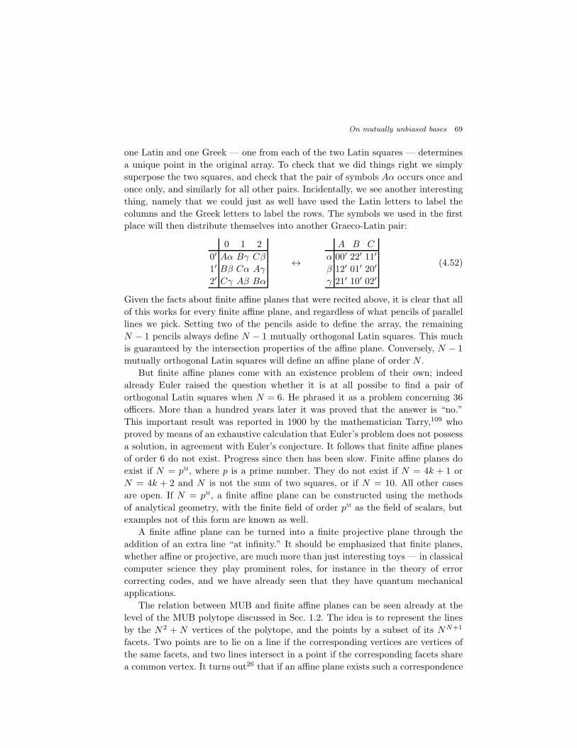
On mutually unbiased bases 69
one Latin and one Greek — one from each of the two Latin squares — determines
a unique point in the original array. To check that we did things right we simply
superpose the two squares, and check that the pair of symbols Aα occurs once and
once only, and similarly for all other pairs. Incidentally, we see another interesting
thing, namely that we could just as well have used the Latin letters to label the
columns and the Greek letters to label the rows. The symbols we used in the first
place will then distribute themselves into another Graeco-Latin pair:
0 1 2
0′ Aα Bγ Cβ
1′ Bβ Cα Aγ
2′ Cγ Aβ Bα
↔
A B C
α 00′ 22′ 11′
β 12′ 01′ 20′
γ 21′ 10′ 02′
(4.52)
Given the facts about finite affine planes that were recited above, it is clear that all
of this works for every finite affine plane, and regardless of what pencils of parallel
lines we pick. Setting two of the pencils aside to define the array, the remaining
N − 1 pencils always define N − 1 mutually orthogonal Latin squares. This much
is guaranteed by the intersection properties of the affine plane. Conversely, N − 1
mutually orthogonal Latin squares will define an affine plane of order N .
But finite affine planes come with an existence problem of their own; indeed
already Euler raised the question whether it is at all possibe to find a pair of
orthogonal Latin squares when N = 6. He phrased it as a problem concerning 36
officers. More than a hundred years later it was proved that the answer is “no.”
This important result was reported in 1900 by the mathematician Tarry,109 who
proved by means of an exhaustive calculation that Euler’s problem does not possess
a solution, in agreement with Euler’s conjecture. It follows that finite affine planes
of order 6 do not exist. Progress since then has been slow. Finite affine planes do
exist if N = pm, where p is a prime number. They do not exist if N = 4k + 1 or
N = 4k + 2 and N is not the sum of two squares, or if N = 10. All other cases
are open. If N = pm, a finite affine plane can be constructed using the methods
of analytical geometry, with the finite field of order pm as the field of scalars, but
examples not of this form are known as well.
A finite affine plane can be turned into a finite projective plane through the
addition of an extra line “at infinity.” It should be emphasized that finite planes,
whether affine or projective, are much more than just interesting toys — in classical
computer science they play prominent roles, for instance in the theory of error
correcting codes, and we have already seen that they have quantum mechanical
applications.
The relation between MUB and finite affine planes can be seen already at the
level of the MUB polytope discussed in Sec. 1.2. The idea is to represent the lines
by the N2 + N vertices of the polytope, and the points by a subset of its NN+1
facets. Two points are to lie on a line if the corresponding vertices are vertices of
the same facets, and two lines intersect in a point if the corresponding facets share
a common vertex. It turns out26 that if an affine plane exists such a correspondence

70 T. Durt, B.-G. Englert, I. Bengtsson, and K. Zyczkowski
can always be set up, and the N2 selected facets will then be placed in such a way
that their centers form a regular simplex in RN2−1. This construction needs neither
finite fields nor the special feature that the vertices of the polytope correspond to
one-dimensional projectors on Hilbert space. But when they do, it is possible to
choose — following Wootters92–94 — the special set of Wigner operators that we
have discussed in Sec. 4.2.3, and to relate the construction to the partition of the
Heisenberg–Weyl group that is associated with the MUB:35 Then each basis is
associated with a straight line that passes through the origin in the plane.
Whether there is a deeper relation between the existence problem for MUB
and the existence problem for finite affine planes is not known today. It has been
conjectured that such a relation exists,110, 111 but a recent attempt to use a pair of
Graeco-Latin squares that does exist when N = 10 to construct a set of four MUB
in this dimension failed.112 It is interesting to notice that if N mutually orthogonal
Latin squares exist, then there always exist N + 1 of them. Similarly, if N MUB
exist, then there always exist N + 1 of them.113
In the 19th century, the combinatorial structures now known as finite geometries
were studied more concretely by geometers, who realized them as configurations of
lines and points, or more generally as configurations of subspaces of a complex
projective space.114 In 1844 Hesse, following earlier work by Plucker, studied a
configuration of 9 lines and 12 points in the projective plane, such that each line
contains 4 points and each point lies on 3 lines.115 Translated into the language of
quantum theory, where the projective plane is the set of rays in a three-dimensional
Hilbert space (N = p = 3), Hesse’s twelve points are indeed the twelve kets that
compose the four MUB of three kets each. His construction was generalized to the
case of arbitrary prime N by Segre,116 who therefore in a sense discovered the
maximal sets of MUB in prime dimensions — although some necessary ingredi-
ents, including the quantum mechanical significance of the construction, were very
naturally missing.
Segre’s starting point was an elliptic curve in complex projective space,117 whose
symmetry group consists of the Heisenberg–Weyl group together with an extra
reflection, an element of order 2. When N is an odd prime, there are N2 such
reflections, since the Heisenberg–Weyl group acts on them in accordance with (4.24),
which corresponds to the condition (W4) in (4.22). In our terminology this means
that he introduced a discrete parity operator with the matrix representationv
[W0,0]a,b = δ0,a⊕b . (4.53)
This operator is both hermitian and unitary, with eigenvalues ±1, and in fact it
splits the Hilbert space into two subspaces, of dimension n and n− 1 respectively,
where N = 2n − 1 is an odd prime. There are altogether N2 such subspaces of
dimension n, and Segre observed that there exists N2 +N vectors such that each
subspace contains N + 1 of the vectors, and each vector lies in exactly N of the
vSince N is an odd prime, the field addition ⊕ is modulo-N addition.
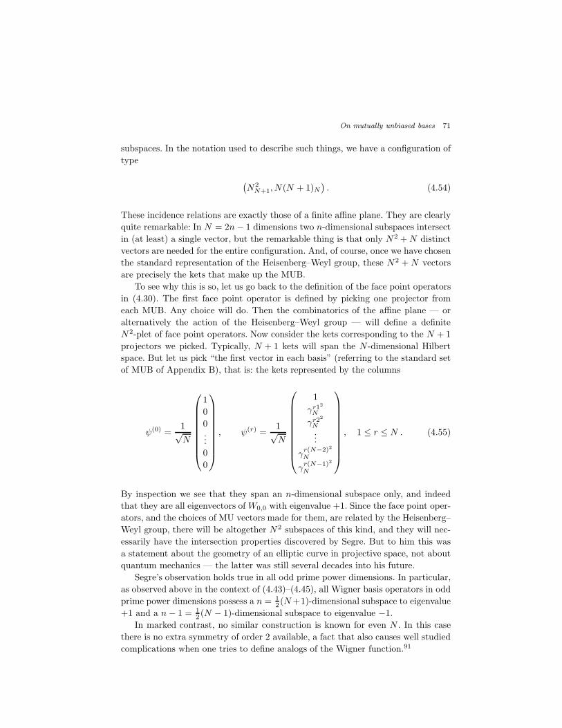
On mutually unbiased bases 71
subspaces. In the notation used to describe such things, we have a configuration of
type
(N2
N+1, N(N + 1)N). (4.54)
These incidence relations are exactly those of a finite affine plane. They are clearly
quite remarkable: In N = 2n− 1 dimensions two n-dimensional subspaces intersect
in (at least) a single vector, but the remarkable thing is that only N2 +N distinct
vectors are needed for the entire configuration. And, of course, once we have chosen
the standard representation of the Heisenberg–Weyl group, these N2 + N vectors
are precisely the kets that make up the MUB.
To see why this is so, let us go back to the definition of the face point operators
in (4.30). The first face point operator is defined by picking one projector from
each MUB. Any choice will do. Then the combinatorics of the affine plane — or
alternatively the action of the Heisenberg–Weyl group — will define a definite
N2-plet of face point operators. Now consider the kets corresponding to the N + 1
projectors we picked. Typically, N + 1 kets will span the N -dimensional Hilbert
space. But let us pick “the first vector in each basis” (referring to the standard set
of MUB of Appendix B), that is: the kets represented by the columns
ψ(0) =1√N
1
0
0...
0
0
, ψ(r) =1√N
1
γr12
N
γr22
N...
γr(N−2)2
N
γr(N−1)2
N
, 1 ≤ r ≤ N . (4.55)
By inspection we see that they span an n-dimensional subspace only, and indeed
that they are all eigenvectors ofW0,0 with eigenvalue +1. Since the face point oper-
ators, and the choices of MU vectors made for them, are related by the Heisenberg–
Weyl group, there will be altogether N2 subspaces of this kind, and they will nec-
essarily have the intersection properties discovered by Segre. But to him this was
a statement about the geometry of an elliptic curve in projective space, not about
quantum mechanics — the latter was still several decades into his future.
Segre’s observation holds true in all odd prime power dimensions. In particular,
as observed above in the context of (4.43)–(4.45), all Wigner basis operators in odd
prime power dimensions possess a n = 12 (N+1)-dimensional subspace to eigenvalue
+1 and a n− 1 = 12 (N − 1)-dimensional subspace to eigenvalue −1.
In marked contrast, no similar construction is known for even N . In this case
there is no extra symmetry of order 2 available, a fact that also causes well studied
complications when one tries to define analogs of the Wigner function.91
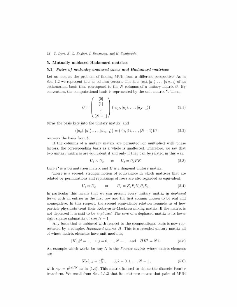
72 T. Durt, B.-G. Englert, I. Bengtsson, and K. Zyczkowski
5. Mutually unbiased Hadamard matrices
5.1. Pairs of mutually unbiased bases and Hadamard matrices
Let us look at the problem of finding MUB from a different perspective. As in
Sec. 1.2 we represent kets as column vectors. The kets |u0〉, |u1〉, . . . , |uN−1〉 of anorthonormal basis then correspond to the N columns of a unitary matrix U . By
convention, the computational basis is represented by the unit matrix 1. Then,U =
〈0|〈1|...
〈N − 1|
(|u0〉, |u1〉, . . . , |uN−1〉
)(5.1)
turns the basis kets into the unitary matrix, and(|u0〉, |u1〉, . . . , |uN−1〉
)=(|0〉, |1〉, . . . , |N − 1〉
)U (5.2)
recovers the basis from U .
If the columns of a unitary matrix are permuted, or multiplied with phase
factors, the corresponding basis as a whole is unaffected. Therefore, we say that
two unitary matrices are equivalent if and only if they can be related in this way,
U1 ∼ U2 ⇔ U2 = U1PE . (5.3)
Here P is a permutation matrix and E is a diagonal unitary matrix.
There is a second, stronger notion of equivalence in which matrices that are
related by permutations and rephasings of rows are also regarded as equivalent,
U1 ≈ U2 ⇔ U2 = E2P2U1P1E1 . (5.4)
In particular this means that we can present every unitary matrix in dephased
form: with all entries in the first row and the first column chosen to be real and
nonnegative. In this respect, the second equivalence relation reminds us of how
particle physicists treat their Kobayashi–Maskawa mixing matrix. If the matrix is
not dephased it is said to be enphased. The core of a dephased matrix is its lower
right square submatrix of size N − 1.
Any basis that is unbiased with respect to the computational basis is now rep-
resented by a complex Hadamard matrix H . This is a rescaled unitary matrix all
of whose matrix elements have unit modulus,
|Hi,j |2 = 1 , i, j = 0, . . . , N − 1 and HH† = N1 . (5.5)
An example which works for any N is the Fourier matrix whose matrix elements
are
[FN ]j,k = γjkN , j, k = 0, 1, . . . , N − 1 , (5.6)
with γN = e2πi/N as in (1.4). This matrix is used to define the discrete Fourier
transform. We recall from Sec. 1.1.2 that its existence means that pairs of MUB
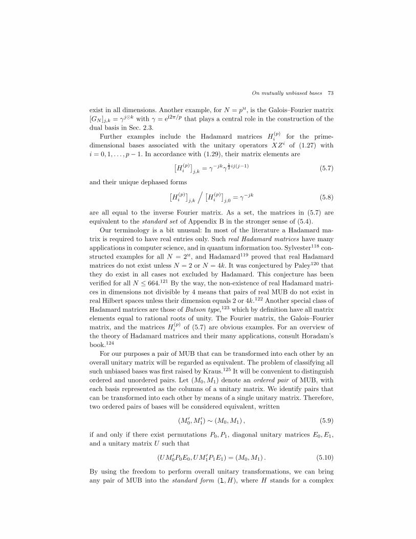
On mutually unbiased bases 73
exist in all dimensions. Another example, for N = pm, is the Galois–Fourier matrix
[GN ]j,k = γj⊙k with γ = ei2π/p that plays a central role in the construction of the
dual basis in Sec. 2.3.
Further examples include the Hadamard matrices H(p)i for the prime-
dimensional bases associated with the unitary operators XZi of (1.27) with
i = 0, 1, . . . , p− 1. In accordance with (1.29), their matrix elements are
[H
(p)i
]j,k
= γ−jkγ1
2ij(j−1) (5.7)
and their unique dephased forms
[H
(p)i
]j,k
/ [H
(p)i
]j,0
= γ−jk (5.8)
are all equal to the inverse Fourier matrix. As a set, the matrices in (5.7) are
equivalent to the standard set of Appendix B in the stronger sense of (5.4).
Our terminology is a bit unusual: In most of the literature a Hadamard ma-
trix is required to have real entries only. Such real Hadamard matrices have many
applications in computer science, and in quantum information too. Sylvester118 con-
structed examples for all N = 2m, and Hadamard119 proved that real Hadamard
matrices do not exist unless N = 2 or N = 4k. It was conjectured by Paley120 that
they do exist in all cases not excluded by Hadamard. This conjecture has been
verified for all N ≤ 664.121 By the way, the non-existence of real Hadamard matri-
ces in dimensions not divisible by 4 means that pairs of real MUB do not exist in
real Hilbert spaces unless their dimension equals 2 or 4k.122 Another special class of
Hadamard matrices are those of Butson type,123 which by definition have all matrix
elements equal to rational roots of unity. The Fourier matrix, the Galois–Fourier
matrix, and the matrices H(p)i of (5.7) are obvious examples. For an overview of
the theory of Hadamard matrices and their many applications, consult Horadam’s
book.124
For our purposes a pair of MUB that can be transformed into each other by an
overall unitary matrix will be regarded as equivalent. The problem of classifying all
such unbiased bases was first raised by Kraus.125 It will be convenient to distinguish
ordered and unordered pairs. Let (M0,M1) denote an ordered pair of MUB, with
each basis represented as the columns of a unitary matrix. We identify pairs that
can be transformed into each other by means of a single unitary matrix. Therefore,
two ordered pairs of bases will be considered equivalent, written
(M ′0,M
′1) ∼ (M0,M1) , (5.9)
if and only if there exist permutations P0, P1, diagonal unitary matrices E0, E1,
and a unitary matrix U such that
(UM ′0P0E0, UM
′1P1E1) = (M0,M1) . (5.10)
By using the freedom to perform overall unitary transformations, we can bring
any pair of MUB into the standard form (1, H), where H stands for a complex
74 T. Durt, B.-G. Englert, I. Bengtsson, and K. Zyczkowski
Hadamard matrix. But this still leaves some freedom to perform permutations and
rephasings from the left, because
(1, H1) ∼ (EP1P−1E−1, EPH1P1E1) = (1, EPH1P1E1) . (5.11)
The conclusion is that two pairs of ordered MUB, written in standard form, are
equivalent if and only if the two Hadamard matrices are equivalent in the sense of
(5.4),
(1, H1) ∼ (1, H2) ⇔ H1 ≈ H2 . (5.12)
Haagerup126 devised a useful way of testing for this kind of equivalence. The ma-
trices H(p)i of (5.7) are equivalent to each other.
Now consider unordered pairs of MUB, denoted by M0,M1. The freedom to
perform overall unitary transformations implies that (1, H) ∼ (H†,1). It follows
that
1, H ∼ 1, H† . (5.13)
Therefore unordered pairs of MUB may be equivalent even when the ordered pairs
are not. Indeed
1, H1 ∼ 1, H2 ⇔either H1 ≈ H2 ,
or H1 ≈ H†2 .
(5.14)
5.2. Triplets of mutually unbiased bases and circulant matrices
The question when two MUB triplets, say, are equivalent is a little bit involved. In
an ordered triplet the first two bases are kept fixed, one of them being the standard
basis and the other some fixed Hadamard matrix H1. Then the freedom to perform
further permutations and rephasings from the left is severely restricted, and we can
only say that
(1, H1, H2) ∼ (1, H1, H3) ⇒ H2 ≈ H3 . (5.15)
The converse is false. Equivalence of unordered sets of k+1 MUB can be discussed
similarly, but becomes harder and harder to check in practice because there are
k + 1 different choices of the basis to be represented by the unit matrix. Keep-
ing this limitation in mind, a collection of k + 1 ordered MUB (1, H1, . . . , Hk) is
called homogeneous if all the Hadamard matrices Hi, i = 1, . . . , k, are equivalent,
and heterogeneous if there is a pair of inequivalent matrices among the Hadamard
matrices.27
Two Hadamard matrices H1 and H2 are said to be MUHM if
1√NH†
1H2 = H3 , (5.16)
where H3 is a Hadamard matrix too. This is interesting because it implies that
the triplet (1, H1, H2) represents three MUB. More generally a set of N MUHM is
equivalent to a collection of N + 1 MUB.
On mutually unbiased bases 75
Triplets of MUB that include the Fourier matrix have an interesting interpre-
tation in terms of the discrete Fourier transform. Given a sequence of complex
numbers zi, 0 ≤ i ≤ N − 1, its Fourier transform is
z = Fz ⇔ z = F †z . (5.17)
The column vector whose components are zi/√N is unbiased with respect to the
Fourier basis if and only if the sequence zi is unimodular, |zi|2 = 1, and it is
unbiased with respect to the standard basis if and only if zi is unimodular. Hence
vectors that are unbiased with respect to both the standard basis and the Fourier
basis are in one-to-one correspondence to sequences obeying
|zi|2 = |zi|2 = 1 (5.18)
for all values of i. Such sequences are called biunimodular.126, 127 The first examples
were in effect produced by Gauss. When N is odd they are
z(n,m)j = e
2πiN
(mj2 + nj) (5.19)
where m,n are integers modulo N and the greatest common divisor of m and N
equals 1. To prove that these sequences are biunimodular we must perform a Gauss
sum, as discussed in Appendix C.
Biunimodular sequences have an interesting property that emerges when one
studies the autocorrelation function
Γa =1
N
N−1∑
i=0
z∗i za+i . (5.20)
An easy calculation shows that
Γa =1
N
N−1∑
i=0
|zi|2γaiN . (5.21)
Hence, if the sequence is biunimodular it obeys
Γa = δa,0 . (5.22)
Therefore zi and za+i, with a fixed and nonzero, are orthogonal vectors.
Any column vector can be used to define a circulant matrix, where each column
is obtained from the preceding one by shifting all its elements cyclically in such
a way that all the diagonal elements are the same.128 For an explicit example see
(5.49) below. The matrix elements are
Cij = zi−j (modN) . (5.23)
With this definition a circulant matrix is a Hadamard matrix if and only if the
sequence zi is biunimodular. It follows that all vectors unbiased with respect to
both the standard basis and the Fourier basis can be collected into a set of circulant
Hadamard matrices whose columns form bases that are unbiased with respect to the
standard and Fourier bases. There can be no “stray” unbiased vectors not belonging
76 T. Durt, B.-G. Englert, I. Bengtsson, and K. Zyczkowski
to an unbiased basis. We observe that any circulant matrix is diagonalized by the
Fourier matrix. More precisely, if the first column of the circulant matrix C is
defined by the sequence zi, then
F †CF = diag(z0, z1, . . . , zN−1) . (5.24)
It follows that all circulant matrices commute. Moreover, via (5.16) this confirms
that F and C represent a pair of unbiased bases.
An example of a MUB triplet of this type is the triplet consisting of the eigen-
vectors of the three cyclic subgroups of the Heisenberg–Weyl group which exist in
all dimensions: the three abelian subgroups composed of the powers of X , Z, and
XZ of Sec. 1.1.6, for instance. When N = p is prime, one known solution for a
complete set of MUHM consists of 1, F , and N − 1 circulant matrices constructed
from the biunimodular sequences (5.19) given by Gauss; see Appendix B.
It is natural to ask if there are other solutions. In fact this is a discrete version
of the Pauli problem:129 Given the modulus of a function and that of its Fourier
transform, is the function uniquely determined? Bjorck and coworkers looked into
this question,127 and they found all biunimodular sequences for N ≤ 8. Equiva-
lently, they found all vectors unbiased to the Fourier matrix in these dimensions.
For N = 5 there are 20 vectors, all of them given by Gauss’s formula, for N = 6
there are 48 vectors, including 12 given by Gauss, for N = 7 there are 532 vectors,
including 42 given by Gauss, and for N = 8 there is an infinite number of solutions.
This is true whenever N contains a square factor,130 while the number of solutions
is always finite for prime N .131
There are also MUHM triplets that do not include the Fourier or the Galois–
Fourier matrix. We will see examples later.
5.3. Classification of Hadamard matrices of size N ≤ 5
ForN ≤ 5 the classification of all Hadamard matrices under the equivalence relation
(5.4) is complete. All complex 2×2 Hadamard matrices are equivalent to the Fourier
matrix F2, here without the 1/√2 factor of (1.22),
F2 =
(1 1
1 −1
). (5.25)
This is a real Hadamard matrix. When N = 3, the set of all inequivalent Hadamard
matrices contains the only element
F3 =
1 1 1
1 γ γ2
1 γ2 γ
, (5.26)
where γ = e2πi/3 as usual.126 When N = 5, all complex Hadamard matrices are
again equivalent to the Fourier matrix F5.126 The known maximal sets of MUB in
these dimensions, and indeed in all prime dimensions, consist of the standard basis
On mutually unbiased bases 77
together with equivalent Hadamard matrices of the form H = EF , for p different
choices of a diagonal unitary matrix E.
This remark about prime dimensions is illustrated by the matrices in (5.7) except
that the inverse Fourier matrix appears there, but that is only one permutation away
from the Fourier matrix itself. Indeed, we could have the Fourier matrix just as well,
simply by interchanging the roles of X and Z in (1.27) and using the eigenstates
of X as the computational basis. Since X and Z are unitarily equivalent, the two
sets of MUB are as well.
For N = 4 the situation is different: There exists a one-parameter family of
equivalence classes,
F4(a) =
1 1 1 1
1 eia −1 −eia1 −1 1 −11 −eia −1 eia
. (5.27)
Hadamard119 himself proved that all N = 4 Hadamard matrices are equivalent to a
member of this family, for some value 0 ≤ a < π of the phase a. If a = π2 , this is the
standard Fourier matrix F4. Choosing a = 0 produces the Galois–Fourier matrix
F4(0) ≈ F2 ⊗ F2, which is a real Hadamard matrix.
5.4. Affine families and tensor products
Why does the continuous family appear when N = 4? To analyze this question we
keep N arbitrary, multiply the matrix elements of the core of the dephased form of
a given Hadamard matrix by arbitrary phase factors, and expand to first orders in
the angles:
Hij → Hijeiφij ≃ Hij(1 + iφij) , 1 ≤ i, j ≤ N − 1 . (5.28)
Then we solve the unitarity equations to first order in the angles φij . This is a
linear system, but the number of equations exceeds the number of unknowns.
The number of free parameters in the solution of this linearized problem is called
the defect of the matrix H . It can be explicitly determined by computing the rank
of a certain matrix.132 The defect gives an upper bound on the dimension of any
continuous set of inequivalent Hadamard matrices containing H . If the defect is
nonzero it can happen that the solution to the linearized unitarity equations holds
to all orders, in which case we speak of an affine family of Hadamard matrices.133
It can also happen that the full unitarity equations are obeyed if the angles become
nonlinear functions of each other, and then we have a nonaffine family. If the defect
is zero the matrix is said to be isolated.
It is known that the defect of the Fourier matrix is zero whenever N is a prime
number, hence there are no continuous families containing the Fourier matrix in
these dimensions.132 On the other hand, whenever N = N1N2 is a composite num-
ber one can produce continuous affine families from any choice of Hadamard ma-
trices in dimensions N1 and N2.126, 134 If both N1 and N2 are prime, N = p1p2, the
78 T. Durt, B.-G. Englert, I. Bengtsson, and K. Zyczkowski
construction gives a (p1 − 1)(p2 − 1)-dimensional orbit of inequivalent Hadamard
matrices including the Fourier matrix, which explains what happens for N = 4.
A more basic, and quite important, fact about tensor product Hilbert spaces
is the following: Let HA1 , . . . , H
Ak be a set of k MUHM of size NA, while
HB1 , . . . , H
Bk denotes a set of k MUHM of size NB. Then the tensor products
HA1 ⊗HB
1 , . . . , HAk ⊗HB
k form a set of k unbiased Hadamard matrices in CNANB .
To prove this it is enough to check that condition (5.16) is obeyed. When k = 2,
we have
1√N
(HA1 ⊗HB
1 )†(HA2 ⊗HB
2 ) =1√NA
HA1
†HA
2 ⊗1√NB
HB1
†HB
2 . (5.29)
The matrix on the right-hand side is a Hadamard matrix by assumption, and we are
done. Note that the pair with cross terms HA1 ⊗HB
2 , HA2 ⊗HB
1 is also unbiased,
but these Hadamard matrices are not unbiased with respect to the pair used in
(5.29). Hence by tensoring two sets of k MUHM of dimension NA and NB we will
obtain exactly k MUHM of the product structure in the extended space of size
N = NANB, but not more of them. This is the construction mentioned at the end
of Sec. 1.1.6 for NA = 2, NB = 3, and k = 3.
We say that the Hadamard matrixH is separable if it is equivalent to any matrix
of the product form
H ≈ HN1⊗HN2
, (5.30)
where HN1and HN2
are N1 × N1 and N2 × N2 Hadamard matrices, respectively.
If this is not the case, the Hadamard matrix H of size N1N2 will be called entan-
gled. This concept requires that a concrete tensor product decomposition is given
beforehand. One may find a Hadamard matrix of size N = 12 which is separable
with respect to the 2 × 6 factorization, but entangled with respect to the 3 × 4
splitting. An example is the matrix F2 ⊗ S6, where S6 is the Tao matrix that will
be discussed in the next section.
5.5. Hadamard matrices of size N = 6
N = 6 is the smallest composite number for which the two factors are different,
the smallest integer that is not a power of a prime. It is the smallest dimension for
which the MUB existence problem is open, and it is also the smallest dimension for
which the classification of all Hadamard matrices is an unsolved question. But the
hunt for N = 6 Hadamard matrices is ongoing, and was brought to a sunny plateau
recently by Karlsson.135, 136
We begin by defining an H2-reducible Hadamard matrix as a Hadamard matrix
for which all its 2 × 2 submatrices are themselves Hadamard matrices. Karlsson
proved the theorem that a 6× 6 Hadamard matrix is H2-reducible if and only if it
contains a single 2 × 2 Hadamard submatrix. As a simple corollary, H2-reducible
Hadamard matrices are very easy to recognize: A 6 × 6 Hadamard matrix is H2-
reducible if and only if its dephased form contains a matrix element equal to −1.135
On mutually unbiased bases 79
With the sole exception of the Tao matrix,137 all analytically known examples take
this form. Moreover, the set of such Hadamard matrices belong to a three-parameter
family that was explicitly constructed by Karlsson.136
Karlsson starts with the ansatz
H =
1 1 1 1 1 1
1 −1 z1 −z1 z2 −z21 z3 • • • •1 −z3 • • • •1 z4 • • • •1 −z4 • • • •
, (5.31)
where the zi are phase factors and the 2× 2 blocks that have not been written out
are guaranteed to be Hadamard matrices. We used the fact that four phase factors
that add to zero form a rhombus in the complex plane, which is why they pair up
in the way indicated. This ansatz is rewritten as
H =
F2 Z1 Z2
Z312Z3AZ1
12Z3BZ2
Z412Z4BZ1
12Z4AZ2
. (5.32)
This matrix will be unitary if and only if
A+B = F2 , A−B =√3F2iΛ , Λ†Λ = 1 , Λ† = Λ . (5.33)
The unitary 2 × 2 matrix Λ, and a fortiori the matrices A and B, will therefore
depend on two free parameters that parameterize a sphere — which can be thought
of as the equator of the group SU(2). We find
A =
(A11 A12
A∗12 −A∗
11
)(5.34)
with
A11 = −1
2+ i
√3
2(x1 + ix2 + x3) , A12 = −1
2+ i
√3
2(x1 − ix2 − x3) (5.35)
and
B(x1, x2, x3) = A(−x1,−x2,−x3) , (5.36)
where the three real parameters (x1, x2, x3) are constrained by
x21 + x22 + x23 = 1 . (5.37)
Actually, another solution is Λ = ±1, but in the end this gives only Hadamard
matrices that are equivalent to one of the above.
It remains to ensure that all matrix elements are unimodular. The conditions
for this can be written in an elegant form using Mobius transformations that take
the unit circle to the unit circle. Indeed
z23 =MA(z21) =MB(z
22) , z24 =MA(z
22) =MB(z
21) , (5.38)

80 T. Durt, B.-G. Englert, I. Bengtsson, and K. Zyczkowski
where
M(z) =αz − ββ∗z − α∗ (5.39)
with the respective parameter values
αA = A212 , βA = A2
11 , αB = B212 , βB = B2
11 (5.40)
for MA and MB. Provided that at least one of these Mobius transformations is
non-degenerate these equations can be solved (up to a sign) for z2, z3, z4 in terms
of z1, say, so together they contribute only one real parameter to the family of H2-
reducible Hadamard matrices. There are four points where both transformations
are degenerate, namely
(x1, x2, x3) = (0, 0,±1) and (x1, x2, x3) = (±1, 0, 0) . (5.41)
Hence the parameter space has three dimensions, and can be roughly described as
a circle bundle over a two-dimensional sphere, but with four special points where
the circle has been blown up to a torus.
It would be desirable to work out exactly what choices of the three parameters
lead to equivalent Hadamard matrices. This problem has been solved only partially.
Changing the sign of any zi leads to equivalent Hadamard matrices. It is also known
that the transformations
(x1, x2, x3)→ (−x1,−x2, x3)→ (x1,−x2,−x3)→ (−x1,−x2,−x3) (5.42)
lead to equivalent Hadamard matrices if supplemented by appropriate transforma-
tions of the phase factors zi. Hence at most one octant of the sphere is needed in
the parameterization.
It remains to describe some examples of special interest. The first family to be
discovered was the affine Fourier family126
F (a, b) =
1 1 1 1 1 1
1 γz1 γ2z2 γ3 γ4z1 γ5z21 γ2 γ4 1 γ2 γ4
1 γ3z1 z2 γ3 z1 γ3z21 γ4 γ2 1 γ4 γ2
1 γ5z1 γ4z2 γ3 γ2z1 γz2
(5.43)
with γ = γ6 = ei2π/6 here while z1 = ei2πa and z2 = ei2πb. In the construction
the two free parameters a, b arise because a six-dimensional space can be written
as a tensor product. For this subfamily the equivalence problem has been fully
understood.27 Thus there is a discrete group acting on the square, or torus, pa-
rameterized by a, b. It is a semi-direct group of a dihedral group with a discrete
translation group. This dihedral group is the symmetry group of a regular hexagon.
The result is that the original square is divided into 144 equivalent triangles of
equal area. One of them has corners at (0, 0), (16 , 0) and (16 ,112 ), and every affine
F (a, b) is equivalent to one for which (a, b) lies within this triangle.

On mutually unbiased bases 81
The twin family of transposed matrices FT(a, b) can be parameterized in an
analogous way. These two families intersect at the Fourier matrix itself,
F6 = F (0, 0) = FT(0, 0) ≈ F2 ⊗ F3 ≈ F3 ⊗ F2 . (5.44)
The equivalence happens because the factors of 6 = 2 · 3 are relatively prime; see
Ref. 138 for a general discussion of equivalences between tensor products of Fourier
matrices.
In the family of H2-reducible Hadamard matrices one finds the Fourier family
at the special point (x1, x2, x3) = (0, 0, 1), while the transposed Fourier family sits
at (x1, x2, x3) = (1, 0, 0); recall that both Mobius transformations of (5.38)–(5.40)
become degenerate at these points. Curiously the one parameter family FT(0, b)
also sits at (0, 0, 1), and similarly F (a, 0) also sits at (1, 0, 0).
One more affine family is known, namely the Dita family,134 which in dephased
form is given by
D(a) =
1 1 1 1 1 1
1 −1 i −i −i i
1 i −1 iz −iz −i1 −i iz∗ −1 i −iz∗1 −i −iz∗ i −1 iz∗
1 i −i −iz iz −1
with z = ei2πa . (5.45)
We obtain all inequivalent examples if we impose the restriction − 18 < a ≤ 1
8 . It
includes the Butson-type matrix D6(0), known as the Dita matrix, and composed of
fourth roots of unity. This can be found in several different places within the three-
parameter family, reflecting the fact that the equivalence problem for the latter is
unsolved. One possibility is to set x1 = x2 = x3, in which case the Dita family is
parameterized by the phase factor z1.
Another Hadamard matrix of special interest is the circulant matrix127
C6 =
1 id −d −i −d∗ id∗
id∗ 1 id −d −i −d∗−d∗ id∗ 1 id −d −i−i −d∗ id∗ 1 id −d−d −i −d∗ id∗ 1 id
id −d −i −d∗ id∗ 1
, (5.46)
where
d =1−√3
2+ i
√√3
2, d∗d = 1 . (5.47)
The unimodular number d solves the equation d2 − (1−√3)d+ 1 = 0. It is known
that every circulant Hadamard matrix is equivalent to either F6 or C6.
Before Karlsson’s work several non-linear subfamilies of Hadamard matrices
were known. The first to be found (by Beauchamp and Nicoara139) was the one-
parameter family B(θ) containing all Hadamard matrices equivalent to a hermitian

82 T. Durt, B.-G. Englert, I. Bengtsson, and K. Zyczkowski
F
FT
B(θ)
D(a)
C6
C6
C6
C6
C6
C6
D6D6
D6
D6
D6
D6
Fig. 2. Szollosi’s two-dimensional family of N = 6 complex Hadamard matrices interpolatesbetween the generalized Fourier matrix F = F
(
16, 0)
and the hermitian familyB(θ), which includesC6 and D6. It is parametrized by the common interior of two deltoids. There are actually several“leaves” over the interior, and it is divided into six equivalent sectors. Dita’s affine family D(a),see (5.45), is represented by a circle inscribed into the figure.
matrix. It interpolates between C6 and D6(0) in a complicated way. It is included as
the boundary of a two-parameter family of bicirculant Hadamard matrices found
by Szollosi.140 By definition, a bicirculant matrix is divided into four blocks of
equal size, each block being a circulant matrix in itself. Szollosi’s family contains
all bicirculant matrices with two independent blocks only, according to the pattern
X6 =
(A B
B† −A†
), (5.48)
where H is bicirculant because A and B are circulant,
A =
a b c
c a b
b c a
, B =
d e f
f d e
e f d
. (5.49)
The individual entries are unimodular phase factors. Since any two circulant ma-
trices commute the unitarity conditions are quite simple to state. Szollosi ended
up with an appealing picture of the resulting two-parameter family. In the complex
plane the parameter space is bounded by two deltoids related by a reflection. By
definition a deltoid is a 3-hypocycloid, that is the curve traced out if you place the
tip of your pen at the rim of a wheel, and then let this wheel roll inside a larger
wheel whose inner rim has three times the radius of the rolling wheel; see Fig. 2.
The picture is that of an umbrella, and in fact of two superposed umbrellas because
above each point there are two inequivalent matrices that can be represented as
the transposes of each other. Thus we have two two-parameter families X6(α) and
XT6 (α) coming together at their common boundary. One can easily check that they
are subfamilies of Karlsson’s family.
On mutually unbiased bases 83
Another one-parameter family of symmetric Hadamard matrices141 was ex-
tended to a two-parameter family by Karlsson.142 This family can be obtained
by setting z1 = z2 and z3 = z4 in the ansatz (5.32). Interestingly it is then possible
to solve explicitly for the matrices A and B in terms of the phases z1 and z3.
The elegance of the available constructions is very encouraging, but they are not
the end of the story. It has been conjectured27 that a four-parameter family exists.
One reason for this is that the defect of all included matrices has been found to be
four, whenever it has been checked,27 and moreover there is by now strong numerical
evidence for the conjecture.143, 144 Yet, the set of inequivalent N = 6 Hadamard
matrices is disconnected, because there is also an isolated matrix that does not
belong to any continuous family. This is a symmetric Butson-type Hadamard matrix
composed of third roots of unity only, known as Tao’s matrix.137, 145 It is isolated
because its defect vanishes. One does not know if other isolated matrices exist.
5.6. Hadamard matrices for N ≥ 7
Some general facts are known also in higher dimensions, in particular affine families
stemming from known Hadamard matrices have been much studied. As we have
already mentioned, the Fourier matrix is an isolated matrix if and only if N is a
prime number.132 When N is a power of a prime, N = pm, all affine orbits stemming
from the Fourier matrix are explicitly known. The dimension of these orbits reads
d = pm−1[(p − 1)m − p] + 1 and is equal to the defect of FN .132 It is also known
that every real Hadamard matrix admits an affine orbit if N ≥ 12.146 In prime
dimensions, affine orbits cannot pass through the Fourier matrix, but Petrescu
found an example for N = 7 which contains a Butson-type matrix built from sixth
roots of unity.147
All circulant Hadamard matrices up to N ≤ 9 have been found.127 When N
contains a square factor this includes a continuous family,130 whereas the number is
finite for all prime N .131 Many block circulant examples are also known.148 Special
methods for constructing Hadamard matrices include one based on tiling abelian
groups,149 one based on N equiangular vectors in N/2 dimensions,150 as well as a
method for constructing Hadamard matrices of size N from matrices of size N/2.
This gives a rich supply of examples with N = 8.151, 152 And, of course, there are
many ad hoc constructions. A catalog of known Hadamard matrices for N ≤ 16 is
available,133 also as an updated internet version.153
5.7. All mutually unbiased bases for N ≤ 5
Since we know that the Hadamard matrix in dimensions 2, 3, and 5 is unique
up to equivalences it seems reasonable to expect that the maximal set of MUB
is also unique up to an overall unitary transformation. When N = 2 a maximal
set of MUB can be thought of — as we did in Sec. 1.2 — as a regular octahedron
inscribed in the Bloch sphere, and the uniqueness follows from the fact that all such
octahedra are related by a rotation, corresponding to a unitary transformation in
84 T. Durt, B.-G. Englert, I. Bengtsson, and K. Zyczkowski
the N = 2 Hilbert space. Equivalently, there is the observation of Sec. 1.1.6 that
q-bit operators are associated with directions in R3 and complementary observables
must refer to orthogonal directions.
Uniqueness continues to hold for N = 3 and N = 5, although a complicated
calculation is needed to see this.76 The explicit form of unbiased Hadamard matrices
forming one maximal set of MUHM for any prime N = p is provided in Appendix B.
Another, equivalent, maximal set is composed of the matrices H(p)i in (5.7).
The case N = 4 is more interesting because of its one-parameter family of
inequivalent Hadamard matrices. It is also simple enough that the calculations can
be done by hand.77 We begin by looking for ordered MUB triplets of the form
(1, F4(a), H), where F4(a) is written in the standard form (5.27) and H is some
Hadamard matrix obtained by enphasing F4(a), possibly with its rows permuted.
After going through all the possibilities, one finds that there are exactly three
families of ordered triplets of MUB, with 2 or 1 + 2 free parameters each:
(1, F4(a), H(1)(φ1;α1)
),(1, F4(0), H
(2)(φ2;α2)),(1, F4(0), H
(3)(φ3;α3)).
(5.50)
The third members of these triplets are given by
H(1)(φ1;α1) =
1 1 1 1
eiα1 ei(α1 + φ1) −eiα1 −ei(α1 + φ1)
−1 1 −1 1
eiα1 −ei(α1 + φ1) −eiα1 ei(α1 + φ1)
,
H(2)(φ2;α2) =
1 1 1 1
eiα2 ei(α2 + φ2) −eiα2 −ei(α2 + φ2)
−eiα2 ei(α2 + φ2) eiα2 −ei(α2 + φ2)
1 −1 1 −1
,
H(3)(φ3;α3) =
1 1 1 1
1 −1 1 −1−eiα3 −ei(α3 + φ3) eiα3 ei(α3 + φ3)
eiα3 −ei(α3 + φ3) −eiα3 ei(α3 + φ3)
, (5.51)
respectively. Regarded as unordered triplets, the last two are actually special cases
of the first, so there is a single 1 + 2 parameter family of unordered triplets.
It is straightforward to check that none of these families contains a quartet of
MUB. The only way to obtain a quartet is to pick the third member of two different
ordered triplets. Moreover, there is only one way in which this can be done, namely
to set
α1 = α2 = α3 =π
2, a = φ1 = φ2 = φ3 = 0 . (5.52)
This leads to the standard solution for a maximal set of MUB, which is thereby
shown to be unique up to an overall unitary transformation. For N = 5 there are
two inequivalent triplets.77
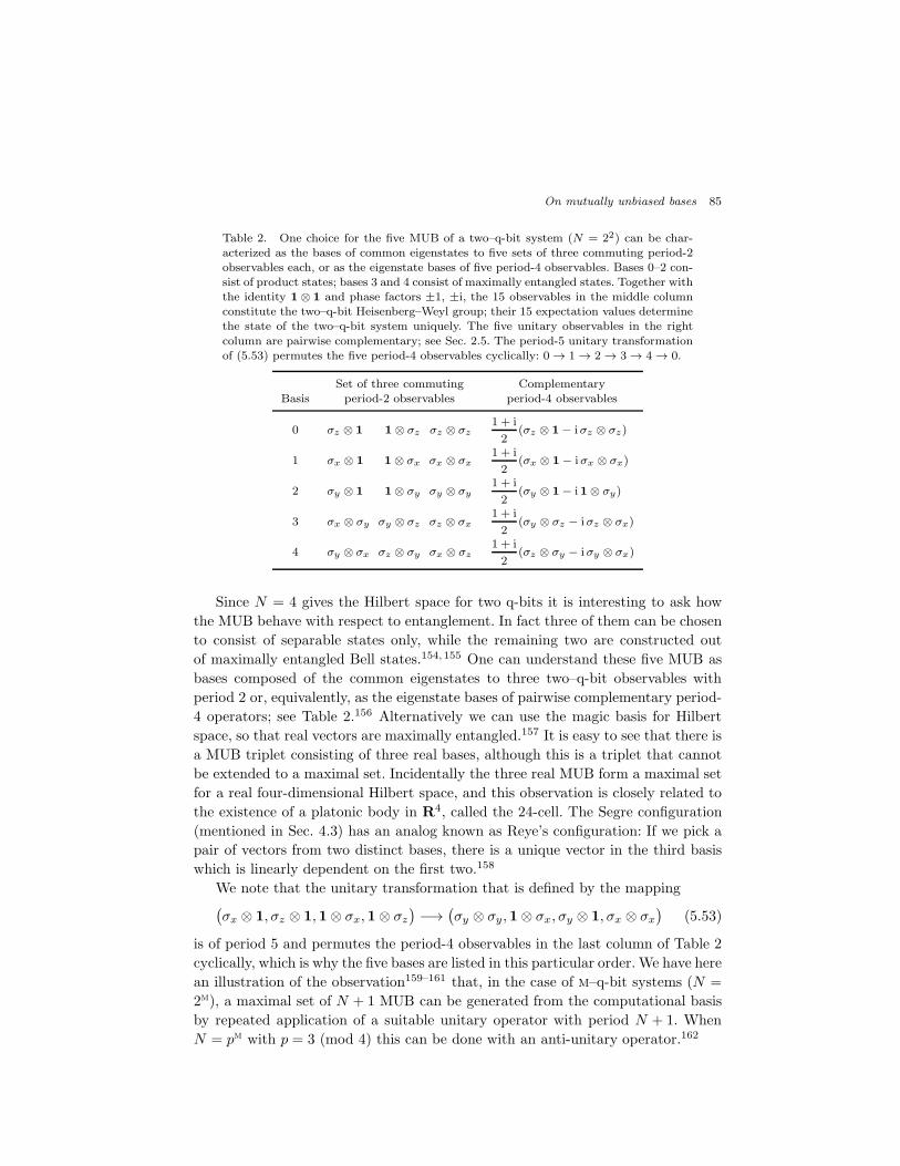
On mutually unbiased bases 85
Table 2. One choice for the five MUB of a two–q-bit system (N = 22) can be char-acterized as the bases of common eigenstates to five sets of three commuting period-2observables each, or as the eigenstate bases of five period-4 observables. Bases 0–2 con-sist of product states; bases 3 and 4 consist of maximally entangled states. Together withthe identity 1⊗ 1 and phase factors ±1, ±i, the 15 observables in the middle columnconstitute the two–q-bit Heisenberg–Weyl group; their 15 expectation values determinethe state of the two–q-bit system uniquely. The five unitary observables in the right
column are pairwise complementary; see Sec. 2.5. The period-5 unitary transformationof (5.53) permutes the five period-4 observables cyclically: 0 → 1 → 2 → 3 → 4 → 0.
Set of three commuting ComplementaryBasis period-2 observables period-4 observables
0 σz ⊗ 1 1⊗ σz σz ⊗ σz1 + i
2(σz ⊗ 1− iσz ⊗ σz)
1 σx ⊗ 1 1⊗ σx σx ⊗ σx1 + i
2(σx ⊗ 1− iσx ⊗ σx)
2 σy ⊗ 1 1⊗ σy σy ⊗ σy1 + i
2(σy ⊗ 1− i 1⊗ σy)
3 σx ⊗ σy σy ⊗ σz σz ⊗ σx1 + i
2(σy ⊗ σz − iσz ⊗ σx)
4 σy ⊗ σx σz ⊗ σy σx ⊗ σz1 + i
2(σz ⊗ σy − iσy ⊗ σx)
Since N = 4 gives the Hilbert space for two q-bits it is interesting to ask how
the MUB behave with respect to entanglement. In fact three of them can be chosen
to consist of separable states only, while the remaining two are constructed out
of maximally entangled Bell states.154, 155 One can understand these five MUB as
bases composed of the common eigenstates to three two–q-bit observables with
period 2 or, equivalently, as the eigenstate bases of pairwise complementary period-
4 operators; see Table 2.156 Alternatively we can use the magic basis for Hilbert
space, so that real vectors are maximally entangled.157 It is easy to see that there is
a MUB triplet consisting of three real bases, although this is a triplet that cannot
be extended to a maximal set. Incidentally the three real MUB form a maximal set
for a real four-dimensional Hilbert space, and this observation is closely related to
the existence of a platonic body in R4, called the 24-cell. The Segre configuration
(mentioned in Sec. 4.3) has an analog known as Reye’s configuration: If we pick a
pair of vectors from two distinct bases, there is a unique vector in the third basis
which is linearly dependent on the first two.158
We note that the unitary transformation that is defined by the mapping(σx ⊗ 1, σz ⊗ 1,1⊗ σx,1⊗ σz
)−→
(σy ⊗ σy,1⊗ σx, σy ⊗ 1, σx ⊗ σx
)(5.53)
is of period 5 and permutes the period-4 observables in the last column of Table 2
cyclically, which is why the five bases are listed in this particular order. We have here
an illustration of the observation159–161 that, in the case of m–q-bit systems (N =
2m), a maximal set of N + 1 MUB can be generated from the computational basis
by repeated application of a suitable unitary operator with period N + 1. When
N = pm with p = 3 (mod 4) this can be done with an anti-unitary operator.162

86 T. Durt, B.-G. Englert, I. Bengtsson, and K. Zyczkowski
Table 3. Number Nv of kets unbiased with respect to a given complex Hadamard matrixand the number Nt of bases (not mutually unbiased) which can be formed out of them.
Matrix F (a, b) F (0, 0) F ( 16, 0) D(0) D(b) D(c) S6
Nv 48 48 48 120 120 48 90Nt 8 16 70 10 4 4 0
5.8. Triplets of mutually unbiased bases in dimension 6
Since a complete list of all possible sets of five MUB in N = 4 can be constructed
by hand one might guess that the case of N = 6 could easily be settled with a com-
puter. Numerical searches have been performed by many, but it seems that the first
published account is the one by Zauner,21 who was led to conjecture that at most
three MUB can be found. By now the evidence for his conjecture is overwhelming,
but not quite conclusive, which tells us something about how fast the complexity
of a Hilbert space grows with dimension.
The problem of classifying all pairs of MUB is equivalent to the problem of
classifying Hadamard matrices. With partial results on this problem available, one
can go on to ask what pairs can be extended to triplets of MUB, and in how
many ways this can be done. For the Fourier family of Hadamard matrices (and
its transpose), a clear picture has emerged.163–165 There is very strong evidence
that the number of kets unbiased to the bases represented by the pair(1, F (a, b))
equals 48, regardless of the values taken by the parameters a, b, with F (a, b) as
introduced in (5.43). For generic values of the parameters these vectors can be
collected into eight different unbiased bases which, however, are not MU. Some
values of the parameters are special in this regard: The Fourier matrix F (0, 0)
admits 16 unbiased bases,87 and F (16 , 0) admits up to 70. Note that these values of
the parameters are special also because they correspond to singular points in the
moduli space of all Hadamard matrices of this type, and that F (16 , 0) is very special
because it is also included in the bicirculant family X6(α).
The evidence consists in computer calculations for a large number of members
of the family,163 and also a proof that there exists a vicinity of (a, b) = (0, 0) where
the number of unbiased vectors is constant164 and equal to 48. In one version, the
procedure begins with the observation that the condition for a ket to be unbiased
with respect to the bases pair corresponding to (1, H), for some Hadamard matrix
H , is a set of multivariate polynomial equations that can in principle be brought to
“diagonal” form (in the way one would do Gauss elimination for linear equations)
by means of Grobner bases for the polynomials. In the end polynomial equations
in single variables are solved to high enough accuracy. The procedure works nicely
for all of the affine families, while results for the nonaffine families are somewhat
uncertain because of more stringent demands on computer memory.
In Table 3, we show the number Nv of kets unbiased to the computational basis
and one additional listed basis, as well as the number Nt of bases (or triplets of
On mutually unbiased bases 87
MUB) that can be formed from these vectors.163 The results for the twin families
F (a, b) and FT(a, b) are similar, and hence results for the latter are not given
explicitly. For the Dita family D(a) of (5.45) one finds that the result depends
on the parameter value; if |a| ≤ 0.0177 there are 120 unbiased vectors, and if
0.0177 ≤ |a| ≤ 18 there are 48 of them. This takes care of all inequivalent values
of a. Note that the Butson-type matrix D(0) is quite exceptional; moreover, in
this case the phases that define the unbiased kets are known exactly. The isolated
Butson-type matrix S6 does not admit even a single triplet of MUB.
Exactly what makes the unbiased vectors collect into bases in some, but not
all cases, is imperfectly understood. For triplets of MUB involving F (0, 0), we have
given the explanation in terms of the discrete Fourier transform,27 and for the affine
family F (a, b) some partial understanding exists.164
Some continuous families of triplets of MUB are known. In particular, Zauner
showed that any bicirculant Hadamard matrix gives rise to a triplet because (5.16)
can be solved for H1 and H2 if H3 is a specified bicirculant Hadamard matrix.21 In
fact, the entire set of triplets in N = 4 dimensions can be shown to arise in this way.
For N = 6, this means that Szollosi’s bicirculant family X6(α) gives rise to a two-
parameter set of triplets. Another continuous family of the form(1, F (0, b(t)), H(t)
)
has been constructed by Jaming et al.;164 the third member of their triplet family
belongs to the Fourier family.
5.9. A maximal set of mutually unbiased bases when N = 6?
We now ask whether any of the explicitly known triplets of MUB can be extended to
a quartet. The answer is that none of them can,87 and the failure can be expressed
quantitatively.27 If a quartet involving the Fourier matrix did exist, one would be
able to find a pair of bases among the 16 bases unbiased with respect to (1, F ) suchthat the Grassmannian distance between them is equal to unity. However, the best
one can do is D2c = 0.93. Remembering that a random pair of bases are situated at
a distance given by D2c = 0.86, this is not impressive. Other pairs of MUB have not
been treated in quite that much detail, but Jaming et al. recently proved that no
quartets of MUB including any member of the Fourier family F (a, b) can exist.164
The proof involves approximations of the elements of the columns that represent the
kets by rational roots of unity, exhaustive computer searches, and careful estimates
of the errors involved.
Direct numerical searches for maximal sets have been carried out,21, 166 but
relatively few such investigations have been published. Butterley and Hall167 have
conducted a search based on the minimization of a suitable function. The minimiza-
tion proceeds by picking a point at random in some parameter space, and changing
it until a minimum is reached. The problem is that this minimum may not be the
global minimum, so the procedure could miss its target even if the target — in
this case a quartet of MUB — is there. Indeed, the success rate was 60.4% when
N = 5, but only 0.9% when N = 7. No quartets were found for N = 6. This result
88 T. Durt, B.-G. Englert, I. Bengtsson, and K. Zyczkowski
is suggestive but not definitive.
Brierley and Weigert168 concentrated on finding MU constellations, defined as
up to N + 1 sets of orthogonal kets that are MU with respect to each other. It
is not required that the sets have N members. In fact, for N = 6 they were able
to find seven sets with two members each. This constellation is denoted by 276,while a quartet of MUB is the constellation 646, in a notation that should now be
obvious (given the fact that six orthogonal vectors automatically define a seventh,
unbiased to all vectors that are unbiased with respect to the original six). They then
proceeded to search for constellations that necessarily exist if the quartet exists,
such as 6, 3, 3, 36, 6, 4, 3, 26, and so on. Altogether they found 17 examples
of such constellations for which their success rate in dimension 6 was zero. The
advantage of the procedure is that the parameter spaces in which the search is
conducted are comparatively small — in the two quoted examples there are 40
parameters, as opposed to 70 parameters for a quartet of MUB. The success rates
for similar calculations in N = 7 were high.
Hence we feel that the answer to the question in the title of this subsection must
be “no.” It is fair to say, however, that a structural understanding of this negative
result is missing. A precise translation into Euler’s problem of the 36 officers (see
Sec. 4.3) could provide this — if there is one, and if the translation provides a
structural understanding of the latter problem.
5.10. Heisenberg–Weyl group approach for N = 6
We have seen how the abelian subgroups of the Heisenberg–Weyl group identify the
maximal set of MUB if N is a power of a prime, whereby the construction of the
MUB relies heavily on the properties of the Galois field with N elements. As noted
earlier, this construction is not applicable for other values ofN , simply because there
is no corresponding Galois field. The failure of this approach, therefore, says nothing
about the existence of maximal sets of MUB in non–prime-power dimensions. As
noted repeatedly, this existence problem is open, even in the most intensely studied
case of N = 6.27, 87, 164, 167–169
Since the Galois–Fourier construction of the Heisenberg–Weyl group,
which works so well for prime power dimensions, cannot be applied for
N = 6, 10, 12, 14, . . ., one could try to repeat the procedure with operations that do
not form a field; for instance, we could try to use distributive rings with N elements,
possibly the modulo-N ring that suffices for statements like (1.5).w For N = 6 the
only ring is the modulo-6 ring, and we have the usual N2 = 36 Heisenberg–Weyl
unitary operators of Sec. 1.1.4.
Let us see. The powers of the N + 1 = 7 operators of (1.27) do form seven
abelian subgroups, but they do not exhaust all 36 products XjZk because quite
wRecall footnote ‘a’: In marked contrast to a field, a ring may have zero products of nonzeroelements, such as 2⊙6 3 = 0.

On mutually unbiased bases 89
Table 4. The twelve abelian subgroups of order six of the modulo-6 Heisenberg–Weylgroup of unitary operators. The six elements of each subgroup are given by the powers ofthe period-6 unitary operator that generates the subgroup. These generators XmZn are
listed in the second column without, however, displaying the phase factors ei(π/6)mn
that are needed when the product mn is odd to compensate for the (−1)mn factor in(1.20). The last column shows which six other generators are complementary partners.
Period-6 ComplementarySubgroup observable partners
0 X 1, 5, 6, 7, 9, 101 XZ 0, 2, 6, 7, 8, 112 XZ2 1, 3, 6, 8, 9, 103 XZ3 2, 4, 6, 7, 9, 114 XZ4 3, 5, 6, 7, 8, 105 XZ5 0, 4, 6, 8, 9, 116 Z 0, 1, 2, 3, 4, 57 X2Z 0, 1, 3, 4, 10, 118 X2Z3 1, 2, 4, 5, 10, 119 X2Z5 0, 2, 3, 5, 10, 1110 X3Z 0, 2, 4, 7, 8, 911 X3Z2 1, 3, 5, 7, 8, 9
a few of these products belong to more than one subgroup. For example, we have
X2Z2 = (XZ)2 = (XZ4)2 and, therefore, the operators XZ and XZ4 are not
complementary.
In total, there are twelve abelian subgroups of six elements each, the identity
plus five more interesting ones, obtained as powers of period-6 unitary operators.
In Table 4 we see that each of the these twelve “generators” has six complementary
partners, so that the corresponding bases are MU. But there are not more than
three bases that are pairwise MU. For instance, the bases ‘0’ and ‘1’ are MU and
are both MU with bases ‘6’ and ‘7’, but these are not MU themselves, so that ‘0,1,6’
and ‘0,1,7’ are MUB triplets whereas ‘0,1,6,7’ is not a MUB quartet.
Similarly, the modulo-4 ring construction fails for N = 4.38 The modification
that replaces the Galois field shifts by modulo-N shifts simply does not work,
except when N is prime (Sec. 1.1.6) and the two ways of shifting coincide.
6. Brief summary and concluding remarks
We used the Galois-shift based Heisenberg–Weyl group to construct first maximal
sets of MUB in prime power dimensions and then the generalized Bell states as-
sociated with them. Several applications to quantum information processing were
discussed, some in considerable detail: dense coding and teleportation, quantum
cryptography and cloning machines, the Mean King’s problem and state tomogra-
phy. Owing to the somewhat unconventional parameterization in terms of numbers
that are both field elements and ordinary integers, the approach we presented is
relatively new, and some results are rather recent.34, 38 There are yet other applica-
tions of these techniques, including the discrete phase operators170 (that would cor-

90 T. Durt, B.-G. Englert, I. Bengtsson, and K. Zyczkowski
respond to the dual group in our terminology), and there are interesting connections
between MUB and SIC POVMs21, 86, 87, 171–173 that present appealing applications
in the framework of tomography and deserve further study.
Some of these applications do not require the basic operations (addition and
multiplication) of a field, a ring structure suffices, as is the case for instance for the
SIC POVMs, teleportation, dense coding, or the discrete Weyl-type phase space
function. All of them can be realized by use of the usual modulo-N operations for
Hilbert spaces of arbitrary dimension. For the construction of maximal sets of MUB,
the modulo-N rings are good enough in prime dimensions only, that is: when they
are fields. This fact enables us to design the prime-distinguishing function described
in Appendix C.
For what concerns the construction of MUB, the dimensionality seems to play a
crucial role. The reasons why prime power dimensions are so special are not clearly
understood as yet, and it is certainly worth investigating this problem in the future.
We offer a speculation below that is suggested by the significance of the Hilbert
space dimension in quantum physics.
It is worth emphasizing that the search for maximal sets of inequivalent MUB
in each dimension is related to several different mathematical problems. The liter-
ature contains, beside the aforementioned constructions that use orthogonal uni-
tary matrices35, 174, 175 and discrete phase space,79, 94, 176 an abundance of valu-
able papers on the MUB problem related to group theory,35, 94, 177–179 angular mo-
mentum,180, 181 finite fields and affine planes,26, 170 and mutually orthogonal Latin
squares.112, 182 Nearly all of these constructions rely on properties of primes and
prime powers and on an underlying finite field.85, 181, 183–187 After some translation
the problem is equivalent to that of finding mutually orthogonal Cartan subalge-
bras in the Lie algebra of SL(N).76, 188 The problem also occurs in radar science,189
operator algebra,190 and coding theory.63 Geometric approaches to the problem are
developed in Refs. 26, 191, and 192.
Let us try to collect here the information concerning the number of known
MUB, which depends on the number-theoretic properties of the dimension N . The
following list, which by its nature is unavoidably incomplete, contains statements
about MUB and MUHM, which are easily translated into the respectively other
terminology with the aid of (5.1) and (5.2).
(a) Maximal sets of MUB exist for all prime power dimensions, N = pm.
(b) If the dimension is not a power of a prime, N 6= pm, maximal sets of MUB are
not known. It is highly unlikely that there are sets of MUB for N = 6 with
more than three bases.
(c) For any N ≥ 2 there exists at least one triplet of MUB. This is equivalent to
the statement that there exists at least a pair of MUHM.
(d) For N = 2, 3, 4, and 5, all maximal sets of N + 1 MUB are equivalent.
(e) For N > 3, there are certain sets of MUHM that cannot be extended to a
maximal set.
On mutually unbiased bases 91
(f) In prime dimension, N = p, all known sets of MUHM are equivalent to the
standard set of Appendix B. It seems unlikely that there are other nonequiva-
lent sets of MUHM, but we are not aware of a formal proof that they do not
exist.
(g) The case of a prime power dimension, N = pm, can be naturally interpreted
as a system of m quantum degrees of freedom, each described in its own p-
dimensional Hilbert space. In this case several sets of MUB may exist with
different entanglement properties of the basis states. A complete set of MUB
represented by block-circulant Hadamard matrices was constructed by Combes-
cure.193 For instance, for two, three, or four q-bits (N = 4, 8, or 16) the num-
ber of different sets of MUB constructed out of operators belonging to the
Heisenberg–Weyl group is one, four, and seventeen, respectively.78, 79, 154
(h) In certain square dimensions, N = d2, the known sets of MUB are larger than
would follow from the factorization of d. Wocjan and Beth182 show that k
mutually orthogonal Latin squares of order N enable one to construct k + 2
MUB in dimension N2. For N = 262 this yields six MUB. On the other hand,
the product-ket construction described at the end of Sec. 1.1.5 yields at most
pa1
1 + 1 MUB in dimension N = pa1
1 · · · pann with p1 < p2 < · · · < pn, whenever
the dimension is not a prime power. It has been established194 that one cannot
do better by using any other group to replace the Galois-shift Heisenberg–Weyl
group.
Finally, a list entry about continuous degrees of freedom:
(i) Continuous degrees of freedom have, as a rule, a continuum of MUB. An ex-
ception is the periodic degree of freedom (“motion along a circle”) for which
only one pair of MUB is known.
Items (a), (b), and (g) invite a speculation about the difference between Hilbert
space dimensions N that are a power of a prime and those that are other composite
numbers. In the spirit of Sec. 1.1.5, we follow Schwinger’s4–6 guidance and associate
one quantum degree of freedom with each prime factor of N . If different primes
occur, we surely have a physical system composed of different components. But if
there is only one prime, we could have indistinguishable components, in which case
the physical system behaves as one whole and the separation into the m subsystems
of (g) is artificial because the labels m = 0, 1, . . . ,m− 1 are physically meaningless.
From this physical point of view, then, it is quite satisfactory that prime power
dimensions are not so different from prime dimensions (maximal sets of MUB for
both) while other dimensions are not on the same footing (relatively few bases that
are MU). A clear-cut demonstration that, indeed, there are no maximal sets of
MUB for N 6= pm is surely desirable.

92 T. Durt, B.-G. Englert, I. Bengtsson, and K. Zyczkowski
Acknowledgments
It is a pleasure to thank W. Bruzda, A. Ericsson, J.-A. Larsson, and W. Tadej
for a long-term collaboration on research projects related to mutually unbiased
bases and for allowing us to mention some of their unpublished results. We are also
grateful to V. Cappellini, M. Grassl, Z. Jelonek, M. Matolcsi, A. Scott, A. Uhlmann,
and S. Weigert for inspiring discussions and to C.W. Chin, P. Dita, R. Nicoara,
A. Schinzel, A.J. Skinner, and F. Szollosi for helpful correspondence. We also thank
S. Chaturvedi for explaining much of Segre’s construction before we knew it was
already known. Sincere thanks to P. Cara for patiently answering our questions
about finite fields, and to A. Eusebi for attracting our attention to a sign error in
Ref. 34 and correspondence on this subject.
The authors gratefully acknowledge support from the ICT Impulse Program
of the Brussels Capital Region (project Cryptasc), the Interuniversity Attraction
Poles program of the Belgian Science Policy Office, under grant IAP P6-10 (pho-
tonics@be), and the Solvay Institutes for Physics and Chemistry (TD); the A∗Star
Grant 012-104-0040 (BGE); VR, the Swedish Research Council (IB); the grant
DFG-SFB/38/2007 of Polish Ministry of Science and Higher Education, Founda-
tion for Polish Science and European Regional Development Fund, under agreement
no MPD/2009/6 (KZ). Centre for Quantum Technologies is a Research Centre of
Excellence funded by Ministry of Education and National Research Foundation of
Singapore.
Appendix A. Generalized position and momentum operators for
spherical coordinates
We denote the cartesian coordinate operators by A1, A2, and A3, and their com-
plementary partners are the (linear) momentum operators B1, B2, and B3. The
Heisenberg commutation relations
[Aj , Bk
]= iδj,k1 (A.1)
state that we have three independent copies of the A,B pair of Secs. 1.1.7 and 1.1.8.
The operators R,Θ, E for the spherical coordinates, introduced in Secs. 1.1.9–1.1.11
are related to the cartesian Ajs in the familiar way,
A1 = R sinΘE + E†
2,
A2 = R sinΘE − E†
2i,
A3 = R cosΘ , (A.2)
On mutually unbiased bases 93
so that the relations
R =√A2
1 +A22 +A2
3 ,
tanΘ
2=
√R−A3
R+A3,
E =A1 + iA2√A2
1 +A22
(A.3)
express the spherical coordinate operators in terms of the cartesian coordinate
operators.
Their complementary partners are linear functions of the cartesian momenta,
S =
3∑
j=1
1
2(AjBj +BjAj) ,
Ω =1
R
((A1B1 +B2A2
)A3 −
(A2
1 +A22
)B3
),
L = A1B2 −A2B1 . (A.4)
Of these, the generator S of scaling transformations and the generator L of rotations
around the A3 axis are familiar operators, whereas Ω is not standard textbook fare.
Of the fifteen commutators that involve two different ones of the operators in
(A.3) and (A.4) all vanish except for
[R,S] = iR ,
[tan
Θ
2,Ω]= i tan
Θ
2,
[E,L
]= −E , (A.5)
as one can verify with the aid of
[f(A1, A2, A3), Bk
]= i
∂
∂Akf(A1, A2, A3) . (A.6)
The numerical spherical coordinates (x, y, z) = (r sinϑ cosϕ, r sinϑ sinϕ, r cosϑ)
are singular for z = ±r and, in particular, for r = 0 and these singularities are
inherited by the corresponding operators. The factors R in (1.72) and sinΘ in
(1.79) bear witness thereof.
Appendix B. Standard sets of mutually unbiased Hadamard
matrices for prime dimension
For completeness we provide here an explicit form of a maximal set of N MUHM
in the case of an arbitrary odd prime dimension, N = p ≥ 3. It is different from,
and supplements, the example of (5.7).
As a first element in the set of MUHM let us choose the Fourier matrix (5.6),
H(0) = FN . Then introduce the diagonal unitary N × N matrix EN with matrix
elements
[EN ]jk = δj,k ei 2πN
j2 where j, k = 0, 1, 2, . . . , N − 1 . (B.1)
94 T. Durt, B.-G. Englert, I. Bengtsson, and K. Zyczkowski
It allows us to define a sequence of N matrices(H(0), H(1), . . . , H(N−1)
), where
H(r) = ErNH
(0) for r = 0, 1, 2, . . . , N − 1 . (B.2)
By construction all these matrices are complex Hadamard matrices. Furthermore,
the products
Xr−s =1√NH(s)†H(r) =
1√NF †NE
r−sN FN (B.3)
are Hadamard matrices for all r 6= s from the set 0, 1, . . . , N − 1 if and only if
the dimension N is an odd prime.
Hence the set H(0), H(1), . . . , H(N−1) is a set of N MUHM, referred to as the
standard set of MUHM, which generates the standard set of N +1 MUB, according
to (5.16). We observe that, just like the set (5.7), this set of Hadamard matrices is
homogeneous, since all its members arise by enphasing the same Fourier matrix FN ,
hence they are equivalent and share the same core. The equivalence of the standard
set of MUHM and the set of (5.7) is shown with the aid of the identity
1
2j(j − 1) =
1
2q(q − 1) + q(j − q)2 (mod N) with q =
1
2(N + 1) , (B.4)
which is valid for all odd N values.
Appendix C. A prime-distinguishing function
We return to Sec. 1.1.6, but now consider the N + 1 operators of (1.27) for arbitrary
values of N ≥ 2. In accordance with
(XZn
)N=
1 if N is odd
(−1)n1 if N is even
= (−1)(N−1)n (C.1)
for n = 0, 1, 2, . . . , N − 1, the eigenkets |n, k〉 of XZn obey the eigenvalue equation
XZn|n, k〉 = |n, k〉βN (n)γkN with βN (n)N = (−1)(N−1)n . (C.2)
For n = 0, we have the eigenkets of X and choose βN (0) = 1 to enforce consistency
with (1.6)–(1.8), that is: |0, j〉 = |j〉; for n = 1, 2, . . . , N − 1 we choose a convenient
convention for βN (n) in (C.11) below. As always, we have γN = ei2π/N here, and
we recall the Weyl commutation rule γNXZ = ZX, the central algebraic property
of the period-N unitary operators X and Z introduced in Sec. 1.1.2.
The projector on the kth eigenstate of XZn is given by the appropriate analog
of (1.12),
|n, k〉〈n, k| = 1
N
N−1∑
l=0
(XZn
βN (n)γkN
)l
. (C.3)
On mutually unbiased bases 95
We use this to evaluate the transition probability between |n, k〉 and |0, j〉 in terms
of a trace,
∣∣〈0, j|n, k〉∣∣2 = tr
1
N2
N−1∑
l,l′=0
(XZn
βN (n)γkN
)l(X
γjN
)l′
=1
N2
N−1∑
l=0
βN (n)−lγ(j−k)lN tr
(XZn
)lX−l
, (C.4)
where we have recognized that only terms with l + l′ = 0 (mod N) contribute to
the double sum.
As an immediate consequence of(XZn
)l= γ
1
2nl(l−1)
N X lZnl, we get
tr(XZn
)lX−l
= Nγ
1
2nl(l−1)
N δ(N)nl,0 , (C.5)
where we meet the modulo-N Kronecker symbol that is defined by
δ(N)j,k =
1 if j = k (mod N) ,
0 if j 6= k (mod N) .(C.6)
To proceed further, we write
N = N1N2 ≥ 2 ,
n = mN1 ≥ 1 , (C.7)
where N1 is the greatest common divisor of n and N , N1 = gcd(n,N) ≥ 1, which
implies that m and N2 are co-prime, gcd(m,N2) = 1. For l = l1N2 + l2 with
l1 = 0, 1, . . . , N1 − 1 and l2 = 0, 1, . . . , N2 − 1, we then have
δ(N)nl,0 = δ
(N)ml2N1,0
= δ(N2)ml2,0
= δ(N2)l2,0
, (C.8)
so that
tr(XZn
)lX−l
= Nγ
1
2ml1N(l1N2−1)
N δ(N2)l2,0
= N(−1)ml1(l1N2−1)δ(N2)l2,0
= N(−1)(N2−1)l1δ(N2)l2,0
, (C.9)
where we encounter a distinction between even and odd N2 values that is quite
similar to the even-odd distinction in (C.1). The last equality in (C.9) recognizes
that l1(l1N2 − 1) is even when N2 is odd and that m is odd when N2 is even.
After combining the various ingredients, (C.4) turns into
∣∣〈0, j|n, k〉∣∣2 =
1
N
N1−1∑
l1=0
(−1)(N2−1)l1βN (n)−l1N2γ(j−k)l1N1
, (C.10)
and upon imposing
βN (n)N2 = (−1)N2−1 (C.11)
96 T. Durt, B.-G. Englert, I. Bengtsson, and K. Zyczkowski
we arrive at
∣∣〈0, j|n, k〉∣∣2 =
1
N2δ(N1)j,k , (C.12)
with the slightly frivolous convention of δ(1)j,k = 1 for all j, k. Inasmuch as
βN (n) =
γ2N2
= γN1
2N = eiπ/N2 if N2 is even
1 if N2 is odd
for n = 1, 2, . . . , N − 1
(C.13)
obeys the requirement in (C.2) and also meets the constraint (C.11), it is indeed
permissible to impose the latter. Other choices for βN(n), as permitted by (C.2),
differ from this βN (n) by a power of γN , equivalent to a cyclic relabeling of the
states in the nth basis.
In summary, we have√N∣∣〈0, j|n, k〉
∣∣ =√N1δ
(N1)j,k with N1 = gcd(n,N) (C.14)
for n = 1, 2, . . . , N − 1. It follows that the 0th basis and the nth basis are MU only
if gcd(n,N) = 1, which can be true for all n only if N is prime: The N +1 bases of
eigenstates of the operators in (1.27) do not constitute a maximal set of MUB if N
is composite.
The general-N version of (1.29) is
〈l|n, k〉 = 1√NβN (n)−lγ−kl
N γ1
2nl(l−1)
N , (C.15)
which follows from (C.2) upon recalling that 〈l|Z = γlN 〈l| and 〈l + 1|X = 〈l|. Thisagrees with (1.29) for odd N values, for which βN (n) = 1. For k = j + a in (C.14)
we then have
√N∣∣〈0, j|n, j + a〉
∣∣ = 1√N
∣∣∣∣∣
N−1∑
l=0
(βN (n)γaN
)−l
γ1
2nl(l−1)
N
∣∣∣∣∣ =√N1δ
(N1)a,0 , (C.16)
where we choose
a =
1
2(N − 1)n if N2 is odd,
1
2(N − 1)n− 1
2N1 if N2 is even,
(C.17)
so that
βN (n)γaN = γ(N−1)n2N (C.18)
and, therefore,
1√N
∣∣∣∣∣
N−1∑
l=0
γ−(N−1)nl2N γ
1
2nl(l−1)
N
∣∣∣∣∣ =1√N
∣∣∣∣∣
N−1∑
l=0
γ(l−N)ln2N
∣∣∣∣∣ =√N1δ
(N1)a,0 (C.19)

On mutually unbiased bases 97
for all N = 2, 3, 4, . . . and n = 1, 2, . . . , N − 1. After taking into account that
a 6= 0 (mod N1) if N is even and N2 is odd and m is odd
whereas a = 0 (mod N1) otherwise, (C.20)
this states that
1√N
∣∣∣∣∣
N−1∑
l=0
γ(N−l)ln2N
∣∣∣∣∣ =
0 if N even with bothN
gcd(n,N)and
n
gcd(n,N)odd,
√gcd(n,N) else,
(C.21)
which can also be verified by expressing the sum over l in terms of standard Gauss
sums;195 see, for example, pages 85–90 in Ref. 196.
It follows from (C.21) that the function N 7→ g(N) that is defined by
g(N) =
N−1∑
n=1
(1√N
∣∣∣∣∣
N−1∑
l=0
γ(N−l)ln2N
∣∣∣∣∣− 1
)(C.22)
for N > 1 can be evaluated as
g(N) =
N−1∑′
n=1
√gcd(n,N)− (N − 1) , (C.23)
where the primed summation omits all even-N terms for which both N/ gcd(n,N)
and n/ gcd(n,N) are odd. There are no omissions if N is odd or a power of 2.
The g( ) of (C.22) is a prime-distinguishing function in the sense of
g(N) = 0 if N is prime,
g(N) 6= 0 if N is composite, (C.24)
because gcd(n,N) = 1 for all n when N is prime, whereas gcd(n,N) > 1 for some n
when N is composite. In the latter situation, the right-hand side of (C.23) contains
a sum of the irrational square roots of the prime factors of N , and possibly products
of these square roots, with positive integer weights, and no such sum can be rational,
so that g(N) is irrational and g(N) = 0 is impossible.x
For odd N , equivalent forms of g(N) are
g(N) =
N−1∑
n=1
(1√N
∣∣∣∣∣
N−1∑
l=0
γ1
2(l−1)ln
N
∣∣∣∣∣− 1
)
=
N−1∑
r=1
(1√N
∣∣∣∣∣
N−1∑
l=0
γrl2
N
∣∣∣∣∣− 1
), (C.25)
of which the first is obtained from (C.22) by the shift l → l + 12 (N − 1) in the sum
over l, and the second identity follows from (B.4) with r = nq. Here we make contact
xWe owe this argument to M. Grassl.

98 T. Durt, B.-G. Englert, I. Bengtsson, and K. Zyczkowski
with Appendix B, inasmuch as
g(N) =
N−1∑
r=1
(∣∣∣[Xr]ii
∣∣∣− 1
)=
N−1∑
r=1
(1√N
∣∣∣∣[F†NE
r−sN FN ]ii
∣∣∣∣− 1
), (C.26)
in accordance with (B.3); the index i is arbitrary here because the Xrs are circulant
matrices. For N = p, an odd prime, we encounter in (C.25) the well known Gauss
sum196
∣∣∣∣∣
p−1∑
j=0
γrj2
∣∣∣∣∣ =√p . (C.27)
As just demonstrated, it is needed to check explicitly that the Hadamard matrices
given in Appendix B really are MU when the dimension is prime (see, for instance,
Refs. 22 and 34), and (C.27) is also a key ingredient for conceiving a maximally
entangling quantum gate that generalizes the two–q-bit cnot gate in arbitrary
dimension.197
Concerning the composite-N case of (C.24), we can be more specific about
g(N) 6= 0. In fact,
g(N) > 0 if N is odd and composite
or N is a multiple of 4, (C.28)
and g(N) < 0 can only occur when N is an odd multiple of 2. The case of composite
odd N is immediate because there are no terms omitted in (C.23). For even N , we
exploit the identity
g(2mν
)= g
(2m)+
2m − 2(m−1)/2
2−√2
g(ν) +2m − 2m/2
2−√2
(√ν − 1
)
+2(m−1)/2(2m/2 − 1− 2−1/2
)(ν − 1) , (C.29)
which is valid for m = 1, 2, . . . and odd ν ≥ 3; it holds also for ν = 1 if we adopt
the convention that g(1) = 0. The first three summands on the right-hand side of
(C.29) cannot be negative, whereas the fourth is positive for m > 1 and negative
for m = 1. Indeed, we have
g(2p) =
√p− 1
2 +√2
(√2 + 1−√p
)(C.30)
when p is an odd prime.
The value of g(2m), needed in (C.29), is available as the p = 2 version of the
general prime-power value of g(N) that is given by
g(pm) =(pm/2 − 1
)(p(m−1)/2 − 1
)for p prime. (C.31)
We have, in particular, g(2p) < 0 for p ≥ 7, g(2p2) < 0 for p ≥ 29, and g(2pm) < 0
for p ≥ 37 when m > 2. A survey for N up to 2 × 10⁶ established that there are
92, 676, 6 949, 77 310, and 155 150 N values not exceeding 103, 104, 105, 106, and
2× 10⁶, respectively, for which g(N) < 0. These matters are illustrated in Fig. 3.

On mutually unbiased bases 99
0
0.2
0.4
0.6
0.8
2 10 18 26 34 42 50
N
0
0.2
0.4
0.6
0.8
g(N)
N − 1
Fig. 3. The prime-distinguishing function g(N) of (C.21) for 2 ≤ N ≤ 50; for normalization, thefunction values are divided by N − 1. Straight lines connect successive values of g(N)/(N − 1)to guide the eye. Filled squares show where g(N) = 0, which happens when N is prime. Emptysquares indicate g(N) 6= 0 and so identify composite N values. Consistent with (C.28), we haveg(N) < 0 for N = 14, 22, 26, 34, 38, and 46, with the respective g(N) values given by (C.30).
Equations (C.29) and (C.30) are particular cases of the general factorization
formula
h(N1N2) = h(N1)h(N2) if gcd(N1, N2) = 1 , (C.32)
where the auxiliary function N 7→ h(N) is defined by
h(N) = g(N) +
N +√N − 1 if N is odd
N +1
2
√N − 1 if N is even
=1
4
(3− (−1)N
)√N +
N−1∑
n=1
1√N
∣∣∣∣∣
N−1∑
l=0
γ(N−l)ln2N
∣∣∣∣∣ (C.33)
for N = 1, 2, 3, . . .; consistent with the convention g(1) = 0, we have h(1) = 1. One
establishes (C.32) by an exercise in counting that exploits the explicit form of g(N)
in (C.23).
We observe, as an immediate consequence of (C.32), that
h(N) = h(pm1
1
)h(pm2
2
)h(pm3
3
)· · · (C.34)
if N = pm1
1 pm2
2 pm3
3 · · · is the prime-factor decomposition of N . In conjunction with
(C.31) this facilitates the computation of g(N) without an actual evaluation of the
summations in (C.22) or (C.23).
As a final remark we note that the derivation of (C.21) with quantum-mechanical
reasoning in the context of searching for MUB in dimension N seems to indicate
that the existence problem of maximal sets of MUB and MUHM is related to
number-theoretical properties of the dimension. We leave the matter at that.

100 T. Durt, B.-G. Englert, I. Bengtsson, and K. Zyczkowski
Appendix D. Mutually unbiased bases for N = 4
In accordance with (2.70), the set of MUHM for the maximal set of MUB forN = pm
of Sec. 2 is given by[H
(N)j
]k,l
=√N〈eNk |ejl 〉 = αj
⊖k
∗γ⊖k⊙l (D.1)
for j, k, l = 0, 1, . . . , N − 1, so that H(N)j = A
(N)j G−1
N is the product of the inverse
Galois–Fourier matrix with matrix elements[G−1
N
]k,l
= γ⊖k⊙l (D.2)
and the diagonal matrix of phase factors[A
(N)j
]k,l
= δk,lαj⊖k
∗(D.3)
with A(N)0 = 1N and H
(N)0 = G−1
N in particular for the 0th basis, the dual basis.
The conventional choices for αjl are found in (2.58) for odd N and in (2.65) for even
N . For even N = 2m, we note that ⊖l = l for all field elements and G−1N = GN
since γ = −1 .
As an example, we consider N = 4 with the field addition and multiplication
tables of Table 1(a). The Fourier–Galois matrix G4 is the tensor product of G2 with
itself,
H(4)0 = G−1
4 = G4 =
1 1 1 1
1 −1 1 −11 1 −1 −11 −1 −1 1
=
(G2 G2
G2 −G2
)= G2 ⊗G2 , (D.4)
where G2 is the 2× 2 Hadamard matrix of (1.22). We are reminded here of the sign
sequences in (4.37). The binary components l = (l0, l1) of the four field elements
0 = (0, 0), 1 = (1, 0), 2 = (0, 1), and 3 = (1, 1) are needed for the calculation of the
phase factors
N = 4 : αj⊖l
∗= αj
l
∗=
1∏
m,n=0
(−i)j⊙(lm2m)⊙(ln2n) (D.5)
along with 20 ⊙ 20 = 1, 20 ⊙ 21 = 21 ⊙ 20 = 2, 21 ⊙ 21 = 3. This gives
αj0
∗= 1 , αj
1
∗= (−i)j⊙1 = (−i)j , αj
2
∗= (−i)j⊙3 , (D.6)
and
αj3
∗= (−i)j⊙1
[(−i)j⊙2
]2(−i)j⊙3 = (−i)j+j⊙3(−1)j⊙2 . (D.7)
The resulting phase matrices are A(4)0 = 14 and
A(4)1 =
1 0 0 0
0 −i 0 0
0 0 i 0
0 0 0 1
, A
(4)2 =
1 0 0 0
0 −1 0 0
0 0 −i 0
0 0 0 −i
, A
(4)3 =
1 0 0 0
0 i 0 0
0 0 −1 0
0 0 0 i
,
(D.8)
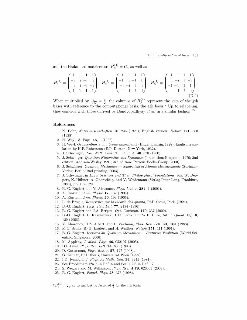
On mutually unbiased bases 101
and the Hadamard matrices are H(4)0 = G4 as well as
H(4)1 =
1 1 1 1
−i i −i i
i i −i −i1 −1 −1 1
, H
(4)2 =
1 1 1 1
−1 1 −1 1
−i −i i i
−i i i −i
, H
(4)3 =
1 1 1 1
i −i i −i−1 −1 1 1
i −i −i i
.
(D.9)
When multiplied by 1√N
= 12 , the columns of H
(4)j represent the kets of the jth
bases with reference to the computational basis, the 4th basis.y Up to relabeling,
they coincide with those derived by Bandyopadhyay et al. in a similar fashion.35
References
1. N. Bohr, Naturwissenschaften 16, 245 (1928); English version: Nature 121, 580(1928).
2. H. Weyl, Z. Phys. 46, 1 (1927).3. H. Weyl, Gruppenthorie und Quantenmechanik (Hirzel, Leipzig, 1928), English trans-
lation by H.P. Robertson (E.P. Dutton, New York, 1932).4. J. Schwinger, Proc. Natl. Acad. Sci. U. S. A. 46, 570 (1960).5. J. Schwinger, Quantum Kinematics and Dynamics (1st edition: Benjamin, 1970; 2nd
edition: Addison-Wesley, 1991; 3rd edition: Perseus Books Group, 2000).6. J. Schwinger, Quantum Mechanics — Symbolism of Atomic Measurements (Springer-
Verlag, Berlin, 2nd printing, 2003).7. J. Schwinger, in Exact Sciences and Their Philosophical Foundations, eds. W. Dep-
pert, K. Hubner, A. Oberschelp, and V. Weidemann (Verlag Peter Lang, Frankfurt,1985), pp. 107–129.
8. B.-G. Englert and Y. Aharonov, Phys. Lett. A 284, 1 (2001).9. A. Einstein, Ann. Physik 17, 132 (1905).
10. A. Einstein, Ann. Physik 20, 199 (1906).11. L. de Broglie, Recherches sur la theorie des quanta, PhD thesis, Paris (1924).12. B.-G. Englert, Phys. Rev. Lett. 77, 2154 (1996).13. B.-G. Englert and J.A. Bergou, Opt. Commun. 179, 337 (2000).14. B.-G. Englert, D. Kaszlikowski, L.C. Kwek, and W.H. Chee, Int. J. Quant. Inf. 6,
129 (2008).15. Y. Aharonov, D.Z. Albert, and L. Vaidman, Phys. Rev. Lett. 60, 1351 (1988).16. M.O. Scully, B.-G. Englert, and H. Walther, Nature 351, 111 (1991).17. B.-G. Englert, Lectures on Quantum Mechanics — Perturbed Evolution (World Sci-
entific, Singapore, 2006).18. M. Appleby, J. Math. Phys. 46, 052107 (2005).19. D.I. Fivel, Phys. Rev. Lett. 74, 835 (1995).20. D. Gottesman, Phys. Rev. A 57, 127 (1998).21. G. Zauner, PhD thesis, Universitat Wien (1999).22. I.D. Ivanovic, J. Phys. A: Math. Gen. 14, 3241 (1981).23. See Problems 2-12a–c in Ref. 6 and Sec. 1.2.6 in Ref. 17.24. S. Weigert and M. Wilkinson, Phys. Rev. A 78, 020303 (2008).25. B.-G. Englert, Found. Phys. 28, 375 (1998).
yH(4)4 = 14, so to say, but no factor of 1
2for the 4th basis.

102 T. Durt, B.-G. Englert, I. Bengtsson, and K. Zyczkowski
26. I. Bengtsson and A. Ericsson, Open Syst. Inf. Dyn. 12, 107 (2005).27. I. Bengtsson, W. Bruzda, A. Ericsson, J.-A. Larsson, W. Tadej, and K. Zyczkowski,
J. Math. Phys. 48, 052106 (2007).28. J.H. Conway, R.H. Hardin, and N.J.A. Sloane, Exp. Math. 5, 93 (1996).29. D. Deutsch, Phys. Rev. Lett. 50, 631 (1983).30. I. Bia lynicki-Birula, Phys. Lett. A 103, 253 (1984).31. S. Wehner and A. Winter, e-print arXiv:0907.3704[quant-ph] (2009).32. G. Karpilovski, Field theory (Marcel Dekker Inc., New York and Basel, 1988).33. B. Nagler and T. Durt, Phys. Rev. A 68, 042323 (2003).34. T. Durt, J. Phys. A: Math. Gen. 38, 5267 (2005).35. S. Bandyopadhyay, P. Boykin, V. Roychowdhury, and F. Vatan, Algorithmica 34,
512 (2002).36. A. Eusebi and S. Mancini, Quant. Inf. Comp. 9, 950 (2009).37. M. Planat and P. Jorrand, J. Phys. A: Math. Theor. 41, 182001 (2008).38. T. Durt, e-print arXiv:quant-ph/0401046 (2004).39. T. Durt, Cosmos 2, 21 (2006).40. T. Durt, D. Kaszlikowski, J.-L. Chen, and L.C. Kwek, Phys. Rev. A 69, 032313
(2004).41. D. Bruß, Phys. Rev. Lett. 81, 3018 (1998).42. D. Bruß and C. Macchiavello, Phys. Rev. Lett. 88, 127901 (2002).43. Y.C. Liang, D. Kaszlikowski, B.-G. Englert, L.C. Kwek, and C.H. Oh, Phys. Rev. A
68, 022324 (2003).44. S.L. Braunstein, A. Mann, and M. Revzen, Phys. Rev. Lett. 68, 3259 (1992).45. C.H. Bennett and S.J. Wiesner, Phys. Rev. Lett. 69, 2881 (1992).46. A.S. Holevo, Probl. Peredachi Inf. 9, 3 (1973); English translation: Probl. Inf.
Transm. (USSR) 9, 177 (1973).47. R.F. Werner, J. Phys. A: Math. Gen. 34, 7081 (2001).48. M.S. Zubairy, Phys. Rev. A 54, 4368 (1998).49. Z. Zhang, Y. Liu, and D. Wang, Phys. Lett. A 372, 28 (2007).50. C.H. Bennett, and G. Brassard, in Proc. IEEE Int. Conf. on Computers, Systems,
and Signal Processing, Bangalore, India (1984), p. 175.51. P. Boykin and V. Roychowdhury, Phys. Rev. A 67, 042317 (2003).52. H. Bechmann-Pasquinucci and W. Tittel, Phys. Rev. A 61, 062308 (2000).53. N.J. Cerf, Acta Phys. Slov. 48, 115 (1998).54. N.J. Cerf, Phys. Rev. Lett. 84, 4497 (2000).55. N.J. Cerf, J. Mod. Opt. 47, 187 (2000).56. N.J. Cerf, T. Durt, and N. Gisin, J. Mod. Opt. 49, 1355 (2002).57. C.A. Fuchs, N. Gisin, R.B. Griffiths, C.-S. Niu, and A. Peres, Phys. Rev. A 56, 1163
(1997).58. R.B. Griffiths and C.-S. Niu, Phys. Rev. A 56, 1173 (1997).59. C.-S. Niu and R.B. Griffiths, Phys. Rev. A 60, 2764 (1999).60. D. Bruss, M. Cinchetti, G.M. D’Ariano, and C. Macchiavello, Phys. Rev. A 62,
012302 (2000).61. A.K. Ekert, Phys. Rev. Lett. 67, 661 (1991).62. D. Gottesman, Phys. Rev. A 54, 1862 (1996).63. R. Calderbank, E.M. Rains, P.W. Shor, and N.J.A. Sloane, Phys. Rev. Lett. 78, 405
(1997).64. M.A. Nielsen, and I.L. Chuang, Quantum Computing and Quantum Information
(Cambridge University Press, Cambridge, 2000).65. D. Gottesman, Quantum Error Correction and Fault-Tolerance, in Encyclopedia of
On mutually unbiased bases 103
Mathematical Physics, vol. 4, eds. J.-P. Francoise, G.L. Naber, and S.T. Tsou (Else-vier, Oxford 2006); available as e-print arXiv:quant-ph/0507174 (2005).
66. M. Zukowski, A. Zeilinger, M.A. Horne, and A.K. Ekert, Phys. Rev. Lett. 71, 4287(1993).
67. J.-W. Pan, D. Bouwmeester, H. Weinfurter, and A. Zeilinger, Phys. Rev. Lett. 80,3891 (1998).
68. M. Halder, A. Beveratos, N. Gisin, V. Scarani, C. Simon, and H. Zbinden, NaturePhys. 3, 692 (2007).
69. H.-J. Briegel, W. Dur, J.I. Cirac, and P. Zoller, Phys. Rev. Lett. 81, 5932 (1998).70. L. Vaidman, Y. Aharonov, and D.Z. Albert, Phys. Rev. Lett. 58, 1385 (1987).71. Y. Aharonov and B.-G. Englert, Z. Naturforsch. 56a, 16 (2001).72. P.K. Aravind, Z. Naturforsch. 58a, 2212 (2003).73. T. Durt, Int. J. Mod. Phys. B 20, 1742 (2006); and e-print arXiv:quant-ph/0401037
(2004).74. A. Klappenecker and M. Rotteler, e-print arXiv:quant-ph/0502138 (2005).75. M. Reimpell and R.F. Werner, Phys. Rev. A 75, 062334 (2007).76. A.I. Kostrikin and P.H. Tiep, Orthogonal Decompositions and Integral Lattices, de
Gruyter Expositions in Mathematics 15 (Walter de Gruyter, Berlin, 1994).77. S. Brierley, S. Weigert, and I. Bengtsson, e-print arXiv:0907.4097[math-ph] (2009).78. J.L. Romero, G. Bjork, A.B. Klimov and L.L. Sanchez-Soto, Phys. Rev. A 72, 062310
(2005).79. G. Bjork, J.L. Romero, A.B. Klimov, and L.L. Sanchez-Soto, J. Opt. Soc. Am. B
24, 371 (2007).80. D. Kaszlikowski, A. Gopinathan, Y.C. Liang, L.C. Kwek, and B.-G. Englert, Phys.
Rev. A 70, 032306 (2004).81. B.-G. Englert and J. Rehacek, J. Mod. Opt. 57, 218 (2010).82. E.P. Wigner, Phys. Rev. 40, 749 (1932).83. M. Hillery, R.F. O’Connell, M.O. Scully, and E.P. Wigner, Phys. Rep. 106, 121
(1984).84. M.G.A. Paris and J. Rehacek (eds.), Quantum State Estimation, Lecture Notes in
Physics 649 (Springer-Verlag, Berlin, 2004).85. W.K. Wootters and B.D. Fields, Ann. Phys. (NY) 191, 363 (1989).86. J.M. Renes, R. Blume-Kohout, A.J. Scott, and C.M. Caves, J. Math. Phys. 45, 2171
(2004).87. M. Grassl, in Proc. ERATO Conf. on Quantum Information Science 2004 (EQIS
2004); also: e-print arXiv:quant-ph/0406175 (2004).88. A.J. Scott and M. Grassl, e-print arXiv:0910.5784[quant-ph] (2009).89. U. Leonhardt, Measuring the quatum state of light (Cambridge University Press,
1997).90. A. Vourdas, Rep. Progr. Phys. 67, 267 (2004).91. S. Chaturvedi, E. Ercolessi, G. Marmo, G. Morandi, N. Mukunda, and R. Simon,
Pramana 65, 981 (2005).92. W.K. Wootters, Ann. Phys. (NY) 176, 1 (1987).93. W.K. Wootters, IBM J. Res. Dev. 48, 99 (2004).94. K.S. Gibbons, M.J. Hoffman, and W.K. Wootters, Phys. Rev. A 70, 062101 (2004).95. D. Gross, Appl. Phys. B 86, 367 (2007).96. R.J. Glauber, Phys. Rev. 131, 2766 (1963).97. B.-G. Englert, J. Phys. A: Math. Gen. 22, 625 (1989).98. R.P. Feynman, in Quantum Implications, eds. B.J. Hiley and F.D. Peat (Routledge
& Kegan Paul, London and New York, 1987).
104 T. Durt, B.-G. Englert, I. Bengtsson, and K. Zyczkowski
99. T. Durt, C. Kurtsiefer, A. Lamas-Linares, and A. Ling, Phys. Rev. A 78, 1 (2008).100. A.O. Pittenger and M.H. Rubin, J. Phys. A: Math. Gen. 38, 6005 (2005).101. G. Nogues, A. Rauschenbeutel, S. Osnaghi, P. Bertet, M. Brune, J.M. Raimond, S.
Haroche, L.G. Lutterbach, and L. Davidovich, Phys. Rev. A 62, 054101 (2000).102. P. Bertet, A. Auffeves, P. Maioli, S. Osnaghi, T. Meunier, M. Brune, J.M. Raimond,
and S. Haroche, Phys. Rev. Lett. 89, 200402 (2002).103. B.-G. Englert, N. Sterpi, and H. Walther, Opt. Commun. 100, 526 (1993).104. J. Rehacek, B.-G. Englert, and D. Kaszlikowski, Phys. Rev. A 70, 052321 (2004).105. T. Durt, J. Laser Phys. 11, 1557 (2006).106. T. Durt, Open Syst. Inf. Dyn. 13, 403 (2006).107. D.M. Appleby, I. Bengtsson, and S. Chaturvedi, J. Math. Phys. 49 012102 (2008).108. M.K. Bennett, Affine and Projective Geometry (Wiley, New York, 1995).109. G. Tarry, C. R. Ass. Fr. Av. Sci. Naturelles 1, 122 & 2170 (1900).110. M. Saniga, M. Planat, and H. Rosu, J. Opt. B: Quantum Semiclass. 6, L19 (2004).111. T. Paterek, B. Dakic, and C. Brukner, Phys. Rev. A 79, 012109 (2009).112. T. Paterek, M. Paw lowski, M. Grassl, and C. Brukner, e-print arXiv:0910.1439
[quant-ph] (2009).113. M. Weiner, e-print arXiv:0902.0635[math-ph] (2009).114. F. Klein, Vorlesungen uber die Entwicklung der Mathematik im 19. Jahrhundert
(Springer, Berlin, 1926).115. O. Hesse, Crelle’s J. 28, 68 (1844).116. C. Segre, Math. Ann. 27, 296 (1886).117. K. Hulek, Asterisque 137, 1 (1986).118. J.J. Sylvester, Phil. Mag. 34, 461 (1867).119. J. Hadamard, Bull. Sci. Math. 17, 240 (1893).120. R.E.A.C. Paley, J. Math. Phys. 12, 311 (1933).121. H. Kharaghani and B. Tayfeh-Rezaie, J. Comb. Des. 13, 435 (2005).122. P.O. Boykin, M. Sitharam, M. Tarifi, and P. Wocjan, e-print arXiv:quant-ph/0502024
(2005).123. A.T. Butson, Can. J. Math. 15, 42 (1963).124. K.J. Horadam, Hadamard matrices and their applications (Princeton University
Press 2007).125. K. Kraus, Phys. Rev. D 35, 3070 (1987).126. U. Haagerup, in: Operator Algebras and Quantum Field Theory (Rome) (Interna-
tional Press, Cambridge, MA, 1996), p. 296.127. G. Bjorck and B. Saffari, C. R. Acad. Sci. Paris, Ser. I 320, 319 (1995).128. M. L. Mehta, Elements of Matrix Theory (Hindustan Publishing Corporation, Delhi,
1977).129. W. Pauli, in Handbuch der Physik 24 eds. H. Geiger and K. Scheel. (Springer, Berlin,
1933), pt. 1, p. 98.130. J.-C. Faugere, Finding all the solutions of Cyclic 9 using Grobner basis techniques,
in Lecture Notes Series on Computing, vol. 9, eds. K. Shirayanagi and K. Yokoyama(World Scientific, Singapore 2001), p. 1.
131. U. Haagerup, e-print arXiv:0803.2629[math.AC] (2008).132. W. Tadej and K. Zyczkowski, Lin. Alg. Appl. 429 447 (2008).133. W. Tadej and K. Zyczkowski, Open Syst. Inf. Dyn. 13, 133 (2006).134. P. Dita, J. Phys. A: Math. Gen. 37, 5355 (2004).135. B.R. Karlsson, e-print arXiv:1003.4133[math-ph] (2010).136. B.R. Karlsson, e-print arXiv:1003.4177[math-ph] (2010).137. T. Tao, Math. Res. Lett. 11, 251 (2004).
On mutually unbiased bases 105
138. W. Tadej, Lin. Alg. Appl. 418, 719 (2006).139. K. Beauchamp and R. Nicoara, Lin. Alg. Appl. 428, 1833 (2008).140. F. Szollosi, Proc. Am. Math. Soc. 138, 921 (2010).141. M. Matolcsi and F. Szollosi, Open Syst. Inf. Dyn. 15, 93 (2008).142. B.R. Karlsson, J. Math. Phys. 50 082104 (2009).143. A.J. Skinner, V.A. Newell, and R. Sanchez, J. Math. Phys. 50, 012107 (2009).144. B.R. Karlsson, private communication with IB (2010).145. G.E. Moorhouse, The 2-transitive complex Hadamard matrices, preprint available at
http://www.uwyo.edu/moorhouse/pub/ (2001).146. F. Szollosi, Eur. J. Combin. 29, 1219 (2008).147. M. Petrescu, PhD thesis, University of California at Los Angeles (1997).148. R. Craigen, W.H. Holzmann, and H. Kharaghani, J. Combin. Design 5 319 (1998).149. M. Matolcsi, J. Reffy, and F. Szollosi, Open Syst. Inf. Dyn. 14, 247 (2007).150. R.B. Holmes and V.I. Paulsen, Lin. Alg. Appl. 377, 31 (2004).151. P. Dita, e-print arXiv:0901.0982[math-ph] (2009).152. P. Dita, e-print arXiv:1002.4933[math-ph] (2010).153. The URL is http://chaos.if.uj.edu.pl/∼karol/hadamard.154. J. Lawrence, C. Brukner, and A. Zeilinger, Phys. Rev. A 65, 032320 (2002).155. C. Brukner and A. Zeilinger, Phys. Rev. Lett. 83, 3354 (1999).156. B.-G. Englert and N. Metwally, J. Mod. Opt. 47, 2221 (2000).157. C.H. Bennett, D.P. DiVincenzo, J. Smolin, and W.K. Wootters, Phys. Rev. A 54,
3824 (1996).158. P. K. Aravind, Found. Phys. Lett. 13, 499 (2000).159. R. Gow, e-print arXiv:math/0703333 (2007).160. W.K. Wootters and D.M. Sussman, e-print arXiv:0704.1277[quant-ph] (2007).161. O. Kern, K.S. Ranade, and U. Seyfarth, e-print arXiv:0912.4661[quant-ph] (2009).162. D.M. Appleby, e-print arXiv:0909.5233[quant-ph] (2009).163. S. Brierley and S. Weigert, Phys. Rev. A 79, 052316 (2009).164. P. Jaming, M. Matolcsi, P. Mora, F. Szollosi, and M. Weiner, J. Phys. A: Math.
Theor. 42, 245305 (2009).165. W. Bruzda, MSc thesis, Jagiellonian University, Cracow (2006); available online at
http://chaos.if.uj.edu.pl/∼karol/prace/Br06.pdf.166. W. Bruzda, private communication with KZ (2008).167. P. Butterley and W. Hall, Phys. Lett. A 369, 5 (2007).168. S. Brierley and S. Weigert, Phys. Rev. A 78, 042312 (2008).169. C. Archer, J. Math. Phys. 46, 022106 (2005).170. M. Planat, H. Rosu, and M. Saniga, AIP Conf. Proc. 734, 315 (2004).171. S. Colin, J. Corbett, T. Durt, and D. Gross, J. Opt. B: Quantum Semiclass. Opt. 7,
S778 (2005).172. D.M. Appleby, H.B. Dang, and C.A. Fuchs, e-print arXiv:0707.2071[quant-ph]
(2007).173. D.M. Appleby, in Proc. Vaxjo Conf. on Foundations of Probability and Physics–5,
eds. L. Accardi et al., AIP Conf. Proc. 1101 (New York 2009); available as e-printarXiv:0905.1428[quant-ph] (2009).
174. A.Yu. Vlasov, in Gravitation, Cosmology and Elementary Particles, eds. V. Dorofeev,A.Yu. Pavlov, and E. Poberii (SPb UEF Publishing, St. Petersburg, 2004) p. 147;available as e-print arXiv:quant-ph/0302064 (2003).
175. A.O. Pittenger and M.H. Rubin, Lin. Alg. Appl. 390, 255 (2004).176. J.P. Paz, A.J. Roncaglia, and M. Saraceno, Phys. Rev. A 72, 012309 (2005).177. M.R. Kibler, Int. J. Mod. Phys. B 20, 1802 (2006).
106 T. Durt, B.-G. Englert, I. Bengtsson, and K. Zyczkowski
178. P. Sulc and J. Tolar, J. Phys. A: Math. Gen. 40, 15099 (2007).179. O. Albouy and M.R. Kibler, Sigma 3, 076 (2007).180. M.R. Kibler, Int. J. Mod. Phys. B 20, 1792 (2006).181. M.R. Kibler, J. Phys. A: Math. Theor. 42, 353001 (2009).182. P. Wocjan and T. Beth, Quant. Inf. Comp. 5, 93 (2005).183. M. Daoud and M.R. Kibler, J. Phys. A: Math. Theor. 43, 115303 (2010).184. H.F. Chau, e-print arXiv:quant-ph/0212055 (2002).185. S. Chaturvedi, Phys. Rev. A 65, 044301 (2002).186. A. Klappenecker and M. Roetteler, Lecture Notes in Computer Science 2948
(Springer Verlag, Berlin, 2004) p. 137.187. A. Vourdas, J. Phys. A: Math. Theor. 40, R285 (2007).188. P.O. Boykin, M. Sitharam, P.H. Tiep, and P. Wojcan, Quant. Inf. Comp. 7, 371
(2007).189. W.O. Alltop, IEEE Trans. Inform. Theory 26 350 (1980).190. S. Popa, J. Operator Theory 9, 253 (1983).191. A.B. Klimov, J.L. Romero, G. Bjork, and L.L. Sanchez-Soto, J. Phys. A: Math. Gen.
40, 3987 (2007).192. A.B. Klimov, J.L. Romero, G. Bjork, and L.L. Sanchez-Soto, Ann. Phys. (NY) 324,
53 (2009).193. M. Combescure, J. Math. Phys. 50, 032104 (2009).194. M. Aschbacher, A.M. Childs, and P. Wocjan, J. Algebr. Comb. 25, 111 (2007).195. C.W. Chin, private communication with BGE (2010).196. S. Lang, Algebraic Number Theory, Grad. Texts in Math. 110 (Springer-Verlag, New
York, 2nd edition 1994, 3rd printing 2000).197. T. Durt, L.C. Kwek, and D. Kaszlikowski, Phys. Rev. A 77, 042318 (2008).
Related Documents