On Diffeomorphism Invariance and Black Hole Quantization L¯ asma Alberte Arnold Sommerfeld Center LMU Munich A thesis submitted for the degree of Master of Science June 2010

Welcome message from author
This document is posted to help you gain knowledge. Please leave a comment to let me know what you think about it! Share it to your friends and learn new things together.
Transcript

On Diffeomorphism Invariance
and Black Hole Quantization
Lasma Alberte
Arnold Sommerfeld Center
LMU Munich
A thesis submitted for the degree of
Master of Science
June 2010

1. Reviewer: Prof. Dr. Viatcheslav Mukhanov
2. Reviewer: Prof. Dr. Ivo Sachs
Day of the defense: 21st June 2010
On Diffeomorphism Invariance and Black Hole
Quantization
Lasma Alberte
Arnold Sommerfeld Center
LMU Munich
A thesis submitted for the degree of
Master of Science
June 2010
We consider the question of the quantization of the black hole area. It is suggested
that the physical Hilbert space of quantum microstates of the black hole horizon
area can be related with the state space built by the generators of two dimensional
diffeomorphism transformations. The spatial constraints of general relativity are,
therefore, expanded on a toroidal spacelike surface. The properties of the resulting
algebra are explored, and the highest-weight representation space for this algebra
is constructed. We argue that the operators of the two dimensional diffeomorphism
algebra should be included in the set of operators which are needed for an algebraic
description of a quantum black hole. The degeneracy of the black hole horizon area
might then be associated to the degeneracy of the operator which is diagonal in
the highest-weight representation space. A formal expression for the degeneracy is
derived, and its asymptotics might give the correct degeneracy to reproduce the
Bekenstein-Hawking entropy formula for black holes.

iv
Acknowledgements
I would like to express my gratitude first and foremost to my advisor
Slava Mukhanov for the amount of time which he has devoted to sup-
porting me in my work and to discussing topics related and unrelated
to my thesis. I am especially grateful for the enormous patience he
has shown while doing this. His valuable guidance and criticisms have
inspired me more than anything else.
I owe the same amount of thanks to my mother and sister for being
constantly proud of me without any reason. It obliged me to make it
worth it.
I am very delighted to thank Carl and Alberto for proof reading my
thesis and for all the conversations we have had since I know them.
It is my pleasure to thank Sarah, Cristiano, Alex, Alberto, and Nico
for creating a very pleasant atmosphere at the department and all the
fun we have had together. Especially I would like to thank to Alex for
motivating me to complete my thesis, and also for the cake.
I am also indebted to Dieter Lust and Robert Helling for organising the
TMP school. It has been a great intelectual pleasure and joy to spend
these two years at the LMU.
Last but not least, I would like to express my gratituted to DAAD who
made it possible for me to study here in Munich and do the work I love.

ii

Contents
1 Introduction 1
1.1 Quantum Effects in Black Holes . . . . . . . . . . . . . . . . . . . . 1
1.2 Thermodynamics of a Quantum Black Hole . . . . . . . . . . . . . 3
1.3 Observational Consequences of Discrete Area Spectrum . . . . . . . 5
1.4 Quantum Black Holes as Atoms. Outlook . . . . . . . . . . . . . . 6
2 Constrained Hamiltonian systems 9
2.1 The Hamilton Formalism and Constraints . . . . . . . . . . . . . . 10
2.1.1 Action in Canonical Form . . . . . . . . . . . . . . . . . . . 10
2.1.2 Action in Parametrized Form . . . . . . . . . . . . . . . . . 12
2.2 The Covariant Form of General Relativity . . . . . . . . . . . . . . 14
2.2.1 Diffeomorphism Invariance of General Relativity . . . . . . . 14
2.2.2 The Hamilton Formalism . . . . . . . . . . . . . . . . . . . . 15
2.2.2.1 Splitting the Spacetime in 3+1 . . . . . . . . . . . 16
2.2.2.2 Constraints in ADM Formalism . . . . . . . . . . . 17
3 Diffeomorphisms and Physical Quantum States in String Theory 19
3.1 Symmetries of the Polyakov Action . . . . . . . . . . . . . . . . . . 19
3.2 The Canonical Form of the Polyakov Action . . . . . . . . . . . . . 21
3.3 Mode Expansions . . . . . . . . . . . . . . . . . . . . . . . . . . . . 22
3.3.1 Constraints in Light-cone Worldsheet Coordinates . . . . . . 22
3.3.2 Constraints in Minkowski Worldsheet Coordinates . . . . . . 25
3.3.3 Generators of Diffeomorphism Transformations . . . . . . . 26
3.4 Old Canonical Quantization . . . . . . . . . . . . . . . . . . . . . . 28
3.5 Light-cone Gauge Quantization . . . . . . . . . . . . . . . . . . . . 31
3.5.1 Residual Gauge Symmetry . . . . . . . . . . . . . . . . . . . 31
iii

CONTENTS
3.5.2 Light-cone Gauge . . . . . . . . . . . . . . . . . . . . . . . . 32
3.6 Physical States . . . . . . . . . . . . . . . . . . . . . . . . . . . . . 33
3.6.1 Vertex Operators . . . . . . . . . . . . . . . . . . . . . . . . 33
3.6.2 Transverse Physical States . . . . . . . . . . . . . . . . . . . 35
3.6.3 No Ghost Theorem for D = 26 and a = 1 . . . . . . . . . . . 36
4 On Representations of the Virasoro Algebra in Conformal Field
Theory 41
4.1 Classical Conformal Field Theory . . . . . . . . . . . . . . . . . . . 41
4.1.1 Conformal Symmetry . . . . . . . . . . . . . . . . . . . . . . 41
4.1.2 Conformal Ward Identities . . . . . . . . . . . . . . . . . . . 43
4.1.3 Generators of Conformal Transformations . . . . . . . . . . 45
4.1.4 Primary Fields . . . . . . . . . . . . . . . . . . . . . . . . . 46
4.2 Radial Quantization of Conformal Field Theories . . . . . . . . . . 46
4.2.1 Operator product expansion . . . . . . . . . . . . . . . . . . 48
4.3 Central Charge and the Virasoro Algebra . . . . . . . . . . . . . . . 48
4.4 Hilbert Space of Conformal Fields . . . . . . . . . . . . . . . . . . . 50
4.4.1 Operator-state Correspondence . . . . . . . . . . . . . . . . 50
4.4.2 Highest-weight Representations. Verma Module . . . . . . . 50
4.4.3 Singular Vectors and Spurious States . . . . . . . . . . . . . 52
4.5 Degeneracy of Highly Excited States . . . . . . . . . . . . . . . . . 53
4.5.1 Partition Function on the Torus . . . . . . . . . . . . . . . . 54
4.5.2 Derivation of the Cardy Formula . . . . . . . . . . . . . . . 55
4.5.3 Combinatorial Approach to the Counting of States . . . . . 56
4.5.4 Level Density of Physical States in String Theory . . . . . . 57
4.5.5 Applications to 2 + 1 dimensional black holes . . . . . . . . 58
5 Quantum Black Holes 59
5.1 The Area Spectrum . . . . . . . . . . . . . . . . . . . . . . . . . . . 59
5.2 The Origins of Black Hole Entropy . . . . . . . . . . . . . . . . . . 60
5.3 Predictions Due to the Existence of Discrete Area Spectrum . . . . 62
5.4 An Algebraic Description of Black Holes . . . . . . . . . . . . . . . 63
5.5 Properties of the Area Operator . . . . . . . . . . . . . . . . . . . . 64
iv

CONTENTS
6 Diffeomorphism algebra in gravity 67
6.1 Discretization of constraints . . . . . . . . . . . . . . . . . . . . . . 67
6.2 On Quantum Anomalies of 2D Diffeomorphism Algebra . . . . . . . 68
6.2.1 Central Extension in One Dimension . . . . . . . . . . . . . 68
6.2.2 Central Extension for the Two Dimensional Diffeomorphism
Algebra . . . . . . . . . . . . . . . . . . . . . . . . . . . . . 69
6.3 Non-central Extensions of the 2D Virasoro Algebra . . . . . . . . . 74
6.4 Eigenspace of the Constraint Operators . . . . . . . . . . . . . . . . 76
6.4.1 Eigenspace of Decoupled L10J and L2
I0 . . . . . . . . . . . . . 76
6.4.2 Eigenspace of Coupled L100, L2
00 without Central Extension . 78
6.4.3 Degeneracy . . . . . . . . . . . . . . . . . . . . . . . . . . . 81
6.4.4 Eigenspace of Coupled L100, L2
00 with Central Extension . . . 86
6.5 Speculations . . . . . . . . . . . . . . . . . . . . . . . . . . . . . . . 89
6.6 Possible Relation with the Quantization of Black Holes . . . . . . . 92
7 Conclusions 95
Bibliography 97
v

CONTENTS
vi

1
Introduction
As challenging as it may be, the problem of the unification of general relativity
and quantum mechanics will only be truly solved in combination with some ob-
servational confirmation. A theory without experimentally verified predictions will
always remain “just a theory”. The question of how we are going to know whether a
theory of quantum gravity is correct is still an open one. The Planck scale at which
the effects of quantum gravity should become relevant is far beyond the reach of
current experimental devices. Even the LHC, which is going to reach 10TeV scale,
is still 1015 orders of magnitude below the Planck scale. Thus, even if one has a
mathematically consistent theory of quantum gravity there is no obvious way to
test it. This gives rise to a natural question: are there any quantum gravity effects
observable at the energies accessible today?
Quantum gravity effects can be very important for black holes. Thus, these are
natural candidates to look for possible hints or consistency checks. The question
we wish to address in this work is the quantization of the area of black holes. We
will begin by briefly recalling what quantum effects are relevant for the black hole
physics and what macroscopically observable consequences a discrete area spectrum
could have.
1.1 Quantum Effects in Black Holes
The quantum effects, which are relevant for black hole physics are vacuum polar-
ization and particle creation in the presence of an external field [1]. If the external
field is strong and can be described classically it is called a classical background.
1

1. INTRODUCTION
This background changes the vacuum fluctuations of quantum fields by shifting
their zero-point energy levels. Hence, the vacuum is “deformed”. The shift of the
energy levels can be measured and this is called the vacuum polarization effect. If,
on the other hand, the amount of energy which the quantum field receives from the
background field is larger than the difference between the energy levels of the oscil-
lator modes of the quantum field, then we have particle production in an external
field.
A prominent example of particle creation is the Schwinger effect in quantum
electrodynamics, where a positron-electron pair is produced in a strong static elec-
tric field. The fact that the “virtual particles” have opposite charge is crucial, as
in the external electric field they are moving in opposite directions. In such a way
they are separated and can gain a sufficient amount of energy to become real.
In black hole physics both particle production and vacuum polarization effects
are important. The vacuum polarization corresponds to the appearance of local
terms which modify the gravitational action. In the case of external gravitational
field this modification becomes relevant if the curvature of the spacetime approaches
the Planck curvature RPl = c3
~G ∼ 1065cm−2. However, for black holes of mass
M MPl the curvature reaches the Planck scale only “deep inside” the event
horizon. Hence, the vacuum polarization effects seem to be negligible outside the
black hole.
Let us now consider the possibility of particle creation by a graviational field.
The fact that the total energy of the created particle pair has to be zero in grav-
itational field would imply that one of the particles has negative energy. While
negative-energy states can exist in a nonstatic gravitational field, it seems to be
impossible to convert a virtual particle-antiparticle pair into a pair of real particles
in a static gravitational field. However, Hawking predicted [2] that nonrotating
black holes emit radiation with a black body thermal spectrum of temperature
TH =κ
2π(1.1)
and thus evaporate. This implies a probability w ∼ exp(−E/kTH) of finding an
emitted particle with energy E. This probability corresponds to that of particle
pair production as a result of vacuum quantum fluctuations in a gravitational field
of strength κ. The quantity κ is called the black hole surface gravity and it is equal
2

1.2 Thermodynamics of a Quantum Black Hole
to 1/(4M) for nonrotating black holes. Hawking radiation is therefore an example
of a purely quantum effect which should be detectable for an observer outside the
black hole.
In order for a black hole to have significant Hawking radiation within the lifetime
of our universe its initial mass has to be smaller than ∼ 1015g (compare with the
solar mass M = 2 · 1033g). Such black holes are called primordial black holes as
they could have been formed only in the early universe. In the present-day universe
these black holes could radiate with sufficiently high temperature to be detected.
However, there is currently no evidence for the existence of primordial black holes,
and therefore no observational verification of the Hawking effect has been found.
Nevertheless, it seems that Hawking radiation is indeed one of the most impor-
tant predictions for quantum effects in gravity which could in principle be observ-
able today. Still, the real nature of Hawking radiation at the quantum level is not
yet unambigously established. This is because, in order to derive the continuous
thermal spectrum for black hole radiation, we are considering quantum fluctua-
tions of matter fields on a classical black hole background. However, in a theory of
quantum gravity, quantum fluctuations of the black hole horizon should be taken
into account. This indicates that the character of the Hawking radiance spectrum
could be modified even for large black holes. In order to investigate these possible
modifications of the Hawking radiation due to the effects of quantum gravity, we
turn now to the thermodynamics of black holes.
1.2 Thermodynamics of a Quantum Black Hole
Even prior to the discovery of black hole radiation Bekenstein postulated that
a black hole possess a certain entropy. This conclusion originated from the “no
hair conjecture” [3] which states that a stationary black hole is described only
by few parameters: its mass M , angular momentum J , charge Q, and area A =
A(M,J,Q). Therefore, if a black hole absorbs matter with certain entropy, then
from the point of view of an outside observer the total entropy of the universe
would decrease. This would in turn violate the second law of thermodynamics
unless the black hole would itself have entropy. Hawking’s theorem [4] that the area
of a classical black hole is non-decreasing lead Bekenstein [5] to conclude that the
black hole entropy should be proportional to its surface area. The proportionality
3

1. INTRODUCTION
coefficient S = A/4 was fixed only after the prediction of Hawking radiation [6].
This was done by using the following expression, which relates the characteristic
parameters of a non-extremal black hole [7]:
M2 =A
16π
(1 +
4πQ2
A
)2
+4πJ2
A. (1.2)
Differentiating this relation leads to the analogue of the first law of thermodynamics
for black holes
dM =κ
16πdA+ ΩdJ + φdQ, (1.3)
Here Ω is the angular velocity and φ is the electric potential of the black hole. In
the prefactor of dA one can recognize the expression for the Hawking temperature
(1.1) and read off the proportionality coefficient.
Returning to the quantum description of a black hole, we know that in quantum
mechanics both angular momentum and charge can only take discrete values. In
combination with equation (1.3) this could be considered as the first indication that
the mass and the area of black hole should take discrete values as well. Moreover,
the area eigenvalues should be uniformly spaced as an = αl2Pln where α is some
universal constant [6].
Another justification for a discrete horizon area spectrum was proposed by
Mukhanov [8]. He assumed that a black hole is quantized and that every black hole
with mass M can be associated with some macrostate at energy level n. In analogy
with statistical mechanics one can define the entropy of a particular black hole
macrostate as the logarithm of the number of its possible internal configurations
g(n):
S = ln g(n). (1.4)
The degeneracy g(n) can be identified with number of different ways to reach the
level n, starting from the ground state n = 0 and then going up the staircase of
energy levels in all possible ways. This gives
g(n) = 2n−1.
For equidistant area levels this leads to the Bekenstein-Hawking entropy formula,
and thus justifies the initial assumption that the area spectrum is discrete.
4

1.3 Observational Consequences of Discrete Area Spectrum
1.3 Observational Consequences of Discrete Area
Spectrum
For a nonrotating black hole with zero electric charge, its mass is related to the
area as M2 = A/(16π). Hence, a discrete area spectrum implies a discrete mass
spectrum M ∼√n. It follows that the spectrum of Hawking radiation is not
continuous but is instead a line spectrum [8; 9]. Moreover, the energy spacing
between consecutive levels corresponds to the frequency ω0 = (8πM)−1 ln 2 for
M MPl. The full emission spectrum is then given by spectral lines at frequencies,
which are multiples of ω0, whose envelope is the Hawking thermal spectrum. For
primordial black holes this gives a sharp, observable line spectrum as a direct
consequence of a discrete and uniform black hole horizon area spectrum.
There is, however, no general agreement on the spacing of the area levels. Sev-
eral authors (see [10] and references therein) have suggested a non-uniform level
spacing. In particular, using the loop quantum gravity approach to black hole
physics, Rovelli and Smolin [11; 12] initially proposed the area spectrum
A ∼∑i
√ji(ji + 1). (1.5)
The index ji takes integer and half-integer values and labels a spin-ji link, which
refers to a possible surface separating two adjacent volume quanta labeled by i.
In distinction from the Bekenstein-Mukhanov black hole emission spectrum, the
quantum loop area spectrum implies that the spacing between spectral lines is
infinitesimal and effectively reproduces the Hawking’s thermal spectrum. However,
this result and the degeneracy of an area eigenvalue depends very much on the
convention about which spin-ji links are considered to be physically distinguishable
and thus have to be taken into account in the sum (1.5). Fully indistinguishable
links (see ref.[13] for precise meaning of this) fail to reproduce the area-entropy
relation, i.e. one gets S ∼ At with t < 1. Moreover, the minimal change in the
area is no longer restricted to the Planck area.
After introducing the notion of fully distinguishable links, they were able to
reproduce the Bekenstein-Hawking entropy law with an equidistant area spectrum
Aj = j + 1/2 [13]. This agrees with the result of Bekenstein and Mukhanov.
5

1. INTRODUCTION
1.4 Quantum Black Holes as Atoms. Outlook
Since there has been no experimental evidence for either semiclassical Hawking
radiation or the line spectrum of black holes, the question of whether the spec-
trum of horizon area is equidistant or not still does not have a definite answer,
and further work to determine of the correct area quantization is necessary. In
this work we will use the conjecture of Bekenstein that small black holes can be
described in a similar manner as elementary particles in quantum mechanics [10].
He claimed that a black hole is fully characterised by a closed set of quantum op-
eratorsQ, J
2, Jz, A
and some creation operators Rλs for black holes in their
various states. Using purely algebraic methods he was able to derive the algebra of
the creation and area operators. However, no physical justification of the origin of
either of the operators A or Rλs was given. The operator Q classically originated
as the electric charge of the black hole, whereas in quantum mechanics it is con-
verted into the generator of U(1) gauge transformations. Since general relativity
is invariant under diffeomorphism transformations, the corresponding generators
should also be included among the operators needed for a complete description of
a black hole quantum state.
Motivated by this observation, we will investigate the properties of the algebra
of the diffeomorphism constraints Hα, which arise in the covariant form of general
relativity [14]. We will review the methods of the Hamiltonian formalism in chapter
2. As we will discover, the two dimensional diffeomorphism algebra of spacelike
constraints can be regarded as a two dimensional extension of the Virasoro algebra.
The latter is of great importance in string theory and conformal field theory(CFT)
where it is the algebra of the generators of conformal transformations. The role of
diffeomorphisms in string theory and CFT will be discussed in chapters 3 and 4.
In chapter 5 we will present the algebraic description of black holes, suggested by
Bekenstein in the light of knowledge from string quantization.
A detailed discussion of quantum extensions of two dimensional diffeomorphism
algebra will be provided in chapter 6. In analogy with conformal field theory we
will consider the highest-weight representation space of the diffeomorphism algebra
on a closed two dimensional spacelike surface. We will consider the possibility to
identify the area and creation operators in Bekenstein’s description with some of
6
1.4 Quantum Black Holes as Atoms. Outlook
the operators present in the diffeomorphism algebra of general relativity. Summary
and conclusions will be given in chapter 7.
7

1. INTRODUCTION
8

2
Constrained Hamiltonian systems
The usual approach to describe the dynamics of a classical field theory is the ac-
tion principle. The invariance of the action under some group of local symmetry
transformations leads to severe restrictions on the allowed form of the Lagrangian
density. This makes it possible to guess the Lagrangian even if the explicit nature
of the theory is not known. The quantum theory is then derived by the approach
of canonical quantization. It seems, however, that the symmetries which are ap-
parent in the Lagrange formalism tend to “disappear” on the way to the Hamilton
formalism. Moreover, the explicit distinction between spatial and time coordinates
in the canonical form of the action looks rather artificial for diffeomorphism in-
variant theories such as general relativity. However, the local symmetries seem to
also be explicit in the Hamiltonian formalism [15], which is much more suitable for
quantization. The aim of this chapter is to rewrite the action of general relativity
in canonical form and to derive the constraints which both generate the dynamics
of general relativity and account for the diffeomorphism invariance of the Einstein
action. We will, therefore, begin with a quick review of the basics of the Hamilton
formalism with constraints and reveal the role of reparametrization invariance in
this formalism.
9

2. CONSTRAINED HAMILTONIAN SYSTEMS
2.1 The Hamilton Formalism and Constraints
2.1.1 Action in Canonical Form
Let us start with the classical action
S =
∫dt L(q, q, t), (2.1)
where q = q1, . . . , qn denotes the set of generalized coordinates, and n is the
number of degrees of freedom. This yields the Euler-Lagrange equations
d
dt
(∂L
∂qi
)=∂L
∂qi. (2.2)
After introducing conjugated momenta,
pi ≡∂L
∂qi, (2.3)
and defining the Hamiltonian as
H(p, q) = piqi − L(q, q, t) (2.4)
the equations of motion become
qi =∂H
∂pi, pi = −∂H
∂qi. (2.5)
These are first order differential equations, which leads to the Hamilton formalism
sometimes being referred to as the first order formalism. Introducing the classical
Poisson bracket for some functions f(q, p), g(q, p) of canonical variables q and p
f, g =∂f
∂qi∂g
∂pi− ∂g
∂qi∂f
∂pi(2.6)
enables us to rewrite equations (2.5) as Heisenberg equations
qi =qi, H
, pi = pi, H . (2.7)
10

2.1 The Hamilton Formalism and Constraints
The Poisson bracket of the generalized coordinates with their conjugated momenta
is qi, pj = δij. This can be straightforwardly translated into equations for quan-
tum operators by replacing the canoncial variables q, p with non-commuting quan-
tum operators satisfying the equal-time commutation relation [qi, pj] = i~δij. From
this it follows that the classical Poisson bracket can be substituted with quantum
commutator according to the rule
[. . . ] = i~ . . . . (2.8)
It thus seems that for quantizing a theory all we need is a Hamilton function.
Here we return to the question of whether the Hamiltonian reflects all the sym-
metries of the Lagrangian we started with. An important contribution in this
direction is due to Dirac [16] who developed the quantum theory of constrained
Hamiltonian systems, in which the canonical variables obey the constraint equa-
tions Cα(q, p) ≡ 0. These reflect the presence of a local symmetry in the system,
and, thus, the algebra obeyed by the constraints is the algebra of the generators
of the symmetry transformations. In the canonical formalism these constraints are
taken into account by adding them to the Hamiltonian:
HT (q, p) = H(q, p) + NαCα, (2.9)
where Nα = Nα(q, p) are Lagrangian multipliers.
The constraints arise, for example, in cases when the conjugated momenta pi
are not mutually independent and thus there exist several linear combinations of
momenta which are zero even if the corresponding momenta themselves do not
vanish. Constraints arising this way are called primary constraints. Dirac gave
a neat example to explain the origin of such constraints. Consider a Lagrangian
which is a homogeneous function of the first degree in velocities:
qi∂L
∂qi= L.
From here it follows that the Hamiltonian H = piqi−L is zero and thus there are no
dynamics. But let us count the degrees of freedom. We started with n coordinates
qi, but, because of the specific form of Lagrangian, the conjugated momenta can
only depend on the ratios of velocities. Out of n variables only n − 1 ratios can
11

2. CONSTRAINED HAMILTONIAN SYSTEMS
be built, which leaves one combination C1(p, q) of q’s and p’s equal to zero. This
can now be multiplied by an arbitrary function N1, and the total Hamiltonian is
HT = N1C1. Hence, we have included some extra information in our Hamiltonian
as a direct consequence of a certain symmetry of the original Lagrangian.
2.1.2 Action in Parametrized Form
As we have seen so far, starting from a classical action principle and passing to the
first order formalism we were able to obtain a quantum theory. The subtle point
which we have neglected so far is whether the resulting quantum theroy is still
Lorentz invariant. Although we started with a classically Lorentz invariant theory,
the equations of motion in Hamiltonian form (2.7) are not manifestly covariant.
The reason for this is that by referring to one absolute time, we break the four
dimensional Lorentz symmetry. In order to ensure relativistic invariance, let us
treat the “absolute time” t as another generalized coordinate which “evolves” as a
function of some “new time” τ . Then a system with n degrees of freedom described
by n coordinates qi, becomes a system of n+1 degrees of freedom with qn+1 = t(τ).
As a result the action becomes
S =
∫dt L(q, q, t) (2.10)
=
∫dτ L∗(q, q′, qn+1, qn+1′, τ),
where q′ ≡ dq/dτ . Rewriting the action in canonical form leads to
S =
∫dτdt
dτ
(n∑i=1
pidqi
dτ
dτ
dt−H(q, p)
)
=
∫dτ
(n∑i=1
piqi′ − qn+1
′H(p, q)
).
After identifying pn+1 = −H(q, p) the last term can be absorbed in the sum.
This relation between the new conjugated momenta and the Hamiltonian can be
rewritten as a constraint
C0(q, p) ≡ pn+1 +H(q, p) = 0
12

2.1 The Hamilton Formalism and Constraints
and taken into account in the action as
S =
∫dτ
(n+1∑i=1
piqi′ −N0C0(q, p)
), (2.11)
where q and p now denote the set of n + 1 variables and N0 is the Lagrange
multiplier. From here it is obvious that we now have obtained the reparametrization
invariance of the “time” variable τ → τ(τ). This will give an extra factor dτ/dτ
in front of the Lagrange multiplier N0. But, as long as N0 = N0(τ) is an arbitrary
function of the parameter τ only, the “time” reparametrization corresponds to a
trivial redefinition of the Lagrange multiplier N0(τ) = dτdτ
N0(τ). Thus, we have
rewritten the action (2.10) in a manifestly covariant form.
In the case that there are m extra constraints like, for example, the primary
constraints introduced in the previous section they can also be taken into account
in the action:
S =
∫dτ
(n+1∑i=1
piqi′ −
m∑α=0
NαCα
). (2.12)
This is called the action in parametrized form. Note that the Hamilton function of
a theory whose action is expressed in parametrized form, according to (2.4), is just
a combination of constraints
HT (q, p) =m∑α=0
NαCα(q, p).
In such a case we say that the Hamilton function is weakly zero. The resulting
equation of motion for a general function of dynamical variables, g(q, p), is then
dg(q, p)
dτ≈
g,
m∑α=0
NαCα(q, p)
. (2.13)
The curly equality sign means that the constraints have to be set to zero after
the equation of motion is solved. The reparametrization τ → τ ′(τ) leaves the
equation of motion unaffected and thus it is obvious that the resulting theory is
now covariant.
13
2. CONSTRAINED HAMILTONIAN SYSTEMS
2.2 The Covariant Form of General Relativity
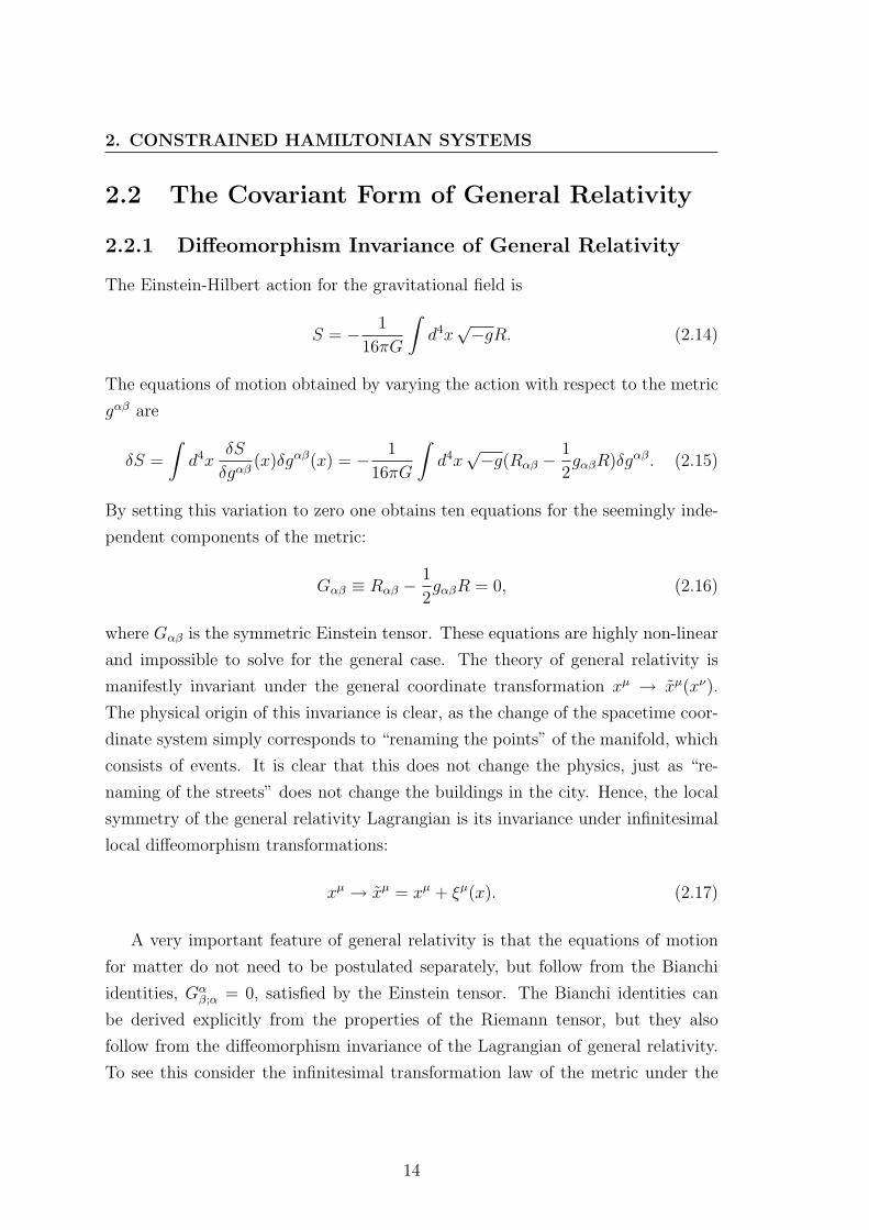
2.2.1 Diffeomorphism Invariance of General Relativity
The Einstein-Hilbert action for the gravitational field is
S = − 1
16πG
∫d4x√−gR. (2.14)
The equations of motion obtained by varying the action with respect to the metric
gαβ are
δS =
∫d4x
δS
δgαβ(x)δgαβ(x) = − 1
16πG
∫d4x√−g(Rαβ −
1
2gαβR)δgαβ. (2.15)
By setting this variation to zero one obtains ten equations for the seemingly inde-
pendent components of the metric:
Gαβ ≡ Rαβ −1
2gαβR = 0, (2.16)
where Gαβ is the symmetric Einstein tensor. These equations are highly non-linear
and impossible to solve for the general case. The theory of general relativity is
manifestly invariant under the general coordinate transformation xµ → xµ(xν).
The physical origin of this invariance is clear, as the change of the spacetime coor-
dinate system simply corresponds to “renaming the points” of the manifold, which
consists of events. It is clear that this does not change the physics, just as “re-
naming of the streets” does not change the buildings in the city. Hence, the local
symmetry of the general relativity Lagrangian is its invariance under infinitesimal
local diffeomorphism transformations:
xµ → xµ = xµ + ξµ(x). (2.17)
A very important feature of general relativity is that the equations of motion
for matter do not need to be postulated separately, but follow from the Bianchi
identities, Gαβ;α = 0, satisfied by the Einstein tensor. The Bianchi identities can
be derived explicitly from the properties of the Riemann tensor, but they also
follow from the diffeomorphism invariance of the Lagrangian of general relativity.
To see this consider the infinitesimal transformation law of the metric under the
14

2.2 The Covariant Form of General Relativity
transformation (2.17):
gαβ(x)→ gαβ(x) = gαβ(x)− gαβ,λ ξλ + gβλξ;αλ + gαλξ;β
λ , (2.18)
⇒ δgαβ = ξα;β + ξβ;α. (2.19)
Note that the argument x is the same on both sides. Thus we compare the metric
at different points of the manifold, which have the same coordinate values in both
coordinate systems xµ and xµ. Under this transformation the action changes
as
δS = − 1
16πG
∫d4x√−gGαβδg
αβ
= − 1
16πG
∫d4x√−gGαβ(ξα;β + ξβ;α)
= − 1
8πG
∫d4x√−gG;β
αβξα (2.20)
= 0,
and from this it follows that Gαβ;α = 0. Hence, we have derived the Bianchi identities
by exploiting the invariance of the action under diffeomorphisms, and without
explicitly referring to the properties of Ricci scalar.
2.2.2 The Hamilton Formalism
As we have seen, one consequence of the invariance of general relativity under
general coordinate transformations is that the number of independent components
of metric is reduced from ten to six. Hence, there are only six dynamical variables
in general relativity, and these will appear with first order time derivatives in the
canonical form of the action. To rewrite the Lagrangian of general relativity in the
first order form we use the Hilbert-Palatini formalism. In this one treats the metric
and the connection as independent variables and thus the Lagrangian is linear in
first derivatives of g and Γ.
We will begin with the action
S =
∫d4x√−gR (2.21)
15

2. CONSTRAINED HAMILTONIAN SYSTEMS
where we adapt the sign and units conventions of [14]. Furthermore, we will use
Planck units throughout the rest of our work. In the spirit of previous chapter
we see that the action is written in an already reparametrization invariant form
with no particular role associated to the time coordinate. This implies that the
total Hamiltonian of general relativity vanishes weakly and can be expressed as
linear combination of the constraints, which reflect the diffeomorphism invariance
of the theory. There are four allowed diffeomorphism transformations associated
with each spacetime direction, and, hence, we expect four constraints arising on
the way to the Hamilton formalism. In order to find these we will exploit gauge
freedom to choose a particularly convenient coordinate system.
2.2.2.1 Splitting the Spacetime in 3+1
Let us slice the spacetime into a one-parameter family of spacelike hypersurfaces.
The use of this specific spacetime decomposition does not, of course, impair the
general invariance of the theory under arbitrary coordinate transformations. Us-
ing this splitting we will rewrite the action of general relativity in parametrized
form (2.12), where the Hamiltonian and time parameter are again introduced as a
conjugated pair of generalized coordinates.
Consider two such subsequent spacelike hypersurfaces Σt and Σt+dt with t =
const and t + dt = const respectively. The geometry of the “earlier” hypersurface
is described by the 3-dimensional metric
γij(t, x, y, z)dxidxj;
the metric on the “later” hypersurface is
γij(t+ dt, x, y, z)dxidxj.
In order to fix the geometry of the spacetime one has to specify the rules by
which the points on different equal-time slices are connected. This enables one to
calculate the proper interval ds2 between two spacetime points xµ = (t, xi) and
xµ + dxµ = (t+ dt, xi + dxi) by using the Pythagorean theorem:
ds2 = γij(dxi + Nidt)(dxj + Njdt)− (N0dt)2.
16

2.2 The Covariant Form of General Relativity
This yields to 3+1 decomposition of the metric tensor
(gαβ) =
(−N2 + NiN
i Ni
Ni γij
)(2.22)
The covariant lapse and shift variables are given by
Ni = γijNj, N0 = N0 = N
and the inverse of the metric is
(gαβ)
=1
N2
(−1 Ni
Ni N2γij −NiNj
). (2.23)
For the proper volume element the determinant will be needed
g = det(gαβ) = −N2γ, with γ ≡ det(γij).
2.2.2.2 Constraints in ADM Formalism
In this section we are going to rewrite the action (2.21) of general relativity in the
first order form. When we say first order we mean that we are looking for a form
in which the generalized coordinates and momentum appear in the Lagrangian in
the combination pq, i.e. with first time derivatives. After varying the action with
respect to p and q one obtains first order equations of motion. Furthermore, we
will use Hilbert-Palatini method and treat the quantities g and Γ independently.
The end result for the Lagrangian density is:
L = πij γij −NαHα, (2.24)
where πij are momenta conjugated to γij and defined in terms of the extrinsic
curvature Kij,
πij = −γ1/2(Kij − γijK
)Kij =
1
2N−1 (Ni;j + Nj;i − γij,0) , K = γijKij,
17

2. CONSTRAINED HAMILTONIAN SYSTEMS
and Nα are the lapse and shift variables introduced above. Hα are the constraints
due to the diffeomorphism invariance of general relativity
H0 = Gijklπijπkl −√γ(3)R (2.25)
Hi = −2γijπjl|l , (2.26)
where
Gijkl =1
2√γ
(γikγjl + γilγjk − γijγkl).
(3)R is the intrinsic curvature of a hypersurface of constant time t and the vertical
bar denotes the covariant derivative with respect to the 3-metric γij. After using
the generalized Poisson brackets
γij(x), πkl(y)
= δ
(ki δ
l)j δ(x, y) =
1
2(δki δ
lj + δliδ
kj )δ(x, y), (2.27)
where x and y denote two different points on the spacetime manifold, we can derive
the following equal-time Poisson brackets for the constraints
H0(x),H0(y) = γij(x)Hj(x)∂
∂xiδ(x, y)− γij(y)Hj(y)
∂
∂yiδ(x, y),
Hi(x),H0(y) = H0(x)∂
∂xiδ(x, y), (2.28)
Hi(x),Hj(y) = Hj(x)∂
∂xiδ(x, y)−Hi(y)
∂
∂yjδ(x, y).
These then form a closed set of constraints, i.e. in the language of Dirac they are
first class constraints. The H0 constraint, being the generator of translations in
the time direction, describes the time evolution of the gravitational field, while Hi
generate diffeomorphism transformations on the hypersurface Σt.
18

3
Diffeomorphisms and Physical
Quantum States in String Theory
In this chapter the role of the diffeomorphism invariance in string theory is in-
vestigated. We will begin with the classical theory and will show how the diffeo-
morphism constraints arise in both the Lagrange and Hamilton formalisms. We
then consider the canonical and light-cone gauge quantization of string theory and
explore how the classical constraints are resolved in these approaches. In the con-
clusion an explicit construction of the physical quantum string state space by the
use of vertex operators is presented. This chapter follows the books [17; 18].
3.1 Symmetries of the Polyakov Action
Consider a free bosonic string. Its trajectory in the target spacetime covers a two
dimensional hypersurface called a worldsheet. We parametrize this hypersurface
by one timelike coordinate τ and one spacelike coordinate σ taking values in the
range σ ∈ [0, 2π]. The worldsheet coordinates (τ, σ) are mapped to target space
coordinates Xµ(σ, τ), where µ = 0, ..., D − 1. Target space is assumed to be D-
dimensional, flat Minkowski space with the metric ηµν = (−1, 1, . . . , 1). The action
for the string has to be proportional to the area of the worldsheet. This is a two-
dimensional generalization of the action for a relativistic particle moving along
geodesics. Instead of minimizing the length of the worldline, the string minimizes
the area of its worldsheet.
19

3. DIFFEOMORPHISMS AND PHYSICAL QUANTUM STATES INSTRING THEORY
In practice it is more convenient to work with the Polyakov action
S = −T2
∫d2σ√−ggαβ(σ, τ)ηµν(X)∂αX
µ∂βXν , (3.1)
Here gαβ(σ) is the metric on the string worldsheet. Since no time derivatives of the
metric appear in the Lagrangian, the equations of motion for gαβ are the constraints
in string theory. After imposing these constraints, the action reduces to the area of
the worldsheet. The proportionality constant T = 12πα′
is a parameter of dimension
[L]−2 and has a physical interpretation as the tension of the string, i.e. potential
energy per unit length. α′ is a conventional parameter called the Regge slope
parameter. The indices that α, β take values 0, 1 while µ, ν = 0, ..., D − 1.
The Polyakov action (3.1) is invariant under both global, D-dimensional, Poincare
transformations and local diffeomorphism transformations on the string worldsheet.
This action can also be interpreted as describing D scalar fields Xµ(τ, σ) in a curved
two-dimensional spacetime. The invariance under general coordinate transforma-
tions enables us, by appropriate choice of gauge, to bring the worldsheet metric to
a conformally flat form:
gαβ → gαβ = e2Φηαβ.
This choice of worldsheet metric is referred to as conformal gauge. Moreover, the
action is also locally Weyl invariant, i.e. the transformation
gαβ(τ, σ)→ Ω2(τ, σ)gαβ(τ, σ)
leaves it unchanged. Hence the conformal factor e2Φ drops out of the Polyakov
action which in conformal gauge becomes
S = −T2
∫d2σηαβ∂αX
µ∂βXµ. (3.2)
However, some reparametrization freedom is still left because requiring that ds2 =
e2Φ(dτ 2 − dσ2) does not uniquely fix the coordinate system. In fact, in the world-
sheet light-cone coordinates
σ± = τ ± σ, ∂± =1
2(∂τ ± ∂σ)
20

3.2 The Canonical Form of the Polyakov Action
the line element becomes ds2 = e2Φdσ+dσ−. Under conformal transformations
σ± → σ±(σ±) it transforms to ds2 = e2Φdσ+dσ−. The prefactor has changed, but
the metric is still conformally flat. This residual symmetry plays an important role
in string theory. I will consider it in detail in section 3.5.1.
In conformal gauge the equations of motion for Xµ are
∂α∂αXµ = 0. (3.3)
As we have assumed that the worldsheet metric is an independent field, then the
equation of motion for gαβ also has to be satisfied. Recalling the definition of the
energy-momentum tensor
Tαβ = − 2
T
1√−g
δS
δgαβ= 0,
it turns out that satisfying the equations of motion for gαβ classically corresponds
to setting Tαβ = 0. These are the constraints of string theory. In conformal gauge
the constraint equations are
C0 ≡ T00 = T11 =1
2(X2 +X ′2) = 0, (3.4)
C1 ≡ T01 = T10 = X ·X ′ = 0. (3.5)
Here X ≡ ∂X∂τ
, X ′ ≡ ∂X∂σ
, and the scalar product is denoted as X ·X = ηµνXµXν .
3.2 The Canonical Form of the Polyakov Action
In this section we will treat string theory as a theory for D massless scalar fields
on a two dimensional background with metric gαβ. Instead of choosing conformal
gauge, we will use the 1+1 decomposition for the metric gαβ:
ds2 = −(N2 −N1N1)dτ 2 + 2N1dσdτ + γ11dσ2, (3.6)
where N and N1 are the lapse and shift respectively. After introducing the momenta
conjugated to the scalar field Xµ:
πµ =∂L
∂Xµ=
√γ11
N(Xµ −N1Xµ
′), (3.7)
21

3. DIFFEOMORPHISMS AND PHYSICAL QUANTUM STATES INSTRING THEORY
the Polyakov action (3.1) in the first order Hamilton formalism takes the following
form
S =
∫d2σ (πµX
µ −NαCα), (3.8)
where T ≡ 1, N0 = N√γ
and N1 the lapse and the shift are Lagrange multipliers and
the constraints are
C0 =1
2(π2 +X ′2), C1 = πµX
′µ. (3.9)
Note that in the conformal gauge gαβ = ηαβ the conjugated momenta in (3.7)
reduce to πµ = Xµ and the constraints reduce to (3.4) and (3.5). The following
equal-time Poisson brackets for the constraints can be derived as
Ci(σ), Ci(σ′) = C1(σ)
∂
∂σδ(σ, σ′)− C1(σ′)
∂
∂σ′δ(σ, σ′),
C0(σ), C1(σ′) = C0(σ)∂
∂σδ(σ, σ′)− C0(σ′)
∂
∂σ′δ(σ, σ′) (3.10)
with i = 0, 1. These constraints are consequences of the diffeomorphism invariance
of the Polyakov action.
3.3 Mode Expansions
3.3.1 Constraints in Light-cone Worldsheet Coordinates
Consider a closed string which obeys the periodicity condition
Xµ(τ, σ) = Xµ(τ, σ + 2π).
In terms of the worldsheet light-cone coordinates equations of motion (3.3) can be
written as
∂+∂−Xµ = 0. (3.11)
The general solution for these equations can be written as a sum of left- and right-
moving modes
Xµ(τ, σ) = XµL(σ+) +Xµ
R(σ−).
22

3.3 Mode Expansions
The most general solution of equation (3.11) is then the following expansion in
Fourier series (the coefficients are adjusted to agree with common notations)
XµL(σ+) =
1
2xµ +
1
2α′pµσ+ + i
√α′
2
∑n 6=0
1
nαµne−inσ
+
,
XµR(σ−) =
1
2xµ +
1
2α′pµσ− + i
√α′
2
∑n6=0
1
nαµne−inσ
−, (3.12)
where xµ and pµ are the position and momenta of the center of mass of the string.
By demanding that πµ = Xµ and Xµ obey the canonical Poisson bracket one can
show that the Fourier coefficients αµn have the following Poisson brackets
αµm, ανn = αµm, ανn = imδm+nηµν (3.13)
αµm, ανn = 0.
The requirement that XR and XL are real functions leads to further restrictions on
the Fourier components
αµ−n = (αµn)†, αµ−n = (αµn)†.
For later use and reference let us write down the expressions for Xµ(τ, σ) and its
derivatives explicitly:
Xµ(τ, σ) = xµ + α′pµτ + i
√α′
2
∑n6=0
1
n
(αµne
−inσ− + αµne−inσ+
), (3.14)
Xµ(τ, σ) =
√α′
2
(∑n
αµne−inσ+
+∑n
αµne−inσ−
), (3.15)
Xµ′(τ, σ) =
√α′
2
(∑n
αµne−inσ+ −
∑n
αµne−inσ−
). (3.16)
23

3. DIFFEOMORPHISMS AND PHYSICAL QUANTUM STATES INSTRING THEORY
where αµ0 ≡ αµ0 ≡√
α′
2pµ. The constraints (3.4) in light-cone coordinates become
T+− = T−+ = 0, (3.17)
L(τ, σ) ≡ T−− =1
2(T00 − T01) = (∂−X)2 =
α′
2
∑m,n
αn−m · αme−inσ−
= 0, (3.18)
L(τ, σ) ≡ T++ =1
2(T00 + T01) = (∂+X)2 =
α′
2
∑m,n
αn−m · αme−inσ−
= 0.
Hence the light-cone constraints L, L are related to “Minkowski worldsheet” con-
straints C0, C1 as
L =1
2(C0 − C1) (3.19)
L =1
2(C0 + C1).
The above expansions can be written in a shorter form
L(τ, σ) = α′∑n
Lne−inσ−
= 0,
L(τ, σ) = α′∑n
Lne−inσ+
= 0 (3.20)
Here we have introduced the Virasoro modes Ln, Ln. They are the Fourier coeffi-
cients of the above expansion, evaluated at time τ = 0,
Ln =1
2
∑m
αn−m · αm =1
2πα′
∫ 2π
0
dσe−inσL(0, σ), (3.21)
Ln =1
2
∑m
αn−m · αm =1
2πα′
∫ 2π
0
dσeinσL(0, σ).
The Poisson brackets for Ln and Ln can be calculated directly from definitions
(3.21) and Poisson brackets (3.13). This yields the Virasoro algebra
Ln, Lm = −i(n−m)Lm+n,Ln, Lm
= −i(n−m)Lm+n, (3.22)
Ln, Lm
= 0.
24

3.3 Mode Expansions
As the Virasoro operators Ln and Ln decouple, we will often consider only one copy
of these algebras.
The constraint equations (3.17) in terms of the Virasoro modes become:
Ln = Ln = 0, ∀n.
3.3.2 Constraints in Minkowski Worldsheet Coordinates
We can similarly expand the constraints (3.4) in a Fourier series on the circle as
Ci(0, σ) =+∞∑
n=−∞
(Ci)neinσ, (Ci)n =
1
2π
∫ 2π
0
dσ Ci(0, σ)e−inσ. (3.23)
From the Poisson brackets (3.10) it follows that the Fourier modes (Ci)n also obey
the Virasoro algebra
(Ci)n, (Ci)m = −i(n−m)(Ci)n+m, (3.24)
(C0)n, (C1)m = −i(n−m)(C0)n+m.
In distinction from the light-cone constraint algebra (3.22), the modes (C0,1)n do
not decouple. In terms of string oscillators the Fourier coefficients of C1, C0 at
τ = 0 can be expressed as
(C0)n =1
2
∑m
(α−n−m · αm + αn−m · αm), (3.25)
(C1)n =1
2
∑m
(α−n−m · αm − αn−m · αm).
Further we observe that the Fourier modes Ln, Ln and (C0)n, (C1)n are not related
as in eq. (3.19). Instead they satisfy
(C0)n = L†n + Ln,
(C1)n = L†n − Ln.
This is due to the differences in the Fourier expansions (3.21) and (3.24). However,
the constraints C0, C1 are both more natural and easier to interpret because the
distinction between timelike and spacelike coordinates is preserved.
25

3. DIFFEOMORPHISMS AND PHYSICAL QUANTUM STATES INSTRING THEORY
3.3.3 Generators of Diffeomorphism Transformations
There is a straightforward interpretation of both sets of Virasoro operators Ln, Ln
and (C0)n, (C1)n. This can be clearly seen by calculating the action of the gener-
ators Ln, Ln on the target space coordinates Xµ:
Ln, Xµ(τ, σ) = einσ−∂−X
µ (3.26)Ln, X
µ(τ, σ)
= einσ+
∂+Xµ (3.27)
Hence, the Virasoro operators Ln (Ln) generate the residual diffeomorphism trans-
formations which preserve the conformal gauge. As σ− (σ+) is an angular variable
in the mode expansion of XL (XR) then it can also be said that Ln (Ln) generate
diffeomorphisms on the circle.
Similarly, for the equal time constraints (C0)n, (C1)n we have
(C0)n, Xµ(τ, σ) = e−inσ
(Xµ cosnτ − iX ′µ sinnτ
)(3.28)
(C1)n, Xµ(τ, σ) = e−inσ
(−iXµ sinnτ +X ′
µcosnτ
). (3.29)
Here the time and space directions of the worldsheet are mixed and the interpre-
tation might seem confusing. In order to clarify this, let us, instead of choosing a
given moment of time τ = 0, consider a constant spatial coordinate σ = 0. Then
the constraints C0 and C1 become
C0(τ, σ = 0) =α′
2
∑n,m
(αn−m · αm + αn−m · αm) e−inτ , (3.30)
C1(τ, σ = 0) =α′
2
∑n,m
(αn−m · αm − αn−m · αm) e−inτ .
We then define the corresponding Fourier coefficients as
(A0)n ≡1
2
∑m
(αn−m · αm + αn−m · αm) , (3.31)
(A1)n ≡1
2
∑m
(αn−m · αm − αn−m · αm) . (3.32)
In order to calculate the Poisson bracket for two fields, which are given at differ-
26

3.3 Mode Expansions
ent moments of time, in generic case, one should use the time evolution operator
determined by the Hamiltonian, to “bring the fields” to equal times. However, one
can formally use the expressions (3.30) and Poisson brackets (3.13) to derive the
following relations:
Ci(τ), Ci(τ′) = −
(C0(τ)
∂
∂τδ(τ, τ ′)− C0(τ ′)
∂
∂τ ′δ(τ, τ ′)
), (3.33)
C0(τ), C1(τ ′) = −(C1(τ)
∂
∂τδ(τ, τ ′)− C1(τ ′)
∂
∂τ ′δ(τ, τ ′)
). (3.34)
Note that these equations are very similar to the Poisson brackets (3.10). One
should be aware, however, that the equal-time Poisson brackets are universal, i.e.
they do not depend on the equations of motion. Meanwhile, the “equal-space
Poisson brackets” were derived by explicitly using the solution of the equations
of motion. However, the solutions of string theory are mode expanded in the
light-cone worldsheet coordinates σ± = τ ± σ. Hence, the space and time world-
sheet coordinates appear in combinations of the light-cone coordinates only. It
follows then from the remaining gauge invariance of Polyakov action that under
the conformal transformation σ− → −σ− the roles of the coordinates τ and σ are
exchanged. Therefore, the equal-time Poisson brackets have the same structure as
the “equal-space Poisson brackets”.
The action of (A0)n and (A1)n on coordinates Xµ is
(A0)n, Xµ(τ, σ) = einτ
(Xµ cosnσ + iXµ′ sinnσ
), (3.35)
(A1)n, Xµ(τ, σ) = einτ
(iXµ sinnσ +Xµ′ cosnσ
), (3.36)
which coincides with (3.28) if one substitutes σ = −τ and (A1)n = −(C0)n. After
rewriting(C0)n, X
µ(0, σ) = e−inσXµ
(C1)n, Xµ(0, σ) = e−inσXµ′,
(A0)n, X
µ(τ, 0) = einτXµ
(A1)n, Xµ(τ, 0) = einτXµ′.
(3.37)
the physical interpretation of C0 and C1 is obvious. Hence, the C0 constraint gen-
erates time translations and the C1 constraint generates spatial diffeomorphisms.
27

3. DIFFEOMORPHISMS AND PHYSICAL QUANTUM STATES INSTRING THEORY
3.4 Old Canonical Quantization
As we have seen so far - the Polyakov action, initially invariant under diffeomor-
phism and Weyl transformations, was simplified by choosing the conformal gauge.
Still, there is a residual symmetry left which does not affect the choice of conformal
gauge. More precisely, the action is still invariant under conformal transformations
σ± → σ±(σ±). This gauge symmetry was a direct consequence of promoting the
worldsheet metric gαβ to a dynamical variable. This resulted in additional con-
straint equations which still have to be imposed once the solutions of the equations
of motion for target space coordinates Xµ are found. In the worldsheet light-cone
coordinates the final form of the subsidiary conditions was Ln = Ln = 0.
How can we quantize the dynamical degrees of freedom of the string? The
Gupta-Bleuler method known from quantum electrodynamics suggests that the
system should be first quantized cannonically and that afterwards the constraint
equations in the form of operator equations on our wave functions have to be
imposed. So let us promote the target space coordinates Xµ to operator valued
fields and define their conjugated momenta as πµ = 12πα′
Xµ. We further demand
that they obey the canonical equal-time commutation relations
[Xµ(σ), πν(σ′)] = iδ(σ − σ′)ηµν
⇒ [αµn, ανm] = [αµn, α
νm] = nηµνδn+m,0, [xµ, pν ] = iηµν . (3.38)
After redefining an = αn√n
and a†n = α−n√n
with n > 0, one obtains the familiar
commutation relations for the harmonic oscillator
[aµn, a
ν†m
]= δn,mη
µν , [an, am] =[a†n, a
†m
]= 0. (3.39)
This suggests that we interpret a†n and an as creation and annihilation operators
respectively. The redefinition we performed above was only useful to see clearly
that αµn and αµ−n can be associated with some kind of creators and annihilators and
can be further used to build a Fock space. The corresponding analysis is valid also
for α. Thus every scalar field Xµ(σ) gives rise to an infinite number of creation
and annihilation operators.
28

3.4 Old Canonical Quantization
Basing on this analogy we define the vacuum state of the Fock space as
αµn |0〉 = αµn |0〉 = 0, n > 0. (3.40)
We should be aware, however, that there is one more degree of freedom arising
from the zero mode of the oscillators αµ0 , αµ0 . This is pµ, which corresponds to the
momenta of the center of mass of the string. Hence, we denote |0; p〉 as a state which
is annihilated by the oscillators αµn, αµn, n > 0 and has a center of mass momentum
pµ. We will further restrict the discussion to one of the sets of oscillator modes
only. However, we keep in mind that αµ0 = αµ0 =√
α′
2pµ. This relation translates
into the level matching condition L0 = L0 for closed strings.
Now we can build excited states by acting on the vacuum state with creation
operators. Every state in the Fock space can be schematically written as
|λ〉 =∞∏n=1
D−1∏µ=0
(αµ−n)µn |0; p〉 . (3.41)
The Fock space defined above cannot be the physical Hilbert space though. This
can be seen immediately after considering the state α0−n |0〉. In order to calculate
its norm the commutation relations (3.39) for the time component have to be used.
As a result this state has negative norm 〈0|α0nα
0−n |0〉 = −n. But we know that
the physical space should not contain any ghosts. In order to resolve this problem,
one has to implement the Virasoro constraints obtained in the classical theory,
Ln = 0, ∀n, in the quantum theory.
First, let us see, how these classical modes translate into quantum operators.
Because of the normal ordering of creation and annihilation operators, two mod-
ifications of the Virasoro algebra have to be made. The only normal ordering
ambiguities arise in the zero mode L0, because αn−m commutes with αm unless
n = 0. Thus some unknown ordering constant a will appear. One chooses to define
the quantum operator L0 to be the normal ordered expression
L0 =1
2α2
0 +∞∑n=1
α−n · αn (3.42)
and to include the normal ordering constant a by replacing L0 → L0−a everywhere.
For the same reason an extra term in the commutation relations [Ln, L−n] appears.
29

3. DIFFEOMORPHISMS AND PHYSICAL QUANTUM STATES INSTRING THEORY
It is determined by demanding that the Jacobi identity is satisfied. The quantum
Virasoro algebra is then
[Lm, Ln] = (m− n)Lm+n +D
12m(m2 − 1)δm+n,0. (3.43)
In quantum theory the physicality conditions have to be implied as operator equa-
tions on the states Ln |φ〉 = 0, ∀n. This condition is too strong, because it leaves
us with an empty Hilbert space, and must be replaced by a weaker requirement
similarly to Gupta-Bleuler quantization. Namely, we demand that every physical
state is annihilated by positive frequency modes only. Then by choosing normal
ordering convention as ’negative frequency modes on the left and positive frequency
modes on the right,’ every matrix element between two physical states vanishes.
Thus, the physicality conditions for a quantum state |φ〉 read:
Ln |φ〉 = 0, ∀n > 0 (3.44)
(L0 − a) |φ〉 = 0. (3.45)
Classically (a = 0) the condition L0 = 0 translates into a relation between the mass
squared and the oscillator modes of the closed string on the mass shell:
M2 = −pµpµ = −2α20
α′= − 4
α′
(1
2α2
0
)=
4
α′
∞∑n=1
α−n · αn. (3.46)
Thus, there is a natural choice for the quantum mass squared operator:
M2 =4
α′
(−a+
∞∑n=1
α−n · αn
). (3.47)
After introducing the number operator N ≡∑∞
n=1 α−n · αn, we have
M2 =4
α′(−a+N), (3.48)
L0 =1
2α2
0 +N.
The commutation relations with the creation and annihilation operators are:
[N,αn] = −nαn, [N,α−n] = nα−n, ∀n > 0. (3.49)
30

3.5 Light-cone Gauge Quantization
When the number operator acts on the basis state |λ〉 in eq. (3.41), its eigenvalue
is the sum of the mode numbers of the creation operators
N |λ〉 = Nλ |λ〉 , with Nλ =∞∑n=1
25∑µ=0
nµn. (3.50)
Therefore, the eigenstates |λ〉 can be classified according to their eigenvalues Nλ.
It is then said that the state |λ〉 is of the level Nλ.
3.5 Light-cone Gauge Quantization
The idea behind this approach to quantizing the string is to eliminate the non-
dynamical degrees of freedom before passing to quantum mechanics. This is done
by exploiting the remaining symmetry of the Polyakov action so that the constraint
equations can be resolved at the classical level. This envolves a choice of a particular
gauge, which appears to break the Lorentz invariance. However, it can be shown
that by appropriate choice of normal ordering constant a and spacetime dimension
D, the Lorentz invariance can be preserved.
3.5.1 Residual Gauge Symmetry
As was mentioned several times before, even after fixing gαβ = e2Φηαβ the Polyakov
action is still invariant under conformal transformations σ± → σ±(σ±). The world-
sheet coordinates τ = 12(σ+ + σ−) and σ = 1
2(σ+ − σ−) transform into
τ =1
2(σ+(σ+) + σ−(σ−)), (3.51)
σ =1
2(σ+(σ+)− σ−(σ−).
From here it follows that the coordinate τ can be an arbitrary solution of the wave
equation (∂2τ − ∂2
σ
)τ = 0.
This is exactly the equation of motion for the target space coordinates. Thus we
can use the remaining gauge freedom to set τ equal to one of the coordinates Xµ.
The coordinate σ is then determined by eq.(3.51).
31

3. DIFFEOMORPHISMS AND PHYSICAL QUANTUM STATES INSTRING THEORY
3.5.2 Light-cone Gauge
Let us first introduce the light-cone coordinates in spacetime as
X± =1√2
(X0 ±XD−1),
XI = X i, i = 1, . . . , D − 2.
The light-cone gauge corresponds to the choice of the coordinate τ to be propor-
tional to X+, i.e.
X+(τ, σ) = x+ + p+τ.
Then the X−(τ, σ) coordinate is completely determined by the constraint equations
(X ±X ′)2 = 0 as
(X− ±X−′) =1
2α′p+(XI ±XI ′)2. (3.52)
One can introduce the transverse Virasoro modes for the coordinates XI . In com-
plete analogy with previous definitions (3.21) they are expressed as
L⊥n =1
2
∑m
αIn−mαIm, L⊥n =
1
2
∑m
αIn−mαIm,
where the repeated indices I = 1, . . . D − 2 denote summation over the transverse
dimensions. Consequently, from the expansion of X− coordinates
X− +X−′=√
2α′∑n
α−n e−inσ+
,
X− −X−′ =√
2α′∑n
α−n e−inσ−
one can read off the equations for oscillator modes:
√2α′α−n =
2
p+L⊥n ,
√2α′α−n =
2
p+L⊥n . (3.53)
Hence, the only degrees of freedom left after imposing the light-cone gauge are:
p+, x−0 , xI0, α
In. This choice of gauge is not covariant, however, and breaks Lorentz
invariance, since the choice of components 0 and D − 1 for defining the light-cone
coordinates was completely arbitrary. One can show that in order for the quantum
Lorentz generators to obey the Poincare algebra, the constant values a = 1 and
32

3.6 Physical States
D = 26 have to be chosen for bosonic strings.
3.6 Physical States
As was mentioned before, the Fock space built by creation operators αµ−n, µ =
0, . . . , D acting on the vacuum state is not the physical state space which is spanned
by all positive norm states |φ〉 that satisfy the Virasoro condition Ln |φ〉 = 0, n > 0
and the mass-shell condition (L0 − a) |φ〉 = 0. In this section we will show how to
construct the physical state space without explicitly using the transverse oscillators
αI−n.
3.6.1 Vertex Operators
The first step in order to unambigously define the physical state space is to associate
an operator Vφ to every on-shell physical state |φ〉. This will allow us to build new
physical states from the old ones. What conditions should this new operator fulfill?
First of all, it should be transformed into itself by the Virasoro algebra. Imposing
this condition is necessary because the time evolution of any local quantum operator
is determined by the corresponding Hamilton operator, which on the open string
space is L0− a. Let us show that operators which satisfy this demand are actually
the primary operators from conformal field theory1. Consider a field V (σ = 0, τ) ≡V (τ) on the open string Hilbert space. It is said that an operator has a conformal
weight h if under an arbitrary change of variables τ → τ ′ it transforms like
V ′(τ ′) =
(dτ
dτ ′
)hV (τ).
Written in infinitesimal form this transformation law becomes
δV (τ) = −εdVdτ
+ hVdε
dτ. (3.54)
Rewriting eq. (3.26) at the point σ = 0 and substituting the Poisson bracket with
commutator leads to
[Lm, Xµ(τ)] = −ieimτXµ(τ).
1We will discuss this in more detail in the next chapter. For now we will only use some ofmost essential properties of primaries.
33
3. DIFFEOMORPHISMS AND PHYSICAL QUANTUM STATES INSTRING THEORY
Hence, the target space coordinates Xµ(τ) have conformal weight h = 0, and we
conclude that Virasoro operators generate transformations (3.54) with the infinites-
imal parameter given by ε = −ieimτ . Thus for a field of arbitrary conformal weight
(3.54) can be written
[Lm, V (τ)] = eimτ(−i ddτ
+mh
)V (τ). (3.55)
If the operator V (τ) is expandable in a Fourier series, this condition can be imposed
on the Fourier modes An as
[Lm, An] = (m(h− 1)− n)Am+n. (3.56)
One can check that if |φ〉 is a given physical state and the operator V (τ) has
conformal dimension h = 1, then the state |φ′〉 = A0 |φ〉 is again a physical state.
Therefore, we conclude that we are looking for an operator of conformal weight
h = 1. In this case the transformation law (3.55) can be expressed as a total time
derivative:
[Lm, V (τ)] = −i ddτ
(eimτV (τ)). (3.57)
The second condition we have to impose on the vertex operator is that if at time
τ and σ = 0 a physical state of momentum −kµ is emitted by vertex operator
V (k, τ), then it should increase the momentum of the initial state by an amount
kµ. This suggests that the vertex operator has to be proportional to eik·x(τ) with
x(τ) being the center of mass position of the string at time τ . So let us try the
simplest expression we can come up with:
V (k, τ) ≡: eik·X(0,τ) : . (3.58)
By straightforward calculation one can show that this operator has conformal
weight h = k2/2 for open strings. In the case k2 = 0 this gives h = 0, and,
hence, the expression (3.58) cannot be used as vertex operator describing the emis-
sion of a massless meson. However, one can show that the conjugated momenta
Xµ has h = 1, which is exactly what we are looking for. Thus, the next try should
be the following
Vζ(k, τ) = ζ · dXdτ
exp[ik ·X], (3.59)
34

3.6 Physical States
where ζµ(k) is the polarization vector. If k · ζ = 0 then this expression has no
short distance singularities in the operator product expansion and Vζ(k, τ) can be
used as vertex operator. This condition on the polarization vector ensures that the
vertex operators are in one-to-one correspondance with physical states.
3.6.2 Transverse Physical States
In this section we present the Del Giudice, Di Vecchia and Fubini (DDF) con-
struction used to construct operators AIn, which when applied to the ground state
give all possible transverse physical states. Note that we only refer to the states
which correspond to the transverse oscillator modes αIn, where I = 1, .., D − 2, as
introduced in the light-cone quantization.
Let us first choose the ground state to be the tachyonic ground state |p0; 0〉,which fulfills the mass shell condition p2
0 = 2. Suppose that the tachyon is in a
particular state with p+0 = 1, p−0 = −1 and pI0 = 0. Also define a vector kµ0 with
components k−0 = −1, k+0 = kI0 = 0, and, thus, k0 · p0 = 1. This kinematic setup
will be used throughout the construction of physical states.
We now define allowed states such that if the mass is given to be α′M2 = N − 1
then the momentum has to be pµ = pµ0 − Nkµ0 . Any physical state obeying the
mass shell condition can be Lorentz transformed into such a configuration.
As we discovered in the previous section, one can build new massless physical
states from already existing physical state via applying the vertex operator (3.59).
From our kinematical setup it follows that we are only studying states with a wave
vector which is an integer multiple of the null vector defined above, i.e. kµ = nkµ0 .
In this case the vertex operator for transverse polarizations is
V I(nk0, τ) = XI(τ)einX+(τ), (3.60)
where X+(τ) = x+ + τ . It follows that V I(nk0, τ) = V I(nk0, τ + 2π). We define
AIn =1
2π
∫ 2π
0
V I(nk0, τ)dτ =1
2π
∫ 2π
0
XI(τ)einx+
einτ dτ. (3.61)
The operators AIn can be interpreted as the Fourier modes of a periodic operator
which behaves as a primary field with weight h = 1 under the transformations
generated by Lm at a given point σ = 0. Because of the periodicity condition, AIn
35

3. DIFFEOMORPHISMS AND PHYSICAL QUANTUM STATES INSTRING THEORY
commutes with the Virasoro operators, as can be calculated from (3.57). As we
will see later, this is actually the most important property an operator has to fulfill
in order to generate physical states .
The following properties of operators AIn can be derived by direct computation:
[Lm, AIn] = 0
[N,AIn] = nAIn (3.62)
[AIm, AJn] = mδIJδm+n
AI†n = AI−n
AIn |0; p0〉 = 0, n > 0.
From here it is obvious that the AIn have the same properties as the transverse
oscillators αIn and therefore states of the form
|f〉 = AI1−1AI2−2...A
Im−m |0; p0〉 (3.63)
satisfy the Virasoro conditions and have N =∑rIr. In other words, these states
are physical, linearly independent, and have positive metric. We will call generic
states of the form (3.63) DDF states, and the space spanned by them we denote
F . As the operators AIn are in one-to-one correspondence with the algebra of
transverse oscillators, we can then conclude that they form a D − 2 dimensional
physical subspace of the complete Fock space.
3.6.3 No Ghost Theorem for D = 26 and a = 1
The purpose of this section is to show that there are no ghosts if we choose the
spacetime dimension to be D = 26 and normal ordering constant a = 1. The idea of
the proof is to show that all states in the complete Fock space built from oscillator
modes as shown in (3.41) can be identified with DDF states, which are physical,
positive norm states, according to the previous section. We will sketch the proof as
it is necessary for further discussion, but only its main steps and results. Detailed
proof can be found in [17].
Let us define the operators
Km = k0 · αm, (3.64)
36

3.6 Physical States
where the scalar product is taken over all spacetime dimensions. This operator has
the following properties
[Km, Ln] = mKm+n, [Km, Kn] = 0 (3.65)
Kn |f〉 = 0, n > 0.
Here and henceforth we will take |f〉 to be a DDF state. We also define K to be a
space spanned by all the states of the form
|k〉 =∞∏n=1
Kµn−n |f〉 . (3.66)
We now are going to explore the properties of the states built by acting on DDF
states with operators L−n and K−n. We introduce
|λ, µ, f〉 ≡ Lλ1−1L
λ2−2 . . . L
λm−mK
µ1
−1 . . . Kµm−m |f〉 (3.67)
with the eigenvalue P of the number operator defined as
P ≡∑
rλr +∑
sµs. (3.68)
The ordering in (3.67) was chosen arbitrarily and this is possible due to the com-
mutation relations of the L’s and K’s. Once an ordering is chosen we will stay to
this convention throughout the calculation. Also note that the subscript m is the
same for both the L’s and K’s. This is done only for the elegance of notation and
denotes the highest order of operators K or L used to build a given state. It is still
allowed that λm = 0 if µm 6= 0.
We now claim that the states (3.67) are linearly independent. To show this
consider the matrix of inner products of states (3.67) for a given value of P and
some DDF state |f〉:
MPλ,µ;λ′,µ′ = 〈f |Kµn
n . . . Kµ1
1 Lλnn . . . Lλ11
Lλ′1−1 . . . L
λ′m−mK
µ′1−1 . . . K
µ′m−m |f〉 , (3.69)
where P =∑rλr +
∑sµs =
∑rλ′r +
∑sµ′s. One can then show that there exists
an ordering of the states like i = λ, µ < j = λ′, µ′ such that the matrix MPij
37

3. DIFFEOMORPHISMS AND PHYSICAL QUANTUM STATES INSTRING THEORY
takes the form a11 a12 a13 a14
a21 a22 a23 0
a31 a32 0 0
a41 0 0 0
. (3.70)
The states (3.67) are then linearly independent because det(MP ) 6= 0.
There are two kinds of states with nonzero inner products: the states made
out of L’s or K’s only, or states with an equal number of L’s and K’s. The latter
restriction is needed because the evaluation process of the elements of MP consists
of commuting the operators past each other in order to get an L0 or K0 acting on
the DDF state. If there would be more operators K than L, then an operator Kn
coming from the left with n > 0 would hit |f〉 and give zero. After these remarks
it is easy to define an appropriate ordering and to prove the claim.
The important remark has to be made that the presence of K operators is
crucial. They are the key ingredients which ensure the non-singularity of matrix
MP . The calculation of the determinant of inner product matrix for the states
made out of L’s only (Kac determinant) is of great importance in CFT and gives
restrictions on the allowed values of the conformal weights h and the central charges
c.
One can also check that any two states built from two orthogonal DDF states
|f〉 and |g〉 which are L0 eigenstates are also orthogonal, as are the states built upon
them. This allows us to conclude that the states (3.67) made from all possible DDF
states and λ, µ running over all strings of L’s and K’s are linearly independent.
Let us summarize. We have so far two sets of states. The first set is the Fock
space built by acting on the string vacua with oscillators. A generic state in this
space can be written as25∏ρ=0
∞∏n=1
(αρ−n)εn,ρ |0〉 . (3.71)
The second set of states is the one introduced in (3.67). More explicitly, any such
state can be written as a product
∞∏n=1
Lλn−n ·Kµn−n ·
24∏I=1
(AI−n
)βn,I |0〉 . (3.72)
38

3.6 Physical States
We claim now that every state in the bosonic open string Fock space (3.71) can be
expressed as a linear combination of basis states (3.72). To prove this one has to
show that the number of states with a given eigenvalue 〈N〉 of the number operator
N =25∑ρ=0
∞∑n=1
αρ−nαnρ (3.73)
is the same for both (3.71) and (3.72). For the Fock space states this gives
〈N〉 =∑n,ρ
nεn,ρ (3.74)
and for the states (3.72)
〈N〉 =∞∑n=1
n
(λn + µn +
24∑I=1
βn,I
). (3.75)
The combinatorics of 26 ε’s and one λ, one µ, and 24 β’s is the same. Thus we can
use the states (3.72) as the basis of the Fock space instead of (3.71). These states
are not all physical though. What we have shown so far is only that they span the
whole Fock space built from oscillators.
Further, let us define a spurious state. A state |ψ〉 is called spurios if it satisfies
the constraint (L0 − a) |ψ〉 = 0 and is orthogonal to every physical state |φ〉, i.e.
〈φ|ψ〉 = 0. We denote such states with |s〉, and call the space they span S. Every
state of the form (3.72) is spurious if it has at least one operator Ln in it. The
rest of the states belong to K since they contain the operators K only. Hence, any
state |φ〉 in the Fock space can be written as a sum
|φ〉 = |s〉+ |k〉 . (3.76)
From here it follows that if |φ〉 is an eigenstate of L0, then |s〉 and |k〉 are also
eigenstates of L0 with the same eigenvalue. One can further show that if |φ〉 is a
physical state then |s〉 and |k〉 are also physical states. This is true, however, only
if D = 26 because this value is used explicitly in the proof of the claim. The last
39

3. DIFFEOMORPHISMS AND PHYSICAL QUANTUM STATES INSTRING THEORY
step is to consider a general form of a state (3.66). This can be written as a sum
|k〉 = |f〉+∑α
∞∏n=1
Kµn,α−n |fα〉 ≡ |f〉+ |k〉, (3.77)
and one can show that if |k〉 is physical, then the decomposition (3.77) simply
becomes |k〉 = |f〉. Hence, every physical state in the K space is a DDF state.
Thus we conclude that every physical state |φ〉 can be decomposed into a sum of a
physical spurious state |s〉 and a DDF state |f〉 which by its construction is physical
|φ〉 = |s〉+ |f〉 . (3.78)
Finally, we are able to prove that there are no ghosts in the physical Hilbert space
which is a subspace of states spanned either by (3.71) or (3.72) fulfilling the Virasoro
condition (Lm − aδm0) |φ〉 = 0, ∀m ≥ 0:
〈φ|φ〉 = (〈s|+ 〈f |) (|s〉+ |f〉)
= 〈s|s〉+ 〈f |s〉+ 〈s|f〉+ 〈f |f〉
= 〈f |f〉 ≥ 0.
40

4
On Representations of the
Virasoro Algebra in Conformal
Field Theory
Here the construction of the highest-weight representation of the Virasoro algebra
in conformal field theory is investigated. We first review the basic notions and
techniques used in conformal field theory [19; 20]. Then we conclude the chapter
with the calculation of the level density of highly excited states and compare the
results with string theory. Finally we discuss the relation between this and black
hole physics.
4.1 Classical Conformal Field Theory
4.1.1 Conformal Symmetry
By definition the conformal transformations are a subgroup of the diffeomorphism
transformations xµ → x′µ, under which the metric remains invariant up to an
overall scale factor, i.e.
gµν(x)→ gµν(x) = Ω(x)gµν(x). (4.1)
41

4. ON REPRESENTATIONS OF THE VIRASORO ALGEBRA INCONFORMAL FIELD THEORY
An infinitesimal coordinate transformation can be written in terms of conformal
Killing vector fields Xµa as
xµ → x′µ = xµ + ξµ(x) = xµ + εaXµa .
For translations, rotations and dilations this yields1
ξµ(T )(x) = ενXµν = ενδµν
ξµ(R)(x) = ε(νρ)Xµ(νρ) = ε(νρ)(δ
µνxρ − δµρxν)
ξµ(D)(x) = εxµ. (4.2)
In d-dimensional (d > 2) space of signature (p, q) the conformal group is finite and
the conformal algebra is isomorphic to so(p+ 1, q + 1).
The defining equation (4.1) for infinitesimal conformal coordinate transforma-
tions xµ → xµ + εµ(x) in two dimensional Euclidean space reduces to the Cauchy-
Riemann differential equations
∂1ε1 = ∂2ε2, ∂1ε2 = −∂2ε1. (4.3)
If we complexify the Euclidean coordinates and coordinate transformations as
z = x1 + ix2, z = x1 − ix2,
εz(z, z) = ε(z, z)1 + iε2(z, z), εz(z, z) = ε1(z, z)− iε2(z, z),
then the equations (4.3) imply holomorphic dependence of the conformal trans-
formations εz = εz(z) and εz = εz(z). Therefore the two dimensional conformal
transformations can be identified with analytic coordinate transformations
z → f(z), z → f(z).
This allows us to treat z and z as two independent variables. By independent we
mean that a priori z 6= z∗. the condition z = z∗ is only a section in our C2 space
which recovers the initial 2d Euclidean space. Hence, we have complexified the
1The round brackets here are only indicating the distinction between different kinds of indicesand have nothing to do with the symmetrization.
42

4.1 Classical Conformal Field Theory
initial real 2d Euclidean space to a 2d complex space R2 → C2. In two spacetime
dimensions, then, the local1 conformal group is the set of all analytic maps of the
complex plane onto itself, which is obviously an infinite dimensional group.
4.1.2 Conformal Ward Identities
In a quantum field theory the main objects of interest are the correlation functions
which are defined via the path integral as
〈φ(x1)...φ(xn)〉 =1
Z
∫[dφ]φ(x1)...φ(xn)e−S[φ]. (4.4)
It is natural to demand the invariance of correlation functions under symmetry
transformations that leave the action itself invariant. The consequences of some
symmetry on correlation functions is expressed in the form of Ward identities.
More precisely, Noether theorem states that the variation of the action δS[φ, δφ] ≡S[φ+ δφ]− S[φ] can be expressed in terms of a current jµa as
δS =
∫ddx(∂µj
µa )εa. (4.5)
This current is then conserved on the mass shell, i.e. where the classical equations
of motion are satisfied,
∂µjµ = 0. (4.6)
For correlation functions, conservation of the current leads to the Ward identities
∂
∂xµ〈jµa (x)φ(x1)...φ(xn)〉 = −i
n∑j=1
δ(x− xi) 〈φ(x1)...Gaφ(xj)...φ(xn)〉 , (4.7)
where Ga is the generator of the symmetry transformation
δφ = φ′ − φ = −iGaεa.
This tells us that the current is conserved away from the insertions of the field φ.
Any field theory consistent with general relativity has to be diffeomorphism
invariant. Therefore, let us consider an infinitesimal general coordinate transfor-
1Globally only Killing vectors corresponding to translations, rotations, dilations, and specialconformal transformations are well-defined.
43

4. ON REPRESENTATIONS OF THE VIRASORO ALGEBRA INCONFORMAL FIELD THEORY
mation under which the matter fields transform like φi(x)→ φi(x) = φi(x)+δφi(x).
The variation of the action functional of matter, Sm[gµν , φ], has to vanish
δSm =
∫ddx
δSm
δgµν(x)δgµν(x) +
∫ddx
δSm
δφi(x)δφi(x) = 0. (4.8)
We then introduce the energy-momentum tensor in a spacetime with Euclidean
signature as
Tµν = − 2√g
δSm
δgµν. (4.9)
Then the Ward identities for diffeomorphism transformations in two dimensions
reads
n∑j=1
〈φ(x1)...δφ(xj)...φ(xn)〉 =1
2
∫d2x√g δgµν(x) 〈T µν(x)φ(x1)...φ(xn)〉 . (4.10)
If we assume that the unperturbed background metric is flat δµν , then the square
root√g = 1, and the metric perturbations become δgµν = −(ξµ,ν + ξν,µ). Thus,
n∑j=1
〈φ(x1)...δφ(xj)...φ(xn)〉 = −∫d2x ∂µξν(x) 〈T µν(x)φ(x1)...φ(xn)〉 (4.11)
= −∫d2x (∂µεa)Xaν + εa∂µXaν (x)·
· 〈T µν(x)φ(x1)...φ(xn)〉 ,
where in the second line the metric perturbations were expressed in terms of Killing
vector fields ∂µξν = ∂µ(εaXµa ). For conformal transformations given in equations
(4.2) the second term vanishes only if the energy-momentum tensor is symmetric
and traceless. Hence, this is a sufficient, but not a necessary, condition for a
conformal symmetry to be generated by the energy-momentum tensor. As there
are no counterexamples found so far, we will assume that classically the energy-
momentum tensor is symmetric and traceless. So finally, after combining (4.7) and
(4.11), we have∫d2x(∂µεa)Xaν(x) 〈T µν(x)φ(x1)...φ(xn)〉 =
∫d2x 〈(∂µεa)jµaφ(x1)...φ(xn)〉. (4.12)
This gives the relation between the energy-momentum tensor and the conserved
44

4.1 Classical Conformal Field Theory
current of the conformal symmetry of the action functional
jµa = XνaTµν . (4.13)
In flat space, the energy-momentum tensor is the conserved current due to the
translational symmetry with infinitesimal, position dependent parameter. There-
fore, ∂µTµν = 0.
4.1.3 Generators of Conformal Transformations
In terms of the variables z and z the scale invariance and conservation of the
energy-momentum tensor can be rewritten as1
∂Tzz + ∂Tzz = 0, ∂Tzz + ∂Tzz = 0 (4.14)
Tzz = Tzz = 0.
Therefore, only the holomorphic and anti-holomorphic parts of the energy-momentum
tensor T (z) ≡ Tzz and T (z) ≡ Tzz are non-zero. The Ward identity (4.10), rewrit-
ten with z and z, takes the form
δεε 〈A〉 =1
2πi
∮C
dzε(z) 〈T (z)A[φ]〉 − 1
2πi
∮C
dzε(z)⟨T (z)A[φ]
⟩. (4.15)
The integration contour encircles the origin and all the points inside the set of the
fields A[φ] ≡ φ(x1)...φ(xn), as the identity (4.15) is identically zero elsewhere.
From complex analysis we know that every meromorphic (∂zφ(z) = 0) function
can be expanded in a Laurent series. Hence, the coordinate change ε(z) becomes
ε(z) =∑n∈Z
zn+1εn.
The generators of conformal transformations can then be defined as
Ln =1
2πi
∮dz zn+1T (z)
T (z) =∑n∈Z
z−n−2Ln. (4.16)
1the notation ∂ ≡ ∂z and ∂ ≡ ∂z is introduced here
45

4. ON REPRESENTATIONS OF THE VIRASORO ALGEBRA INCONFORMAL FIELD THEORY
4.1.4 Primary Fields
The fields of greatest importance in conformal field theory are the ones transform-
ing under conformal transformations in a way that the form φh,h(z, z)dzhdzh is
conformally invariant. Such a field φh,h(z, z) is called a primary field. It follows
that a primary field transforms as
φ(z, ˜z) = φ(z, z)
(dz
dz
)h(dz
d˜z
)hand (h, h) is called a conformal weight. The infinitesimal form of this transforma-
tion law reads
δε,εφ(z, z) = [(h∂ε+ ε∂) + (h∂ε+ ε∂)]φ(ε, ε). (4.17)
The appropriate Laurent expansion of a primary field reads
φ(z) =∑n∈Z
z−n−hφn,
φn =1
2πi
∮dz zn+h−1φ(z). (4.18)
4.2 Radial Quantization of Conformal Field The-
ories
In order to cannonically quantize a conformal field, the notion of a time axis has to
be introduced. So far we have been working with Euclidean coordinates described
by a single complex coordinate z = x1 + ix2. We may proceed by parametrizing
the complex z plane as follows:
z = ew, w = τ + iσ. (4.19)
By restricting the range of σ coordinate to σ ∈ [0, 2π), this corresponds to a
mapping of a cylinder w to a complex plane z. The coordinate τ ∈ (−∞,∞) can
then be regarded as time. The infinite past and future, τ = ±∞, is mapped to
the points z = 0,∞ respectively. The circles of fixed radius around the origin on
the z plane are interpreted as equal time slices. Hence, the time ordering required
46

4.2 Radial Quantization of Conformal Field Theories
in quantum mechanics translates into a radial ordering in conformal field theory.
Therefore, we introduce the radial ordering operator R
R(A(z)B(w)) =
A(z)B(w), if |z| > |w|
B(w)A(z), if |z| < |w|.(4.20)
The equal-time commutator is then defined as
[Tε, φ(w, w)] = lim|z|→|w|
∮dz
2πiε(z)T (z)φ(w, w)
with the integration contour encircling the point w.
The conformal Ward identity (4.15) can be rewritten as
δε,εφ(w, w) =1
2πi
(∮[dz T (z)ε(z), φ(w, w)] +
[dz T (z)ε(z), φ(w, w)
]). (4.21)
In analogy to the classical definition of conserved charge, let us define the charge
corresponding to a conformal coordinate transformation z → z + ε(z) as
Qε =
∮dz
2πiε(z)T (z). (4.22)
From the mode expansions (4.16) it follows that
Qε =∑n∈Z
εnLn (4.23)
After rewriting the holomorphic part of the Ward identity (4.21) in terms of Ln
δεφ(z) = [∑n∈Z
εnLn, φ(z)] (4.24)
one recognizes the mode expansion coefficients Ln as generators of a local conformal
transformation. This is in agreement with our knowledge from string theory, as
there the Virasoro operators generated the remaining gauge transformations which
were left after the conformal gauge was fixed. These symmetries corresponded
to the conformal transformations of the worldsheet light-cone coordinates τ ± σ.
Hence, string theory in conformal gauge is a conformal field theory.
47

4. ON REPRESENTATIONS OF THE VIRASORO ALGEBRA INCONFORMAL FIELD THEORY
4.2.1 Operator product expansion
We note that the conformal Ward identity (4.21) is only non-zero if there is a
singularity in the operator product limz→w T (z)φ(w). The correlation functions
of fields typically also have singularities at the points where the fields inside the
correlator coincide. This corresponds to infinite quantum fluctuations once the field
is localized. In general we call an expression, which reflects the singular behavior of
the product of two or more local operators an operator product expansion (OPE).
Thus, for example, the OPE of a primary field with the energy-momentum
tensor can be derived from (4.21) and is
T (z)φ(w, w) ∼ h
(z − w)2φ(w, w) +
1
z − w∂wφ(w, w). (4.25)
“∼” means that expressions like (4.25) are valid when the product is inserted into
a correlation function. The OPE’s for products of the stress tensor with primary
fields and for products of the primary fields themselves contain all the information
about dynamics and can actually substitute for a conformal field theory Lagrangian.
4.3 Central Charge and the Virasoro Algebra
The OPE for the energy-momentum tensor with itself is:
T (z)T (w) ∼ c/2
(z − w)4+
2T (w)
(z − w)2+
∂T (w)
(z − w). (4.26)
The factor 2 in front of the second term on the right hand side suggests that
T is a quasi-primary field with conformal weight h = 2. This is violated by the
anomalous term that has appeared due to the scale invariance condition of two point
correlation functions. In other words, the first term gives the 2-point correlation
function of the stress tensor
〈T (z)T (0)〉 =c/2
z4.
The constant c is the central charge and depends on the conformal field theory for
which the energy momentum tensor is computed for. Classically c = 0.
48

4.3 Central Charge and the Virasoro Algebra
After combining equations (4.26) and (4.16) one can derive the following commu-
tation relation defining the Virasoro algebra:
[Ln, Lm] = (n−m)Ln+m +c
12n(n2 − 1)δn+m,0 (4.27)
with c being the central charge from the equation (4.26).
Let us consider the OPE (4.26) in its infinitesimal form
δεT (w) = [Tε, T (w)] =
∮w
dz ε(z)T (z)T (w)
= [ε(w)∂w + 2∂wε(w)]T (w) +c
12∂3wε(w). (4.28)
For a finite transformation z = f(w) this gives
T (z)→ T (w) =
(dz
dw
)2
T (z) +c
12S[z;w], (4.29)
where we have introduced the Schwartzian derivative
S[f ;w] =∂wf∂
3wf − 3
2(∂2wf)2
(∂wf)2. (4.30)
For the conformal transformation z = ew from the cylinder (with coordinates w)
to the plane (with coordinates z) one obtains the following relation between the
corresponding energy-momentum tensors
Tcyl(z) = z2T (z)− c
24=∑n∈Z
Lnz−n − c
24, (4.31)
and, hence, the zero modes of the Virasoro algebra are shifted
(L0)cyl = (L0)plane −c
24. (4.32)
Note that this also changes the Hamilton operator on the cylinder.
49

4. ON REPRESENTATIONS OF THE VIRASORO ALGEBRA INCONFORMAL FIELD THEORY
4.4 Hilbert Space of Conformal Fields
4.4.1 Operator-state Correspondence
The vacuum of a conformal field theory is defined as a state |0〉 which is invariant
under global conformal transformations. This means that it is annihilated by op-
erators L−1, L0, L1. The condition that T (z) |0〉 is regular at z = 0 gives further
restrictions
Ln |0〉 = 0, n ≥ −1.
This implies the vanishing of the vacuum expectation value of the energy-momentum
tensor, i.e. 〈0|T (z)|0〉 = 0.
The CFT in-states are defined by applying the CFT operators to the vacuum,
|Ain〉 = limz→0
A(z) |0〉 ≡ A(0) |0〉 .
The limit z → 0 in radial quantization corresponds to τ → ∞. Therefore, we
have assumed that the CFT fields are asymptotically free and can be used as CFT
in-states.
The primary states are defined as |h〉 ≡ φh(0) |0〉, and are often called highest-
weight states. From the OPE between the stress tensor and primary fields φh it
follows that L0 |h〉 = h |h〉, and likewise, we have Ln |h〉 = 0, ∀n > 0. The excited
states above the asymptotic state |h〉 can be obtained by applying the raising
operators L−n.
4.4.2 Highest-weight Representations. Verma Module
The simplest conformal field theories are characterized by a Hilbert space made of
a finite number of representations of the Virasoro algebra. These include discrete
statistical models at their critical points (Ising model, etc.). Such theories are
called minimal models, and their correlation functions are completely determined
once the corresponding partition function is known. It turns out that in order for
a representation of the Virasoro algebra to be unitary, very severe restrictions are
put on the central charge and highest-weight of the theory under consideration.
Therefore, if the central charge is known, there is only a limited number of allowed
values for the highest-weight. Hence, the partition function of a physical theory is
50

4.4 Hilbert Space of Conformal Fields
completely determined by algebraic methods. Therefore, the analysis of highest-
weight representations is a very powerful tool.
Let us construct representations of the Virasoro algebra
[Ln, Lm] = (n−m)Ln+m +c
12n(n2 − 1)δn+m,0. (4.33)
We denote by |h〉 the highest-weight state, an eigenstate of operator L0 with eigen-
value h,
L0 |h〉 = h |h〉 . (4.34)
From the commutation relations it follows that
L0 (Ln |h〉) = (h− n) (Ln |h〉) ,
and, hence, the state Ln |h〉 is an eigenstate of L0 operator. Since to every highest-
weight state |h〉 there is related some primary field of conformal weight h, the
operators Ln lower and raise (depending on the sign of n) the conformal dimension
of the field. Therefore, the operators Ln with n > 0 are called lowering operators,
and L−n are called raising operators. The condition that the vacuum expectation
value of the energy-momentum tensor has to vanish translates into the condition
Ln |h〉 = 0, ∀n > 0.
It is important to note that in order to satisfy this condition it is sufficient to
impose
L1 |h〉 = L2 |h〉 = 0, (4.35)
since all higher level operators can be turned into linear combinations of L1 and
L2 by repeated use of commutation relations. All other basis states of the rep-
resentation can be obtained by successive application of raising operators on the
highest-weight state:
L−n1L−n2 . . . L−nm |h〉 , 1 ≤ n1 ≤ n2 ≤ · · · ≤ nm. (4.36)
51

4. ON REPRESENTATIONS OF THE VIRASORO ALGEBRA INCONFORMAL FIELD THEORY
This state is then an eigenstate of operator L0 with an eigenvalue
h′ = h+m∑i=1
ni = h+N.
We call such a state a descendant state of the highest-weight state |h〉 of level
N . The Hermitian conjugate is defined as: L†n = L−n. The only non-zero inner
products are among the descendant states of the same level.
The Verma module, generated by the set Ln is denoted as V (c, h) and is
completely determined once the values of the conformal dimension and central
charge are given.
Note the analogy with string theory. The mass shell condition (L0− a) |φ〉 = 0,
together with the physicality condition Ln |φ〉 = 0, ∀n > 0 translates into saying
that |φ〉 is a highest-weight state of conformal weight a. It follows that the physical
states of string theory are the highest-weight states of conformal field theory. We
also note, that from the point of view of operator L0 there is no difference between
the states built as descendants by repeated application of the oscillator modes of
the string αµ−n or the Virasoro operators L−n. The L0 eigenvalue is the same in
both cases.
4.4.3 Singular Vectors and Spurious States
For certain values of the central charge c and the conformal weight h it might
happen that the Verma module V (c, h) is reducible. This is to say, that there is a
subspace that is itself a representation of the Virasoro algebra. This is the case if
among the descendants of |h〉 there exists a state |χ〉 such that it is a highest-weight
state itself, i.e. Ln |χ〉 = 0, ∀n > 0.
Such states are also called null states. They generate their own Verma module,
which is a submodule of the initial module V (c, h). The null states (and also
their descendants) are orthogonal to any other state in the original Verma module,
including themselves. To see this consider a descendant state of singular vector |χ〉
L−r1L−r2 . . . L−rm |χ〉 . (4.37)
If |χ〉 is itself a descendant of the original highest-weight state |h〉 of level N , then
the level of the descendant (4.37) is∑
i ri + N . The only possible non-zero inner
52
4.5 Degeneracy of Highly Excited States
product can come from the states of the same level, i.e.
〈h|Lkn . . . Lk1L−r1 . . . L−rm |χ〉
with∑
i ki >∑
i ri. Therefore, one can bring the Lk’s to the right and they will
annihilate the highest-weight state |χ〉.The physical meaning of such subspaces is that the states of this submodule trans-
form among themselves under conformal transformations. Hence, by identifying
the states which differ from each other only by a state of zero norm, one is iden-
tifying two states which differ from each other only by conformal transformation.
After having quotiened out all the zero norm states, one obtains an irreducible
representation of the Virasoro algebra.
Again there is an analogy with string theory. In order to prove that the DDF
states span the whole physical positive norm space we considered the orthogonal
complement of the DDF state space F . This complement was built by acting
on DDF states |f〉 with operators K−n and L−n. From the point of view of L0
operators, they both were acting as raising operators. By this we mean that the
level of the DDF states was raised by applying operators K−n or L−n. The main
idea of the proof was to show that every physical, non-negative norm state in string
Fock space can be written as
|φ〉 = |f〉+ |s〉 , (4.38)
where |s〉 was proven to be a spurious state of zero norm. Then we concluded, that
the only physical states with positive norm are the DDF states |f〉. However, only
in the case of D = 26 it is possible to have enough null states for the splitting of
every physical state of the open string Hilbert space as in eq. (4.38). Thus, the
reason for the quite unnatural choice of 26 dimensions in the string theory can be
derived from the purely algebraic considerations of reducible Verma modules.
4.5 Degeneracy of Highly Excited States
There are two common methods for determining the number of states at the energy
level N for a specific conformal field theory. The first one is to use the partition
function to obtain the level density. The second approach is to simply count the
53
4. ON REPRESENTATIONS OF THE VIRASORO ALGEBRA INCONFORMAL FIELD THEORY
number of different ways how to reach the level N starting from the vacuum state.
We will, therefore, begin this section with considering the partition function on the
torus. We will then recall how the modular invariance of the partition function
can be used to derive the Cardy formula for the level density ρ(N) of a given
highest-weight representation [21].
4.5.1 Partition Function on the Torus
We have seen so far that the holomorphic and antiholomorphic sectors of a confor-
mal field theory which is deefined on the whole complex plane completely decouple.
Hence, each sector could in principle describe a distinct theory, which seems to be
quite unphysical. As an example we recall that in string theory, although the left-
and right-moving modes of the closed string were decoupled, still the level matching
condition L0 = L0 had to be imposed. The left-right sectors of a conformal field
theory can be coupled through the geometry of the space. We will, therefore, study
conformal field theories on the torus, which is topologically equivalent to the com-
plex plane with periodic boundary conditions in two directions. Defining a lattice
on a complex plane corresponds to providing two lattice vectors and identifying all
the points which differ from each other by an integer linear combination of these
vectors. Hence, to uniquely specify a lattice on the complex plane one only has to
fix two complex numbers w1 and w2. As the partition function can be interpreted as
zero point function, it has to be conformally invariant. Therefore, only the relative
angle and ratio of the two complex numbers w1 and w2 are important. By setting
w1 = 1 one can define the modular parameter of the torus as τ = w2 = τ1 + iτ2
with τ1 = Rew2 and τ2 = Imw2. Recall that with the exponential mapping (4.19)
the complex plane was mapped to an infinite cylinder. Hence, the first of the two
identifications is already fixed, and the first of the lattice vectors w1 points along
the circumference of the cylinder. The second identification can be performed as
follows - first “go” further up along the cylinder axis by a stretch equal to Imw2
and then “make a twist along” the circumference of the cylinder by Rew2.
The states of a conformal field theory on the torus are propagated by Hamilto-
54
4.5 Degeneracy of Highly Excited States
nian and momentum operators, which are defined as
Hcyl = (L0)cyl + (L0)cyl
Pcyl = (L0)cyl − (L0)cyl.
The translation in Eucledian time corresponds to going in the Imτ = Imw2 direction
and is done by the Hamilton operator. The translation in space is equivalent to
moving along the circumference of the cylinder by a stretch Reτ = Rew2, and is
generated by the momentum operator. The partition function is then the trace
over all possible states on the torus. This yields the following expression
Z(τ, τ) = Tr e−2πImτHe2πiReτP
= Tr e2πiτ(L0)cyle−2πiτ(L0)cyl . (4.39)
This partition function is invariant under modular transformations by construction.
Global modular transformations are generated by two basis elements S : τ → τ+1
and T : τ → − 1τ. The latter will be of great importance for us. Rewriting
the equation (4.39) in terms of q ≡ e2πiτ , and substituting (4.32) gives the final
expression for the partition function on the torus
Z(τ, τ) = Tr qL0−c/24qL0−c/24. (4.40)
4.5.2 Derivation of the Cardy Formula
The Cardy formula for the density of the eigenstates of the operator L0 on the
N -th level is
ρ(N) ≈ exp
2π
√cN
6
, (4.41)
where c is the central charge. The anti-holomorphic part is suppressed for nota-
tional simplicity. We will recall the key ideas of the proof of this formula. The full
derivation can be found in [22].
First, we consider a partition function on the two-torus of modulus τ of the
kind
Z ′(τ, τ) = Tre2πiτL0e−2πiτ L0 =∑
ρ(N, N)e2πiNτe−2πiNτ . (4.42)
55

4. ON REPRESENTATIONS OF THE VIRASORO ALGEBRA INCONFORMAL FIELD THEORY
As we have seen in previous section, this is not a modular invariant partition
function. However, the weight ρ(N, N) corresponds to the density of states with
eigenvalues N, N for the operators L0, L0 respectively. By contour integration one
can extract the degeneracy
ρ(N, N) =1
(2πi)2
∫dq
qN+1
dq
qN+1Z ′(q, q),
where we have substituted the parameter q ≡ e2πiτ . Let us further consider the
holomorphic dependence only. We observe that the modular invariant partition
function (4.40) is related to (4.42) by
Z ′(τ) = e2πic24
τZ(τ).
In particular, the partition function Z(τ) is invariant under τ → −1/τ . For Z ′(τ)
this translates into the following equality
Z ′(τ) = e2πic24
τZ(τ) = e2πic24
τZ(−1
τ) = e
2πic24
τe2πic24
1τZ ′(−1
τ).
The level density is then
ρ(N) =
∫dτ e−2πiNτe
2πic24
τe2πic24
1τZ ′(−1/τ). (4.43)
For large N , the extremum of the exponent is at τ ≈ i√
c24N
. Evaluating the above
integral with the saddle point approximation then gives the Cardy formula (4.41).
However, this approach does not explicitly display which states are being counted.
4.5.3 Combinatorial Approach to the Counting of States
A more straightforward method to determine the density of states ρ(N) is based on
the combinatorics of creation operators. Consider as an example a single bosonic
field, whose creation and annihilation operators αn obey the algebra
[αn, αm] = nδn+m,0.
56
4.5 Degeneracy of Highly Excited States
The oscillator vacuum |0〉 is defined as
αn |0〉 = 0, for n > 0. (4.44)
The operators α−n are then used to create the excited states. Since [L0, α−n] =
nα−n, and L0 |0〉 = 0, it follows that
L0
m∏j=1
α−nj |0〉 =m∑j=1
nj
m∏j=1
α−nj |0〉 .
The number of the eigenstates of L0 at the excited level N can be expressed as
the number of partitions p(N) of an integer N into a sum of integers. For large
integers N , the asymptotic behavior of the number of partitions is given by the
formula [23]:
p(N) ∼ 1√48N
e2π√
N6 . (4.45)
This agrees with the Cardy formula for c = 1.
4.5.4 Level Density of Physical States in String Theory
Every physical state in the open string state space can be written as
24∏I=1
∞∏n=1
(αI−n)λIn |0〉 , (4.46)
where |0〉 denotes the oscillator vacuum (4.44). We neglect the momentum of the
center of mass of the string as this is of no relevance to this discussion. The λIn’s are
the occupation numbers, and the open string number operator N =∑
m αIn−mα
Im
acting on the state (4.46) returns the eigenvalue N =∑
n,I nλIn. We note that this
is simply an extension of the previous discussion of one scalar field to D − 2 = 24
scalar fields. The generalization of (4.45) to a partition with D − 2 “colors” gives
pD−2(N) ∼ 1√2
(D − 2
24
) (D−2)+14
N−(D−2)+3
4 exp
(2π
√(D − 2)N
6
).
57

4. ON REPRESENTATIONS OF THE VIRASORO ALGEBRA INCONFORMAL FIELD THEORY
For the case D = 26 this yields
p24(N) ∼ 1√2N−27/4 exp
(2π
√24N
6
). (4.47)
Hence, the bosonic string theory can effectively be treated as a conformal field
theory of central charge c = D − 2.
4.5.5 Applications to 2 + 1 dimensional black holes
It has been shown that the asymptotic symmetry group of 2+1 dimensional gravity
with a negative cosmological constant Λ = −1/l2 is generated by two copies of the
Virasoro algebra [24], with central charges
cL = cR =3l
2G.
These central charges are classical and appear in the Hamilton formalism as the
canonical generators of the asymptotic symmetries. Hence, the degrees of freedom
of a black hole horizon in 2+1 dimensions at the spatial infinity are described by a
conformal field theory. The asymptotic growth of the level density then yields:
S = 2π
√cNR
6+ 2π
√cNL
6. (4.48)
For a three dimensional black hole of Banados, Teitelboim and Zanelli (BTZ) of
mass M and angular momentum J this relation can be rewritten as
S = π
√l(lM + J)
2G+ π
√l(lM − J)
2G, (4.49)
where the relations M = 1l(L0 + L0) and J = L0 − L0 have been used [25]. This is
in exact agreement with the Bekenstein-Hawking entropy for a BTZ black hole
S =π
G
√Gl(Ml +
√M2l2 − J2).
However, in order for this scenario to be acceptable one must first show that the
BTZ black hole can be obtained as a solution of a consistent theory of quantum
gravity on AdS3 (see [26] and references therein).
58
5
Quantum Black Holes
The state of current knowledge about the quantization of black holes will be pre-
sented in this chapter. This discussion follows closely a paper of Bekenstein [6].
The basic heuristic properties of the algebra of black hole horizon area will be
presented.
5.1 The Area Spectrum
The goal of this section is to give some justification of why the area of a black
hole should be quantized. We also wish to discuss some main characteristics of the
eigenvalue spectrum of the horizon area.
Let us recall the notion of an adiabatic invariant in classical mechanics. It is a
quantity A(p, q) which changes little during a time period while the Hamiltonian
H changes significantly. Ehrenfest has shown that all action integrals of the form
A =∮pdq are adiabatic invariants. In the old Bohr-Sommerfeld theory Jacobi
actions are quantized in integers∮pdq = 2πn~. Combining this knowledge suggests
that any classical adiabatic invariant corresponds to a quantum operator with a
discrete spectrum. We wish to argue that the horizon area of a black hole is an
adiabatic invariant.
Let us consider a classical Kerr-Newman black hole of mass M , electric charge
Q, angular momentum J and area A satisfying the relation
M2 =A
16π
(1 +
4πQ2
A
)2
+4πJ2
A. (5.1)
59

5. QUANTUM BLACK HOLES
Now we will imagine a point particle approaching the black hole. On the black hole
horizon the particle has a turning point. This process is happening very slowly and
thus can be considered a classically reversible process [27]. The change in the area
of the black hole ∆A can be calculated by varying the expression (5.1). The result
shows that the area remains unchanged. Hence, it is indeed a classical adiabatic
invariant. This in correspondence with the theorem of Ehrenfest suggests that the
horizon area of a quantum black hole must have a discrete eigenvalue spectrum.
In quantum mechanics the notion of a point particle does not exist anymore
and one has to take into account the finite size of the particle. The smallest radius
b that one can associate to an elementary particle with mass m is of the order of its
Compton length b = ξ~/m. Here ξ is a number of order unity. Bekenstein showed
that the absorption of a particle necessarily involves an increase in the horizon area
[6]. The reason for this is that the center of mass of the particle cannot be localized
directly on the black hole horizon, and is instead a distance b away from it. The
minimal change in area is then
(∆A)min = 8πµb = 8πξ~ ≡ αl2Pl. (5.2)
Observe that the minimal increase in the horizon area is universal and does not de-
pend on any other properties of the black hole. Therefore (∆A)min can be regarded
as the spacing between the eigenvalues of area operator A. Thus, the spectrum of
area eigenvalues is positive and uniformly spaced
an = αl2P (n+ η); η > −1, n ∈ N. (5.3)
The parameter η has been introduced in order to take into account the possible
vacuum area.
5.2 The Origins of Black Hole Entropy
The results of the previous section suggest that a black hole of given area A consists
of n = A/αl2P equal pieces. If one assumes that all these area patches are equivalent
then there is an equal number k of microscopic eigenstates, hidden to an external
observer inside of every area patch. Hence, the total number of different quantum
60

5.2 The Origins of Black Hole Entropy
states of the horizon is
N = kA/αl2P . (5.4)
We can imagine then, that the black hole is built by adding one piece of area
at every moment of time. Each such area quantum is an independent degree of
freedom by itself. Therefore, one can interpret the black hole entropy statistically
as the logarithm of the number of different quantum states the black hole is made
of. One can consider the black hole horizon area as being split into small parts,
each of them containing k “particles”. The entropy is reflected in our missing
knowledge about the microscopic internal state of the black hole. This leads to the
expression
S =ln k
α
A
l2P(5.5)
for the entropy, which when compared to the Bekenstein-Hawking entropy
SBH =1
4A+ const (5.6)
suggests that α = 4 ln k.
If one now accepts proportionality between black hole entropy and horizon
area, then one can follow Mukhanovs approach to determine the degeneracy gn of
a given area eigenvalue an [8]. From statistical physics we know that the entropy
of some macroscopic configuration is given by the logarithm of the number of its
microstates. As the black hole entropy is directly related to the horizon area, one
can calculate the degeneracy of a particular area eigenvalue as
gn = exp(SBH)
= exp(an/4αl2P ) (5.7)
= g1 exp(α
4(n− 1)),
where g1 ≡ exp(α4(η + 1)) denotes the degeneracy of black hole ground state. In
order for gn to be an integer number, some restrictions on g1 and α have to be
imposed. In the original paper of Mukhanov a nondegenerate black hole ground
state was assumed, i.e. g1 = 1, which lead to degeneracy gn = 2n−1. However, a
doubly degenerate black hole ground state would be a better choice, as this allows
us to set the constant η to zero. Thus the choice of g1 = 2 corresponds to setting
61
5. QUANTUM BLACK HOLES
η = 0, α = 4 ln 2. This gives the following area spectrum and its degeneracy:
an = 4l2p ln 2 · n, n ∈ N; (5.8)
gn = 2n. (5.9)
A simple explanation for this degeneracy comes from combinatorics. It describes
in how many ways one can get up the staircase to the n-th level. In the case of
horizon area the “staircase” would be the levels of area eigenvalues. Finally, we
rewrite the expression of the degeneracy as
gn = en ln 2. (5.10)
5.3 Predictions Due to the Existence of Discrete
Area Spectrum
In order to see what macroscopic consequences the quantization of the black hole
horizon area has, let us consider a black hole with zero charge and zero angular
momentum. Then we have from (5.1) the following relation:
M2 =A
16π⇒ M ∼
√n. (5.11)
This implies that due to the discreteness of the area spectrum, the mass spectrum
is also discrete. Taking into accout the formula (5.8) one can derive the following
mass level spacing
ω0 ≡ ∆M/~ =ln 2
8πM. (5.12)
By analogy with atomic physics a black hole should be able to make a spontaneous
transition from mass level n to n− 1. This could explain the Hawking radiation in
the limit of highly excited black holes. However, from eq. (5.12) we are expecting a
line spectrum with frequencies, which are multiples of ω0. This is in contradiction
with the continuous thermal spectrum of the Hawking radiation. In the case of very
massive black holes the intensity of radiation is exponentially surpressed, but for
primordial black holes the first lines should be detectable. There have been some
attempts to coincide the line spectrum with the continuous Hawking spectrum
62

5.4 An Algebraic Description of Black Holes
by arguing, for example, that the spectral lines are broadened so much that the
spectrum becomes continuous. However, the broadening of a line is negligible [9],
i.e.∆ω
ω0
∼ 0.019γ, (5.13)
where γ is a numerical factor of order unity. This suggests that the line spectrum
is in fact sharp.
5.4 An Algebraic Description of Black Holes
Let us assume that a quantum black hole state is desribed by the eigenvalues
of the set of operatorsQ, J2, Jz, A
. The spectrum of the first three opera-
tors is well known from atomic physics. The eigenvalues are, Q qe; q = integer,J2 j(j + 1)~2, and Jz m~ = −j~,−(j − 1)~, . . . , (j − 1)~, j~, with j being a
nonnegative integer or half-integer. We have no information whatsoever about the
spectrum of the area operator. It is, however, possibile to derive its characteristic
properties from algebraic considerations. Bekenstein proposed the following ax-
ioms:
Axiom 1: The horizon area operator A is positive, semi-definite, and has a discrete
spectrum an; n ∈ N. The degeneracy of an eigenvalue gn is independent of the
quantum numbers j, m, q.
The fact that the degeneracy is independent of quantum numbers coming from
other operators is due to the consideration that the operators A, Q, J2, and Jz
mutually commute.
Axiom 2: There exist some operators Rλs with λ = njmq which play the role of
creation operators of the black holes, i.e. a state Rλs |vac〉 is a black hole with hori-
zon area an, corresponding eigenvalues of angular momentum, and some internal
quantum nuber s.
This internal quantum number distinguishes between states with equal horizon
area. We do not know any characteristics of this number, but we do know that the
area spectrum is degenerate in the sense that for an external observer the internal
configurations of a black hole remain invisible.
Axiom 3: The operators A, J , Q, Rλs and [A,Rλs] form a closed, linear, infinite-
dimensional nonabelian algebra.
63

5. QUANTUM BLACK HOLES
The properties of operator Rλs, listed in Axiom 2, impose severe restrictions on the
commutation relations between Rλs and the rest of operators. After demanding
that the vacuum state is invariant under rotations and has zero area and charge,
one obtains the following commutation relations
[Jz, Rλs] = mλ~Rλs, (5.14)
[J±, Rλs] =√jλ(jλ + 1)−mλ(mλ ± 1)~Rnjmλ±1qs (5.15)
[Q,Rλs] = qλeRλs. (5.16)
After considering the Jacobi identities involving A, Rλs, and any of the remaining
operators it follows that the commutation relations of operator [A,Rλs] are exactly
the same as the ones for Rλs, listed above. This allows us to write the operator as
[A,Rλs] = aλRλs + Tλs (5.17)
with Tλs |vac〉 = 0 in order for [A,Rλs] |vac〉 = aλRλs |vac〉 to be fulfilled. One
can further show that [A, Tλs] must be expressible as a linear combination of other
operators A, J , Q, Rλs, Tλs. Hence, it is possible to redefine the operator Rλs in
such a way that the new operator Rnewλs creates the same black hole states as Rλs
and satisfies the commutation relation
[A,Rnewλs ] = aλR
newλs . (5.18)
Henceforth we use only the “new” creation operator and drop the superscript.
5.5 Properties of the Area Operator
One can check that
ARκsRλt |vac〉 = (aκ + aλ)RκsRλt |vac〉 , (5.19)
i.e. the horizon area of the state RκsRλt |vac〉 is the sum of the horizon areas
of the states Rκs |vac〉 and Rλt |vac〉. This suggests that the eigenvalues of the
area operator are additive. Nonetheless, it could still be possible that the state
RκsRλt |vac〉 describes two black holes and not one. In this case the relation (5.19)
64

5.5 Properties of the Area Operator
would be a triviality. It can, however, be shown that, when one operates on a
vacuum state with the commutator [Rκs, Rλt], the resulting state describes a one-
black hole state:
[Rκs, Rλt] |vac〉 = |one BH〉 . (5.20)
It follows that
RκsRλt |vac〉 = |one BH〉+ |two BH〉 . (5.21)
Hence, the eigenvalue aκ + aλ can be used to describe a one-black hole as well as
a two-black hole state.
By taking hermitian conjugate of equation (5.18) one obtains
[A,R†λs] = −aλR†λs (5.22)
and thus
AR†κsRλt |vac〉 = (aλ − aκ)R†κsRλt |vac〉 . (5.23)
Several conclusions can be drawn here. First, the operators R†κs annihilate the
vacuum and, thus, can be considered as lowering operators. This further implies
that the state R†κsRλt |vac〉 is a purely one-black hole state, as a lowering operator
cannot have created an extra black hole. Second, positive differences of one-black
hole area eigenvalues are also allowed eigenvalues of a black hole. This also implies
that only integer area eigenvalues are allowed, and that the set na1; n ∈ N spans
the entire spectrum of eigenvalues of A.
65

5. QUANTUM BLACK HOLES
66
6
Diffeomorphism algebra in gravity
The goal of this chapter is to determine the quantum physical states of a two di-
mensional spacelike surface embedded in a four dimensional spacetime. When we
quantize a scalar field the Fock space is built by creation and annihilation opera-
tors, which are determined by the mode expansion of the solution of wave equation
satisfied by a free scalar field. In general relativity the gravitational field equations
are very nonlinear, so there exist no obvious analogue of creation and annihilation
operators.
As we have seen in string theory, the target space coordinates satisfy the wave equa-
tions. However, the situation there is complicated by the existence of constraints
due to the diffeomorphism invariance of the worldsheet hypersurface. Since, in
general relativity the diffeomorphism constraints satisfy an algebra similar to the
algebra of string theory constraints, one could try to use the methods developed in
string theory to study the diffeomorphism invariant states in gravity.
6.1 Discretization of constraints
Let us parametrize the spacetime in such a way that the first two spacelike coordi-
nates parametrize a two-dimensional surface, and thus the diffeomorphism trans-
formations of this surface are generated by the first two constraints. The mutual
Poisson bracket is given by
Hi(x),Hj(y) = Hj(x)∂
∂xiδ(x, y)−Hi(y)
∂
∂yjδ(x, y), (6.1)
67

6. DIFFEOMORPHISM ALGEBRA IN GRAVITY
where i, j take values 1, 2 corresponding to the coordinates on the surface.
In quantum theory the constraints become operators and the Poisson brackets
are replaced by commutators as [. . . ] = i . . . . For simplicity let us consider a
two dimensional surface with the topology of a torus T2. Then the constraints can
be expanded in a Fourier series as:
H1(x) =∞∑
n=−∞
L1nmeinx
1+imx2
, (6.2)
H2(x) =∞∑
n=−∞
L2kle
ikx1+ilx2
.
Taking into account that δ(x, y) =∑
n,m ein(x1−y1)+im(x2−y2), and substituting into
(6.1), we find that the operators Linm obey the following algebra:
[L1nm, L
1kl] = (n− k)L1
n+k,m+l, (6.3)
[L2nm, L
2kl] = (m− l)L2
n+k,m+l,
[L1nm, L
2kl] = mL1
n+k,m+l − kL2n+k,m+l.
6.2 On Quantum Anomalies of 2D Diffeomor-
phism Algebra
Because of normal ordering ambiguities, there could be some kind of central ex-
tension of the diffeomorphism algebra. Here we will consider several possibilities.
Let us first recall the central extension of Virasoro algebra in the one dimensional
case.
6.2.1 Central Extension in One Dimension
Consider the 1D Virasoro algebra
[Lm, Ln] = (m− n)Lm+n +c
12m(m2 − 1)δm+n,0. (6.4)
68
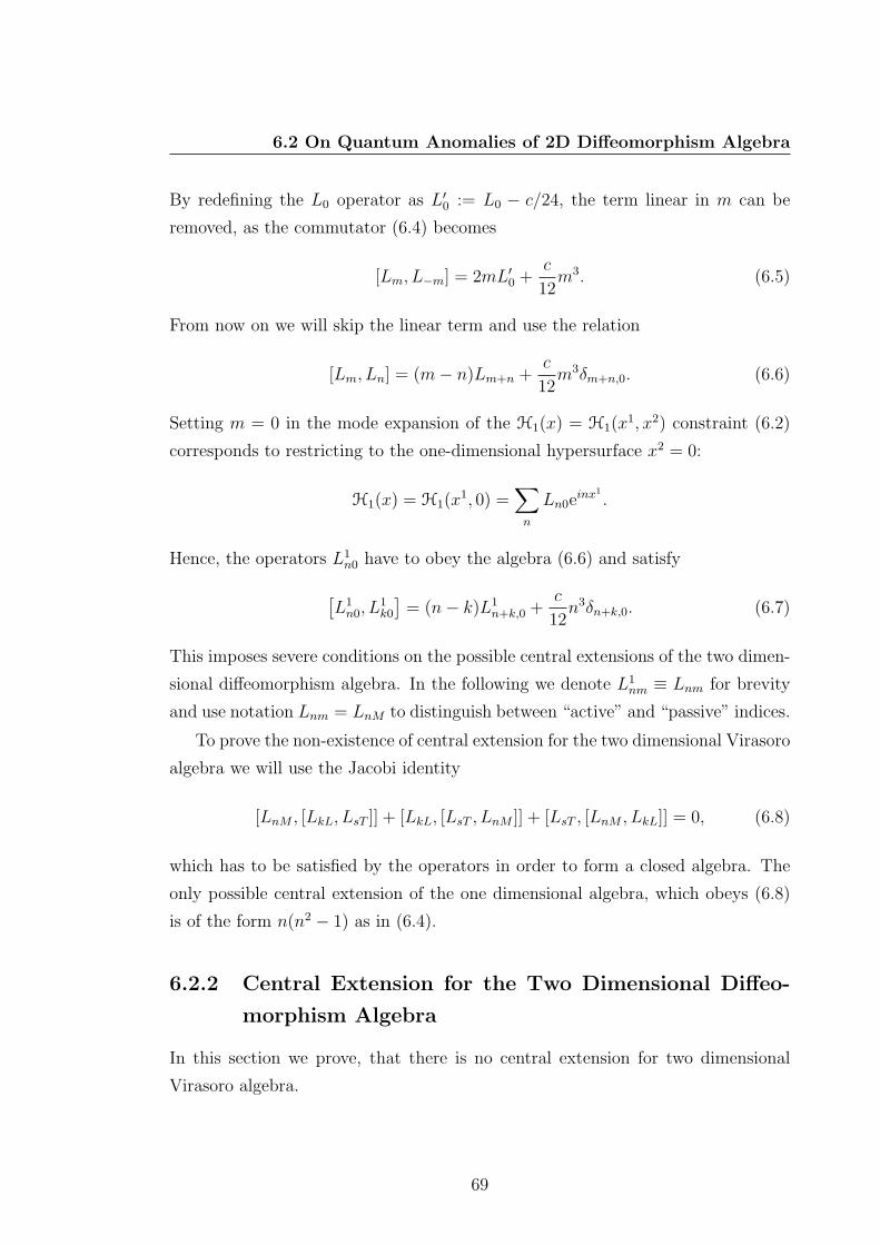
6.2 On Quantum Anomalies of 2D Diffeomorphism Algebra
By redefining the L0 operator as L′0 := L0 − c/24, the term linear in m can be
removed, as the commutator (6.4) becomes
[Lm, L−m] = 2mL′0 +c
12m3. (6.5)
From now on we will skip the linear term and use the relation
[Lm, Ln] = (m− n)Lm+n +c
12m3δm+n,0. (6.6)
Setting m = 0 in the mode expansion of the H1(x) = H1(x1, x2) constraint (6.2)
corresponds to restricting to the one-dimensional hypersurface x2 = 0:
H1(x) = H1(x1, 0) =∑n
Ln0einx1
.
Hence, the operators L1n0 have to obey the algebra (6.6) and satisfy
[L1n0, L
1k0
]= (n− k)L1
n+k,0 +c
12n3δn+k,0. (6.7)
This imposes severe conditions on the possible central extensions of the two dimen-
sional diffeomorphism algebra. In the following we denote L1nm ≡ Lnm for brevity
and use notation Lnm = LnM to distinguish between “active” and “passive” indices.
To prove the non-existence of central extension for the two dimensional Virasoro
algebra we will use the Jacobi identity
[LnM , [LkL, LsT ]] + [LkL, [LsT , LnM ]] + [LsT , [LnM , LkL]] = 0, (6.8)
which has to be satisfied by the operators in order to form a closed algebra. The
only possible central extension of the one dimensional algebra, which obeys (6.8)
is of the form n(n2 − 1) as in (6.4).
6.2.2 Central Extension for the Two Dimensional Diffeo-
morphism Algebra
In this section we prove, that there is no central extension for two dimensional
Virasoro algebra.
69

6. DIFFEOMORPHISM ALGEBRA IN GRAVITY
• Proposition 1
The most general central extension, which would still satisfy (6.8), can be
written as
[LnM , LkL] = (n− k)Ln+k,M+L + n3δn+k,0f(M,L) + g(M,L). (6.9)
Proof
Assume that instead of functions f(M,L), g(M,L) we have f(n, k|M,L)
and g = g(n, k|M,L) and demand that (6.9) reduces to (6.7) in the case
M = L = 0. It follows that
f(n, k|0, 0) = a, a ∈ R
⇒ f(n, k|M,L) = f(M,L) with f(0, 0) = a.
Similarly, g(n, k|0, 0) has to satisfy
g0(n, k) ≡ g(n, k|0, 0) = bn(n2 − 1), b ∈ R.
From this it follows then that the function g can be separated into g(n, k|M,L) =
g0(n, k) + g(M,L) with g(0, 0) = 0. The function g0 can be absorbed into
the term n3δn+k,0f(0, 0) and L0. Therefore we asssume that g0 ≡ 0 and
f(0, 0) = c12
. Hence,
g(n, k|M,L) = g(M,L) with g(0, 0) = 0.
• Proposition 2
f(M,L) = f(L,M), (6.10)
g(M,L) = −g(L,M). (6.11)
Proof
Use the antisymmetry of the commutator, i.e. [LnM , LkL] = − [LkL, LnM ].
70

6.2 On Quantum Anomalies of 2D Diffeomorphism Algebra
This gives
[LnM , LkL] = (n− k)Ln+k,M+L + n3δn+k,0f(M,L) + g(M,L),
[LkL, LnM ] = (k − n)Ln+k,M+L + k3δn+k,0f(L,M) + g(L,M)
= −(n− k)Ln+k,M+L − n3δn+k,0f(L,M) + g(L,M).
Comparing both expressions leads to f(M,L) = f(L,M) and g(M,L) =
−g(L,M) q.e.d.
• Proposition 3
f(M,L) = f(M + L), (6.12)
g(M,L) ≡ 0. (6.13)
Proof
According to our assumption (6.9) and the following discussion, the functions
f(M,L) and g(M,L) are defined to be mutually independent. Therefore,
the Jacobi identity (6.8) also has to be satisfied independently. Hence, two
equations have to be fulfilled:
((k − s)n3f(M,L+ T ) + (s− n)k3f(L, T +M) + (n− k)s3f(T,M + L)
)·
· δn+k+s,0 = 0,
(k − s)g(M,L+ T ) + (s− n)g(L, T +M) + (n− k)g(T,M + L) = 0.
As f and g do not dependen on “active” indices, the above equations can be
satisfied only if
f(M,L+ T ) = f(L, T +M) = f(T,M + L),
g(M,L+ T ) = g(L, T +M) = g(T,M + L).
By setting T = 0 these become
f(M,L) = f(L,M) = f(0,M + L) ≡ f(M + L), (6.14)
g(M,L) = g(L,M) = g(0,M + L). (6.15)
71

6. DIFFEOMORPHISM ALGEBRA IN GRAVITY
Equation (6.14) proves the first part of claim. Taking into account the anti-
symmetry of g, the second equation becomes g(M,L) = −g(M,L). Hence,
g(M,L) ≡ 0. Note, that from eq. (6.14) it follows that
f(M,−M) = f(0, 0) =c
12∀M.
Thus, the most general two dimensional Virasoro algebra with a central ex-
tension obeys the algebra
[LnM , LkL] = (n− k)Ln+k,M+L + n3δn+k,0f(M + L), (6.16)
[MNm,MKl] = (m− l)MN+K,m+l + nm3δm+l,0f(N +K), (6.17)
where MNm ≡ L2nm. The second relation was written by analogy, with active
and passive indices exchanged. The functions f and f can be different.
• Proposition 4
If
[Lnm,Mkl] = mLn+k,m+l − kMn+k,m+l, (6.18)
then f = f = 0.
Proof
The Jacobi identities
[Lnm, [Mkl,Mst]] + [Mkl, [Mst, Lnm]] + [Mst, [Lnm,Mkl]] = 0,
[Mmn, [Llk, Lts]] + [Llk, [Lts,Mmn]] + [Lts, [Mmn, Llk]] = 0
lead to the conditions
(sl3 − kt3)f(n+ k + s)δm+l+t,0 = 0,
(sl3 − kt3)f(n+ k + s)δm+l+t,0 = 0.
Since, both equations have to be satisfied for arbitrary values of indices, it
follows that both functions have to be zero.
72

6.2 On Quantum Anomalies of 2D Diffeomorphism Algebra
• Proposition 5
Assume the following central extension of the commutator [L,M ]:
[LNm,MkL] = mLN+k,m+L − kMN+k,m+L + g(m, k|N,L), (6.19)
[MkL, LNm] = kMk+N,L+m −mLk+N,L+m + g(k,m|L,N),
where capital letters denote “passive” indices again. The arguments in g are
grouped according to their “active” or “passive” action.
Then g(m, k|N,L) = g(m+ L|k,N) with g(m+ L|k,N) = −g(m+ L|N, k).
Proof
Consider the Jacobi identity:
0 = [Lnm, [Mkl,Mst]] + [Mkl, [Mst, Lnm]] + [Mst, [Lnm,Mkl]]
= (l − t)g(m, k + s|n, l + t)−mg(k, t+m|l, s+ n) +mg(s,m+ l|t, n+ k)+
+ (sl3 − kt3)δm+l+t,0f(k + s+ n) + (L, M terms).
By setting l = t we obtain
0 = −m(g(k,m+ l|l, s+ n)− g(s,m+ l|l, n+ k)) + l3(s− k)δm+2l,0f(k + s+ n).
For m 6= −2l this gives the following equality
g(k,m+ l|l, s+ n) = g(s,m+ l|l, n+ k).
It can be satisfied only if g(m, k|n, l) = g(m+ l|k, n).
Hence, the commutators (6.19) become
[LNm,MkL] = mLN+k,m+L − kMN+k,m+L + g(m+ L|N, k), (6.20)
[MkL, LNm] = kMk+N,L+m −mLk+N,L+m + g(L+m|k,N).
From the antisymmetry [LNm,MkL] = −[MkL, LNm] it follows that g(m +
L|k,N) = −g(m+ L|N, k).
• Proposition 6
g(t|n, k) = 0, ∀t 6= 0 ⇒ g(t|n, k) = δt,0g(n+ k) ⇒ g(n) ≡ 0.
73

6. DIFFEOMORPHISM ALGEBRA IN GRAVITY
Proof
Consider the Jacobi identity with two “passive” and one “active” index.
0 = [Ln0, [Ml0,M0t]] + [Ml0, [M0t, Ln0]] + [M0t, [Ln0,Ml0]]
= [Ln0,−tMlt] + [M0t,−lMl+n,0]
= −tg(t|n, l)− lt3δt,0f(l + n) + (L, M terms).
The second term always vanishes, and, therefore, g(t|n, l) = 0, ∀t 6= 0. We
can then write it in the form g(t|n, k) = δt0h(n, k). Returning back to the
initial Jacobi identity
0 = [Lnm, [Mkl,Mst]] + [Mkl, [Mst, Lnm]] + [Mst, [Lnm,Mkl]]
it follows that
(l − t)h(n, k + s) + (l + t)h(k, s+ n)− (l + t)h(s, n+ k) + (sl3 − kt3)f(k + n+ s) = 0.
Hence, it can only be fulfilled if h(n, k) = g(n + k). After inserting this in
the expression above, it follows that
(l − t)g(n+ k + s) + (sl3 − kt3)f(n+ k + s) = 0.
This cannot be satisfied. Therefore, we conclude, that g(n) ≡ 0.
It follows from proposition 6.2.2 that g = f = f ≡ 0. Hence, there is no
central extension for the two dimensional Virasoro algebra.
6.3 Non-central Extensions of the 2D Virasoro
Algebra
As it was found by Moody and Larsson [28; 29; 30], the algebra can be supplemented
with a non-central extension. This means that instead of adding some function of
c-numbers, as in the case of a central extension, one can extend the algebra (6.3)
by adding certain operators. The commutators derived by Larsson, rewritten for
74

6.3 Non-central Extensions of the 2D Virasoro Algebra
the two dimensional case, are
[L1nm, L
1kl
]= (n− k)L1
n+k,m+l − nk(c1 + c2)(nS1n+k,m+l +mS2
n+k,m+l) (6.21)[L2nm, L
2kl
]= (m− l)L2
n+k,m+l −ml(c1 + c2)(nS1n+k,m+l +mS2
n+k,m+l)[L1nm, L
2kl
]= mL1
n+k,m+l − kL2n+k,m+l − (c1mk + c2nl)(nS
1n+k,m+l +mS2
n+k,m+l)
with non-central extensions defined via the operators Sµ. These obey the commu-
tation relations:
[L1nm, S
1kl
]= lS2
n+k,m+l[L1nm, S
2kl
]= −kS2
n+k,m+l[L2nm, S
1kl
]= −lS1
n+k,m+l (6.22)[L2nm, S
2kl
]= kS1
n+k,m+l[Sinm, S
jkl
]= 0.
and satisfy the identity
nS1nm +mS2
nm = 0, (6.23)
which follows from the antisymmetry of the commutator algebra, [Lnm, Lkl] =
− [Lkl, Lnm].
Some restrictions on the operators Si and constants ci follow from the 1D
Virasoro algebra. Consider the commutator (6.21) with m = l = 0:
[L1n0, L
1k0
]= (n− k)L1
n+k,0 − n2k(c1 + c2)S1n+k,0 (6.24)
From the defining relation (6.23) it follows that
nS1n0 = 0, ∀n
which can be satisfied for all values of n only if S1n0 is proportional to Kronecker
delta. The same argument applies to S20m and thus
S1n0 = S1
00δn0 (6.25)
S20m = S2
00δm0.
75

6. DIFFEOMORPHISM ALGEBRA IN GRAVITY
Substituting in the commutators gives
[L1n0, L
1k0
]= (n− k)L1
n+k,0 + n3(c1 + c2)S100δn+k,0 (6.26)[
L20m, L
20l
]= (m− l)L2
0,m+l +m3(c1 + c2)S200δm+l,0.
Comparison of (6.7) and (6.26) yields the following relations for the constants in a
non-central extension
(c1 + c2)S100 =
c
12(6.27)
(c1 + c2)S200 =
c
12,
where c and c are central charges for L1 and L2 respectively. It follows from here
that the operators Si00 are numbers and, hence, commute with Li’s.
6.4 Eigenspace of the Constraint Operators
In a conformal field theory of conformal weight h and central charge c all infor-
mation necessary to find the correlation functions is encoded in its highest-weight
representation space (Verma module V (c, h)), which is spanned by the eigenstates
of L0 operator. By following this analogy let us explore the properties of the space
spanned by the eigenstates of Li00.
6.4.1 Eigenspace of Decoupled L10J and L2
I0
Let us consider the Virasoro algebra
[L1nm, L
1kl] = (n− k)L1
n+k,m+l, (6.28)
[L2nm, L
2kl] = (m− l)L2
n+k,m+l,
[L1nm, L
2kl] = 0,
where for simplicity, we have assumed that the constraint operators L1nm and L2
nm
commute, and that there are no extensions. Denote by |J〉 an eigenstate of L10J
76
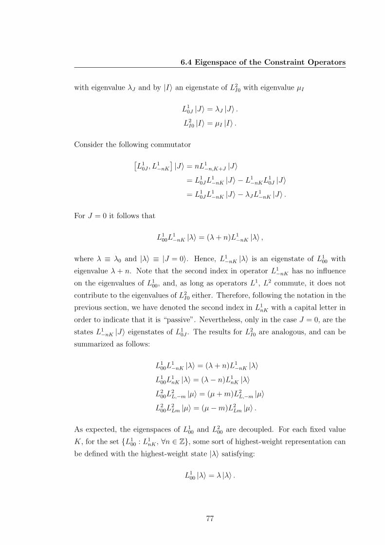
6.4 Eigenspace of the Constraint Operators
with eigenvalue λJ and by |I〉 an eigenstate of L2I0 with eigenvalue µI
L10J |J〉 = λJ |J〉 .
L2I0 |I〉 = µI |I〉 .
Consider the following commutator
[L1
0J , L1−nK
]|J〉 = nL1
−n,K+J |J〉
= L10JL
1−nK |J〉 − L1
−nKL10J |J〉
= L10JL
1−nK |J〉 − λJL1
−nK |J〉 .
For J = 0 it follows that
L100L
1−nK |λ〉 = (λ+ n)L1
−nK |λ〉 ,
where λ ≡ λ0 and |λ〉 ≡ |J = 0〉. Hence, L1−nK |λ〉 is an eigenstate of L1
00 with
eigenvalue λ + n. Note that the second index in operator L1−nK has no influence
on the eigenvalues of L100, and, as long as operators L1, L2 commute, it does not
contribute to the eigenvalues of L2I0 either. Therefore, following the notation in the
previous section, we have denoted the second index in L1nK with a capital letter in
order to indicate that it is “passive”. Nevertheless, only in the case J = 0, are the
states L1−nK |J〉 eigenstates of L1
0J . The results for L2I0 are analogous, and can be
summarized as follows:
L100L
1−nK |λ〉 = (λ+ n)L1
−nK |λ〉
L100L
1nK |λ〉 = (λ− n)L1
nK |λ〉
L200L
2L,−m |µ〉 = (µ+m)L2
L,−m |µ〉
L200L
2Lm |µ〉 = (µ−m)L2
Lm |µ〉 .
As expected, the eigenspaces of L100 and L2
00 are decoupled. For each fixed value
K, for the set L100 : L1
nK , ∀n ∈ Z, some sort of highest-weight representation can
be defined with the highest-weight state |λ〉 satisfying:
L100 |λ〉 = λ |λ〉 .
77

6. DIFFEOMORPHISM ALGEBRA IN GRAVITY
The descendants are built by successively applying the raising operators L1−nK , ∀n >
0 on the highest-weight state. The gauge invariance condition, which has to be im-
posed is then L1nK |λ〉 = 0, ∀n > 0. We note that
L100
(L1
0K |λ〉)
= λ(L1
0K |λ〉).
Hence, the eigenvalue λ is double degenerate for each fixed K. However, the set
L100 : L1
nK , ∀n ∈ Z cannot be interpreted as one copy of the Virasoro algebra
labeled by K. The reason for this is the fact that this set does not form a closed
algebra:
[L1nK , L
1mK ] = (n− k)L1
n+m,2K .
The Verma module of the whole Virasoro algebra of operators L1, defined by the
commutators (6.28), is spanned by the descendant states, which are obtained by
repeated action on the highest-weight state |λ〉 with all possible raising operators
L1−nK , ∀K ∈ Z. However, the degeneracy of each eigenvalue of L1
00 is infinite.
This is very unphysical and as such we will no longer discuss the decoupled two
dimensional diffeomorphism algebra.
6.4.2 Eigenspace of Coupled L100, L
200 without Central Ex-
tension
Let us now take into account the non-commutativity of the constraint operators
L1 and L2, and consider the algebra
[L1nm, L
1kl] = (n− k)L1
n+k,m+l,
[L2nm, L
2kl] = (m− l)L2
n+k,m+l, (6.29)
[L1nm, L
2kl] = kL2
n+k,m+l −mL1n+k,m+l.
In this section we will investigate the highest-weight representation of the algebra
(6.29) and what is the increase in the degeneracy Γ(N) of level N .
We define the state |λµ〉 as
L100 |λµ〉 = λ |λµ〉 , L2
00 |λµ〉 = µ |λµ〉 . (6.30)
78

6.4 Eigenspace of the Constraint Operators
As before, one finds the following relations:
L100L
i−nM |λµ〉 = (λ+ n)Li−nM |λµ〉 ,
L100L
inM |λµ〉 = (λ− n)LinM |λµ〉 ,
L200L
iN,−m |λµ〉 = (µ+m)LiN,−m |λµ〉 , (6.31)
L200L
iNm |λµ〉 = (µ−m)LiN,m |λµ〉 ,
with i = 1, 2. Hence, the operators L100 and L2
00 have the same eigenspace, as they
commute. The corresponding eigenvalues are different though.
In order to construct the highest-weight representation space of the Virasoro alge-
bra (6.29), one has to point out one generator A0 which is diagonal in the repre-
sentation space. This operator determines the highest-weight of the Verma module
and defines the notion of raising and lowering operators of the eigenvalues of A0.
The choice of A0 for the 1d Virasoro algebra was unambiguous, as there were no
two generators which commute. Therefore, we have chosen the diagonal operator
to be A0 = L0:
L0 |h〉 = h |h〉 , Ln |h〉 = 0, ∀n > 0.
The basis for the other states in the representation space was obtained by applying
the raising operators Ln.
In string theory and conformal field theory one has two decoupled Virasoro
algebras Ln andLn
. In order to extend the basis of the representation space
to both eigenstates of L0 and L0, the diagonal operator A0 of the representation
was defined as A0 = L0 +L0. This choice was justified because the operator L0 +L0
corresponds to the closed string Hamiltonian. However, we could have, in principle,
defined a different A′0 of the form
A′0 = aL0 + bL0, a, b ∈ N,
A′0∣∣hh⟩ = (ah+ bh)
∣∣hh⟩ .By this choice the highest-weight of the representation is changed, h+ h→ ah+bh.
The A′0 eigenvalue of descendants of level Ntot = N + N is then
N ′ = a(h+N) + b(h+ N).
79

6. DIFFEOMORPHISM ALGEBRA IN GRAVITY
Still, the different values of a, b do not change the degeneracy of the level Ntot.
In practice, the choice a = b corresponds to some overall factor. If a 6= b, we are
introducing some kind of anisotropy. Hence, it seems that setting a = b = 1 is
indeed the most natural choice.
Among the generators of the algebra (6.29), there are two mutually commuting
operators L100 and L2
00 with the same eigenspace. In the analogy with conformal
field theory we define the diagonal operator A0 of the highest-weight representation
as
A0 = L100 + L2
00 ⇒(L1
00 + L200
)|λµ〉 = (λ+ µ) |λµ〉 .
Hence, the state |λµ〉 is a highest weigth state with respect to operator A0 of weight
λ+ µ. A basis state of the representation space can be written in general form as
|λ′µ′〉 =∏l
i=0(L1
0,−i)α0i(L1
−1,−i)α1i . . . (L1
−ni,−i)αnii∏m
j=0(L2
0,−j)β0j(L2
−1,−j)β1j . . . (L2
−nj ,−j)βnjj |λµ〉 , (6.32)
with α00 = β00 ≡ 0. The tilde over the products means that the operators for
different values of i are ordered in ascending order from left to right. This is possible
due to the commutation relations and once the convention is chosen it has to remain
fixed in order to ensure that the eigenstates (6.32) are linearly independent. Indices
αij (βij) count the number of times the operator L1−i,−j, (L2
−i,−j) was used.
Note, that only the operators Li−n,−m with negative indices were used as the
raising operators in order to insure, that the state |λµ〉 has the smallest A0 eigen-
value among the basis states of the representation space. This condition can be
written as
Linm |λµ〉 = 0, ∀n,m > 0. (6.33)
This is equivalent to demanding that the diffeomorphism constraints vanish in the
operator sense, i.e. that for any two physical states |φ〉, |ψ〉
⟨ψ|Linm|φ
⟩= 0, ∀n ∈ Z.
80

6.4 Eigenspace of the Constraint Operators
The A0 eigenvalue of the state (6.32) is then
N = λ+ µ+NL1 +NL2 , (6.34)
NL1 =l∑
i=0
ni∑k=0
(k + i)αki, (6.35)
NL2 =m∑j=0
nj∑k=0
(k + j)βkj, (6.36)
where NLi counts only the eigenvalues of A0 which arise from the operators Li−n,−m
in the state (6.32).
6.4.3 Degeneracy
To find the degeneracy Γ(N) of a given eigenvalue N = NL1 + NL2 it is useful to
first find the degeneracy of the eigenvalue NL1 . The degeneracy Γ(N) can then be
found later as
Γ(N) =N∑
NL1=0
Γ(NL1)Γ(N −NL1).
In order to simplify the notation we will skip the superscript and denote the eigen-
value NL1 simply as NL.
Let us subdivide the degeneracy of the value NL as
Γ(NL) =
NL∑n=1
Γn(NL),
where Γn(NL) denotes the degeneracy of the eigenvalue NL which arises from a state
which is built by n operators L−p−r. An example for a state which contributes to
Γ3(8) would be:
L−2−1L−30L−1−1 |0〉 .
Hence, our task now is to calculate the degeneracy Γn(NL) of a given value of
NL when the number n of the operators L, which are used to build the states, is
fixed. We proceed by counting the number of different ways one can distribute the
value NL among n operators L. This corresponds to the number of partitions of an
integer number NL into a sum of exactly n integers, and it is denoted by pn(NL).
81

6. DIFFEOMORPHISM ALGEBRA IN GRAVITY
For the example considered above p3(8) = 5, as it can be seen from:
8 = 1 + 1 + 6
8 = 1 + 2 + 5
8 = 1 + 3 + 4 (6.37)
8 = 2 + 2 + 4
8 = 2 + 3 + 3
The order of the different terms in the sum does not matter. Once the splitting is
known, we have to consider each of them separately. Therefore we denote these by
αk(n,NL), where the index k = 1, . . . , pn(NL). For (6.37) this means:
α1 = 1, 1, 6
α2 = 1, 2, 5
α3 = 1, 3, 4
α4 = 2, 2, 4
α5 = 2, 3, 3
We will now consider one of the strings αk(n,NL). It denotes one of the possible
ways of writing the number NL as a sum of exactly n integers. αk is only a label
of one of such splittings. Hence, every αk denotes a set Aαk(n,NL) of states which
are built in a certain way. Every state of the form
L−p1,−r1 . . . L−pn,−rn |0〉
belongs to one of the sets Aαk . For example, the state
L−1−2L−30L−1−1 |0〉 ∈ Aα5(3, 8). (6.38)
We now denote the numbers in every string as αk = µ1, µ2, . . . , µn. Each number
µj is a label associated to each operator L−p−r and gives the value of the sum of
the indices p and r, hence, µj = p+ r. For a given µj there is a certain amount of
possibilities how it can be obtained. For example, if µj = 3, it can originate from
82
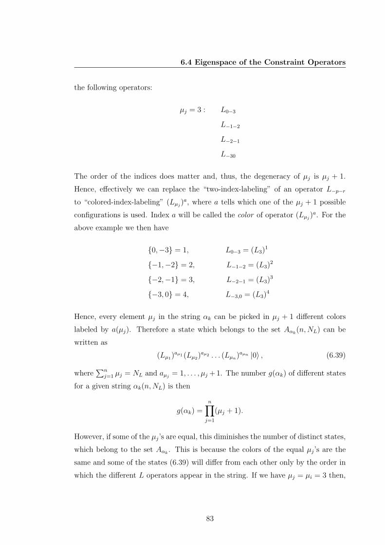
6.4 Eigenspace of the Constraint Operators
the following operators:
µj = 3 : L0−3
L−1−2
L−2−1
L−30
The order of the indices does matter and, thus, the degeneracy of µj is µj + 1.
Hence, effectively we can replace the “two-index-labeling” of an operator L−p−r
to “colored-index-labeling” (Lµj)a, where a tells which one of the µj + 1 possible
configurations is used. Index a will be called the color of operator (Lµj)a. For the
above example we then have
0,−3 = 1, L0−3 = (L3)1
−1,−2 = 2, L−1−2 = (L3)2
−2,−1 = 3, L−2−1 = (L3)3
−3, 0 = 4, L−3,0 = (L3)4
Hence, every element µj in the string αk can be picked in µj + 1 different colors
labeled by a(µj). Therefore a state which belongs to the set Aαk(n,NL) can be
written as
(Lµ1)aµ1 (Lµ2)
aµ2 . . . (Lµn)aµn |0〉 , (6.39)
where∑n
j=1 µj = NL and aµj = 1, . . . , µj + 1. The number g(αk) of different states
for a given string αk(n,NL) is then
g(αk) =n∏j=1
(µj + 1).
However, if some of the µj’s are equal, this diminishes the number of distinct states,
which belong to the set Aαk . This is because the colors of the equal µj’s are the
same and some of the states (6.39) will differ from each other only by the order in
which the different L operators appear in the string. If we have µj = µi = 3 then,
83

6. DIFFEOMORPHISM ALGEBRA IN GRAVITY
for example, only one of the products
(L3)1(L3)2 = L0−3L−1−2
(L3)2(L3)1 = L−1−2L0−3
can be a part of a properly ordered basis state of the representation space of the
2d diffeomorphism algebra.
Suppose that the element µi appears in a given string αk exactly l times. Then
the number of distinct states in the set Aαk is
g(αk) =n∏j=1µj 6=µi
(µj + 1)C l(µi + 1),
where
C l(µi + 1) =(µi + l)!
l!µi!
are the combinations with repetitions. They count the number of different ways
how to choose l elements out of a set of µi + 1 elements, if the order does not
matter and repetitions are allowed.
Now, if there are several values of µj which appear more than once in the string
αk (e.g. 2, 2, 3, 3), we have to take this into account as well. We denote by s
the number of repeated elements, each of which appears li times and i = 1, . . . , s.
Then the number of distinct states in the set Aαk is
g(αk) =n∏j=1µj 6=µi
(µj + 1) ·s∏i=1
C li(µi + 1). (6.40)
The indices µj, li, and s are, however, dependent on the specific string αk chosen,
hence, we add an index k to each of these indices: µjk, lik, sk. The total degeneracy
of the eigenvalue NL which is distributed among n operators L is then
Γn(NL) =
pn(NL)∑k=1
g(αk).
This corresponds to the number of restricted, colored partitions of an integer num-
84

6.4 Eigenspace of the Constraint Operators
ber NL in exactly n parts with additional condition that the number of colors
depends on the specific partition. The generating function for colored partitions in
the non-restricted case is well-known [31]. However, there is no general solution of
our knowledge for the case of interest.
The total degeneracy of the value NL is
Γ(NL) =
NL∑n=1
pn(NL)∑k=1
g(αk). (6.41)
The non-trivial task is to calculate g(αk), as we need to determine the values of
µjk, lik, and sk for every string αk. Still, it is possible to calculate the degeneracy
Γ(NL) nummerically by following the steps which were explained above. The results
are presented in Figure 6.1. From there we conclude that for large values of N the
asymptotic behavior of the degeneracy seems to be
Γ(N) ∼ e2N3/4
.
However, it seems that for higher values of N the degeneracy will deviate from
these asymptotics.
Figure 6.1: The degeneracy of the states as a function of the energy level N .
85

6. DIFFEOMORPHISM ALGEBRA IN GRAVITY
6.4.4 Eigenspace of Coupled L100, L
200 with Central Exten-
sion
Let us finally consider the full two dimensional quantum diffeomorphism algebra
[L1nm, L
1kl
]= (n− k)L1
n+k,m+l − nk(c1 + c2)(nS1n+k,m+l +mS2
n+k,m+l), (6.42)[L2nm, L
2kl
]= (m− l)L2
n+k,m+l −ml(c1 + c2)(nS1n+k,m+l +mS2
n+k,m+l),[L1nm, L
2kl
]= mL1
n+k,m+l − kL2n+k,m+l − (c1mk + c2nl)(nS
1n+k,m+l +mS2
n+k,m+l).
Because of the appearance of the operators Sinm, the complete representation space
of the algebra (6.42) is no longer spanned by the states (6.32).
To see this, let us first consider a state L−n−mL−k−l |λµ〉, with the ordering
n ≤ k, m ≤ l as explained below eq.(6.32). This is an eigenstate of the operator
A0 = L100 +L2
00 with eigenvalue λ+ µ+ n+ k +m+ l, and thus is one of the basis
states of the highest-weight representation of (6.42).
Consider now a state
L−k−lL−n−m |λµ〉
for the same values of indices. The order of the indices is no longer correct, and,
therefore, this is not a basis state. It is still an eigenstate of A0 and, hence, belongs
to the Verma module. This means, that it can be rewritten as a linear combination
of the basis states by using the commutation relations (6.42):
L−k−lL−n−m |λµ〉 = [L−k−l, L−n−m] |λµ〉+ L−n−mL−k−l |λµ〉
= (−k + n)L−k−n,−l−m |λµ〉+ L−n−mL−k−l |λµ〉
− kn(c1 + c2)(−kS1
−k−n,−l−m − lS2−k−n,−l−m
)|λµ〉 .
The last two terms in this expression are new and cannot be expressed in terms of
states (6.32). This leads us to the conclusion that the states in (6.32) do not form
a complete set of linearly independent eigenstates of the operator A0 = L100 + L2
00.
In order to resolve this problem, one has to check whether the states Sinm |λµ〉,i = 1, 2 are eigenstates of L1
00, L200, what are the eigenvalues, and what is the
86
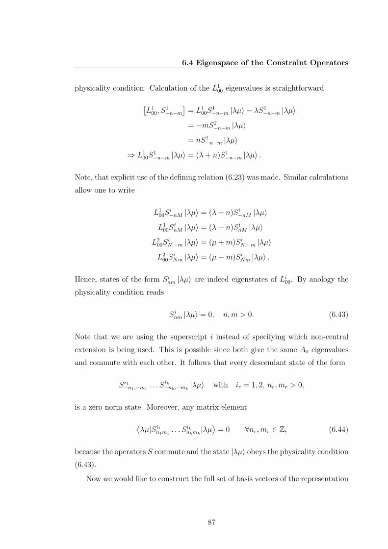
6.4 Eigenspace of the Constraint Operators
physicality condition. Calculation of the L100 eigenvalues is straightforward
[L1
00, S1−n−m
]= L1
00S1−n−m |λµ〉 − λS1
−n−m |λµ〉
= −mS2−n−m |λµ〉
= nS1−n−m |λµ〉
⇒ L100S
1−n−m |λµ〉 = (λ+ n)S1
−n−m |λµ〉 .
Note, that explicit use of the defining relation (6.23) was made. Similar calculations
allow one to write
L100S
i−nM |λµ〉 = (λ+ n)Si−nM |λµ〉
L100S
inM |λµ〉 = (λ− n)SinM |λµ〉
L200S
iN,−m |λµ〉 = (µ+m)SiN,−m |λµ〉
L200S
iNm |λµ〉 = (µ−m)SiNm |λµ〉 .
Hence, states of the form Sinm |λµ〉 are indeed eigenstates of Li00. By anology the
physicality condition reads
Sinm |λµ〉 = 0, n,m > 0. (6.43)
Note that we are using the superscript i instead of specifying which non-central
extension is being used. This is possible since both give the same A0 eigenvalues
and commute with each other. It follows that every descendant state of the form
Si1−n1,−m1. . . Sik−nk,−mk |λµ〉 with ir = 1, 2, nr,mr > 0,
is a zero norm state. Moreover, any matrix element
⟨λµ|Si1n1m1
. . . Siknkmk |λµ⟩
= 0 ∀nr,mr ∈ Z, (6.44)
because the operators S commute and the state |λµ〉 obeys the physicality condition
(6.43).
Now we would like to construct the full set of basis vectors of the representation
87

6. DIFFEOMORPHISM ALGEBRA IN GRAVITY
space of the 2D Virasoro algebra. The defining relation
nS1nm +mS2
nm = 0 (6.45)
suggests that S1 and S2 are linearly dependent. Even so, if one would like to
replace all S2−n−m operators with − n
mS1−n−m then this would correspond to negative,
mostly non-integer L100 and L2
00 eigenvalue states. Hence, both Si should be used
independently as raising operators.
In the section 6.3 we have shown that S1n0 = δn0S
100 and S2
0n = δn0S200. However,
this is not true for the operators S10n and S2
n0. Moreover, they cannot be used to
build descendant states, because this would lead to infinitely degenerate ground
state. Indeed,
(L100 + L2
00)S10−n |λµ〉 =
([L1
00, S10−n] + [L2
00, S10−n] + (λ+ µ)S1
0−n)|λµ〉
= −nS20−n |λµ〉+ (λ+ µ)S1
0−n |λµ〉
= (λ+ µ)S10−n |λµ〉 .
A general basis state of the Fock space is then
|λ′µ′〉 =∏l
i=0(L1
0,−i)α0i(L1
−1,−i)α1i . . . (L1
−ni,−i)αnii∏m
j=0(L2
0,−j)β0j(L2
−1,−j)β1j . . . (L2
−nj ,−j)βnjj
∏l
p=1(S1−1,−p)
η1p . . . (S1−np,−p)
ηnpp∏m
r=1(S2−1,−r)
ρ1rj . . . (S2−nr,−r)
ρnrr |λµ〉 ,
(6.46)
where the previous notations are used and operators are always ordered as L1L2S1S2.
Also α00 = β00 = 0, because this corresponds to the highest-weight state itself.
All descendant states with the number of S operators exceeding the number of
L operators are zero norm states. It follows from (6.44) and the commutation
relation [L, S] ∼ S. For further remarks let us calculate the norm of a state
88
6.5 Speculations
L1−n−mS
1−k−l |λµ〉:
〈λµ|S1klL
1nmL
1−n−mS
1−k−l |λµ〉 =
= 〈λµ|S1kl
([L1
nm, L1−n−m] + L1
−n−mL1nm
)S1−k−l |λµ〉
= 〈λµ|S1kl
(2nL1
00 + n2(c1 + c2)(nS100 +mS2
00))S1−k−l |λµ〉+ 〈λµ|S1
klL1−n−m[L1
nm, S1−k−l] |λµ〉
= 2n 〈λµ|S1kl
([L1
00, S1−k−l] + S1
−k−lL100
)|λµ〉 − l 〈λµ|S1
klL1−n−mS
2n−k,m−l |λµ〉
= −l 〈λµ| [S1kl, L
1−n−m]S2
n−k,m−l |λµ〉
= l2 〈λµ|S2k−n,l−mS
2n−k,m−l |λµ〉 .
This is only non-zero if n = k and m = l. Therefore we conclude that only the
states with the total sum of the first (second) indices of L operators being larger 1
than the sum of the corresponding indices of S operators can have non-zero norm.
The L100 eigenvalue N1 of the state (6.46) is the sum of the first indices of all
the raising operators. To see this let us calculate the L100 eigenvalue of the state
|φ〉 ≡ L1−n−mL
2−k−lS
1−g−f |λµ〉 as an example
L100 |φ〉 =
[L1
00, L1−n−mL
2−k−lS
1−f−g
]|λµ〉+ λ |φ〉
= L1−n−mL
2−k−l
[L1
00, S1−f−g
]|λµ〉+
[L1
00, L1−n−mL
2−k−l
]S1−f−g |λµ〉+ λ |φ〉
= L1−n−mL
2−k−l(−g)S2
−f−g |λµ〉+ L1−n−m
[L1
00, L2−k−l
]S1−f−g |λµ〉
+[L1
00, L1−n−m
]L2−k−lS
1−f−g |λµ〉+ λ |φ〉
= (λ+ n+ k + f) |φ〉 .
The degeneracy of the L100 + L2
00 eigenvalue thus increases. However, by analogy
with the previous chapter, we conclude that the asymptotics still remain as in
Figure 6.1.
6.5 Speculations
In this section we would like to point out some analogies between the Fock space
spanned by the states (6.46) and the Fock space of the string theory spanned by
(3.67). We will then reveal the difficulties arising in the case of two dimensional
diffeomorphisms.
1Indices n, m are positive integers
89

6. DIFFEOMORPHISM ALGEBRA IN GRAVITY
Let us start with rewriting the state (6.46) in the form:
|α, β , λµ〉 =∞∏
n,m=0
(L1−n−m)α
1nm(L2
−n−m)α2nm(S1
−n−m)β1nm(S2
−n−m)β2nm |λµ〉 . (6.47)
Here α = α1, α2 and β = β1, β2 are strings of non-negative integers and
α100 = α2
00 = β100 = β2
00 = 0. Comparison with equations (3.67) and (3.72) to-
gether with commutation relations (3.65) and (6.22) leads to several observations.
First, the operators S and the operators K of string theory obey very similar com-
mutation relations with diffeomorphism generators and they both appear in the
basis states of the corresponding Fock spaces. We know that the operators K were
crucial for proving that the states (3.67) are indeed linearly independent. With
appropriate ordering we were able to bring the inner product matrix MP in the
form (3.70), which ensured that det(MP ) 6= 0. Therefore one could ask whether
the same procedure can be performed here, but with operators S “playing the role”
of the operators K? Without going into details, we just mention that it is possible
to define an ordering of states (6.47) similar to the ordering, which was used in
string theory [17]. However, several elements on the minor diagonal are zero as a
consequence of the fact that S1n0 = S2
0n = 0 if n 6= 0. This property of S operators
followed from the defining relation nS1nm + mS2
nm = 0, which is not present in the
1D case. Hence, the determinant of the two dimensional analogue of the ordered
matrix MP is zero, and we conclude that the operators S cannot be associated to
the operators K.
Second, we note that in the description of closed two dimensional spacelike
surfaces the physical DDF states of string theory are substituted with the highest-
weight states |λµ〉. While the construction of DDF states is clear and was presented
in section 3.6.3, the physical origin of the states |λµ〉 is unknown. In string theory
it was shown that the physical states are built with the negative frequency modes
of the transverse oscillators αI−n. However, there is no such analogue in general
relativity.
One might exploit the fact that the transverse Virasoro operators are expressed
90

6.5 Speculations
via oscillators as
L⊥n =1
2
∑m
αIn−mαIm, with
[αIn, αIm] = nδn+m,0,
and try to find an analogous expansion of operators L1nm, L
2nm. Indeed, if one
defines
L1nm =
1
2
∑k,l
J1n−k,m−lJ
1kl, (6.48)
L2nm =
1
2
∑k,l
J2klJ
2n−k,m−l
with
[J1nm, J
1kl] = nδn+k,0δm+l,0,
[J2nm, J
2kl] = mδn+k,0δm+l,0,
then it satisfies the commutation relations [L1nm, L
1kl], [L2
nm, L2kl] in (6.29). However,
no expansion which would satisfy the mutual commutator [L1nm, L
2kl] was found.
The difficulties arise when we are defining the commutation relation [J1nm, J
2kl]. If
it is zero, then the operators L1 and L2 commute. If it is a c-number, then the
commutator becomes
[L1, L2] ∼ J1J2.
Such a mixed term is absent in the definitions (6.48). Thus, either the commutator
[J1nm, J
2kl] gives some operator, or the expansions (6.48) have to be modified. How-
ever, none of the possibilities is trivial, and therefore there is no obvious expansion
of the operators Linm. If there would exist a construction of the generators of the
2d diffeomorphisms in terms of operators J i, which form an affine Lie algebra, then
the operators could, by analogy with string theory, be used to generate physical
states.
In such a case there would still remain one unanswered question, namely,
whether the states like
|φ〉 = J i−k−l |0〉
91

6. DIFFEOMORPHISM ALGEBRA IN GRAVITY
would obey the gauge invariance condition
Linm |φ〉 = 0, ∀n,m > 0?
Recall that in string theory [L⊥n , αI−k] = kαIn−k and thus
L⊥n(αI−k |0〉
)= kαIn−k |0〉 = 0, if n ≥ k.
Hence, the operator L⊥n does not “kill” the state αI−k |0〉 in the general case. The
reason why a state built from the transverse oscillators is physical, is that in the
light-cone gauge quantization the constraints of conformal invariance L = L = 0
are solved explicitly, and thus have no longer to be imposed on the quantum states
built with the raising operators αI−n. In general relativity, however, it is not possible
to resolve the constraint equations explicitly, because these are very non-linear. On
the other hand, the issue with non-physical states in string theory arose only due
to the fact that the C0 constraint was used in the definitions of the operators L
and L. This, combined with the commutation relation [α0n, α
0m] = −nδn+m,0 lead
to negative-norm states. The Virasoro constraints were then used to single out
these negative-norm states. As in the description of 2d spacelike surfaces only the
constraints H1 and H2 were used, we believe that there should be no ghost states
among the states, generated by the “transverse” raising operators J1 and J2.
6.6 Possible Relation with the Quantization of
Black Holes
In sections 5.4 and 5.5 an algebraic description of black holes was presented as it
was proposed by Bekenstein [5]. It follows that a nonrotating black hole can be
described by a closed set of operators A,Q,Rnqs, where A is the area operator
with eigenvalues an, Q is the generator of gauge transformations with eigenvalues
labeled by q, and Rnqs is the creation operator of a black hole state Rnqs |0〉 with
eigenvalues an, q, and s, where s is some internal quantum number accounting for
the degeneracy of a given area eigenvalue. These operators satisfy the following
92

6.6 Possible Relation with the Quantization of Black Holes
properties:
[A,Rnqs] = anRnqs, (6.49)
[A,R†nqs] = −anRnqs, (6.50)
ARnqsRmqt |0〉 = (an + am)RnqsRmqt |0〉 , (6.51)
[A,Q] = 0, (6.52)
[Q,Rnqs] = qRnqs. (6.53)
Among the operators in the two dimensional diffeomorphism algebra, there are
two kinds of operators which could be of relevance for the quantum algebra of
a black hole. First, consider the operators Linm with n and m not equal to zero
simultaneously. From the commutation relations (6.31) it follows that these can be
interpreted as the raising and lowering operators of the eigenvalues of the operator
A0 = L100 +L2
00. Hence, the properties of the operators A0 and Linm are very similar
to (6.49), (6.50), and (6.51). This suggests that we identify the operator A0 as the
area operator and the operators Linm as the creation-annihilation operators of the
black hole states.
On the other hand, we know that the operators Linm are the generators of the
2d diffeomorphism transformations, and thus should be instead associated to the
operators Q, which account for the gauge transformations. Hence, it seems that the
operators Linm should be used as constraints for identifying physical states which
differ from each other only by a diffeomorphism transformation, instead of creating
and annihilating states that correspond to different values of the black hole horizon
area. However, in analogy with the light-cone gauge quantization in string theory
we could say that the H0 and H3 constraints impose the physicality conditions,
while the H1 and H2 constraints generate the transformations between different
physical states. This is, however, not a solid statement. Nevertheless, we suggest
the identification of the operatos A0 with the area operator and the operators Linm
with the “transverse” creation and annihilation operators.
93

6. DIFFEOMORPHISM ALGEBRA IN GRAVITY
94

7
Conclusions
In this work we have explored the role of diffeomorphism invariance in general
relativity. The possible relation between distinct physical black hole microstates
corresponding to a given area eigenvalue and the quantum states, built by succes-
sive application of the generators of diffeomorphism transformations on the vacuum
state, was investigated. We have, first, reviewed the use of the one dimensional dif-
feomorphism algebra (Virasoro algebra) in string theory and compared it to that of
conformal field theory. The emphasis was laid on the construction of physical state
space in string theory and the highest-weight representation space in conformal
field theory.
We have, further, been looking for a physical justification of the operators which
generate the quantum states of a black hole. The possible relevance of quantum
generators of spatial diffeomorphism transformations to the area quantization of
spacelike surfaces was considered. Two of the spatial constraints of general rela-
tivity were expanded in a Fourier series on a surface with the topology of a torus.
The properties of the resulting two dimensional diffeomorphism algebra were ex-
plored. It was shown that the 2d diffeomorphism algebra does not have a central
extension. Instead, the algebra has a non-central extension, which is given by a set
of operators that were previously absent.
We have found that this algebra can be characterized by highest-weight repre-
sentations, similarily as it was done for the 1d Virasoro algebra in conformal field
theory. The highest-weight representations of the 2d diffeomorphism algebra, con-
sisting of the operators L1nm and L2
nm, were considered, first, without including the
95

7. CONCLUSIONS
non-central extensions. It was then shown that the degeneracy of a given eigen-
value of the diagonal operator A0 = L100 + L2
00 is increased in comparison with the
degeneracy of L0 + L0 eigenvalues in string and conformal field theories.
Further, the properties of the operators which generate the non-central exten-
sion of the 2d diffeomorphism algebra were explored. It was shown that these
contribute as raising and lowering operators of the highest-weight representation.
Therefore, the Hilbert space which corresponds to the 2d diffeomorphism algebra
with non-central extensions is larger than in the case without extensions. Hence,
the degeneracy of an eigenvalue of the operator A0 also increases.
The operator A0 can be associated with the area operator, as it seems that it
obeys its properties, as listed by Bekenstein [5]. However, not all of the descendant
states, built by repeated action with the raising operators on the highest weight
state, are physical states. Some of them do not satisfy the physicality condition
Linm |φ〉 = 0, ∀n,m > 0. Instead, some of the descendants of a physical state |φ〉are the states which differ from it by a 2d diffeomorphism transformation. Further
investigation to understand how the physical states of a closed surface could be
produced is needed. The properly modified H0 constraint might happen to be
necessary, as it is responsible for generating dynamics in general relativity [32],
and further work in this direction should be done.
96
Bibliography
[1] V. P. Frolov, (ed. ) and I. D. Novikov, (ed. ). Black hole physics: Basic conceptsand new developments. Dordrecht, Netherlands: Kluwer Academic (1998) 770 p. 1
[2] S. W. Hawking. Black hole explosions. Nature, 248:30–31, 1974. 2
[3] R. Ruffini and Wheeler J.A. Phys. Today, 24:30, 1971. 3
[4] S. W. Hawking. Gravitational radiation from colliding black holes. Phys. Rev.Lett., 26:1344–1346, 1971. 3
[5] J. D. Bekenstein. Black holes and the second law. Nuovo Cim. Lett., 4:737–740,1972. 3, 92, 96
[6] J. D. Bekenstein. Extraction of energy and charge from a black hole. Phys. Rev.,D7:949–953, 1973. 4, 59, 60
[7] D. Christodoulou. Reversible and irreversible transforations in black holephysics. Phys. Rev. Lett., 25:1596–1597, 1970. 4
[8] Viatcheslav F. Mukhanov. Are Black Holes Quantized? JETP Lett., 44:63–66,1986. 4, 5, 61
[9] Jacob D. Bekenstein and Viatcheslav F. Mukhanov. Spectroscopy of the quan-tum black hole. Phys. Lett., B360:7–12, 1995. arXiv:gr-qc/9505012. 5, 63
[10] Jacob D. Bekenstein. Quantum black holes as atoms. 1997. 5, 6
[11] Carlo Rovelli and Lee Smolin. Discreteness of area and volume in quantumgravity. Nucl. Phys., B442:593–622, 1995. arXiv:gr-qc/9411005. 5
[12] Carlo Rovelli. Quantum gravity. Cambridge, UK: Univ. Pr. (2004) 455 p. 5
[13] A. Alekseev, A. P. Polychronakos, and M. Smedback. On area and entropy ofa black hole. Phys. Lett., B574:296–300, 2003. arXiv:hep-th/0004036. 5
[14] Bryce S. DeWitt. Quantum Theory of Gravity. 1. The Canonical Theory. Phys.Rev., 160:1113–1148, 1967. 6, 16
97

BIBLIOGRAPHY
[15] Viatcheslav F. Mukhanov and A. Wipf. On the symmetries of Hamiltoniansystems. Int. J. Mod. Phys., A10:579–610, 1995. arXiv:hep-th/9401083. 9
[16] P.A.M Dirac. Lectures on Quantum Mechanics. Dover Publications (New York,2001). 11
[17] Michael B. Green, J. H. Schwarz, and Edward Witten. Superstring Theory.Vol. 1: Introduction. Cambridge, Uk: Univ. Pr. ( 1987) 469 P. ( Cambridge MonographsOn Mathematical Physics), sect. 2.3. 19, 36, 90
[18] B. Zwiebach. A first course in string theory. Cambridge, UK: Univ. Pr. (2004) 558p. 19
[19] P. Di Francesco, P. Mathieu, and D. Senechal. Conformal field theory. NewYork, USA: Springer (1997) 890 p. 41
[20] S. V. Ketov. Conformal field theory. Singapore, Singapore: World Scientific (1995)486 p. 41
[21] John L. Cardy. Operator Content of Two-Dimensional Conformally InvariantTheories. Nucl. Phys., B270:186–204, 1986. 54
[22] Steven Carlip. What we don’t know about BTZ black hole entropy. Class. Quant.Grav., 15:3609–3625, 1998. arXiv:hep-th/9806026. 55
[23] G.H. Hardy and S. Ramanujan. Asymptotic Formulae in Combinatory Analysis.Proc. London Math. Soc., 17:75, 1918. 57
[24] J. David Brown and M. Henneaux. Central Charges in the Canonical Realiza-tion of Asymptotic Symmetries: An Example from Three-Dimensional Gravity.Commun. Math. Phys., 104:207–226, 1986. 58
[25] Andrew Strominger. Black hole entropy from near-horizon microstates. JHEP,02:009, 1998. arXiv:hep-th/9712251. 58
[26] Danny Birmingham, Ivo Sachs, and Siddhartha Sen. Entropy of three-dimensional black holes in string theory. Phys. Lett., B424:275–280, 1998. arXiv:hep-th/9801019. 58
[27] D. Christodoulou and R. Ruffini. Reversible transformations of a charged blackhole. Phys. Rev., D4:3552–3555, 1971. 60
[28] S.E. Rao and R.V. Moody. Vertex representations for N-toroidal Lie algebrasand a generalization of the Virasoro algebra. Comm. Math. Phys., 159:239, 1994. 74
[29] T. A. Larsson. Central and noncentral extensions of multigraded Lie algebras.J. Phys., A25:1177–1184, 1992. 74
98
BIBLIOGRAPHY
[30] T. A. Larsson. Manifestly covariant canonical quantization of gravity and dif-feomorphism anomalies in four dimensions. 2007. arXiv:0709.2540. 74
[31] G. Andrews. The Theory of Partitions. Encyclopedia of mathematics and its applica-tions, Vol. 2 Addison-Wesley (1976). 85
[32] F. G. Markopoulou. Gravitational Constraint Combinations Generate a LieAlgebra. Class. Quant. Grav., 13:2577–2584, 1996. arXiv:gr-qc/9601038. 96
99

Erklarung
Hiermit versicher ich an Eides statt, diese Arbeit selbstandig angefertigt
zu haben und keine anderen als die angegebenen Hilfsmittel verwendet
zu haben.
Munchen, am 15. Juni 2010
Related Documents


![NOTES ON SCALE-INVARIANCE AND BASE-INVARIANCE FOR … · arXiv:1307.3620v1 [math.PR] 13 Jul 2013 NOTES ON SCALE-INVARIANCE AND BASE-INVARIANCE FOR BENFORD’S LAW MICHAŁ RYSZARD](https://static.cupdf.com/doc/110x72/5aee16367f8b9a45569086fd/notes-on-scale-invariance-and-base-invariance-for-13073620v1-mathpr-13-jul.jpg)